1
Department of Informatis
Gigabit Linespeed
paket analyzer on an
IXP2400 network
proessor
Masteroppgave
Morten Pedersen
Gigabit Linespeed packet analyzer on an IXP2400
network processor
Morten Pedersen
Contents
1 Introduction
1.1 Background and Motivation
1.2 Problem Statement . . . . .
1.3 Research method . . . . . .
1.4 Main contributions . . . . .
1.5 Outline . . . . . . . . . . .
.
.
.
.
.
.
.
.
.
.
.
.
.
.
.
.
.
.
.
.
.
.
.
.
.
.
.
.
.
.
.
.
.
.
.
.
.
.
.
.
.
.
.
.
.
.
.
.
.
.
.
.
.
.
.
.
.
.
.
.
.
.
.
.
.
.
.
.
.
.
.
.
.
.
.
.
.
.
.
.
2 Hardware
2.1 Overview . . . . . . . . . . . . . . . . . . . . . . . . . .
2.2 IXP2400 chipset . . . . . . . . . . . . . . . . . . . . . . .
2.2.1 XScale . . . . . . . . . . . . . . . . . . . . . . .
2.2.2 Microengines . . . . . . . . . . . . . . . . . . . .
2.2.3 Memory types . . . . . . . . . . . . . . . . . . .
2.2.4 SRAM Controllers . . . . . . . . . . . . . . . . .
2.2.5 ECC DDR SDRAM Controller . . . . . . . . . . .
2.2.6 Scratchpad and Scratch Rings . . . . . . . . . . .
2.2.7 Media and Switch Fabric Interface (MSF) . . . . .
2.2.8 PCI Controller . . . . . . . . . . . . . . . . . . .
2.2.9 Hash Unit . . . . . . . . . . . . . . . . . . . . . .
2.2.10 Control and Status Registers Access Proxy (CAP) .
2.2.11 XScale Core Peripherals . . . . . . . . . . . . . .
2.3 Radisys ENP2611 . . . . . . . . . . . . . . . . . . . . . .
2.4 Summary . . . . . . . . . . . . . . . . . . . . . . . . . .
.
.
.
.
.
.
.
.
.
.
.
.
.
.
.
.
.
.
.
.
.
.
.
.
.
.
.
.
.
.
.
.
.
.
.
.
.
.
.
.
.
.
.
.
.
.
.
.
.
.
.
.
.
.
.
.
.
.
.
.
.
.
.
.
.
.
.
.
.
.
.
.
.
.
.
.
.
.
.
.
.
.
.
.
.
.
.
.
.
.
.
.
.
.
.
.
.
.
.
.
.
.
.
.
.
.
.
.
.
.
.
.
.
.
.
.
.
.
.
.
.
.
.
.
.
.
.
.
.
.
.
.
.
.
.
.
.
.
.
.
.
.
.
.
.
.
.
.
.
.
.
.
.
.
.
.
.
.
.
.
.
.
.
.
.
.
.
.
.
.
.
.
.
.
.
.
.
.
.
.
.
.
.
.
.
.
.
.
.
.
.
.
.
.
.
.
.
.
.
.
.
.
.
.
.
1
1
2
2
2
2
.
.
.
.
.
.
.
.
.
.
.
.
.
.
.
4
4
4
4
8
10
11
12
12
12
13
13
13
14
14
16
3 Related work
3.1 Network Monitoring . . . . . . . . . . . . . . . . . . . . . . . . . . . . . . .
3.1.1 Cisco NetFlow . . . . . . . . . . . . . . . . . . . . . . . . . . . . . .
3.1.2 Fluke . . . . . . . . . . . . . . . . . . . . . . . . . . . . . . . . . . .
3.1.3 Wildpackets . . . . . . . . . . . . . . . . . . . . . . . . . . . . . . . .
3.1.4 Netscout . . . . . . . . . . . . . . . . . . . . . . . . . . . . . . . . .
3.1.5 Summary . . . . . . . . . . . . . . . . . . . . . . . . . . . . . . . . .
3.2 Network Processors . . . . . . . . . . . . . . . . . . . . . . . . . . . . . . . .
3.2.1 Pipelining vs. Multiprocessors - Choosing the Right Network Processor
System Topology . . . . . . . . . . . . . . . . . . . . . . . . . . . . .
3.2.2 Building a Robust Software-Based Router Using Network Processors .
3.2.3 Offloading Multimedia Proxies using Network Processors . . . . . . .
1
17
17
17
18
18
18
18
19
19
20
22
3.3
3.2.4 SpliceNP: A TCP Splicer using A Network Processor . . . . . . . . . .
Thoughts/Discussion . . . . . . . . . . . . . . . . . . . . . . . . . . . . . . .
4 Design and Implementation of a Real-time Packet Logger
4.1 Overview . . . . . . . . . . . . . . . . . . . . . . . . . .
4.1.1 SRAM hash tables . . . . . . . . . . . . . . . . .
4.1.2 SDRAM ring buffer . . . . . . . . . . . . . . . .
4.1.3 RX microengine . . . . . . . . . . . . . . . . . .
4.1.4 Logger microengine . . . . . . . . . . . . . . . .
4.1.5 TX microengines . . . . . . . . . . . . . . . . . .
4.1.6 XScale . . . . . . . . . . . . . . . . . . . . . . .
4.1.7 Intel 21555 bridge . . . . . . . . . . . . . . . . .
4.1.8 Host computer kernel . . . . . . . . . . . . . . . .
4.1.9 Client program . . . . . . . . . . . . . . . . . . .
4.1.10 MySQL database . . . . . . . . . . . . . . . . . .
4.1.11 Database reader . . . . . . . . . . . . . . . . . . .
4.2 Design and implementation choices . . . . . . . . . . . .
4.2.1 Programming language . . . . . . . . . . . . . . .
4.2.2 Stream table memory . . . . . . . . . . . . . . . .
4.2.3 Processing of finished stream entries . . . . . . . .
4.2.4 Connection to the network . . . . . . . . . . . . .
4.2.5 RX block . . . . . . . . . . . . . . . . . . . . . .
4.2.6 SDK . . . . . . . . . . . . . . . . . . . . . . . .
4.3 How to start the system . . . . . . . . . . . . . . . . . . .
4.4 SRAM hash tables . . . . . . . . . . . . . . . . . . . . .
4.5 SDRAM ring buffer and shared memory . . . . . . . . . .
4.6 XScale program . . . . . . . . . . . . . . . . . . . . . . .
4.6.1 Initialization . . . . . . . . . . . . . . . . . . . .
4.6.2 Normal operation . . . . . . . . . . . . . . . . . .
4.7 Microengine program . . . . . . . . . . . . . . . . . . . .
4.7.1 Microengine assembly . . . . . . . . . . . . . . .
4.7.2 Macros . . . . . . . . . . . . . . . . . . . . . . .
4.7.3 Memory access . . . . . . . . . . . . . . . . . . .
4.7.4 Hash unit . . . . . . . . . . . . . . . . . . . . . .
4.7.5 Interrupts and scratch rings . . . . . . . . . . . . .
4.7.6 Mutex . . . . . . . . . . . . . . . . . . . . . . . .
4.7.7 Signals . . . . . . . . . . . . . . . . . . . . . . .
4.7.8 Program Flow RX Block . . . . . . . . . . . . . .
4.7.9 Program Flow Logger . . . . . . . . . . . . . . .
4.8 XScale, Intel 21555 nontransparent bridge and host kernel
4.8.1 Data transfer over PCI bus . . . . . . . . . . . . .
4.8.2 Irq . . . . . . . . . . . . . . . . . . . . . . . . . .
4.9 Host kernel driver . . . . . . . . . . . . . . . . . . . . . .
4.9.1 Description . . . . . . . . . . . . . . . . . . . . .
4.9.2 SDRAM PCI transfer . . . . . . . . . . . . . . . .
4.9.3 IRQ . . . . . . . . . . . . . . . . . . . . . . . . .
2
.
.
.
.
.
.
.
.
.
.
.
.
.
.
.
.
.
.
.
.
.
.
.
.
.
.
.
.
.
.
.
.
.
.
.
.
.
.
.
.
.
.
.
.
.
.
.
.
.
.
.
.
.
.
.
.
.
.
.
.
.
.
.
.
.
.
.
.
.
.
.
.
.
.
.
.
.
.
.
.
.
.
.
.
.
.
.
.
.
.
.
.
.
.
.
.
.
.
.
.
.
.
.
.
.
.
.
.
.
.
.
.
.
.
.
.
.
.
.
.
.
.
.
.
.
.
.
.
.
.
.
.
.
.
.
.
.
.
.
.
.
.
.
.
.
.
.
.
.
.
.
.
.
.
.
.
.
.
.
.
.
.
.
.
.
.
.
.
.
.
.
.
.
.
.
.
.
.
.
.
.
.
.
.
.
.
.
.
.
.
.
.
.
.
.
.
.
.
.
.
.
.
.
.
.
.
.
.
.
.
.
.
.
.
.
.
.
.
.
.
.
.
.
.
.
.
.
.
.
.
.
.
.
.
.
.
.
.
.
.
.
.
.
.
.
.
.
.
.
.
.
.
.
.
.
.
.
.
.
.
.
.
.
.
.
.
.
.
.
.
.
.
.
.
.
.
.
.
.
.
.
.
.
.
.
.
.
.
.
.
.
.
.
.
.
.
.
.
.
.
.
.
.
.
.
.
.
.
.
.
.
.
.
.
.
.
.
.
.
.
.
.
.
.
.
.
.
.
.
.
.
.
.
.
.
.
.
.
.
.
.
.
.
.
.
.
.
.
.
.
.
.
.
.
.
.
.
.
.
.
.
.
.
.
.
.
.
.
.
.
.
.
.
.
.
.
.
.
.
.
.
.
.
.
.
.
.
.
.
.
.
.
.
.
.
.
.
.
.
.
.
.
.
.
.
.
.
.
.
.
.
.
.
.
.
.
.
.
.
.
.
.
.
.
.
.
.
.
.
.
.
.
.
.
.
.
.
.
.
.
.
.
.
.
.
.
.
.
.
.
.
.
.
.
.
.
.
.
.
.
.
.
22
23
25
25
26
27
27
27
27
28
28
28
28
29
29
29
29
30
30
31
31
32
33
33
37
38
38
39
40
40
41
41
42
43
44
45
45
46
48
48
49
49
49
51
51
4.10 Client program at the Host
4.10.1 Driver hookup . .
4.10.2 MySQL . . . . . .
4.10.3 Program flow . . .
4.11 Summary . . . . . . . . .
.
.
.
.
.
.
.
.
.
.
.
.
.
.
.
.
.
.
.
.
.
.
.
.
.
.
.
.
.
.
.
.
.
.
.
.
.
.
.
.
.
.
.
.
.
.
.
.
.
.
5 Evaluation
5.1 Overview . . . . . . . . . . . . . . . . . . .
5.2 PCI transfer . . . . . . . . . . . . . . . . . .
5.3 Database bandwidth . . . . . . . . . . . . . .
5.4 Microengine program evaluation . . . . . . .
5.4.1 Test programs . . . . . . . . . . . . .
5.4.2 How many contexts are needed? . . .
5.4.3 Sending data between two computers
5.4.4 Sending data between four computers
5.5 Ability to monitor in real time . . . . . . . .
5.6 Live Test . . . . . . . . . . . . . . . . . . . .
5.7 Discussion . . . . . . . . . . . . . . . . . . .
.
.
.
.
.
.
.
.
.
.
.
.
.
.
.
.
.
.
.
.
.
.
.
.
.
.
.
.
.
.
.
.
.
.
.
.
.
.
.
.
.
.
.
.
.
.
.
.
.
.
.
.
.
.
.
.
.
.
.
.
.
.
.
.
.
.
.
.
.
.
.
.
.
.
.
.
.
.
.
.
.
.
.
.
.
.
.
.
.
.
52
52
52
53
54
.
.
.
.
.
.
.
.
.
.
.
.
.
.
.
.
.
.
.
.
.
.
.
.
.
.
.
.
.
.
.
.
.
.
.
.
.
.
.
.
.
.
.
.
.
.
.
.
.
.
.
.
.
.
.
.
.
.
.
.
.
.
.
.
.
.
.
.
.
.
.
.
.
.
.
.
.
.
.
.
.
.
.
.
.
.
.
.
.
.
.
.
.
.
.
.
.
.
.
.
.
.
.
.
.
.
.
.
.
.
.
.
.
.
.
.
.
.
.
.
.
.
.
.
.
.
.
.
.
.
.
.
.
.
.
.
.
.
.
.
.
.
.
.
.
.
.
.
.
.
.
.
.
.
.
.
.
.
.
.
.
.
.
.
.
.
.
.
.
.
.
.
.
.
.
.
.
.
.
.
.
.
.
.
.
.
.
.
.
.
.
.
.
.
.
.
.
.
55
55
55
57
58
58
59
61
63
68
71
73
6 Conclusion
6.1 Summary . . . . . . . . . . . . . . . . . . . .
6.2 Contributions . . . . . . . . . . . . . . . . . .
6.2.1 A working, line speed traffic analyzer .
6.2.2 Intel SDK vs Lennert Buytenheks SDK
6.2.3 Assembler code . . . . . . . . . . . . .
6.2.4 Large tables and hash unit . . . . . . .
6.2.5 PCI . . . . . . . . . . . . . . . . . . .
6.3 Future work . . . . . . . . . . . . . . . . . . .
.
.
.
.
.
.
.
.
.
.
.
.
.
.
.
.
.
.
.
.
.
.
.
.
.
.
.
.
.
.
.
.
.
.
.
.
.
.
.
.
.
.
.
.
.
.
.
.
.
.
.
.
.
.
.
.
.
.
.
.
.
.
.
.
.
.
.
.
.
.
.
.
.
.
.
.
.
.
.
.
.
.
.
.
.
.
.
.
.
.
.
.
.
.
.
.
.
.
.
.
.
.
.
.
.
.
.
.
.
.
.
.
.
.
.
.
.
.
.
.
.
.
.
.
.
.
.
.
.
.
.
.
.
.
.
.
76
76
77
77
77
77
77
77
77
i
Abstract
Network monitoring is getting more and more important. We might get government laws about
monitoring and storing data about network traffic [1] [2]. To monitor a 1Gb/s link, extract and
store information from every network stream or connection is very hard on a regular computer
with a regular network card. The problem is that the processing of each packet has to be done on
the host computer, and the packets needs to be transferred over a bus. There is special hardware
to do network monitoring and analysis, but this is expensive at 1Gb/s.
In this project, we are going to look at how network processors can be used to implement
a lowoverhead, linespeed, gigabit packet analyzer. As the speed of the network increases, the
regular computer is getting more and more problems to keep up with all the data that is needed
to be copied back and forth on the PCI bus, so we will use a PCI card with network interface
and network processors.
Network processors may be a solution to some of the problems. They can be programmed
to process each packet on the card at line speed, and are designed from the ground to handle
network traffic.
We have built a gigabit packet monitor and analyzer that consists of a regular computer and
a Radisys ENP2611 card [3] with the Intel IXP2400 chip set [4].
Our system can be used in two ways: 1) connected to a mirrored (SPAN) port on a switch
and 2) as an intermediate node (bump in the wire) analyzing and forwarding packets. One
reason to use a mirror port is that if our Logger crashes, it will not affect the network. Another
reason is that we do not delay network traffic.
We will give examples of usage of the specialized hardware, e.g., the hash unit which can
be used to locate the right entry in a table spread over two SRAM channels.
You will also see how you can have the XScale make interrupts to the host computer that ends
up as a signal to an application in user land. We used the Georgia Tech PCI driver [5] to transfer
data from the IXP card to the host computer over the PCI bus.
At the end, we will have some tests to see how the card performs. The last test is from a
real world network at our university. We were logging all traffic in the building for computer
science for about half an hour. And yes, our Logger does work.
In summary, we present a linespeed gigabit packet monitor and analyzer running on a commodity PC with a commodity network processor.
Chapter 1
Introduction
The speed of the network increases everywhere. You can now some places get 1Gbps to your
house [6, 7]. As more people get higher bandwidth, the backbone of the network needs to keep
up. This includes servers and routers.
Network processors are processors especially made for network processing. They are simple, specialized, and fast. We will take a look at the different resources on a network card,
and try to explain them. We will also take a look at what others have written about network
processors. Finally, we describe an implementation and evaluation of a traffic monitor on the
IXP2400
1.1 Background and Motivation
As Internet traffic increases, the need to monitor the traffic increases too. Internet service
providers might want to monitor their traffic to see what they need to upgrade, or what kind of
traffic their customers produce. There are government laws or laws that might be made [1] [2],
that make the Internet service providers log all traffic. To be able to log all traffic, you need to
log many connections a second, so specialized hardware will be needed. Network processors
are well suited for this. Another usage is logging data in universities or companies that develop
hardware or software to see that their systems produce the right network traffic.
Network processors are designed to process packets at linespeed. They are often connected
to different kinds of fast memory to be able to work fast enough. Their chipset often utilize
many processors to get more work done in parallel. Since the network processor(s) can be
placed on the network card itself, they are close to the network and do not need to copy or move
data over buses like the PCI bus to process the packets.
Network processors can help to make servers get higher throughput and less latency because more of the processing occurs on the network card itself where the network processors
are placed. They try to offer the speed from ASIC designs and the programmability from computer based servers by being especially designed for handling network traffic, and have enough
registers, memory types and hardware support so that they can be programmed. Network processors can also do some packet processing to lighten the load on the host computer even more.
Network processors are fairly new, so it is not easy to get code examples and documentation
about how to do things. Another challenge is that we in the Intel IXP2xxx [8] system have
one “core” processor and 8 microengines which need to cooperate. A microengine is a simple
but fast processor designed to do handle network packets fast. Additionally, there are a lot of
1
different memory types and hardware supported operations. So careful consideration is required
to make an optimal implementation.
1.2 Problem Statement
When we started on this project, the only known way to communicate with the IXP card from
the host computer was with the IXP cards 100Mbit/s network link and its serial port. Since the
card is a 64bit PCI card, we needed to find a PCI driver that worked, or develop one. We also
need to support interrupts, so that the IXP card can tell the host computer that there are data
ready to be read, and we need to come up with a design that allows the data to be transferred
from the IXP to the host computer.
Since we can have many thousands connections at the same time, we also need to understand
the hardware hashunit well, since we are using it to find the right entry without a linear search,
which will take too much time and resources. All the connections need to be stored in memory
in a efficient manner, to avoid memory bottlenecks.
The code needs to be fast so the system can handle as many connections as possible. We
wanted to write the microengine code in assembler to have as much control as possible. Another
reason for writing in assembler is that we have problems with the C compiler.
All the entries need to be stored in a database, we used the MySQL database. The question
is how many connections it can store in one second. We need to make sure we have a database
system with enough write performance.
Network traffic can have spikes, that mean a lot of connections in a short time. We wanted
to design our system in a way that spikes are evened out. If there is a spike, we want the data to
arrive at the database at a lower rate.
1.3 Research method
We have designed, implemented, and tested the system on real hardware. There exist some
tools for simulation of the IXP2400 card.
1.4 Main contributions
It works! The IXP2400 card can be used as a line speed packet logger. Additionally we have
documented the hash unit, found a PCI driver that works, although at a very slow bandwidth.
All the code for the mirror version is written in GPL, or open source, there is no copyprotected
code. We found that Lennert Buytenhek [9] has written some code that can reset, load code into,
and start the microengines. This means that we do not use any of the software development kit
provided by Intel. This code enables us to restart the program on the IXP card without resetting
it.
1.5 Outline
Chapter 2 describes the hardware in the Radisys ENP2611 card which includes the IXP2400
chipset.
2
Chapter 3 is about related work. It talks about papers related to our work, and systems similar
to our logger.
Chapter 4 is our design. Why we did the things we did and how we did it.
Chapter 5 is tests we performed and their results. This even includes a test from the real world,
as we tested our system at the network at our university.
Chapter 6 is our conclusion.
3
Chapter 2
Hardware
2.1 Overview
The Network processor card we are using in this project has the IXP2400 chipset [8] from Intel
integrated in the Radisys ENP2611 card [3]. It is a regular PCI card. It has the 64bit PCI
connectors, but can be used in a 32bit PCI slot like the one we are using in our computer. The
system can run without any help from the host computer. However, at boot, it needs a DHCP
server to get its operating system and file system. This is the strength of the card. It can do a lot
of computing locally, and only send the information that the host need up to the main general
purpose CPU. It is great for operations that enable the microengines to do simple computings
at each packet and let the XScale deal with more complex tasks that happens less frequently.
For storage of data larger than its memories, the host computer’s hard drives can be used by
transferring the data over the PCI bus. To get an overview of the technology and its capabilities,
we first take a look at the chipset and then the card as a whole.
2.2 IXP2400 chipset
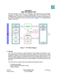
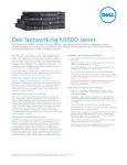
The IXP2400 [8] is Intel’s second generation network processor chipset, and it retires the previous IXP1200 [10]. It has many different resources to make packet processing as effective as
possible. A simple layout can be seen in figure 2.1. We can see the components that are shared.
For example, all microengines and the XScale share the SRAM and the SDRAM. This is a real
advantage for multistage packet handling. The code that receives packets reads in the packets,
and only sends a 32bit handle to the microengines that take care of the next step. If the XScale
needs to see the packet, it gets the same 32 bit handle. This way there is a little copying to have
the packet accessed from different places. The chipset also has hardware SRAM and Scratch
memory rings. These are intended for making a queue for handles. You typically have one ring
to transfer the packet handle from one stage or process to another. Below, we take a look at the
different components.
2.2.1 XScale
The XScale is a 32bit, 600MHz, general purpose RISC CPU, compatible with ARM version 5.
It does not have hardware floating point, but vector floating point is supported by a coprocessor.
4
Figure 2.1: Overview of IXP chipset
It also includes the Thumb instruction set (ARM V5T) [11] and the ARM V5E DSP extensions [11]. It has 32KB cache for instructions and 32KB for data. The processor has several
different types of memory mapped in a continuous region to make it easier to access it all, see
figure 2.3 and table 2.1. Here is an example of how we map the Control and Status Register
Access Proxy (CAP) registers into a variable so we can access it.
cap_csr = ioremap_nocache(0xc0004000, 4096);
See IXP2400_2800 [12] section 4.1.3.3 for the address to the Fast Write CSR. According to
ioremap_nocache’s manual page: “Ioremap_nocache performs a platform specific sequence of
operations to make bus memory CPU accessible via the readb/readw/readl/writeb/ writew/writel
functions and the other mmio helpers.” Our version of Ioremap_nocache is a function that
Lennert Buytenhek [9] has implemented. In figure 2.2 you see how we use the mapped memory
to access the hash unit’s registers to initialize it. Read IXP2400_2800 [12] section 5.6.2 to see
how we got the addresses.
void hash_init(void) {
unsigned int *hashunit;
hashunit = (unsigned int*) (cap_csr + 0x900);
// 48bit multipler registers:
hashunit[0] = 0x12345678;
hashunit[1] = 0x87654321;
// 64bit multipler registers:
hashunit[2] = 0xabcd8765;
hashunit[3] = 0x5678abcd;
// 128bit multipler registers (four of these):
hashunit[4] = 0xaabb2367;
hashunit[5] = 0x6732aabb;
hashunit[6] = 0x625165ca;
hashunit[7] = 0x65ca1561;
}
Figure 2.2: Memory map example
5
Note that the microengines do not do the memory mapping, so we have to translate the
addresses when we access the same byte from XScale and the microengines.
The XScale is used to initialize the other devices, it can do some processing of higher level
packets, and e.g. set up connections, but most of the packet processing is supposed to be done
at the microengines. It can also be used to communicate with the host computer over the PCI
bus. The XScale can sustain a throughput of one multiply/accumulate (MAC) every cycle. It
also has a 128 entry branch target buffer to predict the outcome of branch type instructions to
increase speed. Endianness is configurable and chosen under booting. This way the CPU can
be either little or big endian. Not at the same time, but it is still impressive. It also supports
virtual memory and runs the kernel in kernel level and the user programs in user level. It runs
MontaVista Linux [13] or VxWorks [14] for embedded platforms on our board.
Figure 2.3: XScale memory map
6
Area:
Content:
00000000-7FFFFFFF
SDRAM, XScale Flash RAM
80000000-8FFFFFFF
SRAM Channel 0
90000000-9FFFFFFF
SRAM Channel 1
A0000000-AFFFFFFF
SRAM Channel 2 (IXP2800 only)
B0000000-BFFFFFFF
SRAM Channel 3 (IXP2800 only)
C0000000-C000FFFF
Scratchpad CSRs
C0004000-C0004FFF
CAP Fast Write CSRs
C0004800-C00048FF
CAP Scratchpad Memory CSRs
C0004900-C000491F
CAP Hash Unit Multiplier Registers
C0004A00-C0004A1F
CAP IXP Global CSRs
C000C000-C000CFFF
Microengine CSRs
C0010000-C001FFFF
CAP XScale GPIO Registers
C0020000-C002FFFF
CAP XScale Timer CSRs
C0030000-C003FFFF
CAP XScale UART Registers
C0050000-C005FFFF
PMU?
C0080000-C008FFFF
CAP XScale Slow Port CSRs
C4000000-4FFFFFF
XScale Flash ROM (Chip-select 0) (16MB 28F128J3)
C5000000-C53FFFFF
FPGA SPI-3 Bridge Registers (Chip-select 0)
C5800000
POST Register (Chip-select 0)
C5800004
Port 0 Transceiver Register (Chip-select 0)
C5800008
Port 1 Transceiver Register (Chip-select 0)
ContentC580000C
Port 2 Transceiver Register (Chip-select 0)
C5800010
FPGA Programming Register (Chip-select 0)
C5800014
FPGA Load Port (Chip-select 0)
C5800018
Board Revision Register (Chip-select 0)
C580001C
CPLD Revision Register (Chip-select 0)
C5800020-C5FFFFFF
Unused (Chip-select 0)
C6000000-C63FFFFF
PM3386 #0 Registers (Chip-select 1)
C6400000-C67FFFFF
PM3387 #1 Registers (Chip-select 1)
C6800000-CBFFFFFF
Unused (Chip-select 1)
C6C00000-CFFFFFFF
SPI-3 Option Board (Chip-select 1)
C7000000-C7FFFFFF
Unused (Chip-select 1)
C8000000-C8003FFF
Media and Switch Fabric (MSF) Registers
CA000000-CBFFFFFF
Scratchpad Memory
CC000100-CC0001FF
SRAM Channel 0 Queue Array CSRs
CC010000-CC0101FF
SRAM Channel 0 CSRs
CC400100-CC4001FF
SRAM Channel 1 Queue Array CSRs
CC410100-CC4101FF
SRAM Channel 1 CSRs
CC800100-CC8001FF
SRAM Channel 2 Queue Array CSRs (IXP2800 only)
CC810100-CC8101FF
SRAM Channel 2 CSRs (IXP2800 only)
CCC00100-CCC001FF
SRAM Channel 3 Queue Array CSRs (IXP2800 only)
CCC10100-CCC101FF
SRAM Channel 3 CSRs (IXP2800 only)
CE000000-CEFFFFFF
SRAM Channel 0 Ring CSRs
CE400000-CE4FFFFF
SRAM Channel 1 Ring CSRs
CE800000-CE8FFFFF
SRAM Channel 2 Ring CSRs (IXP2800 only)
CEC00000-CECFFFFF
SRAM Channel 3 Ring CSRs (IXP2800 only)
D0000000-D000003F
SDRAM Channel 0 CSRs
D0000040-D000007F
SDRAM Channel 1 CSRs (IXP2800 only)
D0000080-D00000BF
SDRAM Channel 2 CSRs (IXP2800 only)
D6000000-D6FFFFFF
XScale Interrupt Controller CSRs
D7000220-D700022F
XScale Breakpoint CSRs
D7004900-D700491F
XScale Hash Unit Operand/Result CSRs
D8000000-D8FFFFFF
PCI I/O Space Commands
DA000000-DAFFFFFF
CI Configuration Type 0 Commands
DB000000-DBFFFFFF
PCI Configuration Type 1 Commands
DC000000-DDFFFFFF
PCI Special and IACK Commands
???
System Control Coprocessor (CP15)
???
Coprocessor 14 (CP14)
DE000000-DEFFFFFF
IXP PCI Configuration Space CSRs
DF000000-DF00015F
PCI CSRs
E0000000-FFFFFFFF
PCI Memory Space Commands
Table 2.1: The memory map for the XScale.
7
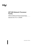
2.2.2 Microengines
Figure 2.4: Overview of microengine components
The IXP2400 also has eight microengines which also run at 600MHz. For a simple picture
of what they look like inside, see figure 2.4. They have a six stage pipeline and are 32bit
processors that are specialized to deal with network tasks. They are somewhat simple. Their
lack of stack means that you need to keep track of the return address when programming them.
If you want to do nested calls, you need to allocate register in each procedure so it knows where
to return. Their code is loaded by the XScale and they have a limited space for the code. It is
stored in the Control Store that can be seen in figure 2.4. It holds 4096 instructions, each 40 bits
8
wide.
Another thing is that you need to manually declare signals and wait for them when writing
to a ring or memory. You can choose to run them with either four or eight contexts or threads.
A context swap is similar to a taken branch in timing [4]. This is nice when you parallelize
problems for hiding memory latencies, e.g. if a context is waiting for memory, another context
could run.
Another limitation can be seen from figure 2.4, that is that the execution datapath needs its
operands to be from different sources. You can not add two registers that both are in the A bank.
The assembler takes care of the assignment of registers and gives you an error if the registers
can not be assigned without a conflict [12].
They have many options for memory storage:
* Their own individually 2560 (640 32bit words) bytes of local memory.
* SDRAM.
* DDR SDRAM.
* The Scratchpad memory
* Hardware rings.
A ring is a circular buffer. It is very nice to use to implement packet queues. You have one
processor putting the packet handles in a ring and another one picks them up. This way you do
not have to use mutexes since the operations are hardware supported and atomic. And it is also
a way to have one microengine produce data for two or more microengines. The microengines
do not have all memory types mapped out in a single address space as mentioned above for
the XScale. Each type of memory has its own capabilities and they have different instructions
to access each memory type.(See section 2.2.3). You need to know what type of memory you
are using when you declare it. SRAM channel 0 is located at address 0x0 and channel 1 is at
0x4000 0000, so to some degree they have a address map.
The microengines’ branch prediction assumes “branch not taken”, i.e. to optimize your
programs, you should write your code so that the branches are not taken most of the time. It is
not really a branch prediction, it just reads the next instruction after the branch. To optimize,
you can use a defer[n] argument after the branch if you have code that can be executed if the
branch is taken or not. n is the number of instructions that can be done while the microengine
figures out if it branches or not. Usually, n is 1-3.
In the code below, the first line is a branch, and we use defer[1] to let the line under execute
whether the branch is taken or not. If the branch is not taken, no damage is done, and we do
not use more clockcycles than without the defer option. If the branch is not taken, we save a
clockcycle since we can start the last line before the branch code is finished.
bne[get_offset_search_start#],defer[1] alu[–, $entry_w1, xor, iphigh] /* Check local IP */
Each microengines have the following features:
* 256 general purpose registers.
* 512 transfer registers.
9
* 128 next neighbor registers.
* 640 32-bit words of local memory
* A limited instruction storage. 4Kx40bit-instructions for each microengine.
* 16 entry CAM (Content Addressable Memory) [15] with 32 bit for each entry.
* It has control over one ALU.
* Its own unit to compute CRC checksums. CRC-CCITT and CRC-32 are supported.
These resources are shared by all contexts. With context we mean threads that the microengine
can run at the same time. This is a way to hide memory latency, if one context has to wait, the
microengine just runs another one.
The next neighbor registers can be seen in figure 2.1 as arrows from one microengine to
its neighbor. This can be used if two microengines are working on the same task and need to
transfer data between themselves without using any shared resources.
They can not write to console, so debugging is a little more tricky. Add the fact that there can
be multiple microengines having multiple threads doing the same code, debugging can require
some thinking. But, since we have 8 of these microengines and they have a lot of possibilities,
they are very useful. You just have to think about what you want to use them for.
2.2.3 Memory types
It is important to use as fast memory as you can, since it can take a long time to read or write to
“slow” memory. Use registers and local memory as much as you can. The relative speed of the
different memory types is shown in Table 2.2. The information in table 2.2 is taken from [15].
Type of memory Relative access time Bus width Data rate
Local memory
1
NA
on chip
Scratchpad
10
32
on chip
SRAM
14
32
1.6Gb/s
SDRAM
20
64
2.4Gb/s
Table 2.2: Access time for memory types
However, the faster the type of memory, the less storage it has. Local memory in microengines is very fast, it is made up of registers, but we only have 2560 bytes of it in each
microengine. Remember that you can read/write in parallel over different memory types and
channels. A channel is an independent “path” to a memory unit. You can read or write to each
memory channel independently of the other ones. SDRAM has a higher bandwidth than one
SRAM channel, but with SRAM you can use two channels in parallel, which gives a larger
total bandwidth than SDRAM. SRAM is faster for small transfers, e.g. meta data and variables.
The SRAM read or write instruction can read or write up to 8x4 byte words at the same time.
The SDRAM read or write instruction can read or write up to 8x8 byte words. This can save
you some memory access, if you plan what you need to read or write. Local memory for the
10
microengines can not be shared. The intended use is to store the actual packet in SDRAM, and
the packet meta data in SRAM.
In our forwarding version, which uses the Intel Software Developer Kit (SDK) [16], we pass
a 32 bit handle, which includes a reference to both the SRAM metadata and the SDRAM packet
data, when we want to give the packet to the next processor or ring. (See Figure 2.5) The “E”
Buffer Handle structure
Bit number:
31 30 29
E S
0
24 23
Seg.
count
Offset in [D,S]RAM
E = End of Packet bit
S = Start of Packet bit
Seg. count tells how many buffers used for
this packet
Offest is the offset to DRAM and SRAM
where packet is stored
Figure 2.5: Packet handle
and “S” bit tells if it is the end or the start of a packet. If the packet is small enough to fit in
one buffer, both bits are set. We have a buffer size of 2048 bytes which is larger than a Ethernet
frame, so all packets should be in one buffer. The 24bit offset gives you the address to both
SRAM metadata and SDRAM packet data. To get the SRAM metadata address you leftshift the
offset with 2 bits. For the SDRAM data address we leftshift the offset 8 bits. For SDRAM the
number of bits to leftshift will depend on the buffersize. A 2048KB buffer like we use in the
forwarding version, requires an 8 bit leftshift.
In our version for a mirror port on a switch, we made the logger read the data directly from
the media switch fabric (MSF) without any data being copied to or from SDRAM. We will
explain this in chapter 4.
2.2.4 SRAM Controllers
The Chipset has two SRAM Controllers. These work independently of each other. Atomic
operations that are supported by hardware are swap, bit set, bit clear, increment, decrement, and
add operations. Both controllers support pipelined QDR synchronous SRAM. Peak bandwidth
is 1.6 GBps per channel as seen in table 2.2. They can address up to 64MB per channel. The
data is parity protected. This memory can be used to share counters and variables between
microengines and between microengines and the XScale. One usage of this memory is to keep
metadata for packets, and variables that is shared between both microengines and XScale.
11
2.2.5 ECC DDR SDRAM Controller
ECC DDR SDRAM is intended to use for storing the actual packet and other large data structures. The chipset has one 64bit channel (72 bit with ECC) and the peak bandwidth is 2.4GBps.
We see from table 2.2 that the SRAM has lower latency, but SDRAM has the higher bandwidth
per channel. The memory controller can address up to 2GB, which is impressive for a system
that fits on a PCI card.
One thing to point out is that memory is byte-addressable for the XScale, but the SRAM
operates with an access unit of 4 bytes and the SDRAM 8 bytes. The interface hardware reads
all bytes and gives you only what you want, or it reads all bytes first, changes only the one you
write and writes the whole unit back to memory.
2.2.6 Scratchpad and Scratch Rings
The scratchpad has 16KB of general purpose storage which is organized in 4K 32bit words.
It includes hardware support for the following atomic operations: bit-set, bit-clear, increment,
decrement, add, subtract, and swap. Atomic swap makes it real easy to implement mutexes to
make sure that shared variables do not get messed up if more than one process tries to write to
them at the same time, or a process reads a variable and needs to prevent others from reading or
writing to it before it writes the new value back.
It also supports rings in hardware. These rings are useful to transfer data between microengines. For example, the packet handles are transferred here. The memory is organized as 4K
32bit words. You can not write just a byte, you need to write the whole 32bit word. We can
have up to 16 rings which can be from 0 to 1024 bytes. A ring is like a circular buffer. You
can write more items to them, even if the receiver has not read the items that are in the ring.
This is the third kind of memory the microengines and the XScale can use. We can use all types
concurrently to get a lot done in parallel.
2.2.7 Media and Switch Fabric Interface (MSF)
This chip is used as a bridge to the physical layer device (PHY) or a switch fabric. It contains
one sending and one receiving unit which are independent from each other. Both are 32bit. They
can operate at a frequency from 25 to 133MHz. The interface includes buffers for receiving and
transmitting packets.
Packets are divided into smaller pieces called mpackets by the MSF. The mpackets can be
64, 128, or 256 bytes large. If a network packet is larger than the mpacket size you are using,
you need to read all the mpackets that belongs to one network packet and put it together. The
MSF is very programmable so it can be compatible with different physical interface standards.
The MSF can be set up to support Utopia level 1/2/3, POS-PHY level 2/3, or SPI-3, or
CSIX-L1 [11]. UTOPIA is a protocol for cell transfer between a physical layer device and a
link layer device (IXP2400), and is optimized for transfers of fixed size ATM cells. POS-PHY
(POS=Packet Over SONET) is a standard for connecting packets over SONET link layer devices
to physical layer. SPI-3 (POS-PHY Level 3) (SPI-3=System Packet Interface Level 3) is used
to connect a framer device to a network processor. CSIX (CSIX=Common Switch Interface)
defines an interface between a Traffic Manager and a switch fabric for ATM, IP, MPLS, Ethernet
and other data communication applications [17].
12
If you like, you can use this interface directly. There are instructions that allow you to read
and send data using it. In our mirror version, we read the first 64 bytes from the network packets
directly from the MSF.
2.2.8 PCI Controller
We also got a 64bits/66MHz PCI 2.2 Controller. It communicates with the PCI interface on the
Radisys card helped by three DMA channels.
2.2.9 Hash Unit
The Hash unit has hardware support for making hash calculations. Such support is nice when
you need to organize data in tables. You can use the hash unit to know which table index to
store or retrieve an entry. It can take a 48, 64, or 128bit argument, and give a hash index with
the same size out. Three hash indexes can be created using a single microengine instruction.
It uses 7 to 16 cycles to do a hash operation. It has pipeline characteristics, so it is faster to
do multiple hash operations from one instruction than multiple separate instructions. There are
separate registers for the 48, 64, and 128bit hashes. The microengines and the XScale share
this hash unit, so it is easy to access the same hash table from both processor types. The hash
unit uses some base numbers to make the hash value, You need to write these numbers to their
designated registers before you use it. The hash unit uses an algorithm to calculate the hash
value, and the base numbers are used in that calculation.
We use the hash unit to access our table of streams in a effective way, we will have more
about this in section 4.7.4.
2.2.10 Control and Status Registers Access Proxy (CAP)
The Control and Status Registers Access Proxy is used for communication between different
processes and microengines. A number of chip-wide control and status registers are also found
here. The following is an overview of its registers and their meanings:
* Inter Thread Signal is a signal a thread or context can send to another thread by writing
to the InterThread_Signal register. This enables the thread to sleep waiting for the
completion of another task on a different thread. We use this in our logger, to be sure that
the packets are processed in order. This is important in e.g. TCP handshake. All threads
have a Thread-Message register where they can post a message. Other threads can
poll this to read it. The system makes sure only one gets the message, to prevent race
conditions.
* The version of the IXP2400 chipset and the steppings can be read in the CSR (CAP).
* The registers to the four count down timers is also found here.
* The Scratchpad Memory CSRs (CAP CSR) are located here. These are used to set up the
scratch rings. The scratch rings are used in our logger to communicate between microengines.
13
* IXP_RESET_0 and IXP_RESET_1 is two of the registers found here. IXP_RESET_0
is used to reset everything except for the microengines. IXP_RESET_1 is used to reset
the microengines.
* We also find the hash unit configuration registers here.
* The serial port that we use on the IXP card has its configuration registers here.
2.2.11 XScale Core Peripherals
The XScale Core Peripherals consists of an Interrupt Controller, four timers, one serial Universal Asynchronous Receiver/Transmitter(UART) port, eight General Purpose input/output circuits, interface for low speed off-chip peripherals, and registers for monitoring performance.
The Interrupt Controller can enable or mask interrupts from timers, interrupts from microengines, PCI devices, error conditions from SDRAM ECC, or SPI-3 parity error. The IXP2400
has four count down timers that can interrupt the XScale when they reach zero. The timers can
only be used by the XScale. The countdown rate can be set to the XScale clock rate, the XScale
clock rate divided by 16, or the XScale clock rate divided by 256. Each microengine has its
own timer, which we use to put timestamps in the entry for the start and endtime of a stream.
The microengine timers are not part of XScale Core Peripherals.
IXP2400 also has a standard RS-232 compatible UART. This can be used as an interface
with the IXP chipset from a serial connection from a computer.
The General Purpose pins can be programmed as either input or output and can be used for
slow speed IO as LEDs or input switches. The interface for low off-chip peripherals is used for
Flash ROM access, and other asynchronous device access. The monitoring registers can show
how well the software runs on the XScale. It can monitor instruction cache miss rate, TLB miss
rate, stalls in the instruction pipeline, and number of branches taken by software.
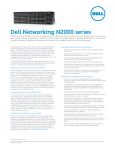
2.3 Radisys ENP2611
Figure 2.6 gives you a layout of the Radisys ENP2611. The development card includes the
IXP2400 chipset as described above and the following components.
* Two SODIMM sockets for 200-pin DDR SDRAM: They are filled with 256MB ECC
memory in our card.
* 16MB StrataFlash Memory: The bootcode and some utilities are kept here.
* Three 1Gps Ethernet Interfaces: The PM3386 controls two interfaces and PM3387 controls one. These go to sfp GBICS slots that you can put either copper or fiber ports in.
These are the network interfaces you can see marked as “3x1 Gigabit Optical Transceiver
Ports 0,1,2” in figure 2.6
* SCSI Parallel Interface v3. (SPI-3) bridge FPGA: This is the link between the PM3386
and PM3387 controllers and the IXP2400
14
Figure 2.6: The Radisys ENP2611 card. Note that one of the PM3386 should read PM3387.
Picture is taken from [18].
* Two PCI to PCI Bridges: One is a non-transparent Intel 21555 PCI-to-PCI bridge [19]
which connects the internal PCI bus in the IXP2400 chipset to the PCI bus on the host
computer. It lets the XScale configure and manage its PCI bus independently of the host
computers PCI system. The 21555 forwards PCI transactions between the PCI buses and
it can translate the addresses of a transaction when it gets to the other bus. This resolves
any resource conflicts that can happen between the host and IXP PCI buses. The IXP
system is independent of the host computer, and both assign PCI addresses to the devices
connected to their bus at boot [20]. It has registers for both local (XScale) side and host
side where it defines the address ranges to respond to and the addresses to translate to.
These registers must be set up right to make the translation work. The 21555 can also be
used to make interrupts on the PCI buses, e.g., an interrupt on the host computer PCI bus
will end up as an interrupt on the host computer kernel. The other one is a TI PCI2150
transparent PCI bridge which connects to an Ethernet interface.
* Intel 82559 10/100 Ethernet Interface: It can be used for debugging, to load the operating
system with DHCP/TFTP, or mount NFS filesystems. Is not meant to be used in the router
infrastructure.
* Clock Generation Device: System clock for the IXP2400, and interface clocks for the
15
IXP2400 MSF/FPGA and FPGA/PM338x interfaces.
“Network Systems Design” [15] is a book that describes this card. It talks about networks
in general first, then gets into network processors, and at last it is about the IXP2xxx series
specifically. It does a good job of explaining how the different parts of the card works.
2.4 Summary
We believe that special hardware is necessary to handle the network traffic as it grows further.
Residents are getting faster and faster network connections, 10 and 100 or even 1000Mbps is
already available some places [6] [7]. With all this bandwidth, there will be a new market for
streaming of data. Sport events, movies, and video conferences are some of the things that
come to mind that require high bandwidth. Online games, video conferences, and virtual reality
applications require low latency, and network processors can help make that happen by enabling
application dependent processing without full TCP/IP handling. The online games will grow,
and they will need to send more and more detailed information to more and more participants.
If two players are shooting at each other, low latency is crucial. A lot of them will need the
same information. Intelligent routers will help to make this more efficient and with less latency
by sending the same data to all the players in the same area instead of sending the same data
over again between the routers.
We have in the IXP2400 a powerful tool to do packet processing. Its large memories can
hold a lot of information and it can do a lot of computing with its XScale and microengines.
Intel has put a lot of thought into this chipset. There are a lot of hardware supported features,
rings and atomic memory operations which can save a lot of time designing software, and speed
up execution.
It is important to get a good understanding of the system before we implement a service
on the card. We need to program it so that all resources are put to good use. We have eight
microengines with four or eight threads each, hardware rings, locks, and hash operations, the
XScale CPU and then we have the host computer. Furthermore, we need to know what we
can cut up into a pipeline and let different microengines do a part each and pass it on to the
next one. We also need to consider how many pipeline stages we can use, versus how much
we can parallelize. Considering memory access, we do not want many processes trying to
access the same memory at the same time. We got SRAM, SDRAM, Scratch memory, and each
microengines local memory on the IXP card, and local memory on the host computer. The host
computer’s harddrive can also be used for storage. To make the system perform at its best, we
need to think through and plan what memory to use for what and in which order. However, this
is one of the coolest pieces of hardware we have seen.
16
Chapter 3
Related work
Here we are going to take a look a similar works. We first look at related technologies or
systems. Lastly we look at other works with network processors.
3.1 Network Monitoring
3.1.1 Cisco NetFlow
Cisco has a product called NetFlow [21] [22], which is a network protocol which runs on Cisco
equipment for collecting IP traffic information. According to Cisco, NetFlow can be use for
network traffic accounting, usage-based network billing, network planning, security, Denial of
Service monitoring capabilities, and network monitoring. From Wikipedia we see that it can
give the records shown in Table 3.1.
* Version number
* Sequence number
* Input and output interface snmp indices
* Timestamps for the flow start and finish time
* Number of bytes and packets observed in the flow
* Layer 3 headers:
* Source and destination IP addresses
* Source and destination port numbers
* IP protocol
* Type of Service (ToS) value
* In the case of TCP flows, the union of all TCP flags observed over the life of the flow.
Table 3.1: The values given by NetFlow
This is pretty much the same as we are doing with our IXP card. We have not tried NetFlow,
or even seen a router equipped with it, so we can not tell how it works. We believe that you
can only get it on Cisco routers and not on their switches. The data is received from the router
using User Datagram Protocol (UDP) or Stream Control Transmission Protocol (SCTP) by a
NetFlow collector, which runs on a regular PC.
17
3.1.2 Fluke
Fluke has gigabit and 10 gigabit network analyzers [23]. Their OptiView Link Analyzer
is described as: “OptiView Link Analyzer provides comprehensive visibility for network and
application performance troubleshooting on Ethernet networks, all in an ASIC architecture for
real-time monitoring and packet capture up to line rate Gigabit speeds. Link Analyzer is rack
mountable and provides 10/100 and full duplex Gigabit Ethernet network monitoring and troubleshooting.” We found a price for it on Internet [24], it was close to $30 000. This model has
two interfaces for monitoring, both can be 1Gb/s.
They also have a 10Gb/s model called XLink Analyzer [25]. “XLink Analyzer is a
solution for high speed enterprise data centers. XLink provides the means to simultaneously
analyze multiple 10Gigabit or 1Gigabit Ethernet links without the risk of missing a packet. This
performance helps solve network and application problems faster, while maintaining higher
uptime and performance for end users.” This one is more expensive. A interface card with two
10Gb/s interfaces runs around $72 000 [26], a card with four 1Gig/s interfaces cost around $46
000 [27], and you need a chassis, the least expensive is a Single Slot XLink Chassis
that costs $7 600 [28].
3.1.3 Wildpackets
According to WildPacket, their Gigabit network solutions [29] provides real-time capture and
analysis of traffic, capturing high volumes of traffic without dropping any packets and provide
expert diagnostics and rich graphical data that accelerate troubleshooting. They have solutions
for 1Gb/s and 10Gb/s network analysis. WildPacket’s Gigabit Analyzer Cards are hardware
designed to handle Gigabit traffic analysis. When capturing packets at full line rate, the card
merges both streams of the full-duplex traffic using synchronized timestamps. The card can
also slice and filter packets at full line rate speed to give a better analysis.
3.1.4 Netscout
This company has 10/100/1000 Ethernet and 10 Gigabit Ethernet capture and analysis solutions [30]: “The nGenius InfiniStream, when combined with NetScout analysis and reporting
solutions, utilizes packet/flow analysis, data mining and retrospective analysis to quickly and
efficiently detect, diagnose and verify the resolution of elusive and intermittent IT service problems.” They can capture data at 10Gb/s and have impressive storage configurations ranging
from 2TB to 15TB. We did not find any prices for these systems, but we do not think they are
cheap.
3.1.5 Summary
The proprietary gigabit analyzers are expensive, which makes it interesting to see what can be
done with a regular computer and an IXP card. Another reason to use network processors are
that we can program them to do what we want. If your analyzer is an ASIC, you can not change
too much of it, since it is hardware. Our card can be programmed to do new and very special
packet inspections. In the next section, we will look at other papers about network processors.
18
3.2 Network Processors
In this section, we are going to look at some examples of related work that has been done with
network processors. We will see that there are many possibilities, and that network processors
have a great potential to reduce the load on their host computer and increase throughput.
3.2.1 Pipelining vs. Multiprocessors - Choosing the Right Network Processor System Topology
The author of [31] try to see how to best organize the next generation’s network processors.
Do we want to parallelize the work over many processors, put them in a long pipeline, or a
combination of both?
The new network processors will have a dozen of embedded processor cores. Routers have a
lot of new requirements, e.g. firewalls, web server load balancing, network storage, and TCP/IP
offloading. To make this work fast enough, routers have to move away from hard-wired ASIC
to programmable network processors (NPs). Since not all packets in the network traffic depend
on each other, network processors can parallelize the processing. You can arrange processing
engines in two ways, parallel or pipeline, or you can choose to use a combination. Figure 3.1
shows first a pipeline, secondly a multiprocessor approach, and lastly a hybrid. One important
result in the paper is that the systems’ performance can vary by a factor of 2-3 from the best to
the worst configuration of the CPUs.
Figure 3.1: Pipelining vs multiprocessors
The author used a program called "PacketBench" to emulate systems with different configurations. As workload they chose some common applications:
* IPv4-radix. An application that does RFC1812-compliant packet forwarding and uses a
radix tree structure to store entries in the routing table [32].
* IPv4-trie. Similar to IPv4-radix, but uses a trie structure with combined level and path
compression for the route table lookup [33].
* Flow classification. Classifies the packets passing through the network processor into
flows.
* IPSec Encryption. An implementation of the IP Security Protocol.
19
To analyze the tradeoffs of the different arrangements of CPUs, they randomly placed the jobs
to find the best balanced pipeline possible, so that they did not have one pipeline stage that is too
slow. That would have made the whole pipeline slow. To get the highest throughput, they had
to consider the processing time on each element on the system board, the memory contention
on the memory interfaces, and the communication between the stages [31].
They found that many configurations was slow compared to the best one. The throughput
scaled good with respect to pipeline depth, which is how many CPUs you have in a pipeline. It
was roughly proportional to the number of processors. For pipeline width, which is how many
CPUs you have in parallel, it increases in the beginning, but reaches a ceiling fast around 4 to
6 CPUs. This is because they all try to access the same memory interfaces. If you add more
memory interfaces, you can get more performance, each memory interface can handle about
two processing elements before it starts to slow things down.
Memory contention is the main bottleneck. Even if they increased to 4 memory channels,
the memory access time is still the part that takes most time in a pipeline stage. To get the
memory access time comparable to communication and synchronization, the service time needs
to be low. Processor power is not the limiting factor in these systems. After memory delay, they
have communication and synchronization to wait for. To get programs to run fast on network
processors, they learned that they need to have fast memory systems. The more interfaces, the
better. One nice thing about the IXP2400 is that there are many separate memory systems, the
SRAM, each microengines memory, the scratchpad, and the common SDRAM. The ability to
use more threads, so another thread can run then a threads need to wait for memory access,
improves throughput.
One important remark they made is that they do not take multithreading into account. They
admit that this is a powerful way to hide memory latency. The IXP2400 card has 4 or 8 context
for each microengine. However, this will not increase the total memory bandwidth, just make it
utilized better. E.g. a context stops when it has to wait for memory, and an other context takes
over the processing unit. Context switches are really fast on the IXP system, it is the same time
as a branch [12].
They do only simulate general purpose CPUs, the IXP card has some hardware implemented
solutions, e.g., hash functions, rings, registers to the next microengine, and more, which should
make things faster, and may save some memory access.
3.2.2 Building a Robust Software-Based Router Using Network Processors
In [34], the goal is to show how an inexpensive router can be build from a regular PC and an
IXP1200 development board. One other point is that a router based on network processors is
very easy to change, when new protocols or services are needed. The authors managed to make
it close to 10 times faster than a router based on a PC with regular NICs.
The PC they are using is a Pentium III 733MHz with an IXP1200 evaluation board containing one StrongARM and six microengines all at 200MHz. The board also has 32MB DRAM,
2MB SRAM, and 4KB Scratch memory, and 8x100Mbps Ethernet ports. One important advantage with this setup is that the packets in the data plane, which is the lowest level of packets is
processed by the microengines, and the ones in the control plane, that needs more processing,
can be handled by the XScale or the host CPU. This way they can utilize the power of the microengines to do the simple processing fast at line speed, and the more demanding packets can
20
be processed by a more general purpose CPU.
As Figure 3.2 shows, when a packet arrives, a classifier first looks at it to select a forwarder
to send it to. The forwarder is a program that processes the packet and/or determines where it is
going to be routed to. The forwarder takes the packet from its input queue, and when it is done
processing the packet, it puts the packet in an output queue where an output scheduler transmits
the packet to the network again. One advantage of this modularized way is that it is easy to
make new forwarders and install them. Forwarders can run on microengines, the StrongARM,
or the CPU(s) in the host computer.
Queue
In queue
Frwdr
Queue
Sch.
Clas.
Queue
Frwdr
Out queue
Queue
Figure 3.2: Classifying, forwarding, and scheduling packets
They tested the microengines performance in forwarding packets, and they found that they
are able to handle packets from all eight network interface at line speed. The packets were
minimum sized, 64 byte. This gives a forwarding rate of 1.128Mpps(Mega packets per second).
The StrongARM was able to forward packets at 526Kpps polling for new packets. It was
significantly slower using interrupts. To use the host computer’s CPU, they had the StrongARM
send packets to it. This method used all the StrongARMs cycles, but they get 500 cycles to use
on each packet on the Pentium. This way they could forward 534Kpps. Keep in mind that they
can not use the Pentium and the StrongARM at full speed at the same time, since they are using
the StrongARM to feed the Pentium. At a forwarding rate of 1.128Mpps, each microengine has
the following resources to use to process a 64 byte MAC-Packet (MP):
* Access to 8 general purpose 32-bit registers.
* Execute 240 cycles of instructions.
* Perform 24 SRAM transfers.
* Do 3 hashes from the hardware hashing unit.
This evaluation is based on worst case load, since they are forwarding minimum sized packets at
line speed. Their approach was able to get a forwarding rate of 3.47Mpps between ring buffers.
This is much faster than the 1.128Mpps that is the maximum bandwidth for all eight 100Mbps
network ports. They also showed that new forwarders could be injected into the router without
degrading its robustness. This group also states that the IXP is not an easy thing to program.
Spalink et. al. [34] wrote a good paper, just too bad it was not done on the new IXP2xxx
chipset. We found their comparison of the microengines, the StrongARM and the Pentium
useful. One interesting contradiction is that Spalink et.al. [34] do not consider memory to be
a big bottleneck, while the emulation in the "Pipelining vs. Multiprocessors" [31] paper states
memory as the primary bottleneck. So either the memory latency hiding techniques works well,
or the paper did not take the IXP’s different kinds of memory into account. The authors also did
some calculations of what could be done on the card, and it was promising. The new IXP2400
has even more resources and faster processors, so it is even better.
21
3.2.3 Offloading Multimedia Proxies using Network Processors
The paper “Offloading Multimedia Proxies using Network Processors” [35] looks at the benefits of offloading a multimedia proxy cache with network processors doing networking and
application level processing. The authors have implemented and evaluated a simple RTSP control/signaling server and an RTP forwarder. All the processing is done by the IXP card.
The Radisys ENP2505 is a fourth generation network processor. It has four 100Mbps Ethernet interfaces, one general purpose 232MHz StrongARM processor, six network processors
called microengines, and three types of memory: 256MB SDRAM for packet store, 8MB
SRAM for tables, and 8MB scratch for rings and fast memory. It is the same IXP chipset as the
previous article but put on a different board. It is a conventional Linux running on the StrongARM. On traditional routers, all packets have to be sent from the NIC up to the host computer
for processing. This takes time due to copying, interrupt, bus transfers, and checksumming.
Instead, they are doing all of this on the IXP card to get the latency down.
To cache data, they need to send the data up to the host computer. But they can still improve
upon a regular PC based router. They can queue many packets on the card, and when they do
have enough, they can have fewer and more efficient card-to-host transfers and disk operations.
A Darwin streaming server and a client to get a QuickTime movie was used to test the router
which was in between the server and client. If a packet was to be forwarded, the microengines
did that themselves. If it needed more processing, it was sent to the StrongARM. The results
are promising, a data item can be forwarded in a fraction of the time used by a traditional PC
based router.
We needed to get PCI transfer to work or find someone who has done it to get the cache and
other things to work. The paper gives us another proof that network processors are very useful
in handling different network traffic.
3.2.4 SpliceNP: A TCP Splicer using A Network Processor
Here, we have an article [36] that teaches us that TCP splicing can reduce the latency tremendously in a router. To make even more reductions, this paper looks at use network processors.
More specific, the authors are using the Intel IXP2400.
You can make a content aware router by having an application that first gets a request from
a client, and then the application chooses a server. The router has then two connections, one to
the server and one to the client, and need to copy data between them so the client gets the data
from the server. TCP splicing is a technique that removes the need to copy data by splicing the
two connections together, so that the forwarding is done in the IP layer.
However, switches based on regular PCs have performance issues due to interrupts, moving
packets over the PCI bus, and large protocol stack overhead. ASIC based switches are not
programmable enough although they have very high processing capacity. Network processors
combine good flexibility with processing capacity. For [36], the authors are using the XScale
to create connections to servers and clients. After that, the data packets can be processed by
the microengines, so that no data needs to be copied over the PCI bus. There are four ways in
which the IXP card can make TCP splicing faster than a Linux based software splicer:
* First, the microengines use polling instead of interrupts like a regular PC does.
* Second, all processing is done at the card, so there is no data to copy over the PCI bus.
22
* Third, on a regular PC, the OS has overhead like context switches and the network processors are optimized for packet processing which processes packets more efficiently.
* Fourth, IXP cards have eight microengines and an XScale, so one can do a lot of things
in parallel to increase throughput.
The splicing is done with one microengine to process packets from clients and one for servers,
more microengines might get better throughput. All PCs were running Linux 2.4.20. Linux
based switches had a 2.5GHz P4 with two 1Gbps NICs. The server ran an Apache web server
on dual 3GHz Xeons and 1GB RAM. The client was another P4 at 2.5GHz and was running
hffperf.
Compared to a Linux based switch the latency is reduced by 83.3% (0.6ms to 0.1ms) with
a file of 1KB. For larger files this is is even better. At 1024KB the latency is reduced by 89.5%.
Throughput is increased by 5.7x for a 1KB file and 1024KB file it is 2.2x.
This is another example that network processors are useful. We also see that they are using
the XScale to do the setup of connections and more complex tasks, and use the microengines
for packets that are common and simple to handle. It is also interesting to see the computing
power of this card. You can get a lot of things done with only a few of the microengines.
3.3 Thoughts/Discussion
As the papers above show, network processors can really speed things up. Computers are getting faster, but much of the increased speed is in the CPU, the bandwidth to the PCI bus grows
a lot slower. In addition, you still got user and kernel level context switches and have to wait
for PCI transfers. Simultaneously, the bandwidth of network cards get higher, 1Gbps is normal,
and 10Gbps cards are available [37] [38]. As for the sound cards and graphics cards hardware
acceleration came a long time ago. We do believe that the future will bring more hardware accelerated network cards. We already have NICs that compute IP/UDP/TCP checksums, collect
multiple packets before they send an interrupt to the host computer. Some even have TCP/IP
stacks onboard [15] p.107-109, so the host computer get most of the network work done by the
network card itself, and the network card is able to do it faster. The host CPU can then spend
its time to do other tasks.
Network processors have a lot of potential. They are a little finicky to program, and there
are a lot of things that need to be figured out. However, their high throughput and low latency
capabilities make them really interesting as the Internet grows. There will always be more need
for more bandwidth.
One neat thing about IXP network processor is that it runs Linux and boots from Dynamic
Host Configuration Protocol (DHCP) and Trivial File Transfer Protocol (TFTP). Thus, you get
a Linux system running on your network card. This is great. It also makes a known, open,
and good platform to develop on. The fact that the CPUs are programmable makes it easy to
change the router’s behavior, add a new protocol or other features. It might be hard to make it
as efficient as possible on the microengines, but it can be done without soldering, flashing of
BIOS, or other inconvenient ways. Some things may even be ported from other Linux projects.
It is important to make some good libraries for the card, so that each developer does not
have to implement all things from scratch, for example, PCI transfer and functions to make and
send various packets. It would be nice to have the TCP Splicer [36] as a program or kernel
23
module. There should also be agreement on some standards to how to name things and where
to access modules/files/handles, so that we do not end up with a different system at each place
incompatible with all other.
In the next chapter, we will present our project: A real time logger using the IXP card
as a hardware accelerator. It is not easy to look at each packet on a gigabit link with a regular
computer. We will use the IXP card to look at the individual packets and just send the data about
the finished streams to the host computer. This is something we think is possible after reading
the reports in this chapter. Our main concern is transferring data over the PCI bus. This was
something no one at our university had done. After some research we found some information
on a mailinglist [39]. Another issue was if we could make all parts to work together and fast
enough.
24
Chapter 4
Design and Implementation of a Real-time
Packet Logger
We are going to see if we can build a real time packet logger. That is a system that can be put on
a network connection and log every stream or connection that goes through it. With stream or
connection we mean a TCP connection, an UDP datastream or a series of ICMP packets, e.g.,
generated by a ping command. There is no problem logging other streams, but it takes time to
program it all. The idea is that an administrator can use regular SQL queries to monitor network
traffic on his network. If someone is trying to get unauthorized access we can look at where
the packets come from and the port numbers that are used. We will get one entry in an SQL
database for each such stream. The stream entries will be updated regularly by setting some
variables. Another thing is monitoring. What kind of traffic do we have? Could it be smart to
move a server to a different place? There might come government laws that require companies
or ISPs to store all their streams for a period of time [1] [2]. Which is a challenge with a high
bandwidth network connection.
4.1 Overview
Figure 4.1 shows how the packet logger can be used in a network that has a switch that is able
to mirror a port. A mirror port is a port on the switch that is set up to get whatever packets that
goes through another port, this is called SPAN in Cisco language. If the network does not have
such a switch, we can use the Logger to forward each packet between the networks as shown
in figure 4.2. We recommend the first version. It gives no extra latency, and our system can not
affect the traffic. The second version can be used if you do not have a switch with a mirror port.
From figure 4.3, you see how the data is going through the system. The microengines get
each packet, read the headers and determine what kind of stream it is. Each stream has its
own entry in the SRAM hash tables. When a stream is finished or needs to be updated in the
database, the XScale copies the entry from the SRAM hash table to the SDRAM ring buffer.
For each 10 copied entries, or after a timeout, the XScale sends the host computer an interrupt
via the 21555 bridge. The host kernel turns the interrupt into a SIGUSR1 signal that the client
application gets. The application uses the gtxip [5] kernel device driver to copy the entries from
the IXP SDRAM ring buffer to itself and uses SQL queries to enter it into the SQL database.
First we will take a overview of what each part does, and then we take a closer look at the parts.
25
Figure 4.1: Setup of Logger and switch in a network
Figure 4.2: Setup of Logger forwarding packets in a network
Figure 4.3: Overview of components and data flow
4.1.1 SRAM hash tables
We have two SRAM memory areas. They contain stream table entries. The stream table entries
are stored in the hash tables, see figure 4.6, and contain all the information we have about a
stream. We have written more about the SRAM hash tables in section 4.4.
26
4.1.2 SDRAM ring buffer
The SDRAM shared memory is used to copy data to the host over the PCI bus. It is also used
for synchronizing time and let the client know the XScale’s load. We have written more about
the SDRAM ring buffer in section 4.5.
4.1.3 RX microengine
The RX, or receive, part is the one that gets the packets from the media switch fabric’s (MSF)
physical ports. In the forwarding version, the RX then assign a handle to them, and puts the
handle in a scratch ring so the logger microengine can process the whole network packet. This
version of the RX is made by Intel and is a part of the SDK [16].
In the mirror version of the logger, the RX just sends the first 32 bit of the receive status
word (RSW) [11] from the MSF to the logger microengine over the scratch ring. This enables
the logger to read the first 64 bytes of the network packet directly from the MSF. This RX block
is made by us. Read more about this in section 4.2.5.
4.1.4 Logger microengine
The Logger microengine is reading the headers of each packet. By header we mean IP, TCP,
ICMP and UDP headers. There is no problem adding more headers also for more high-level protocols, it is just to write the code. However, this is not supposed to be a complete packetlogger,
just some basic stuff to see if it could be done in real time.
The microengine first gets the handle from the RX block, then checks if it has an entry for
the stream, if not it makes one. Next it takes a mutex to make sure that not two or more contexts
are updating the same entry at the same time. It updates the entry with the bytes sent and the
time of the last packet. (Except for TCP since we know from its state when it is closed, and
sets the time for the last packet then.) We use one microengine with eight contexts for this. The
reason for not using more is that one microengine is enough. (see section 5.4.2 for the test.)
We use signals to make sure all the packets are processed in order. The signals we use are sent
from one context to the next, this is hardware supported, so it will be more complicated over
two microengines. Read more about the program flow in section 4.7.9.
4.1.5 TX microengines
The TX is the microengine that transmits the packets out to the network again if we are forwarding packets. Our logger microengine puts the handle on a scratch ring that the TX block
reads. It reads the packet from SDRAM and makes the media switch fabric (MSF) transmit it
on the network again. The TX block also frees the buffer(s) that the packet uses so that they can
be reused. We use the TX block from the Intel SDK [16]. We do not know so much about this
block, we have just used it and it seems to work. If we receive a packet on port 0, we send it
to port 1, and if we get one on port 1, we transmit it on port 0. We do not have any tables over
addresses for computers.
If we use our mirror version of the logger, the TX block is not used.
27
4.1.6 XScale
The XScale loops through the SRAM hash tables and sees if any TCP entries are done, for the
stateless streams we look at the time for the last seen packet. If the stateless stream is older than
a certain value, we consider the stream as ended and copy it to the SDRAM ring buffer. We also
send an interrupt to the host computer when it is time for the client application to read from the
SDRAM ring.
To make this a real time logger, we can also update streams that are not ended yet. We
check if starttime for the stream is over a limit and send the data to the host. Later, when we
read through the hash tables, we update the ones that are still running. This is useful for streams
that are longer than minutes, so the data from the database will be “smooth” and not jump
whenever a long stream with many megabytes is terminating. We have written more about the
program for the XScale in section 4.6.
4.1.7 Intel 21555 bridge
The Intel 21555 bridge is a part of the Radisys ENP-2611 card [3]. It is a non-transparent PCI to
PCI bridge that connects the internal 64bit PCI bus to the PCI bus that the card is inserted in in
the host computer. The PCI bus on the IXP card is initialized by the IXP card, and the PCI bus
on the host computer is initialized by the host computer chipset. The 21555 bridge is needed to
be able to translate PCI addresses between the two PCI buses. Translation is needed since we
can have a device on one bus with the same physical address as a different device on the other
bus. When the XScale decides that the client needs to copy entries, it writes to a register in the
Intel 21555 non transparent bridge (see section 2.3), so that the bridge makes an interrupt on
the host side PCI bus. It also needs to be set up for the PCI transactions to work. Read section
4.8 for more about setting up the 21555 bridge.
4.1.8 Host computer kernel
A device driver is a program that runs in the kernel itself. It usually makes the operating system
able to communicate with a piece of hardware. In this case, the device driver makes the host
talk to the IXP card. The kernel device driver module of the host computer gets the interrupts
that come from the 21555 bridge and sends a signal to the client program that runs on the host
computer. The device driver module also copies the data from the SDRAM shared ring buffer
to the client when the client asks for it. Read section 4.8 for more about setting up the 21555
bridge.
4.1.9 Client program
The client program reads the data of ended connections from the shared SDRAM buffer in the
IXP card. It then makes SQL queries that it sends to the MySQL [40] server, so the data gets
stored there. The program waits for a signal from the XScale that tells it that there is data ready
to be processed. The client program gets the signal from the host computer kernel whenever the
kernel gets an interrupt from the XScale. We can read many entries at the same time to utilize
the PCI bandwidth better, get fewer interrupts and make the processors spend more time at one
place instead of jumping back and forth all the time. We have more about the client program in
section 4.10.
28
4.1.10 MySQL database
The client then writes the information into a vanilla MySQL [40] database. Since this is a
very common way of storing data, all possible combinations of queries about the data can be
answered, using normal SQL queries. Read more about the MySQL database in section 4.10.2.
4.1.11 Database reader
A database reader would be a program that just sends SQL queries to the database to see what
is going on. Since the system is real time, we can use it to monitor the network. We can see the
IP addresses that talked together, the ports that are used, who transferred most bytes or packets,
etc. At what time did those connections find place. We can see from the IP addresses that started
the transactions if anybody runs a server locally.
This program is not written though. We just use the mysqld program that are a part of
MySQL [40] to do some testing. This is a regular SQL client program and is not very important
for this project.
4.2 Design and implementation choices
4.2.1 Programming language
We choose to write the code for the microengines comprising the RX and the Logger in assembler. First and most important, it is the coolest way of programing. With assembler you have
control of what is going on and where things get done and where data is kept. Knowing this
you can set up your structs and registers so that you can get all the data you want to read into
one read operation. It is much easier to utilize the hardware at its best with assembler. The IXP
assembler is pretty smart for an assembler. You have virtual names for the registers you use, and
the assembler assigns them to physical registers. That makes it much easier to read the code,
and you do not have to worry about the registers being on the same bank. (See section 2.2.2.)
The assembler also gives you a count of minimum free registers. You can get software that
prints a graph over free registers and signals over time, we did not use this though. That is nice
for final optimizations where you can use the free registers to hold constants. We could have
used C, but the C compiler has issues. It gets really confused when it gets too much code. You
can insert { } around some code to help it figure out what variables that need to be in registers
at what time. In figure 4.4 we have two examples of the same code. The code to the left is
“normal” C code, the one to the right has { and } around the for loop and has the variable i
declared within it. This way the C compiler has a better idea of when the variable i needs to be
in a register and when it can be freed from one. If you are going to make a large program in C
on the microengines, try to help the compiler as much as you can.
We thought that writing all in assembler would take more time to code in the beginning but
pay off in debugging time. We learned that changing assembler code is not too much fun, and
should have spent more time planning it all out before we started. For example we had only
total bytes transferred and no account of which way they went. So, we needed to rewrite the
assembler code so that we could see how many bytes that were transferred each way. There
were a lot of bugs made when the code was changed.
29
#include<stdio.h>
#include<stdio.h>
int main(void) {
int a,b,i;
int main(void) {
int a,b;
a=0;
b=a;
printf("hei\n");
for(i=0;i<10;i++)
a=a+i;
printf("a=%i\n",a);
b=b*2;
return 0;
}
a=0;
b=a;
printf("hei\n");
{
int i;
for(i=0;i<10;i++)
a=a+i;
}
printf("a=%i\n",a);
b=b*2;
return 0;
}
Figure 4.4: How to help the C compiler to use less registers.
For a while, we had the microengine send an interrupt to the XScale when a TCP stream
was done. This worked, but we think that it is better to check if the TCP streams are done when
we are looping through the SRAM tables. First, we do not get as many context swaps whenever
the XScale gets an interrupt. Secondly, we can get flooded with interrupts, and the scratch ring
we use to send the address of the TCP streams which are done, could be flooded too. The third
reason is to try to avoid spikes of data sent to the host computer. If the XScale reads a certain
amount of entries a second, a sudden spike of ended streams on the network will get evened
out, so the host application is less likely to get flooded with data. A small drawback is that the
database is not updated right away when a TCP stream ends. This delay is adjustable, so you
can decide how much SRAM bandwidth the XScale can use to update the database. We have
written more about this delay and tested it in section 5.5.
4.2.2 Stream table memory
Since only SRAM and SDRAM are big enough to hold the stream table, it had to be one of
them. And since we are reading a few bytes each time, we went for the SRAM. SRAM has
lower latency than SDRAM. (See section 2.2.3 for more about memory types.) Since we have
two SRAM channels, it will be faster if we can use them both at the same time. See section 4.4 to
see how this is done. And we put the ring buffer of ended streams to be sent to the host computer
into SDRAM. The host computer is reading this in bulks, so we can utilize the bandwidth.
4.2.3 Processing of finished stream entries
For many connections per second, another way to store the data, is to use the third port on the
IXP card to send UDP packets to one or more dedicated SQL servers. We could pack 10 or more
streams in one UDP packet and send to the servers. If you had 10 SQL servers, you could send
one UDP packet to each one in a round robin fashion. This way you get 10 times the bandwidth
to the SQL databases. Another benefit is that this makes scaling easy. The user program to
get queries from the databases has to be a little more complex, since it has to get information
30
from many databases, but this is a small problem compared to handling many connections per
second on a single SQL server. This is not implemented. We have MySQL installed on the host
computer to store the ended streams in, and use the Radisys cards PCI bus to copy the entries
to the database. To see benchmarks of this, see section 5.3.
4.2.4 Connection to the network
The best way to use the Logger is to put in on a mirror port on the switch that has the connection
you want to log. This way we do not introduce any delay, and if our program messes something
up, nobody else will notice. Another big benefit from this is that we do not have to care about
forwarding the packets. We can free microengines from sending packets, and use them for other
tasks. This allows us to avoid having the packets in SDRAM, which saves a lot of SDRAM
access.
We ran into a problem though; We were loosing packets. After a lot of testing, rewriting the
RX block twice, and a lot of thinking, we realized that the 1Gbit/s link that we were monitoring
were duplex, that is that it can have 1Gbit/s each direction, and we were monitoring that over
one 1Gbit/s port. So if the traffic both ways exceeded 1Gbit/s together, we would loose packets
to our logger. However, the Cisco 2970 switch can be set up to have two ports monitoring one
port. One port gives the IXP card the RX traffic of the monitored port, and the other one the TX
traffic.
We also have a version that forwards packets. This can be useful if you do not have a switch
with a mirror port, or want to implement packet filtering. Since this copies every bit that goes
through the network, it is easy to modify the logger to change e.g. IP addresses in packets.
4.2.5 RX block
The RX block can work in two different ways. We can use the Logger to forward packets from
one interface to another, or connect to a mirror port as described above. We recommend the
last approach, copying just the headers of the packet to the logger and drop packets instead of
forwarding them.
The forwarding RX code we use is from the Intel SDK [16], version 3.5, and can run on
one or two microengines. It should run faster on two microengines, but we could not get it to
work. The code consists of many macros, and is hard to understand. This code copies the whole
packet from the network into SDRAM and makes a handle that it puts on a scratch ring so that
the logger microengine can process it.
In the mirror version of the logger we based our RX block on some code written by Lennert
Buytenhek [9]. This code proved to be much easier to understand and modify. Instead of
making up a handle, we realized that all we need is contained in the 32 first bits of the receive
status word (RSW) [11]. We just pass the first 32 bits of it along to the logger as a handle over
a scratch ring. This is also the fastest way of doing it, since we only send to the logger what
we need, and let the hardware make the handle for us. What we really like, is that we are not
copying anything to SDRAM. The logger reads the packet content directly from the MSF into
its registers.
31
4.2.6 SDK
In the class (inf506?) that teaches about this card, we used the Intel SDK [16]. It works, but has
some issues. No one we know has figured out how to restart the microengines without resetting
the IXP card. This is painful enough by itself, and when you add the fact that you can not reset
the card when you have the gtixp PCI driver loaded, you can easily loose a lot of hair...
The SDK is not well documented so it is hard to find out how to do things. You will need
a lot of time to become familiar with it. One of our supervisors on this project, gave us the
following magic to find functions in the SDK:
find . -name \*.h -exec grep -i hash {} /dev/null \;
This searches through all the header files and prints the file name and the line that contains
hash. There are many files in the Intel SDK so it is not easy to figure out where the definition
is. Especially when you do not know what the function is called. You have to try with hash,
and hope that the function’s name contain hash. We spent a lot of time wondering if there was
a function, and where it might be.
The SDK has a meta packet structure that is big, we don’t use all entries, and we are not
sure what all of them are good for.
In defense of the Intel SDK, we do believe that it is fast and efficient code, they use a lot of
preprocessor statements to make the code fast. It is probably more tested and widely used than
Lennert Buytenhek’s code. There are a lot of options and preprocessor definitions that can be
set to tweak the code. It seems to be pretty generic and can be used in a lot of applications, as
you e.g. can see from all the entries in the meta packet structure.
We found that Lennert Buytenhek has written what we need to load the microcode [9], stop
and start the microengines without resetting the IXP card. His code has not too many comments,
but equipped with the Intel hardware documentation, we are able to understand it. The code is
very straightforward and does not have all the confusing macros going everywhere as in the
Intel SDK. We do not use anything from the Intel SDK anymore in our mirror version of the
program, except for the microengine assembler. The forwarding version uses the RX and TX
block from the SDK and some definitions. With Lennert Buytenhek’s code, we can just start the
XScale/microengine program again without any hassles, and our code is easier to understand.
Since we can understand Lennerts Buytenhek’s code easier, we can change it to do what we
need it to do. For example, we completely rewrote his RX block to make it do what we needed
and nothing more. After the assembler is done with the source file(.uc), it uses a perl script
to make a .ucode file. The perl script is uengine-0.0.37/lib/list_to_header.pl,
where uengine-0.0.37 is the root directory of Lennert Buytenhek’s code. We include the
result from this operation in the Xscale code with a regular #include statement. This gives
us the code needed to program the microengines. A code example of this and how to load the
microcode, start and stop the microengines is shown in figure 4.5.
In figure 4.5 you see how the microcode that is generated from the source files for the RX
block and logger is included. Next line is a reset of the microengines, then the microengines’
timestamp counters are set to 0 and started. The two next lines load the microcode into the microengines. RXME and LOGGERME is just a preprocessor definition to make it easier change microengine number. logger is defined in the file packet_logger.ucode, and loggerrx
is defined in the file ixp2400_rx.ucode. ixp2000_uengine_start_contexts starts
the microengines. The first argument is microengine number, and the other one is a mask to
which context to start.
32
#include "loggerrx/ixp2400_rx.ucode"
#include "logger/packet_logger.ucode"
...
ixp2000_uengine_reset(0xffffffff);
ixp2000_uengine_init_timestamp_counters();
ixp2000_uengine_load(RXME, &loggerrx);
ixp2000_uengine_load(LOGGERME, &logger);
ixp2000_uengine_start_contexts(LOGGERME, 0xff);
ixp2000_uengine_start_contexts(RXME, 0xff);
Figure 4.5: Usage of Lennert Buytenheks code
4.3 How to start the system
Starting the system sounds easy, but it gave us problems. If you have the gtixp [5] kernel device
driver loaded, you can not do a make reset. make reset makes the make program run
a little utility called enptool with the argument reset. Lennert Buytenhek [9] has written
the enptool. It is run from the host computer, and uses the PCI bus to reset the IXP card.
Resetting the IXP card while the kernel device driver is loaded makes the host computer freeze
and you have to reboot. The DHCP server needs to be started at the right time. If it starts up
when host computer boots with the /etc/init system it will not work. If you wait too long,
the IXP card will time out. The XScale program gets time and date from the client when it
starts. However, the XScale program just waits until it gets its time, so there is no problem with
that. In order to make it work, we had to do:
* Reboot hostcomputer
* Manually start the DHCP server right after boot with:
/etc/init.d/dhcpd start.
* Make sure the MySQL server is running.
* Load the gtixp device driver with:
insmod gtixp.ko
* Start the client program on the host computer. We named it client.
* Start the XScale program by logging into the IXP card and type ./wwbump for the
forwarding version or ./loadscript for the mirror version. We use minicom over a
serial cable to get a shell on the the card.
The gtixp device driver is described in section 4.9. Minicom is a Unix program that is used to
communicate over a serial port. We have a connection from the serial port on the IXP card and
one on the host computer.
4.4 SRAM hash tables
The SRAM hash tables contain all the information we have about a stream. The microengines
read each packet that the card receives, find out what stream it belongs to, and update the
33
corresponding stream table entry. When a stream is ended, it gets copied to SDRAM by the
XScale and the host computer can read it and update the MySQL database.
We got 65536 entries on each SRAM channel. The bigger the table is, the easier it is to find
a free entry and we can have more entries at the same time. The drawback of a big table is that it
has to be read by the XScale to see if an entry needs to be forwarded to the host application, so
the bigger the table, the more SRAM access do we need to go through it all. Read more about
this in section 5.5. The reason for 65536 entries is that the mask that we are AND’ing with is the
number of entries - 1, which is called STREAM_MASK, and gives the number 0xFFFF. To use
AND is a fast way to make a large number point to an index within the stream table. In 0xFFFF
all bits are set in the mask, we do not have zeroes between the ones. The mask will be 1111
1111 1111 1111 written in binary. This requires the number of entries to be a power of two,
e.g., 65536 or 32768. If you AND with a mask with zeroes, you will get places in your table
that will not get used. Since we use a hash to find the entry, we might not find the right entry
without some linear search, if another stream has the same hash value. With 131 072 entries,
since we have two channels, we should be able to have about 86 000 streams at the same time,
and only do one hash calculation and look at that entry and its two neighbors to find the right
one on average.
For a TCP stream, it uses the destination and source IP address, port numbers and IP protocol
for TCP, that is 6, to calculate a hash. For a UDP stream, it uses the same, but 17 as protocol
number. For ICMP, we use the IP addresses and the ID field value from the ICMP header in
the iplow_srcport field in the stream table struct. For iplow_destport we simply put
0 since we do not have anything better. We need to have something for the port, since we are
using it as an argument for the hash calculation. And its protocol is 1 as it is in the IP header.
For bytes from iplow to iphigh, we do a trick. Since the ICMP packet is of fixed size and we
can calculate the number of bytes transferred by multiplying with the number of packets, we
can use this field for something else. We use one bit for each packettype, see table 4.1. This
way we can see from the database what kind of connection we had, e.g., a “ping” stream will
have bits number 0 and 5 set.
Let us explain the fields in the stream_table struct shown in figure 4.6. iplow is the lower
IP address of the destination and source IP. We sort the IP addresses so the lower number gets
called iplow and the higher iphigh. It is our way to identify the stream. iplow_srcport
is the source port in the stream seen from the iplows view and the same for iplow_destport.
For ICMP, we use iplow_srcport as ID field. In and out interfaces are the physical ports
on the card, where the fiber or copper cables go. If valid is 0, the entry is free, if it is 1, the
entry is in use, and 2 means that the stream is ended. This is where we look at to see if the entry
can be used to store a new stream. For stateless streams, we do not know if they are ended or
not, so such a stream can be over even if this bit is 1. upd is the number of iterations through
the hash tables since the entry was updated to the database last time. This field is only 4 bits
wide, which means that the longest update rate is each 16. iteration of the hash tables. This is
used as a tool to adjust how often the entries are updated. Read more about the update of entries
in 4.6.2. If iplow_start is set, the lower IP address started this stream. mutex tells if this
entry is locked or not. We do not want two threads to update the same entry at the same time,
so we use this mutex to prevent it.
Another thing is that the microengines and the XScale are big endian, but the Intel CPU at
the host computer is a little endian. We quickly learned to apply ntohl statements to convert
from big to little endian in the host application code, but there were more problems. The stream
34
ICMP packet types
Packet type:
Bit number:
ECHO_REPLY
0
DESTINATION_UNREACHABLE
1
SOURCE_QUENCH
2
REDIRECT_MESSAGE
3
ALTERNATE_HOST_ADDRESS
4
ECHO_REQUEST
5
ROUTER_ADVERTISEMENT
6
ROUTER_SOLICITATION
7
TIME_EXCEEDED
8
PARAMETER_PROBLEM
9
TIMESTAMP
10
TIMESTAMP_REPLY
11
INFOMATION_REQUEST
12
INFOMATION_REPLY
13
ADDRESS_MASK_REQUEST
14
ADDRESS_MASK_REPLY
15
TRACEROUTE
16
DATAGRAM_CONV_ERROR
17
MOBILE_HOST_REDIRECT
18
MOBILE_REG_REQUEST
19
MOBILE_REG_REPLY
20
DOMAIN_NAME_REQUEST
21
DOMAIN_NAME_REPLY
22
SKIP
23
PHOTURIS
24
Table 4.1: The bit positions for the ICMP packet codes
table was OK as long as you read whole 32 bit entries, but the 8 and 16 bit ones where messed
up. We made a little endian stream struct version for the Intel CPU so it could find the values
where the XScale and microengines had written them.
We use the hardware hash unit to get a hash value. Remember we said we have two SRAM
tables? We just use the least significant bit in the hash value to choose between them. We
rightshift the hash value to get rid of that bit. We then use an AND operation with (stream
entries - 1) to get the hash value within the stream table. Then we multiply it with the size of
one entry to get the offset in memory from the start of the table. Since multiplication is weird
at best on the microengines [12], we choose to do two leftshifts and an add instead. To leftshift
with 5 bits is the same as multiply with 32. To leftshift with 3 bits is to multiply with 8. Add
the two results together and you have multiplied the index with 40.
The line in figure 4.7 reads from SRAM into $entry_w0 registers [12]. The nice
thing is that stream_table_base and offset is added together to make up the final
address to read from, which makes it very simple to have a starting point in memory and an
index as offset. The microengines have 0x0 as start for SRAM channel 0 and 0x4000 0000 for
35
typedef struct stream_table_t {
unsigned int
iplow;
unsigned int
iphigh;
unsigned short iplow_srcport;
unsigned short iplow_destport;
unsigned int
protocol
:8;
//Source ip address was ipsrc
//Dest ip address
was ipdest
//Source port number for tcp/udp, ID for ICMP
//Dest port number for tcp/udp, 0 for ICMP
//Ip protocol
unsigned int
unsigned int
iplow_int
iphigh_int
:4; //In and out interface on IXP board. 0xF is unknown
:4; //In and out interface on IXP board. 0xF is unknown
unsigned int
unsigned int
state
valid
:8; //State of TCP connection.
:2; //bit 0-1: Useage:
unsigned int
upd
:4; //bit 2-5: How many iterations since last update
unsigned int
unsigned int
iplow_start :1; //bit 6: Iplow started stream: 0:no
1:yes
mutex
:1; //bit 7: Mutex:
0:free 1: taken
unsigned int
unsigned int
bytes_iplow_to_iphigh;
bytes_iphigh_to_iplow;
//Bytes transfered from iplow to iphigh
//Bytes transfered from iphigh to iplow
unsigned int
unsigned int
packets_iplow_to_iphigh;
packets_iphigh_to_iplow;
//Packets send from iplow to iphigh, packet types in ICMP
//Packets send from iphigh to iplow, 0 for ICMP
unsigned int
unsigned int
starttime;
endtime;
0:free 1:in use 2:ended
//Time stream started
//Time stream ended
} stream_table_t;
Stream table
Figure 4.6: Stream table
sram[read, $entry_w0, stream_table_base, offset, 4], sig_done[sig_done]
Figure 4.7: SRAM read
channel 1 which makes it easy to use both SRAM channels in the same code. The number 4
at the end tells the assembler that 4*4 Byte words will be read into four registers starting at
$entry_w0.
The SRAM hash tables are defined in the file dlsystem.h for the forwarding version, and
logger_cfg.h in the mirror version. This file contains many system definitions and memory
maps. In figure 4.8 we show how the definitions look like. Here is STREAM_TABLE_SRAM_BASE_CH0 the address to the start of the hash table on SRAM channel 0 for the XScale and
STREAM_TABLE_SRAM_BASE_UE_CH0 is the same place for the microengines. STREAM_TABLE_SRAM_BASE_CH1 the address to the start of the hash table on SRAM channel 1 for the
XScale and STREAM_TABLE_SRAM_BASE_UE_CH1 is the same place for the microengines.
Using the Intel SDK [16], RX and TX block, as we do in the forwarding version, it is not
really obvious what memory that is used or not, so we moved some around in the dlsystem.h
file and did some trial and error to find these areas. We also printed out memory areas with the
XScale to see if they were zero, and hoped that it meant they were unused. This is not really
the way you should do it, but when you lack documentation, you do what you have to!
The mirror port version does not have the problem of allocating memory, since we have
written all the code, and we know all the memory that is used and where it is used. It does not
36
//We use both channels:
#define STREAM_TABLE_SRAM_BASE_CH0
#define STREAM_TABLE_SRAM_BASE_UE_CH0
#define STREAM_TABLE_SRAM_BASE_CH1
#define STREAM_TABLE_SRAM_BASE_UE_CH1
#define
#define
#define
#define
#define
#define
STREAM_ENTRIES
STREAM_MASK
STREAM_SIZE
STREAM_ENTRY_SHIFT1
STREAM_ENTRY_SHIFT2
STREAM_TABLE_SRAM_SIZE
0x80065000
0x65000
0x90065000
0x40065000
65536 //must be power of 2
(STREAM_ENTRIES - 1)
40
//bytes was 32
5
// <<5 = *32
3
// <<3 = *8
(STREAM_ENTRIES * STREAM_SIZE)
Figure 4.8: Stream Table Definitions
depend on the SDK files.
4.5 SDRAM ring buffer and shared memory
The purpose for the SDRAM ring buffer and shared memory area is to copy the stream_table entries from the SRAM to the host client program. We could have read it directly
from the SRAM to the host, but chose this approach. Since we copy each entry to be sent to the
XScale to a ring buffer, we can read many entries at the same time over the PCI bus. The more
data you can send at the same time the better, we show numbers for this in section 5.2. You
utilize the hardware better and it take less resources. It also makes it easier to reuse entries in
the SRAM table since we make a copy of them and mark them as ended right away.
Another reason for using a ring buffer is that we do not have to worry about mutexes since
when the data is written, the IXP card is done with it. We have two shared variables, HOST_LAST_WRITTEN and HOST_LAST_READ which point to the last entry which is written by
the XScale and read by the client. The SDRAM variables are defined in dlsystem.h for the
forwarding version, and logger_cfg.h in the mirror version. See figure 4.9 for the section
of the file containing the SDRAM. The XScale read both to find where to write next entry,
and writes only HOST_LAST_WRITTEN. The client also reads both to see which one to read
first and writes HOST_LAST_READ to tell the XScale that it is done with the entries. Because
HOST_LAST_WRITTEN is only written by the XScale and only after it has written the entries
to the shared memory and HOST_LAST_READ is only written by the client and only after it has
read the entries, we do not need to protect them with mutexes. XSCALE_LOAD is a variable in
which the XScale saves its system load so that the client can show the load for both the local
system’s CPU and the IXP’s XScale. HOST_DATETIME is used by the client program to write
its time and date to, so the XScale can set its time when it starts. ME_PRCS_CNT is the number
of logger contexts that are busy working on a packet at the moment. We add to the counter for
each packet we get from the RX block, and decrease when we ship it to the TX block, or drop
the handle if we do not forward the packets. The SDRAM also acts as an buffer, so if we get a
burst of connections, we can store them there so the client and the MySQL server do not have
to deal with them all at the same time.
Since the stream_table entries are copied, it is easy for the microengines to know which
entries are free or not. They just look at the valid fields bit 0 and 1. When the XScale considers
a stream as done, it copies it to the SDRAM and sets the bit to 0 and the microengines can reuse
it.
37
We need one way or another to keep track of which entries to copy to the host, so we figured
this was the easiest one. We could have just stored the indexes somewhere and used them to
copy right from the SRAM arrays. However, that would make it harder to copy many entries at
the same time. We do believe that it is faster to copy the entries from SRAM to SDRAM and
then do a burst over the PCI bus than copy one and one entry over the PCI bus. This is proven
in our test in section 5.2.
The array and variables are defined in dlsystem.h or logger_cfg.h as memory addresses. The logger_cfg.h version is a little bit different since it does not use the SDK
code. ENTRIES_AT_ONCE tells the XScale how many entries it copies to the SDRAM shared
#ifndef
#define
#define
#define
#define
#define
#define
#define
HOST_SDRAM_BASE
HOST_LAST_WRITTEN
HOST_LAST_READ
XSCALE_LOAD
ME_PRCS_CNT
HOST_DATETIME
HOST_SDRAM_BASE
HOST_ENTRIES
//Same size as the stream entry
#define
HOST_ENTRIES_SIZE
0x1900000
0x1900004
0x1900008
0x190000c
0x1900010
0x1900014
1000
STREAM_SIZE
//How many entries we send at each interrupt
#define
ENTRIES_AT_ONCE
10
#endif
Figure 4.9: SDRAM settings in dlsystem.h
memory before it sends an interrupt to the host system. We did some tests in section 5.2 to see
what the best value is. HOST_ENTRIES is how many entries there are in the SDRAM ring
buffer.
The client also tries to read up to ENTRIES_AT_ONCE entries at the same time to use the
PCI bus efficiently. We have only one client, but if the client becomes a bottleneck, we could
have more of them, e.g., in a quad CPU system we could have two clients and two MySQL
threads run at the same time. If more clients run, they need to have a mutex so they do not read
the same entries and mess up the HOST_LAST_READ variable. The mutex can be local on the
host system though. The XScale does not care how data is read. This makes implementing the
mutex for the readers easier.
4.6 XScale program
4.6.1 Initialization
The XScale loads the microcode for the microengines, feeds it to them and starts them. It is
important to verify the code before you start the microengines. If you give them something that
does not pass the verification, the card will freeze. And to reset it over the PCI bus will not help.
The host computer needs to be rebooted.
The IXP board does not remember the time and date after a reboot. That can to be set with
the regular date Unix command in a shell running on the XScale. We use a shared SDRAM
variable to sync the time and date, see figure 4.9. The client writes the epoc, which is the
38
number of seconds since 00:00:00 1970-01-01 UTC, to the SDRAM variable and the XScale
reads it and sets its time.
The XScale also turns on the Timestamp feature of the microengines. Each microengine
has its own timer. It is 64 bits long and counts up every 16 cycles [12]. We need to stop the
counting before setting them to zero, and then turn them on again.
We also use the XScale to initialize the hash unit. (See section 2.2.9.) It is implemented in
hardware so it is great to find the right index in hashtables quickly.
4.6.2 Normal operation
The main purposes of the XScale code is to copy streams from the SRAM hash tables to the
SDRAM ring buffer and tell the client program that there is new data.
There are two kinds of data streams, stateful and stateless. TCP is stateful, it has a 3-way
handshake to start a connection and a similar one to end one. With ICMP and UDP on the
other hand, we do not know if a stream is done, e.g., we can not know if a Ping command is
terminated. To determine if a stateless stream is over, we set a timer from last packet seen,
and wait. If we get another packet, the timer is reset. If we do not get another packet before
the timer expires, we consider the stream as ended. The timers are defined in dlsystem.h
or logger_cfg.h and are shown in table 4.2. The UDPTIMEOUT and ICMPTIMEOUT
timers are measured in seconds. With TCP, the microengine monitor the state, and when a
Constants for updating the database
Name:
Value: Description:
LOOPDELAY
10000 Time to wait between reads in hash table
UDPTIMEOUT
30 Time to end stream after last packet
UDPUPDATERATE
10 Update database for a running UDP streams
ICMPTIMEOUT
30 Time to end stream after last packet
ICMPUPDATERATE
10 Update database for running ICMP streams
TCPUPDATERATE
10 Update database for running TCP streams
Range:
[0 - 232 ]
[0 - 232 ]
[-1,15]
[0 - 232 ]
[-1,15]
[-1,15]
Table 4.2: How we set the timers for updating the database and when a stream is considered
done.
stream is termintated it sets its TCP state to closed. For UDP and ICMP, we need to check the
SRAM tables entries to see if any stream has its last packet older than our limit. To spread
the load on the SRAM, we read some entries and wait some microseconds before we read
again. We alternate between reading SRAM channel 0 and channel 1. Since the XScale and the
microengines share the same memory, the more we can distribute the SRAM access the better.
When a stream is considered done, we copy the entry to the SDRAM ring buffer so the
client program can read it. We send an interrupt to the host at the end of each loop through the
hash tables if there are new data, so the client program knows that there is new data ready. We
also send a interrupt if we are over a limit of new entries, for now, we are using 10 entries, as
shown in figure 4.9. This gives us fewer interrupts, and PCI transfers with more data for each
transfer.
Imagine a TCP stream that is going on for days. If we only update the MySQL database
when the stream is terminated, we will not get a real time system. If the TCPUPDATERATE is
39
-1 we do not write the TCP stream to the database before it is ended. A TCPUPDATERATE of
0, updates the database each time the XScale reads the hash table. A TCPUPDATERATE of 15,
updates the database only each 16. time the XScale reads the hash table. ICMPUPDATERATE
and UDPUPDATERATE work the same way. How often, or how long time the XScale uses
to read the hash tables are adjusted by the LOOPDELAY constant. The XScale code reads
10 entries from each hash table channel before it waits. A LOOPDELAY of 10000 makes the
XScale use around 1 second to read through all entries if there are 32768 entries in each channel.
We have tested the system with different LOOPDELAYs and hash table sizes in section 5.5. If
we update the entry in the database, we copy the entry to the SDRAM ring in the same way as
we did with ended streams. We do not change the usage bit in the valid field.
If we stop tracking TCP state, we do not need the packets to be processed in order, and it
would be easier to use more microengines. However, it seems that one microengine is enough
to process the packets from a duplex gigabit link, see section 5.4.2. We could use another
microengine if we need deeper processing of the packets. For example, if we want to analyze
some specific TCP packets, we use this block to find the packets, and use a scratch ring to send
the packets to another microengine that only processes such packets.
This program has been rewritten many times. In the beginning it got an interrupt from the
logger for each ended TCP stream and copied it to the SDRAM ring buffer at once. Since the
XScale has to go through all the SRAM entries anyway, we handle all the streams the same way.
We also save the context swaps that an interrupt would give, and we are evening out spikes. Lets
say that 4000 TCP streams ended in a tenth of a second. If we were using interrupts, we would
get a lot of context swaps and copying at once, but with our new approach, the TCP streams
would just be marked as finished, and the Xscale would copy them to SDRAM ring buffer as it
got to them. This design combined with the SDRAM ring buffer is meant to remove the spikes
in done streams as the data gets to the database. The paper [34] also concludes that polling is
faster than interrupts.
4.7 Microengine program
4.7.1 Microengine assembly
There are 8 threads running the same code, so everything must be optimized to use as little
resources as possible. Read and write as little as possible, and when you do, try to read all you
need in one operation. Additionally we must have mutexes on each stream_table entry so
no more than one microengine is updating it at the same time.
Microengines have no stack, so you can not do recursion. (not that we miss recursion.) The
part we miss is return addresses for functions. With no stack you need to store your return
address yourself in a register. We have a register called rtn_reg where we store the address
before we branch to the function, see figure 4.10.
load_addr[rtn_reg, TCPACK_found_entry#]
br[get_offset#]
TCPACK_found_entry#:
Figure 4.10: How we store return address before we call a function
40
At the end of the function we use the assembly instruction rtn[rtn_reg]to return to the
address in the register.
This will make the microengine jump back to TCPACK_found_entry#: when it is done
with the get_offset function.
If you want to call a function in a function, you need to copy the rtn_reg into another
register, put your new return address into rtn_reg, call the function, and then after the function returns, copy the original address back to rtn_reg. It is not a problem when you get used
to it.
When a microengine needs to wait for another unit to complete a task, we can call ctx_arb[signalname] that swaps out the running context so another can run while this thread
is waiting for the unit to complete. From section 2.2.2 we know that they change contexts fast.
The microengines have a lot of registers. We are using 8 contexts per microengine. That
gives each context 32 general purpose registers, 16 SRAM or next neighbor registers and 16
DRAM transfer registers. If you run the microengine in 4 context mode, you get twice the
registers. We can save some instructions by keeping some constants in registers. We have for
example some masks, 0xFF, 0xFFFF, 0xFFFFFF, and the number 0x1 stored in registers all the
time.
4.7.2 Macros
Macros are nice for code that gets used in more than one place. They can have their own
registers and can even take arguments. The macro in figure 4.11 is a simple macro that reads
the timestamp and puts it in a global register called timer. We use this when we need a new
timestamp for the first or the last packet in a stream. Macros do not need return addresses since
they are just copied into the code before assembly by the preprocessor. We also avoid branch
and return code, that saves cycles, and the pipeline does not need to be flushed because of the
branches. The drawback is that if you use a macro 10 times, you get 10 times the code, while
a function only has its code written once, but at the cost of expensive branching. We have an
example of a function in figure 4.17.
4.7.3 Memory access
SRAM and SDRAM can read or write many bytes in one instruction [12], see section 2.2.3. We
are keeping IP addresses, port numbers, protocol and valid fields in the start of the stream_table struct. This way, we can read all we need to know in one read operation to see if the
entry is free when we make a new entry, or if this is the one we are looking for when we search.
When we update an entry, we start by reading from the protocol entry. We could have started
with state, but since we need to read whole 32 bit, we start with protocol. Since IP addresses and
port numbers do not change, we do not need to read or write them on updates. (See stream_table in figure 4.6.) There are places we need to do two writes to write all to SRAM, e.g.,
when make_entry writes the whole entry.
This is nice with assembler. You can make it do just what you want, and only that. And since
we have made the structs, we can save some SRAM accesses by organizing the stream_table in this way.
41
//////////////////////////////////////////////////////////////////////////////
// Name: get_time
// Does: Reads 64bit time stamp and converts it to seconds since reset.
// Input: None
// Output: Time in seconds since reset of time stamp in global register timer
//////////////////////////////////////////////////////////////////////////////
#macro get_time()
.begin
.reg timestamp_high timestamp_low
//Read time stamp registers, see IXP2400_IXP2800 3.2.37
local_csr_rd[timestamp_low]
immed[timestamp_low, 0]
local_csr_rd[timestamp_high]
immed[timestamp_high, 0]
//The timestamp counts up one for each 16 cycles. That means 37.5 million
//timestamps a second. We rightshift by 25 to get close to a second per
//incerement. It is 33.554 million cycles for our second. We fix the
//difference by multiplication in the XScale.
alu[timestamp_low, --, b, timestamp_low, >>25]
alu_shf[timer, timestamp_low, OR, timestamp_high, <<7]
.end
#endm
Figure 4.11: The macro for getting time from the microengine timestamp
4.7.4 Hash unit
The hardware hash unit is really fast and is described in section 2.2.9. It needs to be initialized
before usage, and we do that on the XScale. After that it is just to copy the arguments you
want into its registers. We use the two IP addresses as the first two arguments. The 16 bit
portnumbers are combined into one 32 bit value that we use as argument number 3. Ip_type
is protocol and becomes argument number 4. It is not 32 bit, but we can still use it. The code
we use to make a hash value is in figure 4.12. After we call the hash_128 instruction that
generates the hash value, we call ctx_arb, explained in section 4.7.1 When the hash value is
ready, it is in register $entry_w0. So when we got the index for a entry, we need to check if
/* hash IP address, port and protocol */
alu[$entry_w0, --, b, iplow]
alu[$entry_w1, --, b, iphigh]
alu[highlowport, iplow_destport, or, iplow_srcport, <<16]
alu[$entry_w2, --, b, highlowport]
alu[$entry_w3, --, b, ip_type]
hash_128[$entry_w0, 1], sig_done[hash_done]
ctx_arb[hash_done]
alu[cnt, --, b, 0x0] //resets entry couter in search loop.
alu[hash, --, b, $entry_w0]
Figure 4.12: Code to calculate a hash value
this is the right one. The code for that is in figure 4.13. If we got the right entry, we continue, if
not we look at the next entry. When we make a new entry, we check if the entry we get from the
hash value is free, if it is not, we check the next one. We look at the next one until we find the
one we are looking for. But what if there is a new stream that has no entry yet. Wouldn’t that
make the search function search all entries with a lot of SRAM accesses? Good question, glad
you asked. We made a shortcut. When we make a new entry we count how many entries we
42
//Read in the first 4 longwords from stream array.
sram[read, $entry_w0, stream_table_base, offset, 4], sig_done[sig_done]
ctx_arb[sig_done]
// Verify that values in the entry match the search keys
br_bclr[$entry_w3, 0, get_offset_search_start#]
// Check valid bit
alu[tmp, --, b, $entry_w3, >>24]
alu[--, tmp, xor, ip_type] // Check protocol
bne[get_offset_search_start#],defer[1]
alu[--, $entry_w2, xor, highlowport] // Check both ports at once
bne[get_offset_search_start#],defer[1]
alu[--, $entry_w1, xor, iphigh] /* Check local IP */
bne[get_offset_search_start#],defer[1]
alu[--,$entry_w0, xor, iplow] /* Check remote IP */
bne[get_offset_search_start#]
Figure 4.13: Code for searching for the right entry
skip to get to a free one, and we remember the largest number skipped in a variable in scratch
memory. This value needs to be shared between all contexts in all microengines, and we use
scratch memory since it is the fastest memory type that can be shared. See the code from the
make_entry function in figure 4.14. cnt is the number of “skips” for this entry. max_cnt
is the global value read from scratch memory, e.g., if the make entry function skipped 5 entries
at most for all entries made, we know that the search function only needs to skip 5 entries before
it knows that the entry is not in the stream_table.
//First we need to read the max_cnt from scratch memory
scratch[read, $scratch_cnt, scratch_base_reg, MAX_CNT_ADDR, 1], sig_done[sig_done]
ctx_arb[sig_done]
alu[max_cnt, --, b, $scratch_cnt]
make_entry_cnt_start#:
//Then we compare it to the count from this insert
alu[--, max_cnt, -, cnt]
// if cnt < max_cnt
bhs[make_entry_not_update_max_cnt#] // jump to label
//We write the new max count back to scratch memory using atomic swap
alu[$scratch_cnt, --, b, cnt]
alu[max_cnt, --, b, cnt]
scratch[swap, $scratch_cnt, scratch_base_reg, MAX_CNT_ADDR], sig_done[sig_done]
ctx_arb[sig_done]
//Lastly we need to check if the value we got back from swap is
//lower than what we wrote. To see if another ME wrote a higer value
//in the middle of our update. We do a branch to the start for this.
alu[cnt, --, b, $scratch_cnt]
br[make_entry_cnt_start#]
make_entry_not_update_max_cnt#:
Figure 4.14: Code for updating scratch max_cnt shared variable
4.7.5 Interrupts and scratch rings
It is real easy to send an interrupt to the XScale Figure 4.15 sends interrupt “a” to the XScale.
cap[fast_wr, 0, xscale_int_a] //Sends XScale interupt a.
Figure 4.15: Makes an interrupt to the XScale
43
To send an address to the XScale using the scratch ring, we can do as in figure 4.16. The
data we write to the scratch ring does not have to be an address, any 32 bit or shorter value can
be put in a scratch ring. Figure 4.16 puts the content of register $outoffset in scratchring
scratch[put, $outoffset, ringnum, 0, 1], sig_done[sig_done]
ctx_arb[sig_done]
Figure 4.16: Sends an address to the XScale
number ringnum + 0. The last one is reference count. It is how many registers to read into the
ring starting from $outoffset [12].
4.7.6 Mutex
To be sure that only one thread updates an entry at the same time, we use mutexes. It is the
mutex field in the stream_table entry. Since we have one mutex for each entry, we have
too many to fit in scratch memory, so we need to have them in SRAM. We already have the
hash tables in SRAM, so we put it in the hast table entry itself. Another benefit of this is that
we free the mutex as we are updating the hash table entry as shown in figure 4.18. So we do
not have to do a separate write to free the mutex. One other idea is if we have one mutex cover
multiple entries, we can have them in scratch memory. That will require a separate write to free
the mutex. However, since the load on the SRAM is large, it could be faster. In figure 4.17,
we have the function that is used to acquire a mutex. It reads the mutex, checks if it has the
//////////////////////////////////////////////////////////////////////////////
// Name: get_entry_mutex
// Does: Waits until mutex is free and takes it
// Input: offset to entry
// Output: None
//////////////////////////////////////////////////////////////////////////////
.subroutine
get_entry_mutex#:
.reg myoffset
.reg $mutex
.sig mutex_sig
alu[myoffset, offset, +, 12]
get_entry_mutex_read#:
immed[$mutex, 128] //Position of mutex in entry is bit 7
sram[test_and_set, $mutex, stream_table_base, myoffset], sig_done[mutex_sig]
ctx_arb[mutex_sig]
br_bset[$mutex, 7, get_entry_mutex_read#] // Check mutex
rtn[rtn_reg]
.endsub // get_entry_mutex
Figure 4.17: Code for getting a mutex
mutex and if it got the mutex, it just returns. If it did not get the mutex, it tries again until it
gets it. Since it swaps itself out and lets another thread run with the ctx_arb[mutex_sig]
instruction, we do not use a lot of microengine cycles. The mutex is given back when the caller
is done with the entry. We use XOR to set the mutex bit to zero and write the entry back into
SRAM as you can see from figure 4.18.
We have another mutex for creating a TCP entry. We ran into a problem that if the SYN
packet was retransmitted, our logger made one entry for each of them, which is not correct.
44
...
alu[tmp_w0, tmp_w0, XOR, 0x80] //Flips mutex to free.
alu[$entry_w0, --, b, tmp_w0] //protocol ... mutex
...
sram[write, $entry_w0, stream_table_base, ouroffset, 7], sig_done[sig_done]
ctx_arb[sig_done]
Figure 4.18: Code for returning a mutex
So we made a mutex that assured that when one thread had started to see if a TCP entry was
entered, no one else could start the procedure before the first one was done. This mutex is kept
in scratch memory, since it is faster.
4.7.7 Signals
We use signals between threads in the logger microengine to be sure that all packets are processed in the order they are received. This is easy on the IXP since there is hardware support for
signals. There is one signal making sure that all packets are fetched in order, and another one
to make sure the TCP code for each packet is done in order. We still use the mutex because the
signals just make sure that the TCP code is entered in the right order. Two threads could access
the same entry with just signals and no mutex. The signals work by having the threads stop at
a certain point and wait for a signal. The signal is given by the previous thread after it has gotten its signal. The mutexes allows two different TCP streams to be handled simultaneously by
two threads, but makes sure that only one thread works on one stream, while the signals makes
sure that the all packets are processed in order when they enter the TCP code. If one context
“passes” the one before it, it can mess up a TCP handshake. A thread can “pass” another one
if both want to access some memory and the latter thread gets its data first. Or a thread has to
wait for a mutex, but the one after it does not. See figure 4.19 to see an example of our use of
signals.
This is one reason that we use only one microengine for this block. If we use more, it gets
harder to make sure that everything is processed in order.
//Wait for signal
ctx_arb[sig1]
//Signals the context that is one greater, (modulo # of contexts)
//with signal sig1.
local_csr_wr[SAME_ME_SIGNAL, (0x80 | (&sig1 << 3))]
Figure 4.19: Code for making signals
The SAME_ME_SIGNAL control status register allows a thread to signal another context
in the same microengine. The data is used to select which Context and signal number is set.
See [12] for more information about the signals.
4.7.8 Program Flow RX Block
The RX block is responsible for reading the mpackets from the media switch fabric (MSF), and
send send the data to the Logger. We have two different RX blocks.
45
The mirror version of the logger uses an RX block that is based upon Lennert Buytenhek’s
RX block [9], but heavily modified by us. This RX block only send the first 32 bit of the Receive
Status Word (RSW) [4] to the logger. An mpacket is a small packet from the MSF. Mpackets
put together forms a normal network packet. We have a table showing the RSW in table 4.3.
RBUF is the RAM that holds received packets in the MSF. The data is stored in sub-blocks and
Bit:
0-4
5-6
7
8
9
10
11
12
13
14
15
16-23
24-30
31
32-47
48-63
Receive Status Word
Desription:
Channel number from which the cell originated
Reserved
MPHY-32 Channel identifier
SOP Error, indication a protocol violation
Null receive. The Rx_Thread_Freelist timeout expired before any more data was received
RX Err. Receive Error.
Parity Error.
In-Band Address Parity Error. Used only in SPI-3 MPHY-4/MPHY-32 to indicate that
a parity error was seen during the in-band address cycle.
Error. A receive error, parity error, or a protocol violatio n is detected.
EOP. End Of Packet
SOP. Start of packet.
Byte Count. The number of data bytes from 1 to 256. 256 is coded as 0x00.
Element. The element number in the RBUF that holds the data.
Reserved
Checksum. Ones complement 16bit checksum for the mpacket.
Reserved
Table 4.3: The information in the Receive Status Word
called elements. We use Channel number to see from which interface we got the packet. This
program does just what we need and not much more. A TCP packet over the network can be
large, and a normal RX block, like the one in Intel’s SDK [16], would read it all into SDRAM
and put a handle to the packet on a scratch ring so that another block can process it. Since the
mpackets that this program gets from the MSF are either 64, 128, or 256 Bytes large, there can
be a lot of mpackets to make up one TCP packet. We are using 64 Bytes mpackets. Our system
is just interested in the start of the packet where the headers are. So we just read in the first
mpacket in each packet, that is the mpacket with the SOP or start of packet, bit set. We discard
the rest of the mpackets.
Our forwarding version of the logger uses Intel’s RX block from the SDK. This copies the
whole network packet into SDRAM and sends a handle to the logger microengine. The handle
is described in section 2.2.3. When the packet is sent out on the network again, the packet has
to be read from SDRAM. This is a lot of memory access that we do not have with the mirror
version. However, if you do not have a switch with a mirror port, this is what you have to
do. Another advantage with the forwarding version is that it lets you add functionality, like
deeper inspection of packets or denying some packets forwarding. The mirror version can not
change the packets or stop some of them. Since we are supposed to make a network monitor and
are not supposed to change anything, we think the mirror version is to be preferred. Network
administrators like the idea that it can not change anything or add latency to their networks.
4.7.9 Program Flow Logger
The first thing this program does is to get a handle from the scratch ring from the RX block. You
might want to read figure 4.3 again to get the big picture. In the mirror version of our logger we
get the RSW from the RX block. From the RSW, or handle, we find the interface number that
46
the packet was received on. In the forwarding version, we get a packet handle, see section 2.2.3
from the SDK [16] RX block. Then we read in the headers of the packet, and see if it is an IP
packet, if so we start getting the information we need from it.
We could have logged ARP packet too, but we chose not to because MAC addresses are
only important for the local network. We identify computers by their IP address.
First, we get the length of IP header, source and destination IP addresses and protocol from
the packet. The mirror version only does one read from the MSF while processing the packet in
the logger, while the forwarding version only does one read of packet data from the SDRAM.
To make this work, we need to get the length of the IP header to see which SDRAM transfer
registers the TCP, UDP or ICMP header starts. The code in figure 4.20 reads in TCP source and
destination port and the flags field.
br!=byte[ip_header_lenght, 0, 5, TCP6#] // if IP header lenght != 5 goto TCP6#
alu[iplow_srcport, $$dram7, AND, mask4]
alu_shf[iplow_destport, --, b, $$dram8, >>16]
alu[flags, $$dram10, AND, 0x3F]
TCP6#:
br!=byte[ip_header_lenght, 0, 6, TCP7#] // if IP header lenght != 6 goto TCP7#
alu[iplow_srcport, $$dram8, AND, mask4]
alu_shf[iplow_destport, --, b, $$dram9, >>16]
alu[flags, $$dram11, AND, 0x3F]
br[TCP_done_read_header#]
TCP7#:
br!=byte[ip_header_lenght, 0, 7, TCP8#] // if IP header lenght != 7 goto TCP8#
alu[iplow_srcport, $$dram9, AND, mask4]
alu_shf[iplow_destport, --, b, $$dram10, >>16]
alu[flags, $$dram12, AND, 0x3F]
br[TCP_done_read_header#]
TCP8#:
br!=byte[ip_header_lenght, 0, 8, TCP9#] // if IP header lenght != 8 goto TCP9#
alu[iplow_srcpor only do \textbf{one} read from thet, $$dram10, AND, mask4]
alu_shf[iplow_destport, --, b, $$dram11, >>16]
alu[flags, $$dram13, AND, 0x3F]
br[TCP_done_read_header#]
TCP9#:
....
Figure 4.20: Code for reading in TCP header
This makes more code, and does not look good, but it enables us to only access the MSF
RBUF or the SDRAM once. This code was written when we were using the SDK RX block
and the packets were stored in SDRAM. SDRAM has a good bandwidth, but a long latency, so
it was important that we accessed it as little as we could.
Using the mirror version we do not think it is crucial to read only once from the RBUF, but
the code was already written and it works. We still think our code is faster than reading from
the RBUF two or more times, but we have not done any measurements. There is similar code
for UDP and ICMP.
After we have read the headers of the packet, we search for the stream in the stream table.
If we can not find it, it is a new stream, and we make a new entry. You can read more about
the hash unit and searching in section 4.7.4. If it is a TCP packet, we need to look at the SYN,
ACK, RST, and FIN flags to see what kind of packet it is, and if necessary, update the state field
in the stream table entry. We also need to add bytes sent and increase packets sent. We keep
track of bytes and packets sent in both directions. If it is UDP or ICMP, we also need to update
the endtime field, which says when the last packet in the stream was observed. For TCP we set
47
the endtime when the connection is ended and set its state to ended, so that the XScale knows
that it is done.
We also have to make sure that the packets are processed in order so that we get the TCP
handshake right. This is done by signals, and is described in section 4.7.7.
If we are using the mirror version, we can just drop the packet, which is done by freeing the
RBUF element. We are actually freeing the RBUF element right after we read in the packet.
When we are using the forwarding version, the last part is to ship the packet out on the network
again.
4.8 XScale, Intel 21555 nontransparent bridge and host kernel
4.8.1 Data transfer over PCI bus
To transfer data from the XScale SDRAM and to the client program over the PCI bus is a little
bit tricky. The XScale maps its SDRAM so that it can be accessed by the PCI bus. It maps
SRAM and PCI CSR as well, but we do not use them. You can also write to the 0xE0000000..0xFFFFFFFF physical memory range, and you will make PCI transactions. (See figure 2.3.)
First, we need to find the PCI address that the SDRAM is mapped to:
* PCI_DRAM_BAR, section 5.9.1.7 in [12]: “This register is used to specify the base address of the PCI accessible DRAM when using a memory access.” In our card, we have
PCI_DRAM_BAR: 0x40000008. Which means that the memory is prefetchable and in the
PCI bus at address 0x40000000. This is the number that needs to be written into the DS2
register in the 21555 bridge, seen in the code in figure 4.23.
* PCI_DRAM_BAR_MASK, section 5.9.2.16 in [12]: “This register is used to specify the
window size for the PCI_SRAM_BAR register.” In our card we have PCI_DRAM_BAR_MASK: 0x0FF00000. which means that SDRAM is enabled, prefetchable and has
256MB.
To read these registers, you first need to get the base address from the map over XScale
memory. (See figure 2.3, or section 4.1 in [12].) That is 0xDF00 0000 for PCI Controller CSRs
(Control Status Register) and 0xDE00 0000 for IXP PCI Configuration Registers. And you add
the offset address for PCI_DRAM_BAR from section 5.9.1 in [12], which is 0x18. Do the same
for PCI_DRAM_BAR_MASK and you get the XScale code in figure 4.21 to read the registers:
unsigned int *adr;
adr = (unsigned int*) halMe_GetVirXaddr(0xde000018, 0);
printf("PCI_DRAM_BAR: %x\n", *adr);
adr = (unsigned int*) halMe_GetVirXaddr(0xdf000100, 0);
printf("PCI_DRAM_BAR_MASK: %x\n", *adr);
//PCI_DRAM_BAR
//PCI_DRAM_BAR_MASK
Figure 4.21: Code for reading in PCI registers
The next step is to set up the 21555 bridge, see section 2.3. Some of its registers are set
during host and/or IXP card boot, and there are some that we do not need. We read the documentation about the 21555 [19], the IXP card [12], a book about Linux device drivers [20],
48
and a mailinglist [39] until we got it to work. We did not try to figure out everything about the
21555.
In the output from cat /proc/pci seen in figure 4.22, we also find an entry for the
21555 bridge. It tells us that the CSRs are at 0xE0100000. We need to know this since we
Bridge: PCI device 8086:b555 (Intel Corp.) (rev 3).
IRQ 41.
Master Capable. Latency=64. Min Gnt=4.Max Lat=48.
Non-prefetchable 32 bit memory at 0xe0100000 [0xe0100fff].
I/O at 0x100000 [0x1000ff].
Prefetchable 32 bit memory at 0xe0200000 [0xe02fffff].
Prefetchable 32 bit memory at 0xe0300000 [0xe03fffff].
Prefetchable 32 bit memory at 0xe4000000 [0xe7ffffff].
Figure 4.22: Output from cat /proc/pci on the IXP card
mmap this memory to write to the 21555 registers to make an interrupt and to set up the PCI
translation. You can read the section about Address decoding in [19] to find that the offset to
the Downstream Memory 2 (DS2) register is 0x70. Keep in mind that the 21555 is little endian
and the XScale is big endian. We write the address we got from PCI_DRAM_BAR here. The
code for initialization is shown in figure 4.23.
4.8.2 Irq
We also use the 21555 to make interrupts on the host computer. At the end of the InitHostIrq
code in figure 4.23, you see that we clear an IRQ mask in a 21555 register. From section 11.3
in [19] we read: “The primary interrupt pin, p_inta_l, is asserted low whenever one or more
Primary Interrupt Request bits are set and their corresponding Primary IRQ Mask bits are 0”.
Whenever we need to make an interrupt we use the macro shown in figure 4.24. This sets the
interrupt register and the 21555 makes an interrupt on the host side PCI bus. The interrupt
register is 16 bit wide. So, we can make the host device driver take different actions according
to the value that it reads from the register. It is the host kernel device driver’s duty to unset the
interrupt register.
4.9 Host kernel driver
4.9.1 Description
The gtixp [5] 1 device driver is the program that enables the “client” user program to read and
write to the IXP card’s SDRAM. The driver does this by mapping the IXP card’s resources
into host computer memory. The gtixp driver does not support DMA, so it is rather slow. (See
section 5.2 for a test of its bandwidth.) If you need to map a large portion of IXP memory, the
kernel has to be patched with a patch called “bigphys area” [41], it reserves physical memory
for drivers at boot time. The amount of SDRAM that is mapped can be set in the main.c file.
You need to add bigphysarea=4096 to the argument line in the Linux loader you are using.
1
We did not write the gtixp driver [5], we found out that some nice fellows at Georgia Tech had written one. The authors according to the source code is Himanshu Raj <[email protected]> and Ivan Ganev
<[email protected]>.
49
//Here we initialize the 21555 so we can use it to send data over the PCI bus
//and generate interrups on the host side PCI bus that will end up in the
//host kernel.
int InitHostIrq(void) {
if ((mem_fd = open("/dev/mem", O_RDWR | O_SYNC ) ) < 0) {
printf("open: can’t open /dev/mem \n");
return -1;
}
//We map the memory the addresses where the 21555 is located.
//The address is assigned from the PCI system at boot.
//Do lspci -vn or cat /proc/pci on the IXP card and look for:
//Bridge: PCI device 8086:b555 (Intel Corp.) (rev 3)
//In that device look for:
//Non-prefetchable 32 bit memory at 0xe0100000 [0xe0100fff]
//And you got the address that we need to map.
//Defined in logger_cfg.h or dlsystem.h as ADDRESS21555.
pci_io_mem = (unsigned char *)mmap((caddr_t) 0,
PAGE_SIZE,
PROT_READ|PROT_WRITE,
MAP_SHARED|MAP_FIXED,
mem_fd,
ADDRESS21555 //from cat /proc/pci
);
if ((long) pci_io_mem < 0) {
printf("mmap: mmap error: pci_io_mem\n");
return -1;
}
i21555_regs = (volatile unsigned char *)pci_io_mem;
//Sets 21555 DS2 register.
//We need to write 0x4000 0000 to the 32 bit register at address
//I21555_CSR_DS2. Since XScale is big endian and 21555 is little endian.
//We write 0x40 to byte number 4 in the register.
i21555_regs[I21555_CSR_DS2+3] = 0x40;
//Clears the IRQ mask on the 21555 to its host side by writing
//a 1 to the bit for the interrupt in the
//Primary Clear IRQ Mask Register.
//To make an interrupt, the mask must be set and the interrupt register
//needs to be clear.
i21555_regs[I21555_CSR_PRIMARY_CLEAR_IRQ_MASK] = 0x4; //(0xa0)
return 0;
}
Figure 4.23: Code to initialize the Intel 21555 Bridge
//Makes the IRQ on the 21555 to its host side.
#define MakeHostIrq (i21555_regs[I21555_CSR_PRIMARY_SET_IRQ] = 0x4)// (0x9c)
Figure 4.24: Macro to make an interrupt
This gives you 4096 4KB pages to use for device driver memory. It is a Linux kernel patch that
is not so easy to find, and you need the right one for your kernel version.
The gtixp driver seems to follow the normal procedures for a Linux kernel driver [20]. It can
handle more than one IXP card, we have not tried though. It looks through the card’s resources
and finds the 21555’s CSR memory region, IXP’s CSR memory region, and IXP’s SDRAM
50
memory region.
When you load the driver, keep an eye on /var/log/messages as the driver will tell
you if it succeeded or not. If all is good, try ls -lh /proc/driver/ixp0/ and you
should get the result given in figure 4.25. The driver uses ioremap to allocate the SDRAM I/O
total 50M
dr-xr-xr-x
dr-xr-xr-x
-rw-rw-rw-rw-rw-rw-rw-rw-rw-rw-rw-rw-rw-rw-rw-rw-rw-rw-
2
3
1
1
1
1
1
1
root
root
root
root
root
root
root
root
root
0 Apr 19 16:04 .
root
0 Apr 19 16:04 ..
root 4.0K Apr 19 16:04 bridgeCsr
root 1.0M Apr 19 16:04 ixpCsr
root 16M Apr 19 16:04 mempool
root
0 Apr 19 16:04 reset_bridge
root 32M Apr 19 16:04 sdram
root
0 Apr 19 16:04 signal
Figure 4.25: Directory listing of gtixp resources
memory region from a physical PCI address to virtual kernel space. When the client is reading
or writing the sdram file, the driver uses memcpy_[to,from]_io to perform I/O on the
memory allocated by ioremap. So the client thinks it is accessing the SDRAM as a file, but the
driver copies the data over the PCI bus in the background.
When the driver is loading, it scans the information from the PCI bus to see if it can find a
21555 Bridge in a PCI slot. If so, it reads its resources, to see at what addresses the resources are
kept. It also registers the IRQ of the 21555 Bridge so that its IRQ handler gets called whenever
there is an IRQ.
4.9.2 SDRAM PCI transfer
In figure 4.25, sdram is the file that the client program reads and writes to when transferring
data between the IXP cards SDRAM and the host over the PCI bus. The user program on the
host computer that has the signal file open gets a SIGUSR1 signal from the driver, when
the driver gets an interrupt from the kernel. reset_bridge is to reset the PCI bridge after
resetting the card, we did not get it to work. We did not play with the other files, but the
brigdeCsr is the CSRs for the 21555 and ixpCsr is the CSR of the IXP card.
You can use the od command as in figure 4.26 to read the contents of SDRAM starting at
26MB. See section 4.10.3 to see how we read the file in the client.
od -x -Ax /proc/driver/ixp0/sdram -j0x01a00000
Figure 4.26: Example of reading from IXP’s SDRAM
4.9.3 IRQ
The gtixp [5]driver also handles IRQ from the 21555. It registers the interrupt that the 21555 is
assigned when the host computer boots. When that interrupt is triggered, all drivers that have
that IRQ are called until one of them claims it. In x86, there are few interrupts, so some devices
have to share. The driver checks the 21555 interrupt register to see if it is our interrupt. If it
is not, it returns IRQ_NONE, and the kernel asks the next device driver. If it is our interrupt,
51
the driver clears the interrupt and sends a SIGUSR1 signal to the program having the signal file
open.
4.10 Client program at the Host
4.10.1 Driver hookup
The client runs on the host computer. It needs the gtixp [5] driver to be loaded before it starts.
See section 4.3 for how to start the system. The client program opens the file /proc/driver/ixp0/signal. The gtixp driver checks to see if any program has this file open
when it gets an interrupt. If so, the driver sends a SIGUSR1 signal to that program. This is a
nice way of getting hardware interrupts to user level programs. The client then just waits for a
signal that indicates that there is new data in the SDRAM ring buffer to be read. The way we
read the shared SDRAM on the IXP card is to open the file /proc/driver/ixp0/sdram
that the gtixp driver made, as shown in figure 4.27.
//gtixp drivers mapping of the IXP cards sdram.
mem_fd = open("/proc/driver/ixp0/sdram", O_RDWR | O_SYNC );
if (mem_fd < 0) {
perror("open(\"/proc/driver/ixp0/sdram\")");
exit(-1);
}
Figure 4.27: How host application opens sdram file
4.10.2 MySQL
The client also connects to a MySQL database to store its entries. Our idea was that instead
of trying to come up with a smart idea to store the ended streams, we can just use a normal
SQL database. With SQL, we can also make all kinds of data queries. We could also move
the database to another computer. (See section 4.2.3). If we got more than one computer with
IXP cards that logged traffic and had a really fast SQL server, we could use that one. We do not
know much about databases. There might be other databases that are more optimized for storing
a lot of entries fast. There are probably ways to tune MySQL to be faster for our application,
and maybe ways to set up the tables to make it work faster. This is something that must be given
a lot of thought if this logger is going to be used in the real world. We are having this project
only to see if an IXP card can be used as a real time logger, so we have not used too much time
on the database part.
We are using version 4.1.10a of MySQL, it was the one that the Suse Linux configuration
program set up for us. We chose MySQL since it is free, was easy to install on our Suse host
computer with its packet manager, and we have used it before. The table we are using has the
columns shown in table 4.4.
We need to have a lot of fields as key. The same IP can talk to another same IP address at
the same portnumbers at the same protocol, but we not at the same time. As portnumbers roll
around, time passes. The SQL server runs on the host computer, which gives us no network
restrictions. The host has a regular IDE harddrive, which is probably rather slow. We do not
52
Stream database table
Field Name:
Key Description:
iplow
y
Lowest IP address of stream
iphigh
y
Highest IP address of stream
iplow_srcport
y
Src. port number of lowest IP address for TCP/UDP, ID for ICMP
iplow_destport
y
Dest. port number of lowest IP address tor TCP/UDP, 0 for ICMP
protocol
y
Protocol for stream
iplow_int
Physical interface of lowest IP
iphigh_int
Physical interface of highest IP
stime
y
Time that stream started
etime
Time that stream ended
bytes_iplow
Bytes from iplow to iphigh for TCP/UDP, packet types for ICMP
bytes_iphigh
Bytes from iphigh to iplow, 0 for ICMP
packets_iplow
Packets from iplow to iphigh
packets_iphigh
Packets from iphigh to iplow
iplow_started
Is one if lowest IP started stream
Table 4.4: The fields and keys in the SQL database
know if this is limits the performance for our application though. The default Storage Engine
was MyISAM which claims to be: “Very fast, disk based storage engine without support for
transactions. Offers fulltext search, packet keys, and is the default storage engine.” Sounds
good to us, so we kept it that way. If it should be slow, we can choose MEMORY(HEAP)
Storage Engine. It says it is faster but can loose data if the server goes down.
4.10.3 Program flow
When we get a signal, we read first the HOST_LAST_WRITTEN and HOST_LAST_READ
variable, see section 4.9. From figure 4.28 we see how we can read 4 variables from IXP
SDRAM in one PCI transfer. From them we know the first entry to read and how many there
are to read. Knowing where from and how long to read, we read in all the entries and converts
int readin[4];
//We read in last_written, last_read, xscale_load and ME_prcs_cnt in one pci read.
lseek(mem_fd, HOST_LAST_WRITTEN , SEEK_SET);
read(mem_fd, readin, 16);
Figure 4.28: How host application reads shared SDRAM variables
them to little endian as we go. Remember that we also have a little endian version of the
stream_table struct to help the little endian CPU get things right.
Done reading, we need to update the HOST_LAST_READ variable, so that we do not read
the same entries again, and the XScale knows that the client is done with the entries so we
can reuse them. Since the IXP card forgets its date and time, this program helps it out. We
read the date and time on the host computer and write it into the HOST_DATETIME variable in
SDRAM. (See section 4.9.)
53
For monitoring purposes, this program shows the load on the XScale and the host and the
number of disk I/Os in progress. We also get the number of packets in process by the microengines. We can use it to monitor SRAM congestion. The idea is that if the SRAM memory
channels are being overloaded, the microengines will not be able to finish their packets, and the
counter will reach the number of available threads. We do not think that this will be a problem.
We get the XScale load from the XSCALE_LOAD variable in SDRAM. This is just a tool to see
if there might be any congestion.
4.11 Summary
We see that the system has a lot of different parts. Each packet goes through the microengines
that make entries for each stream in the SRAM stream tables and updates them as new packets
arrive. The XScale goes through the stream tables periodically to see if there are finished
streams or if there is too long since the data was updated. It copies the finished entry to the
SDRAM ring buffer and interrupts the host computer when there are enough done streams, or
entries that are due for an update. The host computer kernel signals the client application when
it receives the interrupt from the IXP card. The client copies the entries from the IXP card’s
SDRAM ring buffer over the PCI bus with help from the kernel device driver. The client lastly
makes an SQL call to the MySQL database to record the information of the stream.
We can alter the configuration some. We can use the forwarding version, if we have to
forward the packets. There can be one or two microengines handling the incoming packets if
we use this RX block. The other option is to use the mirror version, if we have a switch with a
mirror port and do not want to alter the network traffic.
We can have multiple SQL servers that we use if that should be a performance problem. For
now we have the MySQL server on the host computer. If the host computer gets slow, we could
get a host with multiple CPUs. The host computer, a Dell Optiplex GX260 has 32bit 33MHz
PCI bus. It might help to get a host computer with 64bit, 66MHz PCI bus, or better.
There are a lot of things to figure out to make it all to work, and it also has to work fast
enough. In the next chapter, we will do some testing to see how it performs.
54
Chapter 5
Evaluation
5.1 Overview
This is the chapter for testing our logging system. We have first tested the bandwidth over the
PCI bus for the gtixp [5] device driver. How many entries we could write from the XScale
over the PCI bus and into the host computer’s database per second is also tested. There are
also some tests to see how many contexts and microengines are needed. Section 5.5 describes
how the XScale program can be tuned for different scenarios. We start with measuring the PCI
bandwidth. Thus, we first present some benchmarks looking at the PCI transfer, database and
microengine performance before evaluating the systems ability to monitor gigabit traffic in real
time with a real live test.
5.2 PCI transfer
We measured the time it took the client program to transfer data over the PCI bus from the IXP
SDRAM to host computer memory. This test will tell us if the datapath from the IXP card to
the host computer is fast enough for our purpose. If the datapath is too slow, we are unable to
store the information we collect, and we have a big problem. We are using the gtixp [5] driver
on the host computer to be able to communicate with the IXP card. Since it is a 32 bit 33MHz
PCI interface, we do expect it to be fast enough. The code that was used in the client program
for the tests is shown in figure 5.1. We also tried to use the C function gettimeofday to read
the time, and the results were the same. Here num_of_bytes is how many bytes we read in
unsigned int readin[100000];
u_int64_t starttime, endtime;
mem_fd = open("/proc/driver/ixp0/sdram", O_RDWR | O_SYNC );
/* First, get start time */
__asm __volatile (".byte 0x0f, 0x31": "=A" (starttime));
lseek(mem_fd, 0x0 , SEEK_SET);
read(mem_fd, readin, num_of_bytes);
/* Now get end time */
__asm __volatile (".byte 0x0f, 0x31": "=A" (endtime));
Figure 5.1: How we measured time on the host application
the different tests.
55
55
Microseconds
50
45
40
35
30
25
20
15
0
20
40
60
80
100
Bytes
Figure 5.2: Time for transferring small datasizes over the PCI bus
35000
30000
Microseonds
25000
20000
15000
10000
5000
0
0
20000
40000
60000
80000
100000
Bytes
Figure 5.3: Time for transferring large datasizes over the PCI bus
We see from figure 5.2 that the time required to move 1 Byte is almost the same as for 10
Bytes. This is why we read the last_written, last_read, xscale_load and ME_prcs_cnt in one PCI read in the client program.
The time used to read one entry, or 40 Bytes, is 30 microseconds, the time to read 10
entries is 151 microseconds. The effect of reading 10 entries at a time is that we get twice the
throughput. If we read 20 entries, we save about 20 microseconds compared to two reads of 10
entries each. We are not saving so much time anymore. This is the reason we try to send an
interrupt to let the client read 10 entries each time. For values over 100 bytes it is not much to
save to read only one time, as you can see in figure 5.3.
We measured the time it took to read 100 000 Bytes. That was 34 000 microseconds.
56
That gives a less than impressive bandwidth of 2.9MB/s. The Intel 21555 Bridge is capable of
66MHz and 64bit, and the PCI bus in the host computer is 33MHz and 32bit, so we doubt that
it can be the problem. We know that the gtixp [5] driver does not use DMA, and we do believe
this is the reason for the poor bandwidth.
For our application, we can get around 6600 reads of 400 Bytes a second. That is 66 000
entries a second. So even though the PCI throughput is very small, it is big enough for us. The
bandwidth will be tested in the next section, too. There we will see how many entries we can
transfer from the XScale to the MySQL database in a second.
5.3 Database bandwidth
This section is about testing how many entries we can write to the MySQL database in a second.
Testing this is important, since it will tell us how many streams a second the whole Logger will
handle. The whole system is not faster than its slowest link. We know from section 5.2 that the
PCI bus is fast enough, but our concern now is the MySQL database server. How many SQL
INSERT queries can it handle in a second? Does the MySQL server get slower if it has millions
of records in its database already?
Here, we modified the program running on the XScale to make data to send to the database.
It is just a simple for-loop that makes 1000 entries then waits before making 1000 new ones
and so on. This way we can test how many entries a second the whole chain from the XScale,
through the PCI bus, the kernel driver, the client program and the MySQL database can handle.
We found that 4000 entries a second can work as long as there are no other processes on the
host computer that need CPU. If e.g. the screensaver starts, we are loosing data. The load on the
host CPU was also quite high, it could be above 2. A load at 1 equals that one program wanting
to use all the CPU power. At 2, it is the same workload for the CPU as 2 programs want to use
all its power at the same time. At 5000 entries a second, it looses most of the data.
We also let it run for 21 hours and 45 minutes at a rate of 1000 entries a second to see
if the Logger was affected by many entries in the database. This time should generate about
78.300.000 entries, because the program makes 1000 entries and then waits a second. Since it
takes some time to make the entries, we will end up with less than 1000 entries a second. After
the 21 hours and 45 minutes the database had 76.413.741 entries and the load on the host was
around 0.5. This tells us that many entries do not slow down the database.
The performance of the database can probably be improved further by tuning the MySQL
database, or find another database that is more optimized for storing a lot of data fast. Another
fact is that the hostcomputer is not the fastest computer around. It is a DELL Optiplex GX260
with 512MB RAM and a 2,0GHz Intel P4 with 512KB CPU cache. Having a faster computer
with more CPUs would probably make it all work faster. Maybe a faster storage solution than
our IDE harddrive will help too.
We are now happy to know that all the system from the XScale to the database can handle
1000 entries in a second for a long time, and bursts up to 4000 for a short time. The system is
not slowed down because of millions of entries in the database either. These results were better
than we expected. The programs that run on the microengines need also to be tested. Next, we
will talk about analysis of the code on the IXP card.
57
5.4 Microengine program evaluation
Here, we are going to discuss memory usage and analyze the code. It is very important that we
access memory as little as possible. When we have to, we try to read all we need at one time.
This is especially important for SDRAM with its high latency and good bandwidth. See section
2.2.3 for the memory latencies. SRAM is a little better, but we still need to plan all our access,
so we do not access it too much.
In our forwarding version of the packet logger code, we only have one SDRAM read, and
no write. If we disable the TX block, that will free more SDRAM access, since the TX block
will need to read the packet from SDRAM to send it.
In the mirror version of the logger, the RX block gets the packet from the media switch
fabric (MSF) and then just sends the first 32 bit of the Receive Status Word (RSW) [4] to the
logger, and the logger gets the first 64 bytes of data from the packet directly from the MSF. So,
we have no SDRAM access in the RX or logger block, and we have no TX block.
We can count the instructions and SRAM, DRAM, Scratch memory and ring operations to
see how many cycles are needed to process one packet. There are also 8 contexts that run on one
microengine, and it can swap context in about the same time as taking a branch [4]. This makes
it harder to count instructions, since it is hard to know if there is a context that can be swapped
in that does not wait for IO. (See section 2.2.2 for more about microengines). There are many
paths in our code a packet can follow based on its type. Even TCP packets have different paths
based on the flags they have. Some packets are sent seldom, e.g. TCP handshakes or reset
packets, while the packets that contain data are much more frequent. That makes it even harder
to analyze how it will perform. Another thing that is hard to predict is memory utilization. For
example, both XScale and the logger read and write to SRAM, it is not easy to know if the
SRAM will be a bottleneck or not. So we choose to just test it for different streams and see how
it performed instead of analyzing. In the next section, we will present our two friends, client
and server. Those are our test programs that we use to evaluate our logger.
5.4.1 Test programs
To test our system, we need something to test them with. This section is about those two
programs. The tests are performed with a pair of programs we wrote to check TCP bandwidth
between different computers in different networks. It has a client part that just sends some data
that happens to be in the memory area it gets from malloc. The server just receives the data.
This way, we do not have to worry about disk access times, and that data has to be processed
by some program before it is sent. The programs are also very simple, and we know them well.
Their options are shown in table 5.1.
The server is without the -t option. For the client, you add the name or IP address of the
server at the end. The default port number is 5000. Receive buffer size is the receive buffer size
used by the operating system, and is set using the setsockopt function. Send buffer is the
send buffer size used by the operating system, and is also set with a setsockopt function.
The defaults of these two buffers are set by the operating system, and their size can vary. IO size
is the number of bytes given as parameter to the write and read functions. Number of threads is
not a very good name, it is just how many parallel TCP connections we establish between the
server and the client. Debug gives more information about how the program works, useful for
debugging.
58
Name
-p
-r
-s
-l
-i
-t
-d
Description
Which portnumber to use
Receive buffer size
Send buffer size
Message size in bytes for test
Io size, bytes on each write/write
Number of connections
Turn on debug output
Table 5.1: The options for the client and server program
The server binds and listens to the given port number on both IPv4 and IPv6 if present, and
waits for connections. We use an endless loop with poll to decrease latency, because it is crucial
to keep overhead to a minimum. When it gets a new connection, it accepts and sets the send and
receive buffer size and disables the TCP Nagle [42] so all data is sent without waiting. The TCP
Nagle algorithm tries to pack many packets into one to save the number of packets that need
to be sent through the network. The server reads from all threads until it has gotten all bytes
of the message. When the server has read the first part of the message, we use the C function
gettimeofday to start a timer and when it has all bytes we call gettimeofday again to
get the endtime. From this time difference and message size we calculate the bitrate. Since IO
size of data is received before we start the servers timer, the client’s measurement is probably
more accurate. However it is still interesting to have timers and bitrate in both server and client.
When we use poll, the kernel needs to parse through all entries in the array sent to it. If the
entry is -1 it jumps to the next entry. If a thread “in the middle” gets done first, we will get a
“hole” in the array which the kernel has to read and pass each time. But since our threads are
done sending data almost at the same time, we did not implement code to move the elements in
the struct to prevent this.
If more threads are specified, we send the same amount of bytes on each one, except when it
does not add up. 50 bytes on 4 threads, for example, would be 12 on each of the 3 first ones and
14 on thread 5. We start the timers just before the main poll loop to get the time measurement
as correct as possible. The client has one timer for each thread and stops it right after we sent
all bytes for that thread. An additional timer is used to measure the time for all threads to finish.
Output is done after all bytes are sent, to keep overhead down while measuring. Parts of the
code is from the book [43]. Now that we are done with the introductions, let us put the programs
to work in the next section.
5.4.2 How many contexts are needed?
Here we are going to look at how the number of microengines and active contexts in the logger
affects the forwarding rate. We are using the test programs introduced in section 5.4.1, with
different numbers of threads. We do this test to see the number of microengines and contexts
that is needed to be able to forward packets at 1Gb/s.
The tests in this section are done with the Intel SDK [16] RX block with the forwarding
version of the logger, see figure 5.5. The switch used is a Cisco 2970. In the first test, we
hooked up the card to a mirror port on the switch and dropped the packets instead of forwarding
59
Figure 5.4: IXP card setup on a mirror port.
Figure 5.5: IXP card setup to forward packets.
them. The setup is shown in figure 5.4. The arrows are the network cables (Cat5e). In the second
test we had the same setup, but still ran the forwarding code, and there was no connection at
the forwarding port. In the third test, all data was transferred through the IXP card using the
forwarding code and port, shown in figure 5.5.
This test was done early in our development. The logger code did not use signals for synchronization at this time. (See section 4.7.7). That made it possible to run the logger code over
many microengines. We configured the logger to run on 4 microengines and on 4 contexts on
each microengine. (See table 5.2).
Additionally, we wanted to see how it would perform on only 1 context on 1 microengine,
that is the fourth test. We still run all packets through the IXP card. We have to admit that we
were a little surprised to see that it was the same throughput as with all contexts. Each test ran
6 times, and we removed the lowest and highest number and did an average of the remaining
4. This is not really precise statistics, but good enough too see if there are big differences in
throughput if we change the number of contexts or threads.
Measuring throughput in Mbit/s
Test setup : MEs contexts 1 thread 5 threads 10 threads 20 threads
1.test
4
4
594
564
550
548
2.test
4
4
548
567
566
563
3.test
4
4
540
544
565
556
4.test
1
1
546
580
573
576
Table 5.2: What throughput we get from different setups
We can conclude that for up to 600Mbit/s over 20 streams, the IXP card forwards packets as
fast as the switch. It was not expected that only one context in one microengine could forward
everything by itself.
60
In our mirror version of the Logger, we use 8 contexts on one microengine for the RX block,
and 8 context on one microengine for the logger. Also, in the mirror version, the logger and RX
block do not copy the whole packet to SDRAM, as the system does in this test. This test shows
that we can implement our code for the RX block and the logger on one microengine each, and
also that we are able to handle higher bandwidths. In the next section, we will start to see how
our mirror RX block is able to monitor a gigabit connection between two computers.
5.4.3 Sending data between two computers
When we test our system, we want to try to get as close to 1Gb/s as possible. From section
5.4.2, we know that one of our computers can not fill a 1Gb/s link by itself. In this test we
will have one computer send data to another. Our test setup is shown in figure 5.6. This test is
done with the mirror version of the code, and gives us an idea of what we can expect when we
send data between four computers, which will be done in the next test, to get closer to 1Gb/s.
We use the test programs from section 5.4.1 for this test. One of the computers is running the
client, and the other the server. The names of the computers refer to the last number in their
Figure 5.6: Setup of test computers and switches
IP address. Host 53, or computer 53, is the computer with IP address 192.168.2.53. We send
2x109 bytes over 4 threads. Each box in the figures is the bytes transferred by one thread. The
number of bytes transferred is shown in figure 5.7, while the number of packets sent is in figure
5.8. Figure 5.9 shows the bit rate of each connection.
We see that different computers send different number of packets. More packets give more
overhead, that gives more total bytes sent. We also see that there are not the same number of packets sent over each thread. Note that the results from computer 53 to 52 stand
out, it has the largest difference in sent packets. We do not know the reason for this. All
computers are Dell Optiplex GX260 using the onboard Intel Corporation 82540EM
61
526
525
106 x Bytes
524
523
522
521
520
519
518
517
53->52
46->55
52->53
55->46
Figure 5.7: Bytes transferred. Each box is one thread
500000
480000
460000
Packets
440000
420000
400000
380000
360000
340000
320000
53->52
46->55
52->53
55->46
Figure 5.8: Packets transferred. Each box is one thread
Gigabit Ethernet Controller (rev 02) network interface. Computer 46 and 55
use the 2.6.18-5-686 kernel, while 52 uses 2.6.11bigphys, and 53 is using 2.6.11.4-20a-default. There might be some differences between the kernels. We checked the Cisco
switch using its serial interface, and it had not dropped any packets to the mirror ports.
Also note that all the threads had over 518 million bytes sent, which is reasonable for a 500
million bytes payload. Now that we have an idea of what to expect, we move on. Next is the
tests that sends data between four computers.
62
850
Mbit/s
800
750
700
650
600
55->46
52->53
46->55
53->52
Figure 5.9: Bandwidth of connections. Each box is one thread
5.4.4 Sending data between four computers
This section is comparing Intel’s SDK [16] RX block and our mirror RX block. We also look
at different configurations of communication between the computers. To get closer to 1Gb/s in
bandwidth, we need more than two computers in our test, as we saw in section 5.4.2. It is also
interesting to see what is happening when you get close to maximum theoretical bandwidth.
Testing with 2 computers sending 2x109 bytes each over 4 threads each to 2 other computers,
as shown in figure 5.6 gave us problems. This test should give us more than 500 million bytes
in each thread.
In the beginning, our Logger was loosing packets. First we thought the Intel SDK RX block
was too slow, so we wrote a new one. We were still loosing packets, so we rewrote the RX
block to only send the first 64 bytes of each packet to the logger. We did a test where computer
53 was sending data to computer 52, and at the same time, computer 55 was sending to 46. We
were still loosing packets as you can see in figure 5.10, and figure 5.11, at the boxes labeled 1
mirrorport. Each box is the bytes or packets transferred by one thread.
Each thread should be over 500 million bytes, but we do not even get 400 million bytes. We
are measuring all bytes in the IP and TCP header as sent data. From section 5.4.3 we see that we
should at least have 345000 packets. These packets with 40 bytes in IP and TCP headers give
13.800.000 extra bytes. This gives a total size of 513.800.000 bytes. However, there might be
some collisions, and the switch or network cards in the computers drop some packets since we
are close to the maximum bandwidth. It gets harder and harder to find the source of missed or
extra packets the closer to maximum theoretical bandwidth we get. However, we are not doing
good enough.
After some more thinking, it occurred to us that the port we are monitoring is full duplex.
This means that it can have 1Gb/s going both ways at the same time and the connection from the
switch to our IXP card is only 1Gb/s. So we should loose packets if the port we were monitoring
had a throughput where the flows both ways were over 1Gbp/s combined.
63
540
520
106 x Bytes
500
480
460
440
420
400
380
1 mirrorport
53->52
55->46
2 mirrorports
53->52
55->46
Figure 5.10: Bytes transferred by threads. One and two mirrorports. Each box is one thread.
500000
Packets
450000
400000
350000
300000
250000
1 mirrorport
53->52 55->46
2 mirrorports
53->52
55->46
Figure 5.11: Packets transferred by threads. One and two mirrorports. Each box is one thread.
We then set up the Cisco 2970 switch to monitor the port with two ports, one that mirrored
the TX traffic and one for the RX traffic. This way we can monitor the port even if there is
1Gbit/s traffic both ways. Figure 5.10 and figure 5.11, show that we are doing much better now,
at the boxes labeled 2 mirrorports,
Each thread or box in the figure, is over 500 million bytes. From section 5.4.3, we see that
we are in the same range as then we are transferring between two computers.
Since we wrote a new RX block, we wanted to see how it performs compared to Intel’s SDK
RX block. To see if it makes any difference, we did the same test on both. In this test, computer
64
53 was sending to computer 46, at the same time as computer 52 was sending to computer 55.
We have 4 threads in each connection, and send 2x109 bytes. The results are shown in figure
5.12 and figure 5.13.
525.5
106 x Bytes
525.45
525.4
525.35
525.3
525.25
525.2
Intel SDK RX
53->46 52->55
Our mirror RX
53->46
52->55
Intel SDK RX
53->46 52->55
Our mirror RX
53->46
52->55
Figure 5.12: Bytes transferred by threads by the RX blocks. Each box is one thread.
488300
488250
Packets
488200
488150
488100
488050
488000
Figure 5.13: Packets transferred by threads by the RX blocks. Each box is one thread.
We see that they transfer approximately the same number of bytes and packets. Still, one
box represents one thread. Well, the tests are not exactly the same. We believe the difference is
caused by the test computers. See section 5.4.3 where we wrote about the test computers.
65
There are still some strange things though. If we swap 52 and 46, in the figure 5.6, so that
53 sends to 52 and 46 sends to 55, we get the results shown in figure 5.14 and 5.15. We wanted
to see if this is the case with the Intel SDK RX block as well, so we did the same test with that
RX block as shown in the figure. The Intel SDK RX block gives the same result.
530
525
106 x Bytes
520
515
510
505
500
495
490
Intel SDK RX
53->52
46->55
Our mirror RX
53->52
46->55
Figure 5.14: Bytes transferred by threads by the RX blocks. Each box is one thread.
500000
Packets
450000
400000
350000
300000
Intel SDK RX
53->52 46->55
Our mirror RX
53->52
46->55
Figure 5.15: Packets transferred by threads by the RX blocks. Each box is one thread.
We see that we did not get all packets going from 46 to 55. Our program is the same, and
the same switches were used. We only changed which computer sent data to which. In both
66
tests, the data goes opposite ways. We do not know why this happens, or where the problem is.
We tried to swap the ports for 52 and 46 on the switch, but that did not change anything.
We do not know the reason for this. The Cisco 2970 switch has not dropped packets according to its statistics, however, we do not know about the CNet switch, since it does not have a
management interface.
If both computers send the traffic the same way, we seem to get all bytes, but the difference
in observed packets is large. In this test 55 is sending to 52 and 53 to 46. This is shown in figure
5.16 and 5.17.
520
519.5
106 x Bytes
519
518.5
518
517.5
517
516.5
516
55->52
53->46
Figure 5.16: Bytes transferred by threads. Each box is one thread.
Our IXP card gets the same packets if the traffic comes from one or two interfaces, so that
all packets come from one interface, should not affect our Logger. Since both computers are
sending data the same way, they will try to send more data than the line can transfer. This
might be the reason for the big difference in sent packets. The CNet switch in figure 5.6 might
drop packets if its buffers are full, and the computers need to retransmit. The logger is running
on eight contexts in one microengine, and we know from section 5.4.2, that this is enough for
logging the packets.
The lesson learned from this section is that our mirror RX and Intel’s SDK RX block both
perform well enough for line speed. Networks can behave in ways that are hard to explain.
We also saw that when getting very close to line speed, we can get some strange behavior.
We swapped computer 52 and 46, and ended up with different results, which is strange. Most
important is that our system is able to monitor close to line speed. If we could have made
smaller packets, it would stress the system even more. This might be an interesting test, but we
felt like these tests and the real live test in section 5.6 is enough to show that the Logger works.
In the next section, we will see how much time the XScale uses to read through all the entries
in the hash table.
67
390000
380000
Packets
370000
360000
350000
340000
330000
55->52
53->46
Figure 5.17: Packets transferred by threads. Each box is one thread.
5.5 Ability to monitor in real time
One important measure is whether our system is able to monitor and analyze the traffic in real
time, and therefore we will look at how long time it takes from when a stream is done until an
interrupt is sent to the host computer. A stream is any TCP, UDP or ICMP connection that we
monitor. This time determines how much of a real time system the logger is. We need to read
through all of the hash tables to update all ended streams, or streams that needs to be updated
in the database. Our ability to monitor in real time depends on how fast we can read the hash
tables.
The XScale reads through the hash tables to see if there are any streams that are done or
need to be updated in the database. This time depends on two things, how big the tables are,
and how much delay we have in the procedure that reads the hash tables. We use this delay
so the XScale is not using too much of the SRAM bandwidth, which it shares with the logger
microengine. If the XScale is reading from the SRAM memory as fast as possible, we might
use so much of the SRAM’s bandwidth that the logger microengine can not get access to the
SRAM to update the entries. This is a tradeoff which could be investigated to see how often
we can read without influencing the monitoring itself. As a side effect, it also helps to even out
spikes of ended streams. If a lot of streams are done at the same time, this delay will help the
client program to process the entries over a longer time.
For our monitoring system to work, we need every packet to generate an update in the
SRAM hash tables. This is not easy to test, since we do not get an error in the program if a
thread has to wait too long to get access to SRAM. Our current approach is to have the XScale
use as little as possible of the SRAM bandwidth. Our code reads 10 entries from each channel
before it waits. If we read too many entries at once, we will use too much SRAM bandwidth,
too few entries will make the code inefficient and use a long time to read all the entries. We
choose 10 entries because we believe that it is a reasonable amount.
Our code without any delay uses 40ms to go through 65536 entries in each channel to see
68
if there are some entries that need to be updated. We first tried the C function udelay(n),
which waits for n microseconds, to stop the XScale from reading too fast.
Figure 5.18 shows how much delay we get.
400
350
Seconds
300
250
200
150
100
50
0
0
20000
40000
60000
80000
100000
udelay(n)
Figure 5.18: Time to read through a hash table with 32768 entries in each channel with udelay
This is not a good solution for us. Even with udelay(0) we use over 50 seconds to
read through the table. We have not implemented udelay(n), so we do not know why
udelay(0) gives a long delay. Maybe it makes the operating system change context and
try to run another program.
Since there is only our program running on the XScale, we tried an active wait implemented
with the for loop:
for(wait=0;wait<iterations;wait++) k=wait*243;
Here we can adjust the number of iterations to wait for a longer or shorter period. The number
of iterations can be set in dlsystem.h for the forwarding version, or logger_cfg.h for
the mirror version, and is named LOOPDELAY. k=wait*243; does not do anything useful,
it just makes the XScale do something. If we do not have anything here, the compiler might
optimize away the whole loop.
This works much better as seen in figure 5.19 and 5.20. The hash table has 32768 entries
in each channel in this test. With this code we can have a little delay if there is little network
traffic to monitor and we want the results in the database fast. If there is a lot of network traffic,
and it is not important to update the database fast, we can use a longer delay. One other way to
adjust the system is the number of entries in the stream tables. In figure 5.21, we have different
numbers of entries in each table. A small number of entries can be useful in a lab where the
system is logging a few streams, and you want the results in the database fast. If you monitor
a router or a switch with many users, a big hash table is nice to make sure that enough entries
are free, and you do not mind that the database is updated one minute after the stream is done.
We use a hash function to assign a stream to an entry in the hash table. See section 4.4 for more
about the stream tables, and section 4.7.4 to see how we use the hash unit. Since the streams
69
60
12000
55
10000
50
Milliseconds
Milliseconds
14000
8000
6000
4000
45
40
35
30
2000
25
0
20
0
20000 40000 60000 80000 100000
0
Iterations in for loop
50
100
150
200
250
300
Iterations in for loop
Figure 5.19: Time to read through table with for Figure 5.20: Time to read through table with for
loop as delay.
loop as delay. Zoomed in.
30
25
Seconds
20
15
10
5
0
8196
16392 24588 32784 40980 49176 57372 65568
Number of entries
Figure 5.21: Time to read through a hash table with the for loop with 100000 iterations as delay
are placed pseudo-randomly in the hash table, and the XScale reads from the beginning to the
end, the numbers in the tables are worst case. It can happen that a thread finishes just before the
XScale reads it, or it can finish just after it is read. On average, the time before a stream is done
until it is processed by the XScale is half of the time in the tables.
Another factor is that we do not have to make an interrupt to the host for each finished entry.
The constant ENTRIES_AT_ONCE decides how many finished entries we write to the SDRAM
ring buffer before we send an interrupt. This can be adjusted, currently we have it set to 10.
However, we always send an interrupt if there are one or more finished streams after we are
done going through the hash table.
We have seen that the XScale’s program can be adjusted according to what the logger is
used for. It can be used to give a fast update to the database, or to handle many connections at
the same time. Furthermore, it seems to be able to handle the packets at line speed in the lab.
70
Our next test will show how our logger works in the “real world”.
5.6 Live Test
We were allowed to test our system at the IFI (Department of Computer Science) building at
UIO (University in Oslo). This is a very important test since it will show if our system will
work in the real world, and not only in theory.
We were connected to one SPAN port on a Cisco 2970 Switch, which gave us both in and
outgoing traffic at one port at the switch. All computer clients in the building have to go through
that port to get to the servers in the building or to an outside network. Traffic was a little low
since some people were on winter vacation. There were around 23 finished streams a second,
which is a lot less than our system can handle, as seen in section 5.3. We were connected for
35-40 minutes, there were no technical problems that prevented us from logging for a longer
time. However, the network administrators do not like that someone gets a copy of all traffic for
a long time. 1 We can get the number of finished streams from the database with regular SQL:
SELECT COUNT(*) FROM stream;
The result is given as shown in figure 5.22.
+----------+
| COUNT(*) |
+----------+
|
59305 |
+----------+
Figure 5.22: How many entries we got in the live test.
We have listed what the different fields are used for in table 4.4. To see the 10 connection that
transferred the most bytes, we can use:
SELECT iplow,iphigh, iplow_srcport, iplow_destport, protocol, bytes_iplow,bytes_iphigh
FROM stream s order by bytes_iplow desc limit 10;
and:
SELECT iplow,iphigh, iplow_srcport, iplow_destport, protocol, bytes_iplow,bytes_iphigh
FROM stream s order by bytes_iphigh desc limit 10;
The results are shown in figure 5.23 and 5.24. One issue with our approach is that iplow and
iphigh can be the same IP address, but in different streams. This makes it a little harder to
get the right information out of the database. The reason for this design is that it makes it real
easy to find the right stream for the logger. There are probably ways to make an SQL query get
just what you need, we do not have a lot of experience with SQL, and it is not the main focus
of this project.
Our Logger is a computer at IFI. So we started Firefox to see if we get logged. We used the
SQL statement to get the information:
1
For example, if someone uses telnet, we have their password in plain text. Our Logger does not log any data
from packets, so we are unable to get any passwords from the logs. However, it would not be hard to rewrite our
software to look for passwords.
71
+------------+------------+---------------+----------------+----------+-------------+--------------+
| iplow
| iphigh
| iplow_srcport | iplow_destport | protocol | bytes_iplow | bytes_iphigh |
+------------+------------+---------------+----------------+----------+-------------+--------------+
| 2179992551 | 2180007566 |
445 |
49164 |
6 | 1763541651 |
9695834 |
| 2180006267 | 2180007120 |
445 |
1586 |
6 | 1029750941 |
21441516 |
| 2179992560 | 2180007566 |
1499 |
5979 |
17 |
203797294 |
4491456 |
| 2179990824 | 2180007120 |
445 |
1583 |
6 |
37858918 |
15138829 |
| 1357900961 | 2180007526 |
80 |
4701 |
6 |
37724969 |
475826 |
| 1123638704 | 2180007306 |
80 |
1519 |
6 |
20398463 |
291566 |
| 1249708627 | 2180007306 |
80 |
1488 |
6 |
19252130 |
268277 |
| 135055229 | 2180008869 |
80 |
2171 |
6 |
18178327 |
312663 |
| 1094080390 | 2180008868 |
80 |
3900 |
6 |
15851553 |
253819 |
| 2180006204 | 2180007018 |
445 |
1172 |
6 |
12126054 |
479799 |
+------------+------------+---------------+----------------+----------+-------------+--------------+
10 rows in set (0.10 sec)
Figure 5.23: The 10 biggest senders of iplow
+------------+------------+---------------+----------------+----------+-------------+--------------+
| iplow
| iphigh
| iplow_srcport | iplow_destport | protocol | bytes_iplow | bytes_iphigh |
+------------+------------+---------------+----------------+----------+-------------+--------------+
| 2180007461 | 2688837028 |
50705 |
1755 |
6 |
1396292 |
41804614 |
| 2180006267 | 2180007120 |
445 |
1586 |
6 | 1029750941 |
21441516 |
| 2179990824 | 2180007120 |
445 |
1583 |
6 |
37858918 |
15138829 |
| 2180006969 | 2180008932 |
34270 |
80 |
6 |
727847 |
13759126 |
| 2180008981 | 2253130755 |
51666 |
80 |
6 |
115190 |
13543570 |
| 2179992609 | 2180006955 |
2049 |
692 |
6 |
5689576 |
12272716 |
| 2180007237 | 2653321738 |
60939 |
80 |
6 |
135379 |
10582894 |
| 2180008981 | 3231061052 |
51660 |
80 |
6 |
160952 |
10238828 |
| 2180006969 | 2180008932 |
34292 |
80 |
6 |
528343 |
10224763 |
| 2179992551 | 2180007566 |
445 |
49164 |
6 | 1763541651 |
9695834 |
+------------+------------+---------------+----------------+----------+-------------+--------------+
10 rows in set (0.10 sec)
Figure 5.24: The 10 biggest senders of iphigh
SELECT * FROM stream s where iplow = 2180006452 or iphigh = 2180006452;
Where 2180006452 = 0x81F04234 which gives 129.240.66.52, which is our IP address. It is a
little work to get the IP address in a human form, but again, it is easy to write code for this in a
client program designed to get information from the database. The result is seen in figure 5.25.
We see that every line has our IP as either iplow or iphigh. Since we were using Firefox,
which is a client tool, we are always the one starting a stream. We can see this from figure 5.25,
if our IP is iplow, iplow_started is 1. Packets_iphigh and packets_iplow are the
number of packets sent by iphigh and iplow. We can see that we were on the webpages to
www.vg.no. They have the IP address 193.69.165.21 which gives 3242566933 in our storage
system, That the protocol is 6 tells us that it is a TCP stream, and since our destination port is
80 we know that it is a HTTP stream. This entry is on line number 10 in figure 5.25. Iplow_int and iphigh_int are useless when we have a mirror from one switch going to one port
in our IXP card. All will be on the same interface. If we are using two mirrorports, one for
each direction of the mirrored port, like we did in section 5.4.4, we can see the side of the
switch each host is on. If we mirror a port going to another switch, the traffic going in to the
switch will be mirrored to one interface on the IXP card, and the traffic going from the switch
will be on another interface. If the system is used without a mirrorport, and forwards packets,
iplow_int and iphigh_int are also useful. stime and etime are the times the stream
started and ended, this is encoded as seconds since the epoch, which is the time 00:00:00 on
72
January 1, 1970. Our entry to www.vg.no started 1203339194 seconds since epoch, which is
Mon Feb 18 2008 13:53:14, and ended 1203339215, which is 11 seconds later. Bytes_iplow
and bytes_iphigh is the number of bytes sent by the hosts. We see that iphigh has sent
the most bytes, 340266 versus 33275, this makes sense since www.vg.no is server and iphigh of
this connection. A specially written client could have looked up all the IP addresses and showed
them, the start and endtime could be in human form, and we could calculate the datarate of each
stream. But as we have said before, our objective was to find out if a logger could be made
with the IXP card. To write the client application is not a technical problem, it is just another
program analyzing data from a regular SQL database.
+------------+------------+---------------+----------------+----------+-----------+------------+------------+->
| iplow
| iphigh
| iplow_srcport | iplow_destport | protocol | iplow_int | iphigh_int | stime
|
+------------+------------+---------------+----------------+----------+-----------+------------+------------+->
| 1177191948 | 2180006452 |
80 |
4209 |
6 |
0 |
0 | 1203339026 |
| 2180005890 | 2180006452 |
53 |
1026 |
17 |
0 |
0 | 1203339024 |
| 2180006452 | 2184774937 |
1242 |
80 |
6 |
0 |
0 | 1203339024 |
| 2180006452 | 3242566941 |
1926 |
80 |
6 |
0 |
0 | 1203339196 |
| 1359455993 | 2180006452 |
80 |
4642 |
6 |
0 |
0 | 1203339196 |
| 2180006452 | 3242566941 |
1927 |
80 |
6 |
0 |
0 | 1203339196 |
| 1044777771 | 2180006452 |
80 |
2992 |
6 |
0 |
0 | 1203339196 |
| 2180006452 | 3242566941 |
1924 |
80 |
6 |
0 |
0 | 1203339194 |
| 2180006452 | 3242566941 |
1925 |
80 |
6 |
0 |
0 | 1203339194 |
| 2180006452 | 3242566933 |
1184 |
80 |
6 |
0 |
0 | 1203339194 |
| 2180006452 | 3242566969 |
2377 |
80 |
6 |
0 |
0 | 1203339200 |
| 1044777771 | 2180006452 |
80 |
2994 |
6 |
0 |
0 | 1203339196 |
| 2180006452 | 3242566969 |
2378 |
80 |
6 |
0 |
0 | 1203339200 |
| 2180006452 | 3242566941 |
1936 |
80 |
6 |
0 |
0 | 1203339197 |
| 1359455993 | 2180006452 |
80 |
4677 |
6 |
0 |
0 | 1203339231 |
| 2180006452 | 3243788195 |
4803 |
80 |
6 |
0 |
0 | 1203339217 |
| 2180006452 | 3270339381 |
2890 |
80 |
6 |
0 |
0 | 1203339197 |
| 1359455993 | 2180006452 |
80 |
4682 |
6 |
0 |
0 | 1203339231 |
| 2180006452 | 3243788195 |
4804 |
80 |
6 |
0 |
0 | 1203339217 |
<------------+-------------+--------------+---------------+----------------+---------------+
etime
| bytes_iplow | bytes_iphigh | packets_iplow | packets_iphigh | iplow_started |
<------------+-------------+--------------+---------------+----------------+---------------+
1203339036 |
692 |
1085 |
3 |
4 |
0 |
1203339026 |
988 |
386 |
6 |
6 |
0 |
1077531036 |
2161 |
17489 |
16 |
21 |
1 |
1203339196 |
873 |
8535 |
9 |
8 |
1 |
1203339196 |
6343 |
1612 |
8 |
9 |
0 |
1203339196 |
927 |
939 |
5 |
4 |
1 |
1203339196 |
599 |
668 |
3 |
4 |
0 |
1203339194 |
1038 |
16772 |
15 |
14 |
1 |
1203339194 |
1077 |
16128 |
14 |
13 |
1 |
1203339215 |
33275 |
340266 |
218 |
266 |
1 |
1203339215 |
1310 |
5712 |
9 |
8 |
1 |
1203339196 |
1529 |
747 |
3 |
5 |
0 |
1203339215 |
1310 |
4814 |
9 |
8 |
1 |
1203339197 |
956 |
1019 |
5 |
4 |
1 |
1203339231 |
4949 |
2017 |
7 |
8 |
0 |
1203339217 |
773 |
708 |
5 |
4 |
1 |
1203339197 |
2468 |
48785 |
34 |
37 |
1 |
1203339231 |
19110 |
1954 |
16 |
17 |
0 |
1203339217 |
885 |
637 |
5 |
4 |
1 |
Figure 5.25: The log from the computer we used
The Live Test showed that our Logger system works in a real world environment. The
network we tested on did not stress the system as it only had around 23 finished streams a
second. It would have been fun to test our system in a more utilized network, but we do not
know about anyone who will let us get a copy of all their network traffic.
5.7 Discussion
We found a PCI driver [5] that works for our purpose. It lacks DMA support, so it is really
slow, but fast enough for us. To make DMA support for this driver, or write a new one would
73
be important for future work with this card. To send an interrupt from the IXP card to the host
computer works well.
We were able to understand the hardware hash unit and use it to find the right entry in the
hash tables. Hardware hashing is a really fast way to look up entries in a big table.
All the code for the microengines was written in assembler. It took some time to get into
it, and even more time in debugging when we changed something in the code. However, we do
believe it was worth the effort.
We were able to write the mirror version on the logger without copyrighted code. As an
extra bonus, we could restart our program on the XScale and microengines without resetting
the IXP card like we did with the Intel SDK code.
The system works in the real world. We had it tested at our university. Even if this was the
test that stressed our card the least, we do think that it is the most important one, since it shows
that the Logger does work.
We were surprised over how much a single context in one microengine can do. (See section
5.4.2 for the test.) At the start of the project, we were planning to use 4 contexts on 4 microengines. But because of this test, and the fact that it is harder to synchronize the contexts if they
are spread over multiple microengines, we settled with one microengine and 8 contexts. If our
program needed more registers at the same time, we had to use 4 contexts, since the contexts
share the physical registers.
We were a little surprised of the results in section 5.4.3. The number of transferred bytes
is almost the same, but the number of packets transferred has a big difference. The logs from
the Cisco switch show that there are no dropped packets. We do not know the reason for this.
Maybe the TCP/IP stacks on the host computers do not do the transfer in the same way, or
choose different parameters. They had a different version of the 2.6 kernel.
We can use the Logger under different scenarios. If you choose a small SRAM hash table
and a small delay, the Logger can act fast to ended streams. The results will be in the database
in a short time. This will limit the number of simultaneous streams that we can monitor, and the
XScale will use more of the SRAM bandwidth. To monitor a network with a heavy load, we
suggest that the delay is increased and the number of entries in each SRAM hash table is set to
65536.
In a lab, where we do not have many connections at the same time, we can use a small hash
table. This will make our logger give fast results. For a big company or a university, there will
be many connections at the same time, and they might not need to get the results immediately.
Here we can use a large hash table and large delay for the XScale, so the logger can access the
SRAM without many interruptions.
The code in this project can be utilized in other projects as well. The way we used hardware
hashing and the SRAM is an easy thing to reuse. If someone makes the PCI driver use DMA,
our way of transferring data to and from the host computer can be used in scenarios like [35].
In our project, we used 2 microengines. One for the RX block, and one for the logger. A
third microengine was used if we used the forwarding version. Then we used the XScale and the
host CPU. Our data flowed through 4 CPUs in its way into the database. This shows the power
of utilizing different CPUs. We used fast and simple network processors to process each packet
in the network, and more general purpose CPUs like the XScale and the Intel CPU in the host
computer to process the finished streams. The real time Logger would not have worked without
network processors. This is another example that network processors are useful. The fact that
the network processors, the XScale, SRAM, and SDRAM are one a single PCI card, makes the
74
IXP card very usable to do packet processing where every packet needs to be processed. Since
these network processors are on the network card, we do not need to copy data over a PCI bus
to process it.
We have shown that a gigabit network analyzer can be made with an IXP card in a regular
computer.
75
Chapter 6
Conclusion
6.1 Summary
Network monitoring is increasingly important. We get more and more laws about monitoring
and storing data about phone and computer networks [1] [2]. To monitor a 1Gb/s link and store
all network streams or connections is very hard on a regular computer with a regular network
card. We wanted to show that a gigabit network analyzer could be made from a PCI card with
an Intel IXP chipset and a regular computer.
We got the packet logger to work at line speed, using a Radisys ENP2611 card [3]. This card
includes the Intel IXP2400 chip set [4]. The Intel IXP chip set is well suited for this purpose,
with hardware units like microengines, XScale, hash unit, shared memory, etc. It is easy to
work with and gives great flexibility. Two microengines were used for the processing of each
packet, and the XScale was used to copy information about the finished streams to a shared
SDRAM ring buffer. At last, the Intel CPU in the host computer reads the packets from the ring
buffer and enters them into the MySQL database.
To get to this point, we had to overcome some problems. First, we needed to understand the
hardware hash unit. Next, we needed to find a way to get the data to the client program using
the PCI bus. We found that Georgia Tech had written a PCI driver [5] that worked for us.
All the code for the microengines was written in assembler. It took some time to get into it,
and even more time in debugging when we changed something in the code, but it was worth the
effort. The code could not have been so effective using the buggy C compiler, and we would
not have had the same control over what was being done. With assembler, we know how many
bits are read and what registers are used to store them.
At the end, we ran some tests on the Logger. We tested how fast we could transfer data over
the PCI bus, how many entries the XScale can send to the database a second, and the bandwidth
of the microengines. Lastly, we did a test in a real world network.
All the source code for the mirror version is open source. Since the Intel SDK [16] is
copyrighted, we wanted to try to avoid it, so we could give our source code away. Instead of the
Intel SDK, we found, and modified some code made by Lennert Buytenhek [9], so it worked
for our application.
76
6.2 Contributions
6.2.1 A working, line speed traffic analyzer
We showed that the Intel IXP chip set is able to be used as a network logger. The system
was tested in a real world network at our university. It can handle between 1000 - 4000 ended
streams a second and can store millions of entries in the database.
6.2.2 Intel SDK vs Lennert Buytenheks SDK
Lennert Buytenhek’s code [9] can be used instead of the Intel SDK [16] to load code into the
microengines, start and restart them without resetting the IXP card. We were able to write the
mirror version on the logger without any copy protected code. Lennert Buytenhek has also
given examples of an RX and a TX block. We modified his RX block for our Logger.
6.2.3 Assembler code
Since we had problems with the C compiler, and wanted full control, we wanted to make the
programs for the microengines with assembler, which we had little experience with in the beginning. With assembler we are able to control the microengines better, we can specify what
registers that are to be used, and how many bytes to read. Programming in assembler was the
right choice for us.
6.2.4 Large tables and hash unit
Using the hardware hash unit and both SRAM channels, we were able to have 65536 entries in
each SRAM channel and find the right entry fast.
6.2.5 PCI
We gave an example of how to make interrupts on the host computer from the XScale over the
PCI bus. The gtixp IXP PCI driver [5] was used in this task. It demanded a recompilation of
the host computer kernel and some modifications of the driver itself to make it work. The client
program was able to read from a ring buffer in SDRAM on the IXP card when there was data
ready for it.
6.3 Future work
It would have been fun to test the Logger with a bigger network than our department network,
to see how it would perform under a larger load in a real network. The problem is that it is not
easy to find a large network that we are allowed to put our Logger to work. We do also believe
that our Logger does work, which makes this test not very important. However, it would be very
fun. To log a real network for a longer time, would also be a nice test to see how it performs
over weeks or months.
The most important thing to be done, as we see it, is to make a PCI driver that uses DMA.
Using DMA, the driver would be able to transfer data a lot faster. The Georgia Tech. driver [5]
77
that we are using, performs good enough for our usage, but is way too slow, for example, if
other data should be transferred like in a scenario where payload is cached. Since the Georgia
Tech. driver is open source, we could rewrite it. We are not sure if it is faster to rewrite it than
to start from scratch. It is a shame that we have a PCI card with lots of CPUs and memory and
are not able to communicate with it in a reasonable speed.
Another improvement could be deeper packet inspection. We could read the beginning
of the TCP packets and figure out what kind of traffic it is. This is not hard, it is only time
consuming to program the microengines to do some more work and our goal was to prove that
such a logger could be efficiently built on our equipment. One microengine could be dedicated
to only work on deeper inspection of the TCP packets that carries data. Another microengine
could handle UDP traffic. If we add some fields in the database, we would be able to record our
results as well.
Depending on the switch, we might get packets with a VLAN frame. We could write code
so that we are able to read these packets as well. The packets that went through the port we were
monitoring in the Live Test had VLAN headers, but the Cisco switch sent us packets without
the VLAN header. We have not tested our logger on other switches, but they might have VLAN
headers on the mirror ports. If we want to use the forwarding version of the logger, we will get
VLAN packets if the network has VLAN on our connection. If the speed of the SQL server
Figure 6.1: How we can use multiple SQL servers
limits our logger, we could use multiple SQL servers. One way to connect to these could be
through one of the network ports on the IXP card. We can use two ports to get packets from the
switch and the third one to a cluster of SQL servers as shown in figure 6.1.
If we use the XScale to make UDP packets with the data from 10 finished streams, and send
them to the SQL servers in a round robin fashion, we would get a really fast SQL server system.
It would be a little harder to get data from the SQL servers, since the same query needs to be
sent to each server. An alternative might be to hash each stream to find which server to send it
to. We are not sure if this could be made efficient.
To make all our code open source, we need to write a new RX and TX block, too. Lennert
Buytenhek has an example of an RX and a TX block that might can be used or modified to
78
work. Right now, only the mirror version is open source. The RX block used in the mirror
version can not be used in a forwarding version.
Finally, to make it easier for the end user, we can write an SQL client application and a nice
GUI for presentation of the data. This application is used for getting information from the SQL
database. For now, we are just using the MySQL mysqld program to access the data in the
database.
79
Bibliography
[1] http://www.nettavisen.no/it/article1519916.ece?pos=10, January 2008.
[2] http://sv.wikipedia.org/wiki/datalagringsdirektivet, March 2008.
[3] Radisys ENP-2611 Hardware Reference.
http://www.radisys.com/service_support/
tech_solutions/techsupportlib_detail.cfm?productid=131, October 2004.
[4] Intel IXP2400 Network Processor. Hardware reference manual, July 2005.
[5] H. Raj and I. Ganev. http://www-static.cc.gatech.edu/ ganev/gtixp/index.html, September
2007.
[6] http://vader.canet4.net/gigabit/gigabit.html.
[7] http://www.labs2.se/pr/press2004113001.htm.
[8] http://www.intel.com/design/network/products/npfamily/ixp2400.htm.
[9] Lennert Buytenhek. http://svn.wantstofly.org/uengine/trunk/lib/.
[10] http://www.intel.com/design/network/products/npfamily/ixp1200.htm.
[11] Intel. Intel IXP2400 Network Processor Hardware Reference Manual, November 2003.
[12] Intel IXP2400 and 2800 Network Processor. Programmer’s reference manual, July 2005.
[13] Monta vista webpage: http://www.mvista.com/.
[14] http://en.wikipedia.org/wiki/vxworks, February 2008.
[15] Douglas E. Comer. The Network Systems Design. Prentice Hall, 2006.
[16] http://www.intel.com/design/network/products/npfamily/tools/ixp2400_tools.htm, February 2007.
[17] http://www.csix.org.
[18] Enp-2611 data sheet, 2005.
[19] Intel 21555 Non-Transparent PCI toPCI Bridge. User manual, July 2001.
[20] Jonathan Corbet, Alessandro Rubini, and Greg Kroah-Hartman. Linux Device Drivers.
O’Reilly, 2005.
80
[21] http://www.cisco.com/en/US/products/ps6645/products_ios_protocol_option_home.html,
February 2008.
[22] Wikipedia: http://en.wikipedia.org/wiki/Netflow, February 2008.
[23] http://www.flukenetworks.com/fnet/en-us/products/family.htm?currentcategorycode=
INET&categorycode=LANH!, April 2008.
[24] http://pc.pcconnection.com/1/1/111525-fluke-networks-optiview-link-analyzer-80gbhard-drive-opv-la2 hd.html, April 2008.
[25] http://www.flukenetworks.com/fnet/en-us/products/XLink/Overview.htm?categorycode=
LANH&PID=53236, April 2008.
[26] http://www.pcconnection.com/IPA/Shop/Product/Detail.htm?sku=8194727, April 2008.
[27] http://www.pcconnection.com/IPA/Shop/Product/Detail.htm?sku=8194735, April 2008.
[28] http://www.pcconnection.com/IPA/Shop/Product/Detail.htm?sku=8194698, April 2008.
[29] http://www.wildpackets.com/solutions/technology/gigabit, April 2008.
[30] http://www.netscout.com/products/infinistream.asp, April 2008.
[31] Ning Weng and Tilman Wolf. Pipelining vs. multiprocessors - choosing the right network processor system topology. In Proc. of Advanced Networking and Communications
Hardware Workshop (ANCHOR 2004) in conjunction with The 31st Annual International
Symposium on Computer Architecture (ISCA 2004), page unknown, Munich, Germany,
June 2004.
[32] F. Baker. Requirements for ip version 4 routers rfc 1812. In Network Working Group, June
1995.
[33] S. Nilsson and G. Karlsson. Ip-address lookup using lc-tries. In IEEE Journal on Selected
Areas in Communications, 17(6), pages 1083–1092, June 1999.
[34] Tammo Spalink, Scott Karlin, Larry Peterson, and Yitzchak Gottlieb. Building a robust
software-based router using network processors. In Proceedings of the 18th ACM symposium on Operating systems principles (SOSP), pages 216–229, Banff, Alberta, Canada,
October 2001.
[35] Øyvind Hvamstad, Carsten Griwodz, and Pål Halvorsen. Offloading multimedia proxies using network processors. In Proceedings of the International Network Conference
(INC’05), pages 113–120, Samos Island, Greece, July 2005.
[36] Li Zhao, Laxmi Bhuyan, and Ravi Iyer. Splicenp: A tcp splicer using a network processor.
In ACM Symposium on Architectures for Network and Communications System, pages
135–143, Princeton, USA, October 2005.
[37] http://www.networkworld.com/news/2005/022805tengnic.html, January 2008.
[38] http://www.deviceforge.com/news/NS3314793237.html, January 2008.
81
[39] ixp2xxx IXP2400/IXP2800 Developer’s List. https://lists.cs.princeton.edu/mailman/listinfo/ixp2xxx.
[40] http://www.mysql.com/, February 2008.
[41] http://wwwcs.uni-paderborn.de/cs/heiss/linux/bigphysarea.html, March 2008.
[42] http://en.wikipedia.org/wiki/Nagle’s_algorithm, April 2008.
[43] W. Richard Stevens, Bill Fenner, and Andrew M. Rudoff. UNIX Network Programming.
The Sockets Networking API. Addison Wesley, third edition, 2004.
82