Download AMBER 8.0 Drug - DNA Complex Tutorial

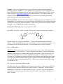
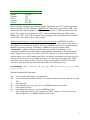
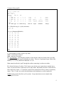
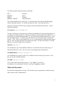
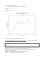
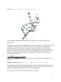
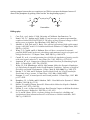
AMBER 8.0 Drug/DNA Complex Tutorial
John E. Kerrigan, Ph.D.
Robert Wood Johnson Medical School
The University of Medicine and Dentistry of New Jersey
675 Hoes Lane
Piscataway, NJ 08854
USA
(732) 235-4473 phone
(732) 235-5252 fax
[email protected]
1
Synopsis. Today you will learn how to use one of the most versatile molecular dynamics
modeling packages, AMBER 8. [1] The AMBER suite of programs was developed by the late
Peter A Kollman and colleagues at the University of California San Francisco (UCSF). See the
Amber webpage at http://amber.scripps.edu for more information. The Amber package was
designed with the ability to address a wide variety of biomolecules including proteins and
nucleic acids as well as small molecule drugs.
Research Problem. We will work on the complex of a DNA minor groove binding drug (γ-oxapentamidine). We will take the x-ray crystal structure (166D.PDB) [2] of the complex, and study
its behavior in water using molecular dynamics. Make a new project directory using the “mkdir”
command. Copy 166D.pdb and pet.pdb to this directory.
Preparation of the drug. Open your pet.pdb file in MOE.
Open MOE. Go to File > Open > pet.pdb (Click on Auto Connect and Center in the dialog).
H
O
H
N
H
N
H
O
O
H
N
H
N
H
H
Open the Builder by Clicking on the Builder … button on the right-hand side of the MOE
window. Change the formal charge of one of the nitrogens of each aminidinium group to +1 (i.e.
one nitrogen on each side of the molecule). Use the Element: tools in Molecule Builder.
Edit > Add Hydrogens
IMPORTANT: Each atom of the drug molecule must have a unique name! MOE does not do
this automatically! Click on Labels > Name to display the atom names. Select each Hydrogen
atom one-by-one and give it a unique name using the atoms dialog. Select the atom with your
mouse (turns pink) then Click on Atoms (right-hand side menu) > Atom Manager Click on
Selection only. Highlight the hydrogen atom in the Atom Manager and change the name from H
to H# (where # is the next number in the sequence; examine to see if the other hydrogen atoms
are numbered otherwise start numbering from 1.). When you are finished, replace the existing
file with the new file.
File > Save As > File Format: PDB : pet.pdb
The table below shows the AMBER names for nucleic acid residues. Those names with a D are
for DNA residues and those with an R are for RNA residues. A terminal 5′ residue would be
indicated by e.g. DA5 and a 3′ residue would be e.g. DT3. However, Leap will recognize the
normal nucleic acid names given and assume them to be DNA. Leap is able to differentiate 3′
from 5′ residues.
2
Group or Residue
Adenine
Thymine
Uracil
Cytosine
Guanine
Residue Name, Alias
DA, RA
DT
RU
DC, RC
DG, RG
Open 166D.pdb in nedit and open pet.pdb in nedit. Replace the old “PET” residue coordinate
records with the new PET coordinates. IMPORTANT: Remember to include the “TER” card
between the DNA and the ligand (i.e. “PET” residue) and place a “TER” card at the end of the
ligand. The Amber Leap program uses “TER” cards to distinguish between different chains.
Without the “TER” card, Leap will assume that everything is one chain and therefore “bonded”
to each other. Save the new file as “dna_pet.pdb”.
Making a special topology “prep” input file to describe the drug. AMBER has a residue
topology database to describe all of your nucleic acid residues as well as amino acid residues if
you happen to be working with a protein. However, AMBER does not have a special topology
database to describe your drug. Fortunately, AMBER has a special program called
“antechamber”, which is designed to build a topology prep file for your drug. [1] In
combination with DivCon (a semi-empirical QM program), antechamber will compute partial
atomic charges for your drug. We will use AM1-BCC charges[3], as these charges scale best
with the charge set we will be using on our DNA. By default, antechamber will write a prep file
with the general amber force field (gaff) atom types. To write a prep file with regular Amber
atom types, use the –at amber flag. However, always use the gaff force field for your small
molecules. Issue the following command from within your working directory.
antechamber –nc 2 –rn PET –i pet.pdb –fi pdb –o pet_bcc.prep –fo
prepi –c bcc
What the command line flags mean:
-nc
-rn
-i
-fi
-o
-fo
-c
is the net molecular charge (very important!)
is the residue name (default is MOL) Use a name here that you know is used in your pdb
file!
is the input file
is the input file type (e.g. pdb, mol2; see AMBER manual for more info)
is the output file name
is the output file type (e.g. prepi for AMBER prep file)
is the charge type used (bcc will compute AM1-BCC charges; rc will read in charges
from the input file; see AMBER manual for more info)
3
Contents of the prep file
0
0
2
This is a remark line
molecule.res
PET
XYZ 0
CORRECT
OMIT DU
BEG
0.0000
1 DUMM DU
M
0 -1
2 DUMM DU
M
1
0
3 DUMM DU
M
2
1
4 N1
n3
M
3
2
5 H4
hn
E
4
3
-2
-1
0
1
2
0.000
1.449
1.522
1.540
1.010
.0
.0
111.1
111.208
59.922
.0
.0
.0
180.000
-148.384
angle
dihedral
.00000
.00000
.00000
-0.456
0.334
… etc
#
name type
LOOP (Describe
C1
C6
C13
C8
ts connectivity
bnd len
charge
ring (i.e. cyclic) structures)
IMPROPER (Improper dihedrals)
C4
N1
C7
N2
C7
C5
C4
C3
C4
C6
C5
H5
C5
C1
C6
H6
C4
C2
C3
H7
C3
C1
C2
H8
C6
C2
C1
O1
C9 C13
C8
O2
C8 C10
C9 H17
C9 C11 C10 H18
C14 C10 C11 C12
C11
N3 C14
N4
C11 C13 C12 H20
C8 C12 C13 H19
DONE
STOP
# - atom number for atom I (can be any atom)
name – atom name for atom I
type – atom type for atom I
ts – Tree Structure – Describes the geometry of the structure and how it links to the rest of the
“larger” structure if this prep file describes a residue. There are 5 topological types: Main, Side,
Branch, (3, 4, 5, & 6), and End or M, S, B, 3 etc., E.
Main atoms describe the “path” through the residue connecting it to the next residue.
E is for the End atom of a chain. The E atoms can only have one connection to another heavy
atom. S (side) must have connections to two other atoms. B (branch) must have connections to
three other heavy atoms. A 3 atom has a total of four connections to heavy atoms (a quaternary
atom). The 4, 5, and 6 are used to describe higher order bonding (e.g. metal complexes).
LOOP closing section describes cyclic systems. Loop connections are not counted when
assigning M, S, B, etc.
4
DUMMY ATOMS – Three are required. These are used to define the space axes for the residue.
They must be given the topological description of “M”, and must be of the “Dummy” atom type,
DU.
connectivity – Here is what the 3 numbers mean in reference to atom I:
1st number – The atom # to which atom I is connected.
2nd number – The atom # to which atom I makes an angle along with NA(I)
3rd number – The atom # to which atom I makes a dihedral with NA(I) & NB(I).
NA(I)
NB(I)
NC(I)
bnd len – Equilibrium bond length between atom I and NA(I).
angle – The bond angle between NB(I), NA(I) and I.
dihedral – The dihedral angle between NC(I), NB(I), NA(I), and I
charge – The partial atomic charge on I.
LOOP – Describes a loop closing bond for each cyclic ring in the molecule.
IMPROPER – Tells amber which ‘improper’ torsion angles are to be used for the calculation. In
united atom models, improper torsions are used to keep asymmetric centers from racemizing. In
addition improper torsions are used to enforce planarity in cyclic ring systems in both united and
all atom models. The improper torsions are to be defined in such a way that the proper torsions
are not duplicated.
Use parmchk to check the parameters.
parmchk –i pet_bcc.prep –f prepi –o frcmod
Check the frcmod file contents (use more frcmod). You will notice that there are a few
parameters that needed estimates based on existing parameters. The output has no warnings
about unknown atoms or parameters. Therefore, we may proceed.
Contents of the frcmod file:
remark goes here
MASS
BOND
ANGLE
n3-c2-ca
ca-os-c3
66.300
62.700
124.550
118.150
same as c2-c2-n3
same as c2-os-c3
DIHE
IMPROPER
ca-n3-c2-n3
1.1
180.0
2.0
Using default value
5
ca-ca-ca-ha
ca-ca-ca-os
1.1
1.1
180.0
180.0
2.0
2.0
Using default value
Using default value
NONBON
xLeap and tLeap – These programs perform the same function with the difference being that
xLeap opens in an x-window interface and tLeap operates from a terminal prompt (no GUI).
The principal function of these programs is to prepare the AMBER coordinate (inpcrd) and
topology (prmtop) files.
xleap –s –f leaprc.ff99
The leaprc.ff99 file loads the parameters for the AMBER99 force field. [4, 5] The leaprc.gaff
file loads the parameter set for the general amber force field, which is used to describe your
small molecule.
In the leap window or prompt type the following commands one at a time:
source leaprc.gaff
mods = loadAmberParams frcmod
loadAmberPrep pet_bcc.prep
nap = loadPdb dna_pet.pdb
check nap
The check reveals a warning for the charge of the unit as being nonzero and it is a fraction! The
fraction arises due to a little bug in antechamber’s partial charge assignments. Leap will not
create a topology file for molecules of fractional charge (you will get an error!). The easy fix for
this problem is to add the small fractional difference to one of the charges (or, if necessary,
spread it out over several charges) in the pet_bcc.prep file. For example, our overall complex
charge was –19.99900; therefore, we need to add –0.001 to bring this total to –20.000. We
selected one electronegative atom in our drug structure and added –0.001 to it.
Type Quit to exit the xLeap program. Remove the old leap.log file (rm leap.log).
Edit the pet_bcc.prep file and make the appropriate charge correction(s).
Run xLeap and repeat the same sequence of commands (a new leap.log file will be saved).
After using the check command you will notice that you still have a warning about charge;
however, at least the charge is not fractional. We will add counterions to neutralize the overall
charge. To look at the unit in a graphical display use the “edit” command.
edit nap
6
The following mouse buttons perform as indicated:
LEFT MIDDLE RIGHT MIDDLE + RIGHT -
Selection
Rotate
Translate
Zoom In and Out
The structure should be fine at this point. You should notice that Leap has added hydrogen
atoms to the DNA structure. To exit the unit editor use Unit > close from the menu.
Solvate the structure in TIP3P water [6] using a truncated octahedron periodic box. Use the
following command;
solvateOct nap TIP3PBOX 8.0
You have told Leap to solvate the unit in a truncated octahedral box using a spacing distance of
8.0 angstroms around the molecule. Ideally, you should set the spacing at no less than 8.5 Å (~ 3
water layers) to avoid periodicity artifacts. [7] For particle-mesh ewald electrostatics, [8, 9] our
box side length must be > 2 X NB cutoff. We will use a 9.0 Å cutoff; therefore, our box side
must be > 18 Å. Our box side length will be (2 X 8) + DNA dimension, which should be greater
than 18. Now, lets add counterions to neutralize the charge. We had a total charge of –20.000;
therefore, we need 20 sodium ions to neutralize.
addIons nap Na+ 0
The command we just issued (addIons) added Na+ ions until the total net formal charge = 0.
This should add 20 Na+ ions. Now we can save the topology and coordinate files!
saveAmberParm nap pet.top pet.crd
As an additional step, you may want to save a PDB file of the model you just created. To do
this, just use the savePdb command.
savePdb nap pet_na.pdb
You’re done with file preparation (hooray!). Type “Quit” to exit xLeap!
Use Rasmol to view your model. In the winterm, type “rasmol pet_na.pdb”.
Molecular Dynamics
We’ll do these computations in 4 steps. The first three steps are preparatory and the last step is
what is known as the “production run”.
7
Step 1. Energy Minimization of the System. We perform a steepest descents energy
minimization to relieve bad steric interactions that would otherwise cause problems with or
dynamics runs.
Using the Sander program. The SANDER program is the number crunching juggernaut of the
AMBER software package. SANDER will perform energy minimization, dynamics and NMR
refinement calculations. You must specify an input file to tell SANDER what computations you
want to perform and how you would like to perform those computations. Study the input file for
energy minimization below.
The contents of the min1.in file.
Initial restrained minimization on DNA & DRG, 10 cut
&cntrl
imin = 1,
maxcyc = 1000,
ncyc = 250,
ntb = 1,
ntr = 1,
cut = 10
/
Hold the DNA & DRG fixed
500.0
RES
1
25
END
END
What it all means in a nutshell. There are many more settings above than we can possibly
explain here. So, for more in-depth info please consult the AMBER User’s Manual. The
settings important for minimization are highlighted and explained below.
&cntrl and / – Most if not all of your instructions must appear in the “control” block (hence
&cntrl).
cut = nonbonded cutoff in angstroms.
ntr = Flag used to perform position restraints (1 = on, 0 = off)
imin = Flag to run energy minimization (if = 1 then perform minimization; if = 0 then perform
molecular dynamics).
macyc = maximum # of cycles
ncyc = After ncyc cycles the minimization method will switch from steepest descents to
conjugate gradient.
ntmin = Flag for minimization method. (if = 0 then perform full conjugate gradient min with the
first 10 cycles being steepest descent and every nonbonded pairlist update; if = 1 for ncyc cycles
steepest descent is used then conjugate gradient is switched on [default]; if = 2 then only use
steepest descent)
dx0 = The initial step length
dxm = The maximum step allowed
drms = gradient convergence criterion 1.0E-4 kcal/mol•Å is the default
8
Hold the DNA and the DRG fixed
500.0 (This is the force in kcal/mol used to restrain the atom positions.)
RES 1 25 (Tells AMBER to apply this force to residue #’s 1 to 25).
Command line in general (Example only):
sander –O –i min.in –o min.out –p prmtop –c inpcrd –r restrt [ref refc –x mdcrd –v mdvel –e mden –inf mdinfo]
Issue the following command to run your energy minimization.
nohup sander –O –i min1.in –o min1.out –p pet.top –c pet.crd –r
pet_min1.rst –ref pet.crd &
Monitor the progress using “tail –20 min1.out” command.
Step 2. Minimization of whole system, no restraints.
Contents of min2.in file
System minimization on DNA & DRG, 10 cut
&cntrl
imin = 1,
maxcyc = 1500,
ncyc = 500,
ntb = 1,
ntr = 0,
cut = 10
/
END
nohup sander –O –i min2.in –o min2.out –p pet.top –c
pet_min1.rst –r pet_min2.rst &
Step 3. Position-Restrained Dynamics. This initial dynamics run is performed to relax the
positions of the solvent molecules. In this dynamics run, we will keep the macromolecule atom
positions restrained (not fixed, however). In a position-restrained run, we apply a force to the
specified atoms to minimize their movement during the dynamics. The solvent we are using in
our system, water, has a relaxation time of 10 ps; therefore we need to perform at least > 10 ps of
position restrained dynamics to relax the water in our periodic box.
Contents of md1.in
position restrained dynamics, model 1, 10.0 cut
&cntrl
imin = 0,
irest = 0,
ntx = 1,
ntb = 1,
cut = 10,
ntr = 1,
ntc = 2,
9
ntf = 2,
tempi = 0.0,
temp0 = 300.0,
ntt = 3,
gamma_ln = 1.0,
nstlim = 10000, dt = 0.002,
ntpr = 100, ntwx = 500, ntwr = 1000
/
Hold the drug and DNA fixed
10.0
RES 1 25
END
END
ntb = 1 Constant volume dynamics.
imin = 0 Switch to indicate that we are running a dynamics.
nstlim = # of steps limit.
dt = 0.002 time step in ps (2 fs)
temp0 = 300 reference temp (in degrees K) at which system is to be kept.
tempi = 0 initial temperature (in degrees K)
ig = ### seed for random number generator
heat = 0 multiplier for velocities (default = 0.0).
ntt = 3 temperature scaling switch (1 = Langevin Dynamics)
gamma_ln = 1.0 collision frequency in ps-1 when ntt = 3 (see Amber 8 manual).
tautp = 1.0 Time constant for the heat bath (default = 1.0) smaller constant gives tighter
coupling.
vlimit = 20.0 used to avoid occasional instability in dynamics runs (velocity limit; 20.0 is the
default). If any velocity component is > vlimit, then the component will be reduced to vlimit.
comp = 44.6 unit of compressibility for the solvent (H2O)
ntc = 2 Flag for the Shake algorithm (1 – No Shake is performed; 2 – bonds to hydrogen are
constrained; 3 – all bonds are constrained).
tol = #.##### relative geometric tolerance for coordinate resetting in shake.
The additional blocks that follow are the nmr restraint instructions. We will gradually warm the
system from 100 K to 300 K in the first picosecond; followed by maintaining the temperature at
300 K.
You will note that we used a smaller restraint force (10.0 kcal/mol). For dynamics, one only
needs to use 5 to 10 kcal/mol restraint force when ntr = 1 (uses a harmonic potential to restrain
coordinates to a reference frame; hence, the need to include reference coordinates with the –ref
flag.). Larger restraint forces lead to instability in the shake algorithm with a 2 fs time step.
Larger restraint force constants lead to higher frequency vibrations, which in turn lead to the
instability. Excess motion away from the reference coordinates is not possible due to the
steepness of the harmonic potential. Therefore, large restraint force constants are not necessary.
nohup sander –O –i md1.in –o md1.out –p pet.top –c pet_min2.rst
–r pet_md1.rst –x pet_md1.mdcrd –ref pet_min2.rst –inf md1.info
&
10
Monitor the progress using “tail –40 md1.out”. Our computation took about 1.8 hours to
complete on a 2.7 GHz linux workstation.
Step 4. The Production Run. This is where we do the actual molecular dynamics run. You will
do a 100 ps run.
Contents of md2.in
dynamics w/PME, DNA-Drug, 9.0 cut, 50 ps
&cntrl
imin = 0, irest = 1, ntx = 7,
ntb = 2, pres0 = 1.0, ntp = 1,
taup = 2,
cut = 10, ntr = 0,
ntc = 2, ntf = 2,
tempi = 300.0, temp0 = 300.0,
ntt = 3, gamma_ln = 1.0,
nstlim = 50000, dt = 0.002,
ntpr = 100, ntwx = 500, ntwr = 1000
/
END
ntp = 1 md with isotropic position scaling.
ntb = 2 constant pressure
pres0 = 1 reference pressure in bar
taup = 2.0 pressure relaxation time in ps
Issue the following command to run your dynamics simulation.
nohup sander –O –i md2.in –o md2.out –p pet.top –c pet_md1.rst –
r pet_md2.rst –x pet_md2.mdcrd –ref pet_md1.rst –inf md2.info &
Monitor the progress using “tail –40 md2.out”. Our 100 ps run took approximately 11 hours to
run on a 2.7 GHz linux workstation.
Analysis
Note: The sample data presented here will be different from your data if you started with crystal
structure. We used the result from an Autodock docking as our starting complex based on the
same crystal structure.
Copy process_mdout.perl to your working project directory. Use the “which” command to
determine the location of your perl interpreter (type “which perl”). On the SGI, the location
(after #!) should be /usr/sbin/perl. Check to make sure that the path in the perl script (1st line in
the script) matches whatever path was given by the result of your which command. Make sure
that the program is executable (use chmod 755 filename) where filename = process_mdout.perl.
./process_mdout.perl md1.out md2.out
11
The resulting files are readable by the Grace program (http://plasma-gate.weizmann.ac.il/Grace/
) or as space delimited files in Excel.
We will take a look at summary.EPTOT (potential energy plot). Here is our result…
The potential energy fluctuates throughout the simulation. The general trend is toward lower
energy after a jump in energy during the restrained dynamics (water pre-equilibration), which is
a good sign that the dynamics is leading toward lower energy conformations. Plot other files.
Use Microsoft Excel and read in the file as a space delimited file.
summary.TEMP gives the temperature fluctuation with time.
summary.PRES gives the pressure fluctuation with time.
The RMS plot. We will use the ptraj program.
Contents of rms.in
trajin pet_md1.mdcrd
trajin pet_md2.mdcrd
rms first out pet_rms.dat :1-25 time 1.0
trajin – specifies trajectory file to process
rms – computed RMS fit to the first structure of the first trajectory read in.
12
out – specifies name of output file
:1-25 – perform rmsd analysis on residues 1 through 25 only.
ptraj pet.top < rms.in
xmgrace pet_rms.dat
The model is beginning to equilibrate from 75 ps onward.
Analysis of hydrogen bonds over the course of the trajectory. Use the following input file to
ptraj.
trajin pet_md2.mdcrd
donor DC O2
acceptor PET N2’ H64
hbond distance 3.5 angle 120.0 donor acceptor neighbor 2 series hbond
DONOR/ACCEPTOR – use to specify the donor acceptor heavy atoms.
DISTANCE – use to specify the cutoff distance in angstroms between the heavy atoms
participating in the interaction.
ANGLE – The H-bond angle cutoff (donor-H-acceptor) in degrees.
SERIES – Directs H-bond data summary to STDOUT.
13
ptraj pet.top < hbond.in > pet_hbond.dat
View detailing the hydrogen bond being analyzed. (Image created using VMD [10] and
Raster3D [11])
The statistical analysis in the pet_hbond.dat file will be most important. Look for those H-bonds
with a high % occupancy (> 60%). These are the more stable H-bonds. The higher the %
occupancy; the better. Note that in our analysis we observe no output (i.e. empty files) for
pet_hb1. This is because the acceptor atoms in the ligand share no interaction with donor atoms
in the DNA. When analyzing H-bond data, it is best to establish reasonable guidelines for the
distance and angle cutoffs. A recent paper by Chapman et al. provides a nice discussion of
hydrogen bond criteria. [12]
The AMBPDB Conversion Program
How to use the ambpdb program to convert an amber restart coordinate file to a PDB file. For
example:
ambpdb –aatm –bres –p pet.top < pet_md2.rst > pet_md2.pdb
The –aatm flag insures that the hydrogen atom names conform to PDB standard and the –bres
flag insures that the residue names conform to PDB standard. Do not use the –bres flag if you
will be using this pdb file as input to xLeap for another computation!
First, remove the water molecules from the PDB file you created.
14
grep –v ‘WAT’ pet_md2.pdb > pet_md2_nw.pdb
Using X3DNA to examine the DNA structure.
The X3DNA program is a very useful tool for analyzing the stereochemical and other 3dimensional aspects of nucleic acids. X3DNA was developed by Xiang-Jun Lu in Wilma
Olson’s research group at Rutgers University (see http://rutchem.rutgers.edu/~xiangjun/3DNA/
for more information and a copy of the user manual). [13] You must start from a PDB file.
Analyze either your average structure or the last frame saved by Amber (i.e. the restrt file
converted to a pdb with ambpdb).
First, edit out the drug and all other HETAM records in a text editor. Start with the find_pair
utility (used to establish the base pair information).
find_pair myfile.pdb myfile.inp
Use the analyze program to carry out the analysis.
analyze myfile.inp
You now have an analysis of the structure of the DNA from the drug-DNA complex. Next, you
will make a comparison to the equilibrated DNA without drug. Download the dna.pdb file from
the course webpage and perform the same analysis on it. Compare differences in the minor and
major groove widths especially in the proximity of where the drug binds.
Questions to consider:
1. The authors (Nunn, et al.; ref #2) claim that the only interaction(s) they observe in their
structure is between the amidinium NH and the O4′ of the deoxyribose sugar. What hydrogen
bond interactions do you observe from your dynamics run?
2. The authors note that a chain of water molecules exist along the mouth of the minor groove
just outside the bound drug. Do you observe a similar pattern in the water structure of your
model? (Hint: Use the pet_md.restrt file; convert to a PDB using the ambpdb command to view
with any viewer – or – use moil-view to view the structure.).
3. Pentamidine has a higher binding affinity for this DNA duplex than does γ-oxa-pentamidine.
Make the appropriate structural change and develop a new prep file for pentamidine using
antechamber. Perform a dynamics run of the pentamidine complex and the γ-oxa-pentamidine,
each for 200 ps duration (i.e. nstlim = 100000). Perform the usual analysis. How does
pentamidine compare with γ-oxa-pentamidine in terms of number of hydrogen bonds with the
DNA? How do the interaction energies (Eint = Evdw + Eelec) of the two complexes compare
(Compare the energies of the average in-vacuo structures only.)? How does the minor groove
15
spacing compare between the two complexes (use 3DNA or measure the distance between P
atoms of the phosphates by picking 4 that ‘bracket’ the drug binding region.)?
H
O
H
N
H
N
O
H
H
N
H
N
H
H
Pentamidine
Bibliography:
1.
2.
3.
4.
5.
6.
7.
8.
9.
10.
11.
12.
13.
Case, D.A., et al., Amber 8. 2004, University of California: San Francisco, CA.
Nunn, C.M., T.C. Jenkins, and S. Neidle, Crystal structure of gamma-oxapentamidine
complexed with d(CGCGAATTCGCG)2. The effects of drug structural change on DNA
minor-groove recognition. Eur J Biochem, 1994. 226(3): p. 953-61.
Jakalian, A., D.B. Jack, and C.I. Bayly, Fast, efficient generation of high-quality atomic
charges. AM1-BCC model: II. Parameterization and validation. J Comput Chem, 2002.
23(16): p. 1623-41.
Wang, J., P. Cieplak, and P.A. Kollman, How well does a restrained electrostatic
potential (RESP) model perform in calculating conformational energies of organic and
biological molecules? J. Comput. Chem., 2000. 21(12): p. 1049-1074.
Cornell, W., et al., A second generation force field for the simulation of proteins, nucleic
acids, and organic molecules. J. Am. Chem. Soc., 1995. 117(19): p. 5179-5197.
Jorgensen, W., et al., Comparison of Simple Potential Functions for Simulating Liquid
Water. J. Chem. Phys., 1983. 79: p. 926-935.
Weber, W., P.H. Hünenberger, and J.A. McCammon, Molecular Dynamics Simulations
of a Polyalanine Octapeptide under Ewald Boundary Conditions: Influence of Artificial
Periodicity on Peptide Conformation. J. Phys. Chem. B, 2000. 104(15): p. 3668-3575.
Darden, T., D. York, and L. Pedersen, Particle Mesh Ewald: An N-log(N) method for
Ewald sums in large systems. J. Chem. Phys., 1993. 98: p. 10089-10092.
Essmann, U., et al., A smooth particle mesh ewald potential. J. Chem. Phys., 1995. 103:
p. 8577-8592.
Humphrey, W., A. Dalke, and K. Schulten, VMD - Visual Molecular Dynamics. J. Molec.
Graphics, 1996. 14.1: p. 33-38.
Merritt, E.A. and D.J. Bacon, Raster3D: Photorealistic Molecular Graphics. Methods
Enzymol., 1997. 277: p. 505-524.
Fabiola, F., et al., An Improved Hydrogen Bond Potential: Impact on Medium Resolution
Protein Structures. Protein Sci., 2002. 11: p. 1415-1423.
Lu, X. and W. Olson, 3DNA: a software package for the analysis, rebuilding and
visualization of three-dimensional nucleic acid structures. Nucleic Acids Res., 2003.
31(17): p. 5108-5121.
16