Download Embedding data in an audio signal, using acoustic OFDM

Institutionen för systemteknik
Department of Electrical Engineering
Examensarbete
Embedding data in an audio signal, using acoustic
OFDM
Examensarbete utfört i Kommunikationssystem
vid Tekniska högskolan i Linköping
av
Shuai Wang
LiTH-ISY-EX--11/4518--SE
Linköping 2011
Department of Electrical Engineering
Linköpings universitet
SE-581 83 Linköping, Sweden
Linköpings tekniska högskola
Linköpings universitet
581 83 Linköping
Embedding data in an audio signal, using acoustic
OFDM
Examensarbete utfört i Kommunikationssystem
vid Tekniska högskolan i Linköping
av
Shuai Wang
LiTH-ISY-EX--11/4518--SE
Handledare:
Erik Axell
isy, Linköpings universitet
Examinator:
Mikael Olofsson
isy, Linköpings universitet
Linköping, 12 October, 2011
Avdelning, Institution
Division, Department
Datum
Date
Division of Communication Systems
Department of Electrical Engineering
Linköpings universitet
SE-581 83 Linköping, Sweden
Språk
Language
Rapporttyp
Report category
ISBN
Svenska/Swedish
Licentiatavhandling
ISRN
Engelska/English
Examensarbete
C-uppsats
D-uppsats
Övrig rapport
2011-10-12
—
LiTH-ISY-EX--11/4518--SE
Serietitel och serienummer ISSN
Title of series, numbering
—
URL för elektronisk version
http://www.commsys.isy.liu.se
http://www.ep.liu.se
Titel
Title
Embedding data in an audio signal, using acoustic OFDM
Författare Shuai Wang
Author
Sammanfattning
Abstract
The OFDM technology has been extensively used in many radio communication
technologies. For example, OFDM is the core technology applied in WiFi, WiMAX
and LTE. Its main advantages include high bandwidth utilization, strong noise immunity and the capability to resist frequency selective fading. However, OFDM
technology is not only applied in the field of radio communication, but has also
been developed greatly in acoustic communication, namely the so called acoustic
OFDM. Thanks to the acoustic OFDM technology, the information can be embedded in audio and then transmitted so that the receiver can obtain the required
information through certain demodulation mechanisms without severely affecting
the audio quality.
This thesis mainly discusses how to embed and transmit information in audio
by making use of acoustic OFDM. Based on the theoretical systematic structure, it
also designs a simulation system and a measurement system respectively. In these
two systems, channel coding, manners of modulation and demodulation, timing
synchronization and parameters of the functional components are configured in the
most reasonable way in order to achieve relatively strong stability and robustness
of the system. Moreover, power control and the compatibility between audio and
OFDM signals are also explained and analyzed in this thesis.
Based on the experimental results, the author analyzes the performance of the
system and the factors that affect the performance of the system, such as the type
of audio, distance between transmitter and receiver, audio output level and so on.
According to this analysis, it is proved that the simulation system can work steadily
in any audio of wav format and transmit information correctly. However, due
to the hardware limitations of the receiver and sender devices, the measurement
system is unstable to a certain degree. Finally, this thesis draws conclusions of the
research results and points out unsolved problems in the experiments. Eventually,
some expectations for this research orientation are stated and relevant suggestions
are proposed.
Nyckelord
Keywords
acoustic, acoustic OFDM, power control, embed
Abstract
The OFDM technology has been extensively used in many radio communication
technologies. For example, OFDM is the core technology applied in WiFi, WiMAX
and LTE. Its main advantages include high bandwidth utilization, strong noise immunity and the capability to resist frequency selective fading. However, OFDM
technology is not only applied in the field of radio communication, but has also
been developed greatly in acoustic communication, namely the so called acoustic
OFDM. Thanks to the acoustic OFDM technology, the information can be embedded in audio and then transmitted so that the receiver can obtain the required
information through certain demodulation mechanisms without severely affecting
the audio quality.
This thesis mainly discusses how to embed and transmit information in audio
by making use of acoustic OFDM. Based on the theoretical systematic structure, it
also designs a simulation system and a measurement system respectively. In these
two systems, channel coding, manners of modulation and demodulation, timing
synchronization and parameters of the functional components are configured in the
most reasonable way in order to achieve relatively strong stability and robustness
of the system. Moreover, power control and the compatibility between audio and
OFDM signals are also explained and analyzed in this thesis.
Based on the experimental results, the author analyzes the performance of the
system and the factors that affect the performance of the system, such as the type
of audio, distance between transmitter and receiver, audio output level and so on.
According to this analysis, it is proved that the simulation system can work steadily
in any audio of wav format and transmit information correctly. However, due to
the hardware limitations of the receiver and sender devices, the measurement
system is unstable to a certain degree. Finally, this thesis draws conclusions of the
research results and points out unsolved problems in the experiments. Eventually,
some expectations for this research orientation are stated and relevant suggestions
are proposed.
v
Acknowledgments
First of all I would like to thank my superviser Erik Axell for his kindness and
patience to solve problems that I encountered during my thesis work. I would
also like to thank professor Mikael Olofsson for his guidance of the whole thesis
procedure. Secondly, I would like to thank:
My lover Yingying Huang for her support in Sweden during my thesis work.
My parents for their moral support during my master study period.
Last but not least, I would like to thank all my friends in Sweden who are
accompanying with me during the past two years.
SHUAI WANG
Linköping,Sweden,2011
vii
Abbreviations
ASCII
AWGN
CP
DBPSK
DC
FDM
FEC
FFT
GI
GUI
ICI
IFFT
ISI
LTE
M-PSK
OFDM
QAM
QPSK
SDR
SNR
URL
WGN
WiFi
WiMAX
American Standard Code of Information Interchange
Additional White Gaussian Noise
Cyclic Prefix
Differential Binary Phase-Shift Keying
Direct Current
Frequency Division Multiplexing
Forward Error Correction
Fast Fourier Transform
Guard Interval
Graphical User Interface
Inter-Carrier Interference
Inverse Fast Fourier Transform
Inter-Symbol Interference
Long Term Evolution
M Phase-Shift Keying
Orthogonal Frequency Division Multiplexing
Quadrature Amplitude Modulation
Quadrature Phase-Shift Keying
Signal-to-Distortion Ratio
Signal-to-Noise Ratio
Universal Resource Locator
White Gaussian Noise
Wireless Fidelity
World Interoperability for Microwave Access
Contents
1 Introduction
1.1 Problem Formulation . . . . . . . . . . . . . . . . . . . . . . . . . .
1.2 Thesis Objective . . . . . . . . . . . . . . . . . . . . . . . . . . . .
1.3 Thesis Outline . . . . . . . . . . . . . . . . . . . . . . . . . . . . .
2 Background of acoustic OFDM
2.1 OFDM . . . . . . . . . . . . . .
2.1.1 Orthogonality . . . . . .
2.1.2 Advantages of OFDM .
2.1.3 System Model . . . . . .
2.2 Acoustic OFDM . . . . . . . .
2.2.1 Power Control . . . . .
2.2.2 Compatibility . . . . . .
1
1
2
2
.
.
.
.
.
.
.
.
.
.
.
.
.
.
.
.
.
.
.
.
.
.
.
.
.
.
.
.
.
.
.
.
.
.
.
.
.
.
.
.
.
.
.
.
.
.
.
.
.
.
.
.
.
.
.
.
.
.
.
.
.
.
.
.
.
.
.
.
.
.
.
.
.
.
.
.
.
.
.
.
.
.
.
.
.
.
.
.
.
.
.
5
5
6
6
9
10
11
11
3 Method
3.1 Information Transformation . . . . . . . . . .
3.2 Channel Coding . . . . . . . . . . . . . . . . .
3.2.1 Convolutional Code . . . . . . . . . .
3.2.2 Interleaving . . . . . . . . . . . . . . .
3.2.3 Viterbi Decoding . . . . . . . . . . . .
3.3 Modulation Method . . . . . . . . . . . . . .
3.4 Pilot . . . . . . . . . . . . . . . . . . . . . . .
3.5 Power Control . . . . . . . . . . . . . . . . . .
3.6 Compatibility between audio and useful data
3.7 Timing Synchronization . . . . . . . . . . . .
.
.
.
.
.
.
.
.
.
.
.
.
.
.
.
.
.
.
.
.
.
.
.
.
.
.
.
.
.
.
.
.
.
.
.
.
.
.
.
.
.
.
.
.
.
.
.
.
.
.
.
.
.
.
.
.
.
.
.
.
.
.
.
.
.
.
.
.
.
.
.
.
.
.
.
.
.
.
.
.
.
.
.
.
.
.
.
.
.
.
.
.
.
.
.
.
.
.
.
.
.
.
.
.
.
.
.
.
.
.
.
.
.
.
.
.
.
.
.
.
13
13
13
14
15
16
16
16
18
20
20
4 Implementation
4.1 Simulation System . . . . . . . .
4.1.1 Information Source . . . .
4.1.2 Channel Coding . . . . .
4.1.3 DBPSK Modulation . . .
4.1.4 Power Control . . . . . .
4.1.5 OFDM Modulation . . . .
4.1.6 Frequency Conversion . .
4.1.7 The Signal Compatibility
.
.
.
.
.
.
.
.
.
.
.
.
.
.
.
.
.
.
.
.
.
.
.
.
.
.
.
.
.
.
.
.
.
.
.
.
.
.
.
.
.
.
.
.
.
.
.
.
.
.
.
.
.
.
.
.
.
.
.
.
.
.
.
.
.
.
.
.
.
.
.
.
.
.
.
.
.
.
.
.
.
.
.
.
.
.
.
.
.
.
.
.
.
.
.
.
23
25
27
27
28
28
29
29
33
.
.
.
.
.
.
.
xi
.
.
.
.
.
.
.
.
.
.
.
.
.
.
.
.
.
.
.
.
.
.
.
.
.
.
.
.
.
.
.
.
.
.
.
.
.
.
.
.
.
.
.
.
.
.
.
.
.
.
.
.
.
.
.
.
.
.
.
.
.
.
.
.
.
.
.
.
.
.
.
.
.
.
.
.
.
.
.
.
.
.
.
.
.
.
.
.
.
.
.
.
.
.
.
.
.
.
xii
Contents
.
.
.
.
.
.
.
.
.
.
.
.
.
.
.
.
.
.
.
.
.
.
.
.
.
.
.
.
.
.
.
.
.
.
.
.
.
.
.
.
.
.
.
.
.
.
.
.
.
.
.
.
.
.
.
.
.
.
.
.
.
.
.
.
.
.
.
.
.
.
.
.
.
.
.
.
.
.
.
.
.
.
.
.
.
.
.
.
.
.
.
33
35
35
37
37
37
42
. . . . . . . . . . . .
. . . . . . . . . . . .
. . . . . . . . . . . .
. . . . . . . . . . . .
. . . . . . . . . . . .
. . . . . . . . . . . .
. . . . . . . . . . . .
Sender and Receiver
. . . . . . . . . . . .
. . . . . . . . . . . .
. . . . . . . . . . . .
. . . . . . . . . . . .
.
.
.
.
.
.
.
.
.
.
.
.
.
.
.
.
.
.
.
.
.
.
.
.
.
.
.
.
.
.
.
.
.
.
.
.
.
.
.
.
.
.
.
.
.
.
.
.
.
.
.
.
.
.
.
.
.
.
.
.
.
.
.
.
.
.
.
.
.
.
.
.
.
.
.
.
.
.
.
.
.
.
.
.
.
.
.
.
.
.
.
.
.
.
.
.
.
.
.
.
.
.
.
.
.
.
.
.
.
.
.
.
.
.
.
.
.
.
.
.
.
.
.
.
.
.
.
.
.
.
.
.
.
.
.
.
.
.
.
.
.
.
.
.
45
45
45
45
48
49
51
52
52
53
54
56
58
6 Conclusions and future work
6.1 Conclusions . . . . . . . . . . . . . . . . . . . . . . . . . . . . . . .
6.2 Future Work . . . . . . . . . . . . . . . . . . . . . . . . . . . . . .
59
59
59
Bibliography
61
A User Manual of The System GUI
A.1 Simulation System . . . . . . . . . . . . . . . . . . . . . . . . . . .
A.2 Measurement System . . . . . . . . . . . . . . . . . . . . . . . . . .
63
63
65
B Programming Codes
B.1 Simulation System . . . . . . . . . . . . . . . . . . . . . . . . . . .
B.2 Measurement System . . . . . . . . . . . . . . . . . . . . . . . . . .
66
66
70
4.2
4.1.8 Channel . . . . . . . . .
4.1.9 GUI . . . . . . . . . . .
4.1.10 Receiver . . . . . . . . .
Measurement System . . . . . .
4.2.1 Channel . . . . . . . . .
4.2.2 Timing Synchronization
4.2.3 GUI . . . . . . . . . . .
5 Evaluation
5.1 Test Environment . . . .
5.2 Simulation Result . . . .
5.2.1 Power Spectrum
5.2.2 Bit Error Rate .
5.2.3 Audio Distortion
5.3 Measurement Result . .
5.3.1 Audio Type . . .
5.3.2 Distance between
5.3.3 Sound Level . . .
5.3.4 SDR . . . . . . .
5.3.5 Audio Distortion
5.3.6 Limitations . . .
.
.
.
.
.
.
.
.
.
.
.
.
.
.
.
.
.
.
.
.
.
.
.
.
.
.
.
.
.
.
.
.
.
.
.
.
.
.
.
.
.
.
.
.
.
.
.
.
.
Chapter 1
Introduction
In the development of today’s communication technology, the widely used techniques of information exchange such as WiFi, WiMAX and LTE are achieved
through radio communication technologies. These techniques share one common
feature by using Orthogonal Frequency Division Multiplexing (OFDM). As a core
technology in many communication standards, OFDM has been extensively applied mainly due to its high bandwidth utilization rate, strong noise immunity
and the capability to resist frequency selective fading [1]. Also, OFDM technology
cannot only be applied in radio communication technology, but in acoustic signal
transmission, namely the so called acoustic OFDM [2]. Making good use of the
advantages of the OFDM technology, acoustic OFDM can modulate the useful information, which is then transmitted in air or water with the help of sound sending
devices such as loudspeakers. In this way, the receiver, such as a microphone could
obtain such useful information through some kind of demodulation mechanisms,
once they received the sound. Acoustic OFDM is mostly applied in underwater
information exchange [3], for example in the short distance information exchange
between different hulls. However, another more updated application of acoustic
OFDM is embedding data in different audio to transmit the information. The high
frequency band of the audio is partly replaced by OFDM signals and the impact
on the audio quality can be mitigated by using power control of OFDM signals [2].
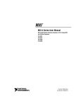
The idea behind acoustic OFDM is showed in Figure 1.1. Before acoustic OFDM,
several approaches have been proposed to derive useful data from the audio signals
such as echo hiding [4], phase coding [5] and spread spectrum [6]. How ever these
methods can only achieve a very low data rate. Thanks to this technology, some
short information such as a URL or media information advertising can all be effectively transmitted to the terminal end like a mobile phone through the manner
of audio such as music.
1.1
Problem Formulation
In common acoustic OFDM technology, the sender could directly broadcast the
OFDM signals through an audio generator such as a loud speaker. This kind of
1
2
Introduction
Figure 1.1. The algorithm of acoustic OFDM
sound is usually screaming noise similar to white Gaussian noise, which would impact people’s normal life once used in the real world. However, if the OFDM signal
is embedded in an audio signal and transmitted in the manner of power control,
no noise will be produced and the audio quality will not be affected much. More
importantly, the useful information could be transmitted effectively in this way.
There are mainly three issues discussed in this paper. One is how to embed OFDM
information into an audio signal and to transmit information without affecting the
audio quality too much. Second, how to control the power of OFDM information
and realize the compatibility between audio and OFDM signals. Third, how to
make use of MATLAB simulation results to study the factors that affect the stability and robustness of the acoustic OFDM system as well as to which degree those
different factors affect the audio quality and the performance of the communication
system.
1.2
Thesis Objective
This thesis project aims to realize the following points:
1. Complete detailed study and analysis of acoustic OFDM systems.
2. Design the acoustic OFDM simulation system and measurement system.
3. Study the factors such as audio type, audio output level and distance between
microphone and loudspeaker which affect the robustness of the system by
analyzing the operating results of the designed system.
1.3
Thesis Outline
Chapter 1 gives an overview of the application of OFDM technology in the field
of acoustics and how to make use of acoustic OFDM to transmit information. In
addition, this chapter also proposes the overall research direction of this thesis
1.3 Thesis Outline
3
and the required experiments based on software. Finally, the objective of this
thesis is pointed out clearly.
Chapter 2 makes a further introduction of the theories of OFDM technology and
how the OFDM technology realizes relatively high utilization of the frequency
band, strong noise immunity and strong capability to resist frequency selective
fading. Moreover, the theories of acoustic OFDM technology will be described in
detail, and the power control technique and the combination manner between
audios and OFDM signals will be especially elaborated on.
Chapter 3 describes the systematic theory structure established in the
experiments, including channel coding, modulation-demodulation, power control,
compatibility design of audio and OFDM signals and the manner of timing
synchronization.
Chapter 4 elaborates on the simulation system and implementation method
based on the design theories. Besides, the difference between the two systems
and possible problems are also analyzed in this chapter.
Chapter 5 first describes the testing environment of the experiment, and then
analyzes the testing results of the two experiment systems. For the measurement
experiment, we will mainly focus on the factors that could affect the
experimental result.
Chapter 6 concludes the research results of this thesis and it also makes related
evaluation of the experiments mentioned in chapter five. In addition, some
problems which still exist and demand prompt solutions are described. Finally,
the research direction of the problem that I have dealt with in this thesis will be
proposed in this chapter.
Chapter 2
Background of acoustic
OFDM
2.1
OFDM
OFDM is the abbreviation of Orthogonal Frequency Division Multiplexing. It is
a special case of Frequency Division Multiplexing (FDM) for which the carriers
are orthogonal. OFDM uses a lot of orthogonal subcarriers to carry and transmit
data. The data will be divided into several parallel channels or streams and each
subcarrier will occupy one channel. For each subcarrier the data will be modulated
with a conventional modulation scheme such as BPSK or PSK with high orders
at a low symbol rate. Before introducing OFDM, we need to clarify the difference
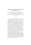
between FDM and OFDM in terms of frequency spectrum distribution. Figure
2.1 illustrates the spectrum distributions of FDM and OFDM respectively.
Figure 2.1. The spectrum utilization for FDM and OFDM
From Figure 2.1 we know that for the FDM modulation method, the signals
will be modulated and sent out in different subcarriers at the same time. In
addition, there is a protection interval in the frequency domain between every two
subcarriers to resist inter-carrier interference (ICI) [1]. Therefore, the utilization
ratio of the spectrum is relatively low. For OFDM, every two subcarriers will
overlap with each other, which can save a lot of spectrum to transmit more data.
5
6
2.1.1
Background of acoustic OFDM
Orthogonality
Orthogonality is a key point for the OFDM technology. In every OFDM signal
period, the neighboring subcarriers are orthogonal [1]. To understand the concept
of orthogonality, we assume that there are two signals x(t) and y(t) which are
orthogonal, and then they will meet the following equation in the time domain:
1
T
ZT
∗
x (t) · y (t) = 0
0
∗
where (·) denotes complex conjugate operator, T is the time period for one OFDM
symbol.
In frequency domain, orthogonality means that the value of each subcarrier is
exactly zero at the central frequency of its neighboring subcarriers which will not
result in inter carrier interference (ICI).
2.1.2
Advantages of OFDM
High Utilization Ratio of Spectrum
Due to its advantages, the OFDM technology has been widely applied in the field
of radio communications. According to the previous introduction, it is known that
the overlaps of adjacent subcarriers can raise the spectrum utilization ratio. In
the following, we will describe two other merits of OFDM.
High Anti-Interference Capability
An OFDM system adopts multiple carriers mode to transmit data. For each
carrier the number of bits can be adjusted according to the signal-to-noise ratio
(SNR) of each carrier, i.e. for the carriers with high SNR more data bits will be
assigned. So the anti-noise capability of OFDM system is enhanced. Due to the
reflection phenomenon, the transmitted signal is affected by multipath propagation
and the receiver will obtain several versions of the useful data with different latency.
Therefore inter-symbol interference can easily occur if there is no protection for
this case. Figure 2.2 depicts this situation.
Figure 2.2. ISI for OFDM signals without guard interval
Considering the fact that ISI will occur frequently without a protection mechanism, we will set a guard interval (GI) [1] between adjacent OFDM signals. This
2.1 OFDM
7
guard interval should be longer than the time period of the channel pulse response
to ensure that the inter-symbol interference can be eliminated. Figure 2.3 shows
the GI distribution in OFDM signals.
Figure 2.3. The distribution of guard intervals in OFDM symbols
For the simple case a guard interval will be filled with zero values, namely
silent guard interval, which means that no information is conveyed in it. The
inter-symbol interference problem can be truly resisted in this way. However,
due to the influence of the latency caused by multipath propagation, there will
be several different versions for each signal at the receiver. Consequently, when
the same OFDM signals with different latencies are received, the phase difference
between adjacent subcarriers will not maintain an integer cycle. This will cause the
loss of orthogonality among these subcarriers, and finally cause the inter-carrier
interference in the process of OFDM demodulation at the receiver. Figure 2.4
demonstrates the reason that causes ICI.
Figure 2.4. The ICI problem for adjacent subcarriers
In order to solve this problem, a concept called cyclic prefix (CP) [1] should
be introduced, which is showed as Figure 2.5.
If we replicate the data with the same length as GI from the end of the useful data frame and substitute the original guard interval, then the OFDM signals
8
Background of acoustic OFDM
Figure 2.5. The distribution of cyclic prefix in OFDM symbols
formed in this way can still keep the orthogonality between the neighboring subcarriers in the course of demodulation. Accordingly, inter-channel interference can
be avoided. Figure 2.6 explains how CP ensures the orthogonality between the
neighboring subcarriers of OFDM signals.
Figure 2.6. The effect of cyclic prefix for persistence of the orthogonality of subcarriers
High Capacity for Fading Resistance
Due to the existence of multiple carriers, some of the subcarriers might be seriously
influenced by the frequency selective fading and no data can be correctly transmitted on these subcarriers. However, the subcarriers that are affected by the fading
will still work steadily and robustly. So the data transmission on these subcarriers
will not be influenced too much. Figure 2.7 illustrates what the frequency selective
fading is and how it affects the channel.
Although the power of some subcarriers is restricted due to the influence of
frequency selective fading, the other subcarriers can still work with normal power.
This can achieve a low bit error rate for the data transmission.
2.1 OFDM
9
Figure 2.7. The effect of frequency selective fading on multiple carriers
2.1.3
System Model
A fully-formed OFDM system should consists of the parallel/serial conversion,
modulation/demodulation and time/frequency conversion. Figure 2.8 illustrates
the theoretical structure of the transmitter for an OFDM system.
Figure 2.8. The transmitter for an OFDM system
As is showed in the figure, after one serial-to-parallel conversion, the signals
will be conveyed through several subchannels. By using, for example, M-PSK
or QAM modulation, the information bits will be mapped into a constellation
diagram. This will show the information bits in the complex plane which is also a
conversion from time domain to frequency domain. Then the modulated symbols
are processed by IFFT to form the OFDM symbols. Moreover, the role played by
IFFT here is not only to convert signals from frequency domain to time domain,
but also to achieve the orthogonality among subcarriers. Complex signals that are
derived from IFFT will be divided into real and imaginary components before going
through a digital-to-analog conversion. Then, these analog signals will be used to
modulate cosine and sine waves at certain frequency. Finally the data of the real
part and imaginary part will be combined and sent out from the radiation device.
Referring to Figure 2.8, the mathematical expression of the low-pass OFDM signals
10
Background of acoustic OFDM
can be written as
s(t) =
N
−1
X
Xk ej2πkt/T , 0 ≤ t < T,
k=0
where Xk is the modulated symbol, N is the number of subcarriers, T is the
period of an OFDM symbol. Here the bandwidth of each subcarrier should equal
to 1/T which can guarantee the orthogonality between every two subcarriers. This
property can be indicated as the following expression:
1
T
ZT
(e
) (e
j2πk1 t/T ∗
j2πk2 t/T
0
1
)dt =
T
ZT
ej2π(k1 −k2 )t/T dt = 0.
0
In real systems, problems such as inter-carrier interference or inter-symbol interference should all be taken into consideration, so cyclic prefix should be added
in to resist these influences. Under the condition of utilizing cyclic prefix, the
expression of a low-pass OFDM signal can be written as the following:
PN −1
j2πkt/T
s(t) =
, −Tg ≤ t < T, where Tg is the length of the guard
k=0 Xk e
interval in which the cyclic prefix is transmitted.
At the receiver, all the signals will be converted down to baseband, and then the
time domain signals will be processed by FFT after the digital-to-analog conversion. Finally, the original signals are obtained through demodulation and parallelto-serial conversion. Moreover, the demodulator should utilize the demodulation
mode corresponding to the modulator of the sender, namely the demodulation
mechanism for M-PSK or QAM. Figure 2.9 reveals the theoretical structure of the
receiver for an OFDM receiver.
Figure 2.9. The receiver for an OFDM system
2.2
Acoustic OFDM
Based on the OFDM technology, acoustic OFDM is used to transmit useful information by making use of an acoustic channel. This thesis mainly discusses how
2.2 Acoustic OFDM
11
to embed data in an audio signal by using acoustic OFDM without influencing
the audio quality too much. Therefore, acoustic OFDM has two new features
compared with OFDM. First, the power of OFDM signals should be under control. Second, some certain mechanism is required to integrate audio with OFDM
signals.
2.2.1
Power Control
Power control is a core content in this thesis. One way to embed signals into audio
without impacting on the audio quality is to mimic the original audio signals by
using power-controlled signals. The audio signals in high frequency band will be
substituted by this kind of power-controlled signals. The whole process will be
achieved in frequency domain. In this way, the audio quality can still persist in a
good situation and the useful data will also be transmitted correctly.
2.2.2
Compatibility
Compatibility means that the audio signals are compatible with the modulated
useful information. On the one hand, the sampling rate of the useful signals will
increase after the OFDM modulation. On the other hand, the audio will not only
be used to control the power of the useful signals, but also integrated with the
OFDM signals. Therefore, we need to consider how to ensure the same sampling
rates of the two signals during integration, or a series of problems will arise. As
to this issue, we use the method of re-sampling. Since the sampling rate of useful
information will increase after the OFDM modulation, we will up-sample the audio
signals to increase more sampling points in a unit time. This method will realize
the compatibility of these two kinds of signals during their integration, and it
will not bring any influence on the quality of the original audio. The specific
implementation method will be elaborated on in the following chapters.
Chapter 3
Method
An acoustic OFDM system is composed of several subsystems, each of which plays
its special role. This chapter will explain the theoretical structure and implementation methods of these subsystems in the experiment.
3.1
Information Transformation
Information is some kind of meaningful signs that can be understood by human
being and make people react to them. However, in the world of computer we can
not simply transmit a word or a number in their original type. The computer can
only accept binary information which means that we need to find an approach to
make the real life information compatible with the computer. Or we can not do
any digital signal processing such as the channel coding and modulation in this
thesis experiment. In computers each letter, number or sign has an unique number
to represent it and this number could be decimal or binary. This is the so called
ASCII which stands for American Standard Code of Information Interchange. If
we want to handle some information in a computer, we can just transform the
real life information into ASCII with their binary type, and then the computer
will identify this kind of information. Figure 3.1 shows an example of how the
information transformation works.
In my thesis experiment the source information is some kind of text message or
URL, so for the transmitter I need to transform them into their binary type first
by using ASCII, and then process the binary sequences in the system. Also for the
receiver we need to revert the information by using ASCII from binary sequences
into the type that people can understand.
3.2
Channel Coding
Channel coding is aiming to achieve the role of error correction by adding in some
new supervisory code elements according to certain rules. It cannot only match
with the statistical properties of the channel, but also enhance the communication
13
14
Method
Figure 3.1. Information Transformation
reliability. Therefore, the information will have some redundancy after the channel
coding. The channel coding method utilized in this experiment is the combination
of a convolutional code and interleaving.
3.2.1
Convolutional Code
A convolutional code is a kind of forward error correction code (FEC) [7], which
has an excellent capability of correcting random errors. Figure 3.2 is an example
of a convolutional code with a rate of 1/3 and constraint length of 2.
Figure 3.2. An example of a convolutional encoder with rate 1/3 and constraint length
2
From the figure above we know that this system has three registers, one input and
3.2 Channel Coding
15
three outputs. The system will generate three output values from each input data,
and then shift the state values of the registers to the right side corresponding to
the input value. The iteration will keep working until all the information bits are
encoded. The mathematical expression for this system is:
• y1 (t) = u(t) + u(t − 1) + u(t − 2)
• y2 (t) = u(t − 1) + u(t − 2)
• y3 (t) = u(t) + u(t − 2)
The three equations above are binary addition which means that the inputs and
outputs are binary and the addition calculation will follow the binary addition
rules.
The convolutional code adopted in this experiment has a rate of 1/3 and constraint length of 7. Its specific parameter configuration will be elaborated on in
the following chapters.
3.2.2
Interleaving
Bit errors often happen continuously in the process of signal transmission, and
that is because some fading valley points which last for a long time will influence
the continuous bit information. Moreover, most of the channel coding methods can
implement the error correction effectively only for signal error or errors with short
length. As a result, in order to correct the burst errors, interleaving is needed to
disperse these errors [8]. In this way, long-string bit errors can be transformed into
short-string bit errors which will make the forward error correction more effective.
Figure 3.3 shows the working principle of a pattern of interleaving.
Figure 3.3. The algorithm of Interleaving by using matrix where the data is written
column-wise and read row-wise
The interleaving mode applied in this thesis is general block interleaving,
namely to interleave the rows or columns of the original bit matrix in accordance
16
Method
with certain rules so that the data of the original rows or columns are switched
to other locations. In this way, the possible bit errors can be fully dispersed, thus
greatly improving the capability of the error correction.
3.2.3
Viterbi Decoding
From the description in the previous subsection, we know that the convolutional
encoder can be considered as a finite state machine. It has 2n states where n is the
number of registers in the system, so we can also represent the output of the system
on a Trellis diagram. Trellis diagram is used to illustrate how the states of the
coding system change in time. It does not only show the instantaneous transitions
but also gives the most probable system outputs and the state transitions. After
handled by the convolutional encoder, the coded signals can be decoded by using
the Viterbi algorithm. Viterbi algorithm is a kind of decoder that utilizes the
maximum likelihood decoding method. Based on the received information, the
Viterbi decoder can find a route which has the most likely information sequence
corresponding to the original transmitted information on the Trellis diagram. This
route is also called Viterbi path on which a cluster of the information bits is exactly
the one we should obtain through the decoding process [7][8].
3.3
Modulation Method
The digital signal has a very poor capability of anti-interference and anti-noise
when it propagates in the channel. What’s more, under normal conditions, the information which can be transmitted in the channel should be analog signals. Consequently, in order to promote the channel utilization rate and anti-interference capability, digital signals will be combined with some kind of carrier signals through
a certain modulation approach which can also facilitate Digital-to-Analog Conversion. For acoustic OFDM, the main modulation approach is M-PSK. In this
experiment, we use the approach of differential binary phase shift keying (DBPSK).
DBPSK transmits data in the way of shifting the carrier phases, namely using the
phase shift to modulate carriers and finally send out binary information. For example, if ’0’ and ’1’ respectively represent adding 0◦ and 180◦ to the current phase
of the carrier, then the output waveform of DBPSK can be shown as Figure 3.4 in
case that the input signals are ’1001’ and the phase reference is 0◦ . One advantage
of utilizing DBPSK is that the bit error rate caused by the phase ambiguity can
be offset [9].
3.4
Pilot
In telecommunications, a pilot is a kind of signal which is transmitted with the
useful signal for supervisory, control or equalization purposes. There are two
common distributions for pilots which are block type and comb type. For block
type the pilots will be distributed in different time interval, and for comb type the
3.4 Pilot
17
Figure 3.4. The timing diagram for DBPSK
pilots will be deployed at different frequencies or subcarriers. Figure 3.5 illustrates
the pilots arrangement.
Figure 3.5. Pilot arrangement
For most of the time we can use pseudorandom signals as the pilots. A pseudorandom signal is a kind of signal that appears to be random but it is not. Pseudorandom sequences have statistical randomness, however they are generated by
certain deterministic causal processes. This process will restrict the length of the
randomness, and after that the process will produce exactly the same sequence.
Pseudorandom signal is very useful for lab testing or experimental verification.
The process to generate pseudorandom signals is easier to produce than a truly
random one. So we alway use pseudorandom signals to substitute the real random
signals.
Due to the phase ambiguity problem pilots are used to do the channel estimation in most of the OFDM systems . The phase of the modulated signal will be
changed after the channel. We can not adjust the phase error efficiently because it
is impossible to predict the phase change precisely by measuring the useful signal
18
Method
itself. Therefore we transmit pilots which have known phases in the channel, and
then measure the phase change of pilots as an reference for the phase adjustment
of useful signals. Channel estimation can correct the phase ambiguity problem,
decrease the bit error rate and enhance the system stability.
3.5
Power Control
To understand the functionality of power control we can refer to Figure 3.6 which
compares the difference when using power control or not.
Figure 3.6. The power spectrum of the system with and without power control
From the figure above we know that if we combine the audio signal and the OFDM
symbols without power control, the spectrum of the mixed signal in the high
frequency band will maintain at a constant value. This situation will bring a lot
of noise to the audio signal. However, if we use power control, the power of the
high frequency band will vary continuously and mimic the power of the original
audio to diminish the noise and mitigate the audio distortion. In particular, the
power control procedure is performed in the frequency domain. Once the audio
is converted to the frequency domain, the amplitude values of the corresponding
passband will be extracted to control the power of the modulated symbols [10].
The schematic diagram is shown in Figure 3.7.
According to this diagram, the power control takes place in the frequency
domain after the modulation. The power in the corresponding frequency band of
the audio signal will be derived to control the power of useful signals. Then the
audio signal in the low frequency band is combined with the useful symbols which
are OFDM-modulated before they are emitted. One problem of power control
is that the power of the useful signals will not be zero while the audio power at
some frequencies will be zero. Hence, we need to set a threshold value for the
audio control module, and this will prevent the power of the useful signals from
becoming zero and avoid the occurrence of higher bit error rate.
3.5 Power Control
Figure 3.7. The mechanism of Power Control
19
20
3.6
Method
Compatibility between audio and useful data
The low frequency band of the audio signal needs to be combined with the power
controlled OFDM symbols before being transmitted through the air. Therefore,
the two signals can be mixed together only if they share some common characteristics. Since the frame mode is used for the signal transmission in the experiment,
the audio signal and the useful symbols should be the same in terms of the frame
length and the frame interval. It also means that the sampling frequencies of these
two signals must be the same. However, it is not easy to meet this demand. The
sampling rates of the useful signals are different before and after OFDM modulation. Meanwhile, the power control of the audio data takes place before the
modulation and its combination with useful signals takes place after the modulation. Considering this fact, we need to re-sample the audio signals to ensure the
same sampling rate corresponding to the useful signals. Figure 3.8 illustrates the
way how audio signals are combined with the OFDM symbols.
Figure 3.8. The combination mechanism for audio and OFDM signals
As shown in figure 3.8, re-sampling consists of two steps: up sampling with
larger factor and down sampling with smaller factor. Since the factor for the upsampling is greater than the factor for the down-sampling, the audio quality will
not be affected from this procedure. Finally, the overall sampling rate will be
in accordance with the modulated useful signals. More details about the factor
configurations will be described in the following chapters.
3.7
Timing Synchronization
The role of timing synchronization is to obtain the starting position of the useful
signals at the receiver, and then demodulate the OFDM signals and recover the
transmitted information. This thesis mainly adopts coarse synchronization to
obtain the start position of the useful signal. We add some kind of pseudo-random
noise into the low frequency band of the audio signal, and then at the receiver
an autocorrelation module will be utilized to derive a peak point which will be
the coarse start point of the useful symbols. This principle is mostly utilized in
the measurement system and in simulation system we use simulation channel to
substitute the real channel. Moreover, for the simulation system the influences
from Doppler Effect will not be considered and the environment noise will also
3.7 Timing Synchronization
21
be set to a low level. Therefore, we do not use coarse synchronization technology
in the simulation system. The specific implementation of these systems will be
explained clearly in the following chapter.
Chapter 4
Implementation
The experiment in the thesis is composed of two systems which are simulation
system and measurement system. For the simulation system, all the functionalities
such as the channel coding/decoding, modulation/demodulation and power control
are achieved in Matlab/Simulink. The main target for designing this system is to
test the performance of an acoustic OFDM system. The noise tolerance is also a
factor to be considered. For the measurement system, the signal processing part
is completed by Matlab/Simulink, and the simulation channel will be substituted
by a real life channel which consists of a microphone and a loudspeaker or a pair
of audio input/output devices. Table 4.1 illustrates the system parameters.
Subcarriers
OFDM carrier frequency
Symbol interval
Cyclic prefix
Modulation method
Channel coding
Timing synchronization
Sampling frequency
Data rate
33+4(pilots)
6400 - 8000 Hz
1024 samples
600 samples
DBPSK
Convolutional coding+Interleaving
Coarse synchronization
44100 Hz
896 bit/s
Table 4.1. The System Parameters [11]
The data transmission mode in the experiment is frame-based. One frame contains one OFDM symbol and the length of one frame is 1024 samples. The source
information has 11 samples in one frame at the beginning. Since the error correction code rate is 1/3, so the useful data in one frame will become 33 samples after
the channel coding which is also the number of subcarriers for data carrying, and
another 4 pilots will be distributed in these 33 subcarriers for channel estimation
[12]. As we designed in the experiment there are 37 subcarriers which will be used
to transmit information in the bandwidth of 1600Hz and other 987 samples in the
OFDM symbol will be padded with zeros. So we set the OFDM symbol interval
23
24
Implementation
as 1024 samples and the sampling frequency as 44100 Hz. The bandwidth of each
subcarrier can be calculated as follows:
Fs
44100
=
≈ 43 Hz,
N
1024
where N is the symbol interval and Fs is the sampling frequency.
So the total bandwidth for the data transmission in this system is:
Fs
44100
× Nsub =
× 37 ≈ 1594 Hz,
N
1024
where Nsub is the number of subcarriers.
Due to the existence of a cyclic prefix, the final length of one data frame is
1624 samples. Meanwhile, DBPSK can generate one data symbol from one bit or
we can say one symbol stands for one information bit. So the data rate for this
system is showed in the following expression:
Ndata ×
Fs
44100
≈ 896 bits/s ≈ 0.9 kbps,
= 33 ×
N + Npre
1024 + 600
where Ndata is the number of useful data subcarriers and Npre is the length of
cyclic prefix.
From the result of the equation we know that the system has the ability to
transmit some kind of short information in a few seconds. As we mentioned above,
the pilots are used for the channel estimation, and they need to be distributed in
the useful data subcarriers. Figure 4.1 shows the distribution of these four pilots.
As we know from the figure, the bandwidth will be divided into 37 subcarriers in
Figure 4.1. The pilot distribution in the subcarriers
the frequency domain. Four subcarriers with the indexes of 1,13,25,37 will be used
to transmit the pilot information which is a pseudo random sequence.
In the experiment we do not need to do the phase recovery due to the usage
of DBPSK modulation. However the pilots are still added in to be an optional
configuration in case that we use some other modulation methods such as BPSK
or QPSK. The experiment environment including the software and hardware are
showed in table 4.2 below.
4.1 Simulation System
Software
Laptop
Loudspeaker
Microphone
25
MATLAB Version 7.11.0.584 (R2010b)
ACER Aspire 5738ZG
LOGITECH S-220 2.1 Speaker
Cosonic MK-208 (Frequency range: 100-16KHz, Sensitivity: -58dB)
Table 4.2. The Configuration of Software and Hardware
What needs to be declared is that the sampling frequency of the audio input/output hardware driver should be configured correctly in the experiment. The
sampling frequency used in Matlab is 44100 Hz in this experiment. So the sampling frequency of the audio input/output hardware driver could be set as 192 kHz.
Due to this configuration, no data will be lost during the transmission through the
hardware such as the microphone and loudspeaker. Another configuration is that
for the 2.1 loudspeaker, the bass value should be set to zero and the functionality
of the loudspeaker will be only amplifying the sound level of the audio. In this
experiment we only test the mono audio signals, and the two loudspeakers that
we used in the testing will transmit the same audio signals synchronously which
can enhance the sound pressure and increase the stability of the system.
4.1
Simulation System
The simulation system consists of three components, namely, M-file, Simulink
module and GUI. M-file with the suffix ’.m’ consists of the programming code. It
is the centrum of this system and all other components should be controlled by the
M-file. Simulink modules will be responsible for the signal processing of the whole
system. GUI is an user interface which can be used by the customers to control the
system and also display the simulation results. Based on the theoretical structure
of the system mentioned in the previous chapters, we have established a real life
simulation model as showed in Figure 4.2.
It is verified that this system can work steadily and robustly. The whole system
has two inputs, one is the binary sequence which is converted from the text message
on the GUI, and another input is the audio resource which can also be selected
from the GUI. The only audio type that can be used here is wav format. The
system has three outputs. As we can see in Figure 4.2, ’au1’ and ’au2’ are used to
calculate the audio distortion and ’rec’ is the useful binary information obtained
from this simulation system. In this system, some useful blocks such as the bit
error rate block and the spectrum view block are utilized to assist surveying the
status of the system. All these blocks can work without the GUI controller. More
details about the implementation of each subsystem will be given in the following
subsections.
26
Implementation
Figure 4.2. The structure of the simulation system
4.1 Simulation System
4.1.1
27
Information Source
As mentioned above there are two inputs, one is the useful data and another one
is an audio signal. The whole system is running under the frame mode. After
several tests, finally we use 11 samples in one frame as the useful data input and
the frame interval is set to be
1024
N
=
≈ 0.023 s,
Fs
44100
where N is the symbol interval and Fs is the sampling frequency.
For the audio signal, the length of the frame is set to 1024 and the sampling
frequency is 44.1kHz, so the frame interval is also around 0.023s. In Figure 4.2 a
selector module is used to select one of the audio channels to do the signal processing if the audio source is a stereo type, and the other channel will be discarded.
Since what we want to survey is whether the audio quality is influenced by the
acoustic OFDM signals, it is not so important to choose stereo audio or mono
audio. And the selection step will also decrease the complexity of the simulation
system.
4.1.2
Channel Coding
Channel coding is achieved by convolutional coding and interleaving. Figure 4.3
illustrates the way that these two parts work together.
Figure 4.3. The structure of channel coding
The convolutional code used in this experiment has the rate of 1/3 and the
constraint length of 7. In Matlab we can realize this convolutional code by using
the command ‘poly2trellis(7,[171 133 157])’. In this command, the first number 7
represents the constraint length, and the last three numbers which are the default
values in the system will compose the code generator with the rate of 1/3. After
the coding step, the length of the frame will increase from 11 to 33 samples due
to the coding rate and the frame interval is still 0.023s. Two types of interleaving
have been used in the experiment, namely, matrix interleaving and general block
interleaving which can be illustrated in Figure 4.4. We use two interleavers to
enhance the error correction capability of the channel coding and improve the
stability of the system. The matrix interleaving method will read in data row wise
28
Implementation
and read out data column wise. For the block interleaving all the rows of the
matrix will be rearranged and each row will be located at a different position. The
frame length and frame interval will be unchanged after the interleaving.
Figure 4.4. The structure of interleaving
4.1.3
DBPSK Modulation
As we described in the previous subsection, after the channel coding the useful
data in one frame is composed of 33 samples. In the system one sample represents
one bit information. During the DBPSK modulation, these 33 information bits
will be converted into 33 complex symbols, so the rate is 1 bit/symbol. What is
worth noting is that the signals are transformed from time domain into frequency
domain after the DBPSK modulation. The frame length and the frame interval
are also unchanged after the modulation.
4.1.4
Power Control
The power control module is divided into two parts, the first part is used to
extract the spectrum information from the audio signal and the second part is
used to control the power of the useful data. Figure 4.5 gives an illustration of
the first part of power control. The audio signal is transformed from time domain
into frequency domain by FFT, and then the spectrum values between 6400Hz
and 8000Hz will be extracted and prepared for the next step.
Figure 4.5. The mechanism of power control for the first step
The second step of the power control module will be integrated with the OFDM
modulation block. That is because the power control should be achieved after the
pilot distribution in the useful data subcarriers. Consequently, the power control
will work on 37 subcarriers in which there are 33 data subcarriers and 4 pilot
4.1 Simulation System
29
subcarriers. The method to control the power of the symbols is illustrated in
Figure 4.6.
From Figure 4.6 we know that the power control is equivalent to the spectrum
control. In this step a threshold value should be set for the modulated symbols
because the power of the audio signal could drop down to zero, however, the power
of the useful data should not be zero after the power control. So we use a saturation
block to control the lower limit of the control information. A large value of the
lower limit will bring high bit error rate. In the experiment, we set the lower limit
as 1e-3 W/Hz to restrict the power ratio between the audio and the useful data.
The output of the saturation block will be used to control the power of the useful
data which is showed in Figure 4.6. Here in Figure 4.7 we can see that there are
38 subcarriers which consists of 33 useful data subcarriers, four pilot subcarriers
and one DC carrier with complex zero. Here we use complex zero to simulate the
DC carrier. In the real life system the null DC carrier can be used to eliminate the
DC offset by utilizing a DC block filter since there is no information around DC
[13]. In the simulation system it does not matter whether we use this DC carrier
or not. After all the operations above the frame interval of the useful data is still
0.023s.
4.1.5
OFDM Modulation
In the experiment, the OFDM modulation is implemented in two steps. The first
step is the pilot distribution in the data subcarriers. In the second step, we need
to insert the DC carrier, and then pad zeros in the tail of each frame to make sure
that each frame consists of 1024 samples. Next IFFT will be executed to finish the
OFDM modulation. After this kind of modulation, the data can be transformed
from frequency domain to time domain; meanwhile, the signal will be modulated
to the low pass band with the bandwidth of 1600Hz. The OFDM modulation
increases the length of the data frame but does not affect the duration of a frame
interval. So the length of the frame after the OFDM modulation will be 1024
samples but the frame interval is still 0.023s. Figure 4.8 illustrates the module of
OFDM modulation.
4.1.6
Frequency Conversion
The frequency conversion is an important step in a real communication system.
It composes of up conversion and down conversion. In normal conditions, the
digital signal processing will be handled at baseband which is not suitable for radio
communication and long distance transmission. Consequently, for the transmitter
we need to use an up-converter to shift the baseband signal to high frequency
band. For the receiver we also need a down-converter to revert the signal from
high frequency band to baseband.
Up Conversion
In the experiment we use the baseband OFDM signal to modulate the sine and
cosine waves at the carrier frequency 7.2kHz. These signals will be summed as
30
Implementation
Figure 4.6. The structure of power control for the second step
4.1 Simulation System
Figure 4.7. The DC distribution in the subcarriers
Figure 4.8. The structure of OFDM modulation
31
32
Implementation
the up-converted signal and then transmitted from the transmitter. Figure 4.9
illustrates the procedure of up conversion.
Figure 4.9. Up conversion
Down Conversion
For down conversion the signal at high frequency band will be multiplied by sine
and cosine waves at the carrier frequency 7.2kHz, and this will create signals
centered on 2 × 7.2kHz = 14.4kHz, so a low-pass filter will be used to eliminate
these components. Figure 4.10 shows the procedure of down conversion.
Figure 4.10. Down conversion
4.1 Simulation System
4.1.7
33
The Signal Compatibility
We know that the cyclic prefix is used to avoid the inter-symbol interference and
the inter-carrier interference. In this system the last 600 symbols of the data frame
with length of 1024 will be used as the cyclic prefix of the original data frame. In
Matlab we can use a selector block to achieve this step and after that the length
of the new data frame becomes 1624 and the frame interval is still 0.023s. For
the status above, the audio signal should also have the same frame length and
frame interval to be compatible with the OFDM data frame. In this experiment
we adopt the method of re-sampling which is illustrated in Figure 4.11.
Figure 4.11. The way to re-sample the audio signal
The original audio signal should be handled first by a low pass filter with the
pass band of 5512.5Hz, and then each sample of the audio signal should be repeated
203 times to achieve the up-sampling step. Here we repeat each sample to make
sure that after the down-sampling we can still get the same audible quality as the
original audio signal. The length of the audio frame after the up-sampling will be
1024 × 203 = 207872. After the up-sampling, a down-sampling module with factor
128 will be utilized to decrease the frame length to 207872 ÷ 128 = 1624. Figure
4.12 illustrates the procedure of audio re-sampling.
After these operations we know that the frame lengths of the audio signal and
the useful data are the same, meanwhile, after the re-sampling, the frame interval
of the audio signal is unchanged which can be verified by the following expression:
Ntotal × nup
1624 × 128
=
≈ 0.023s,
Fs × ndown
44100 × 203
where Ntotal is the length of an OFDM symbol, nup is the up-sampling factor, Fs
is the sampling frequency and ndown the down-sampling factor.
4.1.8
Channel
For the simulation system we use a simulation channel which consists of additive white Gaussian noise (AWGN) and some delays. Figure 4.13 illustrates the
structure of the channel.
In this figure there are three channels with different delays which are then
combined and go through an AWGN channel module. Channel A is the channel
without delay and it can be used to mimic the real signal which transmits directly
to the receiver without the influence of obstacles. Channel B is the channel with 57
samples delay and the gain of the channel is set to 0.15. Channel C is the channel
with 500 samples delay and the gain of the channel is set to 0.1. For channel B
34
Implementation
Figure 4.12. The processing of audio re-sampling
4.1 Simulation System
35
Figure 4.13. The channel structure of the simulation system
and C we set smaller gains to mimic the situation that the reflected signals will
be weakened when transmitting in the real channel. After combining these three
channels an additional white Gaussian noise model will be used to simulate the
existing noise in the real life and the signal-to-noise ratio in the model will be set
to 15dB.
4.1.9
GUI
The GUI of this system is built by the GUI toolkit in Matlab and it has the
following functionalities:
• audio selection
• transmission of standalone OFDM signals
• transmission of acoustic OFDM signals without power control
• transmission of acoustic OFDM signals with power control
• switch between audible mode and spectrum view mode
• play and stop the audio only
• changeable simulation time
• data rate, bit error rate and audio deviation illustration
• changeable data source
The GUI module used in this experiment is shown in Figure 4.14 and more
details about how to operate this system can be found in Appendix A.
4.1.10
Receiver
The mechanism of the receiver is similar to the transmitter due to that each block
in the receiver is a conversion of the corresponding block in the transmitter. The
only difference in the receiver is that the channel decoding is achieved by Viterbi
decoding.
36
Implementation
Figure 4.14. The GUI for the simulation system
4.2 Measurement System
4.2
37
Measurement System
The measurement system consists of four components which are M-file, Simulink
model, audio input/output devices and GUI. The Simulink model is responsible
for the signal processing, the audio input/output devices substitute the simulation
channel and the GUI has the same functionalities as the one used in the simulation system. The model of the measurement system is divided into two parts
which are transmitter and receiver. Figure 4.15 illustrates the transmitter of the
measurement system.
From the figure above, we know that the channel used in the simulation system
is substituted by an audio-player block and an audio-recorder block which are
corresponding to a loudspeaker and a microphone in the real life channel. Figure
4.16 illustrates the module of the receiver.
From Figure 4.15 and Figure 4.16, we know that the measurement system
is similar to the simulation system except the channel. So each branch of the
measurement system can refer to that of the simulation system.
4.2.1
Channel
As mentioned above, the channel used in the measurement system is composed of
a loudspeaker and a microphone which together substitute the simulation channel.
In figure 4.17 and figure 4.18 we find that the speaker and the microphone both
are connected with a laptop. There is no obstacle between the loudspeaker and the
microphone and the distance between them is around 1 meter which is changeable.
4.2.2
Timing Synchronization
As we mentioned in chapter 3, there is no timing synchronization for the simulation
system. However, for the measurement system we need an appropriate mechanism
to obtain the start position of the useful data. In this experiment, we utilize a
coarse timing synchronization method for which the Bark code will be hidden in
the beginning of the audio signal [14]. The ’hidden’ means that we should control
the power of the Bark code to ensure that it will not affect the audio quality. We
use Bark code because it has the feature of high autocorrelation. So it is easy to
find a peak point at the start position of the useful data after an autocorrelation
operation. Bark code in this experiment will be combined with the audio signal
directly in time domain which can be illustrated in Figure 4.15. From the figure
we know that the Bark code is combined with the original audio signal in a simple
way, i.e. an addition operation. The power of the Bark code will be controlled by
a constant gain which can make sure that the Bark code is inaudible during the
transmission of the audio signal.
Figure 4.20 shows Bark code in time domain and the signal after an autocorrelator. From this figure we know that Bark code is highly correlated and the
maximal value of its autocorrelation function appears at the beginning of Bark
code signal. So after we combine the audio signal and Bark code, we can use an
38
Implementation
Figure 4.15. The transmitter of the measurement system
4.2 Measurement System
Figure 4.16. The receiver of the measurement system
39
40
Implementation
Figure 4.17. The loudspeaker used in the measurement system
Figure 4.18. The microphone used in the measurement system
4.2 Measurement System
Figure 4.19. The whole measurement system
Figure 4.20. Bark code and its autocorrelation
41
42
Implementation
autocorrelator to derive the starting position of Bark code. Since we also need
to combine the audio signal with the OFDM signal synchronously, so the starting
point of Bark code can also be consider as the starting position of the OFDM
signal. This is the way how the timing synchronization works. In this experiment
we use "barker code generator" model in simulink to generate a Bark code with
code length 2 at the transmitter, and at the receiver we determine the starting
point of the OFDM signal by using an autocorrelator model. A peak value will
appear at the beginning of the autocorrelated signal. Figure 4.21 can illustrate
this procedure. To determine whether it is the peak of Bark code, we utilize a
Figure 4.21. The way to do the timing synchronization by using Bark code
threshold with the value 0.05 to decide the position of the peak. Since we only use
Bark code with length 2 in one frame at the beginning of the audio signal and pad
zero sequences after that, so there is only one peak value which should appear at
the beginning of the audio signal.
4.2.3
GUI
There are many similarities between the simulation system and the measurement
system, so the GUI of the measurement system is almost the same as the one used
in the simulation system except that the receiving mechanism is a little different.
For the measurement system, the receiver and the signal processing module will
run asynchronously. So the GUI in the system will have two buttons to control the
data transmission and the signal processing individually. Figure 4.22 illustrates
the GUI for the measurement system and more details about how to operate this
4.2 Measurement System
system can be found in Appendix A.
Figure 4.22. The GUI for the measurement system
43
Chapter 5
Evaluation
5.1
Test Environment
The analysis of the experimental results will be divided into two steps due to that
we have established two systems, namely, simulation system and measurement
system. First of all we need to know that the whole experiment will be processed
in an enclosed environment and in these two systems the Doppler Effect will be
ignored.
For the simulation system we will survey the influences on the SNR of the
system and the audio distortion which are caused by the transmitted OFDM signal.
Since we only use one modulation method, the system data rate will be fixed in
the experiment which has been described in chapter 4.
For the measurement system we mainly consider the factors of the environment
noise and the distance between the loudspeaker and the microphone. These elements will affect the bit error rate of the system and the audio distortion directly.
5.2
5.2.1
Simulation Result
Power Spectrum
To explain the working principle of acoustic OFDM, we have carried out a series of
testing to observe the signal spectrum. Figure 5.1 illustrates the power spectrum
of the standalone OFDM signal.
As we can see the bandwidth of the OFDM signal is around 1.6 kHz. There
is no power control on it, so the value of its spectrum is nearly constant. At the
central frequency there is attenuation due to the existence of a DC subcarrier.
Figure 5.2 and Figure 5.3 illustrates the power spectrum of the OFDM signals
which are shifted from low frequency band to high frequency band with the central
frequency of 7.2 kHz.
This is still a standalone OFDM signal which has no power control. In the
experiment one of the functionalities for our system is transmitting this kind of
signal without the audio signal.
45
46
Evaluation
Figure 5.1. The power spectrum of the OFDM signal in low pass band
Figure 5.2. The power spectrum of the OFDM signal in high pass band(1)
5.2 Simulation Result
47
Figure 5.3. The power spectrum of the OFDM signal in high pass band(2)
Figure 5.4 is the combination of the audio signal with type of piano and the
OFDM signal without power control.
Figure 5.4. The power spectrum of the combined signals without power control
So as we can see in the figure it is just a simple addition operation between the
audio signal and the OFDM signal. This will bring a lot of noise to the original
audio signal and it is unacceptable in our real life.
Figure 5.5 illustrates the power spectrum of the combination between the audio
signal and the power-controlled OFDM signal.
From this figure we can see that the power spectrum of OFDM signal varies
over time to mimic the power spectrum of the audio signal. As a result, the noise
caused by the OFDM signal will be weakened or eliminated. This is the primary
48
Evaluation
Figure 5.5. The power spectrum of the combined signals with power control
feature of acoustic OFDM. For figure 5.5 we assume that the average power of the
power-controlled OFDM signal is around -85dBW/Hz.
Due to that the environment noise for the measurement system is controlled
under an acceptable level, so for the simulation system we also set a low level
environment noise to make sure that the system can work stably and obtain a good
enough experiment result. We have also tested the system at different noise levels
to analyze how the noise can influence the system performance in the following
sections.
5.2.2
Bit Error Rate
In the simulation system one of the factors that affect the system performance
is the environment noise. Figure 5.6 illustrates the experiment result when the
power of the standalone OFDM signal is -85dBW/Hz.
There are two curves in the figure above. The curve with circles represents the
relationship between the bit error rate and the signal-to-noise ratio (SNR) for the
standalone OFDM signal, and the curve with triangles represents the relationship
between the bit error rate and the signal-to-noise ratio (SNR) for the acoustic
OFDM signal which is power-controlled and combined with the audio signal. From
figure 5.6 we know that the bit error rate of the system will decrease when SNR
of the system rises for the curve with triangles, meanwhile, the system with the
standalone OFDM signal will achieve a better performance than the system with
the OFDM signal embedded in an audio signal. In the experiment we have tested
three different messages showed below:
• ’hello world’
• ’http://www.liu.se’
• ’Embedding data in an audio signal,using acoustic OFDM’
5.2 Simulation Result
49
Figure 5.6. The relationship between SNR and the bit error rate for the simulation
system
We found that the system with the standalone OFDM signal will correctly transmit
and receive all the messages even when SNR is equal to 1dB and BER approximates
with 0.05. For the system with the OFDM signal embedded in an audio signal
the SNR value is around 8dB and BER is around 0.047 when the messages can be
correctly and stably transmitted.
5.2.3
Audio Distortion
For the simulation system another factor which should be considered in the experiment is the audio distortion. If we correctly transmit the messages at the cost of
high audio distortion, we will say that the experiment is failure. For our designed
systems, the basic requirement is that the data embedment will not affect the audio quality a lot which means that the audio distortion will be under an acceptable
level. We calculate the audio distortion by computing the mean square value of
the difference between the original audio signal and the audio signal combined
with the useful message. The following equation illustrates how to calculate the
audio distortion.
N
1 X
2
Daudio =
(si (n) − so (n)) ,
N n=0
where Daudio is the audio distortion, N is the time interval with the unit second,
si (n) is the original signal and so (n) is the audio signal combined with the useful
signal.
This value is varying over time. Figure 5.7 shows the comparison of the audio
50
Evaluation
distortion between the power-controlled signal and the non-power-controlled signal
in case that the power of the standalone OFDM signal is -85dBW/Hz and the
average power of the acoustic OFDM signal is around -85dBW/Hz.
Figure 5.7. The comparison of audio distortion for power-controlled system and nonpower-controlled system
In the figure above the curve with circles represents the audio distortion of the
combined signals without power control, and the curve with triangles represents
the audio distortion of the combined signals with power control. From the figure
we know that the audio distortion of the power-controlled signal is lower than
the one without power control and the average gain during 7 seconds is around
0.0032. The audio distortion of the former one is out of the range of human’s
hearing. This is also a reason why we can here little noise from the audio signal
which is combined with the power-controlled OFDM signal.
For the previous experiment the power of the standalone OFDM signal is set to
-85dBW/Hz which is a constant value. But we also need to know how the signal
power affects the audio quality. Figure 5.8 illustrates the relationship between the
audio distortion and the power of the acoustic OFDM signal for different kinds of
audio. In this figure we assume that the audio distortion for all types of audio is
an average value when the audio is played 5 seconds.
From this figure we apparently find that the speech can achieve lower audio
distortion than any other kind of audio when the power of the acoustic OFDM signal rises. That is because for speech most of its frequency components concentrate
at the low frequency band which is normally less than 5kHz. The power-controlled
signal is arranged in the high frequency band with the central frequency 7.2kHz.
So the power of the power-controlled OFDM signal will be almost the same at
different subcarriers and the value of the power is very low which will lead to a
5.3 Measurement Result
51
Figure 5.8. The relationship between the audio distortion and the power of the acoustic
OFDM signal for simulation system
lower audio distortion. For other types of audio, their frequency components will
distribute both at low frequency band and high frequency band. Consequently,
the power of the power-controlled acoustic OFDM signal will vary continuously
with the audio signal. Since the acoustic OFDM signal can not mimic the original
audio signal precisely from time to time, so the audio distortion of piano, guitar
and song will rise to a higher level than that of speech.
5.3
Measurement Result
The testing of the measurement system is a very important step for our experiment. In this step we can explore how our theoretical designing can be used in
a real life system and what is the difference between the simulation system and
the measurement system. Figure 5.9 illustrates the scenario of our measurement
system.
In this room there are several experimental devices. L represents a laptop
which controls the whole system. S represents a loudspeaker which will be used
to play sounds. M represents a microphone which will be used to collect sounds.
There is no obstacle in between these devices, so this room can be considered as
a sealed environment.
52
Evaluation
Figure 5.9. The scenario of the measurement system
5.3.1
Audio Type
For decreasing the complexity of the experiment and enhance the operability of
our system, the only audio format we used in the measurement system is ’wav’.
The wav format is a kind of high-quality lossless audio format which is developed
by Microsoft Corporation. The tone quality of the audio in this format is similar
with CD-quality. So this kind of audio signal will be appropriate to be used in
our measurement system which can achieve a precise measurement on the audio
distortion.
5.3.2
Distance between Sender and Receiver
One of the tests in our experiment concerns the transmission capability of the
measurement system with varying channel distance. Here we use assume that the
power of the standalone OFDM signal is -85dBW/Hz and the average power of
the power-controlled OFDM signal is around -85dBW/Hz. Figure 5.10 illustrates
the testing results for the audio type of piano.
The horizontal axis in the figure represents the distance between the loudspeaker and the microphone with the unit of meter, and the vertical axis represents the bit error rate. The curve with circles denotes the transmission of the
standalone OFDM signal, and the curve with triangles denotes the OFDM signal embedded in an audio signal. From the figure we know that with the same
distance the curve with triangles has a higher bit error rate than the curve with
circles which is in accordance with the previous simulation result. For the acoustic
OFDM signal, the bit error rate of the measurement system can reach 0.1 when the
distance is 1.7 meters. In this condition a lot of error bits occur and the stability
of the system is dropping down rapidly. For this experiment we can conclude that
the standalone OFDM signal can be transmitted correctly in the measurement
system when the channel distance is less than 2.5 meters and the acoustic OFDM
signal can be transmitted correctly in this system when the distance is less than
5.3 Measurement Result
53
Figure 5.10. The transmission capability of the measurement system with varied channel distance
1.2 meters.
5.3.3
Sound Level
Another factor we need to consider in the measurement system is the sound level
which can influence the system performance. For this testing we need to control
the volume of the loudspeaker to observe the bit error rate of the system. We also
assume that the channel distance is 0.5 meter, the power of the standalone OFDM
signal is -85dBW/Hz and the average power of power-controlled OFDM signal is
around -85dBW/Hz. Figure 5.11 illustrates the relationship of the bit error rate
of the measurement system and the sound level.
For the measurement the sound level is measured in dBSPL or dBSP L for
which SPL stands for sound pressure level. Mostly we can just use dB to indicate
the sound level. Sound pressure level is a logarithmic measure of a sound with
certain sound pressure to a reference value. It is measured in dB compared with
a reference level. Commonly we use 20RMS as the ’zero’ reference. Here dBSPL
or dBSP L is not a SI unit but an approach to measure the sound pressure level.
In this figure the curve with circles represents the relation between the sound
level and the bit error rate for the standalone OFDM signal, and the curve with
triangles represents this relationship for the OFDM signal embedded in an audio
signal. As we know from figure 5.11, the bit error rate of the whole system will
have an attenuation when the sound pressure enhances continuously. We also test
different kinds of audio such as speech, piano, guitar and song in the measurement
system and figure 5.12 shows the relationship between the sound level and the bit
error rate of the system for these audio types. Here we still set the average power
of the power-controlled OFDM signal as around -85dBW/Hz. From the figure we
54
Evaluation
Figure 5.11. The transmission capability of the measurement system
know that the system can achieve the best performance for speech. But for other
types of audio the system will become unstable and inefficient. This is because for
the music there are a lot of high-frequency components which need to be used to
control the power of the OFDM signal. However, for the speech most of the sound
components are located in low frequency band and the power spectrum in high
frequency band approximates zero. So to some degree the OFDM signal embedded
in the speech has no power control but decreases its power spectrum under the
threshold of audibility.
5.3.4
SDR
Another interesting experiment for the measurement system is about the relationship between the signal bit error rate and SDR which stands for signal-to-distortion
ratio. We know that when we increase the volume of the loud speaker or move
the speaker and microphone closer, the power of the signal for both the audio and
the OFDM parts will be increased. It also means that the OFDM signal power
is proportional to the totally received power. When we increase the power of the
OFDM signal, the audio distortion will also increase and the bit error rate of the
signal will have some relative changes. Figure 5.13 illustrates this relationship
for the measurement system without power control and figure 5.14 is for power
controlled measurement system.
From these two figures we know that speech has higher SDR and achieves lower
bit error rate than other types of audio when the powers of the OFDM signal are
equal, no matter it is power-controlled or non-power-controlled. Piano, guitar and
song have the similar feature that the bit error rate will decrease sharply when the
SDR increases.
5.3 Measurement Result
55
Figure 5.12. The comparison of the bit error rate for different type of audio, for powercontrolled OFDM signal
Figure 5.13. The relationship between BER and SDR for different types of audio(without power control)
56
Evaluation
Figure 5.14. The relationship between BER and SDR for different types of audio(with
power control)
The difference between figure 5.13 and figure 5.14 is that for the system without
power control the bit error rate is much lower than the power-controlled system
when the power of the non-power-controlled OFDM signal is similar with the
average power of the power-controlled OFDM signal.
5.3.5
Audio Distortion
For the measurement system we also need to calculate the audio distortion for
different types of audio. We choose different types of audio files to test the audio
distortion over time and assume the average power of the power-controlled OFDM
signal is around -85dBW/Hz. Figure 5.15 shows the audio distortion for different
types of audio.
From this figure we know that the audio of speech can achieve the lowest
distortion compared with other types of audio. Piano, guitar and song have the
similar audio distortion.
For the measurement system we still need to inspect the relationship between
the audio distortion and the power of useful signal. Figure 5.16 illustrates this
relationship for different kinds of audio. Here we still assume that the audio
distortion is an average value by playing different kinds of audio for 5 seconds and
the average power of the power-controlled OFDM signal is around -85dBW/Hz.
From this figure we can get the same conclusion as the simulation system that
the speech will achieve much lower audio distortion than other kinds of audio
when the power of OFDM signal increases. But we can also find that all the audio
distortions in the measurement system is much larger than that in the simulation
5.3 Measurement Result
57
Figure 5.15. The audio distortion for different kinds of audio for power-controlled
OFDM signal
Figure 5.16. The relationship between the audio distortion and the power of the powercontrolled OFDM signal for measurement system
58
Evaluation
system. The main reason for this situation is that the real life system will be
restrained by the hardware and the environment. Therefore it can not reach the
ideal level as in the simulation system.
5.3.6
Limitations
For the whole experiment, these two systems can fulfill the requirements and
achieve a good performance at most of the time. However, due to the limitations
of the experimental environment and the experiment devices, the control of the bit
error rate and the audio distortion is not in an ideal degree. So the stability of these
two systems should be improved in the future. Especially for the measurement
system, the accuracy of deriving the start position of the useful data is low due to
the use of the coarse timing synchronization, and it also affects the stability of the
measurement system or causes the system to crash in some unusual conditions.
Chapter 6
Conclusions and future work
6.1
Conclusions
This thesis has mainly researched how to embed data in an audio signal using
acoustic OFDM. The key point of this technology is that the combination of the
audio signal and the useful data will not affect the audible quality of the audio
signal. In the experiment we established two systems which are simulation system and measurement system. These two systems can fulfill the requirements of
this thesis and work robustly in some proper conditions. These two systems can
transmit the standalone OFDM signal, as well as the OFDM signal embedded in
an audio signal. The data rate in the system can reach almost 0.9kbit/s. In the
experiment we also tested the systems from different aspects such as the audio
type and the channel distance to analyze how these factors can affect the system
performance. As a result, we found that the measurement system can still transmit the acoustic OFDM signal correctly when the channel distance is up to 1.2
meters. So the whole experiment could be considered as efficient and successful.
6.2
Future Work
More work should be done in the future for the research on this topic. As I said in
the previous chapters, we simplified several configurations of the system in order to
decrease the complexity of the system and enhance its operability. It means that
we omitted or discarded some functionalities or steps which are not so important
in the system. So for the future work, the following work can be done to improve
the performance of the system:
1. Support different formats of the audio signal such as mp3, acc, etc.
2. Support more types of files to be transmitted in the system such as PDF,
image, etc.
3. Apply more than one modulation methods such as BPSK or QPSK for
which channel estimation will be required as well.
59
60
Conclusions and future work
4. Utilize a more precise timing synchronization method to derive the useful
data at the receiver.
5. Create a more beautiful and easy-to-use GUI for people who are not studying
the relevant area.
6. Improve the structure of the system to provide better functionalities with
high stability.
I believe that the system will work better after these improvements. I also trust
that more potential research methods on this topic will be created and introduced
and this technology will be utilized in our daily life in the future.
Bibliography
[1] R. Prasad. OFDM for Wireless Communication Systems. Artech House,
Norwood, MA, 2004.
[2] H. Matsuoka, Y. Nakashima, and T. Yoshimura. Acoustic communication
with ofdm signal embedded in audio. In 29th Audio Engineering Society
Conference, Seoul, Korea, Sep. 2006.
[3] B. Li, S. Zhou, M. Stojanovic, L. Freitag, and P. Willett. Multicarrier communication over underwater acoustic channels with nonuniform doppler shifts.
IEEE Jornal on Oceanic Engineering, 33:198–209, 2008.
[4] D. Gruhl, A. Lu, and W. Bender. Echo hiding. In Information Hiding’96,
pages 293–315, 1996.
[5] Y. Yardimic, A. E. Cetin, and R. Ansari. Data hiding in speech using phase
coding. In ESCA. Eurospeech97, pages 1679–1682, Greece, Sept. 1997.
[6] L. Boney, A. H. Tewfik, and K. N. Hamdy. Digital watermarks for audio
signals. In IEEE Intl. Conf. on Multimedia Computing and Systems, pages
473–480, March 1996.
[7] U. Madhow. Fundamentals of Digital Communication, pages 294–310. 9780-521-87414-4. Cambridge University Press, 2008.
[8] J. J. Kong and Keshab K. Parhi. Interleaved convolutional code and its
viterbi decoder architecture. EURASIP Journal on Applied Signal Processing,
13:1328–1334, 2003.
[9] J. Proakis. Digital Communications. McGraw-Hill, 5 edition, Aug. 2000.
[10] H. Matsuoka, Y. Nakashima, and T. Yoshimura. Acoustic ofdm system and
its extension. In The Visual Computer, volume 25, no. 1, pages 3–12. Springer
Berlin/Heidelberg, Oct. 2009.
[11] Y. Nakashima, H. Matsuoka, and T. Yoshimura. Evaluation and demonstration of acoustic ofdm. In Fortieth Asilomar Conference on Signals, pages
1747–1751. Systems and Computers, Oct. 2006.
61
62
Bibliography
[12] O.A. Alim, N. Elboghdadly, M.M. Ashour, and A.M. Elaskary. Simulation
of channel estimation and equalization for wimax phy layer in simulink. In
Computer Engineering Systems, 2007. ICCES ’07. International Conference
on, pages 274–279, Nov. 2007.
[13] D. P. Mcnamara. Wireless communication unit and method for dc offset
estimation. Technical report, Wireless Technology Solutions LLC, May 2011.
http://www.freepatentsonline.com/y2011/0103449.html.
[14] J. W. Huang, Y. Wang, and Y. Q. Shi. A blind audio watermarking algorithm
with self-synchronization. In Circuits and Systems, 2002. ISCAS 2002. IEEE
International Symposium on, volume 3, pages 627–630, May 2002.
Appendix A
User Manual of The System
GUI
HOW TO START
To run the system, please open the main m-file for the simulation system or the
measurement system, for example, open acoustic_simulation.m for the simulation
system, and then click Debug->Run acoustic_simulation.m or click F5 on the
keyboard to run the system. You can also simply type the file name in Matlab in
case that the files are in the search path.
A.1
Simulation System
The operation steps can be followed as Figure A.1.
1. choose the audio file which is used to transmit the useful data;
2. choose the simulation time with the unit ’second’;
3. choose whether to embed the acoustic OFDM signal in the audio or not;
4. choose whether to control the power of the acoustic OFDM signal;
5. choose whether to listen to the audio or view the dynamic power spectrum
graph when the system is ongoing;
6. input the message that you want to transfer in the system;
7. start the system;
8. observe the received message which should be the same as the one you input
in the sixth step;
9,10,11. more simulation results will be displayed here;
12,13. you can play or stop the original audio without running the simulation
system which should be like a wave player.
14. you can exit the system by clicking this button.
63
64
User Manual of The System GUI
Figure A.1. The GUI for the simulation system
Figure A.2. The GUI for the measurement system
A.2 Measurement System
A.2
65
Measurement System
The operation steps in the measurement is similar with the one in the simulation
which can be followed as Figure A.2.
1. choose the audio file which is used to transmit the useful data;
2. choose the simulation time with the unit ’second’;
3. choose whether embed the acoustic OFDM signal in the audio;
4. choose whether to control the power of the acoustic OFDM signal;
5. input the message that you want to transfer in the system;
6. start to transmit the acoustic OFDM signal embedded in the audio signal
through the real channel;
7. try to receive and do the signal processing after the audio transmission;
8. observe the received message which should be the same as the one you input
in the sixth step;
9,10. more simulation results will be displayed here;
11,12. you can play or stop the original audio without running the simulation
system which should be like a wave player.
13. you can exit the system by clicking this button.
Appendix B
Programming Codes
B.1
Simulation System
function varargout = acoustic_ofdm(varargin)
gui_Singleton = 1;
gui_State = struct('gui_Name',
mfilename, ...
'gui_Singleton', gui_Singleton, ...
'gui_OpeningFcn', @acoustic_ofdm_OpeningFcn, ...
'gui_OutputFcn', @acoustic_ofdm_OutputFcn, ...
'gui_LayoutFcn', [] , ...
'gui_Callback',
[]);
if nargin && ischar(varargin{1})
gui_State.gui_Callback = str2func(varargin{1});
end
if nargout
[varargout{1:nargout}] = gui_mainfcn(gui_State, varargin{:});
else
gui_mainfcn(gui_State, varargin{:});
end
function acoustic_ofdm_OpeningFcn(hObject, eventdata, handles, varargin)
open_system('Acoustic_ofdm_DBPSK_FINAL_AUDIO');
set_param('Acoustic_ofdm_DBPSK_FINAL_AUDIO/audio','sw','0');
set_param('Acoustic_ofdm_DBPSK_FINAL_AUDIO/ofdm ...
mod/powercontrol','sw','0');
set_param('Acoustic_ofdm_DBPSK_FINAL_AUDIO/ofdm ...
mod/sat','LowerLimit','1e−3');
set_param('Acoustic_ofdm_DBPSK_FINAL_AUDIO/auon','sw','1');
set_param('Acoustic_ofdm_DBPSK_FINAL_AUDIO/scope','OpenScopeAtSimStart',0);
set(handles.checkbox7,'string','mode switch −> audio');
guidata(hObject, handles);
set(handles.checkbox1,'value',0);
set(handles.checkbox2,'enable','off');
set_param('Acoustic_ofdm_DBPSK_FINAL_AUDIO/tp','sw','0');
uicontrol(handles.sender);
function varargout = acoustic_ofdm_OutputFcn(hObject, eventdata, handles)
66
B.1 Simulation System
67
varargout{1} = handles.output;
function sender_Callback(hObject, eventdata, handles)
function sender_CreateFcn(hObject, eventdata, handles)
if ispc && isequal(get(hObject,'BackgroundColor'), ...
get(0,'defaultUicontrolBackgroundColor'))
set(hObject,'BackgroundColor','white');
end
function receiver_Callback(hObject, eventdata, handles)
function receiver_CreateFcn(hObject, eventdata, handles)
if ispc && isequal(get(hObject,'BackgroundColor'), ...
get(0,'defaultUicontrolBackgroundColor'))
set(hObject,'BackgroundColor','white');
end
function pushbutton1_Callback(hObject, eventdata, handles)
data_input=get(handles.sender,'string');
audio_input=get(handles.audname,'string');
set(handles.receiver,'string','');
set(handles.ber,'string','0');
set(handles.trans,'string','0');
set(handles.dis,'string','0');
val1=get(handles.checkbox1,'value');
val2=get(handles.checkbox2,'value');
if ¬isempty(data_input) && ¬isempty(audio_input)
data_bin_num=bingen(data_input);
N=length(data_bin_num);
sim_time=(1024/44100)*(N/11);
frameN=ceil(N/11);
if sim_time > str2num(get(handles.edit7,'string'))
msgbox(strcat('simulation time needs > ...
',num2str(sim_time)),'error','warn');
else
assignin('base','data_bin_num',data_bin_num);
set_param('Acoustic_ofdm_DBPSK_FINAL_AUDIO/up/s1','N',num2str(frameN));
set_param('Acoustic_ofdm_DBPSK_FINAL_AUDIO/s2','N',num2str(frameN));
sim('Acoustic_ofdm_DBPSK_FINAL_AUDIO',[0 ...
str2num(get(handles.edit7,'string'))]);
data_orig=char(bin2dec(num2str(reshape(rec(35:35+N−1),7,[])')))';
set(handles.receiver,'string',data_orig);
end
else
msgbox('please select audio or input the data that you want to ...
send','error','warn');
return;
end
trans_rate=round(33*1/(1624/44100));
assignin('base','ber',ber);
ber_s=ber(:,1);
set(handles.ber,'string',ber_s(end));
set(handles.trans,'string',trans_rate);
if val1==1 && val2==1
au=au1−au2;
audiv=mean(au.^2);
set(handles.dis,'string',audiv);
68
Programming Codes
end
guidata(hObject,handles);
function pushbutton2_Callback(hObject, eventdata, handles)
close();
function axes1_CreateFcn(hObject, eventdata, handles)
axes(hObject);
imshow('LIU.jpg');
function checkbox1_Callback(hObject, eventdata, handles)
val=get(hObject,'value');
if val==0
set(handles.checkbox2,'enable','off');
set(handles.checkbox2,'value',0);
set_param('Acoustic_ofdm_DBPSK_FINAL_AUDIO/audio','sw','0');
set_param('Acoustic_ofdm_DBPSK_FINAL_AUDIO/ofdm ...
mod/powercontrol','sw','0');
set_param('Acoustic_ofdm_DBPSK_FINAL_AUDIO/tp','sw','0');
set(handles.dis,'string',0);
set(handles.dis,'enable','off');
else
set(handles.checkbox2,'enable','on');
set_param('Acoustic_ofdm_DBPSK_FINAL_AUDIO/audio','sw','1');
set_param('Acoustic_ofdm_DBPSK_FINAL_AUDIO/tp','sw','1');
end
function axes2_CreateFcn(hObject, eventdata, handles)
axes(hObject);
imshow('ISY.gif');
function edit4_Callback(hObject, eventdata, handles)
function edit4_CreateFcn(hObject, eventdata, handles)
if ispc && isequal(get(hObject,'BackgroundColor'), ...
get(0,'defaultUicontrolBackgroundColor'))
set(hObject,'BackgroundColor','white');
end
function checkbox5_Callback(hObject, eventdata, handles)
function checkbox6_Callback(hObject, eventdata, handles)
function edit6_Callback(hObject, eventdata, handles)
function edit6_CreateFcn(hObject, eventdata, handles)
if ispc && isequal(get(hObject,'BackgroundColor'), ...
get(0,'defaultUicontrolBackgroundColor'))
set(hObject,'BackgroundColor','white');
end
function checkbox2_Callback(hObject, eventdata, handles)
val=get(hObject,'value');
if val==0
set_param('Acoustic_ofdm_DBPSK_FINAL_AUDIO/ofdm ...
mod/powercontrol','sw','0');
set(handles.dis,'string',0);
set(handles.dis,'enable','off');
B.1 Simulation System
else
set_param('Acoustic_ofdm_DBPSK_FINAL_AUDIO/ofdm ...
mod/powercontrol','sw','1');
set(handles.dis,'enable','inactive');
end
function edit7_Callback(hObject, eventdata, handles)
function edit7_CreateFcn(hObject, eventdata, handles)
if ispc && isequal(get(hObject,'BackgroundColor'), ...
get(0,'defaultUicontrolBackgroundColor'))
set(hObject,'BackgroundColor','white');
end
function pushbutton4_Callback(hObject, eventdata, handles)
global aud;
aud_name=get(handles.audname,'string');
if ¬isempty(aud_name)
play(aud);
else
msgbox('please select an audio source','error','warn');
end
function pushbutton5_Callback(hObject, eventdata, handles)
global aud;
aud_name=get(handles.audname,'string');
if ¬isempty(aud_name)
stop(aud);
else
msgbox('no audio needs to stop','error','warn');
end
function trans_Callback(hObject, eventdata, handles)
function trans_CreateFcn(hObject, eventdata, handles)
if ispc && isequal(get(hObject,'BackgroundColor'), ...
get(0,'defaultUicontrolBackgroundColor'))
set(hObject,'BackgroundColor','white');
end
function ber_Callback(hObject, eventdata, handles)
function ber_CreateFcn(hObject, eventdata, handles)
if ispc && isequal(get(hObject,'BackgroundColor'), ...
get(0,'defaultUicontrolBackgroundColor'))
set(hObject,'BackgroundColor','white');
end
function dis_Callback(hObject, eventdata, handles)
function dis_CreateFcn(hObject, eventdata, handles)
if ispc && isequal(get(hObject,'BackgroundColor'), ...
get(0,'defaultUicontrolBackgroundColor'))
set(hObject,'BackgroundColor','white');
end
function edit11_Callback(hObject, eventdata, handles)
69
70
Programming Codes
function pushbutton6_Callback(hObject, eventdata, handles)
[filename,filepath]=uigetfile('*.wav','select an audio file');
allpath=strcat(filepath,filename);
if isequal(filename,0)
msgbox('nothing has been selected','warn');
else
set(handles.audname,'string',filename);
set_param('Acoustic_ofdm_DBPSK_FINAL_AUDIO/From ...
audio','inputFilename',allpath);
[original_audio,f]=wavread(allpath);
global aud;
aud=audioplayer(original_audio,f);
end
function audname_Callback(hObject, eventdata, handles)
function audname_CreateFcn(hObject, eventdata, handles)
if ispc && isequal(get(hObject,'BackgroundColor'), ...
get(0,'defaultUicontrolBackgroundColor'))
set(hObject,'BackgroundColor','white');
end
function l1_Callback(hObject, eventdata, handles)
function radiobutton2_Callback(hObject, eventdata, handles)
function l2_Callback(hObject, eventdata, handles)
function pcl_SelectionChangeFcn(hObject, eventdata, handles)
function slider3_Callback(hObject, eventdata, handles)
function slider3_CreateFcn(hObject, eventdata, handles)
if isequal(get(hObject,'BackgroundColor'), ...
get(0,'defaultUicontrolBackgroundColor'))
set(hObject,'BackgroundColor',[.9 .9 .9]);
end
function checkbox7_Callback(hObject, eventdata, handles)
val=get(hObject,'value');
if val==0
set_param('Acoustic_ofdm_DBPSK_FINAL_AUDIO/auon','sw','1');
set_param('Acoustic_ofdm_DBPSK_FINAL_AUDIO/scope','OpenScopeAtSimStart',0);
set(hObject,'string','mode switch −> audio');
else
set_param('Acoustic_ofdm_DBPSK_FINAL_AUDIO/auon','sw','0');
set_param('Acoustic_ofdm_DBPSK_FINAL_AUDIO/scope','OpenScopeAtSimStart',1);
set(hObject,'string','mode switch −> spectrum view');
end
B.2
Measurement System
function varargout = acoustic_measurement(varargin)
gui_Singleton = 1;
B.2 Measurement System
71
gui_State = struct('gui_Name',
mfilename, ...
'gui_Singleton', gui_Singleton, ...
'gui_OpeningFcn', @acoustic_measurement_OpeningFcn, ...
'gui_OutputFcn', @acoustic_measurement_OutputFcn, ...
'gui_LayoutFcn', [] , ...
'gui_Callback',
[]);
if nargin && ischar(varargin{1})
gui_State.gui_Callback = str2func(varargin{1});
end
if nargout
[varargout{1:nargout}] = gui_mainfcn(gui_State, varargin{:});
else
gui_mainfcn(gui_State, varargin{:});
end
function acoustic_measurement_OpeningFcn(hObject, eventdata, handles, ...
varargin)
handles.output = hObject;
set(handles.checkbox2,'enable','off');
load('bark.mat');
assignin('base','bark',bark);
guidata(hObject, handles);
open_system('Acoustic_ofdm_DBPSK_FINAL_without_AUDIO_R');
open_system('Acoustic_ofdm_DBPSK_FINAL_without_AUDIO_S');
set_param('Acoustic_ofdm_DBPSK_FINAL_without_AUDIO_S/ofdm ...
mod1/powercontrol','sw','0');
set_param('Acoustic_ofdm_DBPSK_FINAL_without_AUDIO_S/tp','sw','0');
set_param('Acoustic_ofdm_DBPSK_FINAL_without_AUDIO_S/audio','sw','0');
set_param('Acoustic_ofdm_DBPSK_FINAL_without_AUDIO_S/Gain2','gain','30');
set_param('Acoustic_ofdm_DBPSK_FINAL_without_AUDIO_S/up/Gain2','gain','10');
function varargout = acoustic_measurement_OutputFcn(hObject, ...
eventdata, handles)
varargout{1} = handles.output;
function pushbutton1_Callback(hObject, eventdata, handles)
data_input=get(handles.sender,'string');
audio_input=get(handles.audname,'string');
set(handles.receiver,'string','');
val1=get(handles.checkbox1,'value');
val2=get(handles.checkbox2,'value');
if ¬isempty(data_input) && ¬isempty(audio_input)
data=bingen(data_input);
N=length(data);
assignin('base','N',N);
assignin('base','data',data);
frameN=ceil(N/11);
set_param('Acoustic_ofdm_DBPSK_FINAL_without_AUDIO_S/up/s1','N',num2str(frameN));
set_param('Acoustic_ofdm_DBPSK_FINAL_without_AUDIO_S/s2','N',num2str(frameN));
sim('Acoustic_ofdm_DBPSK_FINAL_without_AUDIO_S',[0 ...
str2num(get(handles.edit7,'string'))]);
set(hObject,'enable','on');
assignin('base','tran',tran);
trans_rate=round(33*1/(1624/44100));
set(handles.trans,'string',trans_rate);
if val1==1
au=au1−au2;
72
Programming Codes
audiv=mean(au.^2);
set(handles.dis,'string',audiv);
end
else
msgbox('please select audio or input the data that you want to ...
send','error','warn');
return;
end
function sender_Callback(hObject, eventdata, handles)
function sender_CreateFcn(hObject, eventdata, handles)
if ispc && isequal(get(hObject,'BackgroundColor'), ...
get(0,'defaultUicontrolBackgroundColor'))
set(hObject,'BackgroundColor','white');
end
function pushbutton2_Callback(hObject, eventdata, handles)
close();
function receiver_Callback(hObject, eventdata, handles)
function receiver_CreateFcn(hObject, eventdata, handles)
if ispc && isequal(get(hObject,'BackgroundColor'), ...
get(0,'defaultUicontrolBackgroundColor'))
set(hObject,'BackgroundColor','white');
end
function pushbutton3_Callback(hObject, eventdata, handles)
a=[];
sim('starpoint');
tran=evalin('base','tran');
N=evalin('base','N');
[val,point]=max(star(0.5e5+1:end));
tran2=tran((point+0.5e5):end);
assignin('base','tran2',tran2);
sim('Acoustic_ofdm_DBPSK_FINAL_without_AUDIO_R');
data_out=char(bin2dec(num2str(reshape(rec(35:35+N−1),7,[])')))';
assignin('base','rec',rec(35:35+N−1));
set(handles.receiver,'string',data_out);
function edit3_Callback(hObject, eventdata, handles)
function edit3_CreateFcn(hObject, eventdata, handles)
if ispc && isequal(get(hObject,'BackgroundColor'), ...
get(0,'defaultUicontrolBackgroundColor'))
set(hObject,'BackgroundColor','white');
end
function pushbutton3_ButtonDownFcn(hObject, eventdata, handles)
function checkbox1_Callback(hObject, eventdata, handles)
val=get(hObject,'value');
B.2 Measurement System
73
if val==0
set_param('Acoustic_ofdm_DBPSK_FINAL_without_AUDIO_S/audio','sw','0');
set(handles.checkbox2,'enable','off');
set(handles.dis,'enable','off');
set(handles.dis,'string',0);
set(handles.checkbox2,'value',0);
set_param('Acoustic_ofdm_DBPSK_FINAL_without_AUDIO_S/ofdm ...
mod1/powercontrol','sw','0');
set_param('Acoustic_ofdm_DBPSK_FINAL_without_AUDIO_S/tp','sw','0');
else
set_param('Acoustic_ofdm_DBPSK_FINAL_without_AUDIO_S/audio','sw','1');
set(handles.checkbox2,'enable','on');
end
function checkbox2_Callback(hObject, eventdata, handles)
val=get(hObject,'value');
if val==0
set_param('Acoustic_ofdm_DBPSK_FINAL_without_AUDIO_S/ofdm ...
mod1/powercontrol','sw','0');
set_param('Acoustic_ofdm_DBPSK_FINAL_without_AUDIO_S/tp','sw','0');
set(handles.dis,'enable','off');
set(handles.dis,'string',0);
else
set_param('Acoustic_ofdm_DBPSK_FINAL_without_AUDIO_S/ofdm ...
mod1/powercontrol','sw','1');
set_param('Acoustic_ofdm_DBPSK_FINAL_without_AUDIO_S/tp','sw','1');
set(handles.dis,'enable','inactive');
end
function axes3_CreateFcn(hObject, eventdata, handles)
axes(hObject);
imshow('ISY.gif');
function audname_Callback(hObject, eventdata, handles)
function audname_CreateFcn(hObject, eventdata, handles)
if ispc && isequal(get(hObject,'BackgroundColor'), ...
get(0,'defaultUicontrolBackgroundColor'))
set(hObject,'BackgroundColor','white');
end
function pushbutton4_Callback(hObject, eventdata, handles)
[filename,filepath]=uigetfile('*.wav','select an audio file');
allpath=strcat(filepath,filename);
if isequal(filename,0)
msgbox('nothing has been selected','warn');
else
set(handles.audname,'string',filename);
set_param('Acoustic_ofdm_DBPSK_FINAL_without_AUDIO_S/From ...
audio','inputFilename',allpath);
[original_audio,f]=wavread(allpath);
global aud;
aud=audioplayer(original_audio,f);
end
74
Programming Codes
function pushbutton5_Callback(hObject, eventdata, handles)
global aud;
aud_name=get(handles.audname,'string');
if ¬isempty(aud_name)
play(aud);
else
msgbox('please select an audio source','error','warn');
end
function pushbutton6_Callback(hObject, eventdata, handles)
global aud;
aud_name=get(handles.audname,'string');
if ¬isempty(aud_name)
stop(aud);
else
msgbox('no audio needs to stop','error','warn');
end
function axes1_CreateFcn(hObject, eventdata, handles)
axes(hObject);
imshow('ISY.gif');
function trans_Callback(hObject, eventdata, handles)
function trans_CreateFcn(hObject, eventdata, handles)
if ispc && isequal(get(hObject,'BackgroundColor'), ...
get(0,'defaultUicontrolBackgroundColor'))
set(hObject,'BackgroundColor','white');
end
function dis_Callback(hObject, eventdata, handles)
function dis_CreateFcn(hObject, eventdata, handles)
if ispc && isequal(get(hObject,'BackgroundColor'), ...
get(0,'defaultUicontrolBackgroundColor'))
set(hObject,'BackgroundColor','white');
end
function edit7_Callback(hObject, eventdata, handles)
function edit7_CreateFcn(hObject, eventdata, handles)
if ispc && isequal(get(hObject,'BackgroundColor'), ...
get(0,'defaultUicontrolBackgroundColor'))
set(hObject,'BackgroundColor','white');
end