Download Computational Material Failure

COM-MAT-FAIL
Computational Material Failure
User Guide
CIMNE
2013
Contents
1 Overview of commatfail
1.1 Modules and database . . .
1.2 Stages . . . . . . . . . . . .
1.3 The main program . . . . .
1.4 Description of files managed
1.5 File commands . . . . . . .
1.6 Code comments . . . . . . .
.
.
.
.
.
.
.
.
.
.
.
.
.
.
.
.
.
.
.
.
.
.
.
.
.
.
.
.
.
.
.
.
.
.
.
.
.
.
.
.
.
.
.
.
.
.
.
.
.
.
.
.
.
.
.
.
.
.
.
.
.
.
.
.
.
.
.
.
.
.
.
.
.
.
.
.
.
.
.
.
.
.
.
.
.
.
.
.
.
.
.
.
.
.
.
.
.
.
.
.
.
.
.
.
.
.
.
.
.
.
.
.
.
.
.
.
.
.
.
.
1
1
2
2
2
3
3
2 Input data file for commatfail
2.1 Creating input data file . . . . . . . . . . . . . . .
2.2 Creating the problem basics . . . . . . . . . . . . .
2.3 Creating the stage . . . . . . . . . . . . . . . . . .
2.4 Creating the stage basics . . . . . . . . . . . . . . .
2.5 Creating the material data base . . . . . . . . . . .
2.6 Creating the material properties . . . . . . . . . .
2.7 Creating the sub-material properties . . . . . . . .
2.8 Defining curves . . . . . . . . . . . . . . . . . . . .
2.9 Establishment of the basis of sections . . . . . . . .
2.10 Creating the sections . . . . . . . . . . . . . . . . .
2.11 Establishment of the basis of nodes . . . . . . . . .
2.12 Creating the node set . . . . . . . . . . . . . . . .
2.13 Creating the subset of nodes . . . . . . . . . . . . .
2.14 Establishment of the Basis of Elements . . . . . . .
2.15 Creating the set of elements . . . . . . . . . . . . .
2.16 Creating the boundary conditions . . . . . . . . . .
2.17 Allocation of conditions on the degrees of freedom
2.18 Creating the localization data module . . . . . . .
.
.
.
.
.
.
.
.
.
.
.
.
.
.
.
.
.
.
.
.
.
.
.
.
.
.
.
.
.
.
.
.
.
.
.
.
.
.
.
.
.
.
.
.
.
.
.
.
.
.
.
.
.
.
.
.
.
.
.
.
.
.
.
.
.
.
.
.
.
.
.
.
.
.
.
.
.
.
.
.
.
.
.
.
.
.
.
.
.
.
.
.
.
.
.
.
.
.
.
.
.
.
.
.
.
.
.
.
.
.
.
.
.
.
.
.
.
.
.
.
.
.
.
.
.
.
.
.
.
.
.
.
.
.
.
.
.
.
.
.
.
.
.
.
.
.
.
.
.
.
.
.
.
.
.
.
.
.
.
.
.
.
.
.
.
.
.
.
.
.
.
.
.
.
.
.
.
.
.
.
.
.
.
.
.
.
.
.
.
.
.
.
.
.
.
.
.
.
.
.
.
.
.
.
.
.
.
.
.
.
.
.
.
.
.
.
.
.
.
.
.
.
.
.
.
.
.
.
.
.
.
.
.
.
.
.
.
.
.
.
.
.
.
.
.
.
.
.
.
.
.
.
.
.
.
.
.
.
.
.
.
.
.
.
.
.
.
.
.
.
.
.
.
.
.
.
.
.
.
.
.
.
.
.
.
.
.
.
.
.
.
.
.
.
.
.
.
.
.
.
.
.
.
.
.
.
.
.
.
.
.
.
.
.
.
.
.
.
.
.
.
.
.
.
.
.
.
.
.
.
.
.
.
.
.
.
.
.
.
.
.
.
5
5
5
7
8
10
11
12
13
15
16
17
18
19
20
21
23
24
26
. . . . . . . . .
. . . . . . . . .
. . . . . . . . .
by commatfail
. . . . . . . . .
. . . . . . . . .
.
.
.
.
.
.
.
.
.
.
.
.
.
.
.
.
.
.
3 commatfail problemtype for GiD
3.1 Problemtype instalation . . . . . . . .
3.2 Loading the commatfail problemtype
3.3 Using the commatfail problemtype . .
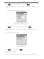
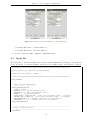
3.3.1 Problem Data window . . . . .
3.3.2 Interval Data window . . . . .
3.3.3 Conditions window . . . . . . .
3.3.4 Materials window . . . . . . . .
.
.
.
.
.
.
.
.
.
.
.
.
.
.
.
.
.
.
.
.
.
.
.
.
.
.
.
.
.
.
.
.
.
.
.
.
.
.
.
.
.
.
.
.
.
.
.
.
.
.
.
.
.
.
.
.
.
.
.
.
.
.
.
.
.
.
.
.
.
.
.
.
.
.
.
.
.
.
.
.
.
.
.
.
.
.
.
.
.
.
.
.
.
.
.
.
.
.
.
.
.
.
.
.
.
.
.
.
.
.
.
.
.
.
.
.
.
.
.
.
.
.
.
.
.
.
.
.
.
.
.
.
.
.
.
.
.
.
.
.
.
.
.
.
.
.
.
.
.
.
.
.
.
.
.
.
.
.
.
.
.
.
.
.
.
.
.
.
.
.
.
.
.
.
.
.
.
.
.
.
.
.
29
29
29
30
30
31
32
33
4 User example for commatfail
4.1 Problem to solve . . . . . .
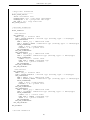
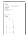
4.2 Generating the input file . .
4.3 Input file . . . . . . . . . .
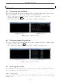
4.4 Processing the problem . .
4.5 Post-processing the problem
.
.
.
.
.
.
.
.
.
.
.
.
.
.
.
.
.
.
.
.
.
.
.
.
.
.
.
.
.
.
.
.
.
.
.
.
.
.
.
.
.
.
.
.
.
.
.
.
.
.
.
.
.
.
.
.
.
.
.
.
.
.
.
.
.
.
.
.
.
.
.
.
.
.
.
.
.
.
.
.
.
.
.
.
.
.
.
.
.
.
.
.
.
.
.
.
.
.
.
.
.
.
.
.
.
.
.
.
.
.
.
.
.
.
.
.
.
.
.
.
.
.
.
.
.
.
.
.
.
.
35
35
35
39
44
44
.
.
.
.
.
.
.
.
.
.
.
.
.
.
.
.
.
.
.
.
.
.
.
.
.
.
.
.
.
.
iii
commatfail user guide
4.6
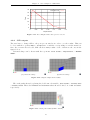
Showing the results . . . . . . . . . . . . . . . . . . . . . . . . . . . . . . . . . . . . . 44
4.6.1 Curve plots . . . . . . . . . . . . . . . . . . . . . . . . . . . . . . . . . . . . . 44
4.6.2 GiD outputs . . . . . . . . . . . . . . . . . . . . . . . . . . . . . . . . . . . . 45
5 Strain injection implementation in commatfail
5.1 Subroutine calcimpstg 2 . . . . . . . . . . . .
5.1.1 Description . . . . . . . . . . . . . . . .
5.1.2 Procedure . . . . . . . . . . . . . . . . .
5.2 Subroutine cfint e2dstd sssdlt wsda . . . .
5.2.1 Description . . . . . . . . . . . . . . . .
5.2.2 Procedure . . . . . . . . . . . . . . . . .
5.3 Subroutine le calc . . . . . . . . . . . . . . . .
5.3.1 Description . . . . . . . . . . . . . . . .
5.3.2 Procedure . . . . . . . . . . . . . . . . .
5.4 Subroutine smoth var . . . . . . . . . . . . . .
5.4.1 Description . . . . . . . . . . . . . . . .
5.4.2 Procedure . . . . . . . . . . . . . . . . .
.
.
.
.
.
.
.
.
.
.
.
.
.
.
.
.
.
.
.
.
.
.
.
.
.
.
.
.
.
.
.
.
.
.
.
.
.
.
.
.
.
.
.
.
.
.
.
.
.
.
.
.
.
.
.
.
.
.
.
.
.
.
.
.
.
.
.
.
.
.
.
.
.
.
.
.
.
.
.
.
.
.
.
.
.
.
.
.
.
.
.
.
.
.
.
.
.
.
.
.
.
.
.
.
.
.
.
.
.
.
.
.
.
.
.
.
.
.
.
.
.
.
.
.
.
.
.
.
.
.
.
.
.
.
.
.
.
.
.
.
.
.
.
.
.
.
.
.
.
.
.
.
.
.
.
.
.
.
.
.
.
.
.
.
.
.
.
.
.
.
.
.
.
.
.
.
.
.
.
.
.
.
.
.
.
.
.
.
.
.
.
.
.
.
.
.
.
.
.
.
.
.
.
.
.
.
.
.
.
.
.
.
.
.
.
.
.
.
.
.
.
.
.
.
.
.
.
.
.
.
.
.
.
.
.
.
.
.
.
.
.
.
.
.
.
.
.
.
.
.
.
.
47
47
47
47
49
49
49
52
52
52
53
53
53
A Interface subroutines
A.1 Interface calc stress . . .
A.1.1 Description . . . . .
A.1.2 Cases . . . . . . . .
A.2 Interface calc stress sssd
A.2.1 Description . . . . .
A.2.2 Cases . . . . . . . .
A.3 Interface e2dstd . . . . . .
A.3.1 Description . . . . .
A.3.2 Cases . . . . . . . .
A.4 Interface elemset . . . . . .
A.4.1 Description . . . . .
A.4.2 Cases . . . . . . . .
A.5 Interface calc celas . . . .
A.5.1 Description . . . . .
A.5.2 Cases . . . . . . . .
A.6 Interface stiff e2dstd . .
A.6.1 Description . . . . .
A.6.2 Cases . . . . . . . .
.
.
.
.
.
.
.
.
.
.
.
.
.
.
.
.
.
.
.
.
.
.
.
.
.
.
.
.
.
.
.
.
.
.
.
.
.
.
.
.
.
.
.
.
.
.
.
.
.
.
.
.
.
.
.
.
.
.
.
.
.
.
.
.
.
.
.
.
.
.
.
.
.
.
.
.
.
.
.
.
.
.
.
.
.
.
.
.
.
.
.
.
.
.
.
.
.
.
.
.
.
.
.
.
.
.
.
.
.
.
.
.
.
.
.
.
.
.
.
.
.
.
.
.
.
.
.
.
.
.
.
.
.
.
.
.
.
.
.
.
.
.
.
.
.
.
.
.
.
.
.
.
.
.
.
.
.
.
.
.
.
.
.
.
.
.
.
.
.
.
.
.
.
.
.
.
.
.
.
.
.
.
.
.
.
.
.
.
.
.
.
.
.
.
.
.
.
.
.
.
.
.
.
.
.
.
.
.
.
.
.
.
.
.
.
.
.
.
.
.
.
.
.
.
.
.
.
.
.
.
.
.
.
.
.
.
.
.
.
.
.
.
.
.
.
.
.
.
.
.
.
.
.
.
.
.
.
.
.
.
.
.
.
.
.
.
.
.
.
.
.
.
.
.
.
.
.
.
.
.
.
.
.
.
.
.
.
.
.
.
.
.
.
.
.
.
.
.
.
.
.
.
.
.
.
.
.
.
.
.
.
.
.
.
.
.
.
.
.
.
.
.
.
.
.
.
.
.
.
.
.
.
.
.
.
.
.
.
.
.
.
.
.
.
.
.
.
.
.
.
.
.
.
.
.
.
.
.
.
.
.
.
.
.
.
.
.
.
.
.
.
.
.
.
.
.
.
.
57
57
57
57
57
57
57
58
58
58
59
59
59
59
59
59
59
59
59
.
.
.
.
.
.
.
61
61
61
62
62
62
63
63
.
.
.
.
.
.
.
.
.
.
.
.
.
.
.
.
.
.
.
.
.
.
.
.
.
.
.
.
.
.
.
.
.
.
.
.
.
.
.
.
.
.
.
.
.
.
.
.
.
.
.
.
.
.
.
.
.
.
.
.
.
.
.
.
.
.
.
.
.
.
.
.
.
.
.
.
.
.
.
.
.
.
.
.
.
.
.
.
.
.
.
.
.
.
.
.
.
.
.
.
.
.
.
.
.
.
.
.
.
.
.
.
.
.
.
.
.
.
.
.
.
.
.
.
.
.
.
.
.
.
.
.
.
.
.
.
.
.
.
.
.
.
.
.
.
.
.
.
.
.
.
.
.
.
.
.
.
.
.
.
.
.
B Variables
B.1 Variables of the e2dstd set of elements . . .
B.2 Gauss point variables . . . . . . . . . . . . .
B.3 Element variables . . . . . . . . . . . . . . .
B.4 Section variables . . . . . . . . . . . . . . .
B.5 Material variables . . . . . . . . . . . . . . .
B.6 Sub-Material variables . . . . . . . . . . . .
B.7 Elemental real variables for elements of type
iv
.
.
.
.
.
.
.
.
.
.
.
.
.
.
.
.
.
.
.
.
.
.
.
.
.
.
.
.
.
.
.
.
.
.
.
.
.
.
.
.
.
.
.
.
.
.
.
.
.
.
.
.
.
.
.
.
.
.
.
.
.
.
.
.
.
.
.
.
.
.
.
.
e2dstd .
.
.
.
.
.
.
.
.
.
.
.
.
.
.
.
.
.
.
.
.
.
.
.
.
.
.
.
.
.
.
.
.
.
.
.
.
.
.
.
.
.
.
.
.
.
.
.
.
.
.
.
.
.
.
.
.
.
.
.
.
.
.
.
.
.
.
.
.
.
.
.
.
.
.
.
.
.
.
.
.
.
.
.
.
.
.
.
.
.
.
.
.
.
.
.
.
.
.
.
.
.
.
.
.
.
.
.
.
.
.
.
.
Introduction
The preliminary purpose of this document is to aid commatfail users and developers in getting
some basic tools when using the code for themselves. It was conceived after the research work of
many people, and as the final work to stop the implementation of new features in this code. It can
not be viewed neither as a rigorous manual nor an exhaustive description of each line in the code.
Readers who are a only user of the code, and are not interested in the implementation of new
features, should probably go to read only chapter 2 and 3. Those chapters will guide the user
through the rules to keep in mind when writing or creating an input file. For developers, we
recommend a careful reading of the entire document, so they have a better idea of how the code is
structured.
Pre-requisites
The commatfail users do not require to have additional software in their machines. Executable
binaries are already compiled for Windows platform, and should be used in a command line prompt.
The commatfail developers should have installed Microsoft Visual Studio 2010, and Intel Visual
Fortran Composer 2011. Other IDEs compilers are not recommended for a correct functionality of
the code.
Installation
There is no need to install commatfail. If the pre-requisites are met, the solution file commatfail.sln
should open in Microsoft Visual Studio with no problems.
Running commatfail and commatfailpost
Binaries and input file should be in the same working directory. Computations should be done in
a command line prompt with:
commatfail <input_file_name>
If GiD will be used to see the results, post-process should be done after computations in a
command line prompt with:
commatfailpost <input_file_name>
After post-process, results can be seen opening the file “<input_file_name>_s1.flavia” in GiD
pre/post processor.
Clarity of the code
Finite element codes are no exception when facing the dilemma of clarity versus efficiency. Even
though those are not opposite concepts, an effort to achieve one tends to lack the other. The
v
commatfail user guide
programming philosophy adopted in the development of commatfail has been the optimization of
procedures. This does not mean that the creators of the code have done their best to make it as
comprehensible as possible.
Portability
Most commatfail routines are written in a standard Fortran 90 programming language, but some
small details are only valid for Intel Fortran Compiler. Currently the code is already configured in
a Microsoft Visual Basic 2010 solution, and its usage with other compilers and IDE’s could need
some extra configurations for its correct operation.
General convention for character fonts
The meaning associated to specific font styles is given below. Standard typos are not explained
here, and some exceptions could be highlighted in the text and not here.
Description
Scalar values and functions
Vectors
Second order tensors
Forth order tensors
Spaces
Fortran codes, plain text, file names
Key or button pressing indications
Software menus
Example
a, α, A
a, n
B, σ
C, S
U, V
<input>.dat,
NEW_MATERIAL
Apply , esc File > Save as, Data > Problem data
vi
Chapter 1
Overview of commatfail
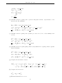
commatfail is a multipurpose finite element code written in Fortran 90. As many finite element
codes, it has only the calculus process of a problem. That means that all needed information is
taken from an input file before the computations start, and all results are written in the output
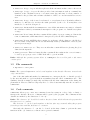
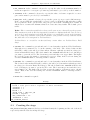
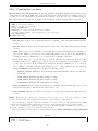
files when finished. Figure 1.1 shows this basic way of how commatfail works1 .
Figure 1.1: commatfail basic operating process
To perform a simulations with commatfail:
1. Place the input file and the executable commatfail file in the same directory.
2. Navigate to that directory through a command window.
3. Execute: commatfail <input_file>
After the calculations are done, post-process can be done by:
1. Place the executable file commatfailpost in the same directory.
2. Execute in the command window: commatfailpost <input_file>
The user could write a simple script to execute those commands more efficiently, especially
when more than one simulation is to be done sequentially.
1.1
Modules and database
Once the input file is supplied, there are some subroutines in commatfail which reads all the
problem data, and create a temporary database to check whether all required fields are complete.
If so, an internal database is created to be used later while the calculations are done. This database
is stored in modules2 , and its main role is to communicate among the calculation subroutines and
keep the variables in one place.
These modules can be found in the files whose name ends with *_db.f90. Some of those modules
are:
• elmset_db.f90: stores the information on element sets.
1
Note that the input and output files should be generated and read with some external software capable of
pre-process and post-process a finite element problem.
2
This implies that variables are global and not local. This brings advantages, e.g. not use many variables as input
and output arguments in all subroutines
1
commatfail user guide
• nodeset_db.f90: stores the information on nodes, as the coordinates.
• mat_db.f90: stores the information of materials properties.
1.2
Stages
A simulation in commatfail can be done by stages, which may have different conditions of loads
or element properties. Suppose that we
The type of stages allowed are:
• NEW_PROBLEM
• NEW_STAGE
• RESTART_STAGE
• RESTART_CALC
• RESTART_NEWMSH
1.3
The main program
The main commatfail procedure is done by mainpg. It can be divided into three basic parts:
1. Initialization and input data. The initialization of the execution parameters is carried out in
this phase, at the very beginning of the execution of the program. The reading precess of the
input data is done at the beginning of each stage from the input data text file or the restart
file.
2. The incremental finite element procedure. This is the main body of the program, where all
the numerical calculations associated to the finite element method are done. This procedure
is done one time for each stage of the problem, after reading the input data. Essentially it
consist of a time-steps integration process with an interface routine (calcstg) that chooses
the calculation method depending on the integration scheme: implicit, explicit, or implicitexplicit.
This comprises all output operations necessary to print converged finite element solutions
into the results file and/or dump an image of the database into a restart output file. Output
routines are called from inside the main loop over load increments.
3. Write output results. This comprises all output operations necessary to print converged
finite element solutions into the results or restart files.Those routines write in files with
the correct format to be read with the post-processor commatfailpost. Output files from
commatfailpost are then in the correct format to be imported in GiD.
1.4
Description of files managed by commatfail
commatfail manages the opening and closing of files through two routines. The routine that
handles the opening of files is called “openfi” while the routine that manages the closing of files is
called “closefi”. In turn, both depend on a common module called “filevar_db” in which units
and extensions are defined. The manipulation of files at the programming level required to make
co-ordinated development of this module and these two routines.
• commatfail .dat: This file actually corresponds to the data file that will be used by the
program and it is a single file with normal ASCII characters. One of the first tasks of
commatfail when launching a new calculation is to build this file from the data files provided
by the user. In case the data file provided by the user is unique, commatfail.dat is a copy
of it.
2
Chapter 1. Overview of commatfail
• <name>.scr: A type of report file that replicates all the information that comes to the screen.
• <name>.rpt: A type of report file that provides basic information such as command line
launched, if the calculation is new or a restart, start date and time of release, number of
elements for the problem, and real time calculation of CPU, etc. and it is useful for a novice
user.
• <name>.rsn: A type of file focused on advanced or very advanced user. It includes all information to be introduced to monitor the tasks performed by the code. You may have even
intended to be used in debug mode.
• <name>.rsf: An internal file in commatfail to save all the information necessary to relaunch
the calculation either by an unwanted interruption of the program or to launch a new phase
or stage.
• <name>.sun: It is a binary file that contains all the results of post-processing problem in the
form of commatfail, which must then be interpreted by the module commatfailpost.
• <name>.nlb: It is an ASCII file that contains, for each stage, all the changes to the labels of
the nodes that overlap with other nodes automatically added by commatfail or added by the
user in previous stages.
• <name>.c01, <name>.c02, etc.: They are text files that contain all data for plotting the plots
defined in the input file.
• <name>_s1.flavia: This is a binary file that contains all the results in the correct format to
be read by pre/post-process tool GiD. It should be open from GiD.
Rules. Although the operating system allows it, commatfail does not allow path or file names
contain spaces.
1.5
File commands
• ImportFile = <file_name>
Rules. The command ImportFile can be located anywhere in the data file. However, it must be the
only command line.
One of the first tasks undertaken by commatfail is to interpret the file or data file provided
by the user and make a copy from them in an auxiliary data file called “commatfail .dat”. The
auxiliary data file is unique (a single file) and this is the file that commatfail reads during implementation. However, this is a temporary file to be deleted automatically after the execution of
commatfail.
1.6
Code comments
commatfail allows you to enter any comments deemed necessary in order to help or clarify or
interpret the data file. However, comments will be given by the program. The comments in the
data file are marked by the characters “!” Or “#”.
Rules. The character “#” should be located in the first column which indicates the program that
the entire row is a comment.
The character “!” can be located anywhere on the line after any command, telling the program
from that position until the final line is a comment.
Obviously, the character “!” can also be located in the first column to perform the same
functions as the “#” character, so this is a more general command.
3
Chapter 2
Input data file for commatfail
2.1
Creating input data file
BEGIN_PROBLEM and END_PROBLEM identify, respectively, the beginning and the end of the actual data
file.
BEGIN_PROBLEM
< problem body data >
END_PROBLEM
• BEGIN_PROBLEM: is the keyword to specify the beginning of the actual data file.
• END_PROBLEM: is the keyword to indicate the ending of the actual data file.
Rules. The definition of this field is mandatory in every data file. It is the field that encompasses
all other fields in the data file that can be defined and interpreted by the program. However, it only
allows defining a single data input field.
This field may contain general commands such as the import file (ImportFile), the title of the
problem (Begin_Problem_Basics or End_Problem_basics) or the definition of stages (New_Stage or
End_New_Stage). Any command outside this field is not interpreted by the program.
BEGIN_PROBLEM
B E G I N _ PR O B L E M _ B A S I C S
...
EN D_ PR OB LE M_ BA SI CS
NEW_STAGE
...
END_NEW_STAGE
END_PROBLEM
2.2
Example
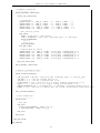
Creating the problem basics
BEGIN_PROBLEM_BASICS and END_PROBLEM_BASICS are the key words that identify the beginning and
the end, respectively, of the general data of the problem such as the name (title) of the problem,
size or the default time integration scheme, the solver and the tolerance of the stages.
BEGIN_PROBLEM_BASICS
TITLE = < Problem Title >
SCRLEVEL = < number >
RSNLEVEL = < number >
NDIME = < Problem Dimension >
STAGE_TYPE = < Type of stage >
5
commatfail user guide
SOLVER_TYPE = < Solver Type >
MAX_ITERATION = < Max . no . of iterations per time step >
TOLERANCE = < Convergence tolerance >
MESH_POST = Option < YES / NO >
EN D_ PR OB LE M_ BA SI CS
• BEGIN_PROBLEM_BASICS: is the command or keyword that identifies the beginning of the field.
• END_PROBLEM: is the command or keyword that identifies the end of the field.
• TITLE: is the command or keyword used to indicate the title of the problem described by the
data file. Must be preceded by a string or sentence.
• SCRLEVEL: is the command or keyword used to indicate the level of messages going to be
appeared on screen and in the *.scr file. This command must be preceded by a positive
integer that indicates the level of messages per screen (the higher the number the greater
number of messages will appear). By default the value is considered 0.
• RSNLEVEL: is the command or keyword used to indicate the level of messages in the file *.rsn.
This command must be preceded by a positive integer that indicates the level of messages
per screen (the higher the number the greater number of messages will appear). By default
the value is considered 0.
• NDIME: is the command or keyword used to indicate the dimension of the problem. This
command must be preceded by a positive integer that indicates the dimension of the problem:
1 to 1D problems (there are currently no scheduled element for 1D), 2 and 3 for 2D problems
and for 3D problems.
• STAGE_TYPE: is the command or keyword to indicate the type of stage (e.g. an incremental
integration scheme in time implied a re-accommodation or body) and should be preceded
by a keyword predefined by the program according to the types of stages that has been
implemented. Currently, the program takes into consideration the following:
– IMPLICIT_NR: implicit integration scheme using Newton-Raphson scheme.
– IMPLICIT_NR_V2: implicit integration scheme using Newton-Raphson scheme similar to
the preceding but which converges in one step if the problem is linear (default option).
– EXPLICIT: explicit integration scheme (not scheduled yet).
– BODY_MOVE: rearranging or moving solid rigid bodies (not scheduled yet).
The default option “IMPLICIT_NR” is assigned when this command is not explicitly stated
in some of the stages. However, the obligation of the command depends on the type of
SOLVER_TYPE.
• SOLVER_TYPE: is the command or keyword to indicate the type of solver to be used and should
be preceded by a keyword predefined by the program according to the type of solver that
has already been implemented. Currently, the program takes into consideration the following
solvers:
– GAUSSJORDAN: direct solver by Gauss-Jordan elimination with full matrix. Use of this
solver is limited, for smaller examples.
– LU: direct solver with full storage array. Use of this solver is not meant to medium/large
problems, so its use is limited only to debug small examples.
– SUPERLU: direct solver with storage of the sparse matrix type. This constraint solver has
the ability to contain the decomposition of the matrix in memory.
6
Chapter 2. Input data file for commatfail
• MAX_ITERATION: is the command or keyword to specify the value for the maximum number of
iterations required for convergence per time step and must be preceded by a whole number.
• TOLERANCE: is the command or keyword to specify the value of tolerance required for convergence and it must be preceded by a real number.
• MESH_POST: is the command or keyword to specify the option of post process for different stage.
If the option is YES the results will be post-processed for all meshes although these results
are not partners. If the option is NO, only post-processed mesh containing those results, in
which case it overwrites the filenames that are not associated any results. The default option
is NO.
Rules. This is a mandatory field whose absence will create an error that will stop the program.
This statement is made in the data input field (if stated in a different field will cause an error)
and can be located anywhere in the field although it is recommended to write at the beginning.
It can contain any command on the general variables of the problem and any command outside
this field will not be interpreted as Problem Basics.
Problem Basics no one field to another field may contain either one Problem Basics Field
Stage.
• SCRLEVEL: the command is optional and can be located anywhere in the field Problem Basics,
although it is recommended to be in the starting of the field. The declared value in this
field will be valid for the whole problem, unless otherwise explicitly specified in a Stage (see
Creation Basics Field Stage). The whole number into SCRLEVEL indicates the level of messages
you want to get in the screen. The lowest integer is 0 and there is no upper limit. The higher
the level the greater the number of messages per screen. Thus, if the level is 0 during the
execution minimum number of messages will be written.
• RSNLEVEL: the command is optional and can be located anywhere in the field Problem Basics.
The declared value in this field will be valid for the whole problem, unless explicitly specified
in a Stage (see Creation Basics Field Stage). The whole number into RSNLEVEL indicates the
level of messages you want to get in the file *.rsn. The lowest integer is 0 and there is no
upper limit for it. The higher the level the greater the number of messages sent to the file
*.rsn. Thus, if the level is 0 during the execution minimum number of messages will be
written.
• NDIME: this command is required.
Example
BEGIN_PROBLEM BASICS
TITLE = 5061 piece with a sequence of three movements
SCRLEVEL = 1
RSNLEVEL = 1
NDIME = 2
STAGE_TYPE = IMPLICIT_NR
SOLVER = SuperLU
MAX_ITERATION = 100
TOLERANCE = 1d -6
EN D_ PR OB LE M_ BA SI CS
2.3
Creating the stage
NEW_STAGE and END_NEW_STAGE are the key words that identify the beginning and the end of the field
respectively with the data describing the Stage.
7
commatfail user guide
NEW_STAGE
< Stage body data >
END_NEW_STAGE
• NEW_STAGE is the command or keyword used to indicate the beginning of the field.
• END_NEW_STAGE is the command or keyword used to indicate the end of the field.
Rules. This field can contain any command. Any command on the information of Stage located
outside the field will not be interpreted as a figure of the Stage.
A transaction may not contain field to another field Stage. However, it can contain other fields
such as field Stage Basics, Material field, Section field, the Set of Elements field, etc.
NEW_STAGE
BE GI N_ ST AG E_ BA SI CS
...
END_STAGE_BASICS
BEGIN_MATERIAL
...
END_MATERIAL
END_NEW_STAGE
2.4
Example
Creating the stage basics
BEGIN_STAGE_BASICS and END_STAGE_BASICS are the key words that identify the beginning and the
end respectively of the general data of a stage as it includes information on stage name, size or time
integration scheme, the solver, the tolerance, the number of increments or the time of completion
of the stage.
BE GI N_ ST AG E_ BA SI CS
TITLE = < Title of the stage >
SCRLEVEL = < enter number >
RSNLEVEL = < enter number >
STAGE_TYPE = < Type of stage >
SOLVER_TYPE = < Type of solver >
MAX_ITERATION = < Max no . of iterations per step >
TOLERANCE = < tolerance of convergence >
NUMBER_STEPS = < No . of increments of the stage >
NUMBER_POST = < No . of steps for post - processing >
PERIOD_POST = < time period for post - processing >
END_TIME = < final time of the stage >
DYNAMIC_TYPE = < Type of dynamic integration >
MESH_POST = < YES / NO >
END_STAGE_BASICS
• BEGIN_STAGE_BASICS: is the command or keyword that identifies the beginning of the field.
• END_STAGE_BASICS: is the command or keyword that identifies the end of the field.
• TITLE: is the command or keyword used to indicate the title of the stage. Must be preceded
by a string or sentence.
• SCRLEVEL: is the command or keyword used to indicate the level of messages on screen and in
the *.scr file in the stage. This command must be preceded by a positive integer that indicates
the level of messages per screen (the higher the value the greater number of messages). By
default the value is considered 0.
8
Chapter 2. Input data file for commatfail
• RSNLEVEL: is the command or keyword used to indicate the level of messages in the file *.rsn
during the stage. This command must be preceded by a positive integer that indicates the
level of messages per screen (the higher the value the greater number of messages). By default
the value is considered 0.
• STAGE_TYPE: is the command or keyword to indicate the type of stage and should be preceded
by a keyword predefined by the program according to the types of Stages implemented.
Currently, the program takes into consideration the following:
– IMPLICIT_NR: implicit integration scheme using Newton-Raphson scheme.
– IMPLICIT_NR_V2: implicit integration scheme using Newton-Raphson scheme similar to
the preceding but which converges in one step if the problem linear (default option).
– EXPLICIT: explicit integration scheme (not implemented yet).
– BODY_MOVE: rearranging or moving solid rigid bodies (not implemented yet).
• SOLVER_TYPE: is the command or keyword to indicate the type of Solver to use during the
stage and must be preceded by a keyword predefined by the program according to the type
of solver implemented (see “Problem basics”).
• MAX_ITERATION: is the command or keyword to specify the value for the maximum number of
iterations for convergence for the stage and should be preceded by a whole number.
• TOLERANCE: is the command or keyword to specify the value of convergence tolerance for the
stage and should be preceded by a real number.
• NUMBER_STEPS: is the command or keyword used to indicate the number of increments or time
steps for the stage. This command must be preceded by a positive integer indicating the
number of increments.
• NUMBER_POST: is the command or keyword used to indicate the number of post-processing
carried out on the stage following a long constant frequency. This command must be preceded
by a positive integer indicating the number of increments.
• PERIOD_POST: is the command or keyword used to indicate the frequency of post-processing
carried out on the stage by defining the time period. This command must be preceded by a
positive real number indicating the number of increments.
• END_TIME: is the command or keyword to specify the value of the final moment of the stage
and should be preceded by a real number.
• DYNAMIC_TYPE: is the command or keyword used to indicate the type of dynamic integration
to be used for the stage and should be preceded by a keyword. Currently, the code supports
the dynamic integration:
– STATIC: Keyword to specify a static calculation (default option). Requires no additional
parameters.
– G_ALPHA: Keyword to specify a dynamic calculation using the general Alpha-method.
This method requires the definition of additional parameters.
• MESH_POST: is the command or keyword to specify the option type in the post-processing stage.
If the option is YES is post-processed all meshes although these results are not partners. If the
option is NO only post-processed mesh containing those results, in which case it overwrites
the filenames that are not associated any results.
• BEGIN_DYNAMIC_PARAMETERS: keyword which opens the field to interpret the parameters of the
dynamic integration.
9
commatfail user guide
• END_DYNAMIC_PARAMETERS: keyword closing the field which is used to interpret the parameters
of the dynamic integration.
Rules. The field of STAGE_BASICS is declared within a Stage Field (if declared in a different field
will cause an error) and can be located anywhere in the field although it is strongly recommended
that it is the first stage of the field or in case some messages may be lost during reading. It can
contain any command of general variables and any command on this field, if written outside this
field will not be interpreted as Stage Basics.
No other field can contain Stage Basics. However, when a new stage is set (NEW_STAGE END_NEW_STAGE) it is necessary to define a field as STAGE_BASICS which defines the characteristics of
the new stage.
The command SCRLEVEL is optional and can be located anywhere in the Stage Basics field, however it is strongly recommended to write it in the beginning or otherwise some messages might be
lost during reading. The declared value in this field will overwrite the value that was defined in
the Problem Basics (see Problem Basics). The whole number into SCRLEVEL indicates the level of
messages you want to get in the screen. The lowest integer is 0 and says there is no upper limit.
The higher the level the greater the number of messages per screen. Thus, if the level is 0 during
the execution only the minimum number of messages will be written.
The command RSNLEVEL is optional and can be located anywhere in the Stage Basics field, however it is strongly recommended to write it in the beginning or otherwise some messages might be
lost during the reading. The declared value in this field will overlap the value that was defined in
the Problem Basics (see field Problem Basics). The whole number into RSNLEVEL indicates the level
of messages you want to get into the file *.rsn. The lowest integer is 0 and says there is no upper
limit. The higher the level the greater the number of messages sent to the file *.rsn Thus, if the
level is 0 during the execution only the minimum number of messages will be written.
The command STAGE_TYPE is mandatory if it has not been declared in the Problem Basics.
However, compulsory SOLVER_TYPE command depends on the integration scheme employed.
Commands such as NUMBER_STEPS, NUMBER_POST, PERIOD_POST and END_TIME are unique to the
stage.
Commands NUMBER_POST and PERIOD_POST are optional and mutually exclusive. In case both are
set simultaneously, the information defined by the command NUMBER_POST precedes over that defined
by the command PERIOD_POST. In the event that the stage does not define any of these commands,
only the final stage will be post-processed.
Example
BE GI N_ ST AG E_ BA SI CS
TITLE = Stage pressing - First movement of punches
SCRLEVEL = 3
RSNLEVEL = 3
SOLVER = SuperLU
MAX_ITERATION = 100
TOLERANCE = 1d -3
NUMBER_STEPS = 100
NUMBER_POST = 3
End_time = 1d -2
END_STAGE_BASICS
2.5
Creating the material data base
BEGIN_MATERIAL and END_MATERIAL are, respectively, the key words that identify the beginning and
the end of the materials database.
BEGIN_MATERIAL
DELETE = < label of the material >
10
Chapter 2. Input data file for commatfail
NEW_MATERIAL
< body defining new material data >
END_NEW_MATERIAL
END_MATERIAL
• BEGIN_MATERIAL: is the keyword indicating the starting of the material data.
• END_MATERIAL: is the key word to indicate the end of the material data.
• DELETE: This is the keyword to specify the name of material (label) to be removed from the
database of material. Must be preceded by the label for the material to be removed.
• NEW_MATERIAL: Keyword which opens the data field that defines a material database (see scope
of materials).
• END_NEW_MATERIAL: Key word which closes the field with the data that define a material
database (see scope of materials).
Rules. This field allows you to communicate with the database of materials used in the calculation,
creating and removing the materials from the database. The following commands may be repeated
as necessary: DELETE, NEW_MATERIAL and END_NEW_MATERIAL.
BEGIN_MATERIAL
DELETE = material_1
DELETE = material_2
Example
NEW_MATERIAL
...
END_NEW_MATERIAL
NEW_MATERIAL
...
END_NEW_MATERIAL
END_MATERIAL
2.6
Creating the material properties
NEW_MATERIAL and END_NEW_MATERIAL are, respectively, the key words that identify the beginning
and the end of the data set that defines a material.
NEW_MATERIAL
NAME = < material label >
TYPE = < type of_material >
NEW_SUBMATERIAL
< properties of the material >
E ND _ N EW _ S U BM A T ER I A L
END_NEW_MATERIAL
• NEW_MATERIAL: is the keyword that indicates the beginning of the data that characterize the
material.
• END_NEW_MATERIAL: is the keyword that indicates the end of the data that characterize the
material.
11
commatfail user guide
• NAME: is the keyword to specify the name of material (label) that will identify the database and
must be preceded by a word that will gain the category label. It is a mandatory parameter
and is recommended to be located at the beginning of the field.
• TYPE: is the keyword to specify the type of material (if material is a standard or defined by
the user, etc.) and must be preceded by a keyword predefined by the program according to
the type of material. It is a mandatory parameter and must be located at the beginning of
the field before the definition of submaterials.
• NEW_SUBMATERIAL: Keyword which opens the field of sub-material, which defines at least a
portion of the material characteristics such as the elastic model, the surface creep, and so on.
(see submaterials field).
• END_NEW_SUBMATERIAL: Keyword which closes the sub-material field.
Rules. This field can contain any command or data on the parameters of the material, and any
information on the material located outside the field shall not be interpreted.
It is mandatory to define a label identifying the material, which is achieved through the NAME
command in this field. Failure generates an error in reading inputs that will stop the program.
To define the material properties one can define as many sub-fields of material as needed.
It is mandatory to define the type of material before the submaterials, which is achieved through
the TYPE command at the beginning of this field. Omission of this or statement after submaterial
generates an error in reading inputs that will stop the program.
NEW_MATERIAL
NAME = material_1
TYPE = ELASTOPLASTIC
NEW_SUBMATERIAL
...
E ND _ N EW _ S UB M A TE R I A L
END_NEW_MATERIAL
2.7
Example
Creating the sub-material properties
NEW_SUBMATERIAL and END_NEW_SUBMATERIAL are, respectively, the key words that identify the begin-
ning and the end of the data set that defines the characteristics of the material or the submodel
(e.g. the elastic model, the surface creep, hardening laws, etc).
NEW_SUBMATERIAL
NAME = < label of_sub - material >
TYPE = < type of_sub - material >
BEGIN_PARAMETERS
< properties of the sub - material >
END_PARAMETERS
NEW_CURVE
< curves that define the points of the sub - material >
END_NEW_CURVE
NEW_SUBMATERIAL
< defining nested sub - material >
E ND _ N EW _ S UB M A TE R I A L
END _ N EW _ S UB M A T ER I A L
• NEW_SUBMATERIAL: is the keyword that indicates the beginning of the data that characterize
the sub-material. If this keyword is declared within the field itself, it implies declaring another
submodel of material nested in the actual submodel.
12
Chapter 2. Input data file for commatfail
• END_NEW_SUBMATERIAL: is the keyword that indicates the end of the data that characterize the
sub-material. If there is another submodel within the stated submodel, then this keyword
closes the later field.
• NAME: is the keyword to specify the name of the material submodel (label) that will identify
the sub-material. Must be preceded by a word that will gain the category label. It is a
mandatory parameter and is recommended to be located at the beginning of the field.
• TYPE: is the keyword to specify the type of submodel (linear elastic, elastoplastic, etc.), and
must be preceded by a keyword predefined by the program according to the type of material
submodel. It is a mandatory parameter and is recommended to be located at the beginning of the field with the only restriction to be observed that it comes before the command
BEGIN_PARAMETERS.
• BEGIN_PARAMETERS: Keyword which opens the field to interpret the constants that define the
submodel of material such as elastic model, surface creep, and so on.
• END_PARAMETERS: Key word which declares the closing of the field of material parameters for
the submodel.
• NEW_CURVE: Keyword that paves the way to interpret a curve (see Definition field curves).
• END_NEW_CURVE: Key word which declares the closing of the field of material curves.
Rules. This field can contain any command or data on the parameters of submodel, and any
material information located outside shall not be interpreted.
It is mandatory to define a label identifying the material, which is achieved through the NAME
command in this field. Failure generates an error in reading inputs that will stop the program. It
is also mandatory to define the type of submodel through the TYPE command, the omission of which
also generates a reading error that stops the execution.
To define the properties of the submodel, it is defined by a single field parameter (BEGIN_PARAMETERS
and END_PARAMETERS), but you can define as many fields as necessary curves to define the submodel
material.
It is allowed that a submodel of material can be composed of different submodels of material so
that the base material is dynamic and flexible.
NEW_SUBMATERIAL
NAME = model_elastic_1
TYPE = ELASTIC_LINEAR
BEGIN_PARAMETERS
YOUNG = 2.1 E +6
POISSON = 0.29
END_PARAMETERS
NEW_CURVE
...
END_NEW_CURVE
E ND _ N E W_ S U BM A T ER I A L
2.8
Example
Defining curves
NEW_CURVE and END_NEW_CURVE are the key words that identify the beginning and the end respectively
of the data set that define a curve, which may be defined by a cloud of points or any other data
set and define the interpretation of which is scheduled.
13
commatfail user guide
NEW_CURVE
NAME = < label of the curve >
TYPE = < type of curve >
BEGIN_PARAMETERS
< body hat defines the curve >
END_PARAMETERS
END_NEW_CURVE
• NEW_CURVE: is the keyword that indicates the beginning of the data that characterizes the
curve.
• END_NEW_CURVE: is the keyword that indicates the end of the data that characterizes the curve.
• NAME: is the keyword to specify the name of the curve (label) that will identify the rest of the
curves defined on the basis of corresponding curves. Must be preceded by a word that will
gain the category label. It is a mandatory parameter and is recommended to be located at
the beginning of the field.
• TYPE: is the keyword to specify the type of the curve (if a cloud of points or any other family
of curves that is scheduled) and should be preceded by a keyword predefined by the program
according to the type of curve. It is a mandatory parameter and is recommended to be located
at the beginning of the field with the only restriction to be observed that it comes before the
field BEGIN_PARAMETERS. Currently, the program takes into consideration the following types:
– BY_POINTS: curve defined by points.
• BEGIN_PARAMETERS: Keyword that paves the way to interpret the data that define the curve.
• END_PARAMETERS: Key word that closes the field of parameters that define the curve.
Rules. This field can contain any command or data on the curves and any command or data
outside of it will not be interpreted.
It is mandatory to define a label that identifies and distinguishes the rest of the curve, which
is achieved through the NAME command in this field. Failure generates an error in input reading
that stops the program. Furthermore, the label of the curve is restricted to the set of curves defined
by the base curve. Two different materials, for example, can have separate curves with identical
labels and there is no conflict because the discrimination between the two is done via the label on
the material and therefore are two different base curves.
It is also mandatory to define the type of curve through the TYPE command, the omission of
which also generates a reading error that stops the execution.
The data of the curve are introduced in a single field parameter (BEGIN_PARAMETERS and END_PARAMETERS).
Example
NEW_CURVE
NAME = curve_1
TYPE = BY_POINTS
BEGIN_PARAMETERS
! --- Curve defined by 3 points
0.0 0.0
1.0 20.0
2.0 -20.0
END_PARAMETERS
END_NEW_CURVE
14
Chapter 2. Input data file for commatfail
2.9
Establishment of the basis of sections
BEGIN_SECTION and END_SECTION are the key words that identify the beginning and end of all the
additional data associated with the element (including the reference material) and are not directly
related to the geometric definition of the mesh.
BEGIN_SECTION
DELETE = < section label >
ASSOCIATE : SECTION = < section label > MATERIAL = < material label >
NEW_SECTION
< body that defines all or part of the base sections >
END_NEW_SECTION
END_SECTION
• BEGIN_SECTION: is the keyword that indicates the beginning of the data for the sections.
• END_SECTION: is the keyword that indicates the end of the data for the sections.
• DELETE: This is the keyword to specify the section name (label) to be removed from the
database. Must be preceded by the label of the section to remove.
• ASSOCIATE: is the keyword to specify the link to the material section. This option must be
accompanied by keywords:
– SECTION: followed by the label of the section to associate.
– MATERIAL: followed by the material label that is associated with the section.
• NEW_SECTION: Keyword which opens the field with data that defines a section of the database.
• END_NEW_SECTION: Key word here closes the field with data that defines a section of the
database.
Rules. This field allows you to communicate with the Section database containing data associated
with the element type (e.g. material associated with an element of the mesh, if the problem is a
two-dimensional plane strain, etc.). The following commands may be repeated as necessary: such
as: DELETE, NEW_SECTION and END_NEW_SECTION.
ASSOCIATE option should be used when the material associated with the section is removed and
then re-created. In these circumstances, the association of the section breaks at the time when the
material is removed; it is necessary to re-link the material for the purpose of the program and is
considered as a new material.
Example
BEGIN_SECTION
DELETE = section_1
DELETE = section_2
ASSOCIATE : SECTION = section_1 MATERIAL = material_1
NEW_SECTION
...
END_NEW_SECTION
NEW_SECTION
...
END_NEW_SECTION
END_SECTION
15
commatfail user guide
2.10
Creating the sections
NEW_SECTION and END_NEW_SECTION are the key words that identify the beginning and end respectively
of the data set associated with each of the sections involved in the mesh (for example, if a body
is composed of two materials, it would have at least two sections each one of which would be
associated respectively with the elements of the mesh and with the material they are made).
NEW_SECTION
NAME = < section label >
TYPE = < type of section >
BEGIN_PARAMETERS
MATERIAL = < associated material label >
< body that define the properties of section >
END_PARAMETERS
END_NEW_SECTION
• NEW_SECTION: is the keyword that indicates the beginning of the data that characterize the
section.
• END_NEW_SECTION: is the keyword that indicates the end of the data that characterize the
section.
• NAME: is the keyword to specify the section name (label) that will identify in the database of
the sections. Must be preceded by a word that will gain the category label. It is a mandatory
parameter and is recommended to be located at the beginning of the field.
• TYPE: is the keyword to specify the type of section, and therefore that data is needed and
should be interpreted. Must be preceded by a keyword predefined by the program according
to the type of section. It is a mandatory parameter and is recommended to be located at
the beginning of the field with the only restriction to be observed that it is before the field
BEGIN_PARAMETERS. Currently, the code has the following options:
– MATERIAL_SECTION: Elements: 3D elements in general and that they only need to associate
a material.
– PLANE_STRAIN: Elements 2D plane strain problems.
– PLANE_STRESS: Elements 2D plane strain problems.
– AXISIMMETRIC: Elements 2D axisymmetric problems.
• BEGIN_PARAMETERS: Keyword that paves the way to interpret the data that define the section
such as the material to which it is associated, and so on.
• END_PARAMETERS: Keyword closing the field used to describe the parameters that define the
section.
Rules. This field can contain any command or data on the sections and any command or data
located outside shall not be interpreted in relation to the database of the sections.
It is mandatory to define a label that identifies the section, which is achieved through the NAME
command in this field. Failure generates an error in input reading that will stop the program.
It is also mandatory to define the type of section through the TYPE command, the omission of
which also generates a read error that stops the execution.
The section data is introduced into a single field parameter (BEGIN_PARAMETERS and END_PARAMETERS).
NEW_SECTION
NAME = section_1
TYPE = PLANE_STRESS
Example
16
Chapter 2. Input data file for commatfail
BEGIN_PARAMETERS
MATERIAL = AL4030
THICK = 1.0 E -3
END_PARAMETERS
END_NEW_SECTION
2.11
Establishment of the basis of nodes
BEGIN_NODE_SET and END_NODE_SET are the key words that identify the beginning and end respectively
of the data set (node labels and their coordinates) associated with the set of nodes.
BEGIN_NODE_SET
DELETE_SET = < node set label >
DELETE_SUBSET = < node subset label >
NEW_NODE_SET
< body that defines the set of nodes >
END_NEW_NODE_SET
NEW_NODE_SUBSET
< body that defines the subset of nodes >
E ND _ N EW _ N O DE _ S UB S E T
END_NODE_SET
• BEGIN_NODE_SET: is the keyword that indicates the beginning of the data for the node.
• END_NODE_SET: is the keyword that indicates the end of the data for the node.
• DELETE_SET: is the keyword to specify the name of the set of nodes (label) to be removed from
the database. Must be preceded by the label for the set of nodes to remove.
• DELETE_SUBSET: is the keyword to specify the name of the subset of nodes (label) to be removed
from the database. Must be preceded by the label for the subset of nodes to remove.
• NEW_NODE_SET: Keyword which opens the field of the data that define a set of nodes in the
database (see section Creating the “Node Set”).
• END_NEW_NODE_SET: Key word here closes the field with the data that define a set of nodes in
the database (see section Creating the “Node Set”).
• NEW_NODE_SUBSET: Keyword which opens the field with the data defining a grouping of nodes
in the database (see section Creating the “Subset of Nodes”).
• END_NEW_NODE_SUBSET: Key word here closes the field with the data defining a grouping of
nodes in the database (see section Creating the “Subset of Nodes”).
Rules. This field allows you to communicate with the database of Set of nodes that contain data
associated with nodes (tags and coordinates). The commands such as, DELETE_SET or NEW_NODE_SET
and END_NEW_NODE_SET may be repeated as necessary.
The set of nodes should be interpreted as how to declare the program all nodes involved in the
problem. This statement should be made for at least one set of nodes that may be unique regardless
of the type of problem. However, this statement can subdivide the set of nodes in a number of sets,
for the sake of clarity (e.g. a set of nodes for each body that composes the problem).
It is mandatory that the nodes are declared through a set of nodes, but a node can not belong
simultaneously in two or more different sets of nodes.
If a calculation for adding new nodes after remeshing is produced, it is possible to change the
labels of the nodes added when they come into conflict with the labels of nodes generated during
remeshing. In this case, all references to the nodes in the corresponding stage (like the table of
17
commatfail user guide
connectivities, degrees of freedom of a node, etc) are considered for the new added nodes whose
labels have been corrected.
This field also allows communication with the database Subset of Nodes that contain data associated with any particular group of nodes (identified only by their labels). This may be repeated as
necessary with the commands DELETE_SUBSET or NEW_NODE_SUBSET and END_NEW_NODE_SUBSET.
The subset of nodes to be interpreted as ways of defining groups of nodes. This is especially
useful when these nodes share a common property which is referenced throughout instead of a group
(e.g. a set of nodes that have the same displacement).
When a subset of nodes is cleared during a stage with the command DELETE_SUBSET, then during
this stage it can not generate a subset of nodes with the same name as the deleted one. It avoids
ambiguities in interpreting the subset of nodes.
The nodes can belong to several subsets of nodes (subset) or none.
BEGIN_NODE_SET
DELETE_SET = node_set_1
NEW_NODE_SET
...
END_NEW_NODE_SET
NEW_NODE_SUBSET
...
E ND _ N EW _ N OD E _ SU B S E T
END_NODE_SET
2.12
Example
Creating the node set
NEW_NODE_SET and END_NEW_NODE_SET are the key words that identify the beginning and end respec-
tively of the data set associated with each of the sets of nodes that make up the mesh (e.g. the
discretization of several bodies could be represented as a set of nodes for each body).
NEW_NODE_SET
NAME = < node set label >
BEGIN_PARAMETERS
< node_1 > < coord_1 > < coord_2 > < coord_3 >
< node_1 > < coord_1 > < coord_2 > < coord_3 >
< node_1 > < coord_1 > < coord_2 > < coord_3 >
...
END_PARAMETERS
END_NEW_NODE_SET
• NEW_NODE_SET: is the keyword that indicates the beginning of the data that characterize the
set of nodes.
• END_NEW_NODE_SET: is the keyword that indicates the end of the data that characterize the set
of nodes.
• NAME: is the keyword to specify the name of the set of nodes (tag) that will identify you in
the set of nodes database. Must be preceded by a word that will gain the category label.
Although it is an optional parameter it is recommended and situated at the beginning of the
field.
• BEGIN_PARAMETERS: Keyword employee who opened the field to interpret the data that define
the set of nodes: label and coordinates.
• END_PARAMETERS: Keyword closing the field that is used to interpret the data that define the
set of nodes.
18
Chapter 2. Input data file for commatfail
Rules. This field should appear in the data file at least once. It can contain any command or data
on the set of nodes and any command or data located outside shall not be interpreted as a figure
corresponding to the database of sets of nodes.
The label that identifies the set of nodes is introduced through the NAME command in this field.
Its omission is not recommended, and it assigns a default value corresponding to the word NODE_SET
followed by a number.
A node can not belong to different sets of nodes.
Data from the set of nodes (tags and coordinates) for the discretization are introduced into single
field parameters (BEGIN_PARAMETERS and END_PARAMETERS).
NEW_NODE_SET
NAME = nodeset -1
BEGIN_PARAMETERS
1 0.000 0.000
2 5.000 0.000
3 10.00 0.000
4 0.000 5.000
5 5.000 5.000
6 10.00 5.000
7 0.000 10.00
8 5.000 10.00
9 10.00 10.00
10 0.000 15.00
11 5.000 15.00
12 10.00 15.00
END_PARAMETERS
END_NEW_NODE_SET
2.13
Example
Creating the subset of nodes
NEW_NODE_SUBSET and END_NEW_NODE_SUBSET are the key words that identify the beginning and end
respectively of the data set associated with a group of nodes having some common features and
will be used in the program later jointly (e.g. nodes with a same contour).
NEW_NODE_SUBSET
NAME = < node subset label >
BEGIN_PARAMETERS
< node_1 >
< node_2 >
< node_3 >
...
END_PARAMETERS
E ND _ N E W_ N O DE _ S UB S E T
• NEW_NODE_SUBSET: is the keyword that indicates the beginning of the data that characterize
the subset of nodes.
• END_NEW_NODE_SUBSET: is the keyword that indicates the end of the data that characterize the
subset of nodes.
• NAME: is the keyword to specify the name of the subset of nodes (tag) that will identify you
in the cluster nodes database. Must be preceded by a word that will gain the category label.
Although it is an optional parameter is recommended and is situated at the beginning of the
field.
19
commatfail user guide
• BEGIN_PARAMETERS: Keyword which opens the field to interpret the nodes (labels) that make
up the group.
• END_PARAMETERS: Keyword closing the field used to interpret the nodes (labels) that make up
the group.
Rules. This field is optional in the data file and can be declared at the base of nodes (defined by
BEGIN_NODE_SUBSET and END_NODE_SUBSET), but alternatively there are other fields in the data file
where they can be declared. It can contain any command or data on the subset of nodes and any
command or data located outside shall not be interpreted as a figure corresponding to the database
of the subset of nodes.
The label that identifies the subset of nodes is introduced through the NAME command within
this field is required.
The inclusion of a node in a subset does not mean that the node should be declared in the
corresponding field to the set of nodes database.
The data for the subset of nodes (labels) for the discretization are introduced into single field
parameters (BEGIN_PARAMETERS and END_PARAMETERS).
NEW_NODE_SUBSET
NAME = node - subset -1
BEGIN_PARAMETERS
1
2
3
4
5
6
END_PARAMETERS
END _ N EW _ N OD E _ S UB S E T
2.14
Example
Establishment of the Basis of Elements
BEGIN_ELEMENT_SET and END_ELEMENT_SET are the key words that identify the beginning and end of
all the additional data associated with the set of elements such as type of element connectivities,
material, etc.
BEGI N_ELE MENT_S ET
DELETE = < label for the set of elements >
NEW_ELEMENT_SET
< body that defines all or part of the set of elements >
E ND _ N EW _ E LE M E NT _ S E T
END_ELEMENT_SET
• BEGIN_ELEMENT_SET: is the keyword that indicates the beginning of the data for the base
elements.
• END_ELEMENT_SET: is the keyword that indicates the end of the data for the base elements.
• DELETE: This is the keyword to specify the name of the set of elements (tag) to be removed
from the database. Must be preceded by the label for the set of elements to delete.
• NEW_ELEMENT_SET: Keyword which opens the field to the data that define a set of elements of
the database (see section Creating the “Set of Elements”).
• END_NEW_ELEMENT_SET: Key word here closes the field with the data that define a set of elements
of the database (see section Creating the “Set of Elements”).
20
Chapter 2. Input data file for commatfail
Rules. This field allows you to communicate with the database set containing elements data associated with elements or equivalent (e.g. mesh type, the order of integration, design, etc). This may
be repeated as necessary or DELETE commands NEW_ELEMENT_SET and END_NEW_ELEMENT_SET.
BEG IN_ELE MENT_S ET
DELETE = element_set_1
DELETE = element_set_2
NEW_ELEMENT_SET
...
E ND _ N EW _ E L EM E N T_ S E T
NEW_ELEMENT_SET
...
E ND _ N EW _ E L EM E N T_ S E T
END_ELEMENT_SET
2.15
Example
Creating the set of elements
NEW_ELEMENT_SET and END_NEW_ELEMENT_SET are the key words that identify the beginning and end
respectively of the data set associated with each of the sets of elements of the mesh (e.g. the
discretization of several bodies are represented with a set of elements for each body).
NEW_ELEMENT_SET
NAME = < element set label >
TYPE = < type of element set >
FORMULATION = < problem formulation >
SUBTYPE = < subtype of element set >
QUADRATURE = < quadrature type >
NGAUS = < number of integration points >
MGAUS = < number of mass matrix integr . points >
BEGIN_PARAMETERS
< node_1 > < node_2 > ... .. < node_n > < section >
< node_1 > < node_2 > ... .. < node_n > < section >
< node_1 > < node_2 > ... .. < node_n > < section >
...
END_PARAMETERS
E ND _ N E W_ E L EM E N T_ S E T
• NEW_ELEMENT_SET: is the keyword that indicates the beginning of the data that characterize
the set of elements.
• END_NEW_ELEMENT_SET: is the keyword that indicates the end of the data that characterize the
set of elements.
• NAME: is the keyword to specify the name of the set of elements (tag) that will identify the
set in the database set of elements. Must be preceded by a word that will gain the category
label. It is a mandatory parameter and is recommended to be located at the beginning of the
field.
• TYPE: is the keyword to specify the type of elements of the set, and therefore that data that
is needed and should be interpreted. Must be preceded by a keyword predefined by the
program depending on the set of elements. It is a mandatory parameter and is recommended
to be located at the beginning of the field with the only restriction to be declared before the
BEGIN_PARAMETERS field and other parameters for the type of elements. The elements that are
currently available are:
– E2DSTD: 2D standard isoparametric element.
21
commatfail user guide
– E2DPFEM: 2D isoparametric particle element (PFEM).
– E3DSTD: 3D standard isoparametric element.
– E3DPFEM: 3D isoparametric particle element (PFEM).
• FORMULATION: This is the keyword that indicates the type of formulation used for the set of
elements in question and must be preceded by a keyword predefined by the program according
to the formulation. Currently, the program takes into account the following:
– SMALL_STRA_SMALL_DISP_LA: Formulation for an updated Lagrangian with small deformations and small displacements.
– SMALL_STRA_SMALL_DISP_LT: Formulation for a total Lagrangian with small deformations
and small displacements.
– LARGE_STRA_LARGE_DISP_LA: Formulation for an updated Lagrangian with large deformations and large displacements.
– SMALL_STRA_SMALL_DISP_LT_WSDA: Formulation for a total Lagrangian with small deformations and small displacements, plus the capacity to generate weak and strong discontinuities.
• SUBTYPE: the keyword to specify the type of element within the category of elements E2DSTD
and must be preceded by a keyword predefined by the program according to the type of item.
Currently, the program takes into consideration the following types:
– LINEAR_TRIANGLE: 3-node triangular element.
– LINEAR_QUAD: Element 4 square nodes.
• QUADRATURE: is the keyword to specify the quadrature type used for integration and should
be preceded by a keyword predefined by the program depending on the quadrature rule.
Currently, the program takes into consideration the following types:
– GAUSS: Gauss-Legendre Quadrature
• NGAUS: is the keyword to specify the number of integration points and should be preceded by
a positive integer.
• MGAUS: is the keyword to specify the number of integration points of the mass matrix and
should be preceded by a positive integer.
• BEGIN_PARAMETERS: Keyword employee who opened the field to interpret the data that define
the set of elements such as grid connectivity.
• END_PARAMETERS: Keyword closing the field used to interpret the data that define the set of
elements.
Rules. This field can contain any command or data on the set of elements and any command or
data located outside shall not be interpreted in relation to a database of sets of elements.
It is mandatory to define a label that identifies the set of elements, which is achieved through the
NAME command in this field. Failure generates an error in input reading that will stop the program.
It is also mandatory to define the type of elements set by the TYPE command, the omission of
which also generates a read error that stops the execution.
Depending on the type of element, some additional commands to be used to define the set of
elements. Furthermore, data from the set of elements for the discretization are introduced into a
single field parameters (BEGIN_PARAMETERS and END_PARAMETERS).
The FORMULATION SMALL_STRA_SMALL_DISP_LT_WSDA is only implemented for the element type
E2DSTD.
22
Chapter 2. Input data file for commatfail
Example
NEW_ELEMENT_SET
NAME = set_elements_1
TYPE = E2DSTD
FORMULATION = S m a l l _ S t r a _ S m a l l _ D i s p _ L A
SUBTYPE = Linear_Triangle
BEGIN_PARAMETERS
1 2 4 Section_1
2 5 4 Section_1
2 3 5 Section_1
3 6 5 Section_2
4 5 7 Section_1
5 8 7 Section_1
5 6 8 SECTION_2
6 9 8 SECTION_2
7 8 10 Section_2
8 11 10 Section_2
8 9 11 Section_2
9 12 11 Section_2
END_PARAMETERS
E ND _ N E W_ E L EM E N T_ S E T
2.16
Creating the boundary conditions
BEGIN_BOUNDARY_CONDITIONS and END_BOUNDARY_CONDITIONS are the key words that identify the be-
ginning and end respectively of the data set associated with the boundary conditions.
BEGIN_BOUNDARY_CONDITIONS
B E G I N _ DO F _ C O N D I T I O N S
< Def . degrees of freedom imposed ( Dirichlet conditions ) >
EN D_ DO F_ CO ND IT IO NS
BEGIN_ADD_NODE_SUBSET
DELETE_SUBSET = < label of subset to eliminate >
NEW_NODE_SUBSET
< body of nodes set with imposed DOF >
E ND _ NEW _ N OD E _ S UB S E T
E ND _ A DD _ N O DE _ S UB S E T
END_BOUNDARY_CONDITIONS
• BEGIN_BOUNDARY_CONDITIONS: is the keyword that indicates the beginning of the data corresponding to the definition of boundary conditions.
• END_BOUNDARY_CONDITIONS: is the keyword that indicates the end of the data corresponding to
the definition of boundary conditions.
• BEGIN_DOF_CONDITIONS: is the keyword that indicates the beginning of the data corresponding
to the definition of the Dirichlet conditions for specific degrees of freedom (such as a standard
displacement of solids).
• END_DOF_CONDITIONS: is the keyword that indicates the end of the data corresponding to the
definition of the Dirichlet conditions for specific degrees of freedom.
• BEGIN_ADD_NODE_SUBSET: is the keyword that indicates the beginning of the data to manage
the subset of nodes of the corresponding node database.
• END_ADD_NODE_SUBSET: is the keyword that indicates the end of data to manage the subset of
nodes of the corresponding node database.
23
commatfail user guide
• DELETE_SUBSET: is the keyword to specify the name of the subset of nodes (label) to be removed
from the database. Must be preceded by the label for the subset of nodes to remove. This
parameter must be contained in the BEGIN_ADD_NODE_SUBSET and END_ADD_NODE_SUBSET.
• NEW_NODE_SUBSET: Keyword which opens the field with the data defining a group of nodes
in the database (see section Creating the “Subset of Nodes”). This field must be contained
between BEGIN_ADD_NODE_SUBSET and END_ADD_NODE_SUBSET.
• END_NEW_NODE_SUBSET: Key word here closes the field with the data defining a group of
nodes (see section Creating the “Subset of Nodes”). This field must be contained between
BEGIN_ADD_NODE_SUBSET and END_ADD_NODE_SUBSET.
Rules. This field allows you to communicate with the database that defines the contour, allowing
you to create, modify or delete the contour of each stage. For that reason, this field may contain
other fields such as DOF. (or others that are planned in the future) This field may be absent but
can never be repeated.
As a general rule, the condition defined on a contour of the degrees of freedom of a particular
problem will continue in subsequent phases unless the condition is explicitly removed or modified to
that degree of freedom.
BEGIN_BOUNDARY_CONDITIONS
BEGIN_DOF_CONDITIONS
...
EN D_ DO F_ CO ND IT IO NS
END_BOUNDARY_CONDITIONS
2.17
Example
Allocation of conditions on the degrees of freedom
BEGIN_DOF_CONDITIONS and END_DOF_CONDITIONS are the key words that identify the beginning and
end of all the data associated with the contour on the degrees of freedom.
BE G I N _ D O F _ C O N D I T I O N S
DELETE : CURVE = < label of curve to eliminate >
NEW_CURVE
< bodyefining new curve >
END_NEW_CURVE
DELETE : NODE = < node > DOF1 DOF2 ... DOFn
DELETE : NODE_SUBSET = < label > DOF1 DOF2 ... DOFn
DELETE : RESET_ALL_DOF
CREATE : NODE = < node > /
DOF1 = [ REAL < value >] [ WORD : < curve label >]
FACTOR_DOF1 < value > = /
DOF2 = [ REAL < value >] [ WORD : < curve label >]
FACTOR_DOF2 = < value >
CREATE : NODE_SUBSET = < label of node subset > /
DOF1 = [ REAL < value >] [ WORD : < curve label >]
FACTOR_DOF1 = < value > /
DOF2 = [ REAL < value >] [ WORD : < curve label >]
FACTOR_DOF2 = < value >
EN D_ DO F_ CO ND IT IO NS
/
/
/
/
• BEGIN_DOF_CONDITIONS: is the keyword that indicates the beginning of the data corresponding
to the definition of the conditions imposed on the degrees of freedom.
• END_DOF_CONDITIONS: is the keyword that indicates the end of the data corresponding to the
definition of the conditions imposed on the degrees of freedom.
24
Chapter 2. Input data file for commatfail
• NEW_CURVE: Keyword that paves the way to interpret a curve (see Definition field curves).
• END_NEW_CURVE: Key word here closes the field of curves which specify the conditions on the
contour of degrees of freedom.
• DELETE: This is the keyword to specify that it will eliminate a curve or a contour of the
database. This option must be accompanied by one of the following keywords:
– CURVE: Keyword to specify removal of a curve. This word should be followed by the label
of the curve you want to delete.
– RESET_ALL_DOF: Keyword to specify removal of all conditions imposed on the degrees of
freedom defined in steps (stages) above as well as curves that are associated.
– NODE: Keyword to specify removal of conditions imposed on a node. This keyword must
be followed by the number of the node followed by the word / s key that identifies the
degree of freedom to be eliminated. You can delete all or some of the contour of the
node.
– NODE_SUBSET: Keyword to specify removal of conditions imposed on all the nodes that
comprise the subset of nodes specified. This keyword should be followed by the label
that identifies the grouping of nodes (subset), followed by the word key that identifies
the degree of freedom to be eliminated. As was the case above, it can remove some or
all the contour of the subset.
• CREATE: is the keyword to specify that you will create a contour. This option must be
accompanied by one of the following keywords:
– NODE: Keyword to specify the node on which it is required to define the boundary
conditions. This keyword must be followed by the number of the node followed by the
word / key that identifies the degree of freedom to be prescribed, after the KEY is
specified the size of the prescription that can be defined through a numerical value or
through a curve. In the case of a numeric value, type the keyword followed by the REAL
value, whereas if it is a curve, type the keyword followed by the label WORD of the
curve. Moreover, it can be possible (not mandatory) to specify a factor that modifies
the value. To do this, use the keyword composed of the root FACTOR and the keyword
that specifies the degree of freedom, followed by the numeric value of the defined factor.
Also on this node and on the same line of data file one or more of the contour can be
created, each of which corresponds to the degree of freedom to be restricted.
– NODE_SUBSET: Keyword to specify the subset of nodes on which one needs to define the
boundary conditions. This keyword should be followed by the label that identifies the
grouping of nodes (subset), followed by the word / key that identifies the degree of
freedom to be prescribed, after the KEY is specified the prescription that can be defined
through a numerical value or through a curve. In the case of a numeric value, type the
keyword followed by the REAL value, whereas if it is a curve, type the keyword followed by
the label WORD of the curve. In addition, you can specify a factor (not required) amending
the prescribed value. To do this, use the keyword composed of the root FACTOR and the
keyword that specifies the degree of freedom, followed by the numeric value that defines
the factor.
As was the case earlier on this group of nodes (subset) and on the same line of data file
one or more conditions can be created on the contour subset of nodes, each of which
corresponds to the degree of freedom to be restricted.
• Currently, the program considers the following keywords to identify the degrees of freedom:
– DISP_X: Displacement in the X direction or first coordinate axis.
– DISP_Y: Displacement in the Y direction or second coordinate axis.
25
commatfail user guide
– DISP_Z: Displacement in the Z direction or third coordinate axis.
Rules. This field allows you to communicate with the database that defines the conditions imposed
on the contour of degrees of freedom of the problem, allowing you to create, modify or delete these
conditions. In this connection it must be borne in mind that if not erased, they remain in memory
during the following stages. Moreover, if the data of previous stages is already stored in a memory,
once it reads back the data file, the information it had in memory is overwritten.
This field contains an independent basis curves that is managed with the commands DELETE: to
remove curves and NEW_CURVE, END_NEW_CURVE to create curves and you can define as many times
as needed. However, this base curve is only accessible through the field BEGIN_DOF_CONDITIONS and
END_DOF_CONDITIONS.
BE G I N _ D O F _ C O N D I T I O N S
NEW_CURVE
NAME = disp
TYPE = BYPOINTS
BEGIN_PARAMETERS
0.00 0.00
1.00 0.25
2.00 1.00
END_PARAMETERS
END_NEW_CURVE
CREATE : NODE = 2 DISP_X = REAL :
CREATE : NODE = 7 DISP_X = REAL :
DELETE : NODE = 1 DISP_Y
DELETE : NODE = 15 DISP_X DISP_Y
DELETE : NODE = 16 DISP_Y
CREATE : NODE = 3 = DISP_X WORD :
FACTOR_DISP_X = 2.0
CREATE : NODE = 9 = DISP_X WORD :
EN D_ DO F_ CO ND IT IO NS
2.18
Example
0.0 DISP_Y = REAL : 0.0
0.0
disp DISP_Y = REAL : 1.0 /
disp
Creating the localization data module
BEGIN_LOCALIZATIONDATA and END_LOCALIZATIONDATA identify, respectively, the beginning and the
end of the strain injection parameters.
BE G I N _ L O C A L I Z A T I O N D A T A
DIS_INJ_TYPE = < injection type >
TAU_MXD = < tau for regular zone >
TAU_LOC = < tau for localization >
Q_INJECTION = <q for injection >
Q_INF = <q at infinity >
NORMAL_REFERENCE NX = <x component >
PARAK = < bandwidth fraction >
EN D _ L O C A L I Z A T I O N D A T A
NY = <y component >
• BEGIN_LOCALIZATIONDATA: is the keyword to specify the beginning of the field of strain injection
data.
• END_LOCALIZATIONDATA: is the keyword to specify the end of the field of strain injection data.
• DIS_INJ_TYPE: is the command to indicate the strain injection type. Currently, the code has
the following options:
– WD_inj
26
Chapter 2. Input data file for commatfail
– SD_inj
– Sym_SD_inj
– No_dis_inj
• TAU_LOC: is the command to indicate the value of τloc for the first injection.
• TAU_MXD: is the command to indicate the value of τmxd for the elements that has not been
injected.
• Q_INJECTION: is the command to specify the value of qinj , which indicate the moment for
injection.
• Q_INF: is the command to specify the lowest value of q.
• NORMAL_REFERENCE: is the command to specify the Cartesian components of the vector of
reference that will help to choose the direction of discontinuity n. NX refers to component x,
and NY to the component y of the vector.
• PARAK: is the command to specify the band width in Strong Discontinuities Analysis, as a
fraction of l(e) .
Rules. All parameters TAU_MXD, TAU_LOC, Q_INJECTION, Q_INF, and PARAK must have values between
0.0 and 1.0.
Example
BEGIN_LOCALIZATIONDATA
DIS_INJ_TYPE = SD_inj
TAU_MXD = 0.1
TAU_LOC = 0.0
Q_INJECTION = 0.70
Q_INF = 0.1
NORMAL_REFERENCE NX = 0.70710678 NY = -0.70710678
PARAK = 1.00
END_LOCALIZATIONDATA
27
Chapter 3
commatfail problemtype for GiD
The commatfail problemtype is an user-interface specifically designed for the pre-processor GiD.
Using this interface is possible to prepare the data-file for the mechanical solver commatfail. The
result files obtained from the analysis can be loaded in the post-processing window of GID. Using
this interface it is possible to run a mechanical analysis according to the following steps:
• Geometry definition: it is possible to create and/or import the CAD geometry that defines
the mechanical system to be analyzed.
• Materials: it is possible to select from a material data-base the material properties to be assigned to each volume previously defined. It is also possible to modify the material properties
according to the user specification.
• Conditions: the user should assign corresponding loading and boundary conditions.
• Finite element mesh: a finite element mesh can be generated for both 2D and 3D analysis.
3.1
Problemtype instalation
Before trying to do anything, the user need to have the pre and post processor GiD installed in the
computer. It can be freely downloaded from http://www.gidhome.com.
All the configuration files of the problemtype are in the folder commatfail.gid. The only thing
the user have to do to install the commatfail problemtype is place that folder into the corresponding
problemtypes folder of GiD:
Windows : c:\Program Files\<GiD_directory>\<GiD_version>\problemtypes
Linux : <GiD_directory>/<GiD_version>/problemtypes
MacOS : Applications/<GiD_directory>/<GiD_version>/problemtypes
Restart GiD to complete installation.
3.2
Loading the commatfail problemtype
To load commatfail problemtype interface, choose from the top menu: Data > Problem type >
commatfail . When pre-process is finished, the user can generate the commatfail input file by
choosing from the top menu: Files > Export > Calculation Files..., and save the *.dat input file.
29
commatfail user guide
(a) load problemtype
(b) export file
Figure 3.1: Loading the problemtype and exporting the *.dat input file
Within this pre-processor it is either possible to import a CAD geometry (IGES, DXF, etc.) or
design a new one with all the CAD tools usually available in any CAD system.
3.3
Using the commatfail problemtype
Once the user have loaded the problemtype, he will have the options that commatfail will need to
perform the calculations. Next, the problemtype interface is described.
3.3.1
Problem Data window
Access it with the top menu: Data > Problem Data
(a) General problem basics
(b) Elements set
Figure 3.2: Problem data window for commatfail problemtype
This window deals with the definition of the analysis to be performed. General problem basics,
and Elements set cards are available:
30
Chapter 3. commatfail problemtype for GiD
General problem basics
• Title problem: Field to specify some name or title to the problem. It can contain spaces, and
it is recommended to use only alphanumeric characters.
• Screen messages: This option allows the user to choose the quantity of messages to be shown
on the screen while the calculus is running.
• Dimensions: Use this option to specify the geometrical dimension of the problem: 1D, 2D,
3D.
• Stage type: Use this option to specify the type of calculation to be used in the analysis.
• Solver type: Use this option to specify the type of solver that the user want to use in the
analysis when solving the finite element matrix equations.
• Max iteration: Specify in this field the maximum number of iterations allowed in each timestep.
• Tolerance: Specify in this field the accuracy that define a tolerance (precision) for the nonlinear solver.
Elements set
• Elements type: Choose the type of elements of the problem. The type of element should be
consistent with the dimension of the test.
• Elements formulation: Choose the finite element formulation to be executed for the problem.
• Elements subtype: Chose the subtype of elements if any.
3.3.2
Interval Data window
Access it with the top menu: Data > Interval Data
(a) Stage basics
(b) Strain localization data
Figure 3.3: Interval data window for commatfail problemtype
This window deals with the definition of the general data of each stage of load to be performed.
Outside the window, some actions over stages are:
• Data > Interval > New : creates a new load stage.
• Data > Interval > Current : defines which load stage is the actual one.
• Data > Interval > Delete : deletes a load stage.
Stage basics, and Strain localization data cards are available:
31
commatfail user guide
Stage basics
• Title stage: Write in this field a title to the stage. It serve the user to remember what
happens in that stage or to distinguish it from the others. This field can contain spaces, and
it is strongly recommended to use only alpha-numeric characters.
• Process steps: Specify here the number of steps of the stage. Increasing this number will
increase both the time of the analysis and the quality of the results.
• Post-process steps: Specify here how many of the process steps will be in the post-process.
It must never be higher than the process steps.
• End time: Specify the final time for the stage so the analysis can compute the size of each
time-step in the actual stage.
Strain localization data
• Injection type: Choose here the type of injection for the material failure process.
• Tau mixed: White the value of the stabilization parameter for the regular zone. The moment
of the first strain injection (bifurcation time).
• Tau localized: White the value of the stabilization parameter for the localized zone. The
second injection (strain discontinuity).
• Q injection: Specify the fraction of q to inject the reduced integration.
• Q infinite: Specify the fraction of q to inject the strong discontinuity.
• Normal reference: Specify the two Cartesian components for the reference normal vector.
• Parameter K: Write the fraction of the element size for strong discontinuity band width.
3.3.3
Conditions window
Access it with the top menu: Data > Conditions
(a) Constraints
(b) Displacements
(c) Plots
Figure 3.4: Conditions window for commatfail problemtype
Opening the condition window the user will be able to assign constraints, plots or imposed
displacements to points of the mesh.
Point constraints
The Point-Constraints condition should be used to assign the boundary conditions to the geometry.
32
Chapter 3. commatfail problemtype for GiD
Point plots
The Point-Plots condition can be used to specify any curve the user wants to plot after the analysis.
Point displacements
The Point-Displacements condition should be used to impose some known displacement to any
point in the mesh. The displacement can be defined by a 2, 3, 4, or 5 points curve.
3.3.4
Materials window
Access it with the top menu: Data > Materials
(a) Elastic
(b) Elastop-plastic
Figure 3.5: Materials window for commatfail problemtype
33
Chapter 4
User example for commatfail
4.1
Problem to solve
Here we will sole step by step the problem sketched on the Figure 4.1.
Figure 4.1: Sketch of the problem to solve
4.2
Generating the input file
The following steps will guide the user through the geometry generation and the assignment of the
required properties for this example. All these steps should be done in GiD, after the installation
of commatfail problemtype.
1. Create a new file: File > New
2. Create the geometry:
(a) Geometry > Create > Object > Rectangle
(b) To create the first corner of the rectangle, write into the command line: 0,0 + enter
(c) To create the second corner of the rectangle, write into the command line: 4,2 + enter
The screen should look like the one shown in Figure 4.2.
35
commatfail user guide
Figure 4.2: Geometry of the problem
3. Load the commatfail problemtype: Data > Problem type > commatfail
4. Establish the problem data: Data > Problem data
(a) General problem basics
(b) Elements set
Figure 4.3: Problem data
5. Establish the interval data: Data > Interval data
36
Chapter 4. User example for commatfail
(a) Stage basics
(b) Strain localization data
Figure 4.4: Interval data
6. Create the mesh: Use the GiD tools from the top menu Mesh to create a structured mesh
that look like the one on Figure 4.5.
(a) Establish a structured mesh: Mesh > Structured > Surfaces > Assign number of cells
(b) Select the created rectangle surface + esc (c) Enter the number 4 + Assign
(d) Select the vertical left line + esc (e) Enter the number 8 + Assign
(f) Select the horizontal top line + esc (g) Generate the mesh: Mesh > Generate mesh
Figure 4.5: Mesh of the problem
7. Assign the point constraints to some points: Data > conditions + Point-Constraints condition:
(a) x = 0.0 and y = 0.0
37
commatfail user guide
(b) Assign + Select the 5 left points (1, 3, 6, 11, 16) + Finish 8. Assign known displacement to some points: Data > conditions + Point-Displacement condition:
(a) Specify the properties of the displacement curve
Figure 4.6: Displacement curve properties
(b) Assign + Select the 5 right points (40, 42, 43, 44, 45) + Finish 9. Assign a point to create a force-displacement plot: Data > conditions + Point-Plots condition:
(a) Specify the properties of the plot
Figure 4.7: Plot properties
(b) Assign + Select the point 43 + Finish 10. Materials: Data > Materials
(a) Create two new materials of type elasto-plastic with the properties on Figure 4.8
38
Chapter 4. User example for commatfail
(a) Material 1
(b) Material 2
Figure 4.8: Creation of two new material of elasto-plastic type
(b) Assign Material 2 to element number 4
(c) Assign Material 1 to all other elements
11. Generate input file: Files > Export > Calculation file. . .
4.3
Input file
The input file to run this example was generated with commatfail probemtype, and is shown
below. It can also be found as example1.dat in the folder examples that comes with the download.
!
!
!
!
!
!
!
===================================================================
File generated by commatfail . gid problemtype
Input file for problem : example 1
===================================================================
BEGIN_PROBLEM
! Basic problem information
! ------------------------B E G I N _ P R OBLEM_BASICS
TITLE = example 1
SCRLEVEL = 3 ! screen messages level
RSNLEVEL = 3 ! rsn file messages level
NDIME = 2 ! problem dimension
STAGE_TYPE = IMPLICIT_NR2 ! stage type ( existing types --> stgtype )
SOLVER_TYPE = SUPER_LU ! solver type ( existing types --> solvtype )
MAX_ITERATION = 50 ! maximum iterations for convergence
TOLERANCE = 1e -6 ! tolerance level for convergence
EN D_ PR OB LEM_BASICS
! ----------------------------------------------------------------! Stage : horizontal load
! ----------------------------------------------------------------NEW_STAGE
39
commatfail user guide
! Stage basic information
! ----------------------BE GI N_ ST AGE_BASICS
TITLE = horizontal load
NUMBER_STEPS = 600 ! time - steps ( increments )
NUMBER_POST = 100 ! postprocess time - steps
END_TIME = 100 ! stage final time
END_STAGE_BASICS
! Materials definition
! -------------------BEGIN_MATERIAL
! New material
NEW_MATERIAL
NAME = Mat_1 ! material label
TYPE = ELASTO_PLASTIC2 ! material type ( existing types --> mat % mtype )
NEW_SUBMATERIAL
NAME = Submat_el_1 ! submaterial label
TYPE = ELASTIC_LINEAR ! submaterial type ( existing types --> sbmat % stype )
BEGIN_PARAMETERS
YOUNG = 10000 ! young modulus
POISSON = 0.45 ! poisson ratio
END_PARAMETERS
E ND _ NEW_SUBMATERIAL
NEW_SUBMATERIAL
NAME = Submat_pl_1 ! submaterial label
TYPE = J2_IMPLEX ! submaterial type ( existing types --> sbmat % stype )
BEGIN_PARAMETERS
SIGMAU = 100.0 ! elastic limit
HARD_TYPE = LINEAR ! hardening type
GFVAL = 8.0 ! plastic modulus
END_PARAMETERS
E ND _ NEW_SUBMATERIAL
END_NEW_MATERIAL
! New material
NEW_MATERIAL
NAME = Mat_2 ! material label
TYPE = ELASTO_PLASTIC2 ! material type ( existing types --> mat % mtype )
NEW_SUBMATERIAL
NAME = Submat_el_2 ! submaterial label
TYPE = ELASTIC_LINEAR ! submaterial type ( existing types --> sbmat % stype )
BEGIN_PARAMETERS
YOUNG = 10000 ! young modulus
POISSON = 0.45 ! poisson ratio
END_PARAMETERS
E ND _ NEW_SUBMATERIAL
NEW_SUBMATERIAL
NAME = Submat_pl_2 ! submaterial label
TYPE = J2_IMPLEX ! submaterial type ( existing types --> sbmat % stype )
BEGIN_PARAMETERS
SIGMAU = 80.0 ! elastic limit
HARD_TYPE = LINEAR ! hardening type
GFVAL = 8.0 ! plastic modulus
END_PARAMETERS
E ND _ NEW_SUBMATERIAL
END_NEW_MATERIAL
END_MATERIAL
! Sections definition
40
Chapter 4. User example for commatfail
! ------------------BEGIN_SECTION
! New section
NEW_SECTION
NAME = Sec_1 ! section label
TYPE = PLANE_STRAIN ! section type ( existing types --> sec % stype )
BEGIN_PARAMETERS
MATERIAL = Mat_1 ! material label associated
END_PARAMETERS
END_NEW_SECTION
! New section
NEW_SECTION
NAME = Sec_2 ! section label
TYPE = PLANE_STRAIN ! section type ( existing types --> sec % stype )
BEGIN_PARAMETERS
MATERIAL = Mat_2 ! material label associated
END_PARAMETERS
END_NEW_SECTION
END_SECTION
! Nodes sets definition
! --------------------BEGIN_NODE_SET
! New node set
NEW_NODE_SET
NAME = Nodes_coord ! node set label
BEGIN_PARAMETERS
1
0
1
2
0.25
1
3
0
0.75
4
0.25
0.75
5
0.5
1
6
0
0.5
7
0.25
0.5
8
0.5
0.75
9
0.5
0.5
10
0.75
1
11
0
0.25
12
0.25
0.25
13
0.75
0.75
14
0.5
0.25
15
0.75
0.5
16
0
0
17
1
1
18
0.25
0
19
1
0.75
20
0.75
0.25
21
0.5
0
22
1
0.5
23
0.75
0
24
1.25
1
25
1
0.25
26
1.25
0.75
27
1.25
0.5
28
1
0
29
1.25
0.25
30
1.5
1
31
1.5
0.75
32
1.5
0.5
33
1.25
0
34
1.5
0.25
41
commatfail user guide
35
1.75
36
1.75
37
1.5
38
1.75
39
1.75
40
2
41
1.75
42
2
43
2
44
2
45
2
END_PARAMETERS
END_NEW_NODE_SET
1
0.75
0
0.5
0.25
1
0
0.75
0.5
0.25
0
END_NODE_SET
! Elements sets definition
! -----------------------BEG IN_ELEMENT_SET
! New element set
NEW_ELEMENT_SET
NAME = Elem_set_1 ! element set label
TYPE = E2DSTD ! element set type ( existing types --> esetyp )
FORMULATION = S M A L L _ S T R A _ S M A L L _ D I S P _ L T _ W S D A ! element set formulation ( existing types -SUBTYPE = LINEAR_QUAD ! element set subtype ( existing types --> etype )
BEGIN_PARAMETERS
1 18 12 11 16 Sec_1
2 21 14 12 18 Sec_1
3 23 20 14 21 Sec_1
4 28 25 20 23 Sec_2
5 33 29 25 28 Sec_1
6 37 34 29 33 Sec_1
7 41 39 34 37 Sec_1
8 45 44 39 41 Sec_1
9 12 7 6 11 Sec_1
10 14 9 7 12 Sec_1
11 20 15 9 14 Sec_1
12 25 22 15 20 Sec_1
13 29 27 22 25 Sec_1
14 34 32 27 29 Sec_1
15 39 38 32 34 Sec_1
16 44 43 38 39 Sec_1
17 7 4 3 6 Sec_1
18 9 8 4 7 Sec_1
19 15 13 8 9 Sec_1
20 22 19 13 15 Sec_1
21 27 26 19 22 Sec_1
22 32 31 26 27 Sec_1
23 38 36 31 32 Sec_1
24 43 42 36 38 Sec_1
25 4 2 1 3 Sec_1
26 8 5 2 4 Sec_1
27 13 10 5 8 Sec_1
28 19 17 10 13 Sec_1
29 26 24 17 19 Sec_1
30 31 30 24 26 Sec_1
31 36 35 30 31 Sec_1
32 42 40 35 36 Sec_1
END_PARAMETERS
E N D_ N EW_ELEMENT_SET
END_ELEMENT_SET
42
Chapter 4. User example for commatfail
! Boundary conditions
! ------------------B E G I N _ B O U N D AR Y _ C O N D I T I O N S
B E G IN_DOF_CONDITIONS
! Constraints
CREATE NODE =
CREATE NODE =
CREATE NODE =
CREATE NODE =
CREATE NODE =
1 DISP_X = REAL : 0.0 DISP_Y = REAL : 0.0
3 DISP_X = REAL : 0.0 DISP_Y = REAL : 0.0
6 DISP_X = REAL : 0.0 DISP_Y = REAL : 0.0
11 DISP_X = REAL : 0.0 DISP_Y = REAL : 0.0
16 DISP_X = REAL : 0.0 DISP_Y = REAL : 0.0
! New curve by points
NEW_CURVE
NAME = horiz_disp ! curve label
TYPE = BYPOINTS ! curve type ( existing types --> crv % ctype )
BEGIN_PARAMETERS
0.0 0.0
100.0 0.3
END_PARAMETERS
END_NEW_CURVE
! Displacement by
CREATE NODE = 40
CREATE NODE = 42
CREATE NODE = 43
CREATE NODE = 44
CREATE NODE = 45
curves
DISP_X
DISP_X
DISP_X
DISP_X
DISP_X
=
=
=
=
=
WORD
WORD
WORD
WORD
WORD
:
:
:
:
:
horiz_disp
horiz_disp
horiz_disp
horiz_disp
horiz_disp
FACTOR_DISP_X
FACTOR_DISP_X
FACTOR_DISP_X
FACTOR_DISP_X
FACTOR_DISP_X
=
=
=
=
=
1
1
1
1
1
EN D_DOF_CONDITIONS
E N D _ B O UN D AR Y_ C ON D IT IO N S
! Strain localization data
! -----------------------B E G I N _ LOC AL IZ ATI ON DA TA
DIS_INJ_TYPE = SD_INJ ! injection type ( existing types --> dis_inj_type )
TAU_MXD = 0.1 ! tau for regular zone (0 -1)
TAU_LOC = 0.0 ! tau for localized zone (0 -1)
Q_INJECTION = 0.95 ! fraction of q to inject reduced integration [0 -1]
Q_INF = 0.1 ! fraction of q to inject strong discontinuity [0 -1]
NORMAL_REFERENCE NX = 0.70710678 NY = -0.70710678 ! reference normal vector
PARAK = 0.01 ! fraction of element size for strong discontinuity band width (0 -1)
E N D _ L O CALIZATIONDATA
! Plots definition
! ---------------BEGIN_PLOTS
! New plot
NEW_PLOT
X - AXIS DISPLACEMENT : NODE = 43 F_X
Y - AXIS REACTION : NODE = 43 F_X
END_PLOT
END_PLOTS
END_NEW_STAGE
END_PROBLEM
43
commatfail user guide
! End of file
4.4
Processing the problem
After having the input file, the user should have the following files in the same folder in order to
make the computations: example1.dat, commatfail.exe, commatfailpost.
The processing phase is launched
with the following command in a command prompt:
commatfail example1 + enter The beginning and ending of this process should look like shown in Figure 4.9
(a) Begin of process
(b) End of process
Figure 4.9: Processing the problem
4.5
Post-processing the problem
The post-processing phase is launched
with the following command in the same command prompt:
commatfailpost example1 + enter The beginning and ending of this process should look like shown in Figure 4.10
(a) Begin of process
(b) End of process
Figure 4.10: Processing the problem
4.6
Showing the results
The additional files created during the process and post-process phases contain the information to
show the results in a more user-friendly way.
4.6.1
Curve plots
Curve plot data for node 43 are stored in the files: example1.c01. The plot of those data is shown
in Figure 4.11.
44
Chapter 4. User example for commatfail
30
'example1.c01'
25
Force
20
15
10
5
0
0
0.05
0.1
0.15
0.2
0.25
0.3
Displacement
Figure 4.11: Force-Displacement curve plot for node 43
4.6.2
GiD outputs
The user have to change GiD to the post-process window in order to see the results. This can
be done with the top menu Files > Postprocess or with the corresponding icon in the menu bar.
Once the *.flavia file is loaded, GiD can show many results. Some of them are the ones in the
figures below.
Deformed shape can be shown with the top menu: View results > Deformation > TOTAL
DISP .
(a) Undeformed shape
(b) Deformed shape
Figure 4.12: Graphic displacement results
The crack path is shown by plotting the double smooth variable: View results > Contour lines
> Double smoth . Then, the minimum and maximum values should be fixed on −0.001 and 0.001,
respectively.
Figure 4.13: Crack path results (Double smoth)
45
commatfail user guide
The bifurcated and injected elements are shown with: View results > Contour fill > ebif .
(a) Post-process step 8
(b) Post process step 60
Figure 4.14: Injection procedure results (EL-ebif)
46
Chapter 5
Strain injection implementation in
commatfail
This chapter explain in a more comprehensible language than the original source Fortran 90 files
the implementation of the methods for the Strain Injection Techniques in Numerical Modeling of
Propagating Material Failure. The complete formal explanation of this implementation can be
found at Dias et al. (2012).
Principal subroutines related with the implementation of the strain injection techniques in
commatfail are explained here.
5.1
Subroutine calcimpstg 2
5.1.1
Description
Calculate stage integration for implicit scheme.
5.1.2
Procedure
1. Initialize stage variables [calcimpstg init]
F ext = 0, F int = 0, R̂ = 0, . . .
2. Begin loop over time-steps (n)
(a) Remesh if required [remesh]
(b) Initialize residual variable and vector
||r|| = 0
R̂ = 0
(c) Modify DOF by prescribed DOF in first iteration of the actual time-step (actualization
of displacements) [calc odof]
un+1 = un+1 + δu
(d) Compute forces and residual vectors for initial displacement [calc resid 2]
47
commatfail user guide
F
F
ext
int
=
=
A
Z
N bn+1 dΩ +
e∈Ω
A
Z
T
Ω(e)
B
R = F ext − F
N
t∗n+1
dΓ
[calc extload]
Γσ
Z
e∈Ω
(e)
T
Ω(e)
int
(e)T
(e)
σ̃ n+1 (∆un+1 )
dΩ , r = r̂(∆un+1 )
[cfint e2dstd sssdlt wsda]
[calc forctoresid]
(e) Begin loop over time-step iterations (k) until the error gets lower than certain tolerance
or a maximum number of iterations is complete
||r|| = 0
i. Calculate stiffness matrix [calc stiff]
K̂ =
A
e∈Ω
K̂
(e)
(e)
(e)
(e)−1
(e)
= K uu − K u[[u]] K [[u]][[u]] K [[u]]u
[stiff e2dstd sssdlt wsda]
ii. Calculate condensate residual [conds resid e2dstd c2]
k
R̂ = R −
A
e∈Ω
(e)
(e)−1
K u[[u]] K [[u]][[u]] r (e)
iii. Solve the general system of equations for δu and [[u]]
IF arclength solver is used
δuk ← K̂ δuk = R̂
k
[arclen, actualizedof]
ELSE
k
δuk ← K̂ δuk = R̂ [solver, actualizedof]
k
[[u]]n+1 = K −1
r
−
k
δu
[act condsvar e2dstd c2]
[[u]]u
[[u]][[u]]
iv. Update displacement and increment
k
ukn+1 = uk−1
n+1 + δu
∆un+1 = ukn+1 − un
v. Compute forces and residual vectors for actual iteration [calc resid 2]
F ext =
F
int
=
A
Z
e∈Ω
A
N T bn+1 dΩ +
Ω(e)
R = F ext − F
B
Ω(e)
int
(e)
N T t∗n+1 dΓ
[calc extload]
Γσ
Z
e∈Ω
Z
(e)T
(e)
σ̃ n+1 (∆un+1 )
[calc forctoresid]
48
dΩ , r = r̂(∆un+1 )
[cfint e2dstd sssdlt wsda]
Chapter 5. Strain injection implementation in commatfail
vi. Error calculation
p
||F int || = F int T F int
p
||R|| = RT R
1 + ||F int ||
||R||
||r||
r =
1 + ||F int ||
F =
End loop over time-step iterations if F < tol and r < tol
(f) Write plot info [wroutplot e2dstd]
(g) Actualize converged values [actimstg 2]
(h) Write post-process info [wroutpost]
(i) Write restart file [restart wr]
End loop over time-steps when stage is over
3. Write output results of last step [wroutpost]
5.2
5.2.1
Subroutine cfint e2dstd sssdlt wsda
Description
Computes the vector of internal forces of elements of type E2DSTD for the symmetric and nonsymmetric strong discontinuity approach. The superscript (e) in equations indicate an elemental
quantity.
5.2.2
Procedure
1. Begin loop over all elements
(a) Read previously calculated values
l(e) , k (e) , ∆u, [[u]] , ∇ϕ, n, . . .
(b) Assign mixed formulation values depending on the injection stage
τ (e) = 0.0
∀e ∈ Ωinj ; Ωinj ⊂ {Ωmxd , ΩDis }
τ (e) = 1.0
∀e ∈ Ω\Ωinj
general constitutive models
= 0.1
∀e ∈ Ω\Ωinj
isochoric constitutive models[input.dat >> TAU MXD = 0.1]
ξ (e) = 0.0
∀e ∈ Ω\ΩDis
ξ (e) = 1.0
∀e ∈ ΩDis
τ
(e)
[input.dat >> TAU LOC = 0.0]
(c) Compute integration variables on each of the 6 gauss-points
49
commatfail user guide
det (J )gp
(e)
dVgp
dV (e)
[calc jacob]
= wgp det (J gp )
ngp X
(e)
=
dVgp
gp=1
(e)
dV6
de = (e)
l
(d) Calculate stress for gauss-point 5 (reduced integration scheme, representative of the
stress at the discontinuity)
B (e) = ∇N
[calc bdef sssdlt bstd]
(e)
1
(e)
[[u]](e) + ξ (e) (e) n(e) [[u]](e)
∆εS = B (e) ∆u(e) − ξ (e) ∇ϕh
h
(e)
(e)
s (e)
σ n+1 = Σ̇ ∇ u = ∆εS
[calc stress]
(e) Calculate stress for gauss-point 6 (elastic process is forced once a discontinuity is injected)
B (e) = ∇N
[calc bdef sssdlt bstd]
(e)
[[u]](e)
∆ε(e) = B (e) ∆u(e) − ξ (e) ∇ϕh
(e)
σ n+1 = Σ̇ ∇s u(e) = ∆ε(e)
[calc stress]
(f) Calculate stress for regular gauss-points 1,2,3,4 (standard 2 × 2 gauss points for quadrilateral elements)
B (e) = ∇N
[calc bdef sssdlt bstd]
(e)
h
(e)
(e)
(e)
(e)
∆ε = B ∆u − ξ
∇ϕ
[[u]](e)
(e)
[calc stress]
σ n+1 = Σ̇ ∇s u(e) = ∆ε(e)
(g) Compute the increment of stress
h
i
(e)
(e)
(e)
(e)
(e)
∆σ̃ n+1 = 1 − ξ (e) τ (e) σ n+1 − σ (e)
+
1
−
τ
σ
−
σ
+
n
n
n+1
i
h
(e)
(e)
(e)
(e)
(e)
σ n+1 − σ (e)
+ γW \SD σ n+1 − σ n
+ ξ (e) 1 − γW \SD
n
(h) Compute the new stress
(e)
(e)
σ̃ n+1 = σ̃ (e)
n + ∆σ̃ n+1
(i) Elemental internal forces vector
50
Chapter 5. Strain injection implementation in commatfail
F int(e) =
ngp
X
(e)
σ̃
B (e)T
gp
n+1
gp=1
gp
(e)
dVgp
(j) Compute increment of different stresses
(e)
(e)
(e)
(e)
(e)
∆σ n+1 = σ n+1 − σ n
∆σ n+1 = σ n+1 − σ (e)
n
(k) If the symmetric strong discontinuity formulation is used
(e)T
(e)
(e)
r (e) = n(e)T ∆σ n+1 de(e) − ∇ϕ
∆σ n+1 ∗ dV (e)
else (if non-symmetric)
(e)
r (e) = n(e)T ∆σ n+1 de(e) −
1
l(e)
∇ϕ
(e)T
(e)
∆σ n+1 ∗ dV (e)
(l) Compute residual
(e)k
r n+1 = −ξ (e) r (e)
k
k−1
||r n+1 || = ||r n+1 ||
+
r
(e)k
r n+1
T
(e)k
r n+1
(m) Assemblage of internal force vector
F int
n+1 =
A
e∈Ω
F int(e)
(n) Calculation of characteristic length
"
l(e) =
#−1
∂Ni
cos θ +
sin θ φi
∂x
∂y
nc X
∂Ni
i=1
[le calc]
(o) Compute the band width for Strong Discontinuity analysis
k∞ = parak ∗ l(e) [input.dat >> PARAK = 0.01]

(e)

l

∀q ≤ qSD inj

(q − qSD inj )
∀qSD inj < q < q∞
h(e) = k∞ − k∞ − l(e) exp A

(q − qk∞ )


k
∀q ≥ q∞
∞
or for Weak Discontinuity analysis
51
commatfail user guide
h(e) = l(e)
(p) Write output elemental results [output vector, output scalar]
En loop over elements
2. Perform the double smoothing process to determine the crack path [smoth var]
AM
"
AM
ψ = M −1
L
µ=
5.3
(e)−1
e∈Ω
M −1
L e∈Ω
(e)−1
(e)
M L α(e)
n
(e)
ML
dψ
dn
(e) #
Subroutine le calc
5.3.1
Description
Performs the double smooth procedure for the computation of the crack path.
5.3.2
Procedure
1. Choose vector normal to discontinuity n
IF n is to be chosen from to one more collinear to v = ∇u/||∇u||
(a) Get the two normals to the discontinuity obtained from previous bifurcation analysis,
and select one comparing with v = ∇u/||∇u||.
n1 , n2 ← bifurcation()
d1 = n1 · v
d2 = n2 · v
(
n = n1
IF d1 > d2 ⇒
m = n2
(
n = n2
IF d1 < d2 ⇒
m = n1
(b) Rotate the normal vector if needed, after comparing with a reference normal introduced
by the user [input.dat >> NORMAL REFERENCE NX = 0.70710678 NY = -0.70710678]
select = n · nref
(
n = −n
IF select < 0 ⇒
m = −m
ELSE ⇒ call n previously chosen as the one more collinear with v = ∇µ/||∇µ|| after double
smoothing process [smoth var] of the last time-step
2. Compute angle from normal components
52
Chapter 5. Strain injection implementation in commatfail
θ = arctan
nx
ny
3. Establish values of φ for each corner node according to their position with respect to the local
axes
IF x0i ≥ 0 ⇒ φi = 1 ELSE φi = 0
4. Calculate the characteristic length for the actual integration point
l(e) (ξ, η) =
"nnode X ∂Ni (ξ, η)
∂x
i=1
#−1
∂Ni (ξ, η)
cos θ +
sin θ φi
∂y
5. Compute vecrtor v to compare with n in the next time-step
∇u = [∇N ] ∆u
p
||∇u|| = ∇u(1, 1)2 + ∇u(1, 2)2 + ∇u(2, 1)2 + ∇u(2, 2)2
p
||∇u||x = ∇u(1, 1)2 + ∇u(1, 2)2
p
||∇u||y = ∇u(2, 1)2 + ∇u(2, 2)2
∇u
∇u
v = min
,
||∇u||x ||∇u||y
5.4
Subroutine smoth var
5.4.1
Description
Performs the double smooth procedure for the computation of the crack path.
5.4.2
Procedure
1. Compute elemental mass matrix and assemble the global mass matrix
M=
A
Z
N
e∈Ω
(e)T
N
(e)
dΩ
Ω(e)
2. Begin loop over elements to make the first smooth
(a) Compute elemental mass matrices
M
(e)
Z
=
N (e)T N (e) dΩ
Ω(e)
(b) Calculate local smoothing variable at element nodes
53
commatfail user guide
α(e)
n
Z
N (e)T α(e) dΩ
=
Ω(e)
(c) Assemble to calculate first smooth variable
ψ = M −1
L
A
e∈Ω
(e)
M (e)−1 M L αn(e)
End loop for first smooth variable
3. Begin loop over elements to compute derivatives and make the second smooth process
(a) Compute normal derivative of the first smooth variable make it the second variable to
smooth
dψ
dn
(e)
= ∇N (e) ψ (e) n(e)
(b) Compute elemental mass matrices
M
(e)
Z
N (e)T N (e) dΩ
=
Ω(e)
(c) Assemble to calculate second smooth variable
µ = M −1
L
A
e∈Ω
"
(e)
M (e)−1 M L
dψ
dn
(e) #
End loop for second smoothing
4. Compute the function ϕ(e) which is going to take unit or null values for nodes belonging to
Ω+ and Ω− , respectively. It is calculated searching for the sides crossed by the discontinuity.
One can know which side is crossed looking for a change of sign in the variable µ between
the nodes that define the side.
IF
side
sign µside
=
6
sign
µ
⇒ side crossed
i
j
then, the function ϕ(e) may take values as
ϕ(e)


[0 1 0 0]




[0 0 1 0]




[1 0 1 1]
=
[1 1 0 1]





[0 0 0 1]




..
.
54
Chapter 5. Strain injection implementation in commatfail
5. Calculate the gradient of the function
∇ϕ(e) = ∇N (e)T ϕ(e)
6. Begin loop over elements to choose vector normal to discontinuity n, only IF n is to be chosen
from to one more collinear to v = ∇µ/||∇µ||
(a) Compute the derivative of the smooth variable and the vector to select n
∇µ = ∇N (e)T µ
p
||∇µ|| = ∇µ(1)2 + ∇µ(2)2
∇µ
v=
||∇µ||
(b) Get the two normals to the discontinuity obtained from previous bifurcation analysis,
and select one comparing with v = ∇µ/||∇µ||.
n1 , n2 ← bifurcation()
d1 = n1 · v
d2 = n2 · v
(
n = n1
IF d1 > d2 ⇒
m = n2
(
n = n2
IF d1 < d2 ⇒
m = n1
(c) Rotate the normal vector if needed, after comparing with a reference normal introduced
by the user [input.dat >> NORMAL REFERENCE NX = 0.70710678 NY = -0.70710678]
select = n · nref
(
n = −n
IF select < 0 ⇒
m = −m
End loop over elements to choose n
55
Appendix A
Interface subroutines
This chapter shows some subroutines of commatfail that serve as interfaces between general procedures and specific calculus. These interfaces are a comprehensible way to determine which specific
procedure will be used. For example: the computation of stresses in a small strain and small
deformation formulation can be different for each constitutive material model. Then, the interface
calc stress sssd is used here to indicate the procedure to follow.
A.1
A.1.1
Interface calc stress
Description
Chooses the next interface whether the problem is based on small strain and small displacement
or not. As commatfail is still in a development stage, it has only the option for small strains and
small displacements, but other formulations can be implemented.
A.1.2
Cases
Table A.1: Options in interface calc stress
Case
’SMALLSTRASMALLDISPLA’
’SMALLSTRASMALLDISPLT’
’SMALLSTRASMALLDISPLTBSTD’
’SMALLSTRASMALLDISPLTBBAR’
’SMALLSTRASMALLDISPLTWSDA’
A.2
A.2.1
Action
CALL calc
CALL calc
CALL calc
CALL calc
CALL calc
stress
stress
stress
stress
stress
sssd
sssd
sssd
sssd
sssd
Interface calc stress sssd
Description
Call specific subroutines to calculate stress for small strains and small dispacements formulation.
A.2.2
Cases
Table A.2: Options in interface calc stress sssd
Case
’ELASTIC’
’ELASTOPLASTIC’
Action
CALL calc stress sssd el
CALL calc stress sssd elpl
Continue on next page
57
commatfail user guide
Table A.2 – continued from previous page
Case
’ELASTOPLASTIC2’
’ELASTICDAMAGE’
’RANKINEMODEL’
’RANKINEMODEL2’
’RANKINEMODEL3’
’MATTEST’
A.3
A.3.1
Action
CALL calc
CALL calc
CALL calc
CALL calc
CALL calc
CALL calc
stress
stress
stress
stress
stress
stress
sssd
sssd
sssd
sssd
sssd
sssd
elpl2
eldmg
rankine
rankine2
rankine3 v3
mattest
Interface e2dstd
Description
Choose the following interface of calls for specific tasks depending on the type of finite element.
A.3.2
Cases
Table A.3: Options in interface e2dstd
Case
’RESTART RD’
’RESTART WR’
’CALCDOF’
’CALC FINT’
’CALC FEXT’
’CALC FDYN’
’OUTPUT’
’CALC STIFF’
’CALC DYN STIFF’
’GET REMESH DATA’
’TRANSF REMESH DATA’
’GET LNODS’
’GET BOUND’
’MESH OUTPUT’
’SEARCH’
’ARRGESET’
’DELETE’
’GET ELEM GEOMETRY’
’GET ELEM TYPE’
’GET SECTION TYPE’
’GET NAME LIST’
’REMESH CHECK’
’CALC EMASS’
’DENSITY CHECK’
’GET NODE LIST’
’GET NGBR’
’wroutplot’
’CONDS RESID’
Action
CALL rest rd e2dstd
CALL rest wr e2dstd
CALL cdof e2dstd
CALL cfint e2dstd
CALL cfext e2dstd
CALL cfdyn e2dstd
CALL wroutpost e2dstd
CALL stiff e2dstd
CALL stiff dyn e2dstd
CALL rmshedata e2dstd
CALL transfedata e2dstd
CALL stdtrianmesh
CALL getlnods e2dstd
CALL getlnodb e2dstd
CALL wroutmsh e2dstd
found = TRIM(lwcase(ename)) ==
TRIM(lwcase(eset%ename))
CALL ini e2dstd
CALL del e2dstd
CALL get gtype e2dstd
strng = eset%etype
CALL get section e2dstd
CALL inc vstg
EXIT
CALL emass e2dstd
CALL denschk e2dstd
CALL get nodelist
CALL get ngbr
CALL wroutplot e2dstd
CALL conds resid e2dstd
Continue on next page
58
Appendix A. Interface subroutines
Table A.3 – continued from previous page
Case
’ACT CONDSVAR’
’PROD CONDSVAR’
A.4
A.4.1
Action
CALL act condsvar e2dstd
CALL prod condsvar e2dstd
Interface elemset
Description
Choose the following interface of calls for specific tasks depending on the type of finite element.
A.4.2
Cases
Table A.4: Options in interface elemset
Case
elmtyp(1)=’E2DSTD’
elmtyp(2)=’E3DSTD’
elmtyp(3)=’E2PFEM’
elmtyp(4)=’E3PFEM’
elmtyp(5)=’E2DMIX’
elmtyp(6)=’E2DMXD’
A.5
A.5.1
Action
CALL e2dstd
CALL e3dstd
CALL e2dpfem
CALL e3dpfem
CALL e2dmix
CALL e2dmxd
Interface calc celas
Description
Choosses between two subroutines that calculate the constitutive tensor for linear elastic material,
according to the type of problem to solve.
A.5.2
Cases
Table A.5: Options in interface calc stress
Case
’ELASTICLINEAR’ → ’PLANESTRAIN’
’ELASTICLINEAR’ → ’PLANESTRESS’
A.6
A.6.1
Action
CALL calc isolin celas
CALL calc isolin celas pstress
Interface stiff e2dstd
Description
Call specific subroutines to calculate the stiffness matrix for element type E2DSTD, according to
the formulation of the problem.
A.6.2
Cases
59
commatfail user guide
Table A.6: Options in interface stiff e2dstd
Case
’SMALLSTRASMALLDISPLA’
’SMALLSTRASMALLDISPLT’
’SMALLSTRASMALLDISPLTBSTD’
’SMALLSTRASMALLDISPLTBBAR’
’SMALLSTRASMALLDISPLTWSDA’
Action
CALL stiff
CALL stiff
CALL stiff
CALL stiff
CALL stiff
60
e2dstd
e2dstd
e2dstd
e2dstd
e2dstd
sssdla
sssdlt
sssdlt bstd
sssdlt bstd
sssdlt wsda
Appendix B
Variables
This chapter is for the users not used to the program variable saving system. It will help to know
where is located each variable of the set of elements e2dstd.
B.1
Variables of the e2dstd set of elements
Variables for the hole set of elements of type e2dstd. This set of variables is stored in one variable
of type tp_e2dstd.
Table B.1: Element set variables (tp_e2dstd)
Variable
ename
etype
eform
qtype
nelem
nnode
ngaus
mgaus
lnods(:,:)
posgp(:,:)
posgpm(:,:)
weigp(:)
weigpm(:)
nshape(:,:)
nshapem(:,:)
nderiv(:,:,:)
nderivm(:,:,:)
dmass(:,:)
gv(:)
ev(:)
next
B.2
Type
character
character
character
character
integer
integer
integer
integer
real
real
real
real
real
real
real
real
real
real
Description
Set name
Element type
Formulation type
Quadrature type
Number of elements
Number of nodes/element
Number of Gauss points
Number of Gauss points for mass matrix
Conectivities
Gauss point coordinates
Gauss point coord. for mass matrix
Gauss point weigths
Gauss point weigths for mass matrix
Shape functions
Shape functions for mass matrix
Shape fun. derivatives
Shape fun. derivatives for mass matrix
Mass integration point by element
tp_e2dstd_gp Gauss point internal variables array
tp_e2dstd_el Element variables
tp_e2dstd
Pointer to next set of elements
Gauss point variables
Gauss point internal variables are stored in variable gv of type tp_e2dstd_gp.
61
commatfail user guide
Table B.2: Gauss point internal variables (tp_e2dstd_gp)
Variable
Type
Description
gausv(:,:) real
Internal las converged variables
tmpgv(:)
tp_rv Temporal step increment variables
eout(:)
tp_out Post-process data by integration point
B.3
Element variables
Element variables are stored in variable ev of type tp_e2dstd_el.
Table B.3: Element variables (tp_e2dstd_el)
Variable Type
Description
tp_sec Section label by element
integer Integer variables by element
real
Real variables by element
real
Condensate variable by element
tp_gout Post-process data by element
sec
elmi(:)
elmr(:)
elmc(:)
gout(:)
B.4
Section variables
Section variables are stored in variable sec of type tp_sec.
Table B.4: Section variables (tp_sec)
Variable Type
sname
character
secnum
integer
stype
character
props(:) real
mat
next
B.5
tp_mat
tp_sec
Description
Section user label
Section number
Section type
Section properties
Material data
Pointer to next section
Material variables
General material variables are stored in variable mat of type tp_mat.
Table B.5: Material variables (tp_mat)
Variable
Type
character
integer
character
integer
Description
mname
Material user label
matnum
Material number
mtype
Material type
nsbmat
Number of sub-material model
heads, lasts tp_sbmat List of submaterial models
next
tp_mat
Pointer to next material
62
Appendix B. Variables
B.6
Sub-Material variables
General sub-material variables are stored in variable heads and lasts of type tp_sbmat.
Table B.6: Sub-Material variables (tp_sbmat)
Variable
sname
stype
smodel(:)
props(:)
ncurve
headc, lastc
nsbmat
heads, lasts
next
B.7
Type
character
character
character
real
integer
Description
Sub-Material user label
Sub-Material type
Sub-Material models
Sub-Material real properties
Number of curves
tp_crv
List of associated curves
integer
Number of sub-material level
tp_sbmat List of sub-material models inside sub-material
tp_sbmat Pointer to next sub-material
Elemental real variables for elements of type
e2dstd
Table B.7: Element real variables for e2dstd (ev%elmr(:))
Variable Type
elmr(1)
l(e)
elmr(2)
qbif
elmr(3)
n1 (x)
elmr(4)
n1 (y)
elmr(5)
n2 (x)
elmr(6)
n1 (y)
elmr(7)
k (e)
elmr(8)
||∇u||
∇u(x)/||∇uxy ||
elmr(9)
elmr(10) ∇u(y)/||∇uxy ||
elmr(11) de = dV (6)/l(e)
elmr(12) nn1 (x)
elmr(13) nn1 (y)
elmr(14) nm2 (x)
elmr(15) nm1 (y)
elmr(16) qinj
elmr(17) qsda
elmr(18) qq
elmr(19) gn
elmr(20) ∇ϕ(x)
elmr(21) ∇ϕ(y)
elmr(22)
elmr(23)
elmr(24)
elmr(25)
elmr(26)
GG
||∇µ||
∇µ(x)/||∇µ||
∇µ(y)/||∇µ||
Description
Characteristic length of the element
Component x of the first vector n from bifurcation analysis
Component y of the first vector n from bifurcation analysis
Component x of the second vector n from bifurcation analysis
Component y of the second vector n from bifurcation analysis
Band width for Strong Discontinuity
Norm of the displacements gradient
Normalized displacement gradient vector to select n
Normalized displacement gradient vector to select n
Used for integration in the internal force calculations
Component x of the vector n selected from n1 and n2
Component y of the vector n selected from n1 and n2
Component x of the vector perpendicular to n selected from n1 and n2
Component y of the vector perpendicular to n selected from n1 and n2
Internal variable to make the double smoothing process
Component x of function ϕ gradient
Component y of function ϕ gradient
This field is not used for any variable
Norm of the internal variable gradient
Component x of normalized internal variable gradient vector to select n
Component y of normalized internal variable gradient vector to select n
63
Appendix B. Variables
Bibliography
Ivo F Dias, Javier Oliver, and Alfredo E Huespe. Strain Injection Techniques in Numerical Modeling
of Propagating Material Failure. Number 134 in Monograph CIMNE. International Center for
Numerical Methods in Engineering (CIMNE), 2012. ISBN 9788494024375.
65