1
Integration des Petrinetz-Analysators TimeNET
in die Modellanalyseumgebung MOSEL
Diplomarbeit im Fach Informatik
vorgelegt von
Björn Beutel
geboren am 26. Juli 1969 in Mainz
Angefertigt am
Institut für Informatik
(Lehrstuhl für Verteilte Systeme und Betriebssysteme)
Universität Erlangen-Nürnberg
Betreuer: Dipl.-Inf. Jörg Barner
Prof. Dr. rer. nat. Fridolin Hofmann
Beginn der Arbeit: 15. Oktober 2002
Abgabe der Arbeit: 15. April 2003
Ich versichere, dass ich die Arbeit ohne fremde Hilfe und ohne Benutzung anderer als
der angegebenen Quellen angefertigt habe, und dass die Arbeit in gleicher oder ähnlicher
Form noch keiner anderen Prüfungsbehörde vorgelegen hat und von dieser als Teil einer
Prüfungsleistung angenommen wurde. Alle Ausführungen, die wörtlich oder sinngemäß
übernommen wurden, sind als solche gekennzeichnet.
Dieses Werk ist urheberrechtlich geschützt. Alle Rechte liegen beim Verfasser.
Dieses Werk darf in vollständiger, unveränderter Form weitergegeben werden.
Es darf aus diesem Werk zitiert werden, wenn das Zitat als solches erkennbar ist und die
Quelle angegeben wird.
ii
Kurzfassung
MOSEL (Modelling, Specification and Evaluation Language) ist eine textuelle Computersprache für die Beschreibung von stochastischen dynamischen Modellen und aus diesen Modellen resultierenden Leistungsmaßen; außerdem ist es der Name einer Modellierungsumgebung, mit der solche Beschreibungen analysiert und die angegebenen Leistungsmaße berechnet werden. Mit MOSEL können komplexe Systeme modelliert werden, wie Kommunikationsnetzwerke, Produktionsanlagen, Computersysteme, und viele weitere. Wie stochastische
Petrinetze basiert es auf Stellen (die in MOSEL “Knoten” genannt werden) und Transitionen (die “Regeln” heißen). Für die eigentliche Auswertung ruft das MOSEL-Programm
ein externes Tool auf, nachdem es die MOSEL-Beschreibung in das Beschreibungsformat des
jeweiligen Tools übersetzt hat. Bisher konnten zu diesem Zweck das Petrinetz-Analyse-Tool
SPNP und das Markov-Analyse-Tool MOSES verwendet werden. In der vorliegenden Arbeit beschreibe ich, wie ich TimeNET, ein weiteres Petri-Netz-Analysetool, in die MOSELUmgebung eingebunden habe. Der Hauptvorteil von TimeNET gegenüber den bisherigen
Tools ist seine Unterstützung für nicht-markovsche stochastische Modelle.
Die ursprüngliche MOSEL-Sprache enthält einige Sprachelemente, wie Variablen und Funktionen im Format der Programmiersprache C, die durch die Schnittstellen-Sprache von
TimeNET nicht unterstützt werden. Deswegen habe ich die Sprache MOSEL stark
überarbeitet. Die überarbeitete Fassung trägt den Namen “MOSEL-2”. Die Semantik von
MOSEL-2 habe ich formal definiert, indem ich ein Verfahren angebe, das ein MOSEL-2Modell in einen stochastischen Prozess mit endlichem Zustandsraum und stetiger Zeitbasis
abbildet.
Die vorliegende Arbeit enthält eine praktische Einführung in die Modellierung mit MOSEL2, die sich vor allem an Personen ohne Erfahrung in der Erstellung stochastischer Modelle
richtet. Für Personen, die bereits mit MOSEL modelliert haben, werden in einem Kapitel die
Unterschiede zwischen MOSEL und MOSEL-2 dargestellt, und es werden Vorschläge gemacht,
wie bestimmte nicht mehr unterstützte Sprachelemente von MOSEL in MOSEL-2 umgesetzt
werden können. In einer exemplarischen Anwendung von MOSEL-2 wird der Energieverbrauch einer Festplatte bei variierender Last modelliert. Schließlich wird MOSEL-2 mit den
textuellen stochastischen Modellbeschreibungssprachen CSPL und SHARPE verglichen.
iii
iv
Integration of the Petri Net Analysator TimeNET
into the Model Analysis Environment MOSEL
Diploma Thesis in Computer Science
written by
Björn Beutel
born 26th July, 1969 in Mainz
Department of Computer Science
(Distributed Systems and Operating Systems)
University of Erlangen-Nürnberg
Advisors: Dipl.-Inf. Jörg Barner
Prof. Dr. rer. nat. Fridolin Hofmann
Begin: 15th October, 2002
Submission: 15th April, 2003
c 2003 Björn Beutel.
Copyright °
Permission is granted to copy and distribute this document provided it is complete and
unchanged.
Parts of this work may be cited provided the citation is marked and its source is referenced.
2
Abstract
MOSEL (Modelling, Specification and Evaluation Language) is a textual computer language
for the description of stochastic dynamic models and performance measures that result from
such models, and it is the name of a modelling environment by which such descriptions can
be analysed and their given performance measures can be computed. With MOSEL, complex
systems can be modelled, like communication networks, production lines, computer systems,
and many more. Like stochastic Petri Nets, it is based on places (which are called “nodes”
in MOSEL) and transitions (which are called “rules”). For actual evaluation, the MOSEL
environment calls an external tool after having translated the MOSEL description into the
respective tool’s description format. Until now, the Petri Net analysis tool SPNP and the
state analysis tool MOSES can be used for this purpose. In the present thesis, I describe how
I have integrated TimeNET, a Petri Net analysis tool, into the MOSEL environment. The
main advantage of TimeNET compared with the present tools is its support of non-Markovian
stochastic models.
The original MOSEL language contains some language features, like variables and functions in
the style of the C programming language, which are not supported by TimeNET’s interface
language. Therefore I have revised the MOSEL language; the revised language is called
MOSEL-2. I have defined the semantics of MOSEL-2 formally by detailing a procedure that
maps a MOSEL-2 description onto a continuous-time stochastic process with finite state
space.
The present thesis contains a practical introduction into modelling with MOSEL-2, which
primarily addresses users with little experience in the specification of formal models. For
people which have already used MOSEL for modelling, the differences between MOSEL and
MOSEL-2 are detailed in a chapter of its own, and for many of the obsolete MOSEL language
features, equivalent MOSEL-2 constructs are suggested. As a real-world example, it is shown
how MOSEL-2 can by used to model the power consumption of a hard disk. Finally, MOSEL-2
is compared to two other textual description languages for stochastic modelling, CSPL and
SHARPE.
3
Contents
1 Introduction
6
1.1
Stochastic Modelling and Evaluation . . . . . . . . . . . . . . . . . . . . . . .
6
1.2
The Modelling Environment MOSEL . . . . . . . . . . . . . . . . . . . . . . .
12
1.3
The Petri Net Tool TimeNET . . . . . . . . . . . . . . . . . . . . . . . . . . .
14
1.4
Thesis Overview . . . . . . . . . . . . . . . . . . . . . . . . . . . . . . . . . .
18
2 Definition of the MOSEL-2 Modelling Language
2.1
2.2
2.3
19
Core MOSEL-2 . . . . . . . . . . . . . . . . . . . . . . . . . . . . . . . . . . .
21
2.1.1
Lexical items . . . . . . . . . . . . . . . . . . . . . . . . . . . . . . . .
21
2.1.2
Expressions . . . . . . . . . . . . . . . . . . . . . . . . . . . . . . . . .
22
2.1.3
Conditions . . . . . . . . . . . . . . . . . . . . . . . . . . . . . . . . .
24
2.1.4
MOSEL-2 File Structure . . . . . . . . . . . . . . . . . . . . . . . . . .
25
2.1.5
Nodes . . . . . . . . . . . . . . . . . . . . . . . . . . . . . . . . . . . .
25
2.1.6
Assertions . . . . . . . . . . . . . . . . . . . . . . . . . . . . . . . . . .
25
2.1.7
Rules . . . . . . . . . . . . . . . . . . . . . . . . . . . . . . . . . . . .
25
2.1.8
Results . . . . . . . . . . . . . . . . . . . . . . . . . . . . . . . . . . .
28
Full MOSEL-2 . . . . . . . . . . . . . . . . . . . . . . . . . . . . . . . . . . .
29
2.2.1
MOSEL Compatibility . . . . . . . . . . . . . . . . . . . . . . . . . . .
29
2.2.2
Strings . . . . . . . . . . . . . . . . . . . . . . . . . . . . . . . . . . . .
29
2.2.3
Constants . . . . . . . . . . . . . . . . . . . . . . . . . . . . . . . . . .
29
2.2.4
Enumerations . . . . . . . . . . . . . . . . . . . . . . . . . . . . . . . .
30
2.2.5
Nodes with Implicit Capacity . . . . . . . . . . . . . . . . . . . . . . .
30
2.2.6
Functions . . . . . . . . . . . . . . . . . . . . . . . . . . . . . . . . . .
31
2.2.7
Rule Extensions . . . . . . . . . . . . . . . . . . . . . . . . . . . . . .
32
2.2.8
Result Extensions . . . . . . . . . . . . . . . . . . . . . . . . . . . . .
33
2.2.9
Pictures . . . . . . . . . . . . . . . . . . . . . . . . . . . . . . . . . . .
33
2.2.10 Loops . . . . . . . . . . . . . . . . . . . . . . . . . . . . . . . . . . . .
34
Core MOSEL-2 semantics . . . . . . . . . . . . . . . . . . . . . . . . . . . . .
37
4
3 The MOSEL-2 Evaluation Environment
3.1
3.2
45
Command line options . . . . . . . . . . . . . . . . . . . . . . . . . . . . . . .
45
3.1.1
CSPL options . . . . . . . . . . . . . . . . . . . . . . . . . . . . . . . .
47
3.1.2
MOSES options . . . . . . . . . . . . . . . . . . . . . . . . . . . . . . .
47
3.1.3
TimeNET options . . . . . . . . . . . . . . . . . . . . . . . . . . . . .
47
Tool-specific restrictions . . . . . . . . . . . . . . . . . . . . . . . . . . . . . .
52
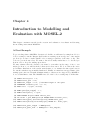
4 Introduction to Modelling and Evaluation with MOSEL-2
54
5 Example: Power Dissipation of a Hard Disk
73
6 Porting Models from MOSEL to MOSEL-2
79
6.1
MOSEL Constructs Changed or Missing in MOSEL-2 . . . . . . . . . . . . .
79
6.2
New MOSEL-2 Constructs . . . . . . . . . . . . . . . . . . . . . . . . . . . . .
88
7 Implementation of MOSEL-2
89
8 Categorization of MOSEL-2 and Comparison
95
9 Conclusion
101
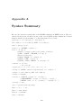
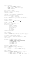
A Syntax Summary
104
B Bibliography
107
C Glossary
110
5
Chapter 1
Introduction
The subject of this thesis is the integration of the Petri Net analysis and simulation tool
TimeNET (see [TimeNET]) into the modelling environment MOSEL (see [BBH]). This work
is located in the area of stochastic modelling and evaluation for the purpose of performance
and reliability analysis; therefore this chapter contains a short overview over that area in Section 1.1. The MOSEL environment will be described (in Section 1.2), as well as the TimeNET
tool (in Section 1.3). The MOSEL description is rather short, since the complete description
of the revised MOSEL language will be the subject of later chapters. In Section 1.4, the
overall structure of the present thesis will be sketched.
1.1
Stochastic Modelling and Evaluation
The theory of probabilities is a helpful tool to evaluate complex dynamic systems like computer architectures, communication networks, production lines, and many more. Typically,
we know, or can estimate, certain values for components of such systems, like the expected
lifetime of an individual computer in a redundant high-security computer system, or the average number of parts that a station in a production line can produce per hour. We also know
how those components depend on each other, for example, how the reliability of a redundant
computer system depends on the reliabilities of the individual computers it is built of, or
which other stations are connected to a certain station in a production line.
The following methods, taken from [BBH], page 1, can be used to calculate certain quantitative measures for the system as a whole, like the life time of the whole computer system or
the number of parts that can be manufactured by the production line:
• Build a prototype whose architecture is identical to the system to be modelled. The
relevant parameters of the prototype’s components used should be close to the parameters of the actual system’s components. The behaviour of that prototype, especially
the measures of interest, can be measured by observation.
• Simulate the behaviour of the system in a computer model. Stochastic models are
usually simulated using discrete event simulation (DES), which is based on the Monte
Carlo method: The probabilistic quantities of the model’s components are replaced by
random quantities with the same probabilistic distribution. The simulation is repeated
for many runs (typically several thousand times) or for very long runs, so that the
random quantities will approximate the probabilistic quantities. DES can model a
wide range of models, but the number of repetitions that are needed to gain acceptable
accuracy may be very high.
6
• Create a mathematical model of the system and do a computer-based numerical analysis
on it. Approximative analysis methods are used for models that are intractable by exact
methods or whose exact solution would consume too much time and space. Even if exact
solution methods are used, instabilities of the numerical algorithms may have a great
influence on the quality of the results in practice. Analytical methods are only known
for a limited subset of stochastic models, although research is going on to develop
analytical methods for more general model types.
In the following, we will only deal with simulative and analytical methods.
Stochastic models can be used to gain the following types of result measures ([BBH], pages
63–64):
Performance Measures: These are values like system throughput, response time or utilization of components or the whole system, under the assumption that the system does
not fail.
Reliability: This is the probability that the system will work without failure during a certain
time period. Also of interest is the mean time span until the first failure happens.
Availability: This is the probability that the system is working at a certain time point.
Performability Measures: These are measures that take temporary performance degradations into account. Performance may be reduced by the failure of parts of the system.
Performability measures may be seen as a combination of performance measures and
availability.
Stochastic modelling needs a sound mathematical basis. For virtually all model types, the
methods used for stochastic analysis and simulation are formalised in terms of stochastic processes and Markov chains, so I’ll give a brief informal sketch of them. For more information,
refer to [BBH], chapter 2.
• A stochastic process is a family of random variables that share a common value space,
which is called the process’ state space. The random variables are indexed by a discrete
or continuous parameter. Since we want to model dynamic systems, we will always
use time as the process’ parameter; the random variable that is indexed by a specific
time point gives the state of the process at this time point. If the time parameter is
continuous, we speak of a continuous-time stochastic process; if the values of the time
parameter have a constant step width, we speak of a discrete-time stochastic process.
• A stochastic process with discrete state space is called a stochastic chain.
• A Markov chain is a stochastic chain which is memoryless, i.e., the future behaviour of
the process only depends on its current state, not on the past behaviour.
• A Markov chain is homogeneous if the probabilistic behaviour of the process at time t +
∆t only depends on the state at time t and on ∆t, but not on t itself. For a homogeneous
discrete-time Markov chain (DTMC), this means that the transition probabilities from
any state to any state in one time step are time-independent constants. The transition
probability from one state to another is then geometrically distributed over ∆t. —
For a homogeneous continuous-time Markov chain (CTMC), the time-derivatives of the
transition probabilities are time-independent constant as well. As is well-known from
calculus, the transition probabilities have exponential distributions over ∆t. In both
7
2p
2;3
p
0;3
1;3
p: Failure rate of a processor
m: Failure rate of a memory module
3m
2p
p
1;2
2;2
2m
m
2;0
0;2
2m
2p
2;1
x;y: State with x working processors
and y working memory modules
3m
p
1;1
0;1
m
1;0
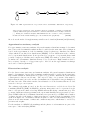
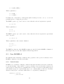
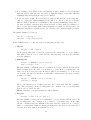
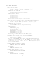
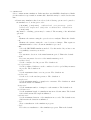
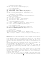
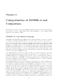
Figure 1.1: An example of a continuous-time Markov chain, taken from [BBH], page 73.
cases, the transition probabilities between any two states and for any time range can
be computed from these values. Indeed, such computations actually play an important
role in numerical analysis algorithms for many stochastic modelling languages.
For practical stochastical modelling, the following model types have gained wide-spread use,
as explained in [BBH], chapter 3:
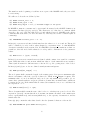
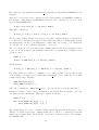
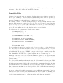
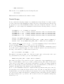
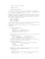
Markov Chains: Markov Chains, when used as a model type, are strongly connected to
the mathematical term which has been explained earlier, but for practical reasons they
must be homogeneous and are limited to finite state spaces (since each state has to be
specified explicitly).
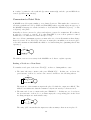
Usually, such a Markov Chain has a graphical representation, in which each circle
represents a state and each arc represents a transition between two states. Each arc
is labelled by the transition probability in one time step (for DTMCs) or by the timederivative of the transition probabilities (for CTMCs). For an example, see Figure 1.1.
Markov Chains “are usually larger and difficult to analyze, but they can also model
situations that cannot be represented using non-state-space-models” [BBH, page 72].
As soon as the models get more complex, Markov Chains are usually difficult to create,
maintain and understand. To overcome the need to specify each state explicitly, highlevel modelling types like queuing networks and stochastic Petri nets can be used, which
are mapped onto DTMCs or CTMCs for analysis. More about Markov Chains can be
found, for example, in [STP].
Queuing Networks:
A queuing network consists of service centers and customers (often called jobs).
A service center consists of one or more servers and one or more queues to hold
customers waiting for service. When a customer arrives at a service center, it enters
one of the servers or one of the queues. If there are customers waiting when a
busy server becomes idle, the next customer to be served is selected according to
a scheduling discipline (sometimes also called queueing discipline). The queueing
delay is the time period a customer waits in a service center before it enters one
8
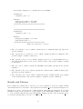
p0 = 0.1
Disk1
CPU
p1 = 0.55
service time: 20
p2 = 0.35
service time: 10
Disk2
service time: 30
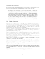
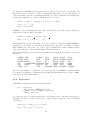
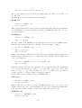
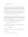
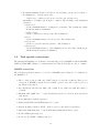
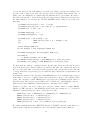
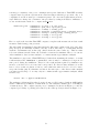
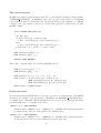
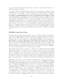
Figure 1.2: An example of a queueing model, taken from [BBH], page 67.
of the servers. The response time is the amount of time a customer spends at the
service center, including the queueing delay and the service time. [...]
A queueing network in which customers arrive from an external source, spend time
in the network, and depart is said to be open. A queuing network in which there is no
eternal source of customers and no departures is said to be closed . [BBH, page 64]
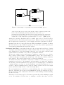
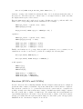
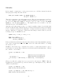
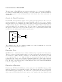
Among the queueing disciplines that are usually supported are First-Come-FirstServed , Last-Come-First-Served and Infinite Server . Figure 1.2 shows a closed queuing
model. Queues are represented by open rectangles, servers are represented by circles.
Queuing networks were among the first modelling formalisms for dynamic stochastic
models, but the are only of limited expressive power, since they cannot express dependencies among individual customers in the system.
Stochastic Petri Nets: A stochastic Petri net is also a state-based model type, but its
descriptive level is higher than that of Markov Chains. They are based on (pure) Petri
nets, which allow to model the dynamic behaviour of processes, like concurrency and
synchronisiations, but which do not allow for quantitative analysis.
A Petri net consists of places and transitions, which are connected by arcs. A place
may contain a variable number of indistinguishable tokens. The current number of
tokens in each place determines the current state of the Petri net, which is called the
net’s marking. The initial marking is part of a Petri net definition.
A transition may have any number of input arcs, which are arrows that go from the
transition’s input places to the transition, and any number of output arcs, which are
arrows that go from the transition to its output places. If each input place of a transition
contains at least one token, we say the transition is enabled and may fire, i.e., be
executed. When a transition fires, it removes a single token from each of its input
places, and adds a single token to each of its output places.
If several transitions are enabled in a certain marking, then any of these transitions
may fire. This introduces some non-determinism into the model, which is needed to
model concurrency. If no transition is enabled in a certain marking, then that marking
is called absorbing.
The directed reachability graph of a Petri net represents all possible markings as graph
nodes. If a transition can lead from one marking to another, then these nodes are
9
t1
t2
t1
t2
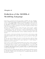
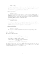
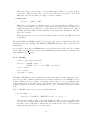
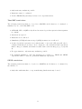
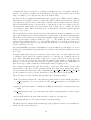
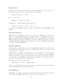
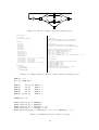
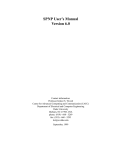
Figure 1.3: A simple Petri net before and after firing t1, taken from [BBH], page 74.
connected by an edge in the graph. The reachability graph is usually constructed
by depth-first or breadth-first exploration of the state space, starting with the initial
marking. It is useful for the examination of a Petri net’s structural properties.
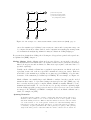
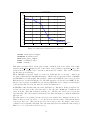
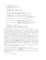
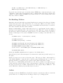
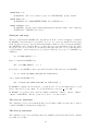
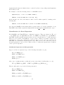
Figure 1.3 shows a Petri net, before and after a transition has fired, respectively. Places
are represented by circles, tokens are shown as black dots in the circles, and transitions
are displayed as rectangles.
A Stochastic Petri Net (SPN) adds time to a Petri net: each transition has a probabilistic delay which starts when the transition has been enabled. When the delay has passed
and the transition is still enabled, then it actually fires. The delays are exponentially
distributed, which allows the Petri net to be converted to a Markov chain for analysis
(by state-space generation). Usually, not the expected value of the delay is given, but
the expected value of its reciprocal, the firing rate. If several transitions are enabled at
the same time, the rule whose delay has passed first will fire.
Generalized Stochastic Petri Nets (GSPN) proposed by Ajmone Marsan et al. [ABC]
are the extension of Stochastic Petri nets obtained by allowing the transitions of the
underlying PN to be immediate as well as timed. Immediate transitions (graphically
represented by thin black bars) are assumed to fire in zero time as soon as they are
enabled. Timed transitions (represented by rectangular boxes or thick bars) are all
associated exponentially distributed firing times with rates just as in SPNs.
When both immediate and timed transitions are enabled in a marking, only the
immediate transitions can fire; the timed transitions behave as they are not enabled.
When marking m enables more than one immediate transition, it becomes necessary
to specify a probability mass function according to which the first transition to fire
is chosen. The marking of a GSPN can be classified to vanishing marking in which
at least one immediate transition is enabled, and tangible marking in which only
timed transitions [or none] are enabled. The reachability graph of a GSPN can be
converted to a Continuous-time Markov chain by eliminating the vanishing markings
[which yields a Reduced Reachability Graph (RRG)] and can be solved using different
solution methods [...].
[BBH, page 76]
The probabilistic behaviour of a stochastic Petri net can be evaluated at a given time
point after it has been started with its initial marking; this is called a transient evaluation. The long-time behaviour of a stochastic Petri net can be studied by a so-called
stationary or steady-state evaluation.
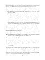
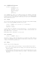
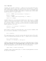
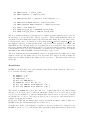
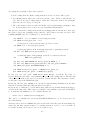
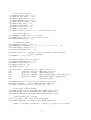
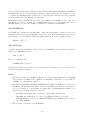
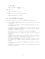
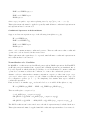
Figure 1.4 shows an example of a GSPN.
Many extensions to Petri nets [and GSPNs] have been proposed in order to increase
either the modeling convenience or the modeling power . Structural extensions that
effect only the modelling convenience provide a powerful way to improve the ability
of Petri nets to model real problems. Some accepted extensions of this type are:
10
rate mu3
rate mu1
p1
p2
1−p1
rate mu2
1−p2
Figure 1.4: A GSPN, taken from [STP], page 136.
Arc multiplicity representing the case when more than one token is to be removed
from or to a place in case of firing.
Inhibitor arc from place p to transition t disables t in all markings in which p is
not empty. [If the inhibitor arc has a multiplicity m, it disables t in all markings
in which p has less than m tokens.]
Transition priorities are integer priority levels assigned to each transition. A
transition is enabled only if no other higher priority transition is enabled.
Marking dependent arc multiplicity allows the multiplicity of an arc to vary
according to the marking of the net.
[BBH, page 75]
Another extension are guards. A guard is a condition in textual form that belongs to a
transition. This condition must be met by the marking in order to enable the transition.
Guards are useful to express relations between distant places, and they do not change
the current marking. Guards are well-fitted for many purposes where the enabling of a
transition is difficult to be controlled by arcs.
For the analysis of performability measures, so-called stochastic reward networks (SRN)
have been introduced, which are based on GSPNs. In an SRN, rewards may be specified
for some places, which are real-valued functions that depend on the number of tokens
in that place. They are used to compute the model’s result measures.
GSPNs have a high expressive power, compared with queuing networks, and they allow
more concise descriptions than Markov Chain tools. Recent extensions of GSPNs,
like MRSPNs (Markov Regenerative Stochastic Petri Net) and DSPNs (Deterministic
and Stochastic Petri Net) [German1], allow to use other firing distributions for timed
transitions besides the exponential distribution.
Stochastic Process Algebras:
Process algebras are abstract languages used for the specification and design of concurrent systems. [...] In the process algebra approach systems are modeled as collections of entities, called agents, which execute atomic actions. These actions are the
building blocks of the language and they are used to describe sequential behaviors
which may run concurrently, and synchronisations or communications between them.
[...]
In CCS [Milner’s Calculus of Communicating Systems, a form of PA’s] two agents
communicate when one performs an action, a say, while the other performs the
complementary action ā. [...] The grammar of the language makes it possible to
construct an agent which has a designated first action (prefix); has a choice over
alternatives (choice); or has concurrent possibilities (composition). [...] In CSP
[Hoare’s Communicating Sequential Processes, another form of PA’s] two agents
communicate by simultaneously executing actions with the same label. [. . . ]
11
def
Mem = (get, >).(use, µ).(rel , >).Mem
def
Proc = (think , p1 λ).(local , m).Proc + (think , p2 λ).(get, g).(use.µ).(rel , r).Proc
def
Sys 1 = (Proc k Proc) ./L M em
L = {get, use, rel }
Figure 1.5: An example PEPA model from [HR], page 238
Performance Evaluation Process Algebra (PEPA) extends classical process algebra
by associating a random variable, representing duration, with every action. These
random variables are assumed to be exponentially distributed and this leads to a
clear relationship between the process algebra model and a continuous time Markov
chain (CTMC).
PEPA models are described as interactions of components. Each component can
perform a set of actions: an action [...] is described as a pair (α, r) [...], where α
[...] is the type of the action and r [...] is the parameter of the negative exponential
distribution governing its duration.
[HR]
Figure 1.5 shows a simple PEPA model. Besides PEPA, there exist some other SPA
formalisms and tools, like TIPP (Timed Process for Performance Evaluation [GHR]),
MPA (Markovian Process Algebra [Buchholz]) and EMPA (Extended Markovian Process Algebra [BDG]).
Stochastic process algebras have inherent compositional features, so they are well-fitted
for compositional modelling. But the algebraic notation is rather mathematical and
unfamiliar for practicians without the necessary background in computer-science.
Other models: Some other graphical model types especially for reliability analysis are also
frequently used, such as Fault Trees and Reliability Graphs. In contrast to the four
presented model types, they are not state-based. Instead, they use the combinatorial
laws of probability for evaluation. Therefore, they can only model events that are
stochastically independent. For details, refer to [BBH].
For all presented model types, with the exception of stochastic process algebras, models are
typically built using graphical notations. These notations are intuitive and easy to debug if
the models are not too big, but they require specialised graphical input tools. Furthermore,
graphical representations of bigger models are hard to construct, to read and to debug.
Therefore, some graphical and textual modelling languages, like the Stochastic Petri-Net
Language SPNL [German2], which is a graphical-textual hybrid, allow the composition of
bigger models from smaller parts with well-defined interfaces.
1.2
The Modelling Environment MOSEL
MOSEL [BBH] has been developed by Helmut Herold at Universität Erlangen-Nürnberg,
Germany. Its name stands for “Modelling, Specification and Evaluation Language”.
MOSEL is a modelling language targeted at the description and quantitative evaluation of
stochastic dynamic models. Using MOSEL, complex systems can be modelled, like communication networks, production lines, computer systems, and many more. The models that
are described in MOSEL will be evaluated by a modelling environment that is also called
“MOSEL”, using numeric analysis methods.
The basic modelling primitives of a MOSEL model are nodes and rules. Functionally, they
are like the places and transitions, respectively, of a stochastic Petri Net. The state of a
12
/***========== M/E2/1 server
and
M/M/1 server ==============*/
/*---------------- NODES -------------------------------------*/
NODE N1[K; Phase1[1]; Phase2[1]]=K;
NODE N2[K]=0;
/*---------------- NOT ---------------------------------------*/
NOT N1+Phase1+Phase2+N2 != K;
/*---------------- Rules -------------------------------------*/
FROM N1
TO Phase1 IF Phase1+Phase2==0;
FROM Phase1 TO Phase2 WITH mue11;
FROM Phase2 TO N2
WITH mue12;
FROM N2
TO N1
WITH mue2;
/*---------------- RESULTs -----------------------------------*/
RESULT IF (N2!=0) rho2 += PROB;
RESULT MEAN N1;
RESULT DIST N2;
RESULT>>
lambda2 = rho2*mue2;
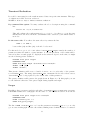
Figure 1.6: An example of a MOSEL description
MOSEL model is determined by the values of all its nodes; the rules describe the possible
transitions between these states. Each rule fires either immediately when its conditions are
met, or it has a stochastic delay that is exponentially distributed. To get an impression how
a MOSEL model description looks like, see Figure 1.6, which is presented without any further
explanation.
The real evaluation will not be done by MOSEL itself; instead, the MOSEL model will
be analysed by an external analysis tool. For this purpose, the MOSEL model description
will be translated into the format that is used by the respective tool. This tool is invoked
automatically by the MOSEL environment, its results are read in and written to the MOSEL
result file. Optionally, the results may be displayed is graphs. The graph description(s), in
the proprietary IGL format (“Intermediate Graphics Language”), are written to a separate
file. The graphs can be displayed, printed or changed using the IGL interpreter, which is
part of the MOSEL program suite.
So far, the following stochastic analysis tools are supported:
• The stochastic Markov analysis tool MOSES [BGJZ], developed at Universität
Erlangen-Nürnberg, Germany.
• The Petri Net analysis tool SPNP [SPNP], developed at Duke University, USA.
The MOSEL environment is already prepared for the integration of other stochastic analysis
or simulation tools, due to its modular structure.
13
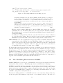
1.3
The Petri Net Tool TimeNET
The Petri Net Tool TimeNET [TimeNET] [ZFGH1] [ZFGH2] is actually a collection of tools
that support the creation, testing, and evaluation (analysis and simulation) of stochastic
Petri nets. “The development of TimeNET has been influenced by other software tools like
GreatSPN, SPNP and UltraSAN. The first version of TimeNET was a major revision of the
tool DSPNexpress, which had been developed at TU Berlin since 1991” [ZFGH2].
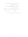
TimeNET supports the following types of Petri net models:
Hierarchical Coloured Petri Nets (HCPN): Coloured Petri Nets can contain ordinary
tokens, which are all undistinguishable, as well as coloured tokens, which can be distinguished by their different colours. Coloured Petri Nets are useful to model manufacturing systems where different parts must be distinguished. Complex manufacturing
systems can be managed by hierarchical decomposition of the net.
Fluid Stochastic Petri Nets (FSPN): The FSPN formalism is an extension of the GSPN
formalism. It does not only know places that contain a number of tokens, but it also
allows places that contain a continuous amount of fluid, represented by a non-negative
real number. That fluid can “flow” along through fluid arcs, in a constant flow, as long
as the corresponding transition is enabled. Alternatively, a certain amount of fluid can
be removed or deposited at once. Second Order FSPNs can also model a stochastic
variation of the flow. FSPNs are useful for performance and dependability analysis
of systems containing continuous components such as time, liquid, temperatures, or
others. For more information, see [Wolter].
Extended Deterministic and Stochastic Petri Nets (eDSPN): This Petri Net type
is an extension of the GSPN type. Transitions in eDSPNs are not limited to immediate
and exponential firing distributions:
The firing delay of transitions in eDSPNs can either be zero (immediate), exponentially distributed, deterministic, or belong to a class of general distributions called
expolynomial . Such a distribution function can be piecewise defined by exponential
polynomials and has finite support. It can even contain jumps, making it possible
to mix discrete and continuous components. Many known distributions (uniform,
triangular, truncated exponential, finite discrete) belong to this class.
[ZFGH2]
An eDSPN is also referred to as a MRSPN (Markov Regenerative Stochastic Petri Net).
This name stems from an analysis method for such nets which is used by TimeNET
for stationary analysis. An eDSPN whose general distributions are all deterministic is
called a DSPN (Deterministic and Stochastic Petri Net).
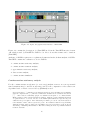
All those Petri net types can be created and modelled using the graphical user interface
Agnes (A generic net editing system). Figure 1.7 shows an eDSPN that is just being edited
in Agnes. Agnes has an interface to each analysis tool and simulation tool: It can ask the
user for evaluation options using a dialog window, run the tool, read in the computed result
values, and display the results. For all Petri net types, evaluation by simulation is possible
as well as numeric analysis for certain subtypes.
In the present thesis, we will only consider eDSPNs, since they fit naturally into the existing
MOSEL language. The MOSEL language just has to be extended by adding means to specify
other distributions besides the exponential and immediate distributions.
14
Figure 1.7: Agnes, the graphical user interface of TimeNET.
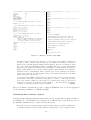
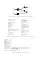
Figure 1.8 contains the description of a TimeNET model in the TimeNET interface format
.TN, which is used by TimeNET’s eDSPN tools. More about this format can be found in
[TimeNET].
Analysis of eDSPNs requires more sophisticated numerical methods than analysis of GSPNs.
TimeNET contains five evaluation tools for eDSPNs:
1. continuous-time stationary analysis;
2. continuous-time transient analysis;
3. approximative stationary analysis;
4. discrete-time analysis;
5. continuous-time simulation.
Continuous-time stationary analysis
For the continuous-time steady-state (or stationary) analysis, at most one non-exponential
timed transition may be enabled at any time point. For the computation of the solution, an
algorithm based on Markov renewal theory [Kulkarni] is used:
For a steady-state [...] analysis of a stochastic Petri net model of any kind, the reachability
graph is computed next. [...] Subnets of immediate transitions are evaluated in isolation
[...] . The reduced reachability graph of a GSPN is isomorphic to a continuous-time
Markov chain, because of memoryless state changes. Only the corresponding linear system
of equations has to be solved. In case of an eDSPN (and DSPNs as a special case), an
additional step is required. The underlying stochastic process is only memoryless at
some instants of time, called regeneration points. If a transition with non-exponentially
distributed firing delay is enabled in a marking, the next regeneration point is chosen
after firing or disabling this transition. The time of firing the next exponential transition
is taken otherwise.
15
-- FILE erlang4phases.TN CONTAINING STRUCTURAL DESCRIPTION OF A NET
NET_TYPE:
DESCRIPTION:
PLACES:
TRANSITIONS:
DELAY_PARAMETERS:
MARKING_PARAMETERS:
REWARD_MEASURES:
DSPN
?
5
4
2
1
1
-- LIST OF MARKING PARAMETERS (NAME, VALUE, (X,Y)-POSITION):
MARKPAR K 20 1.39 4.22
-- LIST OF PLACES (NAME, MARKING, (X,Y)-POSITION (PLACE & TAG)):
PLACE
PLACE
PLACE
PLACE
PLACE
P1
P2
P3
P4
P5
K
0
0
0
1
2.5 1.06 2.44
2.48 2.58 2.4
3.78 2.58 3.7
5.4 2.58 5.36
2.5 3.58 2.46
0.88
2.86
2.88
2.86
3.4
TRANSITION T2 arrival SS EXP RE 0 0 1 0 1.000000 3.2 2.5 3.0 2.8 0 0
INPARCS 1
1 P2 0
OUTPARCS 1
1 P3 0
INHARCS 0
TRANSITION T3 arrival SS EXP RE 0 0 1 0 1.000000 4.5 2.5 4.5 2.8 0 0
INPARCS 2
4 P3 0
1 P1 0
OUTPARCS 2
1 P4 0
1 P5 0
INHARCS 0
TRANSITION T4 service SS DET RE 0 0 1 0 1.000000 6.6 2.5 6.6 2.8 0 0
INPARCS 1
1 P4 0
OUTPARCS 1
1 P1 0
INHARCS 0
-- LIST OF DELAY PARAMETERS (NAME, VALUE, (X,Y)-POSITION):
-- DEFINITION OF PARAMETERS:
DELAYPAR service 0.1 1.39 4.59
DELAYPAR arrival 0.125 1.39 4.82
-- MARKING DEPENDENT FIRING DELAYS FOR EXP. TRANSITIONS:
-- LIST OF TRANSITIONS
-(NAME, DELAY, ENABLING DEPENDENCE, KIND, FIRING POLICY,
-PRIORITY, ORIENTATION, PHASE, GROUP, GROUP_WEIGHT,
-(X,Y)-POSITION (TRANSITION, TAG & DELAY), ARCS)
-- MARKING DEPENDENT FIRING DELAYS FOR DET. TRANSITIONS:
-- PROBABILITY MASS FUNCTION DEFINITIONS FOR GEN. TRANSITIONS:
-- MARKING DEPENDENT WEIGHTS FOR IMMEDIATE TRANSITIONS:
TRANSITION t1 1 SS IM RE 1 0 1 0 1.000000 1.7 2.5 1.7 2.8 0 0
INPARCS 2
1 P1 0
1 P5 0
OUTPARCS 2
4 P2 0
1 P1 0
INHARCS 0
-- ENABLING FUNCTIONS FOR IMMEDIATE TRANSITIONS:
-- MARKING DEPENDENT ARC CARDINALITIES:
-- REWARD MEASURES:
MEASURE Server1
E{#P1};
-- END OF SPECIFICATION FILE
Figure 1.8: Example .TN file for TimeNET.
By taking only the regeneration points into account, a discrete-time Markov chain is embedded. [...] The evolution of the stochastic process during the enabling of a transition
with non-exponentially distributed firing delay is analysed. At most one transition of this
type can be enabled per marking for this type of analysis. Therefore only exponential transitions may fire during the enabling period, resulting in a continuous-time subordinated
Markov chain (SMC) of the non-exponential transition. The transient and cumulative
transient solution of this Markov chain computes [the one-step transition probabilities
between two regeneration points and the average sojourn times in the states of the SMC
until regeneration, respectively]. [...]
[For the embedded DTMC,] a linear system of equations based on the [one-step transition
probabilities between two regeneration points] has to be solved [...]. The state probabilities of the actual stochastic process can then be obtained as the mean sojourn time in
each state between two regeneration points. Finally, [...] the user-defined performance
measures are calculated from the state probabilities.
[ZFGH2]
More about Markov renewal theory can be found in [Kulkarni], more about its application
for the stationary evaluation of eDSPNs in [CGL].
Continuous-time transient analysis
Continuous-time transient analysis requires that non exponential timed transitions must be
deterministic (so only DSPNs can be analysed in a transient state), and that at most one
deterministic transition may be enabled at any time point.
The method is based on supplementary variables, which capture the elapsed enabling time
of transitions with non-exponentially distributed firing delays. State equations can be
16
1
0
3
p
2
1
1
1
0
1
1−p
Figure 1.9: DTP representations of a geometric and a deterministic distribution, respectively.
derived for the description of the dynamic behaviour of DSPNs, consisting of partial and
ordinary differential equations which are combined with initial and boundary conditions.
[...] During the transient analysis, TimeNET shows the evolution of the performance
measures from the initial marking up to the transient time graphically.
[ZFGH2]
More about the method of supplementary variables can be found in [German1] and [German3].
Approximative stationary analysis
For approximative stationary analysis, all general transition distributions must be deterministic, but several deterministic transitions may be enabled at the same time. The technique is
based on the approximation of the deterministic delays by phase-type distributed stochastic
delays which are modified Cox distributions [ZFGH2]. A Cox distribution is the combination of exponential distributions. It is represented by a sequence of exponential phases with
possibly complex probabilities and complex rates [BBH]. The number of phases used to approximate the deterministic distributions may be set by the user. Higher numbers lead to
more accuracy, but also to a bigger state space. More about the approximation technique
used can be found in [German4].
Discrete-time analysis
For the discrete-time stationary and transient analysis, all general transition distributions
must be deterministic, but several deterministic transitions may be enabled at the same time.
Exponential transition distributions are replaced by geometric distributions, their natural
counterparts for discrete model time. The expected delay of a geometric delay must be
higher than the time base scale, and the deterministic fire delays must be integer multiples of
the time base scale. This solution method is well-suited for clocked activities like in a clocked
network or in a processor system.
The evaluation algorithm is based on the Discrete Deterministic and Stochastic Petri Net
formalism (DDSPN) [ZCH]. In DDSPNs, arbitrary firing times can be represented as the
time to absorption in a finite absorbing DTMC with an underlying constant time step. The
geometric distribution that approximates the exponential distribution is represented by a twophase DTMC, while the deterministic distribution is represented by a DTMC whose number
of phases depends on the number of time steps that are contained in the deterministic delay,
as show in Figure 1.9. A transition will fire in phase 0. Since several transitions may go to
phase 0 at the same instant, conflicts and confusions may arise, which must be resolved by
priorities and weights.
For the analysis of a DDSPN, the markings and the phases of each transition are part of the
state space of the underlying DTMC.
17
Continuous-time simulation
For the stationary and transient simulation, any general transition distribution can be used,
and several generally distributed transitions may be enabled at the same time.
The simulation can be executed in a sequential or distributed manner, i.e. multiple simulation replications run on multiple hosts in a workstation cluster, using a master/slave
concept. [...] Since samples from the transient phase do not represent the steady-state
behavior of the model, the length of this phase is detected automatically by the simulation
component and the samples from this phase are discarded. [...] Usually a TimeNET simulation run stops after a user-specified accuracy of the results has been achieved, which is
checked statistically. The accuracy can be controlled [...]. The standard simulation allows
two types of variance estimation, which is necessary to detect the already reached accuracy. The normal case is the application of variance estimation based on spectral variance
analysis. In many cases, a variance reduction technique based on control variates can be
applied successfully.
[TimeNET]
1.4
Thesis Overview
During my work on the integration of TimeNET into the MOSEL environment, I had to
realize that some important language features of MOSEL cannot be properly translated into
the description language used by TimeNET. Also, some language characteristics of MOSEL
were quite irregular and/or hard to understand for newcomers. Therefore, I revised the
MOSEL language and called the revised form “MOSEL-2”.
Chapter 2 contains the complete language definition of MOSEL-2. Its semantics is described
by explaining how to convert a MOSEL-2 description into a stochastic process and how to
gain result measures from that process.
Chapter 3 explains how to invoke the MOSEL-2 environment in order to evaluate a model.
Since each analysis tool that can be used by MOSEL-2 has its own command line options, a
large number of command line options are available for MOSEL-2.
Chapter 4 gives a practical introduction into modelling with MOSEL-2 for people who are
not acquainted with MOSEL.
Chapter 5 shows a practical real-world example of evaluation with MOSEL-2: the power
comsumption of a hard disk will be modelled.
Chapter 6 explains the differences between MOSEL and MOSEL-2. For most MOSEL language constructs that have been changed or eliminated, we suggest how to translate them
into equivalent MOSEL-2 constructs.
Chapter 7 explains the internal steps of the MOSEL-2 evaluation environment, and also some
implementation aspects that might be of interest.
Chapter 8 categorizes the MOSEL-2 language in terms of specification languages and software
ergonomy; MOSEL-2 will be compared with the stochastic modelling languages CSPL and
SHARPE.
Chapter 9 summarizes the present thesis and suggests some future work.
18
Chapter 2
Definition of the MOSEL-2
Modelling Language
In this chapter, we will define the syntax and semantics of MOSEL-2. The name “MOSEL-2”
stands for “Modelling, Specification and Evaluation Language”, revised definition. MOSEL2 is based on the original MOSEL definition, as described in [BBH]. A revision was needed
since the original MOSEL definition contained language elements that are not supported by
the TimeNET tool, but which were needed for the convenient description of larger models, as
C-like functions and variables. The differences between the original version and the revised
version are described in Chapter 6.
The purpose of MOSEL-2 is to model complex systems, like computer systems, communication networks or production systems, in order to evaluate their performance, reliability,
or similar measures. Parts of the model may be defined stochastically, like the processing
time of an individual component or the successor of a station in a production system. The
given model may be analysed numerically or it may be simulated, yielding the desired result
measures.
Nodes are used to describe the model’s state. In a specific state, each node has a certain
value, which is an integer number in the range from 0 to a node-dependent maximum. This
maximum is called the node’s capacity. The node’s value range is the set of its possible
values.
The state space is the cartesian product of the nodes’ value ranges. It is bounded (i.e. finite),
since the value ranges are all finite. At time t = 0, the process is in its initial state. This
initial state is composed of the initial node values, which have to be stated explicitly or
implicitly in the model description.
Rules are used to describe how the system may change from one state to another. A rule may
change the model’s state by setting some nodes to specific values and/or by incrementing or
decrementing the values of some nodes. A rule is generally appliable to a set of states. This
set is specified by the rule’s explicit conditions, and implicitly by some of the rule’s actions;
for example, a rule may not set a node to a negative value or to a value that exceeds its
capacity. If the rule is appliable in the current state, we say it is enabled . Several rules may
be enabled at the same time.
Each rule is given a probabilistic firing time distribution. This firing time distribution specifies
how much time will pass from the point when the rule has been enabled up to the point when
the rule will be actually executed. Special subcases are deterministic firing times and rules
that will fire immediately.
19
Not every state in the state space may be reachable; which states are actually reachable
depends on the initial state and on the rules that lead from one state to the next.
We will define the semantics of a MOSEL-2 description by describing how it can be converted into a stochastic chain, that means, a stochastic process with finite state space. This
stochastic chain is reached in three steps:
1. The MOSEL-2 description is translated into a mathematical model called the Explicit
State Model (ESM).
2. The Explicit State Model is converted to a process with mixed continuous/discrete
state space and continuous time base. The state space of the Markov process consists
of the states of the ESM, but supplementary real numbers have been added to each
state, which indicate the remaining firing times for each rule. Since the remaining firing
times are part of the process’ state space, we can predict the probabilistic behaviour
in the future from the current behaviour and do not need to examine past states. In
other words, the process is Markovian. (This technique has been inspired by [German1],
chapter 6.)
3. From that Markov process, we can derive a stochastic chain with finite state space by
dropping the remaining firing times in the states. This new process is generally not
Markovian. It is Markovian, indeed, if the MOSEL-2 description from which it has
been derived only contains immediate rules and exponentially distributed rules.
It is easier to define the semantics on a subset of the MOSEL-2 language only, which we
call Core MOSEL-2 . The semantics of the full MOSEL-2 language can then be explained in
terms of Core MOSEL-2. So this chapter is divided into the following sections:
Section 2.1 Definition of Core MOSEL-2.
Section 2.2 Definition of Full MOSEL-2. The meanings of additional elements of MOSEL-2
are defined in terms of Core MOSEL-2.
Section 2.3 Definition of the semantics of Core MOSEL-2. This shows how a MOSEL-2
description can be formally translated into a stochastic process.
The syntax formalism EBNF
The syntax of MOSEL-2 will be formally described by means of the Extended Backus-Naur
Formalism (EBNF) [Wirth]. Its descriptive power is equivalent to context-free grammars, but
EBNF grammars are usually more concise. Aspects of the MOSEL-2 language that cannot
be expressed by context-free grammars are explained in plain English. An EBNF production
looks like
a ::= b “OR” c .
The syntactic symbol a in this example denotes the syntactic unit to be defined. The part
to the right of the “::=” shows how the symbol a can be constructed as a sequence of the
symbols b, the keyword “OR” and the symbol c. The full stop indicates the end of the
production. MOSEL-2 keywords and other characters that are part of MOSEL-2, like “+”
and “..”, must be enclosed in quotes (“ ”) when used in an EBNF production.
If there are several productions that define a, they are all valid as alternatives. The EBNF
operator “|” can be used as an abbreviation for such alternatives:
20
a ::= b (OR | AND) c .
This is equivalent to
a ::= b OR c .
a ::= b AND c .
Normally, the concatenation of subsequent symbols takes precedence over “|”, so we need
parentheses here to change the precedence.
The EBNF operator “[ ]” can be used to denote that the enclosed expression is optional:
a ::= [“-”] b .
This is equivalent to:
a ::= b .
a ::= “-” b .
The EBNF operator “{}” can be used to denote that the enclosed expression is optional and
can be repeated:
a ::= b {“+” c} .
This is equivalent to the recursive definition:
a ::= b x .
x ::= “+” c x .
x ::= .
The EBNF productions of the MOSEL-2 syntax are embedded in the MOSEL-2 definition of
this chapter; they are also listed alphabetically in Appendix A.
2.1
Core MOSEL-2
We will first define elementary constructs, and go up later to the top-level constructs of Core
MOSEL-2, namely nodes, rules and results.
2.1.1
Lexical items
MOSEL-2 is a format-free language, which means that indentation and line breaks have
no special meaning. Any sequence of spaces, tabulator stops and new-line characters is
called whitespace and is ignored. (Actually, there are three exceptions: (1) in strings, spaces
and tabulator stops are copied literally, (2) a “//” comment must be ended by a new-line
character, and (3) two consecutive names have to be separated by whitespace).
comment ::= “//” line
| “/*” text “*/” .
21
A comment in a MOSEL-2 description is ignored. There are two forms of comments, both
known from C/C++, namely a one-line comment that starts with “//” and ends at the end
of the current line, and a free form that starts with “/*”, may contain any text including line
breaks, and ends with “*/”. Such comments may not be nested.
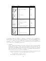
number ::= digits [“.” digits] [(“e” | “E”) [“+”| “-”] digits] .
digit ::= “0” | . . . | “9” .
digits ::= digit {digit} .
MOSEL-2 does not distinguish integer values and floating point values; integer values are
just a subset of the floating point values.
identifier ::= (letter | “ ”) {letter | digit | “ ”} .
letter ::= “A” | . . . | “Z” | “a” | . . . | “z” .
An identifier may be used as the name of a node, a result, or a duration. In Full MOSEL-2,
it may also be the name of a constant, an enumeration, a function, or a named condition.
Each identifier can only denote one of those types. It must have a single definition in the
source text. Each use of the identifier must follow that definition.
The following names are reserved keywords with special meanings; they may not be used as
identifiers:
AFTER
CURVE
FLOOR
OR
PRS
TIME
AND
DIST
FROM
PARAMETER
RATE
TO
ASSERT
ELIF
FUNC
PICTURE
RESULT
UTIL
AVG
ELSE
IF
PRD
SIN
WEIGHT
COND
ENUM
MEAN
PRINT
SQRT
WITH
CONST
EXTERN
NODE
PRIO
STEP
XLABEL
CUM
FIXED
NOT
PROB
THEN
YLABEL
Two successive names, i.e. identifiers or reserved keywords, in a MOSEL-2 description must
be separated by whitespace. Capital letters are different from small letters, so “node”, “NODE”
and “Node” are all different names.
2.1.2
Expressions
A MOSEL-2 expression yields a floating point value.
expr ::= simple-expr
| “IF” condition “THEN” simple-expr
{“ELIF” condition “THEN” simple-expr }
“ELSE” simple-expr .
A conditional expression starts with an “IF”, and yields the value of the first simple-expr for
which the associated condition holds. If no condition holds, it yields the value of the final
simple-expr .
simple-expr ::= term {(“+” | “-”) term} .
term ::= factor {(“*” | “/”) factor } .
22
The arithmetic operators “+”, “-”, “*” and “/” are supported. Division by zero is forbidden
and yields an error. The arithmetic operators are left-associative. The operators “*” and
“/” have higher priority, unless the evaluation order is changed by parentheses.
factor ::= atom {“^” atom} .
The operator “^” is right-associative and used for exponentiation. The exponentiation base
(the left operand of an exponentiation) must be positive.
atom ::= “(” expr “)” .
Parentheses can be used to express and/or change the evaluation order.
atom ::= (“SIN” | “SQRT” | “FLOOR”) “(“ expr “)” .
“SIN(expr )” yields the sine of expr , where expr is measured in radians.
“SQRT(expr )” yields the non-negative square root of expr , which must be non-negative.
“FLOOR(expr )” yields the largest integer value that is not greater than expr .
atom ::= number | result | node .
result ::= identifier .
node ::= identifier .
A result name (see Section 2.1.8) in an expression yields the value of the respective result. A
node name (see Section 2.1.5) in an expression yields its state-dependent value.
atom ::= [“AVG”] “PROB” “(” condition “)”
| [“CUM” | “AVG”] “MEAN” “(” state-expr “)”
Conditions and expressions in a PROB or MEAN construct are evaluated for each state. A
node name in such a construct evaluates to the node’s value in that state. A PROB construct
yields the overall probability of all states where condition holds. A MEAN construct yields
the expectation value of state-expr , i.e. the sum of state-expr evaluated for all states, each
term weighed by the probability of its state.
The keywords PROB and MEAN may be prefixed by AVG if the analysis is transient, which
computes the time-averaged probability or expectation value, i.e., the values are evaluated
and integrated in the time span from t = 0 up to the evaluation time point and divided by
the length of the time span. The keyword MEAN may be prefixed by CUM if the analysis is
transient, computing the cumulated expectation value, i.e., the expectation value is evaluated
and integrated in the time span from t = 0 up to the evaluation time point.
This definition of MOSEL-2 expressions is very general. There exist several subtypes of
MOSEL-2 expressions, which have certain limitations:
• Probability Expressions
23
p-expr ::= expr .
A p-expr (for probability expression) is an expression that defines the value of a result
(see Section 2.1.8). It may not contain any conditional expressions, node names, and
functions (see Section 2.2), except those who are part of PROB or MEAN constructs.
A result name in a p-expr yields the value of that result.
• State Expressions
state-expr ::= expr .
A state-expr is a state-dependent expression. It can be used in a MEAN, RATE or
WEIGHT construct, in a condition (see Section 2.1.3), or in a function definition (see
Section 2.2.6). It may contain conditional expressions, node names, and functions, but
no PROB or MEAN constructs, and no result names.
• Constant Expressions
const-expr ::= expr .
A const-expr is an expression that is used to define a constant (see Section 2.2.3). It may
not contain any conditional expressions, PROB or MEAN constructs and no functions,
named conditions, results, and nodes, either. A constant expression can be used in an
AFTER rule part (see Section 2.1.7) and in a constant definition.
• Integer Expressions
int-expr ::= const-expr .
An int-expr is a constant expression that must yield a non-negative integer value.
2.1.3
Conditions
A condition is defined as follows:
condition ::= and-condition {“OR” and-condition} .
and-condition ::= not-condition {“AND” not-condition} .
not-condition ::= [“NOT”] simple-condition .
simple-condition ::= state-expr compare-oper state-expr
| “(” condition “)” .
compare-oper ::= “=” | “/=” | “<=” | “>=” | “<” | “>” .
A condition is state-specific. It is used in PROB constructs and in IF rule parts. OR-ed
and AND-ed conditions are shortcut-evaluated, so “node > 0 AND 1/node = 1” is a valid
expression, although “1/node = 1” is illegal if node = 0.
24
2.1.4
MOSEL-2 File Structure
mosel-file ::= {const-def }
node-def {node-def }
{assertion}
{func-def | cond-def }
rule-def {rule-def }
results
{picture-def }
A Core MOSEL-2 file consists of node definitions, assertions, rule definitions, result definitions, and picture definitions, in that order. Constant definitions (const-def ), function definitions (func-def and cond-def ) and picture definitions (picture-def ) are part of Full MOSEL-2
and are defined in Section 2.2.
2.1.5
Nodes
A node is associated with a name and a value range. The values are integer numbers ranging
from 0 to a node-specific maximum, called the node’s capacity.
node-def ::= “NODE” node “[” max-value “]” [“:=” initial-value] “;” .
max-value ::= int-expr .
initial-value ::= int-expr .
node-def defines a node with name node and a value range {0, . . . , max-value}. The node’s
initial value will be initial-value or 0, if initial-value is omitted. initial-value must be an
integer number in {0, . . . , max-value}.
In this chapter, maxnode will stand for node’s max-value.
2.1.6
Assertions
assertion ::= “ASSERT” condition “;” .
An assertion contains a condition that must hold in every reachable state. This construct is
useful to debug a MOSEL-2 description. When the analyzer finds a reachable state for which
condition does not hold, it reports an error.
2.1.7
Rules
A rule is composed of the following parts:
• A precondition, which describes the subspace of states in which the rule is enabled.
• One or more actions, which describe the changes of the current state that take place
when the rule fires.
• A firing distribution. When the rule gets enabled, it may fire immediately, after a fixed
time interval, with exponentially distributed probability, or with (discrete) uniform
distribution.
25
• A re-enabling policy. When a rule gets disabled, it may remember or forget the time
that has elapsed while the rule was enabled. This has impact on the time until the
remaining firing delay when the rule gets re-enabled.
• A priority and a weight. If several rules are enabled and may fire at the same time,
only one of the rules with maximum priority will do so. Let S be the set of all rules
that are enabled, may fire at a certain time point, and have maximum priority. Let t be
the sum of weights of all those rules. Then each rule of S fires with a probability w/t,
where w is the rule’s weight. Timed rules always have a weight of 1 and a priority of 0.
Immediate rules have a default priority of 1, but they can be assigned higher priorities.
The syntax definition of a rule is:
rule-def ::= rule-parts “;” .
rule-parts ::= rule-part {rule-part} .
A rule definition may be composed of the following parts, in any order:
• IF part
rule-part ::= “IF” condition .
An IF part specifies that condition is a guard for the current rule, i.e. a precondition
that must be true in order to enable the rule. IF parts may occur more several times
in a rule definition.
• FROM part
rule-part ::= “FROM” node [“(” arity “)”] .
arity ::= int-expr | node .
The first variant of a FROM part is a combination of a precondition and an action.
In the pre-firing state, the value of node must be ≥ arity. In the post-firing state, the
value of node is decreased by arity. If arity is omitted, it is assumed to be 1. If arity is
a node name, the state-dependent node value will be taken as arity. If arity is constant,
it must be positive.
rule-part ::= “FROM” node “[” node-value “]” .
node-value ::= int-expr .
The second variant is a precondition and may only be used if the rule also contains a
part “TO node[value]”. In the pre-firing state, the condition node = node-value must
hold in order to enable the rule.
FROM parts may occur several times in a rule definition.
• TO part
rule-part ::= “TO” node [“(” arity “)”] .
The first variant of a TO part is a combination of a precondition and an action. In
the pre-firing state, the condition node ≤ maxnode −arity must hold. If the same
rule also contains a rule part “FROM node(arity 2 , then the condition node − arity 2 ≤
maxnode −arity must hold instead. In the post-firing state, the value of node is increased
by arity. If arity is omitted, it is assumed to be 1.
26
rule-part ::= “TO” node “[” node-value “]” .
The second variant is an action. In the post-firing state, the value of node will be set
to node-value.
TO parts may occur several times in a rule definition.
• RATE part
rule-part ::= “RATE” rate .
rate ::= state-expr .
This part specifies that the rule has an exponential firing time distribution with mean
rate, which must be a positive floating point value. A RATE part may only occur once
in a rule definition.
• AFTER part
rule-part ::= “AFTER” delay .
delay ::= const-expr .
The first variant of an AFTER part specifies that the rule has a deterministic firing
time and fires delay time units after enabling. The delay must be positive.
rule-part ::= “AFTER” start “..” end .
start ::= const-expr .
end ::= const-expr .
The second variant specifies that the rule has a uniform firing time distribution and
fires in the interval from start to end time units after enabling. The inequality 0 ≤
start < end must hold.
rule-part ::= “AFTER” start “..” end “STEP” step .
step ::= const-expr .
The third variant is used in a rule that has a discrete uniform firing time distribution
, i.e., it fires with uniform probability at one of the time points start, start + step,
start + 2 · step, . . . , end . The inequality 0 ≤ start < end must hold, step must be
positive and (end − start)/step must be an integer number.
A rule definition may contain at most one AFTER part.
• PRIO part
rule-part ::= “PRIO” priority .
priority ::= int-expr .
This sets the rule’s priority to priority. A PRIO part may only occur once in a rule
definition and it can only be used in an immediate rule; if it is omitted in an immediate
rule, a priority 1 will be assumed. A timed rule always has a priority of 0.
• WEIGHT part
rule-part ::= “WEIGHT” weight .
weight ::= state-expr .
27
This part sets the rule’s weight to weight, which must evaluate to a positive floating
point value. This part may only occur once in a rule and it can only be used in an
immediate rule; if it is omitted, a weight of 1 will be assumed.
• Policy part
rule-part ::= “PRD” | “PRS” .
This part sets the rule’s re-enabling policy to pre-emptive different (PRD) or preemptive resume (PRS), respectively. A rule with policy PRD forgets the elapsed enabling time when it gets disabled. A rule with policy PRS remembers the elapsed
enabling time when disabled; this will influence the firing time distribution when the
rule gets re-enabled.
This part may only occur once in a rule definition. If it is omitted, the PRD policy will
be assumed.
The parts RATE and AFTER exclude each other in a rule. If none of them is used, the rule
fires immediately after enabling. The PRIO and WEIGHT parts may only be used if the rule
is immediate.
No node may be used in several FROM parts or several TO parts of a rule. If a node contains
a part “TO node[new value]”, then an (optional) FROM part using that node must have the
form “FROM node[old value]”.
2.1.8
Results
results ::= [time-def ] {result-def } .
time-def ::= “TIME” number ”;”
| “TIME” start “..” end “STEP” step-width “;” .
start ::= number .
end ::= number .
step-width ::= number .
Normally, a MOSEL-2 model is evaluated in its stationary state, but the result part can be
preceded by a time definition, which causes a transient evaluation of the MOSEL-2 model.
A time definition can give a single, non-negative time point, or a set of equidistant time
points, ranging from a start time point to an end time point, where the distance between two
evaluation points is step-width. The inequations 0 ≤ start < end and step-width > 0 must
hold.
In Core MOSEL-2, there are two types of result definitions:
1. Proper results:
result-def ::= (“PRINT” | “RESULT”) result “:=” p-expr “;” .
Such a result definition defines result and assigns the value of p-expr to it. The value
of result can be used in subsequent result definitions. If the keyword PRINT is used,
the value of the result will be written into the result file and can be used in picture
definitions that may follow (see Section 2.2.9).
28
2. Durations:
result-def ::= “PRINT” duration “:=” “TIME” “TO” condition “;” .
duration ::= identifier .
Such a result definition prints a duration, i.e. the expected time span until condition
holds for the first time. The duration can be used in picture definitions (see Section 2.2.9). It must not be used in subsequent result definitions.
2.2
Full MOSEL-2
Full MOSEL-2 is an extension of Core MOSEL-2. The additional language constructs do
not increase the expressiveness of MOSEL-2, they only improve its usability for the concise
and readable description of stochastic models by adding “syntactic sugar”. The following
language constructs are defined in terms of Core MOSEL-2, which implicitly defines their
semantics.
2.2.1
MOSEL Compatibility
For compatibility with the original MOSEL language, you can use “=” (instead of “:=”) as
assignment operator , you can use “==” (instead of “=”) to test for equality , and you can use
“WITH” (instead of “RATE”)for exponential distributions . The old and new forms may be
mixed.
2.2.2
Strings
string ::= “"” sequence of printable chars “"” .
Full MOSEL-2 is equipped with an additional lexical element, namely the string. A string
may contain any sequence of printable chars, including spaces, but it must not contain double
quotes “"” and it must not exceed line boundaries. Strings are used to define labels in picture
definitions.
2.2.3
Constants
const-def ::= “CONST” constant “:=” const-expr “;” .
atom ::= constant .
constant ::= identifier .
A CONST definition defines a floating point constant. In all following places in the MOSEL-2
source text where constant is used in an expression, it will yield the value of const-expr .
const-def ::= “PARAMETER” constant “:=” range {“,” range} “;” .
range ::= const-expr
| const-expr “..” const-expr [“STEP” const-expr ] .
29
A PARAMETER definition specifies that the model description actually specifies multiple
models that differ in the value of this parameter. For each parameter value that is listed, a
model will be analysed where the parameter is assigned this value:
PARAMETER parameter := range 1 , . . . , range n
In all places further down in the MOSEL-2 source text where parameter is used in an expression, it will yield the value in range 1 , . . . range n that is assigned to parameter in the current
model. There are two types of ranges:
1. A range may be of the form “const-expr ”, which represents the value of that expression.
2. A range may be of type “start..end STEP step”, where start ≤ end and step > 0.
This represents the values start, start + step, start + 2 · step, . . . , end . If “STEP step”
is omitted, the value 1 will be assumed for step.
If there is a total of n PARAMETER definitions in a MOSEL-2 file, where for i ∈ {1, . . . , n},
name i is assigned num i values, then a total of num 1 × · · · × num n models will be analysed,
with all possible combinations of values assigned to name 1 , . . . , name n .
2.2.4
Enumerations
const-def ::= “ENUM” enum “:=” “{” constant {“,” constant} “}” “;” .
enum ::= identifier.
An enumeration definition defines an enumeration name together with integer constants,
counting from 0, that belong to that enumeration:
ENUM enum := {name 0 , . . . , name n };
This defines integer constants name 0 , . . . , name n with values 0, . . . , n, respectively.
atom ::= enum .
When used in an expression, enum evaluates to n.
2.2.5
Nodes with Implicit Capacity
node-def ::= “NODE” node [“:=” initial-value] “;” .
In many models, the maximum value of a node is implicitly given by the initial state and the
rules of the model that might change the node’s value. (Example: If, for a given node, all
rules in a model can only decrease the node’s value, then the maximum value of the node is
equal to its initial value.) In such a case, the explicit capacity can be omitted in the node
definition and will be determined by the analysis tool. Such a node has an implicit capacity.
30
2.2.6
Functions
Sometimes, state-dependent expressions or conditions are used repeatedly in rule and/or
result definitions. Functions can be used as placeholders for such expressions or conditions.
They can help making the MOSEL-2 description shorter and easier to read. MOSEL-2 offers
two subtypes of functions: the FUNC , which evaluates to a numerical value, and the COND,
which is a placeholder for a logical condition.
func-def ::= “FUNC” function [formal-args] “:=” state-expr “;” .
function ::= identifier .
cond-def ::= “COND” named-cond [formal-args] “:=” condition “;” .
named-cond ::= identifier .
A FUNC definition func-def associates the identifier function with state-expr . A COND
definition cond-def associates the identifier named-cond with condition. When subsequently
used, a function evaluates to state-expr or condition, respectively. Node names are allowed
in state-expr and condition, i.e. the function gets the current state as an implicit argument.
Explicit arguments are also allowed:
formal-args ::= “(” formal-arg {“,” formal-arg} “)” .
formal-arg := identifier .
In the definition of a function, the defined name may be followed by a list of identifiers, called
the formal arguments, which must be enclosed in parentheses.
atom ::= formal-arg .
The formal arguments may be used in the expression that defines the function. They will be
replaced by actual values when the function is called , i.e., evaluated as part of an expression.
atom ::= function [actual-args] .
actual-args ::= “(” state-expr {“,” state-expr } “)” .
A FUNC is evaluated when its name is part of an expression. If that function has been defined
using formal arguments, then actual arguments must be given and the number of actual
arguments and the number of formal arguments must match. When function is evaluated,
the i-th formal argument is replaced by the value of the i-th actual argument.
simple-condition ::= named-cond [actual-args] .
A COND is evaluated when its name is part of a condition. Actual arguments are treated in
the same way as for functions.
31
2.2.7
Rule Extensions
• A rule may have variants:
rule-def ::= rule-parts “{” rule-parts “;” {rule-parts “;”} “}” .
Imagine a rule with variants like:
rule-parts0 { rule-parts1 ; rule-parts2 ; rule-parts3 ; }
This is equivalent to the rules:
rule-parts0 rule-parts1 ;
rule-parts0 rule-parts2 ;
rule-parts0 rule-parts3 ;
The rule-parts1 , rule-parts2 , rule-parts3 are called local rules.
• A rule may have local rules that can only be enabled when the global rule has fired:
rule-def ::= rule-parts “THEN” “{” rule-parts “;” {rule-parts “;”} “}” .
Imagine a rule with local rules like:
rule-parts0 THEN { rule-parts1 ; rule-parts2 ; rule-parts3 ; }
This is equivalent to:
NODE implicit node[1];
...
rule-parts0 TO implicit node;
FROM implicit node rule-parts1 ;
FROM implicit node rule-parts2 ;
FROM implicit node rule-parts3 ;
The rule-parts1 , rule-parts2 , and rule-parts3 are called local rules.
• FROM and TO rule parts may contain a pseudo node “EXTERN”:
from-or-to-part ::= “EXTERN” .
A rule part “FROM EXTERN” may be used to mark a rule that models an “import”
of items from the exterior, while a rule part “TO EXTERN” may be used to mark a
rule that models an “export” of items to the exterior. These rule parts are ignored
when the model is evaluated.
• Multiple FROM rule parts may be combined:
FROM node1 FROM node2(5) FROM node3
is equivalent to
FROM node1, node2(5), node3
• Multiple TO rule parts may be combined:
TO node1 TO node2(5) TO node3[down]
is equivalent to
TO node1, node2(5), node3[down]
32
2.2.8
Result Extensions
atom ::= [“AVG”] “UTIL” “(“ node “)” .
The expression “UTIL(node)” is an abbreviation for “PROB(node > 0)”, while the expression
“AVG UTIL(node)” is an abbreviation for “AVG PROB(node > 0)”. “UTIL” stands for
“utilization”.
result-def ::= “PRINT” [“AVG”] DIST node “;” .
Such a result definition prints the distribution of node, i.e. the probabilities of each node
value. If the analysis is transient and AVG is used, the probabilities will be time-averaged.
The given definition would be equivalent to the following result definitions (n := maxnode ),
if result names could be arbitrary strings:
PRINT “P{node = 0}” := [AVG] PROB(node = 0);
...
PRINT “P{node = n}” := [AVG] PROB(node = n);
If the capacity of node has been defined by giving an enumeration name, the constants of
that enumeration will be used to denote the possible values of node.
For each node, only one such result definition is allowed, so you can either print the current
distribution or the time-averaged distribution of a node. For a node with implicit capacity,
the result definitions “PRINT DIST node” and “PRINT AVG DIST node” are not allowed.
2.2.9
Pictures
MOSEL-2 may optionally generate a file with plot graphs. This file is produced in IGL format
(Intermediate Graphics Language) and the graphs contained herein can be viewed, printed
and edited using the IGL interpreter written by Helmut Herold. The individual graphs are
called pictures in MOSEL-2, and their shapes are described in the picture definitions, which
make an optional part of a MOSEL-2 file.
picture ::= “PICTURE” [pic-title] {pic-element} [“;”] .
pic-title ::= string .
A picture definition can contain an optional picture title, which will be displayed on the top
of the picture graph. The picture description is a sequence of elements that may appear in
any order.
pic-element ::= “PARAMETER” pic-param .
pic-param ::= “TIME” | parameter .
A picture’s parameter may be a MOSEL-2 parameter or the parameter TIME (if transient
analysis of a time range has been selected). The values of that parameter are displayed along
the x-axis. If there are too many values for the parameter (more than about ten), then
the x-axis gets subdivided in a scale with regular intervals. A picture can only have one
parameter.
33
pic-element ::= “CURVE” curve {“,” curve} .
curve ::= (result | duration) [label] .
label ::= string .
A picture may contain one or more curve definitions. A curve is a set of values of a result
or a duration, one for each value of the picture’s parameter. Only results in a PRINT
result definition can be used in a picture definition. In the graph, the values are marked by
automatically selected symbols, like circles and triangles, and connected by solid lines. If there
are free parameters in the model description, i.e. parameters than the picture’s parameter, a
set of curves will be created for each curve definition, one curve for each combination of the
free parameter’s values.
A curve definition may get an optional label, which will be displayed to the right of the
rightmost point of that curve and, additionally, in the picture’s legend. In a curve’s label,
a substring “$pic-param” will be replaced by the value of pic-param. If the curve label is
omitted in a curve definition, a standard curve label will be used, which consists of the result
or duration name, followed by the values of the free parameters in parentheses.
pic-element ::= “CURVE” [“AVG”] “DIST” node [label ] .
To show the distribution of a node, i.e. the probabilities of all node values, you may use
this alternative curve definition. The picture’s parameter is implicitly set to the node’s value
range, so you must not explicitly define it. If the node’s capacity is an enumeration, the
x-axis will be labeled by the values of that enumeration. The curve label is treated the same
as described for ordinary curve definitions. If you use this type of curve definition, you must
not define other curves for the same picture.
If you want to use a node’s distribution in a picture definition, you must have a “PRINT
DIST node;” result definition in your MOSEL-2 file; if you want to show its time-averaged
distribution, you must have a “PRINT AVG DIST node;” result definition.
pic-element ::= “FIXED” fixed-param {“,” fixed-param} .
fixed-param ::= pic-param “=” const-expr .
To reduce the number of free parameters in a picture, each parameter (except the picture’s
parameter) may be fixed to one of its possible values. A parameter may not be fixed to two
or more values in the same picture definition.
pic-element ::= “XLABEL” string
| “YLABEL” string .
The picture’s x-axis or y-axis can be assigned a label using the XLABEL or YLABEL construct, respectively. Each construct may only be used once in a picture definition.
2.2.10
Loops
loop ::= “@” range-list {range-list} “{”body“}” .
range-list ::= “<” loop-range {“,” loop-range} “>” [“"”link“"”] .
34
An “@” character in a MOSEL-2 source text introduces a loop. A loop is a preprocessor
expression and can be used anywhere in a MOSEL-2 source text. When the MOSEL-2
description is parsed, the loop is expanded and the expansion is re-fed into the input of the
parser. In the simple case – if we only have one range list in our loop – the loop is expanded
by repeating the body as many times as specified by the range list of body.
The replacement body can be any text with balanced curly brackets (“{}”). That means, the
number of opening brackets must match the number of closing brackets and no prefix of body
may have more closing brackets than opening ones. The body may span multiple source lines.
The optional concatenation link may contain any text, but no newline or ”"”. The link is
inserted between repetitive expansions of the loop.
The body gets expanded for each loop range in the range list, as described for the following
individual cases:
Numbers:
loop-range ::= loop-value
| loop-value “..” loop-value .
A loop range may be a single number, or a sequence of integer values, given by its lower
and the upper limits, which must be integer values.
loop-value ::= (number | constant | “#”[cardinal ]) [(“+” | “-”) cardinal ] .
cardinal ::= digits .
A loop value may be denoted as a literal, as the name of a constant, or as a loop index
starting with “#” (see below). If the value is integer, an integer displacement may be
added to that value, or subtracted from that value. A constant used as a loop value
must not depend on a parameter.
Enumerations:
loop-range ::= enum .
A loop range may be an enumeration name. In this case, the loop body will be expanded
for each constant that belongs to enum.
Parameters:
loop-range ::= parameter .
A loop range may be a parameter name. In this case, the loop body will be expanded
for each value of parameter .
Evaluation time points:
loop-range ::= “TIME” .
If transient evaluation of the model is selected, then a loop range may be “TIME”. In
this case, the loop body will be expanded for each time point for which the model will
be evaluated.
Identifiers:
35
loop-range ::= identifier .
If the loop range is a single identifier and does not fit into any of the above categories,
the loop body will be expanded once for this identifier.
For example,“@<1..3>"*"{(a-b)}” would expand to “(a-b) * (a-b) * (a-b)”.
The form of a loop with multiple range lists will be treated as multiple nested single loops.
For example:
@<1..3>"+"<1..2>"*"{c}
is equivalent to
@<1..3>"+"{@<1..2>"*"{c}}
and expands to
@<1..2>"*"{c} + @<1..2>"*"{c} + @<1..2>"*"{c}
which in turn expands to
c * c + c * c + c * c
The value for which the loop body is expanded is called the loop index . It can be referenced
anywhere in the loop body by the following construct:
loop-index ::= “#” | “##” | “<#” [cardinal ] [(“+” | “-”) cardinal] “>” .
A “#” or a “<#>” will be replaced by the current loop index. If the current loop index is an
integer number, an integer displacement may be added or subtracted. Example: “<# + 2>”
will be replaced by the current loop index + 2.
If loops are nested, a “##” in a loop body will stand for the combined loop index, which
consists of the indexes of all surrounding loops, concatenated by “ ”. To access the index
of an individual loop, put the loop number (1 for the outmost loop) behind an “#” and put
angle brackets around it. For example, to access the index of the 2nd loop, use “<#2>”.
An example: The loop
@<1..3><2,3,5>{CONST A## := <#2 + 2>;}
will be expanded to the definitions
CONST
CONST
CONST
CONST
CONST
CONST
CONST
CONST
CONST
A1_2
A1_3
A1_5
A2_2
A2_3
A2_5
A3_2
A3_3
A3_5
:=
:=
:=
:=
:=
:=
:=
:=
:=
4;
5;
7;
4;
5;
7;
4;
5;
7;
36
2.3
Core MOSEL-2 semantics
This section describes how a Core MOSEL-2 description can be translated into a stochastic
process with continuous time parameter and finite state space, i.e. a stochastic chain. This
will be done in the following three steps:
1. We describe the translation process from MOSEL-2 to the Explicit State Model (ESM).
2. We define a Markov process that is based on the ESM. We do so by adding the remaining
firing times of all rules to each state of the explicit state model, which gives us enough
information to predict the probabilistic behaviour of the process in the future from the
current state only, without regarding any past states.
3. From that Markov process, we derive a stochastic chain that does not necessarily need
to be Markovian, but which has the same state space as the ESM.
Finally, we show how the results measures can be computed from the transient or steady-state
probabilities of the stochastic chain.
The Explicit State Model
To simplify the definition of the stochastic process, we will first translate a MOSEL-2 description into a static mathematical model which has an explicit state space. This model is
called Explicit State Model (ESM). In this section, we will define the structure of an ESM.
The translation process from MOSEL-2 to the ESM will be described in the next section.
Let N be the set of nodes in a MOSEL-2 description, identified by their names.
Every node n ∈ N is associated with its value range, which is the set of integer values which
the node can assume: VR n := {0, . . . , maxn } .
The global state space GS is the cartesian product of all nodes’ value ranges:
GS :=
Y
VR n .
n∈N
Any order of the value ranges can be used. For a global state s and a node n ∈ N , we denote
n’s corresponding value as sn .
In a MOSEL-2 description, every node n is given an initial value is n ∈ VR n . This defines
the initial state is ∈ GS .
Let R be the set of rules in a MOSEL-2 description. Every rule r ∈ R is associated with the
following attributes:
• An enabling set, EN r ⊂ GS . The rule r is enabled in every state s ∈ EN r , and disabled
in all other states.
• A state transition, tr r : EN r 7→ GS . If r fires, the state changes from s ∈ EN r to
tr r (s).
• An accumulative probabilistic firing distribution fd r : [0, ∞) 7→ [0, 1]. Assume r gets
enabled at t0 = 0, and X be the random variable for r’s firing time. Then fd r (t) :=
P {X ≤ t}, for any t ≥ 0. This function must be isotonic and fd r (t) → 1 for t → ∞.
37
• A re-enabling policy pol r ∈ {prd, prs}. If pol r = prs, the rule will “remember” the time
span for which it has been enabled, even after disabling. If pol r = prd, the rule will
“forget” that time span. This makes a difference for timed non-exponentional firing
distributions.
• A priority pr r ∈ Integer. If several rules are enabled and may fire at the same time,
only the rules with the highest priority will really fire.
• A state-dependent weight function wr : EN r 7→ (0, ∞). If several rules with maximum
priority and total weight tw may fire at the same time in state s ∈ EN r , the rule that
is actually firing will be chosen probabilistically. Rule r will be chosen with probability
wr (s)/tw .
So the explicit state model consist of the following parts:
• The global state space GS.
• The initial state is ∈ GS .
• The rule set R.
And for each r ∈ R:
• An enabling set EN r ⊂ GS .
• A state transition tr r : EN r 7→ GS .
• A firing distribution fd r : [0, ∞] 7→ [0, 1].
• A re-enabling policy pol r ∈ {prd, prs}.
• A priority pr r .
• A weight function wr : EN r 7→ (0, ∞).
Translating a MOSEL-2 description into an Explicit State Model
Every MOSEL-2 node has a corresponding ESM node, nodeinN , with the same name and
VR node := {0, . . . , maxnode }.
Every MOSEL-2 rule is translated into an ESM rule r ∈ R by the following procedure:
Preconditions:
• A part “IF condition” is translated into the set of all states s ∈ GS for which
condition holds.
• A part “FROM node(arity)” is translated into the set of all states s ∈ GS for
which snode ≥ arity.
• A part “TO node(arity)” is translated into the set of all states s ∈ GS for which
snode ≤ maxnode −arity.
• A part “FROM node[value]” is translated into the set of all states s ∈ GS for
which snode = value.
38
The enabling set EN r is defined as the intersection of all those sets.
Actions:
For each enabling state s ∈ EN r , we define a state s0 ∈ GS , which is the current state
after r has fired in state s:
• If r contains a part “FROM node(arity 1 )” and a part “TO node(arity 2 )”, then
s0node := (snode − arity 1 ) + arity 2 .
• If r contains a part “FROM node(arity)”, then s0node := snode − arity.
• If r contains a part “TO node(arity)”, then s0node := snode + arity.
• If r contains a part “TO node[value]”, then s0node := value.
• For each other node, define s0node := snode .
State s0 is well-defined since every node may only occur in a single FROM part and/or
in a single TO part. Since s0 is the successor state of s if r has fired, we set tr r (s) := s0 .
This defines tr r , the state transition of r.
Firing distributions:
If r contains a part “RATE rate”, then rate may be a state-dependent firing rate, so r
fires with exponential distribution whose actual rate is rate(s) ∈ (0, ∞) for s ∈ EN r .
For each possible rate λ ∈ rate(ENr ), we have to create a separate rule whose enabling
set is confined to rate −1 ({λ}) and whose firing distribution is fd r (t) := 1 − e−λt for
t ≥ 0.
All other distributions are state independent:
If r contains a part “AFTER time”, then r fires deterministically, i.e.:
½
fd r (t) :=
0 if t < time
1 if t ≥ time
If r contains a part “AFTER start..end ”, then r fires with uniform distribution, i.e.:
0
fd r (t) :=
(t − start)/(end − start)
1
if t < start
if start ≤ t ≤ end
if t > end
If r contains a part “AFTER start..end STEP step”, then r fires with discrete uniform
distribution, i.e.:
0
fd r (t) :=
(i + 1)/(n + 1)
1
if t < start
if i := b(t − start)/stepc ∈ {0, . . . , n}
if t ≥ end
where n := (end − start)/step.
If r contains no RATE or AFTER part, then r fires immediately, i.e. fd r (t) := 1 for
t ≥ 0.
Re-enabling policies:
If r contains the part “PRS”, then set the policy of r to pol r := PRS, i.e., r will
remember the elapsed enabling time even after disabling.
If r contains the part “PRD” or no policy part at all, then set the policy of r to
pol r := prd, i.e., r will forget the elapsed enabling time when disabled.
39
Priorities:
If r contains a part “PRIO prio”, then define the priority of r as pr r := prio. If r
contains no PRIO part, set pr r := 0.
Weights:
If r contains a part “WEIGHT weight” (which is only allowed for immediate rules),
then set the weight function of r to wr (s) := weight for each s ∈ EN r .
Note that weight might be state-dependent, so the values of wr (s) may vary for different
s ∈ EN r . (The actual firing probability of an enabled immediate rule is equal to its
relative weight and depends on the priorities and weights of the other enabled rules, as
explained below.)
If r contains no WEIGHT part, set wr (s) := 1 for each s ∈ EN r .
The Markov Process
Assume we have an Explicit State Model, as previously defined. Then we can derive a
Markov process from it that describes the temporal, dynamic behaviour which is governed
by the firing distributions and weights of the model’s rules. Recall that the ESM consists of
the following parts:
• The global state space GS.
• The initial state is ∈ GS .
• The rule set R.
And for each r ∈ R:
• An enabling set EN r ⊂ GS .
• A state transition tr r : EN r 7→ GS .
• A firing distribution fd r : [0, ∞] 7→ [0, 1].
• A re-enabling policy pol r ∈ {prd, prs}.
• A priority pr r .
• A weight function wr : EN r 7→ (0, ∞).
A Markov process is a family (Xt )t≥0 of random variables, where t is the time parameter. A
Markov process is memory-less, which means, that for any t0 , ∆t ≥ 0, any Borel set S and
any family of Borel sets (St )0≤t≤t0 with P {Xt ⊂ St ; 0 ≤ t ≤ t0 } > 0, we have
P {Xt+∆t ⊂ S | Xt ⊂ St ; 0 ≤ t ≤ t0 } = P{Xt0 +∆t ⊂ S | Xt0 ⊂ St0 }.
We will only deal with time-homogeneous Markov processes, i.e. processes with
P{Xt+∆t ⊂ S | Xt ⊂ S0 } = P{X∆t ⊂ S | X0 ⊂ S0 }
for all t, ∆t ≥ 0 and all Borel sets S, S0 .
40
In the class of Markov processes that we need, the random variables have values in the Markov
space MS := GS × [0, ∞] × . . . × [0, ∞], where [0, ∞] = [0, ∞) ∪ {∞}. The Markov space is
|
{z
}
|R| factors
composed of the global space and of the remaining firing time (RFT) for each rule r ∈ R.
An element of the Markov space is called a Markov state. (The additional RFTs are called
supplementary variables; this technique has been inspired by [German1], chapter 6.)
For each Markov state s ∈ MS , gs(s) ∈ GS denotes its corresponding global space.
For each Markov state s ∈ MS and each rule r ∈ R, the remaining firing time rft r (s) ∈ [0, ∞]
is part of s. If 0 < rft r (s) < ∞, then r will fire if it is enabled for rft r (s) time units.
For t ≥ 0, the random variable Xt may not sojourn in any Markov state m ∈ MS with
rft r (m) = 0 for any enabled rule r ∈ R, since this would mean that r could fire at time t, and
consequently, that Xt would change to another Markov state, so Xt would be ambiguous.
Such Markov states are called vanishing states, since they are not visible in the Markov
process. Markov states with rft r (m) > 0 for every enabled r ∈ R are called tangible states.
The Tangible Hull
For a vanishing Markov state m ∈ MS , we define its tangible hull as follows: Set m0 := m.
Then we iteratively compute the sequence of successor states m1 , m2 , . . . ∈ MS until we
reach a tangible state. This computation has to take the firing probabilities into account, so
we might actually reach several tangible states, where their probabilities sum up to 1. The
successor states are computed as follows:
Be i ∈ {1, 2, . . .}, and F ⊂ R the non-empty set of rules that may fire immediately in state
mi , i.e., rft r (mi ) = 0 and mi ∈ ENr for r ∈ F . Of all those rules, only consider the set of
rules P with maximum priority:
n
¯
¯
o
P := r ∈ F ¯ pr r ≥ max
(pr r0 ) .
0
r ∈F
P
The total weight tw := r0 ∈P wr0 (gs(mi )) is the sum of the weights of all rules in P . Each
rule r ∈ P will fire with the probability wr (gs(mi ))/tw that equals the relative weight of r.
If rule r fires in state mi−1 , we compute its successor state mi as follows:
• Set the new global state gs(mi ) := tr r (gs(mi−1 )).
• For each rule r0 ∈ R that is enabled in gs(mi ), and whose remaining firing time is ∞,
choose a new remaining firing time according to its firing time distribution fd r0 . Do
this also for r (which has just fired) if it is still enabled:
rft r0 (mi ) ∈ [0, ∞) for r0 ∈ R with gs(mi ) ∈ EN r0 and (rft r0 (mi−1 ) = ∞ or r0 = r)
• For each rule with policy PRD that is disabled in gs(mi ), set its remaining firing time
to ∞. Do this also for r if it is now disabled:
rft r0 (mi ) := ∞
for each r0 ∈ R with gs(mi ) 6∈ EN r0 and (pol r0 = prd or r0 = r)
• For each other rule, leave its remaining firing time:
rft r0 (mi ) := rft r0 (mi−1 )
41
for each other r0 ∈ R
Setting a remaining firing time rft according to a firing distribution fd implies:
1. P {rft ∈ (a, b]} = fd (b) − fd (a) for each a, b with 0 ≤ a < b,
2. P {rft = b} = fd (b) − supa<b fd (a) for each b > 0, and
3. P {rft = 0} = fd (0).
We repeat to compute m1 , m2 , . . . until we have a tangible state mi . If we never reach a
tangible state, we have a vanishing loop. The probability to get into a vanishing loop from
m must not be > 0. (Such vanishing loops cannot be detected by examining the ESM
model alone; the flow in the model has to be checked, for example by generating the reduced
reachability graph.)
The set of all tangible states that can be reached from m, together with their respective
probabilities, is the tangible hull of m.
Deriving the Markov Process
The initial state X0 of the Markov process must contain the remaining firing times of all
rules, and it must not be a vanishing state. So we will construct the initial Markov state in
two steps: we add the RFTs and we compute its tangible hull:
1. Define m ∈ MS as follows:
• gs(m) := is.
• rft r (m) ∈ [0, ∞) for each r ∈ R with m ∈ EN r .
Choose rft r (m) probabilistically according to the rule’s firing time distribution fdr .
• rft r (m) := ∞ for each r ∈ R with m 6∈ EN r .
2. Set X0 to the tangible hull of m. As a consequence, X0 may contain multiple states
whose probabilities sum up to 1.
The states (Xt )t>0 probabilistically depend on X0 as follows:
Let us assume that, at time t0 ≥ 0, Xt0 is in a certain state m ∈ MS . We know that m is
a tangible state, because the Markov process only contains tangible states. So the next rule
will fire at t1 > t0 , where t1 := t0 + min{rft r (m)|r ∈ R with m ∈ ENr }. Thus, the family
(Xt )t0 ≤t<t1 will behave deterministically if Xt0 = m, and we can define the future states
mt ∈ MS for t ∈ [t0 , t1 ] as follows:
• gs(mt ) := gs(m) .
• rft r (mt ) := rft r (m) − (t − t0 ) for each r ∈ R with m ∈ EN r .
• rft r (mt ) := rft r (m) for each r ∈ R with m 6∈ EN r .
For t ∈ [t0 , t1 ), mt is a tangible state, and we have Xt = mt . But mt1 is a vanishing state, and
Xt1 probabilistically assumes the states of the tangible hull of mt1 . Therefore, the stochastic
process (Xt )t≥0 does not contain any vanishing states.
42
The Stochastic Process
The stochastic process (Yt )t≥0 with Yt = gs(Xt ) has a finite state space, so it is a stochastic
chain, but not necessarily Markovian. If the firing distribution of all rules is immediate or
exponential, then it is well-known that (Yt )t≥0 is a continuous-time Markov chain (CTMC),
since immediate and exponential firing-distributions are memoryless.
Result Measures
The values of the result measures of a Core MOSEL-2 model description can be derived from
the stochastic chain (Yt )t≥0 , which has been defined above.
Stationary Analysis: If no time definition is given (neither in the MOSEL-2 model nor in
the command line), the result measures will be evaluated in the stationary state of the
Markov process. For many processes, including all continuous-time Markov models, the
stationary state can be defined as
Y∞ := lim Yt .
t→∞
If (Yt )t≥0 is not Markovian, then that limit need not exist, since the process may be
periodic. So we need a more general definition of the stationary state in this case:
1
t→∞ t
Y∞ := lim
Z t
0
Yu du.
An expression “PROB (condition)” will be evaluated as
P {y ∈ Y∞ | condition holds in y}.
An expression “MEAN (state-expr)” will be evaluated as
E{state-expr (Y∞ )}
(Remember that a state-expr is state-dependent and can therefore be understood as a
real-valued function.)
Transient Analysis: If a time definition is given, then the MOSEL-2 model will be evaluated at time points t1 , . . . , tn for n ≥ 1 . Be t ∈ {t1 , . . . , tn }.
An expression “PROB (condition)” will be evaluated as
P {y ∈ Yt | condition holds in y}.
An expression “AVG PROB (condition)” will be evaluated as
1
t
Z t
0
P {y ∈ Yu | condition holds in y} du.
An expression “MEAN (state-expr)” will be evaluated as
E{state-expr (Yt )}
43
An expression “AVG MEAN (state-expr)” will be evaluated as
1
t
Z t
0
E{state-expr (Yu )} du
An expression “CUM MEAN (state-expr)” will be evaluated as
Z t
0
E{state-expr (Yu )} du
Durations: An expression “TIME TO condition” will be evaluated as
Z ∞
0
E{Zt } dt
where for t ∈ [0, ∞):
½
Zt :=
0
1
if condition holds for Yu , with u ∈ [0, t]
else
44
Chapter 3
The MOSEL-2 Evaluation
Environment
Currently, there exists no analysis or simulation tool that can immediately evaluate a MOSEL2 description, but the modelling environment “MOSEL-2” can translate a MOSEL-2 description into a description for a Markov analyser (MOSES) or one of two Petri Net Analyzers
(SPNP and TimeNET). The program MOSEL-2 has been developed as part of this thesis and
is based on the program MOSEL by Helmut Herold, who also designed the original version
of the MOSEL language [BBH].
In this chapter, the calling syntax for the MOSEL-2 environment and the restrictions for the
specific analysis tools are described.
The MOSEL-2 environment has been written in standard ISO C90. A few POSIX extensions
have been used, but the program should be easily portable to other operating systems, like
Microsoft Windows. For the generation of the lexical scanner, the GNU program “flex” is
used. The syntactic parser is generated by the GNU program “bison”. Both programs are
available from “http://www.gnu.org”. For evaluation purposes, at least one of the tools
MOSES [BGJZ], SPNP (version 6 or later) [SPNP], or TimeNET (version 3.0) [TimeNET],
has to be installed on the computer system.
3.1
Command line options
The MOSEL-2 environment is called from a shell using the following command line syntax:
mosel2 options input-file
The parameter input-file is the name of a MOSEL-2 description file, which usually has the
suffix “.mos”. This MOSEL-2 file is read in, parsed and checked for errors.
The options are prefixed by a dash “-”. Each option is denoted by a single letter, like “-s”.
Multiple options can follow a single dash, like “-Ts”, which has the same meaning as “-T
-s”. Some options need an argument; this argument must immediately follow the option,
separated by whitespace.
MOSEL-2 knows the following options:
“-c”
Creates a CSPL output file from the input file. It may be processed by the SPNP tool.
45
A CSPL file has the suffix “.c”.
“-m”
Creates a MOSLANG output file from the input file. It may be processed by the
MOSES tool. A MOSLANG file has the suffix “.spec”.
“-T”
Creates a TimeNET output file from the input file. It may be processed by one of the
TimeNET tools. A TimeNET file has the suffix “.TN”.
“-s”
Causes MOSEL-2 to start the selected tool, to read in the results and to create a result
file. If the input file contains picture definitions, an IGL file will also be created. The
tool-specific output file and all intermediate files created by the selected tool are deleted.
“-o option”
Passes an option on to the selected tool. The options that can be used are tool-specific;
they are described in detail in the following sections.
“-tstart”
Selects a transient evaluation at time point start. This option is not allowed if the input
file already contains a time definition. Note that the arguments must immediately follow
the “-t”, without any intervening whitespace.
“-tstart,end,step-width”
Selects a transient evaluation in the time span from start to end , in steps of step-width.
This option is not allowed if the input file already contains a time definition. Note that
the arguments must immediately follow the “-t”, without any intervening whitespace.
“-r result-file”
Normally the name of the result file is derived from the name of the input file by
replacing its suffix by “.res”. By using this option, you can give an arbitrary name to
the result file.
“-i igl-file”
Normally the name of the IGL file is derived from the name of the input file by replacing
its suffix by “.igl”. By using this option, you can give an arbitrary name to the IGL
file.
“-k”
Causes MOSEL-2 to keep the tool-specific output file and the intermediate files created
by the selected tool. This is helpful for debugging.
“-v”
Normally, the terminal output of the evaluation tool is not shown. This option evaluates
“verbosely”: the output of the selected tool is written to the terminal.
“-d”
Dumps the internal MOSEL-2 model after parsing the input file.
“-h”
Prints some help information about the calling syntax of MOSEL-2.
46
Only one tool can be used in a single evaluation run of the MOSEL-2 environment. The
name of the tool-specific output file is equal to the input file name, but the suffix of the
input file will be replaced by the tool-specific suffix, e.g., the call “mosel2 -c example.mos”
will create a CSPL file named “example.c”. If the input file contains parameters, multiple
output files have to be created, each one with a different combination of parameter values.
In this case, the output files contain an additional number in their names: “example 1.c”,
“example 2.c”, etc.
The meaning of the arguments behind the option “-o” depends on the selected tool. Since
the MOSEL-2 options are evaluated from left to right, the tool selection (“-c”, “-m” or “-T”)
must preceed any tool-specific options.
3.1.1
CSPL options
A CSPL option may be set in one of the following ways from the MOSEL-2 command line:
“-o option=value”
The CSPL option will be set to value.
“-o +option”
The CSPL option will be set to “yes”.
“-o -option”
The CSPL option will be set to “no”.
The case of option and value does not matter, so “PR DOT” and “pr dot” are equivalent.
Any number of CSPL options may be given in the MOSEL-2 command line. The possible
options and their values are shown in Figure 3.1. For the meaning of these options, refer to
[SPNP], pages 50–60. In CSPL, the option names are written in capital letters and prefixed
by “IOP ” or “FOP ”, and the values are prefixed by “VAL ”.
3.1.2
MOSES options
If the MOSES tool is selected, only one option may be passed on to MOSES. It consists of a
method name and an optional iteration count:
“-o method ”
The direct MOSES analysis method will be used. The direct methods are “crout”,
“grassmann”, “lpu” and “multilevel”.
“-o method ,count”
The iterative MOSES analysis method will be used with count iterations. The iterative
methods are “power” (Jacobi method) and “power2” (Gauss-Seidel method).
The default method is “lpu”. For details concerning the methods, refer to [BGJZ].
3.1.3
TimeNET options
TimeNET offers a number of tools for analysis and simulation. The actual TimeNET tool
is selected by the kind of evaluation (stationary or transient) and by one of the options
47
Option
pr rset
pr rgraph
pr mark order
pr merg mark
pr full mark
usename
pr mc
pr dermc
pr mc order
pr prob
pr probdtmc
pr dot
mc
ssmethod
ssdetect
sspres
tsmethod
cumulative
sensitivity
iterations
precision
elimination
ok absmark
ok vanloop
ok trans m0
ok van m0
abs ret m0
debug
Values
yes, no, tan
yes, no
canonic, lexical, matrix
yes, no
yes, no
yes, no
yes, no
yes, no
fromto, tofrom
yes, no
yes, no
yes, no
ctmc, dtmc
sssor, gasei, power
yes, no
non-negative real number
tsunif, foxunif
yes, no
yes, no
non-negative integer number
non-negative real number
redonthefly, redafterrg, rednever
yes, no
yes, no
yes, no
yes, no
non-negative real number
yes, no
Default Value
no
no
canonic
yes
no
no
no
no
fromto
no
no
no
ctmc
sssor
yes
0.25
foxunif
yes
no
2000
1E-6
redonthefly
no
no
yes
yes
0.0
no
Figure 3.1: The analysis options of the SPNP tool.
“-o analysis” (this is the default), “-o approx”, “-o discrete” and “-o simulation”.
All TimeNET tools can take additional options which can be passed via the MOSEL-2 option
“-o "options"”. What options are actually allowed depends on the specific TimeNET tool.
A summary of these options follows below; for more information about the meaning of those
options, please refer to [TimeNET], pages 27–42.
“-o analysis”
Selects continuous-time analysis. In every state of the model, only one non-exponential,
non-immediate rule may be enabled. If the model is analysed in its stationary state, the
rules may have any MOSEL-2 firing distributions. If the model is analysed in a transient
state, the rules may have immediate, exponential or deterministic firing distributions.
The following options can be given to the analysis tool:
• If stationary analysis is selected, you may pass the following options (in the given
order) to use the slower, but stable EMC explicit solution method:
-E (-s|-p) (-d|-i count) [-a count]
The meaning of the individual options is:
48
“-s”
Select sequential execution.
“-p”
Select parallel distributed execution.
“-d”
Solve the linear equation system directly.
“-i count”
Solve the system iteratively in count iterations.
“-a count”
Select high-precision arithmetic with count bits.
The default options for stationary analysis are “-E -s -d”.
• If stationary analysis has been selected, you may pass the following options (in
the given order) to use the faster, but instable fill-in avoidance solution method:
-I (-s|-p) (-u|-l|-r seed ) [-v] [-a count]
The meaning of the individual options is:
“-s”
Select sequential execution.
“-p”
Select parallel distributed execution.
“-u”
Start with a uniform state probability vector.
“-l”
Start with a state probability vector loaded from a file.
“-r seed ”
Start with a random probability vector with random seed .
“-v”
Save the final state probability vector to a file.
“-a count”
Select high-precision arithmetic with count bits.
• If transient analysis has been selected, the following options can be passed to the
analysis tool, in any order:
“-p real-number ”
Set the general precision to real-number . The default is 1E-7.
“-s real-number ”
Set the step size of the iterative calculation to real-number . The default is
0.1.
“-c integer-number ”
Set the cluster size to integer-number . The default is 10.
“-a”
Use alternative algorithm. Try this option if the default algorithm fails.
“-x”
Show result curves graphically.
“-o approx”
Selects continuous-time approximative analysis. Only stationary analysis is available.
Rules may have immediate, exponential or deterministic firing distributions. Multiple
deterministic rules may be enabled at the same time.
The following options can be passed to the approximative analysis tool in any order:
49
“-m (automatic|iterate|stable|direct)”
Set the solution method for the linear equation system. The default is “direct”.
“-p real-number ”
Set the general precision to real-number . The default is 1E-10.
“-i integer ”
Set the number of iterations to integer . The default is 1000.
“-t real-number ”
Set the largest value that is dropped to zero (“drop tolerance”). The default is 0.
“-r integer ”
Set the real number of phases for the Cox distribution to integer . The default is
10.
“-c integer ”
Set the virtual number of phases for the Cox distribution to integer . The default
is the real number of phases.
“-o discrete”
Selects discrete-time analysis. Rules may have immediate, exponential or deterministic
firing distributions. Multiple deterministic rules may be enabled at the same time. The
mean firing delays of exponential rules must be greater than the discrete time base,
while the firing delays of deterministic rules must be a multiple of the discrete time
base.
The following options can be passed to the approximative analysis tool, in the given
order:
(-en|-em|-et) (-a|-i) iterations scale precision
Any number of trailing options may be omitted. The meaning of the individual options
is:
“-en”
Select normal computation of the state space. This is the default.
“-em”
Select method “memo” for the computation of the state space. This is more
efficient than “-en” in many cases.
“-et”
Select method “time” for the computation of the state space. This is more efficient
than “-en” in many cases.
“-a”
Solve the linear equation system directly. This is the default.
“-i”
Solve the linear equation system iteratively.
“iterations”
Set the maximum number of iterations for the iterative solution method. The
default is 1000.
“scale”
Set the discrete time base to 1/scale time units. The default is 1.
“precision”
Set the general arithmetic precision. The default is 1E-7.
50
“-o simulation”
Select continuous-time simulation. Rules may have any MOSEL-2 distribution. Multiple rules with non-exponential, non-immediate distribution may be enabled at the same
time.
• If stationary simulation has been selected, the following options can be passed to
the simulation tool, in the given order:
(-S|-C|-RS) (-Ton|-Toff) confidence-level error-percentage epsilon
random-seed samples-max firings-min model-time-max real-time-max
(-Voff|-Von)
Any number of trailing options may be omitted. The meaning of the individual
options is:
“-S”
Estimate the variance using the spectral variance analysis. This is the default.
“-C”
Estimate the variance using the control variates technique. This requires a
minimum number of five concurrent simulation processes.
“-RS”
Select the RESTART simulation method. Use this method if you have some
very unlikely events in your model.
“-Ton”
Use automatic detection of the initial transient period. This is the default.
“-Toff”
Don’t use automatic detection of the initial transient period.
“confidence-level”
Set the confidence level in percent. The default is 95.
“error-percentage”
Set the permitted difference at the confidence level for probability measures
in percent. The default is 50.
“epsilon”
Set the maximum relative error in percent. The default is 10.
“random-seed ”
Set the seed for the random generator. The default is 1.
“samples-max ”
Set the maximum number of samples for a measure. The default is 0, which
means the number is unlimited.
“firings-min”
Set the minimum number of firings for each transition. The default is 50.
“model-time-max ”
Set the maximum length of a simulation run in model time units. The default
is 0.0, which means the length is unlimited.
“real-time-max ”
Set the maximum duration of the simulation in seconds. The default is 0.0,
which means the duration is unlimited.
“-Von”
Show a visualisation of the simulation progress.
“-Voff ”
Don’t show a visualisation of the simulation progress. This is the default.
51
• If transient simulation has been selected, the following options can be passed to
the simulation tool, in the given order:
samples-max confidence-level epsilon random-seed real-time-max
Any number of trailing options may be omitted. The meaning of the individual
options is:
“samples-max ”
Set the maximum number of samples for a measure. The default is 0, which
means the number is unlimited.
“confidence-level”
Set the confidence level in percent. The default is 95.
“epsilon”
Set the maximum relative error in percent. The default is 10.
“random-seed ”
Set the seed for the random generator. The default is 1.
“real-time-max ”
Set the maximum duration of the simulation in seconds. The default is 0.0,
which means the duration is unlimited.
3.2
Tool-specific restrictions
The analysis and simulation tools that are currently supported by MOSEL-2, namely MOSES,
SPNP and TimeNET, all impose certain restrictions on the models they are able to evaluate.
MOSES restrictions
The following restrictions must be obeyed for a MOSEL-2 model that is to be analysed by
the MOSES tool:
• The boolean operators “OR” and “NOT” may not be used in conditions. There is one
exception: a MOSEL-2 assertion needs a NOT operator, but only on the top-level of
the asserted expression.
• In comparisons, the left side must only contain nodes, while the right side must be
constant.
• FLOOR, SIN, SQRT and “^” (exponentiation) may not be used in state-dependent
expressions.
• Nodes must have explicit capacities.
• Functions (FUNCs and CONDs) may not be used.
• Assertions must contain a “NOT” on the top-level of the asserted expression.
• Only rules with immediate or exponential firing distributions may be used.
• A rule’s PRIO part is ignored.
• A rule’s policy (PRD or PRS) is ignored.
52
• Only stationary analysis is possible.
• Durations cannot be evaluated.
• A rule’s FROM/TO parts may not have node-dependent arities.
TimeNET restrictions
The following restrictions must be obeyed for a MOSEL-2 model that is to be analysed or
simulated by one of the TimeNET tools:
• A FLOOR, SIN, or SQRT is only allowed in a state-dependent expression if its argument
is constant.
• Assertions are ignored.
• Durations are not allowed.
• Cumulative (CUM) and time-averaged (AVG) measures are not allowed.
• A state-dependent expression in a result measure or in a rule’s IF part will only be
evaluated with integer precision. As a consequence, all constants in such expressions
must be integer constants, and division rounds down to the next integer (e.g. 3/2 yields
1).
• For approximation, only stationary analysis is possible.
• For transient simulation, only basic measures are possible, i.e., PROB and MEAN
expressions cannot be used as operands in arithmetic expressions.
SPNP restrictions
The following restrictions must be obeyed for a MOSEL-2 model that is to be analysed by
the SPNP tool:
• Only rules with immediate or exponential firing distributions may be used.
53
Chapter 4
Introduction to Modelling and
Evaluation with MOSEL-2
This chapter contains a tutorial for the creation and evaluation of stochastic models using
the modelling environment MOSEL-2.
A First Example
To get a feeling what a MOSEL-2 description looks like, we will start by a simple model of a
border crossing for trucks. Imagine that tracks are arriving at an average rate of five trucks
per hour (so we have a rather small border crossing), regardless of the time of day. The
border is open 16 hours a day. We want to know how many trucks have to be checked per
hour in order to keep the waiting queue short.
We may estimate that the clearance rate must be somewhere in the range of five to ten
trucks per hour, so we will check the behaviour for these rates. We do not know the exact
probabilistic distribution of the trucks’ arrival times, so we assume the time span between
two trucks’ arrivals is exponentially distributed. Finally, we must have an upper limit of the
waiting queue, since models with an infinite number of states are not supported by MOSEL-2.
So we set this limit to 100. The MOSEL-2 model of the border crossing may look like this:
(1)
(2)
(3)
(4)
(5)
CONST arrival_rate := 5;
CONST hours_open := 16;
CONST max_length := 100; // maximum length of the queue
PARAMETER clearance_rate := 5..10;
ENUM state := {open, closed};
(6) NODE queue[max_length] := 0;
(7) NODE border[state] := open;
(8)
(9)
(10)
(11)
FROM EXTERN TO queue RATE arrival_rate;
IF border = open FROM queue TO EXTERN RATE clearance_rate;
FROM border[open] TO border[closed] AFTER hours_open;
FROM border[closed] TO border[open] AFTER 24 - hours_open;
(12) PRINT mean_queue_length := MEAN(queue);
(13) PRINT prob_queue_full := PROB(queue = max_length);
54
The numbers at the beginning of each line are not part of the MOSEL-2 file, they are added
for referencing.
We will now look at the model line by line.
(1) CONST arrival_rate := 5;
(2) CONST hours_open := 16;
(3) CONST max_length := 100; // maximum length of the queue
In MOSEL-2, numeric constants can be given symbolic names by the CONST definition, as
demonstrated in lines (1), (2), and (3). The characters “//” introduce a comment which
extends to the end of the line (like in C++) and which is ignored. MOSEL-2 also allows
comments that start with “/*” and end with “*/” and may exceed line boundaries (like C
comments).
(4) PARAMETER clearance_rate := 5..10;
In line (4), a parameter is defined, which may have the values 5, 6, 7, 8, 9, and 10. The model
will be evaluated for each of those values assigned to clearance rate. So this MOSEL-2
description actually describes six models. If a MOSEL-2 description contains more than one
parameter, then the model will evaluated for each possible combinations of the parameter
values.
(5) ENUM state := {open, closed};
In line (5), an enumeration named state is defined, which consists of two symbolic constants:
open, which has value 0, and closed, which has value 1. Such enumerations are useful to
define symbolic names for different states of the model, e.g. the opening state of the border.
In lines (6) and (7) two nodes are defined, namely border and queue:
(6) NODE queue[max_length] := 0;
The node queue shall contain the length of the waiting queue. It is given a maximum value
that it can assume, called the capacity of that node, which is max length for queue. The
minimum value of a node is always 0, and a node can only assume integer values. (So we
cannot have partial trucks in our queue.) Each node must have an initial value, which is 0
for queue in our case. If the initial value is omitted, 0 is assumed for it, so we could have left
the expression “:= 0”.
(7) NODE border[state] := open;
The node border shall contain the state of the border, i.e., whether it is opened or closed. The
expression “[state]” means that the node border can assume all values of the enumeration
state: open (which is 0), and closed (which is 1), so the capacity of border is 1, and its
initial value is 0.
Lines (8)–(11) contain the rules that describe the the dynamic behaviour of the model.
(8) FROM EXTERN TO queue RATE arrival_rate;
55
Line (8) models the arrival of a new truck: It increments the value of the node queue by
1, which is expressed by the rule part “TO queue”. The part “FROM EXTERN” is ignored
by the analysis tool, it is merely a hint for the (human) creator or reader of the model,
that the MOSEL-2 description is an open model, which may “get” items from the exterior
(e.g. trucks). The part “RATE arrival rate” tells us (and MOSEL-2) that the rule will fire,
i.e. be executed, with exponential distribution and with an average rate of arrival rate.
(9) IF border = open FROM queue TO EXTERN RATE clearance_rate;
Line (9) models the clearance of a truck in the queue: It decrements the value of queue by
1, which implies that the rule can only be executed if queue > 0. The rule has another
necessary condition, namely “border = open”, so the trucks are only checked if the border
is open. We say a rule is enabled if all its conditions are met. The rule part “TO EXTERN” is
the counterpart to “FROM EXTERN” and it is ignored as well.
(10) FROM border[open] TO border[closed] AFTER hours_open;
Line (10) models the change of the border’s state from open to closed. The rule fires when
a fixed time interval, namely hours open, has passed since the rule has been enabled. Such
a distribution is called deterministic.
(11) FROM border[closed] TO border[open] AFTER 24 - hours_open;
In the next morning, the border has to be re-opened. This is modeled by line (11).
(12) PRINT mean_queue_length := MEAN(queue);
Line (12) defines a result measure: mean queue length will be assigned the average value of
the node queue, and it will be printed to the result file.
(13) PRINT prob_queue_full := PROB(queue = max_length);
Line (13) defines another result measure: prob queue full will be assigned the probability
that the condition “queue = max length” is met, and it will also be printed to the result
file.
This model can be analysed by the MOSEL-2 environment using the TimeNET analysis tool.
If the MOSEL-2 description has been saved as a file “border.mos”, the following command
line will start MOSEL-2:
mosel2 -Ts border.mos
The option “-Ts” tells MOSEL-2 to translate the model to TimeNET format (T) and to start
the TimeNET analysis tool (s). TimeNET is needed here since it is the only tool for which
MOSEL-2 supports deterministic distributions at the moment. The results of the analysis
will be stored in a file “border.res”.
A MOSEL-2 description is subdivided into seven sections which must occur in the following
order:
1. The optional constant definition section, which contains constant definitions, parameter
definitions and enumeration definitions. In the present example, this part comprises
lines (1)–(5).
56
Stationary analysis of "border.mos" by TimeNET
Parameters:
clearance_rate = 5
Results:
mean_queue_length = 95.1663
prob_queue_full = 0.333333
=======================================
...
...
=======================================
Parameters:
clearance_rate = 10
Results:
mean_queue_length = 15.0283
prob_queue_full = 0
=======================================
Figure 4.1: Result file “border.res”
2. The node definition section, which contains the node definitions (lines (6)–(7) in the
present example).
3. The optional function definition section, which contains the function definitions. The
present example contains no functions.
4. The optional assertion section, which contains assertions, i.e. logical-arithmetical conditions that must hold for each of the reachable states. The present example contains
no assertions.
5. The rule section, which contains the MOSEL-2 rules (lines (8)–(11) in the present
example).
6. The optional result section, which contains the result measure definitions (lines (12)–
(13) in the present example).
7. The optional picture section, which contains the picture definitions that create graphs
of the result measures. The present example contains no picture definitions.
Results and Pictures
If we evaluate the example file “border.mos”, we get a result file “border.res”, which contains
all result measures for each value of the parameter clearance rate. It is shown in Figure 4.1.
Often, it is easier to interprete the result measures when they are displayed as a graph.
MOSEL-2 supports the generation of such graphs via the PICTURE definition. If we want
to create a picture that shows how the mean queue length depends on the clearance rate,
we add the following lines to the file “border.mos”:
57
mean queue length
trucks
100
90
80
70
60
50
40
30
20
10
5
6
7
8
9
10
clearance
rate
Figure 4.2: IGL picture generated from “border.mos”.
PICTURE "mean queue length"
PARAMETER clearance_rate
CURVE mean_queue_length
XLABEL "clearance rate"
YLABEL "trucks";
This defines a picture titled “mean queue length”, which shows how the values of the result
measures mean queue length depend on the values of the parameter clearance rate. The
x-axis is labeled “clearance rate”, and the x-axis is labeled “trucks”. The order of all lines
but the first one is arbitrary.
When MOSEL-2 is started again, it creates an additional file “border.igl”. IGL is an
acronym for Intermediate Graphics Language, which is the proprietary format of MOSEL
and MOSEL-2 for result graphs. The pictures contained in an IGL file can be viewed by the
IGL interpreter, as shown in Figure 4.2. The IGL interpreter is described in [BBH]. It also
allows to save a picture as an Embedded PostScript (EPS) file, and to change several features
of the pictures, like the font, the title, the scales, and many more.
In MOSEL-2, time measures like rates and delays have no dimension. In the present model,
we have used an hour as the base time unit, so the rule part “AFTER 16” actually means
“after 16 hours”. But this decision is arbitrary, we could have also selected a second as the
base time unit. The only restriction is that the base time unit must be consistent within the
whole model.
The values have been evaluated for the stationary state, which can be imagined as the probabilistic behaviour of the model for t → ∞. For most models, the values of all result measures
converge in this case. (The present model is an exception, since the length of the queue
oscillates between daytime and night. Here the stationary state is actually the time-averaged
limit for t → ∞, as described in Section 2.3.)
58
Transient Evaluation
It would be interesting how the result measures behave in specific time instants. This type
of evaluation is called transient evaluation.
MOSEL-2 offers two ways to initiate transient evaluation:
By command line option: You may evaluate the above description using the command
line
mosel2 -Ts -t0,72,2 border.mos
This will evaluate the result measures for t = 0, 2, 4 . . . , 72, where t = 0 is the time
instant where the model is in the deterministic state described by the initial values of
its nodes.
In the source file: You achieve the same effect if you insert the line
TIME 0..72 STEP 2;
between line (11) and line (12) of the file “border.mos”.
For this model, we get 6 · 37 = 222 values for mean queue length, namely the number of
parameters times the number of time instants. So the interpretation of the results will be
easier if we have a result graph. To display how the values in depend on the time, we might
use the following picture definition:
PICTURE "mean queue length"
PARAMETER TIME
CURVE mean queue length "$clearance rate trucks/h"
XLABEL "time [h]"
YLABEL "trucks";
This picture definition will create a bunch of curves, one for each value of the parameter clearance rate. The string "$clearance rate trucks/h" labels each of these curves,
“$clearance rate” being replaced by the actual value of that parameter.
The picture definition will generate the graph shown in Figure 4.3. In this graph, you can
see the different behaviour of the queue length during daytime and night.
Loops
If we like to have a separate graph for each value of clearance rate, we must write a separate
PICTURE definition for each graph. For the value “5”, the definition would look as follows:
PICTURE "mean queue length for 5 trucks/h"
PARAMETER TIME
FIXED clearance_rate = 5
CURVE mean_queue_length;
The line “FIXED clearance rate = 5” sets the parameter clearance rate to 5, so we only
get one curve in this graph. For the other values, similar picture definitions have to be written.
59
mean queue length
trucks
100
clearance rate
90
5 trucks/h
6 trucks/h
80
7 trucks/h
8 trucks/h
70
9 trucks/h
60
10 trucks/h
50
40
30
20
10
0
0
10
20
30
40
50
60
70
80
time [h]
Figure 4.3: IGL picture generated from “border.mos”, transient analysis.
To abbreviate the tedious repetition of picture definitions, MOSEL-2 offers the possibility to
generate them by using the loop preprocessor construct:
@<clearance_rate>{ PICTURE "mean queue length for # trucks/h"
PARAMETER TIME
FIXED clearance_rate = #
CURVE mean_queue_length; }
The character “@” starts a loop. The part in angle brackets (“<>”) is called the loop range.
The part in braces (“{}”) is called the loop body. The loop body gets expanded , i.e., it will
be treated as if it were inserted several times in the source text, the number of repetitions
being determined by the loop range. In the present example, the loop range comprises all
six values of the parameter clearance rate, so the loop body will be expanded six times,
creating six picture definitions.
For each expansion, the current value of the loop range is called the loop index. It can be
referenced in the loop body by the special character “#”. In the present example, “#” would
expand to “5”, “6”, “7”, “8”, “9” and “10”, respectively, since these are the values of the
parameter clearance rate. So we would get a picture definition for each of the parameter
values.
If we like to have a separate picture for every time point at which the model is evaluated, we
would write:
@<TIME>{ PICTURE "mean queue length after # hours"
PARAMETER clearance_rate
FIXED TIME = #
CURVE mean_queue_length; }
60
Here, the roles of the parameter clearance rate and the special parameter TIME have been
swapped.
Since the loop is a preprocessor construct, it can be used anywhere in a MOSEL-2 definition.
For example, a finite sum in any MOSEL-2 expression can be expressed by a loop. Look at
the following MOSEL-2 line:
IF @<1..4>"+"{node_#} = 0 TO node_1 RATE 1;
This will be expanded to
IF node_1 + node_2 + node_3 + node_4 = 0 TO node_1 RATE 1;
The loop range in this example is an explicit range that comprises all integer values from 1
to 4. The lower bound and/or the upper bound of that range may be constant names as well.
An explicit range can also be an enumeration of values, like “<1,2,3,4>”, or a combination
of both, like “<1..3,5>”, which is equivalent to “<1,2,3,5>”.
The “"+"” in the above loop is called a link . A link is placed between two expansions of the
loop body. It can be used to put anything between the loop expansions, for example logical
operators, as in
CONST n := 3;
...
IF @<1..n>"AND"{node_# = 0} TO node_1 RATE 1;
which expands to
IF node_1 = 0 AND node_2 = 0 AND node_3 = 0 TO node_1 RATE 1;
If you have defined a constant, e.g. “CONST k := 5;”, and you want to use its value as part
of an identifier, you cannot use a construct like “node k[10]”, but you may use a loop with
a single-valued range: The lines
NODE @<k>{node_#}[10];
@<k>{ NODE node_#[10]; }
will both be expanded to “NODE node 5[10];”. (So you can choose your favourite line.)
Imagine you want to define a series of identical nodes, but the last one should be the only
one with a non-zero initial value. This can be written as follows:
CONST n := 4;
@<1..n-1>{ NODE node_#[20] := 0; }
@<n>{ NODE node_#[20] := 20; }
...
The explicit range “<1..n-1>” contains a number that is subtracted from its upper bound.
This is a so-called displacement. Displacements can be added to or subtracted from any
number in an explicit range. They can also be used in loop index references. For example,
the MOSEL-2 line
61
@<1..n-1>{ FROM node_# TO node_<#+1> RATE 1/10;
}
defines n − 1 rules, each of which decrements the value of a node and increments the value of
the next node. The index reference “<#+1>” has to be in angle brackets to make clear that
the displacement is part of the reference.
Even an enumeration can be used as a loop range. In that case, the loop indexes will be the
names of the corresponding values in the enumeration. For example,
ENUM cpu_states := {down, slow, fast};
NODE cpu[cpu_states];
...
@<cpu_states>{ PRINT cpu_# := PROB(cpu = #); }
expands to:
ENUM cpu_states := {down, slow, fast};
NODE cpu[cpu_states] := down;
...
PRINT cpu_down := PROB(cpu = down);
PRINT cpu_slow := PROB(cpu = slow);
PRINT cpu_fast := PROB(cpu = fast);
Finally, an identifier in a loop range that is neither a parameter, nor a constant, nor an
enumeration, can also be used as a loop index. For example, the following lines
@<io,cpu,disk>{ NODE #[10]; }
...
@<io,cpu,disk>{ PRINT mean_# := MEAN(#); }
would expand to
NODE io[10];
NODE cpu[10];
NODE disk[10];
...
PRINT mean_io := MEAN(io);
PRINT mean_cpu := MEAN(cpu);
PRINT mean_disk := MEAN(disk);
Functions (FUNCs and CONDs)
Let us look at a model for reliability analysis: We have a high-security system, for example in
an aircraft, that consists of redundant components, namely three sensors and five computers.
The system is considered to be operational if at least two sensors and two computers are
working. A single sensor has a mean time to failure of 60 000 hours, while a single computer
has only a mean time to failure of 2 000 hours. We assume that the actual lifetimes are
exponentially distributed. We want to know the mean time to failure of the whole system,
and the probability that the system is still working at a fixed time point. An appropriate
MOSEL-2 model “aircraft.mos” might look as follows:
62
(1) CONST sensor_count := 3;
(2) CONST computer_count := 5;
(3) ENUM state = {down, up};
(4) CONST sensor_lifetime := 60000;
(5) CONST computer_lifetime := 2000;
(6) @<1..sensor_count>{ NODE sensor_#[state] := up; }
(7) @<1..computer_count>{ NODE computer_#[state] := up; }
(8) FUNC sensors := @<1..sensor_count>"+"{sensor_#};
(9) FUNC computers := @<1..computer_count>"+"{IF computer_# = up
THEN 1 ELSE 0};
(10) COND system_down := sensors < 2 OR computers < 2;
(11) @<1..sensor_count>{ FROM sensor_#[up] TO sensor_#[down]
RATE 1 / sensor_lifetime; }
(12) @<1..computer_count>{ FROM computer_#[up] TO computer_#[down]
RATE 1 / computer_lifetime; }
(13) TIME 0..3000 STEP 100;
(14) PRINT prop_sys_up := PROB(NOT system_down);
(15) PRINT time_sys_down := TIME TO system_down;
In lines (6) and (7), we define one node for each sensor and computer, using loops.
In line (8), we define a FUNC named “sensors”, whose value is the number of working
sensors. A FUNC might be thought of as a named expression. In contrast to a constant,
nodes (whose values are state-dependent) might be used in the FUNC’s definition. In the
FUNC sensors, we add the values of all nodes. Since the value of the constant down is 0
and the value of the constant up is 1, we achieve the desired result.
Line (9) is similar to line (8), but here we do not sum up the values of the nodes directly.
Instead, we add 1 if the node’s value is up and 0 else. The “IF. . . THEN. . . ELSE. . . ” expression is also called a conditional expression. This construct would also work if we had used
“ENUM state = {up, down};” in line (3), while the construct in line (8) would not.
Line (10) defines a COND system down, which is similar to a FUNC, but it defines a condition,
not an expression. In its definition, the FUNCs sensors and computers are called. Note that
in a MOSEL-2 function call, unlike in many other programming languages, no parentheses are
following the function name (unless the function has explicit parameters, which are explained
below).
In lines (11) and (12), a rule is defined for each component of the system, which changes from
state up to down with the appropriate rate.
Line (13) states for which instants a transient analysis should be performed.
Line (15) defines a duration named time sys down. A duration is the mean time interval
until a certain condition holds.
Durations are only supported by the analysis tool SPNP, so we must use this tool when
running MOSEL-2:
mosel2 -cs aircraft.mos
63
FUNCs and CONDs are both called functions. They can be used to define complex expressions that would look ugly in the place where that definition is needed. For example, if a
firing rate of a rule depends on a node’s value in a non-regular fashion, we could define the
firing rate by a FUNC, as we do in the following example:
FUNC mue_io := IF io = 1 THEN
ELIF io = 2 THEN
ELIF io = 3 THEN
ELIF io = 4 THEN
ELIF io = 5 THEN
ELIF io = 6 THEN
ELIF io = 7 THEN
ELIF io = 8 THEN
ELSE
...
FROM io TO cpu RATE mue_io;
1 /
1 /
1 /
1 /
1 /
1 /
1 /
1 /
0;
28
18.667
15.5553
13.998
13.0668
12.4443
11.99991
11.6669
The “IF. . . THEN. . . ELSE” expression in this example is extended by several “ELIF. . . ”
parts. “ELIF” is an abbreviation for “ELSE IF”. The value of the whole expression is the
value of the first expression whose condition holds. If no condition holds, the expression after
the keyword “ELSE” is used.
A function may have explicit arguments which are placeholders in the function’s definition
for an expression that is passed to it when the function is called, as in the following example:
FUNC min(a,b) := IF a <= b THEN a ELSE b;
...
FROM n1, n2 TO n3 RATE mue * min(n1, n2);
This is equivalent to
FROM n1, n2 TO n3 RATE mue * (IF n1 <= n2 THEN n1 ELSE n2);
We notice that n1 and n2 (the actual arguments) take the positions of a and b (the formal
arguments) in the definition of min. As we can also see, explicit parameters must be enclosed
in parameters, in the function definition as well as in the function call. Since arguments are
always numeric values, we do not need to give an explicit type in the function definition,
unlike in most programming languages.
An alternative aircraft model
We can write an alternative version of the “aircraft.mos” model in which we do not create a
node for each component of the system, but use two nodes instead that keep the number of
working sensors and computers, respectively:
(1) CONST sensor_count := 3;
(2) CONST comp_count := 5;
(3) CONST sensor_lifetime := 60000;
(4) CONST computer_lifetime := 2000;
64
(5) NODE sensors := sensor_count;
(6) NODE computers := computer_count;
(7) COND system_down := sensors < 2 OR computers < 2;
(8) FROM sensors RATE sensors / sensor_lifetime;
(9) FROM computers RATE computers / computer_lifetime;
(10) TIME 0..3000 STEP 100;
(11) PRINT prop_sys_up := PROB(NOT system_down);
(12) PRINT time_sys_down := TIME TO system_down;
The node definitions in lines (5) and (6) have no explicit capacities (which would be enclosed
in brackets), so we say they have implicit capacities. Their actual maximum values are
determined by their initial values and by the rules that may change the nodes’ values. Since
both values may only be decremented, we know that sensor count and computer count are
the implicit capacities of sensors and nodes, respectively. The analysis tools SPNP and
TimeNET use the following method to determine the node’s capacities: they explore the
state space starting with the initial state and record each state that is reachable. If states are
found in which a node exceeds a certain hard-coded limit, an error will reported. For SPNP,
this limit is 200, while TimeNET can deal with values of up to 65535.
The node sensors may represent multiple sensors, so we must adapt the failure rate to that
number: in line (8), the failure rate is state dependent: If n sensors are still working, the
failure rate is n times as high as the failure rate for one sensor. – The same holds for the rule
in line (9).
Assertions
MOSEL-2 can check that each of the reachable states holds certain conditions, called assertions, as in the following example:
(1)
(2)
(3)
(4)
(5)
(6)
(7)
CONST k := 10;
CONST n := 4;
NODE N1[k] := k;
@<2..n>{ NODE N#[k]; }
ASSERT N1 + N2 + N3 + N4 = k;
@<2..n>{ FROM N1 TO N# RATE mue * N1; }
@<2..n>{ FROM N# TO N1 RATE mue * N#; }
The assertion “ASSERT N1 + N2 + N3 + N4 = k;” requires that all nodes’ values always
sum up to k. If a state can be reached in which this condition does not hold, an error will
reported by the analysis tool, and the analysis fails. Assertions are not needed for simple
models like the one above, but bigger models are more error-prone, and assertions are a
valuable debugging aid for them.
By the way: in line (4), the initial values of the nodes N2, N3 and N4 are omitted. Therefore,
MOSEL-2 uses the default initial value 0 for these nodes.
Normally, the output of the analysis tool will not be shown, but this can be changed by the
MOSEL-2 option “-v”, so you should use this option when using assertions in your model in
65
order to see any error messages. Unfortunately, the TimeNET analysis tool does not support
assertions, so they will be ignored if TimeNET is being used.
Immediate Rules
So far, we have met rules with exponentially distributed firing times, which are specified by
the rule part “RATE expr ”, and rules with deterministic firing times, which are specified by
“AFTER expr ”. But many models can be described easier if we can assume that certain model
states are vanishing, i.e., they will change to another state immediately.
For example, consider a computer which gets new jobs in exponentially distributed time
intervals with a mean rate of 0.2 jobs per second. Up to 10 jobs may be queued, and the
processor can process one job at a time, which takes 4 seconds. In one of five cases, the job
must be processed again, so it will be re-entered into the queue. We are interested in the
processors’ mean utilization and in the distribution of the queue’s length.
The following model “computer.mos” describes our computer:
(1) NODE queue[10] := 0;
(2) NODE processed[1] := 0;
(3) FROM EXTERN TO queue RATE 0.2;
(4) FROM queue TO processed AFTER 4;
(5) FROM processed TO EXTERN WEIGHT 4;
(6) FROM processed TO queue WEIGHT 1;
(7) PRINT utilization := UTIL(queue);
(8) PRINT DIST queue;
The rules in lines (5) and (6) are immediate rules, because they have no explicit distribution
rate. They may both fire immediately if the value of node processed is non-zero. If several
rules may fire at the same time instant, the rule that will actually fire will be selected
probabilistically. The rule part “WEIGHT” can give a rule a bigger or smaller weight. The
rule in line (5) with “WEIGHT 4” will be selected four times as often as the rule in line (6)
with “WEIGHT 1”. If a rule has no explicit weight, it will get a default weight of 1.
In line (7) of the above model, we compute the utilization of queue, i.e. the probability that
queue > 0. In line (8), the node distribution of queue, i.e. the probabilities of all its possible
values, is printed.
The order in which immediate rules may fire may also be determined by the rule part “PRIO
number”. If several immediate rules are enabled at the same time, only the rule that has
the highest priority assigned will fire. If several rules have maximum priority, the rule that
will actually fire will be probabilistically selected by the rules’ weights, as explained above.
Priorities must be non-negative integer numbers. If the “PRIO” keyword is missing in a rule,
then an immediate rule will get the default priority 1, while a non-immediate rule will get
the default priority 0.
All states of the model in which processed is non-zero will change immediately. Therefore
such states are called vanishing states. An immediate rule may lead from one vanishing state
to another vanishing state. This is legal, as far as the system will eventually return to a
tangible (non-vanishing) state, i.e. a state in which no immediate rule is enabled.
66
Subrules
In the example “computer.mos” of the previous section, we could have written the rules in
lines (4)–(6) as a single rule with subrules:
FROM queue AFTER 4 THEN { TO EXTERN WEIGHT 4;
TO queue WEIGHT 1; }
This rule is equivalent to the rules in lines (4)–(6). The node processed is not used here,
so it can be eliminated. Instead, MOSEL-2 creates an implicit node that will be set to 1 by
the global rule “FROM queue AFTER 4”, and reset to 0 by one of the local rules “TO EXTERN
WEIGHT 4;” and “TO queue WEIGHT 1;”. The implicit rule is not accessible to the user,
although it is part of the MOSEL-2 model.
Although a rule with subrules seems to be a unit, it actually consists of several rules that
may fire at different times. Imagine that the global rule already has fired and set the implicit
node to 1. If the local rules are not immediate, or if they are all blocked, then no local rule
may fire. This has to be taken into consideration when using local rules. Take a look at the
following excerpt of a MOSEL-2 model:
ASSERT node_1 + node_2 + node_3 = 10;
...
FROM node_1 RATE 1
THEN { TO node_2 WEIGHT 4;
TO node_3 WEIGHT 1; }
If the global rule fires and node 2 and node 3 have already reached their maximum capacities,
none of the local rules may fire and the sum of the nodes’ values will evaluate to 9, causing
the assertion to fail.
MOSEL-2 offers another type of subrules: If you have a condition that should be part of
several rules, you can use that condition as a global rule and the individual rules – without
the condition – as local rules:
IF CPU = up AND mode = idle
{
FROM driverq TO mode[driver];
IF driverq = 0
FROM kernelq TO mode[kernel];
IF driverq = 0 AND kernelq = 0 FROM userq
TO mode[user];
}
(Please note that the opening brace is not preceded by the keyword “THEN”. This distinguishes the present subrule type and the subrule type with implicit nodes.) This rule
definition is equivalent to:
IF CPU = up AND mode = idle
FROM driverq TO mode[driver];
IF CPU = up AND mode = idle AND driverq = 0
FROM kernelq TO mode[kernel];
67
IF CPU = up AND mode = idle AND driverq = 0 AND kernelq = 0
FROM userq TO mode[user];
In general, the global rule part of a subrule without THEN may contain any rule part or any
combination of rule parts, as long as they can be combined with each of the local rules. For
example, you may not have a RATE in a global rule and in one of its local rules, since a rule
may only contain one RATE.
Re-Enabling Policies
Immediate rules and rules with exponential distribution are memory-less: their probabilistic
behaviours depend only on the current state, not on the past. This does not hold for deterministic rules: It makes a difference how long a deterministic rule has already been enabled,
since that determines the time when it will fire.
Imagine a multi-tasking computer that runs batch jobs of equal lengths, but who might be
interrupted at irregular intervals to run an interactive task. When the computer has finished
the interactive task and resumes the current batch job, it will continue at the point where
it has been interrupted. Let’s write a MOSEL-2 model for it, using a base time unit of one
second:
(1) ENUM states := {interactive, batch};
(2) NODE queue[20];
(3) NODE state[states] := batch;
(4)
(5)
(6)
(7)
FROM state[batch] TO state[interactive] RATE 1/50;
FROM state[interactive] TO state[batch] RATE 1/10;
FROM EXTERN TO queue RATE 1/10;
IF state = batch FROM queue TO EXTERN AFTER 8 PRS;
(8) PRINT DIST queue;
In line (2), MOSEL-2 initializes the node queue to the default value 0.
Lines (4) and (5) model the interruption by an interactive task; line (6) adds batch jobs to
the queue.
In line (7), batch jobs are removed from the queue. The keyword “PRS”, which stands for
“Pre-emptive Resume”, causes the rule to take the passed enabling time into account, even
when the rule has been disabled and re-enabled again. This is just what we want.
If we had a poor multi-tasking system that does not allow to resume a pre-empted job, we
would restart the current batch job after each interruption. This can be modelled if “PRS”
is replaced by the keyword “PRD”, which stands for “Pre-emptive Repeat Different”. The
policy PRD is the default policy if neither keyword is used.
Arities
Sometimes a rule in a MOSEL-2 model should decrement or increment a value by an amount
greater than one, for example in the following production (or bottling) system:
68
A bottling factory might be have three stations:
1. Four bottling stations. Each bottling station needs two seconds to fill a bottle.
2. A packaging station where the bottles are put into cases. Twelve bottles fit into one
case, three from each bottling station. After all bottles have arrived, the packaging
station needs 3 seconds to do its work.
3. The control station, where a worker checks the cases for glass damages, missing bottles
etc. A check takes 4–8 second for one case, with uniform distribution.
The queues between the bottling stations and the packaging station can take 30 bottles each,
the queue between the packaging station and the control station can take ten cases. The
resulting MOSEL-2 model “bottling.mos” looks as follows:
(1) CONST n := 4; // Number of bottling stations.
(2) CONST bottles_per_case := 12;
// Bottles of *one* station that go into a case.
(3) CONST row := bottles_per_case/n;
// Waiting queues from bottling stations to packing station.
(4) @<1..n>{ NODE bottle_queue_#[30]; }
(5)
// Waiting queue from packing station to control station.
NODE case_queue[10];
(6) @<1..n>{ FROM EXTERN TO bottle_queue_# AFTER 2; }
(7) @<1..n>{ FROM bottle_queue_#(row) } TO case_queue AFTER 3;
(8) FROM case_queue TO EXTERN AFTER 4..8;
(9) PRINT mean_bottle_queue := MEAN(bottle_queue_1);
(10) PRINT mean_case_queue := MEAN(case_queue);
In line (7), the rule parts “FROM bottle queue #(row)” decrement the value of
bottle queue # by the value of row (which is three) for each bottling station. The rule will
only be enabled if the nodes can be decremented by that amount. The expression “(row)”
is called the arity of the FROM rule part.
In line (8), the rule part “AFTER 4..8” specifies a uniform firing distribution in the time
interval of 4–8 time units after that rule has been enabled.
In the model “bottling.mos”, several timed rules with non-exponential distribution may be
enabled in the same state. This cannot be handled by the analysis component of TimeNET,
so we must use the simulation tool to evaluate that model:
mosel -Ts -o simulation bottling.mos
The option “-o simulation” selects the TimeNET simulation tool. See Section 3.1.3 for
more information.
An arity can by used in a FROM rule part as well as in a TO rule part; their meanings are
analogous. An arity expression may be a constant expression, as above, or a node name. A
node name as arity can be used to set a node’s value to zero:
69
...FROM node(node)...
This can also be accomplished by the following rule part:
...TO node[0]...
Which method is actually used is a matter of taste.
Nested Loops
Let us consider the following example: A communication network may be a chain of pointto-point connections. The transmission delays between two adjacent stations are known, but
in our model, we need the transmission delays of any pair of stations, adjacent or not. In
MOSEL-2, we could compute the transmission delays as in the following extract of a model
file:
(1)
(2)
(3)
(4)
(5)
CONST
CONST
CONST
CONST
CONST
k := 5; // Number of
d1 := 12.3; // Delay
d2 := 5.2; // Delay
d3 := 9.5; // Delay
d4 := 7.8; // Delay
stations
between stations
between stations
between stations
between stations
1
2
3
4
and
and
and
and
2
3
4
5
in
in
in
in
milliseconds
milliseconds
milliseconds
milliseconds
(6) @<1..k>{ CONST delay_#_# := 0; }
(7) @<1..k-1><#+1..k>{ CONST delay_<#1>_<#2> := @<#1..#2-1>"+"{d<#3>}; }
(8) @<2..k><1..#-1>{ CONST delay_<#1>_<#2> := @<#2..#1-1>"+"{d<#3>}; }
The constants delay m n, for m, n ∈ {1, . . . , 5}, is the transmission delay between stations
m and n in milliseconds. For m = n, they are set to zero in line (6).
For m < n, the transmission delays are computed in line (7). This line contains three nested
loops. The outer loop has the range “<1..k-1>”. It has no explicit body, but is followed by
the range of the middle loop. This is an abbreviation for
@<1..k-1>{ @<#+1..k>{ CONST ...; } }
The middle loop’s range is “<#+1..k>”. Its lower bound, “#+1”, is the index of the outer
loop, incremented by one. The loop body of the middle loop is
CONST delay_<#1>_<#2> := @<#1..#2-1>"+"{d<#3>};
Since this body is part of two nested loops, the loop index is no longer unambiguous, so we
have to add the number of the loop to each loop index reference, like “<#1>” for the index
of the outer loop and “<#2>” for the index of the middle loop. The body again contains an
inner loop, whose range depends on the indexes of the outer and middle loop. The inner loop
expands to the finite sum of the distances between #1 and #2.
For m > n, the transmission delays are computed in line (8), which is analogous to line (7).
You may have noticed that the index references “#1” and “#2” are surrounded by angle
brackets in the loop body, but not if they are used as part of a loop range. The angle brackets
“<>” are needed to make clear that the loop number is part of the index reference. Without
the angle brackets, the loop reference “#1” would be read as “#” (which is ambiguous),
followed by a “1”.
70
Expressions and Conditions
So far, we have used lots of arithmetical expressions in our examples without any explicit
explanation. Now it is time to learn a little bit more about them.
MOSEL-2 expressions can use the arithmetic operators “+”, “-”, “*”, “/”, and “^” (exponentiation). Evaluation is done with floating-point precision, so “3/2” evaluates to 1.5, not
to 1. Integer values are just a subset of the floating point values, so there is no difference
between “1” and “1.0” .
The exponentiation operator has the highest priority and is right-associative, i.e. “x ^ y ^ z”
is equivalent to “x ^ (y ^ z)”. All other operators are left-associative, so “x - y - z” is
equivalent to “(x - y) - z”, for example.
Additionally, MOSEL-2 offers the following arithmetical functions:
FLOOR: The expression “FLOOR(x)” yields the largest integer number that is not larger
than x.
SIN: The expression “SIN(x)” yields the sine of x, where x is measured in radians.
SQRT: The expression “SQRT(x)” returns the non-negative square root of x.
Finally, the conditional expression “IF. . . THEN. . . ELSE. . . ” can be used in MOSEL-2 expressions. If it is used as a subexpression, it has to be enclosed in parentheses.
A MOSEL-2 condition may use the comparison operators “<”, “>”, “=”, “<=” (≤), “>=” (≥)
and “/=” (6=) to compare two numeric values. For C enthusiasts, “==” can be used as an
alias for “=”, and “!=” can be used as an alternative for “/=”.
Subconditions may be negated by the logical operator “NOT” or connected by the logical
operators “AND” and “OR”. The logical operator “AND” has higher priority than the logical
operator “OR”, so the condition
a < b OR c = d AND e > f
is equivalent to
a < b OR (c = d AND e > f)
MOSEL-2 uses short-circuit evaluation for the logical operators “AND” and “OR”. That
means, if the first operand of an “AND” operator evaluates to “FALSE”, then the second
operand will not be evaluated at all. This can be used to prevent division by zero: The
condition “a = 0 OR 1 / a < 10” will not report an error message if a is zero.
Result Measures Revisited
In transient analyses, the result expressions MEAN(expression) and PROB(condition) yield
the mean value and the probability, respectively, at a certain instant. Sometimes timeaveraged result measures might be of more interest, especially in performability analyses.
For example, a generator in a power station is constructed for a use of twenty years. Major
damages occur with a mean rate of one damage in five years. The generator’s power will
71
decrease linearly by 1/20 of the initial power with every damage, but after ten damages, the
generator will be shut down. Also, the generator may break fatally with a mean delay of
thirty years. For simplicity, we assume that all distributions are exponential. We want to
know the total amount of electrical energy that is being generated during these twenty years.
For this evaluation, we can write the following MOSEL-2 model, using a year as the base
time unit:
(1) CONST initial_power := 100; // in MW
(2) CONST hours_per_year := 24 * 365.25; // approximately
(3) ENUM bool := {yes, no};
(4) NODE damages[9] := 0;
(5) NODE working[bool] := yes;
(6) COND power := IF working = yes
(7)
THEN initial_power * (1 - damages / 20);
(8)
ELSE 0;
(9) TO damages RATE 1/5;
(10) IF damages = 9 TO working[no] RATE 1/5;
(11) FROM working[yes] TO working[no] RATE 1/30;
(12) TIME 20;
// Result measures are in MWh
(13) PRINT average_energy := AVG MEAN(power * hours_per_year);
(14) PRINT total_energy := CUM MEAN(power * hours_per_year);
We increment the number of damages in lines (9) and (10), and derive the current power
from it in lines (6)–(8). Fatal breaks are modelled by line (11). We evaluate the model at
the end of the usage time, as specified by line (12). Line (13) computes the average amount
of energy that has been generated per year, while line (14) computes the total amount for all
twenty years.
In a transient evaluation, the expression “AVG MEAN(expression)” yields the time-averaged
mean value of expression, evaluated in the time span from t = 0 up to the evaluation time
point. The expression “CUM MEAN(expression) yields the accumulated mean value for
that time span. Time-averaged probabilities can be evaluated by “AVG PROB(condition)”.
Time-averaged and cumulative result measures are only supported by SPNP.
Until now, we have only seen so-called basic measures, which consist of a single MEAN,
PROB or UTIL expression. But MOSEL-2 allows such basic measures to be operands in
arithmetic expressions that are called complex measures, like:
PRINT mean_total := MEAN(zone_1) + MEAN(zone_2) + MEAN(zone_3);
RESULT prob_blocks_1 := UTIL(blocks_1);
RESULT prob_blocks_2 := UTIL(blocks_2);
RESULT prob_blocks_3 := UTIL(blocks_3);
PRINT prob_blocks := @<1..3>"+"{alpha_# * prob_blocks_#};
If a result definition starts with “RESULT” instead of “PRINT”, then the result will not be
printed in the result file, nevertheless it can be used in subsequent result definitions.
72
Chapter 5
Example: Power Dissipation of a
Hard Disk
In this chapter, we will examine a real-word example, namely a model for the power dissipation of a notebook hard disk for a specific operating system strategy and varying I/O
traffic.
Modern hard disks make use of several operating modes that are associated with different
levels of consumption. In the present example, we will model the IBM DCRA 22160 hard
disk (a 2.5" notebook drive with ATA interface), which can assume the following operating
modes [Beutel]:
Reading, Writing: When the hard disk reads from the disks or writes to them, it has a
typical power dissipation of 3.5 W.
Seeking: The drive is in seek mode when the read/write heads are positioned on a new
cylinder. The typical power dissipation in this mode is about 3.5 W.
Performance Idle: When no more read or write requests are waiting, the hard disk changes
to performance idle mode immediately. “In performance idle mode, all electronic components remain powered and full frequency servo remains operational” [IBM]. The
average power consumption in this mode is 2.1 W.
Low Power Idle: When the disk has remained in performance idle mode for a certain period, it automatically changes to low power idle mode. “In low power idle mode,
additional electronics are powered off, and the head is parked near the mid-diameter of
the disk without servoing. [...] The transition time is dynamically managed by user’s
recent access pattern, instead of fixed times” [IBM]. According to [Beutel], the period
spent in performance idle mode before switching to low power idle mode varies from 0
to 4 seconds, with an average of 2 seconds. Typically, 0.75 Watts are dissipated in this
mode.
Standby: The operating system may initiate a change to standby mode, in which the hard
disk spindle motor is switched off. This mode should only be used if no I/O requests
are expected in the near future. Power dissipation in this mode is 0.275 W.
Switching from standby mode to any other mode (and vice versa) is relatively costly, concerning energy and time, since the drive’s spindle motor has to be started (or stopped). A
shutdown, i.e. a switch from low power idle mode to standby mode, takes 12.8 seconds and
73
consumes 16.8 Joules. A wakeup, i.e. a switch from standby mode to performance idle mode,
takes 2.5 seconds and consumes 8.0 Joules [Beutel]. The drive’s I/O transfer rate is in the
range of 1 MByte per second (the drive has been built in 1996).
In our model, the operating system will buffer write requests; up to 1 MBytes will be buffered.
The buffered blocks will be written to disk if the buffer is full; if any block in the buffer is
older than 60 seconds, the whole buffer will be written back even if the buffer is not full yet.
The OS will switch from low power idle mode to standby mode after a predefined delay. We
will parametrise this standby delay in the range from 2–40 in order to examine the effects
of its variation. If the disk is in standby mode, it will spin up only when an I/O request is
going to be processed.
The arrival pattern of I/O requests depends on the applications that are running on a computer. We assume that read requests and write requests arrive at the OS kernel in bundles.
The lengths of the bundles are geometrically distributed with parameter p = 0.2: if a bundle
arrives, it has length n with probability (1 − p)n−1 · p. We assume the time between the
arrival of I/O requests bundles to be exponentially distributed; we will use a mean rate of
0.1 write requests bundles per second, and vary the mean rate of read requests between 0.01
and 0.5 bundles per second.
The actual MOSEL-2 description “harddisk.mos” is given in Figure 5.1 and Figure 5.2. Power
measures are given in Watts, energy measures are given in Joules, and time measures are given
in seconds.
Normally, single disk blocks can be written to a write buffer. Since our write buffer has a size
of 1 MBytes, and a disk block contains 512 Bytes, we could have up to 2000 blocks in our
write buffer. Modelling such a buffer would lead to a state explosion. To reduce the state
space of our model, we divide the write buffer in relatively large chunks of 50 KB. This size
will also be used as the base unit of single read/write requests, since the comsumption of
time and energy of such a chunk is not much higher than for a single block.
The constant definitions in lines (1)–(17) should be clear, as we have already described the
characteristics of the drive and the operating system. The read write delay in line (10) is
derived from the I/O transfer rate. The constants bundle prob write and bundle prob read
are the parameters for the geometric distribution of the I/O request bundle lengths.
The nodes that are defined in lines (20)–(24) have the following meanings:
disk represents the current state of the disk; the possible states are defined in line (18), where
lp idle stands for “low power idle mode” and “perf idle stands for “performance idle
mode”;
buffer represents the number of chunks (of 50 KBytes each) that are currently in the write
buffer;
fill buffer has the value “yes” when the write buffer is currently filled by a write request
bundle;
write signals whether the write buffer should be written to the disk now;
read signals whether a read request bundle is currently arriving.
The function power, which is defined in lines (25)–(30), yields the current power consumption,
which depends on the disk’s mode.
74
(1)
(2)
(3)
(4)
(5)
(6)
(7)
(8)
(9)
(10)
// Disk characteristics.
CONST perf_idle_power := 2.1;
CONST lp_idle_power := 0.945;
CONST standby_power := 0.275;
CONST shutdown_delay := 12.8;
CONST shutdown_energy := 16.8;
CONST wakeup_delay := 2.5;
CONST wakeup_energy := 8.0;
CONST active_power := 3.5;
CONST lp_idle_delay := 2;
CONST read_write_delay := 0.05; // in seconds per 50 KB
// OS characteristics.
(11) PARAMETER standby_delay := 2..40 STEP 2;
(12) CONST buffer_size := 20; // in units of 50 KB
(13) CONST max_buffer_age := 60;
(14)
(15)
(16)
(17)
// Assumed I/O traffic.
CONST write_request_rate := 0.1;
PARAMETER read_request_rate := 0.5, 0.2, 0.1, 0.04, 0.02, 0.01;
CONST bundle_prob_write := 0.2;
CONST bundle_prob_read := 0.2;
(18) ENUM disk_states := {lp_idle, perf_idle, standby, shutdown, wakeup,
reading, writing};
(19) ENUM bool := {no, yes};
(20)
(21)
(22)
(23)
(24)
NODE
NODE
NODE
NODE
NODE
disk[disk_states] := lp_idle;
buffer[buffer_size] := 0;
fill_buffer[bool] := no;
write[bool] := no;
read[bool] := no;
(25) FUNC power := IF
(26)
ELIF
(27)
ELIF
(28)
ELIF
(29)
ELIF
(30)
disk
disk
disk
disk
disk
=
=
=
=
=
lp_idle
perf_idle
standby
shutdown
wakeup
THEN
THEN
THEN
THEN
THEN
ELSE
lp_idle_power
perf_idle_power
standby_power
shutdown_energy / shutdown_delay
wakeup_energy / wakeup_delay
active_power;
(31) COND disk_ready := (disk = lp_idle OR disk = perf_idle);
(32) COND disk_down := (disk = standby OR disk = shutdown);
(33) COND io_requested := (read = yes OR write = yes);
// Disk power saving mechanism.
(34) FROM disk[perf_idle] TO disk[lp_idle] AFTER lp_idle_delay;
(35) FROM disk[lp_idle] TO disk[shutdown] AFTER standby_delay;
(36) FROM disk[shutdown] TO disk[standby] AFTER shutdown_delay;
// Spin up disk if it is needed.
(37) IF io_requested AND disk_down TO disk[wakeup];
(38) FROM disk[wakeup] TO disk[perf_idle] AFTER wakeup_delay;
Figure 5.1: Description “harddisk.mos” models the power dissipation of a hard disk.
75
// Incoming read request bundles.
(39) FROM read[no] TO read[yes] RATE read_request_rate;
// Processing read requests.
(40) IF disk_ready AND read = yes {
(41) TO disk[reading], read[yes] WEIGHT 1 - bundle_prob_read;
(42) TO disk[reading], read[no] WEIGHT bundle_prob_read;
(43) }
(44) FROM disk[reading] TO disk[perf_idle] AFTER read_write_delay;
// Incoming write request bundles.
(45) FROM fill_buffer[no] TO fill_buffer[yes] RATE write_request_rate;
// Buffer write requests.
(46) IF fill_buffer = yes TO buffer {
(47) TO fill_buffer[yes] WEIGHT 1 - bundle_prob_write;
(48) TO fill_buffer[no] WEIGHT bundle_prob_write;
(49) }
// Trigger writing when buffer is full.
(50) IF buffer > 0 FROM write[no] TO write[yes] AFTER max_buffer_age;
(51) IF buffer = buffer_size FROM write[no] TO write[yes];
// Write from buffer to disk.
(52) IF disk_ready AND write = yes FROM buffer TO disk[writing];
(53) FROM disk[writing] TO disk[perf_idle] AFTER read_write_delay;
(54) IF buffer = 0 FROM write[yes] TO write[no];
// Result measures.
(55) PRINT mean_power := MEAN(power);
(56) PRINT prob_pending_io := PROB(io_requested AND disk = wakeup);
Figure 5.2: Description “harddisk.mos” models the power dissipation of a hard disk (continued).
In lines (37) and (38), we spin up the disk if an I/O request is waiting. A possible shutdown
will be aborted.
In lines (40)–(44), incoming read request bundles are processed. The rule in lines (40)–(43)
and the rule in line (44) fire alternately until node read is reset in line (42). The geometric
distribution of the bundle’s length is modeled by the weights of the subrules in lines (41) and
(42).
The write buffer is filled by write requests in line (46)–(49); the procedure is similar to the
read request handling in lines (40)–(44), but does not affect the disk’s state.
In line (52), we write to disk if writing has been triggered by line (50) or (51), and the disk
is ready. Line (53) terminates writing a single chunk and line (54) terminates writing the
whole buffer.
As result measures, we compute the expected power consumption in line (55). Since pending
I/O requests may slow down the computer’s operation, we are also interested in the probability that an I/O operation is requested but the disk has not recovered from standby mode
yet, which is computed in line (56).
Actually, the given model cannot be evaluated by TimeNET: In line (55), the function power
is used to compute the result measure mean power. It is defined in lines (25)–(30), using
76
non-integer constants for the power consumption in specific disk states. TimeNET currently
computes state-dependent expressions in reward measures with integer precision only, so it
complains about the non-integer constants in power. We can remedy this situation in two
ways: Either we change the constants to integer values by scaling from Watt to milliwatt, or
we use an alternative method to compute mean power:
PRINT mean_power :=
+
+
+
+
+
+
PROB(disk
PROB(disk
PROB(disk
PROB(disk
PROB(disk
PROB(disk
PROB(disk
=
=
=
=
=
=
=
lp_idle) * lp_idle_power
perf_idle) * perf_idle_power
standby) * standby_power
shutdown) * (shutdown_energy / shutdown_delay)
wakeup) * (wakeup_energy / wakeup_delay)
reading) * active_power
writing) * active_power;
Here we exploit the fact that TimeNET computes complex result measures from basic result
measures with floating point precision.
The rules with deterministic delays that switch the disk’s state, in lines (34), (35), (36), (38),
(44), and (53), are mutually exclusive, but any of these rules may be concurrently enabled
with the deterministic rule in line (50), which checks the write buffer age. Thus we must
select an evaluation method that can deal with concurrent deterministic rules, so we can use
either simulation, discrete-time analysis, or continuous-time approximative analysis.
The simulation component of TimeNET has problems when estimating the variance of certain
result measures, like “PROB(disk = shutdown)”, since it may be constant for a longer model
time period during the simulation. Therefore, the result measures gained by simulation are
inexact, even when a low error rate has been specified. For discrete-time analysis, we would
have to select a time resolution of 0.05 sec, since this is the time needed for a read or write,
as specified in line (10). For this time resolution, the state-space of the discrete-time analysis
gets unacceptably large. So we may only use continuous-time approximative analysis, which
is started by:
mosel2 -Tsv -o approx harddisk.mos
The analysis of all 120 models takes about five hours on a PC equipped with an AMD Athlon
with 1.5 GHz and 256 MBytes of main memory. The analysis consumes up to 150 MBytes
of main memory. The computed mean power consumption is shown in Figure 5.3, and the
computed probability of pending I/O caused by the wake-up delay is shown in Figure 5.4.
77
mean power [W]
2.2
2
0.5 rrps
1.8
1.6
0.2 rrps
1.4
0.1 rrps
1.2
1
0.04 rrps
0.02 rrps
0.01 rrps
0
5
10
15
20
25
30
35
40
delay until
standby [s]
rrps: read requests per second
Figure 5.3: Mean power consumption, as computed by “harddisk.mos”.
P(I/O pending)
0.18
0.16
read requests per second
0.5
0.14
0.2
0.1
0.12
0.04
0.1
0.02
0.01
0.08
0.06
0.04
0.02
0
0
5
10
15
20
25
30
35
40
delay until
standby [s]
Figure 5.4: Probability of pending I/O, as computed by “harddisk.mos”.
78
Chapter 6
Porting Models from MOSEL to
MOSEL-2
This chapter deals with the differences between the original MOSEL language, as described
in [BBH], and MOSEL-2. I will also give hints how an existing MOSEL description can be
translated into a MOSEL-2 description.
Section 6.1 deals with features of MOSEL that have been abolished or changed in MOSEL-2,
and how to translate them into equivalent MOSEL-2 constructs. A short summary of all
constructs that have been introduced in MOSEL-2 is given in Section 6.2.
6.1
MOSEL Constructs Changed or Missing in MOSEL-2
The following language constructs of MOSEL do not exist in MOSEL-2, so they must be
expressed by other language constructs of MOSEL-2:
Constant definitions
“#define constant const-expr ” in MOSEL should be translated into “CONST constant :=
const-expr ;” in MOSEL-2 . Besides, a CONST definition can evaluate arithmetic expressions,
including “^” (exponentiation), “SQRT” (square root), “SIN” (sine), and “FLOOR” (round
down to nearest integer).
A “#define” with multiple values can be translated into a parameter definition:
#define name value 1 value 2 value 3 ..value 4
should be translated into
PARAMETER name := value 1 , value 2 , value 3 ..value 4 ;
A parameter range can have an explicit step width, like
PARAMETER mu := 0.1..0.9 STEP 0.1;
This is an abbreviation for
PARAMETER mu := 0.1, 0.2, 0.3, 0.4, 0.5, 0.6, 0.7, 0.8, 0.9;
79
Enumerations
The syntax of the enumeration definition has changed in MOSEL-2, in order to have a more
regular syntax (upper-case keywords only). An old-style definition
enum state {down, up, idle};
has to be rewritten as
ENUM state := {down, up, idle};
Assignments to constants within an enumeration, like
enum state = {down = 1, up = 2, idle = 3};
are not allowed in MOSEL-2. In this case, define the individual constants in MOSEL-2 using
CONST.
Variable declarations
HELP, INPUT, and OUTPUT variables are not allowed in MOSEL-2 since they are not
supported by the TimeNET analysis tool. INPUT variables of a MOSEL model must be
changed to CONST definitions in MOSEL-2. They have been abolished since a model with
INPUT variables is underspecified and therefore incomplete. HELP variables may be replaced
by CONST definitions, which can contain arithmetic operators. OUTPUT variables should
be replaced by results in MOSEL-2.
Function definitions
General C function definitions are not allowed in MOSEL-2. They must be replaced either
by a FUNC, which yields a numeric value, or a COND, which yields a boolean value and can
be used in place of a condition.
MOSEL-2 functions (FUNCs and CONDs) may be state-dependent, i.e., their values may
depend on the current values of the model’s nodes: A node name in a function definition
yields the current value of that node when that function is called. Since the model’s nodes
are only known to the MOSEL-2 environment after parsing the node definitions, functions
may only be defined after the node definition part.
Functions may get explicit arguments, like
FUNC min(a,b) := IF a < b THEN a ELSE b;
Since they are always numeric, no explicit type has to be given for them. A function without
explicit arguments is written without parentheses.
The NODE part
In MOSEL-2, a node with a capacity given as an enumeration name is treated like an ordinary
node. Unlike in MOSEL-2, there will be no subnodes created for that node.
80
A node definition without an explicit capacity is treated differently in MOSEL and MOSEL-2.
In MOSEL-2, such nodes have implicit capacities, which means that the analysis tool has
to derivate the maximum value of that node by exploring the reachable state space, starting
from the initial state and using the model’s rules.
Multidimensional nodes and subnodes have been eliminated in MOSEL-2, since they were
practically never used. Definitions of multidimensional nodes or nodes with subnodes in
MOSEL must be resolved into multiple ordinary node definitions in MOSEL-2.
The START part
A START part, which is used in MOSEL to define the initial values of all nodes, has been
eliminated since the positional matching of the nodes and their initial values is error-prone
and sensitive to model changes. Define the initial values in the nodes’ definitions, like:
NODE foo[10] := 5;
The NOT part
A NOT construct in MOSEL is called assertion in MOSEL-2, and its syntax is different.
Therefore, a MOSEL assertion
NOT condition ;
has to be translated into
ASSERT NOT condition ;
The keyword “NOT” is now used to express negation in conditions, so a new keyword for
assertions seems more natural.
Rules
• The keywords “W” and “WITH”, which denote an exponential firing rate in a MOSEL
rule, should be translated into “RATE” for MOSEL-2. Currently, you can still use
“WITH”, for compatibility reasons.
• The keywords FROMC, FROMM, FROME, TOC, TOM, and TOE are not allowed in
MOSEL-2. The FROMC and TOC constructs of MOSEL only check the current state,
but do not change it, so their names are misleading. The FROMM and TOM do not
check the current state, which is error-prone.
– FROMC and TOC should be replaced by appropriate IF rule parts;
– FROMM and TOM should be replaced by FROM and TO, respectively.
– FROME should be replaced by “FROM EXTERN”, and TOE should be replaced
by “TO EXTERN”.
• The following construct is legal in MOSEL:
81
enum state = {idle, up, down};
...
NODE cpu[state];
...
FROM idle TO up WITH 0.1;
If no other node has capacity “state”, then the line “FROM idle TO up WITH 0.1;”
is an abbreviation for “FROM cpu[idle] TO cpu[up] WITH 0.1;”. In MOSEL-2, this
is not allowed. The long form has to be used.
• The keyword “P”, which denotes a probability of a MOSEL rule, has been changed to
“WEIGHT” in MOSEL-2. A “WEIGHT” is only allowed for immediate rules, and the
sum of weights of all immediate rules that are enabled at any time does not need to be
1. For example, consider the following rules:
FROM a TO b WEIGHT 1;
FROM a TO c WEIGHT 2;
FROM a TO d WEIGHT 3;
If node a is non-zero, all three rules are enabled. The three rules fire with probabilities
1/6, 2/6, and 3/6, respectively, which yields a total probability of 1.
• A MOSEL rule with subrules must be translated into one of two forms that are offered
by MOSEL-2:
1. Consider the MOSEL example
IF cpu
FROM
FROM
FROM
}
== up {
idle
TO busy IF n1 >= b;
cpu[busy]
TO cpu[wait] WITH mue_1;
wait, n1(b) TO n2(b), idle;
This means that the global rule part should be part of every local rule. So this
rule is equivalent to
IF cpu == up FROM idle
TO busy IF n1 >= b;
IF cpu == up FROM cpu[busy]
TO cpu[wait] WITH mue_1;
IF cpu == up FROM wait, n1(b) TO n2(b), idle;
The global rule is integrated as a part of each local rule. For this application of
local rules, you can use the same syntax in MOSEL-2, too.
2. Consider the MOSEL example
FROM
TO
TO
TO
}
kernel WITH 1.0 / kerneltime IF state_CPU == up_CPU {
user
P 1.0 - pio - pdone;
driver
P pio;
idle, kernelq P pdone;
This defines a global rule whose firing is a necessary condition for the enabling of
the immediate local rules. So this rule is equivalent to
NODE temp[1] = 0;
...
FROM kernel WITH 1.0/kerneltime IF state_CPU == up_CPU TO temp;
FROM temp TO user
P 1.0 - pio - pdone;
82
FROM temp TO driver
FROM temp TO idle, kernelq
P pio;
P pdone;
In MOSEL-2, such a rule type must be expressed by putting a “THEN” in front
of the opening brace:
FROM
THEN
TO
TO
TO
}
kernel RATE 1 / kerneltime IF state_CPU = up_CPU
{
user
WEIGHT 1.0 - pio - pdone;
driver
WEIGHT pio;
idle, kernelq WEIGHT pdone;
• Conditional expressions, which might be used in firing rates, have a new syntax that is
easier to parse:
FROM io TO driverq WITH io == 1 ? 1.0
io == 2 ? 1.0
...
io == 9 ? 1.0
1.0
/ 28.00,
/ 18.667,
/ 11.4037,
/ 11.20
In MOSEL-2, this would be
FROM io TO driverq RATE (IF
io = 1 THEN 1 / 28
ELIF io = 2 THEN 1 / 18.667
...
ELIF io = 9 THEN 1 / 11.4037,
ELSE
1 / 11.20);
The parentheses are optional here, but they are useful to distinguish the conditional
firing rate from an IF rule part. In this example, you may also note that integer literals
and floating-point literals are not distinguished, as they are in MOSEL: The expression
1/28 yields 0.0357... in MOSEL-2, not 0, as it would in MOSEL.
• In MOSEL-2, a rule priority may be only given behind the keyword “PRIO”, while
MOSEL additionally allows rule priorities in brackets after the probability of an immediate transition or after the firing rate of an exponential transition.
• Priorities may be given in MOSEL as well as in MOSEL-2, but their meaning is different
if a priority is given to a non-immediate (timed) rule: In MOSEL, an enabled timed
rule with a given priority disables all rules with lower priorities. In MOSEL-2, it does
not. Instead, if multiple rules are going to fire at the same time instant, the priority
will be used to decide which rule will actually fire. This is useful to control the firing
order in discrete-time analysis where such conflicts are quite common.
Results
A new, more general scheme of result definitions has been developed, so most MOSEL result
definitions must be translated:
1. “RESULT name = MEAN node;” is written as “RESULT name := MEAN(node);” in
MOSEL-2.
83
2. “RESULT DIST node;” must be changed to “PRINT DIST node;”.
3. “RESULT name = UTIL node;” must be changed to “RESULT name := UTIL(node);”.
4. “RESULT MTTA” in MOSEL yields the mean time that has passed until the system
runs into an absorbing state. An absorbing state is a state in which no rule is enabled.
MOSEL-2 instead offers the more general concept of durations: The result definition
PRINT duration := TIME TO condition;
prints the mean time that has passed until a state is reached in which condition is
true. Such states need not be absorbing. This makes reliability evaluation in MOSEL-2
easier: The rules of the model need not be disabled if the system is in a failure state.
5. ”RESULT IF (condition) actions;” is a conditional result definition. An action in such
a RESULT definition is a variable assignment. There is no general scheme to translate
this into MOSEL-2, but in most cases, such a RESULT definition adds the probabilities
of all states in which condition holds:
RESULT IF (condition) result += PROB;
This can be translated into the MOSEL-2 construct
RESULT result := PROB(condition);
The keyword “RESULT>>” for result measures that should be put into the result file has
been changed to “PRINT” in MOSEL-2.
Reward values
In MOSEL, reward values are associated with the possible values of a node. They have been
abandoned in MOSEL-2. If you want to associate a numeric reward value with each value of
a certain node, use the conditional expression. Take the following MOSEL example:
NODE driverq[3] = 0 REWARDS 3.1 2.4 1.3 0.7;
This can be expressed in MOSEL-2 as:
NODE driverq[3] := 0;
FUNC driverq_reward := IF
ELIF
ELIF
ELIF
driverq
driverq
driverq
driverq
=
=
=
=
0
1
2
3
THEN
THEN
THEN
THEN
ELSE
3.1
2.4
1.3
0.7
0;
The you can use “driverq reward” as a state-dependent reward value in your result definitions.
84
The reward function
MOSEL’s specialised reward measures make use of a user-supplied C function that is named
“REWARD FUNCTION”. In MOSEL-2, there is no specific reward function. A MOSEL
reward function must be transformed into an expression that is the argument of a MEAN
construct. Of course, function calls can be used in that expression. Consider the following
MOSEL example:
...
double REWARD_FUNCTION(void)
{
int min, max;
if (processors_up > memories_up)
{ max = processors_up; min = memories_up; }
else
{ min = processors_up; max = memories_up; }
return max * (1 - pow(1 - 1.0/max, min));
}
...
NODE processors_up[3] = 3;
NODE memories_up[5] = 5;
...
RESULT>> MEAN REWARDss;
This could be translated into the following MOSEL-2 model:
...
NODE
NODE
...
FUNC
FUNC
processors_up[3] := 3;
memories_up[5] := 5;
helper(a,b) := a * (1 - (1 - 1/a) ^ b);
reward := IF processors_up > memories_up
THEN helper(processors_up, memories_up)
ELSE helper(memories_up, processors_up);
...
PRINT result := MEAN(reward);
Reward measures
The reward measures in MOSEL have been replaced by the more regular scheme of the MEAN
expression. To translate a reward measure to MOSEL-2, the REWARD FUNCTION has to
be translated into a MOSEL-2 FUNC (which is referenced below as func) and the individual
reward measure has to be translated as follows:
RESULT name = MEAN REWARDat;
Translate this to “RESULT name := MEAN(func);”. MOSEL-2 knows that this measure
is transient if the whole model is analysed in a transient state.
RESULT name = MEAN REWARDss;
Translate this to “RESULT name := MEAN(func);”. MOSEL-2 knows that this measure
is stationary if the whole model is analysed in its stationary state.
85
RESULT name = MEAN AccREWARDss;
This reward measure unfortunately has no MOSEL-2 equivalent yet.
RESULT name = MEAN AccREWARDuntil;
Translate this to “RESULT name := CUM MEAN(func);”. This type can only be used if
the whole model is analysed in a transient state.
RESULT name = MEAN AccREWARDper;
Translate this to “RESULT name := AVG MEAN(func);”. This type can only be used if
the whole model is analysed in a transient state.
Pictures
Picture definitions in MOSEL-2 do not have all the possibilities of MOSEL picture specifications, since it has been a goal of the revision to keep the language small and since many
features of a picture can be customized after the picture generation, by using the IGL interpreter. Only the following MOSEL picture parameters are supported in MOSEL-2 (the
syntax of many of them has changed):
-TITLE string
In MOSEL-2, a picture’s title is optional. If given, it must be enclosed in double quotes
and follow the keyword PICTURE that starts a picture definition.
-NOLOOPPACKUP
In MOSEL-2, a picture definition always defines only one picture. If you want to have
a separate picture for each parameter value, enclose the picture definition in a loop and
use the construct “FIXED parameter = value” to select the parameter value of the
picture:
PARAMETER mue := 0.1..0.9 STEP 0.1;
...
@<mue>{ PICTURE "utilization for mue = #"
FIXED mue = #
PARAMETER TIME
CURVE util;
}
XSCALE name
In MOSEL-2, the graph’s parameter is determined by “PARAMETER name”.
XSCALE -ARROWTEXT string
In MOSEL-2, use “XLABEL string”.
YSCALE -ARROWTEXT string
In MOSEL-2, use “YLABEL string”.
CURVE result, ...
In MOSEL-2, this is unchanged.
86
CURVE DIST node
In MOSEL-2, only one node may be part of a “CURVE DIST” picture element.
CURVE TIME name, ...
In MOSEL-2, use “PARAMETER TIME” and “CURVE name, . . . ”.
CURVE -CAPTION string
In MOSEL-2, put the caption string immediately behind the name of the result in a
CURVE part: “CURVE result string”.
Shortcuts and loops
The use of shortcuts in MOSEL was only allowed in front of selected language constructs.
In MOSEL-2, shortcuts have been replaced by loops. Loops are not handled by the parser
itself, but they are preprocessed by the lexical scanner. Therefore, they can appear anywhere
in a MOSEL-2 source, but they have to be introduced by a special character, the “@”. Since
the preprocessor does not know about syntactic structures, the part of a loop that should be
repeated must be enclosed in braces (“{ }”) and is called the loop body. So a MOSEL loop
definition
<1..3> NODE n#[max] = 0;
has to be written in MOSEL-2 as
@<1..3>{ NODE n#[max] := 0; }
For nested loops, MOSEL-2 offers a special abbreviation. The nested loop in MOSEL:
<1..3> <down,up> FROM n<#1>[#2] TO n<#1>[idle];
can be written in MOSEL-2 as
@<1..3><down,up>{ FROM n<#1>[#2] TO n<#1>[idle]; }
In MOSEL-2, a simple “#” in a nested loop yields an error. To access a single index, e.g. the
index of the 2nd loop, use “<#2>”. To access all indexes, joined by “ ”, use “##”.
In MOSEL, a loop index can be used in a simple calculation: “<#+1>”, “<#-2>”, “<#*3>”,
“<#/4>”. In MOSEL-2, only the operators “+” and “-” are allowed here.
The #include statement
The “#include” preprocessor statement has been abolished. This forces the user to write a
complete MOSEL-2 description in a single file.
The #string statement
The “#string” preprocessor statement has been eliminated. It was mostly used in combination with a loop range:
87
#string sum x + x# :
...
FROM a TO b WITH x1 $sum x(<2..3>);
This results in a rule
FROM a TO b WITH x1 + x2 + x3;
In MOSEL-2, you may yield the same result by writing
FROM a TO b RATE @<1..3>"+"{x#};
6.2
New MOSEL-2 Constructs
The following constructs have been introduced in MOSEL-2 by the language revision:
• A general RESULT/PRINT definition can use closed expressions for arbitrary complex
result measures.
• A rule can have a deterministic or (discrete) uniform firing distribution, specified by
the AFTER rule part.
• An immediate rule can have a WEIGHT part to control the probability of its firing
with respect to other immediate rules that are enabled at the same time. This is a
generalization of MOSEL’s “P” rule part.
• The NOT operator for boolean negation has been introduced in MOSEL-2.
• FUNC and COND definitions are MOSEL-2 replacements for the full blown C functions
in MOSEL.
• MOSEL-2 offers two forms of local rules: In ordinary local rules, each local rule is
augmented by the rule parts of the global rule it belongs to. In local rules marked by
THEN, the local rules depend on the global rule via an implicit node.
• The CONST and PARAMETER constructs are replacements for “#define”. Values in
those definitions may be arithmetic expressions. This partly compensates the lack of
variables.
• A general loop construct, which replaces MOSEL’s loops and “#string” construct, has
been introduced.
• MOSEL-2 uses a new form of the conditional operator “IF” which is parsable by LL(1)
and recursive descent parsers.
88
Chapter 7
Implementation of MOSEL-2
In this chapter, I will present some implementation aspects of the MOSEL-2 environment that
has been developed as part of this thesis. I will concentrate on the conversion to TimeNET,
since this tool has been newly integrated into MOSEL-2.
Parsing a MOSEL-2 File
The MOSEL-2 input file is analysed in two phases, which are interwoven:
Scanning: The input file is read in and split into tokens by the lexical scanner . A token may
be a keyword, a number, a name, a string, a special char (like “;”) or a special char
sequence (like “:=”). Comments and whitespaces are deleted. If a loop is encountered
in the source text, it will be read and expanded immediately. The expanded loop will
be re-fed to the scanner’s input stream and read by the scanner before the following
characters are scanned. The scanner is generated by the GNU tool “flex” from the
MOSEL-2 source file “scanner.l”.
Parsing: The token stream of the scanner is parsed and an internal representation of the
input model is built. The parser is generated by the GNU tool “bison” from the
MOSEL-2 source file “parser.y”.
The MOSEL-2 environment scans and parses the input file in one pass. This requires that
each name, like a node name or a constant name, must have been defined before it can be
used.
Invoking an Analysis Tool
Depending on the MOSEL-2 command line options, the MOSEL-2 model will be converted to the format of one of the supported tools: MOSES (in create moslang(), file
“moslang.c”), SPNP (in create cspl(), file “cspl.c”), or TimeNET (in create timenet(),
file “timenet.c”). For each parameter combination – this is called setting in MOSEL-2 –, a
separate model file will be created.
The analysis tool will be called (by one of the functions run moses(), run spnp(), or
run timenet() in file “result.c”), and the result file that has been created by the selected
analysis tool will be parsed. The results are stored in an internal data structure (defined
89
in “result.c”), printed to the result file (by write results()), and the optional IGL file is
created (by write igl file()).
Conversion to Petri Nets
A MOSEL-2 model is quite similar to a stochastic Petri net. This makes the conversion to
a Petri net (which is needed by SPNP and TimeNET) rather easy, although some aspects of
the MOSEL-2 language are a little bit harder to deal with, like “FROM node[state]” or “TO
node[state]” rule parts.
Generally, nodes are converted to places, and rules are converted to transitions. IF conditions
in rules are converted to guards. Note that TimeNET does not allow guards for timed
transitions, so we must use a work-around (see below).
Since a node has a maximum capacity, we must take care of it in all transitions that change
that node’s state. For a “TO N (a)” rule part, we must place an inhibitor arc from n’s place
to the rule’s transition which limits the number of tokens in that place (assuming that N has
capacity c):
a
c−a+1
N
The inhibitor arc is not necessary if the MOSEL-2 node has no explicit capacity.
Setting a Node to a New State
To translate a rule part of the form “TO N [b]”, we have to distinguish two cases:
1. The same rule may contain a rule part “FROM N [a]”. In this case, we know the
previous state of the node, and we can convert both rules to the following subnet:
a+1
a
b
N
The input arc of the transition empties the place N , while the output arc refills N . The
inhibitor arc makes sure that the transition only fires if exactly a tokens are in N .
2. The same rule does not contain a rule part “FROM N ...”. In this case, we do not know
the previous state of the node, so we must empty the corresponding place in the Petri
net using an input arc with variable arity:
#N
b
N
The arity “#N ” means that the input arcs takes as many tokens as are in place N .
90
Conversion to TimeNET
The file format of TimeNET has some restrictions that have to be dealt with by MOSEL-2.
For example, the TimeNET interface language does not know functions, and timed transitions
may not have guards. In the following sections, I will describe how those restrictions are
circumvented.
Guards for Timed Transitions
In TimeNET, timed transitions must not have guards, although guards are allowed for immediate transitions. To translate IF rule parts in MOSEL-2 rules, we need a way to simulate
such guards: We create an auxiliary place which, when non-empty, represents that the guard’s
condition is true; the place will be filled by an immediate transition that is enabled by the
guard and inhibited by the auxiliary place. The place must be emptied immediately when
the guard’s condition is no longer true; this is achieved by a complementary transition that
is enabled by the auxiliary place and the negated guard:
guard: cond
auxiliary place
guard: NOT cond
auxiliary transitions
The auxiliary place and the auxiliary transitions for timed transitions are created in
print transitions() in file “timenet.c”.
Expression Trees
MOSEL-2 has to transform and/or evaluate arithmetic-logic expressions in many places.
Therefore, it uses a general internal format to store such expressions: An expression is stored
as a ternary tree. Number literals, constants, nodes, and function calls are the leaves of such
a tree. Operators like “*”, “/”, “AND” and “NOT” are represented by inner nodes. The tree is
ternary since the operator “IF” needs three arguments, namely the condition, the expression
that is used if the condition holds, and the expression that is used if the condition does not
hold. All other operators are monary or binary. Expression trees are defined in the MOSEL-2
source in “expr.h” and “expr.c”.
Expansion of Functions
Functions (i.e. FUNCs and CONDs) are an important part of the MOSEL-2 language, which
make the description of non-trivial models easier. Unfortunately, they have no counterpart in
the TimeNET description language. The solution is to expand a function call in the expression
where it is used. This is known as inline expansion in compiler technology. Explicit formal
91
arguments in the function definition have to replaced by their corresponding actual arguments
in the function call.
For example, look at the following extract of a MOSEL-2 model:
FUNC min(a,b) := IF a <= b THEN a ELSE b;
...
FROM N1, N2 TO N3 RATE mue * min (N1, N2);
In the last line, the call of the function “min” would be inline-expanded, resulting in the
following line:
FROM N1, N2 TO N3 RATE mue * (IF N1 <= N2 THEN N1 ELSE N2);
Of course, the MOSEL-2 environment will not generate such code, but the equivalent code in
TimeNET format. Inline expansion is implemented in expr replace names() in file “expr.c”.
Normalisation of a State Expression
Both MOSEL-2 and TimeNET have conditional operators. They are written as “IF cond
: expr ELSE expr ” in TimeNET and “IF cond THEN expr ELSE expr ” in MOSEL-2.
TimeNET only allows an IF expression in the top level of an expression, i.e., an IF expression
may not be an operand of an arithmetic or logic operator. Therefore we must normalize the
expression, i.e., move any conditional operators to the top level, before we can use it in
TimeNET. We normalize an expression in two steps: First, we move all conditional operators
from subexpressions to the top level. Then we remove conditional expressions in conditions
of the top-level expression.
Conditional Operators in Subexpressions
Suppose we have an expression expr of the following form (where m ≥ 0):
IF cond 1 THEN expr 1
ELIF cond 2 THEN expr 2
...
ELIF cond m THEN expr m
ELSE expr m+1
where expr i contains an inner conditional operator inner that looks like (where n > 0):
IF cond 01 THEN expr 01 ELIF . . . ELIF cond 0n THEN expr 0n ELSE expr 0n+1
Then we will replace expr by the following expression:
IF cond 1 THEN expr 1
ELIF cond 2 THEN expr 2
...
ELIF (cond i AND cond 01 ) THEN expr i,1
...
ELIF (cond i AND cond 0n ) THEN expr i,n
92
ELIF cond i THEN expr i,n+1
...
ELIF cond m THEN expr m
ELSE expr m+1
where expr i,j is equal to expr i after replacing inner by expr 0j (for j = 0, . . . , n + 1).
This replacement rule must be applied repeatedly until all inner conditional expressions in
subexpressions have been removed.
Conditional Operators in Subconditions
Suppose we have an expression expr of the following form (where m ≥ 0):
IF cond 1 THEN expr 1
ELIF cond 2 THEN expr 2
...
ELIF cond m THEN expr m
ELSE expr m+1
where cond i contains an inner conditional operator. Then we will remove that conditional
operator in cond i as described in the next section.
This replacement rule again has to be repeated until all inner conditional expressions in
subconditions have been removed.
Normalization of a Condition
In MOSEL-2, conditions are used in IF rule parts, and in PROB expressions. In TimeNET,
an IF rule part gets translated into a guard, and a PROB expression gets translated into a
P{cond } expression, which yields the probability of cond . Both must not contain conditional
operators, so we must normalize the condition, i.e., remove the conditional operators.
Assume cond is a condition that contains a comparison comparison of the form “expr 1 compoper expr 2 ”, where expr 1 or expr 2 , or both, contain a conditional expression and comp-oper
is a comparison operator (<, =, . . . ). For simplicity, let’s assume that expr 2 contains a
conditional expression.
First, we have to normalize expr 2 , as described above, so it will look like (where n > 0):
IF cond 01 THEN expr 01 ELIF . . . ELIF cond 0n THEN expr 0n ELSE expr 0n+1
Then we will replace comparison by:
(cond 01 AND (expr 1 comparison expr 01 ))
OR ((NOT cond 01 ) AND cond 02 AND (expr 1 comparison expr 02 ))
...
OR ((NOT cond 01 ) AND . . . AND (NOT cond 0n ) AND (expr 1 comparison expr 0n+1 ))
The NOT conditions can be factorized out, so the whole expression may be a little bit shorter.
This replacement rule must be applied until all conditional expressions have been removed.
93
Conversion of a MEAN Expression
A MEAN(expr ) expression in MOSEL-2 will be translated to “E{expr }” in TimeNET which
yields the expectation of expr , but TimeNET does not allow IF expressions in expr . Instead,
it offers an expression type “E{expr IF cond}” which computes the expected value of expr ,
which is set to zero where cond does not hold. If we have an expression that contains IF
expressions, we must convert it to a sum of such conditional expectations, as follows:
First, normalize the expression, so it will look like
IF cond 1 THEN expr 1 ,
ELIF cond 2 THEN expr 1 ,
...
ELIF cond n THEN expr n ,
ELSE expr n+1
where no expr i and no cond i , for any i, contains any IF expression.
Then create the following TimeNET expression:
E{expr 1 IF cond 1 }
+ E{expr 2 IF NOT (cond 1 ) AND cond 2 }
...
+ E{expr n IF NOT (cond 1 OR . . . OR cond n−1 ) AND cond n }
+ E{expr n+1 IF NOT (cond 1 OR . . . OR cond n )}
Simplification of Expressions
Inline expansion and normalisation of expressions may create very large expressions. Therefore, MOSEL-2 tries to simplify each expression before writing it to the TimeNET file. The
simplifications are quite simplistic:
• Constant folding replaces a constant subexpression by its value.
• We exploit arithmetic and logic identities like 1 · x = x, 0 · x = 0, 1/(1/x) = x.
These simplifications are implemented in simplify expr() in file “expr.c”.
94
Chapter 8
Categorization of MOSEL-2 and
Comparison
In this chapter, I will categorize the MOSEL-2 language in terms of specification languages
and software ergonomy. Additionally, I will compare MOSEL-2 to some existing textual
languages for stochastic modelling.
MOSEL-2 as a Specification Language
Jane Hillston and Marina Ribaudo [HR] state three features that may be present or absent in
performance modelling paradigms. These are compositionality, abstraction, and formality.
Compositionality is the ability to build larger structures from smaller ones. This is inherently
supported by stochastic process algebras. MOSEL-2 supports compositionality for result
measures; the defining expression of a result measure may contain other result measures. A
MOSEL-2 model itself is just a set of nodes and rules which may not subdivided into smaller
parts by any language means, so it is not compositional. Since complex systems are often
inherently composed of smaller parts, it would be helpful for clarity and adaptability if this
could be reflected in the MOSEL-2 model.
A modelling language is abstract if complex models can be built from detailed components
but disregarding internal behaviour when it is appropriate to do so [HR, page 237]. Programming languages, for clarification, may use the concepts of functions and modules as
devices for abstraction. In MOSEL-2, abstraction is supported for result measures, since
they may contain functions. On the level of the MOSEL-2 network, no abstraction facilities
are provided, but they would be desirable.
A modelling language is formal if its syntax and its semantics are defined exclusively by
formal means. To define the syntax of a textual specification language, some sort of contextfree grammar formalism is usually used, like EBNF (see Chapter 2). Since it can only
define the context-free aspects of the syntax, additional rules must be given for its contextsensitive aspects, like the consistent use of identifiers. This is normally done in informal
English. The language definition of MOSEL-2 uses this approach. The situation is similar
for the semantics of MOSEL-2: We show in Section 2.3 how a MOSEL-2 model can be
mapped onto an underlying stochastic process, which gives a mathematical notation of its
behaviour. Thus we have a formal semantic model for MOSEL-2. The translation process
is explained in natural language, by mapping each constituent of a MOSEL-2 description to
this model. Therefore, the language definition is much more readable than it would be if it
95
were defined in purely formal terms, and it can be understood without the knowledge of a
semantic specification language.
According to [Wing], a (formal) specification language provides a notation, a semantic domain
(formalized as a set of semantic objects), and a precise rule defining which objects satisfy
each specification. The semantic domain can differ largely between specification languages.
For example, programming languages are “used to specify functions from input to output,
computations, predicate transformers, relations, and machine instructions” [Wing]. Stochastic modelling languages are usually used to specify stochastic processes, or similar constructs
from the theory of probabilities. These processes are the semantic domain of stochastic modelling languages, but the purpose of a stochastic modelling language is to gain result measures
by analysis or simulation from the specification; therefore tool support is needed. The specification must be complete, i.e., no non-determinisms, like unspecified firing distributions,
may be left. Usually such underspecifications are eliminated by assumptions that stem from
intuition or empirical evidence. The requirement of completeness distinguishes stochastic
modelling languages from specification languages which are used in the software development
process.
MOSEL-2 and Petri Nets
Stochastic Petri nets make a large field in the area of stochastic modelling, at least in academics. Analysis and simulation techniques for GSPNs are well-investigated, and evaluation
methods for non-Markovian Petri Nets are also known. MOSEL-2 is strongly connected to
Petri Nets, since two of its evaluation tools (TimeNET and SPNP) are Petri net analysators.
Most Petri net tools offer a graphical user interface (GUI) for the construction of Petri nets.
These interfaces are intuitive and instructive, since the overall structure of a net can be understood “at a glance”. Furthermore, many Petri net GUIs offer a token game: They let the
user play with the net by triggering enabled transitions and thus changing the marking. Using the token game, the user can check the model for correctness and consistency. MOSEL-2
does not have such capabilities, since its input is purely textual.
Using a GUI, larger Petri nets are harder to construct and to maintain, since their graphical
representation usually does not fit on the screen anymore. Therefore, most Petri net GUIs
allow the working area to be scrolled, but since only a part of the current model is shown at
any time, the display is still confusing. Some Petri nets (for example HCPNs in TimeNET)
may be hierarchically decomposed, which helps alleviate this problem. For larger Petri nets,
an optimal, or at least non-confusing, placement of places, transitions and especially arcs is
hard to find. Automatical tool support for the placement is lacking in all GUIs that I know
of.
MOSEL-2 is better suited for the construction and maintenance of larger models than monolithic graphical Petri nets, as has been proven by the porting of an IEEE 801.11 WLAN
model [HG], which was initially written in the hierarchical compositional textual-graphical
Petri net language SPNL [German2] and consists of about 100 places and 150 transitions.
The loop construct of MOSEL-2 was a great help to model replicated subsystems, although
a MOSEL-2 language construct for the composition of submodels (as in SPNL) would be
desirable. Comments may be inserted anywhere in a MOSEL-2 file and have proven to be
very useful for the documentation and structuring of larger descriptions. The fixed order
of the MOSEL-2 section – constants, nodes, functions, and rules – is not so well-suited for
the description of large models: nodes and functions are defined apart from the rules that
use them. A division of a MOSEL-2 file into only two sections, namely model description
96
and result measures, seems to be more desirable. Modifications of the WLAN model are
rather easy; for example, we had to simulate a discrete uniform firing distribution, which
is supported by SPNL, but not by the TimeNET simulation tool used by MOSEL-2. That
modification was quickly accomplished without any problems.
MOSEL-2 and CSPL
When MOSEL-2 uses the SPNP tool for analysis, the model description is converted into
the CSPL format (C-based SPN Language). But CSPL descriptions can also be written
directly by the user, as demonstrated by numerous examples in the SPNP Manual [SPNP].
Figure 8.2 shows an example from page 86 of that manual (the analysis options are omitted
here). The Petri net is graphically shown in Figure 8.1. Figure 8.3 shows an equivalent
MOSEL-2 description.
In CSPL, the Petri net structure is built up in function net() by calling functions that
generate nodes, transitions, and arcs, respectively. Marking-dependent reward functions are
defined as ordinary C functions. Result measures are evaluated in the function ac final().
MOSEL-2 descriptions are usually more readable and much shorter than equivalent CSPL
descriptions, as demonstrated in the presented example. In MOSEL-2, reward functions that
are used as arguments for marking-dependent weights or result measures need not be defined
explicitly; instead, expressions can be included in the rule definition or result definition,
respectively. The same holds for guards. On the other hand, CSPL offers the full power of
the C programming language, since it is embedded into C as a function library. Furthermore,
transitions have names in CSPL, so their firing rate can be used as a result measure, while
MOSEL-2 rules are anonymous. This is the reason why the firing rates in the present example
must be computed from the utilization of the input places.
MOSEL-2 and SHARPE
SHARPE (Symbolic Hierarchical Automated Reliability amd Performance Evaluator) [STP]
is a modelling environment that supports a variety of model types, like fault trees, task graphs,
Markov chains and GSPNs, and offers alternative analysis algorithms for them, from which
the user can choose. As an example, the GSPN in Figure 8.4 has been modelled in SHARPE,
as shown in Figure 8.5. The same model can be modelled in MOSEL, as shown in Figure 8.6.
The GSPN description in Figure 8.5 is subdivided into six sections, each of which is terminated
by an “end” [STP]:
1. the places together with their initial numbers of tokens;
2. the timed transition names, types and rates;
3. the immediate transition names and weights;
4. input arcs and multiplicities;
5. output arcs and multiplicities;
6. inhibitor arcs and multiplicities.
97
p2
p0
t2
p4
t0
t4
p1
t1
p3
t3
Figure 8.1: “Molloy’s example”, taken from [SPNP], page 86.
#include "user.h"
void options() {
(options are omitted here)
}
void ac_init() {
fprintf(stderr,"\nExample from Molloy’s Thesis\n\n");
pr_net_info(); /* information on the net structure */
}
void net() {
void ac_reach() {
fprintf(stderr,"\nThe RG has been generated\n\n");
pr_rg_info(); /* information on the reachability graph */
}
place("p0");
init("p0",1);
place("p1");
place("p2");
place("p3");
place("p4");
/* general marking dependent reward functions */
double ef0() { return((double)mark("p0")); }
double ef1() { return((double)mark("p1")); }
double ef2() { return(rate("t2")); }
double ef3() { return(rate("t3")); }
double eff() { return(rate("t1") * 1.8 + (double)mark("p3") * 0.7); }
rateval("t0",1.0);
rateval("t1",3.0);
rateval("t2",7.0);
rateval("t3",9.0);
rateval("t4",5.0);
iarc("t0","p0");
iarc("t1","p1");
iarc("t2","p2");
iarc("t3","p3");
iarc("t4","p3");
void ac_final() {
oarc("t0","p1");
oarc("t1","p3");
oarc("t2","p4");
oarc("t3","p1");
iarc("t4","p4");
oarc("t0","p2");
solve(INFINITY);
pr_mc_info(); /* information about the Markov chain */
pr_expected("mark(p0) ",ef0);
pr_expected("mark(p1) ",ef1);
pr_expected("mark(t2) ",ef2);
pr_expected("mark(t3) ",ef3);
pr_expected("rate(t1) * 1.8 + mark(p3) * 0.7",eff);
pr_std_average(); /* default measures */
oarc("t4","p0");
}
int assert() {
if (mark("p3") > 5)
return(RES_ERROR);
else
return(RES_NOERR);
}
}
Figure 8.2: SPNP description of Molloy’s example, taken from [SPNP], page 87.
NODE p0 := 1;
@<1..4>{ NODE p#; }
FROM
FROM
FROM
FROM
FROM
p0
p1
p2
p3
p3, p4
TO
TO
TO
TO
TO
p1, p2 RATE 1.0;
p3
RATE 3.0;
p4
RATE 7.0;
p1
RATE 9.0;
p0
RATE 5.0;
ASSERT p3 <= 5;
PRINT
PRINT
PRINT
PRINT
PRINT
expected_p0 := MEAN(p0);
expected_p1 := MEAN(p1);
expected_t2 := UTIL(p2) * 7.0;
expected_t3 := UTIL(p3) * 9.0;
expected_result := UTIL(p1) * 3.0 * 1.8 + MEAN(p3) * 0.7;
Figure 8.3: MOSEL-2 description of Molloy’s example.
98
tcov
pnodesup
tnfail
pcov
prob: F
pnodedown
N
tuncov
prob: 1−F
rate: #pnodesup*lamN
pringfail
plinksup
tlfail
N
rate: #plinksup*lamL
Figure 8.4: GSPN model of ring network, taken from [STP], page 199.
* input arcs
pnodesup tnfail 1
plinksup tlfail 1
pnodedown tcov 1
pnodedown tuncov 1
end
* output arcs
tnfail pnodedown 1
tlfail pringfail 1
tcov pcov 1
tuncov pringfail 1
end
* inhib arcs
pringfail tnfail 1
pringfail tlfail 1
pcov tcov N-1
end
bind lamL 0.000001
bind lamN 0.000001
gspn ringrelg(N,F)
* places
pnodesup N
pnodedown 0
plinksup N
pringfail 0
pcov 0
end
* timed trans
tnfail dep pnodesup lamN
tlfail dep plinksup lamL
end
* immed trans
tcov ind 1-F
tuncov ind F
end
cdf(ringrelg;16,.2)
end
Figure 8.5: SHARPE description for ring network, taken from [STP], page 200.
CONST lamL := 1E-6;
CONST lamN := 1E-6;
CONST N := 16;
CONST F := 0.2;
NODE pnodesup := N;
NODE plinksup := N;
NODE pringfail[1];
NODE pcov[1];
NODE pnodedown[1];
IF pringfail = 0 FROM pnodesup TO pnodedown RATE pnodesup * lamN;
FROM plinksup TO pringfail RATE plinksup * lamL;
FROM pnodedown { TO pringfail WEIGHT F;
TO tcov
WEIGHT 1-F; }
PRINT mttf := TIME TO pringfail > 0;
Figure 8.6: MOSEL-2 description for ring network.
99
Comments start with an asterisk at the beginning of a line. Guards are not available in
SHARPE Petri nets. SHARPE model descriptions are quite dense, since they use a minimum
amount of “syntactic sugar”. For example, you must know the order of the sections to tell
apart the input arcs, the output arcs and the inhibitor arcs. The present example contains a
comment at the beginning of each section that indicates its function, but these comments are
not checked by the SHARPE environment. Therefore the lack of “syntactic sugar” decreases
the descriptions’ readability, at least for people that are not accustomed to the SHARPE
language. The strict order of the sections prohibits to put all arcs in a subpart that belongs
to a specific transition; this prevents the user from structuring the description after the
structure of the modelled system.
In the MOSEL-2 language, the FROM and TO parts of a rule (which correspond to a transition’s input and output arcs) are part of the rule definition. This is usually more readable.
But MOSEL-2 does not allow to mix nodes and rules that belong to the same subsystem,
either. This would be a desirable change in the MOSEL-2 language.
MOSEL-2 and Stochastic Process Algebras
The basic modelling primitives of MOSEL-2 and Stochastic Process Algebra (SPA) languages,
like PEPA [HR] or TIPP [GHR], are quite different. SPAs are composed of actions that may
synchronise by sharing the same name. The state space of a process algebra is not given
explicitly, but it is derived as part of the analysis. In MOSEL-2, the nodes that determine
the model’s state are explicitly specified, and their values are explicitly changed by the rules.
MOSEL-2 rules are anonymous, so they cannot be composed into more complex rules (apart
from the fact that a rule may have subrules). In SPAs, the computation of throughput
of activities is straightforward, which does not hold for MOSEL-2. On the other hand, a
MOSEL-2 model may contain elaborated state-based reward measures, which are difficult or
even impossible to define for an SPA model. As experience has shown, both formalisms are
suitable to write concise model descriptions.
100
Chapter 9
Conclusion
In this chapter, I will summarize the what has been done in the present thesis. I will also suggest possible further extensions to the MOSEL-2 language that would increase its expressive
power or its suitability to write concise, readable descriptions of complex models.
What has been achieved?
The topic of the present thesis was to integrate the Petri Net analysis tool TimeNET into the
model analysis environment MOSEL. The original version of MOSEL, as described in [BBH],
is very much orientated towards the abilities of CSPL, the model description language of
SPNP. Therefore MOSEL, like CSPL, allows the user to write functions in the C programming
language, and to use variables. These elements of the language MOSEL are very helpful when
modelling complex systems. TimeNET’s model description language, “.TN”, unfortunately
does not support these language elements, which hinders the translation of a MOSEL model
to the .TN format, or even makes it impossible.
Therefore I have revised the MOSEL language, calling the revised version “MOSEL-2”. It
offers, among other features, FUNCs and CONDs as a replacement for MOSEL’s, which are
fitted to the needs of MOSEL-2 models. MOSEL’s variables have been replaced by constants,
whose values can be arbitrary arithmetic expressions, unlike in MOSEL, wich only allows
literal numbers. Also, MOSEL-2 allows additional stochastic distribution types that can be
used for the rules’ firing delays, like deterministic distributions or uniform distributions. A
result measure in a MOSEL-2 model can be defined as the expectation value of any statedependent expression, or as the probability of any state-dependent condition. Finally, result
measures themselves can be used as operands in other arithmetic expressions.
On this occasion, I also changed some hard-to-understand constructs in MOSEL to more
pleasant forms, like the result measures for probabilities. Some features have been generalised,
like MOSEL’s shortcuts (loops) and macros, which have been replaced by the new loop
construct. Other features that have practically never been used have been eliminated, like
nested nodes, and some features have been changed to a more regular form, like the varieties
of reward measures in MOSEL.
In the original language definition of MOSEL, only the syntax has been defined formally.
The semantics of a MOSEL model was defined partly by informal text, partly by examples,
and partly by showing the generated CSPL code of a certain MOSEL construct. —- In order
to have an exact definition of the meaning of a MOSEL-2 model, I have formally defined the
semantics of MOSEL-2. To that aim, I have subdivided the language definition in two parts:
101
(1) Core MOSEL-2, which offers the full expressive power of MOSEL-2 using a minimum
number of language features, and (2) Full MOSEL-2, which extends Core MOSEL-2 by
additional language features that make modelling in MOSEL-2 more convenient and clearer
but do not increase its expressive power.
The semantics of Core MOSEL-2 is defined by a giving a method that maps a Core MOSEL-2
description onto a stochastic chain in three steps:
1. A description is mapped from the Core MOSEL-2 format onto the so-called Explicit
State Model (ESM). The ESM is very similar to the MOSEL-2 model, but it is more
regular and uses mathematical notation.
2. The ESM is mapped onto a continuous-time Markov process, whose states correspond
to the states of the ESM, but which additionally contain a supplementary variable
for each rule which specifies the remaining time until the rule will be executed. By
adding these supplementary variables, the process is always Markovian, even when the
corresponding ESM contains rules with non-Markovian distributions.
3. The Markov process is mapped onto a stochastic chain with finite state space by dropping the supplementary variables.
Finally, formal definitions show how the MOSEL-2 result measures can be derived from that
Markov process.
The semantics of the additional language features of Full MOSEL-2 is defined by giving
equivalent Core MOSEL-2 constructs for them.
The MOSEL language revision and the integration of the TimeNET support required substantial changes in the MOSEL environment. In retrospect, a total rewrite of the MOSEL
environment would have required less effort.
The MOSEL-2 environment has been tested by translating about twenty smaller and larger
MOSEL descriptions to MOSEL-2, partly by the me and partly by Jörg Barner, my advisor.
They were analysed using the tools SPNP and TimeNET, and the results have been compared.
SPNP proved to be generally more stable than TimeNET, concerning program failures as
well as accuracy of the results. This might be partly caused by the more complex algorithms
needed to solve eDSPNs, which are a generalization of GSPNs (the Petri net class that can
be solved by SPNP). We have also encountered models that were solved more accurately by
TimeNET than by SPNP.
By the integration of TimeNET, MOSEL-2 can now analyse (and simulate) models that
include deterministic and (discrete) uniform firing distributions. This facilitaties the analysis
of more realistic models, for example in the area of network communication.
But, of course, MOSEL-2 inherits all the weaknesses of the analysis tools it uses. Nonexponential, non-immediate firing distributions are costly to deal with in analysis. Therefore,
non-trivial models that use such distributions usually require much analysis time and lots of
memory.
The present thesis contains a practical introduction into modelling with MOSEL-2, which
primarily addresses users without former knowledge in the description of formal models. As
a real-world example, a MOSEL-2 model for the power consumption of a hard disk is given.
For people which are already accustomed to modelling with MOSEL, the differences between
MOSEL and MOSEL-2 are detailed in an own chapter, and for many of the obsolete MOSEL
language features, equivalent MOSEL-2 constructs are suggested.
102
Possible Future Work
Due to lack of time, I have only implemented the most important firing distributions that
are handled by TimeNET (immediate, exponential, deterministic, uniform and discrete uniform). General expolynomial distributions (including Dirac impulses) have been left out
from MOSEL-2. Since expolynomial distributions can represent, or at least approximate, a
number of distributions that are of practical significance, it seems desirable to implement expolynomial distributions in MOSEL-2. Expolynomial distributions are difficult to deal with
since their overall probabilities must not necessarily be 1. Therefore it would also be helpful if MOSEL-2 could “normalize” expolynomial distributions, so that they yield an overall
probability of 1.
Bigger models of, say, more than 100 lines, may often be decomposed into functional parts:
certain constants, nodes, functions and rules taken together may form a functional part of
the model which is only loosely coupled to the remaining parts. It is desirable, then, to group
those definitions together in a own subsection of the MOSEL-2 description. The fixed order
of the sections in a MOSEL-2 description does not allow this, since all constant definitions
must precede all node definitions, etc. Therefore, it would be desirable to relax the order of
the definitions, allowing to intermix the definitions of constants, nodes, functions, and rules.
Results and pictures should perhaps remain in a section of its own, since they make up the
evaluation part, in contrast to the modelling part, which consists of nodes and rules.
Two of the tools that are supported by MOSEL-2, namely SPNP and TimeNET, support
Fluid Stochastic Petri Nets (FSPNs), which have been sketched in the TimeNET description
in Chapter 1. The MOSEL-2 language could be extended to support FSPNs.
A current research topic is the modularisation of complex stochastic models, as already stated
in Chapter 1, since it helps the modeller to keep the overall view, and since decomposition
can sometimes be exploited by analysis tools, resulting in faster and more memory-efficient
analysis. Therefore, the revision and extension of the MOSEL-2 language to implement some
mechanism of modularization is a worthwile goal.
103
Appendix A
Syntax Summary
Here are all context-free syntax rules of the MOSEL-2 language in EBNF notation. They are
extracted from Section 2.1 and Section 2.2, and ordered alphabetically. Definitions of lexical
items are marked by an asterisk (“*”). The start symbol is mosel-file.
actual-args ::= “(” state-expr {“,” state-expr } “)” .
and-condition ::= not-condition {“AND” not-condition} .
arity ::= int-expr | node .
assertion ::= “ASSERT” condition “;” .
atom ::=
|
|
|
|
|
|
“(” expr “)”
number | constant | result | node | enum | formal-arg
(“SIN” | “SQRT” | “FLOOR”) “(” expr “)”
function [actual-args]
[“AVG”] “PROB” “(” condition “)”
[“AVG”] “UTIL” “(“ node “)”
[“CUM” | “AVG”] “MEAN” “(” state-expr “)” .
comment* ::= “//” line
| “/*” text “*/” .
compare-oper ::= “=” | “/=” | “<=” | “>=” | “<” | “>” .
cond-def ::= “COND” named-cond [formal-args] “:=” condition “;” .
condition ::= and-condition {“OR” and-condition} .
constant ::= identifier .
const-def ::= “CONST” constant “:=” const-expr “;”
| “PARAMETER” constant “:=” range {“,” range} “;”
| “ENUM” enum “:=” “{” constant {“,” constant} “}” “;” .
const-expr ::= expr .
curve ::= (result | duration) [string] .
digit* ::= “0” | . . . | “9” .
digits* ::= digit {digit} .
duration ::= identifier .
enum ::= identifier .
104
expr ::= simple-expr
| “IF” condition “THEN” simple-expr
{“ELIF” condition “THEN” simple-expr }
“ELSE” simple-expr .
factor ::= atom {“^” atom} .
fixed-param ::= pic-param “=” const-expr .
formal-arg := identifier .
formal-args ::= “(” formal-arg {“,” formal-arg} “)” .
from-or-to-part ::= node [“(” arity “)”]
| node “[” int-expr “]” .
func-def ::= “FUNC” function [formal-args] “:=” state-expr “;” .
function ::= identifier .
identifier * ::= (letter | “ ”) {letter | digit | “ ”} .
int-expr ::= const-expr .
letter * ::= “A” | . . . | “Z” | “a” | . . . | “z” .
mosel-file ::= {const-def }
node-def {node-def }
{func-def | cond-def }
rule-def {rule-def }
{result-def }
{picture-def } .
named-cond ::= identifier .
node ::= identifier .
node-def ::= “NODE” node [“[” int-expr “]”] [“:=” int-expr ] “;” .
not-condition ::= [“NOT”] simple-condition .
number * ::= digits [“.” digits] [(“e” | “E”) [“+”| “-”] digits] .
p-expr ::= expr .
pic-element ::=
|
|
|
|
|
“CURVE” curve {“,” curve}
“CURVE” [“AVG”] “DIST” node [string]
“FIXED” fixed-param {“,” fixed-param}
“PARAMETER” pic-param
“XLABEL” string
“YLABEL” string .
pic-param ::= “TIME” | parameter .
picture ::= “PICTURE” [string] {pic-element} [“;”] .
range ::= const-expr
| const-expr “..” const-expr [“STEP” const-expr ] .
result ::= identifier .
result-def ::= (“PRINT” | “RESULT”) result “:=” p-expr “;”
| “PRINT” [“AVG”] “DIST” node “;”
| “PRINT” duration “:=” “TIME” “TO” condition “;” .
105
results ::= [time-def ] {result-def } .
rule-def ::= rule-parts “;”
| rule-parts “{” rule-parts “;” {rule-parts “;”} “}”
| rule-parts “THEN” “{” rule-parts “;” {rule-parts “;”} “}” .
rule-part ::=
|
|
|
|
|
|
|
|
“AFTER” const-expr
“AFTER” const-expr “..” const-expr
“FROM” from-or-to-part {“,” from-or-to-part}
“IF” condition
“PRIO” int-expr
“TO” from-or-to-part {“,” from-or-to-part}
“WEIGHT” state-expr
“RATE” state-expr
“PRD” | “PRS” .
rule-parts ::= rule-part {rule-part} .
simple-condition ::= state-expr compare-oper state-expr
| “(” condition “)”
| named-cond [actual-args] .
simple-expr ::= term {(“+” | “-”) term} .
state-expr ::= expr .
string* ::= “"” sequence of printable chars “"” .
term ::= factor {(“*” | “/”) factor } .
time-def ::= “TIME” number [“..” number “STEP” number ] “;” .
106
Appendix B
Bibliography
[ABC] M. Ajmone Marsan, G. Balbo, G. Conte: A Class of Generalized Stochastic Petri
Nets for the Performance Evaluation of Multiprocessor Systems. Pages 93–123 in: ACM
Transations on Computer Systems 2, 1984.
[BBH] Khalid Begain, Gunter Bolch, Helmut Herold: Practical Performance Modeling. Application of the MOSEL Language. Kluwer Academic Publishers, 2000.
[BDG] M. Bernardo, L. Donatiello, R. Gorrieri: Modeling and Analyzing Concurrent Systems with MPA. In: Proceedings of the 2nd Process Algebra and Performance Modeling
Workshop, 1994.
[Beutel] Björn Beutel: Saving Energy by Coordinating Hard Disk Accesses.. Studienarbeit
SA-I4-2002-06, Institut für Informatik, Universität Erlangen, 2002.
http://www4.informatik.uni-erlangen.de/SA/pdf/SA-I4-2002-06-Beutel.pdf
[BGJZ] Gunter Bolch, Stefan Greiner, Hermann Jung, Raimund Zimmer: The Markov Analyzer MOSES . Technical Report TR-I4-10-94, Institut für Informatik, Universität Erlangen, 1994.
http://www4.informatik.uni-erlangen.de/TR/pdf/TR-I4-94-10.pdf
[Buchholz] Peter Buchholz: On a Markovian Process Algebra. Technical Report 500/1994,
Universität Dortmund, 1994.
[CGL] Gianfranco Ciardo, Reinhard German, Christoph Lindemann: A characterization
of the stochastic process unterlying a stochastic Petri net. Pages 506–515 in: IEEE
Transactions on Software Engineering 20 , 1994.
[German1] Reinhard German: Performance Analysis of Communication Systems. Modeling
with Non-Markovian Stochastic Petri Nets. John Wiley & Sons, 2000.
[German2] Reinhard German: SPNL: Processes as Language-Oriented Building Blocks of
Stochastic Petri Nets. Pages 123–134 in: Raymond A. Marie, Brigitte Plateau, Maria
Calzarossa, Gerardo Rubino (Eds.): Computer Performance Evaluation: Modelling
Techniques and Tools, 9th International Conference, St. Malo, France, June 3–6, 1997,
Proceedings. Lecture Notes in Computer Science 1245. Springer-Verlag 1997.
[German3] Reinhard German: New Results for the Analysis of Deterministic and Stochastic Petri Nets. Pages 114–123 in: Proc. IEEE Int. Performance and Dependability
Symposium 1996 .
107
[German4] Reinhard German; Analysis of Stochastic Petri Nets with Non-Exponentially
Distributed Firing Times. Dissertation, Technische Universität Berlin, 1994.
[GHR] N. Götz, U. Herzog, M. Rettelbach: Multiprocessor and Distributed System Design;
The Integration of Functional Specification and Performance Analysis using Stochastic
Process Algebras. Pages 121–146 in: Proc. of the 16th Int. Syrup. on Computer Performance Modelling, Measurement and Evaluation (PERFORMANCE ’93). Lecture
Notes in Computer Science 729, Springer-Verlag, 1993.
[HG] Armin Heindl, Reinhard German: Performance modeling of IEEE 802.11 wireless
LANs with stochastic Petri nets. Pages 139–164 in: Performance Evaluation, Volume
44, 2001.
[HR] Jane Hillston, Marina Ribaudo: Stochastic Process Algebras: a new Approach to Performance Modeling. Chapter 10 in: K. Bagchi, J. Walrand, G. Zobrist (editors): Modeling and Simulation of Advanced Computer Systems. Gordon Breach, 1998.
http://www.dcs.ed.ac.uk/home/stg/pepa/tutorial.ps.gz
[IBM] OEM Hard Disk Drive Specification for DCRA-22160 (2160 MB) 2.5-Inch Hard Disk
Drive with ATA Interface, Revision 2.0 . IBM Corporation, 1996.
http://www.storage.ibm.com/hdd/support/dcra/dcra_sp.pdf
[Kulkarni] V. G. Kulkarni: Modeling and Analysis of Stochastic Systems. Chapman and
Hall, 1995.
[SPNP] Kishor S. Trivedi et al.: SPNP User’s Manual, Version 6.0 .
http://www.ee.duke.edu/~kst/software_packages.html
[STP] Robin Sahner, Kishor S. Trivedi, Antonio Puliafito: Performance and Reliability
Analysis of Computer Systems. An Example-Based Approach Using the SHARPE Software Package. Kluwer Academic Publishers, 1995.
[TimeNET] Armin Zimmermann et al.: TimeNET 3.0 User Manual. A Software Tool
for the Performability Evaluation with Stochastic Petri Nets. Technische Universität
Berlin, 2001.
http://pdv.cs.tu-berlin.de/~timenet/TimeNET-UserManual30.ps.gz
[Wendler] Cornelia Wendler: Systematischer Vergleich von Spezifikationssprachen mit praktischen Beispielen. Diploma Thesis DA-I4-96-9, Universität Erlangen, 1996.
[Wing] Jeannette M. Wing: A Specifier’s Introduction to Formal Methods. Pages 8–23 in:
IEEE Computer , Volume 23, Number 9, September 1990.
[Wirth] Niklaus Wirth: Programming in Modula 2 . 3rd Edition. Springer-Verlag, 1985.
[Wolter] Katharina Wolter: Performance and Dependability Modelling with Second Order
Fluid Stochastic Petri Nets. Dissertation, Technische Universität Berlin, 1999.
[ZCH] Robert Zijal, Gianfranco Ciardo, Günter Hommel: Discrete Deterministic and
Stochastic Petri Nets. Pages 103–117 in: Klaus Irmscher, Christian Mittasch, Klaus
Richter (Editors): MMB ’97, Messung, Modellierung und Bewertung von Rechen- und
Kommunikationssystemen, 9. ITG/GI-Fachtagung. VDE-Verlag, 1997.
108
[ZFGH1] Armin Zimmermann, Jörn Freiheit, Reinhard German, Günter Hommel: Petri Net
Modelling and Performability Evaluation with TimeNET 3.0 . Pages 188–202 in: 11th
Int. Conf. on Modelling Techniques and Tools for Computer Performance Evaluation
(TOOLS’2000). Lecture Notes in Computer Science 1786, Springer Verlag, 2000.
http://pdv.cs.tu-berlin.de/~azi/texte/tools2000.html
[ZFGH2] Armin Zimmermann, Reinhard German, Jörn Freiheit, Günter Hommel:
TimeNET 3.0 Tool Description. Presented at the Int. Conf. on Petri Nets and Performance Models, Zaragoza, Spain, 1999.
http://pdv.cs.tu-berlin.de/~azi/texte/PNPM99_info.html
109
Appendix C
Glossary
Distribution: see Node Distribution or Firing Distribution.
Duration: A special result measure in MOSEL-2 that gives the expected time until a certain
condition holds.
EBNF: Extended Backus Naur Form. A formal device to define the syntax of a programming or specification language, whose expressivity is identical to Context Free
Grammars.
eDSPN: An extension of GSPN, which additionally allows general firing distributions for
transitions.
Firing Distribution: A probabilistic distribution of a rule’s firing delay, started at the moment when the rule is being enabled. Examples: immediate, deterministic, exponential
and uniform distribution.
GSPN: Generalized Stochastic Petri Net. A stochastic timed Petri Net formalism with (1)
timed transitions that fire with exponentially distributed probabilistic transition delays
and (2) immediate transitions.
IGL: Intermediate Graphics Language. The proprietary format of MOSEL and MOSEL-2
in which result graphs are stored. Also the name of the TCL/Tk program that displays
and prints these graphs.
Node Distribution: A complex result measure that gives the probabilities for all possible
values of a node.
PRD: Pre-emptive Different. A re-enabling policy for rules (in MOSEL-2) and transitions
(in stochastic Petri Nets), stating that the remaining firing time is re-sampled when
the rule/transition is re-enabled.
PRS: Pre-emptive Resume. A re-enabling policy for rules (in MOSEL-2) and transitions
(in stochastic Petri Nets), stating that the remaining firing time at the time point when
the rule/transition got disabled is used when the rule/transition is re-enabled.
Remaining Firing Time: The time span that has still to elapse until an enabled rule
fires. In simulations, this time span is usually determined by a random generator with
appropriate probabilistic distribution when the rule is being enabled.
110