Download Manual - Amalgamated Instrument Co Pty Ltd

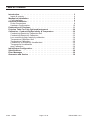
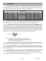
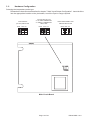
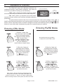
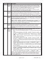
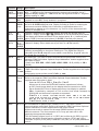
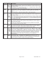
PM4-2CO
Dual Input
Conductivity/Resistivity
Process Monitor/Controller
Operation and Instruction Manual
AMALGAMATED INSTRUMENT CO PTY LTD
Unit 5, 28 Leighton Place Hornsby
NSW 2077 AUSTRALIA
Telephone: +61 2 9476 2244
Facsimile: +61 2 9476 2902
ACN: 001 589 439
e-mail: [email protected]
Internet: www.aicpl.com.au
Table of Contents
Introduction . . . . . . . . . . . . . . . . . . . . . . . . . . . . . . . . . . . . 3
Inputs & outputs . . . . . . . . . . . . . . . . . . . . . . . . . . . . . . . . . 4
Mechanical Installation. . . . . . . . . . . . . . . . . . . . . . . . . . . . . . 5
Cell Installation . . . . . . . . . . . . . . . . . . . . . . . . . . . . . . . . . 6
Electrical Installation . . . . . . . . . . . . . . . . . . . . . . . . . . . . . . . 7
Probe Connections . . . . . . . . . . . . . . . . . . . . . . . . . . . . . . . 8
Hardware Configuration . . . . . . . . . . . . . . . . . . . . . . . . . . . . 10
Explanation of Functions . . . . . . . . . . . . . . . . . . . . . . . . . . . . 11
Function Table For Fully Optioned Instrument . . . . . . . . . . . . . . . . 20
Calibration - Conductivity/Resistivity & Temperature . . . . . . . . . . . . 22
Conductivity/Resistivity Calibration Null . . . . . . . . . . . . . . . . . . . . 22
Conductivity/Resistivity Calibration . . . . . . . . . . . . . . . . . . . . . . 22
Low conductivity/high resistivity calibration . . . . . . . . . . . . . . . . . . 24
Temperature Calibration Null . . . . . . . . . . . . . . . . . . . . . . . . . 25
Temperature Calibration . . . . . . . . . . . . . . . . . . . . . . . . . . . . 25
Conductivity or Resistivity Uncalibration . . . . . . . . . . . . . . . . . . . . 25
Temperature Uncalibration . . . . . . . . . . . . . . . . . . . . . . . . . . 25
ppm Calibration . . . . . . . . . . . . . . . . . . . . . . . . . . . . . . . . 26
Input/Output Configuration . . . . . . . . . . . . . . . . . . . . . . . . . . . 27
Specifications . . . . . . . . . . . . . . . . . . . . . . . . . . . . . . . . . . 28
Error Messages . . . . . . . . . . . . . . . . . . . . . . . . . . . . . . . . . 29
Guarantee and Service . . . . . . . . . . . . . . . . . . . . . . . . . . . . . 30
2C06
06D09
Page 2 of 30
PM42COMA-1.6-0
1
Introduction
This manual contains information for the installation and operation of the PM4-2CO dual input
conductivity/resistivity monitor. The PM4 is a general purpose auto ranging monitor which may be
configured to accept inputs from a range of conductivity/resistivity cells with cell constants ranging from
K=0.01 to K=100. Ranges and typical cell factors are shown in the table below.
Cell Range Guide
Cell K
Factor
K=0.01
K=0.1
K=1.0
K=2.0
K=10.0
K=20.0
uS/cm
o
0 - 125 @ 25 C
o
0 - 1,250 @ 25 C
o
10 - 12,500 @ 25 C
o
20 - 25,000 @ 25 C
o
100 - 125,000 @ 25 C
o
200 - 250,000 @ 25 C
uS/m
mS/cm
o
0 - 12,500 @ 25 C
o
0 - 125,000 @ 25 C
-
mS/m
o
0 - 0.125 @ 25 C
o
0 - 1.25 @ 25 C
o
0.01 - 12.5 @ 25 C
o
0.02 - 25 @ 25 C
o
0.1 - 125 @ 25 C
o
0.2 - 250 @ 25 C
o
0 - 12.5 @ 25 C
o
0 - 125 @ 25 C
o
1 - 1,250 @ 25 C
o
2 - 2,500 @ 25 C
o
10 - 12,500 @ 25 C
o
20 - 25,000 @ 25 C
An input is also provided for a temperature sensor for automatic temperature compensation. The
PM4 can accept 100Ω RTD, 1000Ω RTD, LM335 or 100Ω thermistor type temperature sensors . The
temperature sensor input or default temperature setting is common to both input channels.
The default display can be set to either resistivity or conductivity, the display will toggle between
channel 1, channel 2, percent rejection and temperature indication by pressing either the ^ or v button. The
default display is channel 1, the instrument will revert to this display after switch on and will automatically
revert to channel 1 after approx. 1 minute if the display has been toggled to a different value. When a display
other than channel 1 is viewed a message will flash approximately every 8 seconds to indicate what value is
being displayed e.g. Ch 2 will flash prior to channel 2 reading, Pc.rJ prior to percent rejection and “C prior
to the temperature. The conductivity display units can be set to show either milliSiemens per metre,
milliSiemens per centimetre, microSiemens per metre or microSiemens per centimetre. The resistivity
display is in MΩ. The percent rejection display is calculated from the following formula:
 C 2 C1 
−


 0.65 0.5 
x 100%
% Rejection =
 C2 


 0.65 
Where: C2 (channel 2 input) is inlet (feed) conductivity in uS/cm
C1 (channel 1 input) is outlet (product) conductivity in uS/cm
0.65 converts inlet conductivity to TDS (total dissolved solids)
0.5 converts outlet conductivity to TDS
Calibration, setpoint and other set up functions are easily achieved by push buttons (located at the
rear panel or front panel depending on model). A standard inbuilt relay provides an alarm/control function,
additional relays, retransmission and DC output voltage may also be provided.
Unless otherwise specified at the time of order, your PM4 has been factory set to a standard
configuration. Like all other PM4 series instruments the configuration and calibration are easily changed by
the user. Initial changes may require dismantling the instrument to alter PCB links, other changes are made
by push button functions.
Full electrical isolation between power supply, conductivity/resistivity cell and retransmission
output is provided by the PM4, thereby eliminating grounding and common voltage problems. This isolation
feature makes the PM4 ideal for interfacing to computers, PLCs and other data acquisition devices.
The versatile PM4 has various front panel options, therefore in some cases the pushbuttons may be
located on the front panel as well as the standard rear panel configuration.
Page 3 of 30
PM42COMA-1.6-0
1 .1
Inputs & outputs
Input:
One or two
conductivity cells
and one
temperature sensor
A1
A2
A3
A4
Output:
1 x setpoint relay
Optional outputs:
Up to six extra
setpoint relays.
Analog output
(single or dual)
Serial comms
(RS232 or RS485)
BCD/binary retransmission
2 2 % 3 5
P
F
Process units
Alarm annunciator LEDs
(5 digit LED display only)
Setup pushbuttons
AMALGAMATED INSTRUMENT CO
100
5 3 6 2 3 0
1
50
2
%
F
P
Conductivity mS/cm
3
25
4
0
6
6 digit model
75
P
6
7
*
5
F
Bargraph plus
5 digit model
Page 4 of 30
PM42COMA-1.6-0
2
Mechanical Installation
If a choice of mounting sites is available then choose a site as far away as possible from sources of
electrical noise such as motors, generators, fluorescent lights, high voltage cables/bus bars etc. An IP65
access cover which may be installed on the panel and surrounds is available as an option to be used when
mounting the instrument in damp/dusty positions. A wall mount case is available, as an option, for situations
in which panel mounting is either not available or not appropriate. A portable carry case is also available, as
an option, for panel mount instruments.
Prepare a panel cut out of 45mm x 92mm +1 mm / -0 mm (see diagram below). Insert the instrument
into the cut out from the front of the panel. Then, from the rear of the instrument, fit the two mounting brackets
into the recess provided (see diagram below). Whilst holding the bracket in place, tighten the securing
screws being careful not to over-tighten, as this may damage the instrument.
Hint: use the elastic band provided to hold the mounting bracket in place whilst tightening securing screws.
Vertical mounting
(bar graph displays)
45mm
Horizontal mounting
92mm
45mm
PANEL
CUT
OUT
PANEL CUT OUT
Mounting bracket
(2 off)
115mm
92mm
9.5mm
max
9mm
10mm
48mm
44mm
91mm
53mm
111mm
96mm
104mm
Page 5 of 30
PM42COMA-1.6-0
2 .1
Cell Installation
When installing conductivity cells it is important to locate the cell in a position where the pipe is
always completely full. The cell electrodes must be in complete contact with the water sample. If air is
trapped around the cell electrode it will cause errors in the measurement. If oil, grease or any insulating
material is allowed to build up on the electrode surface measurement errors will also occur.
K=1.0
K=0.1
Figure 1
Ideal
Installation
method
Modified ‘t’ fitting
for in-line flow
(horizontal or vertical)
Ideal Installation
method
Modified ‘t’ fitting
elbow installation
(horizontal or vertical)
Acceptable,
slightly recessed
TBPS cells are suitable for installation into non metallic
pipework. Ideally the cell should be installed from the side of the
fitting as shown in figure 1. This method is less likely to be subjected
to trapped air. The “T” fitting should be modified to allow the face of
the cell to be flush with the inside of the fitting or pipe wall. It is
acceptable for the cell to be slightly recessed when the cell is
installed from the side of the fitting.
Alternatively a ¾” BSP hole may be drilled/threaded into
the side of a fitting such as an existing elbow or “T” fitting.
It is acceptable to install the cell from the top or bottom of
the pipe or fitting provided care is taken to prevent air pockets or
build up of sediment.
In applications where the pipe diameter is less than 50mm
the reduced sample volume around the cell electrodes may affect
the accuracy of the reading. In these applications in-line calibration
correction is recommended. For installation into the side wall of a
tank, vessel etc. the information above applies.
Acceptable,
caution avoid
air pocket
NOT acceptable
for horizontal
installation
Acceptable
for clean water
with no sediment
Acceptable - (but not ideal),
for clean water
with no sediment
TBTH and TBTHHT cells are suitable for installation into
metallic and non metallic pipework. The cell measurement is made
on the inside of the cell body ensuring it is virtually unaffected by
the surrounding sample or volume.
The cell may be mounted in a horizontal or vertical
position and is usually installed into a modified “T” fitting. The cell
will provide a reliable and stable reading as long as there is a flow
through the cell.
Figure 2
Ideally the cell should be installed into an elbow
installation with the flow entering the cell at the base opening and
exiting from the holes around the perimeter (see figure 2). This
method will provide a fast response. Alternatively the cell may be
installed across the flow as shown in figure 3, note this is not
recommended for K=10 cells. This will provide a stable and
accurate measurement, but the response time will be slower. In
most applications this will not present a problem. TBTH and
TBTHHT cells are also suitable for installation into sample flow
lines. These are usually installed in a flow bypass or a sample to
waste arrangement. Sample line measurement usually provides a
slower response, but has the advantage of allowing the cell to be
removed without disturbing the process.
Page 6 of 30
Modified ‘T’ fitting
elbow installation
(horizontal or vertical)
Figure 3
Modified ‘T’ fitting
for in-line flow
(horizontal or vertical).
TBTH cells only, not
suitable for TBLR cells.
PM42COMA-1.6-0
3
Electrical Installation
The PM4 Panel Meter is designed for continuous operation and no power switch is fitted to the unit.
It is recommended that an external switch and fuse be provided to allow the unit to be removed for servicing.
The terminal blocks allow for wires of up to 2.5mm2 to be fitted. Connect the wires to the appropriate
terminals as indicated below. Refer to other details provided in this manual to confirm proper selection of
voltage, polarity and input type before applying power to the instrument. When power is applied to the
instrument an initial display of **** followed by other status displays indicates that the instrument is
functioning.
A B C D E F H J K
1 2 3 4 5 6 7 8 9 10 11 12 13 14
MAINS EARTH
COM
AC NEUTRAL (DC+)
AC ACTIVE
OUT
IN
N/O
RELAY 1
CONDUCTIVITY
PROBE 2 INPUT
GND
(DC-)
OUT
IN
+
CONDUCTIVITY
PROBE 1 INPUT
3 WIRE TEMPERATURE
- PROBE INPUT
Instrument Rear Panel
1
MAINS EARTH
2
240VAC NEUTRAL
3
240VAC ACTIVE
4
5
RELAY 1
COM
6
RELAY 1
N/O
7
RTD
8
RTD
3 WIRE
9
RTD
+
10
CONDUCTIVITY IN
11
CELL 1
OUT
12
GND
13
CONDUCTIVITY IN
14
CELL 2
OUT
MODEL No:
PM4-2CO-240-5E-A
OPTIONAL OUTPUTS
A OUTPUT V/I
B OUTPUT V/I
+
SERIAL No:
Instrument Data Label (example)
Page 7 of 30
PM42COMA-1.6-0
3 .1
Probe Connections
Conductivity/Resistivity Cells
The conductivity/resistivity cell is connected to pins 10 & 11 (cell 1) and 13 & 14 (cell 2) at the rear of
the instrument. Pins 10 & 13 are the input connections i.e. the current input from the cell. Pins 11 and 14 are
the output connections. If using a centre core type cell the centre core wire should be connected to Pin 10.
Ensure that the PRbE CNSt & PRb2 CNSt function has been correctly set for probe type.
For example AIC conductivity/resistivity cells with temperature compensation sensors are all wired
with Red, Black, Blue and Yellow (or White on older models) inner core cable. See the note below for details
of TBPS cells without temperature compensation sensors. The wiring connections are as below.
Cell in
Cell out
Temperature +
Temperature Shield
Cell wiring colour codes
AIC Cells
Blue
Yellow (or White)
Red
Black
n/a
TBTH Cell
+ TEMP
IN OUT
CELL
Junction head
connector layout
for TBTH cell.
TBLR
Cell
Outer
Electrodes
or Cell Out
yellow or
white wire
Centre
Electrodes
or Cell In
blue wire
SDI Cells
Black
White
Red
Green
Clear
Wires :Red
Black
Blue
Yellow or White
TBPS Cells
Cells In and Out
blue & yellow
(or white) wires
may be connected
either way around
with TBPS types
Page 8 of 30
PM42COMA-1.6-0
Cell Wiring
Connect the cell as shown below.
7 8 9 10 11 12 13 14 PM4 rear
terminals
SHIELDS
CELL OUT
CELL IN
CELL 2
CELL OUT
CELL IN
CELL 1
TEMPERATURE
PROBE
Note: only one temperature probe input
is provided. The temperature probe may
be inbuilt in one of the cells or can be
a separate temperature probe.
Temperature Probes
The PM4-2CO will accept 2 or 3 wire RTD (100Ω or 1000Ω), LM335, 100Ω thermistor or UU25J1
thermistor type temperature sensors. Wiring for these sensors is as shown below. Ensure that the links for
the temperature probe type are set (see “Hardware Configuration” section which follows) and that the "C
tYPE function is set to the appropriate type.
100Ω and 1000Ω RTDs
2 Wire configuration or
100Ω thermistor or
UUB25J1 thermistor.
Note: If using the UUB25J1
a 220Ω resistor must be
placed across terminals 7 & 9
7
8
7
9
Link 7 & 8
8
9
100Ω and 1000Ω RTDs
2 Wire Configuration,
100Ω thermistor
or UUB25J1 thermistor
Note: If using the UUB25J1 a
220 resistor must be placed
across terminals 7 and 9
Link 7 & 8
220Ω
UUB25J1
RTD
7
8
100Ω and 1000Ω
9
100Ω and 1000Ω RTDs
3 Wire configuration
RTDs
3 Wire Configuration
RTD
7
LM335 Temperature sensor
8
-
9
+
LM335 Temperature
Transducer
LM335
Page 9 of 30
PM42COMA-1.6-0
3 .2
Hardware Configuration
Selecting the temperature probe type
Dismantle the instrument as described in chapter 7 titled “Input/Output Configuration”. Insert the links
into the appropriate location on the pin header, to suit the input or range required.
1000 OHM RTD
(PT1000) SELECTED
100 OHM RTD (PT100)
or 100 OHM THERMISTOR
or UUB25J1 THERMISTOR
SELECTED
1000R 100R 335
1000R 100R 335
LK1 LK2 LK3
LK1 LK2 LK3
LM335 SEMICONDUCTOR
SENSOR SELECTED
1000R 100R 335
LK1 LK2 LK3
Main Circuit Board
Page 10 of 30
PM42COMA-1.6-0
4
Explanation of Functions
The PM4-2CO setup and calibration functions are
configured through a push button sequence. Two levels of
access are provided for setting up and calibrating:-
Front view of instrument
SETUP
PUSHBUTTONS
A1
A2
A3
A4
FUNC mode (simple push button sequence) allows
access to commonly set up functions such as alarm setpoints.
5 2 6 2 3
P
F
F
Process Units
CAL mode (power up sequence plus push button
sequence) allows access to all functions including calibration
parameters.
The push buttons located at the front of the instrument are used to alter settings. Once CAL or
FUNC mode has been entered you can step through the functions, by pressing and releasing the F push
button, until the required function is reached. Changes to functions are made by pressing the ^ or v push
button (in some cases both simultaneously) when the required function is reached.
Entering FUNC Mode
P
F
P
1. Remove power from
the instrument. Hold in the F
button and reapply power.
The display will briefly indicate
CAL as part of the
"wake up messages" when
the CAL message is seen
you can release the
button. Move to step 2 below.
F
2. When the "wake up"
messages have finished
and the display has settled
down to its normal reading
press, then release the
F button.
Move to step 3 below.
P
F
3. Within 2 seconds of
releasing the F button
press, then release
the ^ and
buttons
together. The display will
now indicate FUNC followed
by the first function.
No special power up procedure
is required to enter FUNC mode.
P
F
1. When the "wake up"
messages have finished
and the display has settled
down to its normal reading
press, then release the
F button.
P
F
2. Within 2 seconds of
releasing the F button
press, then release
the ^ and
buttons
together. The display will
now indicate FUNC followed
by the first function.
^
Entering CAL Mode
^
Note: If step 1 above has been completed then the
instrument will remain in this CAL mode state until
power is removed. i.e. there is no need to repeat step 1
when accessing function unless power has been removed.
Page 11 of 30
PM42COMA-1.6-0
Example: Entering FUNC mode to change alarm 1 high function A1Hi from OFF to 100
Press & release F
then press
^v
1 0 0
F U N C
Press & release
F until
Press & release
Press & release
F
P or F until
A 1 H i
F U N C
Press & release
O F F
^ until
E n d
Example: Entering CAL mode to change decimal point dCPt function from 0 to 0.02
Switch off
instrument
Press & release F
then press
^v
.0 0 2
Press & hold
F
F U N C
Switch on
instrument
Press & release
F until
Press & release
Press & release
F
P or F until
Hold F until
C A L
Press & release
0
d C P t
F U N C
Release F
^ until
E n d
The alarm, brightness, retransmission and bargraph functions below are accessible via
mode.
Note that “x” in the alarm functions is used to indicate any alarm number e.g. if 3 setpoint alarm relays are
fitted then A1.Lo, A2.Lo and A3.Lo will all seen as functions on the display.
Each alarm may be set to follow channel 1, channel 2, percent rejection or temperature, see Ax function for
details.
Function Range
AxLo
Any
display
value
AxHi
Any
display
value
Description
Alarm low setpoint - displays and sets the low setpoint value for the designated
alarm relay. The low alarm setpoint may be disabled by pressing the ^ and v
pushbuttons simultaneously. When the alarm is disabled the display will indicate
OFF . Use ^ or v to adjust the setpoint value if required. The alarm will activate
when the displayed value is lower than the setpoint value. Each relay may be
configured with both a low and high setpoint if required, if so the relay will be
activated when the display reading moves outside the band set between low and
high setpoints.
Alarm high setpoint - displays and sets the high setpoint value for the designated
alarm relay. The high alarm setpoint may be disabled by pressing the ^ and v
pushbuttons simultaneously. When the alarm is disabled the display will indicate
OFF. Use ^ or v to adjust the setpoint value if required. The alarm will activate
when the displayed value is higher than the setpoint value. Each relay may be
configured with both a low and high setpoint if required, if so the relay will be
activated when the display reading moves outside the band set between low and
high setpoints.
Page 12 of 30
PM42COMA-1.6-0
Function Range
AxHY
0 to
9999
units
Description
Alarm hysteresis [deadband] - displays and sets the alarm hysteresis limit and is
common for both high and low setpoint values. The hysteresis value may be
used to prevent too frequent operation of the setpoint relay when the measured
value stays close to the setpoint. Without a hysteresis setting (AxHY set to zero)
the alarm will activate when the display value goes above the alarm setpoint (for
high alarm) and will reset when the display value falls below the setpoint, this can
result in repeated on/off switching of the relay at around the setpoint value. The
hysteresis setting operates as follows:
In the high alarm mode, once Display Value
the alarm is activated the input
must fall below the setpoint
A Hi
value minus the hysteresis
A HY value
value to reset the alarm.
A Hi
Relay
e.g. if A1Hi is to 50.0 and minus
activates
A HY
A1Hy is set to 3.0 then the
at this value
Relay
or above
setpoint output relay will
resets
below this
activate once the display value
value
goes above 50.0 and will
reset when the display value
goes below 47.0
Alarm high operation with hysteresis
Time
(50.0 minus 3.0).
Display Value
In the low alarm mode, once
the alarm is activated the input
must rise above the setpoint
Relay
value plus the hysteresis
resets
value to reset the alarm.
above this
Relay
e.g. if A1Lo is to 20.0 and
value
activates
AxLo
at this value
A1Hy is set to 10.0 then
plus
or below
AxHY
the alarm output relay will
AxHY value
activate when the display
AxLo
value falls below 20.0 and
will reset when the display
Alarm low operation with hysteresis
Time
value goes above 30.0
(20.0 plus 10.0).
The hysteresis units are expressed in displayed engineering units.
Axtt
0 to 60 Alarm trip time - displays and sets the alarm trip time and is common for both
seconds alarm high and low setpoint values. The trip time is the delay time before the
alarm relay will activate, or trip, when an alarm condition is present. The alarm
condition must be present continuously for the trip time period before the alarm
will trip. This function is useful for preventing an alarm trip due to short non
critical deviations from setpoint. The trip time is selectable over 0 to 60 seconds.
Axrt
0 to 60 Alarm reset time - displays and sets the alarm relay reset time. With the alarm
seconds condition is removed the alarm relay will stay in its alarm condition for the time
selected as the reset time. The reset time is selectable over 0 to 60 seconds.
Axn.o or Axn.o Alarm x normally open or normally closed - displays and sets the setpoint alarm
Axn.c
or
relay action to normally open (de-energised) or normally closed (energised),
Axn.c when no alarm condition is present. A normally closed alarm is often used to
provide a power failure alarm indication.
brgt
0 to 15 Display brightness - displays and sets the digital display brightness. The display
brightness is selectable from 0 to 15, where 0 = lowest intensity and 15 =
highest intensity. This function is useful for improving the display readability in
dark areas or to reduce the power consumption of the instrument.
The functions which follow are accessible via CAL mode only.
Page 13 of 30
PM42COMA-1.6-0
Function Range
rEC_
Any
display
value
rEC~
Any
display
value
bAr_
Any
display
value
bAr~
Any
display
value
bAr
tYPE
bAr,
S.dot,
d.dot,
C.bAr
Description
Recorder/retransmission output low value - refer to the separate “PM4 Panel
Meter Optional Output Addendum” booklet supplied when this option is fitted.
Displays and sets the analog retransmission (4 to 20mA, 0-1V or 0-10V) output
low value (4mA or 0V) in displayed engineering units. e.g. if a 4mA output is
required for a display value of 0 then REC_ should be set to 0.
The retransmission output can be set to follow channel 1, channel 2, percent
rejection or temperature, see REC function for details.
Recorder/retransmission output high value - refer to the separate “PM4 Panel
Meter Optional Output Addendum” booklet supplied when this option is fitted.
Displays and sets the analog retransmission (4 to 20mA, 0-1V or 0-10V) output
high value (20mA, 1V or 10V) in displayed engineering units. e.g. if a 20mA
output is required for a display value of 1000 then REC~ should be set to 1000.
Bar graph display low value - seen only in bargraph display instruments.
Displays and sets the bar graph low value i.e. the value on the 7 segment display
at which the bargraph will start to rise. This may be independently set anywhere
within the display range of the instrument.
Note: The bAr~ and bAr_ settings are referenced from the 7 segment display
readings, not the bargraph scale values. The bargraph scale may scaled
differently to the 7 segment display or may be set to display a different channel,
% rejection or temperature, see the bar function.
Bargraph display high value - seen only in bargraph display instruments.
Displays and sets the bar graph high value i.e. the value on the 7 segment
display at which the bargraph will reach its maximum indication (all LED’s
illuminated). May be independently set anywhere within the display range of the
instrument.
Bar graph display operation mode - seen only in bargraph display instruments.
Allows selection of bargraph operation mode choices are:
bAr - conventional solid bargraph display i.e. all LED’s illuminated when at full
scale.
When scaling the display use the bAr_ and bAr~ functions e.g. bAr_ = 0
and bAr~ = 100 will give a bargraph with no segments lit at a 7 segment
display reading of 0 and all segments lit with a 7 segment display reading of
100.
S.dot - single dot display. A single segment will be lit to indicate the input
readings position on the scale.
When scaling the display use the bAr_ and bAr~ functions e.g. bAr_ = 0
and bAr~ = 100 will give a bargraph with the bottom segment lit at a 7
segment display reading of 0 and the top segment lit with a 7 segment display
reading of 100.
Note: this could also be set up as a centre zero single dot display by entering a
negative value and positive value. e.g. bAr_ = -100, bAr~ = 100.
d.dot - double dot display. Two segments will be lit to indicate the input
reading position on the scale. The reading should be taken from the middle of
the two segments.
When scaling the display use the bAr_ and bAr~ functions e.g. bAr_ = 0
and bAr~ = 100 will give a bargraph with the bottom two segments lit at a 7
segment display reading of 0 and the top two segments lit with a 7 segment
display reading of 100.
Note: this could also be set up as a centre zero single dot display by entering a
negative value and positive value. e.g. bAr_ = -100, bAr~ = 100.
C.bAr - centre bar display. The display will be a solid bargraph but will have its
zero point in the middle of the display. If the seven segment display value is
positive the bargraph will rise. If the seven segment display value is negative
then the bargraph will fall.
Page 14 of 30
PM42COMA-1.6-0
Function
bAr
tYPE
continued
Ch 2
drnd
Ch 1
dCPt
Ch 2
dCPt
FLtr
bAud
Prty
O.Put
Range
bAr,
S.dot,
d.dot,
C.bAr
on or
OFF
0 to
5000
units
Description
When scaling the display use the bAr_ and bAr~ functions e.g. bAr_ = 0 and
bAr~ = 100 will give a bargraph with all the bottom half segments lit at a 7
segment display reading of -100 and all the top segments lit with a 7 segment
display reading of 100.
Channel 2 on or off - this function should be set to on if both input channels are
required or set to OFF if only channel 1 is required.
Display rounding - displays and sets the display rounding value. This value may
be set to 0 - 5000 displayed units. Display rounding is useful for reducing the
instrument resolution without loss of accuracy in applications where it is
undesirable to display to a fine tolerance. e.g. if set to 10 the instruments will
display in multiples of 10.
0,
Channel 1 decimal point selection - displays and sets the decimal point for
0.1,
channel 1 display. Use the ^ or v pushbuttons to set the decimal point position.
0.02 or The display will indicate as follows: 0 (no decimal point), 0.1 (1 decimal point
0.003 place), 0.02 (2 decimal point places) or 0.003 (3 decimal point places).
0,
Channel 2 decimal point selection - displays and sets the decimal point for
0.1,
channel 2 display. Other details are as per the Ch 1 dCPt function.
0.02 or
0.003
0 to 8
Digital filter - displays and sets the digital filter value. Digital filtering is used for
reducing susceptibility to short term interference. The digital filter range is
selectable from 0 to 8, where 0 = none and 8 = most filtering. A typical value for
the digital filter would be 3.
300 to Set baud rate - only seen if serial communications option fitted. Refer to the
38.4
separate “PM4 Panel Meter Optional Output Addendum” booklet supplied when
this option is fitted.
Select from 300, 600, 1200, 2400, 4800, 9600, 19.2 (19200) or 38.4
(38400)
nonE, Set parity - only seen if serial communications option fitted. Refer to the separate
EUEn
“PM4 Panel Meter Optional Output Addendum” booklet supplied when this option
or odd is fitted.
Select parity check to either nonE, EUEn or odd.
dISP, Set RS232/485 interface mode - only seen if serial communications option fitted.
Cont
Refer to the separate “PM4 Panel Meter Optional Output Addendum” booklet
or
supplied when this option is fitted.
POLL
Select diSP, Cont, POLL, A.buS or M.buS
Allows user to select the RS232/485 interface operation as follows:disP Sends image data from the display without conversion to ASCII.
Cont Sends ASCII form of display data every time display is updated.
POLL Controlled by computer or PLC as host. Host sends command via
RS232/485 and instrument responds as requested.
A.buS
- is a special communications mode used with Windows
compatible optional PC download software. Refer to the user manual
supplied with this optional software.
M.bus - Modbus RTU protocol.
Addr
0 to 31 Set unit address for polled (POLL) mode (0 to 31) - only seen if serial
communications option fitted. Refer to the separate “PM4 Panel Meter Optional
Output Addendum” booklet supplied when this option is fitted.
Allows several units to operate on the same RS485 interface reporting on
different areas etc. The host computer or PLC may poll each unit in turn
supplying the appropriate address.
The unit address ranges from 0 to 31 (DEC) but is offset by 32 (DEC) to avoid
clashing with ASCII special function characters (such as <STX> and <CR>).
Therefore 32 (DEC) or 20 (HEX) is address 0, 42 (DEC) or 2A (HEX) addresses
unit 10.
Page 15 of 30
PM42COMA-1.6-0
Function Range
dG.OP
bin2,
bin,
b.SCL
or bcd
Description
Digital output operating mode - seen only with digital output option. Refer to the
separate “PM4 Panel Meter Optional Output Addendum” booklet supplied when
this option is fitted.
Select from bin2 - signed binary output, bin - unsigned binary output, b.SCL
- scaled binary output, bcd - BCD output.
dG.OP
AIo or Output polarity - seen only with digital output option. Refer to the separate “PM4
AHi
Panel Meter Optional Output Addendum” booklet supplied when this option is
fitted.
Select either A Io - active low output or A Hi - active high output.
bcd
0 to
BCD - start display position - seen only with digital output option. Refer to the
Strt
number separate “PM4 Panel Meter Optional Output Addendum” booklet supplied when
of
this option is fitted.
display This function affects BCD mode only and determines the number of digits to skip
digits
when outputting from the display. Select from 0 to number of display digits minus
minus 4 4. e.g. for a 6 digit display you may select 0 to 2, if 2 is selected then the four left
most digits will be output.
dig_
Any
Scaled digital output low reading - seen only with digital output option. Refer to
display the separate “PM4 Panel Meter Optional Output Addendum” booklet supplied
value
when this option is fitted.
Accepts any valid display value. Determines the low startpoint for the b.SCL
mode and has no affect on other modes.
dig~
Any
Scaled digital output low reading - seen only with digital output option. Refer to
display the separate “PM4 Panel Meter Optional Output Addendum” booklet supplied
value
when this option is fitted. Accepts any valid display value. Determines the high
startpoint for the b.SCL mode and has no affect on other modes.
"C tyPE NONE, Temperature probe type - displays and sets the temperature probe type used.
100,
Selections available are NONE (no temperature probe),100 (100Ω RTD), 1000
1000, (1000Ω RTD), L335 (LM335), t100 (100Ω thermistor) or 25J1 (UUB25J1 type
L335, thermistor). Hardware links must also be set to suit the probe type used. See the
t100
“Hardware Configuration” and “Electrical Installation” chapters. Temperature
or
compensation is common to both input channels i.e. the temperature sensor
25J1
input will be applied to both channel 1 and channel 2 for temperature
compensation.
def "C
0.0 to
Default temperature - displays and sets the default temperature for manual
o
200.0 compensation when "C tyPE is set to NONE. Range is 0.0 to 200.0 C. This is
the temperature value which will be used for compensation if no temperature
sensor is used. The value is common to both input channels.
Page 16 of 30
PM42COMA-1.6-0
Function Range
SOL
-6.00
SLPE
to
0.00
Description
Solution slope - displays and sets the solution slope, variable from -6.00 to
0.00. The solution slope gives the temperature coefficient of the solution
o
measured as a % per C (this figure is needed since each individual solution’s
conductivity/resistivity will vary differently with temperature). A typical value is 2%
o
per C.
Enter the solution value, if known, if the solution slope is not known then it can
be obtained as follows:
o
1. Set the slope setting to 0.00% per C
2. Place the cell into a sample of the process solution. Measure the
temperature of the solution or alter the temperature to a desired level, this
temperature is shown as T1 in the formula below. Allow the reading to stabilise
and note the reading.
3. Bring the solution up to a higher temperature and allow the reading to
stabilise, again note the reading.
4. Use the formula below to calculate the solution slope.


1


  T 2 − T 1 
 Conductivity or Resistivity at T 1
x 100
− 1
Slope = 

 Conductivity or Resistivity at T 2
5. Enter the result as the solution slope.
SOL "C
PRbE
CNSt
PRb2
CNSt
H. OFF /
H. ON
CAL1
NULL
Ch1
CAL1 &
Ch1
CAL2
0.0
to
100.0
0.01,
0.05,
0.1,
0.5,
1.0,
2.0,
5.0,
10,
50 or
100
As
above
Solution temperature - displays and sets the solution temperature (T1) to be used
with the solution slope function above.
Channel 1 probe constant - displays and sets the channel 1 probe cell constant
(K number).
Values of:
0.01, 0.05, 0.1, 0.5, 1.0, 2.0, 5.0, 10, 50 or 100 may be selected.
Channel 2 probe constant - displays and sets the channel 2 probe cell constant
(K number) values of 0.01, 0.05, 0.1, 0.5, 1.0, 2.0, 5.0, 10, 50 or 100 may
be selected.
H. OFF Hydrogen ion compensation - displays and sets the hydrogen ion compensation
or H. ON feature to either be on or off. See “Calibration/Resistivity & Temperature” section
for details. When measuring high purity water solutions compensation needs to
be made for hydrogen ions as well as temperature. When set to H. ON the
+
instrument compensates for the H and OH solvent ions that have an effect on
water conductivity/resistivity. When set to H. ON the instrument compensates for
+
the H and OH- solvent ions which become prevalent at low conductivity. These
ions have an effect on water conductivity/resistivity due to having different
temperature compensation curves to water. This setting is common to both input
channels.
n/a
Null calibration - null calibration allows the channel 1 probe to be referenced to
the instruments display value at zero conductivity. See “Calibration Conductivity/Resistivity & Temperature”, chapter for details.
n/a
Channel 1 calibration points - displays and sets channel 1 calibration points. See
“Calibration/Resistivity & Temperature” chapter for full details of setting up.
CAL1 when used after CAL NULL sets the calibration slope, CAL2
compensates the calibration curve for head resistance.
Page 17 of 30
PM42COMA-1.6-0
Function Range
CAL2
n/a
NULL
Ch2
n/a
CAL1 &
Ch2
CAL2
"C NULL n/a
CAL "C
n/a
cond
unit
uS.cM,
uS.M,
MS.cM
or
MS.M
UCAL
Ch1
n/a
UCAL
Ch2
n/a
UCAL "C n/a
Set
dISP
P.but
SPAC
cond
or
RESt
NONE,
Hi,
Lo or
HiLo
A1,
A1-2
or
A1-3
Description
Null calibration - null calibration allows the channel 2 probe to be referenced to
the instruments display value at zero conductivity. See “Calibration Conductivity/Resistivity & Temperature”, chapter for details.
Channel 2 calibration points - displays and sets channel 2 calibration points. See
“Calibration/Resistivity & Temperature” chapter for full details of setting up.
CAL1 when used after CAL NULL sets the calibration slope, CAL2
compensates the calibration curve for head resistance.
Temperature probe null - Null calibration allows the temperature probe to be
referenced to the instruments display value with zero input. See “Calibration Conductivity/Resistivity & Temperature” chapter for details.
Temperature probe calibration - used to calibrate the temperature probe. Ensure
that correct temperature probe has been selected under the "C tYPE function.
See “Calibration - Conductivity/Resistivity & Temperature” chapter for details.
Conductivity measuring units - seen only if SEt dISP set to cond.
Used to set the measuring units for conductivity measurement.
Select uS.cM to display in microSiemens per centimetre.
Select uS. M to display in microSiemens per metre
Select MS.cM to display in milliSiemens per centimetre
Select MS. M to display in milliSiemens per centimetre
Channel 1 uncalibration - used to set the channel 1 conductivity or resistivity
calibration back to the factory calibration values. This function should only be
used when calibration problems exist, and it is necessary to clear the calibration
memory.
Channel 2 uncalibration - used to set the channel 2 conductivity or resistivity
calibration back to the factory calibration values. This function should only be
used when calibration problems exist, and it is necessary to clear the calibration
memory.
Temperature probe uncalibration - used to set the temperature probe calibration
back to the factory calibration values. This function should only be used when
calibration problems exist, and it is necessary to clear the calibration memory.
Set default display - the default display can be set to either conductivity (cond)
or resistivity (RESt). Select the default display required via the ^ or v buttons.
P button function - displays and sets the operation of the front panel P push
button.
The functions available are:
NONE - no function, pressing the P button has no effect.
Hi - peak memory, display will show the highest reading in memory from the
time the instrument was last switched on. The function will time out after 20
seconds and return to normal measurement.
Lo - valley memory, display will show the lowest reading in memory from the
time the instrument was last switched on. The function will time out after 20
seconds and return to normal measurement.
Hi Lo - display will toggle between the highest and the lowest reading in
memory each time the P button is pressed. The function will time out after 20
seconds and return to normal measurement.
Setpoint access - sets the access to the alarm relays set points. The following
choices are available;
A1 - Allows setpoint access to alarm 1 only.
A1-2 - Allows access to alarms 1 and 2 only.
A1-3 - Allows access to alarms 1, 2 and 3 only etc. up to the maximum
number of relays fitted. For this function to operate the remote input R.INP
function must be set to SP.AC.
Page 18 of 30
PM42COMA-1.6-0
Function Range
Ax
ch1,
ch2,
Pc.rJ
or "C
REC
ch1,
ch2,
Pc.rJ
or "C
bar
ch1,
ch2,
Pc.rJ
or "C
dG.OP
ch1,
ch2,
Pc.rJ
or "C
Description
Alarm mode - the alarms setpoints may be set to operate from either the channel
1, channel 2, percent rejection or temperature reading. Select ch 1 for channel
1, ch 2 for channel 2, pc.rJ for percent rejection or "C for temperature.
The alarm will still operate on the selected mode even if the display is not in that
mode. e.g. if A1 is set to "C and the display is showing a conductivity reading
then the alarm 1 will still operate if the sensed temperature goes above the alarm
1 high setpoint or below the alarm 1 low setpoint.
Analog retansmission mode - seen only when the analog retransmission option is
fitted.
The analog retransmission option may be set to operate from either the channel
1, channel 2, percent rejection or temperature values. Note: only the mode
selected at the SEt OPER function or the temperature can be selected. Select
ch 1 for channel 1, ch 2 for channel 2, pc.rJ for percent rejection or "C for
temperature. Set the REC_ and REC~ functions to suit the output mode
selected. Note: if set for conductivity, resistivity then the output will go to full
scale (20mA, 1V or 10V) if the display goes to overrange (-or- displayed). If set
for temperature retransmission an overrange display will cause the analog output
to revert to the default temperature set at the dEF "C function i.e. if required the
default temperature can be set to a value which will give required analog output if
an overrange, e.g. open circuit, occurs.
Bargraph display mode - seen only in bargraph instruments.
The bargraph display may be set to operate from either the channel 1, channel 2,
percent rejection or temperature reading. Select ch 1 for channel 1, ch 2 for
channel 2, pc.rJ for percent rejection or "C for temperature. This feature allows
one display on the seven segment display and a separate display on the
bargraph e.g. channel 1 on the seven segment display and % rejection on the
bargraph.
Digital output mode - seen only when digital retransmission used. Refer to the
separate “PM4 Panel Meter Optional Output Addendum” booklet supplied when
this option is fitted.
The digital retransmission may be set to operate from either the channel 1,
channel 2, percent rejection or temperature reading. Select ch 1 for channel 1,
ch 2 for channel 2, pc.rJ for percent rejection or "C for temperature.
As with the Ax function the retransmission will operate on the selected mode
even if the display is not in that mode.
Returning to the normal measure Mode
Important; When the calibration is complete, it is advisable to return the instrument to the normal
mode (where calibration functions cannot be tampered with). To return to the normal mode - turn off the
instrument power - wait a few seconds and then restore power.
Page 19 of 30
PM42COMA-1.6-0
5
Function Table For Fully Optioned Instrument
Initial display
Meaning of display
Next display
Default
setting
AxLo
Alarm x low setpoint value
Setpoint value or OFF
OFF
AxHi
Alarm x high setpoint value
Setpoint value or OFF
OFF
AxHy
Alarm x hysteresis
Axtt
Alarm x trip time
Axrt
Alarm x reset time
No of seconds before reset
0
Axn.o or Axn.c
Alarm x action N/O or N/C
Axn.o or Axn.c
Axn.o
brGt
rEC_
rEC~
bAr_
bAr~
bAr tYPE
Ch2
drnd
Ch1 dCPt
Ch 2 dCPt
FLtr
bAUd
PrtY
O.Put
Addr
dG.OP
dG.OP
bcd Strt
diG_
diG~
"C tYPe
def "C
SOL SLPE
SOL "C
PRbE CNSt
PRb2 CNSt
H. OFF / H. ON
Ch 1 NULL
Ch 1 CAL1
Ch 1 CAL2
Hysteresis value
in measured units
No of seconds
before relay trips
Display brightness
0 to 15
First analog output low limit
Value in memory
First analog output high limit
Value in memory
Bar graph low reading
Value in memory
Bar graph high reading
Value in memory
The functions below are accessible only via CAL mode.
Bar graph operation mode
bAr, S.dot, d.dot or C.bAr
Channel 2 on or off
on or OFF
Display rounding
1 to 5000
Decimal point setting
0, 0.1, 0.02 etc.
for channel 1
Decimal point setting
0, 0.1, 0.02 etc.
for channel 2
Digital filter range 0 to 8
0 to 8 (8=most filtering)
300, 600, 1200, 2400, 4800,
Baud rate
9600,19.2 or 38.4
Parity select
NONE, EUEN or ODD
Output
diSP, Cont, POLL, A.bus or
continuous or controlled
M.buS
Address
Value in memory
Digital output type
bin2, bin, b.SCL or bcd
Digital output polarity
A Io or A Hi
BCD Mode - start display
Value in memory
Digital output low reading
Value in memory
(signed binary mode)
Digital output low reading
Value in memory
(signed binary mode)
NONE, 100, 1000,
Temperature probe type
L335 , t100 or 25J1
Default temperature
0 to 200
Solution temperature slope
-6.00 to 0.00
Solution temperature
0.0 to 100.0
0.01, 0.05, 0.1, 0.5,1.0, 2.0,
Probe 1 cell constant
5.0,10, 20, 50 or 100
0.01, 0.05, 0.1, 0.5,1.0, 2.0,
Probe 2 cell constant
5.0,10, 20, 50 or 100
Hydrogen ion compensation
H. OFF or H. ON
Cell 1 conductivity null
See calibration chapter
calibration
Slope calibration cell 1
See calibration chapter
Resistance
See calibration chapter
compensation cell 1
Page 20 of 30
10
0
Record your
settings
See following
table
See following
table
See following
table
See following
table
See following
table
See following
table
15
0
1000
0
100
bAR
on
1
0
0
2
9600
NONE
Cont
bin2
A Io
0
0
1000
L335
25
-2.00
25.0
0.1
0.1
H.OFF
n/a
n/a
n/a
PM42COMA-1.6-0
Initial display
"C NULL
CAL "C
cond unit
UCAL Ch 1
UCAL Ch 2
UCAL "C
SEt DISp
P.but
Cell 2 conductivity null
calibration
Slope calibration cell 2
Resistance
compensation cell 2
Temperature null Calibration
Calibrate temperature probe
Conductivity measuring units
Uncalibrate conductivity cell 1
Uncalibrate conductivity cell 2
Uncalibrate temp. probe
Set default display
P button function
SPAC
Setpoint access
Ax
Alarm mode for alarms 1, 2 etc.
Ch 2 NULL
Ch 2 CAL1
Ch 2 CAL2
REC
bar
dG.OP
Next display
Default
setting
See calibration chapter
n/a
See calibration chapter
n/a
See calibration chapter
n/a
See calibration chapter
See calibration chapter
uS.cM, uS. M, MS.cM or MS. M
See calibration chapter
See calibration chapter
See calibration chapter
RESt or cond
NONE, Hi, Lo, or HiLo
A1, A1-2, A1-3 etc to A1-7
if sufficient relays fitted
n/a
n/a
uS.cM
n/a
n/a
ch 1, ch 2, Pc.rJ or "C
ch 1
ch 1, ch 2, Pc.rJ or "C
ch 1
ch 1, ch 2, Pc.rJ or "C
ch1
ch 1, ch 2, Pc.rJ or "C
ch1
Meaning of display
First analog retransmission
mode
Bargraph display mode
Digital output
retransmission mode
Record your
settings
cond
NONE
A1
See following
table
Functions shown shaded on this table will be displayed only when those options are fitted.
Settings for relays - record settings here
A1
A2
A3
A4
AxLo
AxHi
AxHY
Axtt
Axrt
Axn.o or Axn.c
Ax
Page 21 of 30
PM42COMA-1.6-0
6
Calibration - Conductivity/Resistivity & Temperature
The PM4-2CO has provision for calibration slope and head resistance compensation
conductivity/resistivity calibration. A null calibration feature (see CAL NULL) allows the probe to be
referenced to the instrument at a zero conductivity level. A null calibration should be undertaken before a
single or two point calibration to ensure that the probe and instrument are matched. Before calibrating the
instrument it is also important to ensure that the correct cell constant has been chosen (see PRbE CNSt
and PRb2 CNSt). Ch1 CAL1 (or Ch2 CAL1 for channel 2) together with the Ch1 NULL (or Ch2 NULL)
function sets the calibration slope, the Ch1 CAL2 (or Ch2 CAL2) reading is used to compensate for head
resistance.
When using a temperature probe temperature calibration is carried out within the "C NULL and
CAL "C functions, ensure that the correct temperature probe type has been selected (see "C tYPE) and
that the appropriate links have been set (see the ”Electrical Installation" chapter).
Calibration Functions
To enter the calibration mode the instrument must be powered up and functions entered via CAL mode as
illustrated on the first page of chapter 4 “Explanation of functions”.
6 .1
Conductivity/Resistivity Calibration Null
Null calibration allows the conductivity/resistivity cell to be referenced to the meter. The instrument
should be nulled before calibration. To null the instrument the following procedure should be followed.
1. If a temperauture compensation sensor is used check that the temperature reading is correct and
calibrate the temperature reading if necessary, see “Temperature Calibration Null” and “Temperature
Calibration” sections in this chapter. Also check that the SOL SLPE function is correctly set. If no
temperature sensor is being used check that the SOL “C function is set to the required default
temperature.
2. Clean the cell to be nulled in pure water, dry the cell and place in air. Allow time for the reading to
stabilise.
3. Enter the calibration mode and setup mode then step through the functions until Ch1 NULL (or
Ch2 NULL) is displayed.
4. Press ^ and v together, the display will show a reading (this reading will be taken as zero upon
completion).
5. Press F , the display will show NULL End. When the instrument returns to normal measure mode
the reading from the probe in air will be zero. If any other message is seen refer to the “Error Messages”
appendix.
6 .2
Conductivity/Resistivity Calibration
After performing the null calibration as previously described place the required probe in a solution of
known conductivity or resistivity (for resistivity calibration ensure that the calibration solution resistivity is
not above 1MΩ). Allow time for the instrument reading to stabilise. Follow the procedure below.
1. Enter the CAL mode and step through the instructions until Ch1 CAL1 appears (or Ch2 CAL1 if
calibrating channel 2 input).
2. Press ^ and v together, the display will show a value with Ch1 CAL1 (or Ch2 CAL2) flashing
every few seconds.
3. Press and release F, the display will show a value with Ch1 SCL1 (or Ch2 SCL1) flashing every
few seconds.
4. Adjust the value displayed to the known solution value using the ^ and v pushbuttons.. .
5. Press and release F, the display will show CAL1 End followed by Ch1 CAL2 (or Ch2 CAL2). If
any other message is seen (see “Error Messages” appendix) then the calibration will need to be
repeated. If required a second point, Ch1 CAL2 (or Ch2 CAL2), may now be taken to compensate
for head resistance, if this is required move on to step 6, if this is not required simply press and release
F until the FUNC End message is seen.
6. Clean the probe in pure water then insert into a second solution of known conductivity/resistivity.
Note: the second solution must have at least 500uS/cm difference (or 10x difference for resistivity) in
value from the first solution, see note below if it is not possible to have a 500uS/cm difference (or 10x
difference for resistivity) in the process you are using.
Page 22 of 30
PM42COMA-1.6-0
7. Repeat steps 2 to 5 for the second calibration point values.
Note: If the range you are using does not allow for a 500uS/cm difference (or 10x difference for
resistivity) between CAL1 and CAL2 then you should use the Null Calibration and CAL1 only. The
solution used for CAL1 should be as close as possible to the highest figure you will be using.
SCL1
Display Value
CAL2
SCL2
CAL1
NULL
Input
Example - Channel 1 conductivity null and single point calibration
Clean and dry the cell
and place it in air then enter
CAL mode,see page 10
The message Ch1 CAL1 will
be seen. Place the cell into
a solution of known conductivity
then press ^ and v
simultaneously.
Press and release F until the
Ch1 NULL function is reached
A “live” display will now be seen.
If the "live" display is stable
press the F button. The
message Ch1 SCL1 will be seen
Press ^ and v
simultaneously a "live"
display will now be seen
If the "live" display is stable
press the F button. The
message SCL1 will be seen
Use the ^ or v button to
enter the required value
for the input then press
and release F to accept the
new scaling value
Press F , the message
NULL End should now
be seen
Press and release F until
the FUNC End message
is seen and the display
returns to normal measurement
Page 23 of 30
PM42COMA-1.6-0
Equivalent resistance values - The following table shows equivalent resistances for various conductivity
levels and cell constants. If errors are encountered in the display value or if difficulties are encountered in
calibration then an appropriate value resistor can be used in place of the cell to perform basic checks on the
PM4 operation.
Cell K
Factor
K=10.0
K=10.0
K=10.0
K=1.0
K=1.0
K=1.0
K=1.0
K=0.1
K=0.1
K=0.1
K=0.1
6 .3
Cell resistance for calibration and cell simulation
mS/cm
uS/cm
uS/m
Substitute
(milliSiemens/cm) (microSiemens/cm) (microSiemens/m)
Resistance
100
100,000
10,000,000
100Ω (100Ω)
10
10,000
1,000,000
1,000Ω (1kΩ)
1
1,000
100,000
10,000Ω (10kΩ)
10
10,000
1,000,000
100Ω (100Ω)
1
1,000
100,000
1,000Ω (1kΩ)
0.1
100
10,000
10,000Ω (10kΩ)
0.01
10
1,000
100,000Ω (100kΩ)
1
1,000
100,000
100Ω
0.1
100
10,000
1,000Ω (1kΩ)
0.01
10
1,000
10,000Ω (10kΩ)
0.01
1
100
100,000Ω (100kΩ)
Low conductivity/high resistivity calibration
Low conductivity/high resistivity calibration difficulties often occur due to the fact that once a sample is
exposed to air the conductivity will rise rapidly due to the absorption of carbon dioxide. Also the installation
conditions such as pipe diameter and material can affect the reading i.e. if the cell is calibrated outside its
normal installation position the calibration may inaccurate once the cell is installed due to the effect on
conductivity paths in the pipe. Ideally calibration should take place with the cell in its normal measuring
position and a calibration reference cell & display mounted close to this cell but not so close as to electrically
interfere. If this is not possible and the cell has to be removed for calibration then the best way to avoid
contamination is to put flowing product solution into the bottom of a container and allow it to flow over the
side. The cell is then placed in the solution as shown in the diagram below.
Cell
If possible cover top of beaker
to reduce air contact
Flow to waste
Product
solution
Note that when a resistivity display is being used and calibration using high resitivity solutions is
required the PM4-2CO should be set to display conductivity rather than resistivity using the SEt dISP
function. The calibration should then take place as a conductivity calibration and when calibrated the display
set back to read resistivity. This procedure is necessary since the resitivity null calibration value is too close
to high resitivity solution values to give an accurate calibration slope.
The conversion formula is: Conductivity = (1/resistivity) x K factor
e.g. for 16MΩ resistance and a K=0.1 cell:
Conductivity = (1/16000000) x 0.1 = 0.006 uS/cm or 6 uS/m
Page 24 of 30
PM42COMA-1.6-0
6 .4
Temperature Calibration Null
Note: the temperature sensor type should be selected, using the "C tYPE function, and
appropriate links set, prior to calibration.
The temperature null calibration function, "C NULL, allows the temperature input to be nulled or
zeroed. This procedure only needs to be executed upon initial calibration or if the temperature probe is
changed. Ensure that correct temperature probe has been selected under the "C tYPE function and that
appropriate hardware links have been set for the probe type (see the “Input/output configuration” chapter).
Step through the functions until "CNULL is reached. Place shorting wires across the temperature input pins
(pins 7, 8 and 9). Press both ^ and v together, a temperature will be displayed. Press F, the message "C
NULL End should be displayed. If any other message is seen refer to the “Error Messages” appendix.
6 .5
Temperature Calibration
The temperature calibration is a single point calibration. Place the temperature sensor in an
accurately known temperature environment and allow to stabilise. To enter the temperature calibration
mode enter CAL mode (see “Explanation of functions” chapter) and step through the functions by pressing
the F button until the display shows CAL "C. Press the ^ and v simultaneously the display will show CAL
"C followed by the live temperature reading. Press the F button, the display will now show "C followed by a
value. Now press the ^ or v button to set the correct temperature value then press the F button, the display
will read CAL1 End indicating that the calibration is complete. If any other message is seen refer to the
”Error Messages" appendix.
6 .6
Conductivity or Resistivity Uncalibration
This function sets the instrument calibration back to the factory calibrated value. Uncalibrate is useful as a
temporary measure when the probe is replaced and on the spot recalibration is difficult or when a calibrating error
exists due to incorrect calibration. To enter the uncalibrate mode follow the procedure described above and step
through the functions by pressing the F button until the display shows UCAL Ch1 (or UCAL Ch2). Press the
^ and v pushbuttons simultaneously the display will show UCALEnd indicating that the calibration is cleared.
If any other message is seen refer to the “Error Messages” appendix.
6 .7
Temperature Uncalibration
This function sets the instrument calibration back to that of an ideal temperature sensor. Uncalibrate is
useful as a temporary measure when the probe is replaced and on the spot recalibration is difficult or when a
calibrating error exists due to incorrect calibration. To enter the uncalibrate mode follow the procedure described
above and step through the functions by pressing the F button until the display shows UCAL "C. Press the ^
and v pushbuttons simultaneously the display will show UCAL End indicating that the calibration is cleared. If
any other message is seen refer to the ”Error Messages" appendix.
Page 25 of 30
PM42COMA-1.6-0
6 .8
ppm Calibration
No special calibration funcitons are provided for ppm calibration. If a channel is required to show
ppm values then select conductivity as the display type and either enter the known ppm for the sample or
multiply the known conductivity value by the ppm factor for the solution being measured (ppm factor
examples in table below). For example if sea water is being measured in ppm then at the CAL1/SCL1
function use the known conductivity of the sea water multiplied by 0.56 e.g. if the know value of the sea water
is 30,000 uS/cm then enter 16800 as the SCL1 value.
The null calibration and uncalibration procedure are the same as previously described for
conductivity.
Standard solution
NaCl
442
(40% sodium sulphate,
40% sodium bicarbonate,
20% sodium chloride)
KCL
CaCO3
Use
Salt water & dairy products
General fresh water e.g. rivers,
lakes and reverse osmosis water
Suggested ppm FACt value
0.560
0.860
Can be used in applications where
in place of a NaCl standard is used
but is n ormal ly use d a s a
conductivity rather than ppm
standard
Boiler and cooling tower water
0.580
0.480
Returning to the normal measure mode
When the calibration procedure has been completed, it is advisable to return the instrument to the
normal mode (where calibration functions cannot be tampered with). To return to the normal mode turn off
power to the instrument, wait a few seconds and then restore power.
Page 26 of 30
PM42COMA-1.6-0
7
Input/Output Configuration
If you need to alter the input or output configuration proceed as follows:
1. Remove the plug in terminals from
the rear of the instrument
2. Remove 4 x self tapping screws from back
cover, remove back cover by pulling it away
from the instrument
3. Using a screwdriver, loosen the
earth screw which passes through
the PCB then slide out the board or
boards
Remove earth screw
which passes through the
case then slide out
the printed circuit board
4. Configure the PCB links as required, see appropriate chapter
5. Slide PCB back into the case
6. Re tighten the earth screw which passes through the PCB
7. Refit back cover and fix with the self tapping screws
8. Plug the terminal strips back into the rear of the instrument
Page 27 of 30
PM42COMA-1.6-0
8
Specifications
Technical Specifications
Input:
Temperature Input:
Measuring Range:
Accuracy:
Sample Rate:
A/D Converter:
Microprocessor:
Ambient Temperature:
Humidity:
Display:
Power Supply:
Power Consumption:
Output (standard):
Relay Action:
Output Options
Extra Relays:
Analog Retransmission:
Serial Communications:
Digital output:
Regulated DC supply:
Physical Characteristics
Bezel Size:
Case Size:
Panel Cut Out:
Connections:
Weight:
1 or 2 Conductivity/Resistivity cells
(K=0.01, 0.05, 0.1, 0.5, 1.0, 2.0, 5.0, 10, 20, 50 or 100)
100Ω RTD, 1000Ω RTD, LM335,
100Ω thermistor UUB25J1 thermistor or manual temperature setting
0.00 to 9999 uS/cm, or equivalent in mS/cm, mS/m or uS/m,
o
0.00 to 18MΩ and -40 to 120 C
Better than 1% of full scale
Each channel is sampled every 2 seconds
20,000 count Dual Slope integrating
MC68HC11 CMOS
o
o
LED -10 to 60 C, LCD -10 to 50 C
5 to 95% non condensing
5 digit 14.2mm + status LEDs + 4 way keypad.
6 digit 14.2mm + 4 way keypad
LED Bar Graph 20 segment bar + 4 digit 7.6mm plus 3 way keypad
LED Bar Graph 20 segment bar + 5 digit 7.6mm + relay status LEDs
AC 240V, 110V or 24V 50/60Hz or DC isolated wide range 12 to 48V.
Special supply types 32VAC, 48VAC 50/60Hz or DC isolated 50 to 110V
also available. Note: supply type is factory configured.
AC supply 4 VA max,
DC supply, consult supplier (depends on display type & options)
1 x relay, Form, A rated 5A resistive
Programmable N.O. or N.C.
One or three extra relays, same specs as Relay 1
4 to 20mA, 0 to 1V or 0 to 10V link selectable
4 to 20mA output can drive into 1kΩ load maximum.
RS232 or RS485 (selectable for ASCII or Modbus RTU)
Binary or BCD retransmission 16 bits (PNP or NPN factory configured)
±12VDC (24VDC) standard or link selectable ±5VDC (10VDC)
20mA maximum current output.
DIN 48mm x 96mm x 10mm
44mm x 91mm x 120mm behind face of panel
45mm x 92mm +1mm & -0mm
Plug in screw terminals (max 1.5mm wire)
400 gms Basic model, 450 gms with option card
Page 28 of 30
PM42COMA-1.6-0
9
Error Messages
PM4 Conductivity meter error messages
NULL ERR - (null error)
Reading too high when trying to null. Possible causes are wet or dirty cell or faulty cable.
"C NULL ERR - (temperature null error)
Over range reading from probe. Possible causes are incorrect link setting, incorrect probe type
selected and faulty probe wire.
"C OFSt ERR - (temperature offset error)
The offset required to null the temperature probe was too great. Check probe connections and link
settings.
"C NONE - (no temperature probe type selected)
Indicates that no temperature probe type has been selected. If a temperature probe is to be used select
one at the “C tYPE function.
"C SPAN ERR - (temperature span error)
o
o
The temperature for calibration was outside the range allowed i.e. outside the -10 C to 200 C range.
Check that correct temperature probe is selected and that correct links are selected..
"C GAIN ERR - (temperature gain error)
The temperature gain was more than 10% away from expected gain. Check probe selection and
connection is correct, check for faulty probe.
CAL1 ERR - (calibration point 1 error)
The conductivity or resistivity input is too high, check for correct cell constant selection, check cell for
short circuit.
CAL1 SPAN ERR - (calibration point 1 span error)
The CAL1 conductivity/resistivity must be at least 5% away from the null value. Try calibration again
with a higher conductivity or lower resistivity solution, ensure than null calibration was correctly carried
out.
CAL GAIN ERR - (calibration gain error)
The gain value after calibration was more than 10 times higher or lower than expected. Possible
causes are incorrect calibration procedure, incorrect cell constant selection or faulty cell.
CAL2 ERR - (calibration point 2 error).
See CAL1 ERR
CAL2 SPAN ERR - (calibration point 2 span error)
The second calibration point must be at least 5 times greater than the CAL1 point and at least
500uS/cm or 10x less for resistivity. Increase the conductivity/resistivity of the solution to at least
500uS/cm or decrease the resistivity by at least 10x and try again or recalibrate CAL1 at a lower value.
CAL2 GAIN ERR - (calibration point 2 gain error)
See CAL GAIN ERR
CAL2 RESt ERR - (calibration point 2 resistance error)
Indicates that the calibration resistance constant has been calculated at either a negative value or a
value greater than 20Ω (i.e. excessive lead resistance). Check cell connections and CAL2 calibration
procedure.
Note: It is essential in conductivity measurement that the resistance across the cell is always greater
than 80Ω. If the resistance is less than this then it may be necessary to use a cell with a higher cell
constant e.g. it may be necessary to change from K=0.1 to K=1. The resistance at any given
conductivity level can be found from the formula:
Resistance (Ohms ) = K factor ×
1
conductivity
cm
e.g. for a K=0.1 cell in a 2000 uS/cm solution the resistance is 50 Ohms (see below) which is not
acceptable. Changing to a K=1 cell would result in an acceptable resistance of 500 Ohms.
Resistance = 01
. ×
1
= 50 Ohms
2000 × 10 −6
Page 29 of 30
PM42COMA-1.6-0
10
Guarantee and Service
The product supplied with this manual is guaranteed against faulty workmanship for a period of 2
years from the date of dispatch.
Our obligation assumed under this guarantee is limited to the replacement of parts which, by our
examination, are proved to be defective and have not been misused, carelessly handled, defaced or
damaged due to incorrect installation. This guarantee is VOID where the unit has been opened, tampered
with or if repairs have been made or attempted by anyone except an authorised representative of the
manufacturing company.
Products for attention under guarantee (unless otherwise agreed) must be returned to the
manufacturer freight paid and, if accepted for free repair, will be returned to the customers address in
Australia free of charge.
When returning the product for service or repair a full description of the fault and the mode of
operation used when the product failed must be given.
In any event the manufacturer has no other obligation or liability beyond replacement or repair of
this product.
Modifications may be made to any existing or future models of the unit as it may deem necessary
without incurring any obligation to incorporate such modifications in units previously sold or to which this
guarantee may relate.
This document is the property of
the instrument manufacturer
and may not be reproduced in whole or part without the
written consent of the manufacturer.
This product is designed and manufactured in Australia.
Page 30 of 30
PM42COMA-1.6-0