Download Odyssey 3.0 Manual

ii
End-User License Agreement For LI-COR Odyssey
Software
IMPORTANT - READ CAREFULLY: This LI-COR End-User License Agreement (EULA), is a legal
agreement between you (either an individual or a single entity), ("Licensee"), and LI-COR, Inc.,
having a principal place of business in Nebraska, ("Licensor" or "LI-COR") for the LI-COR
software identified above which includes computer software, associated media, printed
materials and "online" or electronic documentation ("SOFTWARE PRODUCT"). By installing,
copying, or otherwise using the SOFTWARE PRODUCT, you agree to be bound by the terms of
this EULA. If you do not agree to the terms of this EULA, do not install or use the SOFTWARE
PRODUCT; you may, however, return it to LI-COR, Inc. for a full refund.
SOFTWARE PRODUCT LICENSE
THIRD PARTY SOFTWARE: The SOFTWARE PRODUCT contains third party software ("Third
Party Software") which require notices and/or additional terms and conditions. Such required
Third Party Software notices and/or terms and conditions are located in the Odyssey Software Help
System and are made a part of and incorporated by reference into this EULA. By accepting this
EULA, you are also accepting the additional terms and conditions set forth therein. THE SOURCE
CODE VERSIONS OF THIRD PARTY ORIGINAL CODE ARE AVAILABLE UNDER THE TERMS
AND CONDITIONS OF EACH THIRD PARTY LICENSE. ANY WARRANTY MADE AVAILABLE
UNDER THIS EULA IS OFFERED BY LI-COR ALONE.
The SOFWARE PRODUCT is protected by copyright laws and international copyright treaties, as
well as other intellectual property laws and treaties. The SOFTWARE PRODUCT is licensed, not
sold.
1. GRANT AND SCOPE OF LICENSE. This Agreement grants you the following limited rights:
1.1 Applications Software. You may install and use one copy of the SOFTWARE PRODUCT, or any prior
version for the same operating system, on a single computer.
1.2 Storage/Network Use. You may also store or install a copy of the SOFTWARE PRODUCT on a storage
device, such as a network server, used only to install or run the SOFTWARE PRODUCT on your other
computers over an internal network; however, you must acquire and dedicate a license for each separate
computer on which the SOFTWARE PRODUCT is installed or run from the storage device. A license for
the SOFTWARE PRODUCT may not be shared or used concurrently on different computers.
1.3 Multiple Users License. If you have acquired this Agreement in accordance with a Multiple User's
License from LI-COR, you may make the number of additional copies of the computer software portion of
the SOFTWARE PRODUCT as authorized in writing by LI-COR, and you may use each copy in the manner
specified above.
iii
2. DESCRIPTION OF OTHER RIGHTS AND LIMITATIONS. Notwithstanding the license granted
above, Licensor retains all of its ownership and license rights in the Licensed Program (and all
Modifications and Enhancements).
2.1 Not for Resale Software. The SOFTWARE PRODUCT is not available for resale and therefore,
notwithstanding other sections of the Agreement, you may not resell, or otherwise transfer for value, the
SOFTWARE PRODUCT.
2.2 Limitations on Reverse Engineering, Decompilation, and Disassembly. You may not reverse
engineer, decompile, adapt, translate, disassemble, or create derivative works based up any portion of the
SOFTWARE PRODUCT, except and only to the extent that such activity is expressly permitted under a
Third Party Software license or by applicable law.
2.3 Separation of Components. The SOFTWARE PRODUCT is licensed as a single product. Its
component parts may not be separated for use on more than one computer.
2.4 Rental. You may not rent, lease, or lend the SOFTWARE PRODUCT.
2.5 Support Services. LI-COR may provide you with support services related to the SOFTWARE
PRODUCT ("Support Services"). Use of Support Services is governed by LI-COR polices and programs
described in the user manual, in "online" documentation, and/or in other LI-COR-provided materials. Any
supplemental software code provided to you as part of the Support Services shall be considered part of the
SOFTWARE PRODUCT and is subject to the terms and conditions of this Agreement. With respect to
technical information you provide to LI-COR as part of the Support Services, LI-COR may use such information for its business purposes, including for product support and development. LI-COR will not utilize
such technical information in a form that personally identifies you.
2.6 Treatment of Licensor Confidential Information. Licensee shall maintain all proprietary and confidential information embodied in the Software Product, including, without limitation, the Source Code and
any Intellectual Property related thereto ("Confidential Information"), in confidence and shall not use it for
any purpose other the purposes contemplated by this Agreement. In addition, Licensee shall hold all information regarding Licensor's operations and business systems in trust and confidence for Licensor and shall
not use and disclose such information to any person, and Licensee shall require the same of all of Licensee
personnel who engage in work under this Agreement. This obligation shall survive the expiration and
termination of this Agreement. To ensure that this responsibility is met, Licensee shall instruct all of
Licensee personnel and the personnel of Licensee's agents or permitted assigns who engage in work under
this Agreement that they shall keep such information confidential regardless of whether their relationship
with Licensee is terminated at some future time.
2.6.1. Exceptions. Notwithstanding Section 2.5:
2.6.1.1. Licensee may disclose Confidential Information: (a) to those persons who have a need to
know such information to accomplish the purposes of this Agreement; or (b) upon the prior written
approval of Licensor.
2.6.1.2. The obligations of Section 2.5 shall not apply to information that is: (a) in the possession
of Licensee without obligation of confidence to Licensor before receipt thereof from Licensor; (b)
available to the public without fault of Licensor; or (c) is disclosed to Licensee, without restriction,
by a third party who is not under any legal obligation (either by agreement with Licensor or
otherwise) prohibiting such disclosure.
iv
2.6.1.3. Licensee may disclose Confidential Information to governmental agencies or in litigation,
as required by law. Licensee will give Licensor the greatest practicable notice of any such
compelled disclosure.
2.7 Treatment of Licensee Confidential Information by Licensor. Licensor will have no confidentiality
obligation with regard to confidential material or information that is: (a) in the possession of Licensor
without obligation of confidence to Licensor before receipt thereof from Licensee; (b) available to the
public without fault of Licensor; or (c) is disclosed to Licensor, without restriction, by a third party who is
not under any legal obligation (either by agreement with Licensee or otherwise) prohibiting such
disclosure. Licensor may disclose Licensee confidential material to governmental agencies or in litigation,
as required by law. Licensor shall give Licensee the greatest practicable notice of any such compelled
disclosure.
2.8. Return of Confidential Information. Upon expiration or termination of this Agreement, each party
shall deliver to the other Confidential Information that is in its possession.
2.9. Irreparable Harm. The parties agree that breach of the above obligations shall be deemed to cause
irreparable harm.
3. UPGRADES/ENHANCEMENTS. If the SOFTWARE PRODUCT is labeled as an upgrade, you
must be properly licensed to use a product identified by LI-COR as being eligible for the upgrade
in order to use the SOFTWARE PRODUCT. A SOFTWARE PRODUCT labeled as an upgrade
replaces and/or supplements the product that formed the basis for your eligibility for the
upgrade. You may use the resulting upgraded product only in accordance with the terms of this
Agreement. If the SOFTWARE PRODUCT is an upgrade component of a package of software
programs that you licensed as a single product, the SOFTWARE PRODUCT may be used and
transferred only as part of that single product package and may not be separated for use on more
than one computer.
4. COPYRIGHT. All title and copyrights in and to the SOFTWARE PRODUCT (including but not
limited to any images, photographs, animations, video, audio, and text incorporated into the
SOFTWARE PRODUCT) are owned by LI-COR or its suppliers. The SOFTWARE PRODUCT is
protected by copyright laws and international treaty provisions. Therefore, you must treat the
SOFTWARE PRODUCT like any other copyrighted material except that you may install the
SOFTWARE PRODUCT on a single computer provided you keep the original solely for backup
or archival purposes. Also, you may not copy the printed materials accompanying the
SOFTWARE PRODUCT.
5. U.S. GOVERNMENT RESTRICTED RIGHTS. The SOFTWARE PRODUCT and documentation
are provided with RESTRICTED RIGHTS. Use, duplication, or disclosure by the Government is
subject to restrictions as set forth in subparagraph (c)(1)(ii) of the Rights in Technical Data and
Computer Software clause at DFARS 252.227-7013 or subparagraphs (c)(1) and (2) of the
Commercial Computer Software - Restricted Rights at 48 CFR 52.227- 19, as applicable.
Manufacturer is LI-COR, Inc./4421 Superior Street/Lincoln, NE 69504.
v
6. REPRESENTATIONS AND WARRANTIES
6.1. Warranty.
6.2. Licensor warrants that (a) the Software Product will perform substantially in accordance with the
accompanying written materials for a period of ninety (90) days from the date of receipt.
6.3. Limitations: SUBJECT TO THE ABOVE PROVISION IN SECTION 6.2, LICENSOR DISCLAIMS ALL
OTHER REPRESENTATIONS OR WARRANTIES, EXPRESS, IMPLIED, OR STATUTORY, INCLUDING,
BUT NOT LIMITED TO, ANY IMPLIED REPRESENTATIONS OR WARRANTIES OF
MERCHANTABILITY, TITLE, NON-INFRINGEMENT OR FITNESS FOR A PARTICULAR PURPOSE. IN
NO EVENT SHALL LI-COR OR ITS SUPPLIERS BE LIABLE FOR ANY SPECIAL, INCIDENTAL, INDIRECT
OR CONSEQUENTIAL DAMAGES WHATSOEVER (INCLUDING, WITHOUT LIMITATION, LOSS OF
BUSINESS INFORMATION, OR ANY OTHER PECUNIARY LOSS) ARISING OUT OF THE USE OF OR
INABILITY TO USE THE SOFTWARE PRODUCT OR THE PROVISION OF OR FAILURE TO PROVIDE
SUPPORT SERVICES, EVEN IF LI-COR HAS BEEN ADVISED OF THE POSSIBILITY OF SUCH
DAMAGES. IN ANY CASE, LI-COR'S ENTIRE LIABILITY UNDER ANY PROVISION OF THIS
AGREEMENT SHALL BE LIMITED TO THE GREATER AMOUNT OF ACTUALLY PAID BY THE
LICENSEE FOR THE SOFTWARE PRODUCT OR U.S. $5.00; PROVIDED, HOWEVER, IF YOU HAVE
ENTERED INTO A LI-COR SUPPORT SERVICES AGREEMENT, LI-COR'S ENTIRE LIABILITY
REGARDING SUPPORT SERVICES SHALL BE GOVERNED BY THE TERMS OF THAT AGREEMENT.
6.4. Exclusive Remedy: TO THE EXTENT THAT THE LICENSOR IS LIABLE, THE EXCLUSIVE REMEDY,
AT LI-COR'S OPTION SHALL BE EITHER (A) RETURN OF THE PRICE PAID, IF ANY, OR (B) REPAIR OR
REPLACEMENT OF THE LICENSED PROGRAM THAT DOES NOT MEET LI-COR'S LIMITED
WARRANTY AND WHICH IS RETURNED TO LI-COR WITH A COPY OF PROOF OF PURCHASE. This
Limited Warranty is void if failure of the Software Product has resulted from accident, abuse, or
misapplication. Any replacement Software Product will be warranted for the remainder of the original
warranty period or thirty (30) days, whichever is longer. Outside of the United States, neither of these
remedies nor any product support services offered by LI-COR are available without proof of purchase
from an authorized international source.
7. DISPUTE RESOLUTION
7.1. In the event of a dispute involving the interpretation or application of any provision of this
Agreement, the parties agree not to commence litigation until they have first notified each other of their
intent to implement the terms of this Section after first having employed their best efforts to jointly
resolve such dispute. If the parties cannot resolve their differences in such fashion within thirty (30)
days of either party's receipt of such notice of the intent of the other party to implement the terms of this
Section, the following alternative dispute resolution process (the venue of which shall be Lincoln,
Nebraska) shall be immediately implemented:
7.2. Upon written request of either party, the dispute will be referred for negotiation to representatives of
the parties who have no direct operational responsibility for the matters involved in the dispute and who
have authority to resolve the dispute.
7.3. If these representatives have not agreed on a resolution of such dispute within ten (10) Business
Days of its referral to them, the dispute shall be promptly submitted to a neutral adviser (the "Adviser")
who shall be chosen from the list of arbitrators registered with the American Arbitration Association. For
purposes of this Section, "Business Day" shall mean each weekday and the hours of such weekday in
vi
which Licensee is open for business. The Adviser shall, within fourteen (14) days of the submission,
recommend, in writing, a procedure for resolving the dispute and shall specify in such writing whether
such procedure shall be binding, non-binding or involve a combination of binding and non-binding
procedures.
7.4. If the parties do not mutually agree upon the process recommended b the Adviser within ten (10)
Business Days of their receipt of the Adviser's written recommendation, they shall promptly convene a
non-binding hearing (the "Mediation"). The rules for Mediation will be established by the Adviser, after
consultation with the parties.
7.5. If the dispute cannot be resolved, either through the procedure recommended by the Adviser or
through the Mediation, within such period as the Adviser shall deem reasonable, the Adviser shall, at
the request of either party, certify to the parties that the matter is incapable of resolution.
7.6. No litigation may be commenced concerning the dispute until the Adviser has certified in writing
that the dispute is incapable of resolution, provided that any party may commence litigation: (a) on any
date after which such litigation could be barred by an applicable statute of limitations; or (b) if litigation
is otherwise necessary to prevent irreparable harm to the moving party.
7.7. Each party shall bear its own expenses in connection with the alternative dispute resolution
procedures set forth in this Section, except that the parties shall split equally the fees and expenses of the
Adviser, including the costs associated with any Mediation, and the fees and expenses of any other
person designated by the Adviser to assist the parties.
7.8. All communications made in connection with the alternative dispute resolution procedure set forth
in this Section shall be treated as communications for the purpose of settlement and as such shall be
deemed to be confidential and inadmissible in any subsequent litigation by virtue of Rule 408 of the
Federal Rules of Evidence, as the same may be amended from time-to-time.
8. TERMINATION
8.1. Termination:
8.1.1. By Licensor: Licensor may terminate this Agreement: (a) immediately upon Licensee's
copying, or modification of the Licensed Program, transfer of possession of any copy of the Licensed
Program to any third party, other than as contemplated under this Agreement or otherwise
authorized in writing by Licensor, or other failure to comply with the terms and conditions of this
Agreement; or (b) upon thirty (30) days prior written notice for non-payment results from a good faith
dispute between the parties. In such event, Licensee must destroy all copies of the Software Product
and all of its component parts.
8.1.2. By Licensee: Licensee may terminate this Agreement: (a) immediately, upon Licensor's breach
of the obligations in Article 7; or (b) upon thirty (30) days prior written notice thereof to Licensor.
8.2. Bankruptcy Termination: In the event Licensor enters bankruptcy, the laws and rules of the
Bankruptcy Code will govern the enforceability of this agreement.
9. MISCELLANEOUS
9.1. Headings: Unless otherwise stated, all references to Articles and Sections refer to the articles and
sections of this Agreement. The headings of the Articles and Sections of this Agreement are for
convenience only and in no way limit or affect the terms or conditions of this Agreement.
9.2. Governing Law: This Agreement shall be governed by and construed and enforced in accordance
with the laws of the State of Nebraska (without regard to the principles of conflicts of laws embodied
vii
therein) applicable to contracts executed and performable in such state if the product was acquired in
the United States. If the product was acquired outside the United States, then local law may apply.
9.3. Severability: If any provision or any portion of any provision of this Agreement is construed to be
illegal, invalid or unenforceable, such provision or portion thereof shall be deemed stricken and deleted
from this Agreement to the same extent and effect as if it were never incorporated herein, but all other
provisions of this Agreement and the remaining portion of any provision that is construed to be illegal,
invalid or unenforceable in part shall continue in full force and effect; provided that the resulting
construction of the Agreement does not frustrate the main purpose of the Agreement.
9.4. Entire Agreement: This Agreement constitutes the entire agreement between the parties and
supersedes all previous agreements, promises, representations, understandings and negotiations,
whether written or oral, between the parties with respect to the subject matter hereof. Any modification
and/or amendment to this Agreement must be in writing and executed by both parties.
9.5. Survival: The provisions of Articles 1,2,6 and 7 shall survive termination or expiration of the
Agreement.
9.6. Successors and Assigns; Change of Control: All the terms and conditions of this Agreement are
binding upon and inure to the benefit of the parties hereto, their successors, legal representatives, and
permitted assigns. Licensee may transfer, lease, assign or sublicense its entire right, interest and
obligation hereunder to any third party who enters into a substitute version of this Agreement.
9.7. No Relationship Between the Parties: Neither party shall represent itself as the agent or legal
representative of the other or joint venture for any purposes whatsoever, and neither shall have any right
to create or assume any obligations of any kind, express or implied, for or on behalf of the other in any
way whatsoever.
9.8. Non-Waiver: A failure of either party to enforce at any time any term, provision, or condition of this
Agreement, or to exercise any right or option herein, shall in no way operate as a waiver thereof, nor
shall any single or partial exercise preclude any other right or option herein, in no way whatsoever shall
a waiver of any term, provision or condition of this Agreement be valid unless in writing, signed by the
waiving party, and only to the extent set forth in such writing.
9.9. Notices: Unless expressly stated otherwise, all notices required herein shall be given in writing and
shall be delivered (and notice shall be deemed effective upon delivery) in person, by courier, or sent by
certified United States mail, postage prepaid, return receipt requested, to the following address:
LI-COR, Inc. 4421 Superior Street P.O. Box 4425 Lincoln, Nebraska 68504 USA
LI-COR, Odyssey, and IRDye trademarks contained in the Software Product are trademarks or registered trademarks of
LI-COR, Inc. Third party trademarks, trade names, and product names may be trademarks or registered trademarks of
their respective owners. You may not remove or alter any trademark, trade names, product names, logo, copyright or
other proprietary notices, legends, symbols, or labels in the Software Product. This EULA does not authorize you to
use LI-COR’s or its licensors’ names or any of their respective trademarks.
viii
EXHIBIT A
JAVA ADVANCED IMAGING SAMPLE INPUT/OUTPUT SOURCE CODE LICENSE
Copyright © Sun Microsystems, Inc. All Rights Reserved.
Redistribution and use in source and binary forms, with or without modification, are permitted
provided that the following conditions are met:
-Redistributions of source code must retain the above copyright notice, this list of conditions and
the following disclaimer.
-Redistribution in binary form must reproduce the above copyright notice, this list of conditions
and the following disclaimer in the documentation and/or other materials provided with
distribution.
Neither the name of Sun Microsystems, Inc. or the names of contributors may be used to endorse
or promote products derived from this software without specific prior written permission.
This software is provided “AS IS,” without a warranty of any kind. ALL EXPRESS OR IMPLIED
CONDITIONS, REPRESENTATIONS AND WARRANTIES, INCLUDING ANY IMPLIED
WARRANTY OF MERCHANTABILITY, FITNESS FOR A PARTICULAR PURPOSE OR NONINFRINGEMENT, ARE HEREBY EXCLUDED. SUN AND ITS LICENSORS SHALL NOT BE LIABLE
FOR ANY DAMAGES SUFFERED BY LICENSEE AS A RESULT OF USING, MODIFYING OR
DISTRIBUTING THE SOFTWARE OR ITS DERIVATIVES. IN NO EVENT WILL SUN OR ITS
LICENSORS BE LIABLE FOR ANY LOST REVENUE, PROFIT OR DATA, OR FOR DIRECT,
INDIRECT, SPECIAL, CONSEQUENTIAL, INCIDENTAL OR PUNITIVE DAMAGES, HOWEVER
CAUSED AND REGARDLESS OF THE THEORY OF LIABILITY, ARISING OUT OF THE USE OF
OR INABILITY TO USE SOFTWARE, EVEN IF SUN HAS BEEN ADVISED OF THE POSSIBILITY
OF SUCH DAMAGES.
You acknowledge that Software is not designed, licensed or intended for use in the design,
construction, operation or maintenance of any nuclear facility.
Publication Number 984-09386. Printed January 2008.
LI-COR is an ISO9001 registered company. © 2001-2008 LI-COR Inc. All rights reserved. Specifications subject to
change. LI-COR, Odyssey and IRDye are trademarks or registered trademarks of LI-COR, inc. Adobe and Acrobat are
registered trademarks of Adobe Systems Inc. Windows and Microsoft are registered trademarks of Microsoft Corporation. The Odyssey Infrared Imager and IRDye reagents are covered by U.S. patents, foreign equivalents, and patents
pending.
ix
Table Of Contents
Chapter 1: Introduction
How to Learn Odyssey ................................ 1
Selecting an Application Settings File at
Startup......................................................... 2
Setting Up Users and Scanners .................... 2
The Odyssey Help System ........................... 3
Toolbars ...................................................... 4
Context-Sensitive Menus ............................. 4
Correcting Mistakes ..................................... 5
Odyssey File and Project Organization........ 5
Projects, Scans, and Analyses ...................... 6
Displaying Projects, Scans, and Analyses in
the Main Odyssey Window...................... 6
Folders View ............................................ 7
Scans View .............................................. 8
Thumbnails View ..................................... 9
Chapter 2: Starting Scans
How to Start Scans ................................... 11
Starting Standard Scans in an Existing
Project....................................................... 11
Starting a Standard Scan in a New Project... 12
Scanner Console Window for
Standard Scans .......................................... 13
Naming a Scan and Entering a
Description................................................ 14
Changing the Default Scan Name .......... 14
Previewing a Scan (Optional) .................... 15
Selecting a Scan Group ............................. 16
Setting Scanner Paramters for Standard
Scans......................................................... 16
Loading Preset Parameters...................... 16
Editing Scan Parameters For Standard
Scans ..................................................... 19
Placing Samples on the Scan Surface......... 24
Starting a Standard Scan.............................27
Stopping a Scan .........................................28
Completing the Scan ..................................29
Creating and Editing Preset Parameters.......31
Using The Modify Scan Preset Window....32
Scanning Multiple Microplates......................33
Stopping a Multi-plate Scan .......................36
Multiple Scan Settings .............................36
Chapter 3: Creating a New Analysis
Overview ...................................................39
Opening the New Analysis Window .......... 39
Naming the Analysis............................... 40
Entering a Description ............................ 40
Copying Images From Another Analysis.. 41
Manipulating Images.................................. 41
Flipping an Image ................................... 42
Rotating an Image ................................... 42
Performing Background Subtraction........ 43
Cropping Images ..................................... 43
Using Image Filters.................................. 44
Changing Brightness and Contrast........... 45
Saving an Analysis ..................................... 46
Deleting an Analysis .................................. 46
Having More Than One Analysis Open......47
Chapter 4: Importing and Exporting
Scans and Images
Searching for Scans ....................................50
Downloading Scans ...................................51
Importing Scans .........................................53
Importing Images .......................................53
Importing Images From Other Imaging
Systems...................................................54
Exporting Images........................................55
x
Exporting an Image View ....................... 55
Exporting the TIFF Images ...................... 57
Exporting 8-bit Grayscale Images ........... 58
Exporting Colorized TIFF Files................ 58
Flip or Rotate to New Analysis................... 59
Crop to New Analysis ................................ 60
Crop to Multiple Images ............................ 61
Exporting Scans ......................................... 64
Backup ...................................................... 64
Chapter 5: Creating Lanes and
Finding Bands
Before You Begin....................................... 65
Creating or Opening an Analysis............ 65
Single Channel vs. Overlaid Image
Channels................................................ 65
Creating the First Lane ............................... 66
Finding Straight Lanes ............................ 66
Finding Curved Lanes............................. 67
Moving and Resizing Lanes ....................... 68
Moving Lanes......................................... 68
Linked Lanes .......................................... 68
Changing Lane Width ............................ 69
Changing Lane Height............................ 69
Changing Lane Shape............................. 69
Copying and Pasting Lanes ........................ 70
Copying Multiple Lanes ......................... 71
Using the Paste Special Command ......... 71
Deleting Lanes ....................................... 71
Creating Multiple Lanes ............................. 72
Verifying Band Finding .............................. 73
Too Many Bands .................................... 74
Not Enough Bands.................................. 74
Fine-Tuning Band Finding ...................... 74
Verifying Band Markers Are Centered..... 74
Verifying Bands Are Fully Enclosed ........ 75
Refinding Bands ..................................... 76
Using the Lane Profile Window ................. 76
Understanding the Lane Profile .............. 77
Displaying Band Centers ........................ 78
Displaying Band Boundaries...................79
Displaying Band Background
Fluorescence ..........................................79
Displaying Lane Background
Fluorescence ..........................................80
Displaying Lane Profiles With Background
Fluorescence Removed...........................80
Controlling Band Finding Using the Lane
Profile Window ......................................81
Comparing Lane Profiles ............................82
Normalizing Bands in Lanes.......................83
Normalization Procedure........................83
Creating and Using Lane Templates ...........85
Saving a Lane Template ..........................85
Placing Lanes Using a Template .............86
Deleting a Lane Template .......................86
Using the Application Settings....................86
Profile Width ..........................................87
Total Width ............................................88
Band Finding Threshold..........................88
Display Migration ...................................88
Lane Color..............................................89
Displaying Band Quantification as a
Percentage..............................................89
Image View Display Settings for Lanes....89
Chapter 6: Band Sizing
Checking the Application Settings ..............91
Checking the Display Migration Settings ....93
Band Sizing in Single Channel Mode .........94
Switching Image Channels......................95
Using Size Standard Sets ............................95
Creating Size Standard Sets.....................96
Editing Size Standard Sets .......................98
Deleting Size Standard Sets.....................98
Using Size Standard Sets.........................98
Applying Standards to the Image...........100
Adding MW Lines One-at-a-Time ............100
Adding MW Lines.................................101
Editing Molecular Weight Lines................104
xi
Moving Whole Lines ............................ 105
Adding Points to a Line ........................ 105
Moving Points ...................................... 106
Plotting Size Standards ............................ 107
Setting the Interpolation Method .......... 107
Setting Units for Standards ................... 108
Reviewing the Standards Plot for Each
Lane..................................................... 108
Chapter 7: Drawing Features on
Images
Overview ................................................ 111
Drawing Features on the Image ............... 111
Using Details View to Position Features... 112
Resizing and Deleting Features................ 114
Moving Features ...................................... 114
Copying and Pasting Features .................. 115
Adding Multiple Features......................... 116
Setting the Drawing Mode to
Continuous .......................................... 116
Using the Multiple Features Tool.......... 116
Automatically Adjusting Feature Locations 118
Using the Adjust Location Settings........ 119
Adding Multiple Features Using Grids ..... 123
Creating Grid Templates....................... 124
Deleting Grid Templates ...................... 125
Editing a Grid Template........................ 125
Grid Parameters ................................... 126
Measuring Size and Distance on the
Image ................................................... 128
Applying Grids to Images ........................ 128
Applying a Grid Automatically ............. 129
Moving a Grid Manually ...................... 129
Deleting a Grid .................................... 130
Resizing a Grid..................................... 130
Rotating a Grid..................................... 131
Moving Shapes..................................... 131
Changing the Shape Size or Type ......... 132
Displaying Grid Data in the Grid Sheet ... 133
Changing Font Size in the Grid Sheet .... 134
Copying Grids Between Analyses............. 134
Using Subgrids .........................................135
Designing a Subgrid ............................. 135
Designing a Main Grid ......................... 137
Using the Auto Shape Tool....................... 140
Naming Features and Adding
Annotations..............................................140
Renaming Multiple Features ................. 141
Adding Text Annotations ...................... 141
Changing an Annotation ....................... 142
Copying and Pasting Annotations ......... 142
Rotating Annotations ............................ 142
Other Annotations You May See........... 143
Hiding Annotations .............................. 143
Chapter 8: Quantification
Overview .................................................145
Quantification and Concentration
Calculations .............................................146
Displaying Quantification Values............. 146
Entering the Concentration of Standards... 148
Setting the Interpolation Method........... 149
Reviewing the Standards Plot................ 150
Changing and Deleting Concentration
Standards .................................................151
Using the Details View for Background
Verification ..............................................151
Comparing Data Using Details View .... 153
Choosing the Background Calculation
Method ....................................................154
Determining the Current Background
Method .................................................154
Changing the Background Method........ 155
No Background .................................... 156
Average, Median, and User-Defined
Background Methods............................ 156
Using the Lane Background Method
for Bands ..............................................158
Requantifying After Changing Background
xii
Method ................................................ 158
Quantification Using Grids ...................... 159
Chapter 9: In-Cell Western Module
Overview................................................. 161
Starting a New In-Cell Western
Analysis ................................................... 162
Applying a Grid Automatically............. 162
Automatic Calculations ........................ 163
Changing ICW Parameters for the
Current Analysis ...................................... 163
Applying a Different ICW Template ..... 164
Temporarily Changing the ICW
Parameters ........................................... 164
Well Types Tab .................................... 165
Well Links Tab ..................................... 165
Calculations Tab .................................. 167
Applying the Changes .......................... 168
Examining the ICW Response Data.......... 170
Excluding Empty Wells......................... 170
Sorting Data ......................................... 171
Color-Coded Cells for Percent Response
Values.................................................. 171
Color-Coded Relative Intensity Values... 171
Recalculating Response Data ............... 172
Standard Deviation of Linked Wells ..... 172
Exporting Response Data...................... 172
Displaying Integrated Intensity in Kilo
Units .................................................... 173
Creating, Editing, and Deleting ICW
Templates ................................................ 173
Creating Reports for In-Cell Westerns........ 175
Printing and Saving Reports.................. 175
Changing the ICW Report Template ..... 176
ICW Export Settings.............................. 178
Assay Optimization With Z’-factor
Calculations............................................. 178
Enabling Z’-Factor Calculations............ 179
Viewing Z’-Factor Values ..................... 180
Chapter 10: Reports and Data Export
Report Table View ...................................183
Printing and Exporting Reports .................184
Printing Reports ....................................185
Exporting Report Files ...........................186
Report Settings ......................................186
Creating Report Templates .......................188
Choosing Fields to Include in the
Report ..................................................190
Saving the Template .............................190
Field Definitions...................................191
Plug-in Reports.........................................196
Launching Plug-in Reports ....................197
Editing Plug-in Reports..........................198
Adding and Deleting Plug-ins ...............201
Troubleshooting Plug-in Reports...........201
Graphing Data .........................................202
Using Templates ...................................204
Displaying and Exporting Statistics ...........205
Printing an Image View ............................206
Viewing and Printing the Scanner Log......207
Chapter 11: Changing the
Appearance of Scanned Images
Image Display Adjustments ......................209
Changing How Image Data Are
Mapped to the Monitor.........................210
Changing Image Display Style ..............212
Adjusting Image Curves ............................. 213
Using the Intensity Adjustment Curve .... 214
Using the Histogram............................... 217
Cropping, Rotating and Flipping Images ....219
Magnifying the Image...............................219
Zoom Functions on the Toolbar ............219
Keyboard Shortcuts ...............................220
Overlaid Images.......................................221
Aligning Images .......................................221
Changing to Grayscale Image Display
Style.........................................................223
xiii
Changing to Color Image Display Style.... 223
Changing to Pseudo Color Image Display
Style ........................................................ 223
Switching Between Image Channels ........ 223
Displaying a Second Image View
Window .................................................. 224
Hiding Image Annotations ....................... 224
Using the Application Settings to Display
Labels...................................................... 225
Changing Font Specifications ............... 226
Displaying Data in Tool Tips................ 227
Using the Image View Display Settings.... 227
Setting the Default Sensitivity for New
Images ................................................. 227
Changing Image Colors From
Red/Green............................................ 228
Extending the Text Display Area Around
Images ................................................. 228
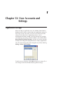
Chapter 12: User Accounts and
Settings
Application Settings................................. 229
User Administration................................. 230
Changing Your Own Password............. 230
Managing Your Own Scan Groups....... 231
System Administration ............................. 234
Account Rights..................................... 236
Managing Users ................................... 235
Managing Scan Groups ........................ 237
Scanner Information............................. 238
Scanner Diagnostics............................. 238
Scanner Update ................................... 240
Adding and Deleting Scanners................. 242
Adding Scanners via Auto Discovery.... 243
Manually Adding Scanners................... 243
Editing and Deleting Scanners.............. 244
Chapter 13: Calculation Descriptions
Derivation of the Mathematical
Expressions ..............................................245
Definition of Terms............................... 245
Assumptions .........................................246
Integrated Intensity and Integrated Pixel
Volume ................................................246
Odyssey Calculations............................... 249
Number of Pixels, Pixel Area, and Shape
Area......................................................249
Background ..........................................249
Raw Integrated Intensity........................ 250
Integrated Intensity ............................... 250
Average Intensity .................................. 251
Trimmed Mean ..................................... 251
Peak Intensity .......................................251
Minimum Intensity................................ 251
Signal-to-Noise Ratio ............................ 252
Concentration.......................................252
Probability ............................................252
Molecular Weight................................. 253
Percent Saturation................................. 254
Percent Response for ICW Assays ......... 254
Z’-Factor Calculations........................... 256
Index
iii
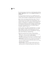
1
Chapter 1: Introduction
How to Learn Odyssey
If you are upgrading from a previous version of Odyssey® software,
a list of changes for version 3.0 can be found in the help system. In
addition, movies that illustrate new software features can be viewed
by choosing Help > What’s New.
The best way for new users to learn Odyssey is to work through the
tutorials in the Tutorial Manual. The Tutorial Manual is a step-by-step
guide that introduces you to scanning with the Odyssey Imager, as
well as analysis with Odyssey software. The overview of Odyssey in
the Tutorial Manual will familiarize you with basic operation of the
entire system.
When you are ready for more information, this User Guide is a
reference manual with complete descriptions of sizing and quantification, as well as features of the Odyssey In-Cell Western Module.
The Odyssey In vivo Imaging Guide describes optional software
module and operational details for scanning mice using the Odyssey
MousePOD™ Imaging Accessory.
Sample preparation is described in the Odyssey Application
Protocols Manual and in the pack inserts enclosed with reagents.
Operation and maintenance of the Odyssey instrument can be found
in the Odyssey Operator’s Manual. Documentation of the server
software inside the Odyssey instrument is also included in the
Operator’s manual. User account management, networking, troubleshooting, scan control, and software updates are all discussed.
2 CHAPTER 1
Introduction
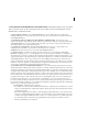
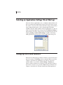
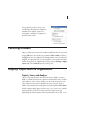
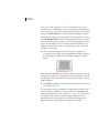
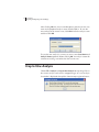
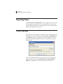
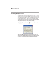
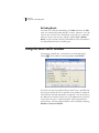
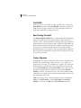
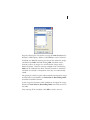
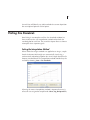
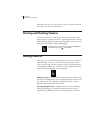
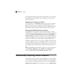
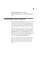
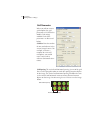
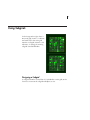
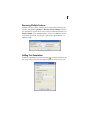
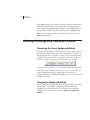
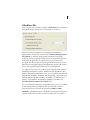
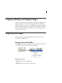
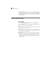
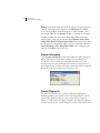
Selecting an Application Settings File at Start-up
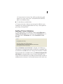
When the Odyssey application starts, a window is displayed that asks
the user to choose the application settings file for the current session.
This makes it easy for users to have their own settings file that determines important parameters such as background calculation
method. Until you understand the Odyssey application, it is best to
choose the default application settings stored in Odyssey_Settings as
shown below. The active settings file can be changed at any time by
choosing Settings > Select Active Settings. Chapter 12 describes
adding, deleting and changing the active application settings file.
Setting Up Users and Scanners
Before you can do anything in Odyssey software, you must have your
own user account. The Settings menu is used to to add user accounts.
Chapter 12 describes this procedure. The Odyssey instrument
network address must also be added (Settings > Scanners) to
Odyssey software before the instrument can be operated. Odyssey
instruments (scanners) are generally added during installation, but
Chapter 12 describes this function should you need to perform it.
3
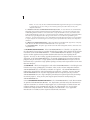
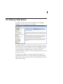
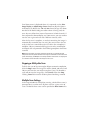
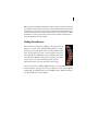
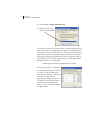
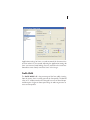
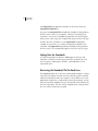
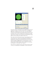
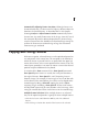
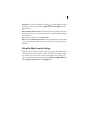
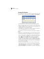
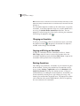
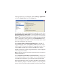
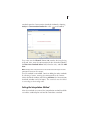
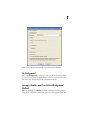
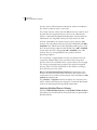
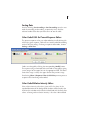
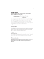
The Odyssey Help System
The Odyssey help system can be invoked by choosing Help >
Contents or by pressing F1 on the keyboard.
The Help window has two frames. The left frame contains navigational links. Click a topic to display content for the topic in the right
frame. Folders in the navigational frame contain additional topics
and are opened by clicking their plus symbol. To search for
something specific, click the search tab (magnifying glass icon) and
enter the search text.
The help system contains most of the information found in the
Tutorial Manual and this User Guide. However, the information is
organized in a more task-oriented way that should help if you forget
how to do something.
4 CHAPTER 1
Introduction
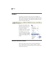
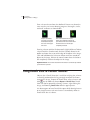
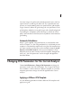
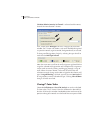
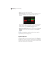
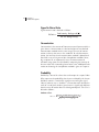
Toolbars
The Odyssey user interface makes extensive use of toolbars to
provide single-click access to most functions. The function of each
tool is given in a tool tip that can be displayed by stopping the cursor
over the tool on the toolbar. A description of each tool can also be
found in the online help system.
Most tools on the toolbar corresponds to a menu choice on the
menu bar that does the same
function. The examples
throughout this manual use both
the toolbar and menu functions.
If the toolbars get in your way,
you can easily hide them. To hide
a toolbar, choose View > Toolbars
and deselect the toolbar you want
to hide.
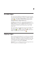
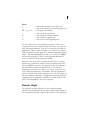
Context-Sensitive Menus
Odyssey has context-sensitive menus that change depending on
what is selected when the menu is opened. To open a contextsensitive menu select a feature on the image, such as a band marker,
and right-click the image.
5
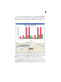
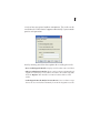
Using context sensitive menus you
can do things like open the Properties
window for an object, rotate text
annotations, and plot a histogram of
quantification values.
Correcting Mistakes
Odyssey software has extensive "Undo" capabilities that are accessed
on the Edit menu. By continuing to choose Edit > Undo or clicking
the
tool, you can undo the last 100 operations since the Odyssey
program was opened (with a few exceptions). The number of undo’s
can be changed in the Application Settings (choose Settings > Application and select General from the settings list).
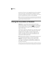
Odyssey Project and File Organization
Projects, Scans, and Analyses
Odyssey file organization starts with the project folder. A project
folder is a folder anywhere on a local or network drive that is used to
store Odyssey scans. Project folders can be used to separate scans
into a logical structure that compliments your research. Project
folders are created when new projects are started (choose File > New).
Within a project folder there can be many scans. Each scan is a folder
containing one or two TIFF images from the Odyssey Imager,
depending on whether probes for one or both dyes were used. Scans
6 CHAPTER 1
Introduction
can be started from the New Project window or by clicking the Scan
button on the toolbar (
) if a project is already open.
Scan folders also contain the analysis files generated when an
analysis is performed on the scan. Analysis files hold all the data
(concentrations, etc.) and annotations created when the scan was
analyzed. At the end of each new scan, the first analysis on the new
image files is saved. A set of images can be analyzed as many times
as needed. A new analysis can be created by clicking the New
Analysis button on the toolbar (
).
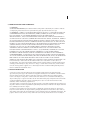
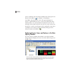
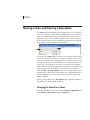
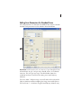
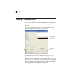
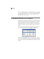
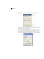
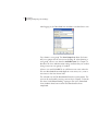
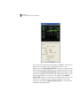
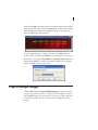
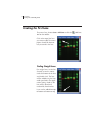
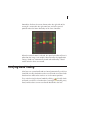
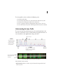
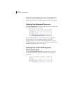
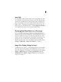
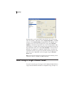
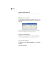
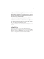
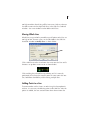
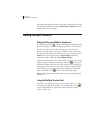
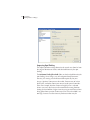
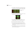
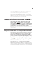
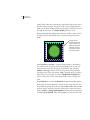
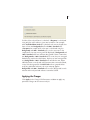
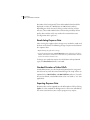
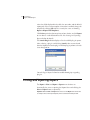
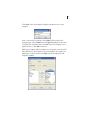
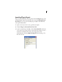
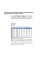
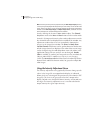
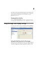
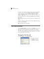
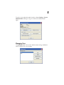
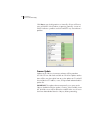
Displaying Projects, Scans, and Analyses in the Main
Odyssey Window
The main Odyssey window shown below is the default window
configuration that displays the Scans view (left) and the Image view
window (right).
Scans View
Image View
The Scans view is always open (left) and lists the projects, scans, and analyses
for the current project. Double clicking on an analysis opens an Image view
(right) containing the images from the analysis.
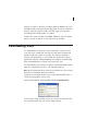
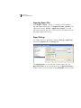
7
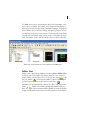
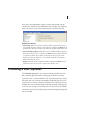
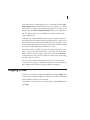
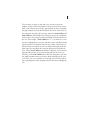
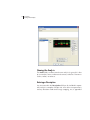
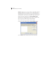
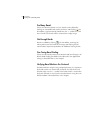
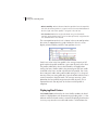
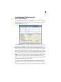
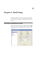
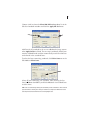
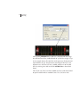
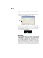
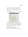
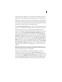
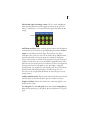
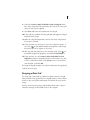
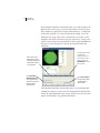
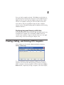
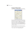
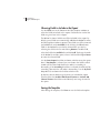
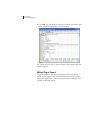
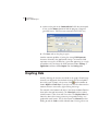
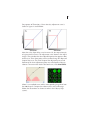
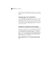
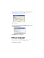
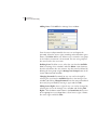
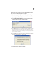
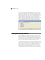
The View menu can be used to display other file information in the
main Odyssey window. The Folders view (shown below) displays a
directory tree similar to that found in Windows Explorer. The purpose
of the Folders view is to aid in finding and opening Projects, which
are displayed in the Scans view (center). The Thumbnails view shows
a thumbnail sized image of the scan or analysis selected in the Scans
view. The Folders, Scans, and Thumbnails views are discussed below.
Folders View
Scans View
Thumbnails View
Image View
Folders view and Thumbnails view can be opened using the View menu.
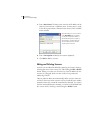
Folders View
Folders view is opened (or hidden) by choosing View > Folders View.
A close button in the upper right corner hides the view. Odyssey
project folders, which contain scans, have a unique icon (
), as do
the scan folders (
) within project folders. Projects that are open
and have been edited are shown with a pencil icon (
).
All folders can be expanded by clicking the “plus” icon next to the
folder (
). Folders can also be expanded by double-clicking
them. When an Odyssey project folder is double-clicked, the project
is opened and shown in the Scans view. The context menu that opens
8 CHAPTER 1
Introduction
by right-clicking on a folder can also be used to open and close a
folder.
Note: Starting with Odyssey software version 3.0, project folders can be stored in any
location. Local drives and mapped network drives generally offer the best performance.
In addition to browsing for projects and scans in Folders view, a
search function (File > Scan > Search for Scans) is available to find
scans if the file name is known or partially known. The list of recently
open projects on the File menu is also a fast way to open projects.
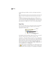
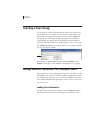
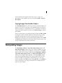
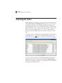
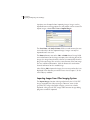
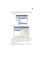
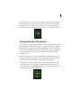
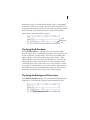
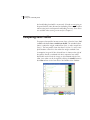
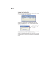
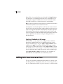
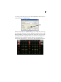
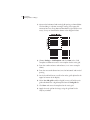
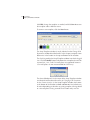
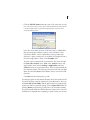
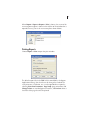
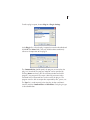
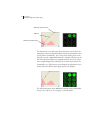
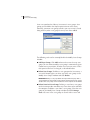
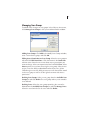
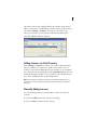
Scans View
The Scans view shows all scans and analyses for the current project.
The name of the current project is shown in Scans view and
highlighted in Folders view.
Project
Scan
Analyses
In the project named “Bandsizing” above, there is one scan named
“Western” and two analyses named “First_Analysis” and
“MyAnalysis”. The project above has only one scan, but for projects
with many scans it may be useful to sort the scans. Right-clicking the
project name opens a context menu with choices for sorting scans by
name or date, using either ascending or descending order. The
default sort order can be set by choosing Settings > Application and
selecting General from the Settings List.
To view all the analyses associated with a scan, click the “plus” icon
(
) to expand the scan folder. To open an analysis, double-click
it in the scans list. The first analysis in a scan folder can be opened
9
by double-clicking the scan folder. An analysis can also be opened
using Thumbnails view as described below.
A scan or analysis can be deleted by selecting it in the Scans view
and pressing Delete on the keyboard. An analysis can also be deleted
by right-clicking the analysis and choosing Delete Scan from the
popup menu. Additionally, the operating system can be used to
delete files in the normal way. If Odyssey software is open when files
are deleted using the operating system, the Scans view will not
immediately show the files have been deleted. The refresh button
(
) in the upper right corner of Scans view can be used to refresh
the scan list and show any changes.
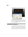
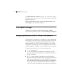
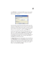
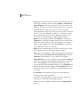
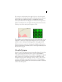
Thumbnails View
Thumbnails view is opened (or hidden) by choosing View > Thumbnails View. A close button in the upper right corner hides the view.
One composite, two-channel thumbnail image is shown for each
analysis in the scan folder. Double-clicking a thumbnail image opens
the corresponding analysis.
Initially if a scan or analysis is not selected in the scan list, the
message “No Thumbnail Defined” is displayed. All the thumbnails
are created as soon as a scan or analysis is selected. The thumbnails
are real files that are saved as JPEG files in the scan folder. The file
name convention is ScanName_AnalysisName_tn.jpg. If changes are
made to the image, such as cropping or rotating, these changes will
not be updated in the thumbnail until the analysis is saved.
iii
11
Chapter 2: Starting Scans
How to Start Scans
Scans on the Odyssey Imager can be started using the Windows®based Odyssey Software, an Internet browser, or from the front panel
of the Odyssey Imager. Chapter 6 of the Odyssey Operator’s Manual
discusses starting scans using an Internet browser. Front panel
operation is described in Chapter 7 of the Odyssey Tutorial Manual
and Chapter 3 of the Odyssey Operator’s Manual. The remainder of
this chapter is dedicated to starting both standard scans and multiple
microplate scans with Odyssey software. Scanning mice with the
MousePOD™ Accessory is discussed in the Odyssey In vivo Imaging
Guide included with the MousePOD.
Before a scan can be started, a project must be open so the new scan
can be stored in the open project.
Starting Standard Scans in an Existing Project
Existing projects are opened by choosing File > Open or by clicking
on the toolbar. The four most recently opened projects are also
listed toward the bottom of the File menu. The number of recent
projects listed can be increased to as many as 10 in the Application
settings (choose Settings > Application and select General from the
Settings List).
Once a project is open, a standard scan can be started by clicking
on the toolbar or choosing File > Scan > Scan. After entering
12 CHAPTER 2
Starting Scans
your user name and password, the Scanner Console window is
opened, allowing scans to be started as described below.
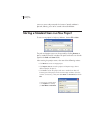
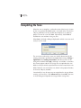
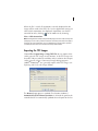
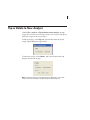
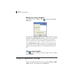
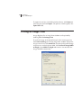
Starting a Standard Scan in a New Project
To start a new project in Odyssey Software, choose File > New.
The path and project name can be entered by clicking Browse to
open a standard "new file" window. File paths and names can also be
typed in the Path and Name fields.
After entering the project name, take one of the following actions:
• Click Done to create an empty project.
• Click Import Scan to create the project and import images from a
different project (Chapter 3).
• Click Scan to create the project and start a standard scan that will
become part of the project. In the Scanner Login window, select the
scanner (if necessary), enter your User Name and Password, and click
OK.
If someone else is already logged
in, click Logout before entering
your User Name and Password.
13
Note: User names and passwords must be added by a user with Administrator
(admin) access privileges. The system administration functions (Settings >
System Administration) are used to add users and set access privileges (see
Chapter 12).
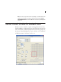
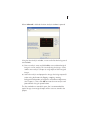
Scanner Console Window for Standard Scans
Whether a scan is started in a new or existing project, the Scanner
Console window is used to specify the scan parameters and start the
scan. It can also be used for a quick preview scan. During each scan,
the Scanner Console displays the scan in real time as it is collected
and displays progress indicators for the scan.
14 CHAPTER 2
Starting Scans
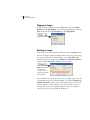
Naming a Scan and Entering a Description
The Name field is not editable at the beginning of a scan. The default
scan name is filled in automatically according to the naming conventions in the Application Settings. The default name may be blank, a
sequential name, or a time stamp (shown below). At the end of the
scan, the default name can be accepted or replaced with a different
name before the file is stored on the computer.
The name in the Name field is also the scan name that will be stored
on the hard drive of the Odyssey instrument. If "blank" is the current
naming convention, a time stamp will be used for the scan name on
the Odyssey instrument. If the default name is replaced with a new
scan name at the end of the scan, the scan name on the computer
will be different than the original scan name on the hard drive in the
Odyssey instrument. The original scan name can be viewed by
choosing Edit > Scan Description to view the scan description. The
original name is also listed in the tool tip that is displayed when the
cursor is stopped over a scan name in the Scans view of the main
Odyssey window.
Entering a description in the Description field is optional; however,
descriptions can be included in reports.
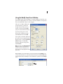
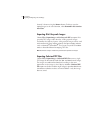
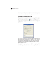
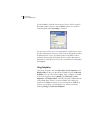
Changing the Default Scan Name
To change the default scan name, choose Settings > Application and
select Naming Conventions from the Settings List.
15
Since these are Application settings, naming conventions can be
saved in the settings files for individual users (Chapter 12), allowing
each user to have scan names automatically entered as desired.
Default Scan Names:
• Time Stamp: When the Scanner Control window is opened, the current
year, month, day, hour, minutes, and seconds is entered in the Name field
automatically. This time stamp can be edited or appended with other text.
• Last Used Name Sequence: When the Scanner Control window is opened,
the name of the last scan is entered in the Name field and appended with
a sequential number. For example, if MyScan was the last scan name,
Odyssey will present MyScan_1 as the default name for the next scan,
followed by MyScan_2, etc.
• Empty: When the Scanner Control window is opened, the Name field is
left blank so the user can enter a name at the end of a scan.
Previewing a Scan (Optional)
Click Preview (optional) in the Scanner Console window to scan a
low resolution preview before starting high resolution scanning.
A preview scan is a low resolution scan at the lowest quality setting
that takes only a few minutes to complete, depending on scan area.
A preview scan can be used to check fluorescent signal intensity or
to adjust the scan area before high resolution scanning. Adjusting the
scan area (see Setting Scanner Parameters for Standard Scans below)
can shorten scan times by reducing the amount of empty background
that is scanned.
16 CHAPTER 2
Starting Scans
Selecting a Scan Group
A scan group is a special directory on the Odyssey instrument that
has restricted access. Initially, users have access to the Public scan
group and a scan group that matches their user name. Additional
scan groups can be created for special purposes. For example, if
several people are doing scans for a particular research project, it
might be useful to keep all scans for that project in one scan group.
The Group drop-down list is used to select the scan group in which
the new scan will be stored.
Scan groups are added and deleted by clicking Modify (next to
Group). See Chapter 12 for complete information on scan groups.
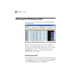
Setting Scanner Parameters for Standard Scans
Scan parameters, such as resolution and scan area, can all be entered
individually in the Scanner Console window or loaded from stored
sets called Presets. For most scans it is easiest to load Preset parameters and then edit individual parameters, such as scan area, to match
the current scan.
Loading Preset Parameters
Sets of scan parameters can be chosen from the Preset drop-down
list. When a Preset is chosen, all existing scan parameters in the
17
Scanner Console window are replaced by scan parameters stored in
the Preset file.
Odyssey software initially has four Preset files for general use – one
for membranes, two for gels, and one for microplates. In addition,
there are four Preset files for the MousePod™ In Vivo Imaging
Accessory: one for each of the three mouse positions in the
MousePod and one for all three positions at once.
Note: For older instruments, Odyssey Server Software version 2.0 or above is required
in order to have enough focus offset to scan a microplate. See Odyssey Operator’s
Manual to determine software version number.
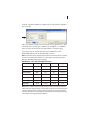
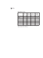
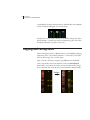
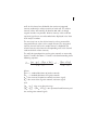
Membrane, Gel, and Microplate Presets
Membrane
DNA Gel
169
169
169
169
medium
medium
medium
medium
0.0
2.0
0.5
3.0 mm
Channels
700, 800
700, 800
700, 800
700, 800
Intensity
5.0
8.0
5.0
5.0
Scan Origin
0,0
0,0
0,0
0,0
10,10
10,10
10,10
13,9
Resolution
Quality
Focus Offset
Scan Size
Protein Gel Microplate2
Note: There are Presets both in the Odyssey Imager itself and in Odyssey Software.
The Presets in the Odyssey Imager are used when starting scans from the front panel
or from an Internet browser. Presets in Odyssey Software are used only in Odyssey
Software. Information on using, modifying, and saving Presets in the Odyssey Imager
can be found in the Odyssey Operator’s Manual.
18 CHAPTER 2
Starting Scans
MousePOD™ Presets
Full
Pod
Scan
Mouse
Center
Position
Mouse
Left
Position
Mouse
Right
Position
169
169
169
169
Quality
medium
medium
medium
medium
Focus Offset
1.0 mm
1.0 mm
1.0 mm
1.0 mm
Channels
700, 800
700, 800
700, 800
700, 800
Intensity
L1.0, L2.0
L1.0, L2.0
L1.0, L2.0
L1.0, L2.0
0,0
8,0
0,0
15,0
25,19
9,19
10,19
10,19
Resolution
Scan Origin
Scan Size
See Odyssey In vivo Imaging Guide for details on scanning with the
Odyssey MousePOD Accessory.
19
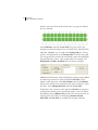
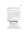
Editing Scan Parameters for Standard Scans
All scan parameters are listed in the middle of the Scanner Console
window. Each parameter can be edited as described below.
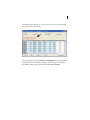
Resolution can be set to 21, 42, 84, 169, or 337 µm. For typical scans
of membranes or gels, 169 µm scans should suffice. As resolution
increases, file sizes get very large. The table below shows the
resolution and scan size limits for starting scans with Odyssey
Software.
File sizes under 7 MB per image scan well and can be analyzed in
Odyssey Software without cropping the image into smaller pieces.
File sizes from 7 - 14 MB are marginal and Odyssey Software may
20 CHAPTER 2
Starting Scans
run out of memory during a scan. Scans with file sizes larger than
14 MB per image can be performed using the browser interface as
described in the Odyssey Operator’s Manual, but should not be
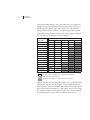
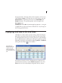
attempted with Odyssey Software. The table below shows typical
combinations of resolution and scan size, with shading to indicate
file sizes that are too large for Odyssey Software.
Scan Size
5 x 5 cm
5 x 10 cm
5 x 15 cm
5 x 20 cm
5 x 25 cm
10 x 10 cm
10 x 15 cm
10 x 20 cm
10 x 25 cm
15 x 15 cm
15 x 20 cm
15 x 25 cm
20 x 20 cm
20 x 25 cm
25 x 25 cm
337 µm
44k
88k
132k
176k
220k
176k
264k
352k
440k
396k
528k
660k
704k
800k
1.1M
169 µm
175k
350k
525k
700k
875k
700k
1.0M
1.4M
1.7M
1.6M
2.1M
2.6M
2.8M
3.5M
4.4M
Resolution
84 µm
708k
1.4M
2.1M
2.8M
3.5M
2.8M
4.1M
5.6M
7.0M
6.3M
8.4M
10.6M
11.3M
14.1M
17.6M
42 µm
2.8M
5.7M
8.5M
11.3M
14.2M
11.3M
17.0M
22.7M
28.3M
25.5M
34.0M
42.5M
45.4M
56.7M
70.9M
21 µm
11.3M
22.6M
34.0M
45.3M
56.7M
45.3M
68.0M
90.7M
113.3M
102.0M
136.0M
170.0M
181.4M
226.7M
283.4M
File size is small enough to scan with Odyssey Software.
Marginal for Odyssey Software.
Scan should be started in using the browser interface.
Odyssey Software also has limitations on the size of images that can
be analyzed. The total size of all open images should not exceed
20-25 MB. One analysis with two 10MB images will use up most of
the memory resources. However, if your typical image size is 2 MB,
five separate analyses can be opened. Large scans can be cropped
into smaller pieces using the browser software if necessary.
21
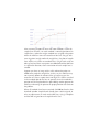
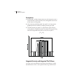
For band sizing applications, the resolution setting can be checked
by looking at the lane profiles (Chapter 5). If the lane profile shows
many small jagged peaks on the larger peaks of bands (as contrasted
with smooth peaks), this may indicate the resolution is too coarse.
These jagged peaks will influence the accuracy of band finding. If the
small peaks are caused by lack of resolution, choosing a smaller
resolution value should improve the problem.
Quality controls scan speed and ultimately how many detector
readings are processed for a given area on the membrane in order to
make one pixel on the image. For typical scans, Medium is recommended, but there are five settings. Choosing Highest quality will
reduce noise in the image data, but significantly increase scanning
time due to the slower scanning speed. Similarly, choosing Lowest
will decrease scan time, but increase noise in the image data. For
high resolution scans where samples have very little fluorescence,
High or Highest may be a better choice than Medium. When Quality
is set too low, the image may become noisy or "grainy", particularly
in the background.
Focus Offset should always be zero when scanning membranes. For
gels, set Focus Offset to half the gel thickness, in millimeters. For
microplates recommended by LI-COR (Operator’s Manual, Chapter 3),
focus offset is 3 mm. The maximum possible focus offset is 4 mm.
Select Microplate (flip image) when scanning single microplates.
When selected, images are flipped automatically after each scan so
the origin (well A1) of the plate is in the upper left corner. (Microplate
images must be flipped because the plate is scanned through the
bottom.) Deselect Microplate (flip image) when scanning
membranes, gels or mice.
The Channels check boxes is used to specify whether to detect
fluorescence in the 700 channel, the 800 channel, or both. When
both are selected, fluorescence from each dye is detected separately
and stored in a separate image file.
22 CHAPTER 2
Starting Scans
The Intensity fields control the detector sensitivity and affect the
band intensity on the image. If the intensity is set too high, the
detector may saturate and produce white areas in the middle of
intense bands/dots. (Saturated pixels are colored cyan if the image is
being displayed as a grayscale image.) If the intensity is set too low,
the image may not show any fluorescence even though there is
adequate signal from the samples. LI-COR Presets use an intensity
value of 5.0 for membranes, 8.0 for DNA gels and 5.0 for protein gels
or microplates. These settings may need to be optimized for your gels
or membranes due to the differing background fluorescence of
various materials. Intensity values from 1 to 10 in increments of 0.5
can be chosen, as well as low intensity values L0.5 to L2.0. L2.0 is
the lowest intensity value Odyssey can use for scanning.
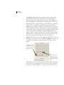
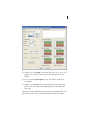
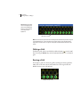
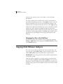
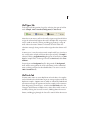
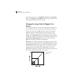
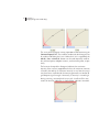
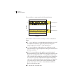
Scan Area parameters are used to specify the portion of the 25 x 25
centimeter scan surface to scan. The Size and Origin (cm) can be set
by clicking and dragging a rectangle on the scan grid as shown
below.
Click and hold down the
mouse button in the
lower left corner of the
area to be scanned.
Drag the cursor to the
upper right corner of
the area to be scanned
and release the mouse
button.
To reposition the scan area, click inside the red rectangle and drag
the scan area to a new position. To resize the scan area, move the
cursor over one of the red lines or corners until an arrow cursor is
23
displayed. With the arrow cursor displayed, click and drag to resize.
To reset the scan area, click and drag a new rectangle on the scan
grid, starting outside the current red rectangle. If necessary, doubleclick outside the current red rectangle to erase it before drawing a
new one.
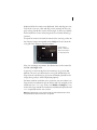
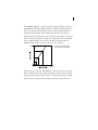
The tip of the arrow in the front left corner of the scanning surface on
the Odyssey Imager corresponds to the Origin of X=0, Y=0 on the
scan grid in the Scanner Console window.
Left border
of scan area
Lower border
of scan area
See the Odyssey
Operator’s Manual for
additional information
on sample placement.
Origin
If the size and origin are known, the dimensions can be entered in
the Size and Origin fields.
In general, it is best not to place the membrane or gel at the 0,0
position. The scan area drawn on the scan grid should always be
larger than the membrane or gel so text annotations placed on the
image during analysis will be displayed properly.
For low or medium resolution scans, make the scan area about 1 cm
larger than the membrane or gel on all four sides. For example, if the
membrane size is 5 x 5 cm, set the scan Width and Height to 7 cm,
and set the Origin to 0,0. The membrane would then be placed at the
1 x 1 cm position on the scan surface.
Note: After setting the scan area, check the file size at the bottom of the Scanner
Console window to make sure the size is acceptable.
24 CHAPTER 2
Starting Scans
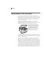
Placing Samples on the Scan Surface
In general, it is easier to place the membrane or gel on the scan
surface before drawing the scan area on the scan grid. If the sample
is placed first, the 1 cm grid lines on the scan surface can be used to
determine where to draw the scan area on the scan grid in the
Scanner Console window.
Membranes should be placed face down with the top of the
membrane toward the front of the Odyssey Imager. (Orientation can
be changed by flipping or rotating the image as needed.)
Tip: Rectangular membranes (or gels)
will scan faster if the long dimension of
the membrane is oriented horizontally
along the front border of the scan area.
Placement in a vertical orientation
requires the laser microscope to travel
further and increases scan time.
Consult the Operator’s Manual and Odyssey Protocol pack inserts for
tips on handling membranes and remember to touch the membrane
only with a clean forceps.
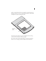
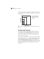
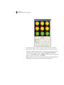
Orienting a single microplate for a standard scan is somewhat
different (scanning multiple microplates is described later in this
chapter). A plastic microplate alignment guide is used to position the
microplate at a known location on the scan surface. Push the guide
into the lower left corner until it contacts the bezel surrounding the
scan surface on both the front and left sides. Place the microplate on
the scanning surface and slide it into position until it contacts both
the front and left side of the alignment guide. The first well in the first
row (A1) should be toward the back and left side of the alignment
25
guide as shown below. When the microplate is placed against the
alignment guide, the scan size and origin parameters in the default
microplate scan preset should work well.
A1
Alignment
Guide
A1
After placing the membrane, gel, or microplate on the scanning
surface, close the lid on the Odyssey Imager.
For scanning mice with the MousePOD™ Accessory, consult the
Odyssey In vivo Imaging Guide included with the MousePOD.
26 CHAPTER 2
Starting Scans
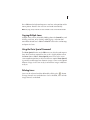
Starting a Standard Scan
To start a standard scan, click the Start Scan button in the Scanner
Console to send the scan parameters to the Odyssey Imager and start
the scan.
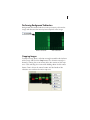
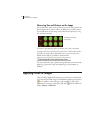
The images are displayed in real time in the area of the Scanner
Console window where the scan grid was located.
The images are
displayed as they
are scanned.
Status line.
Progress bar.
At the bottom of the Scanner Console window, the status line
indicates the time required to finish the scan. The progress bar
indicates the percentage of the scan area that has been scanned. In
the message area, the message "System Cooling" may be displayed
initially, which indicates that the detectors in the laser microscope
are being cooled to their operational temperature.
27
If no fluorescence is displayed where it is expected, click the Alter
Image Display button to adjust the image (see Chapter 11). If bands
are just dim, use brightness and contrast adjustments. If there are no
bands, move the Linear Manual Sensitivity slider (auto adjustments
off). The Adjust Image Curves window can also be used to make
similar adjustments.
By default, the 700 and 800 channel images are shown overlaid. If
the color scheme is the default red/green color scheme, areas that are
yellow have intense fluorescence in both channels. To look at each
channel separately during scanning, the Alter Image Display window
can also be used to display one channel at a time.
If no fluorescence is visible, even after sensitivity adjustments, or if
there is signal saturation (white pixels), cancel the scan (described
below), and start the scan again using new values for the Intensity
scan parameter in the Scanner Console. If fluorescence is too strong,
use lower intensity values.
The scan ends automatically when the entire scan area has been
scanned. As the images are collected, image files are created both on
the hard disk of the Odyssey Imager and on the computer.
Stopping a Scan
To finish a scan before automatic completion, click the Stop button
in the Scanner Console window. The image files will be closed and
saved, allowing the files to be analyzed.
To abandon a scan and not save the image files, click Cancel rather
than Stop.
28 CHAPTER 2
Starting Scans
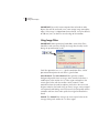
Completing the Scan
When the scan is complete, a reduced version of the image is shown
on the scan grid and the Save button is activated so the scan on the
Odyssey hard drive can be saved to the computer in an Odyssey
project. To save the scan click Save. Alternatively, click Close to
abandon the scan without saving any files.
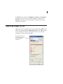
When Save is clicked, a dialog in displayed in which a new scan and
analysis can be saved.
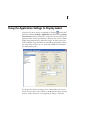
The scan name and analysis name are initially determined by the
naming conventions specified in the Application settings (Settings >
Application then Naming Conventions), but these names can be
changed as needed. When OK is clicked, a scan folder is created in
the current project and the TIFF image files are copied to the scan
folder. An analysis with the specified name is also created in the scan
folder. Both the scan and analysis are shown in the project directory
in the main Odyssey window.
Occasionally, it may be necessary to manipulate the images before
creating a new analysis. Click Advanced rather than OK in the Save
As Scan dialog to manipulate the images before saving them.
29
When Advanced is clicked, the New Analysis window is opened.
Using the New Analysis window, a scan can be finished using one of
two methods:
1) Enter an analysis name and click OK to save unaltered original
images in a new analysis. To start analyzing the images, create
another new analysis (Chapter 4) using copies of these original
images.
2) Name the analysis and prepare the images for sizing or quantification using the buttons for flipping, cropping, rotating,
background subtraction, or brightness and contrast adjustments.
(See Chapter 3.) Then, click OK to create the new analysis and
proceed with sizing or quantification.
The first method uses more disk space, but is recommended for
typical images since original copies of the scans are stored in the
project.
30 CHAPTER 2
Starting Scans
If there is a problem with the scan and you do not want to analyze
the images, click Cancel in the New Analysis window instead of OK.
Clicking Cancel removes the new scan from the project that was
open when the scan was started.
Creating and Editing Preset Parameters
After scanning a few of your own samples, you may want to create a
set of Preset scan parameters or edit an existing Preset to match your
scanning methods. The instructions below describe creating and
editing Preset parameters for Odyssey Software. To create your own
Presets in the Odyssey instrument, consult the Odyssey Operator’s
Manual.
The Preset parameters displayed in the Scanner Console window can
be created or modified by choosing Settings > Scan Presets.
The Scan Presets window lists all presets. To edit a preset, select it
from the list and click Edit. To create a new preset, either click New
or edit an existing preset and click Save As in the Modify Scan Preset
window.
31
Using the Modify Scan Preset Window
The Modify Scan Preset window is used to modify each of the scan
parameters displayed in the Scanner Console Window. Scan parameters were defined earlier in this chapter.
After you are done editing the
scan parameters, check the
image size to make sure it is
under 14 MB and click OK if
you just want to edit the Preset.
If you want to create a new
Preset with a different name,
click Save As instead of OK.
If you make a mistake and want
to set all values to stored factory
default values, click the Default
Values button. To abandon
changes without saving them,
click Cancel.
Note: The status of the Microplate (flip
image) parameter is ignored when a
preset is used for a multi-plate scan.
The images are always flipped for multiplate scans.
Tip: The Modify Scan Preset window can also be opened by clicking Modify in the
Scanner Console window as shown below. Note, however, that the Scan Area fields
are not editable unless the Modify Scan Preset Window is opened from the Settings
menu.
32 CHAPTER 2
Starting Scans
Scanning Multiple Microplates
When scanning microplates, Odyssey can scan up to six microplates
simultaneously. During a multi-plate scan, a separate scan and
analysis is created for each microplate and they are added to the
current project. For example, if there are six microplates, six scan
files and their corresponding analysis files will be created. Odyssey
relies on standard size plates being placed in a known location, so it
is important to use the alignment guide and place the plates as
described below. Use the following procedure to scan multiple
microplates.
1) Create an empty new project or open an existing project in which
to store the new scans (described earlier in this chapter).
2) Choose File > Scan > Scan Multiple Plates.
3) In the Scanner Login window, enter your User Name and
Password (case sensitive) and click OK, if necessary.
4) In the Scan Multiple Plates Setup window, enter a base name for
the scan or accept the default base name that is automatically
entered according to the Multiple Scan settings (Settings menu).
Note: Odyssey appends the base name with a sequential identifier for each microplate.
In the window below, if 2005-Mar-29-4PM is the base name, Odyssey will automatically
use 2005-Mar-29-4PM-1 as the scan name for the first plate, followed by 2005-Mar-294PM-2, etc. If another scan is started using the same base name, a letter is also
appended. Thus, the first scan with a duplicate base name would be 2005-Mar-294PM-a-1, the second would be 2005-Mar-29-4PM-a-2, etc. The letter is incremented
each time a new scan is initiated using a duplicate base name.
33
5) Choose the scan Group in which to store the scan. (Use of scan
groups in the Odyssey instrument is described earlier in this
chapter.)
6) Enter a common Description (if any) that will be used for all
microplates.
7) Choose a set of Preset scanner parameters designed for microplates (such as the default Microplate2 preset) and skip to the
next step.
Alternatively, the individual scan parameters can be edited. The scan
parameters are the same as those described earlier for standard
34 CHAPTER 2
Starting Scans
scans, with a few exceptions. First, the scan dimensions are not
editable since a standard plate size is assumed. If non-standard plates
are used, the scan size can be changed in the Multiple Scan settings.
Second, set Focus Offset to 3.0 for standard microplates as recommended in the Odyssey Operator's Manual. The last difference is that
the Scan Multiple Plates function automatically flips images to the
correct orientation so the image has well A1 in the upper left corner.
Presets for microplates can be created as described earlier in this
chapter, but note that the scan size and origin are not used by the
multiple scan software.
8) Set the number of plates to scan. If less than six plates are
scanned, click the plate icons corresponding to empty locations
in six-through-one order. Deselected plates appear as shown
below.
Plates should be added to the Odyssey scanning surface in the order
(1 through 6) shown in the multi-plate scan setup window. Consult
the Operator's Manual for more details on placement of the scanning
guide and plates.
9) Click Start to send the scan parameters to the Odyssey instrument
and start the first scan.
The image from the first microplate is displayed in real time in the
Scanner Console window. The name extension in the Name field
indicates which plate is being scanned (-1, -2, etc.). The status line at
the bottom of the Scanner Console window indicates the time
required to finish scanning the current plate and a progress bar
indicates how much of the plate area has been scanned.
35
If no fluorescence is displayed where it is expected, use the Alter
Image Display or Adjust Image Curves button to adjust brightness
and contrast. By default, the 700 and 800 channel images are shown
overlaid. If the default red/green color scheme is being used, the
areas that are yellow have intense fluorescence in both channels. If
these adjustments do not display any fluorescence, you may need to
start the scan again and scan with a different intensity value.
After the first scan is complete, an analysis containing the images is
automatically created for the scan using the same name as the last
analysis that was created. When the scan of the first microplate is
complete, Odyssey automatically begins to scan the second plate
and repeats the scan procedure until all designated plates have been
scanned.
Note: If the microplates are poorly centered in the images, try adjusting the grid
template to match the grid to the wells in the image. If some wells are truncated or the
grid is off the image, see Multiple Scan settings below for instructions on changing the
scan offset to center the wells on the image for new scans.
Stopping a Multi-plate Scan
To finish the scan of the current plate before automatic completion,
click the Stop button. The image files will be closed and saved, and
Odyssey will start the scan of the next plate (if any). To abandon a
scan and not save the image files, click Cancel rather than Stop.
Clicking Cancel also cancels all other plates from being scanned.
Multiple Scan Settings
In the setup window for multi-plate scanning, a default base name is
presented that is used to name all plate scans for a given series of
scans. The default base name can be specified on Base Name tab in
36 CHAPTER 2
Starting Scans
the Multiple Scan Settings window. To open the Multiple Scan
settings, choose Settings > Multiple Scan.
The default name can be set to the current date, the current date plus
current hour, or user designated text.
In the setup window for multi-plate scanning, the user is not given
the option of setting the scan size or XY offset. This is because the
scan size is based on a standard microplate size. The scan size and
XY offset for microplates recommended by LI-COR are shown below.
37
These settings are only a guide and every instrument may not
produce images with the microplate exactly centered. If the microplate is not centered in the image, proceed with analysis and adjust
the grid template to match the location of the wells. If the wells are
truncated or if the grid is off the image, adjust the Scan X Offset and
Scan Y Offset in the Multiple Scan settings to center the microplates
in the images. Only integer numbers should be entered and units are
0.1 mm. For example, a Scan X Offset of “15” is an offset of 1.5 mm.
For non-standard plates scan sizes and offsets have to be determined
experimentally. Start with the default values above and increase or
decrease them as needed. Set the scan width and height inside the
plate edges, but outside of the rectangle defining the well boundaries. Set the Scan X Offset to the distance along the X-axis from the
right boundary of one scan to the left boundary of the next scan.
Similarly, set the Scan Y Offset to the distance along the Y-axis from
the upper boundary of one scan to the lower boundary of the next
scan. If the scan size and offset are changed, you will also need to
edit a grid template so the template matches the non-standard plate
size.
iii
39
Chapter 3: Creating a New Analysis
Overview
An analysis holds all the sizing or quantification data created when
a scan is analyzed. For each scan, there can be many analyses. At the
end of each new scan, a new analysis is named and saved along with
the new scan, as described in Chapter 2.
For existing scans, a new analysis can be created by choosing
File > Analysis > New Analysis to open the New Analysis window.
Creating a new analysis makes copies of images from another
analysis, allowing the images can be analyzed separately from the
original analysis.
A new analysis may need to be created for a variety of reasons. For
example, if the original image had multiple membranes scanned for
different users, each user may want to independently analyze the
portion of the image that is of interest to them. If the original image
is in the wrong orientation, a new analysis can be created to flip or
rotate the image.
Opening the New Analysis Window
To start a new analysis, open a project and click on the scan
containing the images you want to copy into the new analysis. Next,
choose File > Analysis > New Analysis to open the New Analysis
window.
40 CHAPTER 3
Creating A New Analysis
Naming the Analysis
The Name field is used to name the new analysis. In general it is best
to use numbers, letters, underscore characters, or dashes. Do not use
slashes, colons, or commas.
Entering a Description
Any text entered in the Description field can be included in reports
after analysis is complete (Chapter 10). A list of the scan parameters
and any alterations made to the image (cropping, etc.) is appended
41
to the end of the description. When the analysis is open, the
description can be edited at any time by choosing Edit > Analysis
Description.
Copying Images From Another Analysis
The Available Analysis list in the New Analysis window displays all
images in the current scan that can be copied into the new analysis.
When an analysis is selected from the list, a "thumbnail" view of the
images that will be copied is shown in the Analysis Image section of
the window.
If there are two images in the selected analysis, both the 700 and 800
check boxes will be selected, indicating that both images will be
imported. To copy only one of the images to the new analysis,
deselect the image that is not wanted. See descriptions of the Undo
and Reset buttons below for information about changing images after
image manipulations have been performed.
Manipulating Images
The Flip, Rotate, Subtract, Crop, Filter, Adjust Image Curve, and
Alter Image Display buttons in the New Analysis window are used
to alter images before they are added to a new analysis. The Undo
button cancels the last change made using the Flip, Rotate, Subtract,
Crop, Filter, Adjust Image Curves, and Alter Image Display buttons.
Odyssey has multiple undo capability, so clicking Undo multiple
times steps backward through each change made since the New
Analysis window was opened. To undo all changes in the New
Analysis window, click Reset. After clicking Reset or using Undo to
reverse all changes, the images selected in the Available Analysis
panel can be changed.
42 CHAPTER 3
Creating A New Analysis
Flipping an Image
To flip an image vertically, click the Flip button and select Top to
Bottom from the Flip Options. To flip an image horizontally, click the
Flip button and select Left to Right from the Flip Options.
Rotating an Image
If the image is not in the desired orientation, click the Rotate button
and use the Rotate Options window to rotate the image. If the image
was scanned sideways or upside-down, use the Direction radio
buttons to rotate the image either Clockwise or Counter-Clockwise,
and then choose 90, 180, or 270 degrees of rotation.
Note: The image does
not need to be
“straight” or in any
particular orientation
to be analyzed.
If the membrane was place on the scanner at a slight angle, it can be
straightened using the free rotation option. First choose Clockwise or
Counter-Clockwise rotation. Next, click Free and enter the desired
rotation in degrees. Note, however, that quantification results are
changed due to image interpolation when images are rotated to
some angle that is not a multiple of 90 degrees.
43
Performing Background Subtraction
Background subtraction finds the minimum intensity value on the
image and subtracts that intensity from all pixels in the image.
Before subtraction.
After subtraction.
Cropping Images
To crop an image, draw a selection rectangle around the desired area
of the image and click the Crop button. The selection rectangle is
drawn by moving the cursor to one of the four corners of the crop
area. Click and drag the cursor while holding down the left mouse
button. Don't release the mouse button until the border of the
selection area encloses the entire crop area.
44 CHAPTER 3
Creating A New Analysis
IMPORTANT: Be careful not to crop too close to bands or other
objects that will be analyzed. Leave some empty image around the
edges. If the image is cropped too close to bands, it may be difficult
to add text, lanes, or features near the edge of the window.
Using Image Filters
IMPORTANT: When quantifying bands/dots, none of the filters
should be used since they change the image data, thereby invalidating the quantification results.
Each filter operation uses a 3 x 3 pixel convolution filter. A brief
operational description of each filter is given below.
Noise Removal: The Noise Removal filter typically removes
background speckles from an image. Noise removal calculates a
median pixel value within the 3x3 filter region and replaces the
current pixel value with the median. Noise removal is most
noticeable where the median replaces pixel values that are much
brighter or darker. For band sizing on "noisy" images, noise removal
can improve band-finding accuracy because the lane profile will be
smoother and have fewer noise peaks that might be identified as
bands.
Smooth: The Smooth filter changes the current pixel value to the
average of the pixels within the 3x3 filter region.
45
Local Maximum and Minimum: The Local Maximum filter replaces
the current pixel value with the maximum pixel value within the 3x3
filter region. Similarly Local Minimum replaces the current pixel
value with the minimum pixel value within the filter region. The
Local Maximum filter reduces noise on images where there are
background pixels that are much darker than surrounding pixels. The
Local Minimum filter reduces noise on pixels where the background
is fairly uniform except for some pixels that are much brighter than
others.
Sharpen: The Sharpen filter multiplies each pixel in the region by
sharpening coefficients and then sums the pixel values to create a
new pixel value that replaces the current pixel value. The sharpening
coefficients have been chosen so the edges of objects are enhanced.
Changing Brightness and Contrast
When the New Analysis window is opened, the image thumbnail is
shown using the last-used brightness and contrast settings. For repetitive scans the last-used settings may work well. For other scans,
brightness and contrast may need adjustment in order to see any
fluorescence in the image. If fluorescence cannot be seen, changing
brightness or contrast may be necessary to perform other image
manipulations like cropping.
To change the brightness and contrast or to view only one of the two
images, click either Adjust Image Curve or Alter Image Display. The
operation of these two functions is described in Chapter 11.
46 CHAPTER 3
Creating A New Analysis
Saving an Analysis
Any of the following methods can be used to save analysis files.
• Choose File > Save (or Ctrl+s) is used to save a project. All analyses with
unsaved changes will be saved. Similarly, File > Save As saves all files and
any unsaved changes from the current project to a new project folder.
• Choose File > Analysis > Save Analysis to save only the current analysis.
All other analyses with changes will remain unsaved.
• Choose File > Analysis > Save As New Analysis to save the current analysis
as a new analysis. Rename the analysis using the Scan Name field if the
new analysis will be saved in the current scan. To save the analysis in a
new scan, change the Scan Name (an analysis cannot be saved to an
existing scan other than the current scan).
Note: The Save Analysis and Save As New Analysis menu choices can also be
accessed by right-clicking an analysis in the project directory tree and choosing the
desired menu choice from the contextual popup menu.
Deleting an Analysis
Caution: Use this function very carefully. The analysis is deleted
immediately when this function is performed and the deleted
analysis cannot be recovered.
To delete an analysis, click the analysis in the Scans view in the
Odyssey window and choose File > Analysis > Delete Analysis.
47
Having More Than One Analysis Open
More than one analysis can be open at once, allowing images to be
compared. When multiple image views are open, the Window menu
can be used to switch between windows. The window name includes
both the scan name and analysis name. Clicking the analysis name
in the Scans view will also bring that analysis window to the front.
iii
49
Chapter 4: Importing and Exporting
Scans and Images
There are four methods to get scan images into a project in Odyssey
software:
• Start a Scan: Images are automatically transferred to the computer when
the scan is completed.
• Download a Scan: Scans started using one-button scanning on the
Odyssey Imager can be retrieved from the instrument using the
Download Scans function.
• Import a Scan: Scans stored in any Odyssey project can be imported into
the current project.
• Import Images: Images that no longer have a scan file (*.scn) can be
imported into the current project and stored under a new scan name.
Starting a new scan is discussed in Chapter 2. The remaining three
methods for importing images are discussed in this chapter. The
following methods to export scans and save images to a new analysis
are also discussed:
• Export Scans: Saves a copy of the current scan to any specified location.
• Flip or Rotate to New Analysis: Copies image files from the current
analysis into a new analysis and flips or rotates the images in the new
analysis.
• Crop to New Analysis: Crops image files in the current analysis and
saves the cropped images in a new analysis.
• Crop to Multiple Images: Crops the current images using the scan area
in a scan preset file and saves the cropped images to a new analysis.
50 CHAPTER 4
Importing and Exporting Scans and Images
Searching for Scans
Before importing or exporting a scan, you may need to search for it.
Choose File > Scan > Search for Scans to generate a list of all scans
in a folder or disk drive. A file dialog is displayed to choose the
starting location for the search. If all Odyssey projects are kept in one
folder, that folder may be a good starting place for the search. Entire
drives can be searched by starting at C:, D:, etc. Note, however,
starting at a specific folder takes less time than searching an entire
drive.
During the search, any folder in the specified path is assumed to be
a scan folder if *.scn and *.tif files are found in the folder. Scan
folders found during the search are listed in a search results window.
Any scan in the search list can be opened by double clicking the
appropriate row, or by clicking a row and clicking Open Project. If a
search is still in progress, opening a scan stops the search, and opens
the project containing the scan.
51
Initially, the table is sorted in ascending order by Scan name. Click
the Scan header to switch to descending order. To sort by a different
column, click the column header and click again to switch from
ascending to descending order as needed.
To close the search window click Close. Close can also be clicked
during a search to stop the search and close the window.
Downloading Scans
The Download Scan function is most commonly used to retrieve
scans that were started from the Odyssey front panel keypad and
stored in Odyssey’s public scan group (see Odyssey Operator's
Manual). By comparison, a scan started from within the Odyssey
application software is downloaded to the computer automatically
when the Save button is clicked at the end of the scan.
The Download Scan function can also be used to download another
copy of a completed scan that is still stored on Odyssey.
Note: Odyssey should not be used as a long-term storage device for scans. It is best to
download scans immediately after they are finished.
A project must be open before scans can be downloaded. Either a
new or existing project can be used.
Start the download by choosing File > Scan > Download Scan.
In the Scanner Login window, select the scanner on which the files
are stored and enter your user name and password.
52 CHAPTER 4
Importing and Exporting Scans and Images
After logging in, the Download Scan window is used to select a scan.
First, choose a scan group. The Scan Group drop-down list shows
only scan groups that the current user belongs to. After choosing a
scan group, select a scan from the Available Scans list. Chapter 12
describes the User Administration settings and how they are used to
change access to scan groups, if needed.
Select a scan and click OK. To use a different scan name when the
files are downloaded (to avoid duplicate scan names, etc.), enter a
new name in the Scan Name field.
The selected scan will be downloaded into the current project. The
scan can be analyzed by creating a new analysis (Chapter 3) after the
files have finished downloading. A progress bar in the Download
Scan window shows how much of the download has been
completed.
53
Importing Scans
Occasionally, it may be necessary to copy a scan from one project to
another to reorganize the projects. Choosing File > Scan > Import
Scan imports scans from other projects into the current project. All
analyses associated with the imported scan are also copied along
with the scan.
A project must be open before scans can be imported. After choosing
File > Scan > Import Scan, use the standard file selection window to
find the scan and open it. Only scan files (*.scn) are listed in the file
selection window. Change the Files of Type field to All Files if you
want to see all files. If a scan is not listed in a directory where it is
expected to be, the scan file may have been deleted. In this case,
choose File > Scan > Import Images instead of Import Scan (or
download the scan from the Odyssey instrument).
Importing Images
During each scan, a scan file (*.scn) and one or two TIFF images
(*.TIF) are created. If the original scan file has been lost or deleted,
choosing File > Scan > Import Images can be used to import just the
TIFF image files from a scan. Import Images can only import images
from a local or network storage device, not from the Odyssey Imager.
Note: When only images are imported, analysis files are not imported. The image
resolution and scan remarks are also not imported since these data are in the scan file.
Always use Import Scan if you want to import analysis files with the images.
54 CHAPTER 4
Importing and Exporting Scans and Images
A project must be open before importing images. Images can be
imported into an existing project or a new project can be created. To
import images, choose File > Scan > Import Images.
The Scan Name and Analysis Name fields are used to name the new
scan and analysis for the imported images. Images can only be
imported into a new scan.
The Browse buttons next to the 700- and 800-channel image fields
are used to browse for the image to import. After selecting one of the
images, the image from the other channel is automatically found as
long as the two image files are in the same directory. If the two image
files are in different directories, click the button next to the other
channel to browse for the second image.
After clicking OK to import the images, the new scan and analysis are
displayed in the directory tree of the Scans view (Chapter 1) in the
main Odyssey window.
Importing Images From Other Imaging Systems
The Import Images function is designed primarily for LI-COR TIFF
images created by the Odyssey Imager. However, some 16-bit
grayscale TIFF images from other imaging systems can also be
imported. 8-bit grayscale TIFF images from common image editing
programs cannot be imported.
55
Exporting Images
Exporting an Image View
Choose File > Export Image > Export Image View to save the image
to a JPEG or TIFF file. The portion of the image saved is the portion
visible in the Image View. In the case of a pseudo color image, the
pseudo color legend is appended to the right side of the image when
it is exported. Before the image is saved, the image is shown in the
Export View window and the file size is listed.
The image can be saved at a resolution of 72 dpi or 300 dpi. 72 dpi
is generally preferred for electronic slide presentations and web
applications. Some journals, however, require that images have a
300 dpi resolution or greater.
With either resolution, there is the same number of pixels in the file.
The pixels stored in the file are exactly the same as the pixels shown
on the computer monitor. To get the highest quality image for print
applications, make the image as large as possible on screen before
exporting it to a file. This will build an image file with as many image
pixels as possible. (To get even more pixels in the file, use the Windows
Control Panels to set the display resolution to a high level.)
56 CHAPTER 4
Importing and Exporting Scans and Images
The image can be saved in three file formats. TIFF files will have the
largest file size and the highest quality because there is no
compression. The High Quality JPEG File setting uses a slight amount
of JPEG compression to reduce file size, but still maintains very high
image quality. Medium Quality JPEG File moderately compresses the
image, which produces some noticeable compression artifacts in the
image compared to an image that is not compressed. Medium
Quality JPEG images are useful for e-mails due to the small file size
and may be suitable for web or slide presentations if the image
artifacts are acceptable. Medium Quality JPEG files are not recommended for print publication.
57
When the file is saved, all annotations currently displayed on the
image will be saved in the JPEG file. Use the Application settings to
select which annotations are displayed. Annotations can also be
turned off or on by clicking
on the toolbar or by choosing
View > Hide Annotations.
Note: If the Application Settings (Image View Display) have been used to enlarge the
text display area in order to prevent annotations from being truncated at the edge of
the image, this extra text display area is included when an image view is exported
(assuming the extra text area is visible in the Image View window).
Exporting the TIFF Images
Choose File > Export Image > Copy TIFF Files to save copies of the
16-bit grayscale TIFF images to any location. 16-bit TIFF images can
be used in Odyssey software and other analysis software that accepts
16-bit grayscale images. Commercial image editing programs
(Adobe® Photoshop®, etc.) generally require 8-bit TIFF images (see
Exporting 8-bit Grayscale Images below).
The Browse button opens a standard file selection window. If
Automatically fill all Channel Locations is selected, the path for the
second channel is automatically updated when the path for the first
58 CHAPTER 4
Importing and Exporting Scans and Images
channel is chosen using the Browse button. To always save the
copied images in the same location, select Remember this Location
Next Time.
Exporting 8-bit Grayscale Images
Choose File > Export Image > 8-bit Grayscale TIFF to export 8-bit
grayscale TIFF images rather than the 16-bit grayscale images
scanned by the Odyssey System. 8-bit grayscale images can be used
with commercial image editing software and presentation software
such as Microsoft® PowerPoint®. The Create Grayscale Tiff window
works as described above for copying TIFF files.
Note: Quantitative analysis should not be performed on exported 8-bit images.
Exporting Colorized TIFF Files
Choose File > Export Image > Colorized TIFF File to save a single
TIFF image file that contains both the 700- and 800-channel images.
The images are colorized and overlaid, resulting in the same
appearance as the images in the Odyssey window. Colorized TIFF
File export can also be used for single images in pseudo color format.
Annotations and other markers are not included -- only the image
data are saved.
59
Flip or Rotate to New Analysis
Choose File > Analysis > Flip or Rotate to New Analysis to copy
image files from the current analysis into a new analysis and flip or
rotate the images in the new analysis.
To flip the images, select Flip and select the direction to flip the
images (top-to-bottom or right-to-left).
To rotate the images, select Rotate, and select the direction and
degrees to rotate the images.
Note: To rotate the images by an increment other than 90 degrees, create a new
analysis and rotate the images in the New Analysis window (Chapter 3).
60 CHAPTER 4
Importing and Exporting Scans and Images
After clicking OK, the Save As window opens with the current scan
name and a proposed analysis name already filled in. To save the
new analysis to the current scan, click OK or edit the analysis name
and then click OK.
To save the new analysis in a new scan, enter a new Scan Name and
Analysis Name (optional) before clicking OK. An analysis cannot be
saved to an existing scan other than the current scan.
Crop to New Analysis
Choose File > Analysis > Crop to New Analysis to crop image files in
the current analysis and save the cropped images in a new analysis.
A reminder is displayed that explains how to crop a region of interest.
61
After clicking OK, move the mouse cursor to one corner of the region
of interest on the image. Click and hold down the left mouse button
while dragging the cursor to the opposite corner if the region of
interest. Release the mouse button.
To save cropped images in the current scan, click OK or edit the
analysis name and then click OK. To save the images in a new scan
and analysis, change the Scan Name and Analysis Name (optional)
before clicking OK. An analysis cannot be saved to any scan other
than the current scan or a new scan.
Crop to Multiple Images
Choose File > Scan > Crop to Multiple Images to crop the current
images using the scan area in a scan preset file (Chapter 2) and save
the cropped images to a new analysis. If necessary, create and save
scan preset(s) with the scan area equal to the cropped size of the
images.
62 CHAPTER 4
Importing and Exporting Scans and Images
Example: Suppose you are using the Odyssey MousePod, which has
three mouse positions. The original scan was collected with the
FullPodScan preset, which creates one image that includes all three
mouse positions. Now, however, it would be more convenient to
analyze each mouse separately. The Crop to Multiple Images
function can be used to create three new analyses using the scan
presets for the left, middle and right mouse positions.
Here is how the three new analyses can be created.
1) Begin by choosing File > Scan > Crop to Multiple Images.
2) Click Add to add a scan preset to the list of scan presets.
63
3) Choose a scan preset that has a scan area in the correct position
to use as a cropping template (the MouseRightPosition preset in
our example).
4) Click OK.
5) Repeat steps 2 - 4 for the center (MouseCenterPosition) and left
(MouseLeftPosition) mouse positions. If there are any other scan
presets you would like to use, add them to the list. The current
images can be cropped many different ways by choosing
additional scan presets.
6) Click OK to crop the current images and save each of the three
cropped images in new analysis files.
64 CHAPTER 4
Importing and Exporting Scans and Images
Exporting Scans
Choose File > Scan > Export Scan to save a copy of the current scan
to any location (network, local, etc.) specified in the Select Destination Folder window. The scan folder and all of its contents will be
copied, including all analysis files.
Project Backup
For archival or safety purposes, the project that is currently open can
be backed up to any destination by choosing File > Backup Project.
Click Browse to open a standard file selection window or enter a
path for the destination folder. Files can be stored on any local or
network drive.
If you intend to frequently back up projects to the same directory
after making changes, click Overwrite Files in the Destination
Folder so the older copy is overwritten by the new version.
65
Chapter 5: Creating Lanes and
Finding Bands
Lanes can be created by several methods. Typically, lanes are created
one at a time by selecting the lane tool, clicking at the top-center of
a lane, and then double-clicking at the bottom-center. Lane boundaries are drawn according to the lane width specified in the Application settings. Immediately after a lane is created, all bands are
identified and marked with a band marker.
Before You Begin...
Creating or Opening an Analysis
An analysis must be open in order to add lanes to scanned images.
For new scans, a new analysis is created as described in Chapter 2.
For an existing analysis, double click the analysis in the navigation
tree to open it.
Single Channel Display vs. Overlaid Image Channels
Scans with two images can be displayed in single channel mode, or
with both image channels overlaid as a composite image. Lanes are
usually added with images overlaid because lanes are added to both
images simultaneously. Lanes can also be added to each image
channel separately, if desired. After adding lanes, each image must
be analyzed separately in single channel mode (Chapters 6 and 8).
Before creating lanes, click
on the tool bar until both images are
overlaid in a composite image (assuming the scan has two images).
66 CHAPTER 5
Creating Lanes and Finding Bands
Creating the First Lane
To create a lane, choose Lane > Add Lane or click the
tool on the toolbar.
Click at the top of the lane
you want to add. The mouse
pointer should be horizontally centered in the lane.
Finding Straight Lanes
For straight lanes (vertical or
slanted), center the mouse
under the bottom of the lane
and double-click. The lane
will be added using the lane
width specified in the Application Setting. Bands in the
lane will be found and
enclosed by band markers.
Lanes can be added from topto-bottom or bottom-to-top.
(add lane)
67
TIP: If you click and hold down the left mouse button at the top of the lane and drag the
mouse downward to the bottom of the lane, a white dashed line extends from the point
of the mouse click to the current cursor position. The white line indicates where the
centerline of the lane will be. The white line in useful for creating straight lanes. When
the white line is in the correct position, release the mouse button and double-click
where the endpoint of the line should be.
Finding Curved Lanes
For curved lanes, begin by clicking at the top-center of
the lane as usual. Next, add inflection points by singleclicking in the center of the lane at various points in the
lane. Single-clicking creates a multi-segment lane line
consisting of all the points that were clicked. Finish the
curved lane by double-clicking the last point. The more
a lane curves, the more inflection points will be
required to make the lane conform to the image.
After the first lane is added, additional lanes can be added using the
same technique. For greater efficiency, however, lanes can be copied
and pasted, or multiple lanes can be added at once. Both techniques
are described later in this chapter.
68 CHAPTER 5
Creating Lanes and Finding Bands
Moving and Resizing Lanes
Moving Lanes
To move a lane with image channels overlaid,
click the lane to select it (changes color).
Move the cursor into the middle of the lane
until the cursor shows arrows in all directions. With the "all arrows" cursor displayed,
click and drag the lane to a new position.
If lanes are moved in single channel mode
rather than with channels overlaid, an error
message will be displayed if the lanes are still
linked.
Linked Lanes
When lanes are added to overlaid images, the lanes on both
channels are "linked". In other words, when the images are overlaid
and the lane position or width is changed, lanes on both the 700 and
800 channel images will be changed. Certain operations, such as
trying to change lane width in single channel mode, will "unlink" the
lanes on the two images. Band markers are never linked and can
never be edited with channels overlaid. Bands in the lanes are found
independently and automatically on both images immediately after
lanes are marked.
69
Changing Lane Width
To change lane width, click the lane to select it. Move
the cursor over the left or right boundary of the lane
until the cursor turns to a right-left arrow cursor. With
the right-left cursor displayed, click and drag one side
of the lane boundary (the centerline and opposite
boundary are not moved).
To symmetrically change both left and right lane
boundaries, click the Properties button (
), and
select the Symmetric Left and Right Boundaries check
box.
Changing Lane Height
To change lane height, click the lane to select it. Move
the cursor over the top or bottom boundary line of the
lane until the cursor turns to an up-down arrow cursor.
With the up-down cursor displayed, click and drag the
lane boundary to a new position.
Changing Lane Shape
If one of the end points is not centered in the lane and needs to be
moved to match the shape of the lane on the image, start by clicking
the end point to select it. When the end point changes color and is
70 CHAPTER 5
Creating Lanes and Finding Bands
surrounded by the white selection box as shown below, the end point
can be clicked and dragged to a new location.
Straight lanes can be made vertical or slanted by moving one of the
two end-points. Curved lanes can be reshaped using the same clickand-drag method on any point in the lane.
Copying and Pasting Lanes
After creating the first lane, additional lanes can be added by copying
and pasting lanes. This method, however, is useful only if the other
lanes on the image have a similar shape.
Copy a lane by selecting it and pressing Ctrl+c on the keyboard.
Lanes are pasted at the cursor position, unless the Paste Special
command is used. Move the mouse cursor to a point on the image
that is centered and at the top of an unmarked lane (shown below).
71
Press Ctrl+v on the keyboard to paste a new lane at the position of the
mouse pointer. Bands in the new lane are found automatically.
Note: Cut, Copy, Paste, and Undo are also available as tools on the left-side toolbar.
Copying Multiple Lanes
Multiple lanes can be selected by holding down the Control key and
clicking each lane, or by clicking and dragging a selection box
around the desired lanes. Ctrl+c and Ctrl+v can then be used to copy
and paste the lanes.
Using the Paste Special Command
The Paste Special choice on the Edit menu can also be used to paste
lanes that have been copied, but the result is slightly different than
the Paste choice (Ctrl+v). Paste Special pastes lanes in the exact
same coordinate position as the lanes that were copied. Paste Special
is generally used to copy lanes between images. Lanes can be copied
between images in the same analysis or between images in different
analyses.
Deleting Lanes
Lanes can be selected and then deleted by clicking the (
) button.
If image channels are overlaid when a lane is deleted, lanes in both
image channels are deleted.
72 CHAPTER 5
Creating Lanes and Finding Bands
Creating Multiple Lanes
The Add Multiple Lanes tool can be used any time there are evenly
spaced lanes on the image. This tool does not "find" lanes, but instead
creates the specified number of lanes and spreads them evenly over
the area marked by the user. Only vertical, straight lanes can be
created. Before starting, check the default lane width using the Application settings as described at the end of this chapter.
Start by clicking the multi-lane tool ( ) or choosing Lane >
Add Multiple Lanes. In the Add Multiple Lanes window, enter the
number of lanes to create and click OK.
After clicking OK, click and drag a rectangle over the image area
where the lanes should be added. Start in the center (horizontally) of
the first lane, at a height that will correspond to the upper lane
73
boundaries. Release the mouse button when the right side of the
rectangle is centered in the right-most lane and at the vertical
position where the lower boundary of the lanes should be.
When the mouse button is released, the specified number of lanes is
placed on the image. Lane width is determined by the Application
settings. Bands are automatically found and enclosed by a band
marker after the lanes are created.
Verifying Band Finding
After lanes are created and bands are found automatically, each lane
should be visually checked to make sure all bands are marked with
band markers and that the markers are in the correct position.
First, switch to single channel mode by clicking
. Visually check
and make sure there is a band marker (rectangle) surrounding every
band, and that there are no extra bands identified in the lane.
74 CHAPTER 5
Creating Lanes and Finding Bands
Too Many Bands
If there are too many bands in a lane, bands can be deleted by
clicking an unwanted band marker to select it and clicking
on
the toolbar. Legitimate bands should have the '+' symbol centered
over a band. False bands will be centered over empty image.
Not Enough Bands
Bands are added by clicking (
) on the toolbar, centering the
mouse pointer over the band on the image and clicking the left
mouse button. Repeat the procedure for additional missing bands.
Fine-Tuning Band Finding
If there are consistently too many or too few bands on all images, the
default band finding threshold can be adjusted in the Application
settings as described later in this chapter.
Verifying Band Markers Are Centered
For both molecular weight sizing and quantification, it is important
that band markers are centered in the bands. Visually check each
band to make sure the '+' symbol in the band marker is centered in
the band. All bands in a lane can be checked at once using the Lane
Profile window as described later in this chapter.
75
If a band marker is not centered it should be moved by selecting the
band marker and moving the cursor to the center of the band marker.
When the cursor changes to an all-arrows cursor, click-and-drag
vertically to move the band marker until the '+' symbol is centered.
Verifying Bands Are Fully Enclosed
If the bands are going to be quantified, make sure each band is fully
enclosed by the band marker and that each band marker is properly
placed for the background calculation method in use (see Chapter 8).
In general, the band marker lines should be over empty background
image, if possible, and not touch any pixels that represent band
fluorescence.
For MW sizing, placement of the band marker boundaries is not as
important as long as only one band is enclosed in each band marker.
If bands are not fully enclosed, sizing will be unaffected.
To change the size of a band marker, select the band marker and
move the cursor over the top or bottom boundary line. When the
cursor changes to an up-down arrow cursor, click-and-drag to move
the boundary to the desired position.
76 CHAPTER 5
Creating Lanes and Finding Bands
Re-finding Bands
If mistakes are made in band editing, the Undo choice on the Edit
menu can sequentially undo each edit. At times, however, it may be
easier to just start over. To re-find bands using Odyssey’s automatic
software, select a lane or lanes and then choose Lane > Refind
Bands. Use this function carefully! All band data in the selected lanes
are deleted before bands are found again.
Using the Lane Profile Window
A fluorescence profile for a selected lane can be displayed by
clicking
on the toolbar or choosing Lane > Lane Profile.
The title bar of the lane profile indicates which lane is profiled and
the image on which the lane is located. If lane profiles are opened
with channels overlaid, two profiles are opened – one for the lane in
the 700 channel and one for the lane in the 800 channel. Similarly,
if more than one lane is selected, profiles will be opened for all
selected lanes. All lane profile windows can be closed by choosing
Window > Close Lane Profiles.
77
The lane profile can be used for the following tasks:
• To check band finding
• To verify that band markers are centered on the fluorescence peaks
• To change band finding threshold and re-find bands
• To view a graphical display of background fluorescence in the lane
• To view the fluorescence peaks with background fluorescence removed
Understanding the Lane Profile
The X-axis of the lane profile represents the vertical position in the
lane. The scale for the X-axis is shown above the graph and units are
user selectable in the Application settings for lanes.
Band centers.
Y-Axis
Average intensity
of all pixels within
the lane profile
width for a given
row of pixels.
Lane
Top
X-Axis
Molecular weight or band
migration value. Migration
in pixels is shown.
Lane
Bottom
Lane profile width
(percentage from
settings).
Lane rotated 90° counter-clockwise for illustration.
Units for the X-axis can be:
• Pixel Location (shown): distance in pixels from the image to the band
center in pixels.
78 CHAPTER 5
Creating Lanes and Finding Bands
• Relative Mobility: Relative distance from the top of the lane. The top of the
lane (left side of lane profile) is assigned a value of zero and the bottom of
the lane (right side of lane profile) is assigned a value of one.
• Size Standard: Molecular weight calculated using sized standards
currently applied to the image. Units are those previously assigned to the
size standard when it was created.
The cursor position on the X-axis is shown in the cursor tool tip when
the cursor is stopped over the graph. Below, the X-axis is set to
display relative mobility and the cursor position is 0.14.
Each Y-axis value in the lane profile is the average intensity of all
pixels within the profile width for a given row of pixels in the lane.
The profile width of the lane is determined by the Application
settings for lanes. Profile width is the percentage of the lane width
(centered in the lane) used to calculate the lane profile. For a lane
that is 40 pixels wide and a profile width setting of 75%, the pixel
intensity values are averaged for the 15 pixels on both sides the lane's
vertical centerline (30 pixels total). The average intensity is then
plotted on the lane profile to represent that row of pixels. This is
repeated for each row of pixels in the lane until the profile is
complete.
Displaying Band Centers
With Band Centers selected in the Lane Profile window, the band
number is displayed on each fluorescence peak along with a '+' that
indicates where the band marker is centered. Displaying band centers
is an easy way to make sure each band marker is centered over the
79
band on the image. In the lane profile below, band 5 is not properly
centered since the center marker is not on the apex of the peak. If the
image for band 5 were examined, the center of the band marker would
not be centered in the fluorescence on the image and should be
moved so the correct size will be assigned.
Band
Boundary
Line
Displaying Band Boundaries
When Band Boundaries is selected in the Lane Profile window,
vertical magenta lines are placed on the profile at the beginning and
end of each band, as shown above. These lines correspond to the
upper and lower sides of the band marker on the image. If lane
finding identifies too many bands, band boundaries are useful for
identifying false bands. False bands are usually centered on some
small noise peak in the fluorescence curve rather than on a fluorescence peak. If a band marker is too small, it will be apparent in the
lane profile because the band boundaries will be on the sides of a
peak rather than down in the image "noise" between peaks.
Displaying Band Background Fluorescence
With Band Background selected, the calculated band background is
displayed as a horizontal line between the band boundary lines.
Band Background Line
80 CHAPTER 5
Creating Lanes and Finding Bands
Displaying the band background line can be useful in determining
whether to use the band background or lane background as the
background calculation method during quantification (see Chapter 8).
Displaying Lane Background Fluorescence
When Lane Background is selected, a profile for the lane background
is displayed beneath the lane profile.
Lane Background Line
The lane background line is calculated by selecting appropriate
minima points from the lane profile. Displaying the band
background line can be useful in determining whether to use the
band background or lane background as the background calculation
method during quantification (see Chapter 8).
Displaying Lane Profiles With Background
Fluorescence Removed
When Lane Background Removed is selected in the Lane Profile
window, the lane profile is displayed with the lane background
subtracted.
81
Controlling Band Finding Using the
Lane Profile Window
The Threshold slider in the Lane Profile window is used to control the
band finding software in order to more accurately find the correct
number of bands in a lane.
As the Threshold slider is moved, band finding is changed in real time
and bands are added or deleted on the lane profile as the slider
moves. If the threshold is set too high, too many bands will be found
when new lanes are pasted or created. If the threshold is set too low,
too few bands will be found. The correct threshold setting for a given
lane is the threshold setting at which the number of bands matches
the number of fluorescence peaks. After adjusting the threshold, click
Apply to apply the changes to the lane on the image. To optimize the
default threshold setting, observe typical threshold settings on a
variety of scans and then change the Application settings (described
below) to match the typical threshold.
On images with a lot of background noise, the profile may be very
jagged with noise peaks on the sides of larger fluorescence peaks.
These noise peaks can cause inaccuracy in band finding even though
82 CHAPTER 5
Creating Lanes and Finding Bands
the band finding threshold is set correctly. If bands are not going to
be quantified, the Noise Removal or Smoothing filters can be used to
reduce noise peaks and improve band finding accuracy. These filters
are available when starting a new analysis (Chapter 3).
Comparing Lane Profiles
To compare lane profiles for two or more lanes, select the lanes (Ctrl
+ click) and choose Lane > Multi Lane Profile. The window below
shows a molecular weight standard lane (lane 1) and a sample lane
(lane 5). The lane profiles show that band 1 in lane 5 is at the same
pixel location as band 4 in the molecular weight standards lane.
A composite image of all the selected lanes is shown to the right of
the profiles. Bands are colored with their respective lane colors.
Band labels to the left of the image are also colored with the lane
color. Lane colors can be changed by clicking the Modify button in
the Color column in the lane table at the bottom of the window.
83
Clicking in the appropriate cell in the Band Symbol column of the
lane table and selecting a symbol from the list of symbols changes
the band symbol used in the lane profile.
To simplify the lane profiles, all lanes for a given channel can be
turned off by deselecting either the 700 or 800 check box. Individual
lanes can be turned off using the check boxes in the Show Lane
column.
Normalizing Bands in Lanes
The sample normalization function allows one image channel to be
used as a reference to normalize bands in lanes in the second image
channel.
Normalization Procedure
1) With image channels overlaid, add lanes.
2) Click
and then
as needed until the channel is displayed
that will be used as the reference channel.
3) Examine each lane in the reference channel image and make sure
there is only one band per lane. Delete any surplus band markers.
4) Click
to display both images again and select (Ctrl + click)
the lanes to normalize.
84 CHAPTER 5
Creating Lanes and Finding Bands
5) Choose Lane > Sample Normalization.
6) Choose the reference
channel and click OK.
The reference channel is used to calculate a normalization factor for
each selected lane. The band having the highest integrated intensity
is assigned a normalization factor of 1.0. This reference band is then
used to calculate the normalization factor for all other selected lanes
by dividing the band integrated intensity by the integrated intensity
of the reference band. On the sample image, a band’s normalized
integrated intensity is calculated by
Band Integrated Intensity / Lane Normalization Factor
After the calculations are complete,
the normalization factors are shown
in a table. The table shown to the
right indicates that lane 3 contained
the reference band and was
assigned a normalization factor of
1.0. Both the normalization factor
and the normalized integrated
intensity can be included in reports
or exported data.
85
Creating and Using Lane Templates
Lane templates record lanes from one analysis so they can be applied
to another analysis with similar lane patterns. Lane templates work
well in repetitive experiments, such as those in which the LI-COR
MPX Blotter is used to produce images with consistent lane and band
patterns. Lane templates record all sample lanes, band markers,
molecular weight standard lanes, and the applied set of molecular
weights.
Saving a Lane Template
Start by doing all of the tasks below.
■
Create all lanes using the single- or multi-lane creation tools. The
multi-lane tool works well for sample lanes from the LI-COR MPX
Blotter (or similar blotting systems) since the lanes are uniform.
■
Edit the band markers. Add or delete band markers as needed.
Adjust band marker size as needed.
■
Apply molecular weight standards to the standard lane.
After completing the tasks above, click
or choose Lane > Save
Lanes as Template to save the current lanes and molecular weight
standards to a template.
Enter a name and
click OK.
86 CHAPTER 5
Creating Lanes and Finding Bands
Placing Lanes Using a Template
To place lanes from a template, click
Multi Lanes.
or choose Lane > Place
In the template selection window, select a template from the list and
click OK. Unless Refind Bands on Lanes is selected, lanes and band
markers are placed in exactly the same position as the original
analysis and molecular weight standards are applied in the same
way. If Refind Bands on Lanes is selected, lanes are placed in the
same position, but the stored band markers are discarded and the
automatic band finding software is used to find bands within the
lanes.
Deleting a Lane Template
Click
to open the template selection window. Select a template
and click Delete.
Using the Application Settings
To open the Application settings for lanes, choose Settings > Application and then select Lane from the Settings List.
87
Application settings for lanes are used to control the characteristics
of a lane when it is first created. Adjusting the Application settings for
lanes can increase band finding accuracy and make the initial lane
boundaries more closely match the lanes in the image.
Profile Width
The Profile Width field is the percentage of the lane width (starting
from the center) that is used to generate the lane profile. The default
value of 75 seldom needs to be changed, but unusual band shapes
could require a higher or lower percentage in order to generate an
accurate lane profile.
88 CHAPTER 5
Creating Lanes and Finding Bands
Total Width
Each new lane is created with a width, in millimeters, equal to the
Total Width parameter. Setting Total Width to match the typical lane
width on your images minimizes the lane width adjustments that
need to be made when creating new lanes.
Band Finding Threshold
The Band Finding Threshold slider is used to control the band finding
software in order to more accurately find the correct number of
bands in a lane. If the threshold is set too high, too many bands will
be found when new lanes are pasted or created. If the threshold is set
too low, too few bands will be found. The proper threshold setting for
a given lane can be determined using the Lane Profile window
(described earlier in this chapter). After using the profile window to
observe typical thresholds for a variety of scans, the default value can
be set more accurately.
Display Migration
Band positions on images with bands in lanes can be specified in one
of three units: pixel location, percent of lane, or as a molecular
weight value (assuming size standards are assigned). The number of
decimal places used when the value is displayed can be changed
using the Decimal Places field. Pixel Location is the number of scan
lines (rows of pixels) from the top of the image. When Relative
Mobility is chosen, the top of the lane is 0% and the bottom 100%
and bands are assigned a percentage based on position between the
top and bottom of the lane.
Note: In the Image View, the band migration value is labeled Pix
Locn when Pixel Location is selected, Rel Mob when Relative
Mobility is selected, and MW when Size Standard is selected.
89
Lane Color
The lane border color and font color can be changed for lanes that
are selected or unselected using the two sets of font color controls.
Controls are provided to pick colors for both color and black-andwhite image display styles (some colors do not work well for both
display styles). Changing the lane/font color can make it easier to
distinguish lanes from band markers. (Choose Image View Features
in the Application settings list to set band marker color.)
Displaying Band Quantification as a Percentage
When Use Band's Percentage of Total Lane Integrated Intensity is
selected, the data value for each band is not integrated intensity, but
rather the band's percentage of the total integrated intensity of all
bands in the lane. The percentage is displayed in the tool tip as the
cursor passes over a band and is substituted for the Integrated
Intensity quantification value if the display of quantification values
(Settings > Application > Image View Features) is enabled.
Image View Display Settings for Lanes
In addition to Lane settings, a useful setting for lanes can be found in
the Image View Display settings of the Application settings. If lane
names or annotations are truncated at the edge of the image, choose
Settings > Application and select Image View Display from the
Settings List. Select Small or Large extended text area around the
image (see Chapter 11).
iii
91
Chapter 6: Band Sizing
Before bands can be sized, an analysis with lanes defined must be
open. All bands within the lanes are automatically found when the
lanes are created. Creating lanes and finding bands is described in
Chapter 5.
Checking the Application Settings
Before sizing bands on an image, it is a good idea to check the Application settings to see how annotations will be displayed. Click
on the toolbar to open the Application settings for image view
features.
92 CHAPTER 6
Band Sizing
The settings for image view features can also be opened by choosing
Settings > Application and then selecting Image View Features in the
Settings List.
The settings for image view features are an important part of any
analysis because they can be used to reduce the "screen clutter" that
can occur when annotations are displayed on closely spaced screen
objects. There are two groups of Image View settings – those for
selected screen features and those for unselected features. One
strategy to reduce screen clutter is to treat selected and unselected
features (i.e. band markers, etc.) differently. If all annotations are
turned on for selected features and all annotations except boundaries
are turned off for unselected features, the display will stay uncluttered and each individual feature can be clicked to display its
annotation (molecular weight, etc).
In other situations, like exporting annotated images, it is useful to
have annotations turned on for unselected features. For example,
before exporting an image it may be advantageous to turn on
molecular weight (MW) values for unselected features so all MW
values will be shown on the exported image.
Each of the Image View Feature settings is described below:
• Name: Name is either the auto-entered, default object name, or a user-
entered name in the object properties (Edit > Properties).
• Description: Description is blank by default for many objects, but can be
entered in the object properties. Descriptions can be included in reports.
• Quantification: Quantification values are displayed as Integrated Intensity
or Concentration, depending on the Application settings for Display
Values. This annotation is generally turned off for band sizing unless bands
in the lanes are to be quantified.
• Molecular Weight: The Molecular Weight annotation displays band
migration in the gel as molecular weight, scan line on the image, or
percentage of the lane according to the Application settings for Lanes
93
(described below). If migration is displayed as molecular weight, values
are displayed as “n/a” (not assigned) until molecular weight standards have
been identified.
• Boundary: Each feature (i.e. lane, circle, rectangle, band marker, etc.) has
a boundary. If boundaries are turned off, only the text annotations will
remain.
Turning off the tool tips (Show Shape Tool Tips) or changing the font
used for annotations can also reduce screen clutter. Changing the
normal or selected color of the font, reducing the size of the font, or
even changing to a different font can improve the readability of
notations on the image. A sample of the currently selected font and
font colors is shown in the Fonts Example area. Separate controls are
provided to pick font colors for both color and black-and-white
image display styles (some colors do not work well for both display
styles). Annotations can be rotated 45 or 90 degrees counterclockwise using the Rotation list.
Checking the Display Migration Settings
Odyssey can display the migration of a band through the gel as a
molecular weight value, scan line (pixel row) on the image, or a
percentage of the lane. To change the way band migration is
displayed, choose Settings > Application Settings and then select
Lane from the Settings List.
94 CHAPTER 6
Band Sizing
Band positions can be specified in one of three units in the Image
View, lane profiles, and reports. When Display Migration in the Lane
settings is set to Pixel Location, band positions are reported as the
number of scan lines from the top of the image. When Relative
Mobility is selected, the top of the lane is 0% and the bottom 100%
and bands are assigned a percentage based on position between the
top and bottom of the lane. When Size Standard is selected, band
positions are reported as a molecular weight value, assuming size
standards have been assigned. The number of decimal places used
when the value is displayed can be changed using the Decimal
Places field.
Note: In the Image View, abbreviations for Pixel Location, Relative Mobility, and Size
Standard are “Pix Locn" , "Rel Mob", and "MW" respectively.
Band Sizing in Single Channel Mode
If a scan has two images, the images can be displayed individually in
single channel mode or overlaid in a composite image (Chapter 11).
95
When an analysis with two images is opened for the first time, the
images are overlaid so lanes can be added (Chapter 5). After adding
lanes, each image must be analyzed separately in single channel
mode.
Switching Image Channels
To display a single image, choose View > Single Channel or click
on the toolbar. After a single image is displayed, click
, if
necessary, to switch between channels until the channel with the
molecular weight marker bands is displayed.
Using Size Standard Sets
After lanes are defined and bands are edited, the molecular weight
(MW) of each MW standard band needs to be assigned. Molecular
weights are assigned by adding one MW line for each MW standard
band. MW lines, when properly placed, connect all the points of
equal MW on the gel. Thus, each intersection between a MW line
and the centerline of a lane represents the same MW. For gels where
the bands slant or smile, the MW line must be reshaped to follow the
contour of the gel as described later in this section.
Note: Odyssey requires an equal number of MW standard bands in each standards
lane. MW sets must also have exactly the same number of standards as there are
bands in the standards lanes.
MW weight lines can be added individually, as described later in this
chapter, or in groups that are stored as molecular weight sets. For
repetitive scanning with the same molecular weight standards,
molecular weight sets save time and eliminate having to enter each
molecular weight standard for every image. Creating MW standard
lines individually is more useful when a certain set of standards is
going to be used for a only few gels.
96 CHAPTER 6
Band Sizing
Creating Size Standard Sets
After lanes are created and bands are found, MW sets can be created
by choosing Settings > Size Standard Sets.
The table in the Size Standards Sets window shows the name,
number of standards in the set, units, and sort order for each set.
Click New to start a new set.
Enter a name for the
new MW set and
click OK.
Names cannot contain any of the following characters: / \ * ? : < > |.
It is also not necessary to enter any file name extensions.
The Edit Size Standards Set window can be used to enter the size of
all standards in the set, select the units, and specify the sort order for
the set.
97
Begin by selecting the units for the set using the Units drop-down list.
Basepairs, kilobasepairs, daltons, and kilodaltons can be selected.
Standards are added by entering the value of the molecular weight
standard in the Value field and clicking Add. Standards can be
entered as either an integer or a mixed number (integer with a
decimal fraction). Continue entering standard values and clicking
Add until all standards have been entered. The order in which the
standards are entered is unimportant since they are automatically
sorted.
For typical gels with the highest MW standard at the top of the image
and the lowest at the bottom, the Sort Values in Descending Order
check box should be selected.
If your image has the lowest MW standards at the top of the image,
deselect the Sort Values in Descending Order check box to reverse
the order.
After entering all the standards, click OK to save the new set.
98 CHAPTER 6
Band Sizing
Deleting a Standard From a Set
To delete a standard, select the standard in the list and click the
Delete button.
Editing Size Standard Sets
Any MW standard set can be edited by double-clicking a set in the
Size Standard Sets window or by selecting the set and clicking the
Edit button.)
In the Edit Size Standards Set window standards can be added or
deleted as described above under Creating MW Sets.
Deleting Size Standard Sets
To delete a size standard set, select it in the Size Standard Sets
window and click the Delete button. If only one standard within a
set needs to be deleted, edit the set as described above.
Using Size Standard Sets
Start by choosing Lane > Edit Size Standards or by clicking
the toolbar.
on
Remember that lanes must be found and only one image displayed before molecular
weight bands can be identified.
99
Choose a MW set from the Select MW Std Set drop-down list in the
Edit Size Standards window and click the Apply Std Set button.
MW lines for all standards in the set are added to the image at once
when Apply Std Set is clicked. The next step is to identify which lanes
contain standard bands and then automatically match the MW lines
to the bands in the standards lanes.
To select the lanes containing standards, click Select Lanes to set the
Edit Mode to Select Lanes.
Select all lanes containing size standards. After selecting the first
lane, hold down the Ctrl key and click additional size standard lanes
to select them.
TIP: Lanes are selected by clicking the centerline, but the centerline is often covered
by band markers. Clicking near the top or bottom is usually easier. When the lane is
selected, the dashed centerline turns to the highlight color.
100 CHAPTER 6
Band Sizing
When all the size standard lanes are selected, click Snap To Lanes.
The MW lines are snapped to the bands in the standards lanes. A
control point (square) is added to the center of each MW marker
band and the MW line is drawn between the control points.
Note: In sample lanes, molecular weight standards are assigned at the points where
the molecular weight lines cross the centerline of the lane.
Control points are inflection points on the line that can be moved.
For gels with even band migration, no other editing may be necessary
since the straight lines between control points accurately represent
the location of that molecular weight across the gel. For gels with
smiles, the MW lines need to be edited and reshaped so the MW line
curves and follows the contour of the gel. Editing MW lines is
described below.
Applying Standards to the Image
The MW lines are now shown on the image, but have not been
permanently applied. MW lines are applied to only the current
image or to both images using the Apply or Apply to Both buttons
(respectively). Apply is used when analyzing one image or when
each image has its own MW markers. When Apply to Both is clicked,
the MW lines on the current image are used to size bands on both
images (MW bands don’t need to be present on the second image).
When Apply to Both or Apply is clicked, the size standards are
identified and all sample bands are automatically sized.
Adding MW Lines One-at-a-Time
The Edit Size Standards window described above can also be used
for adding MW lines individually, rather than in sets. For gels with a
few size standards that will be run just a few times, it is better to add
101
size standards individually for each gel, rather than to save a set that
would become useless after the gels are run.
Adding MW lines individually is very similar to using size standard
sets, except that each MW line is created individually by entering its
MW in the Edit Size Standards window.
As with size standard sets, the number of MW lines added must
exactly match the number of bands in the lanes containing
standards. After the MW lines are added, the lines are “snapped” to
their respective bands and the MW of each sample band is found as
soon as the MW lines are applied to the image.
In order to add MW lines, lanes should be found and only one image
displayed.
Adding MW Lines
MW lines are added by choosing Lane > Edit Size Standards.
Individual MW lines are added by entering the size in the New MW
Value field and clicking Add MW Line. Later in the chapter you will
see how to change the units in the Size Standards window.
102 CHAPTER 6
Band Sizing
After clicking Add MW Line, a MW line is displayed on the image
that will connect all the standard bands of a particular weight (75 bp
in the example above). The MW line itself represents all the points of
equal MW on the gel. The placement and shape of the line is not
important yet. After the first line is added, add the rest of the MW
lines by entering their MW and click Add MW Line as described
above.
After all the size lines have been added, the lines need to be linked
to specific MW bands in standards lanes. First, the lanes with
103
standards need to be selected. Click the Select Lanes radio button to
set the Edit Mode to Select Lanes.
With the edit mode set to Select Lanes, the centerline of a lane can
be selected by clicking it. To select additional standards lanes, hold
down the Ctrl key and click the centerline of the lane. All lanes with
standards should be selected and there should be no sample lanes
selected. If a lane is difficult to select because the center-line is
covered with band markers, click near the top or bottom of the lane.
104 CHAPTER 6
Band Sizing
Click the Snap To Lanes button in the Edit Size Stds window to link
the MW lines to bands in the standards lanes.
When lines are snapped to the bands, control points are added and
MW lines are drawn as described above for MW standard sets. After
the MW lines are snapped to the bands, the lines must be applied to
the image using the Apply to Both or Apply buttons (see Applying
Standards to the Image above).
Editing Molecular Weight Lines
On images where fragments had differential migration rates during
electrophoresis, bands may "smile", "frown", or be slanted. For band
sizing to be accurate, molecular weight lines must follow the contour
of the gel, whatever shape that might be. The point at which the MW
line crosses the centerline of the lane is assigned the same molecular
weight as the line. Therefore, if the MW line crosses the centerline
105
too high or too low, band sizing will be inaccurate. Odyssey software
has tools to move and reshape MW lines in the Edit size standards
window – the same window used to add the MW lines.
Moving Whole Lines
Whole lines may need to be moved because all points on the line are
too high or low. To move a line, set the Edit Mode in the Edit Size
Standards window to Modify Lines as shown below.
Click a MW line to select it and move the cursor over the line until it
becomes an up-down arrow cursor as shown below.
Click and drag the selected line up or down until it is correctly
positioned, then release the mouse button. To move more than one
line, hold down the Ctrl key while clicking multiple lines.
Adding Points to a Line
To accommodate smiles, frowns, or other irregular electrophoresis
artifacts, it is necessary to add extra points to the MW line. After the
points are added, the next section below shows how to move the
106 CHAPTER 6
Band Sizing
points into new positions that follow the contour of bands on the
image.
To add points to MW lines, change the Edit Mode in the Edit Size
Standards window to Add Points, as shown below.
Click on a MW line at a position where an inflection point needs to
be added. Any line can be clicked and any number of points can be
added by continuing to point-and-click, as long as the Edit Mode is
still set to Add Points. To stop adding points, switch to one of the
other edit modes like Modify Points.
Moving Points
When the Edit Mode in the Edit Size Standards window is changed
to Modify Points, any individual points can be clicked and dragged
to a new position. On images with large smiles or frowns, it may be
necessary to add many additional points to make the molecular
weight line conform to the curve. (Remember that the point where
the MW line crosses the centerline of a lane is where that molecular
weight standard is located in that particular lane). For images with
smiles or other curves, plotting the size standards (described below)
107
for each lane will identify any MW standards that are out of position
due to misplaced points or lack of points.
Plotting Size Standards
Band sizing is not complete until the Size Standards window has
been used to set the size interpolation method and to check the
standards plot for each lane. The rest of this chapter discusses how to
accomplish these important goals.
Setting the Interpolation Method
When molecular weight standards are applied to an image, sample
bands of unknown MW weight are automatically sized using a
mathematical method to interpolate the size of sample bands that lie
between standard bands. The interpolation method should always be
verified by choosing Lane > Size Standards.
Selecting the correct interpolation method is important because it
affects the size assigned to sample bands. Linear, Log, Reciprocal Fit,
108 CHAPTER 6
Band Sizing
and Exponential interpolation methods can be chosen from the
Interpolation Method list.
In general, the Reciprocal Fit interpolation method usually produces
the best results. There are exceptions, however. If the plot of the
standards is very linear, the Linear interpolation may yield slightly
better results. If the image has sample bands with a size that is higher
or lower than the standards, use the Exponential interpolation
method. Any time there is a need to extrapolate beyond the size
standards, the Exponential interpolation method usually produces
the best results. The interpolation applies to all lanes on the image.
Setting Units for Standards
Like the interpolation method, the Units apply to all lanes and
should be set before examining the plot of the standards for each
lane. Basepairs, kilobasepairs, daltons, and kilodaltons can be
selected for units.
Reviewing the Standards Plot for Each Lane
The Lane drop-down list in the Size Standard plot window is used to
select the lane to plot. Start with the lanes containing MW standards.
Look for anomalous bands. For example, if the smooth curve in the
plot below is broken by a standard that is too high or too low, use the
Edit Size Standards window to review the position of the MW line of
the lane in question. The line may be snapped to the wrong band or
the size may be incorrectly assigned.
109
After reviewing the plots for lanes with MW standards, review the
sample lanes to make sure each standard is correctly positioned. In
sample lanes, molecular weight standards are assigned at the points
where the MW lines cross the centerline of the lane. For gels with
even migration (straight molecular weight lines), the plots of sample
lanes will be very similar to standards lanes. For gels with smiles or
other gel artifacts where extra points are added to bend the MW lines
in a particular direction, close examination of each sample lane is
needed.
Suppose you have an image with a smile and too few points are
added to the molecular weight line. In this case, the MW line may
not accurately follow the contour of the gel and may cross the
centerline of a lane at a point that is too high. This will be revealed
in the standards plot for the lane in question since the standard in
question will be misplaced on the plot. Adding another point to the
MW line and moving the point to the proper position will eliminate
the problem.
When all standards have been examined, click OK to close the Size
Standards window. Sample bands already have a MW assigned, so
after any adjustments are make to the MW lines, sizing is complete
and the MW assigned to each sample band is final.
iii
111
Chapter 7: Drawing Features on
Images
Overview
For images that do not have bands in lanes, analysis begins by
drawing individual features (circles, squares, etc.) that surround all
the fluorescent dots or bands in the image. Features can be drawn on
the image using a shape tool (rectangle, circle, oval, free form shape,
etc.). A grid tool is also available to quickly apply features to an
image in a regularly spaced grid pattern. The grid tool is ideal for
scans of microplates. Each grid can also have a subgrid in each grid
cell, making the grid tool useful for protein arrays.
Drawing Features on the Image
For quantification, each image should be analyzed separately. When
adding individual features to an image, only one image should be
displayed. Begin by clicking
on the toolbar until only one image
is displayed in Single Channel mode (assuming the scan has two
images).
Click the shape tool in the toolbar that most closely matches the dot
or band on the image. Rectangle
, Circle
, Oval
and
Freeform
tools are available.
112 CHAPTER 7
Drawing Features on Images
Draw a feature that encloses the dot/band. Features are drawn the
same way they are in most drawing programs. Rectangles, circles,
and ovals are drawn as shown below.
Imagine a bounding
rectangle surrounding
the band/dot and place
the cursor in the upper
left corner.
Click and hold down the mouse
button. Drag downward and to the
right. Release the mouse button when
the fluorescence on the image is
completely enclosed.
Drawing a feature with the Freeform tool is slightly different. To draw
a feature with the Freeform tool, click the Freeform button in the
toolbar and move the cursor to the edge of the object in the image.
Click and hold down the left mouse button and trace around the
object on the image. Release the mouse button when the freeform
line completely encloses the object in the image.
Keyboard Shortcut: The last tool selected from the toolbar is automatically selected
again when F5 is pressed.
Using Details View to Position Features
Odyssey has a Details View that is useful for verifying that a feature
is correctly positioned and is large enough to enclose the fluorescence on the image. To open the Details View, select a feature and
click
on the toolbar or choose Report > Details View. Details
View can also be opened by selecting a feature, right clicking the
image, and choosing Details View from the pop-up menu.
It is advantageous to leave Details View open while drawing features
on an image because each new feature is immediately shown in
Details View after it is drawn.
113
Details View shows an enlarged view of the dot/band along with the
shape that surrounds it. The center of the feature surrounding the
dot/band is marked by the blue cross hairs. The sides of the blue
rectangle are the horizontal and vertical boundaries of the feature on
the image. In the case of a rectangle feature, the blue line actually
represents the rectangle. The curves to the right and below the image
plot the intensity of the pixels below the cross hairs.
First, make sure the feature on the image is large enough to enclose
all the fluorescence. To get the best background calculation for
quantification, all pixels on the outside perimeter of the blue line
should be empty background pixels (no fluorescence). For smeared
bands or closely spaced dots this may not be possible, but the
background calculation method can be changed to accommodate
the image data, as described in the Chapter 8.
After the feature is properly sized, examine the cross hairs to make
sure they are centered over the band/dot. If a feature needs to be
114 CHAPTER 7
Drawing Features on Images
moved to center it in the cross hairs, the feature must be moved on
the image rather than in Details View.
Resizing and Deleting Features
If a feature (circle, etc.) is too large or too small, move the cursor
toward a corner until the cursor turns to a diagonal arrow as shown
below. With the diagonal arrow cursor displayed, the feature can be
enlarged or reduced by clicking and dragging.
To delete a feature, select the feature and press the Delete key
on the keyboard or click
on the toolbar.
Moving Features
If the cross hairs in Details View indicate that a feature needs to be
moved in order to center it, move the cursor to the center of the
feature on the image until the cursor has arrows in all four directions,
as shown below. When the “all-arrows” cursor is displayed, features
can be clicked and dragged to a new position.
Nudging Features: It can be difficult to precisely place objects with
the mouse. Selected features can be nudged one pixel at a time using
the arrow keys on the keyboard, as long the all arrows cursor is
displayed within the border of the feature.
Selecting Multiple Features: Multiple features can be selected by
clicking and dragging a selection rectangle around them, or by
control clicking additional features after selecting the first feature.
115
Automatically Adjusting Feature Locations: Although features can
be moved manually, it is often easier let Odyssey software adjust the
locations of selected features. As described later in this chapter,
choosing Analyze > Adjust Feature Location automatically moves
features over any nearby fluorescence in the image. Successful use of
the automatic adjustment software depends on the features being
near the fluorescence that should be enclosed and large enough to
enclose the fluorescence without being so large that extraneous
fluorescence gets enclosed.
Copying and Pasting Features
With one exception, selected features can be copied and pasted, or
cut and pasted, in the normal way. The exception is the location at
which the feature is pasted. Features are pasted with the upper left
corner of the feature at the current position of the mouse cursor. The
normal paste procedure is to move the mouse cursor to the desired
position and press Ctrl+v on the keyboard.
A variation of the Paste command is the Paste Special command.
Paste Special pastes features in exactly the same pixel locations as
the original features. Paste Special is useful for pasting features
between images. For example, if one image has an array of dots with
circles drawn circles around them, the circles can be copied to the
second image by doing a Select All, copying the circles (Ctrl+c),
switching images and doing a Paste Special. All the circle features
will be pasted in precisely the same location as the first image, eliminating the need to draw all the circle features on the second image.
Multiple Feature Selection: When multiple features are selected,
they can be copied and pasted as a group. To select multiple features:
• Click the first feature. Hold down the Ctrl key and click additional
features.
• Click and drag a selection box around all the features to be selected.
116 CHAPTER 7
Drawing Features on Images
After copying and pasting features, they can be automatically moved
into the correct position using the Adjust Feature Location function
described later in this chapter.
Adding Multiple Features
Setting the Drawing Mode to Continuous
The drawing mode tool ( ) can be used to toggle the drawing mode
for features (shapes) between drawing single features and drawing a
new feature each time you click and drag across the image. To
determine which mode is currently selected, move the cursor over
the drawing mode tool and read the tool tip. A menu choice on the
Analyze menu also toggles between Single Shapes (indicating
continuous mode is selected) and Continuous Shapes.
Suppose you want to draw five circles and the mode is set to Single
Shapes. Begin by clicking the drawing mode tool ( ) to change to
Continuous Shapes, click the circle tool, and then click and drag on
the image to create the first circle. After releasing the mouse button,
click and drag again for the second shape and repeat until all five
shapes are drawn. Click
to resume drawing single shapes.
Note: The drawing mode tool works with only the circle, ellipse, rectangle, freeform
and text tools.
Using the Multiple Features Tool
When there are equidistant image features (bands, spots, etc.) along
an imaginary straight or curved line, the multiple features tool (
)
can be used to add a user-specified number of equally spaced
features (circles, etc.).
117
Features are added along a straight or curved line that starts from the
center of an existing feature and ends at a point where the user
double clicks the mouse. The first step is to add the first feature and
select it. Since this feature is one end point of the imaginary line
connecting the image features, it should be on the left, right, top, or
bottom side of the line.
After selecting the first feature, click the multiple features tool (
choose Analyze > Add Multiple Features.
) or
In the Add Multiple Features window, start by specifying the number
of features to add and whether the features should be spaced equally
in the horizontal or vertical dimension. Features are named with a
prefix (base name) and a numbered extension (see Name Example in
the window above). Name extension numbers are incremented for
each feature, moving in the specified direction: left-to-right, right-toleft, top-to-bottom, or bottom-to-top.
Adding Features Along a Straight Line
The next step is to draw the line. Click Continue to return to the
image. For a straight line, double click in the center of the spot/band
118 CHAPTER 7
Drawing Features on Images
at the opposite end of the line from the initial feature. The imaginary
line connecting the two points can be horizontal, vertical or any
angle in between.
Adding Features Along a Curved Line
For curved lines, click Continue and then single click at inflection
points along the curve until reaching the spot/band on the end
opposite the initial feature. Double click at the end point to exit line
draw mode and the specified number of features will be drawn.
Disabling the Add Multiple Features Window
For applications with repetitive sample configurations, the Add
Multiple Features window may not be necessary and can be disabled
by selecting Don't show this dialog at the start of 'Add Multiple
Features' action. For example, if many blots with multiple rows from
an 8-channel pipettor are scanned, there is no reason to specify to
add seven features for every row. With the Add Multiple Features
window turned off, all that is necessary is to add the initial feature,
click the Multiple Features tool, and double click in the center of the
last spot. The latest configuration (number of features, names, etc.) of
the Multiple Features tool is always stored in memory for the next
use.
Note: If the Add Multiple Features window is turned off, it can be turned back on by
choosing Settings > Application, selecting General from the Settings List, and
deselecting the Don't show the Create Multi Features Dialog check box.
Automatically Adjusting Feature Locations
When placing features (circles, squares, polygons, etc.) on an image,
it is not necessary to place them precisely because selected features
can be moved to enclose nearby fluorescence by choosing Analyze >
Adjust Feature Location. After selecting the features, Adjust Feature
119
Location can also be invoked by clicking
on the toolbar or right
clicking the image and choosing Adjust Feature Location from the
pop-up menu.
Note: The Adjust Feature Location function moves features only. It does not size them.
If the initial size is too small to enclose the fluorescence, features will not be moved to
optimal locations.
Tip: If features are misplaced, choose Edit > Undo.
Note: Even though Adjust Feature Location can be used with grids or features within
grids, it generally does not place features accurately due to the fluorescence of the
plate walls.
Using the Adjust Location Settings
The locations of selected features on the image are moved based on
a localized search for maximum signal. The Adjust Locations settings
are used to refine the search criteria and improve spot finding. To
open the Adjust Location settings, choose Settings > Application and
select Adjust Location from the Settings List.
120 CHAPTER 7
Drawing Features on Images
Improving Spot Finding
The Adjust Location settings determine the search area (how far from
the original location to search) and threshold intensity for spot
finding.
The Minimum Finding Threshold slider sets the threshold intensity for
spot finding. Since images vary in background and fluorescent
intensity, this setting must be determined empirically for your
images. Spurious fluorescence due to dirt, fluorescence of microplate walls, and other fluorescent sources needs special consideration. For example, dirt that fluoresces brightly near a selected
feature can cause the feature to be moved to the wrong location.
Setting the threshold to a higher intensity may prevent features from
being placed over spurious fluorescence, but if the threshold is set
too high, features near low intensity fluorescent dots may be
121
misplaced. Feature locations may need to be adjusted manually on
images with a lot of bright spurious fluorescence near image features.
Keeping the search area small is generally desirable, even though it
means the initial feature locations must be near the final locations. If
the search area is too large, the search may find a bright piece of dirt
some distance away from the target fluorescence.
The Search Area Extension slider is used to increase or decrease the
image area around a selected feature that is searched for maximum
fluorescent signal. The area searched is defined differently for
features within grids and features drawn on the image. For a feature
within a grid, setting Search Area Extension to Small confines the
search area to the boundaries of the grid cell. Setting Search Area
Extension to Large expands the search area to twice the height and
width of one grid cell, centered in the center of the original grid cell.
For a feature drawn on the image, setting Search Area Extension to
Small extends the search in all directions (top, left, bottom, right) by
one quarter of the minimum dimension of the feature. Setting Search
Area Extension to Large expands the search in all directions by the
minimum feature dimension. Enlarging the search area slows the
software.
Note: If Adjust Feature Location is used with microplate images that have fluorescence from the microplate walls, grid features may not be accurately placed no matter
how the threshold and search area are configured.
While new feature locations are being calculated, a variety of
warnings or error messages may be displayed depending on the
image features and original location of the features. To suppress these
messages, deselect Display Interactive Messages. (Messages can still
be viewed by double clicking the message bar at the bottom of the
Odyssey Window to display the Status Message History window.)
122 CHAPTER 7
Drawing Features on Images
Grid Features and Image Alignment
For grids, the settings can also be used to move all the selected grid
features by an equal amount and to reset features to their original
location if not found.
If Reset Cell Locations If Not Found is selected, selected features in
a grid are moved to the center of their respective grid cells if a
location cannot be found using the Minimum Finding Threshold.
Features not associated with grids are never moved if their location
cannot be found.
All features within grids are moved the same distance when Move All
Cells Together Within The Grid is selected and a consistency
threshold is met. Features will not be moved unless a user-defined
number of features are found to require approximately the same
movements for correct positioning. The number of features that must
exhibit consistent movement is entered in the Number of Features
Required field.
When the location of features in a grid are adjusted, images are
automatically aligned if Automatically Align Images is selected and
the number of features requiring the same offset is equal to or greater
than the number of features specified in the Number of Features
Required field.
After alignment, the fluorescent features of the two images should be
in the same positions. The status line at the bottom of the Odyssey
window indicates which image was offset and by how much,
assuming the alignment was successful (in some cases it may be
necessary to double click the status line to open the message history
window).
Important: There is no undo operation for the image alignment
routine because the TIFF image files are immediately changed.
123
Restoring Default Adjust Location Settings
Click Restore Defaults to change the Adjust Location settings to the
values shown in the Adjust Locations window at the beginning of this
section.
Adding Multiple Features Using Grids
Odyssey’s grid tool can be used to apply an array of features, all at
once. For regularly spaced image features, such as those created by
microplates or manually placed spots in dot blots, the grid tool can
save considerable time compared to manually placing each feature
using the shape tools. For protein arrays, the grid tool can also be
used to apply subgrids, which are grids within each cell of a larger
grid.
Grids are often applied to images for In-Cell Western assays or other
analyses that have independent background calculation methods. To
accommodate this, the background calculation method (Analyze >
Background Method) is changed to No Background when a grid is
added (either manually or automatically as described below). If you
want to use one of the other background calculation methods, apply
the grid, select the background shape, and set the background
method by choosing Analyze > Background Method.
Before a grid can be applied, a grid template must be defined that
specifies the size and placement of the grid, as well as the size of the
features and whether the features are circles or rectangles. Grid
templates for typical 96- and 384-well plates are supplied with
Odyssey software and can be modified as needed to create new
templates.
124 CHAPTER 7
Drawing Features on Images
Creating Grid Templates
The Grid Template settings are used to save grid templates. The Grid
Template settings are opened by choosing Settings > Grid Templates.
A grid template can be created using one of the following methods:
•
Copy an existing template. Select a template in the Grid Templates
window, click Edit, change the grid parameters (listed below), and
click Save As to name the edited template.
•
Click New in the Grid Templates window, change the grid parameters, and click Save As to name the new template.
Grid templates can also be saved from the main Odyssey window as
follows:
• After placing a grid and adjusting it to match the image, leave the
grid selected and open the grid properties to save the grid parameters to a grid template. Grid properties are opened by right clicking
the image and choosing Properties or by clicking the properties
button (
) on the left toolbar. After opening the properties
window, click Create Template to open the Modify Grid Settings
window with all the parameters filled in to match the grid selected
in the Image View window. Review the parameters, click Save As,
and name the new template.
•
A special type of grid template can be saved by selecting a grid,
right clicking the image in the Image View window, and selecting
Save Grid As Template in the popup menu (or choose Analyze >
Save Grid As Template). This method can be used to visually adjust
125
the grid and save the grid settings after the grid is correctly
positioned. This method also stores additional grid parameters that
cannot be entered in the Grid Template settings. For example, if you
rotate a grid, right click the image, and choose Save Grid As
Template, the amount of rotation will be stored in the template,
even though rotation is not a parameter that can be entered in the
Grid Template settings. Any changes become part of the template
when Save Grid As Template is clicked.
Note: Templates saved using Save Grid As Template are not editable; nor can they
be used for creating subgrids.
Deleting Grid Templates
To delete a template, select the template in the Grid Templates
window and click Delete.
Editing a Grid Template
1) Select a template from the template list in the Grid Templates
window and click Edit.
2) Change the grid parameters as needed.
3) Click OK to save the changed grid template.
126 CHAPTER 7
Drawing Features on Images
Grid Parameters
When you edit or create a
grid template, the grid
parameters are listed in the
Modify Grid settings
window. Each of the
parameters are discussed
below.
Grid Size: Enter the number
of rows and columns in the
array of image features. For
example, to create a
template for a 96-well
microplate, you would
enter 8 rows and 12
columns (horizontal orientation).
Grid Spacing: The vertical and horizontal spacing (in mm) of the grid
lines can be changed in order to match the spacing between objects
on the image. The vertical and horizontal spacing should be the same
as the vertical and horizontal center-to-center distance between
objects on the image. See Measuring Size and Distance on the Image
below.
Vertical Grid Spacing
Horizontal Grid Spacing
127
Offset From Upper Left Image Corner: These X and Y coordinates
determine the placement of the upper left corner of the grid. The
offset, in millimeters, is measured from the upper left corner of the
image.
Y Offset
X Offset
Well Shape and Size: Either circle or square features will be placed
in the center of each cell on the grid depending on whether Circle or
Square is selected for the well shape. The physical size of the
well/spot is the actual size (mm) of the feature to be added to each
grid cell (normally just large enough to surround all the fluorescence). Physical size is used to accurately place the grid. The quantification size specifies the size analyzed during quantification and is
often the same as the physical size. However, if there is background
fluorescence from the microplate in the well edges, setting the
quantification size slightly less than the physical size will eliminate
quantification of background signal. See Measuring Size and
Distance on the Image below for details on measuring the size of
image features.
Column and Row Labels: These buttons control whether the row and
column labels on the outside of the grid are numbers or letters.
Display Grid Lines: When this check box is selected, grid lines are
shown on the image.
Use Sub-grids: The Use Sub-grids check box and the Sub-grid drop
down list for specifying a sub-grid are discussed below in Using Subgrids.
128 CHAPTER 7
Drawing Features on Images
Measuring Size and Distance on the Image
Size and distance values in the grid settings must be fairly precise for
optimal operation, but these values are difficult to visually estimate.
Size and distance on the image can be determined precisely using
the selection rectangle.
Example for measuring
grid spacing.
To measure grid spacing, offset, or feature size, drag a selection
rectangle over the area to be measured. The X-Y dimensions of the
selection rectangle will be displayed in the status message at the
bottom of the Odyssey window as shown below.
The measured values give a good starting point that can be refined by
applying a grid to the image and adjusting the grid template as
needed.
Applying Grids to Images
Grids are always applied to both images in exactly the same location,
so it is best to have both images overlaid before applying the grid (use
in the toolbar). After defining a grid template, a grid can be
applied to an image by clicking the grid tool (
) on the toolbar or
choose Analyze > Add Grid.
129
In the Select Grid window, select the grid template from the Grid
Name drop-down list and click OK to apply the grid to the image.
To change the grid template before applying it, click the Modify
button in the Select Grid window and change the grid parameters as
described above under Grid Parameters.
After clicking OK, the grid is automatically placed on the image with
the upper left corner at the X,Y offset specified in the grid template.
Applying a Grid Automatically
If you have the In-Cell Western Module for Odyssey Software, grids
can be applied automatically (Odyssey software finds the correct
position) as described in Chapter 9.
Moving a Grid Manually
If the grid is not placed in an optimal position, start by clicking the
grid to select it. Next, move the cursor inside the grid so the allarrows cursor is displayed. With the all-arrows cursor displayed,
click and drag the grid until the circle or rectangle features are in the
best possible alignment with the objects in the image.
130 CHAPTER 7
Drawing Features on Images
Tip: While the all-arrows
cursor is displayed, the
grid can be nudged one
pixel at a time using the
arrow keys on the
keyboard.
All arrows cursor.
Note: It is not necessary for features on the image to be centered in grid cells. The grid
is provided merely as a visual aid and is not used in analysis. The only thing that is
important is that the circles or squares in the grid surround the fluorescence in the
image.
Deleting a Grid
To delete a grid, select it and click the delete button (
) on the tool
bar. Pressing the Delete key on the keyboard also deletes a selected
grid.
Resizing a Grid
To reshape a grid, first select the grid by clicking one of the grid lines.
Move the cursor over one of the border lines of the grid until the
double-arrow cursor is displayed.
Double-arrow cursor.
131
With the double arrow cursor displayed, click and drag the left or
right border line to resize the grid horizontally. Click and drag the
upper or lower border line to resize the grid vertically.
Note: A grid can also be resized by deleting it, modifying the grid template and applying
the grid again.
Rotating a Grid
To Rotate a grid, select the grid and move the cursor over the lower
right corner of the grid until the curved rotation cursor is displayed.
Rotation cursor.
With the rotation cursor displayed, click and drag the cursor upward
or downward to rotate the grid.
Moving Features
To move individual features, first click the feature to select it and
move the cursor inside the feature until the all-arrows cursor is
displayed. With the all-arrows cursor displayed, click and drag the
feature until it encloses all the fluorescence on the image.
Multiple features can be selected by
holding down the Ctrl key while
clicking additional features, or by
dragging a selection rectangle around
multiple features.
132 CHAPTER 7
Drawing Features on Images
Note: The circle or rectangle features in the grid do not have to stay within the boundaries of the grid cells. The only thing that is important is that the features fully enclose
the fluorescence in the image. The grid lines are only a visual placement aid.
Changing the Feature Size or Type
The size of a feature or type of feature can be changed after a grid is
applied using the grid properties. To open the grid properties, select
the grid and click the properties (
) button. Right clicking the
image and choosing Properties from the popup menu also opens the
grid properties.
The grid size and spacing are listed in the Properties for information
only. To change the number of rows or columns in a grid, delete the
grid, change the Grid Template settings, and apply the grid again.
Grid spacing can be changed by reshaping the grid as described
above in Resizing A Grid.
If the initial features are too large or small when the grid is applied,
the Well Shape and Size fields can be used to change the size or even
133
the type of feature. To change from circles to squares, or vice versa,
select Circle or Square. To change the size of the feature, enter the
Well Diameter in millimeters for circles or the Well Width and
Height for squares. The grid description can be changed in the
Description field.
IMPORTANT: When OK is clicked to apply the properties, a new grid
is applied that uses the new features and well sizes. Any changes to
the existing grid will be lost.
Displaying Grid Data in the Grid Sheet
Grid objects are often closely spaced, making it difficult to display
data values next to the features on the image. For this reason, data
are not displayed on the image. Instead, a grid sheet is used to display
data in table format for each feature in the grid. A grid sheet can be
opened by selecting the grid and then choosing Analyze > GridSheet
or the grid sheet button (
) on the toolbar.
The numbering or
lettering of rows and
columns in the grid
sheet corresponds to
rows and columns in the
grid.
Data for one channel at a time is displayed in the Grid Sheet. To
switch between channels, use the Channel drop-down menu. The
Show menu can be used to display integrated intensity, concen-
134 CHAPTER 7
Drawing Features on Images
tration, or raw intensity values (see Chapter 13 for calculation
descriptions).
The values shown in the Grid Sheet can easily be transferred to a
spreadsheet for plotting or analysis. Click Export to create a text file
with tab-separated values. The text file will contain all data in the
Grid Sheet, plus a header that describes the scan. Click Copy to copy
all data to the clipboard. Individual rows can be selected by Controlclicking the row(s) and pressing Ctrl+c to copy the data to the
clipboard. Reports and the "Microsoft Excel for Grids" plug-in report
can also be used to export grid data. The Print button sends the entire
grid sheet to the specified printer in the page orientation of your
choosing.
Changing Font Size in the Grid Sheet
The font size used in the Grid Sheet can be changed by choosing
Settings > Application and changing the Grid Sheet Font Size setting
in the General settings.
Copying Grids Between Analyses
The easiest way to copy a grid from one analysis to the other is to
select the grid, choose Edit > Copy, switch to another analysis and
choose Edit > Paste to paste the grid into the second analysis.
IMPORTANT: Any existing grid in an analysis will be replaced when
a new grid is pasted.
Grids can also be saved for use in future analyses by selecting the
grid and choosing Analyze > Save Grid as Template. The new grid
template can then be applied using the grid tool like any other grid
template. Note, however, that templates saved in this fashion cannot
be edited.
135
Using Subgrids
In the image to the right, there is
one main grid (2 rows x 1 column)
and each cell in the main grid
contains a subgrid (10 rows x 10
columns). A strategy for creating
subgrids is outlined below.
Designing a Subgrid
A subgrid cannot be resized after it is included in a main grid, so the
first task is to create the subgrid and adjust its size.
136 CHAPTER 7
Drawing Features on Images
1) Click and drag a selection rectangle as shown below to measure
the grid spacing. The width and height of the rectangle will be
listed in the status message at the bottom of the Odyssey window.
Example for measuring
grid spacing.
2) Measure the size of a well/spot by dragging a selection rectangle
that encloses the fluorescence as shown below.
3) Choose Settings > Grid Template and click New in the Grid
Templates Window to create a new template for the subgrid.
4) Enter the number of rows and columns in the subgrid.
5) Enter the horizontal and vertical spacing measured in Step 1.
6) Select the type of feature (circle/square) and enter the value
measured in Step 2 for the "physical" and "quantify" size (vary the
“quantify” size if you need to quantify an area that is less than the
entire well/spot).
7) Enter a small number, such as 0.5, for X and Y offsets. When the
subgrid is applied, it will be in the upper left corner of the image,
which is fine for this design phase.
137
8) Select the Center in Main Grid When Used as Sub-grid check
box so the subgrid will be centered in the cells of the main grid
when the main grid is applied.
9) Click Save and name the template for the subgrid.
10)In the Odyssey window, click the grid tool and apply the subgrid
template to the image.
11)Move the subgrid into position and size the entire subgrid to fit
the image as needed.
12)Check to make sure the feature size in the subgrid is correct. If
not, click
on the toolbar to open the properties and change
the feature size to fit. Repeat as necessary.
13)After the grid and grid features are correctly sized, click
on
the toolbar to open the properties and click Create Template.
14)Check to make sure the Center in Main Grid When Used as
Subgrid check box is selected and enter small numbers (e.g. 0.5)
in the X- and Y-offset fields. Click Save As, enter a name for the
new template, and click OK.
The original subgrid template can either be deleted, or changed and
used for the main grid.
Designing a Main Grid
The main grid is specified in a different template than the subgrid.
Each cell of the main grid will have a subgrid inside it, so the number
of cells in the main grid should match the number of arrays on the
image.
Start by measuring the spacing and location dimensions using the
selection rectangle as described earlier in this chapter.
138 CHAPTER 7
Drawing Features on Images
1) Measure the horizontal and vertical grid spacing as shown below.
Click and drag a selection rectangle starting in the upper left
corner of one array. Drag downward and to the right until the next
arrays (if any) are contacted as shown in the diagram below.
2) Choose Settings > Grid Template and click New in the Grid
Templates window to create a new template for the main grid.
3) Enter the number of rows and columns (2 x 2 in our example
above).
4) Enter the measured dimensions (mm) for horizontal and vertical
spacing.
5) Set the X and Y offsets to a small value so the grid is placed in the
upper left corner of the display.
6) Select Use Sub-grids to add a subgrid in every cell of the main
grid and choose the subgrid template from the Sub-grids list.
7) Click Save and name the template for the main grid.
8) Apply the main grid to the image using the grid tool in the
Odyssey window.
139
9) Move the grid from its initial location and place it so the features
in the subgrid are aligned as well as possible with the fluorescence on the image.
Tip: When a subgrid is selected, right clicking the image opens a pop-up menu that has
several useful choices for selecting all or part of a subgrid (single rows, columns, etc.).
10)Select Analyze > Adjust Feature Location to move the features to
their final location. If spot finding is not very accurate, select Edit >
Undo Adjust Feature Locations, change the spot finding parameters in the Application settings (discussed earlier in this chapter),
and select Analyze > Adjust Feature Location again. On images
with a lot of extraneous fluorescence (e.g. microplates with
fluorescing side walls), it may be necessary to move the features
manually to their final locations.
Tips:
•
•
•
If the main grid cannot be moved far enough because it contacts the
side of the image, move the subgrids instead. An easy way to select
all the subgrids is to select the main grid, right click on the image,
and select Select All Subgrids On Grid from the context menu. All
the subgrids can then be moved by clicking and dragging them. The
subgrids can be moved outside of the cells of the main grid without
causing any problems.
If the main grid template is to be used for multiple similar images, the
template can be fine-tuned by measuring the X and Y offsets and
entering the offsets in the main grid template. After the grid is in its
final location, draw a selection rectangle from the upper left corner
of the image to the upper left corner of the main grid and get the
offsets from the status message at the bottom of the Odyssey window.
Alternatively, the properties can be opened and another template
created, thereby storing the current X- and Y-offsets and all other
values in the new template.
The Save Grid As Template command on the Analyze menu is also
useful for saving grid templates in certain cases. The utility of this
command is based on the fact that it saves everything about a grid
140 CHAPTER 7
Drawing Features on Images
(i.e. much more information than is in the grid template). It saves
everything about the grid, including any adjustments to individual
features, grid rotation, etc.
Using the Auto Shape Tool
The purpose of the Auto Shape tool (
) is to automatically create a
feature that encloses fluorescence from irregularly shaped tumors or
organs of small animals. The Auto Shape tool is disabled unless you
have purchased a key to unlock the software for the Odyssey
MousePOD™ Module.
Naming Features and Adding Annotations
Each feature drawn on the image is automatically assigned an ID
number by Odyssey software. To make a dot or band easier to
identify on reports, a name and description can be assigned. To name
a dot/band, select the feature that encloses it and click Properties
(
) on the toolbar. The name and description are retained with the
feature.
Name or description annotations are not displayed unless they are
enabled in the Application settings (see Chapter 11) in order for them
to be displayed.
141
Renaming Multiple Features
Multiple features can be simultaneously renamed by selecting the
features and choosing Analyze > Rename Selected Shapes. Features
are named with a prefix (base name) and a numbered extension (see
Name Example in the window below). Names are added to features
in the order specified: left-to-right, right-to-left, top-to-bottom, or
bottom-to-top.
Adding Text Annotations
To add an annotation, click the text tool (
) and then click once on
the image where you want the upper left corner of the text to start.
142 CHAPTER 7
Drawing Features on Images
Note: If feature names or annotations are truncated at the edge of the image, use the
Application Settings to extend the text area around the image as described at the end
of Chapter 11.
The Annotation Properties window can be used to enter a single line
annotation, set the font properties of the text, or add a border to the
text using the Include Border Around Text check box. The text
properties can be changed at a later time by selecting the annotation
and clicking the properties tool (
).
Changing an Annotation
To change an annotation, click the annotation to select it and click
the properties button (
) to open the Annotation Text Properties
window. Make changes and click OK.
Copying and Pasting an Annotation
To copy an annotation, click the annotation to select it, choose
Edit > Copy, move the mouse cursor to the location where the
annotation should be pasted, and choose Edit > Paste. A copy of the
annotation will be pasted at the cursor position.
Rotating Annotations
After adding text annotations, annotations can be rotated using one
of two methods. To change the rotation for all annotations on the
image, choose Settings > Application and use the Rotation field in
Image View Features to change the rotation to none, 45 degrees
counterclockwise, or 90 degrees counterclockwise. Annotations can
also be rotated by selecting them, right-clicking the image, and
choosing the rotation from the popup menu. The popup menu allows
each annotation to be rotated independently, rather than applying
the same rotation to all annotations.
143
Other Annotations You May See
Either integrated intensity or concentration will be displayed after a
feature is created, depending on the Application settings. If concentration values are displayed, the concentration is n/a (not assigned)
until concentration standards are assigned and the concentration of
unknown dots/bands can be calculated.
If the Application settings are set to display integrated intensity
values, integrated intensity will be displayed immediately after the
feature is drawn.
Hiding Annotations
If annotations obscure other image features, annotations can be
temporarily hidden by clicking
on the toolbar, or by choosing
View > Hide Annotations. To view hidden annotations, click
on
the toolbar again, or choose View > Show Annotations.
Note: To reduce screen clutter, use the Application settings to control which annotations are displayed for both selected and unselected features.
iii
145
Chapter 8: Quantification
Overview
Quantification can begin after a new analysis is started or an existing
analysis is opened (Chapter 3). Before quantification, features must
be drawn on the image (Chapter 7), or lanes and bands must be
found (Chapter 5) for images with bands in lanes.
For scans with both 700 and 800 channel images, concentration
standards in one channel cannot be used to quantify dots or bands in
the other channel. Concentration standards for both dyes must be
loaded and each image channel must be analyzed separately in
Single Channel mode.
After all the features are drawn, concentration standards are
identified by selecting the feature surrounding the standard and using
the Concentration Standards window to enter the concentration.
Odyssey requires that concentration standards be added in order
(either lowest-to-highest or highest-to-lowest). Visually identifying all
the concentration standards on the image before beginning will
make it easier to add the standards in the correct order.
As soon as the concentrations of all standards are entered, the concentrations of all sample dots or bands are automatically calculated.
146 CHAPTER 8
Quantification
Quantification and Concentration Calculations
When a feature is drawn over fluorescence in an image, the image
data within the feature are quantified immediately. This applies to
features like rectangles or ovals that are explicitly drawn and to band
markers that are automatically assigned when lanes are created.
When a feature is quantified, Integrated Intensity is calculated.
Integrated Intensity has also been referred to as Pixel Volume in other
software. Integrated Intensity is the sum of the intensity values for all
pixels enclosed by a feature, multiplied by the area of the feature
(counts mm2). Since background pixels should not be part of this
calculation, background is calculated and subtracted. Several
methods are available for calculating background. The calculation
method is selected in the Application settings as described later in
this chapter. Chapter 13 describes all of the calculations used in
Odyssey software.
When the concentration of each standard is identified, a concentration value is assigned to the calculated integrated intensity for
each standard. After the standards are all identified, concentration
values of sample dots/bands are calculated from their integrated
intensities using the interpolation method specified by the user.
Displaying Quantification Values
The Application settings determine how concentration and quantification values are displayed for band sizing or quantification on
membrane scans.
147
To change how values are displayed, choose Settings > Application
and select Display Values from the Settings List.
Quantification values can be displayed as integrated intensity (select
Integrated Intensity (counts-mm2)), raw integrated intensity (select
Raw Integrated Intensity (counts)), or concentration (select Concentration). The number of decimal places used when the concentration
value is displayed can be changed using the Decimal Places field.
Values are displayed both above a feature (if turned on) and in a tool
tip as the cursor passes over a feature.
When Display Values as Kilo Integrated Intensity is selected, all
integrated intensity values are divided by 1000 to make the values
easier to read. This changes the display of integrated intensity values
in all windows including the Grid Sheet window, ICW Analysis
window, Details View, and any integrated intensity values displayed
in the Image View window.
Note: The Application settings control whether quantification values are displayed on
the image (see Chapter 11).
When Substitute Trimmed Mean for Saturated Pixels is selected, the
calculated Trimmed Mean value (Chapter 133) is substituted for any
saturated pixels enclosed in a given feature before quantification.
Raw integrated intensity values (in counts) should be used cautiously
when comparing shapes, as detailed in Chapter 13. Raw integrated
intensity values vary with resolution and the size of the feature drawn
148 CHAPTER 8
Quantification
on the image. Do not use raw integrated intensity values to compare
features from images scanned at different resolutions. Similarly,
image features drawn on the image must be exactly the same size if
their raw integrated intensity values are to be compared.
Note: For a band in a lane, the quantification value of the band can also be expressed
as the band's percentage of the total integrated intensity of all bands in the lane (see
Application settings at the end of Chapter 5).
Entering the Concentration of Standards
Important: For scans with both 700 and 800 channel images,
concentration standards in one channel cannot be used to quantify
bands in the other channel. Concentration standards for both dyes
must be loaded and each image must be analyzed separately in
Single Channel mode.
Concentration standards are identified using a shape tool (rectangle,
circle, oval or freeform shape) to draw a feature that encloses the
standard. Circles or rectangles in a grid can also be used as
standards. On images where lanes have been added, the band
markers surrounding the concentration standard bands can be
selected and used for quantification.
Note: Image background can be added as a "standard" by drawing a feature around an
area of uniform background and adding it as a standard as described below.
Important: Concentration standards must be added in either
ascending or descending order. To help add the standards in the
correct order, visually identify all concentration standards on the
image before beginning.
After drawing a feature around a concentration standard, or selecting
an existing feature like a band marker encompassing a concentration
149
standard, open the Concentration Standards window by choosing
Analyze > Concentration Standards or click
on the toolbar.
First, make sure the Channel (700 or 800) matches the image being
analyzed. Next, enter the concentration for the selected standard in
the Enter New Standards Values field, select the units, and click Add
New.
Note: Changing units changes the units for all standards on both images. The units
need only be set once for each analysis.
The first standard is now added. Continue adding the other standards
by selecting a feature, entering the concentration in the Concentration Standards window, and clicking Add New (the Concentration
Standards window can be left open). The standards must be added
in ascending or descending order.
Setting the Interpolation Method
After the standards are entered, the interpolation method should be
set and the standards plot reviewed for anomalous standards.
150 CHAPTER 8
Quantification
The concentration standards plot shows integrated intensity on the
X-axis plotted against concentration on the Y-axis. For each dot or
band of unknown concentration, Odyssey uses the integrated
intensity of the dot/band and interpolates between the known values
of the concentration standards to find the concentration of the
unknown dot/band.
In general, the Reciprocal Fit interpolation method usually produces
the best results. There are exceptions, however. If the plot of the
standards is very linear, the Linear interpolation may give slightly
better results. If the image has sample dots/bands that are a higher or
lower concentration than any of the standards, use the Log interpolation method. Whenever there is a need to extrapolate beyond the
known concentration standards, the Log interpolation method
usually produces the best results.
Reviewing the Standards Plot
The standards plot should also be used to look for anomalous
standards. Any standard that is out of position on the plot may need
editing. For example, if a set of standards has a linear plot, but the
straight line is broken by a standard that is too high or too low, the
standard should be reviewed. Standard #2 in the standards plot
below appears to have a concentration value that is too high.
When reviewing the anomalous standards, make sure the standards
are fully enclosed and that the feature drawn on the image is
151
centered over the fluorescence. Also make sure that the correct
concentration has been assigned to the correct feature.
After examining the standards for one channel, use the Channel
drop-down list to switch to the other channel and examine the plot
of the concentration standards on the other image.
Changing and Deleting Concentration Standards
After a concentration standard is defined in the Concentration
Standards window, it cannot be changed. To assign a different
concentration value to a standard, all standards must be cleared and
reassigned using the new values. Standards are cleared by clicking
the Clear button in the Concentration Standards window.
Note: Deleting a feature on the image that encloses a concentration standard does not
delete the standard.
Using the Details View for Background Verification
Having the Details View open when new features are drawn on the
image gives immediate access to a variety of useful information
about the newly quantified feature. Details View also provides an
easy way to compare data values for various features on the image.
The Details View is opened by choosing Report > Details View or by
clicking
on the toolbar. Details view can also be opened by
selecting a feature, right-clicking the image, and choosing Details
View from the pop-up menu.
With Details View open, an enlarged view of the band/spot is
displayed each time a feature is added to the image. Details View is
useful for verifying the location of the feature over the band/spot and
the background calculation method. The feature shown surrounding
152 CHAPTER 8
Quantification
the band/spot should be examined to make sure it fully encloses the
fluorescence on the image. On the image below, the circle feature
fully encloses the spot and is roughly centered over it, as indicated
by the blue crosshairs. If a feature needs to be moved, it must be
moved on the image rather than in Details View. (Features can be
nudged in one pixel increments using the arrow keys as long as the
mouse cursor is over the selected feature.) To the right and below the
image are curves that plot the intensity of the pixels below the
crosshairs.
Any column in the
Details View can be
moved by dragging its
header left or right to
a new position.
Click Show Only
Quantified Pixels to
turn all pixels black
except for those that
will be used for
quantification.
The background method
used when the
integrated intensity of
this feature was calculated is listed in the
Bknd Method column of
the data table.
Click Select Fields to
change which fields
are displayed in
Details View.
Each dot/band should be examined to make sure the background
method was correct. In most cases one background method will be
correct for most dots/bands on an image, but there may be a few that
require recalculation using a different method.
153
As mentioned earlier, the sides of the blue rectangle in Details View
are the horizontal and vertical boundaries of the feature on the
image. The pixels on the outside perimeter of the blue rectangle are
the pixels used for background calculations.
In the Details View shown above, the pixels just outside the blue
rectangle on all four sides are empty background pixels. For this
reason, either the Average or Median-All method (defined below) are
appropriate. Both of these background calculation methods use the
pixels surrounding all four sides of the blue rectangle.
Suppose, however, that there was another dot very close to the dot
shown in Details View and that fluorescence from the second dot
contacted the left side of the blue rectangle. In that case, the left side
should not be used in the background calculation because the added
fluorescence would increase the calculated background. The
Average and Median-All methods would not be appropriate because
they use all four sides. In this case, the Median method that uses only
the top and bottom lines would be the appropriate background
method. The User Defined background method could also be used.
Comparing Data Using Details View
Details View lists a variety of useful values, including concentration.
With the Details View open, each time a feature is selected, the information for that feature is added to the table. To compare the concentration of two features, just select them and examine the values in the
Concentration column. To clear the table, click the Clear button. A
description of each column in Details View can be found in the field
definitions for reports in Chapter 10. The calculation descriptions in
Chapter 13 provide additional information.
The values shown in the table in Details View can easily be transferred to a spreadsheet for plotting or other operations. Click Export
to create a text file (tab-separated values) containing a header that
describes the scan and all the data in the Details View data table.
154 CHAPTER 8
Quantification
Click Copy to copy all the data in the Details View data table to the
clipboard. Individual rows can be copied by Control-clicking the
row(s) and pressing Ctrl+c to copy the data to the clipboard. To print
the Details View table to the default printer, click the Print button.
Note: Data can also be viewed, exported or printed using the menu choices on the
Report menu (Chapter 10).
Choosing the Background Calculation Method
Determining the Current Background Method
The background method is stored with each analysis and is listed in
the tool tip that opens when the cursor is stopped over an analysis in
the navigation pane. If an analysis is open, the current background
method is always shown in the message line in the lower right corner
of the main Odyssey window as shown below (Ave. Backgnd).
A message containing the current background method is displayed
when an analysis is opened unless the message is turned off in the
General Application Settings. Stopping the cursor over the
background tool in the toolbar also displays the current background
method in a tool tip.
Changing the Background Method
The background method sets the background calculation method for
quantification. (See Chapter 9 for the background calculation
method for In-Cell Western assays.) To change the background
method for the current analysis, choose Analyze > Background
Method.
155
Each of the background methods is briefly described below.
No Background
When No Background is selected, zero is used for the background.
This is the best choice for applications such as In-cell Western assays
that have their own background calculation method.
Average, Median, and User-Defined Background
Methods
Both the Average and Median methods calculate the background
using pixels around the perimeter of the area being quantified. The
156 CHAPTER 8
Quantification
Details View shows the feature drawn around the fluorescence and a
blue bounding rectangle. The pixels used in the background calculation are the pixels between the blue rectangle in Details View and
the edge of the image. The Border Width parameter in the
Background Method window determines the width, in pixels, of the
image outside the blue border that is used for background calculation.
To illustrate the
location of the pixels
used for Average or
Median background
methods, the pixels
have been covered
with diagonal lines.
When Median or Average is selected, background is calculated as
the median value or average of the background pixels on the userselected sides of the blue rectangle, respectively. After selecting
Median or Average, choose which line segments of the perimeter
rectangle to use in the calculation. If All is selected, pixels in all four
sides of the blue rectangle are used. If Top/Bottom or Right/Left is
chosen, only pixels in the two indicated sides of the rectangle are
used.
User Defined: To use the User Defined background method, display
both image channels and draw a feature on the image over an area
of typical background. The feature will be added to both 700 and 800
channel images. With the channels still overlaid, select the feature,
choose Analyze > Background Method and change the background
method to User Defined. After clicking Save, any new features will
157
be quantified using the new user-defined background. The
background feature is labeled 'background' to distinguish it from
other features. To use more than one feature as background, select
(Ctrl + click) all background features before opening the Background
Methods window.
Note: For some applications, such as in vivo imaging, background features are added
to each image individually, rather than with channels overlaid.
The background in the User Defined method is calculated as the
average intensity of the pixels enclosed by the feature that is selected.
To find out what the calculated background value is, open the
Background settings again. The calculated background value is
shown next to the User Defined radio button. If the scan is a twochannel scan, a value is shown for each channel (channel 700
followed by channel 800). The values are also shown in Details View.
Choosing Between Average, Median, or User Defined: The blue
rectangle in Details View should be observed when determining
which background method to use. If the pixels just outside the blue
rectangle are dark background pixels, then either the Average
method or the Median method with All boundaries will produce
good results. If there are bands that are vertically close together with
fluorescence in between them, it is best not to use the top and bottom
segments in the background calculation. Median with Right/Left
segments will produce good results. Similarly, when bands or dots
are horizontally close together with fluorescence in between, the
Median method with Top/Bottom will produce good results as long
as the top and bottom line segments are over empty background. In
cases where there is a lot of fluorescence from other bands/dots,
neither the Right/Left or Top/Bottom lines may be usable. In this
case, use the User Defined method as described above.
158 CHAPTER 8
Quantification
Using the Lane Background Method for Bands
The Use Lane Background Method For Bands check box is used
when band markers within lanes are selected for quantification.
When Use Lane Background Method For Bands is selected, the band
background is calculated using the lane background profile (see
Chapter 6 for information on lane profiles). The band background is
calculated as the average intensity of the two points where the band
boundary intersects the lane background profile (Chapter 5). The
lane background profile can be displayed by selecting lanes and
choosing Lane > Lane Profile to open the lane profiles window.
When Use Lane Background Method For Bands is selected and
bands in lanes are being quantified, all other background settings
(average, median, user-defined, or no background) are ignored. If
there are both bands in lanes and other features being quantified, the
lane background method will be used (if selected) for bands in lanes,
and the other features will be quantified using average, median, userdefined, or no background, depending on which method is selected.
Note: The background method used for each feature can be included in reports and is
displayed in the data table in Details View.
Requantifying After Changing Background Method
When changes are made to the background method, all existing
features and band markers are automatically quantified again. Any
new features or band markers added to the image will be quantified
using the new background calculation method. A manual method to
requantify features is also available. To recalculate existing features,
choose Analyze > Requantify.
159
Quantification Using Grids
After all the features in the grid are properly positioned (Chapter 7),
quantification can proceed as described earlier in this chapter.
Concentrations are assigned to wells containing concentration
standards by selecting the individual circle or square features and
choosing Analyze > Concentration Standards.
Integrated intensities can be viewed immediately in the Grid Sheet
(choose Analyze > Grid Sheet). After the concentration standards are
assigned, concentration values are automatically calculated for all
other features in the grid. Concentration values can also be viewed
by generating a report (Chapter 10) that lists the concentrations for
each feature.
Note: Background calculations are set to No Background when a grid is applied to an
image, so a background method should be selected before quantification.
iii
161
Chapter 9: In-Cell Western Module
Notice: Features described in this chapter are disabled unless you have
purchased and imported a key to unlock the In-Cell Western Module.
Overview
It has been well documented that protein phosphorylation/dephosphorylation by kinases and phosphotases is a critical process
regulating almost every aspect of life. Abnormal phosphorylation is
a cause or consequence of major diseases like cancer, diabetes, and
rheumatoid arthritis. An In-Cell Western assay has been developed to
simultaneously detect both the phosphorylated protein and
normalize for total protein (relative number of cells in each well). InCell Westerns are highly reproducible, sensitive, and linear over a
wide dynamic range. Features distinguishing In-Cell Westerns for
analysis of signal transduction from other currently available
technologies include: (1) Near infrared probes with
excitation/emissions at 700nm and 800nm minimize interference
from auto-fluorescence of cells and plastic plates, and from chemical
compounds and other materials, particularly potential drug candidates. (2) In situ detection to simplify sample handling and avoid the
degradative effects of sample extraction. (3) Simultaneous
assessment of two targets enables quantitative and accurate
measurement of phosphorylation of one target because of data
normalization with the another target. Furthermore, the Odyssey InCell Western software has been designed for the purposes of
background subtraction, data normalization, and percentage
response of each sample over positive controls.
162 CHAPTER 9
Odyssey In-Cell Western Module
Starting a New In-Cell Western Analysis
This section describes the operation of Odyssey software after
samples have been prepared according to one of the ICW protocols
in the Odyssey Application Protocols.
1) Place the microplate on the Odyssey scan surface and align it
using the alignment guide. Only 96- or 384-well microplates can
be analyzed with Odyssey In-Cell Western software module. (See
Operator's Manual for tips on scanning microplates.)
2) Start the scan and select the Microplate preset or a similar preset.
3) When the scan is complete, click Save and accept the default
scan and analysis names or enter new names.
Applying a Grid Automatically
Note: Grids can also be placed manually as discussed in Chapter 7. Automatic grid
alignment is only available in the In-Cell Western Module.
For microplate scans, Odyssey software can automatically place
grids on images as long as the images meet certain restrictions. To
automatically place a grid, choose In-Cell Western > Align Grid.
Select a grid template that matches the microplate and click OK.
Automatic grid placement is only available for images of 96- or 384well microplates that have been scanned using Odyssey software 2.0
and above. Trying to automatically place grids on older images will
generate at error message. Microplate images should be approximately 12 cm W x 8 cm H, and the microplate should be approximately centered in the scan area. For some images, such as those
with weak fluorescence, grid alignment may fail, in which case the
grid is placed according to the X and Y offset specified in the grid
template.
163
On some images the grid may be placed correctly, but the circle or
square features are too large or too small. This is possible because
features are sized according to the size specified in the grid template.
To get a better fit, delete the grid, change the size parameters in the
grid template, and place a new grid. Images with a lot of background
surrounding the microplate wells and images in which the microplate is not centered are also likely to cause problems with automatic
grid finding.
Automatic Calculations
When a grid is applied, integrated intensity is calculated for each
well (see Chapter 13). After integrated intensity is calculated, percent
response is calculated for sample wells using the ICW template that
was most recently used. Results can be viewed by choosing In-cell
Western > View ICW Analysis. If the current microplate is setup
differently than the most recently used ICW template (background
wells, etc.), the ICW parameters can be changed and applied as
described below.
Changing ICW Parameters for the Current Analysis
Choose In-Cell Western > Change ICW Parameters to change the
parameters used in the ICW Calculations. The Change ICW Parameters window is used to switch to a different template, or just make
temporary parameter changes that will be applied to the current
analysis.
Applying a Different ICW Template
Use the following procedure to load a different ICW template and
apply it to a grid.
164 CHAPTER 9
Odyssey In-Cell Western Module
1) Choose In-cell Western > Change ICW Parameters.
2) Click the Load From Template button at the bottom of the Change
ICW Parameters window.
3) Select an ICW template from the list and click OK.
Modify the template
as needed before
applying it. (This is a
permanent template
modification.)
Note: The new template must have he same number of wells as the grid on the image.
4) Click Apply in the Change ICW Parameters window to apply the
new template and recalculate the response data for each well
using the well designations and calculation setup in the template.
Temporarily Changing the ICW Parameters
The Change ICW Parameters window is also used to change the
parameters for the current ICW calculations without permanently
changing a template. The Change ICW Parameters window is divided
in to three tabbed panels that are used to specify how the microplate
is loaded, which rows/columns to average, and which calculations to
perform. Each of the tabbed panels is discussed below.
165
Well Types Tab
To change well designations, begin by selecting the type of well to
mark (Sample, 100% Standard, Background, or Not Used).
Move the cursor over a well on the well assignment grid and click to
assign the selected well type to that well. Multiple well assignments
can be made at once by clicking and dragging through a range of
wells. When the mouse button is released, all wells within the
selection rectangle change to the color assigned to the chosen well
type.
In some cases, it may be easier to mark sample wells last, since there
are usually more sample wells than other types of wells. If Sample is
selected, clicking Assign Remaining designates all wells that are Not
Used as sample wells. To change all wells to Not Used, click Clear
All Rows.
If more than one Background well is designated, all Background
wells will be averaged for the ICW calculations (unless individual
rows are being analyzed as described below). The same is true for
100% Standard wells.
Well Links Tab
If two or more rows are exact duplicates of each other, the samples
can be linked in the calculations to get an average response of all the
duplicate samples. Suppose rows A and B are identically loaded and
you want to average the response of similar samples in the two rows.
After designating the well types, switch to the Well Links tab in the
Change ICW Parameters window. Next, select all the wells in rows A
and B by clicking the first well in row A, holding down the mouse
button, and dragging through the last cell in row B. When the mouse
166 CHAPTER 9
Odyssey In-Cell Western Module
button is released, all the wells in both rows turn green to indicate
they are selected.
Select Link Rows and click Create Link. The green wells in the
template turn black to indicate they are linked. Each individual link
(A01-B01, A02-B02, etc.) is listed in the Existing Links list. During
analysis, the linked wells in the Existing Links list will be averaged.
The average will be used in ICW calculations rather than individual
integrated intensity values. Only sample wells are averaged. (All
Background and 100% Standard wells are always averaged.)
Additional links between wells with identical samples can be added
by continuing to select the wells and click Create Link. To link
columns rather than rows, click Link Columns rather than Link Rows.
To link a few wells that are not part of entire rows or columns, select
the wells, select Independent Link, and click Create Link.
To dissolve a link, select the wells and click Unselect to change the
well type from linked (green) to unlinked (white). Links can also be
dissolved by clicking Remove All to remove all current row links, or
selecting links in the link list and clicking Remove Selected.
Shift+click and Ctrl+click are available for multiple selections.
167
Calculations Tab
After assigning any well links, click the Calculations tab. A complete
description of the calculations can be found in Chapter 13.
When the ICW calculations start, background subtraction is
performed on all wells for each channel if Subtract Background on
All Channels is enabled. (Background subtraction is normally
enabled.) During background subtraction, the integrated intensities
of all wells designated as "background" in a given channel are
averaged and subtracted from the integrated intensity of every well.
References to integrated intensity throughout the rest of this discussion
refer to the original integrated intensity minus background.
In a typical ICW analysis, the 700-channel might be used to detect
phosphorylated proteins and the 800-channel used to detect total
protein. Phosphorylated proteins in this case are probed with IRDye®
680-labeled secondary antibodies and total protein is detected using
IRDye® 800CW-labeled secondary antibodies. The 800-channel,
which is used to detect total protein, should be selected in the
Calculate Relative Intensity in Channel field.
The next calculation compares integrated intensity values in the 800channel (total protein) in order to find the well with maximum
integrated intensity. All wells designated as Sample or 100%
Standard in the 800-channel are divided by the maximum integrated
intensity to obtain the relative intensity of each well. The relative
168 CHAPTER 9
Odyssey In-Cell Western Module
intensity values will be between 0.0 and 1.0, which also indicates
the relative number of cells in each well.
The relative intensity values from the 800-channel can now be used
to normalize the integrated intensity values in the 700-channel,
which is used to detect phosphorylated proteins. To normalize the
700-channel, the integrated intensity for each well in the 700channel is divided by the relative intensity values from the 800channel. This normalized value for each well is divided by the 100%
Standard of the 700-channel and multiplied by 100 to give a value
that is the percentage response to the control in the 100% Standard.
If more than one well is designated 100% Standard in the 700channel, they are averaged before being used to calculate
percentage response.
The calculation is slightly different if rows are linked in the well
assignment window. When rows are linked, all the integrated
intensity values for the linked wells in a given column are averaged.
The average integrated intensity replaces the original integrated
intensity values in all the linked wells in the column, resulting in
them all having the same value.
Note: If the Calculate Relative Intensity in Channel field is deselected for a twochannel scan, the percent response will be calculated for both channels with no
normalization. For each channel, the relative intensity values are divided by the 100%
Standard and multiplied by 100.
The Calculate % Response check box displays the channel(s) that
will be used to calculate percent response. It cannot be deselected
and has no other purpose but to provide information.
Analyzing Individual Rows or Columns
When the Individual Row Analyses and Individual Column Analyses
check boxes are not checked, the ICW calculations are performed as
described above.
169
If either of these check boxes is checked, %Response is calculated
using only the wells within a given row or column. For example,
when Individual Row Analyses is checked, each row analyzed must
have at least one Background well and 100% Standard well.
%Response for sample wells in the row is calculated using the
Background and 100% Standard well(s) in the same row as the
sample wells. An error message will be displayed if Background and
100% Standard wells have not been designated. If there is more than
one Background or 100% Standard well in a row, they are averaged
before being used in the calculations, but they are not averaged with
any Background or 100% Standard wells outside the row. When
individual rows are analyzed, wells between rows cannot be linked,
so any links designated on the Well Links tab are ignored. When
analyzing individual columns, the same concept applies:
Background and 100% Standard wells must be designated in each
column to be analyzed and columns cannot be linked.
Applying the Changes
Click Apply in the Change ICW Parameters window to apply any
parameter changes to the current analysis.
170 CHAPTER 9
Odyssey In-Cell Western Module
Examining the ICW Response Data
ICW response data can be viewed by choosing In-Cell Western >
View ICW Analysis.
If the data table is empty and a red status message is displayed
indicating “Invalid ICW calculation parameters...”, the ICW calculation parameters (background wells, 100% response wells, etc.) have
not been set up. To set up the ICW calculation parameters, click
Change Params to open the Change ICW Parameters window
(described earlier in this chapter).
Excluding Empty Wells
Initially, all wells are shown in the data table. Wells that were designated as "Not Used" in the well assignment window (listed as Unused
in the Well Type column) can be excluded from the data table by
selecting Show Only Used, rather than Show All.
171
Sorting Data
Start by selecting Sort Ascending or Sort Descending to set the sort
order to ascending or descending, respectively. Next, click the
column header of the data you want to use to sort the table.
Color-Coded Cells for Percent Response Values
The percent response values are color coded to visually distinguish
cells with a given response. Table cells are initially colored according
to the ICW View settings. To change response color codes, choose
Settings > ICW View.
Colors are changed by clicking the corresponding Modify button.
The response range associated with each color is changed by typing
a new integer for the upper limit in the appropriate field. The lower
limit of the range is always the upper limit of the previous range.
Deselecting Show %Response Colors in ICW View prevents percent
response cells from being color coded.
Color-Coded Relative Intensity Values
If the relative intensity value for a given well is less than 3X the
standard deviation of the background, the data will be listed in the
ICW Analysis window with a font that is bold and red. Similarly, data
values are orange when relative intensity is less than 10X standard
172 CHAPTER 9
Odyssey In-Cell Western Module
deviation of the background. These color-coded valued could be
displayed in either the 700 Relative or 800 Relative column,
depending on which channel is being used to calculate relative
intensity. These color-coded values indicate the possibility of low
quality data and the wells may need to be examined for errors
(misalignment of the grid, etc.).
Recalculating Response Data
After viewing the response data, changes may need to be made and
the data recalculated. The following changes require recalculation of
the response data:
• Repositioning the grid on the image.
• Using the ICW parameters (In-Cell Western menu) to change well desig-
nations, linked lanes or how the calculations are performed (the channel
used as the relative channel, etc.).
If changes are made that require the calculations to be performed
again, the Recalculate button is activated.
Standard Deviation of Linked Wells
Standard deviations are calculated and reported for the integrated
intensities of any wells that were linked during ICW setup. Values are
reported in the 700 II Std Dev and 800 II Std Dev columns. For wells
that are not linked, standard deviation values are listed as "n/a" (not
applicable).
Exporting Response Data
Response data can be exported to a tab delimited text file by clicking
Export. Use the standard file dialog to enter a file name and add any
file name extension that your analysis program may require.
173
Data can also be copied or printed. Click Print to send the data to
the default printer. To copy the entire data set to the clipboard, press
Ctrl+a to select all cells, and then Ctrl+c to copy the data. Single
columns are copied by clicking the column header to select the
entire column and pressing Ctrl+c to copy the data. (Multiple
columns can be selected by holding down the Ctrl key while clicking
additional columns.)
Displaying Integrated Intensity in Kilo Units
The integrated intensity columns for the 700- and 800-channels may
be displayed in standard units or divided by 1000 to make the
numbers more readable. Chapter 8 describes how to use the Application settings (General) to change the display units.
Creating, Editing, and Deleting ICW Templates
ICW templates can be created, edited or deleted by choosing
Settings > ICW Setup.
The In-Cell Western Analysis Templates window lists all current
templates and a few of their distinguishing parameters. To edit or
delete a template, select the template in the list and click the Edit or
Delete button, respectively. To copy a template, select the template,
174 CHAPTER 9
Odyssey In-Cell Western Module
click Edit, change the template as needed, and click Save As to save
the template under a different name.
To create a new template, click the New button.
The Setup Template window is nearly identical to the Change ICW
Parameters window described earlier in this chapter except for some
differences in the buttons at the top and bottom of the window.
The first thing to do in the Setup Template window is to check the grid
size. Click the Modify button and choose the microplate that will be
scanned: 96-, 384-, and 1536-well plates are supported, however
1536-well plates are not recommended for ICW assays.
The three tabbed panels in the center of the Setup Template window
are identical to those describe earlier in Changing ICW Parameters
for the Current Analysis. In the Setup Template window, the buttons
at the bottom of the window are Save and Save As. One or both may
be active depending on whether an existing template is being edited
or a new template is being created. These buttons only save the
175
current template. The ICW parameters in the current analysis are
unchanged.
Creating Reports for In-Cell Westerns
In-Cell Western reports are not available in the standard Odyssey
Software. Standard reports are discussed in Chapter 10.
Printing and Saving Reports
To print an ICW report or save it to a file, choose Print ICW or Export
ICW (respectively) from the Report menu. The form of the report is
determined by the ICW report template, which can be changed as
described below.
176 CHAPTER 9
Odyssey In-Cell Western Module
Changing the ICW Report Template
Choosing Report > ICW Report Template opens the ICW Export
Definition window that can be used change the ICW report template.
The arrangement of data in a report is determined by choosing the
column on which to sort and whether the data should be sorted in
ascending or descending order. The Export section is used to output
data for all cells in the table or to exclude cells that are marked as
empty wells in the microplate. When Include Header Information is
selected, information about the project, scan, and analysis is
included in the beginning of the file. If Include Header Information
is selected, the report will also include Z'-factor values if Z'-factor
calculations are enabled.
The name for the export file can be entered using one of the two
methods described below. This file name will be the default file name
listed in the Save File window when the report is exported.
•
Enter a simple file name in the Export File Name field.
177
•
Click the Edit File Name button to create a file name that includes
text, such as the analysis name, that is added automatically when the file
is created. Names that are generated automatically save time when
scanning multiple plates.
In the file name above, the text "ICW Data From" is followed by
two auto-entered text blocks (analysis name and date). Autoentered text blocks can be separated by entering underscore
characters, spaces, or other text as needed. An example of how a
file name might look is shown in the Example field.
Text that can be automatically inserted in the file name includes
the Date, Time, Project name, Scan name, Analysis name, and
organization name (choose Settings > Application and select
General to enter an organization name). To insert a placeholder for
the auto-entered text, select the type of text to enter from the dropdown list and click Insert. Place holders always start with a tilde
character.
Click OK when finished entering a title.
The directory path sets the default directory where the report file will
be saved. To always store the report in the same directory as the scan,
click Save File in Scan Folder and the path will be set automatically.
A path can also be entered by typing it in the Export Path field or by
clicking Browse and selecting a path from a file selection window.
The path entered will be the default directory shown in the Save File
window that is opened when exporting a report. Make sure to enter
178 CHAPTER 9
Odyssey In-Cell Western Module
the Export File Name and Path in such as way as to create a unique
file for each scan, unless there is a reason to overwrite the export file
with every new scan.
When finished making changes to the ICW report template, click
Save Settings to save the report template.
ICW Export Settings
Another way to display the ICW Export Definitions window
described in the previous section is to choose Settings > ICW Export.
Assay Optimization With Z’-factor Calculations
Calculating the Z'-factor for an assay produces a statistically derived,
dimensionless value that can be used to characterize the quality of
an assay during assay optimization and validation. The Z’-factor
indicates whether the assay has sufficient dynamic range and low
enough data variability to generate meaningful data. See the calculation descriptions in Chapter 13 to learn how Z'-factor is calculated.
Z'-factor values are always 1 or less as described below.
■
Z' = 1 is an ideal assay.
■
1 > Z' ≥ 0.5 indicates a high quality assay exhibiting a wide
separation between signals for positive and negative controls, and
low data variability.
■
0.5 > Z' > 0 may indicate a low quality assay with marginal
distinction between signals for positive and negative controls, and
higher data variability. However, an acceptable Z'-factor target
value should be determined prior to performing final validation of
an assay. An assay with a relatively low number of data points,
such as the number obtained from a 96-well plate, may produce
179
a Z'-factor value less than 0.5 but still be considered a good
quality assay if the same value is acheived between different
plates run on different days.
■
Z' ≤ 0 indicates unreliable data.
A Z'-factor value that is close to zero or negative indicates assay
conditions have not been optimized or the assay is not capable of
generating meaningful data.
Enabling Z'-Factor Calculations
Z'-factor calculations are enabled by choosing In-Cell Western >
Change ICW Parameters and switching to the Calculations tab. At
the bottom of the Calculations tab, select Calculations are for
Z-Factor.
When Calculations are for Z-Factor is selected, In-Cell Western
calculations are not performed and any well links are ignored if links
are defined on the Links tab of the Change ICW Parameters window.
If background wells are loaded, make sure Subtract Background on
All Channels is selected. When using Z'-factor calculations, one
image channel should always be used for normalization in order to
compensate for variations in cell number between wells. Make sure
180 CHAPTER 9
Odyssey In-Cell Western Module
Calculate Relative Intensity in Channel is selected and the correct
channel for normalization is chosen.
Next, switch to the Well Types tab in the Change ICW Parameters
window. For Z'-factor calculations, each well should be designated
as a positive control, negative control, background well, or not used.
To change well designations, begin by selecting the type of well to
mark from the Well Type Selector.
Move the cursor over a well on the well assignment grid and click to
assign the selected well type to that well. Multiple well assignments
can be made at once by clicking and dragging through a range of
wells. When the mouse button is released, all wells within the
selection rectangle change to the color assigned to the chosen well
type. If Assign Remaining is clicked, any wells that are Not Used will
be assigned the currently selected well type. Clicking Clear All Rows
changes all wells to unused.
Viewing Z'-Factor Values
Choose In-Cell Western > View ICW Analysis to see the calculated
Z'-factor value. The Z'-factor is listed in red above the data table in
the View ICW Analysis window. Standard deviation and mean of the
positive and negative controls are also listed. Percent response fields
181
in the data table contain "n/a" since ICW values are not calculated
during Z'-factor calculations.
If the ICW export settings (Settings > ICW Export) are configured to
include header information in reports, the Z'-factor values will be
included in reports generated by clicking Print or Export.
iii
183
Chapter 10: Reports and Data Export
This chapter discusses the standard reporting features of Odyssey
software. ICW reports, which are available in the optional In-Cell
Western Module, are discussed in Chapter 9.
Report Table View
Analysis data for selected features (grids, etc.) can be viewed or
exported in table format by choosing Report > Report View.
The Report View menu choice is disabled until image features are
selected and only data for selected features are displayed in the table.
The report template, selected in the Template drop-down list, deter-
184 CHAPTER 10
Reports and Data Export
mines the fields displayed in the table, the sort order, and the default
export path. If the current template is not what is needed, change the
template by clicking Edit (which is exactly the same as choosing
Report > Report Field Templates).
Click Print to print the data to a printer of your choice, or click Export
to save data in a tab delimited text file. See Printing and Exporting
Reports below for details.
The Launch Plug-in button displays a list of available plug-in reports.
After selecting a plug-in and clicking Launch, data are transferred
from the Report View to the plug-in and the plug-in performs the task
it was designed for.
Consult Plug-in Reports below for troubleshooting tips regarding
plug-ins.
Printing and Exporting Reports
The Report > Print and Report > Export menu choices are
functionally the same as opening the Report View and clicking the
Print or Export button, respectively.
Important: Both the Print and Export menu choices on the Report menu format data
according to the current report template, which is selected in the Report View.
185
When Report > Export or Report > Print is chosen, the name of the
current report template is shown in the title bar of the window that is
opened (Feature_Data is the current template shown below).
Printing Reports
Choose Report > Print to open the print window.
The default report title in the Title field is controlled by the Report
Application Settings, but the title can be changed as needed. The
scan parameters (resolution, etc.) can be appended to a report by
selecting Print Scan Parameters. Page Setup (page orientation) and
Change Printer are standard printer functions, and Preview shows a
facsimile of the page that will be printed.
186 CHAPTER 10
Reports and Data Export
Exporting Report Files
When Report > Export is chosen, a standard save file window is
opened and the default path is the Report File Name and Path in the
Application Settings (Settings > Application > Report). The field
separation character (tab, etc.) used in the file is also determined by
the Report Application Settings.
Report Settings
The report settings are opened by choosing Settings > Application
and selecting Report from the Settings List.
The Export Options are all related to creation of data files. The
Report File Name can be entered directly in the Report File Name
field or a name can be created by clicking Edit Name. Names created
187
using Edit Names can contain placeholders for text such as project
name, scan name, etc. The file name is assembled automatically
when the report is exported.
In the title above, two auto-entered text blocks (project name and
scan name) are followed by a file name extension (.txt). Auto-entered
text blocks can be separated by commas, spaces, or other text as long
as the resulting file name remains a legal file name. An example of
how the file name might look is shown in the Example field.
Text that can be entered automatically includes the date, time,
analysis name, project name, scan name, organization name, and
report name. (Choose Settings > Application and then General to
enter the organization name.) To insert a text placeholder at the
cursor position, select the type of text to enter from the dropdown list
and click Insert. Placeholders always start with a tilde character.
Click OK when finished entering a title.
The Report Path (location of the exported file) can be entered directly
in the Report Path field, or by clicking Browse to browse for the path
using a standard file selection window. All exported reports will be
stored in the same folder using the selected path. To store exported
report files in the same folder as the scan, rather than a central
location, select Save File in Scan Folder.
188 CHAPTER 10
Reports and Data Export
Analysis programs have varying requirements for input data files.
Include Field Names in Report can be deselected if the analysis
program does not allow field names at the top of each column. A
comma, tab, or space can be chosen as the Field Separator character.
The separator character is used by analysis programs to separate data
values into columns. The separator character is also important for
plug-ins since this character is automatically used as the field
separator. Any plug-in designed for Microsoft Excel, for example,
should use a tab as a field separator.
The Report Title can be entered as text, or a combination of userentered text and text that is automatically entered by Odyssey
software when the report is created. To use auto-entered text blocks,
click Edit Title and use the Insert button to add placeholders for autoentered text as described above for the report file name.
After configuring the report settings, click Save to store the new
report settings. Note that these settings are saved only for the current
Application settings file.
Creating Report Templates
Report templates are used for printed reports and for creating the
data table in the report view. The current template can be selected or
edited in the report view. Report templates can also be created,
edited or deleted by choosing Reports > Report Field Templates.
189
Click New in the Select Report Template window to start a new
template.
Enter a name for the template in the Name field and select the
template type. Select Feature from the Type drop-down list to create
a template for selected features or Lane if the new template is for a
report on lanes. Click OK to continue.
Both Feature reports and Lane reports are created the same way. The
only difference is the fields that can be included in the report. The
report type is always listed in the Type field at the top of the Edit
Template window.
190 CHAPTER 10
Reports and Data Export
Choosing Fields to Include in the Report
Use the Fields area at the bottom of the Edit Template window to
select the fields to include in the report. Definitions for each of the
fields are given later in this chapter.
The In Use list shows fields that will be included in the report. By
default, several fields are automatically added to the In Use list when
the Edit Template window is opened. These fields can all be removed
and added back to the Available list by clicking the Clear button.
Fields in the In Use list can also be removed one at a time by
selecting the field in the list and clicking Remove. To add a field,
select the field in the Available list and click Add. To change the order
in the In Use list and the report, select a field and click Up or Down
to move the selected field.
Use the Sort Output check box to choose whether to sort the report
data. If Sort Output is selected, you can choose the field by which
records will be sorted and whether the order is ascending or
descending. If the Ascending check box is selected, the order will be
ascending, otherwise the sort order is descending. Use the By Field
drop-down list to choose the field on which to sort.
By default, data for both image channels are included in reports.
Deselect either the Include 700 Channel Features or Include 800
Channel Features check box to include only one image channel in
the report.
Saving the Template
After editing the template, click Save to save the finished template.
191
Field Definitions
Feature Reports
Field
Definition
ID
ID numbers are automatically assigned to every
feature (lane, circle, square, etc.)
Name
User-supplied name entered in the properties.
Description
User-supplied description entered in the properties.
Lane Name
User-entered name for the lane (entered in the
Properties).
Channel
Name of the channel (700 or 800) in which the feature is found.
Concentration
Calculated concentration of the feature.
Conc. Units
Units selected in the Concentration Standards
window.
Raw Int. Intensity See description in Chapter 13.
Int. Intensity
See description in Chapter 13.
Avg. Intensity
Average intensity of all pixels that comprise the feature. See description in Chapter 13.
Peak Intensity
Highest intensity value of all pixels that comprise
the feature.
Minimum Inten- Lowest intensity value of all pixels that comprise
sity
the feature.
Pixels
Number of pixels in the feature.
Shape Area
Area of a feature in mm2. Area is the number of pixels multiplied by the area per pixel. Area per pixel,
a=(resolution x 10-3)2.
192 CHAPTER 10
Reports and Data Export
Field
Definition
Width
Width of an imaginary bounding rectangle around
the feature.
Height
Height of an imaginary bounding rectangle around
the feature.
Shape
Shape of a feature (circle, rectangle, etc.).
Ref Point X
X-coordinate value of the upper left corner of the
feature.
Ref Point Y
Y-coordinate value of the upper left corner of the
feature.
Center X
X-coordinate value of the center of the feature.
Center Y
Y-coordinate value of the center of the feature.
Background
Background value calculated for the feature. See
description in Chapter 13.
Bkgd Method
Background calculation method used to calculate
background. See Chapter 8.
Project
Name of project containing the feature.
Scan
Name of scan containing the feature.
Analysis
Name of analysis containing the feature.
MW
Molecular weight of a band.
MW w/units
Same as MW with units label.
%Sat
Number of saturated pixels divided by the total
number of pixels, multiplied by 100 to give a percentage.
Probability
See description in Chapter 13.
Trimmed Mean
See description in Chapter 13.
SN Ratio
Signal-to-Noise Ratio. See Chapter 13.
193
Field
Definition
Std. Dev.
Standard Deviation of background pixels.
Background SD
Multiplier
See Odyssey In vivo Imaging Guide Chapter 3.
Values in this field are irrelevant unless the feature
was created with the Auto Shape tool.
Normalized I. I.
Normalized integrated intensity. See Chapter 13.
194 CHAPTER 10
Reports and Data Export
Lane Reports
Field
Definition
ID
ID numbers are automatically assigned to every
feature (lane, band, etc.)
Name
User-entered name for a band (entered in Properties).
Number
Band number automatically assigned by Odyssey.
Lane Name
Name for the lane (entered in the Properties).
Description
Description entered in the object properties by the
user.
# Bands
Total number of bands in the lane.
Channel
Name of channel (700 or 800) where lane is found.
Concentration
Calculated concentration of a band.
Conc. units
Units selected in the Conc. Standards window.
MW
Molecular weight of a band.
MW w/units
Same as MW with units label.
Background
Background value calculated for the feature. See
description in Chapter 13.
Bkgd Method
Background calculation method used to calculate
background. See Chapter 8.
Rf
Relative mobility (Rf) is a measure of the distance a
band has migrated as a percentage of the total lane
length. Rf values are therefore a decimal value
between 0 and 1.
Pixels
Number of pixels in the feature.
Shape Area
Area of a band in mm2. Area is the number of pixels
multiplied by the area per pixel. Area per pixel,
a=(resolution x 10-3)2.
195
Field
Definition
% Sat
Number of saturated pixels divided by total number
of pixels, multiplied by 100 to give a percentage.
Project
Name of project containing the lane.
Scan
Name of scan containing the lane.
Analysis
Name of analysis containing the lane.
% Total I.I.
Percent of total integrated intensity of all bands in a
lane.
Raw Int. Intensity See description in Chapter 13.
Integrated Inten- Integrated intensity.
sity
Normalization
Factor
A multiplier between 0 and 1 used to normalize
each lane in the reference channel.
Normalized I.I.
Normalized Integrated Intensity.
196 CHAPTER 10
Reports and Data Export
Plug-in Reports
A variety of plug-in reports can be accessed via the Plug-in menu. A
description of each plug-in is given below.
Plug-in Name
Plug-in Type
Plug-in Description
Feature Data Report Report
Sends data for all selected features to
Excel. The data sent for each feature
is dictated by a report template
named Feature_Data, which can be
modified to change the report. Only
data for selected features are
included in the report.
Microsoft Excel for
Grids
Grid
Sends grid data to Excel. Choose
Report > Grid Fields Plug-in Template
to control which data are exported.
Microsoft Excel for
ICW
ICW
Sends response data and integrated
intensities to Excel using the current
ICW report template.
Microsoft Excel for
features
Shape
Exports all data for all features to
Excel.
ReagentsWebLink
Command
Executes a command line statement
that launches Internet Explorer and
sets the page to the Odyssey reagents
page at www.licor.com.
197
Launching Plug-in Reports
Plug-ins are launched by selecting them from the Plug-in menu. The
example below shows the procedure for using the Microsoft Excel
for Grids plug-in. Any user-created plug-in reports will follow the
same general procedure.
1) Open the analysis that has the grid data to export.
2) Choose Plug-in > Microsoft Excel for Grids.
3) In the Launch Plug-In window, select Create New File and enter
a file name. The current analysis name from the Odyssey scan is
entered as the default file name. An existing file can be
overwritten by selecting Open Existing File and selecting a file
from the file list.
198 CHAPTER 10
Reports and Data Export
4) Click OK. The Microsoft Excel program should start and the grid
data should be displayed in a new worksheet.
See Troubleshooting Plug-in Reports below if the program does not
execute properly.
Editing Plug-in Reports
Though most parameters for plug-in reports will not need to be
edited, plug-in reports such as those for Microsoft Excel include a
path to the application (*.exe file) that may require editing for new
versions of Microsoft Office.
199
To edit a plug-in report, choose Plug-in > Plug-in Settings.
In the Plug-in list, select the plug-in report that needs to be edited and
click Edit. The Name field is the only field that does not directly
influence the operation of the plug-in.
The Command Line should specify the program to start when the
plug-in is launched. The program and path can be specified by
clicking Browse and using the file selection window to find the
program. Any program that accepts a data file parameter when
launched from a command line can be used in the plug-in. The
program must be able to accept data separated by tabs, spaces, etc.
The Type list is used to specify what the plug-in does and how it
interacts with the Command Line and Parameters. Each plug-in type
is described below:
200 CHAPTER 10
Reports and Data Export
•
Grid exports a matrix of values for each field specified in the Grid
Fields Plug-in Template (edit by choosing Report > Grid Fields in
Plug-in Template). Data are arranged in a matrix that matches the
features in the grid. For example, if integrated intensity is one of the
exported fields for a grid that matches a 96-well microplate,
integrated intensity values for each feature in the grid are arranged
in an 8 x 12 matrix, followed by another 8 x 12 matrix for some
other specified field. Data are only exported for fields that are
selected in the Grid Fields Plug-in Type Template window.
•
Report is used for plug-in reports. When Report is selected, the
Template list is activated so a report template can be selected. Only
data for the fields specified in the report template are exported.
When a report template is selected, the Parameters are automatically modified to use the new template.
•
Shape exports a complete data set for each selected feature (shape).
(The complete data set is all fields available in reports.)
•
ICW exports the complete In-Cell Western data set that is displayed
in table form when In-Cell Western > View ICW Analysis is chosen.
Parameters should always be set to %data for ICW exports.
•
Command Only is the same as typing the contents of the Command
field and the Windows command prompt, followed by the parameters in the Parameters field. To understand this plug-in type,
examine the default ReagentsWebLink plug-in. The Command field
contains the path to Internet Explorer and the Parameters field is the
URL for the page that Internet Explorer is supposed to open when
it launches.
The Parameters field should normally be one of the following:
•
%data for plug-ins that export data.
•
%template= for report plug-ins, where the text that follows the
equal sign is the name of a valid report template.
•
Parameters that must follow the command for a Command Only
plug-in.
201
Important: Select the features or grid for which to export data before
running the plug-in. Only data for selected features are exported to
plug-ins.
Adding and Deleting Plug-ins
Plug-ins are created by choosing Plug-in > Manage Plug-ins and
clicking the Add button in the Plug-in List window. The Name,
Command Line, Parameters, Type, and Template can be entered as
described above.
When plug-ins are no longer needed, they can be deleted from the
list in the Plug-in List window by selecting them and clicking Delete.
Troubleshooting Plug-in Reports
The most common problem is that the path to the analysis program
receiving the data (Excel, etc.) is not correct. If the program is not
found when the plug-in is launched, an error message is displayed.
To change the path, use the following procedure:
1) Choose Plug-in > Manage Plug-ins.
2) Select the plug-in to be edited from the list and click Edit.
202 CHAPTER 10
Reports and Data Export
3) Make sure the path in the Command Line field is the correct path.
If not, use the Browse button to find the program. (Programs
generally have a .EXE file name extension (EXCEL.EXE, etc.).
4) Click Save and run the plug-in again.
Another common problem is having the wrong Field Separator
character selected in the Application Settings. An incorrect field
separator can result in all data for a given row appearing in a single
spreadsheet cell. To change the field separator choose Settings >
Application and then choose Report from the Settings List.
Graphing Data
Start by selecting the features to include in the graph. If both image
channels are displayed, data for both channels will be included in
the initial graph. To open a chart view, click
on the toolbar or
choose Report > Chart View. Chart View can also be chosen on the
contextual menu accessed by right clicking the image.
The controls in the bottom half of the Chart View window allow the
chart to be changed interactively. The Chart Style can be used to
switch between a line chart and a bar chart. The Display Values list
shows the data value (average intensity, integrated intensity, etc.)
graphed for each feature. The list also shows the Channel the data
belong to and the Color used for identification. Existing values can
203
be changed using the drop-down menus in the Field and Channel
columns. Color can be changed by clicking the color button in the
appropriate row and choosing a new color from the color palette.
To remove a set of data values, click the row number (first column)
to select the row and click Remove. To add a set of data values, click
Add and then set the Field, Channel, and Color as desired.
The X-Axis Properties button can be used to change the label on the
X-axis and to change the sort order of the features on the X-axis. The
Axis Label field can be used to switch between the feature name and
204 CHAPTER 10
Reports and Data Export
ID. When Sort is selected, features on the X-Axis will be sorted in
descending order using the selected Field. Features are sorted in
ascending order when Ascending is selected.
The font size on the X-axis is set automatically and decreases as the
number of data points increases. If more than 45 data points need to
be plotted on the X-Axis, the labels become unreadable and are
removed automatically. Information about a specific data point is
displayed in a tool tip when the cursor is moved over the data point
and stopped.
Using Templates
Chart View templates store the Chart Style, X-Axis Properties, and
Display Values so they can quickly be loaded using the Load From
Template list in the Chart View window. After a template is loaded,
it can be changed by clicking Modify. The Chart Style, X-Axis
Properties, and Display Values in the Edit Template window operate
as described above for the Cart View window. After editing the
template, click Save to change the current template or Save As to
create a new template. New templates can also be created by
choosing Settings > Chart View Templates.
205
Displaying and Exporting Statistics
Statistics can be displayed for a set of features by selecting the
features and choosing Report > Stat Table View. The Statistics Table
displays the median, average, standard deviation, minimum and
maximum for the following variables for the set of selected features:
• Raw Integrated Intensity
• Integrated Intensity
• Peak Intensity
• Average Intensity
• Trimmed Mean
• Concentration
• Background
Each of these variables is described in the Chapter 13.
The Count column indicates the total number of features selected for
a given channel. For the statistics shown above, 20 features were
selected in both the 700 channel and 800 channel (channels were
overlaid when 20 features were selected).
206 CHAPTER 10
Reports and Data Export
To export the statistics in tab-delimited text format, click Browse to
select the path and click Export. (The path can also be typed in the
Export Path field.
Printing an Image View
Images displayed in an Image View window can be printed by
choosing File > Print Image View.
To scale the image so the printed image fits the current page size,
click Scale to Fit Page in the Print Image View window. To print the
image at actual size, click Actual Size. To constrain the printed image
so it prints at a certain height or width, click Set Size for Image Width
or Height, select Width or Height and enter the size to which the
image should be constrained.
207
Scan parameters (resolution, etc.) can be printed with the image by
selecting Print Scan Parameters with Image. Click Page Setup to
select portrait or landscape page orientation. To change printers
before printing, click Change Printer. The Preview button displays
the image as it will appear on the printed page.
After making changes, click Print to send the image and all annotations to the printer. The visible portion of the image is printed with all
current features including annotations, brightness and contrast
changes, zoom, etc. Any portion of the image that is scrolled outside
of the window boundaries will not be printed. For pseudo color
images, the pseudo color legend will be appended to the right side
of the image.
Note: If the Application Settings (Image View Display) have been used to enlarge the
text display area in order to prevent annotations from being truncated at the edge of
the image, this extra text display area is included when an image view is printed
(assuming the extra text area is visible in the Image View window).
Viewing and Printing the Scanner Log
Choosing Report > Scanner Log displays the scanner log of the
Odyssey Imager. From this window the log can also be printed. The
scanner log is useful for diagnosing problems. LI-COR technical
support may request a copy of the scanner log when diagnosing
problems.
iii
209
Chapter 11: Changing the Appearance
of Scanned Images
Image Display Adjustments
Choose View > Alter Image Display to open the Alter Image Display
window. The Alter Image Display window can also be opened by
clicking
on the tool bar.
The name of the image
corresponding to each
group of controls is
shown in the upper left
corner.
210 CHAPTER 11
Changing The Appearance Of The Image
Each image has its own set of Brightness, Contrast, and Sensitivity
sliders. The Brightness and Contrast sliders change the appearance
of the background and bands in the image.
Changing How Image Data Are Mapped to the
Monitor
If a scan appears blank, the cause may be due to failed reactions, but
it may also be because the sensitivity needs adjustment. Odyssey
image files contain over 65000 grayscale values, but the typical
computer monitor can display only 256 grayscale values. This
requires a scheme to “map” grayscale values in the image to the
monitor. Three Sensitivity controls are provided that give alternative
methods of mapping grayscale values to the monitor. Typically, either
Linear Auto or Linear Manual gives the best results. A manual
Logarithmic-mapping method is also provided.
Linear Auto uses computer algorithms to predict the sensitivity that
will give the best image appearance. When Linear Auto fails, choose
Linear Manual and use the sensitivity slider to interactively change
the sensitivity until the image appears the way you want. Linear
mapping, which is preferred in most applications, can best be
explained by considering a graph that has image grayscale values on
the X-axis and monitor grayscales on the Y-axis.
Linear grayscale
mapping.
211
With Linear mapping, a given change in image intensity results in a
proportional change in display intensity. The three filled circles on
the X-axis above represent the grayscale values of three bands of
relatively low intensity. When bands have low intensity on the
monitor, the most common way to “intensify” the bands is to change
the sensitivity setting. This changes the slope of the linear response
line as shown below. The result is that low intensity bands are
displayed with higher grayscale values on the monitor.
Linear grayscale mapping
after increasing sensitivity.
Increasing the sensitivity will produce satisfactory results as long as
there are no bands on the image with high grayscale values. Bands
with high grayscale value will saturate as the sensitivity is increased.
When there are bands over the entire grayscale range but weak
212 CHAPTER 11
Changing The Appearance Of The Image
bands need to be intensified, Logarithmic mapping can help because
it intensifies the display of weak bands while preventing strong bands
from saturating.
Logarithmic mapping intensifies weak bands while
keeping strong bands from
saturating.
Note: These image display controls only influence image display and do not change
image data.
Changing Image Display Style
Most analysis functions are performed with only one of the two
images displayed. The Show This Image check boxes in the Alter
Image Display window are used to show or hide one of the two
images. Similar controls for selecting which image to display are
discussed later in this chapter.
If only one image is displayed, the image can be switched between
color and black-and-white using the Show Colored Image and Show
Gray Scale Image radio buttons. When an image is displayed as
grayscale, the Show White Bands on Black check box can be used to
invert the image display style to white bands on a black background.
(Normally fluorescence shows up as dark bands on a "white"
background.)
213
The Reset button changes the Brightness, Contrast, and Sensitivity
back to the way they were when the window was opened. The
Default button changes the image display settings to the default
programmed settings.
Adjusting Image Curves
Adjust Image Curves window can be opened by clicking
on the
tool bar or choosing View > Adjust Image Curves. The Adjust Image
Curves window can also be opened from the Scanner Console
window or the New Analysis window.
The channel area is used
to select the channel to
view and change its
appearance.
214 CHAPTER 11
Changing The Appearance Of The Image
Note: If the images were previously adjusted using the Alter Image Display function,
a message may be displayed indicating the image curve settings are not stored for the
image. There is not always a direct conversion between the two image manipulation
methods used in Alter Image Display and Adjust Image Curves, so defaults are used
when switching back and forth between the two methods.
Start by selecting the channel (700 or 800) to adjust. The Channel
drop down menu or the Next and Prev buttons can be used to switch
channels. A histogram of intensity values and an adjustment curve for
the selected channel are displayed in the middle of the window. Any
adjustments made to the curves are immediately shown on the
image(s) in the Image View window. The Show and Only Show
Current Channel check boxes can be used to determine whether one
or both image channels are displayed. The color of the current image
can be changed using the color drop down menu (the colors in the
Application settings for new analyses are not changed). Pseudo
Color is available as a color if you have purchase a key to unlock the
Odyssey MousePOD™ module (see Odyssey In vivo Imaging
Guide). The Invert Grayscale check box inverts the color map (whites
become black and blacks become white) for grayscale and pseudo
color images.
Using the Intensity Adjustment Curve
The intensity adjustment curve graphically illustrates how grayscale
values in the image file are mapped to the display. As indicated
below, the X-axis is the original or input intensity value from the TIFF
image file. The Y-axis is the grayscale value that is output to the
display. For both axes, dark pixels (lowest intensity) are located near
the origin. The intensity adjustment curve is used to calculate the
output intensity for a given input intensity.
215
For purposes of illustration, a linear intensity adjustment curve is
shown in figures A and B below.
Note that as the slope of the curve increases (B), the output intensity
of a given pixel increases. The adjustment curve shown in the Adjust
Image Curves window has three adjustable points that appear as dots
on the curve. These three points can be used to change the slope and
shape of the curve. The initial shape of the adjustment curve and
location of the three adjustment points are calculated by Odyssey
software. To revert to the initial calculated curve, click Auto End Pts.
Above is an unedited curve and the corresponding image data from
the 800-channel. Compare these data to the curves and images
below (the illustrations are shown in color in the Odyssey help
system).
216 CHAPTER 11
Changing The Appearance Of The Image
Maximum adjustment point
Midpoint
Minimum adjustment point
The adjustment curve and image above illustrate several effects of
moving the minimum adjustment point (lower left) toward the center
(it only moves horizontally). First, many of the darker pixels in the
input file are now mapped to black on the monitor. (All pixels to the
left of the adjustment point are mapped to black.) The result is that
areas composed primarily of dark pixels are now nearly black. The
second effect is a slight increase in the slope of the adjustment curve,
which will make some of the brighter pixels even brighter.
The adjustment points have additional functions with pseudo color
images. See Odyssey In vivo Imaging Guide for details.
217
The maximum adjustment point (upper right) can also be moved
horizontally. As the adjustment point is moved to the left, all pixels
to the right of the adjustment point are mapped to maximum
intensity and become much brighter. As the maximum adjustment
point is moved to the left, the slope of the adjustment line increases,
making many of the other pixels brighter as well.
The midpoint can be dragged in only the vertical dimension. As the
midpoint is moved, the shape of the adjustment curve is changed,
which results in dark pixels and bright pixels being adjusted by
different amounts. It general, changing the midpoint will have the
greatest impact on the mid tone pixels, but the bright and dark pixels
will also be changed.
Using the Histogram
Linear vs. Log: The histogram shows the number of pixels (Y-axis) that
have a given grayscale intensity value (X-axis). When Linear is
selected in the Adjust Image Curves window, the histogram is plotted
with a linear Y-axis. For images that have many dark pixels and
comparatively few pixels with high intensity values, a linear Y-axis
can make it difficult to see high intensity values. Clicking Log to
switch to a log scale for the Y-axis can make it easier to see intensity
values with fewer pixels.
218 CHAPTER 11
Changing The Appearance Of The Image
The X-axis of the histogram can be expanded or contracted using the
Contract/Expand slider. The scroll bar underneath the histogram can
be used to scroll along the X-axis. When the X-axis is expanded, the
Min Pt., Cntr, and Max Pt. buttons can be used to quickly scroll to
the minimum point, midpoint (center), and maximum point, respectively.
The bar over the top of the histogram indicates the maximum
intensity. If the cursor is stopped over the bar, the maximum intensity
is listed in the tool tip. If maximum intensity its very low, the image
may have been scanned with the intensity parameter set too low to
get adequate signal strength. Conversely, if intensity is set too high
during scanning, saturated pixels may result. A red bar all the way
across the intensity indicator, as shown below, indicates saturation.
219
Cropping, Rotating, and Flipping Images
In Odyssey, most image manipulations like cropping, flipping, and
rotating are done in the New Analysis window as described in
Chapter 3. When a new analysis is added, the image can be flipped,
rotated, cropped, or filtered as needed. The background fluorescence
can also be subtracted. These functions are accessible only when a
new analysis is created.
Magnifying the Image
All of the zoom functions described in this section can also be
accessed via the View menu.
Zoom Functions on the Toolbar
Click
on the toolbar to magnify the image. Click the down arrow
next to the magnify icon to access other functions.
Zoom Menu Choices:
•
Zoom In: Same as described above
•
Zoom Out: Decreases image magnification
220 CHAPTER 11
Changing The Appearance Of The Image
•
100%: Returns the zoom level to 100%
•
Zoom by Dragging: Click and drag a rectangle around an area to
zoom in on and release the mouse button when the area is
enclosed.
The rectangular region is enlarged to fit in the current Image View
window. To get a lot of magnification, enlarge the Image View
window before using the Zoom by Dragging function.
•
Restore Zoom: Restore Zoom works in conjunction with Zoom by
Dragging and resets to the zoom level prior to using Zoom by
Dragging.
Use the drop-down magnification list to select a specific
magnification (percent of original size).
Keyboard Shortcuts
Function key F11 increases image magnification. Unlike Zoom In on
the View menu, however, the zoom is centered at the cursor position
as long as the cursor is over some part of the image. Function key F12
zooms out, centered at the cursor position.
221
Overlaid Images
For scans that have both 700- and 800-channel images, the images
are automatically overlaid when an analysis is opened. To display a
single image, choose View > Single Channel or click the overlay
button (
) on the tool bar. The overlay button toggles between
Channels Overlaid and Single Channel display.
The View menu changes when a single channel is displayed. The
Single Channel menu changes to Channels Overlaid, which is used
to overlay the images again. In addition, menus are activated to
switch between channels and to switch between various image
display styles.
Icons on the tool bar are activated to change the image display style
from color to grayscale (
), or back to color (
), as well as
pseudo color (
) if you have the optional Odyssey MousePOD™
Module. To switch between channels, click (
).
Aligning Images
When scanning at high resolution (84, 42, and 21 µm), it is possible
for the 700- and 800-channel images to be misaligned. The image
below shows a microplate scan where the 700-channel image (red)
is horizontally offset from the 800-channel (green) image. Images
can be aligned by choosing File > Align Images.
Important: There is no undo operation for image alignment because
the TIFF image files are immediately changed.
222 CHAPTER 11
Changing The Appearance Of The Image
To correct an offset, start by using the zoom buttons to make the
offset clearly visible. Next, select the reference channel that stays
stationary while the other channel is moved. Last, move the channel
not designated as the reference using the Alignment Direction
buttons. The Up, Down, Left, and Right buttons move the image one
pixel at a time. To start over, click Reset.
Note: The Application settings can be used to enable automatic image alignment when
the Adjust Locations function is used to move features (see Chapter 7).
223
Changing to Grayscale Image Display Style
If a single image is displayed (rather than two images overlaid), the
image display style can be switched to grayscale by clicking
in
the tool bar or choosing View > Grayscale.
The Alter Image Display window can also be used to switch between
grayscale and color display as discussed earlier in this chapter.
Changing to Color Image Display Style
While a single image is displayed, the image display style can be
switched to color by clicking
in the tool bar or choosing View >
Color. The Alter Image Display window can also be used to switch to
the color display style as discussed earlier in this chapter.
Changing to Pseudo Color Image Display Style
The pseudo color display tool on the tool bar is grayed out unless you
have purchased a key to unlock the Odyssey MousePOD™ Module.
See the Odyssey In vivo Imaging Guide for details on pseudo image
display.
Switching Between Image Channels
If a single image is displayed (rather than two images overlaid),
clicking
in the tool bar or choosing the channel on the View
menu switches between the 700-channel image and the 800channel image. If the 700-channel image is displayed, Channel 800
224 CHAPTER 11
Changing The Appearance Of The Image
can be chosen from the View menu as shown below. If the 800channel image is displayed, the last choice on the View menu will be
Channel 700.
Displaying a Second Image View Window
For scans with both a 700- and 800-channel image, a second image
view can be opened by choosing View > Display 2nd View or by
clicking
on the tool bar.
The two image view windows are displayed side-by-side in the
Odyssey window. If the first image view was in single channel mode
before selecting Display 2nd Channel, the second image view will be
the opposite channel. If the first image view shows both channels
overlaid, the second image view will be the 800-channel image in
single channel mode.
Hiding Image Annotations
If annotations obscure other image features, all annotations can be
temporarily hidden by clicking
on the tool bar or choosing
View > Hide Annotations.
To view hidden annotations, click
choose View > Show Annotations.
on the tool bar again or
To reduce screen clutter, the Application settings can be used to
control which annotations are displayed, as described below.
225
Using the Application Settings to Display Labels
Image View Feature settings are opened by clicking
on the tool
bar or by choosing Settings > Application and then selecting Image
View Features from the settings list. Image View Feature settings are
important when analyzing membranes because they can be used to
display integrated intensity, molecular weight, or other values over
each band/spot. For grids, labels are not displayed regardless of how
the Image View Features are set. (Manually added text annotations
are displayed on grids.)
The Image View Feature settings can be used to reduce the "screen
clutter" that can occur when labels are displayed on closely spaced
features. Notice that there are two groups of settings – those for
226 CHAPTER 11
Changing The Appearance Of The Image
selected features and those for unselected features. One strategy to
reduce screen clutter is to treat selected and unselected features
differently. If all desired labels for selected features are turned on and
all labels except boundaries are turned off for unselected features,
the display will stay uncluttered and individual features can be
clicked to display their labels.
In other situations, like exporting annotated images, it is useful to
have labels for unselected features turned on. Turning on quantification values for unselected features, for example, displays all
quantification values on the image.
Each type of label is described below:
• Name: Name is either the auto-entered default name or a name entered in
the properties.
• Description: Description is blank by default for many features, but can be
entered in the properties.
• Quantification: Quantification values are displayed as Integrated Intensity
or Concentration depending on the Application settings.
• Molecular Weight: The Molecular Weight annotation displays band
migration in the gel as molecular weight, scan line on the image, or
percentage of the lane according to the Application settings (described
below). Molecular weight values are displayed as “n/a” (not assigned) until
molecular weight standards have been identified.
• Boundary: Each feature (circle, etc.) has a boundary. If boundaries are
turned off only the text annotations, if any, will remain.
Changing Font Specifications
The font used to annotate features can also be changed to reduce
screen clutter. Changing the normal or selected color of the font,
reducing the size of the font, or even changing to a different font can
improve the readability of annotations on the image. A sample of the
currently selected font and font colors is shown in the Fonts Example
area at the bottom of the window. Separate controls are provided to
227
pick colors for both color and black-and-white image display styles
(some colors do not work well for both display styles). Annotations
can be rotated 45 or 90 degrees counter-clockwise using the
Rotation drop-down list.
Displaying Data in Tool Tips
When the Show Shape Tool Tips check box is selected, data values
are displayed in a tool tip when the cursor is stopped over a feature.
Using the Image View Display Settings
The Image View Display settings are opened by choosing Settings >
Application and selecting Image View Display from the Settings List.
Setting the Default Sensitivity for New Images
When a new scan is opened for the first time, the image is displayed
using the sensitivity value shown in the Image View Display settings.
Generally, the Auto setting provides good results. However, if the
228 CHAPTER 11
Changing The Appearance Of The Image
sensitivity always needs adjustment after opening new images, the
default sensitivity can be changed by picking a value from the Sensitivity list.
Changing Image Colors From Red/Green
Using the 700 Channel and 800 Channel drop-down lists, the color
of the 700- and 800-channel images for any new analysis can be
changed to red, green, or blue. Each channel must have a different
color to distinguish fluorescence from each channel when channels
are overlaid. Choose View > Adjust Image Curves to change colors
for the current analysis.
Extending the Text Display Area Around Images
When features or annotations are drawn near the edge of an image,
some of the text (data values, etc.) associated with the feature may be
truncated at the edge of the image. This is most likely to happen
when Extended Text Area Around Image Edges is set to None (the
default). If some of the text on an image is truncated, increase the text
display area by setting Extended Text Area Around Image Edges to
Small or Large. This does not add pixels to the image data, it only
allows truncated text to be displayed.
Note: This additional text display area is included when an image view is printed
(File > Print Image View) or exported to a file (File > Export Image > Export Image
View).
229
Chapter 12: User Accounts and
Settings
Application Settings
When the Odyssey application starts, the window shown below is
displayed, which can be used to choose the application settings for
the current session. This makes it easy for users to have their own
settings file that determines important parameters such as
background calculation method. In labs that do not have multiple
users, however, the settings selection window is not needed. When
Don't Show This Dialog At Startup is selected, the settings selection
window will no longer be displayed when the Odyssey application
starts. The active settings file can be changed at any time by choosing
Settings > Select Active Settings.
To add a new set of settings, click Add and name the settings file. A
new settings file will be created containing default settings.
230 CHAPTER 12
User Accounts and Settings
A settings file can also be created by copying the active settings file.
To copy a settings file, choose Settings > Select Active Settings,
select an application settings file and click OK. Next, choose
Settings > Application, change any of the application settings, and
save a new settings file by clicking the Save As button and naming
the new file.
Note: Only Application settings are stored. Other settings such as ICW Setup are not
stored.
To delete a settings file, select it in the Set Active Application Settings
window, and click Delete.
Note: The last settings file cannot be deleted.
User Administration
The User Administration menu choice on the Settings menu is used
to change your own password and scan groups. User accounts,
passwords, and scan groups are stored on the Odyssey instrument.
See System Administration below to make changes to user accounts
or scan groups other than your own.
Changing Your Own Password
1) Choose Settings > User Administration.
If someone else is already logged
in, click Logout before entering
your User Name and Password.
231
2) Select a scanner from the Scanner list and enter the User Name
and Password of your account. Click OK to continue. (See
Scanner Settings if no scanners are listed.)
3) Click Change Password and enter your current password in the
Old Password field.
4) Enter a new password in the New Password field and repeat it in
the Re-enter Password field.
5) Click OK to change your password.
Managing Your Own Scan Groups
1) Choose Settings > User Administration.
2) Select a scanner from the Scanner list and enter the user name
and password of your account. Click OK to continue.
3) Click Manage Scan Groups.
232 CHAPTER 12
User Accounts and Settings
Scans are stored on the Odyssey instrument in scan groups. Scan
groups are like folders that require permission to access them.
Normally, your own scan group (matches your user name) is listed,
along with any other scan groups that may have been added.
The following tasks can be accomplished in the Modify Scan Groups
window:
■ Add Scan Groups: Click Add and enter the name of a new scan
group. The user who created the scan group is automatically given
Control access permission. All other users have no access unless
their permisssion level is changed, as described below.
■ Delete Scan Groups: To delete a scan group on the instrument, a
user with Control rights can select any of the scan groups in the
Modify Scan Groups window and click Delete.
IMPORTANT: Deleting a scan group deletes all images within the group. After a
group is deleted, it is not possible to restore images that were in the group. Images
stored in other scan groups on the instrument or on the computer are not deleted.
■ Delete Scans In A Scan Group: Deleting a scan from a scan group
on the instrument does not delete any scans that may be stored on
the computer. To delete a scan from a scan group, select the scan
group in the Modify Scan Groups window and click Manage
Scans. All scans in the scan group are listed. Select a scan and
233
click Delete to permanently delete a scan and all associated files
(image files, scan logs, etc). To delete multiple scans, use
Shift+Click or Ctrl+Click to select additional files before clicking
Delete.
■ Edit Permissions To Your Scan Group: Any user with Control
permission can allow other users to access their scan group to start
new scans, analyze scans or delete scans that in the scan group.
To change access for a given user, select the scan group in the
Modify Scan Groups window and click Edit Permissions. All users
are listed along with their current permission levels. Select a user
and click the down-arrow button in the Permission column to
drop down a list of permission levels. Select None to prevent a
user from accessing your scan group. Select Access to give a user
the ability to download and analyze scans in your scan group.
Select Change to give a user the the ability to start new scans that
are stored in your scan group as well as all the rights that come
with Access permission.
■ Backup: To quickly backup all files in a given scan group on the
Odyssey instrument, users with Control permission can click
Backup in the Modify Scan Groups window.
In the Backup Scan Group window, enter a destination folder or
click Browse to open a standard file selection window. To move
scans to the destination folder rather than copying them, select the
check box labeled Remove Scan Group Images After Transfer To
234 CHAPTER 12
User Accounts and Settings
Destination Folder. To overwrite scans that are already in the destination folder, select the check box labeled Overwrite Images In
The Destination Folder. After configuring the backup, click OK to
transfer the files.
System Administration
Account Rights
To use the System Administration functions on the Settings menu,
you must be logged in with an account that has Administrator access
rights. There are three levels of access rights:
■ None. Accounts with access rights set to None are inactive and the
user cannot access data or start runs.
■ Control. Most users are given Control access rights, allowing them
to start new runs and access data in scan groups to which the user
has been given access permission.
■ Administrator. Includes all the Control rights, plus the ability to
change any user account or scan group, update system software
and other setup and diagnostic functions. For greatest security,
accounts with Administrator access rights should not be used for
daily operation.
235
To use the system administration functions, choose Settings > System
Administration and log in using an account with Administrator
rights.
Managing Users
Click Manage Users in the System Administration settings window to
make changes to any user account.
236 CHAPTER 12
User Accounts and Settings
Adding Users: Click Add in the Manage Users window.
Enter the name and password for the new user and repeat the
password. Select the access rights according to the definitions given
above. Click OK to add the user. When a user is created, a scan group
in the Odyssey instrument is also created. The new scan group has
the same name as the user name.
Deleting Users: To delete a user, select the user from the Available
User list (Manage Users window) and click Delete. Note, however,
that this only deletes the user account. Any data must be deleted by
deleting the scan group using the Manage Scan Groups button in the
System Administration window.
Changing Passwords: Passwords for any user can be changed by
selecting the user from the Available User list in the Manage Users
window and clicking Change Password. Enter the new password and
then verify the password by entering it again and click OK.
Editing Access Rights: Access rights for any user can be changed by
selecting the user in the Manage Users window and clicking Edit
Rights. Click the down-arrow button in the Permission column next
to the appropriate user to drop down a list of access rights. Choose
the access rights and click Close.
237
Managing Scan Groups
To add or make changes to scan groups in the Odyssey instrument,
click Manage Scan Groups in the System Administration window.
Adding Scan Groups: Click Add in the Modify Scan Groups window,
enter a name for the group, and click OK.
Editing Access Permission to a Scan Group: Select the scan group to
edit and click Edit Permissions. Click the button in the Permission
column across from the user name whose access permission you
want to change. Select a new permission level and click Close. Select
None to prevent a user from accessing the scan group. Select Access
to give a user the ability to download and analyze scans. Select
Control to give a user the ability to start new scans that will be stored
in the scan group as well as all the rights that come with Access
permission.
Deleting Scan Groups: Select a scan group from the Available Scan
Groups list and click Delete. The scan group and any scans stored in
it are deleted.
Deleting Scans: Select the scan group containing the scan to be
deleted from the Available Scan Groups list and click Manage Scans.
Select the scan from the list of scans and click Delete.
238 CHAPTER 12
User Accounts and Settings
Backup: To quickly backup all the files in a given scan group from the
Odyssey instrument to the computer, click Backup in the Modify
Scan Groups window. In the Backup Scan Group window, enter a
destination folder or click Browse to open a standard file selection
window. To move the scans to the destination folder rather than
copying them, select the check box labeled Remove Scan Group
Images After Transfer To Destination Folder. To overwrite scans that
are already in the destination folder, select the check box labeled
Overwrite Images In The Destination Folder. After configuring the
backup, click OK to transfer the files.
Scanner Information
Click Scanner Information in the System Administration settings to
display the Scanner Information window. The items displayed
include the scanner name, serial number and software version
number of the instrument software. The minimum and maximum
focus depth are the smallest and largest values that will be accepted
for the focus offset parameter when starting a scan.
Scanner Diagnostics
The Odyssey instrument has a built-in procedure to diagnose
hardware problems that could result in faulty operation. If you are
experiencing difficulty with your instrument, the first step is to
contact LI-COR Technical Support. Someone in Technical Support
may ask you to run the scanner diagnostic routine. This routine runs
239
a series of tests on various hardware components. The results can be
e-mailed to LI-COR Technical support automatically if your network
permits such operations.
Start by selecting one of the three options for e-mailing the results:
• Never Send Diagnostic Results: Displays results but does not e-mail them.
• Always Send Diagnostic Results: Always sends results to LI-COR Technical
Support and also to any e-mail address included in the carbon copy (CC)
field. The Reply To field should be used to include the address of the
sender.
• Send Diagnostic Results Only If An Error Occurs: Same as above except
that results are e-mailed to LI-COR only if one of the diagnostic tests fails.
240 CHAPTER 12
User Accounts and Settings
Click Run to start the diagnostic test. Normally, all tests will have a
status of PASSED if the hardware is operating normally. A status of
FAILED indicates a problem and INCOMPLETE may also indicate a
problem.
Scanner Update
Updates to the Odyssey instrument software will be posted on
LI-COR’s FTP site and made available on CD-ROM. Update notifications will be sent that explain how to get the update on CD and will
also include the FTP address, name, and password to download the
update file.
IMPORTANT: The update software temporarily uses space on the
Odyssey hard disk while the update is running. If the hard disk is too
full, the oldest scans will be deleted as needed. Make sure all scans
have been downloaded from the Odyssey before proceeding.
241
Whether you have an update CD or have downloaded the update
files via FTP, the update procedure is as follows:
1) If you have an update CD, insert the CD into the drive. If you
downloaded the update file, make sure the file is accessible on
your computer or network drive.
2) Click Update Scanner Software in the System Administration
window to open the Scanner Update window.
3) Click Browse and use the standard file selection window to select
the update file from CD or disk drive. If the update file name is
not displayed, make sure that all file types are being displayed in
the file selection window.
4) Click Update. An information window is displayed that explains
what the update procedure is going to do.
5) Click Yes to start the software installation.
242 CHAPTER 12
User Accounts and Settings
There will be several minutes of apparent inactivity while the new
software is being uploaded. When the update is complete, a report is
displayed that indicates the success of the update procedure. If the
update was successful, the word “success” is displayed next to each
update component as shown below. Contact LI-COR Technical
Support if any of the update components fail. Technical Support may
request a copy of the update log. The path to the update log file (a
text file) is displayed at the bottom of the update report window.
Adding and Deleting Scanners
The network address of any Odyssey instrument (scanner) must be
added to Odyssey software before the instrument can be operated.
Odyssey instruments are generally added during installation, but this
section describes using the Scanner settings in the event of network
changes, or if the instrument is moved to a different network.
Each time Odyssey software starts, any scanners on the same network
as the computer are automatically detected and added to the list of
available scanners. If the scanner is on a different network than the
computer and the networks are connected by a router, Odyssey
software will not automatically detect the scanner, but the scanner
can be added to the scanner list manually. (Chapter 4 of the Odyssey
243
Operator's Manual has complete details on network setup for the
Odyssey instrument.) To add, delete, or edit a scanner on the scanner
list, choose Settings > Scanners. The Scanner List contains all
Odyssey instruments that have been automatically detected or
manually added to Odyssey software.
Adding Scanners via Auto Discovery
When Settings > Scanners is chosen, any scanners detected when
Odyssey software was started are shown in the scanner list. If a
scanner is turned on or added to the same network as the computer,
the scanner list can be updated by clicking Auto Discover to start the
automatic discovery routine. If an instrument is not auto-discovered,
it has to be added manually as described below.
Note: If the computer and Odyssey instrument are on different networks that are
connected by a router, the Odyssey instrument will not be found during automatic
discovery.
Manually Adding Scanners
Use the following steps to manually add a scanner to the list of
scanners.
1) Click the Add button in the Scanner List dialog.
2) Enter a Name that identifies the scanner.
244 CHAPTER 12
User Accounts and Settings
3) Enter a Host Name. The Host Name must be the IP address of the
Odyssey instrument or a valid host name. If a host name is used,
it must be registered with a Domain Name Server (DNS) available
to the network.
Note that leading zeros are not entered
in the Host Name field. For example,
you may be told that the IP address is
242.027.044.249 (a fictitious address),
but the address should be entered as
242.27.44.249 as shown in the Add
Scanner window to the left.
4) Enter a Description to identify the scanner (optional).
5) Click OK to add the scanner.
Editing and Deleting Scanners
Scanners can be edited or deleted by opening the Scanner Settings,
selecting the name in the scanner list, and clicking the Edit or Delete
button. Editing a scanner may be necessary if the IP address for the
scanner has changed, which can occur when using automatic
addressing (DHCP).
Odyssey software does not automatically delete scanners from the
scanner list because some scanners may be turned off or on another
networks where they cannot be automatically detected. If a scanner
has been removed from your network, a scanner can be deleted from
the scanner list by selecting it and clicking the Delete button.
245
Chapter 13: Calculation
Descriptions
One of the most important features that Odyssey brings to protein
analysis on membranes is the ability to provide linear quantitative
data. This chapter describes the calculations that are vital to understanding how to use the quantification tools in Odyssey software.
Derivation of the Mathematical Expressions
Understanding the derivations and assumptions supporting the
mathematical expressions will make it easier to use the computed
data properly.
Definitions of terms
•
•
•
•
•
•
Feature – any area enclosed by a user using Odyssey shape tools.
Spot – an area with increased intensity (spot) within a feature.
Pixel – the smallest area unit of an image that is measured with a
single intensity value.
Pixel area (a, mm2) – the physical area of an image pixel in mm2.
Signal intensity (or just intensity) – signal counts measured in a
single pixel per unit time.
Sample – The physical material on a membrane that generates the
signal giving rise to a spot.
246 CHAPTER 13
Calculation Descriptions
Assumptions
1) Background is uniform (though not necessarily constant) across a
feature whether a spot is present or not, and regardless of the size
of the feature or image spot.
2) After correcting for background, the signal in an image spot is
proportional to the amount of sample generating the spot.
3) The total intensity per pixel (I ) is equal to the signal intensity
arising from the sample in the pixel area (Is) plus the signal arising
from the background of the pixel area (b). So, for pixel ‘i’,
Ii = Isi + bi
Integrated Intensity and Integrated Pixel Volume
An image can be considered a three dimensional object in which
two dimensions are the x and y plane of the image and the third
247
dimension is the pixel intensity. Consider an image containing spots
with features drawn around them. The graph above shows a slice
through one such feature containing an image spot. The x-axis represents pixels and the z-axis is signal intensity per pixel. This graph is a
two dimensional representation of a three dimensional object that
also extends along a y-axis into and out of the paper.
The total signal measured in pixel ‘i’ is the area (a) of the pixel times
its height (I ). This is called pixel volume (v). So for pixel ‘i’
vi = a Ii
Pixel volume is the appropriate measure of signal strength because it
takes into account both the magnitude of the signal and the area over
which it is distributed, which in turn is related to the distribution of
sample that is generating the signal.
The total signal from the entire spot is just the summation of all the
pixels and is called total pixel volume (V).
n
n
i=1
i=1
V = ∑ vi = a ∑ Ii
(1)
From assumption 3, ∑Ii = ∑(Isi + bi), and rearranging,
∑Isi = ∑Ii - ∑bi
(2)
The expression ∑Isi gives the summed intensity over the spot that is
contributed by the sample after correcting for background. The last
term on the right can be rewritten as n [(1/n)∑ bi ], or just n b, so
∑Isi = ∑Ii - n b. Clearly, the net pixel volume of the spot Vs is just
a∑Isi , so
Vs = a ( ∑Ii - n b)
(3)
248 CHAPTER 13
Calculation Descriptions
The quantity calculated by equation 3 is also called the Integrated
Intensity, and by assumption 2, it is proportional to the amount of
sample on the membrane.
Note that the Integrated Intensity is the net pixel volume for the spot
alone and is independent of feature size. If a feature is redrawn so it
includes increasing numbers of background pixels, the sum of the
pixels (∑Ii) will increase, but since the background is assumed
uniform, the increase in n b will compensate appropriately.
In practice, the background correction is not exact both because a
uniform background is not necessarily constant and statistical fluctuations can and do occur, but also because the background is not
always uniform. Nevertheless, you can confirm that Integrated
Intensity is substantially independent of feature size by drawing
features of varying sizes around a spot with a uniform background
and observing in the Details View that the Integrated Intensity
changes very little.
Note also that Integrated Intensity is substantially independent of
resolution. Lower resolution means fewer and larger pixels. For
features that are large compared to pixel size, the intensities
recorded for pixels in similar locations over the feature will be about
the same regardless of pixel size because the intensities are determined by the amount of sample and/or background at each location;
but as the pixels get larger, the number of terms in the summation
gets smaller, so the sum gets smaller. This is compensated by the
increase in pixel area a.
Normally, background pixels are taken from three or so rows of
pixels adjacent to the perimeter of a rectangle that encloses the
feature drawn on the image. If one of the sides of the rectangle
includes an anomaly, then either the two horizontal sides or the two
vertical sides can be selected. If spots are too close to reliably isolate
uniform background, then another region on the gel can be selected
from which to compute b; however, the number of pixels n is always
249
equal to the number of pixels included in the feature itself. If you
want to remove background correction as a variable, set background
equal to zero. In that case, it is best to draw your features so they fit
the spots as closely as possible and use Integrated Intensity as the
measure.
Integrated Intensity should be used as the basis for quantitative
measurements.
Odyssey Calculations
Number of Pixels, Pixel Area, and Shape Area
The number of image pixels enclosed by a feature is the variable
Pixels, which can be listed in reports. The area enclosed by a feature
(mm2) is reported in the variable Shape Area.
Shape Area = Pixels × a
where area per pixel, a = (resolution × 10-3)2.
Background
Background (b) is the average intensity of pixels selected as the
background region,
b = Σbi/nb
where bi is the intensity of the i th background pixel and nb is the
number of pixels in the region selected as background.
The pixels used to calculate background are assigned by choosing
Analyze > Background Method. The background can be set to No
Background, Average, Median, User Defined, or Lane Background
Method For Bands. Chapter 8 describes each of the background
methods in detail.
250 CHAPTER 13
Calculation Descriptions
Raw Integrated Intensity
Raw Integrated Intensity is defined as
Raw Integrated Intensity = ΣIi
where Ii is the total intensity of the i th pixel enclosed by the feature.
Units are counts.
Raw Integrated Intensity has all of the properties of Integrated
Intensity, except it varies with resolution. When pixel size is small
compared to feature size, the values of large pixels will be similar to
that of small pixels over the same area, but the number of small
pixels will greatly exceed the number of large pixels so the sums will
also vary. Raw Integrated Intensity is not multiplied by pixel size to
correct for this. Therefore, it makes comparisons between experiments, where resolution could differ, more subject to misinterpretation. For this reason, Raw Integrated Intensity should not be used to
quantify image spots.
Integrated Intensity
Integrated intensity is defined as
Integrated Intensity = a(ΣIi – Pixels b)
where area per pixel, a = (resolution × 10-3)2, and Pixels is the
number of pixels enclosed by the feature. Units are counts-mm2
(integrated pixel volume).
When background is uniform, integrated intensity is independent of
both the size of feature drawn on the image and the resolution.
Integrated intensity is proportional to the amount of dye-labeled
antibodies on the membrane and therefore can be accurately used for
quantification.
251
Average Intensity
When background is zero, average intensity is raw integrated
intensity divided by the pixel count.
Average Intensity =
Raw Integrated Intensity
Pixel Count
Since average intensity is dependent on feature area, it should not be
used to quantify image spots. Average intensity can be used only
when an image spot has uniform intensity, for example when
estimating background (with background correction turned off).
Average intensity should not be used when there are both spot and
background intensities within the defined feature.
Trimmed Mean
Trimmed Mean is similar to Average Intensity, except that five percent
of pixels with the highest and lowest pixel intensities are excluded
from the intensity summation and pixel count.
Peak Intensity
Peak intensity is the highest pixel intensity within a feature. The peak
intensity value does not have background intensity subtracted.
Minimum Intensity
Minimum intensity is the lowest pixel intensity within a feature. The
minimum intensity value does not have background intensity
subtracted.
252 CHAPTER 13
Calculation Descriptions
Signal-to-Noise Ratio
Signal-to-noise ratio is defined as follows:
SN Ratio =
Peak Intensity - Background (b)
Std. Dev. Background (b)
Concentration
Concentration is the amount of fluorescent material present within a
given feature. Concentration is calculated relative to user-defined
concentration standards on the same image. The units of concentration are always the same as the standards. To calculate concentration, the intensity of each concentration standard is plotted and
fitted with a curve using one of four interpolation methods: linear,
log, reciprocal fit, or exponential. Next, the concentration of
unknown image spots are calculated by comparing the intensity of
the area within the surrounding feature to the curve. Additional information on choosing the interpolation method is given in Chapter 8.
Probability
Probability is one of the values that can be output in a report. Probability represents the probability that the area enclosed by the feature
boundary contains a statistically significant area of higher signal.
Odyssey software uses a “Student’s” t-Test to determine whether the
mean of a set of pixels inside a given feature is significantly different
from the mean of another data set of background pixels. The t-Test is
defined as follows:
Students t-Test:
( n s × n b × dof ) ⁄ ( n s + n b ) ( a s – a b )
tTest = ------------------------------------------------------------------------------------------( νs)(ns – 1) + ( νb)(nb – 1)
253
Where:
ns
nb
dof = (nb+ns-2)
as
ab
νs
νb
is the number of pixels in the signal area
is the number of pixels in the background area
is the degrees of freedom
is the average of signal pixels
is the average of background pixels
is the variance of signal pixals
is the variance of background pixels
The value of the t-Test can be positive or negative. If the t-Test is
negative, then the mean of pixels within the feature is less than the
mean of background pixels. Since this is meaningless for Odyssey
applications, Odyssey software reports “n/a” if the t-Test is negative.
(Odyssey software versions prior to 1.1, however, did report negative
values.). The reported probability (usually “n/a”, -0.99%, or 10000%)
will also be meaningless if there is no background defined or if
“Lane” is selected as the background method.
When the value of the t-Test is positive and not zero, it is further
refined using a published, iterative statistical algorithm that calculates a probability in percent. This algorithm was translated from a
perl translation of the Pascal function on p. 81 of “Statistical
Computing in Pascal” by D. Cooke, A.H. Craven, and G.M. Clark
(1985: Edward Arnold (Pubs) Ltd: London). The Pascal algorithm is
itself a translation of the Fortran algorithm “AS 3” by B.E. Cooper of
the Atlas Computer Laboratory, as reported in (among other places)
“Applied Statistical Algorithms” edited by P. Griffiths and I.D. Hill
(1985: Ellis Horwood Ltd.; W. Sussex, England).
Molecular Weight
The molecular weights of bands in a lane are determined by
comparison to the positions of molecular weight standard bands in
lanes containing standards. Chapter 6 discusses the use of molecular
254 CHAPTER 13
Calculation Descriptions
weight standards to calibrate the molecular weight of unknown
bands.
Percent Saturation
Percent saturation is one of the values that can be output on reports
(Chapter 10). Percent saturation is defined as the number of saturated
pixels divided by the total number of pixels enclosed in a feature,
multiplied by 100 to give a percentage.
Percent Response for ICW Assays
When ICW calculations start, all wells designated as background
(see Chapter 9) are averaged for the 700-channel image. Similarly,
the 800-channel background wells are averaged, resulting in each
channel having its own background intensity value. Assuming that
background subtraction is enabled, which it normally should be, the
average background intensity for the 700 channel is subtracted from
the integrated intensity of each well in the 700 channel. The same
calculation is performed on the wells of the 800-channel image
using its corresponding background and integrated intensity values.
References to integrated intensity throughout the rest of this
discussion refer to the original integrated intensity minus background
intensity.
Odyssey software allows complete flexibility in how the image
channels are used, but suppose the 700 channel is used to detect
phosphorylated proteins and the 800 channel is used to detect total
protein. In this example, the 800 channel would be designated as the
channel used to calculate relative intensity, which indicates the
relative number of cells. In the channel used to calculate relative
intensity, Odyssey software starts by finding the well with the
maximum integrated intensity. All wells designated as Sample or
100% Standard in the 800 channel are divided by the maximum
255
integrated intensity to obtain the relative intensity of each well. The
relative intensity values will normally be between 0.0 and 1.0,
though negative numbers are possible. (Negative relative intensities
indicate the original integrated intensity was lower than the average
background when the background was subtracted). Relative intensity
values with low statistical significance are color coded when
displayed in the View ICW Analysis window.
Continuing the example, the next step is to use the relative intensity
values from the 800 channel to normalize integrated intensity values
in the 700 channel. To normalize the 700 channel, the integrated
intensity for each well in the 700 channel is divided by the relative
intensity value from the corresponding well in the 800 channel.
Next, all wells designated 100% Standard in the 700 channel are
averaged. The normalized value for each well is then divided by the
100% Standard of the 700 channel and multiplied by 100 to give a
value that is the percentage response to the control in the 100%
Standard.
The calculation is slightly different if rows are linked. When rows are
linked, all the integrated intensity values for the linked wells in a
given column are averaged. The average integrated intensity replaces
the original integrated intensity in each of the linked wells.
Note: If the Calculate Relative Intensity in Channel field in the ICW parameters is
deselected (Chapter 9), the percent response will be calculated for both channels with
no normalization. For each channel, the relative intensity values are divided by the
100% Standard and multiplied by 100.
ICW calculations are performed as described above when a whole
microplate is analyzed. If the Individual Row Analyses or Individual
Column Analyses check boxes are checked on the Calculations tab
of the ICW Parameters window, %Response is calculated using only
the wells within a given row or column. For example, when
Individual Row Analyses is checked, each row analyzed must have
at least one Background well and 100% Standard well. %Response
for sample wells in the row is calculated using the Background and
256 CHAPTER 13
Calculation Descriptions
100% Standard well(s) in the same row as the sample wells. An error
message will be displayed if Background and 100% Standard wells
have not been designated. If there is more than one Background or
100% Standard well in a row, they are averaged before being used
in the calculations, but they are not averaged with any Background
or 100% Standard wells outside the row. When individual rows are
analyzed, wells between rows cannot be linked, so any links designated on the Well Links tab are ignored. When analyzing individual
columns, the same concept applies: Background and 100%
Standard wells must be designated in each column to be analyzed
and columns cannot be linked.
Z'-Factor Calculations
Before an assay can be used with various test compounds, the assay
should be optimized for reagents, protocols, instrumentation,
kinetics, and other conditions not related to the test compounds.
Calculating the Z'-factor* for an assay provides a method to evaluate
whether assay conditions are optimized. Z'-factor is a dimensionless
value that indicates whether the assay has sufficient dynamic range
and low enough data variability to generate meaningful data.
When Z'-factor calculations start, all wells designated as background
in the 700 channel are averaged and the same is done for the 800
channel. Assuming that background subtraction is enabled, which it
normally should be, the average background intensity for the 700
channel is subtracted from the integrated intensity of all 700-channel
wells. The background is also subtracted from the 800 channel
image.
During setup, one channel is designated as the channel used to
calculate relative intensity. This channel is used to normalize for
sample loading by detecting a housekeeping protein or protein stain.
In the channel used to calculate relative intensity, Odyssey software
starts by finding the well with the maximum integrated intensity. All
257
wells in this channel are divided by the maximum integrated
intensity to obtain the relative intensity of each well. The relative
intensity values will normally be between 0.0 and 1.0, though
negative numbers are possible. Relative intensity values with low
statistical significance are color coded when displayed in the View
ICW Analysis window.
The next step is to use the relative intensity values to normalize
integrated intensity values in the sample channel. The integrated
intensity for each well in the sample channel is divided by the
relative intensity value from the corresponding well in the channel
used to calculate relative intensity.
The wells designated positive and negative controls are now ready
for the Z'-factor calculations. Z'-factor is calculated according to the
following equation:
Z' =
|µc+ − µc-| − (3σc+ + 3σc-)
|µc+ − µc-|
=1−
(3σc+ + 3σc-)
|µc+ − µc-|
Where:
3σc+ = 3 standard deviations of positive controls
3σc- = 3 standard deviations of negative controls
µc+ is the mean of the positive controls (maximum signal)
µc- is the mean of the negative controls (minimum signal)
and
|µc+ − µc-| is the assay dynamic range
|µc+ − µc-| − (3σc+ + 3σc-) is the separation band between positive and negative control signals.
258 CHAPTER 13
Calculation Descriptions
These variables are represented in the illustration below.
µc+
Signal
3σc+
Data Variability Band
Separation Band
3σc-
µc-
0
Data Variability Band
96
Sample #
Dimensionless Z'-factor values are always 1 or less as described
below.
■
Z' = 1 is an ideal assay. As standard deviations become very small
or the difference between signals for positive and negative
controls approaches infinity, Z'-factor approaches 1.
■
1 > Z' ≥ 0.5 indicates a high quality assay exhibiting a wide
separation between signals for positive and negative controls, and
low data variability.
■
0.5 >Z' > 0 may indicate a low quality assay with marginal
distinction between signals for positive and negative controls, and
higher data variability. However, an acceptable Z'-factor target
value should be determined prior to performing final validation of
an assay. An assay with a relatively low number of data points,
such as the number obtained from a 96-well plate, may produce
a Z'-factor value less than 0.5 but still be considered a good
quality assay if the same value is acheived between different
plates run on different days.
■
Z' ≤ 0 indicates unreliable data.
259
A Z'-factor value that is close to zero or negative indicates that assay
conditions are not optimized or the assay is not capable of generating
meaningful data.
* Zhang, J.-H., Chung, T.D., and Oldenburg, K.R. 1999. A Simple Statistical
Parameter for Use in Evaluation and Validation of High Throughput Screening
Assays. J. Biomol. Screen. 4: 2, 67-73.
iii
261
A
adding scanners (Odyssey instruments)
align overlaid images ....................................... 221
analysis
button .......................................................... 6
definition ..................................................... 6
description ................................................. 40
delete........................................................... 9
naming....................................................... 40
new...................................................... 28, 39
opening multiple analyses .......................... 47
saving ........................................................ 46
analyze menu
adjust feature location ...................... 115, 118
add grid ................................................... 128
add multiple features................................ 117
background method ......................... 123, 154
concentration standards ........................... 149
grid sheet ................................................. 133
rename selected shapes............................ 141
requantify................................................. 158
save as grid template ................................ 124
annotations
adding.............................................. 140, 141
changing .................................................. 142
concentration............................................. 92
copying and pasting ................................. 142
hiding ...................................................... 143
molecular weight ....................................... 92
n/a (not assigned) ..................................... 143
rotating .................................................... 142
application settings
adjust location ......................................... 119
changing the active application settings ... 229
deleting the active application settings ..... 230
image view display .................................... 89
image view features ..................... 89, 92, 142
lanes .................................................... 86, 93
naming conventions................................... 28
report ....................................................... 186
saving a new application settings file ....... 229
selecting settings file at startup ............. 2, 229
undo settings................................................ 5
auto shape tool ................................................ 140
average background method ....................153, 155
average intensity ..............................................251
B
background calculations ..................................249
background display (lane profiles) ......................79
background subtraction................................43, 80
background method
choosing...........................................151, 155
current background method......................154
definitions of background methods ...........155
details view ..............................................113
grids (no background method) ..................123
lane background method ..........................158
verifying ...................................................151
backing up projects ............................................64
backing up scan groups....................................233
band markers
too many or too few ...................................74
centering ..............................................74, 78
hiding boundary lines .................................93
refinding ...............................................76, 81
resizing.................................................75, 79
band finding
controlling ..................................................81
refinding bands.....................................76, 81
threshold ..............................................81, 88
C
channels scan parameters...................................21
comparing lane profiles......................................82
concentration calculation.................................252
concentration standards
add in order......................................145, 148
adding ......................................................148
changing and deleting ..............................151
for two channel scans ...............................145
interpolation method ................................149
plotting .....................................................149
context sensitive menus
right clicking an image .................................3
cropping images
in the new analysis window .......................43
262 INDEX
crop image and save to new analysis ..........60
crop multiple images ..................................61
cropping, flipping, rotating images ...........219
D
details view
background verification ............................151
blue rectangle...........................................153
changing column order ............................152
comparing data ........................................153
copying, printing, exporting data ..............153
cross hairs ................................................113
opening ...................................................112
verifying background calculation method ..113
verifying feature boundaries .....................113
E
edit menu
analysis description ....................................41
undo ............................................................5
export
data from details view ..............................153
icw response data .....................................172
F
features
add multiple features tool .........................116
continuous drawing mode ........................116
copying and pasting .................................115
deleting ....................................................114
drawing single features .............................111
F5 (repeat shortcut) ...................................112
hiding boundary lines .................................93
moving .....................................................114
moving automatically .......................115, 118
moving features in grids............................131
naming .............................................140, 141
resizing.....................................................114
selecting multiple features ................114, 115
single shape drawing mode ......................116
tools .........................................................111
verifying feature boundaries .....................112
file menu
align images............................................. 221
analysis > new analysis .............................. 39
crop to new analysis .................................. 60
crop multiple images.................................. 61
delete analysis............................................ 46
download scan........................................... 51
export image view...................................... 55
export TIFF images ............................... 57, 58
export scan ................................................ 64
flip or rotate to new analysis ...................... 59
import scan ................................................ 53
import images ............................................ 53
new (project) ................................... 4, 11, 12
open .......................................................... 11
print image view ...................................... 206
recent projects ........................................... 11
save ........................................................... 46
save analysis .............................................. 46
save as new analysis .................................. 46
scan ........................................................... 11
scan multiple microplates .......................... 32
search for scans...................................... 8, 50
files
deleting........................................................ 9
storage location............................................ 8
search for scans............................................ 8
size (based on resolution)........................... 20
starting scans.............................................. 11
sequential naming...................................... 32
flip image
new analysis window................................. 42
flip and save in new analysis...................... 59
focus offset scan parameter................................ 21
folders view
opening........................................................ 7
fonts
color, size, rotation .................................... 93
G
grainy images .................................................... 21
graphing data................................................... 202
grayscale image display ................................... 212
263
grids
adjust feature locations automatically ...... 122
applying a grid to an image ...................... 128
applying grids automatically .................... 162
changing feature size or type.................... 132
copying grids ........................................... 134
creating grid templates ............................. 124
default background method .................... 123
deleting.................................................... 130
moving the entire grid .............................. 129
moving individual features ....................... 131
parameters (size, spacing, etc.) ................. 126
quantification........................................... 159
resizing .................................................... 130
rotating a grid........................................... 131
subgrids ................................................... 135
grid sheet
change font .............................................. 134
export, copy, print data ............................ 134
opening.................................................... 133
grid templates
copying templates .................................... 124
creating templates .................................... 124
editing and deleting ................................. 125
H
help system
opening........................................................ 3
using ............................................................ 3
I
ICW (In-Cell Western) assays
applying grids automatically .................... 162
automatic calculations ............................. 163
averaging (linking) wells........................... 165
calculations...................................... 167, 172
changing ICW templates .......................... 163
color codes .............................................. 171
designating well types .............................. 165
exporting response data ........................... 172
overview .................................................. 161
percent response calculation .................... 254
reports...................................................... 175
standard deviation of linked wells ............ 172
templates - creating, editing, deleting .......173
viewing analysis data................................170
image
adjust curves.............................................213
annotations.................................................92
alter image display................................27, 45
adjust image curves ..............................27, 45
background subtraction ..............................43
brightness and contrast .....................209, 213
changing channels......................................95
colors .......................................................228
copying from another analysis ....................41
crop....................................................43, 219
downloading ..............................................51
export .......................................55, 57, 58, 64
flip......................................................42, 219
flip or rotate and save in new analysis ........59
grayscale display ......................................212
import.........................................................53
local min/max replace filter ........................45
magnify ....................................................219
measuring size..........................................128
noise removal filter .....................................44
overlaid ......................................................65
printing.....................................................205
rotate ..................................................42, 219
sensitivity controls ....................................210
single channel ......................................65, 95
smoothing filter...........................................44
text area....................................................228
image view features settings ...............................92
import images ....................................................53
import scan
from new project window...........................12
from file menu ............................................53
in-cell western menu
align grid ..................................................162
change ICW parameters............................163
view ICW analysis ............................163, 170
integrated intensity ...................................246, 250
intensity scan parameter
ranges and recommendations .....................22
adjusting.....................................................27
intensity adjustment curves ..............................213
264 INDEX
interpolation method (size standards) .......108, 149
L
lane background method .................................158
lane menu
add lane .....................................................66
add multiple lanes ......................................72
edit size standards ..............................98, 101
lane profile .................................................76
multi lane profile ........................................82
place multi lanes ........................................86
sample normalization .................................84
save lanes as template ................................85
size standards ...........................................107
lane profiles
lane profile window ...................................76
multi lane profiles.......................................82
profile width setting ....................................87
lanes
application settings .....................................87
color...........................................................89
copying and pasting ...................................70
creating straight lanes .................................66
creating curved lanes..................................67
creating multiple lanes ...............................72
deleting ......................................................70
displaying quantification as a percentage ...89
display migration settings ...........................88
editing size standards .................................98
moving .......................................................68
normalization .............................................83
profile width...............................................87
reshaping....................................................69
resizing.......................................................69
selecting .....................................................99
selecting size standard lanes .......................99
templates....................................................85
width..........................................................88
lane templates
deleting ......................................................86
placing .......................................................86
saving.........................................................85
linear fit interpolation method ..........................150
linear auto/manual sensitivity controls .............210
logarithmic sensitivity control .................. 210, 212
local min/max pixel replace filter....................... 45
log interpolation method ................................. 150
M
median background method ..................... 153,155
membranes
setting scan area......................................... 23
placement on odyssey................................ 24
measuring distance on the image............. 128, 136
microplates
alignment guide ......................................... 24
focus offset................................................. 34
placement on odyssey................................ 24
scanning multiple....................................... 32
microplate flip image check box........................ 21
minimum intensity .......................................... 251
molecular weight
calculation ............................................... 253
displaying .................................................. 92
molecular weight standards (see size standards)
mousepod
preset parameters ....................................... 18
see in vivo imaging guide
N
names
default scan names..................................... 14
scans.......................................................... 14
new analysis window ........................................ 29
no background method.................................... 155
noise removal filter ............................................ 44
normalizing lanes .............................................. 83
P
peak intensity .................................................. 251
percent response calculation (ICW assay) ........ 254
percent saturation calculation.......................... 254
pixel location ........................................ 77, 88, 94
plug-in reports
default reports .......................................... 196
editing...................................................... 198
launching................................................. 197
265
preview scan
starting ....................................................... 15
preset
creating parameter sets (presets) ................. 30
default presets ............................................ 17
editing.................................................. 30, 31
loading....................................................... 16
odyssey instrument presets ......................... 18
probability calculation ..................................... 252
project
backup....................................................... 64
creating.................................................. 5, 12
opening...................................................... 11
definition ..................................................... 5
Q
quality scan parameter....................................... 21
quantification
calculations.............................................. 146
displaying .......................................... 92, 146
displaying a band as a percentage of lane .. 89
overview .................................................. 145
units......................................................... 147
using grids................................................ 159
using lanes ............................................... 158
R
raw integrated intensity.................................... 250
reciprocal fit interpolation method................... 150
relative mobility .................................... 78, 88, 94
report menu
details view...................................... 112, 151
chart view ................................................ 202
export ...................................................... 184
export ICW .............................................. 175
ICW report template................................. 176
print ......................................................... 184
print ICW ................................................. 175
report field templates ............................... 188
report view............................................... 183
stat table view .......................................... 205
report settings .................................................. 186
report templates
choosing fields .........................................190
creating ....................................................188
field definitions.........................................191
resolution scan parameter
recommendations ......................................19
related file sizes ..........................................20
rotate annotations.............................................142
rotate image
new analysis window .................................42
rotate and save image to new analysis ........59
rotate grid.........................................................131
S
scan
canceling..............................................27, 35
channels scan parameter ............................21
default scan name.......................................14
definition ......................................................5
delete ...................................................8, 237
downloading ..............................................51
export .........................................................64
focus offset scan parameter.........................21
import.........................................................53
intensity scan parameter .............................22
microplates (multiple) .................................32
name ........................................14, 28, 35, 54
origin and size ............................................22
parameters and presets ...............................16
preview scan ..............................................15
quality scan parameter................................21
scan area parameter....................................22
scan group - selecting .................................16
scanner console..........................................13
searching for scans .....................................50
starting scans ..............................6, 11, 12, 26
stopping ...............................................27, 35
scan area parameters
moving and resizing ...................................22
setting size for membranes..........................23
scan grid ............................................................22
scan group
backup .............................................233, 238
deleting ....................................................237
selecting .....................................................16
266 INDEX
changing deleting, adding ................232, 237
permissions ..............................................233
scan parameters
editing ........................................................19
scanner add or delete .......................................242
scanner diagnostics ..........................................238
scanner information .........................................238
scanner log ......................................................207
scanner update.................................................240
scans view
opening scans and analyses ......................6, 7
refresh button ...............................................9
searching for scans .............................................50
sequential file names..........................................32
settings menu
adjust location..........................................119
display values...........................................147
grid templates...........................................124
ICW export.......................................178, 181
ICW setup ................................................173
ICW view .................................................171
multiple scan..............................................36
scan presets ................................................30
scanner.....................................................242
select active settings .................................229
size standard sets ........................................96
system administration ...............................234
user administration ...................................230
shapes (see features)
signal-to-noise ratio..........................................252
single channel view ...........................................95
size standard display migration ..............78, 88, 94
size standards
adding manually.......................................100
adding points to MW lines........................106
applying to images ...........................100, 104
changing ....................................................98
control points ...........................................100
creating sets................................................96
deleting ......................................................98
interpolation method ................................108
moving points on MW lines......................106
plotting size standards ..............................107
select lanes...............................................103
snap to lanes ............................................ 100
units......................................................... 108
smoothing filter.................................................. 44
statistics - display and export ........................... 205
subgrids
designing a subgrid .................................. 135
system administration
account rights .......................................... 234
adding and deleting users......................... 236
backing up scan groups............................ 238
changing user passwords.......................... 236
changing user access rights ...................... 236
managing scan groups.............................. 237
system cooling message..................................... 26
T
text display area around images....................... 228
tool tips
hiding ........................................................ 93
toolbars
hiding and viewing ...................................... 4
thumbnails view
opening........................................................ 9
double clicking thumbnail images to open .... 9
trimmed mean ................................................. 251
U
updating Odyssey instrument software............. 240
user administration
changing password on your account ........ 231
managing your scan groups...................... 231
(see system administration also)
user-defined background method .................... 153
undo
toolbar button or edit menu ........................ 5
undo settings................................................ 5
V
view menu
adjust image curves.................................. 213
alter image display ................................... 209
channels overlaid..................................... 221
single channel.................................... 95, 221
267
toolbars........................................................ 4
thumbnails view, folders view ...................... 7
Z
Z’-factor calculations
description ............................................... 256
enabling................................................... 179
overview .................................................. 178
viewing Z’-factor values ........................... 180
zoom by dragging ............................................ 219
zooming in/out on an image ............................ 219
iii
iii
iii