Download The first section is a fragment of the user`s manual of the Queuing

The first section is a fragment of the user's manual of the Queuing Model
Generator module which is a part of the Bluesss simulation package.
The second section is a summary of some examples of other Bluesss modules.
For more examples of applications consul the demo, available from
http://www.raczynski.com/pn/demopn.htm
SECTION 1:
Bluesss - Queuing Model Generator module
GETTING STARTED
To create the first model we will simulate a simple example of a queuing system.
EXAMPLE. A bank employs two tellers. Clients enter the bank every 1 minute on average and form
separate queues for each teller. A new client selects the shortest queue. The tellers work with
different speed. The first one has the average service time equal to 1.7 and the average service
time of the other is equal to 3.0. Suppose that the input flow of clients is of type Poisson, and that
the service time distribution of the two tellers is second order Erlang. We want to see the lengths of
the two queues and the standard final statistics, taken over 480 time units (final simulation model
time in minutes).
Enter the QMG program (execute it directly or from the Bluesss main program, queuing option).
First, select File and New model. The Edit menu will appear. Select Draw/view option. A menu
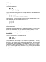
with block icons will appear at left. Now define the model structure. To draw a block, select the
icon with mouse click. Then drag it to the place where you want to put it. The blocks which inputand
output points coincide are connected automatically. To connect blocks that do not follow each other
on the screen, use LINKS. . The final model image should be as follows.
Now, go out from the drawing mode (use the END DRAW button). From the main menu select File
and Save as. Give the name to the file (e.g. Firstone) where you want to save your model. The
blocks still have no parameters defined. To define the parameters select Define block parameters
from the main menu, and then All undefined yet. Now, QMG will scan the blocks and ask you to
give the necessary parameters. You must provide the following (in the parenthesis there are
suggested values).
Generator:
Distribution: type Negexp(1.0). This defines the Poisson flow of clients with mean 1 between arrivals
(supposing the time unit to be one minute).
Initial time - the time when the first client arrives (type 0)
Max entities to generate - (type 0 for unlimited)
Batch size - clients may arrive in groups. (type 1 if they arrive one by one).
Queues:
Fifo/Lifo/Random - a character which defines the queue type (let it be F, the default value)
Max length - if greater than zero, the queue will be limited. If the limit is reached, no more entities
can enter it. (Type 0 for unlimited queue).
Zero/non-zero initial length. If it is Z then the queue is initialized as empty one. If N, then the
executable program will ask for the initial length. Note that the initial length is given at run time (type
Z)
Cost per time unit - this is the cost of maintaining an entity in the queue for one time unit. Most
QMG blocks have this parameter. If different from zero then the cost will be added to the final total
operation cost (type 0 if you do not want to calculate the system operation cost).
Split point:
First, select one of the split rule options:
By priority - you must provide priorities for outputs. The entity will look for the output of higher
priority. If it cannot take this way (for example server or assembly that follows is busy etc.), then the
next possible output is checked, according to the priorities.
By probability - you must give N-1 probabilities, N being the number of outputs. The Nth probability
will be calculated, so that the sum is equal to one.
Other rule - you can define any other selection rule. It may be any selection algorithm that can be
defined as a C++ function. You must provide the corresponding function call.
(Select the Other rule option and type MINQ. This is a predefined selection rule that selects the
output connected to the shortest queue).
Servers:
Distribution - this is the function call to a random numbers generator. The service time will be
generated by the specified generator. (Type Erlang(2,1.7) for the first server, Erlang(2,3.0) for the
other).
Additional delay - after leaving the server, the entity (client) can have additional delay before
reaching the next block. This may be, for example a transport delay or other delay between blocks
(type 0).
Cost per time unit - like for the queues, you can declare the cost per time unit for the server.
Cost per operation - this cost is independent on the time. Each time the service ends, this cost is
added to the total cost (type 0 for the two costs).
Resources - the servers may need additional resources, like a tool or an operator. The use of
additional resources is somewhat complicated, see the QMG RESOURCES section for details.
(leave this field empty)
Resource logic - do not care, may be AND or OR.
Terminal point
Termination number - if it is N>0, then the simulation will terminate after N entities have entered the
block. However, you must give the simulation final time anyway. It is like parameter in the GPSS
SIMULATE instruction. It is not recommended to use this parameter if not necessary. (Type 0).
After defining the above parameters, save the model again. Now select Generate code and then
Generate and run.
Next, the following menu appears:
Prepare files for VARAN
Use semaphores
Use animator
Generate SVOP template
The "files for VARAN" are files with extension SIM, where a series of model trajectories is stored.
These files will be used by the VARAN program to make the dynamic variance analysis. Select this
option to see more statistics. The Use semaphores should be selected only if you use QMG
semaphores to control the inputs of the blocks (this is not the case in this model). You also can
select Use animator option. This is not recommended for first model runs. This mode will not
animate the model. It only creates the *.ANI file to be used by the Bluesss animator. See the
Animator section for more detail.
Generate SVOP template option can be used to create an empty procedure SVOP and store it in a
file. Remember that SVOP is used only if you want to handle semaphores or to perform userdefined operations over the attributes of the entity that enters a block. If so, then you must prepare
the procedure before or after the QMG session. The SVOP template can help you because it has
the complete procedure header with the formal parameters properly declared. Be careful and not
overwrite the file if you have already prepared and stored it.
Next, you are asked to select queues which will be displayed as functions of time. Select the two
queues. The last question QMG asks you is the list of include files. The first file is, by default
"RFirstone" (remember that Firstone is name you gave the model while saving it). The Rfirstone is a
C++ code that contains an auxiliary C++ part of the target code. Other files, if any, can contain userdefined random number generators or selection rules.
Now, QMG generates the model Bluesss code and invokes other Bluesss modules. In what follows,
you only should accept the default settings, so you will need to make some mouse clicks. First, the
Bluesss program is translated to C++. Then, C++ compilation follows. C++ compiler will generate
several warnings. Ignore the warnings. If the compilation fails, there is something wrong in the
model. Probably a C++ compilation error occurred. Return to the QMG program and check block
parameters. You can make it using the View parameters and All blocks option. Check the
distributions and other data for possible C++ syntax errors. After correcting eventual errors,
generate code again.
If no compilation errors occur, then the simulation program is invoked.
Now, you only give the model final time (type 480), the scale parameter (default 50) and the number
of repetitions of the simulation run (type 1). The scale of 50 means that the queue which contains
50 entities (clients) will fit to the whole screen.
Then, the simulation runs. You can see the two queues as the moving red bars. The numbers of
clients who reach the terminal points are shown as green bars, and the status of the servers (BUSY
or FREE) is indicated. After simulating 480 time units you will see the plots for the two queues
(length as function of time), and the final statistics. The statistics are shown and stored in the ASCII
file named FINSTA.TXT which can be imported to Word or other applications. The final statistics are
as follows.
Final Statistics:
Final time =
480.00
QUEUES:
Av waiting time
QUEUE3 :
12.369
QUEUE4 :
21.149
SERVERS:
SERV5 :
SERV6 :
TERMINAL:
TERM7:
TERM8:
Total cost =
Service time
477.051
471.650
Count
282
158
Lmax
16
15
Lmin
0
0
Idle time
2.949
8.350
Av length
7.510
7.332
Idle %
0.61
1.74
Lost
0.00
0.00
Lost
0.00
0.00
Served
282.00
158.00
0.00
The queue statistics show the average waiting time, maximal and minimal queue length, and
average length. The LOST columns show the number of entities lost at the corresponding blocks. In
most cases it should be zero.
For the servers, you can see the total time in service, idle time, % of idle time, lost and served
entities.
For the terminal points the corresponding counters show the number of entities that enter the block.
Note that the two queues have similar length. This occurs, because the new client selects the
shorter queue to wait in. However, the average waiting time in the second queue is two times
greater, because the second teller is about two times slower than the first. This obviously reflects in
the number of clients served by the two tellers.
Now, repeat the simulation, starting with Bluesss- Queues. Declare the use of the VARAN utility
("Create files for VARAN"). At the run time declare, say, 80 repetitions of the simulation run. This
will create a set of *.SIM files. After running the simulation the VARAN program will be invoked.
You also can do this executing VARANW.EXE (Utilities - VARAN). You will see more statistics, as
functions of time (see VARAN section for more detail).
Example: Group and ungroup - a trip
This is and example of an application of the group and ungroup blocks.
Let us simulate a trip by airplane from California to Florida. We simulate the check-in queue,
boarding queue, the flight, and the luggage claim in Florida with the corresponding queue. The
following QMG scheme can be used:
The passengers are generated in the block 1 and form a queue 2 to check in. Then, they pass to a
boarding room and form other queue (group block 3). It is a small air line, with no fixed schedule. If
there are 30 persons waiting the queue, then they form a group and depart. Then, they board an
airplane and fly to Florida. It is supposed that the airplane isalways available and waits until there
are 30 persons in the boarding room. The flight is simulated using the conveyor block number 1. On
the animation screen the passenger group is displayed using an airplane icon. Once the group
(airplane) reaches the target airport in Florida, the passengers reappear as separate entities
(ungroup block number 5. Then, they for a queue number 6 to claim the luggage and after obtaining
it (server 7) they go out of the airport (terminal point 8). The model parameters are as follows:
Generator 1 inter-arrival distribution: Negexp(4.5)
All the queues: FIFO, unlimited.
Server 3: Service time Erlang, order 2, main 4
Group block 4: Group size 30
Conveyor (the flight route): length 1500, speed 6 (km and km/minute)
Server 7 : distribution Erlang, order 2, main 4
Once you have created the model, run it in "Using animator" mode and final time of several
thousand units (minutes). You will observe that the waiting time in queue 6 is always about two
times greater than the waiting time in the queue 2, despite the fact that the average passengers
flow per time unit is the same. This is due to highly irregular arrivals of passengers, ungrouped in
the block 5, when an airplane arrives.
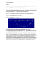
The following animation was done using a satellite map of the United States as the scenario
background. The corresponding entity routes have been defined (queues and flight route) and two
icons assigned, one being a person, the other the airplane icon.
To see animation, first run your simulation. After terminating the simulation run, you will see a
simple simulation directly over the model scheme. To see the animation over the animation
scenario, invoke the Animator from the main Bluesss menu. Enjoy the icon movements on the
scenario screen and see how the queues change. Before using the animator and editing the
scenario consult the Animator Manual.
SECTION 2
Other Bluesss examples. These are only summaries of the examples which are included in
the Bluesss package. To run the models you must be a Bluesss user.
--------------------------------------------------------------------------------------------------------------------------Bluesss code
Use the Translation/run option of the main Bluesss menu to open and simulate the examples.
trigger.csm
This code is a complete Bluesss program. The declaration in the first line introduces two reference
variables a and b that will be used as pointers to two objects created n
i the main program section.
Then, a process declaration follows. The process type isPerson and the two objects of this type
can be generated to run concurrently. There is only one event (namedone) declared inside the
process. With the outlne instruction each object reports itself on the screen as active one. Note that
the attribute name is used to identify the object that issues the message. The instructionschedule
b->one to TIME+1 schedules the event one of the object B to be executed at actual time plus one.
Observe that the if..else instruction means: "If I am a then let b become active within one time unit,
otherwise let a activate within one time unit". This means that the two objects a and b activate each
other and the program triggers between the objects a and b.
cats.csm - an example of Bluesss inheritance mechanism
This is an example of inheritance and multiple object model. It can be used to check the virtual
memory management on your computer and the speed of the Bluesss event queue mechanism.
Three processes are defined in the model: A CAT , HE, and SHE. A CAT includes the following
events: to hunt, to eat, to sleep and to die. HE is a male cat, he inherits all the properties of' A CAT,
but can also fight with other cats. As the result of this event, one of them may die. The process SHE
is a female cat, she inherits all the properties from A CAT, but she can have several little cats in
certain time intervals. In the main program only one object is generated, of type SHE. After some
time SHE has lillte cats, they start with their own activities, and the population grows. Note that even
with several thousands of cats (some tens of thousands of events in the event queue) the program
slow-down is not significative. The program speed is limited rather by the text display procedure.
ODE Examples
Examp1.equ
The equations of EXAMP1 are:
dx1 / dt  x2
dx2 / dt  p1 1  x1   p2 ( x2 ) 3
This is a simple dynamic system of second order (oscillator with damping). Note that the damper is
non-linear and the parameter p2 controls the damping. On the edit screen of the ODE module
(DIFEQC) the equations appear as follows
dx1 / dt = x[2];
dx2 / dt = p[1]*(1-x[1])-Pow(x[2],3)*p[2];
Output expressions. This part of the model specification must be defined to transform the state
vector into the model output vector. In EXAMP1 the outputs are
Y1 = x [1] + x [2]
Y2 = x [1] + x [2]
Y3 = x [1]
Y4 = x [2]
You must select at least one of the outputs. The selected variables will be shown on the
simulation result screens.
Run the model with simulation final time=20. The model uses two parameters. Try it with p[1]=3 and
p[2]=20. These values are stored in the initial conditions/parameters fiel examp1.icc, so you can
read them from that file.
As the result you will see the time-plots for the selected output signals. Note that the system
oscillates, and the oscillations are not sinoidal.
Consult: DIFEQC manual, "Getting started" section
Rigid2.equ
This is a stiff system described by the following equations.
dx1 / dt  1000 x1  x2
dx2 / dt  1001x1  2 x2
The eigenvalues of the coefficient matrix on the right side are very different, one of them being
thousand times greater that the other. Running the simulation you can observe that the process has
a “slow” and a “fast” component. However, the integration routine works well. The initial conditions
for this example are stored in file rigid2.icc. The final simulation time is equal to 0.5 and the
integration step is 0.0001. The initial conditions for x [1] and x [2] , stored in rigid2.icc, are equal to
0.5 and 0.1, respectively. On the plots you can observe the slow component in which the transition
process is in its starting stage, and the fast one that terminates approximately at t = 0.005. To see
the initial part (fast transition process) with greater resolution, use small integration step, for
example 0.00005.
Signal Flow Examples
exa.cpg
This file containes an example of a control system with a PID controller. It can be opened using
Continuous -> Signal flow option of the main Bluesss menu.
This is a simple system of automatic control. The node U is the set point, the link E->Y is a PID
controller, link Y->X is the controlled process, in this case an inertial object of the second order. The
link X->V is the measurement instrument (first order inertia). The signal ate node E represents the
control error (the difference U - V). The transfer functions are as follows:
link E - Y : a PID controller, with gain P1, integration time T2 and differentiation tiem P2.
link Y - X : the controlled process : 1 / (s*s + 3s + 1)
link X - V : measurement : 1 / (0.1s + 1)
Such simulation can be useful while looking for optimal setting of the controller.
Run this model with the simulation final time between 7 and 15. Usin this model you can carry our
the "varying parameter" experiment. The signal flow module generates the model equations and
invokes the ODE (DIFEQC) module. Select "normal run" and then "Varying parameter" simulation
mode. DIFEQC will generate the Bluesss code and invoke the C++Bulder. Run the model. At the
run time you will be asked to give the number of the parameter to be changed automatically. This
may be any of the PID parameters. Type, for example, 1 to change P1 (you tyme the parameter
number only and not the parameter name). This will change the controller gain. Declare the range
for the paramater as, for example, 2 to 20. Note that you must enter the parameter definition
screen, because the model uses three parameters. If you read the initial conditions/parameters from
the file (exa.icc), then the parameters will be P2 = 20, P3 = 0.1. Of course, you cannot change the
parameter number 1, because it will be changed automatically by the program. As the result of the
program run you will see the plots of the output signals for P1= 2 to 20, changed in 25 steps. .
exa2.cpg
This model is similar to exa.cpg, but has two input nodes: U for the set point and Z for the
disturbance. Link E-Y is a P controller, Y-X is the controlled process with inertia of the third order.
P[2] is the controller gain and p[3] is the gain for the disturbance input. The parameter P[1] is
reserved for the input signal at the node Z. While generating the model equation, the input at U
should be defined as unit step, and the input at Z shoud be "Other" , P[1].
The signal on P[1] is calculated in a user functions stored in the file parvar.cpp. This file must be
listed on the include file list of FLOWDC.
The initial conditions and parameters are stored in the file exa2.icc. The final simulation time is
equal to 15 model time units, p[2] = 3 and P[3] = 8.
After terminating the simulation, Bluesss automatically invokes the VARAN program.
Bond graph examples
Mechsys.bnd
Recall that bond graph is a graphical representation of the dynamics of a physical system, used
mainly to simulate mechanical systems or electrical circuits.
This example is described in the sections "Getting started" and "Bond graphs" of the manual of the
Bond Graph module of Bluesss.
After entering the BONDWC program (directly, or from the main BLUESSS program, Bond graphs
option), select File, New graph and Edit model structure. First you must define the nodes. Select
Draw a node and Flow source to put the SF node. Make a click on the point where you want to put
the node. Then, you are asked to define the node parameters. This parameter is the velocity
applied to the system as an external excitation. To be able to apply the excitation as any function of
time, define the parameter of this node as FUN1(). The FUNx() node parameters are interpreted by
BONDWC as external functions (do not forget to add the parantheses() ). The function code may be
created later on. In the same way put all other nodes: the "0" node, "1" node, "L"node, "R" node,
and "C" node. For each node except those of type "0" and "1" you must provide the corresponding
parameters. The parameters may be:
Node L : 2 (the mass)
Node C : 1 (spring constant)
Node R : 0.2 (damping)
The node type will be followed by comma and the corresponding node number. Now define the
bonds. Select Draw a bond to define bonds. From the bond menu always select the first one, a
simple bond without causalities. For each bond you must give the corresponding flow and effort.
These parameters are:
Bond SF - 0 : effort F, flow V
Bond 0 - L : effort F, flow W
Bond 0 - 1 : effort F, flow PX
Bond 1 - C : effort G, flow PX
Bond 1 - R : effort HX, flow PX
After defining the model structure select Causality and Generate. BONDWC will put the causalities
to the model.
Now, save the model use the File Save as menu option. Give the file name, for example
MYGRAPH. This example is also available on the original BLUESSS disks stored as
MECHSYS.BND model. Add FUN1.CPP file to the INCLUDE FILE list : this will be the file where
you will store the FUN1 function. You still cannot run the simulation, because the model needs the
function FUN1. Exit the program and prepare the following C++ code using any text editor.
float FUN1(){
if(TIME>0.1)return 10.0; else return 0.0;}
Preparing the code, it is recommended to use the #ifndef....#endif clause to avoid multiple
definitions of the function body. The code can be as follows:
#ifndef MYFUN
#define MYFUN
//----- function definition
#endif
This is a simple excitation (the velocity 10 during 0.1time units). Note that TIME is the model time.
Store the function in FUN1.CPP file and return to BONDWC. Now Open your model (MYGRAPH)
and select the Generate/run - Generate and run menu option. You will be asked if you wish to
calculate the integrals of the flows. In the case of a mechanical system these are the positions, so
respond Y. Next, BONDWC processes the model. You will be shown the list of state variables. In
this case the variables are as follows.
x[1] is V
x[2] is G
The integrals of tlow variables are:
x[3] integral of V
x[4] integral of W
x[5] integral of PX
You also will see the node parametersand the system equations. In the equation d[n] stands for
d(xn)/dt.
Select Generate code and then Generate and run.
Now select the simulation mode. DIFEQ supports the following simulation modes.
Varying parameter
Preparing files for VARAN
Simple run (default)
Consult the DIFEQC help for detail about these run options.
Select Simple run. You also must give the name of the BLUESSS process and the name of the file
where the BLUESSS code will be stored. Then, only confirm defaults or presscontinue or start
buttons. On the list of include file list will appear the file FUN1.CPP. Do not change it, this is your
FUN1 function. You also will see the list of output signals. Select all items from the list. After this,
BONDWC generates the system equations file MYGRAPH.EQU and invokes the DIFEQC program.
It will read the equations, generate BLUESSS code, invoke the BLUESSS-to-C++ translator, and
finally run the simulation.
At the run time you must define the parameters. Give the following.
Final time = 2
Integration step = 0.008
The integration step should be about 5000 time smaller than the simulation final time
The initial conditions will appear with the default value zero. Do not change them.
For mor detailed description of the run options consult theDIFEQC
The model file, equations file, BLUESSS code file and the parameters file can have the same
name: they are given different extensions automatically (BND, EQU, CSM, and ICC, respectively).
Now the simulation runs. You will see the plots of the signals at the selected nodes.
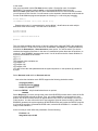
A non-linear circuit
The file RRC.BND contains the bond graph for the following simple circuit.
The resistance R2 is assumed to be non-linear. The non-linearity is given by then function FUN2,
inserted into the resulting Pascal or BLUESSS code by the user after analyzing the graph and
generating the program. The file RRCFUN.PAS contains an example of a possible code for FUN2.
Try to execute the program with the following data, to see the influence of the non-linearity (time
unit is supposed to be 1 second):
v1 = 100V
R1 = 100 ohm
final model time = 0.01
initial conditions zero.
c = 0.000001 F ( 0.01 microfarads)
float FUN2(float v){
if(v<70) return 2000; else return 400;}
This function makes the resistance r2 variable, depending on the voltage on r2. If the voltage is less
than 70, then r2=2000, otherwise r2=400. In the bond graph model the parameter of the node r2 is
FUN2(x[1]). Note that x[1] is equal to vc, the voltage on the capacitor. The variable vc in not visible
from inside of FUN2. The following figure is the bond graph of the model
Associated files: RRCFUN.CPP, RRC.ICC
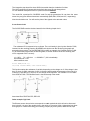
Other example: fig11.bnd
The Bluesss screen shown below corresponds to certain mechanical which will not be discussed
here in detail. It is one of the models given in the article of Francoise Cellier, Hierarchical non-linear
bond graphs: a unified methodology for modeling complex physical systems, SIMULATION, April
1992.
Run this example with the final simulation time between 10 and 30.
Queuing models : QMG module
The following models are stored in the Bluesss directory:
assem.blw - a simple manufacturing cell with buffers and an assembly operation
assem0.blw - a simple manufacturing cell with buffers and an assembly operation. The
assembled parts are routed to different outputs according to the generator block where they are
generated. The source information (number of generating block) is stored as an additional attribute
X of the part).
Associated files: assemof.cpp, assem0sv.cpp.
andek.blw - a queuing system with additional resources. The AND logic is used for the resource
request. Associated file: andekr.cpp
orek.blw - a queuing system with additional resources. The OR logic is used for the resource
request. Associated file: orekr.cpp
conv6.blw - a manufacturing cell with conveyor. Can be used to carry out the animation.
Associated file: conv5s.cpp
If you select "Use animator" option while generating the code, then the executable program will
generat the animation file (*.an2), which can be used by the animator.
Consult the manual of the QMG module for a more detailed description of these models.