1
GeoCell User Manual
Version 1.8.18
May 2014
ABSTRACT
GeoCell is a stand-alone executable program offering a
cross-platform GUI that exposes OSSIM library functionality.
This document provides guidelines for operations.
Table of Contents
1 Overview...........................................................................3
2 Basic Operations................................................................4
3 Visual Exploitation...........................................................11
4 Metric Exploitation...........................................................16
04.18.14
2
1 Overview
GeoCell is a stand-alone executable program offering a cross-platform
GUI that exposes OSSIM library functionality. This document provides
guidelines for its operation.
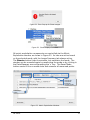
To verify the software version, select ossim-geocell->About
ossim-geocell and the window shown in Figure 1 is displayed.
Figure 1. About GeoCell Window
04.18.14
3
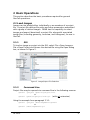
2 Basic Operations
This section describes the basic procedures required for general
GeoCell operations.
2.1 Load Images
Images can be loaded either individually or as members of a project
file. A project file defines file paths and other parameters associated
with a group of related images. OMAR has the capability to select
images and export (download) a project file, along with associated
image files (including geometry, overview, and histogram), for use in
GeoCell.
2.1.1
GUI
To load an image or project via the GUI, select File->Open Image or
File->Open Project and choose the desired file using the Open dialog
box, as shown in Figure 2.
Figure 2. Image/Project File Selection
2.1.2
Command Line
Project files may be opened via command line in the following manner:
geocell –project /path/to/project/file
or
geocell /path/to/project/file.gcl (with gcl extension)
Using the example from paragraph 2.1.1:
geocell –project /data/regTest03.geocell
or
geocell /data/regTest03.gcl
04.18.14
4
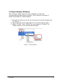
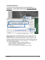
2.2 Open Display Windows
After loading, image chains must be selected to create the
corresponding image display windows. With reference to Figure 3,
follow these steps to create displays:
1. Expand the source entry list by clicking on the small triangle next
to “Source”
2. Select desired sources and right-click to reveal pop-up menu
3. Select “Chains”, then “Affine” for raw images or “Default” (or
“Map Projection”) for orthorectified images
Figure 3. Chain Selection
04.18.14
5
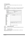
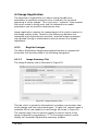
2.3 Image Menu
The Image menu includes actions that apply to the current active
display.
2.3.1
Export
Select this menu item to export an image. The format of the exported
image is chosen from the <select write type> dropdown menu, as
shown in Figure 4.
Figure 4. Image Export Window
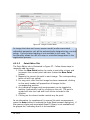
2.3.2
Export Keywordlist
Select this menu item to export a standard OSSIM keyword list for the
image.
2.3.3
Band Selection
Select this menu item to choose the desired bands for a multi-band
image, as shown in Figure 5.
04.18.14
6
Figure 5. Band Selector
2.3.4
Brightness Contrast
Select this menu item to perform brightness/contrast alterations to the
image, as shown in Figure 6.
Figure 6. Brightness/Contrast Window
2.3.5
Geometry Adjustment
Select this menu item to perform manual geometric adjustments to the
image using its adjustable parameters, as shown in Figure 7. See
paragraph 4.3.3 for additional information on saving parameters and
the relationship of the window and the topic of image registration.
04.18.14
7
Figure 7. Parameter Adjustments Window
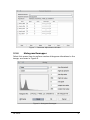
2.3.6
Histogram Remapper
Select this menu item to perform custom histogram alterations to the
image, as shown in Figure 8.
Figure 8. Histogram Remapper
04.18.14
8
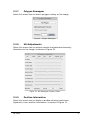
2.3.7
Polygon Remapper
Select this menu item to draw a polygon overlay on the image.
Figure 9. Polygon Remapper
2.3.8
HSI Adjustments
Select this menu item to perform custom hue/saturation/intensity
alterations to the image, as shown in Figure 10.
Figure 10. HSI Remapper Property Editor
2.3.9
Position Information
Select this menu item to display a window showing continuous
(dynamic) cursor position information, as shown in Figure 11.
04.18.14
9
Figure 11. Position Information Window
2.3.10
04.18.14
View
10
3 Visual Exploitation
This section describes the functions related to GeoCell’s visual image
manipulation capabilities.
3.1 Image Combiners
GeoCell has access to OSSIM’s collections image combiners. This
section provides examples of several of those functions, using a raster
map and image for clarity.
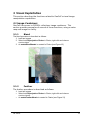
3.1.1
Blend
The blend procedure is described as follows:
1. Load two images
2. Select both Reprojection Chains in Chains, right-click and choose
Combine>Blend
3. An ossimBlendMosaic is created in Chains (see Figure 12)
Figure 12. Image Blend
3.1.2
Feather
The feather procedure is described as follows:
1. Load two images
2. Select both Reprojection Chains in Chains, right-click and choose
Combine>Feather
3.
An ossimFeatherMosaic is created in Chains (see Figure 13)
04.18.14
11
Figure 13. Image Feather
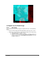
3.1.3
Combiner From Factory
Use of a combiner not explicitly available in the Combine menu is
described as follows:
1. Load two images
2. Select both Reprojection Chains in Chains, right-click and choose
Combine>Select from Factory
3. A selection window is displayed, as shown in Figure 14
Figure 14. Combine Selection Window
4.
Select desired filter; for example, an ossimTwoColorView is created in
Chains (see Figure 15)
04.18.14
12
Figure 15. Two-Color Multiview
3.2 Digital Terrain Model Usage
3.2.1
Hill Shade
The hill shade procedure allows creation of a pseudo 3D view. It is described as
follows:
1. Load an overlay image and DTM reformatted to raster (e.g. srtm_xx.ras)
2. Select srtm_xx.ras in Sources, right-click and choose Chains>Image Normals
a. A Normals Chain is created in Chains
b. Expansion of the entry allows manipulation of its filter properties; for
example, the gain of the ossimImagePlaneNormalFilter has been
changed in Figure 16
04.18.14
13
Figure 16. ossimImagePlaneNormalFilter Properties
3.
Select the map + Normals Chain in Chains, right-click and choose
Combine>Hill Shade
c. A ossimBumpShadeTileSource is created in Chains
d. Expansion of the entry allows manipulation of its filter properties; for
example, the hill shade light source azimuth and elevation angles are
shown in Figure 17
Figure 17. Hill Shaded Map
3.3 Planetary View
Planetary view provides the capability for advanced 3D viewing. Activation of this
view is described as follows:
1. Load image(s) of choice
2. Select all in Chains, right-click and choose Planetary View from context menu
3. Press <Select Syncing> and select Full
04.18.14
14
4. Image Viewer (map or image) display and control:
• Left-click/roam induces synchronized motion in all displays, including the
Planetary Viewer
• Wheel moves image up/down
• Shift/wheel turn zooms in/out
1. Planetary Viewer display and control:
• Note that both images appear mosaicked
• Left-click/roam moves image within display window
• Right-click/roam zooms image within display window
• Middle-click/roam (not wheel turn) induces eye point motion
up/down - raises/lowers look angle
right/left - rotates azimuth
• Hot keys reset
lower case ‘u’ rotates back to north-up
upper case ‘U’ resets eye view to nadir
• At higher look angles, relief should be visible in background
Figure 18. Planetary Viewer
Note that the Planetary Viewer may fail if the workstation’s graphics
adapter does not adequately support OpenGL.
04.18.14
15
4 Metric Exploitation
This section describes the functions related to GeoCell’s
photogrammetric exploitation capabilities.
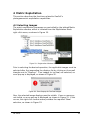
4.1 Selecting Images
The metric exploitation processes are controlled by the tabbed Metric
Exploitation window, which is initiated from the Exploitation Mode
right-click menu, as shown in Figure 19.
Figure 19. Registration Window Selection
Prior to selecting the desired operation, the applicable images must be
selected after first expanding the displays list by clicking on the small
triangle next to “Displays”. If no images (or too few) are selected, an
error pop-up is displayed, as shown in Figure 20.
Figure 20. Error Pop-up for Too Few Images
Also, the selected image displays must be visible. If one or more are
not visible, an error pop-up is displayed, as shown in Figure 21. If this
occurs, the right-click context menu provides the required ‘Show’
selection, as shown in Figure 22.
04.18.14
16
Figure 21. Error Pop-up for Show Images
Figure 22. Show Displays Selection
All metric exploitation components are controlled via the Metric
Exploitation window, as shown in Figure 23. Its tabs are active based
on the selected mode, with the Image Summary tab always active.
The Dismiss button hides the window, but maintains the mode. The
window can be revealed again by reselecting the mode or by clicking in
the Data Manager area and pressing the ‘s’ key. The Reset Mode
button resets to the no mode state and removes all measured points.
Tabs
Tabs
selectively
selectively
activated
activated
based
onon
based
current
mode
current
mode
Tab
always
Tab
always
active
active
Figure 23. Metric Exploitation Window
04.18.14
17
4.2 Geopositioning
This section describes geopositioning component of metric
exploitation. The point positioning function is NOT CERTIFIED FOR
TARGETING. The Point Position tab is illustrated in Figure 24.
Single-ray
Single-ray
intersections
intersections
forfor
each
each
image
point
image
point
Multi-ray
Multi-ray
intersection
intersection
forfor
allall
image
image
points
points
Figure 24. Point Position Tab
After measuring the corresponding point in each image, press the
Drop Point button to execute the intersection (“point drop”). The
results are written to the summary window. These results include
individual single-ray intersections with the elevation surface and one
multi-ray spatial intersection using all image rays. The display uses
the following abbreviations:
1. DD: longitude, latitude in decimal degrees
2. HAE (also WGE): height above ellipsoid (WGS84)
3. MSL: height above mean sea level
4. ECEF: earth-centered earth-fixed Cartesian frame
04.18.14
18
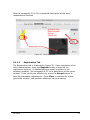
4.3 Image Registration
The objective of registration is to adjust camera model error
parameters to minimize projection error (residuals) for tie points
appearing in all the images. This is not just a “cosmetic” bias removal,
the sensor model is being used, and the adjusted error model
parameters can be saved for downstream uses.
Image registration requires the measurement of tie points common to
the image overlap areas. Based on the differences between the
measured and projected point positions, selected image parameters
are adjusted through a mathematical process known as a bundle
adjustment.
4.3.1
Register Images
The Metric Exploitation-Registration tabbed window is composed of
three tabs that are described in the following paragraphs.
4.3.1.1
Image Summary Tab
The Image Summary tab is illustrated in Figure 25.
Figure 25. Image Summary Tab
This tab, which is primarily informational, provides a convenient view
of the images and their associated types. A right-click context menu is
available off the row header for each image, as shown in Figure 26.
The context menu can be used to toggle the control status of the
image (indicated by appending a “C” to the image number) and to
display its Parameter Adjustments summary window.
04.18.14
19
Figure 26. Image Context Menu
An image that does not have a sensor model (and/or associated
adjustable parameter set) will be automatically designated as a control
image. Control status toggling is not available in this case. This
functionality allows the use of a map or controlled image base in the
registration process.
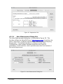
4.3.1.2
Point Editor Tab
The Point Editor tab is illustrated in Figure 27. Follow these steps to
manually add tie points:
1. Press the New Point button to create a new table column and
increment the current point indicator (below the New Point
button).
2. Measure the current tie point in each image. The corresponding
table cell will turn yellow.
3. For any point, after the first image has been measured, clicking
on the point header will preposition all images to the
corresponding position.
4. Any individual image point measurement can be toggled to
inactive (indicated by red) by clicking on the cell. The point’s
symbol will also turn red and it will not be included in the
solution.
5. Clicking on its column header revisits any tie point.
As an alternative (or supplement) to manual tie point measurement,
press the Auto button to activate the Auto Measurement dialog box. If
the opencv plugin and associated OpenCV library is not available will
be grayed out, indicating that it is not available.
04.18.14
20
Refer to paragraph 4.3.1.4 for a detailed description of the auto
measurement function.
Activate Auto
Measurement
Dialog
(Optional)
Figure 27. Point Editor Tab
4.3.1.3
Registration Tab
The Registration tab is illustrated in Figure 28. Upon completion of tie
point measurement, press the Register button to execute the
registration solution. A detailed solution report is written to the
summary window. See paragraph 4.3.2 for a description of the report
content. If the results are satisfactory, press the Accept button to
save the parameter adjustments. Press Clear to remove the report,
ignore the solution, and perform additional tie point editing.
04.18.14
21
Figure 28. Registration Tab
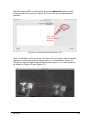
4.3.1.4
Auto Measurement Dialog Box
The Auto Measurement dialog box is illustrated in Figure 29. This
function utilizes the OpenCV library (http://opencv.org/) to perform tie
point (“key point” in OpenCV terminology) matching for overlapping
image pairs. This tabbed window is composed of two tabs:
Configuration, which allows limited interaction with OpenCV
parameters, and Collection, which provides execution and review of
the matching process.
Figure 29. Auto Measurement Dialog Box
04.18.14
22
The Configuration tab (Figure 29) includes two frames containing
parameter controls, described as follows:
• Collection Configuration
Max Matches / Patch
Allows specification of the maximum number of tie points
collected per patch.
Use Grid Adapted Detection
If checked, use OpenCV’s GridAdaptedFeatureDetector
adaptor
Grid Layout (default = 1X1)
{Disabled if “Use Grid Adapted Detection” is not checked}
Allows adaptation of the detector (via
GridAdaptedFeatureDetector) to partition the source image
into a grid and detect points in each cell.
•
OpenCV Configuration
Detector
Allows selection of the feature detector; including the
following
ORB (Oriented FAST and Rotated BRIEF)
BRISK (Binary Robust Invariant Scalable Keypoints)
FAST (Features from Accelerated Segment Test)
STAR
GFTT (Good Features to Track)
MSER (Maximally Stable Extremal Region)
Extractor (or Descriptor-Extractor)
Allows selection of the feature descriptor-extractor (“binary”
CV_8U descriptors only); including the following
FREAK (Fast Retina Keypoint)
ORB (Oriented FAST and Rotated BRIEF)
BRIEF (Binary Robust Independent Elementary
Features)
BRISK (Binary Robust Invariant Scalable Keypoints)
Matcher
Allows selection of the feature matcher; including the
following
BruteForce-Hamming
BruteForceHammingLUT
FlannBased (Fast Library for Approximate Nearest
Neighbors)
The point collection ROI can be defined in either image by left
button/mouse drag action. When the mouse drag is complete the
image is automatically zoomed to full resolution and the ROI is
delineated with an overlay rectangle.
04.18.14
23
One the desired ROI is delineated, press the Execute button on the
Collection tab illustrated in Figure 30 to run the auto measurement
process.
Run auto
measurement
process
Figure 30. Auto Measurement Collection Tab
Upon completion of the process, the OpenCV Correlation Patch window
appears to show the matched point pairs, as illustrated in Figure 31,
along with ossimTieMeasurementGenerator report in the text window,
as shown in Figure 32 and Figure 33.
Figure 31. OpenCV Correlation Patch Window
04.18.14
24
Figure 32. Accepted Collection Report, Part 1
Accept auto
measurement results
Figure 33. Accepted Collection Report, Part 2
The report includes selected performance measures extracted from the
OpenCV process plus a configuration summary. The metrics include
the following:
• Total number of points found before filtering
• Distance filter particulars
• Total number of points found after filtering
• OpenCV queryIdx and trainIdx, as well as distance, for each
selected tie point pair (limited by the “Max Matches”
parameter)
If the correlation result is satisfactory, press the Accept button and
control returns to the Point Editor tab (paragraph 4.3.1.2), where
additional point editing can occur if necessary.
04.18.14
25
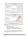
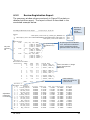
4.3.2
Review Registration Report
The summary window shown previously in Figure 28 contains a
detailed solution report. The report content is described in the
annotated example below.
Number
ofof
Number
adjustable
adjustable
image
image
parameters
parameters
ossimAdjustmentExecutive Report
Tue 02.19.13 10:18:55
~~~~~~~~~~~~~~~~~~~~~~~~~~~~~~~~~~~~~~~~~~~~~~~~~~~~~~~~~
Images:
1:
/data/Space_Coast/Test/po_176062_pan_0000000.ntf
2: /data/Space_Coast/Test/3V050726P0000820271A0100007003410_00574200.ntf
3:
/data/Space_Coast/Test/M1BS.tif
Observations:
1
0.00
Tie point
summary
list
2
0.00
3
0.00
( nan, nan, nan, WGE )
Tie point image
1
( 2664.9, 6957.3 )
2
( 1353.9, 14498.8 ) coordinates (s,l)
3
( 4429.7, 4352.8 )
( nan, nan, nan, WGE )
1
( 2687.2, 6996.5 )
2
( 1396.7, 14513.9 )
3
( 4438.6, 4367.7 )
( nan, nan, nan, WGE )
1
( 2759.6, 6786.7 )
2
( 1309.9, 14306.7 )
3
( 4466.0, 4283.5 )
Iteration 0...
Measurement Residuals...
observation
image
samp
1
1
-13.6
1
2
-9.4
1
3
-7.8
Adjustable
parameter
corrections
line
-8.9
-4.7
-5.1
initial_meas
( 2664.9, 6957.3 )
( 1353.9, 14498.8 )
( 4429.7, 4352.8 )
2
2
2
1
2
3
-13.7
-9.1
-7.7
-9.3
-4.1
-5.4
( 2687.2, 6996.5 )
( 1396.7, 14513.9 )
( 4438.6, 4367.7 )
3
3
3
1
2
3
-13.1
-9.0
-7.9
-8.7
-4.1
-5.5
( 2759.6, 6786.7 )
( 1309.9, 14306.7 )
( 4466.0, 4283.5 )
______________Mean:
-10.1
-6.2
RMS:
Iteration 1...
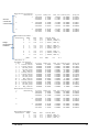
Parameter Corrections...
n im
parameter
1 1
intrack_offset
2 1
crtrack_offset
3 1
intrack_scale
4 1
crtrack_scale
5 1
map_rotation
6 2
intrack_offset
7 2
crtrack_offset
8 2
intrack_scale
9 2
crtrack_scale
10 2
map_rotation
11 3
intrack_offset
12 3
crtrack_offset
13 3
intrack_scale
14 3
crtrack_scale
15 3
map_rotation
04.18.14
a_priori
0.00000
0.00000
0.00000
0.00000
0.00000
0.00000
0.00000
0.00000
0.00000
0.00000
0.00000
0.00000
0.00000
0.00000
0.00000
total_corr
-4.42692
-6.07293
-2.06101
8.96572
0.00600
-3.45761
-2.44296
-3.20288
3.58490
-0.00018
-5.15540
-5.39114
6.69311
-4.60951
-0.00367
10.4
6.5
nPar:
nPar:
nPar:
5
5
5
Tie
point
ground
coordinates
Tie
point
ground
coordinates
“nan”
indicates
uninitialized
“nan”
indicates
uninitialized
actual
coordinates
indicate
actual
coordinates
indicate
generated
from
control
image
generated
from
control
image
Initial (“iteration 0”) image
space discrepancies
(residuals)
Data
summary
Data
summary
subgroups
repeat
forfor
subgroups
repeat
each
iteration
each
iteration
last_corr initial_std
-4.42692
50.00000
-6.07293
50.00000
-2.06101
50.00000
8.96572
50.00000
0.00600
0.10000
-3.45761
50.00000
-2.44296
50.00000
-3.20288
50.00000
3.58490
50.00000
-0.00018
0.10000
-5.15540
50.00000
-5.39114
50.00000
6.69311
50.00000
-4.60951
50.00000
-0.00367
0.10000
prop_std
25.13001
28.72990
49.55460
42.26942
0.09838
25.89186
31.14816
48.28139
40.63788
0.09395
11.65369
15.80003
38.37173
45.34128
0.09936
26
Ground
coordinate
corrections
Image
measurement
residuals
Observation Corrections...
n
observation
a_priori
1
1
28.59735
-80.68278
-26.83644
total_corr
3.92079
-2.71886
0.17051
last_corr initial_std
3.92079
50.00000
-2.71886
50.00000
0.17051
50.00000
prop_std
22.61567
22.91156
28.04424
2
2
28.59700
-80.68255
-28.33215
3.47060
-2.52333
2.04273
3.47060
-2.52333
2.04273
50.00000
50.00000
50.00000
22.56157
22.85947
28.06490
3
3
28.59890
-80.68181
-29.76113
3.31765
-2.38507
1.41584
3.31765
-2.38507
1.41584
50.00000
50.00000
50.00000
22.66972
22.90460
28.05215
Measurement Residuals...
observation
image
samp
1
1
-0.1
1
2
0.0
1
3
-0.0
line
-0.0
-0.1
0.3
initial_meas
( 2664.9, 6957.3 )
( 1353.9, 14498.8 )
( 4429.7, 4352.8 )
2
2
2
1
2
3
-0.1
0.0
0.2
-0.0
0.0
-0.1
( 2687.2, 6996.5 )
( 1396.7, 14513.9 )
( 4438.6, 4367.7 )
3
3
3
1
2
3
0.2
-0.0
-0.2
0.0
0.1
-0.2
( 2759.6, 6786.7 )
( 1309.9, 14306.7 )
( 4466.0, 4283.5 )
______________Mean:
0.0
-0.0
RMS:
Iteration 2...
Parameter Corrections...
n im
parameter
1 1
intrack_offset
2 1
crtrack_offset
3 1
intrack_scale
4 1
crtrack_scale
5 1
map_rotation
6 2
intrack_offset
7 2
crtrack_offset
8 2
intrack_scale
9 2
crtrack_scale
10 2
map_rotation
11 3
intrack_offset
12 3
crtrack_offset
13 3
intrack_scale
14 3
crtrack_scale
15 3
map_rotation
0.1
0.1
a_priori
0.00000
0.00000
0.00000
0.00000
0.00000
0.00000
0.00000
0.00000
0.00000
0.00000
0.00000
0.00000
0.00000
0.00000
0.00000
total_corr
-4.42816
-6.06469
-2.06194
8.97259
0.00599
-3.45382
-2.44302
-3.20447
3.57827
-0.00015
-5.15030
-5.38992
6.67994
-4.61720
-0.00367
last_corr initial_std
-0.00124
50.00000
0.00824
50.00000
-0.00092
50.00000
0.00687
50.00000
-0.00000
0.10000
0.00379
50.00000
-0.00006
50.00000
-0.00158
50.00000
-0.00663
50.00000
0.00003
0.10000
0.00510
50.00000
0.00121
50.00000
-0.01318
50.00000
-0.00769
50.00000
0.00000
0.10000
prop_std
25.12279
28.75264
49.55560
42.25599
0.09838
25.89526
31.17639
48.27970
40.63471
0.09394
11.65931
15.78122
38.39727
45.33730
0.09936
Observation Corrections...
n
observation
a_priori
1
1
28.59735
-80.68278
-26.83644
total_corr
3.92032
-2.71938
0.17089
last_corr initial_std
-0.00047
50.00000
-0.00052
49.99998
0.00038
50.00000
prop_std
22.61620
22.90708
28.04453
2
2
28.59700
-80.68255
-28.33215
3.47040
-2.52389
2.04298
-0.00019
-0.00057
0.00026
50.00000
49.99999
50.00000
22.56179
22.85459
28.06496
3
3
28.59890
-80.68181
-29.76113
3.31785
-2.38592
1.41519
0.00020
-0.00085
-0.00066
50.00000
49.99999
50.00000
22.66964
22.89936
28.05243
Measurement Residuals...
observation
image
samp
1
1
-0.1
1
2
0.0
1
3
-0.0
04.18.14
line
-0.0
-0.1
0.3
initial_meas
( 2664.9, 6957.3 )
( 1353.9, 14498.8 )
( 4429.7, 4352.8 )
27
Post-solution
summary
2
2
2
1
2
3
-0.1
0.0
0.2
0.0
0.0
-0.1
( 2687.2, 6996.5 )
( 1396.7, 14513.9 )
( 4438.6, 4367.7 )
3
3
3
1
2
3
0.2
-0.0
-0.2
0.0
0.1
-0.2
( 2759.6, 6786.7 )
( 1309.9, 14306.7 )
( 4466.0, 4283.5 )
______________Mean:
-0.0
-0.0
RMS:
0.1
0.1
ossimAdjustmentExecutive Summary...
Valid Exec:
true
Nbr Ground Pts:
3
Observation
Nbr Image Points:
9
metrics
Nbr Images:
3
Nbr Parameters:
15
------------------------Iteration
Solution Converged: true
Solution Diverged: false
convergence
Max Iter Exceeded: false
information
Max Iterations:
7
Convergence Crit:
5.0%
SEUW Trace...
Iter
SEUW
0
36.918
1
0.622
2
0.622
Standard
Standard
error
ofof
unit
error
unit
Tue 02.19.13 10:18:55
weight
per
weight
per
~~~~~~~~~~~~~~~~~~~~~~~~~~~~~~~~~~~~~~~~~~~~~~~~~~~~~~~~~~
iteration
iteration
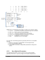
Additionally, the following terminology is used in the summary report:
1. a_priori: provisional estimate of parameter/ground coordinate
2. total_corr: total correction for all iterations
3. last_corr: correction computed from last iteration
4. initial_std: standard deviation of provisional estimate
5. prop_std: propagated standard deviation
6. SEUW:
standard error of unit weight
At a top level, the following factors generally indicate an acceptable
solution:
1. Solution converged, as illustrated in the example above
2. Decreasing/stabilized SEUW
3. Reasonable corrections to adjustable parameters and ground
points
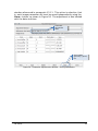
4.3.3
Save Adjusted Parameters
The adjusted parameters may be saved in the standard OSSIM
geometry file format (.geom) by using the Parameter Adjustments
04.18.14
28
window referenced in paragraph 4.3.1.1. This action is selective, that
is, each image parameter set must be saved independently using the
Save… button, as shown in Figure 34. The adjustment is also labeled
with the date and time.
Automatic
Automatic
adjustment
adjustment
label
label
Save
OSSIM
Save
OSSIM
geometry
(.geom)
geometry
(.geom)
file
file
Figure 34. Parameter Adjustments Window - Saving Parameters
04.18.14
29
4.4 Mensuration
TBD
04.18.14
30