Download Visual Traffic Simulation

Visual Traffic Simulation
Thomas Fotherby
June 2002
Individual Project
Final Report
MEng Computing Degree
Supervisor: Jeff Magee
Second Marker: Susan Eisenbach
Department of Computing
Imperial College
Abstract
The growth of applications in the area of Intelligent traffic systems (ITS) in
recent years is generating an increasing request for tools to help in design
and assessment of traffic systems. ITS uses software systems to control
signalled junctions in order to improve traffic conditions.
The Visual Traffic Simulation project aims to provide an implementation
to approximate urban vehicle movement using a microscopic simulation approach. The development of a microscopic traffic simulator represents a
double challenge: firstly traffic and network modelling and secondly how
to embed the models in a software platform interfacing with the user in a
friendly and efficient way. The project describes the current state of the art
in traffic systems and also provides research into traffic models and animation algorithms for displaying the simulation.
The conclusion is that this system successfully provides a visualisation of
a user-defined traffic flow and is capable of comparing how different road
infrastructures influence traffic systems. Extensive documentation will allow
users to extend or change the simulation to fit their own modelling criteria.
Key words: Traffic visualisation, Microscopic Approach, Graphical Interface.
i
Acknowledgements
I would like to thank my project supervisor, Professor Jeff Magee, for his
help and guidance with this project and in particular for the authorship of
the timing code that I have used. I would also like to thank my second
marker, Susan Eisenbach for her suggestions during the project review. For
programming pointers and design issues I’d like to thank two of my peers in
particular, Fahad Khan and Chloe Cowland.
ii
Contents
1 Introduction
1.1 Project Motivation
1.2 Project Objectives
1.3 Project End-Users
1.4 Report overview .
.
.
.
.
.
.
.
.
.
.
.
.
.
.
.
.
.
.
.
.
.
.
.
.
.
.
.
.
.
.
.
.
.
.
.
.
.
.
.
.
.
.
.
.
.
.
.
.
.
.
.
.
.
.
.
.
.
.
.
.
.
.
.
.
.
.
.
.
.
.
.
.
.
.
.
.
.
.
.
.
.
.
.
.
.
.
.
.
.
.
.
.
.
.
.
.
1
1
2
3
5
2 Project Background
2.1 Introduction to Simulation . . . . . . . . . . . . . . . . . . . .
2.2 Introduction to traffic modelling . . . . . . . . . . . . . . . .
2.2.1 Microscopic approaches . . . . . . . . . . . . . . . . .
2.2.2 Aggregated Macroscopic approaches . . . . . . . . . .
2.2.3 Unsignalised intersection Theory . . . . . . . . . . . .
2.2.4 Traffic flow at signalised Intersections . . . . . . . . .
2.2.5 Traffic light calculations . . . . . . . . . . . . . . . . .
2.3 Introduction to traffic simulation . . . . . . . . . . . . . . . .
2.4 Examples of Commercial Traffic modelling and simulation tools.
2.5 ITS (Intelligent Transport Systems) . . . . . . . . . . . . . .
2.5.1 Signalised junction algorithms . . . . . . . . . . . . . .
2.6 Graphics considerations . . . . . . . . . . . . . . . . . . . . .
6
6
7
8
11
13
13
15
17
18
21
25
27
3 Requirements Specification
3.1 Road Network Designer .
3.2 Visual Simulation . . . . .
3.3 Documentation . . . . . .
3.4 Further Project Modules .
.
.
.
.
.
.
.
.
.
.
.
.
.
.
.
.
.
.
.
.
.
.
.
.
.
.
.
.
.
.
.
.
.
.
.
.
.
.
.
.
.
.
.
.
.
.
.
.
.
.
.
.
.
.
.
.
.
.
.
.
.
.
.
.
.
.
.
.
.
.
.
.
.
.
.
.
.
.
.
.
29
30
31
33
33
4 Design and Implementation
4.1 Design methodology . . .
4.2 Implementation . . . . . .
4.3 Application Architecture .
4.4 Component Design . . . .
4.4.1 Road Designer . .
4.4.2 Simulation . . . .
.
.
.
.
.
.
.
.
.
.
.
.
.
.
.
.
.
.
.
.
.
.
.
.
.
.
.
.
.
.
.
.
.
.
.
.
.
.
.
.
.
.
.
.
.
.
.
.
.
.
.
.
.
.
.
.
.
.
.
.
.
.
.
.
.
.
.
.
.
.
.
.
.
.
.
.
.
.
.
.
.
.
.
.
.
.
.
.
.
.
.
.
.
.
.
.
.
.
.
.
.
.
.
.
.
.
.
.
.
.
.
.
.
.
.
.
.
.
.
.
34
34
34
35
36
36
46
iii
iv
CONTENTS
5 Evaluation
5.1 Analysis of car movement . . . . . . .
5.2 Non-signalled Junctions . . . . . . . .
5.3 Signalled Junctions . . . . . . . . . . .
5.4 Bridges . . . . . . . . . . . . . . . . .
5.5 Gridlock situations . . . . . . . . . . .
5.6 Performance . . . . . . . . . . . . . . .
5.7 Design changes . . . . . . . . . . . . .
5.8 Design problems and possible solutions
5.9 Usability . . . . . . . . . . . . . . . . .
5.10 Proposed Project Extensions . . . . .
.
.
.
.
.
.
.
.
.
.
.
.
.
.
.
.
.
.
.
.
.
.
.
.
.
.
.
.
.
.
.
.
.
.
.
.
.
.
.
.
.
.
.
.
.
.
.
.
.
.
.
.
.
.
.
.
.
.
.
.
.
.
.
.
.
.
.
.
.
.
.
.
.
.
.
.
.
.
.
.
.
.
.
.
.
.
.
.
.
.
.
.
.
.
.
.
.
.
.
.
.
.
.
.
.
.
.
.
.
.
.
.
.
.
.
.
.
.
.
.
.
.
.
.
.
.
.
.
.
.
6 Conclusion
A User Manual
A.1 The Goal of the
A.2 The Editor . .
A.2.1 Interface
A.2.2 Usage .
A.3 The Simulator .
A.3.1 Interface
A.3.2 Usage .
56
57
58
59
64
64
67
67
68
70
71
72
VIS-SIM Project
. . . . . . . . . .
. . . . . . . . . .
. . . . . . . . . .
. . . . . . . . . .
. . . . . . . . . .
. . . . . . . . . .
.
.
.
.
.
.
.
.
.
.
.
.
.
.
.
.
.
.
.
.
.
.
.
.
.
.
.
.
.
.
.
.
.
.
.
.
.
.
.
.
.
.
.
.
.
.
.
.
.
.
.
.
.
.
.
.
.
.
.
.
.
.
.
.
.
.
.
.
.
.
.
.
.
.
.
.
.
.
.
.
.
.
.
.
.
.
.
.
.
.
.
.
.
.
.
.
.
.
.
.
.
.
.
.
.
.
.
.
.
.
.
.
73
73
74
74
75
76
77
77
B Developer Manual
79
B.1 Extending the car following model . . . . . . . . . . . . . . . 79
B.2 Adding new types of junction . . . . . . . . . . . . . . . . . . 79
B.3 Developing ITS features . . . . . . . . . . . . . . . . . . . . . 80
C Demonstration Website
81
List of Figures
2.1
2.2
2.3
2.4
2.5
2.6
2.7
2.8
The components of a visual simulation . . . . . . . . . . . . .
7
Block diagram of Car-following . . . . . . . . . . . . . . . . . 10
Basic Driver Perception-action Process [18] . . . . . . . . . . 10
Deterministic component of Delay models . . . . . . . . . . . 14
A configuration of routes on a T-Junction . . . . . . . . . . . 15
Junction path directed-graph . . . . . . . . . . . . . . . . . . 16
Junction path conflict diagram . . . . . . . . . . . . . . . . . 16
An example of the latest animation quality on WATSIM by
KLM Associates [6] . . . . . . . . . . . . . . . . . . . . . . . . 17
2.9 SimTraffic 5.0 by TrafficWare. (http://www.trafficware.com) 22
2.10 SHIVA: Simulated Highways for Intelligent Vehicle Algorithms [19]. 22
2.11 WATSim simulation of proposed design for a freeway/arterial
interchange in Howard County, Maryland performed by KLD
Associates, Inc. . . . . . . . . . . . . . . . . . . . . . . . . . . 23
2.12 LogixProTraffic Control Lab. “Utilising TON Timers” . . . . 23
4.1
4.2
4.3
4.4
4.5
4.6
4.7
4.8
4.9
4.10
4.11
4.12
4.13
4.14
4.15
4.16
VIS-SIM architecture in UML . . . . . . . . . . . . . . . .
UML diagram of the RoadDesigner . . . . . . . . . . . . .
Parallel lines . . . . . . . . . . . . . . . . . . . . . . . . .
Screenshot demonstrating hypothetical parallel road lanes
Junction handle placement . . . . . . . . . . . . . . . . .
Junction graphics . . . . . . . . . . . . . . . . . . . . . . .
Non-signalled priority representations . . . . . . . . . . .
Line Clipping . . . . . . . . . . . . . . . . . . . . . . . . .
UML diagram of XML components . . . . . . . . . . . . .
XML interface . . . . . . . . . . . . . . . . . . . . . . . .
Screenshot of the RoadDesigner . . . . . . . . . . . . . . .
UML diagram of the SimPanel . . . . . . . . . . . . . . .
Intersection of two lines . . . . . . . . . . . . . . . . . . .
Distance car moves given an angle from the x axis . . . .
Screenshot of the running simulation . . . . . . . . . . . .
results display avaliable to the user . . . . . . . . . . . . .
.
.
.
.
.
.
.
.
.
.
.
.
.
.
.
.
35
36
38
39
40
41
42
43
43
44
45
46
48
49
54
55
5.1
Junction paths . . . . . . . . . . . . . . . . . . . . . . . . . .
58
v
.
.
.
.
.
.
.
.
.
.
.
.
.
.
.
.
vi
LIST OF FIGURES
5.2
5.3
5.4
5.5
5.6
Non-signalled junction congestion test . . . . . . . . . . . . .
An efficiency test comparing a actuated junction with a nonactuated junction . . . . . . . . . . . . . . . . . . . . . . . . .
An efficiency test comparing a adaptive junction with a nonadaptive junction . . . . . . . . . . . . . . . . . . . . . . . . .
Vehicles in a gridlock situation (with a cars future path shown)
Gridlock time comparison test . . . . . . . . . . . . . . . . . .
A.1 The Editor interface . . . . . . . . . . . . . . . . . . . . . . .
A.2 The Simulator interface . . . . . . . . . . . . . . . . . . . . .
A.3 A graph of the simulation data . . . . . . . . . . . . . . . . .
59
62
63
65
66
74
77
78
Chapter 1
Introduction
This report is intended to document the final year project, “Visual Traffic
Simulation”. It covers the design, development and evaluation of an application simulating road traffic using models of common road junctions and
driving behaviour. The background section of this document contains research into traffic-modelling theories needed for the application. The design
and implementation sections describe how the theory can be programmed
into a piece of software. A large part of the project is involved with programming a fast and accurate graphical display of the traffic simulation
data. These programming techniques are described in the implementation
section of this document.
1.1
Project Motivation
Transportation is an important aspect of both the economy and our lifestyle. In the United States, 20 percent of Gross National Product is spent
on transportation. 150 million automobiles and another 50 million trucks
travel an average of 10,000 and 50,000 miles per year on the US highway
system that comprises of more than 4 million miles [3]. Congestion and
environmental issues are an increasing problem that attracts much research.
The motivation of the project is the observation that road-traffic networks
are model-based systems ideally suited to an object-oriented programming
approach. Each component in a traffic network can be modelled by an object
that specifies its behaviour and interaction rules. Examples of objects that
occur in a road network are vehicles, roads, junctions and traffic lights. The
1
2
1.2. PROJECT OBJECTIVES
simulation is a record of all the interactions that occur when the different
objects are applied to the same environment.
Councils are currently spending large sums of money on “Intelligent traffic
systems” that use software systems to control large sets of traffic lights to
improve traffic conditions over a wide area. These ITS systems are described
in more detail in the background section of this report. ITS systems are
tested on traffic simulations before being commercially deployed and these
simulations produce results that influence multi-million pound decisions that
council’s take when planning road construction. This project aims to be
extendable to involve ITS components that can be programmed and tested
in the application.
1.2
Project Objectives
The project aims to investigate traffic models and fit them into a flexible
graphical user interface to provide a customisable system for the user. The
application should allow a subsection of a road network to be modelling in
a matter of minutes and to be visually presented on the screen in a clear
way. The model can then be animated through time with traffic shown
drawn-to-scale. The application will provide an interface to specify traffic
intensity levels before animation starts or to dynamically change it during
animation. The application will also provide statistical results for any data
that is run on the simulation. Finally, the code to the simulation will be
publicly available, clear and documented to allow users to extend or change
the simulation to fit their modelling criteria.
A large focus of the project is making it accessible and to this end much of
it should run on a standard web browser. This is to keep in the spirit of it
being an educational project to explore and test traffic phenomenon.
The application should be able to be used to test and compare how different
road set-ups influence traffic systems. The project will be a complete selfcontained software product and the “visual” part of the project means it
will contain both a simulation and animation component.
In summary, there will be three parts to the project.
1. An interface to build any road network and tools to describe traffic
data supplied to the network according to a time dimension.
3
1.3. PROJECT END-USERS
2. A simulation interface to watch the model run through time on the
data supplied and produce suitable results.
3. Documentation on the projects background and methods to use or
continue development on the project.
1.3
Project End-Users
Since there are many accurate commercial simulations currently in use, this
project is best suited as an educational tool. It aims to help people understand the behaviour of traffic in a visual way. The focus of the project will
be in the animation of traffic and the resulting visualisation allows easy interpretation of results to untrained observers. The project will also provide
a simple and quick way to specify the layout of a road-network, and the
ability to dynamically change settings as the animation runs.
A significant part of the project will be available from the web meaning the
general public can access it. As an example of the educational value of the
application I have used it to create an educational web site describing some
traffic phenomenon. This is described in the appendix section. The project
would be most useful to a researcher who wants a pre-built traffic visualisation that they can modify to test a hypothesis about traffic or to simulate a
new intelligent traffic-light network that they have designed. The graphical
approach to the project would be useful in communicating their results or
methods without the need for knowledge of their particular strategy. The
project could also be used as a graphical front-end to an existing simulation.
Related documentation and web site
The project web site contains additional documentation and is the home of
the on-line applet version of the project.
http://www.doc.ic.ac.uk/~tf98/Project
The source code and an API (in the form of Javadocs) are also available from
this web site. There is also a logbook that documents the project progress
and highlights some of the implementation problems.
4
1.3. PROJECT END-USERS
Conventions
References to other documents or web pages used as a source are marked
with a bracketed identifier, e.g. [1] which refers to the ’References’ section
at the end of this document.
Terminology
The following is a list of common terms used.
Road designer
Road Network
Signalled Junction
VIS-SIM
VIS-SIM-LITE
This is the term used to describe the editor section
of the project application that allows road networks
to be created and edited.
This term describes a series of roads and junctions
connected together. Other terms used are Road Infrastructure and Road schematics.
This term describes a junction where traffic is controlled by traffic lights.
This is the name of the main project application.
This is the name of the part of the project application
that runs in a web-browser. It is cut down version of
the main application with many of the file options
missing.
The following is a list of all the acronyms used in this document, and their
relevant expansion.
ITS
UTC
Intelligent Transport System
Urban Traffic Control
API
LOS
UML
Application Programming Interface
Level of service (a measure of a junctions performance)
Unified Modelling Language
5
1.4
1.4. REPORT OVERVIEW
Report overview
Following this introduction section is a discussion on background information that is relevant to the project area. A system specification sets out
exactly what the project application is trying to achieve and a detailed
design section shows the decisions that were taken before implementation.
There is a discussion on the technology used and future possibilities of the
project in an implementation section. An evaluation section gives a detailed
explanation of the projects results. The final section of the report is the
conclusion, outlining the success of the project along with its limitations.
The appendices of this document provide guides to the system for end users
who wish to use the system and for programmers wishing to modify it.
Chapter 2
Project Background
This section of the report aims to introduce the background information
to traffic simulation and modelling as well as other areas of interest to the
project such as intelligent traffic systems and computer animation considerations.
2.1
Introduction to Simulation
Simulation is used to answer “what if?” questions about things that are
too complex or expensive to test for-real. It can be defined as “a dynamic
representation of some part of the real world achieved by building a computer model and moving it through time” [15]. Traffic systems have always
come under intensive investigation using modelling and simulation. The
model describes a particular abstraction of the proposed or real-world system and is built in the initial effort of comprehending the system. There
are four components that, when brought together by a model, result in a
visual simulation (see Fig 2.1). The first component is the data that will be
applied to the model, i.e. the traffic statistics and information. The second
component is the simulation algorithm that calculates vehicle movements
(cars or whatever else e.g. trams, bicycles, pedestrians) with their specific
acceleration and deceleration behaviour. The third component of a visual
simulation is the animation component, representing the simulation results
as movements of vehicles on the computer screen. Thus, simulated traffic
is easy to observe and to evaluate. Validation is the last component, it is
necessary to fit the model and data to real traffic situations. The model
binds the four components and represents the merger of the physical laws of
6
7
2.2. INTRODUCTION TO TRAFFIC MODELLING
the objects involved in traffic systems and the layout of the traffic network.
Figure 2.1: The components of a visual simulation
Examples of uses of traffic simulation and modelling:
• To help make planning decisions by assessing risks, costs and benefits
of a new traffic proposal.
• The analysis and study of different variations within traffic planning
projects.
• To uncover “black spots” (Dangerous or particularly congested areas)
and propose solutions.
• Optimisation of local and co-ordinated traffic light control systems.
• Detection of bottlenecks.
• The analysis of interactions of different kinds of traffic.
• To provide traffic predictions.
• Pre-emption projects for public transport.
2.2
Introduction to traffic modelling
Traffic modelling theories seek to describe in a precise mathematical way the
interactions between vehicles and their operators (the mobile components)
and the infrastructure (the immobile components). The infrastructure consists of the road network and all its operational elements: control devices,
signs, marking, etc. Mathematical modelling of traffic flow behaviour is a
prerequisite for a number of important tasks including transportation planning, incident detection, control strategy design, simulation, forecasting and
in evaluating energy consumed by transportation systems [2].
8
2.2. INTRODUCTION TO TRAFFIC MODELLING
The scientific study of traffic flow had its beginnings in the 1930’s with the
application of probability theory of road traffic and the study of models
relating volume and speed and the investigation of performance of traffic
at intersections (Bruce Greenshields 1947) [3]. After World War Two, with
the tremendous increase in use of automobiles and the expansion of the
highway system, there was also a surge in the study of traffic characteristics
and the development of traffic flow theories. The 1950’s saw theoretical
developments based on a variety of approaches, such as car-following model,
traffic wave theory and queueing theory. By 1959 traffic flow theory had
developed to the point where it appeared desirable to hold an international
symposium. Since that time numerous other symposia have been held on a
regular basis dealing with a variety of traffic related topics. In June 1992
the Transportation Research Board Committee of the Theory of Traffic Flow
recommended the writing of an updated document on the state-of-the-art
of traffic theory. The document that they produced contains much of the
underlying theory of today’s traffic modelling techniques, it can be found at
reference [3].
Traffic models fall into two categories: Microscopic approaches and Aggregated macroscopic approaches.
2.2.1
Microscopic approaches
These approaches try to understand the behaviour of a traffic system by
modelling the individual vehicles that compose the traffic flow. The CarFollowing model is an example that describes the modelling of the motion
(position and speed) of a vehicle in terms of the motion of the preceding
vehicle (i.e. the behaviour of the driver-vehicle system in a stream of interacting vehicles). The main application of such models are to obtain a
better understanding of the driver-vehicle system behaviour which can lead
to the development of new safety devices and to provide the basic component
of microscopic simulation models which test or improve new traffic control
strategies.
The general form of car-following models can be represented by the stimulusresponse reaction at time t:
Response(t + T ) = Sensitivity ∗ Stimulus(t)
• T is the reaction time of the driver-vehicle system.
[1, 2]
(2.1)
9
2.2. INTRODUCTION TO TRAFFIC MODELLING
• Response is the magnitude of the reaction from the driver (e.g. deacceleration).
• Stimulus is the magnitude of what causes a Response (e.g. the difference in velocity between the lead car and the follower).
I.e. The response of successive drivers in the traffic stream is to accelerate
or decelerate in proportion to the magnitude of the stimulus at time t after
a time lag T .
Simple mathematical car-following models are linear and formulate equation
2.1 in terms of a second order differential equation:
ẍf (t + T ) = λ[ẋl (t) − ẋf (t)]
[3]
(2.2)
where:
ẍf (t + T )
=
λ
=
ẋl (t)
ẋf (t)
=
=
Instantaneous acceleration of a following vehicle at
time t + driver reaction time (T ).
An sensitivity coefficient determined by Response =
λstimulus
Instantaneous speed of a lead vehicle at time t.
Instantaneous speed of a following vehicle at time t.
A more complete representation of car following would include a set of equations describing the dynamic properties of the vehicle and the roadway characteristics. It would also include the psychological and physiological properties of drivers as well as couplings between vehicles other than the forward
nearest neighbour. Furthermore, it would include equations describing the
state of the traffic and variables for different types of vehicles in the traffic
flow. This model also does not take into account limits to how fast a car
can brake or accelerate.
Simple models are not very satisfactory because they do not take account
properly for stability. Local stability is concerned with the response of a following vehicle to a fluctuation in the motion of the vehicle directly in front of
it (i.e it is concerned with the localised behaviour between pairs of vehicles).
Non-linear car-following models postulate more complex relationships that
describe stability better. Asymptotic stability is concerned with the manner
in which a fluctuation in the motion of any vehicle is propagated through
a line (platoon) of vehicles (see discussion of traffic waves in following sections). Asymptotic stability can be approximated by adding to equation
10
2.2. INTRODUCTION TO TRAFFIC MODELLING
2.2 so that additional vehicles influence a following vehicles motion. For
example the “Next-Nearest Vehicle coupling”:
ẍn+2 (t + T ) = λ1 [ẋn+1 (t) − ẋn+2 (t)] + λ2 [ẋn (t) − ẋn+2 (t)] [3]
(2.3)
Figure 2.2: Block diagram of Car-following
From Fig 2.2 it can be seen that the “Human factor” will have an enormous influence to the mathematical models used to describe car-following.
Human factors have been studied extensively in the context of a personmachine control system, the motor vehicle. The easier measurements are
discrete components of performance, largely centred on neuromuscular and
cognitive time lags. These measurement describe perception-reaction times,
control movement times, responses to the presentation of traffic control devices, handling of hazards, and finally how different segments of the driving
population may differ in performance. There are more difficult human factors to study such as control performance at steering, braking and speed
control and harder still, lane keeping, car following, overtaking and gap
acceptance.
Figure 2.3: Basic Driver Perception-action Process [18]
11
2.2. INTRODUCTION TO TRAFFIC MODELLING
Car-following models applied to a number of successive vehicles are capable
of describing the movement of a long string of vehicles. To simulate a multilane road additional modules describing lane changing or overtaking can be
added to the microscopic model. Example pseudo-code:
function vehicle_updating (vehicle v) {
if (vehicle v is at a junction) {
apply junction-movement model;
} else {
if (vehicle v has to change lane) {
apply lane-changing model;
} else if (vehicle v has not changed lane) {
apply car-following model;
}
}
update statistics;
}
At unsignalised junctions a vehicle can consult a gap-acceptance model to
calculate whether or not it is safe to pull-out into the junction and continue
its journey. As a model incorporates more and more real-life behaviour,
the simulation that will use the model becomes capable of more and more
realism.
Microscopic analyses runs into two major difficulties when applied to a street
network. Firstly, each street block and intersection are modelled individually. A proper accounting of the interactions between adjacent components
(particularly in the case of closely spaced traffic signals) quickly leads to
intractable problems. Secondly, since the analysis is performed for each network component, it is difficult to summarise the results in a meaningful fashion so that the overall network performance can be evaluated. Simulations
help these problems to some degree but often do so by using macroscopic
methods alongside a core microscopic approach.
2.2.2
Aggregated Macroscopic approaches
Despite the involvement of drivers with different individual behaviour, traffic
flow can be viewed from a macroscopic point of view as a fluid with particular well defined characteristics [1]. In this approach, the concept of “flow
variables” lead to a macroscopic description of traffic flow. Flow variables:
12
2.2. INTRODUCTION TO TRAFFIC MODELLING
• Flow (or volume) refers to the distribution of the vehicles in time.
(vehicles per hour)
• Concentration (or density) refers to the distribution of vehicles in
space. (vehicles per kilo-meter)
• Occupancy refers to the proportion of time a vehicle is in a particular
place. It is usually measured by an induction loop buried under the
surface of the road that can detect when a vehicle is above it.
• Time-mean-speed refers to arithmetic mean of the instantaneous speeds
of the vehicles passing a given point during a given time period.
• Space-mean-speed refers to the arithmetic mean of the instantaneous
speeds of the vehicles on a given length of road at a given instant.
These variables are used in models that try to characterise traffic streams.
For example, traffic density is related to traffic volume by a relationship
known as the fundamental diagram. The fundamental diagram provides
maximum flow at a critical density value. If density is further increased
(e.g. due to entering traffic), traffic volume decreases and a more or less
severe congestion results.
Early theoretical road traffic studies tried to establish analogies with physical laws of incompressible fluids. The analogy only worked for high concentrations of traffic but the kinematic wave theory helped to model some
traffic phenomena such as bottlenecks and shock waves. Kinematic waves
are pressure waves in fluids. The consideration of a hydrodynamic theory
of traffic, suggested by fluid flow analogies, has proved significant and has
enabled several traffic control practices to be improved [1]. Hydrodynamic
theory is based on three fundamental principles:
1. The continuous representation of variables (flow variables).
2. The law of conservation of mass (the same number of cars enter a road
section as leave it).
3. The statement of fundamental design (traffic speed is a function of
traffic concentration).
One use of the kinematic wave theory is to explain the phenomenon of
shock-waves. Shock-waves form in heavy traffic when drivers tend to drive
too close to the vehicle in front, so there isn’t enough time to react smoothly
when confronted with heavy braking. In this case, if one following vehicle
13
2.2. INTRODUCTION TO TRAFFIC MODELLING
slows down slightly, the next has to brake harder, the next harder still, and
so on. This is a case of oscillation with positive feedback. With any luck,
the cycle is broken if one driver has had the sense to leave a bigger gap. In
the worst circumstances the cycle is broken by a crash.[9]
Macroscopic models are capable of describing the dynamic evolution of traffic flow on long roads and traffic networks, they are used for purposes of
prediction and also for models of fuel consumption.
2.2.3
Unsignalised intersection Theory
Unsignalised intersections are the most common type of intersection. They
give no positive indication or control to the driver. The driver alone must
decide when it is safe to enter the intersection, typically they look for a safe
opportunity or gap in the conflicting traffic. This model of driver behaviour
is called “gap acceptance”. The gap acceptance process has three elements.
The first is the extent drivers find gaps or opportunities of a particular
size useful when attempting to enter the intersection. The second is the
manner in which gaps of a particular size are made available to the driver.
In particular the pattern and arrival times of the gap are important. The
third element is the interaction between streams of traffic at the intersection.
At unsignalised intersections the driver must respect the priority of other
drivers.
2.2.4
Traffic flow at signalised Intersections
A statistical theory of traffic flow is needed in order to provide estimates
of delays and queues at isolated intersections and the effects upstream of
the traffic signals. A level of service (LOS) for an intersection can be calculated based on its performance. In general, currently used delay models at
intersections are described in terms of a deterministic and stochastic component to reflect both the fluid and random properties of traffic flow [3]. The
stochastic component of delays is founded on steady-state queueing theory
which defines the traffic arrival and service time distributions. The deterministic component is founded on the fluid theory of traffic flow and can be
described with a diagram such as Fig 2.4.
A principal observation of signalled junctions are that vehicles pass the
junction in “bunches” that are separated by a time equivalent to the red
signal. This is called the platooning effect. A related effect, called the
14
2.2. INTRODUCTION TO TRAFFIC MODELLING
Figure 2.4: Deterministic component of Delay models
filtering effect relates to the observation that the number of vehicles passing a
signal during one cycle does not exceed some maximum value corresponding
to the signal throughput. The effect of vehicle bunching weakens as the
platoon moves downstream, since vehicles in it travel at various speeds,
spreading over the downstream road section. This phenomenon is called
platoon diffusion or dispersion.
The introduction of traffic-responsive control, either in the form of actuated
or traffic-adaptive systems requires a different approach to formulating models of delay. Delays at traffic actuated control intersections largely depend
on the controller setting parameters, which include the following aspects:
unit extension, minimum green, and maximum green. Unit Extension is the
extension green time for each vehicle as it arrives at the detector. Minimum
green is the summation of the initial interval and one unit extension. Maxi-
15
2.2. INTRODUCTION TO TRAFFIC MODELLING
mum green is the maximum green time allowed to a specific phase, beyond
which, even if there are continuous calls for the current phase, green will be
switched to the competing approach.
Adaptive signal control systems are generally considered superior to actuated control because of their true demand responsiveness. Adaptive control
adheres to a explicit intersection/network delay minimisation rather than
simple actuation. Adaptive systems can improve performance of traffic systems more effectively due to the periodic nature of busy spells such as rushhours which the control systems can learn from.
2.2.5
Traffic light calculations
Signalled junctions take much of the blame for congestion from vehicle
drivers. There has been much research by ITS into computing optimal
conditions for signalled junctions.[13]
Fig 2.5 is a T-junction with 6 routes that a vehicle can take (A-F)[11]
Figure 2.5: A configuration of routes on a T-Junction
A set of routes is conflict-free if no pair of members of the set conflict with
each other. Travel on such a set can be allowed concurrently without danger
of collision.
The aim is to find maximum conflict-free sets. First inputs, outputs and
intermediate nodes are drawn (see Fig 2.6).
16
2.2. INTRODUCTION TO TRAFFIC MODELLING
Figure 2.6: Junction path directed-graph
The junction paths can be specified in terms of paths from node to node
(see table below):
A = 1-2-3
B = 1-2-4
C = 3-2-1
D = 3-2-4
E = 4-2-1
F = 4-2-3
Figure 2.7: Junction path conflict diagram
Conflict free sets are sets of routes not connected in the conflict diagram.
Maximal conflict free sets: {A,B,E}, {A,C,D}, {A,D,E},{D,E,F}
Example solution for a signal phase: {{A,C,D}, {A,B,E}, {D,E,F}}. This
enables every route once in the cycle, with routes A,D,E (which have less
conflict) getting longer phases, and with each phase representing maximal
conflict-free traffic flow. Calculating optimal timing intervals for each phase
depends on the traffic flow through the routes.
17
2.3
2.3. INTRODUCTION TO TRAFFIC SIMULATION
Introduction to traffic simulation
Digital computer programs to simulate traffic flow have been developed from
1950 onwards. Macroscopic simulations gained interest since the 1960s [1].
Simulations allow the user an opportunity to evaluate alternative strategies
before implementing them in the field. Rural simulations were developed
more slowly that urban simulations because the lower traffic volumes do
not make simulation cost-effective. Traffic simulations were first developed
independently by different countries and often to investigate a small problem
domain. The first simulations were developed on large government and
university mainframe computers. Recent simulations are a combination of
the work of many earlier simulations from many countries and therefore
often cover a much wider problem domain.
With the increasing power of computers, simulations began to incorporate
animation techniques. These allowed viewing the overall performance of a
traffic system design while providing an excellent means of communicating
the result patterns to officials and the general public.
Figure 2.8: An example of the latest animation quality on WATSIM by
KLM Associates [6]
18
2.4. EXAMPLES OF COMMERCIAL TRAFFIC MODELLING AND
SIMULATION TOOLS.
2.4
Examples of Commercial Traffic modelling and
simulation tools.
Many road traffic simulations have been developed to investigate many different aspects of traffic management. Other traffic simulation applications
exist for air, rail and sea transport but this document only investigates road
simulations. The most popular type of simulations are motorway and urban
systems due to the high traffic densities and problems of congestion making
them the most cost-effective type of traffic-simulation. There are also many
domain specific simulations such as intersection control and environmental
simulations.
Motorway (Freeway, Corridor) Traffic Modelling
Motorway simulations have been popular due to the high traffic densities
and problems of congestion making them the most cost-effective type of
traffic-simulation.
SCOT (Simulation of COrridor Traffic) evaluates control policies along urban freeway corridors.
MicroSIM micro-simulator simulates the German freeway-network at least
in real-time using parallel computation techniques.
SIMAUT simulates freeways and on and off ramps based on the hydrodynamic theory of traffic flow (Macroscopic simulator).
CORFLO (CORridor FLOw) was designed to simulate traffic on various
types of roadways (urban streets, arterials and freeways) at a macroscopic
level of detail.
Urban Traffic Modelling
Urban traffic simulators have been used to model urban congestion. They
have to cope with large numbers of vehicles and signalled junctions.
NETSIM (Network Simulation) is used to help traffic engineers analyse potential urban traffic system designs.
SIMNET simulates the simplified movement of individual vehicles in connected street networks.
19
2.4. EXAMPLES OF COMMERCIAL TRAFFIC MODELLING AND
SIMULATION TOOLS.
Intersection Design Simulations
The design of intersections is a complex problem that is important component in getting efficient traffic flow results in a larger network.
TEXAS (Traffic Experimental and Analytical Simulation) helped with the
need to redesign Texas highways and street systems due to the complexity
of intersection design.
TRAFFICQ developed for the UK Department of Transport is designed to
aid the evaluation of alternative traffic management plans for networks.
SIGART was developed to extend knowledge of roundabouts and the development of signal-controlled roundabouts.
Rural Traffic Modelling
Rural simulators are less common because they are less cost effective than
urban simulators. Rural simulators pay particular attention to models of
road slopes and over-taking behaviour
ROADSIM (Rural road Simulator) microscopically simulates the movement
of vehicles along two lane two-way rural roads.
Signal-Timing and control system Simulations
Traffic signal control is a system for synchronising the timing of any number
of traffic signals in an area, with the aim of reducing stops and overall vehicle
delay or maximising throughput. Traffic signal control varies in complexity,
from simple systems that use historical data to set fixed timing plans, to
adaptive signal control, which optimises timing plans for a network of signals
according to traffic conditions in real-time. With the increase in population
size, historical data for traffic-light timing information becomes obsolete
within a year [13].
SIGOP II (SIGnal OPtimization) is a traffic signal optimisation model. It
is designed to generate optimal traffic signal timing plans for arterial or grid
networks.
CYRANO (CYcle-free Responsive Algorithm for Network Optimisation) is
a traffic signal optimisation model for real time traffic control. It generates
network signal timing plans for undersaturated conditions. [7]
20
2.4. EXAMPLES OF COMMERCIAL TRAFFIC MODELLING AND
SIMULATION TOOLS.
DYNEMO is used for the development, evaluation and optimisation of trafficcontrol systems for urban networks.
FLEXSYT (flexible network and traffic control simulation study tool) is a
tool that uses a traffic control programming language (TRAFCOL) developed by Dutch traffic engineers in the study of traffic control programs.
Public-Transport Traffic Modelling
As a response to a government initiative for public transport, simulations
have made attempts to find more efficient routes for public transport vehicles.
AVM is a model developed to simulate the operation of buses equipped
with automatic vehicle monitoring systems. Buses were simulated moving
through a background traffic stream; stopping to discharge and pick up
passengers; and responding to in-vehicle displays informing the driver of his
schedule adherence.
TRAF-NETSIM was used to develop an adaptive bus priority system [8].
MISSION facilitates general traffic, bus, trams, light-railways for analyse of
public transport systems and noise levels.
Traffic Congestion Simulations
Congestion is the main target of investigation by many simulations. Long
queues can entrap cars that do not wish to pass through the bottleneck that
generated them, compounding the problem and causing spillovers. Congestion management is aimed at queue avoidance and containment.
ACCESS (Area-wide Control of Congested System) is a computer model
which implements a critical intersection control and queue management policy for saturated network condition.
INTRAS (Integrated Traffic Simulation) is used for the detection of stopped
vehicles and the necessary steps required to remove the stoppage. It helped
to develop freeway incident detection techniques for the Federal Highway
Administration.
21
2.5. ITS (INTELLIGENT TRANSPORT SYSTEMS)
Evacuation Simulations
IDYNEV (Interactive DYnamic EVacuation Model) was developed for the
Federal Emergency Management Agency. It is used to develop evacuation
plans and to estimate evacuation times in response to natural and technological disasters.
TRAD (Traffic Routing and Distribution) is designed to route traffic from
areas at risk to the periphery of an emergency planning zone so as to minimise evacuees exposure to risk.
Environmental Simulations
Governments and environmental agencies are often interested in fuel-consumption
and emission rates made by traffic vehicles.
The TRansportation ANalysis SIMulation System (TRANSIMS) is a set
transportation and air quality analysis and forecasting procedures developed
to meet the Clean Air Act [14].
Graphical Traffic Simulations
Many modern simulations now have a graphical front end.
GTRAF (Graphic TRAFfic) was designed to offer the user of the NETSIM
and CORFLO simulation models a graphical means of displaying results.
The package include traffic animation capabilities as well as static displays,
graphs, and “snapshots” of system status at user-specified times. For examples of graphical displays see Figures 2.9, 2.10, 2.11 and 2.12.
2.5
ITS (Intelligent Transport Systems)
“ITS is the term commonly used to describe the use of electronic systems
for the management of road traffic and other modes of transport to improve
decision making by network operators and users” [4]. New technology available to councils has the power to increase the efficiency of road systems
and so many councils are introducing intelligent transport systems as pilot
22
2.5. ITS (INTELLIGENT TRANSPORT SYSTEMS)
(a) Editor
(b) Simulator
Figure 2.9: SimTraffic 5.0 by TrafficWare. (http://www.trafficware.com)
Figure 2.10: SHIVA: Simulated Highways for Intelligent Vehicle Algorithms [19].
schemes to test the technology’s effectiveness. Example uses of ITS are as
traffic management tools to ensure maximum efficiency of a road network:
• Monitoring and predicting traffic conditions.
• Co-ordinating traffic signals to minimise delays and queues.
• Giving ’green waves’ through traffic signals.
• Improving emergency vehicle response times.
• Detection and management of incidents on the highway network.
23
2.5. ITS (INTELLIGENT TRANSPORT SYSTEMS)
Figure 2.11: WATSim simulation of proposed design for a freeway/arterial
interchange in Howard County, Maryland performed by KLD Associates,
Inc.
Figure 2.12: LogixProTraffic Control Lab. “Utilising TON Timers”
ITS systems are also being used as electronic payment, access control and
enforcement systems, such as automatic tolling, vehicle recognition and restriction. Camera networks are used extensively in ITS systems for traffic
signal and speed enforcement and also for video surveillance.
Many road-junctions today are fitted with an induction loop under the surface of the road that can detect whether a car is above it. An inductive loop
is simply a coil of wire embedded in the road’s surface. Inductive loops work
by detecting a change of inductance caused by large steel objects positioned
in the loops magnetic field. Signal junctions of this kind are called “vehicleactuated” because the junction knows where cars are waiting. Simple advances in technology such as this are the components than are being included
into wider ITS systems. Signals and pelican crossings can be synchronised
by a central computer which carries out continuous calculations to determine
the most efficient settings to assist traffic and pedestrian movements. Traffic management systems can be connected to the internet so commuters can
24
2.5. ITS (INTELLIGENT TRANSPORT SYSTEMS)
tap into real-time traffic data before they leave their driveways [16]. Closed
Circuit Television (CCTV) images can be transferred directly to a central
control room where operators are able to identify causes of congestion and
intervene through control systems. Many councils currently use this system
but ITS systems are trying to develop recognition software used on CCTV
images to automate congestion corrective measures. Fixed traffic cameras
have a constant background and therefore it is easier to detect moving objects for image recognition techniques. In the event of a system failure, the
system can notify the appropriate engineers and then fall back on baseline
information.
Many benefits are obtained from the implementation of an effective Urban
Traffic Control (UTC) system, not only for traffic in the town or city involved
but also for the local economy and environment [10]. These benefits are well
proven and include:
• Substantial savings in journey times
• Reduction in the number of stops, leading to smoother traffic flow and
reduced congestion.
• Greater fuel economy and reduced environmental pollution
• Fewer accidents due to less driver frustration
• Greater safety for pedestrians at regular crossing places
• Easier adjustment of traffic signal timings as traffic patterns change
• Improved monitoring giving instant reports of traffic signal failures
• Quicker fault detection and response
• Reduced journey times for emergency vehicles
Traffic simulations are used to develop, evaluate and optimise ITS software
systems. Simulations use various methods to try to optimise traffic flow
however it must be considered that traffic data available to a simulation is
only limited by the model provided, however in a real situation it becomes
increasing expensive to get more real-time traffic data. For example many
junctions could be optimised using queue length information however this
may be expensive and difficult to install in practise. Current technology
uses two types of detector: passage and presence [3]. Passage detectors, also
called point or small-area detectors, include a small loop and detect motion
or passage when a vehicle crosses the detector zone. Presence detectors, also
25
2.5. ITS (INTELLIGENT TRANSPORT SYSTEMS)
called area detectors, have a larger loop and detect presence of vehicles in
the detection zone. The information most widely available at a reasonable
cost to signalled junctions is a measurement of cars that pass a particular
point of the road. Simulations should bear this in mind.
2.5.1
Signalised junction algorithms
To achieve an optimum traffic flow on a given road network map, it is necessary to adjust general algorithms to that map. An evaluation of a situation
at a signalled junction as more road users pass can provide feedback to the
junction controller. Feedback can be used in reinforcement learning algorithms. Another family of learning algorithms that are common to junction
controllers are genetic algorithms. Genetic algorithms are used for optimisation to minimise a cost function. A genetic algorithm creates a population
of solutions and applies genetic operators such as mutation and crossover
to evolve the solutions in order to find the best one. A number of different
junction heuristics will now be explained:
Random Junctions. These essentially assign a random timing interval
to each junction node every time slot, disregarding any data on road users
or infrastructure. The reason it might be of use, besides its simplicity to
implement and for comparison, is its robustness. Facing large amounts of
spawning road users, a random algorithm will continue to get some to their
destination, albeit inefficiently.
The randomisation gives, over a longer time frame, each traffic light about
the same period for green as for red, making busy junctions clog up and free
ones stay green uselessly. This may seem a useless algorithm, but it is fairly
close to what is used in current controllers!
Most Cars. The traffic lights will be initialised to the setting that will
let the most cars pass. This might not mean the best setting, even for one
junction, because junctions do not communicate, and road users on linked
lanes might not be able to proceed because the decision about that lane at
the next traffic light is different. Most Cars relieves the most clogged up
lanes, but does not take into account how full lanes are in comparison with
others.
Hill-Climbing. This heuristic calculates the gain for each waiting road user
per sign per junction input node and sets the lights green for the sign with
the best score. It can work well in simulations but can’t be implemented in
real because of the lack of information about the road-users at junctions.
26
2.5. ITS (INTELLIGENT TRANSPORT SYSTEMS)
Longest Queue. The number of road users waiting for a traffic light to turn
green (not the ones actually on the lane; some of these may be able to move,
and are thus not waiting) are counted, and this decides the combination of
traffic lights to be turned green in the next time slot. This is also useful for
other junctions, because the longest line in a lane has the highest chance of
being full, and so full lanes that impede the movement at other junctions
get dealt with first. Making decisions based on the longest queue is of little
use though when a high number of road users try to follow the same path:
lanes may get full, and, even when being dealt with first, the road users on
these will be stuck because of the next lane being full.
Relative Longest Queue. The number of road users on a lane is divided
by the length of the lane to get relative rewards for traffic light settings.
The disadvantage of short roads as in the normal longest queue algorithm
disappears.
Best First. There are several ways to turn lights green for lanes and of
these the setting with most road users waiting is seen as most rewarding
and chosen. The length and number of lanes of roads decides how many
road users can be on it at the same time, and this decides the combinations
of lanes most often given the go ahead. As a consequence, combinations of
short and narrow (with few lanes) roads might get clogged up and still be
passed over because of larger roads getting preference at their junction.
Reinforcement learning. These are algorithms which will try to find a
optimal policy for the traffic lights that will minimise the waiting time of
the road-users. To do so it calculates the gain for each traffic light, then
it selects the configuration of traffic lights per road crossing which has the
highest summed gain value.
The gain of each traffic light is determined by the road-users who are in the
waiting queue of this traffic light. Each one of the road-users gives a vote
for red and green, denoted by Q(green) and Q(red), the difference between
them is the benefit for this road-user to put this traffic light to green. All
benefits are summed and form the gain of this traffic light.
Initially the Q values for red and green are set to zero for all possible situations. When a road-user moves this will change the Q value of that situation.
After a while, when all possible situations have occurred a couple of times,
the system will learn a optimal policy which will result in an increase of
performance.
The Q value for a current situation is calculated by summing over each pos-
27
2.6. GRAPHICS CONSIDERATIONS
sible situation (target) which is reachable for this road-user at this situation.
Per target the chance of reaching this target (from this situation) is multiplied by the instant reward plus the reward for reaching the next situation.
This reward of the next situation is subjected to a certain discount factor,
this will make sure that past event won’t influence future decisions to much.
In formula form an example could look like:
P - probability that a certain other junction is reached if the current
critical light is green or red
R - reward for actions
V - the average waiting time until destination, disregarding traffic light
decision
j - Junction property.
Q=
2.6
P
[P ∗ (R + j ∗ V )]
[20]
Graphics considerations
The on-screen graphics for this project will all be simple 2D line and shape
drawing. Since urban roads often consist of straight-line sections, the graphical algorithms that draw the roads, cars and junctions will make use of
straight-line geometry. The background research needed for this is obtained
by reading graphics API’s and I will rely on past experience with graphics. Much of the calculations will use simple angle geometry and geometry
transformations such as the affine transform. Information for these kind of
calculations can be found in an A-level mathematics textbook and where
used will be described in the design section.
Programming languages today are event-driven. Events triggered from various sources are caught and handled by the software code. This is effective
for interacting with the user as the events that they generate by using the
application determine the change of state of the application. Events include
mouse movements and button clicks.
Animation is the frequent updating of a static image at a speed that will
appear to a viewer as smooth motion. Animation runs according to a time
dimension that all objects of the simulation are synchronised to. The timer
will generate an event each tick that all objects known to the timer must
act upon. Some animations suffer from screen flicker if the user can see
the screen being updated. Double-buffering is a technique to smooth out
28
2.6. GRAPHICS CONSIDERATIONS
animations by drawing to an off screen image and updating the screen with
the whole image in one go so the viewer can’t see each individual drawing
occur. These sorts of animation considerations are researched by studying
the libraries and API of the programming language used. The design section
of this document will cover the specific implementation in more detail.
The simulation will run according to the model programmed into the application. To deliver results to the user it must also collect data generated
as it is run. This data can then be displayed to the user in graphical form
or written to a file for later analysis. XML is a language used to structure
documents and data. It is a standard for saving and loading simple data
files such as road network specifications.
Now that much of the background research has been covered, a requirements specification will follow to set out how the researched material will
be included in the project application.
Chapter 3
Requirements Specification
This section of the report will deliver a requirements specification for the
application that was the result of the project. It is a direct guide to the
functionality of the application and also tries to dicuss the reason a particular
requirement was designed. The specification has been modified from the
original to reflect the exact nature of the final piece of software. Changes
from the original specification are documented thoroughly in the relevant
sections of the report.
The focus of the project is the graphical animation of traffic simulation.
This specification therefore aims to increase the scope of the graphical component and reduce the complexity of other areas by choosing to implement
the simplest traffic model or programming technique wherever there is a
choice. The specification tries to strike a balance to ensure the project has
enough scope in non-graphical areas to produce practical results. The specification is also careful to make the project extendible so that more accurate
traffic models could be incorporated into it. It tries to do this by requiring
documentation for users and developers.
The project consists of two application components, namely the Road Network Designer and the Visual Simulation. Further to this there is a documentation component and further project modules.
29
30
3.1
3.1. ROAD NETWORK DESIGNER
Road Network Designer
This section of the application should allow a user to quickly design simple
schematic road diagrams (road networks). They will do this by drawing
“roads” onto an initially blank canvass. It should be imagined that the
design is a sub-section of a larger road network. Cars will therefore enter
and exit at roads which have been drawn to connect to the edge of the
canvass. These roads will be called input and output roads. A car will start
at any input road and can get to any linked output road.
The components of a road network should be drawn to scale (e.g x pixels
per meter) and road lanes are simplified to a constant width (e.g. 2.5m).
The width of a road will be determined by the number or lanes the road
has. For example, a two-way traffic road is made from lanes of opposite
direction side-by-side. Lanes should be easily added or removed from a
road by dragging the side of the road to or away from the centre-line. The
maximum number of lanes on a road in any one direction should be four.
To reduce the scope of the project and to make it quick to use many simplifications to the real-world must be made. For example the terrain is assumed
to be always flat and only one vehicle dimension should be used initially
(Ford escort dimensions approximately 4.3m by 1.6m).
To make the application easier to use, features should work in a familiar
way. For example, drawing roads should be like drawing lines in a drawing
package such as paint. Each new section of a road follows on from the
previous section. Specifying information should be done by right-clicking on
a particular object and selecting required behaviour from the pop-up box
that will be presented. For the application to be realistic and produce useful
results the user must be able to specify the traffic-data that the simulator
will use. A road input should be able to be specified with a “busyness”
variable that will determine how much traffic enters the network at that
particular input.
A road network is a composition of junctions with connecting roads linking
junction with junction. To make joining components together easier there
should be a grid that components will snap to.
Two roads should never intersect each other, instead an object should be
placed to define how the roads interact. The object will be called a junction but maybe a bridge (over or under) or a junction (signalled or nonsignalled). Roundabouts are a common junction but will not be in the
31
3.2. VISUAL SIMULATION
scope of the project. A junction should be able to be toggled to any of the
other options available (if suitable). For simplicity, at any point on the map
only one junction can occur. (e.g. you can’t have a over-pass going over a
signalled junction). Right clicking a junction should bring up a “junctionspecification” pop-up box where the user can select features of the junction.
For example a junction may be made vehicle actuated or adaptive from this
pop-up box.
A give-way junction is composed of a main route and either one incoming or
one outgoing slip road (or both i.e. a crossroads). Non-signalled junctions
should respect a priority system. The highest priority route always has a
greater or equal number of lanes to a slip road.
For the application to be quick to use there must be sensible default values.
The default junction will be a signalled junction. There should also be
controls to change values dynamically when the simulation is running.
Before the user moves from a road network design to the visual simulation
they must have specified a valid road network. In a valid road network all
road sections must end at either a junction or the edge of the canvass.
Once a road network design has been created a user should be able to save
it to a file and should be able to load other designs. They should also be
able to specify an image to use as a backdrop to a design.
3.2
Visual Simulation
This section should present animated graphics with drawn-to-scale vehicles
moving through the geometry of the system. The traffic that is animated
is generated and controlled according to statistics specified by the user for
each component of the design.
Each vehicle will behave according to a model. Every detail of the model
must be specified to get the required behaviour of traffic in the road network.
Cars obey a speed limit which is their “top speed”. An example maybe
between 50 and 60 kilometres/hour (31-37mph). When cars enter an input
road they enter at their “top speed” at positions and times according to a set
traffic-model specified by the user. If a car can’t enter the network because
there are other cars blocking the way it should queue at the input. The
user should have access to information about the queue length at any input.
Cars do not take independent decisions. A car travel route and the lane it
32
3.2. VISUAL SIMULATION
is in depends entirely on its starting position and the random allocation of
its future path. There is no lane changing model so cars can only change
lanes at junctions.
Cars will always try to go at their top speed when possible but their speed
is governed by the “car-following model”. The “car-following model” means
a car will travel at its top speed limit unless it is within 10m of another car
and it must de-accelerate to match the other cars speed by the time there
is a 1m distance. A car will stop if it is 1m or less from another car on the
same lane.
At a suitable distance before an obstruction such as a red light or a giveway sign or if there is stopped traffic ahead a car should de-accelerate with
a constant value to stop in time. This is the pull-up model.
At a non-signalled junction cars on the main route are unaffected and travel
as normal according to the car-following model. Cars on the slip roads “pull
up” to the give-way line to check for oncoming traffic. They can then join
the main-route if they aren’t going to obstruct the cars on the main-route.
I.e. there must be a suitably large clear section of traffic on the main route.
This is the gap-acceptance model.
The signal for a signalled junction is three-phase. Go is green, stop is red.
Orange means stop if approaching but continue if moving fast and extremely
close. Signals are independent for each input lane. Cars will “pull-up” to
the stop line if the signal is red, or orange. On a green signal the car is
specified an output lane (according to the traffic-model of the junction) and
will travel to the output lane in a direct route. Traffic light timing intervals
will be initially split fairly between different sets. However, traffic lights can
be re-programmed to be more intelligent. The colour of a traffic light will
be conveyed on the screen by the colour of the stop line at a particular lane.
There should be dynamic traffic controls to influence the simulation as it is
run. One of the main controls should be the speed at which the simulation
runs. This would enable users with different machine specifications to run
the simulation at the optimum speed. The speed of cars is another key
adjustable variable. In addition the simulation must be pauseable.
There should be information avaliable to the user about the features of the
simulation. A user should be able to know where a car intends to go by
clicking on a car and being shown its future path. They should be able to
find out the length of a queue at any input and the timing of a set of traffic
lights.
33
3.3. DOCUMENTATION
The most important part of the simulation is the results it generates. There
should be information avaliable for:
•
•
•
•
•
•
The current frame number of the simulation.
How many cars have entered the road network.
How many cars have exited the road network.
How many cars are currently on the road network.
The average speed of all the cars currently on the screen.
A measure of congestion (e.g. percentage of road surface covered by
vehicles) for the current frame.
The user should be able to request a graph of the current road network. The
graph should show the simulations throughput, average speed and congestion for a particular time period. These results will allow the level of service
of a particular road network to be deduced.
3.3
Documentation
Since this project will be written with a view to being extendable, documentation of the project application and the project code is particularly
important. There should be two sets of documentation, one for a user and
one for a developer. Documentation for the user should consist of an on-line
users guide with a tutorial and example run-through. Documentation for a
developer should consist of a on-line developers guide, program API (such
as JavaDocs) and on-line viewable commented code. This report also acts
as substantial documentation on background and design.
3.4
Further Project Modules
Time permitting, the project could be extended to include some features of
ITS. The application could allow the user an interface to specify whether
a junction is adaptive or vehicle actuated. It could try to compute optimal timing intervals for single junctions and to implement central control
of multiple junctions to try and co-ordinate the green lights for multiple
junctions.
Given the requirements discussed above the next section of the report will
document how the application has been designed and implemented.
Chapter 4
Design and Implementation
This design document aims to take the core features of the project application and describe the design decisions and implementation details.
4.1
Design methodology
The programming language chosen for this project was java (version 1.4).
The main reasoning behind this decision was due to wanting part of the
application to run in a web browser as an applet. Java has a standard
API which is excellent for programming 2D graphics and graphical user
interfaces. An important feature of java is that it is object orientated. This
is extremely important for a highly modular environment like building traffic
system models because of its inheritance and information hiding properties.
As one would expect from a program of any substantial size it employs a
few design patterns which will be described at the relevant places.
4.2
Implementation
The Main application is approximately 10,500 lines of original java code
spread over 81 classes. Some of these classes were deemed general enough
to separate into two java packages. There is a further package used for the
project timing system that was written by my supervisor. The other project
34
35
4.3. APPLICATION ARCHITECTURE
parts are smaller but do contain approximately 500 further lines of original
code.
The code was written with extension and maintainence in mind. It is commented with JavaDoc style comments to explain each class and method and
to provide and API to potential future developers.
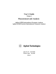
4.3
Application Architecture
Main
RoadDesigner
Controller
RoadNetwork
Model
SimPanel
View
Figure 4.1: VIS-SIM architecture in UML
The project neatly divides into three parts that will be describe separately.
These three parts are analogous to the model view controller design pattern.
The network designer (Controller ) builds and edits a road network (Model ).
The simulation (View ) applies traffic to the model and records results.
The glue between the Editor and the Simulator is a mediator class called
Main that contains the main() method. It contains all the applications
controls such as the buttons and the menu bar. Main also contains the
action listener providing the functionality for the controls. It handles the
switch between the Editor and the Simulator and it directs events generated
by the controls to the interface that is currently deployed. In a switch
Main changes the buttons and menu item available to the user and swaps
the visible panels between the Editor and the Simulator. The mediator
pattern means Main is the only class with detailed knowledge of all the core
application classes thereby increasing maintainability and promoting looser
coupling between these classes.
36
4.4
4.4.1
4.4. COMPONENT DESIGN
Component Design
Road Designer
RoadDesigner
*
*
Road
1
Junction
InputPopup
Popup
JunctionPopup
Figure 4.2: UML diagram of the RoadDesigner
The Editor (Road Designer ) is the section of the application that enables the
user to design a road model. The question arises as to how the model should
be visually represented. Initially I imagined a road network model being
represented as a directed-graph with nodes as junctions and paths between
nodes as road-lanes. The advantages of using directed-graphs might be that
they could show more explicitly which lanes link to which other lanes. There
are also java packages to handle directed-graphs. This idea was rejected in
favour of a representation of the road network using graphics of roads and
junctions so as to provide a more intuitive and natural representation. The
tradeoff is that users aren’t explicitly shown the paths a car can take at a
junction.
Following is a discussion on the principle design issues of the Editor.
Roads
Perhaps the primary algorithm of the application is one which allows the user
to draw roads on the screen. A road is a path with a start and end that the
user can create and extend. More specifically, it has a centre-line dividing
one direction of lanes from the other and it is composed of individual lanes of
any permutation. Java’s GeneralPath object seems perfect for drawing road
37
4.4. COMPONENT DESIGN
lanes. The GeneralPath class represents a geometric path constructed from
straight lines, quadratic and cubic (Bezier) curves. The GeneralPath API
has a method to add lines to an existing path, so that the path is extendable.
Using the existing GeneralPath API and a library of my own GeneralPath
functions I extended the functionality of paths to suit all the functions I
need for lanes. Unfortunately GeneralPath is declared final so rather than
using inheritance I built a Road class with an array of GeneralPaths as the
individual lanes. To allow modification of a path point once it has been
drawn I have drawn a “handle” or “control-point” at the end of each path
segment. If a user clicks on one of these handles an event is triggered where
the program can modify the path so that the current handle follows the
users mouse. The graphics of a lane is drawn first with a thick black line
and then with a thiner grey line over the top. This gives a grey lane with a
black outline. Since a road is an array of lanes, odd number array indices are
left lanes, even number array indices are right lanes and lane index 0 is the
centre-line of a road. The centre lane is the reference path for all the other
paths however some non-trivial calculations are needed for lanes to remain
parallel to the reference path at bends in the road. Fig 4.3 demonstrates
that parallel lanes must lie along the angle bisector of the centre-line.
A line joining (x1 , y1 ) and (x2 , y2 ) can be specified by the equation:
y2 − y1
y − y1
=
x − x1
x2 − x1
The gradient of the line is:
m=
y2 − y1
∆y
=
x2 − x1
∆x
The equation can therefore be simplified to:
y − y1 = m(x − x1 )
The angle of a line section at a particular point is measured as the angle
from the x axis. It is calculated using:
The sign of the gradient can be confusing as the screen co-ordinates are in
the 4th quadrant of X-Y co-ordinate space whereas it is usually calculated
in the 1st quadrant of X-Y co-ordinate space.
38
4.4. COMPONENT DESIGN
(x2,y2)
dy
Q
(x1,y1)
tan(θ) =
x-axis
dx
∆y
∆x
θ = tan−1 (m)
(x3,y3)
Center Line
a2
(x4,y4)
H
D
Parallel road lanes
Q
(x2,y2)
a1
(x1,y1)
b
Bisecting Line
(a) Relationship of lanes to the
centre-line angle bisector
(b) Defining measurements
Figure 4.3: Parallel lines
The angle bisector (b) is calculated:
(
b=
(a1 + a2)/2,
if (a1 > a2)
(a1 + a2)/2 − 180◦ , otherwise
The angle Q can now be calculated:
Q = a1 + (180◦ − b)
If D is the distance lanes should be apart from the centre-line, H can be
calculated:
D
D
sin(Q) = ( H
) ⇒ H = ( sin(a1+(180
◦ −b)) )
Given the co-ordinate (x2, y2) of the centre-line bend, (x4, y4) of a road-lane
is defined by:
39
4.4. COMPONENT DESIGN
x4 = x2 ± xH ∗ cos(b)
y4 = y2 ± xH ∗ sin(b)
where x is the index of the lanes (depends on whether it is a 1,2,3,4... laned
road).
Figure 4.4: Screenshot demonstrating hypothetical parallel road lanes
Junctions
In terms of the Editor a junction is simply a object that roads need to
connect to. A design decision was taken for junctions to be rectangular
and to join a maximum of four roads. This is understood to cater for the
majority of junctions and any other decision would add an enormous amount
of complexity to both determining the junctions shape and to the simulation
component of the junction. Each side of the junction has a “handle” that
an end of a road must “snap to”. The length of a junction side and the
position of the handle must be calculated so that the road neatly squares
to the junction even when the junction has a odd number of lanes (See Fig
4.5).
The Junction class has a reference to each road that may be connected to
one of its handles. The junction can calculate Dx by calling a getRoadLeftWidth() and getRoadRightWidth() methods for each of its connected roads.
40
4.4. COMPONENT DESIGN
D2
D1
Handle1
D8
D3
Handle4
Junction
Handle2
D7
Handle3
D6
D4
D5
(a) Important distances
(b) Screenshot
Figure 4.5: Junction handle placement
Although a junction is rectangular, it is not as simple as calling “g.DrawRect(x,y,w,h);”
to draw it because it can be at any rotation. Instead the junction shape is
determined by an array of 9 points (4 corners, 4 handles and the centre point
(x[0],y[0])). The best way to describe the rotation method is through the
code:
public void rotate(double newAngle) {
radAngle += newAngle; //Update global variable to track current angle.
AffineTransform t = new AffineTransform();//Build transform object
t.setToIdentity();
//Initilize
t.translate(x[0],y[0]);
//Translate to origin
t.rotate(newAngle);
//Rotate by an angle
t.translate(-x[0],-y[0]);
//Translate back to old position
GeneralPath pathShape = collapseToPath();
pathShape.transform(t);
s = pathShape;
extractFromPath(pathShape);
}
//Get shape from point array
//Transform the shape
//Update global shape variable
//Set point array from shape
This method rotates the junction shape but also updates the point array
that defines the junction corners and handles so that any roads connected
with the junction can be updated with new end coordinates.
Different types of junctions need different graphical representations. Fig 4.6
shows how I have represented each junction. Signalled junctions are filled
with a TexturePaint that was designed with yellow diagonal lines on a road
surface background. A “over” or “under” bridge is represented using thicker
41
4.4. COMPONENT DESIGN
(a) Signalled junction
(b) Non-signalled junction
(c) Bridge over
(d) Bridge under
Figure 4.6: Junction graphics
lines on the relevant side. Non-signalled junctions are more complex because
they need to show the user which side of the junction has priority (see Fig
4.7). Two sides have priority and the other are drawn with a dotted side line
representing a lack of priority. The priority of the junction goes to the two
sides with the biggest roads. If there is more than two equally large roads
then priority will go to the two roads that were latest modified by the user
(thereby giving control to the user). The yellow centre-line helps to clarify
the decision by joining the two roads with priority.
Line Clipping
Any valid road in the Editor must start and end at either a junction or
the edge of the map (the drawing bounds). Users are working with whole
roads rather than lanes and this means a road may have lanes that don’t
match the drawing bounds (see Fig 4.8 for an example). The lane ends must
either be extended or cut-short. Calculations for this can be done using line
intersection algorithms, either for lines or line segments. The easier case
is if a end segment of a lane intersects the drawing bounds. In which case
it needs cutting-short. Otherwise the lane end segment is imagined to be
42
4.4. COMPONENT DESIGN
(a) East/West priority
(b) North/South priority
(c) North/East priority
Figure 4.7: Non-signalled priority representations
infinitely long and intersection is again tested with the drawing bounds. The
problem is that it is unknown which drawing bounds edge to clip to. It can
be calculated by getting all the edge intersection points and using the one
which is closest to the lane end-point. Unfortunately Java doesn’t have a
method to get the intersection point of two lines.
Line 1 equation: y − l1y1 = l1m(x − l1x1 )
Line 2 equation: y − l2y1 = l2m(x − l2x1 )
At the intersection point the two lines will have the same value of x and y.
This point can be found by solving the simultaneous equations:
x=
(l2m ∗ l2x1 ) + l1y1 − (l1m ∗ l1x1 ) − l2y1
l2m − l1m
y = l1m(x − l1x1 ) + l1y1
Saving and loading
Any set of actions that uses up the users time should be storable and retrievable. I did not look further than using an XML method to achieve this.
XML is the standard for structuring data. One particular design advantage
of XML is that it provides inter-operability between heterogeneous systems
thereby increasing the possibility that the project may be useful to others.
43
4.4. COMPONENT DESIGN
(a) Before Clipping
(b) After Clipping
Figure 4.8: Line Clipping
java.io.PrintWriter
XMLSaver
XMLWriter
XMLStack
XMLLoader
XMLElement
InputStreamReader
XMLReader
1
*
XMLFileWriter
XMLAttributes
Figure 4.9: UML diagram of XML components
The design of XML saving and loading is based on the Chain of Responsibility design pattern. The chain of responsibility pattern allows a number of
classes to attempt to handle a request, without any of them knowing about
the capabilities of the other classes. The save is initiated by the user and
the head of the chain saves itself and passes on the request to the objects it
encapsulates. These objects then save themselves and forward the request
so that it percolates all through the chain and all objects are saved.
Objects only need to know what to save and load and not how to save their
data. The XMLSaver and XMLLoader code handles how saving and loading
works. Each object has to know its XML name, how to save/load its own
data and which children to pass on the save/load request. All objects to
save and load must implement the interface shown in Fig 4.10. The imple-
44
4.4. COMPONENT DESIGN
mentation details of the XML code heavily relies on Java’s string routines
to parse or construct XML documents.
XMLSerializable
+getXMLName(): String
+saveSelf(): XMLElement
+saveChilds(): void
+loadSelf(): void
+loadChilds(): void
Figure 4.10: XML interface
In my design of the final XML document, objects are XML Elements (tags
such as <Road></Road>) and an objects data is stored as XML Attributes
inside it’s tag’s (e.g. <Road start=”x,y”>). Encapsulated objects exist
inside their parents tags thereby forming a tree structure.
In addition to saving and loading a road network, the application offers the
user a choice to save as an applet. The end result of this is the generation of
a html page which, if viewed in a browser would show a running simulation of
the current road network. The applet only shows the simulation, it does not
provide any interaction controls. The purpose of this piece of functionality
is to facilite the creation of web-pages describing traffic modelling anotated
with visual animations. See Appendix C for an example.
The implementation of save as an applet needed to save as normal and then
use the saved file as input to an applet. The html file to run the applet is
written using a skeleton text file with markers where correct names need to
be inserted. A file search and replace class was written to accomplish this.
All the applet code and the specification file is packaged up in a single jar
archive file to avoid file clutter and to save disk space and download time.
Applets normally can’t input files, however when the file is inside the jar
archive it can get security permissons to convert it into an inputstream.
Usability considerations
When a programmer is also the designer, tester and evaluater usability considerations often get neglected. There are many details incorporated into
the design to try to improve the user interface. Firstly, the application is
solely controlled by the mouse through an iconic graphical user interface.
The interface is split into three areas of control, the currently displayed
panel, an additional control panel and the menu-bar. Any controls that
are inappropriate to the users current actions are disabled and greyed-out
thereby minimising the clutter of controls. Drawing roads is designed to
45
4.4. COMPONENT DESIGN
feel familiar to users who have used applications where lines can be drawn.
Drawn components are aligned with a grid so that a regular layout is made
easier for the user. Drawn components are manipulated by handles. Handles
also snap to the grid and other handles (where relevant). These handles are
highlighted in red when the mouse passes over them to show the user that
they are control points.
Figure 4.11: Screenshot of the RoadDesigner
Fig 4.11 shows some of the discussed usability features and demonstrates a
question-mark texture which forms when two roads cross without the user
selecting a junction.
The implementation of highlighting areas of the road network model is done
using Java’s shapes. RoadDesigner objects record what their shape is on the
screen and when the mouse is moved, the co-ordinates are tested in relation
to all the shapes. If the mouse co-ordinates are inside a shape, that shape
is highlighted by being filled with red. Any Road shapes that intersect oneanother are filled with a question-mark texture representing that the user
needs to specify a junction at that place.
46
4.4. COMPONENT DESIGN
4.4.2
Simulation
SimPanel
RoadNetwork
1
*
1
JunctionModel
CarGenerator
*
LaneModel
GiveWayJunctionModel
1
1
Sig1JunctionModel
CarContainer
*
TurnOffJunctionModel
Car
*
LaneSection
BridgeJunctionModel
*
JunctionPath
AdaptiveSig1JunModel
Sig2JunctionModel
AdaptiveSig2JunModel
Figure 4.12: UML diagram of the SimPanel
The SimPanel aims to animate vehicles on a road network that was draw
by the user using the RoadDesigner.
Following is a discussion on the principle design issues of SimPanel.
The timing system
It is important for simulations to track a time component and the design to
do this uses frame numbers where incremental frames represent time passing.
Events in the simulation are triggered by a timer. The timer package I
have used is written by my supervisor, Professor Jeff Magee. Any class
that reacts to the timer needs to register with the timer and implement the
timers interface which includes the methods pretick() and tick(). The timer
ticks after a certain amount of time. At each tick the timer runs through its
list of registered classes and calls first their pretick() and then their tick()
methods. So for example, in the Car class the pretick method calculates the
47
4.4. COMPONENT DESIGN
cars new location and in the SimPanels tick() method, all the cars are drawn
to a backbuffer. The last action of a tick is that the backbuffer is labeled
with the current frame number and is swapped onto the screen. This design
combines a back-buffering approach to animation with the necessesity of
clearly presenting the time dimension to the user.
The timer runs in its own thread and sleeps by x milliseconds in between
each tick. The user has direct control of the speed of the timer by controlling
x through a slider. The simulation can also be paused by suppressing the
timers ability to tick.
The vehicle movement model
The simplest mathematical car-following model is linear. This means that
as long as there’s no obstruction (another car or a red light) in front of a
vehicle, it will travel at the speed limit of k kilometres per hour. If a car
gets within a distance of L metres from an obstruction, it will reduce its
speed proportionally to that distance. If a car gets within a distance of l
metres from an obstruction, it will stop altogether.
Let x denote the distance in metres between two cars (measured from the
front of one to the back of another, or between the front of one car and a
red light ahead).
The speed v of the car is:


 k,
if x >= L
between0andk, if l < x < L
v=

 0
if x <= l
In the second case, l < x < L, we’re assuming the car changes speed proportionally to changes in distance, so that v is given by a “linear” function
of x (the graph of v as a function of x is a straight line). This means that
v = mx + c for two constants m and c. These constants can be determined
from the two conditions:
1. v=0 when x=l
2. v=k when x=L;
48
4.4. COMPONENT DESIGN
therefore:


 k
v=
if x >= L
mx + c if l < x < L


0
if x <= l
From these, we can solve for m and c in terms of the three fundamental
numbers k, l, and L:
1. v = mx + c
2. 0 = lm + c therefore c = −lm (A) or m = −c/l (C)
3. k = Lm + c therefore c = k − Lm (B) or m = (k − c)/L (D)
4. From A and B −lm = k − Lm therefore m = k/(L − l)
5. From C and D −c/l = (k − c)/L therefore c = kl/(l − L)
These three numbers (k, l, and L) therefore, completely determine the traffic
behaviour. The design decision to use the simplest model possible allows the
project a wider scope in other aspects, however the model suffers in realistic
factors such as drivers’ reaction times, or limits to how fast a car can brake
or accelerate.
Animation of cars
A cars shape is a polygon. The centre of the polygon is positioned in the
centre of a lane. The rotation of the polygon is dependent upon the direction
of its current lane.
Figure 4.13: Intersection of two lines
In the Fig 4.13 the gradient of l1 is m1 and the gradient of l2 is m2 .
49
4.4. COMPONENT DESIGN
tan(α) =
opposite
adjacent
tan(α1) =
⇒
l1y2 −l1y1
l1x2 −l1x1
= m1 and tan(α2) =
l2y2 −l2y1
l2x2 −l2x1
= m2
whilst: θ = α1 − α2
⇒ tan(θ) = tan(α1 − α2)
⇒ tan(θ) =
tan(α1)−tan(α2)
1+tan(α1)∗tan(α2)
⇒ tan(θ) =
m1 −m2
1+m1 ∗m2
In particular if the lines are perpendicular, then:
θ = 0.5π and m1 ∗ m2 = −1
So to draw a car on a road of gradient m the car image must be rotated
tan− 1(m).
The rotation is done using an affine Transformation similar to the method
described for junctions. The rotation only needs to occur at a change of
lane direction, otherwise the car can be moved by simply shifting all the
cars polygon-points by the difference in x and y of the new position to the
old.
A cars new location after a moving a certain number of pixels in any direction
can be calculated using the Pythagoras theorem. If θ is the angle between
the x-axis and the direction of the car, then the distance moved is explained
in Fig 4.14.
D
y -=
D*
Sin(Q)
D
Q
Q
x += D*Cos(Q)
x -= D*Cos(Q)
Q
Q
D
y +=
D*
Sin(Q)
D
Figure 4.14: Distance car moves given an angle from the x axis
For a car to know how far away it is to another car the distance of two
50
4.4. COMPONENT DESIGN
points needs to be calculated:
distance =
p
∆x2 + ∆y 2 where ∆x = x2 − x1 and ∆y = y2 − y1 .
The speed of a car can be calculated from:
speed =
distance
time
The acceleration of a car is its change in speed in time:
acceleration = ∆ velocity
time
The cars are implemented as sprites, i.e. they are entities that know how
to draw themselves. The drawing of objects is based on the visitor design
pattern. The SimPanel keeps a list of all the cars and iterates through the
list telling each car in the list to draw itself onto the background it supplies.
It is therefore visiting each of the car classes in turn.
Since colour information is a powerful influence for visualisation systems a
car is drawn with it’s speed shown both as a number inside the car and
by colour-coding the rectangle that represents the car. The draw method
contains a look up table to determine what colour should represent the cars
speed, a brighter colour represents a faster speed.
Car generation
Unlike real-world world behaviour, it is important for simulations to be able
to specify exactly how many cars enter the system in a given time interval.
Without this it would be difficult to compare two road variations because
they wouldn’t run on the same data. The design is that the user can specify
exactly how many ticks of the clock occur before a car is generated at a
particular input. They do this by right clicking on a road input and selecting
a time lag in a pop-up box. In order to avoid the artificial look of “pulses”
of cars entering a road network at the same time a small random offset is
allocated to each input before the first car enters.
Often a congested road will block incoming traffic from entering the road
system. In this case the vehicle must be added to a queue at their particular
input. If congestion clears, cars from the queue should enter the network. A
user can check the size of a input queue by clicking the mouse on the input.
51
4.4. COMPONENT DESIGN
Junction models
Modelling the junctions of a road network is the most complex part of the
project. The models need to refect real-life behaviour of traffic at junctions.
This difficulty arises due to the large number of junction formats used on
roads.
One design option could be an interface for users to design their own junctions and save them to a list for later use. The problem is that when objects
need a lot of customising it increases complexity enormously because many
exceptional cases seem to crop-up that need to be catered for. The design
process is also often complex and time consuming for the user (something
this project aims to avoid). An alternative design was to provide less choice
of junctions but to make them much more generic. As an example, if the
user has to design junctions, they’d have to specify one for each permutation
of lanes and turning options and traffic light sets, whereas a generic junction
adapts automatically to any number of lanes and connecting roads.
The best solution would be to implement both choices however due to time
constraints the generic junction approach was taken. This is possible because
it was found the majority of junctions can be modelled from a few generic
cases. It is also the approach that is easiest for the user. The project provides
two types of signalled junctions, one where opposite light sets synchronise so
traffic is given a option to go straight ahead or turn left (but not right), the
other is where any output can be reached but only one side of the junction
is green any any point in time. If other junctions are needed they would
need to be manually programmed into the system for which a development
guide is given (See Appendix B).
Put simply a junction is a link through which cars can get from an input
to a legal output. In the real-world a vehicle driver decides when to enter
a junction and which output to go to. Since they follow traffic signals and
signs at the junction the outcome to their decision can be thought of as
a function of the lane that they are in and the behaviour of the junction.
This is how vehicle behaviour at junctions is modelled in the simulation.
Vehicles are assigned one of the legal output lanes and they are denied
access to the junction unless it is appropriate for them to continue. In the
real-world the driver chooses where to go whereas, in the simulation the
junction effectively chooses where they go by assigning them a output lane.
This is a philosophical design decision based on the observation that when
examining a road system one does not know information on where individual
cars are going however statistical knowledge is known about the proportion
of traffic that go one way or another at a junction.
52
4.4. COMPONENT DESIGN
The heuristics a junction used to allow or deny a vehicle passage is dependent on the type of junction. The template design pattern was used in the
implementation of junctions, a abstract parent JunctionModel class leaves
methods to be implemented by concrete children resulting in a known template for all junctions.
Bridges. Bridges are not junctions in the real-world but it was convenient
to model them in the same way as junctions because they occur when two
roads cross and the user needs to specify which road is above the other. A
vehicle entering a bridge will always exit it on the same lane. i.e. a bridge
has no extra turning options and never denies access to vehicles.
Non-signalled junctions. Currently, there are two designs for non-signalled
junctions that will cover many situations but not all. They are designed so
that some roads have priority over others and so vehicles on a non-priority
lane may be denied access.
Type 1. Most Non-signalled junctions are deployed where cars need to turn
onto or off a main road. In this case the priority flow of traffic shouldn’t be
disturbed by cars waiting. They should wait until there is a suitable gap in
the main flow of traffic. The gap-acceptance model is as simple as testing
the distance of priority cars to the junction and accepting the decision to
pull-out if no cars are within Xm. All cars on the junction also follow the
heuristic that if there is a car on a conflicting junction path they should not
enter the junction. This stops collisions occurring if a car pulled out too
early into oncoming traffic.
Type 2. Other types of non-signalled junctions occur on non-busy roads
that allow cars to take any junction path. These types of junction are not
often used when roads have more than two lanes. In the model only one
vehicle is allowed in the junction at any one time. This means vehicles can
turn right and be safe from interfering with the opposite stream traffic. The
implementation of these junctions uses a semaphore which a vehicle must
get to enter the junction and must put when exiting the junction. The vehicle that can get the semaphore is determined by two queues, a priority
queue contains cars waiting on a priority lane and a wait queue contains
cars waiting on a non-priority lane. The head of the priority queue gets the
semaphore first and cars on the waiting queue only get the semaphore if the
priority queue is empty.
Signalled junctions. These junctions are controlled by traffic-lights which
operate as in the real-world. I.e. a red light at a lane will deny access to
vehicles, vehicles treat amber lights as red lights if they are far enough away
to de-accelerate in time otherwise they treat a amber light as green. In addition a rule is needed where a car will not enter a junction if there are other
53
4.4. COMPONENT DESIGN
cars still on the junction on interfering paths. Using these heuristics alone
does not work in a congested environment because cars end up forming a
traffic jam in the middle of the junction. It is therefore necessary to add
rules so that a car won’t enter a junction if the car in front is moving slowly
or if there is no space for it to fit on the other side of the junction. The
lights of the junction signals are contained in sets and each set is given a
green-light time where it will stay green before turning red. The sets are
cycled through as each green-light time passes. The user can set the greenlight time manually.
Type 1. The variation of different junctions is essentially in what the turning options are for the cars at the junction and therefore also the traffic light
sets that synchronise with each other. The first type of signalled junction
allows vehicles to either go straight on or turn left if they are in the left
lane or turn right if they are in the right lane. The problem is that for this
to be easily implemented only one side of lights at a time turn green, it is
therefore not a realistic approach.
Type 2. The lack of a realistic junction is solved by a signalled junction
where opposite sets of lights synchronise allowing opposite traffic to pass
each other or turn left. The majority of real-world signalled junctions work
in this way.
ITS models
The simulation provides two of the basic constructs of ITS, vehicle actuated
traffic lights and adaptive traffic lights. Vehicle actuated traffic light sets
only turn green if there is a vehicle waiting at them otherwise they skip to
the next step. Adaptive traffic lights use an algorithm to score each traffic
light set based on the number of cars waiting at the lights. green-light time
is deducted from the set with the lowest score and added to the set with the
highest score. A good balance is always met because if a set of lights has
too low a green-light time more cars will end up waiting and this increase
the sets score so that its green-light time is recovered. The change in time
occurs frequently and in small steps. There is also a minimum time for a
light set unless the junction is vehicle actuated. The adaption algorithm is
essentially a hill climbing algorithm, it tries to find the best solution in the
local area.
Successful ITS systems have junctions that synchronise and communicate
with each other. The simulation does not implement communicating junctions but has an option that tries to synchronise the largest path of signalled
junctions to create a green wave. This is achieved by resetting the light sets
on the path and offsetting their respective change times by a certain amount
54
4.4. COMPONENT DESIGN
calculated by dividing the distance the two junctions are apart by the average speed of a car.
Collecting results
A number of key results are calculated and stored as the simulation is run.
There are three levels of scope for the results. Immediate results are calculated based only on the information of the current frame. Fig 4.15 is a
screenshot showing how the immediate information is displayed on the panel.
Users can suppress this information from showing or from being recorded.
Figure 4.15: Screenshot of the running simulation
Fig 4.15 displays:
•
•
•
•
•
•
Current simulation frame number
Total cars that have entered the simulation
Total cars that have exited the simulation
Total number of cars that are currently on the screen
Average speed or cars
Average congestion of roads
55
4.4. COMPONENT DESIGN
There is also information based on either the last x frames or from the entire
history of the simulation. The statistics panel (see Fig 4.16) gives a snapshot
of the results at a certain frame of the simulation. The snap shot shows the
Throughput of the simulation. This is the number of cars that pass through
the road network per time interval (cars exited / frame number). For a
dynamic update of the simulation data the user can open a graph panel to
see how number of cars, average speed or average congestion changes over
time. The graph will be updated every second.
(a) Traffic Graph
(b) Statistics Snapshot
Figure 4.16: results display avaliable to the user
The next section of the report starts from a finished implementation of the
project application and evaluates it in terms of its strengths and weaknesses.
Chapter 5
Evaluation
This section of the report aims to test and analyse the project application
to determine its strengths and weaknesses and to determine what one can
learn from it. Much of the evaluation is of a qualitative nature however the
application has the capability to produce statistics and graphs that can help
in a more quantitative way.
Traffic modelling and simulation is a vast and complex subject and an area
of active research. Commercial simulations tend to concentrate on limited
areas of the subject and don’t broaden out beyond realistic boundaries. The
objective of this project was clear in that the project would not involve the
kind of accuracy that existing commercial simulations implement but will
provide an easier interface for untrained users. This suggests that validation
tests are less important than usability and visualisation quality.
The scope of the project made it impossible to model all the behaviour that
is needed for a valid traffic simulation. The scale of the roads and vehicles is
simplistic and car accelerations are fixed. The car-following model is linear
and basic, there is no overtaking or lane changing model. Vehicle collisions
are not modelled or tested for, and there is little individual driver behaviour.
There is no model for roundabouts or a tool to specify all junctions. The
users can only set speed limits globally not for each road. There are no
smooth corners, and no non-flat terrain. Traffic is all of one type and there
are no pedestrian crossings. The simulation is therefore not able to take any
accurate measurements of real road-infrastructure situations.
Having discussed some of the project limitations the strong points for the
application will now be outlined. The simulation is extremely flexible al56
57
5.1. ANALYSIS OF CAR MOVEMENT
lowing a user to model many different kinds of road-infrastructure models
quickly. The graphical user interface allows interesting traffic behaviour to
be designed and viewed in a matter of minutes. The simulation can compare
models for efficiency in a number of different ways, presenting results in a
clear graphical way. The visual simulation makes in clear what is happening on the road network. It is easy to see how fast cars are going and how
congested the system is becoming. Last but not least the application is well
documented and extendible.
5.1
Analysis of car movement
The simulation determines that a simple linear car-following model gives
a fairly convincing visualisation of vehicle movement. Acceleration can be
clearly seen when a car leaves a junction and de-acceleration is smooth when
a vehicle approaches an object such as a traffic light or stationary car. A
platoon of cars forms when faster cars are behind a slower car and the
platoon behaves in a stable manner that one would expect. The simulation
provides controls to set the top speed of vehicles to either be set at x kmh−1
or to vary between x and y kmh−1 . It can be shown that over a certain
congestion percentage, when vehicles at varying speeds enter the simulation
the average speed always converges to the lower speed bracket. This is
because faster cars get stuck behind slower cars and vehicles slow down for
junctions thereby reducing the total average speed.
In the simulation road users that spawn at an edge node have not got a
specific destination, they will stay in the same lane until there is a choice
at a junction and then they will be given a path to take. The simulation
uncovered a potential design flaw for junctions. The model of junctions
is such that it is often only the extremity lanes (furthest inside or outside
lanes) that has a choice in which junction path to take. It can be seen from
fig 5.1 that the middle lane doesn’t have a choice in where to go.
This issue doesn’t invalidate the junction model because junctions with roads
of three or more lanes are fairly rare and may well implement the same
behaviour as the simulation.
If cars did have a specific destination their path though the network could
be implemented with Dijkstra’s shortest path algorithm. A large advantage
of this would be that the simulation could calculate the average journey time
for vehicles. This statistic is interesting because it is an example of information that a simulation can easy acquire but would be next to impossible to
58
5.2. NON-SIGNALLED JUNCTIONS
(a) Junction paths with roads of
2 lanes
(b) Junction paths with roads of
3 lanes
Figure 5.1: Junction paths
acquire in a real situation. In the project application the destination of a car
is not deterministic and so average journey time is not a relevant statistic.
5.2
Non-signalled Junctions
There are two types of non-signalled junctions implemented.
The first type uses a simple gap-acceptance model and is practical in many
situations where cars need to turn onto or off a main road. Priority flow is
unaffected by the junction except the left most lane has the choice of turning
off. Vehicles wanting to turn onto the main road (Vehicles waiting) must
wait until a suitable gap occurs.
The second type only allows one car inside the junction at any one time but
that car has the choice of any junction output. Although this is a flexible
junction it is designed for junctions with a low traffic density and was found
to cause large queues in situations where two cars frequently arrive at the
junction at the same time. The problem is that the junction breaks the flow
of priority traffic as they have to wait for one car at a time to pass through
the junction.
Fig 5.6 demonstrates a test for the two types of non-signalled junctions. The
two road networks were run for 2000 frames and then the graph function was
invoked to help analysis. The one-car-at-a-time give-way junction ended up
59
5.3. SIGNALLED JUNCTIONS
(a) One-car-at-a-time give-way
junction
(b) Gap acceptance give-way
junction
(c)
(d)
Figure 5.2: Non-signalled junction congestion test
with an average car speed of 2 kmh−1 and a congestion level of 38%. The
gap acceptance give-way junctions has a higher variance but has an average
car speed of 20 kmh−1 and a congestion level of 6%. The gap acceptance
give-way junction is the only valid option to use in roads that spawn vehicles
at a rate above the time it takes one vehicle to pass through the junction.
They produce a good visualisation of waiting cars nipping out onto the
junction when there is space for them to safely do so.
5.3
Signalled Junctions
Analogous to non-signalled junctions there are two types of signalled junctions.
The first is the more practical case of where opposite sets of lights synchronise allowing traffic to flow past one-another. Right-turns are obviously
60
5.3. SIGNALLED JUNCTIONS
unavailable for this kind of junction.
The second type of signalled junction is not seen in real-world examples
but is flexible and useful for comparison purposes. Only one side of lights
is green at any time meaning cars can turn right as well as left or going
straight ahead.
The common problem for signalled junctions is that in a congested environments vehicles would enter a signalled junction at a green light and meet
a traffic jam formed from subsequent congestion. This would block the
junction for other vehicles on other sides of the junction. Although this
behaviour is sometimes seen in real-life, the simulation should try to avoid
gridlock situations as much as possible. More rules were needed to restrict
traffic entering a junction if they won’t be able to exit it. The problem was
that it was very easy to over-constrain a junction so that vehicles didn’t
enter it and the probability of gridlock increased. The problem isn’t apparent for single junctions but multiple connected junctions accentuate the
problem. Some rules that initially seemed obvious were found to be inappropriate. An example is Do not enter the junction if there isn’t space to exit.
This causes problems with platoons of vehicles because they won’t stream
through, the flow will judder because as a vehicle passes over the junction
another vehicle would believe there’s no room on the other side and so will
slow down. The obvious thing to do is factor in the speed of the car in front
so that caution on entering the junction should only be taken if the speed is
slow thereby indicating congestion. There are cases however when platoons
de-accelerate quickly (especially in a linear car-following model) so that the
problem still occurs. There is also the question of how much space should
be on the other side of the junction. If there is room for just one car on the
other side of the junction and a car moves to fill it the vehicle behind would
find it difficult to calculate that it shouldn’t move because the space will be
filled up. Calculations for the vehicles to make these kind of decisions are
often computationally expensive when done on a large scale as they involve
looping through all the cars waiting at a junction and performing a test.
For a smooth animation, calculation done by each individual car should be
kept to a minimum and instead it is best to compute something relevant to
each junction that vehicles can use. As an example, in my implementation
a junction has a variable called is OK T o Go which if true means a car
can enter the junction without danger and won’t have to do any of its own
calculations.
Compared to normal junctions, vehicle actuated junctions never reduce the
efficiency of a road network, however the simulation shows that there are
situations when they don’t make any difference. This occurs for busy junc-
61
5.3. SIGNALLED JUNCTIONS
tions when there is invariably a car waiting at a light. This information is
useful because it can help save money on installing actuation systems that
wouldn’t have an effect.
Fig 5.3 shows a comparison between an actuated and non-actuated junction.
One side of the side is specified to have calm traffic. It can be seen that
the actuated junction increases both the maximum and minimum average
speeds and also shows how the period of the lights oscillates at a much lower
frequency.
Adaptive junctions make decisions on light times based on the longest queue
at each light-set. The set with the longest queue is given the largest amount
of green-light time. This is often useful if one side is busier than another but
is of little use when a high number of road users try to follow the route: lanes
may get full, and, even when being dealt with the longest, the road users
on these will be stuck because of the next lane being full. These junctions
also have a habit of increasing congestion inside the road network because
if there is a large input queue they facilitate the entry of vehicles. This
will flood the road network and jam it up. There tends to be a threshold
on a road network where beyond a certain frequency of cars entering the
network, it jams up and operates very poorly. The simulation does not
provide delicate enough tools to determine this threshold. The reason for
this threshold is that the input traffic-intensity of one junction will be a
function of the output traffic-intensities of other junctions, however there
is a time lag involved. The more congested a road, the larger the time lag
which allows more cars to enter the network and worsen the problem.
62
5.3. SIGNALLED JUNCTIONS
(a)
(b) Average speed (Actuated
Junction)
(c) Average speed (Non-actuated
Junction)
Figure 5.3: An efficiency test comparing a actuated junction with a nonactuated junction
63
5.3. SIGNALLED JUNCTIONS
(a) Road infrastructure set-up
(b) Adaptive Statistics
(d) Adaptive Graph
(c)
Non-adaptive
Statistics
(e) Non-adaptive Graph
Figure 5.4: An efficiency test comparing a adaptive junction with a nonadaptive junction
64
5.4. BRIDGES
Fig 5.4 shows a comparison between a two adaptive and non-adaptive junctions. The adaptive junctions provide a speed up in average speed of 3
kmh−1 and a drop of congestion of 1%. The light times adapting to give
more green light time on the busiest light-sets has reduced the variance of
the average speed graph for adaptive junctions. It should be noted that the
total time period in one light-set cycle is constant, the percentage of that
time for each set varies. This can be seen because the frequency of the two
graphs is the same.
The application provides a tool to synchronise a straight path of signalled
junctions. The synchronisation works by forming a wave of green lights down
the path of synchronised junctions. The problem of the synchronisation is
that it only works in one direction of the path. The other direction is effected
negatively. One solution would be to reverse the direction of waves at each
pulse. This increases fairness but reduces the overall efficiency. The best
thing to do would be to dynamically solve which path of junctions is the
busiest by a large proportion and send green waves through that path until
the congestion is worse somewhere else. This is something the application
could be modified to do if more time was avaliable.
5.4
Bridges
There is really nothing to analyse for bridges, they behave exactly as normal
lanes. They do however increase the scope of the application to model more
situations and improve overall visualisation quality.
5.5
Gridlock situations
Gridlock is a traffic jam in which a grid of intersecting streets is so completely congested that no vehicular movement is possible. In the real-world
vehicles can reverse and shift about so as to eventually break from the gridlock, however without modelling this behaviour a simulation can get stuck
indefinitely. Identifying potential situations of gridlock is a useful property
of the simulation. Fig 5.5 shows a gridlock situation where cars round a
path of junctions all want to turn left but won’t move because there’s no
space for them on the other side of the junction.
While testing the application it was realized that it was often hard to discover the reason for a gridlock situation. In some cases the simulation would
65
5.5. GRIDLOCK SITUATIONS
Figure 5.5: Vehicles in a gridlock situation (with a cars future path shown)
stop running due to a coding error rather than gridlock. It was found useful
to develop a tool to aim to discover the reason for gridlock. The user can
click on a car and information about the car is displayed on the screen. The
information needed to discover gridlock is where the vehicle is trying to get
to. The future path of the car is drawn onto the screen. Using the future
path of a number of cars that have stopped enables the reason for their
deadlock to be discovered.
It was found that gridlock is more likely to occur when a series of signalled
junctions are placed so that a circular path is possible for a platoon of
vehicles. The closer the junctions are to each other the quicker gridlock
forms. Turn off points are also a good method to help to slow down the
occurrence of gridlock. See Fig 5.6 for an example.
66
5.5. GRIDLOCK SITUATIONS
(a) Gridlock formed after 2570
frames
(b) Gridlock formed after 4101
frames
(c) Gridlock formed after 5844
frames
Figure 5.6: Gridlock time comparison test
67
5.6
5.6. PERFORMANCE
Performance
Although the application will run fine on any of the laboratory computers it
was found to be desirable to use machines with processors above 400 MHz.
The performance of the application decreases as it contains more objects.
The Editor becomes slower when using larger road networks because it has
to do more checks for each user event. The situation that is particularly
resource intensive is when a user moves a junction. It this case the new
position of the junction and the 4 connecting roads needs re-calculating
and the computation often can’t keep up with how fast the user moves the
mouse thereby looking jerky. The frame-rate of the simulation decreases as
it contains more cars. The number of cars that still results in a good visualisation depends on the machine specification. Using a 1800 MHz processor,
a subjective minimum speed is reached when a road network contains 500
cars.
5.7
Design changes
Inevitably, there were some requirements originally designed in the outsourcing report that didn’t make it into the final application. It should be
mentioned that more functionality was added to the final application than
was not included in it. The original design was to have four components
in the application. The planned data specification and simulation results
components were factored into the final editor and simulation components
to abstract the details from the user. The final application contains two
types of non-signalled and signalled junctions whereas the original design
only considered one of each. It was found that to model real-world situations a wider choice of junction models was needed. The reason why the
original design only considered one type of signalled junction was that a
Data specification component of the application was going to allow the user
to customise each junction to a high degree. In particular the final application doesn’t allow the probability of which turning a car will take at a
junction to be specified. Linked to this functionality was the requirement
that the simulation should have an option whereby if set, would run exactly
the same data thereby producing exactly the same visualisation every time
it is started. The problem is that the there are many random components
in the simulation and it was found difficult and slow to store each decision
so that the decision could be repeated if necessary. A few examples of the
random components are: an individual cars top speed, destination decisions,
turning choices, traffic lights initial colours, traffic generation, etc. Logging
68
5.8. DESIGN PROBLEMS AND POSSIBLE SOLUTIONS
all the data would enable more extensive results, however it was felt that
it was not necessary due to the performance overhead and higher memory
requirements that would result.
Further modules that were completed in the final application include the
basic constructs of ITS, particularly vehicle-actuated junctions, adaptive
junctions and synchronised junction paths.
5.8
Design problems and possible solutions
The design and implementation of a large project in a limited time span
inevitably involves many problems. One of the first issues was in designing
the scope of the project. It was not realistic to break new ground in the area
of traffic simulation within a six month project so instead the focus was put
on designing a well engineered system with an intuitive user interface that
produces a good visualisation of traffic flow. A key decision was to make the
system flexible so the user could design many different road infrastructures
and expect them to be be simulated realistically. This customisation was
a problem because there are many complexities involved with stopping the
user doing invalid actions. Negative tests (sometimes called monkey tests)
are designed to test whether the application deals with nonsensical input
effectively (see the usability section).
When designing many of the geometric algorithms necessary for the Editor
it was found confusing to convert to screen co-ordinates where the top-left
part of the screen is (0, 0). It would be worth considering programming a
conversion function to convert the screen to normal co-ordinates to allow
algorithms to be designed easier.
Some thought was put into how curves could be used in the application to
represent road bends. It has been proven that it is impossible to get parallel
Bezier curves. Since the design for road lanes is that they run parallel to a
centre-line, using Bezier curves would require a huge design shift. It seems
there is a solution easily implemented in openGL but not in the standard
java graphics library. The idea is to represent a road with a single path
(made from lines, Bezier curves, cubic curves etc) that is textured with an
image representing a multi-laned road. This method would be simpler and
faster than my design when using the Editor component of the application,
however it would be tricky to convert this “road image” to lanes used in the
simulation.
69
5.8. DESIGN PROBLEMS AND POSSIBLE SOLUTIONS
An important aspect in a simulation is the timing variable that controls the
speed at which it runs. This variable changes how many pixels a vehicle will
move at its current speed and should be kept constant once it has been set
otherwise the simulation will distort the visualisation of traffic by for example, subtly speeding up vehicles over some frames. The problem is that the
programmer doesn’t have control of when java updates the screen, repaint()
requests don’t occur immediately, they get queued and displayed when and
if resources are avaliable. The simulation timing controls therefore can’t be
governed by the true frame rate. The method I used to solve this was to
abide by a frame rate but to paint to a back-buffer at each frame not to the
screen. This means the paint is guaranteed to happen and can accurately
control the simulation timing. The real screen is undated with the current
back-buffer frame as often as possible. The screen may skip back-buffer
frames every now and again but the frame number is shown in the simulation so the user is made aware when this happens and it will not affect
the timing variable of the simulation. This method also avoids ConcurrentModificationException’s since when the screen update occurs, there are no
calculations about vehicle positions, instead this is done in concrete code
and the update just swaps the current screen image to a back-buffer image.
The disadvantage is that whereas paint() only does the time-consuming image creating when it is needed (when the screen is updated), the application
does it every frame, even if paint() isn’t going to update the screen.
During the final stages of the project many problems were experienced getting the application to work as an applet. It was suggested that to ensure a
browser runs the applet in a known version of the Java Virtual Machine the
html page should require a pluggin. The design was for the user to click a
java button that would open up the application in a pop-up window. This
would mean the html page with the button would be quick to load as the
entire applet code would not need downloading until the button is clicked.
It would also help unify the applet with the application. The only difference
would be in the extra class for the applet to display a button and load the
application in a new frame when clicked. The applet also disables many of
the file options like loading and saving. To run the program as an applet it
needs to be packaged up as a JAR archive. If this is done images and other
files such as XML specification files can be accessed if they are inside the
JAR archive. The problem is that in the “save as a applet” option a XML
specification file is created and needs adding to the jar archive for the current simulation. A method to programmatically add a file to an archive was
not found and instead a script is created that the user has to run manually.
The script inserts the file into the archive successfully but is not machine
independent. This is something that could be improved upon.
70
5.9
5.9. USABILITY
Usability
Usability is subjective and a hard entity to measure however throughout
the design of the project it has been peer reviewed and critical comments
were acted upon. It was found that the more flexible the application the
less usable it became. This is because it gives the user more room to make
erroneous decisions. Negative tests are designed to test whether the application deals with nonsensical input effectively. The application does not
try to limit the user and it is therefore easy to produce road networks that
are nonsense in the real-world. The application prevents the user doing actions in an invalid situation, for example, it will not let the user progress to
the simulation panel unless the current road map is valid. The application
tries to produce appropriate error messages, for example, the application
will produce an error message if the user tries to load an unrecognised file.
The application also tries to correct mistakes that the user has made, for
example, if the user has a graph panel open in the simulation and moves
back to the editor, the graph panel will close automatically.
During the latter stages of the project a usability test was performed by two
peers following a set of instructions. Ideally it would have been better to
get more people to test the application and for them to be from less of a
computing background. Unfortunately there was not time to implement all
but the most minor comments that they made.
The largest problem that the testers commented on was the move from the
Editor to the Simulation. The button to do this is grayed-out unless there
is a valid road network and the testers often found they did not know why
their road network is not valid. The most common reason why they didn’t
have a valid network was that roads weren’t connected to the edge of the
screen. They suggested a tool to tell the user why their network is not
valid. They were also frustrated by the lack of an undo button. The feature
that they said was the most un-usable was rotating a junction. They said it
was un-intuitive that dragging the mouse upwards would rotate the junction
one-way and down the other way. They suggested the mouse pointer icon
to change to a rotation icon where appropriate and that rotation should be
done by moving the mouse in a circular fashion. Features that they would
most like to see included are smooth corners, different types of traffic and a
zoom in/out function.
It is hard to evaluate the applications usability over other simulations which
haven’t been seen running. During research, less than ten traffic simulation applets were discovered on the internet. These tend to be extremely
simplistic. There was a large project called the “Green Light District” [20]
71
5.10. PROPOSED PROJECT EXTENSIONS
which is open-source and downloadable from sourceforge.net. This project
models traffic in more depth but takes longer and doesn’t produce a better
visualisation of traffic.
5.10
Proposed Project Extensions
The project was written with extension is mind. Extending the traffic models
would be the first thing to do to improve the projects realism and accuracy.
It would be good to use the projects XML component used for loading
and saving to interface with a commercial simulator. In this way it could
provide a graphical front end to an accurate commercial simulation. Other
ideas include:
• Junction modelling tool. This would allow users to specify pathways through a junction and then automatically analyse conflicting
paths and suggest optimal signal sets.
• Emergency vehicle tracking. This would track police cars and
ambulances and could adjust traffic signals at junctions to speed up
their journey times and divert traffic away from incidents.
• Map reading and junction recognition. A program could try
image recognition techniques on maps or aerial photographs to produce
models of real road networks.
• Web interface to the application. It should be possible to publish
estimated journey times to a web interface to allow commuters to view
traffic situations or to generate automatic planned best journey routes.
Now that the project has been evaluated, all that remains is to summerise
the project in a conclusion.
Chapter 6
Conclusion
The results of the project are a set of simple traffic models and algorithms
embedded in a fully independent application that can quickly model simple urban road networks. The application contains a simulation to animate
user-defined traffic data on a road network and is able to produce intuitive
visualisations of traffic flow. The results of the simulation enable different
road networks to be compared for efficiency. Documentation and background information also help annotate the project application.
Road simulations are complex programs that have been developed for forty
years. This project did not have the scope to break new ground in traffic
modelling. The limitations of the project also invalidates any accuratecritical results inferred from using it. This project did however show the
public a simulator that is quick to learn, easy to understand and educational
to use. It is highly accessible and well-engineered, giving it potential for
further development.
From this project it has been learnt that object-orientated approaches to
traffic simulation do well to accommodate the necessary modular design of
different traffic models. Simple traffic models can lead to good visualisations
of traffic flow however the visualisations are resource intensive limiting the
number of vehicles in the simulation to approximately 500 using todays
standard PC’s. It is possible to produce a flexible approach to designing
road networks however flexible junction heuristics and traffic-lights prove
problematic.
72
Appendix A
User Manual
Welcome to VIS-SIM, the visual traffic simulation. With this documentation it will only be a short while before you can create complex city maps,
populate them with various road users, and explore in depth the relations
between traffic control and commuters. You can jump right into the program, letting the intuitive interface guide you from Editor to Simulator, try
out one of the standard maps, or follow the step-by-step examples, acquiring
the knowledge about VIS-SIM you need to use it to its maximum potential.
This application presents you with a tool with which you can visualise and
evaluate various city layouts with minimum user input. VIS-SIM is open
source, giving you a tool for the future, that is able to keep up with advances in traffic technology such as Intelligent Traffic Systems and control
configurations.
A.1
The Goal of the VIS-SIM Project
You probably are held up by a traffic light once in a while. Ever wondered
whether their controlling mechanisms could not better suit the flow of traffic?
New advances in physical detection of passing road users and improved
traffic light control algorithms are to be combined to optimise traffic flow
in the future. Deciding the best use of these new technologies is best done
by detailed simulation, to find out whether a costly new system would be
profitable when applied to a certain infrastructure - this is the purpose of
VIS-SIM.
73
74
A.2. THE EDITOR
All facets of the problem are dealt with: map creation, experimenting
with various traffic densities and control algorithms, and statistical analysis. Moreover, the program is open for future improvement because of its
open source nature.
A.2
The Editor
The Editor is the place to start exploring VIS-SIM’s creative capabilities.
The Editor window is the part of the program in which maps can be created,
saved, loaded, and modified.
Map creation is the process of drawing roads and placing junctions to form
a valid infrastructure. Afterwards, the number of lanes on roads, algorithms
for the traffic lights and starting frequencies for road users can be set. Road
users and traffic light changes are not visible in the Editor, only in the
Simulator.
A.2.1
Interface
Figure A.1: The Editor interface
75
A.2.2
A.2. THE EDITOR
Usage
When you start the Editor you get a blank map with the draw road button
selected. From here you can either load a map or start one from scratch.
1. From the middle of the drawing area click and drag out an initial road
lane with the mouse.
2. You have drawn a lane-segment.
3. Click on a lane segment control-point (there is one at either end).
Then move the mouse to see where lane will extend to. Click to place
the extension.
4. Drag control-points to re-locate lanes.
5. Now either drag or extend your lane so that both sides are at the edge
of the drawing area.
6. If you have done it right, the button labelled “The Sim” should be
clickable.
7. Click this button and cars will drive along your lane. For the moment
this is quite boring so lets make a better road system.
8. Click the “Editor” button to go back to the Editor.
9. You can reverse the direction of your lane. Click on the “Rotate”
button, Click in the triangle that shows you which direction the lane
is currently pointing, the direction should be reversed. Remember to
go back to road drawing mode by clicking “Draw Road”.
10. To extend a lane into a road, click on a lane-section triangle and drag
out the road up to a maximum of 8 lanes.
11. You can also drag out one side or the other of a road to just multiply
lanes in a particular direction.
12. To join two roads together you can join up the 2 roads endpoints and
they will merge.
13. To delete a section of a road, you can click on the “delete” button and
then click on the road handle you want to delete. Again, make sure
you go back to the road drawing mode afterwards by clicking on the
“Draw Road” button.
14. Roads that you join to the edge of the map will spawn cars. The
spawning frequency determines how busy the road is and how congested a map will get. You set the “busyness” of an input node by
right clicking an input and putting the value you want in the pop-up
box.
Adding Junctions:
76
A.3. THE SIMULATOR
1. Click on the “Draw Junction” button.
2. You can add a junction directly into a road by clicking in a road. If
you have drawn a crossroads, you can click inside the cross-roads.
3. Or you can add a junction onto the drawing canvass and then join
roads to the junction handles.
4. If you want to remove a junction, Click on the “delete” button and
then click on any junctions you want to delete.
5. If the orientation of a junction needs to be changed, Click the “Rotate” button, click inside the junction and the drag the mouse upwards
to rotate the junction anti-clockwise and downwards for a clockwise
rotation.
6. If all your roads either end at a junction or at the edge of the drawing
area the “The Sim” button should be enabled and you can see your
road system with cars on it.
7. A junction can be toggled to other types of junctions by clicking on
it with the “Junction” button pressed. Alternatively, right-click on a
junction and select the type of the junction in the pop-up box.
8. This pop-up box also allows you to select the timing of traffic lights
and whether the junction is vehicle-actuated or adaptive.
Other Features:
1. If you make a mess of things click the file menu and select “new” to
blank out the drawing canvass.
2. If you are not drawing only editing, use the “select” button and you
can move both junctions and roads.
3. To save the map go to the file menu and select the save option. The
actions are similar to load a map.
4. To use a particular image as a backdrop to the Editor select the “Display” menu and choose “Load Backdrop”.
A.3
The Simulator
The Simulator is where the real exploration of traffic interaction takes place.
In the Simulator window the loaded map is animated with its road users and
the traffic lights show their status. The only changes that can be applied in
the Simulator are those concerning the speed of cars in the system, however
you do have access to statistics that the simulator generates as it runs.
77
A.3.1
A.3. THE SIMULATOR
Interface
Figure A.2: The Simulator interface
A.3.2
Usage
Road users will flow across their lanes, and halt only at red lights or full
lanes. During simulation, you may temporarily put the simulation on hold
with Pause, or reset it with Stop. You can change the speed of the simulation
using the slider-bar. This effectively determines how often the simulation
clock ticks.
Some statistics are shown on the Simulation panel. These can be hidden by
selecting the “Display” menu item and un-checking the “Show Information”
option. For more statistics you can bring up a statistics snapshot which will
give information about that particular frame.
78
A.3. THE SIMULATOR
Or you can bring up a graph showing how certain information is varying
with time. You can select a graph for the “number of cars on the screen”,
“average speed” or “average congestion”. You can also overlay different
graphs to compare them.
There is an option to turn off the recording of data. This should be used if
you want the simulation visualisation to run at maximum speed.
Figure A.3: A graph of the simulation data
Appendix B
Developer Manual
This manual will describe how a developer would go about extending the
VIS-SIM application to include new models or behaviour. It will describe
three extension areas, extending the car-following model, adding new types
of junctions, and developing ITS features. You might find it useful to look
at the code API and the internal code comments which can be found from
the project homepage.
B.1
Extending the car following model
A car is called to calculate it’s new position in the pretick() method that
is generated by the simulation clock. In the current car-following model
a method is called that returns the distance to the next object. There
is also a method to return the speed of the object in front. To change
the car-following model simply replace the existing method called implement Basic Car Following Model() with the new model. The new model
will need to modify the acceleration, speed and position of the car. Given
an angle and a pixel value there is a method to update the cars graphical
position called setNewPosition(pixelsCanMove,carAngle).
B.2
Adding new types of junction
There are two parts to adding a new junction into the system. The first is
the graphical representation of the junctions used in the editor. The second
79
80
B.3. DEVELOPING ITS FEATURES
is the junction model that influences cars in the simulation.
In the Junction class for the editor you should add a static variable and
name it according to your new junction, you should also increment the
variable defining how many types of junctions there are. If the junction
does not look like a signalled junction then you must add a case into the
drawJunction method that will display the graphics of the junction.
To build the junction model you will need a new class that is a child of
JunctionModel. You must register your new class with the RoadNetwork
class so that when it receives a junction of this type it will instantiate this
new class rather than one of the pre-existing junctions. The new class for
the junction should set up the junction paths from each input lane to any
output lane. It should set up traffic-light sets and determine how light sets
change.
B.3
Developing ITS features
The RoadNetwork class knows everything about which lanes connect to
which junctions. It is the main class to use when more global information is needed about a road infrastructure. Each junction and lane has a ID
number and meta-information such as whether a lane connects to a junction
or a map edge. ITS should be able to control signals at any junction so a
new class should be created that will link junctions together in a meaningful
way so the signals can be manipulated intelligently.
Appendix C
Demonstration Website
As an example of the educational value that the project has potential for, I
have created a demonstration website including applets showing animations
of particular elements of the simulation. For example the traffic phenomenon
of gridlock is explained and then demonstrated in a visualisation.
http://www.doc.ic.ac.uk/~tf98/Project/ExampleWebSite
81
Bibliography
[1] Markos Papageorgiou (1991) Concise encyclopaedia of traffic and transportation systems. ISBN:0-08-036203-6
[2] Microscopic traffic simulation for Advanced Transport Telematic (ATT)
systems analysis, a parallel computing version. J.Barcelo, J.L.Ferrer, D.
Garcia and R. Grau, Centre de Recherche sur les Transports, Universite
de Montreal (http://www.tss-bcn.com/crtpap1st.pdf)
[3] Traffic Flow Theory carried out by Oak Ridge National Laboratory under the guidance of an advisory committee established by Transportation Research Boards Committee A3A11. (http://www-cta.ornl.
gov/cta/research/trb/tft.html)
[4] Kent County Council. Intelligent Transport Systems (http://www.
kent.gov.uk/sp/roads/inteltrans.html)
[5] SMARTEST Project. (Simulation Modelling Applied to Road Transport European Scheme Tests) Micro-simulation links. (http://www.
its.leeds.ac.uk/projects/smartest/links.html)
[6] KLM.
Development
of
Simulation
kldassociates.com/simmod.htm)
models
(http://www.
[7] The Traffic Simulation Group at the ZPR (http://www.zpr.
uni-koeln.de/GroupBachem/VERKEHR.PG/)
[8] US Department Of Transportation Adaptive Control of Transit Operations. (http://www.fta.dot.gov/library/technology/APTS/ITS/
CHAP0.HTM)
[9] TRAFFIC WAVES. William Beaty 1998 (http://www.amasci.com/
amateur/traffic/traffic1.html)
[10] Urban Traffic Control (UTC) Systems. SIEMENS (http://www.
siemens.co.uk/traffic/utc.htm)
82
83
BIBLIOGRAPHY
[11] Lecture course on Models of Concurrent Computation. Iain Phillips,
Imperial College.
[12] Traffic Signal Actuators: Am I Paranoid? 1993, 1997, John S. Allen
(http://www.bikexprt.com/bicycle/actuator.htm)
[13] Traffic Signal Control. ITS Decision. 11/01/01 (http://www.path.
berkeley.edu/~leap/TTM/Traffic_Control/traffic_signal_
report.htm)
[14] TRansportation ANalysis SIMulation System (TRANSIMS). Los
Alamos National Laboratory, Operated by the University of California for the U.S. Department of Energy (http://www-transims.tsasa.
lanl.gov/index.html)
[15] Drew, D.R. (1968) Traffic flow theory and control. New York:
MacGraw-Hill
[16] Lights years ahead. Chicago’s state-of-the-art traffic system. (http:
//www.fcw.com/civic/articles/2000/Nov/civ-tech-11-00.asp)
[17] Simulation of Traffic Systems - An Overview, Matti Pursula, Transportation Engineering, Helsinki University of Technology (http://
publish.uwo.ca/~jmalczew/gida_5/Pursula/Pursula.html)
[18] Hakkinen S., and Luoma, J. (1991) Traffic psychology (in Finnish).
Publication 534. Espoo: Otatieto Oy.
[19] Investigators: Rahul Sukthankar and John Hancock. (http://almond.
srv.cs.cmu.edu/afs/cs/usr/rahuls/www/shiva.html)
[20] Green Light District: a microscopic simulation. (http://www.
students.cs.uu.nl/swp/2001/isg/public/GLDdocs/index.html)