1
An open source PIC code for high energy density physics
Users
Manual
U NIVERSITY OF WARWICK
Users Manual for the EPOCH PIC codes
Last manual revision by:
Keith B ENNETT
EPOCH written by:
Chris B RADY
Keith B ENNETT
Holger S CHMITZ
Christopher R IDGERS
Project coordinators:
Tony A RBER
Roger E VANS
Tony B ELL
September 10, 2015, EPOCH Version 4.3.4
Contents
1 FAQs
1.1 Is this manual up to date? . . . . . . . . . . . . . . . . . . . . . . . . . . . . . . . . . .
1.2 What is EPOCH? . . . . . . . . . . . . . . . . . . . . . . . . . . . . . . . . . . . . . . .
1.2.1 Features of EPOCH . . . . . . . . . . . . . . . . . . . . . . . . . . . . . . . . .
1.3 The origins of the code . . . . . . . . . . . . . . . . . . . . . . . . . . . . . . . . . . . .
1.4 What normalisations are used in EPOCH? . . . . . . . . . . . . . . . . . . . . . . . . .
1.5 What are those num things doing everywhere? . . . . . . . . . . . . . . . . . . . . . . .
1.6 What is an input deck? . . . . . . . . . . . . . . . . . . . . . . . . . . . . . . . . . . . .
1.7 I just want to use the code as a black box, or I’m just starting. How do I do that? . . .
1.8 What is the auto-loader? . . . . . . . . . . . . . . . . . . . . . . . . . . . . . . . . . . .
1.9 What is a maths parser? . . . . . . . . . . . . . . . . . . . . . . . . . . . . . . . . . . .
1.10 I am an advanced user, but I want to set up the code so that less experienced users can
use it. How do I do that? . . . . . . . . . . . . . . . . . . . . . . . . . . . . . . . . . . .
1.11 I want to develop an addition to EPOCH. How do I do that? . . . . . . . . . . . . . . .
1.12 I want to have a full understanding of how EPOCH works. How do I do that? . . . . .
.
.
.
.
.
.
.
.
.
.
4
4
4
4
4
4
5
5
5
5
5
.
.
.
5
6
6
2 EPOCH for end users
2.1 Structure of the EPOCH codes . . . . . . . . . .
2.2 Libraries and requirements . . . . . . . . . . . . .
2.3 Compiling and running EPOCH . . . . . . . . . .
2.4 Compiler flags and preprocessor defines . . . . . .
2.5 Running EPOCH and basic control of EPOCH1D
.
.
.
.
.
.
.
.
.
.
.
.
.
.
.
.
.
.
.
.
.
.
.
.
.
.
.
.
.
.
.
.
.
.
.
.
.
.
.
.
.
.
.
.
.
.
.
.
.
.
.
.
.
.
.
.
.
.
.
.
.
.
.
.
.
.
.
.
.
.
.
.
.
.
.
.
.
.
.
.
.
.
.
.
.
.
.
.
.
.
.
.
.
.
.
.
.
.
.
.
.
.
.
.
.
.
.
.
.
.
7
7
8
8
9
11
3 The EPOCH input deck
3.1 control block . . . . . . . . . . . . . . . .
3.1.1 Dynamic Load Balancing . . . . . .
3.1.2 Automatic halting of a simulation .
3.2 boundaries block . . . . . . . . . . . . .
3.2.1 CPML boundary conditions . . . .
3.2.2 Thermal boundaries . . . . . . . .
3.3 species block . . . . . . . . . . . . . . . .
3.3.1 Particle migration between species
3.3.2 Ionisation . . . . . . . . . . . . . .
3.4 laser block . . . . . . . . . . . . . . . . .
3.5 fields block . . . . . . . . . . . . . . . . .
3.6 window block . . . . . . . . . . . . . . . .
3.7 output block . . . . . . . . . . . . . . . .
3.7.1 Dumpmask . . . . . . . . . . . . .
3.7.2 Directives . . . . . . . . . . . . . .
3.7.3 Particle Variables . . . . . . . . . .
3.7.4 Grid Variables . . . . . . . . . . . .
3.7.5 Derived Variables . . . . . . . . . .
3.7.6 Other Variables . . . . . . . . . . .
3.7.7 Data Averaging . . . . . . . . . . .
3.7.8 Single-precision output . . . . . . .
3.7.9 Multiple output blocks . . . . . . .
3.8 output global block . . . . . . . . . . . .
3.9 dist fn block . . . . . . . . . . . . . . . .
3.10 probe block . . . . . . . . . . . . . . . . .
3.11 collisions block . . . . . . . . . . . . . . .
3.12 qed block . . . . . . . . . . . . . . . . . .
.
.
.
.
.
.
.
.
.
.
.
.
.
.
.
.
.
.
.
.
.
.
.
.
.
.
.
.
.
.
.
.
.
.
.
.
.
.
.
.
.
.
.
.
.
.
.
.
.
.
.
.
.
.
.
.
.
.
.
.
.
.
.
.
.
.
.
.
.
.
.
.
.
.
.
.
.
.
.
.
.
.
.
.
.
.
.
.
.
.
.
.
.
.
.
.
.
.
.
.
.
.
.
.
.
.
.
.
.
.
.
.
.
.
.
.
.
.
.
.
.
.
.
.
.
.
.
.
.
.
.
.
.
.
.
.
.
.
.
.
.
.
.
.
.
.
.
.
.
.
.
.
.
.
.
.
.
.
.
.
.
.
.
.
.
.
.
.
.
.
.
.
.
.
.
.
.
.
.
.
.
.
.
.
.
.
.
.
.
.
.
.
.
.
.
.
.
.
.
.
.
.
.
.
.
.
.
.
.
.
.
.
.
.
.
.
.
.
.
.
.
.
.
.
.
.
.
.
.
.
.
.
.
.
.
.
.
.
.
.
.
.
.
.
.
.
.
.
.
.
.
.
.
.
.
.
.
.
.
.
.
.
.
.
.
.
.
.
.
.
.
.
.
.
.
.
.
.
.
.
.
.
.
.
.
.
.
.
.
.
.
.
.
.
.
.
.
.
.
.
.
.
.
.
.
.
.
.
.
.
.
.
.
.
.
.
.
.
.
.
.
.
.
.
.
.
.
.
.
.
.
.
.
.
.
.
.
.
.
.
.
.
.
.
.
.
.
.
.
.
.
.
.
.
.
.
.
.
.
.
.
.
.
.
.
.
.
.
.
.
.
.
.
.
.
.
.
.
.
.
.
.
.
.
.
.
.
.
.
.
.
.
.
.
.
.
.
.
.
.
.
.
.
.
.
.
.
.
.
.
.
.
.
.
.
.
.
.
.
.
.
.
.
.
.
.
.
.
.
.
.
.
.
.
.
.
.
.
.
.
.
.
.
.
.
.
.
.
.
.
.
.
.
.
.
.
.
.
.
.
.
.
.
.
.
.
.
.
.
.
.
.
.
.
.
.
.
.
.
.
.
.
.
.
.
.
.
.
.
.
.
.
.
.
.
.
.
.
.
.
.
.
.
.
.
.
.
.
.
.
.
.
.
.
.
.
.
.
.
.
.
.
.
.
.
.
.
.
.
.
.
.
.
.
.
.
.
.
.
.
.
.
.
.
.
.
.
.
.
.
.
.
.
.
.
.
.
.
.
.
.
.
.
.
.
.
.
.
.
.
.
.
.
.
.
.
.
.
.
.
.
.
.
.
.
.
.
.
.
.
.
.
.
.
12
13
16
16
16
18
18
19
22
22
24
26
27
28
30
30
32
33
34
34
35
35
36
38
39
41
42
43
1
.
.
.
.
.
.
.
.
.
.
.
.
.
.
.
.
.
.
.
.
.
.
.
.
.
.
.
.
.
.
.
.
.
.
.
.
.
.
.
.
.
.
.
.
.
.
.
.
.
.
.
.
.
.
.
.
.
.
.
.
.
.
.
.
.
.
.
.
.
.
.
.
.
.
.
.
.
.
.
.
.
.
.
.
.
.
.
.
.
.
.
.
.
.
.
.
.
.
.
.
.
.
.
.
.
.
.
.
3.13 subset block . .
3.14 constant block .
3.15 The maths parser
3.15.1 Constants
3.15.2 Functions
3.15.3 Operators
.
.
.
.
.
.
.
.
.
.
.
.
.
.
.
.
.
.
.
.
.
.
.
.
.
.
.
.
.
.
.
.
.
.
.
.
.
.
.
.
.
.
.
.
.
.
.
.
.
.
.
.
.
.
.
.
.
.
.
.
.
.
.
.
.
.
.
.
.
.
.
.
.
.
.
.
.
.
.
.
.
.
.
.
.
.
.
.
.
.
.
.
.
.
.
.
.
.
.
.
.
.
.
.
.
.
.
.
.
.
.
.
.
.
.
.
.
.
.
.
.
.
.
.
.
.
.
.
.
.
.
.
.
.
.
.
.
.
.
.
.
.
.
.
.
.
.
.
.
.
.
.
.
.
.
.
.
.
.
.
.
.
.
.
.
.
.
.
.
.
.
.
.
.
.
.
.
.
.
.
.
.
.
.
.
.
.
.
.
.
.
.
.
.
.
.
.
.
.
.
.
.
.
.
.
.
.
.
.
.
.
.
.
.
.
.
.
.
.
.
.
.
.
.
.
.
.
.
.
.
.
.
.
.
.
.
.
.
.
.
45
46
47
47
49
50
4 EPOCH use in practice
4.1 Specifying initial conditions for particles using the input deck . . . . . . .
4.1.1 Setting autoloader properties from the input deck . . . . . . . . . .
4.2 Manually overriding particle parameters set by the autoloader . . . . . . .
4.2.1 EPOCH internal representation of particles . . . . . . . . . . . . . .
4.2.2 Setting the particle properties . . . . . . . . . . . . . . . . . . . . .
4.2.3 Grid coordinates used in EPOCH. . . . . . . . . . . . . . . . . . . .
4.2.4 Loading a non-thermal particle distribution. . . . . . . . . . . . . .
4.3 Lasers . . . . . . . . . . . . . . . . . . . . . . . . . . . . . . . . . . . . . .
4.4 laser blocks in multiple dimensions. . . . . . . . . . . . . . . . . . . . . . .
4.5 Restarting EPOCH from previous output dumps . . . . . . . . . . . . . . .
4.6 Parameterising input decks . . . . . . . . . . . . . . . . . . . . . . . . . . .
4.7 Using spatially varying functions to further parameterise initial conditions
.
.
.
.
.
.
.
.
.
.
.
.
.
.
.
.
.
.
.
.
.
.
.
.
.
.
.
.
.
.
.
.
.
.
.
.
.
.
.
.
.
.
.
.
.
.
.
.
.
.
.
.
.
.
.
.
.
.
.
.
.
.
.
.
.
.
.
.
.
.
.
.
.
.
.
.
.
.
.
.
.
.
.
.
.
.
.
.
.
.
.
.
.
.
.
.
51
51
51
52
52
54
55
56
57
57
59
60
62
5 Basic examples of using EPOCH
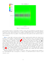
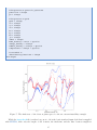
5.1 Electron two stream instability . . . . . . . . . . . . . . . . . . . . . . . . . . . . . . . .
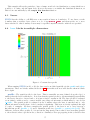
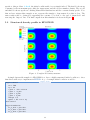
5.2 Structured density profile in EPOCH2D . . . . . . . . . . . . . . . . . . . . . . . . . . .
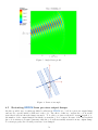
5.3 A hollow cone in 3D . . . . . . . . . . . . . . . . . . . . . . . . . . . . . . . . . . . . . .
63
63
66
67
6 Using IDL to visualise data
6.1 Inspecting Data . . . . . . . . . .
6.2 Getting Help in IDL . . . . . . .
6.3 Manipulating And Plotting Data
6.4 1D Plotting in IDL . . . . . . . .
6.5 Postscript Plots . . . . . . . . . .
6.6 Contour Plots in IDL . . . . . . .
6.7 Shaded Surface Plots in IDL . . .
6.8 Interactive Plotting . . . . . . . .
.
.
.
.
.
.
.
.
.
.
.
.
.
.
.
.
.
.
.
.
.
.
.
.
.
.
.
.
.
.
.
.
.
.
.
.
.
.
.
.
.
.
.
.
.
.
.
.
.
.
.
.
.
.
.
.
.
.
.
.
.
.
.
.
.
.
.
.
.
.
.
.
.
.
.
.
.
.
.
.
.
.
.
.
.
.
.
.
.
.
.
.
.
.
.
.
.
.
.
.
.
.
.
.
.
.
.
.
.
.
.
.
.
.
.
.
.
.
.
.
.
.
.
.
.
.
.
.
.
.
.
.
.
.
.
.
.
.
.
.
.
.
.
.
.
.
.
.
.
.
.
.
.
.
.
.
.
.
.
.
.
.
.
.
.
.
.
.
.
.
.
.
.
.
.
.
.
.
.
.
.
.
.
.
.
.
.
.
.
.
.
.
.
.
.
.
.
.
.
.
.
.
.
.
.
.
.
.
.
.
.
.
.
.
.
.
.
.
.
.
.
.
.
.
.
.
.
.
.
.
.
.
.
.
.
.
.
.
.
.
.
.
.
.
.
.
.
.
71
74
74
75
75
77
77
78
79
7 Using VisIt to visualise data
7.1 LLNL VisIt . . . . . . . . . . . . .
7.2 Obtaining And Installing VisIt . . .
7.3 Compiling The Reader Plugin . . .
7.4 Loading Data Into VisIt . . . . . .
7.5 Contour Plots in VisIt . . . . . . .
7.6 1D Plotting in VisIt . . . . . . . .
7.7 Shaded Surface Plots in VisIt . . .
7.8 Creating User-Defined Expressions
7.9 Creating Movies . . . . . . . . . . .
7.10 Remote Visualisation . . . . . . . .
7.11 Parallel Visualisation . . . . . . . .
.
.
.
.
.
.
.
.
.
.
.
.
.
.
.
.
.
.
.
.
.
.
.
.
.
.
.
.
.
.
.
.
.
.
.
.
.
.
.
.
.
.
.
.
.
.
.
.
.
.
.
.
.
.
.
.
.
.
.
.
.
.
.
.
.
.
.
.
.
.
.
.
.
.
.
.
.
.
.
.
.
.
.
.
.
.
.
.
.
.
.
.
.
.
.
.
.
.
.
.
.
.
.
.
.
.
.
.
.
.
.
.
.
.
.
.
.
.
.
.
.
.
.
.
.
.
.
.
.
.
.
.
.
.
.
.
.
.
.
.
.
.
.
.
.
.
.
.
.
.
.
.
.
.
.
.
.
.
.
.
.
.
.
.
.
.
.
.
.
.
.
.
.
.
.
.
.
.
.
.
.
.
.
.
.
.
.
.
.
.
.
.
.
.
.
.
.
.
.
.
.
.
.
.
.
.
.
.
.
.
.
.
.
.
.
.
.
.
.
.
.
.
.
.
.
.
.
.
.
.
.
.
.
.
.
.
.
.
.
.
.
.
.
.
.
.
.
.
.
.
.
.
.
.
.
.
.
.
.
.
.
.
.
.
.
.
.
.
.
.
.
.
.
.
.
.
.
.
.
.
.
.
.
.
.
.
.
.
.
.
.
.
.
.
.
.
.
.
.
.
.
.
.
.
.
.
.
.
.
.
.
.
.
.
.
.
.
.
.
.
.
.
.
.
.
.
.
.
.
.
80
80
80
81
82
83
85
86
87
88
89
91
2
A Changes between version 3.1 and 4.0
A.1 Changes to the Makefile . . . . . . . . . . . . . .
A.2 Major features and new blocks added to the input
A.3 Additional output block parameters . . . . . . . .
A.4 Other additions to the input deck . . . . . . . . .
. . .
deck
. . .
. . .
.
.
.
.
.
.
.
.
.
.
.
.
.
.
.
.
.
.
.
.
.
.
.
.
.
.
.
.
.
.
.
.
.
.
.
.
.
.
.
.
.
.
.
.
.
.
.
.
.
.
.
.
.
.
.
.
.
.
.
.
.
.
.
.
.
.
.
.
.
.
.
.
.
.
.
.
92
92
92
93
93
B Changes between version 4.0 and 4.3
93
B.1 Changes to the Makefile . . . . . . . . . . . . . . . . . . . . . . . . . . . . . . . . . . . . 93
B.2 Additions to the input deck . . . . . . . . . . . . . . . . . . . . . . . . . . . . . . . . . . 94
B.3 Changes in behaviour which are not due to changes in the input deck . . . . . . . . . . . 95
C References
96
3
1
FAQs
1.1
Is this manual up to date?
Whenever a new milestone version of EPOCH is finalised, the version number is changed and this manual
is updated accordingly. The version number of the manual should match the first two digits for that of
the EPOCH source code. This version number is printed to screen when you run the code. The line
looks something like the following:
Welcome to EPOCH2D Version 4.3.3
(commit v4.3.3-3-g3ed1a0e--clean)
Here, only the number “4.3” is important.
Since version 3.1 of the manual, new additions and changes are mentioned in the appendix.
1.2
What is EPOCH?
EPOCH is a plasma physics simulation code which uses the Particle in Cell (PIC) method. In this
method, collections of physical particles are represented using a smaller number of pseudoparticles, and
the fields generated by the motion of these pseudoparticles are calculated using a finite difference time
domain technique on an underlying grid of fixed spatial resolution. The forces on the pseudoparticles
due to the calculated fields are then used to update the pseudoparticle velocities, and these velocities
are then used to update the pseudoparticle positions. This leads to a scheme which can reproduce the
full range of classical micro-scale behaviour of a collection of charged particles.
1.2.1
Features of EPOCH
• MPI parallelised, explicit, second-order, relativistic PIC code.
• Dynamic load balancing option for making optimal use of all processors when run in parallel.
• MPI-IO based output, allowing restart on an arbitrary number of processors.
• Data analysis and visualisation options include ITT IDL, LLNL VisIt and Mathworks MatLab.
• Control of setup and runs of EPOCH through a customisable input deck.
1.3
The origins of the code
The EPOCH family of PIC codes is based on the older PSC code written by Hartmut Ruhl and retains
almost the same core algorithm for the field updates and particle push routines. EPOCH was written
to add more modern features and to structure the code in such a way that future expansion of the code
is made as easy as possible.
1.4
What normalisations are used in EPOCH?
Since the idea from the start was that EPOCH would be used by a large number of different users and
that it should be as easy as possible to “plug in” different modules from different people into a given
copy of the code, it was decided to write EPOCH in SI units. There are a few places in the code where
some quantities are given in other units for convenience (for example charges are specified in multiples
of the electron charge), but the entire core of the code is written in SI units.
4
1.5
What are those num things doing everywhere?
Historically using the compiler auto-promotion of REAL to DOUBLE PRECISION was unreliable, so EPOCH
uses “kind” tags to specify the precision of the code. The num suffixes and the associated definition
of REALs as REAL(num) are these “kind” tags in operation. The num tags force numerical constants to
match the precision of the code, preventing errors due to precision conversion. The important thing
is that all numerical constants should be tagged with an num tag and all REALs should be defined as
REAL(num).
1.6
What is an input deck?
An input deck is text file which can be used to set simulation parameters for EPOCH without needing
to edit or recompile the source code. It consists of a list of blocks which start as begin:blockname
and end with end:blockname. Within the body of each block is a list of key/value pairs, one per line,
with key and value separated by an equals sign. Most aspects of a simulation can be controlled using
an input deck, such as the number of grid points in the simulation domain, the initial distribution of
particles and initial electromagnetic field configuration. It is designed to be relatively easy to read and
edit. For most projects it should be possible to set up a simulation without editing the source code at
all. For more details, read “3” (Section 3).
1.7
I just want to use the code as a black box, or I’m just starting. How
do I do that?
Begin by reading “5” (Section 5). There’s quite a lot to learn in order to get started, so you should
plan to read through all of this section. You will also need to refer to “3” (Section 3). Next, look at the
code and have a play with some test problems. After that re-read this section. This should be enough
for testing simple problems.
1.8
What is the auto-loader?
Throughout this document we will often refer to the “auto-loader” when setting up the initial particle
distribution. In the input deck it is possible to specify a functional form for the density and temperature
of a particle species. EPOCH will then place the particles to match the density function and set the
velocities of the particles so that they match the Maxwellian thermal distribution for the temperature.
The code which performs this particle set up is called the “auto-loader”.
At present, there is no way to specify a non-Maxwellian particle distribution from within the input
deck. In such cases, it is necessary to edit and recompile the EPOCH source code. The recommended
method for setting the initial particle properties is to use the “manual load” function as described in
Section 4.2.
1.9
What is a maths parser?
As previously mentioned, the behaviour of EPOCH is controlled using an input deck which contains a
list of key/value pairs. The value part of the pair is not restricted to simple constants but can be a
complex mathematical expression. It is evaluated at run time using a section of code called the “maths
parser”. There is no need for the end user to know anything about this code. It is just there to enable
the use of mathematical expressions in the input deck. Further information about this facility can be
found in Section 3.15.
1.10
I am an advanced user, but I want to set up the code so that less
experienced users can use it. How do I do that?
See “4.6” (Section 4.6).
5
1.11
I want to develop an addition to EPOCH. How do I do that?
A slightly outdate developers manual exists which should be sufficient to cover most aspects of the
code functionality. However, the code is written in a fairly modular and consistent manner, so reading
through that is the best source of information. If you get stuck then you can post questions on the
CCPForge forums.
1.12
I want to have a full understanding of how EPOCH works. How do I
do that?
If you really want to understand EPOCH in full, the only way is to read all of this manual and then
read through the code. Most of it is commented.
6
EPOCH for end users
2
This manual aims to give a complete description of how to set up and run EPOCH as an end user.
Further details on the design and implemetation of the code may be found in Arber et al. [1] and
Ridgers et al. [2].
We begin by giving a brief overview of the EPOCH code-base, how to compile and run the code.
Note that throughout this user manual, instructions are given assuming that you are typing commands
at a UNIX terminal.
2.1
Structure of the EPOCH codes
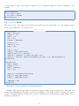
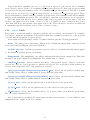
When obtained, the EPOCH codes all have a similar structure. If the tarred and gzipped archive
(commonly referred to as a tarball) is downloaded and unpacked into the user’s $HOME directory, then
the extracted contents will consist of a directory named “$HOME/epoch-4.3.3” (with “4.3.3” substituted
by the current version number) and the subdirectories and files listed below.
Alternatively, if the code is checked out from the CCPForge subversion repository with the command
svn checkout --username <user> http://ccpforge.cse.rl.ac.uk/svn/epoch
then the directory will be “$HOME/epoch/trunk”. In this case, the directories “$HOME/epoch/branches”
and “$HOME/epoch/tags” will also be created. These two directories are entirely unnecessary. You can
avoid creating them by checking out the subversion repository using the following command
svn co --username <user> http://ccpforge.cse.rl.ac.uk/svn/epoch/trunk epoch
All the required source code will then be contained in a directory named “$HOME/epoch”.
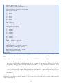
Once the code has been obtained, the top-level directory will contain the following 5 directories and
two files
• epoch1d - Source code and other files required for the 1D version of EPOCH.
• epoch2d - Source code and other files required for the 2D version of EPOCH.
• epoch3d - Source code and other files required for the 3D version of EPOCH.
• MatLab - The files for creating a plug-in for the Mathworks MatLab visualisation tool for reading
SDF files generated by an EPOCH run.
• VisIt - The files for creating a plug-in for the LLNL VisIt parallel visualisation tool for reading
SDF files generated by an EPOCH run.
• CODING STYLE - This document contains the conventions which must be used for any code
being submitted for inclusion in the EPOCH project.
• epoch tarball.ssh - This is a shell script which is used for creating the tarred and gzipped archives
of EPOCH which are posted to CCPForge each time a new release is made.
The three EPOCH subdirectories all have a similar structure. Inside each of the epoch{1,2,3}d
directories, there are 4 sub-directories:
• src - The EPOCH source code.
• IDL - The IDL routines needed to open the SDF files which the code outputs.
• example decks - A sample data directory containing example input deck files.
• Data - This is an empty directory to use for running simulations.
there are also 5 files:
• COMMIT - Contains versioning information for the code.
7
• Changelog.txt - A brief overview of the change history for each released version of EPOCH.
• Makefile - A standard makefile.
• Start.pro - An IDL script which starts the IDL visualisation routines. Execute it using “idl Start”.
• unpack source from restart - Restart dumps can be written to contain a copy of the input decks
and source code used to generate them. This script can be used to unpack that information from
a given restart dump. It is run from the command line and must be passed the name of the restart
dump file.
2.2
Libraries and requirements
The EPOCH codes are written using MPI for parallelism, but have no other libraries or dependencies.
Currently, the codes are written to only require MPI1.2 compatible libraries, although this may change to
require full MPI2 compliance in the future. Current versions of both MPICH and OpenMPI implement
the MPI2 standard and are known to work with this code. The SCALI MPI implementation is only
compliant with the MPI1.2 specification and may loose support soon. There are no plans to write a
version of EPOCH which does not require the MPI libraries.
The code is supplied with a standard GNU make Makefile, which is also compatible with most other
forms of the make utility. In theory it is possible to compile the code without a make utility, but it is
much easier to compile the code using the supplied makefile.
2.3
Compiling and running EPOCH
To compile EPOCH in the supplied state, you must first change to the correct working directory. As
explained in Section 2.1, the root directory for EPOCH contains several subdirectories, including separate
directories for each of the 1D, 2D and 3D versions of the code. To compile the 2D version of the code,
you first switch to the “epoch2d” directory using the command
cd $HOME/epoch/epoch2d
and then type
make
and the code will compile. There are certain options within the code which are controlled by compiler
preprocessors and are described in the next section. When the code is compiled, it creates a new directory
called “bin” containing the compiled binary which will be called epoch1d, epoch2d or epoch3d. To
run the code, just execute the binary file by typing:
./bin/epoch2d
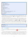
or whatever the correct binary is for the dimensionality of the code that you have. You should be given
a screen which begins with the EPOCH logo, and then reads:
Welcome to EPOCH2D Version 4.3.3
(commit v4.3.3-3-g3ed1a0e--clean)
The code was compiled with the following compile time options
*************************************************************
Per particle weighting -DPER_PARTICLE_WEIGHT
Tracer particle support -DTRACER_PARTICLES
Particle probe support -DPARTICLE_PROBES
*************************************************************
Code is running on 1 processing elements
Specify output directory
8
At this point, the user simply types in the name of the (already existing) output directory and the
code will read the input deck files inside the specified directory and start running. To run the code in
parallel, just use the normal mpirun or mpiexec scripts supplied by your MPI implementation. If you
want the code to run unattended, then you will need to pipe in the output directory name to be used.
The method for doing this varies between MPI implementations. For many MPI implementations (such
as recent versions of OpenMPI) this can be achieved with the following:
echo Data | mpirun -np 2 ./bin/epoch2d
Some cluster setups accept the following instead:
mpirun -np 2 ./bin/epoch2d < deck.file
where “deck.file” is a file containing the name of the output directory. Some cluster queueing systems
do not allow the use of input pipes to mpirun. In this case, there is usually a “-stdin” command line
option to specify an input file. See your cluster documentation for more details.
As of version 4.2.12, EPOCH now checks for the existence of a file named “USE DATA DIRECTORY”
in the current working directory before it prompts the user for a Data directory. If such a file exists, it
reads it to obtain the name of the data directory to use and does not prompt the user. If no such file
exists, it prompts for a data directory name as before. This is useful for cluster setups in which it is
difficult or impossible to pipe in the directory name using a job script.
The “Makefile” supplied with EPOCH is setup to use the Intel compiler by default. However, it
also contains configurations for gfortran, pgi, g95, hector and ibm (the compiler suite used on IBM’s
BlueGene machines). In order to compile using one of the listed configurations, add the “COMPILER=”
option to the “make” command. For example
make COMPILER=gfortran
will compile the code using the gfortran compiler and appropriate compiler flags. You can also compile
the code with debugging flags by adding “MODE=debug” and can compile using more than one processor
by using “-j<n>”, where “<n>” is the number of processors to use. Note that this is just to speed up
the compilation process; the resulting binary can be run on any number of processors.
2.4
Compiler flags and preprocessor defines
As already stated, some features of the code are controlled by compiler preprocessor directives. The
flags for these preprocessor directives are specified in “Makefile” and are placed on lines which look like
the following:
DEFINES += $(D)PER_PARTICLE_WEIGHT
On most machines “$(D)” just means “-D” but the variable is required to accommodate more exotic
setups.
Most of the flags provided in the “Makefile” are commented out by prepending them with a
“#” symbol (the “make” system’s comment character). To turn on the effect controlled by a given
preprocessor directive, just uncomment the appropriate “DEFINES” line by deleting this “#” symbol.
The options currently controlled by the preprocessor are:
• PER PARTICLE WEIGHT - Instead of running the code where each pseudoparticle represents
the same number of real particles, each pseudoparticle can represent a different number of real
particles. Many of the codes more advanced features require this and it is turned on by default.
It can be turned off to save on memory, but this is recommended only for advanced users.
• TRACER PARTICLES - Gives the option to specify one or more species as tracer particles. Tracer
particles are specified like normal particles, and move about as would a normal particle with
the same charge and mass, but tracer particles do not generate any current and are therefore
passive elements in the simulation. Any attempt to add particle collision effects should remember
9
that tracer species should not interact through collisions. The implementation of tracer particles
requires an additional “IF” clause in the particle push, so it is not activated by default.
• PARTICLE PROBES - For laser plasma interaction studies it can sometimes be useful to be able
to record information about particles which cross a plane in the simulation. Since this requires
the code to check whether each particles has crossed the plane in the particles pusher and also to
store copies of particles until the next output dump, it is a heavyweight diagnostic. Therefore,
this diagnostic is only enabled when the code is compiled with this directive.
• PARTICLE SHAPE TOPHAT - By default, the code uses a first order b-spline (triangle) shape
function to represent particles giving third order particle weighting. Using this flag changes the
particle representation to that of a top-hat function (0th order b-spline yielding a second order
weighting).
• PARTICLE SHAPE BSPLINE3 - This flag changes the particle representation to that of a 3rd
order b-spline shape function (5th order weighting).
• PARTICLE ID - When this option is enabled, all particles are assigned a unique identification
number when writing particle data to file. This number can then be used to track the progress of
a particle during the simulation.
• PARTICLE ID4 - This does the same as the previous option except it uses a 4-byte integer instead
of an 8-byte one. Whilst this saves storage space, care must be taken that the number does not
overflow.
• PHOTONS - This enables support for photon particle types in the code. These are a pre-requisite
for modelling synchrotron emission, radiation reaction and pair production (see Section 3.12).
• TRIDENT PHOTONS - This enables support for virtual photons which are used by the Trident
process for pair production.
• PARTICLE COUNT UPDATE - Makes the code keep global particle counts for each species on
each processor. This information isn’t needed by the core algorithm, but can be useful for developing some types of additional physics packages. It does require one additional MPI ALL REDUCE
per species per timestep, so it is not activated by default.
• PREFETCH - This enables an Intel-specific code optimisation.
• PARSER DEBUG - The code outputs more detailed information whilst parsing the input deck.
This is a debug mode for code development.
• PARTICLE DEBUG - Each particle is additionally tagged with information about which processor
it is currently on, and which processor it started on. This is a debug mode for code development.
• MPI DEBUG - This option installs an error handler for MPI calls which should aid tracking down
some MPI related errors.
• NO IO - This option disables all file I/O which can be useful when doing benchmarking.
• PER PARTICLE CHARGE MASS - By default, the particle charge and mass are specified on a
per-species basis. With this flag enabled, charge and mass become a per-particle property. This
is a legacy flag which will be removed soon.
If a user requests an option which the code has not been compiled to support then the code will give
an error message as follows:
10
*** WARNING ***
The element "particle_probes" of block "output" cannot be set
because the code has not been compiled with the correct preprocessor options.
Code will continue, but to use selected features, please recompile with the
-DPARTICLE_PROBES option
It is also possible to pass other flags to the compiler. In “Makefile” there is a line which reads
FFLAGS = -O3 -fast
The two commands to the right are compiler flags and are passed unaltered to the FORTRAN compiler.
Change this line to add any additional flags required by your compiler.
By default, EPOCH will write a copy of the source code and input decks into each restart dump.
This can be very useful since a restart dump contains an exact copy of the code which was used to
generate it, ensuring that you can always regenerate the data or continue running from a restart. The
output can be prevented by using “dump source code = F” and “dump input deck = F” in the output
block. However, the functionality is difficult to build on some platforms so the Makefile contains a line
for bypassing this section of the build process. Just below all the DEFINE flags there is the following
line:
# ENCODED_SOURCE = dummy_encoded_source.o
Just uncomment this line and source code in restart dumps will be permanently disabled.
2.5
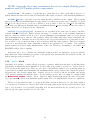
Running EPOCH and basic control of EPOCH1D
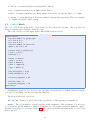
When the code is run, the output is
Command line output
d########P d########b
.######b
d####### d##P
d##P
d########P d###########
d###########
.########## d##P
d##P
---------- ---------------- P
d########P d####,,,####P ####.
.#### d###P
d############P
d########P d#########P
####
.###P ####.
d############P
d##P
d##P
####
d####
####.
d##P
d##P
d########P d##P
###########P
##########P d##P
d##P
d########P d##P
d######P
#######P d##P
d##P
Welcome to EPOCH2D Version 4.3.3
(commit v4.3.3-3-g3ed1a0e--clean)
The code was compiled with the following compile time options
*************************************************************
Per particle weighting -DPER_PARTICLE_WEIGHT
Tracer particle support -DTRACER_PARTICLES
Particle probe support -DPARTICLE_PROBES
*************************************************************
Code is running on 1 processing elements
Specify output directory
At which point the end user should simply type in the name of the directory where the code output
is to be placed. This directory must also include the file “input.deck” which controls the code setup,
specifies how to set the initial conditions and controls the I/O. Writing an input deck for EPOCH is
11
fairly time consuming and so the code is supplied with some example input decks which include all the
necessary sections for the code to run.
3
The EPOCH input deck
Most of the control of EPOCH is through a text file called input.deck. The input deck file must be in
the output directory which is passed to the code at runtime and contains all the basic information which
is needed to set up the code, including the size and subdivision of the domain, the boundary conditions,
the species of particles to simulate and the output settings for the code. For most users this will be
capable of specifying all the initial conditions and output options they need. More complicated initial
conditions will be handled in later sections.
The input deck is a structured file which is split into separate blocks, with each block containing
several “parameter” = “value” pairs. The pairs can be present in any order, and not all possible
pairs must be present in any given input deck. If a required pair is missing the code will exit
with an error message. The blocks themselves can also appear in any order. The input deck is
case sensitive, so true is always “T”, false is always “F” and the names of the parameters are always lower case. Parameter values are evaluated using a maths parser which is described in Section 3.15.
If the deck contains a “\” character then the rest of the line is ignored and the next line becomes
a continuation of the current one. Also, the comment character is “#”; if the “#” character is used
anywhere on a line then the remainder of that line is ignored.
There are three input deck directive commands, which are:
• begin:block - Begin the block named block.
• end:block - Ends the block named block.
• import:filename - Includes another file (called filename) into the input deck at the point where the
directive is encountered. The input deck parser reads the included file exactly as if the contents
of the included file were pasted directly at the position of the import directive.
Each block must be surrounded by valid begin: and end: directives or the input deck will fail. There are
currently fourteen valid blocks hard coded into the input deck reader, but it is possible for end users to
extend the input deck. The fourteen built in blocks are:
• control - Contains information about the general code setup.
• boundaries - Contains information about the boundary conditions for this run.
• species - Contains information about the species of particles which are used in the code. Also
details of how these are initialised.
• laser - Contains information about laser boundary sources.
• fields - Contains information about the EM fields specified at the start of the simulation.
• window - Contains information about the moving window if the code is used in that fashion.
• output - Contains information about when and how to dump output files.
• output global - Contains parameters which should be applied to all output blocks.
• dist fn - Contains information about distribution functions that should be calculated for output.
• probe - Contains information about particle probes used for output.
12
• collisions - Contains information about particle collisions.
• qed - Contains information about QED pair production.
• subset - Contains configuration for filters which can be used to modify the data to be output.
• constant - Contains information about user defined constants and expressions. These are designed
to simplify the initial condition setup.
3.1
control block
The control block sets up the basic code properties for the domain, the end time of the code, the load
balancer and the types of initial conditions to use.
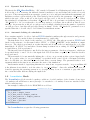
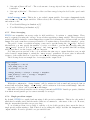
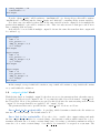
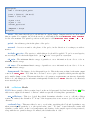
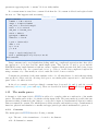
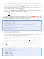
The control block of a valid input deck for EPOCH2D reads as follows:
control block
begin:control
# global number of gridpoints
nx = 512 # in x
ny = 512 # in y
# global number of particles
npart = 10 * nx * ny
# final time of simulation
t_end = 1.0e-12
# nsteps = -1
# size of domain
x_min = -0.1e-6
x_max = 400.0e-6
y_min = -400.0e-6
y_max = 400.0e-6
# dt_multiplier = 0.95
# dlb_threshold = 0.8
# restart_snapshot = 98
# field_order = 2
# stdout_frequency = 10
end:control
As illustrated in the above code block, the “#” symbol is treated as a comment character and the
code ignores everything on a line following this character.
The allowed entries are as follows:
nx, ny, nz - Number of grid points in the x,y,z direction. This parameter is mandatory.
npart - The global number of pseudoparticles in the simulation. This parameter does not need
to be given if a specific number of particles is supplied for each particle species by using the “npart”
directive in each species block (see Section 3.3). If both are given then the value in the control block
will be ignored.
13
nsteps - The number of iterations of the core solver before the code terminates. Negative numbers
instruct the code to only terminate at t end. If nsteps is not specified then t end must be given.
t end - The final simulation time in simulation seconds before the code terminates. If t end
is not specified then nsteps must be given. If they are both specified then the first time restriction
to be satisfied takes precedence. Sometimes it is more useful to specify the time in picoseconds or
femtoseconds. To accomplish this, just append the appropriate multiplication factor. For example,
“t end = 3 * femto” specifies 3 femtoseconds. A list of multiplication factors is supplied in Section 3.15.1.
{x,y,z} min - Minimum grid position of the domain in metres. These are required parameters.
Can be negative. “{x,y,z} start” is accepted as a synonym. In a similar manner to that described
above, distances can be specified in microns using a multiplication constant. eg. “x min = 4 * micron”
specifies a distance of 4µm.
{x,y,z} max - Maximum grid position of the domain in metres. These are required parameters.
Must be greater than {x,y,z} min. “{x,y,z} end” is accepted as a synonym.
dt multiplier - Factor by which the timestep is multiplied before it is applied in the code, i.e. a
multiplying factor applied to the CFL condition on the timestep. Must be less than one. If no value is
given then the default of 0.95 is used.
dlb threshold - The minimum ratio of the load on the least loaded processor to that on the
most loaded processor allowed before the code load balances. Set to 1 means always balance, set to
0 means never balance. If this parameter is not specified then the code will only be load balanced at
initialisation time.
restart snapshot - The number of a previously written restart dump to restart the code from.
If not specified then the initial conditions from the input deck are used.
Note that as of version 4.2.5, this parameter can now also accept a filename in place of a number.
If you want to restart from “0012.sdf” then it can either be specified using “restart snapshot = 12”, or
alternatively it can be specified using “restart snapshot = 0012.sdf”. This syntax is required if output
file prefixes have been used (see Section 3.7).
field order - Order of the finite difference scheme used for solving Maxwell’s equations. Can be
2, 4 or 6. If not specified, the default is to use a second order scheme.
stdout frequency - If specified then the code will print a one line status message to stdout
after every given number or timesteps. The default is to print nothing to screen (ie. “stdout frequency
= 0”).
use random seed - The initial particle distribution is generated using a random number
generator. By default, EPOCH uses a fixed value for the random generator seed so that results are
repeatable. If this flag is set to “T” then the seed will be generated using the system clock.
nproc{x,y,z} - Number of processes in the x,y,z directions. By default, EPOCH will try to pick
the best method of splitting the domain amongst the available processors but occasionally the user may
wish to override this choice.
smooth currents - This is a logical flag. If set to “T” then a smoothing function is applied to
the current generated during the particle push. This can help to reduce noise and self-heating in a simulation. The smoothing function used is the same as that outlined in Buneman [3]. The default value is “F”.
14
field ionisation - Logical flag which turns on field ionisation. See Section 3.3.2.
use bsi - Logical flag which turns on barrier suppression ionisation correction to the tunnelling
ionisation model for high intensity lasers. See Section 3.3.2. This flag should always be enabled when
using field ionisation and is only supplied for testing purposes. The default is “T”.
use multiphoton - Logical flag which turns on modelling ionisation by multiple photon
absorption. This should be set to “F” if there is no laser attached to a boundary as it relies on laser
frequency. See Section 3.3.2. This flag should always be enabled when using field ionisation and is only
supplied for testing purposes. The default is “T”.
particle tstart - Specifies the time at which to start pushing particles. This allows the field to
evolve using the Maxwell solver for a specified time before beginning to move the particles.
use exact restart - Logical flag which makes a simulation restart using exactly the same
configuration as the original simulation. If set to “T” then the domain split amongst processors will
be identical along with the seeds for the random number generators. Note that the flag will be ignored if the number of processors does not match that used in the original run. The default value is “F”.
allow cpu reduce - Logical flag which allows the number of CPUs used to be reduced from
the number specified. In some situations it may not be possible to divide the simulation amongst all
the processors requested. If this flag is set to “T” then EPOCH will continue to run and leave some of
the requested CPUs idle. If set to “F” then code will exit if all CPUs cannot be utilised. The default
value is “T”.
check stop file frequency - Integer parameter controlling automatic halting of the code.
The frequency is specified as number of simulation cycles. Refer to description later in this section.
The default value is 10.
stop at walltime - Floating point parameter controlling automatic halting of the code. Refer
to description later in this section. The default value is -1.0.
stop at walltime file - String parameter controlling automatic halting of the code. Refer to
description later in this section. The default value is an empty string.
simplify deck - If this logical flag is set to “T” then the deck parser will attempt to simplify
the maths expressions encountered after the first pass. This can significantly improve the speed of
evaluation for some input deck blocks. The default value is “F”.
print constants - If this logical flag is set to “T”, deck constants are printed to the “deck.status”
file as they are parsed. The default value is “F”.
use migration - Logical flag which determines whether or not to use particle migration. The
default is “F”. See Section 3.3.1.
migration interval - The number of timesteps between each migration event. The default is 1
(migrate at every timestep). See Section 3.3.1.
Most of the control block is self explanatory, but there are two parts which need further description.
15
3.1.1
Dynamic Load Balancing
The first is the dlb threshold flag. “dlb” stands for Dynamic Load Balancing and, when turned on,
it allows the code to rearrange the internal domain boundaries to try and balance the workload on each
processor. This rearrangement is an expensive operation, so it is only performed when the maximum load
imbalance reaches a given critical point. This critical point is given by the parameter “dlb threshold”
which is the ratio of the workload on the least loaded processor to the most loaded processor. When
the calculated load imbalance is less than “dlb threshold” the code performs a re-balancing sweep, so if
“dlb threshold = 1.0” is set then the code will keep trying to re-balance the workload at almost every
timestep. At present the workload on each processor is simply calculated from the number of particles
on each processor, but this will probably change in future. If the “dlb threshold” parameter is not
specified then the code will only be load balanced at initialisation time.
3.1.2
Automatic halting of a simulation
It is sometimes useful to be able to halt an EPOCH simulation midway through execution and generate
a restart dump. Two methods have been implemented to enable this.
The first method is to check for the existence of a “STOP” file. Throughout execution, EPOCH will
check for the existence of a file named either “STOP” or “STOP NODUMP” in the simulation output
directory. The check is performed at regular intervals and if such a file is found then the code exits
immediately. If “STOP” is found then a restart dump is written before exiting. If “STOP NODUMP”
is found then no I/O is performed.
The interval between checks is controlled by the integer parameter “check stop frequency” which can
be specified in the “control” block of the input deck. If it is less than or equal to zero then the check is
never performed.
The next method for automatically halting the code is to stop execution after a given elapsed walltime. If a positive value for “stop at walltime” is specified in the control block of an input deck then
the code will halt once this time is exceeded and write a restart dump. The parameter takes a real
argument which is the time in seconds since the start of the simulation.
An alternative method of specifying this time is to write it into a separate text file. “stop at walltime file”
is the filename from which to read the value for “stop at walltime”. Since the walltime will often be
found by querying the queueing system in a job script, it may be more convenient to pipe this value
into a text file rather than modifying the input deck.
3.2
boundaries block
The boundaries block sets the boundary conditions of each boundary of the domain. Some types
of boundaries allow EM wave sources (lasers) to be attached to a boundary. Lasers are attached at the
initial conditions stage.
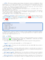
An example boundary block for EPOCH2D is as follows:
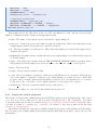
boundaries block
begin:boundaries
bc_x_min = simple_laser
bc_x_max_field = simple_outflow
bc_x_max_particle = simple_outflow
bc_y_min = periodic
bc_y_max = periodic
end:boundaries
The boundaries accepts the following parameters:
16
bc {x,y,z} min - The condition for the lower boundary for both fields and particles. “xbc left”,
“ybc down” and “zbc back” are accepted as a synonyms.
bc {x,y,z} min {field,particle} - The condition for the lower boundary for {fields,particles}.
“xbc left {field,particle}”, “ybc down {field,particle}” and “zbc back {field,particle}” are accepted as
a synonyms.
bc {x,y,z} max - The condition for the upper boundary for both fields and particles.
“xbc right”, “ybc up” and “zbc front” are accepted as a synonyms.
bc {x,y,z} max {field,particle} - The condition for the upper boundary for {fields,particles}.
“xbc right {field,particle}”, “ybc up {field,particle}” and “zbc front {field,particle}” are accepted as a
synonyms.
cpml thickness - The thickness of the CPML boundary in terms of the number of grid cells
(see Section 3.2.1). The default value is 6.
cpml kappa max - A tunable CPML parameter (see Section 3.2.1).
cpml a max - A tunable CPML parameter (see Section 3.2.1).
cpml sigma max - A tunable CPML parameter (see Section 3.2.1).
There are ten boundary types in EPOCH and each boundary of the domain can have one and only
one of these boundaries attached to it. These boundary types are:
periodic - A simple periodic boundary condition. Fields and/or particles reaching one edge of the
domain are wrapped round to the opposite boundary. If either boundary condition is set to periodic
then the boundary condition on the matching boundary at the other side of the box is also assumed
periodic.
simple laser - A characteristic based boundary condition to which one or more EM wave sources
can be attached. EM waves impinging on a simple laser boundary are transmitted with as little
reflection as possible. Particles are fully transmitted. The field boundary condition works by allowing
outflowing characteristics to propagate through the boundary while using the attached lasers to specify
the inflowing characteristics. The particles are simply removed from the simulation when they reach
the boundary.
simple outflow - A simplified version of simple laser which has the same properties of
transmitting incident waves and particles, but which cannot have EM wave sources attached to it.
These boundaries are about 5% more computationally efficient than simple laser boundaries with no
attached sources. This boundary condition again allows outflowing characteristics to flow unchanged,
but this time the inflowing characteristics are set to zero. The particles are again simply removed from
the simulation when they reach the boundary.
reflect - This applies reflecting boundary conditions to particles. When specified for fields, all
field components are clamped to zero.
conduct - This applies perfectly conducting boundary conditions to the field. When specified for
particles, the particles are reflected.
open - When applied to fields, EM waves outflowing characteristics propagate through the
17
boundary. Particles are transmitted through the boundary and removed from the system.
cpml laser - See Section 3.2.1.
cpml outflow - See Section 3.2.1.
thermal - See Section 3.2.2.
NOTE: If simple laser, simple outflow, cpml laser, cpml outflow or open
are specified on one or more boundaries then the code will no longer
necessarily conserve mass.
Note also that it is possible for the user to specify contradictory, unphysical boundary conditions. It
is the users responsibility that these flags are set correctly.
3.2.1
CPML boundary conditions
There are now Convolutional Perfectly Matched Layer boundary conditions in EPOCH. The implementation closely follows that outlined in the book “Computational Electrodynamics: The Finite-Difference
Time-Domain Method” by Taflove and Hagness [4]. See also Roden and Gedney [5].
CPML boundaries are specified in the input deck by specifying either “cpml outflow” or “cpml laser”
in the boundaries block. “cpml outflow” specifies an absorbing boundary condition whereas “cpml laser”
is used to attach a laser to an otherwise absorbing boundary condition.
There are also four configurable parameters:
cpml thickness - The thickness of the CPML boundary in terms of the number of grid cells.
The default value is 6.
cpml kappa max, cpml a max, cpml sigma max - These are tunable parameters
which affect the behaviour of the absorbing media. The notation follows that used in the two references
quoted above. Note that the “cpml sigma max” parameter is normalised by σopt which is taken to
be 3.2/dx (see Taflove and Hagness [4] for details). These are real valued parameters which take the
following default values: cpml kappa max=20, cpml a max=0.15, cpml sigma max=0.7
An example usage is as follows:
begin:boundaries
cpml_thickness = 16
cpml_kappa_max = 20
cpml_a_max = 0.2
cpml_sigma_max = 0.7
bc_x_min = cpml_laser
bc_x_max = cpml_outflow
bc_y_min = cpml_outflow
bc_y_max = cpml_outflow
end:boundaries
3.2.2
Thermal boundaries
Thermal boundary conditions have been added to the “boundaries” block. These simulate the existence
of a “thermal bath” of particles in the domain adjacent to the boundary. When a particle leaves
the simulation it is replace with an incoming particle sampled from a Maxwellian of a temperature
18
corresponding to that of the initial conditions. It is requested using the keyword “thermal”. For
example:
begin:boundaries
bc_x_min = laser
bc_x_max = thermal
end:boundaries
3.3
species block
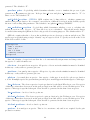
The next section of the input deck describes the particle species used in the code. An example species
block for any EPOCH code is given below.
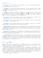
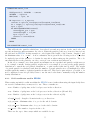
species block
begin:species
name = Electron
charge = -1.0
mass = 1.0
frac = 0.5
# npart = 2000*100
# tracer = F
density = 1.e4
temp = 1e6
temp_x = 0.0
temp_y = temp_x(Electron)
density_min = 0.1 * den_max
density = if(abs(x) lt thick, den_max, 0.0)
density = if((x gt -thick) and (abs(y) gt 2e-6), 0.0, density(Carbon))
end:species
begin:species
name = Carbon
charge = 4.0
mass = 1836.0*12
frac = 0.5
density = 0.25*density(Electron)
temp_x = temp_x(Electron)
temp_y = temp_x(Electron)
dumpmask = full
end:species
Each species block accepts the following parameters:
name - This specifies the name of the particle species defined in the current block. This name can
include any alphanumeric characters in the basic ASCII set. The name is used to identify the species
in any consequent input block and is also used for labelling species data in any output dumps. It is a
mandatory parameter.
19
NOTE: IT IS IMPOSSIBLE TO SET TWO SPECIES WITH THE
SAME NAME!
charge - This sets the charge of the species in multiples of the electron charge. Negative numbers
are used for negatively charged particles. This is a mandatory parameter.
mass - This sets the mass of the species in multiples of the electron mass. Cannot be negative.
This is a mandatory parameter.
npart - This specifies the number of pseudoparticles which should be loaded into the simulation
domain for this species block. Using this parameter is the most convenient way of loading particles
for simulations which contain multiple species with different number densities. If npart is specified in
a species block then any value given for npart in the control block is ignored. npart should not be
specified at the same time as frac within a species block.
frac - This specifies what fraction of npart (the global number of particles specified in the control
block) should be assigned to the species.
NOTE: frac should not be specified at the same time as npart for a given
species.
npart per cell - Integer parameter which specifies the number of particles per cell to use for the
initial particle loading. At a later stage this may be extended to allow “npart per cell” to be a spatially
varying function.
If per-species weighting is used then the value of “npart per cell” will be the average number of
particles per cell. If “npart” or “frac” have also been specified for a species, then they will be ignored.
To avoid confusion, there is no globally used “npart per species”. If you want to have a single value
to change in the input deck then this can be achieved using a constant block.
dumpmask - Determines which output dumps will include this particle species. The dumpmask
has the same semantics as those used by variables in the “output” block, described in Section 3.7. The
actual dumpmask from the output block is applied first and then this one is applied afterwards. For
example, if the species block contains “dumpmask = full” and the output block contains “vx = always”
then the particle velocity will be only be dumped at full dumps for this particle species. The default
dumpmask is “always”.
dump - This logical flag is provided for backwards compatibility. If set to “F” it has the same
meaning as “dumpmask = never”. If set to “T” it has the same meaning as “dumpmask = always”.
tracer - Logical flag switching the particle species into tracer particles. Tracer particles are
enabled with the correct precompiler option, and when set for a given species make that species move
correctly for its charge and mass, but contribute no current. This means that these particles are passive
tracers in the plasma. “tracer = F” is the default value.
identify - Used to identify the type of particle. Currently this is used primarily by the QED
routines. See Section 3.12 for details.
immobile - Logical flag. If this parameter is set to “T” then the species will be ignored during
the particle push. The default value is “F”.
The species blocks are also used for specifying initial conditions for the particle species. The initial
conditions in EPOCH can be specified in various ways, but the easiest way is to specify the initial
20
conditions in the input deck file. This allows any initial condition which can be specified everywhere in
space by a number density and a drifting Maxwellian distribution function. These are built up using the
normal maths expressions, by setting the density and temperature for each species which is then used
by the autoloader to actually position the particles.
The elements of the species block used for setting initial conditions are:
density - Particle number density in m−3 . As soon as a density= line has been read, the values
are calculated for the whole domain and are available for reuse on the right hand side of an expression.
This is seen in the above example in the first two lines for the Electron species, where the density is
first set and then corrected. If you wish to specify the density in parts per cubic metre then you can
divide by the “cc” constant (see Section 3.15.1). This parameter is mandatory.
density min - Minimum particle number density in m−3 . When the number density in a cell
falls below density min the autoloader does not load any pseudoparticles into that cell to minimise the
number of low weight, unimportant particles. If set to 0 then all cells are loaded with particles. This is
the default.
density max - Maximum particle number density in m−3 . When the number density in a cell
rises above density max the autoloader clips the density to density max allowing easy implementation
of exponential rises to plateaus. If it is a negative value then no clipping is performed. This is the default.
mass density - Particle mass density in kg m−3 . The same as “density” but multiplied by the
particle mass. If you wish to use units of g cm−3 then append the appropriate multiplication factor.
For example: “mass_density = 2 * 1e3 / cc”.
temp {x,y,z} - The temperature in each direction for a thermal distribution in Kelvin.
temp - Sets an isotropic temperature distribution in Kelvin. If both temp and a specific temp x,
temp y, temp z parameter is specified then the last to appear in the deck has precedence. If neither are
given then the species will have a default temperature of zero Kelvin.
temp {x,y,z} ev, temp ev - These are the same as the temperature parameters described
above except the units are given in electronvolts rather than Kelvin.
drift {x,y,z} - Specifies a momentum space offset in kg ms−1 to the distribution function for
this species. By default, the drift is zero.
offset - File offset. See below for details.
It is also possible to set initial conditions for a particle species using an external file. Instead of
specifying the initial conditions mathematically in the input deck, you specify in quotation marks the
filename of a simple binary file containing the information required.
external initial conditions
begin:species
name = Electron
density = ’Data/ic.dat’
offset = 80000
temp_x = ’Data/ic.dat’
end:species
An additional element is also introduced, the offset element. This is the offset in bytes from the
start of the file to where the data should be read from. As a given line in the block executes, the file
21
is opened, the file handle is moved to the point specified by the offset parameter, the data is read and
the file is then closed. Therefore, unless the offset value is changed between data reading lines the
same data will be read into all the variables. The data is read in as soon as a line is executed, and so
it is perfectly possible to load data from a file and then modify the data using a mathematical expression.
The file should be a simple binary file consisting of floating point numbers of the same precision
as num in the core EPOCH code. For multidimensional arrays, the data is assumed to be written
according to FORTRAN array ordering rules (ie. column-major order).
NOTE: The files that are expected by this block are SIMPLE BINARY
files, NOT FORTRAN unformatted files. It is possible to read FORTRAN
unformatted files using the offset element, but care must be taken!
3.3.1
Particle migration between species
It is sometimes useful to separate particle species into separate energy bands and to migrate particles
between species when they become more or less energetic. A method to achieve this functionality has
been implemented. It is specified using two parameters to the “control” block:
use migration - Logical flag which determines whether or not to use particle migration. The
default is “F”.
migration interval - The number of timesteps between each migration event. The default is 1
(migrate at every timestep).
The following parameters are added to the “species” block:
migrate - Logical flag which determines whether or not to consider this species for migration.
The default is “F”.
promote to - The name of the species to promote particles to.
demote to - The name of the species to demote particles to.
promote multiplier - The particle is promoted when its energy is greater than “promote multiplier” times the local average. The default value is 1.
demote multiplier - The particle is demoted when its energy is less than “demote multiplier”
times the local average. The default value is 1.
promote density - The particle is only considered for promotion when the local density is less
than “promote density”. The default value is the largest floating point number.
demote density - The particle is only considered for demotion when the local density is greater
than “demote density”. The default value is 0.
3.3.2
Ionisation
EPOCH now includes field ionisation which can be activated by defining ionisation energies and an
electron for the ionising species. This is done via the species block using the following parameters:
22
ionisation energies - This is an array of ionisation energies (in Joules) starting from the
outermost shell. It expects to be given all energies down to the fully ionised ion; if the user wishes to
exclude some inner shell ionisation for some reason they need to give this a very large number. Note
that the ionisation model assumes that the outermost electron ionises first always, and that the orbitals
are filled assuming ground state. When this parameter is specified it turns on ionisation modelling.
If you wish to specify the values in Electron-Volts, add the “ev” multiplication factor (see Section 3.15.1).
ionisation electron species - Name of the electron species. This can be specified as an
array in the event that the user wishes some levels to have a different electron species which can be
handy for monitoring ionisation at specific levels. “electron” and “electron species” are accepted as
synonyms.
For example, ionising carbon species might appear in the input deck as:
begin:species
charge = 0.0
mass = 1837.2
name = carbon
ionisation_energies = (11.26*ev,24.38*ev,47.89*ev,64.49*ev,392.1*ev,490.0*ev)
ionisation_electron_species = \
(electron,electron,electron,fourth,electron,electron)
rho = den_gas
end:species
begin:species
charge = -1.0
mass = 1.0
name = electron
rho = 0.0
end:species
begin:species
charge = -1.0
mass = 1.0
name = fourth
rho = 0.0
end:species
If “ionisation electron species” is not specified then the electron species are created automatically
and are named according to the ionising species name with a number appended. For example
begin:species
name = Helium
ionisation_energies = (24.6*ev,54.4*ev)
dump = F
end:species
With this species block, the electron species named “Helium1” and “Helium2” are automatically
created. These species will also inherit the “dump” parameter from their parent species, so in this
example they will both have “dump = F” set. This behaviour can be overridden by explicitly adding a
species block of the same name with a differing dumpmask. eg.
23
begin:species
name = Helium1
dump = T
end:species
Field ionisation consists of three distinct regimes; multiphoton in which ionisation is best described
as absorption of multiple photons, tunnelling in which deformation of the atomic Coulomb potential is
the dominant factor, and barrier suppression ionisation in which the electric field is strong enough for
an electron to escape classically. It is possible to turn off multiphoton or barrier suppression ionisation
through the input deck using the following control block parameters:
use multiphoton - Logical flag which turns on modelling ionisation by multiple photon
absorption. This should be set to “F” if there is no laser attached to a boundary as it relies on laser
frequency. The default is “T”.
use bsi - Logical flag which turns on barrier suppression ionisation correction to the tunnelling
ionisation model for high intensity lasers. The default is “T”.
3.4
laser block
Laser blocks attach an EM wave source to a boundary which is set as simple laser.
laser block
begin:laser
boundary = x_min
id = 1
intensity_w_cm2 = 1.0e15
lambda = 1.06 * micron
pol_angle = 0.0
phase = 0.0
t_profile = gauss(time,40.0e-15,40.0e-15)
t_start = 0.0
t_end = 80.0e-15
end:laser
As already mentioned in the discussion of laser boundaries in the boundaries block, lasers are
attached to compatible boundaries here in the initial conditions deck.
boundary - The boundary on which to attach the laser. In 1D, the directions can be either
x min or x max. “left” and “right” are accepted as a synonyms. In 2D, y min and y max may also be
specified. These have synonyms of “down” and “up”. Finally, 3D adds z min and z max with synonyms
of “back” and “front”.
amp - The amplitude of the E field of the laser in V /m.
intensity - The intensity of the laser in W/m2 . There is no need to specify both intensity and amp
and the last specified in the block is the value used. It is mandatory to specify at least one. The amplitude of the laser is calculated from intensity using the formula amp = sqrt(2*intensity/c/epsilon0).
“irradiance” is accepted as a synonym.
24
intensity w cm2 - This is identical to the intensity parameter described above, except that
the units are specified in W/cm2 .
id - An id code for the laser. Used if you specify the laser time profile in the EPOCH source rather
than in the input deck. Does not have to be unique, but all lasers with the same id will have the same
time profile. This parameter is optional and is not used under normal conditions.
omega - Angular frequency (rad/s not Hz) for the laser.
frequency - Ordinary frequency (Hz not rad/s) for the laser.
lambda - Wavelength in a vacuum for the laser specified in m. If you want to specify in µm then
you can multiply by the constant “micron”. One of lambda or omega (or frequency) is a required
parameter.
pol angle - Polarisation angle for the electric field of the laser in radians. This parameter is
optional and has a value of zero by default. The angle is measured with respect to the right-hand triad
of propagation direction, electric and magnetic fields. Although the 1D code has no y or z spatial axis,
the fields still have y and z components. If the laser is on x min then the default E field is in the
y-direction and the B field is the z-direction. The polarisation angle is measured clockwise about the
x-axis with zero along the Ey direction. If the laser is on x max then the angle is anti-clockwise.
Similarly, for propagation directions:
y min - angle about y-axis, zero along z-axis
z min - angle about z-axis, zero along x-axis
y max - angle anti-clockwise about y-axis, zero along z-axis
z max - angle anti-clockwise about z-axis, zero along x-axis
pol - This is identical to pol angle with the angle specified in degrees rather than radians. If both
are specified then the last one is used.
phase - The phase profile of the laser wavefront given in radians. Phase may be a function of both
space and time. The laser is driven using sin(ωt + φ) and phase is the φ parameter. There is zero
phase shift applied by default.
profile - The spatial profile of the laser. This should be a spatial function not including any values
in the direction normal to the boundary on which the laser is attached, and the expression will be
evaluated at the boundary. It may also be time-dependant. The laser field is multiplied by the profile
to give its final amplitude so the intention is to use a value between zero and one. By default it is a
unit constant and therefore has no affect on the laser amplitude. This parameter is redundant in 1D
and is only included for consistency with 2D and 3D versions of the code.
t profile - Used to specify the time profile for the laser amplitude. Like profile the laser
field is multiplied by this parameter but it is only a function of time and not space. In a similar
manner to profile, it is best to use a value between zero and one. Setting values greater than one
is possible but will cause the maximum laser intensity to grow beyond amp. In previous versions of
EPOCH, the profile parameter was only a function of space and this parameter was used to impose
time-dependance. Since profile can now vary in time, t profile is no longer needed but it has been
kept to facilitate backwards compatibility. It can also make input decks clearer if the time dependance
is given separately. The default value of t profile is just the real constant value of 1.0.
t start - Start time for the laser in seconds. Can be set to the string “start” to start at the
beginning of the simulation. This is the default value. When using this parameter, the laser start is
25
hard. To get a soft start use the t profile parameter to ramp the laser up to full strength.
t end - End time for the laser in seconds, can be set to the string “end” to end at the end
of the simulation. This is the default value. When using this parameter, the laser end is clipped
straight to zero at t>t end. To get a soft end use the t profile parameter to ramp the laser down to zero.
If you add multiple laser blocks to the initial conditions file then the multiple lasers will be additively
combined on the boundary.
In theory, any laser time profile required is possible, but the core FDTD solver for the EM fields
in EPOCH produces spurious results if sudden changes in the field intensity occur. This is shown in
Figures 1 and 2. The pulse shown in Figure 1 used a constant t profile and used t end to stop the laser
after 8fs. Since the stopping time was not an exact multiple of the period, the result was to introduce
spurious oscillations behind the pulse. If the laser had a finite phase shift so that the amplitude did not
start at zero, a similar effect would be observed on the front of the pulse.
t_profile=1
t_end=8e-15
Figure 1: A laser pulse with a sharp cutoff shows numerical artefacts behind the pulse.
Figure 2 instead used a Gaussian window function with a characteristic width of 8fs as well as using
t end to introduce a hard cutoff. It can clearly be seen that there are no spurious oscillations and the
wave packet propagates correctly, showing only some dispersive features.
There is no hard and fast rule as to how rapid the rise or fall for a laser can be, and the best advice
is to simply test the problem and see whether any problems occur. If they do then there are various
solutions. Essentially, the timestep must be reduced to the point where the sharp change in amplitude
can be accommodated. The best solution for this is to increase the spatial resolution (with a comparable
increase in the number of pseudoparticles), thus causing the timestep to drop via the CFL condition.
This is computationally expensive, and so a cheaper option is simply to decrease the input.deck
option dt multiplier. This artificially decreases the timestep below the timestep calculated from the
internal stability criteria and allows the resolution of sharp temporal gradients. This is an inferior
solution since the FDTD scheme has increased error as the timestep is reduced from that for EM waves.
EPOCH includes a high order field solver to attempt to reduce this.
3.5
fields block
The next type of block in the EPOCH input deck is the fields block. This allows you to specify the
electric and magnetic fields at any point in the domain. An example block is shown below:
26
t_end=14e-15
Figure 2: A laser pulse with a smooth temporal profile shows no artefacts.
fields block
begin:fields
ex = sin(pi*x/length_x)
ey = cos(pi*x/length_x)
ez = 0
bx = 1.0
by = -1.0
bz = 0
end:fields
Once again, this is a very simple block needing only limited explanation. All field variables are
accessible by name and can be read back using the appropriate commands from the maths parser (see
Section 3.15). The possible parameters are as follows:
ex, ey, ez - The electric field vectors pointing in all three directions. The default value is zero.
bx, by, bz - The magnetic field vectors pointing in all three directions. The default value is zero.
offset - File offset. The field values may also be specified using a binary file in a similar way to
that used for species variables. See Section 3.3 for more details.
Any valid maths parser expression can be used to set up the fields, and no check is made to ensure
that the ∇.B = 0 is satisfied.
3.6
window block
EPOCH can include an optional block which causes the simulation domain to operate as a moving
window. At present, it is only possible to have the window moving at a constant speed parallel to the x
direction, although the window does not have to start moving at t = 0. When the window moves, the
code removes particles from the left hand edge of the domain and introduces new particles at the right
hand edge. The new particles are placed by re-evaluating the species density, temperature and drift
using the new time and spatial coordinates. The block looks like:
27
begin:window
move_window = T
window_v_x = 3.0e8
window_start_time = 7.0e-13
bc_x_min_after_move = simple_outflow
bc_x_max_after_move = simple_outflow
end:window
move window - Logical flag determining whether or not to move the window. If the window
block is absent then this is the same as setting move window to “F”.
window v x - The speed in m/s of the window.
window start time - The time in seconds at which the window should start moving.
bc x min after move - The boundary condition which should apply to the left boundary
after the window has started moving. This is to allow the swapping of a laser boundary to a simple
outflow boundary. Boundary codes are the same as when just specifying normal boundaries. If a
boundary value isn’t specified then it is assumed that the boundary isn’t changed when the window
starts moving. “xbc left after move” is accepted as a synonym.
bc x max after move - The boundary condition which should apply to the right boundary
after the window has started moving. “xbc right after move” is accepted as a synonym.
3.7
output block
Output in EPOCH is handled using the custom designed SDF file format (Self Describing Format). A
detailed specification of this format is available elsewhere, although this is only of interest to developers
wishing to write new libraries. EPOCH comes with readers for ITT IDL, LLNL VisIt and Mathworks
MatLab. The IDL reader is also compatible with the open source GDL tool.
There are two styles of output block supported by EPOCH. The first style, which will be referred to
as the “traditional” style, is the method that has been supported by EPOCH since its inception. With
this method, a single output block governs all the output dumps which are to be performed. There are
a few levels of output which give some small amount of flexibility over what gets dumped but these do
not allow for a very fine-grained control.
In version 4.0 of EPOCH, a new style was introduced in which multiple named output blocks may be
specified allowing for much greater flexibility. The existence of a “name” parameter is what determines
that an output block is the new style rather than the traditional style.
Most of the parameters are shared by both styles. The following sections document the traditional
style of output block and any differences between the two styles are described in Section 3.7.9.
What the code should output and when it should output it is specified in the “output” block of the
input deck. An example output block is shown below:
output block
begin:output
# If use_offset_grid is true then the code dumps a grid which
# displays positions relative to the left hand edge of the window
use_offset_grid = F
# number of timesteps between output dumps
dt_snapshot = 1.0e-14
# Number of dt_snapshot between full dumps
full_dump_every = 10
28
restart_dump_every = -1
force_final_to_be_restartable = T
# Properties at particle positions
particles = never
px = never
py = never
pz = never
vx = never
vy = never
vz = never
charge = never
mass = never
particle_weight = never
# Properties on grid
grid = always
ex = always
ey = always
ez = always
bx = always
by = always
bz = always
jx = always
jy = always
ekbar = always + species
mass_density = never + species
charge_density = always
number_density = always + species
temperature = always + species
distribution_functions = always
particle_probes = never
end:output
There are three types of output dump in EPOCH which are used for different purposes. These types
are:
• normal - The most frequent type of output dump in EPOCH is a normal dump.
• full - A full dump is usually written every 10 or so normal dumps. A full dump contains all the
data that a normal dump contains and should also contain any information which is needed only
infrequently, whether this is the full particle information or a large distribution function. It is
possible to turn off full dumps completely.
• restart - A restart dump is a dump where the code guarantees to write enough data to allow the
code to restart from the output. Output dumps are guaranteed to contain all the information in a
normal dump and, if they coincide with the timing for a full dump, will also contain the full dump
information.
Information will never be written into a file twice, even if two conditions for it being written are
satisfied (i.e even if px should be dumped both because it is a full dump and a restart dump, px will
only be written once).
29
Note that these dump levels only really make sense for the traditional style of output block and are
not really required when the new style is used.
3.7.1
Dumpmask
When specifying which type of output dump to write a variable to there are eight options which can
be specified for each variable and can be combined by addition. Some combinations make no sense
but are formally valid. The first four options specify at which output types the variable is to be dumped:
never - If the variable is not a required restart variable then it will never be written. If it is a
required restart variable then it will be written only at restart dumps.
full - This variable will be written at full dumps only.
always - This variable will be written at full, normal and restart dumps.
restart - This variable will be written at restart dumps only. Note that variables required for
restarting the code are always written to restart dumps. This flag is to enable the writing of additional
variables into such dump files.
For grid variables derived from summing over particles (ie. “ekbar”, “mass density”, “charge density”,
“number density”, “temperature”) the following two parameters also apply.
species - The derived variable should be output on a species by species basis. It is combined with
a dumpmask code by addition as in:
charge density = always + species.
no sum - The output for this derived variable should not be summed over all species. By default,
derived variables are summed over all species. If you don’t want to include this sum, you must use the
“no sum” flag. It is combined with a dumpmask code by addition as in:
charge density = always + species + no sum.
Most grid variables may be averaged over time. A more detailed description of this is given in
Section 3.7.7. Data averaging is specified using the following dumpmask parameters.
average - The output for this variable should be averaged over time. The time span over which
the variable will be averaged is controlled using flags described in Section 3.7.2.
snapshot - By default, the “average” parameter replaces the variable with an averaged version
of the data. Adding this flag specifies that the non-averaged variable should also be dumped to file.
When applied to a variable, these codes are referred to as a dumpmask.
3.7.2
Directives
The first set of options control the type and frequency of output dumps. They are used as follows
disabled - Logical flag. If this is set to “T” then the block is ignored and never generates any
output. The default value is “F”.
dt snapshot - Sets the interval between normal output dumps in simulation seconds. Setting
zero or negative means that the code will output every step of the core solver. The code does NOT
guarantee that outputs will be exactly dt snapshot apart, what is guaranteed is that the next output
30
will be after the first iteration which takes the simulation to a time ≥ dt snapshot from the last
output. As with other variables which specify a unit of time, it can be specified in more convenient unit
by using a multiplication factor (see Section 3.15.1). For example, “dt snapshot = 5 * femto” will set
it to be 5 femtoseconds. The default value is a large number which will never trigger an output.
nstep snapshot - Sets the number of timesteps between normal output dumps. Setting zero or
negative means that the code will output every step of the core solver. If dt snapshot is also specified
then both conditions are considered and output will be generated when either condition is met. The
default value is a large integer which will never trigger an output.
full dump every - The number of normal output dumps between full output dumps. Setting
to zero makes every dump a full dump. Setting to a negative number stops the code from producing
any full dumps. This is the default.
restart dump every - The number of normal output dumps between restart dumps. Setting
to zero makes every dump a restart dump. Setting to a negative number stops the code from producing
any restart dumps. This is the default.
force first to be restartable - Logical flag which determines whether the file written at
time zero is a restart dump. The default value is “F”.
force last to be restartable - Force the code to override other output settings and make
the last output dump it writes be a restart dump. Any internal condition which causes the code to
terminate will make the code write a restart dump, but code crashes or scheduler terminations will not
cause the code to write a restart dump. “force final to be restartable” is accepted as a synonym. The
default value is “T”.
dump first - Logical flag which determines whether to write an output file immediately after
initialising the simulation. The default is “T”.
dump last - Logical flag which determines whether to write an output file just before ending
the simulation. The default is “T” if an output block exists in the input deck and “F” otherwise.
“dump final” is accepted as a synonym.
time start - Floating point parameter which specifies the simulation time at which to start
considering output for the block. Note that if “dump first” or “dump last” are set to true for this block
then dumps will occur at the first or last timestep regardless of the value of the time start parameter.
This also applies to the three following parameters. The default value is 0.
time stop - Floating point parameter which specifies the simulation time at which to stop
considering output for the block. The default value is the largest possible float.
nstep start - Integer parameter which specifies the step number at which to start considering
output for the block. The default value is 0.
nstep stop - Integer parameter which specifies the step number at which to stop considering
output for the block. The default value is the largest possible integer.
dump cycle - If this is set to a positive integer then the output file number will be reset to zero
after the specified cycle number is reached. eg. if “dump cycle = 2” then the sequence of output dumps
will be 0000.sdf, 0001.sdf, 0002.sdf, 0000.sdf, 0001.sdf, etc. The default is 0, so dump cycling never
occurs.
31
dump cycle first index - If this is set to a positive integer then the value is used as the
first index to use when cycling output dumps due to the “dump cycle” parameter. For example,
if “dump cycle = 2” and “dump cycle first index = 1” then the sequence of output dumps will be
0000.sdf, 0001.sdf, 0002.sdf, 0001.sdf, 0002.sdf, 0001.sdf, etc. The default is 0.
dump source code - EPOCH has the ability to write its own source code into restart dumps.
This is generated at compile time and embedded into the binary and so is guaranteed to match that
corresponding to the running code. EPOCH comes with a script called unpack source from restart
which can be used to unpack the source code from a restart dump. To use this script, just type
unpack source from restart <sdf filename>
at the command-line. If this logical flag is set to false then the feature will be disabled. The default
value is “T”.
dump input decks - If this logical flag is set to true then a copy of the input decks for the
currently running simulation is written into the restart dumps. The default value is “T”.
dt average - When averaged variables are being output to file, this parameter specifies the
simulation time period over which averaging is to occur. “averaging period” is accepted as a synonym.
nstep average - When averaged variables are being output to file, this parameter specifies
the number of time steps over which averaging is to occur. “min cycles per average” is accepted as a
synonym. If both dt average and nstep average are specified, the code will use the one which gives
the longest simulation time-span.
use offset grid - When using moving windows some visualisation programs (notably VisIt)
show the motion of the window by moving the visualisation window rather than by changing the x-axis.
Setting this option to “T” causes the code to write another grid which always gives the offset relative
to the left hand edge of the window rather than the true origin. Performs no function when not using
the moving window. The default value is “F”.
filesystem - String parameter. Some filesystems can be unreliable when performing parallel I/O.
Often this is fixable by prefixing the filename with ‘ufs’ or ‘nfs’. This parameter supplies the prefix to
be used. The default value is an empty string.
file prefix - Although this parameter is supported by the traditional style of output block, its
primary purpose is for use with multiple output blocks so it is documented in Section 3.7.9.
A few additional parameters have been added for use with the new style of output block. These are
documented in Section 3.7.9.
3.7.3
Particle Variables
The next set are per particle properties. If you wish to plot these according to their spatial positions,
you must include the “particle grid” in your output variables. All entries have a default dumpmask of
“never”.
particle grid - Requests the output of particle positions. This is a restart variable. No particle
variables can be plotted in VisIt unless this is dumped. If any particle variables are written then
the “particle grid” is automatically written unless “particle grid = never” is specified. The synonym
“particles” may also be used.
32
px, py, pz - The dumpmasks for the particle momenta. Restart variable.
vx, vy, vz - The dumpmasks for the particle velocities.
charge - The dumpmask for the charge of a given particle. This has no effect if the code is not
compiled with the flag “-DPER PARTICLE CHARGE MASS” (see Section 2.4).
mass - The dumpmask for the mass of a given particles. This has no effect if the code is
not compiled with the flag “-DPER PARTICLE CHARGE MASS” (see Section 2.4). The synonym
“rest mass” may also be used.
particle weight - The dumpmask for the weighting function which describes how many real
particles each pseudoparticle represents. Restart variable.
ejected particles - If requested then all the particles which have left the simulation domain
since the last output dump of this type are included in the output. The list of ejected particles is
treated as if it were a separate species and the particle variables which get written are requested using
the other particle variable flags (ie. “particle grid”, etc). Once the data has been written, the ejected
particle lists are reset and will accumulate particles until the next requested output dump.
particle energy - The dumpmask for per-particle kinetic energy.
relativistic mass - The dumpmask for per-particle relativistic mass (ie. not rest mass).
gamma - The dumpmask for per-particle relativistic gamma (ie. [1 − (v/c)2 ]−1/2 ).
optical depth - The dumpmask for per-particle optical depth. Restart variable. This option is
only supplied for debugging purposes and should not be required by most users.
trident optical depth - The dumpmask for per-particle optical depth used by the Trident
model. Restart variable. This option is only supplied for debugging purposes and should not be
required by most users.
qed energy - The dumpmask for per-particle QED-related particle energy. Restart variable.
This option is only supplied for debugging purposes and should not be required by most users.
id - Global particle ID. See below for details.
Particle IDs are useful if you want to track the progress of each particle throughout the simulation.
Since they increase the size of each particle data structure, they are disabled by default and must be
enabled using a compiler flag. The “PARTICLE ID” flag will use an 8-byte integer to represent the ID
and “PARTICLE ID4” uses a 4-byte integer. They are written to file using the “id” flag.
Note: In the current implementation, the particle IDs are passed between processors and written to
file using REAL numbers. This means that in double precision the maximum particle ID is 253 ∼ 1016 .
This should be ample for the foreseeable future. However, if the code is compiled for single precision
then the maximum ID is 224 = 16777216. Probably not big enough.
3.7.4
Grid Variables
The next set of parameters specify properties which are defined on a regular cartesian mesh. All entries
have a default dumpmask of “never”.
33
grid - The dumpmask for the Cartesian grid which defines the locations of the grid variables. No
grid variables can be plotted in VisIt unless this variable is output. If any grid variables are written
then the “grid” is automatically written unless “grid = never” is specified. The synonym “field grid”
may also be used.
ex, ey, ez - The electric field vectors pointing in all three directions. Restart variables.
bx, by, bz - The magnetic field vectors pointing in all three directions. Restart variables. In 1D
bx is a trivial variable because of the Solenoidal condition. It is included simply for symmetry with
higher dimension codes.
jx, jy, jz - The current densities pointing in all three directions. Restart variables.
3.7.5
Derived Variables
The final set of parameters specify properties which are not variables used in the code but are derived
from them. The first six variables are derived by summing properties of all the particles in each grid
cell. The resulting quantities are defined on the regular cartesian mesh used for grid variables. All
entries have a default dumpmask of “never”.
ekbar - Mean kinetic energy on grid. Can have species dumpmask.
ekflux - Mean kinetic energy flux in each direction on the grid. Can have species dumpmask.
mass density - Mass density on grid. Can have species dumpmask.
charge density - Charge density on grid. Can have species dumpmask.
number density - Number density on grid. Can have species dumpmask.
temperature - Isotropic temperature on grid. Can have species dumpmask.
poynt flux - Poynting flux in each direction.
3.7.6
Other Variables
distribution functions - Dumpmask for outputting distribution functions specified in the
input deck. Each individual distribution function can have its own dumpmask and these will be applied
after the value of “distribution functions” has been considered. For example, if the output block
contains “distribution functions = full” and the dist fn block (see Section 3.9) contains “dumpmask =
always” then the distribution function will only be output at full dumps.
particle probes - Dumpmask for outputting particle probes specified in the input deck. Each
individual particle probe can have its own dumpmask and these will be applied after the value of
“particle probes” has been considered. For example, if the output block contains “particle probes =
always” and the dist fn block contains “dumpmask = full” then the particle probe will only be output
at full dumps.
absorption - This is a two-valued output variable. It accepts a dumpmask in the same manner
as other output variables. When selected, two numbers will be calculated and written to file:
34
1. “Absorption/Laser enTotal” - The total amount of energy injected into the simulation by laser
boundaries.
2. “Absorption/Abs frac” - The fraction of the total laser energy being absorbed by the open boundaries.
total energy sum - This is also a two-valued output variable. It accepts a dumpmask in the
same manner as other output variables. When selected, the following two numbers will be calculated
and written to file:
1. “Total Particle Energy in Simulation (J)”
2. “Total Field Energy in Simulation (J)”
3.7.7
Data Averaging
EPOCH can accumulate an average value for field variables to be written to output dumps. These
may be requested by using the “average” keyword when specifying a dump variable. The non-averaged
variable will still be written to restart dumps where required for restarting the code but not full or normal
dumps. If you also want the non-averaged variable to be written then you can add the “snapshot” option.
The period of time over which averaging occurs can be specified using the “dt average” keyword.
Alternatively, you may specify the number of cycles over which to perform the averaging using the
“nstep average” keyword. If both “dt average” and “nstep average” are specified then the averaging
will be performed over the longest of the two intervals.
Note that previous versions of the code would alter the time step to ensure that there were enough
cycles between output dumps to satisfy the “nstep average” parameter. However, since it affects the
accuracy of the result, this is no longer the case and only a warning message is issued.
The following shows an example use of averaging in the output block.
begin:output
dt_snapshot = 1.0e-15
full_dump_every = 10
dt_average = 1.0e-17
charge_density = always + average + snapshot
mass_density = full + average + snapshot
ekbar = full + average
end:output
With this configuration, “charge density” will be written in both normal and averaged form at
normal, full and restart dumps. “mass density” will be written in both forms at full dumps. Only the
average value of “ekbar” will be written at full dumps.
Only field and derived variables can be averaged currently in EPOCH. Particle properties, distribution functions and particle probes cannot currently be averaged.
3.7.8
Single-precision output
By default, EPOCH is compiled and run using double precision arithmetic. This is the only method
which has been fully tested and the method that we recommend to other users of the code. However,
this also means that data files can get very large.
To avoid this problem, it is possible to run the code in double precision but convert the data to
single precision when writing to disk. This is done by adding the “single” field the the dumpmask of an
output variable. It can be specified on a per-variable basis.
35
begin:output
dt_snapshot = 8 * femto
grid = always
ex = always
ey = always + single
end:output
In this example, the grid variable “ex” will be written as a double precision array and “ey” will be
converted to single precision.
Dumping variable averages adds an extra field variable for each average requested. These take up
memory during runtime but do not influence the simulation behaviour in any way. For this reason, if
the average is to be written out in single precision then it may as well be stored in a single precision
variable. This behaviour can be requested using the “average single” dumpmask flag.
3.7.9
Multiple output blocks
In more recent versions of EPOCH, it is now possible to have multiple “output” blocks in the input
deck, each with their own “dt snapshot” or “nstep snapshot” and their own set of output variables.
The syntax remains the same as the original “output” block syntax with the addition of “name” and
“restartable” fields.
The “name” field specifies the file name to use for the output list. Each time EPOCH generates an
output dump, it writes an entry into the file “<name>.visit”. This can be used to find all the output
dumps of a specific output block. It is named with a “.visit” suffix to enable its use as a file grouping
list in the VisIt data analysis tool, but it is just a plain text file so it can equally be used by any other
program.
If two output blocks are written at the same time, the output will be combined into a single file.
The “restartable” field specifies that the output block should generate output dumps containing all
the information necessary to restart a simulation.
The following parameters are supported by the new style of output block in addition to those for the
traditional style:
name - Identifies the output block with a name which is required when multiple output blocks are
used.
restartable - Specifies whether or not the output for this block is a restartable dump.
dump at times - Floating point parameter which specifies a set of simulation times at which to
write the current output block. This can only be used with named output blocks. The values are given
as a comma separated list. eg. “dump at time = 0, 0.15, 1.1”. The name “times dump” is accepted as
a synonym. By default the list is empty.
dump at nsteps - Integer parameter which specifies a set of step numbers at which to write
the current output block. This can only be used with named output blocks. The values are given as a
comma separated list. eg. “dump at nsteps = 5, 11, 15”. The name “nsteps dump” is accepted as a
synonym. By default the list is empty.
file prefix - String parameter. It is sometimes useful to distinguish between dumps generated by
the different output blocks. This parameter allows the user to supply a file prefix to be prepended to
all dumps generated by the current output block. See below for further details. The default value is an
empty string.
36
rolling restart - Logical flag. If set to “T”, this sets the parameters required for performing
rolling restarts on the current block. It is a shorthand for setting the following flags: “dump cycle
= 1”, “restartable = T” and “file prefix = roll”. With rolling restarts enabled the first file will be
named “roll0000.sdf” and the second will be “roll0001.sdf”. The third dump will again be named
“roll0000.sdf”, overwriting the first one. In this way, restart dumps can be generated throughout the
duration of the simulation whilst limiting the amount of disk space used.
The following parameters cannot be used in conjunction with the new style of output block:
• full dump every
• restart dump every
• force first to be restartable
• force last to be restartable
• use offset grid
The “file prefix” parameter warrants some further discussion. This parameter prepends the given
prefix to all files generated by the output block in which it is specified. For example, if “file prefix =
aa” is set then files generated by the output block will be named “aa0000.sdf”, etc. instead of just
“0000.sdf”.
This also allows different variables to different files at the same time step. For example, here are two
output blocks which do not use file prefixes:
begin:output
name = o1
nstep_snapshot = 1
charge_density = always
end:output
begin:output
name = o2
dump_at_nsteps = 10
restartable = T
end:output
With this input deck, we want to have the “charge density” derived variable at every snapshot and
then periodically write a restart dump. The problem is that the dump file “0010.sdf” contains both the
restart information and the “charge density” variable. At the end of the run we can’t just delete the
large restart dumps without losing the smaller variables at that time step.
With the new version we would add a prefix to one or both blocks:
begin:output
name = o1
file_prefix = small
nstep_snapshot = 1
charge_density = always
end:output
begin:output
name = o2
37
nstep_snapshot = 10
restartable = T
end:output
Now the “charge density” will be written to “small0000.sdf”, etc. At step 10, two files will be written:
“small0010.sdf” containing just the charge density and “0000.sdf” containing all the restart variables.
Note that some care must be taken, since if the same variable is in the output block for multiple file
prefixes then multiple copies will be written to file. This obviously uses more disk space and is more
time consuming than necessary.
It should also be noted that if multiple output blocks use the same file stem then their output will
be combined. eg:
begin:output
name = o1
file_prefix = a
dump_at_nsteps = 2,4
ex = always
end:output
begin:output
name = o2
file_prefix = a
dump_at_nsteps = 3,4
ey = always
end:output
begin:output
name = o3
file_prefix = b
dump_at_nsteps = 4
ez = always
end:output
In this example, at step 2 a0000.sdf contains ex, step 3 a0001.sdf contains ey, step 4 a0002.sdf contains
ex, ey and b0000.sdf contains ez.
3.8
output global block
With the introduction of multiple output blocks, there are now a few parameters that only make sense to
be applied globally across all output blocks. To accommodate this, a new block named “output global”
has been added. Most of the parameters accepted by this block have the same meaning as those in the
“output” block except that they are applied to all “output” blocks.
The parameters that can be specified in the “output global” block are as follows:
force first to be restartable - Logical flag which determines whether the file written at
time zero is a restart dump. The default value is “F”.
force last to be restartable - Force the code to override other output settings and make
the last output dump it writes be a restart dump. Any internal condition which causes the code to
terminate will make the code write a restart dump, but code crashes or scheduler terminations will not
cause the code to write a restart dump. “force final to be restartable” is accepted as a synonym. The
38
default value is “T”.
dump first - Logical flag which determines whether to write an output file immediately after
initialising the simulation. The default is “F”.
dump last - Logical flag which determines whether to write an output file just before ending
the simulation. The default is “T” if an output block exists in the input deck and “F” otherwise.
“dump final” is accepted as a synonym.
time start - Floating point parameter which specifies the simulation time at which to start
considering output for the block. Note that if “dump first” or “dump last” are set to true for this block
then dumps will occur at the first or last timestep regardless of the value of this parameter. This also
applies to the three following parameters. The default value is 0.
time stop - Floating point parameter which specifies the simulation time at which to stop
considering output for the block. The default value is the largest possible float.
nstep start - Integer parameter which specifies the step number at which to start considering
output for the block. The default value is 0.
nstep stop - Integer parameter which specifies the step number at which to stop considering
output for the block. The default value is the largest possible integer.
sdf buffer size - Integer parameter. When writing particle data to an SDF file, the data is first
transferred into an output buffer. The size of this buffer can have a big impact on the overall speed of
writing dump files. This parameter allows the size of the buffer to be specified in bytes. The default
value is 67108864 (64 MB).
filesystem - String parameter. Some filesystems can be unreliable when performing parallel I/O.
Often this is fixable by prefixing the filename with ‘ufs’ or ‘nfs’. This parameter supplies the prefix to
be used. The default value is an empty string.
use offset grid - When using moving windows some visualisation programs (notably VisIt)
show the motion of the window by moving the visualisation window rather than by changing the x-axis.
Setting this option to “T” causes the code to write another grid which always gives the offset relative
to the left hand edge of the window rather than the true origin. Performs no function when not using
the moving window. The default value is “F”.
3.9
dist fn block
Sometimes it is useful to reconstruct part of the full phase space for one or more particle species.
This functionality is provided through a dist fn block. The distribution function is integrated over all
dimensions which are not axes of the distribution function.
Calculating distribution functions requires some degree of integration of data leading to various
possible ways of normalising the resulting distribution function. In EPOCH, distribution functions are
normalised so that the value at every point of the distribution function is the number of particles within
that cell of the distribution function, ignoring all phase space directions which are not considered as an
axis of the distribution function. Summing the distribution function should give the total number of
real particles (as opposed to computational pseudoparticles) in the simulation.
An example dist fn block is given below:
39
dist fn block
begin:dist_fn
name = x_px
ndims = 2
dumpmask = always
direction1 = dir_x
direction2 = dir_px
# range is ignored for spatial coordinates
range1 = (1,1)
range2 = (-50.0e-20,50.0e-20)
# resolution is ignored for spatial coordinates
resolution1 = 1
resolution2 = 5000
restrict_py = (-3.0e-20,3.0e-20)
include_species:Electron
include_species:Carbon
end:dist_fn
name - The name of the distribution function when it is output. This name is appended with
the name of each species for which the data is output and so, for example, when applied to a species
named carbon the output is called x px Carbon. The Cartesian grid which describes the axes of the
distribution function would then be called grid x px Carbon.
ndims - The number of dimensions in this phase space reconstruction. Due to difficulties in
visualising data in more than three dimensions, this is restricted to being 1, 2 or 3.
dumpmask - Determines which output dumps will include this distribution function. The
dumpmask has the same semantics as those used by variables in the “output” block, described in
Section 3.7. The dumpmask from “distribution functions” in the output block is applied first and then
this one is applied afterwards. For example, if the dist fn block contains “dumpmask = full” and the
output block contains “distribution functions = always” then this distribution function will be only be
dumped at full dumps. The default dumpmask is “always”.
directionn - This is the phase space to sample along axis n. This can be any one of: dir x, dir y,
dir z, dir px, dir py, dir pz, dir en, dir gamma m1, dir xy angle, dir yz angle, dir zx angle with spatial
codes only being available in dimensionalities of the code which have that direction. Therefore dir z
does not exist in EPOCH1D or EPOCH2D and dir y does not exist in EPOCH1D.
The flags “dir xy angle”, “dir yz angle” and “dir zx angle” calculate the distribution of particle
momentum directions in the X-Y, Y-Z and Z-X planes.
rangen - The range between which this axis should run. This is in the form of (minimum,
maximum). Any particle which exceeds the range is ignored. In the current version of EPOCH, the
“rangen” parameter is ignored when applied to a spatial direction. For momentum directions this
parameter is specified in kg ms−1 . If the range of a momentum direction is set so that the maximum
and the minimum are equal then the code will automatically set the range to exactly span the range of
particle momenta at the point of writing the dump.
40
NOTE: Currently the range parameters have to be simple floating point
numbers and NOT maths parser expressions.
resolutionn - The number of gridpoints in a given direction. Once again this is ignored for
spatial dimensions where the resolution is always the same as the resolution of the underlying simulation.
include species - Specifies a species which should be included in the output. This is useful
since it is rare that momentum limits are appropriate for both electrons and ions, so usually for a given
dist fn block only electrons or ions are considered. It is possible to have two dist fn blocks with the
same name but different momentum ranges and different include species settings produce the effect of
a single diagnostic for all species in the output file.
restrict {x,y,z,px,py,pz} - Restrictions are specified in the same way as ranges, but have
a subtly different behaviour. Ranges specify the range of a visible axis on the resulting distribution
function, whereas restrictions allow you to specify minimum and maximum values for each spatial
and momentum direction and use only particles which fall within this range when calculating the
distribution function. Restrictions can be specified even for properties which are not being used as axes.
It is possible to set a restriction that is more restrictive than the range applied. This is not trapped
as an error and such parts of the distribution function are guaranteed to be empty. The available
spatial restrictions depend on the dimensionality of the code. Therefore, attempting to set restrict z in
EPOCH1D will produce a warning.
At present, the code to calculate the distribution functions has one limitation: it ignores particle
shape functions when calculating properties on the spatial axis, meaning that the result is less smooth
than normal properties from the code.
3.10
probe block
Sometimes it is useful to consider all the properties of particle which pass through a point/line/plane
(depending on dimension) in the simulation. To allow this, it is possible to specify one or more Particle
Probe blocks in the input deck. These record copies of all particles which cross a point/line/plane in
a given direction which meet minimum and maximum kinetic energy criteria and output the particle
properties into the normal output files. Particle probes record the positions, momenta and weight
of all particles passing through the plane. To use particle probes, the code must be compiled with
the -DPARTICLE PROBES compiler option. This is a fairly heavyweight diagnostic since each particle position must be tested from within the particle push. The code will run faster if it is not compiled in.
The probe is specified in terms of a point in the plane and the normal vector to the plane which is
to be monitored. Particles are only recorded if they cross the plane in the direction given by the normal
vector. If you want to record particles travelling in both directions then use two particle probes, one
with an opposite signed normal vector to the other.
41
begin:probe
name = electron_back_probe
point = (50.0e-6, -50.0e-6)
normal = (1.0, 0.0)
ek_min = 0.0
ek_max = -1.0
include_species:s1
dumpmask = always
end:probe
name - The name that the probe should have in output dumps. Output variables are then named
this as a prefix. For example, the block shown above will result in the name electron back probe px
for the x momentum. The particle positions would just be called electron back probe.
point - An arbitrary point in the plane of the probe.
normal - A vector normal to the plane of the probe, in the direction of crossings you wish to
monitor.
include species - The species to which this probe should be applied. To probe several species,
use several probe blocks in the input deck. “probe species” is accepted as a synonym.
ek min - The minimum kinetic energy of particles to store information about. Set to 0 for no
minimum kinetic energy.
ek max - The maximum kinetic energy of particles to store information about. Set to -1 for no
maximum kinetic energy.
dumpmask - The dump code for this particle probe. This is the same as that for the main output
controls in input.deck. Note that the code has to store copies of particles which pass through the
probe until a dump occurs. This means that the code’s memory requirements can increase drastically
if this code only dumps probe information infrequently. If this is set to never then the code effectively
never uses the probe.
3.11
collisions block
EPOCH has a particle collision routine based on the model presented by Sentoku and Kemp [6]. This
adds a new output block named “collisions” which accepts the following three parameters.
use collisions - This is a logical flag which determines whether or not to call the collision
routine. If omitted, the default is “T” if any of the frequency factors are non-zero (see below) and “F”
otherwise.
coulomb log - This may either be set to a real value, specifying the Coulomb logarithm to use
when scattering the particles or to the special value “auto”. If “auto” is used then the routine will
calculate a value based on the local temperature and density of the particle species being scattered,
along with the two particle charges. If omitted, the default value is “auto”.
42
collide - This sets up a symmetric square matrix of size nspecies × nspecies containing the collision
frequency factors to use between particle species. The element (s1,s2) gives the frequency factor used
when colliding species s1 with species s2. If the factor is less than zero, no collisions are performed. If
it is equal to one, collisions are performed normally. For any value between zero and one, the collisions
are performed using a frequency multiplied by the given factor.
If “collide” has a value of “all” then all elements of the matrix are set to one. If it has a value of “none”
then all elements are set to minus one.
If the syntax “species1 species2 <value>” is used, then the (species1,species2) element of the matrix is
set to the factor “<value>”. This may either be a real number, or the special value “on” or “off”. The
“collide” parameter may be used multiple times.
The default value is “all” (ie. all elements of the matrix are set to one).
collisional ionisation - If this logical flag is set to “T” then the collisional ionisation model is
enabled. This process is independent of field ionisation (Section 3.3.2). However, in order to set up
collisional ionisation you must also specify ionisation energies and electrons in a species block (see
Section 3.3.2). The default value is “F”.
For example:
collisions
begin:collisions
use_collisions = T
coulomb_log = auto
collide = all
collide = spec1 spec2 off
collide = spec2 spec3 0.1
end:collisions
With this block, collisions are turned on and the Coulomb logarithm is automatically calculated.
All values of the frequency array are set to one except (spec1,spec2) is set to minus one (and also
(spec2,spec1)) and (spec2,spec3) is set to 0.1
3.12
qed block
EPOCH can model QED pair production, synchrotron emission and radiation reaction as described
in Duclous et al. [7]. It is enabled using the compiler flag “-DPHOTONS”. Additionally, the Trident
process is enabled using “-DTRIDENT PHOTONS”.
A new input deck block named “qed” has been added which accepts the following parameters:
use qed - Logical flag which turns QED on or off. The default is “F”.
qed start time - Floating point value specifying the time after which QED effects should be
turned on. The default is 0.
produce photons - Logical flag which specifies whether to track the photons generated by
synchrotron emission. If this is “F” then the radiation reaction force is calculated but the properties of
the emitted photons are not tracked. The default is “F”.
photon energy min - Minimum energy of produced photons. Radiation reaction is calculated
for photons of all energies, but photons with energy below this cutoff are not tracked. The default is 0.
photon dynamics - Logical flag which specifies whether to push photons. If “F” then photons
are generated, but their motion through the domain is not simulated and they stay where they were
43
generated. The default is “F”.
produce pairs - Logical flag which determines whether or not to simulate the process of pair
generation from gamma ray photons. Both produce photons and photon dynamics must be “T” for
this to work. The default is “F”.
qed table location - EPOCH’s QED routines use lookup tables to calculate gamma ray
emission and pair production. If you want to use tables in a different location from the default, specify
the new location using this parameter. The default is “src/physics packages/TABLES”.
use radiation reaction - Logical flag which determines whether or not to calculate the
radiation reaction force. If set to “F” then the force is not calculated. This should nearly always
be enabled when using the QED model. It is only provided for testing purposes. The default value is “T”.
QED also requires that the code now know which species are electrons, positrons and photons. The
species type is specified using a single “identify” tag in a species block. To specify an electron the block
in the deck would look like
begin:species
name = electron
frac = 0.5
rho = 7.7e29
identify:electron
end:species
Once the identity of a species is set then the code automatically assigns mass and charge states for
the species. Possible identities are:
electron - A normal electron species. All species of electrons in the simulation must be identified
in this way or they will not generate photons.
positron - A normal positron species. All species of positron in the simulation must be identified
in this way or they will not generate photons.
photon - A normal photon species. One species of this type is needed for photon production
to work. If multiple species are present then generated photons will appear in the first species of this type.
bw electron - The electron species for pair production by the Breit-Wheeler process. If a species
of this type exists then electrons from the pair production module will be created in this species. If no
species of this type is specified then pair electrons will be generated in the first electron species.
bw positron - As above but for positrons.
trident electron - The electron species for pair production by the Trident process. If a species
of this type exists then electrons from the pair production module will be created in this species. If no
species of this type is specified then pair electrons will be generated in the first electron species.
trident positron - As above but for positrons.
proton - A normal proton species. This is for convenience only and is not required by the pair
production routines.
44
A species should be identified only once, so a “bw electron” species does not need to also be identified
as an “electron” species. If the code is running with “produce photons=T” then a photon species must
be created by the user and identified. If the code is running with “produce pairs=T” then the code must
specify at least one electron (or bw electron) species and one positron (or bw positron) species. These
species will usually be defined with zero particles from the start of the simulation and will accumulate
particles as the simulation progresses. The code will fail to run if the needed species are not specified.
The basic input deck has now been considered fully but it is possible for an end user to add new
blocks to the input deck As a result, a version of the code which you have obtained from a source
other than CCPForge may include other input deck blocks. These should be described in additional
documentation provided with the version of the code that you have.
3.13
subset block
It is possible to restrict the number of particles written to file according to various criteria. For example,
you can now output the momentum of all particles which have a gamma lower than 1.8 or the positions
of a randomly chosen subset of a given species.
A new input deck block named “subset” is defined which accepts the following parameters:
name - The name given to this subset. This is used to identify the subset in the output block and
is also used when labelling the data in the SDF files.
include species - Add the given particle species to the set of particles that this subset applies
to. By default, no particle species are included.
dumpmask - The dumpmask to use when considering this subset in an output block. This takes
the same form as the output block dumpmask. The default value is “always”.
random fraction - Select a random percentage of the particle species. This is a real value
between zero and one. If 0 is specified, no particles are selected. If 1 is specified, all the particles are
selected. If 0.2 is specified, 20% of the particles are selected.
{px,py,pz,weight,charge,mass,gamma} min - Select only the particles with momentum, weight, charge, mass or gamma which is greater than the given value.
{px,py,pz,weight,charge,mass,gamma} max - Select only the particles with momentum, weight, charge, mass or gamma which is less than the given value.
{x,y,z} min - Select only the particles whose position lies above the given value.
{x,y,z} max - Select only the particles whose position lies below the given value.
id min,max - Select only the particles whose “id” is greater than or less than the given values.
The “id” field is explained below.
Once a subset has been defined, the subset name can then be used in place of (or in addition to) the
dumpmask in an “output” block. For example:
45
begin:subset
name = background
random_fraction = 0.1
include_species:electron
include_species:proton
end:subset
begin:subset
name = high_gamma
gamma_min = 1.3
include_species:electron
end:subset
begin:output
particles = background + high_gamma + always
px = background + high_gamma
py = background
pz = always
end:output
In this example, three “px” blocks will be written: “Particles/background/electron/Px”, “Particles/background/proton/Px” and “Particles/high gamma/electron/Px”. The “background” blocks will
contain 10% of the each species, randomly selected. The “high gamma” block will contain all the
electrons with a gamma greater than 1.3.
There will also be “Particles/background/electron/Py” and “Particles/background/proton/Py”
block containing y-momentum for the same 10% random subset of particles. Finally, the “Particles/All/electron/Pz” and “Particles/All/proton/Pz” will contain the z-momentum for all particles.
The final selection criteria given in the list above is “id min” and “id max”. As of EPOCH version
4.0, the code can now assign a unique ID field to every particle in the simulation. This can be useful for
tracking specific particles as they move through a simulation. As this field adds extra memory requirements to the particles, it is disabled by default and must be compiled in using the “-DPARTICLE ID”
compiler flag.
Particle IDs can be written to file using the “id” variable name in the “output” block. Eg.
begin:output
particles = always
id = always
end:output
3.14
constant block
The constant block type helps to make the input deck more flexible and maintainable. It allows you
to define constants and maths parser expressions (see Section 3.15) which can be used by name later in
the deck.
Constants are simply maths parser expressions which are assigned to a name as shown above. When
the name is used on the right hand side of a deck expression it is replaced by the expression it was
assigned with. This expression may be a simple numerical constant, a mathematical expression or a
function. Constants may contain spatially varying information without having to pre-calculate them at
every location in the domain. To those familiar with FORTRAN codes which use statement functions,
46
parameters appearing in the “constant” block are fairly similar.
If a constant name is reused in a constant block then the old constant is deleted and replaced with
the new one. This happens without warning.
constant block
begin:constant
lambda = 1.06 * micron
omega = 2.0*pi*c/lambda
den_crit = critical(omega)
scale = 3.5 * micron
den_max = 5.0*den_crit
thick = 300e-9
pplength = 6000e-9
widscale = 5.0e-6
t_wid = (10.0e-6)/c
amax = 1.0
wy = 1e-6
y = 0.0
slope = exp(-2.0*(y/wy)^2)
blob = gauss(sqrt(x^2+y^2),0.0,1.0e-6)
end:constant
Using constants can be very helpful when dealing with long, complicated expressions since they allow
the expression to be broken down into much simpler parts. They can also be used to get around the
FORTRAN string length limitation built into many compilers which prevents deck lines being longer
then 512 characters long. As a general rule, it is a good idea to break down complicated expressions
using constants or by other means, in order to make the deck look more readable.
Constants are persistent for the entire runtime of the code, allowing them to be used when specifying
time profiles for lasers, and also allowing developers to use maths parser expressions for other internal
parts of the code where needed.
In the above example, several pre-defined constants have been used (pi and c) and also several
functions (critical, exp, gauss and sqrt). These are described in Section 3.15.1 and Section 3.15.2.
3.15
The maths parser
A discussion of the input deck for EPOCH would not be complete without consideration of the maths
parser. The maths parser is the code which reads the input decks. The parser makes it possible that any
parameter taking a numerical value (integer or real) can be input as a mathematical expression rather
than as a numerical constant. The maths parser is fairly extensive and includes a range of mathematical
functions, physical and simulation constants and appropriately prioritised mathematical operators.
3.15.1
Constants
The maths parser in EPOCH has the following constants
• pi - The ratio of the circumference of a circle to its diameter.
• kb - Boltzmann’s constant.
47
• me - Mass of an electron.
• qe - Charge of an electron.
• c - Speed of light.
• epsilon0 - Permeability of free space.
• mu0 - Permittivity of free space.
• ev - Electronvolt.
• kev - Kilo-Electronvolt.
• mev - Mega-Electronvolt.
• micron - A convenience symbol for specifying wavelength in microns rather than metres.
• milli - 10−3
• micro - 10−6
• nano - 10−9
• pico - 10−12
• femto - 10−15
• atto - 10−18
• cc - A convenience symbol for converting from cubic metres to cubic centimetres (ie. 10−6 )
• time - Initial simulation time.
• x,y,z - Grid coordinates in the x,y,z direction.
• ix,iy,iz - Grid index in the x,y,z direction.
• nx,ny,nz - Number of grid points in the x,y,z direction.
• dx,dy,dz - Grid spacing in the x,y,z direction.
• {x,y,z} min - Grid coordinate of the minimum x,y,z boundary.
• {x,y,z} max - Grid coordinate of the maximum x,y,z boundary.
• length {x,y,z} - The length of the simulation box in the x,y,z direction.
• nproc {x,y,z} - The number of processes in the x,y,z directions.
• nsteps - The number of timesteps requested.
• t end - The end time of the simulation.
It is also possible for an end user to specify custom constants both within the code and from the
input deck. These topics are covered later in this subsection. An example of using a constant would be:
length x = pi
48
3.15.2
Functions
The maths parser in EPOCH has the following functions
• abs(a) - Absolute value.
• floor(a) - Convert real to integer rounding down.
• ceil(a) - Convert real to integer rounding up.
• nint(a) - Convert real to integer rounding to nearest integer.
• sqrt(a) - Square root.
• sin(a) - Sine.
• cos(a) - Cosine.
• tan(a) - Tangent.
• asin(a) - Arcsine.
• acos(a) - Arccosine.
• atan(a) - Arctangent.
• sinh(a) - Hyperbolic sine.
• cosh(a) - Hyperbolic cosine.
• tanh(a) - Hyperbolic tangent.
• exp(a) - Exponential.
• loge(a) - Natural logarithm.
• log10(a) - Base-10 logarithm.
• log base(a,b) - Base-b logarithm.
• gauss(x, x0 , w) - Calculate a Gaussian profile in variable x centred on x0 with a characteristic width
2
w. f (x) = exp
√ (−((x − x0 )/w) ). In this expression the full width at half maximum is given by
f whm = 2w ln 2
• supergauss(x, x0 , w, n) - This is identical to “gauss” except it takes a fourth parameter, n, which
is the power to raise the exponential argument to.
• semigauss(t, A, A0 , w) - Calculate a semi Gaussian profile in variable t with maximum amplitude
A, amplitude at t = 0 A0 and width w. The parameter A0 is used to calculate t0 , the point at
which the Gaussian reaches its maximum value. For t less than t0 the profile is Gaussian and for
t greater than t0 it is the constant A.
p
t0 = w − ln (A0 /A)
(
A exp (−((t − t0 )/w)2 ), t < t0
f (t) =
A,
otherwise
• interpolate(interp var,....,n pairs) - Linear interpolation function, explained later.
• if(a,b,c) - Conditional function. If a != 0 the function returns b, otherwise the function returns c.
49
• density(a) - Returns the density for species a.
• temp {x,y,z}(a) - Returns temperature in the x, y or z direction for species a.
• temp(a) - Returns the isotropic temperature for species a.
• e{x,y,z}(x,y,z) - Returns the x, y or z component of the electric field at the specified location.
• b{x,y,z}(x,y,z) - Returns the x, y or z component of the magnetic field at the specified location.
• critical(ω) - Returns the critical density for the given frequency ω. ie. ncrit (ω) = ω 2 m0 0 /e2
It is also possible for an end user to specify custom functions within the code. An example of using
a function would be:
length x = exp(pi)
The use of most of these functions is fairly simple, but “interpolate” requires some additional explanation. This function allows a user to specify a set of position,value pairs and have the code linearly
interpolate the values between these control points. This function is mainly intended for ease of converting initial conditions from other existing PIC codes, and the same effect can usually be obtained more
elegantly using the “if” command. The structure of the “interpolate” command is as follows: The first
parameter is the variable which is to be used as the axis over which to interpolate the values. This can in
general be any valid expression, but will normally just be a coordinate axis. The next 2n entries are the
position,value pairs and the final parameter is the number of position,value pairs. The slightly clunky
syntax of this command is unfortunately necessary to allow it to work with some fairly fundamental
features of the maths parser used in EPOCH.
3.15.3
Operators
The maths parser in EPOCH allows the following operators
• a + b - Addition operator.
• a - b - Subtraction operator or unary negation operator (auto-detected).
• a * b - Multiplication operator.
• a / b - Division operator.
• a^b - Power raise operator.
• a e b - Power of ten operator (1.0e3 = 1000).
• a lt b - Less than operator. Returns 1 if a < b, otherwise returns 0. Intended for use with if.
• a gt b - Greater than operator. Returns 1 if a > b, otherwise returns 0.
• a eq b - Equality operator. Returns 1 if a == b, otherwise returns 0.
• a and b - Logical and operator. Returns 1 if a != 0 and b != 0, otherwise returns 0.
• a or b - Logical or operator. Returns 1 if a != 0 or b != 0, otherwise returns 0.
These follow the usual rules for operator precedence, although it is best to surround more complex
expressions in parenthesis if the precedence is important. It is not possible at this time to specify custom
operators without major changes to the code. An example of using an operator would be:
length x = 10.0 + 12.0
50
EPOCH use in practice
4
4.1
Specifying initial conditions for particles using the input deck
If the initial conditions for the plasma you wish to model can be described by a number density and
temperature profile on the underlying grid then EPOCH can create an appropriate particle distribution
for you. The set of routines which accomplish this task are known as the autoloader. For many users,
this functionality is sufficient to make use of the code and there is no need to deal with the internal
representation of particles in EPOCH.
The autoloader randomly loads particles in space to reproduce the number density profile that was
requested. It then sets the momentum components of the particles to approximate a Maxwell-Boltzmann
distribution corresponding to the temperature profile. Sometimes this is not the desired behaviour, for
example you may wish to model a bump-on-tail velocity distribution. It is currently not possible to
specify these initial conditions from the input deck and the particles must be setup by modifying the
source code.
There are two stages to the particle setup in EPOCH
• auto load - This routine is called after reading and parsing the input deck. It takes care of allocating
particles and setting up their initial positions and momenta using the initial conditions supplied
in deck file. It is not necessary to recompile the code, or even have access to the source to change
the initial conditions using this method.
• manual load - Once particles have been allocated they can have their properties altered in this
routine. By default it is an empty routine which does nothing.
4.1.1
Setting autoloader properties from the input deck
To illustrate using the autoloader in practice, we present an example for setting up an isolated plasma
block in 2D. This would look like:
begin:species
name = s1
# first set density in the range 0->1
# cut down density in x direction
density = if ((x gt -1) and (x lt 1),1.0,0.2)
# cut down density in y direction
density = if ((y gt -1) and (y lt 1),density(s1),0.2)
# multiply density by real particle density
density = density(s1)*100.0
# Set the temperature to be zero
temp_x = 0.0
temp_y = temp_x(s1)
# Set the minimum density for this species
density_min = 0.3*100.0
end:species
begin:species
# Just copy the density for species s1
density = density(s1)
51
# Just copy the temperature from species s1
temp_x = temp_x(s1)
temp_y = temp_y(s1)
# Set the minimum density for this species
density_min = 0.3*100.0
end:species
An important point to notice is that the two parts of the logical expressions in the input deck are
enclosed within their own brackets. This helps to remove some ambiguities in the functioning of the
input deck parser. It is hoped that this will soon be fixed, but at present ALWAYS enclose logical
expressions in brackets.
4.2
Manually overriding particle parameters set by the autoloader
Since not all problems in plasma physics can be described in terms of an initial distribution of thermal
plasma, it is also possible to manually control properties of each individual pseudoparticle for an initial
condition. This takes place in the subroutine manual load in the file user interaction/ic module.f90.
Manual loading takes place after all the autoloader phase, to allow manual tweaking of autoloader
specified initial conditions.
4.2.1
EPOCH internal representation of particles
Before we can go about manipulating particle properties in manual load, we first need an overview
of how the particles are defined in EPOCH. Inside the code, particles are represented by a Fortran90
TYPE called “particle”. The current definition of this type (in 2D) is:
TYPE particle
REAL(num), DIMENSION(3) :: part_p
REAL(num), DIMENSION(c_ndims) :: part_pos
#ifdef PER_PARTICLE_WEIGHT
REAL(num) :: weight
#endif
#ifdef PER_PARTICLE_CHARGE_MASS
REAL(num) :: charge
REAL(num) :: mass
#endif
TYPE(particle), POINTER :: next, prev
#ifdef PARTICLE_DEBUG
INTEGER :: processor
INTEGER :: processor_at_t0
#endif
END TYPE particle
Note the presence of the preprocessor directives, meaning that charge and mass only exist if the
-DPER PARTICLE CHARGE MASS define was put in the makefile. If you want to access a property that
does not seem to be present, check the preprocessor defines.
The “particle” properties can be explained as follows:
• part p - The momentum in 3 dimensions for the particle. This is always of size 3.
• part pos - The position of the particle in space. This is of the same size as the dimensionality of
the code.
52
• weight - The weight of this particle. The number of real particles represented by this pseudoparticle.
• charge - The particle charge. If the code was compiled without per particle charge, then the code
uses the charge property from TYPE(particle species).
• mass - The particle rest mass. If the code was compiled without per particle mass, then the code
uses the mass property from TYPE(particle species).
• next, prev - The next and previous particle in the linked list which represents the particles in the
current species. This will be explained in more detail later.
• processor - The rank of the processor which currently holds the particle.
• processor at t0 - The rank of the processor on which the particle started.
Collections of particles are represented by another Fortran TYPE, called particle list. This
type represents all the properties of a collection of particles and is used behind the scenes to deal with
inter-processor communication of particles. The definition of the type is:
TYPE particle_list
TYPE(particle), POINTER :: head
TYPE(particle), POINTER :: tail
INTEGER(KIND=8) :: count
! Pointer is safe if the particles in it are all unambiguously linked
LOGICAL :: safe
TYPE(particle_list), POINTER :: next, prev
END TYPE particle_list
• head - The first particle in the linked list.
• tail - The last particle in the linked list.
• count - The number of particles in the list. Note that this is NOT MPI aware, so reading count
only gives you the number of particles on the local processor.
• safe - Any particle list which a user should come across will be a safe particle list. Don’t change
this property.
• next, prev - For future expansion it is possible to attach particle lists together in another linked
list. This is not currently used anywhere in the code.
An entire species of particles is represented by another Fortran TYPE, this time called
particle species. This represents all the properties which are common to all particles in a
species. There are lots of entries which are only compiled in when compile-time flags are specified. The
definition without any such flags is:
TYPE particle_species
! Core properties
CHARACTER(string_length) :: name
TYPE(particle_species), POINTER :: next, prev
INTEGER :: id
INTEGER :: dumpmask
REAL(num) :: charge
53
REAL(num) :: mass
REAL(num) :: weight
INTEGER(KIND=8) :: count
TYPE(particle_list) :: attached_list
! Injection of particles
INTEGER(KIND=8) :: npart_per_cell
REAL(num), DIMENSION(:), POINTER :: density
REAL(num), DIMENSION(:,:), POINTER :: temperature
END TYPE particle_species
This definition is for the 2D version of the code. The only difference for the other two versions is the
number of dimensions in the density and temperature arrays.
• name - The name of the particle species, used in the output dumps etc.
• next, prev - Particle species are also linked together in a linked list. This is used internally by the
output dump routines, but should not be used by end users.
• id - The species number for this species. This is the same number as is used in the input deck to
designate the species.
• dumpmask - Determine when to include this species in output dumps. Note that the flag is ignored
for restart dumps.
• charge - The charge in Coulombs. Even if PER PARTICLE CHARGE MASS is specified, this is
still populated from the input deck, and now refers to the reference charge for the species.
• mass - The mass in kg.
• weight - The per-species particle weight.
• count - The global number of particles of this species (NOTE may not be accurate). This will only
ever be the number of particles on this processor when running on a single processor. While this
property will be accurate when setting up initial conditions, it is only guaranteed to be accurate
for the rest of the code if the code is compiled with the correct preprocessor options.
• attached list - The list of particles which belong to this species.
The last three entries are only used by the particle injection model.
4.2.2
Setting the particle properties
The details of exactly what a linked list means in EPOCH requires a more in-depth study of the source
code. For now, all we really need to know is that each species has a list of particles. A pointer
to the first particle in the list is contained in species_list(ispecies)%attached_list%head. Once
you have a pointer to a particle (eg. current), you advance to the next pointer in the list with
current => current%next.
After all the descriptions of the types, actually setting the properties of the particles is fairly simple.
The following is an example which positions the particles uniformly in 1D space, but doesn’t set any
momentum.
54
SUBROUTINE manual_load
TYPE(particle), POINTER :: current
INTEGER :: ispecies
REAL(num) :: rpos, dx
DO ispecies = 1, n_species
current => species_list(ispecies)%attached_list%head
dx = length_x / species_list(ispecies)%attached_list%count
rpos = x_min
DO WHILE(ASSOCIATED(current))
current%part_pos = rpos
current%weight = 1.0_num
rpos = rpos + dx
current => current%next
ENDDO
ENDDO
END SUBROUTINE manual_load
This will take the particles which have been placed at random positions by the autoloader and
repositions them in a uniform manner. In order to adjust the particle positions, you need to know about
the grid used in EPOCH. In this example we only required the length of the domain, “length x” and
the minimum value of x, “x min”. A more exhaustive list is given in the following section. Note that
I completely ignored the question of domain decomposition when setting up the particles. The code
automatically moves the particles onto the correct processor without user interaction.
In the above example, note that particle momentum was not specified and particle weight was set
to be a simple constant. Setting particle weight can be very simple if you can get the pseudoparticle
distribution to match the real particle distribution, or quite tricky if this isn’t possible. The weight
of a pseudoparticle is calculated such that the number of pseudoparticles in a cell multiplied by their
weights equals the number of physical particles in that cell. This can be quite tricky to get right, so in
more complicated cases it is probably better to use the autoloader than to manually set up the number
density distribution.
4.2.3
Grid coordinates used in EPOCH.
When setting up initial conditions within the EPOCH source (rather than using the input deck) there
are several constants that you may need to use. These constants are:
• nx - Number of gridpoints on the local processor in the x direction.
• ny - Number of gridpoints on the local processor in the y direction (2D and 3D).
• nz - Number of gridpoints on the local processor in the z direction (3D).
• length {x,y,z} - Length of domain in the x, y, z directions.
• {x,y,z} min - Minimum value of x, y, z for the whole domain.
• {x,y,z} max - Maximum value of x, y, z for the whole domain.
• n species - The number of species in the code.
There are also up to three arrays which are available for use.
55
• x(-2:nx+3) - Position of a given gridpoint in real units in the x direction.
• y(-2:ny+3) - Position of a given gridpoint in real units in the y direction (2D and 3D).
• z(-2:nz+3) - Position of a given gridpoint in read units in the z direction (3D).
4.2.4
Loading a non-thermal particle distribution.
While the autoloader is capable of dealing with most required initial thermal distributions, you may
want to set up non-thermal initial conditions. The code includes a helper function to select a point from
an arbitrary distribution function which can be used to deal with most non-thermal distributions. To
use the helper function, you need to define two 1D arrays which are the x and y axes for the distribution
function. An example of using the helper function is given below.
SUBROUTINE manual_load
TYPE(particle), POINTER :: current
INTEGER, PARAMETER :: np_local = 1000
INTEGER :: ispecies, ip
REAL(num) :: temperature, stdev2, tail_width, tail_height, tail_drift
REAL(num) :: frac, tail_frac, min_p, max_p, dp_local, p2, tail_p2
REAL(num), DIMENSION(np_local) :: p_axis, distfn_axis
temperature = 1e4_num
tail_width = 0.05_num
tail_height = 0.2_num
tail_drift = 0.5_num
DO ispecies = 1, n_species
stdev2 = kb * temperature * species_list(ispecies)%mass
frac = 1.0_num / (2.0_num * stdev2)
tail_frac = 1.0_num / (2.0_num * stdev2 * tail_width)
max_p = 5.0_num * SQRT(stdev2)
min_p = -max_p
dp_local = (max_p - min_p) / REAL(np_local-1, num)
DO ip = 1, np_local
p_axis(ip) = min_p + (ip - 1) * dp_local
p2 = p_axis(ip)**2
tail_p2 = (p_axis(ip) - tail_drift * max_p)**2
distfn_axis(ip) = EXP(-p2 * frac) &
+ tail_height * EXP(-tail_p2 * tail_frac)
ENDDO
current=>species_list(ispecies)%attached_list%head
DO WHILE(ASSOCIATED(current))
current%part_p(1) = sample_dist_function(p_axis, distfn_axis)
current=>current%next
ENDDO
ENDDO
END SUBROUTINE manual_load
56
This example will set the particles to have a bump-on-tail velocity distribution, a setup which is not
possible to do using only the input deck. It is not necessary to normalise the distribution function, as
this is done automatically by the sample dist function function.
4.3
Lasers
EPOCH has the ability to add EM wave sources such as lasers at boundaries. To use lasers, set the
boundary that you wish to have a laser on to be of type simple laser and then specify one or more
lasers attached to that boundary. Lasers may be specified anywhere initial conditions are specified.
4.4
laser blocks in multiple dimensions.
Figure 3: Constant laser profile
When running EPOCH in 2D or 3D, the laser can be modified spatially via the profile and phase
parameters. These are briefly outlined in Section 3.4 but in this section we will describe them in a little
more depth.
profile - The spatial profile for the laser. This is essentially an array defined along the edge (or
surface) that the laser is attached to. It is clear that the spatial profile is only meaningful perpendicular
to the laser’s direction of travel and so it is just a single constant in 1D. The laser profile is evaluated
as an initial condition and so cannot include any temporal information which must be encoded in
t profile. The spatial profile is evaluated at the boundary where the laser is attached and so only
spatial information in the plane of the boundary is significant. This is most clearly explained through
a couple of examples. In these examples the spatial profile of the laser is set to vary between a
flat uniform profile (profile = 1) and a Gaussian profile in y (profile = gauss(y,0,2.5e-6)). The
difference between these profiles is obvious but the important point is that a laser travelling parallel
to the x-direction has a profile in the y direction. Similarly a laser propagating in the y-direction has
57
Figure 4: Gaussian laser profile
a profile in the x direction. In 3D this is extended so that a laser propagating in a specified direction
has a profile in both orthogonal directions. So a laser travelling parallel to the x axis in 3D would have
a profile in y and z. Since 3D lasers are very similar to 2D lasers, they will not be considered here in
greater detail, but in 3D, it is possible to freely specify the laser profile across the entire face where a
laser is attached.
phase - Phase shift for the laser in radians. This is a spatial variable which is also defined across
the whole of the boundary on which the laser is attached. This allows a user to add a laser travelling
at an angle to a boundary as shown in Figure 5. The setup for this is not entirely straightforward and
requires a little bit of explanation. Figure 6 illustrates a laser being driven at an angle on the x min
boundary. Different wave fronts cross the y-axis at different places and this forms a sinusoidal profile
along y that represents the phase. The wavelength of this profile is given by λφ = λ/ sin θ, where λ is
the wavelength of the laser and θ is the angle of the propagation direction with respect to the x-axis.
The actual phase to use will be φ(y) = −kφ y = −2πy/λφ . It is negative because the phase of the wave
is propagating in the positive y direction. It is also necessary to alter the wavelength of the driver since
this is given in the direction perpendicular to the boundary. The new wavelength to use will be λ cos θ.
Figure 5 shows the resulting Ey field for a laser driven at an angle of π/8. Note that since the boundary
conditions in the code are derived for propagation perpendicular to the boundary, there will be artefacts
on the scale of the grid for lasers driven at an angle.
Using this technique it is also possible to focus a laser. This is done by using the same technique as
above but making the angle of propagation, θ, a function of y such that the laser is focused to a point
along the x-axis.
58
Figure 5: Angled laser profile
y
k
λ
x
λφ
θ
Figure 6: Laser at an angle
4.5
Restarting EPOCH from previous output dumps
Another possible way of setting up initial conditions in EPOCH is to load in a previous output dump
and use it to specify initial conditions for the code. The effect of this is to restart the code from the
state that it was in when the dump was made. To do this, you just set the field “restart snapshot” to
the number of the output dump from which you want the code to restart. Because of the way in which
the code is written you cannot guarantee that the code will successfully restart from any output dump.
To restart properly, the following must have been dumped
59
• Particle positions.
• Particle momenta.
• Particle species.
• Particle weights.
• Relevant parts of the electric field (If for example it is known that ez == 0 then it is not needed).
• Relevant parts of the magnetic field.
It is possible to use the manual particle control part of the initial conditions to make changes to a
restarted initial condition after the restart dump is loaded. The output files don’t include all of the
information needed to restart the code fully since some of this information is contained in the input
deck. However, a restart dump also contains a full copy of the input deck used and this can be unpacked
before running the code.
If specific “restart” dumps are specified in the input deck, or the “force final to be restartable” flag
is set then in some cases the output is forced to contain enough information to output all the data.
These restart dumps can be very large, and also override the “dumpmask” parameter specified for a
species and output the data for that species anyway.
4.6
Parameterising input decks
The simplest way to allow someone to use EPOCH as a black box is to give them the input.deck files
that control the setup and initial conditions of the code. The input deck is simple enough that a quick
read through of the relevant section of the manual should make it fairly easy for a new user to control
those features of the code, but the initial conditions can be complex enough to be require significant
work on the part of an unfamiliar user to understand. In this case, it can be helpful to use the ability
to specify constants in an input deck to parameterise the file. So, to go back to a slight variation on an
earlier example:
begin:species
name = s1
# first set density in the range 0->1
# cut down density in x direction
density = if ((x gt -1) and (x lt 1),1.0,0.2)
# cut down density in y direction
density = if ((y gt -1) and (y lt 1),density(s1),0.2)
# multiply density by real particle density
density = density(s1)*100.0
# Set the temperature to be zero
temp_x = 0.0
temp_y = temp_x(s1)
# Set the minimum density for this species
density_min = 0.3*100.0
end:species
begin:species
60
name = s2
# Just copy the density for species s1
density = density(s1)
# Just copy the temperature from species s1
temp_x = temp_x(s1)
temp_y = temp_y(s1)
# Set the minimum density for this species
density_min = 0.3*100.0
end:species
The particle density (100.0) is hard coded into the deck file in several places. It would be easier if
this was given to a new user as:
begin:constant
particle_density = 100.0 # Particle number density
end:constant
begin:species
name = s1
# first set density in the range 0->1
# cut down density in x direction
density = if ((x gt -1) and (x lt 1),1.0,0.2)
# cut down density in y direction
density = if ((y gt -1) and (y lt 1),density(s1),0.2)
# multiply density by real particle density
density = density(s1)*particle_density
# Set the temperature to be zero
temp_x = 0.0
temp_y = temp_x(s1)
# Set the minimum density for this species
density_min = 0.3*particle_density
end:species
begin:species
name = s2
# Just copy the density for species s1
density = density(s1)
# Just copy the temperature from species s1
temp_x = temp_x(s1)
temp_y = temp_y(s1)
# Set the minimum density for this species
61
density_min = 0.3*particle_density
end:species
It is also possible to parameterise other elements of initial conditions in a similar fashion. This is
generally a good idea, since it makes the initial conditions easier to read an maintain.
4.7
Using spatially varying functions to further parameterise initial conditions
Again, this is just a readability change to the normal input.deck file, but it also makes changing and
understanding the initial conditions rather simpler. In this case, entire parts of the initial conditions
are moved into a spatially varying constant in order to make changing them at a later date easier. For
example:
begin:constant
particle_density = 100.0 # Particle number density
profile_x = if((x gt -1) and (x lt 1),1.0,0.2)
profile_y = if((y gt -1) and (y lt 1),1.0,0.2)
end:constant
begin:species
name = s1
# multiply density by real particle density
density = particle_density * profile_x * profile_y
# Set the temperature to be zero
temp_x = 0.0
temp_y = temp_x(s1)
# Set the minimum density for this species
density_min = 0.3*particle_density
end:species
begin:species
name = s2
# Just copy the density for species s1
density = density(s1)
# Just copy the temperature from species s1
temp_x = temp_x(s1)
temp_y = temp_y(s1)
# Set the minimum density for this species
density_min = 0.3*particle_density
end:species
This creates the same output as before. It is now trivial to modify the profiles later. For example:
62
begin:constant
particle_density = 100.0 # Particle number density
profile_x = gauss(x,0.0,1.0)
profile_y = gauss(y,0.0,1.0)
end:constant
begin:species
name = s1
# multiply density by real particle density
density = particle_density * profile_x * profile_y
# Set the temperature to be zero
temp_x = 0.0
temp_y = temp_x(s1)
# Set the minimum density for this species
density_min = 0.3*particle_density
end:species
begin:species
name = s2
# Just copy the density for species s1
density = density(s1)
# Just copy the temperature from species s1
temp_x = temp_x(s1)
temp_y = temp_y(s1)
# Set the minimum density for this species
density_min = 0.3*particle_density
end:species
This changes the code to run with a Gaussian density profile rather then a step function. Again,
this can be extended as far as required.
5
Basic examples of using EPOCH
In this section we outline a few worked examples of setting up problems using the EPOCH input deck.
5.1
Electron two stream instability
An obvious simple test problem to do with EPOCH is the electron two stream instability. An example
of a nice dramatic two stream instability can be obtained using EPOCH1D by setting the code with
the following input deck files.
input.deck
begin:control
nx = 400
npart = 20000
63
#final time of simulation
t_end = 1.5e-1
#size of domain
x_min = 0
x_max = 5.0e5
end:control
begin:boundaries
bc_x_min = periodic
bc_x_max = periodic
end:boundaries
begin:constant
drift_p = 2.5e-24
temp = 273
dens = 10
end:constant
begin:species
# Rightwards travelling electrons
name = Right
charge = -1
mass = 1.0
frac = 0.5
temp_x = temp
drift_x = drift_p
rho = dens
end:species
begin:species
# Leftwards travelling electrons
name = Left
charge = -1
mass = 1.0
frac = 0.5
temp_x = temp
drift_x = -drift_p
rho = dens
end:species
begin:output
# number of timesteps between output dumps
dt_snapshot = 1.5e-3
# Number of dt_snapshot between full dumps
full_dump_every = 1
64
# Properties at particle positions
particles = always
px = always
# Properties on grid
grid = always
ex = always
ey = always
ez = always
bx = always
by = always
bz = always
jx = always
ekbar = always
mass_density = never + species
charge_density = always
number_density = always + species
temperature = always + species
# extended io
distribution_functions = always
end:output
Figure 7: The final state of the electron phase space for the two stream instability example.
While the input.deck file is rather long, most of it is the basic standard input deck that is supplied
with EPOCH, with only the length of the domain, the final time and the time between snapshots
65
specific to this problem. ic.deck, the initial conditions file, is very simple indeed. The first block sets up
constants for the momentum space drift, the temperature and the electron number density. The second
and third blocks set up the two drifting Maxwellian distributions and the constant density profile. Note
that we have written this example as two separate files simply to demonstrate how this is done. The
same result would be obtained by appending the contents of “ic.deck” to the end of “input.deck” and
removing the “import” line. The final output from this simulation is shown in Figure 7.
5.2
Structured density profile in EPOCH2D
Figure 8: Complex 2D density structure
A simple but useful example for EPOCH2D is to have a highly structured initial condition to show
that this is still easy to implement in EPOCH. A good example initial condition would be:
input.deck
begin:control
nx = 500
ny = nx
x_min = -10 * micron
x_max = -x_min
y_min = x_min
y_max = x_max
nsteps = 0
npart = 40 * nx * ny
end:control
begin:boundaries
bc_x_min = periodic
bc_x_max = periodic
bc_y_min = periodic
66
bc_y_max = periodic
end:boundaries
begin:constant
den_peak = 1.0e19
end:constant
begin:species
name = Electron
density = den_peak*(sin(4.0*pi*x/length_x+pi/4))*(sin(8.0*pi*y/length_y)+1)
density_min = 0.1*den_peak
charge = -1.0
mass = 1.0
frac = 0.5
end:species
begin:species
name = Proton
density = density(Electron)
charge = 1.0
mass = 1836.2
frac = 0.5
end:species
begin:output
number_density = always + species
end:output
The species block for Electron is specified first, setting up the electron density to be a structured 2D
sinusoidal profile. The species block for Proton is then set to match the density of Electron, enforcing
charge neutrality. On its own this initial condition does nothing and so only needs to run for 0 timesteps
(nsteps = 0 in input.deck). The resulting electron number density should look like Figure 8
5.3
A hollow cone in 3D
A more useful example of an initial condition is to create a hollow cone. This is easy to do in both 2D
and 3D, but is presented here in 3D form.
input.deck
begin:control
nx = 250
ny = nx
nz = nx
npart = 2 * nx * ny * nz
x_min = -10 * micron
x_max = -x_min
y_min = x_min
y_max = x_max
z_min = x_min
z_max = x_max
nsteps = 0
end:control
67
begin:boundaries
bc_x_min = simple_laser
bc_x_max = simple_outflow
bc_y_min = periodic
bc_y_max = periodic
bc_z_min = periodic
bc_z_max = periodic
end:boundaries
begin:output
number_density = always + species
end:output
begin:constant
den_cone = 1.0e22
ri = abs(x - 5.0e-6) - 0.5e-6
ro = abs(x - 5.0e-6) + 0.5e-6
xi = 3.0e-6 - 0.5e-6
xo = 3.0e-6 + 0.5e-6
r = sqrt(y^2 + z^2)
end:constant
begin:species
name = proton
charge = 1.0
mass = 1836.2
frac = 0.5
rho = if((r gt ri) and (r lt ro), den_cone, 0.0)
rho = if((x gt xi) and (x lt xo) and (r lt ri), den_cone, rho(proton))
rho = if(x gt xo, 0.0, rho(proton))
end:species
begin:species
name = electron
charge = -1.0
mass = 1.0
frac = 0.5
rho = rho(proton)
end:species
To convert this to 2D, simply replace the line r = sqrt(y^2+z^2) with the line r = abs(y). The
actual work in these initial conditions is done by the three lines inside the block for the Proton species.
Each of these lines performs a very specific function:
1. Creates the outer cone. Simply tests whether r is within the range of radii which corresponds
to the thickness of the cone and if so fills it with the given density. Since the inner radius is x
dependent this produces a cone rather than a cylinder. On its own, this line produces a pair of
cones joined at the tip.
2. Creates the solid tip of the cone. This line just tests whether the point in space is within the outer
radius of the cone and within a given range in x, and fills it with the given density if true.
68
3. Cuts off all of the cone beyond the solid tip. Simply tests if x is greater than the end of the cone
tip and sets the density to zero if so.
Figure 9: Cone initial conditions in 3D
Figure 10: Cone initial conditions in 2D
69
This deck produces and initial condition which looks like Figure 9 and Figure 10 in 3D and 2D
respectively.
The details presented above are a first rough guide to using EPOCH. To clearly understand EPOCH
it is best to now try some simple examples. To view the results you will have to jump forward to “6”
(Section 6).
70
6
Using IDL to visualise data
The EPOCH distribution comes with procedures for loading and inspecting SDF self-describing data
files. The IDL routines are held in the IDL/ directory for each of the epoch*d/ directories. There is
also a procedure named Start.pro in each of the epoch*d/ directories which is used to set up the IDL
environment.
To load data into IDL, navigate to one of the base directories (eg. epoch/trunk/epoch2d/ where
epoch/ is the directory in which you have checked out the Subversion repository) and type the following:
$> idl Start
IDL Version 7.1.1, Mac OS X (darwin x86_64 m64). (c) 2009, ITT Visual Informat...
Installation number: .
Licensed for use by: STAR404570-32University of Warwick
%
%
%
%
%
%
%
%
%
%
%
%
%
%
%
%
%
%
%
%
%
%
%
%
%
%
%
%
%
%
%
%
%
%
%
%
%
%
Compiled
Compiled
Compiled
Compiled
Compiled
Compiled
Compiled
Compiled
Compiled
Compiled
Compiled
Compiled
Compiled
Compiled
Compiled
Compiled
Compiled
Compiled
Compiled
Compiled
Compiled
Compiled
Compiled
Compiled
Compiled
Compiled
Compiled
Compiled
Compiled
Compiled
Compiled
Compiled
Compiled
Compiled
Compiled
Compiled
Compiled
Compiled
module:
module:
module:
module:
module:
module:
module:
module:
module:
module:
module:
module:
module:
module:
module:
module:
module:
module:
module:
module:
module:
module:
module:
module:
module:
module:
module:
module:
module:
module:
module:
module:
module:
module:
module:
module:
module:
module:
PARTICLEPHASEPLANE.
TRACKEX_EVENT.
ISOPLOT.
READVAR.
LOADCFDFILE.
HANDLEBLOCK.
GETMESH.
GETMESHVAR.
GETSNAPSHOT.
READVAR.
LOADSDFFILE.
SDFHANDLEBLOCK.
SDFGETPLAINMESH.
SDFGETLAGRANMESH.
SDFGETPOINTMESH.
SDFGETPLAINVAR.
SDFGETPOINTVAR.
SDFGETCONSTANT.
SDFCHECKNAME.
INIT_SDFHELP.
GETDATA.
GETSTRUCT.
EXPLORE_DATA.
EXPLORE_STRUCT.
LIST_VARIABLES.
QUICK_VIEW.
GET_WKDIR.
SET_WKDIR.
INIT_STARTPIC.
SWAPCHR.
CHECKNAME.
RETURNIDLUSABLE.
RETURNFRIENDLYTYPENAME.
INIT_CFDHELP.
INIT_WIDGET.
GENERATE_FILENAME.
COUNT_FILES.
LOAD_RAW.
71
% Compiled module: GET_SDF_METATEXT.
% Compiled module: VIEWER_EVENT_HANDLER.
% Compiled module: EXPLORER_EVENT_HANDLER.
% Compiled module: XLOADCT_CALLBACK.
% Compiled module: LOAD_DATA.
% Compiled module: DRAW_IMAGE.
% Compiled module: LOAD_META_AND_POPULATE_SDF.
% Compiled module: CLEAR_DRAW_SURFACE.
% Compiled module: SDF_EXPLORER.
% Compiled module: EXPLORER_LOAD_NEW_FILE.
% Compiled module: CREATE_SDF_VISUALIZER.
% Compiled module: VIEWER_LOAD_NEW_FILE.
% Compiled module: LOADCT.
% Compiled module: FILEPATH.
% LOADCT: Loading table RED TEMPERATURE
IDL>
This starts up the IDL interpreter and loads in all of the libraries for loading and inspecting SDF
files.
We begin by inspecting SDF file contents and finding out what variables it contains. To do this we
execute the list variables procedure call which is provided by the EPOCH IDL library.
At each timestep for which EPOCH is instructed to dump a set of variables a new data file is created.
These files take the form 0000.sdf. For each new dump the number is incremented. The procedure
call accepts up to two arguments. The first argument is mandatory and specifies the number of the
SDF file to be read in. This argument can be any integer from 0 to 9999. It is padded with zeros and
the suffix ‘.sdf’ appended to the end to give the name of the data file. eg. 99 ⇒ ‘0099.sdf’. The next
arguments is optional. The keyword “wkdir” specifies the directory in which the data files are located.
If this argument is omitted then the currently defined global default is used. Initially, this takes the
value “Data” but this can be changed using the set wkdir procedure and queried using the get wkdir()
function.
IDL> list_variables,0,"Data"
Available elements are
1) EX (ELECTRIC_FIELD) : 2D Plain variable
2) EY (ELECTRIC_FIELD) : 2D Plain variable
3) EZ (ELECTRIC_FIELD) : 2D Plain variable
4) BX (MAGNETIC_FIELD) : 2D Plain variable
5) BY (MAGNETIC_FIELD) : 2D Plain variable
6) BZ (MAGNETIC_FIELD) : 2D Plain variable
7) JX (CURRENT) : 2D Plain variable
8) JY (CURRENT) : 2D Plain variable
9) JZ (CURRENT) : 2D Plain variable
10) WEIGHT_ELECTRON (PARTICLES) : 1D Point variable
11) WEIGHT_PROTON (PARTICLES) : 1D Point variable
12) PX_ELECTRON (PARTICLES) : 1D Point variable
13) PX_PROTON (PARTICLES) : 1D Point variable
14) GRID_ELECTRON (GRID) : 2D Point mesh
15) GRID_PROTON (GRID) : 2D Point mesh
16) EKBAR (DERIVED) : 2D Plain variable
17) EKBAR_ELECTRON (DERIVED) : 2D Plain variable
18) EKBAR_PROTON (DERIVED) : 2D Plain variable
19) CHARGE_DENSITY (DERIVED) : 2D Plain variable
72
20) NUMBER_DENSITY (DERIVED) : 2D Plain variable
21) NUMBER_DENSITY_ELECTRON (DERIVED) : 2D Plain variable
22) NUMBER_DENSITY_PROTON (DERIVED) : 2D Plain variable
23) GRID (GRID) : 2D Plain mesh
24) GRID_EN_ELECTRON (GRID) : 1D Plain mesh
25) EN_ELECTRON (DIST_FN) : 3D Plain variable
26) GRID_X_EN_ELECTRON (GRID) : 2D Plain mesh
27) X_EN_ELECTRON (DIST_FN) : 3D Plain variable
28) GRID_X_PX_ELECTRON (GRID) : 2D Plain mesh
29) X_PX_ELECTRON (DIST_FN) : 3D Plain variable
IDL>
Each variable in the SDF self-describing file format is assigned a name and a class as well as being
defined by a given variable type. The list variables procedure prints out the variable name followed
by the variable’s class in parenthesis. Following the colon is a description of the variable type.
To retrieve the data, you must use the getdata() function call. The function must be passed a
snapshot number, either as the first argument or as a keyword parameter “snapshot”. It also accepts
the wkdir as either the second argument or the keyword parameter “wkdir”. If it is omitted alltogether,
the current global default is used. Finally, it accepts a list of variables or class of variables to load. Since
it is a function, the result must be assigned to a variable. The object returned is an IDL data structure
containing a list of named variables.
To load either a specific variable or a class of variables, specify the name prefixed by a forward slash.
It should be noted here that the IDL scripting language is not case sensitive so Px can be specified as
either “/Px” or “/px”.
We will now load and inspect the “Grid” class, this time omitting the optional “wkdir” parameter.
This time we will load from the third dump file generated by the EPOCH run, which is found in the file
0002.sdf since the dump files are numbered starting from zero.
73
6.1
Inspecting Data
IDL> gridclass = getdata(1,/grid)
IDL> help,gridclass,/structures
** Structure <22806408>, 11 tags, length=536825024, data length=536825016, refs=1:
FILENAME
STRING
’Data/0001.sdf’
TIMESTEP
LONG
43
TIME
DOUBLE
5.0705572e-15
GRID_ELECTRON
STRUCT
-> <Anonymous> Array[1]
GRID_PROTON
STRUCT
-> <Anonymous> Array[1]
GRID
STRUCT
-> <Anonymous> Array[1]
X
DOUBLE
Array[1024]
Y
DOUBLE
Array[512]
GRID_EN_ELECTRON
STRUCT
-> <Anonymous> Array[1]
GRID_X_EN_ELECTRON
STRUCT
-> <Anonymous> Array[1]
GRID_X_PX_ELECTRON
STRUCT
-> <Anonymous> Array[1]
IDL> help,gridclass.grid,/structures
** Structure <1701168>, 5 tags, length=12376, data length=12376, refs=2:
X
DOUBLE
Array[1025]
Y
DOUBLE
Array[513]
LABELS
STRING
Array[2]
UNITS
STRING
Array[2]
NPTS
LONG
Array[2]
Here we have used IDL’s built in “help” routine and passed the “/structures” keyword which
prints information about a structure’s contents rather than just the structure itself.
Since “Grid” is a class name, all variables of that class have been loaded into the returned data
structure. It is a nested type so many of the variables returned are structures themselves and those
variables may contain structures of their own.
The “Grid” variable itself contains “x” and “y” arrays containing the x and y coordinates of the 2D
cartesian grid. The other variables in the “Grid” structure are metadata used to identify the type and
properties of the variable. In order to access the “Grid” variable contained within the “gridclass”
data structure we have used the “.” operator. In a similar way, we would access the “x” array contained
within the “Grid” variable using the identifier “gridclass.grid.x”.
6.2
Getting Help in IDL
IDL is a fairly sophisticated scripting environment with a large library of tools for manipulating data.
Fortunately, it comes with a fairly comprehensive array of documentation. This can be accessed by
typing ? at the IDL prompt.
IDL> ?
% ONLINE_HELP: Starting the online help browser.
IDL>
74
The documentation is divided into books aimed at users or developers and is fully searchable and
cross indexed.
6.3
Manipulating And Plotting Data
Once the data has been loaded from the SDF file we will want to extract the specific data we wish to
analyse, perhaps perform some mathematical operations on it and then plot the results.
To do this we must learn a few basic essentials about the IDL scripting language. Since we are all
familiar with the basic concepts shared by all computer programming languages, I will just provide a
brief overview of the essentials and leave other details to the excellent on-line documentation.
IDL supports multidimensional arrays similar to those found in the FORTRAN programming language. Whole array operations are supported such as “5*array” to multiply every element of “array”
by 5. Also matrix operations such as addition and multiplication are supported.
The preferred method for indexing arrays is to use brackets. It is possible to use parenthesis instead
but this usage is deprecated. Column ordering is the same as that used by FORTRAN, so to access
the (i, j, k)th element of an array you would use “array[i,j,k]”. IDL arrays also support ranges so
“array[5:10,3,4]” will return a one dimensional array with five elements. “array[5:*]” specifies
elements five to n of an n element array. “array[*,3]” picks out the third row of an array.
There are also a wide range of routines for querying and transforming arrays of data. For example,
finding minimum and maximum values, performing FFTs, etc. These details can all be found by
searching the on-line documentation.
Finally, IDL is a full programming language so you can write your own functions and procedures for
processing the data to suit your needs.
6.4
1D Plotting in IDL
The most commonly performed plot and perhaps the most useful data analysis tool is the 1D plot. In
IDL, this is performed by issuing the command plot,x,y where “x” and “y” are one dimensional arrays
of equal length. For each element “x[i]” plotted on the x-axis the corresponding value “y[i]” is plotted
along the y-axis. As a simple example:
75
IDL> plot,[1,2,3],[2,2,5]
Gives rise to the following plot:
As a more concrete example, we will now take a one-dimensional slice through the 2D
“Number Density” array read in from our SDF data file. In this example we will give the x
and y axes labels by passing extra parameters to the “plot” routine. A full list of parameters can be
found in the on-line documentation. In this example we also make use of the “$” symbol which is IDL’s
line continuation character.
IDL> data = getdata(0)
IDL> plot,data.x,data.number_density[*,256],xtitle=’x’, $
IDL>
ytitle=’number density’
This command generates the following plot:
76
6.5
Postscript Plots
The plots shown so far have just been screen-shots of the interactive IDL plotting window. These are
fairly low quality and could included as figures in a paper.
In order to generate publication quality plots, we must output to the postscript device. IDL maintains
a graphics context which is set using the set plot command. The two most commonly used output
devices are “x” which denotes the X-server and “ps” which is the postscript device. Once the desired
device has been selected, various attributes of its behaviour can be altered using the device procedure.
For example, we can set the output file to use for the postscript plot. By default, a file with the name
“idl.ps” is used.
Note that this file is not fully written until the postscript device is closed using the device,/close
command. When we have finished our plot we can resume plotting to screen by setting the device back
to “x”.
IDL>
IDL>
IDL>
IDL>
IDL>
IDL>
set_plot,’ps’
device,filename=’out.ps’
plot,data.x,data.number_density[*,256],xtitle=’x’, $
ytitle=’number density’,charsize=1.5
device,/close
set_plot,’x’
This set of commands results in the following plot being written to a file named “out.ps”.
By default, IDL draws its own set of fonts called “Hershey vector fonts”. Much better looking results can
be obtained by using a postscript font instead. These options are passed as parameters to the device
procedure. More details can be found in the on-line documentation under “Reference Guides ⇒ IDL
Reference Guide ⇒ Appendices ⇒ Fonts”.
6.6
Contour Plots in IDL
Whilst 1D plots are excellent tools for quantitive analysis of data, we can often get a better qualitative
overview of the data using 2D or 3D plots.
One commonly used plot for 2D is the contour plot. The aptly named contour,z,x,y procedure
takes a 2D array of data values, “z”, and plots them against x and y axes which are specified in the 1D
77
“x” and “y” arrays. The number of contour lines to plot is specified by the “nlevels” parameter. If
the “/fill” parameter is used then IDL will fill each contour level with a solid colour rather than just
drawing a line at the contour value.
The example given below plots a huge number of levels so that a smooth looking plot is produced.
“xstyle=1” requests that the x axes drawn exactly matches the data in the “x” variable rather than
just using a nearby rounded value and similarly for “ystyle=1”.
IDL>
IDL>
IDL>
IDL>
IDL>
n=100
levels=max(data.number_density)*findgen(n)/(n-1)
colors=253.*findgen(n)/(n-1)+1
contour,data.number_density,data.x,data.y,xstyle=1,ystyle=1, $
levels=levels,/fill,c_colors=colors
Issuing these commands gives us the contour plot shown below. Note that the colour table used is
not the default one but has been constructed to be similar to the one used by VisIt.
6.7
Shaded Surface Plots in IDL
Another method for visualising 2D datasets is to produce a 3D plot in which the data is elevated in the
z direction by a height proportional to its value. IDL has two versions of the surface plot. surface
produces a wireframe plot and shade surf produces a filled and shaded one. As we can see from the
following example, many of IDL’s plotting routines accept the same parameters and keywords.
The first command shown here, loadct,3, asks IDL to load the third colour table which is
“RED TEMPERATURE”.
IDL> loadct,3
IDL> shade_surf,data.number_density,data.x,data.y,xstyle=1, $
IDL>
ystyle=1,xtitle=’x’,ytitle=’y’,ztitle=’number density’,charsize=3
78
6.8
Interactive Plotting
Finally, in recent versions of IDL it is now possible to perform all of these plot types in an interactive graphical user interface. The corresponding procedures are launched with the commands iplot,
icontour and isurface.
IDL> iplot,data.x,data.number_density[*,256]
79
IDL is an extremely useful tool but it also comes with a fairly hefty price tag. If you are not part of
an organisation that will buy it for you then you may wish to look into a free alternative. It is also a
proprietary tool and you may not wish to work within the restrictions that this imposes.
There are a number of free tools available which offer similar functionality to that of IDL, occasionally
producing superior results.
For a simple drop-in replacement, the GDL project aims to be fully compatible and works with
the existing EPOCH IDL libraries after a couple of small changes. Other tools worth investigating are
“yorick” and “python” with the “SciPy” libraries. At present there is no SDF reader for either of these
utilities but one may be developed if there is sufficient demand.
7
Using VisIt to visualise data
7.1
LLNL VisIt
LLNL’s VisIt software is a parallel data visualisation package (https://wci.llnl.gov/codes/visit/).
EPOCH comes with source code for the plug-in needed to allow VisIt to load the SDF output files
which are generated by EPOCH. There are full manuals for VisIt which can be downloaded from the
above link so no further details will be given here. To build the plug-in, first ensure that the visit binary
is in the $PATH environment variable. Then simply type “make visit” in one of the epoch{1,2,3}d
directories. For more experienced users of VisIt, the xml file which is used to generate the plug-in is
supplied in the VisIt subdirectory, called SDF2.xml.
Whilst IDL is an excellent tool for visualising 1D and 2D datasets, it is extremely poor when it comes
to dealing with 3D data. For this purpose, we recommend the use of the “VisIt” visualisation tool.
The other great advantage that VisIt has over IDL is the ability to render in parallel, enabling the
visualisation of huge datasets which IDL would be incapable of dealing with.
• Initially developed by the Department of Energy (DOE) Advanced Simulation and Computing
Initiative (ASCI)
• Now developed and maintained by the Lawrence Livermore National Laboratory along with a
group of external contributors
• Written in C++ and supports python and Java interfaces
• Available for UNIX (Irix, Tru64, AIX, Linux, Solaris), Mac OS X (10.3 - 10.9), and Windows
platforms
• Open source and freely available under the BSD license
• Plots, operators and database readers are implemented as plugins allowing the VisIt to be dynamically extended at run-time
• Powerful set of tools for manipulating, analysing and visualising 3D datasets
• Parallel and distributed architecture for visualising huge data sets
7.2
Obtaining And Installing VisIt
Both the source code and pre-compiled binaries are available for download from the projects web page
which is found at the URL https://wci.llnl.gov/codes/visit/home.html
80
There are full instructions for compiling the project from source code along with build scripts written
to help ease the process. However, this is not recommended as it is an extremely large tool and the
compilation takes hours to complete. It is usually far easier to download a pre-compiled binary which
matches your system architecture.
However, occasionally compilation may be a necessary step. Linux in particular is a moving target
and it is not always possible to find a binary which matches the particular combination of libraries
installed on your system.
The easiest way to install the VisIt tool is to ask the system administrator to do it for you. However,
this may not always be the best option. The system in question may be run by someone who is not
concerned with your particular software needs or has insufficient skills to deal with the task. In any
case, VisIt has a fairly rapid release schedule and you may find that some functionality you need is not
present in the version installed on the machine.
Fortunately, for all these scenarios it is usually quite easy to install a copy in your own home directory.
Just find a binary on the web page https://wci.llnl.gov/codes/visit/executables.html which
closely matches your machine and download it. This can be unpacked into your home directory with the
command tar xzf visit2 7 1.linux-x86 64.tar.gz. The actual name of the file will vary depending
on which version you downloaded. This will unpack the VisIt binary into a subdirectory named visit/.
Now all that is necessary is to add this to your search path. eg. export PATH=$HOME/visit/bin:$PATH
These instructions illustrate the steps required for installing your own copy of VisIt when you have
no other choice. VisIt is an extremely large program, so if a version is already available then it is usually
better to use the installed version.
The machines at Warwick have a recent version of VisIt installed which is available via the “modules”
system. To make use of it you must first issue the command module load visit.
7.3
Compiling The Reader Plugin
One piece of compilation which is almost always necessary is that of the SDF reader plugin. This
is shipped as source code in a subdirectory of the EPOCH repository. It is located in the VisIt/
subdirectory of the main epoch/ directory. The reader will work for any SDF file generated by any code
which uses the SDF I/O routines. You do not need a separate reader for each version of EPOCH.
81
To compile, first navigate to one of the epoch*d/ directories in your EPOCH repository. Just type
“make visit” and the build scripts should take care of the rest. The SDF reader plugin will be installed
into the directory $HOME/.visit/linux-intel/plugins/databases/ on your system. Note that the
linux-intel/ component will vary depending on your machine operating system and architecture.
Each time you install a new version of VisIt you must recompile the reader to match the new
installation. It will also occasionally be necessary to recompile when changes occur to the SDF data
format or the reader plugin itself. The developers will notify users if this is the case, although it does
no harm to regularly recompile the reader as a matter of course.
We will see later that it is possible to do remote data visualisation with VisIt in which the GUI
is launched and interacted with on one machine and the data files are located on a separate machine
entirely. In this situation the reader must be installed on the remote machine and must match the setup
there. The setup on the local machine is unimportant. In fact it is not even necessary to have the
plugin installed on the local machine. This is particularly useful when using a Windows environment to
analyse data located on a remote UNIX workstation.
7.4
Loading Data Into VisIt
The most straightforward method for loading data into VisIt is to start the application and then
browse the filesystem for the dataset you are interested in. This is done by selecting “File ⇒ Open
file” from the VisIt menu bar. A file selection dialogue will appear allowing you to browse directories
along with the options to filter the results according to a given regular expression and grouping options.
By default, VisIt will attempt to group all files containing the same suffix and some kind of numbering
system into a sort of virtual database.
The right-hand pane of this window shows a list of selected files which will appear in the main VisIt
window when you are finished.
An alternative method of specifying the data file to open is to pass a command line option when the
tool is launched. An example of this method is visit -o Data/0000.sdf. When the file is specified
in this manner the list of files shown in the VisIt window will also include the full list of files in the
82
dataset’s subdirectory and all the files in the current working directory. The other SDF files will be
grouped together in a virtual database.
Yet another method for selecting the dataset to use is by opening a previously saved session file. We
will discuss this further in a later section.
Once an SDF file has been successfully loaded the “Add” menu item will become un-greyed and the
cycle numbers for each file in the virtual database will be displayed. If we navigate to one of the plot
types we are able to select the variable to plot from a drop-down list.
7.5
Contour Plots in VisIt
We will now replicate each of the plots which we generated using IDL in earlier sections. For reasons
which will soon become clear we begin with the contour plot and move on to the 1D plot in the next
section.
83
Having opened the same dataset we were using in the IDL discussion we now select the “Add” menu
item. Notice that many of the plot types listed here are greyed out and cannot be selected. This is
because many of the plots are dependent on the type or dimensionality of the variable to be plotted. If
our dataset contains no variables which match the required properties for a plot, the plot menu will be
disabled.
For the current dataset there is no “Boundary” plot available since this requires multi-material data
and none of our variables meet that criteria.
The list contains a menu item for a “Contour” plot. We are not going to select this item since it
only generates a contour plot with lines indicating each contour level and not a filled version. Instead
we choose “Add ⇒ Pseudocolor ⇒ Derived ⇒ Number Density” and then hit the “Draw” button.
There are many settings which can alter the visual appearance of plots generated by VisIt. The first
point of call is usually to open up the “Plot Attributes” or “Operator Attributes” dialogue corresponding
to the plot in question. A simpler method for accomplishing this task is to double-click on the plot in
the main VisIt menu pane which will launch the corresponding “Plot Attributes” dialogue.
If it is the operator attributes you wish to change, click on the white arrow on the left hand side
of the plot in the main VisIt menu pane. This will drop down to reveal a list containing the plot
and all operators acting on it. Double-clicking on an operator will launch the corresponding “Operator
Attributes” dialogue.
84
Another important tool for controlling the appearance of plots can be found in “Controls ⇒ Annotation” from the VisIt menu bar. This allows all of the plot annotations to be modified such as the
legend, title, axis labels, etc.
7.6
1D Plotting in VisIt
A 1D plot in VisIt is called a “Curve” plot. We already mentioned that this was greyed out because we
have no one dimensional variables in our data file.
The solution to this dilemma is the lineout operator which extracts a one dimensional array from a
2D or 3D variable. This operator is selected by pressing the button with red and blue lines located at
the top of the plot window.
Once the button has been pressed, we can click and drag anywhere in the “Pseudocolor” plot window.
When we release the mouse button a new plot window pops up containing a “Curve” plot of the data
just selected.
85
In order to change the attributes for this plot, we must first select “Active window” number 2 in the
main VisIt pane.
7.7
Shaded Surface Plots in VisIt
Again, we will confusingly refuse to pick the obvious plot type for this task. There is “Surface” plot
listed in the menu. However, most of the time the “Elevator” operator does what we want and also
gives us more flexibility.
The first step is to do a “Pseudocolor” plot of “Number Density” as we did before. Next select
the “Operator Attributes ⇒ Transforms ⇒ Elevate” menu item. In the pop up dialogue click on the
“Elevation height relative to XY limits?” and then “Apply”. Click “Yes” when the warning dialogue
pops up.
86
To make this plot look similar to the one generated by IDL, we have changed the colour table using
“Controls ⇒ Color table”. We also changed the axis appearance with the annotations menu discussed
earlier and changed the height of the elevation using the min and max operator attributes.
7.8
Creating User-Defined Expressions
VisIt comes with an extremely powerful method of manipulating data before visualising the results. The
basic idea is that an array is transformed by applying a set of mathematical functions on all its elements
and then the result is defined as a new variable. Once defined, this variable behaves in exactly the same
way as any of the variables read from the data file.
As an example, we can combine the three components of electric field to generate a single electric
field vector.
87
Now when we return to the “Add” menu we see that the “Vector” and “Streamline” plot types now
have an entry for our newly defined vector.
7.9
Creating Movies
A compelling visualisation of numerically generated data is often made by combining a series of images
into a movie. This can be an invaluable method for illustrating the basic behaviour of a system as it
changes over time. Alternatively rotating around a 3D scene can sometimes give a much better idea
of the structure in the model being presented. There can also be much to gain by constructing visual
fly-throughs of a scene, dynamically slicing through sets of data or combinations of all these techniques.
VisIt provides several facilities for generating movies from your data. The simplest of these is to
select the “File ⇒ Save movie” menu item. This pops up a movie wizard which will walk you through
the process of generating a simple linear movie based on the time-advancing snapshots represented by
your virtual database of files. Alternatively you can select one of the pre-defined movie templates which
manipulate the currently selected plot and create a movie from that.
Creating a simple time advancing movie is as simple as walking through the wizard dialogue and
selecting from the self-explanatory options presented to you.
For many uses, the wizard will give exactly the desired results. However it is occasionally useful to
have a little more control over how the movie is created. In such cases it can be useful to specify an
image format such as “PNG” to save to rather than “MPEG”. VisIt will then generate one image per
frame and number them consecutively. At the end of the process the images can be converted into a
movie using whatever tool best accomplishes the task.
88
Another useful tip is to select the “Later, tell me the command to run” radio button. This will output
a long command which can run from a UNIX terminal screen. The advantage is that no X session is
required so the command can be run in the background. It also becomes a simple task to interrupt the
job at any point and resume it from where it left off at a later date. In a similar manner it is easy to
resume a job which crashes half way through for any reason.
More complex movies can be created by using VisIt’s keyframing facility which allows you to change
animation attributes such as view or plot attributes as the animation progresses. Further information
about this somewhat complex task can be found in the on-line help.
Finally, you can use VisIt’s python scripting interface to programmatically describe the details of
each frame as the movie progresses. This approach offers far more flexibility in what can be achieved
but is also much more involved and time consuming than the previous two methods. Again, further
information on this subject can be found in the on-line help system.
7.10
Remote Visualisation
It was mentioned earlier that it is possible to perform remote visualisation using VisIt. This is a process
in which the data files being interrogated reside on a different machine to the one on which the VisIt
GUI runs and where the results are plotted.
This method of working can be extremely useful when the data is generated on a powerful machine
located in an external environment such as a large cluster. Another common use is when EPOCH is
executed on a UNIX machine and the desktop used for visualisation is running Windows.
It is sometimes possible to run a graphical tool on the remote machine and tunnel the X-server
session through to the local machine but this can be quite slow and unstable. When connecting to a
remote VisIt instance the only data which needs to be sent between machines is the pre-rendered image
and a few simple plotting commands. Naturally, this can be a much faster approach.
Also, as mentioned before, it is possible to use a machine on which the reader plugin is difficult or
impossible to compile for and connect to a machine on which the reader is already installed.
In order to use the remote visualisation facility, you must first set up a “Host profile” for the remote
machine using the “Options ⇒ Host profiles” menu item. The pre-compiled binaries are shipped with a
long list of pre-defined host profiles. These are unnecessary for anyone not affiliated and can safely be
removed by deleting the directory $HOME/visit/current/.visit/ (assuming you have unpacked the
VisIt tarball into your home directory).
89
Create a new profile by clicking on the “New Host” button and filling out some of the form fields.
The important ones to change are “Host nickname”, “Remote host name”, “Host name aliases” and
“Username”. If the visit binary is not in your default search path on the remote machine then you must
specify its location by filling in the “Path to VisIt installation” field.
Now click “Apply” and “Dismiss” followed by the “Options ⇒ Save Settings” menu item to ensure
that the profile is saved for future sessions.
Data on the remote machine can now be loaded by selecting “File ⇒ Open file” and picking the
desired host profile from the drop down list of “Hosts”. VisIt will wait for the remote process to launch
and then continue with the file selection procedure but now displaying files located on the remote machine
rather than the local one. From this point on everything should work as before except you should see
the name of the remote machine in the “Selected files” dialogue.
90
7.11
Parallel Visualisation
Parallel visualisation is performed in almost exactly the same manner as remote visualisation. Again,
you must create a host profile for the purpose except this time you need to set up a parallel launch
profile in the “Launch Profiles” tab pane. Click the “New Profile” button, give the profile a name and
then set the required options in the “Parallel” tab on the bottom section of the page. Selecting the
“Launch parallel engine” radio button will allow you to set the various launch options which relate to
the cluster on which the job will run.
The major difference now is due to the fact that VisIt must be launched by an external job script
which fits in with the queueing system used by the parallel machine. Usually you will need to consult
with the system administrator of the cluster to confirm which launch method and arguments to use.
The details of job launch can be better understood by reading through the “User documentation”
section provided at http://www.visitusers.org/. Of particular help here is the “Getting VisIt to
run in parallel” section and the “How VisIt Launching works” entry in the “Developer documentation”
section.
91
A
Changes between version 3.1 and 4.0
A.1
Changes to the Makefile
Some changes have been made to the Makefile. These are documented in Section 2.4.
The following compile-time defines have been added to the Makefile:
• NO IO
• PARTICLE ID
• PARTICLE ID4
• COLLISIONS TEST
• PHOTONS
• TRIDENT PHOTONS
• PREFETCH
The following compile-time defines have been removed from the Makefile:
• COLLISIONS
• SPLIT PARTICLES AFTER PUSH
• PARTICLE IONISE
A.2
Major features and new blocks added to the input deck
• CPML boundary conditions - See Section 3.2.1
• Thermal boundary conditions - See Section 3.2.2
• Collisions - See Section 3.11
• QED - See Section 3.12
• Subsets - See Section 3.13
• Ionisation - See Section 3.3.2
• Single-precision output - See Section 3.7.8
• Multiple output blocks - See Section 3.7.9
• Particle migration - See Section 3.3.1
92
A.3
Additional output block parameters
The following parameters have also been added to the “output” block (see Section 3.7.2):
• dump first
• dump last
• force first to be restartable
• ejected particles
• absorption
• id
• name
• restartable
A.4
Other additions to the input deck
• npart per cell - See Section 3.3
• dir {xy,yz,zx} angle - See Section 3.9
• particle tstart - See Section 3.1
• identify - See Section 3.3
Finally, the input deck now has a method for writing continuation lines. If the deck contains a “\”
character then the rest of the line is ignored and the next line becomes a continuation of the current
one.
B
Changes between version 4.0 and 4.3
B.1
Changes to the Makefile
Some changes have been made to the Makefile. These are documented in Section 2.4.
The following compile-time define has been added to the Makefile:
• MPI DEBUG
The following compile-time define has been removed from the Makefile:
• FIELD DEBUG
93
B.2
Additions to the input deck
The following parameters have been added to the “control” block of the input deck (see Section 3.1):
• nproc{x,y,z}
• smooth currents
• field ionisation
• use exact restart
• allow cpu reduce
• check stop file frequency
• stop at walltime
• stop at walltime file
• simplify deck
• print constants
• The “restart snapshot” parameter now accepts filenames
The following parameters have been added to the “output” block of the input deck (see Section 3.7):
• disabled
• time start
• time stop
• nstep start
• nstep stop
• dump at times
• dump at nsteps
• dump cycle
• dump cycle first index
• filesystem
• file prefix
• rolling restart
• particle energy
• relativistic mass
• gamma
• total energy sum
• optical depth
94
• qed energy
• trident optical depth
• The default value of “dump first” is now “T”
The following parameter has been added to the “collisions” block of the input deck (see Section 3.11):
• collisional ionisation
The following parameter has been added to the “qed” block of the input deck (see Section 3.12):
• use radiation reaction
The following parameter has been added to the “species” block of the input deck (see Section 3.3):
• immobile
The following parameters were changed in the “laser” block of the input deck (see Section 3.4):
• The “phase” parameter can now be time varying
• The “profile” parameter can now be time varying
The following parameters have been added to the list of pre-defined constants (see Section 3.15.1).
• nproc {x,y,z}
• nsteps
• t end
• cc
There has also been a new “output global” block added to the input deck. This is documented in
Section 3.8.
B.3
Changes in behaviour which are not due to changes in the input deck
• The species “drift” property is now applied to particles whilst the moving window model is active.
In previous versions of the code, this property was ignored once the moving window began.
• Ionisation species now inherit their “dumpmask”. See Section 3.3.2 for details.
• Default values for ignorable directions were added. This change allows submitting 3D or 2D input
decks to a 1D version of EPOCH and 3D input decks to a 2D version of EPOCH. Any references
to y/z will be set equal to zero unless overridden by a deck constant. Other y/z values also assume
sensible defaults, eg. 1 grid cell, 1 metre thick, etc.
• Automatic byte swapping is carried out by the SDF library. The library now checks the endianness
of the SDF file and byte-swaps the data if required.
• “qed” blocks may now be present even if the code was not compiled using the “-DPHOTONS”
flag. The code will only halt if “use qed=T” inside the “qed” block.
• The code now checks for the Data directory in a file named “USE DATA DIRECTORY” before
prompting at the command-line. This allows the code to be run without waiting for input at the
command-line.
• The field and particle grids are now automatically written to SDF output files if they are needed.
• The Data directory may now contain a ‘/’ character.
95
C
References
[1] T. D. Arber, K. Bennett, C. S. Brady, A. Lawrence-Douglas, M. G. Ramsay, N. J. Sircombe, P. Gillies,
R. G. Evans, H. Schmitz, A. R. Bell, and C. P. Ridgers, “A particle-in-cell code for laser-plasma
interactions: test problems, convergence and accuracy,” J. Comput. Phys. (submitted), 2014.
[2] C. Ridgers, J. Kirk, R. Duclous, T. Blackburn, C. Brady, K. Bennett, T. Arber, and A. Bell, “Modelling gamma-ray photon emission and pair production in high-intensity lasermatter interactions,”
J. Comput. Phys., vol. 260, pp. 273 – 285, 2014.
[3] O. Buneman, “TRISTAN: The 3-D Electromagnetic Particle Code.” in Computer Space Plasma
Physics: Simulations Techniques and Software, 1993.
[4] A. Taflove and S. C. Hagness, Computational Electrodynamics: The Finite-Difference Time-Domain
Method. Artech House, 2000.
[5] J. Roden and S. Gedney, “Convolution pml (cpml): An efficient fdtd implementation of the cfs-pml
for arbitrary media,” Microw. Opt. Technol. Lett., 2000.
[6] Y. Sentoku and A. J. Kemp, “Numerical methods for particle simulations at extreme densities and
temperatures: Weighted particles, relativistic collisions and reduced currents,” J. Comput. Phys.,
2008.
[7] R. Duclous, J. G. Kirk, and A. R. Bell, “Monte carlo calculations of pair production in high-intensity
laserplasma interactions,” Plasma Phys. Contr. F., vol. 53, no. 1, p. 015009, 2011.
96