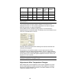
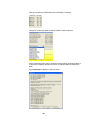
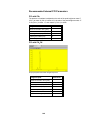
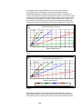
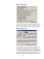
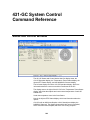
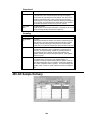
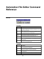
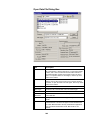
1
NOTICE: Varian, Inc. was acquired by Agilent Technologies in May 2010. This document is provided as a courtesy but is no longer kept current and thus will contain historical references to Varian. For more information, go to www.agilent.com/chem. Varian, Inc. 2700 Mitchell Drive Walnut Creek, CA 94598-1675/USA 240-MS GC/MS Ion Trap MS Workstation Version 6 Software Operation Manual ©Varian, Inc. 2009 Printed in U.S.A. 395416800:3 Trademark Acknowledgments Microsoft is a registered trademark of the Microsoft group of companies. Other brand and product names are trademarks or registered trademarks of their respective owners. Contents Introduction...............................................................................................................................5 Additional Manuals .....................................................................................................................................................5 Workstation Toolbar.................................................................................................................7 Overview.....................................................................................................................................................................7 Workstation Toolbar Options ......................................................................................................................................8 System Control .......................................................................................................................13 Overview...................................................................................................................................................................13 Navigating System Control .......................................................................................................................................13 Manual Control Tab ..................................................................................................................................................30 Auto Tune Tab ..........................................................................................................................................................38 Temperatures Tab ....................................................................................................................................................43 Diagnostics Tab ........................................................................................................................................................46 Startup/Shutdown Tab ..............................................................................................................................................51 Acquisition Tab .........................................................................................................................................................56 MS Operation Parameters........................................................................................................................................58 Effects of Hardware Configuration Changes ............................................................................................................61 GC System Control Window.....................................................................................................................................61 Configuring the GC/MS System ...............................................................................................................................67 Creating Methods with the Wizard ........................................................................................85 Method Builder Window............................................................................................................................................87 240-MS Method Builder ............................................................................................................................................92 450-GC Methods ....................................................................................................................................................128 431-GC Methods ....................................................................................................................................................138 Acquiring GC/MS Data .........................................................................................................141 Injecting a Single Sample .......................................................................................................................................141 Injecting Multiple Samples......................................................................................................................................147 Automation File Editor ............................................................................................................................................152 Automated MS Report Generation .........................................................................................................................157 Security Administration .......................................................................................................159 Overview.................................................................................................................................................................159 Passwords ..............................................................................................................................................................159 Application Locking.................................................................................................................................................160 File Revision Settings .............................................................................................................................................161 240-MS Ionization Techniques ............................................................................................163 1 Ionization Modes.....................................................................................................................................................163 Internal Electron Ionization .....................................................................................................................................163 Internal Positive Chemical Ionization......................................................................................................................166 External Electron Ionization....................................................................................................................................171 External Positive or Negative Chemical Ionization.................................................................................................174 Hybrid Positive or Negative Chemical Ionization....................................................................................................178 Ion Preparation Techniques ................................................................................................181 MS/MS - Tandem Mass Spectrometry ...................................................................................................................181 Selected Ion Storage ..............................................................................................................................................185 System Control Command Reference ................................................................................187 System Control Menus ...........................................................................................................................................187 240-MS System Control Command Reference...................................................................195 Display ....................................................................................................................................................................195 System Control Tabs ..............................................................................................................................................196 Manual Control .......................................................................................................................................................197 Auto Tune ...............................................................................................................................................................202 Temperature(s) .......................................................................................................................................................208 Diagnostics .............................................................................................................................................................209 Startup/Shutdown ...................................................................................................................................................212 Acquisition ..............................................................................................................................................................214 450-GC System Control Command Reference...................................................................217 Status and Control Window ....................................................................................................................................217 8400/8410 SampleList Window Extensions ...........................................................................................................230 431-GC System Control Command Reference...................................................................233 Status and Control Window ....................................................................................................................................233 8400/8410 SampleList Window Extensions ...........................................................................................................237 240-MS Method Builder Command Reference ...................................................................241 Internal EI and CI....................................................................................................................................................242 450-GC Method Command Reference.................................................................................251 450-GC AutoSampler .............................................................................................................................................251 450-GC Sample Delivery........................................................................................................................................259 450-GC Injector ......................................................................................................................................................260 450-GC Flow/Pressure ...........................................................................................................................................262 450-GC Column Oven ............................................................................................................................................266 450-GC Detectors...................................................................................................................................................267 450-GC Analog Output ...........................................................................................................................................274 450-GC Data Acquisition ........................................................................................................................................275 431-GC Method Command Reference.................................................................................277 431-GC AutoSampler .............................................................................................................................................277 Automation File Editor Command Reference ....................................................................283 2 Menus .....................................................................................................................................................................283 Main Toolbar...........................................................................................................................................................284 Open Automation File Dialog Box ..........................................................................................................................285 Save Automation File As Dialog Box......................................................................................................................286 Print Setup Dialog Box ...........................................................................................................................................286 Edit Notes Dialog Box.............................................................................................................................................287 RecalcList Window .................................................................................................................................................287 SampleList Window ................................................................................................................................................293 SequenceList Window ............................................................................................................................................299 3 4 Introduction This manual explains acquiring data, building methods, and operating the Varian 240-MS Ion Trap with MS Workstation with either the 450-GC or the 431-GC. The manual describes the configuration of the 450-GC for standard Ethernet communication. Information in this manual is also on the Help menu. Additional Manuals 240-MS Ion Trap Hardware Operation Manual The Hardware Operation Manual provides the necessary information for using, and maintaining your 240-MS system. Information is also in Help. MS Workstation Software Reference Manual This Manual guides you in the in the operation of the MS Workstation Software. These operations include displaying and reviewing chromatographic and mass spectral data, library searching, and quantitative analysis. Although these tutorials use Saturn 2000 ion trap files, they illustrate the principles of the MS Workstation software. 450-GC User Manual This manual is included on the Varian MS Workstation CD-ROM and describes the operation of the 450-GC. 430-GC and 431-GC User Manual This manual is included on the Varian MS Workstation CD-ROM and describes the operation of the 431-GC 5 6 Workstation Toolbar Overview The applications of the Varian MS Workstation Toolbar are Methods, Data Files, SampleLists, RecalcLists, SequenceLists, and Reports. Installing additional MS Workstation options, such as Star Finder and Star Custom Report Writer, may add other application buttons to the Workstation Toolbar. The following is a brief introduction to the applications. Later sections explain each in detail. As you move the cursor over a button, the name of the application appears below the cursor. Click an icon to launch the application. Name of Application Large Icons Description System Control/ Automation Monitor instrument status, and perform automated injections and batch recalculations. View/Edit Methods View and edit instrument operation, data acquisition, and data handling methods. Edit Automation Files Do off-line editing of SampleLists, RecalcLists, and SequenceLists. Review/Process MS Data Review chromatograms and spectra; perform library searches, and review and process quantitation results. Standard MS Reports Create, edit, and view standard MS reports. Custom MS Reports Create, edit, and view customized MS reports. Security Administration Set MS Workstation security options and passwords. SMS/MS File Conversion Convert data files between DOS and Windows formats. Batch Reporting Generate standard reports for a group of Data Files by dragging and dropping them on the Batch Report Window. View/Edit Chromatograms Review GC chromatograms, edit data handling parameters, and recalculate results. Standard Chrom Reports Preview standard chromatogram and results reports. 7 Name of Application Large Icons Description Compound Set Editor Create and edit sets of compounds in the MS Data Handling Method allowing activation or deactivation under automation. Quick Start Run a sample without using a Sample List. Quick Link Buttons The QuickLink buttons are on the right of the application icons. They correspond to most recently used Data Files and Methods. Most Recently Used Data File: Display operations for the Most Recently Used Data File. Select a data file from a list of most recently used files. Most Recently Used Method: Display actions for the Most Recently Used Method or select a different method from the list of most recently used methods. Workstation Toolbar Options Moving the Workstation Toolbar You can move the Workstation Toolbar to any edge of the Windows screen. Click an area of the Workstation Toolbar that does not contain Application or QuickLink buttons and drag the toolbar to the preferred edge of the screen. The next time you open Workstation the toolbar will be at that spot. You can display the Workstation Toolbar as a Windows Taskbar icon. Select Move to Windows Taskbar from the Workstation Toolbar options menu. Taskbar icons appear in the lower right (or bottom) of the Windows Taskbar, (the bar on which the Start button appears). When displayed as a Taskbar icon, the toolbar no longer takes up space on the screen. When you click a Workstation Toolbar icon, the options menu is displayed. 8 Workstation Toolbar Menu Put cursor over an area of the Workstation Toolbar without an application or QuickLink button, and right-click to display a menu. Move to Windows Taskbar Display the Workstation Toolbar as a Windows Taskbar icon. Select Move to Windows Taskbar from the Workstation Toolbar options menu. Taskbar icons appear in the lower right of the Windows Taskbar. Click the Workstation Toolbar icon to display the options menu. Show/Hide Applications on Toolbar Select the applications for the Workstation Toolbar. The left side lists the applications shown on the toolbar and the right side list the applications that are installed but not shown on the toolbar. To remove an icon from the toolbar, select it from the top list and click Remove. To add an icon to the toolbar, select it from the bottom list and click Add. 9 Enable/Disable Instrument Modules Enable instrument modules. When an instrument module is available, it appears in System Control. If the corresponding instrument is connected and turned on, you can create a Method section for it, and format reports. The list on the left shows all instrument modules that are currently installed and enabled. The list on the right shows all instrument modules that are installed but not enabled. To disable an instrument module, select it from the list on the left and click Disable. To enable an instrument module, select it from the list on the right and click Enable. Application Descriptions When this item is checked, application descriptions are displayed when the mouse moves over application icons. Small Buttons on Toolbar When Small Toolbar Buttons is enabled, a smaller version of the Toolbar opens. Notice that the graphics for some icons are slightly different. Run Application List the applications in the Workstation Toolbar. Click to open an application. 10 Help on Select an item from this list to display the online help. Pick Data File for Quick Link Button List of the eight most recently used Data Files in order of use. Select a Data File from this list to change the Data File displayed in the Quick Link button to the selected file. Pick Method for Quick Link Button List of the eight most recently used Methods in order of use. Select a Method from this list to change the Method displayed in the Quick Link button to the selected file. Help on Workstation Toolbar Displays help for the open application. Product Support Web Site If you have Internet access and a web browser installed on your computer, this opens the MS Workstation Product Support Web Site. This site has the latest software and documentation updates for the MS Workstation products, and additional notes, tips, and answers to frequently asked questions. Visit this site periodically to see new information. About Workstation About has information about the software version, installation information, and lists the modules installed. The following is an example, your version may be different. 11 Validate Installed Files - Uses checksums to test and document errors. Print a report documenting the file system tested, the success, or failure of the test, the date printed and tested, the ID of the person logged in (if login IDs are used). You can include a signature line. For more details, see online help. Quit Close the Workstation Toolbar. 12 System Control Overview This section briefly describes the features of System Control. Later sections explain how to use these features. Navigating System Control System Control includes features such as, the System Control Menu bar, System Control Toolbar, Keypad Dialog, Chromatogram/ Spectrum Toolbar, and Chromatogram/Spectrum Displays. 13 File Menu Activate Method: Select an existing method. This sets the conditions for the GC, MS, AutoSampler, and data handling parameters. Upload Active Method from Modules: Save conditions from the existing modules in a new or existing method. This method becomes the active method. New SampleList: Create a SampleList. Open SampleList: Open an existing SampleList. New RecalcList - Create a recalculation list. Open RecalcList - Select an existing recalculation list. NOTE: Process a RecalcList in System Control or in MS Data Review. In MS Data Review, from the Quantitation menu, select Process/Review RecalcList. Although Processing a RecalcList takes longer from System Control, AutoLink functions including automated reporting with templates such as EnviroPro, ToxProPlus, and Multicompound Reports can also be used. New SequenceList - Create a sequence list. Open SequenceList - Select an existing sequence list. 14 Print and Printer Setup are described in the MS Workstation Software Reference Manual. Edit Menu Click Edit and select Edit Module Info. Each module has a message log and documentation screen. Use the Module Information Editor to record performance, maintenance, hours used, or other comments. Use the Add, Edit, and Delete buttons to record your comments. 15 Inject Single Sample Menu Use Inject Single Sample to enter sample information before making an injection. The Module window must be in acquisition mode before making an injection. Click Inject in the bottom left corner to begin either a manual or an autosampler injection. Select a Sample Type from the list: Click Injection Notes to enter a description or comment. Use AutoLink to enter commands and parameters. Enter a command to execute a program after the data file acquisition is completed. For example, you can activate a custom MS Report to print the sample reports. To run a Custom MS Report in automation: 1. Type the directory path and the name of the Custom MS Report template (for example C:\VarianWS\EPA525.swt). Note that Custom MS Reports templates should always be stored in the VarianWS directory. 2. Click Browse to select the command executable file. 3. Click OK after making your selection. 16 Automation Menu The following shows the Automation menu and describes the options. Begin SampleList: Automation starts at line 1 and ends at the last line. Open SampleLists from the File menu. Begin Sequence: Begin an open SequenceList. You can change methods and SampleLists during an automated run. Open the Sequence from the File menu. Begin At: Start automation at a particular sequence or SampleList line and run until the last line is completed. A SampleList or SequenceList must be open to use this feature. Suspend Automation: Stops automation at the last completed sample. Resume Automation: Start automation after it has been suspended. Automation starts from where it was suspended. Stop Automation: End automation immediately and resets all modules. Reset Modules: Bring the various modules to their ready states. Enable Automated Printing: Allow printer functions to work during automation. Recalculate Menu The following shows the Automation menu and describes the options. Begin RecalcList: Start an automated Recalculation. A Recalculation list must be prepared and opened under the File menu to do this. 17 Begin at Selected RecalcList Line: Process a Recalculation list starting with a chosen line and proceeding with the rest of the list. View Calibration Curves: View curves for the calibrated compounds in the active method. The Calibration Curve is saved as part of the Method. NOTE: Do Recalculation in System Control or in MS Data Review. From the Quantitation menu, select Process/Review Recalc List. Processing a Recalc List takes longer when done from System Control than in MS Data Review but allows AutoLink functions such as automated reporting with Custom MS Reports templates such as ToxProPlus or EnviroPro. Instrument Menu The following shows the Instrument menu and describes the options. 240-MS: The configured instrument. Configuration: Add new modules to the existing instrument. Remove Module Names: Remove any associations between Module Names and Module Addresses. This allows you to connect a Module with a different Module Name at that address. The next time the associated Module connects at that address, you will be prompted to select the correct name for the Module. Instrument 1 Faults: View faults in a module of in Instrument 1. Periodically click the update key to check for new faults without opening the dialog box. 18 Setup Ethernet Communication: Set up the communication between the GC and System Control Setup COMM Ports: Set up communication between System Control and modules communicating with the Workstation through the Serial ports on the PC. The first time you start System Control, the Star Communication Configuration Wizard starts automatically. Windows Menu The following describes the Windows menu. Show Module Windows: Display the configured module windows. In this example, the modules available are the 450-GC and the 240-MS (4000). Iconize Module Windows: Create icons of individual module windows at the bottom of the screen. Show Automation Windows: View the open automation screens. The possibilities are SampleList, RecalcList, and SequenceList. Iconize Automation Windows: Create an icon of any open automation screen windows to access windows behind the automation windows. Arrange Icons: Arrange existing icons in a row at the bottom of the System Control window. SequenceList: Display the active SequenceList. SampleList: Display the active SampleList. RecalcList: Display the active RecalcList. 19 Instrument 1 Status: View the status of the modules connected to the system. Message Log: View the event log for the MS module. The log error messages for all configured modules. The last section of the Windows menu displays the attached modules and their status: 4000.01: Click to display the MS module control screen. NOTE: The 240-MS uses the same drivers as the 4000 MS. 20 450-GC.02: Click to display the 450-GC module control screen. 21 Help Menu The Help menu has the following options. Select Help Topics from the Help menu to display the following. Click an item in the Contents box to open it. In the Help dialog box, from the Index tab, select a topic. Click the topic and the click Display. To use the Find dialog, type in a key word or phrase, select a matching word, click a topic, and click display. 22 About Workstation About has information about the software version, installation information, and a list of the instrument modules installed. The following is an example. Validate Installed Files - Uses checksums to test and document errors. Print a report documenting the file system tested, the success, or failure of the test, the date printed and tested, the ID of the person logged in (if login IDs are used). A signature line can be included. For more details, see online help. System Control Toolbar The system control toolbar is near the top of the screen. The following describes the functions. Item Description Create a new automation file. First button: open an existing automation file. Second button: open the Message Log file. View/edit or print a Method. Open a Method. Edit notes for an automation file. Edit Module information for any online Module. 23 Item Description Open Instrument 1 Status Inject a single sample. Start an open RecalcList. Start an open SampleList. Start an open SequenceList Suspend a running list. Begin a list. Stop a running list. Module Keypad Dialog Click Hide Keypad, to display a larger chromatogram and spectrum windows during data acquisition. Click Show Keypad to restore the MS Keypad Dialog. Click one of the tabs at the top of the Keypad Dialog to select the 240-MS Module modes: “See Manual Control Tab” on page 30,”Module Attributes” on page 37, ”Temperatures Tab” on page 43, “Diagnostics Tab” on page 46, “Startup/Shutdown Tab” on page 51, or ”Acquisition Tab” on page 56 for more information. Chromatogram Toolbar View the Chromatogram display when the MS module is in Acquisition mode. The Chromatogram Toolbar appears in the upper left corner of the display. 24 Hide the toolbar. Click in the upper left of the display to restore the toolbar. Expand chromatogram to full scale on x and y axes Click Previous-Scale to return the chromatogram display to the last scaling before the current one. If you zoomed the chromatogram twice to view smaller time/intensity ranges, the third click brings you back through the previous scales. Click Scale to choose between Auto Scale and Fixed Mode Intensity. Click Chro Display to display this menu. Click Spectrum Select to display the spectra. The chromatogram display stops updating. Click Chromatogram Viewer to load the acquiring data file into MS Data Review to compare this data file with other data and do analysis. Click Base Peak Chromatograms button to switch the display from the TIC (or plotted chromatogram) to the Intensity of Base Peak. Chromatogram Preferences Right-click the chromatogram window to display a menu that offers these selections Chromatogram Plot Preferences, Report Preferences, or General Preferences. Use Chromatogram Plot Preferences to modify the appearance of the plot. These setting are used in chromatogram plot displays and reports in all MS applications, including Standard MS Reports, and Custom MS Reports. 25 Use Report Preferences to select chromatogram and spectrum report options. 26 Use General Preferences to change the appearance of numbers and fonts. Spectrum Toolbar The Spectrum display can be viewed when the 240-MS module is in Manual Control, Auto Tune, or Acquisition modes. The Spectrum Toolbar appears in the upper left. The toolbar functions are as follows: Click the Arrow to hide the toolbar. Click in the upper left of the display to restore the toolbar. Click Full-Scale to normalize the chromatogram vertically and horizontally. Double-clicking in the lower left corner of the display has the same effect. Click Previous-Scale to return the chromatogram display to scaling last used. If the chromatogram was zoomed twice to view smaller time/intensity ranges, this steps back through the previous scales. Click Spectrum Report to preview the spectrum report, which can be printed. Click Scale to choose between Auto Scale and Fixed Mode Intensity. Click Display Options to choose Plot, Ion/Intensity List, or Summary Information for the display. Click Display Type to choose between graphical or text displays of mass spectra. Also, display additional information about the spectrum. 27 Spectrum Preferences Right click the spectrum window to open a menu. From this menu, you can select Spectra Plot Preferences, Report Preferences, or General Preferences. Use Spectra Plot Preferences to modify the appearance of the plot. Use Report Preferences to select chromatogram and spectrum report options. 28 Use General Preferences to change the way numbers and fonts appear. Configuring the Real-Time Chromatogram Display Click the Acquisition tab. If you are in a different mode and start a SampleList or Inject a Single Sample, the mode automatically changes to Acquisition. During an analysis, you can view the chromatogram. Click Default View to display the Spectrum and Chromatogram side by side. Select Chromatogram to view the chromatogram as it is acquired. Click Hide Keypad to expand the display. In the following picture, the text information at the top is hidden and the chromatogram is expanded. 29 To display the Keypad, click Show Keypad. Select Spectrum and Chromatogram to display them side by side. You can dock the Spectrum window, for example, you can position it above the Chromatogram. Manual Control Tab In Manual Control, the status of the MS module is displayed in real time. The window has two panes, the MS Keypad above, and the Spectrum/Module Attributes display below. The features that are displayed depend on the screen resolution set in the Display section of Microsoft Windows Control Panel. Configuring the Display Slide the Scroll Bar on the right side to view the lower section of the keypad. Click the Splitter Bar to expand the keypad viewing area and the Scroll Bars above the Splitter bar to scroll the view. 30 Splitter bar Scroll bars The MS Icon The ion trap icon is on the left side of the MS Keypad. If the icon text is red, the ion trap is disabled and the current Active Method segment is a filament/multiplier delay with an ionization mode of None. The ion trap is also disabled if there is an instrument Fault. Changing the Active Method Segment to 2 changes the trap status to enable and the color of the icon text changes to black. If the icon is not currently disabled, click in the center of the ion trap to turn on the trap. The icon text turns green indicating the ion trap is on. Click the icon of the RF, Multiplier, or Ion Source (Filament) to turn them on individually. Quick Control Toolbar Below the trap icon are options for turning on the Trap, the Ion Gauge, and the flow of either Calibration Gas or CI Gas. When the trap is turned on (the active method segment must have an ionization method other than None), a mass spectrum appears in the spectrum display. 31 If the Calibration Gas is turned on in EI mode, you can see the characteristic spectrum with prominent ions at m/z 69, 131, 264, 414, and 502. The mass assignments of these ions and of m/z 464 and 614 are checked during the Mass Calibration procedure in the Auto Tune mode. When the ion gauge is turned on a pressure reading is displayed in the area above the trap icon in the MS Keypad. In the following image, the ion trap is in Internal mode. Manual Control Tabs Manual Control has the following tabs: Method, Active Segment, Checks and Adjustments and Module Attributes. Active Segment Active Segment is shown with General Parameters displayed in the lower pane. The top displays: Ionization On, Scan Type, Ionization, and Scan Mode. 32 The Scan Type selection has the following options: The Scan Mode selection has the following options: Examine and edit the parameters in the active MS method and observe the effects of these changes on the mass spectra being acquired. See “Creating Methods with the Wizard” on page 85 for more information. The ionization and ion preparation modes in the current method segment determine the tab dialog views. Click Activate Changes after editing a parameter to implement the change. Click Upload MS Method to save the changes. Click Edit Method to open the method in Method Builder. 33 Checks and Adjustments Four adjustments may be made in the Checks and Adjustments tab dialog. Calibration Gas Adjustment NOTE: If you are doing an initial tune (for example, when first starting up a system), the integrator zero may be far enough off that even with the cal gas closed all the way down, the cal gas adjustment indicates success. There are interrelationships between the Cal Gas, the Integrator Zero, and the Electron Multiplier. Because of these, stabilize the settings by performing the Cal Gas adjustment more than once. Initially, set the Cal Gas to the midpoint (8 turns) and perform the Integrator Zero tune. Then perform the Electron Multiplier tune. Now, go back to the Cal Gas adjustment to set the pressure. Keep doing these 3 steps until the Cal Gas and Electron Multiplier settings stabilize. Use the Calibration Gas valve inside the front door of the MS. The valve has a black knob with the number 0 labeled on it. Turn the valve counterclockwise to increase Cal Gas flow and clockwise to decrease the flow. Adjust the flow so that the readback in the Adjustment Results field indicates that the flow is OK as seen in the following. 34 CI Gas Adjustment 1. Check that the appropriate CI reagent is plumbed into the CI gas inlet in the rear of the MS or contained in the Liquid CI reagent vial. 2. Select CI Gas Adjustment. 3. Select the appropriate CI reagent from the Reagent menu. 4. Adjust the flow using the CI Gas valve inside the front door (labeled with numeral 3). 5. Turn the valve clockwise to increase the flow or counterclockwise to decrease the flow. Adjustments Results describes the spectrum when the gas is properly adjusted. RF Ramp Adjustment Use the RF Ramp Adjustment to determine if the RF voltage is in tune over the entire mass range. After starting, use a screwdriver to adjust the RF coil screw inside the front door of the MS. Follow the instructions in the Adjustment Results field until the value of the highest part of the graph is at a minimum. 35 Air/Water Check Before doing the Air/Water check, run the Set Electron Multiplier Auto Tune The Air/Water Check routine determines the relative amount of air and water vapor in the vacuum manifold. When the Air/Water screen is displayed, the following occurs: The filament, electron multiplier, and RF voltage are turned on; AGC is turned off; and the scan range is set to display the air/water spectrum (m/z 14 to 45). The air background is proportional to the width of the peak for m/z 28 at 10% peak height. The water background is proportional to the ratio of m/z 19 to m/z 18. For Internal Mode, the ionization time is fixed at 300 µsec. For External Mode, the intensity of the highest peak (m/z 18, 19, and 28) is adjusted to a suitable level. Width of m/z 28 at 10% Peak Height Ratio 9/18 Acceptance Criteria < 1.0 m/z < 20% OK ,No Leak < 1.8 m/z < 50% Small Leak < 3.1 m/z < 91% Significant Leak > 3.1 m/z > 91% Massive Leak 36 For External (and Hybrid) Mode, the acceptance criteria (Ratio of m/z 19/18) for the presence of water is the same as the Internal mode. However, a number of External (and Hybrid) parameters may affect the intensity of the air peak at m/z 28 (for example, damping gas flow rate, DC offset voltage, or lens voltages). If a massive air peak is present, turn off the Damping Gas flow and run Air/Water Check again. If no peaks are present with the damping gas off, then the most likely cause of a massive nitrogen peak (m/z 28) is inadequate flushing of filters or the helium line, or both, rather than a leak in the mass spectrometer. If the nitrogen peak (m/z 28) is observed with the damping gas off, please see the Troubleshooting section for more information on finding air leaks. The CI Plumbing Leak Test is run automatically after the Air/Water Test. The CI solenoid valve opens and air/water levels are checked. Initially, these values may be high. Open the CI valve and flush for (or left under vacuum) several minutes before doing this test. High water level is indicated both by the intensity of the ion at m/z 18 but also by + the percentage of ions at m/z 19 (H3O ) relative to m/z 18. The water level is high after the instrument is first pumped down after maintenance. Baking the instrument overnight should bring the level down to an acceptable level. A high air level as shown in the example suggests that there may be a leak in the vacuum system or GC. See the troubleshooting section in the 240-MS Hardware Operation Manual. Module Attributes Select a filament. The two filaments in External, Internal, or Hybrid configurations reduce maintenance time. Override the Electron Multiplier voltage setting from Auto Tune by entering the desired voltage. Adjust the High Mass Calibration to improve the accuracy of mass assignments of samples that range from 650 to 1000 m/z. Increase the sensitivity of the detection of low mass ions (<100 m/z), especially for EPA method 521 37 Auto Tune Tab Auto Tune is an automated process for optimizing the MS performance over the entire mass range. NOTE: Perform Auto Tune after restarting the system each time the system is shut down and vacuum is broken. Also, perform AutoTune after doing a bakeout. Before performing Auto Tune, check the RF ramp, air/water, and cal gas settings from the Adjustments tab in Manual Control. Many tuning features use Perfluorotributylamine (FC-43) ions to adjust MS parameters such as voltages, and gain values to optimize the signal. Most Auto Tune functions are performed in EI mode, even if the active method is Internal CI, External CI, or one of the Hybrid CI modes. For the last two situations, the CI volume is automatically retracted from the external ionization source during Auto Tune routines. When major maintenance is performed, such as cleaning the ion trap or source or switching between internal and external ionization modes, run all Auto Tune routines. After changing operating conditions, such as trap temperature or helium buffer gas flow rate, run the related tuning function. Run specific routines periodically to check the system. The Auto Tune window has three sections: Control and Status, Spectrum and Event Messages Auto Tune Method 38 Control and Status Click Start Auto Tune to start the selected routines. Click Stop Auto Tune to stop the selected routines. The Action field shows the tuning routine in progress. The State field shows if the MS is executing an auto tune routine or idle. Spectrum and Event Message Window Select the areas to display during the auto tune tests from the list. Click Hide Keypad button to hide the upper portion of the screen and expand the lower. 39 Module Attributes displays information stored from the last autotune. View the log after doing an Auto Tune. Auto Tune Methods The available auto tune functions depend on the instrument configuration. The following are the functions available for an internal source. Other functions are only needed when the instrument is in Hybrid or External ionization configuration. Auto Tune is performed in the order listed. All of the auto tune methods are selected if you click Select All, or cleared if you click Clear All. To perform Auto Tune click the desired check boxes and click Start Auto Tune. Click Stop Auto Tune to stop the auto tune at any time. Integrator Zero 40 The Integrator Zero Adjustment sets the signal level from the Integrator Circuitry with the filament off. When the filament is off, the major source of signal coming from the circuitry is electronic noise. The Integrator zero is adjusted so the average value of electronic noise is slightly greater than zero. The acceptance range is between 0.3 and 0.5 counts. The integrator records signals only when ions actually strike the dynode and electrons emitted from the dynode strike the electron multiplier. Set Electron Multiplier Before starting the Set Electron Multiplier gain algorithm, adjust the RF Full Scale to calibrate the cal gas ion at m/z 502. The Set Electron Multiplier method adjusts the multiplier voltage and ion time to look at low-mass fragments from the unstable m/z 502 ion. The algorithm sets the multiplier voltage so each electron emitted by the dynode creates a known signal from the multiplier. The gain in this example is 3.71 x 10⁵. Occasionally, systems with an external or hybrid source fail this adjustment. Increasing the flow of FC-43 usually allows the multiplier gain to be set. An Event Window message is displayed. When the 10 5 gain voltage of the electron multiplier reaches 2000V order a new multiplier. When the 10 5 gain voltage exceeds 2500V, install a new multiplier. Electron Lens Tuning In the external ion source, electrons are continuously directed into an ion volume containing the sample to be ionized. Eventually the interior surface of the ion volume becomes contaminated by material that can charge up and disturb the extraction of ions from the ion source. To minimize ion volume contamination, the MS pulses electrons into the ion volume only when needed for ionization. Two plates bracket the filament to control electron pulsing. The plate closest to the ion volume is the Electron lens, and the plate away from the ion volume is the Repeller lens. The Electron lens is positive and Repeller lens negative to admit electrons into the ion volume during the ionization period. Otherwise, the voltages are reversed to exclude electrons from the ion volume. Tuning the Electron/Repeller lens voltages is important for linear signal response and filament lifetime. The four variables are the Electron lens ON and OFF voltages, and Repeller lens ON and OFF voltages. ON and OFF. The Electron lens ON voltage optimizes electron transmission to the ion volume; Electron lens OFF voltage excludes 41 electrons from the ion volume. The Repeller Lens ON and OFF voltages balance the emission current. Electron/Repeller Lens Adjustment: Electron lens tuning involves measuring the transient behavior of the emission current immediately after the lenses are switched on or off. If the lenses are unbalanced, the emission current changes in time and is proportional to the imbalance. If the balance is outside the range of 200 to 300 µA, the algorithm searches the optimal values by changing values of four variables one at a time. If the best voltage is not found, an error message is generated for lens tuning and auto tune and the last values are restored. When Electron Lens Tuning is selected, an additional, Turn on CI gas flow during tune, option appears. For CI methods in External or Hybrid mode, tune the Electron/Repeller lens with the CI plunger (CI volume) in place and the CI gas turned on. Adjust the CI gas flow in Manual Control before doing this tune function. Ion Lens Tuning The Ion Lens system has of three lenses (Lens 1, 2 & 3). Tune these lenses using Cal Gas ions at m/z 131 and 414. Optimum voltages are determined based on weighted intensities of the two ions. RF Full Scale Adjust Run this routine before doing mass calibration and trap function calibration. The RF Full Scale Adjust routine coarsely adjusts the mass calibration of the ion trap. Successive adjustments are performed on PFTBA calibration gas ions at m/z 69, 414, and 614. For this algorithm to work properly, the specified ions must be stable and present in sufficient intensity (>20 counts) under normal scanning conditions. Mass Calibration During Mass Calibration, the calibration gas valve opens and the electron multiplier, filament, and RF voltage turn on. The algorithm uses the calibration compound ions at m/z 69, 131, 264, 414, 464, and 614 to create a calibration curve. The nitrogen peak (m/z 28) is not used for calibration. A fixed offset at m/z 0 was empirically determined to give proper mass assignments between m/z 10 and 69. The calibration is extrapolated from the highest observed calibration ion to the maximum mass (m/z 1000). Mass calibration is performed in both normal scanning (5,000 (m/z)/sec) and fast scanning (10,000 (m/z)/sec) modes. Factors Affecting Mass Calibration The calibration ions must be present in sufficient intensity (> 20 counts) and stable under normal scanning conditions for mass calibration to be successful. Because temperature changes can shift the mass calibration, do the following after the trap reaches its equilibrium point (approximately 2 hours after the setpoint temperature has been established). For External and Hybrid modes, changing the trap damping gas flow may require both Mass Calibration and Trap Frequency Calibration. After ion source temperature changes, the mass assignments may be affected. 42 Trap Frequency Calibration After completing mass calibration, do the trap frequency calibration. This determines resonant frequencies for the generation of notched waveforms used in most modes of operation. In particular, the resonant frequencies for FC-43 ions at m/z 69, 264 and 414 are determined. For m/z 264 two q values are determined. NOTE: Do Trap Frequency Calibration each time you do a mass calibration. After the Trap Frequency Calibration is done, the Event Message Window displays the frequency values for the two trap function calibration points. Nominal values are 249 kHz and 248 kHz, respectively. These values can vary up to 4 kHz between instruments. Trap DC Offset Voltage The trap offset is a DC voltage applied to the ion trap electrodes (end caps and ring electrode) to help inject externally generated ions into the trap. The signal is maximized with the intensity of the m/z 414 ion from FC-43 to optimize the midpoint of the mass range. The trap offset has a range from 3 to 15 volts. Use lower voltages to increase in the relative abundance at the low end of the mass range. If your application involves fragile compounds, using a lower setting can minimize fragmentation. Temperatures Tab Control and Status 43 Control and Status displays: Conditions: Identifies if Analysis or Bakeout temperatures are active. State: Displays if the system is Ready or Equilibrating. Hold Time: Shows the remaining time of a bakeout. NOTE: Hold Time does not start counting down until bakeout temperatures are reached or until the system has warmed up for 20 minutes. Operating Conditions Operating Conditions displays readbacks of the current temperatures in each zone. Event Messages and Module Attributes Display After executing changes, the event log at the bottom of the screen updates with the time and a description of the event. Module Attributes is another selection. Setting Analysis and Bakeout Temperatures Click Save to activate changes. Click Restore to return to the settings before the changes. The following table displays information about the temperature ranges and default setting for the temperature zones of the different ionization modes. 44 Temp Zone Min Max Default External Default Internal or Hybrid Default Bakeout Ion Trap 50 270 100 150 220 Manifold 0 120 50 50 110 Transfer Line 0 350 170 170 250 Ion Source 0 300 180 N/A 250 NOTE: If the manifold temperature is 70 °C or higher, the source temperature is limited to 250 °C. Type the temperature for either Analysis or Bakeout in the tab area. All temperature units are °C. The ion source temperature zone does not appear when the instrument is in Internal configuration. Click the Bakeout tab to set Bakeout temperatures. The default bakeout temperatures are on the previous table. The bakeout time can be between 0 and 100 hours. The default time is 8 hours. Generally, bakeout the system after restarting from instrument shutdown and venting to the atmosphere. During bakeout, the manifold is heated to remove water and other volatile contaminants such as residual light hydrocarbons. The 50 °C default manifold temperature is used for acquiring MS data. The transfer line temperature should not be lower than 30 °C below the highest temperature of the GC column oven program in the active method. NOTE: The transfer line should NOT be heated above the maximum isothermal temperature specified for the capillary column. Adjustments After Temperature Changes After changing the ion trap temperature, let the system equilibrate for 2 hours after the trap temperature reaches the set point. After equilibrium is reached, check the RF tuning and adjust if necessary. Run Mass Calibration and Trap Frequency Calibration in Auto Tune. 45 Bakeout Click Start Bakeout to start a bakeout. The State becomes Equilibrating until bakeout temperatures are reached, then Holding until the Hold Time counts down to zero. NOTE: Hold Time does not start counting down until bakeout temperatures are reached or until 20 minutes have elapsed. After bakeout, the trap, manifold, transfer line, and source temperatures return to the Analysis set points. To change bakeout duration or temperatures during a bakeout, click Stop Bakeout, make the changes, save them, and restart the bakeout. Diagnostics Tab Use the Diagnostics tab to: Monitor the status of the vacuum system, applied voltages, and temperatures. Do diagnostic tests. The Diagnostics tab is divided into two panes, the Keypad above and the Module Window and Event Messages display below. 46 The Keypad Field The upper portion of the screen has three sections: Control and Status, Monitoring, and Diagnostics Tests. Control and Status State displays: Idle when diagnostic tests are not being performed. Running when tests are in progress. Function displays Monitoring Status The name of diagnostic test being done The Start Diagnostic button available after a test is selected in the Diagnostic Test tab dialog. After selecting and starting a diagnostic test, the results are displayed in the Event Messages display at the bottom of the screen. Monitoring Tab Select the desired ion trap features to monitor in the Trap On/Off area. Select Ion Source to display the filament emission current in the Ion Source area. Select Multiplier/Dynode to display the voltages of the electron multiplier and conversion dynode in the Trap area. Select RF Control to display the Entrance and Exit Trapping Field Dipole values. Select Waveform with RF Control to display the Dipole and Quadrupole Supplemental Waveform Voltages. Select Ion Gauge to display the ion gauge pressure in µtorr in the Ion Gauge area. 47 NOTE: If System Control is started in Diagnostics Mode, no method was activated and the Dynode readback is a default value of about positive 9,000V. After a method is activated in Manual Control or Acquisition, the correct Dynode voltage associated with the method is displayed in Diagnostics. Diagnostic Tests Click Select All to select all the diagnostic tests. Click Clear All to deselect all the diagnostic tests. Monitor and Event Messages Test results are displayed in the event messages window. If a test fails, see the troubleshooting section in the 240-MS Hardware Operation Manual Configuring the Monitor and Event Messages Display Click Hide Keypad to displaying the Monitor window and Event Messages in a larger area Click Show Keypad to display the keypad. Select from the menu to display the Monitor Window Only or the Event Messages Only or both. Vacuum System The turbomolecular pump current and power readings displayed are typical during routine operation. In this example, the instrument is in External configuration with the Trap Damping Gas flow, which is the auxiliary Helium, at 1 mL/min. The values for current and power are lower in Internal configuration. The ion gauge readings depend on the auxiliary Helium flow; in this case, the system is in External configuration and the reading of about 29 µTorr is reasonable for an auxiliary flow of 1 mL/min. The reading drops to 6 µTorr when the auxiliary flow is turned off in Startup/Shutdown mode. In Internal configuration the pressure should be <10 µTorr. The foreline pressure is determined with a thermocouple gauge detector; its reading is strongly influenced by the auxiliary Helium flow as well. 48 Trap The readings for the multiplier and conversion dynode voltages are displayed when Multiplier/Dynode is checked in the Monitoring tab dialog in the keypad. The multiplier reading is always negative and reflects the voltage drop between ground and the entrance of the multiplier. The dynode voltage should be close to 10,000V; the polarity is the opposite of the ions being detected. Waveform System The readings for Entrance/Exit End Cap Trapping Field Dipole are displayed when RF control is checked and the RF button is checked in the Monitoring tab dialog. The values should be 100 ±1%. Dipole and Quadrupole Supplemental Waveform readings are activated when RF control is checked and the Waveform button is checked in the Monitoring tab dialog. The values should be near 100%. Temperatures Display the current temperatures of the heated zones. The temperatures of both Entrance and Exit End Caps are displayed. When changing the trap temperature use this to monitor the process. 49 Ion Source (Internal) Emission current is set between 10 and 100 Amps when the system is in Internal configuration. The emission reading may vary by 1 Amp from the value set in the MS method. Balance measures how well balanced the emission current is between ionization on and off. Deviation measures the total deviation of emission current as ionization turns on and off. It indicates the ability of the lens to provide a symmetrical pulse of electrons into the source. If the Deviation is greater than 5 µAmps, tune the electron lens. Filament Bias is voltage relative to ground. The bias is -11.7V for EI mode and -9.8V for CI mode. Filament status can be OK, Open, or Untested. If the Filament is untested, determine the status by activating that filament in Manual Control and returning to Diagnostics mode. Gate is pulsed to +120V during ionization and -120V at other times so electrons enter the trap only when they are needed for ionization. Ion Source (External or Hybrid) Emission current default in External or Hybrid configuration is 25 Amps. In negative CI External or Hybrid, the emission current default is 250 Amps. The emission reading may vary by several Amps from this value. Balance measures how well balanced the emission current is between ionization on and off. Deviation measures the total deviation of emission current as ionization turns on and off. It indicates the ability of the lens to provide a symmetrical pulse of electrons into the source. If Deviation > 5 µAmps, tune the electron lens. Filament bias is the voltage relative to ground. The bias is always 70V in External and Hybrid modes. Filament status can be OK, Open, or Untested. If the Filament is untested, determine the status by activating that filament in Manual Control and returning to Diagnostics mode. For analysis of positive ions, Lens 2 is pulsed negative during ionization and positive otherwise so that ions enter the trap only when they are needed. For negative CI, Lens 2 is pulsed positive during ionization. 50 Lens voltages are set by Lens Tuning in Auto Tune. The ring and end cap offsets are set by the Trap DC Offset Voltage in Auto Tune. Event Messages Display Display messages when diagnostic tests are performed. Startup/Shutdown Tab 51 Status and Control Conditions are either Start Up, Analysis or Shut Down. State is Ready, Shutting Down, or Starting Up. Vacuum System The vacuum system is either Not Ready or Ready. The turbomolecular pump speed must be 100% for the Ready state to be reached. Pneumatics If the instrument is in External or Hybrid configuration, this field shows if auxiliary Helium damping gas is flowing to the ion trap. Damping gas flow is required for adequate mass spectral resolution and sensitivity in External mode. Although sensitivity is compound-dependent, start with a flow of 1 mL/min. The flow rate is listed in the Current Set Points area. This is not displayed for Internal configuration. Getter Control When the instrument is in External configuration, the getter removes water and other contaminants from the helium damping gas flow. Turn on the getter heater after turning on the damping gas flow. This is not displayed for the Internal configuration. 52 Current Set Points Heated Zones The current set points of all heated zones are displayed. The source temperature is not shown when the instrument is in Internal configuration. Vacuum System The pump speed is shown in the vacuum system field. It should be 100 2% during normal operation. Pneumatics The auxiliary Helium flow rate is shown for instruments in External configuration. The flow is set in the Module Attributes tab dialog of Manual Control. Turn the flow on by clicking Turn On under Damping Gas in the Control and Status field. It is not displayed in Internal configuration. Getter Control The getter removes water, oxygen, and other contaminants from the Helium auxiliary damping gas flow. This field is shown only when the instrument is in External or Hybrid configuration. After starting the system and turning on the Damping Gas flow, click Turn On in the Getter Control field to heat the getter to its operating temperature of 400 °C. It is not displayed is in Internal configuration. 53 Operating Conditions Heated Zones The current temperatures of all heated zones are shown. Compare these readings with the set points to the left in the Current Set Points field. Vacuum System The speed of the turbomolecular pump is 100% 2% during normal operation. Monitor the speed during Startup/Shutdown. The rate the turbomolecular pump starts up is proportional to how long it has been shut down. After short shutdowns, for example instrument maintenance, the time to reach 100% speed should be less than 2 minutes. After extended shutdowns, the pump speed increases in stages related to power consumption. This slower startup improves pump lifetime. NOTE: Failure to reach 100% pump speed in a reasonable time indicates a vacuum leak and corrective action should be taken. See the troubleshooting section in the 240-MS Hardware Operation Manual. Pneumatics If the instrument is in External or Hybrid configuration, the damping gas flow rate and Inlet Pressure are displayed. Compare the flow rate to the set point in the Current Set Points field. This does not appear when the instrument is in Internal configuration. Getter Control If the instrument is in External or Hybrid configuration and the Damping Gas and Getter Heater are turned on, the getter temperature is displayed. Compare this temperature to the set point of 400 °C in the Current Set Points field. This does not appear when the instrument is in Internal configuration. 54 Shutting Down the System Click Shut Down in the upper left corner of the screen, to shut down the MS. The heaters turn off and the speed of the turbo pump gradually reduced to 35% of full speed. The turbo pump speed reduces as the heated zones cool. After the temperature zones are cooled, turn off the main power using the switch on the back. Manually vent the system for at least 5 minutes by opening the vent lever on the front panel. NOTE: Retract the transfer line before lifting the analyzer assembly from the vacuum manifold. Failing to retract the transfer line can cause damage to the transfer line tip and to the trap assembly. Starting Up the System Monitor the increase in Pump Spin Speed during system startup in Operating Conditions. The software is locked in the Startup/Shutdown mode until the speed reaches 100%. The temperature readings for heated zones increase in the Operating Conditions field. If the system is in External or Hybrid configuration, turn on the Damping Gas flow and the Getter Heater in the Status Control field after the Pump Spin Speed reaches 100%. NOTE: Failure of the system to reach 100% pump speed in about five minutes indicates a vacuum leak. Take the appropriate corrective action listed in the ‘Troubleshooting’ section in the Hardware Operation Manual. 55 Acquisition Tab About Running Analyses Click the Acquisition tab. If you start an analysis while the instrument is in another mode, the software automatically shifts the MS into Acquisition mode. After starting Acquisition the yellow (Not Ready) light turns green indicating that the MS is ready for analysis. If the GC is not ready, a Not Ready message is displayed at the top. After the GC and AutoSampler become ready, the Not Ready message changes to Ready. To determine the individual ready states of the components, display the Window menu and the status of the modules are displayed at the bottom. Run an analysis as a single sample or use an automated sequence. To run a single sample, see “Injecting a Single Sample” on page 141. To run in automation, see “Injecting Multiple Samples” on page 147. Status and Control Before an acquisition starts, the Status and Control field looks like the following. The Run Time is 0.00 minutes because the run has not started. The End Time is the run length specified for the MS in the active method. The Ready and No Fault lights are green. Use Start Acquisition to override automation and start a run automatically before the system becomes Ready. However to save the file name of a run started this way, re-activate the method after saving changes and return to System Control. Wait For ReadyIn: Use this feature with external devices that are not networked to the system such as Purge and Trap systems. If Wait For ReadyIn is selected, the system waits for a signal before starting an acquisition. 56 After an acquisition starts, the run time increases in 0.01 minute increments. Stopping Acquisition terminates the MS run but does not terminate the GC run. Terminate the GC run from the GC module window, which is opened from the Windows menu. To increase the end time, click End Time and select the desired time. NOTE: Changing the End Time for the MS module does not change the GC End Time. Extend the GC run time from the GC keypad. MS Method Before an acquisition starts, the active method in Segment 1 is usually a Filament/Multiplier Delay. The delay is long enough to keep the MS off until after the GC solvent eludes. After a run is started, the Segment Number increments after the start time for each segment is reached. The Segment Description is the user-entered description in the Segment Description field of the MS Acquisition Method in the active method. The Scan Description shows the ionization and ion preparation methods; these methods are chosen in the Scan Type/Group and Ionization fields of the Method Segment field of the method. Scan Range is the acquisition mass range. 57 Operating Conditions Data File shows the name of the file being acquired. The Scan Number, Ionization Time, and Ion Count for the current scan are displayed in their respective fields. This display updates with every scan throughout the GC/MS run. MS Operation Parameters Electron Multiplier Gain In normal operation, the electron multiplier gain is set up to produce about 10 5 electrons per ion. The Set Electron Multiplier method in Auto Tune automatically determines the multiplier voltage needed. Changing the multiplier voltage changes the gain of the MS. NOTE: The calibration and analysis runs must be done with the same gain value. Under certain circumstances (low background, small signal), increasing the electron multiplier gain by +100 or +200 volts above 10 5 improves detection... Use the same multiplier gain for calibration curves and unknown samples. Emission Current The emission current is an adjustable parameter in Internal configuration only. It is set at a fixed 25 Amps for Hybrid and External configurations. As a starting point for Internal configuration full-scan analyses, set the emission current so the ionization time is slightly less than the Maximum Ionization Time for the method. This gives the instrument its best dynamic range when data are automatically scaled to account for adjustable ionization time. If the ionization time is already lower than the max ion time when it is set for 10 Amps, the sensitivity is not enhancement (as reflected by signal-to-noise enhancement) by increasing the emission current. Sometimes, using a high emission current may improve sensitivity. One example is EI/MS/MS in Internal configuration where the MS/MS isolation step eliminates the higher background that would normally arise from a high emission current. 58 Ion Trap and Ion Source Temperatures Internal or Hybrid Configuration The ion trap temperature must be high enough to prevent analytes from condensing on trap surfaces. The chromatographic peaks tails as a result of condensation. Trap temperatures can be 50-75 °C below the highest temperature for the GC column temperature ramp without compromising chromatographic performance. Certain compounds (such as straight chain hydrocarbons) fragment more at higher ion trap temperatures. Use a low column flow rate and a trap temperature below 150 °C to improve the mass spectra when fragile ions are present. After the system shuts down and is vented to atmosphere, bakeout at elevated temperatures to rapidly removal water vapor. After this, reduce the trap temperature to 150-175 °C. Use the manifold bakeout functions to do this overnight and reset the temperatures to operating conditions automatically. External Configuration A low ion trap temperature does not cause tailing of chromatographic peaks when the instrument is in External configuration, although a Source temperature set too low may cause similar effects. Bakeout the system after doing maintenance. AGC Target TIC Value In EI mode with AGC on, the target TIC value determines how many ions AGC allows into the ion trap during the ionization time. While increasing the target TIC value increases peak heights, increasing it too far causes a loss of mass resolution. This results in mass miss-assignments or incorrect isotope abundance ratios. For full-scan EI operation, a target TIC of 20,000 is a good starting point. Under special circumstances such as MS/MS, a much lower target TIC, such as 5,000, is required. As the m/z distribution of the stored ions becomes smaller, fewer ions can be trapped without a loss of resolution. Using MS Methods in System Control The Startup Methods When you open System Control the Startup1.mth or the last active Method is activated. The Startup method is a copy of the Default method. Use it to build new MS methods. The Default method is placed in the file directory to ensure the existence of a valid method. Do not alter this method when developing new methods Change the Startup method to create a customized set of parameters for building methods. NOTE: In building new methods, clicking Defaults puts instrument-valid default values in the section, regardless of the values placed in the Default.mth. To change Methods, click the Activate a Method button on the System Control Toolbar or choose Activate Method from the File menu. 59 Editing Methods from the MS Status and Control Window Edit the method in Manual Control and click Upload MS Method to save the changes. However to edit other sections such as data handling, reports, or the GC sections, click Edit Method in either Manual Control or Acquisition to open the method in Method Builder. Method Builder opens with the active Method loaded. You can edit that section or other sections of the Method. After editing and closing the Method Builder window, you are prompted to reactivate the Method. Reactivating the Method downloads the changes. NOTE: If you access the active method from Method Builder via the Workstation Toolbar, and then close the method editor or save a file, the method must be reactivated in System Control. To reactivate the current method, click the button for the method (in this example startup1.mth) in the System Control toolbar and then select Re-Activate Method. Changing Method End Time from the MS Status and Control Window To change the end time of the acquisition from the Status and Control window: 1. Click End Time. 2. Enter a new end time and click OK. 60 Effects of Hardware Configuration Changes System Control restarts after the configuration is changed, for example from External to Internal configuration. When the MS module connects, it compares the current configuration stored in the current Module Attributes with the configuration reported by the hardware. If these do not match, the Module Attributes are updated (preset) to the appropriate configuration. A similar process occurs for the default method (Default.mth). After making a hardware configuration change, new methods have the appropriate instrument configuration by default. NOTE: To preset Module Attributes run all Auto Tune routines, as the prior Auto Tune results are invalid. GC System Control Window 450-GC Instrument Window After the 450-GC is configured, it is displayed in the Instrument Window. Use the instrument window to monitor the status of all modules, inject samples, and do batch Recalculations. 61 Double-click in the instrument area or select the instrument from the Instrument menu to view the 450-GC Status and Control window. In MS Workstation, use the Windows menu to select the 450-GC module. If the Status and Control Windows for the modules configured in the instrument are not currently displayed, select Show Module Windows from the Windows menu and select a module to display at the bottom of the menu. Elements of the System Control Toolbar Most System Control Toolbar buttons correspond to a menu command. Rest the cursor on a button to display a description of its function. Note the buttons controlling the SampleList, Sequence, and RecalcList become available activating a corresponding automation file. 450-GC Status and Control Window The keypad has the 450-GC Operation parameters, Temperature Zone set points and readbacks, and the Sample Delivery Status. If a detector other than the MS is used, monitor the signal in the area below the keypad. 62 View the conditions of multiple detectors horizontally or vertically. Change the component status to display details of each component. Click a temperature zone entry to select the corresponding component status or to select the component status from the list. Component status is displayed in detail. Click View Setup to display the 450-GC Setup. 63 450-GC Real Time Chromatogram Display The 450-GC displays data in real time. Click Hide Keypad to display only the chromatogram. ---- Hide/unhide the Toolbar. Set both the amplitude and time axes to full scale. Set the amplitude axis to full scale. Set the time axis to full scale. Return to previous stored scaling. Go to next stored scaling. Enable/disable the Auto Scale feature. Enable/disable the cursor display. Select the background color for the display. Drag an area of the display to see a more detailed section of the plot, or zoom in both axes by pressing and holding the left mouse button on the spot you want to enlarge. (Hold the Shift key down to zoom out.) 64 431-GC Instrument Window After the 431-GC is configured, it is displayed in the Instrument Window. Double-click in the instrument area or select the instrument from the Instrument menu to view the 431-GC Status and Control window. In MS Workstation, use the Windows menu to select the 431-GC module. 65 If the Status and Control Windows for the modules configured in the instrument are not currently displayed, select Show Module Windows from the Windows menu and select a module to display at the bottom of the menu. Elements of the System Control Toolbar Most System Control Toolbar buttons correspond to a menu command. Rest the cursor on a button to display a description of its function. Note the buttons controlling the SampleList, Sequence, and RecalcList become available activating a corresponding automation file. 431-GC Status and Control Window The Workstation Status and Control window for the 431-GC displays, operation parameters, Temperature Zone set points, and readbacks. 66 Click Setup to display the 431-GC Setup. Configuring the GC/MS System Starting System Control the First Time Before opening System Control for the first time, confirm the instrument configuration and that any instrument modules that are not part of the system have been disabled. To enable or disable instrument modules see the Workstation Toolbar section, “Enable/Disable Instrument Modules” on page 10. In this section, GC refers to either the 450-GC or the 431-GC. Configuring the Instrument Before configuring the system, determine if you are going to put the Workstation on a company network or an isolated network. The following determines the order in which you should read the sections. If an Ethernet card has not been installed and configured on your PC, read “Installing and Configuring the Ethernet Card in Your PC” on page 68 and the correct option of the following: ”Configuring TCP/IP Parameters with No Company Network” on page 70. ”Configuring TCP/IP Parameters for a Company Network on page 71. 1. Read “Connecting Your GC to Your PC or Network” on page 72. 2. If you have not already installed the Varian MS Workstation, do so before proceeding. No Company Network: See ”Configuring the GC Communication (No Company Network)” on page 73. 67 Company Network: Read “Configuring the GC for a Company Network” on page 75. 3. Continue reading the rest of the sections, starting with “Adding a GC and MS in System Control” on page 80. Installing and Configuring the Ethernet Card in Your PC NOTE: This is a generic description. See the Windows and Ethernet card documents for more detailed information. See the installation instructions packaged with your Ethernet card for information on installing the Ethernet card in your computer. Before proceeding, your Ethernet card should be recognized by your Windows version. When done, the Network Neighborhood icon should appear on your Windows desktop. NOTE: For the following procedure, using disks other than the ones that were used for the original Windows installation may result in an Ethernet driver version mismatch that prevents Windows from starting. Should this occur, it may be necessary to remove the Ethernet Board from the computer to remove the incorrect Ethernet drivers. To configure the network settings for communication with the GC: 1. Click Settings from the Start menu. 2. Click Control Panel. 3. Double-click Network Connections. 4. Double-click Local Area Connection in the Network Connections window. 5. Click Properties in the Local Area Connection Status window. 68 6. Select Internet Protocol (TCP/IP) and click Install. 69 7. Select Protocol and click Add. 8. Click Have Disk if you have an installation disk for this component or click the Protocol you want to install and click OK. NOTE: If you are not connecting your Workstation to a company network (that is, you are not assigned an IP address by a Network Administrator), follow the next three steps. If you are connecting your Workstation to a company network, see “Configuring the GC for a Company Network” on page 75. Configuring TCP/IP Parameters with No Company Network After completing steps 1 through 5 for Installing and Configuring the Ethernet Card in Your PC, continue as follows: 1. Select TCP/IP from the network components list and click Properties. 70 2. Enter an IP address in the range 10.2.128.1 through 10.255.255.254. If you are adding more than one Workstation to this network, each Workstation PC must have a unique IP address within this range. The Subnet Mask is automatically set to 255.0.0.0. Do not change this value. 3. Ensure that there are no entries in the Gateway, and that Domain Name Server (DNS) and WINS Configuration are disabled. NOTE: These entries are not used in an isolated network. They may cause problems if they are present. 4. Delete settings from a previous configuration. 5. Click OK in the Network dialog box. 6. Reboot Windows for the changes to take affect. NOTE: See Communication Problems in the Diagnostic and Troubleshooting section for information about diagnostic tools to verify that your network installation is correct. Configuring TCP/IP Parameters for a Company Network After completing steps 1 through 5 for Installing and Configuring the Ethernet Card in Your PC continue as follows: 71 1. Select TCP/IP from the network components list and click Properties. 2. Contact your Network Administrator (or whoever assigns IP addresses in your network) to get the appropriate address. Note that each Workstation PC must have a unique IP address. Enter the appropriate Subnet Mask to be used with this IP address. 3. Obtaining an IP address Your Network Administrator may instruct you to obtain an IP address automatically by clicking Obtain an IP address automatically. NOTE: Contact your Network Administrator (or whoever assigns IP addresses for your network) to see what the appropriate settings are for your Gateway, and whether Domain Name Server (DNS) and WINS Configuration are needed. Your Network Administrator specifies the parameters for the Advanced window. 4. Reboot Windows for the changes to take affect. NOTE: See Communication Problems in the Diagnostic and Troubleshooting section for information about diagnostic tools to verify that your network installation is correct. Connecting Your GC to Your PC or Network See the “Communications” section of the User Manual of your GC for instructions on connecting your GC to the PC or a company network. Before proceeding, your GC should be connected to your PC or network. 72 Configuring the GC Communication (No Company Network) Use the following instructions if both the GC and Varian MS Workstation PC are not on a company network dedicated to Varian MS Workstations and the instruments they control. In this case, a Network Administrator does not assign IP addresses. NOTE: If connecting your GC and Varian MS Workstation PC to a multi-purpose company network managed by a Network Administrator, see Configuring the GC Communication for a Company Network. One GC may be connected directly to a Workstation. 1. After configuring your computer’s network settings, click System Control. 2. When System Control is opened the first time, use the Configuring Communication Wizard to guide you through the setup and network connections of your GC. 73 3. Click Next until the Setup Ethernet Ports window opens. 4. Click Setup. 5. Click the desired GC and click OK. This example uses a 450-GC. NOTE: If more than one Workstation is to be connected on the same network, only one Workstation should manage the IP addresses for all connected GCs (others should have the Manage IP addresses from this Workstation checkbox unchecked). If more than one Workstation is managing IP addresses, naming conflicts may arise. 6. As the GC is powered on, an entry is added to the table. For each entry, an IP address is automatically assigned. For each GC, provide a host name to identify it in the Varian MS Workstation. You cannot connect to a GC until you provide it a name. 7. Click Manage IP addresses from this Workstation checkbox to manage the IP address from this Workstation. As the GC is turned on, its Ethernet address is added to the list. 74 8. Click OK. NOTE: Proceed to “Using a Password to Protect BOOTP Settings” on page 79. Configuring the GC for a Company Network Do the following to connect both the GC and Varian MS Workstation PC are to a company network, that is, a multi-purpose network used for services in addition to instrument control. In this case, a Network Administrator assigns IP addresses. If the GC and the Varian MS Workstation computer are the only devices being connected, see “Configuring the GC Communication (No Company Network)” on page 73. You may connect virtually any number of 450-GCs or 431-GCs and any number of Varian MS Workstation computers to a company Ethernet network. Depending upon your network configuration, MS Workstation may control all 450-GCs or 431-GCs on the network. 1. After configuring the network settings, click System Control. 2. If opening System Control for the first time, use the Wizard to guide you through the setup and network connections of your GC. NOTE: Before proceeding with this section, consult your Network Administrator about whether a central BOOTP Server is available on the network. 75 3. If IP addresses are managed by a central BOOTP Server, then proceed to “Specifying IP Addresses from a Central BOOTP Server”. 4. If IP addresses are specified by a Network Administrator but not centrally managed, then continue reading “Specifying IP Addresses from System Control”. Specifying IP Addresses System Control Use the following procedure to manage IP addresses from System Control. 1. When System Control opens for the first time, use the Configuring Communications Wizard to guides you. 2. Click Next until the Setup Ethernet Ports window opens. 3. Click Setup to display the BOOTP Server dialog box. 4. Check Manage IP addresses from this Workstation box to enable the BOOTP Server. The BOOTP Server has a table listing all GCs to which IP 76 addresses may be assigned. If GCs are already connected to the network and powered on, their Ethernet addresses will appear in the table. NOTE: If more than one Workstation is being connected on the same network, only one Workstation should manage the IP addresses for all GCs connected (all others should have the Manage IP addresses from this Workstation checkbox unchecked). The Workstation acting as BOOTP Server must remain running all the time to allow other Workstations to connect to GCs. If more than one Workstation is managing IP addresses, naming conflicts may arise. 5. Enter a host name for each GC. IP addresses are not assigned to a GC until a name is entered. You may manually assign any IP address to any GC. 6. Click OK after entering all addresses and names. 7. If you select Assign IP addresses starting from box, the bottom portion of the dialog changes. 8. Enter the number of IP addresses you want to assign automatically. Enter the starting address here. As the GCs are powered on, IP addresses are assigned consecutively starting with this address. NOTE: Proceed to ”Using a Password to Protect BOOTP Settings” on page 79. 77 Specifying IP Addresses: Central BOOTP Server NOTE: For 450-GC only. To enable BOOTP Mode: 1. Locate the DHCP/Fixed IP switch behind the GC. 2. Switch to DHCP. To edit IP addresses: 1. Obtain the Ethernet address for each GC from the GC front panel or the label on the Ethernet card. 2. Turn on the GC and press any key on the GC keypad to allow it to start in local mode. The Ethernet addresses are automatically loaded into the BOOTP Server list for GCs. 3. After the GC has completed its initialization process, press the button showing a tools graphic (such as a wrench) on the GC keypad. 4. Press Setup on the keypad. 5. Press the System tab on the keypad. 6. Press Change on the keypad. 7. In the Change network setting dialog box, press the IP address on the keypad. NOTE: A stylus is located below the keypad for your convenience. 8. Press the corresponding numbers on the keypad to enter the IP address. 9. Press OK on the keypad, to save network settings. 10. Press OK on the keypad, to return to Home. The GC Ethernet address automatically appears if the BOOTP Server is automatically updated by network devices. NOTE: The BOOTP Server is updated less frequently over time by network devices. The BOOTP Server may not receive an update for up to a minute from any given GC. 11. After entering the Ethernet address for each networked GC into the BOOTP Server, power the GC off then on again. 12. Check that the IP address displayed or a display on the front panel of each GC (in the Remote/Local Control screen) matches the intended address entered into the BOOTP Server. If they do not match, verify the Ethernet address, updating the BOOTP Server if necessary. Powering the GC off and on updates the IP address. NOTE: If IP addresses are managed from a central location by a Network Administrator, then the BOOTP Server on your workstation must be disabled. Verify that Manage IP addresses from this Workstation is unchecked in the Setup BOOTP Server dialog box. 78 Using a Password to Protect BOOTP Settings To restrict access to the BOOTP Server, enable password protection in the BOOTP Server dialog box. 1. If the Setup Ethernet Ports dialog box is not displayed, select the Setup Ethernet Communications menu item from the Instrument menu to display the Communication Wizard. 2. Click Next to advance to the Setup Ethernet Ports dialog box. 3. Click Setup. 4. Check Require password entry for this dialog. The next time you enter the BOOTP Server from the Setup Ethernet window, you are prompted for a password. After you successfully enter a password, you may change it. Enter a new password twice. The initial password is blank (no password). To set your password initially, enter the desired password in the Enter new password and Re-enter new password fields. Enter the password each time you open the BOOTP Server. 79 NOTE: See Recovering a Lost Password for BOOTP Server Access in the Diagnostics/Troubleshooting section for instructions on resetting the password. Adding a GC and MS in System Control After you configure the Workstation computer and GC for network communication, you may select one GC to be controlled from each Varian MS Workstation. If it is not already running, start System Control. The Communication Configuration Wizard will open if you have not yet configured your GC Ethernet connections. 1. Click Next button to advance to the Setup Ethernet Ports dialog box. 2. Click the Address of where you want to assign a GC. 3. Click the GC that you wish to connect to the address and click OK. This example uses a 450-GC. NOTE: If you are running on a company network, only GCs on the same local subnet appear in the Select Available Modules dialog box. To connect to a GC in a different subnet, type its IP Address directly into the IP address field in the Setup Ethernet Ports dialog box. Consult your Network Administrator about subnets on your network. 4. The Setup Ethernet Ports Dialog Box shows the GC connected to the Workstation. In this example, a 450-GC is connected to Port 44. Status shows the GC is online and The IP address of the GC displayed. Click OK, and wait for the GC to connect. 80 After the GC connects to System Control, a GC icon appears at the bottom of the Configuration Window. The icon is labeled 450-GC.44, and the Host Name of the GC is appended to the label. The number 44 is a System Control communication address. Modules and Instruments Defined The Varian 240-MS system consists of the 240-MS and either a 450-GC or a 431-GC. A third module is present if you have the Combi PAL AutoSampler. NOTE: The CP-8400 and CP-8410 AutoSamplers do not have a separate icon but are included on the GC Status and Control Window. These modules have addresses and the message logs frequently refer to them. The modules and allowed addresses are listed on the following table. Module Name Address Mass Spectrometer 240-MS 56 Gas Chromatograph 450-GC 44 AutoSampler Combi PAL 24 Elements of the Configuration Screen After the GC connects to System Control, configure it in an Instrument by moving its icon from the Available Modules of the Configuration Window into the Instrument Area. 81 System Control remembers where to put the icon the next time that the system connects. Place the GC icon in the AutoStart Module window if either a CP-8400 or CP-8410 AutoSampler is used with the GC. If a Combi PAL is used, place the Combi PAL icon inside the AutoStart Module window. If the GC operates without an AutoSampler controlled from the Varian MS Workstation, leave the AutoStart Module box empty. If you are using a sampling device, the device must be connected to the synchronization port of the GC. Setting Instrument Parameters Use the Instrument Parameters to enter information such as the description of the Instrument, Operator’s name, and Max Errors. The instrument name appears in the instrument window. The instrument and operator names appear on any automated reports generated by MS Workstation. The Ready File is not used with 240-MS. When the maximum number of non-fatal errors (Max Errors) is exceeded during automation, the automation sequence halts. Setting this value to zero disables 82 this feature. You are optionally prompted for this information when you start an automated sequence of injections or Recalculations. If the Prompt on Automation Start box is checked, this dialog will appear when an Automation is started. This feature can be particularly useful if different operators use the GC/MS instrument. NOTE: Do not enter any characters in the Ready File field or the MS will not become Ready for injections. For example, if the characters aa were entered in the Ready File field, the System Control title bar would have the warning Waiting for ‘aa’ Ready as shown here. Even a space character can cause this problem. Running MS Methods without GC Methods To run an MS method without the GC module or GC method: 1. Open System Control. 2. Select Configuration from the Instrument menu. 3. Click and drag the GC icon, and AutoSampler icon, if present, from the middle field to below the bar labeled Available Modules. When an MS method is activated, the GC method will not be downloaded. To activate the GC and AutoSampler modules, move the icons into the active field. 83 84 Creating Methods with the Wizard To create a new method using the wizard for either the 450-GC or the 431-GC: 1. Click the Method Builder icon on the Workstation Toolbar. 2. Click Create a New Method File. To not display this message again, check the box Do not display this dialog at startup. 3. Select Instrument 1 and click Next. Use Custom configuration to create methods on a PC remote from the instrument 4. Select the detector(s) for post-run processing and click Next. 85 5. Select the data channels and type(s) of post-run processing for each detector, and then click Next to display the next detector. 6. Select the post run processing sections, and click Next. 7. Click Finish to add to the method. The wizard creates a Method containing all the sections needed to control the hardware, collect data, and do the post- 86 run processing specified. The Method contains default values for all parameters. See the MS Workstation Software Reference Manual for information about data handling and reports. Method Builder Window Overview The Method Builder Window has two panes. The directory pane, on the left is an outline of the Method. The parameters pane is on the right. Clicking an item in the Directory to change the display in the Parameters pane. Move the splitter bar separating the panes to resize them. Method Builder Window Features The menu choices are File, Edit, View, Window, and Help. If all of the choices in View are selected, as in the preceding figure, the following are displayed: Main toolbar with the menu choices. Directory toolbar to navigate the Directory outline. Window toolbar to change the display or hide the directory. Status bar, at the bottom of the Method Builder window to inform you of the status of the method. Display and edit multiple Method files in the Method Builder. 87 Method Parameters The Parameters pane displays the content of the method section selected in the Directory. Four types of windows can be displayed in the Parameters pane: method file information, method notes, hardware module descriptions, and editable parameters for the instrument modules, data handling, and reports. File Information Click the file name at the top of the Directory to display method-related information, including name and directory path, creation and modification dates, file size, file attributes, and the revision history. Method Notes Select Method Notes to display a blank Parameters pane with a text cursor. Enter notes about the method such as sample preparation, column information, and laboratory practices. Copy and paste text from a Microsoft Word or Excel document into the Method Notes, however, graphics/images cannot be copied and pasted in. Method Notes are printed when the Method is printed. 88 Instrument Modules Click the branches of the directory tree to display other instrument modules that are in the method. The Parameter pane displays the panes with editable parameters for controlling the instrument, for data acquisition, and for post-run data processing and reporting. Importing Method Sections To import method sections from other methods: 1. From the File menu, select Import Section to open the Import Method File dialog. 2. Click the name of the desired method file. 3. Click the Method Section(s) to import or click Select All to select all. 4. Click Import to import the selected section to your method. If the Method has sections with the same module address and channel ID, you are prompted to assign a new module address and channel number to the imported section or overwrite the existing section in the current method. 89 Deleting Method Sections To delete a method section: 1. Open the Method containing the sections you wish to remove. 2. From the File menu, select Delete Section. 3. Select the method section(s) you wish to delete and click Delete. You are prompted for confirmation before each section is deleted. Printing Method Section(s) To print method section(s): 1. Click the Print icon on the Toolbar. 90 2. Select the desired Method sections and click Print. Password Protecting a Method 1. Click Set Password on the Method Builder Toolbar. 2. Type the password and then type it again to confirm. After a Method is password protected, use it in System Control for instrument control, data acquisition, and data handling. Use it in Method Builder also. Enter the password to save Method changes. It is now locked and can be edited only if the password is known. 91 240-MS Method Builder Hiding or Showing the Directory Pane To set up the MS Method Builder; from the Directory, click MS Acquisition Method, to display it in the Parameters pane. Hiding the Directory Click Hide Directory on the Window toolbar to display the Parameters pane fullscreen. Selecting the MS Instrument Configuration Configuration Menu The three hardware configurations are: Internal, External, and Hybrid, which define the ionization mode for data acquisition. The choices are Electron Ionization (EI) or Chemical Ionization (CI) and Internal, External or Hybrid. 92 When changing from one ionization configuration to another, for example, from Internal ionization to External ionization, either activate an existing method or build a new method for the new ionization configuration. If changing the ionization configuration in a method, the existing Time Segment information is replaced with a default section for the new ionization configuration. Internal Configuration Options In the internal configuration, create a method to collect EI or CI data, or build a method with multiple time segments to collect either EI or CI data. CI in internal configuration can only be performed on positive ions. This is PCI. External Configuration Options In the external configuration, create an External EI method or an External CI method but not a method with both EI and CI segments. However, in CI mode, collect either positive CI (PCI) or negative CI (NCI) data during each segment. When an External CI method is active, the CI ion volume in the external ion source is automatically inserted except when Auto Tune methods are run. Hybrid Configuration Options Perform Hybrid methods only in positive or negative ion CI modes (PCI or NCI) except when Auto Tune methods requiring EI mode are run. CI reagent ions are formed in the external ion source and drawn into the ion trap to react with compounds eluting from the GC column. Hybrid HPS Ionization (High Pressure Source) is performed with the CI volume inserted into the ion source whereas LPS (Low Pressure Source) Ionization occurs in the EI source configuration. Choosing the MS Acquisition Data Type Only Profile or Centroid data may be collected. Centroid Data The standard data acquisition type is Centroid. The apex of each mass peak is reported as ion and intensity data is reported to one decimal place, for example, m/z 231.2. Centroid data are required for library searches and quantitation. Profile Data Profile data files are much larger because ten data points are collected at each m/z. Use profile data to determine the charge state of multiply charged ions and to diagnose difficulties with mass resolution or mass assignment. 93 Editing Chromatographic Time Segments Divide the analysis into chromatographic time segments to acquire data differently. The default method has a 3 minute filament/multiplier delay in Time Segment 1 before the instrument turns on to collect data in Segment 2. This protects the system during the elution of the sample solvent front. For complicated analyses, such as GC/MS/MS on multiple analytes, you can define up to 250 time segments for a single analysis. The maximum run time is 650 minutes. Click the row numbers on the left side of the segment table to select a segment. Add: Add a new segment with the same MS parameters of the last segment in the table (except for the segment description). Insert: Insert a new row before the currently selected row with the same parameter values. Delete: Delete the currently selected row. Default button: Restore system default parameters to the current segment. Restore: Restore current segment parameters that were present when the method was first opened or last saved. Segment Description: Enter a description of up to 60 characters. Start and End time: Enter the desired time in minutes. Scan Description: Entered automatically based on the Scan Type and Ionization mode chosen. 94 Chromatogram Time Gaps in Multi-Segment Methods Depending upon the instrument configuration, acquire data in different Ion Modes (EI/CI - Auto/Fixed) and using different Ion Preparation techniques. After multiple segments are acquired, MS Data Review displays each segment independently in the Chromatogram display. There is no connection between the last point in one segment and the first point of the next segment. There is a minor gap in time between segments, which is less than one second. Programming Individual Time Segments Select features in the upper part of the Method Segment to display the appropriate tabs in the lower part. Ionization On If Ionization On is not checked, the filament and multiplier are OFF during the segment. This is the default setting for Segment 1 when new methods are created to protect the filament and multiplier from damage by the solvent front during GC/MS runs. Ionization mode None can be used for other time segments. NOTE: For all data acquisition segments the Ionization On, box must be checked. Scan Type 95 The scan type is either full-scan or one of several types of ion preparation techniques. The default is Full. Full: Full-scan data for the selected mass range AMD: Automated Method Development of MS/MS conditions. Up to ten voltages for collision-assisted dissociation of the MS/MS precursor ion can be tested on a single chromatographic peak using this feature. Once the best dissociation condition has been identified, it can be selected for MS/MS, MRM, or MS n . MS/MS: MS/MS, or tandem mass spectrometry, is the isolation of a precursor ion formed during ionization, dissociation of the precursor ion by applying energy, trapping and scanning the resulting product ions. You can select multiple precursor ions. MS n : This is multistage MS/MS, in which a product ion from one tandem MS experiment becomes the precursor ion for the next stage. MS 3 , MS 4 , up to MS n . The practical analytical range of MS n has not yet been evaluated at introduction of the 240-MS system. SIS: Selected Ion Storage allows selection of up to 6 ion ranges for monitoring. Ionization The available ionization modes depend on instrument configuration. Internal EI and CI offers either option; External and Hybrid offer but one ionization mode for a given configuration choice. Scan Mode The default scan mode is normal. Normal: This Scan Mode uses a prescan in Automatic Gain Control mode to determine optimum ionization time, and then ions are scanned at 5000 (m/z)/sec to collect the mass spectrum. Fast: This Scan Mode also uses a prescan in Automatic Gain Control mode to determine optimum ionization time, but ions are scanned at 10000 (m/z)/sec to collect the mass spectrum. Fastest: This Scan Mode does not use a prescan and ions are scanned at 10000 (m/z)/sec to collect the mass spectrum. This mode is only available in Full scan type. 96 Check Calibrant On? to turn on the FC-43 calibration gas during an acquisition segment. Overview of Ionization Methods There are five sets of ionization parameters depending upon instrument configuration. In this section, the parameters for controlling each mode are discussed. “Setting Internal EI Method Parameters” on page 97. “Setting Internal PCI Method Parameters” on page 101. “Setting External EI Method Parameters” on page 104. “Setting External PCI and NCI Method Parameters” on page 107. ”Setting Hybrid PCI and NCI Method Parameters” on page 109. Setting Internal EI Method Parameters See “Internal Electron Ionization” on page 97 for information about the theory of electron ionization. General Parameters Select Scan Time to adjust the seconds/scan. The minimum # of uScans to average and data rate will be automatically computed. Select uScans Averaged to adjust the # of uScans to average. The Maximum Scan Time and data rate will be automatically computed. Scan Time, uScans Averaged, and Data Rate are linked. The number of microscans averaged is updated when the scan time is adjusted and vice versa. There is a trade-off between how rapidly spectra are collected and the reproducibility of mass spectra or peak areas. As more microscans are averaged, the relative intensities of ions in the mass spectrum become more reproducible. However, one needs to keep in mind that collecting more data points across a chromatographic peak will improve peak area reproducibility on replicate injections. 97 Averaging three scans yields good spectral quality and an acceptable data rate. The Mass Defect allows for a systematic correction of the difference between the nominal mass of an ion and its exact mass. Its importance arises from the fact that the NIST library reports molecular weights to the nearest integer mass unit only, whereas the 240-MS stores ion/intensity pairs with a mass assignment to the nearest tenth of a mass unit. For library searching, ion masses are rounded to the nearest integer. If the m/z of an ion happens to fall close to the 0.5 m/z crossover point, it may be assigned to the wrong mass. This is more likely for molecules with higher molecular weights, since the mass defects for several atoms may add together to produce a sizable mass defect. The Multiplier Offset adjusts the EM voltage as much as 300V relative to the current multiplier setting in the Module Attributes tab dialog in Manual Control. This is usually the 10 5 gain value from Auto Tune. Sometimes better sensitivity is achieved, particularly in techniques such as MS/MS, when the multiplier voltage is increased. Adjust this for each segment. Select Customize to adjust the Count Threshold. The Count Threshold is normally 1 count; a value of 2-3 counts reduces the number of low-level ions reported in the mass spectrum. This approach may improve library searches and reduce data file size at the cost of somewhat less detailed information in the mass spectra. Ionization Control Automatic Gain Control: Specify the Target Total Ion Current, or TIC. The Automatic Gain Control (AGC) algorithm uses the ion count from a prescan at fixed ion time, and this target value, to calculate an ion time needed to fill the ion trap with the target number of ions during the analytical scan. The objective is to fill the trap with an optimal number of ions during each analytical scan. The Target TIC is usually not set below 10,000 for full scan acquisitions, but it should also not be set too high or spectral distortions due to space charge, loss of MS resolution and/or shift in mass assignments for strong chromatographic peaks, may result. Typically, a Target TIC between 20,000 and 40,000 counts gives the best results. Customize features: Use the customized features to run fixed ion time experiments and/or to change the Maximum Ion Time for Automatic Gain 98 Control. Fixed ion time experiments are generally limited to diagnostic tests and are not advised for qualitative or quantitative analysis in the ion trap. Maximum Ion Time: Changing this can improve the sensitivity of techniques such as MS/MS or SIS. This parameter can be increased to 65,000 sec. If the ion time in the baseline of the chromatogram is not reduced below the maximum ion time, the ion trap is not being filled with ions to the level designated by the Target TIC. Three things can be done in Internal EI mode to increase the ion signal: 1) raise the emission current, 2) raise the multiplier voltage, or 3) increase the Maximum Ion Time. If using the third approach and there is data for quantitation, make sure that enough data points are collected across the chromatographic peaks for reliable quantitation. Collect at least five, but preferably seven or more data points for good quantitative data. Use Fast Data Rate to use higher Maximum Ion Times without compromising quantitative data quality. Internal EI Parameters The emission current, the current of electrons produced by the filament, controls the number of electrons that enter the trap. For full scan data acquisition, adjust the emission current so the AGC ion time of the baseline is approximately the maximum ion time. This gives the system the maximum dynamic range. The number of ions stored in baseline scans require the Maximum Ion Time and the AGC Ion Time decreases for chromatographic peaks. In EI/MS/MS, where the MS/MS isolation step eliminates the higher chemical background from a high emission current, an emission currents of 50-100 µA can proportionately increase sensitivity over that of the default 10 µA current. Full Scan Parameters Type the lower and upper limits of the mass range to be acquired. With Customize active, program up to six different segments of the acquisition mass range. Use Insert, Add, and Delete to adjust the number of segments. Notice, the RF Storage Level can be programmed for each segment as well as the Ion Time Factor. When a scan is performed in Auto mode, the prescan is followed by an ionization time and scan of each segment needed to cover the Mass Range designated to the left of the segment table. The actual Ion Time for each segment is the AGC Ion Time multiplied by the percentage in the Ion Time Factor field. 99 Setting Up the Method for DFTPP or BFB Tuning From the Tune Type field, select BFB Tune or DFTPP Tune. This displays a segment table in which mass ranges and Ion Time Factors are suggested to meet the US EPA tune requirements for determination of environmental contaminants. BFB tune is used for volatiles analysis and DFTPP tune for semi-volatile analyses. The following is the set of factors for DFTPP Tune. To meet DFTPP tune requirements, use these parameters as a starting point, and check the relative ratios of ions in the spectrum of DFTPP compared to the requirements of the particular semi-volatile method. If needed, adjust the Ion Time Factor for particular segments to increase or decrease the abundance of key ions. Use the Varian EnviroPro software to generate DFTPP Tune and other reports needed for environmental analyses. 100 Select BFB Tune to display a table of parameters that is a good starting point toward meeting US EPA tuning requirements for volatiles analyses. NOTE: The recommended starting parameters for DFTPP and BFB are somewhat different for Internal and External EI modes. Setting Internal PCI Method Parameters For more details on the theory of positive chemical ionization and how it is implemented in this instrument, See the 240-MS Ionization Techniques section, “Internal Positive Chemical Ionization” on page 166. General Parameters Scan Time, uScans Averaged, and Data Rate are linked. The number of microscans averaged is updated when the scan time is adjusted and the other way around. There is a trade-off between how quickly spectra are collected and the reproducibility of the mass spectra or peak areas. As more microscans are averaged, the relative intensities of ions in the mass spectrum become more reproducible. However, collecting more data points across a chromatographic peak improves peak area reproducibility on replicate injections. Average three scans to get good spectral quality along with an acceptable data rate. The Mass Defect allows a systematic correction of the difference between the nominal mass of an ion and its exact mass. The NIST library reports molecular 101 weights to the nearest integer mass unit only, whereas the 240-MS stores ion/intensity pairs with a mass assignment to the nearest tenth of a mass unit. For library searching, ion masses are rounded to the nearest integer. If the m/z of an ion is close to the 0.5 m/z crossover point, it may be assigned to the wrong mass. This is more likely for molecules with higher molecular weights, since the mass defects for several atoms may add together to produce a sizable mass defect. The Multiplier Offset adjusts the EM voltage as much as 300V relative to the current multiplier setting in the Module Attributes tab dialog in Manual Control (usually the 10 5 gain value from Auto Tune). Sometimes better sensitivity is achieved, particularly in techniques such as MS/MS, when the multiplier voltage is increased. Adjust this for each segment. Select Customize to adjust the Count Threshold. The Count Threshold is normally 1 count; a value of 2-3 counts reduces the number of low-level ions reported in the mass spectrum. This approach may improve library searches and reduce data file size at the cost of somewhat less detailed information in the mass spectra. Ionization Control The default Target TIC for positive chemical ionization is 5000. The target can be set as high as 65,000. Click Customize, to run fixed ion time experiments with ion times as high as 65,000 sec or to change the Maximum Ion Time for CI Auto experiments. Turn on the CI Gas and the ion trap in Manual Control and check the ion time in CI Auto mode. If this time is less than 1,000 sec, decreasing the Max Ion Time may improve performance. The closer the actual ionization time is to the Max Ion time, the closer the actual reaction time is to the Max Reaction Time. Internal CI Parameters Set the emission current set between 10 and 100 Amps. Settings above 10 Amps do not improve performance unless the ion time in the baseline of the chromatogram is at the Max Ion Time. View this value by clicking Customize in the Ionization Control tab dialog. Setting the emission current so that the ion time in the baseline is just below the Max Ion Time gives the widest dynamic range for the CI method. 102 Select one of the four CI Reagents. Select Parameters for any of four internal PCI reagents. If you create parameters for a new reagent or change the parameters for one of these reagents, save these changes under a new name that is added to your list of selections. The default values for Reagent Low Mass and Reagent High Mass vary depending on the selected CI reagent. When the Customize button is clicked, the Reaction Storage Level and the Ejection Amplitude are also reagent dependent. These features are all discussed in more detail in “Internal Positive Chemical Ionization” on page 166. The reagent Low Mass must be low enough so reagent ions can be created and stored. For example, formation of the methane reagent ions at m/z 17, 29, and 41 requires that the CH 3 , and the CH4 precursor ions be stored. Therefore, the default Reagent Low Mass for methane is 15 m/z. Methanol has its reagent ions at m/z 33 and 47, so a higher default Reagent Low Mass value of 25 m/z is appropriate. The Reagent High Mass value may be decreased to exclude one of the CI reagent ions. For example, set the value to 40 to exclude the 41 reagent ion of methane. However, since there are still neutral methane molecules in the ion trap, the m/z 41 ion can be recreated by reactions of 29 ions with methane. 103 Click Customize, to change the Reaction Storage Level or the Ejection Amplitude. The Ejection Amplitude is applied at the end of the ionization time to eject unwanted high mass EI artifact ions. Usually you do not need to adjust the default value. The Reaction Storage Level affects the storage efficiency for high mass ions. When this value is set below 25 m/z, storage of ions above m/z 200 is poor. Ammonia PCI is not a default option for Internal PCI because its reagent ion is m/z 18. The final adjustable parameter in the Customize screen area is the Maximum CI Reaction Time. The operating range is from 1-2000 mSec. Depending on the CI reagent and the target compound of the analysis, varying this parameter may significantly affect sensitivity. Full Scan Parameters Typically, only a single mass range segment is used in PCI, so enter the values for the Low Mass and High Mass of the acquisition range. However, as the following figure shows, you can enter up to six non-contiguous mass ranges, separated by at least 10 m/z. This feature can also be time programmed on a chromatographic segment basis. You can tailor the CI acquisition ranges for CI to different target analytes depending on the mass spectrum of each compound. The following is an example of a three-range acquisition. Setting External EI Method Parameters For more information on the theory of electron ionization and how it is implemented in this instrument, see “External Electron Ionization” on page 171. 104 General Parameters Scan Time, uScans Averaged, and Data Rate are linked. The number of microscans averaged is updated when the scan time is adjusted and the other way around. Adjust the seconds/scan Adjust the # of uScans to average There is a trade-off between how quickly spectra are collected and the reproducibility of mass spectra or peak areas. As more microscans are averaged, the relative intensities of ions in the mass spectrum become more reproducible. Collecting more data points across a chromatographic peak improves peak area reproducibility for replicate injections. The average of three scans provides good spectral quality and an acceptable data rate. The Mass Defect allows for a systematic correction of the difference between the nominal mass of an ion and its exact mass. The NIST library reports molecular weights to the nearest integer mass unit only, whereas the 240-MS stores ion/intensity pairs with a mass assignment to the nearest tenth of a mass unit. For library searching, ion masses are rounded to the nearest integer. If the m/z of an ion happens to fall close to the 0.5 m/z crossover point, it may be assigned to the wrong mass. This is more likely for molecules with higher molecular weights, since the mass defects for several atoms may add together to produce a sizable mass defect. The Multiplier Offset adjusts the EM voltage as much as 300V relative to the current multiplier setting in the Module Attributes tab dialog in Manual Control .this is usually the105 gain value from Auto Tune. Sometimes better sensitivity is achieved, particularly in techniques such as MS/MS, when the multiplier voltage is increased. This can be adjusted for each segment. Select Customize to adjust the Count Threshold. The Count Threshold is normally 1 count; a value of 2-3 counts reduces the number of low-level ions reported in the mass spectrum. This approach may improve library searches and reduce data file size at the cost of somewhat less detailed information in the mass spectra. Ionization Control Enter The Target Total Ion Current, or TIC. The Automatic Gain Control (AGC) algorithm uses the ion count from a prescan at fixed ion time, along with this target value, to calculate an ion time necessary to fill the ion trap with the target number of ions during the analytical scan. The objective is to fill the trap with an optimal number of ions during each analytical scan. The Target TIC is usually not 105 set below 10,000 for full scan acquisitions, do not set it too high or spectral distortions due to space charge, loss of MS resolution and/or shift in mass assignments for strong chromatographic peaks, may result. Typically, a Target TIC between 20,000 and 40,000 counts gives the best results. Click Customize, to run fixed ion time experiments or to change the Maximum Ion Time for Automatic Gain Control. Fixed ion time experiments are generally limited to diagnostic tests and are not advised for qualitative or quantitative analysis. Changing the Maximum Ion Time can improve the sensitivity of techniques such as MS/MS or SIS. This parameter can be increased to 65,000 sec. If the ion time in the baseline of the chromatogram does not decrease below the maximum ion time, the ion trap is not being filled with ions to the level designated by the Target TIC. To increase the ion signal in External EI mode, either raise the multiplier voltage or increase the Maximum Ion Time. If using Maximum Ion Time, at least five, but preferably seven or more data points are needed for reliable quantitative data. Using Fast Data Rate may allow the use of higher Maximum Ion Times without compromising quantitative data quality. Full Scan Parameters Enter the lower and upper limits of the mass range to be acquired. Click Customize to program up to six different segments. Use Insert, Add, and Delete to adjust the number of segments. 106 Program the RF Storage Level or the Ion Time Factor for each segment. If excessive fragmentation happens, decrease the RF storage level below 35 m/z for a given segment of the acquisition range. Note that lowering the RF storage level below 35 m/z decreases the storage efficiency for high-mass ions, particularly above 250 m/z. When a scan is performed in Auto mode, the prescan is followed by an ionization time and scan of each segment needed to cover the Mass Range designated to the left of the segment table. The actual Ion Time for each segment is the AGC Ion Time multiplied by the percentage in the Ion Time Factor field. Setting External PCI and NCI Method Parameters For more details on the theory of chemical ionization and how it is implemented in this instrument, see “External Positive or Negative Chemical Ionization” on page 174 in the 240-MS Ionization Techniques section. General Parameters Scan Time, uScans Averaged, and Data Rate are linked. The number of microscans averaged is updated when the scan time is adjusted and vice versa. There is a trade-off between how quickly spectra are collected and the reproducibility of mass spectra or peak areas. As more microscans are averaged, the relative intensities of ions in the mass spectrum become more reproducible. Adjust the seconds/scan to average Adjust the # of uScans to average Collecting more data points across a chromatographic peak improves peak area reproducibility on replicate injections. 107 Average three scans to get good spectral quality and an acceptable data rate. Mass Defect allows for a systematic correction of the difference between the nominal mass of an ion and its exact mass. The NIST library reports molecular weights to the nearest integer mass unit only, whereas the 240-MS stores ion/intensity pairs with a mass assignment to the nearest tenth of a mass unit. For library searching, ion masses are rounded to the nearest integer. If the m/z of an ion happens to fall close to the 0.5 m/z crossover point, it may be assigned to the wrong mass. This is more likely for molecules with higher molecular weights, since the mass defects for several atoms may add together to produce a sizable mass defect. The Multiplier Offset adjusts the EM voltage as much as 300V relative to the current multiplier setting in the Module Attributes tab dialog in Manual Control. This is usually the 10 5 gain value from Auto Tune. Sometimes better sensitivity is achieved, particularly in techniques such as MS/MS, when the multiplier voltage is increased. Adjust this for each segment. Select Customize to adjust the Count Threshold. The Count Threshold is normally 1 count; a value of 2-3 counts reduces the number of low-level ions reported in the mass spectrum. This may improve library searches and reduce data file size at the cost of somewhat less detailed information in the mass spectra. Ionization Control The default Target TIC for positive or negative chemical ionization is 5,000. The target can be set as high as 65,000. Click Customize to run fixed ion time experiments with ion times as high as 2,500 sec or to change the Maximum Ion Time for CI Auto experiments. Turn on the CI Gas and the ion trap in Manual Control and check the ion time in CI Auto mode. 108 Setting External CI Parameters Although there are several CI reagents, methane is the reagent of choice for chemical ionization when the instrument is in External configuration. Full Scan Parameters Enter the start and end mass for the acquisition range. Do not use a start mass below 50 for External PCI with methane. Reagent ions are counted in the prescan and cause the results in ion times to be too short. Setting Hybrid PCI and NCI Method Parameters Use positive or negative chemical ionization methods in Hybrid configuration. For more information on the theory of chemical ionization and how it is implemented in this instrument, see “Hybrid Positive or Negative Chemical Ionization” on page 178. General Parameters Scan Time, uScans Averaged, and Data Rate are all linked. The number of microscans averaged is updated when the scan time is adjusted and vice versa. There is a trade-off between how rapidly spectra are collected and the reproducibility of mass spectra or peak areas. As more microscans are averaged, the relative intensities of ions in the mass spectrum become more reproducible. 109 Collecting more data points across a chromatographic peak improves peak area reproducibility on replicate injections. Average three scans to get good spectral quality and an acceptable data rate. Adjust the # of seconds/scan Adjust the # of uScans to average Use Mass Defect to systematically correct the difference between the nominal mass of an ion and its exact mass. The NIST library reports molecular weights to the nearest integer mass unit only, whereas the 240-MS stores ion/intensity pairs with a mass assignment to the nearest tenth of a mass unit. For library searching, ion masses are rounded to the nearest integer. If the m/z of an ion happens to fall close to the 0.5 m/z crossover point, it may be assigned to the wrong mass. This is more likely for molecules with higher molecular weights, since the mass defects for several atoms may add together to produce a sizable mass defect. The Multiplier Offset adjusts the EM voltage as much as 300V relative to the current multiplier setting in the Module Attributes tab dialog in Manual Control. This is usually the 10 5 gain value from Auto Tune. Sometimes better sensitivity is achieved, particularly in techniques such as MS/MS, when the multiplier voltage is increased. Make this adjustment for each segment. Select Customize to adjust the Count Threshold. The Count Threshold is normally 1 count; a value of 2-3 counts reduces the number of low-level ions reported in the mass spectrum. This approach may improve library searches and reduce data file size at the cost of somewhat less detailed information in the mass spectra. Ionization Control The default Target TIC for positive or negative chemical ionization is 5,000. The target can be set as high as 65,000. Click Customize, to run fixed ion time experiments with ion times as high as 65,000 sec, or to change the Maximum Ion Time for CI Auto experiments. Turn on the CI Gas and the ion trap in Manual Control and check the ion time in CI Auto mode. 110 Hybrid Parameters Set the Reagent Low Mass and Reagent High Mass values to bracket the CI reagent ion mass range of interest. The Reagent Low Mass must be set to at least 10 m/z below the mass of the lowest reagent ion of interest without a loss of intensity for that reagent ion. Adjust these parameters in Manual Control with the View box checked in the field to the right of this dialog. The Reagent Low Mass parameter sets the RF storage level to exclude ions below the selected m/z. This is not a precise way to perform isolation. By contrast, the Reagent High Mass isolation step occurs after the ionization time, when resonant waveforms are applied to the ion trap end caps to eliminate ions with m/z above the selected Reagent High Mass. Ejection Amplitude: the voltage of the waveforms for high mass isolation of CI reagent ions. The default value is 15V. Max Reaction Time: the maximum time in use allowed for CI reaction. If the ion time is reduced below the maximum based on the results of the prescan, the ion time will be scaled back proportionately. The allowed range for this parameter is 1-2000 sec. Reaction Storage Level: the RF storage level in the ion trap during CI reaction, following the ionization period. Do not set it above the m/z of the CI reagent ion of the CI reaction, or else these ions are ejected from the ion trap. The CI Background Mass: the lowest m/z counted during the CI prescan. It can be higher than the low mass of the acquisition range but is usually set to or below the Start Mass value. The Polarity: either positive or negative hybrid CI. Set the Start and End Mass ions to View in this dialog. Click the View box when the method is opened in Manual Control to observe the effects of Reagent Start Mass and Reagent End Mass isolation adjustments. Manually turn on the ion trap and CI gas icons to observe the CI reagent ions. 111 Full Scan Parameters Typically, only a single mass range segment is used in CI, so type in the values for Low Mass and High Mass of the acquisition range. A maximum of six non-contiguous mass ranges (separated by at least 10 m/z) can be entered. This can be time programmed for each chromatographic segment. Tailor the CI acquisition ranges for CI to different target analytes depending on the mass spectrum of each compound. The following is an example of a acquisition with three range. 112 Overview of Ion Preparation Methods Ion Preparation Methods The two fundamental processes in mass spectrometry are ion creation and ion analysis. Because the ion trap stores ions before the ion analysis step, it is possible to insert ion preparation steps to manipulate the ion population before the mass spectrum is collected. This manipulation can consist of simply ejecting certain ions or ranges of ions from the ion trap (Selected Ion Storage, or SIS). More involved ion preparation is required for tandem mass spectrometry (MS/MS). In this process, Precursor Ions of a selected are first isolated by application of waveforms to the ion trap end cap electrodes. Then the isolated ions are dissociated by using additional waveforms to induce energetic collisions with helium in the ion trap. For some applications, ion preparation methods improve both selectivity and sensitivity significantly. The 240-MS ion trap performs SIS and MS/MS by ion preparation methods that modify the scan function. Advantages associated with ion preparation methods are similar to those of other sample preparation methods, such as, reduced noise, increased selectivity, and improved sensitivity. MS/MS Ion Prep Method The following show MS/MS parameters available to the user with the customize option. Each MS/MS step, isolation, dissociation, and scanning, follow across the table. The parameters you can add with the customize option are discussed in the “Customizing a Non-Resonant Method’ section on page 117 and the “Customizing a Resonant Method” on page 118. Isolation of the Precursor Ion The Precursor Ion Mass (m/z) range is 50 to 1000 m/z. 113 NOTE: Use integer mass values if the mass isolation window (next step) is greater than 1.5 m/z. If the window size is less than 1.5 m/z, or if the mass defect of the precursor ion is greater than approximately 0.3 m/z, use the exact fractional mass. The Isolation Window (m/z) The full mass isolation window range is 1.0 to 14.0 m/z; the actual range is dependent on the precursor ion. The default value is 3.0 m/z. Integral and fractional mass isolation windows are both accepted. If an isolation window smaller than 1.5 m/z is used, then the exact mass of the precursor ion should be entered in Precursor Ion Mass. Maximum Isolation Window as a Function of Precursor Mass Precursor Ion (m/z) <80 <100 <120 <180 <280 <420 >420 Maximum Isolation Window (m/z) 3.0 4.0 5.0 7.0 10.0 12.0 14.0 NOTE: Begin method development with a mass isolation window of 3 m/z to ensure that the ion is centered in the window. For example for a precursor ion mass of 502 m/z and a mass isolation window of 3 m/z, ions of masses 501, 502, and 503 m/z would be isolated. If you need to reduce the window because of interfering ions, do so in a later step because the customized parameters may require optimization. NOTE: Some ions are more easily dissociated during the isolation step. Therefore, increasing the window may reduce the ion loss by dissociation at the expense of selectivity. Dissociation of the Precursor Ion Select either Non-Resonant or Resonant for Waveform Type. Excitation Storage Level (Resonant or Non-Resonant excitation) The excitation storage level is the RF storage level in m/z when the dissociation waveform is applied following isolation. The excitation storage level range depends on the precursor mass, but the lowest product ion must be more than several mass units above the excitation storage level. A starting excitation storage level for a precursor ion can be calculated using the “q” calculator. Right-click a field in the MSMS parameters table to select the “q” calculator. 114 The optimum excitation storage level is a tradeoff between a storage level high enough to allow fragmentation of the precursor ion and a storage level low enough to allow efficient trapping of the lowest m/z product ion. A higher excitation storage level allows more energy to be imparted to the precursor ions by allowing a higher excitation amplitude. The storage efficiency for product ions is reduced if the storage level is greater than about 70% of the m/z of the ion. For some analyses, a compromise may be needed to observe product ions. The excitation storage level selected may result in reduced trapping efficiency of the product ions. Generally, the highest recommended excitation storage level is the product ion m/z divided by 1.4. For example, if the product ion m/z is 140, then the excitation storage level should not be higher than m/z 100 for optimum trapping efficiency of the product in. 115 The MS “q” Calculator The MS “q” Calculator is available in all Ion Preparation Options. Change the “q” value for a given precursor ion to display a new excitation storage level. NOTE: Set the excitation storage level to avoid ejection of the lowest mass product ion. If a precursor ion of m/z 403 dissociated to product ions with m/z values of 350, 200, and 131, do not use a storage level value above 94 m/z (131/1.4=94). In the scientific literature, storage RF values are often reported in terms of the Mathieu “q” parameter. The value of the “q” parameter determines the stability of the precursor ion trajectory. More stable trajectories allow higher excitation voltages to be applied before ions are ejected from the trap. Empirically, a “q” value of 0.4 provides an optimum yield of product ions. Enter the desired “q” value and the corresponding CID storage RF value (m/z) is calculated. Excitation Amplitude in Volts The amplitude range for non-resonant excitation is 0 to 120 volts. For resonant excitation, the range is 0 to 60 volts. The default values are 20 volts for non-resonant excitation methods 0.2 volts for resonant excitation methods NOTE: If the excitation amplitude used is too large, the precursor ion and product ion spectra are absent because both ions are ejected from the trap. If the value is too small, the precursor ion spectrum is dominant and the product ion spectrum is weak or missing. 116 Scanning the Product Ions Type Product Ion Start and End Masses for the mass range. Customizing a Non-Resonant Method The parameters in the MS/MS Ion Prep Method Editor window are necessary to create a MS/MS Ion Prep Method file. Some applications may require further customization. Ionization Precursor Ion (m/z): The precursor ion is the desired ion m/z isolated in the MS/MS isolation step. Both Resonant and Non-Resonant Methods use the Precursor Ion m/z value. For more information, review the previous table titled Maximum Isolation Window as a Function of Precursor Mass. Ionization Storage Level (m/z) : The m/z value RF is maintained during ionization and the coarse isolation step. The range is 30 to 100 m/z, with a default value of 35 m/z. Isolation Low Edge Offset (m/z): The mass offset that optimizes the ejection of the mass just below the precursor ion mass. The Low Edge Offset range is -0.5 m/z to 0.5 m/z. The default value is 0. Increasing the mass offset (increasing the default from 0 to 0.1 m/z) makes the isolation window on the low mass side of the precursor ion larger. Decreasing the offset (decreasing from the default 0 to -0.5 m/z) decreases the window on the low mass side. Adjust the offset to minimize the amplitude of the adjacent masses below the precursor ion. Initially, adjust in 0.2 m/z increments. High Edge Offset (m/z): The mass offset that optimizes the ejection of the mass just above the precursor ion mass. The High Edge Offset range is -0.5 m/z to 0.5 m/z. The default value is 0. Increasing the mass offset by increasing the default from 0 to 0.1 m/z, makes the isolation window on the high mass side of the precursor ion larger. Decreasing the offset by decreasing from the default 0 to 0.1 m/z, decreases the window on the high mass side. Adjust the offset to minimize the amplitude of the adjacent masses below the precursor ion. Initially, adjust in 0.2 m/z increments. If the Low or High Edge Offset range is not sufficient to completely isolate the desired ions, either increase (in the case of desired ions not being present) or decrease (in the case of unwanted ions being isolated) the isolation window. High Mass Ejection (volts): Amplitude of broadband waveform that ejects masses above the isolated precursor ion. Default value is 35 volts. If precursor ions are 117 lost due to dissociation, reduce this amplitude. However, some ions with a higher m/z than the precursor ion may not be ejected. Dissociation Waveform Type: The waveform type is either resonant or non-resonant. Resonant waveforms are harmonious with the frequencies of ions held in the ion trap and Non-resonant waveforms are not. Excitation Storage Level (m/z): The RF storage level in m/z when the dissociation waveform is applied following isolation. The excitation storage level range depends on the precursor mass, but the lowest product ion must be more than several mass units above the excitation storage level. Use the “q” calculator to determine a starting excitation storage level for a precursor ion. Right-click any of fields in the MS/MS parameters table to display the “q” calculator. The optimum excitation storage level is a tradeoff between a storage level high enough to allow fragmentation of the precursor ion and a storage level low enough to allow efficient trapping of the lowest m/z product ion. The higher the excitation storage level, the more energy than can be imparted to the precursor ions. Excitation Amplitude (volts): Voltage that excites the precursor ion and causes it to dissociate into product ions. The amplitude range for non-resonant excitation is 0 to 120 volts. For resonant excitation, the range is 0 to 60 volts. The default values are 0.2 volts for the resonant excitation method and 20 volts for the nonresonant excitation method. If the excitation amplitude is too large, the precursor ion and product ion spectra are absent because both ions are ejected from the trap. If the value is too small, the precursor ion spectrum is dominant and the product ion spectrum is weak or missing. Excitation Time (msec): The time required for collision-induced dissociation (CID) by ion excitation. The excitation time range is 0 to 650 msec. The default excitation time is 20 msec for both resonant and non-resonant excitation. Customizing a Resonant Method The parameters in the MS/MS Ion Prep Method Editor window are needed to create a MS/MS Ion Prep Method file. For most applications, this information is sufficient. However, some applications may require further customization. Click Customize to display more parameters, which are Ionization, Isolation and Dissociation. 118 Ionization Precursor Ion (m/z): The precursor ion is the desired ion m/z isolated in the MS/MS isolation step. Both Resonant and Non-Resonant Methods use the Precursor Ion m/z value. For more information, review the previous table titled Maximum Isolation Window as a Function of Precursor Mass. Ionization Storage Level (m/z): The m/z value at which the RF is maintained during ionization and the coarse isolation step. The range is 30 to 160 m/z, with a default value of 35 m/z. Isolation Isolation Window (m/z): The full mass isolation window range is 1.0 to 14.0 m/z. The actual range depends on the precursor ion. The default value is 3.0 m/z. Integral and fractional mass isolation window values are both accepted. If an isolation window smaller than 1.5 m/z is used, then enter the exact mass of the precursor ion in the Precursor Ion Mass field. If the Low or High Edge Offset range is not sufficient to completely isolate the desired ions: Increase the Isolation Window if desired ions are not present. Decrease the Isolation Window if unwanted ions are isolated. Low Edge Offset (m/z): The mass offset that optimizes the ejection of the mass just below the precursor ion mass. The Low Edge Offset range is -0.5 m/z to 0.5 m/z. The default value is 0. Increasing the mass offset by increasing the default from 0 to 0.1 m/z, makes the isolation window on the low mass side of the precursor ion larger. Decreasing the offset by decreasing from the default 0 to 0.5 m/z, decreases the window on the low mass side. Adjust the offset to minimize the amplitude of the adjacent masses below the precursor ion. Initially, adjust in 0.2 m/z increments. High Edge Offset (m/z): The mass offset that optimizes the ejection of the mass just above the precursor ion mass. The High Edge Offset range is -0.5 m/z to 0.5 m/z. The default value is 0. Increasing the mass offset by increasing the default from 0 to 0.1 m/z, makes the isolation window on the high mass side of the precursor ion larger. Decreasing the offset by decreasing the default from 0 to -0.1 m/z, decreases the window on the high mass side. Adjust the offset to minimize the amplitude of the adjacent masses below the precursor ion. Initially, adjust in 0.2 m/z increments. High Mass Ejection (volts): Amplitude of broadband waveform that ejects masses above the isolated precursor ion. Default is 35 volts. If precursor ions are lost due to dissociation, reducing this may help. However, some ions with an m/z higher than the precursor ion may not be ejected. 119 Dissociation Waveform Type: The waveform type is either resonant or non-resonant. Resonant waveforms are harmonious with the frequencies of ions held in the ion trap. Non-resonant waveforms are not harmonious with the frequencies of the ions held in the ion trap. Excitation Storage Level (m/z): The RF storage level in m/z when the dissociation waveform is applied following isolation. The excitation storage level range depends on the precursor mass, but the lowest product ion must be more than several mass units above the excitation storage level. A starting excitation storage level for a precursor ion can be calculated using the “q” calculator. The “q” calculator is accessed by right-clicking on any of the fields in the MS/MS parameters table. The optimum excitation storage level is a tradeoff between a storage level high enough to allow fragmentation of the precursor ion and a storage level low enough to allow efficient trapping of the lowest m/z product ion. A higher excitation storage level allows more energy to be imparted to the precursor ions by allowing a higher excitation amplitude. Excitation Amplitude (volts): Voltage that excites the precursor ion causing it to dissociate into product ions. The amplitude range for non-resonant excitation is 0 to 120 volts. For resonant excitation, the range is 0 to 60 volts. The default values are 0.2 volts for the resonant excitation method and 20 volts for the nonresonant excitation method. If the excitation amplitude is too large, the precursor ion and product ion spectra are absent because both ions are ejected from the trap. If the value is too small, the precursor ion spectrum dominants and the product ion spectrum is weak or missing. Excitation Time (msec): The excitation time is the time required for collisioninduced dissociation (CID) by ion excitation. The excitation time range is 0 to 650 msec. The default excitation time is 20 msec for both resonant and non-resonant excitation. Modulate RF: Whether the RF storage field is modulated during resonant CID. Modulation greatly reduces any effect of changing secular frequency with concentration. Number of Frequencies: The number of frequencies at which the CID excitation waveform is applied. The range is 1 to 119 frequencies, odd numbers only. The default value is 1 frequency applied at the end caps. A value of 3 generates three frequencies: the resonance frequency and frequencies 500 Hz above and below that frequency CID Frequency Offset: For certain applications it may be desirable to offset the dissociation frequency. The CID frequency can be adjusted between 10 kHz. CID frequency. The offset can only be applied to a single frequency. If the number of frequencies is greater than 1, this field is hidden. 120 Customizing Precursor Ion Isolation To further optimize precursor ion isolation, reduce the isolation window by building a method with a mass isolation window of 3 m/z, an excitation time of 0 sec, and a CID (excitation) amplitude of 0 volts. Observe the isolation of the precursor ion without the influence of CID. Use the exact fractional mass of the ion for the precursor ion mass. For practice, use a fixed sample source, such as perfluorotributylamine (PFTBA) calibration gas, or the column bleed obtained by raising the gas chromatograph oven temperature. Adjust the isolation parameters to isolate a single ion. Selecting an Excitation Technique The sample compound and matrix determine which excitation technique to use. Resonant excitation works well with most compounds, but non-resonant excitation works better with others. Begin your analysis with resonant excitation because it works with most compounds. If the desired results cannot be obtained, switch to non-resonant excitation. Optimizing the Non-Resonant (or Resonant) CID Parameters Do the following to optimize the non-resonant or resonant excitation CID parameters. Determine whether the CID (excitation) amplitude used was too large or too small. NOTE: If the CID (excitation) amplitude was too large, the precursor ion and product ion spectra are absent because both ions are ejected from the trap. If the value was too small, the precursor ion spectrum dominants and the product ion spectrum are weak or missing. Increase or decrease the CID (excitation) amplitude the spectra changes. For non-resonant CID, use 10 volt steps and for resonant CID, use 0.2 volt steps. Continue to increase or decrease the CID (excitation) amplitude, but in smaller increments until suitable ion spectra are obtained. Adjust the excitation time in 10 mvolt steps to optimize the spectra. NOTE: If the precursor ion is ejected instead of forming a product ion, increase the excitation storage level and adjust the excitation amplitude. In general, increasing the excitation storage level requires a higher amplitude to dissociate the ions. Do not raise the excitation storage level above the storage level where the product ions will not be stored. Customizing the Resonant Excitation Method Practice with a known source such as perfluorotributylamine (PFTBA) calibration gas or the column bleed, which obtained by raising the gas chromatograph oven temperature. Iteratively adjust the excitation storage level, excitation amplitude, and excitation time to optimize precursor-to-product ion conversion. The optimum excitation amplitude is slightly different when using RF modulation. NOTE: If the amplitude is sufficiently large, the precursor ion is ejected. Precursor ion ejection indicates that the CID frequency applied to the end caps is properly resonant and that the trap was calibrated correctly . 121 To excite multiple ions at once, increase the CID bandwidth by increasing the Number of Frequencies from 1 to 3 frequencies. This increases the mass range around the precursor ion that is excited. Use several frequencies with or without modulation. These may be useful for exciting isotopic clusters. Automated Method Development Use automated Method Development to optimize CID conditions for product ion formation in a MS/MS method. AMD uses up to 10 different sets of conditions for the same precursor ion. When using Automated Method Development (AMD) option, adjust the Scans Averaged (General Parameters) ion time to 1 microscan per analytical scan. This ensures the maximum number of cycles through the different voltages (scan segments) across each peak. To determine the optimum excitation storage level and excitation voltage using AMD: 1. Determine the precursor ion and retention time for each compound from an injection using normal EI mode. Build a multi-segment acquisition method, with one segment per compound. 2. Use the default conditions with Automatic Method Development to determine the mass of the product ion(s). AMD allows the CID voltage to be incremented on a scan-by-scan basis (20v, 40v, 60v) for up to 10 scans and then the cycle repeats. 3. After the m/z value of the product ion is determined, make the following calculation. Product ion m/z divided by 1.4 = the highest CID, RF excitation level. For example, if the product ion is m/z 140, then the excitation storage level should be no higher than 100 to ensure good trapping efficiency of the product ion. 4. Optimize the CID voltage. Do this with two injections using AMD. The first injection can use voltage increments of 10 volts (Non-resonant) or 0.2 volts (Resonant). The second injection uses smaller increments of the excitation amplitude near the optimal level. The optimal excitation amplitude and excitation storage level depend on the compound and the analysis. With the optimal excitation amplitude, the precursor ion may be completely dissociated and only the product ions are scanned, or a small fraction of the precursor is still present and both precursor and product ions are scanned. Determining the Optimum Voltage for Non-Resonant Excitation Using Automated Method Development (AMD) To determine the optimum voltage for non-resonant excitation using AMD while injecting the precursor compound and 20 V Excitation Amplitude steps. 122 1. Set the excitation amplitude for scan segment 1 to 0 volts to verify that the precursor ion is isolated without a large loss in intensity. 2. Inject the sample and examine the spectra across the peak. 3. Set the excitation RF equal to the lowest mass product ion expected divided by 1.4. If the product ions are not known, start with the excitation RF = 48 m/z. 4. Set the AMD method to cycle through excitation voltages using increments of 10 or 20 volts. If you need a more accurate value for the excitation voltage, change the excitation amplitude steps to 2 or 3 volts for each group near the best values found with the 10-volt increments and re-inject the sample. NOTE: If you raised the RF level to trap the lowest product ion and the number of product ions is not satisfactory, try another precursor ion or switch to resonant excitation. Some ions are sufficiently stable that they eject from the trap before they acquire enough energy to dissociate. Also, try increasing the excitation time. Determine the optimum voltage by plotting the product ion intensity data as a function of CID (excitation) amplitude as shown. Nonresonant Excitation of a Typical Ion 1200 Parent ion 1000 Product 800 Ion Intensity 600 (m/z) Product ion 1 Product ion 2 400 200 0 0 10 20 30 40 50 60 70 80 90 100 Excitation amplitude (volts) CID Excitation Amplitude (volts) In the previous example, the optimal excitation amplitude would be about 40V. This is because there is still some precursor ion present, the primary product ion intensity is at the maximum, and the secondary product ion has just started to form. Determine the optimum storage level by plotting the product ion intensity data as a function of CID (excitation) amplitude for different RF levels 123 In the following example, the storage level of 48 m/z has a very narrow optimal excitation range. This may result in a change in dissociation over time as the excitation energy output drifts. NOTE: The maximum yield of product ions shifts to higher CID (excitation) amplitudes as the RF level is increased. Save AMD conditions to MS/MS. Product Ion Formation vs. Excitation RF for a Typical Ion Using Nonresonant Excitation RF=48 m/z 1000 900 800 700 600 500 400 300 200 100 0 0 10 20 30 40 RF=63 m/z 50 60 RF=95 m/z 70 80 90 100 Excitation amplitude (volts) Determining the Optimum Voltage for Resonant Excitation Using Automated Method Development (AMD) To use AMD to determine the optimum voltage for resonant excitation while injecting the precursor compound: 1. Set the excitation storage level equal to the lowest mass product ion expected divided by 1.4. If the product ions are unknown, start with 48 m/z and an excitation time of 20 ms. 2. Set the AMD method to cycle through excitation voltages using increments of 0.2 or 0.5 volts. 3. Plot the product ion intensity data as a function of CID (excitation) amplitude to determine the optimum voltage. The following is typical breakdown curve for resonant excitation using modulation. The optimal excitation amplitude for maximizing product ions is around 0.5 volts. The optimal excitation amplitude for producing both product ions 1 and 2 is around 1.2 volts. Save AMD to the MS/MS method. 124 Resonant Excitation of a Typical Ion 1200 1000 Product Ion Intensity (m/z) Parent ion 800 Product ion 1 600 Product ion 2 400 200 0 0 1 2 3 4 5 6 7 Excitation amplitude (volts) CID Excitation Amplitude (volts) MS/MS with Different Precursor Ions Multiple Reaction Monitoring (MRM) is doing MS/MS with different precursor ion masses and different dissociation parameters. A maximum of ten different precursor ions can be used. This is useful, if a target compound and a labeled standard have a mass difference larger than the maximum allowed isolated window and co-elude. Set the 240-MS acquisition method for 3 microscans per analytical scan. Each scan function has its own data channel. When doing quantitation, MS Data Review analyzes these channels separately. Each MRM scan function must be optimized individually using AMD. Save the optimal AMD conditions to a MS/MS method by selecting the line and changing the scan type from AMD to MS/MS. NOTE: If you are doing linearity studies using MRM, you may need to change the default prescan ionization time of 300 sec to obtain optimal linearity. This value depends on the compound and the concentration range. MS/MS/MS (or MSn) MSn uses sequential MS isolation, dissociation and trapping steps to gain information about a given precursor ion. A product ion from a previous CID step is isolated and becomes the precursor ion for the next CID step. The additional dissociation step increases the selectivity of analyte over background or for additional structure information. MS3 uses two precursor ions for sequential dissociation. MS10, or MS/MS/MS/MS/MS/MS/MS/MS/MS/MS, is 9 isolation and dissociation steps before the final scan of product ions. The optimization of MS n is similar to MS/MS. First, determine optimized conditions for MS/MS of the first precursor ion. Optimize the conditions for dissociation of the product ion (entered as the second precursor ion). Sequential injections using the MS 3 method may be needed. If the second, or third, generation product ion is in the original EI or CI spectrum, then use AMD to find the optimum conditions. 125 Selected Ion Storage Use Selected Ion Storage (SIS) with either External EI or Internal EI to control the number of ions in the trap to achieve optimum mass resolution. With the Selected Ion Storage (SIS) option, store specific ions in the ion trap. Success requires that no excessive space charge build up. SIS eliminates unwanted ions by ejecting them from the trap using a technique known as resonant ion ejection. SIS enriches the sample ions relative to the unwanted matrix ions by ejecting the latter throughout ionization. Operational Modes for SIS Enable SIS using the scan Type/Group box. Use SIS in several modes; Single-Ion mode, Multiple-Ion mode, Range mode, and Cluster mode. The Ionization Storage Level, Target Factor (Ion Time Factor), and Waveform Scale Factor can be adjusted for each mass segment. The Waveform Scale Factor can be autoscaled, based on the calibration, or set. NOTE: There is a minimum gap of 10 m/z between the end of one segment and the start of the next segment. Single Ion Mode Use Single Ion Mode to select a single ion to store. The Single Ion mode of SIS removes the background noise from the analysis. However, since there is only one ion, there is no secondary information, and therefore the compound cannot be confirmed. NOTE: Unit mass isolation can only take place at low masses; at higher masses, a range of ions is stored even when a single mass is entered. 126 Multiple-Ion Mode Use the Multiple-Ion Mode to collect several ions from a single analyte. This allows for confirmation of compound identity through ion ratio confirmation. Up to six ions can be specified in a single time segment. Range Mode Use the Range Mode to eliminate sections of the spectra where high background ions are present, such as a column bleed at 207 m/z. Up to 6 ranges can be analyzed in a single time segment. Cluster Mode Use the Cluster Mode, which is a combination of the Range and the Multiple-Ion Modes, to store the ion clusters of a selected compound. This is useful when looking at chlorinated or brominated compounds. The Cluster Mode retains all of the isotope ratio information but removes most of the background ions for better sensitivity. The clusters of octachlorobiphenyl ether at 201, 372, and 442 are shown in the previous example. 127 450-GC Methods 450-GC Windows Click 450-GC in Method Builder to display the Module Control Parameters. Change the module address in the parameter window so a method developed for an instrument using one module address can be easily modified for another instrument at a different module address. The 450-GC Method section has eight windows: Autosampler Sample Delivery Injector Flow/Pressure Column Oven Detector Output Data Acquisition Each window has parameters for controlling the GC during a chromatographic run. If the 240-MS is the only detector and samples are injected by syringe, the Sample Delivery, Detector, Output, and Data Acquisition sections do not apply. For more information see the 450-GC User Manual. 128 Checking Method End Times Windows that can be edited, except for the Column Oven window and Detector window display the current end time of the column oven program at the bottom. If you enter program end times for parameters other than the column oven, that exceed the column oven end time, the following warning is displayed. When the Method is downloaded to the GC, component program end times that exceed the column oven end time are truncated. Injector Window The Injector window contains up to three Injector Programs (Front, Middle, and Rear). The isothermal 1177 and temperature programmable 1079 injectors can be used with the 240-MS. Use Injector Programs to specify the temperature set point and split ratio of the isothermal 1177 Injectors, and to specify the temperature ramp and split ratio of the programmable 1079 Injector. 129 1079 Injector To control the Oven Power and the Injector Coolant from the Injector window, do the following: 1. After you turn the coolant and oven on, select the desired temperature in the Enable Coolant at (C) drop down list, and select the desired Coolant Timeout (min). 2. Type in a temperature ramp program to heat and/or cool the 1079 injector. 3. The first row contains the initial temperature and hold time for the 1079 injector. The 1079 equilibrates to this setting when the method is activated, and is restored to this setting after each chromatographic run is completed. 4. The following rows are for each ramp segment. Each segment ramps to the specified temperature at the specified rate (assuming the rate is achievable), and then holds the temperature for the specified time. NOTE: The Rate field in the first row is always blank and cannot be edited. Also, the Total field cannot be edited. 1079 Split Ratio If the 1079 Injector is connected to a Type 21 EFC, click Split Ratio to open the Split Ratio Time Program. 130 NOTE: The Type 21 EFC must be configured in the corresponding position in the Flow/Pressure Section before the Split Ratio can be programmed. Specifically, to build a 1079 Split Ratio Program, a Front 1079 must have a corresponding Front Type 21 EFC, a Middle 1079 must have a corresponding Middle Type 21 EFC, and a Rear 1079 must have a corresponding Rear Type 21 EFC. Use the Split Ratio spreadsheet to build a Split Ratio Time Program to control the 1079 injector / Type 21 EFC combination. The first row of the spreadsheet contains the Initial Split State and Split Ratio for the 1079 injector. The 1079 equilibrates to this setting when the method is activated, and is restored to this setting when each chromatographic run is completed. The following rows contain the time-programmed settings for the 1079 Split Ratio. The Split Valve is switched to the ratio in each row at the indicated time. This is a typical program for a splitless injection. A low split ratio conserves carrier gas while keeping contaminants from building up in the injector. The injector is kept splitless for about 1 minute so all of the analytes are focused on the column. A split ratio of 100 after injection flushes residual solvent from the injector. 1177 Injector The 1177 Injector window has controls for the Injector Oven and the Split Ratio. 131 NOTE: The Type 21 EFC in the corresponding position in the Flow/Pressure Section must be configured before the Split Ratio can be programmed. Specifically, to build an 1177 Split Ratio Program, a Front 1177 must have a corresponding Front Type 21 EFC, a Middle 1177 must have a corresponding Middle Type 21 EFC, and a Rear 1177 must have a corresponding Rear Type 21 EFC. Use the Split Ratio spreadsheet to build a Split Ratio time program to control the 1177 injector / Type 21 EFC combination. The first row of the spreadsheet contains the Initial Split State and Split Ratio for the 1177 injector. The 1177 equilibrates to this setting when the method is activated, and is restored to this setting when each chromatographic run is completed. The following rows contain the time programmed settings for the 1177 Split Ratio. The Split Valve is switched to the ratio in each row at the indicated time. The following is a typical program for a splitless injection. A low Split Ratio conserves carrier gas while keeping contaminants from building up in the injector. The injector is kept splitless for about 1 minute so that all analytes injected can focus on the column. A Split Ratio of 100 after injection flushes residual solvent from the injector. Flow/Pressure Window The Flow/Pressure window can have up to three Electronic Flow Control (EFC) Programs (Front, Middle, and Rear). To set up an EFC, do the following: 1. Use the tabs to select the EFC Program to edit. 2. Select the type of EFC at each position, or none if no EFC is installed at that position. 132 Type 21 EFC (for 1079/1177 Injectors) The Flow/Pressure window for a Type 21 EFC has a pressure ramp table. The first row of the spreadsheet contains the Initial pressure and hold time for the Type 21 EFC. The EFC equilibrates to this setting when the method is activated, and is restored to this setting when each chromatographic run is completed. The following rows contain the programmed settings for each the ramp segments. Each segment ramps to the specified pressure at the specified rate (assuming the rate can be achieved), and then holds the pressure for the specified time. NOTE: The Rate field in the first row is always blank and cannot be edited. Also, the Total field cannot be edited. 133 Selecting Constant Column Flow mode disables the spreadsheet and enables the Constant Flow rate field. When the method is activated in System Control, MS Workstation downloads the appropriate pressure program corresponding to the Column Temperature program, the Column Setup Length and Diameter, the Carrier Gas, and the ambient Barometric Pressure. These parameters are specified at the 450-GC front panel, and the Barometric Pressure is measured by the 450-GC at the time the Method is downloaded. The 450-GC runs the pressure program to hold the Column Flow at the specified value as the Column Temperature is ramped during each run. Column Oven Window Use the Column Oven Program to specify the Coolant Parameters and Stabilization Time of the Column Oven, and to specify a programmable temperature ramp. Turn the Coolant or the Oven on or off. Set the Coolant temperature and Coolant Timeout in minutes. Create a temperature ramp program to heat or cool the Column Oven. The first row of the spreadsheet has the Initial temperature and hold time for the Column Oven. The Column Oven equilibrates to this setting, and stabilizes for the specified Stabilization Time, when the method is activated, and is restored to this setting when each chromatographic run is completed. The following rows contain the programmed settings for each of the ramp segments. Each segment ramps to the specified temperature at the specified rate (assuming the rate can be achieved), and then holds the temperature for the specified time. NOTE: The Rate field in the first row is always blank and cannot be edited. Also, the Total field cannot be edited. 134 Autosampler Window The Autosampler window contains sampling parameters for the 8400/8410 Autosampler. The parameters include the sampling syringe size, the penetration depth for sample and solvent wash vials, the default clean and clean modes, and the injection modes. Default clean steps are used if automation is stopped or a serious fault is detected. Select Pre and Post injection syringe clean modes. Injection Mode There are seven injection modes: Standard Split/Splitless, Standard On-Column, Neat, Viscous and Volatile, User Defined, and SPME. See online Help for a detailed description of all Injection Mode parameters. 135 Auto-Configuring the Method When you edit a 450-GC Method while the corresponding GC is online in System Control, you are warned if the Method configuration does not match the hardware on the GC. Click Yes to change the Method to match the GC. Click No to accept the Method. If you auto-configure the Method, the following dialog is displayed. Uploading the Method from the 450-GC Save the GC method in the Varian MS Workstation. Method editing can be done on the 450-GC front panel and then save the Method for later use on the Workstation. To upload the 450-GC Method to System Control, select Upload Active Method from Modules from the System Control File menu. You are prompted for the name of the file to save the Method. The active Method in System Control is updated with 450-GC parameters. The Startup Method When you start System Control and display an Instrument Window, the last active Method for that instrument is activated. When System Control starts, it returns to the initial settings in the Method that was last used. 136 To change Methods, click the Activate a Method button on the System Control Toolbar. Editing 450-GC Methods Click the Method button in the 450-GC Status and Control Window to open the active Method. Edit any Method section. After you edit the Method and close the Method Builder window, you are prompted to reactivate the Method. Reactivating the Method downloads the changes to the Module. 137 431-GC Methods 431-GC Windows Click the 431-GC in Method Builder to display the Module Control Parameters. Change the module address in the parameter window so that a method developed for an instrument using one module address can be easily modified for another instrument at a different module address. The 431-GC Method section has two windows: GC Control Autosampler Each window has parameters that control the GC during a chromatographic run. 431-GC Control The GC Control window has four sections. Constant Column Flow Mode Selecting Constant Flow on, shows the spreadsheet. The first row of the spreadsheet contains the initial pressure and hold time. The instrument equilibrates to this setting when the method is activated, and is restored to this setting after each chromatographic run is completed. The following rows contain the programmed settings for each the ramp segments. Each segment ramps to the specified pressure at the specified rate (assuming the rate can be achievable), and then holds the pressure for the specified time. NOTE: The Rate field in the first row is always blank and cannot be edited. Also, the Total field cannot be edited. Injector Oven Turn the injector oven on or off, set the injector temperature, split state, and split ratio. 138 Column Oven Stabilization Time The first row of the spreadsheet contains the initial temperature and hold time. The instrument equilibrates to this setting when the method is activated, and is restored to this setting after each chromatographic run is completed. The following rows contain the programmed settings for each the ramp segments. Each segment ramps to the specified temperature at the specified rate (assuming the rate is achievable), and then holds the temperature for the specified time. NOTE: The Rate field in the first row is always blank and cannot be edited. Also, the Total field cannot be edited. 431-GC Control The GC Autosampler window has four sections, which are similar for the 8400 and the 8410 autosamplers. The parameters include the sampling syringe size, the penetration depth for sample and solvent wash vials, the default clean and clean modes, and the injection modes. Default clean steps are used if automation is stopped or a serious fault is detected. Select Pre and Post injection syringe clean modes. 139 Injection Mode There are seven injection modes: Standard On-Column, Standard Split/Splitless, Neat, Viscous and Volatile. See online Help for a detailed description of all Injection Mode parameters. Editing 431-GC Methods Click the Method button in the 450-GC Status and Control Window to open the active Method and edit Method sections. After editing the Method and closing the Method Builder window, you are prompted to reactivate the Method. Reactivating the Method downloads the changes to the Module. 140 Acquiring GC/MS Data Injecting a Single Sample Using the Inject Single Sample Dialog Box To inject a single sample from System Control using the Inject Single Sample dialog box do the following 1. The two ways you can open the Inject Single Sample dialog box are as follows: Click Inject Single Sample from the Inject menu. Click Inject Single Sample on the toolbar. 2. The Inject Single Sample dialog box is automatically configured to match the sampling device. Inject Single Sample Dialog Box The following describes the fields of the top row of the Inject Single Sample Dialog Box: Sample Name: Enter the sample name. See Data file Generation for more information about how to generate sample names. 141 Sample Type: The choices are as follows: Cal level: If the Sample Type is calibration, designate which calibration level you are injecting. There are ten levels. Inj: Specify the number of injections. Each calibration level can be injected up to nine times. Injection Notes: Enter notes about the sample. AutoLink: See Specifying Data Handling Parameters section for more information. In the Vial, Injection Volume, and Injectors Used fields, enter information about the sample. The fields beginning with Amt. Std. are for data files acquired with standard GC detectors. The following describes the lower portion of the Inject Single Sample Dialog Box. Inject the Sample using the Method: Use the Browse button to select a method. Defaults: Change the default entries in the table, such as Injection Volume, Injector Used, etc. After defining new defaults, click the Save button to activate the new defaults. Data Files: Change the location and name of the Data Files. RecalcLIst: Automatically generate a Recalc list associated with single sample acquisitions. Inject: Click to start the run. 142 Specifying the Data File Name and Path Data File names can be up to 255 characters long. Sample ID, injection date, module name, and injection number can be embedded in the file name making the Data File name correlate with each sample injection. Click the Data Files button to open the Data File Generation dialog box. Use the left side of the Data File Generation dialog box to select the drive letter and subdirectory (path) where the data files are to be stored. Use the Data File names field to create a file name “specification.” Follow the directions to generate file names containing specific information. The Example field shows a dynamic example update as you type in the specification. 143 Specifying Individual Sample Data Handling Parameters NOTE: Data Handling Parameters in the Sample List are applied only to data collected with standard GC detectors. The Method used for the injection specifies most data handling parameters. Some parameters may vary for each sample and therefore must specified. The following Data Handling parameters can be specified for individual samples: Unidentified Peak Factor/. Multiplier: The peak height or area is multiplied by this value. Divisor: The peak height or area is divided by this value. Amount Standard: If one Internal Standard is used. See the MS Workstation Regulatory Compliance Manual for a complete description of how these parameters calculate results. Specifying a RecalcList Create a new RecalcList, append to an existing RecalcList, or neither create nor update a RecalcList. Click the RecalcList button to open the dialog box. If you create a new RecalcList, this automatically-generated RecalcList does overwrite an existing RecalcList. If a RecalcList with the same file name exists, the newly created RecalcList will have number appended to its file name to make it unique and to prevent the older RecalcList from being overwritten. Alternatively, you may select the checkbox to overwrite the RecalcList each time the SampleList begins 144 Monitoring the Status of the Run After making an injection, monitor the status of the run in the instrument window. The module status is shown in the status and control windows and on the Toolbar. Automation actions and errors are logged in the Message Log; the most recent entry is at the bottom of the list. Double-click the status bar at the bottom of the instrument window, to display entire Message Log window. Each Message Log entry is stamped with the time they occurred. Using QuickStart to Acquire a Single Sample QuickStart is a fast way to inject a single sample without using System Control. You can customize QuickStart and it is ideal for setting up instruments for routine use. See the online help in QuickStart for further details. 145 To use QuickStart: 1. Click the QuickStart button. 2. QuickStart starts System Control and waits for modules to log in. After the instrument is ready, the QuickStart dialog opens. Type the instrument number, name, and operator in the top three fields. Type the sample name and descriptions, in the next three fields. Either modify the method or click Browse to open an existing method. Click in the Folder for Data File Storage field to select a path. Click AutoLink to add post-run processing commands. For example, you can Browse for a Custom MS Report Editor software template and insert it as an AutoLink command. Custom MS Report Editor reports automatically print at the end of the run. Choose the Sample Type. NOTE: Selecting Baseline creates an Analysis file type for GC/MS data. Click the Hardware button to select parameters for your AutoSampler. Sampling information is specific for the sampling device. Note that Factor, Multiplier, and Divisor fields apply only to data acquired with standard GC detectors, not MS data files. Level is the Calibration level if that is the sample type. 146 Injecting Multiple Samples Using a SampleList in System Control From the file menu select a New SampleList or open an existing SampleList. The SampleList window for the open SampleList contains fields specific for the configured sampling device. Change the size of spreadsheet columns by dragging their border. Right-click the column headers for formatting options. When the table is scrolled to the right, the Sample Name column does not scroll. This helps to keep track of the information being entered. 147 SampleList Dialog Box Sample Name: Type the sample name. The final name of the file is set using the Data Files button. If only % s is listed in the Data Files dialog, the sample name will be as you entered it here. Sample Type: There are several choices. Use the scroll bar to see all options. Cal level: If the Sample Type is calibration, designate which calibration level you are injecting. You can enter up to ten levels. Inj: Specify the number of injections of your sample. Up to nine replicate injections can be made of each calibration level. Injection Notes: Enter notes about the sample. AutoLink: See Specifying Data Handling Parameters section for more information. In the Vial, Injection Volume, and Injectors Used fields, enter information about the sample. The fields beginning with Amt. Std. are for data files acquired with standard GC detectors. Inject the Sample using the Method: In the field below this header, use the Browse button to select a method. Select the Method to use for the run. Click the Browse to select a file using Windows Explorer. 148 SampleList Commands Add: Adds a new line to the end of the list. Insert: Inserts a new line before the currently active line. Delete: Deletes the currently active line. Fill Down: When sections of columns or entire lines are highlighted, the information in the top highlighted row is repeated to the lowest selected row. Add Lines: Add lines to the Sample list, type the common information in the dialog box. Defaults: Change the default entries in the table. After defining new defaults, click Save to activate the new defaults. Data Files: Change the location and name of the Data Files here. RelcalcList: Generate a Recalc list associated with single sample acquisitions. Begin: Click Begin, you are prompted for the Method to use. Enter the method name or Browse for the Method file. Click OK to download the Method and start the run. If using a manual injector or a sampling device not controlled by MS Workstation, start the device manually. Changing Default SampleList Entries When you add a new row to a SampleList, default values are entered in each cell. To change the default values, click Default in the open SampleList window. The following dialog box opens. Type the desired default values and click Save. Monitoring the Status of the Run After making an injection, monitor the status of the run in the instrument window. The module status is shown in the status and control windows and on the Toolbar. 149 Automation actions and errors are logged in the Message Log; the most recent entry is at the bottom of the list. Double-click the status bar at the bottom of the instrument window, to display entire Message Log window. All Message Log entries are stamped with the time they occurred. Saving SampleLists for Later Use After you change the open SampleList, the changes are automatically saved to the SampleList file and are used for the automated runs that are in progress. To edit a SampleList other than the open SampleList, use the offline Automation File Editor application described in the next section of this manual. Using More Than One Method for Injections MS Workstation allows you to perform automated injections using more than one method. There are two ways to do this. Changing the active Method from within the SampleList. Use a Sequence. Changing the Method in the SampleList To change the Method during injections using a Method in a SampleList row: 1. Select Activate Method from the Sample Type cell. 2. Click the AutoLink button in the row that you are working. The Activate Method dialog box opens. 150 3. Enter the name of the Method or use Browse to pick the Method. When this line is encountered during automated injections, the specified Method is activated. Any number of Methods can be used in the SampleList. Using the Sequence Window There are two ways to open the Sequence window to specify multiple Methods and SampleLists to be processed during automation: From the file menus, choose either a New SequenceList or an existing SequenceList. From the toolbar, click the New or Open Automation File button. The Sequence window for the open Sequence is displayed. Click Add to add lines to Sequence List. 151 Choose the action from the drop down box. Browse for a Method and SampleList file in the active cells. Press Begin to start the automation. Automation File Editor Overview Use Automation File Editor to create and edit SampleLists, RecalcLists, and SequenceLists outside of System Control. The off-line Automation File Editor allows access to these files without disrupting automated runs occurring in System Control. NOTE: SampleLists and Sequences that are active and running in System Control cannot be accessed simultaneously in the off-line Automation File Editor. Accessing the Automation File Editor Click the Automation File Editor icon on the Workstation Toolbar. Creating or Editing a RecalcList Choose a New RecalcList or Open an existing RecalcList from the File menu. The RecalcList window for the open RecalcList opens. It contains many fields in the SampleList. While the SampleList may contain AutoSampler and sample specific data handling information, the RecalcList contains the Data File name and data handling information specific for the data file. See the SampleList section for descriptions of these fields. 152 Relcalc Notes: Type notes about the Recalculation of the Data File. AutoLink: Enter post calculation operations. Report: Generate a report for the currently data file. If a data file is not highlighted in the Data File column, no report is generated. Actions: If a report was generated with the Report button, click Actions to show the actions that can be done. Creating or Editing a SampleList 1. From the File menu, choose a New SampleList or Open an existing SampleList. 2. Select a SampleList Section Type from the List. 153 3. The SampleList window opens. SampleList Dialog Box Sample Name: Type the sample name. The final name of the file is set using the Data Files button. If only % s is listed in the Data Files dialog, the sample name appears as you entered it. Sample Type: Use the scroll bar to see all options. Cal level: If the Sample Type is calibration, designate which calibration level you are injecting. You can enter up to ten levels. Inj: Specify the number of injections of your sample. Up to nine replicate injections can be made of each calibration level. Injection Notes: Enter notes about the sample. AutoLink: See Specifying Data Handling Parameters section for more information. In the Vial, Injection Volume, and Injectors Used fields, enter information about the sample. The fields beginning with Amt. Std. are for data files acquired with standard GC detectors. 154 Inject the Sample using the Method: Use the Browse button to select a method. Select the Method to use for the run. Click the Browse to select a file using Windows Explorer. SampleList Commands Add: Add a new line to the end of the list. Insert: Insert a new line before the currently active line. Delete: Delete the currently active line. Fill Down: When sections of columns or entire lines are highlighted, the information in the top highlighted row is repeated to the lowest selected row. Add Lines: Add lines to the Sample list, type the common information in the dialog box. Defaults: Change the default entries in the table. After defining new defaults, click Save to activate the new defaults. Data Files: Change the location and name of the Data Files. RelcalcList: Generate a Recalc list associated with single sample acquisitions. Begin: Prompts for the Method to use. Enter the method name or Browse for the Method file. Click OK to download the Method and start the run. If using a manual injector or a sampling device not controlled by MS Workstation, start the device manually. Specifying the Data File Name and Path Data File names can be up to 255 characters long. Sample ID, injection date, module name, and injection number can be embedded in the file name making the Data File name correlate with each sample injection. Click Data File, to display the Data Files Generation dialog box. Use this box to select the path and the file name specification for the data file. From the left side of the Data File Generation dialog box select the drive letter and subdirectory (path) where the data files are to be stored. Specifying the Data File Name and Path Data File names can be up to 255 characters long. Sample ID, injection date, module name, and injection number can be embedded in the file name making the Data File name correlate with each sample injection. Click the Data Files button to open the Data File Generation dialog box. Use the left side of the Data File Generation dialog box to select the drive letter and subdirectory,path where the data files are to be stored. Use the Data File names field to create a file name specification. Follow the directions to generate file names with specific information. The Example field shows a dynamic example that update as you type in the specification. 155 Specifying a RecalcList Create a new RecalcList, append to an existing RecalcList, or neither create nor update a RecalcList. Click the RecalcList button to open the dialog box. If you create a new RecalcList, this RecalcList overwrites an existing RecalcList. If a RecalcList with the same file name exists, the new RecalcList has a number appended to its file name to make it unique and to prevent the older RecalcList from being overwritten. Or, select the checkbox to overwrite the RecalcList each time the SampleList begins Changing Default SampleList Entries When you add a new row into a SampleList, default values are used for each cell. To change the default values, click Default in the open SampleList window. The following dialog box opens. Type the desired default values and click Save. 156 Using More Than One Method for Injections You have two ways to perform automated injections using more than one method. Changing the active Method from within the SampleList. See that section for more information. Use a Sequence. See that section for more information. Automated MS Report Generation Overview After adding Report sections to the Method, generate automated reports from System Control after each injection, after Recalculations, or using a Print action in the Sequence window. Disable automated Report printing during the course of an automated sequence of injections or Recalculations by disabling automated printing from the Automation menu in the Instrument window. Disabling automated printing is like disconnecting the printer, automation continues but no reports are printed. 157 158 Security Administration Overview The Security Administration window contains three categories of security parameters. These features are tools for compiling with 21CFR part 11. Passwords Application Locking File Revision Settings Click the Security button on the Workstation Toolbar to open the Security Administration window. Passwords Item Description Password for this application Specify the password required to enter the Security Administration application. NOTE: that there is no way to recover this password if it is lost, so document the password in a secure location. Change Method Passwords Method passwords can be added, changed, and removed from the Security Administration application. Click Select Method to browse and select the desired Method. After selecting the method, you are either prompted for a new password (if no previous password exists for the Method), or are prompted for the old and new password (if the Method already contains a password). NOTE: If creation of new passwords is disabled in the File Revision tab, you cannot add a new password to a Method that does not already contain one. Change or add Method passwords in the Method Builder and Interactive Graphics applications. 159 Item Description Remove Method Passwords Security Administrators can remove Method passwords without entering the existing password. This is useful if the password for a Method was lost. Click Select Method, select the desired Method, and the password are removed. Application Locking Item Description Unlocked Applications List the top-level windows running and not locked. Select any number of them and click Lock.They move to the Locked Applications list and their windows are disabled (they will not respond to mouse or keyboard input). Note applications locked by the Security Administration stay locked after the Security Administration application closes. List the top-level windows currently running and locked. Select any number of them and click Unlock. They move to the Unlocked Applications list and their windows are enabled (they respond to mouse or keyboard input). Locked Applications 160 File Revision Settings Item Description Require Revision Log entry when changes to Methods are saved. When checked, prompts the user for a description of changes when a Method file is altered and saved. Update Revision Log in Data Files with Recalculation date, time, and Method name. The Revision Log appears: Listed in the Notes of the File Open dialog box. Listed in the Method Builder application window when the Method is open. Included in the Method printout. When checked, Data Files are updated with a time stamp and Method name when they are recalculated (either from System Control or from Interactive Graphics). The Data File Revision Log can be included in printed reports. Enable results deletion from "Open Data File" dialog boxes. When checked, a button appears in the Open Data File dialog box allowing results to be deleted from a specified channel of a Data File. Results deletion is logged in the Data File's Revision Log. This option only affects standard GC results. GC/MS results are not deleted. Disable creation of new passwords in Method files. When checked, new passwords cannot be added to Methods. Methods containing passwords prompt you for the password before changes are saved. 161 162 240-MS Ionization Techniques Ionization Modes The following is a list of the ionzation modes of the 240-MS. Note, some of these are optional “Internal Electron Ionization” on page 163 “Internal Positive Chemical Ionization” on page 166 “External Electron Ionization” on page 171 ”External Positive or Negative Chemical Ionization” on page 174 “Hybrid Positive or Negative Chemical Ionization” on page 178 Internal Electron Ionization About Internal Electron Ionization Electron ionization is used for many applications. All of the sample ionization, fragmentation, storage, and scanning steps occur within the ion trap. Electron ionization generates fragments specific to the compound and these fragments compose a fingerprint spectra. This technique is not selective and generates ions for all compounds. While EI is sensitive, the sensitivity can be improved by using ion preparation techniques to reduce interfering ions. Forming Ions In EI, electrons are gated into the ion trap during the ionization period. These electrons collide with the neutral sample molecules A, removing an additional electron to create energetically excited molecular ions A . Some of the excited molecular ions equilibrate through collisions with helium but others undergo unimolecular decomposition to create various fragment ions, fi . This set of fragment ions, characteristic of the sample molecule, makes up the mass spectrum. 163 The Scan Function for Internal EI In electron ionization mode, electrons emitted by a filament, interact with sample molecules to form ions. In internal ionization mode, ion formation occurs in the trap. In external ionization mode, electron and chemical, ion formation occurs in the source. A set of lenses guide the ions to the trap. For both internal and external ionization, the ions are stored and stabilized in the ion trap cavity by an RF field applied to the ring electrode of the ion trap. The ion trap has a maximum storage capacity for ions, beyond this mass resolution and spectral quality deteriorate. The number of ions created is proportional to the ionization time. The longer the ionization time the more ions are produced. Automatic Gain Control (AGC) controls the ionization time to maintain the number of ions in the trap at the optimum level. Four modes of operation (Internal EI, External EI, External CI, and Hybrid CI) use a similar scanning sequence that involves Automatic Gain Control (AGC) to scan ions out of the trap. The AGC scan function consists of a prescan and up to six scan segments. The prescan uses a fast scan rate and the number of ions detected in the prescan is used to calculate the ionization time for the succeeding scan segments. The following figure illustrates the AGC prescan and four scan segments corresponding to the following four portions of the mass range (default values): 10 m/z to 99 m/z, 100 mz/ to 249 m/z, 250 m/z to 399 m/z, and 400 m/z to 1000 m/z. One scan involves one complete ramping of the RF voltage over the mass range selected. The RF voltage is ramped at a constant rate of approximately 5000 (m/z)/sec for normal scan and 10000 (m/z)/sec for fast scan. One complete scan at this rate produces a microscan. Prescan Analytical Scan Segments 1 - 4 RF Low mass High mass End of Segment Variable Ionization Time Scan Segment Setup Period The first scan segment follows the prescan. Each segment has two parts: a setup period and a scanning period. Each setup period has the following four stages: 164 First stage: The RF voltage is set to near 0V for 2 milliseconds to allow the RF voltage generator circuit to stabilize while the trap is cleared of all ions. Second stage: The RF voltage is set to, and stabilized at, the storage voltage selected to store, or trap, all ions of interest in the ion trap. Third stage: Energetic electrons from the heated filament are accelerated into the ion trap, where they interact with sample molecules to form sample ions. For external ionization, the ion formation occurs within the source with subsequent transfer of ions to the trap by a set of lenses. The newly formed sample ions stabilize in their orbits at the storage voltage. This stabilization period is the cool time. The length of this period is fixed. Fourth stage: The dynode and electron multiplier are adjusted, and the RF voltage is ramped quickly from the storage voltage to a value appropriate to begin the mass scanning of the segment. Scan Segment Scanning Period During the scanning period, the RF voltage is steadily increased, causing ions of increasing m/z to be ejected from the trap, to be detected by the dynode and electron multiplier. The AGC software automatically selects an ionization time from 10 sec to 65 sec for each of the scan segments of the microscan, depending on the amount of analyte in the ion trap and the tuning parameters. An estimate of the number of ions formed in the ion trap is provided by a prescan with a varying ionization period (10 to 2500 sec). For low levels, such as baseline or small GC peaks, the maximum ionization time of 65 milliseconds is selected, to offer maximum sensitivity. As the amount of analyte increases, the ionization time is decreased automatically to prevent overloading the ion trap with ions. The ion signals in each microscan are scaled automatically to compensate for the variation in ionization time. Microscans may be averaged to improve the spectral quality. To optimize trapping the ions of interest, a notched waveform is applied during ionization for internal EI mode. For external EI and external CI mode, a notched waveform is applied after the ions are trapped. The ions are analyzed by applying radio frequency (RF) to the ring electrode encircling the trap cavity. As the voltage increases on the ring electrode, ions are sequentially ejected from the trap according to their mass-to-charge (m/z) ratio. Supplemental waveform voltages are applied to the end cap electrodes during the analysis to improve mass resolution and mass axis stability. The ions scanned out of the trap strike the conversion dynode and eject electrons that are repelled to the electron multiplier. The conversion dynode is held at -10 KV and the voltage on the multiplier is adjusted to provide an enhancement of about 10 5 . The signal is sent through an integrator to collect an intensity reading for each m/z. MS data are stored as sets of ion-intensity pairs for each m/z over the acquired mass range. A complete mass spectrum is stored for each analytical scan. Ion Preparation Options The 240-MS can use a combination of waveforms applied to ion trap electrodes to isolate or remove specific ions once they have been formed and are stored in the trap. Options like Selected Ion Storage (SIS) and MS/MS can be performed on the ions stored in the ion trap before mass analysis occurs. In MS/MS a parent ion is 165 isolated and then dissociated by energetic collisions with helium buffer gas to form product ions. In SIS, resonant waveforms are applied to eject unwanted ions within the stored mass range and fill the trap only with ions in the mass range(s) of interest. The Internal configuration can have SIS, MS/MS, MS n , and MRM as ion preparation options. SIS is included with all instruments, while MS/MS, MS n , and MRM are available with the MS/MS option. Internal Positive Chemical Ionization About Internal Chemical Ionization Chemical ionization (CI) provides mass spectral data that complement electron ionization (EI) data for the analysis of complex compounds. The generation of ions in chemical ionization is a two-step process. A CI reagent gas is introduced into the ion trap. The reagent gas is ionized by EI. Then, the sample molecules are ionized by ion-molecule reactions with the reagent gas ions. CI is a softer ionization technique than EI. That is, CI imparts less energy to the sample molecules than does EI. Thus, the ionized sample molecule undergoes less fragmentation, and an ion indicative of the molecular weight is more likely to be observed. In addition to molecular weight confirmation, CI mass spectra often provide other significant structural information that may not be available from EI mass spectra. Adjusting CI Pressure 1. Connect a reservoir containing the chosen reagent, liquid or gas, to the CI Gas inlet block using the correct restrictor. Use the 50 mL/min CI restrictor for liquid CI reagents when you are in Internal configuration. 2. Open the CI needle valve 6-7 turns counterclockwise. 3. Open the CI gas valve solenoids by clicking on the CI Gas Control on the System Control page and allow the vapor flow from the reservoir to equilibrate. If, after allowing time for equilibration, there is not enough CI gas entering the trap, open the needle valve further by turning it clockwise. 4. While observing the spectrum in Adjust CI Gas (checks and adjustments tab), turn the CI needle valve to increase or decrease the amount of reagent entering the trap until the resolution between M and M+1 just starts to degrade. Forming Reagent Ions Initially, reagent gas ions are formed as the reagent gas is ionized by interaction with electrons emitted by the filament. The ion trap operates in a pulsed mode. The supply of reagent ions is created during the ionization pulse and consumed during the reaction period to form analyte ions. In internal mode, the CI reagent can be either liquid or gas. The most common reagents are methane, methanol, acetonitrile, and isobutane. 166 NOTE: Reagent ion formation can be a complex process. For example, when methane is used as the reagent gas, reagent gas ions are formed as follows: First, methane is ionized to form two primary ions: CH4 + e ( CH4 ) + 2e CH4 + e CH3 + e + H These primary ions then react very rapidly to form predominantly the secondary ions, CH5 and C 2H5 : ( CH4 ) + CH4 CH5 + CH3 CH3 + CH4 C 2H5 + H 2 PCI Reactions in the Ion Trap Four reactions types occur in positive chemical ionization. Symbolizing the sample analyte by A with mass M and the neutral reagent by R, these are: Proton Transfer The reagent ion donates a proton to the sample molecule to produce a protonated analyte, sometimes called a pseudomolecular ion with mass M+1. RH A AH R This is the most commonly-recognized PCI reaction. The AH+ ion may fragment to lower-mass ions because of excess energy deposited during the PCI reaction. Charge Transfer The CI reagent may only transfer charge to the analyte molecule by electron transfer to the reagent. RH A A RH Adduct Ion Formation The whole CI reagent ion may bond to the sample molecule to create an adduct ion. RH A ARH Hydride Abstraction Some reagent ions can remove a hydrogen atom to create an analyte product ion that is still positively-charged but with a weight of M-1. R A [ A H] RH 167 Recommended Internal PCI Parameters PCI with CH4 The pressure of methane is adjusted so the ratio of the peak heights at mass 17 (CH5+) to mass 16 (CH4+) is about 10:1; the ratio of the peak heights at mass 17 to 29 (C2H5+) is about 1:1; and mass 41 (C3H5+) is visible. Reagent Gas Methane Maximum Ionization Time (sec) 2000 Maximum Reaction Time (sec) 60 CI Storage Level (m/z) 13 CI Background Mass (m/z) 45 Ejection Amplitude (v) 9.0 PCI with CH3CN Properly Adjusted Acetonitrile Reagent Spectrum Reagent Liquid Acetonitrile Maximum Ionization Time (sec) 2000 Maximum Reaction Time (sec) 40 CI Storage Level (m/z) 19 Background Mass (m/z) 65 Ejection Amplitude (v) 15 Target TIC 5000 Prescan Ion Time (sec) 100 168 PCI with CH3OH Properly Adjusted Methanol Reagent Spectrum Reagent Liquid Methanol Maximum Ionization Time (sec) 2000 Maximum Reaction Time (sec) 40 CI Storage Level (m/z) 19 Background Mass (m/z) 55 Ejection Amplitude (v) 15 Target TIC 5000 Prescan Ion Time (sec) 100 Internal PCI Scan Function EI space charge control uses the integrated ion current from a prescan to calculate the analytical scan ionization time. By contrast, Internal CI space charge control does not use a prescan to measure the charge formed. Internal CI uses a portion of the ions detected during the previous analytical scan to calculate the ionization and reaction times for the next analytical scan. The following figure shows the scan function for internal chemical ionization. 169 E RF A B C Ionization D Reaction Scanning Internal CI Scan Function A Ionization of the Reagent: time determined by the previous scan B Ejection of unwanted ions using waveform C Reaction of reagent ions with sample molecules, time determined from previous scan D Ejection of ions with masses lower than the start mass of scan range E Acquisition of CI mass spectrum In Chemical ionization reagent ions are formed by electron impact. These reagent ions react with the sample to form product ions by ion-molecule reactions. The ionization and reaction storage RF can be set at the same level or different levels. Unwanted sample ions, formed by electron ionization during the formation of the reagent ions, are ejected by a broadband waveform prior to the chemical ionization step. The ion trap operates in a pulsed mode. The supply of reagent ions is created during the ionization pulse and consumed during the reaction period to form analyte ions. The number of analyte ions depends on the concentration of the analyte, the initial reagent ion intensity, and the reaction time. Because the spectral intensity is proportional to sample concentration and reaction time, linear calibration curves can be obtained. During the internal CI scan, the following occur: The reagent gas is ionized for the length of time determined by the previous scan. (A) All ions with a mass greater than the reagent ions are ejected, such as, all EI ions from the sample. (B) Reagent ions react with sample molecules to form sample ions. (The reaction time was determined by the previous scan.) (C) Reagent ions are ejected. (D) 170 The CI mass spectrum is acquired for the sample ions. (E) All EI artifact ions above Reagent High Mass are ejected by applying a broadband waveform between the ionization and reaction periods. Fragmentation can be observed in CI spectra due to the energy imparted when the proton is transferred from the reagent ion to the sample molecule. Scanning Ions to Collect Mass Spectra The scanning process for chemical ionization is similar to that for electron ionization. After the ionization, trapping, and ion preparation steps, ions are scanned out to the conversion dynode and electron multiplier. Mass scanning occurs by increasing the RF voltage on the ring electrode; the mass spectrum is collected from low to high mass over the user-designated scan range. In positive mode, electrons are ejected from the conversion dynode held at -10000V and repelled to the electron multiplier. In negative mode, positive ions are ejected from the +10000V dynode and repelled toward the multiplier. The signal is 5 enhanced about 10 by the multiplier and sent through an integrator to collect intensity for each m/z. MS data are stored as sets of ion-intensity pairs for each m/z over the acquired mass range. A complete mass spectrum is stored for each analytical scan. External Electron Ionization Information Important for External EI Ionization Energy Positive ions are formed in electron ionization by the impact of energetic electrons (70 eV) on neutral molecules. The minimum energy necessary to remove an electron from the neutral to create a positive molecular ion is called the ionization energy or the ionization potential of the molecule. Thus for molecule A: A e A 2e Ionization ~ 10 eV Unimolecular Decomposition For most organic molecules, the ionization potential is between 10-11 electron volts (eV). If the energy of the electrons striking molecule A is higher than this by several eV, the collision of the electron with the target molecule may deposit enough internal energy to the molecular ion to cause fragmentation. If there are several chemical bonds in the molecule, different fragment ions and neutrals will be produced: A e A 2e Ionization ~ 10 eV He A f1 n1 Fragmentat ion f2 n 2 f3 n3 171 The minimum energy required to create a fragment ion is called the appearance energy or the appearance potential for the fragment ion. The fragmentation of molecular ions is fast time compared to other processes in the mass spectrometer. In fact, it happens so fast molecular ions fragment before they have time to collide with other atoms, molecules, or surfaces in the external ion source. Trapping Process Ions are transferred to the ion trap by applying voltages of the opposite polarity to the three lenses between the ion source and the ion trap. Lens voltages are negative for PCI and positive for NCI. The voltages on the lenses are tuned in Auto Tune to optimize focusing of the ions toward the ion trap. The Trap DC offset voltage applied to the ion trap creates a potential well to trap all ions above a mass determined by the RF Storage Level. The default RF storage level is 35 m/z, so only ions above this m/z are stored in the ion trap. Several performance issues are related to the setting for the RF storage level. First, the efficiency for storing high mass ions (> 300 m/z) seems to reach its peak for an RF storage level of about 45-50m/z. If this were the only consideration, the default value in the Method Builder would be set at this value. However, looking at the NIST library search results for a wide variety of compounds, found that using a lower RF storage level of 35 m/z as the default gives better search results. Upon closer examination, fragile ions in the spectra of some compounds, particularly ions at low mass, could decompose due to energetic collisions with Helium buffer gas as they enter the ion trap from the external source. If the RF storage level default was set to 35 m/z decomposition during ion transport for most ions was reduced or eliminated. Sometimes using RF storage values as low as 20-30 m/z for lower mass segments reduces these effects further. Link to NIST Database The NIST Chemistry Web Book contains a wealth of information on organic thermochemistry, including the mass spectra found in the NIST 2005 Library: http://webbook.nist.gov/chemistry/ The subsection on Gas-Phase Ion Thermochemistry by Lias and Bartmess gives a detailed explanation of the gas phase energetics relevant to mass spectrometry. http://webbook.nist.gov/chemistry/ion/ External EI Scan Function with Automatic Gain Control (AGC) In External EI mode, electrons emitted by a filament interact with sample molecules to form ions in the ion source where unimolecular fragmentation occurs immediately. The sample molecular and fragment ions are transferred to the ion trap by a set of lenses. The ions are stored and stabilized in the ion trap cavity by an RF field applied to the ring electrode of the ion trap. The ion trap has a maximum storage capacity, beyond which mass resolution and spectral quality deteriorate. The number of ions created is proportional to the ionization time, with more ions being produced the longer the ionization time. AGC controls the ionization time in order to maintain the number of ions in the trap at the optimum level. 172 Four modes of operation (Internal EI, External EI, External CI, and Hybrid CI) use a similar scanning sequence involving AGC to scan ions out of the trap. The AGC scan function consists of a prescan and up to six scan segments. The prescan uses a fast scan rate and the number of ions detected in the prescan is used to calculate the ionization time for the subsequent scan segments. The following figure shows the AGC prescan and four scan segments corresponding to the following four portions of the mass range (default values): 10 to 99 m/z, 100 to 249 m/z, 250 to 399 m/z, and 400 to 1000 m/z. One scan involves one complete ramping of the RF voltage over the mass range selected by the user. The RF voltage is ramped at a constant rate of approximately 5000 (m/z) / sec for normal scan and 10000 (m/z)/ sec for fast scan. One complete scan at this fixed rate produces a microscan. Prescan Analytical Scan Segments 1 - 4 RF Low mass High mass End of Segment Variable Ionization Time The AGC Scan Function Scan Segment Setup Period The first scan segment follows the prescan. Each segment is divided into two parts: a setup period and a scanning period. Each setup period is subdivided into the following four stages: First stage: The RF voltage is set to near 0V for 2 milliseconds. This setting allows the RF voltage generator circuit to stabilize while clearing the trap cavity of all ions. Second stage: The RF voltage is set to, and stabilizes at, the storage voltage selected to store, or trap, all ions of interest in the ion trap cavity. Third stage: Energetic electrons from the heated filament are accelerated into the ion source to ionize sample molecules with subsequent transfer of these ions to the trap by a set of lenses. The newly formed sample ions are then permitted to stabilize in their orbits at the storage voltage. This stabilization period is referred to as the cool time. The length of this period is fixed. 173 Fourth stage: The dynode and electron multiplier is made ready, and the RF voltage is ramped quickly from the storage voltage to a value appropriate to begin the mass scanning of the segment. Scan Segment Scanning Period During scanning, the RF voltage steadily increases, causing ions of increasing m/z to be ejected from the trap, to be detected by the dynode and electron multiplier. The AGC software automatically selects an ionization time from 10 sec to 65 sec for each of the six scan segments of the microscan, depending on the amount of analyte in the ion trap and the tuning parameters. An estimate of the number of ions formed in the ion trap is provided by a prescan with a varying ionization period (10 to 2500 sec). For low levels (e.g., for baseline or small GC peaks) the maximum ionization time of 65 milliseconds is selected, which offers maximum sensitivity. As the amount of analyte increases, the ionization time is decreased automatically in order to prevent overloading of the ion trap with ions. The ion signals in each microscan are scaled automatically to compensate for the variation in ionization time. Microscans are averaged to improve the spectral quality. To optimize trapping of the ions of interest for external EI and external CI mode, a notched waveform is applied after the ions are trapped. The ions are analyzed by applying a radio frequency (RF) voltage to the ring electrode encircling the trap cavity. As the voltage increases on the ring electrode, ions are sequentially ejected from the trap according to their mass-to-charge ratio. Supplemental waveform voltages are applied to the end cap electrodes during the analysis to improve mass resolution and mass axis stability. The ions scanned out of the trap strike the conversion dynode, and eject electrons that are repelled to the electron multiplier. The conversion dynode is held at -10 KV and the voltage on the multiplier is adjusted to provide an enhancement of about 10 5 . The signal is then sent through an integrator to collect an intensity reading for each m/z. MS data are stored as sets of ion-intensity pairs for each m/z over the acquired mass range. A complete mass spectrum is stored for each analytical scan. External Positive or Negative Chemical Ionization About External Chemical Ionization Chemical ionization (CI) provides mass spectral data that complements electron ionization (EI) data for the analysis of complex compounds. The generation of ions in chemical ionization is a two-step process. A CI reagent gas is introduced into the ion source. For chemical ionization, a special CI ion source volume of the reagent gas is ionized by EI. Then, the sample molecules are ionized by ionmolecule reactions with the reagent gas ions. CI is a softer ionization technique than EI. That is, CI imparts less energy to the sample molecules than does EI. Thus, the ionized sample molecule undergoes less fragmentation, and an ion indicative of the molecular weight is more likely to be observed. In addition to molecular weight confirmation, CI mass spectra often provide other significant structural information that may not be available from EI mass spectra. 174 Adjusting CI Pressure Set the flows by observing the ion gauge pressure in Manual Control. Adjust the flow of reagent gas so that the ion gauge reading is between 50 and 80 µTorr. Forming Reagent Ions In the first step, reagent gas ions are formed as the reagent gas is ionized by interaction with electrons emitted by the filament. In external mode, the CI reagent can be either liquid or gas. The most common reagents are methane and ammonia. For ammonia, the reagent ion is the protonated reagent, NH4+. NOTE: Reagent ion formation can be a complex process. For example, when methane is used as the reagent gas, reagent gas ions are formed as follows: First, methane is ionized to form two primary ions: CH 4 + e ( CH 4 ) + 2e CH 4 + e CH 3 + e + H These primary ions then react very rapidly to form predominantly the secondary ions, CH 5 and C 2 H 5 ( CH 4 ) + CH 4 CH 5 + CH 3 CH 3 + CH 4 C 2 H 5 + H 2 The function of the reagent in negative CI is to act as a source of electrons and then to “thermalize”, or lower the kinetic energy of the electrons. Only electrons with energies less than 1-2 eV can attach and form negative ions by electron capture. Transferring Analyte Ions to the Ion Trap As chemical ionization occurs in the ion source, product ions are continuously being directed toward the ion trap by the lenses between the source and the ion trap. Loss of electrons from negative ions or fragmentation of positive ions can occur during this transfer process. Lowering RF storage levels may reduce this effect but remember that using too low an RF storage level reduces trapping efficiency for high-mass ions. PCI Reactions in the Ion Source Four reactions types can occur in positive chemical ionization. In the following descriptions A is the Analyte or sample molecule and R is the reagent gas. Proton Transfer The reagent ion donates a proton to the sample molecule to produce a protonated analyte, sometimes called a pseudomolecular ion, with mass M+1. RH A AH R This is the most commonly-recognized PCI reaction. Note that the AH+ ion may fragment to lower-mass ions because of excess energy deposited during the PCI reaction. 175 Charge Transfer The CI reagent may transfer only charge to the analyte molecule by electron transfer to the reagent. RH A A RH Adduct Ion Formation The CI reagent ion may bond in its entirety to the sample molecule to create an adduct ion. RH A ARH Hydride Abstraction Some reagent ions have a tendency to remove a hydrogen atom to create an analyte product ion that is still positively-charged but having a weight of M-1. R A [ A H] RH NCI Reactions in the Ion Source Many reactions occur in negative chemical ionization. First, the reagent is ionized by Electron Ionization to create a thermalized or low-energy electron: e (70 eV) R e ( 1 eV ) R Using CH4 (Methane) as an example: e(70 eV) CH4 e ( 1 eV ) CH4 These low-energy electrons react with the analyte A: e ( 1 eV ) A A Recommended External CI Reagents Methane is the most frequently used CI reagent for both positive and negative chemical ionization. Ammonia can also be used for External PCI. Liquid CI reagents are not recommended for External CI. Liquid reagents have insufficient vapor pressure for the high-pressure reactions required. External CI Scan Function Ions are formed in external chemical ionization and a set of lenses transfer the ions to the ion trap. A RF field applied to the ring electrode stores and stabilizes the ions in the ion trap. The ion trap has a maximum storage capacity, beyond which mass resolution and spectral quality deteriorate. The number of ions created is proportional to the ionization time, with more ions being produced the longer the ionization time. Automatic Gain Control (AGC) controls the ionization time to maintain the number of ions in the trap at the optimum level. Four modes of operation (Internal EI, External EI, External CI, and Hybrid CI) use a similar scanning sequence, which involves Automatic Gain Control (AGC) to scan ions out of the trap. The AGC scan function consists of a prescan and up to six scan segments. The prescan uses a fast scan rate and the number of ions detected in the prescan is used to calculate the ionization time for the six scan segments. The following figure shows the AGC prescan and four scan segments 176 corresponding to the following four portions of the mass range (default values): 10 to 99 m/z, 100 to 249 m/z, 250 to 399 m/z, and 400 to 1000 m/z. One scan involves one complete ramp of the RF voltage over the mass range selected by the user. The RF voltage is ramped at a constant rate of approximately 5000 (m/z)/sec for normal scan and 10000 (m/z)/sec for fast scan. One complete scan at this fixed rate produces a microscan. Prescan Analytical Scan Segments 1 - 4 RF Low mass High mass End of Segment Variable Ionization Time The AGC Scan Function Scan Segment Setup Period Four reactions types occur in positive chemical ionization. Each segment is divided into two parts: a setup period and a scanning period. Each setup period is subdivided into the following four stages: First stage: The RF voltage is set to near 0V for 2 milliseconds. This allows the RF voltage generator circuit to stabilize while clearing the trap cavity of all ions. Second stage: The RF voltage is set to, and stabilizes at, the storage voltage selected to store, or trap, all ions of interest in the ion trap cavity. Third stage: Energetic electrons from the heated filament are accelerated into the ion trap, where they interact with sample molecules to form sample ions. For external ionization mode, the ion formation occurs within the source with subsequent transfer of ions to the trap by a set of lenses. The newly formed sample ions stabilize in their orbits at the storage voltage. This stabilization period is the cool time. The length of this period is fixed. Fourth stage: The dynode and electron multiplier become ready, and the RF voltage is ramped quickly from the storage voltage to a value appropriate to begin mass scanning the segment. 177 Scan Segment Scanning Period During the scanning period the RF voltage increases steadily, causing ions of increasing m/z to be ejected from the trap and detected by the dynode and electron multiplier. AGC software automatically selects an ionization time from 10 µsec to 65,000 sec for each of the scan segments of the microscan, depending on the amount of analyte in the ion trap and the tuning parameters. An estimate of the number of ions formed in the ion trap is provided by a prescan with a varying ionization period (10 to 2,500 µsec). For low levels, such as, baseline or small GC peaks, the maximum ionization time of 65 milliseconds is selected. This offers maximum sensitivity. As the amount of analyte increases, the ionization time is decreased automatically to prevent overloading ion trap with ions. The ion signals in each microscan are scaled automatically to correct for the variation in ionization time. Microscans are averaged to improve the spectral quality. To optimize trapping of the ions of interest, a notched waveform is applied during ionization for internal EI mode. For external EI and external CI mode, a notched waveform is applied after the ions are trapped. The ions are analyzed by applying a radio frequency (RF) voltage to the ring electrode encircling the trap cavity. As the voltage increases on the ring electrode, ions are sequentially ejected from the trap according to their mass-to-charge ratio. Supplemental waveform voltages are applied to the end cap electrodes during the analysis to improve mass resolution and mass axis stability. The ions scanned out of the trap strike the conversion dynode, and eject electrons that are repelled to the electron multiplier. The conversion dynode is held at -10 KV and the voltage on the multiplier is adjusted to provide an enhancement of about 10 5 . The signal is sent through an integrator to collect an intensity reading for each m/z. The data is stored as sets of ion-intensity pairs for each m/z over the acquired mass range. A complete mass spectrum is stored for each analytical scan. Hybrid Positive or Negative Chemical Ionization Hybrid CI Scan Function In the Hybrid CI configuration, the external ion source is installed, but the transfer line directs the sample into the ion trap. CI reagent ions are generated in the external source and only the selected reagent ions are stored in the ion trap. These trapped reagent ions react with sample molecules as they enter the ion trap, forming CI product ions by ion-molecule reactions. Use Hybrid CI with either positively-charged or negatively-charged reagent ions. The ion trap operates in a pulsed mode. Reagent ions are created only during the ionization pulse and consumed during the reaction period to form analyte ions. The number of analyte ions depends on the concentration of the analyte, the initial reagent ion intensity, and the reaction time. Space charge control in the Hybrid CI mode is achieved using the results from an AGC prescan to calculate the ionization time and reaction time for the analytical scan. Because the spectral intensity is proportional to sample concentration and reaction time, linear calibration curves can be obtained. 178 End Mass RF E Start Mass A B Ionization C D Reaction Scanning During the Hybrid CI analytical scan, the following occurs: A The reagent gas is ionized for the length of time determined by the prescan. B The selected reagent ions are stored in the ion trap. Ejection of ions above the Selected Reagent High Mass is accomplished by applying a broadband waveform between the ionization and reaction periods. C Reagent gas ions react with sample molecules to form sample ions. (The reaction time is determined by the prescan.) D Reagent ions are ejected. E The Hybrid CI mass spectrum is acquired for the sample ions. The ionization and reaction storage RF can be set at the same level or different levels. Use the View Reagent Ions function to tune the isolation of individual reagent ions. Scanning Ions to Collect Mass Spectra The scanning process for hybrid chemical ionization is similar to that for electron ionization. After the ionization, trapping, and ion preparation steps, ions are scanned out to the conversion dynode and electron multiplier. Mass scanning is implemented by increasing the RF voltage on the ring electrode; the mass spectrum is collected from low to high mass over the designated scan range. In positive mode, electrons are ejected from the conversion dynode held at -10000V and repelled to the electron multiplier. In negative mode, positive ions are ejected from the +10000V dynode and repelled toward the multiplier. The multiplier enhances the signal by about 10 5 and sends it through an integrator to collect an intensity for each m/z. A set of ion-intensity pairs for each m/z in the acquired mass range is stored in the data file. A complete mass spectrum is stored for each analytical scan. 179 180 Ion Preparation Techniques MS/MS - Tandem Mass Spectrometry Overview MS/MS is the isolation of a precursor ion formed by either EI or CI ionization, the dissociation of the precursor ion by energetic collisions with helium atoms, and the trapping and scanning of the resulting product ions. The following explain the usefulness of MS/MS: Optimally filling the ion trap with the selected precursor ion. Obtaining qualitative structural information about the sample by forming the product ion spectrum Increasing the signal-to-noise ratio by eliminating interfering matrix ions in the product ion spectrum through isolation and dissociation. The only ions in the product ion mass spectrum originate from ions that fall into the isolation window. The MS/MS Scan Function Eject < m Eject > m RF Voltage Ionization 181 Isolation Dissociation Scanning This section describes the four basic operations in 240-MS Ion Trap Tandem Mass Spectrometry (MS/MS): Ion formation and matrix ion ejection. Precursor ion isolation. Product ion formation through collision-induced dissociation. Product ion mass scanning. Ion Formation and Matrix Ion Ejection Ionization of the sample and co-eluting matrix occurs by electron or chemical ionization. A notched waveform is applied to the end caps of the ion trap as described previously to resonantly eject ions above and below the specified precursor ion mass. Removal of most of the space charge from the trap improves mass resolution in subsequent MS/MS steps. The ions remaining in the trap include the optimum number of precursor ions, along with ions in the coarse isolation window. Precursor Ion Isolation The precursor ions are then isolated from any remaining matrix ions in a two-step process. The first step ejects the ions with masses below the precursor ion mass by ramping the RF amplitude while applying the supplemental waveforms to the end cap electrodes. This step resonantly ejects all ions having masses up to, and including, the mass just below the precursor ion mass. The supplemental waveforms are then turned off. In the second step, a broadband waveform (WF2) is applied to the trap to simultaneously eject all masses above the precursor ion mass. Isolation occurs at elevated RF levels where mass resolution is optimal. Thus, it is possible to achieve unit mass isolation over the entire mass range of the ion trap, which may be useful for isolating a single mass in an isotopic cluster, or in separating the precursor ion from interfering matrix ions. Product Ion Formation Product ions are formed from the precursor ions by collision-induced dissociation (CID). The precursor ions constantly undergo collisions with helium gas in the ion trap. Normally these collisions involve relatively small energies, but if the translational energy of the precursor ion is increased, the collisions may convert the translational kinetic energy into internal vibrational energy. If the precursor ion acquires enough vibrational energy, one or more chemical bonds in the ion may be broken, forming ions of lower m/z than the original precursor ion. The ion distribution that results from the CID process depends on the characteristics of the precursor ion and the amount of energy that has been converted into internal vibrational energy. The amount of energy converted to internal energy in the precursor ion depends on the number of collisions (excitation time), the relative energy of the collisions (CID excitation amplitude), and the rate that the internal energy is removed by collisional deactivation (related to the excitation method). Collision-induced dissociation in the ion trap is always in competition with ion ejection. If the CID excitation amplitude is too large, the precursor ion will be ejected to the trap electrodes before it can collide with background helium atoms. If the CID 182 excitation amplitude is too small, the energy of the precursor ion does not exceed the internal energy threshold required to break the chemical bonds and form product ions. This is because energy is constantly being removed by low energy collisional deactivation. Therefore, the CID excitation amplitude and the excitation time are used to optimize the CID process in conjunction with an appropriate choice of excitation method. The translational kinetic energy of the precursor ion can be increased using either of two methods. Each method requires application of a waveform to the ion trap. The waveform amplitude is called the CID excitation amplitude, and the length of time that the waveform is applied is called the excitation time. The first method involves non-resonant excitation. A low frequency supplemental dipole field is applied to the end caps of the trap, resulting in an instantaneous change in the potential energy of the ion in the trapping field. The dipole field is an electric field oriented along the axis of the trap. The restoring force of the trapping field converts the newly increased potential energy of the ion into increased translational kinetic energy. A portion of this kinetic energy is then converted into internal vibrational energy upon subsequent collisions. This process is repeated during each oscillation cycle of the low frequency dipole field. An advantage of using non-resonant excitation is that it is not critical to match the applied dipole frequency to that of the ion. Consequently, electronic drift, space charge effects, and sample concentration do not affect the method. The result is reproducible product ion spectra. This method is useful with precursor ions that fragment by the breakage of a single weak chemical bond to form highly stable ions containing functional groups that do not undergo significant rearrangements. A disadvantage of the method is that it is not selective with respect to excitation of ions in the trap. Therefore, the method cannot be selectively tuned to excite ions having a particular m/z only. The method is also less useful with precursor ions in which multiple chemical bonds are broken and with precursor ions that undergo complex rearrangements following collision-induced dissociation. The second method for increasing the precursor ion kinetic energy involves resonant excitation. This method requires application of a high frequency supplemental dipole field to the end caps of the ion trap. The frequency must match the oscillation frequency of the trapped ion. The resonant frequency of the trapped ion depends on ion mass, space charge within the ion trap, RF trapping field amplitude, and other instrumental factors. Thus, it is difficult to precisely calculate its value. The amplitude of the RF trapping field is therefore modulated over a fixed range. As the resonant frequency of the trapped ion depends on the magnitude of the RF field, modulating the RF field amplitude results in a modulation of the resonant frequency of the ion. Modulation of this frequency causes the frequency of the ion to periodically match that of the applied supplemental dipole field. Thus, the energy coupled to ion motion is maximized, and the effects of shifts in the ion resonant frequency are minimized. The resonant excitation method is selective to the mass range that is excited. It permits coupling of energy to the motion of an ion having a particular m/z value in a very controlled way. Consequently, at the correct excitation amplitude, the rate that the amplitude of the ion motion increases is just balanced by the rate that energy is removed by collisions. The ion is not ejected and energy can be deposited as internal energy by increasing the number of collisions. Increasing the excitation time increases the number of collisions. It is possible to fragment precursor ions that require multiple chemical bonds to be broken or undergo significant rearrangements. Periodic modulation through ion resonance results in 183 an averaging of the energy coupled into the ion motion and provides a reproducible product ion spectrum, even if the concentration changes. An additional parameter is available with resonant excitation. Increasing the number of CID frequencies permits simultaneous excitation of ions within a range of masses. This helps to excite an entire isotopic cluster at once. As the number of CID frequencies increases, the range of excited masses also increases. At a given number of CID frequencies, the range of excited masses increases with increasing ion mass, and decreases with increasing excitation RF storage level. Mass Range Excited Excitation RF Storage Level (m/z): 48 60 m/z=500 50 m/z=400 m/z=200 m/z=300 40 30 20 m/z=100 10 0 1 5 9 13 17 21 25 29 33 37 41 Number of CID Frequencies Mass range excited vs. number of CID frequencies for an excitation RF storage level of 48 m/z Mass Range Excited Excitation RF Storage Level (m/z): 143 30 m/z=500 25 m/z=400 m/z=300 20 15 m/z=200 10 5 0 1 5 9 13 17 21 25 29 33 37 Number of CID Frequencies m/z=500 m/z=400 m/z=300 m/z=200 Mass range excited vs. number of CID frequencies for an excitation RF storage level of 143 m/z Note that at a storage level of 48 m/z and with 9 CID frequencies, the mass range increases from 3 to 40 m/z when the precursor ion mass increases from 100 to 400 m/z. Given a precursor ion mass of 400 m/z and 9 CID frequencies, 184 41 the mass range decreases from 40 m/z for a storage level of 48 m/z to a range of 12 m/z for a storage level of 143 m/z. Product Ion Mass Scanning After the formation of the product ions by collision-induced dissociation, an RF ramp is used with the supplemental waveforms to resonantly scan ions from the trap to the conversion dynode and electron multiplier. This process generates the product ion mass spectrum. Chemical Ionization/MS/MS Use Chemical ionization (CI) to selectively fill the ion trap. In this case, the ion formation and matrix ion ejection steps described previously are modified. The three subsequent MS/MS operations, precursor ion isolation, product ion formation, and product ion mass scanning, are inserted into the basic CI scan function (following the ionization and reaction steps) to create the CI/MS/MS scan function. EI/MS/MS and CI/MS/MS Automatic Space Charge Control Space charge control for EI/MS/MS and CI/MS/MS uses a prescan to measure the number of precursor ions obtained using the same scan function as the analytical scan up through the fine isolation step. Based on the signal intensity of the precursor ions in the prescan, an ionization time is calculated for the analytical scan that maintains the optimum number of ions in the trap, even as the sample and matrix levels change, resulting in consistent, reproducible product ion spectra. Lower target values may be needed in MS/MS to prevent adverse space charging effects. The following target values, based on the isolated precursor ion, are recommended. Precursor Ion Target 60 m/z 150 10000 150 m/z 500 5000 500 m/z 1000 2000 Selected Ion Storage Selected Ion Storage Scan Function Use Selected Ion Storage (SIS) with external EI or internal EI to store and scan narrow or discontinuous mass ranges. Unwanted parts of the mass range are ejected using waveforms. SIS can provide library-searchable EI spectra for target compound analysis. However, because the isolation waveform is applied at a low q value, unit mass isolation is not possible across the mass range. In SIS mode, space charging is controlled by using the results from an AGC prescan to calculate the ionization time for each analytical scan. Each SIS segment uses its own prescan and only ions in the specified range are collected. 185 The stored spectrum is the sum of the individual spectra from each individual scan segment. NOTE: Because each SIS segment has its own prescan and analytical ionization time, the reported ion time for each analytical scan reflects a subset of the ion time data. The reported ion time is the shortest ion time among the set of SIS segment ion times. Use this information to identify situations where overloading may distort mass spectra. Distortion is likely when the ion time becomes very short, approaching the minimum ion time of 10µsec. Segment 1 Prescan #1 RF Segment 2 Analytical Scan #1 Prescan #2 Analytical Scan #2 End of Segment Low Variable mass Ionization Time The following happens during the SIS scan: 1. The prescan measures the number of ions within the specified scan segment and calculates an ionization time for the associated analytical scan segment. 2. The selected range of ions is stored in the ion trap. 3. The SIS mass spectrum is acquired for the range of sample ions. Scanning Ions to Collect Mass Spectra SIS scanning is similar to full scan electron ionization. After the ionization, trapping, and ion preparation steps, ions are scanned out to the conversion dynode and electron multiplier. Mass scanning happens by increasing the RF voltage on the ring electrode; the mass spectrum is collected from low to high mass over the designated scan range. In positive mode, electrons are ejected from the conversion dynode held at -10000V and repelled to the electron multiplier. In negative mode, positive ions are ejected from the +10000V dynode and repelled toward the multiplier. The multiplier enhances the signal by about 10 5 and sends it through an integrator to collect an intensity for each m/z. MS data are stored as sets of ion-intensity pairs for each m/z over the acquired mass range. A complete mass spectrum is stored for each analytical scan. 186 System Control Command Reference System Control Menus File Menu Menu Item Description Activate Method Activate a Method and download the Instrument Control sections to the modules. Upload Active Method from Modules Name the Method that receives the instrument control sections uploaded from all modules connected to the instrument. New SampleList Name a new SampleList. Open SampleList Open an existing SampleList. New RecalcList Name a new RecalcList. 187 Menu Item Description Open RecalcList Open an existing RecalcList. New SequenceList Name a new Sequence. Open SequenceList Open an existing Sequence. Print Print the contents of the active window in System Control. Printer Setup Select a printer and set options. Open the Print Setup dialog box from the Star Printer Setup dialog box. The Varian MS Workstation only uses the printer for instrument 1. Remember Last Open Files When checked, after startup, System Control restores the active Method and any automation files open when System Control was last closed. Exit Close System Control. If System Control is in the process of performing a critical operation, a prompt opens before the application closes. Edit Menu The following commands are for use with SequenceLists, SampleLists, and RecalcLists. Menu Item Description Cut Delete a selection and copy it to the Clipboard. Remove or move a selected part of a spreadsheet or entered text. Copy Copy a selection to the Clipboard. This duplicates a selection and places the duplicate in a new place (using Paste). Paste Insert previously cut or copied information stored in the Clipboard into a spreadsheet. Clear Delete a selection but leave the Clipboard unchanged. Add Add a new line in a SequenceList, SampleList, or RecalcList. 188 Menu Item Description Insert Insert a new line in a SequenceList, SampleList, or RecalcList. Select All Select all lines in a SequenceList, SampleList, or RecalcList. Fill Down Copy the contents of the top cell in a series of highlighted cells to the cells below it. Use this to quickly edit all the cells in a column. Edit Notes Open the Edit Notes Dialog Box to edit the notes associated with the SequenceList, SampleList, RecalcList, or Method file in the active window. Edit Module Info Open the Module Information Editor Dialog Box to edit the Module Information associated with the module in the active window. Inject Menu Menu Item Description Inject Single Sample... Opens the appropriate Inject Single Sample Dialog Box. Inject a single sample without building a SequenceList and SampleList manually. For more information on the Inject Single Sample dialog, please see Acquiring GC/MS Data, “Injecting a Single Sample” on page 141. 189 Automation Menu Menu Item Description Begin SampleList Start the open SampleList. The active method is downloaded to the instrument(s). Begin Sequence Start the open Sequence. The method specified in the first line of the sequence is downloaded to the instrument(s) and the corresponding Sample List is activated. Begin at Selected SampleList Line Start the open SampleList at the selected SampleList line. This is enabled when a SampleList is open. After selecting this, a prompt for the line in the SampleList appears. Use this when recovering from a power failure that interrupted a run. Begin at Selected Sequence Line Begin the open Sequence at the selected Sequence line. This is enabled when a Sequence is open. After selecting this item, a prompt for the line in the Sequence appears. Use this when recovering from a power failure that interrupted a run. Suspend Automation Suspend execution of automation after the current run has been completed. Resume Automation Resume execution of automation after it was suspended. Stop Automation Stop the current run, reset all modules simultaneously, and suspend automation. Reset Modules Stop the current run, and reset all modules simultaneously. Automation proceeds to the next injection after all modules are in the Ready state. Enable Automated Printing Turn printing of reports automatically generated during any automation action on or off. Use this to disable printing (if the printer is out of paper, for example) without modifying the Print Options of the Report Method. Recalculate Menu 190 Menu Item Description Begin RecalcList Begin recalculating the open RecalcList using the active Method. Begin at Selected RecalcList Line Begin the open RecalcList at the selected RecalcList line. This item is enabled when a RecalcList is open. After this is selected, a prompt for the line in the RecalcList opens. This is useful for recovering from a power failure that interrupted a run. View Calibration Curves Open the Open a Method File to View Curves dialog box to view calibration curves stored in a Method file. Instrument Menu The Instrument Menu commands switch the display between the configuration screen and the instrument. Menu Item Description #:instrument name Display the Instrument Status window and Status and Control windows for the named Instrument, for example 240-MS #1. Configuration Display the System Control Configuration window. Remove Module Names Open a dialog that lists the associations you set up. Select items from this list to remove individual associations, in preparation for renaming LC modules. Instrument # Faults Display the Instrument Faults dialog box, which shows recent and self-test messages and faults. The list of faults may be printed from this dialog box. Setup Ethernet Communications Available if an optional module driver is installed that uses Ethernet to communicate with the device. See the Operation Manual for your module driver for a detailed description if applicable. Allows set-up of the communication between the 450GC and System Control. Setup ADC Board I/O Ports Open the Setup ADC Board I/O Ports Dialog Box to configure the ADC Board base address and determine the Switch S1 settings for each ADC Board. Applicable only if the ADC Board module driver is installed. Setup COMM Ports Available if an optional module driver is installed that uses Serial I/O to communicate with the device. See the Operation Manual for your module driver, such as the 450-GC, for more information. 191 Configuration Window The Configuration screen has two parts: the Instrument window and the Available Modules window. Initially, modules are displayed in the Available Modules window as they log in, and can be added to the Instrument by clicking and dragging the module icon into the Instrument window. The configuration of modules is saved when System Control closes, and modules are restored automatically to their proper locations when System Control is opened. Use the AutoStart Module area to designate which module starts the system in Automation. If you are not using an AutoSampler or other automated injection device, do not place any module in this area. If you are using a 450-GC with an 8400 AutoSampler, place the GC icon in the Auto start area. If you are using a Combi PAL AutoSampler, place the AutoSampler icon in the AutoStart area. If you are using another device that starts the system through the Sync signal inputs of the GC, leave the AutoStart area empty. Use the Instrument 1 Parameters dialog to enter an instrument name and operator name. Leave the Ready File blank for 240-MS operations. The Max Errors number sets the allowable number of non-fatal errors during Automation. When the limit is reached, Automation halts. An entry of 0 defeats this feature. Use Prompt on Automation Start checkbox to view and edit information in this dialog each time Automation is started. 192 Windows Menu Menu Item Description Show Module Windows Open the Status and Control windows for all the modules in the Instrument. It is disabled when all the windows are open, even if some are hidden under others. Iconize Module Windows Iconize the Status and Control windows for all the modules in the Instrument. It is disabled when all the windows are ionized. Show Automation Windows Display the windows for all the automation files open in the Instrument. It is disabled when all the automation windows are open, even if some are hidden under others. Iconize Automation Windows Iconize the windows for all the automation files in the Instrument. It is disabled when all the windows are ionized. Arrange Icons Arrange the icons, if any, in a row at the bottom of the System Control window. SequenceList Open the window for the selected file or moves it to the front. Used to display the open SequenceList, SampleList, or RecalcList. SampleList: RecalcList Instrument Status Message Log Configuration Log Display the corresponding window for the instrument or moves it to the front. Used to see the instrument status, Message Log, or Configuration Log. 193 Menu Item Description (only if Configuration window is open) Module Window (name varies depending on module) Display the Status and Control window for the chosen module or brings it to the front. Help Menu Menu Item Description Help Topics Displays the Help Topics window for System Control. Product Support Web Site If you have Internet access and a web browser installed on your computer, this option will automatically open the Varian MS Workstation Product Support Web Site. Here you will find the latest software and documentation updates for the Varian MS Workstation suite of products, along with additional notes, tips, and answers to frequently asked questions. You may wish to visit the site periodically for new information. About System Control Displays the About Box for the System Control application. The About Box contains information about the software version, installation information, and a list of the instrument control modules that you have installed. You can also validate the installed Workstation files from this dialog. 194 240-MS System Control Command Reference Display Display the 240-MS status and control window when the 240-MS module is configured in System Control. Click 4000.01 from the Widows menu to open the 240-MS status and control window or expand the 4000.xx icon, in the lower left of the System Control window. The 240-MS and the 4000 MS use the same drivers. 195 System Control Tabs Most of the 240-MS functions are accessed in Control and Status. The six tabs are as follows: Manual Control: Interactive adjustment of the method parameters of the active method. Use the Checks and Adjustments tab to adjust the CI gas and Cal gas flow, RF ramp, and check the air/water levels. Use the Module Attributes tab to select filament 1 or 2, electron multiplier voltage settings, and Trap Damping Gas Flow (External mode). Auto Tune: Run the built in tuning routines of the 240-MS. Temperatures: Set trap, manifold, and transfer line temperatures for normal operation and for Bakeout, and set the timer for the Bakeout period. Diagnostics: Run built in diagnostic routines to assess the state of the vacuum system and electronics. Startup/Shutdown: Start or shut down the vacuum system and heated zones in an orderly manner. Acquisition: Run samples and acquire data files, often in conjunction with the Inject and Automation menus of the System Control window. Hide/Show Keypad Hide the Control and Status window by clicking Hide Keypad. This becomes Show Keypad, which restores the Control and Status display. While the keypad is hidden, the On/Off controls for the trap, Cal Gas, and CI gas are still accessible, as well as the method segment selector and the Profile/Centroid control. 196 Manual Control Manual Control is linked with the Method Builder. A method may be built in Method Builder, activated in System Control, and then manipulated segment by segment in Manual Control. A method may be modified and fine tuned in Manual Control, then uploaded and saved under the same name or as a new named method. The important distinction is that the changes made in Manual Control are seen immediately in the real time spectrum display, using Cal Gas or background ions as a surrogate sample, or using a device such as a Chromatoprobe to provide a continuous supply of a sample. Control and Status Control and Status displays a graphic of the ion trap system and status of the vacuum system and temperatures. Click the trap in the graphic display to turn on or off the ion source, RF system and multiplier. Click the ion sources, RF and multiplier to turn these parameters on and off individually. Edit Method Edit Method opens Method Builder with the method currently active in System Control. Upload MS Method Upload MS Method to open a Save Method dialog, which allows the MS method parameters currently active in System Control to be copied to an existing method, or to a new method name. Changes made in Manual Control must be Activated using the Activate Changes before they can be uploaded. Checkboxes Click the Trap checkbox to turn on the ion trap. Click the Ion Gauge checkbox to monitor the pressure inside the trap. Click the Calibration Gas and CI Gas to open the valves, letting those gasses into the trap. Method Segment: Activate Changes/Restore After one or more changes have been made through Manual Control these buttons become active. To make changes made through Manual Control a part of the active method, click Activate Changes. Before this, press Restore to reverse changes and to restore the method segment to its previous condition. To make changes a permanent part of the active method, click Activate Changes, then click Upload MS Method, select a folder and file name, and save the method. When you leave Manual Control or change the Segment number, you are prompted to save changes that were not activated Active Method Segment Number Use the active method segment control to select an existing segment of the active method for review or modification in Manual Control. In Manual Control you cannot delete existing segments or add segments. Scan Function Channels Some 240-MS methods use into multiple channels. The channels are like a subset of a segment. The scan conditions differ from channel to channel. 197 Channels are most often used for MSn and MRM type of scans. In Manual Control, you can continuously scan a single channel, rotate through them sequentially, which happens in the acquisition mode. Mass Data Type Centroid data is the default acquisition type, as data handling, library searching, and spectral comparison can be done from this type of data. Profile data is typically used mainly for diagnostic purposes. Profile files are also approximately 10 times larger, but can be converted to centroid format after acquisition. Intensity Normalization Click to turn normalization on or off. When it is on, the intensities are normalized based on the maximum ion time. Normalization is different for EI and CI. CI: Intensities are multiplied by the square of the ion time ratio. EI: Intensities are multiplied by the ion time ratio. The ion time ratio is the maximum ion time specified, divided by the actual ionization time for that scan segment. Method The Method functions in the following figure use the internal EI mode of operation. Details of other ionization modes and ion preparation options are in the Method Builder section of the manual. The begin and end times of the segments cannot be changed in the Method Segments window. You can add, insert, or delete segments using the buttons to the left of the segments. Full Scan EI General Parameters: The Scan Time and Scans Averaged fields are linked with each other and with the Scan Type, Ionization, and Scan Mode fields. If you adjust the Scans Averaged value, the Scan Time and Data Rate values also change. The values depend upon the Scan Type, Ionization mode, and Scan Mode selected. Changing the Scan Time changes the values for Scans Averaged and Data Rate. Defaults returns all values to defaults for the selected Scan Type, Ionization mode, and Scan Mode. If the Ionization On box is not checked, all other controls become inactive, indicating that the segment is a Filament/Multiplier Delay segment. 198 Full Scan EI Ionization Control: Use Ionization Control to set the Automatic Gain Control (AGC) target, the total number of ions the system will attempt to generate within the trap, using up to the Maximum ionization time selected. A lower target reduces space charge effects on resolution, while a higher target may improve quantitation. Click Customize to display Ionization Time. If the Fixed Ionization Time box is checked, the AGC adjustment of ionization time is replaced by the fixed ionization time selected. Click Defaults to restore the default times for the segment Scan Type, Ionization mode, and Scan Mode. Full Scan EI –Internal EI Parameters: Use Internal EI Parameters to set the filament emission current. Higher current leads to more ionization and thus higher sensitivity, but may also lead to shorter filament lifetime. Full Scan EI – Full Scan Parameters: Use Full Scan Parameters to select the mass range for this segment. You can customize the mass range, RF storage level, and ion time factor for each segment, to optimize the sensitivity for selected compounds, or match the desired spectral characteristics required for tuning with BFB or DFTPP. 199 Checks and Adjustments The Checks and Adjustments tab allows adjustment of CI gas and Cal gas flow, RF ramp, and a check of air/water levels. For the Cal Gas and CI reagent adjustments, the MS parameters are set up to produce and collect characteristic ions of the gas being adjusted. The software then monitors the amplitude and resolution of these ions as the needle valve controlling gas flow is adjusted. The system contains built-in criteria for adjustment of the common CI reagents: methane, iso-butane, ammonia, methanol, and acetonitrile. A gauge display shows if the flow is too high, too low, or OK, and the spectrum of the gas is displayed allowing the user to make adjustments based on the needs of the analysis. Use RF Ramp Adjustment to fine tune the RF by adjusting the tuning the screw in the front panel of the 240-MS, while observing a graphical display of the RF ramp. Proper adjustment will give a smooth linear ramp with minimum amplitude. Use the air/water check to diagnose the state of the vacuum system. Generally, a narrow peak for the nitrogen ion at m/z 28 indicates you do not have a vacuum leak problem. A broad nitrogen peak may indicate an air leak, but it might also indicate nitrogen contamination in the helium carrier supply. The water level in the system can be estimated from the relative amounts of the m/z 18 and 19 peaks. The more water in the system, the larger the m/z 19/18 ratio. Module Attributes Use the Module Attributes tab to do the following: Select a filament. Set the electron multiplier voltage. 200 Adjust the high mass calibration for samples that have m/z ratios higher than the highest m/z ratio in the calibration mix. Increase the sensitivity of detecting low mass ions (<100 m/z). This is useful for EPA method 521. High Mass Calibration Use high mass calibration to improve the accuracy of mass assignments in the high mass ranges. Add a mass calibration point greater than the highest calibration point determined by Autotune. To add a high mass calibration point: 1. Inject a compound with a known m/z between 650 and 1000 m/z. Note the observed m/z. 2. Select Adjust high mass calibration. 3. Enter the observed m/z and the expected exact m/z. 4. Click Activate Changes and the new calibration point becomes part of the mass calibration table. If you leave the Module Attributes tab and then return Adjust high mass calibration is not selected, but the expected mass value contains your entered. Repeat the high mass calibration each time you do an Autotune. Low Mass Enhancement Increase the sensitivity of the detection of low mass ions (<100 m/z), especially for EPA method 521. Use the option only when analyzing masses below 200 m/z. Using this application lowers dipole voltages for the scan function. and may cause incorrect mass assignment for mass fragments greater than 200 m/z. To enhance the sensitivity of the detection of low mass ions: 1. Select Enable. 2. Click Activate Changes to apply the low mass enhancement values. NOTE: After enabling or disenabling this option, the RF Full Scale Adjust, the Mass Calibration and Trap Frequency Calibration must be recalibrated in Auto Tune. 201 Auto Tune Auto Tune is an automated process for optimizing the 240-MS performance over the entire mass range. It is necessary to perform Auto Tune when the instrument is first set up. NOTE: Each time the system is shut down, perform Auto Tune when the system is restarted and after running a bakeout. Before doing Auto Tune, it is advisable to check RF ramp, air/water, and cal gas settings under the Adjustments tab in Manual Control mode. Many tuning features involve using Perfluorotributylamine (FC-43) ions to adjust 240-MS parameters (voltages, gain values, etc.) to optimize the signal. Most Auto Tune functions are performed in EI mode, even if the active method is Internal CI, External CI, or one of the Hybrid CI modes. For the last two cases, the CI volume is automatically retracted from the external ionization source during most Auto Tune routines. After doing major maintenance, such as cleaning the ion trap or source or switching between internal and external ionization modes, run all Auto Tune routines. Some routines should be run after changing operating conditions, such as trap temperature or helium buffer gas flow rate. Specific routines may be run periodically as part of a system check. 202 There are three major sections to the Auto Tune window: the Control and Status display, the Spectrum and Event Message windows, and the Auto Tune Method display. Control and Status Click Start Auto Tune to start the selected Auto Tune routines. Click Stop Auto Tune to stop Auto Tune. The Action field shows the tuning routine that is being performed. The State field displays whether the 240-MS is currently executing an auto tune routine or is idle. 203 Spectrum and Event Message Window Select Module Attributes from the Spectrum and Events Window. The current Module Attributes displays the information stored from the last auto tune. When you are finished, performing the auto tune you can view this information, which is stored in an auto tune log. Auto Tune Methods Each auto tune method automatically performs a required function for tuning the MS. Each instrument configuration has different checks. Auto Tune methods are generally performed in the order listed, beginning with Integrator Zero. Click Select All to select all auto tune methods. Click Clear All to clear all auto tune methods. To perform Auto Tune, select the desired routines, and click Start Auto Tune. Stop auto tune at any time by clicking the Stop Auto Tune. 204 Integrator Zero The Integrator Zero Adjustment routine sets the signal level coming from the Integrator Circuitry with the filament off. When the filament is off, the major source of signal coming from this circuitry is electronic noise. The Integrator zero is adjusted such that the average value of electronic noise is slightly greater than zero. The acceptance range is between 0.3 and 0.5 counts. The integrator should then record signals only when ions actually strike the dynode and electrons emitted from the dynode strike the electron multiplier. Set Electron Multiplier Before starting the EM gain algorithm, the RF Full Scale is adjusted so that the cal gas ion at m/z 502 is calibrated. The Set Electron Multiplier method 205 adjusts the multiplier voltage and ion time to look at low-mass fragments from the unstable m/z 502 ion. The objective is to set the multiplier voltage such that each electron emitted by the dynode will create a known signal from the multiplier. The gain in this example is 3.71 x 10 5 . When the 10 5 gain voltage of your electron multiplier reaches 2000V, order a new multiplier. When the 10 5 gain voltage exceeds 2500V install a new multiplier. Electron Lens Tuning In typical external ion sources, electrons are continuously directed into an ion volume containing the sample to be ionized. Eventually the interior surface of the ion volume becomes contaminated by material that can charge up and disturb the extraction of ions from the ion source. To minimize ion volume contamination, the 240-MS pulses electrons into the ion volume only when needed for ionization. Two plates bracket the filament to control electron pulsing. The plate closest to the ion volume is the electron lens, and the plate away from the ion volume is the repeller lens. The electron lens is set positive and the repeller lens negative to admit electrons to the ion volume only during the ionization period. Otherwise, the voltages are reversed to exclude electrons from the ion volume. Tuning the electron/repeller lens voltages is important for linear signal response and filament lifetime. The four variables are electron lens ON and OFF voltages, and repeller lens ON and OFF voltages. ON and OFF, See ionization ON and OFF. The electron lens ON voltage is set to optimize electron transmission to the ion volume; electron lens OFF voltage is set to thoroughly exclude electrons from the ion volume. The Repeller Lens ON and OFF voltages balance the emission current. Electron/Repeller Lens Adjustment: Electron lens tuning involves measuring the transient behavior of the emission current immediately after the lenses have been switched on or off. If the lenses are unbalanced, the emission current will change in time and be proportional to the imbalance. If the balance is outside the range of 200 to 300 µA, the algorithm will search the optimal values by changing values of four variables one at a time. If it fails to find the best voltage, setting for lens tuning, auto tune will generate an error message, and restore the last values in the instrument. When the Electron Lens Tuning Box is clicked, an additional Turn on CI gas flow during tune option appears. For CI methods in External or Hybrid mode, the electron/repeller lens must be tuned with the CI plunger (CI volume) in place and the CI gas turned on. The user should adjust the CI gas flow in Manual Control before doing this tune function. Ion Lens Tuning The Ion Lens system consists of three lenses (Lens 1, 2 & 3). These lenses are tuned using Cal Gas ions at m/z 131 and 414. Optimum voltages are determined based on weighted intensities of the two ions. RF Full Scale Adjust NOTE: Perform RF Full Scale Adjust before performing mass calibration and trap function calibration. 206 The RF Full Scale Adjust routine coarsely adjusts the mass calibration of the ion trap. Successive adjustments are performed on PFTBA calibration gas ions at m/z 69, 414, and 614. For this algorithm to work properly, it is important that the specified ions are stable and present in sufficient intensity (>20 counts) under normal scanning conditions. Mass Calibration When this begins, the calibration gas valve is opened and the electron multiplier, filament, and RF voltage are turned on. The algorithm uses the calibration compound ions at m/z 69, 131, 264, 414, 464, and 614 to create a calibration curve. The nitrogen peak (m/z 28) is not used for calibration. A fixed offset at m/z 0 has been empirically determined to give proper mass assignments between m/z 10 and 69. The calibration is extrapolated from the highest observed calibration ion to the maximum mass (m/z 1000). Mass calibration is performed in both normal scanning (5,000 (m/z)/sec) and fast scanning (10,000 (m/z)/sec) modes. Factors Affecting Mass Calibration The calibration ions must be present in sufficient intensity (> 20 counts) and stable under normal scanning conditions for mass calibration to be performed. Temperature changes can shift the mass calibration. Allow the trap to reach its equilibrium point (approximately 2 hours after the set-point temperature are established) before starting mass calibration. For External and Hybrid modes, changing the trap damping gas flow may require both Mass Calibration and Trap Frequency Calibration. There could be subtle effects on mass assignments after the ion source temperatures are changed. Trap Frequency Calibration After mass calibration is completed, calibrate the trap frequency. This determines the resonant frequencies required for the generation of notched waveforms, which are used for most modes of operation. In particular, the resonant frequencies for FC-43 ions at m/z 69, 264 and 414 are determined. For m/z 264, two q values are determined. The method takes several minutes to complete. NOTE: Perform Trap Frequency Calibration after each mass calibration. After completing Trap Frequency Calibration, the Event Message Window displays the secular frequency values for the two trap function calibration points. Nominal values are 249 kHz and 248 kHz, respectively. These values can vary up to 4 kHz between instruments. Trap DC Offset Voltage The trap offset is a DC voltage applied to the ion trap electrodes (end caps and ring electrode) to facilitate the injection of the externally generated ions into the trap. The intensity of the m/z 414 ion from FC-43 is used to maximize the signal, which optimizes the midpoint of the mass range. The trap offset has a range from 3 to 15 volts. Use lower voltages to increase the relative abundance at the low end of the mass range. Use a lower setting for less fragmentation. 207 Temperature(s) Set the temperature zones of the mass spectrometer in the temperatures tab for both normal operation and Bakeout, and to initiate and terminate Bakeout. The Status display can display either Event messages about the execution of the temperature commands, or Module Attributes detailing the instrument configuration, temperature setpoints, and results of manual and Autotune procedures. Analysis Temperature setpoints, entered in the Analysis dialog, are executed when the instrument is not in Bakeout mode. Allow temperatures to stabilize for 2 to 3 hours in Analysis mode before tuning or acquiring data. Trap Temperature Enter a temperature between50 and 250 C. The default is 150 C. Operate the trap at the lowest temperature consistent with proper chromatographic performance, typically about 50°C less than the maximum column temperature. Manifold Temperature Enter a temperature between 0 and 120 °C. However, a setpoint near or below the ambient temperature can not be achieved, because the manifold is not cooled. The default setpoint is 35 °C. Manifold heating is used primarily for Bakeout. Transfer Line Temperature Enter a temperature between 0 and 350 °C. However, a setpoint near or below the ambient temperature can not be achieved, because the transfer line is not cooled. The default setpoint is 170 °C. Do not heat the transfer line above the maximum operating temperature of the capillary column installed in the GC. Save/Restore These buttons become active only after a change has been made in the Temperatures dialog. Press Save to execute any changes to setpoints made since the last Save or the opening of the dialog. Press Restore to discard any changes made since the last Save or the opening of the dialog, and restore setpoints to the way they were before. If changes are pending when 208 you leave the Temperature dialog, you are prompted to save or discard the changes. Bakeout Use the Bakeout tab to set temperatures and a timer to control Bakeout mode. Change these parameters only when Bakeout is not active. Trap Temperature Enter a temperature between 50 and 250 °C The default is 150 °C, and a typical setpoint for Bakeout is 220 °C. Manifold Temperature Enter a temperature between 0 and 120 °C. The default setpoint is 35 °C. Transfer Line Temperature Enter a temperature between 0 and 350 °C. The default setpoint is 170 °C. Do not heat the transfer line above the maximum operating temperature of the capillary column installed in the GC. Hold Time Hold Time is the duration of the Bakeout, starting when the system components reach their Bakeout temperature setpoints. Range is 0 to 72 hours. The default is 8 hours. Start/Stop Bakeout Start Bakeout activates the Bakeout temperature setpoints and enables the Bakeout timer when the setpoints are reached. Stop Bakeout resets the temperature setpoints to the Analysis values and resets the Bakeout timer. Diagnostics The Diagnostics tab provides control and status for monitoring and diagnosing nearly every system in the Mass Spectrometer. 209 Control and Status The Control and Status area indicates the state of the Diagnostics system (Idle or Running) and the function the Diagnostics system is running. The normal function is Monitoring Status but cycles through various test functions once the Start Diagnostics button is clicked. Monitoring Tab Provide choices for monitoring Ion Trap and Ion Gauge components. Selecting the Ion Source checkbox activates the Emission, Balance and Deviation parameters in the Ion Source data area (lower Monitor Window section). Selecting the Multiplier/Dynode checkbox activates the Multiplier and Dynode parameters in the Trap data area (lower Monitor Window section). Selecting the RF Control checkbox activates the Waveform System data area (lower Monitor Window section). Under the RF Control checkbox, two buttons (RF and Waveform) indicate which elements of the Waveform System are monitored. Selecting the RF radio button activates the Entrance End Cap Trapping Field Dipole percentage and Exit End Cap Trapping Field Dipole percentage. Selecting the Waveform radio button activates the Dipole Supplemental Waveform percentage monitor and the Quadrupole Supplemental Waveform percentage monitor. Selecting the Ion Gauge checkbox adds the Ion Gauge to the components monitored and tested. Select the filament to monitor (Filament 1 or Filament 2) by selecting the appropriate button. 210 Diagnostic Tests Tab The Diagnostic Tests Tab provides a checklist of the diagnostic tests to run. There are three diagnostic tests : System Verification, Waveform Generator, and Scan and Acquisition Test. There are two buttons: Select All and Clear All. Display Display either Monitor Window and/or Event Messages by choosing the desired display from the menu next to the Keypad button. Event Messages are a log of actions and events that occurred during Diagnostic and Monitoring. In most cases, there are messages indicating if certain tests Started, Passed, and Completed. The Monitor Window displays the status and values of the following systems: Vacuum, Trap, Waveform, Temperatures, and Ion Source. Select both Monitor Window and Event Messages at the start of any diagnostic test or monitoring. After selecting which components to activate and diagnose, click Start Diagnostic in the Control and Status Area. The Monitor Window has the following areas, which indicate the value and status of their respective components. Vacuum System Indicates the status of the Turbo Pump, Ion Gauge, and Foreline Pressure. The Turbo Pump area indicates the pump status (Stopped, Running), the pump speed, the pump current (in mAmps), and pump power (in Watts). The Ion Gauge area indicates the ion gauge pressure (in µTorr) and the status of the Filaments (OK, open, broken). The Foreline Pressure is indicated in mTorr. Trap The Trap section in the Monitor Window is active only if the Multiplier/Dynode checkbox was selected in the Monitoring Tab (top level). The Trap Area (if active) indicates the Multiplier voltage and Dynode voltage (in Volts). Waveform System The Waveform System area is active when RF Control is selected in the Monitoring Tab (top area). The percentages of the Entrance End Cap Trapping Field Dipole and Exit End Cap Trapping Field Dipole are indicated when RF is chosen under the RF Control checkbox. The percentages of the Dipole Supplemental Waveform and Quadrupole Supplemental Waveform are indicated when Waveform is chosen under the RF Control checkbox. Temperatures Indicates the temperatures of the Entrance End Cap, Exit End Cap, Manifold, and Transferline (in degrees C). Ion Source Indicates the values and status for the following components: 211 Emission current (in µAmps) shows the Ion Source emission current. Balance of the ion source (in µAmps per second). This is a proprietary diagnostic that determines the quality of the ion source and is used for instrument tuning and troubleshooting. Deviation of the Ion Source Balance (in µAmps) relates to the proprietary diagnostic used to determine the quality of the ion source and for instrument tuning and troubleshooting. Filament Bias of the ion source (in Volts). Filament 1, Filament 2 status indicates either OK or open (broken or faulty filament). Gate status and voltage indicates the voltage for the ions source gate when it is On and Off. Emission, Balance, and Deviation are active if the Ion Source checkbox was selected in the Trap area of the Monitoring Tab. Startup/Shutdown The Startup/Shutdown tab provides status and control for the vacuum system, the heated zones, and the damping gas pneumatics. Start Up/Shutdown When the system is shut down, the Start Up button is displayed. Press the Startup button to start the pumping system and the zone heaters. The status display shows the heated zone setpoints and current temperatures, with information about the turbo pump spin and current draw. After the system is started, the Shut Down button is displayed. Pressing this begins an orderly shutdown of the vacuum system and the heated zones. Monitor the progress o on the status displays. 212 Vacuum System status indicates if the Vacuum system is Ready. To adjust damping gas, see the Manual Control Tab instructions. See Startup/Shutdown Tab instructions to turn on the damping gas. Pneumatics: Damping Gas Turn On/Turn Off If the Damping gas option is installed, the Turn On/Turn Off button allows you to control the damping gas flow. Set the flow rate in the Module Attributes tab of Manual Control. Getter Control Heater: Turn On/Turn Off If the Damping Gas option is installed, the Heater Turn On/Turn Off button allows you to control the heater. The heater cannot be turned on until the Damping Gas is turned on. The getter temperature setpoint is fixed at 400 °C. Current Set Points The Current Set Points area displays the set points for Heated Zones, Vacuum System, Pneumatics and Getter Control. Heated Zones indicates the temperature set points for the Trap, Manifold and Transferline (C). Vacuum System indicates the set Pump Spin Speed. It is displayed as a percentage of the ideal pump spin speed (100%). Pneumatics indicates if the Flow Rate is set or not (ON or OFF). Getter Control indicates if the temperature of the Getter Control has been set or not (ON or OFF). Operating Conditions The Operating Conditions area displays the actual conditions, which can be compared with the set points. Heated Zones indicates the actual temperatures of the Trap, Manifold, and Transferline (°C). Vacuum System indicates the actual Pump Spin Speed and current of the vacuum system (mAmps). Pneumatics displays the actual Flow Rate (mL/min) and Inlet Pressure (psi). Getter Control displays the actual temperature of the Getter Control (°C). Display Display either Event Messages or Module Attributes. Event Messages are a log of actions and events, which have occurred during the Startup or Shutdown process. Module Attributes displays the current instrument configuration, temperature setpoints, date and results of the most recent manual adjustments, date and results of the most recent Autotune procedures, and a log of tuning errors. 213 Acquisition Selecting the Acquisition button activates the 240-MS module for analysis. The module loads the information for the active method so that it is ready to collect data according to the conditions in the method. A screen similar to the following, is displayed on the left side of your monitor. After few moments, the red lights turn green. This is indicates that the 240MS module is ready for analysis. If the GC or AutoSampler are not ready, a Not Ready message is displayed at the top of the screen. After the GC and AutoSampler become ready, the Not Ready message changes to Ready. To determine the individual ready states of the components, go to the top pulldown menu under Windows and see the states for the 240-MS, 450-GC, and AutoSampler modules. After all components are ready, you can start an analysis. Start Acquisition Click Start Acquisition to immediately start collecting data with the currently active method. Edit Method Click Edit Method to open the Method Builder application and load the currently active method. Wait for ReadyIn When checked, the state of the ReadyIn sync port is included in the checks the system performs to determine if the system is Ready. The ReadyIn port is used to interface to an external device such as a Purge and Trap sampler. End Time The End Time is initially set equal to the end time of the active method. Change the end time to either shorten or prolong the end time of the data acquisition. NOTE: this does not affect the end time of the GC method. 214 Status Display Spectrum Toolbar Click the blue arrow to hide the toolbar. Click the upper left of the full screen display to restore the toolbar. Click the full scale button to normalize the spectrum in the vertical and horizontal directions. Double-click the lower left corner to do the same. Click the previous scale button to restore the previous X and Y scales. Click the spectrum plot button to open a window with the spectrum. Click the scale button to choose between Auto Scale Intensity and Fixed Scale Intensity. Click the mass range button to choose between Acquired Mass Range, Fixed Mass Range, or Maximum. Click to switch between graphics and text displays of ion intensity and status information. Chromatogram Toolbar Click the blue arrow to hide the toolbar. Click the upper left of the full screen display to restore the toolbar. Click the full scale button to normalize the chromatogram vertically and horizontally. Double-click the lower left corner of the scale to do the same. Click the previous scale button to restore previous settings. Click the scale button to select between Auto Scale Intensity and Fixed Scale Intensity. Click Chro Display to display the selection. Click a feature in the chromatogram to display the related spectrum in the Spectrum window. When not enabled, the Spectrum window display continuously updates the most recently acquired spectrum. Link to MS Data Review. If an acquisition is running, click it to open MSDR opens with the current acquisition as the active chromatogram; if MSDR was open, the current acquisition is added as the active 215 chromatogram. If no acquisition is running and the chromatogram window is blank when clicked, MSDR opens with a file select dialog. Base Peak Chromatograms switches the display from the TIC (or plotted chromatogram) to the Intensity of Base Peak. 216 450-GC System Control Command Reference Status and Control Window The 450-GC Status and Control window has five display areas; the 450-GC Operation display, the Temperature. Zones Status display, the Component Status display, the 8400/8410 Carousel display, and the Chromatogram display. The left-most display area is the 450-GC Operation display, which contains information about the current run and the overall state of the GC. The display area to the right of the 450-GC is the Temperature Zones Status display, which shows the setpoint and current actual temperature of each heated zone in the GC. Next is the Component Status display. Select the component for which you wish to see more detailed status information, including ready and fault status for the selected component. You can change the component being displayed using the selection box below the display area, or by clicking on the corresponding temperature zone entry in the temperature zone status display. 450-GCs that have an 8400 AutoSampler or 8410 AutoInjector installed will have another display area, the 8400/8410 Carousel display, that shows a graphical representation of the 8400 or 8410 Carousel. This display 217 graphically shows, which vials are to be sampled, which vials have been sampled, which vial is currently being sampled. Below these display areas is the Chromatogram display. A selection box above the chromatogram allows you to select the channels for which you want to view the real-time chromatogram. 450-GC Operation Display The 450-GC Operation display is in the left portion of the 450-GC Status and Control window. Item Description Run Time Show the elapsed time in minutes since the beginning of the run. The maximum run time is 999.99 minutes. End Time Show the time the run ends. State Ready, Running, Stabilizing, Equilibrating, Computing, Needs Monitor, Monitoring, Sampling, Connecting, or Not Ready Show the state of the GC. The light appears green if the GC is Ready or Running. Otherwise, the light is red. Fault/No Fault indicator No Fault (green light) or Fault (red light). Valves Display the 450-GC valve status. A plus sign (‘+’) precedes the valve number if its state is energized. A minus sign (‘-‘) precedes the valve number if the valve is in the default state or if the valve is unused. Start If the system is Ready, start the GC Method and sends a start signal to the GC. Equivalent to pressing Start on the front panel of the GC. The Start button is disabled unless the 450-GC is in the Ready state. Reset Reset the GC, advancing it to the next state. If RUNNING, the GC aborts the current run, goes to the READY state, and continues with the next injection in the Sequence. Equivalent to pressing Stop on the front panel of the GC. Method Open the Method Builder application for editing the active 450-GC method. GLP Display information about the IP address, the current revisions of the interface library and GC driver, the main board, the keypad, the IOC, the IOE and the number of strokes on the A/S plunger. When a hazardous or disabling fault occurs, any run in progress will halt and the affected component will shut down. If the fault is recoverable, then the run is not terminated. 218 Temperature Zones Status Display The temperature zones status display is in the middle portion of the 450-GC Status and Control window. The display includes the setpoints and actual temperatures of the column oven, the three zones that can be cooled and heated, and the three zones that only be heated. The display is Fault if a fault occurs, or Off if the zone oven is off. If the zone has not been configured by the 450-GC, then N/A is displayed for the setpoints and actual temperature. Click a of the temperature zone entry to display the corresponding component status in the Component Status Display. The LEDs indicate the status of each temperature zone. If the zone is not configured or the zone oven is off, the LED is gray. If the temperature zone is Not Ready or there is a fault, then the LED is red. Otherwise, the LED is green. Component Status Display The Component Status display, is in the right portion of the 450-GC Status and Control window. Select the component from the drop down box. 219 Column Oven Status Item Description Ready Yes or No The column oven is Ready (Yes) if the setpoints were reached and stabile. Fault Yes or No Displayed if a fault in the column oven component has occurred. Oven Power On or Off Displays if the column oven is turned off or on. Coolant On or Off Displays if the column oven coolant is enabled in the active method. Setpoint -99 to 450 °C Displays the column oven programmed temperature setting in the active method. Actual -99 to 450 °C Displays the actual temperature of the column oven. Stabilization Time 0.00 to 10.00 min Displays the 450-GC column oven stabilization time in minutes. The stabilization time counts down from the programmed method value and then displays 0.00 minutes when the stabilization period is over. Enable Column Oven Coolant at 30 °C to 450 °C Displays the programmed column oven temperature. Timeout 0.01 min to 999.99 min Displays the programmed coolant time-out value. Timed Out Yes or No Displays Yes if the coolant time-out period has elapsed. 220 AutoSampler Status This option is only shown on 450-GCs that have an 8400 AutoSampler or 8410 AutoInjector connected to them. Item Description 8400/8410 State Ready or Running Current Vial 0 through 99 for 8400 AutoSampler 1 through 21 for 8410 AutoInjector Plunger Strokes Shows the number of times that the syringe plunger has been stroked up and down. This can be used to help monitor syringe wear and plan for syringe replacements. Injection Mode Shows the injection mode specified in the active 450-GC method. Injection number: x of y x and y are any number between 1 and 9. Shows the number of the injection that is currently being run and the total number of injections scheduled for that sample. Injectors used Pos 1 Pos 2 Pos 1 then 2 Pos 2 then 1 Shows the injector positions that the 8400/8410 will use for current run. 2nd Injection Duplicate or Advance This field is only displayed when the 8400/8410 is in Dual Mode or Duplicate Mode. Tray Orientation (8410 AutoInjector Only) Vials 1 through 10, Vials 11 through 16, or Vials 17 through 21 Shows the range of vials accessible from the current 8410 carousel location. 221 Sample Delivery Status Item Description Valve 1 through Valve 7 If the valves are configured in the 450-GC, displays the assigned valve name and current state at the 450-GC. The possible valve names, default state of the valve, and the energized state of the valve are listed. Name Default State Energized State Unused Off On Front Split On (split) Off (splitless) Middle Split On (split) Off (splitless) Rear Split On (split) Off (splitless) Gas Sampling Fill Inject Liquid Sampling Fill Inject Sample Off On Internal Std Off On Surrogate Std Off On Series Bypass Series Bypass Backflush to Detector Backflush to vent Forward Backflush Forward Backflush Column Selection Column 1 Column 2 Injection to detector Backflush Inject Injection to vent Backflush Inject Alternate injection Column 1 Column 2 Simultaneous Injection Fill Inject Methanizer Bypass Series Bypass Sample Preconcentration Trap SPT Desorb SPT Trap External Event A Off On External Event B Off On External Event C Off On External Event D Off On 222 1177 Injector Status Item Description Ready Yes or No The 1177 injector oven is Ready (Yes) after the setpoints stabilize. Fault Yes or No Displays if there is a fault in the 1177 injector component. 1177 Oven On or Off Displays if the 1177 injector oven component is turned off or on at the 450-GC. The 1177 injector is an isothermal injector. Setpoint 50 to 450 °C Displays the 1177 injector oven programmed temperature setting in the active method. Actual 50 to 450 °C Displays the actual temperature of the 1177 injector oven at the 450GC. Split State On or Off Displays the current split state of the 1177 injector method. Split Ratio 1 to 10000 or Off Displays the split ratio of the 1177 injector method. The split ratio is defined as the (Column Flow + the Split Flow) / the Column Flow. 1079 Injector Status Item Description Ready Yes or No Ready (Yes) after the setpoints are reached and stabile. Fault Yes or No Displays if a fault in the 1079 injector component has occurred. 1079 Oven On or Off Displays if the 1079 injector oven component is turned off or on. Coolant On or Off Displays if the 1079 injector oven coolant is enabled in the active method. Setpoint -99 to 450 °C Displays the 1079 injector oven programmed temperature setting in the active method. Actual -99 to 450 °C Displays the actual temperature of the 1079 injector oven at the 450GC. Split State On or Off Displays the current split state of the 1079 injector method. Split Ratio 1 to 10000 or Off Display the current split ratio. The split ratio is defined as the (Column Flow + the Split Flow) / the Column Flow. Enable 1079 Injector Coolant at 30 °C to 450 °C Display the temperature at which the coolant is enabled. Timeout 0.01 min to 999.99 min Display the programmed time-out value in the active method. Timed Out Yes or No Displays Yes if the coolant time-out period has elapsed for the 1079 injector oven. 223 1041/1061 Injector Status Item Description Ready Yes or No Ready (Yes) after the setpoints are reached and stabile. Fault Yes or No Displayed if a fault has occurred. 1041/1061 Oven On or Off Displayed if the injector oven is turned off or on at the 450-GC. The 1041 and 1061 injectors are isothermal injectors. Setpoint 50 to 450 °C Displays the 1njector oven programmed temperature setting in the active method. Actual 50 to 450 °C Displays the actual temperature of the oven. SPT Injector Status Item Description Ready Yes or No Ready (Yes) after the setpoints are reached and stabile. Fault Yes or No Displayed if a fault in the has occurred. SPT Oven On or Off. Displayed if the oven component is turned off or on at the 450-GC. Coolant On or Off. Displayed if the oven coolant is enabled in the active method. Setpoint -99 to 450 °C Display the oven programmed temperature setting in the active method. Actual -99 to 450 °C Display the actual temperature of the oven in the 450-GC. Enable SPT Coolant at 30 °C to 450 °C Display the programmed injector oven temperature at which the oven coolant is enabled. Timeout 0.01 min to 999.99 min Display the programmed coolant time-out value in the active method for the oven. Timed Out Yes or No Yes displayed if the coolant time-out period has elapsed for the oven. Type 21 and 25 Injector EFC Flow/Pressure Status Item Description Ready Yes or No Ready (Yes) after the setpoints are reached and stable. Fault Yes or No Displayed if a fault has occurred. Pressure 0.1 to 150 psi 224 Item Description Setpoint Display the column head pressure setting in the method. Actual Pressure 0.1 to 150 psi Display the actual column head pressure at the 450-GC. Column Flow Display, in mL/min, the column flow rate calculated from the column head pressure, column temperature, and column parameters (carrier gas, column length, and internal diameter). Linear Velocity Display, in cm/sec, the column linear velocity calculated from the column head pressure, column temperature, and column parameters (carrier gas, column length, and internal diameter). Total Flow Display, in mL/min, the total flow rate through the system. Split State On or Off Display the current split state of the 1079/1177 injector method. Split Ratio 1 to 10000 Display the current split ratio of the 1079/1177 injector method. The split ratio is defined as the (Column Flow + the Split Flow) / the Column Flow. Type 23 Injector EFC Flow/Pressure Status Item Description Ready Yes or No Ready (Yes) after the setpoints are reached and stable. Fault Yes or No Displayed if a fault has occurred. Flow Setpoint 0.1 to 50 mL/min Display the programmed column flow rate setting in the active method. Actual Flow 0.1 to 50 mL/min Display the actual column flow rate calculated from the measured head pressure and column parameters (carrier gas, column length, and internal diameter). Pressure Display, in psi, the measured column head pressure. Linear Velocity Display, in cm/sec, the column linear velocity calculated from the column head pressure, column temperature, and column parameters (carrier gas, column length, and internal diameter). 225 Type 24 Injector EFC Flow/Pressure Status Item Description Ready Yes or No Ready (Yes) after the setpoints are reached and stable. Fault Yes or No Displayed if a fault has occurred. Pressure Setpoint 0.1 to 150 psi Display the column head pressure setting in the method. Actual Pressure 0.1 to 150 psi Display the actual column head pressure at the 450-GC. Column Flow Display, in mL/min, the column flow rate calculated from the column head pressure, column temperature, and column parameters (carrier gas, column length, and internal diameter). This value is not displayed if the column length has not been set in the 450-GC column parameters setup. Total Flow 1 to 1000 mL/min Display the programmed total flow rate in the active method. Linear Velocity Display, in cm/sec, the column linear velocity calculated from the column head pressure, column temperature, and column parameters (carrier gas, column length, and internal diameter). TCD Status Item Description Ready Yes or No. Fault Yes or No. Displays if a fault in the TCD detector component has occurred. TCD Electronics On or Off Displays the TCD Electronics setting in the active method. Range 0.05, 0.5, or 5.0 Displays the current TCD Range setting Time Const Fast (50 sec) or Slow (200 sec) Displays the electrometer time constant setting from the TCD Adjustments in the active method. Filament Temp 0 to 490 °C Displays the TCD Filament Temperature setting in the active method. Current Displays, in mA, the actual TCD current. Balance Pct Displays, in %, the TCD bridge balance. On the 450-GC, the bridge is balanced automatically each time an Autozero is performed and should normally set around 0%. A large offset in bridge balance (+ or -) could indicate a potential problem. Polarity Displays the current TCD Polarity setting, Positive or negative Detector Signal Displays, in mV, the actual TCD detector signal at the 450-GC. Bunch Size Displays the data acquisition bunch size. Freq Displays the data acquisition bunch rate, in Hz. 226 FID Status Item Description Ready Yes or No. The FID detector is Ready (Yes) after the setpoints are achieved and stabilized. The FID detector is Not Ready (No) if readiness to start a run has not been achieved or if, during a run, the FID detector becomes not ready or goes “out of tolerance”. Some reasons the GC may go Not Ready during a run are: the temperature program is too aggressive, the oven door is opened, the coolant runs out, the power line voltage drops, etc. Fault Yes or No. Displayed if a fault in the FID detector component has occurred. FID Electronics On or Off Display the FID Electronics setting in the active method. Range 9, 10, 11, or 12 Display the FID Range initial condition setting or the timeprogrammed setting in the active method. Time Const Fast (50 sec) or Slow (200 sec) Display the electrometer time constant setting from the FID Adjustments in the active method. Detector Signal Display, in mV, the actual FID detector signal at the 450-GC. Bunch Size Display the data acquisition bunch size. Freq Display the data acquisition bunch rate, in Hz. ECD Status Item Description Ready Yes or No. Fault Yes or No. Displayed if a fault in the ECD detector component has occurred. ECD Electronics On or Off Display the ECD Electronics setting in the active method. Range 1 or 10 Display the current ECD Range setting. Time Const Fast (50 sec) or Slow (200 sec) Display the electrometer time constant setting from the ECD Adjustments in the active method. Detector Signal Display, in mV, the actual ECD detector signal at the 450-GC. Bunch Size Display the data acquisition bunch size. Freq Display the data acquisition bunch rate, in Hz. TSD Status Item Description Ready Yes or No. Fault Yes or No. Display if a fault in the TSD detector component has occurred. ECD Electronics On or Off Display the ECD Electronics setting in the active method. TSD Bead Power On or Off Display the current TSD Bead Current setting Range 9, 10, 11, or 12 Display the current TSD Range setting 227 Item Description Time Const Fast (50 sec) or Slow (200 sec) Display the electrometer time constant setting from the TSD Adjustments in the active method. Bead Current 2.4 to 3.8 A or Off Display the TSD Bead Current setting in the active method or Off if the Bead Power is off. Detector Signal Display, in mV, the TSD detector signal at the 450-GC. Bunch Size Display the data acquisition bunch size. Freq Display the data acquisition bunch rate, in Hz. PFPD Status Item Description Ready Yes or No. Fault Yes or No. Displayed if a fault in the PFPD detector component occurred. PFPD Electronics On or Off Display the PFPD Electronics setting in the active method. Range 8, 9, or 10| Display the current PFPD Range setting. Square Root Mode On or Off Displas the PFPD Square Root Mode setting in the active method. Interactive Scaling The following actions can be done in the chromatogram display window: Action Effect of Action Left click and drag a selection. Any section of the chromatogram display may be expanded to fill the chromatogram window by clicking and dragging the cursor to enclose the area of interest on the display. Whenever the display scaling is less than full scale in either axis, the appropriate scroll bar(s) will be displayed at the right or bottom of the display to allow scrolling of the display. Left double click. Zoom out to full scale. Left click and hold Zoom isometrically from the cursor, or if you are holding the control key down, zooms out from that point. After PowerZooming begins, move the cursor around while the mouse button is held down to change the zoom point. 228 450-GC Setup Dialog The 450-GC Setup dialog displays the hardware configuration information input through the GC keyboard and currently saved in the GC memory. Use the Print button to print a copy for your records. The OK button closes the dialog. Use the other buttons to input additional configuration information. 8400 Dual Mode Setup The 8400 AutoSampler can inject into two contiguous injectors in the same chromatographic run. Use The 8400 Dual Mode Setup to define the configuration used when that capability is invoked. The 8400 can inject into front and middle, or middle and rear, injectors, and each of the injectors can be connected through an analytical column to any of the installed detectors. When the 8400 AutoSampler or 8410 AutoInjector is used in Dual Mode, use this dialog box to assign the detector channels to the data file for the corresponding sample. In Dual Mode operation, two data files are created; 229 one for the first sample injected, the other for the second sample injected. The samples that are injected are identified by their 8400/8410 Injection Position as either Position 1 or Position 2. The user specifies which detector information to associate with each 8400/8410 Injection Position. 8400/8410 SampleList Window Extensions When a 450-GC controls an 8400 AutoSampler or 8410 AutoInjector, the SampleList for that instrument contains the following device-dependent fields. Many of these SampleList fields are only shown and available for editing when the 8400 AutoSampler or 8410 AutoInjector is used in Duplicate Mode or Dual Mode. See the help on the generic SampleList Window for a description of the fields that are not listed. Field Description 2nd Sample Name (Dual Mode operation only) Up to 19 characters Set the name of the second sample injected. This column is only displayed when the 2nd Injection is “Advance” or “Clean & Adv”. 2nd Inject Notes (Dual Mode operation only) Up to 180 characters Open the Notes window for the selected second sample to edit or create a note about the sample. This column is only displayed when the 2nd Injection is “Advance” or “Clean & Adv”. Vial 0 through 99 for 8400 AutoSampler 1 through 21 for 8410 AutoInjector Set the AutoSampler vial number of each sample in the SampleList. When the 2nd Injection is “Advance” or “Clean & Adv”, two sequentially numbered vials are shown. The first vial is injected on the first injection and the next vial location is sampled for the second injection. Injection Volume 0.1 to 5.0 L or 0.1 to 10 µL or 1 to 100 L depending on syringe volume. Set the injection volume of the sample in microliters. When the SampleList is edited in System Control, the maximum value allowed is set to the syringe size currently configured in the 450-GC setup. During operation, if the sample volume plus solvent volume, internal standard addition volume, and air gaps volume specified in the active method on the 450-GC exceeds the syringe volume, a 450-GC hardware fault will occur. The Star Workstation halts automation and resets the 450-GC. After changing the method settings and/or the injection volume to reduce the total below the installed syringe volume shown in the 450-GC setup screen, begin the SampleList at the selected line to bypass the samples that have been run. 230 2nd Inj Volume (Duplicate Mode or Dual Mode operation only) 0.1 to 5.0 L or 0.1 to 10 µL or 1 to 100 L depending on syringe volume. Set the injection volume in microliters for the second injection of the sample in Duplicate Mode or the injection of the second sample in Dual Mode. When the SampleList is edited in System Control, the maximum value allowed is set to the syringe size currently configured in the 450-GC setup. During operation, if the sample volume plus solvent volume, internal standard addition volume, and air gaps volume specified in the active method on the 450-GC exceed the syringe volume, a 450-GC hardware fault occurs. This causes MS Workstation to halt automation and reset the 450-GC. After changing the method settings and/or the injection volume to reduce the total below the installed syringe volume shown in the 450-GC setup screen, begin the SampleList at the selected line to bypass the samples that have been run. Injectors Used Pos 1, Pos 2, 1 then 2, or 2 then 1 Select the 8400 Injection position to use for the sample. If the 8400 is not configured for both injection positions, entering the wrong position causes the sample line to be skipped and a “Bad Injector” message to be entered into the message log. To run samples in Duplicate Mode or Dual Mode, select either “1 then 2” or “2 then 1”. 2nd Injection (Duplicate Mode or Dual Mode operation only) Duplicate, Advance, Clean & Dup, or Clean & Adv Specify what the 8400 does before making the second injection during a run. Duplicate Mode: If “Duplicate” or “Clean & Dup” is selected, the same sample is used for both injections. This is called Dual Mode: If “Advance” or “Clean & Adv” is selected, the 8400 advance to the next vial location and injects from any vial that is there for the second sample injection. Injection Delay (Duplicate Mode or Dual Mode operation only) 0.0 and 0.1 through 10.0 minutes Set the time delay between the first injection and the second injection in Duplicate Mode and Dual Mode operation. When the value is 0.0, the injection time delay is off. For values other than zero, the 8400 prepares and loads the syringe for the second injection. When the syringe is loaded, it moves to the inject position and waits for the injection delay to time out before injecting. If the injection delay times out before the sample is injected, an error message saying that the injection delay timed out before injection is put in the message log. 8400/8410 Carousel Display When an 8400 AutoSampler or 8410 AutoInjector is connected to the 450GC, the Carousel display is visible in the 450-GC Status and Control window. 231 8400 AutoSampler Carousel 8410 AutoInjector Carousel Item Description Red fill Indicate vials, listed in the active SampleList, that were not sampled or are missing. Green fill Indicate the vial (vials in Dual Mode) being sampled. Blue fill Indicate the vials in the active SampleList that were sampled. Action Description Click a vial position Display the vial number for that position for 5 seconds Double-click a vial position Open the Inject Single Sample dialog box to inject a single sample. Double -click center Display the active SampleList, if selected Double-click outside carousel Display the active RecalcList, if selected. 232 431-GC System Control Command Reference Status and Control Window The 431-GC Status and Control window has five display areas; the 431-GC Operation display, the Temperature. Zones Status display, the Injector EFC Status display, and the 8400/8410 Carousel display, The left-most display area is the 431-GC Operation display, which has information about the current run and the overall state of the GC. The display area to the right of the 431-GC is the Temperature Zones Status display, which has the setpoint and current actual temperature of each GC heated zone. Under the temperature zone is the Oven Status. Next is the Injector EFC Status display, which has information about the injector. 431-GCs with an 8400 AutoSampler or 8410 AutoInjector display the 8400/8410 Carousel. The display shows which vials are to be sampled, which vials have been sampled, and which vial is being sampled. 233 431-GC Operation Display The 431-GC Operation display is in the left portion of the 431-GC Status and Control window. Item Description Run Time The elapsed time in minutes after the run started. The maximum run time is 999.99 minutes. End Time The time the run ends. State Ready, Running, Stabilizing, Equilibrating, Computing, Needs Monitor, Monitoring, Sampling, Connecting, or Not Ready The state of the GC. The light is green if the GC is Ready or Running. Otherwise, the light is red. Fault/No Fault indicator No Fault (green light) or Fault (red light). Start If the system is Ready, starts the GC Method and sends a start signal to the GC. Equivalent to pressing Start on the front panel of the GC. The Start button is disabled unless the GC is in the Ready state. Reset Reset the GC, advancing it to the next state. If RUNNING, the GC aborts the current run, goes to the READY state, and continues with the next injection in the Sequence. Equivalent to pressing Stop on the front panel of the GC. Method Open the Method Builder application to edit the active method. When a hazardous or disabling fault occurs, any run in progress is halted and the affected component shut down. If the fault is recoverable, then the run is not terminated. Temperature Zones Status Display Temperature zones includes the setpoints and actual temperatures of the column oven, the three zones that can be cooled and heated, and the three zones that only be heated. The display is Fault if a fault occurs, or Off if the zone oven is off. If the zone was not configured by the 431-GC, then N/A is displayed for the setpoints and actual temperature. Click a temperature zone entry to display the corresponding component status in the Component Status Display. 234 The LEDs indicate the status of each temperature zone. If the zone is not configured or the zone oven is off, the LED is gray. If the temperature zone is Not Ready or there is a fault, the LED is red. Otherwise, the LED is green. Injector EFC Status Display Item Description Ready Yes or No. The Type 21 or 25 EFC Injector is Ready (Yes) when the setpoints are achieved and stabilized. Fault Yes or No. Displayed if a fault in the Type 21 EFC component has occurred. Type 1 Pressure Setpoint 0.1 to 100 psi Display the programmed column head pressure setting in the active method. Actual Pressure 0.1 to 100 psi Display the actual column head pressure in the GC. Column Flow Display, in mL/min, the column flow rate calculated from the column head pressure, column temperature, and column parameters (carrier gas, column length, and internal diameter). Linear Velocity Display, in cm/sec, the column linear velocity calculated from the column head pressure, column temperature, and column parameters (carrier gas, column length, and internal diameter). Total Flow Display, in mL/min, the total flow rate through the system. Split State On or Off. Display the current split state of the 1177 injector method. Split Ratio 1 to 10000 Display the current split ratio of the 1177 injector method. The split ratio is defined as the (Column Flow + the Split Flow) / the Column Flow. 235 AutoSampler Status This option is only shown on 431-GCs that have an 8400 AutoSampler or 8410 AutoInjector connected to them. Item Description 8400/8410 State Ready or Running Current Vial 0 through 99 for 8400 AutoSampler 1 through 21 for 8410 AutoInjector Plunger Strokes Displays the number of times that the syringe plunger has been stroked up and down. This can be used to help monitor syringe wear and plan for syringe replacements. Tray Orientation (8410 AutoInjector Only) Vials 1 through 10, Vials 11 through 16, or Vials 17 through 21 Shows the range of vials accessible from the current 8410 carousel location. 8400 Dual Mode Setup The 8400 AutoSampler can inject into two contiguous injectors in the same chromatographic run. The 8400 Dual Mode Setup dialog allows you to define the configuration to be used when that capability is invoked. The 8400 can inject into front and middle, or middle and rear, injectors, and each of the injectors can be connected through an analytical column to any of the installed detectors. When the 8400 AutoSampler or 8410 AutoInjector is used in Dual Mode, use this dialog box to assign the detector channels to the data file for the corresponding sample. In Dual Mode operation, two data files are created; 236 one for the first sample injected, the other for the second sample injected. The samples that are injected are identified by their 8400/8410 Injection Position as either Position 1 or Position 2. The user specifies in the table which detector information to associate with each 8400/8410 Injection Position. 8400/8410 SampleList Window Extensions When a 450-GC controls an 8400 AutoSampler or 8410 AutoInjector, the SampleList for that instrument contains the following device-dependent fields. Many of these SampleList fields are only shown and available for editing when the 8400 AutoSampler or 8410 AutoInjector is used in Duplicate Mode or Dual Mode. See help on the generic SampleList Window for a description of the fields not listed. . Field Description 2nd Sample Name (Dual Mode operation only) Up to 19 characters Set the name of the second sample injected. This is only displayed when the 2nd Injection is “Advance” or “Clean & Adv”. 2nd Inject Notes (Dual Mode operation only) Up to 180 characters Open the Notes window for the selected second sample to edit or create a note about the sample. This column is only displayed when the 2nd Injection is “Advance” or “Clean & Adv”. Vial 0 through 99 for 8400 AutoSampler 1 through 21 for 8410 AutoInjector Set the AutoSampler vial number of each sample in the SampleList. When the 2nd Injection is “Advance” or “Clean & Adv”, two sequentially numbered vials are shown. The first vial is injected on the first injection and the next vial location is sampled for the second injection. Injection Volume 0.1 to 5.0 L or 0.1 to 10 µL or 1 to 100 L depending on syringe volume Set the injection volume of the sample. When the SampleList is edited in System Control, the maximum value allowed is set to the syringe size currently configured in the 450-GC setup. During operation, if the sample volume plus solvent volume, internal standard addition volume, and air gaps volume specified in the active method on the 450-GC exceeds the syringe volume, a 450-GC hardware fault will occur. This will cause the Star Workstation to halt automation and reset the 450-GC. After changing the method settings and/or the injection volume to reduce the total below the installed syringe volume shown in the 450-GC setup screen, you should begin the SampleList at the selected line to bypass the samples that were run. 237 2nd Inj Volume (Duplicate Mode or Dual Mode operation only) 0.1 to 5.0 L or 0.1 to 10 µL or 1 to 100 L depending on syringe volume Set the injection volume in microliters for the second injection of the sample in Duplicate Mode or the injection of the second sample in Dual Mode. When the SampleList is edited in System Control, the maximum value allowed is set to the syringe size currently configured in the 450-GC setup. During operation, if the sample volume plus solvent volume, internal standard addition volume, and air gaps volume specified in the active method on the 450-GC exceed the syringe volume, a 450-GC hardware fault occurs. This causes MS Workstation to halt automation and reset the 450-GC. After changing the method settings and/or the injection volume to reduce the total below the installed syringe volume shown in the 450-GC setup screen, begin the SampleList at the selected line to bypass the samples that have been acquired. Injectors Used Pos 1, Pos 2, 1 then 2, or 2 then 1 Select the 8400 Injection position used for the sample. If the 8400 is not configured for both injection positions, entering the wrong position causes the sample line to be skipped and a “Bad Injector” message to be entered into the message log. To run samples in Duplicate Mode or Dual Mode, select either “1 then 2” or “2 then 1”. 2nd Injection (Duplicate Mode or Dual Mode operation only) Duplicate, Advance, Clean & Dup, or Clean & Adv Specifies the action that the 8400 takes before making the second injection during a run. Duplicate Mode: If you choose “Duplicate” or “Clean & Dup”, the same sample is used for both injections. Dual Mode: If you choose “Advance” or “Clean & Adv”, the 8400 advances to the next vial location and samples the vial, if any, that is there for the second sample injection. Injection Delay (Duplicate Mode or Dual Mode operation only) 0.0 and 0.1 through 10.0 minutes Set the time delay between the first injection and the second injection in Duplicate Mode and Dual Mode operation. When the value is 0.0, the injection time delay is turned off and not used. For values other than zero, the 8400 prepares and loads the syringe for the second injection. After the syringe is loaded, it moves to the inject position and waits for the injection delay to time out before injecting. If the injection delay times out before the sample is injected, an error message saying that the injection delay timed out before injection is put in the message log. . 238 8400/8410 Carousel Display When an 8400 AutoSampler or 8410 AutoInjector is connected to the 450GC, the Carousel display is shown in the 450-GC Status and Control window. 8400 AutoSampler Carousel 8410 AutoInjector Carousel Item Description Red fill Indicate vials, listed in the active SampleList, not sampled, or missing. Green fill Indicate the vial (vials in Dual Mode) currently being sampled. Blue fill Indicate the vials in the active SampleList that were sampled. Action Description Click a vial position Display the vial number for that position for 5 seconds Double-click a vial Open the Inject Single Sample dialog box to inject a single sample. position Double -click in center Display the active SampleList, if one is selected Double-click outside carousel Display the active RecalcList, if one is selected. 239 240 240-MS Method Builder Command Reference The Method Builder commands are dependant on the Instrument Configuration. In the following figure, the Instrument Configuration is External EI. 241 Internal EI and CI Item Description Instrument Configuration The GC and MS are set to the configuration of the instrument connected to the Varian MS Workstation. For the 240-MS Internal Configuration, both EI and CI can be performed during the same run and so there is only one internal setting. For the 240-MS External Configuration, you can do External EI or External CI. Both external EI and CI segments can be done in a single run. Acquisition Data Type Centroid or Profile. Centroid is the preferred and default acquisition data type, as data handling, library searching, and spectral comparison can be done from this type of data. Profile data is typically used for diagnostic purposes. Profile files are also approximately 10 times larger, but can be converted to centroid after acquisition. Chromatographic Time Segments Use the Chromatographic Time Segments table to time-program analysis conditions. Up to 250 time segments can be created for runs up to 650 minutes. By default, the start of the run is a Filament/Multiplier Delay segment so that the system is not be stressed during the elution of the chromatographic solvent. Following this segment, you can acquire the mass spectra in fullscan with a single analysis segment. However, you can change variables such as acquired mass range, insert MS/MS segments for individual analytes, and optimize the instrument for each analyte. Double-click the required field to edit the Segment Description, Start, and End times. Segment Description Describe the nature of the segment, which can be a stage in the scan or a name of a compound eluting during the segment. The options are: Ionization On, Scan Type, Ionization Type, and Scan Mode. Start (min.) Indicates the time the segment begins. Click to edit the Start Time. The Start Time entered becomes the End Time of the preceding segment. End (min.) Indicates the time the particular segment ends. Click to edit the End Time. The End Time entered becomes the Start Time of the next segment. Scan Description Indicate the Scan Type and Ionization Type. Edit the Scan Type and Ionization Type in the lower Method Segment window. Changing these values changes the Scan Descriptions in the upper window. Add Add a chromatographic time segment to the end of the Chromatographic Time Segment Table. Adding a segment copies all parameters from the last segment into the newly created segment. The default duration for the newly created segment is 1.00 minute. Insert Insert a chromatographic time segment before the currently selected row of the Chromatographic Time Segment table. Inserting a segment copies all of the parameters from the currently selected segment into the newly created segment. Inserting a segment essentially splits the currently selected segment into two segments of equal duration. Delete Delete one or more selected segments from the Chromatographic Time Segment table. However, there must be one segment in the method. To delete multiple segments, select the entire row for each segment. 242 Item Description Defaults Set the selected segment to default values for the selected instrument configuration. Every field of the segment is set to default values. Restore Restore the values of chromatographic time segment from the original method file or from the last time the file was saved within the current editing session. Restore is only valid for saved or existing method files. For a new method file, Defaults sets the segment values to default values. Method Segment Control which MS scan function is performed. The different scan functions in the Internal configuration are EI and CI, Full scan, AMD, MS/MS, MRM, MSn, SIS, and µSIS. For each Scan Segment has parameters for creating the exact method required for each Chromatographic Time Segment. To view the options Ionization must be On. Ionization On (radio button) If Ionization On is not checked, the filament and multiplier are OFF during the segment. This is the default setting for Segment 1 when a new method is created, to protect the filament and multiplier from damage by the solvent front during GC/MS runs. Ionization can be turned off during other time segments. NOTE: For all data acquisition segments, the Ionization must be On. Scan Type This menu has seven Scan Types: Full, AMD, MS/MS, MRM, MS n, SIS, and µSIS. Selecting a scan type loads the default values for that Scan Type into the Parameters and Control tabs in the lower section. Ionization The ionization options, EI and CI, depend on the Instrument Configuration. Internal EI and CI can be done for each segment. External and Hybrid require that all segments of the method be acquired by a selected ionization mode. Scan Mode May have 1 or more options depending on which Scan Type and Ionization type selected. The Scan Modes are Normal, Fast, and Fastest. Setpoints Open a dialog box with an option to turn the Calibrant On. Choose this to turn on the FC-43 calibration gas during an acquisition segment. General Parameters (Tab) The set point default values depending on which Scan Type and Ionization type are selected. There are five set points: Scan Time, Scans Averaged, Data Rate, Mass Defect, and Multiplier Offset. An additional parameter, Count Threshold, is available when the Customize is selected. Scan Time, Scans San Time Range: 0.02 – 30 seconds (full range) Averaged, Data Scans Averaged Range: 1 to 99 Rate Scan Time, Scans Averaged, and Data Rate all linked. The number of scans averaged is updated when the scan time is adjusted and vice versa. The best way to set the scan time is to set the mass range from the Scan Parameters tab and then change the scans averaged to three. Three scans averaged gives the best compromise between a high chromatographic data rate and good spectral averaging. There is a trade-off between how rapidly spectra are collected and the reproducibility of mass spectra or peak areas. As more microscans are averaged, the relative intensities of ions in the mass spectrum become more reproducible. However, collecting more data points across a chromatographic peak improves peak area reproducibility for replicate injections. 243 Item Description Mass Defect -500 to +5000 milli mass units per 100 mass units (mmu/100u) The Mass Defect allows a systematic correction of the difference between the nominal mass of an atom (or ion) and its exact mass. The importance of the Mass Defect arises from the fact that the NIST library reports molecular weights to the nearest integer mass unit only, whereas the 240-MS stores ion/intensity pairs with a mass assignment to the nearest tenth of a mass unit. For library searching, ion masses are rounded to the nearest integer. If the m/z of an ion happens to fall close to 0.5 m/z, it may be assigned to the wrong mass. This is more likely for molecules with higher molecular weights, since the mass defects for several atoms may add together to produce a sizable mass defect. Multiplier Offset Range: -300 to +300 volts The Multiplier Offset adjusts the EM voltage as much as +/- 300V relative to the multiplier setting in the Module Attributes tab dialog in Manual Control (this is usually the 105 gain value from Auto Tune). Sometimes better sensitivity is achieved, particularly in techniques such as MS/MS, when the multiplier voltage is increased. Each segment can have a different value. Use the same multiplier gain for determining the calibration curve and analyzing unknown samples. Ionization Control (Tab) The Ionization Control Tab has either 1 or 2 editable fields depending on the Scan Type selected. The Automatic Gain Control Target TIC (Total Ionization Count) always appears, although with differing default values depending on the Scan Type. When either AMD or MRM is selected, there is a field for the Prescan Ion Time (in microseconds) for that segment. Also, click Customize to display additional options to configure Fixed Ionization time, Max Ionization Time and Prescan Ion Time. Automatic Gain The Automatic Gain Control (AGC) algorithm uses the ion count Control Target TIC from a prescan at a fixed ion time, along with this target value, to calculate an ion time necessary to fill the ion trap with the target number of ions during the analytical scan. The objective is to fill the trap with an optimal number of ions during each analytical scan. The Target TIC is usually not set below 10000 for full scan acquisitions, but do not set it too high or spectral distortions due to space charge (loss of MS resolution and/or shift in mass assignments for strong chromatographic peaks) may result. Typically, a Target TIC between 20000 and 40000 gives the best results. This component is disabled if you choose Fixed Ion Time in Customize. Fixed Ionization Time (Internal EI): 10 – 65,000 microseconds (Internal PCI): 10 – 2,500 microseconds If Fixed Ionization Time is checked, fixed ion time experiments can be done. Fixed ion time experiments are generally limited to diagnostic tests and are not advised for qualitative or quantitative analysis. Selecting this check box disables both the Automatic Gain Control AND the Prescan Ion Time functions and uses your Fixed and Max Ionization times entered. 244 Item Description Max Ionization Time (Internal EI): 10 – 65,000 microseconds (Internal PCI): 10 – 2,500 microseconds Changing the Max Ionization time can improve the sensitivity of techniques such as MS/MS or SIS. This parameter can be increased to 65 milliseconds for Internal EI. If the ion time in the baseline of the chromatogram is not reduced below the maximum ion time, the ion trap is not filled with ions to the level designated by the Target TIC. Three things in Internal EI mode increase the ion signal: 1) raising the emission current, 2) raising the multiplier voltage, and 3) increasing the Maximum Ionization Time. If the third approach is used, and the data is for quantitation, ensure that at least five, but preferably seven or more data points are needed for good quantitative data. Remember that using Fast Data Rate may allow the use of higher Maximum Ionization Times without compromising quantitative data quality. Use Customize in CI ionization to run fixed ion time experiments with ion times as high as 2500 microseconds or to change the Maximum Ion Time for CI Auto experiments. Turn on the CI Gas and the ion trap in Manual Control and check the ion time in CI Auto mode. If this time is less than 1,000 microseconds, decreasing the Max Ion Time may improve performance. Internal EI/CI Parameters (Tab) Internal EI and CI Parameters display an editable field for Emission Current. When in CI mode, additional fields for editing Reagent Gas parameters are available. Emission Current 10 – 100 microAmps (Internal EI/CI) 5 – 250 microAmps (External EI/CI, Hybrid CI The Emission Current (Amps) is the current of electrons produced by the filament and controls the number of electrons that enter the trap. Increasing the emission current so the ion time for the baseline is approximately the maximum ion time, the maximum number of ions ar present. In certain cases, a high emission current can be used to increase the sensitivity. One of these is EI/MS/MS where the MS/MS isolation step eliminates the higher background that would normally arise from a high emission current. This option appears in both EI and CI Methods. Reagent Parameters When a standard reagent (such as, Acetonitrile, Isobutane, Methane, or Methanol) is selected, the CI parameters for the are set automatically, and the default values of the CI parameters do not need to be changed. However, Click Customize to adjust the CI parameters Reaction Storage Level, Ejection Amplitude (V), and Max Reaction time. Edit the parameters to accommodate another CI reagent, such as d3-acetonitrile, and then Save these parameters under a user-selected name. Reagent Low Mass 15 – 149 m/z Reagent Low Mass is the lowest mass stored in the trap during ionization. The combination of Reagent Low and Reagent High Mass and Reaction Storage Level allows for the selection of a specific CI reagent ion. For example, only mass 29 of methane could be used as the reagent ion by ejecting mass 41 during ionization and by reacting at a mass greater than 19 in the reaction step. Reagent High Mass 16 – 150 m/z Reagent High Mass is the highest mass stored in the trap during ionization. All masses above this are ejected during the ionization step. This reduces the number of EI generated ions that are in the trap. The combination of Reagent Low and Reagent High Mass and Reaction Storage Level allows for the selection of a specific CI reagent ion. For example, only mass 29 of methane could be used as the reagent ion if mass 41 is ejected during ionization and by reacting at a mass greater than 19 in the reaction step. 245 Item Description Customize When in CI, the Customize button is visible. Click Customize to display additional parameters. The options include editing the Reaction Storage Level, Ejection Amplitude, and Max Reaction Time. Reaction Storage Level 10 – 150 m/z (full range) Reaction Storage Level is the value of the smallest mass stored in the ion trap during the reaction period. The Reaction Storage Level is typically set to a value lower than the mass of the reagent ion of interest. The optimum Reaction Storage Level depends on the molecular ion of the analyte. Generally, use higher Reaction Storage levels for higher molecular ions without raising the storage level causing the ejection of CI reagent ions. For example, the molecular ion of the analyte is 352 m/z. Using acetonitrile, raising the RF storage level to 25 m/z may give better sensitivity than the default of 19 m/z. If the CI storage level is raised, increase the Ejection amplitude. Ejection Amplitude 0 – 59 volts Ejection Amplitude (V) is a voltage that corresponds to a low mass ejection cutoff that is slightly higher than the Reagent High Mass. This voltage actively ejects unwanted ions (that is, not reagent ions) that are produced during ionization. Generally, higher CI storage values require higher ejection voltages. Do not set the voltage so high as to cause the ejection of CI reagent ions. The Ejection amplitude is applied at the end of the ionization time to eject unwanted high mass EI artifact ions. The default value for each reagent usually does not need adjustment. . Max Reaction Time 1- 2000 milliseconds The maximum time reagent gas ions react with sample molecules to form ions. The typical reaction time is 100 milliseconds. Depending on the CI reagent and the target compound of the analysis, sensitivity may be affected significantly by varying this parameter. <Scan Type> Parameters Display the parameters of Scan Types with the name of the scan type. For example, if AMD is selected, the tab name is AMD Parameters. If Full is selected, the tab name is Full Scan Parameters. Full Scan Parameters Change the values of the Full Scan Parameters Low Mass (m/z) and High Mass (m/z). Click Customize to edit the Tune Type (Auto, BFB, DFTPP, or Single Segment) and enter Low Mass, High Mass, RF Storage Level, and Ion Time Factor for each segment. Low Mass (m/z) 10 – 1000 m/z (full range) Unless the Customize button is active, enter the lower and upper limits of the mass range. If using Customize, then the Low Mass and High Mass are entered in the table High Mass (m/z) RF Storage Level (or Ionization Storage Level) 8 – 150 m/z (full range) The m/z value at which the RF is maintained during ionization and the coarse isolation step. The typical range is 35 to 100 m/z with a default value of 35 m/z. 246 Item Description Ion Time Factor (Target Factor) 1 – 999% When a scan is performed in Auto mode, the prescan is followed by an ionization time and scan of each segment needed to cover the Mass Range designated to the left of the segment table. The actual Ion Time for each segment is the AGC Ion Time multiplied by the percentage in the Ion Time Factor field. If needed, adjust the Ion Time Factor for particular segments to increase or decrease the abundance of key ions. For Full Scan, the Ion Time Factor is specified for both fixed ionization and AGC ionization. For SIS, the Ion Time Factor is specified for fixed ionization and the Target Factor is specified for AGC ionization. Save Save any modification to the tune parameters to allow the tune parameters to be referenced in other methods. Add Add a segment to the end of the Scan Segment table. The range of the previously final segment is divided between that segment and the added segment. For example, if the final segment is m/z 400 to 1000, that segment will cover m/z 400 to 700, and the added segment will cover m/z 701 to 1000. Insert Insert a segment after the currently selected row of the Scan Segment table. Inserting a segment essentially splits the currently selected segment into two segments of equal mass range. Delete Delete one or more selected segments from the Scan Segment table. However, there must always be at least one segment in the table. To delete multiple segments, select the entire row for each segment. Customize Customize displays the Scan Segment table and the associated controls. Clicking Customize again to hide the customizable parameters. These MS/MS-type ion preparation modes, have a table for the AMD, MRM, MS/MS, MSn Scan MS/MS parameters. The three steps of MS/MS (isolation, Parameters dissociation, and scanning) follow across the table. Precursor Ion 50 – 1000 m/z Use integer mass values if the mass isolation window (next column) is greater than 1.5 m/z. If the window size is less than 1.5 m/z, or if the mass defect of the precursor ion is greater than approximately 0.3 m/z, use the exact fractional mass. Isolation Window 1.0 – 14.0 m/z (full range) The full mass isolation window range is 1.0 to 14.0 m/z. The actual range is dependent on the precursor ion. The default value is 3.0 m/z. Both integral and fractional mass isolation windows are accepted. If an isolation window smaller than 1.5 m/z is used, then enter the exact mass of the precursor ion in the Precursor Ion column. When you develop a method, start with a mass isolation window of 3 m/z to ensure that the ion is centered in the window, e.g., given a precursor ion mass of 502 m/z and a mass isolation window of 3 m/z, ions of masses 501, 502, and 503 m/z would be isolated. If there is a need to reduce the window because of interfering ions, this should be done in a later step because the customized parameters may require optimization. Some ions are easily dissociated during the isolation step. Increasing the width of the isolation window will reduce the ion loss by premature dissociation at the expense of selectivity. Range: 247 Item Description Waveform Type Select the Waveform Type by selecting non-resonant or resonant excitation from the list box. The non-resonant method is usually the first choice for reasons of simplicity of operation. Resonant excitation involves exciting the target ions by an RF field of the resonant frequency of the trapped ions. Non-resonant excitation involves exciting the precursor ions using an RF field not at the resonant frequency of the trapped ions. Excitation Storage The Excitation Storage Level is the RF storage level in m/z applied Level (m/z) while the dissociation waveform is applied following isolation. The Excitation Storage level depends on the precursor mass, but the lowest product ion must be more than 2 mass units above the excitation storage level. The excitation storage level for the precursor ion can be calculated using the “q” calculator. The “q” calculator is accessed by right clicking on any of the fields in the MS/MS parameters table. NOTE: Set the excitation storage level to avoid ejection of the lowest mass product ion. If, for example, a precursor ion of 403 m/z dissociated to product ions with m/z values of 350, 200, and 131, you would not want to use an excitation storage level above 126 m/z. Excitation Amplitude (volts) Range (Resonant Excitation): 0 – 59.79 volts Range (Non-resonant Excitation): 0 – 119.58 volt The amplitude range for non-resonant excitation is 0 to 120 volts. For resonant excitation, the range is 0 to 60 volts. The default values are 20 volts for non-resonant excitation and 0.2 volts for resonant excitation. Product Ion Start Mass (m/z), Product Ion End Mass (m/z) Set the Product Ion Start and End Masses (or Low and High masses) to cover the mass range required. More Ranges Use More Ranges to have multiple Product Ion Start and End Masses in a single segment. Click More Ranges to open the Product Ion Mass Ranges Dialog box with a Mass Ranges table. Add Add a line to the end of the Mass Ranges Table. Insert Insert a line after the selected row of the Mass Ranges table. Delete Delete one or more selected rows from the Mass Ranges table. “q” Calculator In scientific literature, storage RF values are often reported in terms of the Mathieu “q” parameter. The value of the “q” parameter determines the stability of the precursor ion trajectory. More stable trajectories allow higher excitation voltages to be applied before ions are ejected from the trap. A “q” value of 0.4 provides an optimum yield of product ions. This calculator determines the corresponding CID storage RF value (m/z) after an ion mass (m/z) and desired “q” value are entered. Customize Click Customize to display parameters the user can change, such as, set points, ionization parameters, or scan function parameters. Click the button again to hide it. Ionization Storage 8 – 150 m/z (full range ) Level (RF Storage Click Customize to open. This value is the m/z value the RF is Level) maintained during ionization and the coarse isolation step. The typical range is 35 to 100 m/z with a default value of 35 m/z. 248 Item Description Low Offset (Low Edge Offset) The default value is 0; -0.5 to 0.5 m/z Click Customize to open. The Low Edge Offset is the mass offset to optimize the ejection of the mass just below the precursor ion mass. Low Edge Offset affects the isolation window on the low mass side of the precursor ion. Increasing the mass offset increases the isolation window on the low mass side of the precursor ion. Decreasing the offset decreases the window on the low mass side. Adjust the offset to minimize the amplitude of the adjacent masses below the precursor ion. Initially, adjust in 0.2 m/z increments. High Offset The default value is 0; -0.5 to 0.5 m/z (High Edge Offset) Click Customize to open. The High Edge Offset is the mass offset to optimize the ejection of the mass just above the precursor ion mass. High Edge Offset affects the isolation window on the high mass side of the precursor ion. Increasing the mass offset increases the isolation window on the high mass side of the precursor ion. Decreasing the offset decreases the window on the high mass side. The offset should be adjusted to minimize the amplitude of the adjacent masses below the precursor ion. Initially, adjust in 0.2 m/z increments High Mass Ejection 0 – 59.7 volts Click Customize to open. The High Mass Ejection is the amplitude of the broadband waveform used to eject masses above the isolated precursor ion. The default High Mass Ejection value is 35 volts. Excitation Time (msec) 0 – 1000 msec Click Customize to open. The Excitation Time is the time allotted for collision-induced dissociation (CID) by ion excitation. The default excitation time is 20 msec for both resonant and non-resonant excitation. Modulate RF Click Customize to open. It specifies if the RF storage field is modulated during resonant CID. This modulation greatly reduces any effect of changing secular frequency with concentration. Number of Frequencies 1 – 119 frequencies (odd numbers only) Click Customize to open. It is the number of frequencies h the CID excitation waveform is applied. The default value is 1 frequency applied at the end caps. A value of 3 generates three frequencies: the resonance frequency and frequencies 500 Hz above and below that frequency. CID Frequency Offset -10 to +10 kHz Click Customize to open. For certain applications, offsetting the dissociation frequency is necessary. The CID frequency can be adjusted between +/- 10 kHz. CID frequency offset can only be applied to a single frequency. If the number of frequencies is greater than 1, this field is hidden. Defaults Use the Defaults button to set the parameters of a method segment to the default values. Generally, any user-modified mass values are preserved. Target Factor (%) Available in SIS Scan Type in Customize mode. The Target factor is also known as Ion Time Factor. When a scan is performed in Auto mode, the prescan is followed by a scan of each segment needed to cover the Mass range designated to the left of the segment table. The actual Ionization Time for each segment is the AGC Ion Time multiplied by the percentage in the Target Factor field. If needed, adjust the Target Factor for particular segments to increase or decrease the abundance of key ions. For SIS, the Ion Time Factor is specified for fixed ionization and the Target Factor is specified for AGC ionization. 249 Item Description Waveform Scale Factor (%) 1 – 999% Option for SIS Scan Type in Customize mode. The Waveform Scale Factor is a relative scaling factor applied to the amplitude of the SIS ejection waveform. Count Threshold In the General Parameters Customize option of all Scan Types. Ions less intense than the selected Count Threshold are regarded as noise and not saved. External EI 25 Amps emission current default. 10,000 count AGC target default. External CI No SIS. Fewer options in Reagent Parameters. Positive/Negative CI option. Single scan segment default. Hybrid CI Emission current default 25 Amps in positive mode, 250 Amps in negative mode. 250 450-GC Method Command Reference 450-GC AutoSampler Operate the 8400 AutoSampler and 8410 AutoInjector in either the liquid injection mode or the proprietary Solid Phase Micro-Extraction (SPME) mode. The AutoSampler window may have up to five sections in the liquid injection mode. The topmost section is common to all modes of operation. All modes of operation include Default Clean and a Clean Mode. When Viscous, Volatile, or User Defined modes are selected, the Internal Standard section is displayed. In User Defined mode, the More User Defined button provides access to the dialog box to set the User Defined parameters. The Default Settings for Predefined AutoSampler Modes contains a table showing the parameters that are used by the 8400/8410 for each of the predefined modes of operation. 251 Item Description AutoSampler Type 8400, 8410, or None Specify if an 8400 AutoSampler or 8410 AutoInjector is installed on the 450-GC. If an 8400 or 8410 is not installed on the GC or is turned off, select None. When 8400 or 8410 is selected, the following items are displayed for editing. Syringe Size (µL) 5 µL, 10 µL, or 100 µL Select the size of the syringe is installed on the 8400/8410 . Injection Mode Std Split/Splitless, Std On Column, Neat, Viscous, Volatile, or User Defined. Set the 8400/8410 parameters for the predefined modes of operation. Changing the injection mode changes the parameters displayed for editing. Do not use the User Defined mode unless you are developing a special injection program. Sample Depth (%) 0 to 100% Specify how far the syringe needle goes into the sample vial. 100% is the bottom of the vial. 0% is the bottom of the vial septum. Solvent Depth (%) 0 to 100% Specify how far the syringe needle goes in the solvent vial. 100% is the bottom of the vial. 0% is the bottom of the vial septum. Default Clean Section Default Cleaning occurs when the Stop button on the front panel of the 450GC, the Reset button on the 450-GC Status Window in System Control, or the Stop Automation menu item in the System Control Automation menu is pressed after the 8400/8410 has started its run and before it has finished its sampling and post-injection washing operations. Default Cleaning also occurs when the 450-GC has a fatal automation fault after the 8400/8410 has started its run and before it has finished sampling and post-injection washing operations. Item Description Vial I, II, or III Specify which of the three solvent vials is used for the Default Cleaning. Volume (µL) 0 to 100 microliters with 100 µL syringe 0 to 10.0 microliters with 10 µL syringe 0 to 5.0 microliters with 5 µL syringe Specify the amount of cleaning solvent drawn up with each syringe cleaning stroke. Strokes 0 to 10 Specify the number of times the cleaning solvent is drawn into the syringe and expelled into the waste cup. 252 Item Description Speed (µL/sec) 1 to 100 µL/per sec with 100 µL syringe 0.1 to 50.0 µL/per sec with 10 µL syringe 0.1 to 25.0 µL/per sec with 5 µL syringe Specify the speed at which the cleaning solvent is drawn into the syringe and the speed at which it is expelled into the waste cup. Clean Mode Section Item Description Pre-Inj Solvent Flushes 0 to 99 Specify the number of times each selected cleaning solvent is drawn into the syringe and expelled into the waste cup before being flushed with the sample or the next cleaning solvent (if more than one cleaning solvent source is specified). Pre-Inj Sample Flushes 0 to 99 Specify the number of times the sample is drawn into the syringe and expelled into the waste cup before the syringe is loaded for injection. Post-Inj Solvent Flushes 0 to 99 Specify the number of times each cleaning solvent is drawn into the syringe and expelled into the waste cup before being flushed with next cleaning solvent (if more than one cleaning solvent source is specified). Clean Solvent Source I, II, III, I & II, I & III, II & III, or I & II & III Select the solvent vial or sequence of solvent vials, to use to flush the syringe before and/or after injection. Internal Standard Section Item Description Use Yes or No If Yes, an internal standard addition is used. When internal standard addition is used, the internal standard solution is drawn into the syringe from the specified solvent vial before the sample is drawn. Vial I, II, or III 253 Select the solvent vial containing the internal standard. Volume (µL) 0 to 99 L with 100 µL syringe 0 to 9.0 μL with 10 µL syringe 0 to 4.9 μL with 5 µL syringe Specify the amount of internal standard drawn into the syringe before it draws the sample. Drawup Speed (µL/sec) 1 to 100 μL/sec with 100 µL syringe 0.1 to 50.0 μL/sec with 10 µL syringe 0.1 to 25.0 μL/sec with 5 µL syringe Specify the speed the internal standard is drawn into the syringe. Pause Time (sec) 0 to 9.9 seconds Specify how long the syringe remains in the internal standard vial after drawing up the internal standard. Air Gap Yes or No If Yes, a 1 μL of room air is drawn into the syringe to create an air gap between the internal standard and the sample. More User Defined Settings Dialog Box Access this dialog box from the More User Defined button. Solvent Plug Settings Item Description Enable Click Enable to use a Solvent Plug Vial I, II, or III Select the solvent vial to use for the solvent plug. Volume (µL) 0 to 100 μL with 100 µL syringe 0 to 10.0 μL with 10 µL syringe 254 0 to 5.0 μL with 5 µL syringe Specify the amount of solvent drawn into the syringe before the sample or internal standard. Drawup Speed (µL/sec) 1 to 100 μL/sec with 100 µL syringe 0.1 to 50.0 μL/sec with 10 µL syringe 0.1 to 25.0 μL/sec with 5 µL syringe Specify how fast the solvent is drawn into the syringe. Pause Time (sec) 0 to 9.9 seconds Specify how long the syringe remains in the solvent vial after drawing up the solvent. Air Gap Yes or No If Yes, a 1 μL of room air is drawn into the syringe to create an air gap before the solvent plug. User Defined Settings Item Description Fill Volume (µL) 0 to 100 μL with 100 µL syringe 0 to 10.0 μL with 10 µL syringe 0 to 5.0 μL with 5 µL syringe Specify the sample volume for each fill stroke. Fill Strokes 0 to 99 Specify the number of the times the sample is “pumped” in and out of the syringe before loading the sample into the syringe. Sample Air Gap Yes or No If Yes, 1 μL of room air is drawn into the syringe to create an air gap before the sample plug. Air Plug after Sample 0 to 100 μL with 100 µL syringe 0 to 10.0 μL with 10 µL syringe 0 to 5.0 μL with 5 µL syringe Specify the volume of room air that is drawn into the syringe after it is loaded with sample. Viscosity Settings 255 Item Description Viscosity Delay (sec) 0 to 9.9 seconds Specify how long the syringe is in the sample vial after drawing up the sample. Fill Speed (µL/sec) 1 to 100 μL/sec with 100 µL syringe 0.1 to 50.0 μL/sec with 10 µL syringe 0.1 to 25.0 μL/sec with 5 µL syringe Specify the speed the sample is drawn into the syringe. Inject Speed (µL/sec) 1 to 100 μL/sec with 100 µL syringe 0.1 to 50.0 μL/sec with 10 µL syringe 0.1 to 25.0 μL/sec with 5 µL syringe Specify the speed the contents of the syringe are expelled into the injector. Pre-Inj Delay (sec) 0 to 99.9 seconds Specify how long the syringe needle is in the injector before expelling the syringe contents. Post-Inj Delay (sec) 0 to 99.9 seconds Specify how long the syringe needle is in the injector after expelling the syringe contents. Default Settings for Predefined AutoSampler Modes The following table lists the parameter settings for each Predefined 8400/8410 modes using a 10 μL syringe. If the predefined modes are not appropriate for your samples, use the User Defined mode. The values listed in this table provide a starting point for setting the various parameters. 256 Parameter Std Std OnSplit/ Column Splitless Solvent Plug Settings: Solvent plug is not used with predefined modes. Use the User Defined mode to do solvent plug injections. Neat* Volatile Viscous PreDefined Settings: Fill Volume 7.5 µL 7.5 µL Not used Not used Not used Fill Strokes 5 5 0* 0 0 Sample Air Gap No No No No No Air Plug after Sample 1 µL 1 µL 1 µL 1 µL 1 µL Viscosity Delay 0 sec 0 sec 0 sec 6 sec 9.9 sec Fill Speed 2 µL/sec 2 µL/sec 2 µL/sec 1 µL/sec 1 µL/sec Inject Speed 50 µL/sec 2 µL/sec 50 µL/sec 1 µL/sec 5 µL/sec Viscosity Settings: Pre-Inj Delay 0 sec 0 sec 0 sec 0 sec 0 sec Post-Inj Delay 0 sec 6 sec 0 sec 0 sec 12 sec *Instead of fill strokes, Neat mode fills the syringe with sample at 2 µL/sec then expels it into the waste cup at 50 µL/sec a total of six times. Then it fills the syringe with sample at 2 µL/sec and expels it back into the sample vial at 50 µL/sec. This “pumping” action is done three times. The sample is then loaded into the syringe and injected using the parameters in the table. Solid Phase Micro-Extraction (SPME) Sampling Mode 257 Use the special Solid Phase Micro-Extraction fibers and fiber holder for SPME mode. Note that you cannot select the SPME Sampling mode from the 450-GC keypad. To configure the system to use SPME set the switch on the syringe sled to the correct position and install the special SPME fiber holder block. This process was adopted to avoid unintentional damage to either SPME hardware or syringes. Clean Mode Do not use the clean mode actions unless you have experience with SPME or have very dirty samples with insoluble materials. Indiscriminate cleaning can introduce contaminants into your analytical run and degrade your results. Item Description Pre-Injection Solvent Strokes 0 to 99 The number of pre-injection solvent clean flushes in the method is done by dipping the fiber into the solvent and waiting for each clean stroke. After the cleaning strokes are completed, the tower rotates over the waste station, the fiber holder descends and the fiber is exposed for drying/desorbing (desorbing requires a heated gas stream to be gently blown over the fiber). Post-injection solvent strokes 0 to 99 Executed the same as pre-inject strokes, following the end of the sample desorb time. Clean Solvent Source I, II, or III The location of solvent vial used for solvent clean. Adsorb Time 0 to 999.99 minutes The time the fiber is exposed to the solvent during each clean stroke. Desorb Time 0 to 999.99 minutes The time the fiber is in the waste cup area after each clean stroke. Derivatization Item Description Use Yes or No If Derivatization is specified, after pre-injection cleaning, the fiber is introduced into the Dramatizing Agent vial specified in the Derivatization page. The fiber penetrates Dramatizing agent vial the depth set for the Solvent penetration depth on the main SPME parameters page. The fiber is exposed for the specified Adsorb time and then withdrawn. Position I, II, or III The position in the solvent vial rack of the Derivatization vial to be used. The default is position III. Adsorb Time 0 to 999.99 minutes The time in which the fiber is exposed to the Derivatizing reagent. Solvent Depth (%) 0 to 100% Use the solvent depth parameter to determine if the fiber is immersed in the Derivatization reagent solution or is exposed to reagent vapors in the headspace above the reagent. 258 Prep-ahead Item Description Use Prep-ahead Yes or No If prep-ahead is used, the AutoSampler will begin the sampling process after the prep-ahead timer has expired. This allows you to sample for extended lengths of time, while the previous sample chromatogram is running, without adversely affecting the throughput of your system. The prep-ahead timer starts after the Auto Sampler has finished all injection actions for the previous injection. Prep-ahead Delay 0 to 999.99 minutes Adjust this time so that sample adsorption is complete just as the GC becomes Ready following the previous sample run. Sampling Item Description Sample Depth (%) 0 to 100% Sample depth determines whether the sample is adsorbed from the liquid sample or from the headspace above the sample. For liquid sampling, carefully adjusting the sample depth so that the fiber holder does not contact the sample liquid prevents sample carryover. Agitation Strokes 0 to 500000 If Headspace sampling is used, no agitation is required. Enter a value of 0. For liquid sampling, agitation is generally desirable to speed adsorption of the sample. Assume approximately 100 agitation strokes per minute of adsorption required. 1,000 agitation strokes is typical. Adsorb Time 0 to 999.99 minutes The adsorb time is executed for each Agitation Stroke. For Headspace sampling or liquid sampling without agitation, enter the total desired adsorption time, for example 10.0 minutes, divided by the number of agitation strokes, typically 1. For liquid sampling with agitation, enter a value of 0, which will allow the maximum agitation rate. 450-GC Sample Delivery 259 Item Description Front Valve Oven Middle Valve Oven Rear Valve Oven The 450-GC can have three valve ovens (front, middle, and rear). The tabs at the top of the window select the valve oven position. Valve Oven Installed Indicate if the Valve Oven at each position is installed by clicking Yes or No. Valve Oven on/off Use the installed Valve Oven by clicking ON. Temperature (°C) Specify the isothermal temperature of each Valve Oven. Time Time settings to program how each valve is used initially and at the indicated time. Valve 1-7 Use the first row to indicate how each valve is used. Click the arrow in the top of each Valve column, and select from the choices displayed in the combo box. The second row contains the initial setting for each Valve when the Method is activated. The following rows contain the time-programmed settings for each of the seven Valves. Add Add a line to the spreadsheet. Insert Insert a line above the selected row in the spreadsheet. Delete Delete the selected row(s) in the spreadsheet. Sort Sort the spreadsheet rows by time. 450-GC Injector Select the injector type for each injector position. The 240-MS can use the 1177 or 1079 injector. 1079 Injector 260 Item Description Injector Oven On or Off Turn the injector oven on or off. Injector Coolant On or Off Turn the coolant valve on when the injector is cooling down. The Coolant valve is used if the Off position is selected. Enable Coolant at (°C) 30° to 450 °C. Specify the temperature to turn on the coolant valve. Coolant Timeout (min) 0.01 to 999.99 min Disable the coolant flow to save coolant after the specified time, if either the injector fails to reach its set temperature or the GC does not go into run. Split Ratio With appropriate EFC type configured, the Split Ratio dialog box opens. Temp (°C) -99° to 450 °C. Rate (°C /min) 1° to 200 °C/min. Rate is displayed in the second and subsequent rows. Hold (min) 0.01 to 999.99 min Total program time cannot exceed 999.99 minutes. Total (min) 0.01 to 999.99 min Time calculated from the injector temperature program. Cannot be edited. Add Add a line to the spreadsheet. Insert Insert a line above the currently selected row in the spreadsheet. Delete Delete the currently selected row(s) in the spreadsheet. 1177 Injector 261 Item Description Temp (°C) 50° to 450 °C. Split Ratio If the appropriate EFC type is configured, the Split Ratio dialog box is displayed. Split Ratio Dialog Box This dialog is displayed from the 450-GC Injector window when a 1079 or 1177 injector is configured with Type 21 EFC. Item Description Time 0.00 to 999.99 minutes Split State On/Off. If the split state is ON, then the sample is split according to the split ratio. If the split state is OFF, then the entire sample enters the column. Split Ratio Off, 1 to 10,000. Use a split ratio of 100 after injection to vent the injector. Use a very low split ratio after flushing to conserve carrier gas. Add Add a line to the spreadsheet. Insert Insert a line above the currently selected row in the spreadsheet. Delete Delete the currently selected row(s) in the spreadsheet. Sort Sort the spreadsheet rows by time. 450-GC Flow/Pressure Electronic Flow Control (EFC) 262 Item Description Front EFC Middle EFC Rear EFC The 450-GC can have three injector EFC modules installed (front, middle, and rear). The tabs at the top of the window select the EFC position. EFC Type None, Type 21 and 25 (for 1079/1177 injectors) Type 24 (for valved systems). Specify the type of EFC installed in the selected position. Type 21 EFC (for 1079 and 1177 injectors) Item Description Pressure (psi) 0.1 to 150.0 psi. Rate (psi/min) to 400.00 psi/min The first line is for to initial conditions only, so a rate cannot be entered. Hold (min) 0.01 to 999.99 min Total (min) to 999.99 min Calculated from the pressure program, cannot be edited. Constant Flow On or off. Click to disable the spreadsheet and allow the system to calculate a pressure program that maintains a specified constant column flow rate. Column Flow (mL/min) Specify the desired constant Column Flow. Add Add a line to the spreadsheet. Insert Insert a line above the selected row in the spreadsheet. Delete Delete the selected row(s) in the spreadsheet. 263 Pressure Pulse Injection If Constant Column Flow mode is selected, the pressure table is grayed out, since the pressure is calculated by the system to increase with column temperature to maintain the selected column flow. Pressure Pulse is another option. Pressure Pulse injection minimizes the expansion of the solvent vapor cloud in the injector and enhances the transfer of the sample to the column, usually in conjunction with a splitless injection. Click Yes and type a pressure and pulse duration for the injection. The system stabilizes all the temperature zones, then increases the pressure to the pulse pressure, stabilizes, and holds until the injection is made and the run starts. The pulse pressure is held for the pulse duration period, and drops to the pressure computed for the constant column flow selected. 264 Type 24 EFC (for systems with valves) Item Description Pressure (psi) 0.1 to 150.0 psi Pressure spreadsheet. Rate (psi/min) 0.1 to 100.0 psi/min. The first line is for the initial conditions, so a rate cannot be entered. For subsequent lines, the rate defines how quickly the pressure entered in the Pressure column is attained. Hold (min) 0 to 999.99 min. Total program time cannot exceed 999.99 min. Define how long the pressure entered in the Pressure column is held constant after that pressure is achieved. Total (min) Calculated based upon the entries in the (previous) 3 columns. Time Flow program spreadsheet. Initial to 999.99 min. Flows are executed as step changes at the programmed times. Commonly used to increase the flow just before a valve is switched. Total Flow (mL/min) 1 to 1000 mL/min Ensure that total flow is adequate for the pressure program steps. Add Add a line to the spreadsheet. This button is next to both the top and bottom spreadsheet. Insert Insert a line above the selected row in the spreadsheet. This button is next to both the top and bottom spreadsheet. Delete Delete the selected row(s) in the spreadsheet. This button is next to both the top and bottom spreadsheet. Sort Sort the spreadsheet rows by time. This button is next to the bottom spreadsheet. 265 450-GC Column Oven Item Description Column Oven Coolant On or Off Specify the use of column coolant. Enable Coolant at (°C) 30° to 450 °C Specify the temperature for the coolant. Coolant Timeout (min) to 999.99 min Provide a safety measure, which saves coolant after the specified time, if either the column fails to reach its set temperature or the GC does not run. Column Oven On or Off Specify if the column oven is used. Stabilization Time (min) 0 to 10.0 min. Specify the column Stabilization Time. Adequate stabilization time improves retention time precision in temperature programmed analyses. Temp (°C) -99° to 450 °C. Rate (°C/min) 0.01° to 100.0 °C/min. The Rate in the first row is always blank and cannot be edited. Hold (min) 0.01 to 999.99 min. Total program time cannot exceed 999.99 minutes. Total (min) 0.01 to 999.99 min. Cannot be edited. Column Oven End Time (Total) is displayed in all time-programmed windows of the Method. Add Add a line to the spreadsheet. Insert Insert a line above the currently selected row in the spreadsheet. Delete Delete the selected row(s) in the spreadsheet. 266 450-GC Detectors Item Description Front Detector Middle Detector Rear Detector The 450-GC can have three detectors (front, middle, and rear). The tabs at the top of the window indicate the detector position. Detector Type None, FID, TCD, TSD, ECD, PFPD Specify the type of detector installed in the selected position. Detector Oven On or Off Turn the detector oven in the selected position on or off. Electronics On or Off. Temperature (°C) 50° to 450 °C. Methanizer Display the Methanizer dialog box for the selected position. 267 FID Detector Item Description Detector Oven On or Off Turn the detector oven on or off. Electronics On or Off Indicate if the installed FID is used. Electronics must be ON to enable the igniter. Temperature (°C) 50° to 450 °C. Time Initial: 0.0 to 999.99 min. Range 9, 10, 11, 12. Autozero Yes or No Yes at initial time means that the FID Autozero is ON continuously before the run starts. Add Add a line to the spreadsheet. Insert Insert a line above the currently selected row in the spreadsheet. Delete Delete the currently selected row(s) in the spreadsheet. Sort Sort the spreadsheet rows by time. Time Constant Slow or Fast. EFC Type None or Type 11 for the FID detector. Make-up Flow (mL/min) 0 to 50 mL/min. H2 Flow (mL/min) 0 to 50 mL/min. Air Flow (mL/min) 0 to 500 mL/min. Methanizer Installed Yes or No Methanizer Oven On or Off Temperature (°C) 50° to 450 °C 268 TCD Detector Item Description Detector Oven On or Off Turn the TCD oven on or off. Electronics On or Off Indicate if the installed TCD is used. Temperature (°C) 50° to 450 °C. Specify the TCD Temperature. Filament Temp (°C) 0° to 390 °C or 0° to 490 °C, depending on the filament temperature limit selected in the Adjustment section of the dialog. Specify the Filament Temperature. Operate the TCD at the lowest practical filament temperature to extend the life of the filament. Time Initial: 0.00 to 999.99 min. Range (mV) 0.05, 0.5, and 5.0 mV. Autozero Yes or No. If Yes at initial time the Autozero is on continuously before the run starts. Autozero also enables the automatic cell balance. Polarity Positive or Negative. Allow Data Handling to process peaks of either polarity. Add Add a line to the spreadsheet. Insert Insert a line above the selected row in the spreadsheet. Delete Delete the selected row(s) in the spreadsheet. Sort Sort the spreadsheet rows by time. Time Constant Slow or Fast. Carrier Gas He or N2/Argon. The automatic filament protection feature is disabled when N2/Argon is selected. Filament Temp Limit (°C) 390° or 490 °C Automatic Filament Protection limits filament temperature to this value during solvent peaks, and other events. 269 Item Description EFC Type None, Type 14, Type 16. The MS auto-senses the installed type. Type 14 is a dual channel EFC used with capillary columns and helium or nitrogen carrier. Type 16 is a dual channel EFC used with capillary columns and hydrogen carrier. Make-up Flow (mL/min) 0 to 50 mL/min. Ref/Make-up Flow (mL/min) 0 to 100 mL/min. TSD Detector Item Description Detector Oven On or Off Turn the detector oven on or off. Detector Electronics On or Off Turn the detector electronics on or off. Temperature (°C) 50° to 450 °C Specify the TSD temperature. Bead Current (A) 2.4 to 3.8 A. Time Initial: 0.00 to 999.99 min. Range 9, 10, 11, 12. Autozero Yes or No If Yes at initial time, the TSD Autozero is on continuously before the run starts. Bead Power On or Off 270 Item Description Time Constant Slow or Fast Add Add a line to the spreadsheet. Insert Insert a line above the currently selected row in the spreadsheet. Delete Delete the currently selected row(s) in the spreadsheet. Sort Sort the spreadsheet rows by time. EFC Type None or Type 12 for the TSD detector. Make-up Flow (mL/min) 0 to 50 mL/min H2 Flow (mL/min) 0 to 6.0 mL/min Air Flow (mL/min) 0 to 200 mL/min 271 ECD Detector Item Description Detector Oven On or Off Turn the ECD oven on or off. Electronics On or Off. Indicate if the installed ECD is used. Temperature (°C) 50° to 450 °C. Time Initial: 0.00 to 999.99 min. Range 1 or 10. Autozero Yes or No When Yes at initial time, the ECD Autozero is on continuously before the run starts. Add Add a line to the spreadsheet. Insert Insert a line above the currently selected row in the spreadsheet. Delete Delete the currently selected row(s) in the spreadsheet. Sort Sort the spreadsheet rows by time. Time Constant Slow or Fast. Cell Current N2 High, N2 Std, CAP, Ar-CH4, Zero. Contact Potential (mV) -800 to +800 mV EFC Type None, Type 13 for the ECD. Make-up Flow (mL/min) 0 to 50 mL/min. 272 PFPD Detector Item Description Detector Oven On or off Turn the PFPD oven on or off. Electronics On or Off Indicate if the installed PFPD is in use. Temperature (°C) 50° to 450 °C Specify the PFPD Temperature. Square Root Mode On or Off Turn the Square Root Mode on or off. Time Initial: 0.00 to 999.99 min. Range 8, 9, 10. Autozero Yes or No. Yes at initial time: the PFPD Autozero is on continuously before the run starts. Add Add a line to the spreadsheet. Insert Insert a line above the selected row in the spreadsheet. Delete Delete the currently selected row(s) in the spreadsheet. Sort Sort the spreadsheet rows by time. Photomultiplier Voltage (V) 300 to 900V. Gate Delay (msec) 0.5 to 20 msec. Gate Width (msec) 0.5 to 20 msec. Trigger Level (mV) 10 to 2000 mV. Use Auto Gain Factor Yes, No. Yes use the built in compensation for gate width. No the user to fine tunes the gain to optimize dynamic range of the amplifier. 273 Item Description Gain Factor 2-63 Used when Use Auto Gain Factor = NO EFC Type None or Type 15 for the PFPD detector. Air 1 Flow (mL/min) 0-50 mL/min. H2 Flow (mL/min) 0-30 mL/min. Air 2 Flow (mL/min) 0-30 mL/min. 450-GC Analog Output The Analog Output window control the analog outputs from the GC. These parameters have no effect on the digital signal transmitted to the Varian Workstation. Item Description Port A Port B Port C The 450-GC can have up to three output ports (A, B, and C). The tabs at the top of the window select the output port position. Port Installed? Yes or No. Indicates if the Port at each position is installed. For the installed Port, the Output time program is used to program the detector signal source and attenuation. Time Initial: 0.00 to 999.99 min. Signal Source Front, Middle, Rear. Attenuation Powers of 2 from 1 to 1024 and Infinite. Add Add a line to the spreadsheet. Insert Insert a line above the currently selected row in the spreadsheet. Delete Delete the currently selected row(s) in the spreadsheet. Sort Sort the spreadsheet rows by time. 274 450-GC Data Acquisition Item Description Detector Bunch Rate Powers of 2 from 1 to 128 points Setting the detector bunch rate in numbers of points, shows the resulting frequency in Hz. The base frequency is 40 Hz. Bunching points causes the frequency to decrease by 40÷bunch rate. With increased bunch rates, less disk space is required for storing the data. With decreased rates, more data is collected. Set the Bunch rate for the narrowest peak of interest in your chromatogram (about 20 points/peak). Noise Monitor Length 16 to 128 bunched points Set the number of points collected during the monitoring period, and show the resulting time in seconds. Set the number of data points used to calculate the baseline noise. Generally, a larger value yields a lower noise calculation. FID/TSD Detector Full Scale 1V, 10V, 100V, 1000V Specify the maximum detector value. The dynamic range of the FID and TSD detectors are equivalent to 1000V full scale, but if the peaks of interest fall significantly below this value, limit the full scale. Since the attenuation setting used by the Standard Report application to scale the chromatogram printout is based on the detector's full scale value, a lower full scale value allows smaller peaks to be scaled with greater resolution. (Font, Middle, Rear) 275 276 431-GC Method Command Reference 431-GC AutoSampler The 8400 AutoSampler and 8410 AutoInjector operate in the liquid injection mode. All injection modes include a Default Clean section and a Clean Mode section. When the Viscous, Volatile or User Defined modes are selected, the Internal Standard section is displayed. In the User Defined mode, the More User Defined button provides access to the dialog box to set the User Defined parameters. The Default Settings for Predefined AutoSampler Modes contains a table with the parameters used by the 8400/8410 for each predefined modes of operation. 277 Item Description AutoSampler Type 8400, 8410, or None Specify if an 8400 AutoSampler or 8410 AutoInjector is installed on the 450-GC. If an 8400 or 8410 is not installed on the GC or is turned off, select None. When 8400 or 8410 is selected, the following editable items are displayed. Syringe Size (µL) 5 µL, 10 µL, or 100 µL Select the size of the syringe installed on the 8400/8410 for this method. Injection Mode Std Split/Splitless, Std On Column, Neat, Viscous, Volatile, or User Defined Set the 8400/8410 parameters for the predefined modes of operation. Changing the injection mode changes the parameters displayed for editing. Use the User Defined mode when developing a special injection program. Sample Depth (%) 0 to 100% Specify how far the syringe needle goes into the sample vial. 100% is the bottom of the vial. 0% is the bottom of the vial septum. Solvent Depth (%) 0 to 100% Specify how far the syringe needle goes into the solvent vial. 100% is the bottom of the vial. 0% is the bottom of the vial septum. Default Clean Section Default Cleaning occurs when Stop Automation is selected after the 8400/8410 has started its run and before it has finished its sampling and post-injection washing operations. Default Cleaning also occurs when the 431-GC has a fatal automation fault after the 8400/8410 has started its run and before it has finished its sampling and post-injection washing operations. Item Description Vial I, II, or III Specify which of three solvent vials is used for Default Cleaning. Volume (µL) 0 to 100 microliters with 100 µL syringe 0 to 10.0 microliters with 10 µL syringe 0 to 5.0 microliters with 5 µL syringe Specify the amount of cleaning solvent for each syringe cleaning stroke. Strokes 0 to 10 Specify the number of times the cleaning solvent is drawn up into the syringe and expelled into the waste cup. Speed (µL/sec) 1 to 100 µL/per sec with 100 µL syringe 0.1 to 50.0 µL/per sec with 10 µL syringe 0.1 to 25.0 µL/per sec with 5 µL syringe Specify the speed the cleaning solvent is drawn into the syringe and the speed it is expelled into the waste cup. 278 Clean Mode Section Item Description Pre-Inj Solvent Flushes 0 to 99 Specify the number of times each selected cleaning solvent is drawn into the syringe and expelled into the waste cup before flushing with the sample or the next cleaning solvent (if more than one cleaning solvent source is specified). Pre-Inj Sample Flushes 0 to 99 Specify the number of times the sample is drawn into the syringe and expelled into the waste cup before the syringe is loaded for injection. Post-Inj Solvent Flushes 0 to 99 Specify the number of times each selected cleaning solvent is drawn up into the syringe and expelled into the waste cup before flushing with next cleaning solvent (if more than one cleaning solvent source is specified). Clean Solvent Source I, II, III, I & II, I & III, II & III, or I & II & III Select which solvent vial or sequence of solvent vials is used to flush the syringe before and after injection. Internal Standard Section Item Description Use Yes or No Click Yes to use an internal standard addition. The internal standard is drawn into the syringe from the specified solvent vial before the sample. Vial I, II, or III Select the solvent vial containing the internal standard. Volume (µL) 0 to 99 L with 100 µL syringe 0 to 9.0 μL with 10 µL syringe 0 to 4.9 μL with 5 µL syringe Specify the amount of internal standard drawn into the syringe before it draws the sample. Drawup Speed 1 to 100 μL/sec with 100 µL syringe 279 (µL/sec) 0.1 to 50.0 μL/sec with 10 µL syringe 0.1 to 25.0 μL/sec with 5 µL syringe Specify the speed the internal standard is drawn into the syringe. Pause Time (sec) 0 to 9.9 seconds Specify how long the syringe remains in the internal standard vial after drawing up the internal standard. Air Gap Yes or No If Yes, 1 μL of air is drawn into the syringe to create an air gap between the internal standard and the sample. More User Defined Settings Dialog Box Click More User Defined to display the following. Solvent Plug Settings Item Description Vial I, II, or III Select the solvent vial to use for the solvent plug. Volume (µL) 0 to 100 μL with 100 µL syringe 0 to 10.0 μL with 10 µL syringe 0 to 5.0 μL with 5 µL syringe Specify the amount of solvent drawn into the syringe before the sample or internal standard. Drawup Speed (µL/sec) 1 to 100 μL/sec with 100 µL syringe 0.1 to 50.0 μL/sec with 10 µL syringe 0.1 to 25.0 μL/sec with 5 µL syringe Specify the speed the solvent is drawn into the syringe. Pause Time (sec) 0 to 9.9 seconds Specify how long the syringe remains in the solvent vial after drawing up the solvent. 280 Air Gap Yes or No If Yes, 1 μL of air is drawn into the syringe to create an air gap before the solvent plug. User Defined Settings Item Description Fill Volume (µL) 0 to 100 μL with 100 µL syringe 0 to 10.0 μL with 10 µL syringe 0 to 5.0 μL with 5 µL syringe Specify the sample volume for each fill stroke. Fill Strokes 0 to 99 Specify the number of the times the sample is “pumped” in and out of the syringe before loading the sample volume into the syringe. Sample Air Gap Yes or No If Yes, a 1 μL of room air is drawn into the syringe to create an air gap before the sample plug. Air Plug after Sample 0 to 100 μL with 100 µL syringe 0 to 10.0 μL with 10 µL syringe 0 to 5.0 μL with 5 µL syringe Specify the volume of air drawn into the syringe after it is loaded with sample. Viscosity Settings 281 Item Description Viscosity Delay (sec) 0 to 9.9 seconds Specify how long the syringe is in the sample vial after the sample is drawn up. Fill Speed (µL/sec) 1 to 100 μL/sec with 100 µL syringe 0.1 to 50.0 μL/sec with 10 µL syringe 0.1 to 25.0 μL/sec with 5 µL syringe Specify the speed the sample is drawn into the syringe. Inject Speed (µL/sec) 1 to 100 μL/sec with 100 µL syringe 0.1 to 50.0 μL/sec with 10 µL syringe 0.1 to 25.0 μL/sec with 5 µL syringe Specify the speed the syringe is expelled into the injector. Pre-Inj Delay (sec) 0 to 99.9 seconds Specify how long the syringe needle is in the injector before expelling the syringe. Post-Inj Delay (sec) 0 to 99.9 seconds Specify the length of time the syringe needle is in the injector after expelling the syringe contents. Default Settings for Predefined AutoSampler Modes The following table lists the parameter settings for each Predefined 8400/8410 mode using a 10 μL syringe. If you need other setting use the User Defined mode. The values listed in this table provide a starting point for setting the parameters. Parameter Std Std OnSplit/ Column Splitless Solvent Plug Settings: Solvent plug is not used with predefined modes. To do solvent plug injections, use User Defined mode. Neat* Volatile Viscous PreDefined Settings: Fill Volume 7.5 µL 7.5 µL Not used Not used Not used Fill Strokes 5 5 0* 0 0 Sample Air Gap No No No No No Air Plug after Sample 1 µL 1 µL 1 µL 1 µL 1 µL Viscosity Delay 0 sec 0 sec 0 sec 6 sec 9.9 sec Fill Speed 2 µL/sec 2 µL/sec 2 µL/sec 1 µL/sec 1 µL/sec Inject Speed 50 µL/sec 2 µL/sec 50 µL/sec 1 µL/sec 5 µL/sec Pre-Inj Delay 0 sec 0 sec 0 sec 0 sec 0 sec Post-Inj Delay 0 sec 6 sec 0 sec 0 sec 12 sec Viscosity Settings: *Instead of fill strokes, Neat fills the syringe with sample at 2 µL/sec then expels it into the waste cup at 50 µL/sec a total of six times. Then it fills the syringe with sample at 2 µL/sec and expels it back into the sample vial at 50 µL/sec. This “pumping” action is done three times. The sample is loaded into the syringe and injected using the parameters in the table. 282 Automation File Editor Command Reference Menus File Menu Menu Item Description New Sub-menu display of RecalcList, SampleList, and Sequence. Select to display the Create a New Automation File dialog box to name a new file of the selected type. Open A sub-menu display of RecalcList, SampleList, and Sequence. Select to display the Open an Automation File dialog box to open an existing automation file of the selected type. Save Save the currently displayed automation file with the existing name. Save As Display the Save Automation File As dialog box, tosave the currently displayed automation file with a new name. Print Print the currently displayed automation file. Printer Setup From the Print Setup Dialog Box, select a printer and set the options. The Print Setup dialog box can be opened from the Printer Setup dialog box. Exit Quit the Automation File Editor. If any file is open and changes are not saved, you are prompted to do so. Edit Menu Menu Item Description Cut Delete a selection and copy it to the Clipboard. Used to remove or move a selected part of a spreadsheet. Copy Copy a selection to the Clipboard. Use this to duplicate a selection and place the duplicate in a new place (using Paste). Paste Insert previously cut or copied information stored in the Clipboard into a spreadsheet. Clear Delete a selection but leaves the Clipboard unchanged. Add Add a new line in a SequenceList, SampleList, or RecalcList. 283 Menu Item Description Insert Insert a new line in a SequenceList, SampleList, or RecalcList. Select All Select all lines in a SequenceList, SampleList, or RecalcList. Fill Down Copy the contents of the top cell in a series of highlighted cells to the cells below it. Use this to edit all the cells in a column quickly. Edit Notes Open the Edit Notes dialog box to edit notes associated with the currently open automation file. Help Menu Menu Item Description Help Topics Display help. Product Support Web Site If you have Internet access and a web browser on your computer, this option automatically opens the Varian MS Workstation Product Support Web Site. This site has the latest software and documentation updates for the Varian MS Workstation suite of products, along with additional notes, tips, and answers to frequently asked questions. Visit this site periodically to see if new information is available. About Automation File Editor Display the About Box for the Automation File Editor application. The About Box contains information about the software version, installation information, and a list of the installed instrument control modules. Validate the installed workstation files. Main Toolbar New Automation File Display the RecalcList, SampleList, and SequenceList. Selecting one to display the Create a New Automation File dialog box. Use this to name a new file of the selected type. Open Automation File Display the RecalcList, SampleList, and SequenceList. Select one to display the Open an Automation File dialog box. Use this to open an existing automation file of the selected type. Save Automation File: Save the currently displayed automation file with the existing name. Save Automation File As Display the Save Automation File As dialog box, which allows you to save the currently displayed automation file with a new name. Print Automation File Print the currently displayed automation file. Cut Delete a selection and copy it to the Clipboard. Use it to remove or move a selected part of a spreadsheet. 284 Copy Copy a selection to the Clipboard. Used it to duplicate a selection and place the duplicate in a new place (using Paste). Paste Insert previously cut or copied information stored in the Clipboard into a spreadsheet. Fill Down Copy the contents of the top cell in a series of highlighted cells to the cells below it. Use it to edit all the cells in a column quickly. Open Automation File Dialog Box Use this dialog box to specify or open an automation file. It contains fields formatted for the type of file you are about to open. Item Description Look in List the available folders and files. To see how the current folder fits in the hierarchy on your computer, click the down arrow. To see what is inside a folder, click it. The box below shows the folders and files in the selected location. Double-click a folder or file in that box to open it. To open the folder one level higher, click the up arrow button on the toolbar. File list List the folders and files in the selected location. Double-click a folder to open it. Use the Look In box to see the hierarchy of folders. To open the folder one level higher, click the up arrow button on the toolbar. File name Show the currently selected file. Files of type Restrict the list of files to those matching the selected type. Recent Files Display a list of recently selected files. When a file is selected from this list, its name is displayed in the File name box. Notes When checked, displays notes and the revision log associated with the selected file. Open Open the selected file. Cancel Cancel file selection. 285 Save Automation File As Dialog Box Use this dialog box to name an automation file. The dialog box contains fields in the format appropriate for the type of file you are saving. Item Description Save in List the available folders and files. To see how the current folder fits in the hierarchy on your computer, click the down arrow. Click a folder to open it. The box below shows the folders and files in the selected location. Double-click a folder or file in that box to open it. To open the folder one level higher, click the up arrow button on the toolbar. To open a new folder in the current directory, click Create New Folder. File list List the folders and files in the selected location. Double-click to open. Use the Save In box to see the hierarchy of folders. To open the folder one level higher, click the up arrow button on the toolbar. File name Show the currently specified file. Save as type Specify the type of file to save. Recent Files Click to display a list of recently selected files. When you select a file from this list, its name is displayed in the File name box. Notes When checked, displays any notes or revision log associated with the currently selected file. Save Save the file with the specified name. Cancel Cancel file saving. Print Setup Dialog Box Use this dialog box to specify the printers that are used by Varian MS Workstation applications both interactively and during automation. 286 Item Description Default Printer Display the printer used when printing interactively from Varian MS Workstation applications. Click Change to select a different printer. Instrument Printers Display the printer used when printing under automation from System Control. Since the Varian MS Workstation is a single instrument workstation, the printer specifications for instruments 2-4 are ignored. Edit Notes Dialog Box Type notes associated with an automation file. View these notes when selecting the file. They are included in the printout. Item Description Notepad Area Show any notes attached to the file. Notes may describe the contents of the file, its uses, restrictions, etc. The Notepad Area is scrollable if the notes exceed the available space. The notes can be edited, either by typing text, or by pasting text from the Clipboard. RecalcList Window Data Files can be added to a RecalcList by clicking on a cell in the Data File column and typing the file name, or by clicking Browse and selecting the file name. Another way to quickly add one or more Data Files to a RecalcList is 287 to select the files of interest in the Explorer and drag them over the RecalcList Window. When you release the mouse button, the Data Files are automatically appended to the RecalcList. Note that a Recalc List may contain standard GC data files (.run extension) as well as MS data files (.sums extension). Some of the Recalc List items described are handled differently for the two data file types. When the list is processed, the appropriate data handling will be used automatically for each data file. Item Description Data File Show the name and path of the Data File for each sample. Sample Name Cannot be edited. Show the name of each sample in the RecalcList. Sample Type Baseline, Analysis, Calibration, Verification, Print Calib, New Calib Block, AutoLink, Activate Method Set the sample type, or automation action, of each line in the RecalcList. Cal. Level 1 to 10 Set the calibration level of each calibration or verification sample in the RecalcList. Inj Cannot be edited Show the number of injections of each sample in the RecalcList. Recalc Notes Up to 180 characters Open the Notes window for the selected record to edit or create a note about the sample. This note is stored separately from the original injection notes. AutoLink Two AutoLink commands when Sample Type is Baseline, Analysis, Calibration, or Verification. One AutoLink command when Sample Type is AutoLink. One Activate Method Command when Sample Type is Activate Method. Open the AutoLink Parameters dialog box to set the options for linking to a remote application during automation through System Control. Open the Activate Method Dialog Box to set the path name for activating a new method during automation of a RecalcList through System Control. Unid Peak Factor 0 to 1,000,000.0 Set a calibration factor for unidentified peaks. Not used by calibration samples. Multiplier 0.000001 to 1,000,000.0 Set a value for the multiplier. Results for the sample are multiplied by this value. Not used by calibration samples. 288 Item Description Divisor 0.000001 to 1,000,000.0 Set a value for the divisor. Results for the sample are divided by this value. Not used by calibration samples. Amount Standard 0.000001 to 1,000,000.0 GC Files: Set the amount of the first internal standard. Used to calibrate results for Internal Standard and Normalized Percent calculations. Not used by calibration samples. MS files: Set an IS Factor, which is used by Analysis and Verification samples. It is multiplied by the appropriate Compound Calibration Level Amount that is in the DH Method being used. Note that internal standards in Analysis and Verification samples always use the amount specified in Calibration Level 1. MultiChannel MultiStandard None, Multiple, Specific Channel GC files: Open the Data Handling Channels dialog box to specify the calibration parameters for up to four different Detector Channels. MS files: Not used by MS data handling. These are GC detector channels that are different from the scan function channels specified in the MS method. Add Add a line to the end of the RecalcList. Insert Add a new line before the highlighted line. Delete Delete the highlighted line in the RecalcList. Fill Down Copy the contents of the top cell in a series of highlighted cells to the cells below it. Use this to edit all the cells in a column quickly. Browse Open the Open Data File dialog box to select a Data File to add to the RecalcList. Report Show the results report for the selected Data File. Defaults Display the Set Defaults dialog box, allowing you to specify default values for each applicable field in the RecalcList. Actions Display a list of applications, which can be opened with the selected data file, e.g., Print Standard Report. Begin Open the Begin RecalcList Dialog Box to specify a method to be used while recalculating or printing all RUN files in this RecalcList, and to then begin recalculating or printing the files. Only available in the System Control version of the RecalcList. Suspend Suspend execution of this RecalcList after the current file has is completed. Only available in the System Control version of the RecalcList. Resume Resume execution of this RecalcList after it was suspended. Only available in the System Control version of the RecalcList. Data Handling Channels Dialog Box NOTE: This dialog box is only used to specify standard GC data handling. MS data handling uses only one detector channel. You can specify the Multiplier, Divisor, and Unidentified Peak Factor on a channel-by-channel basis for up to four different detector channels. And you can specify up to eight internal standards for each of the four channels, for a total of 32 internal standards. 289 If you only want to specify a single Multiplier, Divisor, Unidentified Peak Factor, and Amount Standard to be used for all channels of all detectors, you can use the SampleList, RecalcList or Inject Single Sample dialog box and do not need to use this dialog box. If you plan to specify parameters on a channel-by-channel basis, before opening this dialog box make sure that the active method contains the data handling sections for each channel, and that their peak tables contain the standard peaks (if any) properly named and checked. The dialog box uses information from the active method to help you make the proper specifications for the calibration method in use. If you change the standard peak names in the peak table, revisit this dialog and update the names and amounts of each sample. Item Description Detector Channel Indicate the detector channel specified by the remaining fields in the row. Channels are indicated by the detector module name, bus address, and channel identifier. The combo box contains entries for all channels with data handling sections in the active method. If the desired channel is not visible in the combo box, ensure that the correct method is active and that it contains data handling sections for the desired channel. Calculation Type Internal Std External Std Normalized % No Calibration Indicate the calibration method specified for the detector channel in the active method. To change the calibration method for a specific channel, first click the channel row, and then click Edit Calibration Setup. If the Calculation Type is not Internal Std or Normalized %, the “Edit Standard Peak(s)” button is disabled. Unid Peak Factor 0 to 1,000,000 Set a calibration factor for unidentified peaks. Multiplier 0.000001 to 1.000,000 Set a value for the multiplier. Results for the sample are multiplied by this value. Divisor 0.000001 to 1,000,000 Set a value for the divisor. Results for the sample are divided by this value. Standard Peak 1 40 character standard peak name from peak table Indicate the name of the first Internal Standard Peak. The Amount Standard 1 is applied to the Internal Standard Peak which has the same name. To change the standard peak name for a specific channel, first click the channel row, and then click Edit Standard Peak(s). 290 Item Description Amount Standard 1 0.000001 to 1,000,000 Set the amount of the first internal standard to calibrate results for Internal Standard and Normalized Percent calculations. Standard Peak 2-8 40 character standard peak name from peak table Indicate names of the multiple internal standard peaks present in the peak table of the specific channel. To change the standard peak names for a specific channel first click the channel row, then click Edit Standard Peak(s). If the peak table does not contain multiple internal standards, these fields will be disabled. Amount Standard 2-8 0.000001 to 1,000,000 Set the amounts of the second through eighth internal standards. Use this to calibrate results for Internal Standard and Normalized Percent calculations involving multiple internal standards. If the peak table does not contain multiple internal standards, these fields are disabled. Add Add a line to the end of the list. Insert Add a new row before the highlighted line. Delete Delete the highlighted row from the list. Edit Calibration Setup Open the Calibration Setup Dialog Box to permit inspection and editing of the calibration parameters in the method for the indicated detector channel. Edit Standard Peak(s) Open the Peak Table Dialog Box to permit inspection and editing of the Standard Peak names in the method for the indicated detector channel. Open the Peak Table and press OK to transfer the standard peak names and amounts from the Peak Table to the indicated detector channel row. 291 Open Data File Dialog Box Item Description Look in List the available folders and files. To see how the current folder fits in the hierarchy, click the down arrow. To see what is inside a folder, click it. The box above shows the folders and files in the selected location. Double-click a folder or file in the box to open it. To open the folder one level higher, click the up arrow button on the toolbar. File list List the folders and files in the selected location. Double-click a folder to open it. Also use the Look In box to see the hierarchy of folders. To open the folder one level higher, click the up arrow button on the toolbar. File name Show the currently selected file. Files of type Restrict the list to the files that match the selected type. Run Information Show information about the currently selected file. Result Information Show information about the results, if any, calculated from the current data file. Channel Specify the detector channel. This applies only to standard GC results. Delete Results Delete results from the currently select channel of the currently selected data file. This does not appear if it was disabled from the Varian MS Workstation Security Administration application. This only affects standard GC results. MS results are not deleted. 292 Item Description Open Open the selected data file using the selected channel. Cancel Cancel file selection. SampleList Window The SampleList window contains injection parameters specific to the sample introduction device configured with your instrument. This section describes the generic SampleList fields. See the appropriate Instrument Control help topic in the System Control Reference Help for a description of the device specific extensions to the SampleList. Item Description Sample Name Up to 19 characters Set the name of each sample in the SampleList Sample Type Baseline, Analysis, Calibration, Verification, Print Caleb, New Caleb Block, AutoLink, Activate Method Set the sample type, or automation action, of each line in the SampleList. Cal. Level 1 to 10 Set the calibration level of each calibration or verification sample in the SampleList. Inj 1 to 9 Set the number of injections to be made of the sample. Injection Notes Up to 180 characters Open the Notes window for the selected sample to edit or create a note about the sample. AutoLink Two AutoLink commands when Sample Type is Baseline, Analysis, Calibration, or Verification. One AutoLink command when Sample Type is AutoLink. One Activate Method Command when Sample Type is Activate Method. Open the AutoLink Parameters dialog box to set the options for linking to a remote application during automation through System Control. Open the Activate Method dialog box to set the path name for activating a new method during automation of a SampleList through System Control. Unid Peak Factor 0 to 1,000,000.0 Set a calibration factor for unidentified peaks. Not used by calibration samples. 293 Item Description Multiplier 0.000001 to 1,000,000.0 Set a value for the multiplier. Results for the sample are multiplied by this value. Not used by calibration samples. Divisor 0.000001 to 1,000,000.0 Set a value for the divisor. Results for the sample are divided by this value. Not used by calibration samples. Amount Standard 0.000001 to 1,000,000.0 GC Files: Set the amount of the first internal standard. Used to calibrate results for Internal Standard and Normalized Percent calculations. Not used by calibration samples. MS files: Set an IS Factor used for Analysis and Verification samples. It is multiplied by the appropriate Compound Calibration Level Amount in the DH Method being used. Note that internal standards in Analysis and Verification samples always use the amount specified in Calibration Level 1. MultiChannel MultiStandard None, Multiple, Specific Channel GC files: Open the Data Handling Channels dialog box to specify the calibration parameters for up to four different Detector Channels. MS files: Not used by MS data handling. These are GC detector channels which are different from the scan function channels that may be specified in the MS method. Add Add a line to the end of the SampleList. Insert Add a new line before the highlighted line. Delete Delete the highlighted line in the SampleList. Fill Down Copy the contents of the top cell of a series of highlighted cells to the cells below it. Use this to edit all the cells in a column quickly. Add Lines Display the Add Lines dialog box and specify the number of lines to either insert or append to the spreadsheet, along with the values to use for each applicable field. Certain fields such as Sample ID and vial number can be automatically incremented. Defaults Display the Set Defaults dialog box, and specify default values for each applicable field in the SampleList. Data Files Open the Data File Generation dialog box to specify the naming scheme being used for Data Files generated from injections. If the method contains both MS and standard GC DH method sections, then both sms and run files are generated. RecalcList Open the RecalcList Generation dialog box to specify the options for generating or updating RecalcLists after injections. If the method contains both MS and standard GC DH sections, then the generated Recalc List contains both sms and run files. 294 Select SampleList Section Type Dialog Box A SampleList File may contain multiple SampleList Sections. Each installed AutoSampler can contribute its own unique type of section, having special features that correspond to its special hardware. Generally each installed AutoSampler has its own unique SampleList with special columns for its features. A SampleList File can contain a section for each type of AutoSampler, similar to the way that a Method file can contain a section for each type of Instrument Module. This dialog box lets you pick the specific section that you want to edit in a SampleList file that may contain more than one section. Item Description SampleList section type list box Select a section type to use in building a new SampleList; open the appropriate SampleList window. SampleLists may contain sections for multiple types of sample handling devices, depending on the drivers installed. OK Create a SampleList section of the specified type. Cancel Cancel the SampleList section creation. 295 Data File Generation Dialog Box Item Description Directory for Data Files Show the currently selected directory in which to generate Data Files. New Folder Create and name a new folder in the currently displayed directory. Drives Specify the drive for the Data Files. Data File Names Enter the Data File name specification. Enter as many characters as you wish, but the final file name (including path) must not exceed 255 characters in length. The symbols can be embedded to represent samplespecific information in the Data File name. As the specification is entered, an example file name is shown. OK Accept the name specification. Cancel Cancel the name specification. 296 RecalcList Generation Dialog Box Item Description Do not automatically create and update a RecalcList. RecalcLists are not generated or updated when Data Files are created as a result of injections. Create and update a new RecalcList Enter the name of a new RecalcList to be created when Data Files are generated during injections. If the RecalcList name specified already exists when the injections are performed, a number is appended to the name so that it is unique. Append to an existing RecalcList Browse for an existing RecalcList file. When Data Files are generated as a result of injections, their information will be appended to this file. OK Accept the RecalcList specification. Cancel Cancel the RecalcList specification. 297 AutoLink Parameters Dialog Box With AutoLink, you can specify a program to be executed after all injections of a sample have been performed, or two programs to be executed after each injection of that sample. When AutoLink is a sample type in a SampleList or RecalcList, the associated program is executed after the previous SampleList / RecalcList line has finished. AutoLink can be specified as part of a SampleList line with a Baseline, Analysis, Calibration, or Verification sample type. In such cases, the two AutoLink programs are executed after each injection of the sample. Item Description Command DOS command lines for opening DDE applications. Set the command line for AutoLink to use. Other Parameters Commands understood by the remote application. Provides information to the remote application. Browse Open the Select an AutoLink Program dialog box, to select the name of an AutoLink program and enter it into the Command field. 298 SequenceList Window Item Description Action Show the action chosen for each line in the Sequence. Method Show the Method chosen for each line in the Sequence. Sample/RecalcList Show the SampleList or RecalcList chosen for each line in the Sequence. Add Add a new line to the end of the Sequence. Insert Add a new line above the highlighted line. Delete Delete the highlighted line in the Sequence. Browse Open the Select a Method File or Select a Sample/RecalcList window to browse through directories and find a Method or Sample/RecalcList file to add to the Sequence. 299