1
ELECTRIC LINEAR MOTION PRODUCTS
SSC 1-4 Multi-Axis / Multi-Function
Servo / Stepper Controller
User’s Manual
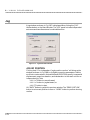
TOL-O-MATIC, INC
Excellence in Motion®
3600-4608A
© Copyright 1998 Tol-O-Matic, Incorporated.
All rights reserved. Axidyne and Tol-O-Matic
are registered trademarks of Tol-O-Matic Incorporated.
All other products or brand names
are trademarks of their respective holders.
8/00
TOL-O-MATIC, INC.
3800 County Road 116
Hamel, MN 55340
763.478.8000 Telephone
763.478.8080 Fax
http://www.tolomatic.com
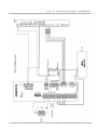
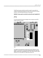
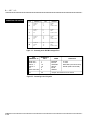
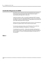
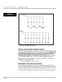
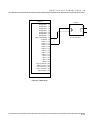
S S C T O A X I O M D R V B A S I C S C H E M AT I C
i
X-AXIS
MSD
GND
L2/N
L1
B–
B+
A–
A+
DIR +
DIR –
STEP +
STEP –
EN +
EN –
FAULT +
FAULT –
GRN
WHT
BLK
YLW
RED
ORG
BLK
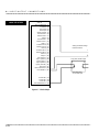
B– = BLU
B+ = RED
A– = YLW
WITH THE MRS171 MOTOR
THE WIRING COLOR CODE IS AS FOLLOWS
A+ = WHT
MTR CMD X
AMP ENBL X
PMW X/STEP X
SIGN X/DIR X
N/C
MTR CMD Y
AMP ENBL Y
PMW Y/DIR Y
SIGN Z/DIR Y
N/C
MTR CMD Z
AMP ENBL Z
PMW Z/STEP Z
SIGN Z /DIR Z
5V
MTR CMD W
AMP ENBL W
PMW W/STEP W
SIGN W/DIR W
GND
MRS
MOTOR
B–
B+
A–
A+
J5
SSC
ANAL 1
ANAL 2
ANAL 3
ANAL 4
ANAL 5
ANAL 6
ANAL 7
GND
5V
OUT 1
OUT 2
OUT 3
OUT 4
OUT 5
OUT 6
OUT 7
OUT 8
IN 8
IN 7
IN 6
IN 5
IN 4(LTCH W)
IN 3(LTCH Z)
IN 2(LTCH Y)
IN 1(LTCH X)
IN COM
ii
J3
SAMP CLK
REVRD
B– AUX W
B+ AUX W
A– AUX W
A+ AUX W
B– AUX Z
B+ AUX Z
A– AUX Z
A+ AUX Z
B– AUX Y
B+ AUX Y
A– AUX Y
A+ AUX Y
B– AUX X
B+ AUX X
A– AUX X
A+ AUX X
5V
GND
J4
J2
GND
5V
ERROR
RESET
SW COM
FWD LIM X
REV LMT X
HOME X
FWD LIM Y
REV LIM Y
HOME Y
FWD LIM Z
REV LIM Z
HOME Z
FWD LIM W
REV LIM W
HOME W
OUT 1
IN COM
LTCH X/IN1
LTCHY/IN2
LTCH Z/IN3
LTCH W/IN4
ABORT IN
MTR CMD X
AMP ENBL X
MTR CMD Y
AMP ENBL Y
MTR CMD Z
AMP ENBL Z
MTR CMD W
AMP ENBL W
A+X
A-X
B+X
B–X
I+X
I–X
A+Y
A–Y
B+Y
B–Y
I+Y
I–Y
A+Z
A–Z
B+Z
B–Z
I+Z
I–Z
A+W
A–W
B+W
B–W
I+W
I–W
+12V
–12V
5V
GND
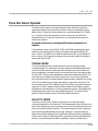
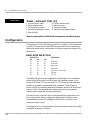
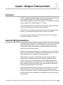
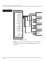
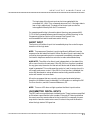
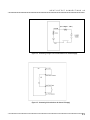
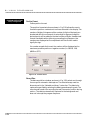
S S C T O M S D B A S I C S C H E M AT I C C O N N E C T I O N
GRN
GND
WHT
L2/N
BLK L1
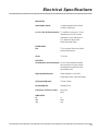
Electrical Specifications
SERVO CONTROL
ANALOG Amplifier Command:
+/-10 Volts analog signal. Resolution 16-bit DAC
or .0003 Volts. 3 mA maximum.
A+, A-, B+, B-, IDX+, IDX- Encoder and Auxiliary TTL compatible, but can accept up to +/- 12 Volts.
Quadrature phase on CHA, CHB. Can accept
single-ended (A+, B+ only) or differential (A+, A-,
B+, B-). Maximum A, B edge rate: 8 MHz.
Minimum IDX pulse width: 120nsec.
STEPPER CONTROL
Pulse
Direction
TTL (0-5 Volts) level at 50% duty cycle. 2,000,000
pulses/sec maximum frequency.
TTL (0-5 Volts)
INPUT/OUTPUT
Uncommitted Inputs, Limits, Home Abort Inputs: 2.2K ohm in series with optoisolator. Requires at
least 1 mA to activate. Can accept up to 28 Volts
without additional series resistor. Above 28 Volts
requires additional resistor.
AN[1] through AN[7] Analog Inputs:
Standard configuration is +/-10 Volt. 12-Bit
Analog-to-Digital convertor, 15 mAmp, 0.005 resolution.
OUT[1] through OUT[8] Outputs:
TTL (0-5vdc, 24mAmp)
IN[1] through IN[8] Inputs:
Optoisolated, 5-28 vdc
AC Power Input, 110 or 220 Vac, 50 or 60 Hz:
2 Amp (Inrush)
200 VA
POWER OUTPUTS
+5V
+12V
-12V
1a
600 ma
20 ma
iii
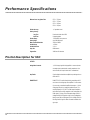
Performance Specifications
Minimum Servo Loop Update Time:
SSC1 — 250 µsec.
SSC2 — 375 µsec.
SSC3 — 500 µsec.
SSC4 — 500 µsec.
Position Accuracy:
Velocity Accuracy:
Long Term
Short Term
Position Range:
Velocity Range:
Motor Command Resolution:
Variable Range:
Variable Resolution:
Array Size:
Program Size:
+/- 1 quadrature count
Phase-locked, better than .005%
System dependent
+/-2147483647 counts per move
up to 8,000,000 cts/sec
16 Bits or 0.0003 V
+/-2 billion
1 * 10-4
8000 elements
1000 lines x 80 characters
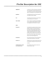
Pin-Out Description for SSC
OUTPUTS
iv
Analog Motor Command
+/- 10 Volt range signal for driving amplifier. In servo mode, motor
command output is updated at the controller sample rate. In the
motor off mode, this output is held at the OF command level.
Amp Enable
Signal to disable and enable an amplifier. Amp enable goes low on
Abort and OE1.
PWM/STEP OUT
PWM/STEP OUT is used for directly driving power bridges for DC
servo motors or for driving step motor amplifiers. For servo motors:
If you are using a conventional amplifier that accepts a +/- 10 Volt
analog signal, this pin is not used and should be left open. The
switching frequency is 16.7 KHZ. The PWM output is available in
two formats: Inverter and Sign magnitude. In the Inverter Mode, the
PWM signal is .2% duty cycle for full negative voltage, 50% for 0
Voltage and 99.8% for full positive charge. In the Sign Magnitude
Mode (Jumper SM), the PWM signal is 0% for 0 Voltage, 99.6% for
full voltage and the sign of the Motor Command is available at the
sign output.
Pin-Out Description for SSC
PWM/STEP OUT
For step motors: The STEP OUT pin produces a series of pulses for
input to a step motor driver. The pulses may either be low or high.
The pulse width is 50%. Upon Reset, the output will be low if the SM
jumper is on. If the SM jumper is not on, the output will be Tri-state.
Sign/Direction
Used with PWM signal to give the sign of the motor command for
servo amplifiers or direction for step motors.
Error
The signal goes low when the position error on any axis exceeds
the value specified by the error limit command, ER.
Output 1–Output 8
These 8 TTL outputs are uncommitted and may be designated by
the user to toggle relays and trigger external events. The output
lines are toggled by Set Bit, SB and Clear Bit, CB instructions.
INPUTS
Encoder, A+, B+
Position feedback from incremental encoder with two channels in
quadrature, CHA and CHB. The encoder may be analog or TTL.
Any resolution encoder may be used as long as the maximum
frequency does not exceed 8,000,000 quadrature states/sec. The
controller performs quadrature decoding of the encoder signals
resulting in a resolution of quadrature counts (4 x encoder cycles).
Note: Encoders that produce outputs in the format of pulses and
direction may also be used by inputting the pulses into CHA and
direction into Channel B and configuring this mode.
Encoder Index, I+
Once-Per-Revolution encoder pulse. Used in Homing sequence or
Find Index command to define home on an encoder index.
Encoder, A-, B-, I-
Differential inputs from encoder. May be input along with CHA, CHB
for noise immunity of encoder signals. The CHA- and CHB- inputs
are optional.
Auxiliary Encoder, Aux A+, Aux B+,
Aux I+, Aux A-, Aux B-, Aux I-
Inputs for additional encoder. Used when an encoder on both
the motor and the load is required.
v
PIN-OUT DESCRIPTION FOR SSC
vi
Abort
A low input stops commanded motion instantly without a controlled
deceleration. Also aborts motion program.
Reset
A low input resets the state of the processor to its power-on
condition. The previously saved state of the controller, along with
parameter values, and saved sequences are restored.
Forward Limit Switch
When active, inhibits motion in forward direction. Also causes
execution of limit switch subroutine, #LIMSWI. The polarity of the
limit switch may be set with the CN command.
Reverse Limit Switch
When active, inhibits motion in reverse direction. Also causes
execution of limit switch subroutine, #LIMSWI. The polarity of the
limit switch may be set with the CN command.
Home Switch
Input for Homing(HM) and Find Edge (FE) instructions. Upon BG
following HM or FE, the motor accelerates to slew speed. A
transition on this input will cause the motor to decelerate to a stop.
The polarity of the Home Switch may be set with the CN command.
Input 1 – Input 8 – Isolated
Uncommitted inputs. May be defined by the user to trigger events.
Inputs are checked with the Conditional Jump instruction and After
Input instruction or Input Interrupt. Input 1 is latch X, Input 2 is latch
Y, Input 3 is latch Z and Input 4 is latch W if the high speed position
latch function is enabled.
Latch
High speed position latch to capture axis position within 20 nano
seconds on occurrence of latch signal. AL command arms latch.
Input 1 is latch X, Input 2 is latch Y, Input 3 is latch Z and Input 4 is
latch W.
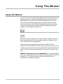
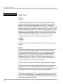
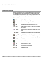
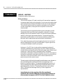
Using This Manual
Using This Manual
Your SSC motion controller has been designed to work with both servo and
stepper type motors. Installation and system setup will vary depending
upon whether the controller will be used with stepper motors, or servo
motors, To make finding the appropriate instructions faster and easier,
icons will be next to any information that applies exclusively to one type
of system. Otherwise, assume that the instructions apply to all types of
systems. The icon legend is shown below.
Attention: Pertains to servo motor use, such as the Tol-O-Matic Axiom Drive.
Attention: Discussion under this icon typically refer to stepper motors, but
also include other drivers that accept step and direction signals, such as
Tol-O-Matic’s MSD Microstepping drive.
Please note that many examples are written for the SSC 4 four-axis
controller. Users of the SSC 3 three-axis controller, SSC 2 two-axis controller
or SSC one-axis controller should note that the SSC 3 uses the axes denoted
as XYZ, the SSC 2 uses the axes denoted as XY, and the SSC uses the X-axis
only.
WARNING: Machinery in motion can be dangerous! It is the responsibility
of the user to design effective error handling and safety protection as part of
the machine. Tol-O-Matic shall not be liable or responsible for any
incidental or consequential damages.
I
Contents
CHAPTER 1 OVERVIEW
Introduction ......................................................................................................1-1
SSC Functional Elements..................................................................................1-2
Microcomputer Section ..............................................................................1-2
Motor Interface............................................................................................1-2
Communication..........................................................................................1-2
System Elements..........................................................................................1-3
CHAPTER 2 SET-UP
Elements You Need ............................................................................................2-1
Installing the SSC .............................................................................................2-2
Eight Steps To Setting Up Your SSC Controller ..........................................2-2
1. Setting Jumpers .....................................................................................2-2
2. Configuring DIP Switches ....................................................................2-5
3. Connecting Power .................................................................................2-5
4. Installing the Tol-O-Motion SSC Software ..........................................2-5
5. Establishing Communication ..............................................................2-6
6. Connections to Drive and Encoder ......................................................2-6
a. Connect the motor ............................................................................2-6
b. Connect the drive enable signal .......................................................2-6
c. Connect the encoders........................................................................2-7
d. Verify proper encoder operation ......................................................2-7
7. Connecting Standard Servo Motors .....................................................2-8
a. Check the Polarity of the Feedback Loop.........................................2-8
b. Set the Error Limit ............................................................................2-8
c. Set Torque Limit................................................................................2-9
d. Connect the Motor ............................................................................2-9
8. Connecting Step Motors......................................................................2-11
a. Install Step Mode jumpers..............................................................2-11
b. Connect step and direction signals ................................................2-11
Tune the Servo System...............................................................................2-15
Torque Mode........................................................................................2-15
Velocity Mode ......................................................................................2-15
CHAPTER 3 COMMUNICATION
Introduction ......................................................................................................3-1
RS232 Ports ........................................................................................................3-1
RS232 - Main Port {P1} ...............................................................................3-1
RS232 - Auxiliary Port {P2}.........................................................................3-1
*RS422 - Main Port {P1}..............................................................................3-1
*RS422 - Auxiliary Port {P2} .......................................................................3-2
Configuration ....................................................................................................3-2
Baud Rate Selection ....................................................................................3-2
Daisy-Chaining...........................................................................................3-3
II
CONTENTS
Synchronizing Sample Clocks ....................................................................3-5
Controller Response to DATA......................................................................3-6
CHAPTER 4 INPUT / OUTPUT CONNECTIONS
Overview ............................................................................................................4-1
General Wiring Guidelines................................................................................4-1
Using Optoisolated Inputs................................................................................4-2
Limit Switch Input ......................................................................................4-2
Home Switch Input .....................................................................................4-2
Homing Routines ........................................................................................4-3
Abort Input ..................................................................................................4-5
Uncommitted Digital Inputs......................................................................4-5
Wiring the Optoisolated Inputs........................................................................4-7
Using an Isolated Power Supply.................................................................4-8
Bypassing the Opto-Isolation: ....................................................................4-8
Changing Optoisolated Inputs From Active Low to High .......................4-10
Reset Input.................................................................................................4-10
Analog Inputs ..................................................................................................4-10
Using the Outputs ...........................................................................................4-11
Analog Command Output & Enable Input .............................................4-11
Offset Adjustment............................................................................................4-14
CHAPTER 5 TOL-O-MOTION SSC
VISUAL PROGRAMMING
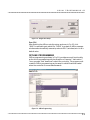
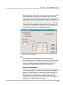
Introduction ......................................................................................................5-1
Installation..................................................................................................5-2
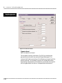
Controller Offline ..............................................................................................5-3
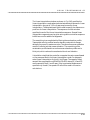
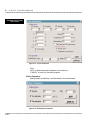
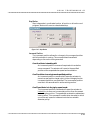
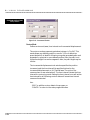
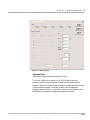
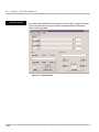
Serial Communication Setup.....................................................................5-3
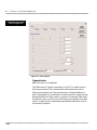
Offline Controller Setup..............................................................................5-5
Offline Programming..................................................................................5-9
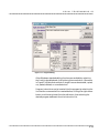
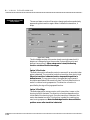
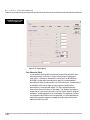
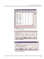
Controller Online ............................................................................................5-10
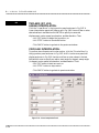
Setup .........................................................................................................5-11
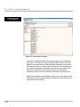
Program Window ......................................................................................5-12
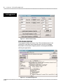
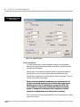
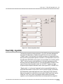
Program Instructions ......................................................................................5-20
Group = Configuration .............................................................................5-21
Group = I/O ................................................................................................5-31
Group = Motion.........................................................................................5-34
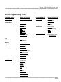
Group = Program Flow .............................................................................5-49
Group = Servo Settings..............................................................................5-63
Group = System Limits ..............................................................................5-66
Group = Mathematical Equation.............................................................5-69
Display .............................................................................................................5-71
III
CONTENTS
Jog.....................................................................................................................5-72
Jog by Position ...........................................................................................5-72
Jog by Speed ...............................................................................................5-73
Two-Axis (XY) Jog: Linear Interpolation..................................................5-74
Circular Interpolation ..............................................................................5-74
Teach by Joystick ..............................................................................................5-75
Terminal ..........................................................................................................5-78
Scope ................................................................................................................5-80
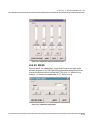
Tune .................................................................................................................5-82
Automatic Tuning .....................................................................................5-82
Manual Tuning .........................................................................................5-83
Tuning the Controller PID filter .....................................................................5-85
Description on the PID Filter....................................................................5-87
Operating a Drive in Torque Mode...........................................................5-88
Operating a Drive in Velocity Mode .........................................................5-88
Perform an Automatic Tune.....................................................................5-89
Fine Tune Response with a Manual Tune................................................5-89
Save the PID Values ...................................................................................5-89
CHAPTER 6 SAMPLE APPLICATIONS
Overview ............................................................................................................6-1
Example Applications.......................................................................................6-1
Wire Cutter ..................................................................................................6-1
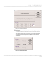
Table Controller ..........................................................................................6-3
CHAPTER 7 TWO-LETTER COMMAND SYNTAX
Introduction ......................................................................................................7-1
Command Syntax .............................................................................................7-1
Coordinated Motion with more than 1 axis ..............................................7-2
Program Syntax...........................................................................................7-3
Controller Response to DATA ............................................................................7-3
Interrogating the Controller .............................................................................7-3
Interrogation Commands...........................................................................7-3
Additional Interrogation Methods. ............................................................7-4
Command Summary ........................................................................................7-5
IV
CONTENTS
CHAPTER 8 PROGRAMMING MOTION
WITH TWO-LETTER COMMAND SYNTAX
Overview ............................................................................................................8-1
Independent Axis Positioning...........................................................................8-1
Command Summary - Independent Axis..................................................8-2
Operand Summary - Independent Axis .....................................................8-2
Independent Positioning Examples ...........................................................8-3
Independent Jogging .........................................................................................8-4
Command Summary - Jogging ..................................................................8-5
Operand Summary - Independent Axis .....................................................8-5
Jog Examples ...............................................................................................8-6
Linear Interpolation Mode ...............................................................................8-6
Specifying Linear Segments ........................................................................8-7
Specifying Vector Acceleration, Deceleration and Speed:..........................8-8
Additional Commands ...............................................................................8-8
Trippoints ....................................................................................................8-8
Trippoint Example......................................................................................8-8
Specifying Vector Speed for Each Segment.................................................8-9
Vector Speed Example.................................................................................8-9
Changing Feedrate ......................................................................................8-9
Command Summary - Linear Interpolation...........................................8-10
Operand Summary - Linear Interpolation..............................................8-10
Linear Interpolation Example..................................................................8-11
Vector Mode: Linear and Circular Interpolation Motion..............................8-13
Specifying Vector Segments.......................................................................8-14
Specifying Vector Acceleration, Deceleration and Speed:........................8-15
Additional Commands .............................................................................8-15
Trippoints ..................................................................................................8-15
Changing Feedrate ....................................................................................8-16
Compensating for Differences in Encoder Resolution ............................8-16
Tangent Motion.........................................................................................8-16
Tangent Motion Example .........................................................................8-17
Command Summary - Vector Mode Motion ...........................................8-18
Operand Summary - Vector Mode Motion...............................................8-18
Vector Mode Example ...............................................................................8-18
Electronic Gearing...........................................................................................8-20
Command Summary - Electronic Gearing..............................................8-21
Operand Summary - Electronic Gearing .................................................8-21
Electronic Gearing Examples ...................................................................8-22
Electronic Cam ................................................................................................8-23
Step 1: Selecting the Master Axis...............................................................8-24
Step 2: Specify the Master Cycle and the Change in the Slave Axis (ES) .8-24
Step 3: Specify the Master Interval and Starting Point............................8-24
Step 4: Specify the Slave Points .................................................................8-25
V
CONTENTS
Step 5: Enable the Ecam............................................................................8-25
Step 6: Engage the Slave Motion...............................................................8-25
Step 7: Disengage the Slave Motion..........................................................8-26
Command Summary - Ecam Mode .........................................................8-28
Operand Summary - Ecam Mode ............................................................8-28
Electronic Cam Example ..........................................................................8-29
Contour Mode..................................................................................................8-30
Specifying Contour Segments ...................................................................8-30
Additional Commands .............................................................................8-31
Command Summary - Contour Mode.....................................................8-32
Operand Summary - Contour Mode........................................................8-32
Contour Example......................................................................................8-32
Teach (Record and Play-Back)........................................................................8-35
Record and Playback Example.................................................................8-35
Dual Loop (Auxiliary Encoder) ......................................................................8-36
Using the CE Command ...........................................................................8-36
Additional Commands for the Auxiliary Encoder ..................................8-37
Backlash Compensation...........................................................................8-37
Dual Loop Example ..................................................................................8-38
Motion Smoothing ..........................................................................................8-39
Using the IT and VT Commands (S curve profiling): ..............................8-39
Servo Motor ...............................................................................................8-40
Using the KS Command (Step Motor Smoothing): .................................8-40
Homing ............................................................................................................8-41
Homing Examples.....................................................................................8-42
High Speed Position Capture (The Latch Function) .....................................8-44
High Speed Position Example ..................................................................8-44
CHAPTER 9 APPLICATION PROGRAMMING
WITH TWO-LETTER COMMAND SYNTAX
Overview ............................................................................................................9-1
Using the SSC Editor to Enter Programs ..........................................................9-1
Edit Mode Commands ................................................................................9-2
Program Format................................................................................................9-3
Using Labels in Programs...........................................................................9-3
Special Labels ..............................................................................................9-4
Commenting Programs ..............................................................................9-5
Executing Programs & Multitasking ................................................................9-6
Debugging Programs ........................................................................................9-7
Commands ..................................................................................................9-7
Operands .....................................................................................................9-8
VI
CONTENTS
Program Flow Commands................................................................................9-9
Event Triggers & Trippoints ........................................................................9-9
SSC Event Triggers.....................................................................................9-10
Event Trigger Examples: ...........................................................................9-11
Conditional Jumps..........................................................................................9-14
Subroutines......................................................................................................9-17
Stack Manipulation ..................................................................................9-18
Mathematical Expressions..............................................................................9-23
Mathematical Expressions .......................................................................9-23
Bit-Wise Operators ....................................................................................9-24
Functions .........................................................................................................9-25
Variables ..........................................................................................................9-26
Assigning Values to Variables:...................................................................9-26
Operands .........................................................................................................9-28
Special Operands (Keywords) ...................................................................9-28
Arrays ...............................................................................................................9-29
Defining Arrays .........................................................................................9-29
Assignment of Array Entries .....................................................................9-29
Automatic Data Capture into Arrays .......................................................9-31
Command Summary - Automatic Data Capture ...................................9-31
Operand Summary - Automatic Data Capture.......................................9-32
Deallocating Array Space..........................................................................9-32
Input of Data (Numeric and String) ..............................................................9-33
Input of Data.............................................................................................9-33
Operator Data Entry Mode .......................................................................9-34
Using Communication Interrupt.............................................................9-35
Output of Data (Numeric and String) .....................................................9-37
Sending Messages......................................................................................9-37
Displaying Variables and Arrays ..............................................................9-40
Formatting the Response of Interrogation Commands ..........................9-40
Formatting Variables and Array Elements...............................................9-41
Converting to User Units ..........................................................................9-43
Programmable Hardware I/O.........................................................................9-43
Digital Outputs .........................................................................................9-43
Digital Inputs ............................................................................................9-44
Input Interrupt Function..........................................................................9-45
Analog Inputs ............................................................................................9-46
Application Programming Examples ............................................................9-47
Wire Cutter ................................................................................................9-47
X-Y Controller ...........................................................................................9-49
Speed Control by Joystick ..........................................................................9-51
Position Control by Joystick ......................................................................9-52
Backlash Compensation by Sampled Dual-Loop ...................................9-53
VII
CONTENTS
CHAPTER 10 HARDWARE & SOFTWARE PROTECTION
Introduction ....................................................................................................10-1
Hardware Protection.......................................................................................10-1
Output Protection Lines ...........................................................................10-1
Input Protection Lines ..............................................................................10-1
Software Protection.........................................................................................10-2
Programmable Error Limit.......................................................................10-2
Programmable Position Limits ................................................................10-3
Off-On-Error .............................................................................................10-3
Automatic Error Routine ..........................................................................10-4
Limit Switch Routine ................................................................................10-4
CHAPTER 11 TROUBLESHOOTING
Overview ..........................................................................................................11-1
Installation ......................................................................................................11-1
Communication..............................................................................................11-2
Stability............................................................................................................11-2
Operation.........................................................................................................11-2
CHAPTER 12 COMMAND REFERENCE
Command Descriptions..................................................................................12-1
Two-Letter Command Summary ...................................................................12-3
AB
Abort ..............................................................................................12-5
AC
Acceleration...................................................................................12-6
AD
After Distance................................................................................12-8
AF
Analog Feedback .........................................................................12-10
AI
After Input ...................................................................................12-11
AL
Arm Latch....................................................................................12-12
AM
After Move ...................................................................................12-13
AP
After Absolute Position ...............................................................12-15
AR
After Relative Position ................................................................12-17
AS
At Speed .......................................................................................12-18
AT
At Time ........................................................................................12-19
AV
After Vector Distance...................................................................12-20
BG
Begin............................................................................................12-21
BL
Reverse Software Limit ...............................................................12-23
BN
Burn System Parameters ............................................................12-24
BP
Burn Program .............................................................................12-26
BV
Burn Variables.............................................................................12-27
CB
Clear Bit.......................................................................................12-28
CC
Configure Communication Port 2 .............................................12-29
CD
Contour Data ..............................................................................12-30
CE
Configure Encoder ......................................................................12-31
VIII
CONTENTS
CI
CM
CN
CR
CS
DA
DC
DE
DL
DM
DP
DT
DV
EA
EB
ED
EG
EM
EN
EO
EP
EQ
ER
ES
ET
FA
FE
FI
FL
FV
GA
GN
GR
HM
HX
II
IL
IN
IP
IT
JG
JP
JS
Communication Interrupt .........................................................12-32
Contouring Mode........................................................................12-34
Configure.....................................................................................12-35
Circle............................................................................................12-36
Clear Sequence............................................................................12-38
Deallocate The Variables and Arrays .........................................12-39
Deceleration ................................................................................12-41
Dual (Aux) Encoder Position......................................................12-43
Download....................................................................................12-44
Dimension...................................................................................12-46
Define Position............................................................................12-47
Delta Time...................................................................................12-49
Dual Velocity ( Dual Loop) .........................................................12-51
Choose ECAM Master .................................................................12-52
Enable ECAM ..............................................................................12-53
Edit ..............................................................................................12-54
ECAM Go Engage ........................................................................12-56
Cam Cycles ..................................................................................12-57
End ..............................................................................................12-58
Echo .............................................................................................12-60
Cam Table Intervals & Starting Point........................................12-61
ECAM Quit (Disengage) .............................................................12-62
Error Limit ..................................................................................12-63
Ellipse Scale.................................................................................12-65
Electronic Cam Table..................................................................12-66
Acceleration Feedforeward .........................................................12-67
Find Edge ....................................................................................12-68
Find Index ...................................................................................12-70
Forward Software Limit .............................................................12-71
Velocity Feedforward ..................................................................12-72
Master Axis for Gearing ..............................................................12-73
Gain.............................................................................................12-75
Gear Ratio ...................................................................................12-76
Home ...........................................................................................12-77
Halt Execution ............................................................................12-79
Input Interrupt............................................................................12-80
Integrator Limit ..........................................................................12-82
Input Variable .............................................................................12-83
Increment Position .....................................................................12-85
Independent Time Constant Smoothing Function ...................12-87
Jog ................................................................................................12-88
Jump to Program Location.........................................................12-89
Jump to Subroutine ....................................................................12-90
IX
CONTENTS
KD
KI
KP
KS
LE
_LF*
LI
LM
_LR*
LS
LZ
MC
MF
MG
MO
MR
MT
NO
OB
OE
OF
OP
PA
PF
PR
QD
QU
RA
RC
RD
RE
RI
RL
RP
RS
<control>R<control>S
SB
SC
SH
SP
ST
TB
TC
X
Derivative Constant....................................................................12-92
Integrator ....................................................................................12-93
Proportional Constant ...............................................................12-94
Step Motor Smoothing................................................................12-95
Linear Interpolation End ...........................................................12-96
Forward Limit Switch Operand (keyword) ...............................12-97
Linear Interpolation Distance ...................................................12-98
Linear Interpolation Mode.......................................................12-100
Reverse Limit Switch Operand (keyword) ...............................12-102
List .............................................................................................12-103
Leading Zeros............................................................................12-104
Motion Complete “In Position” ................................................12-105
Forward Motion to Position .....................................................12-107
Message .....................................................................................12-108
Motor Off ...................................................................................12-110
Reverse Motion to Position .......................................................12-111
Motor Type ................................................................................12-112
No Operation ............................................................................12-114
Output Bit .................................................................................12-115
Off On Error ..............................................................................12-116
Offset..........................................................................................12-118
Output Port ...............................................................................12-119
Position Absolute ......................................................................12-120
Position Format ........................................................................12-122
Position Relative .......................................................................12-124
Download Array........................................................................12-125
Upload Array.............................................................................12-126
Record Array..............................................................................12-127
Record........................................................................................12-128
Record Data...............................................................................12-130
Return from Error Routine .......................................................12-132
Return from Interrupt Routine ................................................12-133
Report Latched Position ...........................................................12-134
Reference Position.....................................................................12-135
Reset...........................................................................................12-137
Master Reset ..............................................................................12-138
Set Bit.........................................................................................12-139
Stop Code ..................................................................................12-140
Servo Here .................................................................................12-141
Speed .........................................................................................12-142
Stop............................................................................................12-144
Tell Status Byte ..........................................................................12-145
Tell Error Code ..........................................................................12-146
CONTENTS
TD
TE
TI
TIME*
TL
TM
TN
TP
TR
TS
TT
TV
TW
UL
VA
VD
VE
VF
VM
VP
VR
VS
VT
WC
WT
XQ
ZR
ZS
Tell Dual Encoder .....................................................................12-148
Tell Error....................................................................................12-149
Tell Inputs..................................................................................12-150
Time Operand (keyword) .........................................................12-151
Torque Limit..............................................................................12-152
Time...........................................................................................12-153
Tangent......................................................................................12-154
Tell Position...............................................................................12-156
Trace ..........................................................................................12-157
Tell Switches ..............................................................................12-158
Tell Torque.................................................................................12-160
Tell Velocity................................................................................12-161
Timeout for IN-Position (MC)..................................................12-162
Upload.......................................................................................12-163
Vector Acceleration ...................................................................12-164
Vector Deceleration...................................................................12-166
Vector Sequence End.................................................................12-168
Variable Format........................................................................12-169
Coordinated Motion Mode .......................................................12-170
Vector Position ..........................................................................12-172
Vector Speed Ratio ....................................................................12-174
Vector Speed ..............................................................................12-176
Vector Time Constant - S Curve ...............................................12-177
Wait for Contour Data..............................................................12-178
Wait ...........................................................................................12-179
Execute Program.......................................................................12-180
Zero............................................................................................12-181
Zero Subroutine Stack ..............................................................12-182
XI
XII
Overview
1
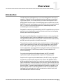
Introduction
The SSC Series are packaged motion controllers designed for stand-alone
operation. Features include coordinated motion profiling, uncommitted
inputs and outputs, non-volatile memory for stand-alone operation and
RS232/RS422 communication. Extended performance capabilities include:
fast 8 MHz encoder input frequency, precise 16-bit motor command output
DAC, +/-2 billion counts total travel per move, faster sample rate, and
multitasking of up to four programs.
Designed for maximum system flexibility, the SSC is available for one to four
axes and can be interfaced to a variety of motors and drives including step
motors, servo motors and hydraulics.
Each axis accepts feedback from a quadrature linear or rotary encoder with
input frequencies up to 8 million quadrature counts per second. For dualloop applications that require one encoder on both the motor and the load,
auxiliary encoder inputs are included for each axis.
The powerful controller provides many modes of motion including jogging,
point-to-point positioning, linear and circular interpolation with infinite
vector feed, electronic gearing and user-defined path following. Several
motion parameters can be specified including acceleration and deceleration
rates, and slew speed. The SSC also provides S-curve acceleration for
motion smoothing.
For synchronizing motion with external events, the SSC includes 8
optoisolated inputs, 8 programmable outputs and 7 analog inputs.
Despite its full range of sophisticated features, the SSC is easy to program.
Programming is performed using the Tol-O-Motion SSC Software which
allows programming to be done in a visual environment that generates two
letter commands to be downloaded to the controller. Experienced users are
able to program the controller directly by using two letter commands in the
terminal mode. To prevent system damage during machine operation, the
SSC provides several error handling features. These include software and
hardware limits, automatic shut-off on excessive error, abort input, and
user-definable error and limit routines.
1-1
1:
OVERVIEW
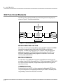
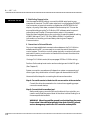
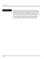
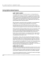
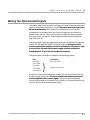
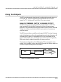
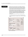
SSC Functional Elements
The SSC circuitry can be divided into the following functional groups as
shown in Figure 1.1 and discussed below.
To H ost
R S-232 / R S-422 S er ia l
C omm unica tion FI FO
80 B ytes
8 TTL O ut
8 D igi tal In
To A mps
I/O
Inte rfa ce
683 40
Mic rocomputer
256 K RA M
64K E PR OM
4 M E EP RO M
8 A na log In
G L-1800
4-A xe s
Motor /E ncode r
Inte rfa ce
Fr om
Lim its
Fr om
E ncoder s
W atch D og
Tim er
Figure 1.1 - SSC Functional Elements
MICROCOMPUTER SECTION
The main processing unit of the SSC is a specialized 32-bit Motorola 68340
Series Microcomputer with 256K RAM, 64 K EPROM and 4 M bytes
EEPROM. The RAM provides memory for variables, array elements and
application programs. The EPROM stores the firmware of the SSC. The
EEPROM allows parameters and programs to be saved in non-volatile
memory upon power down.
MOTOR INTERFACE
For each axis, a GL-1800 gate array performs quadrature decoding of the
encoders at up to 8 MHz, generates the +/-10 Volt analog signal (16 Bit DAC)
for input to a servo amplifier, and generates step and direction signal for
step motor drivers.
COMMUNICATION
Communication to the SSC is via two separately addressable RS232 ports.
The ports may also be configured by the factory for RS422. The serial ports
may be daisy-chained to other SSC controllers.
1-2
OVERVIEW
:1
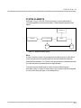
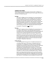
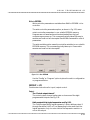
SYSTEM ELEMENTS
As shown in Fig. 1.2, the SSC is part of a motion control system which
includes amplifiers, motors and encoders. These elements are described
below
POWER SUPPLY
COMPUTER
SSC 1-4 CONTROLLER
ENCODER
DRIVER
MOTOR
Figure 1.2 - Elements of Servo systems
Motor
A motor converts current into torque which produces motion. Each axis of
motion requires a motor sized properly to move the load at the desired
speed and acceleration. Tol-O-Matic’s sizing and selection software can help
you calculate motor size and drive size requirements.
The motor may be a step or servo motor and can be brush-type or
brushless, rotary or linear. For step motors, the controller can be configured
to control full-step, half-step, or microstep drives.
1-3
1:
OVERVIEW
SSC FUNCTIONAL ELEMENTS
Amplifier (Drive)
For each axis, the power amplifier converts a +/-10 Volt signal from the
controller into current to drive the motor. The amplifier should be sized
properly to meet the power requirements of the motor. For brushless
motors, an amplifier that provides electronic commutation is required. The
amplifiers may be either pulse-width-modulated (PWM) or linear. They may
also be configured for operation with or without a tachometer. For current
amplifiers, the amplifier gain should be set such that a 10 Volt command
generates the maximum required current. For example, if the motor peak
current is 10A, the amplifier gain should be 1 A/V. For velocity mode
amplifiers, 10 Volts should run the motor at the maximum speed.
For stepper motors, the amplifier converts step and direction signals into
current.
Encoder
An encoder translates motion into electrical pulses which are fed back into
the controller. The SSC accepts feedback from either a rotary or linear
encoder. Typical encoders provide two channels in quadrature, known as
CHA and CHB. This type of encoder is known as a quadrature encoder.
Quadrature encoders may be either single-ended (CHA and CHB) or
differential (CHA,CHA-,CHB,CHB-). The SSC decodes either type into
quadrature states or four times the number of cycles. Encoders may also
have a third channel (or index) for synchronization.
The SSC can also interface to encoders with pulse and direction signals.
There is no limit on encoder line density, however, the input frequency to
the controller must not exceed 2,000,000 full encoder cycles/second or
8,000,000 quadrature counts/sec. For example, if the encoder line density is
10,000 cycles per inch, the maximum speed is 200 inches/second.
The standard voltage level is TTL (zero to five volts), however, voltage levels
up to 12 Volts are acceptable. If using differential signals, 12 Volts can be
input directly to the SSC. Single-ended 12 Volt signals require a bias voltage
input to the complementary inputs.
1-4
Set Up
2
Elements You Need
Before you start, you will need the following system elements:
1. SSC Motion Controller and included cables, RS232, 60 pin ribbon
cable and 26-pin ribbon cable.
2. Breakout terminals - (Optional) for screw terminal accessibility a
60 pin, 26-pin din rail breakout terminal block from Tol-O-Matic is
recommended.
3. Servo motors with Encoder (one per axis) or step motors
4. Motor Driver (Amplifier) e.g. Tol-O-Matic Axiom Servo or Micro
Stepper Drive
5. PC (Personal Computer with RS232 port)
6. Tol-O-Motion SSC Software
For servo motors, the amplifiers should accept an analog signal in the +/-10
Volt range as a command. The amplifier gain should be set so that a +10V
command will generate the maximum required current. For example, if the
motor peak current is 10A, the amplifier gain should be 1 A/V. For velocity
mode amplifiers, a command signal of 10 Volts should run the motor at the
maximum required speed.
For step motors, the amplifiers should accept step and direction signals.
8. For stepper motor operation, you will need an additional 20-pin
ribbon cable, J4, to connect step and direction signals.
2-1
2:
SET UP
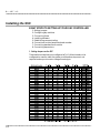
Installing the SSC
EIGHT STEPS TO SETTING UP YOUR SSC CONTROLLER
1. Setting jumpers
2. Configuring dip switches
3. Connecting Power
4. Installing software
5. Establishing communication
6. Connections to drive (amplifiers) and encoder
7. Connecting standard servo motors
8. Connecting step motors
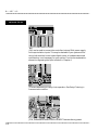
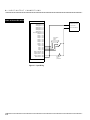
1. Setting Jumpers on the SSC
These switches have been pre configured at Tol-O-Matic based on the
configuration used to order the system, and therefore step one is not
required unless you choose to change the axis type.
2-2
:2
SET UP
The SSC has jumpers inside the controller box which may need to be
installed. To access these jumpers, the cover of the controller box must be
removed. The following describes each of the jumpers.
WARNING: Never open the controller box when AC power is applied to it.
For each axis that will be driving a stepper motor, a stepper mode (SM)
jumper must be connected.
U40
75
C67
U20
74
F3
54
SMX
SMY
SMZ
SMW
OPT
JP40
53
C7
C66
U26
H
JP40
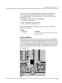
The stepper mode jumpers are located next to the GL-1800 which is the
largest IC on the board. The jumper set is labeled JP40 and the individual
stepper mode jumpers are labeled SMX, SMY, SMZ, SMW. The fifth jumper
of the set, OPT, is for use by Tol-O-Matic technicians only.
2-3
2:
SET UP
INSTALLING THE SSC
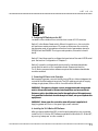
C202
UXY3
RPXY3
INCOM
RP41
LSCOM
RP40
J2
JP41
UXY2
C102
UYZ2
C7
JP41
JP41, can be used to connect the controllers internal 5Vdc power supply
to the optoisolation inputs. This may be desirable if your system will be
using limit switches, home inputs digital inputs, or hardware abort and
optoisolation is not necessary for your system. For a further explanation,
see section Bypassing the Opto-Isolation in Chapter 4.
RP22
C32
JP20
144
ADR1
ADR2
ADR4
C61
C97
EARTH
X1
00
C3
JP 20 sets addressing for daisy-chain operation. See Daisy-Chaining in
communication section.
JP30
JP31
JP 30, 31are used to select RS232 or RS422. These are factory preset.
2-4
:2
SET UP
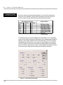
2. Configuring DIP Switches on the SSC
Located on the outside of the controller box is a set of 5 DIP switches.
Switch 1 is the Master Reset switch. When this switch is on, the controller
will perform a master reset upon PC power up. Whenever the controller
has a master reset, all programs and motion control parameters stored in
EEPROM will be ERASED. During normal operation, this switch should
be off.
Switch 2,3 and 4 are used to configure the baud rate of the main RS232 serial
port. See section Configuration in Chapter 3.
Switch 5 is used to configure both serial ports for hardware handshake
mode. Set this switch on for handshake mode. Please note that the
Tol-O-Matic communication software requires that hardware handshake
mode be enabled.
3. Connecting AC Power to the Controller
Before applying power, connect the 60-pin and 26-pin ribbons between the
controller and the breakout terminals. The SSC requires a single AC supply
voltage, single phase, 50 Hz or 60 Hz. from 90 volts to 260 volts.
WARNING: Dangerous voltages, current, temperatures and energy levels
exist in this product and in its associated amplifiers and servo motor(s).
Extreme caution should be exercised in the application of this equipment.
Only qualified individuals should attempt to install, set up and operate this
equipment.
WARNING: Never open the controller when AC power is applied to it.
Applying power will turn on the green light power indicator.
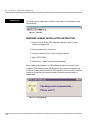
4. Installing the Tol-O-Motion SSC Software
After you have installed the SSC controller and powered up your computer,
install the Tol-O-Motion SSC Software, available for Windows 3.1, 95 and NT,
by running “setup.exe” on disc number 1.
2-5
2:
SET UP
INSTALLING THE SSC
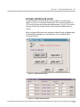
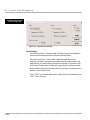
5. Establishing Communication
Use the supplied RS232 cable to connect the MAIN serial port to your
computer or terminal. The SSC main serial port is configured as DATASET.
Your computer or terminal must be configured as a DATATERM for full
duplex, no parity, 8 bits data, one start bit and one stop bit. This can be
accomplished by using the Tol-O-Motion SSC software serial communication setup see Chapter 3 Communication setup in this manual.
Select the baud rate switches on the controller to match the default setting
of 9600. Settings of The PC (19.2 kb, 9600 or1200b). For Additional
information on auxiliary ports and daisy chaining, see Chapter 3
Communication.
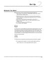
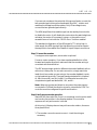
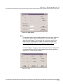
6. Connections to Drive and Encoder
Once you have established communications between the Tol-O-Motion
software and the SSC, you are ready to connect the rest of the motion
control system. The motion control system typically consists of a drive for
each axis of motion, and a motor to transform the current from the drive
into torque for motion.
If using a Tol-O-Matic motor/drive, see pages 2-12 thru 2-14 for wiring.
Perform Online setup to set motor and encoder type and initial PID gain.
(See Chapter 5)
System connection procedures will depend on system components and
motor types. Any combination of motor types can be used with the SSC.
Here are the first steps for connecting the drives and encoders:
Step A: Connect the motor to the drive with no connection to the controller.
Consult the drive documentation for instructions regarding proper
connections and startup.
Step B: Connect the drive enable signal.
Before making any connections from the drive to the controller, you
need to verify that the ground level of the drive is either floating or at
the same potential as earth.
WARNING: When the amplifier ground is not isolated from the power
line or when it has a different potential than that of the SSC ground,
serious damage may result to the SSC controller and amplifier.
2-6
:2
SET UP
If you are not sure about the potential of the ground levels, connect the
two ground signals (drive ground and earth) by a 10 KΩ resistor and
measure the voltage across the resistor. Only if the voltage is zero,
connect the two ground signals directly.
The AEN (amplifier/drive enable) signal can be used by the controller
to disable the motor. It will disable the motor when the watchdog timer
activates, the motor-off command, is given, or the position error
exceeds the error limit with the “Off-On-Error” function enabled.
The standard configuration of the AEN signal is TTL active high. In
other words, the AEN signal will be high when the controller expects
the amplifier to be enabled. See Chapter 4 Input/Output connections.
Step C: Connect the encoders
For stepper motor operation, an encoder is optional.
For servo motor operation, if you have a preferred definition of the
forward and reverse directions, make sure that the encoder wiring is
consistent with that definition.
The SSC accepts single-ended or differential encoder feedback with or
without an index pulse. For encoder connection, simply match the
leads from the encoder you are using to the encoder feedback inputs
on the breakout terminals. The signal leads are labeled XA+ (channel
A), XB+ (channel B), and XI+ (index). For differential encoders, the
complement signals are labeled XA-, XB-, and XI-.
Note: When using pulse and direction encoders, the pulse signal is
connected to CHA and the direction signal is connected to CHB. The
controller must be configured for pulse and direction.
Step D: Verify proper encoder operation.
Start with the X encoder first. Once it is connected, turn the motor shaft
and monitor the position in the display window. The controller
response will vary as the motor is turned.
At this point, if display does not vary with encoder rotation, there are
three possibilities:
1. The encoder connections are incorrect - check the wiring as
necessary.
2-7
2:
SET UP
INSTALLING THE SSC
2. The encoder has failed - using an oscilloscope, observe the encoder
signals. Verify that both channels A and B have a peak magnitude
between 5 and 12 volts. Note that if only one encoder channel fails,
the position reporting varies by one count only. If the encoder failed,
replace the encoder. If you cannot observe the encoder signals, try a
different encoder.
3. There is a hardware failure in the controller- connect the same
encoder to a different axis. If the problem disappears, you probably
have a hardware failure. Consult the factory for help.
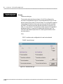
7. Connecting Standard Servo Motors
The following discussion applies to connecting the SSC controller to
standard servo motor drives:
The motor and the drive may be configured in the torque or the velocity
mode. In the torque mode, the amplifier gain should be such that a 10 Volt
signal generates the maximum required current. In the velocity mode, a
command signal of 10 Volts should run the motor at the maximum required
speed.
Step A. Check the Polarity of the Feedback Loop
It is assumed that the motor and drive are connected together and that
the encoder is operating correctly. Before connecting the motor drive to
the controller, read the following discussion on setting Error Limits and
Torque Limits. Note that this discussion uses the X axis as an example.
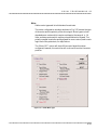
Step B. Set the Error Limit as a Safety Precaution
Usually, there is uncertainty about the correct polarity of the feedback.
The wrong polarity causes the motor to run away from the starting
position. Using the programming terminal, the following parameters
can be given to avoid system damage:
Input the commands:
ER 2000 <CR>
Sets error limit on the X axis to be 2000 encoder
counts
OE 1 <CR>
Disables X axis amplifier when excess position error
exists
If the motor runs away and creates a position error of 2000 counts, the
motor amplifier will be disabled. Note: This function requires the
2-8
:2
SET UP
Amplifier Enable (AEN) signal to be connected from the controller to
the amplifier.
Step C. Set Torque Limit as a Safety Precaution
To limit the maximum voltage signal to your amplifier, the SSC
controller has a torque limit command, TL. This command sets the
maximum voltage output of the controller and can be used to avoid
excessive torque or speed when initially setting up a servo system.
When operating a drive in torque mode, the voltage output of the
controller will be directly related to the torque output of the motor.
The user is responsible for determining this relationship using the
documentation of the motor and drive. The “torque” limit can be set
to a value that will limit the motor’s output torque.
When operating a drive in velocity or voltage mode, the voltage output
of the controller will be directly related to the velocity of the motor.
The user is responsible for determining this relationship using the
documentation of the motor and drive. The “torque” limit can be set
to a value that will limit the speed of the motor.
For example, the following command will limit the output of the
controller to 1 volt on the X axis:
TL 1 <CR>
Note: Once the correct polarity of the feedback loop has been
determined, the torque limit should, in general, be increased to the
default value of 9.99. The servo will not operate properly if the torque
limit is below the normal operating range.
Step D: Connect the Motor
Once the parameters have been set, connect the analog motor
command signal (ACMD) to the drive input.
To test the polarity of the feedback, use the jog by position function.
(See Chapter 5)
When the polarity of the feedback is wrong, the motor will attempt to
run away. The controller should disable the motor when the position
error exceeds 2000 counts. If the motor runs away, the polarity of the
loop must be inverted.
2-9
2:
SET UP
Note: Inverting the Loop Polarity
When the polarity of the feedback is incorrect, the user must invert the
loop polarity and this may be accomplished by several methods. If you
are driving a brush-type DC motor, the simplest way is to invert the two
motor wires (typically red and black). When driving a brushless motor,
the polarity reversal may be done with the encoder. If you are using a
single-ended encoder, interchange the signal CHA and CHB. If, on the
other hand, you are using a differential encoder, interchange only
CHA+ and CHA-.
Note: Reversing the Direction of Motion
If the feedback polarity is correct but the direction of motion is
opposite to the desired direction of motion on a brush DC motor,
reverse the motor leads AND the encoder signals. For a brushless
motor, see documentation for drive on reversing direction of rotation.
Note: Tuning
When the position loop has been closed with the correct polarity, the
next step is to adjust the PID filter parameters, KP, KD and KI. It is
necessary to accurately tune your servo system to ensure fidelity of
position and minimize motion oscillation as described in the tuning
section of this chapter.
2-10
:2
SET UP
8. Connecting Step Motors
In Stepper Motor operation, the pulse output signal of the SSC has a 50%
duty cycle. Step motors operate open loop and do not require encoder
feedback. When a stepper is used, the auxiliary encoder for the corresponding
axis is unavailable for an external connection. If an encoder is used for
position feedback, connect the encoder to the main encoder input
corresponding to that axis. The commanded position of the stepper can
be interrogated with RP or DE. The encoder position can be interrogated
with TP.
The frequency of the step motor pulses can be smoothed with the filter
parameter. The filter parameter has a range between 0.5 and 8, where 8
implies the largest amount of smoothing.
See Command Reference regarding KS, RP, DE, TP and other two letter
commands.
The SSC profiler commands the step motor amplifier. All SSC motion
commands apply in stepper mode. Since step motors run open-loop, the
PID filter does not function and the position error is not generated.
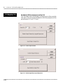
To connect step motors with the SSC you must follow this procedure:
Step A. Install Step Mode jumpers
Each axis of the SSC that will operate a stepper motor must have the
corresponding stepper motor jumper installed. The jumpers are preset
at Tol-O-Matic to match system ordered.
Step B. Connect step and direction signals.
Make connections from controller to motor amplifiers. (These signals
are found on 20 pin breakout connected to J4). Consult the
documentation for your step motor drive. See p2.14 for Tol-O-Matic
MSD connection.
2-11
2: SET UP
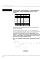
SSC J2 Main; 60 Pin IDC
SSC J4 Driver ; 20- Pin IDC:
1. Zero Volt Ref.
3. Error
5. Limit Switch Common
7. Reverse Limit - X
9. Forward Limit - Y
11. Home - Y
13. Reverse Limit - Z
15. Forward Limit - W
17. Home - W
19. Input Common
21. Latch Y or Input 2
23. Latch W or Input 4
25. Motor Command X
27. Motor Command Y
29. Motor Command Z
31. Motor Command W
33. A+X
35. B+X
37. I+X
39. A+Y
41. B+Y
43. I+Y
45.A+Z
47. B+Z
49. I+Z
51. A+W
53. B+W
55. I+W
57. +12V
59. 5V
1. Motor Command X
3. PMW X/ StepX
5.
7. Amp Enable Y
9. Sign Y/ Dir Y
11. Motor Command Z
13. PMW Z / Step Z
15. 5V
17. Amp Enable W
19. Sign W/ Dir W
2. 5V
4. Reset
6. Forward Limit - X
8. Home - X
10. Reverse Limit - Y
12. Forward Limit - Z
14. Home - Z
16. Reverse Limit - W
18. Output 1
20. Latch X or Input 1
22. Latch Z or Input 3
24. Abort Input
26. Amp Enable X
28. Amp Enable Y
30. Amp Enable Z
32. Ampo Enable W
34. A-X
36. B-X
38. I-X
40. A-Y
42. B-Y
44. I-Y
46. A-Z
48. B-Z
50. I-Z
52. A-W
54. B-W
56. I-W
58. -12 V
60. Zero Volt Ref.
SSC J3 Auxiliary Encoder; 20- Pin IDC:
1. Sample Clock
3. B- Aux W
5. A- Aux W
7. B- Aux Z
9. A- Aux Z
11. B- Aux Y
13. A- Aux Y
15. B- Aux X
17. A- Aux X
19. 5V
2. Reserved
4. B+ Aux W
6. A+ Aux W
8. B+ Aux Z
10. A+ Aux Z
12. B+ Aux Y
14. A+ Aux Y
16. B+ Aux X
18. A+ Aux X
20. Zero Volt Ref.
SSC J5 General I/O; 26- Pin IDC
1. Analog 1
3. Analog 3
5. Analog 5
7. analog 7
9. 5v
11. Output 2
13. Output 4
15. Output 6
17. Output 8
19. Input 7
21. Input 5
23. Input 3 ( Latch Z)
25. Input 1 (Latch X)
2. Analog 2
4. Analog 4
6. Analog 6
8. Zero Volt Ref.
10. Output 1
12. Output 3
14. Output 5
16. Output 7
18. Input 8
20. Input 6
22. Input 4 ( Latch W)
24. Input 2 ( Latch Y)
26. Input Common
AC Power Inputs:
Hot
Neutral
Earth
Connects to 110 or 220 AC
Return for AC
Chassis input
SSC Main Port; 9- Pin:
1. CTS - output
2. Transmit data - output
3. Receive data - input
4. RTS - input
5. Zero Volt Ref.
7. RTS - Input
9. 5V
6. CTS - output
8. CTS - output
SSC - Auxiliary Port; 9- Pin:
1. CTS - input
3. Transmit data - output
5. Zero Volt Ref.
7. RTS - output
9. 5V
Figure 2.1 - SSC Connector Pinout
2-12
2. Amp Enable X
4. Sign X/ Dir X
6. Motor Command Y
8. PMW Y/ Step Y
10.
12. Amp Enable Z
14. Sign Z/ Dir Z
16. Motor Command W
18. PMW W/ Step W
20. Zero Volt Ref.
2. Receive data - input
4. RTS - output
6. CTS - input
8. CTS - input
SET UP
AXIS
X
Y
Z
W
SSC
TERMINAL J2
BREAKOUT
PIN #
ZERO VOLT REF.
MOTOR COMMAND X
A+X
A-X
B+X
B-X
I+X
I-X
ZERO VOLT REF.
1
25
33
34
35
36
37
38
1
ZERO VOLT REF.
MOTOR COMMAND Y
A+Y
A-Y
B+Y
B-Y
F+Y
F-Y
ZERO VOLT REF.
1
27
39
40
41
42
43
44
1
ZERO VOLT REF.
MOTOR COMMAND Z
A+Z
A-Z
B+Z
B-Z
I+Z
I-Z
ZERO VOLT REF.
1
29
45
46
47
48
49
50
1
ZERO VOLT REF.
MOTOR COMMAND W
A+W
A-W
B+W
B-W
I+W
I-W
ZERO VOLT REF.
1
31
51
52
53
54
55
56
1
WIRE COLOR
:2
AXIOM
TERMINAL
WHT/GRAY
GRAY/WHT
RED/BLUE
BLUE/RED
RED/ORG
ORG/RED
BLUE/WHT
ANALOG CMNDANALOG CMND+
ENCODER OUT A+
ENCODER OUT AENCODER OUT B+
ENCODER OUT BENCODER OUT I+
ENCODER OUT ICOMMON
WHT/GRAY
GRAY/WHT
RED/BLUE
BLUE/RED
RED/ORG
ORG/RED
BLUE/WHT
ANALOG CMNDANALOG CMND+
ENCODER OUT A+
ENCODER OUT AENCODER OUT B+
ENCODER OUT BENCODER OUT I+
ENCODER OUT ICOMMON
WHT/GRAY
GRAY/WHT
RED/BLUE
BLUE/RED
RED/ORG
ORG/RED
BLUE/WHT
ANALOG CMNDANALOG CMND+
ENCODER OUT A+
ENCODER OUT AENCODER OUT B+
ENCODER OUT BENCODER OUT I+
ENCODER OUT ICOMMON
WHT/GRAY
GRAY/WHT
RED/BLUE
BLUE/RED
RED/ORG
ORG/RED
BLUE/WHT
ANALOG CMNDANALOG CMND+
ENCODER OUT A+
ENCODER OUT AENCODER OUT B+
ENCODER OUT BENCODER OUT I+
ENCODER OUT ICOMMOM
Figure 2.2 - Connecting to the AXIOM Servo Drives
2-13
2:
SET UP
CONNECTING STEP MOTORS
AXIS
X
Y
Z
W
MSD
TERMINAL
SSC
TERMINAL J4
BREAKOUT
PIN #
STEP X
3
STEP -
DIR X
5V
4
15
DIR STEP+, DIR+
STEP Y
8
STEP -
DIR Y
5V
9
15
DIR STEP+, DIR+
STEP Z
13
STEP -
DIR Z
5V
14
15
DIR STEP+, DIR+
STEP W
DIR W
5V
18
19
15
STEP DIR STEP+, DIR+
Figure 2.3 - Connecting to the MSD Microstepper Drive
SSC
TERMINAL J5
BREAKOUT
PIN #
ANALOG 1
ANALOG 2
INPUT 7
INPUT 8
5V
ZERO VOLT REF.
1
2
19
18
9
8
BROWN
BLACK
ORANGE
WHITE
BLUE
GREEN
5V
26
Jumper wire between Pin 9 and 26
WIRE
Figure 2.5 - Connecting to the JS Joystick
2-14
FUNCTION
X AXIS
Y AXIS
RECORD (LEFT BUTTON)
DONE (RIGHT BUTTON)
SET UP
:2
Tune the Servo System
The intent of this section is to give the user a basic familiarity with the
operating modes of the Axiom series of servo-motor drives and how they
affect tuning. The Axiom drive product line, manufactured by Tol-O-Matic,
Inc., consists of three brushless servo-motor drives and one drive for
brushed motors. For specific instructions on tuning the Axiom see your
drive’s user manual.
For specific instructions on tuning the SSC see the tuning section of
chapter 5.
The brushless motor drives (DV10, DV20, and DV30) are designed to give
optimum performance with modern, permanent magnet brushless AC
servo-motors. The DB20 is for use with traditional brush-commutated DC
servo-motors. All of these drives support two primary modes of operation
when used with the SSC.
TORQUE MODE
The drive produces motor torque proportional to an analog voltage
command signal. For operation in torque mode, the fundamental current
control functions are accomplished automatically by the drive. When the
drive is operating in torque mode, the command source is the analog input
from the SSC, which can be adjusted for offset and scaled by the drive. The
user need only configure the drive to select the correct motor and make
sure the analog input command signal is appropriately supplied. No tuning
of the PID (proportional, integral, derivative) is required in the drive. The
tuning is done in the SSC by adjusting its PID values to achieve the desired
response. The SSC creates a motion profile based on the distance, speed,
acceleration and deceleration of the programmed motion, that determines
the desired motor position at every sampling period. The closing of the
position loop forces the motor to follow the desired position.
VELOCITY MODE
The drive controls motor speed in proportion to an analog voltage
command signal from the controller. The fundamental control function of a
servo drive operating in velocity mode is to control the rotational velocity of
the connected motor with precision. This means that the control response
must have a high bandwidth and enough “stiffness” to prevent external
disturbances (load changes) from significantly affecting velocity regulation.
Tight control of velocity allows positioning moves to be accomplished with
smooth, accurate trajectories. When operated in velocity mode, Axiom
2-15
2:
SET UP
TUNE THE SERVO SYSTEM
2-16
series drives receive their command signal via an external, analog signal
from the SSC. The SSC needs only to handle the position loop calculations
to derive a velocity command by tuning the proportional gain. The drives
require tuning of the velocity PID control algorithm, whereby velocity
control bandwidth and stiffness can be tailored for maximum performance
with a given application. The Axiom software provides a very powerful
tuning and diagnostic interface to aid the user in achieving optimum
velocity control. Tuning of the PID values in the SSC is also required.
Communication
3
Introduction
The SSC has two RS232 ports. The main port is the data set and the auxiliary
port is the data terminal. The main port can be configured through the
switches on the front panel, and the auxiliary port can be configured with
the software. The auxiliary port can either be configured as a general port or
for daisy-chain communications. The auxiliary port configuration can be
saved using the Burn (BN) instruction to write controller parameters to
EEPROM. The RS232 ports also have a clock synchronizing line that allows
synchronization of motion on more than one controller.
RS232 Ports
The RS232 pin-out description for the main and auxiliary port is given
below. Note, the auxiliary port is essentially the same as the main port
except transmit and receive are reversed. The SSC may also be configured
by the factory for RS422. These pin-outs are also listed below.
Note: If you are connecting the RS232 auxiliary port to a terminal or any
device which is a DATATERM, it is necessary to use a connector adapter,
which changes a dataterm to a dataset. This cable is also known as a ‘null’
modem cable.
RS232 - MAIN PORT {P1}
1
2
3
4
5
DTR - output
Transmit Data - output
Receive Data - input
Carrier Detect - input
Zero Volt Ref.
6
7
8
9
Not Used
Not Used
Not Used
Can be connected to +5V or sample
clock with jumpers
RS232 - AUXILIARY PORT {P2}
1
2
3
4
5
Carrier Detect - input
Receive Data - input
Transmit Data - output
Data Terminal Ready
Zero Volt Ref.
6
7
8
9
Not Used
Not Used
Not Used
5V (Can be disconnected or connected
to sample clock with jumpers)
*RS422 - MAIN PORT {P1}
1
2
3
4
5
Data Terminal Ready- output
Transmit Data- output
Receive Data- input
Carrier Detect- input
Zero Volt Ref.
6
7
8
9
Data Terminal Ready+ output
Transmit+ output
Receive+ input
Carrier Detect+ input
3-1
3:
C O M M U N I C AT I O N
RS232 PORTS
*RS422 - AUXILIARY PORT {P2}
1
2
3
4
5
Carrier Detect- input
Receive Data- input
Transmit Data- output
Data Terminal Ready- output
Zero Volt Ref.
6
7
8
9
Carrier Detect+ input
Receive+ input
Transmit+ output
Data Terminal Ready+ output
*Default configuration is RS232. RS422 configuration available by factory.
Configuration
Configure your PC for 8-bit data, one start-bit, one stop-bit, full duplex and
no parity. The baud rate for the RS232 communication can be selected by
setting the proper switch configuration on the front panel according to the
table below.
BAUD RATE SELECTION
SWITCH SETTING
1200
9600
ON
ON
ON
OFF
ON
OFF
OFF
ON
OFF
OFF
OFF
ON
ON
ON
INTERPRETATION
19.2K
OFF
OFF
ON
OFF
ON
ON
ON
300 Baud rate
1200 Baud rate
4800 Baud rate
9600 Baud rate
19200 Baud rate – (Default Setting)
38400 Baud
SELF TEST
The RS232 main port can be configured for handshake or non-handshake
mode. Set the HSHK switch to ON to select the handshake mode. In this
mode, the RTS and CTS lines are used. The CTS line will go high whenever
the SSC is not ready to receive additional characters. The RTS line will
inhibit the SSC from sending additional characters. Note, the RTS line goes
high for inhibit. The handshake should be turned on to ensure proper
communication especially at higher baud rates.
The auxiliary port of the SSC can be configured either as a general port or
for the daisy-chain. When configured as a general port, the port can be
commanded to send ASCII messages to another SSC controller or to a
display terminal or panel.
To configure Port 2 in visual program see communication instruction under
configuration group in Chapter 5.
3-2
C O M M U N I C AT I O N
:3
To configure Port 2 in terminal mode the command is in the format of:
CC m,n,r,p where m sets the baud rate, n sets for either handshake or
non-handshake mode, r sets for general port or the auxiliary port, and p
turns echo on or off.
m - Baud Rate - 300,1200,4800,9600,19200,38400
n - Handshake - 0=No; 1=Yes
r - Mode - 0=General Port; 1=Daisy-chain
p - Echo - 0=Off; 1=On; Valid only if r=0
Note, for the handshake of the auxiliary port, the roles for the RTS and
CTS lines are reversed.
Example:
INSTRUCTION
CC 1200,0,0,1
INTERPRETATION
Configure auxiliary communication port for 1200 baud, no handshake, general
port mode and echo turned on.
DAISY-CHAINING
Up to eight SSC controllers may be connected in a daisy-chain allowing for
multiple controllers to be commanded from a single serial port. One SSC is
connected to the host terminal via the RS232 at port 1 or the main port. Port
2 or the auxiliary port of that SSC is then brought into port 1 of the next SSC,
and so on. The address of each of the SSC is configured by setting the three
address jumpers JP20 (ADR4,ADR2,ADR1) located inside the box near the
main processor IC.
RP22
C32
JP20
144
ADR1
ADR2
ADR4
C61
C97
EARTH
X1
00
C3
JP20
3-3
3:
C O M M U N I C AT I O N
CONFIGURATION
ADR1 represents the 20 bit, ADR2 represents 21 bit, and ADR4 represents 22
bit of the address. The eight possible addresses, 0 through 7, are set
as follows:
ADR4
ADR2
ADR1
ADDRESS
OFF
OFF
OFF
0
OFF
OFF
ON
1
OFF
ON
OFF
2
OFF
ON
ON
3
ON
OFF
OFF
4
ON
OFF
ON
5
ON
ON
OFF
6
ON
ON
ON
7
Programming of the controllers in daisy-chain mode must be done in the
two letter terminal mode.
To communicate with any one of the SSC units, give the command “%A”,
where A is the address of the board. All instructions following this command
will be sent only to the board with that address. Only when a new %A
command is given will the instruction be sent to another board. The only
exception is “!” command. To talk to all the SSC boards in the daisy-chain at
one time, insert the character “!” before the software command. All boards
receive the command, but only address 0 will echo.
Note: The CC command must be specified to configure the port P2 of each
unit.
Daisy Chain Example:
Objective: Control a 7-axis motion system using two controllers, an SSC
4 axis controller and a SSC 3 axis controller. Address 0 is the SSC 4 and
address 1 is the SSC 3.
DESIRED MOTION PROFILE:
Address 0 (SSC 4)
3-4
X Axis is 500 counts
Y Axis is 1000 counts
Z Axis is 2000 counts
W Axis is 1500 counts
C O M M U N I C AT I O N
Address 1 (SSC 3)
X Axis is 700 counts
Y Axis is 1500 counts
Z Axis is 2500 counts
INSTRUCTION
%0
PR 500,1000,2000,1500
%1
PR 700,1500,2500
!BG
INTERPRETATION
Talk only to controller 0 (SSC 4)
Specify X,Y,Z,W distances
Talk only to controller board 1 (SSC 3)
Specify X,Y,Z distances
Begin motion on both controllers
:3
SYNCHRONIZING SAMPLE CLOCKS
It is possible to synchronize the sample clocks of all SSC’s in the daisy-chain.
This involves burning in the command, TM-1, in all SSC’s except for one SSC
which will be the source. It is also necessary to put a jumper on pins 7 and 9
of the JP30 and JP31 jumper blocks.
JP30
JP31
JP30 & JP31
3-5
3:
C O M M U N I C AT I O N
Controller Response to DATA
Most SSC terminal mode instructions are represented by two characters
followed by the appropriate parameters. Each instruction must be
terminated by a carriage return or semicolon.
Instructions are sent in ASCII, and the SSC decodes each ASCII character
(one byte) one at a time. It takes approximately .5 msec for the controller to
decode each command. However, the PC can send data to the controller at a
much faster rate because of the FIFO buffer.
After the instruction is decoded, the SSC returns a colon (:) if the instruction
was valid or a question mark (?) if the instruction was not valid.
For instructions that return data, such as Tell Position (TP), the SSC will
return the data followed by a carriage return, line feed and : .
It is good practice to check for “:” after each command is sent to prevent
errors. An echo function is provided to enable associating the SSC response
with the data sent. The echo is enabled by sending the command EO 1 to
the computer.
Notes:
3-6
Input / Output Connections
4
Overview
The SSC provides optoisolated digital inputs for forward limit, reverse limit,
home, and abort signals. The controller also has 8 optoisolated,
uncommitted inputs (for general use) as well as 8 TTL outputs and 7 analog
inputs configured for voltages between +/- 10 volts.
This chapter describes the inputs and outputs and their proper connection.
Inputs 1-4 and Output 1 are available on both J2 and J5.
Connection to the analog inputs or general inputs 5-8 or all outputs except
Output 1 is accomplished through 26-pin J5 connector on the SSC.
If you plan to use the auxiliary encoder feature of the SSC, you must also
connect to the 20-pin J3 connector.
General Wiring Guidelines
It is always best to keep power wiring separate from control wiring. Properly
terminated shielded cables for control wiring will help ensure minimal
interference problems, but should be combined with good wire routing
practice to ensure optimum results.
Power and control wiring should be run in separate conduit or wiring trays
with as much separation as is practical to achieve. When power and control
cabling needs to cross, it should be done at right angles.
Analog torque or velocity command signals are the most susceptible to
interference from 50/60Hz power wiring. However, encoder and other
control wiring can pick up interference from the 50/60Hz power itself or
transient energy present on the power lines. This transient energy is most
often caused by relays and contactors, other motors and their drives and
welders in a typical industrial environment.
Where a great deal of interference is present on the power lines, a line filter
may be necessary. Choose one with the appropriate voltage and current
rating for the controller. (The drive may also require a line filter.) Also, follow
the manufacturer’s recommendations for installations. This must include a
proper ground.
4-1
4:
INPUT/OUTPUT CONNECTIONS
Using Optoisolated Inputs
LIMIT SWITCH INPUT
The forward limit switch (FLSx) inhibits motion in the forward direction
immediately upon activation of the switch. The reverse limit switch (RLSx)
inhibits motion in the reverse direction immediately upon activation of the
switch. If a limit switch is activated during motion, the controller will make
a decelerated stop using the deceleration rate previously set with the DC
command. The motor will remain in a servo state after the limit switch has
been activated and will hold motor position.
When a forward or reverse limit switch is activated, the current application
program that is running will be interrupted and the controller will
automatically jump to the #LIMSWI subroutine if one exists. This is a
subroutine which the user can include in any motion control program and
is useful for executing specific instructions upon activation of a limit switch.
After a limit switch has been activated, further motion in the direction of the
limit switch will not be possible until the logic state of the switch returns
back to an inactive state. Be careful that the deceleration does not take the
motion past the limit switch, without a #LIMSWI routine to ensure no
further motion in the limit direction. Any attempt at further motion before
the logic state has been reset will result in the following error: “022 - Begin
not possible due to limit switch” error.
The operands, _LFx and _LRx, return the state of the forward and reverse
limit switches, respectively (x represents the axis, X,Y,Z,W etc.). The value of
the operand is either a ‘0’ or ‘1’ corresponding to the logic state of the limit
switch. Using a terminal program, the state of a limit switch can be printed
to the screen with the command, MG _LFx or MG _LRx. This prints the value
of the limit switch operands for the ‘x’ axis. The logic state of the limit
switches can also be interrogated with the TS command. For more details on
TS see the Two-Letter Command Reference (chapter 13).
HOME SWITCH INPUT
The Home inputs are designed to provide reference points for a motion control
application. A transition in the state of a Home input alerts the controller that
a particular reference point has been reached by a moving part in the motion
control system. A reference point can be a switch or an encoder index pulse.
The Home input detects any transition in the state of the switch and toggles
between logic states 0 and 1 at every transition.
4-2
INPUT/OUTPUT CONNECTIONS
:4
HOMING ROUTINES
There are three homing routines supported by the SSC: Find Edge, Find
Index, and Standard Home. To add Homing to Visual Program use the Home
Instruction in the motion group.
Find Edge
The x-axis Find Edge routine is initiated by the command sequence:
FEX <return>, BGX <return>. The Find Edge routine will cause the
motor to accelerate, then slew at constant speed until a transition is
detected in the logic state of the Home input. The motor will then
decelerate to a stop. The acceleration rate, deceleration rate and slew
speed are specified by the user, prior to the movement, using the
commands AC, DC, and SP. It is recommended that a high deceleration
value be used so the motor will decelerate rapidly after sensing the
Home switch. The position is not set to zero
Find Index
The x-axis Find Index routine is initiated by the command sequence:
FIX <return>, BGX <return>. Find Index will cause the motor to
accelerate to the user-defined slew speed (SP) at a rate specified by the
user with the AC command and slew until the controller senses a
change in the index pulse signal from low to high. The motor then
decelerates to a stop at the rate previously specified by the user with
the DC command. Although Find Index is an option for homing, it is
not dependent upon a transition in the logic state of the Home input,
but instead is dependent upon a transition in the level of the index
pulse signal. The position is set to zero
Standard Homing
The x-axis Standard Homing routine is initiated by the sequence of
commands HMX <return>, BGX <return>. Standard Homing is a
combination of Find Edge and Find Index homing. Initiating the
standard homing routine will cause the motor to slew until a transition
is detected in the logic state of the Home input. The motor will
accelerate at the rate specified by the command, AC, up to the slew
speed. After detecting the transition in the logic state on the Home
Input, the motor will decelerate to a stop at the rate specified by the
command, DC. After the motor has decelerated to a stop, it switches
direction and approaches the switch transition point at the speed of
256 counts/sec. When the logic state changes again, the motor moves
forward at the same speed, until the controller senses the index pulse.
After detection, it decelerates to a stop and defines this position as 0.
4-3
4:
INPUT/OUTPUT CONNECTIONS
USING OPTOISOLATED INPUTS
SSC J2
Zero Volt Reference (1)
+ 5 Volts DC (2)
Error output (3)
Reset input (4)
Switch Common (5)
Forward Limit X (6)
Reverse Limit X (7)
Home X (8)
Forward Limit Y (9)
Reverse Limit Y (10)
Home Y (11)
Forward Limit Z (12)
Reverse Limit Z (13)
Home Z (14)
Forward Limit W (15)
Reverse Limit W (16)
Home W (17)
Output 1 (18)
Input Common (19)
Input 1 (Latch X) (20)
Input 2 (latch Y) (21)
Input 3 (Latch Z) (22)
Input 4 (Latch W) (23)
Abort Input (24)
Motor Command X (25)
Drive Enable X (26)
Isolated Power
+5 to +24 VDC
Zero Volt Reference
Brown
Black
Blue
Brown
Black
Blue
Brown
Black
+12 Volts DC
-12 Volts DC
+5 Volts DC
Zero Volt Reference
(57)
(58)
(59)
(60)
Forward Limit
Tol-o-matic Form C
Reed Switch
Normally Closed
Contact
Blue
Home Switch
Tol-o-matic Hall
Effect
Normally Open
Contact
Reverse Limit
Tol-o-matic Form C
Reed Switch
Normally Closed
Contact
Figure 4.1 - Recommended Limit Wiring
NOTE: When wiring limits, normally closed limits must be configured as
active high. This is done using I/O group, dedicated inputs or the CN
command.
4-4
INPUT/OUTPUT CONNECTIONS
:4
The logic state of the Home input can be interrogated with the
command MG _HMX. This command returns a 0 or 1 if the logic state is
low or high, respectively. The state of the Home input can also be
interrogated indirectly with the TS command.
For examples and further information about Homing, see command HM,
FI, FE of the Command Reference and the section entitled ‘Homing’ in the
Programming Motion Section of this manual. See Figure 4.1 for
recommended limit switch and home switch wiring.
ABORT INPUT
The function of the Abort input is to immediately stop the controller upon
transition of the logic state.
NOTE: The response of the abort input is significantly different from the
response of an activated limit switch. When the abort input is activated, the
controller stops generating motion commands immediately, whereas the
limit switch response causes the controller to make a decelerated stop.
ALSO NOTE: The effect of an Abort input is dependent on the state of the
off-on-error function for each axis. If the Off-On-Error function is enabled
for any given axis, the motor for that axis will be turned off when the abort
signal is generated. This could cause the motor to ‘coast’ to a stop since it is
no longer under servo control. If the Off-On-Error function is disabled, the
motor will decelerate to a stop as fast as mechanically possible and the
motor will remain in a servo state.
All motion programs that are currently running are terminated when a
transition in the Abort input is detected. For information on setting the OffOn-Error function, see the Command Reference, OE.
NOTE: The error LED does not light up when the Abort Input is active.
UNCOMMITTED DIGITAL INPUTS
The SSC has 8 uncommitted opto-isolated inputs. These inputs are specified
as INx where x specifies the input number, 1 through 8. These inputs allow
the user to monitor events external to the controller. For example, the user
may wish to have the x-axis motor move 3 inches in the positive direction
when the logic state of IN1 goes low.
4-5
4:
INPUT/OUTPUT CONNECTIONS
USING OPTOISOLATED INPUTS
SSC J5
Analog input 1 (1)
Analog input 2 (2)
Analog input 3 (3)
Analog input 4 (4)
Analog input 5 (5)
Analog input 6 (6)
Analog input 7 (7)
Zero Volt Reference (8)
5 Volts DC (9)
Output 1 (10)
Output 2 (11)
Output 3 (12)
Output 4 (13)
Output 5 (14)
Output 6 (15)
Output 7 (16)
Output 8 (17)
Input 8 (18)
Input 7 (19)
Input 6 (20)
Input 5 (21)
Input 4 (Latch W) (22)
Input 3 (Latch Z) (23)
Input 2 (Latch Y) (24)
Input 1 (Latch X) (25)
Input Common (26)
Figure 4.2 - Input Wiring
4-6
Isolated Power Supply
+5 to +24 VDC
Zero Volt Reference
Four position
selector
switch
Normally
open
push button
INPUT/OUTPUT CONNECTIONS
:4
Wiring the Optoisolated Inputs
The default state of the controller configures all inputs to be interpreted as a
logic one without any connection. (high) The inputs must be brought low to
be interpreted as a zero. With regard to limit switches, a limit switch is
considered to be activated when the input is brought low (or a switch is
closed to zero volt ref.). Some inputs can be configured to be active when
the input is high - see section Changing Optoisolated Inputs from Active
High to Active Low.
The optoisolated inputs are organized into groups. For example, the general
inputs, IN1-IN8, and the ABORT input are one group. Each group has a
common signal which supplies current for the inputs in the group. In order
to use an input, the associated common signal must be connected to
voltage between +5 and +28 volts, see discussion below.
The optoisolated inputs are connected in the following groups:
GROUP
IN1-IN8, ABORT
FLX,RLX,HOMEX
FLY,RLY,HOMEY
FLZ,RLZ,HOMEZ
FLW,RLW,HOMEW
COMMON SIGNAL
INCOM (Input Common)
}
LSCOM (Limit Switch Common)
A logic zero (low) is generated when at least 1mA of current flows from the
common signal to the input. A positive voltage (with respect to the input)
must be supplied at the common signal. This can be accomplished by
connecting a voltage in the range of +5V to +28V into Common Signal of the
input circuitry from a separate power supply.
4-7
4:
INPUT/OUTPUT CONNECTIONS
WIRING THE
OPTOISOLATED INPUTS
Figure 4.3 - The Optoisolated Inputs
USING AN ISOLATED POWER SUPPLY
To take full advantage of opto-isolation, an isolated power supply should be
used to provide the voltage at the common signal connection. When using
an isolated power supply, do not connect the zero volt reference of the
isolated power to the zero volt reference of the controller. A power supply
in the voltage range between 5 to 28 Volts may be applied directly (see
Figure 4-4). For voltages greater than 28 Volts, a resistor, R, is needed in
series with the input such that
1 mA < V supply/(R + 2.2KΩ) < 15 mA
BYPASSING THE OPTO-ISOLATION:
If no isolation is needed, the internal 5 or 12 Volt supply may be used to
power the switches, as shown in Figure 4-5. This can be done by connecting
a jumper between the pins LSCOM or INCOM and internal +5V or +12V. To
close the circuit, wire the desired input to any zero volt reference terminal.
4-8
INPUT/OUTPUT CONNECTIONS
:4
Figure 4.4 - Connecting a single Limit or Home Switch to an Isolated Supply
Figure 4.5 - Connecting Limit switches to the internal 5V supply
4-9
4:
INPUT/OUTPUT CONNECTIONS
WIRING THE
OPTOISOLATED INPUTS
CHANGING OPTOISOLATED INPUTS FROM ACTIVE
LOW TO ACTIVE HIGH
Some users may prefer that the optoisolated inputs be active high. For
example, the user may wish to have the inputs be activated with a logic one
signal. The limit, home and latch inputs can be configured through software
to be active high or low with the CN command. For more details on the CN
command see Chapter 12 of the Two-Letter Command Reference section.
The Abort input cannot be configured in this manner.
RESET INPUT
The reset input is a TTL level, non-isolated signal and is used to locally reset
the SSC without resetting the PC.
Analog Inputs
The SSC has seven analog inputs configured for the range between -10V and
10V. The inputs are decoded by a 12-bit A/D converter giving a voltage
resolution of approximately .005V. The impedance of these inputs is 10 KW.
The analog inputs are specified as AN[x] where x is a number 1 thru 7.
4-10
INPUT/OUTPUT CONNECTIONS
:4
Using the Outputs
The SSC provides several output signals including eight general outputs, an
error signal, ER, and four amplifier enable signals AEN. All the output
signals are TTL. See figures 4.7 and 4.8 for how to wire outputs.
ANALOG COMMAND OUTPUT & ENABLE OUTPUT
The SSC analog command voltage, ACMD, ranges between +/-10V. This
signal, along with Zero Volt Ref., provides the input to the servo power
amplifiers. The power amplifiers must be sized to drive the motors and load.
The gain should be set such that a 10 Volt input results in the maximum
required current.
The SSC also provides an amplifier enable signal (AEN). This signal changes
under the following conditions: the watchdog timer activates, the motor-off
command (MO) is given, or the Enable Off-On-Error command (OE1) is
given and the position error exceeds the error limit. As shown in Figure 4.6,
AEN can be used to disable the amplifier for these conditions.
The standard configuration of the AEN signal is TTL active high. (5 volts =
enable, 0 volt = disable) In other words, the AEN signal will be high when the
controller expects the amplifier to be enabled.
SSC
60-pin
ribbon
60-pin breakout
ACMD
AEN
GND
INPUT
ENABLE
Amp
GND
Figure 4.6 - Connecting AEN to an amplifier
4-11
4:
INPUT/OUTPUT CONNECTIONS
USING THE OUTPUTS
SSC J2
Zero Volt Reference (1)
+ 5 Volts DC (2)
Error output (3)
Reset input (4)
Switch Common (5)
Forward Limit X (6)
Reverse Limit X (7)
Home X (8)
Forward Limit Y (9)
Reverse Limit Y (10)
Home Y (11)
Forward Limit Z (12)
Reverse Limit Z (13)
Home Z (14)
Forward Limit W (15)
Reverse Limit W (16)
Home W (17)
Output 1 (18)
Input Common (19)
Input 1 (Latch X) (20)
Input 2 (latch Y) (21)
Input 3 (Latch Z) (22)
Input 4 (Latch W) (23)
Abort Input (24)
Motor Command X (25)
Drive Enable X (26)
Analog Command Voltage
from SSC to Drive
+
Amp (drive) enable output
+
+
-
-
Solid State Relay
3 to 32 VDC input
+12 Volts DC
-12 Volts DC
+5 Volts DC
Zero Volt Reference
(57)
(58)
(59)
(60)
Figure 4.7 - Enable Output
4-12
INPUT/OUTPUT CONNECTIONS
:4
SSC J5
Output 2
Analog input 1 (1)
Analog input 2 (2)
Analog input 3 (3)
Analog input 4 (4)
Analog input 5 (5)
Analog input 6 (6)
Analog input 7 (7)
Zero Volt Reference (8)
5 Volts DC (9)
Output 1 (10)
Output 2 (11)
Output 3 (12)
Output 4 (13)
Output 5 (14)
Output 6 (15)
Output 7 (16)
Output 8 (17)
Input 8 (18)
Input 7 (19)
Input 6 (20)
Input 5 (21)
Input 4 (Latch W) (22)
Input 3 (Latch Z) (23)
Input 2 (Latch Y) (24)
Input 1 (Latch X) (25)
Input Common (26)
+
+
-
-
Solid State Relay
3 to 32 VDC input
Figure 4.8 - Output wiring
4-13
4:
INPUT/OUTPUT CONNECTIONS
Offset Adjustment
For each axis, the SSC provides offset correction potentiometers to
compensate for any offset in the analog output. These potentiometers have
been adjusted at the factory to produce 0 Volts output for a zero digital
motor command. Before making any adjustment to the offset, send the
motor off command, MO, to the SSC. This causes a zero digital motor
command. Connect an oscilloscope or voltmeter to the motor command
pin. You should measure zero volts. If not, adjust the offset potentiometer
on the SSC until zero volts is observed.
4-14
Tol-O-Motion SSC Visual Programming
5
Introduction
Tol-O-Motion SSC motion control software has been developed to provide a
windows-based and user friendly interface between the Tol-O-Matic multiaxis motion controller and your computer through RS-232 cable. When no
serial communication is established, the Tol-O-Motion SSC allows you to
setup the controller and program. You can setup the controller and save the
controller’s setup parameters to a disk file. The controller’s setup settings
can be loaded from a disk file when the controller is on line. The
programming window can help you to create motion programs in plain
English style (visual code) and generate source code (assembly-like motion
commands) for the controller.
When the controller is online the following features are available:
Display
The display window shows the statues of the controller including I/O and
limit switches.
Terminal
Terminal window is used to edit the two letter source code.
Joystick Teach
Joystick Teach window is used online to create a series of 2 axis linear moves
that can be loaded into a program.
Scope
A data acquisition panel for collecting system data from position, position
error, 2nd encoder position, commanded position, latch, stop code,
switches and torque.
Tune
Used to set PID gains in automatic or manual modes.
Jog
Jogs the axis by position or speed.
5-1
5:
VISUAL PROGRAMMING
INTRODUCTION
Hit F1 key on your keyboard or use the “help” button in the window to get
help anytime.
Figure 5.1 - Menu Bar
WINDOWS 95/98/NT INSTALLATION INSTRUCTION
1. Insert the Tol-O-Motion SSC software installation disk 1 in your
computer’s floppy drive
2. From the start menu, choose run
3. In the Run window, click in the Command Line box
4. Type A:\SETUP.EXE
5. Follow the on –screen instructions that appear
After installing the software, run SSC software to start the motion control
program. The following screen will first show up to communicate with the
controller. Please refer to Controller Offline section if the controller is offline
or refer to Controller Online section when the serial communication is
established.
Figure 5.2 - Startup Message
5-2
VISUAL PROGRAMMING
:5
Controller Offline
If no serial communication is established, the software will display a
message, as shown in Fig. 5.3, which responds no controller is connected or
serial communication settings are incorrect. There are four options available
without the controller connected.
Figure 5.3 - Controller Offline Message
SERIAL COMMUNICATION SETUP
To set serial communication parameters, click the “SERIAL
COMMUNICATION SETUP” option in Fig. 5.3 and hit “OK”, which will
bring up the serial communication window as shown in Fig. 5.4.
The serial communication setting window allows you to select the baud
rate, data bit, stop bit, controller echo, parity, flow control and the
communication port on your computer. You can simply click on appropriate
option for each setting and click “DONE” to resume serial communication.
The default settings of the serial communication parameters are:
Baud rate: 9600
Data bit: 8
Stop bit: 1
Parity: None
Echo: Off
Flow Control: XOn/RTS, Both request-to-send and XOn/XOff
handshaking.
Port: COM1
5-3
5:
VISUAL PROGRAMMING
CONTROLLER OFFLINE
Serial Communication Setup
Be sure to set the communication settings in the controller the same as
those set in the software. The dip switch settings on the controller front
panel corresponding to different baud rate are listed as follows.
Dip Switch Settings
1200(2)
ON
ON
ON
OFF
OFF
OFF
ON
9600(3)
ON
OFF
OFF
ON
OFF
ON
ON
19.2K(4)
OFF
OFF
ON
OFF
ON
ON
ON
Interpretation
300 Baud Rate
1200 Baud Rate
4800 Baud Rate
*9600 Baud Rate
19200 Baud Rate
38400 Baud Rate
Self Test
* default setting
The RS232 main port can be configured for handshake or non-handshake
mode. Set the HSHK switch(5) to ON to select the handshake mode (default
setting). In this mode, the RTS and CTS lines are used. The CTS line will go
high whenever the controller is not ready to receive additional characters.
The RTS line will inhibit the controller from sending additional characters.
Note: the RTS line goes high for inhibit. The handshake should be turned on
to ensure proper communication especially at higher baud rates.
Figure 5.4 - Serial Communication Setup
5-4
VISUAL PROGRAMMING
:5
OFFLINE CONTROLLER SETUP
To perform offline controller setup, click the “Offline controller setup”
option in Fig. 5.3 or click setup toolbar button from main window and hit
“OK”, which will pop up the setup window as shown in Fig. 5.5. Click on the
number of axes of your system, which will pop up the window shown in
Fig. 5.6.
When configure offline controller window is loaded, the set up default value
is automatically loaded from C:\windows\win.ini to configure offline
controller window.
Figure 5.5 - Offline Controller Setup
Figure 5.6 - Configure Offline Controller
5-5
5:
VISUAL PROGRAMMING
CONTROLLER OFFLINE
Offline Controller Setup
Save/Done
After finishing the offline controller setup, click “SAVE” to save settings to a
disk file. Click “DONE” to go to offline message window and automatically
save setup value to file C:\windows\win.ini as a default value.
User Unit
Select user units (available from inch, foot, centimeter, meter, and count)
for each axis in your application or define your own unit (e.g. cc). The user
unit selected here will be used throughout the program.
Scaling
Configure scaling from counts(pulses) to user’s selected unit (default inch)
For example: pitch of leadscrew (turns per inch, TPI) * encoder resolution
(counts per revolution) = total counts per inch.
Configure signal type:
A. Analog: If an analog signal is selected, a servo setup window, as shown in
Fig. 5.7, will show up for you to configure the servo settings.
1. Configure main and/or auxiliary encoders type:
Normal quadrature
Normal pulse and direction
Reversed quadrature
Reverse pulse and direction
Note: For each axis of motion, the controller accepts inputs from
incremental encoders with two channels in quadrature, or 90 electrical
degrees out of phase. The controller performs quadrature decoding of
the two signals (encoder signal A and B), resulting in bi-directional
position information with a resolution of four times the number of full
encoder cycles. For example, a 1000 lines encoder is decoded into 4000
quadrature counts per revolution. An optional third channel or index
pulse (encoder signal I) may be used for homing or synchronization.
Several types of incremental encoders may be used: linear or rotary,
analog or digital, single-ended or differential. Any line resolution may
be used, the only limitation being that the encoder input frequency
must not exceed 2,000,000 full cycles/sec (or 8,000,000 quadrature
counts/sec). The controller also accepts inputs from an additional
encoder for each axis. These are called auxiliary encoders and can be
used for dual-loop applications. The encoder inputs are not isolated.
5-6
VISUAL PROGRAMMING
:5
2. Set PID gains, feedforward gains and compensation gains:
Proportional gain (KP)
Integral gain (KI)
Derivative gain (KD)
Velocity feedforward gain (FV)
Acceleration feedforward gain (FA)
Compensation gain (GN) not used for current version of controller
3. Set servo smoothness time constant ( S-curve ):
The smoothing function filters the acceleration and deceleration in
independent moves to produce a smooth velocity profile. The resulting
profile, known as S-curve, has continuous acceleration and results in
reduced mechanical vibrations. The smoothness sets the bandwidth of
the filter where 0 (lowest) means no filtering and 255 (highest) means
maximum filtering. Note that the filtering results in longer motion time.
Hit “DONE” to exit motor setup or “CANCEL” to cancel setup.
5-7
5:
VISUAL PROGRAMMING
CONTROLLER OFFLINE
Offline Controller Setup
Figure 5.7 - Servo axis setup
B. Step/Dir: If a step or direction signal is selected, a stepper motor setup
window, as shown in Fig. 5.8, will display for setting stepper smoothness.
The parameter smooths the frequency of the step motor pulses. Larger
values of smoothness constant provide greater smoothness. The default
value is 2. Note that the smoothness results in a longer motion time.
Hit “DONE” to finish stepper motor setup or “CANCEL” to cancel setup.
5-8
VISUAL PROGRAMMING
:5
Figure 5.8 - Stepper Axis Setup
Save / Exit
After finishing the offline controller setup, as shown in Fig. 5.5, click
“SAVE” to save settings to a disk file, “DONE” to go back to offline message
window and automatically save setup value to file C:\windows\win.ini as a
default value.
OFFLINE PROGRAMMING
Offline programming, as shown in Fig. 5.9, provides as much functionality
as the online programming with the exception of “execute”, “halt motion”,
“burn program”, and “download” code to the controller. The program code
created in offline programming can be saved in a disk file and be loaded
when the controller is connected afterwards.
Figure 5.9 - Offline Programming
5-9
5:
VISUAL PROGRAMMING
Controller Online
When the serial communication is established, the Axidyne Tol-O-Motion
SSC logo and controller type will be displayed. There are thirteen toolbar
buttons under the Tol-O-Motion SSC main window. Clicking on any of the
buttons will take you to the corresponding stage of operation.
The toolbar buttons are:
Exit
Quit the SSC programming software
Save
Save the current program to a disk file
Open
Open an existing program file from disk drive
Setup
Used to setup the number of axes, motors, encoders,
and PID gain.
Terminal
Terminal window is used to edit the two letter source
code
Program
Program window is used to create motion programs
Joystick Teach Joystick Teach window is used online to create a series
of linear moves that can be loaded into a program
5-10
Display
The display window shows the states of the I/O and
limit switches
Scope
Data acquisition panel
Tune
Tune the system PID gains
Jog
Manual positioning of system
Help
Programming help
:5
VISUAL PROGRAMMING
SETUP
To setup the controller, click the SETUP toolbar button in the main panel as
shown in Fig. 5.10. An Online Controller Setup Window Fig. 5.11 will show
up, the default setup value will be loaded from controller’s EEPROM to setup
window. Use the following functions to save or load the setup parameters
and finish the controller setup.
“Load Setup Parameters From File”: load setting parameters from disk file
which could be created in your offline controller setup.
“Save Setup Parameters to File”: Save setup parameters to a disk file.
“WRITE Setup Parameters to EEPROM”: burn current settings to EEPROM
in the controller. (Save settings and overwrite existing settings in the
controller’s EEPROM)
“DONE”: finish setup and go back to the previous window. Changes are not
saved to EEPROM.
SETUP
Figure 5.10 - Controller Online - Main Panel
5-11
5:
VISUAL PROGRAMMING
CONTROLLER ONLINE
Setup
Figure 5.11 - Online Controller Setup
PROGRAM WINDOW
The program window, as shown in Fig. 5.12, provides an easy-to-use
interface for users who are not familiar with controller’s language.
Executable code and plain English pseudo-code are generated after
defining the application.
Figure 5.12 - Tol-O-Motion Programmer
5-12
VISUAL PROGRAMMING
:5
Application name:
Specify name of the application.
Description:
Brief description of the program for reference.
Menus and Buttons
“DOWNLOAD”
Download the executable code to the controller.
“EXECUTE”
Execute the program currently residing in the controller.
“HALT”
Halt the program and the motion.
“BURN”
Burns program to EEPROM memory.
Program:
The program instructions are arranged in seven groups relating to the
function of each instruction. To select a program instruction first select
the relevent group and then the specific instruction required. In the
program, each instruction is treated as an independent module. For
example, a 2D circular motion is a module which might include several
motion segments (several arc moves with different speeds, accelerations
or decelerations).
There are three general sections to a program. First is the
“Configuration”, second is the “Main Program” and third is the
“Subroutines”. (See Figure 5.13)
5-13
5:
VISUAL PROGRAMMING
CONTROLLER ONLINE
Program Window
Figure 5.13 - Three Sections of Program
A program is started by selecting the relevant group then the desired
instruction. The new instructions are placed after the last instruction
added in the proper section. Subroutines are created by choosing the
subroutine instruction in the Program Flow group, all of the following
instructions are placed in the subroutine until an end of subroutine
instruction is added. Once an end of subroutine is selected the
following instructions will revert back to the end of the main section.
Editing of a program is done by selecting the line or lines that are to be
acted upon and choosing the desired command from the edit menu or
by right clicking the mouse.
5-14
VISUAL PROGRAMMING
:5
Figure 5.14 - Program Editing
Other Windows-standard editing functions are available by selecting
the line(s) to be edited and clicking the right mouse button. (See menu
in Figure 5.14) Note that multiple or single lines can be selected, copied,
cut, pasted, deleted, or commented out.
Program instructions can be inserted into the program by selecting the
line that the command will be inserted before, clicking the right mouse
button, and choosing Insert from the edit menu, then selecting the
desired program statement from the instruction list.
5-15
5:
VISUAL PROGRAMMING
CONTROLLER ONLINE
Program Window
Figure 5.15 - View Code
Using variables in visual program modules instead of fixed values
In the program module, first use “@” followed by the variable name.
Figure 5.16 - Using Variables
5-16
VISUAL PROGRAMMING
:5
Overview of Menu Options
Figure 5.17 - Menu Bar
MENU/OPTIONS
FILE MENU
New
Open
Save
Save As
Print Program
Print Code
Import Module
Back to Main Window
Exit
EDIT MENU
Copy
Cut
Paste
Delete
Modify
RESULT
Open a new program file
Open an existing program file from disk drive
Save the current program to a disk file
Save the current program with a different file name.
Print the program
Print the two letter code generated by the program
Import a code module created by the teach or terminal mode
Go back to main program window
Quit the SSC programming software
Use the Copy command any time you wish to send a copy of program instruction
to the clipboard for later use without disturbing the text as it appears currently in
the program window.
NOTE: Copy is also available by clicking the right mouse button. Clicking the
button and select the “Copy” has the same effect as selecting Edit|Copy.
Keyboard Shortcut: Ctrl + C
Use the Cut command any time you wish to cut or delete selected program
instruction temporarily and hold it in the clipboard for later use.
NOTE: Cut is also available by clicking the right mouse button. Clicking the
button and select the “Cut” has the same effect as selecting Edit|Cut.
Keyboard Shortcut: Ctrl + X
Use the Paste command any time you want to past (insert) program instruction
from the clipboard into your program. You can use the Paste command with the
Cut command to move program instruction, or with the Copy command to
complete the copying process.
NOTE: Paste is also available by clicking the right mouse button. Clicking the
button and select the “Paste” has the same effect as selecting Edit|Paste.
Keyboard Shortcut: Ctrl + V
Delete the current selected program instruction.
NOTE: Delete is also available by clicking the right mouse button. Clicking the
button and select the “Delete” has the same effect as selecting Edit|Delete.
Keyboard Shortcut: Del
Individual program instruction can be modified by selecting Edit|Modify or double
clicking on the line to be modified.
5-17
5:
VISUAL PROGRAMMING
CONTROLLER ONLINE
Program Window
Insert
Insert Comment
Comment Out
View Code
5-18
NOTE: Modify is also available by clicking the right mouse button. Clicking the
button and select the “Modify” has the same effect as selecting Edit|Modify.
Keyboard Shortcut: Ctrl + M
Program instruction can be insert into the program by selecting line that the
command will be insert before, selecting Edit|Insert, then select desired program
instruction.
NOTE: Insert is also available by clicking the right mouse button. Clicking the
button and select the “Insert” has the same effect as selecting Edit|Insert.
Keyboard Shortcut: Ctrl + I
Insert Comment used to include explanatory remarks in program
Syntax: 'Comment
The comment argument is the text of any comment you want to include and
comment argument is not an executable program instruction.
NOTE: Insert Comment is also available by clicking the right mouse button.
Clicking the button and select the “Insert Comment” has the same effect as
selecting Edit|Insert Comment.
Keyboard Shortcut: Ctrl + E
Individual program instruction can be Comment Out by selecting Edit|Comment
Out. When you select “Comment Out”, the single quotation mark will be added to
the head of program instruction. Once the program instruction is comment out, it
is no longer an executable program statement.
NOTE: Comment Out is also available by clicking the right mouse button.
Clicking the button and select the “Comment Out” has the same effect as
selecting Edit|Comment Out.
Keyboard Shortcut: Ctrl + U
Individual program instruction’s code can be viewed by selecting Edit|View
Code.
NOTE: View Code is also available by clicking the right mouse button. Clicking
the button and select the “View Code” has the same effect as selecting Edit|View
Code.
Keyboard Shortcut: Ctrl + D
VIEW MENU
Program
Source Code
Work with the visual program
View the two letter source code created by visual code
OPTION MENU
Program Status
Trace Program
Indicated if the thread is running or not
Choose the thread for trace to run on
HELP MENU
Help on Programming
About
Access the built in help text
Display the version of SSC programming software
VISUAL PROGRAMMING
:5
SSC Programming Tree
PROGRAM GROUP
GROUP INSTRUCTION
PROGRAM GROUP
GROUP INSTRUCTION
2 Letter Code:
2-Letter Code Pop-up window
Servo Settings:
Dual Loop
Feed Forward
Loop Rate
Offset
PID Gains
System Limits:
Following Error
Integrator
Motor Disable Upon
Error
Poition
Torque
Configuration:
Acccel and Decel
Analog Feedback
Arm Latch
Communication
Define Position
Drive
Encoder
Extended I/O
Motor
Position Format
Record Data
User Setup Settings
Variable and Array
Write to EEPROM
Mathmatical Equation:
Mathmatical Equation
Pop-up window
I/O:
Output
Dedicated Inputs
Motion:
2D Circular Interpolation
Abort Motion
Begin Motion
Contour Mode
Electronic Cam
Electronic Gearing
Disable Electronic Gearing
Home
Incremental Position
Linear Interpolation
Motion Parameters
Single Axis Move
Stop Motion
Tangent Motion
Program Flow:
Auto Execution
Clear Screen
End
Execute
Halt Task
Interrupt
Jump
Label
Print
Repeat
Subroutine
User Interface
Wait
Wait For Condition
Zero Subroutine Stack
5-19
5:
VISUAL PROGRAMMING
Program Instructions
GROUP = TWO LETTER SOURCE CODE
Allows the user to add a two letter command to the visual programming
environmnet.
The 2-Letter Source Code window provides discriptions of the arguments
used with each command as well as an example of its usage.
5-20
VISUAL PROGRAMMING
:5
GROUP = CONFIGURATION
Contains thirteen instructions for users to configure the controller settings.
Accel and Decel:
Allows the user to set initial acceleration and deceleration rates for
each axis in the units specified in Setup. The acceleration and
deceleration rates are specfied from this window will be used
throughout the program.
Note: Specify realistic acceleration rates based on your physical system
such as motor torque rating, loads, and amplifier current rating.
Specifying an excessive acceleration will cause large following error
during acceleration and the motor will not follow the commanded
profile.
Figure 5.18 - Accel and Decel
Analog Feedback:
Enable analog feedback for selected axis, Fig. 5.19.
The Analog Feedback command is used to set an axis with analog
feedback instead of digital feedback (quadrature/pulse direction). As
the analog feedback is decoded by a 12-bit A/D converter, an input
voltage of 10 volts is decoded as a position of 2047 counts and a voltage
of -10 volts corresponds to a position of -2048 counts.
5-21
5:
VISUAL PROGRAMMING
PROGRAM INSTRUCTIONS
Group = Configuration
When using Analog Feedback use analog input 1 for x axis and analog
input 2 for 4 axis, etc.
Figure 5.19 - Analog Feedback
Arm Latch:
Enable latch on selected axis.
Often it is desirable to capture the position precisely for registration
applications. The controller provides a position latch feature. This
feature allows the position of X,Y,Z or W to be captured within 25
microseconds of an external signal.
The arm latch command enables the latching function (high speed
position capture) of the controller. When the command is used to arm
the position latches, the encoder position will be captured upon a low
going signal on input 1 (X axis), input 2 (Y axis), input 3 (Z axis), and
input 4 (W axis). Note: The latch must be re-armed after each latching
event. To read the latch position, use controller parameters in the math
equation window.
Figure 5.20 - Arm Latch
5-22
:5
VISUAL PROGRAMMING
Communication:
Configure serial communication port 2 or communication interrupt.
The communication port option, as shown in Fig. 5.21, allows the user
to configure the RS232 port number 2. Port 2 must be configured before
use. The interrupt option configures the communication interrupt for
Port 1 and Port 2. It also enables live communication for Port 1. A
communication interrupt causes a jump to the #COMINT subroutine.
Figure 5.21 - Configure Communication
Port 2 communication:
By selecting the communication port 2 option in Fig. 5.21 and clicking
“OK”, a port 2 communication window will pop up as shown in Fig.
5.22, which allows you to set baud rate, echo, mode(general or daisy
chain), and handshaking.
Figure 5.22 - Port 2 Communication
Communication interrupt:
By selecting the interrupt option in Fig. 5.21 and clicking “OK”, a
communication interrupt window will pop up as shown in Fig. 5.23,
which provides interrupt control for port 1 and 2. This also enables live
data communication control on port 1. If live data is enabled on Port 1,
it will not respond to commands sent from terminal.
5-23
5:
VISUAL PROGRAMMING
PROGRAM INSTRUCTIONS
Group = Configuration
Figure 5.23 - Communication Interrupt
Define Position:
The “define position – Main Encoder” sets the current motor position
and current command position to a user specified value.
The “define position – Aux Encoder” defines the position of the
auxiliary encoders. The auxiliary encoders may be used for dual-loop
applications. It is useful when you need an encoder on the motor and
on the load. The encoder on the load is typically the auxiliary encoder
and is used to verify the true load position. Any error in load position is
used to correct the position.
Click : “ADD” to move encoder position definition for selected axis, and
“EXIT” when finished.
5-24
VISUAL PROGRAMMING
:5
Figure 5.24 - Define Position
Drive:
This window allows users to enable/disable the motor drive. Selecting
the “Disable” option will shut off the servo control and dedicated
amplifier enable signal. The controller will continue to monitor the
motor position. Selecting the “Enable” will cause the controller to
set the commanded position to be the current motor position and
to enable the motor drive for the specified axes.
Use the “Config” or “Program” option to place the code in configuration
or program selection. Select the axis/axes of motor drive to enable or
disable. Click “DONE” when finished.
Figure 5.25 - Drive
5-25
5:
VISUAL PROGRAMMING
PROGRAM INSTRUCTIONS
Group = Configuration
Encoder:
Define encoder type.
The encoder setup window, as shown in Fig. 5.26, configures the
encoder to the quadrature type or the pulse and direction type. It also
allows inverting the polarity of the encoders. The configuration applies
independently to the four main axes encoders and the four auxiliary
encoders. The auxiliary encoder may be mounted on the motor, the
load, or in any position. The auxiliary encoder may be of the standard
quadrature type, or it may be of the pulse and direction type. The
controller also offers the provision for inverting the direction of the
encoder rotation.
Click
“ADD” to add encoder configuration for each axis selected
“DONE” when finished.
Figure 5.26 - Define Encoder Type
5-26
VISUAL PROGRAMMING
:5
Motor:
Define motor type and its initial status for each axis.
The motor configuration window, as shown in Fig. 5.27, selects the type
of the motor and the polarity of the drive signal. Motor types include
standard servo motors which require a voltage in the range of +/- 10
Volts, and step motors which require pulse and direction signals. The
polarity reversal inverts the analog signals for servo motors, and inverts
logic level of the pulse train, for step motors.
The “Motor OFF” option will shut off the control algorithm when
configured, however, the controller will continue to monitor the motor
position.
Figure 5.27 - Define Motor Type
5-27
5:
VISUAL PROGRAMMING
PROGRAM INSTRUCTIONS
Group = Configuration
Position Format:
Define position format.
The position format window, as shown in Fig. 5.28, allows the user to
format the position numbers such as those returned in the display. The
number of digits of integers and the number of digits of decimals can
be selected with this command. An extra digit for sign and a digit for
decimal point will be added to the total number of digits. Hexadecimal
format is available with a dollar sign preceding the characters. Hex
numbers are displayed as 2s complement with the first bit used to
signify the sign.
If a number exceeds the format, the number will be displayed as the
maximum possible positive or negative number (i.e. 999.99, -999,
$8000 or $7FF).
Figure 5.28 - Position Format
Record Data:
The data acquisition window, as shown in Fig. 5.29, selects one through
four arrays for automatic data capture. The selected arrays must be
dimensioned in the “Variable and Array” instruction. The data to be
captured is specified by selecting the data type and sampling rate. The
record mode is useful for recording the real-time motor position during
motion. The data is automatically captured in the background and
does not interrupt the program sequence.
5-28
VISUAL PROGRAMMING
:5
Figure 5.29 - Record Data
User Setup Settings:
Allows the user to save the PID and motor type settings in the program.
Useful if multiple programs are run that require different setup values.
The system setup does not need to be changed when switching
programs.
Variable and Array:
Declare/deallocate variable and array names and define their formats.
Many motion applications include parameters that are variable. For
example, a cut-to-length application often requires that the cut length
be variable. The motion process is the same, however, the length is
changing. To accommodate these applications, the controller provides
for the use of both numeric and string variables. A program can be
written in which certain parameters, such as position or speed, are
defined as variables. The variables can later be assigned by the operator
or determined by the program calculations.
For storing and collecting numerical data, the controller provides array
space for 8000 elements in up to 30 arrays. Arrays can be used to
capture real-time data, such as position, torque and analog input
values. In the contouring mode, arrays are convenient for learning a
position trajectory and later playing it back.
The variable and array window, as shown in Fig. 5.30, defines a single
dimensional array with a name and number (n) of total elements. The
5-29
5:
VISUAL PROGRAMMING
PROGRAM INSTRUCTIONS
Group = Configuration
maximum number of arrays that the user can define is limited to 30.
With the thirty arrays, the maximum number of elements is limited to
8000. If the user needs only one array, then the limitation to maximum
number of elements is still 8000. The first element of the defined array
starts with element number 0 and the last element is at n-1. It also
allows the variables and arrays to be formatted for the number of digits
before and after the decimal point. When displayed, the integer portion
represents the number of digits before the decimal point, and the
fraction portion represents the number of digits after the decimal
point. When in hexadecimal, the string will be preceded by a $. Hex
numbers are displayed as 2s complement with the first bit used to
signify the sign.
If a number exceeds the format, the number will be displayed as the
maximum possible positive or negative number (i.e. 999.99, -999, $8000
or $7FF).
Figure 5.30 - Variable And Array
5-30
:5
VISUAL PROGRAMMING
Write to EEPROM:
Write controller parameters or variables from RAM to EEPROM in the
controller.
The write controller parameters option, as shown in Fig. 5.31, saves
certain controller parameters in non-volatile EEPROM memory.
Programs are not saved and must be downloaded from the host
computer upon power-up. This command typically takes 250 msec to
execute and must not be interrupted. See the BN command for a list of
parameters.
The write variables option saves the controller variables in non-volatile
EEPROM memory. This command typically takes up to 2 seconds to
execute and must not be interrupted.
Figure 5.31 - Burn EEPROM
Use the “Config” or “Program” option to place the code in configuration
or program selection.
GROUP = I/O
Contains two instructions for input / output control.
Output:
The “Control output channel”
The control output channel option sets or clears one of the eight
programmable outputs. See Fig. 5.32.
Define output bit by logical expression: see Fig. 5.33.
The “Define output bit by logical expression” option defines output 1
through 8 as either 0 (off) or 1 (on) depending on the result from the
logical expression. Any non-zero value of the expression results in a
one on the output.
5-31
5:
VISUAL PROGRAMMING
PROGRAM INSTRUCTIONS
Group = I/O
Send data (0-255) to output port: see Fig. 5.34.
The “Send data” option sends data to the output port of the controller.
This option turns on the outputs based on the binary sequence of the
decimal value (“0” is off, “1” is on).
Figure 5.32 - Control Output Channel
Figure 5.33 - Define Output Bit by Logical Expression
5-32
:5
VISUAL PROGRAMMING
Figure 5.34 - Send Data to Output Port
Dedicated Inputs:
Configure the polarity of dedicated home, limit, and latch switches.
See chapter 4 input/output connections. Changing the home switch
from active low to active high also changes the direction of initial
home move.
Figure 5.35 - Dedicated Input Switches
5-33
5:
VISUAL PROGRAMMING
PROGRAM INSTRUCTIONS
Group = Motion
GROUP = MOTION
Contains 14 motion instructions.
2D Circular Motion:
The controller allows a 2-D path consisting of linear and arc segments
to be prescribed. Motion along the path is continuous at the prescribed
vector speed even at transitions between linear and circular segments.
The controller performs all the complex computations of linear and
circular interpolation, freeing the host computer from this time
intensive task.
The smoothing is accomplished by filtering the acceleration profile.
Trapezoidal velocity profiles have acceleration rates which change
abruptly from zero to maximum value. The discontinuous acceleration
results in infinite jerk that causes vibration. The smoothing of the
acceleration profile leads to a continuous acceleration profile and a
finite jerk, which reduces the mechanical shock and vibration.
First, select the proper positive and negative direction for the X and Y
axis on the display by clicking on the axis labels in upper right corner
to change the display to match your system.
As shown in Fig. 5.37, the circular motion programming shows all
necessary parameters for performing an arc move. Select the axes for
circular motion and specify radius, start and sweep angle of the arc and
its direction. Define the motion parameters which are speed,
acceleration, deceleration and smoothness for the move. The sequence
end option is selected to stop at the end of the move or continue to the
next move. Continue from last 2D vector move is used when the
previous move is also a vector move.
The start angle is defined as the angle formed between zero degrees on
the coordinate system and the start of the arc measuring in the
direction of positive rotation. The sweep angle defines the motion of
the arc starting at the start angle through the desired distance in the
selected direction of motion. The direction of the arc can be either
CW or CCW from the start angle. See Fig. 5.36 for a graphical
representation.
Immediately prior to the execution of the first coordinated
movement, the controller defines the current position to be zero for
all movements in a sequence. NOTE: This “local” definition of zero
5-34
VISUAL PROGRAMMING
:5
does not effect the absolute coordinate system or subsequent
coordinated motion sequences. A motion sequence is completed
when the “end of move” is selected.
2D circular motion can be combined with linear interpolation to create
continuous motion.
“ADD” to add current arc segment to 2D this module, or
“CANCEL” to return to the main program.
90
SWEEP
ANGLE
RADIUS
START ANGLE
180
0
270
Figure 5.36 - Definition of Start, Sweep Angle, And Radius
Figure 5.37 - 2D Circular Motion
5-35
5:
VISUAL PROGRAMMING
PROGRAM INSTRUCTIONS
Group = Motion
Abort Motion:
Abort motion and program or abort motion only.
Stops a motion instantly without a controlled deceleration. Will shut off
the motors for any axis in which the off-on-error function is enabled.
Figure 5.38 - Abort Motion
Begin Motion:
Specify independent or coordinated motion to begin.
Multiple axis may be selected.
Figure 5.39 - Begin Motion
Electronic Gearing:
Electronic gearing mode allows 1, 2 or 3 axes to be electronically geared
to one master axis. The master may rotate in both directions and the
geared axes will follow at the specified gear ratio. The gear ratio may be
different for each axis and changed during motion.
The electronic gearing window, as shown in Fig. 5.40, specifies the
master axis and gear ratio for electronic gearing. Only one master may
be specified. The master may be the main encoder input, auxiliary
encoder input, or the commanded position of any axis. The master may
also be the commanded vector move in a coordinated motion of linear
or circular interpolation type.
5-36
:5
VISUAL PROGRAMMING
When the master is a simple axis, it may move in any direction and the
slave follows. When the master is a commanded vector move, the
vector move is considered positive and the slave will move forward if
the gear ratio is positive, and backward if the gear ratio is negative. The
slave axes and ratios are specified in the gear ratio field. The gear ratio
may be different for each geared axis and range between +/-127.9999.
The slave axis will be geared to the actual position of the master. The
master can go in both directions. Specifying zero gear ratio disables
gearing mode. A limit switch also disables the gearing.
Figure 5.40 - Electronic Gearing
Home:
The home instructions may be used to home the motor to a
mechanical reference. This reference is connected to the home input
line. There are three options, find home switch, find edge, and find
index, in the home programming window as shown in Fig. 5.41.
Individual axes may be chosen or all axes may be selected.
Option 1: Find Home Switch
The find home switch potion performs a three-stage homing sequence.
The first stage consists of the motor moving at the user programmed
speed until it sees a transition on the homing input for that axis. The
direction for this first stage is determined by the initial state of the
Homing Input. Once the homing input changes state, the motor
decelerates to a stop. The state of the homing input can be configured
using the “I/O, Dedicated Inputs” instruction.
5-37
5:
VISUAL PROGRAMMING
PROGRAM INSTRUCTIONS
Group = Motion
The second state consists of the motor changing directions and slowly
approaching the transition again. When it detects the transition, it
stops.
Figure 5.41 - Home
The third stage consists of the motor slowly moving forward until it
detects an index pulse from the encoder. It stops at this point and
defines it as position 0. When a step motor is used, the homing
function consists of the first two stages.
j
Option 2: Find Index
The find index option allows the motor to move until an encoder index
pulse is detected. The controller looks for a transition from low to high.
When the transition is detected, motion stops and the position is
defined as zero. To improve accuracy, the speed during the search
should be specified as 500 counts/s or less. The find index function is
useful in custom homing sequences. The direction of motion is
specified by the sign of the jog speed function.
Option 3: Find Edge
The find edge option moves a motor until a transition is seen on the
homing input for that axis. The direction of motion depends on the
initial state of the homing input. Once the transition is detected, the
motor decelerates to a stop. This function is useful for creating your
own homing sequences. Note: the find edge function does not define
position as zero after transition is detected.
5-38
VISUAL PROGRAMMING
:5
Click
“ADD” to include the homing procedure for a selected axis, or
“CANCEL” to return to the main program.
Single Axis Move:
The single axis move window, as shown in Fig. 5.42, includes move by
displacement or speed. Select the move type and motion parameters
for any available axis. Then click
“ADD” to include the motion for a selected axis, or
“CANCEL” to return to the main program.
In the position mode, motion between the specified axes is independent,
and each axis follows its own profile. The user specifies the desired
absolute or relative position, slew speed, acceleration ramp, and
deceleration ramp, for each axis. On execution, the controller profiler
generates the corresponding trapezoidal or triangular velocity profile
and position trajectory. A new command position along the trajectory
is generated every sample period. Motion is complete when the last
position command or target position is generated by the profiler.
The speed mode of Single Axis Move is very flexible because the speed,
direction and acceleration can be changed during motion. It should be
noted that the controller operates as a closed-loop position controller
even while in the motion. The controller converts the velocity profile
into a position trajectory where a new position target is generated
every sample period. This method of control results in precise speed
regulation with phase lock accuracy.
The smoothing function is accomplished by filtering the acceleration
profile. Trapezoidal velocity profiles have acceleration rates which
change abruptly from zero to maximum value. The discontinuous
acceleration results in infinite jerk that causes vibration. The smoothing
of the acceleration profile leads to a continuous acceleration profile
and a finite jerk, which reduces the mechanical shock and vibration.
5-39
5:
VISUAL PROGRAMMING
PROGRAM INSTRUCTIONS
Group = Motion
Figure 5.42 - Single Axis Move
Linear Interpolation:
In linear interpolation, motion between the axes is coordinated to
maintain the prescribed vector speed, acceleration, and deceleration
along the specified path.
When three or more axis are selected, several incremental segments
may be given in a continuous move sequence, making the linear
interpolation mode ideal for following a piece-wise linear path. There is
no limit to the total move length.
When two axis are selected, immediately prior to the execution of
the first coordinated movement, the controller defines the current
position to be zero for all movements in a sequence. NOTE: This
“local” definition of zero does not effect the absolute coordinate
system or subsequent coordinated motion sequences. A motion
sequence is completed when the “end of move” is selected.
2D circular motion can be combined with linear interpolation to create
continuous motion.
5-40
VISUAL PROGRAMMING
:5
The linear interpolation window, as shown in Fig. 5.43, specifies the
linear interpolation mode where selected axis denote the axes for linear
interpolation. Any set of 1,2,3 or 4 axes may be used for linear
interpolation. The displacement field is used to specify the distances or
positions for linear interpolation. The sequence end sub-window
specifies the end of the linear interpolation sequence. Several linear
interpolation segments may be given as long as the controller sequence
buffer has room for additional segments.
The smoothing is accomplished by filtering the acceleration profile.
Trapezoidal velocity profiles have acceleration rates which change
abruptly from zero to maximum value. The discontinuous acceleration
results in infinite jerk that causes vibration. The smoothing of the
acceleration profile leads to a continuous acceleration profile and a
finite jerk, which reduces the mechanical shock and vibration.
It should be noted that the controller computes the vector speed based
on the axes specified in the linear interpolation mode. For example,
select linear interpolation for the X,Y and Z axes. The speed of these
axes will be computed from VS2=XS2+YS2+ZS2, where XS, YS and ZS
are the speed of the X,Y and Z axes. If the incremental displacement
specifies only X and Y, the speed of Z will still be used in the vector
calculations.
5-41
5:
VISUAL PROGRAMMING
PROGRAM INSTRUCTIONS
Group = Motion
Figure 5.43 - Linear Interpolation
Click
“ADD” to add interpolation segment to procedure, or
“CANCEL” to return to the main program.
Motion Parameters:
Specify speed, acceleration, and deceleration for selected axes.
Figure 5.44 - Define Motion Parameters
5-42
:5
VISUAL PROGRAMMING
Stop Motion:
Stop independent, coordinated motion, all motion or all motion and
program. Motors will come to a decelerated stop.
Figure 5.45 - Stop Motion
Increment Position:
The increment position allows for a change in the command position
while the actuator is moving. The command has three effects
depending on the motion being executed.
Case One: Motor is standing still:
An increment position command is equivalent to a relative
move command. The actuator will move to the specified
position at the requested slew speed and acceleration.
Case Two: Motor is moving toward specified position:
An increment position command will cause the actuator to
move to a new position target, which is the old target plus the
incremental position user specified. The incremental position
must be in the same direction as the existing motion.
Case Three: Motor is in the jog-by-speed mode:
The increment position command will cause the actuator to
instantly try to servo an incremental position from the present
instantaneous position. The speed and acceleration parameters
have no effect. This command is useful when two axes in which
one of the axis’ speed is indeterminant due to a variable
diameter pulley.
5-43
5:
VISUAL PROGRAMMING
PROGRAM INSTRUCTIONS
Group = Motion
Figure 5.46 - Incremental Position
Contour Mode:
Define contour axis/axes, time interval and incremental displacement.
The contour mode programming window is shown in Fig. 5.47. This
mode allows any arbitrary position curve for 1,2,3 or 4 axes to be
prescribed which is ideal for following computer generated paths such
as parabolic, spherical or user-defined profiles. Here, the path is not
limited to straight line and arc segments. Also, the path length may be
infinite.
The incremental displacement sub-window specifies the position
increment, and the time interval list specifies the time for the
incremental displacement on X,Y,Z and W axes. The units of the
command are in user selected unit. The time interval list sets the time
interval for contouring mode. Setting the time interval once will set the
time interval for all following contour data until a new time interval
command is selected.
Use:
“ADD” to add the contour data to the program, or
“CANCEL” to return to the main program window.
5-44
VISUAL PROGRAMMING
:5
Figure 5.47 - Contour Mode
Electronic CAM:
The electronic cam is a motion control mode which enables the
periodic synchronization of several axes of motion when one of the
axes is independent and is not necessarily driven by the controller.
The electronic cam is a more general type of electronic gearing which
allows a table-based relationship between the axes. It allows
synchronizing all the controller axes.
The electronic CAM (ECAM) window, as shown in Fig. 5.46, defines
the CAM profile, position for master/slave axis engagement and
disengagement. Each portion of ECAM is described as follows.
Figure 5.48 - Electronic CAM
5-45
5:
VISUAL PROGRAMMING
PROGRAM INSTRUCTIONS
Group = Motion
First: Define electronic CAM motion profile
Start by selecting the master axis and slave axis/axes for the electronic
cam mode. Any available axis may be chosen. Second, specify the
master cycle (M1-M0, see Fig. 5.50) and the net change of slave in one
cycle (S1-S0, see Fig. 5.50). If there is a position offset for the master,
then enter the offset for the master axis. Third, determine number of
data points of the electronic CAM table. Lastly, click the “EDIT ECAM
DATA” button to enter/edit the ECAM data.
Figure 5.49 - ECAM Motion Profile
Figure 5.50 - Define ECAM Motion Profile
A grid table, as shown in Fig. 5.51, is available for entering the CAM
data. Use “COPY” to copy selected data, “PASTE” to paste copied data
to selected field(s), or “CLEAR” to clear highlighted fields.
5-46
VISUAL PROGRAMMING
:5
Figure 5.51 - Edit ECAM Profile Data
Second: Engage slave axis/axes at particular master position
The engage window, as shown in Fig. 5.52, engages an ECAM slave axis
at a specified position of the master. If a value is specified outside of the
master’s range, the slave will engage immediately. Once a slave motor is
engaged, its position is redefined to fit within the cycle.
Figure 5.52 - Engage ECAM
Third: Disengage slave axis/axes at specific master position
The disengage window, as shown in Fig. 5.53, disengages an electronic
cam slave axis at the specified master position. Separate points can be
specified for each axis. If a value is specified outside of the master’s
range, the slave will disengage immediately.
5-47
5:
VISUAL PROGRAMMING
PROGRAM INSTRUCTIONS
Group = Motion
Figure 5.53 - Disengage ECAM
Fourth: Exit electronic CAM mode
Tangent Motion:
Tangent motion instruction, as shown in Fig. 5.54, is used to
continuously position the Z axis tangent to the arc being created by the
X and Y axis in 2D circular or linear motion. Define the scale factor for
the Z axis in counts per revolution and the absolute position of the Z
axis, at which the resulting angle of the Z axis equals zero in the X and Y
coordinated motion plane. Tangent is useful for cutting applications
where a cutting tool must remain tangent to the part.
The start angle is defined as the angle formed between zero degrees on
the coordinate system and the start of the arc measuring in the
direction of positive rotation. The sweep angle defines the motion of
the arc starting at the start angle through the desired distance in the
selected direction of motion. The direction of the arc can be either
CW or CCW from the start angle. See Fig. 5.36 for a graphical
representation.
The smoothing is accomplished by filtering the acceleration profile.
Trapezoidal velocity profiles have acceleration rates which change
abruptly from zero to maximum value. The discontinuous acceleration
results in infinite jerk that causes vibration. The smoothing of the
acceleration profile leads to a continuous acceleration profile and a
finite jerk, which reduces the mechanical shock and vibration.
5-48
:5
VISUAL PROGRAMMING
Figure 5.54 - Tangent Motion
GROUP = PROGRAM FLOW
Contains 15 instructions for program flow controls.
Auto Execution:
Insert the label “#AUTO” at the beginning of program to execute the
program automatically when the controller is power on.
Clear Screen:
The clear screen instruction sends clear screen to Tol-O-Matic SIT or to
SSC terminal mode. Choose the COM port and specify the SIT or the
SSC terminal mode screen.
Figure 5.55 - Clear Screen
5-49
5:
VISUAL PROGRAMMING
PROGRAM INSTRUCTIONS
Group = Program Flow
End:
The end instruction, as shown in Fig. 5.56, includes: end of regular
subroutine, end of error or limit subroutine or end of interrupt
subroutine.
The “End of Subroutine” option is used to designate the end of a
subroutine. If a subroutine has been called by the “Jump to Subroutine”
instruction, the end command will return execution to the instruction
after the “Jump to subroutine” instruction.
The “End of Error or Limit Subroutine” is used to end a position error
handling subroutine or limit switch handling subroutine. The error
handling subroutine begins with the #POSERR label. The limit switch
handling subroutine begins with the #LIMSWI. If the program was
waiting for a trippoint to occur, prior to the interrupt, the trippoint can
either be preserved on return to the main program or the trippoint can
be cleared.
The “End of Input Interrupt” (INIT) subroutine is used to end the
interrupt subroutine beginning with the label #INIT. The end of
interrupt subroutine causes a return to the main program and reenables input interrupts. If the program was waiting for a trippoint to
occur, prior to the interrupt, the trippoint can either be preserved on
return to the main program or the trippoint can be cleared.
The “End of Communication Interrupt Subroutine” (COMINT) is used
to end a communication interrupt subroutine beginning with the label
#COMINT. The end of interrupt causes a return to main program. The
interrupt can either be restored or cleared on return to the main
program. If the program was waiting for a trippoint to occur, prior to
the interrupt, the trippoint can either be preserved on return to the
main program or the trippoint can be cleared
Figure 5.56 - End
5-50
VISUAL PROGRAMMING
:5
Execute:
The execute instruction, as shown in Fig. 5.57, starts a program module
running. Execution will start at the label/name specified. Up to four
programs may be executed simultaneously to perform multitasking. To
run a program, specify the program name and thread number (0-3).
Figure 5.57 - Execute
Halt Task:
The halt instruction, as shown in Fig. 5.56, halts the execution of any of
the four programs that may be running independently in multitasking.
The thread number specifies the program to be halted.
Figure 5.58 - Halt Task
Interrupt:
Specify input interrupt.
The interrupt instruction, as shown in Fig. 5.57, enables the input
interrupt function for the specified inputs. Use “ADD” to add as many
inputs as necessary to the function call, “UNDO” to delete last added
input interrupt or “CLEAR” to clear the input interrupt command
string. If any of the specified inputs go low during program execution,
the program will jump to the subroutine with label #INIT. Any
trippoints set by the program will be cleared. The “end of interrupt”
instruction is used to return from the #INIT routine. The “end of
interrupt” command also re-enables input interrupts.
5-51
5:
VISUAL PROGRAMMING
PROGRAM INSTRUCTIONS
Group = Program Flow
Figure 5.59 - Interrupt
Jump:
The jump instruction, as shown in Fig. 5.60 and 5.61, includes jump to
a label and jump to subroutine.
The “jump to label” causes a jump to a program location on an optional
condition. The program location may be any label. The condition is a
conditional statement which uses a logical operator such as equal to or
less than. A jump is taken if the specified condition is true.
The “jump to subroutine” will change the sequential order of execution
of commands in a program. If the jump is taken, program execution
will continue at the line specified by the destination parameter, which
can be a label name. After the next “end of subroutine” is encountered,
program execution will continue with the instruction following the
“jump to subroutine” instruction. There can be a “jump to subroutine”
command within a subroutine. These can be nested 8 deep in the
controller.
By clicking “Select digital input as condition”, the user can select jump
to a program location or subroutine based on input status.
The alternative is a jump taken if the specified condition is true. click
the “Use Math Func” button to specify the condition using the
mathematical functions. Conditions are tested with logical operators.
The available logical operators are:
<
less than
>
greater than
=
equal to
<=
less than or equal to
>=
greater than or equal to
<>
not equal
5-52
VISUAL PROGRAMMING
:5
Figure 5.60 - Jump (Digital Input as condition)
Figure 5.61 - Jump (by specified condition)
Label:
Enter desired label name in the text field, as shown in Fig. 5.62, to insert
a label to the program.
Figure 5.62 - Label
5-53
5:
VISUAL PROGRAMMING
PROGRAM INSTRUCTIONS
Group = Program Flow
Print:
The print instruction, as shown in Fig. 5.63, sends data out of the
controller to an external display device (Hand held terminal or
monitor). This can be used to alert an operator, send instructions or
return a variable value. Select main or auxiliary to specify which serial
port to send the message. Main = main port, Auxiliary = auxiliary port.
Use “ADD” to add output data and its format (if necessary) to the print
command line, “UNDO” to delete last added data, or “CLEAR” to clear
the print command string.
Figure 5.63 - Print
Repeat:
Repeat instruction allows user to either specify number of cycles to
iterate or trigger condition to repeat. Two lines of code will be created
— begin and end of the repeat loop. Any commands added after the
repeat ask the user if they are to be inside the loop until the first time
“NO” is selected. The user can also cut and paste the begin or end
statement anywhere in the program.
Figure 5.64 - Repeat
5-54
VISUAL PROGRAMMING
:5
Subroutine:
The subroutine instruction, as shown in Fig. 5.65, starts a user defined
or system subroutine. A subroutine is a group of instructions beginning
with a subroutine label and ending with an end command. Subroutines
are called from the main program with the jump subroutine instruction,
followed a conditional statement. Up to 8 subroutines can be nested.
After the subroutine is executed, the program sequencer returns to the
program location where the subroutine was called unless the subroutine
stack is manipulated with the zero subroutine stack instruction.
The system subroutines are:
Input Interrupt subroutine - #INIT
IN_Position subroutine - #MCTIME
Position error subroutine - #POSERR
Limit switch subroutine - #LIMSWI
Communication interrupt subroutine - #COMINT
Figure 5.65 - Subroutine
User Interface:
The user interface instruction, as shown in Fig. 5.66, allows a variable
to be input from a keyboard on either the main or auxiliary serial port.
When the variable input command is executed in a program, the
prompt message is displayed. The operator then enters the variable
value followed by a carriage return. The entered value is assigned to the
specified variable name. The variable input command holds up
execution of following commands in a program until a carriage return
or semicolon is detected. If no value is given prior to a semicolon or
carriage return, the previous variable value is kept. Input Interrupts,
Error Interrupts and Limit Switch Interrupts will still be active.
5-55
5:
VISUAL PROGRAMMING
PROGRAM INSTRUCTIONS
Group = Program Flow
Figure 5.66 - User Interface
Wait:
The wait instruction, as shown in Fig. 5.67, is a trippoint used to time
events. After this command is executed, the controller will wait for the
number of samples specified before executing the next command. If
the loop rate instruction has not been used to change the sample rate
from 1 msec, then the units of the wait command are milliseconds.
Figure 5.67 - Wait
5-56
:5
VISUAL PROGRAMMING
Wait For Condition:
There are five trippoint types, position, speed, clock, motion, and
input, available in the controller.
Trippoint: Position
Wait until absolute or relative position is achieved, Fig. 5.68.
The “after absolute position”, “after distance”, “after relative distance”,
and “after vector distance” options are trippoints used to control the
timing of events.
The “after absolute position” trippoint will hold up the execution of
the following command until the absolute actual position of the
motor crosses the position specified. Only one axis may be specified
at a time. The trippoint will also be cleared by the completion of the
move.
The “after distance” trippoint will hold up the execution of the
following command until the position command has reached the
specified relative distance from the start of the move.
The “after relative” trippoint will hold up execution of the following
command until the specified relative distance has reached from
either last “after relative distance” or “after distance” trippoint, or
from the start of the move. Only one axis may be specified at a time.
The “after vector distance” trippoint is used to hold up execution of
the next command during coordinated moves such as circular or
linear interpolation. This trippoint occurs when the path distance of
a sequence reaches the specified value. The distance is measured
from the start of a coordinated move sequence or from the last “after
vector distance” command.
5-57
5:
VISUAL PROGRAMMING
PROGRAM INSTRUCTIONS
Group = Program Flow
Figure 5.68 - Wait For Position
Trippoint: Speed
Wait until speed is achieved.
The “at speed” trippoint, as shown in Fig. 5.69, occurs when the
generated motion profile has reached the specified speed. This
command will hold up execution of the following command until the
speed is reached. The “at speed” trippoint will operate after either
accelerating or decelerating. If the speed is not reached, the trippoint
will be triggered after the motion is stopped (after deceleration).
5-58
VISUAL PROGRAMMING
:5
Figure 5.69 - Speed Trippoint
Trippoint: Clock
Set reference time and wait for a period of time.
The “clock” trippoint, as shown in Fig. 5.70, is used to hold up
execution of the next command until after the specified time has
elapsed. The time is measured with respect to a defined reference time.
Positive reference value, n, specifies n msec from the reference.
Negative reference value, -n, specifies n msec from the reference and
establishes a new reference after the elapsed time period.
5-59
5:
VISUAL PROGRAMMING
PROGRAM INSTRUCTIONS
Group = Program Flow
Figure 5.70 - Clock Trippoint
Trippoint Motion
Wait until motion is completed.
The “after motion” trippoint, as shown in Fig. 5.71, is used to control
the timing of events. This command will hold up execution of the
following commands until the current move on the specified axis or
axes is completed. Any combination of axes or a motion sequence may
be specified with the “after motion” trippoint. For example, Select axis
XY waits for motion on both the X and Y axis to be complete. Use “after
motion” trippoint with no parameter specified will wait when motion
on all axes is complete.
5-60
VISUAL PROGRAMMING
:5
Figure 5.71 - Motion Trippoint
Trippoint: Input
Wait until input goes high or low.
The “after input” trippoint, as shown in Fig. 5.72, is used in motion
programs to wait until after the specified input has occurred. Select the
status to wait for the input to go high or low.
5-61
5:
VISUAL PROGRAMMING
PROGRAM INSTRUCTIONS
Group = Program Flow
Figure 5.72 - Input Trippoint
Zero Subroutine Stack:
It is possible to manipulate the subroutine stack by using the “zero
subroutine stack” instruction. Every time a jump to subroutine
instruction, interrupt or automatic routine (such as #POSERR or
#LIMSWI) is executed, the subroutine stack is incremented by 1.
Normally the stack is restored with an End instruction. Occasionally it
is desirable not to return back to the program line where the
subroutine or interrupt was called. The “zero subroutine stack”
instruction clears one return of the stack. This allows the program
sequencer to continue to the next line. The “return stack to original
condition” resets the stack to its initial value. For example, if a limit
occurs and the #LIMSWI routine is executed, it is often desirable to
restart the program sequence instead of returning to the location
where the limit occurred.
5-62
:5
VISUAL PROGRAMMING
Figure 5.73 - Zero Subroutine Stack
GROUP = SERVO SETTINGS
Includes five instructions for servo control settings.
Dual Loop:
Enable dual loop control.
The dual loop function, as shown in Fig. 5.74, changes the operation of
the PID filter. It causes the derivative term to operate on the dual
encoder instead of the main encoder. This results in improved stability
in the cases where there is a backlash between the motor and the main
encoder, and where the dual encoder is mounted on the motor.
Figure 5.74 - Dual Loop Control
Feedforward:
Specify feedforward velocity and acceleration gains for servo axis.
The feedforward instruction, as shown in Fig. 5.75, sets the velocity and
acceleration feedforward coefficients. The velocity coefficient,
generates an output bias signal in proportions to the commanded
velocity.
The acceleration coefficient, when scaled by the acceleration, adds a
torque bias voltage during the acceleration phase and subtracts the
bias during the deceleration phase of a motion.
5-63
5:
VISUAL PROGRAMMING
PROGRAM INSTRUCTIONS
Group = Servo Settings
Figure 5.75 - Feedforward Gains
Loop Rate:
Change servo control loop rate, default 1 ms.
The loop rate instruction, as shown in Fig. 5.76, sets the sampling
period of the control loop. Changing the sampling period will
uncalibrate the speed and acceleration parameters. A negative number
turns off the internal clock allowing for an external source to be used as
the time base. The units of loop rate is microsecond.
Figure 5.76 - Loop Rate
Offset:
Servo command offset (volt).
The servo offset instruction, as shown in Fig. 5.77, sets a bias voltage in
the motor command output. This can be used to counteract gravity or
an offset in an amplifier.
5-64
VISUAL PROGRAMMING
:5
Figure 5.77 - Servo Offset
PID Gains:
Specify PID gains for servo axis.
This command can be used to add the PID setting to the program. This
is desirable when running multiple programs on the same controller
that require different PID gains or the load varies enough during
motion that it requires changes in the PID setting. Proportional Gain
designates the proportional constant in the controller filter. Derivative
Gain designates the Derivative constant in the controller filter. Integral
Gain sets the integral gain of the control loop.
Select the “Config” or “Program” option to place the code in
configuration or program selection.
Figure 5.78 - PID Gains
5-65
5:
VISUAL PROGRAMMING
PROGRAM INSTRUCTIONS
Group = System Limits
GROUP = SYSTEM LIMITS
Includes five instructions for configuring system limits.
Following Error:
Define position error tolerance for each axis.
The error tolerance window, as shown in Fig. 5.79, sets the magnitude
of the X,Y,Z and W-axis position errors that will trigger an error
condition. When the limit is exceeded, the error output (J2, pin 3) will
go low (true). If the Off On Error command is active, the motors will be
disabled. The error limit specified by the error tolerance should be high
enough as not to be reached during normal operation. Examples of
exceeding the error limit would be a mechanical jam, or a fault in a
system component such as encoder or amplifier.
Figure 5.79 - Following Error
Motor Disable Upon Error:
Enable/disable motor when error occurred.
The motor off on error window, as shown in Fig. 5.80, sets the controller
to shut off the motor command if a position error in excess of the limit
specified by the error tolerance occurs. When the function is enabled,
an abort either from the abort input or the abort command will shut off
the motor.
5-66
VISUAL PROGRAMMING
:5
If a position error is detected on an axis, and the motion was under an
independent move, only that axis will be shut off. However, if the
motion is a coordinated mode of the types (linear or circular
interpolation), all the participating axes will be stopped.
Figure 5.80 - Motor Disable Upon Error
Position:
Set position limits for each axis.
The position limit window, as shown in Fig. 5.81, sets the forward and
reverse software limits. If the limit is exceeded during motion, motion
on that axis will decelerate to a stop. Reverse motion beyond this limit
is not permitted. The reverse limit is activated at X-1, Y-1, Z-1, W-1.
Forward motion beyond this limit is not permitted. The forward limit is
activated at X+1, Y+1, Z+1, W+1. To disable the reverse limit, scroll
X,Y,Z,W to minimum (left). The forward limit is disabled by setting its
value to maximum.
Figure 5.81 - Position Limit
5-67
5:
VISUAL PROGRAMMING
PROGRAM INSTRUCTIONS
Group = System Limits
Torque:
Set torque limits for each axis. (unit in volt )
The torque limit window, as shown in Fig. 5.82, sets the limit on the
motor command output. For example, a value of 5 limits the motor
command output to 5 volts. Maximum output of the motor command
is 9.996 volts.
Figure 5.82 - Torque Limit
Integrator:
Set integrator limit for each axis. Select the “Config” or “Program”
option to place the code in configuration or program selection.
The integrator window, as shown in Fig. 5.83, limits the effect of the
integrator function in the filter to a certain voltage. For example, 2 volt
limits the output of the integrator of the X-axis to the +/-2 Volt range.
A negative parameter also freezes the effect of the integrator during the
move. For example, -3 limits the integrator output to +/-3V. If, at the
start of the motion, the integrator output is 1.6 Volts, that level will be
maintained through the move.
Figure 5.83 - Integrator Limit
5-68
VISUAL PROGRAMMING
:5
GROUP = MATHEMATICAL EQUATION
The instruction window of the mathematical function is shown in Fig. 5.84.
The numeric range for addition, subtraction and multiplication operations
is +/-2,147,483,647.9999. The precision for division is 1/65,000.
Mathematical operations are executed from left to right. Parentheses can be
used and nested four deep. Calculations within a parentheses have
precedence. Functions may be combined with mathematical expressions.
The order of execution is from left to right. The units of the SIN and COS
functions are in degrees with resolution of 1/128 degrees. The values can be
up to +/-4 billion degrees. The following is the listing of available arithmetic
functions in the motion controller.
1.
2.
3.
4.
5.
6.
7.
8.
9.
10.
11.
12.
13.
SIN: sine
COS: cosine
SQR: square root; accuracy is +/-.0004
ABS: absolute
INT: integer portion
FRAC: fraction portion
RND: rounds number .5 and up to next integer
+: addition
-: subtraction
*: multiplication
/: division
&: logical AND (bit-wise)
|: logical OR (On some computers, a solid vertical line appears as a
broken line)
14. ( ): parentheses
15. IN: read digital input
16. AN: read analog input
Example:
V1=@ABS[V7]
Variable, V1, is equal to the absolute value of variable V7.
V2=5*@SIN[P1]
Variable, V2, is equal to 5 times the sine of the variable, P1.
V3=@IN[1]
Variable, V3, is equal to the digital value of input 1.
V4=@AN[5]
Variable, V4, is equal to the digital value of analog input 5.
S1=7.5*V1/2
Variable, S1, is equal to 7.5 multiplied by V1 and divided by 2
5-69
5:
VISUAL PROGRAMMING
PROGRAM INSTRUCTIONS
Group = Mathematical Equation
COUNT=COUNT+2
The variable, COUNT, is equal to the current value plus 2.
RX=_TPX-(@COS[45]*40)
Puts the position of X minus 28.28 in RX.
Note: 40 * cosine of 45° is 28.28
TEMP=@IN[1]&@IN[2]
TEMP is equal to 1 only if Input 1 and Input 2 are high
Click the “Controller Parameter(s)” button to display lists of parameters,
motion, position or velocity, system configuration, status, and input/output,
that are available to be included in the math function. Select the desired
parameter to return its value from the controller. For example, X3 = _RPX
will assign commanded position of axis X to variable X3.
Click “ADD” to add an equation to the listing.
Figure 5.84 - Mathematical Functions
5-70
VISUAL PROGRAMMING
:5
Figure 5.85 - Controller Parameters
Display
As shown in Fig. 5.86, the display window shows the position of each axis,
input/output status, status of dedicated input switches and system status.
Position is displayed in the unit that was selected in controller setup. The
digital I/O status is shown as red for ON and gray for OFF state. The I/O
name can be modified by clicking the “change I/O name” option and then
selecting the I/O channel. When choosing the “I/O control” option, you can
toggle the controller outputs by clicking the output status indicators on the
screen. Position latch, home, reverse and forward position limit switches,
and controller status of the selected axis are displayed for troubleshooting.
Figure 5.86 - Display Panel
5-71
5:
VISUAL PROGRAMMING
Jog
A jog window, as shown in Fig. 5.87, is displayed after clicking the “JOG”
toolbar button on the Main Window. The “JOG” panel includes independent
axis move and two dimensional coordinated motion.
Figure 5.87 - Jog Motion Main Window
JOG BY POSITION
Clicking “axis X” for independent “jog by position motion” will bring up the
window, as shown in Fig. 5.88, to configure jog motion parameters. Use the
scroll bar or enter values in the text field and hit ENTER to specify incremental
displacement, speed, acceleration, and deceleration in the user’s unit for an
independent jog. Then
click “>>” button to move forward,
click “<<” button to jog backward, or
click “[]” button to stop.
Hit “BACK” button to go back to previous window. The “ZERO POSITION”
button to set current position to zero or “HOME” button to perform homing
routine.
5-72
VISUAL PROGRAMMING
:5
Figure 5.88 - Independent Jog by Incremental Position
JOG BY SPEED
Clicking “axis Z” for independent “jog by speed” motion will pop up the
window, as shown in Fig. 5.89. Specify the jog speed by using the scroll bar
or enter the desired value in the text field. Then click “>>” button to jog
forward, “<<” button to jog backward, or “[]” button to stop.
Figure 5.89 - Independent Jog by Speed
5-73
5:
VISUAL PROGRAMMING
JOG
TWO-AXIS (XY) JOG:
LINEAR INTERPOLATION:
Click the “Linear Move” in the jog motion panel as shown in Fig. 5.87. A
linear interpolation panel will show up as in Fig. 5.90. Use scroll bar or enter
desired values in text field and hit ENTER to specify incremental
displacement, vector speed, acceleration, and deceleration. Then
click “GO” button to begin the jog motion, or
click “STOP” button to terminate motion.
Click “BACK” button to go back to the previous window.
CIRCULAR INTERPOLATION:
To perform two-dimensional circular motion, click the “Circular Move” in
the jog motion panel as shown in Fig. 5.87. An XY circular move panel will
display as shown in Fig. 5.91. Use the scroll bar or enter values in the text
field and hit enter to specify arc radius, start angle (in degree), sweep angle
(in degree), vector speed, acceleration, and deceleration. Then
click “GO” button to start arc move, or
click “STOP” button to stop motion.
Click “BACK” button to go back to previous window.
Figure 5.90 - Linear Interpolation Panel
5-74
VISUAL PROGRAMMING
:5
Figure 5.91 - Circular Interpolation Panel
Teach By Joystick
The teach by joystick window, as shown in Fig. 5.92, has been designed for
two axes (XY) applications. Enable the joystick function by clicking the
“Enable” option. Use the joystick to move the actuators to a desired position.
Specify motion parameters (speed, acceleration, and deceleration) and click
the left button (RECORD) on the joystick to record data. You can also use the
“WAIT” button to place a wait statement in the teaching sequence. After
finishing a series of data acquisitions, click the right button (DONE) on the
joystick to terminate the teach mode. Use “OUTPUT” button to trigger
single/multiple output(s) between moves. (See Figures 5.92, 5.94 and 5.95.)
“Step by step” or “continuous” play back options are available under the
play back sub window. Use the “Edit” menu to edit the speed, acceleration
and deceleration associated with each move. (See Figure 5.93) Collected
data can be saved into a disk file by choosing the “Save Teach Data” option
under the “File” menu. Also, the program code to perform the teach
operation can be saved as a module that can be imported into programs.
5-75
5:
VISUAL PROGRAMMING
TEACH BY JOYSTICK
Use “Save Code As Module” to save teach motion code. To import the teach
motion module,use the import module command under the file menu
when creating program.
Figure 5.92 - Teach By Joystick
5-76
VISUAL PROGRAMMING
:5
Figure 5.93 - Edit Teach Data
Figure 5.94 - Single Output
Figure 5.95 - Multiple Outputs
5-77
5:
VISUAL PROGRAMMING
Terminal
A terminal window, as shown in Fig. 5.100, is available for the user to directly
communicate with the controller using the controller’s two-letter motion
language. Access Terminal from the Online Main Panel toolbar button.
Within Terminal an “EDITOR” is available for programming using the twoletter motion control language. The program code can be downloaded or
uploaded using the editor, as shown in Fig. 5.101. However, the program
function, provides English commands to allow the user to learn and become
efficient in programming with very little practice.
Figure 5.100 - Terminal Panel
5-78
VISUAL PROGRAMMING
:5
Figure 5.101 - Program Editor
5-79
5:
VISUAL PROGRAMMING
Scope
A data acquisition panel, as shown in Fig. 5.102, is available for collecting
system data from position, position error, 2nd encoder position,
commanded position, latch, stop code, switches and torque. Collected data
can be saved to a disk file for post analysis.
Figure 5.102 - Data Acquisition
Clicking “SETUP”, will pop up a setup window as shown in Fig. 5.103, to
configure data type, sampling rate, number and samples and pen color for
acquisition. Up to four data can be collected simultaneously by the motion
controller.
After setup, click the “COLLECT” button to select the start time for data
collection. (See Figure 5.104.) The “START” button starts data collection
after the selected condition.
Time required for data acquisition depends on the sampling rate and
number of samples specified in the setup window. When the controller is
done with the data collection, click the “PLOT” button to display the data.
Use “REDRAW” to redraw the data curves and “SAVE” to save acquired data
into a disk file.
5-80
VISUAL PROGRAMMING
:5
Figure 5.103 - Scope Setup
Figure 5.104 - Collect Data
5-81
5:
VISUAL PROGRAMMING
Tune
Auto tuning and manual tuning methods are available to adjust the PID
gains of the controller. After clicking the “TUNE” button, the tuning method
window will show up as in Fig. 5.104. Select the desired tuning method
either automatic tuning or manual tuning.
Figure 5.105 - Tuning Methods
AUTOMATIC TUNING:
In automatic tuning mode, see Fig. 3.106, specify the axis to tune and the
current PID gains for that selected axis will be displayed. Confirm that drive
is connected properly and enabled. Automatic tuning will move the actuator
back and forth while increasing the KD and KP. When KP and KD have been
determined, KI is increased until desired response is achieved. Click
“START” to begin auto tuning. When tuning is complete, the recommended
PID gains are shown. Use the “SAVE PID GAIN” button to save PID settings
in the controller’s memory permanently.
Figure 5.106 - Auto Tuning
5-82
VISUAL PROGRAMMING
:5
MANUAL TUNING:
In manual tuning mode, see Fig. 107, specify the axis to tune and the current
PID gains and feedforward velocity and acceleration for that selected axis will
be displayed. Adjust the PID gain settings and the feedforward coefficients
by using the scroll bar (or arrows) under of next to the display.
Figure 5.107 - Manual Tuning
Use the “SETUP” button (see figure 5.108) to setup the scope to collect the
“Actual Position” and the “Commanded Position” of the axis that is being
tuned. Configure the data type, sampling rate, number of samples and pen
color. Up to four channels of data can be collected simultaneously by the
motion controller. The “Step Response Step Size (ct)” is based on encoder
counts, a step size should be entered to give the desired amount of actuator
movement. The “Zero position” button should be clicked before the tuning
cycle is started to zero out the graph. The “Start” button starts a manual
5-83
5:
VISUAL PROGRAMMING
TUNE
tune cycle using the values entered for the PID gains. When the cycle is
complete a graph is displayed showing the response of the system. The
tuning data can be saved by clicking “SAVE” button. Use the “SAVE PID
GAIN” button to save PID settings in the controllers non-volatile memory.
Figure 5.108 - Scope Setup for Manual Tuning
5-84
VISUAL PROGRAMMING
:5
Tune the Servo System
The intent of this section is to give the user a basic familiarity with the
operating modes of the Axiom series of servo-motor drives and how they
affect tuning. The Axiom drive product line, manufactured by Tol-O-Matic,
Inc., consists of three brushless servo-motor drives and one drive for
brushed motors. For specific instructions on tuning the Axiom see your
drive’s user manual.
The brushless motor drives (DV10, DV20, and DV30) are designed to give
optimum performance with modern, permanent magnet brushless AC
servo-motors. The DB20 is for use with traditional brush-commutated DC
servo-motors. All of these drives support two primary modes of operation
when used with the SSC.
TORQUE MODE
The drive produces motor torque proportional to an analog voltage
command signal. For operation in torque mode, the fundamental current
control functions are accomplished automatically by the drive. When the
drive is operating in torque mode, the command source is the analog input
from the SSC, which can be adjusted for offset and scaled by the drive. The
user need only configure the drive to select the correct motor and make sure
the analog input command signal is appropriately supplied. No tuning of
the PID (proportional, integral, derivative) is required in the drive. The
tuning is done in the SSC by adjusting its PID values to achieve the desired
response. The SSC creates a motion profile based on the distance, speed,
acceleration and deceleration of the programmed motion, that determines
the desired motor position at every sampling period. The closing of the
position loop forces the motor to follow the desired position.
VELOCITY MODE
The drive controls motor speed in proportion to an analog voltage
command signal from the controller. The fundamental control function of a
servo drive operating in velocity mode is to control the rotational velocity of
the connected motor with precision. This means that the control response
must have a high bandwidth and enough “stiffness” to prevent external
disturbances (load changes) from significantly affecting velocity regulation.
Tight control of velocity allows positioning moves to be accomplished with
smooth, accurate trajectories. When operated in velocity mode, Axiom
series drives receive their command signal via an external, analog signal
from the SSC. The SSC needs only to handle the position loop calculations
to derive a velocity command by tuning the proportional gain. The drives
5-85
5:
VISUAL PROGRAMMING
TUNE THE SERVO SYSTEM
5-86
require tuning of the velocity PID control algorithm, whereby velocity
control bandwidth and stiffness can be tailored for maximum performance
with a given application. The Axiom software provides a very powerful
tuning and diagnostic interface to aid the user in achieving optimum
velocity control. Tuning of the PID values in the SSC is also required.
VISUAL PROGRAMMING
:5
Tuning the Controller PID filter
DESCRIPTION ON THE PID FILTER
Proportional Gain, Kp
Proportional gain is the most common form of control loop compensation.
The proportional gain produces a motor command proportional to the
difference between the commanded motor position and actual motor
position.. The proportional gain factor defines the ratio by which a control
error is multiplied to provide a value for the driving output. The effect of this
action is to force the actual velocity to track the command. Increasing
proportional gain generally increases bandwidth, however, system stability
margins will limit the allowable gain value. Inertial loading is present, to a
greater or lessor degree, in all motor control systems. The inertia seen by the
motor causes velocity to lag torque. Increasing proportional gain can reduce
this lag by generating relatively large driving torque levels for small position
errors. Since a proportional gain term requires some finite amount of error
to produce an output, proportional gain alone will not drive steady-state
error completely to zero.
Integral Gain, Ki
Integral gain is applied to control loops to eliminate steady-state error and
to offset changing load conditions. Integral gain in a position loop produces
a component of torque command that is proportional to the integration
over time of the position error. In other words, the magnitude of the torque
component due to an integral term increases with both the magnitude of
the position error and the length of time the error has existed. In this way, an
integral term can theoretically eliminate steady-state error. Excessive
integral gain will tend to produce oscillatory behavior in the control loop.
Derivative Gain, Kd
Derivative control effectively adds phase lead to a control system. The
derivative term produces a torque component that is proportional to the
rate of change of the position error. For example, if the actual position
began to quickly decrease while the position command did not change, this
would produce a positive rate of change in the position error. The derivative
term would produce a proportional positive torque component. Derivative
gain in the position loop can be increased to improve position smoothness
and damping. Excessive derivative gain will make the control loop very
“noisy”, wasting current.
5-87
5:
VISUAL PROGRAMMING
TUNING THE CONTROLLER
PID FILTER
Acceleration Feedforward Gain, FA
Acceleration feedforward produces a torque component proportional to
the rate of change of the velocity command. This term is not part of the
closed-loop velocity transfer function. As acceleration feedforward gain is
increased, more torque is produced to boost command changes. One use
for acceleration feedforward gain is to help compensate for large load
inertias. A value of acceleration feedforward gain that is too high for the
corresponding system will likely cause current noise (oscillation).
Velocity Feedforward Gain, FV
The velocity feedforward term will produce a torque component directly
proportional to the command velocity. As with acceleration feedforward,
velocity feedforward is not part of the closed-loop velocity control scheme.
Increasing velocity feedforward gain will increase the magnitude of the
torque component produced for a given velocity command. This gain can
be adjusted to help compensate for viscous friction in a system. Viscous
friction is friction that increases as motor speed increases. Judicious use of
velocity feedforward gain can reduce velocity following error. Excessive
values of velocity feedforward gain may increase “hunting” when the motor
tries to remain at rest at a given position.
OPERATING A DRIVE IN TORQUE MODE
A drive may be set in torque mode for vertical applications, or for tension or
force control applications. When controlling a drive in torque mode, the SSC
proportional (Kp) and integral (Ki) and derivative (Kd) gains are most useful
with typical systems. Acceleration feedforward gain (FA) should be applied
only as necessary to help offset large load inertias. Velocity feedforward gain
(FV) can probably be left at zero for most systems. If friction is causing
excessive velocity following errors at high speeds, some FV gain may be
helpful.
OPERATING A DRIVE IN VELOCITY MODE
When a drive is set in velocity mode, it will be tuned first for its Kp, Ki, Kd
values. When controlling a drive in velocity mode the SSC proportional (Kp)
is most useful with typical systems. Small amounts of derivative (Kd) and
integral (Ki) gains may improve performance, but may not be needed.
Acceleration feedforward gain (FA) should be applied only as necessary to
help offset large load inertias. Velocity feedforward gain (FV) can probably
be left at zero for most systems. If friction is causing excessive velocity
following errors at high speeds, some FV gain may be helpful.
5-88
VISUAL PROGRAMMING
:5
PERFORM AN AUTOMATIC TUNE
Automatic tuning should be performed when controlling a drive operating
in torque mode. When controlling a drive operating in velocity mode do
not perform an auto tune; instead proceed to manual tuning. An auto tune
should be done to get an initial starting point for the PID filter. The auto
tune routine starts by increasing the Kd then slowly incrementing the
Kp and testing the response of each increment. The routine continues
increasing Kd and incrementing Kp until the desired response is achieved.
The routine then increased Ki and tests the position error. The auto tune
may not work for all systems, if the auto tune fails to produce a PID filter
with smooth motion proceed to the manual tune and restore the default
values of Kp=6, Ki=0, Kd=64.
FINE TUNE RESPONSE WITH A MANUAL TUNE
Setup the scope to monitor the actual and commanded position. Set the
step count (encoder counts) to a value that will create enough motor
movement to get a usable response (usually about one inch). Click start to
begin the motion and plot the response on the screen (remember to first
click zero position before starting). The goal is for the actual position to
exactly follow the commanded position. Once the actual closely follows the
desired position. Change the setup of the graph to monitor the position
error. The position error graph will show the error in counts during and after
the motion.
SAVE THE PID VALUES
When the final values for Kd, Kp and Ki have been determined they should
be burned into the EEprom memory of the SSC by clicking on “SAVE PID
GAINS” button.
5-89
5:
VISUAL PROGRAMMING
Notes:
5-90