Download watercress manual

WaterCress User Manual
January 2011
1
WaterCress User Manual
Contents
1.0 MODEL DESCRIPTION ................................................................................................................... 7
1.1 Basic Functions - What WaterCress Does................................................................................... 7
1.2 Typical Model Uses ...................................................................................................................... 7
2.0 SYSTEM INSTALLATION AND CONTENTS................................................................................... 3
2.1 Computer Requirements .............................................................................................................. 3
2.2 Install Information for WaterCress................................................................................................ 3
2.3 Software Package Contents......................................................................................................... 3
3. BASIC MODEL STRUCTURE AND OPERATION ............................................................................. 4
3.1 Screen Structure .......................................................................................................................... 4
3.2 Rainfall, Evaporation and/or Flow Data Input ............................................................................. 4
3.3. Node and Link Structure ............................................................................................................. 4
3.4 Nodes and Node data Entry......................................................................................................... 4
3.5 Flow Links .................................................................................................................................... 5
3.5.1 Drainage ............................................................................................................................... 5
3.5.2. Water supply. ....................................................................................................................... 6
3.6. Order of water balance calculation.............................................................................................. 6
3.7. Priorities and Weights and Supply Sequences, .......................................................................... 7
3.8. Water Quality............................................................................................................................... 9
3.8.1 Constraints due to quality ................................................................................................... 10
3.9 Zones ......................................................................................................................................... 10
3.10 Outputs..................................................................................................................................... 11
4. GETTING PREPARED ..................................................................................................................... 12
4.1 Data Required ............................................................................................................................ 12
4.2 Data Files Preparation ............................................................................................................... 12
4.2.1 Introduction ......................................................................................................................... 12
4.2.2 Area Estimation................................................................................................................... 12
4.2.3 Housing (Domestic) Areas .................................................................................................. 14
4.2.4 Industrial/Commercial Areas............................................................................................... 15
4.2.5 Modelling Runoff from Pervious Areas ............................................................................... 16
4.3 Accuracy of Key Data used in the Prediction of Flow. ............................................................... 16
4.3.1 Rainfall data errors.............................................................................................................. 16
4.3.2 Flow data errors ................................................................................................................ 17
5. OPENING SCREEN ......................................................................................................................... 18
5.1 Header Bar ................................................................................................................................. 18
5.2 Files ............................................................................................................................................ 18
5.2.1. To create a new project ..................................................................................................... 18
5.2.2 Selecting the Time-step ...................................................................................................... 18
5.2.3 To Access an Existing Project ............................................................................................ 19
5.3 Other Headers............................................................................................................................ 19
5.3.1 To Project Layout................................................................................................................ 19
5.3.2 Program Setup.................................................................................................................... 19
5.3.2.1 Project Information........................................................................................................... 19
Project Information Storage Location .......................................................................................... 20
5.3.2.2 Change Units ................................................................................................................... 20
6. PROJECT LAYOUT SCREEN ......................................................................................................... 22
6.1 Area A – Project Layout Area..................................................................................................... 22
6.2 Area B – Component Menu........................................................................................................ 22
6.3 Area C – Operation Mode Buttons ............................................................................................. 23
6.4 Area D – Node Icon Styles and Links ........................................................................................ 23
6.5 Area E – Screen Base Area Controls ........................................................................................ 24
6.5.1 Backgrounds ........................................................................................................................... 24
6.5.2 Grid Spacing ....................................................................................................................... 25
6.5.3 Icon Size ............................................................................................................................. 25
6.5.4. Seach for Node Number .................................................................................................... 25
6.5.5. Rainfall and evaporation file .............................................................................................. 25
WaterCress User Manual
6.5.6. Layout Lock........................................................................................................................ 25
6.6 Area F – Header Bar Functions ................................................................................................. 25
6.6.1 File/Export-Import Manager ................................................................................................ 26
6.6.2 Data variations .................................................................................................................... 27
6.6.2.1 Tab 1. Increase Farm Dam Size...................................................................................... 27
6.6.2.2 Tab 2. Increasing dam use .............................................................................................. 27
6.6.2.3 Tab 3. Forestry runoff estimation..................................................................................... 28
6.6.3. Display Options.................................................................................................................. 28
6.7 Establishing a Water System Layout ......................................................................................... 29
6.7.1 Adding Nodes ..................................................................................................................... 29
6.7.2 Moving a Node.................................................................................................................... 30
6.7.3 Deleting a Node .................................................................................................................. 30
6.8 Linking Nodes – Drainage Paths............................................................................................... 30
6.8.1 Drainage paths.................................................................................................................... 30
6.8.2 Adding a Drain Path............................................................................................................ 31
6.8.3 General Drainage and Diversions....................................................................................... 31
6.8.4 Drainage options for a Weir Node ...................................................................................... 31
6.8.5 Drainage options for a Natural Catchment Nodes.............................................................. 32
6.8.6 Drainage options for House and Urban Nodes................................................................... 32
6.8.7 Removing a Drainage Path................................................................................................. 32
6.8.8 Drainage Out of System ..................................................................................................... 32
6.9 Watersupply Links ...................................................................................................................... 33
6.9.1 Supply and Demand Nodes ................................................................................................ 33
6.9.2 Adding Supply Links ........................................................................................................... 33
6.9.3. Removing a SupplyLink ..................................................................................................... 34
6.9.4 Editing a Supply Link .......................................................................................................... 34
6.9.5 Understanding Priorities and Weights ............................................................................... 34
6.9.6 Supply Sequence............................................................................................................... 35
6.10. Node and File Naming Convention ......................................................................................... 35
6.11. Checking file availability .......................................................................................................... 36
7. NODE COMMON DATA INPUTS And PROCESS CALCULATIONS.............................................. 37
7.1 Initiating Data Entry – the Data Entry Icons and Initial Screen .................................................. 37
7.2
Filed Data/Memo ................................................................................................................. 39
7.3 Costs .......................................................................................................................................... 40
7.4 Catchment Data. ...................................................................................................................... 40
7.4.1 Main window ....................................................................................................................... 40
7.4.2 Salinity Model...................................................................................................................... 40
7.5 Storage Setup .......................................................................................................................... 42
7.5.1 Volume Tab......................................................................................................................... 42
7.5.2 Seepage Tab ...................................................................................................................... 43
7.6 Demand..................................................................................................................................... 45
7.6.1 Monthly Fill Levels and Maximum Filling Rate ................................................................... 45
7.6.2 Supply Quality Constraints ................................................................................................. 46
7.6.3 Internal Use......................................................................................................................... 46
7.6.4 Spill downstream................................................................................................................. 46
7.7 Storage Properties ..................................................................................................................... 47
7.7.1 Simple Volume-Area Options ............................................................................................. 47
7.7.2 FEVA – Flow Elevation Volume Area Option ..................................................................... 48
7.8 Routing Functions ................................................................................................................... 50
7.8.1 Flow Storage relationships ................................................................................................. 50
7.9 Diversion Functions................................................................................................................... 51
7.9.1 Baseflow tab window .......................................................................................................... 51
7.9.2. The Fraction Tab................................................................................................................ 52
7.9.3 The Rate Tab ...................................................................................................................... 53
7.9.4 The Constraints tab............................................................................................................. 53
7.10 Calibration. ............................................................................................................................... 53
7.11 Treatment .............................................................................................................................. 54
7.12 Differences between Surface Storage Types ......................................................................... 54
8.0 MODEL COMPONENT NODE DESCRIPTIONS ........................................................................... 55
WaterCress User Manual
8.1. HOUSE Component .................................................................................................................. 55
8.1.1 Introduction ......................................................................................................................... 55
8.1.2 Layout Window ................................................................................................................... 55
8.1.3 Saving and Loading House Setups .................................................................................... 56
8.1.4 Number of Dwellings........................................................................................................... 57
8.1.5 Adjusting Spatial layout ...................................................................................................... 57
8.1.6 Selecting Components........................................................................................................ 57
8.1.7 Creating Internal (Onsite) Links .......................................................................................... 58
8.1.8 Removing Internal Links ..................................................................................................... 59
8.1.9 Drainage and Supply Connections to the Outside World ................................................... 59
8.1.10 House Runoff Calculation ................................................................................................. 60
8.1.11 House Runoff Quality........................................................................................................ 62
8.1.12 House Tanks..................................................................................................................... 62
8.1.13 Setting Demands ............................................................................................................. 63
8.2 URBAN Component ................................................................................................................... 66
8.2.1 Introduction ......................................................................................................................... 66
8.2.2 The Pervious Subcomponent ............................................................................................. 67
8.2.3 Roof and Pavement Subcomponent................................................................................... 67
8.2.4 Demand Subcomponent .................................................................................................... 68
8.2.4.1 Demand Tab .................................................................................................................... 68
8.2.4.2 Quality Tab....................................................................................................................... 68
8.2.4.3 Tank Tab.......................................................................................................................... 68
8.2.4.4 Quality Out Tab................................................................................................................ 68
8.2.4.5 Cost Tab .......................................................................................................................... 68
8.3. DEMAND Component ............................................................................................................... 69
8.3.1 Introduction ......................................................................................................................... 69
8.3.2 Demand Options ................................................................................................................. 69
8.3.2.1 Constant Demand ............................................................................................................ 69
8.3.2.2 Varying Annual................................................................................................................. 70
8.3.3 Set water leaving ................................................................................................................ 71
8.3.4 Cost Functions .................................................................................................................... 71
8.4. TEXT DEMAND Component.................................................................................................... 72
8.4.1 Introduction ......................................................................................................................... 72
8.4.2 Demand Options ................................................................................................................. 72
8.4.2.1 File Demand..................................................................................................................... 72
8.4.2.2 Flow Leaving.................................................................................................................... 72
8.5. Natural Catchment Component................................................................................................. 73
8.5.1 Introduction ......................................................................................................................... 73
8.5.2 Catchment Data Entry ........................................................................................................ 73
8.5.3 Selecting the Rainfall to Runoff Model................................................................................ 73
8.5.4 The water quality generating functions ............................................................................... 74
8.5.5 Routing Entry ...................................................................................................................... 74
8.5.6 Cost Functions .................................................................................................................... 74
8.6 IMPERVIOUS Catchment Component ...................................................................................... 75
8.6.1 Introduction ......................................................................................................................... 75
8.6.2 Catchment Layout............................................................................................................... 75
8.6.3 Selecting the Rainfall to Runoff Model................................................................................ 76
8.6.4 The water quality generating functions ............................................................................... 77
8.6.5 Routing Entry ...................................................................................................................... 77
8.6.6 Cost Functions .................................................................................................................... 77
8.7. TEXT FLOW Component .......................................................................................................... 78
8.7.1 Introduction ......................................................................................................................... 78
8.7.2 File Input Entry.................................................................................................................... 78
8.8 RESERVOIR, TANK AND OFFSTREAM DAM Components .................................................... 80
8.8.1 Introduction ......................................................................................................................... 80
8.8.2 Storage Setup ..................................................................................................................... 81
8.8.3 Demand Setup .................................................................................................................... 81
8.8.4 Storage Geometry Setup .................................................................................................... 81
8.8.5 Routing Setup ..................................................................................................................... 82
WaterCress User Manual
8.8.6 Diversion Functions ............................................................................................................ 82
8.9 AQUIFER Component................................................................................................................ 83
8.9.1 Introduction ......................................................................................................................... 83
8.9.2 Storage Setup ..................................................................................................................... 84
8.9.3 Demand Setup ................................................................................................................... 85
8.9.4 Storage Geometry............................................................................................................... 85
8.10. EXTERNAL SUPPLY Component ......................................................................................... 90
8.10.1 Introduction ....................................................................................................................... 90
8.10.2 Storage Setup ................................................................................................................... 90
Supply Salinity and QCode .......................................................................................................... 90
8.10.3 Cost Functions .................................................................................................................. 90
8.11 MULTI-STORE Component .................................................................................................... 91
8.11.1 Introduction ....................................................................................................................... 91
8.11.2 Storage Setup ................................................................................................................... 91
8.11.2.1 Variation of store across the year .................................................................................. 91
8.11.3 Storage Geometry............................................................................................................. 91
8.11.4 Routing Data Entry............................................................................................................ 91
8.11.5 Calibration......................................................................................................................... 91
8.12. TREATMENT Component....................................................................................................... 92
8.12.1 Introduction ....................................................................................................................... 92
8.12.2 Treatment Parameters ...................................................................................................... 92
8.12.2.1 Sizing Tab ...................................................................................................................... 92
8.12.2.2 Limit Tab ........................................................................................................................ 92
8.12.2.3 Desalination Tab ............................................................................................................ 93
8.12.3 Treatment Costs ............................................................................................................... 93
8.12.4 Calibration......................................................................................................................... 93
8.13 WETLAND Component ........................................................................................................... 94
8.13.1 Introduction ....................................................................................................................... 94
8.13.2 Storage Setup ................................................................................................................... 94
8.13.3 Demand Setup .................................................................................................................. 94
8.13.4 Storage Geometry Setup .................................................................................................. 94
8.13.5 Treatment Process............................................................................................................ 94
8.13.6 Cost Functions ................................................................................................................. 95
8.14 WEIR Component ................................................................................................................... 96
8.14.1 Introduction ....................................................................................................................... 96
8.14.2 Diversion Functions .......................................................................................................... 96
8.15. CHANNEL Component ........................................................................................................... 96
8.15.1 Introduction ....................................................................................................................... 96
8.15.2 The Loss Method .............................................................................................................. 96
8.16 ROUTING Functions........................................................................................................... 98
8.17 SPRING (Groundwater) Separation Component ..................................................................... 99
8.17.1 Introduction ....................................................................................................................... 99
8.17.2 Simple Separated and Re-directed Baseflow................................................................... 99
8.17.3 Using the Spring Component.......................................................................................... 100
9. RAINFALL to RUNOFF MODELS Within WATERCRESS ............................................................ 101
9.1 Accessing, Selecting and Setting Up Runoff Models............................................................... 101
9.1.1 Catchment Characteristic Set. .......................................................................................... 102
9.2 WC1 Model.............................................................................................................................. 102
9.2.1 Model Concept.................................................................................................................. 102
9.2.2 Input Parameters .............................................................................................................. 105
9.3 WC-sd Model........................................................................................................................... 106
9.4 ILCL model (Impervious Model) ............................................................................................... 109
9.4.1 Experience with ILCL Modelling of Urban Runoff in Adelaide .......................................... 110
9.5 AWBM Model .......................................................................................................................... 116
9.5.1 Model Concept.................................................................................................................. 116
9.5.2 Input Parameters (Standard Model) ................................................................................. 117
9.5.3 Non-standard Additions .................................................................................................... 118
9.5.4 Comparison of WC and AWBM Models............................................................................ 118
9.6 Simhyd Model........................................................................................................................... 119
WaterCress User Manual
9.6.1 The model concept ........................................................................................................... 119
9.6.2 Data Input ......................................................................................................................... 119
9.6.3 Discussion......................................................................................................................... 120
9.7 SFB Model............................................................................................................................... 121
9.7.1 The model ......................................................................................................................... 121
9.8 SDI Model (Soil Dryness Index) ............................................................................................... 122
9.8.1 Model Concept.................................................................................................................. 122
9.6.2 Input Parameters .............................................................................................................. 123
9.9 Sacramento model ................................................................................................................... 124
9.9.1 Model Inputs.......................................................................................................................... 124
9.9.2 Model Concept.................................................................................................................. 124
10. OUTPUT OPTIONS: SELECTION AND DEFINITIONS .............................................................. 126
10.1 Model Run without Output Options (Summary Only)............................................................. 126
10.2 Scope of Output Options ........................................................................................................ 126
10.3 Selecting Output Variables..................................................................................................... 126
10.3.1 Adding Outputs ............................................................................................................... 126
10.3.2 Removing and Re-Ordering Outputs .............................................................................. 128
10.3.3 Identification/Definition of options provided .................................................................... 128
11. OUTPUT RESULTS SCREEN ..................................................................................................... 137
11.1 Screen Layout ........................................................................................................................ 137
11.2 Area A. Run. Running Your Project ....................................................................................... 139
11.2.1 Run Information. ............................................................................................................. 139
11.2.2. Running the model......................................................................................................... 140
11.2.3 Alternative Run Information ............................................................................................ 141
11.2.3.1 Quality Code ................................................................................................................ 141
11.2.3.2 Set Calibration ............................................................................................................. 142
11.2.3.3 Auto Calibration ........................................................................................................... 142
11.6.1.4 Multiple Run ................................................................................................................. 142
11.3 Area B and Area A, Headers Hourly... to Summary............................................................... 144
11.3.1 Initial Results Listing. ..................................................................................................... 144
11.3.2 Viewing the Results at other time Steps ......................................................................... 144
11.3 3 Viewing the Results in Summary .................................................................................... 145
11.4 Area B. Time-Series Graphs ................................................................................................. 147
11.4.1 Plotting Outputs................................................................................................................... 147
11.4.1.1 Time Series Plots......................................................................................................... 147
11.4.1.2 X-Y Plots ...................................................................................................................... 147
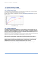
11.4.1.3 Annual rainfall-runoff relationship ................................................................................ 148
11.5 Area C Central Tendency..................................................................................................... 149
11.6 Area A. Remaining Headers ................................................................................................. 150
11.6.1 File .................................................................................................................................. 150
11.6.1.1 Save Current Run ........................................................................................................ 150
11.6.1.2 Load Previous Run. Accessing the last run or a saved run......................................... 150
11.6.1.3 Save Results to File. (One at a time)........................................................................... 151
11.6.1.5 Create Selected WC files............................................................................................. 152
11.6.3 Graph .............................................................................................................................. 152
11.6.4 Additional ........................................................................................................................ 152
11.6.4.1 RFRO curve ................................................................................................................. 152
11.6.4.2 RFRO input .................................................................................................................. 153
11.6.5 Spreadsheet.................................................................................................................... 153
11.6.6 <<< >>> .......................................................................................................................... 153
11.7 AREA B Statistical Output ...................................................................................................... 154
11.7.1 Flow Return and Spell Statistics ..................................................................................... 154
11.7.1.1 Flow: Annual Series ..................................................................................................... 154
11.7.1.2 Flow: Partial Series ...................................................................................................... 154
11.7.2 Spell Statistics ..................................................................................................................... 155
11.7.2.1 Spell: Annual Series - Total above Threshold ............................................................. 155
11.7.2.2 Spell: Annual Series - Maximum Spell ........................................................................ 156
11.7.2.3 Spell: Annual Time Series ........................................................................................... 156
11.7.2.4 Spell: Calculate Exceedence ....................................................................................... 157
WaterCress User Manual
12. MODEL CALIBRATION................................................................................................................ 158
12.1 Steps in Calibration ................................................................................................................ 158
12.2 Entering the Calibration Data ................................................................................................. 158
12.3 Defining Good and Bad Data for Calibration.......................................................................... 159
12.4 Visual Assessment of Calibration Time-series Data .............................................................. 159
12.4.1 Time Series..................................................................................................................... 159
12.4.2 Seasonal (monthly) averages ......................................................................................... 160
12.4.3 Flow Duration.................................................................................................................. 160
12.5 Statistical Comparison of Actual and Modelled...................................................................... 160
13. FILE NAMES, LOCATIONS AND FORMATS .............................................................................. 161
13.1 File Names and Extensions ................................................................................................... 161
13.2 Expected File Locations ......................................................................................................... 161
13.2.1 Rain time series data files............................................................................................... 161
13.2.2 Evaporation Files. ........................................................................................................... 162
13.2.3 Time-series data files for Text Demand, Text Flow, Weir, etc........................................ 162
13.2.4. Flow and Calibration files............................................................................................... 162
13.2.5. FEVA, Image files. ......................................................................................................... 162
13.3 Time-Series Files Header Information ................................................................................... 163
13.3.1 Rainfall/evaporation Files . ............................................................................................. 163
13.3.2 Flow and Calibration Files. ............................................................................................. 164
13.3.3 Text Flow, Text Demand and Weir files.......................................................................... 164
13.4 Other Files.............................................................................................................................. 165
13.4.1 FEVA files ....................................................................................................................... 165
13.5 Recognised Header Time-step and Unit Definitions ............................................................. 165
13.6 Time Series Data listing formats ............................................................................................ 166
WaterCress User Manual
1.0 MODEL DESCRIPTION
1.1 Basic Functions - What WaterCress Does
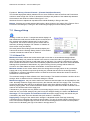
WaterCress (Water Community Resource Evaluation and Simulation System) is a PC based,
continuous time series, total water cycle model, which simulates the passage of flows through natural
and constructed water systems. The model provides statistics on the flows and storages within the
water system over the period of modelling, thus providing information on the performance of the
system against desired outcomes or against alternative system layouts.
At its core is a model to convert catchment rainfall to runoff, but flows may also be introduced as flow
records. The model then tracks flows through water systems established by the user at continuous
equal time-steps of one day, 2hrs, 1hr or 30 mins. Thus the model may be used for both flood and
water supply designs.
The model tracks salinity as a conservative parameter including changes as water of variable salinity
is injected, stored and recovered from saline aquifers. The model also tracks water within broad
quality categories so that different water paths can be reserved to supply different quality demands.
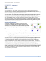
The central features of WaterCress are:
1. An assembly of icons representing specific components of a water system. These can be
clicked and dragged onto the spatial layout page and joined by flow paths in order to simulate
the water system to be trialled. These icons represent all conventional water supply and use
components, such as catchments, dams, treatment plants, aquifers, in-house demands,
irrigation areas, pumps, etc., but present them in a manner which allows trialling of nonconventional supply sources and management processes at a range of different scales.
2. A set of core mathematical relations and data bases which contain all variables and limits
necessary to enable the quantities and qualities of water to be estimated and tracked through
a specified water system. The water inputs to the model are generally derived from one or
more sets of sequential rainfall data bases of adequate length suited to the trial area. Water is
moved through the model to satisfy seasonally variable water demands, as modified by
evaporation and direct rainfall. Secondary data sets define the sizes and rates of all
components in the assembled water system as they pass the water through the system.
3. A series of tabular and graphical outputs which can be chosen and assembled from an output
format menu. These provide the record of performance of any one, or group of components
within the system. The performance will usually be assessed by the designer on the basis of
the amount, reliability and quality of water supplied over the period of record and/or the size
and frequency of peak flow rates, etc.
The model can represent the operation of ’total water cycle’ systems with flows generated by rural or
urban catchments, passing via natural or engineered drainage paths into and through water supply,
sewerage and groundwater systems.
The layouts modelled may range from single on-site system scale to regional scale, including a
mixture of different scales.
Water is moved through the system at a continuous sequence of fixed, selected time steps. The water
balance is recalculated during each time step to account for all the activities performed in the nodes.
A group of components or nodes with their flow links is defined in WaterCress as a Project.
1.2 Typical Model Uses
The model is designed to meet the problems of exploring alternative system layouts at the feasibility
stages. The model has been used successfully to investigate the performance of a new generation of
water system layouts:

involving multiple sources of water of different qualities (eg. traditional catchment sources,
urban stormwater, groundwater, recycled wastewater, desalinated sea water and/or imported
WaterCress User Manual – Model Description
water), and

designed to provide multiple objectives in water supply, flood mitigation and environmental
enhancement.
The multiple sources include those generally available, but, using the WaterCress model, the user can
explore the integration of less conventional sources into existing systems. This can often bring
additional economic and environmental benefits. These benefits were not explored by previous
generations of systems designers partly by virtue of the previous lack of design tools (such as
WaterCress) able to i) examine opportunities offered by integration and ii) design systems providing
multiple objectives.
WaterCress is particularly useful in situations where the designer wishes to explore a range of system
layouts in which the economic value of many system benefits are hard to quantify. While, in theory,
the choice of a "best" system design can be based on a set of pre-determined performance criteria, in
most practical situations where multiple-objectives are involved, the wide range of trade-offs between
competing objectives cannot be adequately expressed in mathematical terms. Moreover, it has been
often found that the existence of certain trade-offs are not identified until well after the design process
has been actually commenced.
In such cases `trial and error’ design approaches are far superior to approaches involving
mathematical optimisation.
WaterCress can be used to demonstrate the performance and implications of alternative systems
designs, in an easily understood manner, to both specialist and lay persons who may be affected by,
and/or interested in the likely performance of the chosen system.
The use of trial and error models such as WaterCress will allow the nature of these trade-offs to
emerge during the design stages and, by its ‘user friendly’ nature, a broader consensus can be
reached on system selection.
By allowing the introduction of advanced treatment into the designed systems, the WaterCress model
allows designers to link any source of water to any demand. Although default tables will indicate high
cost penalties for treatment where the source quality requires considerable treatment to bring it to the
demand standard, default data can be overwritten. The use of the model for exploration of
unconventional systems therefore requires a high degree of responsibility to be shown by all parties
involved in the designs, especially where they may start to involve financial commitments and/or
implications for long term public health.
2
WaterCress User Manual – System Installation
2.0 SYSTEM INSTALLATION AND CONTENTS
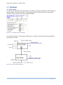
2.1 Computer Requirements
To use the 32 bit WaterCress program the following system configuration is required:

A personal computer running under Windows.

PC I or better video card.

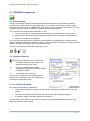
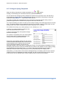
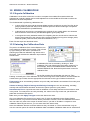
Monitor with at least 16 bit resolution. To set resolution, right click once on the desktop screen
and select Properties. A window will appear, select the Settings tab at the top of the window.
Under the Colour Palette box select High Colour (16 bit). Then left click once on the Apply,
the computer may require to be restarted.

Display area must be set at 800 x 600 or greater. To set screen size, right click on the
desktop screen and select Properties. A window will appear, select the settings tab at the top
of the window. Under the Desktop Area box set the screen and the desktop to 800 x 600 by
moving the button across. Left click once on Apply to accept the changes.
The program has been tested on a Pentium 166MHz with 32MB Ram, under Windows 95 through to
XP, and worked successfully. For Vista and windows 7 the web provides a second loading file.
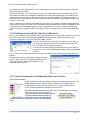
2.2 Install Information for WaterCress
To install WaterCress from a CD-ROM or from the web the user must follow the following instructions:
Select Setup.exe. This will take you into a standard install procedure. WaterCress can be loaded in
any location, but as default it will load on c \Program Files\WC2000.
The user is now able to commence a project session using the WaterCress program. To open a new
project see Section 5.2.1. To open an existing project refer to Section 5.2.3.
2.3 Software Package Contents
The WaterCress model package typically resides within the folder c:\wc2000 from here defined as
<program location>. The actual name and even the drive name are up to the user and are set on
installation.
The WaterCress package consists of:

several text files (*.txt) containing default data for the 18 basic function nodes contained in the
model,

two data folders RAINDATA and FLOWDATA containing libraries of rainfall and flow data files
into which the model user can accumulate his own files while working from one project to
another,

three main operating executables (watecress.exe, wcmain2h.exe and wcmain3h) and

several executables which may be called on for assistance as tools in data input or output
checking and formatting.
3
WaterCress User Manual – Basic Model Structure
3. BASIC MODEL STRUCTURE AND OPERATION
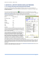
3.1 Screen Structure
There are 3 basic screens in the WaterCress Program
Opening Screen where you select or create your project and define required project information.
Project Layout Screen for establishing the nodes and links making up the Project
Output Results Screen from where the project is run and the results are displayed.
3.2 Rainfall, Evaporation and/or Flow Data Input
Rainfall and evaporation are the usual prime drivers for the model and are converted to flow by a
series of rainfall to runoff models. Recorded flow data (or data generated by other models) may be
used instead (or in conjunction) as the flow driver, or to calibrate the flow predicted from the rainfall.
This data is input to the model through individual ASCI files. A project can access numerous rain and
flow files. The modeller can often apply multipliers to factor the input values up or down to suit the
requirements of the project.
3.3. Node and Link Structure
WaterCress allows the modeller to simulate the flows within a prototype water system by representing
the system as a series of nodes, which represent the various functions or operations of water
infrastructures/proceses (eg dams, weirs, usages, bores, treatments, etc), linked together by a series
of ’free flow’ gravity drainage paths and/or a series of fixed capacity water supply piped paths.
The nodes can be clicked and dragged onto a blank computer screen field and joined by flow paths in
order to specify the water system to be trialled.
A group of components or nodes with their flow linkages is defined in WaterCress as a Project.
3.4 Nodes and Node data Entry
There is a menu of 18 basic node types that the modeller is able to use (as often as required) to make
up a project. Each is described in detail in Sections 7 and 8.
Each node has an associated database which contains all variables necessary to enable the
quantities and qualities of water to be added/ lost/ modified/ diverted etc. as the rainfall and water is
passed through it.
The water inputs to the model are derived from one or more sets of sequential rainfall records of
adequate length suited to the trial area. Water is moved through the model to satisfy seasonally
variable water demands, as modified by evaporation and direct rainfall. Secondary data sets define
the sizes and rates of all components in the assembled water system as they pass the water through
the system.
The designer enters data where this is unique to the system being trialled (eg catchment areas) or
can accept default data already entered into the database, where this is less critical or less variable
(eg loss rates, evaporation pan factors). Time series inputs are most commonly rainfall and
evaporation data.
Included is also a set of core mathematical relations which define the limits and calculate the
operation of the components of the system according to the designer’s selection of systems layout
and sizing and operating data. Operating rules are also included which, for example, allow the
designer to vary both the priorities and proportions of water supplied from the various sources, where
more than one source has water available at any time.
4
WaterCress User Manual – Basic Model Structure
3.5 Flow Links
3.5.1 Drainage
Drainage flows are normally unregulated in terms of flow rate or occurrence. No maximum rate is set
for the movement of water down a drainage path. Drainage rates are usually dictated by rainfall rates,
catchment areas and channel routing, but may also be determined by storage outflow formulae
entered by the modeller.
In nodes where there are more than one drainage and diversion path allowed, drainage links at the
sub-division level are colour coded so that the user can readily identify the different types/qualities:
Pink – diversion path from a diversion type weir, or separated groundwater flow from a catchment
Blue – normal rural or stormwater flows generated by rainfall on catchments,
Green – runoff from roofs from house and urban nodes,
Grey (thin black) – on-site greywater discharged from house and urban nodes,
Black – black sewage discharged from house and urban nodes.
There is no requirement to keep these paths separated and it is left to the user to define appropriate
drainage connections once the flow in a flow path has drained from any node.
Once the colour coded drainage has been joined to the next node downstream (eg a tank) the colour
code will change to that of the downstream node drainage. In the case of a tank this is the normal
blue colour.
The majority of (blue) drainage originates at the most upstream catchment nodes. All nodes further
downstream may receive drainage from upstream and all nodes can transmit drainage through them
to further downstream.
Any node can have more than one drainage path directed to it, however, only one drainage path can
normally be directed from any node (except where separate colour classes of water are involved, eg.
an urban node may have 4 separate colour coded drainage lines coming from it, as above). If two
drainage paths of the same type can actually exist (eg a reservoir with two spillways discharging to
different downstream paths) it will be necessary to use an additional weir node to split the flow just
downstream of the (single) outflow point provided by the model.
For storage type nodes, the downstream transmission of drainage often occurs as spill, after any
inflows have caused the level of the storage to exceed its full capacity. Environmental flows may be
discharged (drained) from storages at all times.
When a node exists at the furthest downstream location in the model, it will spill or drain beyond the
notional boundary of the model. In this case a drainage path cannot be established. However, the
water balance is calculated as though a drainage (spill) path exists.
Note: While drainage links can be directed to any type of node, including demand type nodes, no
demands can ever be supplied directly from the drainage link. Supplies must ALWAYS be
taken from a storage type node via a water supply path. If a drainage link is made to a demand
node the drainage input will be transmitted through the node unchanged. If a drainage link is
established downstream, the inflow will continue down this drainage path outlet, else the node will
merely ’spill’ the flow and the drainage inflow will ’disappear’ from the model.
5
WaterCress User Manual – Basic Model Structure
3.5.2. Water supply.
By comparison, water movement via a supply link is always regulated to a maximum flow rate. The
rate may be changed according to season or some rule, however, no hydraulics are involved and
the water will be supplied at the rate set, providing that that amount is available from the source and it
is of suitable quality for acceptance by the receiving node.
In all cases, supplies are regulated in terms of flow rate and occurrence.
Multiple supply paths can be established between nodes, but only to nodes that have a capacity to
demand water (eg. demand and storage nodes) and from nodes that have a storage capacity.
Storage capacity is provided explicitly in the storage type nodes (eg reservoirs, tanks, etc), but also
implicitly in several others node types (eg town, treatment plant). Nodes that do not contain storage
capacity cannot be linked by supply paths (eg catchments).
A fundamental assumption made in the model is that water is drawn through the network of water
supply links by a set of actual or notional demand nodes. Thus data entered into the model that
controls the rate of water passing through a water supply path is generally entered via the receiving
node, rather than the supplying node. Water is thus drawn through the supply network to meet the
downstream demands, rather than being pushed through the supply network from upstream.
Since supplies may be drawn from one node to the next along a continuous supply pathway
consisting of several storages, any nodes containing storage capacity that are not filled from a
drainage path (mostly storage nodes, but also treatment plants) are programmed to be able to
demand water to recharge themselves from upstream.
Water supplied to a demand node may then either be consumed at the demand node (eg evaporated,
or ’lost’), or a fraction may be returned as wastewater (with an appropriate quality change) to the
drainage system, thus allowing it to be potentially reused downstream.
When a supply path is established a priority and weight is user assigned to the path. Where several
sources are connected to a single demand, these values may be altered by the modeller to achieve a
choice in selection or shandying of the water supplied from the several sources (See 3.7 below).
3.6. Order of water balance calculation
The calculation of flow movements in each time step is performed in two stages with the transfers via
the drainage paths being calculated first, followed by the calculation of the transfers via the supply
paths second, as follows:
Stage 1 Drainage. At the statrt of the timestep, any rainfall or other input data for the time step are
entered and runoff is calculated starting from each of the most upstream tributary nodes. All waters
are moved from their sources via the drainage links in a downstream direction. Routing may be
applied. Drainage flows from different tributaries are amalgamated. Each node in the drainage path
performs its drainage related functions after input of the amalgamated drainage flows from upstream.
If a storage receives drainage and supply inflows/outflows, the effects of supply flows are not taken
into account in the Stage 1 calculations. Wastewaters generated from previous days activities are
similarly transferred via drainage links Evaporation, seepages and leakages are removed and spills
and diversions are transferred further through the system to complete an interim updated (end of time
step) stage 1 water balance.
Stage 2. Water supplies. Supplies are then drawn from storages to satisfy demands. The sequence
of calculation does not often matter, but where it does this is controlled as described in the next
Section (3.7). After the supplies have been calculated the final end of timestep balance is given. The
amounts of wastewater generated from the supplies are placed in temporary storages ready for
release in the next time step.
The importance of the order of calculation of the supplies in reaching this final balance is addressed
below.
6
WaterCress User Manual – Basic Model Structure
3.7. Priorities and Weights and Supply Sequences,
As described, whereas only single drainage paths of a certain type can exist between any two nodes,
multiple supply paths may exist between storages and demand nodes. This multiplicity requires that
the order of supply can be controlled by the modeller in order to ensure that the flows occur in the
manner and priority order intended. An example is provided below.
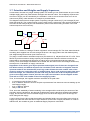
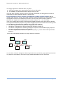
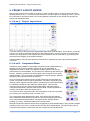
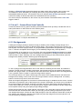
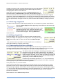
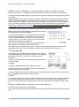
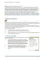
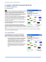
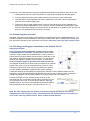
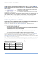
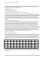
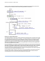
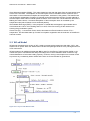
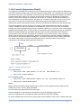
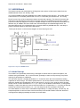
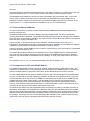
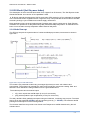
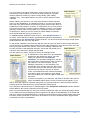
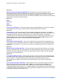
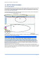
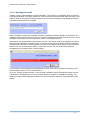
The diagram below shows a simple system comprising a single catchment (C), two storages (S) and
three demands (D). The numbers shown on the nodes are the consecutive node numbers assigned to
the nodes as the example layout was established. (Other nodes with missing numbers in the node
number sequence are not shown).
C7
S3
P1:W1
P1:W1
P1:W1
D1
P1:W1
P1:W1
D4
S9
D8
Catchment C7 drains to a storage S3 which supplies a second storage S9. The three water demands
are taking their supplies from the two storages as shown. All supply paths have their default priority
and weights assigned as shown (see Section 6.9.5).
The stage 1 water balance calculation sequence (see section 3.6) will pass flow from C7 to S3. If this
fills S3 beyond its maximum storage capacity S3 will spill and the amount will be accounted in the
water balance, but drainage will progress no further (since no downstream drainage paths are
shown). Once the drainage calculations have ceased with the status of the two storages determined,
the sequence of calculation of supply commences.
Regardless of the values given by the priorities and weights (even if these are changed from
the default values), the default sequence for calculation of the transfers of supplies from the
upstream nodes to the downstream (receiving) nodes follows the node number order of the
receiving nodes, as set by their order of establishment. If any node receives supply from more
than one storage, the calculation (for that node only) will be in the order set by the priorities
given to its supply paths. If these priorities are equal, the calculation for the supplies to that
node will be in the node number order of the supplying nodes.
Thus, in the example, the supplies would be calculated in the path order:




to (receiving node) d1 from S3 first
then, to d4 from S3 and to d4 from S9 (with equal amounts from these two sources making up the
total supply sought)
then, to d8 from S9 and
lastly to S9 from S3.
Thus, since the availability of water remaining in the storages will be reduced by the amounts of the
preceding supply calculations, the demand d8 will always have the last (and possibly least reliable)
supply, and d1 will have the most relaible supply since it receives first supply from the storage S3
which also gets first supply.
It can be seen from the above that the priorities and weights facility can only influence the priority of
supply to a particular node and has no major influence on the order of supply calculation. In order to
address this, the modeller is given an additional Supply Sequence mechanism.
7
WaterCress User Manual – Basic Model Structure
The supply sequence is used less often, only when
a) a group of storages are in supply series (as for S3 and S9) and/or
b) the reliability of a particular demand is highly critical (say d8).
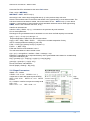
Using the same example, if supply to d8 is to be made most reliable, an arrangement can then be
made using the supply sequence option as shown below.
Every node that can receive a supply is provided with a supply sequence number with the
default supply sequence number zero. When all supply sequence numbers in a model remain at zero,
the supplies continue to be calculated in the order of the receiving node numbers (as above).
Otherwise the supplies are in supply sequence number order (ie 1, 2,..., etc. with 0 last).
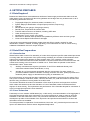
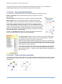
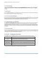
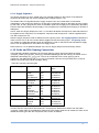
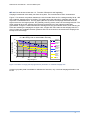
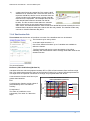
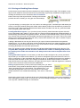
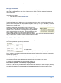
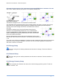
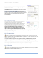
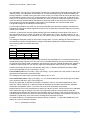
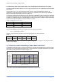
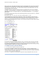
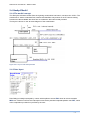
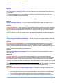
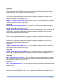
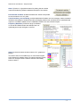
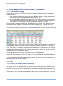
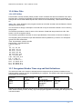
Thus in the example below (with the Priorities and Weights allocated to the supply links for demand
d4 changed for illustrative purposes only) and the Supply Sequences allocated to the receiving nodes
with the objective of increasing the reliability of the supply to D8 as shown:

S9 will be supplied from S3 first (as it has supply sequence number 1)

D8 will then be supplied from S9 (as it has supply sequence number 2)

D1 will then be supplied from remaining storage in S3 (since it has the default supply sequence
zero, but has the lowest receiving node number)

D4 will be supplied last, at first from S3 (as this has priority 1), or from S9 if S3 fails (as this has
priority 2).
In this case, with different priorities, the weight values are irrelevant.
C7
Seq 1
S3
d1
Seq 0
P1: W2
d4
S9
P2: W1
d8
Seq 2
Seq 0
In most cases, when the storages are either large and/or are not linked by supply paths (and thus are
only subject to rare failures), the order of supply makes little difference to the outcomes.
8
WaterCress User Manual – Basic Model Structure
3.8. Water Quality
The WaterCress model currently tracks water quality in only 2 water quality categories, salinity and
'other'. The second category is a relative scale which ranks water quality according to a quality code
number. Any parcel of water moving through the model is accompanied by its salinity and code
number.
Salinity concentration is first estimated as a function of flow rate (see Section 7.4.2). This determines
the mass of salt assumed to enter the flow. The salt is then assumed conserved at is travels
downstream and through the system. Salt is only specifically removed by desalination (see Treatment
node Section 8) and thus its concentration continually changes (and is tracked through the model)
according to flow weighted merging and evaporation. HOWEVER, if a storage evaporates to zero
water holding, the salt load is removed before the next inflow containing its own salinity
concentration is added. (Deposited salt may be removed by wind). Special care should be taken in
modelling open storages in arid areas where salt build up occurs.
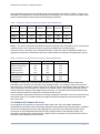
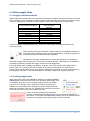
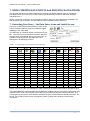
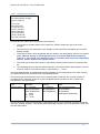
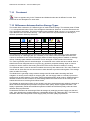
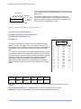
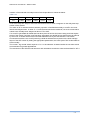
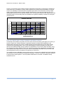
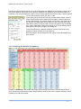
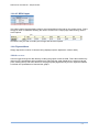
The quality codes are a numerical index within the range 0-19 assigned by the modeller to flow
generated within the model. A notional list of waters of different general quality is given below which is
not comprehensive and is provided for indicative guidance only.
0
1
2
3
4
5
6
7
8
9
Advanced treated Disinfected
Potable supply, filtered, disinfected
Pristine catchment – Raintank (filtered)
Forested catchment - Raw roof runoff
Rural catchment – disinfected
Mixed agriculture catchment
Tertiary treated effluent
Advanced reclaimed / Indirect use
Stormwater following wetland and filter
Secondary treated effluent
10
11
12
13
14
15
16
17
18
19
Stormwater wetland
Resident greywater wetland filter, disinfect
Raw residential stormwater
Secondary treated disinfected effluent
Secondary treated effluent
Raw greywater or commercial stormwater
Filtered primary and disinfected
Septic tank overflow
Raw Black sewage
Toxic Industrial Effluents
Code 0 relates to the best quality water and subsequent increments indicate falling quality of water to
a maximum value of 19. All nodes in the model have input boxes to set the quality code of water being
generated by it and most nodes (demand nodes and storage nodes) that receive water via water
supply paths have a quality code set to identify what quality water is acceptable by it.
Note: Quality codes and salinity ONLY control water movement via water supply paths. Water
delivered by drainage paths is NEVER rejected on the basis of quality codes or salinity.
In many cases, where quality is not an issue, the modeller may simply wish to set all water
generated as code 0 and all demands as code 19, thereby negating the impact of quality codes
and allowing all water being modelled to be suitable for supply to all demands.
Otherwise, all demands are assigned a maximum salinity and code number. For potable demands
these might be 500 mg/L amd code 1. Any water with values greater than either of these will NOT be
then acceptable as a supply to this demand. Garden irrigation may accept 1000 mg/L and code 9, etc.
Although a simple concept, quality codes allow a user to control from what source water being
modelled can be set up as a potential supply source to the different demands (or conversely not
supplied). Therefore quality codes are used to track the general suitability of water for any particular
purpose.
While water is given a code at its creation, the codes are similarly merged and flow weighted as the
flows are mixed. For this reason it is best to keep codes simple, set within large numerical ranges,
and for the modeller to be aware of what changes may be taking place. Codes and salinity may be
output at all points within the model at any timestep (see below).
9
WaterCress User Manual – Basic Model Structure
3.8.1 Constraints due to quality
For drainage links there are no quality constraints applied to the transfer of water from one node to
the next. When two or more waters are mixed within a drainage stream the resulting quality code and
salinity is averaged through flow weighting. This means that within the model raw sewage could be
shandied down to an acceptable drinking quality, therefore the user must be aware of the drain mixing
that is taking place to ensure the water supply is truely acceptable to the demand.
Demands can only be supplied via a water supply link. For all demands you must specify the quality
of water that demand is willing to accept. Thus, supply can only be accepted by a demand node if the
water at the storage node falls within limits pre-determined for the demand. For all demands you must
specify the salinity and quality code of the water that demand is willing to accept.
A quality code mismatch is often the cause for the model failing to supply a particular node.
Quality codes can also cause supplies to under-predict if set to apply constraints when none
are intended by the system designer.
When it comes time for the model to work out whether it can use the water in a particular storage to
satisfy a demand, it compares the salinity and quality code of the source with that demanded, and
only if the demand quality constraint values are larger or equal to the source quality values will the
demand accept that water.
In arid areas, where evaporation may increase the salinity of stored water above acceptable levels,
salinity may be a limiting factor. Being a relatively conservative element salinity is calculated daily in
the same manner as the water balance. Where water is mixed the mixture will assume the volume
weighted average of the mixed volumes. Mixing in storage (with the exception of wetlands) is
assumed to take place immediately and fully throughout the whole volume.
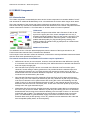
3.9 Zones
The model provides the facility for certain catchment and storage nodes to be grouped together within
zones for the quick application of multipliers to some or all of their rainfall-runoff relations, storages,
volumes or water diversions. It is very useful where a model may have many similar nodes within a
zone, all of which need to have their input data changed on a trial basis to test what-if sceanrios. The
application of the multipliers is described in Section 6.6.1 See Layout Screen Header ’Data Variation’.
Zoning may be applied to:


rural and urban catchments and text flow inputs, and
reservoir, tank, offstream (farm) dams and routstore storages.
Catchment zones are used purely for identification of groups of catchment nodes for ease of
application of modifiers to rainfall - runoff equations. These modifiers (refer section on generic runoff
modification enable modification of runoff parameters over a group (or zone) of nodes.
Storage zones similarly enable multipliers to be applied to (for example) a all farm dam storages and
diversions (to local use) within an identified grouping of dams within a zone. Refer Section 6.6.1.
10
WaterCress User Manual – Basic Model Structure
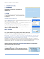
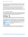
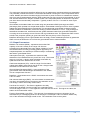
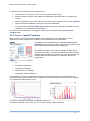
3.10 Outputs
When the model is run, WaterCress offers the modeller a very wide range of outputs that can be
selected and presented in tabular or graphical form. A Summary provides a simple average value for
inflows, outflows, average supplies etc to each node within the model over the period for which the
model has been run.
Details of the selectable outputs are given in Section 10.
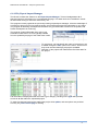
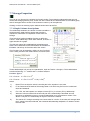
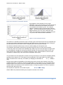
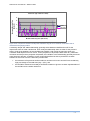
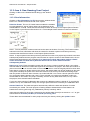
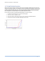
Results can be displayed as time-series at the time-step for which the model is run (daily or hourly).
The same results are also displayed as totals over daily (for hourly data), monthly and annual periods
(for either calendar, financial or water years).
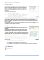
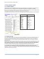
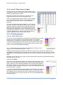
Because of its large extent, hourly data may be filtered so that only selected data is displayed (as
shown adjacent).
These outputs provide the record of performance of any one, or group of components within the
system. The performance will usually be assessed by the designer on the basis of:

The amount and reliability of water supplied over the period of record

Maximum and minimum flow rates, storages, etc

The quality of water supplied and

The average cost of operating the system components.
However, the range of outputs enables the system designer to assess the performance in terms of
such things as the size and frequency of flows, storages and water levels for the maintenance of
environments, etc. In addition, there is provision to convert the outputs to a comma separated variable
(csv) file for further assessment in 3rd party programs such as Excel
.
11
WaterCress User Manual– Getting Prepared
4. GETTING PREPARED
4.1 Data Required
Because the WaterCress model addresses all facets of water supply and demand within rural and
urban water cycles, the amount of data to be gathered can be large and may include some or all of
the following data and/or sources:










Topographic Maps (for catchment areas, boundaries, etc.)
System Maps (for identification of input/output processes, sequencing)
Isohyets
Data locations (rain gauges, flow gauges, dams)
Rainfall, flow, evaporation time-series data
Transfer rates into and out of facilities, including ASR rates
Urban development zones, maps
Identification of roof, paved, open areas
Demands for different water quantities and qualities by different users and user groups
Volume-Area-Depth-Outflow data for storages
It should be recognised that significantly greater time and effort is usually required for data
identification, location, collation, checking, gap filling, error rectification etc. than in model running,
calibration/recalibration and even output analysis.
4.2 Data Files Preparation
4.2.1 Introduction
WaterCress models consist of an assembly of nodes which represent specific water related processes
occurring within the components of the system being modelled, plus a series of links between these
nodes which represent the passage of water between them. The ‘upstream’ nodes generally
represent sub-catchments and the model calculates a continuous time series of runoff from each subcatchment according to the time series of rainfall over it. These flows are passed via the links to
downstream nodes. These either
1)
similarly calculate and merge the generation of runoff from additional tributary subcatchments situated further downstream, or may
2)
simulate any of the processes associated with the components of a water system, ie
processes related to different varieties of storage, diversion via weirs, quality improvement in
treatment plants, supply to demands and recycling of wastewater, etc.
Once the structure of the model has been established, its operation is governed by the values of the
many items of data (ie coefficients, areas, volumes, flow rates, etc.) that are needed to describe and
limit the many processes occurring within the model nodes.
This section describes the method of estimation of the areas of pervious and impervious surfaces
within urban sub-catchments and the derivation of a set of standard models for different defined
degrees of urban density. The implications and performance of the formulae adopted for calculation of
runoff on impervious surfaces is then described.
4.2.2 Area Estimation
Particularly in low to medium rainfall areas (say <1000 mm/a), accurate estimation of the aggregate of
the impervious areas within each catchment is a crucial requirement in order to make an accurate
estimation of the total catchment runoff. The procedures described in the following sections were
developed to provide a best estimate of the impervious and pervious areas based on the time and
information resources available.
The total procedure for separation of sub-catchment, land uses, roof, paved and pervious areas for
input to the WaterCress model is shown diagrammatically below.
12
WaterCress User Manual– Getting Prepared
T o ta l c a tc h m e n t
M u ltip le d ra in a g e s u b c a tc h m e n ts
U n d e v e lo p e d /
ru ra l la n d
R u ra l la n d
H o u s in g a re a s
P a rk s /la rg e r
p e rv io u s a re a s
R e m a in d e r
25% R oad
e a s e m e n ts
P e rv io u s
P aved
75% H ouse
b lo c k s
8 2 % R o o fs/
g a rd e n s
D 1 G a rd e n s
P E R V IO U S 1
In d u s tria l/
c o m m e rc ia l
R o o fs
D 2 G a rd e n s
R o o fs
D 3 G a rd e n s
R o o fs
P E R V IO U S 2
R O O F S
1 8 % P a th s /
d riv e w a y s
R o o fs
P aved
P e rv io u s
P A V E D
Figure 4.1 Decision tree for separation of impervious and pervious areas input to the WaterCress model (D1, D2..
are values for different development densities)
The separation can be undertaken in steps:
Step 1 - The total catchment area is firstly
subdivided into approximately equal sub-areas,
based on elevation contours, isohyets and
drainage path mapped information. Boundaries of
areas with high relief can be mapped accurately
(eg. 49, 51 in Fig 4.2 below). Where there is little
relief, the delineation becomes less accurate
unless access can be arranged with detailed
drainage maps. In all cases boundaries are
selected in an attempt to have only one major
drainage outlet where flow is passed to the next
area.
areas.
Figure 4.2 Definition of drainage paths and sub-
Step 2 - Each sub-area has then been separated into 4 basic land use types:
1. Areas of relatively homogeneous housing, roads and gardens sub-categorized into one of
three different dwelling densities and impervious proportions (shown in Figure 4.3 shaded
red),
2. Industrial/Commercial areas with high impervious proportions (shown in Figure 4.3 shaded
yellow),
3. Undeveloped hills face/rural catchments (shown in Figure 4.3 shaded light green), and
Pervious urban parks and large open areas (shown in Figure 4.3 shaded darker green)
13
WaterCress User Manual– Getting Prepared
These are further described below, with the
modelling for the pervious areas within the urban
areas and the pervious areas in the last two dot
points taken together under the ‘Pervious Areas’
heading in Section 4.2.5 below.
Figure 4.3 Basic landuse types identified and separated.
4.2.3 Housing (Domestic) Areas
Areas of housing comprise a relatively homogeneous assembly of houses, gardens, roads, verges
and small open areas, including a few vacant blocks.
Step 3 - Significant pervious areas such as large parks, recreation areas, watercourse reserves, etc.
within the housing area are identified and digitized as a separate land use and included separately
under the ‘pervious’ classification.
Step 4 - All the remaining housing area is assumed to consist of 25% road easement and 75%
housing blocks, each with a dwelling. Each housing block is assumed to include i) 10% of its area
taken up by impervious paved paths, driveways, etc., ii) a dwelling with an impervious roof area, and
iii) a pervious garden area which includes a small share of the aggregated areas of small communal
parks.
Step 5 – In this example, the housing areas have been separated and classified into three densities,
according to a visually assessment of aerial photos showing the relative proportions of impervious and
pervious areas, as below:
Low Density – assumed roof area = 30% of 90% of the block
area remaining after removal of 10% paved areas. (9.8
dwellings per ha.)
Mid density - assumed roof area = 45% of 90% of block area.
These may be relatively new areas with smaller block areas or
older areas with a lot of ancillary shedding or verandahs etc.
(12.1 dwellings per ha.)
High Density – assumed roof area = 60% of 90% of block area.
These tend to be the latest developments where block sizes are
small and roof areas are large. (13.6 dwellings per ha.)
14
WaterCress User Manual– Getting Prepared
Several samples were taken from similar areas and the averages are shown in Table 4.1 below. The
information on dwellings per hectare (and persons per dwelling, etc.) can be used if the model is later
used for assessments of water supply and wastewater production.
Table 4.1 Fraction of impervious area with respect to total residential area
Housing
Density
Assume
roof %
Roof
fraction
Pavement
fraction
Garden
fraction
House
size m2
Block
area m2
Low
30
0.23
0.07
0.45
230
766
Medium
45
0.34
0.07
0.34
280
622
High
60
0.45
0.07
0.23
330
550
Block sized are continuing to decrease and 300 m2 blocks are now common.
Step 6 - The 25% of assumed road easement area is assumed to be comprised of 15% of impervious
paved area and 10% of pervious areas (ie verges and small areas of unpaved land).
Table 4.2 shows a summary of the assumptions made. A GIS was used to estimate the total of the
impervious paved and roofed areas and pervious areas within the sub-areas designated as housing.
Table 4.2 Impervious area assumed with respect to total residential area.
Low density
Mid density
High density
Impervious road
Pervious road (verge)
House roof area
House Pavement
Garden (pervious)
15%
10%
23%
7%
45%
15%
10%
34%
7%
34%
15%
10%
45%
7%
23%
Total Roof
Total Pavement
Total Pervious
23%
22%
55%
34%
22%
44%
45%
22%
23%
In addition to having an increased impervious fraction, the denser developments are also often
assumed to be connected more directly to the drainage system. For example, while the front part of
the roof may be connected by drain to the road (and hence the formal drainage system) the back roof
often discharges to the backyard and garden or to rainwater tanks. Larger blocks with lower density
clearly have more capacity to discharge water in this way. It is therefore assumed that as block sizes
reduce a lesser proportion of impervious runoff will be lost on-site.
In this example it was assumed that the low density development had 50% of its roof connected to the
stormwater system. The medium density and higher density developments were assumed to have
60% connected.
4.2.4 Industrial/Commercial Areas
The proportions of impervious and pervious areas within each of the sub-areas classified as
Industrial/Commercial have been individually assessed using aerial photos (Google maps). Individual
blocks were visually inspected and then aggregated to give total roof, paved and pervious areas.
Connection of the Industrial/commercial roof and pavement areas to the drainage system was
assumed to be higher than domestic areas. Values of 80% connection for the roof area and 70% for
paved area were adopted across all areas.
15
WaterCress User Manual– Getting Prepared
4.2.5 Modelling Runoff from Pervious Areas
Pervious areas by definition do not include any significant impervious areas. The following example
describes the separation of the various separated pervious areas into two types, using different
versions of the WaterCress pervious catchment rainfall to runoff model. The parameter values chosen
for the versions of the model are adequate to account for different combinations of soils, slopes,
degrees of vegetation, etc. and efficiency of inter-connection to the watercourses and drain systems.
Considerable experience has been gained with the prediction of runoff from rural catchments in the Mt
Lofty ranges. These include runoff from some hills face catchments such as First, Third and Sixth
creeks, but generally within the higher rainfall areas.
Very little direct data exists on runoff from aggregated garden areas and other pervious areas within
urban areas such as parks, recreation areas and watercourse reserves on lower rainfall and the flatter
land. However indirect experience with model calibration of urban area runoff shows that the
proportion of runoff from their pervious areas is usually small to negligible in relation to runoff from
their impervious areas. For aggregated house garden areas this is not surprising in view of the
significant impedance and losses likely to be associated with their cultivation, landscaping and border
fencing.
The model used for the within-urban pervious areas is therefore similar to that for the rural and hills
face areas except that it has been modified by increasing the interception and soil moisture capacities
to reduce the amount of runoff predicted (refer calibration later).
4.3 Accuracy of Key Data used in the Prediction of Flow.
When major discrepancies exist between flows predicted by a rainfall to runoff model and flows as
measured by a gauging station, even after the model has been adjusted by calibration to the
measured flows, the source of the discrepancies may be associated with any of the:

inaccuracy of the rainfall measurements, and/or

inaccuracy of the flow measurements, and/or

inadequacy of the prediction model to take all conditions into account
4.3.1 Rainfall data errors
The accuracy of the rainfall records can be checked by comparing one record against the records of
its neighbours, either directly, or as cumulated totals over several years. Most errors in recording via
pluviometers are associated with power failures, in which case the record is missing all together.
Errors in daily read rainfall records are harder to identify and usually involve non-attendance of the
reader, failure to record readings or entering data on the wrong dates.
The moving of a gauge into a location having a different exposure, or the construction of a building
nearby which changes the exposure, can give a long term change to the readings. The timing of such
events can often be picked up by comparing double mass curves of the cumulated totals of rainfall
recorded by the different raingauges within a local region.
The start of a period of systematic errors, or changed exposure, is revealed as a change in the
relative slopes of the graphed cumulated rainfall totals. Otherwise errors are usually small and are
made even less significant when several rainfall records are used to define the spatial variation of
rainfall across the catchment. It would be very unusual for all gauges to be in error together, although
high winds may cause a group of gauges to under-or over register together.
16
WaterCress User Manual– Getting Prepared
4.3.2 Flow data errors
By contrast, flow is much more difficult to measure and measurements are prone to many sources of
error.
Most stream flows are estimated via separate measurements and calculations involving water depth,
water velocity and cross section area. Under ideal conditions these measurements bear stable
relations to each other which can be estimated by hydraulic calculation or field measurement. Ideal
conditions are rarely met and accurate measurements can usually only be guaranteed if a standard
measuring weir is constructed. These are expensive. Where measurements are taken in natural
channels away from stable concreted sections, measurement conditions are often far from ideal.
Logs, trash accumulations, bank erosion, sediment accumulations and seasonal vegetation growth
substantially alter the relations, often from day to day or week to week. Since the calculations of flow
are made on the basis of the most recent set of relations available, when any changes occur the
calculated flow will be in error until the new set of relations has been established.
Because field measurements to check and/or re-establish the relations are i) often hazardous under
high flow conditions, ii) require skilled operators, and iii) are expensive, they are usually infrequent
and confined to low flows. Often they are not carried out at all. Under most circumstances high flow
measurements are generally recognised as being estimates only.
Thus, unless measurements are carried out in a channel reach where the geometry and surface
roughness are fixed (ie a concreted channel), the flow measurements should be regarded as a guide
only. The measurements are liable to have large random errors due to i) random events, such as
blockages by silt or debris, or ii) systematic errors due to incorrect assumptions made in developing
the hydraulic relations, such as the incorrect estimation of roughness.
17
WaterCress User Manual– Getting Prepared
5. OPENING SCREEN
5.1 Header Bar
The printing on the header bar is greyed until the screen is
activated. The functions of each of the headers are
described below.
5.2 Files
Click on Files at the top LH to either create a new project
or re-access an existing project. The window shown below
RH will appear.
5.2.1. To create a new project
Select the New Project option. A window will appear into which you enter the
name of the project you wish to create.
Give the project a name, preferably only 7 to 10 characters and don't include
spaces. (Spaces will be automatically removed).
On clicking Accept this project name becomes an existing project and its
folder name containing its initial default files will be entered into the list of
other existing projects in the <program folder>. The next time you enter
WaterCress and want to get to this project, you must follow the procedure for
opening an existing project (see below).
Note. You can change the location of where this project is storedby selecting
Manage file folders.
If you view the watercress program folder (<program_folder>) and open the
folder created with the name of your project, you will see that a number of
default files have been added. These files are ready to automatically receive the data and information
you add as you continue to establish your WaterCress model.
IMPORTANT. These default files come from the folder <program folder>\new. The ’new’ folder
is listed with the folders for the existing projects and looks just like another project. NEVER
DELETE ’NEW’ or they will not be available for other projects.
Modification of these files (with caution) can be done to customise your data setup. If you suspect
they have been corrupted then remove them and reload the program. All data transfer and storage in
WaterCress is by ASCI files. Such files are easy to read, modify or recreate as required.
Clicking Accept also activates the previously greyed To Project Layout and Program setup menu
tabs on the top header bar and the time-step selection window below. The time step must be
selected before proceding further (see below).
5.2.2 Selecting the Time-step
The default time-step is daily as this is the time-step in which most
readily available rainfall data exists. As at April 2010 time steps less
than 30 minutes are not fully tested and have been omitted.
18
WaterCress User Manual – Opening Screen
The time-step you choose will apply for all components and for the whole period of your model runs.
If you have some or all sub-daily data (eg 30 minute), but choose to run the model at a longer timestep (eg hourly or daily), the model will automatically sum your sub-daily data to the longer time-step
and perform all calculations and presentations at that time step
If you choose a sub-daily time step (eg hourly), but load (say) daily data, each daily data value will be
divided into equal amounts according to the the proportion of the selected time-step to the daily timestep (eg each daily value will be divided into 24 equal amounts if the hourly time-step is selected). It is
NOT recommended that the model be run at a time-step less than the time-step for which the majority
of data is available to the model.
The time-step is automaytically saved once the tick appears in the window. Clicking on To Project
layout will take you to the Layout Screen. However, before going there it is a good idea to set up the
units that you wish the model to work in. This is accessed under Program Set-up (see below).
5.2.3 To Access an Existing Project
Click Files from the top menu bar of the opening screen (as shown
5.2.2) then Existing Project. The list of current projects will appear in
alphabetical order. Scroll down and click on the project name you
wish to open and then press “Accept” to open the project.
As before, clicking Accept activates the previously greyed To Project
Layout and Program setup menu tabs on the top header bar and the
time-step selection window below.
5.3 Other Headers
The functions of the other Headers on the
Opening Screen are described below.
5.3.1 To Project Layout.
Clicking on this will take you to the next WaterCress model screen where either you can create your
new model or your selected existing model will be displayed. You can perform the same actions by
clicking on To Project Layout at the bottom RH corner of the screen.
5.3.2 Program Setup
Two options are provided when selecting program setup
5.3.2.1 Project Information
Clicking on Project Information reveals a window for the selected
project as displayed on the window to the right.
The top four edit windows in the panel can be used to record and
details to assist in referencing or recording deatils pertaining to the
model.
The four other edit windows can also be altered and these have
specific uses as follows
19
WaterCress User Manual – Opening Screen
Set rainfall gauges and evaporation enables the modeller to define the rainfall and evaporation files
that will be assumed as the default files as nodes are later added to the project layout. This is an
advantage when adding numerous nodes that will use the same rain and evaporation data, since this
information will be automatically added to and used by all nodes as they are added to the model on
the Layout Screen. The information is also automatically carried through to appear at the foot of the
Layout Screen.
This information, as entered via the Project Information window has only limited relevance since once
the modeller is actually in the process of creating the model layout on the Layout Screen, he is able to
over-ride the information entered via the Project Information window for those nodes that require
alternative rainfall or evaporation files for their operation in two ways. Either:

for individual nodes (at any time) by entering the names of the alternative rainfall or
evaporation files into the individual nodes when placed on the Layout Screen

for groups of nodes (before they are placed on the Layout Screen) by over-riding the default
names carried through from the Project Information window and entering the desired names
of the alternative rainfall or evaporation files in the window at the foot of the Layout Screen.
This will then be applied to all new nodes placed on the Layout Screen until altered again.
This is explained again in the description of the Layout Screen.
Easting and Northing define the spatial datum of the top LH corner of the Layout Screen. As
components are added they take their coordinates from the distance they fall from this datum. The
values can be redefined at any time by the user, however, these data are not used in the model
calculations (nor do they change if the component is moved) hence this information is redundant and
may be ignored.
Project Information Storage Location
The above text data, including that entered into the top part of the Project Information window, is
stored in the <program_folder>\yourproject in the file pbd.txt (project broad definition). Thus there is
a PBD file for each project. While it is in ASCI format and can be read, it is recommended that you do
not directly change the data in this file. If a PBD file is lost or corrupted, simply copy the file from
<program_folder>\new into the project folder.
The Project Information window is rendered invisible by clicking “Accept changes” or “X”. The window
can be raised again by clicking Program setup.
5.3.2.2 Change Units
Clicking on Change Units will bring up the window shown
below.
The program may be manipulated to accept sets of different
default units by selecting from the Units and Scale buttons.
Alternatively the scale of the units (eg L, kL, ML) may be set
individually by toggling through the unit scales in the list of 14
categories on the LHS. Units are simply changed by clicking
on the >> button to scroll you through the range available.
By clicking the accept button, your choice of units will be
reflected in all the data entry and reporting locations
throughout the whole model. The choice will also be retained if
the model is closed down and later re-opened.
Alternatively, if not accepted, any changes will only remain
valid for the present session, and will revert to their previous
values after closing and re-opening. Clicking X will hide the
window, but all units requested remain valid for the session.
20
WaterCress User Manual – Opening Screen
If the units are changed at any subsequent time, all the data values already entered as inputs will
automatically be re-scaled to reflect the changed selection you have made. However, for the outputs
values to reflect the re-scaling changes, the program must be rerun.
The first 4 categories generally relate to the size of storages, ranging from the (usually) smallest to
largest.
Rain-Runoff relates to any variable that relates to a depth averaged over an area such as rainfall,
evaporation and catchment runoff (when expressed as a runoff volume averaged over the whole of
the catchment area).
The next two relate to urban areas (often expressed as (say) roof area per dwelling) and water
demands when expressed in per capita terms. The town and urban nodes use these units.
Rural Area usually relates to catchment or irrigation areas.
The next three relate to salinity concentration, unregulated flows in channels and bulk supply flows to
meet demands when not expressed in per capita form.
Length provides the unit for all distance measurements. Elevation usually refers to depth of storages.
Land or infrastructure elevation is not used in the model for any hydraulic calculations.
Store area provides the units for surface areas of storage.
Instantaneous flow is used to define peak rates of flow when the model is used to calculate maximum
flow rates, usually in associated with the selection of sub-daily timesteps
.
21
WaterCress User Manual – Project Layout Screen
6. PROJECT LAYOUT SCREEN
Bring up the Project Layout screen by clicking on either ’Project Layout’ on the top menu bar of the
Opening Screen or the ’ +To Project Layout’ button on the lower right of the Opening Screen. You will
be confronted by the screen below. The model operations accessed on this screen are grouped as
shown and described below.
6.1 Area A – Project Layout Area
If you are starting a new project the large gridded part (Area A) will be blank. This is where you will lay
out your new project. Otherwise the layout of the existing project you have chosen to re-open will be
shown here. Large projects can overflow the screen area and can be accessed by right clicking onto
the screen and dragging in the desired direction.
Various features of the grid are described under Area E, otherwise the grid only provides a passive
visual role.
6.2 Area B – Component Menu
Contains a menu pallette of 18 possible components (each represented by a
different icon and given a different name) that can be assembled in
diagrammatic forms on Area A to represent a water system for which the
performance is to be simulated. The component is selected by left clicking on
the icon, releasing, and then left clicking again onto the layout screen at the
desired location. Any component may be added to a layout (using a separate
identifying name) as many times as required.
Once a component is placed onto the screen it becomes a node within the
system connected to other nodes by flow paths. The same component (eg a
reservoir) which appears several times in a project layout will be represented
by a different numbered node within the system layout. Thus the term
component and node are often used interchangeably, although strictly a
component represents a specific water function while a node represents its
function and location within the project layout.
The names of each component and a short description of its use is provided
by hovering your computer pointer over each icon.
The components (also described as nodes, since this is how they appear
when assembled and linked by flow paths on the layout diagram) are shown
in six rows headed Demand Nodes, Catchment Nodes, Storage Nodes
(making up 2 rows), Treatment Nodes and Transfer Nodes.
While all components perform the functions suggested by these classifications, many perform multiple
functions which cross over to include functions of the other classifications. Thus the House (top LH)
component also acts as a catchment and also contains on-site storage tanks.
22
WaterCress User Manual – Project Layout Screen
The functions performed by each Component are described in Sections 7 & 8. The method of
establishing a project layout is described in the later part of this Section.
6.3 Area C – Operation Mode Buttons
The top three rows of radio buttons are used when assembling or modifying a layout
Model Components must be selected before placing components onto the
layout screen.
Drainage paths must be selected when adding or deleting drainage paths.
Water supply must be selected when adding or deleting supply paths.
More details on the use of these buttons are provided in 6.7 and 6.8 below.
Except when actually performing one of these actions, it does not matter
which of these buttons has been activated. Thus, once established onto the
screen, components may have data entered to them, be moved or be deleted
while in any of these modes – except that deletion of components requires
that the model layout is ’unlocked’ (see the tick box at the base of the Screen
under the description for Area E below).
Clicking on the Status tab will show the priority and weight associated with
each of the water supply lines that have been established.
The Output Options button is used to select the set of time-series output
record results (flow, storage, salinity, etc, etc) calculated by the model for
any particular component or group of components.
When the Output Options button is activated, and when any component on
the screen is left clicked, a list of all the possible outputs that are calculated
by the model for that components will be brought up on the example screen
shown below for a weir component.
In total over 90 different types of time series are calculated by the model for
the 18 component types. The means of selecting outputs are described in
greater detail in Section x. A listing of all the options and their explanations in
given in Section x.
6.4 Area D – Node Icon Styles and Links
Just below this panel is another where you can toggle between the style of icons you prefer. 2 options
are shown below. Currently there are only two types. This will be developed further in later program
development.
23
WaterCress User Manual – Project Layout Screen
Clicking on Show all links shows all drainage and water supply links together. Note, under most
circumstances, when assembling or modifying the layouts, only the link type which is being
assembled/modified is shown. It is therefore wise to re-activate show all links periodically in order to
confirm the totality of all links that have been established and are operating.
The size of all icons assembled on the screen may be increased or decreased via the icon size
toggle in Area E.
6.5 Area E – Screen Base Area Controls
Across the bottom is a long panel containing several windows which provide (or enable the user to
select) information or data common to the whole system.
The features (from L to R) are associated with:
6.5.1 Backgrounds
A background image (usually a catchment map) is added by first creating a bitmap image of the
background required (only works for bitmap at this stage). If the image is specific to the project, it is
best to place it in the the project folder, ie <programfolder>\projectname\ imagename.bmp). Images of
size 4 - 5 Mb are acceptable. Much larger (or more detailed) images may cause problems
The importation of an option for nil, or one of two of the pre-prepared Background maps (or spatial
diagrams) to assist visualisation of the model layout is undertaken by clicking on either of the radio
buttons at the LH side. Selecting one of the backgrounds will bring up the window shown (else if a
background is already loaded it will bring up that background).
To set or change the image filename click on the edit box containing the file name, and follow the
prompts. The file name can contain a path name, but the path name can be omitted if the image is
placed in the project folder. The offsets and the scale are used to adjust the size of the image and its
x and y position. Select “update“ to save the image with the project.
The usual procedure is to create a GIS image of the area to be modelled and then use this as the
background for setting out the node icons in their right locations over the background. It is clearly
easier to do it this way around, than the reverse.
When the image first appears on the screen it will be either larger or smaller than the screen. Use the
scale factor to provide the size of the image on the screen. Remember, the screen can be scrolled to
fit very large images and models, however, in general it is best to keep the the image to about the
screen size. Scaling up or down too far leads to grainy images, and it is better to set the image close
to its required size by using a 3rd party image editing package.
Offsets are best left at 0 and 0 when placing new images. They are mainly used to shift the image in
the horizontal and vertical directions when you are trying to fit an existing component layout into a
new background image. It is best to make small changes to the shift values to assess the movement
they make to the image first. Beware, large shifts may send the image off the screen (where it can
only be viewed by scrolling the screen).
24
WaterCress User Manual – Project Layout Screen
6.5.2 Grid Spacing
Under most circumstances it is best to leave the Grid Spacing at the default of 50 m. The only use
that the spacing value has is in determining link distances that influence costs. (See 6.6.3 for Grid
on/off)
6.5.3 Icon Size
The font Size of the icon may be changed via the toggle. Reducing the icon size assists in reducing
the spread of large projects outside the screen area.
6.5.4. Seach for Node Number
Is very useful when large projects with many nodes have been established. Entering the node number
wanted, and clicking the search tab will shift the whole project layout to position the wanted node at
the vertical centre of the screen vertically above the lock the layout tab.
6.5.5. Rainfall and evaporation file
The Rainfall and Evaporation File windows repeat the same information that has been enterred on
the opening Screen. Changing the information in these windows will have no effect on the project
already assembled on the screen. However, if you are to add many nodes with the same rainfall and
evaporation – setting the file names in these boxes will set the requested rain and evap as the nodes
are added.
6.5.6. Layout Lock.
With the Lock the Layout tab ticked on it is not possible to delete any of the nodes assembled on the
screen. To delete nodes (see later) the lock must first be ticked off. Once a component is deleted it is
not possible to recover it with its entered data intact.
6.6 Area F – Header Bar Functions
This area contains the following headings. The table refers to futher information on them.
Heading
File
To Output
Data variation
Display Options
Further Information
Provides access to Export/Import data manager
Click here to progress to Output Results Screen (Section 11)
Enables quick change to certain input data within catchment zones
Enables choices relating to the Layout Screen display.
The three Headers requiring further detailing are addressed below:
25
WaterCress User Manual – Project Layout Screen
6.6.1 File/Export-Import Manager
The file tab contains the entrance to the Export Import Manager. This tool amalgamates all of
thenode inputs (for all nodes) on to one spreadsheet page. This data can then be modified in a bulk
lot rather than having to visit each node one by one.
This program recently replaced the previously existing import/export manager. It has the advantage of
not having to jump into Excel to make changes, and provides all project file information on one page.
The program is still being developed and therefore only provides basic functions for file update, and
further development is continuing.
The program (named fileupdate.exe) may be run
external to watercress or is more typically initiated
from the spatial layout page of the watercress model.
To commence you first identify the name of the project to be
modified through the files option on the menu. This forces a
drop down window identifying all projects available.
Selection of the project then loads all the file information for
the project
File information is displayed under the nodes “type“ category. Clicking on the type tabs provides
access to all files within the requested project.
To save the changes back into the watercress project click update, and two options are provided.
Currenly only save current page is working
26
WaterCress User Manual – Project Layout Screen
6.6.2 Data variations
The input screen is reached through the Data
variation tab on the top header bar. Four tabs are
shown with the first tab explaining that the three tab
options provided are for quick user comparison of
’what-if’ scenarios.
The multipliers and changes identified in the three tab options refer to the nodes sharing the same
zone numbers which have been assigned on the openning window of the node (eg zone 66 in the
example shown at the RH (see also Section 7.1). Other froups of catchments or storages may share
other common zone numbers. In most cases, however, the zone numbers are not assigned and no
data variations are carried out.
It should be noted that any multipliers entered under the
tab options (see below) are designed to reset to ’off’ (ie
multiplier = 1) each time the project is closed. Thus on reentry to the project all multipliers will be reset to 1. This is
done in order to avoid confusion for later users of the
project when (without their knowledge/memory of these
’hidden’ settings) the model would not generate previously
published (or presently expected) results.
6.6.2.1 Tab 1. Increase Farm Dam Size
This option allows all the dam storages situated in up to 5
different identified zones (ie sharing the common zone
numbers in the Zone data entry boxes) to be varied by
making the single multiplier entries into the window
revealed on clicking on this tab and shown on the RH. The
option simply multiplies all the dam maximum volumes for
all storages within that zone (ie sharing the same Zone
number) by the multiplying factor provided by the user.
“Turn on the multiplying factors“ will activate the multipliers
selected. This box will not be ’ticked’ when you enter (or reenter) the program and thus the actual multipliers used by the model will revert to their default value of
1.
6.6.2.2 Tab 2. Increasing dam use
This option works in a similar manner to that above except
that the multipliers apply to the internal dam uses set for all
dams wthin 5 different zones. The option simply multiplies
the selected dam internal uses by the multiplying factors
provided by the user for each of the zones.
This option only operates on the internal use input for the
dam.
The “Spill downstream instead of use” facility enables environmental releases to be made from the
storages which could be picked up by storage further downstream as a possible supply.
27
WaterCress User Manual – Project Layout Screen
6.6.2.3 Tab 3. Forestry runoff estimation
This option works only all catchment nodes (using any of the rainfall to runoff models) and introduces
an additional (variable) loss to simulate the effects of a changed land use which reduces runoff. The
change is simulated by a set of 3 parameters which may be applied in up to 3 different zones.
The parameters can be rapidly turned on and off by
checking or unchecking the “Turn on multiplying
factors“ check box in the bottom left side of window.
Modification of the node output can be made by
modification to one or a combination of the three
parameters.
The first is a multiplying factor which simply
multiplies the final value of runoff calculated by the
model. If the other 2 optional parameters are applied,
this multiplier comes in last after the other paramerts
have made their changes.
The second parameter introduces a notional canopy loss. Canopy loss is typically 2 -3 mm,
depending on the density of the canopy cover. The loss works an an initial loss and thus a value of 2
mm means the first 2 mm of rainfall in any day is lost and thus the rainfall input to the remainder of the
rainfall to runoff model is reduced. Under South Australian conditions (rainfall 600-800 mm/a), forests
with canopy closure will typically reduce the effective rainfall reaching the ground by 20%. Inspection
of the rainfall depth v frequency relation can assist in setting the canopy loss to be applied.
When this parameter is switched on, the Local rainfall output in the results Summary for all
catchment nodes in the respective zones will show their reported values of annual rainfall reduced by
the application of their zone parameter. These can therefore be compared with the same Local
rainfalls where the forestry variation is not applied.
The third parameter is a multipier factor which acts on the evapotranspiration rate set within the
model. Since forests have higher evapotranspiration rates, this factor may be set at 1.1 -1.2 and
works directly on the evaporation calculations undertaken by the rainfall to runoff models.
Hence Final Runoff (mm) = (Original Runoff – effect due to (2nd) canopy loss parameter - reduction
due to (3rd) higher ET parameter) * (1st) runoff multiplier parameter.
Note: Models containing i) permanent and unambiguous values of dam storage volumes and
usages and ii) rainfall to runoff models calibrated for forest cover are best produced and fully
tested before embarking on the use of these data variations.
6.6.3. Display Options
The Display Options tab at the top LH of the Header bar of the Project Layout Screen provides
options related to the Screen layout
presentation.
Print Layout creates a bitmap of the spatial
layout of your project, including any background
image shown on the screen at the time. The
image is automatically scaled to the size of the
project, even if it overflows the screen). A
window requests the location and name of the
image to be saved. The image can then be printed and be used to notate flows passing through the
project links and/or make other notes.
28
WaterCress User Manual – Project Layout Screen
Re-centre layout returns the spatial layout of the project to the initial start-up location. (To move the
whole layout relative to the screen right click on the screen and drag the project layout to the position
you prefer).See also 6.5 for other screen controls.
Grid on/off is self-explanatory. See 6.5.2 for Grid spacing
Name/number toggles between the node name and the node number being displayed on each node
component on the screen. (updated if necessary)
6.7 Establishing a Water System Layout
6.7.1 Adding Nodes
To commence adding nodes to a layout you must select Model Components
on the ADD selection panel. Note: Clicking on any component in the RH
component menu display area will automatically switch to the ADD model
component mode.
Next, left click (and release) on the type of
(example: Natural catchment icon in the second
menu). Now move the cursor across to the
the location you wish the icon to sit.
component you wish to add
row of the component icon
layout area (A) and left click at
A prompt will now appear asking for the name of the node and
giving an automatic sequential adding position within the project.
The name can be up to 6 characters long and, along with the
allocated number, becomes a unique identifier for this node. Use
alpha numeric characters for the name but do not use spaces. A
space will be automatically replaced with an underscore. It is
preferable to choose a name for the node that will jog your memory
of the actual part of the project it is representing and will distinguish
it from other parts. The model program will not allow you to re-use
the same name for any other Natural catchment, but you can re-use the name for any other type of
component (but once only for any particular component type).
The number automatically allocated may be accepted, but, if you prefer, you may give it any number
lower within the established sequence. This will automatically shift the numbers of all previously
established nodes, with existing numbers equal or greater than the number you select, upwards by 1,
thus retaining a unique number (and name) for each node. Existing drainage path and water supply
links are also adjusted accordingly.
Other nodes established later will be given sequentially increasing numbers. There is thus some
flexibility in allocating numbers to nodes other than in the strict sequence in which they were first
created. However, experience shows that trying to be too clever with this becomes rapidly messy and
confusing and it is often better to accept the automatic sequential numbers. Note: no gaps in the total
number sequence is allowed.
Once ADD is clicked the node will appear on the spatial layout area.
29
WaterCress User Manual – Project Layout Screen
6.7.2 Moving a Node
When building up a layout to be modelled you will often wish to reposition or even delete nodes.
Moving a node is achieved by right clicking on the node and dragging and then releasing the mouse
button.
Right clicking a node will also bring up the window into which all the data for that node is entered. If
the window gets in the way of the move, drag and relocate the update window to a position that
doesn't interfere. (Note: for any subsequent node selections, this data entry window will remain where
you last placed it. It is best to place it in a location where it not going to interefere with building your
project).
In most situations you will only want to move the node a small distance. However if the layout area
becomes very congested, it is possible to drag the whole layout area (plus all the nodes already
located on it) in any direction and by any amount. Thus system layouts may extend beyond the edges
of the visible window.
Note. If you right click on a node and drag, the node moves. If you right click off a node and
drag, the entire spatial extent of the project moves.
6.7.3 Deleting a Node
To delete a node, right click on the node in question. As before, the data entry window will appear.
Click on the Delete Node button situated on the bottom LH corner of the window.
However, note that the delete button will be deactivated if the Lock the Layout checkbox is
checked on. This is located in the lower Area D window of the screen. Therefore ensure this is
checked off if you wish to continue.
When clicked an "are you sure?" window appears. Accepting the delete
is permanent. Warning this has no "undo" method Deleting a node
removes any attached water supply links or drains and changes the
numbering of some components. Note the numbering system of
remaining nodes with a higher number than the node deleted will be
reduced by 1 after this operation.
Note: BEWARE The delete process does not automatically delete the copied number of the
deleted node from the Output Options reporting list, if it has been previously selected for
reporting via the Output Options process. If the deleted node had the highest sequential node
number in the project, this number will remain on the selected Output Options list, but a node with this
number will not exist in the current project. If the project is then re-run with the previous node number
still being requested for output reporting the model will become unstable and may fail with an error
message. Thus, if you delete and do not replace a high numbered node, be safe and remove
any reference to it from the Output Options listing.
Further to the above, deleting and replacing nodes will often remove previous correspondence
between node numbers on the screen layout and those listed in Output Options.
6.8 Linking Nodes – Drainage Paths
Flow paths between nodes are established as either drains (Sect 6.8) or water supply links (Sect
6.9).
6.8.1 Drainage paths
Drainage paths are usually established from catchments, towns, storages, treatment plants, etc. to
represent unregulated natural gravity flows or spills from them to any linked downstream nodes. The
operation of the drainage system is defined by the presence of the drainage links between nodes.
These signify that any water generated at a node, subject to the internal rules of the node, is passed
downstream. Storages receiving drainage inflows from upstream provide a locally available water
source for supply.
30
WaterCress User Manual – Project Layout Screen
The established drainage paths are assumed to always have sufficient capacity to take the largest
flows which could leave the upstream node. Thus the designer is not asked to nominate a capacity for
a drainage path. At present, as far as drains are concerned, the model ignores any elevations set for
the nodes and thus lower elevation nodes may drain into higher elevation nodes via the establishment
of a drainage path. I.e. drainage paths are not presently elevation 'conscious'.
At present the type of conduit used to drain the system is not defined. Future costing options will
require the type of drain established to be nominated. Similarly, future exceedence of the capacity of a
stormwater drainage pipe (or sewer pipe) will not restrict the passage of larger flows along the same
path, but will be counted as a 'failure' of the drain pipe. Linking stormwater components with natural
creeks will initiate no capital cost (although a maintenance cost may be included).
NOTE: All icons which do not have an outward (downstream) drainage path are assumed to be
spilling any water generated within them, or passing through them, ’out of the system’.
6.8.2 Adding a Drain Path
When drainage paths are to be established, deleted or modified the Drainage Paths button (located
at the lower right hand of screen) must be selected. When this is done all existing paths become
visible.
To establish a drainage path, click and hold down the left mouse button
while pointing at the centre of the upstream node. Move the pointer to
the centre of the receiving node and release the mouse button. The
proposed drainage path is now displayed as a blue line and an input
window becomes visible.
Drainage flow as defined is clicked if you wish to add the path as requested. Else, drainage flow
out of system allows you to remove a drainage path if you have followed the above procedure over
the alignment of an existing drain.
Note in some components there is more than one way that water may flow. A second window may
appear asking you to specify which of the outflows should be connected. This is described below.
If the drainage connection is being made from a standard component (ie not containing a diversion
option) a blue line and arrow signifying the link and direction will be displayed on the screen after
drainage flow as defined has been clicked.
6.8.3 General Drainage and Diversions
Nodes generally have only one downstream drainage path. Any node, however may have an
unrestricted number of upstream drainage paths delivering inflow to it. While this might sound
restrictive, in practice there are few situations where this does not mirror normal river and drain
systems, where tributaries converge and distributaries or anabranches are rare.
However, the splitting of drainage flows into two paths can be simulated by certain nodes (Weir,
Natural catchment, House and Urban nodes). These can have subsidiary (diversion) drainage outlet
paths in addition to the main drainage outlet path.
6.8.4 Drainage options for a Weir Node
The weir splits the streamflow in two directions. When the weir is
connected to a downstream node the window shown will appear.
Options
are main stream which is selected to identify the continuation of
the
normal downstream path of a river or drain. If selected, this is
shown
on the layout as a blue line and arrow showing the direction of flow. If a diversion is desired, then a
second connection must be made from the same node to another downstream node. The window will
appear again and this time the Diversion option should be selected.
The proportion of the drainage flow that is diverted by the weir is defined via the diversion
header on the weir node. This is described in Section 8. The diversion is directed along the
diversion link which is signified on the screen by a dashed purple line and arrow.
31
WaterCress User Manual – Project Layout Screen
6.8.5 Drainage options for a Natural Catchment Nodes
A natural catchment node enables the streamflow leaving it to be split into
two directions. These are the normal flow path of overland flow and the
groundwater path. One or both of these are selected when a drainage link
is created or adjusted and requires the decision main stream or
groundwater.
Main stream is selected for the continuation of the normal drainage flow downstream. In most cases
this is used by itself. However, an option is provided to separate out the groundwater flow which has
been generated on the catchment in question and to direct this further downstream. (This is
particularly useful for modelling situations where the groundwater contribution from hilltop catchments
remains underground until it intersects a groundwater table further downstream. The groundwater
contribution will then by-pass any farm dams in the hilltop zone, but can be modelled to re-emerge
further downstream.
The amount of groundwater is dictated by the water released from the groundwater store present in
the rainfall to runoff model.
6.8.6 Drainage options for House and Urban Nodes
The House and Urban nodes can split the drainage flow into four directions.
Options are Grey sewage, Black sewage, Ground runoff and Roof
runoff. In this case Ground Runoff is equivalent to Main stream and the
others are the diversions. These flows are all generated within the workings
of the node in question. Stormwater flow and waste are generated within this node as well as the
internal path of this water. A user may then specifically divert various qualities and quantities of water
to one of four pre-defined outlets. The external expression (outside the node) of these outlets is then
carried through with these outlet paths.
6.8.7 Removing a Drainage Path
To remove a drain you follow the same procedure used to create a drain
between the two nodes in question.
The input window that appears requires you to specify whether:

drainage is to the node specified

drainage is to out of system
To remove the drain click drainage out of system
Alternatively, reselect a drainage path as defined above and if a connection already exists from the
nodes you identified this will automatically be removed and the new connection as requested will be
placed.
6.8.8 Drainage Out of System
Any drainage system has to have an end point and this is simulated in the program by a hidden node
provided with a high component number (9999). This is added automatically at points where spill can
occur. These are points where drainage may spill to "out of system". In the real world this out of
system node would represent a discharge to the sea or to a river. Or it may be discharge of water
outside your area of interest.
Thus it is possible to discard unwanted stormwater from the system if, for example, you wished to
recycle sewage effluent but not stormwater from a town. In this case the black or grey wastewater is
drained to a treatment plant and thence to its reuse point, the stormwater leaves the system.
32
WaterCress User Manual – Project Layout Screen
6.9 Watersupply Links
6.9.1 Supply and Demand Nodes
Water supply links enable water to be transferred (usually at a defined maximum rate) from one model
node to another, which ’demands’ the water. Most components within the model are capable of acting
as both a supplier and a receiver of water transferred via a water supply link. Exceptions are:
Cannot Receive Supplies
Natural catchment
Impervious catchment
Text flow
External Supply
Weir
Channel
Spring
Cannot Supply
Demand
Text Demand
Natural catchment
Impervious catchment
Text flow
An error message will be displayed on the screen if a water supply is attempted between noncomplying nodes.
Water transfers take place wherever a water supply link is established between a
node with supply capability (nodes containing an actual or notional storage) and a
node with an actual or notional demand capability.
Whether/how a storage supplies water to a demand depends on its interaction
with other storage nodes that are also connected to the same demand. This interaction is handled by
the assigning priorities, weights abd supply sequences to all supply links
Priority gives the order of supply to a demand. A priority 1 link to the demand will supply before a
priority 2 link, etc. A priority 0 link will not supply at all. Where two storages are connected to a
demand and have the same priority, the proportion attempted to be taken from each is determined by
the weighting. (see Sect 3.7 for a full description of priorities, weights and supply sequences).
6.9.2 Adding Supply Links
When supply links are to be established, deleted or modified the Water
Supply button at the RH/centre base of the assembly field margin must
be activated. When this is done existing supply links become visible.
Left click on the storage node, hold down the button, and drag and
release over the demand node. Clicking from a non storage node will
display the message” Source is only possible from a storage component”.
Click X to get out as no link can be made from here.
If there is no link existing at this requested
location, a screen appears stating that there is no source link between the
two nodes. To add a link click Add a link. Clicking across an existing link will
provide you the opportunity to either change or remove the link.
33
WaterCress User Manual – Project Layout Screen
If adding or changing a link, a window identifying the the priority and weight
will appear. Set a priority and weighting for the water supply by inserting
the appropriate number in the edit boxes.
When happy with the values set, left click the Adopt Changes button in
the lower window. If show all links is checked, a list will appear giving all
the connections from sources to demands and the priorities and weights that have been assigned.
Alternatively, clicking the status button in the ADD box will display the existing priorities and weights
adjacent to the links.The proposed link is now displayed as a red dashed line and direction arrow. At
any time (before adopt changes) the user may click X to leave without adding or changing a source
link.
6.9.3. Removing a SupplyLink
The steps for the removal of a water supply leading from one component to another are as follows:
Select the water supply checkbox appearing in the ADD box at the bottom right
of the screen.
remove the link.
To remove an existing water supply link, left click on the
upstream (supplying) node, hold down the button and
drag and release over the upstream (demand node). The
window at RH will appear. Selecting Remove will
6.9.4 Editing a Supply Link
Follow the steps in 6.9.3 for removal. If there is already a supply link its
priority and weight are displayed in the entry boxes. You may now change
these. .When happy with the values set, left click the Adopt Changes
button.
At any time the user may click X for cancel ( top RH corner of window) to
leave without adding or changing a source link.
6.9.5 Understanding Priorities and Weights
Priorities and weights are assigned to all water supply links and are only of significance when a
receiving component gets its water supply from more than one other storage node. Ie the priorities
and weights are assessed from the viewpoint of the water receiving component only.
The order in which the receiving (or demanding) node seeks to take
the water from the storage nodes is determined by the assigned
priorities. For example, it may be wished to supply a demand from a
reservoir and an ASR bore and only when the reservoir is empty will
water be taken from an ASR bore. In this case the reservoir will be
given priority 1 and the ASR bore priority 2.
Priorities only have relative significance. I.e. if a node receives its
water from only one other storage node but this is designated as priority two, this will be recognised
as the highest priority and water will be taken regardless.
If the priority is set to 0, no water will flow.
If the receiving node seeks to get its supply from several sources at once and mix them in certain
proportions, it can do so by assigning the same priority to each source and setting the proportions
required through weighting. Thus, if three sources are given the same priority, and are given weights
1, 1 and 2, then all will supply simultaneously, but in the proportions of 1/4, 1/4 and 2/4. If the second
of the sources was to run dry, then the weights will be re-allocated between the two remaining
sources as 1/3 and 2/3.
Refer section 3.7 for a detailed example of use.
34
WaterCress User Manual – Project Layout Screen
6.9.6 Supply Sequence
The Supply sequence is set in a data entry box generally located on the bottom of the demand
window of all nodes that can receive supplies (see example Section 7.6).
The default value of 0 signifies that the supply sequence is in the normal order of calculation
undertaken by the model (see Section 3.6) and that no particular change to that order is being sought
by this node. In many projects the order of calculation (and hence supply) is not particularly important,
however there are situations where supply to one component is necessary before supply to another is
attempted.
Hence, when the Supply Sequence is set > 0, the value will define the sequence order that water is to
be supplied to this component. For example a component with a sequence 1 will be supplied before
one with a sequence of 2.
Note the supply sequence order is different from the priority order. The supply sequence defines the
order in which one or all of the nodes will be supplied across the whole project . The priority order
only relates to a particular demand node and defines the order in which that node will seek its supply
wnen it can be supplied from more than one supply nodes.
Refer section 3.7 for a detailed example of the use of Supply Sequences and Priority Orders.
6.10. Node and File Naming Convention
User selected (variable) parameters for all nodes within a project are stored within the folder
<program_folder>\your_project_name (eg. wc2000\onkaparinga) with the naming convention for the
individual nodes being xxx_yyyyyyy.txt. The xxx is an identifier for the node type (eg cat for
catchment, see table below) and yyyyyy is a six character name the user provides when a node is
added to the project (eg hapval for happy valley).
There are currently 18 node types
Node Grouping
Type of Node
Identifier
Default file
name
Demand Nodes
House
Urban
Demand
Text Demand
Natural
Impervious
Text Flow
Reservoir
Aquifer
Tank
Offstream
External supply
Multi-store
Treatment
Wetland
Weir
Channel
Spring
twn
twn
ind
fop
cat
urb
txt
dam
asr
tan
int
ext
str
stw
wet
div
env
env
twn.base.txt
twn2.base.txt
ind.base.txt
fop.base.txt
cat.base.txt
urb.base.txt
txt.base.txt
dam.base.txt
asr.base.txt
tan.base.txt
int.base.txt
ext.base.txt
str.base.txt
stw.base.txt
wet.base.txt
div.base.txt
env.base.txt
env2.base.txt
Catchment Nodes
Storage Nodes
Treatment Nodes
Transfer Nodes
As each of these components are created in a new project a default file is drawn from the folder
<program_folder>\files (ie wc2000\files). Reference to this folder will shows an instance of each of the
default file name types with the component name "base" as default.
35
WaterCress User Manual – Project Layout Screen
The user may personalise their program by saving their own base files in this directory. The best way
to create a base file is to copy a file from an existing project which which has the base parameters
required by the user, copy it to the <program_folder>\files directory, and rename it with the "base"
identifier (ie discard the old base file). Any new node now added by the user will carry the parameters
of this new base component.
Note. reloading the watercress program will override and replace these base files and therefore
personalised files will be required to be backed up and replaced after a full program reload.
In addition, the house and urban nodes allow a range of setup options to be created which then can
be accessed to modify nodes created. These type files as they are created take the format
xxx_yyyyyy.txt and are also stored in the \files directory. As above the xxx is the identifier of the node
and yyyyyy is the name provided by the user. For the house node the identifier is twn and for urban is
twn2.
6.11. Checking file availability
When you select a project the program undertakes a simple data availability check. This, if a potential
error is found, displays a colour coded “x” in the lower rh corner of the icon (as shown below). A “red
x” identifies that the calibration file cannot be found and a “black x” indicates that a feva file cannot be
found. Calibration and feva files have full path names and therefore can be easily moved or lost.
Fixing requires that the missing file is located using the normal selection process.
A “green x” indicates a missing rainfall file. Rain files do not have path names and must be located in
the project directory. Fixing requires either the missing file be returned to the required location or a
name change rain file input window.
On making these changes the “X” will not automatically disappear
as the checking process occurs when you select the project. Simply
go back to the opening page and click on the “accept” button as
shown. Now when you return to the node layout page the crosses
should be gone. However, there may be more than on error and the
display will only show one color cross. This process may require a
couple of iterations before the layout is clean.
Note. Missing files most often occur when you import data from
other computers.
The “i” information symbol shown above occurs on any node where a “feva” or calibration file is
provided. This is to provide a visual guide to the user as to which nodes external files are linked. The
“i” indicates that the data file has been found. Note. No “i” display is added for rainfall files
36
WaterCress User Manual – Common Data Inputs
7. NODE COMMON DATA INPUTS And PROCESS CALCULATIONS
This Section describes how data is entered into, and the calculation methods used in operational
processes which are common to several nodes (eg setting storage volumes, demands, seepage
calculations etc.).
Where a node has a unique or more complex operation, data entry and calculations undertaken for
that operation may be found in the descriptions of the individual nodes in Section 8.
7.1 Initiating Data Entry – the Data Entry Icons and Initial Screen
The entry of data defining the operation of each of the
nodes comprised within a project is initiated by right
clicking on the node itself.
This will bring up a window similar to that shown at the
RH. The range of icons that will be shown in the same
location (as in the example above), for each of the 18
possible nodes are given in the table below and
described in the following sections.
Table 7.1.1. Data Entry Icons present for each node type.
Node
File
Costs
Catch
House
Urban
Demand
TxtDemd
Natural C
Urban C
Txt Flow
Reservoir
Aquifer
Tank
O/s Dam
External
MltiStore
Treatmnt
Wetland
Weir
Channel
Spring
Y
Y
Y
Y
Y
Y
Y
Y
Y
Y
Y
Y
Y
Y
Y
Y
Y
Y
Y
Y
Y
Y
Y
Y
Y
Y
Y
Y
Y
Y
Y
Y
Y
Y
Y
Y
Y
Y
Y
Store
Demd
Rout
Prpties
Calib
Divert
Treat
Y
Y
Y
Y
Y
Y
Y
Y
Y
Y
Y
Y
Y
Y
Y
Y
Y
Y
Y
Y
Y
Y
Y
Y
Y
Y
Y
Y
Y
Y
Y
Y
Y
Y
Y
Y
Y
Y
Y
Y
Y
Y
Y
Before commencing the icon descriptions, data entered via the initial screen itself is described below.
In the top frame bar is the file name for the data file containing all the data entered via all data entry
methods for the node. The first part of the name (eg cat) defines a file for a natural catchment. The
second part (eg two) is the name that the modeller has given to this particular natural catchment. The
file cat_two.txt will be found in the <wcprogram_folder>\ project name under the same name,
cat_two.txt.
37
WaterCress User Manual – Common Data Inputs
The level below the top frame bar contains the set of data entry file header icons applicable to the
functions covered by the node. There are a total of 10 icons in total (se sect 7.2), however, in general
only 3 to 7 icons will be found for most components depending on the range and complexity of the
functions they perform. Left clicking on any of the icons will bring up the data entry window
applicable to the function(s) covered by the icon, as described in following sections.
Section 7.2 shows the relationship between the different components/node types and the range of
data entry icons present in the header bar for each of them.
The next level down shows the Easting, Northing and Elevation values for the node. The first two
are automatically calculated, based on the data entered into the Opening Screen for the top LH corner
of the screen and the position that the node has been established on the screen. However, the
present model does not take these values into account in its calculations and thus they can be safely
ignored. An elevation may be entered for the node in the elevation window, and the value is used in
some specialised applications involving storages and diversions. However, for most modelling
applications the default elevation which appears in this window is not taken into account in the model
calculations, and thus the values entered may be safely ignored.
The Rain File and Evaporation File are
rainfall and evaporation files being used by
node. The files can be changed in these
windows if required.
the
the
Two options of file input are provided here. In most cases the rain file option will be used which
identifies that the rain file name identified (in the example adel.rai) will exist as an individual file in the
required format. When the model is run, these files will be first sought in the project file. These files
have no path and must be located within the watercress folders in one of 3 locations. In order, the
locations sought are
<wcprogram_folder>\your_project\raindata
<wcprogram_folder>\your_project
<wcprogram_folder>\raindata
Although poor practice, different versions of rainfall files may be in existence, even though they have
the same name (eg. versions spanning different periods, or with gaps filled by different methods, etc.).
It is therefore important to be certain that the rainfall data being accessed by the model is the intended
version.
The rain grid option is primarily used when
the
rain input is provided as a grid of rainfall, in
particular a grid based on local corrected
radar records. Some version of the model do
not
have access to this option and it is greyed out. Selecting rain grid will provide the following options.
Inputs of this type are not input as individual files but as a single file. For this to occur the model must
include an operation node. Unless you are running the model in operational mode you should only
select the rain file input process
The Rain Station factor selected will multiply every rainfall reading contained in the rainfall file by this
factor. The factor is used to adjust the rainfall measured at the location of the rainfall gauge (over the
period of modelling) to the value estimated for the location of the node, or the estimated average
rainfall over the catchment area represented by the node. Until more precise methods have been
proven, the factor has been used to modify a historical rainfall record to represent the rainfall that
might be experienced at the same location under the influence of climate change. Note the rain
station factor is not used when the rain grid option is selected. It is assumed that as a grid of rainfall
is input then the variation of rainfall across the area is adequately handled by the grid itself.
38
WaterCress User Manual – Common Data Inputs
The Zone number. A group of similar nodes (eg catchment or storages) may be assigned a common
zone number so that certain data common to all those included within the same zone may have some
aspect of their data modified by a common factor. (Eg rainfall factors may be modified in steps of 2%
or storages reduced by 5%, etc.). The application of the factors is
described in section 6.6.2.
In addition certain output options allow for the accumulation of certain
elements within an individual zone. The selection within output options
shown to the right allows zone salinity, volume, supply in, supply out,
loss and zone rainfall to be output.
To output the required parameter for a zone the user is required to select
just one node that is included in the zone of question and select the zone
output required.
Accept Changes. The need to accept changes is common to all data entry windows. A common
mistake is to forget to do this. It is particularly dangerous if more than one change has been made.
Data Entry for Individual Data Icons. Further details on data entry specific to certain components is
given in Section 8 where the functions of the individual components are described. A general
description of data entry via each of these icons is given below.
7.2 Filed Data/Memo
This is the only icon which appears on the data entry header bar for all components. It is also the one
that is usually used least (or at all). Clicking on the icon brings up the window shown at the RH. This
window provides two things:
Firstly, by clicking on update memo, the panel below will
appear. The windows provide space for a very brief ‘mindjogger’ in relation to an aspect of the node operation. This
description can be updated by the user.
Second, the window below this description provides a long listing of all the data entered for that node
via all its data entry icons and methods. It can be used to check the correctness of data entries, but
only if you know the order of listing of the data. It is not possible to alter data via this list. If you
wish to alter data it is necessary to re-enter the correct data value via the header icon.
39
WaterCress User Manual – Common Data Inputs
7.3 Costs
Clicking on this icon reveals a window where capital and
operational costs can be entered for the node in question. The
format of each window will be tailored to the particular node.
While costs may be entered, the calculations have received very
little checking to date.
Ultimately the costs will be able to be input in two forms.
Direct entry of estimates of the required annual repayment of
capital, the maintenance per year and the operation cost per
unit volume of water stored or passing, etc.
Indirect entry via a cost file. This is currently under
development. This will allow the costs to be related to changes
in operation scale, for example in optimisation runs.
Cost are tracked through the system, from upstream to downstream, following the flow paths, but the
costs are trapped in storages (even if they spill). The build up of cost in the stores is then passed on
to the demands drawing water from the storages via the supply links. This will result in a cost per unit
volume of water supplied being calculated at each supply location.
7.4 Catchment Data.
7.4.1 Main window
This icon appears for all components/nodes which are involved in the calculation or modification of
runoff as given in Table 7.2.1. For the House and Urban nodes this icon leads to the full layout of the
node, which includes runoff generation, but also provides data entry for internal storage, demands
and recycling.
Data to be entered invariably includes the catchment area. For natural catchments a choice is
provided for the rainfall to runoff model to be used. Because of differences between nodes, details for
nodes carrying the Catchment Layout icon in the header bar are described in more detail in Section 8.
However, one feature in common across all the nodes is the choice of a flow versus salinity model.
This is described below
7.4.2 Salinity Model
One common input window is the salinity model. Clicking on Salinity
model parameters will bring up the window shown to the RH. The
window allows the modeller to input parameters to simulate the
salinity of water leaving the catchment.
The relationship between mean daily flow and mean salinity is often
very complex. The figure shows an example where continuous flow
and salinity readings are plotted as mean daily flow(ML/d) and
salinity (EC) with a line joining consecutive pairs over a 12 year
period.The un-joined data is shown plotted on log-log scales below.
40
WaterCress User Manual – Common Data Inputs
Turretfield Continuous Salinity v Flow Aug 1996 - July 2008
Turretfield Continuous Salinity v Flow Aug 1996 - July 2008
100000
12000
8000
Mean Daily EC
Mean Daily EC
10000
6000
4000
10000
1000
2000
0
100
1
10
100
1000
10000
1
10
100
Flow Ml/d
1000
10000
Flow Ml/d
Figure 7.4.2 Recorded flow salinity relationship for the North Para River at Turretfield
While complex models have been proposed, it is usually sufficient to represent the relationship by a
simple mathematical relationship. Two are provided in the WaterCress mode
Equation 1 - Log(salinity)=Factor1+Factor2xLog(flow) and Max salinity = Factor3.
The graph on the window provides a graphical display of the flow salinity relationship chosen. Varying
the parameters and selecting redraw provides a preview of the result before apply changes is
selected.
In this equation Factor1 is the log value of the salinity when flow = 1 (ie log (flow) = 0). In this
example about 3. As flows increase a negative value for Factor2 will reduce the salinity concentration
at high flow levels. Factor3 can be set at a maximum salinity that will not be exceeded at low flows. In
the plot above, this might be set about 900 EC. The values obviously depend on the units for flow and
salinity. If flow is expressed in mm/day and salinity in mg/L the values of the Factors remain relatively
stable within regions with similar hydrology.
The graphs shown figure 7.4.2b are based on flows and salinity measured in mm/day and mg/L with
Factor1 = 3.2, Factor2= - 0.27 and Factor3 =
Salinity m g/l
10000.0
Salinity mg/l
2500.0
2000.0
1500.0
1000.0
1000.0
100.0
500.0
0.01
0.1
1
10
Flow m m /day
0.0
0
2
4
6
8
10
12
Flow mm/day
2000 mg/L.
Figure 7.4.2b Modelled salinity using equation 1
Salinity = F1*F3 + (F2*flow )/(F3+flow )
Values F1, F2, F3 as show n in legend
Salinity units
10000
1000
100
10
0.001
0.01
0.1
1
Flow units
10
10,000: 200: 0.1
10,000: 50: 0.03
10,000, 200: 0.01
10,000: 50: 0.003
100
Figure 7.4.2c Impact of varying factors 1 -3 on equation 2
41
WaterCress User Manual – Common Data Inputs
Equation 2 Salinity = Factor1*Factor3 + (Factor2*flow)/(flow+Factor3)
The formula asymptotes salinity between Factor1 as a maximum value at low flow and Factor2 as a
minimum value at high flow. Factor 3 determines the slope and position of the relationship between
the maximum and minimum values. Refer figure 7.4.2c.
With three factors to adjust both equations have similar flexibility in fitting to the data.
Beware: Changing the model selected will require a large change to the values of the Factors. If the
Factors are not changed, a change in the model will give highly erroneous salinity values.
7.5 Storage Setup
Clicking on this Icon for the 7 components which display it in
their header bars will reveal a similar window to that shown at
RH, opened at the default Volume tab. For each of the 7
components, the window variously shows further tabs for
data entry including Seepage, Pan Factors or Variation of
Store across Year (see below).
All nodes (with a few omitting some elements) display the
Volume tab under the Storage Setup window. It is therefore
covered in detail here rather than in Section 8
7.5.1 Volume Tab
Maximum volume: defines the level at which spill occurs due to uncontrolled drainage inflows.
Routing (refer later) may cause the volume in the store to exceed this value, but given no further
inflow, the storage will continue to spill water down to this level. If no routing is included any inflows
which exceed the maximum volume are immediately spilled downstream. Since the model calculates
drainage from upstream to downstream, any spill occurring from any storage will be taken into
account in the water balances further downstream on that same time-step.
Minimum volume: is the volume below which the storage will not supply water via any connected
supply path to any demand component (including any internal demand set for the storage itself).
Evaporation in excess of rainfall will continue to draw the level down below this minimum volume in
the absence of other inflows.
The minimum storage is often referred to as "dead" storage. The lowest level a dam can fall to is zero
storage, which is different from the minimum storage or volume.
Maximum supplyout: may be used to define the maximum rate that water can be supplied from this
node. Normally maximum supply rates are set by the demand node NOT the supply node. The facility
is used if a demand node wishes to set different supply rates from different storages to which it is
linked by supply paths. Thus caution should be used in using this value as a similar constraint can be
made on the demand side of the supply link.
If demands in your project are only linked to one storage supply source, or will require supply at equal
rates from any connected storage (using the Priority and Weights facility) it is best to set Maximum
discharge = 0. This signifies no constraint will be set and the supply though the link will only be
controlled by the value set in the demand side (refer section 7.6 Demand).
Supply delay: The age of the water held in storage is calculated at each time step, assuming
complete mixing of inflowing and previously stored water. The age of present inflow is assumed to be
zero, hence the flow weighted age of inflow is also zero and its age does not enter into the equation
below used for calculating the Age of the water in storage at time T:
42
WaterCress User Manual – Common Data Inputs
VolAge(T) = {Vol(T-1)*VolAge(T-1+ t)–Spill(T)*VolAge(T-1)}/{Vol(T-1)+Inflow(T)–Spill(T)}.
Where T is time now, T-1 signifies the status at the end of the last time step and t is the time step.
The storage will not release water to supply unless the age of the water in storage is greater than the
delay days.
Initial Conditions: The Volume, salinity and quality code relate to the starting volume and starting
salinity of the storage. Beware: The Qcode set as the initial condition and the maximum Qcode of
water set as being accepted by the storage when recharged via a supply path from another storage
(see 7.6 Demand) are linked to always show the same value (ie the last value set in either the
Storage or the Demand tabs). Therefore always set the initial Qcode as the maximum Qcode that will
be accepted if a supply is to be arranged into the storage from an external supply source.
Pan factors: Clicking on the pan factors button reveals the window to the right
Water is also lost to the storage by evaporation, for which
three parameters are to be defined:
The initial daily evaporation can be either equal to the mean
monthly value (defined in the evapname.evp file – normally
located in the raindata file) for each month, divided by the
number of days in the month, or may be input as the actual
listed with the rainfall in the rainfall file.
data
Each (initial) daily evaporation value can be multiplied by the
factors given in the window for the relevant month.
The surface area of the water body. This is set by the defined relationship of the volume to area
relationship of the dam. For the calculation of surface area of a storage refer Section 7.8.
7.5.2 Seepage Tab
The storage may be subject to both evaporation and seepage
losses (although these may be made to be zero if it is required
simulate the presence of roofs over the storage or liners
beneath it).
to
Seepage is calculated via two optional formulae depending on
value set for WF.
the
For WF=0:
Seepage(t) = MSR*(Storage volume(t)/(Max volume)
Where storage volume is calculated after all other inflows and
outflows have been accounted for.
Under this formula the seepage rate falls at an exponentially decreasing rate from its maximum rate
(given by MSR) as the volume in storage reduces.
For WF>0:
A two part formula similar to that for infiltration applies, in that a notional storage of water (Seepvol) is
accumulated beneath the modelled storage as a result of previous seepage. This acts as a back
pressure to further reduce the infiltration rate from the rate calculated by the simpler formula above.
Ie:
Seepage(t) = MSR*(Storage volume(t)/Max volume) - WF*Seepvol(t-1)
And Seepvol(t) = SeepVol(t-1)*K+Seepage(t)
Again, the storage volume is that calculated after all other inflows and outflows have been accounted
for.
43
WaterCress User Manual – Common Data Inputs
WF and K must be set at less than 1.0. The size of Seepvol is self regulating.
Seepage is assumed to be totally lost from the system. It is not assumed to drain downstream.
Figure 7.5.2 shows a comparison between the two formulae. Both are for a storage staring full at 1 ML
with a starting seepage rate of 10 kL/day. The graphs show the reduction in seepage rate over 50
days with no additional inflow. The top graph (with WF=0) shows the seepage rate retained at the
highest rate over the longest period, but gradually reducing as the volume in the storage reduces. The
lower graphs all show the seepage rate reduced via the build up of the underlying saturated
groundwater. A higher K value increases the drainage from the groundwater mound, thus reducing its
effect and retaining the seepage at a higher rate. A higher WF value reduces the seepage rate for a
given K value as it multiplies the back pressure effect of the mound on the rate that the seepage can
escape from the storage
Seepage rate reduction over 50 days
for 1 ML Storage w ith no inflow . MSR = 10 kL/day
Seepage rate kL/day
10
WF=0.0,
K=0.0
WF=0.01,
K=0.99
8
WF=0.05,
K=0.99
WF=0.01,
K=0.95
6
4
WF=0.05,
K=0.95
WF=0.1,
K=0.9
2
0
0
10
20
30
40
50
WF=0.1,
K=0.8
Days elapsed
Figure 7.5.2 Effect of varying the seepage function parameters on modelled seepage rate
Unless high quality data is available to calibrate the formulae, only a notional seepage allowance can
be set.
44
WaterCress User Manual – Common Data Inputs
7.6 Demand.
While setting demands is a vital feature common to the House, Urban, Demand, Text Demand and all
storage nodes, the House and Urban nodes do not carry the demand icon in their header. Demands
for these are set via an internal tab accessed by clicking on the ‘mini-nodes’ established on the
internal layout screens access via their header Catchment icons. These are described in Section 8.
Also, while having the demand icons in their headers, the window layouts for the two demand nodes
(Demand and Text Demand) are different and are thus also described in Section 8.
The following descriptions are for the storage nodes only, although aspects will be common to the
other demand nodes..
All storages (on-stream, off-stream, tanks, rainwater tanks,
wetlands and treatment plants) can act as demand nodes
when requesting that water be supplied to them via supply
links to other storages. This demand is initiated if the water
held in the receiving storage falls below a pre-determined
value. When this occurs, the receiving storage will request
to be filled to the pre-determined level from the other
sources.
With minor variations, the window shown is common
similar to all the storage nodes carrying the Demand
icon in their header bars.
It is important to remember that the first 5 input boxes
shown only apply when storages are being filled via
water supply links. The constraints shown on this window
do NOT apply when flows are linked via drainage paths.
7.6.1 Monthly Fill Levels and Maximum Filling Rate
Clicking the ‘set monthly fill levels’ tab provides a set of input
windows which identify the level to which the storage requests to
be filled, from any other connected storage, for each month of
the year.
The values are input as a fraction of the maximum storage to be
attained. For example, setting a level of say 0.5 means that a
transfer of water is sought from other connected storages
(at the maximum filling rate, if possible) until the storage
attains a volume equal to 0.5 x max storage volume.
If the values are set to zero then the storage node will not demand water.
If the storage exceeds the fill level through drainage inflow, the demand switches off. The level will
remain in excess until evaporation, seepage or supply from the storage reduce the storage level back
to the fill level. Once back at the fill level, the storage will again seek to maintain this level by
requesting supplies from other connected storages.
Given a supply is requested by the storage to maintain a certain fill level, the actual supplies received
may be limited by a number of constraints:
First, the volume of transfer is limited by the maximum filling rate. This is defined as a volume per
day. The sub-daily models divide this value in proportion to the timestep used. The water cannot be
transferred to the storage at a rate greater than this amount. This can be assumed to equate to the
capacity of the pipeline supplying the water.
45
WaterCress User Manual – Common Data Inputs
Beware: Check that any discharge rates set for the transferring storages are compatible with
the maximum filling rate set for the receiving storage.
The other constraints relate to the quality accepted. See below.
7.6.2 Supply Quality Constraints
Water will only be supplied when the quality of the source water meets the quality criteria set for the
receiving storage node. These quality demands (salinity and quality code) are set on the Demand
Setup window. Greyed out constraints (turbidity and a general user defined quality) are coming in
future models versions. If the quality code or salinity of a transferring source exceeds the required
maximum values entered, then no water will be accepted from that supply storage.
7.6.3 Internal Use
Internal use is a demand set up within the storage node with the main aim of reducing the number of
nodes to be established, for example where multiple farm dams and associated demands are to be
modelled within a single project. Combining the storage and the demand from that storage into one
node simplifies the project layout.
The internal use as a fraction of storage allows a simple supply to be made from the storage to
simulate (for example) the supply of water for irrigation from the storage. In this mode a defined
fraction of the maximum storage of the dam is attempted to be supplied each year following a monthly
demand pattern set within the Demand distribution tab. Demands for irrigation have often been set
at 0.7 of the maximum storage volume per annum. Where the inflows to the storage cannot supply the
demand in any part of the year, the storage simply empties and under supplies against the demand.
For example – Where the maximum storage volume is set at 20 ML, an internal use fraction set at 0.5
will attempt to supply 10 ML per year at the distribution pattern defined. Supply to meet an internal
demand is given higher priority than for any other demand. As this is internal demand, the volume
supplied may be tracked in the ‘supplied from’ output option listing.
Toggling through the demand distributions will provide a choice of different patterns for the supply to
be taken. The 12 monthly proportions making up the annual demand pattern are listed as sets with
wateruse.txt within the project file. If a pattern cannot be found via toggling, one of these sets may be
altered to define the desired pattern.
7.6.4 Spill downstream
Clicking on ’Spill downstream instead of use’ will discharge the volume intended for daily supply to the
internal demand downstream via the downstream link. This has limited application, but has been used
to store winter runoff to be released in summer for environmental uses.
46
WaterCress User Manual – Common Data Inputs
7.7 Storage Properties
The icon is only found on the headers for storage nodes. The properties addressed under the icon
include the storage geometry and, via the use of the FEVA file, the determination of the outflow (spill)
rate for storages held in excess of the maximum volume up to the spill level.
Clicking on the icon will bring up the window shown below at the RH.
7.7.1 Simple Volume-Area Options
The relationship between the volume of water held within a
storage and the water surface area at that volume is
required for calculation of evaporation losses from the
storage.
There are three options enabling the user to define the
volume - area relationship, which when defined, is shown on
upper window as a graph.
the
The first two options are mathematical expressions and
these can be selected via the radio buttons as Function 0
Function 1 at the top of the lower half of the screen.
or
The Functions can be viewed by clicking on the Functions
in the centre just below the radio buttons, as shown below
tab
These relationships may use up to 6 parameters, input as Factors 1 through 6. The mathematical
functions assuming V = Volume and A = surface area are
Function Type 0
F2
If V < F6 then
A = F3 + F1x V
If V > F6 then
A = F3 + F1x F6
F2
+ F4x ( V-F6 )
F5
Notes:
1)
Note if F6 is set equal to zero the second part of the equation is not used.
2)
F3 is a flat area at the base of the storage when V=0 which may be found in constructed
dams and wetlands.
3)
For V<F6, the first equation is a simple concave (F2>1) or convex (F2<1) relationship.
4)
When the volume reaches F6 the second part of the relationship is activated and can
introduce an additional convex or concave relationship up to the maximum volume. This
allows a complex V-A relationship as might be found for a wetland.
5)
The values of F change according to the units used for V and A. If the units are changed after
the F values have been selected, the model will automatically readjust the F values to match
the new units.
47
WaterCress User Manual – Common Data Inputs
Vol-Area Relationship.
Exam ple using Function Type 0
60
Volume ML
50
40
30
20
10
0
0
1000
2000
3000
4000
5000
Surface Area m 2
.
Figure 7.7.1 Example showing a volume to area relationship for a 50 ML capacity wetland with a top water
surface area of 3850 m2
The values adopted for the example in figure 7.7.1 were:
F1
35
Multiplier for lower volume curve
F2
1.3
Exponent for lower volume curve
F3
200 m2
Flat area at bottom of wetland forming refuge
F4
20
Multiplier for upper volume curve
F5
1.2
Exonent for upper volume curve
F6
30 ML
Transition volume between lower and upper volume curves.
Function Type 1
2
3
4
A = F1 + F2 x V + F3 x V + F4 x V + F5 x V
5
A fitting technique is desirable if this expression is to be used. The FEVA method (see below) is a
simpler way of defining a complex V-A relationship which has been found by survey of a natural or as
constructed storage geometry.
Clicking on Replot will show the graph of the relationship selected.
The third option for entering volume area data, but also including outflow hydraulic data, is a tabular
input defined by requesting a FEVA file input. For this method the user must create an flow elevation - volume - area file (FEVA file) which may be then used by the model.
7.7.2 FEVA – Flow Elevation Volume Area Option
A FEVA file is an flow-elevation-volume-area relationship. It can be used instead of the mathematical
functions for volume-area given above, but it is also used to establish a relation between storage
surchage depth (elevation) and outflow rate, particularly for sub-daily models involved in peak flow
rate investigations.
The FEVA file must be created before you enter the WaterCress Program and must be constructed
using the format shown below to ensure it is read correctly.
It is recommended that you use the letters FEVA somewhere within the file name to remind
yourself of the file format a particular file is in. WaterCress uses a number of different file formats for
different uses and they must not be mixed up.
48
WaterCress User Manual – Common Data Inputs
Table 7.7.2 Example of a FEVA file
*FEVA
The Parks 300 ML storage
cumecs,m,ML,ha,
8
0,15.3,0,50,
0.02,15.4,50,50,
0.1,15.6,270,170,
0.3,15.7,440,250,
0.8,15.8,690,250,
2.5,15.9,940,280,
4.8,16.2,1804,304,
10.0,16.5,2716,304,
The format of the FEVA file is shown above and requires:

The top line is a header which must commence *FEVA to define the type of file to the
program

The second line is a description of the storage to which the FEVA file relates eg The Parks
300 ML storage

The third line are the units associated with the values in the listing below. See the unit options
below. Beware: Placing an unrecognised unit in this line will default the multiplying
factor to 1. This means it will assume the file is in the base units which are sequentially
cumecs, metres, kilolitres and square metres.

The fourth line provides the number of input lines provided, But this must be no greater than
20.

The remaining lines are the raw data of elevation, volume and surface area placed in order of
minimum volume to maximum volume. Note following “ , “ in list.
The listed data must be in numerically increasing order for the lookup tables to be read correctly.
The data must be in the units and in the order specified above.
The third line above provides the units of the numerical table. There are only a certain number of
accepted inputs. These are as shown by the bold alphanumerics as listed on the LH side of the
descriptions in the boxes below.
Flow
Elevation
Volume
Area
cumecs (m3/s)
m (metres)
cm (centimetres)
mm (millimetres)
f
(feet)
ft (feet)
in (inch)
kL (kilolitres)
Ml (Megalitres)
ML (Megalitres)
m2 (metres squared)
ha (hectares)
ha (hectares)
km2 (square kilometres)
The flow units are cumecs and describe the discharge volume from the storage at various elevations
above the spillway elevation. If the tabular discharge and/or elevation are not required then enter zero
into their list position.
49
WaterCress User Manual – Common Data Inputs
7.8 Routing Functions
The routing icon appears on the header of nodes involved in
flow generation, transmission or storage.
Clicking on the icon brings up the window at the RH. The upper
part of the window allows the modeller to enter parameters
(RF1, RF2, RF3, time delay) which are utilised in the choice of
various routing formulae or methods given below.
The first choice given is to select ‘No Routing’. This is the
default setting and is often selected for daily time-step
modelling where timing of flow arrival does not matter.
7.8.1 Flow Storage relationships
If routing is to be selected, the radio buttons give a choice of 4 methods. The Muskingum Cunge
method is currently unavailable and is greyed out.
Method 1. The method provides a simple linear or non-linear relationship:
Store(t) = RF1 x outflow(t)^
RF2
Plus a calculation for continuity of volume:
Store(t) = Store(t-1) + inflow(t) - outflow(t)
Within the model the equations are solved iteratively by trial and error.
Method 2. The equation used by this method can be solved directly:
Outflow(t) = RF1 x (Store(t-1) + Inflow(t))
^RF2
The volume of water retained in the store at the end of the last timestep is added to the current
timestep inflow and outflow is calculated as per the equation. Continuity of volume is assumed, and
therefore outflow(t) is limited by (store + inflow). Care must be taken with the choice of RF1 and
RF2 to ensure outflow does not exceed Store + Inflow.
Method 3 - Weir formulae. Routing using depth rather than volume to calculate outflow.
Outflow(t) = RF1*depth(t)
^RF2
If the spillway outflow versus depth relationship is known and is in the simple form shown above, the
values for RF1 and RF2 will also be known and can be directly inserted into the formula. The depth is
calculated by iteration from the Volume to Area relationship established via the Storage Properties
icon. This may be in the form of the volume area functions or a FEVA file.
Note a FEVA file can also contain the flow/volume relationship but this will be ignored if method 4 is
selected. In this case the model will use tabular data in the feva file to calculate depth from the volume
and use this value in the weir formulae requested.
50
WaterCress User Manual – Common Data Inputs
Method 4 – Feva File. Routing using a FEVA file
The establishment of a FEVA file is described in 7.7.2. The FEVA file allows the user to define in
tabular form the outflow versus storage volume relationship. In this case the elevation (depth) and
surface area parameters are not used, but they (or default values) must still be included in the file.
The method works in a similar method to those above in that Store(t-1) + Inflow(t) are added to
calculate Volume(t). This volume is converted directly to provide the outflow. Often in a storage a
FEVA file is used for both the volume/area relationship and the flow/volume relationship.
Note. To avoid instability occurring in the solution of these equations, particularly in daily
models when large changes in inflow can occur, all of the Methods 2 – 4 divide the inflow into
ten equal parts and calculate the storages and outflows over the 10 sub steps per timestep.
7.9 Diversion Functions
The diversion icon only appears on the headers of the Diversion and the Offstream dam nodes. The
diversion splits a single drainage flow path into two drainage paths. The mainstream continues as the
remnant after the diversion has been calculated and extracted from it.
The amount of flow Diverted is determined by varying any of three parameters which are set in the
first three tabs at the top of the window (RH) that appears when the icon is first clicked. The amount is
then subject to the constraints set in the fourth tab.
The three parameters define:
1)
A base flow required to pass before any diversion is made.
2)
A fraction of the flow in excess of the base flow that is diverted.
3)
A maximum diversion rate. This in effect limits the maximum volume of diversion that can be
made in the time step being used.
7.9.1 Baseflow tab window
The Base tab window is open as the default window. The baseflow
is set by selecting either:
1)
a constant daily baseflow volume to pass downstream.
This amount does not vary throughout the year. All inflows
less than this amount will continue down the mainstream.
Only that part of any inflow greater than this may be
subject to diversion (see next subsections). If a sub-daily
model is being run this amount is divided by the timestep.
2)
a tick in the Constant Monthly Baseflow factors box
activates the 12 monthly boxes. The factors operate for
the month shown on the baseflow value set in the
‘constant rate’ entry box above. Eg. 0.5*5ML/day for
August.
51
WaterCress User Manual – Common Data Inputs
3)
a value read from a time series file. This option is NOT
available for an offstream dam. Since the weir does not
request a rainfall file, this file can be accessed from the
‘vacant’ location on the initial opening screen normally
reserved for the rainfall file. The example above shows
a file named BaseToPass.flo entered into this file
location. The file must be located within the raindata
folder for the project or the project folder under this
same name. The data will follow the same format as a rainfall file but lists the daily flow to be
released before diversion takes place rather than the daily rainfall. The data file header may
commence *WeirEnvRelease daily ML/d
7.9.2. The Fraction Tab
This window sets the fraction of the inflow in excess of the baseflow that is to be diverted.
The fraction may be set by either:
A constant value less than 1.0
One of two different formulae. Up to 5 variables are available to
define the fraction.
The first formula will require a good knowledge of the inflow
variability and measurement units to arrange a sensible value for the
diversion fraction.
The second formula:
DivFract = (DF1*K+DF2*flow)/(K+flow^C)
calculates a fraction which asymptotes between DF1 to DF2 as flow increases from low flow to high
flow. The graph below shows the value of the Diversion Fraction for a range of inflows expressed as
mm depth over the upstream catchment for a range of input parameters A-D where:
A=the diversion fraction when flow is just
greater than baseflow
Variable Weir Flow Diversion Fraction
DivFract=(DF1*B+DF2*flow)/(B+flow^D)
B=K
D=exponent C
The value of K shifts the curve
horizontally. The value of C alters the
slope
Diversion Fraction of
Flow
C=the diversion fraction at high values of
(flow-baseflow) when converted to
mm/day
1.0
0.9
0.8
DF1=1, K=1.0,
DF2=0, C=2
0.7
DF1=1, K=0.1,
DF2=0, C=1
DF1=0, K=1.0,
DF2=1, C=1
0.6
0.5
0.4
0.3
DF1=0.5, K=10,
DF2=1, C=1
0.2
0.1
0.0
0.001
0.01
0.1
1
Flow mm/day
10
100
52
WaterCress User Manual – Common Data Inputs
7.9.3 The Rate Tab
This window sets the maximum flow rate that can be diverted. The
example shows a rate of 5000 kL/day. If the diversion fraction has
been set at 0.5 an inflow of 10,000 kL/day will be divided equally
between diversion and mainstream. If an inflow of 12,000 kL/day
occurs, only 5000 kL will be diverted, 7000 kL will continue in the
mainstream.
The maximum rate may be set to:
1)
A constant amount (as shown), or
2)
An amount set by a time series file. The naming and location
of the file is as explained in 7.9.1 above. As above, this
option is NOT available for an offstream dam.
As an additional feature to the above options, the diversion volume
may be limited by the availability of storage space in a storage node immediately downstream (on the
diversion path) of the weir. This option is not available from an off-stream dam since the diversion
involved with the offstream dam diverts to the offstream dam itself. The option is redundant as
diversion of this form is automatically limited to the capacity of the offstream dam (so that the dam
does not overtop).
The ‘rate limited’ option only works when the diversion path from the weir is connected directly to an
on-stream storage immediately downstream.
7.9.4 The Constraints tab
This window provides other options that may limit (or enhance) the
diversions.
The diversion may be limited to inflows that reach minimum water
quality standards in respect to salinity and Qcode. These are set in
the entry boxes indicated.
In addition, the diversion rules set may be made to apply for all or just
selected months of the year. Where a month is not requested (ie entry
= 0) no diversion will occur. Particular months are set by clicking the
required month box. A "1" indicates that diversion occurs, a "0" means
no diversion will occur in this month.
Diversion depends on the flow passing the diversion point and this
may be enhanced by a small instream storage which carries over flow
from previous days. When a volume is set for the pumping sump the
component will

Divert the requested volume of water if possible.

Any additional daily flow will remain in the pumping pool

If no or limited flow the following day/s the pool will supplement the diversion until empty.
7.10 Calibration.
See Section 12.
53
WaterCress User Manual – Common Data Inputs
7.11 Treatment
This icon appears only in the Treatment and Wetland nodes and is different for each. See
Section 8 for the description for each node.
7.12 Differences between Surface Storage Types
The model offers a selection of 5 different types of surface water storage. The relevant parts of Table
7.1.1 are reproduced below. Each of the storages is described in Section 8. It can be seen that most
of the operations are similar. The major exceptions are marked in Bold type as Y or N, however some
minor difference are not shown this way. The notes below offer a quick reference to identify the
different operations offered by the stores.
Node
Reservoir
Tank
O/s Dam
MultiStore
Wetland
Store
Y
Y
Y
Y
Y
Demd
Y
Y
Y
N
Y
Rout
Y
Y
N
Y
N
Prpties
Y
N
Y
Y
Y
Divert
Treat
Y
Y
The Reservoir is generally used to represent a general purpose water authority or farm type dam
located directly on a drainage path (ie. onstream). It has a fixed volume and spills when the max
volume is exceeded. It can receive and supply water via water supply paths in addition to drainage
inflows. Drainage path releases downstream can be arranged via the Demand icon window.
The Tank is generally used for small storages. It is assumed to be roofed and have vertical sides. It
therefore does not evaporate and is not given any geometric properties relating depth to volume.
However it can be used for flow routing and a FEVA file can be entered in relation to routing.
The Offstream dam is used in catchment studies where many farm dams exist. The node contains an
in-built weir to divert flow into the dam and an in-built demand to provide local irrigation. The storage
does not allow for routing.
The Multi-store is generally a large volume storage used for dual water harvesting and flood
mitigation. It cannot receive inflow via a supply path, but can supply water to a demand (or second
storage such as ASR storage). The water supply storage/harvesting level is set at different levels in
different months so that the volume for flood storage above this level can be set according to the
seasonal risk level of receiving flood inflow events.
The Wetland is used when inflows of poor quality code are to be delayed longer within the storage to
allow natural time-dependant processes to improve water quality, before supplies are taken. The
facility is particularly useful where different upstream inflows have different quality codes and thus
different delay requirements.
Downstream releases can be arranged from all storages by arranging a water supply to a demand
node, then releasing the supplied water as a wastewater stream via a drainage path. The Reservoir,
Offstream dam and Tank provide a fixed supply delay for water quality improvement
.
54
WaterCress User Manual – Node Descriptions
8.0 MODEL COMPONENT NODE DESCRIPTIONS
8.1. HOUSE Component
8.1.1 Introduction
The house component has been established to enable
recycling to occur within a single node (involving runoff
generation, supply, storages, treatment and their interlinking in a simplified manner) thus saving space that would
otherwise be required to accomodate all these functions in
separate nodes on the larger layout screen.
The House component provides i) a mini-spatial system
layout area in which the internal system layout is assembled
and ii) a means for linking these to the larger ’outside’
layout screen, so that the house can be fully integrated into
the larger scale system.
The House layout can represent the on-site water system
for a single dwelling or a group of similar dwellings with
similar on-site systems.
The House internal components may be interlinked to
enable internally generated runoff and/or wastewater to be
directed to meeting part or all of the internal water demand.
As in the real world, any excess supplies and/or un-used flows are disposed back to the ’outside’
world.
The concept of quality coding is used to assist in ensuring only water of suitable quality is supplied to
demands requiring different qualities.
8.1.2 Layout Window
The internal Layout area is accessed by clicking on the
header Catchment icon. The Layout window provides
access to numerous other sub-windows, as described
below. The Layout window is divided into two main parts:
1. The top section provides an area on which i) on-site
runoff surfaces, tanks, connections and demands
can be arranged, and ii) a set of 4 connections
points are provided for linking end-of-onsite-system
drainages back to the ’outside world’ (ie other
nodes on the main model Layout screen).
2. The lower section (not shown on the figure to right)
provides the data input windows for each of the
sub-components identified in the upper section
area.
55
WaterCress User Manual – Node Descriptions
8.1.3 Saving and Loading House Setups
House setups may be saved and then reloaded into other existing house nodes. This enables on-site
layouts to be saved for future use and thus the quick setup of previously established complex layouts.
Clicking the Catchment icon reveals the save or load a set
button at the top of the layout window. Clicking on this button
provides access to creating or using pre-set House setups.
If you are setting up a new project or a new node in an existing project, a default layout will already be
shown on the layout window (along with default values already entered into all data entry locations for
the House node). This layout and all associated data entries are taken from the twn_base file located
in the <program_folder>\files folder.
Loading alternative layouts. If you (or others) have previously saved alternative layouts with their
sets of associated ’base’ data for a House node, the names of these alternatives will appear listed in a
window along with the base set (eg base2, base3...as shown in the example below). You may click on
any of these and the layouts and associated data sets will populate your new node. This is very useful
where you are creating a large model with many House nodes which are the same or similar in layout,
but different to the default base layout.
Loading a alternative set can only be done once you open a House node and have accepted the
default layout. You can then scroll down the list of alternative layouts (if any exist) and either type the
selected layout name into the edit window, or click on the name in the list. Clicking load set will load
the setup parameters and close the input window.
Note: The change process changes the layout and all assocaited data entered for the lau\yout. The
only data NOT changed when the new set is loaded are the number of dwellings and persons
per dwelling which under most situations will always want to be reset to the particulars of the
situation.
Saving alternative layouts: In most cases you will wish to make changes to any of the ’pre-saved’
layouts that you can load via this method. If you have re-arranged a layout (see below for how to do
this) or changed any of the associated data (other than the no of dwellings and persons per dwelling –
see below) and then wish to save your changes for transfer to another future model or to another
future House node in the same model you can then save your layout. It will then appaer as a selection
choice in the new House nodes as they are established.
Saving requires that first you set up the layout exactly how you want it
to be saved. Then provide a reference name for your layout (other than
’base’) and place this in the edit window. The characters twn_ are
automatically appended to the front of the reference name and a
default extension of txt is added automatically. Then click on "Save the
set".
Note that the name ’base’ is reserved for the set of default base files which must not be overwritten. If
this is attempted by typing “base“ in the exit box, an error message will appear. The name requested
can only have a maximum length of 8 characters.
56
WaterCress User Manual – Node Descriptions
8.1.4 Number of Dwellings
The layout established on the Layout window is that of an on-site system suited to one ’dwelling’ or
building. These units are assumed to be replicated and thus the water balance for the node involves
all data for the single unit being multiplied by the number of dwellings, which is input by the user in
the edit box in the upper right hand portion of the window. Similarly demands are input as use per
person and the total demand is calculated by multiplying by the persons per dwelling input into the
upper left hand portion of the layout window.
Changes to number of dwellings or persons per dwelling requires the save layout button to be
clicked.
8.1.5 Adjusting Spatial layout
The Adjust spatial layout mode allows the position of the on-site components on the screen to be
moved thus providing a more readable layout. Move the individual elements by left clicking and
holding, then dragging the cursor to the new position and releasing.
New components may be added in this mode by clicking on the Component List and then ticking
the boxes for the components required. Removing components is the reverse of this procedure.
Removal of a component will also remove all the connections to it. This is the only way of removing a
link (see below). Caution, removal is permanent and can only be reversed by replacement.
When moving the components around you will note that the links are distorted. Don't worry about this,
they will redraw themselves eventually.
Note. Adding and removing, components are not automatically saved,and any changes to the spatial
layout require the clicking of the Save Layout button. Clicking the save layout will automatically
return you to the update information mode.
Make sure you return to the update information mode once alterations are made
8.1.6 Selecting Components
On the upper left hand corner of the Layout screen is a button
“Component List“ which opens the list identifying the subcomponents which can be used in the on-site layout. There are a
total of 13 sub-components covering catchments, storages and
demands. The drawbar will reveal those not shown at the top .
The catchments include 2 selectable roofs and 2
pavements, 3 storage tanks and 6 different
qualities of water that may be demanded. These
are identified as bathing, clothes washing,
drinking, dish washing, toilet and garden.
Wastewater is generated by all demands except
garden watering.
The larger boxes shown on the Layout area (labelled Roof and Ground Runoffs and
Grey and Black Sewers) enable off-site discharge connection points to the outside
world. A House node can discharge up to 4 different qualities of water which can
then be directed to any other node on the bigger ’off-site’ screen.
57
WaterCress User Manual – Node Descriptions
When placing a drain link from a town, the Select Option prompt as
below will appear enabling you to select the correct connection
(Note. If you connect any of these options to a node other than
another House or Urban node, the flow will merge with any other
catchment flow and the drainage path for the merged flows will
appear as a blue line. Only when the discharges are linked to
another House or Urban node will the drainage contents continue to be differentiated and be
represented by drainage links of different colours).
Selecting the components in the listbox places them on the Layout area. Hide the open component list
box by clicking on it again. Note: the checkbox doubles as the mechanism for removing unwanted
links. By un-checking and rechecking a sub-component, all links to this component are removed. Note
this is the only way to remove links.
To adjust the parameter values of the sub-components a series of input windows are provided in the
lower half of the layout window. Left clicking on the sub-component raises the edit window for that
component which is sub-divided into sections by the use of tabbed windows. There are essentially 3
different input types relating to the sub-component type of either Drainage, Storage or Demand.
The layout as provided typically might describe one dwelling and the total water balance for the
component is multiplied by the number of dwellings input by the user in the edit box in the upper right
hand portion of the window. Similarly demands are input as use per person and the total demand is
calculated by multiplying by the persons per dwelling user input also in the upper right hand portion
of the window.
The check buttons in the lower left hand corner indicate which mode you are in. Typically you will
work within the update information mode. The adjust spatial layout allows you to change position
of the sub-components to provide a more understandable descriptions of the model.
The supply sequence when set > 0 defines when the node will be attempted to be supplied. For
example a component with a sequence 1 will be attempted to be supplied before one with a sequence
2. A value of 0 signifies no particular order is necessary (but 0 follows sequences 1 2 3 etc). In many
layouts this order is not particularly important, however there are situations where supply to one
component is necessary before supply to another is attempted.
On acceptance of the layout, save layout saves the information input in this upper component along
with the spatial layout produced.
8.1.7 Creating Internal (Onsite) Links
Links are simply made by left clicking and holding the button down on the subcomponent from which
the water flows, dragging across to the receiving sub-component and then releasing the button. Note:
there is no need to select either Drainage or Water Supply on the Mode button on the Main
Layout screen. Thus the type of link made is not defined by the modeller but is automatically
identified by the program by reference to the component type at the “from” and “to” ends of the
link. Despite this, the same two types of drainage and water supply links are still identified in the
program.
Drainage links are established when catchment sub-components are linked to any tank or exit point to
the outside world (i.e. ground, roof and sewage outfall). Drainage links are also made when a demand
(e.g. wash) is linked to a tank. Here the water supplied the previous day is drained as wastewater to
the tank. A tank can also drain to another tank as a spill, and/or to the outside world. Note, quality
codes and salinity are accounted for in these processes.
Water supply links are made when a tank is linked to a demand. The tanks will attempt to supply
water to meet the demands as a first priority, however, quality codes and salinity constraints still apply
(see later).
58
WaterCress User Manual – Node Descriptions
In summary, the internal links are a greatly simplified and therefore must follow a strict set of rules:
1. Links between the roof or pave catchment to a tank or an exit point are drainage paths.
2. A demand (drink etc) cannot be supplied directly from the roof or pave catchments.
3. The demands must be supplied from tanks, therefore any link from a tank to a demand is
assumed to be a water supply path.
4. Onsite recycling of water supplied from on-site or external sources can be undertaken by
directing the (used) wastewater to an on-site tank. Excess wastewater overflowing the tank
will then follow the drainage link from the tank to an exit point (or by default to the ’ground’ exit
point if a user defined link has not been not made).
8.1.8 Removing Internal Links
Individual components and linkage are included and removed through the component list box. The
checkbox doubles as the mechanism for removing unwanted links. By un-checking and rechecking a
sub-component, all links to this component are removed. Note this is the only way to remove links.
8.1.9 Drainage and Supply Connections to the Outside World
Supply Connections
First priority for meeting demands is always given to water
contained within on-site tanks, provided that the stored water
meets the quality criteria set for the demand. In many cases it is
known that the on-site systems will not be able to meet the on-site
demands for significant proportions of the time, or at all, either in
terms of this quantity or quality. For this reason, in most cases,
back-up supplies may also be drawn from external sources.
The diagram at left shows a House node connected to an External
supply node (node 10) as an external back-up source. It could
have been connected to other sources (e.g reservoirs, aquifers,
etc) with different reliabilities, qualities and/or priority settings.
A particular strength of the WaterCress model is the manner in which different waters may be
arranged to supply different demands at different times of the year by setting quality constraints,
priorities and weights, storage filling patterns and supply sequences. (see Section 3.7)
If a back-up supply is to be provided to any of the 6 on-site
demands from any connected external source, that source must
be connected to the node as shown above AND the ’Use any
external source’ box must be clicked when entering the data for
that demand as shown at the RH. (See also Section 8.1.11)
Note. No water supply paths are made to connect the internal demands to the external
supplieson the internal layout screen. The connections are assumed (but are not shown) as
soon as the ’Use any external source’ box is clicked for that demand.
59
WaterCress User Manual – Node Descriptions
Drainage Connections
Drainage leaving the system is transferred to the "outside world" by linking catchments, tanks or
demands (i.e wastewaters) to one of the 4 Ground runoff, Roof runoff, Grey sewer or Black sewer
connection points.
A default exists such that any sub-component not having a drainage direction set for it will be directed
in the following manner.
1. Roof and Pave goes to Ground runoff.
2. Tanks to Ground runoff.
3. Bath, Wash, Drink, Dish and Toilet to Black sewer.
These links can be set by clicking on the sub-component and hold-drag- and releasing over the exit
point of choice. Note paths from demand elements (drink, toilet etc) can only be to a tank (for internal
recycling of water) or an exit point. Spill from tanks should be directed to the correct exit point (as all
defaults are to Ground runoff).
When the drainage link from the House node to the next node
downstream on the main Layout screen is finally made, a selection
must be made on which of the 4 discharges are being linked. the
choice will be link from the connection. The layout diagram above
shows a Black sewage connection from the House node to a
Treatment plant and a Ground runoff connection to a Wetland. All 4 of the internal House discharges
may be connected to 4 different ’outside world’ downstream nodes.
8.1.10 House Runoff Calculation
Only an initial loss/continuing loss model is available at the present time for calculation of runoff from
the roof and pavement (impervious) catchments.
On a daily basis:
Runoff depth = ( rainfall - initial loss) * ongoing fraction
Runoff volume is calculated from the impervious area and the fraction of this area that is connected to
the drainage system. I.e.
Effective area = (impervious area * fraction area connected).
Runoff Volume per day is therefore = Runoff depth * Effective area.
All parameters used in these calculations are entered in the windows, as shown above.
On a sub-daily time step basis, the same formula applies, ie:
Runoff depth = (rainfall - calculated IL) * ongoing fraction
However, for the sub-daily model, the initial loss is continually calculated at each timestep by tracking
the volume of initial loss accumulated within an IL store, the working of which is shown in figure
8.1.10.
60
WaterCress User Manual – Node Descriptions
IL is the depth of accumulated rainfall that must occur in the
store before the store reaches its capacity of IL and runoff (ie
spill) occurs.
Rainfall mm
Runoff*OF
ILstore
Drain
ILstore*ALI
The store is drained at each time step by an amount of
ALI*ILstore. Larger values of ALI will drain the store more
rapidly and thus increase the total amount of rainfall that is
’lost’ and does not contribute to runoff.
Figure 8.1.10 Runoff calculation for impervious surfaces
For ILstore(t-1)*0.95+Raint(t) >I L:
Runoff(t) = (ILstore(t-1)*0.95+rain(t)-IL)*OF
For ILstore(t-1)*0.95+raint(t) < IL
Runoff(t) = 0
The form of calculation of ILstore for a 16 hour period is shown
adjacent. ILstore is the store at the end of the hour shown. The
Runoff depth must be reduced by the fraction OF and multiplied by
the effective area to provide the volume of runoff for each time
step.
The value of IL entered for the sub-daily timestep model is usually
the initial loss entered for the daily time-step model (eg 1 mm/day
shown in the table, a typical value for an iron roof/gutter in medium
condition). Preliminary investigations for Adelaide rainfall has
shown that in order to maintain the calculated runoff depth
approximately equal when the same rainfall record is used but
different timesteps are employed, different values of ALI must be
used.
Timestep
6 mins
30 mins
1 Hour
6 hrs
1 day
ALI
0.995
0.978
0.957
0.746
0
Hr
1
2
3
4
5
6
7
8
9
10
11
12
13
14
15
16
total
IL =
ALI
1 mm
0.950
Rainfall
mm
0
0
0.2
2
0
0
0
0.2
0
0.4
2
0
0
0
0
0
4.8 mm
ILstore
mm
0
0
0.20
1.00
0.95
0.90
0.86
1.00
0.95
1.00
1.00
0.95
0.90
0.86
0.81
0.77
Runoff
mm
0
0
0
1.19
0
0
0
0.01
0
0.30
1.95
0
0
0
0
0
3.5 mm
If the daily value of IL is assumed to be X mm/day, the values shown above can be seen to fit the
formula;
ALI for timestep T mins = (1 – T/1440), where 1440 is the number of mins in a day.
Remember, Click the update button on the window when all data has been input.
61
WaterCress User Manual – Node Descriptions
8.1.11 House Runoff Quality
The salinity of runoff water is calculated by a simple function
Salinity = 10 ^ (sal Factor1 + sal Factor2 * log10(runoff mm).
Note, in this form, Factor1 and Factor 2 are fitted to the plot of
Log10(salinity) versus Log10(Runoff mm/day).
Salinity is limited to upper maximum salinity (Factor 3).
The quality code of the runoff water is set as the quality code
leaving
Select the update button on the form when input complete
8.1.12 House Tanks
Node storage is controlled by selecting appropriate size tanks
Volume Tab
Storage is based on tanks with size defined as the
individual house tank size. Total storage for the node is
therefore = tank size * number of dwellings.
A tank may be set up to maintain a minimum water
quantity using water drawn from an external source.
This is done by setting the tank fill to parameter to the
fraction of the tank size that you require the external
source to fill the tank per timestep. An input of 1.0 would
mean that the tank would be maintained full, however
values of 0.1 to 0.5 would be more effective in utilising
the on-site inputs while retaining the external supply as a back-up. For example, assuming a 10 kl
tank, if tank ’fill to’ is set to 0.2, then, when the water level in the tank falls below 10 x 0.2 (2 kL), water
from any external source connected will attempt to re-fill the tank to this level.
Set this value to zero if you do not want external water filling the tank. Where a trickle charge
mechanism is required the filling rate may also be restricted.
Note that the internal tanks in the House and Urban nodes do not specify their own level of
acceptance of qcode or salinity, but specify the ’highest’ level of any of the demands which may be
connected to them. (This is not so for the actual Tank node when operating on the main Layout
screen). Thus, an internal tank which is connected to an internal demand for drinking quality (requiring
a qcode of 1) is programmed to adopt this quality standard for its own filling. If a tank is connected to
two demands it will only accept the standard of the highest quality water requested. (Beware, if an
internal tank is supplying demands requiring qcode 1 and 10, and is only connected to an
external source with quality 10, the tank will not accept this water even though it could have
supplied only the quality 10 demand).
62
WaterCress User Manual – Node Descriptions
Discharge Tab
Peak flow rate attenuation. The tanks can also be used to attenuate flow from the node. The
discharge tab enables the user to set aside some detention storage within the tank.
This is set by changing the value of "retain". A value of
0.4 means that the lower 40% of the tank will be
retained, while the upper 60% is only detained
temporarily and will be discharged at the user defined
rate. Water is discharged from this detention storage at
a rate based on the variables R1 and R2 where
Release rate = R1 * storedfraction ^ R2, where
"storedfraction" is equal to the tank stored fraction ie. =
volume stored/tank size
The discharge loss fraction determines the amount (fraction) of the discharge that does not make
the outlet. In this case a zero means no loss and 1 means 100% loss.
Tank Cost Tab
The cost of the rainwater tank can be added based on
capital repayment (and maintenance) in $/year and an
operational cost in $/kL.
8.1.13 Setting Demands
Demand Tab (for Garden Demand see next)
For all uses except gardens, Demand is set as an
average volume per person per day. This is usually
assumed to not change throughout the year for all inHouse demands (eg drinking, toilet, laundry, etc.).
The kL/person/day value is multiplied by the numbers of
dwellings and persons per dwelling and a distribution
factor for each month, which is shown by clicking the
distribution button.
The choice of distribution 0 will maintain the demand as seasonally unchanged. However, it is
possible to introduce a seasonally variable monthly distribution (eg distribution 1) which may be
regarded as varying either the demand per day, the numbers of persons and/or the persons per
dwelling (say between summer and winter), by factors varying
downwards from 1.0.
Twenty different sets of monthly water demand patterns are stored
within the wateruse.txt file within the project folder. The first ten are
used to proportion annual demand values across the year, with the
total of the 12 monthly proportions summing to 1.0. The second ten
can be applied directly to daily demand values (as in this situation)
and have factors ranging from 1.0 downwards. Distributions 0 and 1
for the House and Urban nodes are listed as the 10th and 11th of the
distributions in the project wateruse.txt file. The values may be
changed via access to the wateruse.txt file.
63
WaterCress User Manual – Node Descriptions
The demands can be requested to be supplied entirely by internal sources or may allow a direct
supply to demand shortfalls following internal supply has been attempted. To allow the external
sources to be included the use any external source box needs to be checked. Where an external
source is used, the node will first attempt to achieve all of its supply from its internal tanks. Only if this
can’t be done will it seek water from the external supply.
If the box is not checked the component will only attempt to supply all its water demand from the
internal sources/tanks which may lead to supply shortfalls in low/medium rainfall areas.
Garden Demand
Demand for Garden is handled differently.
Two options for setting the daily irrigation demand for
the Garden are found by toggling between the two
alternatives of Constant Annual:Varying Annual which
rotate when the top LH button is clicked.
For the Constant annual option an annual volume
demand is set and this is then distributed across the
year for each month by clicking on the distribution
button. The demand for each day is then the (Annual
demand * monthly distribution fraction)/(no. of days in the month).
The distribution is set in a similar manner (refer above). In this case the distribution number will relate
to the position within the first 10 on the list.
If the button is clicked/rotated to the Varying annual option the upper part of the window remains the
same, but the lower part contains information and formula which determine whether the daily crop use
is supplied from a notional soil store or requires to be supplied from the irrigation source.
In this option the program calculates the volume
demand based on evaporation and rainfall
conditions.
The method then uses a simple soil moisture store
with maximum capacity set by entering Soil
capacity. The capacity of the store may be changed
by the user. Its size will depend on the soil type and
depth appropriate in the local situation. The store
increases due to rainfall, but only up to the ’full’ level
which equals the soil capacity. When full it ceases to
increase further.
The soil moisture is added to each day by any rainfall and reduced each day by the crop/soil
evapotranspiration loss. The latter is calculated by two alternative ways described below (one of
which is calculated via the values read in from the Evap File shown on the node openning window at
RH), with the larger being adopted.
While the soil store contains some depth it provides an "internal" supply for the crop, thus reducing
the need for a supply from any other source (ie. either from a tank supply internal to the node, or a
source external to the node).
The ET Factor is a constant factor to adjust the daily evaporation
rates calculated from the name.evp input file (ie. similar to a pan
factor).
The Factor button when clicked reveals 12 values (Crop Stress
Factors) as shown in the RH window.
64
WaterCress User Manual – Node Descriptions
The crop stress factor is used to determin the daily crop demand. This demand therefore varies
depending on the season and the assumed crop demand factor. Calculated demand(t) = ET factor x
Evaporation(t) x Crop area
While there is enough water in the soil store to meed the demand calculated then the node makes no
external demand on the system. However when the soil store dries out (summer) the crop demand
calculated is identified as the node demand.
Soilstore(t) = Soilstore(t-1) + rainfall(t) – calculated demand(t)
And:
Irrigation supply = 0
if (Soilstore > calculated demand) or
Irrigation supply = (calculated demand – soilstore) x area
Constraints Tab
Quality constraints of the demanded water are set as a
salinity and quality code. Exceedence of these values will
result in no supply being made.
Quality Tab
Water supplied the previous day may be directed back into
a tank for on-site recycling or into the sewer drainage
system. In both cases a proportion of the supplied water is
assumed to be lost in the use process. The volume loss is
determined by the loss fraction.
This water has a defined salinity and quality code change.
Export salinity is multiplied by a value and export
quality code is set.
Cost Tab
Cost is added in the same way as tanks sect 8.1.11.
65
WaterCress User Manual – Node Descriptions
8.2 URBAN Component
8.2.1 Introduction
The Urban component is essentially the same as the House component but contains details of runoff
and demands for additional facilities likely to be co-located with the houses within larger urban areas.
Since the operations of the House and Urban component are identical for much of their operations,
this section will only describe the additional functions and differences of the Urban component and the
reader is directed to Section 8.1 for information on all other areas of common operation.
Differences
The Urban component has all the same functions for the on-site
layout in the upper part of the screen except that it has only 3
domestic demands instead of the 6 for the House component. The
3 demands are labelled drink, toilet and garden. These relate to
potable standard quality for (say) drinking and (possibly) nonpotable qualities for inside-house (eg toilet) and an outside-house
(eg garden) demands.
Additional Functions
The additions are the 4 function areas displayed across the bottom of the layout window ie, All
Pervious and Non-domestic Roof, Pavement and Demand.
In this respect “Non domestic“ relates to industrial, commercial or municipal infrastructures associated
with the urban area represented by the node.
The internal connections of the Additional Functions require explanation:

AllPervious is shown as unconnected, however, the model assumes that AllPervious (runoff)
is connected to the Ground runoff connection point. AllPervious has no demand and therefore
does not require a supply link.

Non-domestic Roof (runoff) is shown connected to the Ground runoff connection point.
However,if a tank storage volume greater than 0 is provided under the demand input, this
tank storage is placed in the “roof“ path and this may be used to supply part or all of the
demands set in the Non-domestic Demand component. Any link to a non-domestic tank are
not shown but are assumed by the model.

Non-domestic Pavement runoff is assumed to flow with Roof runoff (ie after spill from any
tanks) to any of the four outlets (as selected by the user). Selection of path is by left clicking
over the non-domestic roof or pave buttons and moving the mouse and releasing over the
outlet of choice. An arrow will indicate the path of water. In the example above the runoff is
directed to the Ground runoff connection point. These flows cannot be picked up by any tank
storage set in the upper domestic layout.

Wastewater flow from the Non-domestic demand component is also able to be redirected by
the user to any of the four outlets. Selection of path is by left clicking over the non-domestic
demand button and moving the mouse and releasing over the outlet of choice. An arrow will
indicate the path of water. The example shows connection to the Black sewer connection
point. This wastewater is generated after supply from either the tanks fed from the Nondomestic area roofs (as first priority) or from any external sources attached to the node that
have acceptable quality water, as second priority.
66
WaterCress User Manual – Node Descriptions

Because the 4 Additional Functions cannot be deleted, their linkages are presently fixed.
Other than the supply option from the notional tank storage assumed for the Non-domestic
Roof/Demand function components, no internal arrangement can be made for on-site
recycling for the Non-domestic addititions.
The 4 Additional Function components are described below.
8.2.2 The Pervious Subcomponent
The All pervious sub-component calculates runoff from all pervious areas, including the gardens in
the domestic layout (which was missing from the House node) and parks, recreation areas, open
spaces, undeveloped land, etc etc in the Non-domestic areas.
Clicking on AllPervious brings up the window at right.
The total of all pervious areas included in the enlarged
node comprises the values entered into the top two entry
boxes:
1)
The total of all the pervious areas ncluded in the
non-domestic industrial/ commercial/ municipal
zone areas is input as (say) total hectares.
2)
The house garden pervious areas, (plus any per
dwelling allowance made for road verges, local
parks, etc) are input (say) m2 per dwelling. This area is then multiplied by the number of
dwellings entered at the top of the layout area to give the total of the pervious areas within
the domestic part.
The two areas are then added and are assumed to have similar rainfall to runoff characteristics which
are modelled via the choice of model selected when the Select pervious area model button is
clicked. The pervious area rainfall/runoff models is chosen and set the same way as for the rural
catchment component (see Section 9).
The drainage link from the All Pervious sub-component always goes to the Ground runoff connection
point
8.2.3 Roof and Pavement Subcomponent
The Roof and Pavement sub-components calculate runoff generated from their impervious surfaces
and these have similar inputs to the Domestic area house roofs and pavement. The only significant
difference is that the areas are defined in total hectares (and not per dwelling as for the domestic area
roofs and pavements).
The initial loss, ongoing fraction and antecedent index values
assumed for the Domestic and Non-domestic roofs are assumed to
be the same. Similarly for the inputs for the Pavements. Even
though they are shown separately on the input sheets (see RH),
changing them, on say, the Non-domestic input page will force the
same change on the respective domestic housing input page.
The Fraction area connected, however, may be set different for
the respective impervious domestic and non-domestic surfaces.
The runoffs calculated on these surfaces are assumed to be
combined and are usually directed as a single unit to the (default)
Ground runoff connection point. They may, however, be directed to any of the 4 outlet connection
points.
The QualityOut tabs provide the parameters for the flow versus salinity relations (see Catchments,
Section 7) and the qcode.
67
WaterCress User Manual – Node Descriptions
8.2.4 Demand Subcomponent
Demand. Clicking on Demand reveals the window at RH with
5 tabs.
8.2.4.1 Demand Tab
The Demand window sets the demands for the activities involved in the Industrial/ Commercial/
Municipal zone. These demands are provided with two sets of seasonal distributions and quality
constraints (see next).
Annual Demand relates to all non-irrigation type demand and is entered as a repeating annual
volume. The demand is proportioned between the months in the normal way using the distribution
button and selection of a seasonal pattern. Distributions may be modified by modifying the 12 listed
values in one of the first 10 sets in the Project\wateruse.txt file.
Irrigate Demand is reserved for the irrigation of a defined part of the Commercial Municipal area
entered under the AllPervious tab. The annual volume of demand must be calculated by reference to
the part of this area to be irrigated and the average annual depth of irrigation to be applied. The
distribution of this across the year is assumed to be the same as that set for the Constant Annual
option set for the Domestic Garden sub-component.
The demand identified here could be supplied internally from the non-domestic tank however typically
this demand is supplied from external sources and therefore the use an external source box should
be ticked.
8.2.4.2 Quality Tab
The Quality tab only has one set of quality constraints for both types of demand. Future versions will
set the Irrigation demand constraints equal to those of the gardens. This would allow for two qualities
to be demanded.
8.2.4.3 Tank Tab
The tank is fed from roof runoff. When the Tank size is
set > 0, the demand will take storage from the tank as
first priority. If the tank storage fails and an external
source of acceptable quality is connected, this becomes
the second priority back-up.
As for the tanks in the domestic layout, the tank can be
trickle charged to a proportion of its full capacity from an
external source using the fill to and the filling rate
parameters
8.2.4.4 Quality Out Tab
The quantity and quality of the wastewater is set in the same manner as for other demands returning
wastewater. The wastewater cannot be treated and recycled within the urban node.
8.2.4.5 Cost Tab
The operation of the cost data calculations is untested.
68
WaterCress User Manual – Node Descriptions
8.3. DEMAND Component
8.3.1 Introduction
Industry components represent traditional demands where supplies are provided from external
sources and no explicit water recycling takes place. They are assumed to require a single quality
standard of water and they may discharge a single quality of water to the drainage system. The node
is designed to mimic either an irrigation or manufacturing industry demand.
The component can estimate water demand in 3 ways
1. It can provide either a constant annual demand which may distributed in varying ways or,
2. May adjust the annual demand by suppressing the demand in response to local rainfall or,
3. May be a combination of the above
The component also provides for drainage (ie wastewater) to be released which represents either
irrigation drainage or sewage outfall from a factory. This is expressed as a fraction of supply input and
takes on an appropriate quality code for industrial drainage.
Clicking on the Demand node raises 4 data entry icons.
8.3.2 Demand Options
Three types of demand can be currently set
1)
A constant annual demand, which is the
simplest, and most often used.
2)
A varying annual demand (rainfall
suppression) method which adjusts demand
in relation to rainfall.
3)
A combination of (1) and (2)
In the screen Constant Annual, Variable Annual
demand or a combination of the two is selected by
checking the appropriate button.
8.3.2.1 Constant Demand
The User sets the following parameters:

The annual volume is the constant annual demand expected at a distribution that the user
defines.

The required quality code and salinity that must be met before supply is allowed.

A discharge quality code which leaves the component.
The distribution of the demand can be set by clicking the required distribution button, which will
display the following input window.
69
WaterCress User Manual – Node Descriptions
Monthly Distribution
The monthly distribution for a constant annual demand is requested
within this window.
The distribution of the demand can be set by clicking the required
distribution button. There are 10 pre-set distributions available and
these may be different for each project.
The required distribution is set by clicking on the up/down toggle, and
then Apply changes.
There are two forms of distribution used within the model
1. Domestic garden, irrigation and industrial distribution where the monthly factors relate to the
fraction of the total annual that occur each month. (ie the sum of the monthly fractions add up
to 1.0)
2. Domestic internal demand where the factor defines the proportion of the daily defined use
assumed to be required. For example – A value of 1.0 indicates all of the user defined daily
demand is required.
The reason for the different factors is due to the means by which demand is specified. For urban
domestic use the demand is defined as a rate per day whereas industrial and garden demand is
defined as an annual use.
At present the preset distributions may be changed from within the file wateruse.txt. Within this file
you will see 20 sets of 12 numbers. This file can either be located in the program directory
(<wcprogram folder>) or the project directory (<wcprogram folder>\my project). The program will
search for it first in the project directory. Altering the wateruse.txt in the project directory allows
distributions to be modified for individual projects. If wateruse.txt within the program location is
altered this will affect all projects that are subsequently use wateruse.txt from that location.
The first 10 sets are used for the garden and industrial distributions, the second 10 are used for urban
domestic distributions.
8.3.2.2 Varying Annual
This option will vary the amount of external demand depending on the amount of recent rainfall that
has occurred. This is essentially an irrigation situation and requires as input the area of crop and the
crop use for the crop. The method uses a simple soil moisture store (soil capacity) which it tracks
the amount of moisture available to the plants. This soil moisture store provides an "internal" supply
for the crop, thus reducing the external demand. The capacity of the store may be changed by the
user. Its size depends on the likely carryover appropriate in the local conditions. The store collects
rainfall until full, at which time excess water is spilled. Water is lost from the store at a rate equal to
the larger of daily demand of the crop (crop use * evaporation) or a defined evaporation rate (evap
rate * evaporation). A Crop use factor is input as a constant value for each month.
Where water is available in the soil store this will be used to meet all or part of the daily demand.
Irrigation is deemed to be required when the soil water store drops to zero.
The order of calculations is:
1)
Rainfall input
2)
External demand calculated
3)
Loss due to evaporation
4)
Spill of excess water
This order ensures that any rainfall for the day is taken from the demand.
70
WaterCress User Manual – Node Descriptions
Crop Demand
Crop demand is calculated as a crop use factor x evaporation. The factor can be varied for each
month.
Total demand is therefore = crop demand * area of crop
Soil Capacity
The method uses a simple soil moisture store (soil capacity) which it tracks the amount of moisture
available to the plants. This soil moisture store provides an "internal" supply for the crop, thus
reducing the external demand. The capacity of the store may be changed by the user. Its size
depends on the likely carryover appropriate in the local conditions. The store collects rainfall until full,
at which time excess water is spilled. Water is lost from the store at a rate equal to the larger of daily
demand of the crop (crop use * evaporation) or a defined evaporation rate (evap rate * evaporation).
The evapotranspiration factor is the minimum evaporation factor that occurs for the day. The water
lost equals the ET factor x daily evaporation. This means that although the crop may be set not to be
use water say over winter, evaporation may still be removing water from the soil store.
Water is lost from the store at a rate equal to the larger of daily demand of the crop (crop use *
evaporation) or a defined evaporation rate (evap rate * evaporation).
Quality Requirements
The bottom 3 edit windows define the quality codes required for water transfer. Transfer will only be
made if these quality requirements of the supply water are met.
8.3.3 Set water leaving
Water demanded by this node is either consumed by
the node or passed downstream. The fraction of the
demand not consumed (and therefore passed
downstream) is set by Fraction of demand to
drainage. The water passed to drainage also
undergoes a quality change.
Salinity leaving = Factor 1 + Factor 2 x salinity
supplied to the node.
The quality code leaving is set at the Quality code of
drainage water.
8.3.4 Cost Functions
Clicking on the cost icon brings up the standard costing window, refer section 7.2.2
71
WaterCress User Manual – Node Descriptions
8.4. TEXT DEMAND Component
8.4.1 Introduction
Clicking on the Text Demand node raises 2 data entry icons and an openning window as shown
below.
The text demand component allows the user to define a particular time series demand that requires to
be supplied from source(s) established within the project layout. The file giving the time series
demand is pre-established by the user. The demand may be an historic demand pattern derived from
records. The component is useful if a demand is increasing over the duration of the model project, in
which case a demand with a trend can be pre-prepared and introduced.
A part of the supply to the demand may be returned to the drainage
system as a waste stream.
The text demand file defines the date/time and demand for each
time step. For more information refer Section 13 on file formats
The file name is placed in the opening input screen, the multiplier is the amount you wish the
demand (provided in the file) to be multiplied by. This is useful if you have a demand recorded for a
small number of users which you wish to scale up to a larger number of users.
The file is required to be placed either in the raindata folder in the WaterCress directory (i.e.
<wcprogram_folder>\raindata) or the project folder of the current project (i.e.
<wcprogram_folder>\myproject).The program will search the project file first for the file and if not
found will search in the raindata folder.
8.4.2 Demand Options
8.4.2.1 File Demand
Since the file input only defines the quantity demanded, the
quality demanded must be set separately. The amount of water
ultimately taken by the node depends on whether the quality
constraints are met. In this case if the source had a salinity of 2100
mg/l or a Qcode of 10 the water will not be taken from the source.
8.4.2.2 Flow Leaving
Defines the amount and quality of water that drains from the node.
Water demanded by this node is either consumed by the node or
passed downstream. The fraction of the demand not consumed (and
therefore passed downstream) is set by Fraction of demand to
drainage. The water passed to drainage also undergoes a quality
change.
Salinity leaving = Factor 1 + Factor 2 x salinity supplied to the
node.
The quality code leaving is set at the Quality code of drainage water.
72
WaterCress User Manual – Node Descriptions
8.5. Natural Catchment Component
8.5.1 Introduction
The Natural (rural) Catchment component produces a time series of runoff using relatively complex
rainfallto runoff conversion models and runoff to water quality relationships. A number of model
options are provided to the user. These include an engineered (impervious) catchment which has an
enhanced efficiency of surface runoff generation, thereby increasing the yield, particularly during drier
seasons. The selection of the appropriate rainfall to runoff model and input of the appropriate
parameters will allow a wide range of different catchment types to be simulated.
The natural catchment component calculates runoff from the natural or pervious surfaces (unless
specifically identified by the specialist model) of a rural catchment applied with a single rainfall record.
It is assumed that the surface component of runoff calculated reaches the catchment outlet in the
same time-step as the rainfall unless a separate delay or routing procedure is adopted.
For large catchments which have several raingauges it is best to separate the catchment into a
separate sub catchment for each raingauge and to link the sub-catchments by drainage lines
according to their drainage pattern. A downstream catchment may receive runoff from an upstream
catchment and will add the input flows to those calculated for the downstream catchment to give a
total flow for all the upstream catchments.
Inserting channel routing or storage routing (via wetlands or reservoirs, etc) between the upstream
and downstream components will provide attenuation, losses and delay.
Selecting a natural catchment node raises 5 data entry icons.
8.5.2 Catchment Data Entry
Clicking on the catchment layout icon
will bring up the window below.
This window contains the Area of the catchment and the
Qcode of the water draining from the catchment.
Models calculate runoff from the catchment as a
proportion of the rainfall depth. The runoff depth is
converted to a volumetric measurement by multiplication
by the catchment area.
The quality code of the runoff may limit how this water
can be used. Typically a rural catchment is assumed to
produce water with a quality code of 5. For more detailed
information on quality codes see Section 7.
8.5.3 Selecting the Rainfall to Runoff Model
The catchment window provides two tabs RFRO model parameters and Salinity model
parameters. For salinity models see below.
73
WaterCress User Manual – Node Descriptions
Clicking on RFRO parameters will bring up the window shown
below. The window allows the modeller to select one of 9 rainfall to
runoff models by clicking in the relevant boxes near the
top of the window. Descriptions of the models are given in Section
10.
When the model is selected the data entry boxes for each of the
parameters contained in the model is displayed. The window shows
the entry boxes for the WC-1 model.
At the top of the window is a box labeled Catchment Characteristic
Set. The WaterCress model allows up to 15 different combinations
of the model parameters to be stored and recalled for the RFRO
model selected. Each combination forms a different characteristic set and each is selected and
applied by toggling through the Set box.
A characteristic set contains both the model type and the parameters for that model. Therefore in any
other rural catchment node you create, by setting its characteristic set, you also automatically set its
parameters and model. Further if you change the parameters within a set at any node you change the
parameters for any node with that set.
This allows quick calibration of complex models which are made up of a number of different
catchment types. The list contains most common lumped parameter models used in Australia.
Typically all of these models track soil wetness and groundwater storage. All models provide provision
to input the initial values for Soil store and ground store. The value of initial Soil store may vary
between 0 and MSM+. The value of initial Ground store is only 0 to 1 or 2 mms.
8.5.4 The water quality generating functions
For salinity refer to section 7.2.3
The quality out code of the runoff is the quality code for the flow leaving the catchment. This may
limit how this water can be used further downstream. Typically a natural catchment is assumed to
produce water with a quality code of 5. Refer section on quality code.
8.5.5 Routing Entry
Clicking on the routing icon
brings up the standard routing window. The inputs pertaining to this
window are defined in detail in Section 7.
8.5.6 Cost Functions
Clicking on the cost icon
brings up the standard costing window. The capital cost of any
construction or maintenance program within a catchment to enhance quantity or quality of runoff can
be included here. This is more likely for roaded catchments where runoff is specifically enhanced
requiring a significant capital and maintenance program. Cost input follows the standard cost window,
refer 7.2.2
74
WaterCress User Manual – Node Descriptions
8.6 IMPERVIOUS Catchment Component
8.6.1 Introduction
This component, unlike the House or Urban nodes, only produces runoff from the impervious surfaces
of an urban area, from which significant runoff can occur. Rainfall - Runoff models for this type of
surface do not take soil moisture changes into account and the accuracy of runoff estimation is
dependant on the correct estimate of the surface areas, the losses that take place during the runoff
generation process and during the transfer of the runoff to the catchment outlet. A significant
determinant in the latter is the efficiency of connection of the impervious areas to the drainage
system.
This node does not include methods to estimate runoff from the associated areas of gardens, and
open spaces. However, the runoff from these areas (in developed areas with medium density of
development and rainfall 400-600 mm/a) is low compared to the impervious component. If runoff from
the pervious areas is required, the runoff from these areas should be separately calculated using a
Natural catchment rainfall to runoff model.
Selecting the impervious catchment node raises 5 data entry icons.
8.6.2 Catchment Layout
Clicking on the catchment layout icon
will bring up the window below.
The input window allows the setting the average area of roof, impervious pavement and other
surface (typically a shared road pavement) of a typical developed lot. Since houses generally make
up the majority of developed lots, the lots are referred to as houses. Total runoff from the node
therefore requires the areas to be multiplied by the estimated
total number of houses contained within the catchment area.
Three catchment areas are input on this page.
2
Domestic Roofs
metres per house
Domestic Pavement
metres per house
Other Surface
metres per house
2
2
Note that:

The other surface is typically used to incorporate road
pavement.

the connection fraction is ONLY applied to the roof and
pavement surfaces (the other surface connection is
assumed to be equal to 1)

the diversion losses may also be achieved by increasing the initial losses.

The roof area should include all structures that potentially divert flow to the stormwater
system.

The area of pavement is that surrounding the dwelling which has some connection to the
drainage system

The area of Road pavement includes the impervious areas of the roads and footpaths. If
footpaths can discharge onto grassed verge strips they can be added to Domestic Pavements
so that diversion losses can be applied.
75
WaterCress User Manual – Node Descriptions
While the descriptions relate heavily to domestic situations the component is also often used to
simulate runoff from commercial and industrial areas. Placing a value of 10,000 in the number of
houses edit window then means that values placed in the area edit windows will relate to catchment
areas in hectares.
The model allows 5 urban characteristic sets for each project.
These are labeled set 16 to set 20.
sets allocated for rural catchments.
They are labeled this way because they follow on from the 15
A characteristic set contains both the model and the parameters for that model. Therefore in any other
urban catchment node you create, by setting its characteristic set, you also automatically set its
parameters. Further if you change the parameters within a set at any node you change the
parameters for any node with that set.
The local option may be selected, allowing the user to specifically set parameters for this node only.
8.6.3 Selecting the Rainfall to Runoff Model
Currently only one mode is available with selection of ILCL (initial loss – continuing loss) checkbox in
the top left hand corner. The formulae used in this method for the Impervious, House and Urban
nodes to make continuous estimates of runoff from impervious areas is:
Runoff = Area * (Rainfall – initial loss) * Con * ongoing fraction
when Rainfall > IL, or
Runoff = 0 when Rainfall < initial loss, where:

Runoff is a volume for the time-step

Area is the total of all the individual (impervious) areas of roofs or paved surfaces within the
sub-catchment for which runoff is being calculated,

IL is the Initial Loss assumed for that surface type,

Conn is the degree of connectivity for that surface to the main drainage system, and

OF is the ongoing fraction of rainfall ‘lost’ after the initial loss had been extracted.
The formula can be applied for any time-step, but for time steps less than one day the initial loss
must be adjusted to account for short term wetting and drying periods by introduction of the
antecedent Loss Index (ALI). This is done by utilising the antecedent loss index which is a multiplier
which adjusts the loss rate at each time step.
Daily values for IL can be estimated with some accuracy from plots of event rainfall v event runoff. A
similar value will be obtained from plots of daily rainfall v daily runoff, except that the latter will have
more scatter.
Typical values for IL, Conn and OF that have been found to give good calibrations between the
predicted runoff and the measured runoff for the majority of gauged urban catchments in Adelaide
(which were mainly residential) are:
Parameter
Roofs
Paved Surfaces
IL
1.0 mm/day
2.0 mm/day
OF
0.9
0.8
Con
0.7
0.5
76
WaterCress User Manual – Node Descriptions
8.6.4 The water quality generating functions
For salinity refer to section 7.2.3
The quality out code of the runoff is the quality code you will set as what is leaving the catchment.
This may limit how this water can be used. Typically an urban catchment is assumed to produce water
with a quality code ranging from 9 to 12. Refer section on quality code.
8.6.5 Routing Entry
Clicking on the routing icon
brings up the standard routing window. The inputs pertaining to this
window are defined in detain in section 7.x
8.6.6 Cost Functions
Clicking on the cost icon
brings up the standard costing window. The capital cost of any
construction or maintenance program within a catchment to enhance quantity or quality of runoff can
be included here. This is more likely for roaded catchments where runoff is specifically enhanced
requiring a significant capital and maintenance program. Cost input follows the standard cost window,
refer 7.2.2
77
WaterCress User Manual – Node Descriptions
8.7. TEXT FLOW Component
8.7.1 Introduction
This component creates a drainage flow which is read in via a text file format which typically defines
the date, flow and associated salinity.The flow is incorporated into the drainage system of the model.
Typically this file may contain the flow in units of volume per time-step as either:

A flow record from a gauging station

A flow record created by a previous WaterCress (or other) model.

A flow generated to contain a flood or drought sequence of calculated probability.
On clicking the node the window at RH appears. The file
name is entered in the File data entry window. The file must
be located in the project folder or else a path shown for its
location.
The data must be in the standard flow format (see section X)
The multiplier is used to factor the file information. For
example, the flow may be derived from a gauging station on
a catchment with a different upstream area. The multiplier
can modify the record to represent the flow from the ’text flow’ catchment area. A value of 1.0 is the
default and ensures the flow entered = the file data.
The openning window contains two header data entry icons.
8.7.2 File Input Entry
Clicking on the layout icon
opens the window
adjacent. There are 5 options for entering the data via the
file:
Both flow and salinity read will mean that the program
expects that the input file will contain two columns of data
(in addition to the date/time). The Quality code of the flow
is taken from the input window above.
Flow, salinity and Catchment rain requires the three
sets of values to be read from the file in the order shown.
The rainfall data and area of catchment are only required
in order to enable the average area weighted rainfall is to
be calculated for a project involving multiple subcatchments, of which the text flow node represents one
(or more).
Flow read – salinity calculated requires only the flow to be read from the file. The salinity is then
calculated by a salinity function.
78
WaterCress User Manual – Node Descriptions
For the salinity calculations, “flow“ is required as units of average depth over the catchment (ie
millimetres of flow). However, flow provided by the file is in volume units per timestep. To convert the
file input to flow depth the area of the catchment must be provided. This is input in the adjacent
catchment area window. Factors 1 , 2 and 3 are provided by the user enabling the salinity to be
calculated as a function of flow. (see Section 7)
Salt input read from file and flow calculated enables a defined salt
input (eg kgs/day) to be added to a stream flow as a time series and
to be divided by a constant assumed value of salinity concentration
(“assumed inflow salinity“) in order to calculate the corresponding
flow rate associated with the salt load. The calculated flow and the
assumed salinity are then passed into the project model. The “salt
input“ is not used directly in the model. This method only applies for
streams with a constant salinity concentration.
Constant inflow does not require any file input. A constant value of
flow and salinity is input and no file name is required to be placed in
the file input window.
79
WaterCress User Manual – Node Descriptions
8.8 RESERVOIR, TANK AND OFFSTREAM DAM Components
8.8.1 Introduction
Model calculations involving reservoirs , tanks and off-stream dams are essentially the same, but with
some differences. As such they are lumped together under this heading. The WaterCress model
requires storage to be available and to be drawn on for supplying water to satisfy demands. Water
supplies are sourced from storage components such as these.
The differences are defined as follows

A tank does not lose water to evaporation and therefore does not require a volume area
relationship.

An offstream dam does not influence downstream channel routing and therefore does not
need the routing icon.

The offstream dam involves diversing flow from the main stream and therefore requires a
diversion icon.
Selecting a reservoir component raises the following icon options
The Reservoir (on-stream dam) component is a standard storage component enabling storage,
rainfall and evaporation processes to occur. The reservoir is assumed to be on-stream which means
all flow from the upstream catchments is directed into the reservoir, and the reservoir must be full
before flow continues downstream. Volume/area functions are provided to enable rainfall and
evaporation impacts to be calculated. The flows may be routed via the storage and records of
reservoir inflow, outflow or storage may be used to calibrate simulation modelling.
Selecting a Tank component raises the following icon options
The tank component is a simplified reservoir component which is assumed to be roofed and
therefore enables storage calculations to proceed without having to account for rainfall and
evaporation from its water surface. The tank is located on-stream which means all flow from the
upstream catchments is directed into it and it must be full before flow continues downstream. Typically
the tank is used to hold wastewater or stormwater volumes.
Selecting an off-stream dam component raises the following icon options
The Off-stream dam component is a special case combining the action of a weir diverting flow into an
adjacent reservoir type storage. Diversion ceases when the storage is filled. The amount of diversion
is controlled by rules input by the user.
80
WaterCress User Manual – Node Descriptions
Off-stream for the purpose of this node means the storage NEVER has a catchment of its own
and is ONLY filled by diverting a proportion of the passing creek(s) flow.
The two watercress model
layouts above will both
calculate the storages 9 and 11 as equivalent off stream dams.
If an off-stream dam receives diversions from a passing stream, but is also on-stream and receives
inflow from its own (significant sized) catchment, the WaterCress model layout must adopt the
reservoir node for the storage and NOT the off-stream dam as shown
at the RH.
In general no spill will occur from the off-stream dam since the
diversion to it is automatically limited so as not to overfill the dam.
However rainfall falling on a full storage may overtop the storage and
induce a small spill. This spill is passed down the same channel from
which the diversions are taken.
Both the offsteam dam and the weir have the diversion input icon and
both use the same functions for diversion. The diversion processes are described in detail in section
7.2.8.
The node is very useful in investigations of catchments with multiple farm dams where environmental
flows are of concern and the calculation of diversion and use is similar regardless of whether the
dams are on-stream or off-stream.
8.8.2 Storage Setup
All of the node types use similar parameters and functions for storage. These are defined in
section 7.2.4
8.8.3 Demand Setup
All of the node types use similar parameters and functions for demand. These are defined in
section 7.2.5
8.8.4 Storage Geometry Setup
The on-stream and offstream dam both use the same storage geometry options. These are
defined in section 7.2.6
81
WaterCress User Manual – Node Descriptions
8.8.5 Routing Setup
The on-stream dam and tank both use the same functions options. These are defined in section
7.2.7. The off stream dam does not use routing functions as it is assumed to be a storage off the main
stream.
8.8.6 Diversion Functions
The diversion functions for an offstream dam are identical to the functions for a weir. Refer
section 7.2.8 for details .The off-stream dam diversion function differs from the weir functions in a few
ways.
The storage cannot be overfilled. When the storage fills the diversion rate is automatically reduced to
zero.
The offstream dam uses the rainfall file input for rainfall and evaporation and the FEVA file for dam
volume area relationships. Therefore no file input is available to control the diversion rates. The
options will be hidden when you open the diversion window.
82
WaterCress User Manual – Node Descriptions
8.9 AQUIFER Component
8.9.1 Introduction
The aquifer acts as a water storage, but should only be used to supply water when natural or
managed recharge to the aquifer will approximately balance the withdrawal from it, via a bore. If
groundwater is to be included in a water system as a source of water, without recharge, such a supply
should be modelled by using an External node as the source.
The main purpose of the aquifer node is to track salinity changes as lower salinity water is recharged
and recovered from an aquifer, usually containing higher salinity water. The aquifer is normally
recharged via a constructed recharge bore. A typical situation would be recharge using urban
stormwater generated during the wet season and captured in a wetland, as represented by nodes 11
and 6 in the adjacent diagram. The water recharged to the aquifer from the wetland would be
recovered during the dry season and delivered to a demand, as represented by node 13. Managed
recharge and recovery at fixed injection and withdrawal rates are linked to the aquifer bore by water
supply links. In this situation the aquifer is likely to be confined and the recharge and recovery rates
will be limited by the bore testing information.
Other Recharge Combinations
Variable rate recharge can be simulated by placing the aquifer
component into a drainage path. In the diagram catchment runoff
generated by node 1 passes over the natural recharge area included
in the aquifer facility. Infiltration takes place from the drainage channel
and the infiltration directly recharges the aquifer. In the example, the
remainder of the flow continues on to a downstream reservoir at node
3.
It should be noted that in the model, recharge via a drainage path
may occur as:

uncontrolled variable rate recharge to the aquifer (via channel or spreading basin infiltration),
possibly at occasional large rates and possibly in addition to any recharge supplied to the
aquifer via bore(s), or

recharge from run-of-river flows but with the rate of recharge controlled by the capacity of the
bore(s) and their acceptance limits on salinity and qcode.
The manner in which the aquifer node is attached and its options elected will alter the likely physical
reality of the recharge situation being modelled, as indicated in the 3 examples following:
1. No drainage path exists, recharge is only via supply path(s): This is the normal situation for a
typical aquifer storage and recovery situation, probably involving a confined aquifer. The maximum
assigned recharge rate, salinity and q code assume a regulated situation in which the bore(s) have a
maximum total injection rate and the salinity and qcode are set to bar unacceptable levels.
2. No supply paths exist, recharge is via a drainage path only: Situation a). The recharge to the
aquifer is calculated by an infiltration equation. The recharge is not limited in its maximum rate, salinity
or qcode. At the maximum, this could mimic recharge via onstream or offstream spreading ponds and
similar. Situation b) The recharge from the drainage line is limited by the maximum assigned capacity
of the bore(s) and their salinity and q code limits. The situation mimics a run-of river situation with
recharge limited by the bore limits.
83
WaterCress User Manual – Node Descriptions
3. Both drainage and supply paths exist: In all cases, any recharge via the drainage path calculated
for the time-step under consideration, will have precedence in occupying:
in Situation a) the capacity of the aquifer (only), or
in Situation b) the capacites of the both the recharge bore and the aquifer.
In situation b), only after the recharge via the drainage has been calculated can any spare capacity in
the recharge rate via the bore be accomodated from the supply link(s). This situation could exist
where a recharge bore exists adajacent to an ephemeral natural drainage channel. When the natural
flows have ceased (along with any recharge from them), the stormwater flows from a nearby town can
be recharged via the same bore.
If the recharge to the aquifer was via a large capacity infiltration type situation, it would be more likely
(ie lower cost) that the wetland would be drained to (rather than supplied to) the same infiltration
basin.
Under ALL situations the aquifer may be provided with a continuous natural recharge rate (as an
internal feature of the aquifer node – ie not part of recharge from a drainage path) which is assumed
to have the same salinity as the native salinity of the aquifer.
A percentage of all the recharges (other than the continuous natural recharge) may be assumed lost.
This is a procedure to limit any excess build up of storage within the aquifer.
Selecting an aquifer component raises the following icon options
The node does not use rain or evaporation files and therefore these along with the rain station factor
input are hidden on the aquifer screen
8.9.2 Storage Setup
Maximum Volume
The maximum volume is the volume at which no further
recharge of any kind can occur. If the storage reaches this
value no further recharge will occur until some withdrawal or
loss takes place. In most cases the maximum is set at a
value greater than is ever likely to be achieved during the
model run. Thus, if the maximum storage is reached, any
further natural recharge will cease, any recharge delivered
by drainage links will be diverted past the aquifer (ie spilled
from the aquifer or redirected into the downstream drainage
path) and any supplies directed from external storages
would not be accepted.
The maximum volume represents the level at which surface
flooding via bores, seepage or springs might commence or
aquicludes might be in danger of being ruptured.
Minimum Volume
The minimum volume is the lowest level to which the storage in the aquifer can fall. At this level
withdrawal to supply will cease. The level will remain at this level until further recharge takes place.
The minimum volume is often set at the initial level so that (with zero natural recharge) withdrawal
cannot exceed the total recharge that has occurred since the start of the model run
84
WaterCress User Manual – Node Descriptions
Aquifer Loss
Aquifer loss is set at a percentage value that applies a loss to both the managed recharge (via supply
link) and/or the variable recharge (via the drainage link). It is partly used as a mechanism to limit the
build-up of storage in the aquifer or as a regulatory tool to assist in ensuring that withdrawal from the
aquifer does not exceed the recharge to it in cases when there is natural recharge.
Maximum Discharge
The maximum discharge is the maximum volume (volume per day) that can be extracted from the
aquifer (assumed via a bore – often the same bore used for injection). The model will not allow
extraction to exceed this figure. Where bores have extraction rates which are less than the demand
rates for which the recovered water is to be used, it may be necessary to duplicate bores. The
maximum discharge rate will then be the total rate of the several bores wthdrawing water from the
aquifer.
Initial Conditions
The initial conditions for both volume and salinity indicate the starting position of the aquifer. It is
common to choose the initial condition at or just greater than the minimum storage. It will be
necessary to build up storage in the aquifer in order to produce a workable volume of low salinity
water if the native salinity is higher than that acceptable for use when recovered. Mixing and diffusion
within the aquifer (see below) are working to constantly increase the level of any low salinity water
already recharged, thus it is common that withdrawal does to exceed recharge and there will be a
build up of storage within the aquifer over the modelling period. Where low salinity water is recharged
(say stormwater at 100-200 mg/L), but the acceptable level of salinity of withdrawn water is higher
(say 750 mg/L), there may be a corresponding reduction in the salt load within the aquifer.
The maximum, minimum and initial conditions are best chosen by trial and error. Calibration to
recorded salinity data is highly desirable.
8.9.3 Demand Setup
All of the node types use similar parameters and functions for demand. These are defined in
section 7.2.5
Note that the maximum filling rate applies only to the managed recharge deemed to be entering via a
bore. This will include managed recharge from a drainage line at constant rate and/or recharge
directed to the aquifer node via a supply link. The maximum filling rate is the operational injection
rate set for the recharge bore(s) and is the total of these two recharges. Note that this rate does not
apply to the variable stream recharge option via the drainage link which is deemed to recharge the
aquifer unregulated and not via the bore (although at or close to the bore cell (see aquifer structure).
The internal annual use window should normally be set at zero since any use calculated would be
over and above that occurring via the withdrawal process and would imply that the bore(s) would have
to discharge both the maximum discharge (when operating) plus the internal use (since this latter
could not be used within the aquifer itself).
8.9.4 Storage Geometry
Aquifer Mixing Parameters
The window contains values which relate to the manner in which the aquifer operates in mixing and
difusing the salinity of water recharged into it with that already stored within it. The process is
described in 3.12.4 below.
85
WaterCress User Manual – Node Descriptions
Natural Recharge Parameters
Natural recharge should only be used in situations where it is
necessary to avoid the salinity in the outer parts of the aquifer
from reducing too rapidly due to the action of mixing and
difusion in situations where large volumes of low salinity
recharge water are added. If/when used, in order to avoid
overfilling the aquifer (reaching maximum volume), the
Natural recharge per day should be kept small and the
Natural recharge salinity could be artificially increased
several times above the aquifer native salinity level. Note the
native salinity is that set in the Storage window under Initial
Conditions.
Stream Recharge Parameters
Three options are provided for calculating the amount of water
infiltrated to the aquifer storage;
1)
No recharge will provide zero stream recharge, regardless of any data entries to other
windows. Natural recharge will continue (if data provided).
2)
The Down Bore method will recharge flows to the aquifer up to the value of (MCR) -entered
into the Minimum Constant Recharge window beneath - during the periods when the stream
is flowing, but only up the maximum filling rate and at the acceptable levels of salinity and q
code selected in Demand Setup. This form of recharge is suited to situations where MCR is
assigned a value equal to or less than the capacity of a bore to accept inflows from the
drainage path. If MCR is greater than the maximum recharge rate set in Demand Setup, only
recharge up to the Demand Setup value will occur.
3)
The Stream Natural Recharge method calculates the recharge that is derived from a stream
channel containing variable flow passing over or adjacent to the aquifer. The method works
on the concept of recharge to a unconfined aquifer, where, as more water flows past and
recharges, the local water table rises so that it partially (and eventually fully) blocks the
recharge process. The model simulates this by filling and emptying an imaginary storage,
which, as it fills, increasingly constrains the recharge occurring. The potential recharge to the
aquifer includes all flow up to a fixed flow rate plus a fixed proportion of the flow above that
limit, however this is reduced according to the calculated storage status of the local water
table. Note: The status of the main aquifer does not affect the recharge into it (except that it
will not allow itself to be filled above maximum volume).
This situation mimics the operation of an infiltration from a spreader pond or ’losing’ river reach.
Parameter inputs to the model are provided in the 4 edit boxes provided. The parameters required are
The base recharge rate (BR) – is the maximum base rate at which all the flow is attempted to be
recharged to the aquifer.
The recharge fraction (RF) – is the fraction of the flow above the base level which is additionally
attempted to be recharged to the aquifer
The wetness reduction fraction (WF) – the factor reducing the entry of the recharge amounts
calculated via BR and RF (according to the cumulated status of the local water table and represented
by a ’wetness’ storage operated as part of the model).
The factor governing the rate of draining of the ’wetness’ storage (K).
86
WaterCress User Manual – Node Descriptions
If Q(t) is the flow rate for the day and WS(t-1) is the wetness storage cumulated up to the end of the
previous day (representing the status of the local water table), the calculation of recharge to the
underlying main aquifer is calculated as below:
Recharge to aquifer
R = BR + Q(t)*RF – WS(t-1)*WF
or R = 0 if WS(t-1)*WF > BR + Q(t)*RF
Revised status of wetness storage for next day WS(t) = [WS(t-1) + R]*K
The initial value of WS is not selected by the modeller. It has no maximum value and will adjust its
values to the scale of the flows passing over it according to the values selected for the 4 parameters.
Note BR is a flow rate and RF, WF and K are all fractions between 0 and 1. The actual recharge will
rise as BR and RF are increased. If WF and/or K are set to zero, all potential recharge will be
recharged. It is the difference between WF and K that determine the delay in the time that it takes for
the wetness store to build up and fall and the range of impact that the store has on the calculated
recharge.
Aquifer Cell Structure and Operation
In order to model the mixing of the salinities of the recharged waters with the salinities of the native
groundwater, a mixing model is employed which consists of a series of 10 notionally concentric
cylindrical storage cells located radially as rings outwards about the recharge bore. The storage
contained within each ring increases at a rate defined by the user (cell layout factor). A cell layout
factor of 2 means the volume of each outward cell is 2 times that of its neighbouring inner cell.
Natural recharge is added to the outer edge of the aquifer. All other recharges (by supply or drainage
paths and via a bore or as unregulated recharge) are added or withdrawn from the aquifer centre cell
and the effects of the additions or withdrawals are transmitted across the cell boundaries with mixing
taking place between the exchanged volumes and their salinities and the cell volumes and their
salinities. Diffusion (set as a percentage of each cell volume diffused per day) also exchanges water
across the boundaries. The water exchanges cause the salinity mixing.
The steps in calculation are:
Step 1. Set up initial cell structure
The innermost cell is the bore cell (cell 0) and has a volume v0. The outermost cell (cell 9) has volume
n
v9. The cell volume proportions are calculated as f , where n is the number of the cell and f is the
cell layout factor. Thus, for f = 2, cell 9 will have a volume 2^9 or 512 times larger than that of cell 0.
The proportions are shown in the table below along with the cumulated proportions and the volumes
of each cell and the cumulated volume for an aquifer with an assigned total water storage volume of
10,000 ML.
Cell 0
1
2
3
4
5
6
7
8
9
ratio
1
2
4
8
16
32
64
128
256
512
sum
1
3
7
15
31
64
127
255
511
1023
cell vol
9.8
19.6
39.1
78.2
156.4
312.8
625.6
1251
2502
5006
sum
9.8
29.3
68.4
146.6
303.0
615.8
1241
2493
4995
10000
The cells are then filled from cell 0 outwards by an amount equal to the assigned initial volume. The
salinity will be the assigned initial salinity value, equal to the salinity of the native salinity of the aquifer
groundwater (sn).
87
WaterCress User Manual – Node Descriptions
The remainder of the cell(s) outwards are assumed empty. The diagram below is a not-to-scale
representation of a half filled aquifer. In the example given above, cell 9 would occupy half of the
aquifer storage and all cells to cell 8 would be filled.
Step 2. Re-calculate Cell Volumes and Salinities at each (daily) Time Step.
If the model is runing at a sub-daily time step any additions to the aquifer or withdrawals via either the
water supply or drainage paths are summed to a daily total and all water balance calculations for
the aquifer are made at the daily time-step.
Calculations for Recharge. In all situations
Any constant rate stream recharge via a drainage path with acceptable salinity and qcode is added
to cell 0 at either the maximum filling rate, or at the stream flow rate, whichever is the least (r1).
If the constant rate stream recharge rate has not equalled the maximum filling rate, then any rate
capacity remaining for the bore can be filled by any managed recharge delivered to the aquifer via
a supply path. This is also added to cell 0 providing it also meets the acceptable salinity and qcode
limits (r2).
Any variable rate unregulated stream recharge is also added to cell 0 regardless of its recharge
rate, salinity level or qcode (r3).
Any constant rate natural recharge (if any) is added to the furthest out cell containing storage.
Steps 1. The salinity of the cell 0 is recalculated as [(r1*s1) + (r2*s2) +(r3*s3)+(v0*s0)] = s0(1).
The excess volume in cell 0 (R) with its salinity s(0)1 is added to cell 1. The salinity of cell 1 is
recalculated as [(R*s(0)1) +(v1*s1)] = s1(1).
The excess volume in cell 1 (R) with its salinity s(1)1 is similarly mixed with the contents of cell 2, and
so on for all filled cells. The final cell will have its volume increased by R. If this exceeds its volume,
the next cell will start to fill, but the mathematics is still the same for all filled (or partially filled) cells.
Step 2. Any natural recharge is added to the (partially filled) last cell and volume weighted mixed. If
the cell 9 is filled all further recharges are ceased. Any recharge volumes that would have been
recharged to the aquifer via the drainage lines will spill or continue downstream along the drainage
path. Any natural recharge selected occurs at every time step, regardless of whether recharge,
or recovery, or neither is occurring.
Since the cell volumes increase rapidly away from cell 0, the effects of mixing of the relatively small
volume R has rapidly decreasing impact on the salinities re-calculated for the outer cells, which
therefore remain relatively pristine for long periods. The greater that the initial and maximum volumes
are set, the longer will be the time until any impact reaches the outer cells. However, the inner cells
rapidly attain the avergae salinity of the recharged water.
Calculations for Recovery. Recovery from the aquifer will occur at the nominated daily recovery
rate.
The recovery volume is withdrawn from cell 0 (with part, if necessary, drawn from neighbouring
outward cells). If more than cell 0 is involved, the salinity of water withdrawn from the cells is
averaged by volume weighting. Each cell is then refilled by drawing water from the outside cells, with
salinity mixing being calculated as for recharging. Recovery ceases if the aquifer volume drops below
the minimum volume assigned. However, if the salinity of the native groundwater is in excess of the
maximum acceptable salinity of water recovered, it is more likely that recovery will cease due to the
salinity of the recovered water rising above the acceptable level, rather than the minimum aquifer
volume being reached.
88
WaterCress User Manual – Node Descriptions
It is possible that recharge and recovery may occur in the same time step. (In practice this may
not happen due to time delays in reversing pump settings, etc,. However different agencies
may have different priorities for recharge or recovery, hence the model performs both). The
calculations performed are the same as above, but drainage calculations are always performed
first and supply calculations after.
Calculations for the effects of Diffusion. The calculations for diffusion carry on every day
regardless of whether there is recharge, recovery or nil exchange. The calculation is undertaken after
any of the other calaculations are completed. The rate of diffusion is set as a % and this defines the
volumes of water that are exchanged between adjacent cells on each day.
Diffusion occurs at each boundary between adjacent cells by the outwards exchange of a volume
equal to (Diffusion%/100*Volume of inner cell). The effect of diffusion is to draw in the salinity of the
outer cells and spread out the salinity of the inner cells. If low salinity is being recharged into a higher
salinity aquifer, setting a too high value for diffusion will render any recharged water unacceptable due
to mixing after only a short period, thus reducing the efficiency of the recharge and recovery process.
Diffusion is usually set at 0-1%.
89
WaterCress User Manual – Node Descriptions
8.10. EXTERNAL SUPPLY Component
8.10.1 Introduction
The external supply component can provide an unlimited supply of water at
a user defined quality.
This node is useful in simulating a reticulated water supply or any other
supply that involves the supply of a notionally unlimited supply of water.
Most often it is assigned a low priority (high numerical value) and hence it is
the last volume taken. In this way it is used to define how much an existing
reticulated supply could be reduced by supplying water from local sources.
An external source may also represent an emergency pipeline or water carting. For water carting, the
cost of water is generally high and imposes a cost penalty on the overall rate. Water from an external
source may be invoked according to an operating rule in times of severe drought. The component
may therefore be used to inflict a cost penalty for use within an objective function, ranking periods of
failure of alternative systems.
Selecting an external component raises the following icon options
8.10.2 Storage Setup
The maximum volume which is able to be supplied in a day is set here. The value set is in
volume units per day. Where the model is run sub-daily the maximum supply per timestep is
calculated as a fraction of the daily value.
Supply Salinity and QCode
The external supply component is assumed to be able to
provided and unlimited supply of water (nb. The user sets
the upper limit) which has a constant salinity and quality
code. These quality values are set by the user here.
8.10.3 Cost Functions
Clicking on the cost icon brings up the standard
costing window. The capital cost of any construction or maintenance program within a catchment to
enhance quantity or quality of runoff can be included here. This is more likely for roaded catchments
where runoff is specifically enhanced requiring a significant capital and maintenance program. Cost
input follows the standard cost window, refer 7.2.2
90
WaterCress User Manual – Node Descriptions
8.11 MULTI-STORE Component
8.11.1 Introduction
The multi-store component allows both routing (flow attenuation and time delay) and storage for water
supply and flood mitigation to be modelled. The component contains a storage component enabling
storage, rainfall and evaporation processes to occur. In addition the node can act as a retention
storage in which the volume retained can be altered month by month, and the routing capability allows
a programmed release of water as required by such storages. Selecting a multi-store component
raises the following icon options
8.11.2 Storage Setup
The node uses similar parameters and functions for storage.
These are defined in section 7.2.4. There is one additional input
enabling the variation of the storage across the year.
8.11.2.1 Variation of store across the year
The maximum volume of the storage can be varied month to
month by input, for each month, a fraction of the maximum store.
The maximum volume for a particular month then becomes the
maximum volume as set by the window above multiplied by the
monthly factor set. At the change of month any water held above
this volume will be released at a rate defined by the routing
parameters.
For example - Setting the value in any month equal to one will
set the storage equal to the maximum volume. Setting a value
of 0.5 will set the storage to 0.5 x the maximum volume.
8.11.3 Storage Geometry
These functions are the same as for the dam component and for details refer to section 7.2.6.
8.11.4 Routing Data Entry
Clicking on the routing icon brings up the standard routing window. The inputs pertaining to this
window are defined in detain in section 7.2.7.
8.11.5 Calibration
Clicking on the calibration icon brings up the standard calibration window. The inputs pertaining
to this window are defined in detain in section 7.2.9
91
WaterCress User Manual – Node Descriptions
8.12. TREATMENT Component
8.12.1 Introduction
The treatment process is very simple, initiating a net change in quality code, but at a price.
Selecting a treatment component raises the following icon options
8.12.2 Treatment Parameters
8.12.2.1 Sizing Tab
The plant capacity is the treatment capacity of the plant and has
two influences on the process
1)
The treatment process provides a storage to enable
reuse of treated effluent directly from the treatment
node.
2)
The size of this storage is set equal to the plant capacity.
Inflow of effluent in excess of the plant capacity will
mean the excess untreated waste will be discharged
down the drainage path.
The efficiency of the treatment determines how much of the
sewage inflow becomes available for reuse. A cost function relates the plant capacity to cost of
treatment.
The supply sequence number effects the computational sequence of components that are demanding
a water supply. A treatment component may be connected in either of two ways.
1)
On the path of a drainage line. Here it will treat all water up to the daily capacity of the
treatment plant and retain this at the plant. Excess beyond plant capacity will spill
downstream untreated. Sequence has no meaning under this layout.
2)
Via a water supply path from another storage. Here raw effluent will be held within the other
storage and is supplied to the treatment component for treatment. No excess to the treatment
capacity occurs in this layout as the amount of raw effluent supplied cannot exceed the
capacity of the treatment plant. Note however, the upstream raw effluent storage may
overflow if the storage of effluent exceeds the capacity of the treatment plant to treat it.
8.12.2.2 Limit Tab
The water quality code is a very crude determinand which signifies the amount of treatment which the
water would require before use. Qcodes lie between 0 and 19, the higher the number the worse the
quality of water and the greater the amount (and cost) of treatment.
This section requires input to define the treatment process initiated. Maximum accepted Qcode is
input as the upper limit quality of water to be treated. The treatment process will occur only on water
with a code less than or equal to this code.
When desalination is selected, the maximum accepted salinity is the maixmum salinity that can be
treated. Salinity in excess of this amount will pass untreated.
92
WaterCress User Manual – Node Descriptions
Treatment of turbidity and and a second general quality will be
available in later versions.
The qcode tab provides input defining the quality code the water
will be reduced to.
Example: If treatment will occur from is set to 16 and to
Qcode is set to 8, then water of quality codes 16 to 9 are reduced
to qcode 8. Water of code 17 to19 entering the treatment plant will
pass unchanged and no treated water will be drawn into the
treatment storage.
8.12.2.3 Desalination Tab
If it is known that salinity is likely to exceed the upper limit of
acceptability set for the demand the Treatment plant
component may be used for salinity reduction. The salinity of
the inflowing water will be reduced to the required limit at a
cost. The input field gives an additional location you can input
a cost per kilolitre of treatment. This input is different in that
the cost can be defined as a proportion of the salinity
reduction required. This means a reduction in salinity from
1500 to 1000 mg/l can be made cheaper than say a reduction
from 2000 to 1000 mg/L. The function which may be input by the user is in the form of cost per kl = S1
+ S2 * (salinity reduction) ^ S3 where S1, S2 and S3 are parameters supplied by the user. S3 raises
the salinity reduction to the power.
8.12.3 Treatment Costs
Costs are passed down through the drainage paths until they reach a storage component. At
storage, regardless of spill, the costs will be retained , only passed on to other components which are
supplied water from this storage.
Technically a treatment component is not a storage but acts as one allowing supply to be made
directly from the treatment plant. Unless supply is made directly from the plant it may not be
appropriate to trap the cost of treatment in the treatment plant. This option gives the user the option of
how the cost is transferred.
A tick in this box will spill the contents of the treatment store and the dollar cost down to the next node
in the drainage sequence. No tick enables the component to operate as a storage.
8.12.4 Calibration
Clicking on the calibration icon brings up the standard calibration window. The inputs pertaining
to this window are defined in detain in section 7.2.9
93
WaterCress User Manual – Node Descriptions
8.13 WETLAND Component
8.13.1 Introduction
The wetland essentially operates in a similar way to an onstream reservoir. It has a volume area
relationship, a maximum volume and has the capability of supplying a demand node.
However, the node differs from a reservoir in that it operates as a treatment node by decreasing the
quality code number as the retention time increases. To do this the wetland storage is divided into 10
compartments and water volumes and quality are tracked between them with mixing and diffusion
taking place and the age of the water in the compartments also being tracked. The quality
improvement achieved by the time the water reaches the 10th compartment (from where it is
assumed that any supply is taken) determines the amount and timing of the supply out.
Most input parameters are identical to onstream reservoirs. Those special parameters are detailed
below
Selecting a wetland component raises the following icon options
8.13.2 Storage Setup
The node uses similar parameters and functions for storage. These are defined in Section 7.2.4
8.13.3 Demand Setup
All of the node types use similar parameters and functions for demand. These are defined in
section 7.2.5
8.13.4 Storage Geometry Setup
The on-stream and offstream dam both use the same volume - area options. These are defined in
section 7.2.6. The wetland is usually assumed to be shallow, with maximum depth of the order of only
1 to 2 m. The surface area is therefore large in relation to the volume stored and evaporation losses
may be proportinally higher than for deeper reservoirs.
8.13.5 Treatment Process
RH.
Clicking on the treatment icon brings up the window at the
The treatment process (reducing quality code over time) is
controlled with the first 3 input parameters which determine the
basic range and rate of improvement. Both are subject to effects
due to subsequent inflows and outflows and the mixing assumed.
The quality code will be reduced from the from code number
entered to the to code number entered at a rate of quality code
units entered per day.
In the example shown, if the quality code in any compartment
was 12 one day, then the following day the parcel of water taht had occupied this compartment will fall
0.5 units to 11.5.
94
WaterCress User Manual – Node Descriptions
Similarly the qcodes of water in all compartments will fall by 0.5 units. However, inflowing water from
the wetland’s catchment (which enters at compartment 1) and mixing will displace and mix the waters
contained in the compartments to result in a ’re-mixed’ pattern of q codes within the compartments
(and, in particular, the end compartment from where supplies are taken).
If the wetland receives flow with a quality code greater than 14 (in the example given above) reduction
will not occur as the quality is beyond the specified range. It is important to ensure the higher value is
above any likely inflow qcode value. Similarly the to code = 8 is the lowest that the wetland quality
code will fall to and this must be lower than the maximum qcode that the supplies out will accept.
Water Mixing Parameters
As described above, water (of high quality code) inflowing to the wetland may raise the quality code at
compartment 10 (the supply outlet point) making it unfit for immediate use. Inflow enters the first cell
displacing the previous held water into the next cell(s) downstream. This way the salinity and quality
code of the water varies from one end of the wetland to the other.
This means that medium to small inflows may not immediately affect the ability of the wetland to
supply water. Given sufficient time the quality of this input water may improve to the required quality
before it reaches the supply output point. Large inflows will displace all previous storage and (if the
qcode is higher than the acceptable supply level) supply will cease until the qcodes again fall to
acceptable levels.
The water mixing parameter introduces mixing between the cells. The value is a number between 0
and 100 and relates to the percentage of the adjacent cell volumes that intermix. The intermix volume
(per day) for adjacent cells equals the water mixing parameter multiplied by the maximum cell
volume.The smaller the number the less mixing that occurs. A large number will mean that the
wetland acts in a similar way to a normal storage (with total mixing each day).
Both quality codes and salinity are calculated by the same volume proportional mixing and
displacement mechanisms. However, the salinity does not change with time in the wetland (other than
by evaporation processes).
8.13.6 Cost Functions
Clicking on the cost icon brings up the standard costing window, refer section 7.2.2
95
WaterCress User Manual – Node Descriptions
8.14 WEIR Component
8.14.1 Introduction
The Weir component can divide a drainage stream into two paths, utilising either a series of user
defined functions or an input data file. The diversion mechanism and functions for this component are
identical to those used within the off-stream storage node.
Selecting a weir component raises the following icon options
8.14.2 Diversion Functions
The diversion functions for a weir are defined in section 7.2.8.
8.15. CHANNEL Component
8.15.1 Introduction
Stream loss and routing can be simulated by placing the loss channel node in a drainage path. The
node is also used in the model in a visual sence allowing the user to clearly identify the main channel
of a watercourse with it being fed by adjacent nodes. As water passes through this path a proportion
can be defined to be lost to the system. The remainder will continue downstream.
8.15.2 The Loss Method
The Reducing Loss method calculates the loss that is derived
from a stream channel containing variable flow passing over
pervious landscape. The method works on the concept of
recharge to surrounding river banks, where, as more water
flows past and recharges, the local water table rises so that it
partially (and eventually fully) blocks the loss process. The
model simulates this by filling and emptying an imaginary
storage, which ,as it fills, increasingly constrains the loss
occuring. The potential loss from the river includes all flow up to
a fixed flow rate plus a fixed proportion of the flow above that
limit, however this is reduced according to the calculated
storage status of the local water table.
Note: The process is similar to that assumed for stream
recharge to an aquifer, although in this case water is assued to
be lost from the system and not accounted for further.
96
WaterCress User Manual – Node Descriptions
The amount of water lost to the drainage flow can be varied in a number of ways using the Reducing
Loss Method provided as the loss option.
The first parameter Base recharge (BR) occurs while stream flow exists to support it.
The remaining parameters of the Reducing Loss Method determines how the Base recharge may be
reduced as the channel and its surrounds wet up.
There are 5 input parameters required which are:

Base Loss (Recharge to ground)

Recharge Fraction

Wetness reducing fraction

Storage draining factor (k)

Minimum daily loss (Recharge to ground)
Base recharge (BR) occurs while stream flow exists to support it. If the other parameters in the
method are set to zero then a constant amount of the flow will be lost. The rate provided is in volume
units per day. In sub-daily models the appropriate fraction of this value is assumed.
Recharge fraction (RF) is the value to simulate increased recharge that may occur if flow increases.
The parameter is a fraction between 0 and 1 (usually very close to zero) which when multiplied by the
flow gives an additional amount (in volume units) lost to flow.
Wetness reducing fraction (WF) The wetness reduction fraction WF is the factor to reduce the entry
of the recharge amounts calculated via BR and RF according to the cumulated status of the local
water table and represented by a ’wetness’ storage operated as part of the model.
Storage draining factor (k) The factor governing the rate of draining of the ’wetness’ storage (K).
Minimum daily recharge (k) This parameter allows a minimum rate of loss to occur, even during the
wettest periods. In this case, the influence of WF and K can only reduce the base recharge down to
this value.
Formulae for Operation of Reducing Loss Method
If Q(t) is the flow rate for the day and WS(t-1) is the wetness storage cumulated up to the end of the
previous day (represeting the status of the local water table), the calculation of loss from the stream
channel is calculated as below:
Loss = BR + Q(t)*RF – WS(t-1)*WF or R = 0 if WS(t-1)*WF > BR + Q(t)*RF
Revised status of wetness storage for next day WS(t) = [WS(t-1) + R]*K
The initial value of WS is not selected by the modeller. It has no maximum value and will adjust its
values to the scale of the flows passing over it according to the values selected for the 4 parameters.
Note BR is a flow rate and RF, WF and K are all fractions between 0 and 1. The actual recharge will
rise as BR and RF are increased. If WF and/or K are set to zero, all potential recharge will be
recharged. It is the difference between WF and K that determine the delay in the time that it takes for
the wetness store to build up and fall and the range of impact that the store has on the calculated
loss.
97
WaterCress User Manual – Node Descriptions
8.16 ROUTING Functions
Flow Storage relationship
The method allows a simple linear or non-linear routing
relationship to be made assuming
Store(t) = F1 x outflow(t)
F2
and continuity of volume.
Therefore for the available volume
Store(t) = Store(t-1) + inflow(t) - outflow(t)
F2
The equation S(t) = F1 x O(t) is solved iteratively to
ensure conservation of volume.
O(t) then becomes the outflow.
Simple Power Function
The equation used by this method, Outflow(t) = F1 x
F2
(Store(t-1) + Inflow(t)) does not require to be solved as
such. The volume of water retained at the end of the last
timestep (store) is added to the current time steps inflow
and outflow is calculated as per the equation. Continuity of volume is assumed, and therefore
outflow(t) is limited by (store + inflow).
Routing using a FEVA file
“FEVA” stands for flow elevation volume area. Therefore a feva file allows the user to define in
tabular form the flow verses volume relationship. In this vase the elevation and area parameters are
not used, but they (or default values) must still be included in the file. The method works in a similar
method to those above in that store(t-1) + inflow(t) are added to calculate volume(t). Using this
volume as the lookup variable in the feva lookup table the flow is extracted. The user should refer to
the format required for the FEVA files in section13.4.1.
Note. To avoid sudden changes (and hence instability) particularly in daily models, the simple power
function and the feva file methods calculate the storages and flows over 10 sub steps per timestep.
98
WaterCress User Manual – Node Descriptions
8.17 SPRING (Groundwater) Separation Component
8.17.1 Introduction
Natural (rural) catchment rainfall to runoff models incorporate notional groundwater stores which drain
over a period of time and produce long periods of gradually diminishing base flows. Baseflows are
often difficult to model as they depend on the complex hydrogeological processes in the area and on
the pattern of rainfall sequences. Models rarely have very detailed baseflow distribution functions and
typically resort to representing baseflow by the exponential release of flow from a single ’bucket’ type
storage.
In hilly regions and regions of complex hydrogelogy, groundwater flows may move via different paths
to surface water flows. Baseflows may disappear in certain reaches and only appear again some
distance downstream, or even as springs in adjacent surface catchments.
Since baseflows are very important to the preservation of water environments, the ability to model
groundwater in a more flexible manner is often of advantage. The WaterCress model has two means
for providing this flexibility. The first means does not involve the Spring node and is described
first.
The Spring node allows a slightly more complex baseflow model to be established and is
described second.
8.17.2 Simple Separated and Re-directed Baseflow
In most rainfall to runoff models the predicted surface flow consists of the sum of two or more flow
processes, of which groundwater flow is one (eg. surface flow, interflow and groundwater flow). The
groundwater flow in the WaterCress model may be kept separate from the other flows making up the
surface flow and may be directed to other catchments or parts of the model.
(This facility has also now been programmed for the other rainfall to runoff models available through
the WaterCress model).
The separation of the groundwater discharge (baseflow) is effected when the drainage path from the
natural catchments is linked to any other downstream node. As the link is made the window shown at
RH appears. Clicking on Main Stream will keep the baseflow with
the surface flows and connect both to the downstream node.
Alternatively clicking Groundwater will only connect the baseflow
component of the total flow.
If the ’Mainstream’ has already been selected for connection from
an upstream catchment node, a new connection from the same
node to another downstream node will still bring up the same
Select Option. If ’Groundwater’ is then chosen, baseflow will be
connected via the second path and the first path will revert to
surface flow only (ie Mainstream – Groundwater).
The diagram at RH shows the groundwater (baseflow)
component of the flow generated by the rainfall to runoff model
contained in node 13 bypassing the offstream dam (node 5) and
re-emerging to join the flow generated by the catchment node
17. The groundwater generated by catchment node 14 is kept
with the surface flow and offstream dam node 18 receives the
total of the generated flow.
99
WaterCress User Manual – Node Descriptions
8.17.3 Using the Spring Component
When the Spring component is clicked the header icons
appear
Clicking on the Routing icon reveals the data entry window shown below.
Any flow directed to the Spring node is divided into 3 parts in the proportions set in the data entry
boxes adjacent to Rech-Store1 and Rech-Store2 with the proportion for Rech-Store 3 being the
remainder ie Rech-Store 3 = 1- Rech-Store1+Rech-Store2.
The inflow is usually the groundwater flow, but could be any flow that requires routing via the 3
parallel storages that the 3 different flow proportions are then directed into.
The 3 stores discharge a volume of water per time-step according to the Discharge Index set for each
store. The indexes define what is retained in the store. For example a value of 0.85 means on each
timestep 0.85 of the store is retained and therefore outflow(t) = 0.15 x store(t).
The outflow for next day (t+1) is then {store(t) * 0.85 + inflow(t+1)} * 0.15.
A value of 1.0 means all water is retained in the
store and therefore there is no flow.
A value of 0 means that the flow passes through
the store unchanged.
The outflow is comprised of the sum of the outflows
from the three sets of outflows produced by the
routing of the three proportioned inflows.
Note that the groundwater outflow from the natural
catchment has usually already been routed through
the groundwater store. Passing this flow through
the Loss Discharge Modifier process will only
attenuate it further. (The node cannot ’’de-attenuate“ flows). To provide maximum flexibility of use of
the Spring node it is best to remove the attenuation provided by the rainfall to runoff model by setting
the groundwater store discharge factor = 1, in which case the groundwater store provides no
attenuation and the inflow to the groundwater store is passed directly to the Spring node.
Alternatively, you may link the "main stream" drainage directly to the Spring node in which case the
modifier process can redistribute the total hydrograph into fast, medium and slow recession flows.
(This process can be repeated with a series of Spring nodes in series and/or parallel)
100
WaterCress User Manual – RFRO models
9. RAINFALL to RUNOFF MODELS Within WATERCRESS
9.1 Accessing, Selecting and Setting Up Runoff Models
There are numerous models currently available to calculate runoff from records of rainfall. The
WaterCress model offers a choice of 8 models for natural catchments . Only the ILCL model is used
for urban catchments.
The choice is provided after clicking the
catchment icon on the Header bar on any natural
catchment node. After entering the catchment area and Qual code leaving the catchment. Clicking the
RFRO model parameters tab on the screen will bring up the screen below.
The type of runoff model that will be applied to the rainfall record for the node may be chosen by
ticking one of the windows:
WC-1
parameters (12
WCsd (sub daily)
(15)
ILCL
AWBM
(15)
SimHyd
(8)
Sacram(ento)
(15)
SDI
(9)
SFB
(7)
Hydrolog
(10)
The ILCL model should not normally be selected for natural
catchments but may be useful in particular circumstances.
The ILCL model is automatically selected for the impervious
parts of urban catchments.
These models were developed by many individuals for
varying conditions across Australia. It is not the purpose of
this manual to describe all of these in detail. Detailed
discussion can be found on the web. Some models work
better in particular environments than others. Familiarity with
the model you select is highly desirable. It is also highly
desirable that some runoff data is available to enable the
parameters for the model selected to be adjusted to give a
good calibration between modelled results and recorded results
The example above shows the 12 parameters required (with default values) for the WC-1 model. The
number of parameters required for each model is shown at the LH in the list above. Models with less
parameters are generally easier to use, but may be less versatile than those with a larger number of
parameters.
In addition to the parameter list, the screen also shows Catchment Characteristic Set at the top and
windows to enter initial conditions at the bottom.
101
WaterCress User Manual – RFRO models
9.1.1 Catchment Characteristic Set.
The toggle will bring up 15 sets of parameters previously entered into the model parameter windows
and handed down from one model to the next as default values. Each set (ie Catchment
Characteristic Set) may have been entered and accepted (ie saved) in respect of a different model, or
more likely, many with have been entered and accepted as different versions of the parameter set for
the same model.
The 15 sets, when altered, become project specific, and therefore different projects tend to have
different parameter values saved against the Characteristic Set numbers. When a new project is
created, the file "catch.txt" is transferred from the folder (eg. <program_location>\new) to the current
project folder (eg. <program_location>\projectname) and will contain the default Characteristic Set of
parameters. {You can make your own default Characteristic Set by copying catch.txt from another
project folder (which has been altered to suit your needs) to <Program location>\new}.
Within the “catch.txt” file, the 15 Catchment Characteristic Sets are stored as 15 sets of a sixteen
number sequence in which the first number is the model type identifier, and the remainder being
reserved for the model parameters for this model type. Thus each of the 15 sets contain both the
model type identifier as well as the values of the parameters saved against that Set number.
Toggling through the 15 sets will therefore indicate for which model each set was saved by switching
the tick to the respective model as each set number is brought up.
Being able to save different versions of the Sets has great advantage when setting up projects with
multiple sub-catchments and/or calibrating models. Modelling results may be compared using different
versions of the parameter sets, saved as different set numbers. After the comparisons have been
made, the ‘best set’ of parameters may be recalled and re-installed without having to actually change
all the parameters in the parameter set windows.
The same set of parameters may also be shared between different catchments within the same
model, as the same Characteristic Sets will appear for each catchment node, and changing the
Characteristic Sets for one node will automatically change the parameters for the same model when
being used in other catchment nodes.
A danger exists however, if a different model is selected and
the parameter set shown has been saved for another model.
In this case the parameter set will be totally incompatible for
the new model. Be aware that if you opt to change the model
type you must change the parameter inputs to those required
of the model chosen. For this reason, whenever the model
selection changes, the warning notice shown below appears.
9.2 WC1 Model
This model, was developed for the SA Govt following experience with South Australian rainfall to runoff model calibration in the Mt Lofty Ranges, Barossa Valley and Mid North. The program was
developed in 1988 to estimate the impact of farm dams in the Barossa Valley when it was found most
of the existing models were not able to reproduce the recorded runoff of South Australia’s drier
catchments with annual rainfall in the range 450 to 650mm.
9.2.1 Model Concept
The WC-1 model uses 3 storages, as shown in the below figure, to track the notional vertical passage
of rainfall by gravity through interception, soil moisture and groundwater. The soil store is generally
the main runoff producing component, requiring only changes to 4 of the parameters to produce
reasonable model calibration.
102
WaterCress User Manual – RFRO models
Surface runoff is calculated with possible contributions generated via the calculations performed for
the 3 layers of the model (as surface, interflow and groundwater contributions)
Figure 9.2.1 Layout of WC1 model
The greatest proportion of the flow is usually generated via calculations which notionally track the total
of the saturated surface areas within the catchment. The total saturated area is assumed to be related
to the accumulated soil moisture via a normal distribution equation as shown in the diagrams below.
To calibrate such a model, two parameters are required, the median soil moisture of the catchment
(MSM) and the catchment standard distribution (CD). Typically these values are found to lie between
150 to 250 mm (MSM) and 20 to 80 mm (CD). The selected value of CD should not be greater than 3
times that of the selected value of MSM.
The normal distribution curves (fig 9.2.2) indicate that the majority of the catchment area will share the
MSM value selected above. Small proportions of the catchment area will have soil moisture capacities
of the order of 3 standard deviations lower or higher than the median soil moisture value. To the LH of
the normal diagrams the soil moisture capacity is low and thus the soils will saturate readily and
commence to run off once rainfall commences. To the RH of the diagrams the soil moisture capacities
are high and thus the soils will rarely saturate or run off.
As the rainfalls increase in frequency and amount, the model calculations accumulate the rising level
of storage. The proportion of catchment assumed to be saturated is equal to the area under the
normal distribution curve to the left of the accumulated soil moisture level.
103
WaterCress User Manual – RFRO models
Figure 9.2.2 Distribution of catchment saturation
By integration of the equation for the normal
distribution curve, the proportion of the total catchment
area that is saturated can be related to the level of
accumulated soil moisture fig 9.2.3. For example,
when the moisture content of the soil store reaches
(MSM - 1.6*CD) the saturated area (shaded in the LH
diagram above) is is 5.5% of the catchment area .
When the soil moisture reaches the median level (CD
= 0), 50% of the catchment will be saturated.
Figure 9.2.3 Soil saturation fractions
This method of calculation avoids the need to identify upper and lower bounds and is compatible with
soil and soil moisture distributions identified by catchment surveys. The volume of water running off
the catchment is then the product of the contributing area and the effective rainfall.
The effective rainfall is defined as the volume of water spilling the interception store.
The maximum interception store (IS) may typically range from zero to 30 mm and is tracked
continuously within the model as the varuable im(t). Water may leave the interception storage either
by overtopping the storage thus becoming effective rainfall or it may percolate slowly into the soil
store where it may contribute to an interflow component of flow. This percolation occurs at a rate
calculated in a similar way to the Antecedent Precipitation Index (API).
The percolation rate is independent of season and is governed by the soil wetness multiplier (SWM),
typically set at a value of 0.9. The value set is the proportion of the water held in the store (im(t))
which is retained to the next day. Percolation (or Seepage) is calculated as
S = ( 1 - SWM) x
im(t)
During the wet season the baseflow of the streams are seen to rise but the duration of such flow
remains dependent on relatively continuous rainfall falling on the catchment. It is proposed that this
baseflow return occurs due to the over saturated areas of the catchment returning a fraction of this
moisture back to the streams. As the catchment dries or during long spells of no rain it is expected
that this return will drop to zero.
This interflow is assumed in the model to equal
Ifl = s x SMD x sm(t)
Where SMD is the parameter defining the proportion returned to the stream.
104
WaterCress User Manual – RFRO models
The catchment response is therefore defined by the six parameters mentioned above but evaporation
can potentially override all of these. In semi-arid catchments choosing the correct evaporation rate is
critical. Models use various formulas ranging from linear to power functions to estimate the moisture
loss from soils. Experimentation with the linear model was not found to improve the estimate of runoff
and was discarded for the simpler constant model. Here evapotranspiration is assumed to equal the
pan factor times recorded daily evaporation. Typically a value of 0.6 to 0.7 is used for class A pan
recordings.
Groundwater is simulated within the model using two parameters GWR (recharge) and GWD
(discharge). Both operate in a simple linear fashion. Groundwater recharge is seen to have a greater
relationship with streamflow than total rainfall. This suggests that groundwater recharge requires
similar conditions to streamflow, hence the wetting up of the catchment, to occur. Tying recharge to
streamflow simulates this, which assumes the greater saturated catchment-generated streamflow
occurring the more recharge occurs from the soil to groundwater store. The parameter GWF is used
to define the proportion passing to ground and often this may be up to 20 to 30 percent.
Baseflow discharging from the groundwater store is simply a linear relationship defined by parameter
GWD. No loss is assumed to occur from the groundwater store to external basins.
9.2.2 Input Parameters
Medium soil moisture (MSM) - represents the median field
capacity of the soil. Usually in the range 150-300 mm.
Increasing this value delays the early season initiation of runoff,
decreases surface runoff by providing greater opportunity for
evapotranspiration, but assists (to a lesser extent) in maintaining
late season groundwater flows.
Interception store (IS) - represents the maximum initial
abstraction from rainfall before any runoff can occur. The normal
range is 10-25 mm. A larger value will inhibit runoff after dry
spells and reduce the total amount of runoff.
Catchment distribution (CD) - sets the range of soil moisture
values about MSM. Usual values are 25-60 mm. A larger value
will initiate runoff earlier and more often.
Ground Water Discharge (GWD) - is the proportion of the
groundwater store that discharges as baseflow to the stream.
This is a simple linear function ;
Baseflow = groundwater store x GWD. Usual values are small
0.001 to 0.0001
Soil moisture discharge (SMD) - As soil moisture increases there
is a rise in the baseflow that occurs due to the saturation of the
soil storage. Values are usually small 0.0001.
Pan factor for soil (PF) - This factor is applied to the daily
evaporation calculated from the monthly pan evaporation data.
The usual range is 0.6 to 1.0. The higher the value the less the runoff . The higher the value, the
earlier runoff ceases after winter.
Fraction Groundwater Loss (FGL) - The removal of groundwater store due to irrigation (or just
assumed loss) is a multiplying factor for all recharge. For example a value of 0.6 here means only
40% of the calculated recharge actuall occurs. The remainder is lost to the system.
105
WaterCress User Manual – RFRO models
Store Wetness multiplier (SWM) - This value determines the rate that water from the interception store
moves to the soil store. The depletion of the interception store is calculated as the maximum of the
loss based on the soil wetness multiplier and evaporation, whichever is the greater. The transfer rate
can threfore be independent of season (if required) and ensures that the amount of water retained in
the interception store follows a similar power recession curve of the API. Usual values are around 0.9.
Making this value close to 1 means that depletion of the interception store is controlled by the
evaporation rate (which follows a more seasonal pattern).
Groundwater Recharge (GWR) - is the proportion of rainfall that recharges the groundwater store.
Usual values are 0.05 to 0.3 indicating that 5% to 30% of the flow running off the catchment is
entering the groundwater system.
Creek Loss (CL) - is a reduction factor used to decrease runoff and introduces a loss of CL x
evaporation. This simulates take up of water from riparian vegetation and the reduction of baseflow in
summer months.
9.3 WC-sd Model
WCsd was developed as a version of WC-1 able to operate at time-steps less than daily. WC-1 was
retained as an option within the WaterCress overall model package because of its past significant use
in SA catchments.
WCsd introduces an additional parameter ALI to cater for the effects of high intensity rainfall on dry
catchments (when calculated at sub-daily time-steps) and a choice between either a normal or log
normal distribution of soil water holding capacity. However, the log normal option has not been found
to produce any consistently better results and is thus not recommended for general use
Figure 9.3.1 Layout of the WCsd model
106
WaterCress User Manual – RFRO models
The calculation of runoff due to high intensity rainfall on dry catchments is assumed to take place only
relatively rarely. The calculation is undertaken on a continuous basis using an additional simple soil
storage capacity IL located in the upper layer of the model. The model works in exactly the same way
as the sub-daily version of the ILCL model explained in 9.4 and below, except that, in this case, the
value of IL is chosen at a much higher value than is normal, in order to reduce the frequency at which
runoff via this high rainfall intensity mechanism is produced. (NB. In this case, the runoff from the
more frequent low intensity rainfalls is calculated by the remainder of the WCsd model via the
conceptual storages in its subsequent lower layers.).
As a first approximation, the value of IL should be selected to be equal to the depth of rainfall that is
estimated as required to initiate significant runoff from a dry (summer) catchment within the time-step
chosen for the model.
Table 9.3.1 below gives summer rainfall intensity figures for Adelaide for time-steps of 30 mins to 1
day and ARIs from 2 to 10 years. If a value of IL was chosen at 21.8 mm., and the model run at 1 hr
time-steps, runoff would only be initiated by a 1 hour storm burst by this mechanism about once every
5 years.
The storage mechanism caters for rain bursts of longer than 1 hour by allowing the loss mechanism to
accumulate successive rainfalls into the storage, while allow enabling the infiltration capacity to
recover during each successive time-step.
Table 9.3.1
ARI
(years)
2
5
10
Model Time-step
30 mins
1 hr
Values of IL mm
12.3
16.1
16.7
21.8
20.0
25.8
1 day
48.4
63.0
72.0
The calculation of runoff due to high intensity rainfall is thus undertaken on a continuous basis using a
simple fixed storage capacity of IL mm to act as a cumulative loss and recovery mechanism. During
dry periods the moisture depth contained in the storage is near zero. Rainfall increases the capacity to
a maximum value equal to IL mm and the capacity is diminished at each time by the ALI multiplier.
Assume the storage at the end of the last time step is S(t-1). Assume rainfall this time step is Rf(t).
Thus runoff takes place if S(t-1)*ALI+Rf(t) > IL.mm
If runoff takes place: then runoff(t) = {S(t-1)*ALI+Rf(t) – IL}*OF where OF is the fraction of the runoff
generated that reaches the catchment outlet.
The storage at the start of the next time-step will then be = IL*ALI
If no runoff takes place: If S(t-1)*ALI+Rf(t) < IL, no runoff will take place and the storage at the start
of the next time step will = {S(t-1)*ALI+Rf(t)}*ALI.
During dry spells with no rainfall, the storage converges to zero by successive applications of the
factor ALI, which is less than 1. (NB the storage is calculated in the same manner as the standard
Antecedent Precipitation Index – hence the use of the term Antecedent Loss Index).
Because WCsd can be run at different time-steps, the values of both IL and ALI require to be adjusted
if the model time step is changed. The aim of the adjustment will be to ensure that the total flow
calculated at the different time-steps are approximately equal. However, If the model is being used to
calculate peak flow rates, the choice of a too long time step will inevitably compromise the accuracy of
estimation of peak flows, even if the total or average flows are retained equal.
The relative values of IL at different time-steps is shown in table 9.3.1. A formula established for SA
relates ALI to the chosen time-step as:
ALI = 1- {(timestep in hrs)/24}.
107
WaterCress User Manual – RFRO models
Insertion of the selected time-step into this formula provides ALI values as below.
Table 9.3.2
Time-step
ALI
6mins
30mins
0.995
0.975
1hr
0.955
6hrs
0.755
1day
0.0
Thus at the daily time step ALI becomes redundant and thus does not appear oin the daily time step
version of the models.
The value of OF is selected at the maximum proportion of rainfall that is likely to runoff in the most
intense and largest storm. A value of 1.0 could be assumed as the maximum, but more conservative
values have normally been adopted at about 0.75 to 0.85.
If no runoff is generated all rainfall that has taken place is fed into the lower canopy and interception
stores of the model. If surface runoff has been generated, the rainfall fed into these stores is reduced
by the runoff. It should therefore be noted that infiltration loss by this mechanism is not double
accounted since all the non-runoff-producing rainfall is still assumed to pass into the lower storage
layers of the WC model. By setting the appropriate parameters, the ’lower’ part of WC model will then
work normally.
The normal - log normal switch requires a 0 or 1 to be selected. As stated earlier the normal model is
recommended for general applications.
The remainder of the WCsd model structure and calculations remain the same as described for WC-1
108
WaterCress User Manual – RFRO models
9.4 ILCL model (Impervious Model)
The initial loss continuing loss model (ILCL) uses a simple formulae to make continuous estimates of
runoff from impervious areas from continuous records of daily rainfall. It is essentially the same as that
described in Sect 9.3 for the estimation of runoff from high intensity rainfall used as part of the WCsd
model except that the value of IL is chosen as the minimum amount of rainfall that is required to
produce runoff under average circumstances. Since the ILCL model is used almost exclusively for
runoff estimation from impervious areas, the value of IL is usually of the order of only 0.5 to 2.0 mm.
Since the ILCL model can be used at the sub-daily time-step the antecedent loss index ALI is
employed to track the time based recovery of the loss mechanism as described for the WCsd model..
The loss mechanism is shown in Figure 9.4.1 below. In this representation the amount of storage
capacity available for take up of further loss is identified as ‘space’ and can be seen as the depth
between the present storage level il(t) and the maximum capacity IL of the store. Ie the current space
available for interception loss = IL-il(t-1) where t-1 denotes the end of the last time step of calculation.
When the rainfall exceeds the interception storage space, runoff is generated, but the amount of
runoff is reduced by the factor OF (where OF is equal to (1-CL) and OF and CL are the ongoing
fraction and continuing loss respectively). ‘Surface’ in the diagram is therefore already multiplied by
OF as shown in the formulae below the diagram. The amount of surface runoff is finally reduced by
Con which is the fraction of surface runoff that reaches the catchment outlet via the varying
connectivity of the drainage paths within the catchment.
Figure 9.4.1 Layout of the ILCL model
For a daily model

Daily runoff = Area * (Daily rainfall – IL) * Con * OF

Daily runoff = 0 when rainfall <IL
when rainfall > IL, or
For a sub daily model

Daily runoff = Area * (Daily rainfall – space) * Con * OF

Daily runoff = 0 when rainfall <space
when rainfall > space, or
Where:
Area is the total of all the individual (impervious) areas of roofs or paved surfaces within the subcatchment for which runoff is being calculated,
IL is the Initial Loss assumed for that surface type,
Con is the degree of connectivity for that surface to the main drainage system, and
OF is the ongoing fraction of rainfall ‘lost’ after the initial loss had been extracted.
IL can be estimated with some accuracy from plots of event rainfall v event runoff. A similar value will
109
WaterCress User Manual – RFRO models
be obtained from plots of daily rainfall v daily runoff, except that the latter will have more scatter.
Con*OF together equal the efficiency of runoff, after the effects of the IL abstractions have been taken
into account.
Typical values for IL, Con and OF that have been found to give good calibrations between the
predicted runoff and the measured runoff for the majority of gauged urban catchments in Adelaide
(which were mainly residential) are shown in table 9.4.
OF and Con are assumed as constants for any catchment, regardless of the time-step used. Although
IL should strictly depend on the time-step selected, it has been found that using the values of IL given
in Table 9.4 for all time-steps in conjunction with the values of ALI given in Table 9.5 for the time-step
chosen makes very little difference to the calculation of runoff
Table 9.4 Parameters for ILCL model
Parameter
IL
OF
Con
Roofs
1.0 mm/day
0.9
0.5 - 0.8
Paved Surfaces
2.0 mm/day
0.8
0.0 - 0.8
The formula established for SA which relates ALI to the chosen time-step is:
ALI = 1- {(timestep in hrs)/24}.
Insertion of the selected time-step into this formula provides ALI values as below.
Table 9.5
Time-step
ALI
6mins
30mins
0.995
0.975
1hr
6hrs
0.955
0.755
1day
0.0
Thus at the daily time step ALI becomes redundant and thus does not appear in the daily time step
version of the models.
9.4.1 Experience with ILCL Modelling of Urban Runoff in Adelaide
In calculating total runoff using continuous modelling in a location like Adelaide where there are many
days with only a small rainfall, the influence of IL on the proportion of annual rainfall that is converted
to annual runoff is quite large, as shown in figure 9.4.1
% Loss from Average
Rainfall due to Abstration of
Daily Initial Loss Shown
Adelaide Rainfall 1967-1996. Av 542 mm /a
70
60
50
40
30
20
10
0
0
1
2
3
4
5
6
Initial Loss mm /day
Figure 9.4.1. Reduction in Effective Rainfall due to Abstraction of Initial Losses
110
WaterCress User Manual – RFRO models
Figure 9.4.1 shows the average annual reduction in rainfall due to the abstraction of Initial Losses in
the range 0.5 to 5 mm/day from the 30 year Adelaide rainfall (1967-1996). Ie. the abstraction of 1
mm/day from all daily rainfalls in Adelaide over the period 1967 to 1996 would reduce the average
effective rainfall from 542 mm/a by 19.5%. A 2 mm/day abstraction reduces the average by 32.5%,
etc. Similar reductions would apply to all locations within the Adelaide region with rainfall in the range
450-650 mm. This curve can therefore be used to identify the effect of the (Daily rainfall-IL) part of the
above formula on the prediction of annual runoff.
By inserting the values of IL, OF and Con as given in Table 1 into the WaterCress runoff formula, the
average annual runoff depth per unit area of roof and paved areas as a % of the annual rainfall would
be (1.0-0.195)*0.5*0.9 = 36% and (1.0-0.325)*0.8*0.85 = 46% respectively (where 1-0.195 is the long
term reduction in effective rainfall due to the abstraction of an IL of 1 mm/day, etc.). If (as stated) the
roofed and paved areas are assumed to occupy equal areas, the average runoff coefficient for the
total of the impervious areas would be 41%. If the pervious part of the catchment is assumed to
occupy 50% of the total catchment area, but to generate little runoff, then the runoff coefficient for the
whole catchment would be 20.5%.
By assuming different values for IL, Con, OF and different proportions of roofed, paved and pervious
areas, different average runoff coefficients for the total catchment can be calculated.
Figure 9.4.2 shows a theoretical indicative range of runoff coefficients calculated for catchments with
different proportions of impervious and pervious areas. Obviously, by including pervious areas into the
calculations, which are assumed to have zero runoff, the overall catchment runoff coefficients will be
reduced in direct proportion to the proportion of pervious area. Thus while (from Figure 1) an 80%
runoff coefficient might apply to a ‘stand-alone’ roof with an initial loss of 0.5 mm/day and when
connected directly to the drainage system (ie Con = 1.0) and having an ongoing loss (OF) of 10%, if
the roof was surrounded by an equal area of pervious catchment with zero runoff, the overall runoff
coefficient for the total area would drop to 40%.
IndicativeAnnual Runoff Coefficientsfor Adelaide
90
Thebaseline(lower graph) representsequal areasof
roofedandpavedsurfaceswithInitial Lossesof 1and2
mm/dayandContinuingLossesof 45and65%
.
respectively, ietypical residential values. Thehigher graphs
represent areaswithlower initial lossesandcontinuing
losses. Perviousareasareassumediohavezerorunoff.
80
IndicativeRunoff Coefficient
as%Annual Rainfall
70
60
50
40
30
20
10
0
0
10
20
30
40
50
60
70
80
90
100
%of Catchment withImperviousSurface
Figure 9.4.2 Indicative Runoff Coefficients for Urban catchments with Different proportions of Impervious and
Pervious Areas.
111
WaterCress User Manual – RFRO models
The lower line in Figure 9.4.2 is compatible with the runoff coefficients calculated for a range of
gauged catchments in Adelaide. For example, the Paddocks residential catchment with about 50% of
its area pervious (ie parks and gardens) has a runoff coefficient of 18%. The Parafield catchment
which contains some industrial areas, but also a large area of open escarpment area in addition to the
normal parks and gardens within its residential areas has a coefficient of 16%. The Adelaide Terrace
catchment which contains mainly industrial areas adjacent to South Road with little pervious area has
a runoff coefficient of 40%. Since they can all be represented by the lower line relation, by inference
they must share compatible values of IL, Con and OF. The family of higher lines then represent the
relations for situations having lower values of IL or higher values of Con and OF.
With the exception of Adelaide Terrace, very little data on runoff from industrial areas in South
Australia has been recorded to date. General experience shows that runoff efficiency increases as the
individual sizes of contiguous impervious areas increase, due to the decreasing ratio of edge length
(where infiltration losses may occur) to contributing area. In industrial areas more care is also usually
taken in the designed connection of the impervious areas to collector networks and in the sizing of the
discharge pipes. However, these effects may be counter-balanced if unlined detention/retention
storages are included in future industrial areas.
Runoff from the pervious parts of the catchment is calculated in the WaterCress model via a far more
complicated set of equations which simulate the storage and progressive movement of water through
three layers of the catchment – i) the surface layer, ii) the unsaturated layer of soil beneath the
surface and above the groundwater table and, iii) the groundwater layer.
The addition of the pervious part of the runoff equation is shown in figure 9.4.3. In most cases the
influence of the pervious catchment is small when compared to the urban component.
Event
Runoff
Effect of pervious
area runoff
Initial
loss
Event Rainfall
Approx. 20-50 mm
Figure 9.4.3 Typical form of relation between event rainfall and event runoff for an urban catchment.
The extent if the pervious runoff influence can be assessed by looking at actual catchment data.
Figure 9.4.4 shows the results for a relatively homogeneous small residential catchment of 70 ha in
Adelaide (the catchment of the Paddocks wetland). Over the period 1992-2002 event rainfall was
measured at two locations within the catchment. The catchment is small and has a stable standard
weir for flow measurement. The weir has been calibrated by field measurement during low and
medium to high flows. The quality of data should therefore be good.
112
WaterCress User Manual – RFRO models
Paddocks 0.7 km2. (1992-2002)
Event Runoff Depth mm
18
16
y = 0.2333x - 0.5
R2 = 0.946
14
12
Wet
Medium
10
8
Dry
6
Linear (Medium)
4
2
0
0
10
20
30
40
50
60
70
Event Rainfall Depth mm
Figure 9.4.4. Example pervious runoff influence using Paddocks catchment rainfall event data.
The equation runoff/(catchment area) = 0.23 * rainfall -0.5 is shown as the least squares linear fit to
the data in which the initial loss IL is 0.5 mm and the coefficient of efficiency of runoff (Con * OF) is
0.233 (or approx. 23%). The correlation coefficient shows a good fit at R squared = 0.946.
The linear nature and lack of major scatter shown on Figure 4 confirms that a relatively stable linear
relation exists between rainfall and runoff in urban catchments in Adelaide. While the data is plotted
for events, a similar graph (but with greater scatter) would be obtained using daily data. Calibration
between the model and accurately measured flows can be used to determine the size of the initial
losses on the impervious surfaces, the efficiency of subsequent runoff on the impervious surfaces, the
point of initiation of runoff from the pervious surfaces (not apparent on Fig 9.4.4). If the pervious areas
appear to contribute, the relative proportions of runoff generated on the impervious and pervious
surfaces can be assessed.
The corollary of the above is that any model which has been developed to estimate runoff from rainfall
in urban catchments and which uses this simple form of calculation of runoff should be able to predict
the runoff with a good degree of accuracy, particularly at lower flows. By extension, any measured
flows that do not conform to this general form of relationship (once established by analysis of the bulk
of the rainfall and runoff events) should be regarded as being likely inaccurate in respect to either its
measured rainfall or runoff.
The line shown on Figure 9.4.4 has been fitted to the data falling into the ‘medium’ wet conditions
(defined as having an antecedent precipitation, or wetness index of 10-30 mm). It would be expected
that i) the wetter condition data (API > 30 mm) would lie above the line (ie. greater runoff would be
expected for the same amount of rainfall) and ii) the drier conditions data (API < 10 mm) would lie
below the line (less runoff would be expected for the same amount of rainfall). This tendency can be
seen, particularly if the linear relation was re-drawn curving upwards above about 40 mm of rainfall.
Unfortunately there were not many high rainfall events during this time and none under wetter
conditions to investigate the runoff from impervious parts of the catchment.
It is probable that the accuracy of estimation of urban runoff would be marginally improved if
catchment wetness was included in the prediction equation.
113
WaterCress User Manual – RFRO models
Figure 9.4.5 shows the same relation between rainfall and runoff depth, except that the rainfall and
runoff have been cumulated to monthly totals. Because the monthly total is the addition of several
events, the variability is reduced and the R squared value rises to 0.96. Because monthly rainfall
totals contain several events for which rainfall is insufficient to overcome the initial loss, the % of
rainfall that becomes runoff is reduced to about 20%. The upward curvature of the relationship is still
indicated weakly, but few data points are available and a greater variability is evident for the higher
rainfall months.
Paddocks 1992-2002
35
Monthly Runoff mm
30
25
20
15
10
5
0
0
20
40
60
80
100
120
140
Monthly Rainfall mm
Figure 9.4.5. Monthly rainfall v monthly runoff depth for the Paddocks catchment.
Confirmation that models can predict runoff for urban catchments with a good degree of accuracy is
shown in Figure 9.4.6 which shows the comparison between monthly flows estimated by the
WaterCress model using the runoff to rainfall equations as described above to the flows actually
measured at the gauging station. Since most rainfall stations measure rainfall at the daily time
interval, the model is usually set up to perform its calculations of runoff at the daily time step, using
long sequences of daily rainfall records. The model has recently been extended to calculate runoff
from rainfall at time-steps down to 6 minutes. Where rainfall data is available at these shorter time
intervals greater accuracy in prediction is expected to be achieved.
The model has been calibrated to achieve the best fit by ‘trial and error’ adjustments to the initial loss
and efficiency of runoff coefficients contained in Equation 1 and the 10 different coefficients required
for the pervious area Equation 2. The R squared fit between the recorded v modelled monthly
estimates is 0.82.
114
WaterCress User Manual – RFRO models
Paddocks (Apr 1992-June 2002)
Measured Monthly Flow
(ML/mnth)
25
20
15
Model
Recorded
10
5
0
1
8
15 22 29 36 43 50 57 64 71 78 85 92 99 106 113 120
Modelled Monthly Flow (ML/mnth)
Figure 9.4.6 Comparison between monthly flow estimated using the ILCL rainfall to runoff model and as
measured at the gauging station.
A relatively simple and stable relationship generally exists between rainfall and runoff for the
impervious areas of urban catchments. Such a simple relationship does not exist for the pervious
areas. Under most situations in low rainfall areas (rainfall < 600 mm/a) the pervious areas only
contribute small depths of runoff. Hence, as the proportion of impervious area within any catchment
increases and the pervious proportion decreases, the rainfall to runoff relationship generally becomes
more linear and precise. A rainfall to runoff model will therefore be able to provide an accurate
estimate of the runoff from the catchment provided that:

the total area of impervious surfaces within a catchment is known and this forms a relatively
high percentage of the total area (say > 30%), and

the rainfall is measured accurately at sufficient locations to give an accurate representation of
the rainfall over the whole catchment.
115
WaterCress User Manual – RFRO models
9.5 AWBM Model
This model concept was developed by W Boughton and sections of this text are taken from the
AWBM manual version 2.0 January 1996.
The original AWBM model was established as a daily rainfall runoff model only. The model uses 5
surface stores: 3 to simulate partial areas of runoff, 1 to simulate groundwater and 1 for routing.
Runoff occurs if any of the 3 partial area stores exceeds their capacity. The sizes of the stores are
selected to best simulate the catchments non-linear response to rainfall as its wetness increases.
(The WC models also adopt this concept of variable storage across the catchment but handle it in a
different way to AWBM. The two models each offer advantages and disadvantages which are
discussed below and it is considered that the concepts utilised by AWBM and WC-1 are likely to
produce the best results for semi-arid catchments).
This layout is shown on the structure diagram of the model, figure 9.5.1.
Figure 9.5.1 Layout of AWBM model
9.5.1 Model Concept
The model is a 10 parameter model using 5 storages as shown above to track interception, soil
moisture and groundwater. The 3 soil stores are generally the main runoff producing component
requiring 5 parameters for calibration.
The soil store requires 3 storage parameters C1, C2 and C3 which are the soil moisture holding
capacities of each storage. Two further parameters A1 and A2 are fractions of the catchment which
define the partial area contributed by each of the stores C1 and C2. In the original model, the area
fraction A3 for C3 was calculated as = 1.0 - (A1 + A2). In this localised model version, to add greater
flexibility, a value A3 is able to be set as the area fraction for C3 (less than 1.0 – (A1+A2)) so that the
model may include an area fraction (1.0 – (A1+A2+A3)) that will not contribute runoff at all.
The water balance of each store is calculated independently on a daily time step. At each day, the
evapotranspiration is removed from each store and then the rainfall is added. As these stores are
overtopped the spillage potentially becomes the runoff depth.
116
WaterCress User Manual – RFRO models
When runoff occurs, part of this is directed as recharge to the baseflow store. The amount recharging
the baseflow store is calculated as a constant fraction of the streamflow. This fraction is set by the
parameter BFI. For example a BFI = 0.3 means that the recharge to groundwater will be 30% of the
runoff generated from the soil stores.
A baseflow recession constant (K) controls the amount of discharge that occurs from the baseflow
store (BS). To simulate baseflow, the baseflow store is depleted at the rate of (1-K) x the volume of
water held in the store. For example a value of K = 0.9 will mean baseflow BF = (1 - K ) x storage in
ground store.
The volume of surface water running off the catchment (quick flow) is then the product of (1 - BFI) and
the contributing area. Ie:
Runoff (RO) = (Ro1 x A1 + Ro2 x A2 + Ro3 x A3) x catchment area x (1 - BFI)
Various simplifications are suggested by Broughton to enable quick calibration of the model. The
original AWBM model has built-in default values which may be used as a starting point for calibration,
however, it is usual that these will require some modification to suit the individual catchment. The
default soil stores and partial areas are based on the equivalent average soil storage capacity SSC as
C1 = 0.5 x SSC @ A1 = 0.2
C2 = 0.75 x SSC @ A2 = 0.4
C3 = 1.5 x SSC @ A3 = 0.4
On the basis of local South Australian experience, and to convert the model to work at the sub-daily
time-step, a set of additional parameters have been added to the model and are described in 10.3.3.
By choosing appropriate values, the user may choose to override these parameters thereby providing
a standard Boughton AWBM model working at the daily time-step.
9.5.2 Input Parameters (Standard Model)
C1 - C3 are soil store capacities measured in depth units
A1 – A3 are the proportions of area for each of the soil stores C1, C2 and C3. Note A3 is not a
standard input for AWBM. It is included here (when set less than 1-(A1+A2)) to allow a fraction of the
catchment that does not runoff. If you set A3=0, this value will be ignored and A3 will be calculated as
1-(A1+A2), as per the standard AWBM model.
Pan Factor PF multiplied by the evaporation rate gives the evapo-transpiration rate from the soil
117
WaterCress User Manual – RFRO models
structure.
The linear Routing Coefficient KS determines how much water is retained in a routing store each day.
Note this should be set = 0 if you use other nodes in the project to perform system routing.
The Baseflow Index determines how much water is directed to the groundwater store. In the case
shown, a BFI of 0.85 means after runoff is calculated 85% will pass into the groundwater store.
Baseflow recession K defines the rate that the groundwater is redirected back to the surface. In the
case shown a K = 0.3 means baseflow is calculated to be (1-0.3) * baseflow store.
9.5.3 Non-standard Additions
The above parameters comprise the basic daily time-step AWBM model provided all data entries
below K are set to zero.
Six additional parameters have been added to the basic AWBM model. The minor modification
involving A3 has been described. Three additional parameters are related to sub-daily flow estimation
to take account of high intensity rainfall on dry catchments IL, OF and ALI. The others are a creekloss
factor CL and a canopy interception CI.
Creek Loss CL - is a reduction factor used to decrease runoff and introduces a loss of CL x
evaporation. This simulates rapid (non-exponential) reduction in baseflow due to infltration or riparian
vegetation and will reduce the baseflow, particularly in summer months.
Canopy interception which enables a loss of water in a forest canopy to be accounted for, is described
in the WC-sd model (section 9.3)
The IL,OF, ALI model sits above and is separate from the main AWBM model in exactly the same
way as for the WC-sd model. Although not recommended, the AWBM model may be run with subdaily time-step rainfall data in its standard form by setting IL at a very high value and ALI and OF at
zero.
The operation of the IL, OF, ALI model is described in the WC-sd model in 9.3
9.5.4 Comparison of WC and AWBM Models
The AWBM model adopts a similar concept of variable storage across the catchment as WC1, but
handles it in a different way. It is considered that the concept used by AWBM and WC-1 are likely to
produce the best results for semi-arid catchments, where rainfall ranges from 400 to 700 mm.
The two models utilise the principles in different ways and each offer advantages and disadvantages
The WC-1 model with its smooth relationship between rainfall and runoff produces more continuous
runoff events than the 3 step function of AWBM. For example no runoff will occur in AWBM until the
smallest soil store is filled, where as WC-1 will potentially provide runoff at low moisture stores.
Different catchments may behave differently in this respect (eg runoff may be generated, even in
summer, from relatively impervious areas close to a catchment outlet). In WC-1 this effect has to be
overcome by introducing an interception store and/or Creek Loss.
Of interest is the similar way that the baseflow store is recharged, by taking a constant proportion of
streamflow. Examination of streamflow in the Barossa Valley and the Wakefield River has indicated
that recharge (reflected as baseflow) is closely related to streamflow of the previous winter season. It
appears in semi-arid catchments that the rainfall conditions that provide for streamflow also provide
for recharge. This being said, the constant discharge rate adopted by both models is used by many
others and is more an issue of simplicity rather than being the best function.
118
WaterCress User Manual – RFRO models
9.6 Simhyd Model
9.6.1 The model concept
The Simhyd model was created from the hydrolog model which has been in use since the 1970's. The
model uses 3 stores to simulate fast, interflow and baseflow components of runoff. Various routing
functions are also available but these are not included in this basic model provided.
The layout is shown on the structure diagram of the model below.
Figure 9.6.1 Layout of the Simhyd model
9.6.2 Data Input
Rain falling is initially intercepted by a store which spills an excess EXC when its volume exceeds
INSC mm. Water is lost from this interception store at the potential evapotranspiration rate PET, which
is the evaporation provided in input files by the user.
119
WaterCress User Manual – RFRO models
Infiltration coefficients COEFF and SQ are input by the user and define the amount of excess that is
able to be infiltrated, and therefore the amount of water that will runoff (infiltration excess). The
potential infiltration at any time will be equal to
INF =COEFF x exp(-SQ x SMS/SMSC).
If this value is less than excess then excess runoff will occur.
The amount of infiltration is then split into 3 portions using the parameters SUB and CRAK.
Firstly interflow INT is calculated being equal to
INT = SUB x SMS / SMSC x INF
Then groundwater recharge REC is calculated being equal to
REC = CRAK x SMS / SMSC x (INF - INT)
The remainder = INF - INT - REC is assumed to fill the soil store. However if the soil store volume
SMS becomes greater than its maximum SMSC then this excess will be added to REC which is then
passed to the groundwater store.
The soil store is subject to evaporation loss which is calculated to be
ET = lesser of {EM x SMS/SMSC or PET).
EM is understood to be a user input parameter. However in Simhyd it appears to be set at a constant
value of 10. For the WaterCress version of this model an extra parameter for EM is provided for the
user.
Baseflow BAS is calculated = K x GW. Where GW is the amount held in the groundwater store.
Total runoff becomes equal to SRUN + INT + BAS
9.6.3 Discussion
Hydrolog was used widely in SA in the early 1980's to estimate flow from South Australian catchments
with annual rainfall of 500 to 700 mm. However it was found at the time that the model did not
reproduce the RF/RO relationships faithfully and this led to the development of WC1 and the
consideration of other models such as AWBM.
The problems found centered around the calculation of the infiltration function which was a far too
blunt instrument to explain runoff effectively. It was found in most instances to be calibrated out of
operation in all but extreme rainfall conditions. Without this function this just left a linear interflow
function to explain variances in runoff. In low rainfall areas this was found wanting.
However, it is recognised that the infiltration function could potentially be of value when a sub-daily
timestep is used.
120
WaterCress User Manual – RFRO models
9.7 SFB Model
9.7.1 The model
The SFB model was produced by Broughton in an attempt to simplify the rainfall to runoff modeling to
absolute basics. This was designed as a 3 parameter model (S, F and B) and in this form simply
assumes constant values for the other required variables.
Figure 9.7.1 The watercress input window
This version provides for 7 parameters enabling the non draining components and the groundwater
discharge to be varied.
Figure 9.7.2 Layout of the SFB model
121
WaterCress User Manual – RFRO models
9.8 SDI Model (Soil Dryness Index)
This description of the model has been taken from a paper from G Kuczera, "The Soil Dryness Index
Streamflow Model: An overview of its capabilities" 1988.
A. B. Mount originally developed the Soil Dryness Index (SDI) model in 1972 to calculate fire potential
of the forest fuels as the vegetation dried. Langford et al (in 1978) selected the SDI model to simulate
the land hydrologic cycle on Melbourne's water supply catchments.
Most applications have involved predominately forested water supply catchments in South-Eastern
Australia. It is operated on a daily basis using daily rainfall and daily evaporation. An alternative has
been to use constant monthly evaporation data instead of daily data.
9.8.1 Model Concept
The SDI is a lumped conceptual model of catchment hillslope processes, its structure is shown in
figure 9.8.1.
Figure 9.8.1 Layout of the SDI model
The model is a 9 parameter model using 2 storages (as shown) to track soil moisture and
groundwater. The soil store is generally the main runoff producing component creating 'flash' and
interflow runoff. Baseflow is also generated from the groundwater store.
The model requires two time series inputs

rf(t) which equals the rainfall depth (in mm) for current day

pe(t) which equals the pan evaporation (in mm) for current day.
The daily rainfall is firstly partially intercepted using an initial loss, continuing loss process. The initial
loss is set by the parameter ATHRU, and the continuing loss by ( 1 - BTHRU). The effective rainfall
passing this interception is termed throughfall th.
The function therefore can provide a non-linear runoff response to rainfall determined by the soil
moisture store.
122
WaterCress User Manual – RFRO models
Hortonian Runoff is calculated as the value flash where:
Flash = th(t) x WETFRAC
WETFRAC = WET - WETS x s(t-1)
where th(t) is the current days throughfall and s(t-1) is the previous days soil store
Note the soil moisture store in the SDI model works in the opposite way to most other models. The
soil store is reduced as water is added, hence the reason for the ' - WETS x s(t-1)' in the above
equation. A soil moisture of zero indicates a fully saturated catchment and a value approaching
SMAX, which is the maximum soil store, is dry.
Interflow is calculated as:
Interflow = KI x ( SMAX - s(t-1)). It is based on the previous days soil moisture
KI is a model parameter
Recharge to the groundwater store is assumed to occur when the field capacity is exceeded
rge(t) = -s(t-1) for s(t-1)<0, else rge = 0.
Evapotranspiration is taken from the soil store where:
evp(t) = AEP * PE(t) * ESW * EVPD
PE(t) is the recorded evaporation for day
AEP is a model parameter relating to pan evap
ESW = 1-CEP*(s(t-1)/smax)**2 ifs(t-1)>0 (else =1)
EVPD = 1 - BEP * PE(t)
ESW and EVPD must lie between 0 and 1
The soil store balance is then carried out as:
s(t) = s(t-1) - throughflow + interflow + flash + recharge + evp
Baseflow is calculated as an exponential decay of the groundwater store based on a relationship
using the coefficient kg as:
bf(t) = ground(t-1)*(1 - exp(-kg)) + rge(t)*(1-(1-exp(-kg))/kg)
ground(t) = ground(t-1) + rge(t) - bf(t)
Runoff is therefore calculated as:
Runoff (depth) = flash(t) + ifl(t) +bf(t)
9.6.2 Input Parameters
SMAX = 50 - 120mm
ATHRU = 0.5 - 3 mm BTHRU = 0.9 - 1
catchments in semi arid areas require ATHRU
WET = 0.03 - 0.06
WETS = 0 - 0.01 WETS
set to 0
KI = 0.00002 interflow component usually small
KG = 0.15
AEP = 0.0.7 - 1.0
CEP = 0.60 - 1.0
high
usually
123
WaterCress User Manual – RFRO models
9.9 Sacramento model
9.9.1 Model Inputs
Sacramento is a more complex model requiring in its original form 16 parameters. In this version this
has been reduced to 14 parameters plus one additional to adjust the evaporation (POWER)
Much of the complexity is related to the groundwater modelling and therefore it could be expected that
the model is most suitable for systems with a high baseflow component.
The watercress input window is shown below and typical values for each parameter is shown adjacent
Parameter
Typical Range
LZTWM
UZFWM
UZK
REXP
UZTWM
PFREE
ZPERC
LZFPM
LZSK
PCTIM
LZFSM
LZPK
ADIMP
RSERV
POWER
90 - 400
10 - 80
0.09 - 0.5
0.5 - 3
10 - 100
0.005 - 0.45
1 - 80
5 - 50
0.002 - 0.3
0 - 0.03
5 - 50
0.0001 - 0.3
0 - 0.03
0 - 20
0.5 - 1.0
9.9.2 Model Concept
The model utilises 5 stores, two upper and 3 lower (groundwater). These stores separate storage of
two types, tension and free water. Tension stores are those which retain the water only losing it to
evapotranspiration. The free storage only temporarily detains water which in time will be mobilised
into stream flow.
Rainfall on the upper storages models direct runoff from impervious surfaces, saturated surface runoff
and interflow. The majority of the runoff, generated from the upper store, is interflow, and is based on
linear relationship between soil moisture. This would provide a flow relationship with rainfall which is
averaged over time. Because of this the model is likely designed to model monthly flows.
The complexity of the 3 store groundwater model will likely to be difficult to calibrate but it could also
provide a better flow calibration as it can provide two different stores and rates of groundwater
discharge. However, the equalising of soil moisture across these stores (as required by the model) will
reduce the value of the two stores.
124
WaterCress User Manual – RFRO models
125
WaterCress User Manual – Output Options
10. OUTPUT OPTIONS: SELECTION AND DEFINITIONS
When a project is run, the model calculates drainage and water supply flows into and out of each
node, plus storage, salinity and Qcodes levels, etc,etc and placing these into memory as averages
over all time steps from hourly, daily, monthly, annual, to project total duration. This quantity of data is
far too large to all be output together so, except for a general Summary providing average flows over
the total project duration, all other outputs are only shown when specifically selected by the modeller.
In Sections 10.2 onwards, the range of ouput options, the manner in which the outputs are selected
and the definitions of the terms used are described.
10.1 Model Run without Output Options (Summary Only)
The WaterCress model may be run at any time that you have a project assembled and some valid
time-series input data (ie rainfall or flow data) on which the model can operate. However, if you have
not selected any Output Options for your project, the only output results that you can access following
the model run will be located in the Summary table (see Section 12).
The Summary, as its name suggests, provides a very useful overview of the performance of the
project over the modelling period. In many cases, particularly at the setting up stages of a project, the
Summary output may be completely adequate to check that the model is working, and working in the
manner intended.
However, if you wish to examine the performance of various aspects of the performance in greater
detail, in particular by investigating the time-series variations of the various parts of the model during
the period of the model run, you must identify the particular aspects in the list of options offered in
Output Options and make your selection as described below.
10.2 Scope of Output Options
The model provides more than 90 output options across the 18 node types available in the model.
The number of options available depends on the complexity of processes occurring within the
component. Thus the more complex components (eg the House and Urban components) have of the
order of 30 output options available. Simpler components (eg External) only have a few output
options.
The outputs provide valuable information on the performance of individual nodes and provide
confidence that the layout of the model is working in the manner expected and/or intended by the
modeller.
10.3 Selecting Output Variables
10.3.1 Adding Outputs
If you require to output data from the Output Options menu, you must make your selection before you
enter the output screen (from where you run the model).
On the Area C of the Project Layout screen (see Section 6) click the Output
Options button to raise the Output Options panel.
126
WaterCress User Manual – Output Options
For a new project, the panel will be empty. This is where you enter your
selection(s) of which outputs you wish to be able to examine in greater
detail for particular nodes (eg, inflows, storage levels, spills, salinity
variations, etc) . The outputs will be in the form of a time-series for these
variables.
Before making your selection, you must nominate which Preset Selection
group you are establishing. The default is shown as 1on the row of buttons
at the top of the panel and this is the obvious group number under which to
establish your first selection. However, on subsequent runs you may wish to
set up other groupings of outputs, while not wishing to remove your original
grouping, in which case you can retain up to 5 selection groups as choices
for further runs. When you run the model you will be asked to nominate
which Preset Selection group you wish to run.
To establish/update Selection Preset number 1, click Selection Preset “ 1 “
as shown. If this selection is already populated (the selections will appear in
the panel below) click Clear Preset to blank the sheet. You should now have an empty output option
window similar to the one to the left above.
To add output variables to the panel list left click onto the node you want to select output data from.
The whole range of available output options for that node will appear in two columns on the LH of the
panel, giving the names of the options, a tick box for making a selection and
an index number for that particular selection. A draw bar will enable you to
scrll down if the selection is longer that the panel.
Tick the options you select, say the top two in the example shown
ie."Rainfall and "Catch drain from" (the modelled
outflow from the catchment). When you have
made your selection Click accept/next
catchment. Two numbers will appear in the RH
part of the panel. The first part of each number is
the number of the node for which you are
making the selection (1 in this example). The
second part of the number is the two digit record
of the index number of the selection (ie 01 to 99).
This second part may be common to several
nodes. The names and index numbers and listing
of nodes for which each applies is given below.
This code enables you to see at a glance what outputs you alteady have in
the preset.
To add more outputs to your selection, left click on another node and the
range of available output options for this component now appears. If you
wish to have this output for inspection along with your previous selection, retain the same Selection
Present as before. Otherwise set up a new Selection Present group.
In the example “Catch drain from“ is selected again. Click accept/next component and this selection
will be added to the previous selections in the RH panel.
Note. It is recommended that you limit your number of selections under any Preset grouping to about
10-15. While more may be displayed and/or exported to file (eg Excel spreadsheet), for a normal trial
and error method of investigation/design, reviewing more than about 12 time-series results at any time
becomes counter-productive. If more are to be recorded, it is best to assembled them progressively
via several runs onto a spreadsheet.
127
WaterCress User Manual – Output Options
10.3.2 Removing and Re-Ordering Outputs
To remove any of the selections previously made, simply reclick onto the node in question and then
click the ticked box to turn it off. Click accept/next component and the selection will disappear from
the list.
The order that the selection is made in the RH list is the same order as which the results will appear in
the output listing on the Results Screen. Occasionally, it is useful to have outputs which need to be
compared to each other next to, or near to each other. Thus arranging, or changing the order in which
the selections appear in the RH listing is desirable.
The position that any selection appears in the RH list can be ordered by highlighting the number of the
selection in the list just above the point where you wish your next selection to be placed. Your new
selection will then appear just below this number and above the one below.
Thus to change the order of an existing list, all you have to do is to re-click on the node of the
selection that you wish to move, tick it off from the existing list, highlight the new position that you wish
it to take, and then tick it back on. You may have to revisit several nodes in making your changes.
Remenber to click accept/next component to save your new ordered selection.
10.3.3 Identification/Definition of options provided
The selections that appear when you left click a node will vary depending on the type of node. The
following is a description of the options that may be made available.
The abreviated name is the name that will appear at the head of the column in which the output
values appear. 10.4 List and Descriptions of Output Options
Certain performance values may not appear in the listing below. It is very rare that these cannot be
calculated by summation or differencing of those that do appear. It is always important to have a
diagram of the layout of the project before you and to understand the model operation in order to
assist in obtaining the performance values of interest, either directly via the output options listed, or
indirectly by reference and calculation involving two or more of the output options.
Option 1
Node Rainfall (NodeRain) - This is the rainfall depth on the node (as per the node rainfall file,
modified by the multiplier selected). Spatiallly averaged rainfall on the upstream catchment is
available as CatchRain (see Option 25).
Option 2
Drainage Out (DrainOut) - This is the sum of all drainage paths leaving the node, except when
drainage is also identified as leaving the node via the Diversion path. Diversions are identified and
accounted for in Option 11. If optional drainage diversions are not separated in the Summary listing,
they will be included in DrainOut.
Option 3
Salinity Drain Out (SalDrnOut) - This is the average flow weighted salinity of the option 2 drainage.
128
WaterCress User Manual – Output Options
Option 4
Storage Held/Channel Storage (Store) - Relates only to nodes containing a storage, including those
with a channel store involved in routing. The output values are the storage volume held at the end of
the time-step.
For Natural catchments Store is not available, but soil and groundwater storage are separately
accounted and output via options 28 and 29.
For House and Urban nodes Store is the total storage volume held in the three onsite tanks.
For the Weir node it is the water retained in the diversion sump.
Option 5
Salinity of Storage (SalStore) - This is the salinity associated with the Option 4 storage. It is not
available for the (small) routing storages.
Option 6
Supply Out (SupOut) – Supply out is the total of all water supplied via water supply links discharging
from this node. For House and Urban nodes that have an internal demand for water that is supplied
from the internal sources and storages, and provide no supply out from the node, the term Internal
Supply is used for that part of the internal demand that is satisfied from internal sources within the
node (see GenWat, Option 8). For these nodes, more detailed time-series of supplies provided from
internal and external sources to different demand types are given in Options 70-79 and 81-85.
For Offstream dams, any internal supplies are included as Supply Out.
Option 7
Salinity Supply Out (SalSupOut/IntSalSup) - This is the average flow weighted salinity of the water
supplied in Option 6.
Option 8
Water Generated in Node (WatGain) – This is the drainage water generated in the node itself. It
does not include any water inflowing to the node from upstream. This option is only available for
nodes which generate drainage ie Natural, Impervious, House and Urban nodes and the net effect of
rainfall on open storage surface areas (see Option 15). For storages, It is also calculated before
losses to seepage are extracted. See also Gen RO
Option 9
Salinity of Drainage Generated (SalGen) - This is the salinity of the water generated in option 8
within the node.
Option 10
Drainage In (DrainIn) - This is the total of all water entering the node via drainage paths from
upstream nodes, including diversions from Weirs, baseflows via Springs and runoff and wastewater
from upstream House or Urban nodes. (However, note: If the receiving node is a House or Urban
node, any separated sewer inflows (while still included in DrainIn) will be kept separately accounted
so that they can be accumulated with similar flows generated within the node in question (if such flows
exist). These inflows may not be used as supplies within these nodes, therefore if these paths are
input to the node (in the desire to keep them separately accounted), it will be necessary to ensure that
similar separate outlet paths are created for them (or they will disappear ’out of model’).
Option 11
Drainage Diverted (Divert) or Water Treated (Treat) – This is always drainage diverted from the
’main stream’. The composition of the flow diverted may be different:

for a Weir this is the proportion of the mainstream that is calculated via the formula entered.

for an Offstream dam this is the drainage diverted from the mainstream into the dam.

For a Treatment plant it will be proportion of the mainstream that has been diverted to the
129
WaterCress User Manual – Output Options
plant to be traated and will be output under the heading Treat
Option 12
Salinity Diverted (Sal Dvt) - This is the salinity of the drainage water diverted in Option 11
Option 13
Supply In (Sup In) - This is the volume of water supplied through all water supply links to this node.

For Demand nodes it relates to the amount of water supplied to meet the demand

For storages it relates to the amount of water drawn into the storage as ’requested’ by its setup.

For House and Urban nodes it does not include supplies provided internally from the on-site
systems. These are defined as IntSup (see Option 6).
Option 14
Salinity Supply In (SalSupIn) - This is the average flow weighted salinity of the water supplied to the
node as per Option13.
Option 15
Water Loss (WatLoss) - This is the total loss of water from storages or channels including seepage,
evaporation from open storage surface areas, and water lost internally between supply and
wastewater production or treated water output (for a treatment plant).
Option 16
$ held in Storage ($inStore) – The costs involved in construction or maintaining upstream works all
flow down the stream paths to be trapped in storages. $ costs build up in a storage before being
transfered to a ’customer’ via a supply path. Unlike water, the $ held in storage are not removed by
spill events.. The cost of supplied water is calculated as the proportion of the stored water removed to
supply, multiplied by the dollars held in storage. Used only for storage.
Option 17
QCode of Storage (Qc Store) - The average volume weighted Quality Code of the water held in the
storage. This will usually be the same as for Option 18, but covers periods of storage when no supply
out is taking place.
Option 18
QCode of Drainage in (QcDrnIn) - The flow average Qc of all drainage in
Option 19
Water Recycled (Recycle) – The amount of wastewater that has already passed through supply, has
been reduced by any associated losses and is re-supplied to assist in satisfying internal demands.
Option 20
Blank
Option 21
Blank
Option 22
Blank
130
WaterCress User Manual – Output Options
Option 23
Runoff Generated depth (GenRO) - This is the spatially averaged depth of runoff (typically
expressed in mm) generated from rainfall on Natural and Urban catchment nodes only. It excludes
any inflows from upstream.
Option 24
Catchment Runoff depth (CatchRO) - This is the spatially averaged depth of runoff (typically
expressed in mm) from the entire catchment above and including the node in question. This can be
adjusted to accumulate rainfall for selected month periods only (eg wet season Mar-Oct etc) or the
entire year. It is expressed as node DrainOut/(total area of all upstream runoff generating areas). The
total area excludes surface areas of any upstream open storages, although these may add to (or
detract from) the drainage leaving the downstream node in question
Option 25
Catch Rain (CatchRain) - This is the area weighted rainfall of all catchment nodes that make up the
entire catchment above and including this node. This can be adjusted to accumulate rainfall for
selected month periods only (eg wet season Mar-Oct etc) or the entire year. Typically NodeRain
(Option 1) and CatchRain (this Option) may be plotted against NodeRO (Option 23) and CatchRO
(Option 24), respectively, to provide rainfall runoff relationships.
Option 26
$ Supplied In ($SupIn) – flow weighted average cost per unit volume of water supplied to demand
and storage nodes from all supply sources.
Option 27
$ Supplied Out or $ Supplied Internally ($SupOut or $IntSup) – cost per unit volume of water
supplied from a node. Corresponds to Option 6 with respect to internal supplies to the House and
Urban nodes.
Option 28
Modelled Soil Store (SoilStore) - The total amount of storage currently held within the soil moisture
stores of the Natural catchment as calculated by the rainfall to runoff models. Commonly expressed in
depth (mm).
or Demand (Demand) – The time-series pattern of demand for water set for the demand node in
question.
Option 29
Modelled Groundwater Store (GwStore) - The amount of storage currently held within the
groundwater stores of the Natural catchment as calculated by the rainfall to runoff models. Commonly
expressed in depth (mm).
or Demand Not Met (DemGap) – The time-series of the gap between demand and supply for the
demand node in question. Will be zero for all times when the demand is being met. Used to define the
time, amount and duration of failure events in conjunction with Option 28.
Option 30
Node Evaporation (NodeEvap) - The amount of water being lost to evaporation within the Natural
catchment models (mm) as modified by any pan factor applied.
Maximum Storage Held (MxStore) – Will extract and record the maximum storage value calculated
when the project is run at a short time step, when the results are reported at a longer time step. Eg
when the results are aggregated over the daily, monthly or annual periods will record the maximum
storage that has occurred during those periods.
131
WaterCress User Manual – Output Options
Option 31
Maximum Rate of Drainage Out (MxDrnOut) - Will extract and record the maximum rate of
mainstream drainage outflow calculated when the project is run at a short time step, when the results
are reported at a longer time step. Eg when the results are aggregated over the daily, monthly or
annual periods will record the maximum rate of mainstream drainage outflow that has occurred during
those periods. Used for flood peak analysis.
Option 32
Blank
Option 33
Blank
Option 34
Storage Level (StorElev) - This is the elevation (from the adopted datum) of the water in a storage
as calculated from the storage v depth (elevation) relationship entered for the node.
Option 35
True Drain Out - This is the time-series for the modelled drainage out with periods of unreliable
accuracy data omitted. This time-series is used in the model calibration process for comparison with
observed flow data recorded at the same location over the same time period. The periods of
unreliable data for both modelled and observed data are set by the data quality code selector for the
observed data entered under the Run then Alternative Run then Quality Code headings on the
Results Screen. See Section 13 for information on model calibration.
Option 36
Observed Flow Depth (Obs RO) – This is the complete record of observed flow, expressed as an
average depth over the upstream catchment. It contains both reliable and any less reliable flow data
as described under Option 35. (The same record with the unrelaible data omitted is TruObsRO see
Option 38.
Option 37
Maximum Observed Data (Mx Obs) - This can be used to output the time-series for any observed
data record identified within the node calibration file. Because the time-series is assumed to contain
maximum values, the highest value within each output period is reported rather than the aggregate
value as for other Output Options.
Option 38
True Observed Data (Tru Obs) - Refer Options 36 and 39. This is the same as the Observed data
time-series (option 39) except that poor quality data has been omitted, as per the notes described for
Option 36 above. The Observed data used in this situation is invariable flow data which is
accompanied by the quality code indices used to differentiate the ’true’ (and poor quality) data.
Option 39
Recoded (observed) Data (ObsData) – Observed data can be any time-series data measuring an
aspect of the performance of the project being modelled. For the purposes of calibration, the
Observed data will be entered as a file via the calibration icon of the node that is calculating the
corresponding aspect (See Section 13). To enable calibration to be undertaken, the time-series of the
corresponding aspect as simulated by the model (eg storage, flow salinity, water level, etc), must also
be selected in the same output option group.
132
WaterCress User Manual – Output Options
Option 40-49
Blank
Options 50
Wetland Qcode Cell [0] (Qc(0)Wet) - A wetland is divided into 10 segments (cells) and the water
entering is passed through each cell by mixing, displacement and diffusion. The quality code is
assumed to gradually reduce depending on the cumulated duration of time the water remains within
the cells. Supply out is not taken until the Qcode has reduced to a selected level. To enable
inspection of the working of the Qcode change Options 50-54 are available for outputing the timeseries changes to the Qcode for cells 0 to 4.
or Aquifer Salinity Cell[0] (Sal(0)Aq) - An aquifer is divided into ten cells each holding salinity and
volume information. Water injected into the aquifer enters the first cell (0) and moves out via
displacement and diffusion to the other cells. The reverse occurs on recovery. This process allows the
simulation of fresh water injection into, and recovery from saline aquifers. The time-series changes to
the salinity in the 10 cells (cell 0 to cell 9) is available for output via Output Options 50 to 59.
Options 51 to 54
As above for Wetland cells 1 to 4 ie. Qc(1)Wet to Qc(4)Wet.
or, as above for Aquifer cells 1 to 4 ie. (Sal(1)Aqui) to (Sal(4)Aqui)
Option 55
Wetland Volume Cell(0) (Vol(0)Wet) – As above, a wetland is divided into 10 segments (cells). The
WaterCress model calculates the mixing and age of water by calculations which involve the cell
volumes varying. To enable inspection of the working of the Qcode changes, Options 55-59 are
available for outputing the time-series changes to the wetland cell volumes.
or Aquifer Salinity Cell [5] (Sal(5)Aqui) – continuation of options 50 to 54.
Options 56 to 59
As for Option 55 for Wetland cells 1 to 4 ie. Vol(1)Wet to Vol(4)Wet.
Or, as above for Aquifer cells 6 to 10 ie. (Sal(6)Aqui) to (Sal(9)Aqui)
Options 60 to 69 for House and Urban Nodes only
Note: many of the Option numbers relate to different outputs for the two nodes.
Option 60
BOTH Sewer Drain Out (Sewer) – This is the sum of the black and grey sewer drainage paths
leaving the House or Urban nodes. It may also include the sewer flows coming from upstream nodes,
if these are separately connected to the node.
Option 61
BOTH Salinity of Sewer Drain Out (SalSwOut) - This is the salinity of the water leaving (as defined
in option 60) the node.
Option 62
BOTH External Supply (Ext Sup) – this is the total of the supply provided from outside the House
and Urban nodes to augment any internal (onsite) supplies in satisfying the total of all the demands
within the nodes.
133
WaterCress User Manual – Output Options
Option 63
BOTH Drink External Supply (ExtDrink)- this is the total of the supply provided from outside the
House and Urban nodes to augment any internal (onsite) supplies in satisfying the demands within
the nodes entered via the ’Drinking’ demand window (only).
Option 64
HOUSE - Dish External Supply (ExtDish) – this is the total of the supply provided from outside the
House node to augment any internal (onsite) supplies in satisfying the demands within the node
entered via the ’Dish’ demand window (only).
URBAN – Toilet External Supply (ExtToilt) - this is the total of the supply provided from outside the
Urban node to augment any internal (onsite) supplies in satisfying the demands within the node
entered via the ’Toilet’ demand window (only).
Option 65
HOUSE Bath External Supply (ExtBath) - this is the total of the supply provided from outside the
House node to augment any internal (onsite) supplies in satisfying the demands within the node
entered via the ’Bath’ demand window (only).
URBAN Garden External Supply (ExtGard) - this is the total of the supply provided from outside the
Urban node to augment any internal (onsite) supplies in satisfying the demands within the node
entered via the ’Garden’ demand window (only).
Option 66
HOUSE Wash External Supply (Extwash) - this is the total of the supply provided from outside the
House node to augment any internal (onsite) supplies in satisfying the demands within the nodes
entered via the ’Washing’ demand window (only).
URBAN Industry External Supply (Ext Ind) - this is the total of the supply provided from outside the
Urban node to augment any internal (onsite) supplies in satisfying the demands within the node
entered via the ’Industry’ demand window (only).
Option 67
HOUSE Toilet External Supply (ExtToilt) - this is the total of the supply provided from outside the
House node to augment any internal (onsite) supplies in satisfying the demands within the node
entered via the ’Toilet’ demand window (only).
Option 68
HOUSE Garden External Supply (ExtGard) - this is the total of the supply provided from outside the
House node to augment any internal (onsite) supplies in satisfying the demands within the node
entered via the ’Garden’ demand window (only).
Option 69
BOTH $ External Supply ($ExtSup) - This is to overall cost of external water supplied to the House
and Urban nodes in units $ per unit volume. It is the average cost across all water qualities of water
being supplies (as outputs in options 63 - 68)
Option 70
BOTH Internal Supply (Int Sup) – this is the total of the supply provided from internal (onsite) water
sources inside the House and Urban nodes in attempting to satisfying the total of all the demands
within the nodes.
Option 71
BOTH Drink Internal Supply (IntDrink) - this is the total of the supply provided from internal (onsite)
water sources inside the House and Urban nodes in attempting to satisfying the demands within the
nodes entered via the ’Drinking’ demand window (only).
134
WaterCress User Manual – Output Options
Option 72
HOUSE Dish Internal Supply (IntDish) –this is the total of the supply provided from internal (onsite)
water sources inside the House node in attempting to satisfying the demands within the node entered
via the ’Dish’ demand window (only).
URBAN Toilet Internal Supply (IntToilt) - this is the total of the supply provided from internal
(onsite) water sources inside the Urban node in attempting to satisfying the demands within the node
entered via the ’Toilet’ demand window (only).
Option 73
HOUSE Bath Internal Supply (IntBath) - this is the total of the supply provided from internal (onsite)
water sources inside the House node in attempting to satisfying the demands within the node entered
via the ’Bath’ demand window (only).
URBAN Garden External Supply (IntGard) - this is the total of the supply provided from internal
(onsite) water sources inside the Urban node in attempting to satisfying the demands within the node
entered via the ’Garden’ demand window (only).
Option 74
HOUSE Wash Internal Supply (IntWash) - this is the total of the supply provided from internal
(onsite) water sources inside the House node in attempting to satisfying the demands within the node
entered via the ’Washing’ demand window (only).
URBAN Industry Internal Supply (Int Ind) - this is the total of the supply provided from internal
(onsite) water sources inside the Urban node in attempting to satisfying the demands within the node
entered via the ’Industry’ demand window (only).
Option 75
HOUSE Toilet Internal Supply (IntToilt) - this is the total of the supply provided from internal
(onsite) water sources inside the House node in attempting to satisfying the demands within the node
entered via the ’Toilet’ demand window (only).
Option 76
HOUSE Garden Internal Supply (IntGard) - this is the total of the supply provided from internal
(onsite) water sources inside the House node in attempting to satisfying the demands within the node
entered via the ’Garden’ demand window (only)..
Option 77
Tank1supply (Tnk1Sup) - This is the Water supply that is able to be supplied internally within the
town from tank 1.
Option 78
Tank2 supply - town node - This is the Water supply that is able to be supplied internally within the
town from tank 2.
Option 79
tank3 supply - town node - This is the Water supply that is able to be supplied internally within the
town from tank 3.
Option 80
Cost of Internal Supply ($IntSup) - town node - This is the cost of supplying water from internally
within the node. This is by rainwater tanks and effluent reuse.
Option 81
Tank 1 Volume (Tnk1Vol) - town node - This is the volume of tank 1 in the internal town node water
supply.
135
WaterCress User Manual – Output Options
Option 82
Tank 2 Volume - town node - This is the volume of tank 2 in the internal town node water supply.
Option 83
Tank 3 volume - town node - This is the volume of tank 3 in the internal town node water supply.
Option 84
Tank 4 Volume – Urban node - This is the amount of runoff created from the roof area provided into
the town node.
Option 85
Roof OutPavement runoff created - town node - This is the amount of runoff created from the roof
area provided into the town node.
Option 86
Grey Out
87-93
Blank
Option 94
Zone Storage Salinity (ZnSal) Average salinity of all storages of the component type in the zone.
Option 95
Zone Volume – (ZnVol) - Total volume of water stored in all of the storage components of this type in
the zone.
Option 96
Zone Supply In (ZnSupIn) – total of all water supplied out y Use - store node - This is the total
use of the water used from all of the storages in the zone.
Option 97
Zone Supply Out – (ZnSupOut) This is the total volume of all water supplied to storages in the
zone. Supplied to means water transferred to the storages from external storages by means of water
supply links. It does not include water passed through drainage paths.
Option 98
Zone Loss (ZnLoss)- This is the total loss of the water stored in all of the storages in the zone
caused by evaporation and seepage.
Option 99
Zone Rainfall (ZnRain) - This is the average rainfall in the zone.
136
WaterCress User Manual – Output Results
11. OUTPUT RESULTS SCREEN
11.1 Screen Layout
After completing all project layout, data entry and output selection tasks on the Project Layout Screen,
the Output Screen is brought up by either clicking on To Output on the Header bar of the Project
Layout Screen or Go to Output Page at its bottom RH corner. The Output Screen is where you will
run your project and view the results.
If you have not run your project, the Output Screen will look as shown below, else the upper part of
the Screen (Area B) will be populated by results.
A
B
D
C
Area A is the Header Bar which provides the initiation of model running, access to different displays
of the results and other operations and aids.
The second header in Area A is Run. This is where you make your final selections before running
your model, and then run it (Section 11.2). After running the model the headers Hourly, Daily,
Monthly, Annual and Summary dictate how the immediate results are displayed, and thus these
areas are all described first (Section 11.3).
Area B (Sections 11.3 and 11.4) enables listing of the time-series results for the Output Options
selected on the Project Layout Screen. The default listing is of monthly values, but hourly (if the model
was run at this time step), daily, annual and long term Summary listings can be displayed by toggling
these Headers on the Header bar.
137
WaterCress User Manual – Output Results
Area C (Section 11.5)provides means for plotting the time series
outputs and selecting different statistical analyses of the results:
Plot selected variables enables the listed time series to be plotted
as as time series or as X-Y plots.
Central tendency and variability provides statistical information such as averages, skews, standard
deviations and graphs of seasonal (monthly averages) patterns and exceedences for individual listed
outputs or correlation statistics for the calibration between two sets of listed outputs.
Frequency Estimates provides a range of statistics
on annual and Partial series and different forms of
spell analyses as per the figure on the RH..
Area D is the area where the time-series or X-Y graphs are
plotted.
The area to the far LH enables up to 5 of the listed outputs
to be selected for plotting (via the 5 coloured selector boxes)
and/or for analysis via the 3 selector buttons immediately
below in Area C.
138
WaterCress User Manual – Output Results
11.2 Area A. Run. Running Your Project
Clicking on Run on the Header Bar will bring up the window
shown.
11.2.1 Run Information.
Clicking on Run Information (or F2) brings up the window shown
below. The window functions are set out in 3 parts.
Selection Preset. The row of 5 radio buttons enable the modeller
to toggle between 5 sets of output options to be displayed in the
results tables in Area B. These sets are the same as those at the top of the Output Options window
on the Project Layout Screen refer section 10.3. The example shows Selection Present 2 selected.
Note 1. The two selection numbers need not be the same at the time of running. The Preset number
selected under Run Information will show the results for whatever options have been previously
entered under that Preset number on the Output Options window.
Note 2. If output options have been previously selected for nodes on a project layout which have been
subsequently deleted and the program cannot locate an output to match to that deleted node, the run
will be terminated withg an error message. It is important to check that output options entered
under all Presets are valid and in particular do not call for nodes which have been
subsequently deleted.
Start run at / over. Enter the starting month and year for any common period for which your project
data has data for all the time-series sets required for all nodes in the project. Also enter the number of
years over which the run is to be made. If the model is to be run over the longest period for which time
seies data is common to all the nodes in the project, the starting data may be set earlier than the start
of any data. Similarly the period over which the model is to be run may be enterred as being longer
than the period of common data. However, the model will ONLY run over a common period for which
ALL time-series data is present and correct. The model will not commence calculation until it has
located data for all nodes in the project. Similarly, as soon as any data series ends, for any node in
the project, the model will cease calculation.
If you have short periods of calibration data, ensure the calibration button is ticked off, if you wish the
model to run (in non-calibration mode) over a longer period than that covered by the calibration data.
Assess Data from. The dates and period enterred here define the start and duration of results
recorded by the model. The main purpose of setting different Assess dates to Start dates is to:
enable the model to get through any initialisation period (if needed), and/or
report annual values for the month commencing the assess data month (ie set month to 1 or 7 to give
annual data for calendar (Jan-Dec) or financial (Jul-June) years.
These dates are remembered for each project and may be reset by clicking the update button.
139
WaterCress User Manual – Output Results
11.2.2. Running the model
Clicking on this (or F9) initiates the model calculation. The model run is completed within seconds for
most normal projects. Very large projects run over a long period with short time-steps may take of the
order of 30 secs. Some projects using multiple runs with short time-steps (eg using data generation)
may take several minutes to complete.
When completed normally the message “Program Completed Correctly’ appears on the screen. The
message window must be closed to proceed. ’Normal’ completion means the model has not run out of
data before reaching the end of the period for which it was requested to run.
Alternatively, a message similar to below will be shown. This is also perfectly acceptable, but means
that the model ceased its calculations when it reached the end of the shortest input time-series data
set entered into the project, thus marking the end of the input data common period. Ie the model was
asked to run over a period longer than the input data covered. The results should be perfectly
acceptable up to the date shown on the message.
On occasions error messages may be displayed, in which case the run has failed. The likely errors
are described in Section 16.0 “Potential Errors“.
Once run, clicking the Close button on the "program complete" window will load the results from the
completed run and display them onto the Output Screen (or make then available for display). The
initial form of the results displayed will depend on the last selection made for the presentation of the
results.
140
WaterCress User Manual – Output Results
11.2.3 Alternative Run Information
Clicking this reveals 4 optional tabs as shown, with the Quality Code option defaulted
.
11.2.3.1 Quality Code
The windows allow the model use to enter data quality codes (codes that accompany listed data to
signify the relative level of accuracy of the data) in order to define poor quality (ie Bad code) data that
may then be excluded from consideration when comparing model results with recorded data. (see
Section 12, calibration).
It is common for each recorded data value in a continuous time series to be accompanied by a
numerical number code which signifies its assessed quality (ie. accuracy) and the confidence that can
be placed in this assessment. For example it is normal for good quality data to be given a low number
(eg. 1). Code number 2 may signify good quality, but slightly less confidence. Data that looks strange,
but no particular reason can be found for definitely assessing it to be incorrect may have a code
number 70. Estimated data may have code 150. Missing data may have code 200, etc. Each data
authority usually have their own set of quality codes, which may vary significantly.
In the Quality Code window the WaterCress model enables you to enter the code numbers of all
quality codes for data that you may wish to ignore when you compare the model predictions of (say)
runoff measured at a gauging station against the runoff predicted by the model for the same location.
Data which is deemed to be of acceptable accuracy is defined as “good“ (or “true“), that which is not,
is defined as “bad“.
When selecting model data outputs to be displayed (see Section 10.3) for which calibration data is
also available (ie. against which the model predictions can be compared), 4 versions of the same
output data can be selected. For flow records (the most likely form of calibration data) these are:

Option 2. Drain Out (the time-series of flow leaving the node as predicted by the model.

Option 35. True Drain Out (as above, but omitting the predicted data for those time steps for
which the comparitive observed data has received a “bad’ data classification, as described
above).

Option 39. Observed Data (the time-series of observed flow (including any bad data).

Option 38. True Observed Data (as above, but omitting the observed data for those time
steps which have received a “bad’ data classification).
Up to 5 “bad“ data values can be set, and these are remembered when you leave and re-enter the
program.
141
WaterCress User Manual – Output Results
11.2.3.2 Set Calibration
This operation is described in detail in the Tools manual
11.2.3.3 Auto Calibration
This operation is described in detail in the Tools manual
11.6.1.4 Multiple Run
Multiple run is set up to perform multiple runs with sets of generated rainfall data. The usual purpose
is to provide better definition of extreme events. The model may be run with daily or sub-daily timesteps
142
WaterCress User Manual – Output Results
The program is designed to run only up to 200 years in one run. Generated data is therefore best
bundled into lots of 100 years. Each bundle of 100 years uses rainfall data with file names
incremented for every run step.
For example, if you are using two rainfall stations called adel.rai and belair.rai the rainfall file names
required for multiple runs will be
adel1.rai, adel2.rai, adel3.rai, ...............>
belair1.rai, belair2.rai, belair3.rai................>
The rainfall data must be stored in the same locations as you would store single file runs. However, as
the multiple rainfall data is often used for many different projects it is probably best stored in the
"raindata" folder where it is accessible to all projects.
To initiate the multiple set run, you must first complete a single set run, as you would do normally,
through clicking Run/RUN via the Header Bar menu. In this first run use the normal rain file names (eg
adel.rai, belair.rai with no increment numbers), set the run duration (eg. to 100 years) and select the
required output options for the subsequent runs. This single run therefore sets up of the output
formats ready for a multiple run.
Under Multiple Run attempted over set the number of runs.
The entry boxes below determine the manner in which the output is to be presented, depending on
whether the time-step is daily or sub-daily. 100 runs of 100 years creates 10,000 years of potential
output data, ie 3650,000 potential daily values or 24 times this for hourly values. Because of these
large numbers of potential outputs, the presentation of output data for daily and sub-daily time series
data is handled in a different manner.
For daily time-step data. During a WaterCress project run, output data is accumulated as daily,
hourly and annual totals which are listed in the project folder in the adaily.csv, amonthly.csv and
aannual.csv files. For the multiple run, options are provided to either i) list all the outputs into one long
file for each accumulation, hence all the output will be placed in single adaily.csv, amonthly.csv and
aannual.csv files or ii) output data for each run will be placed in individual files adaily1.csv, adaily2.csv
....>, amonthly1.csv... > aannual1.csv...> files will be created.
For hourly time-step data
For hourly then the accumulation method allows for significant filtering before data is saved thereby
reducing storage space
If you are running an hourly model, and you wish to store hourly data, firstly you need to set a file in
which to store the output data.
The options to filter data are limited at this stage as this section , particularly hourly modelling, is
under development. The option provided allows you to record the top "n" hourly values of a particular
variable for each year. This enables you to search out the peak events.
143
WaterCress User Manual – Output Results
11.3 Area B and Area A, Headers Hourly... to Summary.
11.3.1 Initial Results Listing.
As soon as the "program complete" window is clicked 2 sets of results data become immediately
available these are:
1. the time-series results for the output option set established under the Preset selected, These
are listed under their Option abbreviated names in Area B, and
2. the summary data covering the water balance for each of the nodes in the project layout over
the modelling period for which the model has been run. These are hidden until Summary on
the Header bar is selected. The Summary is described in Section 11.3.3 below
The time-series of calculated results for the output option example shown above (Selection Preset 2)
will be automatically displayed in the tabular Area B of the Output Screen, as shown below. The
Monthly values are initially displayed. The results can be scrolled down on the RH scroll bar and will
cover the selected period of the run (as set in Run Information). The results will be listed in the same
order as they were selected in the Output Options window on the Project layout Screen.
The example shows the monthly time-series values listed for the 8 options selected for output via the
Output Options window The selections covered selected outputs from node nos 21, 22 and 32 (ie.
2110..3205...2206). The headings of each column of results show the Node number (ie 21..32..and
22) and the abridged names of the output option and the units. The results will be shown initially by
default at the monthly time-step. The whole list of monthly totals (or values at the end of each month)
are displayed for each month listed at the LH.
Viewing the data at other time-steps, or in summary form, is described below.
The list can be scrolled down using the RH draw bar. The first and last entry will be those selected in
the Runoff Information window.
If the Preset contains more columns than can be shown oin the computer screen, the overflow can be
displayed by using the horizontal scroll bar.
The average value of each time-series over the whole period is listed in the pink row near the top of
each column.
11.3.2 Viewing the Results at other time Steps
By Clicking on Daily, Monthly or Annual in the Header Bar, the same data can be viewed at these
time-steps. Beware, the daily listed data may take some time to be displayed if the data occupies a
large number of columns over a long period of run time. Allow plenty of time for the daily results to be
displayed. Occasionally it is best to display the annual results before displaying the daily results. The
Annual listed results will be totalled for each year, with each year commencing at the month number
entered into the month box at the Assess data from tab on the Run Information window). Note: The
annual listed results for storages, water levels, etc. are the values at the end of the year.
144
WaterCress User Manual – Output Results
Results for projects that have been run at time-steps less than hourly can be similarly viewed at the
Hourly time-step by clicking the Hourly tab on the Header bar. However, since the hourly data is so
extensive it can only be displayed in parts. Thus a window appears as shown at the LH which requires
you to enter the period which you wish to view.
In the upper part of the window you are provided with a default choice of
viewing all the data in all the tabled columns within a selected period of
months. Alternatively, by entering values in the boxes in the lower part of
the window, the tabled data can be filtered to only show that part of the
data where values for selected data columns are greater than a selected
level. This is particularly useful in windowing in on events which result in
peak levels of flow rate, storage level, salinity etc.
The box at the bottom, enable a recession from the peak levels to be
displayed over the number of hours selected.
Note that data run at time-steps less than hourly cannot be displayed at
time viewed
11.3 3 Viewing the Results in Summary
Clicking on Summary in the Header bar brings up the window shown in the two half figures above
(they are continuous across the Output Screen and the window has to be scrolled horizontally and/or
vertically to reveal its full extent.
145
WaterCress User Manual – Output Results
Basic information on the water balance and costs, averaged over the total period of the run, is
displayed for each node present within the project, as listed in node numerical order on the LH
column. The summary information for each node is presented on one line per node within the 4 colur
coded columns.
The first (red) set of 9 data columns defines the balance for flows passing through each of the nodes.
The basic balance for most nodes is simply:
DrainIn + WaterGain +SupplyIn – WaterLoss = DrainOut + SupplyOut +/- StoreChange
Where:
DrainIn is the sum of all inflows via drainage paths from upstream nodes
WaterGain is the runoff generated by rainfall on the node itself (inc rainfall on storage surfaces)
SupplyIn is the sum of all inflows via water supply paths from upstream nodes
Waterloss is the loss from surface water flows or storages in the node itself (inc evap and seepage
losses from storages)
SupplyOut is the sum of all outflows via supply paths to downstream nodes
DrainOut is the drainage out via the mainstream drainage path (which for most nodes and/or in most
circumstances will be the only outflow drainage path)
StoreChnge is the change in any storage contained within the node over the total period of model run
WaterReuse, SupplyReturn and Divert/Sewer are used in situations where recycling and/or diversions
are involved:
The diagram below shows a hypothetical node containing flows relating to all the column headings
and their relationship (with example flows). The sum of the Node Inputs plus the Net Gain from the
processes within the Node equals the sum of the Node Outputs as given by the equation at the top of
the following diagram showing which Summary Outputs are relevant to each of the project node
components.
The 2 columns in yellow contain the estimation of the total rainfall volume falling onto the node and
the total loss by evaporation from the node surface.
The section in green will provide the cost of water supplied to and from the node per unit of supply.
This information should be ignored until adequately verified.
The section in blue at the RH end shows basic information about the catchment rainfall and runoff,
both with respect to the node itself and to the catchment upstream of the node.
The Summary provides a very quick overview means of assessing the performance of a project and
its individual components. Further detail on the performance of all aspects of each node is provided
via time-series contained in the Hourly,..Annual listings (described above) and via the other facilities
for exporting, graphing and statistical analysis (described below).
146
WaterCress User Manual – Output Results
11.4 Area B. Time-Series Graphs
Area B is reserved for displaying time-series graphs of the
data tabled in Area A or X-Y graphs where one set of tabled
values are plotted against another.
Both sets of graphing are selected by using the set of 6
toggle buttons at the LH side of the graphing area.
Each of the toggle buttons may be set at one of the number
of the columns in the table above. In the example shown 7
whole columns are shown. Up to 18 columns may be
displayed.
The top X-Axis toggle button is defaulted to 1. This refers to
the column number in the tables in Area A above. It can be
seen that Column 1 contains the time steps and thus when
displaying its default value of 1, then the graph becomes a
time-series plot. Alternatively where a value other than one
is placed in this window an X-Y plot is produced between the
X column specified and Y values for the first and second y
columns specified (The red and the blue traces).
11.4.1 Plotting Outputs
11.4.1.1 Time Series Plots
The columns in the spreadsheet are numbered and plotting the times series
is simply a process of placing the appropriate number in the variable
selection box. For example if you wish to plot column 3 and column 7 then,
on the blue Graph Window click the up/down arrows to make it read column
3 and on the red Graph Window click the up/down arrows to make it read
column 7, then click Plot selected variables.
The “L” to the left of the graph number indicates left axis. Clicking on this
toggles the axis between left and right. ( L or R )
Scrolling through the graph is either by the arrows on the top menu, or better, by clicking on the
spreadsheet and using page up and page down (or arrow up and down) on the keyboard. The point
highlighted on the spreadsheet (unless the end of the data is reached) is the left most point on the
graph
Graphing can be made for hourly, daily, monthly and annual by selecting the appropriate summary
step from the top menu bar.
11.4.1.2 X-Y Plots
The input boxes to the left-hand side of the graph sheet provide inputs to the
graph. The 5 coloured windows identify up to 5 traces that will appear on the
graph. Selection of the required spreadsheet column will plot that variable in
time series. Values of "0" will not plot a trace. The white window defines an X
axis variable, which should be set equal to one for a time-series plot, but can
be reset to allow X-Y plotting.
An X-Y plot of the spreadsheet can be made by changing the X axis input box
to identify a column in the spreadsheet greater than 1. Currently only two Y
axis variables can be selected for this option, these being the top two (blue
and red) edit windows. Once the inputs are set, click on the Plot Data button
to view the graph.
147
WaterCress User Manual – Output Results
A separate graph is displayed (banded in green) which may be relocated to enable the viewing of both
the x-y plot and time series simultaneously.
To relocate this graph and/or adjust the axis "right" click on the colour band surrounding the graph to
raise the graph setup window. Click on one of large, standard, medium or small options. The range
and form of the graph can also be adjusted from this window.
To go back to a time series plot simply return the x axis edit box to 1.
11.4.1.3 Annual rainfall-runoff relationship
Capacity is available to accumulate the catchment rainfall throughout the year and compare it to either
recorded or modelled runoff results. The results can then also be compared to a tanh curve allowing
the tanh parameters to be adjusted to fit the modelled or recorded data.
Access to this facility is from the "Output Page" through the menu item Additional/RFRO curve.
Clicking here provides a dropdown menu which allows you to toggle whether you want the tanh
curves plotted. Choose tanh parameters calibrated for other catchments or provide your own
parameters F1 and F2
Define the period of the year that you want rainfall accumulated.
The third option here allows you to plot winter vs annual runoff plots, often which give better a better
fit in some climates.
To accumulate all months either click on the All box or select "1" in every box of the selector. To
choose winter months or any months click to ensure that there is a "1" only on the months you want
accumulated.
Once you have set the months required you must run the program again, then you are able to graph
the tanh curves.
Catchment rainfall is accessed from the the standard output provided in the output options selector
seen in this list as Catch Rain in most components (refer section 6.1). Catch rain is the area weighted
rainfall of the catchment based on the rainfall stations and rainfall station factors you have used and
the areas of each individual catchment node. Catch rain as described above is affected by your
request of which months you wish to be included. ie it is the rainfall accumulated for the year for only
those months you have requested.
If you are only using a single rainfall file, you may use the simple rainfall output (output variable 1 refer
section 6.1) as the x axis value. This ofcourse can only be the annual value, ie specific months cannot
be chosen.
Also on the "output options" selector you would select Catch ro depth (runoff depth) and possibly (if a
calibration file is provided) observed ro depth. The former being the amount the model thinks
occurred the latter is the value from a recorded data input file.
148
WaterCress User Manual – Output Results
To plot these three values once the program is run:

select annual on the top menu item. As it is annual you wish to plot.

place the column number of the rainfall in the X axis box (see information on graphing XY
curves)

place the numbers of the runoff columns in the blue and red positions of the Y axis variables

Click "plot selected variables" and a green XY graph will appear.

If you have also ticked Plot RF/RO type Curves a line trace of the tanh curve based on your
requested curve parameters will also appear.
The tanh curve can be fitted by changing the values of F1 and F2 and clicking plot selected
variables again.
11.5 Area C Central Tendency
When monthly or annual is selected, statistics are completed over the total period of record
requested. For daily, statistics are completed over the total daily record requested.
The statistics are calculated when the Central tendency and
Variability button (lower LH corner of the screen) is pressed, and
three windows (two are graphical) are displayed.
This statistical output is often used to calibrate a rainfall runoff
model, hence a range of comparison statistics are also provided
comparing the first data set to the second. (see also Section 12).
These access how the first data set is related to the second
providing the
2

R

Coefficient of Efficiency

Coefficient of Variation

Standard Error of Estimate

Percentage Volume Difference
A flow distribution curve is included which shows the percentage of the time certain flows are in
exceeded. This provides a direct visual comparison of the two variables chosen, and as for statistics,
only includes the data deemed "good".
A monthly comparison is provided to enable an assessment of the comparable timing of the
comparison variables. This output only occurs when monthly output is selected.
149
WaterCress User Manual – Output Results
11.6 Area A. Remaining Headers
The remaining Headers are File, Graph, Additional, Spreadsheet and <<< >>>. These are described
below.
11.6.1 File
The options available under File are shown in the window at RH. Each are described below.
11.6.1.1 Save Current Run
When you run a WaterCress project, 5 files containing the annual, monthly, daily, hourly timeseries
and summary results of the last run are automatically updated as aannual.csv, amonthly.csv,
adaily.csv, ahourly.csv and
asummary.csv as csv files within the
project folder. (See centre top RH).
If you wish to save the contents of
these files for a particular run before
they get updated by the results of
the next run, you must save them
under a new name and place them
in an archive of your choice.
When you select Save current run
the directory selector appears
allowing you to select the name and
location of where the archive files are to be placed. Double click
within the selector to navigate through and select the archive folder.
The path selected is displayed below the directory selector.
When saving an archive these names have the archive name
appended to the front. For example “aannual.csv” is renamed
“Run1_aannual.csv”. The archive name appended can be 6
characters max. Note the “_” is added automatically and is not
included in the archive name.
Click “save” to save the archive file .
11.6.1.2 Load Previous Run. Accessing the last run or a
saved run
If you have used Save Current Run previously to save the results of any particular runs, you may
restore them back for display on the output results screen by going back into the archive and selecting
the run name of the run you wish to display. This gives a quick way of comparing aspects of different
results.
The user selects either

Current Project – to load the last run stored in the project

Archived Project – to specify the archive to load. This option will lead you to a second screen
to define the location of the archive and archive name.
150
WaterCress User Manual – Output Results
The directory selector allows the directory containing the archive files to be identified. Double click
within the selector to navigate through and select the archive folder. The path selected is displayed
below the directory selector.
The current run files are named “aannual.csv” etc., and the archived files are renamed
“Run1_aannual.csv”, etc. The archive name appended can be 6 characters max. Note the “_” is
added automatically and is not included in the archive name.
Clicking “Load archive files” will load and display the 5 time series files.
11.6.1.3 Save Results to File. (One at a time)
An alternate to save current run that saves only one
results output at a time. Often a more polished output
display or complex computations/analysis of the results is
required which is not readily available in the WaterCress
output. The program therefore provides the facility to
export any of the results listed above (one at a time) to
an external spreadsheet such as Excel.
When “Save results to file“ is clicked a window appears in
which you select the which of the results you wish to save. If
you wish to save more than one of the listed options, each
has to be separately saved and (if required) merged in (say)
Excel. The results are saved as csv files. The program will
lead you through naming the file and selecting a location for
the file to be saved.
151
WaterCress User Manual – Output Results
11.6.1.5 Create Selected WC files
Any one of the listed time-series results given in the
results table as shown at RH can be selected and
reformatted with its individual time/date information in
order to be suitable as a WaterCress input timeseries data file for future model runs.
The method of selection of the results column to be
turned into the file is by noting its column header
number and then selecting this number on the top (blue) Variable Selector toggle buttons below
(Screen Area D). Clicking on the respective ’daily or houly selected column (flo)’ (depending on
whether the time-series is daily or sub-daily) will bring up a “Save As“ windows where the name and
location of the file is to be saved.
11.6.3 Graph
Allows the formatting of the graphs provided on the screen. This can also be accessed by right
clicking on the graph in question.
11.6.4 Additional
11.6.4.1 RFRO curve
When plotting annual rainfall runoff relationships this option allows a tanh curve to be automatically
plotted for comparison purposes. This is only available when the X axis graphical input is set to a
value other than 1
Typically the X axis would be set to the column number holding the
rainfall information and the Y axis could then display up to 2 columns
(flow usually in depth units) defined by the user by placing their column
numbers in the blue and red traces.
When plot graph is pressed a X Y plot of the rain runoff relationship is
displayed plus (if requested by the user via the tick box) a tanh curve (of
user requested shape set by F1 and F2).
Often a plot comparing winter (or other) rainfall and annual runoff
provides a better correlation, and by selecting which months to
accumulate the user can customise their assessment.
The definition of months to accumulate determines which months are accumulated in the catchment
rainfall output parameter. Note it does not affect the node rainfall output parameter.
152
WaterCress User Manual – Output Results
11.6.4.2 RFRO input
This option places the parameters used for the rural rainfall runoff model on the output screen. This is
simply for ease of calibration allowing the used to remain on the output page while running various
runoff options.
Choose the set you wish to modify and change and save as required.
11.6.5 Spreadsheet
Simply adjusts the number of columns being displayed (hence adjusts the column width).
11.6.6 <<< >>>
Used to toggle through the data thereby scrolling the graphs across the data. This is also obtained by
clicking on the spreadsheet being plotted which will toggle the graph displayed to commence at this
point. Clicking the up and down arrows or the page up and page down keys on the keyboard will also
scroll both the spreadsheet of data and the graphs.
153
WaterCress User Manual – Output Results
11.7 AREA B Statistical Output
11.7.1 Flow Return and Spell Statistics
11.7.1.1 Flow: Annual Series
The annual series is calculated by finding the maximum daily flow event within the series for each
year, and then ranking these to determine their return period.
Run the option by selecting annual series and clicking "Calculate Requested Statistic" to produce
graphical output:
11.7.1.2 Flow: Partial Series
The partial series is calculated by identifying all of the flow peaks in the record (perhaps many each
year) and then ranking these to determine their return period. To do this you must define where one
flow period ends and another begins. In this model you may define the break between the events by
meeting 2 requirements of flow. These are input as Threshold and Break and their input is made in
the two edit boxes between the two yellow bands.
A flow sequence is considered completed (or broken) when the flow falls below the threshold flow for
a period of sequential days defined in the edit window break (in the units shown).
If this criteria is not met the program assumes that the flow record is continuous even over yearly
breaks. Selection of these breaking criteria is critical to ensure a reasonable result is obtained.
Rather than there being only one record per year, as for the annual series, there may be numerous
events, which are then plotted against their return period. The calculation of partial series return
period is therefore not as obvious as for the annual series. For this program the return period is
calculated as per rules defined in Australian Rainfall and Runoff (see reference).
Run the option by clicking "Calculate Requested Statistic" to produce the graphical output:
154
WaterCress User Manual – Output Results
11.7.2 Spell Statistics
Spells are defined as the number of sequential days that the flow lies either above or below a
specified threshold value. This is an important issue in calculating environmental flows where usage
may affect how often certain areas of a river are wetted or inundated.
Here you may select either an above or below threshold calculation. Above threshold tracks the
duration of time the flow lies above the threshold flow i.e. the duration of high flow events. Below
threshold tracks the duration of drought or low flow periods. A spell is defined as broken, using a
similar procedure to partial series assessment, when it meets 2 requirements of flow. These are input
as Threshold and Break, and their input is made in the two edit boxes between the two yellow bands.
A spell is considered broken if the flow falls either above or below the threshold flow for a period of
sequential days defined as break.
When tracking spells they may extend over one year into the next, or you may elect to reset the
duration to zero at the beginning of the year. It is certainly possible that the spell of low flow events
may exceed 365 days. This is done by checking the resel durations at end of year check box in the
window, which if checked, will zero the spell at the start of the year.
The report displays all spells from 'n' to 'maximum' days, the value of n may be changed to a number
> 1 in the "minimum duration to report on" edit box.
11.7.2.1 Spell: Annual Series - Total above Threshold
The Annual series will report and plot the total number of days that the flow exceeds the threshold
each year against its return period (for calculation of return period refer annual series for flows above).
Run the option by clicking Calculate Requested Statistic to produce graphical output.
155
WaterCress User Manual – Output Results
11.7.2.2 Spell: Annual Series - Maximum Spell
The Annual series will report and plot maximum duration unbroken spell (either above or below the
threshold, as requested) occurring each year against its return period (for calculation of return period
refer annual series for flows above).
Run the option by clicking "Calculate Requested Statistic" to produce graphical output.
Both Annual Series Graphs look like:
11.7.2.3 Spell: Annual Time Series
A time series plot of the spells is available in two forms:
1. An annual time series plot of the total number of days that flow is either above or below (as
requested) the threshold each year
2. An annual time series plot of the maximum spell period for each year. This is the longest spell
in the year which meets the specified break requirements.
.
The required option is specified by ticking the annual time series and the required option. Run the
option by clicking Calculate Requested Statistic
156
WaterCress User Manual – Output Results
11.7.2.4 Spell: Calculate Exceedence
When running the percentage exceedence option all of the lengths of spells found in the record are
ranked from shortest to longest. The resulting exceedence probability plot indicates the frequency that
a spell of a particular length may occur. This may be used when examining streamflow requirements
to meet a particular environmental need which requires a specific duration (such as fish breeding).
Direct comparison of a landuse impact can be made between the records.
Run the option by clicking "Calculate Requested Statistic" to produce output as:
1. A graphical output displayed on the green bordered graph.
2. The mean number of spells per year.
3. The mean number of days per year that the flow exceeds the specified threshold.
4. From these the mean and median spell length can be found
157
WaterCress User Manual – Model Calibration
12. MODEL CALIBRATION
12.1 Steps in Calibration
Calibration is most often carried out in order to compare the modelled flow results with those
measured at a gauging station and to make adjustments to the rainfall-runoff model to reduce the
differences as much as possible.
The fundamentals in performing calibrations are:

to enter a file into the model at the appropriate location providing a record of the flow at the
gauging station (observed data) over a sufficient period to allow a meaningful comparison
with the modelled flow (modelled data).

to identify and omit from the comparisons any periods of poor quality data in the observed
data so that the model will only be calibrated against good quality data.

to recognise the many statistical means for comparing the two records and to select those
that are most pertinent to the purpose of the project modelling (ie long term average yields,
seasonal yields, peak flow rates, base flow recessions, etc.).
Each of these steps are described below.
12.2 Entering the Calibration Data
The path to a calibration file is via the Balances icon
in the data entry header of most nodes. This is found
by right clicking on the node in question then
selecting the balances calibration tag shown at the
RH figure. This will raise the calibration input window
shown below.
A calibration file can be entered by clicking on “New
Calibration File“ and following the file location prompts. For
this example, folder D:\wc2000\flowdata contains the file
PADDOCKS546.flo file. Note the full path name is used for
calibration files.
As the file contains flow information tick the box “Flow
Passing“ to identify this. If the calibration is to be done using some other measure, and the loaded file
contains this type of data, then the appropriate box relevant to this type of data must be ticked.
Flow passing is an accumulating variable. Ie input is daily and flowsare accumulated for monthly and
annual results.
Volume in Storage, Depth of storage and Salinity of storage are non accumulating, and daily,
monthly and annual results are taken as the end of period (month or year) values.
Instantaneous flow is a special case used in calibration of sub-daily data and is the maximum value
in the period. For example for an hourly timestep, the values in the day month and year will be the
peak flow recorded in that period.
Make sure you click Apply Changes to save the data to the node.
Only one calibration file can be input to each node. If more are selected via the Output Options
selection window, only the first in the list will be processed. However, since the calibration file entered
into one node may refer to the output of another node, if you wish to be able to compare to more
calibration files than just the one, you can enter these into other nodes.
Note: the calibration files are accessed whenever they are ticked on. The model will then only run
over the common period for which all calibration data is available. Calibration data can be switched off
158
WaterCress User Manual – Model Calibration
by clicking on the No Calibration box. The model will then run over the common period for which all
other input data is available.
Reference to Section 10.4 shows that one or more of Output Options 36 to 39 must be selected for
the node(s) in question that contains the calibration file name(s) and pathway(s). By including these
selections in the output list, the data from the file(s) will become available for comparison with any
other time-series calculated by the model and selected via other relevant Output Option numbers (eg
Option 2, Drain Out).
Note: A calibration run need not necessarily be one where you compare a modelled output against a
measured one. Often one model may be compared against another and an option is available to save
a particular time series variable output as a file to calibrate (more correctly compare) against. Also
provision is made to calibrate volume of storage in reservoirs, water level in reservoirs and salinity of
flow.
12.3 Defining Good and Bad Data for Calibration
When a file containing recorded data is used (such as streamflow) it may contain periods of good and
bad quality data. These types data are identified by quality codes and watercress allows you to
complete comparisons on only the parts of the data you wish.
To do this it requires you to input what you identify as bad data. Up
to 5 „bad data“ variables can be set, and these are remembered
when you leave and re-enter the program.
To input this information select run|alternate running methods from
the top menu. This opens a tabbed input window. Select the Quality
code tab
In one or all of the 5 edit boxes identify the quality code number that represents bad data, and click
Accept.
Now when you request output data of type 36 and type
38 (True drain from and True observed data) only the
good data will have values placed against it. The
remainder will be zeroed.
12.4 Visual Assessment of Calibration Time-series Data
12.4.1 Time Series
These comparisons can be plotted by selecting the appropriate columns in the
graph variable selection window. While 5 columns can be plotted, direct
comparisons are only made in the first two, the red and the blue traces.
In the example provided this would be column 3 and 4
Click Plot selected variables and Graph traces will now appear to the right.
This graph shows a direct comparison
between actual and modelled data. Similar
graphing can be made for daily and
annual by selecting the appropriate
summary step from the top menu bar and replotting the
trace.
159
WaterCress User Manual – Model Calibration
12.4.2 Seasonal (monthly) averages
A monthly comparison is provided to enable an assessment of
the comparable timing of the comparison variables. This
output only occurs when monthly output is selected
12.4.3 Flow Duration
A flow distribution curve is included which shows the
percentage of the time certain flows are in exceeded.
This provides a direct visual comparison of the two
variables chosen, and as for statistics, only includes
the data deemed "good".
12.5 Statistical Comparison of Actual and Modelled
Comparison statistics of the output data can be made
by clicking the central tendency and variability button.
For the columns identified in the blue and red traces
of the graph, summary statistics and comparison
statistics are calculated.
When monthly or annual is selected, statistics are
completed over the total period of record requested.
For daily, statistics are completed over the total daily record requested.
This statistical output is often used to calibrate a rainfall runoff model, hence a range of comparison
statistics are also provided comparing the first data set to the second. These access how the first
data set is related to the second providing the
2

R

Coefficient of Efficiency

Coefficient of Variation

Standard Error of Estimate

Percentage Volume Difference
The statistics are calculated when the Central tendency and Variability button (lower LH corner of
the screen) is pressed, and three windows (two are graphical) are displayed.
160
WaterCress User Manual – File Location & Format
13. FILE NAMES, LOCATIONS AND FORMATS
13.1 File Names and Extensions
All data files must be identifiable in text file format (ie. name123.rai or name1999to2007.flo). The "rai"
or "flo" extension types are not mandatory, although they are useful for identifying the contents of the
file. No spaces are allowed in the file name.
13.2 Expected File Locations
The wc2000 program is usually located on the main C or D drive. If you are using a model project
already set up by a person who has set the program directory that is located in the different drive to
your own, the locations of some files required by the model refer to that drive (ie
D:/wc2000/myproject/filename) the model will not find that file and will not run, but will report which file
it could not find, allowing you to go back and change the file path to suit your open drive layout (ie
C/wc2000/myproject/filename).
The model program, when run, will generally always require access to a set of rainfall time-series files
in order to initiate the flow contained within the water system being modelled. However there may be
several other data files required to make the necessary calculations. These include calibration timeseries files (eg flow data) and tabular type files (eg FEVA files) which must be i) located where the
program expects to find them and ii) be in an acceptable format.
The locations (and means for the program to identify the locations) of all data files generally fall into
two categories:

the files are located in one of three nominated folders which are included in the model
structure and are called automatically by the model program, or

the files may be located elsewhere, in which case their location must be identified by their full
path which must be enterred by the model user.
13.2.1 Rain time series data files
These files fall into the first category and are called automatically when located in one of three
nominated locations, the first two of which must be contained in folders named raindata. The file will
have the same name and extension as the name enterred into the rainfall window on the node.

In the general data folder eg <program_folder>\raindata\name.rai. This raindata folder is a
general repository for all data files used by the modeller for all his/her projects. It normally
also contains evaporation and may contain flow data files)

In a specially established additional raindata file established by the modeller in the project
folder, eg <program_folder>\myproject\raindata\name.rai or name.evp, etc. This project
folder will then only contain data specific to the project and avoids having all other non-project
specific data also contained within the same folder).

The rainfall file (name.rai) may also be located in the project folder (ie not in the raindata
folder. Eg <program_folder>\myproject\name.rai. However, located here, the files may be
visually difficult to spot amongst all the other files.
The order that the WaterCress program searches for the data within the 3 possible ’automatic’
locations is actually 3, 2, 1 as listed above.
Where no rainfall file is required for a node operation (eg for a tank) simply input “none”in the rainfall
window on first node data entry window.
The <program_folder>\raindata folder is provided on installation of the model and is designed to be
used as a central repository for the storage of rainfall data (and other time-series data) for all projects
undertaken by the modeller. However, storing the data within the project folder offers some
advantages if, for example, the project including all of its input data needs to be transported to another
computer. This can then be easily done by just grabbing the whole project folder, which will contain all
the necessary project folders and files in one ’grab’. The downside of storing the data files in the
project folder is that it is not available for other projects.
161
WaterCress User Manual – File Location & Format
13.2.2 Evaporation Files.
The evaporation file usually consists of the 12 average monthly pan evaporation values and may be
similarly located with the same three options as the rainfall file. When actual evaporation data is
available as a time series the evaporation values are listed as a second data series with the rainfall
within the rainfall file. The evaporation is then recognised via the information entered into the file
header (see 13.3 below). If actual evaporation data is used, the evaporation and rainfall data lists
must start and finish together.
13.2.3 Time-series data files for Text Demand, Text Flow, Weir, etc.
These components do not require a rainfall file for their operation and use the rainfall data entry
window to define the name of the text file containing the demand, flow or diversion data on which the
node will be operating. These components therefore require that the files on which they operate are
located according to the same rules as for rainfall data, as above.
13.2.4. Flow and Calibration files.
These files are provided with a full path name and therefore fall into the category of files that can be
located anywhere and the information on their location is requested automatically when the window
into which the data is entered is activated. It would be unusual to locate the files outside the wc2000
structure and thus the pathway to the file location may be entered by using the program navigator
routine commencing with <program_folder> and following the pathway to the file. The pathway will
then appear in the entry window.
13.2.5. FEVA, Image files.
These files also have a full path name provided and therefore may be located anywhere.
162
WaterCress User Manual – File Location & Format
13.3 Time-Series Files Header Information
The header is the information that must be placed in the first line of the file immediately before the
data list commences. The header identifies the locations and nature of the following data.
13.3.1 Rainfall/evaporation Files .
As a throwback to earlier versions a rainfall file does not necessarily need a header, but without it
there are a number of limitations being:

rainfall is assumed to be in mm

the file only allows input of 1 variable following the date, dd mm yyyy vvvvv.vv

the file can only consist of daily time-step data.

no identification is provided on the data that follows.
For models using sub-daily data it is therefore mandatory that a header is included, and this is
recommended for all files. The use of a header will also allow the inclusion of evaporation as well as
rainfall.
The header must contain at least three word sets separated by spaces or commas. The example
below shows five, which is also the maximum for a rainfall type file:
*comment, time-step, rainfallunits,quailitycode,units where
*comment (or more specifically the *) allows entry of any text up to 20 characters which helps
identify the file and its content. Make sure no spaces are placed in this sequence, ie
*LocationXrainfallwithgapsfilled NOT * Location X with.....
time-step defines the time step of the following data (see following list for acceptable definitions)
units must be the units of the rainfall (as above)
qualitycode (code) indicates that a numerical code is attached to each rainfall data entry to identify
its quality or reliability. Different data collection authorities use different sets of indicators. In the case
of rainfall data (unlike flow data) the quality code actually plays no part in the program logic and
therefore both the qualitycode header and the quality codes in the data list may be omitted, BUT only
if no evaporation data follows. If evaporation data is included, both the qualitycode header (code) and
default numerical values for the rainfall qualitycode (eg. 1, or any other number) must be included for
each of the rainfall entries in the list, else the program will get out of sequence in reading its data
inputs.
evaporationunits (eg. mm) signifies that evaporation data (in the units indicated) must be read. An
evaporation entry must then be included for each rainfall data entry. No qualitycode is provided for the
evaporation data.
The header information and the data listing may be comma delimited instead of space delimited.
Whichever method is used, both the header and data listing must employ the same method.
Examples of 3 and 5 word set headers will then look like:
*gawlerrainfallgapsfilled hourly mm
*adelrainfall daily mm code mm
*adelrainfall,daily,mm,code,mm
In the second example above, the file will be providing both daily rainfall and evaporation data in mm.
The actual quality code values in the data list will not be used, but the list must contain an integer
number in this column. The data list must always contain the equal number of data column sets as are
given in the header. Examples are given in 13.6.
163
WaterCress User Manual – File Location & Format
13.3.2 Flow and Calibration Files.
The most common use of a time series file of flow data is to provide a comparison between flow
recorded at a particular location with the flow generated by the model for the same location within the
model, and to use this comparison to adjust (or calibrate) the model to give, as close as possible, a
match between the two data sets. While flow is most often used for calibration, the Calibration file may
contain any other recorded data which can be matched by the model operation, eg storage water
levels, water supplied, etc. In the example below the calibration is assumed to be a flow file.
The calibration file header includes only the first four word sets listed for the rainfall file, but all four
sets must be present.
A typical Calibration File containing flow data will have a header similar to the example below:
*StnNoXYZflow , daily , kL/day , qcode
The file may also be comma delimited instead of space delimited. It is important that the qcode is
present as this is used to identify good and bad data in the calibration process. (see 12.3)
13.3.3 Text Flow, Text Demand and Weir files
These time series data file inputs require information describing the units for the input data. Text flow
may contain only flow or it may contain flow and salinity. If it contains only a flow column the header
may look like:
*MannumAdelPumpRecords , daily , ML/d
If the file contains salinity also then it would look like:
*MannumAdelPumpRecords , daily , ML/d , mg/L
164
WaterCress User Manual – File Location & Format
13.4 Other Files
13.4.1 FEVA files
Flow elevation volume area file (FEVA) contain 4 lines of header text and the remainder of the file is
the feva data. A feva file is essentially a lookup table and can be used for numerous operations, for
example the volume area relationship and the volume to flow relationship. These lines are identified
as:
*feva - The „*feva“ identifies to the program that this is a feva file and that it should follow the format
identified for this file type.
The second line is simply a description of the file and is only for the authors benefit. It is not used by
the program.
The third line provides the units for each of the columns of data that are provided in the file. See
section 13.5 for recognised values
The fourth line provides the number of rows of provided data. The number of columns is always 4.
The remaining lines provide the input data with data values sprarated by a comma. For example a
typical FEVA file will look like:
*feva flow elevation volume area file
Kaurna Park - Helps Road drain
cumecs,m,ML,ha,
12
0.0, 0.0, 0.0, 0.0
0.0, 0.50, 3.0, 4.2
0.0, 0.70, 7.0, 6.2
0.0, 0.80, 15.0, 8.2
0.0, 0.90, 30.0, 12.2
0.0, 1.0, 40.0, 16.5
0.05, 1.05, 45.0, 16.5
0.5, 1.1, 70.0, 17
40.0, 1.15, 90.0, 17.1
50.0, 1.5, 489.0, 40.4
63.1, 2.0, 699.0, 42.1
92.9, 2.3, 843.0, 47.8
13.5 Recognised Header Time-step and Unit Definitions
The word sets used in the header to indicate the time-step and units of the data containbed in the
following listing must be in a form recognisable by the program. The different word sets recognised by
the program are listed below:
timesteps
Length or depth
Flow
Salinity
Daily
Hourly
30min
m metre
mm
inch in
kL KL kL/day
ML ML/day ML/hour
GL GL/day
cumecs
cusecs
EC
mg/l ppm
grains
Inputting an unknown definition will cause the program to assume the units are in their base program
units. These are daily, metres, kL/day, mg/l. If the program appears to be reading the wrong units, first
check the header.
165
WaterCress User Manual – File Location & Format
13.6 Time Series Data listing formats
This format can be either space or comma delimited, and no data can be missing otherwise the
program will identify a data sequence error at the point of miss match. Time series data always
commences with the time and date values and ends with the data values for that time.
The time and date data follows the format
day:hour:min,mm,year,data1,data2 (DD:hh:mm,MM,YY,xxx.xx,yyy.yy)
For daily data the format does not include a time value. It provides simply the day, month and year
separated vy commas. For example a daily file will look like
11,3,2005,xxx.xx
12,3,2005,zzz.zz
For hourly data the format includes an hourly value appended to the day value and separated by a
colon. For example an hourly files looks like
11:01,3,2005,xxx.xx
11:02,3,2005,zzz.zz
For sub hourly data the format also includes a minute value appended to the day and hour value and
separated by a colon. For example a 30 minute timestep file looks like
*summerrd,30min,ML
11:01:00,3,2005,xxx.xx
11:01:30,3,2005,zzz.zz
11:02:00,3,2005,vvv.vv
or
*calibrate,30min,ML,code
11:01:00,3,2005,xxx.xx ,1
11:01:30,3,2005,zzz.zz ,1
11:02:00,3,2005,vvv.vv,99
166
Index
A
add
drain path · 31
water supply links · 33
adding nodes · 29
ALI · 106, 109
aquifer node
cell structure and operation · 87
demand · 85
introduction · 83
maximum discharge · 85
maximum volume · 84
minimum volume · 84
recharge combinations · 83
storage geometry · 85
stream recharge · 86
AWBM model · 116
B
background image · 24
baseflow requirements set · 51
basic model structure · 4
C
catchment characteristic set · 102
catchments · 9
changing units · 20
channel node
loss methods · 96
routing functions · 98
component menu · 22
computer requirements · 3
cost functions · 74
cost parameters
modify · 40
create a new project · 18
create wc files · 152
D
data entry · 37
data preparation · 12
delete
node · 30
demand distribution · 46
demand inputs · 45
demand node
demand options · 69
introduction · 69
quality constraints · 71
set water leaving · 71
diversion
baseflow passing · 51
constraints · 53
fraction allowed · 52
rate allowed · 53
diversion functions · 51
drain path
add · 31
house and urban · 32
introduction · 30
limitations · 31
natural catchment · 32
out of system · 32
remove · 32
weir · 31
drainage · 69, 81
drainage paths · 5
E
easting and northing · 20
easting and northing input · 38
elevation input · 38
end of drain line · 32
evaporation file name input · 38
evaporation pan factors · 43
Export-Import manager · 26
external supply node
introduction · 90
storage setup · 90
water quality · 90
F
FEVA file · 48
file
naming convention · 35
file availability · 36
file check · 36
file format
calibration file header · 164
feva files · 165
rainfall file header · 163
time series files · 166
file location
evaporation files · 162
expected locations · 161
flow & calibration files · 162
rain files · 161
file location & format
time series data · 162
fill levels setting · 45
flows · 11
G
get an existing project · 19
167
H
N
house node
adjusting spatial layout · 57
drainage connections · 60
introduction · 55
layout window · 55
load pre-existing setups · 56
number of dwellings · 57
rainwater tanks · 62
removing internal links · 59
runoff calculation · 60
runoff quality · 62
setting demand · 63
setting garden demand · 64
supply connections · 59
naming convention · 35
natural catchment node
introduction · 73
rfro model entry · 73
water quality functions · 74
node
add · 29
data modify · 37
delete · 30
drain paths · 30
linking · 30
move · 30
node and linkage · 4
node memo · 39
node naming convention · 35
I
IL and OF · 106, 109
ILCL model · 109
impervious node
catchment layout · 75
cost functions · 77
introduction · 75
rfro model · 76
water quality · 77
Installation instructions · 3
internal use · 46
L
layout locked · 25
layout screen
background image · 24
changing icon styles · 23
component menu · 22
layout lock · 25
operation mode buttons · 23
project · 22
linking nodes
drain path · 30
load current run · 150
locating rainfall data · 4
M
maximum supply · 42
maximum volume · 42
minimum volume · 42
moving a node · 30
multi store node
introduction · 91
storage setup · 91
multiple runs · 142
O
opening screen description · 18
operation mode buttons · 23
output data · 144
output options · 126
output provided · 11
P
pan factors · 43
priorities and weight · 34
priority and weight · 7
project information · 19
project layout screen · 22
Q
quality code · 10
quality constraints · 10
R
rain file name input · 38
rain station factor · 38
rainfall to runoff models · 101
remove
drain path · 32
water supply links · 34
reservoir · 80
rfro curve · 152
rfro input · 153
rfro model
AWBM model · 116
characteristic sets · 102
ILCL model · 109
Sacramento model · 124
SDI model · 122
168
SFB model · 121
Simhyd model · 119
WC1 model · 102
WCsd model · 106
rfro model selection · 73
rfro models
introduction · 101
routing
FEVA file · 51
functions · 50
weir formulae · 50
routing functions · 50
routing lookup table · 51
running your project · 139
rural catchment node
introduction · 73
S
Sacramento model · 124
salinity model · 40
save current run · 150
save results to file · 151
SDI model · 122
seepage · 43
seepage at maximum volume · 43
select a timestep · 18
setting demand · 45
SFB model · 121
show
all links · 24
Simhyd model · 119
spill downstream · 46
spring node
introduction · 99
redirected baseflow · 99
separated baseflow · 100
storage · 80
storage drainage factor · 43
storage fillto levels · 45
storage inputs · 42
storage properties · 47
supply · 35, 71
supply constraints · 46
supply delay · 42
supply sequence · 35
surface storage nodes
demand setup · 81
diversion · 82
geometry setup · 81
introduction · 80
offstream definition · 81
routing · 82
storage setup · 81
surface storage types · 54
T
temporal variation of data · 27
text demand node
demand options · 72
flow leaving · 72
introduction · 72
text flow node
data entry · 78
introduction · 78
time series graphs · 147
plotting output · 147
town node
adjusting spatial layout · 57
drainage connections · 60
layout window · 55
loading pre-existing setups · 56
number of dwellings · 57
rainwater tanks · 62
removing internal links · 59
runoff quality · 62
setting demand · 63
setting garden demand · 64
supply connections · 59
treatment node
capacity · 92
constraints · 92
cost · 93
desalination · 93
introduction · 92
U
urban node
demand subcomponent · 68
introduction · 66
pervious subcomponent · 67
roof and pavement · 67
V
volume area
FEVA file · 48
volume area lookup table · 48
W
water quality · 9
water recycling · 69
water supply link
demand distribution · 46
edit · 34
fill to levels · 45
internal use · 46
introduction · 33
priority and weight · 34
remove · 34
supply constraints · 46
supply sequence · 35
water supply link add · 33
water supply links · 6
WC-1 model · 102
169
WCsd model · 106
weir node
diversion functions · 96
introduction · 96
wetland node
introduction · 94
treatment process · 94
water mixing parameters · 95
wetness reduction factor · 43
X
xy plots · 147
Z
zone number · 39
170