Download Note - ADAS-EU

Lecture 4
Charge exchange and beam emission
spectroscopy
Preliminaries
Charge exchange spectroscopy is driven by reactions of the form
0
+
X + z0 + Dbeam
(1) → X + z0 ( nl ) + Dbeam
in which an electron is captured from a donor atom in its ground (or an excited) state. The principal
application is usually to capture by the bare nuclei of impurity atoms in the plasma from the ground
state of deuterium, helium or lithium atoms in fast neutral beams. Subsequently the hydrogen-like
impurity ion radiates as
X + z0 −1 ( n ′l ′ ) → X + z0 −1 ( n ′′l ′′ ) + hν
Composite spectral line features of the form n ′ → n ′′ are observed made up from unresolved
n′l ′ → n ′′l ′′ multiplet components. Charge exchange line features often involve high principal
quantum shells and occur over wide spectral ranges including the visible range. In general the
populations of receiver levels are modified by redistributive collisions with plasma ions and electrons
and by fields before radiation emission occurs
The programs of series ADAS3 are associated with neutral beams of hydrogen or helium isotopes and
there are two streams of modelling. The first stream is concerned with modelling and detailed spectral
line emission from hydrogen-like impurity ions in a plasma following charge transfer from fast neutral
beams. It commences with a collection of state selective charge transfer cross-section data at n, nl or
nlm resolution (type ADF01) spanning an extended region of collision energies and n-shells and in
some cases different sources. For interpretation of charge exchange emission lines, effective emission
coefficients for relevant spectral lines emitted by the receiver are required. These are archived in
ADAS data format ADF12. They require special collisional-radiative population calculations for their
evaluation. There are two collisional-radiative processing options, namely for calculations in the
bundle-nl (ADAS308) or bundle-nlj (ADAS306) approximations. The programs ADAS308 and
ADAS306 predict data for arbitrary lines at a fixed set of conditions and show extensive detail of the
line emission. It is convenient to have available more automatic codes which generate ony tables of
ADF12 coefficients over ranges of plasma parameters without the intervening displays. This capability
is provided by ADAS309 and ADAS307 for the bundle-nlj and bundle-nl pictures respectively. The
latter are termed scanning versions of the codes. The associated codes for interrogation of the
fundamental state selective cross-section database and the effective charge exchange emission
coefficient database are ADAS301 and ADAS303 respectively.
The ADAS data formats format
The various relevant classes of data are
adf01
adf02
adf12
adf21
adf26
bundle-n and bundle-nl charge exchange cross-sections
ion impact cross-sections with named participant
charge exchange effective emission coefficients
effective beam stopping coefficients
bundle-n populations of excited states in beams
ADF01
For a specified relative collision energy E i belonging to the tabulation, let the total cross section be
σ tot ( E i ) and the n-shell cross-sections be σ n ( E i ) . The latter are tabulated for nmin ≤ n ≤ nmax for
some n min and nmax . For n ≥ nmax extrapolation is assumed of the form
σ n ( Ei ) = ( nmax / n) β( E ) σ n ( Ei )
i
max
ADAS-EU Course
8-16 Oct. 2009 IPP Garching
The parameter
β ( E i ) is deduced from σ nmax −1 ( Ei ) and σ nmax ( Ei ) and is tabulated in the data set.
σ n ( E i ) are normalised to the total cross-section so that, using the extrapolation equation for
n ≥ nmax
The
σ tot ( Ei ) =
∝
∑σ
n
( Ei )
n = nmin
Explicit l-subshell cross-sections σ nl ( E i ) are tabulated for nmin ≤ n ≤ n max and 0 ≤ l ≤ n − 1. In
extrapolation there are two cases.
Case 1: No l subshell subdivision parameters are given in the ADF01 dataset.. It is assumed that the l
distribution for n > nmax is the same as for nmax so that
⎧σ
σ nl ( E i ) = ⎨ n
max l
⎩
( E i )(σ n ( E i ) / σ nmax ( E i ))
for l ≤ n max − 1
for l ≥ n max
0
4.1.3
Case 2: l subshell parameters are given in the the ADF01 dataset. The parameters are obtained as a fit
to l- subshell cross-section data for a particular n-shell using the program ADAS107. The
parameterisation identifies an l-type , parameter ltyp ( E i ) and an approximate l (non integral) at
which the cross-section behaviour changes from rising at low l to falling at high l, parameter
xlcr ( E i ) . The behaviour is then given by
⎧(2l + 1) pl 2
pl 3
⎩ exp( − (l − xlcr ) )
σ nl ( E i ) ~ ⎨
The normalisation
for l < xlcr
for l < xlcr
n −1
σ n ( Ei ) = ∑ σ nl ( Ei )
l =0
is maintained while the sharpness of the switching between the two forms varies with the l-type. A
detailed description is given in ADAS107.
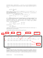
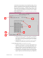
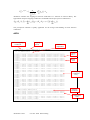
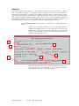
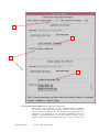
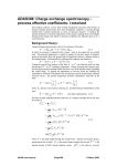
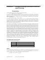
A typical ADF01 organisation is shown for H0 donor to He2 receiver
receiver
n,l
He+ 2
9
2
5
n
2
2
2
l
0
1
0
1
2
3
4
n-extrapolation
parameter
H + 0 (2) / receiver, donor (donor state n=2)
/
/
/ number of energies
/ nmin
/ nmax
0.01
0.02
0.05
0.10
0.20
0.50
1.00
2.00
5.00 / energies
17.00
16.20
15.00
13.86
12.68
11.00
9.65
8.30
5.85 / alpha
1.11E-14 1.18E-14 1.18E-14 1.16E-14 1.16E-14 1.29E-14 1.30E-14 1.34E-14 1.34E-14 / total xsects.
m
/ partial xsects.
0.00E+00 0.00E+00 0.00E+00 0.00E+00 2.75E-18 1.01E-17 1.77E-17 4.81E-17 9.32E-17
0.00E+00 0.00E+00 0.00E+00 0.00E+00 2.20E-18 5.07E-18 7.60E-18 1.22E-17 3.09E-17
0.00E+00 0.00E+00 0.00E+00 0.00E+00 5.50E-19 5.07E-18 1.01E-17 3.60E-17 6.23E-17
.
5
5
5
5
5
5
Total xsect.
Energies
1st block
donor
1.50E-17
0.00E+00
0.00E+00
0.00E+00
0.00E+00
0.00E+00
2.60E-17
0.00E+00
0.00E+00
0.00E+00
0.00E+00
0.00E+00
.
5.30E-17
0.00E+00
0.00E+00
0.00E+00
0.00E+00
0.00E+00
(cm2)
(cm2)
.
9.00E-17
0.00E+00
0.00E+00
0.00E+00
0.00E+00
0.00E+00
1.60E-16
0.00E+00
0.00E+00
0.00E+00
0.00E+00
0.00E+00
3.09E-16
0.00E+00
0.00E+00
0.00E+00
0.00E+00
0.00E+00
5.50E-16
0.00E+00
0.00E+00
0.00E+00
0.00E+00
0.00E+00
9.00E-16
0.00E+00
0.00E+00
0.00E+00
0.00E+00
0.00E+00
1.55E-15
0.00E+00
0.00E+00
0.00E+00
0.00E+00
0.00E+00
ADAS301
The code interrogates state selective charge exchange cross-section files of type ADF01. Data may be
extracted for capture to a selected n-, nl-or nlm-shell of a hydrogen-like or lithium-like receiving ion
depending on the ADF01 file. The data may be interpolated using cubic splines to provide crosssections at arbitrarily chosen impact energies. A minimax polynomial approximation is also made to
ADAS-EU Course
(keV/amu)
8-16 Oct. 2009 IPP Garching
partial
xsects.
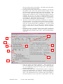
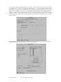
the source data. The source and interpolated cross-section data are displayed and a tabulation prepared.
The tabular and graphical output may be printed and include the minimax polynomial approximation.
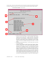
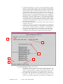
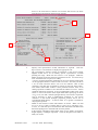
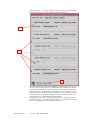
The file selection window is shown below.
1
2
4
3
5
7
6
1.
2.
3.
ADAS-EU Course
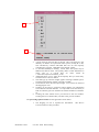
Data root shows the full pathway to the appropriate data subdirectories.
Click the Central Data button to insert the default central ADAS
pathway to the correct data type – ADF01 in this case. Note that each
type of data is stored according to its ADAS data format (adf number).
Click the User Data button to insert the pathway to your own data.
Note that your data must be held in a similar file structure to central
ADAS, but with your identifier replacing the first adas, to use this
facility.
The Data root can be edited directly. Click the Edit Path Name button
first to permit editing.
Available sub-directories are shown in the large file display window.
There are a large number of these, stored by donor which is usually
neutral but not necessarily so (eg. qcx#h0). The individual members are
identified by the subdirectory name, a code and then fully ionised
receiver (eg. qcx#h0_old#c6.dat). The data sets generally contain nlresolved cross-section data but n-resolved and nlm-resolved are
handled. Resolution levels must not be mixed in datasets. The codes
distinguish different sources.The first letter o or the code old has been
used to indicate that the data has been produced from JET compilations
which originally had parametrised l-distribution of cross-sections. The
nl-resolved data with such code has been reconstituted from them. Data
of code old is the preferred JET data. Other sources codes include ory
8-16 Oct. 2009 IPP Garching
4.
5.
6.
7.
(old Ryufuku), ool (old Olson), ofr (old Fritsch) and omo (old
molecular orbital). There are new data such as kvi.
Click on a name to select it. The selected name appears in the smaller
selection window above the file display window. Then its subdirectories in turn are displayed in the file display window. Ultimately
the individual datafiles are presented for selection. Datafiles all have
the termination .dat.
Once a data file is selected, the set of buttons at the bottom of the main
window become active.
Clicking on the Browse Comments button displays any information
stored with the selected datafile. It is important to use this facility to
find out what is broadly available in the dataset. The possibility of
browsing the comments appears in the subsequent main window also.
Clicking the Done button moves you forward to the next window.
Clicking the Cancel button takes you back to the previous window
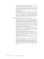
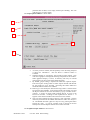
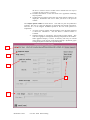
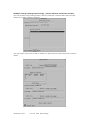
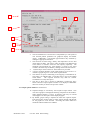
The processing options window has the appearance shown below
1. An arbitrary title may be given for the case being processed. For
information the full pathway to the dataset being analysed is also
shown. The button Browse Comments again allows display of the
information field section at the foot of the selected dataset, if it exists.
2. The output data extracted from the datafile, a ‘charge exchange crosssection’, may be fitted with a polynomial. This is as a function of
relative collision energy per atomic mass unit (eV/amu). Clicking the
Fit Polynomial button activates this. The accuracy of the fitting
required may be specified in the editable box. The value in the box is
editable only if the Fit Polynomial button is active
3. Your settings of collision velocity/energy (output) are shown in the
display window. The velocity/energy values at which the charge
exchange coefficients are stored in the datafile (input) are also shown
for information. The program recovers the output velocities/energies
you used when last executing the program.
4. Pressing the Default Velocity/Energy values button inserts a default set
of velocities/energies equal to the input velocities/energies
5. The Velocity/Energy values are editable. Click on the Edit Table
button if you wish to change the values. A ‘drop-down’ window, the
ADAS Table Editor window: It follows the same pattern of operation
as described in the 18nov-94 bulletin.
6. The specific cross-section data to be extracted is specified by the
window to the right. The level or resolution of the data source is
shown.
7. Activate the Select quantun numbers for processing button to allow new
settings of these quantum numbers. The values in the three smaller
windowsbecome editable depending also on the resolution of the
dataset. Note that the Range of the data in the dataset is displayed.
8. There are special codes to be used to obtain summed cross-sections
over sub-quantum numbers. These are indicated in brackets under the
Total column and should be entered into the editable window if
required.
ADAS-EU Course
8-16 Oct. 2009 IPP Garching
1
7
8
2
3
4
5
9
9.
Clicking the Done button causes the next output options window to be
displayed. Remember that Cancel takes you back to the previous
window.
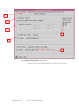
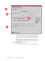
The output options window is shown below
1.
2.
3.
4.
5.
6.
ADAS-EU Course
As in the previous window, the full pathway to the file being analysed
is shown for information. Also the Browse comments button is
available.
Graphical display is activated by the Graphical Output button. This
will cause a graph to be displayed following completion of this window.
When graphical display is active, an arbitrary title may be entered
which appears on the top line of the displayed graph.
By default, graph scaling is adjusted to match the required outputs.
Press the Explicit Scaling button to allow explicit minima and maxima
for the graph axes to be inserted. Activating this button makes the
minimum and maximum boxes editable.
Hard copy is activated by the Enable Hard Copy button. The File name
box then becomes editable. If the output graphic file already exits and
the Replace button has not been activated, a ‘pop-up’ window issues a
warning.
A choice of output graph plotting devices is given in the Device list
window. Clicking on the required device selects it. It appears in the
selection window above the Device list window.
The Text Output button activates writing to a text output file. The file
name may be entered in the editable File name box when Text Output is
on. The default file name ‘paper.txt’ may be set by pressing the button
Default file name. A ‘pop-up’ window issues a warning if the file
already exists and the Replace button has not been activated.
8-16 Oct. 2009 IPP Garching
6
1
2
3
5
4
6
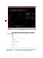
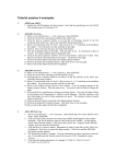
The Graphical output window is shown below
1. Printing of the currently displayed graph is activated by the Print button.
ADAS-EU Course
8-16 Oct. 2009 IPP Garching
1
ADF12
Data from files of type ADF12 contain charge exchange effective emission coefficients for principal
( eff )
quantum shell transitions of hydrogen-like impurity ions, qn→n′ , at a reference beam/plasma condition
( ref )
of beam energy E u
zeff
( ref )
, plasma ion density
( ref )
( ref )
N zeff
, plasma ion temperature Tzeff , plasma z effective
( ref )
and magnetic field strength Bmag . Also they contain the
)
qn(eff
→n ′ at varying plasma conditions
obtained by keeping all the parameters except one at the reference conditions. These are called one( eff )
dimensional scans and there are qn→n′ sets at the following parameter sets:
( ref )
( ref )
{Eu,i : i = 1, I E }, N zeff
, Tzeff
, zeff
( ref )
( ref )
Eu( zeff ) ,{ N zeff : i = 1, I N }, Tzeff
, zeff
, B (ref )
with
Eu( ref ) ∈{Eu,i : i = 1, I E } ,
( ref )
, B (ref ) with N zeff
∈{ N zeff :i = 1, I N },
( ref )
( ref )
( ref )
( ref )
( ref )
Eu , N zeff ,{Tzeff ,i : i = 1, I T }, zeff
,B
with Tzeff ∈{Tzeff ,i : i = 1, I T } ,
( ref )
( ref )
( ref )
Eu(ref ) , N zeff
, Tzeff
,{zeff i :i = 1, I zeff }, B (ref )
( ref )
( ref )
Eu(ref ) , N zeff
, Tzeff
, zeff (ref ) ,{Bi :i = 1, I B }
ADAS-EU Course
zeff (ref ) ∈{zeff i :i = 1, I zeff } ,
( ref )
∈{Bi : i = 1, I B }.
with B
with
8-16 Oct. 2009 IPP Garching
reference
rate coefft
receiver
1-D scans
from ref.
transition
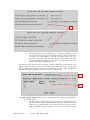
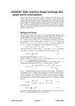
33
SPSCLMS ON HE+2 6-4 H(1S) DONOR 10/7/90
HE2NEW1(4) LMS
ISEL=8
6.52D-10
QEFREF
4.00D+04 5.00D+03 2.50D+13 2.00D+00 3.00D+00
PARMREF
19
12
17
6
1
NPARMSC
1.00D+03 1.50D+03 2.00D+03 3.00D+03 5.50D+03 7.00D+03
ENER
1.00D+04 1.50D+04 2.00D+04 3.00D+04 4.00D+04 5.00D+04
6.00D+04 7.00D+04 8.00D+04 1.00D+05 1.50D+05 2.00D+05
3.00D+05 0.00D+00 0.00D+00 0.00D+00 0.00D+00 0.00D+00
1.67D-13 1.07D-12 2.51D-12 5.02D-12 1.07D-11 1.62D-11
QENER
3.20D-11 7.65D-11 1.65D-10 5.06D-10 6.52D-10 5.82D-10
4.65D-10 3.54D-10 2.58D-10 1.40D-10 3.78D-11 1.25D-11
2.23D-12 0.00D+00 0.00D+00 0.00D+00 0.00D+00 0.00D+00
1.00D+03 2.00D+03 3.00D+03 5.00D+03 7.00D+03 1.00D+04
TIEV
1.30D+04 1.60D+04 1.90D+04 2.20D+04 2.50D+04 3.00D+04
6.53D-10 6.53D-10 6.52D-10 6.52D-10 6.52D-10 6.52D-10
QTIEV
6.51D-10 6.51D-10 6.51D-10 6.51D-10 6.51D-10 6.51D-10
1.00D+11 2.00D+11 3.00D+11 5.00D+11 7.00D+11 1.00D+12
DENSI
2.00D+12 3.00D+12 5.00D+12 7.00D+12 1.00D+13 2.00D+13
2.50D+13 3.00D+13 5.00D+13 7.00D+13 1.00D+14 0.00D+00
0.00D+00 0.00D+00 0.00D+00 0.00D+00 0.00D+00 0.00D+00
6.05D-10 6.11D-10 6.15D-10 6.22D-10 6.27D-10 6.32D-10
QDENSI
6.40D-10 6.44D-10 6.47D-10 6.49D-10 6.50D-10 6.52D-10
6.52D-10 6.52D-10 6.53D-10 6.53D-10 6.53D-10 0.00D+00
0.00D+00 0.00D+00 0.00D+00 0.00D+00 0.00D+00 0.00D+00
1.00D+00 2.00D+00 3.00D+00 4.00D+00 5.00D+00 6.00D+00
ZEFF
0.00D+00 0.00D+00 0.00D+00 0.00D+00 0.00D+00 0.00D+00
6.49D-10 6.52D-10 6.53D-10 6.53D-10 6.53D-10 6.53D-10
QZEFF
0.00D+00 0.00D+00 0.00D+00 0.00D+00 0.00D+00 0.00D+00
3.00D+00 0.00D+00 0.00D+00 0.00D+00 0.00D+00 0.00D+00
BMAG
0.00D+00 0.00D+00 0.00D+00 0.00D+00 0.00D+00 0.00D+00
6.52D-10 0.00D+00 0.00D+00 0.00D+00 0.00D+00 0.00D+00
QBMAG
0.00D+00 0.00D+00 0.00D+00 0.00D+00 0.00D+00 0.00D+00
C----------------------------------------------------------------------C EFFECTIVE COEFFICIENT LIST:
C
C
ISEL
TYPE
ION
INFORMATION
C
------------------C
8.
CX.EMIS. HE+ 1
N = 6 - 4
6559.4
10/7/90 J2460
C-----------------------------------------------------------------------
reference
parameter
values
energy scan
ADAS303
The program interrogates charge exchange spectroscopy effective emission coefficient data sets of type
ADF12 associated with a particular neutral donor. The ADF12 data set collections are for the relevant
hydrogen-like n-n’ spectrum lines grouped according to the recombining ion. The code and data
organisation allows the emission coefficient to be obtained (by interpolation using cubic splines) at
plasma conditions and at relative collision energies of choice. A minimax polynomial approximation
can also be made to the interpolated data. The interpolated data are displayed and a tabulation
prepared. The tabular and graphical output may be printed and include the polynomial approximation.
The file selection window appears first and has the appearance shown below.
1. Data root shows the full pathway to the appropriate data subdirectories.
Click the Central Data button to insert the default central ADAS
pathway to the correct data type. Note that each type of data is stored
according to its ADAS data format (adf number). adf12 is the
appropriate format for use by the program ADAS303. Details of the
organisation of such data is given in the appxa-12. Click the User Data
button to insert the pathway to your own data. Note that your data must
be held in a similar file structure to central ADAS, but with your
identifier replacing the first adas, to use this facility.
2. The Data root can be edited directly. Click the Edit Path Name button
first to permit editing
ADAS-EU Course
8-16 Oct. 2009 IPP Garching
3.
4.
5.
6.
Available sub-directories are shown in the large file display window.
There are a large number of these. They are stored in sub-directories
by donor which is usually neutral but not necessarily so (eg. qef93#h).
The individual members are identified by the subdirectory name, a code
and then fully ionised receiver (eg. qef93#h_be4.dat). The data sets
generally contain many individual spectrum lines. Scroll bars appear if
the number of entries exceed the file display window size. Such data is
generally stored by year number (eg. 93 ) with the most recent data to
be preferred. Click on a name to select it. The selected name appears
in the smaller selection window above the file display window. Then
its sub-directories in turn are displayed in the file display window.
Ultimately the individual datafiles are presented for selection. Datafiles
all have the termination .dat.
Once a data file is selected, the set of buttons at the bottom of the main
window become active.
Clicking on the Browse Comments button displays any information
stored with the selected datafile. It is important to use this facility to
find out what is broadly available in the dataset. The possibility of
browsing the comments appears in the subsequent main window also.
Clicking the Done button moves you forward to the next window.
Clicking the Cancel button takes you back to the previous window
1
2
3
4
6
5
The processing options window is shown below:
1. An arbitrary title may be given for the case being processed. For
information the full pathway to the dataset being analysed is also
shown. The button Browse comments again allows display of the
information field section at the foot of the selected dataset, if it exists.
2. The output data extracted from the datafile may be fitted with a
polynomial. Clicking the Fit Polynomial button activates this. The
accuracy of the fitting required may be specified in the editable box.
ADAS-EU Course
8-16 Oct. 2009 IPP Garching
3.
The value in the box is editable only if the Fit Polynomial button is
active.
Transitions available in the data set are displayed in the transition list
display window. This is a scrollable window using the scroll bar to the
right of the window. Click anywhere on the row for a transition to
select it. The selected transition appears in the selection window just
above the transition list display window.
1
2
3
7
6
4
5
4.
5.
6.
7.
ADAS-EU Course
Energies/velocities for the neutral donor are displayed. The particular
choice of units in use is shown below the table. Your settings of beam
energy/velocity (output) are shown in the display window. The beam
energy/velocity values at which the effective emission coefficients are
stored in the datafile (input) are also shown for information. Click the
Edit Table button to drop-down the ADAS Table Editor. Within Table
Editor you can select which units to use as well as entering you
energy/velocity values for output. Note that final graphed results are of
effective emission coefficient versus beam energy (eV/amu).
The program recovers the output energies/velocities you used when last
executing the program. Pressing the Default Energy/Velocity values
button inserts a default set of energies/velocities equal to the input
values
Effective emission coefficients for the ADF12 database are calculated
at one-dimensional scans in various plasma parameters relative to a
reference set of plasma conditions. Details are given in appxa-12. To
alter the settings, activate the Select supplementary plasma parameters
button.
The sub-windows become active with the output data entry box in each
editable. For information, the reference value of each plasma parameter
is given together with the range of the parameter in its one-dimensional
scan. Values outside the range should not be entered. For data
prepared using processing code ADAS309, the B magnetic field
8-16 Oct. 2009 IPP Garching
parameter has no effect, but is simply used for place holding. The scan
in B Magnetic is of zero length.
The output options window is shown below
1
2
3
4
5
7.
As in the previous window, the full pathway to the file being analysed
is shown for information. Also the Browse comments button is
available.
8. Graphical display is activated by the Graphical Output button. This
will cause a graph to be displayed following completion of this window.
When graphical display is active, an arbitrary title may be entered
which appears on the top line of the displayed graph.
9. By default, graph scaling is adjusted to match the required outputs.
Press the Explicit Scaling button to allow explicit minima and maxima
for the graph axes to be inserted. Activating this button makes the
minimum and maximum boxes editable.
10. Hard copy is activated by the Enable Hard Copy button. The File name
box then becomes editable. If the output graphic file already exits and
the Replace button has not been activated, a ‘pop-up’ window issues a
warning. A choice of output graph plotting devices is given in the
Device list window. Clicking on the required device selects it. It
appears in the selection window above the Device list window.
11. The Text Output button activates writing to a text output file. The file
name may be entered in the editable File name box when Text Output is
on. The default file name ‘paper.txt’ may be set by pressing the button
Default file name. A ‘pop-up’ window issues a warning if the file
already exists and the Replace button has not been activated.
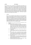
The Graphical output window is shown below
ADAS-EU Course
8-16 Oct. 2009 IPP Garching
2. Printing of the currently displayed graph is activated by the Print button.
1
Calculating CXS effective emission coefficients
The line-of-sight integrated photon emissivity of a charge exchange driven line may be written as
z0 −1)
( z0 −1)
I n(→
n ′ = ∑ I nl → n ′l ′
l ,l ′
=
∫∑ A
nl → n ′l ′
N nl( z0 −1) ds
S l ,l ′
= ∫ [ ∑ Anl → n ′l ′ ( N nl( z0 −1) / N D N ( z0 ) )] N D N ( z0 ) ds
S
l ,l ′
= ∫ [ ∑ q nl( eff→)n′l ′ ] N D N ( z0 ) ds
S
l ,l ′
)
( z0 )
= ∫ q n( eff
ds
→n′ N D N
S
)
( z0 )
≈ q n( eff
ds
→n′ ∫ N D N
S
where S is the path length through the neutral beam / plasma intersection along a spectrometer line-of(z )
sight. N D is the neutral donor number density and N 0 is the number density of fully ionised
impurity atoms.
)
qn(eff
→n ′ is the effective emission coefficient for the whole n → n ′ principal quantum
shell transition and
∫N
D
N ( z0 ) ds is the emission measure. The mean transition energy is
S
ADAS-EU Course
8-16 Oct. 2009 IPP Garching
)
ΔE n,n ′ = ( ∑ ΔE nl ,n ′l ′ qnl( eff→)n ′l ′ ) / qn( eff
→n′
l ,l ′
where ΔE nl ,n ′l ′ is the line component transition energy and
qnl(eff→)n′l ′ is the component effective
( eff )
emission coefficient. The effective emission coefficient qn→n′ may be calculated theoretically. If it is
approximately constant over the emitting volume, then measurement of a charge exchange line
intensity
z0 −1)
I n(→
n ′ allows deduction of the emission measure
∫N
D
N ( z0 ) ds . If neutral beam attenuation
S
to the observed volume is known or calculable then local impurity density may be inferred.
With the effective emission coefficients calculated theoretically, comparison with one observed charge
exchange line intensity allows deduction of the emission measure. Then all other line intensities are
predictable. If more than one line intensity is observed, then a mean emission measure may be deduced
and some comment may be made on the ratios of experimental to theoretical effective emission
coefficients. The organisation of the collisional-radiative modelling in ADAS308 is specifically
designed to allow such comparison. The following points and assumptions are made:
(i) From the theoretical point-of-view the direct capture cross-sections to levels are more fundamental
quantities for comparison with experiment that the effective emission coefficients.
(ii) The dominant fundamental processes modifying the initial distribution of capture are redistribution
within an n-shell and radiative cascade in low and moderate density plasmas. Limiting the collisionalradiative theory to these dominant processes allows a compact invertable relationship to be established
between column emissivities of charge exchange spectrum lines and direct capture cross-sections.
(ii) It is of most practical value to target experiment / theory comparisons on the n-shell distribution of
capture (including the n-shell decrement) in fusion studies. This may be achieved by imposing
theoretical information on the l sub-shell distribution of capture.
( CX )
Consider the monoenergetic direct capture rate coefficients to nl sub-levels q nl
from the initial
( z0 )
0
neutral donor state D (1) by the fully stripped impurity ion with number density N , denoted more
N +.
qnl( CX ) ( E u ) = v σ nl( CX ) ( v )
compactly by
where Eu is the relative collision energy per atomic mass unit so that v =
collision speed, with mp the proton mass and
2 E u / m p is the relative
σ the capture cross-section.
It is supposed that
) ( CX )
qnl(CX ) ( Eu ) = f ((ntheor
qn ( E u )
)l
Since no collisional excitation from lower to higher n-shells is allowed, the populations of the lj
sublevels of the principal quantum shell n ′ ≥ n + 1 may be written as
N n ′l ′ = N D N +
∑
n iv ≥ n +1
)
Wn ′l ′ ,niv qn( CX
iv
Then the equations determining the populations of the sub-shells of the principal quantum shell n are
∑M
( n ) l ,l ′′
) ( CX )
N nl ′′ = N D N + f ( (ntheor
qn +
)l
so that
nl ,n ′l ′
N nlj = N D N +Wnlj ,n qn( CX ) + N D N +
∑
n iv ≥ n +1
with
∑A
N n ′l ′
n ′≥ n +1
l ′′
)
Wnlj ,niv qn( CX
iv
)
( CX )
Wnlj ,n = [∑ M (−n1)lj ,l ′′j′′ f ((ntheor
) l ′′j ′′ ]q n
l ′′j ′′
and
Wnlj ,niv =
∑M
l ′′, j ′′,l ′, j ′
−1
( n ) lj ,l ′′j ′′
Anl ′′j′′,n′l ′j′Wn′l ′j′,niv
The solution can proceed recursively downwards in n with compact vector and array storage.
Tabulations of experimental or theoretical state selective charge exchange cross-section data span a
( CX )
range of principal quantum shells σ nlj ( v ) : n0 ≤ n ≤ n1 . Cascade from levels n > n1 may contribute
significantly to the populations of lower levels especially at high collision energies when the decrease
−α
of the direct charge exchange cross-sections with n is slow ( σ n ~ n
and α ~ 3). However,
ADAS-EU Course
8-16 Oct. 2009 IPP Garching
redistribution amongst lj sub-levels of the higher n-shells is high, approaching statistical in most
circumstances. Therefore the cascade solution is initiated at some nmax (~20 typically) for complete nshell populations only (matrices W
( high)
), with subshells implicitly statistically populated, down to n1
( low)
) is commenced.
whereupon the lj resolved solution (matrices W
In general observable spectrum lines are associated with upper principal quantum shells n ≤ n1 . If
M rep , lines are identified each with a distinct upper n-shells nirep : irep = 1,..., M rep , then a
'condensation' may be imposed such that
q
( CX )
n
M rep
∑L
=
irep=1
and
for n0 ≤ n ≤ n1
( CX )
n ,irep nirep
q
qn( CX ) = ( n / n1 ) α qn(1CX )
for n > n1
giving, after integration along the line-of-sight, a matrix relation
⎡ I
⎢ n1 → n1′
.
⎢
⎢I
⎢⎣ n M rep → n M′ rep
⎤
⎡ a11 .
⎥
⎢
+
⎥ = ( ∫ N D N ds) ⎢ .
S
⎥
⎢a
⎥⎦
⎣ M rep 1
. a1 M rep ⎤ ⎡ q n(1CX ) ⎤
⎥
⎥⎢
.
. ⎥⎢ . ⎥
)⎥
. a M rep M rep ⎥⎦ ⎢⎢q n( CX
⎣ M rep ⎥⎦
The coefficients of the matrix are theoretically calculated quantities. The equations may be solved for
the the
qn(iCX ) and the emission measure
∫N
D
N + ds subject to the constraint
S
M rep
∑q
irep=1
( CX )
nirep
=
M rep
∑q
irep=1
( CX )( theor )
nirep
ADAS308
The code analyses column (line-of-sight integrated) emissivity observations of charge exchange
spectroscopy lines from hydrogenic impurities, occuring through neutral beam / plasma interaction, in
terms of emission measure. It predicts the column intensities of spectral components of the charge
exchange lines, the Doppler broadened line shapes and effective emission coefficients for arbitrary lines
in an l-resolved picture.
The file selection window is shown below.
1.
2.
3.
ADAS-EU Course
Data root shows the full pathway to the appropriate data subdirectories.
Click the Central Data button to insert the default central ADAS pathway to
the correct data type – ADF01 in this case. Note that each type of data is
stored according to its ADAS data format (adf number). Click the User
Data button to insert the pathway to your own data. Note that your data
must be held in a similar file structure to central ADAS, but with your
identifier replacing the first adas, to use this facility.
The Data root can be edited directly. Click the Edit Path Name button first
to permit editing.
Available sub-directories are shown in the large file display window. Scroll
bars appear if the number of entries exceed the file display window size.
There are a large number of these. They are stored in sub-directories by
donor which is usually neutral but not necessarily so (eg. qcx#h0). The
individual members are identified by the subdirectory name, a code and then
fully ionised receiver (eg. qcx#h0_old#c6.dat). The data sets generally
contain nl-resolved cross-section data but n-resolved and nlm-resolved are
handled. Resolution levels must not be mixed in datasets. The ADF01 file
nmaes distinguish different sources. The first letter o or the code old has
been used to indicate that the data has been produced from JET compilations
which originally had parametrised l-distribution of cross-sections. The nl-
8-16 Oct. 2009 IPP Garching
4.
resolved data with such code has been reconstituted from them. Data of
code old is the preferred JET data. Other sources codes include ory (old
Ryufuku), ool (old Olson), ofr (old Fritsch) and omo (old molecular orbital).
There are newer data such as kvi. Additional codes are used for excited
donors such as ex2 for hydrogen n=2. Click on a name to select it. The
selected name appears in the smaller selection window above the file display
window. Then the individual datafiles are presented for selection. Datafiles
all have the termination .dat.
Once a data file is selected, the set of buttons at the bottom of the main
window become active.
1
2
3
4
6
5
5.
6.
7.
Clicking on the Browse Comments button displays any information
stored with the selected datafile. It is important to use this facility to
find out what has gone into the dataset and the attribution of the dataset.
The possibility of browsing the comments appears in the subsequent
main window also.
Clicking the Done button moves you forward to the next window.
Clicking the Cancel button takes you back to the previous window
The processing options window has the appearance shown below
2.
3.
4.
ADAS-EU Course
An arbitrary title may be given for the case being processed. For
information the full pathway to the dataset being analysed is also
shown. The button Browse Comments again allows display of the
information field section at the foot of the selected dataset, if it exists.
Information is given on the fully ionised impurity receiver and the
neutral beam donor. The atomic mass of the receiver must be entered.
The specification of beam parameters, details of observed line of sight
spectral emissivities to be analysed and emissivities to be predicted are
required. Input data of each of these three types may be addressed in
8-16 Oct. 2009 IPP Garching
5.
6.
7.
turn by activation of the relevant button. The window below the button
list then presents the appropriate table.
The Required emissivity predictions button is displayed. This activates
the predictive part of the code which becomes possible once the
observed lines have been analysed in terms of emission measure. Then
any set of lines within the N-shell limits may be predicted. The
standard output includes the mean wavelength and effective emisison
coefficient, but for up to five lines an extended tabulation of line
component emissivities may be produced. Graphs may be produced for
two selected line. Indicate these selections in the Key columnThe table
may be edited by clicking on the Edit Table button.
The Observed spectrum lines table allows introduction of a number of
observed intensities. It is possible to enter values which do not allow a
consistent solution. The code advises of this but it is the responsibility
of the user to check that the data is unblended etc. It is also a usual
practice to enter just one line, possibly with a fictitious emissivity
merely to obtain effective emission coefficients and line component
details.
The Beam parameter information button causes display of the third
editable table in the sub-window. Note that no check is made that the
various beam energy fractions sum to unity. This is the responsibility
of the user.
2
1
5
3
7
6
8
4
9
10
8.
9.
ADAS-EU Course
Enter the plasma environment parameters. These determine the
collisional redistribution of the populations of the recombined plasma
ion. For ADAS308, B Magn. has no effect, but a value should be
entered as a place holder.
The final sub-window allows model and theory choices. Details are
given in the ADAS Manual. For each type, clicking on the selection
window drops down a short menu of choices. Click on the appropriate
choice. The ADAS data base source numerical data of type ADF01 is
the most usual, that is the Use input data set choice button. Note that
8-16 Oct. 2009 IPP Garching
the Select emission measure model choice includes Electron impact
excitation as well as Charge exchange.
10. Extended information on the rates used in the populaiton modelling
may be printed.
11. Clicking the Done button causes the next output options window to be
displayed. Remember that Cancel takes you back to the previous
window.
The Output options window is shown below. Note that two plots are produced if
required. The Plot A is the stick diagram of component line-of-sight emissivities.
The Plot B is of the Doppler broadened profile of the line at the plasma ion
temperature.
1. As in the previous window, the full pathway to the file being analysed
is shown for information. Also the Browse comments button is
available.
2. Graphical display is activated by the Graphical Output button. This
will cause a graph to be displayed following completion of this window.
When graphical display is active, an arbitrary title may be entered
which appears on the top line of the displayed graph. By default, graph
scaling is adjusted to match the required outputs.
1
2
3
4
5
ADAS-EU Course
8-16 Oct. 2009 IPP Garching
3.
Press the Explicit Scaling button to allow explicit minima and maxima
for the graph axes to be inserted. Activating this button makes the
minimum and maximum boxes editable. Plot A axes limits refer to the
‘stick diagram and Plot B axes limits to the Doppler broadened profile.
4. Hard copy is activated by the Enable Hard Copy button. The File name
box then becomes editable A choice of output graph plotting devices is
given in the Device list window. Clicking on the required device
selects it. It appears in the selection window above the Device list
window.
5. The Text Output button activates writing to a text output file. The file
name may be entered in the editable File name box when Text Output is
on. The default file name ‘paper.txt’ may be set by pressing the button
Default file name.
The Graphical output window is shown below
3. Printing of the currently displayed graph is activated by the Print button.
1
Extended CXS capabilities
The charge exchange spectroscopy modelling capabilities of ADAS are still extending. This is largely
motivated by the need to cope with heavier receiver ions beyond argon, which may be partially ionized.
Attention is drawn to two new codes ADAS315 and ADAS316. Many subroutines have been added or
modified to accommodate the new capabilities. The user should check the detailed release notes in
item 4. A number of subroutines have modified parameter sets.
ADAS315: Preparation and extraction of universal adf49/adf01 CX cross-section data
This is a straightforward code which creates and ADF01 file for a specific ion of an element from a zscaleable universal dataset of format ADF49. There are only two datasets of AD49 format
ADAS-EU Course
8-16 Oct. 2009 IPP Garching
corresponding to H(n=1) and H(n=2) donor respectively. The input screen is shown below followed by
the output screen. A choice is possible of output energies. It is to be noted that in the level of
approximation of the universal ADF49 data and the bundle-n application models, only the residual
charge of the recombining ion is relevant. For the high n-shells of importance, the Rydberg electron is
effectively in a hydrogenic state in the Coulomb field of the residual charge. The ADF49 datasets are
subject to change as more fiducial data becomes available and the opimising of the z-scaling
paramterisation is reworked. At this stage ADAS315 and ADAS316 are enabling a first look at the
heavy ion CXS.
Running ADAS315 (an IDL only) code, available also at the command line, in a script allows output
ADF01 files to be generated rapidly for a set of ions of an element.
ADAS-EU Course
8-16 Oct. 2009 IPP Garching
ADAS316: Charge exchange spectroscopy – process effective coefficients: bundle-n
The code calculates charge exchange effective emission coefficients of format ADF12 from and input
ADF01 file, probably created by ADAS315.
The code requires a driver data set and, for bundle-n in ADAS, these have historically been archived in
ADF25.
ADAS-EU Course
8-16 Oct. 2009 IPP Garching
A new sub-directory /a25_p316 has been assigned and a complete redesign of the driver has been
carried out. Also a new read routine exploits the new drivers fully. We would like to move to this type
of driver in the future, where there is substantial guidance to the user in the fields and mnemonics used
in the driver. The driver allows scans over parameters to be specified. In fact the driver is quite
versatile and appropriate to all type of bundle-n calculation . We shall exploit it further for
Bremsstrahlung + free-bound continuum iand quasi-continuum high Rydberg line contributions in the
future.
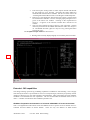
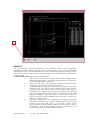
The output screen follows a usual pattern. Output ADF26 (the bundle-n population solution), ADF12
(charge exchange effective emission coefficients) and ADF40 (feature emissivity coefficients) may be
produced. For heavy species CXS, because of the very large number of transitions between highly
excited states, the ADF40 format becomes more useful that ADF12. A graph of the bundle-npopulation solution, at the reference plasma parameters (usually at the centroid of the scans) is
generated and shown with the free–electron capture and charge exchange capture parts separated – as
illustrated below.
Beam stopping and emission
For a neutral beam species A being stopped by fully stripped impurity species and electrons in the
plasma, the stopping coefficient is the effective loss rate coefficient of electrons from A . This
corresponds closely to the effective ionisation rate coefficient or collisional-radiative ionisation
ADAS-EU Course
8-16 Oct. 2009 IPP Garching
coefficient from the ground state of A , where charge transfer losses as well as direct ionisation losses
are included. It is usual to write the coefficient in terms of the plasma electron density N e so that the
( A)
loss rate is N e SCR .
One can apply almost the same modellelling approach to hydrogen (or helium) atoms in a thermal
plasma or to hydrogen atoms in a beam. The practical distinction is made by the assignment of a
translational velocity for beam atoms. This velocity is incorporated in the integrals of beam particle /
plasma particle cross-sections over the Maxwellian distributions in the thermal plasma. For hydrogen
forming part of the thermal plasma, the translational velocity is set to zero. In the latter circumstance,
ion impact collision rates are very small compared with electron impact rates. Also recombination
(both free-electron capture and charge exchange capture) become significant processes. For the
hydrogen atoms in a fast beam, recombination is not relevant and although formally present is ignored
in the results. However the translational velocity can make ion impact collisions more important than
electron collisions.
For hydrogen or hydrogenic ions in a plasma, the largest collision cross-sections are those for which
n=n' and l=l'±1. For these cases the transition energy is nearly zero and the cross-sections are so large
for electron and ion densities of relevance for fusion that it is very good approximation to assume
relative statistical population for the l-states. Thus for hydrogenic systems only populations of
complete n-shells need be evaluated, the bundle-n approximation. The equilibrium populations of the
n-shells, Nn, are the solution of the statistical balance equations
∑[ A
n '→ n
+ u(ν ) Bn '→n + N e q n( e'→) n + N e q n( 'p→) n ] N n '
n '>n
)
( p)
+ ∑ [u(ν ) Bn ''→n + N e q n( e''→
n + N e q n ''→ n ] N n ''
n ''< n
+ N e N + α n( r ) + N e2 N + α n( 3) + N e N + ∫ u(ν ) Bκ →n dκ
p)
= {∑ [u(ν ) Bn→n ' + N e q n( e→) n ' + N e q n( →
n' ]
n '> n
+
∑[ A
n→ n ''
p)
+ u(ν ) Bn→n '' + N e q n( e→) n '' + N e q n( →
n '' ]
n '' < n
p)
+ ∫ u(ν ) Bn→κ dκ + N e q n( e→) ε + N e q n( →
ε }N n
N n is the population of the state X n+ z0 −1 and N + of the parent ion X + z0 . N e is the free electron
density and N p the free proton density. A and B are the usual Einstein coefficients, q
( e)
and q
( p)
denotes collisional rates due to electrons and protons, α n and α n denote radiative and three-body
recombination and u( ν) is the energy density of the radiation field. There is one such equation for
each value of n from 1 to ∞. The equations may be extended by including reactions for other impurity
ions additional to the protons. The radiation field presence in the equations is not of direct relevance to
hydrogen population modelling in a fusion plasma, but it can be exploited in a purely technical manner
to separate the influence of different driving populations in the collisional-radiative sense.
(r )
( 3)
Population results and preparing tabulations
ADAS 310 is the primary code for evaluating beam stopping and emission coefficients for hydrogen
beams. It is too slow in execution for a direct link to inter-pulse experiment analysis and so it is used
to prepare tabulations of effective beam stopping and beam emission coefficients for subsequent lookup. The effective coefficients are most sensitive to the beam particle energy and the plasma ion density
and less sensitive to plasma ion temperature and Z-effective. Suitable tabulations can therefore be built
on a reference set of plasma and beam conditions, a two-dimensional array of coefficients as functions
of beam energy and plasma density at the reference conditions of the other parameters and then onedimensional vectors of the coefficients as functions of each minor parameter at the reference condition
of all the other parameters. ADAS310 accepts as input the definition of these scans, establishes an
ADAS-EU Course
8-16 Oct. 2009 IPP Garching
extended list of cases required to achieve these scans and then executes repeated population
calculations at each set of plasma conditions in the list. ADAS310 can compute the populations for
any mixture of light impurities (hydrogen to neon) in the plasma. It is impractical to deal with all
possible mixtures of impurities. It is our usual practice to execute ADAS310 in turn for each light
impurity from hydrogen to neon treated as a pure species. The mixed species effective coefficients are
constructed from these pure impurity solutions by the theoretical data acquisition routines. The main
population output is very complete and in principle contains all information on possible emitted
spectrum lines up to very high n-shells together with both ionisation and recombination collisionalradiative coefficients. It is archived as ADAS data format ADF26. ADAS310 can also produce
directly the final tabulations of beam stopping coefficient according to ADAS data format ADF21,
however this is normally done using the post-processor program ADAS312.
ADAS304 is the interrogation code on the beam stopping coefficient data base ADF21. It also works
with the beam emission coefficient data base, which is of identical organisation to the stopping
coefficients, and is assigned to ADF22.
In creation of compact interpolable datasets of type ADF21 and ADF22, some simplifications are
made. The stopping coefficient data sets for each impurity species are calculated as though that species
(z )
+z
alone is present in the plasma. For species X 0 , of nuclear charge z0 , of number density N 0 , the
electron density used in the stopping calculation is
Let the stopping coefficient for the impurity species
N e = z0 N ( z0 ) consistent with charge neutrality.
( A ,X )
X + z0 be SCR
then the loss rate is
( A ,X )
( A ,e )
N e SCR
( EB , N ( z0 ) , T ( z0 ) ) = N e SCR
( E B , N ( z0 ) , T ( z0 ) )
( A , z0 )
+ N ( z0 ) SCR
( E B , N ( z0 ) , T ( z0 ) )
distinguishing parts driven by excitation from the ground state of A by electron collisions and by
X + z0 ions respectively. The coefficient is
( A ,X )
( A ,e )
SCR
( EB , N ( z0 ) , T ( z0 ) ) = SCR
( EB , N ( z0 ) , T ( z0 ) )
( A , z0 )
+ (1/ z0 ) SCR
( E B , N ( z0 ) , T ( z 0 ) )
The density dependence of the collisional-radiative coefficient is written in terms of the impurity ion
(z )
density N 0 since ion collisions primarily determine the collisional redistribution..
+z
Consider a set of species { X i 0i : i = 1,.., I } with fractions { f i : i = 1,.., I } , in the plasma causing a
composite stopping. The loss rate may be written approximately as
(A )
( A ,e )
N e SCR
( EB , N I , TI ) ≈ N e SCR
( EB , N I , TI ) +
I
∑N
i =1
( z0 i ) ( A , z0 i )
i
CR
S
( EB , N I , TI )
I
( A,e )
( EB , N I , TI ) +
= ∑ N e,i [ SCR
i =1
( A, z0 i )
(1/ z0i ) SCR
( EB , N I , TI )]
where
I
I
I
i =1
i =1
i =1
N e = ∑ N e,i = ∑ z0i N ( z0i ) = N I ( ∑ z0i f i )
defines the proportions of the electron density contributed by each impurity species.
I
From an ion collisional redistribution point of view, in a composite plasma the
∑z
k =1
2
0k
N k( Z0k ) z+ z0i
weighted density sum is meaningful so the equivalent density of the single impurity X i
correspond to the summed impurity ion density for this purpose is
I
N
( z0i ),equiv
i
= N I ( ∑ z02k f k ) / z02i
k =1
and the equivalent electron density is
ADAS-EU Course
8-16 Oct. 2009 IPP Garching
to
N ei( z0 i ),equiv = (
Ne
I
I
∑ z 0 k fk
)( ∑ z02k fk ) / z0i
k =1
k =1
ADAS310 evaluates the stopping & emission coefficients as a function of electron density. The
approximate composite stopping coefficient is assembled from the pure species coefficients as
I
I
i =1
k =1
( A ,Xi )
(A )
SCR
( EB , N e , TI ) ≈ ∑ [ z0i fi SCR
( EB , N ei( z0 i ),equiv , TI )]/(∑ z0 k f k )
The prescription outlined is equally applicable for the storage and handling of beam emission
coefficients.
ADF21
reference stopping
coefficient
stopping
species
reference
temperature
9 /SVREF=1.798E-07 /SPEC=F /DATE=19/03/97 /CODE=ADAS310
-------------------------------------------------------------------------------25
25 /TREF=2.000E+03
-------------------------------------------------------------------------------5.000E+03 1.000E+04 1.500E+04 2.000E+04 2.500E+04 3.000E+04 3.500E+04 4.000E+04
4.500E+04 5.000E+04 5.500E+04 6.000E+04 6.500E+04 7.000E+04 7.500E+04 8.000E+04
8.500E+04 9.000E+04 9.500E+04 1.000E+05 1.050E+05 1.100E+05 1.150E+05 1.200E+05
1.250E+05
1.000E+12 2.000E+12 3.000E+12 5.000E+12 6.000E+12 7.000E+12 8.000E+12 9.000E+12
1.000E+13 2.000E+13 3.000E+13 5.000E+13 6.000E+13 7.000E+13 8.000E+13 9.000E+13
1.000E+14 2.000E+14 3.000E+14 5.000E+14 6.000E+14 7.000E+14 8.000E+14 9.000E+14
1.000E+15
-------------------------------------------------------------------------------1.036E-07 1.228E-07 1.330E-07 1.404E-07 1.469E-07 1.521E-07 1.557E-07 1.593E-07
1.622E-07 1.641E-07 1.655E-07 1.657E-07 1.652E-07 1.654E-07 1.666E-07 1.683E-07
1.698E-07 1.697E-07 1.692E-07 1.691E-07 1.695E-07 1.703E-07 1.718E-07 1.739E-07
1.766E-07
1.043E-07 1.236E-07 1.339E-07 1.413E-07 1.478E-07 1.530E-07 1.566E-07 1.602E-07
1.631E-07 1.650E-07 1.664E-07 1.667E-07 1.663E-07 1.666E-07 1.678E-07 1.696E-07
1.712E-07 1.712E-07 1.707E-07 1.708E-07 1.712E-07 1.721E-07 1.737E-07 1.759E-07
1.787E-07
.
.
.
1.214E-07 1.429E-07 1.542E-07 1.622E-07 1.689E-07 1.743E-07 1.781E-07 1.821E-07
1.856E-07 1.886E-07 1.915E-07 1.936E-07 1.953E-07 1.977E-07 2.009E-07 2.049E-07
2.087E-07 2.110E-07 2.128E-07 2.150E-07 2.178E-07 2.211E-07 2.249E-07 2.293E-07
2.343E-07
1.218E-07 1.431E-07 1.544E-07 1.624E-07 1.691E-07 1.745E-07 1.783E-07 1.824E-07
1.859E-07 1.889E-07 1.918E-07 1.939E-07 1.957E-07 1.981E-07 2.013E-07 2.053E-07
2.091E-07 2.115E-07 2.133E-07 2.156E-07 2.184E-07 2.217E-07 2.256E-07 2.300E-07
2.350E-07
1.222E-07 1.434E-07 1.546E-07 1.625E-07 1.693E-07 1.747E-07 1.785E-07 1.826E-07
1.861E-07 1.891E-07 1.921E-07 1.942E-07 1.960E-07 1.984E-07 2.017E-07 2.057E-07
2.095E-07 2.119E-07 2.138E-07 2.161E-07 2.189E-07 2.222E-07 2.261E-07 2.306E-07
2.356E-07
-------------------------------------------------------------------------------20 /EREF=6.500E+04 /NREF=6.000E+13
-------------------------------------------------------------------------------1.000E+02 2.000E+02 3.000E+02 5.000E+02 6.000E+02 7.000E+02 8.000E+02 8.966E+02
1.000E+03 2.000E+03 3.000E+03 5.000E+03 6.000E+03 7.000E+03 8.000E+03 8.966E+03
1.000E+04 2.000E+04 3.000E+04 5.000E+04
-------------------------------------------------------------------------------2.021E-07 2.017E-07 1.992E-07 1.945E-07 1.926E-07 1.909E-07 1.894E-07 1.881E-07
1.869E-07 1.798E-07 1.761E-07 1.719E-07 1.706E-07 1.695E-07 1.687E-07 1.680E-07
1.673E-07 1.638E-07 1.623E-07 1.608E-07
--------------------------------------------------------------------------------
ADAS-EU Course
8-16 Oct. 2009 IPP Garching
energy
scan
density
scan
2-D stopping
coefficient
array
reference
conditions
temperature
scan
ADAS304
The code interrogates beam stopping or beam emission coefficient files of type ADF21 or ADF22.
Data is extracted for stopping by a composite plasma consisting of a mixture of protons (deuterons)
and fully ionised impurities. The data is interpolated using cubic splines at selected beam energy,
target density and target temperature triplets. Minimax polynomial fits are made to the interpolated
data. The total stopping and partial stopping by each species are given. The beam emission coefficients
are handled in a similar manner. The interpolated data are displayed and a tabulation prepared. The
tabular and graphical output may be printed and includes the polynomial approximations.
The file selection window is shown below. Its operation is a little different from
usual.
1.
ADF21 is the appropriate format for use by the program ADAS304
(ADAS User Manual, appxb-21). A root path to the correct data type
ADF21 appears automatically. Your personal data of this type should
be held in a similar file structure to central ADAS, but with your
identifier replacing the first adas.
1
2
3
4
5
8
9
2.
ADAS-EU Course
Buttons are present to set the data root to that of the Central data or to
your personal User data (provided it is in ADAS organisation.
Alternatively the ‘data root’ may be edit explicitly.
8-16 Oct. 2009 IPP Garching
6
7
3.
4.
5.
6.
7.
8.
9.
A group name for the input files is entered. This is the name of a subdirectory of ADF21 for a particular beam species (usually H or He).
The sub-directory contains individual data sets for each impurity
contributing to stopping , identified by the element symbol.
To increase flexibility in naming a three letter class prefix may be
added to the data set name. The primary data in central ADAS has no
prefix and so a typical data set name would be
/../adas/adas/adf21/bms#h/bms#h_be.dat.
ADAS304 allows you to select all the impurity files you wish easily.
Click the Reselect Ion List button.
The small pop up selection widget appears showing available species.
Click the toggle buttons of those you wish to include
Click Done to restore the main input widget. Your choices are shown at
the Stopping Ion List.
Clicking on the Browse Comments button displays any information
stored with the selected data-files. It is important to use this facility to
find out what has gone into the data-set and the attribution of the dataset.
Clicking the Done button moves you forward to the next window.
Clicking the Cancel button takes you back to the previous window.
The processing options window has the appearance shown below
1.
ADAS-EU Course
The Stopping ion list is repeated for information.
Comments button is also provided.
8-16 Oct. 2009 IPP Garching
The Browse
1
2
6
5
3
4
7
2.
3.
4.
5.
6.
7.
The extracted data for a selected ion is interpolated by a cubic spline at
user selected plasma parameters for graphical display and tabular
output. Additionally a polynomial approximation may obtained by
making the appropriate selections.
The selection of beam energy, density and temperature sets for data
output must be made. The source values are held as one-dimensional
scans relative to reference values for each impurity separately. The
minimum and maximum for each impurity is shown in the Input
columns. The table may be edited by clicking on the Edit Table button.
Default Output Values and Clear Table buttons are provided.
A choice of which parameter of the input model set to use as the x coordinate of graphs is given. Click on the required button.
The mixture of species contributing to the stopping is assembled at d).
This again is an editable table. Click Edit Table to pop up the ADAS
Table Editor.
The required fractions may then be entered.
Normalisation to unity takes place.
The Exit to Menu icon is present in ADAS304. Clicking the Done
button causes the output options window to be displayed. Remember
that Cancel takes you back to the previous window.
The Output options window is shown below.
12. Graphical display is activated by the Graphical Output button. This
will cause a graph to be displayed following completion of this window.
When graphical display is active, an arbitrary title may be entered
which appears on the top line of the displayed graph.
13. By default, graph scaling is adjusted to match the required outputs.
Press the Explicit Scaling button to allow explicit minima and maxima
for the graph axes to be inserted. Activating this button makes the
minimum and maximum boxes editable.
ADAS-EU Course
8-16 Oct. 2009 IPP Garching
1
2
3
4
14. Hard copy is activated by the Enable Hard Copy button. The File name
box then becomes editable. A choice of output graph plotting devices is
given in the Device list window. Clicking on the required device
selects it. It appears in the selection window above the Device list
window.
15. The Text Output button activates writing to a text output file. The file
name may be entered in the editable File name box when Text Output is
on. The default file name ‘paper.txt’ may be set by pressing the button
Default file name.
The Graphical output window is shown below
4. Printing of the currently displayed graph is activated by the Print button.
ADAS-EU Course
8-16 Oct. 2009 IPP Garching
1
ADAS310
The code calculates the excited population structure, effective ionisation and recombination
coefficients of hydrogen atoms or hydrogenic ions in an impure plasma. A very many n-shell bundle-n
approximation is used. The hydrogen atoms may be part of the thermal plasma or may be in a beam.
The latter case is the only one of relevance for this manual, however the full flexibility of the program
has been retained.
The file selection window appears first as illustrated below.
1.
Enter the beam species (H for hydrogen and its isotopes) and the atomic
charge of the beam species. Only data for neutral beam species is present in
the central ADAS database at this time.
2.
There are two data files to be selected, the expansion file and the charge
exchange file. The procedure is the same in both cases.
3.
A special ADAS data type adf18 is used for such ‘expansion’ and ‘crossreferencing’ files. They fall into various categories, kept in sub-directories,
according to where they map from and to. Thus the sub-directory a09_a04
contains data sets mapping from the adf09 data type into the adf04 data
type. We shall deal with the purposes of these in the discussion of advanced
population modelling in the next release. For the moment note that
bndlen_exp#h0.dat is the one needed here and it sits alone as shown in the
illustration. Always select it.
4.
The charge exchange file is not of importance for neutral beam stopping.
The charge exchange data set is required when hydrogen nuclei can act as
electron receivers from other species. You will see no effect of your
selection here on the beam stopping coefficient but the selection is kept in
for the future. Once a charge exchange data file is selected, the set of
buttons at the bottom of the main window become active.
ADAS-EU Course
8-16 Oct. 2009 IPP Garching
1
3
2
4
The processing options window has the appearance shown below
1.
The various control parameters of the collisional-radiative population
calculation are organised into three groups selected in turn by the buttons
General, Switches (I) and Switches (II). These cause the appropriate set of
parameters to be displayed in the sub-window immediately below the
switches. The default settings for these are reasonable and they can be
ignored as long as only beam stopping is the intent. Switches (I) allow some
ADAS-EU Course
8-16 Oct. 2009 IPP Garching
choices to do with electron collision cross-sections and Switches (II) allow
some choices to do with ion collision cross-sections.
1
4
2
3
2.
3.
4.
5.
6.
ADAS-EU Course
Impurity and representative N-shell information is required. Click the
Representative N-shell buttons to display the appropriate subThe representative N-shells requires specification of the lowest N-shell,
Highest N-shell and a set of sensibly spaced ‘representative’ N-shells
spanning the range. Make sure the lowest is 1 for hydrogen. Make the
highest around 110 and use about 20 representative levels. Use all levels up
to N=10 and then start to space more widely.
A choice of plasma and beam parameters for the scans must be made Click
on the appropriate button to work on each scan in turn. Note that you edit in
a set of values and then choose one to be the reference value of that
parameter. The table may be edited by clicking on the Edit Table button..
The ADAS Table Editor window is then presented with the same set of
editing operations available as are described in bulletin nov18-94. Values
should be monotonic increasing. It has proved helpful to add a Clear Table
button to remove all entries in the output field. When specifying the Beam
energy scan, note that a neutral hydrogen density in the beam is requested.
This is necessary to allow a mathematical separation of the various
influences on the neutral hydrogen population structure and is not an
experimental beam density. A value of order 106 or greater is suitable for
the program operation.
Details of the switches I and II sub-windows are shown. Make sure that
Access to low level data is chosen and Use beam energy informing crosssections. It is this latter piece of information that informs the calculation that
the neutral hydrogen is in the beam and not in the plasma.
In the impurity information sub-window, there are two modes of operation.
Single impurity or Multiple impurities. Click the drop-down list button to
make your choice.
8-16 Oct. 2009 IPP Garching
5
7.
The multiple impurity choice enables us to investigate the influence of an
impurity mixture on the stopping with greater precision. Edit in the fractions
you wish in the usual manner. Note that the impurity density acts nonlinearly in the stopping coefficient and so the linear superposition implied by
the use of ADAS304 is imprecise. It is however very fast which is necessary
in large scale experimental data analysis.
The single impurity case has only one impurity nucleus in addition to protons present in the
plasma. The single impurity case is used to build up such data sets in adf21. Note how the
impurity and protons fit together (equations 4.10.16 and 4.10.17 in the ADAS User Manual).
The proton and electron density choices to be made next influence this.
6
7
The output options window is shown below. It follows the usual pattern except that there is
no graphical output.
1.
The Run Summary Output button activates writing to a text output file. The
file name may be entered in the editable File name box when Run Summary
Output is on. If the file already exits a choice to Replace or Append may be
made. The default file name ‘paper.txt’ may be set by pressing the button
ADAS-EU Course
8-16 Oct. 2009 IPP Garching
Default file name. A ‘pop-up’ window issues a warning if the file already
exists and the Append or Replace button has not been activated.
1
2
4
2.
3.
ADAS-EU Course
Four additional passing files may be produced which are placed in your pass
directory. The first passing file is of ADAS data format ADF26 and contains
line printer formatted pages of data, one page for each individual population
structure case run. The data held on these sheets is very comprehensive. By
appropriate choice of the parameters mentioned in the processing section
above and choice of input files, hydrogen in all its possible conditions in a
fusion plasma can be obtained (beam and non-beam).
Click the Run Now button to initiate the calculations. These are run in foreground since they are of fairly modest duration. A thermometer widget
keeps you informed of the progress of the calculations.
8-16 Oct. 2009 IPP Garching