1
METAS VNA Data Explorer - User Manual V1.6
Michael Wollensack
October 2015
Contents
1 Installation
1.1 System Requirements . . . . . . . . . . . . . . . . . . . . . . . .
1.2 Steps . . . . . . . . . . . . . . . . . . . . . . . . . . . . . . . . . .
2
2
2
2 Overview
2.1 Filetypes . . . . . . . . . . . . . . . . . . . . . . . . . . . . . . . .
2.2 File Explorer . . . . . . . . . . . . . . . . . . . . . . . . . . . . .
2.2.1 Content Menu . . . . . . . . . . . . . . . . . . . . . . . .
3
3
3
3
3 Visualization
3.1 Modes . . . . . . .
3.1.1 Graph . . .
3.1.2 Table . . .
3.1.3 Point . . .
3.1.4 Covariance
3.1.5 Info . . . .
3.2 Math . . . . . . . .
3.3 Uncertainty . . . .
.
.
.
.
.
.
.
.
.
.
.
.
.
.
.
.
.
.
.
.
.
.
.
.
.
.
.
.
.
.
.
.
.
.
.
.
.
.
.
.
.
.
.
.
.
.
.
.
.
.
.
.
.
.
.
.
1
.
.
.
.
.
.
.
.
.
.
.
.
.
.
.
.
.
.
.
.
.
.
.
.
.
.
.
.
.
.
.
.
.
.
.
.
.
.
.
.
.
.
.
.
.
.
.
.
.
.
.
.
.
.
.
.
.
.
.
.
.
.
.
.
.
.
.
.
.
.
.
.
.
.
.
.
.
.
.
.
.
.
.
.
.
.
.
.
.
.
.
.
.
.
.
.
.
.
.
.
.
.
.
.
.
.
.
.
.
.
.
.
.
.
.
.
.
.
.
.
.
.
.
.
.
.
.
.
.
.
.
.
.
.
.
.
.
.
.
.
.
.
.
.
.
.
.
.
.
.
.
.
5
5
5
7
8
9
10
11
11
1
Installation
1.1
System Requirements
The following list describes the minimum software and hardware requirements
of the METAS VNA Data Explorer.
• Microsoft Windows XP
• Microsoft .NET Framework 3.5
• Microsoft Windows Installer 3.1
• At least 512 megabytes (MB) of RAM (1024 MB is recommended)
• At least 32 megabytes (MB) of available space on the hard disk
• Video adapter and monitor with SVGA (800 x 600) or higher resolution
(1280 x 1024 is recommended)
1.2
Steps
The following steps describe the installation of METAS VNA Data Explorer.
1. Double-click on the METAS VNA Data Explorer setup program
2. Accept license agreement
3. Select installation folder
4. Confirm installation
5. Installation complete
After installation, one can start METAS VNA Data Explorer by double-clicking
on its desktop shortcut.
2
2
Overview
The METAS VNA Data Explorer is designed to visualize S-parameter files. The
graphical user interface is split up into two parts. The file explorer is on the left
and the visualization with different tabs is on the right.
2.1
Filetypes
Table 1 shows the supported file types. S-Parameter Data files can only contain
Table 1: File types
Description
S-Parameter Data Binary
S-Parameter Data Xml
S-Parameter Data Covariance Text
S-Parameter Data Touchstone
VNA Data Binary
VNA Data Xml
VNA Data CITI
Extension
(.sdatb)
(.sdatx)
(.sdatcv)
(.s*p)
(.vdatb)
(.vdatx)
(.cti;.citi)
S-parameter data. In contrast VNA Data files can contain receiver values and
ratios of receiver values.
2.2
File Explorer
The following user controls are available:
Root Path sets the root directory.
Browse selects a root directory (default: c:\).
About shows the about box.
Filter sets file filter (default: *.*).
Freq List Browse can be used to select a frequency list file. All selected files
in the tree view will be interpolated (default: None).
Freq List On turns frequency list interpolation on or off (default: Off).
Tree View can be used to select one or multiple files. Additional files can be
selected while holding the CTRL or SHIFT key.
2.2.1
Content Menu
The content menu of the File Explorer provides some tools for post processing
of data sets. All post processing tools propagate the uncertainties of the inputs
to the results. The following tools are available:
Show in Windows Explorer shows a file or directory in the Windows Explorer.
3
Set as Root Path sets the current directory as root path.
New Folder creates a new folder in the current directory.
New Shortcut creates a new shortcut in the current directory.
Save Data As ... saves the current file in another file. Supported file formats
are S-Parameter Data (*.sdatb or *.sdatx), Covariance Text (*.sdatcv),
Touchstone (*.s1p, *.s2p, *.s*p), VNA Data (*.vdatb or *.vdatx) or CITI
(*.cti or *.citi).
Change Port Assignment changes the port assignment.
Change Port Zr changes the reference impedance to a specified complex value
in Ohm.
Math provides the following math tools:
Add (1st + 2nd) adds N -port 1 and N -port 2.
Subtract (1st - 2nd) subtracts N -port 2 from N -port 1.
Subtract (2nd - 1st) subtracts N -port 1 from N -port 2.
Multiply (1st x 2nd) multiplies N -port 1 with N -port 2.
Divide (1st / 2nd) divides N -port 1 by N -port 2.
Divide (2nd / 1st) divides N -port 2 by N -port 1.
Cascade provides the following cascade tools:
Cascade (1st and 2nd) cascades 2N -port 1 with N -port 2 or cascades
2-port 1 with 2-port 2.
Cascade (2nd and 1st) cascades 2N -port 2 with N -port 1 or cascades
2-port 2 with 2-port 1.
Cascade (inv(1st) and 2nd) cascades inverted 2N -port 1 with N -port
2 or cascades inverted 2-port 1 with 2-port 2.
Cascade (inv(2nd) and 1st) cascades inverted 2N -port 2 with N -port
1 or cascades inverted 2-port 2 with 2-port 1.
Cascade (1st and inv(2nd)) cascades N -port 1 with inverted 2N -port
2 or cascades 2-port 1 with inverted 2-port 2.
Cascade (2nd and inv(1st)) cascades N -port 2 with inverted 2N -port
1 or cascades 2-port 2 with inverted 2-port 1.
Merge (lower and upper) merges two data sets at a given frequency point.
Mean Data Set computes the mean of a data set.
Circle Fit Data Set computes the circle fit of a data set.
Properties shows the file or directory properties.
4
3
3.1
Visualization
Modes
METAS VNA Data Explorer supports different view modes:
Graph shows a graphical visualization of multiple files.
Table shows a tabular visualization of a single file.
Point shows an uncertainty budget for one frequency point and one parameter
of a single file.
Covariance shows a covariance matrix for a single frequency point or a single
parameter of a single file.
Info shows file information including MD5 checksum of multiple files.
3.1.1
Graph
The graph tab supports multiple selected files, see Figure 1. The following user
Figure 1: Data Explorer / Graph
controls are available:
SetUp sets up the plots (default: Sx,x Ports: 1, 2).
Conv sets the conversion to None, S/S’, Impedance, Admittance, VSWR or
Time Domain (default: None).
Format sets the data format to Real Imag, Mag Phase, Real, Imag, Mag, Phase
or Cartesian (default: Mag Phase).
Freq log sets the frequency axis to linear or logarithmic (default: Freq lin).
5
Mag format sets the magnitude format to Mag lin (reflection and transmission
linear), Mag log (reflection and transmission logarithmic) or Mag lin log
(reflection linear and transmission logarithmic) (default: Mag lin).
Phase format sets the phase format to Phase 180, Phase 360, Phase Unwrap,
Phase Delay or Group Delay (default: Phase 180).
Unc sets the uncertainty mode to None, Standard or U95 (default: None).
Interaction Mode sets interaction mode to None, Zoom or Pan (default:
None).
Fixed Scale activates or deactivates automatically scaling of the x- and y-axis.
Cursor shows or hides one or two cursors.
Norm normalizes all traces to one selected trace or to the mean value of all
traces (default: None). In the neighboring control one can select if normalization is with respect to value or value and uncertainty. Normalizing to
a value means subtracting certain values from the dataset. The resulting
uncertianties are the same as from the input data. Normalizing to value
and uncertainty means subtracting uncertain numbers from the dataset.
The resulting uncertainties are different from the previous case because
the uncertainties are as well subtracted.
Font specifies the font for the current plots.
Save Image saves the current plots to a bitmap file. Supported file formats
are BMP, JPG and PNG.
Copy Image copies the current plots to the clipboard.
Table 2 shows the different colors for each trace and its associated uncertainty
region.
Table 2: Trace Colors
Trace
1
2
3
4
5
6
7
8
9
10
Value
Unc
6
Color
black
brown
red
orange
yellow
green
blue
violet
gray
light gray
Figure 2: Data Explorer / Table
3.1.2
Table
The first of the selected files will be shown in the table view, see Figure 2. The
following user controls are available:
Conv sets the conversion to None, S/S’, Impedance, Admittance, VSWR or
Time Domain (default: None).
Format sets the data format to Real Imag, Mag Phase or Mag (default: Mag
Phase).
Mag format sets the magnitude format to Mag lin (reflection and transmission
linear), Mag log (reflection and transmission logarithmic) or Mag lin log
(reflection linear and transmission logarithmic) (default: Mag lin).
Phase format sets the phase format to Phase 180, Phase 360, Phase Unwrap,
Phase Delay or Group Delay (default: Phase 180).
Unc sets the uncertainty mode to None, Standard or U95 (default: None).
Freq sets the frequency format to Hz, kHz, MHz or GHz (default: MHz).
Numeric Format sets the numeric format (default: f3).
Save Data saves the current data in a file. Supported file formats are SParameter Data (*.sdatb or *.sdatx), Covariance Text (*.sdatcv), Touchstone (*.s1p, *.s2p, *.s*p), VNA Data (*.vdatb or *.vdatx) or CITI (*.cti
or *.citi).
Save Table saves the current formatted data in a file. Supported file formats
are Text (*.txt) or LATEX(*.tex).
Copy Table copies the current formatted data to the clipboard.
7
One can select one or more rows of the table and copy the data to the clipboard
with CTRL-C or with the context menu of the table. CTRL-A selects all data.
3.1.3
Point
The first of the selected files will be shown in the point view. One can select
one frequency point and one parameter and obtains the uncertainty budget of
the selected data point, see Figure 3. The following user controls are available:
Figure 3: Data Explorer / Point
Freq selects a frequency point for the uncertainty budget (default: None).
Time selects a time point for the uncertainty budget (default: None). Only
visible when conversation is set to Time Domain.
First selects the first frequency or time point.
Last selects the last frequency or time point.
Parameter selects a parameter for the uncertainty budget (default: None).
Conv sets the conversion to None, S/S’, Impedance, Admittance, VSWR or
Time Domain (default: None).
Format sets the format to Real, Imag, Mag, Mag log, Phase, Phase 360, Phase
Unwrap, Phase Delay or Group Delay (default: Mag).
Id shows or hides the uncertainty input ids (default: Hide).
Flat shows a flat or tree uncertainty budget (default: Tree).
Expand All expands all tree nodes.
Collapse All collapses all tree nodes.
8
Sort sets the sort order to Description or Uncertainty (default: Description).
Copy copies the uncertainty budget to the clipboard.
The following items will be shown for the selected data point:
Value indicates the value.
Std Unc shows the standard uncertainty (68% coverage factor, k = 1).
U95 shows the expanded uncertainty (95% coverage factor, k = 2).
Unc Budget shows a tabular visualization of the uncertainty budget.
3.1.4
Covariance
The first of the selected files will be shown in the covariance view. There are two
modes in the covariance view. Either one can select a single frequency point and
obtains the covariance matrix of multiple parameters at the selected frequency
point. Or one can select all frequency points and a single parameter in the
desired format and obtains the covariance matrix for the selected parameter
and format over the hole frequency range, see Figure 4. The following user
Figure 4: Data Explorer / Covariance
controls are available:
Freq selects a frequency point or all frequency points for the covariance view
(default: None).
All selects all frequency points.
First selects the first frequency point.
Last selects the last frequency point.
9
Parameter selects a parameter for the covariance view (default: None).
Format sets the format to Real, Imag, Mag or Phase (default: Mag).
Mode sets the mode to covariance or correlation (default: Covariance).
Numeric Format sets the numeric format (default: e3).
Color shows or hides the graphical representation of the correlation matrix
(default: show).
Save Table saves the current formatted covariance in a file. Supported file
formats are Text (*.txt) or LATEX(*.tex).
Copy Table copies the current formatted covariance to the clipboard as text.
Save Image saves the current covariance to a bitmap file. Supported file formats are BMP, JPG and PNG.
Copy Image copies the current covariance to the clipboard as bitmap.
3.1.5
Info
The info tab supports multiple selected files. One can obtain information about
multiple files by holding the CTRL or SHIFT key and selecting the files. The
info tab shows the file name, size, modification date and computes the MD5
checksum for each selected file. See Figure 5. The following user controls are
Figure 5: Data Explorer / Info
available:
Size shows or hides the file sizes (default: Show).
Data modified shows or hides the file dates (default: Hide).
10
Save Table saves the current information in a file. Supported file formats are
Text (*.txt) or LATEX(*.tex).
Copy Table copies the current information to the clipboard.
3.2
Math
The same equations are used in Graph, Table and Point tab for data conversion
and formatting. Table 3 shows the equations for data conversions in METAS
VNA Data Explorer. Variable x is the input quantity, y is the converted ouptut,
Zr is the reference impedance and Yr is the reference admittance. Index i is the
frequency point, j is the receiver port and k is the source port. Table 4 shows
Table 3: Conversions
Conversion
None
S/S’
Impedance
Admittance
VSWR
Time Domain
Equation
y=x
yjk = xjk /xkj
1+x
Zr
y = 1−x
1−x
y = 1+x Yr
1+|x|
y = 1−|x|
y = ifft (x) with 256 points
the equations used for data formatting. Variable y is the converted input from
Table 3 and z is the formatted output.
Table 4: Formats
Format
Real
Imag
Mag
Mag log
Phase
Phase 360
Phase Unwrap
Phase Delay
Group Delay
3.3
Equation
z = <(y)
z = =(y)
z = |y|
z = 20 log10 (|y|)
z = arg (y)
z = arg (y)
z = unwrap (arg (y))
ϕi
zi = − 2πf
with ϕ = unwrap (arg (y))
i
ϕi −ϕi−1
zi = − 2π(f
with ϕ = unwrap (arg (y))
i −fi−1 )
Uncertainty
There are three different uncertainty modes:
None hides the uncertainty.
Standard shows the standard uncertainty. In a scalar case this means 68%
coverage and k = 1. In a two dimensional case this means 39% coverage
and k = 1.
11
U95 shows the expanded uncertainty. In a scalar case this means 95% coverage
and k = 2. In a two dimensional case this means 95% coverage and
k = 2.45.
Here a scalar quantity consist of only one component, e.g. magnitude of Sparameter, whereas a two dimensional quantity consists of two components, e.g.
complex S-parameter. In graphical representations the dimension is determined
by the number of components shown in one subplot.
The uncertainties are computed with linear uncertainty propagation. This
leads to well known problems when computing the absolute value and phase of
small quantities.
12