Download GRID GENERATION AND ANALYSIS USING CATIA V5 - MBI-Wiki

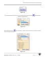
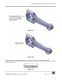
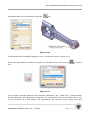
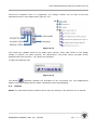
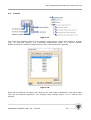
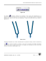
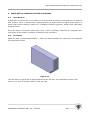
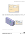
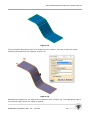
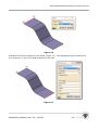
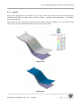
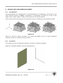
GRID GENERATION AND ANALYSIS USING
CATIA V5
NARENDRA KOMARLA
M-CME
MENTOR
Prof. Dr – Ing. H-B. Woyand
Fachgebiet Maschinenbau-Informatik
GRID GENERATION AND ANALYSIS USING CATIA V5
PREFACE
CATIA V5 has been a versatile tool for CAX requirements in many engineering application. The
intelligible Graphics-user-interface of CATIA (Icon driven approach) is most appealing. Many
engineers, who are familiar with other CAX tools can quickly adapt to CATIA V5 because of its
user-friendliness.
The objective of this manual is to familiarize the “Advanced meshing tools” and “Generative
structural analysis” modules of CATIA V5. The manual is example-driven, so that the user can
adapt similar approach with other parts too. The manual is based on the book,”FEM mit CATIA
V5” by Prof. Hans Bernhard Woyand (in German Language). Screen-shots have been liberally
used to convey the meaning in an enhanced way.
The first chapter introduces steps in FEM and presents from Q&A about meshing in particular.
The next three chapters discuss the use of the most-common elements for generating meshes
and presents analysis results in brief. Structural and frequency analysis are discussed in these
chapters. The last two chapters give a peek into advanced mesh generation techniques such as
shell and hexahedron meshing.
It is urged to refer the CATIA V5 documentation to a maximum extent in order to deepen tool
knowledge. The documentation is complete and an in-dispensable contrivance.
NARENDRA KOMARLA, Matr. No – 950763
2 |Page
GRID GENERATION AND ANALYSIS USING CATIA V5
CONTENTS
1. Introduction
1.1.
1.2.
1.3.
1.4.
Objective of this course
Pre-requisites
Inspiration
Some Q&A about FEA/FEM
2. Structural analysis of an IC-engine connecting rod
2.1.
2.2.
2.3.
2.4.
2.5.
2.6.
---------------------------- 4
---------------------------- 9
Introduction
Preparing the model for analysis
Procedure
Results
Stress calculation of a connecting rod utilizing symmetry boundary conditions
Buckling of the connecting rod
3. Frequency analysis of a Tuning fork
----------------------------21
3.1. Introduction
3.2. Analysis steps
3.3. Results
4. Plate with circular hole in its centre
----------------------------28
4.1. Introduction
4.2. Procedure
4.3. Results
5. Meshing with shell elements
----------------------------32
5.1. Introduction
5.2. Procedure
5.3. Results
6. Meshing with hexahedron elements
----------------------------37
6.1. Introduction
6.2. Procedure
7. Acknowledgements
----------------------------41
8. References
----------------------------41
NARENDRA KOMARLA, Matr. No – 950763
3 |Page
GRID GENERATION AND ANALYSIS USING CATIA V5
1. INTRODUCTION
1.1.
Objective of this course
The objective of this course material is give a basic insight into Grid generation and analysis
techniques using CATIA V5
1.2.
Pre-requisites
The pre-requisites of this course is modelling familiarity using any CAD tool. Knowledge in
CATIA V5 (The basic concepts such as document windows, standards and view toolbars) would
definitely be an added advantage. Apart from this, basic knowledge of Finite Element Methods
would only help in understanding the contents better.
1.3.
Inspiration
 CATIA V5R18 Documentation
 “FEM mit CATIA V5” – Prof. Hans Bernhard Woyand (in German Language)
All CATIA models used or referenced in this material is from the above mentioned book. The
models can be downloaded from the following location:
http://www.mtech.uni-wuppertal.de:8080/MBI
In this webpage, FEM_mit_CATIA_V5.zip can be found under the section CATIA-FEM-Buch,
which can be downloaded.
Please note some of these parts have German names
Some Q&A about FEM/FEA
1. What is Grid Generation/Meshing?
A key step of the finite element method for numerical computation is mesh generation. One is
given a domain (such as a polygon or polyhedron; more realistic versions of the problem allow
curved domain boundaries) and must partition it into simple "elements" meeting in well-defined
ways. There should be few elements, but some portions of the domain may need small
elements so that the computation is more accurate there. All elements should be "well shaped"
(which means different things in different situations, but generally involves bounds on the
angles or aspect ratio of the elements).
2. Broad Classification:
 Un-structured mesh
 Structured mesh
One distinguishes "structured" and "unstructured" meshes by the way the elements meet; a
structured mesh is one in which the elements have the topology of a regular grid. Structured
meshes are typically easier to compute with (saving a constant factor in runtime) but may
NARENDRA KOMARLA, Matr. No – 950763
4 |Page
GRID GENERATION AND ANALYSIS USING CATIA V5
require more elements or worse-shaped elements. Unstructured meshes are often computed
using quadtrees, or by Delaunay triangulation of point sets; however there are quite varied
approaches for selecting the points to be triangulated.
Another classification for meshing is the (auto-meshing)
 Free mesh
 Mapped mesh
Before meshing the model, and even before building the model, it is important to think about
whether a free mesh or a mapped mesh is appropriate for the analysis. In free meshing, the
user specifies a general, qualitative mesh description, ranging from coarse to fine, with 10 or
more gradations between the extremes. The software then generates the mesh accordingly.
Therefore, a free mesh has no restrictions in terms of element shapes, and has no specified
pattern applied to it.
In mapped meshing, the user specifies quantitative information regarding node spacing,
hence, element size, and the software uses the prescribed information to generate nodes and
elements. A mapped mesh is restricted in terms of the element shape it contains and the
pattern of the mesh. A mapped area mesh contains either only quadrilateral or only triangular
elements, while a mapped volume mesh contains only hexahedron elements. In addition, a
mapped mesh typically has a regular pattern, with obvious rows of elements. If a mapped mesh
is desired, we must build the geometry as a series of fairly regular volumes and/or areas that
can accept a mapped mesh.
In either meshing techniques, the software user has some degree of control over the element
mesh
3. Why is meshing required?
Meshing is an essential pre-processing step in Finite Element Analysis. The final solution always
depends on the quality of the mesh used during computation. In simple terms, Meshing means
breaking up of a physical domain into simpler domains called the elements. Usually there are
standard shapes into which the simpler domains are “broken into”.
The basic idea of a mesh-generation scheme is to generate element connectivity data and
nodal-co-ordinate data by reading in the input data for a few key points.
Advanced Meshing Tools allows us to rapidly generate a finite element model for complex parts
whether they are surface or solid. In other words, we can generate associative meshing from
complex parts, with advanced control on mesh specifications.
The Advanced Meshing Tools workbench is composed of the following products:
FEM Surface (FMS): to generate a finite element model for complex surface parts.
FEM Solid (FMD): to generate a finite element model for complex solid parts.
NARENDRA KOMARLA, Matr. No – 950763
5 |Page
GRID GENERATION AND ANALYSIS USING CATIA V5
4. What are the normal steps to be followed in Finite Element Analysis
computation? In particular, what is Pre-processing?
Finite Element Analysis essentially consists of the following 3 steps:
 Pre-processing
 Processing or Solution
 Post-processing
The Pre-processing step is, quite generally, described as ‘defining the model’ and it includes
the following steps:
1.
2.
3.
4.
5.
6.
7.
Define
Define
Define
Define
Define
Define
Define
the
the
the
the
the
the
the
geometric domain of the problem (modelling)
element type(s) to be used
material properties of the elements
geometric properties of the elements (length, area, and the like)
element connectivity (mesh the model)
physical constraints (boundary conditions)
loadings
Once the geometric domain (modelling) of the problem is defined using and CAD application
(CATIA V5 itself is preferable), grid generation is the next process (from Step 2 to Step 5).
Once the grid is generated, the model could be taken forward for stress computation.
The pre-processing step is critical. In no case is there a better example of the computer-related
axiom “garbage in, garbage out.” A perfectly computed finite element solution is of
absolutely no value if it corresponds to the wrong problem. Therefore a high-quality, optimised
grid always leads to a high-quality final output.
5. More about meshing:
A very important aspect of meshing a model with elements is to ensure that, in regions of
geometric discontinuity, a finer mesh (smaller elements) is defined in the region. This is true in
all finite element analyses (structural, thermal, and fluid), because it is known that gradients
are higher in such areas and finer meshes are required to adequately describe the physical
behaviour. In mapped meshing, this is defined by the software user. Fortunately, in free
meshing, this aspect is accounted for by the software.
6. What are the current methods or tools available for Grid generation and
Analysis?
Commercially many tools are available for Grid generation. Part and assembly modelling, pre
processing, processing and post processing could be performed using all leading CAD tools like
Pro-Engineer, Unigraphics, Solidworks, CATIA V5 etc. There are specialised solver tools such as
ANSYS, ABAQUS, MSc Nastran etc which could effectively be used for meshing. Apart from
these, Hypermesh is another CAE tool, which specialises exclusively in meshing.
NARENDRA KOMARLA, Matr. No – 950763
6 |Page
GRID GENERATION AND ANALYSIS USING CATIA V5
7. Why is Grid generation using CATIA V5 a good option?
CATIA is not a specialised tool for Meshing and analysis; however the platform is very userfriendly and sufficient for carrying out any FEM analysis. CATIA is an extremely powerful
modelling tool. Hence the model created in CATIA can directly be transferred to the Advanced
Meshing tool workbench and after finalising the mesh; solution and result interpretation could
be done at a stretch.
8. Analysis in CATIA V5 - Overview:
a. A note on CATIA V5
CATIA
(Computer
Aided
Three-dimensional
Interactive
Application) is
a
multiplatform CAD/CAM/CAE commercial software suite developed by the French company, Dassault
Systems and marketed worldwide by IBM. Written in the C++ programming language, CATIA is
the cornerstone of the Dassault Systems product lifecycle management software suite.
The software was created in the late 1970s and early 1980s to develop Dassault's Mirage fighter
jet, and then was adopted in the aerospace, automotive, shipbuilding, and other industries.
More Information about CATIA V5 could be accessed using the following links:
http://www.ibm.com/CATIA
http://www.3ds.com/products/CATIA/welcome
http://en.wikipedia.org/wiki/CATIA
There are numerous ‘workbenches’ in CATIA V5, and each workbench has a purpose to achieve.
Grid generation is a part of the “Advanced meshing tool” workbench in CATIA V5.
b. User-friendly environment
CATIA Analysis provides designers and analysts with an intuitive user interface that meets their
varied needs. Since the user interface is a natural extension of that in CATIA, it is particularly
easy for CATIA users. They obtain a realistic understanding of the mechanical behaviour by
quickly reviewing design characteristics in a digital mock-up (DMU) environment. The CATIA V5
tools and environment that are common to all CATIA applications, ABAQUS/CAE for CATIA, and
partner solutions, eliminate the problem of lost productivity associated with using multiple
applications.
c. Fast design-analysis loops
CATIA Analysis is an integral part of CATIA. The analysis specifications are an extension of the
part and assembly design specifications, and the analysis is performed directly on the CATIA
geometry. It is, therefore, simple and convenient to perform an analysis to help size parts and
compare the performance of different design alternatives. The impact of design changes can be
rapidly assessed with automatic updates. Designers using CATIA Analysis will naturally use
analysis as part of their design process, affording them a greater understanding of how their
designs perform and improving their ability to deliver the right design the first time.
NARENDRA KOMARLA, Matr. No – 950763
7 |Page
GRID GENERATION AND ANALYSIS USING CATIA V5
d. Multidiscipline collaboration
CATIA Analysis supports concurrent engineering, allowing users to work closely together and
avoid rework. Designers and analysts can collaborate since they have access to the same
environment, eliminating data transfer, rework, and the need to maintain multiple applications
for design and analysis. The CATIA Analysis environment also allows method developers to
create templates that designers can routinely use to perform standard types of analysis.
e. Knowledge-based optimization
The CATIA Analysis products leverage the native CATIA knowledge-based architecture. They
allow designs to be optimized by capturing and studying the knowledge associated with part
design and analysis. The reuse of analysis features and the application of knowledge-based
rules and checks ensure compliance to company best practices. Automation of standard analysis
processes through the use of knowledge ware templates dramatically improves the efficiency of
the design-analysis process.
f. Industry-proven performance
The speed with which analyses can be performed with CATIA Analysis often surprises designers
and simulation experts familiar with other applications. The time it takes to create the finite
element model, solve it, and display results can be a matter of minutes. The robust, built-in
finite element solver and mesh generators balance both accuracy and speed. The adaptive
meshing capability automatically adjusts the mesh to obtain accurate results without timeconsuming manual involvement.
NARENDRA KOMARLA, Matr. No – 950763
8 |Page
GRID GENERATION AND ANALYSIS USING CATIA V5
2. STRUCTURAL ANALYSIS OF AN IC-ENGINE CONNECTING ROD
2.1.
Introduction
In an IC engine, the connecting rod connects the piston to the crank or crankshaft. Together
with the crank, they form a simple mechanism that converts linear motion into rotating motion
The connecting rod is under tremendous stress from the reciprocating load represented by the
piston, actually stretching and being compressed with every rotation, and the load increases to
the third power with increasing engine speed. Failure of a connecting rod, usually called
"throwing a rod" is one of the most common causes of catastrophic engine failure in cars.
Therefore, the stress analysis of a connecting rod assumes high practical importance.
2.2.
Preparing the model for analysis
Before entering the “Generative structural analysis” workbench, the part has to be prepared for
analysis. The properties of the CAD part have to be defined (i.e., Material, isotropy etc) in the
“Part design” module itself. For assigning properties, right click on the part and select
“Properties”
The next task is to enter the Grid generation workbench in CATIA This workbench could be
accessed by the Analysis and Simulation workbench - Advanced meshing tool
Following are the steps to be followed for entering the workbench
Advanced Meshing Tools workbench, represented by
icon, allows the user to rapidly
generate a finite element model for complex parts whether they are surface or solid.
In other words, we can generate associative meshing from complex parts, with advanced
control on mesh specifications.
The Advanced Meshing Tools workbench is composed of the following products:

FEM Surface (FMS): to generate a finite element model for complex surface parts.

FEM Solid (FMD): to generate a finite element model for complex solid parts.
Grids should be generated for Static and Frequency analysis. Therefore, in the first step, one of
these cases should be selected.
On selecting the Static analysis as an example, the next step is to define the “Mesh type” and
“element type” of the mesh.
NARENDRA KOMARLA, Matr. No – 950763
9 |Page
GRID GENERATION AND ANALYSIS USING CATIA V5
2.3.
Procedure
Open the “Pleuelstange_01.CATPart” (Connecting rod) from the download area, which is
http://www.mtech.uni-wuppertal.de:8080/MBI
The compressed file, FEM_mit_CATIA_V5.zip can be found under the section CATIA-FEMBuch, which has to be downloaded.
Figure 2.1
Start – Analyse & Simulation – Generative Structural Analysis. Select the Static Analysis case.
Click on the OCTREE Tetrahedron Mesh to set the size of the mesh, as seen in the Figure 2.2.
Figure 2.2
NARENDRA KOMARLA, Matr. No – 950763
10 | P a g e
GRID GENERATION AND ANALYSIS USING CATIA V5
Figure 2.3
Parameters in this tab:
Size: lets us choose the size of the mesh elements. To know more about the Element Type you
have to choose in the OCTREE Tetrahedron Mesh dialog box, refer to Linear
Tetrahedron and Parabolic Tetrahedron in the Finite Element Reference Guide.
Absolute sag: Maximal gap between the mesh and the geometry.
Proportional sag: Is the ratio between the local absolute sag and the local mesh edge length.
Absolute sag and Proportional sag could modify the local mesh edge length value.
We can give values for both Absolute sag and Proportional sag. The most constraining of the
two values will be used.
Element type: lets us choose the type of element (Linear or Parabolic)
There are various other options that can be used for mesh refinement in the OCTREE
Tetrahedron Mesh dialog. Local, Quality and Others tabs can be used for these.
In our case, the element size and Absolute sag values are entered to be 10mm and 2mm
respectively. The element type is linear. A linear, tetrahedral mesh will be the result. Since the
element type is entered as an input, it is evident that the type of meshing is mapped (or
quantitative).
The next step is to define restraints in our model. The “restraints” tab has to be used for
defining the same, which is as seen in Figure 2.4.
NARENDRA KOMARLA, Matr. No – 950763
11 | P a g e
GRID GENERATION AND ANALYSIS USING CATIA V5
Figure 2.4
Since sliding motion prevails in the inner surface of the connecting rod,
restraint) is applied there.
(Surface slider
Figure 2.5
A user defines restraint,
of the connecting rod (Fix)
“User restraints”, which is used in this case to restrict fee motion
Figure 2.6
NARENDRA KOMARLA, Matr. No – 950763
12 | P a g e
GRID GENERATION AND ANALYSIS USING CATIA V5
Figure 2.7
Figure 2.8
Once these two restraints are defined, the model looks as seen in the picture above.
The next step is to define loads or forces on the model, which can be done by the “Loads”
toolbar (Figure 2.9)
Figure 2.9
NARENDRA KOMARLA, Matr. No – 950763
13 | P a g e
GRID GENERATION AND ANALYSIS USING CATIA V5
Distributed load can be assigned through the
icon.
Figure 2.10
A distributed load of 10000N is applied in the ‘Y’ direction as seen in Figure 2.10.
Once these parameters are defined, the part can be analyzed by clicking on the
icon.
(compute)
Figure 2.11
The compute command calculates the unknown parameters. “All”, “Mesh only”, “Analysis Case
Solution Selection” and “Selection by Restraint” can be selected from the drop-down menu. “All”
can be selected, as a safe option. The computation will consume some system time and
NARENDRA KOMARLA, Matr. No – 950763
14 | P a g e
GRID GENERATION AND ANALYSIS USING CATIA V5
resource to complete. Once it is completed, The “Image” toolbar can be used to find the
parameters seen in the image below (Figure 2.12):
Figure 2.12
The model tree updates itself for the Static case solution, when each button in the Image
toolbar is pushed. For static analysis, the deformation, Von-mises stress, principal stress,
displacements and Precision – all results are important.
To apply the bearing load:
Figure 2.13
The Button
(Animate) displays the animation of the connecting rod. The displacement
pattern may be animated and for better visualization and understanding.
2.4.
Results
Mesh: The node and element numbers can be seen by clicking on the element of our interest
NARENDRA KOMARLA, Matr. No – 950763
15 | P a g e
GRID GENERATION AND ANALYSIS USING CATIA V5
Figure 2.14
Von – Mises stress:
Figure 2.15
NARENDRA KOMARLA, Matr. No – 950763
16 | P a g e
GRID GENERATION AND ANALYSIS USING CATIA V5
Translational Displacement vector:
Figure 2.16
Principal stresses:
Figure 2.17
NARENDRA KOMARLA, Matr. No – 950763
17 | P a g e
GRID GENERATION AND ANALYSIS USING CATIA V5
Precision:
Figure 2.18
Report generation
CATIA V5 generates a report once all parameters are defined. The report is a html document,
which can be stored at any desired location.
Figure 2.19
The icon for report generation is
2.5.
, which can be found in the “Analysis results” toolbar
Stress calculation of a connecting rod utilizing symmetry boundary conditions
The connecting rod is symmetrical about the X-Z plane. These conditions could be exploited to
calculate stresses. Utilising symmetric conditions would save computation time and resource. It
may not be relevant in this case, but is very important in case of huge models, with numerous
elements (and nodes naturally).
NARENDRA KOMARLA, Matr. No – 950763
18 | P a g e
GRID GENERATION AND ANALYSIS USING CATIA V5
Open the “Pleuelstange_02.CATPart” from the download area
Figure 2.20
Similar to the previous case, the surface slider restraint and the user-defined restraint are
applied to the CAD model as seen in Figure 2.20
Figure 2.21
The axial distributed force (in the longitudinal direction) is then applied to the model as seen
Figure 2.22. The force magnitude is 10.000N
NARENDRA KOMARLA, Matr. No – 950763
19 | P a g e
GRID GENERATION AND ANALYSIS USING CATIA V5
Figure 2.22
Once these parameters are defined, the model may be computed for the un-known parameters,
similar to the previous section. The results from the previous model and the half model, utilising
symmetry conditions are comparable.
NARENDRA KOMARLA, Matr. No – 950763
20 | P a g e
GRID GENERATION AND ANALYSIS USING CATIA V5
3. FREQUENCY ANALYSIS OF A TUNING FORK
3.1.
Introduction
A tuning fork is an acoustic resonator in the form of a two-pronged fork with the prongs (tines)
formed from a U-shaped bar of elastic metal (usually steel). It resonates at a specific
constant pitch when set vibrating by striking it against a surface or with an object, and emits a
pure musical tone after waiting a moment to allow some high overtones to die out. The pitch
that a particular tuning fork generates depends on the length of the two prongs. Its main use is
as a standard of pitch to tune other musical instruments.
3.2.
Analysis Steps
Frequency analysis on a tuning fork is carried out using CATIA V5 as illustrated ahead. The CAD
model of the fork is opened and the Generative Structural Analysis module is navigated through
Start – Analysis & Simulation - Generative Structural Analysis.
Frequency analysis is selected out of the 3 options available in Generative Structural Analysis
Open the “Stimmgabel_01.CATPart” (Tuning fork) from the download area
Figure 3.1
The subsequently step is to generate a 3D mesh on the model. This is done as discussed in the
previous case. A finer mesh as compared to the initial case is chosen, because the area of cross
– section is relatively low in this case. A size and absolute sag value of 7.95 and 1.272 are
entered respectively. The element type is a linear tetrahedral mesh. A linear mesh is preferred
because the curvature of the model is less (Figure 3.2)
NARENDRA KOMARLA, Matr. No – 950763
21 | P a g e
GRID GENERATION AND ANALYSIS USING CATIA V5
Figure 3.2
Figure 3.3
The parameters for frequency solution are set by “double clicking” on the “frequency case” in
the model tree.
The required number of modes can be keyed in.
NARENDRA KOMARLA, Matr. No – 950763
22 | P a g e
GRID GENERATION AND ANALYSIS USING CATIA V5
Other parameters:
Method (Iterative subspace, Lanczos)
product is installed)
(only available if ELFINI Structural Analysis (EST)
If Lanczos Method is selected, the Shift option appears which computes the modes beyond a
given value, Auto, 1Hz, 2Hz and so forth. Auto means that the computation is performed on a
structure that is partially free.
Dynamic Parameters (Maximum iteration number, Accuracy)
Mass Parameter: lets the user take into account the structural mass. This check box lets us
exclude the structural mass from the total mass summation when computing the solution of a
frequency case with additional mass.
If the structural mass parameter in a frequency case is excluded without additional masses
(frequency case without masses set), an error occurs while computing the solution.
If the frequency case does not contain any masses set, we do not select this option.
The next step is to define restraints to our tuning fork.
Figure 3.4
This icon can be used to define clamp forces. Two clamp forces, Clamp 1 (2 faces) and
Clamp 2 (1 face) are defined as seen in the pictures below:
NARENDRA KOMARLA, Matr. No – 950763
23 | P a g e
GRID GENERATION AND ANALYSIS USING CATIA V5
Figure 3.5
Once these parameters are defined, the part can be analyzed by clicking on the
icon.
(compute)
Figure 3.6
The compute command calculates the unknown parameters. “All”, “Mesh only”, “Analysis Case
Solution Selection” and “Selection by Restraint” can be selected from the drop-down menu. “All”
can be selected, as a safe option. The computation will consume some system time and
resource to complete. Once it is completed, The “Image” toolbar can be used to find the
parameters as discussed ahead (Figure 3.7).
NARENDRA KOMARLA, Matr. No – 950763
24 | P a g e
GRID GENERATION AND ANALYSIS USING CATIA V5
3.3.
Results
Figure 3.7
The model tree updates itself for the Frequency case solution, when each button is pressed
(Fig.). In frequency analysis, the Transitional displacement Vector is of special interest.
Double-clicking on Transitional displacement vector, the following box appears:
Figure 3.8
Since we had selected 10 modes, the frequency for each mode is displayed in the editor. Each
case can be analyzed separately. The “analysis tools” toolbar (Figure 3.9) is used for this
purpose.
NARENDRA KOMARLA, Matr. No – 950763
25 | P a g e
GRID GENERATION AND ANALYSIS USING CATIA V5
Figure 3.9
The Button
(Animate) displays the animation of the tuning fork displacement at a
particular frequency (Frequency at any required mode). The deformation and the Transitional
displacement vector for the first two frequencies, 713.84 Hz and 808.759 Hz are shown in
Figure 3.10.
Figure 3.10
Individual information (In certain nodes/elements of particular interest) could be accessed by
the
icon. Once the button is pressed, a node can be selected and detailed information
regarding the same is output on the screen. For example, the information at node 115 will look
as seen in the picture ahead (Figure 3.11).
NARENDRA KOMARLA, Matr. No – 950763
26 | P a g e
GRID GENERATION AND ANALYSIS USING CATIA V5
Figure 3.11
NARENDRA KOMARLA, Matr. No – 950763
27 | P a g e
GRID GENERATION AND ANALYSIS USING CATIA V5
4. PLATE WITH A CIRCULAR HOLE IN ITS CENTRE
4.1.
Introduction
A plate with a circular hole in its centre is one of the most commonly used specimens to analyse
pure tension, shear or mixed-mode loading analysis (in plane stress and plane strain cases). A
plate under tensile loading is called a CT (Compact Tension) specimen, which is the case being
presented here.
Since the plate is symmetric about the X and Y axes, symmetry conditions are exploited and
one-fourth of the model is analysed. Following is the procedure:
4.2.
Procedure
Open the part “Lochscheibe2.CATpart”, which has been modelled for symmetry and assigned
the properties of steel.
Figure 4.1
The first task is to generate an appropriate mesh for the part. It is important to have a fine
mesh in our area of interest, which is near the hole.
NARENDRA KOMARLA, Matr. No – 950763
28 | P a g e
GRID GENERATION AND ANALYSIS USING CATIA V5
Figure 4.2
A parabolic Octree tetrahedral mesh is first defined, similar to the previous cases. Since a finer
mesh is required near the hole, a local mesh can be defined there. As per Figure 4.3, a local
mesh of element size 5mm is defined. The edge (highlighted) is selected for the supports. A
smaller tetrahedral local mesh can be seen in the region of interest now.
Figure 4.3
The next task is to assign the boundary conditions for our model. This is done in the usual way
by defining the surface sliders for the model.
NARENDRA KOMARLA, Matr. No – 950763
29 | P a g e
GRID GENERATION AND ANALYSIS USING CATIA V5
Since the part is symmetric about the X and Y axes, and is being treated as a Plane strain case,
where the Z dimension is large, restraints are applied as seen in Figure 4.2
Figure 4.4
To restrain free motion of the part, the face as seen in Figure 4.3 is also constrained.
Figure 4.5
NARENDRA KOMARLA, Matr. No – 950763
30 | P a g e
GRID GENERATION AND ANALYSIS USING CATIA V5
The succeeding step is to define the loads. Loads can be specified as forces or displacements.
Figure 4.6
An enforced displacement
of 0.023mm is applied on the face on which the second slider
restraint is applied. The enforced displacement icon could be accessed from the “loads” toolbar.
4.3.
Results
The model is now ready for analysis. Similar to the previous steps, the computation for the
static case solution is started from the
icon.
Figure 4.7
NARENDRA KOMARLA, Matr. No – 950763
31 | P a g e
GRID GENERATION AND ANALYSIS USING CATIA V5
5. MESHING WITH SHELL ELEMENTS
5.1.
Introduction
Probably, the most critical step in application of the finite element method is the choice of
element type for a given problem. The solid elements discussed till now are among the simplest
elements available for use in stress analysis. Many more element types are available to the
finite element analyst. (Commercial software systems have no fewer than 140 element types)
The differences in elements for stress analysis fall into three categories:
 Number of nodes, hence, polynomial order of interpolation functions
 Type of material behaviour (elastic, plastic, thermal stress, etc)
 Loading and geometry of the structure to be modelled (plane stress, plane strain, axissymmetric, general three dimensional, bending, and torsion)
In case of shell (thin curved plate) structures, specialized elements are required (and available)
for structural analysis. Once the element type has been selected appropriately, the task
becomes that of defining the model geometry as a mesh of finite elements.
Following are some particulars about shell elements:
 Shell element can be either 1-D or 2-D plane element
 Boundary condition is applied at edge/curve
 3-D Structures that consist of thin surfaces are ideal structures for shell element
application
 There is an enormous time saving when shell elements are used in place of 3-D solid
elements
Following are the most well known 2-D shell elements (Figure 5.1)
Figure 5.1
The elements seen are linear triangular element, Triangular element with middle nodes, linear
quadrilateral element and quadrilateral element with middle nodes (serendipity element)
NARENDRA KOMARLA, Matr. No – 950763
32 | P a g e
GRID GENERATION AND ANALYSIS USING CATIA V5
5.2.
Procedure
To illustrate the use of shell elements, consider the following example:
Open the “Schalen.CATPart” from the download area.
Figure 5.2
The model consists of an extruded surface, on which shell elements could be defined. The
material assigned is “Steel”, similar to the previous cases.
The next step is to define the mesh for the part, which is exclusive to this case. The “Advanced
surface mesh” in the “Advanced meshing tools” workbench is used to generate this mesh.
Figure 5.3
NARENDRA KOMARLA, Matr. No – 950763
33 | P a g e
GRID GENERATION AND ANALYSIS USING CATIA V5
Figure 5.4
The pre-defined 2D property has to be assigned to the surface. This can be done by simply
selecting the surface as the supports (Figure 5.5)
Figure 5.5
Restraints are applied on one edge of the surface as seen in Figure 5.6. The highlighted edge is
the selected edge, where the clamp is applied.
NARENDRA KOMARLA, Matr. No – 950763
34 | P a g e
GRID GENERATION AND ANALYSIS USING CATIA V5
Figure 5.6
Distributed forced are applied on the model (Figure 5.7). The highlighted edge is selected for
the “Supports”. A force of 1000N is applied in this case.
Figure 5.7
NARENDRA KOMARLA, Matr. No – 950763
35 | P a g e
GRID GENERATION AND ANALYSIS USING CATIA V5
5.3.
Results
Once these parameters are defined we can now enter the “Generative Structural Analysis”
workbench through the main menu, which is Start – Analysis and Simulation – Generative
Structure Analysis.
The results can be analysed through the well known “Image” toolbar. The von mises stress
(Figure 5.8) and the deformed mesh (Figure 5.9) are seen here
Figure 5.8
Figure 5.9
NARENDRA KOMARLA, Matr. No – 950763
36 | P a g e
GRID GENERATION AND ANALYSIS USING CATIA V5
6. MESHING WITH HEXAHEDRON ELEMENTS
6.1.
Introduction
The generalization of a quadrilateral in three-dimensions is a hexahedron, also known in the
finite element literature as brick. A hexahedron is topologically equivalent to a cube. It has
eight corners, twelve edges or sides, and six faces. It is a volume element.
Finite elements with this geometry are extensively used in modeling three-dimensional solids.
Figure 6.1
Figure 6.1 shows 8 noded (tri-linear), 20 noded (serendipity) and 27 noded hexahedral
elements, which are commonly used in practice.
6.2.
Procedure
To illustrate the use of hexahedral elements, consider the following example:
Open the “Hexaeder.CATPart” from the download area.
Figure 6.2
NARENDRA KOMARLA, Matr. No – 950763
37 | P a g e
GRID GENERATION AND ANALYSIS USING CATIA V5
Figure 6.3
The mesh is created similar to the previous procedure by entering parameters for the mesh size
and offset, after selecting the mesh type and the element type (Figure 6.3)
Once the 2D mesh is created, the “Mesh Transformations” toolbar can be used to create a 3D
mesh (Volume elements). Figure 6.4 gives an insight into this toolbar. The unique feature of
this transformation is that the numbers in the 3D mesh created is a constant. Therefore, as the
size of the 3D element is decreased, the mesh gets finer and vice –versa. Extrude mesher with
translation and rotation is illustrated here:
Figure 6.4
NARENDRA KOMARLA, Matr. No – 950763
38 | P a g e
GRID GENERATION AND ANALYSIS USING CATIA V5
Figure 6.5
Figure 6.6
NARENDRA KOMARLA, Matr. No – 950763
39 | P a g e
GRID GENERATION AND ANALYSIS USING CATIA V5
The mesh is parametric which is typical of CATIA and can be edited freely. If the start angle is
changed to 90 degrees, the model acquires shape as seen in Figure 6.7. It can be observed
here that the number of elements remain the same and thereby the mesh gets denser.
Figure 6.7
Therefore, the Mesh transformations can be a useful and powerful tool to generate 3D meshes
using volume elements. Once the mesh is created on the required geometry, further steps are
similar, as mentioned in the previous sections.
NARENDRA KOMARLA, Matr. No – 950763
40 | P a g e
GRID GENERATION AND ANALYSIS USING CATIA V5
7. ACKNOWLEDGEMENTS
I am highly indebted to Prof. Dr. Hans-Bernhard Woyand, Bergische University, Wuppertal for
giving me an opportunity to work on this project. The work helped me to get an insight towards
the structural analysis module in CATIA V5 and achieve academic targets as well.
It is said that "What the teacher is, is more important than what he teaches". Prof. Woyand is a
excellent individual and has been an immense source of inspiration for his students to emulate.
I would also like to thank Mr. David Elmar for his suggestions.
The project also gave me an opportunity to get familiarised with the practical side of Finite
element analysis. It has aroused keen interest in me to work further in this area.
Narendra Komarla
Matriculation No.: 950763
8. REFERENCES
FEM mit CATIA V5 – Prof. Hans Bernhard Woyand – The manual is based on this book
Fundamentals of Finite Element Analysis – D.V. Hutton
CATIA V5R18 User's Manual was liberally used during the course of this work. The
documentation provides an extensive insight into every module of CATIA V5.
NARENDRA KOMARLA, Matr. No – 950763
41 | P a g e