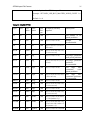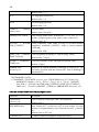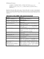
1
Červenka Consulting s.r.o. Na Hrebenkach 55 150 00 Prague Czech Republic Phone: +420 220 610 018 E-mail: [email protected] Web: http://www.cervenka.cz ATENA Program Documentation Part 6 ATENA Input File Format Written by Jan Červenka and Libor Jendele Prague, October 31, 2014 Trademarks: ATENA is registered trademark of Vladimir Cervenka. Microsoft and Microsoft Windows are registered trademarks of Microsoft Corporation. Other names may be trademarks of their respective owners. Copyright © 2000-2014 Červenka Consulting s.r.o. iii CONTENTS 1 INTRODUCTION AND SCOPE OF THE DOCUMENT 7 2 PROGRAM EXECUTION 7 3 INPUT COMMANDS 11 3.1 Changes of Input Commands Syntax in the New Version 11 3.2 General Rules 12 3.3 Main Input Commands 13 3.4 Analysis Identification and Execution Settings 15 3.4.1 The Command &TASK 15 3.4.2 The Command &TERMINATE / &BREAK 15 3.4.1 The Command &JUMP / &LABEL 16 3.4.2 The Command &DEBUG 16 3.4.3 The Command &EVALUATE 17 3.4.4 The Command &BREAK_DEBUG 18 3.4.5 The Command &SELECTION 18 4 THE COMMAND &SET 4.1.1 4.2 The Command &UNITS Topology Definition 25 46 48 4.2.1 The Command &JOINT 48 4.2.2 The Command &LOCAL 48 4.2.3 The Command &GEOMETRY 49 4.2.4 The command &ELEMENT 60 4.2.5 Geometrical imperfections &NODAL_IMPERFECTIONS 70 4.3 Material Definition - The Command &MATERIAL 71 4.3.1 Linear Elastic Isotropic Materials 75 4.3.2 Cementitious Materials 76 4.3.3 Elastic – Plastic materials 119 4.3.4 User Material 123 4.3.5 Interface Material 125 4.3.6 Material Type for Reinforcement 127 4.3.7 Material Type for Spring 132 4.3.8 Microplane Material Type for Concrete 133 iv 4.3.9 Creep Materials 142 4.3.10 Material Type for Combined Material 158 4.3.11 Material Type for Material with Variable Properties 159 4.3.12 Material Type for Material with Temperature Dependent Properties 160 4.3.13 Material Type for Material with Properties Varying in Space 162 4.3.14 Material Types for Simplified Nonlinear Analysis Using CCBeam Element 163 4.4 Load and Boundary Conditions Definition 173 4.5 Step and Execution Commands 187 4.5.1 4.6 The Command &STEP Output Command 4.6.1 4.7 The Command &OUTPUT 187 189 189 Creep Analysis Related Commands 203 4.7.1 The Command &RETARDATION 203 4.7.2 The command &HISTORY_IMPORT 204 Dynamic Analysis Related Commands 205 4.8 4.8.1 Finite element and material model related data 205 4.8.2 Dynamic initial values of state variables 205 4.8.3 CCStructuresDynamic Set parameters 207 4.8.4 Step definition 208 4.8.5 Lumped masses 208 4.8.6 Eigenvalue and eigenvectors analysis 208 4.8.7 Eigenvalues and eigenvectors analysis execution command 209 4.8.8 Sample input data for transient dynamic analysis 210 4.8.9 Sample input data for eigenvalues and eigenvectors analysis 220 4.9 Miscellaneous Commands 226 4.9.1 The Command &FUNCTION 226 4.9.2 The Command &PRE-CRACK 228 4.9.3 The Command &DELETE 228 4.9.4 The Command &INPUT 229 4.9.5 The Command &MESSAGE 229 4.9.6 The Command &ERROR 229 4.9.7 The Command &RESTORE 230 4.9.8 The Command &STORE 230 4.9.9 The Command &PUSHOVER_ANALYSIS 230 4.9.10 Static initial values of state variables 235 ATENA Input File Format 4.10 Preprocessor commands v 237 4.10.1 The Command &T3D_SPEC 237 4.10.2 The command T3D_EXPAND_SELECTIONS 240 4.10.3 The Command &MACRO_JOINT 244 4.10.4 The Command &MACRO_ELEMENT 245 Transport Analysis Related Commands 254 4.11 4.11.1 Transport constitutive material model 255 4.11.2 Transport finite elements 265 4.11.3 Transport initial values of state variables 267 4.11.4 Transport Set parameters 268 4.11.5 The &HISTORY EXPORT command 270 4.11.6 &Transport element load 271 4.11.7 &Transport analysis additional output data 274 5 SAMPLE INPUT FILE 275 5.1 Input file for a sample static analysis. 275 5.2 Input file for a sample transport analysis 278 6 ATENA INPUT FILE KEYWORDS 285 ATENA Input File Format 1 7 INTRODUCTION AND SCOPE OF THE DOCUMENT The program ATENA is a general-purpose finite element code with many special features for non-linear analysis of plain and reinforced concrete structures. This document serves as a manual describing the syntax and format of ATENA input commands in its input file. This command file is often called also input file, and it is used to define finite element model, to specify the loading history and to activate the finite element non-linear analysis. 2 PROGRAM EXECUTION There are several methods how to execute the finite element module ATENA. The heart of the analysis module is contained in a dynamically linked library ATENADLL.DLL. This module can be utilized either via its COM object interface CCCoAtena or from the command console by executing either AtenaConsole.exe or AtenaWin.exe or ATENAStudio.exe program. The CCCoAtena is used by AtenaGUI graphical pre and postprocessor and its use is described in a separate part of ATENA documentation. Here, the starting the analysis usin AtenaConsole, AtenaWin, and ATENAStudio executables is described. The programs are executed as follows: AtenaConsole [/D path] [/P] [/M module_name] [/O] [input_file] [output_file] [message_file] [error_file] [/reset_desktop] [/translate_ids] [/extend_int_output_width] [/extend_real_output_width] [/catch_fp_instructs] [/demo_mode] [/silent] [/num_threads=n] [/num_iters_per_thread=m] AtenaWin [/D path] [/M module_name] [/O] [input_file] [output_file] [message_file] [error_file] [/translate_ids] [/extend_int_output_width] [/extend_real_output_width] [/catch_fp_instructs] [/demo_mode] [/silent] [/batch_execute] [/execute] [/rtf] [/inbuf_size=i] [/outbuf_size=j] [/num_threads=n] [/num_iters_per_thread=m] [/num_unused_threads=m] ATENAStudio [/D path] [/M module_name] [/O] [/inp input_file] [/extend_int_output_width] [/extend_real_output_width] [/catch_fp_instructs] [/demo_mode] [/execute] [/threads=n] 8 AtenaConsole front-end is aimed for batch analyses. Hence, it works only with input and output files, produces no graphics and does not need any user interaction. On the other hand AtenaWin is a windows based application. On start it creates an editable window for each of ATENA’s window. The user can use these windows to edit content of the files, inspect ATENA’s output during the analysis etc. Of course, similar windows can be used for editing any other text file. It also provides graphical windows post processing and windows for 2D plots, which are useful for example for assessing load-displacement diagram of analyzed structure. Note that all windows in AtenaWin are updated already during the analysis. In the above the following notation was used: /D path = specifies path to the working directory where input and output files will be stored. /P = this option forces the program to request manual specification of input and output files. /M module_name = name of main DLL library used for execution. By default, it is assumed CCStructures. The CCStructuresCreep DLL is needed for creep analysis. /O = specifies overwrite flag for output_file, message_file and error_file files. This means that during execution, (or re-execution within AtenaWin) the files are created or overwritten. By default the files are appended, i.e. output of the new analysis is added at the end of the files. input_file = name of a file with Atena input commands. If not specified, standard input from keyboard is assumed. output_file = name of a file for Atena output. If output_file doesn’t exits, it is created. Otherwise it is appended. If output_file is not specified in the command line, then standard output to the screen is assumed. message_file = name of a file for Atena message output. The message file contains compact information on Atena execution as for instance: a log of the execution start and end, convergence performances, severe warning and error messages during execution etc. If message_file doesn’t exits, it is created. Otherwise it is appended. If message_file is not specified in the command line, then standard output to the screen is assumed. error_file = name of a file for Atena error output. The error file contains full information on Atena execution as for instance: a log of the execution start and end, convergence performances, all warning and error messages during execution (incl. their place of invocation) etc. If error_file doesn’t exits, it is created. Otherwise it is appended. If error_file is not specified in the command line, then standard output to the screen is assumed. [/translate_ids] = this option is only for internal use for debugging. Don’t use it. [/extend_int_output_width] [/extend_real_output_width] = double number of digits used to output integer or real numbers, respectively. [/catch_fp_instructs] = flag to catch, (i.e. unmask) floating point exceptions during the execution. Upon occurrence of such exception it will get caught, reported and the execution will be terminated. By default, floating point exceptions are ignored. [/demo-mode] = flag for trial execution. All features are available in trial mode, however, there apply some restrictions towards size of the analyzed problem. ATENA Input File Format 9 [/batch_execute] = option which forces AtenaWin automatically execute the given problem without any user intervention. After the execution all output data are saved and AtenaWin gets terminated. Use this option for batch execution. [/execute] = option which forces AtenaWin automatically execute the given problem without any user intervention. After the execution the AtenaWin session remains running, thereby enabling a subsequent interactive postprocessing [/silent] = flag that forces AtenaWin to output eventual error messages into message_file and error_file. By default, they are output to a message box on the screen. Use this option for batch execution. [/num_threads=n] [/threads=n] = use n threads during the execution. By default all available processor's cores are used. [/num_unused_threads=m]= same as the above but Atena will use number od processor's available threads minus m. The parameter [/num_threads=n] has higher priority. [/num_iters_per_thread=m] = chunk size for dynamic schedule, =0 for static load distribution; default=0 [/inp] = precedes the Input File name. ATENA Studio derives the .out, .msg, and .err filenames from the .inp filename by replacing the extension. Table 1: Environmental variables for AtenaConsole, AtenaWin 1, and ATENA Studio execution Command AtenaConsole 32-bit execution %AtenaConsole% Basic AtenaConsole command, by default executes statics module %AtenaConsoleD% AtenaConsole execution for dynamics analysis %AtenaConsoleC% AtenaConsole execution for creep analysis %AtenaConsoleT% AtenaConsole execution for transport analysis AtenaConsole 64-bit execution %AtenaConsole64% Basic AtenaConsole 64-bit execution, by default executes statics module %AtenaConsoleD64% AtenaConsole 64-bit execution for dynamics analysis %AtenaConsoleC64% AtenaConsole 64-bit execution for creep analysis %AtenaConsoleT64% AtenaConsole 64-bit execution for transport analysis AtenaWin 32-bit execution %AtenaWin% 1 Basic AtenaWin command, by default executes statics module AtenaWin program can be used for runtime visualization of the analysis progress and postprocessing. Starting from ATENA version 5, AtenaWin program is replaced by ATENA Studio. Please, check the program documentation of these programs for more details. 10 %AtenaWinD% AtenaWin execution for dynamics analysis %AtenaWinC% AtenaWin execution for Creep analysis %AtenaWinT% AtenaWin execution for Transport analysis AtenaWin 64-bit execution %AtenaWin64% Basic AtenaWin command for 64-bit execution, by default executes statics analysis %AtenaWinD64% AtenaWin 64-bit execution for dynamics analysis %AtenaWinC64% AtenaWin 64-bit execution for creep analysis %AtenaWinT64% AtenaWin 64-bit execution for transport analysis ATENA Studio 32-bit execution %AtenaStudio% Start 32-bit ATENA Studio, the analysis type can be selected in a dialog ATENA Studio 64-bit execution %AtenaStudio64% Start 64-bit ATENA Studio, the analysis type can be selected in a dialog ATENA Input File Format 3 11 INPUT COMMANDS 3.1 Changes of Input Commands Syntax in the New Version With few exceptions, the current version of ATENA uses the same syntax of input commands the previous version did. The modified input command relates to &OUTPUT commands, The keywords for locations changed as follows The old keyword The new keyword ATTRIBUTE OUTPUT_DATA LOAD LOAD_CASES ELEMENT ELEMENTS ELEMENT IP ELEMENT_IPS NODE NODES ELEMENT NODE ELEMENT_NODES LOAD LOAD_CASES MATERIAL MATERIALS GEOMETRY GEOMETRIES ELEMENT TYPE ELEMENT_TYPES There are available several new or renamed output data, see the Table 124. &CREEP_ANALYSIS_PARAMS commands Creep and shrinkage analysis is a new analysis type not supported in the previous versions. Therefore, all related commands are new. Please refer to the appropriate section of this manual for more details. Note that some more creep commands are available in &CREEP_MATERIAL, &RETARDATION_TIMES, &HISTORY_IMPORT and analysis step definition &CREEP_STEP_DEFINITION &PREPROCESS commands. The preprocess commands can be used to easy FE model mesh generation by use of the T3D generator and for generation of embedded reinforcement bars. Boundary conditions, i.e. specification of concentrated loads and supports can now be defined via &SELECTION and modified &LOAD_PLACE and &LOAD_VALUE commands. List of loaded/supported nodes also can be automatically generated by T3D generator using ELEMPROP “list_name” and NODEPROP “listname” subcommands of T3D commands REGION, VERTEX, SURFACE etc.… &CCStructuresTransport commands, i.e. commands for analysis of moisture and humidity transport within structures. Although most input commands for temperature and humidity transport are the same as those for the other engineering modules, there are some exceptions. This section is devoted to the commands that are available only for the transport analysis. 12 &CCStructuresDynamic module related commands, i.e. commands for dynamic analysis of structures including eigenvalues and eigenvectors analysis. It inherits also a few commands from creep and transport analysis. 3.2 General Rules The following lines introduce general rules for composing Atena and Atena Pollute Transport input commands and syntax that is used to describe them. Each command has form of a sentence (not terminated by dot). The command consists of several tokens (or words) separated by one or more spaces or CR/LF characters. Tokens written in upper case letters with the 1st character being alphabetic denote keywords, e.g. DELETE. Tokens starting with & character refer to a more complicated input structures described elsewhere in the manual. They are not ATENA commands; rather they are to be replaced with an input structure they refer to. This syntax is used to simplify description of complicated commands. Cross-references to these input structures are indicated by & character. Tokens written in lower case italic letters denote value parameters, i.e. nodal coordinate. If name of such a token is enclosed in quotes, a string value (in quotes) is expected, i.e. “file name“, otherwise numerical value is expected. Numerical tokens starting with n or i indicate integer values, whilst parameters starting with x denote real value. Interpretation of Atena keywords is case insensitive. Optional parameter (either a keyword or value) is enclosed in square brackets []. If an input token has to be one of several keywords and/or values, then all its admissible values are enlisted in curled brackets {} separated by vertical bar |, i.e. { NODE | ELEMENT | LOAD } . Default choice is underlined, (if it exists). Right curled bracket with “plus” subscript indicates that Atena input processor accepts one or more tokens from the above list of choice, { { NODE | ELEMENT | LOAD }+ . Right curled bracket with integer subscript n indicates that Atena input processor requires just n times a token from the above list of choice, { x }3 means input of 3 real numbers . Features, which are currently not supported are denoted with . The commands between two EXECUTE keywords can appear in any order. In case of multiple definition, the program accepts always the last definition before the EXECUTE command. The comment syntax corresponds to the C++ style. There are two comment types: C-style comment, where the comment is started by “/*” (i.e. slash and star) characters and ended by “*/” (i.e. star and slash). C++ style where it is assumed that everything following “//” (i.e. two slash) characters up to the end of line is considered to be a comment. ATENA Input File Format 13 3.3 Main Input Commands &MAIN_COMMANDS: { &TASK | &JOINT | &MATERIAL | &GEOMETRY | &ELEMENT | &DELETE | &FUNCTION | &INPUT | &LOAD | &LOCAL | &MESSAGE | &ERROR | &OUTPUT | &RESTORE | &SET | &STEP | &STORE | &UNITS | &T3D_SPEC | &DLL_NAME | &EMPTY | &RETARDATION_TIMES | &HISTORY_IMPORT | &PREPROCESS | &TERMINATE | &BREAK | &NODAL_IMPERFECTIONS | &SELECTION | &MACRO_JOINT | &MACRO_ELEMENT | module_name | &EIGENVECTORS | &PUSHOVER_ANALYSIS | &STATIC_INITIAL_CONDITIONS | &JUMP | &LABEL | &DEBUG | &EVALUATE | ; } The above &MAIN_COMMANDS input structure represent general ATENA input command. Each &ENTRY represents a group of input command that is described later. Most of the present commands are used to define some entity for description of your finite element model. The exception to that is &STEP command that contains a keyword EXECUTE. Processing of this keyword forces ATENA to carry on the analysis. The ATENA input commands can appear in any order in the input file, only the &TASK command has to be the 1st one, as it specifies dimension for many other entities, such as joint coordinates. It is possible to reference an entity prior it was even defined. Although it is not recommended, ATENA does accept that, but don’t forget to define them later! If you do, ATENA will not issue any error or warning messages, as the program assumes default values for most of the undefined entities. Such an error remains usually untapped until issuing the STEP … EXECUTE command. Note that it is possible at any time to modify the finite element model by adding, modifying or removing various modeling entities. The STEP … EXECUTE command uses always current settings of the finite element model. Table 2: Main input commands Keyword/Command Keyword/Command description &TASK Define analysis identification. &JOINT Input joint parameters, such as coordinates etc. &MATERIAL Definition of material types. &GEOMETRY Definition of used geometry. &ELEMENT Element properties definition. &DELETE Delete various entities. &FUNCTION X-Y relationship definition. &INPUT Input redirection. &LOAD Loads and load cases definitions. &LOCAL Set joints using local coordinate system. 14 &MESSAGE Message output redirection. &OUTPUT Output input data and results. &RESTORE Restore a previously saved analysis. &SET Miscellaneous settings. &STEP Step definitions and analyses. &STORE Store current analysis. &UNITS Sets program units. &DLL_NAME Name of dynamic link library, by which processor the following commands should be processed. Currently DLL_NAME is { CCFEMODEL | CCSTRUCTURES | CCSTRUCTURES_CREEP}. &EMPTY Forces the current DLL command processor to return to its “root” position, i.e. its main commands level. &RETARDATION_TIMES Generate retardation times. &HISTORY_IMPORT Import humidity and temperature history for creep analysis. &TERMINATE Immediately terminates the input commands stream &SELECTION Define list of entities, e.g. nodes, that are later used in another command, e.g. definition of boundary conditions. &STATIC_INITIAL_CON DITIONS Set structural initial conditions at nodes, such as reference tepmeratures. module_name Sets a top level for command parsing. module_name must be name of ATENA’s FEM module. Default: nil E.g. CCStructures ; This is to indicate end of the current input command. Control is returned to the top level ( specified by module_name) for parsing a next command. Must be preceded by at least one SPACE character. &JUMP, &LABEL Jump to a particular label while parsing the input document, i.e., skip the commands between &JUMP and LABEL keywords. &DEBUG Set on/off debug mode during Atena execution. &EVALUATE Invoke Atena calculator. ATENA Input File Format 15 3.4 Analysis Identification and Execution Settings 3.4.1 The Command &TASK Syntax: &TASK: TASK [{ NAME “task name“ | TITLE “title“ | DIMENSION n | SPACE { 2D | 3D | AXISYMMETRIC } }+ ] Table 3: &TASK command parameters. Parameter Description NAME “task name“ Task name. E.g.: NAME “task name“ TITLE “title“ Title of the analysis. TITLE “title“ DIMENSION n Problem dimension. n equals 2 or 3 for two or threedimensional analysis. Note that setting of DIMENSION sets also SPACE type. If DIMENSION is 2, then 2D SPACE type is expected. Once DIMENSION type is set, it cannot be changed elsewhere. SPACE Set type of space approximation. It can be 2D, 3D or AXISYMMETRIC, i.e. 2D in axis x and y symmetric with respect to axis y. (Radius of rotation corresponds to axis x). Note that setting of SPACE type sets also problem DIMENSION. Once SPACE type is set, it cannot be changed elsewhere. Note: This command should be the first input, as it specifies dimension several entities read later, i.e. nodal coordinates. 3.4.2 The Command &TERMINATE / &BREAK Syntax: & TERMINATE: TERMINATE {[AT] [MODULE module_name] ID break_id [IGNORE_HITS n_hits]} | {[" user’s string "]} &BREAK: BREAK {[AT] [MODULE module_name] ID break_id [IGNORE_HITS n_hits]} | {[" user’s string "]} Break Atena execution at a particular break point break_id at module module_name after number_of_hits_to_ignore hits. The parameter module_name can be CCFEModel, 16 CCStructures, CCFEModelGenerate.... If no MODULE is specified, the execution terminates at the given break point break_id at any module. If the parameter IGNORE_HITS number_of_hits_to_ignore is not specified, the execution is terminated at the first approach of the specified break point. Several break point ids are recognized, but break point ids 1 and 2 are probably the most important. The former one is placed at entry of a main execution routine of each Atena's modul. Similarly, the latter one is located at the exit of that routine. Alternatevily this command terminates the input commands stream, (i.e. no ID break_id was input), thereby terminating the execution and optionally displays user’s string. If the execution is run from a GUI window, (e.g. AtenaWin), a dialog is displaied before the actual termination/break action that gives the user choice to either accept the break or ignore it and continue the analysis. Batch analyses are broken unconditionally, see the /batch_exec command line switch. The commands BREAK and TERMINATE behave identically, the latter one supported only for input compatibility reasons. Examples: BREAK "Joints' coordinates read" BREAK ID 1 BREAK AT MODULE CCFEModel ID 2 IGNORE_HITS 3 3.4.1 The Command &JUMP / &LABEL Syntax: &JUMP: JUMP [TO] [LABEL] “string with label name” &LABEL: LABEL “string with label name" The first command instructs Atena to ignore all subsequent input data until the second command is found. Thereafter, the input commands are processed in the usual way. Several &JUMP/&LABEL commands can be used in the same file providing they have unique “string with label name". Note that &LABEL commands are ignored, unless a &JUMP command is being processed. 3.4.2 The Command &DEBUG Syntax: &DEBUG: DEBUG {ON | OFF } ATENA Input File Format 17 Set debug mode on/off. If it is on, the execution stops after processing of each main command from input stream. The next command is executed by pressing "Execute after break" button or alternatively press "Execute from the cursor position" button to execute a command at the current cursor position. 3.4.3 The Command &EVALUATE Syntax: &EVALUATE: {EVALUATE|EVAL} "expression_string" This command calculates command from expression_string and output the result to Atena output file. It has the following features: Operators: & | << >> = <> < > <= >= +* / % || ^ ! Functions: Abs, Exp, Sign, Sqrt, Log, Log10 Sin, Cos, Tan, ASin, ACos, ATan Factorial. Erf, ErfInv, Atan2, Pow, SOLVE_QUADRATIC_EQN, SOLVE_CUBIC_EQN Variables: Pi, e you can define your own variables. e.g. eval "cc=10" eval "cc+5" -> 15 Other: Scientific notation supported Error handling supported 18 3.4.4 The Command &BREAK_DEBUG Syntax: &BREAK_DEBUG: BREAK_DEBUG break_id Break execution at specific points. This command is typically used to debug an input data file. The following data points are recognized: Table 4: Table with the recognized execution breakpoints Desired action Value of break_id Do not break. 0 Break on entry to the main model execution routine. 1 Break on exit to the main model execution routine. 2 Break on entry to the generator model execution routine. 4 Break exit entry to the generator model execution routine. 8 Break on entry to the global dofs mapping execution routine. 16 Break on entry to the global dofs mapping execution routine. 32 Break at any of the above points. -1 More break points can be set. To do that set break_id as sum of the required individual break points. 3.4.5 The Command &SELECTION Syntax: &SELECTION : SELECTION “destination_name” { CLEAR | {COMBINE | SEPARATE} “list1” “list2” [“list3”] | RENAME “source_name” | {FROM | AT} from_id [TO to_id [BY by_id]] | LIST { id }+ | {INSERT | INCLUDE} “selection_name” | EXCLUDE “selection_name” | CONNECT | REMOVE “selection_name” | { ACTIVE | INACTIVE } GROUP group_id | [ENFORCED] DELETE {GROUP group_id | JOINT} | GENERATE { [NODES] | [ELEMENT] [OF] {GROUP|GROUP_FROM} group_id} [GROUP_TO group_to] [WITHIN] { BOX [MACRO] [NODES] i1 i2 i3 i4 [i5 i6 i7 i8] | DISTANCE x FROM { POINT [MACRO] [NODES] i1 | LINE [MACRO] [NODES] i1 i2 | PLANE [MACRO] [NODES] i1 i2 i3 } | NEAREST [MACRO] [NODES] i1 | [{{IP | IPS}|{ENODE|ENODES}|{GNODE|GNODES}}] | {SOURCE_NODE_SELECTION sel_nodes | SOURCE_GROUP_SELECTION sel_groups SOURCE_GROUP} | [EXECUTE] | SORT [ { +X | -X} ] [ { +Y | -Y} ] [ { +Z | -Z} ] }+ ATENA Input File Format 19 Table 5: &SELECTION command parameters Parameter Description „destination_name“ Name of the created or modified selection list. CLEAR Clear current content of the list but doesn’t remove the selection itself {COMBINE | SEPARATE} “list1” Combines two or three selection lists into one list or “list2” [“list3”] split one list into two or three selection lists. Used to convert multi_selection lists into ordinary selection list and vice versa. RENAME “source_name” Rename selection “source_name” to „destination_name“ { FROM | AT} from_id Set interval for entity ids to be generated. [TO to_id [BY by_id]] } They are generated for recursive formula id1 from _ id id n id n 1 by _ id up to id n to _ id By default to _ id from _ id , by _ id 1 Example: LIST AT 1 AT 10 FROM 100 TO 150 BY 10 LIST id Entity to be added into the selection , e.g. LIST 23 26 100 INSERT „selection_name“ INCLUDE „selection_name“ Insert entities from the selection_name selection into the selection destination_name. Source entities, which are already present in the selection destination_name, are not inserted, thus avoiding entities‘ duplication. EXCLUDE „selection_name“ Remove entities defined in the selection_name selection from the selection destination_name. Source entities, which are already not present in the selection destination_name, are skipped. CONNECT “selection_name” Connect the source selection "selection_name" with destination selection "destination_name". This is done in the following way: Loop from the first to the last entry of the source selection. For each such entry loop from the last to the first entry of the destination selection. If the current source and destination entries match, the is the point, where "destination_name" and "selection_name" should be connected: keep the current entry in the destination selection and remove all sbsequent entries. Append the source selection starting 20 from the 1st entry behind the matching entry up to the end to the destination selection. If no match is found, the selection are appended with all the entries they originally include. Eg. Destination selection: {2,7,8,3,1,4}, source selection {9,3,5} -> yields destination selection : {2,7,8,3,5} The source selection remains unchanged. SORT This command has sense only for selection containing [ { +X | -X} ] [ { +Y | -Y} ] [ { FE nodes!! Sort entries in the selection according to their reference coordinates. Note that sorting is +Z | -Z} executed immediatelly and thus it makes sense only for selection with all their entries (either previously inputed or with executed thier generation). For example: SORT +X - sort nodes referenced in the selection according with respect to their x coordinate, (from minimum t maximum), SORT -X - the same but in reverse order SORT +X +Y -Z - sort nodes Ni with reference coordinates (xi,yi,zi) with respect to the value xi+yi-zi . By default no sorting is applied. REMOVE Remove the modified selection list. GENERATE { [NODES] | [ELEMENT] [OF] [{GROUP|GROUP_FROM} group_id} [GROUP_TO group_id_to] ] } [WITHIN] BOX [MACRO] [NODES] i1 i2 i3 i4 [i5 i6 i7 i8] [EXECUTE] Data for the selection list generation. The list will include either all nodes or all elements of the group <group_id.... group_id_to> from within a box defined by the macro nodes i1 thru i8 (for 3D case) or a quadrilateral defined by i1 thru i4 (2D case). If group_id is specified, elements are generated, otherwise nodes are generated. The EXECUTE keyword forces to carry out the generation immediately. Otherwise it is done prior a first step execution. SOURCE_NODE_SELECTION sel_nodes Only nodes from selection sel_nodes become candidates for the generation. If not specified, all nodes from the model are considered. SOURCE_GROUP_SELECTION sel_groups SOURCE_GROUP_SELECTION sel_elements Only elements from selections sel_groups; sel_elements become candidates for the generation. If not specified, all elements from the model are considered. GENERATE { [NODES] | Data for the selection list generation. The list will [ELEMENT] [OF] [ {GROUP | include either all nodes or all elements of the group GROUP_FROM} group_id} <group_id.... group_id_to> from within distance x ATENA Input File Format 21 [GROUP_TO group_id_to] ] } [WITHIN] DISTANCE x FROM POINT [MACRO] [NODES] i1 [EXECUTE] with respect to the point defined by the macro nodes i1. If <group_id_....group_id_to> is specified, elements are generated, otherwise nodes are generated. The EXECUTE keyword forces to carry out the generation immediately. Otherwise it is done prior a first step execution. GENERATE { [NODES] | [ELEMENT] [OF] [ {GROUP|GROUP_FROM} group_id} [GROUP_TO group_id_to]] } [WITHIN] DISTANCE x FROM LINE [MACRO] [NODES] i1 i2 [EXECUTE] [INSIDE] Data for the selection list generation. The list will include either all nodes or all elements of the group <group_id.... group_id_to> from within distance x with respect to the line defined by the macro nodes i1 and i2. If group_id is specified, elements are generated, otherwise nodes are generated. The EXECUTE keyword forces to carry out the generation immediately. Otherwise it is done prior a first step execution. If the keyword INSIDE is used, the generation is reestricted only to entities with a node located between the macro node i1 i2. GENERATE { [NODES] | [ELEMENT] [OF] [ {GROUP|GROUP_FROM} group_id} [GROUP_TO group_id_to] ] } [WITHIN] DISTANCE x FROM PLANE [MACRO] [NODES] i1 i2 i3 [EXECUTE] [INSIDE] Data for the selection list generation. The list will include either all nodes or all elements of the group <group_id.... group_id_to> from within distance x with respect to the plane defined by the macro nodes I, i2 and i3. If group_id is specified, elements are generated, otherwise nodes are generated. The EXECUTE keyword forces to carry out the generation immediately. Otherwise it is done prior a first step execution. If the keyword INSIDE is used, the generation is reestricted only to entities with a node located between the macro node i1 i2, i3. GENERATE { [NODES] | [ELEMENT] [OF] [{GROUP|GROUP_FROM} group_id} [GROUP_TO group_id_to]] } NEAREST [MACRO] [NODES] i1 [EXECUTE] Data for the selection list generation. The list will include the nearest node or element of the group <group_id.... group_id_to> with respect to the i1. If group_id is specified, an element is included, otherwise a node is added. The EXECUTE keyword forces to carry out the generation immediately. Otherwise it is done prior a first step execution. Generated a multiselection that includes integrated [{{IP | IPS}|{ENODE|ENODES}|{GNOD points (or element nodes ) instead of global nodes. Use {GNODE|GNODES} to generate selection with global E|GNODES}}] nodes, where each entry must be incidented by a element with group_id>=grouip_id_from and group_id<=group_id_to. { ACTIVE | INACTIVE } GROUP Make active or inactive all elements contained in the group_id selection list that belongs to the group group_id [ENFORCED] DELETE {GROUP group_id | JOINT} Delete elements contained in the selection list that belongs to the group group_id or delete nodes contained in the selection list. 22 If ENFORCED is not specified, all references to a deleted entity remain valid even after the deletion, thereby it is possible later to re-input the entity with new data. Otherwise, the entity and all references to it get unconditionally removed. Example: SELECTION "all_nodes" FROM 1 TO 22 SELECTION "source" LIST 1 2 3 4 5 6 SELECTION "dest" LIST 3 5 12 SELECTION "source" INSERT "dest" SELECTION "source" REMOVE "dest" SELECTION “source” REMOVE SELECTION "source" GENERATE ELEMENTS GROUP 1 WITHIN BOX 101 102 103 104 106 107 108 // 3D case SELECTION "source" GENERATE NODES WITHIN BOX MACRO NODES 101 102 103 104 // 2D case SELECTION "source" GENERATE NODES WITHIN DISTANCE 2.4 FROM POINT MACRO NODES 101 SELECTION "source" GENERATE NODES WITHIN DISTANCE 2.4 FROM LINE MACRO NODES 101 102 SELECTION "source" GENERATE NODES WITHIN DISTANCE 2.4 FROM PLANE MACRO NODES 101 102 103 GENERATE SELECTION "source" GENERATE NODE NEAREST MACRO NODE 101 GENERATE SELECTION "nodes" GENERATE SORT -Y +X SELECTION "border_nodes" CONNECT "next_border_nodes" Generate selection and monitor at IP: SELECTION "IP_NEAREST_985001" GENERATE IPS NEAREST MACRO NODES 985001 group_from 105 group_id_to 302 EXECUTE OUTPUT LOCATION OUTPUT_DATA DATA LIST "SELECTION_IDS_IP_NEAREST_985001" END ; OUTPUT NAME "Monitor1_DISPLACEMENTS #100000" MONITOR_2 LOCATION ELEMENT_IPS MULTI_SELECTION AT "IP_NEAREST_985001" DATA LIST "DISPLACEMENTS_AT_IPS" ITEM AT 1 End ; Generate selection and monitor at NODE: SELECTION "NODE_NEAREST_985001" GENERATE NODE NEAREST MACRO NODES 985001 EXECUTE OUTPUT LOCATION OUTPUT_DATA DATA LIST "SELECTION_IDS_NODE_NEAREST_985001" END ; OUTPUT NAME "Monitor1_DISPLACEMENTS #100000" MONITOR_2 LOCATION NODES NODE AT SELECTION "NODE_NEAREST_985001" DATA LIST "DISPLACEMENTS" ITEM AT 1 End ; ATENA Input File Format SELECTION "ENODE_NEAREST_214" GENERATE ENODE NEAREST MACRO NODES 214 group_from 108 group_to 302 EXECUTE OUTPUT LOCATION OUTPUT_DATA DATA LIST "SELECTION_IDS_ENODE_NEAREST_214" END ; SELECTION "GNODE_NEAREST_214" GENERATE GNODE NEAREST MACRO NODES 214 group_from 108 group_to 302 EXECUTE OUTPUT LOCATION OUTPUT_DATA DATA LIST "SELECTION_IDS_GNODE_NEAREST_214" END ; 23 ATENA Input File Format 4 25 THE COMMAND &SET Syntax: &SET: SET { &ANALYSIS_TYPE | &LINEAR_SOLVER_TYPE | &CONVERGENCE_CRITERIA | &SOLUTION_METHOD | &PREDICTOR_TYPE | &UPDATE_DISPLS_STRATEGY | &ARC_LENGTH_PARAMS | &LINE_SEARCH_PARAMS | &OPTIMIZE_PARAMS | &SERIALIZE_PARAMS | SOLVER_KEYS n | &FATIGUE_PARAMS | &CREEP_ANALYSIS_PARAMS | &DYNAMIC_ANALYSIS_PARAMS | {SOLVE_LHS_BCS_ON" | SOLVE_LHS_BCS_OFF} | &MAX_REF_IDS | { EXTERNAL_IDENTIFIERS | INTERNAL_IDENTIFIERS } 2 |{ DISABLE_REPORT_TASK | ENABLE_REPORT_TASK | REPORT_LOCATION_STEP n} | { DISABLE_REPORT_LOCATION | ENABLE_REPORT_LOCATION } | { USE_BEST_ITERATION_FOR_CRITERION | USE_BEST_ITERATION_FOR_CRITERIA } n1 n2 ... | { UNUSE_BEST_ITERATION_FOR_CRITERION | UNUSE_BEST_ITERATION_FOR_CRITERIA } n1 n2 ... | BEST_ITERATION_MIN_ID n | STEP_LOAD_REDUCTION_ALLOWANCE n | REDUCE_STEP_LOAD_COEFF v | MIN_LHS_BCS_MASTER_NODE_COEFF n }+ Table 6: &SET command parameters Parameter Description &ANALYSIS_TYPE Set what type of analysis is executed, i.e. static, transient etc. &LINEAR_SOLVER_TYPE Use direct or iterative solver (and set some vital parameters for the iterative solver). &CONVERGENCE_CRITERIA Convergence criteria during iteration process within each load step. &SOLUTION_METHOD Choose solution method for the analysis. &ARC_LENGTH_PARAMS Set parameters for Arc Length method. &LINE_SEARCH_PARAMS Set parameters for Line Search method. &PREDICTOR_TYPE Set which type of predictor should be used for building stiffness matrix, (i.e. elastic, tangential or secant). &UPDATE_DISPLS_STRATEGY Strategy for updating displacements during iterations, either each iteration or each load step. &OPTIMIZE_PARAMS Sets whether bandwidth optimization is required and which type. &SERIALIZE_PARAMS Set depth of serialization. Change of this parameter is needed only under very special 2 Not available in ATENA version 4.3.1 and older. 26 conditions and the user would normally use its default setting. {"SOLVE_LHS_BCS_ON" "SOLVE_LHS_BCS_OFF" } | Turns on and off an advance LHS BCs management. By default, it is ON. Do not change this parameter, unless unavoidable and all consequences being well understood. SET SOLVER_KEYS n This command specifies directly in binary form flags for the non-linear solver. It is not aimed for direct use by users. Every setting can be achieved in a more readable form using other parameters of the &SET command. &FATIGUE_PARAMS Parameters for fatigue analysis &CREEP_ANALYSIS_PARAMS Parameters for creep analysis. &DYNAMIC_ANALYSIS_PARAMS Parameters for dynamic analysis &MAX_REF_IDS Set maximum reference ids that are used by the automatic ATENA reference ids generator DISABLE_REPORT_TASK | ENABLE_REPORT_TASK Disable or enable visualisation of task and location within the current execution. It is also possible to report location each n % of the total job. For example REPORT_LOCATION_STEP 10 ensures that for a system of say 200000 equations location is reported for each 20000th equation, e.g. 1, 20001, 40001... DISABLE_REPORT_LOCATION | ENABLE_REPORT_LOCATION | REPORT_LOCATION_STEP n By default these information are enabled and location progress is reported always, so that the user has gets the best info about the analysis. This settings, however, involves some CPU overhead. To maximize the execution speed, disable these reports. { EXTERNAL_IDENTIFIERS | INTERNAL_IDENTIFIERS } Set the way how, Atena entities are are identified. If external identifiers are required, Atena uses ids specified in the iput file. If intenal identifiers are required, Atena uses internal ids starting from 1 to number of a particular entities. Under normal conditions internal ids should not be used. USE_BEST_ITERATION_FOR_CRITE RION | USE_BEST_ITERATION_FOR_CRITE RIA } n1 n2 ... For n>0 and the iterating process within the current step does not yield a converged solution, then the solution is reverted to the best converged iteration based on the convergence criteria n1, n2, ... For n=0 the use of best iteration is reset to not using best_iteration feature. ATENA Input File Format 27 If divergence step's (or iteration's) stop criteria are met, the current step is marked as nonconverged. When this option is combined with STEP_LOAD_REDUCTION_ALLOWANCE n, then the iteration is reverted only when (nnumber of attempts to revert the current step)=0. By default n=0, i.e. this feature is N/A and v=1. , i.e. the step is marked as not converged step. UNUSE_BEST_ITERATION_FOR_CRI TERION | UNUSE_BEST_ITERATION_FOR_CRI TERIA } n1 n2 ... Same as the above but it removes the specified convregence criteria for best_iteration engine. If all criteria are removed, no best_iteration strategy is used . BEST_ITERATION_MIN_ID n Minimum iteration id, for which the iteration is always stored, i.e. regardless its convergence performance. Any subsequent iteration is stored only, if its convergence is better than convergence of any previous iteration. STEP_LOAD_REDUCTION_ALLOWA If n>0 and the iterating process within the current step does not yield a converged solution, then the NCE n current step is re-executed for a reduced load REDUCE_STEP_LOAD_COEFF v increment. This step's re-execution is allowed n times and the load increment in the current reexection is reduced by factor vi, where i=1..n, i.e. number of the step re-execution. By default v=0.5 and n =0. &ANALYSIS_TYPE: { STATIC | &TRANSIENT | &EIGENVALUES } Table 7: &ANALYSIS_TYPE sub-command parameters Parameter Description STATIC Specify static analysis. There are no additional parameters &TRANSIENT Set transient analysis and set some parameters for it. &EIGENVALUES Set some parametyers for eigenvalues analysis. &TRANSIENT: TRANSIENT { [TIME] CURRENT x | [TIME] INCREMENT x | TIME_INTEGRATION { {CRANK_NICHOLSON | THETA x }+ | ADAMS_BASHFORTH } | NEWMARK BETA x | NEWMARK_GAMMA x | HUGHES_ALPHA x | DAMPING { STIFFNESS [COEFFICIENT] x | MASS [COEFFICIENT] x | ®RESSION_DATA }+ ®RESSION_DATA: 28 REGRESSION { MODE mode_id | OMEGA omega_val | KSI ksi_val | WEIGHT weight_val }+ CALCULATE Table 8: &TRANSIENT sub-command parameters Parameter Description [TIME] CURRENT x Sets current time. [TIME] INCREMENT x Sets time increment in steps. TIME_INTEGRATION Set type of temporal integration scheme. If this parameter is not input, then Newmark integration will be used. CRANK_NICHOLSON Use linear trapezoidal integration. THETA x parameter for trapezoidal integration. By default = 0.5. Several other linear temporal integration may be utilized depending on the , e.g. implicit Newton integration for = 1., explicit integration for = 0 etc. For good compromise between convergence and possibility of oscillations values about = 0.85 is recommended. ADAMS_BASHFORTH Adams – Bashforth quadratic temporal integration. NEWMARK BETA x Defines the Newmark’s parameter. NEWMARK GAMA x Defines the Newmark’s parameter. HUGHES_ALPHA x Defines the Hughes damping parameter DAMPING STIFFNESS Defines stiffness matrix coefficient for proportional damping. [COEFFICIENT] x E.g.: DAMPING STIFFNESS COEFFICIENT 0.8 DAMPING MASS Defines mass matrix coefficient for proportional damping. [COEFFICIENT] x E.g.: DAMPING MASS COEFFICIENT 0.8 DAMPING REGRESSION MODE mode_id | OMEGA omega_val | KSI ksi_val | WEIGHT weight_val Generate proportional damping coefficient based on input of modal damping parameters ksi_val. mode_id is id of an eigenmode, for which damping parameter ksi_val and associated weight factor weight_val is input. Values for at least 2 eigenmodes must be given. By default, weight_val=1. The keyword CALCUATE marks the end of the input and execute the regression procedure to transform the current input data for structural damping to the above DAMPING MASS and STIFFNESS coefficients. Example: SET TRANSIENT DAMPING REGRESSION MODE 1 OMEGA 2 KSI 0.002 WEIGHT 0.6 MODE 2 OMEGA 3 KSI 0.03 WEIGHT 0.8 MODE 3 OMEGA 7 KSI 0.04 WEIGHT 1.1 MODE 4 OMEGA 15 KSI 0.1 WEIGHT 0.9 MODE 5 OMEGA 19 KSI 0.14 WEIGHT 0.8 ATENA Input File Format 29 CALCULATE &LINEAR_SOLVER_TYPE: { SOLVER { LU | DSS_LLT | DSS_LDLT | JAC | GS | ILUR | DCG | ICCG | DCGN | LUCN | DBCG | LUBC | DCGS | LUCS | DOMN | LUOM | DGMR | LUGM | PARDISO } | SLAP_ITERATION [LIMIT] n | SLAP_SAVED_VECTOR [LIMIT] n | SOLVER_BLOCK_SIZE n | EXTEND_ACCURACY_FACTOR x | PARDISO_REQUIRED_ACCURACY y | MIN_LHS_BCS_MASTER_NODE_COEFF n }+ Table 9: & LINEAR_SOLVER_TYPE sub-command parameters Parameter Description { SOLVER { LU | DSS_LLT | DSS_LDLT | JAC | GS | ILUR | DCG | ICCG | DCGN | LUCN | DBCG | LUBC | DCGS | LUCS | DOMN | LUOM | DGMR | LUGM } Type of solver for computing linear problem Ax=y. It can be either a direct skyline storage solver, (i.e. LU), or direct sparse storage solver, (i.e. DSS_LLT, DSS_LDLT), or iterative sparse storage solver (i.e. the remaining types). Alternatively, it can be parallel direct sparse solver PARDISO from the MKL provided by Intel Visual Fortran. The skyline and sparse (SLAP) storage schemes are described in the Theoretical Manual for Atena software. The direct sparse solvers DSS_LLT and DSS_LDLT differ in type of factorization, they use. It is LLT and LDLT, respectively. In case of unsymmetric structural matrix both solvers use LU factorisation. The table below lists all the available solvers with their brief characteristic and recommendation for use. Default: LU SOLVER_BLOCK_SIZE This value set granularity size for the solvers DSS_LLT and n DSS_LDLT. It defines a block size during pre-factorisation process. The higher value, the lower number of structural blocks and smaller RAM overhead for mapping the structural matrix. On the other hand, a higher value results in higher waste of RAM to store the actual data of the matrix. It is recommended to set this value to something in range <2…6>. Default: 2 SLAP_ITERATION [LIMIT] n Maximum number of iterations allowed within an iterative linear problem solver. Default: number of structural degree of freedom. SLAP_SAVED_VECTO Number of direction vectors to save and orthogonalize against. R [LIMIT] nsave This parameter is only used by the following iterative solvers: DOMN, LUOM (nsave >=0) and DGMR, LUGM (nsave >0). In all cases nsave <=ndofs, where ndofs is number of degree of freedom. Typically, the higher nsave , the better convergence but also the bigger memory required by the solver. 30 Default value is ndofs /6 for DOMN, LUOM and ndofs /3 for DGMR, LUGM solver. EXTEND_ACCURACY Factor, by which an iterative sparse matrix solver should increase _FACTOR x its requirement upon accuracy. If x>0, the solver will employ residual forces convergence criterion with requested max. error “RELATIVE RESIDUAL ERROR” / x . If x <0, residual displacements convergence criterion will be used with max. error “RELATIVE DISPLACEMENTS ERROR” / x. Recommended values <1..10>. Default: 2 PARDISO_REQUIRED_ Accuracy required by PARDISO solver. ACCURACY [LIMIT] y For y=0, do not perform preconditioned Krylow-Subspace iterations and use LU factorisation instead. Otherwise the value of y controls accuracy of the built-in iterative solver further strenghten by the above EXTEND_ACCURACY_FACTOR factor x. The final required accuracy (expressed in number of non-negligible digits behing the decimal point) is l=log10(y/x). If the problem matrix is unsymmetric, (e.q. transport analysis), CGS iteration replaces the computation of LU. The preconditioner is LU that is computed at the previous step (the first step or last step with a failure) in a sequence of solutions needed for identical sparsity patterns. l controls the stopping criterion of the Krylow-Subspace iteration. CGS 10( l ) is used in the stopping criterion dxi dx0 CGS , with dxi inv( LU ) ri and ri is the residuum at iteration i of the preconditioned KrylowSubspace iteration. If the problem matrix is symmetric (positive definite), (e.g. for static analysis), the same applies, but CG iteration replaces the computation of LU. Example: SET 0.00000001 PARDISO_REQUIRED_ACCURACY limit Default: 0 MIN_LHS_BCS_MAST ER_NODE_COEFF n Set accuracy, (in its abs value) used to assemble and process lhs boundary conditions, particularly master nodes coefficients. If the specified value is too high, although the solution is faster and needs less RAM, it can filter out some important relations within the boundary conditions. On the other hand, if the value is too small, the solution is slower and needs more RAM. In addition, it need not detect and eliminate all redundancies within the boundary conditions and can fail. Note that the effect of this solution parameter can be inspected in "Global matrix LHS BCs ATENA Input File Format 31 statistics" printed in ATENA output file. Example: SET MIN_LHS_BCS_MASTER_NODE_COEFF 1.e5 Default: 1.e-6 Table 10: SOLVER TYPES Type D/I Prep. phase Exec. phase Sym/ Nonsym Temporary memory required Description LU D --- --- S,NS ----- For smaller or illposed problems JAC I ssds sir S,NS 4*(11)+8*(1+4*n) Simple, recommended GS I --- sir S,NS 4*(11+nel+n+1)+8*(1+ 3*n+nel) ILUR I ssilus sir S,NS 4*(13+4*n+nu+nl)+8*( 1+4*n+nu+nl) DCG I ssds scg S 4*(11)+8*(1+5*n) For large symmetric well-posed problems ICCG I ssics scg S 4*(12+nel+n)+8*(1+5* n+nel) For large symmetric problems, recommended DCGN I ssd2s scgn S,NS 4*(11)+8*(1+8*n) For large nonsymmetric wellposed problems LUCN I ssilus scgn S,NS 4*(13+4*n+nl+nl)+8*(1 For large non+8*n+nl+nu) symmetric problems, recommended DBCG I ssds sbcg S,NS 4*(11)+8*(1+8*n) LUBC I ssilus sbcg S,NS 4*(13+4*n+nl+nu)+8*( 1+8*n+nu+nl) DCGS I ssds scgs S,NS 4*(11)+8*(1+8*n) LUCS I ssilus scgs S,NS 4*(13+4*n+nl+nu)+8*( 1+8*n+nu+nl) DOMN I ssds somn S,NS 4*(11)+8*(1+4*n+nsav e+3*n*(nsave+1)) LUOM ssilus somn S,NS 4*(13+4*n+nu+nl)+8*( 1+nl+nu+4*n+nsave+3 *n*(nsave+1)) ssds sgmres S,NS 4*(31)+8*(2+n+n*(nsav I DGMR I not 32 e+6)+nsave*(nsave+3)) LUGM I ssilus sgmres S,NS 4*(33+4*n+nl+nu)+8*( 2+n+nu+nl+n*(nsave+6 )+nsave*(nsave+3)) In the above: n is number of degree of freedom of the problem. nel is the number of nonzeroes in the lower triangle of the problem matrix (including the diagonal). nl and nu is the number of nonzeroes in the lower resp. upper triangle of the matrix (excluding the diagonal). Table 11: EXECUTION PHASES Phase name Description sir Preconditioned Iterative Refinement sparse Ax = b solver. Routine to solve a general linear system Ax = b using iterative refinement with a matrix splitting. scg Preconditioned Conjugate Gradient iterative Ax=b solver. Routine to solve a symmetric positive definite linear system Ax = b using the Preconditioned Conjugate Gradient method. scgn Preconditioned CG Sparse Ax=b Solver for Normal Equations. Routine to solve a general linear system Ax = b using the Preconditioned Conjugate Gradient method applied to the normal equations AA'y = b, x=A'y. sbcg Solve a Non-Symmetric system using Preconditioned BiConjugate Gradient. scgs Preconditioned BiConjugate Gradient Sparse Ax=b solver. Routine to solve a Non-Symmetric linear system Ax = b using the Preconditioned BiConjugate Gradient method. somn Preconditioned Orthomin Sparse Iterative Ax=b Solver. Routine to solve a general linear system Ax = b using the Preconditioned Orthomin method. sgmres Preconditioned GMRES iterative sparse Ax=b solver. This routine uses the generalized minimum residual (GMRES) method with preconditioning to solve non-symmetric linear systems of the form: A*x = b. Table 12: PREPARATION PHASES Phase name Description ssds Diagonal Scaling Preconditioner SLAP Set Up. Routine to compute the inverse of the diagonal of a matrix stored in the SLAP Column format. ssilus Incomplete LU Decomposition Preconditioner SLAP Set Up. Routine to generate the incomplete LDU decomposition of a matrix. The unit lower triangular factor L is stored by rows and the unit upper triangular factor U is ATENA Input File Format 33 stored by columns. The inverse of the diagonal matrix D is stored. No fill in is allowed. ssics Incomplete Cholesky Decomposition Preconditioner SLAP Set Up. Routine to generate the Incomplete Cholesky decomposition, L*D*L-trans, of a symmetric positive definite matrix, A, which is stored in SLAP Column format. The unit lower triangular matrix L is stored by rows, and the inverse of the diagonal matrix D is stored. ssd2s Diagonal Scaling Preconditioner SLAP Normal Eqns Set Up. Routine to compute the inverse of the diagonal of the matrix A*A'. Where A is stored in SLAP-Column format. &CONVERGENCE_CRITERIA: { ABSOLUTE [ ERROR] | RELATIVE [ERROR] } | RESIDUAL ERROR x | DISPLACEMENT ERROR x | ENERGY ERROR x | STEP_STOP_RESIDUAL ERROR FACTOR x | STEP_STOP_DISPLACEMENT ERROR FACTOR x | STEP_STOP_ENERGY ERROR FACTOR x | ITER_STOP_RESIDUAL ERROR FACTOR x | ITER_STOP_DISPLACEMENT ERROR FACTOR x | ITER_STOP_ENERGY ERROR FACTOR x | NEGLIGIBLE_RESIDUAL x | NEGLIGIBLE _DISPLACEMENT x | NEGLIGIBLE_SIZE x | ITERATION [ LIMIT ] n }+ Table 13: &CONVERGENCE_CRITERIA sub-command parameters Parameter Description ABSOLUTE [ERROR] The convergence criteria values are computed using the absolute norm that is using the maximal element of an array in its absolute value. The error is then computed by dividing an iterative value with the value cumulated within the whole step. Note that this keyword can be used also in conjugation with the input NEGLIGIBLE _SIZE n, in which case it has slightly different meaning, see below. RELATIVE [ERROR] The convergence criteria values are computed using the Euclidean norm. The error is then computed by dividing an iterative value with the value cumulated within the whole step. Note that this keyword can be used also in conjugation with the input NEGLIGIBLE _SIZE n, in which case it has slightly different meaning, see below. RESIDUAL ERROR x Convergence limit for absolute value of residual forces. Default value is 0.01. E.g. RESIDUAL ERROR x DISPLACEMENT x ERROR Convergence limit for absolute value of displacement increments. Default value is 0.01. E.g. DISPLACEMENT ERROR x ENERGY ERROR x Convergence limit for value of residual energy, i.e. norm of displacement increment multiplied by norm of residual forces. 34 Not used in transport analysis. Default value is 0.01. E.g. RESIDUAL ERROR x STEP_STOP_RESIDUAL ERROR FACTOR x | STEP_STOP_DISPLACEME NT ERROR FACTOR x | STEP_STOP_ENERGY ERROR FACTOR x | ITER_STOP_RESIDUAL ERROR FACTOR x | ITER_STOP_DISPLACEME NT ERROR FACTOR x | ITER_STOP_ENERGY ERROR FACTOR x Factors for appropriate convergence criterion value. If a convergence criterion value multiplied by the appropriate factor exceeds the related calculated analysis error, then the execution is immediately killed. They are two sets of factors: the first one for checking each iteration and the other one to be exercised at the end of each step. The default value for iteration related factors is 1000, whilst the default value for step related factors is 10. NEGLIGIBLE_SIZE x Size that is already negligible. It affects accuracy of the analysis, particularly calculations of master/slave BCs, fixing of discrete reinforcement and the surrounding solids etc. For example points are assumed identical, if the distance between them is less than the absolute negligible size. Each element must have at each direction size greater than the absolute negligable size. Most iterative procedures compute with accuracy equal to the absolute negligible size. For all the comparisons only the ABSOLUTE negligible size is used. The relative negligable size is employed only to calculate the absolute negligible size, (if not input directly). E.g. SET Absolute stop_displacement error factor 15. Step_stop_displacement error factor 10. Step_stop_residual error factor 53 Iter_stop_displacement error factor 201 Iter_stop_residual error factor 203 SET Relative Step_stop_displacement error factor 54 Step_stop_energy error factor 55 Step_stop_residual error factor 56 Iter_stop_displacement error factor 204 Iter_stop_energy error factor 205 Iter_stop_residual error factor 206 If absolute negligible size is not specified, it is calculated as the product of relative negligible size and the minimum size (in x,y,z direction) of the analyzed problem. By default, relative negligible size is set to 1E-5. NEGLIGIBLE_RESIDUAL x | NEGLIGIBLE _DISPLACEMENT x Negligable values for norm of residual forces/displacements that can be ignored. By default they are set to 1.E-11. E.g. SET Absolute error Negligible_residual 0.1 ATENA Input File Format 35 Relative error Negligible_residual 0.2 ITERATION [LIMIT} n Limit on number of iterations within each step. E.g. ITERATION [LIMIT] n &SOLUTION_METHOD { LINEAR | NEWTON-RAPHSON | NEWTON-RAPHSON_AND_ LINE-SEARCH | ARC-LENGTH_AND_ LINE-SEARCH | { MODIFIED_NR | FULL_NR } }+ } Table 14: &SOLUTION_METHOD sub-command parameters Parameter Description NEWTON-RAPHSON Use Newton Raphson nonlinear solver. ARC-LENGTH Use Arc Length nonlinear solver. Recommended for force loading up to peak load or behind, can scale (reduce) the load. Only for static analysis, i.e., not for probems involving time (transport, creep, nor dynamic analyses). NEWTON-RAPHSON_AND_ LINE-SEARCH Use Line Search nonlinear solver in combination with Newton-Raphson method. ARC-LENGTH_AND_ LINE-SEARCH Use Arc Length nonlinear solver in combination with Use Line Search nonlinear solver. LINEAR Use linear solver. (Note that geometrical non-linearity is disregarded and only linear material can be used). MODIFIED_NR Build stiffness matrix only in the 1st iteration and use it also for subsequent iteration of the step. FULL_NR Build new stiffness matrix in each iteration. &PREDICTOR_TYPE: { ELASTIC_PREDICTOR | TANGENTIAL_PREDICTOR | SECANT_PREDICTOR } Table 15: &PREDICTOR_TYPE sub-command parameters Parameter Description ELASTIC_PREDICTOR Elastic stiffness matrix shall be used to predict displacement increments from structural unbalanced forces. There are no additional parameters for this command. This is option is 36 set by default TANGENTIAL_PREDICTOR Tangential stiffness matrix shall be used to predict displacement increments from structural unbalanced forces. There are no additional parameters for this command. By default elastic stiffness matrix is used. SECANT_PREDICTOR Secant stiffness matrix shall be used to predict displacement increments from structural unbalanced forces. There are no additional parameters for this command. By default elastic stiffness matrix is used &UPDATE_DISPLS_STRATEGY: { UPDATE_IP_EACH_STEP | UPDATE_IP_EACH_ITERATION } Table 16: &UPDATE_DISPLS_STRATEGY sub-command parameters Parameter Description UPDATE_IP_EACH_STEP Specify that material points, (i.e. integration points) should be updated at the end of each (converged) step, (i.e. load increment). It means that stress increments are calculated with respect to the beginning of step rather then previous iteration. It ensures stress increments to be calculated always from “converged” conditions, however as stress increments do not converged to zero (within current step), this approach is more demanding on evaluation of constitutive equations UPDATE_IP_EACH_ITERATION Specify that material points, (i.e. integration points) should be updated at the end of each iteration within a load increment). It means that stress increments are calculated with respect to the beginning of previous iteration. By default material points are updated with respect to loading increments, i.e. steps. See also SET UPDATE_IP_EACH_STEP &ARC_LENGTH_PARAMS: { &ARC_LENGTH_TYPE | &CONSTRAINT_LENGTH_CONTROL | &LOAD_DISPLACEMENT_RATIO | &LOCATION_PARAMS Table 17: &ARC_LENGTH_PARAMS sub-command parameters Parameter Description &ARC_LENGTH_TYPE Set type of Arc Length method and associated constrain. &CONSTRAINT_LENGTH_CONTROL Set several parameters that control Arc Length method ATENA Input File Format 37 &LOAD_DISPLACEMENT_RATIO Control load – displacement calculating Arc Length constrain. scale for &LOCATION_PARAMS Set location where the Arc Length step_length and/or Line Search energy criterion should be calculated. &ARC_LENGTH_TYPE: { CRISFIELD | NORMAL_UPDATE | CONSISTENTLY_LINEARISED | EXPLICIT_ORTHOGONAL} Table 18: &ARC_LENGTH_TYPE sub-command parameters Parameter Description CRISFIELD Crisfield variant of constant step length (including loading space) is to be used. NORMAL_UPDATE Updates of displacements within iteration kept normal to displacements within the step. CONSISTENTLY_LINEARISED Keeps constant projection of step length in the current iteration to direction of the previous iteration. It is linearized form of EXPLICIT_ORTHOGONAL method. EXPLICIT_ORTHOGONAL Keeps constant step length. Unlike CRISFIELD method, it is based on goniometric relationships, thus avoiding solving quadratic equation and difficulty with picking the correct root. From the mechanical point of view it poses identical constraint as CRISFIELD method. &CONSTRAINT_LENGTH_CONTROL: { &ARC_LENGTH_BASE_STEP_LENGTH | &ARC_LENGTH_OPTIMISATION } Table 19: &CONSTRAINT_LENGTH_CONTROL sub-command parameters Parameter Description &ARC_LENGTH_BASE_STEP_LENGTH Set base step_length . &ARC_LENGTH_OPTIMISATION Set the way how to optimize step_length in the current step based on base step_length and convergence performance in the previous step. The base step_length is defined by &ARC_LENGTH_BASE_STEP_LENGTH and by default it corresponds to step_length in the previous step. &ARC_LENGTH_BASE_STEP_LENGTH 38 {ARC_LENGTH_PREVIOUS_STEP_LENGTH | ARC_LENGTH_RESET_STEP_LENGTH | STEP_LENGTH x | STEP_LENGTH_ONCE x | REL_STEP_LENGTH x | REL_STEP_LENGTH_ONCE x | REL_REF_STEP_LENGTH x | REL_REF_STEP_LENGTH_ONCE x | DLAMBDA_MIN x | DLAMBDA_MAX x | REF_DLAMBDA_MIN x | REF_DLAMBDA_MAX x | MIN_STEP_LENGTH x | MAX_STEP_LENGTH x | MIN_REL_STEP_LENGTH x | MAX_REL_STEP_LENGTH x | MIN_REL_REF_STEP_LENGTH x | MAX_REL_REF_STEP_LENGTH x } Table 20: &ARC_LENGTH_BASE_STEP_LENGTH &command parameters Parameter Description ARC_LENGTH_ PREVIOUS_STEP_LENGTH For the current step use base step_length (for possible optimization by &ARC_LENGTH_OPTIMISATION) from the previous step. In case of the 1st step, it acts according to ARC_LENGTH_RESET_STEP_LENGTH. ARC_LENGTH_RESET_STEP_LENGTH For the current step reset base step_length. The actual step_length is step_length resulting from applied load in the 1st iteration of the current step (for = 1). It is always calculated for the 1st step, 1st iteration. STEP_LENGTH x Set directly required step length to x. By default, it is initiated based on load increment, see ARC_LENGTH_RESET_STEP_LENGTH. STEP_LENGTH_ONCE x Same as the above but it is appkued only once. REL_STEP_LENGTH x REL_STEP_LENGTH_ONCE x REL_REF_STEP_LENGTH x REL_REF_STEP_LENGTH_ONCE x | Allows direct setting of in the next step | relative to previous or reference step length. | It can be set only "ONCE", i.e. only in the next subsequent step or in all subsequent steps until a new relevant input. If x==-1, this input is ignored. By default, all these input valus are set to -1, i.e. they are ignored. MIN_STEP_LENGTH MAX_STEP_LENGTH x | Set minimum and/or maximum value step length. If the x value is negative, this check is ignored. By default, x=-1. This input can overwrite DLAMBDA_MIN, DLAMBDA_MAX x MIN_REL_STEP_LENGTH MAX_REL_STEP_LENGTH x x | Set minimum and/or maximum value of current step length related to the step length in the previous step. If the x value is ATENA Input File Format 39 negative, this check is ignored. By default, x=-1 MIN_REL_REF_STEP_LENGTH x MAX_REL_REF_STEP_LENGTH x DLAMBDA_MIN x | DLAMBDA_MAX x REF_DLAMBDA_MIN REF_DLAMBDA_MAX x x | Set minimum and/or maximum value of current step length related to the step length in firrst previous Arc-Length/ Line Srearch step. If the x value is negative, this check is ignored. By default, x=-1 Set minimum and/or maximum value of delta step load increment factor. If the x value is negative, this check is ignored. By default, x=-1. This input can be overwritten by MIN_STEP_LENGTH and MAX_STEP_LENGTH | Set minimum and/or maximum value of delta step load increment factor with respepect to reference load. If the x value is negative, this check is ignored. By default, x=-1. This input can be overwritten by MIN_STEP_LENGTH and MAX_STEP_LENGTH &ARC_LENGTH_OPTIMISATION: { { ARC_LENGTH_CONSTANT | ARC_LENGTH_VARIABLE_CONSERVATIVE_1/2 | ARC_LENGTH_VARIABLE_CONSERVATIVE_1/4 | ARC_LENGTH_VARIABLE_PROGRESSIVE } | REFERENCE_NUMBER_OF_ITERATIONS }+ Table 21: &ARC_LENGTH_OPTIMISATION sub-command parameters Parameter Description ARC_LENGTH_CONSTANT For the current step use step_length unchanged from the previous step. ARC_LENGTH_VARIABLE_CONSERVATIVE_1/2 Adjusts step_length for each load step based on the previous structural behavior: step_length_new= pow(reference_number_of_iteration /last_number_of_iteration,1/2) ARC_LENGTH_VARIABLE_CONSERVATIVE_1/4 Adjusts step_length for each load step based on the previous structural behavior: 40 step_length_new= pow(reference_number_of_iteration last_number_of_iteration,1/4) ARC_LENGTH_VARIABLE_PROGRESSIVE Adjusts step_length for each load step based on the previous structural behavior: step_length_new=pow(last_number _of_iteration/ reference_number_of_iteration,1/2) REFERENCE_NUMBER_OF_ITERATIONS n Set optimum number of iterations per load step to n. This value is used in Arc Length optimization of step_length. By default it is set to n=5. &LOAD_DISPLACEMENT_RATIO: { LOAD_DISPLACEMENT_RATIO x | LOADING_DISPLACEMENT_RATIO_CONSTANT | LOADING_DISPLACEMENT_SCALE_CONSTANT | LOADING_DISPLACEMENT_BERGAN_CONSTANT } Table 22: &LOAD_DISPLACEMENT_RATIO sub-command parameters Parameter Description LOAD_DISPLACEMENT_ Sets the parameter ratio to x. By default, it is 0.2. RATIO x LOADING_DISPLACEMENT_ RATIO_CONSTANT LOADING_DISPLACEMENT_ SCALE_CONSTANT The SW first (i.e. in the 1st load increment) calculates scaling factor =ratio||displacements|| , where =1 and displacements is derived from the loading increment. The calculated is afterwards kept constant. The ratio ||displacements||/ is called bergan coefficient. Adjusts (see the previous option) for each new load step as follows =ratioberganlast This strategy tries to keep the same impact of changes happening in loading and geometric space. LOADING_DISPLACEMENT_ BERGAN_CONSTANT Adjusts (see the previous option) for each new load step as follows =last berganold / berganlast Subscript old stands for one before the last results. This ATENA Input File Format 41 strategy tries to keep the same ratio of influence of loading and geometric space. &LOCATION_PARAMS: LOCATION { NODE { AT n | FROM n1 [TO n2 [BY n3] ] }+ DOF { AT n | FROM n1 [ TO n2 [BY n3] ]}+ COEFF x | REMOVE} Table 23: &LOCATION_PARAMS sub- command parameters Parameter Description LOCATION Specifies list of domains. Each from these domains contains list of structural DOFs and their coefficients used for calculation Arclength step length. REMOVE It destroys list of domains and in the subsequent steps all structural DOFs will be accounted for. NODE It follows list of nodal intervals. Any number of intervals can be specified. DOF It follows list DOFs intervals. Any number of intervals can be specified. AT n Set location at node (or degree of freedom) n. FROM n1 [TO n2 [BY n3]] Sets locations at nodes (or degrees of freedom) by interval. BY default n2 = n1 and n3 = 1. COEFF x Weight factor for the specified DOF. &LINE_SEARCH_PARAMS: { &LINE_SEARCH_ITERATION_CONTROL | &LIMIT_ETA_CONTROL | REFERENCE_ETA x | UNBALANCED_ENERGY_LIMIT x | &LOCATION_PARAMS }+ Table 24: &LINE_SEARCH_PARAMS sub-command parameters Parameter Description &LINE_SEARCH_ Control several parameters for Line Search iteration process. ITERATION_CONTROL &LIMIT_ETA_ Set minimum and maximum value for parameters etc. CONTROL REFERENCE_ETA x Resets to x. UNBALANCED_ Limit for relative work of out-of balanced forces within the “main” iteration. When satisfied, it stops Line search internal iteration loops. By default it is set to x=0.8 It says that Line search has by default reduce work of out-of balanced forces by 20%. ENERGY_LIMIT x 42 &LINE_SEARCH_ITERATION_CONTROL: { LINE_SEARCH_WITHOUT_ITERATIONS | { LINE_SEARCH_WITH_ITERATIONS | LINE_SEARCH_ITERATION_LIMIT n }+ } Table 25: &LINE_SEARCH_ITERATION_CONTROL sub- command parameters Parameter Description LINE_SEARCH_WITHOUT_ Do not carry internal Line search iteration loop within each “main” iteration. ITERATIONS LINE_SEARCH_WITH_ ITERATIONS Carry on internal Line search iteration loop within each “main” iteration. LINE_SEARCH_ Set line-search iteration limit. Default value is 3 iterations. ITERATION_LIMIT n &LIMIT_ETA_CONTROL: { LIMIT_ETA | MINIMUM_ETA x | MAXIMUM_ETA x }+ Table 26: &LIMIT_ETA_CONTROL sub-command parameters Parameter Description LIMIT_ETA Apply limit value for = min ... max. Only multiple of coordinate changes are applied to the next iteration. It is set automatically when issuing either of the commands MINIMUM_ETA x and/or MAXIMUM_ETA x. MINIMUM_ETA x Sets min = x. By default it is set to x=0.1 MAXIMUM_ETA x Sets max = x By default it is set to x=10. &OPTIMIZE_PARAMS: OPTIMIZE [BAND] WIDTH {SLOAN | GIBBS-POOLE | NONE} Table 27: &OPTIMIZE_PARAMS sub-command parameters Parameter Description BAND Dummy keyword. WIDTH Activates bandwidth minimisation and set default method to SLOAN. SLOAN Use Sloan’s algorithm for optimization process GIBBS-POOLE Use Gibbs-Poole’s algorithm for optimization process NONE Don’t optimize band-width. This is default setting. ATENA Input File Format 43 &SERIALIZE_PARAMS: SERIALIZE [MODEL] [STATE] { { BASICS | [AND] NODAL | [AND] ELEMENT | ALL }+ | { DEEP | STANDARD } }+ Table 28: &SERIALIZE_PARAMS sub-command parameters Parameter Description MODEL Dummy keyword BASICS Stores just basic information about the model like number of nodes, materials etc. AND Dummy keyword NODAL Stores data related to nodes of the model, (e.g. displacements) ELEMENT Stores data related to elements of the model, (e.g. strains) ALL Same as coding BASICS NODAL ELEMENT; stores all data STATE Dummy keyword STANDARD Standard serialization depth, i.e. only essential object data is serialized. DEEP All data within objects are serialized. &FATIGUE_PARAMS: { FATIGUE_TASK f_task | FATIGUE_CYCLES f_cycles | FATIGUE_MAX_FRACT_STRAIN_MULT f_mult | FATIGUE_COD_LOAD_COEFF f_codcoeff }+ These parameters only have influence on materials that support fatigue, see the description of the CC3DNonLinCementitious2Fatigue material. Table 29: & FATIGUE_PARAMS sub-command parameters Parameter Description FATIGUE_TASK f_task The FATIGUE_TASK parameter determines the operation (fatigue calculation phase) for the analysis step. 0 - nothing to do with fatigue 1 - store base stress 2 - reset FATIGUE_MAX_FRACT_STRAIN 4 - calculate fatigue damage induced by FATIGUE_CYCLES load cycles. The calculated damage is added to FATIGUE_MAX_FRACT_STRAIN. 8 - apply the fatigue damage stored FATIGUE_MAX_FRACT_STRAIN, multiplied FATIGUE_MAX_FRACT_STRAIN_MULT in by To combine operations in one analysis step, the values are added together (combined by binary or), e.g. storing base stress 44 and resetting fatigue max.fract.strain are requested by the value 3. Typically, FATIGUE_TASK is set to 3 (store base stress + reset fatigue max.fract.strain) before the first step of the load to be cycled and to 0 for the rest steps of the fatigue load, then to 12 (calculate + apply fatigue damage) before the first step applying the damage and to 8 for the rest damage application steps, then to 0 for any following static analysis FATIGUE_CYCLES f_cycles The number of cycles is determined by the FATIGUE_CYCLES parameter in the solutions parameters, set before the load step when the fatigue damage is calculated. The value of 0 means a non-cycling load. FATIGUE_MAX_FRAC Multiplier for max.fract.strain induced by fatigue, e.g. 0.2 if the T_STRAIN_MULT damage is applied in 5 analysis steps f_mult FATIGUE_COD_LOAD Multiplier for the influence of the cycling crack opening _COEFF f_codcoeff displacements when calculating fatigue damage. Equivalent to changing the KSI_FATIGUE material parameter, but can be set separatly for each fatigue load &CREEP_ANALYSIS_PARAMS: { SAMPLE_TIMES_PER_DECADE ndecl | RETARD_TIMES_PER_DECADE ndecl_retard | STOP_TIME execution_stop_time | {MP_METHOD | CS_METHOD} }+ Table 30: & CREEP_ANALYSIS_PARAMS sub-command parameters Parameter Description SAMPLE_TIMES_PER_ Number of integration times per log10 of time span. Note that DECADE ndecl this command affects generation of integration (sample) times by the &CREEP_STEP_DEFINITION sub-command. Hence, the ndecl parameter must be set before the &CREEP_STEP_DEFINITION sub-command. This parameter defines the number of time steps, the program will use to integrate the structural behavior. Creep or other nonlinear effects will cause a redistribution of stresses inside the structure. In order to properly capture such processes a sufficiently small time steps are needed. This time spacing is defined by the number of sample times. Its definition depends on the type of the analyzed structure as well as on the choice of time units. For typical reinforced concrete structures and for the time unit being a day, it is recommended to set this parameter ATENA Input File Format 45 to 2. This will mean that for each load interval longer then 1 day, two sub-steps will be added. For a load that is interval longer then 10 days, 4 sub-steps will be added. For an interval longer than 100 days, it will be 6 sub-steps. Default value: 2. RETARD_TIMES_PER_ Number of retardation times per log10 of time span. Note that DECADE ndecl_retard this command affects generation of retardation times by the &RETARDATION command and hence it must be set beforehand. Alternatively, this value can be set directly in &RETARDATION. Example: If number of retardation times is set to 2, the creep law will be approximated by two points for each time unit in the logarithmic scale. This means two approximation points will be used for the time interval between 0 - 1 day, two points for the interval 1 - 10 days, then two points for 10 - 100 days, etc. So the proper values will depend on the choice of time units. If the time unit is a day, the recommended value is 1 - 2. Default value: 1. STOP_TIME execution_stop_time Time at which the execution should stop [days]. This value must be input at leatest (or anywhere earlier) just before executing a step that should by stopped by this command. If it has not been specified, ATENA assumes STOP_TIME equal to time_end from the &retardation times command. The inputted value of STOP_TIME gets inserted in (automaticly generated) series of sample times but the higher sample times are not modified. Default value: 0 [days] MP_METHOD CS_METHOD | Creep analysis method. CS_METHOD uses simplified approach, in which temperature and humidity in a material point depend only on cross sectional shape and average exterior temperature and humidity. The MP_METHOD uses accurate temperature and humidity at each structural material point and therefore it need additional analysis of moisture and heat transfer. Currently only CS_METHOD is supported. Default value: CS_METHOD. &DYNAMIC_ANALYSIS_PARAMS: { STOP_TIME execution_stop_time | LAST_TIME last_time | {NEWMARK_METHOD | HUGHES_ALPHA_METHOD} }+ Table 31: & DYNAMIC_ANALYSIS_PARAMS sub-command parameters Parameter Description STOP_TIME Time at which the execution should stop. If it is not 46 execution_stop_time defined, (i.e. execution_stop_time=0), then it is assumed execution_stop_time=last_time. Default value: 0 LAST_TIME last_time Last time of the whole analysis. Default value: 0 NEWMARK_METHOD | Dynamic analysis method to be used. HUGHES_ALPHA_METHOD Default value: HUGHES_ALPHA_METHOD &MAX_REF_IDS: MAX_REF_ID { { MACRO_NODES_SMART_IDS_MAP | MACRO_ELEMENTS_SMART_IDS_MAP | MATERIALS_SMART_IDS_MAP | LOAD_CASES_SMART_IDS_MAP | STEPS_SMART_IDS_MAP | FUNCTIONS_SMART_IDS_MAP | GEOMETRIES_SMART_IDS_MAP | ELEMENT_TYPES_SMART_IDS_MAP | NODES_SMART_IDS_MAP | ELEMENT_GROUPS_SMART_IDS_MAP | ELEMENTS_SMART_IDS_MAP [FOR] [GROUP] group_id } max_ref_id }+ Table 32: & MAX_REF_IDS sub-command parameters Parameter {MACRO_NODES_SMART _IDS_MAP | ….. | ELEMENTS_SMART_IDS_ MAP [FOR] [GROUP] group_id } max_ref_id }+ Description Set maximum reference id for a specified data entity. The given value is typically used by the internal ATENA generator, when a request for next reference id is processed. Note that if it is specified max. ref_id for elements, i.e. the command ELEMENTS_SMART_IDS_MAP [FOR] [GROUP] group_id } max_ref_id , then the group id must be id of an already input element group. Any “forwards” specification is not allowed here. Default value: 50000 (for all queues). 4.1.1 The Command &UNITS Syntax: &UNITS: UNITS { { &FORCE_UNITS | &TEMPERATURE_UNITS | &LENGTH_UNITS | &MASS_UNITS | &TIME_UNITS } “units” }+ &FORCE_UNITS: FORCE { N | kN | MN } &TEMPERATURE_UNITS: TEMPERATURE { oC | oF | oK | C | F | K } &LENGTH_UNITS: LENGTH { MM | M | IN } ATENA Input File Format 47 &MASS_UNITS: MASS { KG | TON | LB} &TIME_UNITS: TIME { sec | day } Table 33: Description of available program units Unit type Unit type description Supported Units Force units F N, kN, MN, kips, lbf Length units L mm, m, in Temperature T o C, oF, oK, C = oC, F=oF, K=oK, Mass M kg, ton, lb TIME T sec, day Table 34: Description of derived units Unit type Unit description type Supported units Formula based on basic units (see { sec | day } Table 33) Stress, pressure S Pa, kPa, MPa, psi, ksi F/l2 In some parts of the manual, the default values of certain material parameters are specified. If the parameter is not specified in the input manual, the default value is used. The used default value depends of coarse on the selected unit set. This means that the program converts the default value to the selected unit set. The conversion is done with the help of the following factors, whose value depends on the selected units. Table 35: Value of factor f F for the conversion of force default values Jednotka Faktor f F N 1 000 000 KN 1 000 MN 1 lbf 224809.024733489 Table 36: Value of factor fl for the conversion of length default values Jednotka Faktor fl mm 1 000 48 cm 100 m 1 in 39.3700787401575 Table 37: Value of factor f s for the conversion of stress units Jednotka Faktor f s Pa 1 000 000 kPa 1000 MPa 1 psi 145.037680789469 ksi 0.145037680789469 4.2 Topology Definition 4.2.1 The Command &JOINT This command adds new finite element joints to the model. Syntax: &JOINT: JOINT { &COORDINATES_SPEC }+ &COORDINATES_SPEC: COORDINATES { [ID] n [NCOORDS] ncoords [X] { x }ncoords }+ Table 38: &JOINT command parameters. This command is used to set model joint coordinates. Each joint coordinate should be on a separate line, e.g. [ID] n [X] x1 x2 x3 If ncoords is not specified, it is by default equal to problem dimension, see &TASK. 4.2.2 The Command &LOCAL This command specifies list of finite element joints, whose degree of freedom should be treated in element local coordinate system. ATENA Input File Format 49 Syntax: &LOCAL: LOCAL DOFS JOINTS { n }+ Table 39: &LOCAL command parameters Parameter Description LOCAL DOFS JOINTS List of nodes with local degree of freedom. { n }+ E.g. LOCAL DOFS JOINTS n1, n2, n3, ..... nk 4.2.3 The Command &GEOMETRY Syntax: &GEOMETRY: GEOMETRY ID n [NAME “geometry name”] TYPE &GEOMETRY_SPEC Table 40: &GEOMETRY command parameters Parameter Description ID Geometry identification, e.g. ID n NAME User defined geometry name in quotes, also for identification. E.g.: NAME „geometry name“ TYPE Geometry type in quotes and other geometry type dependent parameters, see &GEOMETRY_SPECIFICATION. &GEOMETRY_SPEC: { &2D_GEOMETRY_SPEC | &3D_GEOMETRY_SPEC | &TRUSS_GEOMETRY_SPEC | &SPRING_GEOMETRY_SPEC | &EXTERNAL_CABLE_GEOMETRY_SPEC | &BEAM_GEOMETRY_SPEC | &LAYERED_SHELL_GEOMETRY_SPEC | &BEAM_3D_SPEC | &BEAM_1D_SPEC }+ &2D_GEOMETRY_SPEC: { “2D” THICKNESS x | { REF_V1_IDS node1 node2 | REF_V1_VECTOR x y [ z] | }+ Table 41: &2D_GEOMETRY_SPEC sub-command parameters Parameter Description THICKNESS Thickness of the two-dimensional object. E.g.: THICKNESS x REF_V1_IDS node2 node1 Define position of an arbitrary vector v1 used throughout definition of local coordinate system for plane 3D and 2.5D 50 elements. The vector is set by coordinates of finite element nodes node1 (tail) and node2 (head). If it is input, it’s projection into the element plane will yield X local coordinate axis. Otherwise, the procedure of establishing X local is written in the Atena theoretical manual. REF_V1_VECTOR x y z Same as tha above, but the arbitrary vector is input directly. &3D_GEOMETRY_SPEC: “3D” Table 42: &3D_GEOMETRY_SPEC sub-command parameters Parameter Description none No parameters needed. &TRUSS_GEOMETRY_SPEC: “Truss” AREA x Table 43: &TRUSS_GEOMETRY_SPEC sub-command parameters Parameter Description AREA Cross sectional area of a truss object. E.g.: AREA x &SPRING_GEOMETRY_SPEC: “Spring” { { AREA | THICKNESS} x | { LOCAL | GLOBAL } [ SPRING] DIRECTION { x }ncoords }2 Table 44: &SPRING_GEOMETRY_SPEC sub-command parameters Parameter Description AREA | THICKNESS Cross-sectional area or spring “thickness” of a point spring or line spring object respectively. Default = 1.0. E.g.: AREA x [ { LOCAL | GLOBAL } ] Spring direction in local or global coordinate system. Local [ SPRING] DIRECTION coordinate system is applicable only for line or plane springs. By default, global coordinate system is assumed. ncoords coordinates defines direction vector, (ncoords equals to problem dimension from &TASK). The direction vector represents not only spring direction, but also its length that is significant in case of geometrically nonlinear analyses. E.g.: [LOCAL] DIRECTION x1 x2 &EXTERNAL_CABLE_GEOMETRY_SPEC: “Cable“ { AREA x | [FRICTION] COEFFICIENT x | [FRICTION] CONSTANT x | RADIUS x | FUNCTION [SLIP] slip_function_id | FUNCTION LOCATION ATENA Input File Format 51 location_function_id | {FIXED|PRESTRESSED} [START | END | BOTH] | PERIMETER x | PRECISION [FACTOR] x | DAMPING [FACTOR] x}9 Table 45: &EXTERNAL_CABLE_GEOMETRY_SPEC sub-command parameters Parameter Description AREA Cross-sectional area or spring “thickness” of a point spring or line spring object respectively. Default = 1.0. E.g.: AREA x COEFFICIENT frictionlin CONSTANT frictionconst RADIUS radius Parameters defining calculating friction force at a deviator (for external cables) or cohesion (for bar with bonds). For external cables the frictional force is computed as follows: Ffrict = ( 1.- a ) max( Fright, Fleft ) + b), where For frictionlin > 0 a = exp(-abs( left - right ) * frictionlin ) else a= -frictionlin For frictioncons > 0 b = abs( left - right ) * frictionconst * radius else b= -frictionconst = angle of cable (in radians), F = force in cable, radius = radius of deviator defined by parameter RADIUS, frictionlin = friction coefficient defined [FRICTION] COEFFICIENT frictionlin, by parameter frictionconst = friction coefficient defined by parameter For bar with bonds: frictionconst defines cohesion stress between the bar and a material, into which the bar is embedded [stress units]. frictionlin is not used. 52 Example: [FRICTION] CONSTANT E.g.: [FRICTION] COEFFICIENT RADIUS x x CONSTANT x FIXED [START | END | If specified, the starting node and/or the end node of the BOTH] reinforcement bar is fixed with respect to the concrete, i.e. it cannot slip. By default, if FIXED command is not used, it can slip everywhere. PRESTRESSED [START | Similar info as that above. PRRESTRESSED START means END | BOTH] the same as FIXED LEFT etc. FUNCTION slip_function_id [SLIP] Id of a function, by which all the coefficients are multiplied, i.e. frictionlin , frictionconst. If not specified, no multiplication occurs. The functional argument is current (total) deviator slip. FUNCTION LOCATION Id of a function, by which all the coefficients are multiplied, location_function_id i.e. frictionlin , frictionconst. If not specified, no multiplication occurs. The functional argument is distance between the 1st node and the current node, for which the slip parameters are calculated. For cables, the two current friction values are calculated frictionconst_current = frictionconst fs(s) fd(dist), and frictionlin_current = frictionlin fs(s) fd(dist), where fs(s) stands for FUNCTION SLIP, and fd(dist) for FUNCTION LOCATION. If a function is not defined, a constant value of 1.0 is considered at its place. For bar with bond, only the first formula is used, defining the actual cohesion (i.e., the maximum possible bond stress): Ccurrent = frictionconst fs(s) fd(dist) is used. PERIMETER x Perimeter of the reinforcement. This value is used only for CCBarWithBond / CCBarWithMemoryBond elements. Default: x=1 [m] FRICTION UNLOAD This parameter is applicable only for the COEFFICIENT x CCBarWithMemoryBond elements. It determines the maximum bond stress for the unloading branch, i.e., to which value the max. bond stress drops after the bond stress sign changes (by default, the bond strength – bond slip envelope is followed during unloading as defined for the loading). ATENA Input File Format 53 Admissible values: res ≤ x ≤ max [stress units], where res is the residual bond stress (last value from the bond strength - bond slip function) and max the maximum bond stress (max. value from the bond strength – bond slip function). PRECISION [FACTOR] x Process x of us internal iterations will stop, if 2 i l errorrel .displ , where is change of slip at cable node i within the last iteration and errorrel .displ is allowed relative displacement error of the problem, see &CONVERGENCE_CRITERIA. usi Default value: x=100000. DAMPING [FACTOR] x Factor for damping during the process of iterative calculation of nodal slips. The slips are updated as follow usi( j ) usi( j 1) x usi( j ) , where j indicates iteration id and i is cable node id. Default value: x=1 &BEAM_GEOMETRY_SPEC: “Beam” { AREA x | [MOMENT] INERTIA_Y x | [MOMENT] INERTIA_Z x | [MOMENT] POLAR x | [MOMENT] TORGUE x | [MOMENT] SHEAR_Y x | [MOMENT] SHEAR_Z x | [WINKLER] [COEFFICIENT] C_1_X x | [WINKLER] [COEFFICIENT] C_1_Y x | [WINKLER] [COEFFICIENT] C_1_Z x | [PASTERNAK] [COEFFICIENT] C_2_X x | [PASTERNAK] [COEFFICIENT] C_2_Y x | [PASTERNAK] [COEFFICIENT] C_2_Z x | [LOCAL] [Z] [AXIS] DIR_X x | DIR_Y x | DIR_Z x | [{SIZE_LOCAL_Y | WIDTH} x ] | [{SIZE_LOCAL_Z}|{HEIGHT} x] | [{KIRCHHOFF}|{MINDLIN}|{TIMOSHENKO}|{TIMOSHENKO_CSF}] | [REDUCE_TM_STIFF ] | [REDUCE_MT_STIFF] | [RO_N x] | [EFF_WIDTH_FACTOR x] | [EFF_HEIGHT_FACTOR x] | [UPDATE_BEAM_DIR] | [MAX_NUMBER_OF_ITERATIONS_FOR_REDUCE_FORCES n] | [MAX_ERROR_FOR_REDUCE_FORCES x] | S_MIN s_min S_MAX s_max T_MIN t_min T_MAX t_max| [BARS NUMBER n { MATERIAL n BAR_AREA x BAR_LOCAL_Y x BAR_LOCAL_Z x}n] } Table 46: &BEAM_GEOMETRY_SPEC sub-command parameters Parameter Description AREA Cross-sectional area of a beam object. Default = 1.0. E.g.: AREA x INERTIA_Y Cross-sectional inertia moment of a beam object with respect to local Y-axis. E.g.: INERTIA_Y x 54 INERTIA_Z Cross-sectional inertia moment of a beam object with respect to local Z-axis. E.g.: INERTIA_Z x POLAR Cross-sectional polar moment of a beam object with respect to local X-axis. E.g.: POLAR x TORGUE Cross-sectional moment of a beam object in torque. E.g.: TORGUE x SHEAR_Y Cross-sectional shear moment of a beam object with respect to local Y-axis. E.g.: SHEAR_Y x SHEAR_Z Cross-sectional shear moment of a beam object with respect to local Y-axis. E.g.: SHEAR_Z x C_1_X Winkler (or C1 Pasternak) coefficient with respect to local Xaxis. E.g.: C_1_X x C_1_Y Winkler (or C1 Pasternak) coefficient with respect to local Yaxis. E.g.: C_1_Y x C_1_Z Winkler (or C1 Pasternak) coefficient with respect to local Zaxis. E.g.: C_1_Z x C_2_X C2 Pasternak coefficient with respect to local X-axis. E.g.: C_2_X x C_2_Y C2 Pasternak coefficient with respect to local Y-axis. E.g.: C_2_Y x C_2_Z C2 Pasternak coefficient with respect to local X-axis. E.g.: C_2_Z x DIR_X X coordinate of a vector defining Z-axis of beam truss local coordinate system. Note that X local coordinate axis corresponds to beam direction and Y local axis is perpendicular to X and Z. E.g. DIR_X x DIR_Y Y coordinate of a vector defining Z-axis of beam truss local coordinate system. E.g. DIR_Y x ATENA Input File Format DIR_Z 55 Z coordinate of a vector defining Z-axis of beam truss local coordinate system. E.g. DIR_Z x {SIZE_LOCAL_Y WIDTH} x | Cross sectional width in direction of the local Y axis. Either of the two keywords can be used. E.g. WIDTH 0.25 {SIZE_LOCAL_Z}|{HEI GHT} x] Cross sectional height in direction of the local Z axis. Either of the two keywords can be used. E.g. HEIGHT 0.25 KIRCHHOFF}|{MINDLI Definition of which modification of the beam FE model should N}|{TIMOSHENKO}|{TI be used. By default, TIMISHERNKO element is selected. It is MOSHENKO_CSF} the only one element that supports nonlinearity. The others ignore it. {REDUCE_TM_STIFF} | Flag for simulating process of material cracking. If it is set on, { REDUCE_MT_STIFF} flexural and bending stiffness of the beam element is reduced {REDUCE_TM_COEFF | by x. By default, it is off, i.e. full stiffness is applied. Default REDUCE_TM_COEFF x} value of the reduction coefficient is 0.5, i.e. 50% reduction is used. Either of the two keywords can be used. RO_N x Coefficient for buckling length of comperessed columns. By default it is 1. E.g. RO_N 0.5 EFF_WIDTH_FACTOR x Coefficient for buckling widtf of comperessed columns’ cross section. By default it is 1. E.g. EFF_WIDTH_FACTOR 0.5 EFF_HEIGHT_FACTOR x Coefficient for buckling height of comperessed columns’ cross section. By default it is 1. E.g. EFF_HEIGHT_FACTOR 0.5 UPDATE_BEAM_DIR Flag for updating beam’s position already during iterations with a load step. By default it is updated only at e ach step. MAX_NUMBER_OF_ITE Maximum number of iterations for establishing force/moment RATIONS_FOR_REDUC equilibrium. Such procedure is needed typically after any of E_FORCES n beam’s nodal forces/moments have been reduced due to material nonlinearity. By default 30 iterations are allowed. MAX_ERROR_FOR_RE DUCE_FORCES x Acceptable relative error for the iteration process described above. By default the value 0.01 is used. S_MIN s_min S_MAX s_max T_MIN t_min T_MAX t_max BARS NUMBER n { MATERIAL n BAR_AREA x Definition of reinforcement bars in the cross section. First number of bars is read and then for each bar its material, area and coordinates are inputed. Note that all the values are specified in isoparametric coordinate system, i.e. in coordinates <s_min..s_max>, (for direction of the cross sectional width) and <t_min…t_max>,m(for height). By 56 BAR_LOCAL_Y x BAR_LOCAL_Z x}n] default, these intervals are set to <-1..1>, which corresponds to isoparametric coordtinates. If the intervals <0..width>, <0..height> are use. the the bar areas and coordinates are input in real coordina system with origin in the left bottom corner. &LAYERED_SHELL_GEOMETRY_SPEC: “LayeredShell” { DETECT_DEPTH {DETECT_VECTOR x1 x2 x3 } | { REF_V1_IDS node1 node2 | REF_V1_VECTOR x y z } | INTERFACE interface_nodes_list | [ SOLID | REINFORCEMENT ] LAYER n [ { [MATERIAL mat_id ] [THICKNESS thick ] [POSITION pos ]} | {SAME_AS layer_id }| REF_THICK x || { REDUCE_TAU_XZ_YZ | REDUCE_TAU_XY | FULL_TAU} }+ THICKNESS_EQN " eqn_string" [REDUCE_TAU_XY] [REDUCE_TAU_XZ] [FULL_TAU] Reduce shears by the factor 0.85. Table 47: &LAYERED_SHELL_GEOMETRY_SPEC sub-command parameters Parameter Description SOLID | REINFORCEMENT The data that follow specify a solid, (i.e. concrete) or reinforcement, (i.e. steel) layer. LAYER n Id of an input layer. [MATERIAL mat_id ] [THICKNESS thick ] [POSITION pos ] Parameters specification for the layer n . Material specification: Material type at an integration point can be defined as follows, (ordered in terms of priority): 1/ For each integration point separately; refer &ELEMENT_MATERIALS, to 2/ By layers, i.e. all IPs within the layer n share the same material mat_id . This achieved this subcommand using MATERIAL mat_id , 3/ Use a default material defined by element group definition command, refer to &ELEMENT_GROUP. Layer thickness thick: Layer thickness (for both solid and reinforcement layers) is defined in term of normalized layer coordinates . Top and bottom shell surfaces have coordinates =1 and =-1, respectively. Total shell thickness is thus 1- (-1)=2, with respect to which all individual layer thickness is scaled. If some solid layers have zero thickness, it is automatically ATENA Input File Format 57 generated as (2.- sum ( all solid layers non-zero thickness ) ) / number of solid layers with zero thickness. If total sum of solid layers thickness does not equal to 2., all input thick and pos parameters (for both solid and reinforcement layers) are scaled appropriately. Layer position pos: It specifies position of the reinforcement layer n. Again, the normalized layer coordinate is used, see above. Note that the parameter applies only to reinforcement layers. Solid layers do not use the pos parameter, as it is assumed that they are located from bottom (layer 1) to top (the last solid layer) of the shell. The position is thus defined by their thickness. SAME_AS layer_id Specifies that the layer n has the same properties as a previously defined layer layer_id DETECT_DEPTH Detect depth of shell elements and reorder element’s {DETECT_VECTOR x1 x2 incidences. If DETECT_VECTOR is not specified, the depth x3 } is chosen to comply with the smallest dimension of the element. Otherwise it is chosen to have the smallest angle with the given vector {x1, x2, x3}. REF_V1_IDS node1 node2 Define position of an arbitrary vector v1 used throughout definition of a shell local coordinated system, see the Atena Theory Manual. The vector is set by coordinates of finite element nodes node1 (tail) and node2 (head). By default, this input need not be specified. In such a case, Atena kernel will construct v3 using the default definition from the Atena Theoretical Manual . REF_V1_VECTOR x y z Same as tha above, but the arbitrary vector is input directly. REF_THICK x Reference thickness used to transform normalized layer coordinates to real coordinates. By default, this value is not specified and in this case actual shell thicknesses at integration points are used instead. This input is particularly useful, if a reinforcement layer is placed at constant distance from the shell bottom or top surface, whereby the shell real thickness is variable. INTERFACE interface_nodes_list Name of list that includes nodal ids, where all 6 shell DOFs should be retained. Use this feature to connect shell elements with other solid elements, e.g. bricks. { REDUCE_TAU_XZ_YZ | Reduce the specified shear(s) by 1/6 of its original value to REDUCE_TAU_XY | compensate for constant shear strain thru cross section. By FULL_TAU}+ default, no reduction is carried out, (recommended). . (Ahmad elements use always full shear strains without any reduction). 58 THICKNESS_EQN " eqn_string String containing equation to caculate shell's thickness. It can conation placeholders "x", "y", "z" that are replaces by actual shell coordinates. Example: THICKNESS_EQN "0.2+x*0.001+y*0.002" &BEAM_3D_GEOMETRY_SPEC: “Beam3D” [DETECT_AXIS [DETECT_AXIS_VECTOR x1 x2 x3 ]] [DETECT_HEIGHT [DETECT_HEIGHT_VECTOR x1 x2 x3 ]] [NUMBER_OF_IPS_IN_R n] [SOLID] HEIGHTS NUMBER n VALUES val1, val2 .. val_n WIDTHS NUMBER n VALUES val1, val2 .. val_n DOMAINS NUMBER n MATERIAL {n|0} QUAD_IDS {FROM n [TO n [BY [n]]] | AT n | LIST i1,i2…} [[REINFORCEMENT] BARS NUMBER n {MATERIAL mat_id ST_AREA a S_COORD s T_COORD t ]n [REDUCE_TAU_XY] [REDUCE_TAU_XZ] [FULL_TAU] Table 48: &BEAM_3D_GEOMETRY_SPEC sub-command parameters Parameter Description SOLID | REINFORCEMENT The data that follow specify a solid, (i.e. concrete) or reinforcement, (i.e. steel) layer. HEIGHTS NUMBER n Total number of solid heights, i.e. number of rows of the s, t VALUES val1, val2 .. val_n raster. It is followed of actual height values. Isoparametric coordinates are used. Otherwise, the input heights are scaled so that their sum will equal to 2. WIDTHS NUMBER n Ditto for widths. VALUES val1, val2 .. val_n Definition of material domains. The quad_ids are counted DOMAINS NUMBER n rowvise starting from the bottom left corner. If material_id is MATERIAL {n|0} QUAD_IDS {FROM n [TO zero, a hole is assumed. n [BY [n]]] | AT n | LIST i1,i2…} [REINFORCEMENT] BARS NUMBER n MATERIAL mat_id ST_AREA a S_COORD s T_COORD t Number of reinforcement reinforcement is assumed DETECT_AXIS {DETECT_AXIS_VECTO R x1 x2 x3 } Detect axis of beam elements and reorder element’s incidences. If DETECT_AXIS_VECTOR is not specified, the axial direction is chosen to comply with the biggest dimension of the element. Otherwise it is chosen to have the smallest angle with the given vector {x1, x2, x3}. “bars”, i.e. quads, where For n bars specify its material id, area and position via s, t coordinates. Isoparametric coordinates are used, otherwise the scaling factors are applied. The factors are those used for scaling solid heights and widths. ATENA Input File Format 59 DETECT_HEIGHT {DETECT_HEIGHT_VEC TOR x1 x2 x3 } Detect height of beam elements and reorder element’s incidences. If DETECT_HEIGHT_VECTOR is not specified, direction of the beam’s height is chosen to comply with the bigger dimension of the element’s cross section. Otherwise it is chosen to have the smallest angle with the given vector {x1, x2, x3}. [NUMBER_OF_IPS_IN_R n Number of integration points in beam’s longitudinal axis. By default 2 IPs are used, however especially in case of heavy material nonlinearity, more IPs may yield more accurate results, as the beam can better locate a material failure. Max. value is 6. [REDUCE_TAU_XY] [REDUCE_TAU_XZ] [FULL_TAU] Reduce shears by the factor 0.85. &BEAM_1D_GEOMETRY_SPEC: “Beam1D” CS_WIDTH_EQN "eqn_expression" CS_HEIGHT_EQN "eqn_expression" VT_X_EQN "eqn_expression" VT_Y_EQN "eqn_expression" VT_ZEQN "eqn_expression" [NUMBER_OF_IPS_IN_R n] [SOLID] HEIGHTS NUMBER n VALUES val1, val2 .. val_n WIDTHS NUMBER n VALUES val1, val2 .. val_n DOMAINS NUMBER n MATERIAL {n|0} QUAD_IDS {FROM n [TO n [BY [n]]] | AT n | LIST i1,i2…} [[REINFORCEMENT] BARS NUMBER n {MATERIAL mat_id ST_AREA a S_COORD s T_COORD t ]n ] [REDUCE_TAU_XY] [REDUCE_TAU_XZ] [FULL_TAU] Table 49: &BEAM_1D_GEOMETRY_SPEC sub-command parameters Parameter Description SOLID | REINFORCEMENT The data that follow specify a solid, (i.e. concrete) or reinforcement, (i.e. steel) layer. HEIGHTS NUMBER n Total number of solid heights, i.e. number of rows of the s, t VALUES val1, val2 .. val_n raster. It is followed of actual height values. Isoparametric coordinates are used. Otherwise, the input heights are scaled so that their sum will equal to 2. WIDTHS NUMBER n Ditto for widths. VALUES val1, val2 .. val_n Definition of material domains. The quad_ids are counted DOMAINS NUMBER n rowvise starting from the bottom left corner. If material_id is MATERIAL {n|0} QUAD_IDS {FROM n [TO zero, a hole is assumed. n [BY [n]]] | AT n | LIST i1,i2…} [REINFORCEMENT] BARS NUMBER n Number of reinforcement reinforcement is assumed “bars”, i.e. quads, where 60 MATERIAL mat_id ST_AREA a S_COORD s T_COORD t CS_WIDTH_EQN "eqn_expression" CS_HEIGHT_EQN "eqn_expression" For n bars specify its material id, area and position via s, t coordinates. Isoparametric coordinates are used, otherwise the scaling factors are applied. The factors are those used for scaling solid heights and widths. Width and height of beam's cross section. Both are given in terms of algebraic expression f(x,y,z), in which the parameters x,y,z, (i.e. coordinates) are substituted automatically based on location a beam using this geometry. Example: CS_WIDTH_EQN "0.5+0.1*x" CS_HEIGHT_EQN "0.1" VT_X_EQN "eqn_expression" VT_Y_EQN "eqn_expression" VT_ZEQN "eqn_expression" Algebraic expressions for x,y,z coordinates of the vector vt. Theey are input in similar way to the above cross section's dimensions. [NUMBER_OF_IPS_IN_R n Number of integration points in beam’s longitudinal axis. By default 2 IPs are used, however especially in case of heavy material nonlinearity, more IPs may yield more accurate results, as the beam can better locate a material failure. Max. value is 6. [REDUCE_TAU_XY] [REDUCE_TAU_XZ] [FULL_TAU] Reduce shears by the factor 0.85. 4.2.4 Example: VT_X_EQN "0" VT_Y_EQN "0" VT_Z_EQN "0.3" The command &ELEMENT Syntax: &ELEMENT: ELEMENT { &ELEMENT_GROUP | &ELEMENT_TYPE | &ELEMENT_INCIDENCES | &ELEMENT_MATERIALS }+ Table 50: &ELEMENT command parameters Parameter Description &ELEMENT_GROUP This sub-command begins the definition of a new element group. This command should be followed by the definition of element connectivity by using the sub-command ELEMENT INCIDENCES &ELEMENT_ TYPE Define a new element type. This element type is later referred to by the sub-command &ELEMENT_GROUP to specify an element type/formulation for an element group. &ELEMENT_INCIDENCES This sub-command should follow the command ATENA Input File Format 61 &ELEMENT_GROUP. It is used to define element connectivities. &ELEMENT_MATERIALS This sub-command should follow the command &ELEMENT_GROUP. It sets material types individually for each material point of the element. If not specified, default material type from &ELEMENT_GROUP is used. &ELEMENT_GROUP: GROUP { ID n [NAME = “element group name”] TYPE n MATERIAL n GEOMETRY n | DELETE | ACTIVE | INACTIVE | ASSOC_LC_ID lc_id}+ Table 51: &ELEMENT_GROUP sub-command parameters Parameter Description ID n Element group identification E.g.: ID n NAME “element group Element group name in quotes, also for identification name” E.g. NAME “element group name“ TYPE n Element type identification. E.g.: TYPE n MATERIAL n Identification number of material to be used for this element group. E.g.: MATERIAL n GEOMETRY n Identification number of geometry to be used for this element group. E.g.: GEOMETRY n DELETE Resets content of the element group to default, i.e. removes its all-previous input data. ACTIVE | INACTIVE Marks all elements within the group as active or inactive. Active elements are included in the analysis, whereas inactive elements are ignored. ASSOC_LC_ID lc_id Associated load case id. This input is generated automatically, however in some cases it allows to manually specify load case id associated with this group. For example, if discrete reinforcement bars are input manually, i.e. not generated, the lc_id says, which load case is used to bind the bar with the surrounding solids. &ELEMENT_TYPE: TYPE { ID n | NAME “element type name” | { LINEAR | NONLINEAR | SEMINONLINEAR } TYPE “element_type” | GAMMA_REF x | GAMMA_COEFF x | PREPARE_CALCULATION | [ "DEFAULT_PROCESSING" | "INITIAL_STRAIN_ONLY_INTO_SOLID" | 62 "INITIAL_STRESS_ONLY_INTO_SOLID" | "INITIAL_STRAIN_ONLY_INTO_REINF" | "INITIAL_STRESS_ONLY_INTO_REINF" ] }+ Table 52: &ELEMENT_TYPE sub-command parameters Parameter Description ID n Element type identification E.g.: ID n NAME Element group name in quotes, also for identification “element type name” E.g.: NAME “My_CCIsoBrick“ LINEAR Forces to ignore all terms due to geometrical non-linearity. Material linearity still may exist. NONLINEAR Forces to account for all terms due to geometrical non-linearity. This is the default setting. SEMINONLINEAR Linear in the 1st iteration, nonlinear in the next iterations. This option is sometimes advantageous, if the structure is loaded by deformations. TYPE Element type in quotes. “element_type” E.g.: TYPE “element_type”, where “element_type” adopts form name<xx_x…>, where x and _ characters in the <> brackets indicate number and location of nodes for hierarchical finite element type name. For instance CCIsoTriangle<xxx_x> indicates a four nodes triangular element CCIsoTriangle with the fourth node located between node 2 and 3. Names of other element types are input directly without the <xx…> decoration, e.g. Spring. The system automatically distinguishes between 2D, 3D or axisymmetric variant of the element used. E.g.: TYPE “CCIsoQuad<xxxx_xx>. GAMMA_REF x Factor for accounting angle between mesh and crack direction. See theoretical manual for more description. GAMMA_COEFF x Factor for accounting angle between mesh and crack direction. See theoretical manual for more description. PREPARE_CALCU Force immediate preprocessing of the input element type for LATION calculation. It is the user’s responsibility to ensure that all needed data are already available, i.e. input. By default this flag is not specified and preprocessing of element types is delayed up to the very last moment prior the execution. ["DEFAULT_PROCESSING" "INITIAL_STRAIN_ONLY_INTO_SOLID "INITIAL_STRESS_ONLY_INTO_SOLID" "INITIAL_STRAIN_ONLY_INTO_REINF" "INITIAL_STRESS_ONLY_INTO_REINF" ] Special flag for processing initial strain/stress load for elements with embedded smeared reinforcement. By default, the load is applied to both solid and reinforcement parts of the element. ATENA Input File Format 63 Table 53: Available element types Element type name Description CCIsoBrick Isoparametric brick element (hexahedron) E.g.: CCIsoBrick<xxxxxxxx> CCIsoWedge Isoparametric wedge element E.g.: CCIsoWedge<xxxxxx> CCIsoTetra Isoparametric tetrahedral element E.g. : CCIsoTetra<xxxx> CCIsoTriangle Isoparametric triangular element E.g.: CCIsoTriangle<xxx> CCIsoQuad Isoparametric quadrilateral E.g.: CCIsoQuad<xxxx> CCQ10 4 nodes quadrilateral element composed of two triangle isoparametric elements. This element must be defined by at least four corner nodes. E.g.: CCQ10<xxxx> CCQ10Sbeta 4 nodes quadrilateral element composed of two triangles. Four corner nodes must define this element. The material model at this element is evaluated at the element center. The constitutive secant matrix evaluated at the element center is used throughout the whole element to calculate element internal forces. E.g.: CCQ10Sbeta<xxxx> CCSpring Spring element defined by a single node. This element type should be used to define a spring support at given node. CCLineSpring Line spring element defined by two nodes. This element type should be used for spring supports along solid element edges. CCPlaneSpring Planar spring element defined by three nodes. This element type should be used for spring supports along faces of solid elements. CCIsoTruss Isoparametric truss element. E.g.: CCIsoTruss<xx> CCIsoASymTruss Isoparametric truss element for axisymmetric problems. The element contributes stiffness in direction of its axis. For adding also radial stiffness, combine this element with the CCCircumferentialTruss or CCCircumferentialTruss2 element. E.g. CCIsoASymTruss<xx> CCIsoGap Gap/Interface element. 64 E.g.: CCIsoGap<xxxx> CCCircumferentialTruss Circumferential truss element. This element is defined by only one node and is used in axi-symmetric analysis to model circumferential reinforcement. It contributes also radial stiffness. E.g.: CCCircumferentialTruss CCCircumferentialTruss2 Circumferential truss element. This element is defined by two nodes and is used in axi-symmetric analysis to model circumferential reinforcement. It is similar to the CCCircumferentialTruss element, however its “cross sectional area” is equal to its length multiplied by its thickness. For adding stiffness also in the element’s axial direction combine this element with the CCIsoASymTruss element. E.g.: CCCircumferentialTruss2 CCExternalCable 2D or 3D truss element for modeling external prestress cables. The bar is anchored at one end and prestressed at the other. The intermediate nodes are deviators, where frictional force is defined, see external geometry definition. The whole bar must consist of one or more elements. All the elements must compose the same element group. CCBarWithBond 2D or 3D truss element for modeling reinforcement bars with specified cohesion with concrete. If exceeded, the bar will slip. The element type uses external cable geometry definitions to specify the appropriate solution parameters. The whole bar must consist of one or more elements. All the elements must compose the same element group. CCAhmadElement33L CCAhmadElement32L CCAhmadElement33H CCAhmadElement32H CCAhmadElement22S CCBeamNL 3D shell elements. The first and the second digits in the element name specify number of integration points for element bending and shear energy. E.g. the digit three says that the element is integrated in 3 IPs in X dir * 3 IPs in Y dir * number of layers. The last letter L,H and S stands for 9-nodes Lagrangian element, for 9 nodes Heterosis element and 8 nodes Serendipity element. See theoretical manual for more details. All the element must use a 3D material and LayeredShell geometry! They specified by 16 nodes, 8 for top and 8 for bottom surface similar to brick elements. The top and bottom middle points for Lagrangian and Heterosis elements (for the bubble functions) are generated automatically. At each node the elements have 3 degree of freedom. As top and bottom node have altogether 6 DOFs and shell theory uses only 5 DOFs per shell node, the z displacement of the bottom node is automatically constrained during the execution. 3D nonlinear beam element. The element uses quadratic interpolation along its axis, so that it can have curvilinear ATENA Input File Format 65 shape. Similar to the implemented CCAhmad elements it is also input as a 3D hexahedral box. Nevertheless, the usual axial nodal points are available (e.g. for checking resulting deformations and rotations. They are generated automatically. CCBeam 3D linear beam element. The element is assumed for a simplified analysis with CCBeamMasonry and CCBeamRCMaterial materials. CCIsoBeamBar<xx> CCIsoBeamBar<xxx> Isoparametric 1D beam element with 2 or three nodes. The elements are similar to CCBeamNL but they are modelled as a bar 1D element. It resembles CCBeamNL element type without its nodes 1-12 to model element's 3D shape. CCIsoShellBrick<xxxxxxx x>... CCIsoShellBrick<xxxxxxx xxxxxxxxxxx>. Isoparametric full 3D shell element (hexahedral curvilinear shape). They are compatible with the same materials as are CCIsoBrick elements. Unlike CCAhmadElement... elements it uses everywhere native 3dofs per node, i.e. no additional constraint of the element's bottom is needed. E.g.: CCIsoShellBrick <xxxxxxxxxxxxxxxxxx> CCIsoShellWedge<xxxxx x>... CCIsoShellWedge<xxxxx xxxxxxx>. Isoparametric full 3D shell element (wedge curvilinear shape). They are compatible with the same materials as are CCIsoBrick elements. Unlike CCAhmadElement... elements it uses everywhere native 3dofs per node, i.e. no additional constraint of the element's bottom is needed. E.g.: CCIsoShellBrick <xxxxxxxxxxxx> CCIsoShellQuad<xxxx> ... Nonlinear shell elements similar to Ahmad elements, however CCIsoShellQuad<xxxxxxx they are specified by 2D curvilinear surface. In each node, they xx> have 3 displacements and 2 rotations. As for material and geometry they use the same data as Ahmad elements defined above. CCIsoShellTriangle<xxx> ... CCIsoShellTriangle<xxxx xx> Nonlinear shell elements similar to CCIsoShellQuad elements, however they have triangular curvilinear shape. In each node, they have 3 displacements and 2 rotations. As for material and geometry they use the same data as Ahmad elements defined above. CCIsoBeamBrick12_3D Isoparametric full 3D beam NL elements. The element uses quadratic interpolation along its axis, so that it can have curvilinear shape. The elements are compatible with materials suitable for full 3D analysis, i.e. material good for CCIsoBrick elements. As for geometry it uses (similar to CCBeamNL) CCBeam3DGeometry data. CCIsoBeamBrick8_3D 66 CCIso-Truss CCCircumferentialTruss CCPlane-Spring X X X X X CCIso-Gap CCLine-Spring CC1DElastIsotropic (*) CCSpring CCQ10Sbeta CCQ10 CCIso-Triangle CCIso-Quad CCIso-Brick Table 54: Element Type and Material Compatibility CCPlaneStressElastIsotropic (*) X X X X X X X X X CCPlaneStrainElastIsotropic (*) X X X X X X X X X X X X X X X X X X X X X X X X X X CC3DElastIsotropic (*) X CCASymElastIsotropic (*) CC3DBiLinearSteelVonMises (*) X X X X X X X X X CC3DCementitious X X X X X X X X X CC3DNonLinCementitious X X X X X X X X X CC3DNonLinCementitious2 (*) X X X X X X X X X CC3DNonLinCementitious2User (*) X X X X X X X X X CC3DNonLinCementitious2Variable X X X X X X X X X X X X X X X X X CCSBETAMaterial X CC2DInterface X CC3DInterface X CCReinforcement X X X X X CCCyclingReinforcement X X X X X X X X CCSmearedReinf X CCCircumferentialSmearedReinf X X X X X X X X CCSpringMaterial CC3DDruckerPragerPlasticity X X X X X X X X X CCMaterialWithVariableProperties X X X X X X X X X CCMaterialWithTempDepProperties X X X X X X X X X CCMaterialWithRandomFields X X X X X X X X X CCCombinedMaterial X X X X X X X X X CC1DElastIsotropic (*) X3 X3 X3 X3 X3 X3 X3 CCIsoShellTriangle CCIsoShellQuad CCIsoShellWedge CCIsoShellBrick Ahmad CCBeamNL CCIsoBeamBrick CCIsoBeamBar CCBeam Table 55 : Element Type and Material Compatibility, (beam and shell elements) X3 ATENA Input File Format 67 CCPlaneStressElastIsotropic (*) CCPlaneStrainElastIsotropic (*) CC3DElastIsotropic (*) X X X X X X X X CC3DCementitious X X X X X X X X CC3DNonLinCementitious X X X X X X X X CC3DNonLinCementitious2 (*) X X X X X X X X CC3DNonLinCementitious2User (*) X X X X X X X X CC3DNonLinCementitious2Variable X X X X X X X X CCReinforcement X3 X3 X3 X3 X3 X3 X3 X3 CCCyclingReinforcement X3 X3 X3 X3 X3 X3 X3 X3 CCSmearedReinf X3 X3 X3 X3 X3 X3 X3 X3 CCCircumferentialSmearedReinf X3 X3 X3 X3 X3 X3 X3 X3 CC3DDruckerPragerPlasticity X X X X X X X X CCMaterialWithVariableProperties X X X X X X X X CCMaterialWithTempDepProperties X X X X X X X X CCMaterialWithRandomFields X X X X X X X X CCCombinedMaterial X X X X X X X X CCASymElastIsotropic (*) CC3DBiLinearSteelVonMises (*) CCSBETAMaterial CC2DInterface CC3DInterface CCSpringMaterial CCBeamMasonryMaterial X CCBeamRCMaterial X 3 For reinforcement. CCIsoShellTriangle CCIsoShellQuad CCIsoShellWedge CCIsoShellBrick Ahmad CCBeamNL CCIsoBeamBrick CCIsoBeamBar CCBeam Table 56 : Beam and shell elements and their element idealisation, material idealisation and geometry type 68 LAYEREDSHELL SHELL SHELL SHAPE_QUADRILATERAL SHAPE_TRIANGLE Element shape4 The above tables apply in full for static and dynamic analysis. As far as creep analysis is concerned, it uses time independent and time dependent materials: Time independent material (as indicated by the name) does not change its behaviour with age. Such a material is e.g. used for reinforcement. Any material from the above table can be used as time independent material for creep analysis. On the other hand, concrete is known to change its properties with time and therefore (within a creep analysis) it must be modelled by a time dependent material &CREEP_MATERIAL. Only materials marked with "*" (from the above table) can be used as the parameter “short_term_material_type", (refering to the definition of &CREEP_MATERIAL). Transport analysis uses completely different element types and element material models. They are described in Section 4.11. Any transport element type can be used in conjugation with any transport material model. &ELEMENT_INCIDENCES: [NNODES num_nodes ] 4 LAYERED_SHELL_2D LAYEREDSHELL THREE_D SHAPE_SHELL_WEDGE_3D LAYERED_SHELL_2D LAYEREDSHELL THREE_D SHAPE_SHELL_BRICK_3D BRICK LAYEREDSHELL SHELL SHAPE_BRICK BRICK LAYEREDSHELL BEAM_3D SHAPE_BRICK BEAM_NL_3D THREE_D SHAPE_BRIC BRICK BEAM_3D SHAPE_BAR BEAM_NL_1D ONE_D Material idealisation SHAPE_BAR BEAM_3D Element idealisation 4 LAYERED_SHELL BEAM_3D BEAM_3D BEAM_ 3D BEAM Element geometry type Defined by a finite element that is used. ATENA Input File Format 69 id1 { n }number_nodes_1 id2 { n }number_nodes_2 … idm { n }number_nodes_m Table 57: &ELEMENT_INCIDENCES sub-command parameters Parameter Description [NNODES num_nodes ] Optional number of element incidences. If not defined, num_nodes is derived from the element’s element type. id Element id. E.g.: n { n }number_nodes Element incidences, i.e. ids of nodes incidenting with the element. number_nodes integer numbers is expected, where number number_nodes is number of element nodes for the particular element type E.g.: n1 n2 [n3 ] .... [n number_nodes ] Note: This command has to follow the command ELEMENT GROUP. Each element incidences data must be input on a separate line. &ELEMENT_MATERIALS: id1 { n }number_of_material_points id2 { n }number_of_material_points … idm { n }number_of_material_points Table 58: &ELEMENT_MATERIALS sub-command parameters Parameter Description id Element id. E.g.: n { n }number_of_material_points Material type at element’s material point. By default, a positive integer value is expected for each material point of the element. If the input value n is zero, it indicates that this and all remaining material points use the default material type. If the input value n is negative, it indicates that this and all remaining material points are of type (-n). If the element uses the same material types in all its material points, the &ELEMENT_MATERIALS command can be omitted and a default material type specified in &ELEMENT_GROUP is adopted. 70 E.g.: 10 20 30 40 E.g. 10 -20 Note: This command has to follow the command ELEMENT GROUP. Each element material type’s data must be input on a separate line. 4.2.5 Geometrical imperfections &NODAL_IMPERFECTIONS The following command can be used to specify initial imperfections of structural geometry. By default, zero nodal imperfections are assumed. The nodal imperfections can be set by the input command &NODAL_IMPERFECTIONS: Syntax: &NODAL_IMPERFECTIONS : NODAL_IMPERFECTIONS [SETTINGS] { &MANUAL_IMPEREFECTIONS_ENTRY | &GENERATED_IMPEREFECTIONS_ENTRY } &MANUAL_IMPEREFECTIONS_ENTRY: { NODE n { TOTAL | INCREMENT | INCREMENTAL} {VALUE | VALUES } val_x val_y [val_z] } Table 59: Nodal Initial Imperfections Definition (manual entries) Sub-Command Description NODE n Set initial conditions for node n. {VALUE | VALUES} val_x Specify initial nodal imperfections in direction of global val_y [val_z] coordinates. 3D problems need 3 values, 2D problems only two values.. {TOTAL | INCREMENT | Set input for total or incremental (with respect to the reference INCREMENTAL } coordinates) values of the imperfect structural geometry. &GENERATED_IMPEREFECTIONS_ENTRY: NODAL IMPERFECTIONS [SETTING] SELECTION "selection_name" | { TOTAL | INCREMENT | INCREMENTAL} GENERATE CONST const_vector | COEFF_X coeff_x_vector | COEFF_Y coeff_y_vector | COEFF_Z coeff_z_vector}+ ATENA Input File Format 71 Table 60: Nodal Initial Imperfections Definition (generated entries) Sub-Command Description SELECTION "selection_name" Name of selection, for which the generation is requested. {GENERATE GENERATE_VEL } Keyword for entities to be generated. The values in global structural directions are generated as linear combination: CONST const_vector COEFF_X coeff_x_vector | COEFF_Y coeff_y_vector | COEFF_Z coeff_z_vecor valuex const (1) x coeff x (1) y coeff y (1) z coeff z (1) valuey const (2) x coeff x (2) y coeff y (2) z coeff z (2) valuez const (3) x coeff x (3) y coeff y (3) z coeff z (3) x,y,z are coordinates of nodes, where the generation is processed. The vector of values, e.g. const_vector must include 3 or 2 values for 2D or 3D problems, respectively. {TOTAL | INCREMENT | INCREMENTAL } Set input for total or incremental (with respect to the reference coordinates) values of the imperfect structural geometry. Example: NODAL_IMPEFECTIONS SETTINGS // 3D NODE 2 TOTAL VALUES 0. 0. 0.001 NODE 3 INCREMENT VALUES 0. 0. 0.0015 ……. NODAL_IMPEFECTIONS SETTINGS // 2D NODE 2 TOTAL VALUES 0. 0.001 NODE 3 INCREMENTAL VALUES 0. 0.0015 ……. NODAL SETTING SELECTION "all_nodes" TOTAL CONST 25. 12. 24. GENERATE // 3D COEFF_X 0. 0. 0. COEFF_Y 0. 0. 0. COEFF_Z 0. 0. 0.01 4.3 Material Definition - The Command &MATERIAL Syntax: &MATERIAL: MATERIAL ID n [NAME “material_name” ] &MATERIAL_TYPE_PARAMS 72 Table 61: &MATERIAL command parameters Parameter Description ID n Material identification E.g.: ID 1 NAME “material_name” Material name in quotes, also for identification E.g.: NAME „my_material“ &MATERIAL_TYPE_PARAMS Material type and type specific parameters &MATERIAL_TYPE_PARAMS: { &LINEAR_ELASTIC_ISOTROPIC | &3DCEMENTITIOUS | &3DNONLINCEMENTITIOUS | &3DNONLINCEMENTITIOUS2 | &3DNONLINCEMENTITIOUS2VARIABLE | &3DNONLINCEMENTITIOUS2USER | &3DNONLINCEMENTITIOUS2SHCC | &3DNONLINCEMENTITIOUS2SFATIGUE | &3DNONLINCEMENTITIOUS3 | &SBETAMATERIAL | &VON_MISES_PLASTICITY | &USER_MATERIAL | &INTERFACE_MATERIAL | &REINFORCEMENT | &REINFORCEMENT_WITH_CYCLING_BEHAVIOR | &SMEARED_REINFORCEMENT | &SPRING | &DRUCKER_PRAGER_PLASTICITY | &MICROPLANE | &CREEP_MATERIAL | &COMBINED_MATERIAL | &VARIABLE_MATERIAL | &MATERIAL_WITH_TEMP_DEP_PROPERTIES | &MATERIAL_WITH_RANDOM_FIELDS &BEAM_MASONRY_MATERIAL | &BEAM_RC_MATERIAL | &BEAM_REINF_BAR_MATERIAL} Table 62: &MATERIALTYPE_PARAMS sub-command parameters Parameter Description &LINEAR_ELASTIC_ISOTROPIC Linear elastic isotropic materials for 1D, Plane Stress, Plane Strain, Axisymmetric and 3D analyses &3DCEMENTITIOUS Material suitable for rock or concrete like materials. &3DNONLINCEMENTITIOUS Materials suitable for rock or concrete like materials. Enhanced &3DCEMENTITIOUS material. &3DNONLINCEMENTITIOUS2 Materials suitable for rock or concrete like materials. This material is identical to 3DNONLINCEMENTITIOUS except that this model is fully incremental. ATENA Input File Format 73 &3DNONLINCEMENTITIOUS2VARI Materials suitable for rock or concrete like materials. This material is identical to ABLE 3DNONLINCEMENTITIOUS2 except that selected material parameters can be defined using a time or load step function. &3DNONLINCEMENTITIOUS2USE R Materials suitable for rock or concrete like materials. This material is identical to 3DNONLINCEMENTITIOUS2 except that selected material laws can be defined by user curves. &3DNONLINCEMENTITIOUS2SHC C Strain Hardening Cementitious Composite material. Material suitable for fibre reinforced concrete, such as SHCC and HPFRCC materials. &3DNONLINCEMENTITIOUS2FATI Based on the 3DNONLINCEMENTITIOUS2 GUE material, suitable for fatigue analysis of rock or concrete like materials. &3DNONLINCEMENTITIOUS3 Materials suitable for rock or concrete like materials. This material is an advanced version of 3DNONLINCEMENTITIOUS2 material that can handle the increased deformation capacity of concrete under triaxial compression. Suitable for problems including confinement effects. &VON_MISES_PLASTICITY Plastic materials with Von-Mises yield condition, e.g. suitable for steel. &DRUCKER_PRAGER_PLASTICITY Plastic materials with Drucker-Prager yield condition. &USER_MATERIAL User defined material (derived from elastic isotropic). The user provides a dynamic link library. &INTERFACE_MATERIAL Interface material for 2D and 3D analysis. &REINFORCEMENT Material for discrete reinforcement. &REINFORCEMENT_WITH_ CYCLING_BEHAVIOR Material for discrete reinforcement subject to cycling loading. &SMEARED_REINFORCEMENT Material for smeared reinforcement. &SPRING Material for spring type boundary condition elements, i.e. for truss element modeling a spring. &MICROPLANE Bazant Microplane material models for concrete &CREEP_MATERIAL Material for creep analysis. These are: CCModelB3 = Bazant-Baweja B3 model CCB3Improved = model same as the above with support for specified time and humidity history 74 CCModelBP_KX = creep model developed by Bazant-Kim, 1991. CCModelCEB-FIP = creep model advocated by CEB-FIP 1978 CCModelACI_78 = creep model by ACI Committee in 1978. CCModelCSN731202 = model recommended by CSN731202 CCModelBP1 = full version of the creep model developed by Bazant-Panulla CCModelBP2 = simplified version of the above model CCModelGeneral = creep model for direct input of material compliance, strength and shrinkage at times typically measured in a laboratory. CCModelFIB_MC2010 = model by CEB-fib bulletin 65 from the year 2010. CCModelEN1992=creep model by Eurocode EN1992.1.1_2006. &COMBINED_MATERIAL This material can be used to create a composite material consisting of various components, such as for instance concrete with smeared reinforcement in various directions. Unlimited number of components can be specified. Output data for each component are then indicated by the label #i. Where i indicates a value of the i-th component. &VARIABLE_MATERIAL This material can be used as an envelope for other materials, whose parameters are not constant during the analysis. A function depending on time or load step can be specified for any material parameter. This can be used only in the connection with fully incremental materials. &MATERIAL_WITH_TEMP_DEP_P ROPERTIES This material can be used as an envelope for other materials, whose parameters depend on temperature. This can be used only in the connection with fully incremental materials. &MATERIAL_WITH_RANDOM_FIE This material can be used to simulate the random LDS spatial distribution of selected material parameters. &BEAM_MASONRY_MATERIAL Material for (reinforced) masonry structures modeled by CCBeal material. ATENA Input File Format 75 &BEAM_RC_MATERIAL Material for (reinforced) structures modeled by CCBeal material &try_reduce_MyMz_keep_NBEAM_R Material for reinforcement bar used in solids EINF_BAR_MATERIAL modeled by either BEAM_RC_MATERIAL or BEAM_MASONRY_MATERIAL material. 4.3.1 Linear Elastic Isotropic Materials 4.3.1.1 Sub-command &LINEAR_ELASTIC_ISOTROPIC Syntax: &LINEAR_ELASTIC_ISOTROPIC: TYPE { “CC1DElastIsotropic”“CCPlaneStressElastIsotropic” | “CCPlaneStrainElastIsotropic” | “CCASymElastIsotropic” | “CC3DElastIsotropic” } { E x | { MU | NY | POISSON } x | RHO x | ALPHA x | IDEALISATION { 1D, PLANE_STRESS, PLANE_STRAIN, AXISYMMETRIC, 3D, SHELL, BEAM_3D, MEMBRANE_AXI} | DAMPING_MASS xM | DAMPING_STIFF xK }+ Table 63: &LINEAR_ELASTIC_ISOTROPIC sub-command parameters Parameter Description Basic properties Ex Elastic modulus. Units: F/(l2) Acceptable range: (0; maximal real number> Default value: 210 x 103 f F / f l 2 {MU | POISSON | NY } Poisson’s ratio. x Units: none Acceptable range: <0; 0.5) Default value: 0.3 Miscellaneous properties RHO x Material density. Units: M/l3 Acceptable range: <0; maximal real number> Default value: 0.00785 f M / fl 3 ALPHA x Coefficient of thermal expansion Units: 1/T Acceptable range: <0; maximal real number> 76 Default value: 0.000012 DAMPING_MASS xM DAMPING_STIFF xK IDEALISATION Mass and stiffness damping factors specified for indiviual element group. They overwrite the same factor set for the whole structure by SET command . Defines the idealisation if material model with higher dimension is to be used in a finite element with lower dimension. For instance in case a 3D model is to be used in 2D configuration. Units: none Acceptable range: { 1D, PLANE_STRESS, PLANE_STRAIN, AXISYMMETRIC, "BEAM_3D", "MEMBRANE_AXI"} 3D "SHELL", Default value: program tries to determine a suitable idealisation based on the dimension of the material model and the dimension of the finite element, where it is used. So in most cases it is not needed to use this command. In certain cases, however, the program cannot determine correctly the idealisation to use. Such a case is for instance, if a 3D model is to be used in 2D element. Then it is necessary to directly specify if plane stress or strain idealisation is to be used. 4.3.2 Cementitious Materials 4.3.2.1 Sub-command &3DCEMENTITIOUS Syntax: &3DCEMENTITIOUS: TYPE “CC3DCementitious” {E x | { MU | POISSON | NY } x | { FT | RT | F_T | R_T} x | { FC | RC | F_C | R_C} x | GF x | WD x | EXC x | BETA x | RHO x | ALPHA x | FT_MULTIP x | SHEAR_FACTOR x | UNLOADING x | IDEALISATION { 1D, PLANE_STRESS, PLANE_STRAIN, AXISYMMETRIC, 3D} | DAMPING_MASS xM | DAMPING_STIFF xK}+ The parameters for this material model can be generated based on compressive cube strength of concrete Rcu (see Table 64). This value should be specified in MPa and then transformed to the current units. Table 64: &3DCEMENTITIOUS sub-command parameters Parameter Description Basic properties Ex Elastic modulus. Units: F/(l2) Acceptable range: (0; maximal real number> Default value: 30 x 103 f F / f l 2 ATENA Input File Format 77 Generation formula: E (6000 15.5 Rcu ) Rcu f F / f l 2 (this formula is valid only if Rcu is compressive cube strength given as positive number in MPa.) { MU | POISSON | NY } Poisson’s ratio. x Units: none Acceptable range: <0; 0.5) Default value: 0.2 { FT | RT | F_T | R_T} x Tensile strength Units: F/(l2) Acceptable range: (0; maximal real number> Default value: 3 f F / f l 2 Generation formula: FT 0.24 R { FC | RC | F_C | R_} x 2 3 cu f F / fl2 Compressive strength Units: F/(l2) Acceptable range: <minimal real number; 0) Default value: -30 f F / f l 2 Generation formula: FC 0.85 Rcu f F / f l 2 Tensile properties GF x Specific fracture energy Units: F/l Acceptable range: (0; maximal real number> Default value: 0.0001 f F / f l Generation formula: GF 0.000025 FT Compressive properties WD x Critical compressive displacement Units: l Acceptable range: <0; maximal real number> Default value: -0.0005 fl Miscellaneous properties EXC x Eccentricity, defining the shape of the failure surface Units: Acceptable range: <0.5; 1.0> 78 Default value: 0.52 BETA x Multiplier for the direction of the plastic flow. Units: Acceptable range: <minimal real number; maximal real number> Recommended range: (-2; 2) Default value: 0.0 RHO x Material density. Units: M/l3 Acceptable range: <0; maximal real number> Default value: 0.0023 f M / fl 3 ALPHA x Coefficient of thermal expansion Units: 1/T Acceptable range: <0; maximal real number> Default value: 0.000012 FIXED x Fixed smeared crack model will be used. Units: none Acceptable range: <0; +> Default value: 0.25 FT_MULTIP x Multiplier for tensile strength in the plastic part of the fractureplastic model in order to ensure that plastic surface and fracture surface intersect each other. Units: none Acceptable range: <0; +> Default value: 2.1 SHEAR_FACTOR x Shear factor that is used for the calculation of cracking shear stiffness. It is calculated as a multiple of the corresponding minimal normal crack stiffness that is based on the tensile softening law. Units: none Acceptable range: <0; +> Default value: 20 UNLOADING x Unloading factor, which controls crack closure stiffness. Acceptable range: <0; 1> 0 - unloading to origin (default) 1 - unloading direction parallel to the initial elastic stiffness ATENA Input File Format IDEALISATION 79 Defines the idealisation if material model with higher dimension is to be used in a finite element with lower dimension. For instance in case a 3D model is to be used in 2D configuration. Units: none Acceptable range: { 1D, PLANE_STRESS, PLANE_STRAIN, AXISYMMETRIC, 3D } Default value: program tries to determine a suitable idealisation based on the dimension of the material model and the dimension of the finite element where it is used. So in most cases it is not needed to use this command. In certain cases however the program cannot determine correctly the idealisation to use, such a case is for instance if a 3D model is to be used in 2D element. Then it is necessary to directly specify if plane stress or strain idealisation is to be used. DAMPING_MASS xM DAMPING_STIFF xK Mass and stiffness damping factors specified for indiviual element group. They overwrite the same factor set for the whole structure by SET command . 4.3.2.2 Sub-command &3DNONLINCEMENTITIOUS &3DNONLINCEMENTITIOUS: TYPE “CC3DNonLinCementitious” { E x { MU | POISSON | NY } x | { FT | RT | F_T | R_T} x | { FC | RC | F_C | R_C} x | { FC0 | RC0 | F_C0 | R_C0} x | GF x | CRACK_SPACING x | TENSION_STIFF x | WD x | EPS_CP x | EXC x | BETA x | RHO x | ALPHA x | FT_MULTIP x | SHEAR_FACTOR x | UNLOADING x | IDEALISATION { 1D, PLANE_STRESS, PLANE_STRAIN, AXISYMMETRIC, 3D} | DAMPING_MASS xM DAMPING_STIFF xK }+ The parameters for this material model can be generated based on compressive cube strength of concrete Rcu (see Table 65). This value should be specified in MPa and then transformed to the current units. Table 65: &3DNONLINCEMENTITIOUS sub-command parameters Parameter Description Basic properties Ex Elastic modulus. Units: F/(l2) Acceptable range: (0; maximal real number> Default value: 30 x 103 f F / f l 2 Generation formula: E (6000 15.5 Rcu ) Rcu f F / f l 2 (this formula is valid only if Rcu is compressive cube strength given as positive number in MPa.) { MU | POISSON | NY } Poisson’s ratio. 80 x Units: none Acceptable range: <0; 0.5) Default value: 0.2 { FT | RT | F_T | R_T} x Tensile strength Units: F/(l2) Acceptable range: (0; maximal real number> Default value: 3 f F / f l 2 2 Generation formula: FT 0.24 Rcu3 f F / f l 2 { FC | RC | F_C | R_C} x Compressive strength Units: F/(l2) Acceptable range: <minimal real number; 0) Default value: -30 f F / f l 2 Generation formula: FC 0.85 Rcu f F / f l 2 Tensile properties GF x Specific fracture energy Units: F/l Acceptable range: (0; maximal real number> Default value: 0.0001 f F / f l Generation formula: GF 0.000025 FT CRACK_SPACING x Crack spacing – average distance between cracks after localization. If zero crack spacing is assumed to be equal to finite element size. Units: l Acceptable range: <0; maximal real number> Default value: 0.0 TENSION_STIFF x Tension stiffening Units: none Acceptable range: <0; 1> Default value: 0.0 Compressive properties ATENA Input File Format EPS_CP x 81 Plastic strain at compressive strength. Units: none Acceptable range: <minimal real number; 0> Default value: -0.001 Generation formula: FC/E { FC0 | F_C0 | RC0 | Onset of non-linear behavior in compression. R_C0 } x Units: F/(l2) Acceptable range: <minimal real number,-FT*2) Default value: -20 f F / f l 2 Generation formula: FT*2.1 WD x Critical compressive displacement Units: l Acceptable range: <0; maximal real number> Default value: -0.0005 fl Miscellaneous properties EXC x Eccentricity, defining the shape of the failure surface Units: Acceptable range: <0.5; 1.0> Default value: 0.52 BETA x Multiplier for the direction of the plastic flow. Units: Acceptable range: <minimal real number; maximal real number> Recommended range: (-2; 2) Default value: 0.0 RHO x Material density. Units: M/l3 Acceptable range: <0; maximal real number> Default value: 0.0023 f M / fl 3 ALPHA x Coefficient of thermal expansion Acceptable range: <0; maximal real number> Default value: 0.000012 FIXED x Fixed smeared crack model will be used. Units: none 82 Acceptable range: <0; +> Default value: 0.25 FT_MULTIP x Multiplier for tensile strength in the plastic part of the fractureplastic model in order to ensure that plastic surface and fracture surface intersect each other. Units: none Acceptable range: <0; +> Default value: 2.1 SHEAR_FACTOR x Shear factor that is used for the calculation of cracking shear stiffness. It is calculated as a multiple of the corresponding minimal normal crack stiffness that is based on the tensile softening law. Units: none Acceptable range: <0; +> Default value: 20 UNLOADING x Unloading factor, which controls crack closure stiffness. Acceptable range: <0; 1> 0 - unloading to origin (default) 1 - unloading direction parallel to the initial elastic stiffness IDEALISATION Defines the idealisation if material model with higher dimension is to be used in a finite element with lower dimension. For instance in case a 3D model is to be used in 2D configuration. Units: none Acceptable range: { 1D, PLANE_STRESS, PLANE_STRAIN, AXISYMMETRIC, 3D } Default value: program tries to determine a suitable idealisation based on the dimension of the material model and the dimension of the finite element where it is used. So in most cases it is not needed to use this command. In certain cases however the program cannot determine correctly the idealisation to use, such a case is for instance if a 3D model is to be used in 2D element. Then it is necessary to directly specify if plane stress or strain idealisation is to be used. DAMPING_MASS xM DAMPING_STIFF xK Mass and stiffness damping factors specified for indiviual element group. They overwrite the same factor set for the whole structure by SET command . 4.3.2.3 Sub-command &3DNONLINCEMENTITIOUS2 &3DNONLINCEMENTITIOUS2: ATENA Input File Format 83 TYPE “CC3DNonLinCementitious2” { E x { MU | POISSON | NY } x | { FT | RT | F_T | R_T} x | { FC | RC | F_C | R_C} x | { FC0 | RC0 | F_C0 | R_C0} x | GF x | CRACK_SPACING x | TENSION_STIFF x | WD x | EPS_CP x | FC_REDUCTION x | EXC x | BETA x | RHO x | ALPHA x | FT_MULTIP x | SHEAR_FACTOR x | AGG_SIZE x | UNLOADING x | IDEALISATION { 1D, PLANE_STRESS, PLANE_STRAIN, AXISYMMETRIC, 3D}| DAMPING_MASS xM DAMPING_STIFF xK}+ This material is identical to the previous material 3DNONLINCEMENTITIOUS but it is internally formulated purely incrementally, while in the previous material only the plastic part of the model is fully incremental, while the fracturing part is based on total formulation. The parameters for this material model can be generated based on compressive cube strength of concrete Rcu (see Table 65). This value should be specified in MPa and then transformed to the current units. Table 66: &3DNONLINCEMENTITIOUS2 sub-command parameters Parameter Description Basic properties Ex Elastic modulus. Units: F/(l2) Acceptable range: (0; maximal real number> Default value: 30 x 103 f F / f l 2 Generation formula: E (6000 15.5 Rcu ) Rcu f F / f l 2 (this formula is valid only if Rcu is compressive cube strength given as positive number in MPa.) { MU | POISSON | NY } Poisson’s ratio. x Units: none Acceptable range: <0; 0.5) Default value: 0.2 { FT | RT | F_T | R_T} x Tensile strength Units: F/(l2) Acceptable range: (0; maximal real number> Default value: 3 f F / f l 2 2 Generation formula: FT 0.24 Rcu3 f F / f l 2 { FC | RC | F_C | R_C} x Compressive strength Units: F/(l2) Acceptable range: <minimal real number; 0) Default value: -30 f F / f l 2 84 Generation formula: FC 0.85 Rcu f F / f l 2 Tensile properties GF x Specific fracture energy Units: F/l Acceptable range: (0; maximal real number> Default value: 0.0001 f F / f l Generation formula: GF 0.000025 FT CRACK_SPACING x Crack spacing – average distance between cracks after localization. If zero crack spacing is assumed to be equal to finite element size. Units: l Acceptable range: <0; maximal real number> Default value: 0.0 TENSION_STIFF x Tension stiffening Units: none Acceptable range: <0; 1> Default value: 0.0 Compressive properties EPS_CP x Plastic strain at compressive strength. Units: none Acceptable range: <minimal real number; 0> Default value: -0.001 Generation formula: FC/E { FC0 | F_C0 | RC0 | Onset of non-linear behavior in compression. R_C0 } x Units: F/(l2) Acceptable range: <minimal real number,-FT*2) Default value: -20 f F / f l 2 Generation formula: FC*2/3 WD x Critical compressive displacement Units: l Acceptable range: <0; maximal real number> Default value: -0.0005 fl FC_REDUCTION x Reduction of compressive strength due to cracking. When cracking occurs, depending on the tensile fracturing strain the ATENA Input File Format 85 compressive strength of the material is reduced using the formula from the modified compression field theory by Collins. The parameter of this command is the limiting relative value of the compressive strength reduction. Units: none Acceptable range: <0; 1> Default value: 0.2 Miscellaneous properties EXC x Eccentricity, defining the shape of the failure surface Units: Acceptable range: <0.5; 1.0> Default value: 0.52 BETA x Multiplier for the direction of the plastic flow. Units: Acceptable range: <minimal real number; maximal real number> Recommended range: (-2; 2) Default value: 0.0 RHO x Material density. Units: M/l3 Acceptable range: <0; maximal real number> Default value: 0.0023 f M / fl 3 ALPHA x Coefficient of thermal expansion Acceptable range: <0; maximal real number> Default value: 0.000012 FIXED x Fixed smeared crack model will be used. Units: none Acceptable range: <0; +> Default value: 0.25 FT_MULTIP x Multiplier for tensile strength in the plastic part of the fractureplastic model in order to ensure that plastic surface and fracture surface intersect each other. Units: none Acceptable range: <0; +> Default value: 2.1 SHEAR_FACTOR x Shear factor that is used for the calculation of cracking shear 86 stiffness. It is calculated as a multiple of the corresponding minimal normal crack stiffness that is based on the tensile softening law. Units: none Acceptable range: <0; +> Default value: 20 AGG_SIZE x Aggregate size for the calculation of aggregate interlock based on the modified compression field theory by Collins. When this parameter is set. The shear strength of the cracked concrete is calculated using the MDF theory by Collins. The input parameter represents the maximal size of aggregates used in the concrete material. Units: l Acceptable range: <0; +> Default value: 0.02 fl UNLOADING x Unloading factor, which controls crack closure stiffness. Acceptable range: <0; 1> 0 - unloading to origin (default) 1 - unloading direction parallel to the initial elastic stiffness IDEALISATION Defines the idealisation if material model with higher dimension is to be used in a finite element with lower dimension. For instance in case a 3D model is to be used in 2D configuration. Units: none Acceptable range: { 1D, PLANE_STRESS, PLANE_STRAIN, AXISYMMETRIC, 3D } Default value: program tries to determine a suitable idealisation based on the dimension of the material model and the dimension of the finite element where it is used. So in most cases it is not needed to use this command. In certain cases however the program cannot determine correctly the idealisation to use, such a case is for instance if a 3D model is to be used in 2D element. Then it is necessary to directly specify if plane stress or strain idealisation is to be used. DAMPING_MASS xM DAMPING_STIFF xK Mass and stiffness damping factors specified for indiviual element group. They overwrite the same factor set for the whole structure by SET command . 4.3.2.4 Sub-command &3DNONLINCEMENTITIOUS2VARIABLE &3DNONLINCEMENTITIOUS2VARIABLE: TYPE “CC3DNonLinCementitious2Variable” { E x { MU | POISSON | NY } x | { FT | RT | F_T | R_T} x | { FC | RC | F_C | R_C} x | { FC0 | RC0 | F_C0 | R_C0} x | GF x | CRACK_SPACING x | TENSION_STIFF x | WD x | EPS_CP x | ATENA Input File Format 87 FC_REDUCTION x | EXC x | BETA x | RHO x | ALPHA x | | FT_MULTIP x | SHEAR_FACTOR x | AGG_SIZE x | UNLOADING x | PARAM “parameter name” F i | IDEALISATION { 1D, PLANE_STRESS, PLANE_STRAIN, AXISYMMETRIC, 3D} | DAMPING_MASS xM DAMPING_STIFF xK}+ This material is identical to the previous material 3DNONLINCEMENTITIOUS2 but its selected material parameters can be changed during the analysis to simulate for instance material degradation. Table 67: &3DNONLINCEMENTITIOUS2VARIABLE sub-command parameters Parameter Description Basic properties Ex Elastic modulus. Units: F/(l2) Acceptable range: (0; maximal real number> Default value: 30 x 103 f F / f l 2 Generation formula: E (6000 15.5 Rcu ) Rcu f F / f l 2 (this formula is valid only if Rcu is compressive cube strength given as positive number in MPa.) { MU | POISSON | NY } Poisson’s ratio. x Units: none Acceptable range: <0; 0.5) Default value: 0.2 { FT | RT | F_T | R_T} x Tensile strength Units: F/(l2) Acceptable range: (0; maximal real number> Default value: 3 f F / f l 2 2 Generation formula: FT 0.24 Rcu3 f F / f l 2 { FC | RC | F_C | R_C} x Compressive strength Units: F/(l2) Acceptable range: <minimal real number; 0) Default value: -30 f F / f l 2 Generation formula: FC 0.85 Rcu f F / f l 2 Tensile properties GF x Specific fracture energy Units: F/l 88 Acceptable range: (0; maximal real number> Default value: 0.0001 f F / f l Generation formula: GF 0.000025 FT CRACK_SPACING x Crack spacing – average distance between cracks after localization. If zero crack spacing is assumed to be equal to finite element size. Units: l Acceptable range: <0; maximal real number> Default value: 0.0 TENSION_STIFF x Tension stiffening Units: none Acceptable range: <0; 1> Default value: 0.0 Compressive properties EPS_CP x Plastic strain at compressive strength. Units: none Acceptable range: <minimal real number; 0> Default value: -0.001 Generation formula: FC/E { FC0 | F_C0 | RC0 | Onset of non-linear behavior in compression. R_C0 } x Units: F/(l2) Acceptable range: <minimal real number,-FT*2) Default value: -20 f F / f l 2 Generation formula: FT*2.1 WD x Critical compressive displacement Units: l Acceptable range: <0; maximal real number> Default value: -0.0005 fl FC_REDUCTION x Reduction of compressive strength due to cracking. When cracking occurs, depending on the tensile fracturing strain the compressive strength of the material is reduced using the formula from the modified compression field theory by Collins. The parameter of this command is the limiting relative value of the compressive strength reduction. Units: none Acceptable range: <0; 1> ATENA Input File Format 89 Default value: 0.2 Miscellaneous properties EXC x Eccentricity, defining the shape of the failure surface Units: Acceptable range: <0.5; 1.0> Default value: 0.52 BETA x Multiplier for the direction of the plastic flow. Units: Acceptable range: <minimal real number; maximal real number> Recommended range: (-2; 2) Default value: 0.0 x Material density. Units: M/l3 Acceptable range: <0; maximal real number> Default value: 0.023 f M / fl 3 ALPHA x Coefficient of thermal expansion Acceptable range: <0; maximal real number> Default value: 0.000012 FIXED x Fixed smeared crack model will be used. Units: none Acceptable range: <0; +> Default value: 0.25 FT_MULTIP x Multiplier for tensile strength in the plastic part of the fractureplastic model in order to ensure that plastic surface and fracture surface intersect each other. Units: none Acceptable range: <0; +> Default value: 2.1 SHEAR_FACTOR x Shear factor that is used for the calculation of cracking shear stiffness. It is calculated as a multiple of the corresponding minimal normal crack stiffness that is based on the tensile softening law. Units: none Acceptable range: <0; +> Default value: 20 90 AGG_SIZE x Aggregate size for the calculation of aggregate interlock based on the modified compression field theory by Collins. When this parameter is set. The shear strength of the cracked concrete is calculated using the MDF theory by Collins. The input parameter represents the maximal size of aggregates used in the concrete material. Units: l Acceptable range: <0; +> Default value: 0.02 fl UNLOADING x Unloading factor, which controls crack closure stiffness. Acceptable range: <0; 1> 0 - unloading to origin (default) 1 - unloading direction parallel to the initial elastic stiffness IDEALISATION Defines the idealisation if material model with higher dimension is to be used in a finite element with lower dimension. For instance in case a 3D model is to be used in 2D configuration. Units: none Acceptable range: { "1D", "PLANE_STRESS", "PLANE_STRAIN", "AXISYMMETRIC", "3D" } Default value: program tries to determine a suitable idealisation based on the dimension of the material model and the dimension of the finite element where it is used. So in most cases it is not needed to use this command. In certain cases however the program cannot determine correctly the idealisation to use, such a case is for instance if a 3D model is to be used in 2D element. Then it is necessary to directly specify if plane stress or strain idealisation is to be used. DAMPING_MASS xM DAMPING_STIFF xK Mass and stiffness damping factors specified for indiviual element group. They overwrite the same factor set for the whole structure by SET command . 4.3.2.5 Sub-command &3DNONLINCEMENTITIOUS2USER &3DNONLINCEMENTITIOUS2USER: TYPE “CC3DNonLinCementitious2User” { E x { MU | POISSON | NY } x | { FT | RT | F_T | R_T} x | { FC | RC | F_C | R_C} x | TENSION_SOFT_HARD_FUNCTION n | CHAR_SIZE_TENSION x | X_LOC_TENSION x | CRACK_SPACING x | TENSION_STIFF x | COMP_SOFT_HARD_FUNCTION x | CHAR_SIZE_COMP x | X_LOC_COMP x | FC_REDUCTION_FUNCTION n | SHEAR_STIFF_FUNCTION n | X_LOC_SHEAR x | SHEAR_STRENGTH_FUNCTION n | TENSILE_STRENGTH_RED_FUNCTION n | EXC x | BETA x | RHO x | ALPHA x | FT_MULTIP x | SHEAR_FACTOR x | UNLOADING x | ATENA Input File Format 91 IDEALISATION { 1D, PLANE_STRESS, PLANE_STRAIN, AXISYMMETRIC, 3D} | DAMPING_MASS xM DAMPING_STIFF xK}+ This material is identical to the previous material 3DNONLINCEMENTITIOUS2 but it allows the user definition of the basic material curves such as tensile softening, compression softening, shear behavior of cracked concrete and tensile strength reduction based on the applied compressive strength. The parameters for this material model can be generated based on compressive cube strength of concrete Rcu (see Table 65). This value should be specified in MPa and then transformed to the current units. See ATENA theory manual for more detailed explanation of this material. Table 68: Parameters for MATERIAL TYPE „CC3DNonLinCementitious2User“. Suitable for rock or concrete like materials Parameter Description Basic properties E Elastic modulus. Format: E x Units: F/(l2) Acceptable range: (0; maximal real number> Default value: 30 x 103 f F / f l 2 Generation formula: E (6000 15.5 Rcu ) Rcu f F / f l 2 (this formula is valid only if Rcu is compressive cube strength given as positive number in MPa.) MU, POISSON, NY Poisson’s ratio. Format: MU x Units: none Acceptable range: <0; 0.5) Default value: 0.2 FT, RT, F_T, R_T Tensile strength Format: FT x Units: F/(l2) Acceptable range: (0; maximal real number> Default value: 3 f F / f l 2 Generation formula: FT 0.24 R 2 3 cu f F / fl2 92 FC , RC, F_C, R_C Compressive strength Format: FC x Units: F/(l2) Acceptable range: <minimal real number; 0) Default value: -30 f F / f l 2 Generation formula: FC 0.85 Rcu f F / f l 2 UNLOADING x Unloading factor, which controls crack closure stiffness. Acceptable range: <0; 1> 0 - unloading to origin (default) 1 - unloading direction parallel to the initial elastic stiffness Tensile properties TENSION_SOFT_ HARD_FUNCTION Index of the function defining the tensile hardening/softening law. The horizontal axis represents strains and vertical axis tensile strength, which should be normalized with respect to ft ' . Format: TENSION_SOFT_HARD_FUNCTION n Units: none Acceptable range: <1;maximal int number> Default value: none Generation formula: default function should have the following points. ( 0.000 ; 1.00 ( 0.75 GF 0.03 f t ' ; 0.25 ( 5 GF 0.03 f t ' ; 0.00 ) ) ) where: GF 0.000025 FT CHAR_SIZE_TENSION Characteristic size for which the various tensile functions are valid. Format: CHAR_SIZE_TENSION x Units: l Acceptable range: (0;maximal real number> ATENA Input File Format 93 Default value: 0.03 fl Generation formula: none X_LOC_TENSION Strain value after, which the softening/hardening becomes localized, and therefore adjustment based on element size is needed. Format: X_LOC_TENSION x Units: none Acceptable range: <0;maximal real number> Default value: 0.0 Generation formula: none CRACK_SPACING x Crack spacing – average distance between cracks after localization. If zero crack spacing is assumed to be equal to finite element size. Units: l Acceptable range: <0; maximal real number> Default value: 0.0 TENSION_STIFF x Tension stiffening Units: none Acceptable range: <0; 1> Default value: 0.0 94 Compressive properties COMP_SOFT_ HARD_FUNCTION Index of the function defining the tensile hardening/softening law. The horizontal axis represents strains and vertical axis compressive strength, which should be normalized with respect to f c' . Format: COMP_SOFT_HARD_FUNCTION n Units: none Acceptable range: <1;maximal int number> Default value: none Generation formula: default function should have the following points. ( 0.000 ; 0.25 ( 0.5*FC/E ; 0.80 ) ( FC/E ; 1.00 ) ( FC/E - 0.005 ; 0.00 CHAR_SIZE_COMP ) ) Characteristic size for which the various compressive functions are valid. Format: CHAR_SIZE_COMP x Units: l Acceptable range: (0;maximal real number> Default value: 0.10 fl Generation formula: none X_LOC_COMP Strain value after, which the softening/hardening becomes localized, and therefore adjustment based on element size is needed. Format: X_LOC_COMP x Units: none Acceptable range: <0;-maximal real number> Default value: -0.001 Generation formula: FC/E ATENA Input File Format FC_REDUCTION_ FUNCTION n 95 Index of the function defining the compressive strength reduction due to cracking. The horizontal axis represents fracturing strains normal to a crack and vertical axis compressive strength, which should be normalized with respect to f c' . Format: FC_REDUCTION_FUNCTION n Units: none Acceptable range: <1;maximal int number> Default value: none Generation formula: default function should have the following points. ( 0.000 ; 1.0 ) ( 0.001 ; 1.0 ) ( 0.005 ; 0.6 ) ( 0.01 ; 0.4 ) ( 0.015 ; 0.3 ) ( 0.05 ; 0.1 ) ( 0.30 ; 0.02 ) 96 Shear properties SHEAR_STIFF_ FUNCTION Index of the function defining the shear retention factor evolution based on tensile strain in the crack direction. The horizontal axis represents strains and the vertical axis the relative reduction of the shear modulus. Format: SHEAR_STIFF_FUNCTION n Units: none Acceptable range: <1;maximal int number> Default value: none Generation formula: default function should have the following points. X_LOC_SHEAR ( 0.00000 ; 1.00 ) ( 1.e-7 ; 1.00 ) ( 1.e-6 ; 0.79 ) ( 1.e-5 ; 0.58 ) ( 0.00010 ; 0.36 ) ( 0.001 ; 0.15 ) ( 0.005 ; 0.01 ) Strain value after, which the softening/hardening becomes localized, and therefore adjustment based on element size is needed. Format: X_LOC_SHEAR x Units: none Acceptable range: <0;maximal real number> Default value: 0.0 Generation formula: none ATENA Input File Format SHEAR_STRENGTH_ FUNCTION n 97 Index of the function defining the shear strength of a cracked concrete based on crack width in the crack direction. The horizontal axis represents strains and the vertical axis the relative value of shear strength with respect to the tensile strength FT. Format: SHEAR_STRENGTH_FUNCTION n Units: none Acceptable range: <1;maximal int number> Default value: none Generation formula: default function should have the following points. ( 0.00000 ; 1.10 ) ( 0.0001 ; 0.87 ) ( 0.0005 ; 0.51 ) ( 0.0010 ; 0.34 ) ( 0.002 ; 0.20 ) ( 0.003 ; 0.15 ) ( 0.005 ; 0.09 ) ( 0.010 ; 0.05 ) Tension-compression interaction TENSILE_STRENGTH_ Index of the function defining the tensile strength reduction RED_FUNCTION based on the compressive stress in other material directions. The horizontal axis represents relative compressive stress normalized with respect to f c' and the vertical axis the relative reduction of the tensile strength with respect to ft ' . Format: TENSILE_STRENGTH_RED_FUNCTION n Units: none Acceptable range: <1;maximal int number> Default value: none Generation formula: default function should have the following points. ( 0.000 ; 1.00 ) ( 1.000 ; 0.20 ) 98 Miscellaneous properties EXC Excentricity, defining the shape of the failure surface Format: EXC x Units: Acceptable range: <0.5; 1.0> Default value: 0.52 BETA Multiplier for the direction of the plastic flow. Format: BETA x Units: Acceptable range: <minimal real number; maximal real number> Recommended range: (-2; 2) Default value: 0.0 RHO Specific material density. Format: RHO x Units: M/l3 Acceptable range: <0; maximal real number> Default value: 0.0023 f M / fl 3 ALPHA Coefficient of thermal expansion Format ALPHA x Units: 1/T Acceptable range: <0; maximal real number> Default value: 0.000012 FIXED Fixed smeared crack model will be used. Format: FIXED x Units: none Acceptable range: <0; +> Default value: 0.25 FT_MULTIP x Multiplier for tensile strength in the plastic part of the fractureplastic model in order to ensure that plastic surface and fracture surface intersect each other. Units: none Acceptable range: <0; +> Default value: 2.1 SHEAR_FACTOR x Shear factor that is used for the calculation of cracking shear ATENA Input File Format 99 stiffness. It is calculated as a multiple of the corresponding minimal normal crack stiffness that is based on the tensile softening law. Units: none Acceptable range: <0; +> Default value: 20 UNLOADING x Unloading factor, which controls crack closure stiffness. Acceptable range: <0; 1> 0 - unloading to origin (default) 1 - unloading direction parallel to the initial elastic stiffness IDEALISATION Defines the idealisation if material model with higher dimension is to be used in a finite element with lower dimension. For instance in case a 3D model is to be used in 2D configuration. Units: none Acceptable range: { 1D, PLANE_STRESS, PLANE_STRAIN, AXISYMMETRIC, 3D } Default value: program tries to determine a suitable idealisation based on the dimension of the material model and the dimension of the finite element where it is used. So in most cases it is not needed to use this command. In certain cases however the program cannot determine correctly the idealisation to use, such a case is for instance if a 3D model is to be used in 2D element. Then it is necessary to directly specify if plane stress or strain idealisation is to be used. DAMPING_MASS xM DAMPING_STIFF xK Mass and stiffness damping factors specified for indiviual element group. They overwrite the same factor set for the whole structure by SET command . 4.3.2.6 Sub-command &3DNONLINCEMENTITIOUS2SHCC &3DNONLINCEMENTITIOUS2SHCC: TYPE “CC3DNonLinCementitious2SHCC” { E x { MU | POISSON | NY } x | { FT | RT | F_T | R_T} x | { FC | RC | F_C | R_C} x | FIBER_VOLUME_FRACTION x | FIBER_E_MODULUS x | FIBER_SHEAR_MODULUS x | FIBER_CROSS_SECTION_FACTOR x | FIBER_DIAMETER x | TENSION_SOFT_HARD_FUNCTION n | CHAR_SIZE_TENSION x | X_LOC_TENSION x | CRACK_SPACING x | TENSION_STIFF x | COMP_SOFT_HARD_FUNCTION x | CHAR_SIZE_COMP x | X_LOC_COMP x | TENSILE_STRENGTH_RED_FUNCTION n | EXC x | BETA x | RHO x | ALPHA x | FT_MULTIP x | SHEAR_FACTOR x | UNLOADING x | IDEALISATION { 1D, PLANE_STRESS, PLANE_STRAIN, AXISYMMETRIC, 3D} |DAMPING_MASS xM DAMPING_STIFF xK }+ 100 This material is similar to the previous material 3DNONLINCEMENTITIOUS2USER but it includes features specific for modeling strain hardening cementitious composites or ultra-high performance fiber reinforced cementitious composite materials (SHCC, UHPFRCC. The parameters for this material model can be generated based on compressive cube strength of concrete Rcu (see Table 65). This value should be specified in MPa and then transformed to the current units. See ATENA theory manual for more detailed explanation of this material. Table 69: Parameters for MATERIAL TYPE „CC3DNonLinCementitious2SHCC“. Suitable for strain hardening cementitious composites or fiber reinforced cementitious composites Parameter Description Basic properties E Elastic modulus. Format: E x Units: F/(l2) Acceptable range: (0; maximal real number> Default value: 27 x 103 f F / f l 2 MU, POISSON, NY Poisson’s ratio. Format: MU x Units: none Acceptable range: <0; 0.5) Default value: 0.2 FT, RT, F_T, R_T Tensile strength Format: FT x Units: F/(l2) Acceptable range: (0; maximal real number> Default value: 4 f F / f l 2 FC , RC, F_C, R_C Compressive strength Format: FC x Units: F/(l2) Acceptable range: <minimal real number; 0) Default value: -16 f F / f l 2 Fiber reinforcement FIBER_VOLUME_FRA Volume fraction of the fibers. CTION Format: FIBER_VOLUME_FRACTION x Units: none Acceptable range: <0;1> ATENA Input File Format 101 Default value: 0.02 FIBER_E_MODULUS Young’s modulus of an individual fiber Format: FIBER_E_MODULUS x Units: F/(l2) Acceptable range: (0; maximal real number> Default value: 30 x 103 f F / f l 2 FIBER_SHEAR_MODU Shear modulus of an individual fiber LUS Format: FIBER_SHEAR_MODULUS x Units: F/(l2) Acceptable range: (0; maximal real number> Default value: 0.15 x 10³ f F / f l 2 FIBER_CROSS_SECTI ON_FACTOR Fiber cross-section shape correction factor Format: FIBER_CROSS_SECTION_FACTOR x Units: none Acceptable range: <0; maximal real number> Default value: 0.9 FIBER_DIAMETER Fiber diameter Format: FIBER_DIAMETER x Units: none Acceptable range: <0; maximal real number> Default value: 0.00004 fl Tensile properties TENSION_SOFT_ HARD_FUNCTION Index of the function defining the tensile hardening/softening law. The horizontal axis represents strains and vertical axis tensile strength, which should be normalized with respect to ft ' . Format: TENSION_SOFT_HARD_FUNCTION n Units: none Acceptable range: <1;maximal int number> Default value: none Generation formula: default function should have the following points. ( 0.000 ; 1.00 ) ( 0.040 ; 1.25 ) 102 ( 0.115 ; 0.00 ) CHAR_SIZE_TENSION Characteristic size for which the various tensile functions are valid. Format: CHAR_SIZE_TENSION x Units: l Acceptable range: (0;maximal real number> Default value: 0.08 fl Generation formula: none X_LOC_TENSION Strain value after, which the softening/hardening becomes localized, and therefore adjustment based on element size is needed. Format: X_LOC_TENSION x Units: none Acceptable range: <0;maximal real number> Default value: 0.04 Generation formula: none CRACK_SPACING x Crack spacing – average distance between cracks after localization. If zero crack spacing is assumed to be equal to finite element size. Units: l Acceptable range: <0; maximal real number> Default value: 0.0 TENSION_STIFF x Tension stiffening Units: none Acceptable range: <0; 1> Default value: 0.0 ATENA Input File Format 103 Compressive properties COMP_SOFT_ HARD_FUNCTION Index of the function defining the tensile hardening/softening law. The horizontal axis represents strains and vertical axis compressive strength, which should be normalized with respect to f c' . Format: COMP_SOFT_HARD_FUNCTION n Units: none Acceptable range: <1;maximal int number> Default value: none Generation formula: default function should have the following points. ( 0.000 ; 0.25 ) ( 0.5*FC/E ; 0.80 ) ( FC/E ; 1.00 ) ( FC/E - 0.005 ; 0.00 ) Note: the x-values should be negative. CHAR_SIZE_COMP Characteristic size for which the various compressive functions are valid. Format: CHAR_SIZE_COMP x Units: l Acceptable range: (0;maximal real number> Default value: 0.15 fl X_LOC_COMP Strain value after, which the softening/hardening becomes localized, and therefore adjustment based on element size is needed. Format: X_LOC_COMP x Units: none Acceptable range: <0;-maximal real number> Default value: -0.0006, i.e. FC/E 104 Tension-compression interaction TENSILE_STRENGTH_ Index of the function defining the tensile strength reduction RED_FUNCTION based on the compressive stress in other material directions. The horizontal axis represents relative compressive stress normalized with respect to f c' and the vertical axis the relative reduction of the tensile strength with respect to ft ' . Format: TENSILE_STRENGTH_RED_FUNCTION n Units: none Acceptable range: <1;maximal int number> Default value: none Generation formula: default function should have the following points. ( 0.000 ; 1.00 ) ( 1.000 ; 0.20 ) Miscellaneous properties EXC Excentricity, defining the shape of the failure surface Format: EXC x Units: Acceptable range: <0.5; 1.0> Default value: 0.52 BETA Multiplier for the direction of the plastic flow. Format: BETA x Units: Acceptable range: <minimal real number; maximal real number> Recommended range: (-2; 2) Default value: 0.0 RHO Specific material density. Format: RHO x Units: M/l3 Acceptable range: <0; maximal real number> Default value: 0.0023 f M / fl 3 ALPHA Coefficient of thermal expansion Format ALPHA x Units: 1/T ATENA Input File Format 105 Acceptable range: <0; maximal real number> Default value: 0.000012 FIXED Fixed smeared crack model will be used. Format: FIXED x Units: none Acceptable range: <0; +> Default value: 1.25 FT_MULTIP x Multiplier for tensile strength in the plastic part of the fractureplastic model in order to ensure that plastic surface and fracture surface intersect each other. Units: none Acceptable range: <0; +> Default value: 2.1 SHEAR_FACTOR x Shear factor that is used for the calculation of cracking shear stiffness. This factor can be used to adjust any value calculated by the SHCC model. Normally it is recommended to be set to 1.0. Units: none Acceptable range: <0; +> Default value: 1 UNLOADING x Unloading factor, which controls crack closure stiffness. Acceptable range: <0; 1> 0 - unloading to origin (default) 1 - unloading direction parallel to the initial elastic stiffness IDEALISATION Defines the idealisation if material model with higher dimension is to be used in a finite element with lower dimension. For instance in case a 3D model is to be used in 2D configuration. Units: none Acceptable range: { 1D, PLANE_STRESS, PLANE_STRAIN, AXISYMMETRIC, 3D } Default value: program tries to determine a suitable idealisation based on the dimension of the material model and the dimension of the finite element where it is used. So in most cases it is not needed to use this command. In certain cases however the program cannot determine correctly the idealisation to use, such a case is for instance if a 3D model is to be used in 2D element. Then it is necessary to directly specify if plane stress or strain idealisation is to be used. 106 DAMPING_MASS xM DAMPING_STIFF xK Mass and stiffness damping factors specified for indiviual element group. They overwrite the same factor set for the whole structure by SET command . 4.3.2.7 Sub-command &3DNONLINCEMENTITIOUS2FATIGUE &3DNONLINCEMENTITIOUS2FATIGUE: TYPE “CC3DNonLinCementitious2Fatigue” { E x { MU | POISSON | NY } x | { FT | RT | F_T | R_T} x | { FC | RC | F_C | R_C} x | { FC0 | RC0 | F_C0 | R_C0} x | GF x | CRACK_SPACING x | TENSION_STIFF x | WD x | EPS_CP x | EXC x | BETA x | RHO x | ALPHA x | FT_MULTIP x | SHEAR_FACTOR x | UNLOADING x | BETA_FATIGUE x | KSI_FATIGUE x | IDEALISATION { 1D, PLANE_STRESS, PLANE_STRAIN, AXISYMMETRIC, 3D} | DAMPING_MASS xM DAMPING_STIFF xK}+ This material is based on the CC3DNONLINCEMENTITIOUS2 material, extended for fatigue calculation. It has an additional parameter, BETA_FATIGUE. It also has additional data attributes DAMAGE_FACTORS, FATIGUE_BASE_STRESS, FATIGUE_CYCLES_TO_FAILURE, FATIGUE_MAX_FRACT_STRAIN. See ATENA theory manual for more detailed description of this material. See the description of FATIGUE_PARAMS for details on fatigue analysis parameters. Table 70: &3DNONLINCEMENTITIOUS2FATIGUE sub-command parameters Parameter Description Basic properties Ex Elastic modulus. Units: F/(l2) Acceptable range: (0; maximal real number> Default value: 30 x 103 f F / f l 2 Generation formula: E (6000 15.5 Rcu ) Rcu f F / f l 2 (this formula is valid only if Rcu is compressive cube strength given as positive number in MPa.) { MU | POISSON | NY } x Poisson’s ratio. Units: none Acceptable range: <0; 0.5) Default value: 0.2 ATENA Input File Format { FT | RT | F_T | R_T} x 107 Tensile strength Units: F/(l2) Acceptable range: (0; maximal real number> Default value: 3 f F / f l 2 Generation formula: FT 0.24 R { FC | RC | F_C | R_C} x 2 3 cu f F / fl2 Compressive strength Units: F/(l2) Acceptable range: <minimal real number; 0) Default value: -30 f F / f l 2 Generation formula: FC 0.85 Rcu f F / f l 2 Tensile properties GF x Specific fracture energy Units: F/l Acceptable range: (0; maximal real number> Default value: 0.0001 f F / f l Generation formula: GF 0.000025 FT CRACK_SPACING x Crack spacing – average distance between cracks after localization. If zero crack spacing is assumed to be equal to finite element size. Units: l Acceptable range: <0; maximal real number> Default value: 0.0 TENSION_STIFF x Tension stiffening Units: none Acceptable range: <0; 1> Default value: 0.0 Compressive properties EPS_CP x Plastic strain at compressive strength. Units: none Acceptable range: <minimal real number; 0> Default value: -0.001 Generation formula: FC/E 108 { FC0 | F_C0 | RC0 | R_C0 } x Onset of non-linear behavior in compression. Units: F/(l2) Acceptable range: <minimal real number,-FT*2) Default value: -20 f F / f l 2 Generation formula: FC*2/3 WD x Critical compressive displacement Units: l Acceptable range: <0; maximal real number> Default value: -0.0005 fl Miscellaneous properties EXC x Eccentricity, defining the shape of the failure surface Units: Acceptable range: <0.5; 1.0> Default value: 0.52 BETA x Multiplier for the direction of the plastic flow. Units: Acceptable range: <minimal real number; maximal real number> Recommended range: (-2; 2) Default value: 0.0 RHO x Material density. Units: M/l3 Acceptable range: <0; maximal real number> Default value: 0.0023 f M / fl 3 ALPHA x Coefficient of thermal expansion Acceptable range: <0; maximal real number> Default value: 0.000012 FIXED x Fixed smeared crack model will be used. Units: none Acceptable range: <0; +> Default value: 0.25 FT_MULTIP x Multiplier for tensile strength in the plastic part of the fracture-plastic model in order to ensure that plastic surface and fracture surface intersect each other. ATENA Input File Format 109 Units: none Acceptable range: <0; +> Default value: 2.1 SHEAR_FACTOR x Shear factor that is used for the calculation of cracking shear stiffness. It is calculated as a multiple of the corresponding minimal normal crack stiffness that is based on the tensile softening law. Units: none Acceptable range: <0; +> Default value: 20 UNLOADING x Unloading factor, which controls crack closure stiffness. Acceptable range: <0; 1> 0 - unloading to origin (default) 1 - unloading direction parallel to the initial elastic stiffness BETA_FATIGUE x Exponent for fatigue calculation. Units: none Acceptable range: (0; +> Default value: 0.06 KSI_FATIGUE x Factor for fatigue damage calculation based on crack opening and closing (COD) Units: none Acceptable range: (0; 1> Default value: 0.0001 IDEALISATION Defines the idealisation if material model with higher dimension is to be used in a finite element with lower dimension. For instance in case a 3D model is to be used in 2D configuration. Units: none Acceptable range: { 1D, PLANE_STRESS, PLANE_STRAIN, AXISYMMETRIC, 3D } Default value: program tries to determine a suitable idealisation based on the dimension of the material model and the dimension of the finite element where it is used. So in most cases it is not needed to use this command. In certain cases however the program cannot determine correctly the idealisation to use, such a case is for instance if a 3D model is to be used in 2D element. Then it is necessary to directly specify if plane stress or strain 110 idealisation is to be used. DAMPING_MASS xM DAMPING_STIFF xK Mass and stiffness damping factors specified for indiviual element group. They overwrite the same factor set for the whole structure by SET command . 4.3.2.8 Sub-command &3DNONLINCEMENTITIOUS3 &3DNONLINCEMENTITIOUS3: TYPE “CC3DNonLinCementitious3” { E x |{ MU | POISSON | NY } x | { FT | RT | F_T | R_T} x | { FC | RC | F_C | R_C} x | GF x | CRACK_SPACING x | TENSION_STIFFENING x | EPS_VP x | { FC0 | RC0 | F_C0 | R_C0} x | SOFT_T x | EXC x | A x | B x | C x | ORDER x | RHO x | ALPHA x | FT_MULT x | SHEAR_FACTOR x | UNLOADING x | IDEALISATION { 1D, PLANE_STRESS, PLANE_STRAIN, AXISYMMETRIC, 3D} | DAMPING_MASS xM DAMPING_STIFF xK}+ This material is an advanced version of 3DNONLINCEMENTITIOUS2 material that can handle the increased deformation capacity of concrete under triaxial compression. It is suitable for problems including confinement effects. The parameters for this material model can be calibrated based on compressive cylinder strength of concrete. Recommended values for various concrete compressive strengths are listed in the table after the parameter descriptions. Table 71: &3DNONLINCEMENTITIOUS3 sub-command parameters Parameter Description Basic properties Ex Elastic modulus Units: MPa Acceptable range: (0; maximal real number> Recommended value : From table below { MU | POISSON | NY } x Poisson’s ratio (ν) Units: none Acceptable range: <0; 0.5) Recommended value : From table below { FT | RT | F_T | R_T} x Tensile strength (ft) Units: MPa Acceptable range: (0; maximal real number> Recommended value : From table below { FC | RC | F_C | R_C} x Compressive strength (fc) Units: MPa Acceptable range: <minimal real number; 0) ATENA Input File Format 111 Default value: -30 Tensile properties GF x Specific fracture energy (Gf) Units: MN/m Acceptable range: (0; maximal real number> Recommended value : From table below CRACK_SPACING x Crack spacing – average distance between cracks after localization. If zero crack spacing is assumed to be equal to finite element size. Units: l Acceptable range: <0; maximal real number> Default value: 0.2 TENSION_STIFFENING x Tension stiffening parameter Units: none Acceptable range: <0; 1> Default value: 0.4 Compressive properties EPS_VP x Plastic volumetric strain at maximum compressive strength ( ε pv,t ). Units: none Acceptable range: <minimal real number; 0> Recommended value : From table below Generation formula: (FC/E) * (1-2*MU) { FC0 | F_C0 | RC0 | R_C0 } x Onset of non-linear behavior in compression (f ) co Units: MPa Acceptable range: <minimal real number,-FT*2) Recommended value : From table below SOFT_T x Slope of softening curve t Units: none Acceptable range: <0; maximal real number> Recommended value : From table below X_LOC_COMP Critical compressive displacement. Strain localization is not used in this model and this value is fixed to 1.0. Units: none 112 Acceptable range: <0; maximal real number> Recommended value : 1.0 Miscellaneous properties EXC x Eccentricity (e), defining the shape of the failure surface Units: none Acceptable range: <0.5; 1.0> Recommended value : From table below Ax Plastic potential function parameters Bx Units: none Cx Acceptable range: any real number Recommended value : From table below ORDER x Polynomial order (n) of the plastic potential function Units: none Recommended value : 3 RHO x Material density. Units: M/l3 Acceptable range: <0; maximal real number> Default value: 0.0023 fM/ft3 ALPHA x Coefficient of thermal expansion Units: 1/T Acceptable range: <0; maximal real number> Default value: 0.000012 FIXED x Fixed smeared crack model will be used Units: none Acceptable range: <0; 1> Default value: 0 FT_MULT x Multiplier (λt) for tensile strength in the plastic part of the fracture-plastic model in order to ensure that plastic surface and fracture surface intersect each other. Units: none Acceptable range: <0; +> Recommended value : From table below ATENA Input File Format 113 SHEAR_FACTOR x Shear factor ( rg ) that is used for the calculation of cracking shear stiffness. It is calculated as a multiple of the corresponding minimal normal crack stiffness that is based on the tensile softening law. Units: none Acceptable range: <0; maximal real number> Default value: 20 UNLOADING x Unloading factor, which controls crack closure stiffness. Acceptable range: <0; 1> 0 - unloading to origin (default) 1 - unloading direction parallel to the initial elastic stiffness IDEALISATION Defines the idealisation if material model with higher dimension is to be used in a finite element with lower dimension. For instance in case a 3D model is to be used in 2D configuration. Units: none Acceptable range: { 1D, PLANE_STRESS, PLANE_STRAIN, AXISYMMETRIC, 3D } Default value: program tries to determine a suitable idealisation based on the dimension of the material model and the dimension of the finite element where it is used. So in most cases it is not needed to use this command. In certain cases however the program cannot determine correctly the idealisation to use, such a case is for instance if a 3D model is to be used in 2D element. Then it is necessary to directly specify if plane stress or strain idealisation is to be used. DAMPING_MASS DAMPING_STIFF xK xM Mass and stiffness damping factors specified for indiviual element group. They overwrite the same factor set for the whole structure by SET command. Recommended values table : FC E 20 30 40 50 60 70 24377 27530 30011 32089 33893 35497 MU 0.2 0.2 0.2 0.2 0.2 0.2 FC -20 -30 -40 -50 -60 -70 FT 1.917 2.446 2.906 3.323 3.707 4.066 FT_MULT 1.043 1.227 1.376 1.505 1.619 1.722 EΧC 0.5281 0.5232 0.5198 0.5172 0.5151 0.5133 FC0 -4.32 -9.16 -15.62 -23.63 -33.14 -44.11 114 EPS_VP 4.92·10-4 6.54·10-4 8.00·10-4 9.35·10-4 1.06·10-3 1.18·10-3 SOFT_T 1.33·10-3 2.00·10-3 2.67·10-3 3.33·10-3 4.00·10-3 4.67·10-3 A 7.342177 5.436344 4.371435 3.971437 3.674375 3.43856 B -8.032485 -6.563421 -5.73549 -5.430334 -5.202794 -5.021407 C -3.726514 -3.25626 -3.055953 -2.903173 -2.797059 -2.719067 ORDER 3 3 3 3 3 3 GF 4.87·10-5 6.47·10-5 7.92·10-5 9.26·10-5 1.05·10-4 1.17·10-4 FC E MU FC FT 80 90 100 110 120 36948 0.2 -80 38277 0.2 -90 39506 0.2 -100 40652 0.2 -110 41727 0.2 -120 4.405 4.728 5.036 5.333 5.618 FT_MULT 1.816 1.904 1.986 2.063 2.136 EΧC 0.5117 0.5104 0.5092 0.5081 0.5071 FC0 -56.50 -70.30 -85.48 -102.01 -114.00 EPS_VP 1.30·10 SOFT_T 5.33·10-3 6.00·10-3 6.67·10-3 7.33·10-3 8.00·10-3 A 3.245006 3.082129 2.942391 2.820644 2.713227 B -4.871993 -4.745867 -4.637358 -4.542587 -4.458782 C ORDER GF -2.659098 3 1.29·10-4 -2.611426 3 1.40·10-4 -2.572571 3 1.50·10-4 -2.540158 3 1.61·10-4 -2.512681 3 1.71·10-4 -3 1.41·10 -3 1.52·10 -3 1.62·10 -3 1.73·10-3 4.3.2.9 Sub-command &SBETAMATERIAL &SBETAMATERIAL: TYPE “CCSBETAMaterial” { E x | { MU | POISSON | NY } x |{ FT | RT | F_T | R_T} x |{ FC | RC | F_C | R_C} x | GF x | WD x | EPS_C x | SHEAR x | ISOFT x | C1 x | C2 x | C3 x | CSOFT x | COMPRED x | CD x | CS x | ROTATED CRACKS | RHO x | ALPHA x | DAMPING_MASS xM DAMPING_STIFF xK }+ The parameters for this material model can be generated based on compressive cube strength of concrete Rcu (see Table 72). ). This value should be positive specified in MPa and then transformed to the current units. Table 72: &CCSBETAMATERIAL sub-command parameters Parameter Description Basic Ex Elastic modulus. Units: F/(l2) Acceptable range: (0; maximal real number> ATENA Input File Format 115 Default value: 30 x 103 f F / f l 2 Generation formula: E (6000 15.5 Rcu ) Rcu f F / f l 2 (this formula is valid only if Rcu is compressive cube strength given as positive number in MPa.) { MU | POISSON | NY } Poisson’s ratio. x Units: none Acceptable range: <0; 0.5) Default value: 0.2 { FT | RT | F_T | R_T} x Tensile strength Units: F/(l2) Acceptable range: (0; maximal real number> Default value: 3 f F / f l 2 2 Generation formula: FT 0.24 Rcu3 f F / f l 2 { FC | RC | F_C | R_C} x Compressive strength Units: F/(l2) Acceptable range: <minimal real number; 0) Default value: -30 f F / f l 2 Generation formula: FC 0.85 Rcu f F / f l 2 Tension ISOFT x Type of tension softening. Units: none Acceptable range: <1.0;5.0> 1.0=Exponential 2.0=Linear 3.0=Local strain 4.0=SFRC 5.0=SFRC local strain Default value: 1.0 Case ISOFT = 1.0 (Exponential) GF x Specific fracture energy Units: F/l Acceptable range: (0; maximal real number> 116 Generation formula: GF 0.000025 FT C1 x Softening parameter 1 Hidden C2 x Softening parameter 2 Hidden C3 x Softening parameter 3 Hidden Case ISOFT = 2.0 (Linear) GF x Specific fracture energy Units: F/l Acceptable range: (0; maximal real number> Generation formula: GF 0.000025 FT C1 x Softening parameter 1 Hidden C2 x Softening parameter 2 Hidden C3 x Softening parameter 3 Hidden Case ISOFT = 3.0 (Local strain) GF x Specific fracture energy Hidden C1 x Softening parameter 1 Hidden C2 x Softening parameter 2 Hidden C3 x Softening parameter 3 Units: none Generation formula for minimum value: C30 = FT/E Acceptable range: <C30; maximal real number> Default value: C30 Case ISOFT = 4.0 (SFRC) GF x Specific fracture energy Units: F/l Acceptable range: (0; maximal real number> ATENA Input File Format 117 Generation formula: GF 0.00125 FT C1 x Softening parameter 1 Units: none Acceptable range: <0; 2> Default value: 1. C2 x Softening parameter 2 Units: none Acceptable range: <0; 1> Default value: 0. C3 x Softening parameter 3 Hidden Case ISOFT = 5.0 (SFRC local strain) GF x Specific fracture energy Hidden C1 x Softening parameter 1 Units: none Acceptable range: <0; 2> Default value: 1. C2 x Softening parameter 2 Units: none Acceptable range: <0; 1> Default value: 0. C3 x Softening parameter 3 Units: none Generation formula for minimum value: C30 = FT/E Acceptable range: <C30; maximal real number> Default value: C30 Compression EPS_C x Compressive strain at compressive strength in the uniaxial compressive test. Normally should be equal to 2*FC/E. Units: none Acceptable range: <minimal real number; 0) Default value: 2*FC/E COMPRED x Reduction of compressive strength due to cracks. 118 Units: none Acceptable range: <0; 1> Default value: 0.8 CSOFT x Type of compression softening. Units: none Acceptable range: <1.0;2.0> 1.0=Crush band 2.0=Softening modulus Default value: 1.0 Case CSOFT = 1.0 (Crush band) WD x Critical compressive displacement Units: l Acceptable range: <0; maximal real number> Default value: -0.0005 fl CD x Compression softening parameter Hidden Case CSOFT = 2.0 (Softening modulus) WD x Critical compressive displacement Hidden CD x Compression softening parameter Units: none Acceptable range: <0; maximal real number> Default value: 0.2 Shear SHEAR x Shear retention factor. Could be fixed or variable. Format for fixed shear retention ”MISC_Shear_Retention_Fixed.bmp”) factor: (Picture, factor: (picture, SHEAR FIXED x Format for variable shear retention ”MISC_Shear_Retention_Variable.bmp”) SHEAR VARIABLE Units: none Acceptable range for fixed value: <0; 1.0> Default value: VARIABLE CS x Tension-compression interaction. ATENA Input File Format 119 Units: none Acceptable values: 0.2, 0.4, 0.6 0.6=Linear 0.4=Hyperbola A 0.2=Hyperbola B Default value: 0.6 (Linear) ROTATED CRACKS Activates rotated crack model. If not used fixed crack model is considered. Units: none Acceptable range: none Default value: not used Miscellaneous DAMPING_MASS xM DAMPING_STIFF xK RHO x Mass and stiffness damping factors specified for indiviual element group. They overwrite the same factor set for the whole structure by SET command . Material density. Units: M/l3 Acceptable range: <0; maximal real number> Default value: 0.0023 f M / fl 3 ALPHA x Coefficient of thermal expansion. Units: 1/T Acceptable range: <0; maximal real number> Default value: 0.000012 4.3.3 Elastic – Plastic materials 4.3.3.1 Sub-command &VON_MISES_PLASTICITY and &DRUCKER_PRAGER_PLASTICITY Syntax: &VON_MISES_PLASTICITY: TYPE “CC3DBiLinearSteelVonMises” { E x | { MU | POISSON | NY } x | YIELD [STRENGTH] x | HARDENING [MODULUS ] x | {R x} | {K1 x} {K2 x} RHO x | ALPHA x | IDEALISATION { 1D, PLANE_STRESS, PLANE_STRAIN, AXISYMMETRIC, 3D} | DAMPING_MASS xM DAMPING_STIFF xK }+ 120 Table 73: &VON_MISES_PLASTICITY sub-command parameters Parameter Description Basic properties Ex Elastic modulus. Units: F/(l2) Acceptable range: (0; maximal real number> Default value: 210 x 103 f F / f l 2 { MU | POISSON | NY } Poisson’s ratio. x Units: none Acceptable range: <0; 0.5) Default value: 0.3 YIELD x Yield strength. Units: F/(l2) Acceptable range: (0; maximal real number> Default value: 200 f F / f l 2 HARDENING x Hardening/softening modulus. HARDENING MODULUS x Units: F/(l2) Acceptable range: <minimal real number; maximal real number> Default value: 0.0 f F / f l 2 Cycling behavior parameters R Scaling of the initial yield surface. If equal to 0, no cycling behavior is considered. For values greater than 0 Bauschinger effect is included. If equal to 1. Format: R x Units: none Acceptable range: <0; 1> Default value: 0.7 (0 – no Bauschinger effect considered) K1 Bauschinger hardening slope Format: K1 x Units: F/(l2) Acceptable range: (0; maximal real number) Default value: 74 000 f F / f l 2 ATENA Input File Format K2 121 Bauschinger memory Format: K2 x Units: none Acceptable range: (0; maximal real number) Default value: 1000 Miscellaneous properties RHO x Material density. Units: M/l3 Acceptable range: <0; maximal real number> Default value: 0.00785 f M / fl 3 ALPHA x Coefficient of thermal expansion Units: 1/T Acceptable range: <0; maximal real number> Default value: 0.000012 DAMPING_MASS xM DAMPING_STIFF xK IDEALISATION Mass and stiffness damping factors specified for indiviual element group. They overwrite the same factor set for the whole structure by SET command . Defines the idealisation if material model with higher dimension is to be used in a finite element with lower dimension. For instance in case a 3D model is to be used in 2D configuration. Units: none Acceptable range: { 1D, PLANE_STRESS, PLANE_STRAIN, AXISYMMETRIC, 3D } Default value: program tries to determine a suitable idealisation based on the dimension of the material model and the dimension of the finite element where it is used. So in most cases it is not needed to use this command. In certain cases however the program cannot determine correctly the idealisation to use, such a case is for instance if a 3D model is to be used in 2D element. Then it is necessary to directly specify if plane stress or strain idealisation is to be used. Syntax: &DRUCKER_PRAGER_PLASTICITY: TYPE “CC3DDruckerPragerPlasticity” { E x | { MU | POISSON | NY } x K x | ALPHA_DP x | WD x | BETA x | RHO x | ALPHA x | IDEALISATION { 1D, PLANE_STRESS, PLANE_STRAIN, AXISYMMETRIC, 3D} | DAMPING_MASS xM DAMPING_STIFF xK}+ 122 The parameters for this material model can be generated based on compressive and tensile strength of the material R c and R t (see Table 74). These values should be specified in MPa and then transformed to the current units. Table 74: &DRUCKER_PRAGER_PLASTICITY sub-command parameters Parameter Description Basic properties Ex Elastic modulus. Units: F/(l2) Acceptable range: (0; maximal real number> Default value: 30 x 103 f F / f l 2 Generation formula: E (6000 15.5 Rcu ) Rcu f F / f l 2 (this formula is valid only if Rcu is compressive cube strength given as positive number in MPa.) { MU | POISSON | NY } Poisson’s ratio. x Units: none Acceptable range: <0; 0.5) Default value: 0.2 ALPHA_DP x Drucker-Prager criterion parameter Units: none Acceptable range: (0; maximal real number> Default value: 0.12 Generation formula: Kx Drucker-Prager parameter k Units: F/(l2) Acceptable range: <minimal real number; 0) Default value: 0.0 f F / f l 2 1 ALPHA_DP f F / f l 2 Generation formula: K Rc 3 Compressive properties WD x Critical compressive displacement Units: l Acceptable range: <0; maximal real number> Default value: -0.0005 fl Miscellaneous properties ATENA Input File Format BETA x 123 Multiplier for the direction of the plastic flow. Units: none Acceptable range: <minimal real number; maximal real number> Recommended range: (-2; 2) Default value: 0.0 RHO x Material density. Units: M/l3 Acceptable range: <0; maximal real number> Default value: 0.0023 f M / fl 3 ALPHA x Coefficient of thermal expansion Units: 1/T Acceptable range: <0; maximal real number> Default value: 0.000012 DAMPING_MASS xM DAMPING_STIFF xK IDEALISATION Mass and stiffness damping factors specified for indiviual element group. They overwrite the same factor set for the whole structure by SET command . Defines the idealisation if material model with higher dimension is to be used in a finite element with lower dimension. For instance in case a 3D model is to be used in 2D configuration. Units: none Acceptable range: { 1D, PLANE_STRESS, PLANE_STRAIN, AXISYMMETRIC, 3D } Default value: program tries to determine a suitable idealisation based on the dimension of the material model and the dimension of the finite element where it is used. So in most cases it is not needed to use this command. In certain cases however the program cannot determine correctly the idealisation to use, such a case is for instance if a 3D model is to be used in 2D element. Then it is necessary to directly specify if plane stress or strain idealisation is to be used. 4.3.4 User Material 4.3.4.1 Sub-command &USER_MATERIAL Syntax: &USER_MATERIAL : TYPE { “CC3DUserMaterial” } { E x | {MU | POISSON | NY } x | {UserParameterN} x | DAMPING_MASS xM DAMPING_STIFF xK}+ 124 Table 75: &USER_MATERIAL sub-command parameters Parameter Description Basic properties (inherited from elastic material) Ex Elastic modulus. Units: F/(l2) Acceptable range: (0; maximal real number> Default value: 210 x 103 f F / f l 2 {MU | POISSON | NY } x Poisson’s ratio. Units: none Acceptable range: <0; 0.5) Default value: 0.3 RHO x Material density. Units: M/l3 Acceptable range: <0; maximal real number> Default value: 0.00785 f M / fl 3 ALPHA x Coefficient of thermal expansion Units: 1/T Acceptable range: <0; maximal real number> Default value: 0.000012 DAMPING_MASS xM DAMPING_STIFF xK IDEALISATION Mass and stiffness damping factors specified for indiviual element group. They overwrite the same factor set for the whole structure by SET command . Defines the idealisation if material model with higher dimension is to be used in a finite element with lower dimension. For instance in case a 3D model is to be used in 2D configuration. Units: none Acceptable range: { 1D, PLANE_STRESS, PLANE_STRAIN, AXISYMMETRIC, 3D, SHELL, BEAM_3D, MEMBRANE_AXI} Default value: program tries to determine a suitable idealisation based on the dimension of the material model and the dimension of the finite element, where it is used. So in most cases it is not needed to use this command. In certain cases, however, the program cannot determine correctly the idealisation to use. Such a case is for instance, if a 3D model is to be used in 2D element. Then it is necessary to directly specify if plane stress or strain idealisation is to be used. ATENA Input File Format 125 Advanced properties UserMaterialDLL "user_lib_name.dll" The name of the user-provided dynamic link library (DLL) implementing the material model. Please note this parameter has to be the first one because the others, except for those inherited from the elastic material, are not be known to the kernel until the user DLL is loaded. User defined properties {UserParameterN} x The acual parameter names are defined in the DLL provided by the user. Only floating point parameters are supported. 4.3.5 Interface Material 4.3.5.1 Sub-command &INTERFACE_MATERIAL Syntax: &INTERFACE_MATERIAL : TYPE { “CC2DInterface” | “CC3DInterface” } { {K_NN | KNN} x | {K_TT | KTT} x | COHESION x | FRICTION x | { FT | RT | F_T | R_T} x {TENSION_SOFT_HARD_FUNCTION n } | {COHESION_SOFT_HARD_FUNCTION n } | K_NN_MIN x | K_TT_MIN x | RESET_DISPLS 5 n}+ Table 76: &INTERFACE_MATERIAL sub-command parameters Parameter Description Basic properties {K_NN | KNN} x Normal stiffness. Units: F/l3 Acceptable range: (0; maximal real number> Default value: 200 x 106 f F / f l 3 {K_TT | KTT} Tangential stiffness. Units: F/l Acceptable range: (0; maximal real number> Default value: 200 x 106 f F / f l 3 { FT | RT | F_T | R_T} x Tensile strength Units: F/l3 Acceptable range: <0; maximal real number> Default value: 0 f F / f l 2 COHESION x 5 Cohesion. Available starting from ATENA version 4.3.1. 126 Units: F/(l2) Acceptable range: <0; maximal real number> Default value: 0.0 f F / f l 2 FRICTION x Friction coefficient. If zero, interface behaves like a no-tension element and full contact in compression is assumed. Units: none Acceptable range: <0; maximal real number> Default value: 0.0 TENSION_SOFT_HAR D_FUNCTION Function which defines uniaxial relative stress-displacement relationship. Relationship should be defined as a set of points starting from (0; 0) and only positive values should be specified. X-coordinates of this function mean normal displacement (units l, range <0,maximal real number), Y-coordinates represent the relative tensile strength with respect to FT (units NONE, range <0;maximal real number)) Default function values: X: 0.0; 0.0001 Y: 1.0; 0.0 Format: TENSION_SOFT_HARD_FUNCTION n Units: none Acceptable range: (1; maximal integer> Default value: none, see command FUNCTION COHESION_SOFT_HA Function which defines uniaxial relative stress-displacement RD_FUNCTION relationship. Relationship should be defined as a set of points starting from (0; 0) and only positive values should be specified. X-coordinates of this function mean shear displacement (units l, range <0,maximal real number), Y-coordinates represent the relative tensile strength with respect to COHESION (units NONE, range <0;maximal real number)) Default function values: X: 0.0; 0.0001 Y: 1.0; 0.0 Format: COHESION_SOFT_HARD_FUNCTION n Units: none Acceptable range: (1; maximal integer> Default value: none, see command FUNCTION ATENA Input File Format 127 Miscellaneous properties K_NN_MIN x Minimal normal stiffness for numerical purposes. Units: F/l3 Acceptable range: (0; maximal real number> Default value: K_NN / 1000 K_TT_MIN x Minimal tangential stiffness for numerical purposes. Units: F/l3 Acceptable range: (0; maximal real number> Default value: K_TT / 1000 RESET_DISPLS n For n>0 this flag forces realignment of the bottom (slave) interface surface/lines of the gap element with respect to its top (master) surface/line, (i.e. the top surface/line is glued to the surrounding structure whilst the bottom surface/line is slipping). This happens at the end of each step. For n<0 the above applies in opposite way. For n=0 no realignment is carried out. The top surface/line of the gap element is the surface/line, whose nodal ids are entered firstly in the gap's incidences. If n 1 , each slave node is given coordinates of its master node. Consequently, this projection is suitable only for gap elements with zero thickness. If n 2 , slave nodal locations are calculated as the normal projection of the corresponding master nodes into surface/line defined by the deformed slave nodes. If n 3 , slave nodal locations are set to coincide with the corresponding master nodes and thereafter they are shifted in the direction to the original position of the slave nodes surface/line. The shift equals to the original gap thickness. 4.3.6 Material Type for Reinforcement 4.3.6.1 Sub-commands &REINFORCEMENT, &REINFORCEMENT_WITH_CYCLING_BEHAVIOR , &SMEARED_REINFORCEMENT and &CIRCUMFERENTIAL_SMEARED_REINFORCEMENT Syntax: &REINFORCEMENT TYPE “CCReinforcement” { E x | FUNCTION n | F_MULTIP x}+ Table 77: &REINFORCEMENT command parameters Parameter Basic properties Description 128 Ex Elastic modulus. Units: F/(l2) Acceptable range: (0; maximal real number> Default value: 210 x 103 MPa FUNCTION a Function which defines uniaxial stress-strain relationship. Relationship should be defined as a set of points starting from (0, 0) and only positive values should be specified. Same relationship will be used in compression. Units: none Acceptable range: (1; maximal integer> Default value: none, see command &FUNCTION. RHO x Material density. Units: M/l3 Acceptable range: <0; maximal real number> Default value: 0.00785 f M / fl 3 ALPHA x Coefficient of thermal expansion Units: 1/T Acceptable range: <0; maximal real number> Default value: 0.000012 F_MULTIP x Function multiplier. Can be used to scale the function defining the stress-strain relationship. Units: none Acceptable range: (1; maximal real number> Default value: 1.0 COMPRESSION x Compression flag. Can be used to deactivate the compressive response of the reinforcement. 0 – reinforcement cannot carry any compressive forces, but only tensile. 1 – reinforcement works both in tension and compression. Units: none Acceptable range: 0 or 1 Default value: 1 Syntax: &REINFORCEMENT_WITH_CYCLING_BEHAVIOR: TYPE “CCCyclingReinforcement” { E x | FUNCTION n }+ Table 78: &REINFORCEMENT_WITH_CYCLING_BEHAVIOR sub-command parameters Parameter Description ATENA Input File Format 129 Basic properties Ex Elastic modulus. Units: F/(l2) Acceptable range: (0; maximal real number> Default value: 210 x 103 MPa FUNCTION n Function which defines uniaxial stress-strain relationship. Relationship should be defined as a set of points starting from (0, 0) and only positive values should be specified. Same relationship will be used in compression. Units: none Acceptable range: (1; maximal integer> Default value: none, see command &FUNCTION Rx Bauschinger effect exponent of Menegotto-Pinto model. Units: none Acceptable range: (0; maximal real number> Default value: 20 C1 x Menegotto-Pinto model parameter Units: none Acceptable range: (0; 1) Default value: 0.925 C2 x Menegotto-Pinto model parameter Units: none Acceptable range: (0; 1) Default value: 0.15 RHO x Material density. Units: M/l3 Acceptable range: <0; maximal real number> Default value: 0.00785 f M / fl 3 ALPHA x Coefficient of thermal expansion Units: 1/T Acceptable range: <0; maximal real number> Default value: 0.000012 130 &SMEARED_REINFORCEMENT TYPE “CCSmearedReinf” { E x | FUNCTION n | RATIO x | DIRECTION x1 x2 [x3] | RHO x | ALPHA x | F_MULTIP x }+ Table 79: &SMEARED_REINFORCEMENT command parameters Parameter Description Basic properties Ex Elastic modulus. Units: F/(l2) Acceptable range: (0; maximal real number> Default value: 210 x 103 MPa FUNCTION a Function which defines uniaxial stress-strain relationship. Relationship should be defined as a set of points starting from (0, 0) and only positive values should be specified. Same relationship will be used in compression. Units: none Acceptable range: (1; maximal integer> Default value: none, see command &FUNCTION. RATIO x Cross-sectional area ratio of the smeared reinforcement with respect to the base material. Units: none Acceptable range: <0;1> Default value: 0.01 DIRECTION x1 x2 [x3] Unit vector defining the smeared reinforcement direction. The third component x3 is required in case of 3D analysis. Units: l Acceptable range: <minimal real; maximal real number> Default value: 1 0 [0] RHO x Material density. Units: M/l3 Acceptable range: <0; maximal real number> Default value: 0.00785 f M / fl 3 ALPHA x Coefficient of thermal expansion Units: 1/T Acceptable range: <0; maximal real number> Default value: 0.000012 F_MULTIP x Function multiplier. Can be used to scale the function defining ATENA Input File Format 131 the stress-strain relationship. Units: none Acceptable range: (1; maximal real number> Default value: 1.0 COMPRESSION x Compression flag. Can be used to deactivate the compressive response of the reinforcement. 0 – reinforcement cannot carry any compressive forces, but only tensile. 1 – reinforcement works both in tension and compression. Units: none Acceptable range: 0 or 1 Default value: 1 &CIRCUMFERENTIAL_SMEARED_REINFORCEMENT TYPE “CCCircumferentialSmearedReinforcement” { E x | FUNCTION n | RATIO x | RHO x | ALPHA x | F_MULTIP x }+ Table 80: & CIRCUMFERENTIAL_SMEARED_REINFORCEMENT command parameters Parameter Description Basic properties Ex Elastic modulus. Units: F/(l2) Acceptable range: (0; maximal real number> Default value: 210 x 103 MPa FUNCTION a Function which defines uniaxial stress-strain relationship. Relationship should be defined as a set of points starting from (0, 0) and only positive values should be specified. Same relationship will be used in compression. Units: none Acceptable range: (1; maximal integer> Default value: none, see command &FUNCTION. RATIO x Cross-sectional area ratio of the smeared reinforcement with respect to the base material. Units: none Acceptable range: <0;1> Default value: 0.01 RHO x Material density. Units: M/l3 Acceptable range: <0; maximal real number> 132 Default value: 0.00785 f M / fl 3 ALPHA x Coefficient of thermal expansion Units: 1/T Acceptable range: <0; maximal real number> Default value: 0.000012 F_MULTIP x Function multiplier. Can be used to scale the function defining the stress-strain relationship. Units: none Acceptable range: (1; maximal real number> Default value: 1.0 4.3.7 Material Type for Spring 4.3.7.1 Sub-command &SPRING Syntax: &SPRING: TYPE “CCSpringMaterial” { K x | FUNCTION n | DAMPING_MASS xM DAMPING_STIFF xK}+ Table 81: &SPRING sub-command parameters Parameter Description Basic properties Kx Initial stiffness. Units: F/l Acceptable range: (0; maximal real number> Default value: 1000.0 DAMPING_MASS xM DAMPING_STIFF xK Mass and stiffness damping factors specified for indiviual element group. They overwrite the same factor set for the whole structure by SET command . ATENA Input File Format FUNCTION n 133 Function which defines uniaxial spring relationship. Relationship should be defined as a set of points starting in compression passing through (0, 0) and extending into tension. a Units: none Acceptable range: (1; maximal integer> Default value: none, see command &FUNCTION 4.3.8 Microplane Material Type for Concrete 4.3.8.1 Sub-command &MICROPLANE Syntax: &MICROPLANE: { &MICROPLANE4 | &CCM4 | &CCM4R | &CCM4RC } &MICROPLANE4 The following microplane based models are supported in ATENA material library: Material models Description &CCMICROPLANE4 Original version of the M4 microplane model for concrete developed by Prof. Bazant and Dr. Cannera, (Northwestern University, IL) &CCM4 Enhanced version of the M5 developed by Prof. Bazant and Mr. Zi, (Northwestern University, IL). This version is prepared for being size independent (resulting in M5 model). A proper calibration is currently in progress and will be added in ATENA as soon as available. &CCM4R Extension of the CCM4 material for analysis taking into the effect of loading rate. &CCM4RC Extension of the CCM4R material model that also accounts for the effect of material creep and shrinkage. &MICROPLANE4 TYPE “CCMicroplane4” { E x | NP n | K1 x | K2 x | K3 x | K4 x | BAND x | IDEALISATION { 1D, PLANE_STRESS, PLANE_STRAIN, AXISYMMETRIC, 3D} } C1 x C2 x … C21 x }+ 134 Table 82: &MICROPLANE sub-command parameters Parameter Description Basic properties Ex Elastic modulus. Units: F/(l2) Acceptable range: (0; maximal real number> Default value: 30 x 103 f F / f l 2 Generation formula: E (6000 15.5 Rcu ) Rcu f F / f l 2 (this formula is valid only if Rcu is compressive cube strength given as positive number in MPa.) {MU | POISSON | NY } Poisson’s ratio. x Units: none Acceptable range: <0; 0.5) Default value: 0.3 Special microplane parameters NP i Number of microplanes Units: None Acceptable values: 21,28,37,61 Default value: 21 K1 x Microplane parameter k1. Units: None Acceptable range: <0; maximal real number> Default value: 1.5 104 Generation formula: k1 0.1156 Rcu / E K2 x Microplane parameter k2. Units: None Acceptable range: <0; maximal real number> Default value: 500 K3 x Microplane parameter k3. Units: None Acceptable range: <0; maximal real number> Default value: 15 K4 x Microplane parameter k4. ATENA Input File Format 135 Units: None Acceptable range: <0; maximal real number> Default value: 150 BAND x Crack band size. Units: l Acceptable range: <0; maximal real number> Default value: 0.003 fl Miscellaneous properties RHO x Material density. Units: M/l3 Acceptable range: <0; maximal real number> Default value: 0.00785 f M / fl 3 ALPHA x Coefficient of thermal expansion Units: 1/T Acceptable range: <0; maximal real number> Default value: 0.000012 IDEALISATION Defines the idealisation if material model with higher dimension is to be used in a finite element with lower dimension. For instance in case a 3D model is to be used in 2D configuration. Units: none Acceptable range: { 1D, PLANE_STRESS, PLANE_STRAIN, AXISYMMETRIC, 3D } Default value: program tries to determine a suitable idealisation based on the dimension of the material model and the dimension of the finite element where it is used. So in most cases it is not needed to use this command. In certain cases however the program cannot determine correctly the idealisation to use, such a case is for instance if a 3D model is to be used in 2D element. Then it is necessary to directly specify if plane stress or strain idealisation is to be used. C1, C2, C3, …. C21 Microplane internal parameters. Program contains default values for these parameters, but the expert users or users familiar with the original work can modify them directly in order to obtain a better fit with experimental data. Syntax: Cx x Default values: (see theory manual for details) 136 c1 =6.20e-1 Normal bound. param. c2 =2.76 Normal bound. param. c3 =4.00 Normal plasticity (EB_N) c4 =70.00 Strain ratio: normal/vol c5 =2.50 Tens. dev. bound. param. c6 =1.30 Comp. dev. bound. yield c7 =50.00 Deviatoric plasticity (EB_D) c8 =8.00 Compressive strength (FCP) c9 =1.30 Dev. bound. param. c10 =7.30e-1 Fric.b. initial slope c11 =2.00e-1 Fric.b.\sig_N inter.@\sig_V=0 c12 =7.00e+3 Fric.b.Speed\sig_N goes zero c13 =2.30e-1 Tensile vol.b. vert. scalar c14 =8.00e-1 Tensile vol.b. slope c15 =1.00 Tensile vol.b. horiz. yield c16 =2.00e-2 Unl. volumetric coeff. c17 =1.00e-2 Unl. volumetric coeff. c18 =1.000 Tensile vol.b. unload.coeff c19 =0.40 Unloading slope interpolator c20 =14.00e-2 Residual strength c21 =0.990 Unloading slope Int. in tens &CCM4: TYPE “CCM4” {&CCM4Params}+ &CCM4Params: { E x | Nplane n | K1 x | K2 x | K3 x | K4 x | ES0 x | VA x | FC x | TSH x | PSI x | ETA_V x | ETA_D x | ETA_N x | MY_U1 x | IDEALISATION { 1D, PLANE_STRESS, PLANE_STRAIN, AXISYMMETRIC, 3D} Table 83: &CCM4Params sub-command parameters Parameter Description Basic properties Ex Elastic modulus. Units: F/(l2) Acceptable range: (0; maximal real number> Default value: 30 x 103 f F / f l 2 ATENA Input File Format 137 Generation formula: E (6000 15.5 Rcu ) Rcu f F / f l 2 (this formula is valid only if Rcu is compressive cube strength given as positive number in MPa.) {MU | POISSON | NY } Poisson’s ratio. x Units: none Acceptable range: <0; 0.5) Default value: 0.3 Special microplane parameters Nplane i Number of microplanes Units: None Acceptable values: 21,28,37,61 Default value: 28 K1 x Microplane parameter k1. Units: None Acceptable range: <0; maximal real number> Default value: 1.65 104 Generation formula: k1 0.1156 Rcu / E K2 x Microplane parameter k2. Units: None Acceptable range: <0; maximal real number> Default value: 160 K3 x Microplane parameter k3. Units: None Acceptable range: <0; maximal real number> Default value: 6.4 K4 x Microplane parameter k4. Units: None Acceptable range: <0; maximal real number> Default value: 450 Shrinkage related parameters ES0 x Ultimate shrinkage of thin cement paste on humidity=0.4. Units: None Default value: 0.00377 VA x Volume fraction of aggregate. 138 Units: None Default value: 0.8 FC x Reference compressive strength in [MPa]. Units: MPa Default value: 39.42 MPa TSH x The time when shrinkage started in [days] Units: days Default value: 28 M5 related extra parameters (related to the material point size) PSI x Ratio of the characteristic size of the material to the size of the current element. Units: None Default value: 1 ETA_V x the ratio of the vertical line which approximates fracture affinity to epsilon plastic Units: None Default value: 1 ETA_D x affinity scaling factor for the deviatoric stress boundary Units: None Default value: 1 ETA_N x affinity scaling factor for the normal stress boundary Units: None Default value: 1 MY_U1 x the ratio between ET and ED Units: None Default value: 1 Miscellaneous properties RHO x Material density. Units: M/l3 Acceptable range: <0; maximal real number> Default value: 0.00785 f M / fl 3 ALPHA x Coefficient of thermal expansion Units: 1/T Acceptable range: <0; maximal real number> ATENA Input File Format 139 Default value: 0.000012 IDEALISATION Defines the idealisation if material model with higher dimension is to be used in a finite element with lower dimension. For instance in case a 3D model is to be used in 2D configuration. Units: none Acceptable range: { 1D, PLANE_STRESS, PLANE_STRAIN, AXISYMMETRIC, 3D } Default value: program tries to determine a suitable idealisation based on the dimension of the material model and the dimension of the finite element where it is used. So in most cases it is not needed to use this command. In certain cases however the program cannot determine correctly the idealisation to use, such a case is for instance if a 3D model is to be used in 2D element. Then it is necessary to directly specify if plane stress or strain idealisation is to be used. &CCM4R: TYPE “CCM4R” { &CCM4RParams | &CCM4Params }+ &CCM4RParams: { REF_TEMPER x | QR x | CR0 x | CR2 x } Table 84: &CCM4RParams sub-command parameters Parameter Description REF_TEMPER x Reference temperature. Units: 0C Default value: 25 0C QR x Activation energy constant. Units: 0 K Default value: 1000 0 K CR0 x Boundary rate shape CR0 constant. Units: 1 sec Default value: 106 sec1 6.4 140 K4 x Boundary rate shape CR2 constant. Units: 1 sec Default value: 8.5 E 3 &CCM4RC: TYPE “CCM4R” { &CCM4RCParams | &CCM4RParams | &CCM4Params }+ &CCM4RCParams: { TIME0 x | HUMIDITY0 x | TEMPERATURE0 | TAU1 x | NUMBER_MAXWELL n | Q1 x | Q2 x | Q3 x | Q4 x | WC x | CC x | AC x | C x | C1 x | CREEP_DEGREE x | VOLUME_POW x | LAMBDA0 x } Table 85: &CCM4RCParams sub-command parameters Parameter Description TIME0 x Initial time. Units: Days Default value: 28 days TEMPERATURE Material initial temperature Units: 0C Default value: 25 0C HUMIDITY Material initial humidity. Units: None Default value: 0.94 TAU1 x Te smallest relaxation time. Units: days Default value: 1.E-6 days NUMBER_MAXWELL n Number of Maxwell or Kelvin units Units: None Default value: 14 Q1 x Creep parameter Q1, (refer to Bazant & Baweja Model B3). If negative, the parameter is estimated according to the above mentioned creep model. Units: 1 MPa Default value: -1 ATENA Input File Format Q2 x 141 Creep parameter Q2, (refer to Bazant & Baweja Model B3). If negative, the parameter is estimated according to the above mentioned creep model. Units: 1 MPa Default value: -1 Q3 x Creep parameter Q3, (refer to Bazant & Baweja Model B3). If negative, the parameter is estimated according to the above mentioned creep model. Units: 1 MPa Default value: -1 Q4 x Creep parameter Q4, (refer to Bazant & Baweja Model B3). If negative, the parameter is estimated according to the above mentioned creep model. Units: 1 MPa Default value: -1 WC x Water cement ratio. Units: None Default value: 0.4 CC x Cement content. Units: kg m3 Default value: 100 AC x kg m3 Aggregate cement ratio. Units: None Default value: 7. C x Proportionality constant between viscosity and microprestress Units: 1 MPa 2 day Default value: 1.E 8 1 MPa 2 day 142 C1 x Proportionality constant in computing the change of capillary tension Units: MPa 0 K Default value: 4. CREEP_DEGREE x MPa 0 K Degree of creep function. Units: None Default value: 0.04 VOLUME_POW x The power of volume fraction. Units: [None] Default value: 0.5 LAMBDA0 x Slope of creep function. Units: None Default value: 1 4.3.9 Creep Materials The creep material definition includes a model for short-term material properties and a model for their variation in time. The former model is called BASE material model, while the latter one is CREEP model. The base model can be any material model that is written in incremental form. Models written in total formulation are not compatible with creep analysis. SHORT_TERM_MATERIAL_DATA entry comprises all short-term material parameters listed in a section describing the short-term material (starting with short tem material type name in quotes). Syntax: &CREEP_MATERIAL: TYPE {&CCModelB3_DATA | &CCModelB3Improved_DATA | &CCModelBP_KX_Data | &CCModelCEB_FIP78_DATA | &CCModelACI78_DATA | &CCModelCSN731202_DATA | &CCModelBP1_DATA | &CCModelBP2_DATA | &CCModelGeneral_DATA | &CCModelFIB_MC2010_DATA | &CCModelEN1992_DATA } BASE [ {TYPE | MATERIAL} ] "short_term_material_type_name" SHORT_TERM_MATERIAL_DATA The parameter BASE contains material type to be used for the short term material model. See Table 54 for more information about the available material models for this parameter. After that the parameters of the short term material will follow. &CCModelB3_DATA CCModelB3 { CONCRETE concrete_type | THICKNESS thick | FCYL28 fcyl28 | E28 e28 | HUMIDITY humidity | DENSITY density | AC ac | WC wc | [SHAPE] ATENA Input File Format 143 FACTOR sfactor | {WATER | AIR | STEAM} [CURING] | [END] [OF] [CURING] TIME endcuring | TOTAL_LOSS total_water_loss | {LOAD | CURRENT} [TIME] time | {LOSS | SHRINKAGE | COMPLIANCE} measured_val }+ Table 86: & CCModelB3 sub-command parameters Parameter Description CONCRETE concrete_type Type of concrete. Only type 1 and 3 are supported for static and types 1-4 for transport analysis. More information available in the Atena Theory Manual. Default value: 1 THICKNESS thick Ratio volume [m3] / surface area [m2] of cross section. For long elements it is approximately cross sectional area [m2] / perimeter [m]. Default value: 0.0767 [m]. FCYL28 fcyl28 Cylindrical material strength in compression [kPa]. Default value: 35100 [kPa]. E28 e28 Short-term material Young modulus at 28 days, i.e. inverse compliance at 28.01 days loaded at 28 days [kPa]. Default value: calculated from fcyl28. HUMIDITY humidity Ambient relative humidity (0.3...1). Default value: 0.780 DENSITY density Concrete density [kg/m3]. Default value: 2125. [kg/m3]. AC ac Total aggregate/cement ratio. Default value: 7.04 WC wc Water/cement ratio. Default value: 0.63 [SHAPE] sfactor FACTOR Cross section shape factor. It should be 1, 1.15, 1.25, 1.3, 1.55 for slab, cylinder, square prism, sphere, cube, respectively. Default value 1.25 {WATER | AIR STEAM} [CURING] | Curing conditions, either under in water or air under normal temperature conditions (WATER | AIR) or steam condition (=STEAM). Default value: AIR [END] [OF] [CURING] Time at beginning of drying, i.e. end of curing. [days]. TIME endcuring Default value: 7 [days]. TOTAL_LOSS Total water loss (at zero humidity and infinite time). 144 total_water_loss Default: 0 [kg] {LOAD | CURRENT} Current or load time for the subsequent measured value. [TIME] time Default: 0 [days] {LOSS | SHRINKAGE | Measured water loss (at current humidity) | shrinkage | material COMPLIANCE} compliance measured_val for previously specified load and measured_val current time. Units of water loss must correspond to units of total_water_loss , shrinkage is dimension-less and compliance is input in kPa-1. &CCModelB3Improved_DATA CCModelB3Improved { CONCRETE concrete_type | THICKNESS thick | FCYL28 f cyl ,28 f f G | E28 E28 | FCYL0_28 cyl 0,28 | FT28 t ,28 | GF28 f ,28 | ALPHA | HUMIDITY humidity | DENSITY density | AC ac | WC wc | [SHAPE] FACTOR sfactor | {WATER | AIR | STEAM} [CURING] | [END] [OF] [CURING] TIME endcuring | EPS_A_INF a , | TAU_A a | TIME_S ts | h H_A_INF a , | TOTAL_LOSS total_water_loss | {LOAD | CURRENT} [TIME] time | {LOSS | SHRINKAGE | COMPLIANCE} measured_val { HISTORY [TIME] time [HUMIDITY] humid [TEMPERATURE] temper }+ }+ Table 87: & CCModelB3Improved sub-command parameters Parameter Description CONCRETE concrete_type Type of concrete. Only type 1 and 3 are supported. THICKNESS thick Ratio volume [m3] / surface area [m2] of cross section. For long elements it is approximately cross sectional area [m2] / perimeter [m]. Default value: 1 Default value: 0.0767 [m]. FCYL28 f cyl ,28 Cylindrical material strength in compression f cyl (28 days ) . This value is crucial for the creep model's prediction, i.e. prediction of material compliance (t , t ') and cylindrical compression strength f cyl (t ) , shrinkage etc. The ratio of f cyl (t ) / f cyl (28 days ) may be used for overiding short f cyl , ft , G f . Note that material compliance/rigidity is overwritten always. Default value: 35100 [kPa]. FCYL0_28 f cyl 0,28 The parameter f cyl 0 (28 days ) . If specified, it is used to calculate f cyl 0 (t ) and overide the corresponding value in the base material. Othewise, the value in the base material remains unchanged. Default value: 0 [MPa] ATENA Input File Format GF28 G f ,28 145 The parameter fracture energy G f (28 days ) . If specified, it is used to calculate G f (t ) and overide the corresponding value in the base material. Othewise, the value in the base material remains unchanged. Default value: 0 [MPa] FT28 ft ,28 The parameter tensile strength ft (28 days ) . If specified, it is used to calculate ft (t ) and overide the corresponding value in the base material. Othewise, the value in the base material remains unchanged. Default value: 0 [MPa] E28 E28 Short-term material Young modulus at 28 days, i.e. inverse compliance at 28.01 days loaded at 28 days [kPa]. It is used by the creep model to predict material compliance (t , t ') . If unspecified, the model calculates its value based on fcyl28. Default value: calculated from fcyl28. ALPHA Coefficient of thermal expansion to be used for calculation t (T ) within the creep material. Default value: 0 HUMIDITY humidity Ambient relative humidity (0.3…1). Default value: 0.780 DENSITY density Concrete density [kg/m3]. Default value: 2125. [kg/m3]. AC ac Total aggregate/cement ratio. Default value: 7.04 WC wc Water/cement ratio. Default value: 0.63 [SHAPE] FACTOR sfactor Cross section shape factor. It should be 1, 1.15, 1.25, 1.3, 1.55 for slab, cylinder, square prism, sphere, cube, respectively. Default value 1.25 {WATER | AIR STEAM} [CURING] | Curing conditions, either under in water or air under normal temperature conditions (WATER | AIR) or steam condition (=STEAM). Default value: AIR [END] [OF] [CURING] Time at beginning of drying, i.e. end of curing. [days]. TIME endcuring Default value: 7 [days]. TOTAL_LOSS total_water_loss Total water loss (at zero humidity and infinite time). Default: 0 [kg] 146 {LOAD | CURRENT} Current or load time for the subsequent measured value. [TIME] time Default: 0 [days] {LOSS | SHRINKAGE | Measured water loss (at current humidity) | shrinkage | material COMPLIANCE} compliance measured_val for previously specified load and measured_val current time. Units of water loss must correspond to units of total_water_loss , shrinkage is dimension-less and compliance is input in kPa-1. { HISTORY [TIME] time [HUMIDITY] humid [TEMPERATURE] temper }+ For each entry of material history the data time , temper and humid must be input. If the data keywords are used, then it doesn’t matter in which order the 3 data are input. Otherwise the indicated order is assumed. The units are days, degrees Celsius and dimension less humidity (in interval 0.3..1). EPS_A_INF a , Autogenous shrinkage at infinity time, (typically negative!). Default value= -0. TAU_A a Half-time of autogenous shrinkage. Default value =30 days TIME_S ts Time of final set of cement. Default value=5 days. H_A_INF ha , Final self-desiccation relatibe humidity. Default value=0.8 &CCModelFIB_MC2010_DATA CCModelFIB_MC2010 { CEMENT_CLASS { 32.5N | 32.5R | 42.5N | 42.5R | 52.5N | 52.5R } | AGGREAGETE { BASALTDENSELIMESTONE | QUARTZITE | LIMESTONE | SANDSTONE | LIGHTWEIGHTSANDSTONE } | THICKNESS thick | FCYL28 f cyl ,28 | E28 E28 | FCYL0_28 f cyl 0,28 | FT28 ft ,28 | GF28 G f ,28 | ALPHA | HUMIDITY humidity | DENSITY density | [END] [OF] [CURING] TIME endcuring | {LOAD | CURRENT} [TIME] time | { SHRINKAGE | COMPLIANCE} measured_val { HISTORY [TIME] time [HUMIDITY] humid [TEMPERATURE] temper }+ }+ Table 88: &CCModelFIB_MC2010 sub-command parameters Parameter Description ATENA Input File Format CEMENT_CLASS { 32.5N | 32.5R | 42.5N | 42.5R | 52.5N | 52.5R } 147 Type of cement, see e.g. http://www.cis.org.rs/en/cms/aboutcement/standardization-of-cement : Strength classes of cement Cements are according to standard strength grouped into three classes, they being: • Class 32,5 • Class 42,5 • Class 52,5 Three classes of early strength are defined for each class of standard strength: • Class with ordinary early strength – N • Class with high early strength – R • Class with low early strength – L Class L can be applied only on CEM III cements. Default value: class_42_5N AGGREAGETE { BASALTDENSELIMES TONE | QUARTZITE | LIMESTONE | SANDSTONE | LIGHTWEIGHTSANDS TONE } Type of aggregate. Note that light weight concrete is detected for concrete with density below 2000kg/m3 and some aditional meassures are taken for LIGHTWEIGHTSANDSTONE aggregate. THICKNESS thick Ratio volume [m3] / surface area [m2] of cross section. For long elements it is approximately cross sectional area [m2] / perimeter [m]. Default value: QUARTZITE Default value: 0.0767 [m]. FCYL28 f cyl ,28 Cylindrical material strength in compression f cyl (28 days ) . This value is crucial for the creep model's prediction, i.e. prediction of material compliance (t , t ') and cylindrical compression strength f cyl (t ) , shrinkage etc. The ratio of f cyl (t ) / f cyl (28 days ) may be used for overiding short f cyl , ft , G f . Note that material compliance/rigidity is overwritten always. Default value: 35100 [kPa]. FCYL0_28 f cyl 0,28 The parameter f cyl 0 (28 days ) . If specified by a positive value, this value is used to calculate f cyl 0 (t ) and overide the corresponding value in the base material. If it is specified as any negative value, f cyl 0 (28 days ) is calculated by FIB_MC2010 based on f cyl (28 days) . Othewise, the value in the base material remains unchanged. Default value: 0 [MPa] 148 GF28 G f ,28 The parameter fracture energy G f (28 days ) . If specified by a positive value, this value is to calculate G f (t ) and overide the corresponding value in the base material. . If it is specified as any negative value, G f (28 days ) is calculated by FIB_MC2010 based on f cyl (28 days ) . Othewise, the value in the base material remains unchanged. Default value: 0 [MPa] FT28 ft ,28 The parameter tensile strength ft (28 days ) . If specified by a positive value, this value is used to calculate ft (t ) and overide the corresponding value in the base material. If it is specified as any negative value, ft (28 days ) is calculated by FIB_MC2010 based on f cyl (28 days) . Othewise, the value in the base material remains unchanged. Default value: 0 [MPa] E28 E28 Short-term material Young modulus at 28 days, i.e. inverse compliance at 28.01 days loaded at 28 days [kPa]. It is used by the creep model to predict material compliance (t , t ') . If unspecified, the model calculates its value based on fcyl28. Default value: calculated from fcyl28. ALPHA Coefficient of thermal expansion to be used for calculation t (T ) within the creep material. Default value: 0 HUMIDITY humidity Ambient relative humidity (0.3…1). Default value: 0.780 DENSITY density Concrete density [kg/m3]. Default value: 2125. [kg/m3]. [END] [OF] [CURING] Time at beginning of drying, i.e. end of curing. [days]. TIME endcuring Default value: 7 [days]. {LOAD | CURRENT} Current or load time for the subsequent measured value. [TIME] time Default: 0 [days] { SHRINKAGE COMPLIANCE} measured_val | Measured shrinkage | material compliance measured_val for previously specified load and current time. Units of water loss must correspond to units of total_water_loss , shrinkage is dimension-less and compliance is input in kPa-1. { HISTORY [TIME] time [HUMIDITY] humid [TEMPERATURE] For each entry of material history the data time , temper and humid must be input. If the data keywords are used, then it doesn’t matter in which order the 3 data are input. Otherwise the indicated order is assumed. The units are days, degrees Celsius ATENA Input File Format temper }+ 149 and dimension less humidity (in interval 0.3..1). &CCModelEN1992_DATA CCModel EN1992 { CEMENT_CLASS { 32.5N | 32.5R | 42.5N | 42.5R | 52.5N | 52.5R } | AGGREAGETE { BASALTDENSELIMESTONE | QUARTZITE | LIMESTONE | SANDSTONE | LIGHTWEIGHTSANDSTONE } | THICKNESS thick | FCYL28 f cyl ,28 | E28 E28 | FCYL0_28 f cyl 0,28 | FT28 ft ,28 | GF28 G f ,28 | ALPHA | HUMIDITY humidity | DENSITY density | [END] [OF] [CURING] TIME endcuring | {LOAD | CURRENT} [TIME] time | { SHRINKAGE | COMPLIANCE} measured_val { HISTORY [TIME] time [HUMIDITY] humid [TEMPERATURE] temper }+ }+ Table 89: &CCModelEN1992 sub-command parameters Parameter Description CEMENT_CLASS { 32.5N | 32.5R | 42.5N | 42.5R | 52.5N | 52.5R } Type of cement, see e.g. http://www.cis.org.rs/en/cms/aboutcement/standardization-of-cement : Strength classes of cement Cements are according to standard strength grouped into three classes, they being: • Class 32,5 • Class 42,5 • Class 52,5 Three classes of early strength are defined for each class of standard strength: • Class with ordinary early strength – N • Class with high early strength – R • Class with low early strength – L Class L can be applied only on CEM III cements. Default value: class_42_5N AGGREAGETE { BASALTDENSELIMES TONE | QUARTZITE | LIMESTONE | SANDSTONE | LIGHTWEIGHTSANDS TONE } Type of aggregate. Note that light weight concrete is detected for concrete with density below 2000kg/m3 and some aditional meassures are taken for LIGHTWEIGHTSANDSTONE aggregate. THICKNESS thick Ratio volume [m3] / surface area [m2] of cross section. For long elements it is approximately cross sectional area [m2] / perimeter [m]. Default value: QUARTZITE Default value: 0.0767 [m]. FCYL28 f cyl ,28 Cylindrical material strength in compression f cyl (28 days ) . This 150 value is crucial for the creep model's prediction, i.e. prediction of material compliance (t , t ') and cylindrical compression strength f cyl (t ) , shrinkage etc. The ratio of f cyl (t ) / f cyl (28 days ) may be used for overiding short f cyl , ft , G f . Note that material compliance/rigidity is overwritten always. Default value: 35100 [kPa]. FCYL0_28 f cyl 0,28 The parameter f cyl 0 (28 days ) . If specified by a positive value, this value is used to calculate f cyl 0 (t ) and overide the corresponding value in the base material. If it is specified as any negative value, f cyl 0 (28 days ) is calculated by FIB_MC2010 based on f cyl (28 days) . Othewise, the value in the base material remains unchanged. Default value: 0 [MPa] GF28 G f ,28 The parameter fracture energy G f (28 days ) . If specified by a positive value, this value is to calculate G f (t ) and overide the corresponding value in the base material. . If it is specified as any negative value, G f (28 days ) is calculated by FIB_MC2010 based on f cyl (28 days) . Othewise, the value in the base material remains unchanged. Default value: 0 [MPa] FT28 ft ,28 The parameter tensile strength ft (28 days ) . If specified by a positive value, this value is used to calculate ft (t ) and overide the corresponding value in the base material. If it is specified as any negative value, ft (28 days ) is calculated by FIB_MC2010 based on f cyl (28 days) . Othewise, the value in the base material remains unchanged. Default value: 0 [MPa] E28 E28 Short-term material Young modulus at 28 days, i.e. inverse compliance at 28.01 days loaded at 28 days [kPa]. It is used by the creep model to predict material compliance (t , t ') . If unspecified, the model calculates its value based on fcyl28. Default value: calculated from fcyl28. ALPHA Coefficient of thermal expansion to be used for calculation t (T ) within the creep material. Default value: 0 HUMIDITY humidity Ambient relative humidity (0.3…1). Default value: 0.780 DENSITY density Concrete density [kg/m3]. ATENA Input File Format 151 Default value: 2125. [kg/m3]. [END] [OF] [CURING] Time at beginning of drying, i.e. end of curing. [days]. TIME endcuring Default value: 7 [days]. {LOAD | CURRENT} Current or load time for the subsequent measured value. [TIME] time Default: 0 [days] { SHRINKAGE COMPLIANCE} measured_val | Measured shrinkage | material compliance measured_val for previously specified load and current time. Units of water loss must correspond to units of total_water_loss , shrinkage is dimension-less and compliance is input in kPa-1. { HISTORY [TIME] time [HUMIDITY] humid [TEMPERATURE] temper }+ For each entry of material history the data time , temper and humid must be input. If the data keywords are used, then it doesn’t matter in which order the 3 data are input. Otherwise the indicated order is assumed. The units are days, degrees Celsius and dimension less humidity (in interval 0.3..1). &CCModelBP_KX_DATA CCModelBP_KX { CONCRETE concrete_type | THICKNESS thick | FCYL28 fcyl28 | E28 e28 | HUMIDITY humidity | DENSITY density | AC ac | WC wc | [SHAPE] FACTOR sfactor | {WATER | AIR | STEAM} [CURING] | [END] [OF] [CURING] TIME endcuring | {LOAD | CURRENT} [TIME] time | {SHRINKAGE | COMPLIANCE} measured_val { HISTORY [TIME] time [HUMIDITY] humid [TEMPERATURE] temper }+ }+ Table 90: & CCModelBP_KX sub-command parameters Parameter Description CONCRETE concrete_type Type of concrete. Only type 1 and 3 are supported. THICKNESS thick Ratio volume [m3] / surface area [m2] of cross section. For long elements it is approximately cross sectional area [m2] / perimeter [m]. Default value: 1 Default value: 0.0767 [m]. FCYL28 fcyl28 Cylindrical material strength in compression [kPa]. Default value: 35100 [kPa]. E28 e28 Short-term material Young modulus at 28 days, i.e. inverse compliance at 28.01 days loaded at 28 days [kPa]. Default value: calculated from fcyl28. HUMIDITY humidity Ambient relative humidity (0.3...1). Default value: 0.780 DENSITY density Concrete density [kg/m3]. 152 Default value: 2125. [kg/m3]. AC ac Total aggregate/cement ratio. Default value: 7.04 WC wc Water/cement ratio. Default value: 0.63 [SHAPE] sfactor FACTOR Cross section shape factor. It should be 1, 1.15, 1.25, 1.3, 1.55 for slab, cylinder, square prism, sphere, cube, respectively. Default value 1.25 {WATER | AIR STEAM} [CURING] | Curing conditions, either under in water or air under normal temperature conditions (WATER | AIR) or steam condition (=STEAM). Default value: AIR [END] [OF] [CURING] Time at beginning of drying, i.e. end of curing. [days]. TIME endcuring Default value: 7 [days]. AS as Total aggregate/find sand ratio. Default value 2.8 {LOAD | CURRENT} Current or load time for the subsequent measured value. [TIME] time Default: 0 [days] { SHRINKAGE COMPLIANCE} measured_val | Measured shrinkage | material compliance measured_val for previously specified load and current time. Units of water loss must correspond to units of total_water_loss , shrinkage is dimension-less and compliance is input in kPa-1. { HISTORY [TIME] time [HUMIDITY] humid [TEMPERATURE] temper }+ For each entry of material history the data time , temper and humid must be input. If the data keywords are used, then it doesn’t matter in which order the 3 data are input. Otherwise the indicated order is assumed. The units are days, degrees Celsius and dimension less humidity (in interval 0.3..1). &CCModelACI78_DATA CCModelACI78 { CONCRETE concrete_type | THICKNESS thick | FCYL28 fcyl28 | HUMIDITY humidity | DENSITY density | AC ac | WC wc | AS as | SLUMP slump | AIR_CONTENT air | {WATER | AIR | STEAM} [CURING] | [END] [OF] [CURING] TIME endcuring | {LOAD | CURRENT} [TIME] time SHRINKAGE } measured_val }+ Table 91: & CCModelACI78 sub-command parameters Parameter Description CONCRETE concrete_type Type of concrete. Only type 1 and 3 are supported. THICKNESS thick Ratio volume [m3] / surface area [m2] of cross section. For long Default value: 1 ATENA Input File Format 153 elements it is approximately cross sectional area [m2] / perimeter [m]. Default value: 0.0767 [m]. FCYL28 fcyl28 Cylindrical material strength in compression [kPa]. Default value: 35100 [kPa]. HUMIDITY humidity Ambient relative humidity (0.3...1). Default value: 0.780 DENSITY density Concrete density [kg/m3]. Default value: 2125. [kg/m3]. AC ac Total aggregate/cement ratio. Default value: 7.04 WC wc Water/cement ratio. Default value: 0.63 AS as Total aggregate/find sand ratio. Default value 2.8 SLUMP slump Slump value [m]. Default value: 0.012m AIR_CONTENT air Air content [%]: Default value: 5%. {WATER | AIR STEAM} [CURING] | Curing conditions, either under in water or air under normal temperature conditions (WATER | AIR) or steam condition (=STEAM). Default value: AIR [END] [OF] [CURING] Time at beginning of drying, i.e. end of curing. [days]. TIME endcuring Default value: 7 [days]. {LOAD | CURRENT} Current or load time for the subsequent measured value. [TIME] time Default: 0 [days] SHRINKAGE measured_val Measured shrinkage measured_val for previously specified load and current time. Unit of shrinkage is dimension-less. &CCModelCEB_FIP78_DATA CCModelCEB_FIP78 { THICKNESS thick | FCYL28 fcyl28 | E28 e28 | HUMIDITY humidity | [END] [OF] [CURING] TIME endcuring | {LOAD | CURRENT} [TIME] time | SHRINKAGE measured_val }+ Table 92: & CCModelCEB_FIP78 sub-command parameters Parameter Description 154 THICKNESS thick Ratio volume [m3] / surface area [m2] of cross section. For long elements it is approximately cross sectional area [m2] / perimeter [m]. Default value: 0.0767 [m]. FCYL28 fcyl28 Cylindrical material strength in compression [kPa]. Default value: 35100 [kPa]. E28 e28 Short-term material Young modulus at 28 days, i.e. inverse compliance at 28.01 days loaded at 28 days [kPa]. Default value: calculated from fcyl28. HUMIDITY humidity Ambient relative humidity (0.3..1). Default value: 0.780 [END] [OF] [CURING] Time at beginning of drying, i.e. end of curing. [days]. TIME endcuring Default value: 7 [days]. {LOAD | CURRENT} Current or load time for the subsequent measured value. [TIME] time Default: 0 [days] SHRINKAGE measured_val Measured (at current humidity) shrinkage measured_val for previously specified load and current time. Unit of shrinkage is dimension-less. &CCModelCSN731202_DATA CCModelCSN731202 { CONCRETE concrete_type, THICKNESS thick | FCYL28 fcyl28 | E28 e28 | HUMIDITY humidity | [END] [OF] [CURING] TIME endcuring | {LOAD | CURRENT} [TIME] time | SHRINKAGE measured_val { HISTORY [TIME] time [HUMIDITY] humid [TEMPERATURE] temper }+ }+ Table 93: & CCModelCSN731202 sub-command parameters Parameter Description CONCRETE concrete_type Type of concrete. Only type 1 and 3 are supported. THICKNESS thick Ratio volume [m3] / surface area [m2] of cross section. For long elements it is approximately cross sectional area [m2] / perimeter [m]. Default value: 1 Default value: 0.0767 [m]. FCYL28 fcyl28 Cylindrical material strength in compression [kPa]. Default value: 35100 [kPa]. E28 e28 Short-term material Young modulus at 28 days, i.e. inverse compliance at 28.01 days loaded at 28 days [kPa]. Default value: calculated from fcyl28. ATENA Input File Format HUMIDITY humidity 155 Ambient relative humidity (0.3...1). Default value: 0.780 [END] [OF] [CURING] Time at beginning of drying, i.e. end of curing. [days]. TIME endcuring Default value: 7 [days]. { HISTORY [TIME] time [HUMIDITY] humid [TEMPERATURE] temper }+ For each entry of material history the data time , temper and humid must be input. If the data keywords are used, then it doesn’t matter in which order the 3 data are input. Otherwise the indicated order is assumed. The units are days, degrees Celsius and dimension less humidity (in interval 0.3..1). {LOAD | CURRENT} Current or load time for the subsequent measured value. [TIME] time Default: 0 [days] SHRINKAGE measured_val Measured shrinkage measured_val for previously specified load and current time. Unit of shrinkage is dimension-less. &CCModelBP1_DATA CCModelBP1 { CONCRETE concrete_type | THICKNESS thick | FCYL28 fcyl28 | HUMIDITY humidity | AC ac | WC wc | GS gs | SC sc | SA sa | CEMENT [MASS] cement_mass | [SHAPE] FACTOR sf | {STEAM | WATER |AIR} [CURING] | [END] [OF] [CURING] TIME endcuring | { LOAD | CURRENT } [TIME] time SHRINKAGE measured_val }+ Table 94: & CCModelBP1 sub-command parameters Parameter Description CONCRETE concrete_type Type of concrete. Only type 1 and 3 are supported. THICKNESS thick Ratio volume [m3] / surface area [m2] of cross section. For long elements it is approximately cross sectional area [m2] / perimeter [m]. Default value: 1 Default value: 0.0767 [m]. FCYL28 fcyl28 Cylindrical material strength in compression [kPa]. Default value: 35100 [kPa]. HUMIDITY humidity Ambient relative humidity (0.3...1). Default value: 0.780 AC ac Total aggregate/cement ratio. Default value: 7.04 WC wc Water/cement ratio. Default value: 0.63 GS gs Coarse/fine aggregate ratio. 156 Default value: 1.3 SC sc Fine aggregate/cement ratio. Default value: 1.8 SA sa Fine/total aggregate ratio. Default value: 0.4 CEMENT cement_mass [MASS] Cement content. [SHAPE] FACTOR sf Default value: 320. kg/m3 Cross section shape factor. It should be 1, 1.15, 1.25, 1.3, 1.55 for slab, cylinder, square prism, sphere, cube, respectively. Default value 1.25 {STEAM | WATER Curing conditions, either under in water or air under normal |AIR} [CURING] temperature conditions (WATER | AIR) or steam condition (=STEAM). Default value: AIR [END] [OF] [CURING] Time at beginning of drying, i.e. end of curing. [days]. TIME endcuring Default value: 7 [days]. {LOAD | CURRENT} Current or load time for the subsequent measured value. [TIME] time Default: 0 [days] SHRINKAGE measured_val Measured (at current humidity) shrinkage measured_val for previously specified load and current time. Unit of shrinkage is dimension-less. &CCModelBP2_DATA CCModelBP2 { CONCRETE concrete_type | THICKNESS thick | FCYL28 fcyl28 | HUMIDITY humidity | AC ac | WC wc | GS gs | SC sc | SA sa | [SHAPE] FACTOR sf | {STEAM | WATER |AIR} [CURING] | [END] [OF] [CURING] TIME time | { LOAD | CURRENT } [TIME] xx SHRINKAGE measured_val }+ Table 95: & CCModelBP2 sub-command parameters Parameter Description CONCRETE concrete_type Type of concrete. Only type 1 and 3 are supported. THICKNESS thick Ratio volume [m3] / surface area [m2] of cross section. For long elements it is approximately cross sectional area [m2] / perimeter [m]. Default value: 1 Default value: 0.0767 [m]. FCYL28 fcyl28 Cylindrical material strength in compression [kPa]. ATENA Input File Format 157 Default value: 35100 [kPa]. HUMIDITY humidity Ambient relative humidity (0.3...1). Default value: 0.780 AC ac Total aggregate/cement ratio. Default value: 7.04 WC wc Water/cement ratio. Default value: 0.63 GS gs Coarse/fine aggregate ratio. Default value: 1.3 SC sc Fine aggregate/cement ratio. Default value: 1.8 SA sa Fine/total aggregate ratio. Default value: 0.4 [SHAPE] FACTOR sf Cross section shape factor. It should be 1, 1.15, 1.25, 1.3, 1.55 for slab, cylinder, square prism, sphere, cube, respectively. Default value 1.25 {STEAM | WATER Curing conditions, either under in water or air under normal |AIR} [CURING] temperature conditions (WATER | AIR) or steam condition (=STEAM). Default value: AIR [END] [OF] [CURING] Time at beginning of drying, i.e. end of curing. [days]. TIME endcuring Default value: 7 [days]. {LOAD | CURRENT} Current or load time for the subsequent measured value. [TIME] time Default: 0 [days] SHRINKAGE measured_val Measured (at current humidity) shrinkage measured_val for previously specified load and current time. Unit of shrinkage is dimension-less. &CCModelGeneral CCModelGeneral { T’ t' | T t | FI fi | EPS eps | FCYL fcyl }+ Table 96: & CCModelGeneral sub-command parameters Parameter Description T’ t' Set effective loading time t' for following data. Default value: none Units: t. T t Set effective observation time t for following data, i.e. a time, 158 when an input value is measured. Default value: none Units: t. FI fi Value of material compliance fi(t.t’) for times t,t’ . Default value: none. Units: 1/S EPS eps Material shrinkage eps(t) at time of observation t. Default value: none Units: none FCYL fcyl Current cylindrical strength in compression fcyl(t’) pertinent for loading time t’ . Note that the value is input as positive value! Default value: none Units: S 4.3.10 Material Type for Combined Material 4.3.10.1 Sub-command &COMBINED_MATERIAL Syntax: &COMBINED_MATERIAL: TYPE “CCCombinedMaterial” COMPONENT id1 [RATIO x1] COMPONENT id2 [RATIO x2] …. COMPONENT id3 [RATIO x3] Table 97: &COMBINED_MATERIAL sub-command parameters Parameter Description Basic properties COMPONENT id Id of the previously defined material, which is to be used a one component of the combined/composite material. Units: none Acceptable range: (1; maximal integer> Default value: none RATIO x Relative contribution of this material to the overall behavior of the combined composite material. Units: none Acceptable range: <0; maximal real number> Default value: 1.0 ATENA Input File Format 159 4.3.11 Material Type for Material with Variable Properties 4.3.11.1 Sub-command &VARIABLE_MATERIAL Syntax: &VARIABLE_MATERIAL: TYPE “CCMaterialWithVariableProperties” BASE id PARAM “name1” F id1 PARAM “name2” F id2 …. PARAM “name3” F id3 Table 98: &VARIABLE_MATERIAL sub-command parameters Parameter Description Basic properties BASE id Id of the previously defined base material, whose parameters will be modified based on the provided functions. Only the following base materials should be used as a base one: CC3DnonLinCementitious2, CC1DElastIstotropic, CCPlaneStressElastIsotropic, CCPlaneStrainElastIsotropic, CC3DelastIsotropic, CCASymElastIsotropic, CC3DDruckerPragerPlasticity, CC3DBiLinearSteelVonMises, CCReinforcement, CCSmearedReinf Units: none Acceptable range: (1; maximal integer> Default value: none Parameter name from the base material whose values will PARAMETER “name” change based on the provided function. The original value of this parameter in the base material is overwritten by the values in the function. The base material should not be used in any other combined material as well as a stand alone material. Otherwise results are unpredictable. PARAM | Units: none Acceptable range: any string Default value: none 160 F| Id of the previously defined function. FUNCTION id Units: none Acceptable range: (1; maximal integer> Default value: none 4.3.12 Material Type for Material with Temperature Dependent Properties 4.3.12.1 Sub-command &MATERIAL_WITH_TEMP_DEP_PROPERTIES This model is to be used to simulate change of material properties due to current temperature. The temperature fields can be imported from a previously performed thermal analysis. Syntax: &MATERIAL_WITH_TEMP_DEP_PROPERTIES: TYPE “CCMaterialWithTempDepProperties” BASE id PARAM “name1” F id1 PARAM “name2” F id2 …. PARAM “name3” F id3 { EPS_T_F id4 | TOTAL n } Table 99: &MATERIAL_WITH_TEMP_DEP_PROPERTIES sub-command parameters Parameter Description Basic properties BASE id Id of the previously defined base material, whose parameters will be modified based on the thermal loading and the provided function. Only the following materials should be used as a base material: CC3DNonLinCementitious2, CC1DElastIstotropic, CCPlaneStressElastIsotropic, CCPlaneStrainElastIsotropic, CC3DelastIsotropic, CCASymElastIsotropic, CC3DDruckerPragerPlasticity, CC3DBiLinearSteelVonMises, CCReinforcement, CCSmearedReinf Units: none Acceptable range: (1; maximal integer> Default value: none PARAM | Parameter name from the base material whose values will ATENA Input File Format 161 PARAMETER “name” change based on the thermal loading and provided function. The original value of this parameter in the base material is overwritten by the values in the function. The base material should not be used in any other combined material as well as a stand alone material. Otherwise results are unpredictable. Units: none Acceptable range: any string Default value: none 162 F| FUNCTION id Id of the previously defined function that defines the dependence of the given material parameter on thermal loading. At each material point this function will define the value of the given material parameter based on the current thermal loading at this material point, i.e. integration point. Units: none Acceptable range: (1; maximal integer> Default value: none EPS_T_F id Id of the previously defined function that defines the evolution of thermal strains. It should be a function of initial strains based on the total temperature at a given point. When this function is defined the alpha parameter for the thermal expansion coefficient in the base material should be set to zero otherwise the thermal expansion is considered two times. Units: none Acceptable range: (1; maximal integer> Default value: none TOTAL n Activates the total formulation, i.e. the stress at each step will be calculated from zero by incremental application of the existing strain tensor. The parameter n defines the number of steps to reach the current strain valus. When this parameter is activated the material model does not consider the loading history, but it is necessary to accurately consider the changes of the elastic modulus in the incremental material formulation. Units: none Acceptable range: (1; maximal integer> Default value: 0 4.3.13 Material Type for Material with Properties Varying in Space 4.3.13.1 Sub-command &MATERIAL_WITH_RANDOM_FIELDS This model is to be used to simulate a spatial distribution of material properties. For instance this model can be used to simulate a random distribution of material parameters over the structure. Syntax: &MATERIAL_WITH_RANDOM_FIELDS: TYPE “CCMaterialWithRandomFields” BASE id FILENAME “name1” ATENA Input File Format 163 Table 100: &MATERIAL_WITH_RANDOM_FIELDS sub-command parameters Parameter Description Basic properties BASE id Id of the previously defined base material, whose parameters will be modified based on the thermal loading and the provided function. Only the following materials should be used as a base material: CC3DNonLinCementitious2, CC1DElastIstotropic, CCPlaneStressElastIsotropic, CCPlaneStrainElastIsotropic, CC3DelastIsotropic, CCASymElastIsotropic, CC3DDruckerPragerPlasticity, CC3DBiLinearSteelVonMises, CCReinforcement, CCSmearedReinf Units: none Acceptable range: (1; maximal integer> Default value: none FILENAME “name” File name containing the spatial distribution of material parameters. Units: none Acceptable range: any string Default value: none 4.3.14 Material Types for Simplified Nonlinear Analysis Using CCBeam Element 4.3.14.1 Sub-command &BEAM_MASONRY_MATERIAL This model can be used for nonlinear analysis of (reinforced) masonry structures modeled by CCBeam elements. It is used for solid part, i.e. masonry. An eventual reinforcements should be modeled by CCBeamReinfBarMaterial. The material conforms with recommendations given by Eurocode and similar codes for practice. The input “design” strengths overwrite values based on input of “characteristic” strengths. Syntax: & BEAM_MASONRY_MATERIAL : TYPE “CCBeamMasonryMaterial” {[E x] | [MU x] | [RHO x] | [ALPHA x] | [F_K x ] | [F_VK0 x] |[COEFF_F_VK x] | [F_VLT x] | [F_VLT_CONST x] | [F_VLT_COEFF x] | [F_XK_INPLANE x ] | [{F_XK_OUTPLANE}|{F_XK} x ] | [R_RATIO x ] | [GAMMA_M] | [F_D x ] | [F_VD x] | [F_XD_INPLANE x ] | [{F_XD_OUTPLANE}|{F_XD} x ] |[ EPS_MU x ] | [EPS_M x] | [ LAMBDA x ] 164 | [ ETA x ] | [ REL_TOL x ] | [ITER_MAX n ] | [ EPS_SMALL x ] | [ ALPHA_STEP x ] | [ ALPHA_TOL x ] | [ FLEX_DRIFT_COEFF x ] | [SHEAR_DRIFT_COEFF x ] | [ STIRRUPS_SPACING x ] | [STIRRUPS_AREA x ] | [STIRRUPS_MATERIAL n] | DAMPING_MASS xM DAMPING_STIFF xK } Table 101: & BEAM_MASONRY_MATERIAL sub-command parameters Parameter Description Ex Young modulus. Units: stresses Default value: 0 MU x Poisson ratio Units: none Default value: 0 RHO x Material density Units: mass/volume Default value: 0 ALPHA x Coefficient of thermal expansion Units: 1/T cceptable range: <0; maximal real number> Default value: 0.000012 DAMPING_MASS xM DAMPING_STIFF xK F_K x Mass and stiffness damping factors specified for indiviual element group. They overwrite the same factor set for the whole structure by SET command . Characteristic material compressive strength, (negative). This input is not used, if the corresponding design value is given. Units: stresses Default value: 0 F_VK0 x Characteristic material initial shear strength, (positive). This input is not used, if the corresponding design value is given. Units: stresses Default value: 0 COEFF_F_VK x Coefficient for normall stress to calculate F_VK. Units: none Default value: 0.4 F_VLT x F_VLT_CONST x Characteristic material limit shear strength – constant part, (positive). Final value is calculated as f vlt f vlt ,const f vlt ,coeff d , ATENA Input File Format 165 where d is element compression stress. This input is not used, if the corresponding design value is given. Units: none Default value: 0 F_VLT_COEFF x F_XK_INPLANE x Characteristic material in-plane tensile strength in bending, (positive). This input is not used, if the corresponding design value is given. Units: stresses Default value: 0 {F_XK_OUTPLANE} | Characteristic material out-of-plane tensile strength in bending, {F_XK} x (positive). This input is not used, if the corresponding design value is given. Units: stresses Default value: 0 R_RATIO x Ratio of mortar thickness to the wall thickness Units: none Default value: 1 GAMMA_M x Partial factor of safety Units: none Default value: 1 F_D x Design material compressive strength, (negative) Units: stresses Default value: 0 F_VD x Design material shear strength, (positive) Units: stresses Default value: 0 F_XD_INPLANE x Design material in-plane tensile strength in bending, (positive) Units: stresses Default value: 0 {F_XD_OUTPLANE}|{ F_XD} x Design material out-of-plane tensile strength in bending, (positive) Units: stresses Default value: 0 EPS_MU x Maximum compressive strain at the corners of cross section, (negative) 166 Units: none Default value: -0.0035 EPS_M x Maximum compressive strain at the centre of cross section, (negative) Units: none Default value: -0.002 LAMBDA x Coefficient to reduce compressed masonry area Units: none Default value: 1. ETA x Coefficient to apply for F_D Units: none Default value: 0.8 REL_TOL x Relative acceptable error in moments/forces Units: none Default value: 0.001 ITER_MAX n Maximum number of iterations for zeroizing of lateral bending moment. Note that the moments are calculated in a coordinate system, whose Y‘ axis is parallel to the resultant moment from My and Mz load. Therefore, moment along Z‘ must be equal zero. Units: none Default value:30 EPS_SMALL x Strain value already assumed neglibable Units: none Default value: 0.001 ALPHA_STEP x Angle step (for resultant moment load) at which the M-N diagram of cross section is cached. For zero or negative value nthing is cached and the appropriate M-N diragram is calculated on run-time basis. Units: none Default value: ALPHA_TOL x 60 Angle difference (for resultatnt moment load) thas is assumed negligible. Units: none Default value: 360 ATENA Input File Format 167 FLEX_DRIFT_COEFF x Coefficinet to check maximum flexural drift. By default x=0.008. If the criterion violated, corresponding beam’s moments are reduced to zero. SHEAR_DRIFT_COEFF Coefficinet to check maximum shear drift. By default x=0.004. x If the criterion violated, corresponding beam’s shear forces are reduced to zero. STIRRUPS_SPACING x Stirrups spacing. Units: length Default value: 0.0 STIRRUPS_AREA x Area of reinforcement stirrups, (typically 2 x stirrup area). Units: length2 Default value: 0.0 STIRRUPS_MATERIAL Id of material, froim which the tirrups are made. n Units: none Default value: NONE 4.3.14.2 Sub-command &BEAM_RC_MATERIAL This model can be used for nonlinear analysis of (reinforced) concrete structures modeled by CCBeam elements. It is used for solid part, i.e. concrete. An eventual reinforcements should be modeled by CCBeamReinfBarMaterial. The material conforms with recommendation given by Eurocode and similar codes for practice. The input “design” strengths overwrite values based on input of “characteristic” strengths. Syntax: & BEAM_RC_MATERIAL : TYPE “CCBeamRCMaterial” {[E x] | [MU x] | [RHO x] | [ALPHA x] | [F_CK x ] | [F_CVK x] | [F_CTK_INPLANE x ] | [{F_CTK_OUTPLANE}|{F_CTK} x ] | [GAMMA_M x] | [F_CD x ] | [F_CVD x] | [F_CTD_INPLANE x ] | [{F_CTD_OUTPLANE}|{F_CTD} x ] |[ EPS_CU x ]|{EPS_C x}|{ LAMBDA x ] | [ ETA x ] | [ REL_TOL x ] | [ITER_MAX n ] | [ EPS_SMALL x ] | [ ALPHA_STEP x ] | [ ALPHA_TOL x ] | [ FLEX_DRIFT_COEFF x ] | [SHEAR_DRIFT_COEFF x ] | [ STIRRUPS_SPACING x ] | [STIRRUPS_AREA x ] | [STIRRUPS_MATERIAL n] | [STIRRUPS_K_I x ] | [STIRRUPS_NI_1 x ] | [STIRRUPS_EFFECTIVE_DEPTH x ] | [STIRRUPS_C_RD_C x] | [ STIRRUPS_NI_MIN x ] | DAMPING_MASS xM DAMPING_STIFF xK} 168 Table 102: &BEAM_RC_MATERIAL sub-command parameters Parameter Description Ex Young modulus. Units: stresses Default value: 0 MU x Poisson ratio Units: none Default value: 0 RHO x Material density Units: mass/volume Default value: 0 ALPHA x Coefficient of thermal expansion Units: 1/T cceptable range: <0; maximal real number> Default value: 0.000012 DAMPING_MASS xM DAMPING_STIFF xK F_CK x Mass and stiffness damping factors specified for indiviual element group. They overwrite the same factor set for the whole structure by SET command . Characteristic material compressive strength, (negative). This input is not used, if the corresponding design value is given. Units: stresses Default value: 0 F_CVK x Characteristic material shear strength, (positive). This input is not used, if the corresponding design value is given. Units: stresses Default value: 0 F_CTK_INPLANE x Characteristic material in-plane tensile strength in bending, (positive). This input is not used, if the corresponding design value is given. Units: stresses Default value: 0 [{F_CTK_OUTPLANE}| Characteristic material out-of-plane tensile strength in bending, (positive). This input is not used, if the corresponding design {F_CTK}x value is given. Units: stresses Default value: 0 ATENA Input File Format GAMMA_M x 169 Partial factor of safety Units: none Default value: 1 F_CD x Design material compressive strength, (negative) Units: stresses Default value: 0 F_CVD x Design material shear strength, (positive) Units: stresses Default value: 0 F_CTD_INPLANE x Design material in-plane tensile strength in bending, (positive) Units: stresses Default value: 0 [{F_CTD_OUTPLANE}| Design material out-off-plane tensile strength in bending, (positive) {F_CTD} x Units: stresses Default value: 0 EPS_CU x Maximum compressive strain at the corners of cross section, (negative) Units: none Default value: -0.0035 EPS_C x Maximum compressive strain at the centre of cross section, (negative) Units: none Default value: -0.002 LAMBDA x Coefficient to reduce compressed masonry area Units: none Default value: 1. ETA x Coefficient to apply for F_D Units: none Default value: 0.8 REL_TOL x Relative acceptable error in moments/forces Units: none Default value: 0.001 ITER_MAX n Maximum number of iterations for zeroizing of lateral bending moment. Note that the moments are calculated in a coordinate system, whose Y‘ axis is parallel to the resultant moment from 170 My and Mz load. Therefore, moment along Z‘ must be equal zero. Units: none Default value: 20 EPS_SMALL x Strain value already assumed neglibable Units: none Default value: 0.001 ALPHA_STEP x Angle step (for resultant moment load) at which the M-N diagram of cross section is cached. For zero or negative value nthing is cached and the appropriate M-N diragram is calculated on run-time basis. Units: none Default value: ALPHA_TOL x 60 Angle difference (for resultatnt moment load) thas is assumed negligible. Units: none Default value: 360 FLEX_DRIFT_COEFF x Coefficinet to check maximum flexural drift. If the criterion violated, corresponding beam’s moments are reduced to zero. Units: none Default value: 0.008. SHEAR_DRIFT_COEFF Coefficinet to check maximum shear drift. If the criterion x violated, corresponding beam’s shear forces are reduced to zero. Units: none Default value: 0.004 STIRRUPS_SPACING x Stirrups spacing. Units: length Default value: 0.0 STIRRUPS_AREA x Area of reinforcement stirrups, (typically 2 x stirrup area). Units: length2 Default value: 0.0 STIRRUPS_MATERIAL Id of material, froim which the tirrups are made. n Units: none Default value: NONE STIRRUPS_K_I x Coefficient k I . Typically no change is needed. ATENA Input File Format 171 Units: none Default value: 0.15 STIRRUPS_NI_1 x Coefficient of compressive strut strength. Typically no change is needed. Units: none Default value: based on f ck . STIRRUPS_EFFECTIV E_DEPTH x Effective depth of the section, typically distance between the centre of the longitudinal reinforcement and the top edge. Typically no change is needed. Units: length Default value: calculated automatically. STIRRUPS_C_RD_C x Coefficient based on National annex. Typically no change is needed. Units: none Default value: 0.18 STIRRUPS_NI_MIN x c . Minimal shear strength. Typically no change is needed. Default value min 0.035 k 2 f ck2 3 1 4.3.14.3 Sub-command &BEAM_REINF_BAR_MATERIAL This model can be used for nonlinear analysis of (reinforced) concrete structures modeled by CCBeam elements. It is used for reinforcement part, i.e. steel. The solid part shoud be modeled by either CCBeamMasonryMaterial or CCBeamRCMaterial. The material conforms with recommendation given by Eurocode and similar codes for practice. Syntax: & BEAM_REINF_BAR_MATERIAL : TYPE “CCReinfBarMaterial” {[E x] | [MU x] | [RHO x] | [ALPHA x] | [F_YK x ] | [F_YVK x] | [GAMMA_M x] | [F_YD x ] | [F_YVD x] | [E_YD_HARD x] | [EPS_YD_MAX x] DAMPING_MASS xM DAMPING_STIFF xK} 172 Table 103: & BEAM_REINF_BAR_MATERIAL sub-command parameters Parameter Description Ex Young modulus. Units: stresses Default value: 0 MU x Poisson ratio Units: none Default value: 0 DAMPING_MASS xM DAMPING_STIFF xK RHO x Mass and stiffness damping factors specified for indiviual element group. They overwrite the same factor set for the whole structure by SET command . Material density Units: mass/volume Default value: 0 ALPHA_TOL x Angle difference (for resultatnt moment load) thas is assumed negligible. Units: none Default value: F_YK x 360 Characteristic material compressive strength, (negative). This input is not used, if the corresponding design value is given. Units: stresses Default value: 0 F_YVK x Characteristic material shear strength, (positive). This input is not used, if the corresponding design value is given. Units: stresses Default value: 0 GAMMA_M x Partial factor of safety Units: none Default value: 1 F_YD x Material strength, (positive) Units: stresses Default value: 0 F_YVD x Material shear strength, (positive) Units: stresses Default value: 0 ATENA Input File Format E_YD_HARD x 173 Hardening young modul Units: stresses Default value: 0 EPS_YD_MAX x Max reinforcement tensile strain Units: none Default value: 0.01 4.4 Load and Boundary Conditions Definition This command defines loads applied in a load case. The following main load types are supported: Table 104: Load and boundary conditions definition types Sub-Command Description &LOAD_DISPLACEMENT Prescribed nodal displacement (i.e. Dirichlet boundary condition), either &SIMPLE_LOAD_DISPLACEMENT, or &COMPLEX_LOAD_DISPLACEMENT &LOAD_FORCES Prescribed nodal forces (i.e. Neumann boundary condition), or either &SIMPLE_LOAD_FORCE &COMPLEX_LOAD_FORCE &LOAD_MASTER_SLAVE Master slave node pairs – prescribed displacement as a linear _NODES combination of other displacements and constant value, (i.e. Cauchy boundary condition). &ELEMENT_LOAD Element loads, either &BODY_ELEMENT_LOAD or &ELEMENT_BOUNDARY_LOAD &TEMPERATURE_ELEMENT_LOAD &ELEMENT_INITIAL_STRAIN_LOAD &ELEMENT_INITIAL_STRESS_LOAD &LOAD_FUNCTION or &MASS_ACCELERATIONS &ELEMENT_INITIAL_GAP_LOAD or &CHLORIDES &CARBONATION or or or or or or &LOAD_FUNCTION Time function id, i.e. id of time (or step id) function defining coefficient for the applied load. See &FUNCTION for the function definition. &SPRING_DEFINITION Spring support boundary condition. &RIGID_BODY, &INVERSE_RIGID_BODY Definition of rigid body and/or inverse rigid body constrains 4.4.1.1 Syntax: The Command &LOAD 174 &LOAD: LOAD CASE { ID n | [NAME “load case name”] | &LOAD_DISPLACEMENT | &LOAD_FORCES | &LOAD_MASTER_SLAVE_NODES | &RIGID_BODY | &INVERSE_RIGID_BODY | &BEAM_NL_CONNECTION | &ELEMENT_LOAD }+ Table 105: General notes on LOAD command The following are general notes on input of boundary conditions: Load case ids > 900000 are reserved for internal use; thus input id <=900000. Specified boundary condition of any type has cumulative character, i.e. if a loading force in a specified degree of freedom is input three times, the actual loading force is tripled. The specified boundary conditions are incremental, i.e. they set change in a particular loading step, (execution time) with respect to the previous step, (previous time). &LOAD_DISPLACEMENT: SUPPORT [&DISPLACEMENT_TYPE] &LOAD_FUNCTION ] {&COMPLEX_LOAD_DISPLACEMENT | &SIMPLE_LOAD_DISPLACEMENT | &SPRING_DEFINITION}+ &DISPLACEMENT_TYPE: TYPE {DISPLACEMENT | VELOCITY | ACCELERATION} Note that displacements boundary conditions, (i.e type = “DISPLACEMENT”), are treated as incremental displacements load, whilst in case of velocities and/or accelerations, (i.e. type = “VELOCITY” or “ACCELERATION”), the input values are considered to be total load, not incremental load. Hence, “VELOCITY” and/or “ACCELERATION” BCs (because of its "total" character) must be specified in the group of "fixed" load within the dynamic load step definition. On the other hand, “DISPLACEMENT" type BCs are typically input within "increment" loads of the stepd definition. &COMPLEX_LOAD_DISPLACEMENT: {COMPLEX {&MASTER_NODES | &SLAVE_NODES | &LOAD_VALUE | RELAX}+ }+ [PROCESS_FLAG {REFERENCE_COORDS | USE_CURRENT_COORDS | COPY_DEFORMATION | COPY_DEFORMATION_ONCE | COPY_NO_DEFORMATION} ] Table 106: COMPLEX_LOAD_DISPLACEMENT description This type of Dirichlet boundary condition sets the following general boundary condition: N ui x u j f j , where i j j 1 In the above equation ui represents all slave degrees of freedom (defined in &SLAVE_NODES), x is the prescribed value (defined in &LOAD_VALUE), u j are the master degrees of freedom and f j are multipliers for the master degrees of freedom (defined ATENA Input File Format 175 in &MASTER_NODES). The index i at the slave degree of freedom u denotes the possibility to enforce the above boundary condition for several slave nodes and their degrees of freedom. The boundary condition has two forms: basic and relaxed. The relaxed form differs from the basic one in the way that during iteration process it transfers out-of-balance forces directly to reactions. This strategy is needed, if the specified boundary condition needs to be applied in form of extra Lagrangian multiplier, which in turn means that it may need an external force to realize the prescribed constrain. In other words, use the relaxed form of the boundary condition for cases, when the structure is already stable before applying a new boundary condition and the new condition is used only to deviate the structure from those stable conditions to slightly different conditions. Use the basic form for cases, when you want connect some macroelements, when no master nodes are specified etc. The PROCESS_FLAG input specifies a special generation of master-slave boundary conditions. These constraints can be generated using either current or reference coordinate system. The first or second method is invoked by inputing the keyword USE_CURRENT_COORDS or REFERENCE_COORDS, respectively. Modeling construction processes typically generates the following problem: we need to connect previously erected (and loaded) parts of a structure with a part of the structure that is new in the construction step. The trouble is that the older part is already deformed and the deformed geometry on the border between the two parts is difficult to figure in the new part. Hence, ATENA offers to model the new part with undeformed shape and then to copy the border displacements (from the old part to the new part). It is achived by use of the option COPY_DEFORMATION, or alternatively COPY_DEFORMATION_ONCE . While the former option ensures copying of border displacements in every step, in which this load is employed, the latter keyword causes the displacements to be copied only once, i.e. in the next step and thereafter the option of COPY_NO_DEFORMATION is used. &SIMPLE_LOAD_DISPLACEMENT: {SIMPLE { &LOAD_PLACE | &LOAD_VALUE }+ }+ Table 107: SIMPLE_LOAD_DISPLACEMENT description This type of Dirichlet boundary condition sets the following general boundary condition: u value It is the simplest way to define prescribed deformation at a specified node and degree of freedom (defined in &LOAD_PLACE). Location of the boundary condition is specified by id of supported node and its supported degree of freedom. Alternatively, the boundary condition can be set for all nodes (and the specified supported degree of freedom), whose ids are stored in a list of ids, see command &SELECTION . In this case, the BC’s value is calculated as follow: u const x coeff _ x y coeff _ y z coeff _ z , see &LOAD_VALUE command fragment. In the above x,y,z are coordinates of node id from the list. This way it is possible to prescribe variable load that depends of coordinates of a node, to which it is applied. Typical example of such a load may by lateral (hydrostatic) pressure applied to a vertical wall of a 176 water tank. &LOAD_FORCE: LOAD TYPE {CONCENTRATED_LOAD | LUMPED_MASS } [&LOAD_FUNCTION] { &COMPLEX_LOAD_FORCE | &SIMPLE_LOAD_FORCE }+ &COMPLEX_LOAD_FORCE: {COMPLEX { &SLAVE_NODES | &LOAD_VALUE }+ }+ &SIMPLE_LOAD_FORCE: {SIMPLE { &LOAD_PLACE | &LOAD_VALUE }+ }+ Table 108: SIMPLE_LOAD_FORCE and COMPLEX_LOAD_FORCE description Both these commands are similar to the above SIMPLE_LOAD_DISPLACEMENT and COMPLEX_LOAD_DISPLACEMENT. They specify an applied force (or mass) at a node, (instead of displacement at a node). &LOAD_MASTER_SLAVE_NODES: { MASTER { &MS_PAIRS | &MS_GROUPS | &MS_SELECTION } [ &MS_PROCESS_FLAGS ] }+ &MS_PAIRS: [SLAVE] [NODAL] PAIRS [ACCEPT_OUTSIDE_ELEMENT] [DISTANCE x] { ni [{REPLACE | REPLACES}] ii }+ &MS_GROUPS: [SLAVE] [NODAL] GROUPS [ACCEPT_OUTSIDE_ELEMENT] [DISTANCE x] [SHAPE shape] { { ni }+ { REPLACE | REPLACES } ii }+ &MS_SELECTION: { SELECTIONS | LISTS } list_of_masters list_of_slaves [DISTANCE x] } &MS_PROCESS_FLAGS: [PROCESS_FLAG {REFERENCE_COORDS | USE_CURRENT_COORDS} | {COPY_DEFORMATION | COPY_DEFORMATION_ONCE | COPY_NO_DEFORMATION} ] | [ SKIP_DOFS_MASK skip_mask ] }+ Table 109: LOAD_MASTER_SLAVE_NODES description The LOAD_MASTER_SLAVE_NODES command structure is a special case of ATENA Input File Format 177 &COMPLEX_LOAD_DISPLACEMENT, when all nodal degrees of freedom of the slave node have to equal to its corresponding master degrees of freedom. This is the case of the above command with “PAIRS” keyword, i.e. the 1st line of the command. The command also can set that all slave degrees of freedom are to be replaced by linear combination of the appropriate degrees of freedom of several master nodes. In this case the “GROUPS” keyword used. For 2D case, master nodes must form line (i.e. 2 master nodes), triangle (i.e. 3 master nodes) or quadrilateral element (i.e. 4 master nodes). For 3D case, the master nodes must form line (i.e. 2 master nodes), tetrahedron (4 master nodes), triangle wedge (i.e. 6 master nodes) or cube element (i.e. 8 master nodes). The master nodes must be input in exactly the same order as used to describe element incidences for an element of the equal type. If nonlinear elements are used, then SHAPE] shape input must specified. It describes shape of the embedded/adjacent elements. It is 1/2/3/4/5/6 for element of shape 3-nodes truss/ 6nodes triangle/ 6, 8 or 9 nodes quadrilateral/ 16 or 18 or 20 nodes brick/ 10 nodes tetrahedron / 15 nodes wedge, respectively. By default, the &MS_GROUPS and &MS_PAIRS boundary conditions are only accepted, if the slave nodes are located inside an element defined by the master nodes or closed to the master_node, respectively. The required accuracy is defined by the parameter DISTANCE. This behavior can be changed by using the flag ACCEPT_OUTSIDE_ELEMENT. If it is defined, the boundary conditions are always accepted. Note that specifying ACCEPT_OUTSIDE_ELEMENT causes skipping some topological checks of the input data that are aimed to trap an errorness user input. Hence, it should be used with the highest care. The ACCEPT_OUTSIDE_ELEMENT flag does not affect the &MS_SELECTION boundary conditions. By default the “PAIRS” command alternative is assumed. The command allows definition one or more of such a coupled pairs or groups. Alternatively, master slaves pairs can be picked up from list of masters and list of slaves automatically. Such a pair is created, if master versus slave node coordinates from the respective lists are closer than absolute distance x. If the x is negative, then for each slave it picks the closest few masters and constrains the slave using linear combination of the picked masters. In this case, the value of absolute distance x has no influence on the selection of masters and is used as the convergence tolerance (in form of absolute (global) coordinate negligible error) in the iterative solution to find coefficients for the displacement of the contributing nodes of the nearest pseudoelement, (defining master nodes), which surrounds the master node. If DISTANCE is not defined, the model NEGLIGIBLE_SIZE is used instead. The PROCESS_FLAG input can be used to specify a special way of master-slave boundary conditions generation. These constrains can be generated using either current or reference coordinate system. Another option is to copy during the generation displacements from master points to slave points. It is useful in modeling of construction process. For a complete description of the PROCESS_FLAG options, see Table 106. skip_mask allows for definition of DOFs that are skipped, i.e. not connected. If skip_mask is not defined, all nodal DOFs are linked. The SKIP_DOFS_MASK skip_mask is used to code, which nodal dofs should be skipped, i.e. which dofs should not be affected by the current master-slave condition. Displacement x,y, .. rotation z corresponds to 0b1, 0b10 ...0b100000. For example, let us want to constrain 178 only displacements x,y and rotation y of nodes with 6 dofs, (3 displacements and three rotations). Using binary biwise notation, we need to constrain dofs 0b010011. The skip_mask is complement of 0b010011, i.e. 0b101100. Hence you must input skip_mask as integer number 44. (0b101100=0x2C=44). &LOAD_VALUE: { [VALUE value ] | { [CONST const ] | [COEFF_X coeff_x] | [COEFF_Y coeff_y ] | [COEFF_Z coeff_z ] } } Table 110: LOAD_VALUE description This command can be used to define a general spatial distribution of loads in the form: f ( x, y, z ) (const x coeff _ x y coeff _ y z coeff _ z ) value &SLAVE_NODES SLAVE { [NODE] ni [DOF] ii }+ &MASTER_NODES MASTER { [NODE] ni [DOF] ii [*] xi }+ &LOAD_PLACE { NODE node | SELECTION “list_name” DOF idof &LOAD_FUNCTION: { [ INCREMENT | TOTAL ] FUNCTION i }2 Table 111: LOAD_FUNCTION description Most boundary conditions (specified by command structure &LOAD) can be adjusted according to the current time. The “adjustment” is defined by a time dependent functions specified by &LOAD_FUNCTION, which in fact, specifies a coefficient for the given boundary condition. The actual coefficint for mutiplying the load is calculated as follows: cti fincr (ti ) ( ftot (ti ) f tot (ti 1 )) , where cti is load multiplier, ftot (t ), fincr (t ) are values of the total and increment load functions at time t, ti and ti-1 is time at current and previous step, respectively. The above formula is applicable for loads that have incremental character. For loads with total character the load multiplier is calculated by: cti fincr (ti ) ftot (ti ) . Examples of such (total) loads are &MASS_ACCELERATIONS, &CHLORIDES, &CARBONATION, &FIRE_BOUNDARY, &MOIST_TEMP_BOUNDARY_LOAD, boundary conditions with &DISPLACEMENT_TYPE == VELOCITY or ACCELERATION etc. Of course, in practice you use either ftot (t ) or f incr (t ) . Nevertheless, theoreticaly both ATENA Input File Format 179 functuions can be used in the same time. If any of ftot (t ), fincr (t ) is not specified, its value is assumed equal one for any t. If neither INCREMENT nor TOTAL keyword is given, then INCREMENT is assumed. Note that the function applies only to “fixed” boundary constraints from &LOAD_VALUE and/or from &ELEMENT_LOAD and not to master-slave DOFs constrains, if the master is not fixed. Even if it is fixed, it applies only to its &LOAD_VALUE part. It cannot be specified for the &LOAD_MASTER_SLAVE_NODES, because the slave degree of freedoms inherit this function from their master degrees of freedom. &ELEMENT_LOAD LOAD [&LOAD_FUNCTION ] { &LOAD_FUNCTION | [INITIAL] &BODY_ELEMENT_LOAD | &BOUNDARY_ELEMENT_LOAD | &TEMPERATURE_ELEMENT_LOAD | &ELEMENT_INITIAL_STRAIN_LOAD | &ELEMENT_INITIAL_STRESS_LOAD | &PRESTRESSING &FIXED_PRESTRESSING | &FIXED_PRESTRAINING|&MASS_ACCELERATIONS | &ELEMENT_INITIAL_GAP_LOAD | &CHLORIDES | &CARBONATION } &LOADED_ELEMS: GROUP group_id [ TO group_id_to [ BY group_id_by]] | [ ELEMENT { { element_id [ TO element_id_to [ BY element_id_by]] } | SELECTION list_name } ] &LOAD_COEFF : [COEFF const ] [COEFF_X coeff_x] [COEFF_Y coeff_y ] [COEFF_Z coeff_z ] &BODY_ELEMENT_LOAD: BODY [ &LOADED_ELEMS ] [ &LOAD_COEF] [ {LOCAL | GLOBAL}] { { X | Y | Z | DOF idof } [VALUE] x }+ &BOUNDARY_ELEMENT_LOAD: BOUNDARY [ &LOADED_ELEMS ] [ &LOAD_COEF] [{LOCAL | GLOBAL} ] [{ANY 6 | SURFACE| EDGE | EDGE_NO_DUPLICATES}] | [ MULTIPLE {YES|NO} ] | [ NODES “loaded_nodes” ] { { X | Y | Z | DOF idof} [VALUE] x }+ [MERGE [ MERGE_STRING str ] [NO_ELEM_OUTPUT ] &TEMPERATURE_ELEMENT_LOAD TEMPERATURE [ &LOADED_ELEMS ] [ &LOAD_COEF] { REFERENCE [TIME] t_ref TARGET [TIME] t_target [ IMPORT GEOMETRY geometry_filename] IMPORT [HISTORY] RESULTS results_filename } | { [VALUE x] | [REF_VALUE ref_x] | [NODE_ID node_id NODE_VALUE node_value | REF_NODE_VALUE ref_node_value | {AUTOMATIC|MANUAL} | TIME_UNITS "time_units"} 6 The option ANY is only available in 4.3.1 and older; starting 4.3.2, the default is "SURFACE" for 3D problems and "BOUNDARY" for 2D and axisymmetric problems. 180 &ELEMENT_INITIAL_STRAIN_LOAD: [INITIAL] STRAIN [ &LOADED_ELEMS ] [ &LOAD_COEF] [IP ip_id] { X | Y | Z | XY | YX | YZ | ZY | XZ | ZX } [VALUE] x_element_initial_strain }+ &ELEMENT_INITIAL_STRESS_LOAD: [INITIAL] STRESS [ &LOADED_ELEMS ] [ &LOAD_COEF] [IP ip_id] { X | Y | Z | XY | YX | YZ | ZY | XZ | ZX } [VALUE] x_element_initial_stress }+ &PRESTRESSING: PRESTRESSING [ &LOADED_ELEMS ] [ &LOAD_COEF] [VALUE] {START_NODE | END_NODE | START_AND_END_NODE } prestres_val &FIXED_PRESTRESSING : FIXED_PRESTRESSING [ &LOADED_ELEMS ] [ &LOAD_COEF] [ DIRECTION ] { START_TO_END | END_TO_START } ] { [VALUE | VALUES] { s_coord value_at_s }+ | VALUE_FNC i } &FIXED_PRESTRAINING [ &LOADED_ELEMS ] [ &LOAD_COEF] [ DIRECTION ] { START_TO_END | END_TO_START } ] { [VALUE | VALUES] { s_coord value_at_s }+ | | VALUE_FNC i } &MASS_ACCELERATIONS_ELEMENT_LOAD: MASS_ACCELERATIONS [ &LOADED_ELEMS ] [ &LOAD_COEF] {LOCAL | GLOBAL} { { X | Y | Z | DOF idof } [VALUE] x }+ &ELEMENT_INITIAL_GAP_LOAD: [INITIAL] GAP [ &LOADED_ELEMS ] INIT_STEP_ID n &CARBONATION: CARBONATION { WATER_MASS x | CEMENT_MASS x | SCM_MASS x | CONCRETE_COVER x | K_CO2 x | CO2 x | RH x | NODES “loaded_nodes” “loaded_nodes” }+ [TYPE_STRING str ] [MERGE [ MERGE_STRING str ] ] [NO_ELEM_OUTPUT ] &CHLORIDES: CHLORIDES { D_REF x | TIME_D_REF x | M_COEFF x | TIME_M_COEFF x | CONCRETE_COVER x | CS x | CL_CRIT x | NODES “loaded_nodes” “loaded_nodes” }+ [TYPE_STRING str ] [MERGE [ MERGE_STRING str ]] [NO_ELEM_OUTPUT ] Example: LOAD PRESTRESSING group 1 VALUE 10000 Table 112: ELEMENT_LOAD description Use the above command structure to define loads applied to finite element(s). Currently the ATENA Input File Format 181 supported types are: Volumetric (mass or body) load in a general direction (defined as a vector in reference coordinate system), &BODY_ELEMENT_LOAD, (e.g. in units KN/m3). It can be specified in global or local coordinate system. Note that some elements do not define a local coordinate system, in which case the option GLOBAL is the same as the LOCAL. Surface/edge load in a general direction (defined as a vector in reference coordinate system), &BOUNDARY_ELEMENT_LOAD, (e.g. in units KN/m2), the load is applied to finite nodes enlisted in the selection “loaded_nodes” . It can be specified in global or local coordinate system. Note that some elements do not define a local coordinate system, in which case the option GLOBAL is the same as the LOCAL. The {ANY 7|SURFACE|{EDGE|EDGE_NO_DUPLICATES}} switch defines toward which type of element boundary is the load applicable. Important: one definition of a boundary load can load each element only at its one edge (or surface); otherwise an error is produced. If you need to load more element’s edges/surfaces simultaneously, split the load into several boundary loads. EDGE_NO_DUPLICATES ensures that only one element can contribute the load along any part of the loaded edge. The EDGE and EDGE_NO_DUPLICATES keywords may be replaced with their synonyms LINE and LINE_NO_DUPLICATES with the same effect. The flag [ MULTIPLE {YES|NO} ] specifies, whether the boundary load is aplicable for multiple surfaces/edges or only for a single surface/edge per one finite element. The MERGE flag is used, if the current boundary load should be merged with a previous boundary load within the same load case. MERGE_STRING str allows merging only boundary loads with the same MERGE_STRING str. The merging is successful, if the current and the other boundary load are of the same type, (edge/surface) and have the same values. Other parameters, (e.g. function_id, coeff_x etc.) are not tested and values from the other boundary load are adopted. If the merging is not successful, then the current boundary load is processed in the same way as it would without the MERGE flag. The NO_ELEM_OUTPUT flag suppress element boundary related output at element level. Note that only single element surface or edge can be loaded within single boundary load. Hence, use MERGE option with caution. TYPE_STRING str is used only for output data aggregation. Element temperature load, &TEMPERATURE_ELEMENT_LOAD that corresponds to element initial strain load, where initial strains are calculated based on material expansion coefficient and specified temperature. The temperature history can also be imported from the associated CCStructuresTransport analysis. In this case one has to input IMPORT subcommand. If results_file_name is specified without geometry_filename_name , it means that imported and current models are identical. If geometry_filename_name is specified, an interpolation between the two models is executed. Note that the IMPORT HISTORY option should be used only, if target and reference times are given, (see REFERENCE [TIME] t_ref | TARGET [TIME] t_target. This is because any loading in ATENA is assumed to be of 7 The option ANY is only available in 4.3.1 and older 182 incremental character. Hence, the TEMPERATURE_LOAD is imported as temperature increments betveen the structural conditions at target and reference time. Alternatively, temperature load increments at element nodes can be input directly using syntax { NODE_ID node_id NODE_VALUE node_value }. Note that element node related input is always added to average element temperature load, see [VALUE] x. Some material laws are temperature denpent and thus they need info about absolute temperatures, rather then temperature increments (used e.g. for element load due the material thermal expansion). These are input thru REF_VALUE ref_x and REF_NODE_VALUE ref_node_value in the similar way as temperature increments via VALUE x and NODE_VALUE node_value. Note that from the transport analysis, i.e. using the IMPORT command, they are imported automatically. The reference temperatures ignores any load coefficient coming from function definition, load case multiplier etc. The AUTOMATIC option causes Atena to automatically update TARGET and REFERENCE TIME according to time at the current and previous step. It is usefull particularly for element tremperature load during creep analysis. If AUTOMATIC, the load is imported from history files and no additional load is acceptable, (such as via VALUE and NODE_VALUE). By default, MANUAL regime is assumed. }. The TIME_UNITS "time_units" allows to specify, which time units were used to calculate and write the transpored analysis results in the file results_file_name. It is specified in the same way as in the Unit command. By default no time unit conversion is made. Initial element strains, &ELEMENT_INITIAL_STRAIN_LOAD, (usable e.g. for pre-stressed conditions) Initial element stresses, &ELEMENT_INITIAL_STRESS_LOAD Prestressing of external cables (i.e. elements CCExternalCable_2D a CCExternalCable_3D), &PRESTRESSING. The prestressing can be applied near the start node, (i.e. the 1st principal node, set by PRESTRESSING .. START_NODE), end node, (i.e. the last principal node set by PRESTRESSING .. END_NODE) or near both ends of the cable set by PRESTRESSING .. START_AND_END_NODE. It is specified as prestress increment. If it is specified in some steps and not specified in the higher steps, then in the higher steps the cable prestressing and nodal slips may change (as a consequence of an additional cable deformation). However the nodal slips at the cable ends will remain the same, i.e. they are fixed. Presstresing orientation can be also input via &EXTERNAL_CABLE_GEOMETRY_SPEC, however such info is overwritten by orientation info within the &PRESTRESSING command. Fixed prestressing, &FIXED_PRESTRESSING, is another type of loading that can be used to set cable prestressing. This is useful, if the cable prestress losses are calculated by a third party software. In fact this type of loading is equivalent to ELEMENT_INITIAL_STRESS_LOAD load, whereby the prestress value is input as a function of the longitudinal bar coordinate s . If this coordinate has the same orientation as the reinforcement bar incidences, than use DIRECTION START_TO_END. Otherwise use DIRECTION END_TO_START. This type of loading allow to prescribe only local sig_xx stress. It is specified as prestress increment. Fixed prestressing as a fuction of the longitudinal coordinaye can be specified directly whithin thi scommand or a seperate funtion can be used. ATENA Input File Format Prestraining of external cable by per element specified &FIXED_PRESTRAINING. It is specified as prestrain increment 183 initial strain, Special type of element "load" is introduced by &ELEMENT_INITIAL_GAP_LOAD. This load is used for gaps that are initially open. Size of the openning is derived from the gap element's thickness at step INIT_STEP_ID n. This load must be included only in a load case being used for the definition of step n. Othe steps will ignore it. CHLORIDES and CARBONATION element load does not represent a real load. It merely forces Atena to calculate degradation of reinforced concrete elements due to progression of carbonation and/or chlorides from their outside surfaces. The input data resembles &BODY_ELEMENT_LOAD. It applies to the parameters NODES “loaded_nodes” “loaded_nodes”, MERGE, MERGE_STRING str and NO_ELEM_OUTPUT. The remaining parameters are: - WATER_MASS, CEMENT_MASS and| SCM_MASS - mass of water, cement and non-active suplementary cementitious material, SCM per 1m3, [weight/volume], - CONCRETE_COVER : thickness of concrete cover layer, [length], default value 0.02m, - K_CO2 : efficiency factor, [-], with typical values 0.3 for silica fume, 0.5 for lowcalcium fly ash, 0.7 for high-calcium fly ash, effective only for concrete with SCM_MASS >0, i.e. not for Portland cement, default value 0.5, - CO2 : content CO2 in the ambient air, [-], default 0.00036, - RH : relative humidity of ambient air RH, [-], default 0.6, - CL_CRIT : critical mass of chlorides per mass of SCM+cement for initialisation of reinforcement corrosion, [-] default 0.014. - CS: mass of chlorides per mass of SCM+cement at surface, [-] default 0.103 -D_REF: reference chloride difussivity at TIME_D_REF , [length^2/time], default 1.e-12m2/sec, -TIME_D_REF: time at which D_REF is specified, [time], default 10 years, -M_COEFF: exponent to calculate time evolution of chloride diffusion D, typically equal to 0.69/0.93/0.66 for structures submerged in salt water/suibject to high-low tide/air exposure regularly sprinkled by salt water -TIME_M_COEFF: time, at which M_COEFF is valid, [time], default 30 years. It is important to note that in case of CHLORIDES and CARBONATION element load the &LOAD_FUNCTION is used to project the "solution" time t to "degradation" time td f (t ) . (It is not a load's multiplier as in the case of other element loads). Volumetric (mass or body) load due to accelerations (increments) in a general direction (defined as a vector in reference coordinate system), &MASS_ACCELERATIONS (e.g. in units m/s2). It can be specified only in global coordinate system. During the load assembling it is replaced by a concentrated force with value (-m*a), where "a" is the specified acceleration and "m" is nodal mass (from calculation of mass matrix, optionally increased by nodal lumped masses). If a load time function is specified, (i.e. being understood as the load accelerogram function), it is assumed that this function defines total accelerations in a time (and not load increments, as it is usual in most other load types). The corresponding load 184 increment at time t t is then calculated as a ( f t t ) f (t ) , where f (t ) is the acceleration function and a is constant acceleration in a particular direction having been input within this load specification. This load is meanigful in dynamic analysis only and because of its "total" character, it must be specified in the group of "fixed" load within the dynamic load step definition, (i.e. not among "increment" loads! The element load is aplied to element groups specified by GROUP group_id [ TO group_id_to [ BY group_id_by]] command tokens. Otherwise all element groups are loaded. For each element group it is possible to load only some elements. Their list is input in ELEMENT SELECTION list_name command tokens. If the list contains a non-existing element, the corresponding entry is ignored. Alternatively, the loaded elements can be input in form of interval ELEMENT element_id [ TO element_id_to [ BY element_id_by]]. In this case, however, one have to be cautious. element_id [ TO element_id_to must exist in the group group_id. For the remaining element groups, i.e. up to group_id_to, internal element numbering is used. E.g. let group group_id has elements 100, 105, 108, 110, 120, 130 and element_id=105, element_id_to=110. Then the remaining loaded element groups (i.e. groups up to group_id_to) receive the load into their second, third and forth element. (The elements within each group are sorted according to their element_id). As usuallly, by default all elements of the group are loaded. In addition, it is possible to use linear spatial interpolation based on the element’s centrepoint coordinates and COEFF_X coeff_x] [COEFF_Y coeff_y ] [COEFF_Z coeff_z ] see Table 110. By default, coeff_x=0, coeff_y=0, coeff_z=0 and const=1. If only GROUP group_id is given (and [ELEMENT element_id] is omitted), then the load applies to all element of the specified element group. An exception to that is prestressing of external cable. This load is always applied in element_id=1 (and only once, if element_id is not specified). Different values of element initial stress and strain can be applied at each material (i.e. integration) point, see IP ip_id input. If ip_id=0, the element load is applied into all material points. Hence, with ip_id=0 the user can specify “uniform” portion of a load (across the element) and then he can define the load deviation at a particular material point ip_id. By default ip_id=0. &SPRING_DEFINITION: SPRING DIRECTION { x }ncoords NODE n MATERIAL n Table 113: &SPRING_DEFINITION sub-command parameters Parameter Description DIRECTION { x }ncoords Spring direction. E.g. DIRECTION x1 x2 [x3] Component x3 is valid only in 3D problems. Positive internal spring force acts in the direction given by this vector. NODE n Node number, in which the spring is applied. MATERIAL n Spring stiffness material id. ATENA Input File Format 185 Table 114: Other parameters for command &LOAD Parameter Description ID n Load case identification. NAME “load case name” Load case name in quotes, also for identification. E.g.: NAME “load case name” MASTER { [NODE] [DOF] ii [*] xi }+ ni List of master nodes, their degrees of freedom and multipliers. E.g.: MASTER NODE n1 DOF i1 * f1 .... NODE nk DOF ik * fk SLAVE { [NODE] ni [DOF] List of slave nodes and their degrees of freedom. They are ii }+ ordered according to MASTER E.g.: SLAVE NODE n1 DOF d1 .... NODE nk DOF dk VALUE x Prescribed nodal value, either displacement or force depending on context. E.g.: VALUE x MASTER [SLAVE] Ids of master-slave nodal pairs. [NODAL] [PAIRS] { ni ii }+ E.g.: MASTER [SLAVE] [NODAL] [PAIRS] n i , n i , 1 1 2 2 n3 i3 ... ni ii NODE n DOF n Node and its DOF specifying a place, where the simple boundary condition is applied. FUNCTION n Id of time function applied atop of a specified boundary condition. E.g.: FUNCTION n { X | Y | Z | DOF idof } Element body load components in reference coordinate [VALUE] system, (in force per volume unit). If DOF idof is used, the specified value applies to a DOF idof . E.g. X [VALUE] x Y [VALUE] x Z [VALUE] x TEMPERATURE Element temperature, (in deg). STRAIN { X | Y | Z | XY | Component of element initial strain components in YX | YZ | ZY | XZ | ZX } reference coordinates system. [VALUE] STRESS { X | Y | Z | XY | Component of element initial stress components in YX | YZ | ZY | XZ | ZX } reference coordinates system. [VALUE] GROUP, ELEMENT Group and element ids, where the ELEMENT_LOAD is applied. 186 &RIGID_BODY RIGID_BODY MASTER_ID n SLAVE_SELECTION list_of_slaves FIX_DOFS dofs_mask Table 115: RIGID_BODY description The RIGID_BODY command structure is a special case of &COMPLEX_LOAD_DISPLACEMENT, when each slave node defined in the selection list_of_slaves should be fixed with respect to the master node n, so that the couple nodes behaves like a rigid frame in the structure. Only dofs specified in dofs_mask are affected. The mask is coded as a bitwise number with 1 for fixed dofs and 0 for skipped dofs. A dof 1 is the most right bit, a dof 2 is the next bit to the left etc. As an example, if you want to fix dislacement x, displacement y and rotation x, you need to set the mask as decimal number 11. (Decimal 11 is binary 1011). &INVERSE_RIGID_BODY INVERSE_RIGID_BODY SLAVE_ID n MASTER_SELECTION list_of_masters FIX_DOFS dofs_mask MASTER_WEIGHTS (w1,w2…) Table 116: INVERSE_RIGID_BODY description The INVERSE_RIGID_BODY command structure is opposite to RIGID_BODY command. While RIGID_BODY specifies that each DOF (in the mask) of each slave from list_of_slaves is to be fixed by master node master_id, here each DOF of slave node should be fixed by DOFs of master nodes defined in list_of_masters, i.e. only number of DOFS constraint equations are generated (irrespective of number of masters!). Weighted average of master nodes DOFs is used, as specified in master_weights. Number of masters weight factors is ecpected to be entered. &BEAM_NL_CONNECTION BEAM_NL_CONNECTION LIST_OF_NODES list_of_nodes SKIP_DOFS_MASK skip_mask MAX_COORDS_TOL max_tol Table 117: BEAM_NL_CONNECTION description The BEAM_NL_CONNECTION command forces ATENA to browse thru all CCBeamNL_3 element groups and elements in it. If position of one element (axial) end node is closed to the same of another element, the two end nodes are connected. If list_of_nodes is not defined, this operation is carried out for all detected nodes. Otherwise, only nodes from the list can be connected. In the same way: this boundary condition connects all detected nodal deggre of freedom, (i.e. typically 6), unless skip_mask.is defined. If it is defined, the DOFs with the corresponding bit set ON are skipped. The last parameter, i.e. max_tol defines proximity region, from where two points are assumed to be candidate for the connection. It is given in absolute length unit, i.g. 0.001. ATENA Input File Format 187 4.5 Step and Execution Commands 4.5.1 The Command &STEP Syntax: &STEP: STEP { ID n1 [ TO n2 [ BY n3 ] ] | &STEP_TYPE_AND_DATA | EXECUTE }+ Currently the following step types are available: &STEP_TYPE_AND_DATA: {&STATIC_STEP_DEFINITION | &TRANSIENT_STEP_DEFINITION | &CREEP_STEP_DEFINITION | &DYNAMIC_STEP_DEFINITION} Table 118: &STEP command parameters Parameter Description ID n1 [ TO n2 [ BY n3 ] ] Steps interval that would be executed by EXECUTE subcommand. By default n3=1, n2= n1. &STEP_TYPE_AND_DA Type and data for a particular load step. Currently STATIC, TRANSIENT, CREEP and DYNAMIC type are available. TA EXECUTE EXECUTE Forces the immediate execution of the steps in interval ID n1 [ TO n2 [ BY n3 ] ]. &STATIC_STEP_DEFINITION: [TYPE] STATIC { NAME “step name“ | ID n }+ {[LOAD] [CASE] ni * xi }+ Table 119: & STATIC_STEP_DEFINITION command parameters Parameter Description STATIC Static load step. NAME “step name“ Step name in quotes that is going to be defined. ID a Integral identification of the step “step name“. [LOAD] [CASE] { ni * xi }+ Linear combination of load cases for step “step name”, which are to be used in this step. E.g.: LOAD CASE 1 * 1.5 2 * 0.8 &TRANSIENT_STEP_DEFINITION: [TYPE] TRANSIENT { NAME “step name“ | ID n }+ {[LOAD] [CASE] ni * xi }+ Table 120: & TRANSIENT_STEP_DEFINITION command parameters Parameter Description TRANSIENT Transport analysis load step. NAME “step name“ Step name in quotes that is going to be defined. 188 ID a Integral identification of the step “step name“. [LOAD] [CASE] { ni * xi }+ Linear combination of load cases for step “step name”, which are to be used in this step. E.g.: LOAD CASE 1 * 1.5 2 * 0.8 &CREEP_STEP_DEFINITION TYPE CREEP { NAME “step name“ | ID n | {AT|RESUME_AT} time | [ {FIXED | INCREMENT } ] [LOAD] [CASE] ni * xi }+ Table 121: & CREEP_STEP_DEFINITION command parameters Parameter Description TYPE CREEP Creep load step. As creep analysis involve numerical time integration, the creep step consists typically of several “static like” integration steps, one for each sample time. It starts at creep step time of the current creep step and stops at min(time of the next creep step, execution_stop_time) (see &CREEP_ANALYSIS_PARAMS.) The analysis cannot exceed time_end, see &RETARDATION. NAME “step name“ Step name in quotes that is going to be defined. ID a Integral identification of the step “step name“. {AT|RESUME_AT} time Time at the beginning of the current creep step, in [days]. If "AT" label is used, ATENA assumes that an additional loading is applied in this step and therefore it automatically refines time integration, (i.e. it resets step time incerements dt to 0.1 days). If "RESUME_AT" label is used, no additional loading is assumed and thus, no special time refinement is carried out. This option can be used for getting user control and produce some print outs, figures etc. during execution of creep analyses. [LOAD] [CASE] | Linear combination of load cases for step “step name”, [{FIXED | INCREMENT }] which are to be used in this step. The FIXED type of load is { ni * xi }+ evenly distributed into all applied integration time sub-steps of the current creep step, whilst the INCREMENT type is used only in the 1st integration sub-step. In the remaining sub-steps they are applied, but load values are a priori zeroised. Typically loads are specified as of INCREMENT type and LHS boundary conditions as of FIXED type. By default the FIXED type is assumed. E.g.: LOAD CASE FIXED 1 * 1.5 2 * 0.8 INCRENENT 3 * 1.3 4 * 10.8 &DYNAMIC_STEP_DEFINITION TYPE DYNAMIC { NAME “step name“ | ID n | AT time | [ {FIXED | INCREMENT } ] [LOAD] [CASE] ni * xi }+ ATENA Input File Format 189 Table 122: & DYNAMIC_STEP_DEFINITION command parameters Parameter Description TYPE DYNAMIC Dynamic analysis related load step. As dynamic analysis involve numerical time integration, the dynamic step consists typically of several “static like” integration steps, one for each sample time. It starts at time of the current step and stops at min( step time of the next dynamic step, execution_stop_time). It behaves similarly to creep analysis, however, dynamic analysis uses equal size sub-step time lenghts. NAME “step name“ Step name in quotes that is going to be defined. ID a Integral identification of the step “step name“. AT time Time at the beginning of the current dynamic step, in [days]. If the step's id is defined in form of an interval, the value of time´ is incremente based on current time increment dt. [LOAD] [CASE] | Linear combination of load cases for step “step name”, [{FIXED | INCREMENT }] which are to be used in this step. The FIXED type of load is { ni * xi }+ evenly distributed into all applied integration time sub-steps of the current dynamic step, whilst the INCREMENT type is used only in the 1st integration sub-step. In the remaining sub-steps they are applied, but load values are a priori zeroised. Typically loads are specified as of INCREMENT type and LHS boundary conditions as of FIXED type. By default the FIXED type is assumed. E.g.: LOAD CASE FIXED 1 * 1.5 2 * 0.8 INCRENENT 3 * 1.3 4 * 10.8 4.6 Output Command Apart from the following tables, please see also the ATENA 3D User’s Manual, section 5.5 Output Data Attributes or the ATENA Studio User’s Manual, section 4.4 Output Data Attributes for additional information about most of the available output quantities. 4.6.1 The Command &OUTPUT Syntax: &OUTPUT : OUTPUT { &OUTPUT_TYPE | { SPLIT_MONITOR_DATA_BY_LOCATION | UNSPLIT_MONITOR_DATA_BY_LOCATION } | NAME “set_name” | &EXPORT_IMPORT | &SUPLEMENT_MONITOR [PRESERVE_OUTPUT_OPTIONS] | |REMOVE | FILE “file_name” | [MAXIMUM | MINIMUM|SUMMATION|AVERAGE] [RECORD] LENGTH x | &LOCATION | | {TRACK | RECORD} &DATA | 190 TRACE { OFF | ON } | RECOVERY {LUMPED | VARIATIONAL| NEAREST_IP } }+ &OUTPUT_TYPE: { STANDARD | { MONITOR | MONITOR_1 | MONITOR_2 | MONITORS| PLOT | PLOT_1 | PLOT_2 } [ EACH {ITERATION | STEP} ] } &EXPORT_IMPORT: { INTERPOLATE { FULL | NONE | STEP } EXPORT {DATA|CMDS} TO "filename" | IMPORT {DATA|CMDS} FROM "filename_1”, "filename_2”… "filename_n” } & SUPLEMENT_MONITOR : SUPLEMENT FROM n ARCHIVES "filename_1”, "filename_2”… "filename_n”" &LOCATION: LOCATION { ELEMENT_IPS | ELEMENT_ NODES | NODES | GLOBAL | LOAD_CASES | ELEMENT_TYPES | MATERIALS | GEOMETRIES | OUTPUT_DATA } &LOCATION_LIST &LOCATION_LIST: {{ GROUP[S] &INTERVAL [ ELEMENT[S] &INTERVAL [ IP[S] &INTERVAL ] ] | GROUP[S] &INTERVAL [ ELEMENT[S] &INTERVAL [ ENODE[S] &INTERVAL ] ] | NODE[S] &INTERVAL | ID[S] &INTERVAL | LOC_1 &INTERVAL [ LOC_2 &INTERVAL [ LOC_3 &INTERVAL ] ] }+ }|{ MULTI_SELECTION AT [SELECTION] multi_selection_list } &INTERVAL: { AT { n | FROM n [TO n [BY n]] | SELECTION selection_list} }+ &DATA: DATA { ALL | { ITEM n [TO n [BY n]] LIST {“output_keyword” [RECALCULATE] { AT n1 FROM ITEM n1 [TO n2 [BY n3]] }+ END }+ } Table 123: &OUTPUT command parameters Parameter Description MONITOR | MONITOR_1 | MONITOR_2 | Adds output set “set_name“ into monitor output requests. Output format is set to produce output data records versus time, in which all output data (for a particular step or iteration, i.e. for a MONITORS EACH particular time) are written into one line. The first word of such line {ITERATION | contains “set_name“, followed by current step id , iteration id and time, and then all output items are sequentially printed one after STEP } another. Use “grep set_name” or similar to extract output lines corresponding to “set_name” output data for their import into a thirty-party post-processing package like spreadsheets etc. The specified output command is processed after completing of ATENA Input File Format 191 every iteration or step. If the keyword MONITOR is specified, the MONITOR_1 set is used. Two output sets are available, one called MONITOR_1 and the other MONITOR_2. Both of them can be used for monitoring output data per iteration or per step, however, it is not recommended to mix ouput monitors per iteration with monitors per step into the same monitor set. (It would result in a table with data delivered by iterations with empty slot for data monitored per step, when convergence was not reached yet.). Hence, one of the monitors is typically used for monitoring output at each iteration and the other for output at each step. Two output sets are particularly useful, if AtenaWin/ Atena Studio is used for execution of the ATENA analysis. This is because AtenaWin/AtenaStudio can directly plot all the data from the monitors into 2D plots without need of any thirty-party SW. However, in this case it is recommended to use the set MONITOR_1 for output monitors per iteration and the set MONITOR_2 for monitors per step, because AtenaWin / AtenaStudio automatically allocates a monitor with information about analysis convergence called "ConvergenceMonitor" into the set MONITOR_1 and it produces convergence information per iteration. The monitor MONITOR_1 is thus pre-selected" to output monitors per iteration and MONITOR_2 remains free for step monitors. The option “MONITORS” is used for export/import data or command from/to the both monitors, i.e. it operates on both sets MONITOR_1 and MONITOR_2. It has nothing to do with definition of a particular output data monitoring. PLOT | PLOT_1 | PLOT_2 EACH {ITERATION | STEP } The way of using the keywords PLOT | PLOT_1 | PLOT_2 is nearly the same as the use of the keyword MONITOR | MONITOR_1 | MONITOR_2. When specified, it (also) creates a set of data that can be printed or drawn in 2D plots. The following table points out the differences: Keyword PLOT | PLOT_1 | PLOT_2 MONITOR | MONITOR_1 | MONITOR_2 Output definition produces actual output: Yes No Output is produced automatically at each step / iteration during execution: No Yes Output data are arranged by lines where each line the current a time at time, (single automatic 192 SPLIT_MONITOR_ DATA_BY_LOCAT ION | UNSPLIT_MONIT OR_DATA_BY_LO CATION corresponds to line marked t=0) execution of the output command, (many lines marked with current t). RAM requirements for storing output: Small. Only current data are stored. Large. Full history is maintained. The data are typically drawn as 2D plots at: (It need not always be the case). a fixed time and many locations at a single location at many times Split the monitor by location or leave it untouched. By default the monitor is not splitted. For example, if we have monitor "NODAL_DISPLACEMENT", it can be split to separate monitors "NODAL_DISPLACEMENT_AT_NODE_1", "NODAL_DISPLACEMENT_AT_NODE_2" ... "NODAL_DISPLACEMENT_AT_NODE_n". ELEMENT_NODE, ELEMENT_IPS AND ELEMENT Location's data are splitted by elements, e.g. "FORCES_AT_GROUP_20_ELEMENT_4". (The level 3 is not accounted for). STANDARD Output format is set to “table” oriented form, i.e. items are printed in separate tables. Each line of such a table presents results for one location. Output command request is processed immediately after its issuing. NAME “set_name” Name of monitor output set. INTERPOLATE { FULL | NONE | STEP } EXPORT {DATA|CMDS} TO "filename" | IMPORT DATA|CMDS} FROM "filename_1”, "filename_2”… "filename_n” Export/Import data from/to specified monitors. The “export” is always for the current step, i.e. time. The import is for time saved in import archives. When importing, linear interpolation of monitored output data can be requested. If “INTERPOLATE STEP” is specified, the imported output data are smoothly connected to the data from the recent step. If “INTERPOLATE FULL” is input, the imported data get connected to the lastly entered value, e.g. typically value for a last previous step, where the data were monitored for the last time. “INTERPOLATE NONE” suppresses any interpolation. "filename" is binary file into which the data are exported. "filename_1”, "filename_2”… "filename_n” are filenames of previously exported data that should be now imported. The “DATA” and “CMDS” options are used to export/import ATENA Input File Format 193 actual output data/monitor output command requests. SUPLEMENT FROM n ARCHIVES "filename_1”, "filename_2”… "filename_n” [PRESERVE_OUTP UT_OPTIONS] Force Atena to automatically add the output data history into the both monitors, (regardless of MONITOR_1/MONITOR_2 option). For each of the specified archive files it restores that file, (i.e. state), executes current output monitor requests and exports all results. After that, it restores back the current state and imports all the exported data, thereby adding output data history, (i.e. monitors) from the specified archives. This command is useful, if at a later time it is needed to add some monitored data from previous times, (i.e. from previous archives). PRESERVE_OUTPUT_OPTIONS causes to use for the supplemented monitor data current settings of the output data conditions, (such as recovery type etc.) rather then the settings, which were in use during the original execution. REMOVE Removes output set “set_name” from monitor output requests. FILE “file_name” Subsequent output will be redirected into file “file_name”. The file is open with new and overwrite attributes. [RECORD] LENGTH x Maximum length of output record. Default value = 120. &LOCATION Specification of location type, where the data should be output. If no location is specified, the whole model is assumed. Some data are available only on one location type, e.g. displacement are of type LOCATION NODES, the other have more, e.g. stress has LOCATION NODES, LOCATION ELEMENT NODE and ELEMENT INTERNAL POINT. The location is also used for TRACE ON/OFF specification (see below). &LOCATION_LIST Output location, i.e. list of nodes, elements etc., where the data should be output. By default output is done at all available locations. Hence for example, in case of LOCATION_IPS the location list GROUP 1 ELEMENTS 2 TO 5 prints data at all internal points of elements 2,3,4, and 5 of group no. 1., list GROUP 2 TO 5 produces output at all IPs of all elements for groups 2 through 5 etc. &INTERVAL Location interval for output. Alternatively location interval can be specified by selection_list. MULTI_SELECTIO Location ids for output are set by the selection list multi_selection_list. E.g. Ids of integration points are input N multi_selection_list. sequentially in the selection list as follows: {groupi, elementi, ipi}, i=1, number of input IPs &DATA List of data to be output. Each data is characterized by associated “output_keyword”. Actual list of available “output_keyword” is in ATENA created dynamically based on current status of the analysis. This list can be printed out in self-explanatory format by 194 the command OUTPUT LOCATION ATTRIBUTE DATA ALL. Some of these “output_keyword“ are also explained in the following table. For more information about the available output data attributes, see also the GUE User Manuals - ATENA Engineering 2D, 3D, ATENA Studio. If only some items of “output_keyword” are desired, define them by ITEM n [TO n [BY n]]. For example, if only stress x and y are needed, type ITEM 1 TO 2. The list of “output_keyword” is terminated by keyword END. If all output data for a particular location type are requested, use keyword ALL (instead of LIST “output_keyword_1” “output_keyword_2” ...END structure). If “RECALCULATE” keyword forces to recalculate the requested output data even if they were previously computed and cached. TRACE {OFF | ON} Flag for tracing results during iterations. By default, data (e.g. at element IPs) can be traced even during iterations; (either by OUTPUT MONITOR EACH ITERATION ... or from ATENA GUI). As this extra output service costs not-negligible resources (mainly RAM), the user may find reasonable to switch off this service in case of extensive analyses (e.g. at areas being not critical for structural over-all behavior). This output is available only for the location ELEMENTS. RECOVERY {LUMPED VARIATIONAL NEAREST_IP } Method for recovering output data akin stress, strain etc. from IPs | to element nodes. It can be either VARIATIONAL, in which case | an energy based is used to do the recovery, or a simplified LUMPED method. The former one is more accurate and theoretically thorough, however it is also more costly in terms of CPU requirements. By default, the LUMPED approach is used. Note that LUMPED is usually preferred for linear elements, whilst VARIATIONAL is the best choice for nonlinear elements. The third option, i.e. NEAREST_IP set values in element nodes to be equal to those at the nearest integration point. This output is available only for the location ELEMENTS. MAXIMUM | MINIMUM|SUMM ATION|AVERAGE Output only maximum, minimum, sum or average of all values over the printed domain, incl. loop over specified data items(=components). {TRACK | RECORD} This flag is significant only for MONITOR output. If TRACK is used, the monitored output data are stored for later output and they are also printed immediately. The keyword RECORD inhibits the immediate output and the data are only stored for later use. Default value: TRACK ATENA Input File Format 195 Table 124: Output-type keywords understood by the command &OUTPUT for the location type OUTPUT_DATA Output keyword Description CURRENT_OUTPUT_DATA_ATTRIBUTES List of output data, (i.e. list of “output_keyword” currently available for output. RETARDATION_TIMES Retardation times used for approximation of creep material compliance function. LOAD_TIMES Times of creep load steps. SAMPLE_TIMES Integration times for creep analysis. GENERATED_CREEP_DATA Exact and approximated values of creep material compliance function generated by a creep material model. STEP_LOAD Load cases applied at the current step. MEASURED_WATER_LOSS Measured laboratory water loss in concrete for improving creep model accuracy. MEASURED_SHRINKAGE Measured laboratory shrinkage in concrete for improving creep model accuracy. MEASURED_COMPLIANCE Measured laboratory compliance of concrete for improving creep model accuracy. MONITOR_SET_1_set_name Output of previously monitored (and stored) output data set set_name in MONITOR 1 or PLOT 1 MONITOR_SET_2_set_name Output of previously monitored (and stored) output data set set_name in MONITOR 2 or PLOT 2. SELECTION_IDS_selection_name List of entities in the selection list selection_name. SELECTION_GEN Data for selection lists generation. DISCRETE_REINFORCEMENT Data for discrete reinforcement generation. Superseded by data attribute DISCRETE_REINFORCEMENT within location type MACRO_ELEMENTS ELAPSED_CPU_TIME Info about execution CPU time within steps. SMART_IDS_MAP_INFO Info about maximum reference ids for the mapped ATENA entities, such as nodes, element groups etc. EIGEN_VALUES Print calculated structural eigenvalues. BEAM_CHECK_M_N_DATA M-N diagrams for CCBeam3D elements with CCBeamMasonryMaterial and/or CCBeamRCMaterial CURRENT_RHS_BC Current values of RHS forces at nodes. CURRENT_LHS_BC Current values of LHS boundary conditions at nodes. CURRENT_SORTED_LHS_BC Same as the above but sorted in different way. FNC_xxx_yyy Output values for function xxx generated by command yyy, see &FUNCTION command. 196 Table 125: Output-type keywords understood by the command &OUTPUT for the location type GLOBAL Output keyword FEMODEL_ CHARACTERISTICS TASK_NAME Description Characteristics of the finite element model. Problem task name. The name specified using the TASK command will be printed to the output stream. Title as it was specified using the TASK command. Step identifications being currently executed. Several parameters characterising solution process. TASK_TITLE STEP_ID SOLUTION_ CHARACTERISTICS EIGENVALUES_CHARACTERIS A few parameters used by eignevalues and TICS eigenvectors analysis CONVERGENCE_CRITERIA Parameters for assessing convergence performance. ARC_LENGTH_PARAMS Parameters relevant for Arc Length method. LINE_SEARCH_PARAMS Parameters relevant for Line Search method. STEP_CONVERGENCE Values of convergence characteristics as printed in “message” file LOAD_CASES_CONTRIBUTION Load cases contribution, i.e. sums of load cases coefficient from the previous steps multiplied by step lambda factor. Note that this values can only be monitored after step, not in iterations. USER_LOAD_CASES_CONTRIB Same as the above, but it prints out only user UTION defined load case. Internally generated load cases are skipped, (e.g. connection between reinforcement and surrounding solids). PUSHOVER_ANALYSIS_PARA Input parameters and results for/of Pushover MS analysis. Note that the analysis is available only for static analysis without creep. Table 126: Output-type keywords understood by the command &OUTPUT for the location type LOAD_CASES Output keyword SUPPORT_SLAVE_NODES SUPPORT_MASTER_NODES LOAD_SLAVE_NODES MASTER_SLAVE_NODES Description List of slave nodes in specification of LHS boundary conditions. List of master nodes in specification of LHS boundary conditions. List of slave nodes in specification of RHS boundary conditions, i.e. nodal loads. For each Master-Slave BC lists id of slave and master nodes, together with their recommended values. ATENA Input File Format ELEMENT_LOAD 197 Data for element load, such as element initial stress/strain load, body/boundary load, prestressing … applied to elements Table 127: Output-type keywords understood by the command &OUTPUT for the location type ELEMENTS Output keyword ELEMENT_INCIDENCES CRACK_ATTRIBUTES Description Element incidences, i.e. element nodal connectivity. Crack attributes at IP. See ATENA 2D User’s Manual, section 2.8.5.29 Results - Load step i - Elements - Crack attributes for details. ELEMENT_MATERIAL_TYPES Material types at element integration points BEAM_NL_MIDPOINT PARAMS Several parameters describing element state/conditions for CCBeam3D element at its middle point, (only for beam with a material derived from CCBeamBaseMaterial). Table 128: Output-type keywords understood by the command &OUTPUT for the location type ELEMENT_IPS Output keyword IP_COORDINATES DISPLACEMENTS_AT_IPS STRAIN TOTAL_STRAIN PRINCIPAL_STRAIN STRESS PRINCIPAL_STRESS PERFORMANCE_INDEX SBETA_STATE_VARIABLES EPS_MI ELEM_INIT_STRAIN_INCR TOTAL_ELEM_INIT_STRAIN ELEM_INIT_STRESS_INCR TOTAL_ELEM_INIT_STRESS Description Coordinates of element internal points (i.e. material integration points). Element displacements at its integration points. Green-Lagrange strains, i.e. total strains minus initial trains due to temperature load and initial strains load. Total strains corresponding to the deformations. Principal engineering strains. Element stresses. Principal element stresses. Index for material performance characteristics. State variables for SBETA material model at element internal points. Similar output is available also for other materials. See ATENA 2D User’s Manual, section 2.8.5.9 Results - Load step i - Nodes - Sbeta State Variables for details. Value of internal creep variables. Current element initial strain increment (total from all loads for the current time step). Current element initial total strain (total from all loads and all time steps). Current element initial stress increment (total from all loads for the current time step). Current element initial total stress (total from all loads and all time steps). 198 ELEM_TEMPERATURE_INCR Current element incrementally applied temperatures (total from all loads for the current time step). ELEM_TOTAL_TEMPERATURE Total temperatures EPS_MI Internal material variables for creep analysis using Dirichlet series. BOND_STRESS Bond stress between reinforcement and concrete. CABLE_FORCE Forces in external cables. FRACTURE_STRAIN Fracture strains PLASTIC_STRAIN Plastic strains CRACK_ATTRIBUTES Crack attributes containing the number of cracks, their direction, openings and surface stresses. See ATENA 2D User’s Manual, section 2.8.5.29 Results - Load step i - Elements - Crack attributes for details. TENSILE_STRENGTH Current values of tensile strength MAXIMAL_FRACT_STRAIN Maximal value of fracture strain reached during the analysis for each material direction. MATERIAL_TRANSFORMATION Coordinate transformation matrix from global to _MATRIX local material coordinate system. CRACKING_MODULI Crack opening stiffnesses for each material direction including shear components. DIRECTION_STATUS Cracking status information for each material direction. PERFORMANCE_INDEX Relative stress error in the evaluation of the material model. YIELD/CRUSH_INFO Yielding/crushing status information SOFT/HARD_PARAMETER Softening/hardening parameter EQ_PLASTIC_STRAIN Equivalent plastic strain. The calculation method depends on the used material model. ELEM_MASS_ACCEL_LOAD_IN Element load increments due to the element’s CR acceleration, (for a particular step), transformed into nodal concentrated forces. TOTAL_MASS_ACCEL_LOAD Total element load due to the element’s acceleration transformed into nodal concentrated forces. BEAM_ELEM_NL_PARAMS A few parameters describing nonlinear behaviour of CCBeam3D elements. Table 129: Output-type keywords understood by the command &OUTPUT for the location type ELEMENT_NODES Output keyword STRAIN TOTAL_STRAIN PRINCIPAL_STRAIN STRESS PRINCIPAL_STRESS Description Green-Lagrange strains, see the same output in the above table. Total strain in the structure. Principal engineering strains. Element stresses. Principal element stresses. ATENA Input File Format SBETA_STATE_VARIABLES PERFORMANCE_INDEX BOND_SLIP BOND_STRESS CABLE_FORCE FRACTURE_STRAIN PLASTIC_STRAIN TENSILE_STRENGTH MAXIMAL_FRACT_STRAIN PERFORMANCE_INDEX YIELD/CRUSH_INFO SOFT/HARD_PARAMETER EQ_PLASTIC_STRAIN ELEMENT_CRACK_VOLUME ELEM_INIT_STRAIN_INCR TOTAL_ELEM_INIT_STRAIN ELEMENT_ORIENTATION ELEM_INIT_STRESS_INCR TOTAL_ELEM_INIT_STRESS ELEM_TEMPERATURE_INCR ELEM_TOTAL_TEMPERATURE INTEG_STRESS ELEM_MASS_ACCEL_LOAD_IN CR TOTAL_MASS_ACCEL_LOAD BEAM_FORCES 199 State variables for SBETA material model at element nodes. Similar output is available also for other materials. See ATENA 2D User’s Manual, section 2.8.5.9 Results - Load step i - Nodes - Sbeta State Variables for details. Index for material performance characteristics. Slips along the bar reinforcement with the reinforcement bond model. Bond stress between reinforcement and concrete. Forces in external cables. Fracturing strains Plastic strains Current values of tensile strength Maximal value of fracture strain reached during the analysis for each material direction. Relative stress error in the evaluation of the material model. Yielding/crushing status information Softening/hardening parameter Equivalent plastic strain. The calculation method depends on the used material model. Coordinates of shell’s volume with cracks Current element initial strain increment (total from all loads for the current time step). Current element initial total strain (total from all loads and all time steps). Element orientation for bricks, Ahmad and beam elements. Useful especially for checking reference depth vectors of shells and beams. Current element initial stress increment (total from all loads for the current time step). Current element initial total stress (total from all loads and all time steps). Current element incrementally applied temperatures (total from all loads for the current time step). Total temperatures Cross sectional forces and moments for bended elements Element load increments due to the element’s acceleration, (for a particular step), transformed into nodal concentrated forces. Total element load due to the element’s acceleration transformed into nodal concentrated forces. Nx,Vy,Vz,Kx,My,Mz beam forces for CCBeam3D element. 200 ULTIMATE_BEAM_FORCES Ultimate Nx,Vy,Vz,Kx,My,Mz beam forces for CCBeam3D element, (only for beam with a material derived from CCBeamBaseMaterial). BEAM_NL_PARAMS Several parameters describing element state/conditions for CCBeam3D element, (only for beam with a material derived from CCBeamBaseMaterial). CARBONATION_DATA_AT_surfa Data about concrete degradation due to ce_name carbonation progressing from surface surface_name CHLORIDES_DATA_AT_surface_ Data about concrete degradation due to chlorides name progressing from surface surface_name Table 130: Output-type keywords understood by the command &OUTPUT for the location type NODES Output keyword NODAL_DEGREES_OF_FREE DOM REFERENCE_NODAL_COOR DINATES CURRENT_NODAL_COORDI NATES STRAIN TOTAL_STRAIN Description Output number of all degrees of freedom or associated DOFs boundary conditions Reference nodal coordinates Current nodal coordinates. Green-Lagrange strains. Total strain including initial strains due to element load. PRINCIPAL_STRAIN Principal engineering strains. STRESS Element stresses. PRINCIPAL_STRESS Principal element stresses. SBETA_STATE_VARIABLES State variables for SBETA material model at nodes. Similar output is available also for other materials. See ATENA 2D User’s Manual, section 2.8.5.9 Results - Load step i - Nodes - Sbeta State Variables for details. PERFORMANCE_INDEX Index for material performance characteristics. DISPLACEMENTS Current minus reference nodal coordinates, (i.e. nodal displacements). PARTIAL_INTERNAL_FORC Internal forces at nodes ES PARTIAL_EXTERNAL_FORC Applied nodal forces (i.e. loading). ES PARTIAL_REACTIONS Global reactions. PARTIAL_RESIDUAL_FORC Applied nodal forces minus internal forces. ES INTERNAL_FORCES Internal forces at nodes (compacted). EXTERNAL_FORCES Applied nodal forces (i.e. loading). (compacted) REACTIONS Global reactions (compacted) ATENA Input File Format RESIDUAL_FORCES 201 Applied nodal forces minus internal forces (compacted). EPS_MI Value of internal creep variables. BOND_STRESS Bond stress between reinforcement and concrete. CABLE_FORCE Forces in external cables. FRACTURE_STRAIN Fracturing strains PLASTIC_STRAIN Plastic strains TENSILE_STRENGTH Current values of tensile strength MAXIMAL_FRACT_STRAIN Maximal value of fracture strain reached during the analysis for each material direction. PERFORMANCE_INDEX Relative stress error in the evaluation of the material model. YIELD/CRUSH_INFO Yielding/crushing status information SOFT/HARD_PARAMETER Softening/hardening parameter EQ_PLASTIC_STRAIN Equivalent plastic strain. The calculation method depends on the used material model. ELEM_INIT_STRAIN_INCR Current element initial strain increment (total from all loads for the current time step). TOTAL_ELEM_INIT_STRAIN Current element initial total strain (total from all loads and all time steps). ELEM_INIT_STRESS_INCR Current element initial stress increment (total from all loads for the current time step). TOTAL_ELEM_INIT_STRESS Current element initial total stress (total from all loads and all time steps). ELEM_TEMPERATURE_INC Current element incrementally applied temperatures R (total from all loads for the current time step). ELEM_TOTAL_TEMPERATU Total temperatures RE EIGENVECTORS_x Structure eigenvectors of the mode x, e.g. EIGENVECTORS_1 to print the 1st eigenvector. IMPERFECTIONS Incremental values of imperfect structural geometry (with regards to its reference coordinates). ACCELERATION Total nodal accelerations within dynamic analysis. Note the difference: other BCs are typically input as an increment per step. VELOCITIES Total nodal accelerations within dynamic analysis. . Note the difference: other BCs are typically input as an increment per step. ELEM_MASS_ACCEL_LOAD Element load increments due to the element’s _INCR acceleration, (for a particular step), transformed into nodal concentrated forces. TOTAL_MASS_ACCEL_LOA Total element load due to the element’s acceleration D transformed into nodal concentrated forces. BEAM_FORCES Nx,Vy,Vz,Kx,My,Mz beam forces for CCBeam3D element. CARBONATION_DATA_AT_s Data about concrete degradation due to carbonation urface_name progressing from surface surface_name 202 CHLORIDES_DATA_AT_surfa ce_name REFERENCE_BORDER_COO RDINATE Data about concrete degradation due to chlorides progressing from surface surface_name Cummulated geometrical distance of output nodes with respect to the previous node. This output data is used as the horizontal coordinate for plots of value along some border, cutting lines etc. Table 131: Output-type keywords understood by the command &OUTPUT for the location type GEOMETRIES Output keyword Description 2DGEOMETRY Parameters for 2D geometry. 3DGEOMETRY Parameters for 3D geometry. BEAM_GEOMETRY Parameters for beam geometry. CABLE_GEOMETRY Parameters for type “external cable” geometry. SPRING_GEOMETRY Parameters for geometry of springs. TRUSS_GEOMETRY Parameters for truss geometry. LAYRED_SHELL_GEOMETRY Parameters for layered shell geometry, (e.g. used by Ahmad degenerated shell element. BEAM_3D_GEOMETRY Parameters for 3D curved beam element. Table 132: Output-type keywords understood by the command &OUTPUT for the location type ELEMENT_TYPES Output keyword Description ELEMENT_TYPE List of defined element types. Table 133: Output-type keywords understood by the command &OUTPUT for the location type MATERIALS Output keyword Description MATERIALS List of defined materials with their parameters. CURRENT_MATERIAL_PAR AMETERS Values of current material parameters for creep analysis like Dirichlet series coefficients, material strength in compression etc. Table 134: Output-type keywords understood by the command &OUTPUT for the location type MACRO_ELEMENTS Output keyword Description MACRO_ELEMENT_DATA Input data characterizing macro elements. See also data MACRO_ELEMENT_INCIDENCES and MACRO_ELEMENT_PROPERTIES ATENA Input File Format 203 DISCRETE_REINFORCEMEN Data for discrete reinforcement generation. T Supersedes data attribute DISCRETE_REINFORCEMENT within location type OUTPUT_DATA MACRO_ELEMENT_INCIDE NCES List of principal macro nodes that define each macro element. MACRO_ELEMENT_PROPER Properties of macroelements and their principal nodes TIES MACRO_ELEMENT_GENER ATED_ELEMENTS List of finite elements that were created during generation of each macro element. MACRO_ELEMENT_GENER ATED_NODES List of FE nodes that were created during generation of each macro element. Table 135: Output-type keywords understood by the command &OUTPUT for the location type MACRO_NODES Output keyword Description MACRO_NODAL_COORDIN ATES Coordinates of macro nodes. Examples: OUTPUT LOCATION OUTPUT_DATA DATA LIST "CURRENT_SORTED_LHS_BC" END OUTPUT NAME "displ" MONITOR_1 EACH ITERATION LOCATION NODES NODE AT 132 DATA LIST "DISPLACEMENTS" ITEM AT 3 END OUTPUT NAME "s_coord" PLOT_2 LOCATION NODES NODE AT SELECTION "border_nodes" DATA LIST "REFERENCE_BORDER_COORDINATE" END ITEM FROM 1 TO 1 ; 4.7 Creep Analysis Related Commands The following section describes commands used for creep analysis. See also and &CREEP_MATERIAL, &CREEP_ANALYSIS_PARAMS &CREEP_STEP_DEFINITION sub-commands. 4.7.1 The Command &RETARDATION The command is used to define retardation times for approximation of material creep compliance function by Dirichlet series. Coefficients of the approximation are set either by the Least Square Method, the case of using DISCRETE [SPECTRUM] keywords, or by Inverse Laplace Transformation, i.e. the case of CONTINUOUS [SPECTRUM]. By 204 continuous is meant ATENA will use continuous rather then discrete retardation spectrum. By default, discrete approach is preferred. The 3rd derivation of the compliance function is employed to compute the Inverse Laplace Transformation. The retardation times will be generated from time_start to time_end (both inclusive) so that there will be ndecl_retard points evenly distributed at log10 time span. The exact meaning of these parameters slightly differs for the case of discrete and continuous approach. It is explained in more details in the ATENA theoretical manual. By default, it is generated one retardation time per log10 days. Note that it is not possible to carry on the analysis beyond time_end and it is not possible regenerate the retardation times later in the analysis, because it would result in serious inaccuracy of compliance function approximation. Syntax: &RETARDATION_TIMES: RETARDATION [TIMES] [FOR] [EXECUTION] [ {DISCRETE | CONTINUOUS}] [SPECTRUM] [TIME[S]] FROM time_start TO time_end RETARD_TIMES_PER_DECADE ndecl_retard 4.7.2 The command &HISTORY_IMPORT The command forces ATENA to import data about humidity and temperature history at structural nodes that were before hand computed by CCStructuresTransport ATENA’s execution module. Syntax: &HISTORY_IMPORT: HISTORY { [IMPORT [GEOMETRY geometry_filename] | [RESULTS] results_filename ]2 | [NUMBER] | [OF] | [INTERVALS] | [FOR] | HUMIDITY num_int_hum | TEMPERATURE num_int_temp | HUMIDITY_ABS_MAX_ERROR err1 | HUMIDITY_REL_MAX_ERROR err2 | TEMPERATURE_ABS_MAX_ERROR err3 | TEMPERATURE_REL_MAX_ERROR err4 | TIME_UNITS "time_units"}+ Table 136: &HISTORY_IMPORT command parameters Parameter Description results_filename Name of binary file with the history. It must be the same as that specified for HISTORY EXPORT command in the CCStructuresTransport module. It should be enclosed in double quote character (“). geometry_filename Name of binary file with geometry of the imported model. It must be the same as that specified for HISTORY EXPORT command in the CCStructuresTransport module. It should be enclosed in double quote character (“). If omitted, identical imported and current models are assumed. num_int_hum Number of intervals into which nodal humidities at each time step should be sorted. By default num_int_hum=1. num_int_temp Number of intervals into which nodal temperatures at each time step should be sorted. By default num_int_temp=1. ATENA Input File Format 205 HUMIDITY_ABS_MAX_ER ROR err1 | HUMIDITY_REL_MAX_ERR OR err2 | TEMPERATURE_ABS_MAX _ERROR err3 | Relative and absolute humidity and temperature “errors” that are considered as negligible. The values are used during mapping of moisture and humidity histories at structural material points. If the tested and master values differ less than as it is required by these maximum “errors”, than no new history is created and the tested material point is mapped towards the master material TEMPERATURE_REL_MAX point. By default, these “errors” are set to 0.1. _ERROR err4 TIME_UNITS "time_units" The TIME_UNITS "time_units" allows to specify, which time units were used to calculate and write the transpored analysis results in the file results_file_name. It is specified in the same way as in the Unit command. By default no time unit conversion is made. 4.8 Dynamic Analysis Related Commands Dynamic analysis of structures has been developed in an engineering module CCStructuresDynamic. Hence, /M CCStructuresDynamic switch must be specified on the ATENA command line, in order to invoke the correct execution module. The included eigenvalues and eigenvectors analysis is available in any engineering module derived for CCStructures, i.e. CCStructures, CCStructuresCreep and CCStructuresDynamic. In general, the module CCStructuresDynamic is (similarly to CCStructuresCreep) an extension of the module CCStructures, from which it inherits many common services and input commands. Other services and input commands are borrowed from CCStructuresCreep and CCStructuresTransport modules. The aim of this section is to describe additional input command that are specific for dynamic analysis and to point out small modification of the commands existing in other engineering modules to serve purposes of dynamic analyses. 4.8.1 Finite element and material model related data Most structural finite element and any structural material available for static analysis can be used also for dynamic analysis. Of course, unlike in statics, dynamic analysis needs proper value of material density, i.e. the RHO parameter. 4.8.2 Dynamic initial values of state variables The initial structural accelerations and velocities at finite nodes are set in a similar way to their specification within CCStructuresTransport module. By default, zero initial accelerations and velocities at nodes are assumed. The nodal initial conditions can &DYNAMIC_INITIAL_CONDITIONS: be set by the input command 206 Syntax: &DYNAMIC_INITIAL_CONDITIONS: NODAL {ACCEL_VEL | VEL_ACCEL | ACCELERATION | VELOCITY } [SETTINGS] { &MANUAL_INITIAL_VALUES_ENTRY | &GENERATED_INITIAL_VALUES } &MANUAL_INITIAL_VALUES_ENTRY: { NODE n VEL vel_x vel_y [vel_z] | ACCEL accel_x accel_y [accel_z] } Table 137: Nodal Initial Conditions Definition (manual entries) Sub-Command Description NODE n Set initial conditions for node n. VEL vel_x vel_y [vel_z] Specify initial nodal velocities in direction of global coordinates. 3D problems need 3 values, 2D problems only two values.. ACCEL accel_x [accel_z] accel_y Input initial nodal acceleration in similar way as the above initial velocities input. &GENERATED_INITIAL_VALUES: NODAL [SETTING] SELECTION "selection_name" | CONST const_vector | COEFF_X coeff_x_vector | COEFF_Y coeff_y_vector | COEFF_Z coeff_z_vector| {GENERATE_ACCEL | GENERATE_VEL} }+ Table 138: Nodal Initial Conditions Definition (generated entries) Sub-Command Description SELECTION "selection_name" Name of selection, for which the generation is requested. {GENERATE_ACCEL | GENERATE_VEL } Keyword for entities to be generated. The values in global structural directions are generated as linear combination: CONST const_vector COEFF_X coeff_x_vector | COEFF_Y coeff_y_vector | COEFF_Z coeff_z_vecor valuex const (1) x coeff x (1) y coeff y (1) z coeff z (1) valuey const (2) x coeff x (2) y coeff y (2) z coeff z (2) valuez const (3) x coeff x (3) y coeff y (3) z coeff z (3) x,y,z are coordinates of nodes, where the generation is processed. The vecor of values, e.g. const_vector must include 3 or 2 values for 2D or 3D problems, respectively. Example: ATENA Input File Format 207 NODAL VEL_ACCEL SETTING NODE 0. 1 VEL 0.0030 0. 0. ACCEL -0.005370861556 0. NODAL VEL_ACCEL SELECTION “my_selection” CONST 0.0030 0. 0. COEFF_X 0. 0. 0. COEFF_Y -0.6523648649 0. 0. COEFF_Z 0. 0. 0.1 GENERATE_VEL CONST -0.005370861556 0. 0. COEFF_X 0. 0. 0. COEFF_Y 0. 0.1 0. COEFF_Z 0. 0. 0. GENERATE_ ACCEL. 4.8.3 CCStructuresDynamic Set parameters The standard SET parameters specified via the &ANALYSIS_TYPE, subcommand &TRANSIENT, are dynamic analysis extended. For more details see the enhanced version of the subcommand, i.e. &TRANSIENT. Table 139: &ANALYSIS_TYPE sub-command parameters Parameter Description &TRANSIENT Set transient analysis and set some parameters for it. Syntax: &TRANSIENT: TRANSIENT { [TIME] CURRENT x | [TIME] INCREMENT x | STOP_TIME execution_stop_time | LAST_TIME last_time | NEWMARK_METHOD | HUGHES_ALPHA_METHOD | } | NEWMARK BETA x | NEWMARK_GAMMA x | HUGHES_ALPHA x | DAMPING STIFFNESS [COEFFICIENT] x | DAMPING MASS [COEFFICIENT] x }+ Table 140: ANALYSIS_TYPE subcommands for the transport analysis Parameter Description [TIME] CURRENT x Sets current time. [TIME] INCREMENT x Sets time increment in steps. STOP_TIME execution_stop_time Time at which the execution should stop. LAST_TIME last_time Set the final time of the analysis. NEWMARK_METHOD Dynamic analysis method to be used. | Default value: HUGHES_ALPHA_METHOD HUGHES_ALPHA_ME THOD NEWMARK BETA x | Defines the Newmark’s parameter, the Newmark’s NEWMARK_GAMMA parameter and the Hughes damping parameter. By default x | HUGHES_ALPHA x these parameters are 0.35, 0.6 and -0.05 respectively. DAMPING STIFFNESS Defines stiffness matrix coefficient for proportional damping. [COEFFICIENT] x E.g.: DAMPING STIFFNESS COEFFICIENT 0.8 208 Default value: 0 DAMPING MASS Defines mass matrix coefficient for proportional damping. [COEFFICIENT] x E.g.: DAMPING MASS COEFFICIENT 0.8 Default value: 0 4.8.4 Step definition Definition of the STEP within dynamic analysis is analogous to the definition for creep step, see &CREEP_STEP_DEFINITION. The only difference is that instead of “TYPE CREEP” you will know use “TYPE DYNAMIC”. 4.8.5 Lumped masses Structural lumped masses are input as a specification of loading case. They are input in the same way as concentrated loads; only LUMPED_MASSES keyword must be used, see simple support, see &LOAD_FORCES. 4.8.6 Eigenvalue and eigenvectors analysis The analysis of structural eigenvalues and eigenvectors is available in any engineering module derived from CCStructures, Currently it comprises modules CCStructure, CCStructureCreep and, of course, CCStructuresDynamic. It uses Inverse subspace iteration methods to find a specified number of the lowest eigenvalues and eigenvectors of the structure. There are few new SET &EIGENVALUES parameters as described below, see &SET, subparameter &ANALYSIS_TYPE Table 141: &Eigenvalue Set sub-command parameters Parameter Description &EIGENVALUES Set some parametyers for eigenvalues analysis. Syntax: & EIGENVALUES: { NUMBER_OF_EIGENVALS n | MAX_EIGENVAL_ERROR r | MAX_NUMBER_OF_SSPACE_ITERATIONS n | REQUEST_STURM_SEQUENCE_CHECK {YES | NO} | MAX_NUMBER_OF_JACOBI_ITERATIONS n | NUMBER_OF_PROJ_VECS n | SHIFT_EIGENVALUES shift, }+ Table 142: The eigenvalue analysis SET parameters Parameter Description NUMBER_OF_EIGENV Sets number of the lowest eigenmodes that should be calculated. ALS n Default value: 10 ATENA Input File Format 209 MAX_EIGENVAL_ERR Maximum eigenvalues error that is tolerated. OR r Default value: 1.E-6 MAX_NUMBER_OF_S Max. number of subspace iterations. SPACE_ITERATIONS n Default value: 16 STURM_SEQUENCE_C Flag for requesting Sturm check that no eigenvalue got missed during the solution. This check is supported only by the direct HECK {YES | NO} skyline solver. Using of a sparse matrix solver will turn down eventual request for the Sturm check. MAX_NUMBER_OF_J Max. number of iteration within Jacobi. The Jacobi procedure ACOBI_ITERATIONS n computes eigenmodes of the projected global eigenvalues problem via minimization of Rayleigh quotient. Hence, within each (“main”) iteration of inverse subspace iteration method another iterating process is executed in Jacobi. The value of n sets maximum number of these iterations that are allowed. Default value: 12 NUMBER_OF_PROJ_V Defines number of projection vector used by Rayleigh quotient ECS n method. It must be equal or bigger than the number of required eigenvalues. Default value: min(2*n_eigenvals, eigenvals+8), n_eigenvals is the number of required eigenvalues. where DAMPING STIFFNESS Defines stiffness matrix coefficient for proportional damping. [COEFFICIENT] x E.g.: DAMPING STIFFNESS COEFFICIENT 0.8 DAMPING MASS Defines mass matrix coefficient for proportional damping. [COEFFICIENT] x E.g.: DAMPING MASS COEFFICIENT 0.8 SHIFT_EIGENVALUES Value by which the structural eigenvalues should be shifted. shift (Eigenvalue is 2nd power of structural circular eigenfrequency). NORMALIZE_EIGENV Flag for request to normalize eigenvectors during iterations. Although this normalizing is source of a small CPU time ECTORS {YES | NO} overhead, it is recommended, because it improves numerical stability of the eigenmode analysis. 4.8.7 Eigenvalues and eigenvectors analysis execution command Eigenvectors and eigenmodes analysis is executed by the following commands: Syntax: &EIGENVECTORS &STATIC_STEP_DEFINITION Static step definition defines structural boundary Dirichlet conditons and is the same as for the case of static analysis. 210 4.8.8 Sample input data for transient dynamic analysis The following lines are an example of input data to analyze a cantilever subject to harmonic concentrated load at its free end. The structure is modeled by a few shell elements. It has a proportional damping. // Forced Vibration Analysis of a Spring Mass System (see vynucene_kmitani.mws) // with proportional dumping // // 3 nonlinear shells + 4th shell as lumped mass at the end // // -for a finer analysis, change e.g. SET TRANSIENT TIME INCREMENT 0.02 // -for Nemark method, change eg. SET TRANSIENT HUGHES ALPHA -0.00 (or uncomment/comment the relevant lines) TASK name "Test Ahmad elems" dimension 3 //----------------------------------------------------------------------------\\ // Material definition \\ //----------------------------------------------------------------------------\\ MATERIAL id 1 name "Spring" type "CC3DElastIsotropic" E 30 Mu 0.00 Rho 0.000000000001 Alpha 1.200E-05 MATERIAL id 2 name "Spring" type "CC3DElastIsotropic" E 30000000 ATENA Input File Format Mu 211 0.00 Rho 156. Alpha 1.200E-05 //----------------------------------------------------------------------------\\ // Element type definition \\ //----------------------------------------------------------------------------\\ ELEMENT TYPE id 1 name "1D Truss" type "CCAhmadElement33L9" //----------------------------------------------------------------------------\\ // Geometry definition \\ //----------------------------------------------------------------------------\\ GEOMETRY ID 1 Name "Spring" TYPE "LayeredShell" SOLID LAYER 1 MATERIAL 1 THICKNESS 0.2 LAYER 2 MATERIAL 1 THICKNESS 0.2 LAYER 3 MATERIAL 1 THICKNESS 0.2 LAYER 4 MATERIAL 1 THICKNESS 0.2 LAYER 5 MATERIAL 1 THICKNESS 0.2 LAYER 6 MATERIAL 1 THICKNESS 0.2 LAYER 7 MATERIAL 1 THICKNESS 0.2 LAYER 8 MATERIAL 1 THICKNESS 0.2 LAYER 9 MATERIAL 1 THICKNESS 0.2 LAYER 10 MATERIAL 1 THICKNESS 0.2 //----------------------------------------------------------------------------\\ // Joint coordinates definition \\ //----------------------------------------------------------------------------\\ JOINT COORDINATES 212 1 0.00e+000 0.00e+000 1.0000000 2 0.00e+000 0.5000000 1.0000000 3 0.00e+000 1.0000000 1.0000000 4 0.00e+000 0.00e+000 0.5000000 5 0.00e+000 1.0000000 0.5000000 6 0.00e+000 0.00e+000 0.00e+000 7 0.00e+000 0.5000000 0.00e+000 8 0.00e+000 1.0000000 0.00e+000 9 0.5000000 0.00e+000 1.0000000 10 0.5000000 1.0000000 1.0000000 11 0.5000000 0.00e+000 0.00e+000 12 0.5000000 1.0000000 0.00e+000 13 1.0000000 0.00e+000 1.0000000 14 1.0000000 0.5000000 1.0000000 15 1.0000000 1.0000000 1.0000000 16 1.0000000 0.00e+000 0.5000000 17 1.0000000 1.0000000 0.5000000 18 1.0000000 0.00e+000 0.00e+000 19 1.0000000 0.5000000 0.00e+000 20 1.0000000 1.0000000 0.00e+000 21 1.5000000 0.00e+000 1.0000000 22 1.5000000 1.0000000 1.0000000 23 1.5000000 0.00e+000 0.00e+000 24 1.5000000 1.0000000 0.00e+000 25 2.0000000 0.00e+000 1.0000000 26 2.0000000 0.5000000 1.0000000 27 2.0000000 1.0000000 1.0000000 28 2.0000000 0.00e+000 0.5000000 29 2.0000000 1.0000000 0.5000000 30 2.0000000 0.00e+000 0.00e+000 31 2.0000000 0.5000000 0.00e+000 32 2.0000000 1.0000000 0.00e+000 33 2.5000000 0.00e+000 1.0000000 ATENA Input File Format 213 34 2.5000000 1.0000000 1.0000000 35 2.5000000 0.00e+000 0.00e+000 36 2.5000000 1.0000000 0.00e+000 37 2.9500000 0.00e+000 1.0000000 38 2.9500000 0.5000000 1.0000000 39 2.9500000 1.0000000 1.0000000 40 2.9500000 0.00e+000 0.5000000 41 2.9500000 1.0000000 0.5000000 42 2.9500000 0.00e+000 0.00e+000 43 2.9500000 0.5000000 0.00e+000 44 2.9500000 1.0000000 0.00e+000 45 2.9750000 0.00e+000 1.0000000 46 2.9750000 1.0000000 1.0000000 47 2.9750000 0.00e+000 0.00e+000 48 2.9750000 1.0000000 0.00e+000 49 3.0000000 0.00e+000 1.0000000 50 3.0000000 0.5000000 1.0000000 51 3.0000000 1.0000000 1.0000000 52 3.0000000 0.00e+000 0.5000000 53 3.0000000 1.0000000 0.5000000 54 3.0000000 0.00e+000 0.00e+000 55 3.0000000 0.5000000 0.00e+000 56 3.0000000 1.0000000 0.00e+000 //----------------------------------------------------------------------------\\ // Element group definition \\ //----------------------------------------------------------------------------\\ ELEMENT GROUP id 1 name "Spring" type 1 material 1 geometry 1 ELEMENT INCIDENCES 214 1 1 13 15 3 6 18 20 8 9 14 10 2 11 19 12 7 4 16 17 2 13 29 17 25 27 15 18 30 32 20 21 26 22 14 23 31 24 19 16 28 37 39 27 30 42 44 32 33 38 34 26 35 43 36 31 28 40 5 3 25 41 29 ELEMENT GROUP id 2 name "Mass" type 1 material 2 geometry 1 ELEMENT INCIDENCES 1 37 53 41 49 51 39 42 54 56 44 45 50 46 38 47 55 48 43 40 52 ELEMENT TYPE ID 1 PREPARE_CALCULATION // Load case No.1 LOAD CASE id 1 name "Permanent supports" // Joint support SUPPORT SIMPLE node 6 dof 1 value 0.0 SUPPORT SIMPLE node 6 dof 2 value 0.0 SUPPORT SIMPLE node 6 dof 3 value 0.0 SUPPORT SIMPLE node 4 dof 1 value 0.0 SUPPORT SIMPLE node 4 dof 2 value 0.0 SUPPORT SIMPLE node 1 dof 1 value 0.0 SUPPORT SIMPLE node 1 dof 2 value 0.0 ATENA Input File Format SUPPORT SIMPLE node 7 dof 1 value 0.0 SUPPORT SIMPLE node 7 dof 3 value 0.0 SUPPORT SIMPLE node 8 dof 1 value 0.0 SUPPORT SIMPLE node 8 dof 3 value 0.0 SUPPORT SIMPLE node 5 dof 1 value 0.0 SUPPORT SIMPLE node 3 dof 1 value 0.0 SUPPORT SIMPLE node 2 dof 1 value 0.0 SUPPORT COMPLEX master 49 1 * 1.0 slave 50 1 SUPPORT COMPLEX master 49 1 * 1.0 slave 51 1 SUPPORT COMPLEX master 49 1 * 1.0 slave 52 1 SUPPORT COMPLEX master 49 1 * 1.0 slave 53 1 SUPPORT COMPLEX master 49 1 * 1.0 slave 54 1 SUPPORT COMPLEX master 49 1 * 1.0 slave 55 1 SUPPORT COMPLEX master 49 1 * 1.0 slave 56 1 // Load case No.2 LOAD CASE id 2 name "Concetrated force" LOAD SIMPLE node 49 dof 1 value 0.25 LOAD SIMPLE node 51 dof 1 value 0.25 LOAD SIMPLE node 54 dof 1 value 0.25 LOAD SIMPLE node 56 dof 1 value 0.25 NODAL SETTING node 49 vel 0.0030 0. 0. accel -0.005370861556 0. 0. node 50 vel 0.0030 0. 0. accel -0.005370861556 0. 0. node 51 vel 0.0030 0. 0. accel -0.005370861556 0. 0. node 52 vel 0.0030 0. 0. accel -0.005370861556 0. 0. node 55 vel 0.0030 0. 0. accel -0.005370861556 0. 0. node 54 vel 0.0030 0. 0. accel -0.005370861556 0. 0. node 55 vel 0.0030 0. 0. accel -0.005370861556 0. 0. 215 216 node 56 vel 0.0030 0. 0. accel -0.005370861556 0. 0. node 45 vel 0.0030 0. 0. accel -0.005370861556 0. 0. node 46 vel 0.0030 0. 0. accel -0.005370861556 0. 0. node 47 vel 0.0030 0. 0. accel -0.005370861556 0. 0. node 48 vel 0.0030 0. 0. accel -0.005370861556 0. 0. node 37 vel 0.0030 0. 0. accel -0.005370861556 0. 0. node 38 vel 0.0030 0. 0. accel -0.005370861556 0. 0. node 39 vel 0.0030 0. 0. accel -0.005370861556 0. 0. node 40 vel 0.0030 0. 0. accel -0.005370861556 0. 0. node 41 vel 0.0030 0. 0. accel -0.005370861556 0. 0. node 42 vel 0.0030 0. 0. accel -0.005370861556 0. 0. node 43 vel 0.0030 0. 0. accel -0.005370861556 0. 0. node 44 vel 0.0030 0. 0. accel -0.005370861556 0. 0. node 1000007 vel 0.0030 0. 0. accel -0.005370861556 0. 0. node 1000008 vel 0.0030 0. 0. accel -0.005370861556 0. 0. //----------------------------------------------------------------------------\\ // Options and switches \\ //----------------------------------------------------------------------------\\ // Parameters Solution Parameters SET Static SET Newton-Raphson SET Iteration Limit 20 SET Displacement Error 0.010 SET Residual Error 0.010 SET Absolute Residual Error 0.010 SET Energy Error 0.010 SET STOP_TIME 3.5 LAST_TIME 3.5 SET TRANSIENT TIME CURRENT 0. INCREMENT 0.1 ATENA Input File Format 217 SET TRANSIENT HUGHES BETA 0.2505 GAMMA 0.5 ALPHA -0.05 DAMPING MASS COEFFICIENT 1.789 STIFFNESS COEFFICIENT 0. //SET TRANSIENT HUGHES BETA 0.2505 GAMMA 0.5 ALPHA -0.05 DAMPING MASS COEFFICIENT 0. STIFFNESS COEFFICIENT 0.1396 SET HUGHES_ALPHA_METHOD //SET TRANSIENT NEWMARK BETA 0.2505 GAMMA 0.5 COEFFICIENT 1.789 STIFFNESS COEFFICIENT 0. DAMPING MASS ////SET TRANSIENT NEWMARK BETA 0.2505 GAMMA 0.5 COEFFICIENT 0. STIFFNESS COEFFICIENT 0.1396 DAMPING MASS //SET NEMARK_METHOD OUTPUT MONITOR_2 NAME "displ_node_1_X" EACH STEP LOCATION NODES Node FROM 49 TO 56 BY 1 DATA LIST "DISPLACEMENTS" END ITEM FROM 1 TO 1 ; OUTPUT MONITOR_2 NAME "force_node_1_X" EACH STEP LOCATION NODES Node FROM 49 TO 56 BY 1 DATA LIST "PARTIAL_INTERNAL_FORCES" END ITEM FROM 1 TO 1 ; //----------------------------------------------------------------------------\\ // Executing \\ //----------------------------------------------------------------------------\\ STEP id 1 TYPE DYNAMIC name "Load No. 1" AT 0.0 INCREMENT 2 * 0.001094800003 LOAD CASE FIXED 1 * 1.0 STEP id 2 TYPE DYNAMIC name "Load No. 2" AT 0.1 INCREMENT 2 * 0.001077716015 LOAD CASE FIXED 1 * 1.0 STEP id 3 TYPE DYNAMIC name "Load No. 3" AT 0.2 INCREMENT 2 * 0.001043814628 LOAD CASE FIXED 1 * 1.0 STEP id 4 TYPE DYNAMIC name "Load No. 4" AT 0.3 INCREMENT 2 * 0.000993624865 LOAD CASE FIXED 1 * 1.0 STEP id 5 TYPE DYNAMIC name "Load No. 5" AT 0.4 INCREMENT 2 * 0.000927929917 LOAD CASE FIXED 1 * 1.0 STEP id 6 TYPE DYNAMIC name "Load No. 6" AT 0.5 INCREMENT 2 * 0.847754933E-3 LOAD CASE FIXED 1 * 1.0 STEP id 7 TYPE DYNAMIC name "Load No. 7" AT 0.6 INCREMENT 2 * 0.754351018E-3 LOAD CASE FIXED 1 * 1.0 218 STEP id 8 TYPE DYNAMIC name "Load No. 8" AT 0.7 INCREMENT 2 * 0.649175706E-3 LOAD CASE FIXED 1 * 1.0 STEP id 9 TYPE DYNAMIC name "Load No. 9" AT 0.8 INCREMENT 2 * 0.533870226E-3 LOAD CASE FIXED 1 * 1.0 STEP id 10 TYPE DYNAMIC name "Load No. 10" AT 0.9 INCREMENT 2 * 0.410233878E-3 LOAD CASE FIXED 1 * 1.0 STEP id 11 TYPE DYNAMIC name "Load No. 11" AT 1.0 INCREMENT 2 * 0.280195968E-3 LOAD CASE FIXED 1 * 1.0 STEP id 12 TYPE DYNAMIC name "Load No. 12" AT 1.1 INCREMENT 2 * 0.145785694E-3 LOAD CASE FIXED 1 * 1.0 STEP id 13 TYPE DYNAMIC name "Load No. 13" AT 1.2 INCREMENT 2 * 0.9100483E-5 LOAD CASE FIXED 1 * 1.0 STEP id 14 TYPE DYNAMIC name "Load No. 14" AT 1.3 INCREMENT 2 * -0.127726738E-3 LOAD CASE FIXED 1 * 1.0 STEP id 15 TYPE DYNAMIC name "Load No. 15" AT 1.4 INCREMENT 2 * -0.262560826E-3 LOAD CASE FIXED 1 * 1.0 STEP id 16 TYPE DYNAMIC name "Load No. 16" AT 1.5 INCREMENT 2 * -0.393297741E-3 LOAD CASE FIXED 1 * 1.0 STEP id 17 TYPE DYNAMIC name "Load No. 17" AT 1.6 INCREMENT 2 * -0.517897375E-3 LOAD CASE FIXED 1 * 1.0 STEP id 18 TYPE DYNAMIC name "Load No. 18" AT 1.7 INCREMENT 2 * -0.634415394E-3 LOAD CASE FIXED 1 * 1.0 STEP id 19 TYPE DYNAMIC name "Load No. 19" AT 1.8 INCREMENT 2 * -0.741033573E-3 LOAD CASE FIXED 1 * 1.0 STEP id 20 TYPE DYNAMIC name "Load No. 20" AT 1.9 INCREMENT 2 * -0.836088172E-3 LOAD CASE FIXED 1 * 1.0 STEP id 21 TYPE DYNAMIC name "Load No. 21" AT 2.0 INCREMENT 2 * -0.918095893E-3 LOAD CASE FIXED 1 * 1.0 STEP id 22 TYPE DYNAMIC name "Load No. 22" AT 2.1 INCREMENT 2 * -0.985777035E-3 LOAD CASE FIXED 1 * 1.0 STEP id 23 TYPE DYNAMIC name "Load No. 23" AT 2.2 INCREMENT 2 * -0.1038075457E-2 LOAD CASE FIXED 1 * 1.0 STEP id 24 TYPE DYNAMIC name "Load No. 24" AT 2.3 INCREMENT 2 * -0.1074175059E-2 LOAD CASE FIXED 1 * 1.0 STEP id 25 TYPE DYNAMIC name "Load No. 25" AT 2.4 INCREMENT 2 * -0.1093512517E-2 LOAD CASE FIXED 1 * 1.0 STEP id 26 TYPE DYNAMIC name "Load No. 26" AT 2.5 INCREMENT 2 * -0.1095786078E-2 LOAD CASE FIXED 1 * 1.0 STEP id 27 TYPE DYNAMIC name "Load No. 27" AT 2.6 INCREMENT 2 * -0.1080960265E-2 LOAD CASE FIXED 1 * 1.0 ATENA Input File Format 219 STEP id 28 TYPE DYNAMIC name "Load No. 28" AT 2.7 INCREMENT 2 * -0.1049266428E-2 LOAD CASE FIXED 1 * 1.0 STEP id 29 TYPE DYNAMIC name "Load No. 29" AT 2.8 INCREMENT 2 * -0.1001199139E-2 LOAD CASE FIXED 1 * 1.0 STEP id 30 TYPE DYNAMIC name "Load No. 30" AT 2.9 INCREMENT 2 * -0.937508473E-3 LOAD CASE FIXED 1 * 1.0 STEP id 31 TYPE DYNAMIC name "Load No. 31" AT 3.0 INCREMENT 2 * -0.859188300E-3 LOAD CASE FIXED 1 * 1.0 STEP id 32 TYPE DYNAMIC name "Load No. 32" AT 3.1 INCREMENT 2 * -0.767460782E-3 LOAD CASE FIXED 1 * 1.0 STEP id 33 TYPE DYNAMIC name "Load No. 33" AT 3.2 INCREMENT 2 * -0.663757294E-3 LOAD CASE FIXED 1 * 1.0 STEP id 34 TYPE DYNAMIC name "Load No. 34" AT 3.3 INCREMENT 2 * -0.549696096E-3 LOAD CASE FIXED 1 * 1.0 STEP id 35 TYPE DYNAMIC name "Load No. 35" AT 3.4 INCREMENT 2 * -0.427057074E-3 LOAD CASE FIXED 1 * 1.0 step id 1 execute step id 2 execute step id 3 execute step id 4 execute step id 5 execute step id 6 execute step id 7 execute step id 8 execute step id 9 execute step id 10 execute step id 11 execute step id 12 execute step id 13 execute step id 14 execute step id 15 execute step id 16 execute step id 17 execute step id 18 execute step id 19 execute step id 20 execute 220 step id 21 execute step id 22 execute step id 23 execute step id 24 execute step id 25 execute step id 26 execute step id 27 execute step id 28 execute step id 29 execute step id 30 execute step id 31 execute step id 32 execute step id 33 execute step id 34 execute step id 35 execute /* end of file */ 4.8.9 Sample input data for eigenvalues and eigenvectors analysis The following as an example of input data for eigenvalue analysis of the structure from the previous section. // Eigenvalue analysis // // A cantilever modelled by 4 nonlinear shells // Cross sectional dimension width=height=1; length=40 // // Exact solution: (see c:\AtenaExamples\Examples\Dynamics\SpringWithLumpedMass\Eigenvalues\cantilever.mw s) // // f1=0.0443Hz // f2=0.278Hz // f3=0.775Hz // // Calculated: ATENA Input File Format 221 // // f1=0.0445Hz // f2=0.299Hz // f3=0.945Hz TASK name "Test Ahmad elems" dimension 3 //----------------------------------------------------------------------------\\ // Material definition \\ //----------------------------------------------------------------------------\\ MATERIAL id 1 name "Spring" type "CC3DElastIsotropic" E 30000000 Mu 0.00 Rho 156. Alpha 1.200E-05 //----------------------------------------------------------------------------\\ // Element type definition \\ //----------------------------------------------------------------------------\\ ELEMENT TYPE id 1 name "1D Truss" type "CCAhmadElement33L9" //----------------------------------------------------------------------------\\ // Geometry definition \\ //----------------------------------------------------------------------------\\ 222 GEOMETRY ID 1 Name "Spring" TYPE "LayeredShell" SOLID LAYER 1 MATERIAL 1 THICKNESS 0.2 LAYER 2 MATERIAL 1 THICKNESS 0.2 LAYER 3 MATERIAL 1 THICKNESS 0.2 LAYER 4 MATERIAL 1 THICKNESS 0.2 LAYER 5 MATERIAL 1 THICKNESS 0.2 LAYER 6 MATERIAL 1 THICKNESS 0.2 LAYER 7 MATERIAL 1 THICKNESS 0.2 LAYER 8 MATERIAL 1 THICKNESS 0.2 LAYER 9 MATERIAL 1 THICKNESS 0.2 LAYER 10 MATERIAL 1 THICKNESS 0.2 //----------------------------------------------------------------------------\\ // Joint coordinates definition \\ //----------------------------------------------------------------------------\\ JOINT COORDINATES 1 00.0e+000 0.00e+000 1.0000000 2 00.0e+000 0.5000000 1.0000000 3 00.0e+000 1.0000000 1.0000000 4 00.0e+000 0.00e+000 0.5000000 5 00.0e+000 1.0000000 0.5000000 6 00.0e+000 0.00e+000 0.00e+000 7 00.0e+000 0.5000000 0.00e+000 8 00.0e+000 1.0000000 0.00e+000 9 05.000000 0.00e+000 1.0000000 10 05.000000 1.0000000 1.0000000 11 05.000000 0.00e+000 0.00e+000 12 05.000000 1.0000000 0.00e+000 13 10.000000 0.00e+000 1.0000000 14 10.000000 0.5000000 1.0000000 15 10.000000 1.0000000 1.0000000 ATENA Input File Format 16 10.000000 0.00e+000 0.5000000 17 10.000000 1.0000000 0.5000000 18 10.000000 0.00e+000 0.00e+000 19 10.000000 0.5000000 0.00e+000 20 10.000000 1.0000000 0.00e+000 21 15.000000 0.00e+000 1.0000000 22 15.000000 1.0000000 1.0000000 23 15.000000 0.00e+000 0.00e+000 24 15.000000 1.0000000 0.00e+000 25 20.000000 0.00e+000 1.0000000 26 20.000000 0.5000000 1.0000000 27 20.000000 1.0000000 1.0000000 28 20.000000 0.00e+000 0.5000000 29 20.000000 1.0000000 0.5000000 30 20.000000 0.00e+000 0.00e+000 31 20.000000 0.5000000 0.00e+000 32 20.000000 1.0000000 0.00e+000 33 25.000000 0.00e+000 1.0000000 34 25.000000 1.0000000 1.0000000 35 25.000000 0.00e+000 0.00e+000 36 25.000000 1.0000000 0.00e+000 37 30.000000 0.00e+000 1.0000000 38 30.000000 0.5000000 1.0000000 39 30.000000 1.0000000 1.0000000 40 30.000000 0.00e+000 0.5000000 41 30.000000 1.0000000 0.5000000 42 30.000000 0.00e+000 0.00e+000 43 30.000000 0.5000000 0.00e+000 44 30.000000 1.0000000 0.00e+000 45 35.000000 0.00e+000 1.0000000 46 35.000000 1.0000000 1.0000000 47 35.000000 0.00e+000 0.00e+000 48 35.000000 1.0000000 0.00e+000 49 40.000000 0.00e+000 1.0000000 50 40.000000 0.5000000 1.0000000 223 224 51 40.000000 1.0000000 1.0000000 52 40.000000 0.00e+000 0.5000000 53 40.000000 1.0000000 0.5000000 54 40.000000 0.00e+000 0.00e+000 55 40.000000 0.5000000 0.00e+000 56 40.000000 1.0000000 0.00e+000 //----------------------------------------------------------------------------\\ // Element group definition \\ //----------------------------------------------------------------------------\\ ELEMENT GROUP id 1 name "Spring" type 1 material 1 geometry 1 ELEMENT INCIDENCES 1 1 13 15 3 6 18 20 8 9 14 10 2 11 19 12 7 4 16 17 13 29 17 25 27 15 18 30 32 20 21 26 22 14 23 31 24 19 16 28 3 25 41 29 37 39 27 30 42 44 32 33 38 34 26 35 43 36 31 28 40 49 51 39 42 54 56 44 45 50 46 38 47 55 48 43 40 52 5 2 4 37 53 41 ELEMENT TYPE ID 1 PREPARE_CALCULATION // Load case No.1 LOAD CASE id 1 name "Permanent supports" // Joint support ATENA Input File Format 225 SUPPORT SIMPLE node 6 dof 1 value 0.0 SUPPORT SIMPLE node 6 dof 2 value 0.0 SUPPORT SIMPLE node 6 dof 3 value 0.0 SUPPORT SIMPLE node 4 dof 1 value 0.0 SUPPORT SIMPLE node 4 dof 2 value 0.0 SUPPORT SIMPLE node 1 dof 1 value 0.0 SUPPORT SIMPLE node 1 dof 2 value 0.0 SUPPORT SIMPLE node 7 dof 1 value 0.0 SUPPORT SIMPLE node 7 dof 3 value 0.0 SUPPORT SIMPLE node 8 dof 1 value 0.0 SUPPORT SIMPLE node 8 dof 3 value 0.0 SUPPORT SIMPLE node 5 dof 1 value 0.0 SUPPORT SIMPLE node 3 dof 1 value 0.0 SUPPORT SIMPLE node 2 dof 1 value 0.0 //----------------------------------------------------------------------------\\ // Options and switches \\ //----------------------------------------------------------------------------\\ // Parameters for dynamic analysis SET NUMBER_OF_EIGENVALS 5 SET MAX_EIGENVAL_ERROR 0.0001 SET MAX_NUMBER_OF_SSPACE_ITERATIONS 14 SET REQUEST_STURM_SEQUENCE_CHECK YES SET MAX_NUMBER_OF_JACOBI_ITERATIONS 10 SET NUMBER_OF_PROJ_VECS 15 //SET solver ICCG SET Optimize width Sloan //----------------------------------------------------------------------------\\ 226 // Executing \\ //----------------------------------------------------------------------------\\ EIGENVECTORS LOAD CASE 1 * 1.0 // STEP ID 1 STATIC NAME "BCs and load" LOAD CASE 1 * 1.0 EXECUTE /* end of file */ 4.9 Miscellaneous Commands 4.9.1 The Command &FUNCTION This command defines an x-y relationship that can be referred to by other commands, when a law or function needs to be specified. Syntax: &FUNCTION: FUNCTION [ { ID n | NAME “name” | TYPE &function_type &FUNCTION_DEFINITION }+ [ {OUTPUT_X | OUTPUT_Y | OUTPUT_INTEGRATE_Y | OUTPUT_DERIVATE_Y OUTPUT_NONE }+ [MIN_VAL_X min_val_x ] [MAX_VAL_X max_val_x ] [INCR_VAL_X incr_val_x ] [OUTPUT_SUFFIX "suffix_string" ] ] Currently the following function types are supported: &function_type: { “CCMultiLinearFunction” } &FUNCTION_DEFINITION: { XVALUES { xi }+ | YVALUES { yi }+ }+ &function_type: { "CCAnalyticFunction" } &FUNCTION_DEFINITION: Y_EQN "y_string" [X_MIN x_min] [X_MAX x_max] [DX dx] where "y_string" contains string with agebraic expression of argument x, x_min, x_max is min/max value of x, dx is used to calulate numerical integral or derivative of the function. By default, dx=1.E-5, x_min=- x_max=-1.E20 Example: TYPE "CCAnalyticFunction" Y_EQN "-1.*12.56^2*sin(12.56*x)" ATENA Input File Format 227 The optional intput, i.e. [ {OUTPUT_X | OUTPUT_Y | OUTPUT_INTEGRATE_Y | OUTPUT_DERIVATE_Y OUTPUT_NONE }+ [MIN_VAL_X min_val_x ] [MAX_VAL_X max_val_x] [INCR_VAL_X incr_val_x] [OUTPUT_SUFFIX "suffix_string" ] ], is for printing and plotting of X, Y and other values of the specified function. Upon issuing this sub-command, Atena creates a new output in OUTPUT_DATA category. The name of the output is assembled as "FUNC_n_type_suffix_string". n, type, suffix_string are respectively function id, one of X, Y, INTEGRATE_Y, DERIVATE_Y depending on OUTPUT_... request and user defined output name suffix. The function is derivated with respect to X and integrated with respect to X within min_val_x and x . If incr_val_x is specified, the requested function values are printed for min_val_x, min_val_x+ incr_val_x, min_val_x+ 2*incr_val_x,.... max_val_x. Otherwise the values are printed only at definition points that falls into interval min_val_x... max_val_x. More output requests can be issued within one FUNCTION command. In case of redefining, i.e. recreating FUNC_n_type_suffix_string output it is sometimes necessary to set on recalculate flag within the OUTPUT command to print the actual data, i.e. use command OUTPUT .... LOCATION OUTPUT_DATA DATA LIST " FUNC_n_type_suffix_string" END ... RECALCULATE. Use command OUTPUT PLOT..... to define horizontal and vertical series that can be later plotted in Atena 2D graph window. Example: Create output series x and 200 0 y dx for a multilinear function id 500, (note that the function must be defined beforehand). The new output data FNC_500_X_REDEFINED and FNC_500_INTEGRATE_Y_REDEFINED are created by command: FUNCTION id 500 MIN_VAL_X 0 MAX_VAL_X 200 INCR_VAL_X 10 OUTPUT_SUFFIX "_REDEFINED" OUTPUT_X OUTPUT_INTEGRATE_Y The series can be plotted using commands: OUTPUT PLOT_2 NAME "new_plot1_fnc_500_X" EACH OUTPUT_DATA DATA LIST "FNC_500_X_REDEFINED" END ; STEP LOCATION OUTPUT PLOT_2 NAME "new_plot1_fnc_500_INTEGRATE_Y" EACH STEP LOCATION OUTPUT_DATA DATA LIST "FNC_500_INTEGRATE_Y_REDEFINED" END ; Note that in order to visualize these plots, (using Atena's Graph Series dialog) don't forget to check the "Values'profile for fixed time" checkbox and set horizontal and vertical fixed time to zero, see description of the PLOT output option. 228 4.9.2 The Command &PRE-CRACK Syntax: PRE-CRACK ELEMENT GROUP n ELEMENT n INTEGRATION [POINT] n NORMAL x1 x2 [x3] Table 143: &PRE-CRACK command parameters Parameter Description ELEMENT GROUP n Element group id in which the pre-defined crack is to be inserted. ELEMENT n Element id in which the pre defined crack is to be inserted. INTEGRATION [JOINT] n Integration point id in which the pre defined crack is to be inserted. This is an optional parameter, if it is not specified, crack is inserted into all integration points. NORMAL x1 x2 [x3] Crack normal direction. 4.9.3 The Command &DELETE Syntax: &DELETE: DELETE [ENFORCED] [{ [ { ELEMENT { GROUP | TYPE } [ID] n [ELEMENT [ID] n ] | TYPE [ID] n } | GEOMETRY [ID] n | JOINT [ID] n | LOAD [CASE] [ID] n | MATERIAL [ID] n | STEP [ID] n | FUNCTION [ID] n }+ ] Table 144: &DELETE command parameters Parameter Description ELEMENT GROUP Delete element group from the model or a single element from the specified element group. E.g. ELEMENT GROUP 3 [ELEMENT 4] ELEMENT TYPE Delete element type from the list of element type definitions. E.g. ELEMENT TYPE 2 GEOMETRY Delete geometry from the model. E.g. GEOMETRY 6 JOINT Delete joint from the model E.g. JOINT 3 LOAD CASE Delete load case from the model. E.g. LOAD CASE 4 MATERIAL Delete material from the list of material types. E.g. MATERIAL 20 STEP Delete step n from the model. ATENA Input File Format 229 E.g. STEP 4 FUNCTION Delete function from the model E.g. FUNCTION 5 ENFORCED 4.9.4 If not specified, all references to a deleted entity remain valid even after the deletion, thereby it is possible later to re-input the entity with new data. Otherwise, the entity and all references to it get unconditionally removed. The Command &INPUT Syntax: &INPUT: INPUT [ [FILE] “file name“ ] Table 145: &INPUT FILE sub-command parameters The command specifies the name of the input file. Following this command the ATENA input stream will be redirected into this file. E.g. INPUT FILE “file name“ 4.9.5 The Command &MESSAGE Syntax: &MESSAGE: MESSAGE FILE “file name“ Table 146: &MESSAGE FILE command parameters This command specifies the name of the message file. All messages following this command will be redirected to this file. E.g. MESSAGE FILE “file name“ 4.9.6 The Command &ERROR Syntax: &ERROR: ERROR FILE “file name“ 230 Table 147: &ERROR FILE command parameters This command specifies the name of the error file. All errors following this command will be redirected to this file. E.g. ERROR FILE “file name“ 4.9.7 The Command &RESTORE Syntax: &RESTORE: RESTORE FROM “file name“ Table 148: &RESTORE command parameters This command reads the finite element model state from the given binary file name. The content of the finite element model is overwritten by the file contents. E.g. RESTORE FROM “file name“ 4.9.8 The Command &STORE Syntax: &STORE: STORE TO “file name“ [EACH n [{STEP|STEPS}|{SUBSTEP|SUBSTEPS}] Table 149: &STORE command parameters This command writes the finite element model state to a binary file. It can write immediately, e.g. STORE TO “file name“, or it can autimatically serialize each n-th, e.g. STORE TO “file name“ EACH n STEPS, or it can carry out the serialization each step and m-th substeps, e.g. STORE TO “file name“ EACH m SUBSTEPS, (for dynamic and creep analyses only). In the case of automatic serialization by steps the filename is appended by ".step_id". The serialization by substeps appends the file name by "_substep_id.step_id". If n==0, then it the automatic serialization is stopped. 4.9.9 The Command &PUSHOVER_ANALYSIS An usual static analysis can be accompanied by the Pushover analysis as advocated in Eurocode. In this case the structure is loaded incrementally and its load-displacement diagram is recorded. After each step the pushover analysis is carried out (using the recorded LD ATENA Input File Format 231 diagram) and if the criteria of the pushover analysis are met, any additional loading, (i.e. subsequent load steps) are ignored. Syntax: &PUSHOVER_ANALYSIS: PUSHOVER_ANALYSIS { IS_ACTIVE n | MONITOR_ID n | FORCE_MONITOR_NAME “name” | FORCE_ITEM_ID n | DISPLS_MONITOR_NAME “name” | DISPLS_ITEM_ID n | GAMMA_FACTOR_D x | GAMMA_FACTOR_F x | GAMMA_FACTOR x | MASS_NORM x | MASS x | PERIOD_T_B x | PERIOD_T_C x | PERIOD_T_D x | ETA_FACTOR x | BETA0 x | SOIL_FACTOR x | ACCEL_GROUND x | ACCEL_GROUND_D x | P_D x | P_F x | EXT_P_F x | PO_STOP_IF_ULS_AND_DLS_FLAG n | PO_STOP_ONLY_IF_UNSTABLE_FLAG n | STOREY_NODES_IDS { n }+ | VERTICAL_AXIS_ID n | HORIZONTAL_AXIS_ID n | STOREY_DLS_COEFF x | EXECUTE}n Table 150: &PUSHOVER_ANALYSIS command parameters IS_ACTIVE n If n=1, carry out pushover analysis at the end of execution of each CCStructures’s step. If the Eurodoce requirements are met, the STOP_FLAG (see below) is set to 1 and any subsequent STEP ..EXECUTE command is ignored. The analysis can resume, only if STOP_FLAG is manually set to 0. Units: none Default: 0 MONITOR_ID n Id of a monitor, where LD diagram from the analysis is stored. It can be 1 or 2 to utilize output monitor 1 or 2. Units: none Default: 1 FORCE_MONITOR_NAME “name” Name of the monitor to record forces (used in the LD diagram). Units: none Default: “LD_DIAGRAM_VALUE_Y“ FORCE_ITEM_ID n Item number used by the above. Units: none Default: 1 DISPLS_MONITOR_NAME “name” Name of the monitor to record displacementss (used in the LD diagram). Units: none Default: “LD_DIAGRAM_VALUE_X“ DISPLS_ITEM_ID n Item number used by the above. Units: none 232 Default: 1 GAMMA_FACTOR_D x Tansformation factor for deformations between MDOF and SDOF, (called Gamma in Eurocode) Units: none Default: 1. GAMMA_FACTOR_F x Tansformation factor for forces between MDOF and SDOF, (called Gamma in Eurocode) Units: none Default: 1. GAMMA_FACTOR x Tansformation factor for forces and deformations between MDOF and SDOF, (called Gamma in Eurocode). Supported for compatibility reasons. Now replaced by GAMMA_FACTOR_D and GAMMA_FACTOR_F Units: none Default: 1. MASS_NORM x Equivalent mass of SDOF, (called m_star in Eurocode) Units: weight, (e.g. kg) Default: 1 MASS x Equivalent mass of MDOF, (used e.g. by Romanian Building Code) Units: weight, (e.g. kg) Default: 1 PERIOD_T_B x Time period T_b from Eurocode, (called T_b in Eurocode) Units: time Default: 0 PERIOD_T_C x Time period T_c from Eurocode, (called T_b in Eurocode) Units: time Default: 0 PERIOD_T_D x Time period T_b from Eurocode, (called T_d in Eurocode) Units: time ATENA Input File Format 233 Default: 0 ETA_FACTOR x Damping correction factor from Eurocode, , (called eta in Eurocode) Units: time Default: 1, (i.e 5. % of viscous damping) BETA0 x Dynamic amplification factor to calculate elastic response spectrum Se(T). Units: none Default: 2.5 SOIL_FACTOR x Soil factor from Eurocode, (called S in Eurocode) Units: time Default: 0 ACCEL_GROUND x Ground acceleration, (ULS), (called a_g in Eurocode) Units: length/time2 Default: 0 ACCEL_GROUND_D x Ground acceleration, (DLS), (called a_Dg in Eurocode) Units: length/time2 Default: 0 P_D x Relative displacement stopping value, (called p_d in Eurocode) Units: none Default: 1.5 P_F x Relative force drop down coefficient to violate PO ULS criterion, (called p_f in Eurocode). Units: none Default: 0.8 EXT_P_F x Relative force drop down coefficient to declare the analysis unstable and stop the execution. Units: none. Default: 0.2 PO_STOP_ONLY_IF_UNSTABLE_FLA If n=1 the analysis continues until the stability criterion is failed (irrespective of the pushover Gn analysis status). 234 If n=0, the pushover analysis is completed based on the pushoover analysis status and the flag PO_STOP_IF_ULS_AND_DLS_FLAG. Default: n=0 PO_STOP_IF_ULS_AND_DLS_FLAG n If n=1, the pushover analysis is completed after both ULS and DLS criteria are met. If n=0, to complete the analysis it suffices to fulfill only the ULS critera. Default: n=0 STOREY_NODES_IDS { n }+ List of node ids for all floors fo the structure. The nodes must be input sorted from the ground to the heigest floor. If an id n=0, then the associated displacement are assumed zero. (It is typically used for gound floor). If the structure has m stories, m+1 node ids are expected. If node node ids are input, DLS check in the Pushover analysis is skipped. Note: For expert users only. Others are discouraged to input this parameter. Atena maintains this parameter automatically and no intervention from the user is needed. Units: none Default: none Example: 0 249 693 VERTICAL_AXIS_ID n Id of model axis to be considered vertical, i.e. axis, where gravity load applies. Units: none Default: 3, (i.e. Z axis) HORIZONTAL_AXIS_ID n Id of model axis, where acceleration is applied. the ground Units: none Default: 1, (i.e. X axis) STOREY_DLS_COEFF x Coefficient coeff DLS to calculate maximum interstory drift: d r coeff DLS h . h is height of store and d r is relative storey drift. Units: none Default: 0.005 EXECUTE Carry out pushover analysis immediately. (By ATENA Input File Format 235 default, this command is not needed, as the analysis is calculated automatically at the end of execution of each load step). 4.9.10 Static initial values of state variables The initial structural state variables at finite nodes are set in a similar way to their specification within CCStructuresTransport module. At the moment, this approach can be used to set only nodal reference temperature in the structure but it is expected to extend in the future. The nodal initial conditions can be set by the input command &STATIC_INITIAL_CONDITIONS: Syntax: &STATIC_INITIAL_CONDITIONS: NODAL TEMPERATURE [SETTINGS] { &STATIC_MANUAL_INITIAL_VALUES_ENTRY | &STATIC_GENERATED_INITIAL_VALUES }+ & STATIC_MANUAL_INITIAL_VALUES_ENTRY: { [BASE_TEMPERATURE base_temp ] [NODE n TEMPERATURE nodal_temp] } Table 151: Static Nodal Initial Conditions Definition (manual entries) Sub-Command Description NODE n Set initial conditions for node n. TEMPERATURE base_temp Specify initial nodal temperature for node n. This value is added to the base temperature below. Units: T Default: 0. BASE_TEMPERATURE nodal_temp Initial base temperature. This value is used for all nodes of the structure. Units: [T] Default: 0. & STATIC_GENERATED_INITIAL_VALUES: NODAL [SETTING] SELECTION "selection_name" | CONST const | COEFF_X coeff_x | COEFF_Y coeff_y | COEFF_Z coeff | GENERATE_TEMP } 236 Table 152: Static Nodal Initial Conditions Definition (generated entries) Sub-Command Description SELECTION "selection_name" Name of selection, for which the generation is requested. CONST const COEFF_X coeff_x | COEFF_Y coeff_y | COEFF_Z coeff_z GENERATE_TEMP Generate reference temperature for nodes in the selection "selection_name" . The values are generated as linear combination: temperature base _ temp const x coeff x y coeff y z coeff z where x,y,z are coordinates of nodes of nodes in the selection. Units: COEFF_F, COEFF_M, COEFF_Z: [T/L] CONST: [T] Default: all constants are set to zero. Note that initial reference temperatures can be set also by applying element temperature load that import temperature history from a previous transport analysis of the structure. In this case the reference nodal tepleratures corresponds to structural conditions at reference time of the first applied element temperature load. As such values typically represent actual real temperatures in the structure, the input described in this paragraph is not needed, (actually temperatures from element temperature load would be added to temperatures from the command &STATIC_INITIAL_CONDITIONS). Example: // initials for temperatures NODAL SETTING NODE i TEMPERATURE temp NODAL SETTING SELECTION "all_nodes" CONST 25. COEFF_X 0.1 COEFF_Y -0.6523 COEFF_Z 0.8 GENERATE_TEMPERATURE NODAL SETTING BASE_TEMPERATURE base_temp // this value is added to specific node temperature, ATENA Input File Format 237 4.10 Preprocessor commands The following section describes ATENA commands for the ATENA native preprocessor to generate FE models. These include mainly commands for running T3D preprocessor and commands for generating reinforcement bars through the analysed structure. Syntax: &PREPROCESS: {&T3D_SPEC | &T3D_EXPAND | &MACRO_JOINT | &MACRO_ELEMENT_SPEC } 4.10.1 The Command &T3D_SPEC T3D FEM mesh generator has been incorporated into ATENA. It is a powerful 3D generator for generating nodes and elements of a FE model. All the T3D related commands must be enclosed between T3D_GENERATE and T3D_END or T3D_GENERATE and RETURN ATENA input commands. The main idea of the generation is to define macro nodes, macro lines, patches etc. that are subsequently used to generate 3D regions. Patch and surface type domains are supported as well. The current implementation of the generator can also be used to generate lists of nodes, see command &SELECTION . Such list is then simply used for definition of Dirichlet and Von Neumann boundary conditions, see subcommands &LOAD_PLACE and &LOAD_VALUE (commands &LOAD_DISPLACEMENT, &LOAD_FORCE). All T3D related commands are described in a separate PDF document. The T3D command line options, see Chapter 7 of T3D documentation, should follow T3D_GENERATE command. T3D_GENERATE command. They must not change in all subsequent call The following are new features of T3D that have not been yet documented in it: 4.10.1.1 The NODEPROP / ELEMPROP parameter Commands CURVE, SURFACE, PATCH, SHELL and REGION can now include additional parameters: NODEPROP ‘nodeprop’ ELEMPROP ‘elemprop’ In similar way, the command VERTEX can additionally include: NODEPROP ‘nodeprop’ The parameter NODEPROP and/or ELEMPROP is used to generate the above mentioned selection lists. Such a list is given name ‘nodeprop’ resp. ‘elemprop’ (notice use of single quote ‘ instead of usual double quote “ !) and it will contain identification ids of all internal FE nodes, resp. elements that were used to generate the T3D entity with the additional parameters. Specify the parameters NODEPROP and ELEMPROP also for boundary entities, (such as for surfaces of T3D region), if the generated list should include also boundary nodes and elements of the T3D entity. 238 4.10.1.2 The subcommand RETURN There is a new T3D command RETURN. It is similar to T3D_END in that it forces command parser to return from T3D back to ATENA. However, T3D_END generates FE mesh before it returns, whilst RETURN does not. Use the command RETURN to specify T3D commands that (for some reason) are mixed with ATENA commands. 4.10.1.3 The parameter ELEMGROUP The commands CURVE, SURFACE, PATCH, SHELL and REGION can include additional parameter ELEMGROUP. The syntax is as follows CURVE curve_id …… ELEMGROUP truss_group_id …. SURFACE surface_id …..ELEMGROUP triangle_group_id quad_group_id… PATCH patch_id ….ELEMGROUP .triangle_group_id quad_group_id… SHELL shell_id ….ELEMGROUP triangle_group_id quad_group_id… REGION region_id … ELEMGROUP tetra_group_id pyram_group_id wedge_group_id hexa_group_id The parameter has to be used in order to say to ATENA, what element group should be used for the generated elements. As T3D generator is capable of generating mixed type FE mesh, i.e. a mesh of several element types, and as (in ATENA) one element group can contain only one element type, it is necessary to input for 2D T3D entities two element groups, one for triangle and the other for quadrilateral elements and similarly four element groups for 3D T3D regions, (tetrahedra, pyramids, wedges and hexahedra (i.e. bricks)). Note that model id, i.e. id from a T3D command will probably differ from generated FEM entity id. For example vertex id will probably differ from generated FEM node id at the same location. This is particularly the case, if T3D is used also for optimisation of solution matrix band. 4.10.1.4 The subcommand REMOVE T3D command REMOVE removes entity and all dependent entities dependent on it from the model. The command syntax is: REMOVE {VERTEX vertex_id | CURVE curve_id | SURFACE surface_id | PATCH patch_id | SHELL shell_id | REGION region_id || ALL } Use of the above new T3D commands and subcommands is demonstrated in the enclosed sample AtenaWin analyses. 4.10.1.5 The parameter EQUIDISTANT The keyword equidistant ensures equidistant distribution of finite elements within an entity. It can be used for any entity with exception of vertices, e.g. curve, surface, region etc. Except for curves, the equidistant property is only applicable for an entity, which is created via a procedure of mapping. For curves, it is applicable subject to no vertices are fixed to that curve. To alleviate this restriction, create a copy of the curve, split it to more curves (already without a fixed vertex) and fixed them to the original curve. Note that the EQUIDISTANT property is automatically propagated to all neighboring entities. ATENA Input File Format 239 Example: surface 11 curve 102 100 103 12 equidistant The subcommand EQUIDISTANT can also be used for unstructured meshes. In this case, however, no curve with the EQUIDISTANT property is allowed to have fixed vertices and splitting of a copied curve (as described above) will help. Note also, that the EQUIDISTANT is not always 100% accurate, especially in case of a higher order meshes. 4.10.1.6 The subcommand OUTPUT The subcommand OUTPUT is used to explicitly control, whether a generated entity should be output (to ATENA), or not. It works in the same way as the OUTPUT parameter from entity definitions. Its main use is to allow editing of FE data from the T3D generator. Suppose you have a T3D model that has been already used to generate a FE model into ATENA and you need to edit that model. The model has been serialized. The procedure of editing the model would be as follows: 1/ Restore the original model. 2/ Go back to T3D. 3/ Using OUTPUT commands suppress output (from T3D to ATENA) of all entities that didn’t change. 4/ Re-define the edited entities. 3/ Re-generate the whole model (and output all the changes into ATENA). Syntax: OUTPUT { YES | NO} { Vertex | CURVE | ….. | REGION } entity_id 4.10.1.7 The subcommand SLAVE The subcommand SLAVE allows connecting of two overlapping surfaces (or neighboring curves and nodes). Its use is rather simple: define the first entity of the pair in a usual way. Define the second entity of the pair and include the keyword SLAVE in its definition. Note that SLAVE is applied only for internal joints, therefore SLAVE must be specified also for all boundary entities and their subentities up to level of boundary vertices. It behaves in exactly the same way as ELEMPRO and NODEPROP keywords. Example: curve 100 vertex 101 104 slave Only vertices with nearly the same coordinates get connected. The “same” property is judged based on 1% octree mesh size. Octree is a special technique by which the 3D space around 240 the model is subdivided into brick shaped regions in order to facilitate faster searching methods. It works for both structured and unstructured meshes. An error message is produced and the generation is terminated, if for a SLAVE node no master node is found. 4.10.2 The command T3D_EXPAND_SELECTIONS The command is used to compile regular and expanded selection lists with finite elements and nodes for a particular geometrical entity by T3D generator. These lists are used to connect a geometrical T3D model with an associated (T3D generated) finite element model. The regular selection lists includes only nodes or elements within the entity and outside its boundary. They are created automatically during the mesh generation by T3D and they are using an actual setting of &T3D_EXPAND_SETTINGS during the generation. The expanded selection lists are regular selection lists expanded by adding nodes and elements on boundaries of the appropriate entity. They are created by commands &T3D_EXPAND_SETTINGS after the T3D mesh generation, i.e. in time, when the regular lists are available. Syntax: &T3D_EXPAND: T3D_EXPAND_SELECTIONS { [ &T3D_EXPAND_SETTINGS ] }+ { [&T3D_EXPAND_ENTITY] }+ &T3D_EXPAND_SETTINGS : [ PROP_GENERATION {NONE | SEMIATOMATIC | AUTOMATIC } ] | [EXPAND_SUFFIX "expand_str"] | [GROUP_SUFFIX "group_str"] | [DEF_VERTEX_FMT_FOR_NODES "vertex_fmt"] | [DEF_MNODE_FMT_FOR_NODES "mnode_fmt"] | [DEF_CURVE_FMT_FOR_NODES "curve_fmt"] | [DEF_PATCH_FMT_FOR_NODES "patch_fmt"] | [DEF_SURFACE_FMT_FOR_NODES "surface_fmt"] | [DEF_SHELL_FMT_FOR_NODES "shell_fmt"] | [DEF_REGION_FMT_FOR_NODES "region_fmt"] | [DEF_MELEMENT_FMT_FOR_NODES "melement_fmt"] | [DEF_BAR_REINFORCEMENT_FMT_FOR_NODES "rc_fmt"] | [DEF_BAR_REINFORCEMENT_FMT_FOR_PRINCIPAL_NODES "prc_fmt"] | [DEF_CURVE_FMT_FOR_ELEMENTS "curve_fmt"] | [DEF_PATCH_FMT_FOR_ELEMENTS "patch_fmt"] | [DEF_SURFACE_FMT_FOR_ELEMENTS "surface_fmt"] | [DEF_SHELL_FMT_FOR_ELEMENTS "shell_fmt"] | [DEF_REGION_FMT_FOR_ELEMENTS "region_fmt"] | [DEF_MELEMENT_FMT_FOR_ELEMENTS "melement_fmt"] | [DEF_BAR_REINFORCEMENT_FMT_FOR_ELEMENTS "rc_fmt"] ] &T3D_EXPAND_ENTITY: [CURVE | SURFACE | SHELL | PATCH | REGION } entity_id1 }+ ATENA Input File Format 241 Table 153: &T3D_EXPAND_SELECTIONS command parameters PROP_GENERATION {NONE | SEMIATOMATIC | AUTOMATIC } Specify mode for creation selection lists of finite nodes and finite elements that are associated with geometrical entities like vertex, curve etc. NONE means that no expanded lists are created, (i.e. a commands akin &T3D_EXPAND_SETTINGS are ignored) and regular selection lists are created only, if NODEPROP or ELEMPROP param is explicitly defined. SEMIAUTOMATIC means that regular and expanded selection lists are created only, if NODEPROP or ELEMPROP param is explicitly. In case of vertices, the NODEPROP param need not be explicitly set. In that case the automated name generation is invoked using DEF_VERTEX_FMT_FOR_NODES. AUTOMATIC mode forces to do the same as the SEMIATOMATIC mode does, but it also creates additional set of lists using the automated name generation. This mode is used to automatically create selection lists of finite nodes and elements for all geometrical entities used in the T3D model, (e.g. vertices, curves etc.) EXPAND_SUFFIX "expand_str" Defines suffix string. All subsequently compiled names of expanded selection lists will be given names that equal the original (T3D) selection lists’ names appended by "expand_str”. Default: "_&T" Example: “_Expanded”. In this case, e.g. an original selection list name “Curve_1” will expand to “Curve_1_Expanded. GROUP_SUFFIX "group_str" Defines suffix string. All subsequently compiled names of selection lists with elements ids will be accompanied also by selection lists with group ids and they will be given names that equal the original (T3D) element ids selection list appended by "group_str" . Default: "_&G" Example: “_AssocGroups”. In this case, e.g. an original selection list name “Curve_1” will expand to “Curve_1_AssocGroups. 242 DEF_VERTEX_FMT_FOR_NODES "vertex_fmt" Defines formatting string akin the “C” language printf(…) function. All subsequently T3D generated names of selection lists that includes list of nodes associated with vertices will be assigned a name that equal to str.Format("vertex_fmt", vertex_id). If a vertex has got explicitly specified the nodeprop parameter, the associated selection list will be given that name. The above applies for PROP_GENERATION=NONE and PROP_GENERATION=SEMIAUTOMATIC. If PROP_GENERATION equals to AUTOMATIC, then the nodeprop is ignored, (or reserved) and DEF_VERTEX_FMT_FOR_NODES "vertex_fmt" definition is used instead. Default: "$N$V%i" Example: “$N$Vertex%i”. In this case, e.g. all finite nodes associated with a vertex 13 will be listed in a selection list that calls $N$Vertex13. DEF_MNODE_FMT_FOR_NODES "mnode_fmt" The same definition as the above for DEF_VERTEX_FMT_FOR_NODES, however, it applies for macro nodes. Default: "$N$MN%i" Example: “$N$MacroNode%i”. In this case, e.g. all finite nodes associated with a macro node 13 will be listed in a selection list that calls $N$MacroNode13. DEF_CURVE_FMT_FOR_NODES "curve_fmt" The same definition as the above for DEF_VERTEX_FMT_FOR_NODES, however, it applies for curves. Default: "$N$C%i" Example: “$N$Curve%i”. In this case, e.g. all finite nodes associated with a curve 13 will be listed in a selection list that calls $N$Curve13. DEF_PATCH_FMT_FOR_NODES "patch_fmt" The same definition as the above for DEF_VERTEX_FMT_FOR_NODES, however, it applies for patches. Default: "$N$P%i" Example: “$N$Patch%i”. In this case, e.g. all finite nodes associated with a ATENA Input File Format 243 patch 13 will be listed in a selection list that calls $N$Patch13. DEF_SURFACE_FMT_FOR_NODE S "surface_fmt" The same definition as the above for DEF_VERTEX_FMT_FOR_NODES, however, it applies for surfaces. Default: "$N$S%i" Example: “$N$Surface%i”. In this case, e.g. all finite nodes associated with a surface 13 will be listed in a selection list that calls $N$Surface13. DEF_SHELL_FMT_FOR_NODES "shell_fmt" The same definition as the above for DEF_VERTEX_FMT_FOR_NODES, however, it applies for shells. Default: "$N$H%i" Example: “$N$Shell%i”. In this case, e.g. all finite nodes associated with a shell 13 will be listed in a selection list that calls $N$Shell13. DEF_REGION_FMT_FOR_NODES "region_fmt" The same definition as the above for DEF_VERTEX_FMT_FOR_NODES, however, it applies for regions. Default: "$N$R%i" Example: “$N$Region%i”. In this case, e.g. all finite nodes associated with a region 13 will be listed in a selection list that calls $N$Region13. DEF_MELEMENT_FMT_FOR_NOD The same definition as the above for ES "melement_fmt"] DEF_VERTEX_FMT_FOR_NODES, however, it applies for macro elements. The list will also include boundary nodes, i.e. it is “expanded: list. Default: " $N$ME%i" Example: “$N$MacroElement%i”. In this case, e.g. all finite nodes associated with a macro element 13 will be listed in a selection list that calls $N$MacroElement13. DEF_BAR_REINFORCEMENT_FM The same definition as the above for T_FOR_NODES "rc_fmt" DEF_VERTEX_FMT_FOR_NODES, however, it applies for reinforcement bar nodes. The list will also include boundary nodes, i.e. it is “expanded: list. Default: "$N$BR%i" 244 Example: “$N$Bar%i”. In this case, e.g. all finite nodes associated with a reinforcement bar 13 will be listed in a selection list that calls $N$Bar13. DEF_BAR_REINFORCEMENT_FM The same definition as the above for T_FOR_PRINCIPAL_NODES DEF_VERTEX_FMT_FOR_NODES, however, it "prc_fmt" applies for principal nodes of reinforcement bars. The list will also include boundary nodes, i.e. it is “expanded: list. Default: " $N$PBR%i" Example: “$N$PrincBar%i”. In this case, e.g. all finite nodes associated with a principal nodes of a reinforcement bar 13 will be listed in a selection list that calls $N$PrincBar13. DEF_CURVE_FMT_FOR_ELEMEN The same formatting strings as the above, but they TS "curveNODES "melement_fmt" are used to assign names to generated list of finite DEF_PATCH_FMT_FOR_ELEMEN elements. TS "patch_fmt" DEF_SURFACE_FMT_FOR_ELEM ENTS "surface_fmt" Default: "$E$C$%i", "$E$P%i", "$E$S%i", "$E$H%i", "$E$R%i", "$E$ME$%i", "$E$BR$%i" DEF_SHELL_FMT_FOR_ELEMENT Example: “$N$MacroNode%i”. S "shell_fmt" In this case, e.g. all finite nodes associated with a DEF_REGION_FMT_FOR_ELEME region 13 will be listed in a selection list that calls $N$Region13. NTS "region_fmt" DEF_MELEMENT_FMT_FOR_ELE MENTS "melement_fmt" DEF_BAR_REINFORCEMENT_FM T_FOR_ELEMENTS "rc_fmt" 4.10.3 The Command &MACRO_JOINT Syntax: &MACRO_JOINT: MACRO_JOINT { &COORDINATES_SPEC | [ENFORCED] [ID] n DELETE }+ &COORDINATES_SPEC: COORDINATES { [ID] n [NCOORDS] ncoords [X] { x }ncoords }+ Table 154: &MACRO_JOINT command parameters This command adds new macro joints to the model. The joints are used for example for reinforcement bar generation. Each macro joint coordinate should be on a separate line, e.g. [ID] n [X] x1 x2 x3 If ncoords is not specified, it is by default equal to problem dimension, see &TASK. ATENA Input File Format 245 This command adds new macro joints to the model or deletes the existing one. The joints are used for example for reinforcement bar generation. Each macro joint coordinate should be on a separate line, e.g. [ID] n [X] x1 x2 x3 If ncoords is not specified, it is by default equal to problem dimension, see &TASK. The “ENFORCED” keyword has the same meaning as in “DELETE” command. 4.10.4 The Command &MACRO_ELEMENT These commands are used to define or remove a macroelement definition, which is employed to generate finite element nodes and elements of a FE model to be analysed. Several types of macroelements exist and one can think of macroelement the same was as about finite element types. Each type of a macroelement set exactly a method for how some finite elements and their nodes should be generated. Input data for a macroelement consists of two parts: macroelement-specific part and macroelement-common part. Each macroelement has its unique name (that conforms with object class name, into which the macroelement is coded). This name must be input exactly and is case-sensitive. Again, the same applies for finite element types. Table 155: &MACRO_ELEMENT supported types CCIsoMacroElement Macroelement to generate a block of elements of a general hexahedral shape (3D case) or a quadrilateral shape (2D case). CCCopyElementSelection Macroelement to create one or more copies of already generated elements. The copied elements can be rotated, shifted and translated. CCExtrudeElementSelection Macroelement to generate elements as an extrusion from a specified surface. Used advantageously to generate interphase elements between surfaces of two solid blocks. CCDiscreteReinforcementME Macroelement definition of discrete reinforcement bars. This macroelement definition supersedes the legacy REINFORCEMENT BAR id GENERATTE … command. CCDiscretePlaneReinforcementME Macroelement definition of discrete reinforcement smeared planes. more macroelement types to come soon…. 246 4.10.4.1 Macroelement common data These are input for all macroelement types, irrespective of their type. Macroelement specific input MACRO_ELEM_DATA_SPEC is described later for each type separately. Syntax: &MACRO_ELEMENT MACRO_ELEMENT melem_id { &GENERATE_SPEC | &UPDATE_SPEC | &DELETE_SPEC ) &GENERATE_SPEC: GENERATE TYPE "type_str" { [THROUGH] NODES { mnode_id }+ | GROUP group_id | COUNTER [{BASE | ELEMENT_BASE | NODAL_BASE}] base_id | NAME "melem_name" | ELEMPROP "elem_prop" | NODEPROR "node_prop" { ID id}+ | MACRO_ELEM_DATA_SPEC | EXECUTE }+ &DELETE_SPEC: { ENFORCED DELETE } | { DELETE } Table 156: &MACRO_ELEMENT command parameters melem_id Unique integer number for the macroelement’s identification. Note that macroelements ids need not be continuous. &GENERATE_SPEC | &UPDATE | &DELETE_SPEC Request to generate, update macroelement melem_id and corresponding data (for generation the keyword “ENFORCED “ “DELETE” command. "type_str" Type of macroelement to be used for finite element generation, see the table &MACRO_ELEMENT supported types above. { [THROUGH] NODES { mnode_id }+ List of ids of macro nodes, which defines geometry of the macroelement. Typically these are ids of some important macroelement boundary nodes are defined but it need not be always the case. For more information refer to description of a particular macroelement. GROUP group_id | COUNTER [{BASE | ELEMENT_BASE | NODAL_BASE}] base_id Id of a group that comprises the generated finite elements. Each macroelement is composed of one or more elements, all of them being from the GROUP group_id . COUNTER [{BASE | ELEMENT_BASE | NODAL_BASE}] base_id allows to set base ids for numbering of generated finite elements and nodes. By default base_id is 50000, so that the first generated element and node will be assigned id 50001. base_id or remove the input of the only). Meaning of is the same in ATENA Input File Format 247 can be set separately for nodes and elements . ELEMPROP "elem_prop" Defines a property that is assigned to each generated finite element. During generation of finite elements a selection list called "elem_prop" is automatically generated (see command &SELECTION) that contains ids of the generated elements. This selection can be later used for e.g. element load definition etc. NODEPROP "node_prop" { ID id}+ Defines a property that is assigned to generated finite element node. Its use is similar to "elem_prop" and exact meaning of "node_prop" ids depends on a type of macroelement. MACRO_ELEM_DATA_SPEC Macroelement type specific data. EXECUTE Forces to generate finite elements immediately. By default, the generation is postponed up to the time when elements are needed, i.e. typically analysis step execution. 4.10.4.2 CCIsoMacroElement MACRO_ELEM_DATA_SPEC data CCIsoMacroElement can be used to generate a quadrilateral or hexahedral block of elements. Geometry of the block is defined by its corner macronodes, see input data { [THROUGH] NODES { mnode_id }+ of input data common to all macroelements. The corner nodes are input in exactly the same way as element incidences of quadrilateral or hexahedral finite isoparametric elements, e.g. the same order of input corner ids is assumed. Both linear and hierarchical quadratic macroelements are supported, i.e. a quadrilateral/hexahedral meshed domain can be specified by 4 to 9 / 8 to 20 macronodes. The macroelement is defined the same way as corresponding isoparametric elements. As for NODEPROP "node_prop" { ID id}+ , (see input data common to all macroelements), the following system for finite nodes identification is used: Finite element nodes that coincide with macronodes are given node_prop from the corresponding macronodes, (if available). Finite element nodes located on an edge of the macroelement are given node_prop being a concatenation of nodal properties of macronodes defining the edge. Both edge’s macronodes must have been assigned nodal property string in order to generate nodal property for intermediate finite element nodes. The same concept is applied for nodal properties for elements on the macroelement surface. Syntax: SHAPE {BAR | QUAD | HEXA } { DIR dir_id | DIVISION nr | DR {dr}+ }+ { LINEAR | QUADRATIC } Table 157: MACRO_ELEM_DATA_SPEC for CCIsoMacroElement macro element parameters SHAPE {BAR | Specifies shape of the macroelement. 1D can specify bar 248 QUAD|HEXA}<xx…x> shape, 2D problems quadrilateral shape and 3D problems can use hexahedral shape (akin an isoparametric brick). The xx…x> string is so called macroelement type decoration, (akin isoparametric element types) and it specifies what macroelement macronodes are input. For example QUAD<xxxx> defines linear quadrilateral macroelement, QUAD<xxxxxxxx> is quadratic quadrilateral macroelement with Serendipity approximation etc. DIR dir_id | DIVISION nr | nr is number of finite elements generated in each principal direction dir_id. By default, elements’ size dr in principal DR {dr}+ direction dir_id is 1/nr . However, it is possible to assign dr explicitly. nr values are expected for each dir_id. If less values are input, the list is toped up with the last input value. If sum of all input dr (for a particular dir_id) doesn’t match 1., it is adjusted appropriately. For example: DIR 2 DIVISION 5 DR 1 2 will generate 5 elements in direction s , the first of them having half size of the others. LINEAR | QUADRATIC Linear or quadratic finite elements will be generated. Note that this input should not be mixed with linear or quadratic shape of macroelement in use. Example: MACRO_ELEMENT 1000 GENERATE TYPE "CCIsoMacroElement<xxxxxxxx_x_x>" THROUGH NODES 201 202 204 203 101 102 104 103 205 206 GROUP 1 COUNTER ELEMENT_BASE 1 NODAL_BASE 1 NAME "Macro block 1" ELEMPROP "Block_1" NODEPROP "N1" ID 1 NODEPROP "N2" ID 2 NODEPROP "N3" ID 3 NODEPROP "N4" ID 4 NODEPROP "N5" ID 5 NODEPROP "N6" ID 6 NODEPROP "N7" ID 7 NODEPROP "N8" ID 8 QUADRATIC SHAPE HEXA DIR 1 DIVISION 4 DIR 2 DIVISION 3 DIR 3 DIVISION 2 DR 0.2 0.2 EXECUTE 4.10.4.3 CCCopyElementSelection MACRO_ELEM_DATA_SPEC data This type of macroelement is used, when a group of elements are repeated in the FE model. In this case it is necessary to input (or generate) only the first occurrence of the elements. These elements are then assigned an element property, so that they can be referred to during creating ATENA Input File Format 249 their copies. The CCCoppyElementSelection macroelement takes responsibility for the process copying of the “master” finite elements. CCCopyElementSelection macroelement can be used for element extrusion, mirroring, rotating etc. The transformation of copied elements is defined by principal SOURCE_NODES {id}3 | {id}4 (i.e. the macroelement’s specific input data) and destination { [THROUGH] NODES { mnode_id }+ , i.e. the macroelement’s common input data. Syntax: SOURCE_NODES {id}3 | {id}4 | SOURCE_ELEMPROP "elemprop" | SOURCE_GROUP id | SOURCE_NODEPROP "nodeprop" | ACCOMPLISH count | [TIMES] }+ Table 158: MACRO_ELEM_DATA_SPEC for CCCopyElementSelection macro element parameters Parameter Description SOURCE_NODES {id}3 Defines ids of source macronodes, whose coordinates should be | {id}4 transformed into destination coordinates of nodes { [THROUGH] NODES { mnode_id }+ . Note that this input data only defines transformation of the model and no actual macronodes will be copied. 2D resp. 3D problem needs 3 resp. 4 of such nodal source-destination nodal pairs. SOURCE_ELEMPROP "elemprop" All elements defined in the selection "elemprop" will be copied. SOURCE_NODEPROP "nodeprop" Selection list "nodeprop" of source nodes, whose copy should be included in a new node selection. Name of the selection will be concatenation of destination “elemprop” and "nodeprop" . If more copies are generated, (see ACCOMPLISH count TIMES data), the name is appended by “$n”, where n is number of additional copy. The same applies for destination “elemprop” . SOURCE_GROUP id Id of element group that contains the elements SOURCE_ELEMPROP "elemprop". By default, GROUP group_id is used. ACCOMPLISH count | [TIMES] Specifies number of copies to be generated. By default one copy is created, i.e. count=1. Example: MACRO_ELEMENT 1001 GENERATE TYPE "CCCopyElementSelection" THROUGH NODES 102 107 104 202 GROUP 1 NAME "Macro block 2" ELEMPROP "Block_2" SOURCE_NODES 101 102 103 201 SOURCE_ELEMPROP SOURCE_NODEPROP "N1N4N5N8" "N5N6N7N8" "N5N8" "N5N6" EXECUTE "Block_1" 250 4.10.4.4 CCExtrudeElementSelection MACRO_ELEM_DATA_SPEC data This type of macroelement is used, when some elements should be generated as an extrusion of elements of a surface. Such an extrusion can be accomplished several times, thereby generating e.g. a set of layers for modeling a complex interphase between two solid blocks. The macroelement reads element group and ids of nodes of the source surface, (from which the extrusion takes place) and it also reads a vector of the extrusion, (defined by NODE and SOURCE_NODE macro nodes). The vector can be of zero length. At the end, the macroelement generates selection lists, (for the two surfaces of extruded elements). They are named as ELEMPROP+”$n”+SOURCE_NODEPROP+”<-” (bottom surface) and ELEMPROP+”$n”+SOURCE_NODEPROP+”->” (top surface), where n is number of copies. If n==0, i.e. the 1st layer, the whole string “$0” is omitted. For example, the sample below would generate the following selections: "Block_3_Block_2_N2N3N6N7<-" "Block_3_Block_2_N2N3N6N7->" "Block_3$1_Block_2_N2N3N6N7<-" "Block_3$1_Block_2_N2N3N6N7->" "Block_3$2_Block_2_N2N3N6N7<-" "Block_3$3_Block_2_N2N3N6N7->" Syntax: SOURCE_GROUP id | SOURCE_NODE id | SOURCE_ELEMPROP "elemprop" | SOURCE_NODEPROP "nodeprop" | ACCOMPLISH count | [TIMES] }+ Table 159: MACRO_ELEM_DATA_SPEC for CCCopyElementSelection macro element parameters Parameter Description SOURCE_NODE id Defines id of a bottom macronode for the extrusion vector. The top node is defined by NODE id. SOURCE_ELEMPROP "elemprop" All elements defined in the selection "elemprop" with nodes defined in SOURCE_NODEPROP "nodeprop" will be used as a base for the extrusion. SOURCE_NODEPROP "nodeprop" See above. SOURCE_GROUP id Id of element group that contains SOURCE_ELEMPROP "elemprop". ACCOMPLISH count | [TIMES] Specifies number of copies to be generated. By default one copy is created, i.e. count=1. the elements Example: MACRO_ELEMENT 1002 GENERATE TYPE "CCExtrudeElementSelection" THROUGH NODE 110 ATENA Input File Format 251 GROUP 2 NAME "MB_3" ELEMPROP "Block_3" SOURCE_NODE 107 SOURCE_ELEMPROP "Block_2" SOURCE_NODEPROP "Block_2_N2N3N6N7" SOURCE_GROUP 1 ACCOMPLISH 3 TIMES EXECUTE 4.10.4.5 CCDiscreteReinforcementME MACRO_ELEM_DATA_SPEC data This macroelement is used to generate discrete reinforcement bars. The element supersedes the legacy command REINFORCEMENT BAR …. The “{ [THROUGH] NODES { mnode_id }+” data from the MACRO_ELEMENT command defines macro nodes, thru which the reinforcement bar should pas; the mnode_1 and mnode_n being the first and the last macro node of the bar. Syntax: MINIMUM [SIZE] x | [EMBEDDED] [IN] [SOLID] [SOLIDS] { AT | FROM} solid_group_id_1 [TO solid_group_id_2] | {NORMAL | TINY [SIZE]} | PROCESS_FLAG { USE_REFERENCE_COORDS | USE_CURRENT_COORDS | COPY_DEFORMATION | COPY_DEFORMATION_ONCE | COPY_NO_DEFORMATION } | REPEAT n | DX dx1 dx2 dx3...| DY dx1 dy2 dy3... | DZ dz1 dz2 dz3...| RESET_EMBEDDED | RECONNECT_NODES }+ Table 160: MACRO_ELEM_DATA_SPEC for CCReinforcementME MACRO_ELEM_DATA_SPEC element parameters Parameter Description [EMBEDDED] [IN] Interval of element groups defining the “master” material, i.e. [SOLID] [SOLIDS] { AT | solids ids, where the bar should be generated. In other words, FROM} solid_group_id_1 the bar will be embedded in the specified material groups. [TO solid_group_id_2] { NORMAL | TINY [SIZE] } If TINY size is defined, then the algorithm used to generate elements of the bar works correctly even in the case, that more neighboring NODES are located with the same elements. If it is not the case, use of NORMAL size is preferable, as it results in much faster element generation. Default value: NORMAL [SIZE] MINIMUM x Minimum length of generated element. If not satisfied, newly generated node is ignored. Default value: 0 [length units] REPEAT n How many additional macro elements should be generated or reconnected. By default n=0, i.e. only one macro element is produced. This option make possible to generate a serie of macro elements using just one input definition. 8 DX dx1 dx2 dx3... Distance in X direction between generated macro elements due 8 Not available in ATENA version 4.3.1 and older. 252 DY dx1 dy2 dy3... DZ dz1 dz2 dz3... to REPEAT n>0. If less then n values are input, the missing entries are derived from the most recent DX input. By default dx=0. The same for DY and DZ input. RESET_EMBEDDED Clear all input in EMBEDDED] [IN] [SOLID] [SOLIDS] { AT | FROM} solid_group_id_1..... RECONNECT_NODES Reconnect generated nodes into the surronding solids. Useful for the case of macro elements' update needed in simulating a construction process. PROCESS_FLAG {...} Process flags have the same meaning as for master-slave boundary conditions used to connect reinforcement bars to tye surrounding solids. Example: MACRO_ELEMENT 1001 GENERATE TYPE "CCDiscreteReinforcementME" THROUGH NODES 100 101 NAME "Bottom reinforcement" MINIMUM 0. GROUP 2 EMBEDDED AT 1 ELEMPROP "Bar_1" NODEPROP "N1" ID 1 NODEPROP "N2" ID 2 REPEAT 2 DX 0 DY 0.02 0.02 DZ 0 // can be only REPEAT 2 DY 0.02 as it remembers the last value EXECUTE MACRO_ELEMENT 1000011 UPDATE REPEAT 9 RESET_EMBEDDED RECONNECT_NODES 4.10.4.6 CCDiscretePlaneReinforcementME MACRO_ELEM_DATA_SPEC data This macroelement is used to generate discrete smeared reinforcement planes. Each reinforcing plane can be of triangular or quadrilateral shape. Its corner boundary nodes are defined by 3 or 4 macro nodes. Syntax: {PLANE n THROUGH NODES { n1 n2 n3 n4 | n1 n2 n3 }}+ MINIMUM [SIZE] x | [EMBEDDED] [IN] [SOLID] [SOLIDS] { AT | FROM} solid_group_id_1 [TO solid_group_id_2] | NORMAL | TINY [SIZE] }+ ATENA Input File Format 253 Table 161: MACRO_ELEM_DATA_SPEC for CCDiscretePlaneReinforcementME MACRO_ELEM_DATA_SPEC element parameters Parameter Description {PLANE n THROUGH NODES { n1 n2 n3 n4 | n1 n2 n3 }}+ Specify 3 or 4 macronodes ids defining triangular or quadrilateral reinforcement plane. [EMBEDDED] [IN] Interval of element groups defining the “master” material, i.e. [SOLID] [SOLIDS] { AT solids ids, where the bar should be generated. In other words, | FROM} the bar will be embedded in the specified material groups. solid_group_id_1 [TO solid_group_id_2] NORMAL [SIZE] | TINY If TINE size is defined, then the algorithm used to generate elements of the smeared reinforcement planes works correctly even in the case, that more neighboring NODES are located with the same elements. If it is not the case, use of NORMAL size is preferable, as it results in much faster element generation. Default value: NORMAL [SIZE] MINIMUM x Minimum distance between nodes of generated element. If not satisfied, newly generated node is ignored. Default value: 0 [length units] Example: MACRO_ELEMENT 1001 GENERATE TYPE "CCDiscretePlaneReinforcementME" PLANE 1 THROUGH NODES 1001 1005 1006 1004 PLANE 2 THROUGH NODES 1005 1002 1003 PLANE 3 THROUGH NODES 1005 1003 1006 NAME "Bottom reinforcement" MINIMUM 0. GROUP 10 EMBEDDED AT 1 ELEMPROP "Plame_1" NODEPROP "N1" ID 1 NODEPROP "N2" ID 2 NODEPROP "N3" ID 3 NODEPROP "N4" ID 4 EXECUTE MACRO_ELEMENT 1001 GENERATE TYPE "CCDiscreteReinforcementME" THROUGH NODES 100 101 NAME "Bottom reinforcement" MINIMUM 0. GROUP 2 EMBEDDED AT 1 254 ELEMPROP "Bar_1" NODEPROP "N1" ID 1 NODEPROP "N2" ID 2 4.11 Transport Analysis Related Commands The moisture and humidity transport analysis in ATENA has been developed in a CCStructuresTransport engineering module. Hence, the “ /M module_name “ parameter from the ATENA command line must read: /M CCStructuresTransport: The CCStructuresTransport module is an extension of CCFEModel, (being the base for all engineering modules in ATENA) and hence most input command for the transport analysis are the same as those e.g. for static analysis of structures. This section describes additional commands that are relevant only for the transport analysis. Generally, it is important to recognize similarity between static and transport analyses. Primary unknowns (i.e. LHS) and loading (i.e. RHS) variables for static analysis are deformations and load forces, respectively. The equivalent entities for the transport analysis are vector of psis (i.e. LHS variables) and vector of fluxes (i.e. RHS variables). The psis encompass nodal relative humidity and temperature. Similarly the vector of fluxes includes moisture ant heat fluxes at structural nodes. If Dirichlet boundary conditions are given that means we are going to fix somewhere humidity and/or temperature value. The same applies for Von Neumann boundary conditions. Similar to static analysis, both LHS and RHS boundary conditions have incremental character, however, sign of Von Neumann boundary conditions now depends on flux’s orientation with respect direction of normal of the surface, where the boundary condition is applied, (and thus unlike in CCStructures the direction of global coordinate axes is irrelevant). Plus sign means an inflow, i.e. flow going in the surface, i.e. in the body and minus sign means an outflow, flow in the surface, i.e. losses. At beginning of the analysis, i.e. at time t=0 a degree of freedom without any LHS and/or RHS boundary condition means a degree of freedom belonging to impermeable surface. There are a few input commands that are meaningful only for transport analysis. These are commands: related to temporal time integration, &Transport Set parameters (and problem’s time step marching execution as it is), needed for definition of transport finite element, &Transport finite elements, specifying transport constitutive material model, &Transport constitutive material, inputting structural initial state conditions, &Transport initial value of state variables, &History export related commands &Transport analysis additional output data. ATENA Input File Format 255 Note also that only Modified Newton-Raphson or Full Newton-Raphson execution method can be used. 4.11.1 Transport constitutive material model The &MATERIAL_TYPE_PARAMS from &MATERIAL command for the case of transport analysis reads: &MATERIAL_TYPE_PARAMS TYPE {&CCModelBaXi94_PARAMS | &CCTransportMaterial_PARAMS | &CCTransportMaterialLevel7_PARAMS } &CCModelBaXi94_PARAMS "CCModelBaXi94" [CONCRETE CONCRETE TYPE n_type RATIO_WC ratio [CEMENT_WEIGHT cem_weight ]] [ TEMPERATURE { [K_TEMP_H x] | [K_TEMP_TEMP x] | [K_TEMP_W x] | [K_TEMP_GRAV x] | [C_TEMP_H x] | [C_TEMP_TEMP x] | [C_TEMP_W x] | [K_TEMP_H_FNC_ID x] | [K_TEMP_TEMP_FNC_ID x] | [K_TEMP_W_FNC_ID x] | [K_TEMP_GRAV_FNC_ID x] | [C_TEMP_H_FNC_ID x] | [C_TEMP_TEMP_FNC_ID x] | [C_TEMP_W_FNC_ID x] }+ &CCTransportMaterial_PARAMS TYPE "CCTransportMaterial" [ TEMPERATURE 0 0 ] | [K_TEMP_W KTw ]| { [K_TEMP_H KTh0 ] | [K_TEMP_TEMP KTT 0 0 0 ] | [C_TEMP_TEMP CTT ] | ] | [C_TEMP_H CTh [K_TEMP_GRAV KTgrav 0 [C_TEMP_W CTw ] | [C_H_T CTt0 ] | [K_TEMP_H_FNC_TEMP_ID f KTTh ] | [K_TEMP_TEMP_FNC_TEMP_ID f KTTT ] | [K_TEMP_W_FNC_TEMP_ID f KTTw ] | [K_TEMP_GRAV_FNC_TEMP_ID f KTTgrav ] | [C_TEMP_H_FNC_TEMP_ID fCTTh ] | [C_TEMP_TEMP_FNC_TEMP_ID fCTTT ] | [C_TEMP_W_FNC_TEMP_ID fCTTw ] | [C_TEMP_T_FNC_TEMP_ID fCTTt ] | [K_TEMP_H_FNC_H_ID f KhTh ] | [K_TEMP_TEMP_FNC_H_ID f KhTT ] | [K_TEMP_W_FNC_H_ID f KhTw ] | [K_TEMP_GRAV_FNC_H_ID f KhTgrav ] | [C_TEMP_H_FNC_H_ID fChTh ] | [C_TEMP_TEMP_FNC_H_ID fChTT ] | [C_TEMP_W_FNC_H_ID fChTw ] | [C_TEMP_T_FNC_H_ID f ChTt ] | [K_TEMP_H_FNC_T_ID f Kt Th ] | [K_TEMP_TEMP_FNC_T_ID f Kt TT ] | [K_TEMP_W_FNC_T_ID f Kt Tw ] | [K_TEMP_GRAV_FNC_T_ID f KhTgrav ] | [C_TEMP_H_FNC_T_ID f CtTh ] | [C_TEMP_TEMP_FNC_T_ID fCtTT ] | [C_TEMP_W_FNC_T_ID fCtTw ] | [C_TEMP_T_FNC_T_ID f CtTt ] }+ ] [WATER 0 0 0 0 { [D_H_H Dwh ] | [D_H_TEMP DwT ] | [D_H_W Dww ] | [D_H_GRAV Dwgrav ]| 256 0 0 0 [C_H_H Cwh ] | [C_H_TEMP CwT ] | [C_H_W Cww ] [C_H_T Cwt0 ] | [D_H_H_FNC_H_ID f Dhwh ] | [D_H_TEMP_FNC_H_ID f DhwT ] | [D_H_W_FNC_H_ID f Dhww ] | [D_H_GRAV_FNC_H_ID f Dhwgrav ] | [C_H_H_FNC_H_ID fChwh ] | [C_H_TEMP_FNC_H_ID fChwT ] | [C_H_W_FNC_H_ID f Chww ] | [C_H_T_FNC_H_ID fChwt ] | [D_H_H_FNC_TEMP_ID f DTwh ] | [D_H_TEMP_FNC_TEMP_ID f DTwT ] | [D_H_W_FNC_TEMP_ID f DTww ] | [D_H_GRAV_FNC_TEMP_ID f DTwgrav ] | [C_H_H_FNC_TEMP_ID fCTwh ] | [C_H_TEMP_FNC_TEMP_ID fCTwT ] | [C_H_W_FNC_TEMP_ID f CTww ] | [C_H_T_FNC_TEMP_ID fCTwt ] | [D_H_H_FNC_T_ID f Dt wh ] | [D_H_TEMP_FNC_T_ID f Dt wT ] | [D_H_W_FNC_T_ID f Dt ww ] | [D_H_GRAV_FNC_T_ID f Dt wgrav ] | [C_H_H_FNC_T_ID fCtwh ] | [C_H_TEMP_FNC_T_ID f CtwT ] | [C_H_W_FNC_T_ID fCtww ] | [C_H_T_FNC_T_ID fCtwt ] }+ ] &CCTransportMaterialLevel7_PARAMS TYPE "CCTransportMaterialLevel7" [SPECIFIC { [DOH_FNC_ID] | [DOH25_FNC_ID] | [B1 val ] | [B2 val ] | [ALPHAINF val ] | [ETA val ] | [A val ] | [QH_POT val ] | [QW_POT val ] | [TH_INIT val ] | [ALPHA_INIT val ] | [TH_INCR_MIN val ] | [TH_INCR_MAX val ] | [TEMPERATURE_INCR_MAX val ] | [CEMENT_MASS val ] | [AGGREGATE_MASS val ] | [FILLER_MASS val ] | [CEMENT_DENSITY val ] | [WATER_DENSITY val ] | [AGGREGATE_DENSITY val ] | [FILLER_DENSITY ival ] | [C_AGGREGATE_TEMP_TEMP val ] | [C_FILLER_TEMP_TEMP val ] | [C_CEMENT_TEMP_TEMP val ] | [C_WATER_TEMP_TEMP val ] | [K_AGGREGATE_TEMP_TEMP val ] | [K_FILLER_TEMP_TEMP val ] | [K_CEMENT_TEMP_TEMP val ] | [K_WATER_TEMP_TEMP val ] | [K_AIR_TEMP_TEMP val ] | [W_F val ] | [H80 val ] | [W80 val ] | [TEMP0 val ] | [A_WV val ] | [A_W val ] | [MI_WV val ] | [TEMP0_ICE val ] | [A_WV_ICE val ] | [EA val ] }+ ] [TEMPERATURE 0 0 ] | [K_TEMP_W KTw ]| { [K_TEMP_H KTh0 ] | [K_TEMP_TEMP KTT 0 0 ] | [C_TEMP_H CTh0 ] | [C_TEMP_TEMP CTT ] | [K_TEMP_GRAV KTgrav 0 [C_TEMP_W CTw ] | [C_H_T CTt0 ] | [K_TEMP_H_FNC_TEMP_ID f KTTh ] | [K_TEMP_TEMP_FNC_TEMP_ID f KTTT ] | [K_TEMP_W_FNC_TEMP_ID f KTTw ] | [K_TEMP_GRAV_FNC_TEMP_ID f KTTgrav ] | [C_TEMP_H_FNC_TEMP_ID fCTTh ] | [C_TEMP_TEMP_FNC_TEMP_ID fCTTT ] | [C_TEMP_W_FNC_TEMP_ID fCTTw ] | [C_TEMP_T_FNC_TEMP_ID f CTTt ] | [K_TEMP_H_FNC_H_ID f KhTh ] | [K_TEMP_TEMP_FNC_H_ID f KhTT ] | [K_TEMP_W_FNC_H_ID f KhTw ] | [K_TEMP_GRAV_FNC_H_ID f KhTgrav ] | ATENA Input File Format 257 [C_TEMP_H_FNC_H_ID fChTh ] | [C_TEMP_TEMP_FNC_H_ID fChTT ] | [C_TEMP_W_FNC_H_ID fChTw ] | [C_TEMP_T_FNC_H_ID f ChTt ] | [K_TEMP_H_FNC_T_ID f Kt Th ] | [K_TEMP_TEMP_FNC_T_ID f Kt TT ] | [K_TEMP_W_FNC_T_ID f Kt Tw ] | [K_TEMP_GRAV_FNC_T_ID f KhTgrav ] | [C_TEMP_H_FNC_T_ID f CtTh ] | [C_TEMP_TEMP_FNC_T_ID fCtTT ] | [C_TEMP_W_FNC_T_ID fCtTw ] | [C_TEMP_T_FNC_T_ID f CtTt ] }+ ] [WATER 0 0 0 0 { [D_H_H Dwh ] | [D_H_TEMP DwT ] | [D_H_W Dww ] | [D_H_GRAV Dwgrav ]| 0 0 0 [C_H_H Cwh ] | [C_H_TEMP CwT ] | [C_H_W Cww ] [C_H_T Cwt0 ] | [D_H_H_FNC_H_ID f Dhwh ] | [D_H_TEMP_FNC_H_ID f DhwT ] | [D_H_W_FNC_H_ID f Dhww ] | [D_H_GRAV_FNC_H_ID f Dhwgrav ] | [C_H_H_FNC_H_ID fChwh ] | [C_H_TEMP_FNC_H_ID fChwT ] | [C_H_W_FNC_H_ID fChww ] | [C_H_T_FNC_H_ID fChwt ] | [D_H_H_FNC_TEMP_ID f DTwh ] | [D_H_TEMP_FNC_TEMP_ID f DTwT ] | [D_H_W_FNC_TEMP_ID f DTww ] | [D_H_GRAV_FNC_TEMP_ID f DTwgrav ] | [C_H_H_FNC_TEMP_ID fCTwh ] | [C_H_TEMP_FNC_TEMP_ID f CTwT ] | [C_H_W_FNC_TEMP_ID f CTww ] | [C_H_T_FNC_TEMP_ID fCTwt ] | [D_H_H_FNC_T_ID f Dt wh ] | [D_H_TEMP_FNC_T_ID f Dt wT ] | [D_H_W_FNC_T_ID f Dt ww ] | [D_H_GRAV_FNC_T_ID f Dt wgrav ] | [C_H_H_FNC_T_ID fCtwh ] | [C_H_TEMP_FNC_T_ID fCtwT ] | [C_H_W_FNC_T_ID fCtww ] | [C_H_T_FNC_T_ID fCtwt ] }+ ] Table 162: &Parameters of the & CCModelBaXi94 within the transport analysis Parameter Description CONCRETE TYPE n_type Type of concrete, resp. type of cement. n_type = <1..4>, n_type =1 for Portland cement etc. Default value: 1 RATIO_WC ratio Water cement ratio. The allowed range is <0.3..0.7. Default value : 0.56 CEMENT_WEIGHT cem_weight This parameter is used to account for moisture loss due to hydration. When the CCModelBaXi94 material model is used, cem_weight should be set 0, because the model takes hydration into account automatically. This option is prepared for some less elaborated material models that cannot deal with hydration moisture loss directly and the (Bazant and 258 Thonguthai 1978; Bazant 1986) model should be used instead. For more information refer to the ATENA Theoretical Manual, section Transport analysis. Default value: 0 [K_TEMP_H x] [K_TEMP_TEMP x] [K_TEMP_W x] [K_TEMP_GRAV x] Coefficients defining heat flux. The heat flux is computed by J T kTh h kTw w kTT T kT 0 , see the ATENA Theoretical manual. Usually, all these coefficients are zero, except kTT =K_TEMP_TEMP=x. Default value: K_TEMP_TEMP = 2.1 W/C/m [C_TEMP_H x] [C_TEMP_TEMP x] [C_TEMP_W x] Coefficients defining heat material capacity. The h w T CT cTh cTw cTT cT 0 , see the t t t t ATENA Theoretical manual. Usually, all these coefficients are zero, except cTT =C_TEMP_TEMP=x. LHST Default value: C_TEMP_TEMP =2.55E6 [J/m^3/C]. [K_TEMP_H_FNC_ID x] [K_TEMP_TEMP_FNC_ID x] [K_TEMP_W_FNC_ID x] [K_TEMP_GRAV_FNC_ID x] [C_TEMP_H_FNC_ID x] [C_TEMP_TEMP_FNC_ID x] [C_TEMP_W_FNC_ID x] All the above heat flux and capacity coefficients are constant with respect to state variables, i.e. humidity and temperature, but can vary in time. This is achieved by multiplying each of the above parameters by a time function. Ids of such a function are specified here. The whole concept is similar to time varying boundary conditions, parameters for material models in static etc. The time functions themselves are given by &FUNCTION. Table 163: &Parameters of the & CCTransportMaterial within the transport analysis Input parameters for user-defined constitutive law for flow governing equations Heat : W div( qw ) t h T w CTh CTT CTw CTt div KTh grad (h) KTT grad (T ) KTw grad ( w) KTgrav t t t Moisture : Q div( qT ) t h T w Cwh CwT Cww Cwt div Dwh grad (h) DwT grad (T ) Dww grad ( w) Dwgrav t t t W , Q states for total amount of moisture per unit volume, [kg/m3 ] and total amount of energy ATENA Input File Format 259 per unit volume, [J/m3 ]. Note that positive value of CTt , Cht causes consumption, so that e.g. hydration heat must be input as negative number. Input always a label followed by an associated real value, (for constant parameter) or integer id of a previously defined function, (for a function definition). If a parameter is skipped, it is assumed either zero or the associated function is assumed to have value 1, i.e. neglected. The T subscript for temperature related parameters is replaced by TEMP string. The subscripts for humidity, water content and time, i.e. sink related terms remain unchanged, i.e. H, W, t respectively. For example CTT is entered as C_TEMP_TEMP etc. All functions are defined separately. Each such a definition is refered by its id, i.e. a integer number. This integer is then specified as a value following the appropriate label. For example the function fCtTT (t ) is defined with id k. Then, the material data input would read C_TEMP_TEMP_FNC_ID k. Significance of the parameters is as follows: CTh CTh0 f ChTh (h) fCTTh (T ) fCtTh (t ) 0 CTT CTT f ChTT (h) f CTTT (T ) fCtTT (t ) 0 CTw CTw fChTw (h) f CTTw (T ) f CtTw (t ) CTt CTt0 fChTt (h) fCTTt (T ) fCtTt (t ) 0 Cwh Cwh f Chwh (h) f CTwh (T ) fCtwh (t ) 0 CwT CwT fChwT (h) f CTwT (T ) fCtwT (t ) 0 Cww Cww fChww (h) fCTww (T ) fCtww (t ) Cwt Cwt0 fChwt (h) fCTwt (T ) fCtwt (T ) KTh KTh0 f KhTh (h) f KTTh (T ) f Kt Th (t ) 0 KTT KTT f KhTT (h) f KTTT (T ) f Kt TT (t ) 0 KTw KTw f KhTw (h) f KTTw (T ) f Kt Tw (t ) 0 KTgrav KTgrav f KhTgrav (h) f KTTgrav (T ) f Kt Tgrav (t ) 0 Dwh Dwh f Dhwh (h) f DTwh (T ) f Dt wh (t ) 0 DwT DwT f DhwT (h) f DTwT (T ) f Dt wT (t ) 0 Dww Dww f Dhww (h) f DTww (T ) f Dt ww (t ) 0 Dwgrav Dwgrav f Dhwgrav (h) f DTwgrav (T ) f Dt wgrav (t ) Default values: All functions are constant and equal to one, i.e. they are disregarded. All other parameters are by default zero with the following exceptions: 260 Chh 225 kg kg , Dhh 1.5 E 6 3 m sm CTT 2.55 E 6 J J , KTT 2.1 3 mC s mC Table 164: &Parameters of the &CCTransportMaterialLevel7 within the transport analysis Parameter Description DOH_FNC_ID id Id of degree of hydration DoH(time) function. It prevails input of DOH25_FNC_ID and analytical calculation of DoH(time) using B1, B2, ALPHAINF and ETA. DOH25_FNC_ID id Id of degree of hydration DoH25(time) function, i.e. DoH function for reference temperature 25oC and relative humidity 1. It is overwriten by DOH_FNC_ID and prevails analytical calculation of DoH(time) using B1, B2, ALPHAINF and ETA B1 val B1 hydration parameter, (see Atena Theory manual). Units: [time-1] Default value: 0.5 hour-1=0.0001389sec-1 B2 val B2 hydration parameter, (see Atena Theory manual). Units: [-] Default value: 0.001 ALPHAINF val Ultimate hydration degree Units:[-] Default value: 0.85 ETA val Microdiffusion of free water through formed hydrates Units: [-] Default value: 7. A val Material parameter a in Eqn. to compute h reduction of capillary moisture. Units: [-] ATENA Input File Format 261 Default value: 7.5 QH_POT val Qh, pot is potential hydration heat Units: [energy/kg of cement] Default value: 500000 J/kg of cement QW_POT val Qw, pot is potential hydration moisture consmption Units: [mass of water/mass of cement, i.e. unitless] Default value: 0.24 kg of water / 1kg cement TH_INIT val of Initial time tini for which ini has been calculated. Typically it is zero. Units: [time] Default value: 0 hour ALPHA_INIT val Initial value of maturity factor. For fresh 0, 1 , and hydrated concrete respectively. Typically it is zero. Units: [-] Default value: 0 TH_INCR_MIN val Units: tmin minimum time increment for integration of maturity factor Units: [time] Default value: 1 second TH_INCR_MAX val tmax maximum time increment for integration of maturity factor Units: [time] Default value: 1 hour TEMPERATURE_INCR_MAX val Time increment for for integration of maturity factor is calculated as follows: t exp(0.03674066933Tmax log(t ) tmin t tmax TEMPERATURE_INCR_MAX val states for Tmax parameter in the above equation. Units: [temperature] Default value: 0.1 0C 262 CEMENT_MASS val Cement mass in concrete mcement . Units: [mass] Default value: 161 kg AGGREGATE_MASS val Fine and coarse aggregeate mass in concrete maggregate . Units: [mass] Default value: 2086 kg FILLER_MASS val Filler mass in concrete m filler . Units: [mass] Default value: 69 kg CEMENT_DENSITY val Cement density. Units: [mass/length3] Default value: 3220 kg/m3 WATER_DENSITY val Water density. Units: [mass/length3] Default value: 1000 kg/m3 AGGREGATE_DENSITY val Density of coarse and fine aggregate. Units: [mass/length3] Default value: 2800 kg/m3 FILLER_DENSITY val Density of filler. Units: [mass/length3] Default value: 2400 kg/m3 C_AGGREGATE_TEMP_TEMP val Heat capacity of aggregate per unit volume Caggregate . Units: [energy/(lenght3 0C)] Default value: 2.352E6 J/( m3 0C) C_FILLER_TEMP_TEMP val Heat capacity of filler per unit volume C filler . Units: [energy/(lenght3 0C)] Default value: 2.268E6 J/( m3 0C) C_CEMENT_TEMP_TEMP val Heat capacity of cement per unit volume Ccement . Units: [energy/(lenght3 0C)] ATENA Input File Format 263 Default value: 2.415E6 J/( m3 0C) C_WATER_TEMP_TEMP val Heat capacity of water per unit volume Cwater . Units: [energy/(lenght3 0C)] Default value: 4.18E6 J/( m3 0C) K_AGGREGATE_TEMP_TEMP val Heat conductivity of aggregate aggregate . Units: [energy/(length time temperature)] Default value: 1.9 J/(m second 0C) K_FILLER_TEMP_TEMP val Heat conductivity of filler filler Units: [energy/(length time temperature)] Default value: 0.6 J/(m second 0C) K_CEMENT_TEMP_TEMP val Heat conductivity of cement cement Units: [energy/(length time temperature)] Default value: 1.55 J/(m second 0C) K_WATER_TEMP_TEMP val Heat conductivity of water water Units: [energy/(length time temperature)] Default value: 0.604 J/(m second 0C) K_AIR_TEMP_TEMP val Heat conductivity of air air Units: [energy/(length time temperature)] Default value: 0.035 J/(m second 0C) W_F val Free water saturation w f Units: [mass/length3] Default value: 127 kg/m3 H80 val Relative humidity h80 for w80 . Units: [-] Default value: 0.8 W80 val Water saturation w80 for h80 . Units: [mass/length3] Default value: 40 kg/m3 TEMP0 val Parameter T0 to calculate saturaturated water vapour pressure psat for temperatures T 0 0C . 264 Units: [temperature] Default value: 234.18 0C. A_WV val Parameter a to calculate saturated water vapour pressure psat for temperatures T 0 0C . Units: [-] Default value: 17.08 A_W val Water absorption coefficient A. Units: [mass/(length2time0.5)] Default value: 0.01 kg/(m2 second0.5) MI_WV val Water vapour diffusion resistance factor Units: [-] Default value: 210. TEMP0_ICE val Parameter T0 to calculate saturatated water vapour pressure psat for temperatures T 0 0C Units: [temperature] Default value: 272.44 0C. A_WV_ICE val Parameter a to calculate saturated water vapour pressure psat for temperatures T 0 0C . Units: [-] Default value: 22.44 EA val Acxtivation energy Ea Units: [energy/mol] Default value: 38300 J/mol All remaining input data in the sections TEMPERATURE and WATER: They are the same as those for &CCTransportMaterial_PARAMS, except by Chh 0.0, Dhh 0. default CTT 0., KTT 0. ATENA Input File Format 265 4.11.2 Transport finite elements The transport analysis uses different types of finite elements. They are input in exactly the same way as for static analysis. The following tables lists all transport analysis element. For each of the supported element the table below also presents name of corresponding a finite element for static analysis, which has the same geometry and nodal ids marking. Table 165: Finite elements to transport analysis with Newton-Cotes integration. Element Description Equivalent element for static analysis with the same geometry IsoQuad4_2D 2D quadrilateral isoparametric elements CCIsoQuad4_2D ... ... IsoQuad9_2D CCIsoQuad9_2D IsoQuad4_Asym ... Axisymmetric elements quadrilateral isoparametric CCIsoQuad4_Asym IsoQuad9_2ASy m IsoTriangle3_2D ... CCIsoQuad9_ASym 2D triangular isoparametric elements CCIsoTriangle3_2D ... ... IsoTriangle6_2D CCIsoTriangle6_2D IsoTriangle3_AS ym Axisymmetric triangular isoparametric elements CCIsoTriangle3_ASy m ... ... IsoTriangle6_AS ym CCIsoTriangle6_ASy m IsoBrick8_3D Hexahedral isoparametric elements CCIsoBrick8_3D ... ... IsoBrick20_3D CCIsoBrick8_3D IsoWedge6_3D Wedge isoparametric elements CCIsoWedge6_3D .... .... IsoWedge15_3D CCIsoWedge15_3D IsoTetra4_3D Tetrahedral isoparametric elements CCIsoTetra4_3D .... .... IsoTetra10_3D CCIsoTetra10_3D IsoTruss2_2D, IsoTruss3_2D, Truss isoparametric elements, 2D, 3D and CCIsoTruss2_2D, axisymmetric. CCIsoTruss3_2D, 266 IsoTruss2_3D, IsoTruss3_3D, CCIsoTruss2_3D, CCIsoTruss3_3D, IsoTruss2_ASym, IsoTruss3_ASym, CCIsoTruss2_ASym, CCIsoTruss3_ASym, Table 166: Finite elements to transport analysis with Gaussian integration. Element Description Equivalent element for static analysis with the same geometry IsoQuadGauss4_2 2D quadrilateral isoparametric elements D CCIsoQuad4_2D ... CCIsoQuad9_2D ... IsoQuad Gauss 9_2D IsoQuad Gauss 4_Asym Axisymmetric elements quadrilateral isoparametric CCIsoQuad4_Asym ... ... CCIsoQuad9_ASym IsoQuad Gauss 9_2ASym IsoTriangle Gauss 2D triangular isoparametric elements 3_2D CCIsoTriangle3_2D ... CCIsoTriangle6_2D ... IsoTriangle Gauss 6_2D IsoTriangle Gauss Axisymmetric triangular isoparametric elements CCIsoTriangle3_ASy 3_ASym m ... ... IsoTriangle Gauss 6_ASym CCIsoTriangle6_ASy m IsoBrick Gauss 8_3D Hexahedral isoparametric elements CCIsoBrick8_3D ... ... CCIsoBrick8_3D IsoBrick Gauss 20_3D IsoWedge Gauss 6_3D .... Wedge isoparametric elements CCIsoWedge6_3D .... CCIsoWedge15_3D ATENA Input File Format 267 IsoWedge Gauss 15_3D IsoTetra Gauss 4_3D Tetrahedral isoparametric elements CCIsoTetra4_3D .... .... CCIsoTetra10_3D IsoTetra Gauss 10_3D 4.11.3 Transport initial values of state variables Each transient analysis, the transport analysis included, needs to know initial values of the structural state variables prior any execution. This is achieved by the following commands: Syntax: &INITIAL_CONDITIONS: NODAL { MAT_H_TEMP | MAT_TEMP_H| H_TEMP_MAT | TEMP_H_MAT | TEMPERATURE | HUMIDITY | MATERIAL} [SETTINGS] { &MANUAL_INITIAL_VALUES_ENTRY | &GENERATED_INITIAL_VALUES } &MANUAL_INITIAL_VALUES_ENTRY: { NODE n | TYPE type | H h | W w | TEMP temp }+ Table 167: Nodal Initial Conditions Definition (manual entries) Sub-Command Description NODE n Set initial conditions for node n. TYPE type Specify type of material used in node n. Note that transport analysis is integrated in finite nodes rather than integration nodes in finite elements and hence material model is related to finite nodes (and not finite elements). Hh|Ww Set initial condition for relative humidity h. Moisture conditions can be equivalently also set by setting the amount of water content w, see the ATENA Theoretical manual for definition of w(. TEMP temperature Set initial temperature in the node [Kelvin] &GENERATED_INITIAL_VALUES: NODAL [SETTING] SELECTION "selection_name" { TYPE type | GENERATE_ H | GENERATE_W | GENERATE_TEMP | CONST const | COEFF_X coeff_x | COEFF_Y coeff_y | COEFF_Z coeff_z}+ 268 Table 168: Nodal Initial Conditions Definition (generated entries) Sub-Command Description SELECTION "selection_name" Name of selection, for which the generation is requested. TYPE type Specify type of material used in nodes in the selection. {GENERATE_H | GENERATE_W | GENERATE_TEMP }1 Keyword for entities to be generated. The value is generated as linear combination: CONST const | COEFF_X coeff_x | COEFF_Y coeff_y | COEFF_Z coeff_z value const x coeff x y coeff y z coeff z x,y,z are coordinates of nodes, where the generation is processed Example: NODAL MAT_H_TEMP SETTING NODE 1 MATERIAL TYPE 1 H 1. TEMP 20 NODAL SELECTION “my_selection” GENERATE_TYPE 1 CONST 0.5 COEFF_X 0. COEFF_Y -0.6523648649 COEFF_Z 0. GENERATE_H CONST -10. COEFF_X 0. COEFF_Y 0. COEFF_Z 0 GENERATE_T 4.11.4 Transport Set parameters The transport analysis SET related input is specified via the ANALYSIS_TYPE subcommand. Table 169: &ANALYSIS_TYPE sub-command parameters Parameter Description &TRANSIENT Set transient analysis and set some parameters for it. &CONVERGENCE_CRIT ERIA Convergence criteria for the transport analysis &TRANSIENT: TRANSIENT { [TIME] CURRENT x | [TIME] INCREMENT x | TIME_INTEGRATION { {CRANK_NICHOLSON | THETA x }+ | ADAMS_BASHFORTH } | REFERENCE_ETA eta}+ Table 170: ANALYSIS_TYPE subcommands for the transport analysis Parameter Description [TIME] CURRENT x Sets current time. [TIME] INCREMENT x Sets time increment in steps. ATENA Input File Format 269 TIME_INTEGRATION Set type of temporal integration scheme. If this parameter is not input, then CRANK_NICHOLSON integration will be used. CRANK_NICHOLSON Use linear trapezoidal integration. THETA x parameter for trapezoidal integration. By default = 0.5. Several other linear temporal integration may be utilized depending on the, e.g. implicit Newton integration for = 1, explicit integration for = 0 etc. For good compromise between convergence and possibility of oscillations values about = 0.85 is recommended. ADAMS_BASHFORTH Adams – Bashforth quadratic temporal integration. REFERENCE_ETA eta Damping factor. t dt t t dt . 0.3..1 ; 1 set totally un-damped analysis. Default: 1 &CONVERGENCE_CRITERIA: { ABSOLUTE [ ERROR] | RELATIVE [ERROR] } | TEMPERATURE ERROR x | HUMIDITY ERROR x | STEP_STOP_TEMPERATURE ERROR FACTOR x | STEP_STOP_HUMIDITY ERROR FACTOR x | ITER_STOP_TEMPERATURE ERROR FACTOR x | ITER_STOP_HUMIDITY ERROR FACTOR x | NEGLIGIBLE_TEMPERATURE x | NEGLIGIBLE _HUMIDITY x }+ Table 171: &CONVERGENCE_CRITERIA sub-command parameters Parameter Description ABSOLUTE [ERROR] The convergence criteria values are computed using the absolute norm that is using the maximal element of an array in its absolute value. The error is then computed by dividing an iterative value with the value cumulated within the whole step. RELATIVE [ERROR] The convergence criteria values are computed using the Euclidean norm. The error is then computed by dividing an iterative value with the value cumulated within the whole step. TEMPERATURE ERROR x Convergence limit for absolute value of temperature increments. Default value is 0.01. E.g. TEMPERATURE ERROR x HUMIDITY ERROR x Convergence limit for absolute value of humidity increments. Default value is 0.01. E.g. HUMIDITY ERROR x STEP_STOP_TEMPERATU Factors for appropriate convergence criterion value. If a RE ERROR FACTOR x | convergence criterion value multiplied by the appropriate factor STEP_STOP_HUMIDITY exceeds the related calculated analysis error, then the execution is 270 ERROR FACTOR x | ITER_STOP_TEMPERATU RE ERROR FACTOR x | ITER_STOP_HUMIDITY ERROR FACTOR x immediately killed. They are two sets of factors: the first one for checking each iteration and the other one to be exercised at the end of each step. The default value for iteration related factors is 1000, whilst the default value for step related factors is 10. E.g. SET Absolute Step_stop_humidity error factor 15. Step_stop_ temperature error factor 53 Iter_stop_ humidity error factor 201 Iter_stop_ temperature error factor 203 SET Relative Step_stop_ humidity error factor 54 Step_stop_ temperature error factor 56 Iter_stop_ humidity error factor 204 Iter_stop_ temperature error factor 206 NEGLIGIBLE_TEMPERAT Values that are negligible, i.e. that can be ignored. By default URE x | NEGLIGIBLE they are set to 1.E-11. _HUMIDITY x E.g. SET Absolute error Negligible_temperature 0.1 Relative error Negligible_temperature 0.2 4.11.5 The &HISTORY EXPORT command The command forces ATENA to export data about humidity and temperature history at structural nodes. These data can be later imported into static analysis by the command &HISTORY_IMPORT. Syntax: &HISTORY_EXPORT: HISTORY [{APPEND | OVERWRITE}] [EXPORT] [TO] [GEOMETRY geometry_filename] | [RESULTS] results_filename] 2 Table 172: Transport analysis HISTORY_EXPORT command parameters Parameter Description results_filename Name of binary file with the history. It must be the same as that specified for HISTORY IMPORT command in the CCStructuresCreep module. It should be enclosed in double quote character (“). geometry_filename Name of binary file with geometry of the exported model. It must be the same as that specified for HISTORY IMPORT command in the CCStructuresCreep module. It should be enclosed in double quote character (“). If omitted, identical imported and current models are assumed. ATENA Input File Format 271 [{APPEND | OVERWRITE }] Open option for the file. By default, the file gets during execution overwritten. [EXPORT] [TO] Ignored keywords. 4.11.6 &Transport element load The transport analysis supports the following types of element load: &BOUNDARY_ELEMENT_LOAD &BODY_ELEMENT_LOAD &FIRE_BOUNDARY LOAD &MOIST_TEMP_BOUNDARY_LOAD &FIRE_BOUNDARY _LOAD: FIRE_BOUNDARY [GROUP group_id [ TO group_id_to [ BY group_id_by]] [ELEMENT { element_id [ TO element_id_to [ BY element_id_by]] | SELECTION list_name }] ] [COEFF const ] [COEFF_X coeff_x] [COEFF_Y coeff_y ] [COEFF_Z coeff_z ] [ [FIRE] [TYPE] { GENERIC | NOMINAL_HC, MODIFIED_HC } ] [CONVECTION hc ] [EMISSIVITY r ] [TEMPERATURE_MAX Tg ,ref ] [TEMPERATURE_MIN Tg ,min ] [TIME_FUNCTION time_id] [NODES "boundary_nodes_list" ] [{EDGE | EDGE_NO_DUPLICATES} | SURFACE } ] Important: Note that unlike other types of static loads (that are input in incremenental manner), the fire boundary load has character of a load potential and thus it must be input in total form. Therefore the load describes (total) fire load conditions ! Table 173: FIRE_BOUNDARY_LOAD parameters for element load Parameter [FIRE] [TYPE] { GENERIC | NOMINAL_HC, MODIFIED_HC USER_CURVE [CONVECTION hc EMISSIVITY r TEMPERATURE_MAX Tg ,ref [TIME_FUNCTION time_id TEMPERATURE_MIN Tg ,min Description Type of fire load to be applied. Convection heat transfer coefficient [W/m2/K]. Default value 50 W/m2K. Emissivity parameter. Default value 0.56. Max. temperature parameter. Id of an user-defined time dependent function. It acts as an extra multiplier of the generated or directly inputed fire boundary load. Ambient temperature prior the fire broke up. (Any generated temperature cannot fall below this value). 272 NODES "boundary_nodes_list" ({EDGE | EDGE_NO_DUPLICATES } | SURFACE } List of boundary load that are load. Type of boundary load, that is applicable for the given fire load. For more explanation see &BOUNDARY_ELEMENT_LOAD. &MOIST_TEMP_BOUNDARY_LOAD: MOIST_TEMP_BOUNDARY &ELEM_LOAD_DATA &MOISTURE_FLUX_DUE_TO_RELATIVE_HUMIDITY_GRADIENT &MOISTURE_ FLUX_DUE_TO_HUMIDITY_RATIO_GRADIENT &MOISTURE_ FLUX_DUE_TO_CEMSTONE_CALC &HEAT_ FLUX_DUE_TO _TEMPERATURE_GRADIENT &HEAT_ FLUX_DUE_TO_EVAPORATED_MOISTURE &COMMON_ MOIST_TEMP _BC_DATA &ELEM_LOAD_DATA: [GROUP group_id [ TO group_id_to [ BY group_id_by]] [ELEMENT element_id [ TO element_id_to [ BY element_id_by]] ] ] | SELECTION list_name }] ] [COEFF const ] [COEFF_X coeff_x] [COEFF_Y coeff_y ] [COEFF_Z coeff_z ] &MOISTURE_FLUX_DUE_TO_RELATIVE_HUMIDITY_GRADIENT: [{ACCOUNT|NEGLECT} [GRADIENT] [OF] RELATIVE_HUMIDITY] [CONVECTION_W hcw ] &MOISTURE_ FLUX_DUE_TO_HUMIDITY_RATIO_GRADIENT: [{ACCOUNT|NEGLECT} [GRADIENT] [OF] HUMIDITY_RATIO] [EVAPORATION_MOISTURE ] [AIR_PRESSURE p] [AIR_VELOCITY v ] [AIR_VELOCITY_FUNCTION air_velocity_fnc_id] &MOISTURE_ FLUX_DUE_TO_CEMSTONE_CALC: [{ACCOUNT|NEGLECT} [GRADIENT] [OF] HUMIDITY_CEMSTONE_CALC] &HEAT_ FLUX_DUE_TO _TEMPERATURE_GRADIENT: [{ACCOUNT|NEGLECT} [GRADIENT] [OF] TEMPERATURE] [CONVECTION_T hcT ] [EMISSIVITY_T rT ] &HEAT_ FLUX_DUE_TO_EVAPORATED_MOISTURE: [{ACCOUNT|NEGLECT} [GRADIENT] [OF] EVAPORATED_MOISTURE] [EVAPORATION_HEAT hwe ] &COMMON_ MOIST_TEMP _BC_DATA: [AMBIENT_HUMIDITY hg ] [MOIST_FUNCTION moist_fnc_id] ATENA Input File Format 273 [AMBIENT_TEMPERATURE Tg ] [TEMP_FUNCTION tempt_fnc_id] [NODES "boundary_nodes_list" ] [{ {EDGE | EDGE_NO_DUPLICATES} | SURFACE} ] Important: Note that unlike other types of static loads (that are input in incremenental manner), the moisture-temperaturee boundary load has character of a load potential and thus it must be input in total form. Therefore the load describes (total) moisture-temperature load conditions ! Table 174: MOIST_TEMP_BOUNDARY_LOAD parameters for element load Parameter AMBIENT_HUMIDITY hg AMBIENT_TEMPERATURE Tg Description Ambient air relative humidity, [-]. Default value: 0.6 Ambient temperature, [oC]. Default: 20 oC Convection moisture transfer coefficient [kg/s/m2]. CONVECTION_W hcw Default value 0. kg/s/m2 EVAPORATION_MOISTURE Evaporation moisture transfer coefficient [kg/(m2s)]. Default value (25+19*v_)/(3600.) kg/s/m2, where v_ is air velocity in ms-2. AIR_PRESSURE p Total (absolute) ambient air pressure, [Pa], (=sum of partial dry air pressure and partial water vapour pressure). Default: normal pressure 101325Pa AIR_VELOCITY v Average ambient air velocity, [m/s], Default =0.m/s Convection heat transfer coefficient [W/m2/K]. CONVECTION_T hcT Default value 20 W/m2K. Heat emissivity parameter, [-] EMISSIVITY_T rT Default value 0.85. Evaporation heat transfer coefficient [J/kg]. EVAPORATION_HEAT hwe Default: this coefficient is automatically set to consume 2270000 J per 1kg of evaporated water. [MOIST_FUNCTION Id of an user-defined time dependent function for moist_fnc_id] ambient moisture, ambient temperature and air [TEMP_FUNCTION tempt_fnc_id] velocity, respectively. It acts as an extra multiplier [AIR_VELOCITY_FUNCTION of the generated or directly inputed moistureair_velocity_fnc_id] temperature boundary load. 274 [{ACCOUNT|NEGLECT} [GRADIENT] [OF] [RELATIVE_HUMIDITY] [TEMPERATURE] [HUMIDITY_RATIO] [EVAPORATED_MOISTURE] [HUMIDITY_CEMSTONE_CALC ] Acount for or neglect various kinds of moisture/heat flux contribution: RELATIVE_HUMIDITY - usual Darcy mositure flux due to gradient of relative humidities, TEMPERATURE - usual heat flux due to temperature gradient HUMIDITY_RATIO - moisture flux due to evaporation, i.e. due to gradient of air humidity ratio gradient, EVAPORATED_MOISTURE - heat flux due to flux of evaporated moisture CEMSTONE_CALC-moisture flux due to evaporation calculated according to http://www.cemstone.com/concrete‐evaporation‐ forecast‐engineers.cfm NODES "boundary_nodes_list" ({EDGE | EDGE_NO_DUPLICATES } | SURFACE } List of boundary load that are load. Type of boundary load, that is applicable for the given fire load. For more explanation see &BOUNDARY_ELEMENT_LOAD. 4.11.7 &Transport analysis additional output data In addition to standard output the transport analysis offers also the following output data Table 175: Transport analysis related Output-type keywords understood by the command &OUTPUT for the location type NODES Output keyword Q_W Q_T CURRENT_PSI_VALUE START_PSI_VALUE Description Moisture nodal fluxes. Heat nodal fluxes. Current values of nodal state variables in nodes at time t t . i.e. at the end of the current time step. Values of nodal state variables in nodes at time t, i.e. at the start of the current time step. Table 176: Transport analysis related Output-type keywords understood by the command &OUTPUT for the location type NODES Output keyword Description TRANSPORT_CONVERGENC Parameters for assessing convergence performance of E_CRITERIA the transport analysis. ATENA Input File Format 5 275 SAMPLE INPUT FILE 5.1 Input file for a sample static analysis. /* Sample analysis: ----------------Analysis of a simple 2D wall comprising quadrilateral and triangle elements, subject to displacement load at nodes 600 and 700. Nodal pairs 300-800 and 200-500 are constrained to have the same displacements. The analysis has several "dummy" entities in order to test deletion process in ATENA input file. - |y | | | 300 |400 800 700 -x-> ------------------------------------| -> 3.33e-6 * | | /| function 20 | | / | | | 20 / | | | / | | 10 | / | ^| | / | || | / 15 | x| | / | 3.33e-6 * || |/ | -> function 20 -x-> -----------------------------------------------------100 (50) 200 500 600 */ // Testing input data format TASK name "Test" TITLE "Test MASTER-SLAVE" DIMENSION 2 // Coordinate definition JOINT COORDINATES 50 0. 0. // dummy object for deletion checking x 276 100 200 700 300 500 400 600 800 0. 0.1 0.2 0.1 0.1 0. 0.2 0.1 0. 0. 0.1 0.1 0. 0.1 0. 0.1 // Material definition MATERIAL ID 71 NAME "Steel" TYPE E 210000 mu 0.2 rho 0.0023 alpha MATERIAL ID 70 NAME "Steel" TYPE E 210000 mu 0.2 rho 0.0023 alpha for deletion checking "CCPlaneStressElastIsotropic" 1.2e-5 "CCPlaneStressElastIsotropic" 1.2e-5 // dummy object // Geometry definition GEOMETRY ID 81 Name "Steel thickness" TYPE "2D" thickness 0.1 GEOMETRY ID 80 Name "Steel thickness" TYPE "2D" thickness 0.1 // dummy object for deletion checking // Element type definition, Should be referred from ELEMENT GROUP // definition ELEMENT TYPE ID 92 NAME "Stupid 2D Triangle #1" TYPE "CCIsoTriangle<xxx>" ELEMENT TYPE ID 91 NAME "Stupid 2D Quad #1" TYPE "CCIsoQuad<xxxx>" ELEMENT TYPE ID 90 NAME "Stupid 2D Quad #1" TYPE "CCIsoQuad<xxxx>" // dummy object for deletion checking // Element group definition ELEMENT GROUP ID 500 TYPE 90 NODES 4 MATERIAL 70 GEOMETRY 80 ELEMENT INCIDENCES // dummy object for deletion checking 10 100 200 300 400 ELEMENT ELEMENT 20 500 10 500 15 100 GROUP ID 2000 TYPE 92 NODES 3 MATERIAL 71 GEOMETRY 81 INCIDENCES 700 800 600 700 200 300 // dummy object for deletion checking ELEMENT GROUP ID 1000 TYPE 91 NODES 4 MATERIAL 71 GEOMETRY 81 ELEMENT INCIDENCES 10 100 200 300 400 // Load function definition FUNCTION ID 20 NAME "Load function" TYPE "CCMultiLinearFunction" XVALUES 0. 2. YVALUES 0. 1. FUNCTION ID 10 NAME "Load function" TYPE "CCMultiLinearFunction" XVALUES 0. 1. YVALUES 1. 1. // Load case 60 definition ATENA Input File Format 277 LOAD CASE ID 60 NAME "Supports" deletion checking SUPPORT SIMPLE node 100 dof 1 value 0.0 node 100 dof 2 value 0.0 400 dof 1 value 0.0 // dummy object for // Load case 61 definition LOAD CASE ID 61 NAME "Supports" SUPPORT SIMPLE node 100 dof 1 value 0.0 node 100 dof 2 value 0.0 node 400 dof 1 value 0.0 // Load case 63 definition LOAD CASE ID 63 NAME "Loads" SUPPORT SIMPLE node 600 dof 1 VALUE 3.33e-6 SUPPORT SIMPLE node 700 dof 1 value 3.33e-6 // Load case 62 LOAD CASE ID 62 SUPPORT COMPLEX MASTER node 200 MASTER node 200 MASTER node 300 MASTER node 300 FUNCTION 20 FUNCTION 20 constraints NAME "Constraints" dof dof dof dof 1 2 1 2 * * * * 1.0 1.0 1.0 1.0 SLAVE SLAVE SLAVE SLAVE node node node node // SUPPORT MASTER SLAVE NODAL PAIRS 5 500 500 800 800 dof dof dof dof 1 2 1 2 2 8 3 value value value value 0.0 0.0 0.0 0.0 // Set analysis options/switches SET Static SET Newton-Raphson SET Displacement error 0.01 SET Residual error 0.01 SET Absolute residual error 0.1 SET Iteration limit 20 // Testing of deletion DELETE ELEMENT GROUP 500 DELETE JOINT 50 DELETE ELEMENT GROUP 2000 ELEMENT 15 DELETE GEOMETRY 80 DELETE ELEMENT TYPE 90 DELETE MATERIAL 70 DELETE LOAD CASE ID 60 DELETE FUNCTION 10 // Apply 1 load steps STEP ID 31 STATIC NAME "Step 1" LOAD CASE 61 * 1.0 62 * 1.0 63 * 1.0 EXECUTE OUTPUT LOCATION GLOBAL DATA ALL OUTPUT LOCATION ELEMENT INTERNAL POINTS group from 1000 to 1000 element from 10 to 20 ip from 1 to 4 278 group from 2000 to 2000 element from 10 to 20 ip from 1 to 3 DATA ALL OUTPUT LOCATION ELEMENT NODES DATA ALL OUTPUT LOCATION ELEMENT DATA ALL OUTPUT LOCATION NODAL DATA ALL OUTPUT LOCATION LOAD CASE DATA ALL /* end of file */ 5.2 Input file for a sample transport analysis /* Testing input data format - LHS and RHS boundary conditions; their values and sign. (for 3D version see transp2_bricks_test.inp) Structure: 2D structure of vertical quadrilaterals Total dimension width*thickness*height=0.15*10.*1. Discretisation: 4 elements per height, one ter width Location: left bottom node (x,y)=(0,0), top right node (x,y)=(0.15,1.) Loading (per step): vertical flux of heat (to the bottom) Initial condition: dT/dy= -20/1.= -20; dT/dx=0; dh/... irrelevant, h=fixed everywhere Flux: qy = K_TEMP_TEMP * dT/dy = 103680 * -20 = -2073600 External forces: sum(Q) = qy*width*thick= -2073600 * 0.15 * 10. = 3110400 Individual force: Q = sum(Q)/2 = 3110400/2 = 1555200 Sign of internal and external forces: Internal forces: positive value corresponds to the flow in direction of outwards normal to the boundary surface External load: positive value corresponds to the flow in direction of inwards normal to the boundary surface In the example below: dT/dy = negative ...-> flow to the bottom; i.e. in direction -y. ATENA Input File Format 279 top surface (nodes 9,10), i.e. y=1 .... internal forces negative, i.e. -1555200; external load positive, i.e. 1555200 bottom surface (nodes 1,2), i.e. y=0 .... internal forces positive, i.e. 1555200; external load negative, i.e. -1555200 ALL EXTERNAL LOADS as well as NON_ZERO LHS BCs (i.e. fixing psi, h) HAVE INCREMENTAL CHARACTER. This means that e.g. LOAD SIMPLE SELECTION "all9-10" dof 2 const 1555200. applied to all steps will produce external forces 1555200. in the 1st step, 3110400. in the 2nd step.... The same applies to nonzero SUPPORT SIMPLE ..... specification. To steps are applied: step 1 .... see the load level defined above, (load_case 1) step 2 .... doubles the above load, (load_case 2 (using "deformation" load increment) or load_case 3 (using "nodal force" load increment) or load_case 4 (using boundary load increment) Use any one of load_case 2-4 to achieve the same loading Initial conditions for the example: NODAL SETTING NODE 1 MATERIAL TYPE 1 H 1. TEMP 20 NODE 2 MATERIAL TYPE 1 H 1. TEMP 20 NODE 3 MATERIAL TYPE 1 H 1. TEMP 25 NODE 4 MATERIAL TYPE 1 H 1. TEMP 25 NODE 5 MATERIAL TYPE 1 H 1. TEMP 30 NODE 6 MATERIAL TYPE 1 H 1. TEMP 30 NODE 7 MATERIAL TYPE 1 H 1. TEMP 35 NODE 8 MATERIAL TYPE 1 H 1. TEMP 35 NODE 9 MATERIAL TYPE 1 H 1. TEMP 40 NODE 10 MATERIAL TYPE 1 H 1. TEMP 40 Boundary conditions: SELECTION "all" list 1 2 3 4 5 6 7 8 9 10; 280 SELECTION "all3-8" list 3 4 5 6 7 8 ; SELECTION "all9-10" list 9 10 ; SELECTION "all1-2" list 1 2 ; SUPPORT SIMPLE SELECTION "all" dof 1 const 0. // fix h SUPPORT SIMPLE SELECTION "all3-8" dof 2 const 0. // fix T LOAD SIMPLE SELECTION "all9-10" dof 2 const 1555200. // fix T LOAD SIMPLE SELECTION "all1-2" dof 2 const -1555200. // fix T Equivalent BC (compared only for ONE step of analysis!!!) SUPPORT SIMPLE SELECTION "all" dof 1 const 0. // fix h SUPPORT SIMPLE SELECTION "all" dof 2 const 0. // fix T */ TASK name "Test analysis for RHS and LHS BCs" TITLE "2D quadrilateral in Y direction with vertical flux of heat to the bottom" DIMENSION 2 // Set analysis options/switches SET Static SET Newton-Raphson //SET Full_NR SET Absolute Displacement error 0.00000001 SET Absolute Residual error 0.00000001 SET Displacement error 0.00000001 SET Residual error 0.00000001 // SET Optimize band width SET TRANSIENT TIME CURRENT 0. INCREMENT 0.00069 SET TRANSIENT TIME_INTEGRATION CRANK_NICHOLSON THETA 1.0 //SET REFERENCE_ETA 0.8 // Coordinate definition JOINT COORDINATES // 4 elements 0.15*0.25 placed vertically ATENA Input File Format 1 0. 0. 2 0.15 0. 3 0. 0.25 4 0.15 0.25 5 0. 0.5 6 0.15 0.5 7 0. 0.75 8 0.15 0.75 9 0. 1. 10 0.15 1. // Material definition MATERIAL ID 1 NAME "Baxant-Xi" TYPE "CCModelBaXi94" CONCRETE CONCRETE TYPE 1 RATIO_WC 0.5 CEMENT_WEIGHT 0.27 TEMPERATURE K_TEMP_TEMP 103680 C_TEMP_TEMP 0.000008 // initial values for psi NODAL SETTING // temperature gradient dT/dy=-20. NODE 1 MATERIAL TYPE 1 H 1. TEMP 20 NODE 2 MATERIAL TYPE 1 H 1. TEMP 20 NODE 3 MATERIAL TYPE 1 H 1. TEMP 25 NODE 4 MATERIAL TYPE 1 H 1. TEMP 25 NODE 5 MATERIAL TYPE 1 H 1. TEMP 30 NODE 6 MATERIAL TYPE 1 H 1. TEMP 30 NODE 7 MATERIAL TYPE 1 H 1. TEMP 35 NODE 8 MATERIAL TYPE 1 H 1. TEMP 35 NODE 9 MATERIAL TYPE 1 H 1. TEMP 40 NODE 10 MATERIAL TYPE 1 H 1. TEMP 40 281 282 // Geometry definition GEOMETRY ID 1 Name "Concrete column" TYPE "2D" thickness 10. // Element type definition, Should be referred from ELEMENT GROUP // definition ELEMENT TYPE ID 1 NAME "2D Iso quadratic" TYPE "IsoQuad<xxxx>" // Element group definition ELEMENT GROUP ID 1 TYPE 1 MATERIAL 1 GEOMETRY 1 ELEMENT INCIDENCES 1 1 2 4 3 2 3 4 6 5 3 5 6 8 7 4 7 8 10 9 SELECTION "all" list 1 2 3 4 5 6 7 8 9 10; SELECTION "all3-8" list 3 4 5 6 7 8 ; // intermediate nodes SELECTION "all9-10" list 9 10 ; // top surface SELECTION "all1-2" list 1 2 ; // bottom surface // Steady state boundary conditions LOAD CASE ID 1 NAME "LC-1" // for fixed nodes dT/dx=-20 from initial conditions and equivalent external load SUPPORT SIMPLE SELECTION "all" dof 1 const 0. // fix h SUPPORT SIMPLE SELECTION "all3-8" dof 2 const 0. // fix T LOAD SIMPLE SELECTION "all9-10" dof 2 const 1555200. // fix T LOAD SIMPLE SELECTION "all1-2" dof 2 const -1555200. // fix T // initialisation STEP ID 1 STATIC NAME "BCs and load" LOAD CASE 1 * 1.0 EXECUTE OUTPUT LOCATION NODES DATA LIST "Q_T" "CURRENT_PSI_VALUES" "EXTERNAL_FORCES" "INTERNAL_FORCES" "REACTIONS" END ATENA Input File Format 283 // break "Execute 2nd step to obtain dT/dx=2* (-20)" ; // load alternative 1 - additional temperature increment induced solely by dT/dy LOAD CASE ID 2 NAME "LC-2 -additional temperature increment" // total dT/dx=-40, i.e. increment at fixed nodes -20, (incr. of Q already in LC-1) SUPPORT SIMPLE SELECTION "all3-8" dof 1 const 0. // fix h; not all DOFs fixed to avoid case of no structural DOFs SUPPORT SIMPLE NODE 1 DOF 2 VALUE 0 SUPPORT SIMPLE NODE 2 DOF 2 VALUE 0 SUPPORT SIMPLE NODE 3 DOF 2 VALUE 5 SUPPORT SIMPLE NODE 4 DOF 2 VALUE 5 SUPPORT SIMPLE NODE 5 DOF 2 VALUE 10 SUPPORT SIMPLE NODE 6 DOF 2 VALUE 10 SUPPORT SIMPLE NODE 7 DOF 2 VALUE 15 SUPPORT SIMPLE NODE 8 DOF 2 VALUE 15 SUPPORT SIMPLE NODE 9 DOF 2 VALUE 20 SUPPORT SIMPLE NODE 10 DOF 2 VALUE 20 ; // load alternative 2 - additional temperature increment induced by dT/dy and dQ at the top and bottom LOAD CASE ID 3 NAME "LC-2 -additional temperature increment" // total dT/dx=-40, i.e. increment at fixed nodes -20, (incr. of Q already in LC-1) SUPPORT SIMPLE SELECTION "all" dof 1 const 0. // fix h SUPPORT SIMPLE NODE 3 DOF 2 VALUE 5 SUPPORT SIMPLE NODE 4 DOF 2 VALUE 5 SUPPORT SIMPLE NODE 5 DOF 2 VALUE 10 SUPPORT SIMPLE NODE 6 DOF 2 VALUE 10 SUPPORT SIMPLE NODE 7 DOF 2 VALUE 15 SUPPORT SIMPLE NODE 8 DOF 2 VALUE 15 LOAD SIMPLE SELECTION "all9-10" dof 2 const 1555200. // fix T LOAD SIMPLE SELECTION "all1-2" dof 2 const -1555200. ; // fix T // load alternative 3 - additional temperature increment induced by dT/dy and dQ at the top and bottom LOAD CASE ID 4 NAME "LC-2 -additional temperature increment" // total dT/dx=-40, i.e. increment at fixed nodes -20, (incr. of Q already in LC-1) SUPPORT SIMPLE SELECTION "all" dof 1 const 0. // fix h 284 SUPPORT SIMPLE NODE 3 DOF 2 VALUE 5 SUPPORT SIMPLE NODE 4 DOF 2 VALUE 5 SUPPORT SIMPLE NODE 5 DOF 2 VALUE 10 SUPPORT SIMPLE NODE 6 DOF 2 VALUE 10 SUPPORT SIMPLE NODE 7 DOF 2 VALUE 15 SUPPORT SIMPLE NODE 8 DOF 2 VALUE 15 LOAD BOUNDARY group 1 TO 1 BY 1 VALUE DOF 2 2073600 NODES "all9-10" LOAD BOUNDARY group 1 TO 1 BY 1 VALUE DOF 2 -2073600 NODES "all1-2" ; //STEP ID 2 STATIC NAME "BCs and load" LOAD CASE 2 * 1.0 execute command for the load alternative 1 EXECUTE // step //STEP ID 2 STATIC NAME "BCs and load" LOAD CASE 3 * 1.0 execute command for the load alternative 2 EXECUTE // step STEP ID 2 STATIC NAME "BCs and load" LOAD CASE 4 * 1.0 execute command for the load alternative 3 EXECUTE // step OUTPUT LOCATION NODES DATA LIST "Q_T" "CURRENT_PSI_VALUES" "EXTERNAL_FORCES" "INTERNAL_FORCES" "REACTIONS" END /* End of File */ ATENA Input File Format 6 285 ATENA INPUT FILE KEYWORDS 1 ARC-LENGTH_AND_LINE-SEARCH.......... 35 AREA................................. 50, 51, 53, 58, 59, 60 1D72, 75, 76, 79, 82, 83, 86, 87, 91, 99, 105, 106, 109, 110, 113, 119, 121, 123, 124, 133, 135, 136, 139 AT18, 19, 41, 58, 59, 188, 189, 190, 197, 217, 218, 219, 251, 252, 253 2 AXIS .......................................................... 53, 58 2D................................................................15, 62 AXISYMMETRIC15, 75, 76, 79, 82, 83, 86, 87, 91, 99, 105, 106, 109, 110, 113, 119, 121, 123, 124, 133, 135, 136, 139 ATTRIBUTE.................................... 11, 190, 193 3 B 3D......................................................................75 3DNONLINCEMENTITIOUS2FATIGUE....106 B 110, 112, 114, 118, 251 BAND .............................................. 42, 133, 135 A BEAM_3D ......................................................... 75 A 27, 28, 32, 33, 74, 110, 112, 114, 118, 133, 196, 207, 220 BETA27, 28, 76, 78, 79, 81, 83, 85, 87, 89, 90, 99, 106, 108, 121, 123, 207 ABSOLUTE........................................29, 33, 269 BETA_FATIGUE .................................. 106, 109 AC140, 141, 142, 143, 144, 145, 151, 152, 153, 155, 156, 157 BODY ............................ 173, 179, 180, 271, 272 C AIR .143, 144, 145, 151, 152, 153, 155, 156, 157 ALL.......43, 44, 45, 190, 193, 238, 277, 278, 279 C 92, 100 ALPHA75, 76, 78, 79, 81, 83, 85, 87, 89, 90, 99, 106, 108, 114, 119, 121, 122, 123, 124, 128, 129, 130, 131, 132, 135, 138 C_1_X ........................................................ 53, 54 ALPHA_DP ............................................121, 122 C_1_Z......................................................... 53, 54 AND..........................35, 43, 44, 45, 46, 180, 187 C_2_X ........................................................ 53, 54 angle............................................................51, 62 C_2_Y ........................................................ 53, 54 ARC_LENGTH_CONSTANT .........................39 C_2_Z......................................................... 53, 54 ARC_LENGTH_PREVIOUS_STEP_LENGTH ......................................................................38 C1 ..... 54, 114, 116, 117, 129, 133, 135, 140, 142 ARC_LENGTH_RESET_STEP_LENGTH.....38 C3 ................................................................... 135 ARC_LENGTH_VARIABLE_CONSERVATIV E_1/2 ............................................................39 CASE174, 187, 188, 189, 190, 214, 215, 217, 218, 219, 224, 226, 228, 277, 278, 282, 283, 284 ARC_LENGTH_VARIABLE_CONSERVATIV E_1/4 ............................................................39 C_1_Y ........................................................ 53, 54 C2 ..................... 54, 114, 116, 117, 129, 133, 135 CCFEMODEL.................................................. 14 ARC_LENGTH_VARIABLE_PROGRESSIVE ................................................................39, 40 CCModelB372, 73, 142, 143, 144, 146, 149, 151, 152, 153, 154, 155, 156, 157 ARC-LENGTH.................................................35 CCSTRUCTURES ........................................... 14 286 CCSTRUCTURES_CREEP ............................. 14 DIR_Y.........................................................53, 54 COEFF41, 61, 62, 70, 71, 178, 179, 180, 206, 207, 235, 236, 267, 268, 271, 272 DIR_Z .........................................................53, 55 COEFFICIENT27, 28, 50, 51, 52, 53, 126, 207, 208, 209, 217 COHESION .................................................... 125 COMBINED....................................... 72, 74, 158 COMPLEX ............. 173, 174, 176, 186, 215, 277 DIRECTION .....................50, 130, 180, 184, 198 DISPLACEMENT33, 34, 36, 37, 40, 173, 174, 175, 176, 186, 237, 269, 270 DISPLACEMENTS ..................30, 197, 200, 217 DOF...................41, 178, 179, 180, 185, 283, 284 DOFS ................................................................49 COMPLIANCE143, 144, 146, 148, 149, 151, 152, 155, 195 DRUCKER .........................72, 73, 119, 121, 122 CONCRETE142, 143, 144, 146, 147, 149, 151, 152, 154, 155, 156, 255, 257, 281 E CONSISTENTLY_LINEARISED ................... 37 EACH................................36, 190, 191, 194, 217 CONSTANT............................. 39, 40, 50, 51, 52 ELASTIC ..............................................35, 72, 75 COORDINATES48, 69, 70, 197, 200, 203, 211, 222, 244, 274, 275, 280 ELASTIC_PREDICTOR ..................................35 COPY_DEFORMATION.................................. 174 CREEP_MATERIAL ........... 11, 72, 73, 142, 203 CRISFIELD ...................................................... 37 CSOFT.................................................... 114, 118 CURING143, 144, 145, 148, 151, 152, 153, 154, 155, 156, 157 CURRENT27, 28, 143, 144, 146, 148, 149, 151, 152, 153, 154, 155, 156, 157, 174, 176, 195, 197, 199, 200, 201, 202, 207, 216, 268, 274, 280, 282, 284 ELEMENT11, 12, 13, 18, 20, 21, 43, 44, 45, 46, 56, 60, 61, 62, 68, 69, 70, 173, 174, 178, 179, 180, 185, 190, 193, 197, 198, 199, 202, 203, 211, 213, 214, 221, 224, 228, 237, 241, 245, 246, 248, 249, 250, 251, 252, 253, 271, 272, 274, 276, 277, 278, 282 ELEMENTS11, 22, 46, 193, 194, 195, 197, 202, 203, 240, 244, 271, 273 EMPTY .......................................................13, 14 ENERGY ..............................33, 34, 41, 269, 270 EPS_C79, 81, 83, 84, 86, 88, 90, 99, 106, 107, 114, 117 CURVE .................................................... 237, 238 EPS_CP...79, 81, 83, 84, 86, 88, 90, 99, 106, 107 CYCLING .................................. 72, 73, 127, 128 ERROR13, 30, 33, 34, 204, 205, 208, 209, 225, 229, 230, 269, 270 D DAMPING...... 27, 28, 51, 53, 207, 208, 209, 217 DATA11, 27, 142, 144, 146, 149, 151, 152, 153, 154, 155, 156, 187, 189, 190, 192, 193, 195, 202, 203, 217, 246, 247, 248, 249, 250, 251, 252, 253, 277, 278, 282, 284 DEF_VERTEX_FMT_FOR_NODES242, 244 243, DELETE12, 13, 18, 21, 61, 228, 241, 244, 246, 277 DENSITY142, 143, 144, 145, 146, 148, 149, 150, 151, 152, 153 DIMENSION.................................... 15, 275, 280 DIR_X ........................................................ 53, 54 EXC76, 77, 79, 81, 83, 85, 87, 89, 90, 98, 99, 104, 106, 108, 110, 112 EXECUTE12, 13, 18, 20, 21, 187, 226, 246, 247, 248, 249, 251, 253, 277, 282, 284 EXPLICIT_ORTHOGONAL ...........................37 F F_C76, 77, 79, 80, 81, 83, 84, 86, 87, 88, 90, 92, 99, 100, 106, 107, 108, 110, 111, 114, 115 F_C079, 81, 83, 84, 86, 88, 90, 99, 106, 108, 110, 111 F_T76, 77, 79, 80, 83, 86, 87, 90, 91, 99, 100, 106, 107, 110, 114, 115, 125 FACTOR29, 30, 33, 34, 51, 53, 76, 78, 79, 82, 83, 85, 87, 89, 90, 98, 99, 101, 105, 106, 109, ATENA Input File Format 110, 113, 114, 118, 143, 144, 145, 151, 152, 155, 156, 157, 269 FATIGUE_BASE_STRESS ...........................106 FATIGUE_COD_LOAD_COEFF..............43, 44 FATIGUE_CYCLES ..................................43, 44 FATIGUE_CYCLES_TO_FAILURE ............106 287 GIBBS-POOLE................................................ 42 GLOBAL.. 50, 179, 180, 190, 196, 271, 272, 277 GROUP18, 20, 21, 22, 46, 56, 60, 61, 69, 70, 179, 180, 185, 190, 193, 213, 214, 224, 228, 240, 241, 246, 248, 249, 250, 251, 252, 253, 271, 272, 276, 277, 282 GROUPS .................................................. 46, 176 FATIGUE_MAX_FRACT_STRAIN.......43, 106 FATIGUE_MAX_FRACT_STRAIN_MULT.43, 44 FATIGUE_PARAMS ...........................25, 26, 43 H HARDENING ........................................ 119, 120 FATIGUE_TASK .............................................43 HISTORY11, 13, 14, 144, 146, 148, 149, 151, 152, 154, 155, 179, 180, 204, 270 FC76, 77, 79, 80, 81, 83, 84, 86, 87, 88, 90, 92, 94, 99, 100, 103, 106, 107, 108, 110, 111, 113, 114, 115, 117, 136, 138 HUMIDITY140, 142, 143, 144, 145, 146, 148, 149, 150, 151, 152, 153, 154, 155, 156, 157, 158, 204, 205 FC079, 81, 83, 84, 86, 88, 90, 99, 106, 108, 110, 111, 113, 114 I FCYL28142, 143, 144, 145, 146, 147, 148, 149, 150, 151, 152, 153, 154, 155, 156 FIXED51, 52, 78, 81, 85, 89, 98, 105, 108, 112, 118, 179, 180, 188, 189, 217, 218, 219 ID 46, 48, 49, 61, 62, 70, 71, 72, 185, 187, 188, 189, 190, 196, 222, 224, 226, 228, 235, 244, 252, 253, 254, 255, 256, 258, 281, 282, 283, 284 FRACTURE....................................198, 199, 201 IDS ................. 25, 26, 46, 49, 56, 57, 58, 59, 195 FRICTION ..................................50, 51, 125, 126 IMPORT11, 13, 14, 179, 180, 189, 190, 192, 204, 270, 271 FILE........................................189, 193, 229, 230 FROM18, 19, 20, 21, 22, 41, 58, 59, 190, 192, 193, 204, 217, 230, 251, 252, 253 FT76, 77, 78, 79, 80, 81, 82, 83, 84, 85, 86, 87, 88, 89, 90, 91, 98, 99, 100, 105, 106, 107, 108, 110, 111, 112, 113, 114, 115, 116, 117, 125, 126 174, 206, 246, 267, 179, 211, 247, 276, 180, 214, 248, 277, INCIDENCES60, 68, 69, 197, 202, 203, 213, 214, 224, 271, 276, 282 INCREMENENTAL LOAD.................. 271, 273 INCREMENT27, 28, 70, 71, 188, 189, 207, 210, 216, 217, 218, 219, 268, 280 FULL_NR.........................................................35 INCREMENTAL LOAD ............................... 174 FUNCTION13, 50, 51, 52, 90, 92, 94, 95, 96, 97, 99, 101, 103, 104, 125, 126, 127, 128, 129, 130, 131, 132, 133, 136, 139, 140, 158, 159, 160, 162, 163, 173, 174, 176, 178, 179, 185, 226, 228, 229, 258, 271, 272, 273, 276, 277 INERTIA_Y ..................................................... 53 G INPUT ...................................................... 13, 229 GAMMA_COEFF ......................................61, 62 INTERNAL.... 190, 193, 200, 217, 277, 282, 284 GAMMA_REF ...........................................61, 62 INTERVALS.................................................. 204 GEOMETRY11, 13, 49, 50, 51, 53, 56, 58, 59, 61, 179, 190, 202, 204, 211, 222, 228, 257, 258, 260, 270, 276, 277, 282 IP 11, 18, 21, 36, 180, 190, 194, 197, 271, 273 GF76, 77, 79, 80, 83, 84, 86, 87, 90, 99, 106, 107, 110, 111, 114, 115, 116, 117 ITEM .............................................. 190, 193, 217 INERTIA_Z ............................................... 53, 54 INITIAL61, 62, 173, 179, 180, 205, 206, 235, 236, 267 INTERFACE...................... 72, 73, 123, 124, 125 IPS .............. 11, 18, 21, 58, 59, 60, 190, 193, 197 ITERATION29, 33, 35, 36, 41, 42, 190, 191, 194 288 J LOCATION36, 37, 41, 50, 52, 189, 190, 193, 217, 277, 278, 282, 284 JOINT13, 18, 21, 48, 69, 70, 211, 222, 228, 237, 240, 241, 244, 245, 246, 247, 249, 250, 251, 253, 275, 277, 280 LOSS.......................143, 144, 145, 146, 149, 195 K M 7, 8, 46, 47, 49, 53, 75, 78, 81, 85, 89, 98, 104, 108, 112, 119, 121, 123, 124, 128, 129, 130, 131, 135, 138, 197, 199, 201, 205, 254 K 46, 47, 121, 122, 125, 127, 132, 133, 136, 139, 140, 158, 159, 160, 162, 163, 199, 204, 228, 255, 256, 258, 270, 278, 280, 281 K1 ........................... 119, 120, 133, 134, 136, 137 M MASTER173, 174, 176, 178, 185, 186, 196, 275, 277 K4 ................................... 133, 134, 136, 137, 140 MATERIAL11, 13, 56, 58, 59, 60, 61, 71, 72, 73, 74, 91, 100, 123, 124, 125, 142, 158, 159, 160, 162, 163, 164, 167, 168, 171, 172, 184, 190, 197, 198, 202, 203, 210, 211, 221, 222, 228, 255, 256, 268, 276, 277, 279, 281, 282 KSI_FATIGUE....................................... 106, 109 MATERIALS .....................................................56 K2 ........................... 119, 121, 133, 134, 136, 137 K3 ........................................... 133, 134, 136, 137 MAXIMUM_ETA ............................................42 L MESSAGE..................................13, 14, 229, 230 LIMIT_ETA ............................................... 41, 42 MICROPLANE...........................72, 73, 133, 134 LINE ................................................................ 35 MINIMUM_ETA..............................................42 LINE, .............................................................. 35 MODIFIED_NR................................................35 LINE_SEARCH_ITERATION_LIMIT ........... 42 MODULUS...............................99, 101, 119, 120 LINE_SEARCH_WITH_ITERATIONS.......... 42 MOISTURE ............143, 144, 145, 151, 152, 153 LINE_SEARCH_WITHOUT_ITERATIONS . 42 MOMENT.........................................................53 LINEAR25, 29, 35, 61, 62, 72, 75, 142, 143, 144, 146, 149, 151, 152, 153, 154, 155, 156, 157, 247, 248 MONITOR......189, 190, 191, 193, 194, 195, 217 LINE-SEARCH ................................................ 35 LIST.. 18, 19, 22, 58, 59, 190, 193, 217, 282, 284 LOAD11, 12, 13, 36, 37, 40, 46, 70, 146, 148, 149, 151, 152, 153, 154, 157, 173, 174, 175, 176, 178, 179, 186, 187, 188, 189, 190, 195, 196, 208, 214, 215, 217, 218, 219, 224, 235, 237, 267, 271, 272, 273, 274, 279, 280, 282, 283, 284 143, 155, 180, 197, 226, 277, 144, 156, 185, 206, 228, 278, MU75, 76, 77, 79, 83, 86, 87, 90, 91, 99, 100, 106, 114, 115, 119, 120, 121, 122, 123, 124, 134, 137 N NAME13, 14, 15, 49, 61, 62, 71, 72, 174, 185, 187, 188, 189, 192, 196, 217, 226, 246, 248, 249, 251, 252, 253, 276, 277, 281, 282, 283, 284 NEWMARK ...................27, 28, 45, 46, 207, 217 LOAD_DISPLACEMENT_RATIO..... 36, 37, 40 NEWTON-RAPHSON .....................................35 LOADING_DISPLACEMENT_BERGAN_CON STANT......................................................... 40 NODAL13, 43, 44, 45, 70, 71, 176, 185, 190, 200, 203, 206, 207, 215, 235, 246, 248, 267, 268, 277, 278, 279, 281 LOADING_DISPLACEMENT_RATIO_CONS TANT........................................................... 40 LOADING_DISPLACEMENT_SCALE_CONS TANT........................................................... 40 LOCAL..... 13, 48, 49, 50, 53, 179, 180, 271, 272 NODE11, 12, 18, 20, 22, 41, 70, 71, 178, 179, 180, 184, 185, 190, 193, 206, 207, 235, 250, 251, 267, 268, 279, 281, 283, 284 NODES11, 18, 20, 21, 22, 46, 173, 174, 176, 178, 186, 190, 193, 196, 198, 200, 203, 217, 240, 241, 242, 243, 244, 246, 247, 248, 249, ATENA Input File Format 250, 251, 252, 253, 271, 272, 273, 274, 276, 278, 282, 284 289 Q4 ................................................................... 141 NOMINAL_HC ................................................271 R NONE ...............42, 126, 190, 192, 240, 241, 242 R_C76, 79, 80, 81, 83, 84, 86, 87, 88, 90, 92, 99, 100, 106, 107, 108, 110, 111, 114, 115 NONLINEAR .............................................61, 62 NORMAL_UPDATE .......................................37 NP ...........................................................133, 134 NUMBER39, 40, 58, 59, 60, 140, 204, 208, 209, 225 R_C079, 81, 83, 84, 86, 88, 90, 99, 106, 108, 110, 111 R_T76, 77, 79, 80, 83, 86, 87, 90, 91, 99, 100, 106, 107, 110, 114, 115, 125 RADIUS ..................................................... 50, 51 O RATIO.. 36, 37, 40, 130, 131, 158, 255, 257, 281 OFF .....................................25, 26, 190, 193, 194 RC38, 39, 76, 77, 79, 80, 83, 86, 87, 90, 92, 99, 100, 106, 107, 110, 114, 115 ON.......................25, 26, 101, 173, 190, 193, 194 OPTIMIZE..................................................25, 42 OUTPUT11, 13, 14, 179, 180, 189, 190, 193, 194, 195, 196, 197, 198, 200, 202, 203, 217, 239, 274, 277, 278, 282, 284 P PASTERNAK...................................................53 RC079, 81, 83, 84, 86, 88, 90, 99, 106, 108, 110, 111 REFERENCE_DLAMBDA............................. 38 REFERENCE_ETA ................. 41, 268, 269, 280 REFERENCE_NUMBER_OF_ITERATIONS ............................................................... 39, 40 REGION ........................................................... 11 PATCH ....................................................237, 238 REINFORCEMENT13, 56, 58, 59, 72, 73, 127, 128, 130, 131, 195, 203, 245, 251, 257 PERIMETER ..............................................51, 52 RELATIVE ........................................ 30, 33, 269 PLANE_STRAIN75, 76, 79, 82, 83, 86, 87, 91, 99, 105, 106, 109, 110, 113, 119, 121, 123, 124, 133, 135, 136, 139 RELAX .......................................................... 174 PLANE_STRESS75, 76, 79, 82, 83, 86, 87, 91, 99, 105, 106, 109, 110, 113, 119, 121, 123, 124, 133, 135, 136, 139 PLASTIC ........................................198, 199, 201 POINTS ..............................44, 45, 190, 193, 277 POISSON75, 76, 77, 79, 83, 86, 87, 90, 91, 99, 100, 106, 114, 115, 119, 120, 121, 122, 123, 124, 134, 137 POLAR .......................................................53, 54 PRAGER.............................72, 73, 119, 121, 122 PRESTRESSING....................................179, 180 PSI.......................70, 71, 206, 235, 236, 267, 268 Q REMOVE............... 18, 20, 22, 41, 189, 193, 238 RESIDUAL .......... 30, 33, 34, 200, 201, 269, 270 RESTORE .......................................... 13, 14, 230 RETARD_TIMES_PER_DECADE .. 44, 45, 204 RETENTION ......................................... 114, 118 RHO75, 76, 78, 79, 81, 83, 85, 87, 89, 90, 99, 106, 108, 114, 119, 121, 123, 124, 128, 129, 130, 131, 135, 138 RT76, 77, 79, 80, 83, 86, 87, 90, 91, 99, 100, 106, 107, 110, 114, 115, 125, 204, 270 S SAMPLE_TIMES_PER_DECADE........... 44, 45 SBETA ........................................... 197, 199, 200 SECANT_PREDICTOR ............................ 35, 36 Q1....................................................................140 SERIALIZE.............................. 25, 43, 44, 45, 46 Q2....................................................................141 SET13, 14, 18, 19, 25, 26, 28, 34, 36, 195, 207, 208, 210, 216, 217, 225, 268, 269, 277, 280 Q3....................................................................141 290 SHAPE142, 143, 144, 145, 151, 152, 155, 156, 157, 176, 247, 248 SHEAR53, 54, 76, 78, 79, 82, 83, 85, 87, 89, 90, 96, 97, 98, 99, 101, 105, 106, 109, 110, 113, 114, 118 /batch_execute ................................................9 /execute.......................................................7, 9 /silent ..............................................................9 T SHEAR_Y .................................................. 53, 54 SHEAR_Z................................................... 53, 54 T 91, 100 SHELL .............................................................. 75 TASK13, 15, 43, 48, 50, 196, 210, 221, 244, 275, 280 SHRINKAGE143, 144, 146, 148, 149, 151, 152, 153, 154, 155, 156, 157, 195 SIMPLE173, 174, 175, 176, 214, 215, 225, 277, 279, 280, 282, 283, 284 SLAVE173, 174, 176, 178, 185, 186, 196, 239, 240, 275, 277 SLOAN............................................................. 42 SMEARED ......................... 72, 73, 127, 130, 131 SOLVER_KEYS ............................ 25, 26, 44, 45 SPRING49, 50, 72, 73, 132, 133, 158, 159, 160, 162, 163, 167, 171, 173, 174, 184, 202 TEMPERATURE46, 140, 144, 146, 148, 149, 151, 152, 154, 155, 173, 179, 180, 185, 198, 199, 201, 204, 205, 255, 256, 271, 273, 281 TENSILE ........................................198, 199, 201 THICKNESS49, 50, 56, 58, 59, 142, 143, 144, 146, 147, 149, 151, 152, 153, 154, 155, 156, 211, 222, 257, 265, 266 TIME27, 28, 44, 45, 46, 47, 143, 144, 145, 146, 148, 149, 151, 152, 153, 154, 155, 156, 157, 179, 180, 195, 204, 207, 210, 216, 268, 269, 271, 272, 273, 280 STANDARD ........................ 43, 44, 45, 190, 192 TIME_INTEGRATION27, 28, 207, 209, 268, 269, 280 STATIC27, 187, 188, 189, 209, 226, 277, 282, 284 TIMES...............................................................11 STEAM143, 144, 145, 151, 152, 153, 155, 156, 157 STEP11, 13, 14, 33, 34, 36, 37, 38, 44, 187, 188, 189, 190, 191, 192, 195, 196, 203, 208, 209, 217, 218, 219, 226, 228, 269, 277, 282, 284 TITLE .......................................15, 196, 275, 280 TO18, 19, 22, 41, 58, 59, 106, 179, 180, 187, 190, 192, 193, 204, 217, 230, 231, 251, 252, 253, 270, 271, 272, 284 TORGUE ....................................................53, 54 STEP_LENGTH......................................... 37, 38 TOTAL LOAD ...............................174, 271, 273 STEPS............................................................... 46 TOTAL_LOSS................................143, 144, 145 STOP_TIME............................... 44, 45, 207, 216 TRACE ...........................................190, 193, 194 STORE ....................................... 13, 14, 230, 231 TRANSIENT27, 28, 207, 208, 210, 216, 217, 268, 280 STRAIN43, 44, 61, 62, 75, 76, 79, 82, 83, 86, 87, 90, 91, 99, 105, 106, 109, 110, 113, 119, 121, 123, 124, 133, 135, 136, 139, 173, 179, 180, 185, 197, 198, 199, 200, 201, 274 STRENGTH90, 97, 99, 104, 119, 120, 198, 199, 201 STRESS62, 75, 76, 79, 82, 83, 86, 87, 90, 91, 99, 105, 106, 109, 110, 113, 119, 121, 123, 124, 133, 135, 136, 139, 173, 179, 180, 185, 197, 198, 199, 200, 201 SUPPORT174, 196, 214, 215, 225, 277, 279, 280, 282, 283, 284 SURFACE ............................................... 237, 238 switches TYPE11, 19, 25, 27, 29, 35, 36, 37, 49, 60, 61, 62, 70, 71, 72, 75, 76, 79, 83, 86, 90, 91, 99, 100, 106, 110, 114, 119, 121, 123, 125, 127, 128, 130, 131, 132, 133, 136, 139, 140, 142, 158, 159, 160, 162, 163, 167, 171, 174, 176, 187, 188, 189, 190, 202, 206, 207, 208, 211, 214, 217, 218, 219, 221, 222, 224, 226, 228, 235, 246, 248, 249, 250, 252, 253, 255, 256, 257, 267, 268, 271, 276, 277, 279, 281, 282 U UNBALANCED_ENERGY_LIMIT ................41 UNITS.............................................13, 14, 46, 47 ATENA Input File Format UPDATE_IP_EACH_ITERATION .................36 UPDATE_IP_EACH_STEP .............................36 291 180, 185, 206, 207, 217, 235, 236, 244, 267, 268, 271, 272 XVALUES ............................................. 226, 276 V XY .......................................................... 180, 185 VALUE11, 70, 174, 175, 176, 178, 179, 180, 185, 237, 271, 272, 274, 277, 283, 284 XZ .......................................................... 180, 185 VARIABLE39, 40, 72, 74, 118, 159, 160, 162, 163, 167, 171 VARIATIONAL ..............................................194 W WATER143, 144, 145, 151, 152, 153, 155, 156, 157, 195 WC140, 141, 142, 143, 144, 145, 151, 152, 153, 155, 156, 157, 255, 257, 281 WD76, 77, 79, 81, 83, 84, 86, 88, 90, 99, 106, 108, 114, 118, 121, 122 WIDTH .............................................................42 Y Y 13, 49, 53, 54, 62, 64, 70, 71, 75, 76, 77, 79, 83, 86, 87, 90, 99, 106, 114, 115, 119, 120, 121, 122, 123, 124, 126, 134, 137, 173, 178, 179, 180, 185, 206, 207, 235, 236, 267, 268, 271, 272, 280 YIELD............................ 119, 120, 198, 199, 201 YVALUES ............................................. 226, 276 YX .......................................................... 180, 185 YZ .......................................................... 180, 185 Z WINKLER ........................................................53 Z 53, 54, 55, 70, 71, 178, 179, 180, 185, 206, 207, 235, 236, 267, 268, 271, 272 X ZX .......................................................... 180, 185 X 13, 48, 49, 53, 54, 64, 66, 68, 70, 71, 90, 93, 94, 96, 99, 102, 103, 111, 126, 173, 178, 179, ZY .......................................................... 180, 185