Download Note - MATsolutions

Operating Manual
➢
Spectrum Analyzer
R&S® FSU3
R&S® FSU31
R&S® FSU46
R&S® FSU8
R&S® FSU32
R&S® FSU50
R&S® FSU26
R&S® FSU43
R&S® FSU67
1166.1660.03
1166.1660.08
1166.1660.26
1166.1660.31
1166.1660.32
1166.1660.43
Printed in Germany
Test and Measurement Division
1166.1725.12-06-
1166.1660.46
1166.1660.50
1166.1660.67
R&S® is a registered trademark of Rohde & Schwarz GmbH & Co. KG
Trade names are trademarks of the owners
1166.1725.12
0.2
E-3
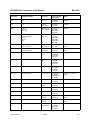
EC Certificate of Conformity
Certificate No.: 2003-35, Page 1
This is to certify that:
Equipment type
Stock No.
Designation
FSU3
FSU8
FSU26
FSU31
FSU32
FSU43
FSU46
FSU50
FSU67
1166.1660.03
1166.1660.08
1166.1660.26
1166.1660.31
1166.1660.32
1166.1660.43
1166.1660.46
1166.1660.50
1166.1660.67
Spectrum Analyzer
complies with the provisions of the Directive of the Council of the European Union on the
approximation of the laws of the Member States
-
relating to electrical equipment for use within defined voltage limits
(73/23/EEC revised by 93/68/EEC)
-
relating to electromagnetic compatibility
(89/336/EEC revised by 91/263/EEC, 92/31/EEC, 93/68/EEC)
Conformity is proven by compliance with the following standards:
EN61010-1 : 2001-12
EN55011 : 1998 + A1 : 1999 + A2 : 2002, Class B
EN61326 : 1997 + A1 : 1998 + A2 : 2001 + A3 : 2003
For the assessment of electromagnetic compatibility, the limits of radio interference for Class B
equipment as well as the immunity to interference for operation in industry have been used as a basis.
Affixing the EC conformity mark as from 2003
ROHDE & SCHWARZ GmbH & Co. KG
Mühldorfstr. 15, D-81671 München
Munich, 2007-06-25
1166.1660.01-s1-
Central Quality Management FS-QZ / Radde
CE
E-7
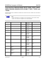
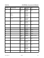
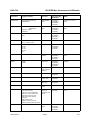
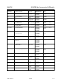
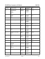
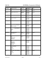
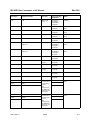
EC Certificate of Conformity
Certificate No.: 2003-35, Page 2
This is to certify that:
Equipment type
Stock No.
Designation
FSU-B4
FSU-B9
FSU-B12
FSU-B18
FSU-B19
FSU-B20
FSU-B21
FSU-B23
FSU-B25
FSU-B27
FSU-B46
FSU-B50
FSU-B73
FSU-B88
FSU-U73
FSP-B10
FSP-B28
1144.9000.02
1142.8994.02
1142.9349.02
1145.0242.02/.04
1145.0394.02
1155.1606.08
1157.1090.02
1157.0907.02
1144.9298.02
1157.2000.02
1163.0434.02
1163.0470.02
1169.5696.03
1157.1432.08/.26
1169.5696.04
1129.7246.02
1162.9915.02
OCXO 10 MHz
Tracking Generator
Output Attenuator
Removable Harddisc
Second Harddisc
Extended Environmetal Spec
LO/IF Connections
Preamplifier 20 dB
Electronic Attenuator
FM Output
46 GHz Frequency Extension
50 GHz Frequency Extension
Vector Signal Analysis
RF Hardware
Vector Signal Analysis
External Generator Control
Trigger Port
complies with the provisions of the Directive of the Council of the European Union on the
approximation of the laws of the Member States
-
relating to electrical equipment for use within defined voltage limits
(73/23/EEC revised by 93/68/EEC)
-
relating to electromagnetic compatibility
(89/336/EEC revised by 91/263/EEC, 92/31/EEC, 93/68/EEC)
Conformity is proven by compliance with the following standards:
EN61010-1 : 2001-12
EN55011 : 1998 + A1 : 1999 + A2 : 2002, Class B
EN61326 : 1997 + A1 : 1998 + A2 : 2001 + A3 : 2003
For the assessment of electromagnetic compatibility, the limits of radio interference for Class B
equipment as well as the immunity to interference for operation in industry have been used as a basis.
Affixing the EC conformity mark as from 2003
ROHDE & SCHWARZ GmbH & Co. KG
Mühldorfstr. 15, D-81671 München
Munich, 2007-06-25
1166.1660.01-s2-
Central Quality Management FS-QZ / Radde
CE
E-7
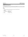
R&S FSU
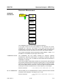
Tabbed Divider Overview
Tabbed Divider Overview
Safety Instructions are provided on the CD-ROM
Tabbed Divider
Documentation Overview
Chapter 1: Putting into Operation
Chapter 2: Getting Started
Chapter 3: Manual Control
Chapter 4: Instrument Functions
Chapter 5: Remote Control – Basics
Chapter 6: Remote Control – Description of Commands
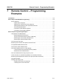
Chapter 7: Remote Control – Programming Examples
Chapter 8: Maintenance and Instrument Interfaces
Chapter 9: Error Messages
Index
1166.1725.12
0.3
E-2
Tabbed Divider Overview
R&S FSU
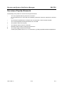
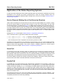
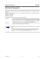
Documentation Overview
The documentation of the R&S FSU consists of base unit manuals and option manuals. All manuals are
provided in PDF format on the CD-ROM delivered with the instrument. Each software option available for
the instrument is described in a separate software manual.
The base unit documentation comprises the following manuals:
•
R&S FSU Quick Start Guide
•
R&S FSU Operating Manual
•
R&S FSU Service Manual
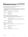
Apart from the base unit, these manuals describe the following models and options of the R&S FSU
Spectrum Analyzer. Options that are not listed are described in separate manuals. These manuals are
provided on an extra CD-ROM. For an overview of all options available for the R&S FSU visit the
R&S FSU Spectrum Analyzer Internet site.
Base unit models:
•
R&S FSU3 (20 Hz to 3.6 GHz)
•
R&S FSU8 (20 Hz to 8 GHz)
•
R&S FSU26 (20 Hz to 26.5 GHz)
•
R&S FSU31 (20 Hz to 31 GHz)
•
R&S FSU32 (20 Hz to 32 GHz)
•
R&S FSU43 (20 Hz to 43 GHz)
•
R&S FSU46 (20 Hz to 40 GHz)
•
R&S FSU50 (20 Hz to 50 GHz)
•
R&S FSU67 (20 Hz to 67 GHz)
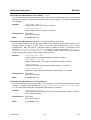
Options described in the base unit manuals:
•
R&S FSU-B4 (OCXO - reference oscillator)
•
R&S FSU-B9 (tracking generator)
•
R&S FSP-B10 (external generator control)
•
R&S FSU-B12 (attenuator for tracking generator)
•
R&S FSU-B18 (removable hard disk)
•
R&S FSU-B19 (second hard disk for R&S FSU-B18 option)
•
R&S FSU-B20 (extended environmental spec)
•
R&S FSU-B21 (external mixer)
•
R&S FSU-B23 (RF preamplifier)
•
R&S FSU-B25 (electronic attenuator)
•
R&S FSU-B27 (broadband FM demodulator)
•
R&S FSP-B28 (trigger port)
1166.1725.12
0.4
E-3
R&S FSU
Tabbed Divider Overview
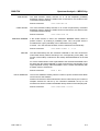
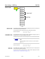
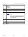
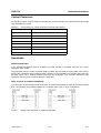
The operating manual is subdivided into the following chapters:
Chapter 1
Putting into Operation
see Quick Start Guide chapters 1 and 2
Chapter 2
Getting Started
gives an introduction to advanced measurement tasks of the R&S FSU which are
explained step by step.
Chapter 3
Manual Control
see Quick Start Guide chapter 4
Chapter 4
Instrument Functions
forms a reference for manual control of the R&S FSU and contains a detailed
description of all instrument functions and their application.
Chapter 5
Remote Control - Basics
describes the basics for programming the R&S FSU, command processing and the
status reporting system.
Chapter 6
Remote Control - Description of Commands
lists all the remote-control commands defined for the instrument.
Chapter 7
Remote Control - Programming Examples
contains program examples for a number of typical applications of the R&S FSU.
Chapter 8
Maintenance and Instrument Interfaces
describes preventive maintenance and the characteristics of the instrument’s
interfaces.
Chapter 9
Error Messages
gives a list of error messages that the R&S FSU may generate.
Index
contains an index for the chapters 1 to 9 of the operating manual.
Service Manual - Instrument
This manual is available in PDF format on the CD delivered with the instrument. It informs on how to check
compliance with rated specifications, on instrument function, repair, troubleshooting and fault elimination.
It contains all information required for repairing the R&S FSU by the replacement of modules. The manual
includes the following chapters:
Chapter 1
Performance Test
Chapter 2
Adjustment
Chapter 3
Repair
Chapter 4
Software Update / Installing Options
Chapter 5
Documents
1166.1725.12
0.5
E-2
Tabbed Divider Overview
1166.1725.12
R&S FSU
0.6
E-2
R&S FSU
1
Putting into Operation
Putting into Operation
For details refer to the Quick Start Guide chapters 1, "Front and Rear Panel", and 2, "Preparing for Use".
1166.1725.12
1.1
E-2
Putting into Operation
1166.1725.12
R&S FSU
1.2
E-2
R&S FSU
2
Getting Started
Getting Started
Introduction . . . . . . . . . . . . . . . . . . . . . . . . . . . . . . . . . . . . . . . . . . . . . . . . . . . . . . . . . . . . . . . . . . 2.2
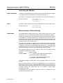
Measuring the Spectra of Complex Signals . . . . . . . . . . . . . . . . . . . . . . . . . . . . . . . . . . . . . . . . 2.3
Intermodulation Measurements . . . . . . . . . . . . . . . . . . . . . . . . . . . . . . . . . . . . . . . . . . . . . . 2.3
Measurement Example – Measuring the R&S FSU’s intrinsic intermodulation
distance . . . . . . . . . . . . . . . . . . . . . . . . . . . . . . . . . . . . . . . . . . . . . . . . . . . . . . . . . . . 2.5
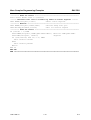
Measuring Signals in the Vicinity of Noise . . . . . . . . . . . . . . . . . . . . . . . . . . . . . . . . . . . . . . . . 2.10
Measurement example – Measuring the level of the internal reference generator
at low S/N ratios . . . . . . . . . . . . . . . . . . . . . . . . . . . . . . . . . . . . . . . . . . . . . . . . . . . . 2.13
Noise Measurements . . . . . . . . . . . . . . . . . . . . . . . . . . . . . . . . . . . . . . . . . . . . . . . . . . . . . . . . . 2.16
Measuring noise power density . . . . . . . . . . . . . . . . . . . . . . . . . . . . . . . . . . . . . . . . . . . . . 2.17
Measurement example – Measuring the intrinsic noise power density of the
R&S FSU at 1 GHz and calculating the R&S FSU’s noise figure . . . . . . . . . . . . . . . 2.17
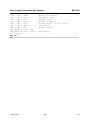
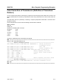
Measurement of Noise Power within a Transmission Channel . . . . . . . . . . . . . . . . . . . . . 2.20
Measurement Example – Measuring the intrinsic noise of the R&S FSU at
1 GHz in a 1.23 MHz channel bandwidth with the channel power function . . . . . . . 2.20
Measuring Phase Noise . . . . . . . . . . . . . . . . . . . . . . . . . . . . . . . . . . . . . . . . . . . . . . . . . . . 2.24
Measurement Example – Measuring the phase noise of a signal generator at a
carrier offset of 10 kHz . . . . . . . . . . . . . . . . . . . . . . . . . . . . . . . . . . . . . . . . . . . . . . . 2.24
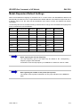
Measurements on Modulated Signals . . . . . . . . . . . . . . . . . . . . . . . . . . . . . . . . . . . . . . . . . . . . 2.27
Measurements on AM signals . . . . . . . . . . . . . . . . . . . . . . . . . . . . . . . . . . . . . . . . . . . . . . 2.28
Measurement Example 1 – Displaying the AF of an AM signal in the time
domain . . . . . . . . . . . . . . . . . . . . . . . . . . . . . . . . . . . . . . . . . . . . . . . . . . . . . . . . . . . 2.28
Measurement Example 2 – Measuring the modulation depth of an AM carrier in
the frequency domain . . . . . . . . . . . . . . . . . . . . . . . . . . . . . . . . . . . . . . . . . . . . . . . . 2.29
Measurements on FM Signals . . . . . . . . . . . . . . . . . . . . . . . . . . . . . . . . . . . . . . . . . . . . . . 2.31
Measurement Example – Displaying the AF of an FM carrier . . . . . . . . . . . . . . . . . 2.31
Measuring Channel Power and Adjacent Channel Power . . . . . . . . . . . . . . . . . . . . . . . . . 2.33
Measurement Example 1 – ACPR measurement on an IS95 CDMA Signal . . . . . . 2.34
Measurement Example 2 – Measuring the adjacent channel power of an IS136
TDMA signal . . . . . . . . . . . . . . . . . . . . . . . . . . . . . . . . . . . . . . . . . . . . . . . . . . . . . . . 2.38
Measurement Example 3 – Measuring the Modulation Spectrum in Burst Mode
with the Gated Sweep Function . . . . . . . . . . . . . . . . . . . . . . . . . . . . . . . . . . . . . . . . 2.41
Measurement Example 4 – Measuring the Transient Spectrum in Burst Mode
with the Fast ACP function . . . . . . . . . . . . . . . . . . . . . . . . . . . . . . . . . . . . . . . . . . . . 2.43
Measurement Example 5 – Measuring adjacent channel power of a W-CDMA
uplink signal . . . . . . . . . . . . . . . . . . . . . . . . . . . . . . . . . . . . . . . . . . . . . . . . . . . . . . . 2.45
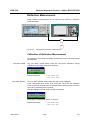
Amplitude distribution measurements . . . . . . . . . . . . . . . . . . . . . . . . . . . . . . . . . . . . . . . . . 2.49
Measurement Example – Measuring the APD and CCDF of white noise
generated by the R&S FSU . . . . . . . . . . . . . . . . . . . . . . . . . . . . . . . . . . . . . . . . . . . 2.49
1166.1725.12
2.1
E-2
Introduction
R&S FSU
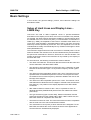
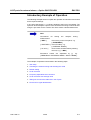
Introduction
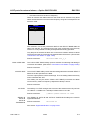
This chapter explains how to operate the R&S FSU using typical measurements as examples.
The basic operating steps such as selecting the menus and setting parameters are described in the Quick
Start Guide, chapter 4, "Basic Operation". Furthermore, the screen structure and displayed function
indicators are explained in this chapter.
Chapter “Instrument Functions” describes all the menus and R&S FSU functions.
All of the following examples are based on the standard settings of the Spectrum Analyzer. These are set
with the PRESET key. A complete listing of the standard settings can be found in chapter “Instrument
Functions”, section “R&S FSU Initial Configuration – PRESET Key” on page 4.6. Examples of more basic
character are provided in the Quick Start Guide, chapter 5, as an introduction.
1166.1725.12
2.2
E-2
R&S FSU
Measuring the Spectra of Complex Signals
Measuring the Spectra of Complex Signals
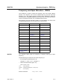
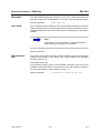
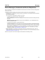
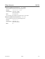
Intermodulation Measurements
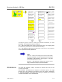
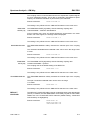
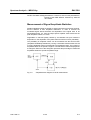
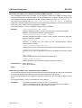
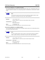
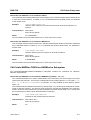
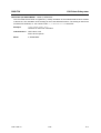
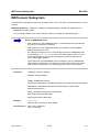
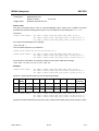
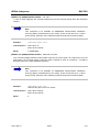
If several signals are applied to a DUT with non-linear characteristics, unwanted mixing products are
generated – mostly by active components such as amplifiers or mixers. The products created by 3rd order
intermodulation are particularly troublesome as they have frequencies close to the useful signals and,
compared with other products, are closest in level to the useful signals. The fundamental wave of one
signal is mixed with the 2nd harmonic of the other signal.
fs1 = 2 × fu1 – fu2
(1)
fs2 = 2 × fu2 – fu1
(2)
where fs1 and fs2 are the frequencies of the intermodulation products and fu1 and fu2 the frequencies of
the useful signals.
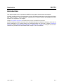
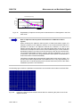
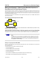
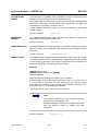
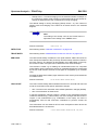
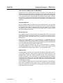
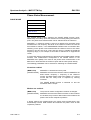
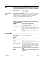
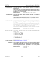
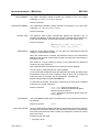
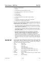
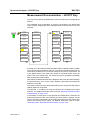
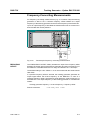
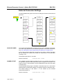
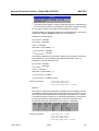
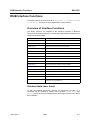
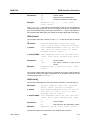
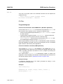
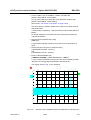
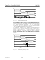
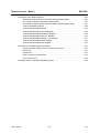
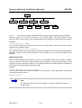
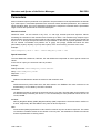
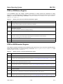
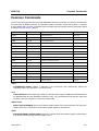
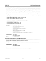
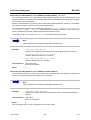
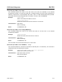
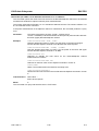
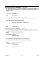
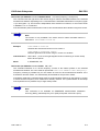
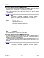
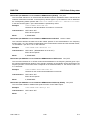
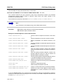
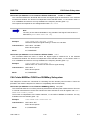
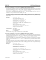
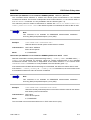
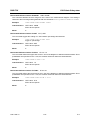
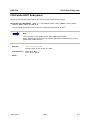
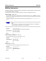
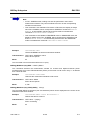
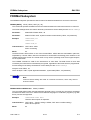
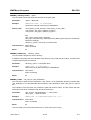
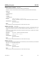
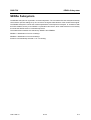
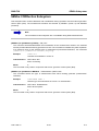
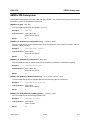
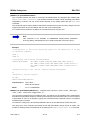
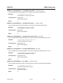
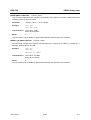
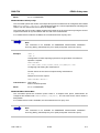
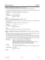
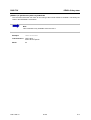
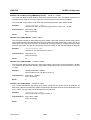
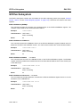
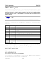
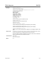
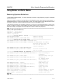
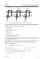
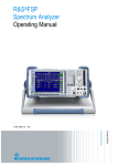
The following diagram shows the position of the intermodulation products in the frequency domain.
Level
Pu1
Pu2
aD3
Ps1
Ps2
∆f
fs1
Fig. 2-1
∆f
f u1
∆f
fu2
fs2
Frequency
3rd order intermodulation products
Example:
fu1 = 100 MHz, fu2 = 100.03 MHz
fs1 = 2 × fu1 – fu2 = 2 × 100 MHz – 100.03 MHz = 99.97 MHz
fs2 = 2 × fu2 – fu1 = 2 × 100.03 MHz – 100 MHz = 100.06 MHz
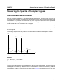
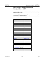
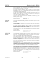
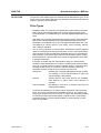
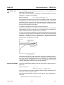
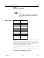
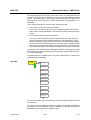
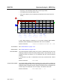
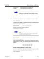
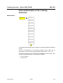
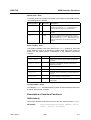
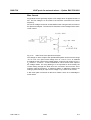
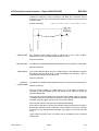
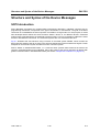
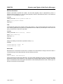
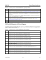
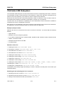
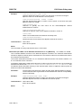
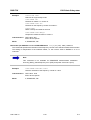
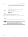
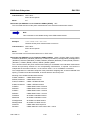
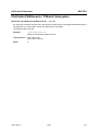
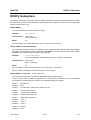
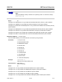
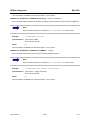
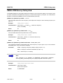
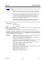
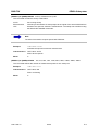
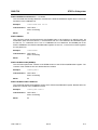
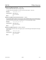
The level of the intermodulation products depends on the level of the useful signals. If the level of the two
useful signals is increased by 1 dB, the level of the intermodulation products is increased by 3 dB. The
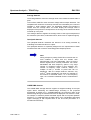
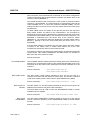
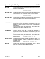
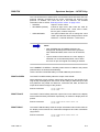
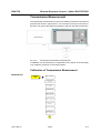
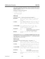
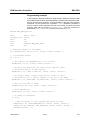
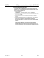
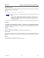
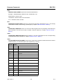
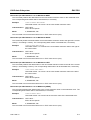
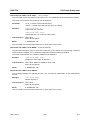
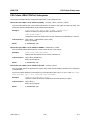
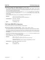
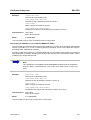
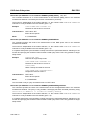
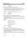
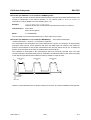
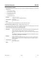
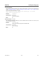
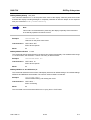
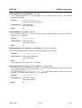
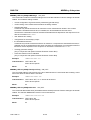
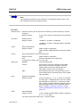
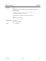
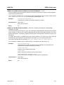
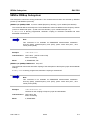
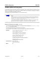
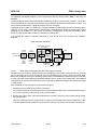
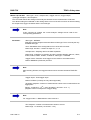
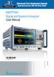
intermodulation distance d3 is, therefore, reduced by 2 dB. Fig. 2-2 shows how the levels of the useful
signals and the 3rd order intermodulation products are related.
1166.1725.12
2.3
E-2
Measuring the Spectra of Complex Signals
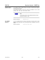
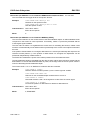
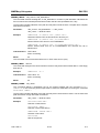
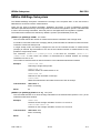
Output
level
R&S FSU
Intercept
point
Compression
Intermodulation
products
Carrier
level
3
aD3
1
1
1
Input level
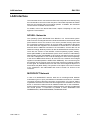
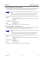
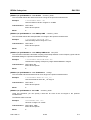
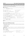
Fig. 2-2
Level of the 3rd order intermodulation products as a function of the level of the useful signals
The behavior of the signals can explained using an amplifier as an example. The change in the level of
the useful signals at the output of the amplifier is proportional to the level change at the input of the
amplifier as long as the amplifier is operating in linear range. If the level at the amplifier input is changed
by 1 dB, there is a 1 dB level change at the amplifier output. At a certain input level, the amplifier enters
saturation. The level at the amplifier output does not increase with increasing input level.
The level of the 3rd order intermodulation products increases 3 times faster than the level of the useful
signals. The 3rd order intercept is the virtual level at which the level of the useful signals and the level of
the spurious products are identical, i.e. the intersection of the two straight lines. This level cannot be
measured directly as the amplifier goes into saturation or is damaged before this level is reached.
The 3rd order intercept can be calculated from the known slopes of the lines, the intermodulation distance
d2 and the level of the useful signals.
TOI = aD3 / 2 + Pn
(3)
with TOI (Third Order Intercept) being the 3rd order intercept in dBm and Pn the level of a carrier in dBm.
With an intermodulation distance of 60 dB and an input level, Pw, of –20 dBm, the following 3rd order
intercept is obtained:
TOI = 60 dBm / 2 + (-20 dBm) = 10 dBm.
1166.1725.12
2.4
E-2
R&S FSU
Measuring the Spectra of Complex Signals
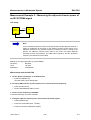
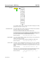
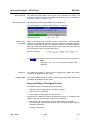
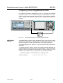
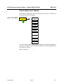
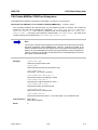
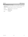
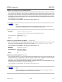
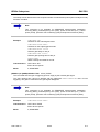
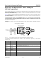
Measurement Example – Measuring the R&S FSU’s intrinsic
intermodulation distance
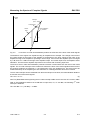
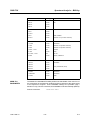
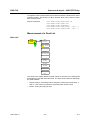
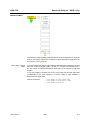
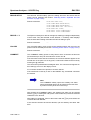
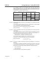
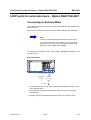
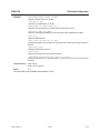
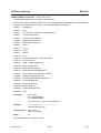
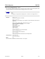
To measure the intrinsic intermodulation distance, use the following test setup.
Test setup:
Signal
Generator 1
R&S
FSP
FSU
Coupler
Signal
Generator 2
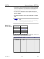
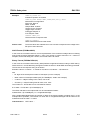
Signal generator settings (e.g. R&S SMIQ):
Level
Frequency
Signal generator 1
-10 dBm
999.9 MHz
Signal generator 2
-10 dBm
1000.1 MHz
Measurement using the R&S FSU:
1. Set the Spectrum Analyzer to its default settings.
➢ Press the PRESET key.
The R&S FSU is in its default state.
2. Set center frequency to 1 GHz and the frequency span to 1 MHz.
➢ Press the FREQ key and enter 1 GHz.
➢ Press the SPAN key and enter 1 MHz.
3. Set the reference level to –10 dBm and RF attenuation to 0 dB.
➢ Press the AMPT key and enter -10 dBm.
➢ Press the RF ATTEN MANUAL softkey and enter 0 dB.
By reducing the RF attenuation to 0 dB, the level to the R&S FSU input mixer is increased.
Therefore, 3rd order intermodulation products are displayed.
4. Set the resolution bandwidth to 5 kHz.
➢ Press the BW key.
➢ Press the RES BW MANUAL softkey and enter 5 kHz.
By reducing the bandwidth, the noise is further reduced and the intermodulation products can be
clearly seen.
1166.1725.12
2.5
E-2
Measuring the Spectra of Complex Signals
R&S FSU
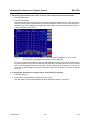
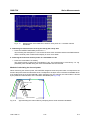
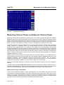
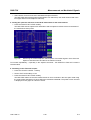
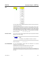
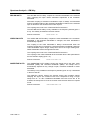
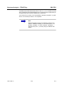
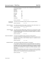
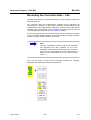
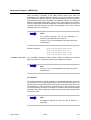
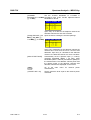
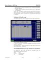
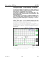
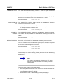
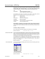
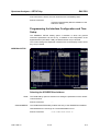
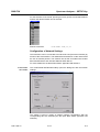
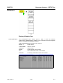
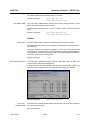
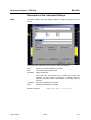
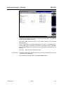
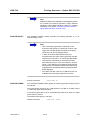
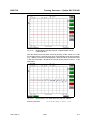
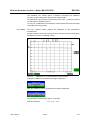
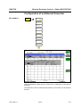
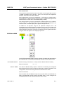
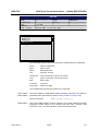
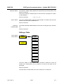
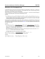
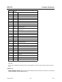
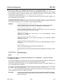
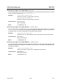
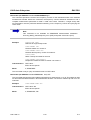
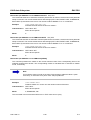
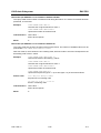
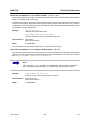
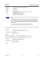
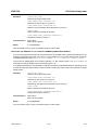
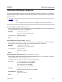
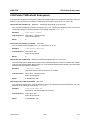
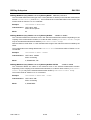
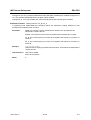
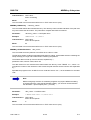
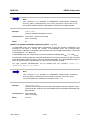
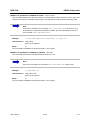
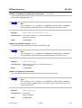
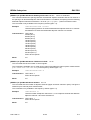
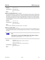
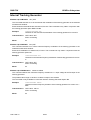
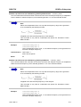
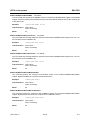
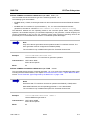
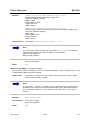
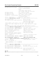
5. Measuring intermodulation by means of the 3rd order intercept measurement function
➢ Press the MEAS key.
➢ Press the TOI softkey.
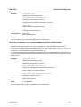
The R&S FSU activates four markers for measuring the intermodulation distance. Two markers are
positioned on the useful signals and two on the intermodulation products. The 3rd order intercept is
calculated from the level difference between the useful signals and the intermodulation products. It
is then displayed on the screen:
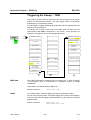
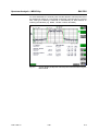
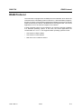
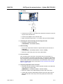
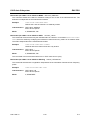
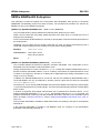
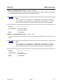
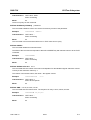
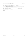
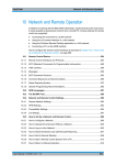
Fig. 2-3
Result of intrinsic intermodulation measurement on the R&S FSU. The 3rd order
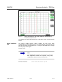
intercept (TOI) is displayed at the top right corner of the grid
The level of a Spectrum Analyzer’s intrinsic intermodulation products depends on the RF level of
the useful signals at the input mixer. When the RF attenuation is added, the mixer level is reduced
and the intermodulation distance is increased. With an additional RF attenuation of 10 dB, the
levels of the intermodulation products are reduced by 20 dB. The noise level is, however, increased
by 10 dB.
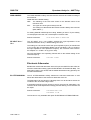
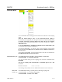
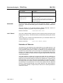
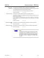
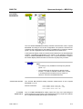
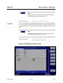
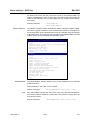
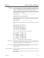
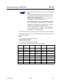
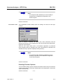
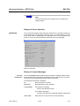
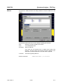
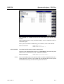
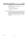
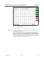
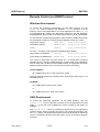
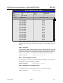
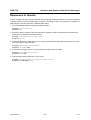
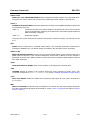
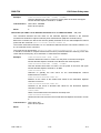
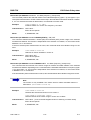
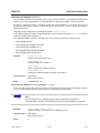
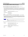
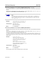
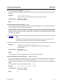
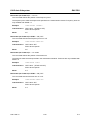
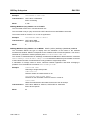
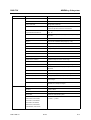
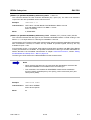
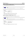
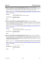
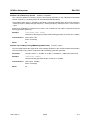
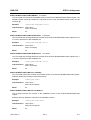
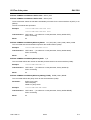
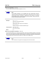
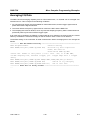
6. Increasing RF attenuation to 10 dB to reduce intermodulation products.
➢ Press the AMPT key.
➢ Press the RF ATTEN MANUAL softkey and enter 10 dB.
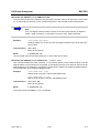
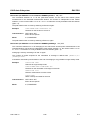
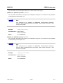
The R&S FSU’s intrinsic intermodulation products disappear below the noise floor.
1166.1725.12
2.6
E-2
R&S FSU
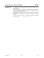
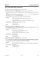
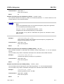
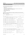
Fig. 2-4
Measuring the Spectra of Complex Signals
If the RF attenuation is increased, the R&S FSU’s intrinsic intermodulation products
disappear below the noise floor.
Calculation method:
The method used by the R&S FSU to calculate the intercept point takes the average useful signal level
Pu in dBm and calculates the intermodulation d3 in dB as a function of the average value of the levels of
the two intermodulation products. The third order intercept (TOI) is then calculated as follows:
TOI/dBm = ½ d3 + Pu
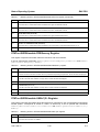
Intermodulation- free dynamic range
The Intermodulation – free dynamic range, i.e. the level range in which no internal intermodulation
products are generated if two-tone signals are measured, is determined by the 3rd order intercept point,
the phase noise and the thermal noise of the Spectrum Analyzer. At high signal levels, the range is
determined by intermodulation products. At low signal levels, intermodulation products disappear below
the noise floor, i.e. the noise floor and the phase noise of the Spectrum Analyzer determine the range. The
noise floor and the phase noise depend on the resolution bandwidth that has been selected. At the
smallest resolution bandwidth, the noise floor and phase noise are at a minimum and so the maximum
range is obtained. However, a large increase in sweep time is required for small resolution bandwidths. It
is, therefore, best to select the largest resolution bandwidth possible to obtain the range that is required.
Since phase noise decreases as the carrier-offset increases, its influence decreases with increasing
frequency offset from the useful signals.
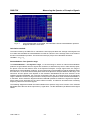
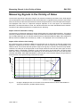
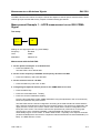
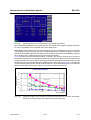
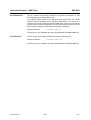
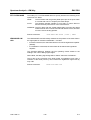
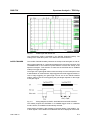
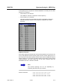
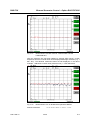
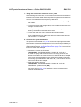
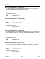
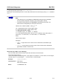
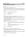
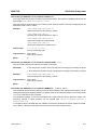
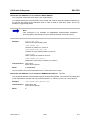
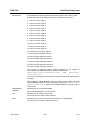
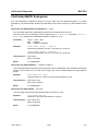
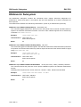
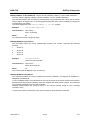
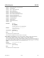
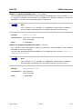
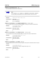
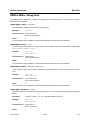
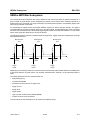
The following diagrams illustrate the intermodulation-free dynamic range as a function of the selected
bandwidth and of the level at the input mixer (= signal level – set RF attenuation) at different useful signal
offsets.
1166.1725.12
2.7
E-2
Measuring the Spectra of Complex Signals
R&S FSU
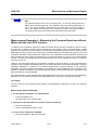
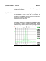
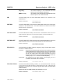
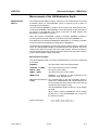
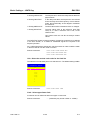
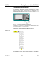
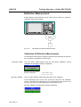
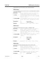
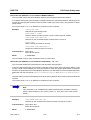
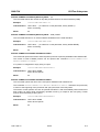
Distortion free dynamic range
1MHz carrier offset
Dynamic range dB
-60
RBW=10 kHz
T.O.I
-70
RBW=1
kHz
RBW=100
Hz
RBW=10
Hz
-80
-90
-100
Thermal noise
-110
-120
-60
-50
-40
-30
-20
-10
Mixer level
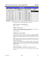
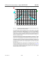
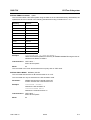
Fig. 2-5
Intermodulation-free range of the FSU3 as a function of level at the input mixer and the set
resolution bandwidth (useful signal offset = 1 MHz, DANL = -157 dBm /Hz, TOI = 25 dBm;
typ. values at 2 GHz)
The optimum mixer level, i.e. the level at which the intermodulation distance is at its maximum, depends
on the bandwidth. At a resolution bandwidth of 10 Hz, it is approx. –42 dBm and at 10 kHz increases to
approx. -32 dBm.
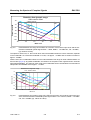
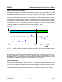
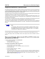
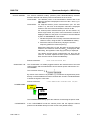
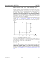
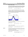
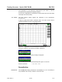
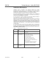
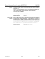
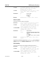
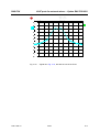
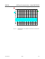
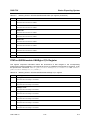
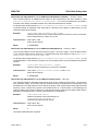
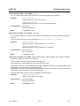
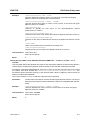
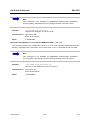
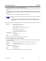
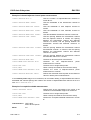
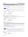
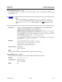
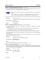
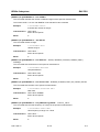
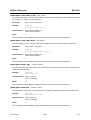
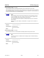
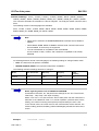
Phase noise has a considerable influence on the intermodulation-free range at carrier offsets between 10
and 100 kHz (Fig. 2-6). At greater bandwidths, the influence of the phase noise is greater than it would be
with small bandwidths. The optimum mixer level at the bandwidths under consideration becomes almost
independent of bandwidth and is approx. –40 dBm.
Distortion free dyn amic range
10 to 100 kHz offset
-60
RBW =10 kHz
Dynamic range dB
T.O.I
RBW =1
kHz
RBW =100
Hz
RBW =10
Hz
-70
-80
-90
-100
Thermal noise
-110
-120
-60
-50
-40
-30
-20
-10
Mixer level
Fig. 2-6
Intermodulation-free dynamic range of the FSU3 as a function of level at the input mixer and
of the selected resolution bandwidth (useful signal offset = 10 to 100 kHz, DANL = -157 dBm
/Hz, TOI = 25 dBm; typ. values at 2 GHz).
1166.1725.12
2.8
E-2
R&S FSU
Aa
1166.1725.12
Measuring the Spectra of Complex Signals
Hint
If the intermodulation products of a DUT with a very high dynamic range are to be
measured and the resolution bandwidth to be used is therefore very small, it is best
to measure the levels of the useful signals and those of the intermodulation
products separately using a small span. The measurement time will be reduced–
in particular if the offset of the useful signals is large. To find signals reliably when
frequency span is small, it is best to synchronize the signal sources and the
R&S FSU.
2.9
E-2
Measuring Signals in the Vicinity of Noise
R&S FSU
Measuring Signals in the Vicinity of Noise
The minimum signal level a Spectrum Analyzer can measure is limited by its intrinsic noise. Small signals
can be swamped by noise and therefore cannot be measured. For signals that are just above the intrinsic
noise, the accuracy of the level measurement is influenced by the intrinsic noise of the Spectrum Analyzer.
The displayed noise level of a Spectrum Analyzer depends on its noise figure, the selected RF
attenuation, the selected reference level, the selected resolution and video bandwidth and the detector.
The effect of the different parameters is explained in the following.
Impact of the RF attenuation setting
The sensitivity of a Spectrum Analyzer is directly influenced by the selected RF attenuation. The highest
sensitivity is obtained at a RF attenuation of 0 dB. The R&S FSU’s RF attenuation can be set in 5 dB steps
up to 70 dB (5 dB steps up to 75 dB with option Electronic Attenuator R&S FSU-B25). Each additional 5
dB step reduces the R&S FSU’s sensitivity by 10 dB, i.e. the displayed noise is increased by 5 dB.
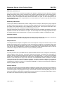
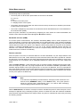
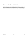
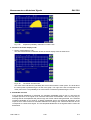
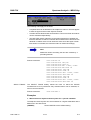
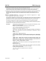
Impact of the reference level setting
If the reference level is changed, the R&S FSU changes the gain on the last IF so that the voltage at the
logarithmic amplifier and the A/D converter is always the same for signal levels corresponding to the
reference level. This ensures that the dynamic range of the log amp or the A/D converter is fully utilized.
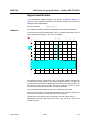
Therefore, the total gain of the signal path is low at high reference levels and the noise figure of the IF
amplifier makes a substantial contribution to the total noise figure of the R&S FSU. The figure below
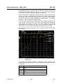
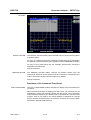
shows the change in the displayed noise depending on the set reference level at 10 kHz and 300 kHz
resolution bandwidth. With digital bandwidths (≤100 kHz) the noise increases sharply at high reference
levels because of the dynamic range of the A/D converter.
14
12
RBW = 10 kHz
rel. noise level /dB
10
8
6
4
RBW = 300 kHz
2
0
-2
-70
Fig. 2-7
-60
-50
-40
-30
-20
Reference level /dBm
-10
Change in displayed noise as a function of the selected reference level at bandwidths of
10 kHz and 300 kHz (-30 dBm reference level)
1166.1725.12
2.10
E-2
R&S FSU
Measuring Signals in the Vicinity of Noise
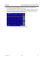
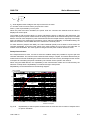
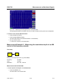
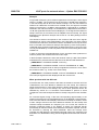
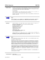
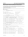
Impact of the resolution bandwidth
The sensitivity of a Spectrum Analyzer also directly depends on the selected bandwidth. The highest
sensitivity is obtained at the smallest bandwidth (for the R&S FSU: 10 Hz, for FFT filtering: 1 Hz). If the
bandwidth is increased, the reduction in sensitivity is proportional to the change in bandwidth. The
R&S FSU has bandwidth settings in 2, 3, 5, 10 sequence. Increasing the bandwidth by a factor of 3
increases the displayed noise by approx. 5 dB (4.77 dB precisely). If the bandwidth is increased by a factor
of 10, the displayed noise increases by a factor of 10, i.e. 10 dB. Because of the way the resolution filters
are designed, the sensitivity of Spectrum Analyzers often depends on the selected resolution bandwidth.
In data sheets, the displayed average noise level is often indicated for the smallest available bandwidth
(for the R&S FSU: 10 Hz). The extra sensitivity obtained if the bandwidth is reduced may therefore deviate
from the values indicated above. The following table illustrates typical deviations from the noise figure for
a resolution bandwidth of 10 kHz which is used as a reference value (= 0 dB).
Noise figure
offset /dB
3
digital RBW
analog RBW
2
1
0
-1
0,01
0,1
1
10
100
1000
10000
RBW /kHz
Fig. 2-8
Change in R&S FSU noise figure at various bandwidths. The reference bandwidth is 10 kHz
Impact of the video bandwidth
The displayed noise of a Spectrum Analyzer is also influenced by the selected video bandwidth. If the
video bandwidth is considerably smaller than the resolution bandwidth, noise spikes are suppressed, i.e.
the trace becomes much smoother. The level of a sinewave signal is not influenced by the video
bandwidth. A sinewave signal can therefore be freed from noise by using a video bandwidth that is small
compared with the resolution bandwidth, and thus be measured more accurately.
Impact of the detector
Noise is evaluated differently by the different detectors. The noise display is therefore influenced by the
choice of detector. Sinewave signals are weighted in the same way by all detectors, i.e. the level display
for a sinewave RF signal does not depend on the selected detector, provided that the signal-to-noise ratio
is high enough. The measurement accuracy for signals in the vicinity of intrinsic Spectrum Analyzer noise
is also influenced by the detector which has been selected. The R&S FSU has the following detectors:
1166.1725.12
2.11
E-2
Measuring Signals in the Vicinity of Noise
R&S FSU
Maximum peak detector
If the max. peak detector s selected, the largest noise display is obtained, since the Spectrum Analyzer
displays the highest value of the IF envelope in the frequency range assigned to a pixel at each pixel in
the trace. With longer sweep times, the trace indicates higher noise levels since the probability of
obtaining a high noise amplitude increases with the dwell time on a pixel. For short sweep times, the
display approaches that of the sample detector since the dwell time on a pixel is only sufficient to obtain
an instantaneous value.
Minimum peak detector
The min. peak detector indicates the minimum voltage of the IF envelope in the frequency range assigned
to a pixel at each pixel in the trace. The noise is strongly suppressed by the minimum peak detector since
the lowest noise amplitude that occurs is displayed for each test point. If the signal-to-noise ratio is low,
the minimum of the noise overlaying the signal is displayed too low.
At longer sweep times, the trace shows smaller noise levels since the probability of obtaining a low noise
amplitude increases with the dwell time on a pixel. For short sweep times, the display approaches that of
the sample detector since the dwell time on a pixel is only sufficient to obtain an instantaneous value.
Autopeak detector
The Autopeak detector displays the maximum and minimum peak value at the same time. Both values
are measured and their levels are displayed on the screen joint by a vertical line.
Sample detector
The sample detector samples the logarithm of the IF envelope for each pixel of the trace only once and
displays the resulting value. If the frequency span of the Spectrum Analyzer is considerably higher than
the resolution bandwidth (span/RBW >500), there is no guarantee that useful signals will be detected.
They are lost due to undersampling. This does not happen with noise because in this case it is not the
instantaneous amplitude that is relevant but only the probability distribution.
RMS detector
For each pixel of the trace, the RMS detector outputs the RMS value of the IF envelope for the frequency
range assigned to each test point. It therefore measures noise power. The display for small signals is,
however, the sum of signal power and noise power. For short sweep times, i.e. if only one uncorrelated
sample value contributes to the RMS value measurement, the RMS detector is equivalent to the sample
detector. If the sweep time is longer, more and more uncorrelated RMS values contribute to the RMS
value measurement. The trace is, therefore, smoothed. The level of sinewave signals is only displayed
correctly if the selected resolution bandwidth (RBW) is at least as wide as the frequency range which
corresponds to a pixel in the trace. At a resolution bandwidth of 1 MHz, this means that the maximum
frequency display range is 625 MHz.
Average detector
For each pixel of the trace, the average detector outputs the average value of the linear IF envelope for
the frequency range assigned to each test point. It therefore measures the linear average noise. The level
of sinewave signals is only displayed correctly if the selected resolution bandwidth (RBW) is at least as
wide as the frequency range which corresponds to a pixel in the trace. At a resolution bandwidth of 1 MHz,
this means the maximum frequency display range is 625 MHz.
1166.1725.12
2.12
E-2
R&S FSU
Measuring Signals in the Vicinity of Noise
Quasi peak detector
The quasi peak detector is a peak detector for EMI measurements with defined charge and discharge
times. These times are defined in CISPR 16, the standard for equipment used to measure EMI emissions.
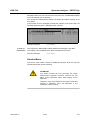
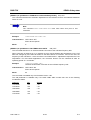
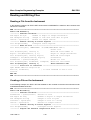
Measurement example – Measuring the level of the internal reference
generator at low S/N ratios
The example shows the different factors influencing the S/N ratio.
1. Set the Spectrum Analyzer to its default state.
➢ Press the PRESET key.
The R&S FSU is in its default state.
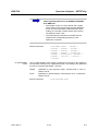
2. Switch on the internal reference generator
➢ Press the SETUP key.
➢ Press the softkeys SERVICE - INPUT CAL.
The internal 128 MHz reference generator is on.
The R&S FSU’s RF input is off.
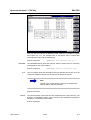
3. Set the center frequency to 128 MHz and the frequency span to 100 MHz.
➢ Press the FREQ key and enter 128 MHz.
➢ Press the SPAN key and enter 100 MHz.
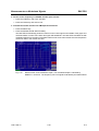
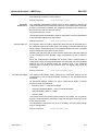
4. Set the RF attenuation to 60 dB to attenuate the input signal or to increase the intrinsic noise.
➢ Press the AMPT key.
➢ Press the RF ATTEN MANUAL softkey and enter 60 dB.
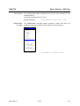
The RF attenuation indicator is marked with an asterisk (*Att 60 dB) to show that it is no longer
coupled to the reference level. The high input attenuation reduces the reference signal which can
no longer be detected in noise.
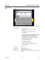
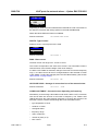
Fig. 2-9
1166.1725.12
Sinewave signal with low S/N ratio. The signal is measured with the autopeak detector
and is completely swamped by the intrinsic noise of the Spectrum Analyzer.
2.13
E-2
Measuring Signals in the Vicinity of Noise
R&S FSU
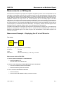
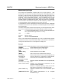
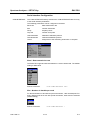
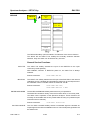
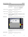
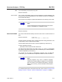
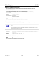
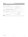
5. To suppress noise spikes the trace can be averaged.
➢ Press the TRACE key.
➢ Press the AVERAGE softkey.
The traces of consecutive sweeps are averaged. To perform averaging, the R&S FSU automatically
switches on the sample detector. The RF signal, therefore, can be more clearly distinguished from
noise.
Fig. 2-10
RF sinewave signal with low S/N ratio if the trace is averaged.
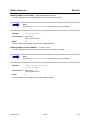
6. Instead of trace averaging, a video filter that is narrower than the resolution bandwidth can be
selected.
➢ Press the CLEAR/WRITE softkey in the trace menu.
➢ Press the BW key.
Press the VIDEO BW MANUAL softkey and enter 10 kHz.
The RF signal can be more clearly distinguished from noise.
Fig. 2-11
1166.1725.12
RF sinewave signal with low S/N ratio if a smaller video bandwidth is selected.
2.14
E-2
R&S FSU
Measuring Signals in the Vicinity of Noise
7. By reducing the resolution bandwidth by a factor of 10, the noise is reduced by 10 dB.
➢ Press the RES BW MANUAL softkey and enter 300 kHz.
The displayed noise is reduced by approx. 10 dB. The signal, therefore, emerges from noise by
about 10 dB. Compared to the previous setting, the video bandwidth has remained the same, i.e. it
has increased relative to the smaller resolution bandwidth. The averaging effect is, therefore,
reduced by the video bandwidth. The trace will be noisier.
Fig. 2-12
1166.1725.12
Reference signal at a smaller resolution bandwidth
2.15
E-2
Noise Measurements
R&S FSU
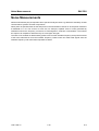
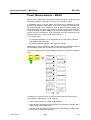
Noise Measurements
Noise measurements play an important role in spectrum analysis. Noise e.g. affects the sensitivity of radio
communication systems and their components.
Noise power is specified either as the total power in the transmission channel or as the power referred to
a bandwidth of 1 Hz. The sources of noise are, for example, amplifier noise or noise generated by
oscillators used for the frequency conversion of useful signals in receivers or transmitters. The noise at
the output of an amplifier is determined by its noise figure and gain.
The noise of an oscillator is determined by phase noise near the oscillator frequency and by thermal noise
of the active elements far from the oscillator frequency. Phase noise can mask weak signals near the
oscillator frequency and make them impossible to detect.
1166.1725.12
2.16
E-2
R&S FSU
Noise Measurements
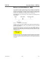
Measuring noise power density
To measure noise power referred to a bandwidth of 1 Hz at a certain frequency, the R&S FSU has an easyto-use marker function. This marker function calculates the noise power density from the measured
marker level.
Measurement example – Measuring the intrinsic noise power density
of the R&S FSU at 1 GHz and calculating the R&S FSU’s noise figure
1. Set the Spectrum Analyzer to its default state.
➢ Press the PRESET key.
The R&S FSU is in its default state.
2. Set the center frequency to 1 GHz and the span to 1 MHz.
➢ Press the FREQ key and enter 1 GHz.
➢ Press the SPAN key and enter 1 MHz.
3. Switch on the marker and set the marker frequency to 1 GHz.
➢ Press the MKR key and enter 1 GHz.
4. Switch on the noise marker function.
➢ Press the MEAS key.
➢ Press the NOISE MARKER softkey.
The R&S FSU displays the noise power at 1 GHz in dBm (1Hz).
Since noise is random, a sufficiently long measurement time has to be selected to obtain stable
measurement results. This can be achieved by averaging the trace or by selecting a very small
video bandwidth relative to the resolution bandwidth.
5. The measurement result is stabilized by averaging the trace
➢ Press the TRACE key.
➢ Press the AVERAGE softkey.
The R&S FSU performs sliding averaging over 10 traces from consecutive sweeps. The
measurement result becomes more stable.
Conversion to other reference bandwidths
The result of the noise measurement can be referred to other bandwidths by simple conversion. This is
done by adding 10 · log (BW) to the measurement result, BW being the new reference bandwidth.
Example:
A noise power of –150 dBm (1 Hz) is to be referred to a bandwidth of 1 kHz.
P[1kHz] = -150 + 10 · log (1000) = -150 +30 = -120 dBm(1 kHz)
1166.1725.12
2.17
E-2
Noise Measurements
R&S FSU
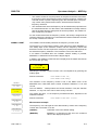
Calculation method:
The following method is used to calculate the noise power:
If the noise marker is switched on, the R&S FSU automatically activates the sample detector. The video
bandwidth is set to 1/10 of the selected resolution bandwidth (RBW).
To calculate the noise, the R&S FSU takes an average over 17 adjacent pixels (the pixel on which the
marker is positioned and 8 pixels to the left, 8 pixels to the right of the marker). The measurement result
is stabilized by video filtering and averaging over 17 pixels.
Since both video filtering and averaging over 17 trace points is performed in the log display mode, the
result would be 2.51 dB too low (difference between logarithmic noise average and noise power). The
R&S FSU, therefore, corrects the noise figure by 2.51 dB.
To standardize the measurement result to a bandwidth of 1 Hz, the result is also corrected by –10 · log
(RBWnoise), with RBWnoise being the power bandwidth of the selected resolution filter (RBW).
Detector selection
The noise power density is measured in the default setting with the sample detector and using averaging.
Other detectors that can be used to perform a measurement giving true results are the average detector
or the RMS detector. If the average detector is used, the linear video voltage is averaged and displayed
as a pixel. If the RMS detector is used, the squared video voltage is averaged and displayed as a pixel.
The averaging time depends on the selected sweep time (=SWT/625). An increase in the sweep time
gives a longer averaging time per pixel and thus stabilizes the measurement result. The R&S FSU
automatically corrects the measurement result of the noise marker display depending on the selected
detector (+1.05 dB for the average detector, 0 dΒ for the RMS detector). It is assumed that the video
bandwidth is set to at least three times the resolution bandwidth. While the average or RMS detector is
being switched on, the R&S FSU sets the video bandwidth to a suitable value.
The Pos Peak, Neg Peak, Auto Peak and Quasi Peak detectors are not suitable for measuring noise
power density.
Determining the noise figure:
The noise figure of amplifiers or of the R&S FSU alone can be obtained from the noise power display.
Based on the known thermal noise power of a 50 Ω resistor at room temperature (-174 dBm (1Hz)) and
the measured noise power Pnoise the noise figure (NF) is obtained as follows:
NF = Pnoise + 174 – g,
where g = gain of DUT in dB
Example:
The measured internal noise power of the R&S FSU at an attenuation of 0 dB is found to be –155 dBm/1
Hz. The noise figure of the R&S FSU is obtained as follows
NF = -155 + 174 = 17 dB
1166.1725.12
2.18
E-2
R&S FSU
Noise Measurements
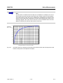
Aa
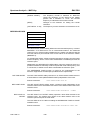
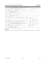
Note
If noise power is measured at the output of an amplifier, for example, the sum of
the internal noise power and the noise power at the output of the DUT is measured.
The noise power of the DUT can be obtained by subtracting the internal noise
power from the total power (subtraction of linear noise powers). By means of the
following diagram, the noise level of the DUT can be estimated from the level
difference between the total and the internal noise level.
0
C o rrectio n
-1
facto r in d B
-2
-3
-4
-5
-6
-7
-8
-9
-10
0
1
2
3
4
5
6
7
8
9
10 11 12 13
14 15
16
T o tal po w er/intrinsic no ise po w er in d B
Fig. 2-13
Correction factor for measured noise power as a function of the ratio of total power to the
intrinsic noise power of the Spectrum Analyzer.
1166.1725.12
2.19
E-2
Noise Measurements
R&S FSU
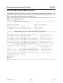
Measurement of Noise Power within a Transmission Channel
Noise in any bandwidth can be measured with the channel power measurement functions. Thus the noise
power in a communication channel can be determined, for example. If the noise spectrum within the
channel bandwidth is flat, the noise marker from the previous example can be used to determine the noise
power in the channel by considering the channel bandwidth. If, however, phase noise and noise that
normally increases towards the carrier is dominant in the channel to be measured, or if there are discrete
spurious signals in the channel, the channel power measurement method must be used to obtain correct
measurement results.
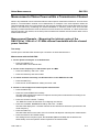
Measurement Example – Measuring the intrinsic noise of the
R&S FSU at 1 GHz in a 1.23 MHz channel bandwidth with the channel
power function
Test setup:
The RF input of the R&S FSU remains open-circuited or is terminated with 50 Ω.
Measurement with the R&S FSU:
1. Set the Spectrum Analyzer to its default state.
➢ Press the PRESET key.
The R&S FSU is in its default state.
2. Set the center frequency to 1 GHz and the span to 2 MHz.
➢ Press the FREQ key and enter 1 GHz.
➢ Press the SPAN key and enter 2 MHz.
3. To obtain maximum sensitivity, set RF attenuation on the R&S FSU to 0 dB.
➢ Press the AMPT key.
➢ Press the RF ATTEN MANUAL softkey and enter 0 dB.
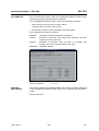
4. Switch on and configure the channel power measurement.
➢ Press the MEAS key.
➢ Press the CHAN POWER ACP softkey.
The R&S FSU activates the channel or adjacent channel power measurement according to the
currently set configuration.
➢ Press the CP/ACP CONFIG ! softkey.
The R&S FSU enters the submenu for configuring the channel.
➢ Press the CHANNEL BANDWIDTH softkey and enter 1.23 MHz.
The R&S FSU displays the 1.23 MHz channel as two vertical lines which are symmetrical to the
center frequency.
➢ Press the PREV key.
The R&S FSU returns to the main menu for channel and adjacent channel power measurement.
➢ Press the ADJUST SETTINGS softkey.
The settings for the frequency span, the bandwidth (RBW and VBW) and the detector are
automatically set to the optimum values required for the measurement.
1166.1725.12
2.20
E-2
R&S FSU
Noise Measurements
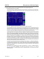
Fig. 2-14
Measurement of the R&S FSU’s intrinsic noise power in a 1.23 MHz channel
bandwidth.
5. Stabilizing the measurement result by increasing the sweep time
➢ Press the SWEEP TIME softkey and enter 1 s.
By increasing the sweep time to 1 s, the trace becomes much smoother thanks to the RMS detector
and the channel power measurement display is much more stable.
6. Referring the measured channel power to a bandwidth of 1 Hz
➢ Press the CHAN PWR / Hz softkey.
The channel power is referred to a bandwidth of 1 Hz. The measurement is corrected by -10 · log
(ChanBW), with ChanBW being the channel bandwidth that was selected.
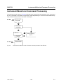
Method of calculating the channel power
When measuring the channel power, the R&S FSU integrates the linear power which corresponds to the
levels of the pixels within the selected channel. The Spectrum Analyzer uses a resolution bandwidth which
is far smaller than the channel bandwidth. When sweeping over the channel, the channel filter is formed
by the passband characteristics of the resolution bandwidth (see Fig. 2-15).
-3 dB
Resolution filter
Sweep
Channel bandwith
Fig. 2-15
Approximating the channel filter by sweeping with a small resolution bandwidth
1166.1725.12
2.21
E-2
Noise Measurements
R&S FSU
The following steps are performed:
•
The linear power of all the trace pixels within the channel is calculated.
Pi = 10(Li/10)
where
Pi = power of the trace pixel i
Li = displayed level of trace point i
•
The powers of all trace pixels within the channel are summed up and the sum is divided by the number
of trace pixels in the channel.
•
The result is multiplied by the quotient of the selected channel bandwidth and the noise bandwidth of
the resolution filter (RBW).
Since the power calculation is performed by integrating the trace within the channel bandwidth, this
method is also called the IBW method (Integration Bandwidth method).
Bandwidth selection (RBW)
For channel power measurements, the resolution bandwidth (RBW) must be small compared to the
channel bandwidth, so that the channel bandwidth can be defined precisely. If the resolution bandwidth
which has been selected is too wide, this may have a negative effect on the selectivity of the simulated
channel filter and result in the power in the adjacent channel being added to the power in the transmit
channel. A resolution bandwidth equal to 1% to 3% of the channel bandwidth should, therefore, be
selected. If the resolution bandwidth is too small, the required sweep time becomes too long and the
measurement time increases considerably.
Detector selection
Since the power of the trace is measured within the channel bandwidth, only the sample detector and
RMS detector can be used. These detectors provide measured values that make it possible to calculate
the real power. The peak detectors (Pos Peak, Neg Peak and Auto Peak) are not suitable for noise power
measurements as no correlation can be established between the peak value of the video voltage and
power.
With the sample detector, a value (sample) of the IF envelope voltage is displayed at each trace pixel.
Since the frequency spans are very large compared with the resolution bandwidth (span/RBW >500),
sinewave signals present in the noise might be lost, i.e. they are not displayed. This is not important for
pure noise signals, however, since a single sample in itself is not important - it is the probability distribution
of all measured values that counts. The number of samples for power calculation is limited to the number
of trace pixels (625 for the R&S FSU).
Aa
Note
To increase the repeatability of measurements, averaging is often carried out over
several traces (AVERAGE softkey in the TRACE menu). This gives spurious
results for channel power measurements (max. –2.51 dB for ideal averaging).
Trace averaging should, therefore, be avoided.
With the RMS detector, the whole IF envelope is used to calculate the power for each trace pixel. The IF
envelope is digitized using a sampling frequency which is at least five times the resolution bandwidth
which has been selected. Based on the sample values, the power is calculated for each trace pixel using
the following formula:
1166.1725.12
2.22
E-2
R&S FSU
P RMS =
Noise Measurements
1
---- ×
N
N
2
∑ si
i=1
si = linear digitized video voltage at the output of the A/D converter
N = number of A/D converter values per pixel of the trace
PRMS = power represented by a trace pixel
When the power has been calculated, the power units are converted into decibels and the value is
displayed as a trace pixel.
The number of A/D converter values, N, used to calculate the power, is defined by the sweep time. The
time per trace pixel for power measurements is directly proportional to the selected sweep time. The RMS
detector uses far more samples for power measurement than the sample detector, especially if the sweep
time is increased. The measurement uncertainty can be reduced considerably. In the default setting, the
R&S FSU therefore uses the RMS detector to measure the channel power.
For both detectors (sample and RMS), the video bandwidth (VBW) must at least be three times the
resolution bandwidth, so that the peak values of the video voltage are not cut off by the video filter. At
smaller video bandwidths, the video signal is averaged and the power readout will be too small.
Sweep time selection
If the sample detector is used, it is best to select the smallest sweep time possible for a given span and
resolution bandwidth. The minimum time is obtained if the setting is coupled. This means that the time per
measurement is minimal. Extending the measurement time does not have any advantages as the number
of samples for calculating the power is defined by the number of trace pixels in the channel.
When using the RMS detector, the repeatability of the measurement results can be influenced by the
selection of sweep times. Repeatability is increased at longer sweep times.
Repeatability can be estimated from the following diagram:
max. error/dB
0
95 % Confidence
level
0.5
1
99 % Confidence
level
1.5
2
2.5
3
10
Fig. 2-16
100
1000
10000
100000
Number of samples
Repeatability of channel power measurements as a function of the number of samples used
for power calculation
1166.1725.12
2.23
E-2
Noise Measurements
R&S FSU
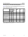
The curves in Fig. 2-16 indicates the repeatability obtained with a probability of 95% and 99% depending
on the number of samples used.
The repeatability with 600 samples is ± 0.5 dB. This means that – if the sample detector and a channel
bandwidth over the whole diagram (channel bandwidth = span) is used - the measured value lies within ±
0.5 dB of the true value with a probability of 99%.
If the RMS detector is used, the number of samples can be estimated as follows:
Since only uncorrelated samples contribute to the RMS value, the number of samples can be calculated
from the sweep time and the resolution bandwidth.
Samples can be assumed to be uncorrelated if sampling is performed at intervals of 1/RBW. The number
of uncorrelated samples (Ndecorr) is calculated as follows:
Ndecorr = SWT × RBW
The number of uncorrelated samples per trace pixel is obtained by dividing Ndecorr by 625 (= pixels per
trace).
Example:
At a resolution bandwidth of 30 kHz and a sweep time of 100 ms, 3000 uncorrelated samples are
obtained. If the channel bandwidth is equal to the frequency display range, i.e. all trace pixels are used
for the channel power measurement, a repeatability of 0.2 dB with a confidence level of 99% is the
estimate that can be derived from Fig. 2-16.
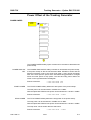
Measuring Phase Noise
The R&S FSU has an easy-to-use marker function for phase noise measurements. This marker function
indicates the phase noise of an RF oscillator at any carrier in dBc in a bandwidth of 1 Hz.
Measurement Example – Measuring the phase noise of a signal
generator at a carrier offset of 10 kHz
Test setup:
Signal
generator
FSU
Settings on the signal generator (e.g. R&S SMIQ):
Frequency:
100 MHz
Level:
0 dBm
1166.1725.12
2.24
E-2
R&S FSU
Noise Measurements
Measurement using R&S FSU:
1. Set the Spectrum Analyzer to its default state
➢ Press the PRESET key.
R&S FSU is in its default state.
2. Set the center frequency to 100 MHz and the span to 50 kHz
➢ Press the FREQ key and enter 100 MHz.
➢ Press the SPAN key and enter 50 kHz.
3. Set the R&S FSU’s reference level to 0 dBm (=signal generator level)
➢ Press the AMPT key and enter 0 dBm.
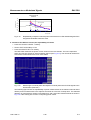
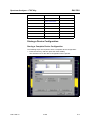
4. Enable phase noise measurement
➢ Press the MKR FCTN key.
➢ Press the PHASE NOISE ! softkey.
The R&S FSU activates phase noise measurement. Marker 1 (=main marker) and marker 2 (= delta
marker) are positioned on the signal maximum. The position of the marker is the reference (level
and frequency) for the phase noise measurement. A horizontal line represents the level of the
reference point and a vertical line the frequency of the reference point. Data entry for the delta
marker is activated so that the frequency offset at which the phase noise is to be measured can be
entered directly.
5. 10 kHz frequency offset for determining phase noise.
➢ Enter 10 kHz.
The R&S FSU displays the phase noise at a frequency offset of 10 kHz. The magnitude of the
phase noise in dBc/Hz is displayed in the delta marker output field at the top right of the screen
(delta 2 [T1 PHN]).
6. Stabilize the measurement result by activating trace averaging.
➢ Press the TRACE key.
➢ Press the AVERAGE softkey.
Fig. 2-17
1166.1725.12
Measuring phase noise with the phase-noise marker function
2.25
E-2
Noise Measurements
R&S FSU
The frequency offset can be varied by moving the marker with the spinwheel or by entering a new
frequency offset as a number.
1166.1725.12
2.26
E-2
R&S FSU
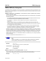
Measurements on Modulated Signals
Measurements on Modulated Signals
If RF signals are used to transmit information, an RF carrier is modulated. Analog modulation methods
such as amplitude modulation, frequency modulation and phase modulation have a long history and
digital modulation methods are now used for modern systems. Measuring the power and the spectrum of
modulated signals is an important task to assure transmission quality and to ensure the integrity of other
radio services. This task can be performed easily with a Spectrum Analyzer. Modern Spectrum Analyzers
also provide the test routines that are essential to simplify complex measurements.
1166.1725.12
2.27
E-2
Measurements on Modulated Signals
R&S FSU
Measurements on AM signals
The Spectrum Analyzer detects the RF input signal and displays the magnitudes of its components as a
spectrum. AM modulated signals are also demodulated by this process. The AF voltage can be displayed
in the time domain if the modulation sidebands are within the resolution bandwidth. In the frequency
domain, the AM sidebands can be resolved with a small bandwidth and can be measured separately. This
means that the modulation depth of a carrier modulated with a sinewave signal can be measured. Since
the dynamic range of a Spectrum Analyzer is very wide, even extremely small modulation depths can be
measured accurately. The R&S FSU has a test routine which measures the modulation depth in %.
Measurement Example 1 – Displaying the AF of an AM signal in the
time domain
Test setup:
Signal
generator
FSU
Settings on the signal generator (e.g. R&S SMIQ):
Frequency:
100 MHz
Level:
0 dBm
Modulation:
50 % AM, 1 kHz AF
Measurement with the R&S FSU:
1. Set the Spectrum Analyzer to its default state
➢ Press the PRESET key.
The R&S FSU is in its default state.
2. Set the center frequency to 100 MHz and the span to 0 kHz
➢ Press the FREQ key and enter 100 MHz.
➢ Press the SPAN key and enter 0 Hz.
3. Set the reference level to +6 dBm and the display range to linear
➢ Press the AMPT key and enter 6 dBm.
➢ Press the RANGE LINEAR softkey.
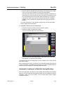
4. Use the video trigger to trigger on the AF signal in order to obtain a stationary display
➢ Press the TRIG key.
➢ Press the VIDEO softkey.
The video trigger level is set to 50% if the instrument is switched on for the first time. The trigger
level is displayed as a horizontal line across the graph. The R&S FSU displays the 1 kHz AF signal
stably in the time domain.
1166.1725.12
2.28
E-2
R&S FSU
Fig. 2-18
Measurements on Modulated Signals
Measuring the AF signal from a 1 kHz AM carrier
The AM/FM demodulator in the R&S FSU can be used to output the AF by means of a loudspeaker.
5. Switch on the internal AM demodulator
➢ Press the MKR FCTN key.
➢ Press the MKR DEMOD softkey.
The R&S FSU switches the AM demodulator on automatically.
➢ Turn up volume control.
A 1 kHz tone is output by the loudspeaker.
Measurement Example 2 – Measuring the modulation depth of an AM
carrier in the frequency domain
Test setup:
Signal
generator
FSU
Settings on the signal generator (e.g. R&S SMIQ):
Frequency:
100 MHz
Level:
-30 dBm
Modulation:
50 % AM, 1 kHz AF
Measurement with the R&S FSU:
1. Set the Spectrum Analyzer to its default state
➢ Press the PRESET key.
The R&S FSU is in its default state.
1166.1725.12
2.29
E-2
Measurements on Modulated Signals
R&S FSU
2. Set the center frequency to 100 MHz and the span to 0 kHz
➢ Press the FREQ key and enter 100 MHz.
➢ Press the SPAN key and enter 5 kHz.
3. Activate the marker function for AM depth measurement
➢ Press the MEAS key.
➢ Press the MODULATION DEPTH softkey.
The R&S FSU automatically positions a marker on the carrier signal in the middle of the graph and
one delta marker on each of the lower and upper AM sidebands. The R&S FSU calculates the AM
modulation depth from the ratios of the delta marker levels to the main marker level and outputs the
numerical value in the marker info field
Fig. 2-19
1166.1725.12
Measurement of AM modulation depth. The modulation depth is indicated by
MDEPTH = 49.345 %. The frequency of the AF signal is indicated by the delta markers
2.30
E-2
R&S FSU
Measurements on Modulated Signals
Measurements on FM Signals
Since Spectrum Analyzers only display the magnitude of signals by means of the envelope detector, the
modulation of FM signals cannot be directly measured as is the case with AM signals. With FM signals,
the voltage at the output of the envelope detector is constant as long as the frequency deviation of the
signal is within the flat part of the passband characteristic of the resolution filter which has been selected.
Amplitude variations can only occur if the current frequency lies on the falling edge of the filter
characteristic. This effect can be used to demodulate FM signals. The center frequency of the Spectrum
Analyzer is set in a way that the nominal frequency of the test signal is on the filter edge (below or above
the center frequency). The resolution bandwidth and the frequency offset are selected in a way that the
current frequency is on the linear part of the filter slope. The frequency variation of the FM signal is then
transformed into an amplitude variation which can be displayed in the time domain.
The R&S FSU's analog 5th order filters with frequencies from 200 kHz to 3 MHz have a good filter-slope
linearity, if the frequency of the R&S FSU is set to 1.2 times the filter bandwidth below or above the
frequency of the transmit signal. The useful range for FM demodulation is then almost equal to the
resolution bandwidth.
Measurement Example – Displaying the AF of an FM carrier
Test setup:
Signal
generator
FSU
Settings on the signal generator (e.g. R&S SMIQ):
Frequency:
100 MHz
Level:
-30 dBm
Modulation:
FM 0 kHz deviation (i.e., FM = off), 1 kHz AF
Measurement with the R&S FSU:
1. Set the Spectrum Analyzer to its default state
➢ Press the PRESET key.
The R&S FSU is in its default state.
2. Set the center frequency to 99.64 MHz and the span to 300 kHz.
➢ Press the FREQ key and enter 99.64 MHz.
➢ Press the SPAN key and enter 300 kHz.
3. Set a resolution bandwidth of 300 kHz.
➢ Press the BW key.
➢ Press the RES BW MANUAL softkey and enter 300 kHz.
1166.1725.12
2.31
E-2
Measurements on Modulated Signals
R&S FSU
4. Set a display range of 20 dB and shift the filter characteristics to the middle of the display.
➢ Press the AMPT key.
➢ Press the RANGE LOG MANUAL softkey and enter 20 dB.
➢ Press the NEXT key.
➢ Set the GRID softkey to REL.
➢ Press the PREV softkey.
➢ Using the spinwheel, shift the reference level so that the filter edge intersects the - 10 dB level line
at the center frequency.
The slope of the 300 kHz filter is displayed. This corresponds to the demodulator characteristics for
FM signals with a slope of approx. 5 dB/100 kHz.
Fig. 2-20
Filter edge of a 300 kHz filter used as an FM-discriminator characteristic
5. Set an FM deviation of 100 kHz and an AF of 1 kHz on the signal generator
6. Set a frequency deviation of 0 Hz on the R&S FSU
➢ Press the SPAN key.
➢ Press the ZERO SPAN.
The demodulated FM signal is displayed. The signal moves across the screen.
7. Creating a stable display by video triggering
➢ Press the TRIG key.
➢ Press the VIDEO softkey.
A stationary display is obtained for the FM AF signal
Result: (-10 ±5) dB; this means that a deviation of 100 kHz is obtained if the demodulator characteristic
slope is 5 dB/100 kHz
1166.1725.12
2.32
E-2
R&S FSU
Fig. 2-21
Measurements on Modulated Signals
Demodulated FM signal
Measuring Channel Power and Adjacent Channel Power
Measuring channel power and adjacent channel power is one of the most important tasks in the field of
digital transmission for a Spectrum Analyzer with the necessary test routines. While, theoretically, channel
power could be measured at highest accuracy with a power meter, its low selectivity means that it is not
suitable for measuring adjacent channel power as an absolute value or relative to the transmit channel
power. The power in the adjacent channels can only be measured with a selective power meter.
A Spectrum Analyzer cannot be classified as a true power meter, because it displays the IF envelope
voltage. However, it is calibrated such as to correctly display the power of a pure sinewave signal
irrespective of the selected detector. This calibration is not valid for non-sinusoidal signals. Assuming that
the digitally modulated signal has a Gaussian amplitude distribution, the signal power within the selected
resolution bandwidth can be obtained using correction factors. These correction factors are normally used
by the Spectrum Analyzer's internal power measurement routines in order to determine the signal power
from IF envelope measurements. These factors are valid if and only if the assumption of a Gaussian
amplitude distribution is correct.
Apart from this common method, the R&S FSU also has a true power detector, i.e. an RMS detector. It
correctly displays the power of the test signal within the selected resolution bandwidth irrespective of the
amplitude distribution, without additional correction factors being required. With an absolute
measurement uncertainty of < 0.3 dB and a relative measurement uncertainty of < 0.1 dB (each with a
confidence level of 95%), the R&S FSU comes close to being a true power meter.
There are two possible methods for measuring channel and adjacent channel power with a Spectrum
Analyzer:
The IBW method (Integration Bandwidth Method) in which the Spectrum Analyzer measures with a
resolution bandwidth that is less than the channel bandwidth and integrates the level values of the trace
versus the channel bandwidth. This method is described in the section on noise measurements.
Measurement using a channel filter.
In this case, the Spectrum Analyzer makes measurements in the time domain using an IF filter that
corresponds to the channel bandwidth. The power is measured at the output of the IF filter. Until now, this
method has not been used for Spectrum Analyzers, because channel filters were not available and the
resolution bandwidths, optimized for the sweep, did not have a sufficient selectivity. The method was
reserved for special receivers optimized for a particular transmission method.
1166.1725.12
2.33
E-2
Measurements on Modulated Signals
R&S FSU
The R&S FSU has test routines for simple channel and adjacent channel power measurements. These
routines give quick results without any complex or tedious setting procedures.
Measurement Example 1 – ACPR measurement on an IS95 CDMA
Signal
Test setup:
Signal
generator
FSU
Settings on the signal generator (e.g. R&S SMIQ):
Frequency:
850 MHz
Level:
0 dBm
Modulation:
CDMA IS 95
Measurement with the R&S FSU:
1. Set the Spectrum Analyzer to its default state.
➢ Press the PRESET key.
The R&S FSU is in its default state.
2. Set the center frequency to 850 MHz and frequency deviation to 4 MHz.
➢ Press the FREQ key and enter 850 MHz.
3. Set the reference level to +10 dBm.
➢ Press the AMPT key and enter 10 dBm.
4. Configuring the adjacent channel power for the CDMA IS95 reverse link.
➢ Press the MEAS key.
➢ Press the CHAN PWR ACP ! softkey.
➢ Press the CP/ACP STANDARD softkey.
From the list of standards, select CDMA IS95A REV using the spinwheel or the cursor down key
below the spinwheel and press ENTER.
The R&S FSU sets the channel configuration according to the IS95 standard for mobile stations
with 2 adjacent channels above and below the transmit channel. The spectrum is displayed in the
upper part of the screen, the numeric values of the results and the channel configuration in the
lower part of the screen. The various channels are represented by vertical lines on the graph.
The frequency span, resolution bandwidth, video bandwidth and detector are selected
automatically to give correct results. To obtain stable results - especially in the adjacent channels
(30 kHz bandwidth) which are narrow in comparison with the transmission channel bandwidth (1.23
MHz) - the RMS detector is used.
1166.1725.12
2.34
E-2
R&S FSU
Measurements on Modulated Signals
5. Set the optimal reference level and RF attenuation for the applied signal level.
➢ Press the ADJUST REF LVL softkey.
The R&S FSU sets the optimal RF attenuation and the reference level based on the transmission
channel power to obtain the maximum dynamic range. The following figure shows the result of the
measurement.
Fig. 2-22
Adjacent channel power measurement on a CDMA IS95 signal
The repeatability of the results, especially in the narrow adjacent channels, strongly depends on the
measurement time since the dwell time within the 10 kHz channels is only a fraction of the complete
sweep time. A longer sweep time may increase the probability that the measured value converges
to the true value of the adjacent channel power, but this increases measurement time.
To avoid long measurement times, the R&S FSU measures the adjacent channel power in the time
domain (FAST ACP). In the FAST ACP mode, the R&S FSU measures the power of each channel
at the defined channel bandwidth, while being tuned to the center frequency of the channel in
question. The digital implementation of the resolution bandwidths makes it possible to select a filter
characteristics that is precisely tailored to the signal. In case of CDMA IS95, the power in the useful
channel is measured with a bandwidth of 1.23 MHz and that of the adjacent channels with a
bandwidth of 30 kHz. Therefore the R&S FSU jumps from one channel to the other and measures
the power at a bandwidth of 1.23 MHz or 30 kHz using the RMS detector. The measurement time
per channel is set with the sweep time. It is equal to the selected measurement time divided by the
selected number of channels. The five channels from the above example and the sweep time of
100 ms give a measurement time per channel of 20 ms.
Compared to the measurement time per channel given by the span (= 5.1 MHz) and sweep time
(= 100 ms, equal to 1.66 ms per 30 kHz channel) used in the example, this is a far longer dwell time
on the adjacent channels (factor of 12). In terms of the number of uncorrelated samples this means
20000/33 µs = 606 samples per channel measurement compared to 1667/33µs = 50.5 samples per
channel measurement.
Repeatability with a confidence level of 95% is increased from ± 1.4 dB to ± 0.38 dB as shown in
Fig. 2-16. For the same repeatability, the sweep time would have to be set to 1.2 s with the
integration method. The following figure shows the standard deviation of the results as a function
of the sweep time.
1166.1725.12
2.35
E-2
Measurements on Modulated Signals
R&S FSU
ACPR Repeatability IS95
IBW Method
1,4
Standard dev / dB
1,2
1
Adjacent channels
0,8
Alternate channels
0,6
0,4
Tx channel
0,2
0
10
100
1000
Sweep time/ms
Fig. 2-23
Repeatability of adjacent channel power measurement on IS95-standard signals if the
integration bandwidth method is used
6. Switch to Fast ACP to increase the repeatability of results.
➢ Press the CP/ACP CONFIG ! softkey.
➢ Set the FAST ACP softkey to ON.
➢ Press the ADJUST REF LVL softkey.
The R&S FSU measures the power of each channel in the time domain. The trace represents
power as a function of time for each measured channel (see Fig. 2-24). The numerical results from
consecutive measurements are much more stable.
Fig. 2-24
Measuring the channel power and adjacent channel power ratio for IS95 signals in the
time domain (Fast ACP)
The following figure shows the repeatability of power measurements in the transmit channel and of
relative power measurements in the adjacent channels as a function of sweep time. The standard
deviation of measurement results is calculated from 100 consecutive measurements as shown in
Fig. 2-23. Take scaling into account if comparing power values.
1166.1725.12
2.36
E-2
R&S FSU
Measurements on Modulated Signals
ACPR IS95 Repeatability
0,35
Standard dev /dB
0,3
0,25
0,2
Adjacent channels
0,15
0,1
Tx channel
0,05
Alternate channels
0
10
100
1000
Sweep time/ms
Fig. 2-25
Aa
Repeatability of adjacent channel power measurements on IS95 signals in the Fast
ACP mode
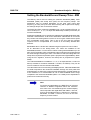
Note on adjacent channel power measurements on IS95 base-station
signals:
When measuring the adjacent channel power of IS95 base-station signals, the
frequency spacing of the adjacent channel to the nominal transmit channel is
specified as ±750 kHz. The adjacent channels are, therefore, so close to the
transmit channel that the power of the transmit signal leaks across and is also
measured in the adjacent channel if the usual method using the 30 kHz resolution
bandwidth is applied. The reason is the low selectivity of the 30 kHz resolution filter.
The resolution bandwidth, therefore, must be reduced considerably, e.g. to 3 kHz
to avoid this. This causes very long measurement times (factor of 100 between a
30 kHz and 3 kHz resolution bandwidth).
This effect is avoided with the time domain method which uses steep IF filters. The
30 kHz channel filter implemented in the R&S FSU has a very high selectivity so
that even with a ± 750 kHz spacing to the transmit channel the power of the useful
modulation spectrum is not measured.
The following figure shows the passband characteristics of the 30 kHz channel filter in the R&S FSU.
Fig. 2-26
Frequency response of the 30 kHz channel filter for measuring the power in the IS 95
adjacent channel
1166.1725.12
2.37
E-2
Measurements on Modulated Signals
R&S FSU
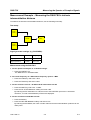
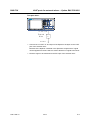
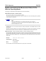
Measurement Example 2 – Measuring the adjacent channel power of
an IS136 TDMA signal
Test setup:
Signal
generator
RF Inp
FSU
Ext Ref IN
Ext Ref Out
Aa
Note
As the modulation spectrum of the IS136 signal leaks into the adjacent channel, it
makes a contribution to the power in the adjacent channel. Exact tuning of the
Spectrum Analyzer to the transmit frequency is therefore critical. If tuning is not
precise, the adjacent channel power ratios in the lower and upper adjacent
channels become asymmetrical. The R&S FSU’s frequency and the generator
frequency are therefore synchronized.
Settings on the signal generator (e.g. R&S SMIQ):
Frequency:
850 MHz
Level:
-20 dBm
Modulation:
IS136/NADC
Measurement with the R&S FSU
1. Set the Spectrum Analyzer to its default state.
➢ Press the PRESET key.
The R&S FSU is in its default state.
2. Set up the R&S FSU for synchronization to an external reference frequency.
➢ Press the SETUP key.
➢ Set the REFERENCE softkey to EXT.
3. Set the center frequency to 850 MHz.
Press the FREQ key and enter 850 MHz.
4. Configure adjacent channel power measurement for IS136 signals.
➢ Press the MEAS key.
➢ Press the CHAN PWR ACP ! softkey.
➢ Press the CP/ACP STANDARD softkey.
1166.1725.12
2.38
E-2
R&S FSU
Measurements on Modulated Signals
➢ Select NADC IS136 from the list of standards and press ENTER.
The R&S FSU performs the power measurement in 5 channels (in the useful channel and in the
two upper and two lower adjacent channels).
5. Setting the optimum reference level and RF attenuation for the measurement
➢ Press the ADJUST REF LEVEL softkey.
The R&S FSU sets the optimum RF attenuation and the optimum reference level on the basis of
the measured channel power.
Fig. 2-27
Measuring the relative adjacent channel power of an NADC signal in each of the two
adjacent channels below and above the transmit channel.
To increase repeatability – especially in the adjacent channels – the R&S FSU’s Fast ACP routine is
recommended.
6. Switching on the Fast ACP routine.
➢ Press the CP/ACP CONFIG ! softkey
➢ Set the FAST ACP softkey to ON.
➢ Press the ADJUST REF LEVEL softkey.
The R&S FSU makes consecutive measurements on the 5 channels in the zero span mode using
the receive filter specified in IS 136 to define the resolution bandwidth. The power in each channel
is displayed on the graph as a function of time.
1166.1725.12
2.39
E-2
Measurements on Modulated Signals
Fig. 2-28
R&S FSU
Measuring adjacent channel power in time domain (Fast ACP)
As the resolution bandwidth is much wider than the one used for the integration method, the results
are much more stable when compared at the same sweep time.
Repeatability can be influenced by the selected sweep time. The results become much more stable
if long sweep times are selected. Since the amplitude distribution is different in different channels
(part of the modulation spectrum falls within the first adjacent channel), the repeatability depends
on the spacing of the measured channel from the transmit channel.
Fig. 2-29 below shows the standard deviation of results in the different channels as a function of
the selected sweep time. The standard deviation for the various sweep times was recorded using
a signal generator as a source. With real DUTs the amplitude distributions in adjacent channels may
be different so that the standard deviation could differ from that shown in Fig. 2-29. To evaluate the
correct measuring time for time-critical measurements at a given standard deviation, the standard
deviation of the ACP values at the output of the real DUT must be determined.
NADC Repeatability
1.4
Standard Deviation / dB
1.2
1
0.8
Adj Channels
Alt1 Channels
0.6
0.4
Tx Channel
0.2
0
10
100
1000
Sweep Time / ms
Fig. 2-29
1166.1725.12
Standard deviation of the results of Fast ACP measurement as a function of selected
sweep time evaluated from 100 measurements per sweep time
2.40
E-2
R&S FSU
Measurements on Modulated Signals
Measurement Example 3 – Measuring the Modulation Spectrum in
Burst Mode with the Gated Sweep Function
Since transmission systems compliant to IS136 use a TDMA method, the adjacent channel power must
also be measured in burst mode. An IS136 TDMA frame is divided into 6 time slots. Two of these slots
are assigned to a subscriber. This means that the ratio of transmit time to off-time for IS136 mobile phones
is only 1:3 (e.g. time slots 1 and 4)
The R&S FSU supports the measurement of the adjacent channel power in the TDMA mode with the
Gated Sweep function.
Test setup with the R&S Signal Generator SMIQ:
SMIQ-Z5
Trigger1
Ext Gate/Trig IN
Par Data Output
Signal
generator
SMIQ
RF Inp
Ext Ref Out
FSU
Ext Ref IN
The R&S SMIQ has to be equipped with options R&S SMIQ-B10 or R&S SMIQ-B20 (modulation coder)
and R&S SMIQ-B11 (data generator).
Option R&S SMIQ-Z5 is required to trigger the R&S FSU. This option is connected to the R&S SMIQ’s
parallel output port. The BNC output Trigger 1 of the R&S SMIQ-Z5 provides a TTL trigger signal on the
rising edge of the IS136 burst, which is used to start the R&S FSU sweep in the Gated Sweep mode.
Aa
Note
The R&S FSU’s IF power trigger is not suitable for IS136. It triggers on every level
edge of the input signal. Since the modulation of the IS136 signal causes level dips
even during the transmit burst, there is no way of ensuring that the R&S FSU is
only triggered on the burst edge.
Settings on signal generator R&S SMIQ:
Switch the signal generator to the IS136 burst mode (time slots 1 and 4 are switched on, the other time
slots are switched off).
The R&S SMIQ is set as follows to generate the signal:
➢ Press the PRESET key.
➢ Press the FREQ key and enter 850 MHz.
➢ Press the LEVEL key and enter -20 dBm.
➢ Press the RETURN key.
➢ Select DIGITAL STANDARD using the spinwheel and press the SELECT key.
➢ Select NADC using the spinwheel and press the SELECT key.
1166.1725.12
2.41
E-2
Measurements on Modulated Signals
R&S FSU
➢ Press the SELECT key.
➢ Select ON using the spinwheel and press the SELECT key.
➢ Press the RETURN key.
➢ Keep turning the spinwheel until SAVE/RECALL FRAME appears in the list and select the menu item
SAVE/RECALL FRAME using the SELECT key.
➢ The cursor is set to GET PREDEFINED FRAME.
➢ Press the SELECT key.
➢ Select UP1TCH using the spinwheel and press the SELECT key.
In the following operating sequence for the R&S FSU, it is assumed that steps 1 to 6 of the previous
example (example no. 2) have already been performed.
1. Configuring the Gated Sweep function on the R&S FSU.
➢ Press the TRIG key.
➢ Press the GATED TRIGGER softkey.
➢ Press the EXTERN softkey.
➢ Press the GATE SETTINGS ! softkey.
The R&S FSU switches to time domain measurement so that the setting of the Gated Sweep
parameters can be checked visually.
➢ Press the SWEEPTIME softkey and enter 10 ms.
Exactly one TDMA burst will be displayed.
➢ Press the GATE DELAY softkey and enter 2 ms or set the Gate Delay using the spinwheel so that
the burst is reliably detected.
➢ Press the GATE LENGTH softkey and enter 5 ms or set the vertical line for the gate length using
the spinwheel so that the burst is reliably detected.
Fig. 2-30
Setting the parameters Gate Delay and Gate Length in time domain. The time interval
required to measure the spectrum is indicated by two vertical lines.
➢ Press the PREV key.
The R&S FSU now performs the ACP measurement only during the switch-on phase of the TDMA
burst. The measurement is stopped during the switch-off phase.
1166.1725.12
2.42
E-2
R&S FSU
Aa
Measurements on Modulated Signals
Note
The selected sweep time is the net sweep time, i.e. the time during which the
R&S FSU is actually measuring. The complete frame of an IS136 signal takes 40
ms. In the above example, measurement only takes place for 2x5 ms within a
frame. The R&S FSU is therefore only measuring for 25% of the frame duration.
The total measuring time is therefore four times that for the CW mode.
Measurement Example 4 – Measuring the Transient Spectrum in Burst
Mode with the Fast ACP function
In addition to the modulation spectrum or adjacent channel power from the modulation of the RF carrier,
the spectrum or adjacent channel power generated by burst edges is also to be measured in TDMA
systems. The spectrum is a pulse spectrum and must be measured with the peak detector. With the usual
IBW method, only the power of the continuously modulated signal can be measured properly. Even if the
modulation spectrum is transmitted in the TDMA mode, the measurement of the modulation spectrum will
work because the burst edges are blanked out for the measurement by means of the Gated Sweep
function. The Spectrum Analyzer performs measurements only if the modulation spectrum is continuous
when the burst is on.
However, the IBW method fails for the spectrum created by the burst edges. As the measurement is
carried out with resolution bandwidths that are very small compared to the signal bandwidth, a spurious
amplitude distribution is obtained in the defined measurement channel because of the resolution
bandwidth. The small resolution bandwidth cannot settle to the peak amplitudes of the test signal. This
problem is avoided in the R&S FSU by performing time domain measurements with the root raised cosine
filter specified in the IS136 standard.
If the peak detector is used instead of the default RMS detector (which is selected when the standard is
selected), the true adjacent channel power generated by the burst edges can also be measured.
Test setup:
The test setup for this example and the settings for R&S SMIQ are identical to those in the previous
example.
Measurement with the R&S FSU:
1. Set the Spectrum Analyzer to its default state.
➢ Press the PRESET key.
The R&S FSU is in its default state.
2. Synchronize the R&S FSU to an external reference frequency.
➢ Press the SETUP key.
➢ Set the REFERENCE softkey to EXT.
3. Set the center frequency to 850 MHz
➢ Press the FREQ key and enter 850 MHz.
1166.1725.12
2.43
E-2
Measurements on Modulated Signals
R&S FSU
4. Configure the adjacent channel power measurement for IS136 signals in Fast ACP mode.
➢ Press the MEAS key.
➢ Press the CHAN PWR ACP ! softkey.
➢ Press the CP/ACP STANDARD softkey.
➢ Select NADC IS136 from the list of standards and press ENTER.
➢ Press the CP/ACP CONFIG ! softkey.
➢ Set the FAST ACP softkey to ON.
The R&S FSU performs the power measurement in 5 channels (in the useful channel and in the
two upper and lower adjacent channels).
5. Set the optimum reference level and RF attenuation for the measurement.
➢ Press the ADJUST REF LEVEL softkey.
The R&S FSU sets the optimum RF attenuation and the optimum reference level on the basis of
the measured channel power.
6. Select the peak detector and increase the sweep time to 10 s.
➢ Press the TRACE key.
➢ Press the DETECTOR softkey.
➢ Press the DETECTOR MAX PEAK softkey.
➢ Press the SWEEP key.
➢ Press the SWEEP TIME softkey and enter 10 s.
The R&S FSU measures the adjacent channel power generated by the burst edges and the
modulation.
Fig. 2-31
1166.1725.12
Adjacent channel power due to modulation spectrum and transient spectrum
2.44
E-2
R&S FSU
Aa
Measurements on Modulated Signals
Note
The peak power display depends on the selected sweep time. The longer the
sweep time, the higher the probability of measuring the highest peak amplitude of
the signal.
With shorter sweep times, level dips can be seen in the time domain traces. These
level dips come from the burst characteristics of the signal. The numerical results,
however, indicate the peak amplitudes during the measurement in the
corresponding channel.
Measurement Example 5 – Measuring adjacent channel power of a WCDMA uplink signal
Test setup:
Signal
generator
FSU
Settings on the signal generator (e.g. R&S SMIQ):
Frequency:
1950 MHz
Level:
4 dBm
Modulation:
3 GPP W-CDMA Reverse Link
Measurement with the R&S FSU:
1. Set the Spectrum Analyzer to its default state.
➢ Press the PRESET key.
The R&S FSU is in its default state.
2. Set the center frequency to 1950 MHz.
➢ Press the FREQ key and enter 1950 MHz.
3. Switch on the ACP measurement for W-CDMA.
➢ Press the MEAS key.
➢ Press the CHAN PWR ACP ! softkey.
➢ Press the CP/ACP STANDARD softkey.
1166.1725.12
2.45
E-2
Measurements on Modulated Signals
R&S FSU
➢ From the list of standards, select W-CDMA 3GPP REV using the spinwheel or the cursor down key
below the spinwheel and press ENTER.
The R&S FSU sets the channel configuration to the 3GPP W-CDMA standard for mobiles with two
adjacent channels above and below the transmit channel. The frequency span, the resolution and
video bandwidth and the detector are automatically set to the correct values. The spectrum is
displayed in the upper part of the screen and the channel power, the level ratios of the adjacent
channel powers and the channel configuration in the lower part of the screen. The individual
channels are displayed as vertical lines on the graph.
4. Set the optimum reference level and the RF attenuation for the applied signal level.
➢ Press the ADJUST REF LEVEL softkey.
The R&S FSU sets the optimum RF attenuation and the reference level for the power in the
transmission channel to obtain the maximum dynamic range. The following figure shows the result
of the measurement:
Fig. 2-32
Measuring the relative adjacent channel power on a W-CDMA uplink signal
5. Measuring adjacent channel power with the Fast ACP method.
➢ Press the CP/ACP CONFIG ! softkey.
➢ Set FAST ACP softkey to ON.
➢ Press the ADJUST REF LVL softkey.
The R&S FSU measures the power of the individual channels in the time domain. A root raised
cosine filter with the parameters α = 0.22 and chip rate 3.84 Mcps (= receive filter for 3GPP WCDMA) is used as the channel filter.
1166.1725.12
2.46
E-2
R&S FSU
Fig. 2-33
Aa
Measurements on Modulated Signals
Measuring the adjacent channel power of a W-CDMA signal with the Fast ACP
method
Note
With W-CDMA, the R&S FSU’s dynamic range for adjacent channel
measurements is limited by the 14-bit A/D converter. The greatest dynamic range
is, therefore, obtained with the IBW method.
Optimum Level Setting for ACP Measurements on W-CDMA Signals
The dynamic range for ACPR measurements is limited by the thermal noise floor, the phase noise and
the intermodulation (spectral regrowth) of the Spectrum Analyzer. The power values produced by the
R&S FSU due to these factors accumulate linearly. They depend on the applied level at the input mixer.
The three factors are shown in the figure below for the adjacent channel (5 MHz carrier offset)
1166.1725.12
2.47
E-2
Measurements on Modulated Signals
R&S FSU
A C L R /d B c
-5 0
-5 5
-6 0
-6 5
to ta l
ACLR
-7 0
-7 5
s p e c tra l
re g ro w th
th e rm a l
n o is e
-8 0
-8 5
phase
n o is e
-9 0
-2 0
-1 5
-1 0
-5
0
M ixe r le v e l / d B m
Fig. 2-34
The R&S FSU’s dynamic range for adjacent channel power measurements on W-CDMA
uplink signals is a function of the mixer level.
The level of the W-CDMA signal at the input mixer is shown on the horizontal axis, i.e. the measured signal
level minus the selected RF attenuation. The individual components which contribute to the power in the
adjacent channel and the resulting relative level (total ACPR) in the adjacent channel are displayed on
the vertical axis. The optimum mixer level is –10 dBm. The relative adjacent channel power (ACPR) at an
optimum mixer level is –77,5 dBc. Since, at a given signal level, the mixer level is set in 5 dB steps with
the 5 dB RF attenuator, the optimum 5 dB range is shown in the figure: it spreads from –13 dBm to –8
dBm. The obtainable dynamic range in this range is 76 dB.
To set the attenuation parameter manually, the following method is recommended:
•
Set the RF attenuation so that the mixer level (= measured channel power – RF attenuation) is
between -13 dBm and -8 dBm.
•
Set the reference level to the largest possible value where no overload (IFOVLD) is indicated.
This method is automated with the R&S FSU’s ADJUST REF LEVEL function. Especially in remote
control mode, e.g. in production environments, it is best to correctly set the attenuation parameters prior
to the measurement, as the time required for automatic setting can be saved.
Aa
1166.1725.12
Note
To measure the R&S FSU’s intrinsic dynamic range for W-CDMA adjacent channel
power measurements, a filter which suppresses the adjacent channel power is
required at the output of the transmitter. A SAW filter with a bandwidth of 4 MHz,
for example, can be used.
2.48
E-2
R&S FSU
Measurements on Modulated Signals
Amplitude distribution measurements
If modulation types that do not have a constant envelope in the time domain are used, the transmitter has
to handle peak amplitudes that are greater than the average power. This includes all modulation types
that involve amplitude modulation -QPSK for example. CDMA transmission modes in particular may have
power peaks that are large compared to the average power.
For signals of this kind, the transmitter must provide large reserves for the peak power to prevent signal
compression and thus an increase of the bit error rate at the receiver.
The peak power, or the crest factor of a signal is therefore an important transmitter design criterion. The
crest factor is defined as the peak power / mean power ratio or, logarithmically, as the peak level minus
the average level of the signal.
To reduce power consumption and cut costs, transmitters are not designed for the largest power that could
ever occur, but for a power that has a specified probability of being exceeded (e.g. 0.01%).
To measure the amplitude distribution, the R&S FSU has simple measurement functions to determine
both the APD = Amplitude Probability Distribution and CCDF = Complementary Cumulative Distribution
Function.
Aa
Note
In the literature, APD is also used for the probability of amplitude violation. This is
the complimentary function to the APD function of R&S FSU. The term PDF
(=Probability Density Function) which is frequently used in the literature
corresponds to the APD function of R&S FSU.
In the APD display mode, the probability of occurrence of a certain level is plotted against the level.
In the CCDF display mode, the probability that the mean signal power will be exceeded is shown in
percent.
Measurement Example – Measuring the APD and CCDF of white noise
generated by the R&S FSU
1. Set the Spectrum Analyzer to its default state.
➢ Press the PRESET key.
The R&S FSU is in its default state.
2. Configure the R&S FSU for APD measurement
➢ Press the AMPT key and enter -60 dBm.
The R&S FSU’s intrinsic noise is displayed at the top of the screen.
➢ Press the MEAS key.
➢ Press the SIGNAL STATISTIC ! softkey.
➢ Set the APD softkey to ON.
The R&S FSU sets the frequency span to 0 Hz and measures the amplitude probability distribution
(APD). The number of uncorrelated level measurements used for the measurement is 100000. The
mean power and the peak power are displayed in dBm. The crest factor (peak power – mean
power) is output as well (see Fig. 2-35).
1166.1725.12
2.49
E-2
Measurements on Modulated Signals
Fig. 2-35
R&S FSU
Amplitude probability distribution of white noise
3. Switch to the CCDF display mode.
➢ Set the CCDF softkey to ON
The APD measurement is switched off and the CCDF display mode is switched on.
Fig. 2-36
The CCDF of white noise
The CCDF trace indicates the probability that a level will exceed the mean power. The level above
the mean power is plotted along the X axis of the graph. The origin of the axis corresponds to the
mean power level. The probability that a level will be exceeded is plotted along the Y axis.
4. Bandwidth selection
If the amplitude distribution is measured, the resolution bandwidth must be set in a way that the
complete spectrum of the signal to be measured falls within the bandwidth. This is the only way of
ensuring that all the amplitudes will pass through the IF filter without being distorted. If the selected
resolution bandwidth is too small for a digitally modulated signal, the amplitude distribution at the
output of the IF filter becomes a Gaussian distribution according to the central limit theorem and so
corresponds to a white noise signal. The true amplitude distribution of the signal therefore cannot be
determined.
1166.1725.12
2.50
E-2
R&S FSU
Measurements on Modulated Signals
A video bandwidth which is large in comparison to the resolution bandwidth (≥ 3 x RBW) must be
selected. This ensures that the amplitude peaks of the signal are not smoothed by the lowpass effect
of the video filter. The video bandwidth is set automatically during statistics measurements.
Since the video bandwidth of the R&S FSU is limited to 10 MHz, lowpass filtering occurs during
measurements with a resolution bandwidth of 10 MHz. Additional band-limiting occurs at a resolution
bandwidth of 10 MHz due to the lowpass filtering at the output of the log amplifier. The latter limits the
video signal to a bandwidth of 8 MHz in order to obtain sufficient suppression of the 20.4 MHz IF. The
level range of the signal amplitudes, e.g. during APD white-noise measurements, is smaller. For
broadband-modulated signals such as W-CDMA signals, the effect depends on the bandwidth
occupied by the signal. At a signal bandwidth of 4 MHz, the amplitude distribution can be measured
correctly with the effective video bandwidth.
5. Selecting the number of samples
For statistics measurements with the R&S FSU, the number of samples NSamples is entered for
statistical evaluation instead of the sweep time. Since only statistically independent samples contribute
to statistics, the measurement or sweep time is calculated automatically. It is indicated on the
R&S FSU display. The samples are statistically independent if the time difference is at least 1/RBW.
The sweep time SWT is, therefore, expressed as follows:
SWT = NSamples /RBW
1166.1725.12
2.51
E-2
Measurements on Modulated Signals
1166.1725.12
R&S FSU
2.52
E-2
R&S FSU
3
Manual Control
Manual Control
For details refer to the Quick Start Guide, chapter 4, "Basic Operation".
1166.1725.12
3.1
E-2
Manual Control
1166.1725.12
R&S FSU
3.2
E-2
R&S FSU
4
Instrument Functions
Instrument Functions
Introduction . . . . . . . . . . . . . . . . . . . . . . . . . . . . . . . . . . . . . . . . . . . . . . . . . . . . . . . . . . . . . . . . . . 4.5
R&S FSU Initial Configuration – PRESET Key . . . . . . . . . . . . . . . . . . . . . . . . . . . . . . . . . . . . . . 4.6
Mode Selection – Hotkey Bar . . . . . . . . . . . . . . . . . . . . . . . . . . . . . . . . . . . . . . . . . . . . . . . . . . . . 4.8
Return to Manual Control – LOCAL Menu . . . . . . . . . . . . . . . . . . . . . . . . . . . . . . . . . . . . . . . . . 4.9
Analyzer Mode . . . . . . . . . . . . . . . . . . . . . . . . . . . . . . . . . . . . . . . . . . . . . . . . . . . . . . . . . . . . . . . 4.10
Frequency and Span Selection – FREQ . . . . . . . . . . . . . . . . . . . . . . . . . . . . . . . . . . . . . . . 4.11
Setting the Frequency Span – SPAN . . . . . . . . . . . . . . . . . . . . . . . . . . . . . . . . . . . . . . . . . 4.15
Level Display Setting and RF Input Configuration – AMPT . . . . . . . . . . . . . . . . . . . . . . . . 4.17
Electronic Attenuator . . . . . . . . . . . . . . . . . . . . . . . . . . . . . . . . . . . . . . . . . . . . . . . . 4.21
Setting the Bandwidths and Sweep Time – BW . . . . . . . . . . . . . . . . . . . . . . . . . . . . . . . . . 4.23
Filter Types . . . . . . . . . . . . . . . . . . . . . . . . . . . . . . . . . . . . . . . . . . . . . . . . . . . . . . . . 4.29
List of Available Channel Filters . . . . . . . . . . . . . . . . . . . . . . . . . . . . . . . . . . . . . . . . 4.30
Sweep Settings – SWEEP . . . . . . . . . . . . . . . . . . . . . . . . . . . . . . . . . . . . . . . . . . . . . . . . . 4.33
Triggering the Sweep – TRIG . . . . . . . . . . . . . . . . . . . . . . . . . . . . . . . . . . . . . . . . . . . . . . . 4.36
Selection and Setting of Traces – TRACE . . . . . . . . . . . . . . . . . . . . . . . . . . . . . . . . . . . . . 4.44
Selection of Trace Functions . . . . . . . . . . . . . . . . . . . . . . . . . . . . . . . . . . . . . . . . . . . . . . . 4.44
Selection of Detector . . . . . . . . . . . . . . . . . . . . . . . . . . . . . . . . . . . . . . . . . . . . . . . . 4.52
Mathematical Functions for Traces . . . . . . . . . . . . . . . . . . . . . . . . . . . . . . . . . . . . . 4.58
Recording the Correction Data – CAL . . . . . . . . . . . . . . . . . . . . . . . . . . . . . . . . . . . . . . . . 4.60
Markers and Delta Markers – MKR . . . . . . . . . . . . . . . . . . . . . . . . . . . . . . . . . . . . . . . . . . 4.63
Frequency Measurement with the Frequency Counter . . . . . . . . . . . . . . . . . . . . . . 4.66
Marker Functions – MKR FCTN . . . . . . . . . . . . . . . . . . . . . . . . . . . . . . . . . . . . . . . . . . . . . 4.71
Activating the Markers . . . . . . . . . . . . . . . . . . . . . . . . . . . . . . . . . . . . . . . . . . . . . . . 4.72
Measurement of Noise Density . . . . . . . . . . . . . . . . . . . . . . . . . . . . . . . . . . . . . . . . 4.72
Phase Noise Measurement . . . . . . . . . . . . . . . . . . . . . . . . . . . . . . . . . . . . . . . . . . . 4.74
Measurement of the Filter or Signal Bandwidth . . . . . . . . . . . . . . . . . . . . . . . . . . . . 4.76
Measurement of a Peak List . . . . . . . . . . . . . . . . . . . . . . . . . . . . . . . . . . . . . . . . . . . 4.77
AF Demodulation . . . . . . . . . . . . . . . . . . . . . . . . . . . . . . . . . . . . . . . . . . . . . . . . . . . 4.79
Selecting the Trace . . . . . . . . . . . . . . . . . . . . . . . . . . . . . . . . . . . . . . . . . . . . . . . . . . 4.81
Change of Settings via Markers – MKR-> . . . . . . . . . . . . . . . . . . . . . . . . . . . . . . . . . . . . . 4.82
1166.1725.12
4.1
E-2
Instrument Functions
R&S FSU
Power Measurements – MEAS . . . . . . . . . . . . . . . . . . . . . . . . . . . . . . . . . . . . . . . . . . . . . . 4.90
Power Measurement in Time Domain . . . . . . . . . . . . . . . . . . . . . . . . . . . . . . . . . . . 4.91
Channel and Adjacent-Channel Power Measurements . . . . . . . . . . . . . . . . . . . . . . 4.97
Setting the Channel Configuration . . . . . . . . . . . . . . . . . . . . . . . . . . . . . . . . . . . . . 4.106
Measurement of Signal Amplitude Statistics . . . . . . . . . . . . . . . . . . . . . . . . . . . . . 4.120
Measurement of Carrier/Noise Ratio C/N and C/No . . . . . . . . . . . . . . . . . . . . . . . . 4.126
Measurement of the AM Modulation Depth . . . . . . . . . . . . . . . . . . . . . . . . . . . . . . 4.129
Measurement of the Third Order Intercept (TOI) . . . . . . . . . . . . . . . . . . . . . . . . . . 4.130
Harmonic Measurement . . . . . . . . . . . . . . . . . . . . . . . . . . . . . . . . . . . . . . . . . . . . . 4.133
Measuring Spurious Emissions . . . . . . . . . . . . . . . . . . . . . . . . . . . . . . . . . . . . . . . 4.135
Basic Settings . . . . . . . . . . . . . . . . . . . . . . . . . . . . . . . . . . . . . . . . . . . . . . . . . . . . . . . . . . . . . . 4.143
Setup of Limit Lines and Display Lines – LINES Key . . . . . . . . . . . . . . . . . . . . . . . . . . . . 4.143
Selection of Limit Lines . . . . . . . . . . . . . . . . . . . . . . . . . . . . . . . . . . . . . . . . . . . . . . 4.144
Entry and Editing of Limit Lines . . . . . . . . . . . . . . . . . . . . . . . . . . . . . . . . . . . . . . . 4.147
Display Lines . . . . . . . . . . . . . . . . . . . . . . . . . . . . . . . . . . . . . . . . . . . . . . . . . . . . . 4.152
Configuration of Screen Display – DISP Key . . . . . . . . . . . . . . . . . . . . . . . . . . . . . . . . . . 4.156
Instrument Setup and Interface Configuration – SETUP Key . . . . . . . . . . . . . . . . . . . . . . 4.162
External Reference . . . . . . . . . . . . . . . . . . . . . . . . . . . . . . . . . . . . . . . . . . . . . . . . . 4.163
External Noise Source . . . . . . . . . . . . . . . . . . . . . . . . . . . . . . . . . . . . . . . . . . . . . . 4.164
RF Preamplifier . . . . . . . . . . . . . . . . . . . . . . . . . . . . . . . . . . . . . . . . . . . . . . . . . . . . 4.164
Transducer . . . . . . . . . . . . . . . . . . . . . . . . . . . . . . . . . . . . . . . . . . . . . . . . . . . . . . . 4.164
Programming the Interface Configuration and Time Setup . . . . . . . . . . . . . . . . . . 4.170
System Information . . . . . . . . . . . . . . . . . . . . . . . . . . . . . . . . . . . . . . . . . . . . . . . . . 4.180
Service Menu . . . . . . . . . . . . . . . . . . . . . . . . . . . . . . . . . . . . . . . . . . . . . . . . . . . . . 4.183
Firmware Update . . . . . . . . . . . . . . . . . . . . . . . . . . . . . . . . . . . . . . . . . . . . . . . . . . 4.186
Saving and Recalling Data Sets – FILE Key . . . . . . . . . . . . . . . . . . . . . . . . . . . . . . . . . . 4.187
Overview . . . . . . . . . . . . . . . . . . . . . . . . . . . . . . . . . . . . . . . . . . . . . . . . . . . . . . . . . 4.187
Storing a Device Configuration . . . . . . . . . . . . . . . . . . . . . . . . . . . . . . . . . . . . . . . . 4.188
Loading a Data Set . . . . . . . . . . . . . . . . . . . . . . . . . . . . . . . . . . . . . . . . . . . . . . . . . 4.189
Automatic Loading of a Data Set during Booting . . . . . . . . . . . . . . . . . . . . . . . . . . 4.190
Copying Data Sets to Disk . . . . . . . . . . . . . . . . . . . . . . . . . . . . . . . . . . . . . . . . . . . 4.191
Description of the Individual Softkeys . . . . . . . . . . . . . . . . . . . . . . . . . . . . . . . . . . . 4.192
Operating Concept of File Managers . . . . . . . . . . . . . . . . . . . . . . . . . . . . . . . . . . . 4.197
Measurement Documentation – HCOPY Key . . . . . . . . . . . . . . . . . . . . . . . . . . . . . . . . . . 4.204
Selecting Printer, Clipboard and File Formats . . . . . . . . . . . . . . . . . . . . . . . . . . . . 4.207
File Formats . . . . . . . . . . . . . . . . . . . . . . . . . . . . . . . . . . . . . . . . . . . . . . . . . . . . . . 4.208
Clipboard . . . . . . . . . . . . . . . . . . . . . . . . . . . . . . . . . . . . . . . . . . . . . . . . . . . . . . . . 4.208
Printer . . . . . . . . . . . . . . . . . . . . . . . . . . . . . . . . . . . . . . . . . . . . . . . . . . . . . . . . . . . 4.208
Selecting Alternative Printer Configurations . . . . . . . . . . . . . . . . . . . . . . . . . . . . . . 4.210
Selecting Printer Colors . . . . . . . . . . . . . . . . . . . . . . . . . . . . . . . . . . . . . . . . . . . . . 4.210
Tracking Generator – Option R&S FSU-B9 . . . . . . . . . . . . . . . . . . . . . . . . . . . . . . . . . . . . . . . 4.213
Tracking Generator Settings . . . . . . . . . . . . . . . . . . . . . . . . . . . . . . . . . . . . . . . . . . . . . . . 4.214
1166.1725.12
4.2
E-2
R&S FSU
Instrument Functions
Transmission Measurement . . . . . . . . . . . . . . . . . . . . . . . . . . . . . . . . . . . . . . . . . . . . . . . 4.217
Calibration of Transmission Measurement . . . . . . . . . . . . . . . . . . . . . . . . . . . . . . . 4.217
Normalization . . . . . . . . . . . . . . . . . . . . . . . . . . . . . . . . . . . . . . . . . . . . . . . . . . . . . 4.218
Reflection Measurement . . . . . . . . . . . . . . . . . . . . . . . . . . . . . . . . . . . . . . . . . . . . . . . . . . 4.223
Calibration of Reflection Measurement . . . . . . . . . . . . . . . . . . . . . . . . . . . . . . . . . 4.223
Calibration Mechanism . . . . . . . . . . . . . . . . . . . . . . . . . . . . . . . . . . . . . . . . . . . . . . . . . . . 4.225
Frequency-Converting Measurements . . . . . . . . . . . . . . . . . . . . . . . . . . . . . . . . . . . . . . . 4.227
External Modulation of the Tracking Generator . . . . . . . . . . . . . . . . . . . . . . . . . . . . . . . . 4.228
Power Offset of the Tracking Generator . . . . . . . . . . . . . . . . . . . . . . . . . . . . . . . . . . . . . . 4.231
External Generator Control – Option R&S FSP-B10 . . . . . . . . . . . . . . . . . . . . . . . . . . . . . . . 4.232
External Generator Settings . . . . . . . . . . . . . . . . . . . . . . . . . . . . . . . . . . . . . . . . . . . . . . . 4.234
Transmission Measurement . . . . . . . . . . . . . . . . . . . . . . . . . . . . . . . . . . . . . . . . . . . . . . . 4.235
Calibration of Transmission Measurement . . . . . . . . . . . . . . . . . . . . . . . . . . . . . . . 4.235
Normalization . . . . . . . . . . . . . . . . . . . . . . . . . . . . . . . . . . . . . . . . . . . . . . . . . . . . . 4.237
Reflection Measurement . . . . . . . . . . . . . . . . . . . . . . . . . . . . . . . . . . . . . . . . . . . . . . . . . . 4.241
Calibration of Reflection Measurement . . . . . . . . . . . . . . . . . . . . . . . . . . . . . . . . . 4.241
Calibration Mechanism . . . . . . . . . . . . . . . . . . . . . . . . . . . . . . . . . . . . . . . . . . . . . . . . . . . 4.242
Frequency-Converting Measurements . . . . . . . . . . . . . . . . . . . . . . . . . . . . . . . . . . . . . . . 4.244
Configuration of an External Generator . . . . . . . . . . . . . . . . . . . . . . . . . . . . . . . . . . . . . . 4.245
List of Generator Types Supported by the R&S FSU . . . . . . . . . . . . . . . . . . . . . . . . . . . . 4.249
LAN Interface . . . . . . . . . . . . . . . . . . . . . . . . . . . . . . . . . . . . . . . . . . . . . . . . . . . . . . . . . . . . . . . 4.254
NOVELL Networks . . . . . . . . . . . . . . . . . . . . . . . . . . . . . . . . . . . . . . . . . . . . . . . . . 4.254
MICROSOFT Network . . . . . . . . . . . . . . . . . . . . . . . . . . . . . . . . . . . . . . . . . . . . . . 4.254
Remote Data Transfer with TCP/IP Services . . . . . . . . . . . . . . . . . . . . . . . . . . . . . 4.255
RSIB Protocol . . . . . . . . . . . . . . . . . . . . . . . . . . . . . . . . . . . . . . . . . . . . . . . . . . . . . . . . . . . . . . 4.257
Remote Control via RSIB Protocol . . . . . . . . . . . . . . . . . . . . . . . . . . . . . . . . . . . . . . . . . . 4.258
Windows Environment . . . . . . . . . . . . . . . . . . . . . . . . . . . . . . . . . . . . . . . . . . . . . . 4.258
UNIX Environment . . . . . . . . . . . . . . . . . . . . . . . . . . . . . . . . . . . . . . . . . . . . . . . . . 4.258
RSIB Interface Functions . . . . . . . . . . . . . . . . . . . . . . . . . . . . . . . . . . . . . . . . . . . . . . . . . . . . . 4.260
Overview of Interface Functions . . . . . . . . . . . . . . . . . . . . . . . . . . . . . . . . . . . . . . . . . . . . 4.260
Variables ibsta, iberr, ibcntl . . . . . . . . . . . . . . . . . . . . . . . . . . . . . . . . . . . . . . . . . . . 4.260
Description of Interface Functions . . . . . . . . . . . . . . . . . . . . . . . . . . . . . . . . . . . . . 4.261
Programming via the RSIB Protocol . . . . . . . . . . . . . . . . . . . . . . . . . . . . . . . . . . . . . . . . . 4.269
Visual Basic . . . . . . . . . . . . . . . . . . . . . . . . . . . . . . . . . . . . . . . . . . . . . . . . . . . . . . 4.269
Visual Basic for Applications (Winword and Excel) . . . . . . . . . . . . . . . . . . . . . . . . 4.272
C / C++ . . . . . . . . . . . . . . . . . . . . . . . . . . . . . . . . . . . . . . . . . . . . . . . . . . . . . . . . . . 4.273
LO/IF ports for external mixers - Option R&S FSU-B21 . . . . . . . . . . . . . . . . . . . . . . . . . . . . 4.276
Connecting an External Mixer . . . . . . . . . . . . . . . . . . . . . . . . . . . . . . . . . . . . . . . . . . . . . . 4.276
Manual Operation . . . . . . . . . . . . . . . . . . . . . . . . . . . . . . . . . . . . . . . . . . . . . . . . . . . . . . . 4.278
1166.1725.12
4.3
E-2
Instrument Functions
R&S FSU
Conversion Loss Tables . . . . . . . . . . . . . . . . . . . . . . . . . . . . . . . . . . . . . . . . . . . . . . . . . . 4.284
Editing a Table . . . . . . . . . . . . . . . . . . . . . . . . . . . . . . . . . . . . . . . . . . . . . . . . . . . . 4.287
Signal Identification . . . . . . . . . . . . . . . . . . . . . . . . . . . . . . . . . . . . . . . . . . . . . . . . . . . . . . 4.291
Remarks Concerning Signal Identification with AUTO ID . . . . . . . . . . . . . . . . . . . . 4.292
Introductory Example of Operation . . . . . . . . . . . . . . . . . . . . . . . . . . . . . . . . . . . . . . . . . . 4.298
Broadband FM Demodulator - Option R&S FSU-B27 . . . . . . . . . . . . . . . . . . . . . . . . . . . . . . 4.304
Settings of the FM demodulator . . . . . . . . . . . . . . . . . . . . . . . . . . . . . . . . . . . . . . . . . . . . 4.305
Trigger Port – Option R&S FSP-B28 . . . . . . . . . . . . . . . . . . . . . . . . . . . . . . . . . . . . . . . . . . . . 4.307
1166.1725.12
4.4
E-2
R&S FSU
Instrument Functions
Introduction
All functions of the Spectrum Analyzer and their application are explained in
detail in this chapter. The sequence of the described menu groups depends on
the procedure selected for the configuration and start of a measurement:
1. Resetting the instrument - PRESET key
2. Setting the mode – hotkey bar and LOCAL key
3. Setting the measurement parameters - keys FREQ, SPAN, AMPT, BW,
SWEEP, TRIG, TRACE, CAL
4. Selecting and configuring the measurement function - keys MKR, MKR->,
MKR FCTN, MEAS, LINES
The instrument functions for general settings, printout and data management
are described at the end of this chapter – keys DISP, SETUP, FILE and HCOPY.
The operating concept is described in the Quick Start Guide, chapter 4, “Basic
Operation”.
The IEC/IEEE-bus commands (if any) are indicated for each softkey. For a fast
overview a list of softkeys with the associated IEC/IEEE-bus commands is
given at the end of chapter “Remote Control – Description of Commands”.
An index at the end of the manual serves as further help for the user.
1166.1725.12
4.5
E-2
Initial configuration – PRESET Key
R&S FSU
R&S FSU Initial Configuration – PRESET Key
PRESET
Using the PRESET key, the R&S FSU can be set to a predefined initial state.
Aa
Notes
The settings are selected in a way that the RF input is
always protected against overload, provided that the
applied signal levels are in the allowed range for the
instrument.
The initial instrument state set by the PRESET key can
be adapted to arbitrary applications using the STARTUP
RECALL function. With this function the STARTUP
RECALL data set is loaded upon pressing the PRESET
key. For further information refer to section “Saving and
Recalling Data Sets – FILE Key” on page 4.187.
Pressing the PRESET key causes the R&S FSU to enter its initial state
according to the following table:
Table 4-1
1166.1725.12
Initial State of R&S FSU
Parameter
Settings
Mode
Spectrum
Center frequency
span/2
Center frequency step size
0.1 * center frequency
Span
model-dependant, see data sheet
RF attenuation
auto (5 dB)
Reference level
-20 dBm
Level range
100 dB log
Level unit
dBm
Sweep time
auto
Resolution bandwidth
auto (3 MHz)
Video bandwidth
auto (10 MHz)
FFT filters
off
Span / RBW
50
RBW / VBW
0.33
Sweep
cont
Trigger
free run
Trace 1
clr write
Trace 2/3
blank
4.6
E-3
R&S FSU
1166.1725.12
Initial configuration – PRESET Key
Parameter
Settings
Detector
auto peak
Trace math
off
Frequency offset
0 Hz
Reference level offset
0 dB
Reference level position
100 %
Grid
abs
Cal correction
on
Noise source
off
Input
RF
Display
Full screen, active screen A
4.7
E-2
Mode Selection – HOTKEY Bar
R&S FSU
Mode Selection – Hotkey Bar
For fast mode selection the R&S FSU has keys located under the measurement
screen, the so-called hotkeys. These hotkeys are displayed depending on the
options installed on the instrument. According to the selected mode, the
corresponding softkey menus are displayed (on the right side of the
measurement screen).
Two keys are reserved for the basic model:
SPECTRUM
SPECTRUM
SCREEN B
The SPECTRUM hotkey sets R&S FSU to analyzer mode.
The analyzer mode is the basic setting of R&S FSU.
Remote command:
SCREEN A /
SCREEN B
INST:SEL SAN
With the SCREEN A / SCREEN B hotkey two different settings can be selected
on the R&S FSU in the FULL SCREEN mode.
In the SPLIT SCREEN mode the key switches between active diagram A and B.
The key designation indicates the diagram which has been activated by means
of the key.
The currently active window is marked by
diagram.
Remote command:
A
or
B
on the right of the
DISP:WIND<1|2>:SEL A
The other keys are described with the corresponding options.
1166.1725.12
4.8
E-2
R&S FSU
Return to Manual Control – LOCAL Menu
Return to Manual Control – LOCAL Menu
The LOCAL menu is displayed on switching the instrument to remote control
mode.
At the same time, the hotkey bar is blanked out and all keys are disabled except
the PRESET key. The diagram, traces and display fields are then blanked out
(they can be activated using the remote control command SYSTem:DISPlay:
UPDate ON).
The menu contains only one softkey, the LOCAL key. The LOCAL key switches
the instrument from remote to manual control, with the assumption that the
remote controller has not previously set the LOCAL LOCKOUT function.
A change in the control mode consists of:
– Enabling the Front Panel Keys
Returning to manual mode enables all inactive keys and turns on the hotkey
bar. The softkey menu which is displayed is the main menu of the current
mode.
Inserting the measurement diagrams
The blanked diagrams, traces and display fields are inserted.
– Generating the message OPERATION COMPLETE
LOCAL
If, at the time of pressing the LOCAL softkey, the synchronization
mechanism via *OPC, *OPC? or *WAI is active, the currently running
measurement procedure is aborted and synchronization is achieved by
setting the corresponding bits in the registers of the status reporting system.
– Setting Bit 6 (User Request) of the Event Status Register
With a corresponding configuration of the status reporting system, this bit
immediately causes the generation of a service request (SRQ) which is used
to inform the control software that the user wishes to return to front-panel
control. This information can be used, e.g., to interrupt the control program
so that the user can make necessary manual corrections to instrument
settings. This bit is set each time the LOCAL softkey is pressed.
Aa
1166.1725.12
Note
If the LOCAL LOCKOUT function is active in the remote
control mode, the front-panel PRESET key is also
disabled. The LOCAL LOCKOUT state is left as soon as
the process controller de-activates the REN line or the
IEC/IEEE-bus cable is disconnected from the
instrument.
4.9
E-2
Spectrum Analysis – SPECTRUM Hotkey
R&S FSU
Analyzer Mode
The analyzer mode is activated by pressing the SPECTRUM hotkey (see also
section “Mode Selection – Hotkey Bar” on page 4.8)
SPECTRUM
The SPECTRUM hotkey selects the analyzer mode.
This mode is the default setting of the R&S FSU.
The functions provided correspond to those of a conventional spectrum
analyzer. The Spectrum Analyzer measures the frequency spectrum of the test
signal over the selected frequency range with the selected resolution and
sweep time, or, for a fixed frequency, displays the waveform of the video signal.
Aa
Note
If two displays (screen A and screen B) are opened after
switch-on of signal analysis, the analyzer mode is only
set for the display activated for entry (marked at the top
right corner of diagram). For the other display, the
previous settings remain valid.
Data acquisition and display of measured values is
sequential: first in the upper and then in the lower
display.
1166.1725.12
4.10
E-2
R&S FSU
Spectrum Analysis – FREQ Key
Frequency and Span Selection – FREQ
The FREQ key is used to specify the frequency axis of the active display
window. The frequency axis can be defined either by the start and stop
frequency or by the center frequency and the span (SPAN key). With two
windows (SPLIT SCREEN) displayed at the same time, the input data always
refer to the window selected in the SYSTEM-DISPLAY menu.
After pressing one of the CENTER, START or STOP softkeys, the value of the
corresponding parameter can be defined in an input window.
CENTER
CF STEPSIZE !
Span <> 0
Span = 0
0.1 * SPAN
0.1 * RBW
0.5 * SPAN
0.5 * RBW
X * SPAN
X * RBW
= CENTER
= CENTER
= MARKER
= MARKER
MANUAL
MANUAL
START
STOP
FREQUENCY OFFSET
SIGNAL TRACK !
TRACK ON/OFF
TRACK BW
TRACK THRESHOLD
SELECT TRACE
EXTERNAL MIXER
(option B21)
CENTER
The CENTER softkey opens the window for manually entering the center
frequency.
The allowed range of values for the center frequency is:
•
for the frequency domain (span >0):
minspan / 2 ≤ fcenter ≤ fmax – minspan / 2
•
and for the time domain (span = 0):
0 Hz ≤ fcenter ≤ fmax
fcenter
center frequency
minspan
smallest selectable span > 0 Hz (10 Hz)
fmax
max. frequency
Remote command:
1166.1725.12
FREQ:CENT 100MHz
4.11
E-2
Spectrum Analysis – FREQ Key
CF STEPSIZE
R&S FSU
The CF STEPSIZE softkey opens a submenu for setting the step size of the
center frequency. The step size can be coupled to the span (frequency domain)
or the resolution bandwidth (time domain) or it can be manually set to a fixed
value. The softkeys are mutually exclusive selection keys.
The softkeys are presented according to the selected domain (frequency or
time).
Softkeys in frequency domain:
0.1 * SPAN
The 0.1 * SPAN softkey sets the step size for the center frequency entry to 10%
of the span.
Remote command:
0.5 * SPAN
FREQ:CENT:STEP:LINK SPAN
FREQ:CENT:STEP:LINK:FACT 10PCT
The 0.5 * SPAN softkey sets the step size for the center frequency entry to 50%
of the span.
Remote command:
X * SPAN
FREQ:CENT:STEP:LINK SPAN
FREQ:CENT:STEP:LINK:FACT 50PCT
The X * SPAN softkey allows the factor defining the center frequency step size
to be entered as % of the span.
Remote command:
= CENTER
FREQ:CENT:STEP:LINK SPAN
FREQ:CENT:STEP:LINK:FACT 20PCT
The = CENTER softkey sets the step size coupling to MANUAL and the step
size to the value of the center frequency. This function is especially useful
during measurements of the signal harmonic content because by entering the
center frequency each stroke of the STEP key selects the center frequency of
another harmonic.
Remote command:
= MARKER
--
The = MARKER softkey sets the step size coupling to MANUAL and the step
size to the value of the marker. This function is especially useful during
measurements of the signal harmonic content at the marker position because
by entering the center frequency each stroke of the STEP key selects the center
frequency of another harmonic.
Remote command:
MANUAL
--
The MANUAL softkey activates the window for entering a fixed step size.
Remote command:
FREQ:CENT:STEP 120MHz
Softkeys in time domain:
0.1 * RBW
1166.1725.12
The 0.1 * RBW softkey sets the step size for the center frequency entry to 10%
of the resolution bandwidth.
4.12
E-2
R&S FSU
Spectrum Analysis – FREQ Key
AUTO 0.1 * RBW corresponds to the default setting.
Remote command:
0.5 * RBW
FREQ:CENT:STEP:LINK RBW
FREQ:CENT:STEP:LINK:FACT 10PCT
The 0.5 * RBW softkey sets the step size for the center frequency entry to 50%
of the resolution bandwidth.
Remote command:
X * RBW
FREQ:CENT:STEP:LINK RBW
FREQ:CENT:STEP:LINK:FACT 50PCT
The X * RBW softkey allows the factor defining the center frequency step size
to be entered as % of the resolution bandwidth.
Values between 1 and 100% in steps of 1% are allowed. The default setting is
10%.
Remote command:
= CENTER
FREQ:CENT:STEP:LINK RBW
FREQ:CENT:STEP:LINK:FACT 20PCT
The = CENTER softkey sets the step size coupling to MANUAL and the step
size to the value of the center frequency. This function is especially useful
during measurements of the signal harmonic content because by entering the
center frequency each stroke of the STEP key selects the center frequency of
another harmonic.
Remote command:
= MARKER
--
The = MARKER softkey sets the step size coupling to MANUAL and the step
size to the value of the marker. This function is especially useful during
measurements of the signal harmonic content at the marker position because
by entering the center frequency each stroke of the STEP key selects the center
frequency of another harmonic.
Remote command:
MANUAL
--
The MANUAL softkey activates the window for entering a fixed step size.
Remote command:
START
FREQ:CENT:STEP 120MHz
The START softkey activates the window for manually entering the start
frequency.
The allowed range of values for the start frequency is:
0 Hz ≤ fstart ≤ fmax - minspan
fstart
start frequency
minspan
smallest selectable span (10 Hz)
fmax
max. frequency
Remote command:
STOP
FREQ:STAR 20MHz
The STOP softkey activates the window for entering the stop frequency.
The allowed range of values for the stop frequency is:
1166.1725.12
4.13
E-2
Spectrum Analysis – FREQ Key
R&S FSU
minspan ≤ fstop ≤ fmax
fstop
stop frequency
minspan
smallest selectable span (10 Hz)
fmax
max. frequency
Remote command:
FREQUENCY
OFFSET
FREQ:STOP 2000MHz
The FREQUENCY OFFSET softkey activates the window for entering an
arithmetical frequency offset which is added to the frequency axis labelling. The
allowed range of values for the offset is -100 GHz to 100 GHz. The default
setting is 0 Hz.
Remote command:
SIGNAL TRACK
FREQ:OFFS 10 MHz
The SIGNAL TRACK softkey switches on the tracking of a signal near the
center frequency. The signal is tracked as long it is in the search bandwidth
around the center frequency defined with TRACK BW and above the level
threshold defined with TRACK THRESHOLD.
For that purpose, the maximum signal is searched (PEAK SEARCH) on the
screen and the center frequency set to this signal (MARKER ->CENTER) after
each frequency sweep within the search bandwidth.
If the signal falls below the level threshold or jumps out of the search bandwidth
around the center frequency, the center frequency is not varied until a signal is
in the search bandwidth above the level threshold. This can be achieved by
manually modifying the center frequency, for example.
On switching on, the softkey is highlighted and the search bandwidth and the
threshold value are marked on the diagram by two vertical lines and one
horizontal line. All these lines are allocated the designation TRK.
At the same time a submenu is opened in which the search bandwidth, the
threshold value and the trace can be modified for the maximum search.
The softkey is only available in the frequency domain (span >0).
Remote command:
TRACK ON/OFF
CALC:MARK:FUNC:STR OFF
The TRACK ON/OFF softkey switches on and off signal tracking.
Remote command:
TRACK BW
CALC:MARK:FUNC:STR OFF
The TRACK BW softkey defines the search bandwidth for signal tracking. The
frequency range is symmetrical with respect to the center frequency.
Remote command:
TRACK THRESHOLD
CALC:MARK:FUNC:STR:BAND 10KHZ
The TRACK THRESHOLD softkey defines the threshold value for signal
detection. The value is always entered as an absolute level value.
Remote command:
SELECT TRACE
CALC:MARK:FUNC:STR:THR -70DBM
The SELECT TRACE softkey selects the trace on which signal tracking is to be
performed.
Remote command:
1166.1725.12
CALC:MARK:FUNC:STR:TRAC 1
4.14
E-2
R&S FSU
Spectrum Analysis – SPAN Key
Setting the Frequency Span – SPAN
The SPAN key opens a menu which offers various options for setting the span.
The entry of the span (SPAN MANUAL softkey) is automatically active for span
> 0 Hz.
For span = 0 Hz the entry for sweep time (SWEEPTIME MANUAL) is
automatically active.
With two windows (SPLIT SCREEN) displayed at the same time, the input data
always refer to the window selected with the SCREEN A/B hotkey.
SPAN
SPAN
MANUAL
SWEEPTIME
MANUAL
FULL SPAN
ZERO SPAN
LAST SPAN
FREQ AXIS
LIN
LOG
.
.
.
SPAN MANUAL
The SPAN MANUAL softkey activates the window for manually entering the
frequency span. The center frequency is kept constant.
The allowed range of span values is
•
for the time domain (span = 0): 0 Hz
•
and for the frequency domain (span >0): minspan ≤ fspan ≤ fmax
fspan
frequency span
minspan
smallest selectable span (10 Hz)
fmax
max. frequency
Remote command:
SWEEPTIME
MANUAL
FREQ:SPAN 2GHz
The SWEEPTIME MANUAL softkey activates the window for entering the
sweep time manually with Span = 0 Hz. The softkey is not available for Span >
0 Hz.
Remote command:
FULL SPAN
SWE:TIME 10s
The FULL SPAN softkey sets the span to the full frequency range of R&S FSU.
Remote command:
1166.1725.12
FREQ:SPAN:FULL
4.15
E-2
Spectrum Analysis – SPAN Key
ZERO SPAN
R&S FSU
The ZERO SPAN softkey sets the span to 0 Hz. The x axis becomes the time
axis with the grid lines corresponding to 1/10 of the current sweep time (SWT).
Remote command:
LAST SPAN
FREQ:SPAN 0Hz
After changing the span setting the LAST SPAN softkey activates the previous
setting. With this function a fast change between overview measurement (FULL
SPAN) and detailed measurement (manually set center frequency and span) is
possible.
Aa
Note
Only values > 0 Hz are restored, i.e. a transition between
time and frequency domain is not possible.
Remote command:
FREQ AXIS LIN/
LOG
--
The FREQ AXIS LIN/LOG softkey switches between linear and logarithmic
scaling of the frequency axis. Switch over is only possible if the stop/start
frequency ratio is ≥10.
The default state is LIN.
The logarithmic frequency axis is only available in analyzer mode and it is not
available in zero span mode, in external mixer mode, with frequency offset or if
the ratio stop frequency / start frequency is below 1.4.
Remote command:
1166.1725.12
DISP:WIND<1|2>:TRAC:X:SPAC LIN
4.16
E-2
R&S FSU
Spectrum Analysis – AMPT Key
Level Display Setting and RF Input
Configuration – AMPT
The AMPT key is used to set the reference level, the maximum level and the
display range of the active window as well as the input impedance and the input
attenuation of the RF input.
The AMPT key opens a menu for setting the reference level and the input
attenuation of the active window. The data entry for the reference level (REF
LEVEL softkey) is opened automatically.
Further settings regarding level display and attenuation can be made in this
menu.
REF LEVEL
RANGE LOG 100 dB
RANGE LOG MANUAL
RANGE LINEAR !
RANGE LINEAR %
RANGE LINEAR dB
UNIT !
dBm
dBmV
dBµV
dBµΑ
dBµW
VOLT
AMPERE
WATT
RF ATTEN MANUAL
RF ATTEN AUTO
MIXER !
MIXER LVL AUTO
MIXER LVL MANUAL
Side menu
REF LEVEL POSITION
REF LEVEL OFFSET
GRID ABS/REL
EL ATTEN AUTO (option B25)
EL ATTEN MANUAL (option B25)
EL ATTEN OFF (option B25)
RF INPUT 50 W / 75 W
1166.1725.12
4.17
E-2
Spectrum Analysis – AMPT Key
REF LEVEL
R&S FSU
The REF LEVEL softkey allows the reference level to be input in the currently
active unit (dBm, dBµV, etc.)
Remote command:
RANGE LOG 100 dB
DISP:WIND:TRAC:Y:RLEV -60dBm
The RANGE LOG 100 dB softkey sets the level display range to 100 dB.
Remote command:
RANGE LOG
MANUAL
DISP:WIND:TRAC:Y:SPAC LOG
DISP:WIND:TRAC:Y 100DB
The RANGE LOG MANUAL softkey activates the manual entry of the level
display range. Display ranges from 1 to 200 dB are allowed in 10 dB steps.
Inputs which are not allowed are rounded to the next valid value.
The default setting is 100 dB.
Remote command:
RANGE LINEAR
DISP:WIND:TRAC:Y:SPAC LOG
DISP:WIND:TRAC:Y 120DB
The RANGE LINEAR softkey selects linear scaling for the level display range of
the Spectrum Analyzerr. In addition, it opens a submenu for selecting % or dB
for the scaling.
When linear scaling is selected, the % scaling is first activated (see also
RANGE LINEAR dB softkey).
Remote command:
RANGE LINEAR %
DISP:WIND:TRAC:Y:SPAC LIN
The RANGE LINEAR % softkey selects linear scaling in % for the level display
range, i.e. the horizontal lines are labelled in %. The grid is divided in decadic
steps. Markers are displayed in the selected unit; delta markers are displayed
in % referenced to the voltage value at the position of marker 1.
Remote command:
RANGE LINEAR dB
DISP:WIND:TRAC:Y:SPAC LIN
The RANGE LINEAR dB softkey selects linear scaling in dB for the level display
range, i.e. the horizontal lines are labelled in dB.
Markers are displayed in the selected unit; delta markers are displayed in dB
referenced to the power value at the position of marker 1.
Remote command:
1166.1725.12
DISP:WIND:TRAC:Y:SPAC LDB
4.18
E-2
R&S FSU
Spectrum Analysis – AMPT Key
UNIT
The UNIT softkey opens a submenu allowing to select the unit for the level axis.
The default setting is dBm.
In general, the Spectrum Analyzer measures the signal voltage at the RF input.
The level display is calibrated in rms values of an unmodulated sinewave signal.
In the default state, the level is displayed at a power of 1 mW (= dBm). Via the
known input resistance of 50 Ω or 75W, conversion to other units is possible.
The units dBm, dBmV, dBµV, dBµA, dBpW, V, A and W are directly convertible.
Remote command:
RF INPUT AC/DC
CALC:UNIT:POW DBM
The RF INPUT AC/DC softkey toggles the RF input of the Spectrum Analyzer
between AC and DC coupling.
Aa
Note
The softkey is only available for models 3, 8 and 26.
Remote command:
RF ATTEN MANUAL
INP:COUP AC
The RF ATTEN MANUAL softkey allows the attenuation to be entered
irrespective of the reference level.
The attenuation can be set in 5 dB steps between 0 and 75 dB.
Other entries will be rounded to the next lower integer value.
If the defined reference level cannot be set for the given RF attenuation, the
reference level will be adjusted accordingly and the warning "Limit reached" will
be output.
1166.1725.12
4.19
E-2
Spectrum Analysis – AMPT Key
Aa
R&S FSU
Note
The 0 dB value can be entered only via the numeric
keypad in order to protect the input mixer against
overload.
Remote command:
RF ATTEN AUTO
INP:ATT 40 DB
The RF ATTEN AUTO softkey sets the RF attenuation automatically as a
function of the selected reference level.
This ensures that the optimum RF attenuation desired by the user is always
used.
RF ATTEN AUTO is the default setting.
Remote command:
MIXER
MIXER LVL AUTO
INP:ATT:AUTO ON
The MIXER softkey opens a submenu for defining the maximum mixer level
attainable for the selected reference level.
The MIXER LVL AUTO softkey activates the automatic calculation of the mixer
level dependent on the selected reference level and the selected RF
attenuation.
Remote command:
MIXER LVL MANUAL
INP:MIX:AUTO ON
The MIXER LVL MANUAL softkey allows the maximum mixer level attainable at
the reference level to be entered.
The available range is 0 to -100 dBm in 10 dB steps.
Remote command:
REF LEVEL
POSITION
INP:MIX -25DBM
The REF LEVEL POSITION softkey allows the reference level position to be
entered.
The setting range is from -200 to +200%, 0% corresponding to the lower and
100% to the upper limit of the diagram.
Remote command:
REF LEVEL
OFFSET
DISP:WIND:TRAC:RPOS 100PCT
The REF LEVEL OFFSET softkey allows the arithmetic level offset to be
entered. This offset is added to the measured level irrespective of the selected
unit. The scaling of the Y axis is changed accordingly.
The setting range is ±200 dB in 0.1 dB steps.
Remote command:
1166.1725.12
DISP:WIND:TRAC:RLEV:OFFS -10dB
4.20
E-2
R&S FSU
GRID ABS/REL
Spectrum Analysis – AMPT Key
The GRID ABS/REL softkey switches between absolute and relative scaling of
the level axis.
GRID ABS is the default setting.
ABS
The labelling of the level lines refers to the absolute value of the
reference level.
REL
The upper line of the grid is always at 0 dB.
The scaling is in dB whereas the reference level is always in the set unit
(dBm, dBmV,..).
For setting RANGE LINEAR (linear scaling, labelling of axes in %) the softkey
is not displayed since the unit % itself implies a relative scale.
Remote command:
RF INPUT 50 Ω /
75 Ω
DISP:WIND:TRAC:Y:MODE ABS
The RF INPUT 50 Ω / 75 Ω softkey switches the input impedance of the
instrument between 50 Ω (= default setting) and 75 Ω.
The setting 75 Ω should be used if the input impedance (50 Ω) is transformed
to 75 Ω using the corresponding adapter unit of type RAZ (= 25 Ω in series to
the input impedance of the Spectrum Analyzer). The correction value used for
the adoption is 1.76 dB = 10 log (75Ω / 50Ω).
All levels specified in this operating manual refer to the default setting of the
instrument (50 Ω).
Remote command:
INP:IMP 50OHM
Electronic Attenuator
Besides the mechanical attenuator at the RF input, the R&S FSU also offers an
electronic attenuation setting (option ELECTRONIC ATTENUATOR B25). The
attenuation range is 0 to 30 dB, with the default attenuation being preset by the
mechanical attenuator.
EL ATTEN MANUAL
The EL ATTEN MANUAL softkey switches the electronic attenuator on and
allows the attenuation of the electronic attenuator to be set.
The attenuation can be varied in 5 dB steps from 0 to 30 dB. Other entries are
rounded to the next lower integer value.
If the defined reference level cannot be set for the given RF attenuation, the
reference level will be adjusted accordingly and the warning "Limit reached" will
be output.
Remote command:
INP:EATT:AUTO OFF
INP:EATT 10 DB
This function is only available with option ELECTRONIC ATTENUATOR B25.
1166.1725.12
4.21
E-2
Spectrum Analysis – AMPT Key
EL ATTEN AUTO
R&S FSU
The EL ATTEN AUTO softkey switches the electronic attenuator on and
automatically sets its attenuation to 0 dB.
The allowed setting range of the reference level ranges from the current
reference level on switching on the electronic attenuator to over 30 dB. If a
reference level is set outside the allowed 30-dB range, setting is performed by
means of the mechanical attenuator. From this new reference level to over 30
dB the setting is again performed with the electronic attenuator.
Remote command:
INP:EATT:AUTO ON
This function is only available with option ELECTRONIC ATTENUATOR B25.
EL ATTEN OFF
The EL ATTEN OFF softkey switches the electronic attenuator off.
Remote command:
INP:EATT:STAT OFF
This function is only available with option ELECTRONIC ATTENUATOR B25.
1166.1725.12
4.22
E-2
R&S FSU
Spectrum Analysis – BW Key
Setting the Bandwidths and Sweep Time – BW
The BW key calls a menu for setting the resolution bandwidth (RBW), video
bandwidth (VBW) and sweep time (SWT) for the frequency sweep. The
parameters may be coupled dependent on the span (stop minus start
frequency) or freely set by the user. When working with a split screen display,
the settings always refer to the active window.
The R&S FSU offers resolution bandwidths from 10 Hz to 20 MHz (FSU43: 10
Hz to 10 MHz) in 1, 2, 3, 5, 10 steps and additionally 50 MHz (not FSU43) as
maximum bandwidth.
Resolution bandwidths up to 100 kHz are realized using digital bandpasses with
Gaussian characteristics. As far as the attenuation characteristic is concerned
they behave like analog filters but have a much higher measurement speed
than comparable analog filters. This is due to the fact that the transient
response can be compensated as a result of an accurately defined filter
behavior.
Bandwidths above 100 kHz are realized using decoupled 5-circuit LC filters.
As an alternative to the analog filters, FFT filters are available for the
bandwidths between 1 Hz and 30 kHz. When working with bandwidths up to 30
kHz, the FFT algorithm offers considerably higher measurement speeds with all
the other settings remaining the same. The reason is that with analog filters the
sweep time required for a particular span is proportional to (Span/RBW2). When
using the FFT algorithm, however, the sweep time is proportional to (Span/
RBW).
The video bandwidths are available in 1, 2, 3, 5, 10 steps between 1 Hz and 10
MHz (to 30 MHz for resoluion bandwidth > 10 MHz, not FSU43). They can be
set in accordance with the resolution bandwidth.
The video filters serve for smoothing the displayed trace. Video bandwidths that
are small compared to the resolution bandwidth average out noise peaks and
pulsed signals, so that only the signal average is displayed. If pulsed signals are
to be measured, it is recommended to use a video bandwidth that is large
compared to the resolution bandwidth (VBW ≥ 10 × RBW) for the amplitudes of
pulses to be measured correctly.
Aa
1166.1725.12
Note
For analog and digital filters, the R&S FSU has overload
reserves of different magnitude above the reference
level. Due to the LO breakthrough the overload display
OVLD responds with digital filters with RBW < 100 kHz,
as soon as the start frequency is selected <6 * resolution
bandwidth, for RBW = 100 kHz, as soon as the start
frequency is below 3 MHz.
4.23
E-2
Spectrum Analysis – BW Key
BW
M EAS
SWEEP
T R IG
R&S FSU
RES BW
MANUAL
MAIN PLL
BANDWIDTH
RBW / VBW
SINE [ 1/3]
VIDEO BW
MANUAL
FFT FILTER
MODE
RB W / VBW
PU LSE[0.1]
SWEEPTIME
MANUAL
VBW MODE
LIN
LOG
RB W / VBW
NO ISE [10]
RES BW
AUTO
RB W / VBW
MANUAL
VIDEO BW
AUTO
SWEEPTIME
AUTO
SPAN /RBW
AUTO [50]
COUPLING
RATIO
SPAN / RBW
MANUAL
DEFAULT
COUPLING
FILTER
TYPE
The BW key opens a menu for setting the resolution bandwidth, the video
bandwidth, the sweep time and their couplings.
The …BW AUTO softkeys are used to couple the functions. The coupling ratios
are selected by means of the COUPLING RATIO softkey.
The …BW MANUAL softkeys allow a parameter to be entered. This parameter
is not coupled to the other parameters.
Aa
Note
With the …BW AUTO softkeys the resolution bandwidth,
the video bandwidth and the sweep time can be entered
separately for the frequency domain (span > 0 Hz) and
the time domain (span = 0 Hz).
But with …BW MANUAL softkeys the selected values
apply to both the frequency and time domain.
RES BW MANUAL
The RES BW MANUAL softkey activates the manual data entry for the
resolution bandwidth.
The resolution bandwidth can be selected in 1/2/3/5/10 steps in the range
between 10 Hz and 20 MHz (FSU43: between 10 Hz and 10 MHz). Additionally
a maximum bandwidth of 50 MHz (not FSU43) is available. The nominal
resolution bandwidth is the 3 dB bandwidth.
1166.1725.12
4.24
E-2
R&S FSU
Spectrum Analysis – BW Key
When FFT filters are used, the lower limit of the bandwidth is 1 Hz. FFT filters
may be used with bandwidths up to 30 kHz.
For numeric inputs, the values are always rounded to the nearest possible
bandwidth. For rotary knob or UP/DOWN key inputs, the bandwidth is adjusted
in steps either upwards or downwards.
For filter type CHANNEL or RRC the bandwidth is selected from the list of
available channel filters given at the end of this section. For data entry, the
cursor keys Uu and Ud scroll through this list.
The manual input mode of the resolution bandwidth is indicated by a green
asterisk (*) on the display.
Remote command:
VIDEO BW
MANUAL
BAND:AUTO OFF;
BAND 1MHz
The VIDEO BW MANUAL softkey activates the manual data entry for the video
bandwidth.
The video bandwidth can be selected in 1/2/3/5/10 steps in the range between
1 Hz and 10 MHz.
For numeric inputs, the values are always rounded to the nearest possible
allowed bandwidth. For rotary knob or UP/DOWN key inputs, the bandwidth is
adjusted in steps either downwards or upwards.
The manual input mode of the video bandwidth is indicated by a green asterisk
(*) on the display.
Remote command:
SWEEP TIME
MANUAL
BAND:VID:AUTO OFF;
BAND:VID 10 kHz
The SWEEPTIME MANUAL softkey activates the manual data entry for the
sweep time. At the same time, the coupling of the sweep time is cancelled.
Other couplings (VIDEO BW, RES BW) remain effective.
In the frequency domain (span > 0 Hz) and for resolution bandwidths above 1
kHz, the allowed sweep times for spans > 3.2 kHz range from 2.5 ms through
to 16000 s. With spans below 3.2 kHz, the maximum allowed sweep time is
reduced to 5 s * span/Hz.
If FFT filters are used, the sweep time is fixed by the span and the bandwidth
and therefore cannot be set.
In time domain (span = 0 Hz), the range of sweep times is 1 µs to 16000 s is
selectable in steps of max. 5% of the sweep time. For numeric inputs, rounding
is made to the nearest possible sweep time. For rotary knob or UP/DOWN key
inputs, the sweep time is adjusted in steps either downwards or upwards.
The manual input mode of the sweep time is indicated by a green asterisk (*)
on the display. If the selected sweep time is too short for the selected bandwidth
and span, level measurement errors will occur. This happens because the
available settling time for the resolution or video filters is too short. In this case,
the R&S FSU outputs UNCAL on the display and marks the indicated sweep
time with a red asterisk (*).
Remote command:
1166.1725.12
SWE:TIME:AUTO OFF;
SWE:TIME 10s
4.25
E-2
Spectrum Analysis – BW Key
RES BW AUTO
R&S FSU
The RES BW AUTO softkey couples the resolution bandwidth to the selected
span. Changing the span causes automatic adjustment of the resolution
bandwidth.
Automatic coupling of resolution bandwidth to span is always recommended
when a favorable setting of the resolution bandwidth in relation to the selected
span is desired for the measurement under request.
The coupling ratio is set in the COUPLING RATIO submenu.
The RES BW AUTO softkey is only available in the frequency domain (span >
0 Hz). The softkey is blanked in the time domain.
Remote command:
VIDEO BW AUTO
BAND:AUTO ON
The VIDEO BW AUTO softkey couples the video bandwidth to the resolution
bandwidth. If the resolution bandwidth is changed, the video bandwidth is
automatically adjusted.
The coupling of the video bandwidth is always recommended when the
minimum sweep time is required for a selected resolution bandwidth. Narrower
video bandwidths require longer sweep times due to the longer settling time.
Wider bandwidths reduce the signal/noise ratio.
The coupling ratio is set in the COUPLING RATIO submenu.
The coupling of the video bandwidth to the resolution filter is also permitted for
the time domain display (span = 0).
Remote command:
SWEEPTIME AUTO
BAND:VID:AUTO ON
The SWEEPTIME AUTO softkey couples the sweep time to the span, video
bandwidth (VBW) and resolution bandwidth (RBW). The sweep time is
automatically adjusted on any change in span, resolution bandwidth or video
bandwidth.
The softkey is only available in the frequency domain (span >0 Hz). It is blanked
in the time domain.
The R&S FSU always selects the shortest sweep time possible without
falsifying the signal. The maximum level error compared to using a longer
sweep time is < 0.1 dB. If additional bandwidth and level errors are to be
avoided, the sweep time is to be set to three times the time offered in coupled
mode.
Remote command:
1166.1725.12
SWE:TIME:AUTO ON
4.26
E-2
R&S FSU
Spectrum Analysis – BW Key
COUPLING RATIO
The COUPLING RATIO softkey opens a submenu for selection of the coupling
ratios.
When the default setting is active, i.e. the COUPLING RATIO softkey is
deactivated (not highlighted), the ratio span/resolution bandwidth (SPAN/RBW)
is 50 (this corresponds to SPAN / RBW AUTO [50]) and the ratio resolution
bandwidth/video bandwidth (RBW/VBW) is 0.33 (this corresponds to RBW /
VBW SINE [1/3]).
If the ratio RBW/VBW or SPAN/RBW is different from the default setting, the
COUPLING RATIO softkey is highlighted.
The softkeys RBW/VBW... are selection keys. Only one softkey can be enabled
at any one time. The softkeys are only effective for the VBW AUTO selection in
the main menu.
The softkeys SPAN/RBW... are also selection keys. They are only effective for
the RBW AUTO selection in the main menu.
RBW/VBW SINE [1/3]
The RBW/VBW SINE [1/3] softkey sets the following coupling ratio:
video bandwidth = 3 × resolution bandwidth.
This is the default setting for the coupling ratio resolution bandwidth/video
bandwidth.
This is the coupling ratio recommended if sinusoidal signals are to be
measured.
Remote command:
BAND:VID:RAT 3
This setting is only effective for the VBW AUTO selection in the main menu.
RBW/VBW
PULSE [.1]
The RBW/VBW PULSE [.1] softkey sets the following coupling ratio:
video bandwidth = 10 × resolution bandwidth or
video bandwidth = 10 MHz (= max. VBW).
1166.1725.12
4.27
E-2
Spectrum Analysis – BW Key
R&S FSU
This coupling ratio is recommended whenever the amplitudes of pulsed signals
are to be measured correctly. The IF filter is exclusively responsible for pulse
shaping. No additional evaluation is performed by the video filter.
Remote command:
BAND:VID:RAT 10
This setting is only effective for the VBW AUTO selection in the main menu.
RBW/VBW
NOISE [10]
The RBW/VBW NOISE [10] softkey sets the following coupling ratio:
video bandwidth = resolution bandwidth/10
At this coupling ratio, noise and pulsed signals are suppressed in the video
domain. For noise signals, the average value is displayed.
Remote command:
BAND:VID:RAT 0.1
This setting is only effective for the VBW AUTO selection in the main menu.
RBW/VBW MANUAL
The RBW/VBW MANUAL softkey activates the manual input of the coupling
ratio.
The resolution bandwidth/video bandwidth ratio can be set in the range 0.001
to 1000.
Remote command:
BAND:VID:RAT 10
This setting is only effective for the VBW AUTO selection in the main menu.
SPAN/RBW
AUTO [50]
The SPAN/RBW AUTO [50] softkey sets the following coupling ratio:
resolution bandwidth = span/50
This coupling ratio is the default setting of the R&S FSU
Remote command:
BAND:RAT 0.02
This setting is only effective for the RBW AUTO selection in the main menu.
SPAN/RBW MANUAL
The SPAN/RBW MANUAL softkey activates the manual input of the coupling
ratio.
The span / resolution bandwidth ratio can be set in the range
1 to 10000.
Remote command:
BAND:RAT 0.1
This setting is only effective for the RBW AUTO selection in the main menu.
DEFAULT
COUPLING
The DEFAULT COUPLING softkey sets all coupled functions to the default state
(AUTO). In addition, the ratio RBW/VBW is set to SINE [1/3] and the ratio SPAN/
RBW to 50 in the COUPLING RATIO submenu (default setting, COUPLING
RATIO softkey not highlighted).
Remote command:
1166.1725.12
BAND:AUTO ON
BAND:VID:AUTO ON
SWE:TIME:AUTO ON
4.28
E-2
R&S FSU
FILTER TYPE
Spectrum Analysis – BW Key
The FILTER TYPE softkey opens the selection list for different filter types. In the
range up to 30 kHz digital band filters with Gaussian characteristic and filtering
with FFT algorithm can be selected.
Filter Types
•
NORMAL (3dB): The resolution bandwidths are implemented by Gaussian
filters with the set 3 dB bandwidth and correspond approximately to the
noise bandwidth. For bandwidths up to 100 kHz, digital bandpass filters are
used.
•
EMI (6dB): The resolution bandwidths are implemented by Gaussian filters
with the set 6 dB bandwidth and correspond approximately to the pulse
bandwidth. For bandwidths up to 120 kHz, digital bandpass filters are used.
The RBW 10 Hz, 100 Hz, 200 Hz, 1 kHz, 9 kHz, 10 kHz, 100 kHz, 120 kHz
and 1 MHz are available
•
FFT: An FFT is performed. For that purpose, the filtered IF signal is digitized
and then transformed into the spectral domain via FFT. The transformation
range depends on the selected filter bandwidths and can be set between 4
kHz to 50 kHz. If the span is larger than the transformation range, several
transformations are performed and the results are appended to each other
in the spectral domain.
If the span is smaller than the transformation range, the measurement
results are interpolated when the number of measurement points provided
by the FFT is smaller than the number of display points in x-direction (625).
A flattop window serves as a window in the time domain so that high
amplitude accuracy as well as good selection are achieved.
Sweep time
Defined by the selected bandwidth and span (reason:
FFT filtering is a block transformation). It cannot be
changed (softkey deactivated).
Detector
Sample detector and peak detector are available.
Peak detector is active when AUTO SELECT is
selected.
Video bandwidth
Not defined in case of FFT; therefore cannot be set
(softkeys deactivated).
Compared to bandpasses, FFT filters lead to significantly reduced sweep
times. For a span of 50 kHz and a bandwidth of 100 Hz, for instance, the
sweep time is reduced from 5 s to 40 ms. FFT filters are particularly suitable
for stationary signals (sinusoidal signals or signals that are continuously
modulated in time). For burst signals (TDMA) or pulsed signals, normal
filters are preferable.
1166.1725.12
4.29
E-2
Spectrum Analysis – BW Key
Aa
R&S FSU
Note
As soon as the FFT filters are active (RBW ≤ 30 kHz) the
sweep time display field (SWT) is replaced by the
acquisition time (AQT) display field.
FFT is a block transformation so the result depends on
the time relation between the data set to be transformed
and the burst or pulsed signal. A gated sweep
measurement for TDMA signals is therefore not provided
if FFT filters are used.
Additionally, a number of especially steep-edged channel filters are available for
power measurement since firmware version 1.10.
A distinction is made between the following filter types:
•
CHANNEL = general, steep-edged channel filters
•
RRC = filters with root-raised cosine characteristic
(RRC = Root Raised Cosine)
When selecting these filter types, the automatic coupling of the resolution
bandwidth to the span is not available. The filters are selected via the RES BW
softkey.
A list of all available channel filters with their associated applications can be
found at the end of this section.
Remote command:
SENS:BAND:RES:TYPE NORM | FFT | CFIL
| RRC | PULSe
List of Available Channel Filters
The channel filters included in the following table can be activated via the
FILTER TYPE softkey and are then available as resolution filters (softkey RES
BW)
They are available for firmware version 1.10 or higher.
Aa
Note
For filters of type RRC (Root Raised Cosine), the filter
bandwidth indicated describes the sampling rate of the
filter.
For all other filters (CFILter) the filter bandwidth is the 3
dB bandwidth.
1166.1725.12
4.30
E-2
R&S FSU
MAIN PLL
BANDWIDTH
Spectrum Analysis – BW Key
Filter Bandwidth
Filter Type
100 Hz
CFILter
200 Hz
CFILter
300 Hz
CFILter
500 Hz
CFILter
1 kHz
CFILter
3 kHz
CFILter
3.4 kHz
CFILter
4 kHz
CFILter
DAB, Satellite
8.5 kHz
CFILter
ETS300 113 (12.5 kHz channels)
10 kHz
CFILter
12.5 kHz
CFILter
CDMAone
14 kHz
CFILter
ETS300 113 (20 kHz channels)
16 kHz
CFILter
ETS300 113 (25 kHz channels)
18 kHz, α=0.35
RRC
TETRA
21 kHz
CFILter
PDC
24.3 kHz, α=0.35
RRC
IS 136
30 kHz
CFILter
CDPD, CDMAone
100 kHz
CFILter
150 kHz
CFILter
192 kHz
CFILter
300 kHz
CFILter
500 kHz
CFILter
1.0 MHz
CFILter
CDMAone
1.2288 MHz
CFILter
CDMAone
1.5 MHz
CFILter
DAB
A0
FM Radio
J.83 (8-VSB DVB, USA)
The MAIN PLL BANDWIDTH softkey defines the bandwidth of the main PLL of
the synthesizer of the Spectrum Analyzer and thus influences the phase noise
of the Spectrum Analyzer. Three bandwidth settings are possible (High /
Medium / Low); if AUTO is selected, the bandwidth is set automatically (default).
Remote command:
1166.1725.12
Application
BAND:PLL AUTO
4.31
E-2
Spectrum Analysis – BW Key
FFT FILTER MODE
R&S FSU
The softkey FFT FILTER MODE allows to specify between the following three
options for FFT filters:
WIDE:
The FFT filters with the greater partial span (this is the span which
is covered with one FFT analysis) are used always.
AUTO:
The firmware decides whether to use wide or narrow filters to
achieve the best performance of the measurement.
NARROW: The FFT filters with the smaller partial span are used, this allows
measurements near a carrier with reduced reference level, because
of a more narrow analog prefilter.
Remote command:
VBW MODE LIN/
LOG
SENS:BWID:FFT WIDE | AUTO | NARR
The VBW MODE LIN/LOG softkey determines the position of the video filter in
the signal path for resolution bandwidths ≤ 100 kHz:
•
If LINear is selected, the video filter will be in front of the logarithmic amplifier
(default).
•
If LOGarithmic is selected, the video filter will be behind the logarithmic
amplifier.
The essential difference between the two operating modes relates to the
settling in the case of falling signal edges:
With LINear, the falling signal edge will be "flatter" than with LOGarithmic.
This is due to the conversion from linear power to logarithmic level units: a
reduction of the linear power by 50% reduces the logarithmic signal level by
only 3 dB.
Remote command:
1166.1725.12
BAND:VID:TYPE LIN
4.32
E-2
R&S FSU
Spectrum Analysis – SWEEP Key
Sweep Settings – SWEEP
The SWEEP key serves for configuring the sweep mode.
The SWEEP key calls a menu in which the sweep mode is defined. In splitscreen mode, the entries made are valid for the active window only.
The CONTINUOUS SWEEP, SINGLE SWEEP and SGL SWEEP DISP OFF
softkeys are mutually exclusive selection keys.
BW
SWEEP
CONTINUOUS
SWEEP
MEAS
TRIG
SINGLE
SWEEP
CONTINUE
SGL SWEEP
SWEEPTIME
MANUAL
SWEEPTIME
AUTO
SWEEP
COUNT
SWEEP
POINTS
SGL SWEEP
DISP OFF
CONTINUOUS
SWEEP
The CONTINUOUS SWEEP softkey activates the continuous sweep mode,
which means that the sweep takes place continuously according to the trigger
mode set.
When working in the split-screen mode and with different settings in the two
windows, screen A is swept first, followed by screen B. When the softkey is
pressed, the sweep is restarted.
CONTINUOUS SWEEP is the default setting of R&S FSU.
Remote command:
SINGLE SWEEP
INIT:CONT ON
The SINGLE SWEEP softkey starts n sweeps after triggering. The number of
sweeps is determined by the SWEEP COUNT softkey.
When working in the split-screen mode, the frequency ranges of the two
windows are swept one after the other.
If a trace is swept using TRACE AVERAGE or MAXHOLD, the value set via the
SWEEP COUNT softkey determines the number of sweeps. If 0 has been
entered, one sweep is performed.
Remote command:
1166.1725.12
INIT:CONT OFF
4.33
E-2
Spectrum Analysis – SWEEP Key
CONTINUE SGL
SWEEP
R&S FSU
The CONTINUE SGL SWEEP softkey repeats the number of sweeps set under
SWEEP COUNT, however without first deleting the trace.
This is particularly of interest when using the functions TRACE AVERAGE and
MAXHOLD, if previously recorded measurement results are to be taken into
consideration for averaging / maximum search.
If SGL SWEEP DISP OFF is active, the screen is switched off also during
repeated sweeps.
Remote command:
SWEEPTIME
MANUAL
INIT:CONM
The SWEEPTIME MANUAL softkey activates the window for entering the
sweep time manually (see also BW menu).
Remote command:
SWEEPTIME AUTO
SWE:TIME 10s
The SWEEPTIME AUTO softkey activates the automatic selection of the sweep
time as a function of the bandwidth of the resolution and video filters (see also
BW menu).
Remote command:
SWEEP COUNT
SWE:TIME:AUTO ON
The SWEEP COUNT softkey activates the window for the entry of the number
of sweeps to be performed by R&S FSU after a single sweep has been started.
If Trace Average, Max Hold or Min Hold is activated, this also determines the
number of averaging or maximum search procedures.
Example
[TRACE1: MAX HOLD]
[SWEEP: SWEEP COUNT: {10} ENTER]
[SINGLE SWEEP]
R&S FSU performs the Max Hold function over 10 sweeps.
The permissible range for the sweep count is 0 to 32767. For sweep count = 0
or 1, one sweep is performed. For trace averaging in the continuous-sweep
mode, R&S FSU performs running averaging over 10 sweeps if sweep count =
0; if sweep count = 1, no averaging is performed.
The sweep count is valid for all the traces in a diagram.
Aa
Note
The number of sweeps set in the TRACE menu is the
same as that in the SWEEP menu.
If SINGLE SWEEP is selected, the measurement stops
after the selected number of sweeps has been
performed.
Remote command:
1166.1725.12
SWE:COUN 64
4.34
E-2
R&S FSU
SWEEP POINTS
Spectrum Analysis – SWEEP Key
The SWEEP POINTS softkey selects the number of measurement samples
acquired during a sweep.
The following numbers of points per sweep are available: 155, 313, 625
(default), 1251, 2501, 5001, 10001, 20001, 40001
Aa
Note
The autopeak detector will be disabled while the number
of points per sweep is ≠ 625.
Remote command:
SGL SWEEP
DISP OFF
SWE:POIN 625
The SGL SWEEP DISP OFF softkey deactivates the display while a single
sweep is being performed. Once the sweep has been completed, the trace is
shown.
Remote command:
1166.1725.12
INIT:DISP OFF;:INIT
4.35
E-2
Spectrum Analysis – TRIG Key
R&S FSU
Triggering the Sweep – TRIG
The TRIG key opens a menu for selection of the various trigger sources, trigger
polarity and external gate function. The active trigger mode is indicated by
highlighting the corresponding softkey.
For video trigger, a trigger threshold can be entered, which is represented in the
diagram as a horizontal line.
To indicate that a trigger mode other than FREE RUN has been set, the
enhancement label TRG is displayed on the screen. If two windows are
displayed, TRG appears next to the appropriate window.
TRIG
FREE RUN
GATE MODE
LEVEL EDGE
VIDEO
POLARITY
POS
NEG
EXTERN
GATE
DELAY
IF POWER
GATE
LENGTH
TRIGGER
OFFSET
DELAY COMP
ON
OFF
SWEEPTIME
POLARITY
POS
NEG
GATED
TRIGGER
GATE
SETTINGS
FREE RUN
The FREE RUN softkey activates the free-run sweep mode, i.e. start of a sweep
is not triggered. Once a measurement is completed, another is started
immediately.
FREE RUN is the default setting of R&S FSU.
Remote command:
VIDEO
TRIG:SOUR
IMM
The VIDEO softkey activates triggering through the displayed voltage.
For the video triggering mode, a horizontal trigger line is shown in the diagram.
It may be used to set the trigger threshold between 0% and 100% of the overall
diagram height.
Remote command:
1166.1725.12
TRIG:SOUR VID
TRIG:LEV:VID 50 PCT
4.36
E-2
R&S FSU
EXTERN
Spectrum Analysis – TRIG Key
The EXTERN softkey activates triggering via a TTL signal at the input connector
EXT TRIGGER/GATE on the rear panel.
The external trigger level can be adjusted in the range from 0.5 V to 3.5 V. The
default value is 1.4 V.
Remote command:
IF POWER
TRIG:SOUR EXT <numeric_value>
SWE:EGAT:SOUR EXT
TRIG:SEQ:LEV:EXT
The IF POWER softkey activates triggering of the measurement via signals
which are outside the measurement channel.
For this purpose, the R&S FSU uses a level detector at the second intermediate
frequency. The detector threshold can be selected in a range between –50 dBm
and -10 dBm at the input mixer. The resulting trigger level at the RF input is
calculated via the following formula:
The bandwidth at the intermediate frequency is 50 MHz. The R&S FSU is
triggered as soon as the trigger threshold is exceeded within a 25 MHz range
around the selected frequency (= start frequency in the frequency sweep).
Thus, the measurement of spurious emissions, e.g. for pulsed carriers, is
possible even when the carrier lies outside the selected frequency span.
Remote command:
TRIGGER OFFSET
TRIG:SOUR IFP
SWE:EGAT:SOUR IFP
The TRIGGER OFFSET softkey activates the window for entering the time
offset between the trigger signal and the start of the sweep.
Triggering is delayed by the entered time with respect to the trigger signal (time
entered > 0) or is started earlier (time entered < 0). The time may be entered in
multiples of 125 ns in the range -100 s to 100 s (default 0 s).
Aa
Note
A negative offset (pretrigger) can be set in the time
domain only (SPAN = 0 Hz) provided GATED TRIGGER
is not active in that domain.
The maximum allowed range and the maximum
resolution of the pretrigger is limited by the set sweep
time:
max. range = - 499/500 × sweep time
max. resolution = sweep time/500.
Pretriggering is not possible when the rms or the
average detector is activated
1166.1725.12
4.37
E-2
Spectrum Analysis – TRIG Key
R&S FSU
As a common input signal is used for both trigger and gate when selecting
EXTERN and IF POWER, changes to the gate delay will affect the trigger delay
(TRIGGER OFFSET) as well.
Remote command:
POLARITY POS/
NEG
TRIG:HOLD
10US
The POLARITY POS/NEG softkey selects the polarity of the trigger source.
The sweep starts after a positive or negative edge of the trigger signal. The
selected setting is highlighted.
The selection is valid for all trigger modes with the exception of FREE RUN; in
the gate mode, it also applies to the gate polarity.
The default setting is POLARITY POS.
Remote command:
TRIG:SLOP
POS
By using a gate in sweep mode and stopping the measurement while the gate
signal is inactive, the spectrum for pulsed RF carriers can be displayed without
the superposition of frequency components generated during switching.
Similarly, the spectrum can also be examined for an inactive carrier. The sweep
can be controlled by an external gate or by the internal power trigger.
Fig. 4-1
1166.1725.12
Pulsed signal GATE OFF
4.38
E-2
R&S FSU
Spectrum Analysis – TRIG Key
Fig. 4-2
TDMA signal with GATE ON
The gated-sweep mode is activated by the GATED TRIGGER softkey. The
setting of the mode takes place in the GATE SETTINGS submenu.
GATED TRIGGER
The GATED TRIGGER softkey switches the sweep mode with gate on and off.
When gate is switched on, a gate signal applied to the rear panel connector EXT
TRIGGER/GATE or the internal IF power detector controls the sweep of the
Spectrum Analyzer. This selection is made via the EXTERN and IF POWER
softkeys for trigger and gate.
The length of the gate signal defines when the sweep is to be interrupted. Here
a differentiation is made between edge-triggered and level-triggered modes: in
case of edge triggering the gate length can be set via the GATE LENGTH
softkey, while in case of level triggering the gate length depends on the length
of the gate signal.
Fig. 4-3
Timing diagram for GATE, GATE DELAY and GATE LENGTH
This softkey requires the EXTERN or IF POWER trigger mode. If a different
mode is active, IF POWER is automatically selected.
Gated-sweep operation is also possible in the time domain. This enables - e.g.
in burst signals - level variations of individual slots to be displayed versus time.
1166.1725.12
4.39
E-2
Spectrum Analysis – TRIG Key
R&S FSU
To indicate that a gate is used for the sweep, the enhancement label GAT is
displayed on the screen. This label appears to the right of the window for which
the gate is configured.
Remote command:
SWE:EGAT ON
SWE:EGAT:SOUR
or:
SWE:EGAT:SOUR
IFP
EXT
GATE SETTINGS
The GATE SETTINGS softkey calls a submenu for making all the settings
required for gated-sweep operation.
At the same time, a transition is made to the time domain (span = 0) and the
time parameters GATE DELAY and GATE LENGTH are represented as vertical
lines. This allows the required gate time parameters to be set easily.
For highly accurate setting of gate delay and gate length, the x axis can be
altered using the SWEEPTIME softkey in a way that the signal range concerned
(e.g. one full burst) is displayed.
Then the sampling time and duration can be set by GATE DELAY and GATE
LENGTH in a way that the desired portion of the signal is shown.
When quitting the submenu, the program will return to the frequency domain
provided it was active before. The original span is restored so the desired
measurement can now be performed with the accurately set gate.
Remote command:
1166.1725.12
--
4.40
E-2
R&S FSU
GATE MODE LEVEL/
EDGE
Spectrum Analysis – TRIG Key
The GATE MODE LEVEL/EDGE softkey selects the trigger mode. Gated sweep
is possible in the level-triggered as well as in the edge-triggered mode.
If level triggering is selected, the GATE LENGTH softkey becomes inactive and
cannot be operated.
Remote command:
POLARITY POS/NEG
SWE:EGAT:TYPE
EDGE
The POLARITY POS/NEG softkey controls the polarity of the EXT TRIGGER/
GATE control line.
In case of level triggering the sweep is stopped by POLARITY POS and a logic
’0’ signal; the signal ’1’ will restart the sweep after the GATE DELAY time has
elapsed.
In case of edge triggering the sweep is continued on a ´0´ to ´1´ transition for
the duration of GATE LENGTH after a delay (GATE DELAY) has elapsed.
Changing the polarity automatically implies a transition of the trigger-edge
polarity (POLARITY softkey in the higher menu).
Remote command:
GATE DELAY
SWE:EGAT:POL
POS
The GATE DELAY softkey activates the window for setting the delay time
between the gate signal and the continuation of the sweep.
This may be useful for taking into account a delay between the gate signal and
the stabilization of an RF carrier for example.
As gate delay, values between 125 ns and 100 s may be set. The position of the
delay on the time axis in relation to the sweep is indicated by the line labelled
GD.
As there is a common input signal for trigger and gate if EXTERN or IF POWER
is selected, changes to the gate delay will affect the trigger delay (TRIGGER
OFFSET) as well.
Remote command:
GATE LENGTH
SWE:EGAT:HOLD
1US
The GATE LENGTH softkey activates the window for setting the sweep duration
of R&S FSU in the edge-triggered mode.
Values between 125 ns and 100 s may be set for the gate length. The length of
the gate in relation to the sweep is indicated by the line labelled GL.
This softkey is only available if GATE MODE EDGE (edge triggering) has been
selected.
Remote command:
SWEEP TIME
SWE:EGAT:LENG
100US
The SWEEP TIME softkey enables the user to change the time axis to obtain a
higher resolution for positioning gate delay and gate length.
When this is to be done, the sweep time temporarily changes; the original value
is restored when the menu is quit.
Remote command:
1166.1725.12
--
4.41
E-2
Spectrum Analysis – TRIG Key
R&S FSU
Measurement example
The modulation spectrum of a GSM 900 signal is to be measured using the
gated-sweep function. The signal is generated by a Signal Generator SME03
whose RF output is directly connected to the RF input of R&S FSU.
Settings on SME03:
FREQ:
802 MHz
Level:
0 dBm: Return
Digital Mod:
Select: GMSK: Select
Source:
Select: PRBS: Select: Return
Level Attenuation:
Select: 60 dB: Return
The SME03 supplies a GMSK-modulated TDMA signal (GSM).
Settings on R&S FSU:
Conventions:
[KEY]
Menu called by this key. All information between the
brackets refers to this menu.
{Number}
Numeric value to be entered for the parameter on hand.
SOFTKEY
Softkey to be used for making a selection or entering a
value.
[PRESET]
[FREQ:
CENTER {802} MHz]
[SPAN
{3.6} MHz]
[AMPT:
REF LEVEL {0} dBm: RF ATTEN MANUAL: {10} dB]
[BW:
RES BW MANUAL: {30} kHz]
[TRACE:
TRACE 1 DETECTOR: RMS]
[SWEEP:
SWEEPTIME MANUAL: {50} ms]
[TRIG:
EXTERN
GATED TRIGGER;
GATE SETTINGS: GATE MODE EDGE; POLARITY POS
SWEEPTIME MANUAL {1} ms: GATE DELAY {300} µs:
GATE LENGTH: {250} µs]
The following figure shows the screen display for setting gate parameters. The
vertical lines for gate delay (GD) and gate length (GL) can be adjusted to the
burst signal by entering numeric values or by means of the rotary knob.
1166.1725.12
4.42
E-2
R&S FSU
Spectrum Analysis – TRIG Key
Fig. 4-4
Setting GATE DELAY and GATE LENGTH in time domain by
means of lines GD and GL
On quitting the GATE SETTINGS menu, R&S FSU returns to the previous
screen.
DELAY COMP ON/
OFF
The DELAY COMP ON/OFF softkey enables the filter group delay
compensation for the external trigger. If a bursted signal is analyzed in zero
span and the delay compensation is on, a change of the RBW will not change
the rising slope of the signal.
Default is OFF.
Aa
Note
The GSM/EDGE application FS-K5 and the 1xEV-DO
BTS application FS-K84 are implicitly using delay
compensation active since their first version.
Remote command:
1166.1725.12
TRIG:HOLD:ADJ:AUTO ON|OFF
4.43
E-2
Spectrum Analysis – TRACE Key
R&S FSU
Selection and Setting of Traces – TRACE
The R&S FSU is capable of displaying up to three different traces at a time in a
diagram. A trace consists of a maximum of 625 pixels on the horizontal axis
(frequency or time). If more measured values than pixels are available, several
measured values are combined in one pixel.
The traces are selected using the SELECT TRACE softkey in the menu of the
TRACE key.
The traces can individually be activated for a measurement or frozen after
completion of a measurement. Traces that are not activated are blanked.
The display mode can be selected for each trace. Traces can be overwritten in
each measurement (CLEAR/WRITE mode), averaged over several
measurements (AVERAGE mode), or a maximum or minimum value can be
determined from several measurements and displayed (MAX HOLD or MIN
HOLD).
Individual detectors can be selected for the various traces. The autopeak
detector displays maximum and minimum values connected by a vertical line.
The max peak detector and min peak detector display the maximum and
minimum value of the level within a pixel. The sample detector displays the
instantaneous value of the level at a pixel. The rms detector displays the power
(rms value) of the measured values within a pixel, the average detector the
average value.
Selection of Trace Functions
The trace functions are subdivided as follows:
•
Display mode of trace (CLEAR/WRITE, VIEW and BLANK)
•
Evaluation of the trace as a whole (AVERAGE, MAX HOLD and MIN HOLD)
•
Evaluation of individual pixels of a trace (AUTOPEAK, MAX PEAK, MIN
PEAK, SAMPLE, RMS, AVERAGE and QUASIPEAK)
The TRACE key opens a menu offering the setting options for the selected
trace.
In this menu, the mode of representing the measured data in the frequency or
time domain in the 625 pixels of the display is determined. Upon start of the
measurement, each trace can be displayed either completely new or based on
the previous results.
Traces can be displayed, blanked and copied. Traces can also be corrected
with the aid of mathematical functions.
The measurement detector for the individual display modes can be selected
directly by the user or set automatically by R&S FSU.
The default setting is trace 1 in the overwrite mode (CLEAR / WRITE), the other
traces 2 and 3 are switched off (BLANK).
The CLEAR/WRITE, MAX HOLD, MIN HOLD, AVERAGE, VIEW and BLANK
softkeys are mutually exclusive selection keys.
1166.1725.12
4.44
E-2
R&S FSU
Spectrum Analysis – TRACE Key
SELECT TRACE
CLEAR/WRITE
MAX HOLD
AVERAGE
VIEW
BLANK
SWEEP COUNT
DETECTOR !
AUTO SELECT
DETECTOR AUTOPEAK
DETECTOR MAX PEAK
DETECTOR MIN PEAK
DETECTOR SAMPLE
DETECTOR RMS
DETECTOR AVERAGE
DETECTOR QPK
DETECTOR CISPR RMS
DETECTOR CISPR AV
TRACE MATH !
T1-T2->T1
T1-T3->T1
TRACE POSITION
TRACE MATH OFF
Side menu
MIN HOLD
HOLD CONT
AVG MODE LOG/LIN
ASCII FILE EXPORT
DECIM SEP
COPY TRACE
SELECT TRACE
The SELECT TRACE softkey activates the entry for the active trace (1, 2, 3).
Remote command:
CLEAR/WRITE
-- (selected via numeric suffix of: TRACe)
The CLEAR/WRITE softkey activates the overwrite mode for the collected
measured values, i.e. the trace is overwritten by each sweep.
In the CLEAR/WRITE display mode all the available detectors can be selected.
In the default mode the autopeak detector (setting AUTO) is selected.
Each time the CLEAR/WRITE softkey is actuated, R&S FSU clears the selected
trace memory and starts the measurement anew.
Remote command:
1166.1725.12
DISP:WIND:TRAC:MODE WRIT
4.45
E-2
Spectrum Analysis – TRACE Key
MAX HOLD
R&S FSU
The MAX HOLD softkey activates the max peak detector.
R&S FSU saves the sweep result in the trace memory only if the new value is
greater than the previous one.
The detector is automatically set to MAX PEAK. The maximum value of a signal
can thus be determined over several sweeps.
This is especially useful with modulated or impulsive signals. The signal
spectrum is filled up upon each sweep until all signal components are detected
in a kind of envelope.
Pressing the MAX HOLD softkey again clears the trace memory and restarts the
max hold mode.
Remote command:
AVERAGE
DISP:WIND:TRAC:MODE MAXH
The AVERAGE softkey activates the trace averaging function. The average is
formed over several sweeps. Averaging can be performed with any of the
detectors available. If the detector is automatically selected by R&S FSU, the
sample detector is used.
Depending on the setting of AVG MODE LOG / LIN, the logarithmic level values
or the measured power/voltage values are averaged.
Averaging is restarted every time the AVERAGE softkey is pressed. The trace
memory is always cleared.
Remote command:
DISP:WIND:TRAC:MODE AVER
Description of averaging
Averaging is carried out over the pixels derived from the measurement
samples. Several measured values may be combined in a pixel. This means
that with linear level display the average is formed over linear amplitude values
and with logarithmic level display over levels. For this reason the trace must be
measured again when changing between LIN and LOG display mode. The
settings CONT/SINGLE SWEEP and running averaging apply to the average
display analogously.
There are two methods for calculating the average. For a sweep count = 0, a
running average is calculated according to the following formula:
Due to the weighting between the new measured value and the trace average,
past values have practically no influence on the displayed trace after about ten
sweeps. With this setting, signal noise is effectively reduced without need for
restarting the averaging process after a change of the signal.
If the sweep count is >1, averaging takes place over the selected number of
sweeps. In this case the displayed trace is determined during averaging
according to the following formula:
1166.1725.12
4.46
E-2
R&S FSU
Spectrum Analysis – TRACE Key
where n is the number of the current sweep (n = 2 ... SWEEP COUNT). No
averaging is carried out for the first sweep but the measured value is stored in
the trace memory. With increasing n, the displayed trace is increasingly
smoothed since there are more single sweeps for averaging.
After the selected number of sweeps the average trace is saved in the trace
memory. Until this number of sweeps is reached, a preliminary average is
displayed.
After completion of averaging, i.e. when the averaging length defined by
SWEEP COUNT is attained, a running averaging is continued with
CONTINUOUS SWEEP according to the following formula:
where
Trace
= new trace
Traceold = old trace
N
= SWEEP COUNT
The display "Sweep N of N" does not change any more until a new start is
triggered.
In the SINGLE SWEEP mode, the number of sweeps is triggered with SWEEP
START. The sweeps are stopped when the selected number of sweeps is
attained. The number of the current sweep and the total number of sweeps are
shown on the display: "Sweep 3 of 200".
VIEW
The VIEW softkey freezes the current contents of the trace memory and
displays it.
If a trace is frozen by VIEW, the instrument settings can be changed without the
displayed trace being modified (exception: level display range and reference
level, see below). The fact that the trace and the current instrument setting do
not agree any more is indicated by an enhancement label "*" at the right edge
of the grid.
If in the VIEW display mode the level display range (RANGE) or the reference
level (REF LEVEL) are changed, R&S FSU automatically adapts the measured
data to the changed display range. This allows an amplitude zoom to be made
after the measurement in order to show details of the trace.
Remote command:
BLANK
DISP:WIND:TRAC:MODE VIEW
The BLANK softkey activates the blanking of the trace on the screen.
Remote command:
SWEEP COUNT
1166.1725.12
DISP:WIND:TRAC OFF
The SWEEP COUNT softkey activates the entry of the number of sweeps used
for averaging. The allowed range of values is 0 to 30000 and the following
should be observed:
•
Sweep Count = 0 means running averaging
•
Sweep Count = 1 means no averaging being carried out
4.47
E-2
Spectrum Analysis – TRACE Key
•
R&S FSU
Sweep Count > 1 means averaging over the selected number of sweeps; in
the continuous sweep mode averaging is performed until the set number of
sweeps is attained and is then continued as running averaging.
The default setting is running averaging (Sweep Count = 0). The number of
sweeps used for averaging is the same for all active traces in the selected
diagram.
Aa
Note
The setting of the sweep count in the TRACE menu is
equivalent to the setting in the SWEEP menu.
Remote command:
SWE:COUN 64
DETECTOR
See following section “Selection of Detector” on page 4.52.
TRACE MATH
See following section “Mathematical Functions for Traces” on page 4.58.
MIN HOLD
The MIN HOLD softkey activates the min peak detector. R&S FSU saves for
each sweep the smallest of the previously stored/currently measured values in
the trace memory. The detector is automatically set to MIN PEAK. In this way,
the minimum value of a signal can be determined over several sweeps.
This function is useful e.g. for making an unmodulated carrier in a composite
signal visible. Noise, interference signals or modulated signals are suppressed
by the min hold function whereas a CW signal is recognized by its constant
level.
Pressing the MIN HOLD softkey again clears the trace memory and restarts the
min hold function.
Remote command:
HOLD CONT
DISP:WIND:TRAC:MODE MINH
The HOLD CONT softkey defines whether the traces in min hold and max hold
mode are reset after some specific parameter changes.
•
OFF: The traces are reset after some definite parameter changes (default)
•
ON: This mechanism is switched off.
In general, parameter changes require a restart of the measurement before
results are evaluated (e.g. with markers). For those changes that are known to
require a new measurement (e.g. modification of the span), the trace is
automatically reset so that erroneous evaluations of previous results are
avoided.
This mechanism can be switched off for those exceptional cases where the
described behavior is unwelcome.
Remote command:
1166.1725.12
:DISP:WIND:TRAC:MODE:HCON ON|OFF
4.48
E-2
R&S FSU
AVG MODE LOG/
LIN
Spectrum Analysis – TRACE Key
The AVG MODE LOG/LIN softkey selects logarithmic or linear averaging for the
logarithmic level display mode.
At the same time the difference calculation is switched between linear and
logarithmic in submenu TRACE MATH.
Remote command:
CALC:MATH:AVER:MODE LIN
With logarithmic averaging, the dB values of the display voltage are averaged
or substracted from each other with trace mathematical functions. With linear
averaging the level values in dB are converted into linear voltages or powers
prior to averaging. Voltage or power values are averaged or offset against each
other and reconverted into level values.
For stationary signals the two methods yield the same result.
Logarithmic averaging is recommended if sinewave signals are to be clearly
visible against noise since with this type of averaging noise suppression is
improved while the sinewave signals remain unchanged.
For noise or pseudo-noise signals the positive peak amplitudes are decreased
in logarithmic averaging due the characteristic involved and the negative peak
values are increased relative to the average value. If the distorted amplitude
distribution is averaged, a value is obtained that is smaller than the actual
average value. The difference is -2.5 dB.
A m p li tu d e
A m p litu d e d i str i b u ti o n
( w i th o u t a v e ra g in g )
2 .5 d B
A m p li tu d e d i str i b u tio n
( a fte r a v e ra g i n g )
P r o b a b il it y d is tr ib u ti o n
This low average value is usually corrected in noise power measurements by a
2.5 dB factor. Therefore the R&S FSU offers the selection of linear averaging.
The trace data are delogarithmized prior to averaging, then averaged and
logarithmized again for display on the screen. The average value is always
correctly displayed irrespective of the signal characteristic.
ASCII FILE EXPORT
The ASCII FILE EXPORT softkey stores the active trace in ASCII format on a
floppy disk.
Remote command:
FORM ASC;
MMEM:STOR:TRAC 1,'TRACE.DAT'
The file consists of the header containing important scaling parameters and a
data section containing the trace data.
The data of the file header consist of three columns, each separated by a
semicolon:
parameter name; numeric value; basic unit
1166.1725.12
4.49
E-2
Spectrum Analysis – TRACE Key
R&S FSU
The data section starts with the key word " Trace <n> " (<n> = number of stored
trace), followed by the measured data in one or several columns (depending on
measurement) which are also separated by a semicolon.
This format can be read in from spreadsheet calculation programs, e.g. MSExcel. It is necessary to define ';' as a separator.
Aa
1166.1725.12
Note
Different language versions of evaluation programs may
require a different handling of the decimal point. It is
therefore possible to select between separators '.'
(decimal point) and ',' (comma) using the DECIM SEP
softkey.
4.50
E-2
R&S FSU
Spectrum Analysis – TRACE Key
Example - file header
File contents
Description
Type; R&S FSU<model>;
Instrument model
Version;1.00;
Firmware version
Date;01.Jul 2005;
Date of data set storage
Mode;Spectrum;
Instrument mode
Center Freq;55000;Hz
Center frequency
Freq Offset;0;Hz
Frequency offset
Span;90000;Hz
Frequency range (0 Hz with zero span and statistics
measurements)
x-Axis;LIN;
Scaling of x axis linear (LIN) or logarithmic (LOG)
Start;10000;Hz
Stop;100000;Hz
Start/stop of the display range.
Unit:
Hz for span > 0, s for span = 0,
dBm/dB for statistics measurements
Ref.Level;-30;dBm
Reference level
Level Offset;0;dB
Level offset
Ref Position;75;%
Position of reference level referred to diagram limits (0% =
lower edge)
y-Axis;LOG;
Scaling of y axis linear (LIN) or logarithmic (LOG)
Level Range;100;dB
Display range in y direction. Unit: dB with x axis LOG, % with
x axis LIN
RF Att;20;dB
Input attenuation
RBW;100000;Hz
Resolution bandwidth
VBW;30000;Hz
Video bandwidth
SWT;0.005;s
Sweep time
Trace Mode;AVERAGE;
Display mode of trace:
CLR/WRITE,AVERAGE,MAXHOLD,MINHOLD
Detector;SAMPLE;
Detector set:
AUTOPEAK,MAXPEAK,MINPEAK,AVERAGE,
RMS,SAMPLE,QUASIPEAK
Sweep Count;20;
Number of sweeps set
Example - data section of the file
1166.1725.12
File contents
Description
Trace 1:;;
Selected trace
x-Unit;Hz;
Unit of x values:
Hz with span > 0; s with span = 0;
dBm/dB with statistics measurements
y-Unit;dBm;
Unit of y values:
dB*/V/A/Ω depending on the selected unit with y axis LOG or
% with y axis LIN
4.51
E-2
Spectrum Analysis – TRACE Key
R&S FSU
File contents
Description
Values; 625;
Number of test points
10000;-10.3;-15.7
Measured values:
10180;-11.5;-16.9
<x value>, <y1>, <y2>
10360;-12.0;-17.4
<y2> being available only with detector AUTOPEAK and
containing in this case the smallest of the two measured
values for a test point.
...;...;
DECIM SEP
The DECIM SEP softkey selects the decimal separator between '.' (decimal
point) and ',' (comma) with floating-point numerals for the function ASCII FILE
EXPORT.
With the selection of the decimal separator different language versions of
evaluation programs (e.g. MS-Excel) can be supported.
Remote command:
COPY TRACE
FORM:DEXP:DSEP POIN
The COPY TRACE softkey copies the screen contents of the current trace into
another trace memory. The desired memory is selected by entering the number
1, 2 or 3.
Upon copying, the contents of the selected memory is overwritten and the new
contents displayed in view mode.
Remote command:
TRAC:COPY TRACE1,TRACE2
Selection of Detector
The detectors of the R&S FSU are implemented as pure digital devices. The
detectors available are the peak detectors which determine the maximum and/
or the minimum value from a number of samples, the rms detector which
measures the power within a pixel, the average, the quasipeak and the sample
detector. The sample detector routes through the sampled data without any
modification or performs a data reduction by suppressing measured values that
cannot be displayed.
The peak detectors compare the current level value with the maximum or
minimum level from the previously sampled data. When the number of samples
defined by the instrument setting is reached, the samples are combined in the
displayed pixels. Each of the 625 pixels of the display thus represents 1/625 of
the sweep range and contains all single measurements (frequency samples) in
this subrange in compressed form. For each trace display mode an optimized
detector is selected automatically. Since peak detectors and sample detector
are connected in parallel, a single sweep is sufficient for collecting all detector
values for 3 traces.
1166.1725.12
4.52
E-2
R&S FSU
Spectrum Analysis – TRACE Key
Peak detectors (MAX PEAK and MIN PEAK)
Peak detectors are implemented by digital comparators. They determine the
largest of all positive (max peak) or the smallest of all negative (min peak) peak
values of the levels measured at the individual frequencies which are displayed
in one of the 625 pixels. This procedure is repeated for each pixel so that for
wide frequency spans and despite the limited resolution of the display a large
number of measurements can be taken into consideration for the display of the
spectrum.
Autopeak detector
The AUTOPEAK detector combines the two peak detectors. The max peak
detector and the min peak detector simultaneously determine the maximum and
the minimum level within a displayed test point and display it as a single
measured value. The maximum and minimum levels within a frequency point
are connected by a vertical line.
Sample detector
The SAMPLE detector routes through the sampled data without any further
evaluation and either displays them directly or, for reasons of speed in case of
short sweep times, first writes them into a memory and processes them
subsequently.
There is no data reduction, i.e. no summing up of measured values of
neighboring frequencies or time samples. If during a frequency sweep more
measured values are obtained than can be displayed, measured values will be
lost. This means that discrete signals might be lost.
The sample detector therefore can only be recommended for a span-toresolution bandwidth ratio of up to approx. 250 in order to ensure that no signal
will be suppressed (example: span 1 MHz, -> min. bandwidth 5 kHz).
RMS detector
The RMS detector forms the rms value of the measured values within a pixel.
To this effect, R&S FSU uses the linear voltage after envelope detection. The
sampled linear values are squared, summed and the sum is divided by the
number of samples (= root mean square). For logarithmic display the logarithm
is formed from the square sum. For linear display the root mean square value
is displayed. Each pixel thus corresponds to the power of the measured values
summed up in the pixel.
The rms detector supplies the power of the signal irrespective of the waveform
(CW carrier, modulated carrier, white noise or impulsive signal). Correction
factors as needed for other detectors for measuring the power of the different
signal classes are not required.
1166.1725.12
4.53
E-2
Spectrum Analysis – TRACE Key
R&S FSU
Average detector
The average detector forms the average value of the measured values within a
pixel.
To this effect, R&S FSU uses the linear voltage after envelope detection. The
sampled linear values are summed up and the sum is divided by the number of
samples (= linear average value). For logarithmic display the logarithm is
formed from the average value. For linear display the average value is
displayed. Each pixel thus corresponds to the average of the measured values
summed up in the pixel.
The average detector supplies the average value of the signal irrespective of
the waveform (CW carrier, modulated carrier, white noise or impulsive signal).
Quasipeak detector
The quasipeak detector resembles the behavior of an analog voltmeter by
evaluating the measured values in a pixel.
The quasipeak detector is especially designed for the requirements of EMC
measurements and is used for evaluating pulse-shaped spurious.
Aa
Note
During a frequency sweep, R&S FSU increments the 1st
local oscillator in steps that are smaller than
approximately 1/10 of the bandwidth. This is to ensure
that the signal level is correctly measured. For narrow
bandwidths and wide frequency spans a very large
number of measured values is thus obtained. The
number of frequency steps, however, always is a
multiple of 625 (= number of pixels that can be
displayed). With the sample detector selected, only
every nth value is displayed. The value of n depends on
the number of measured values, i.e. on the frequency
span, the resolution bandwidth and the measurement
rate.
CISPR RMS detector
The CISPR RMS average detector supplies a weighted reading of the input
signal. When measuring the RMS-average according to the proposed
amendment of CISPR 16-1-1 (CISPR/A/628/CD), the maximum value of the
RMS-average during the measurement time is displayed. The detector is used,
for example, to measure pulsed sinusoidal signals with a low pulse repetition
frequency. It is calibrated with the RMS value of an unmodulated sinusoidal
signal. Averaging is with lowpass filters of the 2nd order (simulation of a
mechanical instrument).
1166.1725.12
4.54
E-2
R&S FSU
Spectrum Analysis – TRACE Key
CISPR average detector
The CISPR average detector supplies a weighted average. When measuring
the average according to CISPR 16-1-1, the maximum value of the linear
average during the measurement time is displayed. The detector is used, for
example, to measure pulsed sinusoidal signals with a low pulse repetition
frequency. It is calibrated with the rms value of an unmodulated sinusoidal
signal. Averaging is with lowpass filters of the 2nd order (simulation of a
mechanical instrument).
DETECTOR
DETECTOR
AUTO
SELECT
DETECTOR
AUTOPEAK
DETECTOR
MAX PEAK
DETECTOR
MIN PEAK
DETECTOR
SAMPLE
DETECTOR
RMS
DETECTOR
AVERAGE
DETECTOR
QPK
The DETECTOR softkey opens a submenu for selecting the detector for the
selected trace. The softkey is highlighted if the detector is not selected with
AUTO SELECT.
The detector can be selected independently for each trace. The AUTO SELECT
mode selects the optimum detector for each display mode of the trace (Clear/
Write, Max Hold or Min Hold).
The softkeys for the detectors are mutually exclusive selection keys.
AUTO SELECT
1166.1725.12
The AUTO SELECT softkey (= default setting) selects the optimum detector for
the set display mode of the trace (Clear/Write, Max Hold and Min Hold) and the
selected filter mode (bandpass/FFT).
Trace display
Detector (bandpass)
Detector (FFT)
Clear/Write
Auto Peak
Max Peak
Average
Sample
Sample
Max Hold
Max Peak
Max Peak
Min Hold
Min Peak
Max Peak
4.55
E-2
Spectrum Analysis – TRACE Key
R&S FSU
The detector activated for the specific trace is identified in the respective trace
display field as follows:
Detector
Auto Peak
AP
Max Peak
PK
Min Peak
MI
Average
AV
RMS
RM
Sample
SA
Quasipeak
QP
Remote command:
DETECTOR
AUTOPEAK
DETECTOR MAX
PEAK
DET:AUTO ON
The DETECTOR AUTOPEAK softkey activates the autopeak detector.
Remote command:
DET APE
The DETECTOR MAX PEAK softkey activates the max peak detector. It is
recommended for measurement of impulsive signals.
Remote command:
DETECTOR MIN
PEAK
DET POS
The DETECTOR MIN PEAK softkey activates the min peak detector. Weak
sinewave signals become clearly visible in noise using this detector. In case of
a composite signal made up of sinewave and impulsive signals, the impulsive
signals are suppressed.
Remote command:
DETECTOR SAMPLE
DET NEG
The DETECTOR SAMPLE softkey activates the sample detector.
It is used for measuring uncorrelated signals such as noise. The power can be
determined with the aid of fixed correction factors for evaluation and the
logarithmic function.
Remote command:
DETECTOR RMS
DET SAMP
The DETECTOR RMS softkey activates the rms detector.
The rms detector supplies the power of the signal independent of the waveform.
For this effect the root mean square of all sampled level values is formed during
the sweep of a pixel. The sweep time thus determines the number of averaged
values and with increasing sweep time better averaging is obtained. The rms
detector is thus an alternative for averaging over several sweeps (see TRACE
AVERAGE).
Since the video bandwidth must be at least 10 times the resolution bandwidth
(RBW) to ensure that video filtering does not invalidate the rms values of the
signal, this ratio is set automatically upon activating the detector.
Remote command:
1166.1725.12
DET RMS
4.56
E-2
R&S FSU
DETECTOR
AVERAGE
Spectrum Analysis – TRACE Key
The DETECTOR AVERAGE softkey activates the average detector.
In contrast to the rms detector, the average detector supplies the linear average
of all sampled level values during the sweep of a pixel.
The same relations as for the rms detector apply (see above).
Remote command:
DETECTOR QPK
DET AVER
The DETECTOR QPK softkey activates the quasipeak detector.
This detector evaluates the sampled level values during the sweep of a pixel
like an analog voltmeter.
On switching the quasipeak detector on the video bandwidth is automatically
set to 10*RBW so as to exclude the influence of the video filter on the signal
evaluation.
Remote command:
DETECTOR CISPR
RMS
DETECTOR CISPR
AV
The DETECTOR CISPR RMS softkey activates the CISPR rms detector.
Remote command:
DET CRMS
The DETECTOR CISPR AV softkey activates the CISPR average detector.
Remote command:
Aa
1166.1725.12
DET QPE
DET CAV
Note
The DETECTOR CISPR RMS and DETECTOR CISPR
AV softkeys are only available in zero span mode. The
bandwidth is limited to the values 200Hz, 9kHz, 120kHz
and 1 MHz. In order to use the normal bandwidths again,
the detector must be changed, e.g. using AUTO
SELECT.
4.57
E-2
Spectrum Analysis – TRACE Key
R&S FSU
Mathematical Functions for Traces
TRACE MATH
TRACE
MATH
TRACE MATH
T1-T2->T1
T1-T3->T1
TRACE
POSITION
REF-T1
->T1
TRACE MATH
OFF
The TRACE MATH softkey opens a submenu in which the difference between
the selected trace to trace 1 is calculated. The softkey is highlighted if a math
function is activated.
1166.1725.12
4.58
E-2
R&S FSU
T1-T2->T1
T1-T3->T1
Spectrum Analysis – TRACE Key
The T1-T2 and T1-T3 softkeys subtract the corresponding traces. The result
displayed is referred to the zero point defined by TRACE POSITION.
To indicate that the trace has been obtained by subtraction, the difference "1 2" or "1 - 3" is indicated on the trace info of trace 1 and in the TRACE main menu
the TRACE MATH softkey is highlighted.
Remote command:
TRACE POSITION
CALC:MATH (TRACE1–TRACE2)
CALC:MATH (TRACE1–TRACE3)
The TRACE POSITION softkey activates the entry of the trace position for 0
difference. The position is stated in % of the diagram height.
The range of values extends from -100% to +200%
Remote command:
TRACE MATH OFF
CALC:MATH:POS 50PCT
The TRACE MATH OFF softkey switches the math function off.
Remote command:
1166.1725.12
CALC:MATH:STAT OFF
4.59
E-2
Spectrum Analysis – CAL Key
R&S FSU
Recording the Correction Data – CAL
The R&S FSU obtains its high measurement accuracy through its inbuilt selfalignment method.
The correction data and characteristics required for the alignment are
determined by comparison of the results at different settings with the known
characteristics of the high-precision calibration signal source of R&S FSU at
128 MHz. The correction data are then available in the instrument as a file and
can be displayed by means of the CAL RESULTS softkey.
For service purposes the use of correction data can be deactivated by means
of the CAL CORR ON/OFF softkey. If the correction data recording is aborted,
the last complete correction data set is restored.
Aa
Note
The term "Calibration" formerly used for the integrated
self alignment was often mistaken for the "true"
calibration of the instrument at the test set in production
and in service. It is therefore no longer used although it
appears in the abbreviated form in the name of keys
("CAL...").
The CAL key opens a menu with the available functions for recording,
displaying and activating the data for self alignment.
1166.1725.12
4.60
E-2
R&S FSU
Spectrum Analysis – CAL Key
Aa
CAL TOTAL
Note
The YIG CORR ON/OFF softkey is available only on
model R&S FSU8 and higher.
The CAL TOTAL softkey starts the recording of correction data of the
instrument.
If the correction data recording has failed or if the correction values are
deactivated (CAL CORR = OFF softkey), the status field indicates
UNCAL
Remote command:
CAL ABORT
*CAL?
The CAL ABORT softkey interrupts the recording of correction data and
restores the last complete correction data set.
Remote command:
CAL CORR ON/OFF
CAL:ABOR
The CAL CORR ON/OFF softkey switches the calibration data on/off.
•
ON: The status message depends upon the results of the total calibration.
•
OFF: The message UNCAL appears in the status line.
Remote command:
YIG CORR ON/OFF
CAL:STAT ON
The YIG CORR ON/OFF softkey switches on or off the automatic, cyclic
correction of the temperature-dependent frequency drift of the YIG filter.
When switched to ON (default setting), it is checked once per minute whether a
frequency correction for the YIG filter is required. Frequency correction is
performed if the temperature has changed by more than 5K relative to the last
instance of correction.
Aa
Note
If the instrument is operated in a temperature-controlled
environment, the cyclic frequency drift correction can –
for time-critical applications – be switched off after an
operating period of ≥ 30 minutes.
This function is available only on model R&S FSU8 and
higher.
Remote command:
1166.1725.12
CORR:YIG:TEMP:AUTO ON | OFF
4.61
E-2
Spectrum Analysis – CAL Key
CAL RESULTS
R&S FSU
The CAL RESULTS softkey calls the CALIBRATION RESULTS table, which
shows the correction data found during calibration.
The CALIBRATION RESULTS table contains the following information:
– date and time of last record of correction values
– overall results of correction value record
– list of found correction values according to function/module
The results have the following meaning:
PASSED
calibration successful without any restrictions
CHECK
deviation of correction value larger than expected, correction
could however be performed
FAILED
deviations of correction value too large, no correction was
possible. The found correction data are not valid.
ABORTED
calibration aborted
Remote command:
PAGE UP /
PAGE DOWN
CAL:RES?
The softkeys PAGE UP and PAGE DOWN scroll one page forward or backward
in the CALIBRATION RESULTS table. They have no function when the table is
closed.
Remote command:
1166.1725.12
--
4.62
E-2
R&S FSU
Spectrum Analysis – MKR Key
Markers and Delta Markers – MKR
The markers are used for marking points on traces, reading out measurement
results and for quickly selecting a display section. R&S FSU provides four
markers per display window. All markers can be used either as markers or delta
markers. The availability of marker functions depends on whether the
measurement is performed in the frequency, time or level domain.
The marker that can be moved by the user is defined in the following as the
active marker.
Fig. 4-5
Examples of marker display
Temporary markers are used in addition to the markers and delta markers to
evaluate the measurement results. They disappear when the associated
function is deactivated.
The measurement results of the active marker (also called marker values) are
displayed in the marker field. The marker info field at the upper right of the
display shows the marker location (here, frequency), the level and the currently
selected trace [T1].
MARKER 1 [T1]
-27.5 dBm
123.4567 MHz
The MKR key calls a menu that contains all marker and delta marker standard
functions. If no marker is active, MARKER 1 will be enabled and a peak search
on the trace carried out. Otherwise, the data entry for the marker activated last
is opened.
1166.1725.12
4.63
E-2
Spectrum Analysis – MKR Key
FR EQ
S P AN
MKR
M KR
R&S FSU
MARKER
MARKER
MARKER 1
MKR->TRACE
MARKER 2
LINK MKR1
AND DELTA1
MARKER 3
MARKER 1/2/3/4
MARKER NORM
DELTA
MARKER 4
CNT RESOL
10 kHz
MARKER
NORM DELTA
CNT RESOL
1 kHz
SIGNAL
COUNT
CNT RESOL
100 Hz
REFERENCE
FIXED
CNT RESOL
10 Hz
MARKER
ZOOM
CNT RESOL
1 Hz
ALL MARKER
OFF
CNT RESOL
0.1 Hz
REF FIXED
REF FXD
ON
OFF
REF POINT
LEVEL
REF POINT
LVL OFFSET
REF POINT
FREQUENCY
REF POINT
TIME
PEAK
SEARCH
SIGNAL ID
The MARKER 1/2/3/4.softkey selects the corresponding marker and activates
it.
MARKER 1 is always the normal marker. After they have been switched on,
MARKERS 2 to 4 are delta markers that refer to MARKER 1. These markers
can be converted into markers with absolute value display by means of the
MARKER NORM DELTA softkey. When MARKER 1 is the active marker,
pressing the MARKER NORM DELTA softkey switches on an additional delta
marker.
Pressing the MARKER 1 to 4 softkey again switches off the selected marker.
1166.1725.12
4.64
E-2
R&S FSU
Spectrum Analysis – MKR Key
Example
[PRESET]
R&S FSU is set to the default setting.
[MKR]
On calling the menu, MARKER 1 is switched on ('1'
highlighted in the softkey) and positioned on the maximum
value of the trace. It is a normal marker and the MARKER
NORMAL softkey is highlighted.
[MARKER 2]
MARKER 2 is switched on ('2' highlighted in the softkey). It is
automatically defined as a delta marker on switching on so the
DELTA is highlighted on softkey MARKER NORM DELTA. The
frequency and level of MARKER 2 with reference to MARKER
1 are output in the marker info field.
[MARKER
The MARKER NORM DELTA softkey is highlighted. MARKER
NORM DELTA] 2 becomes a normal marker. The frequency and level of
MARKER 2 are output as absolute values in the marker info
field.
[MARKER 2]
MARKER 2 is switched off. MARKER 1 is the active marker for
entry. The frequency and level of MARKER 1 are output in the
marker info field.
Remote command:
CALC:MARK ON;
CALC:MARK:X <value>;
CALC:MARK:Y?
CALC:DELT ON;
CALC:DELT:MODE ABS|REL
CALC:DELT:X <value>;
CALC:DELT:X:REL?
CALC:DELT:Y?
When several traces are being displayed, the marker is set to the maximum
value (peak) of the active trace which has the lowest number (1 to 3). In case a
marker is already located there, it will be set to the frequency of the next lowest
level (next peak).
When the split-screen display mode is active, the marker will be placed in the
active window. A marker can only be enabled when at least one trace in the
corresponding window is visible.
If a trace is turned off, the corresponding markers and marker functions are also
deactivated. If the trace is switched on again (VIEW, CLR/WRITE;..), the
markers along with coupled functions will be restored to their original positions
provided the markers have not been used on another trace.
MKR->TRACE
1166.1725.12
The MKR->TRACE softkey places the marker on a new trace. The trace is
selected via a data entry field. Only those traces can be selected which are
visible on the screen in the same window.
4.65
E-2
Spectrum Analysis – MKR Key
R&S FSU
Example
Three traces are presented on the screen. The marker is always on Trace 1 on
switching on.
[MKR ->TRACE] "2"<ENTER>
The marker jumps to Trace 2 but remains on
the previous frequency or time.
[MKR ->TRACE] "3"<ENTER>
The marker jumps to Trace 3. '
Remote command:
LINK MKR1 AND
DELTA1
CALC:MARK1:TRAC 1
CALC:DELT:TRAC 1
With the softkey LINK MKR1 AND DELTA1 the delta marker1 can be linked to
marker1, so if the x-axis value of the marker1 is changed the delta marker1 will
follow on the same x-position. The link is default off, and can be switched on.
Example for setup
•
PRESET
•
TRACE | MAX HOLD
•
TRACE | SELECT TRACE | 2 | AVERAGE
•
MKR (Switches marker1 on)
•
MARKER NORM DELTA | DELTA (Delta Marker 1 ON)
•
MKR-> | MKR->TRACE | 2
•
LINK MKR1 AND DELTA1
Now select the Marker1 (by switching MARKER1 from DELTA back to NORM)
and when changing the x-axis value (by knob wheel or UP/DOWN keys) the
delta marker1 will follow automatically.
The delta marker1 x-value can not be changed away from 0 as long as the link
functionality is active.
Remote command:
CALC:DELT:LINK ON | OFF
Frequency Measurement with the Frequency
Counter
In order to accurately determine the frequency of a signal, R&S FSU is
equipped with a frequency counter which measures the frequency of the RF
signal at the intermediate frequency. Using the measured IF, R&S FSU
calculates the frequency of the RF input signal by applying the known frequency
conversion factors.
The frequency measurement error depends only upon the accuracy of the
frequency standard used (external or internal reference). Although R&S FSU
always operates synchronously irrespective of the set span, the frequency
counter delivers a more exact result than a measurement performed with a
marker. This is due to the following:
1166.1725.12
4.66
E-2
R&S FSU
Spectrum Analysis – MKR Key
•
The marker measures only the position of the pixel on the trace and infers
the frequency of the signal from this value. The trace, however, contains only
a limited number of pixels. Depending upon the selected span, each pixel
may contain many measurement values, which therefore limits the
frequency resolution.
•
The resolution with which the frequency can be measured is proportional to
the measurement time. For this reason, the bandwidth is normally made as
wide as possible and the sweep time as short as possible. This results in a
loss of frequency resolution.
For the measurement with the frequency counter, the sweep is stopped at the
reference marker, the frequency is counted with the desired resolution and then
the sweep is allowed to continue.
SIGNAL COUNT
The SIGNAL COUNT softkey switches the frequency counter on/off.
The frequency is counted at the position of the reference marker (MARKER 1).
The sweep stops at the reference marker until the frequency counter has
delivered a result. The time required for a frequency measurement depends on
the selected frequency resolution. The resolution is set in the side menu.
If no marker is enabled when the SIGNAL COUNT softkey is pressed,
MARKER 1 is switched on and set at the largest signal.
In addition, the SIGNAL COUNT function is displayed in the marker info field on
the screen with [Tx CNT].
MARKER 1 [T1 CNT]
-27.5 dBm
23.4567891 MHz
Switching the SIGNAL COUNT function off is accomplished by pressing the
softkey again.
Remote command:
MARKER
CNT RESOL
10 kHz
CNT RESOL
1 kHz
CNT RESOL
100 Hz
CNT RESOL
10 Hz
CNT RESOL
1 Hz
CNT RESOL
0.1 Hz
1166.1725.12
CALC:MARK1:COUN ON;
CALC:MARK:COUN:FREQ?
The resolution of the frequency counter is set in the NEXT menu of the
MARKER menu. R&S FSU offers counter resolutions between 0.1 Hz and
10 kHz.
The CNT RESOL ... softkeys select the counter resolution. They are selection
switches, i.e. only one of the can be active at any one time.
The marker stop time, i.e. the frequency measurement time, depends on the
selected resolution.
Remote command:
CALC:MARK1:COUN:RES <value>
Measurement example
The frequency of a CW signal is to be determined by means of the frequency
counter with a resolution of 10 Hz.
[PRESET]
R&S FSU is set to the default setting.
[MARKER]
MARKER 1 is switched on and set to the maximum
value of the displayed spectrum.
4.67
E-2
Spectrum Analysis – MKR Key
REFERENCE FIXED
R&S FSU
[SIGNAL COUNT]
The frequency counter is switched on. R&S FSU
counts the frequency of the signal at the marker
position with a resolution of 1 kHz. The counted
frequency is indicated in the marker info field.
[NEXT]
Changes to the submenu for setting the counter
resolution.
[CNT RESOL 10 Hz]
The frequency counter resolution is increased to 10 Hz.
REF FXD ON/OFF
REF POINT LEVEL
REF POINT LVL OFFSET
REF POINT FREQUENCY
REF POINT TIME
REF POINT x-LEVEL
The REFERENCE FIXED softkey defines the level and the frequency or time of
MARKER 1 as a reference for one or several delta markers. The measured
values for one or several markers displayed in the marker info field are derived
from this reference point instead of the current values of the reference marker
(MARKER 1).
On actuating the softkey, reference fixed is switched on and thus, the level value
and the frequency, time or x-level value of MARKER 1 immediately become the
reference point.
Additionally, the REFERENCE FIXED softkey opens the submenu where it is
possible to determine manually a reference point with level and frequency, time
or x-axis level, to define a level offset or deactivate the reference point.
The REFERENCE FIXED function is useful for the measurement of the
harmonic suppression at small span (fundamental not represented).
REF FXD ON/OFF
The REF FXD ON/OFF softkey switches on or off the relative measurement to
a fixed reference value (REFERENCE POINT) independent of the trace.
Remote command:
REF POINT LEVEL
CALC:DELT2:FUNC:FIX ON
The REF POINT LEVEL softkey enters a reference level independent of the
reference marker level. All relative level values of the delta markers refer to this
reference level.
Remote command:
REF POINT LVL
OFFSET
CALC:DELT2:FUNC:FIX:RPO:Y -10dBm
The REF POINT LVL OFFSET softkey specifies a level offset relevant to the
reference level. The relative level values of the delta markers refer to the
reference point level plus the level offset.
The level offset is set to 0 dB on enabling the REFERENCE FIXED or PHASE
NOISE function.
Remote command:
1166.1725.12
CALC:DELT2:FUNC:FIX:RPO:Y:OFFS 0dB
4.68
E-2
R&S FSU
REF POINT
FREQUENCY
Spectrum Analysis – MKR Key
With the REF POINT FREQUENCY softkey a reference frequency can be
manually activated for the delta markers when the REFERENCE FIXED or
PHASE NOISE function is used.
Remote command:
REF POINT TIME
CALC:DELT2:FUNC:FIX:RPO:X 10.7MHz
The REF POINT TIME softkey activates the entry box for the input of a
reference time for the REFERENCE FIXED function in the time domain (span =
0 Hz).
Remote command:
CALC:DELT2:FUNC:FIX:RPO:X 5MS
For phase noise measurement, input of reference time is not possible.
REF POINT x-LEVEL
The REF POINT x-LEVEL softkey activates the entry box for the input of a
reference level on the x-axis for the REFERENCE FIXED function when the
power sweep is active.
Remote command:
CALC:DELT2:FUNC:FIX:RPO:X -5DBM
Measurement example
Small-span harmonics measurement to increase sensitivity
CW signal (e.g. 100 MHz, 0 dBm) with harmonics at the RF input of R&S FSU.
[PRESET]
R&S FSU is set to the default setting.
[CENTER: 100 MHz]
The center frequency of R&S FSU is set to 100 MHz.
[SPAN: 1 MHz]
The span is set to 1 MHz.
[AMPL: 3 dBm]
The reference level is set to 3 dBm (3 dB above the
expected RF level).
[MKR]
MARKER 1 is switched on ('1' highlighted in the
softkey) and set to the signal peak.
[MARKER 2]
MARKER 2 is switched on and automatically defined
as the delta marker (DELTA is highlighted on
MARKER NORM DELTA softkey).
[REFERENCE FIXED] The frequency and level of MARKER 1 are a reference
for the delta marker.
1166.1725.12
[CENTER: 200 MHz]
The center frequency is set to 200 MHz (= frequency
of the 2nd harmonic). The reference level may have to
be reduced to see the 2nd harmonic from the noise.
This does not affect the reference level set with
REFERENCE FIXED.
[MKR->: PEAK]
The delta marker jumps to the 2nd harmonic of the
signal. The level spacing of the harmonic to the
fundamental is displayed in the marker info field.
4.69
E-2
Spectrum Analysis – MKR Key
MARKER ZOOM
R&S FSU
The MARKER ZOOM softkey expands the area around MARKER 1. With the
zoom function, more details of the spectrum can be seen. The desired display
range can be defined in an entry window.
The following sweep is stopped at the position of the reference marker. The
frequency of the signal is counted and the measured frequency becomes the
new center frequency. The zoomed display range is then configured and the
new settings are used by R&S FSU for further measurements.
As long as switching to the new frequency display range has not yet taken
place, pressing the softkey will abort the procedure.
If MARKER 1 is not active when the softkey is pressed, it is automatically
activated and set to the highest peak in the window.
If an instrument setting is changed after selection of MARKER ZOOM, the
function is aborted.
The MARKER ZOOM softkey is only available in the frequency domain
(span > 0).
Remote command:
ALL MARKER OFF
CALC:MARK1:FUNC:ZOOM 1kHz
The ALL MARKER OFF softkey switches off all markers (reference and delta
markers). It also switches off all functions and displays associated with the
markers/delta markers.
Remote command:
1166.1725.12
CALC:MARK:AOFF
4.70
E-2
R&S FSU
Spectrum Analysis – MKR FCTN Key
Marker Functions – MKR FCTN
The MKR FCTN menu offers further measurements with the markers:
– Measurement of noise density (NOISE MEAS softkey)
– Measurement of phase noise (PHASE NOISE softkey)
– Measurement of filter or signal bandwidth (N DB DOWN softkey)
– Activating of AF demodulation (MARKER DEMOD softkey)
On calling the menu, the entry for the last active marker is activated (SELECT
MARKER softkey); if no marker is activated, marker 1 is activated and a
maximum search (PEAK softkey) is performed. The marker can be set to the
desired trace by means of MKR -> TRACE softkey.
SELECT MARKER
PEAK
NOISE MEAS
PHASE NOISE !
PH NOISE ON/OFF
REF POINT LEVEL
REF POINT LVL OFFSET
REF POINT FREQUENCY
PEAK SEARCH
AUTO PEAK SEARCH
N dB DOWN
PEAK LIST !
NEW SEARCH
SORT MODE FREQ/LEVEL
PEAK EXCURSION
LEFT LIMIT / RIGHT LIMIT
THRESHOLD
PEAK LIST OFF
MARKER DEMOD !
MKR DEMOD ON/OFF
AM FM
SQUELCH
MKR STOP TIME
CONT DEMOD
MKR->TRACE
1166.1725.12
4.71
E-2
Spectrum Analysis – MKR FCTN Key
R&S FSU
Activating the Markers
SELECT MARKER
The SELECT MARKER softkey activates the numerical selection of the marker
in the data entry field. Delta marker 1 is selected by input of ' 0 '.
If the marker is switched off, then it is switched on and can be moved later on.
Remote command:
PEAK
CALC:MARK1 ON;
CALC:MARK1:X <value>;
CALC:MARK1:Y?
The PEAK softkey sets the active marker/delta marker to the peak of the trace.
Remote command:
CALC:MARK1:MAX
CALC:DELT1:MAX
Measurement of Noise Density
NOISE MEAS
The NOISE MEAS softkey switches the noise measurement for the active
marker on or off. The corresponding marker becomes the NORMAL marker.
During noise measurement, the noise power density is measured at the position
of the marker. In the time domain mode, all points of the trace are used to
determine the noise power density. When measurements are performed in the
frequency domain, two points to the right and left of the marker are used for the
measurement to obtain a stable result.
The noise power density is indicated in the marker field. With a logarithmic
amplitude units (dBm, dBmV, dBmµV, dBµA) the noise power density is output
in dBm/Hz i.e. as level in 1 Hz bandwidth with reference to 1 mW. With linear
amplitude units (V, A, Ω) the noise voltage density is evaluated in µV/√Hz, the
noise current density in µA/√Hz or the noise power density in µW/Hz.
The following settings have to be made to ensure that the power density
measurement yields correct values:
Detector:
Sample or RMS
Video bandwidth:
≤ 0.1 × resolution bandwidth with sample detector
(corresponds to RBW / VBW NOISE)
≥ 3 × resolution bandwidth with RMS detector
(corresponds to RBW / VBW SINE)
In the default setting, the R&S FSU uses the sample detector for the noise
function.
With the sample detector, the trace can additionally be set to AVERAGE to
stabilize the measured values. With RMS detector used, trace averaging must
not be used since in this case it produces too low noise levels which cannot be
corrected. Instead, the sweep time can be increased to obtain stable
measurement results.
The R&S FSU uses the following correction factors to evaluate the noise
density from the marker level:
1166.1725.12
4.72
E-2
R&S FSU
Spectrum Analysis – MKR FCTN Key
•
Since the noise power is indicated with reference to 1 Hz bandwidth, the
bandwidth correction value is deducted from the marker level. It is
10 × lg (1 Hz/BWNoise), where BWNoise is the noise or power bandwidth of
the set resolution filter (RBW).
•
Sample detector
– As a result of video filter averaging and trace averaging, 1.05 dB is added
to the marker level. This is the difference between the average value and
the RMS value of white noise.
– With a logarithmic level axis, 1.45 dB is added additionally. Logarithmic
averaging is thus fully taken into account which yields a value that is 1.45
dB lower than that of linear averaging.
•
RMS detector
– With the exception of bandwidth correction, no further corrections are
required for the RMS detector since it already indicates the power with
every point of the trace.
To allow a more stable noise display the adjacent (symmetric to the
measurement frequency) points of the trace are averaged.
In time domain mode, the measured values are averaged versus time (after a
sweep).
Remote command:
CALC:MARK:FUNC:NOIS ON;
CALC:MARK:FUNC:NOIS:RES?
Example: Measurement of inherent R&S FSU noise
[PRESET]
The R&S FSU is set to default setting.
[MARKER]
Marker 1 is switched on and set to the maximum value of the
displayed spectrum. Set marker to desired frequency using the
rotary knob.
[NOISE]
The R&S FSU switches the sample detector on and sets the
video bandwidth to 300 kHz (0.1 × RBW). The power density level
of inherent noise is displayed in dBm/Hz in the marker info field.
Aa
1166.1725.12
Note
The R&S FSU noise figure can be calculated from the
measured power density level. It is calculated by
deducting the set RF attenuation (RF Att) from the
displayed noise level. 174 is to be added to the result to
obtain the R&S FSU noise figure.
4.73
E-2
Spectrum Analysis – MKR FCTN Key
R&S FSU
Phase Noise Measurement
PHASE NOISE
PH NOISE ON/OFF
REF POINT LEVEL
REF POINT LVL OFFSET
REF POINT FREQUENCY
PEAK SEARCH
AUTO PEAK SEARCH
The PHASE NOISE softkey switches the PHASE NOISE function on/off.
Additionally, the softkey opens the submenu for manually setting the reference
point. The phase noise measurement can be switched off in the submenu.
MARKER 1 (= reference marker) is used as a reference for the phase noise
measurement. The frequency and level of the reference marker are used as
fixed reference values, i.e. the REFERENCE FIXED function is activated. After
switching on the phase noise measurement the reference level or the center
frequency can thus be set in a way that the carrier is outside the displayed
frequency range, or, for example, a notch filter is switched on to suppress the
carrier.
A noise power density measurement is carried out with the delta marker or delta
markers. This measurement corresponds to the NOISE function in the
MARKER menu (MKR). The result of the phase noise measurement is the
difference in level between the reference point and the noise power density.
The following possibilities can be selected on switching on PHASE NOISE:
No marker enabled:
[MKR FCTN]
MARKER 1 is enabled and set to peak.
[PHASE NOISE]
MARKER 1 becomes the reference marker, MARKER 2 the
delta marker; frequency = frequency of the reference
marker. The delta marker is the active marker, i.e. it can be
moved with the rotary knob or adjusted by entering
numerals.
The PHASE NOISE function is switched on and the
measured value is output.
Markers are enabled:
[MKR FCTN]
The previous marker configuration remains unchanged.
[PHASE NOISE]
MARKER 1 becomes the reference marker. If other markers
are enabled, they become delta markers and measure the
phase noise at their respective positions.
If further markers are enabled during the phase noise measurement, they
automatically become delta markers and measure the phase noise at their
respective positions.
1166.1725.12
4.74
E-2
R&S FSU
Spectrum Analysis – MKR FCTN Key
When the phase noise measurement is switched off, the marker configuration
remains unchanged and the delta markers measure the relative level to the
reference marker (MARKER 1).
The PHASE NOISE function measures the noise power at the delta markers
referred to 1 Hz bandwidth. The sample detector is automatically used and the
video bandwidth set to 0.1 times the resolution bandwidth (RBW). The two
settings are taken into account in the correction values used for the noise power
measurement.
To obtain stable results, two pixels on the right and the left of the respective
delta marker position are taken for the measurement. The procedure for
determining the noise power is identical to the method used for the noise power
measurement (see NOISE softkey). The measured noise level referred to 1 Hz
bandwidth is subtracted from the carrier level at the reference marker
(MARKER 1). The measured values are displayed in the delta marker field in
dBc/Hz (= spacing in dB of the noise power from the carrier level in 1 Hz
bandwidth).
If several delta markers are enabled, only the value read by the active marker
is shown in the marker field. If several delta markers are active, their
measurement results are shown in the marker info field.
The reference value for the phase noise measurement can be defined with REF
POINT LEVEL, REF POINT FREQUENCY and REF POINT LVL OFFSET to
differ from that of the reference marker.
Remote command:
PH NOISE ON/OFF
--
The PH NOISE ON/OFF softkey switches on/off the phase noise measurement.
Switching on is performed by means of the PHASE NOISE softkey and is only
necessary when the phase noise measurement has been switched off in the
submenu.
Remote command:
REF POINT LEVEL
CALC:DELT1:FUNC:PNO ON
CALC:DELT1:FUNC:PNO:RES?
The REF POINT LEVEL softkey activates an entry box for the input of a
reference level other than the reference marker level. The function is identical
to that of the softkey with the same name in the MARKER menu (MKR).
Remote command:
REF POINT LVL
OFFSET
CALC:DELT1:FUNC:FIX:RPO:Y -10dB
The REF POINT LVL OFFSET softkey activates an entry box for the input of an
additional level offset for the phase noise calculation.
This level offset is set to 0 dB on when the REFERENCE FIXED or PHASE
NOISE function is enabled.
Remote command:
REF POINT
FREQUENCY
CALC:DELT:FUNC:FIX:RPO:Y:OFFS 10dB
The REF POINT FREQUENCY softkey activates an entry box for the manual
input of a reference frequency for the REFERENCE FIXED or PHASE NOISE
function.
Remote command:
1166.1725.12
CALC:DELT1:FUNC:FIX:RPO:X 10.7MHz
4.75
E-2
Spectrum Analysis – MKR FCTN Key
PEAK SEARCH
R&S FSU
The PEAK SEARCH sets the reference point level for delta marker 2 in the
selected measurement window to the peak of the selected trace.
Remote command:
AUTO PEAK
SEARCH
CALC:DELT:FUNC:FIX:RPO:MAX
The AUTO PEAK SEARCH softkey activates an automatic peak search for the
reference fixed marker 1 at the end of each particular sweep.
Remote command:
CALC:DELT:FUNC:PNO:AUTO ON | OFF
Measurement example
The phase noise of a CW signal at 100 MHz with 0 dBm level is to be measured
at 800 kHz from the carrier
[PRESET]
The R&S FSU is set to the default setting.
[CENTER: 100 MHz]
The center frequency is set to 100 MHz.
[SPAN: 2 MHz]
The span is set to 2 MHz.
[AMPT: 0 dBm]
The reference level is set to 0 dBm.
[MKR FCTN]
MARKER 1 is switched on and positioned at the
maximum of the displayed trace.
[PHASE NOISE: 800 kHz]
The phase noise measurement is switched on.
The delta marker is positioned on the main marker
and the measured phase noise value is displayed
in the marker info field. The sample detector is
used and the video bandwidth is set to 3 × RBW.
When the phase noise measurement function is
enabled, the entry of the delta marker frequency is
activated. It can be entered directly.
Measurement of the Filter or Signal Bandwidth
N dB DOWN
The N dB DOWN softkey activates the temporary markers T1 and T2 which are
n dB below the active reference marker. Marker T1 is placed to the left and
marker T2 at the right of the reference marker. The value n can be input in a
window.
The default setting is 3 dB.
Span > 0:
The frequency spacing of the two temporary markers is indicated
in the marker info field.
Span = 0:
The pulse width between the two temporary markers is indicated
in the marker info field.
If, for example, it is not possible to form the frequency spacing for the n dB value
because of the noise display, dashes are indicated instead of a measured
value.
1166.1725.12
4.76
E-2
R&S FSU
Spectrum Analysis – MKR FCTN Key
If a negative value is entered than the markers are placed n dB above the active
reference marker. This is then a n dB up function which can be used for notch
filter measurements:
Remote command:
CALC:MARK1:FUNC:NDBD:STAT ON
CALC:MARK1:FUNC:NDBD 3dB
CALC:MARK1:FUNC:NDBD:RES?
CALC:MARK1:FUNC:NDBD:FREQ? 'Span > 0
CALC:MARK1:FUNC:NDBD:TIME? 'Span = 0
Measurement of a Peak List
PEAK LIST
PEAK
LIST
NEW
SEARCH
SORT MODE
FREQ LEVEL
PEAK
EXCURSION
LEFT
LIMIT
RIGHT
LIMIT
THRESHOLD
PEAK LIST
OFF
The PEAK LIST softkey allows the peak values of the trace to be determined
and entered in a list with 50 entries max. The order of the entries is defined by
the SORT MODE:
1166.1725.12
•
FREQ: sorting in ascending order of frequency values (see screenshot); if
span = 0, the entries are sorted in ascending order of time values
•
LEVEL: sorting according to level
4.77
E-2
Spectrum Analysis – MKR FCTN Key
R&S FSU
The search range can be restricted by means of the LEFT LIMIT, RIGHT LIMIT
and THRESHOLD softkeys. The definition of the peak values can be modified
using the PEAK EXCURSION softkey. The MKR->TRACE softkey in the main
menu is used to select the trace for searching peak values.
Opening the list performs a single search at the end of the sweep. The NEW
SEARCH softkey triggers a new sweep, determines the peak values of the trace
at the end of the sweep and enters them in the list.
Use the PEAK LIST OFF key to delete the list from the screen.
Remote command:
NEW SEARCH
INIT:CONT OFF;
CALC:MARK:TRAC 1;
CALC:MARK:FUNC:FPE:SORT X;
INIT;*WAI;
CALC:MARK:FUNC:FPE 10;
CALC:MARK:FUNC:FPE:COUN?;
CALC:MARK:FUNC:FPE:Y?;
CALC:MARK:FUNC:FPE:X?
The NEW SEARCH softkey starts a new peak search and enters the results in
the peak list.
Remote command:
SORT MODE FREQ/
LEVEL
INIT;*WAI;
CALC:MARK:FUNC:FPE 10;
CALC:MARK:FUNC:FPE:COUN?;
CALC:MARK:FUNC:FPE:Y?;
CALC:MARK:FUNC:FPE:X?
The SORT MODE FREQ/LEVEL softkey defines the position of the peak values
in the list:
•
FREQ: sorting in ascending order of frequency values (time values if
span = 0)
•
LEVEL: sorting according to level
Remote command:
1166.1725.12
CALC:MARK:FUNC:FPE:SORT X;
4.78
E-2
R&S FSU
PEAK EXCURSION
Spectrum Analysis – MKR FCTN Key
With level measurements, the PEAK EXCURSION softkey allows the minimum
amount to be entered by which a signal must decrease or increase in order to
be recognized as a maximum by the peak search function.
Values between 0 dB and 80 dB may be entered, the resolution being 0.1 dB
Remote command:
LEFT LIMIT /
RIGHT LIMIT
CALC:MARK:PEXC 6dB
The LEFT LIMIT and RIGHT LIMIT softkeys define the vertical lines F1/F2 in
the frequency domain (span > 0) and T1/T2 in the time domain (span = 0)
between which the search is carried out.
If only one line is active, the F1/T1 line is used as the lower limit; the upper limit
is the stop frequency. If F2/T2 is also active, it defines the upper limit.
Remote command:
THRESHOLD
CALC:MARK:X:SLIM:LEFT 1MHZ
CALC:MARK:X:SLIM:RIGH 10MHZ
CALC:MARK:X:SLIM ON
The THRESHOLD softkey defines a horizontal threshold line which represents
the lower limit of the peak search level range.
Remote command:
PEAK LIST OFF
CALC:THR -20dBm
CALC:THR ON
The PEAK LIST OFF softkey switches off the table with the search results.
Remote command:
--
AF Demodulation
The R&S FSU provides demodulators for AM and FM signals. With these
demodulators, a displayed signal can be identified acoustically through the use
of the internal loudspeaker or with headphones. The frequency at which the
demodulation is enabled is coupled to the markers. The sweep stops at the
frequency determined by the active marker for the selected time and the RF
signal is demodulated. During a measurement in the time domain (span = 0 Hz)
the demodulation is continuously on.
The threshold line (MKR->:SEARCH LIMITS:THRESHOLD) performs a
squelch function in the demodulator. If the threshold is set, the R&S FSU LF
demodulation is switched on only when the signal to be demodulated exceeds
the set threshold.
1166.1725.12
4.79
E-2
Spectrum Analysis – MKR FCTN Key
R&S FSU
MARKER DEMOD
The MARKER DEMOD softkey switches on the audio demodulator and calls a
submenu in which the demodulation mode and the duration of the demodulation
can be selected.
Remote command:
MKR DEMOD ON/
OFF
CALC:MARK1:FUNC:DEM ON
The MKR DEMOD ON/OFF softkey switches the demodulation on/off.
In the frequency range (span >0), the frequency scan is stopped at the
frequency of the active marker with demodulation switched on – provided that
the level is above the threshold line - and the signal is demodulated during the
given stop time.
In the time domain (span = 0) demodulation is continuous, i.e. not only active at
the marker position.
Remote command:
AM
FM
CALC:MARK1:FUNC:DEM ON
The softkeys AM and FM are selector switches one of which only may be active
at a time. They set the desired demodulation mode FM or AM. Default setting
is AM.
Remote command:
SQUELCH
1166.1725.12
CALC:MARK1:FUNC:DEM:SEL AM
CALC:MARK1:FUNC:DEM:SEL FM
The SQUELCH softkey enables the input of a level threshold below which the
audible AF is cut off. The squelch function is associated with the internal trigger
function (TRIGGER menu), which will be switched on automatically with the
squelch. Squelch level and trigger level do have the same value.
4.80
E-2
R&S FSU
Spectrum Analysis – MKR FCTN Key
The default setting for the squelch is off.
Remote command:
MKR STOP TIME
:CALC:MARK1:FUNC:DEM:SQU ON | OFF
:CALC:MARK1:FUNC:DEM:SQU:LEV 80 PCT
The MKR STOP TIME softkey defines the stop time for demodulation at the
marker(s).
The R&S FSU interrupts the frequency sweep at the marker position and
activates the demodulation for the duration of the stop time (see also MKR
DEMOD ON/OFF).
In the time domain (span = 0) the demodulation is continuously active
irrespective of the stop time set.
Remote command:
CONT DEMOD
CALC:MARK1:FUNC:DEM:HOLD 3s
The CONT DEMOD softkey switches on the continuous demodulation in the
frequency domain. If the sweep time is long enough, the set frequency range
can be monitored acoustically.
Remote command:
CALC:MARK1:FUNC:DEM:CONT ON
Selecting the Trace
MKR−>TRACE
The MKR->TRACE softkey sets the active marker to different traces. Only those
traces can be selected which are visible on the screen in the same window.
The function of the softkey is identical to that of the softkey with the same name
in the MKR-> menu.
Example
Three traces are displayed on the screen. The marker is always on Trace 1 on
switching on.
[MKR ->TRACE] "1"<ENTER>
The marker jumps to Trace 2, but remains at
the previous frequency or time.
[MKR ->TRACE] "3"<ENTER>
The marker jumps to Trace 3.
Remote command:
1166.1725.12
CALC:MARK:TRAC 2
4.81
E-2
Spectrum Analysis – MKR-> Key
R&S FSU
Change of Settings via Markers – MKR->
The MKR-> menu offers functions through which instrument parameters can be
changed with the aid of the currently active marker. The functions can be used
on markers and delta markers.
On opening the menu, the entry for the last active marker is activated; if no
marker was enabled, MARKER 1 is activated and a peak search is performed.
SELECT MARKER
PEAK
CENTER = MKR FREQ
REF LEVEL = MKR LVL
NEXT PEAK
NEXT PEAK RIGHT
NEXT PEAK LEFT
SEARCH LIMITS !
LEFT LIMIT / RIGHT LIMIT
THRESHOLD
SEARCH LIMIT OFF
MKR->TRACE
Side menu
MKR->CF STEPSIZE
MIN
NEXT MIN
NEXT MIN RIGHT
NEXT MIN LEFT
EXCLUDE LO
PEAK EXCURSION
AUTO MAX PEAK
AUTO MIN PEAK
MKR FILE EXPORT
DECIM SEP
SELECT MARKER
The SELECT MARKER softkey activates the numerical selection of the marker
in the data entry field. Delta marker 1 is selected by input of ' 0 '.
Remote command:
1166.1725.12
CALC:MARK1 ON;
CALC:MARK1:X <value>;
CALC:MARK1:Y?
4.82
E-2
R&S FSU
PEAK
Spectrum Analysis – MKR-> Key
The PEAK softkey sets the active marker/delta marker to the peak of the trace.
If no marker is active when MKR-> menu is called, MARKER 1 is automatically
switched on and the peak search is performed.
Remote command:
CENTER = MKR
FREQ
CALC:MARK:MAX
CALC:DELT:MAX
The CENTER = MKR FREQ softkey sets the center frequency to the current
marker or delta marker frequency.
A signal can thus be set to the center of the frequency display range, for
example, so that it can then be examined in detail with a smaller span.
The softkey is not available in the time domain (zero span).
Remote command:
CALC:MARK:FUNC:CENT
Example
A spectrum is displayed with a large span after PRESET. A signal off the center
is to be examined in detail:
[PRESET]
R&S FSU is set to the default setting.
[MKR->]
MARKER 1 is switched on and automatically jumps to
the largest signal of the trace.
[CENTER=MKR FREQ] The center frequency is set to the marker frequency.
The span is adapted in such a way that the minimum
frequency (= 0 Hz) or the maximum frequency is not
exceeded.
[SPAN]
REF LEVEL = MKR
LVL
The span can, for example, be reduced using the
rotary knob.
The REF LEVEL = MKR LVL softkey sets the reference level to the current
marker level.
Remote command:
CALC:MARK:FUNC:REF
Example
A spectrum is displayed with a large span after PRESET. A signal off the center
is to be examined in detail:
1166.1725.12
[PRESET]
R&S FSU is set to the default setting.
[MKR->]
MARKER 1 is switched on and automatically jumps
to the largest signal of the trace.
[CENTER=MKR FREQ]
The center frequency is set to the marker
frequency. The span is adapted in such a way that
the minimum frequency (= 0 Hz) or the maximum
frequency is not exceeded.
[REF LEVEL = MKR LVL]
The reference level is set to the measured marker
level.
[SPAN]
The span can, for example, be reduced using the
rotary knob.
4.83
E-2
Spectrum Analysis – MKR-> Key
NEXT PEAK
R&S FSU
The NEXT PEAK softkey sets the active marker/delta marker to the next lower
maximum of the selected trace.
Remote command:
NEXT PEAK RIGHT
CALC:MARK:MAX:NEXT
CALC:DELT:MAX:NEXT
The NEXT PEAK RIGHT softkey sets the active marker/delta marker to the next
lower maximum right of the current marker position on the selected trace.
Remote command:
NEXT PEAK LEFT
CALC:MARK:MAX:RIGH
CALC:DELT:MAX:RIGH
The NEXT PEAK LEFT softkey sets the active marker/delta marker to the next
lower maximum left of the current marker position the selected trace.
Remote command:
AUTO MAX PEAK
CALC:MARK:MAX:LEFT
CALC:DELT:MAX:LEFT
The AUTO MAX PEAK softkey adds an automatic peak search action for
marker 1 at the end of each particular sweep. This function may be used during
adjustments of a device under test to keep track of the current peak marker
position and level.
The current marker search limit settings (LEFT LIMIT, RIGHT LIMIT,
THRESHOLD, EXCLUDE LO) are taken into account.
Remote command:
AUTO MIN PEAK
CALC:MARK:MAX:AUTO ON | OFF
The AUTO MIN PEAK softkey adds an automatic peak search action for
marker 1 at the end of each particular sweep. This function may be used during
adjustments of a device under test to keep track of the current peak marker
position and level.
The current marker search limit settings (LEFT LIMIT, RIGHT LIMIT,
THRESHOLD, EXCLUDE LO) are taken into account.
Remote command:
MKR FILE EXPORT
CALC:MARK:MIN:AUTO ON | OFF
The MKR FILE EXPORT softkey saves the data of all active markers of the
window to a specified file. The format of the decimal point is defined by the
DECIM SEP softkey.
Remote command:
DECIM SEP
MMEM:STOR:MARK 'C:\marker.txt'
The DECIM SEP softkey selects the decimal separator between '.' (decimal
point) and ',' (comma) for the function MKR FILE EXPORT.
Remote command:
1166.1725.12
FORM:DEXP:DSEP POIN
4.84
E-2
R&S FSU
Spectrum Analysis – MKR-> Key
SEARCH LIMITS
The SEARCH LIMITS softkey limits the search range for maximum or minimum
search. The softkey switches to a submenu in which the search range limits can
be set in the x and y direction.
LEFT LIMIT / RIGHT
LIMIT
The LEFT LIMIT and RIGHT LIMIT softkeys define the two vertical lines F1 and
F2 in the frequency domain (span > 0) and T1 / T2 in the time domain (span =
0). The search is performed between these lines in the frequency and time
domain
If only LEFT LIMIT is enabled, line F1/T1 is the lower limit and the upper limit
corresponds to the stop frequency. If RIGHT LIMIT is also enabled, it
determines the upper limit.
Remote command:
1166.1725.12
CALC:MARK:X:SLIM:LEFT 1MHZ
CALC:MARK:X:SLIM:RIGH 10MHZ
CALC:MARK:X:SLIM ON
4.85
E-2
Spectrum Analysis – MKR-> Key
THRESHOLD
R&S FSU
The THRESHOLD softkey defines the threshold line.
The threshold line represents a limit for the level range of the max. search at the
lower end and that of the min. search at the upper end.
Remote command:
SEARCH LIMIT OFF
CALC:THR -20dBm
CALC:THR ON
The SEARCH LIMIT OFF softkey disables all limits of the search range.
Remote command:
MKR->TRACE
CALC:MARK:X:SLIM OFF
CALC:THR OFF
The MKR->TRACE softkey sets the active marker to a new trace. If only one
trace is available on the screen, the softkey does not appear. If several traces
are available on the screen, only these are offered.
Remote command:
CALC:MARK:TRAC 2
Example
Three traces are displayed on the screen. The marker is always on Trace 1 after
switching on.
MKR->CF
STEPSIZE
[MKR ->TRACE] "2" <ENTER>
The marker jumps to Trace 2 but remains at
the previous frequency or time.
[MKR ->TRACE] "3" <ENTER>
The marker jumps to Trace 3.
The MKR->CF STEPSIZE softkey sets the step size for the center frequency
variation to the current marker frequency, and also sets step size adaptation to
MANUAL. CF STEPSIZE remains at this value until the center frequency entry
mode in the STEP menu is switched from MANUAL to AUTO again.
The MKR->CF STEPSIZE function is, above all, useful in the measurement of
harmonics with large dynamic range (narrow bandwidth and narrow span).
The softkey is not available in the time domain (span = 0 Hz).
Remote command:
CALC:MARK:FUNC:CST
Example
The harmonics levels of a CW carrier are to be measured at 100 MHz.
1166.1725.12
[PRESET]
R&S FSU is set to the default setting.
[CENTER: 100 MHz]
R&S FSU sets the center frequency to 100 MHz. The
span is set to 200 MHz.
[SPAN: 1 MHz]
The span is set to 100 MHz.
[MKR->]
MARKER 1 is switched on and set to the maximum
value of the signal.
[NEXT]
R&S FSU switches to the submenu.
[MKR->CF STEPSIZE]
The step size of the center frequency setting equals
the marker frequency (100 MHz).
[CENTER]
The center frequency entry mode is activated.
4.86
E-2
R&S FSU
MIN
Spectrum Analysis – MKR-> Key
[Right key]
The center frequency is set to 200 MHz. The first
harmonic of the test signal is displayed.
[MKR->: PEAK]
The marker is set to the harmonic and the level of the
latter is output in the marker info field.
The MIN softkey sets the active marker/delta marker to the minimum of the
selected trace.
Remote command:
NEXT MIN
CALC:MARK:MIN
CALC:DELT:MIN
The NEXT MIN softkey sets the active marker/delta marker to the next higher
minimum of the selected trace. The search direction is defined in the NEXT
MODE submenu (see above).
Remote command:
NEXT MIN RIGHT
CALC:MARK:MIN:NEXT
CALC:DELT:MIN:NEXT
The NEXT MIN RIGHT softkey sets the active marker/delta marker to the next
higher minimum right of the current marker position on the selected trace.
Remote command:
NEXT MIN LEFT
CALC:MARK:MIN:RIGH
CALC:DELT:MIN:RIGH
The NEXT MIN LEFT softkey sets the active marker/delta marker to the next
higher minimum left of the current marker position on the selected trace.
Remote command:
EXCLUDE LO
CALC:MARK:MIN:LEFT
CALC:DELT:MIN:LEFT
The EXCLUDE LO softkey limits the frequency range for the marker search
functions or disables the limit.
activated
Because of the feed through of the first local oscillator to the first
intermediate frequency at the input mixer, the LO is represented
as a signal at 0 Hz. To avoid the marker jumping to the LO at 0
Hz with the peak function when setting the display range, this
frequency is excluded. The minimum frequency to which the
marker jumps, is ≥ 6 × resolution bandwidth (RBW).
deactivated
No restriction to the search range. The frequency 0 Hz is
included in the marker search functions.
Remote command:
PEAK EXCURSION
CALC:MARK:LOEX ON
The PEAK EXCURSION softkey enables – for level measurements – the entry
of a minimum level value by which a signal must rise or fall so that it will be
identified as a maximum or a minimum by the NEXT PEAK and NEXT MIN
search functions.
Valid entries are from 0 dB to 80 dB; the resolution is 0.1 dB.
Remote command:
1166.1725.12
CALC:MARK:PEXC 10dB
4.87
E-2
Spectrum Analysis – MKR-> Key
R&S FSU
The default setting for the peak excursion is 6 dB. This value is sufficient for the
NEXT PEAK and NEXT MIN functions since, in this mode, the next lower
maximum or next higher minimum will always be detected.
If NEXT PEAK LEFT or NEXT PEAK RIGHT is selected, these functions search
for the next relative maximum left or right of the current marker position
irrespective of the current signal amplitude. Relative maximum is understood to
mean a decrease of the signal amplitude by a defined value – i.e. the peak
excursion – right and left of the amplitude peak.
The 6 dB level change set as a default value may be attained already by the
inherent noise of the instrument. In such a case, the R&S FSU would identify
noise peaks as maxima or minima. The value entered for the PEAK
EXCURSION should therefore be higher than the difference between the
highest and the lowest value measured for the displayed inherent noise.
The following example illustrates the effect of different settings of the PEAK
EXCURSION.
Fig. 4-6
Examples of level measurement with different settings of PEAK
EXCURSION
The following table lists the signals as indicated by marker numbers in the
diagram above, as well as the minimum of the amplitude decrease to both sides
of the signal:
1166.1725.12
signal #
min. amplitude decrease to both sides of the signal
1
30 dB
2
29.85 dB
3
7 dB
4
7 dB
4.88
E-2
R&S FSU
Spectrum Analysis – MKR-> Key
With 40 dB peak excursion, NEXT PEAK, NEXT PEAK RIGHT and NEXT
PEAK LEFT will not find any signal, as the signal level does not decrease by
more than 30 dB to either side of any signal.
Order of signals detected:
PEAK:
signal 1
NEXT PEAK:
signal 1 (no further signal detected)
or
PEAK:
signal 1
NEXT PEAK LEFT:
signal 1 (no further signal detected)
NEXT PEAK RIGHT: signal 1 (no further signal detected)
With 20 dB peak excursion, NEXT PEAK and NEXT PEAK RIGHT will also
detect signal 2, as the signal level decreases at least by 29.85 dB to either side
of this signal, which is now greater than the peak excursion.
Order of signals detected:
PEAK:
Signal 1
NEXT PEAK:
Signal 2
NEXT PEAK:
Signal 2 (no further signal detected)
or
PEAK:
Signal 1
NEXT PEAK LEFT:
Signal 1 (no further signal detected)
NEXT PEAK RIGHT: Signal 2
NEXT PEAK RIGHT: Signal 2 (no further signal detected)
With 6 dB peak excursion, all signals will be detected with NEXT PEAK and
NEXT PEAK RIGHT / NEXT PEAK LEFT.
Order of signals detected:
PEAK:
Signal 1
NEXT PEAK:
Signal 2
NEXT PEAK:
Signal 3
NEXT PEAK:
Signal 4
or
PEAK:
Signal 1
NEXT PEAK LEFT:
Signal 3
NEXT PEAK RIGHT: Signal 1
NEXT PEAK RIGHT: Signal 2
NEXT PEAK RIGHT. Signal 4
1166.1725.12
4.89
E-2
Spectrum Analysis – MEAS Key
R&S FSU
Power Measurements – MEAS
With its power measurement functions the R&S FSU is able to measure all the
necessary parameters with high accuracy in a wide dynamic range.
A modulated carrier is almost always used (except e.g. SSB-AM) for highfrequency transmission of information. Due to the information modulated upon
the carrier, the latter covers a spectrum which is defined by the modulation, the
transmission data rate and the signal filtering. Within a transmission band each
carrier is assigned a channel taking into account these parameters. In order to
ensure error-free transmission, each transmitter must be conforming to the
specified parameters. These include among others:
•
the output power,
•
the occupied bandwidth, i.e. the bandwidth which must contain a defined
percentage of the power and
•
the power dissipation allowed in the adjacent channels.
Additionally the menu contains functions to determine the modulation depth of
AM modulated signals and to measure the 3rd order intercept point.
The measurements and the corresponding settings are selected in the MEAS
menu.
BW
SWEEP
MEAS
TRIG
TIME DOM
POWER
TOI
CHAN PWR
ACP
HARMONIC
DISTOR
MULT CARR
ACP
OCCUPIED
BANDWIDTH
SIGNAL
STATISTIC
C/N
C/No
MODULATION
DEPTH
SPURIOUS
EMISSIONS
SELECT
MARKER
SELECT
MARKER
The MEAS key opens the menu to select and set the power measurement.
The following measurements can be selected:
1166.1725.12
•
Power in the time domain (TIME DOM POWER)
•
Channel power and adjacent-channel power in the frequency domain with a
single carrier (CHAN PWR ACP)
•
Channel power and adjacent-channel power in the frequency domain with
several carriers (MULT CARR ACP)
4.90
E-2
R&S FSU
Spectrum Analysis – MEAS Key
•
Occupied bandwidth (OCCUPIED BANDWIDTH)
•
Carrier-to-noise ratio (C/N, C/No)
•
Amplitude probability distribution (SIGNAL STATISTICS)
•
Modulation depth (MODULATION DEPTH)
•
SPURIOUS EMISSIONS
•
3rd order intercept (TOI)
•
Harmonic distortion (HARMONIC DISTOR)
The above measurements are carried out alternatively.
Power Measurement in Time Domain
With the aid of the power measurement function, the R&S FSU determines the
power of the signal in the time domain (SPAN = 0 Hz) by summing up the power
at the individual pixels and dividing the result by the number of pixels. In this
way it is possible to measure for example the power of TDMA signals during
transmission or during the muting phase. Both the mean power and the rms
power can be measured by means of the individual power values.
The result is displayed in the marker info field.
The measured values are updated after each sweep or averaged over a userdefined number of sweeps (AVERAGE ON/OFF and NUMBER OF SWEEPS)
in order to determine e.g. the mean power over several bursts. For
determination of the peak value (MAX HOLD ON) the maximum value from
several sweeps is displayed.
Example
Marker info field for: MEAN selected, AVERAGE ON and MAX HOLD ON:
MEAN HOLD
MEAN AV
-2.33 dBm
-2.39 dBm
If both the on and off phase of a burst signal are displayed, the measurement
range can be limited to the transmission or to the muting phase with the aid of
vertical lines. The ratio between signal and noise power of a TDMA signal for
instance can be measured by using a measurement as a reference value and
after that varying the measurement range.
Upon switching on power measurement the sample detector is activated
(TRACE-DETECTOR-SAMPLE).
1166.1725.12
4.91
E-2
Spectrum Analysis – MEAS Key
TIME DOM POWER
TIME DOM
POWER
R&S FSU
POWER
ON
OFF
SET
REFERENCE
PEAK
POWER
ABS
REL
RMS
MEAN
MAX HOLD
ON
OFF
STANDARD
DEVIATION
AVERAGE
ON
OFF
LIMITS
ON
OFF
NUMBER OF
SWEEPS
START
LIMIT
STOP
LIMIT
OFF
O
The TIME DOM POWER softkey activates the power measurement in the time
domain and opens a submenu for configuration of the power measurement.
The submenu allows selection of the type of power measurement (rms or mean
power), the settings for max hold and averaging as well as the definition of
limits.
The power evaluation range can be limited by input of limit values.
Aa
POWER ON/OFF
1166.1725.12
Note
This softkey is only available in time domain (SPAN = 0).
The POWER ON/OFF softkey switches the power measurement on and off.
When entering the submenu it is ON since the power measurement is already
switched on with the TIME DOM POWER softkey in the main menu.
4.92
E-2
R&S FSU
Spectrum Analysis – MEAS Key
Aa
Note
The measurement is performed on the trace on which
marker 1 is placed. To evaluate another trace, marker 1
should be set on another trace using the SELECT
TRACE softkey in MARKER menu (MKR).
Remote command:
PEAK
CALC:MARK:FUNC:SUMM:PPE ON
CALC:MARK:FUNC:SUMM:PPE:RES?
CALC:MARK:FUNC:SUMM:RMS ON
CALC:MARK:FUNC:SUMM:RMS:RES?
CALC:MARK:FUNC:SUMM:MEAN ON
CALC:MARK:FUNC:SUMM:MEAN:RES?
CALC:MARK:FUNC:SUMM:SDEV ON
CALC:MARK:FUNC:SUMM:SDEV:RES?
The PEAK softkey switches on the calculation of the peak value from the points
of the displayed trace or a segment thereof.
For the maximum peak, the largest peak value obtained since the activation of
MAX HOLD ON is displayed.
With AVERAGE ON, the peak values of a trace are averaged over several
sweeps and displayed.
The number of sweeps over which the average or the maximum value is
calculated is set with the NUMBER OF SWEEPS softkey.
Remote command:
RMS
CALC:MARK:FUNC:SUMM:PPE ONCALC:MARK:
FUNC:SUMM:PPE:RES?
The RMS softkey switches on the calculation of the rms value from the points
of the displayed trace or a segment of it.
For the maximum peak, the largest rms value obtained since the activation of
MAX HOLD ON is displayed.
With AVERAGE ON, the rms values of a trace are averaged over several
sweeps and displayed.
The number of sweeps over which the average or the maximum value is
calculated is set with the NUMBER OF SWEEPS softkey.
Remote command:
MEAN
CALC:MARK:FUNC:SUMM:RMS ON
CALC:MARK:FUNC:SUMM:RMS:RES?
The MEAN softkey switches on the calculation of the mean value from the
points of the displayed trace or a segment of it. The linear mean value of the
equivalent voltages is calculated.
This can be used for instance to measure the mean power during a GSM burst.
For the maximum peak, the largest mean value obtained since the activation of
MAX HOLD ON is displayed.
1166.1725.12
4.93
E-2
Spectrum Analysis – MEAS Key
R&S FSU
With AVERAGE ON, the mean values of a trace are averaged over several
sweeps and displayed.
The number of sweeps over which the average or the maximum value is
calculated is set with the NUMBER OF SWEEPS softkey.
Remote command:
STANDARD
DEVIATION
CALC:MARK:FUNC:SUMM:MEAN ON
CALC:MARK:FUNC:SUMM:MEAN:RES?
The STANDARD DEVIATION softkey switches on the calculation of the
standard deviation of trace points from the mean value and outputs them as
measured value. The measurement of the mean power is automatically
switched on at the same time.
For the maximum peak, the largest standard deviation obtained since the
activation of MAX HOLD ON is displayed.
With AVERAGE ON, the standard deviations of a trace are averaged over
several sweeps and displayed.
The number of sweeps over which the average or the maximum value is
calculated is set with the NUMBER OF SWEEPS softkey.
Remote command:
LIMIT ON/OFF
CALC:MARK:FUNC:SUMM:SDEV ON
CALC:MARK:FUNC:SUMM:SDEV:RES?
The LIMIT ON/OFF softkey selects the limited (ON) or non-limited (OFF)
evaluation range.
The evaluation range is defined by the START LIMIT and STOP LIMIT softkeys.
If LIMIT = ON, signals are only searched between the two lines.
If only one limit line is switched on, time line 1 is the lower limit and the upper
limit corresponds to the stop frequency. If time line 2 is also switched on, it
defines the upper limit.
If no limit line is switched on, the evaluation range is not limited.
The default setting is LIMIT = OFF.
Remote command:
START LIMIT
CALC:MARK:X:SLIM OFF
The START LIMIT softkey activates the entry of the lower limit of the evaluation
range.
Remote command:
STOP LIMIT
CALC:MARK:X:SLIM:LEFT <value>
The STOP LIMIT softkey activates the entry of the upper limit of the evaluation
range.
Remote command:
SET REFERENCE
CALC:MARK:X:SLIM:RIGH <value>
The SET REFERENCE softkey sets the power values currently measured as
reference values for the calculation of the mean value (MEAN) and the rms
value (RMS). The reference values are used to perform relative measurements.
If the calculation of the mean value (MEAN) and rms value (RMS) is not
switched on, 0 dBm is used as a reference value.
1166.1725.12
4.94
E-2
R&S FSU
Spectrum Analysis – MEAS Key
If the average value (AVERAGE) or maximum value (MAX HOLD) is calculated
over several sweeps, the current value is the measured value summed up at
the actual time.
Remote command:
POWER ABS/REL
CALC:MARK:FUNC:SUMM:REF:AUTO ONCE
The POWER ABS/REL softkey selects the absolute power measurement
(default setting) or relative power measurement. The reference value for the
relative power is defined by SET REFERENCE.
The value 0 dBm is used if the reference value is not defined.
Remote command:
MAX HOLD ON/OFF
CALC:MARK:FUNC:SUMM:MODE ABS
The MAX HOLD ON/OFF softkey switches the display of the maximum peak
obtained from measurements at successive sweeps on and off.
The displayed maximum peak is only updated at the end of a sweep if a higher
value has occurred.
The maximum value can be reset by switching the MAX HOLD ON / OFF
softkey off and on again.
Remote command:
AVERAGE ON/OFF
CALC:MARK:FUNC:SUMM:PHOL ON
CALC:MARK:FUNC:SUMM:PPE:PHOL:RES?
CALC:MARK:FUNC:SUMM:RMS:PHOL:RES?
CALC:MARK:FUNC:SUMM:MEAN:PHOL:RES?
CALC:MARK:FUNC:SUMM:SDEV:PHOL:RES?
The AVERAGE ON/OFF softkey switches averaging over successive sweep
measurements on and off.
The measured values can be reset by switching the AVERAGE ON / OFF
softkey off and on again.
Remote command:
NUMBER OF
SWEEPS
CALC:MARK:FUNC:SUMM:AVER ON
CALC:MARK:FUNC:SUMM:PPE:AVER:RES?
CALC:MARK:FUNC:SUMM:RMS:AVER:RES?
CALC:MARK:FUNC:SUMM:MEAN:AVER:RES?
CALC:MARK:FUNC:SUMM:SDEV:AVER:RES?
The NUMBER OF SWEEPS softkey activates the entry of the number of
sweeps for maximum or average value calculation.
SINGLE SWEEP mode
The R&S FSU performs sweeps until the
selected number of sweeps is reached and
stops then.
CONTINUOUS SWEEP mode Averaging is carried out until the selected
number of sweeps is reached. After that,
averaging is performed in continuous mode
and is then continued as running averaging.
Calculation of the maximum peak (MAX
HOLD) is performed continuously irrespective
of the selected number of sweeps.
The valid range values is 0 to 32767.
1166.1725.12
4.95
E-2
Spectrum Analysis – MEAS Key
R&S FSU
Depending on the specified number of sweeps, averaging is carried out
according to the following rules:
NUMBER OF SWEEPS = 0
Continuous averaging is carried out over 10
measured values.
NUMBER OF SWEEPS = 1
No averaging is carried out.
NUMBER OF SWEEPS > 1
Averaging is carried out over the set number of
measured values.
Aa
Note
This setting is equivalent to the setting of the sweep
count in the TRACE menu.
Remote command:
SWE:COUN <value>
Example
The mean power of a GSM burst with 0 dBm nominal power at 800 MHz is to
be measured.
[PRESET]
Set the R&S FSU to the default setting.
[FREQ: CENTER: 800 MHz]
Set the center frequency to 800 MHz.
[SPAN: ZERO SPAN]
Select time domain display (span = 0 Hz).
[AMPT: 0 dBm]
Set the reference level to 0 dBm.
[BW: RES BW MANUAL: 30
kHz]
Set the resolution bandwidth to 30 kHz in line
with the requirements of the GSM standard.
[SWEEP: SWEEPTIME
MANUAL 600 µs]
Set the sweep time to 600 µs.
[TRIG: VIDEO: 50%]
Use the video signal as trigger source.
[MEAS]
Call the menu for the measurement functions.
[TIME DOM POWER]
Select power measurement in the time domain.
The R&S FSU calculates the mean power from
the points of the whole trace.
The submenu for configuration of the power
measurement is opened. MEAN is already
switched on.
1166.1725.12
[LIMITS ON]
Activate the limitation of the time domain of the
power measurement.
[START LIMIT: 250 µs]
Set the start of the power measurement at 250
µs.
[STOP LIMIT: 500 µs]
Set the end of the power measurement at 500
µs.
4.96
E-2
R&S FSU
Spectrum Analysis – MEAS Key
Aa
Note
The GSM specifications require the power to be
measured between 50% and 90% of the TDMA burst.
The time limits set above approximately correspond to
the required time domain.
Channel and Adjacent-Channel Power
Measurements
For all channel and adjacent-channel power measurements a specified channel
configuration is assumed which is for instance based on a specific radio
communication system.
This configuration is defined by the nominal channel frequency (= center
frequency of the R&S FSU if only one carrier is active), the channel bandwidth,
the channel spacing, the adjacent-channel bandwidth and the adjacent-channel
spacing. The R&S FSU is able to simultaneously measure the power in up to
four transmission channels and up to three adjacent channels (10 channels: 4
transmission channels, 3 lower and 3 upper adjacent channels).
It offers two methods for channel and adjacent-channel power measurement:
•
The integrated bandwidth method (IBW method), i.e. the integration of trace
pixels within the bandwidth of the channel to be measured to the total power
of the channel,
•
The measurement in time domain (Fast ACP) by means of steep resolution
filters simulating the channel.
The two measurements yield the same results. The measurement in time
domain can be performed much faster since the complete signal is measured
within a channel at the same time. With the IBW method, the channel is divided
into subspectra. This is done by means of a bandwidth which is small compared
to the channel bandwidth. These subspectra are then combined by integration
of the trace pixels.
With the IBW method, the transmission channels or adjacent channels are
marked by vertical lines at a distance of half the channel bandwidth to the left
and to the right of the corresponding channel center frequency (see Fig. 4-7
Screen display of adjacent-channel power measurement using the IBW
method).
With the time-domain method, the power versus time is shown for each
channel. The boundaries of the channels are marked by vertical lines (see Fig.
4-8 Screen display of adjacent-channel power measurement using the timedomain method).
For both methods, the results are listed in tables in the lower half of the screen.
The R&S FSU offers predefined standard settings which can be selected from
a table for the common mobile radio standards. Thus, channel configuration is
performed automatically without the need to enter the corresponding
parameters manually.
1166.1725.12
4.97
E-2
Spectrum Analysis – MEAS Key
R&S FSU
For some standards, the channel power and the adjacent-channel power are to
be weighted by means of a root-raised cosine filter corresponding to a receive
filter. This type of filtering is switched on automatically for both methods on
selecting the standard (e.g. NADC, TETRA or 3GPP W-CDMA).
Fig. 4-7
1166.1725.12
Screen display of adjacent-channel power measurement using the
IBW method
4.98
E-2
R&S FSU
Spectrum Analysis – MEAS Key
Fig. 4-8
Screen display of adjacent-channel power measurement using the
time-domain method
Limit values for the adjacent-channel power can be defined for the
measurement. If limit checking is switched on, a pass/fail information indicating
that the power has been exceeded is displayed during the measurement in the
table in the lower half of the screen.
Aa
Note
With the CP/ACP measurement switched on the
functions SPLIT SCREEN and FULL SCREEN are
inhibited.
The channel configuration is defined in the MEAS - CHAN PWR ACP or the
MEAS - MULT CARR ACP menu.
CHAN PWR ACP /
MULT CARR ACP
CP/ACP ON/OFF
CP/ACP STANDARD
CP/ACP CONFIG !
NO. OF ADJ CHAN
NO. OF TX CHAN
CHANNEL BANDWIDTH
CHANNEL SPACING
ACP REF SETTINGS
1166.1725.12
4.99
E-2
Spectrum Analysis – MEAS Key
R&S FSU
CP/ACP ABS/REL
CHAN PWR / HZ
POWER MODE !
CLEAR/WRITE
MAX HOLD
ADJUST SETTINGS
Side menu
ACP LIMIT CHECK
EDIT ACP LIMITS
SELECT TRACE
SET CP REFERENCE
SWEEP TIME
NOISE CORR ON/OFF
FAST ACP ON/OFF
DIAGRAM FULL SIZE
ADJUST REF LVL
The CHAN PWR ACP and MULT CARR ACP softkeys activate channel or
adjacent-channel power measurement either for a single carrier signal (CHAN
PWR ACP) or for several carrier signals (MULT CARR ACP), depending on the
current measurement configuration. In addition, they open a submenu for
defining the parameters for channel power measurement. The softkey selected
is shown in color to indicate that a channel or adjacent-channel power
measurement is active.
Aa
CP/ACP ON/OFF
Note
The softkeys are available only for measurements in the
frequency domain (span > 0).
The CP/ACP ON/OFF softkey switches calculation of the channel power or
adjacent-channel power on and off.
With default settings the measurement is performed by integrating the powers
at the display points within the specified channels (IBW method).
The powers of the adjacent channels are measured either as absolute values
or as relative values referenced to the power of a transmission channel. The
default setting is relative-value measurement (see CP/ACP ABS/REL softkey).
1166.1725.12
4.100
E-2
R&S FSU
Spectrum Analysis – MEAS Key
When multi carrier ACP measurement is activated, the number of test points is
increased to ensure that adjacent-channel powers are measured with adequate
accuracy.
Remote command:
CP/ACP STANDARD
CALC:MARK:FUNC:POW:SEL CPOW|ACP|MCAC
CALC:MARK:FUNC:POW:RES?
CPOW|ACP|MCAC
CALC:MARK:FUNC:POW OFF
The CP/ACP STANDARD softkey opens a table for the selection of the settings
according to predefined standards. The test parameters for the channel and
adjacent-channel measurements are set according to the mobile radio
standard.
The standards available are listed in the table above.
1166.1725.12
4.101
E-2
Spectrum Analysis – MEAS Key
Aa
R&S FSU
Note
For the R&S FSU, the channel spacing is defined as the
distance between the center frequency of the adjacent
channel and the center frequency of the transmission
channel. The definition of the adjacent-channel spacing
in standards IS95 B and C, IS97 B and C and IS98 B and
C is different. These standards define the adjacentchannel spacing from the center of the transmission
channel to the closest border of the adjacent channel.
This definition is also used for the R&S FSU when the
following standard settings are selected:
CDMA IS95 Class 0 FWD
CDMA IS95 Class 0 REV
CDMA IS95 Class 1 FWD
CDMA IS95 Class 1 REV
The selection of the standard influences the following parameters:
•
channel spacing and adjacent-channel spacing
•
channel bandwidth, adjacent-channel bandwidth, and type of filtering
•
resolution bandwidth
•
video bandwidth
•
detector
•
# of adjacent channels
FAST ACP is not available if a WLAN standard or the WiMAX or WiBro standard
is selected.
Trace mathematics and trace averaging are switched off.
The reference level is not influenced by the selection of a standard. To achieve
an optimum dynamic range, the reference level has to be set in a way that
places the signal maximum close to the reference level without forcing an
overload message.
The default setting is CP/ACP STANDARD NONE.
Remote command:
CP/ACP CONFIG
SET CP REFERENCE
1166.1725.12
CALC:MARK:FUNC:POW:PRES <standard>
See following section “Setting the Channel Configuration” on page 4.106.
With channel power measurement activated, the SET CP REFERENCE softkey
defines the currently measured channel power as the reference value. The
reference value is displayed in the CH PWR REF field; the default value is 0
dBm.
4.102
E-2
R&S FSU
Spectrum Analysis – MEAS Key
In adjacent-channel power measurement with one or several carrier signals, the
power is always referenced to a transmission channel, i.e. no value is displayed
for CH PWR REF.
Remote command:
SWEEP TIME
POW:ACH:REF:AUTO ONCE
The SWEEP TIME softkey activates the entry of the sweep time. With the RMS
detector, a longer sweep time increases the stability of the measurement
results.
The function of the softkey is identical to the softkey SWEEP TIME MANUAL in
the BW menu.
Remote command:
NOISE CORR ON/
OFF
SWE:TIM <value>
If the NOISE CORR ON/OFF softkey is activated, the results will be corrected
by the instrument's inherent noise, which increases the dynamic range.
When the function is switched on, a reference measurement of the instrument's
inherent noise is carried out. The noise power measured is then subtracted from
the power in the channel that is being examined.
The inherent noise of the instrument depends on the selected center frequency,
resolution bandwidth and level setting. Therefore, the correction function is
disabled whenever one of these parameters is changed. A disable message is
displayed on the screen.
To enable the correction function in conjunction with the changed setting, press
the softkey once more. A new reference measurement is carried out.
Remote command:
FAST ACP ON/OFF
SENS:POW:NCOR ON
The FAST ACP ON/OFF softkey switches between the IBW method (FAST ACP
OFF) and the time domain method (FAST ACP ON).
With FAST ACP ON the power measurement is performed in the different
channels in the time domain. The R&S FSU sets the center frequency
consecutively to the different channel center frequencies and measures the
power with the selected measurement time (= sweep time/number of channels).
The RBW filters suitable for the selected standard and frequency offset are
automatically used (e.g. root raised cos with IS 136). The list of available
channel filters is included in section “Setting the Bandwidths and Sweep Time
– BW” on page 4.23.
The RMS detector is used for obtaining correct power measurement results.
Therefore this requires no software correction factors.
Measured values are output as a list. The powers of the transmission channels
are output in dBm, the powers of the adjacent channels in dBm (CP/ACP ABS)
or dB (CP/ACP REL).
The sweep time is selected depending on the desired reproducibility of results.
Reproducibility increases with sweep time since power measurement is then
performed over a longer time period.
As a general approach, it can be assumed that approx. 500 non-correlated
measured values are required for a reproducibility of 0.5 dB (99% of the
measurements are within 0.5 dB of the true measured value). This holds true
for white noise. The measured values are considered as non-correlated when
their time interval corresponds to the reciprocal of the measured bandwidth.
1166.1725.12
4.103
E-2
Spectrum Analysis – MEAS Key
R&S FSU
With IS 136 the measurement bandwidth is approx. 25 kHz, i.e. measured
values at an interval of 40 µs are considered as non correlated. A measurement
time of 20 ms is thus required per channel for 1000 measured values. This is
the default sweep time which the R&S FSU sets in coupled mode. Approx. 5000
measured values are required for a reproducibility of 0.1 dB (99%), i.e. the
measurement time is to be increased to 200 ms.
Remote command:
DIAGRAM FULL SIZE
SENS:POW:HSP ON
The DIAGRAM FULL SIZE softkey switches the diagram to full screen size.
Remote command:
ADJUST REF LVL
DISP:WIND1:SIZE LARG|SMAL
The ADJUST REF LVL softkey adjusts the reference level of the R&S FSU to
the measured channel power. This ensures that the settings of the RF
attenuation and the reference level are optimally adjusted to the signal level
without overloading the R&S FSU or limiting the dynamic range by a too small
S/N ratio.
Since the measurement bandwidth for channel power measurements is
significantly lower than the signal bandwidth, the signal path may be overloaded
although the trace is still significantly below the reference level.
Remote command:
SENS:POW:ACH:PRES:RLEV
For manual setting of the test parameters different from the settings made with
ADJUST SETTINGS the following should be observed:
Frequency span
The frequency span must at least cover the channels to be measured plus a
measurement margin of 10%.
For channel power measurement, the span is 1.1 × channel bandwidth.
Aa
Note
If the frequency span is large in comparison with the
channel
bandwidth
(or
the
adjacent-channel
bandwidths) being examined, only a few points on the
trace are available per channel. This reduces the
accuracy of the waveform calculation for the channel
filter used, which has a negative effect on the
measurement accuracy.
We therefore strongly recommend that the formulas
mentioned be taken into consideration when selecting
the frequency span.
1166.1725.12
4.104
E-2
R&S FSU
Spectrum Analysis – MEAS Key
Resolution bandwidth (RBW)
To ensure both an acceptable measurement speed and the required selection
(to suppress spectral components outside the channel to be measured,
especially of the adjacent channels), the resolution bandwidth must not be
selected too small or too large. As a general approach, the resolution bandwidth
is to be set to values between 1% and 4% of the channel bandwidth.
A larger resolution bandwidth can be selected if the spectrum within the channel
to be measured and around it has a flat characteristic. In the standard setting,
e.g. for standard IS95A REV at an adjacent channel bandwidth of 30 kHz, a
resolution bandwidth of 30 kHz is used. This yields correct results since the
spectrum in the neighborhood of the adjacent channels normally has a constant
level. For standard NADC/IS136 this is not possible for example, since the
spectrum of the transmit signal penetrates into the adjacent channels and a too
large resolution bandwidth causes a too low selection of the channel filter. The
adjacent-channel power would thus be measured too high.
With the exception of the IS95 CDMA standards, the ADJUST SETTINGS
softkey sets the resolution bandwidth (RBW) as a function of the channel
bandwidth:
RBW ≤ 1/40 of channel bandwidth.
The maximum possible resolution bandwidth (with respect to the requirement
RBW ≤ 1/40) resulting from the available RBW steps (1, 3) is selected.
Video bandwidth (VBW)
For a correct power measurement, the video signal must not be limited in
bandwidth. A restricted bandwidth of the logarithmic video signal would cause
signal averaging and thus result in a too low indication of the power (-2.51 dB
at very low video bandwidths). The video bandwidth should therefore be
selected at least three times the resolution bandwidth.
The ADJUST SETTINGS softkey sets the video bandwidth (VBW) as a function
of the channel bandwidth as follows:
VBW ≥ 3 × RBW.
The smallest possible VBW with regard to the available step size will be
selected.
Detector
The ADJUST SETTINGS softkey selects the RMS detector.
The RMS detector is selected since it correctly indicates the power irrespective
of the characteristics of the signal to be measured. In principle, the sample
detector would be possible as well. Due to the limited number of trace pixels
used to calculate the power in the channel, the sample detector would yield less
stable results. Averaging, which is often performed to stabilize the
measurement results, leads to a too low level indication and should therefore
be avoided. The reduction in the displayed power depends on the number of
averages and the signal characteristics in the channel to be measured.
1166.1725.12
4.105
E-2
Spectrum Analysis – MEAS Key
R&S FSU
Setting the Channel Configuration
CP/ACP CONFIG
CP/ACP
CONFIG
NO. OF
ADJ CHAN
ACP LIMIT
CHECK
NO. OF
TX CHAN
EDIT
ACP LIMIT
CHANNEL
BANDWIDTH
CHANNEL
SPACING
ACP REF
SPACING
CP/ACP
ABS
REL
CHAN PWR
/ HZ
POWER
MODE
SELECT
TRACE
ADJUST
SETTINGS
The CP/ACP CONFIG softkey opens a submenu for configuration of the
channel power and adjacent channel power measurement independently of the
offered standards.
The channel configuration includes the number of channels to be measured, the
channel bandwidths (CHANNEL BANDWIDTH), and the channel spacings
(CHANNEL SPACING).
Limit values can additionally be specified for the adjacent-channel power (ACP
LIMIT CHECK and EDIT ACP LIMITS) which are checked for compliance
during the measurement.
NO. OF ADJ CHAN
The NO. OF ADJ CHAN softkey activates the entry of the number ±n of adjacent
channels to be considered in the adjacent-channel power measurement.
Numbers from 0 to 12 can be entered.
The following measurements are performed depending on the number of the
channels.
1166.1725.12
0
Only the channel powers are measured.
1
The channel powers and the power of the upper and lower adjacent
channel are measured.
2
The channel powers, the power of the upper and lower adjacent channel
and of the next higher and lower channel (alternate channel 1) are
measured.
3
The channel power, the power of the upper and lower adjacent channel,
the power of the next higher and lower channel (alternate channel 1) and
of the next but one higher and lower adjacent channel (alternate channel
2) are measured.
4.106
E-2
R&S FSU
Spectrum Analysis – MEAS Key
With higher numbers the procedure is expanded accordingly.
Remote command:
POW:ACH:ACP 1
This increased number of adjacent channels is realized for all the relevant
settings like:
ACLR LIMIT CHECK
:CALC:LIM:ACP:ACH:RES?
:CALC:LIM:ACP:ALT1..11:RES?
EDIT ACLR LIMITS
:CALC:LIM:ACP:ACH:STAT ON
:CALC:LIM:ACP:ACH:ABS –10dBm,-10dBm
:CALC:LIM:ACP:ACH:ABS:STAT ON
:CALC:LIM:ACP:ALT1..11 0dB,0dB
:CALC:LIM:ACP:ALT1..11:STAT ON
:CALC:LIM:ACP:ALT1..11:ABS –10dBm,-10dBm
:CALC:LIM:ACP:ALT1..11:ABS:STAT ON
ADJ CHAN
BANDWIDTH
:SENS:POW:ACH:BWID:ALT1..11 30kHz
ADJ CHAN SPACING :SENS:POW:ACH:SPAC:ALT1..11 4MHz
NO. OF TX CHAN
The NO. OF TX CHAN softkey enables the entry of the number of carrier signals
to be considered in channel and adjacent-channel power measurements.
Numbers from 1 to 12 can be entered.
The softkey is available only for multi carrier ACP measurements.
Remote command:
CHANNEL
BANDWIDTH
SENS:POW:ACH:TXCH:COUN 12
The CHANNEL BANDWIDTH softkey opens a table for defining the channel
bandwidths for the transmission channels and the adjacent channels.
ACP CHANNEL BW
CHAN
BANDWIDTH
ADJ
14 kHz
ALT1
14 kHz
ALT2
14 kHz
The transmission-channel bandwidth is normally defined by the transmission
standard. The correct bandwidth is set automatically for the selected standard
(see CP/ACP STANDARD softkey).
With the IBW method (FAST ACP OFF), the channel bandwidth limits are
marked by two vertical lines right and left of the channel center frequency. It can
in this way be visually checked whether the entire power of the signal under test
is within the selected channel bandwidth.
Measurements in the time domain (FAST ACP ON) are performed in the zero
span mode. The channel limits are indicated by vertical lines. For
measurements requiring channel bandwidths deviating from those defined in
the selected standard the IBW method is to be used.
Refer to section “Setting the Bandwidths and Sweep Time – BW” on page 4.23
for a list of available channel filters.
1166.1725.12
4.107
E-2
Spectrum Analysis – MEAS Key
R&S FSU
When measuring according to the IBW method (FAST ACP OFF) the
bandwidths of the different adjacent channels are to be entered numerically.
Since all adjacent channels often have the same bandwidth, the other channels
Alt1 and Alt2 are set to the bandwidth of the adjacent channel on entering the
adjacent-channel bandwidth (ADJ). Thus only one value needs to be entered in
case of equal adjacent channel bandwidths. The same holds true for the ALT2
channels (alternate channels 2) when the bandwidth of the ALT1 channel
(alternate channel 1) is entered.
Aa
Notes
The channel spacings can be set separately by
overwriting the table from top to bottom.
The entry "TX" is only available for the multi carrier ACP
measurement.
Remote command:
CHANNEL SPACING
SENS:POW:ACH:BWID:CHAN 14kHz
SENS:POW:ACH:BWID:ACH 1kHz
SENS:POW:ACH:BWID:ALT1 14kHz
SENS:POW:ACH:BWID:ALT2 14kHz
The CHANNEL SPACING softkey opens a table for defining the channel
spacings for the TX channels as well as for the adjacent channels.
Aa
Note
The entry "TX" is only available for the multi carrier ACP
measurement.
TX channels
The spacing between every TX channels can be defined separately. Therefore
a TX spacing 1-2 for the spacing between the first and the second carrier, a TX
spacing 2-3 for the spacing between the second and the third carrier and so on
can be defined. In order to allow a convenient setup for the system with equal
TX channel spacing, the value of TX spacing 1-2 will be copied in all the spacing
below after entry, the TX spacing 2-3 will be copied in all the spacing below after
entry and so forth.
Aa
1166.1725.12
Note
For different spacings a setup from top to bottom is
necessary
4.108
E-2
R&S FSU
Spectrum Analysis – MEAS Key
If the spacings are not equal the channel distribution according to the center
frequency is as follows:
•
Odd number of TX channels:
The middle TX channel is centered to center frequency.
•
Even number of TX channels:
The two TX channels in the middle are used to calculate the frequency
between those two channels. This frequency is aligned to the center
frequency.
Adjacent channels
Since all the adjacent channels often have the same distance to each other, the
entry of the adjacent-channel spacing (ADJ) causes channel spacing ALT1 to
be set to twice and channel spacing ALT2 to three times the adjacent-channel
spacing (and so on). Thus only one value needs to be entered in case of equal
channel spacing. The same holds true for the ALT2 channels when the
bandwidth of the ALT1 channel is entered.
Aa
Remote command:
1166.1725.12
Note
The channel spacings can be set separately by
overwriting the table from top to bottom
:SENS:POW:ACH:SPAC:CHAN 20kHz
:SENS:POW:ACH:SPAC:ACH 20kHz
:SENS:POW:ACH:SPAC:ALT1 40kHz
:SENS:POW:ACH:SPAC:ALT2 60kHz
4.109
E-2
Spectrum Analysis – MEAS Key
Aa
ACP REF SETTINGS
R&S FSU
Note
If the ACP or MCACP measurement is started all
settings according to the standard including the channel
bandwidths and channel spacings are set and can be
adjusted afterwards.
The ACP REF SETTINGS softkey opens a table for selecting the transmission
channel to which the adjacent-channel relative power values should be
referenced.
ACP REFERENCE CHANNEL
TX CHANNEL 1
TX CHANNEL 2
TX CHANNEL 3
TX CHANNEL 4
TX CHANNEL 5
TX CHANNEL 6
TX CHANNEL 7
TX CHANNEL 8
TX CHANNEL 9
TX CHANNEL 10
TX CHANNEL 11
TX CHANNEL 12
MIN POWER TX CHANNEL
MAX POWER TX CHANNEL
LOWEST & HIGHEST CHANNEL
TX CHANNEL 1 - 12
Selection of one of the channels.
MIN POWER TX
CHANNEL
The transmission channel with the lowest power is
used as a reference channel.
MAX POWER TX
CHANNEL
The transmission channel with the highest power is
used as a reference channel.
LOWEST & HIGHEST The outer left hand transmission channel is the
CHANNEL
reference channel for the lower adjacent channels, the
outer right hand transmission channel that for the
upper adjacent channels.
Aa
Remote command:
1166.1725.12
Note
The softkey is only available for the multi carrier ACP
measurement.
SENS:POW:ACH:REF:TXCH:MAN 1
SENS:POW:ACH:REF:TXCH:AUTO MIN
4.110
E-2
R&S FSU
CP/ACP ABS/REL
Spectrum Analysis – MEAS Key
The CP/ACP ABS/REL softkey (channel power absolute/relative) switches
between absolute and relative power measurement in the channel.
CP/ACP ABS
The absolute power in the transmission channel and in the
adjacent channels is displayed in the unit of the Y axis, e.g. in
dBm, dBmV.
CP/ACP REL
For adjacent-channel power measurements (NO. OF ADJ
CHAN > 0), the level of the adjacent channels is displayed
relative to the level of the transmission channel in dBc.
For channel power measurements (NO. OF ADJ CHAN = 0)
with a single carrier, the power of the transmission channel is
displayed relative to the power of a reference channel defined
by SET CP REFERENCE. This means:
1. Declare the power of the currently measured channel as the
reference value, using the SET CP REFERENCE softkey.
2. Select the channel of interest by varying the channel
frequency (R&S FSU center frequency).
With linear scaling of the Y axis, the power of the new channel
relative to the reference channel (CP/CPref) is displayed. With
dB scaling, the logarithmic ratio 10lg (CP/CPref) is displayed.
The relative channel power measurement can thus also be
used for universal adjacent-channel power measurements.
Each channel can be measured individually.
Remote command:
CHAN PWR / HZ
SENS:POW:ACH:MODE ABS
The CHAN PWR / HZ softkey toggles between the measurement of the total
channel power and the measurement of the channel power referenced to a 1Hz bandwidth.
The conversion factor is
By means of this function it is possible e.g. to measure the signal/noise power
density or use the additional functions CP/ACP REL and SET CP REFERENCE
to obtain the signal to noise ratio.
Remote command:
POWER MODE
:CALC:MARK:FUNC:POW:RES:PHZ ON|OFF
POWER
MODE
CLEAR/
WRITE
MAX HOLD
The POWER MODE softkey opens the submenu for selecting the power mode.
CLEAR/WRITE
1166.1725.12
In the CLEAR/WRITE mode the channel power and the adjacent channel
powers are calculated directly from the current trace (default mode).
4.111
E-2
Spectrum Analysis – MEAS Key
MAX HOLD
R&S FSU
In MAX HOLD mode the power values are still derived from the current trace,
but they are compared with the previous power value using a maximum
algorithm. The higher value is remained.
Remote command:
ADJUST SETTINGS
:CALC:MARK:FUNC:POW:MODE WRIT|MAXH
The ADJUST SETTINGS softkey automatically optimizes the instrument
settings for the selected power measurement (see below).
All instrument settings relevant for a power measurement within a specific
frequency range (channel bandwidth) are optimized for the selected channel
configuration (channel bandwidth, channel spacing):
•
Frequency span:
The frequency span should cover at least all channels to be considered in a
measurement.
For channel power measurements, the frequency span is set as follows:
(No. of transmission channels - 1) × transmission channel spacing +
2 × transmission channel bandwidth + measurement margin
For adjacent-channel power measurements, the frequency span is set as a
function of the number of transmission channels, the transmission channel
spacing, the adjacent-channel spacing, and the bandwidth of one of
adjacent-channels ADJ, ALT1 or ALT2, whichever is furthest away from the
transmission channels:
(No. of transmission channels - 1) × transmission channel spacing +
2 × (adjacent-channel spacing + adjacent-channel bandwidth) +
measurement margin
The measurement margin is approx. 10% of the value obtained by adding
the channel spacing and the channel bandwidth.
•
Resolution bandwidth: RBW ≤ 1/40 of channel bandwidth
•
Video bandwidth: VBW ≥ 3 × RBW
•
Detector: RMS detector
Trace math and trace averaging functions are switched off.
The reference level is not influenced by ADJUST SETTINGS. It can be
separately adjusted with ADJUST REF LVL.
The adjustment is carried out only once; if necessary, the instrument settings
can be changed later.
Remote command:
ACP LIMIT CHECK
The ACP LIMIT CHECK softkey switches the limit check for the ACP
measurement on and off.
Remote command:
EDIT ACP LIMITS
1166.1725.12
SENS:POW:ACH:PRES ACP|CPOW|MCAC|OBW
CALC:LIM:ACP ON
CALC:LIM:ACP:ACH:RES?
CALC:LIM:ACP:ALT:RES?
The EDIT ACP LIMITS softkey opens a table for defining the limits for the ACP
measurement.
4.112
E-2
R&S FSU
Spectrum Analysis – MEAS Key
The following rules apply for the limits:
•
A separate limit can be defined for each adjacent channel. The limit applies
to both the upper and the lower adjacent channel.
•
A relative and/or absolute limit can be defined. The check of both limit values
can be activated independently.
•
The R&S FSU checks adherence to the limits irrespective of whether the
limits are absolute or relative or whether the measurement is carried out with
absolute or relative levels. If both limits are active and if the higher of both
limit values is exceeded, the measured value is marked accordingly.
Aa
Remote command:
SELECT TRACE
Note
Measured values exceeding the limit are marked by a
preceding asterisk.
CALC:LIM:ACP ON
CALC:LIM:ACP:ACH 0dB,0dB
CALC:LIM:ACP:ACH:STAT ON
CALC:LIM:ACP:ACH:ABS –10dBm,-10dBm
CALC:LIM:ACP:ACH:ABS:STAT ON
CALC:LIM:ACP:ALT1 0dB,0dB
CALC:LIM:ACP:ALT1:STAT ON
CALC:LIM:ACP:ALT1:ABS –10dBm,-10dBm
CALC:LIM:ACP:ALT1:ABS:STAT ON
CALC:LIM:ACP:ALT2 0dB,0dB
CALC:LIM:ACP:ALT2:STAT ON
CALC:LIM:ACP:ALT2:ABS –10dBm,-10dBm
CALC:LIM:ACP:ALT2:ABS:STAT ON
The SELECT TRACE softkey selects the trace on which the CP/ACP
measurement is to be performed. Only activated traces can be selected, i.e.
traces not set to BLANK.
Remote command:
SENS:POW:TRAC 1
Examples
1. Measurement of adjacent-channel power for a specific standard:
The adjacent-channel power is to be measured for a signal at 800 MHz with 0
dBm level in line with IS136.
[PRESET]
1166.1725.12
Set the R&S FSU to the default setting.
4.113
E-2
Spectrum Analysis – MEAS Key
R&S FSU
[FREQ: CENTER: 800
MHz]
Set the center frequency to 800 MHz.
[AMPT: 0 dBm]
Set the reference level to 0 dBm.
[MEAS]
Call the menu for the measurement functions.
[CHAN PWR / ACP]
Select the channel and adjacent-channel power
measurement function. The measurement is
performed with the default settings or a previously
defined setting. The submenu for setting the desired
new configuration is opened.
[CP/ACP STANDARD:
select IS136: ENTER]
Select the NADC (IS136) standard.
[CP/ACP CONFIG]
Call the submenu for configuration of the adjacentchannel power measurement.
[NO. OF ADJ CHAN: 2
ENTER]
Select two adjacent channels for the measurement,
i.e. the adjacent channel and the alternate channel
are measured.
[ADJUST SETTINGS]
Set the optimum span, resolution bandwidth (RBW),
video bandwidth (VBW) and detector automatically
for the measurement. The absolute channel power
and the relative power of the adjacent channels are
displayed on the screen.
PREV
[ADJUST REF LVL]
Change to the main menu for channel power
measurement.
Set the reference level equal to the channel power
measured.
2. Measurement with user-specific channel configuration:
Measurement of the adjacent-channel power ratio (ACPR) of an IS95 CDMA
signal at 800 MHz, level 0 dBm. Similar to example 1, the setting can be
simplified by using CP/ACP STANDARD.
1166.1725.12
[PRESET]
Set the R&S FSU to the default setting.
[FREQ: CENTER: 800
MHz]
Set the center frequency to 800 MHz.
[AMPT: 0 dBm]
Set the reference level to 0 dBm.
[MEAS]
Call the menu for the measurement functions.
[CHAN PWR / ACP]
Select the channel and adjacent-channel power
measurement function. The measurement is carried
out with the default settings or a previously defined
setting. The submenu for setting the desired new
configuration is opened.
[CP/ACP CONFIG]
Call the submenu
configuration.
[NO. OF ADJ CHAN:
2 ENTER]
Select two adjacent channels for the measurement,
i.e. the adjacent channel and the alternate channel
are measured.
4.114
for
defining
the
channel
E-2
R&S FSU
Spectrum Analysis – MEAS Key
[CHANNEL
Set the channel bandwidth to 1.23 MHz in
BANDWIDTH: 1.23 MHz: accordance with IS 95. Set the adjacent-channel
Ud: 30 kHz]
bandwidth to 30 kHz.
TX/ACP CHANNEL BW
CHAN
BANDWIDTH
TX
1.23 MHz
ADJ
30 kHz
ALT1
30 kHz
ALT2
30 kHz
Upon entry of 30 kHz for the adjacent channel the
alternate channels are also set to 30 kHz.
[CHAN SPACING: 1.25 Open the list for entering the channel spacings.
MHz:Ud 885 kHz: Ud: 1.98 MHz] Ud: 2.97 MHz] TX/ACP CHAN SPACING
CHAN
TX
ADJ
ALT1
ALT2
SPACING
1.25 MHz
885 kHz
1.98 MHz
2.97 MHz
Upon entry of 885 kHz for the adjacent channel the
channels ALT1 and ALT2 are set to 1770 kHz and
2655 kHz. Upon entry of 1.98 MHz for the alternate
channel 1 the alternate channel 2 is set to 2.97 MHz.
[ADJUST SETTINGS]
PREV
[ADJUST REF LVL]
1166.1725.12
Automatically set the optimum span (= 5 MHz),
resolution bandwidth (RBW = 30 kHz), video
bandwidth (VBW = 300 kHz) and detector (RMS) for
the measurement. The absolute channel power and
the relative power of the adjacent channels and
alternate channels are displayed on the screen.
Go to the main
measurement.
menu
for
channel
power
Set the reference level equal to the channel power
measured.
4.115
E-2
Spectrum Analysis – MEAS Key
R&S FSU
3. Measurement of signal/noise power density (C/No) of an IS95 CDMA
signal (frequency 800 MHz, level 0 dBm)
[PRESET]
Set the R&S FSU to the default setting.
[FREQ: CENTER:
800 MHz]
Set the center frequency to 800 MHz.
[AMPT: 0 dBm]
Set the reference level to 0 dBm.
MEAS]
Call the menu for the measurement functions.
[CHAN PWR / ACP]
Select the channel and adjacent-channel power
measurement. The measurement is performed with
the default setting or a previously defined setting. The
submenu for setting the desired new configuration is
opened.
[CP/ACP CONFIG]
Call the submenu
configuration.
[NO. OF ADJ CHAN: 0
ENTER]
Do not select an adjacent channel for the
measurement, i.e. the measurement is carried out in
one channel only.
for
defining
the
channel
[CHANNEL
Set the channel bandwidth to 1.23 MHz in line with
BANDWIDTH: 1.23 MHz] IS95.
[ADJUST SETTINGS]
PREV
[ADJUST REF LVL]
Set the optimum span (= 5 MHz), resolution
bandwidth (RBW = 30 kHz), video bandwidth (VBW =
300 kHz) and detector (RMS) for the measurement
automatically. The absolute channel power and the
relative power of the adjacent channels and alternate
channels are displayed on the screen.
Go to the main
measurement
menu
for
channel
power
Set the reference level equal to the channel power
measured.
[SET CP REFERENCE] Set the measured channel power as a reference for
the subsequent measurements.
[CP/ACP ABS / REL]
Select relative measurement related to the reference
power set with SET REFERENCE (result 0 dB).
[CHAN PWR / HZ]
Select power measurement
bandwidth (result -60.9 dB).
[FREQ: CENTER: 805
MHz]
Set the center frequency to 805 MHz. The R&S FSU
measures the channel power at 1.23 MHz bandwidth
and outputs the result in dB relative to the reference
power and 1 Hz bandwidth.
related
to 1
Hz
Measurement of Occupied Bandwidth
An important characteristics of a modulated signal is its occupied bandwidth. In
a radio communications system for instance the occupied bandwidth must be
limited to enable distortion-free transmission in adjacent channels. The
occupied bandwidth is defined as the bandwidth containing a defined
percentage of the total transmitted power. A percentage between 10% and
99.9% can be set on the R&S FSU.
1166.1725.12
4.116
E-2
R&S FSU
Spectrum Analysis – MEAS Key
OCCUPIED
BANDWIDTH
The OCCUPIED BANDWIDTH softkey activates measurement of the occupied
bandwidth according to the current configuration and opens the submenu for
configuring the measurement. The softkey is available only in frequency domain
(span > 0) and is highlighted when the measurement is switched on.
In the spectrum display mode, this measurement determines the bandwidth that
contains a predefined percentage of the power of the displayed frequency
range (% POWER BANDWIDTH softkey). The occupied bandwidth is output in
the marker display field and marked on the trace by temporary markers.
Aa
OCCUP BW ON/OFF
1166.1725.12
•
The softkey is only available in the frequency domain
(span > 0).
•
The measurement is performed on the trace with
marker 1. In order to evaluate another trace, marker
1 must be placed on another trace by means of
SELECT TRACE in the MARKER menu
The OCCUP BW ON/OFF softkey switches measurement of the occupied
bandwidth on or off.
Remote command:
% POWER
BANDWIDTH
Note
CALC:MARK:FUNC:POW:SEL OBW
CALC:MARK:FUNC:POW:RES? OBW
CALC:MARK:FUNC:POW OFF
The % POWER BANDWIDTH softkey opens the entry of the percentage of
power related to the total power in the displayed frequency range which defines
the occupied bandwidth (percentage of total power).
4.117
E-2
Spectrum Analysis – MEAS Key
R&S FSU
The valid range of values is 10% to 99.9%.
Remote command:
CHANNEL
BANDWIDTH
SENS:POW:BWID 99PCT
The CHANNEL BANDWIDTH softkey opens an input window for defining the
channel bandwidth for the transmission channel. For measurements in line with
a specific transmission standard, the bandwidth specified by the standard for
the transmission channel must be entered.
The default setting is 14 kHz.
The specified channel bandwidth is used for optimization of the test parameters
of the R&S FSU with ADJUST SETTINGS.
Remote command:
ADJUST REF LVL
SENS:POW:ACH:BWID 14kHz
The ADJUST REF LVL softkey adjusts the reference level of the R&S FSU to
the measured total power of the signal. The softkey is activated after the first
sweep with the measurement of the occupied bandwidth has been completed
and the total power of the signal is thus known.
Adjusting the reference level ensures that the signal path of the R&S FSU will
not be overloaded and the dynamic range not limited by too low a reference
level.
Since the measurement bandwidth for channel power measurements is
significantly lower than the signal bandwidth, the signal path may be overloaded
although the trace is distinctly below the reference level. If the measured
channel power is equal to the reference level, the signal path cannot be
overloaded.
Remote command:
ADJUST SETTINGS
SENS:POW:ACH:PRES:RLEV
The ADJUST SETTINGS softkey optimizes the instrument settings for the
measurement of the occupied bandwidth according to the specified channel
bandwidth.
All instrument settings relevant for power measurement within a specific
frequency range are optimized:
•
frequency span: 3 × channel bandwidth
•
resolution bandwidth: RBW ≤ 1/40 of channel bandwidth
•
video bandwidth: VBW ≥ 3 × RBW
•
detector: RMS
The reference level is not influenced by ADJUST SETTINGS. For an optimum
dynamic range it should be selected in a way that the signal maximum is close
to the reference level.
The adjustment is carried out only once; if necessary, the instrument settings
may be changed later.
Remote command:
1166.1725.12
SENS:POW:PRES OBW
4.118
E-2
R&S FSU
Spectrum Analysis – MEAS Key
Measurement principle
For example, the bandwidth containing 99% of the signal power is to be
determined. The routine first calculates the total power of all displayed points of
the trace. In the next step, the points from the right edge of the trace are
summed up until 0.5% of the total power is reached. Auxiliary marker 1 is
positioned at the corresponding frequency. Then the R&S FSU sums up the
points from the left edge of the trace until 0.5% of the power is reached.
Auxiliary marker 2 is positioned at this point. 99% of the power is now between
the two markers. The distance between the two frequency markers is the
occupied bandwidth which is displayed in the marker info field.
A prerequisite for correct measurement is that only the signal to be measured
is visible on the screen of the R&S FSU. An additional signal would invalidate
the measurement.
To ensure correct power measurement especially for noise signals and to obtain
the correct occupied bandwidth, the following settings should be selected:
RBW
<< occupied bandwidth (approx. 1/20 of occupied bandwidth, for
voice communication type. 300 Hz or 1 kHz)
VBW
≥ 3 × RBW
Detector
RMS or sample
Span
≥2 to 3 × occupied bandwidth
Some of the measurement specifications (e.g. PDC, RCR STD-27B) require
measurement of the occupied bandwidth using a peak detector. The detector
setting of the R&S FSU has to be changed accordingly then.
Example
Measurement of occupied bandwidth of a PDC signal at 800 MHz, level 0 dBm
[PRESET]
Set the R&S FSU to the default setting.
[FREQ: CENTER: 800
MHz]
Set the center frequency to 800 MHz.
[AMPT: 0 dBm]
Set the reference level to 0 dBm.
[MEAS]
Call the menu for the measurement functions.
[OCCUPIED
BANDWIDTH]
Select measurement of the occupied bandwidth and
open the submenu for configuring the measurement.
[% POWER
BANDWIDTH: 99%]
Select 99% for the bandwidth to be measured.
[CHANNEL
BANDWIDTH: 21 kHz]
Enter the channel bandwidth of 21 kHz specified by
PDC.
[ADJUST SETTINGS]
Optimize the measurement parameters for the
specified channel bandwidth.
Allow for a complete frequency sweep so that the
R&S FSU can determine the total signal power.
1166.1725.12
[ADJUST REF LVL]
Adjust the reference level to the measured signal
power.
[TRACE: DETECTOR:
PDC requires measurement
bandwidth using a
4.119
of
the
occupied
E-2
Spectrum Analysis – MEAS Key
R&S FSU
DETECTOR MAX PEAK] peak detector. Therefore, switch on the peak detector
instead of the RMS detector selected by ADJUST
SETTINGS.
Measurement of Signal Amplitude Statistics
Digital modulated signals are similar to white noise within the transmit channel,
but are different in their amplitude distribution. In order to transmit the
modulated signal without distortion all amplitudes of the signal have to be
transmitted linearly, e.g. from the output power amplifier. Most critical are the
peak amplitude values, of course.
Degradation in transmit quality caused by a transmitter two port network is
dependent on the amplitude of the peak values as well as on their probability.
The probability of amplitude values can be measured with the APD function
(Amplitude Probability Distribution). During a selectable measurement time all
occurring amplitude values are assigned to an amplitude range. The number of
amplitude values in the specific ranges is counted and the result is displayed as
a histogram. Each bar of the histogram represents the percentage of measured
amplitudes within the specific amplitude range.
Fig. 4-9
1166.1725.12
Simplified block diagram for APD measurement
4.120
E-2
R&S FSU
Spectrum Analysis – MEAS Key
Fig. 4-10
Display of the amplitude probability distribution
Fig. 4-11
Display of the complementary cumulative distribution function
(CCDF)
Alternate to the histogram display of the APD the Complementary Cumulative
Distribution Function (CCDF) can be displayed. It shows the probability of an
amplitude exceeding a specific value.
For the APD function the x-axis is scaled in absolute values in dBm, whereas
for the CCDF function the x-axis is scaled relative to the MEAN POWER
measured.
1166.1725.12
4.121
E-2
Spectrum Analysis – MEAS Key
R&S FSU
Definitions:
Crest factor = peak voltage to rms
CCDF = complementary cumulative distribution function
Aa
SIGNAL STATISTIC
Note
During an active statistic measurement the functions
FULL SCREEN, SPLIT SCREEN and selection of the
active diagram via SCREEN A / SCREEN B are
disabled.
APD ON/OFF
CCDF ON/OFF
PERCENT MARKER
RES BW
NO OF SAMPLES
SCALING !
X-AXIS REF LEVEL
X-AXIS RANGE
Y-UNIT %/ABS
Y-AXIS MAX VALUE
Y-AXIS MIN VALUE
ADJUST SETTINGS
DEFAULT SETTINGS
ADJUST SETTINGS
CONT MEAS
SINGLE MEAS
The SIGNAL STATISTIC softkey opens a submenu for measurement of signal
statistics.
In the submenu measurement of amplitude probability density (APD) and
complementary cumulative distribution (CCDF) can be selected alternately.
Only one of the signal statistic functions can be switched on at a time.
In default mode all statistic functions are switched off.
With a statistic function switched on the R&S FSU is set into zero span mode
automatically.
The R&S FSU measures the statistics of the signal applied to the RF input with
the resolution bandwidth set. In order not to influence the peak amplitudes the
video bandwidth is automatically set to 10 times the resolution bandwidth. The
sample detector is used for detecting the video voltage.
1166.1725.12
4.122
E-2
R&S FSU
Spectrum Analysis – MEAS Key
APD ON/OFF
The APD ON/OFF softkey switches on or off the amplitude probability
distribution function. When the APD function is switched on, the CCDF function
is switched off automatically.
Remote command:
CCDF ON/OFF
The CCDF ON/OFF softkey switches on or off the complementary cumulative
distribution function. When the CCDF function is switched on, the APD function
is switched off automatically.
Remote command:
PERCENT MARKER
CALC:STAT:APD ON
CALC:STAT:CCDF ON
If the CCDF function is active, the PERCENT MARKER softkey allows to
position marker 1 by entering a probability value. Thus, the power which is
exceeded with a given probability can be determined very easily.
If marker 1 is in the switched-off state, it will be switched on automatically.
Remote command:
RES BW
CALC:MARK:Y:PERC 0...100%
The RES BW softkey sets the resolution bandwidth in the menu STATISTIC
FUNCTION directly without switching to the corresponding menu (BW). The
function of the softkey is identical to the softkey RES BW MANUAL in the BW
menu.
For correct measurement of the signal statistics the resolution bandwidth has to
be wider than the signal bandwidth in order to transmit the actual peaks of the
signal amplitude correctly. Video bandwidth is set to 10 MHz automatically with
a statistic function switched on.
Remote command:
NO OF SAMPLES
BAND 3 MHz
The NO OF SAMPLES softkey sets the number of power measurements taken
into account for the statistics.
Please note that the overall measurement time is influenced by the number of
samples selected as well as by the resolution bandwidth set up for the
measurement as the resolution bandwidth directly influences the sampling rate.
Remote command:
1166.1725.12
CALC:STAT:NSAM <value>
4.123
E-2
Spectrum Analysis – MEAS Key
SCALING
SCALING
R&S FSU
X-AXIS
REF LEVEL
X-AXIS
RANGE
%
Y-UNIT
ABS
Y-AXIS
MAX VALUE
Y-AXIS
MIN VALUE
ADJUST
SETTINGS
DEFAULT
SETTINGS
The SCALING softkey opens a submenu that allows changing the scaling
parameters for both the x- and the y-axis.
X-AXIS REF LEVEL
The X-AXIS REF LEVEL softkey changes the level settings of the instrument
and sets the maximum power to be measured.
The function is identical to softkey REF LEVEL in AMPT menu.
For the APD function this value is mapped to the right diagram border. For the
CCDF function there is no direct representation of this value on the diagram as
the x-axis is scaled relatively to the MEAN POWER measured.
Remote command:
X-AXIS RANGE
CALC:STAT:SCAL:X:RLEV <value>
The X-AXIS RANGE softkey changes the level range to be covered by the
statistics measurement selected.
The function is identical to softkey RANGE LOG MANUAL in AMPT menu.
Remote command:
Y-UNIT %/ABS
CALC:STAT:SCAL:X:RANG <value>
The softkey Y-UNIT %/ABS defines the scaling type on the y-axis. The default
case are the absolute probability. This can be changed to percent values. The
softkeys Y-AXIS MIN and Y-AXIS MAX are using values based on the Y-UNIT
setting.
Remote command:
:CALC:STAT:SCAL:Y:UNIT PCT | ABS
The 0.01%, 0.1%, 1% and 10% value from the CCDF measurement are shown
in the bottom screen half. Those values can also queried via remote:
Remote command:
1166.1725.12
:CALC:STAT:CCDF:X? P0_01 | P0_1 |
P1 | P10
4.124
E-2
R&S FSU
Y-AXIS MAX VALUE
Spectrum Analysis – MEAS Key
The Y-AXIS MAX VALUE softkey defines the upper limit of the displayed
probability range.
Values on the y-axis are normalized which means that the maximum value is
1.0. As the y-axis scaling has a logarithmic axis the distance between max and
min value must be at least one decade.
Remote command:
Y-AXIS MIN VALUE
CALC:STAT:SCAL:Y:UPP <value>
The Y-AXIS MIN VALUE softkey defines the lower limit of the displayed
probability range.
As the y-axis scaling has a logarithmic axis the distance between max and min
value must be at least one decade. Valid values are in the range 0 < value < 1.
Remote command:
ADJUST SETTINGS
CALC:STAT:SCAL:Y:LOW <value>
The ADJUST SETTINGS softkey optimizes the level settings of the R&S FSU
according to the measured peak power in order to gain maximum sensitivity of
the instrument.
The level range is adjusted according to the measured difference between peak
and minimum power for APD measurement and peak and mean power for
CCDF measurement in order to obtain maximum power resolution.
Additionally the probability scale is adapted to the selected number of samples.
Remote command:
DEFAULT SETTINGS
The DEFAULT SETTINGS softkey resets the x- and y-axis scalings to their
PRESET values.
•
x-axis ref level: -20 dBm
•
x-axis range APD: 100 dB
•
x-axis range CCDF: 20 dB
•
y-axis upper limit: 1.0
•
y-axis lower limit: 1E-6
Remote command:
ADJUST SETTINGS
CONT MEAS
CALC:STAT:PRES
see “ADJUST SETTINGS” on page 4.125
The CONT MEAS softkey starts collecting a new sequence of sample data and
calculating the APD or CCDF curve depending on the selected measurement.
The next measurement is started automatically as soon as the indicated
number of samples has been reached ("CONTinuous MEASurement").
Remote command:
1166.1725.12
CALC:STAT:SCAL:AUTO ONCE
INIT:CONT ON;
INIT:IMM
4.125
E-2
Spectrum Analysis – MEAS Key
SINGLE MEAS
R&S FSU
The SINGLE MEAS softkey starts collecting a new sequence of sample data
and calculating the APD or CCDF curve depending on the selected
measurement. At the beginning of the measurement previously obtained
measurement results are discarded.
Remote command:
INIT:CONT OFF;
INIT:IMM
Hint for usage of the marker functions with measurement of signal
statistics
With the signal statistic measurement level always is displayed on x-axis. Y-axis
always is a normalized value between 0 and 1. In contrary to use of marker in
frequency or time domain marker is input in level values and the output is in
percentage values.
Example
Measurement of CCDF of a IS95 BTS signal, level 0 dBm, frequency 800 MHz
[PRESET]
Switch on preset settings.
[FREQ: CENTER: 800
MHz]
Set center frequency to 800 MHz.
[AMPT: 10 dBm]
Set reference level to 10 dBm.
[BW: 3 MHz]
Set resolution bandwidth to 3 MHz (resolution
bandwidth shall be wider then signal bandwidth (1.25
MHz) in order to have the complete signal within the
resolution bandwidth).
[MEAS]
Call the menu for measurement functions.
[SIGNAL STATISTIC]
Call the menu for signal statistics measurement.
[CCDF ON /OFF]
Switch on measurement of the complementary
cumulative distribution function. The R&S FSU
switches to zero span mode. The power of the signal
and the CCDF is calculated for the number of
samples selected. With the CCDF function sample
detector and video bandwidth are set automatically.
[NO OF SAMPLES:
10000]
Set the number of measurement samples to 10000.
[SINGLE MEAS]
Start the measurement sequence. At the end the
resulting trace will display the CCDF for the
measured 10000 samples.
Measurement of Carrier/Noise Ratio C/N and C/No
Using the carrier/noise measurement function, the R&S FSU determines the C/
N ratio which can also be shown normalized to a 1 Hz bandwidth (function C/
No).
To determine the noise power, a channel at the set center frequency is
examined. The bandwidth of the channel is fixed by means of the CHANNEL
BANDWIDTH function.
1166.1725.12
4.126
E-2
R&S FSU
Spectrum Analysis – MEAS Key
The largest signal in the frequency span is the carrier. It is searched when the
function is activated and is marked by means of the REFERENCE FIXED
marker. The noise power of the channel is subtracted from the signal level
obtained (C/N), and in the case of a C/No measurement it is referred to a 1 Hz
bandwidth.
There are two methods for measuring the carrier/noise ratio:
1. The carrier is outside the channel examined:
In this case, it is sufficient to switch on the desired measurement function
and to set the channel bandwidth. The carrier/noise ratio is displayed on the
screen.
2. The carrier is inside the channel examined:
In this case, the measurement must be performed in two steps. First, the
reference measurement is performed with the carrier being active. This is
done by switching on either the C/N or the C/No measurement and waiting
for the end of the next measurement run. Then, the carrier is switched off so
that only the noise of the test setup is active in the channel. The carrier/noise
ratio is displayed after the subsequent measurement has been completed.
The ADJUST SETTINGS function facilitates the selection of the frequency span
appropriate for the channel bandwidth: it automatically sets the SPAN to approx.
4 × channel bandwidth.
The RMS detector is enabled when the power measurement is switched on
(TRACE-DETECTOR-RMS).
C/N C/No
C/N
C/No
C/N
C/No
CHANNEL
BANDWIDTH
F
ADJUST
SETTINGS
The C/N C/No softkey opens the submenu for configuring the carrier/noise ratio
measurement.
The user can choose between measurement without (C/N) and measurement
with reference to the bandwidth (C/No). In addition, it is possible to select the
bandwidth of the channel and to adapt the span.
1166.1725.12
4.127
E-2
Spectrum Analysis – MEAS Key
Aa
C/N and C/No
R&S FSU
Note
The measurements are only available in the frequency
domain (span >0).
The C/N and C/No softkeys enable and disable the measurement of the carrier/
noise ratio, the C/No measurement also being referred to a 1 Hz bandwidth.
The maximum value of the current trace is determined when the function is
activated and is marked by means of the REFERENCE FIXED marker.
Aa
Note
The measurement is performed on the trace where
MARKER 1 is located. To measure another trace,
MARKER 1 has to be shifted to the trace in question
using the SELECT TRACE softkey in the MARKER
menu.
If no marker is active, MARKER 1 is activated when the
function is switched on.
Remote command:
CHANNEL
BANDWIDTH
CALC:MARK:FUNC:POW:SEL CN
CALC:MARK:FUNC:POW:RES? CN
CALC:MARK:FUNC:POW:SEL CN0
CALC:MARK:FUNC:POW:RES? CN0
CALC:MARK:FUNC:POW OFF
The CHANNEL BANDWIDTH softkey opens a window for selecting the
measurement channel bandwidth.
The default setting is 14 kHz.
The specified channel bandwidth allows the optimal setting of the measurement
parameters of the R&S FSU using ADJUST SETTINGS.
Remote command:
ADJUST SETTINGS
SENS:POW:ACH:BWID 14kHz
The ADJUST SETTINGS softkey adapts the span to the channel bandwidth
selected.
For the carrier/noise ratio measurement, the span is set to:
4 × channel bandwidth + measurement margin
The adjustment is performed once; if necessary, the setting can be changed
later on.
Remote command:
1166.1725.12
SENS:POW:ACH:PRES CN | CN0
4.128
E-2
R&S FSU
Spectrum Analysis – MEAS Key
Measurement of the AM Modulation Depth
MODULATION
DEPTH
The MODULATION DEPTH softkey switches on the measurement of the AM
modulation depth. An AM-modulated carrier is required on the screen for
ensuring correct operation.
The level value of MARKER 1 is taken as the carrier level. When this function
is activated, MARKER 2 and MARKER 3 are automatically set symmetrically to
the carrier on the adjacent peak values of the trace as delta markers and
MARKER 2 is activated for the entry.
When the position of MARKER 2 (delta) is changed, MARKER 3 (delta) is
moved symmetrically with respect to the reference marker (MARKER 1).
If the data entry is activated for MARKER 3 (MARKER 1 2 3 4 softkey), the latter
can be moved for fine adjustment irrespective of MARKER 2.
The R&S FSU calculates the power at the marker positions from the measured
levels. The AM modulation depth is calculated from the ratio between the power
values at the reference marker and at the delta markers. When the powers of
the two AM side bands are unequal, the mean value of the two power values is
used for AM modulation depth calculation.
Measurement example
The AM modulation depth of a carrier modulated with 1 kHz is to be measured
at 100 MHz.
[PRESET]
The R&S FSU is set to the default setting.
[CENTER: 100 MHz]
The center frequency is set to 100 MHz.
[SPAN: 5 kHz]
The span is set to 5 kHz.
[AMPT: 0 dBm]
The reference level is set to 0 dBm.
[MKR FCTN]
MARKER 1 is switched on and positioned at the
maximum of the displayed trace.
[MODULATION DEPTH: The measurement of the AM modulation depth is
1 kHz]
switched on. MARKERS 2 and 3 (delta markers) are
set to the adjacent peak values of the trace and are
activated for the frequency entry.
The AM modulation depth is output in % in the marker
info field.
When 1 kHz is entered, MARKER 2 can be exactly
positioned on 1 kHz and MARKER 3 at -1 kHz from
the reference marker.
Remote command:
1166.1725.12
CALC:MARK:FUNC:MDEP ON;
CALC:MARK:FUNC:MDEP:RES?
4.129
E-2
Spectrum Analysis – MEAS Key
R&S FSU
Measurement of the Third Order Intercept (TOI)
If several signals are applied to a transmission two port device with nonlinear
characteristic, intermodulation products appear at its output by the sums and
differences of the signals. The nonlinear characteristic produces harmonics of
the useful signals which intermodulate at the characteristic. The
intermodulation products of lower order have a special effect since their level is
largest and they are near the useful signals. The intermodulation product of
third order causes the highest interference. It is the intermodulation product
generated from one of the useful signals and the 2nd harmonic of the second
useful signal in case of two-tone modulation.
The frequencies of the intermodulation products are above and below the useful
signals. Fig. 4-12 Intermodulation products PU1 and PU2 shows
intermodulation products PI1 and PI2 generated by the two useful signals PU1
and PU2.
P
U1
Level
P
U2
a D3
PI2
PI1
∆f
f
I1
Fig. 4-12
∆f
f
U1
∆f
f
U2
f
I2
Frequency
Intermodulation products PU1 and PU2
The intermodulation product at fI2 is generated by mixing the 2nd harmonic of
useful signal PU2 and signal PU1, the intermodulation product at fI1 by mixing
the 2nd harmonic of useful signal PU1 and signal PU2.
fI1 = 2 × fU1 - fU2
(1)
fI2 = 2 × fU2 - fU1
(2)
The level of the intermodulation products depends on the level of the useful
signals. If the two useful signals are increased by 1 dB, the level of the
intermodulation products increases by 3 dB, which means that spacing aD3
between intermodulation signals and useful signals is reduced by 2 dB. This is
illustrated in Fig. 4-13 Dependence of intermodulation level on useful signal
level.
1166.1725.12
4.130
E-2
R&S FSU
Spectrum Analysis – MEAS Key
Intercept point
Output
level
Com pression
Intermodulation
product
Useful signal
3
1
1
1
Input level
Fig. 4-13
Dependence of intermodulation level on useful signal level
The useful signals at the two port output increase proportionally with the input
level as long as the two port is in the linear range. A level change of 1 dB at the
input causes a level change of 1 dB at the output. Beyond a certain input level,
the two port goes into compression and the output level stops increasing. The
intermodulation products of the third order increase three times as much as the
useful signals. The intercept point is the fictitious level where the two lines
intersect. It cannot be measured directly since the useful level is previously
limited by the maximum two port output power.
It can be calculated from the known line slopes and the measured spacing aD3
at a given level according to the following formula.
(3)
The 3rd order intercept point (TOI), for example, is calculated for an
intermodulation of 60 dB and an input level PU of -20 dBm according to the
following formula:
(4)
TOI
The TOI softkey enables the measurement of the 3rd order intercept point.
A two-tone signal with equal carrier levels is expected at the R&S FSU input.
MARKER 1 and MARKER 2 (both normal markers) are set to the maximum of
the two signals. MARKER 3 and MARKER 4 (both delta markers) are placed on
the intermodulation products. When the function is enabled, the frequency entry
is activated for the delta markers. They can be set manually.
The R&S FSU calculates the third order intercept from the level spacing
between normal markers and delta markers and outputs it in the marker info
field.
Remote command:
1166.1725.12
CALC:MARK:FUNC:TOI ON;
CALC:MARK:FUNC:TOI:RES?
4.131
E-2
Spectrum Analysis – MEAS Key
R&S FSU
Example
A two-tone signal with frequencies of 100 MHz and 101 MHz is applied to the
RF input of the R&S FSU. The level of the two signals is -10 dBm.
SELECT MARKER
[PRESET]
The R&S FSU is set to the default setting.
[CENTER: 100.5 MHz]
The center frequency is set to 100.5 MHz.
[SPAN: 3 MHz]
The span is set to 3 MHz.
[AMPT: -10 dBm]
The reference level is set to -10 dBm.
[MKR FCTN]
MARKER 1 is switched on and set to the signal peak.
[TOI]
The R&S FSU sets the 4 markers to the useful
signals and the intermodulation products and
calculates the third order intercept. The result is
output in the marker info field.
The SELECT MARKER softkey activates the selection of a marker for functions
MODULATION DEPTH and TOI. Thus, the markers can be fine-adjusted for
these functions.
The markers are numerically selected in a data entry field. Delta marker 1 is
selected by entering '0'.
If the marker is in the switch-off state, it will be switched on and can thus be
shifted.
Remote command:
1166.1725.12
CALC:MARK1 ON;
CALC:MARK1:X <value>;
CALC:MARK1:Y?
4.132
E-2
R&S FSU
Spectrum Analysis – MEAS Key
Harmonic Measurement
HARMONIC
DISTORTION
HARMONIC
DISTOR
HARMONIC
ON OFF
NO. OF
HARMONICS
HARMONIC
SWEEPTIME
HARMONIC
RBW AUTO
ADJUST
SETTINGS
The HARMONIC DISTORTION softkey opens this submenu.
In the upper screen the zero span sweeps on all harmonics are shown,
separated by a grid line. This allows a very good overview about the
measurement. In the lower screen the mean RMS results are displayed in
numerical values and the THD values can be seen in the marker info field.
The resolution bandwidth will be automatically adjusted: RBWn = RBW1 * n, if
that RBW is not available the next higher value is used.
HARMONIC ON OFF
The HARMONIC ON OFF softkey activates the harmonic distortion
measurement. With this measurement it is possible to measure easily the
harmonics e.g. from a VCO. In addition the THD (total harmonic distortion) is
calculated in % and dB.
There are 2 possible modes within the harmonic measurement. When entering
the harmonic measurement from a frequency sweep (span > 0 Hz) an automatic
search for the first harmonic is carried out within that given frequency range.
Also a level adjust will be carried out. Is the zero span mode active before
entering the harmonic measurement, the center frequency is unchanged.
Remote command:
NO. OF HARMONICS
With the softkey NO. OF HARMONICS the number of harmonics which shall be
measured can be adjusted. The range is from 1 to 26.
Remote command:
1166.1725.12
:CALC:MARKer:FUNC:HARM:STAT ON | OFF
:CALC:MARK:FUNC:HARM:NHAR <numerical
value>
4.133
E-2
Spectrum Analysis – MEAS Key
HARMONIC
SWEEPTIME
HARMONIC RBW
AUTO
ADJUST SETTINGS
The HARMONIC SWEEPTIME softkey allows to set the value how long the zero
span measurement on each harmonic frequency shall take place. This is an
alias softkey to the normal sweep time of the zero span, therefore the same
parser command is to be used.
The softkey HARMONIC RBW AUTO disables the resolution bandwidth.
Remote command:
:CALC:MARK:FUNC:HARM:BAND:AUTO ON |
OFF
The ADJUST SETTINGS softkey activated he frequency search in the
frequency range from before starting the harmonic measurement (if harmonic
measurement was started from frequency sweep) and the level adjust.
Remote command:
1166.1725.12
R&S FSU
:CALC:MARK:FUNC:HARM:PRES
4.134
E-2
R&S FSU
Spectrum Analysis – MEAS Key
Measuring Spurious Emissions
All real amplifiers also generate unwanted RF products outside the assigned
frequency band. These spurious emissions are usually measured across a wide
frequency range, for example from 9 kHz to 12.75 GHz (ETSI). The analyzer
settings are specified for each frequency range.
SPURIOUS
EMISSIONS
SPURIOUS ON OFF
SWEEP LIST !
EDIT SWEEP LIST
INS BEFORE RANGE
INS AFTER RANGE
DELETE RANGE
NEXT RANGES
PREVIOUS RANGES
ADJUST AXIS
START MEAS
STOP MEAS
LIST EVALUATION
START MEAS
STOP MEAS
Side menu
PEAK SEARCH
PEAKS PER RANGE
MARGIN
VIEW PEAK LIST !
SORT BY FREQUENCY
SORT BY DELTA LIM
ASCII FILE EXPORT
DECIM SEP
PAGE UP / PAGE DOWN
In the Spurious Emissions mode, the R&S FSU performs measurements in
predefined frequency ranges with settings that can be specified individually for
each of these ranges.
For this purpose, the SWEEP TABLE settings or the current device settings are
used. Up to 20 subranges can be defined (they need not directly follow one
another) across which the R&S FSU sweeps in subsequent order. However, the
measurement ranges must not overlap. The measurement parameters can be
selected independently from each other in every subrange (SWEEP LIST
menu, EDIT SWEEP LIST).
Limit lines are defined and displayed irrespective of the sweep ranges, i.e. they
are not part of the sweep ranges. The unit of the limit lines is restricted to dB or
dBm.
1166.1725.12
4.135
E-2
Spectrum Analysis – MEAS Key
R&S FSU
The frequency range where measurements are actually performed is set by the
start and stop frequency parameters of the R&S FSU; these parameters are
independent of the sweep ranges. It is thus possible to define sweep ranges for
a measurement task that can be stored and reloaded and to quickly and easily
set the frequency range to be actually measured by means of two parameters;
complex editing in the sweep table is not necessary.
Aa
SPURIOUS ON OFF
Note
When a limit line is defined in steps, the weaker limit is
used at the frequency point with the straight vertical
section.
The SPURIOUS ON OFF softkey switches the spurious emissions
measurement on or off according to the current configuration.
Remote command:
SWEEP LIST
The SWEEP LIST softkey opens a submenu where predefined sweep ranges
can be edited, or new ranges generated or deleted. A table listing the current
sweep ranges is displayed.
Remote command:
EDIT SWEEP LIST
--
The EDIT SWEEP LIST softkey opens the table for editing the sweep ranges.
SWEEP LIST
Range Start
Range Stop
Filter Type
RBW
VBW
Sweep time mode
Sweep time
Detector
REF-Level
RF-Att. mode
RF-Attenuator
PRE-AMP
Sweep Points
Stop after sweep
Transd. factor
Limit check
Limit
1166.1725.12
SWEEP:MODE LIST switches the spurious list on
SWEEP:MODE AUTO switches the spurious list off
RANGE 1
9 kHz
50 MHz
NORMAL
10 kHz
30 kHz
AUTO
10 ms
Peak
-20 dBm
AUTO
10 dB
OFF
625
ON
LOWFREQ
ON
-13 dBm
RANGE 2
50 MHz
500 MHz
CHANNEL
100 kHz
300 kHz
MANUAL
10 ms
RMS
-20 dBm
MANUAL
10 dB
OFF
625
OFF
MIDFREQ
ON
-13 dBm
4.136
RANGE 3
500 MHz
1 GHz
RRC
3 MHz
10 MHz
AUTO
100 ms
Peak
-20 dBm
AUTO
5 dB
OFF
625
OFF
MIDFREQ
ON
-13 dBm
RANGE 4
RANGE 5
E-2
R&S FSU
Spectrum Analysis – MEAS Key
In the SWEEP LIST table, the individual sweep ranges are set.
Range Start:
Start frequency of the range
Range Stop:
Stop frequency of the range
Filter Type:
Filter type: NORMAL, CHANNEL, RRC
RBW:
Resolution filter bandwidth
VBW:
Video filter bandwidth; not applicable for CHANNEL and
RRC filters
Sweep Time Mode:
AUTO / MANUAL
Sweep Time:
Sweep time; if AUTO is indicated for the sweep time
mode, the automatically calculated sweep time is
displayed. If the cell is edited, the associated sweep time
mode is automatically set to MANUAL.
Detector:
Specifies the range detector: Sample, Average, Max
Peak, RMS, Min Peak and Auto Peak
REF-Level
Reference level in dBm
The upper edge of the displayed screen area is the value
of the maximum reference level, corrected by the
associated transducer factor.
RF-Attenuator-Mode AUTO / MANUAL
RF-Attenuator
Number; as with Sweep Time
PRE-AMP
ON / OFF; preamplifier selection (options B23, B25, if
available)
Sweep Points
Number of sweep points per range (sweep segment).
The number of sweep points must not exceed 100001.
Stop after Sweep
ON / OFF; if ON, the sweep is stopped after the range
and continued only if confirmed by you via a message
box.
Transd. factor
NONE or factor (enter via selection list)
Limit check
ON / OFF (common for all ranges)
Limit
Limit in dBm (enter via selection list)
A temporary limit line _SPUL_IN_ is used, based on the
range limits. This temporary limit line is created at
measurement start and may be copied for other
purposes.
Remote command:
INS BEFORE RANGE
The INS BEFORE RANGE softkey inserts a range in front of the marked line.
Remote command:
INS AFTER RANGE
--
The DELETE RANGE softkey deletes the current range. All higher ranges are
set back by one.
Remote command:
1166.1725.12
--
The INS AFTER RANGE softkey inserts a range following the marked line.
Remote command:
DELETE RANGE
SENS:LIST:RANG<1…20>:…
LIST:RANGe<1…20>:DELete
4.137
E-2
Spectrum Analysis – MEAS Key
NEXT RANGES
R&S FSU
The NEXT RANGES softkey activates the displays of the next higher
subranges, i.e. 6 to 10, 11 to 15 or 16 to 20.
Remote command:
PREVIOUS RANGES
--
The PREVIOUS RANGES softkey activates the displays of the next lower
subranges, i.e. 1 to 5, 6 to 10 or 11 to 15.
Remote command:
ADJUST AXIS
--
The ADJUST AXIS softkey automatically adjusts the frequency axis of
measurement diagram so that the start frequency matches the start frequency
of the first sweep range, and the stop frequency of the last sweep range.
Remote command:
START MEAS
-(via FREQuency:STARt <num_value> /
FREQuency:STOP <num_value>)
Using the START MEAS softkey, you can start the measurement while the
submenu is simultaneously exited.
When the measurement is started, the R&S FSU sets up the measurement
diagram in the selected measurement window and starts the measurement in
the selected mode.
With SINGLE, a single frequency sweep occurs; afterwards the R&S FSU
remains on the stop frequency.
With CONTINUOUS, the measurement continues until it is stopped.
You can stop the measurement with STOP SWEEP.
If a STOP AFTER SWEEP point has been defined in the range, the sweep stops
automatically at the end of the respective range to allow you to change the
external circuitry, for example. This is indicated in a message box:
SWEEP Range# reached CONTINUE/BREAK
If CONTINUE is selected, the sweep is continued in the next range. If BREAK
is selected, the sweep is stopped.
Remote command:
STOP MEAS
INIT:SPUR starts the measurement
INIT:CONM starts the measurement after a
BREAK has been reached
ABORt stops the measurement after a range has
been reached
The STOP MEAS softkey stops the measurement. The measurement data can
be analyzed.
Remote command:
LIST EVALUATION
ABORt
The LIST EVALUATION softkey activates or deactivates the spurious emission
measurement LIST EVALUATION. The peak search evaluation is automatically
done during measurement and the results are displayed in a table in the lower
part of the screen.
Following results are listed:
•
1166.1725.12
frequency range
4.138
E-2
R&S FSU
Spectrum Analysis – MEAS Key
•
frequency of the absolute peak power in this range in dBm
•
level delta to the limit with margin in dB
•
limit check state (by color change and an asterisk at the end of the line if
failed)
Ref -10 dBm
LIMIT CHECK
FAIL
LINE _SPULIN_ FAIL
-20
-30
_SP UL IN_
1
CLRWR
A
-40
-50
-60
-70
-80
-90
SPUEM
-100
Start 1 MHz
S tar t
[ Hz]
199.9 MHz/
St op
[H z]
R BW
[ Hz]
F re q
[ Hz ]
Stop 2 GHz
Pwr Ab s
[d Bm ]
∆ Li mi t
[d B]
1 .00 0 M
3 0. 000 M
10 .00 k
1 .0 116 00 M
-83 .2 2
- 47 .22
30 .00 0 M
1 .00 0 G
1. 000 G
2. 000 G
1 00 .00 k
1 .00 M
9 99 .3 210 00 M
1 .0 009 33 G
-40 .8 0
-35 .3 2
- 22 .80
0 .68 *
If LIST EVALUATION is switched on, the functions PEAKS PER RANGE,
MARGIN, PEAK SEARCH and VIEW PEAK LIST are not available.
Remote command:
:CALCulate1:PEAKsearch:AUTO ON | OFF
STOP MEAS
See “STOP MEAS” on page 4.138.
START MEAS
See “START MEAS” on page 4.138.
PEAK SEARCH
The PEAK SEARCH softkey starts the process of determining the list of the
subrange maximums from the existing sweep results. This procedure can be
repeated as often as desired, e.g. to experiment with the various threshold
settings.
It is activated only after a measurement has been performed with START
MEAS.
Remote command:
PEAKS PER RANGE
The PEAKS PER RANGE softkey activates entry of the number of peaks per
range that are stored in the list. The value range extends from 1 to 50. Once the
selected number of peaks has been reached, the peak search is stopped in the
current range and continued in the next range. The default value is 25.
Remote command:
1166.1725.12
CALC:PEAK
CALC:PEAK:SUBR 1...50
4.139
E-2
Spectrum Analysis – MEAS Key
MARGIN
The MARGIN softkey activates entry of the margin, i.e. the acceptance
threshold for determining the peak list. The limit line is shifted by this value when
the maximums are determined. The value range extends from -200 dB to 200
dB. The default value is 6 dB.
Remote command:
VIEW PEAK LIST
R&S FSU
CALC:PEAK:MARG –200dB...200dB
The VIEW PEAK LIST softkey opens the submenu for viewing the peak list.
It is activated for display only after a PEAK search has been performed with
PEAK SEARCH.
A delta limit of +200dB is listed if no limit check is active.
Remote command:
TRACe? SPURious
The table below shows a peak list after a PEAK SEARCH:
VIEW PEAK LIST
TRACE / Detector
1 RMS
1 RMS
1 RMS
1 AVERAGE
SORT BY
FREQUENCY
FREQUENCY
80.0000 MHz
80.0001 MHz
85.1234 MHz
130.234 MHz
--
The SORT BY DELTA LIM softkey sorts the table according to the entries in the
DELTA LIM column (default) in descending order. If no limit line has been
specified, an offset of 200 dB is assumed for all peaks.
Remote command:
ASCII FILE EXPORT
DELTA LIMIT dB
-5.02
+0.24
-0.02
-5.12
The SORT BY FREQUENCY softkey sorts the table according to the entries in
the FREQUENCY column in descending order.
Remote command:
SORT BY DELTA LIM
LEVEL dBm
-36.02
-30.07
-30.02
-29.12
--
The ASCII FILE EXPORT softkey stores the peak list in ASCII format to a file
on a diskette.
Remote command:
MMEM:STOR:SPUR,'F:\TEST.ASC'
The file has a header containing important parameters for scaling, several data
sections containing the sweep settings per range and a data section containing
the peak list.
The header data is made up of three columns, separated by ';':
parameter name; numeric value; basic unit
The data section for the measurement values starts with the key word "TRACE
<n>:", where <n> includes the number of the used trace. Next comes the peak
list with several columns also separated by ';'.
Spreadsheet programs such as MS Excel can read this format. Use ';' as the
delimiter for the table cells.
1166.1725.12
4.140
E-2
R&S FSU
Spectrum Analysis – MEAS Key
Aa
DECIM SEP
Note
Different language versions of evaluation programs may
require different handling of the decimal point. Using the
DECIM SEP softkey, you can thus choose between the
delimiters '.' (decimal point) and ',' (comma).
In the case of floating-point numbers, use the DECIM SEP softkey to select
between '.' (decimal point) and ',' (comma) as the decimal delimiter for the ASCII
FILE EXPORT function.
By selecting the decimal delimiter, various language versions of evaluation
programs (e.g. MS Excel) are supported.
Remote command:
FORM:DEXP:DSEP POIN
The ASCII export table is structured as follows:
1166.1725.12
4.141
E-2
Spectrum Analysis – MEAS Key
R&S FSU
Example: ASCII export table - file header
File contents
Explanation
Type;R&S FSU;
Model
Version;3.90;
Firmware version
Date;02.Aug 2006;
Storage date of data set
Mode;ANALYZER; SPURIOUS;
Operating mode of the device
Start;9000.000000;Hz
Stop;8000000000.000000;Hz
Start/stop of the span
Unit: Hz
x-Axis;LIN;
Linear (LIN) or logarithmic (LOG) (future feature)
scaling of the x-axis
Sweep Count;1;
Selected number of sweeps
Example: ASCII export table - file data section
File contents
Explanation
TRACE 1:
Selected trace
Trace Mode;CLR/WRITE;
Display mode of trace:
CLR/WRITE,AVERAGE,MAX HOLD,MIN HOLD,
VIEW, BLANK
x-Unit;Hz;
Unit of x values:
y-Unit;dBm;
Unit of y values:
Margin;6.000000:s
Peak List margin
Values;8;
Number of measurement points
1;1548807257.5999999000;65.602280;-5.602280
Measurement values:
<Trace>;<x value>; <y value>;<delta limit>
1;1587207214.4000001000;65.327530;-5.327530
1;2112006624.0000000000;4.388008;55.611992
PAGE UP / PAGE
DOWN
Using PAGE UP and PAGE DOWN, you can scroll forward and backward
through the peak list pages.
They are active only as long as a peak list is displayed.
1166.1725.12
4.142
E-2
R&S FSU
Basic Settings – LINES Key
Basic Settings
In this section, the general settings, printout, and instrument settings are
described in detail.
Setup of Limit Lines and Display Lines –
LINES Key
Limit lines are used to define amplitude curves or spectral distribution
boundaries on the display screen which are not to be exceeded. They indicate,
for example, the upper limits for interference radiation or spurious waves which
are allowed from a unit under test (UUT). For transmission of information in
TDMA (e.g. GSM), the amplitude of the bursts in a timeslot must adhere to a
curve which must fall within a specified tolerance band. The lower and upper
limits may each be specified by a limit line. Then, the amplitude curve can be
controlled either visually or automatically for any violations of the upper or lower
limits (GO/NOGO test).
The instrument supports limit lines with a maximum of 50 data points. 8 of the
limit lines stored in the instrument can be used simultaneously and activated in
the split-screen mode either in Screen A, Screen B or in the two windows. The
number of limit lines stored in the instrument is only limited by the capacity of
the flash disk used.
For each limit line, the following characteristics must be defined:
1166.1725.12
•
The name of the limit line. The limit line data are stored under this name and
can be examined in the table LIMIT LINES.
•
The domain in which the limit line is to be used. Here, a distinction is made
between the time domain (span = 0 Hz) and the frequency domain (span >
0 Hz).
•
The reference of the interpolation points to the X axis. The limit line may be
specified either for absolute frequencies or times or for frequencies which
are related to the set center frequency and times related to the time on the
left edge of the diagram.
•
The reference of the interpolation points to the Y axis. The limit line can be
selected either for absolute levels or voltages or referred to the set maximum
level (Ref Lvl). The position on the display depends on the REF LEVEL
POSITION.
•
With relative reference values for the Y axis, it is possible to enter an
absolute threshold (THRESHOLD) which lowers the relative limit values
(see below).
•
The type of limit line (upper or lower limit). With this information and the
active limit checking function (Table LIMIT LINES, LIMIT CHECK ON, the
R&S FSU checks for compliance with each limit.
•
The limit line units to be used. The units of the limit line must be compatible
with the level axis in the active measurement window.
•
The measurement curve (trace) to which the limit line is assigned. For the
R&S FSU, this defines the curve to which the limit is to be applied when
several traces are simultaneously displayed.
4.143
E-2
Basic Settings – LINES Key
R&S FSU
•
For each limit line, a margin can be defined which serves as a threshold for
automatic evaluation.
•
In addition, commentary can be written for each limit line, e.g. a description
of the application.
Display lines are exclusively used to optically mark relevant frequencies or
points in time (span = 0) as well as constant level values. It is not possible to
check automatically whether the marked level values have been underranged
or exceeded.
Selection of Limit Lines
The LINES key opens the menu for fixing the limit lines and the display lines.
The SELECTED LIMIT LINE display field provides information concerning the
characteristics of the marked limit lines.
In the LIMIT LINES table, the limit lines compatible to the settings of the active
screen can be enabled.
New limit lines can be specified and edited in the NEW LIMIT LINE and EDIT
LIMIT LINE submenus, respectively.
The horizontal and vertical lines of the DISPLAY LINES submenu mark
individual levels or frequencies (span > 0) or times (span = 0) in the diagram.
The SELECTED LIMIT LINE table
characteristics of the marked limit line:
1166.1725.12
Name
name
Domain
frequency or time
Unit
vertical scale
4.144
provides
information
about
the
E-2
R&S FSU
Basic Settings – LINES Key
X-Axis
interpolation
Limit
upper/lower limit
X-Scaling
absolute or relative frequencies/times
Y-Scaling
absolute or relative Y units
Threshold
absolute limit with relative Y units
Comment
commentary
The characteristics of the limit line are set in the EDIT LIMIT LINE (=NEW LIMIT
LINE) submenu.
SELECT LIMIT LINE
The SELECT LIMIT LINE softkey activates the LIMIT LINES table and the
selection bar jumps to the uppermost name in the table.
The following information is offered in the columns of the table:
Name
Enable the limit line.
Compatible
Indicates if the limit line is compatible with the measurement
window of the given trace.
Limit Check
Activate automatic violation check for upper/lower limits.
Trace
Select the measurement curve to which the limit is assigned.
Margin
Define margin.
Name and Compatible - Enabling limit lines
A maximum of 8 limit lines can be enabled at any one time. In split screen mode,
they may be assigned to screen A, screen B or to both screens. A check mark
at the left edge of a cell indicates that this limit line is enabled.
A limit line can only be enabled when it has a check mark in the Compatible
column, i.e. only when the horizontal display (time or frequency) and vertical
scales are identical to those of the display in the measurement window.
Lines with the unit dB are compatible to all dB(..) settings of the Y axis.
If the scale of the y axis or the domain (frequency or time axis) are changed, all
non-compatible limit lines are automatically switched off in order to avoid
misinterpretation. The limit lines must be enabled anew when the original
display is re-displayed.
Remote command:
CALC:LIM3:NAME "GSM1"
CALC:LIM3:UPP:STAT ON
CALC:LIM4:LOW:STAT ON
Limit Check - Activate automatic limit violation check
When LIMIT CHECK ON is activated, a GO/NOGO test is performed in the
active screen. In the center of the diagram, a display window appears which
indicates the results of the limit check test:
1166.1725.12
LIMIT CHECK: PASSED
No violations of active limits.
LIMIT CHECK: FAILED
One or more active limit lines were violated. The
message contains the names of the limit lines
which were violated or whose margins were not
complied with.
4.145
E-2
Basic Settings – LINES Key
R&S FSU
LIMIT CHECK: MARGIN
The margin of at least one active limit lines was not
complied with, however, no limit line was violated.
The message contains the names of the limit lines
whose margins were not complied with.
The following example shows two active limit lines:
LIMIT CHECK: FAILED
LINE VHF_MASK: Failed
LINE UHF2MASK: Margin
A check for violations of limit lines takes place only if the limit line of the
assigned measurement curve (trace) is enabled.
If LIM CHECK is set to OFF for all active limit lines, then the limit line check is
not executed and the display window is activated.
Remote command:
CALC:LIM:STAT ON
INIT;*WAI
CALC:LIM:FAIL?
Trace - Select the measurement curve to which the limit line is
assigned.
The selection of the measurement curve (trace) takes place in an entry window.
Allowed are the integer entries 1, 2 or 3. The default setting is trace 1. If the
selected limit line is not compatible with the assigned measurement curve, then
the limit line is disabled (display and limit check).
Remote command:
CALC:LIM:TRAC 1
NEW LIMIT LINE
See following section “Entry and Editing of Limit Lines” on page 4.147.
EDIT LIMIT LINE
See following section “Entry and Editing of Limit Lines” on page 4.147.
COPY LIMIT LINE
The COPY LIMIT LINE softkey copies the data file describing the marked limit
line and saves it under a new name. In this way, a new limit line can be easily
generated by parallel translation or editing of an existing limit line. The name
can be arbitrarily chosen and input via an entry window (max. of 8 characters).
Remote command:
DELETE LIMIT LINE
The DELETE LIMIT LINE softkey erases the selected limit line. Before deletion,
a message appears requesting confirmation.
Remote command:
X OFFSET
1166.1725.12
CALC:LIM3:COPY 2
or
CALC:LIM3:COPY "GSM2"
CALC:LIM3:DEL
The X OFFSET softkey horizontally shifts a limit line, which has been specified
for relative frequencies or times (X axis). The softkey opens an entry window,
where the value for shifting may be entered numerically or via the rotary knob.
4.146
E-2
R&S FSU
Basic Settings – LINES Key
Aa
Note
This softkey does not have any effect on limit lines that
represent absolute values for the X axis.
Remote command:
Y OFFSET
CALC:LIM3:CONT:OFFS 10kHz
The Y OFFSET softkey vertically shifts a limit line, which has relative values for
the Y axis (levels or linear units such as volt). The softkey opens an entry
window where the value for shifting may be entered numerically or via the rotary
knob.
Aa
Remote command:
Note
This softkey does not have any effect on limit lines that
represent absolute values for the Y axis.
CALC:LIM3:LOW:OFFS 3dB
CALC:LIM3:UPP:OFFS 3dB
Entry and Editing of Limit Lines
1166.1725.12
4.147
E-2
Basic Settings – LINES Key
R&S FSU
A limit line is characterized by
•
its name
•
the assignment of domain (frequency or time)
•
the scaling in absolute or relative times or frequencies
•
the vertical unit
•
the interpolation
•
the vertical scaling
•
the vertical threshold (only with relative vertical scaling)
•
the margin
•
the definition of the limit line as either upper or lower limit.
•
the data points for frequency/time and level.
At the time of entry, the R&S FSU immediately checks that all limit lines are in
accordance with certain guidelines. These guidelines must be observed if
specified operation is to be guaranteed.
•
The frequencies/times for each data point must be entered in ascending
order, however, for any single frequency/time, two data points may be input
(vertical segment of a limit line).
The data points are allocated in order of ascending frequency/time. Gaps
are not allowed. If gaps are desired, two separate limit lines must be defined
and then both enabled.
EDIT LIMIT LINE /
NEW LIMIT LINE
1166.1725.12
•
The entered frequencies/times need not necessarily be selectable in
R&S FSU. A limit line may also exceed the specified frequency or time
domains. The minimum frequency for a data point is -200 GHz, the
maximum frequency is 200 GHz. For the time domain representation,
negative times may also be entered. The valid range is -1000 s to +1000 s.
•
The minimum/maximum value for a limit line is -200 dB to +200 dB for the
logarithmic or 10-20 to 10+20 or -99.9% to + 999.9% for the linear amplitude
scales.
The EDIT LIMIT LINE and NEW LIMIT LINE softkeys both call the EDIT LIMIT
LINE submenu used for editing limit lines. In the table heading, the
characteristics of the limit line can be entered. The data points for frequency/
time and level values are entered in the columns.
Name
Enter name.
Domain
Select domain.
Unit
Select units.
X-Axis
Select interpolation
Limit
Select upper and lower limit value.
X-Scaling
Entry of absolute or relative values for the X axis
Y-Scaling
Entry of absolute or relative values for the Y axis
Margin
Entry of margin.
Threshold
Entry of vertical threshold (only with relative vertical
scaling)
Comment
Enter comments.
4.148
E-2
R&S FSU
Basic Settings – LINES Key
Time/Frequency
Enter time/frequency for the data points.
Limit/dBm
Enter magnitudes for the data points.
Aa
NAME
Note
Domain, unit, X scaling and Y scaling cannot be modified
as soon as reference values have been entered in the
data section of the table.
The NAME softkey enables the entry of characteristics in the table heading.
Name - Enter name
A maximum of 8 characters is permitted for each name. All names must be
compatible with the MS DOS conventions for file names. The instrument stores
all limit lines with the .LIM extension.
Remote command:
CALC:LIM3:NAME "GSM1"
Domain - Select time or frequency domain
The default setting is frequency.
Aa
Remote command:
Note
A change in domain (frequency/time) is only permitted
when the data point table is empty.
CALC:LIM3:CONT:DOM FREQ
X Axis - Select interpolation
Linear or logarithmic interpolation can be carried out between the frequency
reference points of the table. The ENTER key toggles between LIN and LOG
selection.
Remote command:
CALC:LIM3:CONT:SPAC LIN
CALC:LIM3:UPP:SPAC LIN
CALC:LIM3:LOW:SPAC LIN
Scaling - selection of absolute or relative scaling
The limit line can either be scaled in absolute (frequency or time) or relative
units. Any of the unit keys may be used to toggle between ABSOLUTE and
RELATIVE, the cursor must be positioned in the X Scaling
or the Y Scaling line.
1166.1725.12
4.149
E-2
Basic Settings – LINES Key
R&S FSU
X-Scaling ABSOLUTE
The frequencies or times are interpreted as absolute
physical units.
X-Scaling RELATIVE
In the data point table, the frequencies are referred
to the currently set center frequency. In time domain
mode, the left boundary of the diagram constitutes
the reference.
Y-Scaling ABSOLUTE
The limit values refer to absolute levels or voltages.
Y-Scaling RELATIVE
The limit values refer to the reference level (Ref
Level) or, in case a reference line is set, to the
reference line.
Limit values with the unit dB are always relative
values.
The RELATIVE scaling is always suitable, if masks for bursts are to be defined
in the time domain, or if masks for modulated signals are required in the
frequency domain.
An X offset with half the sweep time may be entered in order to shift the mask
in the time domain into the center of screen.
Remote command:
CALC:LIM3:CONT:MODE ABS
CALC:LIM3:UPP:MODE ABS
CALC:LIM3:LOW:MODE ABS
Unit - Select the vertical scale units for the limit line
The selection of units takes place in a selection box. The default setting is dBm.
UNITS
VERTICAL SCALE
dB
dBm
%
dBuV
dBmV
dBuA
dBpW
V
A
W
dBuV/MHz
dBmV/MHz
dBuA/MHz
Remote command:
CALC:LIM3:UNIT DBM
Limit - Select upper/lower limit
A limit line can be defined as either an upper or lower limit.
Remote command:
1166.1725.12
-- (defined by key words :UPPer or :LOWer)
4.150
E-2
R&S FSU
Basic Settings – LINES Key
Margin - Setting a margin.
The margin is defined as the signal-level distance to the limit line. When the limit
line is defined as an upper limit, the margin means that the level is below the
limit line. When the limit line is defined as a lower limit, the margin means that
the level is above the limit line. The default setting is 0 dB (i.e. no margin).
Remote command:
CALC:LIM3:UPP:MARG 10dB
CALC:LIM3:LOW:MARG 10dB
Threshold – Selection of the threshold value with relative Y scaling
With relative Y scaling, an absolute threshold value can be defined which
lowers the relative limit values. The function is useful especially for mobile radio
applications provided the limit values are defined in relation to the carrier power
as long as they are above an absolute limit value.
Example:
Ref -20 dBm
Att 10 dB
RBW 300 Hz
VBW 3 kHz
SWT 100 ms
Marker [T1]
-28.4 dBm
200.0100 MHz
resulting limit
absolute threshold
relative limit line
Center
200 MHz
10 kHz/
Span 100 kHz
The preset value is at -200 dBm. The field is displayed if the value RELATIVE
is entered in the field Y-SCALING.
Remote command:
CALC:LIM3:UPP:THR -30 dBm
or
CALC:LIM3:LOW:THR -30 dBm
Comment - Enter comments
Comments are arbitrary, however, they must be less than 41 characters long.
Remote command:
VALUES
CALC:LIM3:COMM "Upper limit"
The VALUES softkey activates the entry of the data points in the table columns
Time/Frequency and Limit/dB. Which table columns appear depends upon the
Domain selection in the table heading.
The desired frequency/time data points are entered in ascending order (two
repeated frequencies/time values are permitted).
Remote command:
1166.1725.12
CALC:LIM3:CONT:DATA 1MHz,3MHz,30MHz
CALC:LIM3:UPP:DATA -10,0,0
CALC:LIM3:LOW:DATA -30,-40,-40
4.151
E-2
Basic Settings – LINES Key
INSERT VALUE
The INSERT VALUE softkey creates an empty line above the current cursor
position where a new data point may be entered. However, during the entry of
new values, it is necessary to observe an ascending order for frequency/time.
Remote command:
DELETE VALUE
--
The DELETE VALUE softkey erases the data point (complete line) at the cursor
position. All succeeding data points are shifted down accordingly.
Remote command:
SHIFT X LIMIT LINE
R&S FSU
--
The SHIFT X LIMIT LINE softkey calls an entry window where the complete limit
line may be shifted parallel in the horizontal direction.
The shift takes place according to the horizontal scale:
– in the frequency domain in Hz, kHz, MHz or GHz
– in the time domain in ns, µs, ms or s
In this manner, a new limit line can be easily generated based upon an existing
limit line which has been shifted horizontally and stored (SAVE LIMIT LINE
softkey) under a new name (NAME softkey).
Remote command:
SHIFT Y LIMIT LINE
CALC:LIM3:CONT:SHIF 50KHz
The SHIFT Y LIMIT LINE softkey calls an entry window where the complete limit
line may be shifted parallel in the vertical direction.
The shift takes place according to the vertical scale:
– for logarithmic units, relative, in dB
– for linear units, as a factor
In this manner, a new limit line can be easily generated based upon an existing
limit line which has been shifted vertically and stored (SAVE LIMIT LINE
softkey) under a new name (NAME softkey).
Remote command:
SAVE LIMIT LINE
CALC:LIM3:CONT:UPP:SHIF 20dB
CALC:LIM3:CONT:LOW:SHIF 20dB
The SAVE LIMIT LINE softkey stores the currently edited limit line. The name
can be entered in an input window (max. 8 characters)
Remote command:
--
Display Lines
Display lines help to evaluate a trace – as do markers. The function of a display
line is comparable to that of a ruler that can be shifted on the trace in order to
mark absolute values.
The R&S FSU provides two different types of display lines:
1166.1725.12
•
two horizontal level lines for marking levels – Display Line 1/2,
•
two vertical frequency or time lines for marking frequencies or points in time
– Frequency/Time Line 1/2.
4.152
E-2
R&S FSU
Basic Settings – LINES Key
Each line is identified by one of the following abbreviations:
D1
Display Line 1
D2
Display Line 2
F1
Frequency Line 1
F2
Frequency Line 2
T1
Time Line 1
T2
Time Line 2
The level lines are continuous horizontal lines across the entire width of a
diagram and can be shifted in y direction.
The frequency or time lines are continuous vertical lines across the entire height
of the diagram and can be shifted in x direction.
The DISPLAY LINES submenu for activating and setting the display lines
appears different depending on the display mode set in the active measurement
window (frequency or time domain).
If the spectrum is shown (span ≠ 0) the TIME LINE 1 and TIME LINE 2 softkeys
are disabled, whereas in the time domain (span = 0) the FREQUENCY LINE 1
and FREQUENCY LINE 2 softkeys are not available.
Working with display lines
The softkeys for setting and switching the display lines on/off work like triple
switches:
Initial situation: The line is off (softkey with gray background)
1st press: The line is switched on (softkey with red background) and the data
input function is activated. The position of the display line can be selected by
means of the rotary knob, the step keys or a numerical entry in the appropriate
field. The data input function is disabled if another function is activated. The line,
however, remains switched on (softkey with green background).
2nd press: The line is switched off (softkey with gray background).
Initial situation: The line is on (softkey with green background)
1st press: The data input function is activated (softkey with red background).
The position of the display line can be selected by means of the rotary knob, the
step keys or a numerical entry in the appropriate field. The data input function
is disabled if another function is activated. The line, however, remains switched
on (softkey with green background).
2nd press: The line is switched off (softkey with gray background).
1166.1725.12
4.153
E-2
Basic Settings – LINES Key
DISPLAY LINES
DISPLAY
LINES
R&S FSU
DISPLAY
LINE 1
DISPLAY
LINE 2
FREQUENCY
LINE 1
FREQUENCY
LINE 2
TIME
LINE 1
TIME
LINE 2
DISPLAY LINE 1
DISPLAY LINE 2
Frequency Domain
(Span > 0 Hz)
Time Domain
(Span = 0 Hz)
The DISPLAY LINE 1/2 softkeys enable or disable the level lines and allow the
user to enter the position of the lines.
The level lines mark the selected level in the measurement window.
Remote command:
FREQUENCY LINE 1
FREQUENCY LINE 2
CALC:DLIN:STAT ON
CALC:DLIN -20dBm
The FREQUENCY LINE 1/2 softkeys enable or disable the frequency lines 1/2
and allow the user to enter the position of the lines.
The frequency lines mark the selected frequencies in the measurement window.
Aa
Remote command:
TIME LINE 1
TIME LINE 2
Note
The two softkeys cannot be used in the time domain
(span = 0).
CALC:FLIN:STAT ON
CALC:FLIN 120MHz
The TIME LINE 1/2 softkeys enable or disable the time lines 1/2 and allow the
user to enter the position of the lines.
The time lines mark the selected times or define search ranges (see section
“Marker Functions – MKR FCTN” on page 4.71).
1166.1725.12
4.154
E-2
R&S FSU
Basic Settings – LINES Key
Aa
Remote command:
1166.1725.12
Note
The two softkeys cannot be used in the frequency
domain (span > 0).
CALC:TLIN:STAT ON
CALC:TLIN 10ms
4.155
E-2
Basic Settings – DISP Key
R&S FSU
Configuration of Screen Display – DISP Key
The DISPLAY menu allows the configuration of the diagram display on the
screen and also the selection of the display elements and colors. The POWER
SAVE mode is also configured in this menu for the display.
The test results are displayed on the screen of the R&S FSU either in a fullscreen window or in two overlapping windows. The two windows are called
diagram A and diagram B.
In the default setting, the two windows are completely decoupled from each
other, i.e. they behave like two separate instruments. This is very useful, for
example with harmonics measurements or measurements on frequencyconverting DUTs, since the input signal and the output signal lie in different
frequency ranges.
However, specific settings of the two windows (reference level, center
frequency) can be coupled, if required, so that with CENTER B = MARKER A
for example, the shift of the marker in diagram A causes the frequency range
(zoomed in some cases) to be shifted along diagram B.
New settings are performed in the diagram selected via SCREEN A or
SCREEN B hotkey. If only one window is displayed, it is the diagram in which
the measurements are performed; the diagram not displayed is not active for
measurements.
Fig. 4-14
Typical split-screen display, settings are uncoupled
The DISP key opens the menu for configuring the screen display and selecting
the active diagram in SPLIT SCREEN mode.
1166.1725.12
4.156
E-2
R&S FSU
Basic Settings – DISP Key
LINE S
FILE
SCREEN
TITLE
FULL
SCREEN
DISP
SPLIT
SCREEN
REF LEVEL
COUPLED
SELECT
OBJECT
TIME+DATE
ON
OFF
BRIGHTNESS
LOGO
ON
OFF
TINT
ANNOTATION
ON
OFF
SATURATION
DATA ENTRY
OPAQUE
CENTER B
= MARKER A
DEFAULT
COLORS 1
CENTER A
= MARKER B
DEFAULT
COLORS 2
DISPLAY
PWR SAVE
CONFIG
DISPLAY
FULL SCREEN
PREDEFINED
COLORS
The FULL SCREEN softkey selects the display of one diagram. This
corresponds to the default setting of R&S FSU.
In the FULL SCREEN mode, it is possible to switch between two different
device settings by selecting the active window (screen A or screen B).
Switching between SCREEN A and SCREEN B is performed by means of the
corresponding key in the hotkey bar (for details refer to “Mode Selection –
Hotkey Bar” on page 4.8).
It should be noted that the measurements in the FULL SCREEN mode are
performed only in the visible (active) window.
The active window is marked by
Remote command:
SPLIT SCREEN
A
or
B
on the right of the diagram.
DISP:FORM SING
DISP:WIND<1|2>:SEL
The SPLIT SCREEN softkey selects the display of two diagrams. The upper
diagram is designated SCREEN A, the lower diagram SCREEN B.
Switching between SCREEN A and SCREEN B is performed via the
corresponding key in the hotkey bar. The active window is marked by
highlighting fields A and B on the right of the diagram.
Remote command:
REF LEVEL
COUPLED
1166.1725.12
DISP:FORM SPL
The REF LEVEL COUPLED softkey switches the coupling of the reference level
on and off. In addition to the reference level, the mixer level and input
attenuation are coupled with one another.
4.157
E-2
Basic Settings – DISP Key
R&S FSU
For the level measurement, the same reference level and input attenuation
must be set for the two diagrams.
Remote command:
CENTER B
= MARKER A /
CENTER A
= MARKER B
INST:COUP RLEV
The CENTER B = MARKER A and CENTER A = MARKER B softkeys couple
the center frequency in diagram B with the frequency of marker 1 in diagram A
and the center frequency in diagram B with the frequency of marker 1 in
diagram B. The two softkeys are mutually exclusive.
This coupling is useful, e.g. for viewing the signal at the marker position in
diagram A with higher frequency resolution or in the time domain in diagram B.
If marker 1 is off, it is switched on and set to the maximum of the trace in the
active diagram.
Remote command:
CONFIG DISPLAY
CONFIG
DISPLAY
INST:COUP CF_B
INST:COUP CF_A
SCREEN
TITLE
SELECT
OBJECT
TIME+DATE
ON
OFF
BRIGHTNESS
LOGO
ON
OFF
TINT
ANNOTATION
ON
OFF
SATURATION
DATA ENTRY
OPAQUE
DEFAULT
COLORS 1
PREDEFINED
COLORS
DEFAULT
COLORS 2
DISPLAY
PWR SAVE
The CONFIG DISPLAY softkey opens a submenu allowing additional display
items to be added to the screen. In addition, the display power-save mode
(DISPLAY PWR SAVE softkey) and the colors of the display elements can be
set here.
SCREEN TITLE
The SCREEN TITLE softkey activates the entry of a title for the active diagram
A or B. It switches on or off a title that is already input. The length of the title is
limited to max. 20 characters.
Remote command:
1166.1725.12
DISP:WIND1:TEXT 'Noise Meas'
DISP:WIND1:TEXT:STATe ON
4.158
E-2
R&S FSU
TIME+DATE ON/OFF
Basic Settings – DISP Key
The TIME+DATE ON/OFF softkey switches on or off the display of date and
time above the diagram.
Remote command:
LOGO ON/OFF
DISP:TIME OFF
The LOGO ON/OFF softkey switches the Rohde & Schwarz company logo
displayed in the upper left corner of the display screen on or off.
Remote command:
ANNOTATION ON/
OFF
DISP:LOGO ON
The ANNOTATION ON/OFF softkey switches the displaying of frequency
information on the screen on and off.
•
ON: Frequency information is displayed.
•
OFF: Frequency information is not outputted to the display. This can be used
for example to protect confidential data.
Remote command:
DATAENTRY
OPAQUE
DISP:ANN:FREQ ON
The DATAENTRY OPAQUE softkey sets the data entry windows to opaque.
This means that entry windows are underlaid with the background color for
tables.
Remote command:
DEFAULT COLORS 1
DEFAULT COLORS 2
--
The DEFAULT COLORS 1/2 softkeys restores the default settings for
brightness, color tint and color saturation for all display screen elements.
The color schemes have been selected to give optimum visibility of all picture
elements at an angle of vision from above or below. DEFAULT COLORS 1 is
active in the default setting of the instrument.
Remote command:
DISPLAY PWR SAVE
DISP:CMAP:DEF1
DISP:CMAP:DEF2
The DISPLAY PWR SAVE softkey is used to switch on/off the power-save mode
for the display and to enter the time for the power-save function to respond.
After the elapse of this time the display is completely switched off, i.e. including
backlighting.
Aa
Note
This mode is recommended for saving the TFT display
especially when the instrument is exclusively operated in
remote control.
The power-save mode is configured as follows:
1166.1725.12
•
The first keystroke activates the power-save mode and opens the editor for
the response time. The response time is entered in minutes between 1 and
6 minutes and is confirmed by ENTER.
•
The power-save mode is deactivated by pressing the key again.
4.159
E-2
Basic Settings – DISP Key
R&S FSU
On leaving the menu with the power-save mode in the activated state, the
softkey is highlighted in color on returning to the menu and opens again the
editor for the response time. Pressing again the key switches off the powersave mode.
Remote command:
SELECT OBJECT
DISP:PSAV ON
DISP:PSAV:HOLD 15
The SELECT OBJECT softkey activates the SELECT DISPLAY OBJECT table,
with which a graphics element can be selected. After selection, the brightness,
tint and saturation of the selected element can be changed using the softkeys
of the same name. The color changes by means of the PREDEFINED COLORS
softkey can be seen immediately on the display screen.
SE LECT D ISP LA Y O BJEC T
Background
Grid
Function field + status field + data entry text
Function field LED on
Function field LED warn
Enhancement label text
Status field background
Trace 1
Trace 2
Trace 3
Marker
Lines
Measurement status + limit check pass
Limit check fail
Table + softkey text
Table + softkey background
Table selected field text
Table selected field background
Table + data entry field opaq titlebar
Data entry field opaq text
Data entry field opaq background
3D shade bright part
3D shade dark part
Softkey state on
Softkey state data entry
Logo
BRIGHTNESS
The BRIGHTNESS softkey activates entry of the brightness of the selected
graphics element.
Values between 0 and 100% can be entered.
Remote command:
TINT
The TINT softkey activates the entry of the color tint of the selected element.
The entered value is related to a continuous color spectrum ranging from red
(0%) to blue (100%).
Remote command:
1166.1725.12
DISP:CMAP3:HSL< hue>,<sat>,<lum>
DISP:CMAP3:HSL <hue>,<sat>,<lum>
4.160
E-2
R&S FSU
SATURATION
Basic Settings – DISP Key
The SATURATION softkey activates the entry of the color saturation for the
selected element.
The range of inputs is from 0 to 100%.
Remote command:
PREDEFINED
COLORS
DISP:CMAP3:HSL <hue>,<sat>,<lum>
The PREDEFINED COLORS softkey activates a table, with which the
predefined colors for the display screen elements can be selected.
COLOR
BLACK
BLUE
BROWN
GREEN
CYAN
RED
MAGENTA
YELLOW
WHITE
GRAY
LIGHT GRAY
LIGHT BLUE
LIGHT GREEN
LIGHT CYAN
LIGHT RED
LIGHT MAGENTA
Remote command:
1166.1725.12
DISP:CMAP1 to 26:PDEF <color>
4.161
E-2
Spectrum Analyzer – SETUP Key
R&S FSU
Instrument Setup and Interface Configuration
– SETUP Key
The SETUP key opens the menu for configuration of the R&S FSU:
TRANSDUCER
FACTOR
TRD FACTOR
NAME
SOFT
FRONTPANEL
GPIB
TRD FACTOR
UNIT
EDIT TRD
FACTOR
NEW
FACTOR
TRD FACTOR
VALUES
COM
INTERFACE
INSERT
LINE
TIME +
DATE
DELETE
LINE
CONFIGURE
NETWORK
FSP-
NETWORK
LOGIN
FSPB16
DELETE
FACTOR
B16
REFLVL ADJ
AUTO MAN
PAGE
UP
SAVE TRD
FACTOR
PAGE
DOWN
SETUP
REFERENCE
INT
EXT
FIRMWARE
UPDATE
NOISE SRC
ON
OFF
FIRMWARE
UPDATE
PREAMP
ON
OFF
RESTORE
FIRMWARE
TRANSDUCER
UPDATE
PATH
OPTIONS
INPUT
RF
INPUT
CAL
SELFTEST
CAL GEN
128 MHZ
SELFTEST
RESULTS
CAL GEN
COMB
HARDWARE
INFO
INSTALL
OPTION
GPIB
ADDRESS
STATISTICS
REMOVE
OPTION
ID STRING
FACTORY
SYSTEM
MESSAGES
ID STRING
USER
GPIB
LANGUAGE
CLEAR ALL
MESSAGES
FSPB16
FSPB16
GENERAL
SETUP
SYSTEM
INFO
SERVICE
ENTER
PASSWORD
The following settings can be modified here:
1166.1725.12
•
The REFERENCE INT/EXT softkey determines the source of the reference.
For details refer to section “External Reference” on page 4.163.
•
The NOISE SRC ON/OFF softkey switches on and off the voltage supply for
an external noise source. For details refer to section “External Noise Source”
on page 4.164.
•
The PREAMP softkey switches on the RF preamplifier gain. This softkey is
only available with option EL. ATTENUATOR (B25). For details refer to
section “RF Preamplifier” on page 4.164.
•
The TRANSDUCER softkey opens a submenu for entering the correction
characteristics for transducers.
4.162
E-2
R&S FSU
Spectrum Analyzer – SETUP Key
•
The GENERAL SETUP softkey opens a submenu for all the general settings
such as IEC/IEEE-bus address, date and time as well as the configuration
of the device interfaces. FIRMWARE OPTIONS can be installed under this
menu item.
•
The SYSTEM INFO softkey opens a submenu for displaying the hardware
configuration of the instrument, the switching cycle statistics and system
messages.
•
The SERVICE softkey opens a submenu in which special device functions
and system information can be selected for servicing. The password
required for service functions can be entered in this submenu.
•
The SERVICE FUNCTIONS softkey enables additional special settings for
servicing and troubleshooting. It is available after entering the corresponding
password under the SERVICE softkey.
External Reference
The R&S FSU can use the internal reference source or an external reference
source as frequency standard from which all internal oscillators are derived. A
10 MHz crystal oscillator is used as internal reference source. In the default
setting (internal reference), this frequency is available as output signal at rearpanel connector REF OUT, e.g. to synchronize other instruments to the
reference of the R&S FSU.
In the setting REFERENCE EXT, the connector REF IN is used as input
connector for an external frequency standard. In this case all internal oscillators
of the R&S FSU are synchronized to the external reference frequency.
REFERENCE INT /
EXT
The REFERENCE INT / EXT softkey switches between the internal and
external reference.
If the external reference is selected, also the frequency of the external reference
is adjustable between 1 MHz and 20 MHz.
The default value is 10 MHz.
These reference settings are not changed if a preset occurs to maintain the
specific setup of a test system.
Aa
Note
If the reference signal is missing when switching to
external reference, the message "EXREF" appears after
a while to indicate that there is no synchronization.
On switching to internal reference please ensure that the
external reference signal is de-activated to avoid
interactions with the internal reference signal.
Remote command:
1166.1725.12
ROSC:SOUR INT
ROSC:EXT:FREQ <numeric value>
4.163
E-2
Spectrum Analyzer – SETUP Key
R&S FSU
External Noise Source
NOISE SRC ON/OFF
The NOISE SRC ON/OFF softkey switches on or off the supply voltage for an
external noise source which is connected to the NOISE SOURCE connector on
the rear panel of the instrument.
Remote command:
DIAG:SERV:NSO ON
RF Preamplifier
To improve the noise figure, a low-noise preamplifier with variable gain at the
RF input can be switched into the signal path.
PREAMP
The PREAMP softkey switches the preamplifier on and activates the entry of
the preamplifier gain. The preamplifier is switched off by pressing the softkey
again.
The only possible value with option el. attenuator is 20 dB.
Remote command:
Aa
INP:GAIN 0DB
Note
The PREAMP softkey is only available with option EL.
ATTENUATOR (B25).
Transducer
Activating Transducer Factors
The TRANSDUCER softkey opens a submenu enabling the user to activate or
deactivate defined transducer factors, to generate new transducer factors or to
edit existing ones. A table with the transducer factors defined is displayed.
As soon as a transducer is activated, the unit of the transducer is automatically
used for all the level settings and outputs. The unit cannot be changed in the
AMPT menu since the R&S FSU and the transducer used are regarded as one
measuring instrument. Only if the transducer has the unit dB, will the unit
originally set on the R&S FSU be maintained and can be changed.
If a transducer factor is active, the remark TDF appears in the enhancement
labels column.
After all transducers have been switched off, the R&S FSU returns to the unit
that was used before a transducer was activated.
In the analyzer mode, an active transducer for a sweep is calculated once in
advance for every point displayed and is added to the result of the level
measurement during the sweep. If the sweep range changes, the correction
values are calculated again. If several measured values are combined, only one
value is taken into consideration.
1166.1725.12
4.164
E-2
R&S FSU
Spectrum Analyzer – SETUP Key
If the active transducer factor is not defined for the entire sweep range, the
values missing are replaced by zeroes.
TRANSDUCER
TRANSDUCER
TRANSDUCER
FACTOR
EDIT TRD
FAKTOR
NEW
FAKTOR
VIE
DELETE
W
FAKTOR
REFLVL ADJ
AUTO
MAN
PAGE
UP
PAGE
DOWN
The TRANSDUCER softkey opens a submenu for editing existing transducer
factor and sets or creating new transducer factor and sets.
A table with the available factors is displayed, and the active transducer can be
selected from this list.
TRANSDUCER FACTOR
Name
Unit
Cable_1
dB
HK116
dBuV/m
HL223
dBuV/m
The TRANSDUCER FACTOR table contains all the defined factors with name
and unit. If the number of transducer factors defined exceeds the number of
lines available in the table, the user has to scroll through the table.
Only one factor at a time can be activated. A check sign next to the name
indicates that the transducer is active.
TRANSDUCER
FACTOR
The TRANSDUCER FACTOR softkey places the scrollbar on the position of the
active transducer factor.
If a transducer factor is not active, the scrollbar is placed on the first line of the
table.
Remote command:
EDIT TRD FACTOR
1166.1725.12
CORR:TRAN:SEL <name>
CORR:TRAN ON | OFF
The EDIT TRD FACTOR softkey gives access to the submenu for editing and
generating transducer factors. For details refer to section “Entry and Editing of
Transducer Factors” on page 4.166.
4.165
E-2
Spectrum Analyzer – SETUP Key
NEW FACTOR
DELETE FACTOR
R&S FSU
The NEW FACTOR softkey gives access to the submenu for editing and
generating transducer factors. For details refer to section “Entry and Editing of
Transducer Factors” on page 4.166.
The DELETE FACTOR softkey deletes the marked factor.
To prevent deletion by mistake, deletion has to be confirmed.
Remote command:
REFLVL ADJ
AUTO MAN
CORR:TRAN DEL
When a transducer factor is used, the trace is moved by a calculated shift.
However, an upward shift reduces the dynamic range for the displayed values.
With the softkey REFLVL ADJ an automatic reference level offset adaptation
allows to restore the original dynamic range by also shifting the reference level
by the maximum value of the transducer factor.
Remote command:
Aa
[:SENSe<1|2>:]CORRection:TRANsducer:
ADJust:RLEVel[:STATe] ON | OFF
Note
Command CORR:TRAN:SEL has to be sent prior to this
command
PAGE UP
The PAGE UP softkey is used to scroll through large tables that cannot
completely be displayed on the screen.
PAGE DOWN
The PAGE DOWN softkey is used to scroll through large tables that cannot
completely be displayed on the screen.
Entry and Editing of Transducer Factors
A transducer factor is characterized by the following:
•
Reference values with frequency and factor (Values)
•
Unit of the factor (Unit) and
•
Name (Name) to distinguish the various factors.
During entry the R&S FSU checks the transducer factor for compliance with
specific rules that must be met to ensure correct operation.
•
The frequencies for the reference values must always be entered in
ascending order. Otherwise the entry will not be accepted and the following
message is displayed.
Frequency Sequence!
1166.1725.12
4.166
E-2
R&S FSU
Spectrum Analyzer – SETUP Key
•
The frequencies entered may exceed the frequency range of the R&S FSU
since only the set frequency range is taken into account for measurements.
The minimum frequency of a reference value is 0 Hz, the maximum
frequency 200 GHz.
•
The value range for the transducer factor is ±200 dB. If the minimum or
maximum value is exceeded, the R&S FSU outputs the following message:
Min Level -200 dB or
Max Level 200 dB.
•
Gain has to be entered as a negative value, and attenuation as a positive
value.
Aa
NEW FACTOR /
EDIT TRD FACTOR
NEW FACTOR /
EDIT TRD FACTOR
Note
The softkeys in the UNIT submenu of the AMPT key
cannot be operated if the transducer is on.
INSERT LINE
DELETE LINE
TRD FACTOR NAME
TRD FACTOR UNIT
TRD FACTOR VALUES
SAVE TRD FACTOR
The NEW FACTOR and EDIT TRD FACTOR softkeys give access to the
submenu for editing and generating transducer factors.
EDIT TRANSDUCER FACTOR
Name/Unit/Interpolation: Cable
dB
Comment:
FREQUENCY
TDF/dB..
FREQUENCY
1.0000000 MHz
1.000
1.0000000 GHz
5.500
1166.1725.12
4.167
LIN
TDF/dB..
E-2
Spectrum Analyzer – SETUP Key
R&S FSU
Depending on the softkey selected, either the table with the data of the factor
marked (EDIT TRD FACTOR softkey) or an empty table (NEW FACTOR
softkey) is displayed. This table is empty except for the following entries:
Unit:
dB
Interpolation:
LIN for linear frequency scaling
LOG for logarithmic frequency scaling
The features of the factor are entered in the header of the table, and the
frequency and the transducer factor are entered in the columns.
Name
Entry of name
Unit
Selection of unit
Interpolation
Selection of interpolation
Comment
Entry of comment
FREQUENCY
Entry of frequency of reference values
TDF/dB
Entry of transducer factor.
During editing, a transducer factor remains stored in the background until the
factor edited is saved with the SAVE TRD FACTOR softkey or until the table is
closed. A factor that was edited by mistake can be restored by leaving the entry
function.
Comment - Entry of comment
Any comment with a maximum length of 50 characters can be entered.
Remote command:
TRD FACTOR NAME
CORR:TRAN:COMM <string>
The TRD FACTOR NAME softkey is used to enter the name of the transducer
factor. The name may consist of a maximum of 8 characters that have to comply
with the conventions for DOS file names. The instrument automatically adds the
extension .TDF to all transducer factors that are saved.
If an existing name is changed, the factor stored under the previous name is
maintained and is not automatically overwritten by the new version. The old
factor can be deleted later on using the DELETE function. This makes it
possible to copy factors.
Remote command:
TRD FACTOR UNIT
CORR:TRAN:SEL <name>
The TRD FACTOR UNIT softkey gives access to a box for selecting the unit of
the transducer factor
FACTOR UNIT
dB
dBm
dBµV
dBµV/m
dBµA
dBµA/m
dBpW
dBpT
The default setting is dB.
Remote command:
1166.1725.12
CORR:TRAN:UNIT <string>
4.168
E-2
R&S FSU
TRD FACTOR
VALUES
Spectrum Analyzer – SETUP Key
The TRD FACTOR VALUES softkey sets the scrollbar on the first reference
value. The desired reference values for FREQUENCY and TDF/dB must be
entered in ascending order of frequencies. After the frequency has been
entered, the scrollbar automatically goes to the associated level value.
The table can be edited after entry of the first value using the INSERT LINE and
DELETE LINE softkeys. To change individual values later on, the value has to
be selected and a new one entered.
Remote command:
CORR:TRAN:DATA <freq>,<level>
Interpolation - Selection of interpolation
Linear or logarithmic interpolation can be performed between the frequency
reference values of the table. The ENTER key allows the user to select LIN or
LOG (toggle function).
Remote command:
CORR:TRAN:SCAL LIN|LOG
The following diagrams show the effect that interpolation has on the calculated
trace:
Fig. 4-15
Linear frequency axis and linear interpolation
Fig. 4-16
Logarithmic frequency axis and interpolation
INSERT LINE
The INSERT LINE softkey inserts an empty line above the marked reference
value. When entering a new reference value in the line, the ascending order of
frequencies must be taken into consideration, however.
DELETE LINE
The DELETE LINE softkey deletes the marked reference value (complete line).
The reference values that follow move one line up.
Remote command:
SAVE TRD FACTOR
--
The SAVE TRD FACTOR softkey saves the changed table in a file on the
internal hard disk.
If there is already a transducer factor that has the same name, a confirmation
query is output.
1166.1725.12
4.169
E-2
Spectrum Analyzer – SETUP Key
R&S FSU
If the new factor is active, the new values become immediately valid.
Remote command:
-(executed automatically after the definition of the
reference values)
Programming the Interface Configuration and Time
Setup
The GENERAL SETUP softkey opens a submenu in which the general
instrument parameters can be set up. In addition to the configuration of the
digital interfaces (IECBUS, COM), the date and time may be entered.
The current settings are displayed in tabular form on the display screen where
they may be edited.
GENERAL SETUP
Selecting the IEC/IEEE-Bus Address
GPIB
The GPIB softkey opens a submenu for setting the parameters of the remotecontrol interface.
Remote command:
GPIB ADDRESS
--
The GPIB ADDRESS softkey enables the entry of the IEC/IEEE-bus address.
Valid addresses are 0 through 30. The default address is 20.
Remote command:
1166.1725.12
SYST:COMM:GPIB:ADDR 20
4.170
E-2
R&S FSU
ID STRING FACTORY
Spectrum Analyzer – SETUP Key
The ID STRING FACTORY softkey selects the default response to the *IDN?
query.
Remote command:
ID STRING USER
--
The ID STRING USER softkey opens an editor for entering a user-defined
response to the *IDN? query.
Max. length of output string: 36 characters
Remote command:
GPIB LANGUAGE
1166.1725.12
--
The GPIB LANGUAGE softkey opens a list of selectable remote-control
languages:
•
SCPI
•
71100C
•
71200C
•
71209A
•
8560E
•
8561E
•
8562E
•
8563E
•
8564E
•
8565E
•
8566A
•
8566B
•
8568A
•
8568A_DC
•
8568B
•
8568B_DC
•
8591E
•
8594E
4.171
E-2
Spectrum Analyzer – SETUP Key
Aa
R&S FSU
Notes
For 8566A/B, 8568A/B and 8594E, command sets A and
B are available. Command sets A and B differ in the rules
regarding the command structure.
Selecting a language different from "SCPI" will set the
GPIB address to 18 if it was 20 before.
Start / stop frequency, reference level and # of sweep
points will be adapted to the selected instrument model.
8568A_DC and 8568B_DC are using DC input coupling
as default if it is supported by the instrument.
The HP model 8591E is compatible to HP model 8594E,
the HP models 71100C, 71200C, and 71209A are
compatible to HP models 8566A/B.
On switching between remote-control languages, the following settings or
changes will be made:
SCPI:
➢ The instrument will perform a PRESET.
8566A/B, 8568A/B, 8594E:
➢ The instrument will perform a PRESET.
➢ The following instrument settings will then be changed:
1166.1725.12
Model
# of Trace
Points
Start Freq.
Stop Freq.
Ref Level
Input Coupling
8566A/B
1001
2 GHz
22 GHz
0 dBm
DC
8568A/B
1001
0 Hz
1.5 GHz
0 dBm
AC
8560E
601
0 Hz
2.9 GHz
0 dBm
AC
8561E
601
0 Hz
6.5 GHz
0 dBm
AC
8562E
601
0 Hz
13.2 GHz
0 dBm
AC
8563E
601
0 Hz
26.5 GHz
0 dBm
AC
8564E
601
0 Hz
40 GHz
0 dBm
AC
8565E
601
0 Hz
50 GHz
0 dBm
AC
8594E
401
0 Hz
3 GHz
0 dBm
AC
4.172
E-2
R&S FSU
Spectrum Analyzer – SETUP Key
Aa
Remote command:
IF GAIN NORM /
PULS
•
Switch-hitter of the "# of Trace Points" will not take
place until the instrument is switched to the REMOTE
mode. For manual operation (selected with LOCAL
softkey), the number of sweep points (trace points)
will always be set to 1251.
•
The stop frequency indicated in the table may be
limited to the corresponding frequency of the
R&S FSU, if required.
SYST:LANG
"8561E" |
"8564E" |
"8566B" |
"8568B" |
"8594E" |
"71209A"
"SCPI" | "8560E" |
"8562E" | "8563E" |
"8565E" | "8566A" |
"8568A" | "8568A_DC" |
"8568B_DC" | "8591E" |
"71100C" | "71200C" |
The IF GAIN NORM / PULS softkey configures the internal IF gain settings in
HP emulation mode due to the application needs. This setting is only taken into
account for resolution bandwidth < 300 kHz.
NORM
Optimized for high dynamic range, overload limit is close to
reference level.
PULS
Optimized for pulsed signals, overload limit up to 10 dB above
reference level.
Remote command:
1166.1725.12
Notes regarding switch over to 8566A/B and 8568A/
B on R&S FSU
SYST:IFG:MODE PULS
4.173
E-2
Spectrum Analyzer – SETUP Key
R&S FSU
Serial Interface Configuration
COM INTERFACE
The COM INTERFACE softkey activates the COM INTERFACE table for entry
of the serial interface parameters.
The following parameters can be configured in the table:
Baud rate
data transmission rate
Bits
number of data bits
Parity
bit parity check
Stop bits
number of stop bits
HW-Handshake
hardware handshake protocol
SW-Handshake
software handshake protocol
Owner
assignment to the measuring instrument or computer
Baud – Data transmission rate
The R&S FSU supports baud rates between 110 and 19200 baud. The default
setting is 9600 baud.
Remote command:
SYST:COMM:SER:BAUD 9600
Bits – Number of data bits per word
For the transmission of text without special characters, 7 bits are adequate. For
binary data as well as for text with special characters, 8 bits must be selected
(default setting).
Remote command:
1166.1725.12
SYST:COMM:SER:BITS 7
4.174
E-2
R&S FSU
Spectrum Analyzer – SETUP Key
Parity – Bit parity check
NONE
no parity check (default setting)
EVEN
even parity check
ODD
odd parity check
Remote command:
SYST:COMM:SER:PAR NONE
Stop bits – Number of stop bits
Available are 1 and 2. The default setting is 1 stop bit.
Remote command:
SYST:COMM:SER:SBIT 1
HW-Handshake – Hardware handshake protocol
The integrity of data transmission can be improved by the use of a hardware
handshake mechanism, which effectively prevents uncontrolled transmission of
data and the resulting loss of data bytes. For hardware handshake additional
interface lines are used to transmit acknowledge signals with which the data
transmission can be controlled and, if necessary, stopped until the receiver is
ready to receive data again.
A prerequisite for using hardware handshaking is, however, that the interface
lines (DTR and RTS) are connected on both transmitter and receiver. For a
simple 3-wire connection, this is not the case and hardware handshake cannot
be used here.
Default setting is NONE.
Remote command:
SYST:COMM:SER:CONT:DTR OFF
SYST:COMM:SER:CONT:RTS OFF
SW-Handshake – Software handshake protocol
Besides the hardware handshake mechanism using interface lines, it is also
possible to achieve the same effect by using a software handshake protocol.
Here, control bytes are transmitted in addition to the normal data bytes. These
control bytes can be used, as necessary, to stop data transmission until the
receiver is ready to receive data again.
In contrast to hardware handshaking, software handshaking can be realized
even for a simple 3-wire connection.
1166.1725.12
4.175
E-2
Spectrum Analyzer – SETUP Key
R&S FSU
One limitation is, however, that software handshaking cannot be used for the
transmission of binary data, since the control characters XON and XOFF
require bit combinations that are also used for binary data transmission.
Default setting is NONE.
Remote command:
SYST:COMM:SER:PACE NONE
Owner – Assignment of the interface
The serial interface can be assigned alternatively to the measuring instrument
section or to the computer section.
If the interface is assigned to one section of the instrument, it is not available to
the other section.
INSTRUMENT
The interface is assigned to the measuring instrument
section. Outputs to the interface from the computer section
are not possible will get lost.
OS
The interface is assigned to the computer section. It cannot
be used by the measuring instrument section. This means
that remote control of the instrument via the interface is not
possible.
Remote command:
--
Setting Date and Time
TIME+DATE
The TIME+DATE softkey activates the entry of time and date for the internal
real-time clock.
Time - Input of time
In the corresponding dialog box, the time is partitioned into two input fields so
that hours and minutes can be entered independently.
Remote command:
SYST:TIME 21,59
Date - Input of Date
In the corresponding dialog box, the date is partitioned into 3 input fields so that
day, month and year can be input separately.
1166.1725.12
4.176
E-2
R&S FSU
Spectrum Analyzer – SETUP Key
For the selection of the month, pressing a unit key opens a list of abbreviations
wherein the desired month can be selected.
Remote command:
SYST:DATE 1999,10,01
Configuration of Network Settings
The instrument can be connected to an Ethernet LAN (local area network) by
means of the LAN Interface. This allows data transmission via the network and
the use of network printers. The network card is able to handle both 10 MHz
Ethernet IEEE 802.3 and 100 MHz Ethernet IEEE 802.3u.
For more details see the Quick Start Guide, appendix LAN Interface.
CONFIGURE
NETWORK
The CONFIGURE NETWORK softkey opens the dialog box with the network
settings.
The softkey is used to modify an existing network configuration after the
corresponding tabs are selected (see the quick Start Guide, appendix LAN
Interface).
1166.1725.12
4.177
E-2
Spectrum Analyzer – SETUP Key
Aa
R&S FSU
Notes
•
A PC keyboard with trackball (or mouse instead) is
required for the installation/configuration of the
network support.
Remote command:
NETWORK LOGIN
--
The NETWORK LOGIN softkey opens the dialog box with the auto login
settings.
When a network is installed, the preset user name 'Instrument' and the
password 'instrument' can be adapted to a new user (see the Quick Start Guide,
appendix LAN Interface).
With the 'Auto Login' option active, an automatic registration is performed
during booting with the specified user name and password. Otherwise the
Windows XP login request is displayed during booting.
Aa
Remote command:
Notes
•
A PC keyboard with trackball (or additional mouse
instead) is required for the installation/configuration
of the network support.
--
Enabling Firmware Options
The OPTIONS softkey opens a submenu that allows license keys for firmware
options to be entered. Previously installed options are displayed in a table that
opens automatically.
Remote command:
1166.1725.12
*OPT?
4.178
E-2
R&S FSU
Spectrum Analyzer – SETUP Key
OPTIONS
INSTALL OPTION
The INSTALL OPTION softkey opens the data entry for the license keycode of
a firmware option.
On entry of a valid license key the message OPTION KEY OK is displayed in
the status line and the firmware option appears in table FIRMWARE OPTIONS.
On entry of an invalid license key the message OPTION KEY INVALID is
displayed in the status line.
Remote command:
REMOVE OPTION
--
The REMOVE OPTION softkey removes all firmware options from the
instruments. Execution of this function must be confirmed in a message box in
order to avoid removal of the firmware options by mistake.
Remote command:
--
Emulation of the Instrument Front Panel
SOFT FRONTPANEl
The SOFT FRONTPANEL softkey switches the display of the front-panel keys
on and off.
When the front-panel keys are displayed on the screen, the instrument can be
controlled by clicking the respective button with the mouse. This is especially
useful when the instrument in a different site is controlled via a remote-control
program, such as, for instance, the remote desktop of Windows XP, and the
screen contents are transferred to the controller via remote link (see the Quick
Start Guide, appendix LAN Interface).
1166.1725.12
4.179
E-2
Spectrum Analyzer – SETUP Key
R&S FSU
Display resolution
When the display of the front-panel keys is switched on, the screen resolution
of the instrument changes to 1024x768 pixels. Only a section of the total screen
is then displayed on the LC display, which will automatically be shifted on
mouse moves.
In order to obtain a complete display of the user interface, an external monitor
is to be plugged into the corresponding connector at the rear panel. Prior to
performing the resolution change the user is prompted for confirmation whether
the required monitor is connected.
Switching off the front-panel display restores the original screen resolution.
Key assignment
Button labels largely correspond to those of the front-panel keys. The rotation
function of the rotary knob is assigned to the 'KNOB LEFT' and 'KNOB RIGHT'
buttons, the press function (<ENTER>) to 'KNOB PRESS'.
The labels of the softkey buttons (F1 to F9) and of the hotkey buttons (C-F1 to
C-F7) indicate that the keys can be operated directly by means of the
corresponding function keys F1 to F9 or <CTRL>F1 to <CTRL>F7 of a PS/2
keyboard.
Remote command:
SYST:DISP:FPAN ON
System Information
The SYSTEM INFO softkey opens a submenu in which detailed information on
module data, device statistics and system messages is displayed.
1166.1725.12
4.180
E-2
R&S FSU
Spectrum Analyzer – SETUP Key
SYSTEM INFO
Display of Module Data
HARDWARE INFO
The HARDWARE INFO softkey opens a table in which the modules
(INSTALLED COMPONENTS) installed in the instrument are listed together
with the corresponding hardware revisions.
Table HARDWARE INFO consists of six columns:
1166.1725.12
SERIAL #
serial number
COMPONENT
name of module
ORDER #
order number
MODEL
model number of the module
REV
main modification index of the module
SUB REV
secondary modification index of the module
4.181
E-2
Spectrum Analyzer – SETUP Key
R&S FSU
Aa
Note
The screenshot lists the components of an R&S FSU7
without options.
Display of Device Statistics
STATISTICS
The STATISTICS softkey opens the table STATISTICS. This table contains the
model information, serial number, firmware version, and specifications version
of the basic device. Additionally, the operating time of the instrument, the
power-on cycles as well as attenuator switching cycles are displayed.
Model
FIRMWARE VERSIONS - STATISTICS
F S U - 26
Serial #
835526/031
Firmware Rev.
3.70c CP001
BIOS Rev.
V3.0-10-2
Specifications Version
01.00
Memory Size
256 MB
Operating Time (hours)
1825
Power On Cycles
934
Attenuator Cycles
Input RF/Cal
18951
5dB
24053
10dB
7648
20dB
8053
40dB
3491
AC/DC
7179
Remote command:
--
Display of System Messages
SYSTEM
MESSAGES
The SYSTEM MESSAGES softkey opens a submenu including a table in which
the generated system messages are displayed in the order of their occurrence.
The most recent messages are placed at the top of the list.
The following information is available:
No
Device-specific error code
MESSAGE
Brief description of the message
COMPONENT
On hardware messages:
name of the affected module
On software messages:
if needed, the name of the affected software components
DATE/TIME
1166.1725.12
Date and time of the occurrence of the message
4.182
E-2
R&S FSU
Spectrum Analyzer – SETUP Key
Messages that have occurred since the last call to the SYSTEM MESSAGES
menu are marked with an asterisk '*'.
The CLEAR ALL MESSAGES softkey is activated and allows clearing of the
error buffer.
If the number of error messages exceeds the capacity of the error buffer, the
message appearing first is "Message buffer overflow".
Remote command:
CLEAR ALL
MESSAGES
SYST:ERR?
The CLEAR ALL MESSAGES softkey deletes all messages in the table.
The softkey is only available when table SYSTEM INFO is active.
Remote command:
SYST:ERR?
Service Menu
The service menu offers a variety of additional functions which are used for
maintenance and/or trouble shooting.
Ii
ATTENTION
The service functions are not necessary for normal
measurement operation. However, incorrect use can
affect correct operation and/or data integrity of the
R&S FSU.
Therefore, many of the functions can only be used after
entering a password. They are described in the
instrument service manual.
1166.1725.12
4.183
E-2
Spectrum Analyzer – SETUP Key
SERVICE
SERVICE
R&S FSU
INPUT
RF
INPUT
CAL
SELFTEST
CAL GEN
128 MHZ
SELFTEST
RESULTS
CAL GEN
COMB
ENTER
PASSWORD
The SERVICE softkey opens a submenu for selection of the service function.
The INPUT RF and INPUT CAL softkeys are mutually exclusive selection
switches. Only one switch can be active at any one time.
General Service Functions
INPUT RF
The INPUT RF softkey switches the input of the R&S FSU to the input
connector (normal position).
After PRESET, RECALL or R&S FSU power on, the INPUT RF is always
selected.
Remote command:
INPUTCAL
The INPUT CAL softkey switches the RF input of the R&S FSU to the internal
calibration source (128 MHz) and activates the data entry of the output level of
the calibration source. Possible values are 0 dB and –30 dB.
Remote command:
ENTER PASSWORD
DIAG:SERV:INP RF
DIAG:SERV:INP CAL;
DIAG:SERV:INP:CSO 0 DBM
The ENTER PASSWORD softkey allows the entry of a password.
The R&S FSU contains a variety of service functions which, if incorrectly used,
can affect correct operation of the Spectrum Analyzer. These functions are
normally not accessible and are only usable after the entry of a password (see
instrument service manual).
Remote command:
CAL GEN 128 MHZ
1166.1725.12
SYST:PASS "Password"
The CAL GEN 128 MHZ softkey selects a sinusoidal signal at 128 MHz as
output signal for the internal calibration source. The internal pulse generator will
be switched off.
4.184
E-2
R&S FSU
Spectrum Analyzer – SETUP Key
CAL GEN 128 MHZ is the default setting of the FSU.
Remote command:
CAL GEN COMB
DIAG:SERV:INP CAL
DIAG:SERV:INP:PULS OFF
The CAL GEN COMB softkey switches the internal pulse generator on and
allows the pulse frequency to be entered.
Available pulse frequencies are 10 kHz, 100 kHz, 1 MHz, 128 MHz, and 640
MHz.
Remote command:
DIAG:SERV:INP:PULS ON;
DIAG:SERV:INP:PRAT 128MHZ
Selftest
SELFTEST
The SELFTEST softkey initiates the selftest of the instrument modules.
With this function the instrument is capable of identifying a defective module in
case of failure.
During the selftest a message box appears in which the current test and its
result is shown. The test sequence can be aborted by pressing ENTER ABORT.
All modules are checked consecutively and the test result (selftest PASSED or
FAILED) is output in the message box.
Remote command:
SELFTEST RESULTS
*TST?
The SELFTEST RESULTS softkey calls the SELFTEST table in which the
results of the module test are displayed.
In case of failure a short description of the failed test, the defective module, the
associated value range and the corresponding test results are indicated.
Remote command:
PAGE UP /
PAGE DOWN
The PAGE UP or PAGE DOWN softkey sets the SELFTEST RESULTS table to
the next or previous page.
Remote command:
1166.1725.12
DIAG:SERV:STE:RES?
--
4.185
E-2
Spectrum Analyzer – SETUP Key
R&S FSU
Hardware Adjustment
Some of the R&S FSU modules can be realigned. This realignment can
become necessary after calibration due to temperature drift or aging of
components (see service manual instrument).
Ii
ATTENTION
The realignment should be carried out by qualified
personnel since the changes considerably influence the
measurement accuracy of the instrument. This is the
reason why the softkeys REF FREQUENCY, CAL
SIGNAL POWER and SAVE CHANGES can only be
accessed after entering a password.
Firmware Update
The installation of a new firmware version can be performed using the built-in
diskette drive. The firmware update kit contains several diskettes.
The installation program is called in the SETUP menu.
FIRMWARE
UPDATE
The FIRMWARE UPDATE softkey opens the subdirectory for installing/
deinstalling new firmware versions.
Remote command:
FIRMWARE UPDATE
--
The FIRMWARE UPDATE softkey starts the installation program and leads the
user through the remaining steps of the update
Remote command:
--
The firmware update is started as follows:
➢ Insert disk 1 into the floppy drive.
➢ Call SETUP side menu via [SETUP][NEXT]
➢ Open the subdirectory via [FIRMWARE UPDATE]
➢ Start the update via [FIRMWARE UPDATE]
RESTORE
FIRMWARE
UPDATE PATH
The RESTORE FIRMWARE softkey restores the previous firmware version
Remote command:
--
The UPDATE PATH softkey is used to select the drive and directories under
which the archive files for the firmware update are stored.
The firmware update can thus also be performed via network drives or USB
memory sticks/USB-CD-ROM drives.
Remote command:
1166.1725.12
"SYST:FIRM:UPD 'D:\USER\FWUPDATE'"
4.186
E-2
R&S FSU
Spectrum Analyzer – FILE Key
Saving and Recalling Data Sets – FILE Key
Overview
The FILE key calls the following functions:
•
Storage/loading functions for storing (SAVE) instrument settings such as
instrument configurations (measurement/display settings, etc.) and
measurement results from working memory to permanent storage media, or
to load (RECALL) stored data into working memory.
•
Functions for management of storage media (FILE MANAGER). Included
are among others functions for listing files, formatting storage media,
copying, and deleting/renaming files.
The R&S FSU is capable of internally storing complete instrument settings with
instrument configurations and measurement data in the form of data sets. The
respective data are stored on the internal hard disk or, if selected, on a floppy.
The hard-disk and floppy-disk drives have the following names:
floppy disk A:
hard disk D: (hard disk C: is reserved for instrument software)
SAVE
RECALL
EDIT PATH
EDIT COMMENT
ITEMS TO SAVE/RCL !
SELECT ITEMS
ENABLE ALL ITEMS
DISABLE ALL ITEMS
DEFAULT CONFIG
DATA SET LIST
DATA SET CLEAR
STARTUP RECALL
FILE MANAGER !
EDIT PATH
NEW FOLDER
COPY
RENAME
CUT
PASTE
DELETE
SORT MODE !
NAME
DATE
EXTENSION
SIZE
1166.1725.12
4.187
E-2
Spectrum Analyzer – FILE Key
R&S FSU
2 FILE LISTS
Side menu
ASCII FILE EXPORT
DECIM SEP
FORMAT DISK
Side menu
ASCII FILE EXPORT
DECIM SEP
DATA SET CLEAR ALL
Storing a Device Configuration
Storing a Complete Device Configuration
The following steps are required to store a complete device configuration:
➢ Press the FILE key and then press the SAVE softkey.
The selection box for the device configuration will be opened:
1166.1725.12
4.188
E-2
R&S FSU
Spectrum Analyzer – FILE Key
➢ Enter the name of the data set to be stored (in the simplest case, a digit from
0 to 9) and press ENTER. The data set will be stored and the dialog window
closed.
The name of the data set may comprise letters and digits; if required, the
desired directory may precede the name of the data set (the directory will
then automatically be used for further SAVE and RECALL processes).
The help line editor, which can be opened by pressing the CURSOR DOWN
U key, is available for entering file names via the front-panel keypad.
d
For further information on the operation of this editor, see the Quick Start
Guide, chapter “Basic Operation”.
How to enter comments, change the path for the file to be stored and select the
data set from a list is described under the associated softkeys EDIT COMMENT,
EDIT PATH and DATA SET LIST.
The default path for the device configuration is D:\USER\CONFIG. The file
names of the data sets have the extension .FSP.
Storing Parts of a Device Configuration
To store part of a data set (e.g. "All Transducers"), the partial data set has to be
selected beforehand. The following steps are required:
➢ Press the FILE key and then the SAVE softkey.
➢ Press the ITEMS TO SAVE/RCL softkey. The entry focus moves to the first
entry in the Items field.
➢ Use the rotary knob to move the entry focus to the desired entry in the Items
field and select the partial data set by pressing the rotary knob or ENTER.
The selection of already highlighted partial data sets can be cancelled by
pressing the rotary knob / ENTER again.
Softkeys ENABLE ALL ITEMS / DISABLE ALL ITEMS are also available to
select all partial data sets or to cancel the selection.
➢ Move the entry focus to the field File Name using the rotary knob and
activate the text entry by pressing the rotary knob.
➢ Enter file names and store the data set with ENTER.
Loading a Data Set
A data set may be loaded in two different ways:
1. Direct entry of data set name:
➢ Press the FILE key and then press the RECALL softkey.
1166.1725.12
4.189
E-2
Spectrum Analyzer – FILE Key
R&S FSU
➢ Enter the name of the data set to be stored (in the simplest case, a digit
from 0 to 9) and press ENTER. The data set will be loaded.
The name of the data set may comprise letters and digits; if required, the
desired directory may precede the name of the data set (the directory will
then automatically be used for further SAVE and RECALL processes).
The help line editor, which can be opened by pressing the CURSOR
DOWN Ud key, is available for entering file names via the front-panel
keypad.
For further information on the operation of this editor, see the Quick Start
Guide, chapter “Basic Operation”.
2. Selection of data set via a selection list:
➢ Press the FILE key and then press the RECALL softkey.
➢ Press the ITEMS TO SAVE/RCL softkey.
The list of available data sets will be selected:
➢ Select the data set to be loaded with the rotary knob and confirm twice
with ENTER. The data set will be loaded.
If the path for the device configuration is to be changed, this is done via the
EDIT PATH softkey.
When loading device data, the settings of the unloaded partial data sets will
remain unchanged. The R&S FSU recognizes which parts the loaded data set
has and ignores selected but unavailable partial data sets.
Automatic Loading of a Data Set during Booting
When the R&S FSU is delivered, it will load the device setting last activated
when the unit was switched off (provided that the unit was switched off via the
STANDBY switch at the front panel, see the Quick Start Guide, chapter
“Preparing for Use”).
1166.1725.12
4.190
E-2
R&S FSU
Spectrum Analyzer – FILE Key
Moreover, the R&S FSU is also able to automatically load a user-defined data
set. The following operating steps are required:
➢ Press the FILE key and then press the RECALL softkey.
➢ Press the STARTUP RECALL softkey.
The list of available data sets will be selected (see figure “Startup Recall
dialog box” on page 4.197.)
➢ Select the data set to be loaded using the rotary knob and mark with ENTER.
Aa
Notes
•
The selected data set will also be loaded when
pressing the PRESET key.
•
The FACTORY entry will load the last setting that was
activated prior to switch-off when the unit is started
after delivery.
➢ Close the dialog window by pressing ESC twice.
If the path is to be changed for the device configuration, this is done via the
EDIT PATH softkey.
Copying Data Sets to Disk
The saved files of the data sets can be copied from one storage medium (e.g.
drive D:) to another storage medium (e.g. drive A:) or to another directory using
the functions found in the FILE MANAGER submenu. The file extension .FSP
must not be changed.
1166.1725.12
4.191
E-2
Spectrum Analyzer – FILE Key
R&S FSU
Description of the Individual Softkeys
SAVE
The SAVE softkey opens the dialog window for entering the data set to be
stored.
The SAVE table contains the entry fields for editing the data set:
Path
Directory in which the data set is stored.
Files
List of data sets already stored.
File Name
Name of data set.
The name can be entered with or without drive name and
directory; the drive name and directory, if available, will then
appear in the PATH field. The extension of the data name is
ignored.
Comment
Comment regarding the data set.
Items
Selection of settings to be stored.
Remote command:
1166.1725.12
MMEM:STOR:STAT 1,"a:\test02"
4.192
E-2
R&S FSU
RECALL
Spectrum Analyzer – FILE Key
The RECALL softkey activates the dialog window to enter the data set to be
loaded.
The RECALL table shows the current settings regarding the data set:
Path
Directory in which the data set is stored.
Files
List of stored data sets
File Name
Name of data set.
The name can be entered with or without drive name and
directory. The drive name and directory will then appear in the
Path field. A potential extension of the file name is ignored.
Comment
Comment regarding data set.
Remote command:
1166.1725.12
MMEM:LOAD:STAT 1,"a:\test02"
4.193
E-2
Spectrum Analyzer – FILE Key
EDIT PATH
R&S FSU
The EDIT PATH softkey activates the entry of a path name for the device
configuration to be stored/to be loaded:
The desired directory is selected with the rotary knob or the CURSOR UP /
DOWN key and is confirmed by pressing the rotary knob or the ENTER key.
Subdirectories are opened by the CURSOR RIGHT Ur key and closed with the
CURSOR LEFT Ul key.
Remote command:
EDIT COMMENT
--
The EDIT COMMENT softkey activates the entry of commentary concerning the
current data set. The help line editor is opened with CURSOR DOWN.
A total of 60 characters are available for this purpose.
Aa
Remote command:
1166.1725.12
Note
For further information on how to enter the comment text
via the front panel of the unit, see the Quick Start Guide,
chapter “Basic Operation.
MMEM:COMM "Setup for FM measurement"
4.194
E-2
R&S FSU
ITEMS TO SAVE/
RCL
Spectrum Analyzer – FILE Key
The ITEMS TO SAVE/RCL softkey opens a submenu for selecting the data
subsets.
The Save dialog box offers the following selectable data subsets in the Items
field:
Current Settings
These settings include:
•
current configuration of general instrument
parameters
•
current measurement hardware settings
•
active limit lines:
A data set may contain maximum 8 limit lines for each
window. It always contain the activated limit lines and
the de-activated limit lines used last, if any.
Consequently, the combination of the restored
deactivated limit lines depends on the sequence of
use with command MMEM:LOAD.
1166.1725.12
•
the activated transducer factor
•
user-defined color settings
•
configuration for hardcopy output
•
settings of tracking generator (only with option
tracking generator)
All Limit Lines
all limit lines
All Transducer
all transducer factors
All Traces
all traces which are not blanked
Source Cal Data
correction data for tracking generator (only with options
B9 / B10)
4.195
E-2
Spectrum Analyzer – FILE Key
SELECT ITEMS
The SELECT ITEMS softkey moves the selection bar to the first line, left column
of the Items field. An entry is selected. Position the entry focus to the
corresponding partial data set using the cursor keys and then press the ENTER
key in the desired line. The selection is cleared by pressing the key again.
Remote command:
ENABLE ALL ITEMS
MMEM:SEL:NONE
The DEFAULT CONFIG softkey establishes the default selection of the data
subset to be saved and outputs DEFAULT in the ITEMS field of the SAVE/
RECALL DATA SET table.
Remote command:
DATA SET LIST
MMEM:SEL:ALL
The DISABLE ALL ITEMS softkey deselects all partial data sets.
Remote command:
DEFAULT CONFIG
MMEM:SEL:HWS ON (Current Settings)
MMEM:SEL:LIN:ALL ON (All Limit Lines)
MMEM:SEL:TRAC ON (All Traces)
The ENABLE ALL ITEMS softkey marks all partial data sets.
Remote command:
DISABLE ALL ITEMS
R&S FSU
MMEM:SEL:DEF
The DATA SET LIST softkey sets the entry focus to the list Files of all available
data sets. In addition, the DATA SET CLEAR softkey is displayed.
The list Files lists all data sets which are stored in the selected directory.
The Comment and Items fields in the DATA SET CONTENTS column indicate
the saved data subsets and the comment for the currently selected data set.
Remote command:
DATA SET CLEAR
The DATA SET CLEAR softkey deletes the selected data set
Remote command:
1166.1725.12
--
MMEM:CLE:STAT 1, "test03"
4.196
E-2
R&S FSU
STARTUP RECALL
Spectrum Analyzer – FILE Key
The STARTUP RECALL softkey activates the selection of a data set which is
automatically loaded when the instrument is powered on and after PRESET. For
this purpose the Dialog Startup Recall is opened (analogously to DATA SET
LIST).
Fig. 4-17
Startup Recall dialog box
The field Files lists all data sets stored in the selected directory. The currently
selected data set is checked.
In addition to the data sets stored by the user, the data set FACTORY, which
specifies the settings of the instrument before it was last switched off (Standby),
is always present (when unit is delivered).
To select a data set, the entry focus is set to the corresponding entry by means
of the rotary knob and the data set is activated by pressing the rotary knob or
the ENTER key.
If a data set other than FACTORY is chosen, this data set will be loaded when
the unit is switched on or after pressing the PRESET key. Any settings can be
assigned to the PRESET key.
Remote command:
MMEM:LOAD:AUTO 1,"D:
\user\config\test02"
Operating Concept of File Managers
FILE MANAGER
1166.1725.12
The FILE MANAGER softkey opens a menu for managing storage media and
files.
4.197
E-2
Spectrum Analyzer – FILE Key
R&S FSU
The designation and the letter of the current drive are displayed in the upper left
corner of the File Manager dialog.
The table below shows the files of the current directory and potential
subdirectories.
A file or a directory in the table is selected via cursor keys. The ENTER key is
used to switch from one subdirectory to another. The softkeys COPY, RENAME,
CUT and DELETE are only visible if the entry focus is set to a file and not to a
directory.
The dots ".." open up the next higher directory.
EDIT PATH
The EDIT PATH softkey activates the input of the directory which will be used
in subsequent file operations.
The new path is included in the FILE MANAGEMENT table.
1166.1725.12
4.198
E-2
R&S FSU
Spectrum Analyzer – FILE Key
Use CURSOR UP / DOWN to select a drive and confirm your selection with
ENTER.
Open subdirectories by using CURSOR RIGHT, and use CURSOR LEFT to
close them again.
When you have found the subdirectory you looked for, mark it with ENTER.
Remote command:
NEW FOLDER
MMEM:MSIS "a:"
MMEM:CDIR "D:\user "
The NEW FOLDER softkey creates subdirectories.
The entry of an absolute path name (e.g. "\USER\MEAS") as well as the path
relative to the current directory (e.g. "..\MEAS") is possible.
Remote command:
COPY
1166.1725.12
MMEM:MDIR "D:\user\test"
The COPY softkey opens the help line editor to enter the target directory for a
copying process. The file is also copied into the clipboard and can be copied
into a different directory at a later time by means of PASTE.
4.199
E-2
Spectrum Analyzer – FILE Key
R&S FSU
Files can also be copied to a different storage medium by indicating a certain
drive letter (e.g. D:). The selected files or directories will be copied after
terminating the entry with the ENTER key.
Remote command:
RENAME
MMEM:COPY "D:\user\set.cfg","a:"
The RENAME softkey opens the help line editor to rename a file or a directory
(analogously to the COPY softkey).
Remote command:
CUT
The CUT softkey shifts the selected file into the clipboard from where it can be
copied into a different directory at a later time by means of PASTE.
Aa
Remote command:
PASTE
Note
The file in the output directory will only be deleted if the
PASTE softkey has been pressed.
--
The PASTE softkey copies files from the clipboard to the current directory. The
directory is changed by means of the cursor keys and subsequent pressing of
ENTER or via the EDIT PATH softkey.
Remote command:
1166.1725.12
MMEM:MOVE "test02.cfg","set2.cfg"
--
4.200
E-2
R&S FSU
Spectrum Analyzer – FILE Key
DELETE
The DELETE softkey deletes the selected file.
A confirmation query is displayed to avoid unintentional deletion of files.
Remote command:
SORT MODE
SORT MODE
MMEM:DEL "test01.hcp"
MMEM:RDIR "D:\user\test"
NAME
DATE
EXTENSION
SIZE
The SORT MODE softkey opens the submenu to select the sorting mode for the
displayed files.
Directory names are located at the top of the list after the entry for the next
higher directory level ("..").
Remote command:
NAME
The NAME softkey sorts the file list by name.
Remote command:
DATE
--
The EXTENSION softkey sorts the file list by file extension.
Remote command:
1166.1725.12
--
The DATE softkey sorts the file list by date.
Remote command:
EXTENSION
--
--
4.201
E-2
Spectrum Analyzer – FILE Key
SIZE
R&S FSU
The SIZE softkey sorts the file list by size
Remote command:
2 FILE LISTS
--
The 2 FILE LISTS softkey opens a second window for the File Manager. The
entry focus can be moved between the two windows by means of SCREEN A
and SCREEN B hotkeys.
Files can thus very easily be copied and shifted from one directory to the other.
Aa
Note
The second file list can also be opened in the Full Screen
mode via SCREEN B or SCREEN A hotkey.
Remote command:
ASCII FILE EXPORT
-
The ASCII FILE EXPORT softkey stores the active trace in ASCII format to a
disk.
Remote command:
FORM ASC;
MMEM:STOR:TRAC 1,'TRACE.DAT'
The file consists of a header, which contains important scaling parameters, and
a data section, which contains the trace data.
The file header data comes in three columns separated by semicolons (;).
It has the following contents:
parameter name; numerical value; default unit
The data section starts with the key word "Trace <n>", where <n> designates
the number of the trace to be stored. This is followed by the measured data in
columns separated by semicolons (;).
This format can be read by spreadsheet programs such as MS Excel.
A semicolon (;) is to be defined as a separator between the cells of a table.
Aa
Note
Analysis programs may come in different language
versions that require different notations of the decimal
point. By means of the DECIM SEP softkey, a decimal
point (.) or a comma (,) can be selected as decimal-point
notation.
For a detailed description of the ASCII file format, refer to section “Selection and
Setting of Traces – TRACE”, “ASCII FILE EXPORT” on page 4.49 softkey.
1166.1725.12
4.202
E-2
R&S FSU
DECIM SEP
Spectrum Analyzer – FILE Key
By means of the DECIM SEP softkey, one can select between a decimal point
(.) and a comma (,) as decimal-point notation for the ASCII FILE EXPORT
function.
Due to the possibility of selecting between different decimal-point notations,
different language versions of analysis programs (such as MS Excel) can be
supported.
Remote command:
FORMAT DISK
FORM:DEXP:DSEP POIN
The FORMAT DISK softkey formats disks located in drive A:.
To prevent accidental destruction of disk data, confirmation by the user is
requested.
Remote command:
DATA SET CLEAR
ALL
The DATA SET CLEAR ALL softkey deletes all files containing device settings
(data sets) in the selected directory.
Remote command:
1166.1725.12
MMEM:INIT "a:"
MMEMory:CLEar:ALL
4.203
E-2
Spectrum Analyzer – HCOPY Key
R&S FSU
Measurement Documentation – HCOPY Key
The HCOPY key opens the HARDCOPY menu for starting and configuring the
printout.
The installation and configuration of printers is described in the Quick Start
Guide, chapter “Preparing for Use” and appendices “Printer Interface” and “LAN
Interface”.
HCOPY
PRINT
SCREEN
COLOR
ON
OFF
INSTALL
PRINTER
SELECT
OBJECT
PRINT
TRACE
SCREEN
COLORSET
BRIGHTNESS
PRINT
TABLE
OPTIMIZED
COLORS
TINT
USER
DEFINED
SATURATION
DEVICE
SETUP
PREDEFINED
COLORS
DEVICE
1
2
COLORS
COMMENT
SET TO
DEFAULT
Pressing one of the softkeys PRINT SCREEN, PRINT TRACE or PRINT TABLE
in the HCOPY menu initiates the print job. The printer parameters defined in the
DEVICE SETTINGS menu are used for setting up the printer configuration. All
of the display items to be printed are written to the printer buffer. Since the
printer runs in the background, the instrument may be operated immediately
after pressing the PRINT softkey.
With PRINT SCREEN selected, all the diagrams with traces and status displays
are printed as they occur on the screen. Softkeys, open tables and data entry
fields are not printed.
The PRINT TRACE function allows individual traces to be printed. With PRINT
TABLE, tables can be printed.
The DEVICE 1 / 2 softkeys are used for selecting and configuring the output
interface. For detailed information refer to section “Selecting Alternative Printer
Configurations” on page 4.210.
If the PRINT TO FILE option in the DEVICE SETTINGS table is selected, the
printout is directed to a file. Upon pressing one of the PRINT... softkeys, the file
name to which the output data is to be written is requested. An entry field is then
opened for entering the file name. For detailed information refer to section
“Selecting Printer, Clipboard and File Formats” on page 4.207.
1166.1725.12
4.204
E-2
R&S FSU
Spectrum Analyzer – HCOPY Key
The COLORS submenu allows switch over between black-and-white and color
printouts (default), provided that the printer connected can produce color
printouts. In addition, the colors are set in this submenu. For detailed
information refer to section “Selecting Printer Colors” on page 4.210.
•
SCREEN
Output in screen colors.
•
OPTIMIZED (default)
Instead of light colors, dark colors are used for
traces and markers: trace 1 blue, trace 1 black,
trace 3 green, markers turquoise.
•
USER DEFINED
This option enables the user to change the colors
at will. It provides the same setting functions as the
DISPLAY – CONFIG DISPLAY – NEXT menu.
Aa
Notes
•
With SCREEN and OPTIMIZED selected, the
background will always be white and the grid black.
With USER DEFINED, these colors can be selected,
too.
•
Upon activation of the submenu, the color display is
switched over to the selected printout colors. When
the menu is quit, the original color setting is restored.
The COMMENT SCREEN A / B softkeys allow text to be added to the printout
(date and time are inserted automatically).
Use the INSTALL PRINTER softkey to install additional printer drivers.
PRINT SCREEN
The PRINT SCREEN softkey starts the output of test results.
All the diagrams, traces, markers, marker lists, limit lines etc. are printed out as
long as they are displayed on the screen. All the softkeys, tables and open data
entry fields are not printed out. Moreover, comments, title, date, and time are
output at the bottom margin of the printout.
Remote command:
PRINT TRACE
The PRINT TRACE softkey starts the output of all curves visible on the display
screen without auxiliary information. Specifically, no markers or display lines are
printed.
Remote command:
PRINT TABLE
HCOP:ITEM:WIND:TRAC:STAT ON
HCOP:IMM
The PRINT TABLE softkey starts the output of all tables and info lists visible on
the display screen without the measurement diagrams and other information
lying behind.
Remote command:
1166.1725.12
HCOP:ITEM:ALL
HCOP:IMM
HCOP:ITEM:WIND:TABL:STAT ON
HCOP:IMM
4.205
E-2
Spectrum Analyzer – HCOPY Key
DEVICE SETUP
R&S FSU
The DEVICE SETUP softkey opens the dialog where the file format and the
printer can be selected (see section “Selecting Printer, Clipboard and File
Formats” on page 4.207).
Remote command:
DEVICE 1 / 2
HCOP:DEV:LANG GDI;
SYST:COMM:PRIN:ENUM:FIRS?;
SYST:COMM:PRIN:ENUM:NEXT?;
SYST:COMM:PRIN:SEL <Printer>;
HCOP:PAGE:ORI PORT;
HCOP:DEST "SYST:COMM:PRIN";
HCOP:DEST "SYST:COMM:MMEM"
The Spectrum Analyzer is able to manage two hardcopy settings independently
of each other. They are selected via the DEVICE 1 / 2 softkey, which displays
also the associated setting if the DEVICE SETUP dialog is open.
Remote command:
COLORS
--
The COLORS softkey gives access to the submenu where the colors for the
printout can be selected (see section “Selecting Printer Colors” on page 4.210).
Remote command:
COMMENT
--
The COMMENT softkey opens an entry field in which a comment of two lines
(60 characters per line) can be entered for screen A or B.
If the user enters more than 60 characters, the excess characters appear on the
second line on the print-out. At any point, a manual line-feed can be forced by
entering the @ character.
The comment is printed below the diagram area. The comment text appears on
the hardcopy, but not on the display screen.
If a comment should not be printed, it must be cleared.
If the instrument is reset by a click on the PRESET key, all entered comments
are cleared.
Aa
Note
The COMMENT softkey opens the auxiliary line editor
where the desired letters can be entered in the text field
by means of rotary knob and cursor keys.
After clicking the COMMENT softkey, the auxiliary line editor can be reached
with the Ud key. Pressing the rotary knob or the ENTER key inserts the selected
characters in the text line.
After editing is completed, return to the text line with the Uu key and confirm the
comment text with ENTER.
If the entered comment should be aborted, quit the auxiliary line editor with
ESC.
1166.1725.12
4.206
E-2
R&S FSU
Spectrum Analyzer – HCOPY Key
Aa
Note
Only after the auxiliary line editor has been closed with
ESC can the softkeys and hardkeys be operated again.
A detailed description of the auxiliary line editor can be found in the Quick Start
Guide, chapter “Basic Operation”.
Remote command:
INSTALL PRINTER
HCOP:ITEM:WIND2:TEXT 'Comment'
A certain number of printer drivers is already installed on the R&S FSU.
The INSTALL PRINTER softkey opens the Printers and Faxes dialog where
more printer drivers can be installed.
For details refer to the Quick Start Guide, appendix “Printer Interface”.
Remote command:
--
Selecting Printer, Clipboard and File Formats
DEVICE SETUP
The DEVICE SETUP softkey opens the selection dialog for file format and
printer.
Navigation in the dialog is possible by turning the rotary knob; selection of an
item is confirmed by pressing the rotary knob or the ENTER key.
The dialog is closed with ESC (alternatively, the Close button can be selected
with the rotary knob and the dialog can be closed by pressing the rotary knob
or with ENTER).
1166.1725.12
4.207
E-2
Spectrum Analyzer – HCOPY Key
R&S FSU
File Formats
A file format is selected by turning the rotary knob
pressing the rotary knob or the ENTER key.
and then confirmed by
The following file formats can be selected:
BITMAP
BMP format (non-compressed)
WINDOWS METAFILE
Vector format, supported as of Windows 3.1
ENHANCED METAFILE
Vector format, supported as of Windows 95/98/ME/
NT/XP
When a file format is selected, printing to a file is automatic. The file name is
queried when the PRINT SCREEN, PRINT TRACE and PRINT TABLE softkeys
are pressed.
Clipboard
A clipboard is also selected with the rotary knob
pressing the rotary knob or ENTER key.
and then confirmed by
After the PRINT SCREEN, PRINT TRACE or PRINT TABLE softkey has been
pressed, printout is routed to the clipboard. With the aid of the "Process - Insert"
function, the information in the clipboard can then be pasted into other
programs, e.g. Paint, and subsequently processed.
Printer
A printer (also a preconfigured network printer) is selected by selecting Printer
with the rotary knob
and then confirmed by pressing the rotary knob or the
ENTER key.
After confirmation, the entries under Name, Print to File and Orientation are
available for selection with the rotary knob.
1166.1725.12
4.208
E-2
R&S FSU
Spectrum Analyzer – HCOPY Key
To select the printer type, select Name and open the selection list by pressing
the rotary knob or ENTER.
Select the desired printer (in the example "Cannon Bubble-Jet BJC800 (A4")
from the list by means of the rotary knob and confirm by pressing the rotary
knob or ENTER. This closes the list and the cursor is placed on the Name field
again.
Printing to a file is also possible. In this case select Print to File with the rotary
knob and activate or deactivate the associated list by pressing the rotary knob
or the ENTER key.
The printing format is selected under Orientation. In this case, too, pressing the
rotary knob or ENTER opens the selection list.
The desired format (here Portrait) is selected in the list with the rotary knob and
confirmed by pressing the rotary knob or ENTER. This closes the list and the
cursor is placed again on the Orientation field.
The dialog is then closed with ESC or by clicking the Close button.
1166.1725.12
4.209
E-2
Spectrum Analyzer – HCOPY Key
Aa
R&S FSU
Note
The installation of new printer types is described in the
Quick Start Guide, appendix “Printer Interface”.
Selecting Alternative Printer Configurations
The Spectrum Analyzer is capable of managing two independent hardcopy
settings. This, for instance, permits fast switch over between printing to a file or
by a printer.
DEVICE 1 / 2
A selection is made with the DEVICE 1 / 2 softkey which also shows settings
when the DEVICE SETUP dialog is open.
Remote command:
--
Selecting Printer Colors
COLORS
The COLORS softkey gives access to the submenu where the colors for the
printout can be selected. To facilitate color selection, the selected color
combination is displayed when the menu is entered. The previous colors are
restored when the menu is exited.
Remote command:
COLOR ON OFF
--
The COLOR ON OFF softkey switches over from color output to black-andwhite output. All color-highlighted areas are printed in white and all color lines
in black. This improves the contrast on the printout. The default setting is
COLOR ON.
Remote command:
SCREEN COLORS
The SCREEN COLORS softkey selects the current screen colors for the
printout.
Aa
Remote command:
OPTIMIZED COLORS
HCOP:DEV:COL ON
Note
The background is always printed in white and the grid in
black.
HCOP:CMAP:DEF1
The OPTIMIZED COLORS softkey selects an optimized color setting for the
printout to improve the visibility of the colors on the hardcopy.
Trace 1 is blue, trace 2 black, trace 3 green, and the markers are turquoise.
1166.1725.12
4.210
E-2
R&S FSU
Spectrum Analyzer – HCOPY Key
The other colors correspond to the display colors of the DISP – CONFIG
DISPLAY – DEFAULT COLORS 1 softkey.
Aa
Note
The background is always printed in white and the grid in
black.
Remote command:
USER DEFINED
The USER DEFINED softkey opens a submenu for user-defined color selection
(see submenu USER DEFINED COLORS).
Remote command:
SELECT OBJECT
HCOP:CMAP:DEF2
HCOP:CMAP:DEF3
The SELECT OBJECT softkey allows picture elements to be selected to
change their color setting. After selection, the PREDEFINED COLORS,
BRIGHTNESS, TINT and SATURATION softkeys enable the user to change the
colors or brightness, the hue and the color saturation of the element selected.
SE LECT D ISP LA Y O BJ ECT
Background
Grid
Function field + status field + data entry text
Function field LED on
Function field LED warn
Enhancement label text
Status field background
Trace 1
Trace 2
Trace 3
Marker
Lines
Measurement status + limit check pass
Limit check fail
Table + softkey text
Table + softkey background
Table selected field text
Table selected field background
Table + data entry field opaq titlebar
Data entry field opaq text
Data entry field opaq background
3D shade bright part
3D shade dark part
Softkey state on
Softkey state data entry
Logo
Remote command:
BRIGHTNESS
--
The BRIGHTNESS softkey serves for determining the brightness of the graphic
element selected.
A value between 0 and 100% can be entered.
Remote command:
1166.1725.12
HCOP:CMAP5:HSL <hue>,<sat>,<lum>
4.211
E-2
Spectrum Analyzer – HCOPY Key
TINT
The TINT softkey serves for determining the hue of the element selected. The
percentage entered refers to a continuous color spectrum from red (0%) to blue
(100%).
Remote command:
SATURATION
R&S FSU
HCOP:CMAP5:HSL <hue>,<sat>,<lum>
The SATURATION softkey serves for determining the saturation of the element
selected.
A value between 0 and 100% can be entered.
Remote command:
PREDEFINED
COLORS
HCOP:CMAP5:HSL <hue>,<sat>,<lum>
The PREDEFINED COLORS softkey opens a list from which predefined colors
for the displayed elements can be selected:
COLOR
BLACK
BLUE
BROWN
GREEN
CYAN
RED
MAGENTA
YELLOW
WHITE
GRAY
LIGHT GRAY
LIGHT BLUE
LIGHT GREEN
LIGHT CYAN
LIGHT RED
LIGHT MAGENTA
Remote command:
SET TO DEFAULT
HCOP:CMAP1 ... 26:PDEF <color>
The SET TO DEFAULT softkey reactivates the default color setting (=
OPTIMIZED COLORS).
Remote command:
--
Remote command:
1166.1725.12
4.212
E-2
R&S FSU
Tracking Generator – Option R&S FSU-B9
Tracking Generator – Option R&S FSU-B9
During normal operation (without a frequency offset), the tracking generator
emits a signal exactly at the input frequency of the R&S FSU.
For frequency-converting measurements it is possible to set a constant
frequency offset of ±200 MHz between the receive frequency of the R&S FSU
and the output signal of the tracking generator.
Moreover, an I/Q modulation or AM and FM modulation of the output signal can
be provided using two analog input signals.
The output power is level-controlled and can be set in 0.1 dB steps in a range
from -30 dBm to +5 dBm (-100 to + 5 dBm with option R&S FSU-B12).
The tracking generator can be used in all operating modes. Acquisition of test
setup calibration values (SOURCE CAL) and normalization using these
correction values (NORMALIZE) is only possible in the NETWORK operating
mode.
Aa
Note
The RF characteristics of some DUTs is especially
sensitive concerning the input VSWR. In such cases
insertion of 20 dB attenuation between the DUT and the
tracking generator output is highly recommended.
The tracking generator is activated by means of the NETWORK hotkey in the
hotkey bar at the bottom of the screen (for details refer to section “Mode
Selection – Hotkey Bar” on page 4.8.)
1166.1725.12
4.213
E-2
Tracking Generator – Option R&S FSU-B9
R&S FSU
Tracking Generator Settings
The NETWORK hotkey opens a menu for selecting the functions of the tracking
generator.
NETWORK
SOURCE
ON
OFF
CAL
TRANS
SOURCE
POWER
CAL REFL
SHORT
POWER
OFFSET
CAL REFL
OPEN
EXT FM
SOURCE
CAL
NORMALIZE
EXT I/Q
FREQUENCY
OFFSET
REF VALUE
POSITION
MODULATION
REF VALUE
POWER
SWEEP
option B10 only
EXT AM
RECALL
EXT
SOURCE
SAVE AS
TRD FACTOR
EXT SRC
ON
OFF
POWER SWP
ON
OFF
SELECT
GENERATOR
START
POWER
FREQUENCY
SWEEP
STOP
POWER
MODULATION
OFF
GEN REF
INT
EXT
SAVE AS
TRD FACTOR
1166.1725.12
4.214
E-2
R&S FSU
Tracking Generator – Option R&S FSU-B9
Aa
SOURCE ON/OFF
Additional softkeys are available in the displayed menus
for controlling an external generator if option External
Generator Control R&S FSP-B10 is fitted. For detailed
information see section “External Generator Control –
Option R&S FSP-B10” on page 4.232.
The SOURCE ON/OFF softkey switches the tracking generator on or off.
Default setting is OFF
Aa
Remote command:
SOURCE POWER
Note
Note:
•
When the tracking generator is switched on the
maximum stop frequency is limited to 3.6 GHz. This
upper limit is automatically reduced by a frequency
offset set up for the tracking generator.
•
In order to meet the data sheet accuracy for
measurements with active tracing generator the start
frequency must be set to ≥ 3 × Resolution Bandwidth.
•
The minimum sweeptime for measurements with
data sheet accuracy is 100 ms in frequency domain
(span > 0 Hz). Selecting a sweeptime below this limit
will result in the sweeptime indicator field SWT being
supplied with a red asterisk and the message UNCAL
being displayed.
•
FFT filters (FILTER TYPE FFT in BW menu) are not
available when the tracking generator is active.
OUTP:STAT ON
The SOURCE POWER softkey allows the tracking generator output power to
be selected.
The output power can be set in 0.1 dB steps from -30 dBm to +5 dBm (-100 to
+ 5 dBm with option R&S FSU-B12).
If the tracking generator is off, it is automatically switched on when an output
power value is entered.
The default output power is -20 dBm.
Remote command:
1166.1725.12
SOUR:POW -20dBm
4.215
E-2
Tracking Generator – Option R&S FSU-B9
POWER OFFSET
R&S FSU
The POWER OFFSET softkey allows selection of a constant level offset for the
tracking generator.
With this offset for example attenuators or amplifiers at the output connector of
the tracking generator can be taken into account for the displayed output power
values on screen or during data entry.
The valid range is -200 dB to +200 dB in 0.1 dB steps. Positive offsets apply to
an amplifier and negative offsets to an attenuator subsequent to the tracking
generator.
The default setting is 0 dB. Offsets <> 0 will display the enhancement label LVL.
Remote command:
1166.1725.12
SOUR:POW:OFFS -10dB
4.216
E-2
R&S FSU
Tracking Generator – Option R&S FSU-B9
Transmission Measurement
This measurement will yield the transmission characteristics of a two-port
network. The built-in tracking generator serves as a signal source. It is
connected to the input connector of the DUT. The input of the R&S FSU is fed
from the output of the DUT.
SPECTRUM ANALYZER.
. 9kHz . . . 3.6GHz
. FSU
1129.9003.03
PRESET
FREQ
SPAN
AMPT
BW
SWEEP
MKR
MKR
MKR
FCTN
MEAS
TRIG
GHz
7
8
9
4
5
6
1
2
3
kHz
-
Hz
-dBm
CAL
SETUP
HCOPY
0
ESC
CANCEL
.
MHz
dBm
dB
dB..
ENTER
s
V
m
s
mV
µ
sµ
V
n
s
nV
BACK
AF OUTPUT
TRACE
PROBEPOWER
KEYBOARD
LINES
GEN OUTPUT 50Ω
DISP
EXT MIXER
RF INPUT50Ω
FILE
PREV
NEXT
MA
+30 dBm / 50V DC
X
MAX 0V DC
MADE IN GERMANY
GEN
OUTPUT
RF
INPUT
DUT
Fig. 4-18
Test setup for transmission measurement
A calibration can be carried out to compensate for the effects of the test setup
(e.g. frequency response of connecting cables).
Calibration of Transmission Measurement
SOURCE CAL
SOURCE
CAL
CAL TRANS
CAL REFL
SHORT
CAL REFL
OPEN
NORMALIZE
REF VALUE
POSITION
REF VALUE
RECALL
SAVE AS
TRD FACTOR
The SOURCE CAL softkey opens a submenu comprising of the calibration
functions for the transmission and reflection measurement.
1166.1725.12
4.217
E-2
Tracking Generator – Option R&S FSU-B9
R&S FSU
The calibration of the reflection measurement (CAL REFL...) and its
mechanisms are described in separate sections.
To carry out a calibration for transmission measurements the whole test setup
is through-connected (THRU).
CAL TRANS
The CAL TRANS softkey triggers the calibration of the transmission
measurement.
It starts a sweep that records a reference trace. This trace is then used to
calculate the difference for the normalized values.
Fig. 4-19
Calibration curve for transmission measurement
During the calibration the following message is displayed:
After the calibration the following message is displayed:
This message will be cleared automatically after approx. 3 seconds.
Remote command:
CORR:METH TRAN
Normalization
NORMALIZE
1166.1725.12
The NORMALIZE softkey switches the normalization on or off. The softkey is
only available if the memory contains a correction trace.
4.218
E-2
R&S FSU
Tracking Generator – Option R&S FSU-B9
It is possible to shift the relative reference point within the grid using the REF
VALUE POSITION softkey. Thus, the trace can be shifted from the upper border
of the grid to the vertical center of the grid:
Fig. 4-20
Normalized display
In SPLIT SCREEN operation, the normalization is switched on in the currently
active window. Different types of normalization can be active in the two
windows.
Normalization is aborted when the NETWORK operating mode is quit.
Remote command:
REF VALUE
POSITION
CORR ON
The REF VALUE POSITION softkey marks a reference position in the active
window at which the normalization result (calculated difference with a reference
trace) is displayed.
If no reference line is active, the softkey switches on a reference line and
activates the input of its position. The line can be moved within the grid
boundaries.
The reference line is switched off by pressing the softkey again.
The function of the reference line is explained in the section “Calibration
Mechanism” on page 4.225.
1166.1725.12
4.219
E-2
Tracking Generator – Option R&S FSU-B9
Fig. 4-21
Normalized measurement, shifted with REF VALUE
POSITION 50%
Remote command:
REF VALUE
R&S FSU
DISP:WIND:TRAC:Y:RPOS 10PCT
The REF VALUE softkey activates the input of a value which is assigned to the
reference line.
With default settings the reference line corresponds to a difference of 0 dB
between the currently measured trace and the reference trace. Setting the REF
VALUE to a different value helps to compensate for changes to the level
conditions in the signal path after the calibration data have been recorded. If
e.g. after a source calibration a 10 dB attenuation is inserted into the signal path
between DUT and R&S FSU input, the measurement trace will be moved by 10
dB down. Entering a REF VALUE of –10 dB will then result in the reference line
for difference calculation being moved by 10 dB down as well. This means that
the measured trace will be placed on it, as displayed in Fig. 4-22.
REF VALUE always refers to the active window.
1166.1725.12
4.220
E-2
R&S FSU
Tracking Generator – Option R&S FSU-B9
Fig. 4-22
Measurement with REF VALUE -10 dB and REF VALUE
POSITION 50%
After the reference line has been moved by entering a REF VALUE of –10 dB
the deviation from the nominal power level can be displayed with high resolution
(e.g. 1 dB/div). The power is still displayed in absolute values, which means that
in the above example 1 dB below the nominal power (reference line) = 11 dB
attenuation.
Fig. 4-23
Measurement of a 10dB attenuator pad with 1dB/DIV
Remote command:
1166.1725.12
DISP:WIND:TRAC:Y:RVAL -10dB
4.221
E-2
Tracking Generator – Option R&S FSU-B9
RECALL
R&S FSU
The RECALL softkey restores the R&S FSU settings that were used during
source calibration.
This can be useful if device settings were changed after calibration (e.g. center
frequency, frequency deviation, reference level, etc.).
The softkey is only available if:
•
the NETWORK mode has been selected
•
the memory contains a calibration data set.
Remote command:
SAVE AS TRD
FACTOR
SAVE AS TRD FACTOR uses the normalized measurement data to generate a
transducer factor with up to 625 points. The trace data are converted to a
transducer with unit dB after the transducer name has been entered. The
number of points is defined by SWEEP COUNT. The frequency points are
allocated in equidistant steps between start and stop frequency. The generated
transducer factor can be further adapted in the SETUP menu – TRANSDUCER.
The SAVE AS TRD FACTOR softkey is only available if normalization is
switched on.
Remote command:
1166.1725.12
CORR:REC
CORR:TRAN:GEN <name>'
4.222
E-2
R&S FSU
Tracking Generator – Option R&S FSU-B9
Reflection Measurement
Scalar reflection measurements can be carried out by means of a reflectioncoefficient measurement bridge.
SPECTRUM ANALYZER.
. 9kHz . . . 3.6GHz
. FSU
1129.9003.03
PRESET
FREQ
SPAN
AMPT
BW
SWEEP
MKR
MKR
MKR
FCTN
MEAS
TRIG
GHz
7
8
9
4
5
6
1
2
3
kHz
-
Hz
-dBm
CAL
SETUP
HCOPY
0
ESC
CANCEL
.
MHz
dBm
dB
dB..
ENTER
s
V
m
s
mV
µ
sµ
V
n
s
nV
BACK
AF OUTPUT
TRACE
PROBEPOWER
KEYBOARD
LINES
GEN OUTPUT 50Ω
DISP
EXT MIXER
RF INPUT50Ω
FILE
PREV
NEXT
MA
+30 dBm / 50V DC
X
MAX 0V DC
MADE IN GERMANY
GEN
OUTPUT
RF
INPUT
Messbrück
e
DU
T
Fig. 4-24
Test Setup for Reflection Measurement
Calibration of Reflection Measurement
The calibration mechanism for reflection measurement is basically the same as
the one used for transmission measurement.
CAL REFL OPEN
The CAL REFL OPEN softkey starts the open-circuit calibration. During
calibration the following message is displayed:
Remote command:
CAL REFL SHORT
CORR:METH REFL
CORR:COLL OPEN
The CAL REFL SHORT softkey starts the short-circuit calibration.
If both calibrations (open circuit, short circuit) are carried out, the calibration
curve is calculated by averaging the two measurements and stored in the
memory. The order of the two calibration measurements is free.
After the calibration the following message is displayed:
1166.1725.12
4.223
E-2
Tracking Generator – Option R&S FSU-B9
R&S FSU
The message is cleared after approx. 3 seconds.
Remote command:
1166.1725.12
CORR:METH REFL
CORR:COLL THR
4.224
E-2
R&S FSU
Tracking Generator – Option R&S FSU-B9
Calibration Mechanism
Calibration means a calculation of the difference between the currently
measured power and a reference curve, independent of the selected type of
measurement (transmission/reflection). The hardware settings used for
measuring the reference curve are included in the reference data set.
Even with normalization switched on, the device settings can be changed in a
wide area without stopping the normalization. This reduces the necessity to
carry out a new normalization to a minimum.
For this purpose the reference dataset (trace with 625 measured values) is
stored internally as a table of 625 points (frequency/level).
Differences in level settings between the reference curve and the current device
settings are taken into account automatically. If the span is reduced, a linear
interpolation of the intermediate values is applied. If the span increases, the
values at the left or right border of the reference data set are extrapolated to the
current start or stop frequency, i.e. the reference data set is extended by
constant values.
An enhancement label is used to mark the different levels of measurement
accuracy. This enhancement label is displayed at the right diagram border when
normalization is switched on and a deviation from the reference setting occurs.
Three accuracy levels are defined:
Table 4-1
Measurement accuracy levels
Accuracy
Enhancement
label
Reason/Limitation
High
NOR
No difference between reference setting and
measurement
Medium
APX
(approximation)
Change of the following settings:
• coupling (RBW, VBW, SWT)
• reference level, RF attenuation
• start or stop frequency
• output level of tracking generator
• frequency offset of tracking generator
• detector (max. peak, min. peak, sample, etc.)
Change of frequency:
• max. 625 points within the set sweep limits
(corresponds to a doubling of the span)
-
1166.1725.12
Aborted
normalization
4.225
• more than 624 extrapolated points within the current
sweep limits (in case of span doubling)
E-2
Tracking Generator – Option R&S FSU-B9
Aa
R&S FSU
Note
At a reference level (REF LEVEL) of -10 dBm and at a
tracking generator output level of the same value the
R&S FSU operates without overrange reserve, i.e. the
R&S FSU is in danger of being overloaded if a signal is
applied whose amplitude is higher than the reference
line. In this case, either the message OVLD for overload
is displayed in the status line or the display range is
exceeded (clipping of the trace at the upper diagram
border = Overrange).
Overloading can be avoided as follows:
1166.1725.12
•
Reducing the output level of the tracking generator
(SOURCE POWER, NETWORK menu)
•
Increasing the reference level (REF LEVEL, AMPT
menu)
4.226
E-2
R&S FSU
Tracking Generator – Option R&S FSU-B9
Frequency-Converting Measurements
For frequency-converting measurements (e.g. on converter units) the tracking
generator is able to set a constant frequency offset between the output
frequency of the tracking generator and the receive frequency of the R&S FSU.
Up to an output frequency of 200 MHz the measurement can be carried out in
both inverted and normal positions.
SPECTRUM ANALYZER.
. 9kHz . . . 3.6GHz
. FSU
1129.9003.03
PRESET
FREQ
SPAN
AMPT
BW
SWEEP
MKR
MKR
MKR
FCTN
MEAS
TRIG
GHz
7
8
9
4
5
6
1
2
3
kHz
0
.
-
Hz
-dBm
CAL
SETUP
HCOPY
ESC
CANCEL
MHz
dBm
dB
dB..
ENTER
s
V
m
s
mV
µ
µ
s
V
n
s
nV
BACK
AF OUTPUT
TRACE
PROBEPOWER
KEYBOARD
LINES
GEN OUTPUT 50Ω
DISP
EXT MIXER
RF INPUT50Ω
FILE
PREV
NEXT
MA
+30 dBm / 50V DC
X
MAX 0V DC
MADE IN GERMANY
GEN
OUTPUT
RF
INPUT
DUT
Fig. 4-25
FREQUENCY
OFFSET
Test setup for frequency converting measurements
The FREQUENCY OFFSET softkey activates the input of the frequency offset
between the output signal of the tracking generator and the input frequency of
the R&S FSU. Possible offsets are in a range of ±200 MHz in 0.1 Hz steps.
The default setting is 0 Hz. Offsets <> 0 Hz are marked with the enhancement
label FRQ.
If a positive frequency offset is entered, the tracking generator generates an
output signal above the receive frequency of the R&S FSU. In case of a
negative frequency offset it generates a signal below the receive frequency of
the R&S FSU. The output frequency of the tracking generator is calculated as
follows:
Tracking generator frequency = receive frequency + frequency offset.
Remote command:
1166.1725.12
SOUR:FREQ:OFFS 50MHz
4.227
E-2
Tracking Generator – Option R&S FSU-B9
R&S FSU
External Modulation of the Tracking
Generator
MODULATION
MODULATION
MODULATION
EXT
AM
EXT FM
EXT
I/Q
POWER
SWEEP
MODULATION
OFF
The MODULATION softkey opens a submenu for selecting different modulation
modes.
The time characteristics of the tracking generator output signal can be
influenced by means of external signals (input voltage range -1 V to +1 V).
Two BNC connectors at the rear panel are available as signal inputs. Their
function changes depending on the selected modulation:
1166.1725.12
•
TG IN I / AM and
•
TG IN Q / FM
4.228
E-2
R&S FSU
Tracking Generator – Option R&S FSU-B9
The modulation modes can be combined with each other and with the
frequency offset function up to a certain degree. The following table shows
which modulation modes are possible at the same time and which ones can be
combined with the frequency offset function.
Table 4-2
Simultaneous modes of modulation (tracking generator)
Modulation
Frequency
offset
Frequency offset
EXT AM
"
EXT FM
"
EXT I/Q
"
EXT AM
EXT FM
EXT I/Q
"
"
"
"
"
" = can be combined
EXT AM
The EXT AM softkey activates an AM modulation of the tracking generator
output signal.
The modulation signal is applied to the TG IN I / AM connector. An input voltage
of 1 V corresponds to 100% amplitude modulation.
Switching on an external AM disables the active I/Q modulation.
Remote command:
EXT FM
SOUR:AM:STAT ON
The EXT FM softkey activates the FM modulation of the tracking generator
output signal.
The modulation frequency range is 1 kHz to 100 kHz, the deviation can be set
in 1-decade steps in the range of 100 Hz to 10 MHz at an input voltage of 1 V.
The phase deviation h should not exceed the value 100.
Phase deviation h = deviation / modulation frequency
The modulation signal is applied to the TG IN Q / FM connector.
Switching on an external FM disables the active I/Q modulation.
Remote command:
EXT I/Q
SOUR:FM:STAT ON
SOUR:FM:DEV 10MHz
The EXT I/Q softkey activates the external I/Q modulation of the tracking
generator.
The signals for modulation are applied to the two input connectors TG IN I and
TG IN Q at the rear panel of the unit. The input voltage range is ±1 V into 50 Ω.
Switching on an external I/Q modulation disables the following functions:
– active external AM
– active external FM
Functional description of the quadrature modulator:
1166.1725.12
4.229
E-2
Tracking Generator – Option R&S FSU-B9
R&S FSU
I channel
0°
I mod
RF IN
RF OUT
90°
Q channel
Q mod
Fig. 4-26
I/Q modulation
I/Q modulation is performed by means of the built-in quadrature modulator. The
RF signal is divided into two orthogonal I and Q components (in phase and
quadrature phase). Amplitude and phase are controlled in each path by the I
and Q modulation signal. By adding the two components an RF output signal is
generated that can be controlled in amplitude and phase.
Remote command:
MODULATION OFF
The MODULATION OFF softkey switches off the modulation of the tracking
generator.
Remote command:
1166.1725.12
SOUR:DM:STAT ON
SOUR:AM:STAT OFF
SOUR:FM:STAT OFF
SOUR:DM:STAT OFF
4.230
E-2
R&S FSU
Tracking Generator – Option R&S FSU-B9
Power Offset of the Tracking Generator
POWER SWEEP
POWER
SWEEP
POWER SWP
ON
OFF
START
POWER
STOP
POWER
SAVE AS
TRD FACTOR
The POWER SWEEP softkey opens a submenu for activates or deactivates the
power sweep.
POWER SWP ON/
OFF
The POWER SWP ON/OFF softkey activates or deactivates the power sweep.
If the power sweep is ON the enhancement label TGPWR is shown and the
Spectrum Analyzer is set in zero span mode (span = 0Hz). During the sweep
time of the zero span the power at the internal tracking generator is changed
linear from start power to stop power. The start and stop power values are
shown on the right side below the diagram.
Remote command:
START POWER
:SOUR:POW:MODE SWE
:SOUR:POW:MODE FIX
The START POWER softkey defines the start power of the power sweep.
The start power can be set between -30 dBm and +5 dBm.
With the option R&S FSU-B12 the power can be set between -100 and + 5 dBm.
Remote command:
STOP POWER
:SOUR:POW:STAR –20dBm
The STOP POWER softkey defines the stop power of the power sweep.
The stop power can be set between -30 dBm and +5 dBm.
With the option R&S FSU-B12 the power can be set between -100 and + 5 dBm.
The stop value can be smaller than the start value.
Remote command:
1166.1725.12
:SOUR:POW:STOP –10dBm
4.231
E-2
External Generator Control – Option R&S FSP-B10
R&S FSU
External Generator Control – Option R&S FSP-B10
The external generator control option permits to operate a number of
commercially available generators as tracking generator on the R&S FSU.
Thus, scalar network analysis with the R&S FSU is also possible outside the
frequency range of the internal tracking generator when the appropriate
generators are used.
The R&S FSU also permits to set a frequency offset for frequency-converting
measurements when external generators are used. For harmonics
measurements or frequency-converting measurements, it is also possible to
enter a factor, by which the generator frequency is increased or reduced
compared with the receive frequency of the R&S FSU. Only make sure that the
resulting generator frequencies do not exceed the allowed setting range of the
generator.
The level range to be set also depends on the generator used.
The generator is controlled via the – optional – second IECBUS interface of the
R&S FSU (= IEC2, supplied with the option) and, with some Rohde & Schwarz
generators, additionally via the TTL synchronization interface included in the
AUX interface of the R&S FSU.
Aa
Note
The use of the TTL interface enables considerably
higher measurement rates as pure IECBUS control,
because the frequency stepping of the R&S FSU is
directly coupled with the frequency stepping of the
generator.
Therefore, the frequency sweep differs according to the capabilities of the
generator used:
•
In the case of generators without TTL interface, the generator frequency is
first set for each frequency point via IECBUS, then the setting procedure has
to be completed before recording of measured values is possible.
•
In the case of generators with TTL interface, a list of the frequencies to be
set is entered into the generator before the beginning of the first sweep.
Then the sweep is started and the next frequency point selected by means
of the TTL handshake line TRIGGER. The recording of measured values is
only enabled when the generator signals the end of the setting procedure via
the BLANK signal. This method is considerably faster than pure IECBUS
control.
With the SELECT GENERATOR softkey, a list of the supported generators with
the frequency and level range as well as the capabilities used is included.
The external generator can be used in all operating modes. Recording of test
setup calibration values (SOURCE CAL) and normalization with the correction
values (NORMALIZE) are only possible in the NETWORK mode.
1166.1725.12
4.232
E-2
R&S FSU
External Generator Control – Option R&S FSP-B10
Aa
Note
In order to enhance measurement accuracy a common
reference frequency should be used for both the
R&S FSU and the generator. If no independent 10 MHz
reference frequency is available, it is recommended to
connect the reference output of the generator with the
reference input of the R&S FSU and to enable usage of
the external Reference on the R&S FSU via SETUP –
REFERENCE EXT.
Like the internal tracking generator, the external generator is activated by
means of the hotkey bar: MORE hotkey - NETWORK hotkey (for details refer to
section “Mode Selection – Hotkey Bar” on page 4.8).
1166.1725.12
4.233
E-2
External Generator Control – Option R&S FSP-B10
R&S FSU
External Generator Settings
The NETWORK hotkey opens the menu for setting the functions of the external
generator.
CAL
TRANS
EXT SRC
ON
OFF
SOURCE
POWER
CAL REFL
SHORT
SELECT
GENERATOR
POWER
OFFSET
CAL REFL
OPEN
FREQUENCY
SWEEP
SOURCE
CAL
NORMALIZE
FREQUENCY
OFFSET
REF VALUE
POSITION
NETWORK
REF VALUE
GEN REF
INT
EXT
RECALL
EXT
SOURCE
SAVE AS
TRD FACTOR
SOURCE POWER
The SOURCE POWER softkey activates the entry of the generator output level.
The value range depends on the selected generator. For detailed information
see “List of Generator Types Supported by the R&S FSU” on page 4.249.
If both option External Generator Control B10 and option Tracking Generator
B9 are installed, the softkey will modify the output power of the generator
currently in use.
The default output power is -20 dBm.
Remote command:
POWER OFFSET
SOUR:EXT:POW –20dBm
The POWER OFFSET softkey activates the entry of a constant level offset of
the generator. With this offset, attenuator pads or amplifiers connected to the
output connector of the generator can be handled during the input and output
of output levels.
The permissible setting range is -200 dB to +200 dB in steps of 0.1 dB. Positive
offsets handle a subsequent amplifier and negative offsets an attenuator pad.
The default setting is 0 dB; offsets <> 0 are marked by the activated
enhancement label LVL.
Remote command:
1166.1725.12
SOUR:POW:OFFS -10dB
4.234
E-2
R&S FSU
External Generator Control – Option R&S FSP-B10
Transmission Measurement
The transmission characteristic of a two-port network is measured. The external
generator serves as a signal source. It is connected to the input connector of
the DUT. The input of the Spectrum Analyzer is fed from the output of the DUT.
Fig. 4-27
Test setup for transmission measurement
A calibration can be carried out to compensate for the effects of the test setup
(e.g. frequency response of connecting cables).
Calibration of Transmission Measurement
SOURCE CAL
SOURCE
CAL
CAL TRANS
CAL REFL
SHORT
CAL REFL
OPEN
NORMALIZE
REF VALUE
POSITION
REF VALUE
RECALL
SAVE AS
TRD FACTOR
1166.1725.12
4.235
E-2
External Generator Control – Option R&S FSP-B10
R&S FSU
The SOURCE CAL softkey opens a submenu comprising the calibration
functions for the transmission and reflection measurement.
The calibration of the reflection measurement (CAL REFL...) and its functioning
are described in separate sections.
To carry out a calibration for transmission measurements the whole test setup
is through-connected (THRU).
CAL TRANS
The CAL TRANS softkey triggers the calibration of the transmission
measurement.
It starts a sweep that records a reference trace. This trace is then used to obtain
the differences to the normalized values.
Fig. 4-28
Calibration curve for transmission measurement
During the calibration the following message is displayed:
After the calibration sweep the following message is displayed:
This message is cleared after approx. 3 seconds.
Remote command:
1166.1725.12
CORR:METH TRAN
4.236
E-2
R&S FSU
External Generator Control – Option R&S FSP-B10
Normalization
NORMALIZE
The NORMALIZE softkey switches normalization on or off. The softkey is only
available if the memory contains a correction trace.
It is possible to shift the relative reference point within the grid using the REF
VALUE POSITION softkey. Thus, the trace can be shifted from the top grid
margin to the middle of the grid:
Fig. 4-29
Normalized display
In the SPLIT SCREEN setting, the normalization is switched on in the current
window. Different normalizations can be active in the two windows.
Normalization is aborted when the NETWORK mode is quit.
Remote command:
REF VALUE
POSITION
CORR ON
The REF VALUE POSITION softkey (reference position) marks a reference
position in the active window on which the normalization (difference formation
with a reference curve) is performed.
When pressed for the first time, the softkey switches on the reference line and
activates the input of its position. The line can be shifted within the grid limits.
The reference line is switched off by pressing the softkey again.
The function of the reference line is explained in the section “Calibration
Mechanism” on page 4.242.
1166.1725.12
4.237
E-2
External Generator Control – Option R&S FSP-B10
Fig. 4-30
Normalized measurement, shifted with REF VALUE
POSITION 50%
Remote command:
REF VALUE
R&S FSU
DISP:WIND:TRAC:Y:RPOS 10PCT
The REF VALUE softkey activates the input of a level difference which is
assigned to the reference line.
In the default setting, the reference line corresponds to a level difference of 0
dB. If e.g. a 10-dB attenuator pad is inserted between DUT and Spectrum
Analyzer input between recording of the calibration data and normalization, the
trace will be shifted down by 10 dB. By entering a REF VALUE of –10 dB the
reference line for difference formation can also be shifted down by 10 dB so that
it will again coincide with the trace (see Fig. 4-31).
1166.1725.12
4.238
E-2
R&S FSU
External Generator Control – Option R&S FSP-B10
Fig. 4-31
Measurement with REF VALUE -10dB and REF VALUE
POSITION 50%
After the reference line has been shifted by entering REF VALUE –10 dB,
departures from the nominal value can be displayed with high resolution (e.g. 1
dB / Div.). The absolute measured values are still displayed, in the above
example, 1 dB below nominal value (reference line) = 11 dB attenuation.
Fig. 4-32
Measurement of a 10-dB attenuator pad with 1dB/DIV
Remote command:
1166.1725.12
DISP:WIND:TRAC:Y:RVAL -10dB
4.239
E-2
External Generator Control – Option R&S FSP-B10
RECALL
R&S FSU
The RECALL softkey restores the instrument setting with which the calibration
was carried out.
This can be useful if the device setting was changed after calibration (e.g.
center frequency setting, frequency deviation, reference level, etc.).
The softkey is only available if:
•
the NETWORK mode has been selected
•
the memory contains a calibration data set.
Remote command:
SAVE AS TRD
FACTOR
SAVE AS TRD FACTOR uses the normalized measurement data to generate a
transducer factor with up to 625 points. The trace data are converted to a
transducer with unit dB after the transducer name has been entered. The
number of points is defined by SWEEP COUNT. The frequency points are
allocated in equidistant steps between start and stop frequency. The generated
transducer factor can be further adapted in the menu SETUP – TRANSDUCER.
SAVE AS TRD FACTOR is only available if normalization is switched on.
Remote command:
1166.1725.12
CORR:REC
CORR:TRAN:GEN <name>'
4.240
E-2
R&S FSU
External Generator Control – Option R&S FSP-B10
Reflection Measurement
Scalar reflection measurements can be carried out by means of a reflectioncoefficient bridge.
.
SPECTRUM ANALYZER
. 9kHz . . . 3GHz
. FSP
1093.4495.03
PRESET
FREQ
SPAN
AMPT
BW
SWEEP
MKR
MKR
MKR
FCTN
MEAS
TRIG
GHz
7
8
9
4
5
6
MHz
1
2
3
kHz
0
.
-
Hz
-dBm
CAL
SETUP
HCOPY
ESC
CANCEL
dBm
dB
dB..
ENTER
s
V
ms
mV
µs
µV
ns
nV
BACK
AF OUTPUT
TRACE
PROBEPOWER
KEYBOARD
LINES
DISP
GEN OUTPUT 50Ω
EXT MIXER
RF INPUT50Ω
FILE
PREV
NEXT
MAX 0V D C
MA X +30 dB m / 50V DC
MAD E IN G ER MAN Y
GEN OUTPUT
RF INPUT
Messbrücke
DUT
Fig. 4-33
Test setup for reflection measurement
Calibration of Reflection Measurement
The calibration mechanism essentially corresponds to that of the transmission
measurement.
CAL REFL OPEN
The CAL REFL OPEN softkey starts the open-circuit calibration. During
calibration the following message is displayed:
Remote command:
CAL REFL SHORT
CORR:METH REFL
CORR:COLL OPEN
The CAL REFL SHORT softkey starts the short-circuit calibration.
If both calibrations (open circuit, short circuit) are carried out, the calibration
curve is formed by averaging the two measurements and stored in the memory.
The order of measurements is optional.
After the calibration the following message is displayed:
The display is cleared after approx. 3 seconds.
Remote command:
1166.1725.12
CORR:METH REFL
CORR:COLL THR
4.241
E-2
External Generator Control – Option R&S FSP-B10
R&S FSU
Calibration Mechanism
Calibration means a calculation of the difference between the currently
measured power and a reference curve, independent of the selected type of
measurement (transmission/reflection). The hardware settings used for
measuring the reference curve are included in the reference data set.
Even with normalization switched on, the device settings can be changed in a
wide area without stopping the normalization. This reduces the necessity to
carry out a new normalization to a minimum.
For this purpose, the reference data set (trace with 625 measured values) is
stored as a table with 625 points (frequency/level).
Differences in level settings between the reference curve and the current device
settings are taken into account automatically. If the span is reduced, a linear
interpolation of the intermediate values is applied. If the span increases, the
values at the left or right border of the reference data set are extrapolated to the
current start or stop frequency, i.e. the reference data set is extended by
constant values.
An enhancement label is used to mark the different levels of measurement
accuracy. This enhancement label is displayed at the right diagram border when
normalization is switched on and a deviation from the reference setting occurs.
Three accuracy levels are defined:
Table 4-3
Measurement accuracy levels
Accuracy
Enhancement
label
Reason/Limitation
High
NOR
No difference between reference setting and
measurement
Medium
APX
(approximation)
Change of the following settings:
• coupling (RBW, VBW, SWT)
• reference level, RF attenuation
• start or stop frequency
• output level of tracking generator
• frequency offset of tracking generator
• detector (max. peak, min. peak, sample, etc.)
Change of frequency:
• max. 625 points within the set sweep limits
(corresponds to a doubling of the span)
-
1166.1725.12
Aborted
normalization
4.242
• more than 500 extrapolated points within the current
sweep limits (in case of span doubling)
E-2
R&S FSU
External Generator Control – Option R&S FSP-B10
Aa
Note
At a reference level (REF LEVEL) of -10 dBm and at a
tracking generator output level of the same value the
analyzer operates without overrange reserve, i.e. the
analyzer is in danger of being overloaded if a signal is
applied whose amplitude is higher than the reference
line. In this case, either the message OVLD for overload
is displayed in the status line or the display range is
exceeded (clipping of the trace at the upper diagram
border = Overrange).
Overloading can be avoided as follows:
1166.1725.12
•
Reducing the output level of the tracking generator
(SOURCE POWER, NETWORK menu)
•
Increasing the reference level (REF LEVEL, AMPT
menu)
4.243
E-2
External Generator Control – Option R&S FSP-B10
R&S FSU
Frequency-Converting Measurements
For frequency-converting measurements (e.g. on converters) the external
generator is able to set a constant frequency offset between the output
frequency of the generator and the receive frequency of the Spectrum Analyzer
and, in addition, the generator frequency as a multiple of the Spectrum
Analyzer.
SPECTRUM ANALYZER.
. 9kHz . . . 3GHz
. FSP
1093.4495.03
FREQ
PRESET
MKR
7
SPAN
AMPT
BW
SWEEP
MKR
MKR
FCTN
MEAS
TRIG
8
9
GHz
-dBm
CAL
SETUP
HCOPY
4
5
6
MHz
1
2
3
kHz
0
.
-
Hz
ESC
CANCEL
dBm
dB
dB..
ENTER
s
V
ms
mV
µs
µV
ns
nV
BACK
AF OUTPUT
TRACE
PROBEPOWER
KEYBOARD
LINES
GEN OUTPUT 50Ω
DISP
EXT MIXER
RF INPUT50Ω
FILE
PREV
NEXT
MA X 0V DC
MAX +30 dBm / 50V DC
MADE IN G ERMANY
RF INPUT
GEN OUTPUT
DUT
Fig. 4-34
FREQUENCY
OFFSET
Test setup for frequency-converting measurements
The FREQUENCY OFFSET softkey activates the input of the frequency offset
between the output signal of the generator and the input frequency of the
Spectrum Analyzer. The value range depends on the selected generator.
The default setting is 0 Hz. Offsets <> 0 Hz are marked with the enhancement
label FRQ.
If a positive frequency offset is entered, the tracking generator generates an
output signal above the receive frequency of the analyzer. In case of a negative
frequency offset it generates a signal below the receive frequency of the
analyzer. The output frequency of the generator is calculated as follows:
Generator frequency = receive frequency + frequency offset
Remote command:
1166.1725.12
SOUR:EXT:FREQ:OFFS 1GHZ
4.244
E-2
R&S FSU
External Generator Control – Option R&S FSP-B10
Configuration of an External Generator
EXT SOURCE
EXT
SOURCE
EXT SRC
ON
OFF
SELECT
GENERATOR
FREQUENCY
SWEEP
GEN REF
INT
EXT
The EXT SOURCE softkey opens a submenu for configuration of the external
generator.
The R&S FSU is able to manage two generators, one of which can be active at
the time.
1166.1725.12
4.245
E-2
External Generator Control – Option R&S FSP-B10
EXT SRC ON / OFF
R&S FSU
The EXT SRC ON / OFF softkey switches the external generator on or off.
It can only be switched on successfully if the generator has been selected by
means of SELECT GENERATOR and configured correctly by means of
FREQUENCY SWEEP. If one of these conditions is not fulfilled, an error
message will be output.
Aa
Notes
When switching on the external generator by means of
EXT SRC ON, the R&S FSU switches off the internal
tracking generator and starts programming the
generator settings via the IEC/IEEE-bus interface IEC2.
Programming requires takeover of the IEC/IEEE-bus
control at this interface by the R&S FSU. To avoid any
access conflicts, ensure that no other controller is
connected to the IEC2 interface or the external
generator when selecting EXT SRC ON.
The maximum stop frequency is limited to the maximum
generator frequency. This upper limit is automatically
reduced by the set frequency offset of the generator and
a set multiplication factor.
With the external generator switched on, the FFT filters
(FILTER TYPE FFT in the menu BW) are not available.
If an error occurs on the IEC/IEEE bus when
programming the external generator, the generator will
automatically be switched off and the following error
message will be output:
When the external generator is switched off using EXT
SRC OFF, the IEC/IEEE-bus control is handed over
again at the IEC2 interface, i.e. a different controller will
then take over the control of the signal generator.
Remote command:
SELECT
GENERATOR
SOUR:EXT ON
The SELECT GENERATOR softkey opens a table for selection of the generator
and definition of IECBUS address and control interface.
The table permits configuration of two generators so that switching between two
different configurations is easily possible.
The individual fields contain the following settings:
1166.1725.12
4.246
E-2
R&S FSU
External Generator Control – Option R&S FSP-B10
•
SRC
Index of generator selected
•
TYPE
The field opens the list with the available generators:
After completion of the selection, the remaining fields of the table are filled
with the generator characteristics.
A list of generator types supported by the R&S FSU is to be found in section
“List of Generator Types Supported by the R&S FSU” on page 4.249.
•
IFC
This field selects the interface type of external generator 1 or 2. The
following types are available:
– GPIB: IECBUS only, suitable for all generators of other manufacturers
and some Rohde & Schwarz instruments
– TTL: IECBUS and TTL interface for synchronization, for most of the
Rohde & Schwarz generators, see table above.
The two operating modes differ in the speed of the control: Whereas, with
pure IECBUS operation, each frequency to be set must be individually
transferred to the generator, additional use of the TTL interface permits to
program a total frequency list at once and subsequently perform the
frequency stepping via TTL handshake, which is a big advantage in terms of
speed.
Aa
Note
Generators equipped with the TTL interface can also be
operated with IECBUS (= GPIB) only.
Only one of the two generators can be operated with TTL
interface at a time. The other generator must be
configured for IECBUS (GPIB).
•
GPIB ADDR
IECBUS address of the respective generator. Addresses from 0 to 30 are
possible.
•
MODE
Operating mode of generator. The generator activated using the
FREQUENCY SWEEP softkey is automatically set to remote mode
(REMOTE), the other to manual mode (LOCAL).
•
F MIN F MAX
Frequency range of generator. Select the start and stop frequency of the
R&S FSU in a way that the specified range is not exceeded. If the start
frequency lies below F MIN, the generator is only switched on when F MIN
is reached. If the stop frequency lies above F MAX, it is limited to F MAX
when the generator is switched on using the EXT SRC ON/OFF softkey.
1166.1725.12
4.247
E-2
External Generator Control – Option R&S FSP-B10
•
R&S FSU
P MIN P MAX
Level range of generator. This field defines the allowed input range for the
POWER column in the FREQUENCY SWEEP table.
Remote command:
1166.1725.12
SYST:COMM:RDEV:GEN2:TYPE 'SMA01A'
SYST:COMM:RDEV:GEN:LINK TTL
SYST:COMM:GPIB:RDEV:GEN1:ADDR 28
4.248
E-2
R&S FSU
External Generator Control – Option R&S FSP-B10
List of Generator Types Supported by the
R&S FSU
Aa
Generator
1166.1725.12
Note
The R&S SMA and R&S SMU require the following
firmware versions:
•
R&S SMA: V2.10.x or higher
•
R&S SMU: V1.10 or higher
Interface
Type
Generator
Min Freq
Generator
Max Freq
Generator
Min Power
Generator
Max Power
dBm
dBm
SMA01A
TTL
9 kHz
3.0 GHz
-145
+30
SME02
TTL
5 kHz
1.5 GHz
-144
+16
SME03
TTL
5 kHz
3.0 GHz
-144
+16
SME06
TTL
5 kHz
6.0 GHz
-144
+16
SMG
GPIB
100 kHz
1.0 GHz
-137
+13
SMGL
GPIB
9 kHz
1.0 GHz
-118
+30
SMGU
GPIB
100 kHz
2.16 GHz
-140
+13
SMH
GPIB
100 kHz
2.0 GHz
-140
+13
SMHU
GPIB
100 kHz
4.32 GHz
-140
+13
SMIQ02B
TTL
300 kHz
2.2 GHz
-144
+13
SMIQ02E
GPIB
300 kHz
2.2 GHz
-144
+13
SMIQ03B
TTL
300 kHz
3.3 GHz
-144
+13
SMIQ03E
GPIB
300 kHz
3.3 GHz
-144
+13
SMIQ04B
TTL
300 kHz
4.4 GHz
-144
+10
SMIQ06B
TTL
300 kHz
6.4 GHz
-144
+10
SML01
GPIB
9 kHz
1.1 GHz
-140
+13
SML02
GPIB
9 kHz
2.2 GHz
-140
+13
SML03
GPIB
9 kHz
3.3 GHz
-140
+13
SMR20
TTL
1 GHz
20 GHz
-130 2)
+11 2)
SMR20B11 1)
TTL
10 MHz
20 GHz
-130 2)
+13 2)
SMR27
TTL
1 GHz
27 GHz
-130 2)
+11 2)
SMR27B11 1)
TTL
10 MHz
27 GHz
-130 2)
+12 2)
SMR30
TTL
1 GHz
30 GHz
-130 2)
+11 2)
4.249
E-2
External Generator Control – Option R&S FSP-B10
Generator
1)
1166.1725.12
Interface
Type
Generator
Min Freq
R&S FSU
Generator
Max Freq
Generator
Min Power
Generator
Max Power
dBm
dBm
SMR30B11 1)
TTL
10 MHz
30 GHz
-130 2)
+12 2)
SMR40
TTL
1 GHz
40 GHz
-130 2)
+9 2)
SMR40B11 1)
TTL
10 MHz
40 GHz
-130 2)
+12 2)
SMR50
TTL
1 GHz
50 GHz
-130 2)
+9 2)
SMR50B11 1)
TTL
10 MHz
50 GHz
-130 2)
+12 2)
SMR60
TTL
1 GHz
60 GHz
-130 2)
+9 2)
SMR60B11 1)
TTL
10 MHz
60 GHz
-130 2)
+12 2)
SMP02
TTL
10 MHz
20 GHz
-130 3)
+17 3)
SMP03
TTL
10 MHz
27 GHz
-130 3)
+13 3)
SMP04
TTL
10 MHz
40 GHz
-130 3)
+12 3)
SMP22
TTL
10 MHz
20 GHz
-130 3)
+20 3)
SMT02
GPIB
5.0 kHz
1.5 GHz
-144
+13
SMT03
GPIB
5.0 kHz
3.0 GHz
-144
+13
SMT06
GPIB
5.0 kHz
6.0 GHz
-144
+13
SMV03
GPIB
9 kHz
3.3 GHz
-140
+13
SMU200A
TTL
100 kHz
2.2 GHz
-145
+13
SMU02B31
TTL
100 kHz
2.2 GHz
-145
+19
SMU03 4)
TTL
100 kHz
3 GHz
-145
+13
SMU03B31
TTL
100 kHz
3 GHz
-145
+19
SMU04
TTL
100 kHz
4 GHz
-145
+13
SMU04B31
TTL
100 kHz
4 GHz
-145
+19
SMU06
TTL
100 kHz
6 GHz
-145
+13
SMU06B31
TTL
100 kHz
6 GHz
-145
+13
SMX
GPIB
100 kHz
1.0 GHz
-137
+13
SMY01
GPIB
9 kHz
1.04 GHz
-140
+13
SMY02
GPIB
9 kHz
2.08 GHz
-140
+13
HP8340A
GPIB
10 MHz
26.5 GHz
-110
10
HP8648
GPIB
9 kHz
4 GHz
-136
10
HP ESG-A
Series 1000A,
2000A,
3000A,
4000A
GPIB
250 kHz
4 GHz
-136
20
HP ESG-D
SERIES
E4432B
GPIB
250 kHz
3 GHz
-136
+10
Requires the option SMR-B11 to be fitted.
4.250
E-2
R&S FSU
FREQUENCY
SWEEP
External Generator Control – Option R&S FSP-B10
2)
Maximum/minimum power depends on presence of Option SMR-B15/-B17 and set frequency range.
For more details see SMR data sheet.
3)
Maximum/minimum power depends on presence of Option SMP-B15/-B17 and set frequency range.
For more details see SMP data sheet.
The FREQUENCY SWEEP softkey opens a table for setting the generator level
as well as the multiplier and the offset used to derive the generator frequency
from the analyzer frequency.
This table also permits configuration of two generators so that switching
between two different configurations is easily possible.
The individual fields contain the following settings:
•
SRC
Index of selected generator
•
STATE
Selects the active generator. Only one generator can be active at a time. The
operating mode of the active generator is set to remote control in the
SELECT GENERATOR table.
•
POWER
Permits to enter the generator level within the limits P MIN to P MAX of the
SELECT GENERATOR table.
•
NUM
Numerator,
•
DEN
Denominator,
•
OFFSET
Offset, used to derive the generator frequency from the current frequency of
the R&S FSU according to the following formula:
Note that the frequencies resulting from start and stop frequency of the
R&S FSU do not exceed the allowed generator range:
– If the start frequency lies below F MIN, the generator is only switched on
when F MIN is reached.
– If the stop frequency lies above F MAX, the generator is switched off.
When the generator is subsequently switched on using the EXT SRC
ON/OFF softkey, the stop frequency is limited to F MAX.
– If the stop frequency lies below F MIN, the generator is switched off and
the following error message output:
1166.1725.12
4.251
E-2
External Generator Control – Option R&S FSP-B10
R&S FSU
– In the time domain (Span = 0 Hz) the generator frequency is derived from
the set receive frequency of the R&S FSU using the calculation formula.
For the sake of clarity, the formula is also displayed in the table.
The offset setting can be used to sweep in the reverse direction. This can be
achieved by setting a negative offset in the formula above:
Example for reverse sweep:
FAnalyzerStart= 100 MHz
FAnalyzerStop = 200 MHz
FOffset = -300 MHz
Numerator = Denominator = 1
→ FGeneratorStart = 200 MHz
→ FGeneratorStop = 100 MHz
If the offset is adjusted in a way that the sweep of the generator crosses the
0 Hz Frequency, it is indicated by the additional statement “via 0 Hz”.
Example for reverse sweep via 0 Hz
FAnalyzerStart= 100 MHz
FAnalyzerStop = 200 MHz
FOffset = -150 MHz
Numerator = Denominator = 1
→ FGeneratorStart = 50 MHz
→ FGeneratorStop = 50 MHz via 0 Hz
Remote command:
•
:SOUR:EXT:FREQ:NUM 1
:SOUR:EXT:FREQ:DEN 1
:SOUR:EXT:FREQ:OFFS -300MHZ
RESULT
The frequency range of the generator resulting from the calculation formula.
An asterisk (*) after the upper limit indicates that the stop frequency of the
R&S FSU must be adapted when the generator is switched on in order not
to exceed its maximum frequency. In the following illustration, this is true for
the upper generator at a stop frequency of 3.2 GHz of the R&S FSU,
whereas the lower generator does not yet require an adaptation:
Remote command:
1166.1725.12
SOUR:EXT:POW –30dBm
SOUR:EXT:FREQ:NUM 4
SOUR:EXT:FREQ:DEN 3
SOUR:EXT:FREQ:OFFS 100MHZ
4.252
E-2
R&S FSU
GEN REF INT / EXT
External Generator Control – Option R&S FSP-B10
The GEN REF INT / EXT softkey switches over the reference oscillator of the
generator (switch over between internal and external reference source).
Selection EXT allows connecting the external generator to an external
reference frequency source. The internal reference source is selected as the
default setting.
Remote command:
1166.1725.12
SOUR:EXT1:ROSC INT
4.253
E-2
LAN Interface
R&S FSU
LAN Interface
The instrument can be connected to an Ethernet LAN (local area network) using
the LAN interface connector on the rear panel. This makes it possible to transfer
data over the network and to use network printers. In addition, the instrument
can be remote-controlled via the network.
For details, refer to the Quick Start Guide, chapter "Preparing for Use" and
appendix "LAN Interface".
NOVELL Networks
The operating system NETWARE from NOVELL is a server-based system.
Data cannot be exchanged between individual workstations; data transfer takes
place between the PC and a server. This server provides memory space and
the connection to network printers. On a server, data is organized in directories
as under DOS and mapped to the workstation as virtual drives. A virtual drive
behaves like an additional hard disk on the workstation, and the data can be
edited accordingly. Network printers can also be addressed like normal printers.
There are two versions of the NOVELL network operating system: binderybased (NETWARE 3) and NDS-based (more recent versions of NETWARE).
With the older version (NETWARE 3), each server manages its resources on its
own and is independent. A user must be managed on each server separately.
In the case of NDS-based versions, all resources in the network are managed
together in the NDS (NOVELL DIRECTORY SERVICE). The user must log into
the network only once and is given access to the resources according to his/her
access rights. The individual resources and users are managed as objects in a
hierarchical tree (NDS TREE). The position of the object in the tree is referred
to as "CONTEXT" with NETWARE and must be known for access to the
resources.
MICROSOFT Network
In case of a MICROSOFT network, data can be exchanged both between
workstations (peer to peer) and between workstations and servers. The latter
can supply access to files and connection to the printers. On a server, data is
organized in directories as under DOS and mapped to the workstation as virtual
drives. A virtual drive behaves like an additional hard disk on the workstation,
and the data can be edited accordingly. Network printers can also be addressed
like normal printers. A connection is possible to DOS, WINDOWS FOR
WORKGROUPS, WINDOWS95/98/ME, WINDOWS NT/XP.
1166.1725.12
4.254
E-2
R&S FSU
LAN Interface
Remote Data Transfer with TCP/IP Services
The protocol TCP/IP allows the transfer of files between different computer
systems. This requires a program running on the two computers that controls
this data transfer. It is not necessary that the same operating or file system is
used by both computers. For example, a file transfer between DOS/WINDOWS
and UNIX is possible. One of the two partners must be configured as Host and
the other one as Client. However, they may change their roles. Usually, the
system which is able to perform several processes at the same time will play
the host role. The file transfer program usually used under TCP/IP is FTP (File
Transfer Protocol). An FTP host is installed as standard on the majority of UNIX
systems.
If the TCP/IP services are installed, a terminal connection is possible using Start
- Programs - Accessories - Telnet or a data transfer via FTP by means of Start
- Run ftp - OK. Thus all computer systems supporting these universal protocols
can be addressed (UNIX, VMS, etc).
For further information, refer to the corresponding XP literature.
File Transfer via FTP
The total scope of functions and commands is described in the FTP literature.
The following table therefore only contains the major functions:
Setting up the connection
➢ Click Start and then Run in the task bar.
➢ The DOS command FTP starts the program.
➢ The command OPEN <xx.xx.xx.xx> sets up the connection. (xx.xx.xx.xx
= IP address e.g. 89.0.0.13)
Data transfer
•
The command PUT <file name> transfers the data to the target system.
•
The command GET <file name> transfers the data from the target
system.
•
The command TYPE B transfers the data in BINARY format; no conversion
takes place.
•
The command TYPE A transfers the data in ASCII format, converting control
characters so that text files can also be read on the target system.
Examples
PUT C:\AUTOEXEC.BAT
sends the file AUTOEXEC.BAT to the target system.
LCD DATA
changes the current directory on the local machine to subdirectory DATA
CD SETTING
changes to the subdirectory SETTING on the target system
file name = file name e.g. DATA.TXT
1166.1725.12
4.255
E-2
LAN Interface
R&S FSU
Changing the directories
•
The command LCD <path> changes the directory on the local machine as
with DOS.
•
The command LDIR shows the directory contents on the local machine.
These commands refer to the file system of the R&S FSU. If the “L” is omitted
ahead of the commands, they apply to the target system.
1166.1725.12
4.256
E-2
R&S FSU
RSIB Protocol
RSIB Protocol
The instrument is equipped with an RSIB protocol as standard, which allows the
instrument to be controlled by means of Visual C++ and Visual Basic programs,
but also by means of the Windows applications WinWord and Excel as well as
National Instruments LabView, LabWindows/CVI and Agilent VEE. The control
applications run on an external computer in the network.
A UNIX operating system can be installed on an external computer in addition
to a Windows operating system. In this case, the control applications are
created either in C or C++. The supported UNIX operating systems include:
1166.1725.12
•
Sun Solaris 2.6 Sparc Station
•
Sun Solaris 2.6 Intel Platform
•
Red Hat Linux 6.2 x86 Processors
4.257
E-2
RSIB Protocol
R&S FSU
Remote Control via RSIB Protocol
Windows Environment
To access the measuring instruments via the RSIB protocol, the file
RSIB32.DLL must be copied to the Windows system32 directory or to the
directory of the control applications. For 16-bit applications, the file RSIB.DLL
must be additionally copied to the directories mentioned. The files RSIB.DLL
and RSIB32.DLL are included on the instrument in directory D:\R_S\Instr\RSIB.
For the different programming languages, there are files available that contain
the declarations of the DLL functions and the definition of the error codes.
Visual Basic (16 bit):
'RSIB.BAS'
(D:\R_S\Instr\RSIB)
Visual Basic (32 bit):
'RSIB32.BAS'
(D:\R_S\Instr\RSIB)
C:/C++:
'RSIB.H'
(D:\R_S\Instr\RSIB)
For C/C++: programs, import libraries are additionally available.
Import library for RSIB.DLL:
RSIB.LIB'
Import library for RSIB32.DLL: RSIB32.LIB'
(D:\R_S\Instr\RSIB)
(D:\R_S\Instr\RSIB)
The control is performed using the Visual C++ or Visual Basic programs
WinWord, Excel, LabView, LabWindows/CVI or Agilent VEE. Every application
that can load a DLL is able to use the RSIB protocol. The programs use the IP
address of the instrument or its host name to set up the connection.
Via VisualBasic:
ud = RSDLLibfind ("82.1.1.200", ibsta, iberr, ibcntl)
Return to manual operation is possible via the front panel (LOCAL key) or via
the RSIB protocol:
Via RSIB:
ud = RSDLLibloc (ud, ibsta, iberr, ibcntl);
or
ud = RSDLLibonl (ud, 0, ibsta, iberr, ibcntl);
UNIX Environment
To access the measuring equipment via the RSIB interface, copy the
librsib.so.X.Y file to a directory for which the control application has read
rights. X.Y in the file name indicates the version number of the library, for
example 1.0.
The librsib.so.X.Y library is created as a shared library. The applications
using the library need not consider its version. They simply link the library with
the lrsib option. The following instructions have to be observed so that linking
can be successfully performed and the library can be found during program
execution:
1166.1725.12
4.258
E-2
R&S FSU
RSIB Protocol
File link:
•
Use the operating system command In to create a file with the link name
librsib.so and pointing to librsib.so.X.Y in a directory for which the
control application has read rights. Example:
$ ln –s /usr/lib/librsib.so.1.0 /usr/lib/librsib.so
Linker options for creating applications:
•
-lrsib : import library
•
-Lxxx : path information where the import library can be found. This is where
the above file link has been created. Example: -L/usr/lib.
Additional linker options for creating applications (only under Solaris):
•
-Rxxx: path information where the library is searched for during the program
run: -R/usr/lib.
Run-time environment:
•
Set environment variable LD_RUN_PATH to the directory in which the file link
has been created. This is necessary only if librsib.so cannot be found in
the default search path of the operating system and the -R linker option (only
Solaris) was not specified.
For C/C++ programming, the declarations of the library functions and the
definition of error codes are contained in:
C/C++:
1166.1725.12
'RSIB.H'
4.259
(D:\R_S\Instr\RSIB)
E-2
RSIB Interface Functions
R&S FSU
RSIB Interface Functions
This section lists all functions of the DLL "RSIB.DLL" or "RSIB32.DLL" or
"librsib.so", which allow control applications to be produced.
Overview of Interface Functions
The library functions are adapted to the interface functions of National
Instruments for GPIB programming. The functions supported by the libraries are
listed in the following table.
Function
Description
RSDLLibfind()
Provides a handle for access to a device.
RSDLLibwrt()
Sends a zero-terminated string to a device.
RSDLLilwrt()
Sends a certain number of bytes to a device.
RSDLLibwrtf()
Sends the contents of a file to a device.
RSDLLibrd()
Reads data from a device into a string.
RSDLLilrd()
Reads a certain number of bytes from a device.
RSDLLibrdf()
Reads data from a device into a file.
RSDLLibtmo()
Sets time-out for RSIB functions.
RSDLLibsre()
Switches a device to the local or remote state.
RSDLLibloc()
Temporarily switches a device to the local state.
RSDLLibeot()
Enables/disables the END message for write operations.
RSDLLibrsp()
Performs a serial poll and provides the status byte.
RSDLLibonl()
Sets the device online/offline.
RSDLLTestSRQ()
Checks whether a device has generated an SRQ.
RSDLLWaitSrq()
Waits until a device generates an SRQ.
RSDLLSwapBytes
Swaps the byte sequence for binary numeric display (only
required for non-Intel platforms).
Variables ibsta, iberr, ibcntl
As with the National Instrument interface, the successful execution of a
command can be checked by means of the variables ibsta, iberr and
ibcntl. For this purpose, all RSIB functions are assigned references to these
three variables.
1166.1725.12
4.260
E-2
R&S FSU
RSIB Interface Functions
Status word - ibsta
The status word ibsta provides information on the status of the RSIB interface.
The following bits are defined:
Bit designation
Bit
Hex code
Description
ERR
15
8000
Is set when an error has occurred on calling a
function. If this bit is set, iberr contains an error
code that specifies the error in greater detail.
TIMO
14
4000
Is set when a time-out has occurred on calling a
function.
CMPL
8
0100
Is set if the response of the GPIB parser has been
read out completely. If a parser response is read out
with the function RSDLLilrd() and the length of the
buffer is insufficient for the answer, the bit will be
cleared.
Error variable - iberr
If the ERR bit (8000h) is set in the status word, iberr contains an error code
which allows the error to be specified in greater detail. Extra error codes are
defined for the RSIB protocol, independent of the National Instruments
interface.
Error
Error code
Description
IBERR_CONNECT
2
Setup of the connection to the measuring instrument
has failed.
IBERR_NO_DEVICE
3
A function of the interface has been called with an
illegal device handle.
IBERR_MEM
4
No empty memory available.
IBERR_TIMEOUT
5
Time-out has occurred.
IBERR_BUSY
6
The RSIB protocol is blocked by a function that is still
running.
IBERR_FILE
7
Error when reading or writing to a file.
IBERR_SEMA
8
Error upon creating or assigning a semaphore (only
under UNIX).
Count variable - ibcntl
The variable ibcntl is updated with the number of transferred bytes each time
a read or write function is called.
Description of Interface Functions
RSDLLibfind()
The function provides a handle for access to the device with the name udName.
VB format:
1166.1725.12
Function RSDLLibfind (ByVal udName$, ibsta%,
iberr%, ibcntl&) As Integer
4.261
E-2
RSIB Interface Functions
C format:
R&S FSU
short WINAPI RSDLLibfind( char far *udName,
short far *ibsta, short far *iberr, unsigned
long far *ibcntl)
C format (UNIX): short RSDLLibfind( char *udName, short
*ibsta, short *iberr, unsigned long *ibcntl)
Parameters:
udName
Example:
ud = RSDLLibfind ("89.10.38.97", ibsta,
iberr, ibcntl)
IP address of device
The function must be called prior to all other functions of the interface.
As return value, the function provides a handle that must be indicated in all
functions for access to the device. If the device with the name udName is not
found, the handle has a negative value.
RSDLLibwrt
This function sends data to the device with the handle ud.
VB format:
Function RSDLLibwrt (ByVal ud%, ByVal Wrt$,
ibsta%, iberr%, ibcntl&) As Integer
C format:
short WINAPI RSDLLibwrt( short ud, char far
*Wrt, short far *ibsta, short far *iberr,
unsigned long far *ibcntl )
C format (UNIX): short RSDLLibwrt( short ud, char *Wrt, short
*ibsta, short *iberr, unsigned long *ibcntl
)
Parameters:
Example:
ud
Device handle
Wrt
String sent to the device.
RSDLLibwrt(ud, "SENS:FREQ:STAR?", ibsta,
iberr, ibcntl)
This function allows setting and query commands to be sent to the measuring
instruments. Whether the data is interpreted as a complete command can be
set using the function RSDLLibeot().
RSDLLilwrt
This function sends Cnt bytes to a device with the handle ud.
VB format:
Function RSDLLilwrt (ByVal ud%, ByVal Wrt$,
ByVal Cnt&, ibsta%, iberr%, ibcntl&) As
Integer
C format:
short WINAPI RSDLLilwrt( short ud, char far
*Wrt, unsigned long Cnt, short far *ibsta,
short far *iberr, unsigned long far *ibcntl)
C format (UNIX): short RSDLLilwrt( short ud, char *Wrt,
unsigned long Cnt, short *ibsta, short
*iberr, unsigned long *ibcntl)
1166.1725.12
4.262
E-2
R&S FSU
RSIB Interface Functions
Parameters:
Example:
ud
Device handle
Wrt
String sent to the GPIB parser.
Cnt
Number of bytes sent to the device.
RSDLLilwrt (ud, '......', 100, ibsta,
iberr, ibcntl)
Like RSDLLibwrt() this function sends data to a device. The only difference
is that binary data can be sent as well. The length of the data is not determined
by a zero-terminated string, but by the indication of Cnt bytes. If the data is to
be terminated with EOS (0Ah), the EOS byte must be appended to the string.
RSDLLibwrtf
This function sends the contents of a file file$ to the device with the handle
ud.
VB format:
Function RSDLLibwrtf (ByVal ud%, ByVal
file$, ibsta%, iberr%, ibcntl&) As Integer
C format:
short WINAPI RSDLLibwrt( short ud, char far
*Wrt, short far *ibsta, short far *iberr,
unsigned long far *ibcntl )
C format (UNIX): short RSDLLibwrt( short ud, char *Wrt, short
*ibsta, short *iberr, unsigned long *ibcntl
)
Parameters:
Example:
ud
Device handle
file
File whose contents is sent to the
device.
RSDLLibwrtf(ud, "C:\db.sav", ibsta, iberr,
ibcntl)
This function allows setting and query commands to be sent to the measuring
instruments. Whether the data is interpreted as a complete command can be
set using the function RSDLLibeot().
RSDLLibrd()
The function reads data from the device with the handle ud into the string Rd.
VB format:
Function RSDLLibrd (ByVal ud%, ByVal Rd$,
ibsta%, iberr%, ibcntl&) As Integer
C format:
short WINAPI RSDLLibrd( short ud, char far
*Rd, short far *ibsta, short far *iberr,
unsigned long far *ibcntl )
C format (UNIX): short RSDLLibrd( short ud, char *Rd, short
*ibsta, short *iberr, unsigned long *ibcntl
)
Parameters:
Example:
ud
Device handle
Rd
String to which the read data is copied.
RSDLLibrd (ud, Rd, ibsta, iberr, ibcntl)
This function fetches the responses of the GPIB parser to a query.
1166.1725.12
4.263
E-2
RSIB Interface Functions
R&S FSU
In the case of Visual Basic programming, a string of sufficient length must be
generated beforehand. This can be done during the definition of the string or
using the command Space$().
Generation of a string of the length 100:
– Dim Rd as String * 100
– Dim Rd as String
Rd = Space$(100)
RSDLLilrd
This function reads Cnt bytes from the device with the handle ud.
VB format:
Function RSDLLilrd (ByVal ud%, ByVal Rd$,
ByVal Cnt&, ibsta%, iberr%, ibcntl&) As
Integer
C format:
short WINAPI RSDLLilrd( short ud, char far
*Rd, unsigned long Cnt, short far *ibsta,
short far *iberr, unsigned long far *ibcntl
)
C format (UNIX): short RSDLLilrd( short ud, char *Rd,
unsigned long Cnt, short *ibsta, short
*iberr, unsigned long *ibcntl )
Parameters:
Example:
ud
Device handle
cnt
Maximum number of bytes copied from
the DLL into the target string Rd.
RSDLLilrd (ud, RD, 100, ibsta, iberr,
ibcntl)
Like the function RSDLLibrd(), this function reads data from a device. The
only difference is that in this case the maximum number of bytes to be copied
to the target string Rd can be indicated by means of Cnt. This function prevents
writing beyond the end of the string.
RSDLLibrdf()
Reads data from the device with the handle ud into the file file.
VB format:
Function RSDLLibrdf (ByVal ud%, ByVal
file$, ibsta%, iberr%, ibcntl&) As Integer
C format:
short WINAPI RSDLLibrd( short ud, char far
*file, short far *ibsta, short far *iberr,
unsigned long far *ibcntl )
C format (UNIX): short RSDLLibrd( short ud, char *file, short
*ibsta, short *iberr, unsigned long *ibcntl
)
Parameters:
Example:
1166.1725.12
ud
Device handle
file
File to which the read data is written.
RSDLLibrdf (ud, "c:\db.sav", ibsta, iberr,
ibcntl)
4.264
E-2
R&S FSU
RSIB Interface Functions
The file name may as well include a drive or path specification.
RSDLLibtmo
This function defines the time-out for a device. The default value for the timeout is set to 5 seconds.
VB format:
Function RSDLLibtmo (ByVal ud%, ByVal tmo%,
ibsta%, iberr%, ibcntl&) As Integer
C format:
void WINAPI RSDLLibtmo( short ud, short tmo,
short far *ibsta, short far *iberr, unsigned
long far *ibcntl )
C format (UNIX): short RSDLLibtmo( short ud, short tmo, short
*ibsta, short *iberr, unsigned long *ibcntl
)
Parameters:
Example:
ud
Device handle
tmo
Time-out in seconds
RSDLLibtmo (ud, 10, ibsta, iberr, ibcntl)
RSDLLibsre
This function sets the device to the 'LOCAL' or 'REMOTE' state.
VB format:
Function RSDLLibsre (ByVal ud%, ByVal v%,
ibsta%, iberr%, ibcntl&) As Integer
C format:
void WINAPI RSDLLibsre( short ud, short v,
short far *ibsta, short far *iberr, unsigned
long far *ibcntl)
C format (UNIX): short RSDLLibsre( short ud, short v, short
*ibsta, short *iberr, unsigned long
*ibcntl)
Parameters:
Example:
ud
Device handle
v
State of device
0 - local
1 - remote
RSDLLibsre (ud, 0, ibsta, iberr, ibcntl)
RSDLLibloc
This function temporarily switches the device to the 'LOCAL' state.
VB format:
Function RSDLLibloc (ByVal ud%, ibsta%,
iberr%, ibcntl&) As Integer
C format:
void WINAPI RSDLLibloc( short ud, short far
*ibsta, short far *iberr, unsigned long far
*ibcntl)
C format (UNIX): short RSDLLibloc( short ud, short *ibsta,
short *iberr, unsigned long *ibcntl)
Parameter:
1166.1725.12
Device handle
ud
4.265
E-2
RSIB Interface Functions
Example:
R&S FSU
RSDLLibloc (ud, ibsta, iberr, ibcntl)
After switch over to LOCAL state, the instrument can be manually operated via
the front panel. On the next access to the instrument by means of one of the
functions of the library, the instrument is switched again to the REMOTE state.
RSDLLibeot
This function enables or disables the END message after write operations.
VB format:
Function RSDLLibeot (ByVal ud%, ByVal v%,
ibsta%, iberr%, ibcntl&) As Integer
C format:
void WINAPI RSDLLibsre( short ud, short v,
short far *ibsta, short far *iberr, unsigned
long far *ibcntl)
C format (UNIX): short RSDLLibsre( short ud, short v, short
*ibsta, short *iberr, unsigned long
*ibcntl)
Parameters:
Example:
ud
Device handle
v
0 - no END message 1 – send END
message
RSDLLibeot (ud, 1, ibsta, iberr, ibcntl)
If the END message is disabled, the data of a command can be sent with
several successive calls of write functions. The END message must be enabled
again before sending the last data block.
RSDLLibrsp
This function performs a serial poll and provides the status byte of the device.
VB format:
Function RSDLLibrsp(ByVal ud%, spr%,
ibsta%, iberr%, ibcntl&) As Integer
C format:
void WINAPI RSDLLibrsp( short ud, char far*
spr, short far *ibsta, short far *iberr,
unsigned long far *ibcntl)
C format (UNIX): short RSDLLibrsp( short ud, char *spr,
short *ibsta, short *iberr, unsigned long
*ibcntl)
Parameters:
Example:
ud
Device handle
spr
Pointer to status byte
RSDLLibrsp(ud, spr, ibsta, iberr, ibcntl)
RSDLLibonl
This function switches the device to 'online' or 'offline' mode. When it is switched
to ‘offline’ mode, the interface is released and the device handle becomes
invalid. By calling RSDLLibfind again, the communication is set up again.
VB format:
1166.1725.12
Function RSDLLibonl (ByVal ud%, ByVal v%,
ibsta%, iberr%, ibcntl&) As Integer
4.266
E-2
R&S FSU
RSIB Interface Functions
C format:
void WINAPI RSDLLibonl( short ud, short v,
short far *ibsta, short far *iberr,
unsigned long far *ibcntl)
C format:
short RSDLLibonl( short ud, short v, short
*ibsta, short *iberr, unsigned long
*ibcntl)
Parameters:
ud
Device handle
v
Device state
0 - local
1 - remote
Example:
RSDLLibonl(ud, 0, ibsta, iberr, ibcntl)
RSDLLTestSRQ
This function checks the status of the SRQ bit.
VB format:
Function RSDLLTestSrq (ByVal ud%, Result%,
ibsta%, iberr%, ibcntl&) As Integer
C format:
void WINAPI RSDLLTestSrq( short ud, short
far *result, short far *ibsta, short far
*iberr, unsigned long far *ibcntl)
C format (UNIX):
short RSDLLTestSrq( short ud, short
*result, short *ibsta, short *iberr,
unsigned long *ibcntl)
Parameters:
ud
Device handle
result
Reference to an integer value in which
the library returns the status of the
SRQ bit
0 - no SRQ
1 - SRQ active, device requests
service
Example:
RSDLLTestSrq (ud, result%, ibsta, iberr,
ibcntl)
This function corresponds to the function RSDLLWaitSrq. The only difference
is that RSDLLTestSRQ immediately returns the current status of the SRQ bit,
whereas RSDLLWaitSrq waits for an SRQ to occur.
RSDLLWaitSrq
This function waits until the device triggers an SRQ with the handle ud.
1166.1725.12
VB format:
Function RSDLLWaitSrq (ByVal ud%, Result%,
ibsta%, iberr%, ibcntl&) As Integer
C format:
void WINAPI RSDLLWaitSrq( short ud, short
far *result, short far *ibsta, short far
*iberr, unsigned long far *ibcntl)
C format (UNIX):
short RSDLLWaitSrq( short ud, short
*result, short *ibsta, short *iberr,
unsigned long *ibcntl)
4.267
E-2
RSIB Interface Functions
Parameters:
Example:
R&S FSU
ud
Device handle
result
Reference to an integer value in which
the library returns the status of the
SRQ bit
0 - No SRQ occurred during the timeout
1 - SRQ occurred during the time-out
RSDLLWaitSrq( ud, result, ibsta, iberr,
ibcntl );
The function waits until one of the following two events occurs.
•
The measuring instrument triggers an SRQ.
•
No SRQ occurs during the time-out defined with RSDLLibtmo().
RSDLLSwapBytes
This function changes the display of binary numbers on non-Intel platforms.
VB format:
Not provided at present since it is
required only on non-Intel platforms.
C format:
void WINAPI RSDLLSwapBytes( void far
*pArray, const long size, const long count)
C format (UNIX):
void RSDLLSwapBytes( void *pArray, const
long size, const long count)
Parameters:
pArray
Array in which modifications are made
size
Size of a single element in pArray
count
Number of elements in pArray
Example:
RSDLLSwapBytes( Buffer, sizeof(float),
ibcntl/sizeof(float))
This function swaps the display of various elements from Big Endian to Little
Endian and vice versa. It is expected that a coherent storage area of elements
of the same file type (size byte) is transferred to pArray. This function has no
effect on Intel platforms.
Different types of processor architecture store data in different byte sequences.
For example, Intel processors store data in the reverse order of Motorola
processors. Comparison of byte sequences:
1166.1725.12
Byte sequence
Use in
Display in memory
Description
Big Endian
Motorola processors,
network standard
Most significant byte at
least significant address
The most significant
byte is at the left end
of the word.
Little Endian
Intel processors
Least significant byte at
least significant address
The most significant
byte is at the right
end of the word.
4.268
E-2
R&S FSU
RSIB Interface Functions
Programming via the RSIB Protocol
Visual Basic
Programming tips
Access to the functions of the RSIB.DLL
To create Visual Basic control applications, the file RSIB.BAS must be added to
a project for 16-bit Basic programs and the file RSIB32.BAS for 32-bit Basic
programs (D:\R_S\INSTR\RSIB) so that the functions of the RSIB.DLL or
RSIB32.DLL can be accessed.
Generating a response buffer
Prior to calling the functions RSDLLibrd() and RSDLLilrd(), a string of
sufficient length must be generated. This is possible either by defining the string
or using the command Space$().
Generating a string of the length 100:
– Dim Response as String * 100
– Dim Response as String
Response = Space$(100)
If a response is to be output as a string from the measuring instrument, the
appended blanks can be removed using the Visual Basic Function RTrim().
Example:
Response = Space$(100)
Call RSDLLibrd(ud, Response, ibsta, iberr, ibcntl)
Response = RTrim(Response)
' Output of Response
Reading out trace data in real format
Using the function declarations in the file RSIB.BAS or RSIB32.BAS the
responses of the device can be assigned to one string only. If the data are to be
read into an array with float values, the header and the useful data must be read
out with separate function calls.
Example of a header
# 4 2004
Prefix for
binary data
Number of digits of
the following length
indication
Length of data, e.g.
501 pixels
4 bytes/pixel
In order to enable the trace data to be directly read into a float array, a special
function declaration must be created.
1166.1725.12
4.269
E-2
RSIB Interface Functions
R&S FSU
Declare Function RSDLLilrdTraceReal Lib "rsib32.dll" Alias
"RSDLLilrd" (ByVal ud%, Rd As Single, ByVal Cnt&, ibsta%,
iberr%, ibcntl&) As Integer
Example
Dim
Dim
Dim
Dim
Dim
Dim
Dim
Dim
ibsta As Integer
iberr As Integer
ibcntl As Long
ud As Integer
Result As String
Digits As Byte
TraceBytes As Long
TraceData(501) As Single
'
'
'
'
'
'
'
'
Status variable
Error variable
Count variable
Handle for measuring instrument
Buffer for simple results
Number of digits of length indication
Length of trace data in bytes
Buffer for floating point Binary data
' Set up connection to instrument
ud = RSDLLibfind("89.10.38.97", ibsta, iberr, ibcntl)
' Query trace data in real format
Call RSDLLibwrt(ud, "FORM:DATA REAL,32", ibsta, iberr, ibcntl)
Call RSDLLibwrt(ud, "TRACE? TRACE1", ibsta, iberr, ibcntl)
' Read number of digits of length indication
Result = Space$(20)
Call RSDLLilrd(ud, Result, 2, ibsta, iberr, ibcntl)
Digits = Val(Mid$(Result, 2, 1))
' Read length indication
Result = Space$(20)
Call RSDLLilrd(ud, Result, Digits, ibsta, iberr, ibcntl)
TraceBytes = Val(Left$(Result, Digits))
'and store
' Read out trace data
Call RSDLLilrdTraceReal(ud, TraceData(0), TraceBytes, ibsta, iberr,ibcntl)
Programming examples
In this example, the start frequency of the instrument is queried.
Dim
Dim
Dim
Dim
Dim
1166.1725.12
ibsta As Integer
iberr As Integer
ibcntl As Long
ud As Integer
Response As String
4.270
'
'
'
'
'
Status variable
Error variable
Count variable
Handle for measuring instrument
Response string
E-2
R&S FSU
RSIB Interface Functions
' Set up connection to measuring instrument
ud = RSDLLibfind("89.10.38.97", ibsta, iberr, ibcntl)
If (ud < 0) Then
' Error treatment
End If
' Send query command
Call RSDLLibwrt(ud, "FREQ:START?", ibsta, iberr, ibcntl)
' Provide space for response
Response = Space$(100)
' Read response from measuring instrument
Call RSDLLibrd(ud, Response, ibsta, iberr, ibcntl)
In this example, a Save/Recall of the instrument setups is performed.
Dim
Dim
Dim
Dim
Dim
ibsta As Integer
iberr As Integer
ibcntl As Long
ud As Integer
Cmd As String
'
'
'
'
'
Status variable
Error variable
Count variable
Handle for measuring instrument
Command string
' Set up connection to measuring instrument
ud = RSDLLibfind("89.10.38.97", ibsta, iberr, ibcntl)
If (ud < 0) Then
' Error treatment
End If
' Request instrument settings
Cmd = "SYST:SET?"
Call RSDLLibwrt(ud, Cmd, ibsta, iberr, ibcntl)
' Store instrument response in file
Call RSDLLibrdf(ud, "C:\db.sav", ibsta, iberr, ibcntl)
' Reset instrument
Call RSDLLibwrt(ud, "*RST", ibsta, iberr, ibcntl)
' and restore the previous settings
' to this end disable the END message
Call RSDLLibeot(ud, 0, ibsta, iberr, ibcntl)
' first send off command
Call RSDLLibwrt(ud, "SYST:SET ", ibsta, iberr, ibcntl)
' enable the END message again
Call RSDLLibeot(ud, 1, ibsta, iberr, ibcntl)
' and send the data
Call RSDLLibwrtf(ud, "C:\db.sav", ibsta, iberr, ibcntl)
1166.1725.12
4.271
E-2
RSIB Interface Functions
R&S FSU
Visual Basic for Applications (Winword and Excel)
Programming tips
The programming language Visual Basic for Applications (VBA) is supported as
a macro language by various manufacturers. The programs Winword and Excel
use this language for the versions Winword 97 or Excel 5.0 and higher.
For macros created with Visual Basic for Applications, the same tips are valid
as for Visual Basic Applications.
Programming example
Using the macro QueryMaxPeak, a single sweep with subsequent query of the
maximum peak is performed. The result is entered in a Winword or Excel
document.
Sub QueryMaxPeak()
Dim
Dim
Dim
Dim
Dim
ibsta As Integer
iberr As Integer
ibcntl As Long
ud As Integer
Response As String
'
'
'
'
'
Status variable
Error variable
transferred characters
Unit Descriptor (handle)for instrument
Response string
' Set up connection to measuring instrument
ud = RSDLLibfind("89.10.38.97", ibsta, iberr, ibcntl)
If (ud < 0) Then
Call MsgBox("Device with address 89.10.38.97 could" & _
"not be found", vbExclamation)
End
End If
' Determine maximum peak in the range 1-2MHZ
Call RSDLLibwrt(ud, "*RST", ibsta, iberr, ibcntl)
Call RSDLLibwrt(ud, "INIT:CONT OFF", ibsta, iberr, ibcntl)
Call RSDLLibwrt(ud, "FREQ:START 1MHZ", ibsta, iberr, ibcntl)
Call RSDLLibwrt(ud, "FREQ:STOP 2MHZ", ibsta, iberr, ibcntl)
Call RSDLLibwrt(ud, "INIT:IMM;*WAI", ibsta, iberr, ibcntl)
Call RSDLLibwrt(ud, "CALC:MARK:MAX;Y?", ibsta, iberr, ibcntl)
Response = Space$(100)
Call RSDLLibrd(ud, Response, ibsta, iberr, ibcntl)
Response = RTrim(Response) ' Cut off space
' Insert value in current document (Winword)
Selection.InsertBefore (Response)
Selection.Collapse (wdCollapseEnd)
' Terminate connection to measuring instrument
Call RSDLLibonl(ud, 0, ibsta, iberr, ibcntl)
1166.1725.12
4.272
E-2
R&S FSU
RSIB Interface Functions
End Sub
The entry of the peak value in the Winword document can be replaced as
follows for Excel:
' Insert value in current document (Excel)
ActiveCell.FormulaR1C1 = Response
C / C++
Programming tips
Access to the functions of the RSIB32.DLL (Windows platforms)
The functions of the RSIB32.DLL are declared in the header file RSIB.H. The
DLL functions can be linked to a C/C++ program in different ways.
•
Enter one of the supplied import libraries (RSIB.LIB or RSIB32.LIB) into
the linker options.
•
Load the library using the function LoadLibrary() during runtime and
determine the function pointers of the DLL functions using
GetProcAddress(). Before the end of the program, the RSIB.DLL must
be unloaded again using the function FreeLibrary().
When import libraries are used, the DLL is automatically loaded immediately
before the application is started. At the end of the program, the DLL is unloaded
again unless it is still used by other applications.
Access to librsib.so functions (UNIX platforms)
The functions of librsib.so are declared in the header file RSIB.H.
Uppercase/lowercase characters for file names are typically observed under
UNIX. The library functions are linked to a C/C++ program by entering the
-lrsib linker option.
The shared library librsib.so is automatically loaded on starting the
application. The accessibility (for example via standard path) of the library must
be ensured. Refer to section “UNIX Environment” on page 4.258.
Query of strings
If instrument responses are to be further processed as strings, a zero
termination must be appended.
Example
char buffer[100];
...
RSDLLibrd( ud, buffer, &ibsta, &iberr, &ibcntl );
buffer[ibcntl] = 0;
1166.1725.12
4.273
E-2
RSIB Interface Functions
R&S FSU
Programming example
In the following C program example, a single sweep is started on the device with
the IP address 89.10.38.97 and subsequently a marker is set to maximum level.
Prior to the search for maximum, a synchronization to the end of the sweep is
performed. For this purpose the command "*OPC" (Operation complete) is
used to create a service request at the end of the sweep, for which the control
program waits with the function RSDLLWaitSrq(). Then the maximum is
determined ("CALC:MARK:MAX") and the level read out ("Y?").
#define MAX_RESP_LEN 100
short
unsigned long
short
short
char
char
ibsta, iberr;
ibcntl;
ud;
srq;
MaxPegel[MAX_RESP_LEN];
spr;
// Determine handle for instrument
ud = RSDLLibfind( "89.10.38.97", &ibsta, &iberr, &ibcntl );
// if instrument exists
if ( ud >= 0 )
{
// Set timeout for RSDLLWaitSrq() to 10 seconds
RSDLLibtmo( ud, 10, &ibsta, &iberr, &ibcntl );
// Activate SRQ generation via event status register (ESR)
// and enable ESB bit in SRE register
RSDLLibwrt( ud, "*ESE 1;*SRE 32", &ibsta, &iberr, &ibcntl );
// Set single sweep, trigger sweep and use "*OPC" to cause
// the generation of a service request at the end of the sweep
RSDLLibwrt( ud, "INIT:CONT off;INIT;*OPC", &ibsta, &iberr, &ibcntl );
// Wait for SRQ (end of sweep)
RSDLLWaitSrq( ud, &srq, &ibsta, &iberr, &ibcntl );
// Clear RQS/MSS bit
RSDLLibrsp( ud, &spr, &ibsta, &iberr, &ibcntl );
// if sweep is terminated
if (srq)
{
// then set marker to first maximum and query the level
RSDLLibwrt( ud, "CALC:MARK:MAX;Y?", &ibsta, &iberr, &ibcntl );
RSDLLilrd( ud, MaxPegel, MAX_RESP_LEN, &ibsta, &iberr, &ibcntl );
MaxPegel[ibcntl] = 0;
}
1166.1725.12
4.274
E-2
R&S FSU
RSIB Interface Functions
// End connection to instrument
RSDLLibonl (ud, 0, &ibsta, &iberr, &ibcntl ) ;
}
else
{
; // Error Instrument not found
}
1166.1725.12
4.275
E-2
LO/IF ports for external mixers – Option R&S FSU-B21
R&S FSU
LO/IF ports for external mixers - Option R&S FSU-B21
Connecting an External Mixer
To increase the frequency range, the FSU 26/43/46/50 can be operated with
external mixers.
Both two-port and three-port mixers can be used. Connect mixer as follows:
Aa
Note
Use the coaxial cable supplied to feed in the LO signal.
If no external mixers are connected to the Spectrum
Analyzer, cover the two front connectors 'LO OUT / IF IN'
and 'IF IN' with the SMA caps supplied.
To activate the operation mode, press softkey EXTERNAL MIXER in the
frequency menu.
Three-port mixer:
F S U . S P E C T R U M A N A L Y Z E R . 2 0 H z ... 2 6 . 5 G H z
1 1 6 6 .1 6 6 0 .2 6
CO NT RO L
S W EE P
D A TA
V A R IA T ION
M A D E I N G E R MA N Y
IF IN
L O O U T / IF IN
E x te rn a l
M ix e r
LO
IF
RF
R F IN P U T
➢ Connect the 'LO OUT / IF IN' output of the Spectrum Analyzer to the LO port
of the external mixer.
➢ Connect the 'IF IN' input of the Spectrum Analyzer to the IF port of the
external mixer.
➢ Feed the signal to be measured to the RF input of the external mixer.
1166.1725.12
4.276
E-2
R&S FSU
LO/IF ports for external mixers – Option R&S FSU-B21
Two-port mixer:
F S U . S P E C T R U M A N A L Y Z E R . 2 0 H z ... 2 6 . 5 G H z
1 1 6 6 .1 6 6 0 .2 6
CO NT RO L
S W EE P
D A TA
V A R IA T ION
M A D E I N G E R MA N Y
L O O U T / IF IN
E x te rn a l
M ix e r
L O / IF
RF
R F IN P U T
➢ Connect the 'LO OUT / IF IN' output of the Spectrum Analyzer to the LO/IF
port of the external mixer.
Because of the diplexer contained in the Spectrum Analyzer the IF signal
can be tapped from the line which is used to feed the LO signal to the mixer.
➢ Feed the signal to be measured to the RF input of the external mixer.
1166.1725.12
4.277
E-2
LO/IF ports for external mixers – Option R&S FSU-B21
R&S FSU
Manual Operation
The FREQ hardkey opens the menu for selecting the frequency and the
frequency range which has been extended to the functions of external mixing
F R EQ
CENTER
E X T M IX E R
ON
OFF
ED I T
TABLE
I NS E R T
LI N E
CF
S T E P S I ZE
S EL E C T
BA N D
NEW
TABLE
D EL E T E
LI N E
LO A D
TABLE
ST A R T
C O N V LO S S
T A BL E
D EL E T E
TABLE
STOP
ACCEPT
BIAS
CO P Y
TABLE
SA V E
TABLE
F R EQ U E N C Y
OFFSET
SIGNAL ID
SIGNAL
TR A C K
AUTO ID
PAGE UP
PAGE UP
E X T E RN A L
MIXER
AUTO ID
T H R E S HO L D
P A G E D O WN
PA G E D O W N
PAGE UP
P A G E D O WN
Frequency range
The frequency of the input signal can be expressed as a function of the LO
frequency and the selected harmonic of the 1st LO as follows:
fin = n * fLO + fIF
where:
fin
frequency of input signal
n
order of harmonic used for conversion
fLO
frequency of 1st LO 7...15.5 GHz
fIF
intermediate frequency 404.4 MHz
Aa
1166.1725.12
Note
The LO frequency range cannot be used to the full due
to the signal identification functions
(SIGNAL ID and AUTO ID, see section “Signal
Identification” on page 4.291)
4.278
E-2
R&S FSU
LO/IF ports for external mixers – Option R&S FSU-B21
Full-screen level
The maximum reference level to be set is 0 dBm. If an IF signal with a level of
-20 dBm is applied to the LO OUT / IF IN or IF IN input of the Spectrum
Analyzer, full screen level will be attained.
When digital filters are used (IF bandwidths = 100 kHz) the overload limit is
typically approx. 3 dB above the set reference level. IF signals with higher levels
cause the A/D converter to be overloaded (display ‘IFOVL’).
If an analog IF filter is used, the overload limit is determined by the IF amplifier.
In this case, the 1 dB compression point is approximately 6 dB above the
reference level. Overload display ‘OVL’ appears at higher levels.
In addition to the dynamic range of the Spectrum Analyzer, the 1 dB
compression point of the mixer has to be taken into account. The levels of the
input signals should lie well below this value to avoid generation of harmonics
of these signals in the mixer. These are converted by the LO signals harmonics
of higher order and appear in the displayed spectrum.
EXTERNAL MIXER
The EXTERNAL MIXER softkey opens a submenu for setting the parameters of
the external mixer. The softkey automatically switches on the external mixer.
EXT MIXER ON/OFF
External mixing is switched on or off by the EXT MIXER ON/OFF softkey.
Remote command:
SELECT BAND
MIX ON
The SELECT BAND softkey opens a submenu for selecting the waveguide
band and the harmonic to be used and for setting all necessary parameters. The
configuration can be stored using the function SAVE of FILE menu.
Remote command:
--
When the table SELECT BAND is open and you press Enter in a BIAS field the
table is automatically closed. When the BIAS value is now changed the
immediately effect on the measurement trace can be seen.
1166.1725.12
4.279
E-2
LO/IF ports for external mixers – Option R&S FSU-B21
R&S FSU
The table contains the following parameters for each band:
BAND - Designation of waveguide band
Remote command:
MIX:HARM:BAND E
RANGE - Frequency range
The frequency range of the waveguide band or the frequency range which is
covered by the selected harmonic is shown in this field.
Remote command:
--
HARMONIC# - Order of harmonic
Order of harmonic used for conversion The order is selected automatically
depending on the definition made in the EVEN / ODD HARMONICS column.
The lowest order is selected that allows conversion of input signals in the whole
band.
If due to LO frequency the conversion is not possible using one harmonic, the
band is splitted. Frequency range and order of harmonic of the resulting parts
are shown within the field.
Within the band USER the order of harmonic is defined by the user. The
resulting frequency range will be automatically entered into the field RANGE.
The order of harmonic can be between 2 and 64, the lowest usable frequency
being 26,5 GHz.
Remote command:
MIX:HARM 5
EVEN/ODD HARMONICS - Designation of harmonic to be used
Defines if only even, only odd, or even and odd harmonics can be used for
conversion.
1166.1725.12
4.280
E-2
R&S FSU
LO/IF ports for external mixers – Option R&S FSU-B21
EVEN/ODD
EVEN
ODD
EVEN&ODD
Depending on what has been selected within this field the order of harmonic to
be used for conversion will change (shown in the field HARMONIC#).
Within the band USER this field is not editable.
Remote command:
MIX:HARM:TYPE EODD
PORTS - Type of mixer
Defines if a two- or three-port mixer is used.
PORTS
2
3
Remote command:
MIX:PORT 3
BIAS - Bias current
The bias current can range from -10 mA to 10 mA.
The current corresponds to the short-circuit current. The actual bias current is
lower because of the forward voltage of the mixer diode(s).
If CONV LOSS TABLE is activated, changes of the bias current are temporary
only, i.e. the bias current will not be changed within the file selected in CONV
LOSS TABLE. To store the changes press ACCEPT BIAS softkey. (See section
“Bias Current” on page 4.283.)
Remote command:
MIX:BIAS 7mA
AVG CONV LOSS - Average of conversion loss of the external mixer
Remote command:
MIX:LOSS -12DB
CONV LOSS TABLE - Conversion loss depending on frequency
Alternatively to the average value stated under AVG CONV LOSS, conversion
loss can be taken into account as a function of frequency. The CONV LOSS
TABLE field gives the name (without extension) of a binary file stored on the
hard disk. The file contains the following data of the associated mixer:
– type designation of mixer
– serial No. of mixer
– waveguide band
– frequency range
– order of harmonic
– number of ports (2 / 3)
– bias current
1166.1725.12
4.281
E-2
LO/IF ports for external mixers – Option R&S FSU-B21
R&S FSU
– conversion loss as a function of frequency
Within an edit box the tables suited for the band can be selected. Only those
tables are allowed that cover the whole frequency range and correspond to the
harmonic used.
SELECT
<NONE>
Band_A_4
Mixer_4
After selection of a file the parameters BIAS for the SELECT BAND table are
taken from that file. The selected mixer type must correspond to the file entry
PORTS. It is not possible to modify these parameters during operation.
Only that part of the table is taken into account that contains reference values
for frequencies that are covered by the selected order of harmonic. (See section
“Conversion Loss Tables” on page 4.284)
Remote command:
CONV LOSS TABL
The CONV LOSS TABLE softkey opens a submenu for selecting and editing of
conversion loss tables. (See section “Conversion Loss Tables” on page 4.284)
Remote command:
ACCEPT BIAS
MIX:LOSS:TABL mix_1_4
--
The ACCEPT BIAS softkey stores the bias setting selected in the table SELECT
BAND in the file specified in the table.
The user is prompted to confirm the storage. The new setting will be stored only
when confirmed with YES.
This softkey can only be used if CONV LOSS TABLE (conversion loss taken
into account by means of frequency-dependent values) is active.
Remote command:
LO LEVEL
The softkey LO LEVEL changes the LO level of the external mixer LO port from
13.0 dBm to 17.0 dBm in 0.1 dB steps. Default value is 15.5 dB.
Remote command:
SIGNAL ID
AUTO ID
AUTO ID
THRESHOLD
--
[SENSe1:]MIXer:LOPower 16.0dBm
The SIGNAL ID, AUTO ID and AUTO ID THRESHOLD softkeys are used for
signal identification.
Remote command:
MIX:SIGN ON
See section “Signal Identification” on page 4.291.
1166.1725.12
4.282
E-2
R&S FSU
LO/IF ports for external mixers – Option R&S FSU-B21
Bias Current
Single-diode mixers generally require a DC voltage which is applied via the LO
line. This DC voltage is to be tuned to the minimum conversion loss versus
frequency.
Such a DC voltage can be set via the BIAS function using the D/A converter of
the Spectrum Analyzer. The value to be entered is not the voltage but the shortcircuit current.
Fig. 4-35
Bias circuit of the Spectrum Analyzer
The voltage U0 at the output of the operational amplifier can be set in the range
–2.0 to +2.0 V An open-circuit voltage Vbias of –0.5 to +0.5 V is obtained
accordingly at the output of the voltage divider. A short-circuit current of Ishort =
V0 / 200 Ω = -10 mA to + 10 mA is obtained for a short circuit at the output of
the voltage divider. For using biasing it is not important to know exactly the
current flowing through the diode since the conversion loss must be set to
minimum with the frequency. It therefore makes no difference whether the
setting is performed by an open-circuit voltage or by a short-circuit current.
A DC return path is ensured via the 66 Ω resistor, which is an advantage in
some mixers.
1166.1725.12
4.283
E-2
LO/IF ports for external mixers – Option R&S FSU-B21
R&S FSU
Conversion Loss Tables
Conversion loss tables allow the conversion loss of the mixer to be taken into
account as a function of frequency.
CONV LOSS TABLE
EDIT
TABLE
CONV LOSS
TABLE
NEW
TABLE
LOAD
TABLE
DELETE
TABLE
COPY
TABLE
PAGE UP
PAGE DOWN
The CONV LOSS TABLE softkey opens a submenu for selecting and editing of
conversion loss tables. A list box containing all tables currently available opens
by pressing the softkey.
Remote command:
1166.1725.12
--
4.284
E-2
R&S FSU
LO/IF ports for external mixers – Option R&S FSU-B21
Name:
Band:
Harmonic#:
Bias:
Comment:
Freq. range:
PREVIEW
Mixer:
S/N:
Ports:
RS_Band_U_4
U
4
0.00 mA
FS_Z60
12345678
2
40.000 GHz to 60.000 GHz
TABLES
Band_A_2
Band_A_4
Band_Q_4
RS_Band_U_4
Band_W_8
Press ENTER to edit table
The PREVIEW window shows the information characterizing the marked file:
Name
name of marked file
Mixer
type of mixer
Band
waveguide band
S/N
serial No. of mixer
Harmonic#
order of harmonic used for conversion
Ports
type of mixer (two or three port mixer)
Bias
bias current
Comment
comment
Freq range
frequency range
The TABLES table lists the files stored on the hard disk.
EDIT TABLE
NEW TABLE
The EDIT TABLE or NEW TABLE softkey activates a submenu for editing or
generating a file (see following section “Editing a Table” on page 4.287).
Remote command:
LOAD TABLE
1166.1725.12
CORR:CVL:SEL 'LOSS_T_4'
The LOAD TABLE softkey opens a submenu with a table TABLES ON DISK
specifying all files stored on the inserted disk with mixer correction data
(extension ‘.ACL’). The file selected is copied onto the hard disk
4.285
E-2
LO/IF ports for external mixers – Option R&S FSU-B21
R&S FSU
TABLES ON DISK
Band_A_2
Band_A_4
Band_Q_4
RS_Band_U_4
Band_W_8
Press ENTER to load table
Remote command:
--
This function is needed, for example, for the initial loading of correction data of
a new mixer from the supplied diskette to the Spectrum Analyzer hard disk.
The correction data are stored in ASCII format.
Example
# Mixer Name
R&S FS-Z60
# Serial Number
832439/001
# Band
U
# Number of Harmonic
4
# Bias
0.0
# Ports
2
#Comment
R&S FS-Z60 (40..60 GHZ).
# Date
21.02.2003
# Calibration data
(40000000000, 17.49)
(40410000000, 17.5755102)
(40820000000, 17.56102041)
...
...
...
(58780000000, 19.86081633)
(59180000000, 20.08387755)
(59590000000, 19.91693878)
(60000000000, 19.95)
1166.1725.12
4.286
E-2
R&S FSU
DELETE TABLE
LO/IF ports for external mixers – Option R&S FSU-B21
The DELETE TABLE softkey deletes the selected file from the hard disk of the
Spectrum Analyzer.
If the key is pressed, a window opens in which the user is prompted to confirm
or abort deleting.
Remote command:
COPY TABLE
The COPY TABLE softkey copies the selected table. The table is stored under
another name and can be edited later on.
Remote command:
PAGE UP
PAGE DOWN
CORR:CVL:CLE
--
The PAGE UP/PAGE DOWN softkeys are used for scrolling through a selection
list.
Remote command:
--
Editing a Table
EDIT TABLE
NEW TABLE
EDIT
TABLE
INSERT
LINE
DELETE
LINE
NEW
TABLE
SAVE
TABLE
PAGE UP
PAGE DOWN
The EDIT TABLE or NEW TABLE softkey activates a submenu in which all
entries of an existing table can be modified or in which a new table can be
generated
Remote command:
--
The table either contains data of the mixer selected or no data at all.
1166.1725.12
4.287
E-2
LO/IF ports for external mixers – Option R&S FSU-B21
Name:
Band:
Harmonic#:
Bias:
Comment:
R&S FSU
EDIT CONVERSION LOSS TABLE
RS_Band_U_4
Mixer:
U
S/N:
4
Ports:
0.00 mA
FREQUENCY
40.000 GHz
41.000 GHz
42.000 GHz
43.000 GHz
44.000 GHz
45.000 GHz
46.000 GHz
47.000 GHz
48.000 GHz
49.000 GHz
50.000 GHz
51.000 GHz
52.000 GHz
53.000 GHz
54.000 GHz
55.000 GHz
56.000 GHz
57.000 GHz
58.000 GHz
FS_Z60
12345678
2
CONV LOSS /dB
20.5
20.8
20.9
21.1
21.4
21.7
22.2
22.7
23.1
23.3
23.7
24.0
24.5
24.8
25.4
25.8
26.2
26.6
26.8
Data and type designation of the mixer can be entered into the header of the
table.The columns contain the frequencies and the corresponding conversion
losses.
Name - File name
The name of the table is identical with the name of the file (without extension)
in which the table is stored. The entry in this field is mandatory. The name may
consist of a maximum of 10 characters and ends with the harmonic used, e.g.
Mixer_2. The extension (‘.ACL’) will automatically be appended at storing.
Remote command:
CORR:CVL:SEL 'LOSS_T_4'
Mixer - Type designation of mixer
The information in the Mixer field shows the user at a glance to which mixer a
file belongs. Entries in this field are optional.
Remote command:
CORR:CVL:MIX 'FS_Z60'
Band - Designation of waveguide band
A waveguide band can be selected from a list. This field is mandatory.
Remote command:
1166.1725.12
CORR:CVL:BAND E
4.288
E-2
R&S FSU
LO/IF ports for external mixers – Option R&S FSU-B21
S/N - Serial number
Serial number of the mixer. Entries in this field are optional.
Remote command:
CORR:CVL:SNUM '123.4567'
Harmonic# - Order of harmonic
Order of harmonic used for conversion. For the conversion loss is valid for one
harmonic only, entries in this field are mandatory.
Remote command:
CORR:CVL:HARM 4
Ports - Two- or three-port mixer
A list is displayed from which the number of ports (two or three) of the mixer
used can be selected. The entry in this field is mandatory.
Remote command:
CORR:CVL:PORT 3
Bias - Bias setting
The bias current required for the mixer has to be entered in this field. The setting
range is between -10 mA and +10 mA.
The entry in this field is mandatory.
Aa
Remote command:
Note
The current corresponds to the short-circuit current. The
actual bias current is lower because of the forward
voltage of the mixer diode(s).
CORR:CVL:BIAS 7mA
See section “Bias Current” on page 4.283.
Comment
The comment can be freely defined by the user. It may consist of a maximum
of 60 characters. This field need not necessarily to be filled in.
Remote command:
CORR:CVL:COMMENT 'MIXER FOR BAND U'
FREQUENCY/CONV LOSS - Conversion loss table
The reference values must be entered in order of increasing frequencies. A
maximum of 50 reference values can be entered.
Correction values for frequencies between the reference values are obtained by
interpolation. Linear interpolation is performed if the table contains only two
values. If it contains more than two reference values, spline interpolation is
carried out.
1166.1725.12
4.289
E-2
LO/IF ports for external mixers – Option R&S FSU-B21
R&S FSU
Outside the frequency range covered by the table the conversion loss is
assumed to be the same (see illustration below) as that for the first and last
reference value.
Remote command:
CORR:CVL:DATA 1MHZ,-30DB,2MHZ,-40DB
Frequency
qu
INSERT LINE
The INSERT LINE softkey inserts a blank line at the cursor position.
Subsequent entries are shifted downwards by one line.
Remote command:
DELETE LINE
--
The SAVE TABLE softkey stores the edited table on the Spectrum Analyzer
hard disk under the name given in the field NAME. The extension ‘.ACL’ is
automatically appended to the file name.
Remote command:
PAGE UP
PAGE DOWN
--
The DELETE LINE softkey deletes the marked line in the reference value table.
Remote command:
SAVE TABLE
Top limit of table
Bottom limit of table
Conversion loss
Conversion loss
outside the range
covered by the table
--
The PAGE UP / PAGE DOWN softkeys allow to scroll through the selection list.
Remote command:
--
With the PREV hardkey, an edited table can be accepted, checked for
consistency with permissible values and stored on the hard disk under the
specified table name.
The user has to confirm whether he wants to store the table (YES) or not (NO)
or whether storage is to be aborted (CANCEL). After storage has been aborted,
the table comes up again and the user can continue editing.
When the file is stored, an extension is added automatically.
If the name of the table to be stored is already used by another file, the user is
asked if the old table is to be overwritten. If the user does not wish to overwrite
the old file, he can further edit the new table, e.g. assign it a new name not used
so far.
Upon exiting the EDIT menu, the table can be activated from the relevant
selection list.
1166.1725.12
4.290
E-2
R&S FSU
LO/IF ports for external mixers – Option R&S FSU-B21
Signal Identification
In the EXTERNAL MIXER submenu (see section “EXTERNAL MIXER” on
page 4.279), the SIGNAL ID and AUTO ID softkeys activate the functions for
setting the signal identification.
Remote command:
SIGNAL ID
MIX:SIGN ON
The SIGNAL ID softkey activates or deactivates visual signal identification.
Two sweeps are performed alternately. Trace 1 shows the test sweep, trace 2
shows the reference sweep. Trace 3 is not available.
Ref
RBW 3 MHz
VBW 10 MHz
SWT 115 ms
-10 dBm
Marker 1 [T1 ]
-21.75 dBm
52.019230769 GHz
-10
1
-20
1 AP
CLRWR
2 AP
CLRWR
B
-30
-40
-50
-60
-70
-80
-90
-100
-110
Center
50 GHz
2 GHz/
Span
20 GHz
The reference sweep is performed using a LO setting shifted downwards by
2*IF/Harmonic#. Input signals in the wanted sideband that are converted by
means of the set harmonic are displayed in both traces at the same position on
the frequency axis. Image signals and mixer products caused by other
harmonics are displayed in both traces at different positions.
The user identifies the signals visually by comparing the two traces.
Since the LO frequency is displaced downwards in the reference sweep, the
conversion loss of the mixer may differ from the test sweep.
Therefore the level should only be measured in the test sweep (trace 1).
Mathematical functions with traces and trace copy cannot be used in the
SIGNAL ID menu.
1166.1725.12
4.291
E-2
LO/IF ports for external mixers – Option R&S FSU-B21
AUTO ID
R&S FSU
The AUTO ID softkey activates or deactivates automatic signal identification.
AUTO ID basically functions like SIGNAL ID. However, the test and reference
sweeps are converted into a single trace by a comparison of maximum peak
values of each sweep point. The result of this comparison is displayed in trace
3 if SIGNAL ID is active at the same time. If SIGNAL ID is not active, the result
can be displayed in each of the traces 1 to 3 Unwanted mixer products are
suppressed in this calculated trace.
As described for the function SIGNAL ID, real input signals are displayed at the
same frequency in the test and reference sweeps, i.e. theoretically identical
signal levels are expected in the two sweeps at the frequency of the real mixer
product. If the level difference is lower than the tolerance set with AUTO ID
THRESHOLD, the signal obtained in the test sweep is displayed.
If a signal occurs only in the test sweep or reference sweep, it is an unwanted
mixer product. The level of this signal is compared to the noise floor in the other
sweep. If the S/N ratio is sufficiently large, the tolerance limit for the maximum
permissible level difference is exceeded. This means that the signal with the
lower level, i.e. noise in this case, is displayed.
It should be noted that AUTO ID functions according to the fail-safe principle,
i.e. unwanted mixer products may not be detected as such but signals which are
in fact real input signals are not blanked out. See also "Remarks concerning
Signal Identification with AUTO ID".
AUTO ID
THRESHOLD
AUTO ID THRESHOLD allows the maximum permissible level difference to be
fixed between test sweep and reference sweep during automatic comparison
(function AUTO ID). The input range is between 0.1 dB and 100 dB.
Values of about 10 dB (i.e. default setting) generally yield satisfactory results.
See also "Remarks concerning Signal Identification with AUTO ID".
Remarks Concerning Signal Identification with
AUTO ID
Type of signal
The automatic comparison of the test sweep and reference sweep with AUTO
ID can only be usefully applied for signals with time-constant spectrum since the
two sweeps are always required to determine the actual spectrum.
Tolerance for the comparison of test sweep and reference
Since the LO frequency is displaced downwards in the reference sweep, the
conversion loss of the mixer may differ from that of the test sweep. The reasons
for this are the LO output power of the Spectrum Analyzer varying with the
frequency and the non-ideal characteristics of the mixer. A certain tolerance
should therefore be permitted for the comparison of the signal levels in the test
sweep and reference sweep. The user can set this tolerance using the function
AUTO ID THRESHOLD.
If the tolerance set is too tight the signal collected with the reference sweep may
be displayed even for the identification of real signals.
1166.1725.12
4.292
E-2
R&S FSU
LO/IF ports for external mixers – Option R&S FSU-B21
Example
A signal with a frequency of 52.5 GHz is applied to the mixer input. Let the signal
level be –30 dBm. The conversion loss of the mixer is 28 dB at this frequency
in the test sweep and 35 dB in the reference sweep. The user has entered a
tolerance of 5 dB and a conversion loss of 28 dB. Thus, the signal is recorded
with the correct level of –30 dBm in the test sweep, a signal level of –37 dBm is
obtained in the reference sweep. As the difference (7 dB) between the levels is
>5 dB, the signal with the lower level is displayed, i.e. the signal of the reference
sweep. Since the set conversion loss is adapted to the test sweep, the signal
displayed on the Spectrum Analyzer has a level of –37 dBm yielding incorrect
level display.
The tolerance entered corresponds to the minimum S/N ratio which signals
should have to ensure correct identification. If the S/N ratio of a mixer product
is less than the tolerance, the decision criterion is fulfilled even if only the noise
floor is recorded in the reference sweep at the frequency of this mixer product.
Unwanted mixer products are therefore not detected as such by AUTO ID. They
can only be identified by a visual comparison of the two traces using the function
SIGNAL ID.
In order to avoid the visual identification of such unwanted mixer products it is
useful to perform the measurement test in two steps:
In the first step the tolerance is set to the minimum value (0.1 dB). This enables
unwanted mixer products with low S/N ratio to be detected and blanked out.
- [ FREQUENCY : EXTERNAL MIXER : AUTO ID ]
- [ FREQUENCY : EXTERNAL MIXER : AUTO ID THRESHOLD : 0.1 dB ]
To determine the signal levels of real input signals the tolerance is to be set to
the minimum value, e.g. 10 dB, in the second step.
- [ FREQUENCY : EXTERNAL MIXER : AUTO ID THRESHOLD : 10 dB ]
The real input signals are then displayed with the correct level.
Mixer products with low S/N ratio
If the S/N ratio of a mixer product is less than the tolerance set with AUTO ID
THRESHOLD, the level difference between the test sweep and reference
sweep at the frequency of this mixer product is always within limits, even if the
signal occurs in one of the sweeps only. Such mixer products cannot be
identified by AUTO ID. It is therefore recommended to perform a visual
comparison of the test sweep and reference sweep using the function SIGNAL
ID.
An unwanted signal having a S/N ratio corresponding approximately to the
tolerance set with AUTO ID THRESHOLD may not be blanked out permanently.
Due to the fact that the noise display varies from one sweep to another, the S/
N ratio changes and thus the level difference between the test sweep and
reference sweep measured at a frequency too. As a result, the criterion for
detecting unwanted signals is not fulfilled. To blank out unwanted signals
permanently an almost constant noise indication is therefore required. This can
be achieved by reducing the video bandwidth. Since the average noise
indication lies well below the generated noise peak values, the minimum level
diminishes. For identification using AUTO ID signals should have this minimum
level.
1166.1725.12
4.293
E-2
LO/IF ports for external mixers – Option R&S FSU-B21
R&S FSU
Examining unwanted mixer products with small span
With large spans in which non-modulated sinewave signals are represented as
single lines, unwanted mixer products are generally completely blanked out. If
the user, however, examines closer the frequency range containing a blanked
signal using a small span, e.g. an image-frequency response, the spectrum
represented in Fig. 4-36 is obtained.
RBW 200 kHz
100 kHz
SWT 20 ms
* VBW
Ref
-10 dBm
Marker 1 [T1 ]
-81.79 dBm
59.151966026 GHz
-10
-20
1 SA
VIEW
Delta 2 [T1 ]
-10.01 dB
96.153846085 kHz
B
-30
-40
-50
-60
-70
1
-80
2
-90
-100
-110
Center
Fig. 4-36
59.15236667 GHz
1 MHz/
Span
10 MHz
Components of a mixer product blanked out with AUTO ID
There are components of a blanked signal the level difference of which is
smaller than the tolerance predefined with AUTO ID THRESHOLD as
compared with the noise floor. These components are therefore not blanked
out. The tolerance chosen was 10 dB in this example which can be seen at the
level difference between marker and delta marker (display 'Delta 2 [T1]').
Using AUTO ID with large spans
As already described, the comparison of maximum peak values of test and
reference sweep is performed for each sweep point. A trace comprises
yyy…10000 sweep values the number of which is reduced to build the 625
pixels. Each pixel contains the maximum value of the sweep points it consist of.
Therefore a pixel can contain information of a number of frequency steps.
As already described, the comparison of maximum peak values of test and
reference sweep is performed for each sweep point. A trace comprises
yyy…10000 sweep values the number of which is reduced to build the 625
pixels. Each pixel contains the maximum value of the sweep points it consist of.
Therefore a pixel can contain information of a number of frequency steps.
1166.1725.12
4.294
E-2
R&S FSU
LO/IF ports for external mixers – Option R&S FSU-B21
If unwanted mixer products represented at frequencies which slightly differ from
each other occur in the test sweep and reference sweep, the two mixer products
from the test sweep and the reference sweep are displayed by the same sweep
point. They will not be detected as unwanted mixer products by AUTO ID and
therefore not be blanked out. Illustration of this follows:
RBW 3 MHz
VBW 10 MHz
SWT 80 ms
Ref -20 dBm
Marker 1 [T1 ]
-55.56 dBm
29.615384615 GHz
-30
A
-40
1 AP
CLRWR
1
-50
-60
-70
-80
-90
-100
-110
Center 33.2 GHz
Ref
1.34 GHz/
RBW 2 MHz
VBW 5 MHz
SWT 20 ms
0 dBm
Marker 1 [T1 ]
-36.84 dBm
29.608814103 GHz
-10
-20
1 AP
CLRWR
-30
B
1
-40
2
-50
2 AP
CLRWR
Span 13.4 GHz
Delta 2 [T2 ]
-18.47 dB EXT
16.506410256 MHz
-60
-70
-80
-90
Center 29.61538462 GHz
Fig. 4-37
10 MHz/
Span 100 MHz
Screen A: Unwanted mixer product not detected by AUTO ID
Screen B: Unwanted mixer product not detected by AUTO ID and
examined with a small span using SIGNAL ID
An input signal consisting of a large number of spectral components is shown
in Fig. 4-37, screen A. Unwanted mixer products are blanked out with AUTO ID.
If a signal identified as real is examined at approx. 29.615 GHz (see marker in
Fig. 4-37) with a reduced span using SIGNAL ID (see Fig. 4-37, screen B), it
can be seen that the mixer products represented in the test sweep and
reference sweep differ by approx. 16.5 MHz in their frequency. For the span of
13.4 GHz set in Fig. 4-37, screen A, a frequency range of 21,4 MHz is displayed
by one sweep point (selection 625 sweep points).
Very small spans should therefore be selected to ensure correct signal
identification by means of AUTO ID.
Display of mixer products at the same frequency
If the input signal consists of a very large number of spectral components, it will
become more and more probable that two different unwanted mixer products
will be displayed at the same frequency in the test sweep and reference sweep.
Such a case is shown in Fig. 4-38.
1166.1725.12
4.295
E-2
LO/IF ports for external mixers – Option R&S FSU-B21
* RBW
Ref
30 kHz
VBW 100 kHz
SWT 20 ms
-30 dBm
-30
-40
1 SA
AVG
2 SA
AVG
T1
1
-50
T2
R&S FSU
Marker 1 [T1 ]
-45.03 dBm
29.468133910 GHz
ndB [T1]
3.00
BW 19.871794872
Temp 1 [T1 ndB]
-47.99
29.468123654
Temp 2 [T1 ndB]
-48.09
29.468143526
dB
kHz
B
dBm
GHz
dBm
GHz
-60
-70
-80
-90
-100
-110
-120
-130
Center
Fig. 4-38
29.46813391 GHz
20 kHz/
Span
200 kHz
Different mixer products represented at the same frequency in the
test sweep and reference sweep
The external mixer has been working using 2nd order harmonic. The signal
recorded in the test sweep is displayed by trace 1. The IF filter of the Spectrum
Analyzer is represented at a 3 dB bandwidth of 20 kHz, the real IF bandwidth
being 30 kHz. If, however, the 3 dB bandwidth (trace 2) of the signal recorded
in the reference sweep is examined, it will be found to be larger exactly by a
factor of 2. This shows that the two products were generated by mixing with LO
harmonics of different orders
The signal recorded in the test sweep was generated by mixing with 3rd order
harmonic. Since the frequency axis scaling is based on the 2nd order, the mixer
product or the resulting diagram of the IF filter is compressed by a factor of 2/3.
The signal recorded in the reference sweep was generated by mixing with the
fundamental of the LO signal. Since the frequency axis scaling is based on the
2nd order, the mixer product or the resulting diagram of the IF filter is expanded
by a factor of 2.
Automatic identification with a large span is not possible since the two mixer
products are displayed at the same frequency. The diagram shown in Fig. 4-39
is obtained when examining products with a narrow span using AUTO ID. The
user can easily recognize unwanted mixer products from the clear diagram
obtained using AUTO ID or SIGNAL ID.
1166.1725.12
4.296
E-2
R&S FSU
LO/IF ports for external mixers – Option R&S FSU-B21
* RBW
Ref
30 kHz
VBW 100 kHz
SWT 20 ms
-30 dBm
-30
A
-40
1 SA
AVG
-50
-60
-70
-80
EXT
-90
-100
-110
-120
-130
Center
Fig. 4-39
1166.1725.12
29.46813403 GHz
20 kHz/
Span
200 kHz
Signal as in Fig. 4-37, but with the use of AUTO ID
4.297
E-2
LO/IF ports for external mixers – Option R&S FSU-B21
R&S FSU
Introductory Example of Operation
The following example serves to explain the operation of external mixers as well
as the required settings:
A sine wave signal with f = 14.5 GHz is applied to the input of a multiplier. The
spectrum at the multiplier output is to be recorded in the range of 52 to 60 GHz
using a 2-port mixer for the V band. The mixer used is a double-diode mixer.
Aa
Note
Conventions for
measurement:
[ <KEY> ]
setting
the
analyzer
during
Press a key on the front panel, e.g.
[ FREQUENCY ]
[ <SOFTKEY> ] Press a softkey, e.g.
[ EXTERNAL MIXER ]
[ <nn unit> ]
Enter a value and terminate by entering
the unit, e.g. [ 1 MHz ]
Successive entries are separated by [:], e.g.
[ FREQUENCY: EXTERNAL MIXER : SELECT BAND ].
The example of operation is described in the following steps:
1. Test setup
2. Activating the external mixing and selecting the mode
3. Default setting
4. Level correction
5. Frequency-dependent level correction
6. Level correction with average value
7. Taking into account the cable loss in the IF path
8. Functions for signal identification
1166.1725.12
4.298
E-2
R&S FSU
LO/IF ports for external mixers – Option R&S FSU-B21
1. Test setup
F S U . S P E C T R U M A N A L Y Z E R . 2 0 H z ... 2 6 . 5 G H z
1 1 6 6 .1 6 6 0 .2 6
CO NT RO L
S W EE P
D A TA
V A R IA T IO N
M A D E I N G E R MMAA N Y
L O O U T / IF IN
E x te rn a l
M ix e r
L O / IF
RF
M u lt ip lie r
R F IN P U T = 1 4 ,5 G H z
➢ Connect the 'LO OUT / IF IN' output of the Spectrum Analyzer to the LO/
IF port of the external mixer.
➢ Connect the multiplier to the external mixer.
➢ Apply a sinewave signal with f = 14.5 GHz to the input of the multiplier.
2. Activating the external mixing and selecting the mode
➢ Activate the external mixing with
[ FREQUENCY : EXTERNAL MIXER ]
3. Default setting
➢ Prior to the measurement select the required band (in this case the V
band) with
[ FREQUENCY : EXTERNAL MIXER : SELECT BAND]
➢ Select the V band using the cursor keys and ENTER
4. Level correction
The conversion loss of the mixer can be taken into account both as a
function of frequency and with an average value. The frequency-dependent
level correction is used in this example for obtaining a higher precision. First
select a table valid for the selected band. As an alternative, level correction
based on average value can be used (see “Level correction with average
value” on page 4.301).
5. Frequency-dependent level correction
➢ Activate a selection list which contains all tables stored on the hard disk
of the Spectrum Analyzer with
[FREQUENCY : EXTERNAL MIXER : SELECT BAND]
➢ Select the CONV LOSS TABLE field by means of the cursor keys.
➢ If a file with correction data already exists for the mixer used, select a
table valid with the cursor keys or the rotary knob and confirm with
ENTER.
1166.1725.12
4.299
E-2
LO/IF ports for external mixers – Option R&S FSU-B21
R&S FSU
➢ If such a table is not yet available, create a new table with
[CONV LOSS TABLE : EDIT TABLE]
or copy from a disk to the hard disk of the Spectrum Analyzer with
[CONV LOSS TABLE : LOAD TABLE]
(See section “Conversion Loss Tables” on page 4.284)
and select the file created or loaded from a disk in the selection list as
described before.
A selected file is marked by √ and will be drawn into the table SELECT
BAND.
No further settings are necessary since the selected file contains all
required parameters.
➢ Quit the SELECT BAND menu using
[ ESC ] key
A span is automatically set which covers the whole V band (50 to 75
GHz).
➢ Set the frequency range to be examined using
[ FREQUENCY START : 52 GHz ]
and
[ FREQUENCY STOP : 60 GHz ]
➢ Reduce video bandwidth with
[ SWEEP COUPLING : VIDEO BW MANUAL : 1 MHz ]
A correct signal identification using AUTO ID is thus possible (see also
"Remarks concerning Signal Identification with AUTO ID).
The display shown in Fig. 4-40 is obtained.
RBW 3 MHz
1 MHz
SWT 50 ms
* VBW
Ref
-20 dBm
Marker 1 [T1 ]
-36.07 dBm
58.012820513 GHz
-20
A
-30
1 AP
CLRWR
1
-40
-50
-60
-70
EXT
-80
-90
-100
-110
-120
Center
Fig. 4-40
1166.1725.12
56 GHz
800 MHz/
Span
8 GHz
Spectrum at the multiplier output recorded with an external mixer
4.300
E-2
R&S FSU
LO/IF ports for external mixers – Option R&S FSU-B21
6. Level correction with average value
If an average value is to be taken into account instead of the frequencydependent level correction, enter the following parameters for the selected
band in the SELECT BAND table:
➢ Enter the table with
[ FREQUENCY : EXTERNAL MIXER : SELECT BAND} dB ]:
➢ Enter the average of the conversion loss into the field AVG CONV LOSS:
{conversion loss} dB ]
➢ Enter the type of mixer (in this example 2-port mixer) into the field
PORTS.
➢ Enter the permissible harmonic (in this example even, since a doublediode mixer is used) into the field EVEN/ODD HARMONICS:
By pressing ENTER a list box will be opened to select the permissible
harmonic.
The entered average value is taken into account for the spectrum display
irrespective of the frequency. The precision that can be obtained
depends on the frequency response of the mixer. With this type of level
correction measurements can be easily performed at single frequencies.
1166.1725.12
4.301
E-2
LO/IF ports for external mixers – Option R&S FSU-B21
R&S FSU
7. Taking into account the cable loss in the IF path
On performing level correction, the conversion loss of the mixer and also the
insertion loss a0 of the cable used to tap off the IF signal are to be taken into
account. This additional loss is frequency-dependent.
➢ Determine the insertion of the cable at the intermediate frequency fIF =
404.4 MHz.
➢ For level correction with average value, add the cable insertion loss to the
average conversion loss.
➢ For frequency-dependent level correction, increase every reference
value by the insertion loss to the same extent.
➢ For this the cable loss can be entered via a transducer table.
Such a table should only contain two reference values (band start and
end) for which a0 is specified.
8. Functions for signal identification
The spectrum represented in Fig. 4-40 contains the input signal and also a
large number of unwanted mixer products. Two functions are provided by the
Spectrum Analyzer to identify real input signals. The implemented methods
are described in section “Signal Identification” on page 4.291. The AUTO ID
function is used in this example.
➢ Activate the function AUTO ID with
[ FREQUENCY : EXTERNAL MIXER : SIGNAL ID : AUTO ID ] .
To obtain a display with the correct level when using AUTO ID, the
tolerance limit taken as a basis for the use of AUTO ID is to be adapted
to the mixer (see explanations on the AUTO ID function and ”Remarks
concerning Signal Identification with AUTO ID”). The tolerance limit has
been set to 5 dB in this example.
➢ Adapt the tolerance limit with
[ FREQUENCY : EXTERNAL MIXER : SIGNAL ID : AUTO ID
THRESHOLD : {tolerance limit} dB ].
The trace shown in Fig. 4-41 is obtained in which unwanted mixer
products are blanked out.
1166.1725.12
4.302
E-2
R&S FSU
LO/IF ports for external mixers – Option R&S FSU-B21
RBW 3 MHz
1 MHz
SWT 50 ms
* VBW
Ref
-20 dBm
Marker 1 [T1 ]
-35.08 dBm
58.000000000 GHz
-20
-30
1 AP
CLRWR
A
1
-40
-50
-60
-70
EXT
-80
-90
-100
-110
-120
Center
Fig. 4-41
1166.1725.12
56 GHz
800 MHz/
Span
8 GHz
Output spectrum of the multiplier recorded with an external mixer
and AUTO ID
4.303
E-2
Broadband FM Demodulator – Option R&S FSU-B27
R&S FSU
Broadband FM Demodulator - Option R&S FSU-B27
The FM demodulator basically comprises a limiting amplifier, a mixer with a
phase shifter, and a lowpass filter. It is referred to as a coincidence demodulator
or quadrature demodulator. The signal to be demodulated is divided after the
limiting amplifier into a direct path and a path via a λ/4 line (phase shifter). The
phase shifter rotates the phase by 90° at the carrier center frequency. A
multiplier (AND gate) compares the two signals with each other. Aggregate
signals at twice the carrier frequency are generated after demodulation and
suppressed by a lowpass filter. Various lowpass filters, highpass filters and
scaling amplifiers can be connected on the AF side. If the demodulator is off,
the video signal is applied to the output connector; highpass filters can also be
connected before the demodulator.
The FM demodulator is located directly after the IF filter and operates on the
third IF = 20.4 MHz. The largest resolution bandwidth that can be set is
therefore limited to 10 MHz. The following formula is a good approximation of
the bandwidth requirement of an FM-modulated signal:
BFM=2 × (fdev+fmax)
Fdev stands for frequency deviation
and fmax...for the highest frequency of the AF oscillation that is possible.
The FM demodulator is thus limited to a deviation of 5 MHz for small modulation
frequencies.
The output of the module is located on the rear panel of the R&S FSU (Video/
FM Out).
1166.1725.12
4.304
E-2
R&S FSU
Broadband FM Demodulator – Option R&S FSU-B27
Settings of the FM demodulator
FM DEMOD
ON
OFF
REFERENCE
INT
EXT
SETU
P
NOISE SRC
ON
OFF
AF LOWPASS
AUTO
SIGNAL
SOURCE
AF LOWPASS
MANUAL
PREAMP
ON
OFF
AF HIPASS
DC
TRANSDUCER
AF HIPASS
10 HZ
GENERAL
SETUP
FM DEMOD
ANALOG
SYSTEM
INFO
AF HIPASS
100 HZ
AF HIPASS
1 KHZ
SERVICE
FM RANGE
AUTO
FM RANGE
MANUAL
FM DEMOD ON/OFF
The FM demodulator is switched on using the SETUP hardkey, the NEXT
hardkey (to reach the second part of the menu) and the FM DEMOD ANALOG
softkey.
The FM DEMOD ON/OFF softkey is used to switch off FM demodulation.
All FM demodulator parameter settings can be independently switched between
screen A and screen B.
With the setting FM OFF, the video signal is applied to the output.
The default setting is FM OFF.
Remote command:
AF LOWPASS
AUTO
[SENSe<1|2>:]FM
ON | OFF
The AF LOWPASS AUTO softkey couples the AF bandwidth with the resolution
filter according to the following table:
Resolution filter:
Lowpass filter:
–
30 kHz (can only be selected manually)
≤500 kHz
100 kHz
≤1 MHz
300 kHz
≤5 MHz
1 MHz
>5 MHz
5 MHz
The default setting is coupling on.
Remote command:
1166.1725.12
[SENSe<1|2>:]FM:FILTer[:LPASs]:AUTO
ON|OFF
4.305
E-2
Broadband FM Demodulator – Option R&S FSU-B27
AF LOWPASS
MANUAL
R&S FSU
The AF LOWPASS MANUAL softkey activates manual operation of the AF
lowpass filters.
Lowpass filters with the following upper 3 dB limit frequency are available:
30 kHz, 100 kHz, 300 kHz, 1.0 MHz and 5 MHz.
If an attempt is made to set an intermediate value via the IEC/IEEE bus, the
firmware selects the next highest filter.
Remote command:
AF HIPASS DC
AF HIPASS 10 HZ
AF HIPASS 100 HZ
AF HIPASS 1 KHZ
[SENSe<1|2>:]FM:FILTer[:LPASs]:
FREQuency <numeric_value>
The AF HIPASS DC softkey applies the demodulated signal without AC
coupling directly to the output; the DC voltage indicates the carrier offset.
The AF HIPASS 10 HZ, AF HIPASS 100 HZ and AF HIPASS 1 KHZ softkeys
switch highpass filters of the required frequency in the signal path.
The 1 kHz highpass filter should be selected for short settling times.
These highpass filters can also be switched for the FM OFF setting (video signal
via highpass filters).
The default setting is DC coupled (0 Hz).
Remote command:
FM RANGE AUTO
[SENSe<1|2>:]FM:FILTer:HPASs:
FREQuency 0 Hz | 10 Hz | 100 Hz | 1 kHz
The FM RANGE AUTO softkey is used to couple the set frequency deviation
with the resolution filter.
We have: Fdev ≤ 2×RBW
The default setting is coupling on.
Remote command:
FM RANGE
MANUAL
[SENSe<1|2>:]FM[:DEViation]:RANGe:
AUTO ON|OFF
The FM RANGE MANUAL softkey enables manual selection of the frequency
deviation.
The following deviations can be set:
50 kHz, 150 kHz, 500 kHz, 1.5 MHz and 5 MHz.
If an attempt is made to set an intermediate value via the IEC/IEEE bus, the
firmware selects the next highest range.
Remote command:
1166.1725.12
[SENSe<1|2>:]FM[:DEViation]:RANGe[:
UPPer] <numeric_value>
4.306
E-2
R&S FSU
Trigger Port – Option R&S FSP-B28
Trigger Port – Option R&S FSP-B28
An essential performance criterion to be met by automatic test systems is to
minimize the time overhead of the entire test relative to the net measurement
time. A typical test comprises the following steps:
1. Setting of Spectrum Analyzer (frequency, level, bandwidth, measurement
time, trigger source)
2. Setting of device under test (DUT) and activation of its output signal
3. Start of measurement; Spectrum Analyzer waits for trigger signal
4. Generation of trigger signal; test system waits for ready signal from
Spectrum Analyzer
5. Reading of measured data
After the start of a measurement, hardware settling times are allowed for the
R&S FSU before data acquisition is started. Trigger signals received by the
R&S FSU during the settling time will, therefore, be ignored.
This behavior is not critical in most cases, as long as the trigger signal is
periodic and the test signal is stationary.
Trigger Signal Accepted by
Analyzer
Analyzer Setup
Analyzer Settling Time
DUT Output Signal
Data Acquisition
Trigger
Signal
Start of
Measurement
Fig. 4-42
Test with stationary test signal and periodic trigger signal
In the above case, the Spectrum Analyzer will respond to the first trigger signal
received after the settling time.
The situation is quite different, however, if data acquisition is to be started by a
single trigger event. In such a case it is mandatory that settling times have
elapsed before the trigger signal is sent. Otherwise, the trigger signal will not be
identified as a request for data acquisition, and the subsequent query of
measured data will result in a time-out on the controller:
1166.1725.12
4.307
E-2
Trigger Port – Option R&S FSP-B28
R&S FSU
Analyzer Setup
Analyzer Settling Time
DUT Output Signal
Data Acquisition
Analyzer not ready for trigger
valid Trigger
Signal
Start
Measurement
Fig. 4-43
Test with single trigger pulse
A particularly difficult aspect of this problem is the variable settling times, which
are unavoidable in practice. If there is no signal to indicate that the Spectrum
Analyzer is ready to collect measured data, the maximum settling time will have
to be allowed for until the trigger signal is sent, thus ensuring reliable
measurements. This results in considerable – and in many cases unacceptable
– time overhead, depending on the instrument settings.
To minimize this overhead, the port supplies a signal that indicates the
Spectrum Analyzer's readiness to collect measured data. The signal is reset on
detection of the next trigger signal. In this way, a handshake is established
between the Spectrum Analyzer and the DUT and between the Spectrum
Analyzer and the controller, which ensures reliable measurements and reduces
the time overhead to the settling time actually needed by the Spectrum
Analyzer:
Analyzer Setup
Analyzer Settling Time
DUT Output Signal
Data Acquisition
ready for
Trigger
Trigger
Signal
Start
Measurement
Fig. 4-44
1166.1725.12
Test with ready-for-trigger signal
4.308
E-2
R&S FSU
5
Remote Control – Basics
Remote Control – Basics
Overview . . . . . . . . . . . . . . . . . . . . . . . . . . . . . . . . . . . . . . . . . . . . . . . . . . . . . . . . . . . . . . . . . . . . 5.3
Introduction . . . . . . . . . . . . . . . . . . . . . . . . . . . . . . . . . . . . . . . . . . . . . . . . . . . . . . . . . . . . . . . . . . 5.4
Getting Started . . . . . . . . . . . . . . . . . . . . . . . . . . . . . . . . . . . . . . . . . . . . . . . . . . . . . . . . . . . . . . . 5.5
Starting Remote Control Operation . . . . . . . . . . . . . . . . . . . . . . . . . . . . . . . . . . . . . . . . . . . . . . . 5.6
Display Contents during Remote Control . . . . . . . . . . . . . . . . . . . . . . . . . . . . . . . . . . . . . . . 5.7
Remote Control via IEC/IEEE Bus . . . . . . . . . . . . . . . . . . . . . . . . . . . . . . . . . . . . . . . . . . . . 5.8
Setting the Device Address . . . . . . . . . . . . . . . . . . . . . . . . . . . . . . . . . . . . . . . . . . . . 5.8
Return to Manual Operation . . . . . . . . . . . . . . . . . . . . . . . . . . . . . . . . . . . . . . . . . . . . 5.8
Remote Control via RS-232-Interface . . . . . . . . . . . . . . . . . . . . . . . . . . . . . . . . . . . . . . . . . 5.10
Setting the Transmission Parameters . . . . . . . . . . . . . . . . . . . . . . . . . . . . . . . . . . . 5.10
Return to Manual Operation . . . . . . . . . . . . . . . . . . . . . . . . . . . . . . . . . . . . . . . . . . . 5.10
Restrictions . . . . . . . . . . . . . . . . . . . . . . . . . . . . . . . . . . . . . . . . . . . . . . . . . . . . . . . . 5.11
Remote Control in a Network (RSIB Interface) . . . . . . . . . . . . . . . . . . . . . . . . . . . . . . . . . . 5.12
Setting the Device Address . . . . . . . . . . . . . . . . . . . . . . . . . . . . . . . . . . . . . . . . . . . 5.12
Return to Manual Operation . . . . . . . . . . . . . . . . . . . . . . . . . . . . . . . . . . . . . . . . . . . 5.12
Messages . . . . . . . . . . . . . . . . . . . . . . . . . . . . . . . . . . . . . . . . . . . . . . . . . . . . . . . . . . . . . . . . . . . 5.13
IEC/IEEE-Bus Interface Messages . . . . . . . . . . . . . . . . . . . . . . . . . . . . . . . . . . . . . . . . . . . 5.14
Device Messages (Commands and Device Responses) . . . . . . . . . . . . . . . . . . . . . . . . . . 5.15
Structure and Syntax of the Device Messages . . . . . . . . . . . . . . . . . . . . . . . . . . . . . . . . . . . . 5.16
SCPI Introduction . . . . . . . . . . . . . . . . . . . . . . . . . . . . . . . . . . . . . . . . . . . . . . . . . . . . . . . . 5.16
Structure of a Command . . . . . . . . . . . . . . . . . . . . . . . . . . . . . . . . . . . . . . . . . . . . . . . . . . . 5.17
Structure of a Command Line . . . . . . . . . . . . . . . . . . . . . . . . . . . . . . . . . . . . . . . . . . . . . . . 5.20
Responses to Queries . . . . . . . . . . . . . . . . . . . . . . . . . . . . . . . . . . . . . . . . . . . . . . . . . . . . 5.21
Parameters . . . . . . . . . . . . . . . . . . . . . . . . . . . . . . . . . . . . . . . . . . . . . . . . . . . . . . . . . . . . . 5.22
Overview of Syntax Elements . . . . . . . . . . . . . . . . . . . . . . . . . . . . . . . . . . . . . . . . . . . . . . . 5.24
Instrument Model and Command Processing . . . . . . . . . . . . . . . . . . . . . . . . . . . . . . . . . . . . . 5.25
Input Unit . . . . . . . . . . . . . . . . . . . . . . . . . . . . . . . . . . . . . . . . . . . . . . . . . . . . . . . . . . . . . . 5.26
Command Recognition . . . . . . . . . . . . . . . . . . . . . . . . . . . . . . . . . . . . . . . . . . . . . . . . . . . . 5.27
Instrument Data Base and Instrument Hardware . . . . . . . . . . . . . . . . . . . . . . . . . . . . . . . . 5.28
Status Reporting System . . . . . . . . . . . . . . . . . . . . . . . . . . . . . . . . . . . . . . . . . . . . . . . . . . 5.29
Output Unit . . . . . . . . . . . . . . . . . . . . . . . . . . . . . . . . . . . . . . . . . . . . . . . . . . . . . . . . . . . . . 5.30
Command Sequence and Command Synchronization . . . . . . . . . . . . . . . . . . . . . . . . . . . . 5.31
Status Reporting System . . . . . . . . . . . . . . . . . . . . . . . . . . . . . . . . . . . . . . . . . . . . . . . . . . . . . . 5.32
Structure of an SCPI Status Register . . . . . . . . . . . . . . . . . . . . . . . . . . . . . . . . . . . . . . . . . 5.33
Overview of the Status Registers . . . . . . . . . . . . . . . . . . . . . . . . . . . . . . . . . . . . . . . . . . . . 5.35
1166.1725.12
5.1
E-2
Remote Control – Basics
R&S FSU
Description of the Status Registers . . . . . . . . . . . . . . . . . . . . . . . . . . . . . . . . . . . . . . . . . . . 5.36
Status Byte (STB) and Service Request Enable Register (SRE) . . . . . . . . . . . . . . . 5.36
IST Flag and Parallel Poll Enable Register (PPE) . . . . . . . . . . . . . . . . . . . . . . . . . . 5.37
Event-Status Register (ESR) and Event-Status-Enable Register (ESE) . . . . . . . . . 5.37
STATus:OPERation Register . . . . . . . . . . . . . . . . . . . . . . . . . . . . . . . . . . . . . . . . . . 5.38
STATus:QUEStionable Register . . . . . . . . . . . . . . . . . . . . . . . . . . . . . . . . . . . . . . . . 5.38
STATus:QUEStionable:ACPLimit Register . . . . . . . . . . . . . . . . . . . . . . . . . . . . . . . . 5.39
STATus:QUEStionable:FREQuency Register . . . . . . . . . . . . . . . . . . . . . . . . . . . . . . 5.40
STATus:QUEStionable:LIMit<1|2> Register . . . . . . . . . . . . . . . . . . . . . . . . . . . . . . . 5.40
STATus:QUEStionable:LMARgin<1|2> Register . . . . . . . . . . . . . . . . . . . . . . . . . . . 5.41
STATus:QUEStionable:POWer Register . . . . . . . . . . . . . . . . . . . . . . . . . . . . . . . . . 5.42
STATus:QUEStionable:SYNC Register . . . . . . . . . . . . . . . . . . . . . . . . . . . . . . . . . . 5.42
Application of the Status Reporting Systems . . . . . . . . . . . . . . . . . . . . . . . . . . . . . . . . . . . 5.44
Service Request, Making Use of the Hierarchy Structure . . . . . . . . . . . . . . . . . . . . 5.44
Serial Poll . . . . . . . . . . . . . . . . . . . . . . . . . . . . . . . . . . . . . . . . . . . . . . . . . . . . . . . . . 5.44
Parallel Poll . . . . . . . . . . . . . . . . . . . . . . . . . . . . . . . . . . . . . . . . . . . . . . . . . . . . . . . . 5.44
Query by Means of Commands . . . . . . . . . . . . . . . . . . . . . . . . . . . . . . . . . . . . . . . . 5.45
Error Queue Query . . . . . . . . . . . . . . . . . . . . . . . . . . . . . . . . . . . . . . . . . . . . . . . . . . 5.45
Resetting Values of the Status Reporting System . . . . . . . . . . . . . . . . . . . . . . . . . . . . . . . 5.46
1166.1725.12
5.2
E-2
R&S FSU
Overview
Overview
In this chapter you'll find:
•
instructions on how to put the R&S FSU into operation via remote control,
•
a general introduction to remote control of programmable instruments. This includes the description of
the command structure and syntax according to the SCPI standard, the description of command
execution and of the status registers,
•
diagrams and tables describing the status registers used in the R&S FSU.
In chapter “Remote Control – Description of Commands”, all remote control functions are described in
detail. The subsystems are listed by alphabetical order according to SCPI.
Program examples for the R&S FSU can be found in chapter “Remote Control – Programming Examples”.
The remote control interfaces and their interface functions are described in chapter “Maintenance and
Instrument Interfaces”.
1166.1725.12
5.3
E-2
Introduction
R&S FSU
Introduction
The instrument is equipped with an IEC-bus interface according to standard IEC 625.1/IEEE 488.2 and a
RS-232 interface. The connectors are located at the rear of the instrument and permit to connect a
controller for remote control. In addition, the instrument can be remotely controlled in a local area network
(LAN interface).
The instrument supports the SCPI version 1997.0 (Standard Commands for Programmable Instruments).
The SCPI standard is based on standard IEEE 488.2 and aims at the standardization of device-specific
commands, error handling and the status registers (see section “SCPI Introduction” on page 5.16).
The tutorial "Automatic Measurement Control – A tutorial on SCPI and IEEE 488.2" from John M. Pieper
(R&S order number 0002.3536.00) offers detailed information on concepts and definitions of SCPI. For
remote control in a network, refer to section “Remote Control in a Network (RSIB Interface)” on page 5.12.
This section assumes basic knowledge of IEC/IEEE bus programming and operation of the controller. A
description of the interface commands can be obtained from the relevant manuals.
The requirements of the SCPI standard placed on command syntax, error handling and configuration of
the status registers are explained in detail in the following sections. Tables provide a fast overview of the
bit assignment in the status registers. The tables are supplemented by a comprehensive description of
the status registers.
The program examples for IEC-bus programming are all written in VISUAL BASIC.
1166.1725.12
5.4
E-2
R&S FSU
Getting Started
Getting Started
The short and simple operating sequence given below permits fast putting into operation of the instrument
and setting of its basic functions. As a prerequisite, the IEC/IEEE-bus address, which is factory-set to 20,
must not have been changed.
1. Connect instrument and controller using IEC/IEEE-bus cable.
2. Write and start the following program on the controller:
CALL IBFIND("DEV1", analyzer%)
'Open port to the instrument
CALL IBPAD(analyzer%, 20)
'Inform controller about instrument address
CALL IBWRT(analyzer%, '*RST;*CLS')
'Reset instrument
CALL IBWRT(analyzer%, 'FREQ:CENT 100MHz')
'Set center frequency to 100 MHz
CALL IBWRT(analyzer%, 'FREQ:SPAN 10MHz')
'Set span to 10 MHz
CALL IBWRT(analyzer%, 'DISP:TRAC:Y:RLEV -10dBm')
'Set reference level to -10 dBm
The instrument now performs a sweep in the frequency range of 95 MHz to 105 MHz.
3. To return to manual control, press the LOCAL key at the front panel.
1166.1725.12
5.5
E-2
Starting Remote Control Operation
R&S FSU
Starting Remote Control Operation
On power-on, the instrument is always in the manual operating state ("LOCAL" state) and can be operated
via the front panel.
It is switched to remote control ("REMOTE" state)
IEC/IEEE-bus
as soon as it receives an addressed command from a controller.
if it is controlled in a network (RSIB interface), as soon as it receives a command
from a controller.
RS-232
as soon as it receives the command "@REM" from a controller.
During remote control, operation via the front panel is disabled. The instrument remains in the remote
state until it is reset to the manual state via the front panel or via remote control interfaces. Switching from
manual operation to remote control and vice versa does not affect the remaining instrument settings.
1166.1725.12
5.6
E-2
R&S FSU
Starting Remote Control Operation
Display Contents during Remote Control
During remote control, only the LOCAL softkey appears, with which it is possible to return to manual
operation.
In addition, the display of diagrams and results can be blanked out with the command "SYSTem:
DISPlay:UPDate OFF" (default in remote control) to obtain optimum performance during remote
control operation.
During program execution it is recommended to activate the display of results by means of "SYSTem:
DISPlay:UPDate ON" so that it is possible to follow the changes in the device settings and the recorded
measurement curves on the screen.
Aa
1166.1725.12
Note
If the instrument is exclusively operated in remote control, it is recommended to
switch on the power-save mode (POWER SAVE). In this mode, the required
display is completely switched off after a preset time.
5.7
E-2
Starting Remote Control Operation
R&S FSU
Remote Control via IEC/IEEE Bus
Setting the Device Address
In order to operate the instrument via the IEC-bus, it must be addressed using the set IEC/IEEE bus
address. The IEC/IEEE bus address of the instrument is factory-set to 20. It can be changed manually in
the SETUP - GENERAL SETUP menu or via IEC bus. Addresses 0 to 30 are permissible.
Manually:
➢ Call SETUP - GENERAL SETUP menu
➢ Enter desired address in table GPIB-ADDRESS
➢ Terminate input using the ENTER key
Via IEC/IEEE bus:
CALL IBFIND("DEV1", analyzer%)
'Open port to the instrument
CALL IBPAD(analyzer%, 20)
'Inform controller about old address
CALL IBWRT(analyzer%, "SYST:COMM:GPIB:ADDR 18")
'Set instrument to new address
CALL IBPAD(analyzer%, 18)
'Inform controller about new address
Return to Manual Operation
Return to manual operation is possible via the front panel or the IEC/IEEE bus.
Manually:
➢ Press the LOCAL softkey or the PRESET key
Aa
1166.1725.12
Notes
•
Before the transition, command processing must be completed as otherwise
transition to remote control is performed immediately.
•
The keys can be disabled by the universal command LLO (see chapter
“Maintenance and Instrument Interfaces”, section “Interface Messages” on
page 8.6) in order to prevent unintentional transition. In this case, transition to
manual mode is only possible via the IEC/IEEE bus.
•
The keys can be enabled again by deactivating the REN line of the IEC/IEEE
bus (see chapter “Maintenance and Instrument Interfaces”, section “Bus Lines”
on page 8.5).
5.8
E-2
R&S FSU
Starting Remote Control Operation
Via IEC bus:
…
CALL IBLOC(analyzer%)
'Set instrument to manual operation
…
1166.1725.12
5.9
E-2
Starting Remote Control Operation
R&S FSU
Remote Control via RS-232-Interface
Setting the Transmission Parameters
To enable an error-free and correct data transmission, the parameters of the unit and the controller should
have the same setting.
Parameters can be manually changed in menu SETUP-GENERAL SETUP in table COM PORT or via
remote control using the command SYSTem:COMMunicate:SERial:… .
The transmission parameters of the COM interface are factory-set to the following values:
baudrate = 9600, data bits = 8, stop bits = 1, parity = NONE and owner = INSTRUMENT.
For remote control operation, the interface should be allocated to the operating system (owner = OS) so
that the control characters including @ can be recognized by the interface.
Manually:
Setting the COM interface
➢ Call SETUP-GENERAL SETUP menu
➢ Select desired baudrate, bits, stopbit, parity in table COM PORT.
➢ Set owner to OS in table COM PORT.
➢ Terminate input using the ENTER key.
Return to Manual Operation
Return to manual operation is possible via the front panel or via RS-232 interface.
Manually:
➢ Press the LOCAL softkey or the PRESET key.
Aa
Notes
•
Before the transition, command processing must be completed as otherwise
transition to remote control is performed immediately
•
The keys can be enabled again by sending the control string "@LOC" via RS232 (see chapter “Maintenance and Instrument Interfaces”, section “RS-232-C
Interface (COM)” on page 8.9).
Via RS-232:
…
v24puts(port,"@LOC");
Set instrument to manual operation.
…
1166.1725.12
5.10
E-2
R&S FSU
Starting Remote Control Operation
Restrictions
The following restrictions apply if the unit is remote-controlled via the RS-232-C interface:
No interface messages, only control strings (see interface description in chapter “Maintenance and
Instrument Interfaces”, section “RS-232-C Interface (COM)” on page 8.9).
Only the Common Commands *OPC? can be used for command synchronization, *WAI and *OPC are
not available.
Block data cannot be transmitted.
1166.1725.12
5.11
E-2
Starting Remote Control Operation
R&S FSU
Remote Control in a Network (RSIB Interface)
Setting the Device Address
For control of the instrument in a network, it must be accessed using the preselected IP address.
The IP address of the instrument (device address) is defined in the network configuration.
Setting the IP address:
➢ Call SETUP - GENERAL SETUP – CONFIGURE NETWORK menu.
➢ Select Protocols tab.
➢ Under Properties, set IP address for TCP/IP protocol (for details refer to the Quick Start Guide,
appendix LAN Interface).
Return to Manual Operation
Return to manual operation can be made manually via the front panel or remotely via the RSIB interface.
Manually:
➢ Press LOCAL softkey or PRESET key.
Aa
Note
Make sure that the execution of commands is completed prior to switch over since
otherwise the instrument will switch back to remote control immediately.
Via RSIB interface:
…
CALL RSDLLibloc(analyzer%, ibsta%, iberr%, ibcntl&)
'Set device to manual control
…
1166.1725.12
5.12
E-2
R&S FSU
Messages
Messages
The messages transferred via the data lines of the IEC bus (see chapter “Maintenance and Instrument
Interfaces”, section “IEC/IEEE Bus Interface” on page 8.4) can be divided into two groups:
– “IEC/IEEE-Bus Interface Messages”
– “Device Messages (Commands and Device Responses)”
1166.1725.12
5.13
E-2
Messages
R&S FSU
IEC/IEEE-Bus Interface Messages
Interface messages are transferred on the data lines of the IEC bus, the "ATN" control line being active.
They are used for communication between controller and instrument and can only be sent by a controller
which has the IEC/IEEE bus control. Interface commands can be subdivided into
– universal commands and
– addressed commands.
Universal commands act on all devices connected to the IEC/IEEE bus without previous addressing,
addressed commands only act on devices previously addressed as listeners. The interface messages
relevant to the instrument are listed in chapter “Maintenance and Instrument Interfaces”, section “Interface
Functions” on page 8.5.
1166.1725.12
5.14
E-2
R&S FSU
Messages
Device Messages (Commands and Device Responses)
Device messages are transferred on the data lines of the IEC bus, the "ATN" control line not being active.
ASCII code is used.
A distinction is made according to the direction in which they are sent on the IEC/IEEE bus:
– Commands are messages the controller sends to the instrument. They operate the device functions
and request informations.
The commands are subdivided according to two criteria:
•
According to the effect they have on the instrument:
Setting commands cause instrument settings such as reset of the instrument or setting the center
frequency.
Queries cause data to be provided for output on the IEC/IEEE bus, e.g. for identification of the
device or polling the marker.
•
According to their definition in standard IEEE 488.2:
Common Commands are exactly defined as to their function and notation in standard IEEE 488.2.
They refer to functions such as management of the standardized status registers, reset and selftest.
Device-specific commands refer to functions depending on the features of the instrument such
as frequency setting. A majority of these commands has also been standardized by the SCPI
committee (cf. section “SCPI Introduction” on page 5.16).
– Device responses are messages the instrument sends to the controller after a query. They can
contain measurement results, instrument settings and information on the instrument status (cf. section
“Responses to Queries” on page 5.21).
Structure and syntax of the device messages are described in the following section.
1166.1725.12
5.15
E-2
Structure and Syntax of the Device Messages
R&S FSU
Structure and Syntax of the Device Messages
SCPI Introduction
SCPI (Standard Commands for Programmable Instruments) describes a standard command set for
programming instruments, irrespective of the type of instrument or manufacturer. The goal of the SCPI
consortium is to standardize the device-specific commands to a large extent. For this purpose, a model
was developed which defines the same functions inside a device or for different devices. Command
systems were generated which are assigned to these functions. Thus it is possible to address the same
functions with identical commands. The command systems are of a hierarchical structure.
Fig. 5-1 illustrates this tree structure using a section of command system SENSe, which controls the
device-specific settings, that do not refer to the signal characteristics of the measurement signal. Further
examples of structure and syntax are taken from this command system.
SCPI is based on standard IEEE 488.2, i.e. it uses the same syntactic basic elements as well as the
common commands defined in this standard. Part of the syntax of the device responses is defined with
greater restrictions than in standard IEEE 488.2 (see section “Responses to Queries” on page 5.21).
1166.1725.12
5.16
E-2
R&S FSU
Structure and Syntax of the Device Messages
Structure of a Command
The commands consist of a so-called header and, in most cases, one or more parameters. Header and
parameter are separated by a "white space" (ASCII code 0 to 9, 11 to 32 decimal, e.g. blank). The headers
may consist of several key words. Queries are formed by directly appending a question mark to the
header.
Aa
Note
The commands used in the following examples are not in every case implemented
in the instrument.
Common commands
Common commands consist of a header preceded by an asterisk "*" and one or several parameters, if
any.
Examples:
*RST
RESET, resets the device
*ESE 253
EVENT STATUS ENABLE, sets the bits of the event status enable register
*ESR?
EVENT STATUS QUERY, queries the contents of the event status register.
Device-specific commands
Hierarchy:
Device-specific commands are of hierarchical structure (see Fig. 5-1). The different levels are represented
by combined headers. Headers of the highest level (root level) have only one key word. This key word
denotes a complete command system.
Example:
SENSe
This key word denotes the command system SENSe.
For commands of lower levels, the complete path has to be specified, starting on the left with the highest
level, the individual key words being separated by a colon ":".
Example:
SENSe:FREQuency:SPAN 10MHZ
This command lies in the third level of the SENSe system. It sets the frequency span.
1166.1725.12
5.17
E-2
Structure and Syntax of the Device Messages
R&S FSU
SENSe
BANDwidth
FUNCtion
STARt
Fig. 5-1
FREQuency
STOP
DETector
CENTer
SPAN
OFFSet
Tree structure the SCPI command systems using the SENSe system by way of example
Some key words occur in several levels within one command system. Their effect depends on the
structure of the command, that is to say, at which position in the header of a command they are inserted.
Examples:
SOURce:FM:POLarity NORMal
This command contains key word POLarity in the third command level. It defines the polarity between
modulator and modulation signal.
SOURce:FM:EXTernal:POLarity NORMal
This command contains key word POLarity in the fourth command level. It defines the polarity between
modulation voltage and the resulting direction of the modulation only for the external signal source
indicated.
Optional key words
Some command systems permit certain key words to be optionally inserted into the header or omitted.
These key words are marked by square brackets in the description. The full command length must be
recognized by the instrument for reasons of compatibility with the SCPI standard. Some commands are
considerably shortened by these optional key words.
Example:
[SENSe]:BANDwidth[:RESolution]:AUTO
This command couples the resolution bandwidth of the instrument to other parameters. The following
command has the same effect:
BANDwidth:AUTO
Aa
1166.1725.12
Note
An optional key word must not be omitted if its effect is specified in detail by a
numeric suffix.
5.18
E-2
R&S FSU
Structure and Syntax of the Device Messages
Long and short form
The key words feature a long form and a short form. Either the short form or the long form can be entered,
other abbreviations are not permissible.
Example:
STATus:QUEStionable:ENABle 1= STAT:QUES:ENAB 1
Aa
Note
The short form is marked by upper-case letters, the long form corresponds to the
complete word. Upper-case and lower-case notation only serve the above
purpose, the instrument itself does not make any difference between upper-case
and lower-case letters.
Parameter
The parameter must be separated from the header by a "white space". If several parameters are specified
in a command, they are separated by a comma ",". A few queries permit the parameters MINimum,
MAXimum and DEFault to be entered. For a description of the types of parameter, refer to section
“Parameters” on page 5.22.
Example:
SENSe:FREQuency:STOP? MAXimum
This query requests the maximal value for the stop frequency. Response: 3.5E9
Numeric suffix
If a device features several functions or features of the same kind, e.g. inputs, the desired function can be
selected by a suffix added to the command. Entries without suffix are interpreted like entries with the
suffix 1.
Example:
SYSTem:COMMunicate:SERial2:BAUD 9600
This command sets the baudrate of a second serial interface.
1166.1725.12
5.19
E-2
Structure and Syntax of the Device Messages
R&S FSU
Structure of a Command Line
A command line may consist of one or several commands. It is terminated by a <New Line>, a <New Line>
with EOI or an EOI together with the last data byte. The IEC/IEEE driver of the controller usually produces
automatically an EOI together with the last data byte.
Several commands in a command line are separated by a semicolon ";". If the next command belongs to
a different command system, the semicolon is followed by a colon.
Example:
CALL IBWRT(analyzer%,"SENSe:FREQuency:CENTer 100MHz;:INPut:ATTenuation 10")
This command line contains two commands. The first one is part of the SENSe command system and
is used to determine the center frequency of the instrument. The second one is part of the INPut
command system and sets the input signal attenuation.
If the successive commands belong to the same system, having one or several levels in common, the
command line can be abbreviated. For that purpose, the second command after the semicolon starts with
the level that lies below the common levels (see also Fig. 5-1). The colon following the semicolon must
be omitted in this case.
Example:
CALL IBWRT(analyzer%, "SENSe:FREQuency:STARt 1E6;:SENSe:FREQuency:STOP 1E9")
This command line is represented in its full length and contains two commands separated from each
other by the semicolon. Both commands are part of the SENSe command system, subsystem
FREQuency, i.e. they have two common levels.
When abbreviating the command line, the second command begins with the level below SENSe:
FREQuency. The colon after the semicolon is omitted.
The abbreviated form of the command line reads as follows:
CALL IBWRT(analyzer%, "SENSe:FREQuency:STARt 1E6;STOP 1E9")
However, a new command line always begins with the complete path.
Example:
CALL IBWRT(analyzer, "SENSe:FREQuency:STARt 1E6")
CALL IBWRT(analyzer%, "SENSe:FREQuency:STOP 1E9")
1166.1725.12
5.20
E-2
R&S FSU
Structure and Syntax of the Device Messages
Responses to Queries
A query is defined for each setting command unless explicitly specified otherwise. It is formed by adding
a question mark to the associated setting command. According to SCPI, the responses to queries are
partly subject to stricter rules than in standard IEEE 488.2.
1. The requested parameter is transmitted without header.
Example: INPut:COUPling?
Response: DC
2. Maximum values, minimum values and all further quantities, which are requested via a special text
parameter are returned as numerical values.
Example: SENSe:FREQuency:STOP? MAX
Response: 3.5E9
3. Numerical values are output without a unit. Physical quantities are referred to the basic units or to the
units set using the Unit command.
Example: SENSe:FREQuency:CENTer?
Response: 1E6 for 1 MHz
4. Truth values <Boolean values> are returned as 0 (for OFF) and 1 (for ON).
Example: SENSe:BANDwidth:AUTO?
Response: 1 for ON
5. Text (character data) is returned in a short form.
Example: SYSTem:COMMunicate:SERial:CONTrol:RTS?
Response (for standard): STAN
1166.1725.12
5.21
E-2
Structure and Syntax of the Device Messages
R&S FSU
Parameters
Most commands require a parameter to be specified. The parameters must be separated from the header
by a "white space". Permissible parameters are numerical values, Boolean parameters, text, character
strings and block data. The type of parameter required for the respective command and the permissible
range of values are specified in the command description
Numerical values
Numerical values can be entered in any form, i.e. with sign, decimal point and exponent. Values
exceeding the resolution of the instrument are rounded up or down. The mantissa may comprise up to
255 characters, the exponent must lie inside the value range -32000 to 32000. The exponent is introduced
by an "E" or "e". Entry of the exponent alone is not permissible. In the case of physical quantities, the unit
can be entered. Permissible unit prefixes are G (giga), MA (mega), MOHM and MHZ are also
permissible), K (kilo), M (milli), U (micro) and N (nano). It the unit is missing, the basic unit is used.
Example:
SENSe:FREQuency:STOP 1.5GHz = SENSe:FREQuency:STOP 1.5E9
Special numerical
The texts MINimum, MAXimum, DEFault, UP and DOWN are interpreted as values special numerical
values.
In the case of a query, the numerical value is provided.
Example:
Setting command: SENSe:FREQuency:STOP MAXimum
Query: SENSe:FREQuency:STOP?
Response: 3.5E9
MIN/MAX
MINimum and MAXimum denote the minimum and maximum value.
DEF
DEFault denotes a preset value which has been stored in the EPROM. This value conforms to the
default setting, as it is called by the *RST command
UP/DOWN
UP, DOWN increases or reduces the numerical value by one step. The step width can be specified via
an allocated step command (see annex C, List of Commands) for each parameter which can be set
via UP, DOWN.
INF/NINF
INFinity, Negative INFinity (NINF) Negative INFinity (NINF) represent the numerical values -9.9E37 or
9.9E37, respectively. INF and NINF are only sent as device responses.
NAN
Not A Number (NAN) represents the value 9.91E37. NAN is only sent as device response. This value
is not defined. Possible causes are the division of zero by zero, the subtraction of infinite from infinite
and the representation of missing values.
1166.1725.12
5.22
E-2
R&S FSU
Structure and Syntax of the Device Messages
Boolean Parameters
Boolean parameters represent two states. The ON state (logically true) is represented by ON or a
numerical value unequal to 0. The OFF state (logically untrue) is represented by OFF or the numerical
value 0. 0 or 1 is provided in a query.
Example:
Setting command: DISPlay:WINDow:STATe ON
Query: DISPlay:WINDow:STATe?
Response: 1
Text
Text parameters observe the syntactic rules for key words, i.e. they can be entered using a short or long
form. Like any parameter, they have to be separated from the header by a white space. In the case of a
query, the short form of the text is provided.
Example:
Setting command: INPut:COUPling
GROund
Query: INPut:COUPling?
Response: GRO
Strings
Strings must always be entered in quotation marks (' or ").
Example:
SYSTem:LANGuage "SCPI"
or
SYSTem:LANGuage 'SCPI'
Block data
Block data are a transmission format which is suitable for the transmission of large amounts of data. A
command using a block data parameter has the following structure:
Example:
HEADer:HEADer #45168xxxxxxxx
ASCII character # introduces the data block. The next number indicates how many of the following digits
describe the length of the data block. In the example the 4 following digits indicate the length to be 5168
bytes. The data bytes follow. During the transmission of these data bytes all End or other control signs are
ignored until all bytes are transmitted.
1166.1725.12
5.23
E-2
Structure and Syntax of the Device Messages
R&S FSU
Overview of Syntax Elements
The following survey offers an overview of the syntax elements.
a
:
The colon separates the key words of a command.
In a command line the colon after the separating semicolon marks the uppermost command
level.
;
The semicolon separates two commands of a command line. It does not alter the path.
,
The comma separates several parameters of a command.
?
The question mark forms a query.
*
The asterisk marks a common command.
"
Quotation marks introduce a string and terminate it.
#
The double dagger introduces block data.
A white space (ASCII code 0 to 9, 11 to 32 decimal, e.g. blank) separates header and parameter.
1166.1725.12
5.24
E-2
R&S FSU
Instrument Model and Command Processing
Instrument Model and Command Processing
The instrument model shown in Fig. 5-2 has been made viewed from the standpoint of the servicing of
IEC-bus commands. The individual components work independently of each other and simultaneously.
They communicate by means of so-called "messages".
Input unit with
IEC Bus
input puffer
Command
recognition
Data set
Instrument
hardware
Output unit with
output buffer
IEC Bus
Fig. 5-2
Status reportingsystem
Instrument model in the case of remote control by means of the IEC bus
1166.1725.12
5.25
E-2
Instrument Model and Command Processing
R&S FSU
Input Unit
The input unit receives commands character by character from the IEC bus and collects them in the input
buffer. The input unit sends a message to the command recognition as soon as the input buffer is full or
as soon as it receives a delimiter, <PROGRAM MESSAGE TERMINATOR>, as defined in IEEE 488.2, or
the interface message DCL.
If the input buffer is full, the IEC-bus traffic is stopped and the data received up to then are processed.
Subsequently the IEC-bus traffic is continued. If, however, the buffer is not yet full when receiving the
delimiter, the input unit can already receive the next command during command recognition and
execution. The receipt of a DCL clears the input buffer and immediately initiates a message to the
command recognition.
1166.1725.12
5.26
E-2
R&S FSU
Instrument Model and Command Processing
Command Recognition
The command recognition analyses the data received from the input unit. It proceeds in the order in which
it receives the data. Only a DCL is serviced with priority, a GET (Group Execute Trigger), e.g., is only
executed after the commands received before as well. Each recognized command is immediately
transferred to the instrument data base but without being executed there at once.
Syntactical errors in the command are recognized in the command recognition and supplied to the status
reporting system. The rest of a command line after a syntax error is analyzed further if possible and
serviced.
If the command recognition recognizes a delimiter (<PROGRAM MESSAGE SEPARATOR> or
<PROGRAM MESSAGE TERMINATOR>) or a DCL, it requests the instrument data base to set the
commands in the instrument hardware as well now. Subsequently it is immediately prepared to process
commands again. This means for the command servicing that further commands can already be serviced
while the hardware is still being set ("overlapping execution").
1166.1725.12
5.27
E-2
Instrument Model and Command Processing
R&S FSU
Instrument Data Base and Instrument Hardware
Here the expression "instrument hardware" denotes the part of the instrument fulfilling the actual
instrument function - signal generation, measurement etc. The controller is not included.
The instrument data base is a detailed reproduction of the instrument hardware in the software.
IEC-bus setting commands lead to an alteration in the data set. The data base management enters the
new values (e.g. frequency) into the data base, however, only passes them on to the hardware when
requested by the command recognition.
The data are only checked for their compatibility among each other and with the instrument hardware
immediately before they are transmitted to the instrument hardware. If the detection is made that an
execution is not possible, an "execution error" is signalled to the status reporting system. The alteration
of the data base are cancelled, the instrument hardware is not reset.
IEC-bus queries induce the data base management to send the desired data to the output unit.
1166.1725.12
5.28
E-2
R&S FSU
Instrument Model and Command Processing
Status Reporting System
The status reporting system collects information on the instrument state and makes it available to the
output unit on request. The exact structure and function are described in section “Overview of the Status
Registers” on page 5.35.
1166.1725.12
5.29
E-2
Instrument Model and Command Processing
R&S FSU
Output Unit
The output unit collects the information requested by the controller, which it receives from the data base
management. It processes it according to the SCPI rules and makes it available in the output buffer. If the
instrument is addressed as a talker without the output buffer containing data or awaiting data from the data
base management, the output unit sends error message "Query UNTERMINATED" to the status reporting
system. No data are sent on the IEC bus, the controller waits until it has reached its time limit. This
behavior is specified by SCPI.
1166.1725.12
5.30
E-2
R&S FSU
Instrument Model and Command Processing
Command Sequence and Command Synchronization
What has been said above makes clear that all commands can potentially be carried out overlapping.
In order to prevent an overlapping execution of commands, one of commands *OPC, *OPC? or *WAI must
be used. All three commands cause a certain action only to be carried out after the hardware has been
set and has settled. By a suitable programming, the controller can be forced to wait for the respective
action to occur (cf. Table 5-1).
Table 5-1
Synchronization using *OPC, *OPC? and *WAI
Command
Action after the hardware has settled
Programming the controller
*OPC
Setting the operation-complete bit in the ESR
- Setting bit 0 in the ESE
- Setting bit 5 in the SRE
- Waiting for service request (SRQ)
*OPC?
Writing a "1" into the output buffer
Addressing the instrument as a talker
*WAI
Continuing the IEC-bus handshake
Sending the next command
An example as to command synchronization can be found in chapter “Remote Control – Programming
Examples”.
For a couple of commands the synchronization to the end of command execution is mandatory in order
to obtain the desired result. The affected commands require either more than one measurement in order
to accomplish the desired instrument setting (e.g. auto range functions), or they require a longer period
of time for execution. If a new command is received during execution of the corresponding function this
may either lead to either to an aborted measurement or to invalid measurement data.
The following list includes the commands, for which a synchronization via *OPC, *OPC? or *WAI is
mandatory:
Table 5-2
Commands with mandatory synchronization (Overlapping Commands)
Command
Purpose
INIT
start measurement
INIT:CONM
continue measurement
CALC:MARK:FUNC:ZOOM
zoom frequency range around marker 1
CALC:STAT:SCAL:AUTO ONCE
optimize level settings for signal statistic measurement functions
[SENS:]POW:ACH:PRES:RLEV
optimize level settings for adjacent channel power measurements
1166.1725.12
5.31
E-2
Status Reporting System
R&S FSU
Status Reporting System
The status reporting system (cf. Fig. 5-4) stores all information on the present operating state of the
instrument, e.g. that the instrument presently carries out a calibration and on errors which have occurred.
This information is stored in the status registers and in the error queue. The status registers and the error
queue can be queried via IEC bus.
The information is of a hierarchical structure. The register status byte (STB) defined in IEEE 488.2 and its
associated mask register service request enable (SRE) form the uppermost level. The STB receives its
information from the standard event status register (ESR) which is also defined in IEEE 488.2 with the
associated mask register standard event status enable (ESE) and registers STATus:OPERation and
STATus:QUEStionable which are defined by SCPI and contain detailed information on the instrument.
The IST flag ("Individual STatus") and the parallel poll enable register (PPE) allocated to it are also part
of the status reporting system. The IST flag, like the SRQ, combines the entire instrument status in a
single bit. The PPE fulfills the same function for the IST flag as the SRE for the service request.
The output buffer contains the messages the instrument returns to the controller. It is not part of the status
reporting system but determines the value of the MAV bit in the STB and thus is represented in Fig. 5-4.
1166.1725.12
5.32
E-2
R&S FSU
Status Reporting System
Structure of an SCPI Status Register
Each SCPI register consists of 5 parts which each have a width of 16 bits and have different functions (cf.
Fig. 5-3). The individual bits are independent of each other, i.e. each hardware status is assigned a bit
number which is valid for all five parts. For example, bit 3 of the STATus:OPERation register is assigned
to the hardware status "wait for trigger" in all five parts. Bit 15 (the most significant bit) is set to zero for all
parts. Thus the contents of the register parts can be processed by the controller as positive integer.
15 14 13 12
CONDition part
3 2 1 0
15 14 13 12
PTRansition part
3 2 1 0
15 14 13 12
NTRansition part
3 2 1 0
15 14 13 12
EVENt part
3 2 1 0
to higher-order register
&
&
& & & & &
& & & & & & & & &
+ Sum bit
15 14 13 12
Fig. 5-3
ENABle part
& = logical AND
+ = logical OR
of all bits
3 2 1 0
The status-register model
CONDition part
The CONDition part is directly written into by the hardware or the sum bit of the next lower register. Its
contents reflects the current instrument status. This register part can only be read, but not written into or
cleared. Its contents is not affected by reading.
PTRansition part
The Positive-TRansition part acts as an edge detector. When a bit of the CONDition part is changed from
0 to 1, the associated PTR bit decides whether the EVENt bit is set to 1.
PTR bit =1: the EVENt bit is set.
PTR bit =0: the EVENt bit is not set.
This part can be written into and read at will. Its contents is not affected by reading.
NTRansition part
The Negative-TRansition part also acts as an edge detector. When a bit of the CONDition part is changed
from 1 to 0, the associated NTR bit decides whether the EVENt bit is set to 1.
NTR-Bit = 1: the EVENt bit is set.
NTR-Bit = 0: the EVENt bit is not set.
This part can be written into and read at will. Its contents is not affected by reading.
With these two edge register parts the user can define which state transition of the condition part (none,
0 to 1, 1 to 0 or both) is stored in the EVENt part.
1166.1725.12
5.33
E-2
Status Reporting System
R&S FSU
EVENt part
The EVENt part indicates whether an event has occurred since the last reading, it is the "memory" of the
condition part. It only indicates events passed on by the edge filters. It is permanently updated by the
instrument. This part can only be read by the user. During reading, its contents is set to zero. In linguistic
usage this part is often equated with the entire register.
ENABle part
The ENABle part determines whether the associated EVENt bit contributes to the sum bit (cf. below).
Each bit of the EVENt part is ANDed with the associated ENABle bit (symbol '&'). The results of all logical
operations of this part are passed on to the sum bit via an OR function (symbol '+').
ENABle-Bit = 0: the associated EVENt bit does not contribute to the sum bit
ENABle-Bit = 1: if the associated EVENT bit is "1", the sum bit is set to "1" as well.
This part can be written into and read by the user at will. Its contents is not affected by reading.
Sum bit
As indicated above, the sum bit is obtained from the EVENt and ENABle part for each register. The result
is then entered into a bit of the CONDition part of the higher-order register.
The instrument automatically generates the sum bit for each register. Thus an event, e.g. a PLL that has
not locked, can lead to a service request throughout all levels of the hierarchy.
Aa
1166.1725.12
Note
The service request enable register SRE defined in IEEE 488.2 can be taken as
ENABle part of the STB if the STB is structured according to SCPI. By analogy, the
ESE can be taken as the ENABle part of the ESR.
5.34
E-2
R&S FSU
Status Reporting System
Overview of the Status Registers
& = lo gic
15
14
13
12
11
10
9
8
7
6
5
4
3
2
1
0
A ND
= logic
OR
of all bits
SRQ
-&-&-&-&-&-
SRE
not used
Scan results available
HCOPy in progress
CALibrat ing
15
14
13
12
11
10
9
8
7
6
5
4
3
2
1
0
ST B
not used
TR ANsducer break
ACPLimit
SYNC
LMARgin
LIMit
CALibration (= UNC AL)
FR EQ uency
TEMPe rature
POW er
IST flag
Error/event
queue
bla
Output
buffer
ALT2 LOWer FAIL (screen A)
ALT2 UPPer FAIL (screen A)
ALT1 LOWer FAIL (screen A)
ALT1 UPPer FAIL (screen A)
ADJ LOWer FAIL (screen A)
ADJ UPPer FAIL (screen A)
ESE
15
14
13
12
11
10
9
8
7
6
5
4
3
2
1
0
LMARgin
LMARgin
LMARgin
LMARgin
LMARgin
LMARgin
LMARgin
LMARgin
8
7
6
5
4
3
2
1
FAIL
FAIL
FAIL
FAIL
FAIL
FAIL
FAIL
FAIL
CARRier overload (screen A)
No carrier (screen A)
SYNC not found (screen A)
BURSt not found (screen A)
STATus:QUEStionable:SYNC
Screen B
not used
not used
Screen A
15
14
13
12
11
10
9
8
7
6
5
4
3
2
1
0
15
14
13
12
11
10
9
8
7
6
5
4
3
2
1
0
Screen B
not used
LIMit
LIMit
LIMit
LIMit
LIMit
LIMit
LIMit
LIMit
8
7
6
5
4
3
2
1
FAIL
FAIL
FAIL
FAIL
FAIL
FAIL
FAIL
FAIL
15
14
13
12
11
10
9
8
7
6
5
4
3
2
1
0
STATus:QUEStionable:LMARgin <1|2>
STATus:QUEStionable:LIMit <1|2>
STATus:QUEStionable
-&-&-&-&-&-&-&-&-
15
14
13
12
11
10
9
8
7
6
5
4
3
2
1
0
ALT2 LOWer FAIL (screen B)
ALT2 UPPer FAIL (screen B)
ALT1 LOWer FAIL (screen B)
ALT1 UPPer FAIL (screen B)
ADJ LOWer FAIL (screen B)
ADJ UPPer FAIL (screen B)
Screen A
7
6 RQS/MSS
5 ESB
4 MAV
3
2
1
0
PPE
not used
STATus:QUEStionable:ACPLimit
STAT us:OPERation
-&-&-&-&-&-&-
Fig. 5-4
15
14
13
12
11
10
9
8
7
6
5
4
3
2
1
0
7 Power on
6 User Request
5 Command Error
4 Execution Error
3 Device Dependent Error
2 Query Error
1 Request Control
0 Operation Complete
15
14
13
12
11
10
9
8
7
6
5
4
3
2
1
0
not used
LO UNLocked (screen B)
LO UNLocked (screen A)b
OVEN COLD
15
14
13
12
11
10
9
8
7
6
5
4
3
2
1
0
not used
IF_OVerload (screen B)
UNDerload (screen B)
OVERload (screen B)
IF_OVerload (screen A)
UNDerload (sc reen A)
OVERload (screen A)
ESR
ST AT us:QUEStionable: FREQuency
STATus:QUEStionable:POWer
Overview of the status registers
1166.1725.12
5.35
E-2
Status Reporting System
R&S FSU
Description of the Status Registers
Status Byte (STB) and Service Request Enable Register (SRE)
The STB is already defined in IEEE 488.2. It provides a rough overview of the instrument status by
collecting the pieces of information of the lower registers. It can thus be compared with the CONDition part
of an SCPI register and assumes the highest level within the SCPI hierarchy. A special feature is that bit
6 acts as the sum bit of the remaining bits of the status byte.
The STATUS BYTE is read out using the command "*STB?" or a serial poll.
The STB implies the SRE. It corresponds to the ENABle part of the SCPI registers as to its function. Each
bit of the STB is assigned a bit in the SRE. Bit 6 of the SRE is ignored. If a bit is set in the SRE and the
associated bit in the STB changes from 0 to 1, a Service Request (SRQ) is generated on the IEC bus,
which triggers an interrupt in the controller if this is appropriately configured and can be further processed
there.
The SRE can be set using command "*SRE" and read using "*SRE?".
Table 5-3
Meaning of the bits in the status byte
Bit No.
Meaning
2
Error Queue not empty
The bit is set when an entry is made in the error queue.
If this bit is enabled by the SRE, each entry of the error queue generates a Service Request. Thus an error can be
recognized and specified in greater detail by polling the error queue. The poll provides an informative error message.
This procedure is to be recommended since it considerably reduces the problems involved with IEC-bus control.
3
QUEStionable status sum bit
The bit is set if an EVENt bit is set in the QUEStionable: status register and the associated ENABle bit is set to 1.
A set bit indicates a questionable instrument status, which can be specified in greater detail by polling the
QUEStionable status register.
4
MAV bit (message available)
The bit is set if a message is available in the output buffer which can be read.
This bit can be used to enable data to be automatically read from the instrument to the controller (cf. chapter “Remote
Control – Programming Examples”).
5
ESB bit
Sum bit of the event status register. It is set if one of the bits in the event status register is set and enabled in the event
status enable register.
Setting of this bit implies an error or an event which can be specified in greater detail by polling the event status
register.
6
MSS bit (master status summary bit)
The bit is set if the instrument triggers a service request. This is the case if one of the other bits of this registers is set
together with its mask bit in the service request enable register SRE.
7
OPERation status register sum bit
The bit is set if an EVENt bit is set in the OPERation-Status register and the associated ENABle bit is set to 1.
A set bit indicates that the instrument is just performing an action. The type of action can be determined by polling
the OPERation-status register.
1166.1725.12
5.36
E-2
R&S FSU
Status Reporting System
IST Flag and Parallel Poll Enable Register (PPE)
By analogy with the SRQ, the IST flag combines the entire status information in a single bit. It can be
queried by means of a parallel poll (cf. section “Parallel Poll” on page 5.44) or using command "*IST?".
The parallel poll enable register (PPE) determines which bits of the STB contribute to the IST flag. The
bits of the STB are ANDed with the corresponding bits of the PPE, with bit 6 being used as well in contrast
to the SRE. The Ist flag results from the ORing of all results. The PPE can be set using commands "*PRE"
and read using command "*PRE?".
Event-Status Register (ESR) and Event-Status-Enable Register (ESE)
The ESR is already defined in IEEE 488.2. It can be compared with the EVENt part of an SCPI register.
The event status register can be read out using command "*ESR?".
The ESE is the associated ENABle part. It can be set using command "*ESE" and read using command
"*ESE?".
Table 5-4
Meaning of the bits in the event status register
Bit No.
Meaning
0
Operation Complete
This bit is set on receipt of the command *OPC exactly when all previous commands have been executed.
1
This bit is not used
2
Query Error
This bit is set if either the controller wants to read data from the instrument without having send a query, or if it does
not fetch requested data and sends new instructions to the instrument instead. The cause is often a query which is
faulty and hence cannot be executed.
3
Device-dependent Error
This bit is set if a device-dependent error occurs. An error message with a number between -300 and -399 or a
positive error number, which denotes the error in greater detail, is entered into the error queue (cf. chapter “Error
Messages”).
4
Execution Error
This bit is set if a received command is syntactically correct, however, cannot be performed for other reasons. An
error message with a number between -200 and -300, which denotes the error in greater detail, is entered into the
error queue (cf. chapter “Error Messages”).
5
Command Error
This bit is set if a command which is undefined or syntactically incorrect is received. An error message with a number
between -100 and -200, which denotes the error in greater detail, is entered into the error queue (cf. chapter “Error
Messages”).
6
User Request
This bit is set on pressing the LOCAL key.
7
Power On (supply voltage on)
This bit is set on switching on the instrument.
1166.1725.12
5.37
E-2
Status Reporting System
R&S FSU
STATus:OPERation Register
In the CONDition part, this register contains information on which actions the instrument is being
executing or, in the EVENt part, information on which actions the instrument has executed since the last
reading. It can be read using commands "STATus:OPERation:CONDition?" or "STATus:
OPERation[:EVENt]?".
Table 5-5
Meaning of the bits in the STATus.OPERation register
Bit No.
Meaning
0
CALibrating
This bit is set as long as the instrument is performing a calibration.
1 to 7
These bits are not used
8
HardCOPy in progress
This bit is set while the instrument is printing a hardcopy.
9
This bit is not used
10
Sweep Break
This bit is set when end of sweep range is reached (spurious measurement, mode analyzer).
Command “INIT:CONM” has to be used to proceed.
11 to 14
These bits are not used
15
This bit is always 0
STATus:QUEStionable Register
This register comprises information about indefinite states which may occur if the unit is operated without
meeting the specifications. It can be queried by commands STATus:QUEStionable:CONDition? and
STATus:QUEStionable[:EVENt]?.
Table 5-6
Meaning of bits in STATus:QUEStionable register
Bit No.
Meaning
0 to 2
These bits are not used
3
POWer
This bit is set if a questionable power occurs (cf. also section “STATus:QUEStionable:POWer Register” on page 5.42)
4
TEMPerature
This bit is set if a questionable temperature occurs.
5
FREQuency
The bit is set if a frequency is questionable (cf. section “STATus:QUEStionable:FREQuency Register” on page 5.40)
6
This bit is not used
7
This bit is not used
8
CALibration
The bit is set if a measurement is performed uncalibrated (equivalent to label "UNCAL")
9
LIMit (device-specific)
This bit is set if a limit value is violated (see also section “STATus:QUEStionable:LIMit<1|2> Register” on page 5.40)
1166.1725.12
5.38
E-2
R&S FSU
Table 5-6
Status Reporting System
Meaning of bits in STATus:QUEStionable register (Continued)
Bit No.
Meaning
10
LMARgin (device-specific)
This bit is set if a margin is violated (see also section “STATus:QUEStionable:LMARgin<1|2> Register” on page 5.41)
11
SYNC (device-dependent)
This bit is set if, in measurements or premeasurements in GSM MS mode, synchronization to midamble fails or no
burst is found.
This bit is also set if, in premeasurements in GSM MS mode, the result differs too strongly from the expected value
(see also "STATus:QUEStionable:SYNC Register").
12
ACPLimit (device-specific)
This bit is set if a limit for the adjacent channel power measurement is violated (see also section “STATus:
QUEStionable:ACPLimit Register” on page 5.39)
13 to 14
These bits are not used
15
This bit is always 0.
STATus:QUEStionable:ACPLimit Register
This register comprises information about the observance of limits during adjacent power measurements.
It can be queried with commands STATus:QUEStionable:ACPLimit:CONDition? and STATus:
QUEStionable:ACPLimit[:EVENt]?.
Table 5-7
Meaning of bits in STATus:QUEStionable:ACPLimit register
Bit No.
Meaning
0
ADJ UPPer FAIL(Screen A)
This bit is set if in screen A. the limit is exceeded in the upper adjacent channel
1
ADJ LOWer FAIL (Screen A)
This bit is set if in screen A the limit is exceeded in the lower adjacent channel.
2
ALT1 UPPer FAIL (Screen A)
This bit is set if in screen A the limit is exceeded in the upper 1st alternate channel.
3
ALT1 LOWer FAIL (Screen A)
This bit is set if in screen A the limit is exceeded in the lower 1st alternate channel.
4
ALT2 UPPer FAIL (Screen A)
This bit is set if in screen A the limit is exceeded in the upper 2nd alternate channel.
5
ALT2 LOWer FAIL (Screen A)
This bit is set if in screen A the limit is exceeded in the lower 2nd alternate channel.
6
ALT3 to 11 LOWer/UPPer FAIL (Screen A)
This bit is set if in screen A the limit is exceeded in one of the lower or upper alternate channels 3 to 11.
7
not used
8
ADJ UPPer FAIL (Screen B)
This bit is set if in screen B the limit is exceeded in the upper adjacent channel.
9
ADJ LOWer FAIL (Screen B)
This bit is set if in screen B the limit is exceeded in the lower adjacent channel.
1166.1725.12
5.39
E-2
Status Reporting System
Table 5-7
R&S FSU
Meaning of bits in STATus:QUEStionable:ACPLimit register (Continued)
Bit No.
Meaning
10
ALT1 UPPer FAIL (Screen B)
This bit is set if in screen B the limit is exceeded in the upper 1st alternate channel.
11
ALT1 LOWer FAIL (Screen B)
This bit is set if in screen B the limit is exceeded in the lower 1st alternate channel.
12
ALT2 UPPer FAIL (Screen B)
This bit is set if in screen B the limit is exceeded in the upper 2nd alternate channel.
13
ALT2 LOWer FAIL (Screen B)
This bit is set if in screen B the limit is exceeded in the lower 2nd alternate channel.
14
ALT3 to 11 LOWer/UPPer FAIL (Screen B)
This bit is set if in screen B the limit is exceeded in one of the lower or upper alternate channels 3 to 11.
15
This bit is always set to 0.
STATus:QUEStionable:FREQuency Register
This register comprises information about the reference and local oscillator.
It can be queried with commands STATus:QUEStionable:FREQuency:CONDition? and STATus:
QUEStionable:FREQuency[:EVENt]?.
Table 5-8
Meaning of bits in STATus:QUEStionable:FREQuency register
Bit No.
Meaning
0
OVEN COLD
This bit is set if the reference oscillator has not yet attained its operating temperature. 'OCXO' will then be displayed.
1
LO UNLocked (Screen A)
This bit is set if the local oscillator no longer locks. 'LOUNL will then be displayed.
2 to 8
9
not used
LO UNLocked (Screen B)
This bit is set if the local oscillator no longer locks.' LOUNL' will then be displayed.
10 to 14
not used
15
This bit is always 0.
STATus:QUEStionable:LIMit<1|2> Register
This register comprises information about the observance of limit lines in the corresponding measurement
window (LIMit 1 corresponds to Screen A, LIMit 2 to Screen B). It can be queried with commands
STATus:QUEStionable:LIMit<1|2>:CONDition? and STATus:QUEStionable:LIMit<1|2>[:
EVENt]?.
Table 5-9
Meaning of bits in STATus:QUEStionable:LIMit<1|2> register
Bit No.
Meaning
0
LIMit 1 FAIL
This bit is set if limit line 1 is violated.
1166.1725.12
5.40
E-2
R&S FSU
Table 5-9
Status Reporting System
Meaning of bits in STATus:QUEStionable:LIMit<1|2> register (Continued)
Bit No.
Meaning
1
LIMit 2 FAIL
This bit is set if limit line 2 is violated.
2
LIMit 3 FAIL
This bit is set if limit line 3 is violated.
3
LIMit 4 FAIL
This bit is set if limit line 4 is violated.
4
LIMit 5 FAIL
This bit is set if limit line 5 is violated.
5
LIMit 6 FAIL
This bit is set if limit line 6 is violated.
6
LIMit 7 FAIL
This bit is set if limit line 7 is violated.
7
LIMit 8 FAIL
This bit is set if limit line 8 is violated.
8 to 14
not used
15
This bit is always 0.
STATus:QUEStionable:LMARgin<1|2> Register
This register comprises information about the observance of limit margins in the corresponding
measurement window (LMARgin1 corresponds to Screen A, LMARgin2 corresponds to Screen B). It can
be queried with commands STATus:QUEStionable:LMARgin<1|2>:CONDition? and "STATus:
QUEStionable:LMARgin<1|2>[:EVENt]?.
Table 5-10
Meaning of bits in STATus:QUEStionable:LMARgin<1|2> register
Bit No.
Meaning
0
LMARgin 1 FAIL
This bit is set if limit margin 1 is violated.
1
LMARgin 2 FAIL
This bit is set if limit margin 2 is violated.
2
LMARgin 3 FAIL
This bit is set if limit margin 3 is violated.
3
LMARgin 4 FAIL
This bit is set if limit margin 4 is violated.
4
LMARgin 5 FAIL
This bit is set if limit margin 5 is violated.
5
LMARgin 6 FAIL
This bit is set if limit margin 1 is violated.
6
LMARgin 7 FAIL
This bit is set if limit margin 7 is violated.
1166.1725.12
5.41
E-2
Status Reporting System
Table 5-10
R&S FSU
Meaning of bits in STATus:QUEStionable:LMARgin<1|2> register (Continued)
Bit No.
Meaning
7
LMARgin 8 FAIL
This bit is set if limit margin 8 is violated.
8 to 14
not used
15
This bit is always 0.
STATus:QUEStionable:POWer Register
This register comprises all information about possible overloads of the unit.
It can be queried with commands STATus:QUEStionable:POWer:CONDition? and STATus:
QUEStionable:POWer[:EVENt]?.
Table 5-11
Bit No.
0
Meaning of bits in STATus:QUEStionable:POWer register
Meaning
OVERload (Screen A)
This bit is set if the RF input is overloaded. 'OVLD' will then be displayed.
1
UNDerload (Screen A)
This bit is set if the RF input is underloaded. 'UNLD' will then be displayed.
2
IF_OVerload (Screen A)
This bit is set if the IF path is overloaded. 'IFOVL' will then be displayed.
3 to 7
not used
8
OVERload (Screen B)
This bit is set if the RF input is overloaded. 'OVLD' will then be displayed.
9
UNDerload (Screen B)
This bit is set if the RF input is underloaded. 'UNLD' will then be displayed.
10
IF_OVerload (Screen B)
This bit is set if the IF path is overloaded. 'IFOVL' will then be displayed.
11 to 14
not used
15
This bit is always 0.
STATus:QUEStionable:SYNC Register
This register is used only with GSM MS mode. It contains information about sync and bursts not found,
and about premeasurement results exceeding or falling short of expected values.
The bits can be queried with commands STATus:QUEStionable:SYNC:CONDition? and STATus:
QUEStionable:SYNC[:EVENt]?.
1166.1725.12
5.42
E-2
R&S FSU
Table 5-12
Status Reporting System
Meaning of bits in STATus:QUEstionable:SYNC register
Bit No.
Meaning
0
BURSt not found (screen A)
This bit is set if no burst is found in the measurements/premeasurements for phase/frequency error (PFE) or carrier
power versus time (PVT) in GSM MS mode.
If a burst is found in these measurements/premeasurements, the bit is reset.
1
SYNC not found (screen A)
This bit is set if the synchronization sequence (training sequence) of the midamble is not found in the measurements/
premeasurements for phase/frequency error (PFE) or carrier power versus time (PVT) in GSM MS mode.
If the synchronization sequence (training sequence) of the midamble is found in these measurements/
premeasurements, the bit is reset.
2
No carrier (screen A)
This bit is set if, in GSM MS mode, the level value determined in the premeasurements for carrier power versus time
(PVT) and spectrum due to modulation is too low.
The bit is reset at the beginning of the premeasurement (also the description in the GSM Analyzer operating manual).
3
Carrier overload (screen A)
This bit is set if, in GSM MS mode, the level value determined in the premeasurements for carrier versus time (PVT)
and spectrum due to modulation is too high.
The bit is reset at the beginning of the premeasurement (see also the description in the GSM Analyzer operating
manual).
4-14
Not used.
15
This bit is always 0.
1166.1725.12
5.43
E-2
Status Reporting System
R&S FSU
Application of the Status Reporting Systems
In order to be able to effectively use the status reporting system, the information contained there must be
transmitted to the controller and further processed there. There are several methods which are
represented in the following. Detailed program examples are to be found in chapter “Remote Control –
Programming Examples”.
Service Request, Making Use of the Hierarchy Structure
Under certain circumstances, the instrument can send a service request (SRQ) to the controller. Usually
this service request initiates an interrupt at the controller, to which the control program can react with
corresponding actions. As evident from Fig. 5-4, an SRQ is always initiated if one or several of bits 2, 3,
4, 5 or 7 of the status byte are set and enabled in the SRE. Each of these bits combines the information
of a further register, the error queue or the output buffer. The corresponding setting of the ENABle parts
of the status registers can achieve that arbitrary bits in an arbitrary status register initiate an SRQ. In order
to make use of the possibilities of the service request, all bits should be set to "1" in enable registers SRE
and ESE.
Examples (cf. Fig. 5-4 and chapter “Remote Control – Programming Examples”):
Use of command "*OPC" to generate an SRQ at the end of a sweep.
➢ CALL IBWRT(analyzer%, "*ESE 1")Set bit 0 in the ESE (Operation Complete)
➢ CALL IBWRT(analyzer%, "*SRE 32")Set bit 5 in the SRE (ESB)
After its settings have been completed, the instrument generates an SRQ.
The SRQ is the only possibility for the instrument to become active on its own. Each controller program
should set the instrument in a way that a service request is initiated in the case of malfunction. The
program should react appropriately to the service request. A detailed example for a service request
routine is to be found in chapter “Remote Control – Programming Examples”.
Serial Poll
In a serial poll, just as with command "*STB", the status byte of an instrument is queried. However, the
query is realized via interface messages and is thus clearly faster. The serial-poll method has already
been defined in IEEE 488.1 and used to be the only standard possibility for different instruments to poll
the status byte. The method also works with instruments which do not adhere to SCPI or IEEE 488.2.
The VISUAL BASIC command for executing a serial poll is "IBRSP()". Serial poll is mainly used to obtain
a fast overview of the state of several instruments connected to the IEC bus.
Parallel Poll
In a parallel poll, up to eight instruments are simultaneously requested by the controller by means of a
single command to transmit 1 bit of information each on the data lines, i.e., to set the data line allocated
to each instrument to logically "0" or "1". By analogy to the SRE register which determines under which
conditions an SRQ is generated, there is a parallel poll enable register (PPE) which is ANDed with the
STB bit by bit as well considering bit 6. The results are ORed, the result is then sent (possibly inverted)
as a response in the parallel poll of the controller. The result can also be queried without parallel poll by
means of command "*IST".
The instrument first has to be set for the parallel poll using quick-BASIC command "IBPPC()". This
command allocates a data line to the instrument and determines whether the response is to be inverted.
The parallel poll itself is executed using "IBRPP()".
1166.1725.12
5.44
E-2
R&S FSU
Status Reporting System
The parallel-poll method is mainly used in order to quickly find out after an SRQ which instrument has sent
the service request if there are many instruments connected to the IEC bus. To this effect, SRE and PPE
must be set to the same value. A detailed example as to the parallel poll is to be found in chapter “Remote
Control – Programming Examples”.
Query by Means of Commands
Each part of every status register can be read by means of queries. The individual commands are
indicated in the detailed description of the registers. What is returned is always a number which represents
the bit pattern of the register queried. Evaluating this number is effected by the controller program.
Queries are usually used after an SRQ in order to obtain more detailed information on the cause of the
SRQ.
Error Queue Query
Each error state in the instrument leads to an entry in the error queue. The entries of the error queue are
detailed plain-text error messages which can be looked at in the ERROR menu via manual control or
queried via the IEC bus using command "SYSTem:ERRor?". Each call of "SYSTem:ERRor?" provides an
entry from the error queue. If no error messages are stored there any more, the instrument responds with
0, "No error".
The error queue should be queried after every SRQ in the controller program as the entries describe the
cause of an error more precisely than the status registers. Especially in the test phase of a controller
program the error queue should be queried regularly since faulty commands from the controller to the
instrument are recorded there as well.
1166.1725.12
5.45
E-2
Status Reporting System
R&S FSU
Resetting Values of the Status Reporting System
Table 5-15 comprises the different commands and events causing the status reporting system to be reset.
None of the commands, except for *RST and SYSTem:PRESet influences the functional instrument
settings. In particular, DCL does not change the instrument settings.
Table 5-15
Resetting instrument functions
Event
Switching on
supply voltage
Power-On-StatusClear
DCL,SDC
(Device Clear,
Selected
Device Clear)
*RST or
SYSTem:
PRESet
STATus:
PRESet
*CLS
—
—
yes
Effect
0
1
Clear STB,ESR
—
yes
—
Clear SRE,ESE
—
yes
—
—
—
Clear PPE
—
yes
—
—
—
Clear EVENTt parts of the
registers
—
yes
—
—
Clear Enable parts of all
OPERation and QUEStionable
registers, Fill Enable parts of all
other registers with "1".
—
yes
—
—
yes
—
Fill PTRansition parts with "1" ,
Clear NTRansition parts
—
yes
—
—
yes
—
Clear error queue
yes
yes
—
—
—
yes
Clear output buffer
yes
yes
yes
1)
1)
1)
Clear command processing and
input buffer
yes
yes
yes
—
—
—
yes
1) Every command being the first in a command line, i.e., immediately following a <PROGRAM
MESSAGE TERMINATOR> clears the output buffer.
1166.1725.12
5.46
E-2
R&S FSU
6
Remote Control – Description of Commands
Remote Control – Description of
Commands
Introduction . . . . . . . . . . . . . . . . . . . . . . . . . . . . . . . . . . . . . . . . . . . . . . . . . . . . . . . . . . . . . . . . . . 6.3
Notation . . . . . . . . . . . . . . . . . . . . . . . . . . . . . . . . . . . . . . . . . . . . . . . . . . . . . . . . . . . . . . . . . . . . . 6.4
Common Commands . . . . . . . . . . . . . . . . . . . . . . . . . . . . . . . . . . . . . . . . . . . . . . . . . . . . . . . . . . 6.7
ABORt Subsystem . . . . . . . . . . . . . . . . . . . . . . . . . . . . . . . . . . . . . . . . . . . . . . . . . . . . . . . . . . . 6.11
CALCulate Subsystem . . . . . . . . . . . . . . . . . . . . . . . . . . . . . . . . . . . . . . . . . . . . . . . . . . . . . . . . 6.12
CALCulate:DELTamarker Subsystem . . . . . . . . . . . . . . . . . . . . . . . . . . . . . . . . . . . . . . . . . 6.13
CALCulate:LIMit Subsystem . . . . . . . . . . . . . . . . . . . . . . . . . . . . . . . . . . . . . . . . . . . . . . . . 6.21
CALCulate:LIMit:ACPower Subsystem . . . . . . . . . . . . . . . . . . . . . . . . . . . . . . . . . . 6.26
CALCulate:LIMit:CONTrol Subsystem . . . . . . . . . . . . . . . . . . . . . . . . . . . . . . . . . . . 6.33
CALCulate:LIMit:LOWer Subsystem . . . . . . . . . . . . . . . . . . . . . . . . . . . . . . . . . . . . 6.35
CALCulate:LIMit:UPPer Subsystem . . . . . . . . . . . . . . . . . . . . . . . . . . . . . . . . . . . . . 6.37
CALCulate:MARKer Subsystem . . . . . . . . . . . . . . . . . . . . . . . . . . . . . . . . . . . . . . . . . . . . . 6.40
CALCulate:MARKer:FUNCtion Subsystem . . . . . . . . . . . . . . . . . . . . . . . . . . . . . . . 6.51
CALCulate:MARKer:FUNCtion:HARMonics Subsystem . . . . . . . . . . . . . . . . . . . . . 6.63
CALCulate:MARKer:FUNCtion:POWer Subsystem . . . . . . . . . . . . . . . . . . . . . . . . . 6.64
CALCulate:MARKer:FUNCtion:STRack Subsystem . . . . . . . . . . . . . . . . . . . . . . . . 6.72
CALCulate:MARKer:FUNCtion:SUMMary Subsystem . . . . . . . . . . . . . . . . . . . . . . . 6.73
CALCulate:MATH Subsystem . . . . . . . . . . . . . . . . . . . . . . . . . . . . . . . . . . . . . . . . . . . . . . . 6.86
CALCulate:PEAKsearch I PSEarch Subsystem . . . . . . . . . . . . . . . . . . . . . . . . . . . . . . . . . 6.88
CALCulate:STATistics Subsystem . . . . . . . . . . . . . . . . . . . . . . . . . . . . . . . . . . . . . . . . . . . 6.89
CALCulate:THReshold Subsystem . . . . . . . . . . . . . . . . . . . . . . . . . . . . . . . . . . . . . . . . . . . 6.93
CALCulate:UNIT Subsystem . . . . . . . . . . . . . . . . . . . . . . . . . . . . . . . . . . . . . . . . . . . . . . . 6.95
CALibration Subsystem . . . . . . . . . . . . . . . . . . . . . . . . . . . . . . . . . . . . . . . . . . . . . . . . . . . . . . . 6.96
DIAGnostic Subsystem . . . . . . . . . . . . . . . . . . . . . . . . . . . . . . . . . . . . . . . . . . . . . . . . . . . . . . . 6.98
DISPlay Subsystem . . . . . . . . . . . . . . . . . . . . . . . . . . . . . . . . . . . . . . . . . . . . . . . . . . . . . . . . . 6.102
FORMat Subsystem . . . . . . . . . . . . . . . . . . . . . . . . . . . . . . . . . . . . . . . . . . . . . . . . . . . . . . . . . 6.112
HCOPy Subsystem . . . . . . . . . . . . . . . . . . . . . . . . . . . . . . . . . . . . . . . . . . . . . . . . . . . . . . . . . . 6.113
INITiate Subsystem . . . . . . . . . . . . . . . . . . . . . . . . . . . . . . . . . . . . . . . . . . . . . . . . . . . . . . . . . . 6.119
INPut Subsystem . . . . . . . . . . . . . . . . . . . . . . . . . . . . . . . . . . . . . . . . . . . . . . . . . . . . . . . . . . . 6.122
INSTrument Subsystem . . . . . . . . . . . . . . . . . . . . . . . . . . . . . . . . . . . . . . . . . . . . . . . . . . . . . . 6.126
MMEMory Subsystem . . . . . . . . . . . . . . . . . . . . . . . . . . . . . . . . . . . . . . . . . . . . . . . . . . . . . . . . 6.129
OUTPut Subsystem . . . . . . . . . . . . . . . . . . . . . . . . . . . . . . . . . . . . . . . . . . . . . . . . . . . . . . . . . 6.142
SENSe Subsystem . . . . . . . . . . . . . . . . . . . . . . . . . . . . . . . . . . . . . . . . . . . . . . . . . . . . . . . . . . 6.143
SENSe:AVERage Subsystem . . . . . . . . . . . . . . . . . . . . . . . . . . . . . . . . . . . . . . . . . . . . . . 6.144
SENSe:BANDwidth Subsystem . . . . . . . . . . . . . . . . . . . . . . . . . . . . . . . . . . . . . . . . . . . . 6.146
1166.1725.12
6.1
E-2
Remote Control – Description of Commands
R&S FSU
SENSe:CORRection Subsystem . . . . . . . . . . . . . . . . . . . . . . . . . . . . . . . . . . . . . . . . . . . 6.151
SENSe:DETector Subsystem . . . . . . . . . . . . . . . . . . . . . . . . . . . . . . . . . . . . . . . . . . . . . . 6.163
SENSe:FM Subsystem . . . . . . . . . . . . . . . . . . . . . . . . . . . . . . . . . . . . . . . . . . . . . . . . . . . 6.165
SENSe:FREQuency Subsystem . . . . . . . . . . . . . . . . . . . . . . . . . . . . . . . . . . . . . . . . . . . . 6.167
SENSe:LIST Subsystem . . . . . . . . . . . . . . . . . . . . . . . . . . . . . . . . . . . . . . . . . . . . . . . . . . 6.171
SENSe:MIXer Subsystem . . . . . . . . . . . . . . . . . . . . . . . . . . . . . . . . . . . . . . . . . . . . . . . . . 6.182
SENSe:MPOWer Subsystem . . . . . . . . . . . . . . . . . . . . . . . . . . . . . . . . . . . . . . . . . . . . . . 6.186
SENSe:POWer Subsystem . . . . . . . . . . . . . . . . . . . . . . . . . . . . . . . . . . . . . . . . . . . . . . . 6.191
SENSe:ROSCillator Subsystem . . . . . . . . . . . . . . . . . . . . . . . . . . . . . . . . . . . . . . . . . . . . 6.198
SENSe:SWEep Subsystem . . . . . . . . . . . . . . . . . . . . . . . . . . . . . . . . . . . . . . . . . . . . . . . 6.200
SOURce Subsystem . . . . . . . . . . . . . . . . . . . . . . . . . . . . . . . . . . . . . . . . . . . . . . . . . . . . . . . . . 6.206
Internal Tracking Generator . . . . . . . . . . . . . . . . . . . . . . . . . . . . . . . . . . . . . . . . . . . . . . . 6.207
SOURce:EXTernal Subsystem . . . . . . . . . . . . . . . . . . . . . . . . . . . . . . . . . . . . . . . . . . . . . 6.210
STATus Subsystem . . . . . . . . . . . . . . . . . . . . . . . . . . . . . . . . . . . . . . . . . . . . . . . . . . . . . . . . . . 6.214
SYSTem Subsystem . . . . . . . . . . . . . . . . . . . . . . . . . . . . . . . . . . . . . . . . . . . . . . . . . . . . . . . . . 6.222
TRACe Subsystem . . . . . . . . . . . . . . . . . . . . . . . . . . . . . . . . . . . . . . . . . . . . . . . . . . . . . . . . . . 6.233
General Trace Commands . . . . . . . . . . . . . . . . . . . . . . . . . . . . . . . . . . . . . . . . . . . . . . . . 6.233
Number and Format of the Measurement Values for the Different Operating Modes . . . 6.236
TRACe:IQ Subsystem . . . . . . . . . . . . . . . . . . . . . . . . . . . . . . . . . . . . . . . . . . . . . . . . . . . 6.238
TRIGger Subsystem . . . . . . . . . . . . . . . . . . . . . . . . . . . . . . . . . . . . . . . . . . . . . . . . . . . . . . . . . 6.249
UNIT Subsystem . . . . . . . . . . . . . . . . . . . . . . . . . . . . . . . . . . . . . . . . . . . . . . . . . . . . . . . . . . . . 6.252
IEC/IEEE-Bus Commands of HP Models 856xE, 8566A/B, 8568A/B and 8594E . . . . . . . . . 6.253
Introduction . . . . . . . . . . . . . . . . . . . . . . . . . . . . . . . . . . . . . . . . . . . . . . . . . . . . . . . . . . . . 6.253
Command Set of Models 8560E, 8561E, 8562E, 8563E, 8564E, 8565E, 8566A/B,
8568A/B, 8591E, 8594E, 71100C, 71200C, and 71209A . . . . . . . . . . . . . . . . . . . . . . . . . 6.254
Special Features of the Syntax Parsing Algorithms for 8566A and 8568A Models . . . . . 6.271
Special Behavior of Commands . . . . . . . . . . . . . . . . . . . . . . . . . . . . . . . . . . . . . . . . . . . . 6.272
Model-Dependent Default Settings . . . . . . . . . . . . . . . . . . . . . . . . . . . . . . . . . . . . . . . . . . 6.274
Data Output Formats . . . . . . . . . . . . . . . . . . . . . . . . . . . . . . . . . . . . . . . . . . . . . . . . . . . . 6.275
Trace Data Output Formats . . . . . . . . . . . . . . . . . . . . . . . . . . . . . . . . . . . . . . . . . . . . . . . 6.275
Trace Data Input Formats . . . . . . . . . . . . . . . . . . . . . . . . . . . . . . . . . . . . . . . . . . . . . . . . . 6.275
IEC/IEEE-Bus Status Reporting . . . . . . . . . . . . . . . . . . . . . . . . . . . . . . . . . . . . . . . . . . . . 6.276
Differences in GPIB Behavior between the FSP and the FSE Families of Instruments . . . 6.277
1166.1725.12
6.2
E-2
R&S FSU
Introduction
Introduction
This chapter describes all remote control commands of the R&S FSU in detail. For details on the notation
of the remote control commands refer to “Notation” on page 6.4.
Before sending a command sequence consisting of commands described in chapter 6, please make sure
that the spectrum analysis mode is active, by one of the following actions:
•
Perform a preset (*RST).
•
Use the INST:SEL SAN command.
The remote control commands are sorted according to the subsystem they belong to. The following
subsystems are included in this chapter:
•
“Common Commands” on page 6.7
•
“ABORt Subsystem” on page 6.11
•
“CALCulate Subsystem” on page 6.12
•
“CALibration Subsystem” on page 6.96
•
“DIAGnostic Subsystem” on page 6.98
•
“DISPlay Subsystem” on page 6.102
•
“FORMat Subsystem” on page 6.112
•
“HCOPy Subsystem” on page 6.113
•
“INITiate Subsystem” on page 6.119
•
“INPut Subsystem” on page 6.122
•
“INSTrument Subsystem” on page 6.126
•
“MMEMory Subsystem” on page 6.129
•
“OUTPut Subsystem” on page 6.142
•
“SENSe Subsystem” on page 6.143
•
“SOURce Subsystem” on page 6.206
•
“STATus Subsystem” on page 6.214
•
“SYSTem Subsystem” on page 6.222
•
“TRACe Subsystem” on page 6.233
•
“TRIGger Subsystem” on page 6.249
•
“UNIT Subsystem” on page 6.252
Additionally, a subset of IEC/IEEE-bus commands of HP models is supported. These commands are
listed in section “IEC/IEEE-Bus Commands of HP Models 856xE, 8566A/B, 8568A/B and 8594E” on
page 6.253. For information on differences between the FSP and FSE families refer to section
“Differences in GPIB Behavior between the FSP and the FSE Families of Instruments” on page 6.277.
1166.1725.12
6.3
E-2
Notation
R&S FSU
Notation
In the following sections, all commands implemented in the instrument are first listed in tables and then
described in detail, arranged according to the command subsystems. The notation is adapted to the SCPI
standard. The SCPI conformity information is included in the individual description of the commands.
Table of Commands
Command:
In the command column, the table provides an overview of the commands and their
hierarchical arrangement (see indentations).
Parameter:
The parameter column indicates the requested parameters together with their
specified range.
Unit:
The unit column indicates the basic unit of the physical parameters.
Comment:
In the comment column an indication is made on:
– whether the command does not have a query form,
– whether the command has only one query form
– whether the command is implemented only with a certain option of the
instrument
Indentations
The different levels of the SCPI command hierarchy are represented in the table by
means of indentations to the right. The lower the level, the further the indentation to
the right. Please note that the complete notation of the command always includes
the higher levels as well.
Example:
SENSe:FREQuency:CENTer is represented in the table as follows:
SENSe first level
:FREQuency second level
:CENTer third level
Individual
description
The individual description contains the complete notation of the command. An
example for each command, the *RST value and the SCPI information are included
as well.
The operating modes for which a command can be used are indicated by the
following abbreviations:
– A – analyzer
– A-F – analyzer - frequency domain only
– A-T – analyzer - time domain only (zero span)
– GSM/EDGE – GSM/EDGE analyzer
– FM – analog demodulation
Aa
1166.1725.12
Note
The analyzer mode is implemented in the basic unit. For the
other modes, the corresponding options are required.
6.4
E-2
R&S FSU
Upper/lower case
notation
Notation
Upper/lower case letters are used to mark the long or short form of the key words
of a command in the description (see chapter “Remote Control – Basics”). The
instrument itself does not distinguish between upper and lower case letters.
Special characters |
A selection of key words with an identical effect exists for several commands.
These key words are indicated in the same line; they are separated by a vertical
stroke. Only one of these key words needs to be included in the header of the
command. The effect of the command is independent of which of the key words is
used.
Example:
SENSe:FREQuency:CW|:FIXed
The two following commands with identical meaning can be created. They set
the frequency of the fixed frequency signal to 1 kHz:
SENSe:FREQuency:CW 1E3 = SENSe:FREQuency:FIXed 1E3
A vertical stroke in parameter indications marks alternative possibilities in the
sense of "or". The effect of the command is different, depending on which
parameter is used.
Example: Selection of the parameters for the command
DISPlay:FORMat FULL | SPLit
If parameter FULL is selected, full screen is displayed, in the case of SPLit, split
screen is displayed.
[ ]
Key words in square brackets can be omitted when composing the header (cf.
chapter “Remote Control – Basics”, section “Optional key words” on page 5.18).
The full command length must be accepted by the instrument for reasons of
compatibility with the SCPI standards.
Parameters in square brackets can be incorporated optionally in the command or
omitted as well.
{ }
Parameters in braces can be incorporated optionally in the command, either not at
all, once or several times.
Description of
parameters
Due to the standardization, the parameter section of SCPI commands consists
always of the same syntactical elements. SCPI has therefore specified a series of
definitions, which are used in the tables of commands. In the tables, these
established definitions are indicated in angled brackets (< to >) and will be briefly
explained in the following (see also chapter “Remote Control – Basics”, section
“Parameters” on page 5.22).
<Boolean>
This key word refers to parameters which can adopt two states, "on" and "off". The
"off" state may either be indicated by the key word OFF or by the numeric value 0,
the "on" state is indicated by ON or any numeric value other than zero. Parameter
queries are always returned the numeric value 0 or 1.
1166.1725.12
6.5
E-2
Notation
<numeric_value>
<num>
R&S FSU
These key words mark parameters which may be entered as numeric values or be
set using specific key words (character data).
The following key words given below are permitted:
– MINimum – This key word sets the parameter to the smallest possible value.
– MAXimum – This key word sets the parameter to the largest possible value.
– DEFault – This key word is used to reset the parameter to its default value.
– UP – This key word increments the parameter value.
– DOWN – This key word decrements the parameter value.
The numeric values associated to MAXimum/MINimum/DEFault can be queried by
adding the corresponding key words to the command. They must be entered
following the quotation mark.
Example:
SENSe:FREQuency:CENTer? MAXimum
returns the maximum possible numeric value of the center frequency as result.
<arbitrary block
program data>
1166.1725.12
This key word is provided for commands the parameters of which consist of a binary
data block.
6.6
E-2
R&S FSU
Common Commands
Common Commands
The common commands are taken from the IEEE 488.2 (IEC 625-2) standard. A particular command has
the same effect on different devices. The headers of these commands consist of an asterisk "*" followed
by three letters. Many common commands refer to the status reporting system which is described in detail
in chapter “Remote Control – Basics”.
Command
Function
Comment
*CAL?
Calibration Query
query only
*CLS
Clear Status
no query
*ESE
Parameter
0 to 255
Event Status Enable
*ESR?
Standard Event Status Query
query only
*IDN?
Identification Query
query only
*IST?
Individual Status Query
query only
*OPC
Operation Complete
*OPT?
Option Identification Query
query only
no query
*PCB
0 to 30
Pass Control Back
*PRE
0 to 255
Parallel Poll Register Enable
*PSC
0|1
Power On Status Clear
*RST
*SRE
Reset
0 to 255
no query
Service Request Enable
*STB?
Status Byte Query
query only
*TRG
Trigger
no query
*TST?
Self Test Query
query only
*WAI
Wait to continue
no query
*CAL?
CALIBRATION QUERY initiates a calibration of the instrument and subsequently queries the
calibration status. Any responses > 0 indicate errors.
*CLS
CLEAR STATUS sets the status byte (STB), the standard event register (ESR) and the EVENt-part of
the QUEStionable and the OPERation register to zero. The command does not alter the mask and
transition parts of the registers. It clears the output buffer.
*ESE 0 to 255
EVENT STATUS ENABLE sets the event status enable register to the value indicated. The query form
*ESE? returns the contents of the event status enable register in decimal form.
*ESR?
STANDARD EVENT STATUS QUERY returns the contents of the event status register in decimal form
(0 to 255) and subsequently sets the register to zero.
1166.1725.12
6.7
E-2
Common Commands
R&S FSU
*IDN?
IDENTIFICATION QUERY queries the instrument identification.
Example: " Rohde&Schwarz, R&S FSU-26, 123456/789, 3.97"
R&S FSU-26 = Device name
123456/789 = Serial number of the instrument
3.97 = Firmware version number
*IST?
INDIVIDUAL STATUS QUERY returns the contents of the IST flag in decimal form (0 | 1). The IST flag
is the status bit which is sent during a parallel poll (cf. chapter “Remote Control – Basics”).
*OPC
OPERATION COMPLETE sets bit 0 in the event status register when all preceding commands have
been executed. This bit can be used to initiate a service request (cf. chapter “Remote Control –
Basics”).
*OPC?
OPERATION COMPLETE QUERY writes message "1" into the output buffer as soon as all preceding
commands have been executed (cf. chapter “Remote Control – Basics”).
*OPT?
OPTION IDENTIFICATION QUERY checks which options the instrument contains and returns a list of
installed options. The individual options are separated by commas.
Position
Option
1
2
reserved
B4
OCXO
3
reserved
4
reserved
5 to 6
reserved
7
B9
Tracking Generator 3 GHz / can be I/Q-modulated
8
B10
Ext. Generator Control
9
10
reserved
B12
Attenuator f. Tracking Generator
11 to 12
reserved
13
reserved
14
LAN Interface
15 to 18
reserved
19
B21
20 to 22
23
1166.1725.12
Ext. Mixer
reserved
B25
Electronic Attenuator
6.8
E-2
R&S FSU
Common Commands
Position
Option
24
FS-K74
25
26
HSDPA BTS
reserved
FS-K76
27
TD SCDMA BTS
reserved
28
FS-K30
Noise Figure and Gain Measurments
29
FS-K40
Phase Noise Tests
30
FS-K5
GSM-GSM/EDGE
31
FS-K77
TD SCDMA UE
32
FS-K7
FM Demodulator
33
FS-K8
Application Firmware Bluetooth® Transmitter
Measurement
34
FS-K9
Power sensor measurements
35
FS-K72
WCDMA 3G FDD BTS
36
FS-K73
WCDMA 3G FDD UE
37
reserved
38
FS-K82
CDMA2000 Downlink
39
FS-K83
CDMA2000 Uplink
40
FS-K84
1xEV-DO Downlink
41
FS-K85
1xEV-DOUpnlink
42
FS-K86
1xEV-DV Downlink
43
reserved
44
reserved
45
reserved
46
reserved
47
reserved
48
reserved
49
reserved
50...51
reserved
Example:
B3,B4,0,0,0,0,0,B10,0,0,0,0,0,B16,0,0,0,0,0,0,0,0,B25,0,0,0,0,0,0,0,0,0,0,0,0,0,0,0,0,0,0,0,0,0,0,0,0,
0,0,0
*PCB 0 to 30
PASS CONTROL BACK indicates the controller address which the IEC-bus control is to be returned
to after termination of the triggered action.
1166.1725.12
6.9
E-2
Common Commands
R&S FSU
*PRE 0 to 255
PARALLEL POLL REGISTER ENABLE sets the parallel poll enable register to the indicated value.
The query form *PRE? returns the contents of the parallel poll enable register in decimal form.
*PSC 0 | 1
POWER ON STATUS CLEAR determines whether the contents of the ENABle registers are preserved
or reset during power-up.
*PSC = 0
causes the contents of the status registers to be preserved. Thus a service request
can be generated when switching on the instrument, if the status registers ESE and
SRE are suitably configured.
*PSC <> 0
Resets the registers.
The query form *PSC? reads out the contents of the power-on-status-clear flag. The response can be
0 or 1.
*RST
RESET sets the instrument to a defined default status. The command essentially corresponds to
pressing the PRESET key. The default setting is indicated in the description of the commands.
*SRE 0 to 255
SERVICE REQUEST ENABLE sets the service request enable register to the indicated value. Bit 6
(MSS mask bit) remains 0. This command determines under which conditions a service request is
generated. The query form *SRE? reads the contents of the service request enable register in decimal
form. Bit 6 is always 0.
*STB?
READ STATUS BYTE QUERY reads out the contents of the status byte in decimal form.
*TRG
TRIGGER initiates all actions in the currently active test screen expecting a trigger event. This
command corresponds to INITiate:IMMediate (cf. section “TRIGger Subsystem” on page 6.249).
*TST?
SELF TEST QUERY initiates the selftest of the instrument and outputs an error code in decimal form
(0 = no error).
*WAI
WAIT-to-CONTINUE permits servicing of subsequent commands only after all preceding commands
have been executed and all signals have settled (cf. section “*OPC” on page 6.8 and chapter “Remote
Control – Basics”).
1166.1725.12
6.10
E-2
R&S FSU
ABORt Subsystem
ABORt Subsystem
The ABORt subsystem contains the commands for aborting triggered actions. An action can be triggered
again immediately after being aborted. All commands trigger events, and therefore they have no *RST
value.
ABORt
This command aborts a current measurement and resets the trigger system.
Example:
"ABOR;INIT:IMM"
Characteristics: *RST value: 0
SCPI: conforming
Mode:
1166.1725.12
A, GSM/EDGE, FM
6.11
E-2
CALCulate Subsystem
R&S FSU
CALCulate Subsystem
The CALCulate subsystem contains commands for converting instrument data, transforming and carrying
out corrections. These functions are carried out subsequent to data acquisition, i.e. following the SENSe
subsystem.
The numeric suffix is used in CALCulate to make the distinction between the two measurement windows
SCREEN A and SCREEN B:
CALCulate1 = Screen A
CALCulate2 = Screen B.
For commands without suffix, screen A is selected automatically.
Full Screen
The settings are valid for the measurement window selected with the numeric
suffix. They become effective as soon as the corresponding measurement window
has been selected as active measurement window using the command
DISPLay[:WINDow<1|2>]:SELect. Triggering measurements and querying
measured values is possible only in the active measurement window.
Split Screen
The settings are valid for the measurement window selected by means of the
numeric suffix and become effective immediately.
Aa
1166.1725.12
Note
All GSM measurements are performed in screen A. Therefore, commands carrying
a numerical suffix selecting the screen should start either with the numerical
suffix 1 (i.e. CALCulate1) or without a numerical suffix (i.e. CALCulate).
6.12
E-2
R&S FSU
CALCulate Subsystem
CALCulate:DELTamarker Subsystem
The CALCulate:DELTamarker subsystem controls the delta-marker functions in the instrument. The
measurement windows are selected via CALCulate1 (screen A) or 2 (screen B).
CALCulate<1|2>:DELTamarker<1 to 4>[:STATe] ON | OFF
This command switches on and off the delta marker when delta marker 1 is selected. The
corresponding marker becomes the delta marker when delta marker 2 to 4 is selected. If the
corresponding marker is not activated, it will be activated and positioned on the maximum of the
measurement curve.
If no numeric suffix is indicated, delta marker 1 is selected automatically.
Example:
"CALC:DELT3 ON"
'Switches marker 3 in screen A to delta marker mode.
Characteristics: *RST value: OFF
SCPI: device-specific
Mode:
A, GSM/EDGE, FM
CALCulate<1|2>:DELTamarker<1 to 4>:MODE
ABSolute | RELative
This command switches between relative and absolute frequency input of the delta marker (or time
with span = 0). It affects all delta markers independent of the measurement window.
Example:
"CALC:DELT:MODE ABS"
'Switches the frequency/time indication for all delta markers to absolute values.
"CALC:DELT:MODE REL"
'Switches the frequency/time indication for all delta markers to relative to marker 1.
Characteristics: *RST value: REL
SCPI: device-specific
Mode:
A, GSM/EDGE, FM
CALCulate<1|2>:DELTamarker<1 to 4>:AOFF
This command switches off all active delta markers in the selected measurement window (screen A or
screen B).
Example:
"CALC2:DELT:AOFF"
'Switches off all delta markers in screen B.
Characteristics: *RST value: SCPI: device-specific
Mode:
A, GSM/EDGE, FM
This command is an event and therefore has no *RST value and no query.
1166.1725.12
6.13
E-2
CALCulate Subsystem
CALCulate<1|2>:DELTamarker<1 to 4>:TRACe
R&S FSU
1 to 3
This command assigns the selected delta marker to the indicated measurement curve in the indicated
measurement window. The selected measurement curve must be active, i.e. its state must be different
from "BLANK".
Example:
"CALC:DELT3:TRAC 2"
'Assigns deltamarker 3 to trace 2 in screen A.
"CALC:DELT:TRAC 3"
'Assigns delta marker 1 to trace 3 in screen B.
Characteristics: *RST value: SCPI: device-specific
Mode:
A, GSM/EDGE, FM
CALCulate<1|2>:DELTamarker<1 to 4>:X 0 to MAX (frequency | sweep time)
This command positions the selected delta marker in the indicated measurement window to the
indicated frequency (span > 0), time (span = 0) or level (APD measurement = ON or CCDF
measurement = ON). The input is in absolute values or relative to marker 1 depending on the
command CALCulate:DELTamarker:MODE. If Reference Fixed measurement (CALCulate:
DELTamarker:FUNCtion:FIXed:STATe ON) is active, relative values refer to the reference
position are entered. The query always returns absolute values.
Example:
"CALC:DELT:MOD REL"
'Switches the input for all delta markers to relative to marker 1.
"CALC:DELT2:X 10.7MHz"
'Positions delta marker 2 in screen A 10.7 MHz to the right of marker 1.
"CALC2:DELT:X?"
'Outputs the absolute frequency/time of delta marker 1 in screen B
"CALC2:DELT:X:REL?"
'Outputs the relative frequency/time/level of delta marker 1 in screen B
Characteristics: *RST value: SCPI: device-specific
Mode:
A, GSM/EDGE, FM
CALCulate<1|2>:DELTamarker<1 to 4>:X:RELative?
This command queries the frequency (span > 0) or time (span = 0) of the selected delta marker relative
to marker 1 or to the reference position (for CALCulate:DELTamarker:FUNCtion:FIXed:STATe
ON). The command activates the corresponding delta marker, if necessary.
Example:
"CALC:DELT3:X:REL?"
'Outputs the frequency of delta marker 3 in screen B relative to marker 1 or relative
to the reference position.
Characteristics: *RST value: SCPI: device-specific
Mode:
1166.1725.12
A, GSM/EDGE, FM
6.14
E-2
R&S FSU
CALCulate Subsystem
CALCulate<1|2>:DELTamarker<1 to 4>:Y?
This command queries the measured value of the selected delta marker in the indicated measurement
window. The corresponding delta marker will be activated, if necessary. The output is always a relative
value referred to marker 1 or to the reference position (reference fixed active).
To obtain a valid query result, a complete sweep with synchronization to the sweep end must be
performed between the activation of the delta marker and the query of the y value. This is only possible
in single sweep mode.
Depending on the unit defined with CALC:UNIT or on the activated measuring functions, the query
result is output in the units below:
•
DBM | DBPW | DBUV | DBMV | DBUA: Output unit DB
•
WATT | VOLT | AMPere: Output unit W | V | A
•
Statistics function (APD or CCDF) on: Dimensionless output
•
Result display FM (FS-K7): Hz
•
Result display RF POWER (FS-K7): dB
•
Result display SPECTRUM (FS-K7): dB
Example:
"INIT:CONT OFF"
'Switches to single-sweep mode.
"CALC:DELT2 ON"
'Switches on delta marker 2 in screen A.
"INIT;*WAI"
'Starts a sweep and waits for its end.
"CALC:DELT2:Y?"
'Outputs measurement value of delta marker 2 in screen A.
Characteristics: *RST value: SCPI: device-specific
Mode:
A, GSM/EDGE, FM
CALCulate<1|2>:DELTamarker<1 to 4>:MAXimum[:PEAK]
This command positions the delta marker to the current maximum value on the measured curve. If
necessary, the corresponding delta marker will be activated first.
Example:
"CALC2:DELT3:MAX"
'Sets delta marker 3 in screen B to the maximum value of the associated trace.
Characteristics: *RST value: SCPI: device-specific
Mode:
A, GSM/EDGE, FM
This command is an event and therefore has no *RST value and no query.
1166.1725.12
6.15
E-2
CALCulate Subsystem
R&S FSU
CALCulate<1|2>:DELTamarker<1 to 4>:MAXimum:NEXT
This command positions the delta marker to the next smaller maximum value on the measured curve.
The corresponding delta marker will be activated first, if necessary.
Example:
"CALC1:DELT2:MAX:NEXT"
'Sets delta marker 2 in screen A to the next smaller maximum value.
Characteristics: *RST value: SCPI: device-specific
Mode:
A, GSM/EDGE, FM
This command is an event and therefore has no *RST value and no query.
CALCulate<1|2>:DELTamarker<1 to 4>:MAXimum:RIGHt
This command positions the delta marker to the next smaller maximum value to the right of the current
value (i.e. ascending X values). The corresponding delta marker is activated first, if necessary.
Example:
"CALC2:DELT:MAX:RIGH"
'Sets delta marker 1 in screen B to the next smaller maximum value to the right of
the current value.
Characteristics: *RST value: SCPI: device-specific
Mode:
A, GSM/EDGE, FM
This command is an event and therefore has no *RST value and no query.
CALCulate<1|2>:DELTamarker<1 to 4>:MAXimum:LEFT
This command positions the delta marker to the next smaller maximum value to the left of the current
value (i.e. descending X values). The corresponding delta marker will be activated first, if necessary.
Example:
"CALC:DELT:MAX:LEFT"
'Sets delta marker 1 in screen A to the next smaller maximum value to the left of
the current value.
Characteristics: *RST value: SCPI: device-specific
Mode:
A, GSM/EDGE, FM
This command is an event and therefore has no *RST value and no query.
CALCulate<1|2>:DELTamarker<1 to 4>:MINimum[:PEAK]
This command positions the delta marker to the current minimum value on the measured curve. The
corresponding delta marker will be activated first, if necessary.
Example:
"CALC2:DELT3:MIN"
'Sets delta marker 3 in screen B to the minimum value of the associated trace.
Characteristics: *RST value: SCPI: device-specific
Mode:
A, GSM/EDGE, FM
This command is an event and therefore has no *RST value and no query.
1166.1725.12
6.16
E-2
R&S FSU
CALCulate Subsystem
CALCulate<1|2>:DELTamarker<1 to 4>:MINimum:NEXT
This command positions the delta marker to the next higher minimum value of the measured curve.
The corresponding delta marker will be activated first, if necessary.
Example:
"CALC1:DELT2:MIN:NEXT"
'Sets delta marker 2 in screen A to the next higher minimum value.
Characteristics: *RST value: SCPI: device-specific
Mode:
A, GSM/EDGE, FM
This command is an event and therefore has no *RST value and no query.
CALCulate<1|2>:DELTamarker<1 to 4>:MINimum:RIGHt
This command positions the delta marker to the next higher minimum value to the right of the current
value (i.e. ascending X values). The corresponding delta marker will be activated first, if necessary.
Example:
"CALC2:DELT:MIN:RIGH"
'Sets delta marker 1 in screen B to the next higher minimum value to the right of
the current value.
Characteristics: *RST value: SCPI: device-specific
Mode:
A, GSM/EDGE, FM
This command is an event and therefore has no *RST value and no query.
CALCulate<1|2>:DELTamarker<1 to 4>:MINimum:LEFT
This command positions the delta marker to the next higher minimum value to the left of the current
value (i.e. descending X values). The corresponding delta marker will be activated first, if necessary.
Example:
"CALC:DELT:MIN:LEFT"
'Sets delta marker 1 in screen A to the next higher minimum to the left of the current
value.
Characteristics: *RST value: SCPI: device-specific
Mode:
A, GSM/EDGE, FM
This command is an event and therefore has no *RST value and no query.
CALCulate<1|2>:DELTamarker<1 to 4>:LINK
ON | OFF
This command switches on and off a link of delta marker 1 to marker 1. If the link is switched on and
the x-axis value of the marker1 is changed, the delta marker 1 will follow on the same x-position.
The suffix at DELTamarker can only be 1 or not present, because the functionality is only available for
marker1 and delta marker 1.
Example:
"CALC:DELT1:LINK ON"
Switches the link of marker1/delta marker 1 on.
Characteristics: *RST value: OFF
SCPI: device-specific
Mode:
1166.1725.12
A, GSM/EDGE, FM
6.17
E-2
CALCulate Subsystem
R&S FSU
CALCulate<1|2>:DELTamarker<1 to 4>:FUNCtion:FIXed[:STATe]
ON | OFF
This command switches the relative measurement to a fixed reference value on or off. Marker 1 will
be activated previously and a peak search will be performed, if necessary. If marker 1 is activated, its
position becomes the reference point for the measurement. The reference point can then be modified
with commands CALCulate:DELTamarker:FUNCtion:FIXed:RPOint:X and to:RPOint:Y
independently of the position of marker 1 and of a trace. It is valid for all delta markers in the selected
measurement window as long as the function is active.
Example:
"CALC2:DELT:FUNC:FIX ON"
'Switches on the measurement with fixed reference value for all delta markers in
screen B.
"CALC2:DELT:FUNC:FIX:RPO:X 128 MHZ"
'Sets the reference frequency in screen B to 128 MHz.
"CALC2:DELT:FUNC:FIX:RPO:Y 30 DBM"
'Sets the reference level in screen B to +30 dBm
Characteristics: *RST value: OFF
SCPI: device-specific.
Mode:
A, GSM/EDGE
CALCulate<1|2>:DELTamarker<1 to 4>:FUNCtion:FIXed:RPOint:MAXimum[:PEAK]
<numeric_value>
This command sets the reference point level for all delta markers in the selected measurement window
for a measurement with fixed reference point (CALC:DELT:FUNC:FIX:STAT ON) to the peak of the
selected trace.
For phase-noise measurements (CALCulate:DELTamarker:FUNCtion:PNOise:STATe ON), the
command defines a new reference point level for delta marker 2 in the selected measurement window.
Example:
"CALC:DELT:FUNC:FIX:RPO:MAX"
'Sets the reference point level for the delta marker in screen A to the peak of the
trace.
Characteristics: *RST value: SCPI: device-specific
Mode:
A, GSM/EDGE
This command is an event and therefore has no *RST value and no query.
CALCulate<1|2>:DELTamarker<1 to 4>:FUNCtion:FIXed:RPOint:Y
<numeric_value>
This command defines a new reference point level for all delta markers in the selected measurement
window for a measurement with fixed reference point. (CALCulate:DELTamarker:FUNCtion:
FIXed:STATe ON).
For phase-noise measurements (CALCulate:DELTamarker:FUNCtion:PNOise:STATe ON), the
command defines a new reference point level for delta marker 2 in the selected measurement window.
Example:
"CALC:DELT:FUNC:FIX:RPO:Y -10dBm"
'Sets the reference point level for delta markers in screen A to -10 dBm.
Characteristics: *RST value: - (FUNction:FIXed[:STATe] is set to OFF)
SCPI: device-specific
Mode:
1166.1725.12
A, GSM/EDGE
6.18
E-2
R&S FSU
CALCulate Subsystem
CALCulate<1|2>:DELTamarker<1 to 4>:FUNCtion:FIXed:RPOint:Y:OFFSet
<numeric_value>
This command defines an additional level offset for the measurement with fixed reference value
(CALCulate:DELTamarker:FUNCtion:FIXed:STATe ON). For this measurement, the offset is
included in the display of all delta markers of the selected measurement window.
For phase-noise measurements (CALCulate:DELTamarker:FUNCtion:PNOise:STATe ON), the
command defines an additional level offset which is included in the display of delta marker 2 in the
selected measurement window.
Example:
"CALC:DELT:FUNC:FIX:RPO:Y:OFFS 10dB"
'Sets the level offset for the measurement with fixed reference value or the phasenoise measurement in screen A to 10 dB.
Characteristics: *RST value: 0 dB
SCPI: device-specific
Mode:
A, GSM/EDGE
CALCulate<1|2>:DELTamarker<1 to 4>:FUNCtion:FIXed:RPOint:X
<numeric_value>
This command defines a new reference frequency (span > 0) or time (span = 0) for all delta markers
in the selected measurement window for a measurement with fixed reference value (CALCulate:
DELTamarker:FUNCtion:FIXed:STATe ON).
For phase-noise measurements (CALCulate:DELTamarker:FUNCtion:PNOise:STATe ON), the
command defines a new reference frequency or time for delta marker 2 in the selected measurement
window.
Example:
"CALC2:DELT:FUNC:FIX:RPO:X 128MHz"
'Sets the reference frequency in screen B to 128 MHz.
Characteristics: *RST value: - (FUNction:FIXed[:STATe] is set to OFF)
SCPI: device-specific
Mode:
A, GSM/EDGE
CALCulate<1|2>:DELTamarker<1 to 4>:FUNCtion:PNOise:AUTO ON | OFF
This command adds an automatic peak search action for the reference fixed marker 1 at the end of
each particular sweep. This function may be used for tracking of a drifting source whilst phase noise
measurement. The delta marker 2 which shows the phase noise measurement result keeps the delta
frequency value. Therefore the phase noise measurement in a certain offset is valid although the
source is drifting. Only when the marker 2 is reaching the border of the span the delta marker value is
adjusted to be within the span. Choose a larger span in such situations.
Example:
"CALC:DELT:FUNC:PNO 1"
Switches the phase noise measurement on.
“CALC:DELT:FUNC:PNO:AUTO ON”
Activates the automatic peak search.
Characteristics: *RST value: OFF
SCPI: device-specific
Mode:
A
The suffix at DELTamarker is ignored.
1166.1725.12
6.19
E-2
CALCulate Subsystem
R&S FSU
CALCulate<1|2>:DELTamarker<1 to 4>:FUNCtion:PNOise[:STATe] ON | OFF
This command switches on or off the phase-noise measurement with all active delta markers in the
selected measurement window. The correction values for the bandwidth and the log amplifier are taken
into account in the measurement.
Marker 1 will be activated, if necessary, and a peak search will be performed. If marker 1 is activated,
its position becomes the reference point for the measurement.
The reference point can then be modified with commands CALCulate:DELTamarker:FUNCtion:
FIXed:RPOint:X and ...:RPOint:Y independently of the position of marker 1 and of a trace (the
same commands used for the measurement with fixed reference point).
The numeric suffix <1 to 4> with DELTamarker is not relevant for this command.
Aa
Example:
Note
This command is not available during GSM measurements.
"CALC:DELT:FUNC:PNO ON"
'Switches on the phase-noise measurement with all delta markers in screen A.
"CALC:DELT:FUNC:FIX:RPO:X 128 MHZ"
'Sets the reference frequency to 128 MHz.
"CALC:DELT:FUNC:FIX:RPO:Y 30 DBM"
'Sets the reference level to +30 dBm
Characteristics: *RST value: OFF
SCPI: device-specific
Mode:
A
CALCulate<1|2>:DELTamarker<1 to 4>:FUNCtion:PNOise:RESult?
This command queries the result of the phase-noise measurement in the selected measurement
window. The measurement will be switched on, if necessary.
Aa
Example:
Note
This command is not available during GSM measurements.
"CALC:DELT:FUNC:PNO:RES?"
'Outputs the result of phase-noise measurement of the selected delta marker in
screen A.
Characteristics: *RST value: SCPI: device-specific
Mode:
A
This command is only a query and therefore has no *RST value.
1166.1725.12
6.20
E-2
R&S FSU
CALCulate Subsystem
CALCulate:LIMit Subsystem
The CALCulate:LIMit subsystem consists of the limit lines and the corresponding limit checks. Limit lines
can be defined as upper or lower limit lines. The individual Y values of the limit lines correspond to the
values of the X axis (CONTrol). The number of X and Y values must be identical.
8 limit lines can be active at the same time (marked by LIMIT1 to LIMIT8) in screen A and/or screen B.
The measurement windows is selected via CALCulate 1 (screen A) or 2 (screen B).
The limit check can be switched on separately for each measurement screen and limit line. WINDow1
corresponds to screen A, WINDow2 to screen B.
Each limit line can be assigned a name (max. 8 letters) under which the line is stored in the instrument.
An explanatory comment can also be given for each line (max. 40 characters).
Example (analyzer mode):
Definition and use of a new limit line 5 for trace 2 in screen A and trace 1 in screen B with the following
features:
•
upper limit line
•
absolute X axis in the frequency domain
•
5 ref. values: 126 MHz/-40 dB, 127 MHz/-40 dB, 128 MHz/-20 dB, 129 MHz/-40 dB, 130 MHz/-40 dB
•
relative Y axis with unit dB
•
absolute threshold value at -35 dBm
•
no safety margin
Definition of the line:
1. Defining the name: CALC:LIM5:NAME 'TEST1'
2. Entering the comment: CALC:LIM5:COMM 'Upper limit line'
3. Associated trace in screen A: CALC1:LIM5:TRAC 2
4. Associated trace in screen B: CALC2:LIM5:TRAC 1
5. Defining the X axis range: CALC:LIM5:CONT:DOM FREQ
6. Defining the X axis scaling: CALC:LIM5:CONT:MODE ABS
7. Defining the Y axis unit: CALC:LIM5:UNIT DB
8. Defining the Y axis scaling: CALC:LIM5:UPP:MODE REL
9. Defining the X axis values: CALC:LIM5:CONT 126MHZ, 127MHZ, 128MHZ, 129MHZ, 130MHZ
10.Defining the y values: CALC:LIM5:UPP -40, -40, -30, -40, -40
11. Defining the y threshold value: CALC:LIM5:UPP:THR -35DBM
The definition of the safety margin and shifting in X and/or Y direction can take place as from here (see
commands below).
Switching on and evaluating the line in screen A:
1. Switching on the line in screen A: CALC1:LIM5:UPP:STAT ON
2. Switching on the limit check in screen A: CALC1:LIM5:STAT ON
3. Starting a new measurement with synchronization: INIT;*WAI
1166.1725.12
6.21
E-2
CALCulate Subsystem
R&S FSU
4. Querying the limit check result: CALC1:LIM5:FAIL?
Switching on and evaluating the line in screen B is performed in the same way by using CALC2 instead of
CALC1.
Aa
Note
•
This subsystem is not available for GSM/EDGE measurements modulation
accuracy (MAC) and phase frequency error (PFE) (option FS-K5).
•
The names of the limit lines for GSM/EDGE measurements are fixed. The
names must be assigned by the user prior to their use:
CALCulate1:LIMit1:NAME 'xxxU_yz' or
CALCulate1:LIMit2:NAME 'xxxL_yz'
xxx = measurement (PVT / CPW / MOD / TRA)
U = upper limit line (PVT / CPW / MOD / TRA)
L = lower limit line (PVT / CPW)
y = modulation type (_G = GMSK / _E = EDGE)
z = for all measurements blank, only for PVT in multislot: active slots (blank = 1
active slot, 2 = 2 active slots, 3 = 3 active slots, 4 = 4 active slots)
Query:
CALC1:LIM1:FAIL?
CALC1:LIM2:FAIL?
Examples:
•
CPWU_G = upper limit line for Carrier Power measurement, Modulation type
GMSK
•
PVTL_E3 = lower limit line for Power versus Time measurement, Modulation
type EDGE, multislot: 3 active slots
CALCulate<1|2>:LIMit<1 to 8>:CATalog?
This command queries all the names of the limit lines saved on the hard disc.
The syntax of the output is:
<sum of file length of all following files>,<free spaces on hard disc>,<1st file name,<1st file length>,
<2nd file name>,<2 nd file length>,....,<n th file name>,<nth file length>
Example:
"CALC:LIM:CAT?"
Characteristics: *RST value: SCPI: device-specific
Mode:
1166.1725.12
A, GSM/EDGE, FM
6.22
E-2
R&S FSU
CALCulate Subsystem
CALCulate<1|2>:LIMit<1 to 8>:TRACe
1 to 3
This command assigns a limit line to a trace in the indicated measurement window.
Example:
"CALC:LIM2:TRAC 3"
'Assigns limit line 2 to trace 3 in screen A.
"CALC2:LIM2:TRAC 1"
'Assigns limit line 2 to trace 1 in screen B at the same time.
Characteristics: *RST value: 1
SCPI: device-specific
Mode:
A, GSM/EDGE, FM
CALCulate<1|2>:LIMit<1 to 8>:STATe
ON | OFF
This command switches on or off the limit check for the selected limit line in the selected measurement
window.
The result of the limit check can be queried with CALCulate:LIMit<1 to 8>:FAIL?.
Example:
"CALC:LIM:STAT ON"
'Switches on the limit check for limit line 1 in screen A.
"CALC2:LIM:STAT OFF"
'Switches off the limit check for limit line 1 in screen B.
Characteristics: *RST value: OFF
SCPI: conforming
Mode:
A, GSM/EDGE, FM
CALCulate<1|2>:LIMit<1 to 8>:UNIT DBM | DBPW | WATT | DBUV | DBMV | VOLT |DBUA | AMPere
| DB | DEG | RAD | S | HZ | PCT | UNITLESS
This command defines the unit for the associated limit line.
The specification is valid regardless of the measurement window.
DBxx_MHZ indicates the units dBxx/MHz and DBxx_MMHZ indicates the units dBxx/mMHz (the
measured level is referenced to a 1 MHz bandwidth).
Specification of the DB unit automatically switches the limit line over to relative mode. Units other than
DB cause the limit line to switch over to absolute mode.
The units DEG, RAD, S, HZ, PCT are not available in analyzer mode.
Example:
"CALC:LIM4:UNIT DBUV"
'Sets the unit of limit line 4 to dBµV.
Characteristics: *RST value: DBM
SCPI: device-specific
Mode:
1166.1725.12
A, GSM/EDGE, FM
6.23
E-2
CALCulate Subsystem
R&S FSU
CALCulate<1|2>:LIMit<1 to 8>:FAIL?
This command queries the result of the limit check of the limit line indicated in the selected
measurement window. It should be noted that a complete sweep must have been performed for
obtaining a valid result. A synchronization with *OPC, *OPC? or *WAI should therefore be provided.
The result of the limit check responds with 0 for PASS, 1 for FAIL, and 2 for MARGIN.
Example:
"INIT;*WAI"
'Starts a new sweep and waits for its end.
"CALC2:LIM3:FAIL?"
'Queries the result of the check for limit line 3 in screen B.
Characteristics: *RST value: SCPI: conforming
Mode:
A, GSM/EDGE, FM
CALCulate<1|2>:LIMit<1 to 8>:CLEar[:IMMediate]
This command deletes the result of the current limit check for all limit lines in the selected
measurement window.
Example:
"CALC:LIM:CLE"
'Deletes the result of the limit check in screen A
Characteristics: *RST value: SCPI: conforming
Mode:
A, GSM/EDGE, FM
This command is an event and therefore has no *RST value.
CALCulate<1|2>:LIMit<1 to 8>:COMMent
<string>
This command defines a comment for the limit line selected (max. 40 characters). The comment is
independent from the measurement window.
Example:
"CALC:LIM5:COMM 'Upper limit for spectrum'"
'Defines the comment for limit line 5.
Characteristics: *RST value: blank comment
SCPI: device-specific
Mode:
1166.1725.12
A, GSM/EDGE, FM
6.24
E-2
R&S FSU
CALCulate Subsystem
CALCulate<1|2>:LIMit<1 to 8>:COPY 1 to 8 | <name>
This command copies one limit line onto another one. It is independent of the measurement window.
The name of the limit line may consist of max 8 characters.
Parameter:
1 to 8 ::= number of the new limit line or:
<name> ::= name of the new limit line given as a string
Example:
"CALC:LIM1:COPY 2"
'Copies limit line 1 to line 2.
"CALC:LIM1:COPY 'FM2'"
'Copies limit line 1 to a new line named 'FM2'.
Characteristics: *RST value: -SCPI: device-specific
Mode:
A, GSM/EDGE, FM
This command is an event and therefore has no *RST value and no query.
CALCulate<1|2>:LIMit<1 to 8>:NAME
<name of limit line>
This command assigns a name to a limit line numbered 1 to 8. If it does not exist already, a limit line
with this name is created. The command is independent of the measurement window.
The name of the limit line may contain a maximum of 8 characters.
Example:
"CALC:LIM1:NAME 'FM1'"
'Assigns the name 'FM1' to limit line 1.
Characteristics: *RST value: 'REM1' to 'REM8' for lines 1 to 8
SCPI: device-specific
Mode:
A, GSM/EDGE, FM
CALCulate<1|2>:LIMit<1 to 8>:DELete
This command deletes the selected limit line. The command is independent of the measurement
window.
Example:
"CALC:LIM1:DEL"
'Deletes limit line 1.
Characteristics: *RST value: -SCPI: device-specific
Mode:
A, GSM/EDGE, FM
This command is an event and therefore has no *RST value and no query.
1166.1725.12
6.25
E-2
CALCulate Subsystem
R&S FSU
CALCulate:LIMit:ACPower Subsystem
The CALCulate:LIMit:ACPower subsystem defines the limit check for adjacent channel power
measurement.
CALCulate<1|2>:LIMit<1 to 8>:ACPower[:STATe]
ON | OFF
This command switches on and off the limit check for adjacent channel power measurements in the
selected measurement window. The commands CALCulate:LIMit:ACPower:ACHannel:STATe
or CALCulate:LIMit:ACPower:ALTernate:STATe must be used in addition to specify whether
the limit check is to be performed for the upper/lower adjacent channel or for the alternate adjacent
channels.
The numeric suffixes <1 to 8> are irrelevant for this command.
Example:
"CALC:LIM:ACP ON"
'Switches on the ACP limit check in screen A.
Characteristics: *RST value: OFF
SCPI: device-specific
Mode:
A
CALCulate<1|2>:LIMit<1 to 8>:ACPower:ACHannel[:RELative]
0 to 100dB, 0 to 100dB
This command defines the relative limit of the upper/lower adjacent channel for adjacent channel
power measurements in the selected measurement window. The reference value for the relative limit
value is the measured channel power.
It should be noted that the relative limit value has no effect on the limit check as soon as it is below the
absolute limit value defined with CALCulate:LIMit:ACPower:ACHannel:ABSolute. This
mechanism allows automatic checking of the absolute basic values of adjacent channel power as
defined in mobile radio standards.
The numeric suffixes <1 to 8> are irrelevant for this command.
Parameter:
The first numeric value is the limit for the upper (lower) adjacent channel. The
second value is ignored but must be indicated for reasons of compatibility with the
FSE family.
Example:
"CALC:LIM:ACP:ACH 30DB, 30DB"
'Sets the relative limit value in screen A for the power in the lower and upper
adjacent channel to 30 dB below the channel power.
Characteristics: *RST value: 0 dB
SCPI: device-specific
Mode:
A
CALCulate<1|2>:LIMit<1 to 8>:ACPower:ACHannel[:RELative]:STATe
ON | OFF
This command activates the limit check for the relative limit value of the adjacent channel when
adjacent channel power measurement is performed. Before the command, the limit check must be
activated using CALCulate:LIMit:ACPower:STATe ON.
The result can be queried with CALCulate:LIMit:ACPower:ACHannel:RESult?. It should be
noted that a complete measurement must be performed between switching on the limit check and the
result query, since otherwise no valid results are available.
The numeric suffixes <1 to 8> are irrelevant for this command.
1166.1725.12
6.26
E-2
R&S FSU
Example:
CALCulate Subsystem
"CALC:LIM:ACP:ACH 30DB, 30DB"
'Sets the relative limit value in screen A for the power in the lower and upper
adjacent channel to 30 dB below the channel power.
"CALC:LIM:ACP:ACH:ABS -35DBM, -35DBM"
'Sets the absolute limit value in screen A for the power in the lower and upper
adjacent channel to -35 dBm.
"CALC:LIM:ACP ON"
'Switches on globally the limit check for the channel/adjacent channel
measurement in screen A.
"CALC:LIM:ACP:ACH:REL:STAT ON"
'Switches on the check of the relative limit values for adjacent channels in screen A.
"CALC:LIM:ACP:ACH:ABS:STAT ON"
'Switches on the check of absolute limit values for the adjacent channels in screen
A.
"INIT;*WAI"
'Starts a new measurement and waits for the sweep end.
"CALC:LIM:ACP:ACH:RES?"
'Queries the limit check result in the adjacent channels in screen A.
Characteristics: *RST value: OFF
SCPI: device-specific
Mode:
A
CALCulate<1|2>:LIMit<1 to 8>:ACPower:ACHannel:ABSolute
200DBM
-200DBM to 200DBM, -200 to
This command defines the absolute limit value for the lower/upper adjacent channel during adjacentchannel power measurement (Adjacent Channel Power) in the selected measurement window.
It should be noted that the absolute limit value has no effect on the limit check as soon as it is below
the relative limit value defined with CALCulate:LIMit:ACPower:ACHannel:RELative. This
mechanism allows automatic checking of the absolute basic values of adjacent channel power as
defined in mobile radio standards.
The numeric suffixes <1 to 8> in LIMIt are irrelevant for this command.
Parameter:
The first value is the limit for the lower and the upper adjacent channel. The second
limit value is ignored but must be indicated for reasons of compatibility with the FSE
family.
Example:
"CALC:LIM:ACP:ACH:ABS -35DBM, -35DBM"
'Sets the absolute limit value in screen A for the power in the lower and upper
adjacent channel to -35 dBm.
Characteristics: *RST value: -200DBM
SCPI: device-specific
Mode:
1166.1725.12
A
6.27
E-2
CALCulate Subsystem
R&S FSU
CALCulate<1|2>:LIMit<1 to 8>:ACPower:ACHannel:ABSolute:STATe
ON | OFF
This command activates the limit check for the adjacent channel when adjacent-channel power
measurement (Adjacent Channel Power) is performed. Before the command, the limit check for the
channel/adjacent-channel measurement must be globally switched on using CALC:LIM:ACP ON.
The result can be queried with CALCulate:LIMit:ACPower:ACHannel:RESult?. It should be
noted that a complete measurement must be performed between switching on the limit check and the
result query, since otherwise no valid results are available.
The numeric suffixes <1 to 8> in LIMIt are irrelevant for this command.
Example:
"CALC:LIM:ACP:ACH 30DB, 30DB"
'Sets the relative limit value in screen A for the power in the lower and upper
adjacent channel to 30 dB below the channel power.
"CALC:LIM:ACP:ACH:ABS -35DBM, -35DBM"
'Sets the absolute limit value in screen A for the power in the lower and upper
adjacent channel to -35 dBm.
"CALC:LIM:ACP ON"
'Switches on globally the limit check for the channel/adjacent channel
measurement in screen A.
"CALC:LIM:ACP:ACH:REL:STAT ON"
'Switches on the check of the relative limit values for adjacent channels in screen A.
"CALC:LIM:ACP:ACH:ABS:STAT ON"
'Switches on the check of absolute limit values for the adjacent channels in screen
A.
"INIT;*WAI"
'Starts a new measurement and waits for the sweep end.
"CALC:LIM:ACP:ACH:RES?"
'Queries the limit check result in the adjacent channels in screen A.
Characteristics: *RST value: OFF
SCPI: device-specific
Mode:
A
CALCulate<1|2>:LIMit<1 to 8>:ACPower:ACHannel:RESult?
This command queries the result of the limit check for the upper/lower adjacent channel in the selected
measurement window when adjacent channel power measurement is performed.
If the power measurement of the adjacent channel is switched off, the command produces a query
error.
The numeric suffixes <1 to 8> are irrelevant for this command.
Parameter:
1166.1725.12
The result is returned in the form <result>, <result> where
<result> = PASSED | FAILED, and where the first returned value denotes the
lower, the second denotes the upper adjacent channel.
6.28
E-2
R&S FSU
Example:
CALCulate Subsystem
"CALC:LIM:ACP:ACH 30DB, 30DB"
'Sets the relative limit value in screen A for the power in the lower and upper
adjacent channel to 30 dB below the channel power.
"CALC:LIM:ACP:ACH:ABS -35DBM, -35DBM"
'Sets the absolute limit value in screen A for the power in the lower and upper
adjacent channel to -35 dB.
"CALC:LIM:ACP ON"
'Switches on globally the limit check for the channel/adjacent channel
measurement in screen A.
"CALC:LIM:ACP:ACH:STAT ON"
'Switches on the limit check for the adjacent channels in screen A.
"INIT;*WAI"
'Starts a new measurement and waits for the sweep end.
"CALC:LIM:ACP:ACH:RES?"
'Queries the limit check result in the adjacent channels in screen A.
Characteristics: *RST value: -SCPI: device-specific
Mode:
A
This command is a query and therefore has no *RST value.
CALCulate<1|2>:LIMit<1 to 8>:ACPower:ALTernate<1 to 11>[:RELative]
0 to 100dB, 0 to 100dB.
This command defines the limit for the alternate adjacent channels in the selected measurement
window for adjacent channel power measurements. The reference value for the relative limit value is
the measured channel power.
The numeric suffix after ALTernate<1 to 11> denotes the alternate channel. The numeric suffixes <1 to
8> are irrelevant for this command.
It should be noted that the relative limit value has no effect on the limit check as soon as it is below the
absolute limit defined with CALCulate:LIMit:ACPower:ALTernate<1 to 11>:ABSolute. This
mechanism allows automatic checking of the absolute basic values of adjacent channel power as
defined in mobile radio standards.
Parameter:
The first value is the limit for the lower and the upper alternate adjacent channel.
The second limit value is ignored but must be indicated for reasons of compatibility
with the FSE family.
Example:
"CALC:LIM:ACP:ALT2 30DB, 30DB"
'Sets the relative limit value in screen A for the power in the lower and upper
alternate adjacent channel to 30 dB below the channel power.
Characteristics: *RST value: 0DB
SCPI: device-specific
Mode:
1166.1725.12
A
6.29
E-2
CALCulate Subsystem
R&S FSU
CALCulate<1|2>:LIMit<1 to 8>:ACPower:ALTernate<1 to 11>[:RELative]:STATe
ON | OFF
This command activates the limit check for the alternate adjacent channels in the selected
measurement window for adjacent channel power measurements. Before the command, the limit
check must be activated using CALCulate:LIMit:ACPower:STATe ON.
The numeric suffix after ALTernate<1 to 11> denotes the alternate channel. The numeric suffixes <1 to
8> are irrelevant for this command.
The result can be queried with CALCulate:LIMit:ACPower:ALTernate<1 to 11>:RESult?. It
should be noted that a complete measurement must be performed between switching on the limit
check and the result query, since otherwise no valid results are obtained.
Example:
"CALC:LIM:ACP:ALT2 30DB, 30DB"
'Sets the relative limit value in screen A for the power in the lower and upper
second alternate adjacent channel to 30 dB below the channel power.
"CALC:LIM:ACP:ALT2:ABS -35DBM, -35DBM"
'Sets the absolute limit value in screen A for the power in the lower and upper
second alternate adjacent channel to -35 dBm.
"CALC:LIM:ACP ON"
'Switches on globally the limit check for the channel/adjacent channel
measurement in screen A.
"CALC:LIM:ACP:ACH:REL:STAT ON"
'Switches on the check of the relative limit values for the alternate adjacent
channels in screen A.
"CALC:LIM:ACP:ACH:ABS:STAT ON"
'Switches on the check of absolute limit values for the alternate adjacent channels
in screen A.
"INIT;*WAI"
'Starts a new measurement and waits for the sweep end.
"CALC:LIM:ACP:ACH:RES?"
'Queries the limit check result in the second alternate adjacent channels in screen
A.
Characteristics: *RST value: OFF
SCPI: device-specific
Mode:
A
CALCulate<1|2>:LIMit<1 to 8>:ACPower:ALTernate<1 to 11>:ABSolute
-200DBM to 200DBM
-200DBM to 200DBM,
This command defines the absolute limit value for the lower/upper alternate adjacent channel power
measurement (Adjacent Channel Power) in the selected measurement window.
The numeric suffix after ALTernate<1 to 11> denotes the alternate channel. The numeric suffixes <1 to
8> are irrelevant for this command.
It should be noted that the absolute limit value for the limit check has no effect as soon as it is below
the relative limit value defined with CALCulate:LIMit:ACPower:ALTernate<1 to 11>:
RELative. This mechanism allows automatic checking of the absolute basic values defined in mobile
radio standards for the power in adjacent channels.
Parameter:
1166.1725.12
The first value is the limit for the lower and the upper alternate adjacent channel.
The second limit value is ignored but must be indicated for reasons of compatibility
with the FSE family.
6.30
E-2
R&S FSU
Example:
CALCulate Subsystem
"CALC:LIM:ACP:ALT2:ABS -35DBM, -35DBM"
'Sets the absolute limit value in screen A for the power in the lower and upper
second alternate adjacent channel to -35 dBm.
Characteristics: *RST value: -200DBM
SCPI: device-specific
Mode:
A
CALCulate<1|2>:LIMit<1 to 8>:ACPower:ALTernate<1 to 11>:ABSolute:STATe
ON | OFF
This command activates the limit check for the alternate adjacent channels in the selected
measurement window for adjacent channel power measurement (Adjacent Channel Power).
Before the command, the limit check must be globally switched on for the channel/adjacent channel
power with the command CALCulate:LIMit:ACPower:STATe ON.
The numeric suffix after ALTernate<1 to 11> denotes the alternate channel. The numeric suffixes <1 to
8> are irrelevant for this command.
The result can be queried with CALCulate:LIMit:ACPower:ALTernate<1 to 11>:RESult?.
It should be noted that a complete measurement must be performed between switching on the limit
check and the result query, since otherwise no valid results are available.
Example:
"CALC:LIM:ACP:ALT2 30DB, 30DB"
'Sets the relative limit value in screen A for the power in the lower and upper
second alternate adjacent channel to 30 dB below the channel power.
"CALC:LIM:ACP:ALT2:ABS -35DBM, -35DBM"
'Sets the absolute limit value in screen A for the power in the lower and upper
second alternate adjacent channel to -35 dBm.
"CALC:LIM:ACP ON"
'Switches on globally the limit check for the channel/adjacent channel
measurement in screen A.
"CALC:LIM:ACP:ACH:REL:STAT ON"
Switches on the check of the relative limit values for the alternative adjacent
channels in screen A.
"CALC:LIM:ACP:ACH:ABS:STAT ON"
'Switches on the check of absolute limit values for the alternative adjacent
channels in screen A.
"INIT;*WAI"
'Starts a new measurement and waits for the sweep end.
"CALC:LIM:ACP:ACH:RES?"
'Queries the limit check result in the second alternate adjacent channels in screen
A.
Characteristics: *RST value: OFF
SCPI: device-specific
Mode:
1166.1725.12
A
6.31
E-2
CALCulate Subsystem
R&S FSU
CALCulate<1|2>:LIMit<1 to 8>:ACPower:ALTernate<1 to 11>:RESult?
This command queries the result of the limit check for the alternate adjacent channels in the selected
measurement window for adjacent channel power measurements.
The numeric suffix after ALTernate<1 to 11> denotes the alternate channel. The numeric suffixes <1 to
8> are irrelevant for this command.
If the power measurement of the adjacent channel is switched off, the command produces a query
error.
Parameter:
The result is returned in the form <result>, <result> where
<result> = PASSED | FAILED and where the first (second) returned value denotes
the lower (upper) alternate adjacent channel.
Example:
"CALC:LIM:ACP:ALT2 30DB, 30DB"
'Sets the relative limit value in screen A for the power in the lower and upper
second alternate adjacent channel to 30 dB below the channel power.
"CALC:LIM:ACP:ALT2:ABS -35DBM, -35DBM"
'Sets the absolute limit value in screen A for the power in the lower and upper
second alternate adjacent channel to -35 dBm.
"CALC:LIM:ACP ON"
'Switches on globally the limit check for the channel/adjacent channel
measurement in screen A.
"CALC:LIM:ACP:ALT:STAT ON"
'Switches on the limit check for the adjacent channels in screen A.
"INIT;*WAI"
'Starts a new measurement and waits for the sweep end.
"CALC:LIM:ACP:ALT:RES?"
'Queries the limit check result in the second alternate adjacent channels in screen
A.
Characteristics: *RST value: -SCPI: device-specific
Mode:
A
This command is a query and therefore has no *RST value.
1166.1725.12
6.32
E-2
R&S FSU
CALCulate Subsystem
CALCulate:LIMit:CONTrol Subsystem
The CALCulate:LIMit:CONTrol subsystem defines the x axis (CONTrol-axis).
CALCulate<1|2>:LIMit<1 to 8>:CONTrol[:DATA] <numeric_value>,<numeric_value>..
This command defines the X axis values (frequencies or times) of the upper or lower limit lines. The
values are defined independently of the measurement window.
Example:
"CALC:LIM2:CONT 1MHz,30MHz,100MHz, 300MHz,1GHz"
'Defines 5 reference values for the X axis of limit line 2
"CALC:LIM2:CONT?"
'Outputs the reference values for the X axis of limit line 2 separated by a comma.
Characteristics: *RST value: - (LIMit:STATe is set to OFF)
SCPI: conforming
Mode:
A, GSM/EDGE, FM
CALCulate<1|2>:LIMit<1 to 8>:CONTrol:DOMain
FREQuency | TIME
This command defines the frequency or time domain for the x axis values.
Example:
"CALC:LIM2:CONT:DOM TIME"
'Defines the time domain for the X axis of limit line 2.
Characteristics: *RST value: FREQuency
SCPI: device-specific
Mode:
A, GSM/EDGE, FM
CALCulate<1|2>:LIMit<1 to 8>:CONTrol:OFFSet
<numeric_value>
This command defines an offset for the X axis value of the selected relative limit line in the frequency
or time domain.
The unit of values depends on the frequency or time domain of the X axis, i.e. it is HZ with CALC:LIM:
CONT:DOM FREQ and S with CALC:LIM:CONT:DOM TIME.
Example:
"CALC:LIM2:CONT:OFFS 100us"
'Sets the X offset for limit line 2 (defined in the time domain) to 100µs.
Characteristics: *RST value: 0
SCPI: device-specific
Mode:
1166.1725.12
A, GSM/EDGE, FM
6.33
E-2
CALCulate Subsystem
R&S FSU
CALCulate<1|2>:LIMit<1 to 8>:CONTrol:MODE RELative | ABSolute
This command selects the relative or absolute scaling for the X axis of the selected limit line. The
definition is independent of the measurement window.
Example:
"CALC:LIM2:CONT:MODE REL"
'Defines the X axis of limit line 2 as relatively scaled.
Characteristics: *RST value: ABSolute
SCPI: device-specific
Mode:
A, GSM/EDGE, FM
CALCulate<1|2>:LIMit<1 to 8>:CONTrol:SHIFt
<numeric_value>
This command moves a limit line by the indicated value in x direction. In contrast to CALC:LIM:CONT:
OFFS, the line is shifted by modifying the individual x values and not by means of an additive offset.
The shift is independent of the measurement window.
Example:
"CALC:LIM2:CONT:SHIF 50KHZ"
'Shifts all reference values of limit line 2 by 50 kHz.
Characteristics: *RST value: -SCPI: device-specific
Mode:
A, GSM/EDGE, FM
This command is an event and therefore has no *RST value and no query.
CALCulate<1|2>:LIMit<1 to 8>:CONTrol:SPACing
LINear | LOGarithmic
This command selects linear or logarithmic interpolation for the calculation of limit lines from frequency
points.
Example:
"CALC:LIM:CONT:SPAC LIN"
Characteristics: *RST value: LIN
SCPI: device-specific
Mode:
1166.1725.12
A, GSM/EDGE
6.34
E-2
R&S FSU
CALCulate Subsystem
CALCulate:LIMit:LOWer Subsystem
The CALCulate:LIMit:LOWer subsystem defines the lower limit line.
CALCulate<1|2>:LIMit<1 to 8>:LOWer[:DATA]
<numeric_value>,<numeric_value>..
This command defines the values for the selected lower limit line independently of the measurement
window.
The unit must be identical with the unit selected by CALC:LIM:UNIT. If no unit is indicated, the unit
defined with CALC:LIM:UNIT is automatically used.
The units DEG, RAD, S, HZ, PCT are not available in the ANALYZER mode.
Example:
"CALC:LIM2:LOW -30,-40,-10,-40,-30"
'Defines 5 lower limit values for limit line 2 in the preset unit.
"CALC:LIM2:LOW?"
'Outputs the lower limit values of limit line 2 separated by a comma.
Characteristics: *RST value: - (LIMit:STATe is set to OFF)
SCPI: conforming
Mode:
A, GSM/EDGE, FM
CALCulate<1|2>:LIMit<1 to 8>:LOWer:STATe
ON | OFF
This command switches on or off the indicated limit line in the selected measurement window. The limit
check is activated separately with CALC:LIM:STAT ON.
Example:
"CALC:LIM4:LOW:STAT ON"
'Switches on limit line 4 (lower limit) in screen A.
"CALC2:LIM4:LOW:STAT ON"
'Switches on limit line 4 (lower limit) also in screen B.
Characteristics: *RST value: OFF
SCPI: conforming
Mode:
A, GSM/EDGE, FM
CALCulate<1|2>:LIMit<1 to 8>:LOWer:OFFSet <numeric_value>
This command defines an offset for the Y axis of the selected relative lower limit line. In contrast to
CALC:LIM:LOW:SHIFt, the line is not shifted by modifying the individual Y values but by means of
an additive offset. The offset is independent of the measurement window.
Example:
"CALC:LIM2:LOW:OFFS 3dB"
'Shifts limit line 2 in the corresponding measurement windows by 3 dB upwards.
Characteristics: *RST value: 0
SCPI: device-specific
Mode:
1166.1725.12
A, GSM/EDGE, FM
6.35
E-2
CALCulate Subsystem
R&S FSU
CALCulate<1|2>:LIMit<1 to 8>:LOWer:MARGin
<numeric_value>
This command defines a margin to a lower limit line, at which out-of-limit values are signaled (if the
limit check is active), but not handled as a violation of the limit value. The margin is independent of the
measurement window.
Example:
"CALC:LIM:LOW:MARG 10dB"
Characteristics: *RST value: 0
SCPI: device-specific
Mode:
A, GSM/EDGE, FM
CALCulate<1|2>:LIMit<1 to 8>:LOWer:MODE
RELative | ABSolute
This command selects the relative or absolute scaling for the Y axis of the selected lower limit line.
The setting is independent of the measurement window.
Selecting RELative causes the unit to be switched to DB.
Example:
"CALC:LIM:LOW:MODE REL"
'Defines the Y axis of limit line 2 as relative scaled.
Characteristics: *RST value: ABSolute
SCPI: device-specific
Mode:
A, GSM/EDGE, FM
CALCulate<1|2>:LIMit<1 to 8>:LOWer:SHIFt
<numeric_value>
This command shifts a limit line by the indicated value in Y direction. In contrast to CALC:LIM:LOW:
OFFS, the line is shifted by modifying the individual Y values but not by means of an additive offset.
The shift is independent of the measurement window.
Example:
"CALC:LIM3:LOW:SHIF 20DB"
'Shifts all Y values of limit line 3 by 20 dB.
Characteristics: *RST value: -SCPI: device-specific
Mode:
A, GSM/EDGE, FM
This command is an event and therefore has no *RST value and no query.
CALCulate<1|2>:LIMit<1 to 8>:LOWer:SPACing
LINear | LOGarithmic
This command selects linear or logarithmic interpolation for the lower limit line.
Example:
"CALC:LIM:LOW:SPAC LIN"
Characteristics: *RST value: LIN
SCPI: device-specific
Mode:
1166.1725.12
A, GSM/EDGE, FM
6.36
E-2
R&S FSU
CALCulate Subsystem
CALCulate<1|2>:LIMit<1 to 8>:LOWer:THReshold
<numeric_value>
This command defines an absolute threshold value for limit lines with relative Y axis scaling
independently of the measurement window. The absolute threshold value is used in the limit check as
soon as it exceeds the relative limit value.
The unit must correspond to the unit selected with CALC:LIM:UNIT (except dB which is not allowed).
If no unit is indicated, the unit defined with CALC:LIM:UNIT is automatically used (exception: dBm
instead of dB).
The units DEG, RAD, S, HZ, PCT are not available in the ANALYZER mode.
Example:
"CALC:LIM2:LOW:THR -35DBM"
'Defines an absolute threshold value for limit line 2.
Characteristics: *RST value: -200 dBm
SCPI: device-specific
Mode:
A, GSM/EDGE, FM
CALCulate:LIMit:UPPer Subsystem
The CALCulate:LIMit:UPPer subsystem defines the upper limit line.
CALCulate<1|2>:LIMit<1 to 8>:UPPer[:DATA]
<numeric_value>,<numeric_value>..
This command defines the values for the upper limit lines independently of the measurement window.
The number of values for the CONTrol axis and for the corresponding UPPer and/or LOWer limit line
have to be identical. Otherwise default values are entered for missing values or not necessary values
are deleted.
The unit must be identical with the unit selected by CALC:LIM:UNIT. If no unit is indicated, the unit
defined with CALC:LIM:UNIT is automatically used.
The units DEG, RAD, S, HZ, PCT are not available in ANALYZER mode.
Example:
"CALC:LIM2:UPP -10,0,0,-10,-5"
'Defines 5 upper limit values for limit line 2 in the preset unit.
"CALC:LIM2:UPP?"
'Outputs the upper limit values for limit line 2 separated by a comma.
Characteristics: *RST value: - (LIMit:STATe is set to OFF)
SCPI: conforming
Mode:
1166.1725.12
A, GSM/EDGE, FM
6.37
E-2
CALCulate Subsystem
CALCulate<1|2>:LIMit<1 to 8>:UPPer:STATe
R&S FSU
ON | OFF
This command switches on or off the indicated limit line in the selected measurement window. The limit
check is activated separately with CALC:LIM:STAT ON.
Example:
"CALC1:LIM4:UPP:STAT ON"
'Switches on limit line 4 (upper limit) in screen A.
"CALC2:LIM4:UPP:STAT ON"
'Switches on limit line 4 (upper limit) in screen B.
Characteristics: *RST value: OFF
SCPI: conforming
Mode:
A, GSM/EDGE, FM
CALCulate<1|2>:LIMit<1 to 8>:UPPer:OFFSet
<numeric_value>
This command defines an offset for the Y axis of the selected relative upper limit line. In contrast to
CALC:LIM:UPP:SHIFt, the line is not shifted by modifying the individual Y values but by means of
an additive offset. The offset is independent of the measurement window.
Example:
"CALC:LIM2:UPP:OFFS 3dB"
'Shifts limit line 2 by 3 dB upwards in the corresponding measurement windows.
Characteristics: *RST value: 0
SCPI: device-specific
Mode:
A, GSM/EDGE, FM
CALCulate<1|2>:LIMit<1 to 8>:UPPer:MARGin
<numeric_value>
This command defines a margin to an upper limit line, at which out-of-limit values are signaled (if the
limit check is active), but not handled as a violation of the limit value. The margin is independent of the
measurement window.
Example:
"CALC:LIM2:UPP:MARG 10dB"
'Defines the margin of limit line 2 to 10 dB below the limit value.
Characteristics: *RST value: 0
SCPI: device-specific
Mode:
1166.1725.12
A, GSM/EDGE, FM
6.38
E-2
R&S FSU
CALCulate Subsystem
CALCulate<1|2>:LIMit<1 to 8>:UPPer:MODE
RELative | ABSolute
This command selects the relative or absolute scaling for the Y axis of the selected upper limit line.
The setting is independent of the measurement window.
Selecting RELative causes the unit to be switched to DB.
Example:
"CALC:LIM2:UPP:MODE REL"
'Defines the Y axis of limit line 2 as relative scaled.
Characteristics: *RST value: ABSolute
SCPI: device-specific
Mode:
A, GSM/EDGE, FM
CALCulate<1|2>:LIMit<1 to 8>:UPPer:SHIFt
<numeric_value>
This command moves a limit line by the indicated value in Y direction. In contrast to CALC:LIM:UPP:
OFFS, the line is shifted by modifying the individual Y values and not by means of an additive offset.
The shift is independent of the measurement window.
Example:
"CALC:LIM3:UPP:SHIF 20DB"
'Shifts all Y values of limit line 3 by 20 dB.
Characteristics: *RST value: -SCPI: device-specific
Mode:
A, GSM/EDGE, FM
This command is an event and therefore has no *RST value and no query.
CALCulate<1|2>:LIMit<1 to 8>:UPPer:SPACing
LINear | LOGarithmic
This command selects linear or logarithmic interpolation for the upper limit line.
Example:
"CALC:LIM:UPP:SPAC LIN"
Characteristics: *RST value: LIN
SCPI: device-specific
Mode:
A, GSM/EDGE
CALCulate<1|2>:LIMit<1 to 8>:UPPer:THReshold
<numeric_value>
This command defines an absolute threshold value for limit lines with relative Y axis scaling
independently of the measurement window. The absolute threshold value is used in the limit check as
soon as it exceeds the relative limit value.
The unit must correspond to the unit selected with CALC:LIM:UNIT (except dB which is not possible).
If no unit is indicated, the unit defined with CALC:LIM:UNIT is automatically used (exception: dBm
instead of dB).
The units DEG, RAD, S, HZ, PCT are not available in the ANALYZER mode.
Example:
"CALC:LIM2:UPP:THR -35DBM"
'Defines an absolute threshold value for limit line 2.
Characteristics: *RST value: -200 dBm
SCPI: device-specific
Mode:
1166.1725.12
A, GSM/EDGE, FM
6.39
E-2
CALCulate Subsystem
R&S FSU
CALCulate:MARKer Subsystem
The CALCulate:MARKer subsystem checks the marker functions in the instrument. The measurement
windows are assigned to CALCulate 1 (screen A) or 2 (screen B).
CALCulate<1|2>:MARKer<1 to 4>[:STATe]
ON | OFF
This command switches on or off the currently selected marker in the selected measurement window.
If no indication is made, marker 1 is selected automatically. If marker 2, 3 or 4 is selected and used as
a delta marker, it is switched to marker mode.
Example:
"CALC:MARK3 ON"
'Switches marker 3 in screen A on or to marker mode.
Characteristics: *RST value: OFF
SCPI: device-specific
Mode:
A, GSM/EDGE, FM
CALCulate<1|2>:MARKer<1 to 4>:AOFF
This command switches off all active markers in the selected measurement window. All delta markers
and active marker/delta marker measurement functions are switched off.
Example:
"CALC:MARK:AOFF"
'Switches off all markers in screen A.
Characteristics: *RST value: SCPI: device-specific
Mode:
A, GSM/EDGE, FM
This command is an event and therefore has no *RST value and no query.
CALCulate<1|2>:MARKer<1 to 4>:TRACe
1 to 3
This command assigns the selected marker (1 to 4) to the indicated measurement curve in the selected
measurement window. The corresponding trace must be active, i.e. its status must be different from
"BLANK".
If necessary the corresponding marker is switched on prior to the assignment.
Example:
"CALC:MARK3:TRAC 2"
'Assigns marker 3 in screen A to trace 2.
"CALC2:MARK:TRAC 3"
'Assigns marker 1 in screen B to trace 3.
Characteristics: *RST value: SCPI: device-specific
Mode:
1166.1725.12
A, GSM/EDGE, FM
6.40
E-2
R&S FSU
CALCulate Subsystem
CALCulate<1|2>:MARKer<1 to 4>:X
0 to MAX (frequency | sweep time)
This command positions the selected marker to the indicated frequency (span > 0), time (span = 0) or
level (APD measurement or CCDF measurement ON) in the selected measurement window. If marker
2, 3 or 4 is selected and used as delta marker, it is switched to marker mode.
Example:
"CALC1:MARK2:X 10.7MHz"
'Positions marker 2 in screen A to frequency 10.7 MHz.
Characteristics: *RST value: SCPI: device-specific
Mode:
A, GSM/EDGE, FM
CALCulate<1|2>:MARKer<1 to 4>:X:SLIMits[:STATe]
ON | OFF
This command switches between a limited (ON) and unlimited (OFF) search range in the selected
measurement window. The function is independent of the selection of a marker, i.e. the numeric suffix
MARKer<1 to 4> is irrelevant.
If the time domain power measurement is active, this command limits the evaluation range on the
trace.
Example:
"CALC:MARK:X:SLIM ON"
'Switches on search limitation in screen A.
Characteristics: *RST value: OFF
SCPI: device-specific
Mode:
A, GSM/EDGE, FM
CALCulate<1|2>:MARKer<1 to 4>:X:SLIMits:LEFT 0 to MAX (frequency | sweep time)
This command sets the left limit of the search range for markers and delta markers in the selected
measurement window. Depending on the x axis domain the indicated value defines a frequency (span
> 0) or time (span = 0). The function is independent of the selection of a marker, i.e. the numeric suffix
in MARKer<1 to 4> is irrelevant.
If the time domain power measurement is active, this command limits the evaluation range to the trace.
Aa
Example:
Note
The function is only available if the search limit for marker and delta marker is
switched on (CALC:MARK:X:SLIM ON).
"CALC:MARK:X:SLIM ON"
'Switches the search limit function on for screen A.
"CALC:MARK:X:SLIM:LEFT 10MHz"
'Sets the left limit of the search range in screen A to 10 MHz.
Characteristics: *RST value: - (is set to the left diagram border on switching on search limits)
SCPI: device-specific
Mode:
1166.1725.12
A, GSM/EDGE, FM
6.41
E-2
CALCulate Subsystem
R&S FSU
CALCulate<1|2>:MARKer<1 to 4>:X:SLIMits:RIGHt
0 to MAX (frequency | sweep time)
This command sets the right limit of the search range for markers and delta markers in the selected
measurement window. Depending on the x axis domain the indicated value defines a frequency (span
> 0) or time (span = 0). The function is independent of the selection of a marker, i.e. the numeric suffix
in MARKer<1 to 4> is irrelevant.
If the time domain power measurement is active, this command limits the evaluation range to the trace.
Aa
Example:
Note
The function is only available if the search limit for marker and delta marker is
switched on (CALC:MARK:X:SLIM ON).
"CALC:MARK:X:SLIM ON"
'Switches the search limit function on for screen A.
"CALC:MARK:X:SLIM:RIGH 20MHz"
'Sets the right limit of the search range in screen A to 20 MHz.
Characteristics: *RST value: - (is set to the right diagram border on switching on search limits)
SCPI: device-specific
Mode:
A, GSM/EDGE, FM
CALCulate<1|2>:MARKer<1 to 4>:COUNt
ON | OFF
This command switches on or off the frequency counter at the marker position in the selected
measurement window. The count result is queried with CALCulate:MARKer:COUNt:FREQuency?.
Frequency counting is possible only for one marker at a time for each measurement window. If it is
activated for another marker, it is automatically de-activated for the previous marker.
It should be noted that a complete sweep must be performed after switching on the frequency counter
to ensure that the frequency to be measured is actually reached. The synchronization to the sweep
end required for this is possible only in single-sweep mode.
Aa
1166.1725.12
Note
This command is not available for GSM/EDGE measurements modulation
accuracy (MAC), phase/frequency error (PFE) and power versus time (PVT).
6.42
E-2
R&S FSU
Example:
CALCulate Subsystem
"INIT:CONT OFF"
'Switches to single-sweep mode.
"CALC:MARK ON"
'Switches on marker 1 in screen A.
"CALC:MARK:COUN ON"
'Switches on the frequency counter for marker 1.
"INIT;*WAI"
'Starts a sweep and waits for the end.
"CALC:MARK:COUN:FREQ?"
'Outputs the measured value in screen A.
Characteristics: *RST value: OFF
SCPI: device-specific
Mode:
A, GSM/EDGE, FM
CALCulate<1|2>:MARKer<1 to 4>:COUNt:RESolution
0.1 | 1 | 10 | 100 | 1000 | 10000 Hz
This command specifies the resolution of the frequency counter in the selected measurement window.
The setting is independent of the selected marker, i.e. the numeric suffix in MARKer<1 to 4> is
irrelevant.
Aa
Example:
Note
This command is not available for GSM/EDGE measurements modulation
accuracy (MAC), phase/frequency error (PFE) and power versus time (PVT).
"CALC:MARK:COUN:RES 1kHz"
'Sets the resolution of the frequency counter to 1 kHz.
Characteristics: *RST value: 1kHz
SCPI: device-specific
Mode:
1166.1725.12
A, GSM/EDGE, FM
6.43
E-2
CALCulate Subsystem
R&S FSU
CALCulate<1|2>:MARKer<1 to 4>:COUNt:FREQuency?
This command queries the result of the frequency counter for the indicated marker in the selected
measurement window. Before the command, the frequency counter should be switched on and a
complete measurement performed to obtain a valid count result. Therefore, a single sweep with
synchronization must be performed between switching on the frequency counter and querying the
count result.
Aa
Example:
Note
This command is not available for GSM/EDGE measurements modulation
accuracy (MAC), phase/frequency error (PFE) and power versus time (PVT).
"INIT:CONT OFF"
'Switches to single-sweep mode.
"CALC:MARK2 ON"
'Switches marker 2 in screen A.
"CALC:MARK2:COUN ON"
'Switches the frequency counter for marker 2.
"INIT;*WAI"
'Starts a sweep and waits for the end.
"CALC:MARK2:COUN:FREQ?"
'Outputs the measured value of marker 2 in screen A.
Characteristics: *RST value: SCPI: device-specific
Mode:
A, GSM/EDGE
This command is only a query and therefore has no *RST value.
CALCulate<1|2>:MARKer<1 to 4>:LOEXclude
ON | OFF
This command switches the local oscillator suppression for peak search on or off. This setting is valid
for all markers and delta markers in all measurement windows. The numeric suffixes 1|2 and 1 to 4 are
irrelevant.
Example:
"CALC:MARK:LOEX ON"
Characteristics: *RST value: ON
SCPI: device-specific
Mode:
1166.1725.12
A, GSM/EDGE, FM
6.44
E-2
R&S FSU
CALCulate Subsystem
CALCulate<1|2>:MARKer<1 to 4>:Y?
This command queries the measured value of the selected marker in the selected measurement
window. The corresponding marker is activated before or switched to marker mode, if necessary.
To obtain a valid query result, a complete sweep with synchronization to the sweep end must be
performed between the activation of the marker and the query of the y value. This is only possible in
single sweep mode.
The query result is output in the unit determined with CALCulate:UNIT.
In the default setting, the output is made depending on the unit determined with CALC:UNIT; only with
linear level scaling is the output in %.
If the FM Demodulator (FS-K7) is activated, the query result is output in the following units:
•
Result display FM: Hz
•
Result display RF POWER LOG: dBm
•
Result display RF POWER LIN: %
•
Result display SPECTRUM LOG: dBm
•
Result display SPECTRUM LIN: %
Example:
"INIT:CONT OFF"
'Switches to single-sweep mode.
"CALC:MARK2 ON"
'Switches marker 2 in screen A.
"INIT;*WAI"
'Starts a sweep and waits for the end.
"CALC:MARK2:Y?"
'Outputs the measured value of marker 2 in screen A.
Characteristics: *RST value: SCPI: device-specific
Mode:
A, GSM/EDGE, FM
CALCulate<1|2>:MARKer<1 to 4>:Y:PERCent
0 to100%
This command positions the selected marker in the selected window to the given probability. If marker
2, 3 or 4 is selected and used as a delta marker, it is switched to marker mode.
Aa
Example:
Note
The command is only available with the CCDF measurement switched on.
The associated level value can be determined with the CALC:MARK:X? command.
"CALC1:MARK:Y:PERC 95PCT"
'Positions marker 1 in screen A to a 'probability of 95%.
Characteristics: *RST value: SCPI: device-specific
Mode:
1166.1725.12
A
6.45
E-2
CALCulate Subsystem
R&S FSU
CALCulate<1|2>:MARKer<1 to 4>:MAXimum[:PEAK]
This command positions the marker to the current maximum value of the corresponding trace in the
selected measurement window. The corresponding marker is activated first or switched to the marker
mode.
Aa
Example:
Note
If no maximum value is found on the trace (level spacing to adjacent values < peak
excursion), an execution error (error code: -200) is produced.
"CALC:MARK2:MAX"
'Positions marker 2 in screen A to the maximum value of 'the trace.
Characteristics: *RST value: SCPI: device-specific
Mode:
A, GSM/EDGE, FM
This command is an event and therefore has no *RST value and no query.
CALCulate<1|2>:MARKer<1 to 4>:MAXimum:NEXT
This command positions the marker to the next smaller maximum value of the corresponding trace in
the selected measurement window.
Aa
Example:
Note
If no next smaller maximum value is found on the trace (level spacing to adjacent
values < peak excursion), an execution error (error code: -200) is produced.
"CALC:MARK2:MAX:NEXT"
'Positions marker 2 in screen A to the next 'lower maximum value.
Characteristics: *RST value: SCPI: device-specific
Mode:
A, GSM/EDGE, FM
This command is an event and therefore has no *RST value and no query.
1166.1725.12
6.46
E-2
R&S FSU
CALCulate Subsystem
CALCulate<1|2>:MARKer<1 to 4>:MAXimum:RIGHt
This command positions the marker to the next smaller maximum value to the right of the current value
(i.e. in ascending X values) on the corresponding trace in the selected measurement window.
Aa
Example:
Note
If no next smaller maximum value is found on the trace (level spacing to adjacent
values < peak excursion), an execution error (error code: -200) is produced.
"CALC:MARK2:MAX:RIGH"
'Positions marker 2 in screen A to the next lower maximum value to the right of the
current value.
Characteristics: *RST value: SCPI: device-specific
Mode:
A, GSM/EDGE, FM
This command is an event and therefore has no *RST value and no query.
CALCulate<1|2>:MARKer<1 to 4>:MAXimum:LEFT
This command positions the marker to the next smaller maximum value to the left of the current value
(i.e. in descending X values) on the trace in the selected measurement window.
Aa
Example:
Note
If no next smaller maximum value is found on the trace (level spacing to adjacent
values < peak excursion), an execution error (error code: -200) is produced.
"CALC:MARK2:MAX:LEFT"
'Positions marker 2 in screen A to the next lower maximum value to the left of the
current value.
Characteristics: *RST value: SCPI: device-specific
Mode:
A, GSM/EDGE, FM
This command is an event and therefore has no *RST value and no query.
1166.1725.12
6.47
E-2
CALCulate Subsystem
R&S FSU
CALCulate<1|2>:MARKer<1 to 4>:MAXimum:AUTO
ON | OFF
This command switches an automatic maximum peak search for marker 1 at the end of each particular
sweep on and off. The current marker search limit settings (LEFT LIMIT, RIGHT LIMIT, THRESHOLD,
EXCLUDE LO) are taken into account. The numeric suffix at MARKer<1 to 4> is irrelevant.
Example:
"CALC:MARK:MAX:AUTO ON"
Activates the auto search function for marker 1.
Characteristics: *RST value: OFF
SCPI: device-specific
Mode:
A
CALCulate<1|2>:MARKer<1 to 4>:MINimum:AUTO
ON | OFF
This command switches an automatic minimum peak search for marker 1 at the end of each particular
sweep on and off. The current marker search limit settings (LEFT LIMIT, RIGHT LIMIT, THRESHOLD,
EXCLUDE LO) are taken into account. The numeric suffix at MARKer<1 to 4> is irrelevant.
Example:
"CALC:MARK:MIN:AUTO ON"
Activates the auto search function for marker 1.
Characteristics: *RST value: OFF
SCPI: device-specific
Mode:
A
CALCulate<1|2>:MARKer<1 to 4>:MINimum[:PEAK]
This command positions the marker to the current minimum value of the corresponding trace in the
selected measurement window. The corresponding marker is activated first or switched to marker
mode, if necessary.
Aa
Example:
Note
If no minimum value is found on the trace (level spacing to adjacent values < peak
excursion), an execution error (error code: -200) is produced.
"CALC:MARK2:MIN"
'Positions marker 2 in screen A to the minimum value of the trace.
Characteristics: *RST value: SCPI: device-specific
Mode:
A, GSM/EDGE, FM
This command is an event and therefore has no *RST value and no query.
1166.1725.12
6.48
E-2
R&S FSU
CALCulate Subsystem
CALCulate<1|2>:MARKer<1 to 4>:MINimum:NEXT
This command positions the marker to the next higher minimum value of the corresponding trace in
the selected measurement window.
Aa
Example:
Note
If no next higher minimum value is found on the trace (level spacing to adjacent
values < peak excursion), an execution error (error code: -200) is produced.
"CALC:MARK2:MIN:NEXT"
'Positions marker 2 in screen A to the next higher maximum value.
Characteristics: *RST value: SCPI: device-specific
Mode:
A, GSM/EDGE, FM
This command is an event and therefore has no *RST value and no query.
CALCulate<1|2>:MARKer<1 to 4>:MINimum:RIGHt
This command positions the marker to the next higher minimum value to the right of the current value
(i.e. in ascending X direction) on the corresponding trace in the selected measurement window.
Aa
Example:
Note
If no next higher minimum value is found on the trace (level spacing to adjacent
values < peak excursion), an execution error (error code: -200) is produced.
"CALC:MARK2:MIN:RIGH"
'Positions marker 2 in screen A to the next higher minimum value to the right of the
current value.
Characteristics: *RST value: SCPI: device-specific
Mode:
A, GSM/EDGE, FM
This command is an event and therefore has no *RST value and no query.
1166.1725.12
6.49
E-2
CALCulate Subsystem
R&S FSU
CALCulate<1|2>:MARKer<1 to 4>:MINimum:LEFT
This command positions the marker to the next higher minimum value to the left of the current value
(i.e. in descending X direction) on the corresponding trace in the selected measurement window.
Aa
Example:
Note
If no next higher minimum value is found on the trace (level spacing to adjacent
values < peak excursion), an execution error (error code: -200) is produced.
"CALC:MARK2:MIN:LEFT"
'Positions marker 2 in screen A to the next higher minimum value to the left of the
current value.
Characteristics: *RST value: SCPI: device-specific
Mode:
A, GSM/EDGE, FM
This command is an event and therefore has no *RST value and no query.
CALCulate<1|2>:MARKer<1 to 4>:PEXCursion
<numeric_value>
This command defines the peak excursion, i.e. the spacing below a trace maximum which must be
attained before a new maximum is recognized, or the spacing above a trace minimum which must be
attained before a new minimum is recognized. The set value is valid for all markers and delta markers.
The unit depends on the selected operating mode.
Example:
"CALC:MARK:PEXC 10dB"
'Defines peak excursion 10 dB in ANALYZER mode
"CALC:MARK:PEXC 100 HZ"
Defines peak excursion 100 Hz in FM DEMOD mode
Characteristics: *RST value: 6dB
SCPI: device-specific
Mode:
A, GSM/EDGE, FM
The numeric suffix in MARKer<1 to 4> is irrelevant.
1166.1725.12
6.50
E-2
R&S FSU
CALCulate Subsystem
CALCulate:MARKer:FUNCtion Subsystem
The measurement window is selected by CALCulate 1 (screen A) or 2 (screen B).
CALCulate<1|2>:MARKer<1 to 4>:FUNCtion:FPEaks[:IMMediate]
<numeric_value>
This command searches the selected trace for the indicated number of maxima. The results are
entered in a list and can be queried with commands CALC:MARK:FUNC:FPEaks:X? and CALC:
MARK:FUNC:FPEaks:Y?. The number of maxima found can be queried with CALC:MARK:FUNC:
FPEaks:COUNt?. The trace to be examined is selected with CALC:MARK:TRACe. The order of the
results in the list can be defined with CALC:MARK:FUNC:FPEaks:SORT.
Aa
Example:
Note
The number of maxima found depends on the waveform and value set for the Peak
Excursion parameter (CALC:MARK:PEXC), however, a maximum number of 50
maxima are determined. Only the signals which exceed their surrounding values at
least by the value indicated by the peak excursion parameter will be recognized as
maxima. Therefore, the number of maxima found is not automatically the same as
the number of maxima desired.
"INIT:CONT OFF"
'switches to single-sweep mode
"INIT;*WAI"
'starts measurement and synchronizes to end
"CALC:MARK:TRAC 1"
'sets marker 1 in screen A to trace 1
"CALC:MARK:FUNC:FPE:SORT X"
'sets the sort mode to increasing X values
"CALC:MARK:FUNC:FPE 3"
'searches the 3 highest maxima for trace 1
"CALC:MARK:FUNC:COUN?"
'queries the number of maxima found
"CALC:MARK:FUNC:Y?"
'queries the level of maxima found
"CALC:MARK:FUNC:X?"
'queries the frequencies (span <> 0) or time (span = 0) of maxima found.
Characteristics: *RST value: -SCPI: device-specific
Mode:
1166.1725.12
A
6.51
E-2
CALCulate Subsystem
R&S FSU
CALCulate<1|2>:MARKer<1 to 4>:FUNCtion:FPEaks:COUNt?
This query reads out the number of maxima found during the search. If no search for maxima has been
performed, 0 is returned.
Example:
"CALC:MARK:FUNC:FPE 3"
'searches the 3 highest maxima for trace 1
"CALC:MARK:FUNC:FPE:COUN?"
'queries the number of maxima found
Characteristics: *RST value: -SCPI: device-specific
Mode:
A
CALCulate<1|2>:MARKer<1 to 4>:FUNCtion:FPEaks:X?
This query reads out the list of X values of the maxima found. The number of available values can be
queried with CALC:MARK:FUNC:FPEaks:COUNt?.
With sort mode X, the X values are in increasing order; with sort mode Y the order corresponds to the
decreasing order of the Y values.
Example:
"CALC:MARK:FUNC:FPE:SORT Y"
'sets the sort mode to decreasing y values
"CALC:MARK:FUNC:FPE 3"
'searches the 3 highest maxima for trace 1
"CALC:MARK:FUNC:FPE:COUN?"
'queries the number of maxima found
"CALC:MARK:FPE:FUNC:X?"
'queries the frequencies (span <> 0) or time (span = 0) of the maxima found.
Return value:
"107.5E6,153.8E6,187.9E6"
'frequencies in increasing order
"2.05E-3,2.37E-3, 3.71e-3"
'times in increasing order
Characteristics: *RST value: -SCPI: device-specific
Mode:
1166.1725.12
A
6.52
E-2
R&S FSU
CALCulate Subsystem
CALCulate<1|2>:MARKer<1 to 4>:FUNCtion:FPEaks:Y?
This query reads out the list of X values of the maxima found. The number of available values can be
queried with CALC:MARK:FUNC:FPEaks:COUNt?.
With sort mode X, the X values are in increasing order; with sort mode Y the order corresponds to the
decreasing order of the Y values.
Example:
"CALC:MARK:FUNC:FPE:SORT Y"
'sets the sort mode to decreasing y values
"CALC:MARK:FUNC:FPE 3"
'searches the 3 highest maxima for trace 1
"CALC:MARK:FUNC:FPE:COUN?"
'queries the number of maxima found
"CALC:MARK:FUNC:FPE:Y?"
'queries the levels of the maxima found.
Return value:
"-37.5,-58.3,-59.6"
'level in decreasing order
Characteristics: *RST value: -SCPI: device-specific
Mode:
A
CALCulate<1|2>:MARKer<1 to 4>:FUNCtion:FPEaks:SORT
X|Y
This command sets the sort mode for the search for maxima:
Parameter:
X: the maxima are sorted in the list of responses according to increasing X values
Y: the maxima are sorted in the list of responses according to decreasing Y values
Example:
"CALC:MARK:FUNC:FPE:SORT Y"
'sets the sort mode to decreasing y values
Characteristics: *RST value: -SCPI: device-specific
Mode:
A
CALCulate<1|2>:MARKer<1 to 4>:FUNCtion:NDBDown
<numeric_value>
This command defines the level spacing of the two delta markers to the right and left of marker 1 in the
selected measurement window. Marker 1 is always used as the reference marker. The numeric suffix
<1 to 4> is irrelevant for this command.
The temporary markers T1 and T2 are positioned by n dB below the active reference marker. The
frequency spacing of these markers can be queried with CALCulate:MARKer:FUNCtion:
NDBDown:RESult?.
If a negative value is entered than the markers are placed n dB above the active reference marker.
This is then a n dB up function which can be used for notch filter measurements:
1166.1725.12
6.53
E-2
CALCulate Subsystem
Aa
Example:
R&S FSU
Note
This command is not available for GSM/EDGE measurements modulation
accuracy (MAC), phase/frequency error (PFE) and power versus time (PVT).
"CALC:MARK:FUNC:NDBD 3dB"
'Sets the level spacing in screen A to 3 dB.
Characteristics: *RST value: 6dB
SCPI: device-specific
Mode:
A, GSM/EDGE
CALCulate<1|2>:MARKer<1 to 4>:FUNCtion:NDBDown:STATe
ON | OFF
This command switches the "N dB Down" function on or off in the selected measurement window.
Marker 1 is activated first, if necessary. The numeric suffix <1 to 4> is irrelevant for this command.
Aa
Example:
Note
This command is not available for GSM/EDGE measurements modulation
accuracy (MAC), phase/frequency error (PFE) and power versus time (PVT).
"CALC:MARK:FUNC:NDBD:STAT ON"
'Switches on the N-dB-down function in screen A.
Characteristics: *RST value: OFF
SCPI: device-specific
Mode:
1166.1725.12
A, GSM/EDGE
6.54
E-2
R&S FSU
CALCulate Subsystem
CALCulate<1|2>:MARKer<1 to 4>:FUNCtion:NDBDown:RESult?
This command queries the frequency spacing (bandwidth) of the N-dB-down markers in the selected
measurement window. The numeric suffix <1 to 4> is irrelevant for this command.
A complete sweep with synchronization to sweep end must be performed between switching on the
function and querying the measured value in order to obtain a valid query result. This is only possible
in single sweep mode.
Aa
Example:
Note
This command is not available for GSM/EDGE measurements modulation
accuracy (MAC), phase/frequency error (PFE) and power versus time (PVT).
"INIT:CONT OFF"
'Switches to single-sweep mode.
"CALC:MARK:FUNC:NDBD ON"
'Switches on the n-dB-down function in screen A.
"INIT;*WAI"
'Starts a sweep and waits for the end.
"CALC:MARK:FUNC:NDBD:RES?"
'Outputs the measured value of screen A.
Characteristics: *RST value: SCPI: device-specific
Mode:
A, GSM/EDGE
This command is only a query and therefore has no *RST value.
CALCulate<1|2>:MARKer<1 to 4>:FUNCtion:NDBDown:FREQuency?
This command queries the two frequencies of the N-dB-down marker in the selected measurement
window. The numeric suffix <1 to 4> is irrelevant for this command. The two frequency values are
separated by comma and output in ascending order.
A complete sweep with synchronization to sweep end must be performed between switching on the
function and querying the measured value to obtain a valid query result. This is only possible in single
sweep mode.
Aa
1166.1725.12
Note
This command is not available for GSM/EDGE measurements modulation
accuracy (MAC), phase/frequency error (PFE) and power versus time (PVT).
6.55
E-2
CALCulate Subsystem
Example:
R&S FSU
"INIT:CONT OFF"
'Switches to single-sweep mode.
"CALC:MARK:FUNC:NDBD ON"
'Switches on the n-dB-down function in screen A.
"INIT;*WAI"
'Starts a sweep and waits for the end.
"CALC:MARK:FUNC:NDBD:FREQ?"
'Outputs the frequencies of the temporary markers in screen A.
Characteristics: *RST value: SCPI: device-specific
Mode:
A, GSM/EDGE
This command is only a query and therefore has no *RST value.
CALCulate<1|2>:MARKer<1 to 4>:FUNCtion:NDBDown:TIME?
This command queries the two time values of the "N dB Down" markers in the specified measurement
window. The suffix <1 to 4> has no meaning with this command. The two time values are output in
ascending order, separated by commas.
To obtain a valid query response, a complete sweep with synchronization to the sweep end must have
been performed in between activating the function and querying the measurement results. This is
possible only in single-sweep mode.
Aa
Example:
Note
This command is not available with the GSM/EDGE measurements for modulation
accuracy (MAC), phase/frequency error (PFE) and carrier power versus time
(PVT).
"INIT:CONT OFF"
'Switches to single-sweep mode.
"CALC:MARK:FUNC:NDBD ON"
'Switches on the "N dB Down" function in screen A.
"INIT;*WAI"
'Starts a sweep and waits for the end.
"CALC:MARK:FUNC:NDBD:TIME?"
'Outputs the time values of the temporary markers in screen A.
Characteristics: *RST value: SCPI: device-specific
Mode:
A-T, GSM/EDGE
This command is a query only and thus has no *RST value
1166.1725.12
6.56
E-2
R&S FSU
CALCulate Subsystem
CALCulate<1|2>:MARKer<1 to 4>:FUNCtion:ZOOM
<numeric_value>
This command defines the range to be zoomed around marker 1 in the selected measurement window.
Marker 1 is activated first, if necessary.
The subsequent frequency sweep is stopped at the marker position and the frequency of the signal is
counted. This frequency becomes the new center frequency, and the zoomed span is set. In order to
recognize the end of the operation the synchronization to the sweep end should be activated. This is
only possible in single sweep mode.
Example:
"INIT:CONT OFF"
'Switches to single-sweep mode
"CALC:MARK:FUNC:ZOOM 1kHz;*WAI"
'Activates zooming in screen A and waits for its end.
Characteristics: *RST value: SCPI: device-specific
Mode:
A, GSM/EDGE
This command is an event and therefore has no *RST value and no query.
CALCulate<1|2>:MARKer<1 to 4>:FUNCtion:NOISe[:STATe]
ON | OFF
This command switches the noise measurement on or off for all markers of the indicated measurement
window. The noise power density is measured at the position of the markers. The result can be queried
with CALCulate:MARKer:FUNCtion:NOISe:RESult?.
Aa
Example:
Note
This command is not available for GSM/EDGE measurements modulation
accuracy (MAC), phase/frequency error (PFE) and power versus time (PVT).
"CALC2:MARK:FUNC:NOIS ON"
'Switches on the noise measurement for screen B.
Characteristics: *RST value: OFF
SCPI: device-specific
Mode:
1166.1725.12
A, GSM/EDGE
6.57
E-2
CALCulate Subsystem
R&S FSU
CALCulate<1|2>:MARKer<1 to 4>:FUNCtion:NOISe:RESult?
This command queries the result of the noise measurement.
A complete sweep with synchronization to the sweep end must be performed between switching on
the function and querying the measured value in order to obtain a valid query result. This is only
possible in single sweep mode.
Aa
Example:
Note
This command is not available for GSM/EDGE measurements modulation
accuracy (MAC), phase/frequency error (PFE) and power versus time (PVT).
"INIT:CONT OFF"
'Switches to single-sweep mode.
"CALC:MARK2 ON"
'Switches on marker 2 in screen A.
"CALC:MARK:FUNC:NOIS ON"
'Switches on noise measurement in screen A.
"INIT;*WAI"
'Starts a sweep and waits for the end.
"CALC:MARK2:NOIS:RES?"
'Outputs the noise result of marker 2 in screen A.
Characteristics: *RST value: SCPI: device-specific
Mode:
A, GSM/EDGE
This command is an event and therefore has no *RST value and no query.
CALCulate<1|2>:MARKer<1 to 4>:FUNCtion:DEModulation:SELect
AM | FM
This command selects the demodulation type for the audio demodulator. The command is independent
of the measurement window and of the selected marker, i.e. suffixes 1|2 and 1 to 4 are irrelevant.
Example:
"CALC:MARK:FUNC:DEM:SEL FM"
Characteristics: *RST value: AM
SCPI: device-specific
Mode:
1166.1725.12
A
6.58
E-2
R&S FSU
CALCulate Subsystem
CALCulate<1|2>:MARKer<1 to 4>:FUNCtion:DEModulation[:STATe]
ON | OFF
This command switches on or off the audio demodulator when the indicated marker is reached in the
selected measurement window. In the frequency domain (span > 0) the hold time can be defined at
the corresponding marker position with CALCulate:MARKer:FUNCtion: DEModulation:HOLD.
In the time domain (span = 0) the demodulation is permanently active.
Example:
"CALC2:MARK3:FUNC:DEM ON"
'Switches on the demodulation for marker 3 in screen B.
Characteristics: *RST value: OFF
SCPI: device-specific
Mode:
A, GSM/EDGE
CALCulate<1|2>:MARKer<1 to 4>:FUNCtion:DEModulation:HOLDoff
10ms to 1000s
This command defines the hold time at the marker position for the demodulation in the frequency
domain (span > 0). The setting is independent of the measurement window and the selected marker,
i.e. the suffixes <1|2> and <1 to 4> are irrelevant
Example:
"CALC:MARK:FUNC:DEM:HOLD 3s"
Characteristics: *RST value: - (DEModulation is set to OFF)
SCPI: device-specific
Mode:
A, GSM/EDGE
CALCulate<1|2>:MARKer<1 to 4>:FUNCtion:DEModulation:CONTinuous
ON | OFF
This command switches on or off the continuous demodulation in the frequency domain (span >0) in
the selected measurement window. Thus acoustic monitoring of the signals can be performed in the
frequency domain. The function does not depend on the selected marker, i.e. the numeric suffix <1 to
4> is irrelevant.
Example:
"CALC2:MARK3:FUNC:DEM:CONT ON"
'Switches on the continuous demodulation in screen B.
Characteristics: *RST value: OFF
SCPI: device-specific
Mode:
A, GSM/EDGE
CALCulate<1|2>:MARKer<1 to 4>:FUNCtion:DEModulation:SQUelch[:STATe]
ON | OFF
This command enables or disables the squelch function for the audio output.
Example:
"CALC:MARK:FUNC:DEM:SQU ON"
Characteristics: *RST value: OFF
Mode:
1166.1725.12
A
6.59
E-2
CALCulate Subsystem
R&S FSU
CALCulate<1|2>:MARKer<1 to 4>:FUNCtion:DEModulation:SQUelch:LEVel
0 to 100 PCT
This command sets the trigger level for the squelch function.
Example:
"CALC:MARK:FUNC:DEM:SQU ON"
'Switches on the sqelch function.
"CALC:MARK:FUNC:DEM:SQU:LEV 80 PCT"
’Sets the squelch to 80%.
Characteristics: *RST value: 50PCT
SCPI: device-specific
Mode:
A
CALCulate<1|2>:MARKer<1 to 4>:FUNCtion:MDEPth[:STATe]
This command switches on the measurement of the AM modulation depth. An AM-modulated carrier
is required on the screen for correct operation. If necessary, marker 1 is previously activated and set
to the largest signal available.
The level value of marker 1 is regarded as the carrier level. On activating the function, marker 2 and
marker 3 are automatically set as delta markers symmetrically to the carrier to the adjacent maxima of
the trace.
If the position of delta marker 2 is changed, delta marker 3 is moved symmetrically with respect to the
reference marker (marker 1). If the position of delta marker 3 is changed, fine adjustment can be
performed independently of delta marker 2.
The R&S FSU calculates the power at the marker positions from the measured levels.
The AM modulation depth is calculated from the ratio of power values at the reference marker and the
delta markers. If the two AM sidebands differ in power, the average value of the two power values is
used for calculating the AM modulation depth.
The numeric suffix <1 to 4> of :MARKer is irrelevant with this command.
Example:
"CALC:MARK:X 10MHZ"
'Sets the reference marker (marker 1) to the carrier signal at 10 MHz
"CALC:MARK:FUNC:MDEP ON"
'Switches on the modulation depth measurement in screen A.
"CALC:DELT2:X 10KHZ"
'Sets delta markers 2 and 3 to the signals at 10 kHz from the carrier signal
"CALC:DELT3:X 9.999KHZ"
'Corrects the position of delta marker 3 relative to delta marker 2.
Characteristics: *RST value: OFF
SCPI: device-specific
Mode:
1166.1725.12
A, GSM/EDGE
6.60
E-2
R&S FSU
CALCulate Subsystem
CALCulate<1|2>:MARKer<1 to 4>:FUNCtion:MDEPth:RESult?
This command queries the AM modulation depth in the indicated measurement window.
A complete sweep with synchronization to sweep end must be performed between switching on the
function and querying the measured value to obtain a valid query result. This is only possible in single
sweep mode.
The numeric suffix <1 to 4> of :MARKer is irrelevant for this command.
Example:
"INIT:CONT OFF"
'Switches to single-sweep mode.
"CALC:MARK:X 10MHZ"
'Sets the reference marker (marker 1) to the carrier signal at 10 MHz.
"CALC:MARK:FUNC:MDEP ON"
'Switches on the modulation depth measurement in screen A.
"INIT;*WAI"
'Starts a sweep and waits for the end.
"CALC:MARK:FUNC:MDEP:RES?"
'Outputs the measured value of screen A.
Characteristics: *RST value: SCPI: device-specific
Mode:
A, GSM/EDGE
This command is only a query and therefore has no *RST value.
CALCulate<1|2>:MARKer<1 to 4>:FUNCtion:TOI[:STATe]
ON | OFF
This command initiates the measurement of the third-order intercept point.
A two-tone signal with equal carrier levels is expected at the RF input of the instrument. Marker 1 and
marker 2 (both normal markers) are set to the maximum of the two signals. Delta marker 3 and delta
marker 4 are positioned to the intermodulation products. The delta markers can be modified separately
afterwards with the commands CALCulate:DELTamarker3:X and CALCulate:DELTamarker4:
X.
The third-order intercept is calculated from the level spacing between the normal markers and the delta
markers.
The numeric suffix <1 to 4> of :MARKer is irrelevant for this command.
Aa
Example:
Note
This command is not available during GSM measurements modulation accuracy
(MAC), phase-frequency error (PFE), power vs. time (PVT) and carrier power
(CPW).
"CALC:MARK:FUNC:TOI ON"
'Switches on the measurement of the third-order intercept in screen A.
Characteristics: *RST value: OFF
SCPI: device-specific
Mode:
1166.1725.12
A, GSM/EDGE
6.61
E-2
CALCulate Subsystem
R&S FSU
CALCulate<1|2>:MARKer<1 to 4>:FUNCtion:TOI:RESult?
This command queries the third-order intercept point measurement in the indicated measurement
window.
A complete sweep with synchronization to sweep end must be performed between switching on the
function and querying the measured value to obtain a valid query result. This is only possible in single
sweep mode.
The numeric suffix <1 to 4> of :MARKer is irrelevant of this command.
Aa
Example:
Note
This command is not available during GSM measurements modulation accuracy
(MAC), phase-frequency error (PFE), power vs. time (PVT) and carrier power
(CPW).
"INIT:CONT OFF"
'Switches to single-sweep mode.
"CALC:MARK:FUNC:TOI ON"
'Switches the intercept measurement in screen A.
"INIT;*WAI"
'Starts a sweep and waits for the end.
"CALC:MARK:FUNC:TOI:RES?"
'Outputs the measured value of screen A.
Characteristics: *RST value: SCPI: device-specific
Mode:
A, GSM/EDGE
This command is only a query and therefore has no *RST value.
CALCulate<1|2>:MARKer<1 to 4>:FUNCtion:CENTer
This command sets the center frequency of the selected measurement window equal to the frequency
of the indicated marker.
If marker 2, 3 or 4 is selected and used as delta marker, it is switched to the marker mode.
Example:
"CALC:MARK2:FUNC:CENT"
'Sets the center frequency of screen A to the frequency of marker 2.
Characteristics: *RST value: SCPI: device-specific
Mode:
A-F, GSM/EDGE
This command is an "event" and therefore has no *RST value and no query.
1166.1725.12
6.62
E-2
R&S FSU
CALCulate Subsystem
CALCulate<1|2>:MARKer<1 to 4>:FUNCtion:CSTep
This command sets the step width of the center frequency in the selected measurement window to the
X value of the current marker. If marker 2, 3 or 4 is selected and used as delta marker, it is switched
to the marker mode.
Example:
"CALC2:MARK3:FUNC:CST"
'Sets the center frequency of screen B to the same value as the frequency of
marker 3.
Characteristics: *RST value: SCPI: device-specific
Mode:
A-F, GSM/EDGE
This command is an event and therefore has no *RST value and no query.
CALCulate<1|2>:MARKer<1 to 4>:FUNCtion:REFerence
This command sets the reference level in the selected measurement window to the power measured
by the indicated marker. If marker 2, 3 or 4 is selected and used as delta marker, it is switched to
marker mode.
Example:
"CALC:MARK2:FUNC:REF"
'Sets the reference level of screen A to the level of marker 2.
Characteristics: *RST value: SCPI: device-specific
Mode:
A, GSM/EDGE
This command is an event and therefore has no *RST value and no query.
CALCulate:MARKer:FUNCtion:HARMonics Subsystem
The CALCulate:MARKer:FUNCtion:HARMonics subsystem contains the commands for Harmonic
Distortion measurement
CALCulate<1|2>:MARKer<1 to 4>:FUNCtion:HARMonics[:STATe]
ON | OFF
This command switches on or off the measurement of the harmonics of a carrier signal. The carrier
signal is the first harmonic. The function is independent of the marker selection, i.e. the suffix <1|2>
or <1 to 4> of CALCulate or MARKer is irrelevant. It is only available in the frequency domain
(span > 0).
If the measurement is started in the frequency domain (span > 0), the last span will define the search
range for the first harmonic. The level for the first harmonic will also be calculated in the frequency
domain. However, the measurement can also be started in the time domain (span = 0), in which case
the center frequency and the level used will remain unchanged.
Example:
"CALC:MARK:FUNC:HARM ON"
'Switches on the measurement of harmonics.
Characteristics: *RST value: OFF
SCPI: device-specific
Mode:
1166.1725.12
A-F
6.63
E-2
CALCulate Subsystem
R&S FSU
CALCulate<1|2>:MARKer<1 to 4>:FUNCtion:HARMonics:NHARmonics
1 to 10
This command defines the number of harmonics of a carrier signal to be measured. The function is
independent of the marker selection, i.e. the suffix <1|2> or <1 to 4> of CALCulate or MARKer is
irrelevant.
Example:
"CALC:MARK:FUNC:HARM:NHARM 3"
'Sets the number of harmonics to be measured to 3.
Characteristics: *RST value: OFF
SCPI: device-specific
Mode:
A-F
CALCulate:MARKer:FUNCtion:POWer Subsystem
The CALCulate:MARKer:FUNCtion:POWER subsystem contains the commands for control of power
measurement.
Aa
Note
The commands of this subsystem are not available during active GSM
measurements.
CALCulate<1|2>:MARKer<1 to 4>:FUNCtion:POWer:SELect
OBANdwidth | OBWidth | CN | CN0
ACPower | CPOWer | MCACpower |
This command selects – and switches on – one of the above types of power measurement in the
selected measurement window. This function is independent of the selected marker, i.e. the numerical
suffix <1 to 4> appended to MARKer has no effect.
The channel spacings and channel bandwidths are configured in the SENSe:POWer:ACHannel
subsystem.
Please note the following:
If CPOWer is selected, the number of adjacent channels (command: [SENSe:]POWer:ACHannel:
ACPairs) is set to 0. If ACPower is selected, the number of adjacent channels is set to 1, unless
adjacent-channel power measurement is switched on already.
Aa
Note
The channel/adjacent-channel power measurement is performed for the trace
selected with SENSe:POWer:TRACe 1|2|3.This command is not available during
an active GSM measurement.
The occupied bandwidth measurement is performed for the trace on which marker 1 is positioned. To
select another trace for the measurement, marker 1 is to be positioned on the desired trace by means
of CALC:MARK:TRAC 1|2|3.
1166.1725.12
6.64
E-2
R&S FSU
Parameter:
CALCulate Subsystem
ACPower: Adjacent-channel power measurement with a single carrier signal
CPOWer: Channel power measurement with a single carrier signal (equivalent to
adjacent-channel power measurement with NO. OF ADJ CHAN = 0)
MCACpower: Channel/adjacent-channel power measurement with several carrier
signals
OBANdwidth | OBWidth: Measurement of occupied bandwidth
CN: Measurement of carrier-to-noise ratio
CN0: Measurement of carrier-to-noise ratio referenced to 1 Hz bandwidth
Example:
"CALC:MARK:FUNC:POW:SEL ACP"
'Switches on adjacent-channel power measurement in window A.
Characteristics: *RST value: SCPI: device-specific
Mode:
A-F
The parameters CN and CN0 are available only from firmware version 1.40.
CALCulate<1|2>:MARKer<1 to 4>:FUNCtion:POWer:RESult?
OBANdwidth | OBWidth | CN | CN0
ACPower | CPOWer | MCACpower |
This command queries the result of the power measurement performed in the selected window.
If necessary, the measurement is switched on prior to the query.
The channel spacings and channel bandwidths are configured in the SENSe:POWer:ACHannel
subsystem.
To obtain a valid result, a complete sweep with synchronization to the end of the sweep must be
performed before a query is output. Synchronization is possible only in the single-sweep mode.
Aa
Note
This command is not available during an active GSM measurement.
The parameters CN and CN0 are available only from firmware version 1.40.
1166.1725.12
6.65
E-2
CALCulate Subsystem
R&S FSU
Parameters:
ACPower:
Adjacent-channel power measurement
Results are output in the following sequence, separated by commas:
1. Power of transmission channel
2. Power of lower adjacent channel
3. Power of upper adjacent channel
4. Power of lower alternate channel 1
5. Power of upper alternate channel 1
6. Power of lower alternate channel 2
7. Power of upper alternate channel 2
The number of measured values returned depends on the number of adjacent/
alternate channels selected with SENSe:POWer:ACHannel:ACPairs.
With logarithmic scaling (RANGE LOG), the power is output in the currently
selected level unit; with linear scaling (RANGE LIN dB or LIN %), the power is
output in W. If SENSe:POWer:ACHannel:MODE REL is selected, the adjacent/
alternate-channel power is output in dB.
CPOWer:
Channel power measurement
With logarithmic scaling (RANGE LOG), the channel power is output in the
currently selected level unit; with linear scaling (RANGE LIN dB or LIN %), the
channel power is output in W.
1166.1725.12
6.66
E-2
R&S FSU
MCACpower:
CALCulate Subsystem
Channel/adjacent-channel power measurement with several carrier signals
Results are output in the following sequence, separated by commas:
1. Power of carrier signal 1
2. Power of carrier signal 2
3. Power of carrier signal 3
4. Power of carrier signal 4
5. Power of carrier signal 5
6. Power of carrier signal 6
7. Power of carrier signal 7
8. Power of carrier signal 8
9. Power of carrier signal 9
10.Power of carrier signal 10
11. Power of carrier signal 11
12.Power of carrier signal 12
13.Total power of all carrier signals
14.Power of lower adjacent channel
15.Power of upper adjacent channel
16.Power of lower alternate channel 1
17.Power of upper alternate channel 1
18.Power of lower alternate channel 2
19.Power of upper alternate channel 2
The number of measured values returned depends on the number of
carrier signals and adjacent/alternate channels selected with
SENSe:POWer:ACHannel:TXCHannel:COUNt
and
SENSe:POWer:
ACHannel:ACPairs.
If only one carrier signal is measured, the total value of all carrier signals will not
be output.
With logarithmic scaling (RANGE LOG), the power is output in dBm; with linear
scaling (RANGE LIN dB or LIN %), the power is output in W. If SENSe:POWer:
ACHannel:MODE REL is selected, the adjacent/alternate-channel power is
output in dB.
OBANdwidth |
OBWidth:
Measurement of occupied bandwidth
CN:
Measurement of carrier-to-noise ratio
The occupied bandwidth in Hz is returned.
The carrier-to-noise ratio in dB is returned.
CN0:
Measurement of carrier-to-noise ratio referenced to 1 Hz bandwidth.
The carrier-to-noise ratio in dB/Hz is returned.
1166.1725.12
6.67
E-2
CALCulate Subsystem
R&S FSU
Example of channel/adjacent-channel power measurement:
"SENS2:POW:ACH:ACP 3"
'Sets the number of adjacent/alternate channels in
screen B to 3.
"SENS2:POW:ACH:BAND 30KHZ"
'Sets the bandwidth of the transmission channel to
30 kHz.
"SENS2:POW:ACH:BAND:ACH 40KHZ"
'Sets the bandwidth of each adjacent channel to
40 kHz.
"SENS2:POW:ACH:BAND:ALT1 50KHZ"
'Sets the bandwidth of each alternate channel to
50 kHz.
"SENS2:POW:ACH:BAND:ALT2 60KHZ"
'Sets the bandwidth of alternate channel 2 to 60 kHz.
"SENS2:POW:ACH:SPAC 30KHZ"
'Sets the spacing between the transmission channel
and the adjacent channel to 30 kHz, the spacing
between the transmission channel and alternate
channel 1 to 60 kHz, and the spacing between the
transmission channel and alternate channel 2 to
90 kHz.
"SENS2:POW:ACH:SPAC:ALT1 100KHZ"
'Sets the spacing between the transmission channel
and alternate channel 1 to 100 kHz, and the spacing
between the transmission channel and alternate
channel 2 to 150 kHz.
"SENS2:POW:ACH:SPAC:ALT2 140KHZ"
'Sets the spacing between the transmission channel
and alternate channel 2 to 140 kHz.
"SENS2:POW:ACH:MODE ABS"
'Switches on absolute power measurement.
"CALC2:MARK:FUNC:POW:SEL ACP"
'Switches
on
the
adjacent-channel
measurement in screen B.
"INIT:CONT OFF"
'Switches over to single-sweep mode.
"INIT;*WAI"
'Starts a sweep and waits for the end of the sweep.
"CALC2:MARK:FUNC:POW:RES? ACP"
'Queries the result of
measurement in screen B.
"SENS2:POW:ACH:REF:AUTO ONCE"
'Defines the measured channel power as the reference
value for relative power measurements.
adjacent-channel
power
power
If the channel power only is to be measured, all commands relating to adjacent/alternate channel
bandwidth and channel spacings are omitted. The number of adjacent/alternate channels is set to 0
with SENS2:POW:ACH:ACP 0.
Example of occupied bandwidth measurement:
"SENS2:POW:BAND 90PCT"
'Defines 90% as the percentage of the power to be
contained in the bandwidth range to be measured.
"INIT:CONT OFF"
'Switches over to single-sweep mode.
"INIT;*WAI"
'Starts a sweep and waits for the end of the sweep.
"CALC2:MARK:FUNC:POW:RES? OBW"
'Queries the occupied bandwidth measured in screen
B.
Characteristics: *RST value: SCPI: device-specific
Mode:
1166.1725.12
A-F
6.68
E-2
R&S FSU
CALCulate Subsystem
This command is a query and therefore has no *RST value.
CALCulate<1|2>:MARKer<1 to 4>:FUNCtion:POWer:RESult:PHZ
ON | OFF
This command switches the query response of the power measurement results in the indicated
measurement window between output of absolute values (OFF) and output referred to the
measurement bandwidth (ON).
The measurement results are output with CALCulate:MARKer:FUNCtion:POWer:RESult?
Aa
Parameter:
Note
This command is not available during active GSM measurements.
ON: Results output referred to measurement bandwidth.
OFF: Results output in absolute values.
Example of channel/adjacent channel measurement:
"SENS2:POW:ACH:ACP 3"
'Sets the number of adjacent channels in screen B to
3.
"SENS2:POW:ACH:BAND 30KHZ"
'Sets the bandwidth of the main channel to 30 kHz.
"SENS2:POW:ACH:BAND:ACH 40KHZ"
'Sets the bandwidth of all adjacent channels to 40
kHz.
"SENS2:POW:ACH:BAND:ALT1 50KHZ"
'Sets the bandwidth of all alternate adjacent channels
to 50 kHz.
"SENS2:POW:ACH:BAND:ALT2 60KHZ"
'Sets the bandwidth of alternate adjacent channel 2 to
60 kHz.
"SENS2:POW:ACH:SPAC 30KHZ"
'Sets the spacing between channel and adjacent
channel as well as between all adjacent channels to
30 kHz.
"SENS2:POW:ACH:SPAC:ALT1 40KHZ"
'Sets the spacing between adjacent channel and
alternate adjacent channel as well as between all
alternate adjacent channels to 40 kHz.
"SENS2:POW:ACH:SPAC:ALT2 50KHZ"
'Sets the spacing between alternate adjacent channel
1 and alternate adjacent channel 2 to 50 kHz.
"SENS2:POW:ACH:MODE ABS"
'Switches on absolute power measurement.
"CALC2:MARK:FUNC:POW:SEL ACP"
'Switches the adjacent channel power measurement
in screen B.
"INIT:CONT OFF"
'Switches to single-sweep mode.
"INIT;*WAI"
'Starts a sweep and waits for the end.
"CALC2:MARK:FUNC:POW:RES:PHZ ON"
'Output of results referred to the channel bandwidth.
"CALC2:MARK:FUNC:POW:RES? ACP"
'Queries the result of the adjacent channel power
measurement in screen B referred to the channel
bandwidth.
If only the channel power is to be measured, all commands for defining the bandwidths of adjacent
channels as well as the channel spacings are not necessary. The number of adjacent channels is set
to 0 with SENS2:POW:ACH:ACP 0.
1166.1725.12
6.69
E-2
CALCulate Subsystem
R&S FSU
Characteristics: *RST value: SCPI: device-specific
Mode:
A-F
CALCulate<1|2>:MARKer<1 to 4>:FUNCtion:POWer[:STATe]
OFF
This command switches off the power measurement in the selected measurement window.
Aa
Note
This command is not available during active GSM measurements.
Example:
"CALC:MARK:FUNC:POW OFF"
'Switches off the power measurement in screen A.
Characteristics: *RST value: SCPI: device-specific
Mode:
A-F
This command is an event and therefore has no *RST value.
CALCulate<1|2>:MARKer<1 to 4>:FUNCtion:POWer:PRESet NADC | TETRA | PDC | PHS | CDPD |
FWCDma | RWCDma | F8CDma | R8CDma | F19Cdma | R19Cdma | FW3Gppcdma | RW3Gppcdma
| D2CDma | S2CDma | M2CDma | FIS95A | RIS95A | FIS95C0 | RIS95C0 | FJ008 | RJ008 | FIS95C1
| RIS95C1 | TCDMa | NONE | AWLan | BWLan | WIMax | WIBro
This command selects the power measurement setting for a standard in the indicated measurement
window and previously switches on the corresponding measurement, if required. The function is
independent of the marker selection, i.e. the numeric suffix <1 to 4> of MARKer is irrelevant.
The configuration for a standard comprises of the parameters weighting filter, channel bandwidth and
spacing, resolution and video bandwidth, as well as detector and sweep time.
Meaning of the CDMA standard abbreviations:
FIS95A, F8CDma
CDMA IS95A forward
RIS95A, R8CDma
CDMA IS95A reverse
FJ008, F19CDma
CDMA J-STD008 forward
RJ008, R19CDma
CDMA J-STD008 reverse
FIS95C0
CDMA IS95C Class 0 forward
RIS95C0
CDMA IS95C Class 0 reverse
FIS95C1
CDMA IS95C Class 1 forward
RIS95C1
CDMA IS95C Class 1 reverse
FWCDma
W-CDMA 4.096 MHz forward
RWCDma
W-CDMA 4.096 MHz reverse
FW3Gppcdma
W-CDMA 3.84 MHz forward
RW3Gppcdma
W-CDMA 3.84 MHz reverse
D2CDma
CDMA 2000 direct sequence
S2CDma
CDMA 2000 MC1 multi carrier with 1 carrier
1166.1725.12
6.70
E-2
R&S FSU
CALCulate Subsystem
M2CDma
CDMA 2000 MC3 multi carrier with 3 carriers
TCDMa
TD-SCDMA
AWLan
WLAN 802.11a
BWLan
WLAN 802.11b
WIMax
WiMAX (Worldwide Interoperability for Microwave Access)
IEEE 802.16-2004/Cor1-2005
WIBro
WiMAX WiBro (Wireless Broadband)
IEEE 802.16-2004/Cor1-2005
Aa
Note
The settings for standards IS95A and C differ as far as the calculation method of
channel spacings is concerned. For IS95A and J-STD008 the spacing is calculated
from the center of the main channel to the center of the corresponding adjacent
channel, for IS95C from the center of the main channel to the nearest border of the
adjacent channel.
This command is not available during active GSM measurements.
The parameter TCDMa is available only from firmware version 1.40.
Example:
"CALC2:MARK:FUNC:POW:PRES NADC"
'Selects the standard setting for NADC in screen B
Characteristics: *RST value: SCPI: device-specific
Mode:
A-F
CALCulate<1|2>:MARKer<1 to 4>:FUNCtion:POWer:MODE
WRITe | MAXHold
This command selects the Clear Write or Maxhold for Channel Power values.
Example:
"CALC:MARK:FUNC:POW:MODE MAXH"
'Maxhold for Channel Power values
Characteristics: *RST value: WRITe
SCPI: device-specific
Mode:
1166.1725.12
A-F
6.71
E-2
CALCulate Subsystem
R&S FSU
CALCulate:MARKer:FUNCtion:STRack Subsystem
The CALCulate:MARKer:FUNCtion:STRack subsystem defines the settings of the signal track.
CALCulate<1|2>:MARKer<1 to 4>:FUNCtion:STRack[:STATe]
ON | OFF
This command switches the signal-track function on or off for the selected measurement window. The
function is independent of the selected marker, i.e. the numeric suffix <1 to 4> of MARKer is irrelevant.
With signal track activated, the maximum signal is determined after each frequency sweep and the
center frequency is set to the frequency of this signal. Thus with drifting signals the center frequency
follows the signal.
Example:
"CALC:MARK:FUNC:STR ON"
'Switches on the signal track function for screen A.
Characteristics: *RST value: OFF
SCPI: device-specific
Mode:
A-F, GSM/EDGE
CALCulate<1|2>:MARKer<1 to 4>:FUNCtion:STRack:BANDwidth|BWIDth
10Hz to MAX(SPAN)
These commands have the same function. For the selected measurement window they define the
bandwidth around the center frequency within which the largest signal is searched. The function is
independent of the selected marker, i.e. the numeric suffix <1 to 4> of MARKer is irrelevant. It is only
available in the frequency domain (span > 0).
Aa
Example:
Note
The entry of the search bandwidth is only possible if the Signal Track function is
switched on (CALC:MARK:FUNC:STR ON).
"CALC:MARK:FUNC:STR:BAND 1MHZ"
'Sets the search bandwidth for screen A to 1 MHz.
"CALC:MARK:FUNC:STR:BWID 1MHZ"
'Alternative command for the same function.
Characteristics: *RST value: -- (= span/10 on activating the function)
SCPI: device-specific
Mode:
1166.1725.12
A-F, GSM/EDGE
6.72
E-2
R&S FSU
CALCulate Subsystem
CALCulate<1|2>:MARKer<1 to 4>:FUNCtion:STRack:THReshold
-330dBm to +30dBm
This command defines the threshold above which the largest signal is searched for in the selected
measurement window. The function is independent of the selected marker, i.e. the numeric suffix <1
to 4> of MARKer is irrelevant. It is only available in the frequency domain (span > 0).
The response unit depends on the settings defined with CALC:UNIT.
Aa
Example:
Note
The entry of the search bandwidth is only possible if the Signal Track function is
switched on (CALC:MARK:FUNC:STR ON).
"CALC:MARK:FUNC:STR:THR -50DBM"
'Sets the threshold for signal tracking in screen A to -50 dBm.
Characteristics: *RST value: -120 dBm
SCPI: device-specific
Mode:
A-F, GSM/EDGE
CALCulate<1|2>:MARKer<1 to 4>:FUNCtion:STRack:TRACe
1 to 3
This command defines the trace on which the largest signal is searched for in the selected
measurement window. The function is independent of the selected marker, i.e. the numeric suffix <1
to 4> of MARKer is irrelevant. It is only available in the frequency domain (span > 0).
Example:
"CALC2:MARK:FUNC:STR:TRAC 3"
'Defines trace 3 in screen B as the trace for signal tracking.
Characteristics: *RST value: 1
SCPI: device-specific
Mode:
A-F, GSM/EDGE
CALCulate:MARKer:FUNCtion:SUMMary Subsystem
This subsystem contains the commands for controlling the time domain power functions. These are
provided in the marker subsystem for reasons of compatibility with the FSE family.
CALCulate<1|2>:MARKer<1 to 4>:FUNCtion:SUMMary[:STATe]
ON | OFF
This command switches on or off the previously selected time domain power measurements. Thus one
or several measurements can be first selected and then switched on and off together with CALC:
MARK:FUNC:SUMMary:STATe.
The function is independent of the marker selection, i.e. the suffix of MARKer is irrelevant. It is only
available in the time domain (span = 0).
Example:
"CALC:MARK:FUNC:SUMM:STAT ON"
Characteristics: *RST value: OFF
SCPI: device-specific
Mode:
1166.1725.12
A-T, GSM/EDGE
6.73
E-2
CALCulate Subsystem
R&S FSU
CALCulate<1|2>:MARKer<1 to 4>:FUNCtion:SUMMary:PPEak[:STATe]
ON | OFF
This command switches on or off the measurement of the positive peak value in the selected
measurement window.
The function is independent of the marker selection, i.e. the numeric suffix <1 to 4> of MARKer is
irrelevant. It is only available in the time domain (span = 0).
Example:
"CALC:MARK:FUNC:SUMM:PPE ON"
'Switches on the function in screen A.
Characteristics: *RST value: OFF
SCPI: device-specific
Mode:
A-T, GSM/EDGE
CALCulate<1|2>:MARKer<1 to 4>:FUNCtion:SUMMary:PPEak:RESult?
This command is used to query the result of the measurement of the positive peak value in the selected
measurement window. The measurement may have to be switched on previously.
The function is independent of the marker selection, i.e. the numeric suffix <1 to 4> of MARKer is
irrelevant. It is only available in the time domain (span = 0).
A complete sweep with synchronization to sweep end must be performed between switching on the
function and querying the measured value to obtain a valid query result. This is only possible in single
sweep mode.
Example:
"INIT:CONT OFF"
'Switches to single-sweep mode.
"CALC:MARK:FUNC:SUMM:PPE ON"
'Switches on the function in screen A.
"INIT;*WAI"
'Starts a sweep and waits for the end.
"CALC:MARK:FUNC:SUMM:PPE:RES?"
'Outputs the result of screen A.
Characteristics: *RST value: SCPI: device-specific
Mode:
A-T, GSM/EDGE
This command is only a query and therefore has no *RST value.
CALCulate<1|2>:MARKer<1 to 4>:FUNCtion:SUMMary:PPEak:AVERage:RESult?
This command is used to query the result of the measurement of the averaged positive peak value in
the selected measurement window. The query is only possible if averaging has been activated
previously using CALCulate<1|2>:MARKer<1 to 4>:FUNCtion:SUMMary:AVERage.
The function is independent of the marker selection, i.e. the numeric suffix <1 to 4> in MARKer is
irrelevant. It is only available in the time domain (span = 0).
A complete sweep with synchronization to sweep end must be performed between switching on the
function and querying the measured value to obtain a valid query result. This is only possible in single
sweep mode.
1166.1725.12
6.74
E-2
R&S FSU
Example:
CALCulate Subsystem
"INIT:CONT OFF"
'Switches to single-sweep mode.
"CALC:MARK:FUNC:SUMM:PPE ON"
'Switches on the function in screen A.
"CALC:MARK:FUNC:SUMM:AVER ON"
'Switches on the calculation of average in screen A.
"INIT;*WAI"
'Starts a sweep and waits for the end.
"CALC:MARK:FUNC:SUMM:PPE:AVER:RES?"
'Outputs the result of screen A.
Characteristics: *RST value: SCPI: device-specific
Mode:
A-T, GSM/EDGE
This command is only a query and therefore has no *RST value.
CALCulate<1|2>:MARKer<1 to 4>:FUNCtion:SUMMary:PPEak:PHOLd:RESult?
This command is used to query the result of the measurement of the positive peak value with active
peak hold function. The query is only possible if the peak hold function has been activated previously
using CALCulate<1|2>:MARKer<1 to 4>:FUNCtion:SUMMary:PHOLd.
The function is independent of the marker selection, i.e. the numeric suffix <1 to 4> of :MARKer is
irrelevant. It is only available in the time domain (span = 0).
A complete sweep with synchronization to sweep end must be performed between switching on the
function and querying the measured value to obtain a valid query result. This is only possible in single
sweep mode.
Example:
"INIT:CONT OFF"
'Switches to single-sweep mode.
"CALC:MARK:FUNC:SUMM:PPE ON"
'Switches on the function in screen A.
"CALC:MARK:FUNC:SUMM:PHOL ON"
'Switches on the measurement of the peak value in screen A.
"INIT;*WAI"
'Starts a sweep and waits for the end.
"CALC:MARK:FUNC:SUMM:PPE:PHOL:RES?"
'Outputs the result of screen A.
Characteristics: *RST value: SCPI: device-specific
Mode:
A-T, GSM/EDGE
This command is only a query and therefore has no *RST value.
1166.1725.12
6.75
E-2
CALCulate Subsystem
R&S FSU
CALCulate<1|2>:MARKer<1 to 4>:FUNCtion:SUMMary:RMS[:STATe]
ON | OFF
This command switches on or off the measurement of the effective (RMS) power in the selected
measurement window. If necessary the function is switched on previously.
The function is independent of the marker selection, i.e. the numeric suffix <1 to 4> of :MARKer is
irrelevant. It is only available in the time domain (span = 0).
Example:
"CALC2:MARK:FUNC:SUM:RMS ON"
'Switches on the function in screen B.
Characteristics: *RST value: OFF
SCPI: device-specific
Mode:
A-T, GSM/EDGE
CALCulate<1|2>:MARKer<1 to 4>:FUNCtion:SUMMary:RMS:RESult?
This command queries the result of the measurement of the RMS power value in the selected
measurement window.
The function is independent of the marker selection, i.e. the numeric suffix <1 to 4> of :MARKer is
irrelevant. It is only available in the time domain (span = 0).
A complete sweep with synchronization to sweep end must be performed between switching on the
function and querying the measured value to obtain a valid query result. This is only possible in single
sweep mode.
Example:
"INIT:CONT OFF"
'Switches to single-sweep mode.
"CALC:MARK:FUNC:SUMM:RMS ON"
'Switches on the function in screen A.
"INIT;*WAI"
'Starts a sweep and waits for the end.
"CALC:MARK:FUNC:SUMM:RMS:RES?"
'Outputs the result of screen A.
Characteristics: *RST value: SCPI: device-specific
Mode:
A-T, GSM/EDGE
This command is only a query and therefore has no *RST value.
CALCulate<1|2>:MARKer<1 to 4>:FUNCtion:SUMMary:RMS:AVERage:RESult?
This command queries the result of the measurement of the averaged RMS value in the selected
measurement window. The query is only possible if averaging has been activated previously using
CALCulate<1|2>:MARKer<1 to 4>:FUNCtion:SUMMary:AVERage.
The function is independent of the marker selection, i.e. the numeric suffix <1 to 4> of :MARKer is
irrelevant. It is only available in the time domain (span = 0).
A complete sweep with synchronization to sweep end must be performed between switching on the
function and querying the measured value to obtain a valid query result. This is only possible in single
sweep mode.
1166.1725.12
6.76
E-2
R&S FSU
Example:
CALCulate Subsystem
"INIT:CONT OFF"
'Switches to single-sweep mode.
"CALC:MARK:FUNC:SUMM:RMS ON"
'Switches on the function in screen A.
"CALC:MARK:FUNC:SUMM:AVER ON"
Switches on the average value calculation in screen A.
"INIT;*WAI"
'Starts a sweep and waits for the end.
"CALC:MARK:FUNC:SUMM:RMS:AVER:RES?"
'Outputs the result of screen A.
Characteristics: *RST value: SCPI: device-specific
Mode:
A-T, GSM/EDGE
This command is only a query and therefore has no *RST value.
CALCulate<1|2>:MARKer<1 to 4>:FUNCtion:SUMMary:RMS:PHOLd:RESult?
This command queries the result of the measurement of the RMS value with active peak hold in the
selected measurement window. The query is only possible only if the peak hold function has been
activated previously using CALCulate<1|2>:MARKer<1 to 4>:FUNCtion:SUMMary:PHOLd.
The function is independent of the marker selection, i.e. the numeric suffix <1 to 4> of :MARKer is
irrelevant. It is only available in the time domain (span = 0).
A complete sweep with synchronization to sweep end must be performed between switching on the
function and querying the measured value to obtain a valid query result. This is only possible in single
sweep mode.
Example:
"INIT:CONT OFF"
'Switches to single-sweep mode.
"CALC:MARK:FUNC:SUMM:RMS ON"
'Switches on the function in screen A.
"CALC:MARK:FUNC:SUMM:PHOL ON"
'Switches on the peak value measurement in screen A.
"INIT;*WAI"
'Starts a sweep and waits for the end.
"CALC:MARK:FUNC:SUMM:RMS:PHOL:RES?"
'Outputs the result of screen A.
Characteristics: *RST value: SCPI: device-specific
Mode:
A-T, GSM/EDGE
This command is only a query and therefore has no *RST value.
1166.1725.12
6.77
E-2
CALCulate Subsystem
R&S FSU
CALCulate<1|2>:MARKer<1 to 4>:FUNCtion:SUMMary:MEAN[:STATe]
ON | OFF
This command switches on or off the measurement of the mean value in the selected measurement
window.
The function is independent of the marker selection, i.e. the numeric suffix <1 to 4> of :MARKer is
irrelevant. It is only available in the time domain (span = 0).
Aa
Example:
Note
The measurement is performed on the trace on which marker 1 is positioned. In
order to evaluate another trace, marker 1 must be positioned on another trace with
CALC:MARK:TRAC 1|2|3.
"CALC:MARK:FUNC:SUMM:MEAN ON"
'Switches on the function in screen A.
Characteristics: *RST value: OFF
SCPI: device-specific
Mode:
A-T, GSM/EDGE
CALCulate<1|2>:MARKer<1 to 4>:FUNCtion:SUMMary:MEAN:RESult?
This command queries the result of the measurement of the mean value in the selected measurement
window.
The function is independent of the marker selection, i.e. the numeric suffix <1 to 4> of :MARKer is
irrelevant. It is only available in the time domain (span = 0).
A complete sweep with synchronization to sweep end must be performed between switching on the
function and querying the measured value to obtain a valid query result. This is only possible in single
sweep mode.
Example:
"INIT:CONT OFF"
'Switches to single-sweep mode.
"CALC:MARK:FUNC:SUMM:MEAN ON"
'Switches on the function in screen A.
"INIT;*WAI"
'Starts a sweep and waits for the end.
"CALC:MARK:FUNC:SUMM:MEAN:RES?"
'Outputs the result of screen A.
Characteristics: *RST value: SCPI: device-specific
Mode:
A-T, GSM/EDGE
This command is only a query and therefore has no *RST value.
1166.1725.12
6.78
E-2
R&S FSU
CALCulate Subsystem
CALCulate<1|2>:MARKer<1 to 4>:FUNCtion:SUMMary:MEAN:AVERage:RESult?
This command queries the result of the measurement of the averaged mean value in the selected
measurement window. The query is only possible if averaging has been activated previously using
CALCulate<1|2>:MARKer<1 to 4>:FUNCtion:SUMMary:AVERage.
The function is independent of the marker selection, i.e. the numeric suffix <1 to 4> of :MARKer is
irrelevant. It is only available in the time domain (span = 0).
A complete sweep with synchronization to sweep end must be performed between switching on the
function and querying the measured value to obtain a valid query result. This is only possible in single
sweep mode.
Example:
"INIT:CONT OFF"
'Switches to single-sweep mode.
"CALC:MARK:FUNC:SUMM:MEAN ON"
'Switches on the function in screen A.
"CALC:MARK:FUNC:SUMM:AVER ON"
'Switches on the average value calculation in screen A.
"INIT;*WAI"
'Starts a sweep and waits for the end.
"CALC:MARK:FUNC:SUMM:MEAN:AVER:RES?"
'Outputs the result of screen A.
Characteristics: *RST value: SCPI: device-specific
Mode:
A-T, GSM/EDGE
This command is only a query and therefore has no *RST value.
CALCulate<1|2>:MARKer<1 to 4>:FUNCtion:SUMMary:MEAN:PHOLd:RESult?
This command queries the result of the measurement of the mean value with active peak hold in the
selected measurement window. The query is only possible if the peak hold function has been switched
on previously using CALCulate<1|2>:MARKer<1 to 4>:FUNCtion:SUMMary:PHOLd.
The query is possible only if the peak hold function is active. The function is independent of the marker
selection, i.e. the numeric suffix <1 to 4> of :MARKer is irrelevant. It is only available in the time domain
(span = 0).
A complete sweep with synchronization to sweep end must be performed between switching on the
function and querying the measured value to obtain a valid query result. This is only possible in single
sweep mode.
Example:
"INIT:CONT OFF"
'Switches to single-sweep mode
"CALC:MARK:FUNC:SUMM:MEAN ON"
'Switches on the function in screen A
"CALC:MARK:FUNC:SUMM:PHOL ON"
'Switches on the peak value measurement in screen A
"INIT;*WAI"
'Starts a sweep and waits for the end
"CALC:MARK:FUNC:SUMM:MEAN:PHOL:RES?"
'Outputs the result of screen A.
1166.1725.12
6.79
E-2
CALCulate Subsystem
R&S FSU
Characteristics: *RST value: SCPI: device-specific
Mode:
A-T, GSM/EDGE
This command is only a query and therefore has no *RST value.
CALCulate<1|2>:MARKer<1 to 4>:FUNCtion:SUMMary:SDEViation[:STATe]
ON | OFF
This command switches on or off the measurement of the standard deviation in the selected
measurement window. The function is independent of the marker selection, i.e. the numeric suffix <1
to 4> of :MARKer is irrelevant. It is only available in the time domain (span = 0).
On switching on the measurement, the mean power measurement is switched on as well.
Example:
"CALC2:MARK:FUNC:SUMM:SDEV ON"
'Switches on the measurement of the standard deviation in screen B.
Characteristics: *RST value: OFF
SCPI: device-specific
Mode:
A, GSM/EDGE
CALCulate<1|2>:MARKer<1 to 4>:FUNCtion:SUMMary:SDEViation:RESult?
This command queries the results of the standard deviation measurement. The function is
independent of the marker selection, i.e. the numeric suffix <1 to 4> of :MARKer is irrelevant. It is only
available in the time domain (span = 0).
A complete sweep with synchronization to sweep end must be performed between switching on the
function and querying the measured value to obtain a valid query result. This is only possible in single
sweep mode.
Example:
"INIT:CONT OFF"
'Switches to single-sweep mode.
"CALC:MARK:FUNC:SUMM:SDEV ON"
'Switches on the function in screen A.
"INIT;*WAI"
'Starts a sweep and waits for the end.
"CALC:MARK:FUNC:SUMM:SDEV:RES?"
'Outputs the result of screen A.
Characteristics: *RST value: SCPI: device-specific
Mode:
A-T, GSM/EDGE
This command is only a query and therefore has no *RST value.
CALCulate<1|2>:MARKer<1 to 4>:FUNCtion:SUMMary:SDEViation:AVERage:RESult?
This command queries the result of the averaged standard deviation determined in several sweeps in
the selected measurement window. The query is possible only if averaging is active. The function is
independent of the marker selection, i.e. the numeric suffix <1 to 4> of :MARKer is irrelevant. It is only
available in the time domain (span = 0).
A complete sweep with synchronization to sweep end must be performed between switching on the
function and querying the measured value to obtain a valid query result. This is only possible in single
sweep mode.
1166.1725.12
6.80
E-2
R&S FSU
Example:
CALCulate Subsystem
"INIT:CONT OFF"
'Switches to single-sweep mode.
"CALC:MARK:FUNC:SUMM:SDEV ON"
'Switches on the function in screen A.
"CALC:MARK:FUNC:SUMM:AVER ON"
'Switches on the calculation of average in screen A.
"INIT;*WAI"
'Starts a sweep and waits for the end.
"CALC:MARK:FUNC:SUMM:MEAN:SDEV:RES?"
'Outputs the result of screen A.
Characteristics: *RST value: SCPI: device-specific
Mode:
A-T, GSM/EDGE
This command is only a query and therefore has no *RST value.
CALCulate<1|2>:MARKer<1 to 4>:FUNCtion:SUMMary:SDEViation:PHOLd:RESult?
This command queries the maximum standard deviation value determined in several sweeps in the
selected measurement window. The query is possible only if the peak hold function is active.
The function is independent of the marker selection, i.e. the numeric suffix <1 to 4> of :MARKer is
irrelevant. It is only available in the time domain (span = 0).
A complete sweep with synchronization to sweep end must be performed between switching on the
function and querying the measured value to obtain a valid query result. This is only possible in single
sweep mode.
Example:
"INIT:CONT OFF"
'Switches to single-sweep mode.
"CALC:MARK:FUNC:SUMM:SDEV ON"
'Switches on the function in screen A.
"CALC:MARK:FUNC:SUMM:PHOL ON"
'Switches on the peak value measurement in screen A.
"INIT;*WAI"
'Starts a sweep and waits for the end.
"CALC:MARK:FUNC:SUMM:SDEV:PHOL:RES?"
'Outputs the result of screen A.
Characteristics: *RST value: SCPI: device-specific
Mode:
A-T, GSM/EDGE
This command is only a query and therefore has no *RST value.
1166.1725.12
6.81
E-2
CALCulate Subsystem
R&S FSU
CALCulate<1|2>:MARKer<1 to 4>:FUNCtion:SUMMary:PHOLd
ON | OFF
This command switches on or off the peak-hold function for the active time domain power
measurement in the indicated measurement window. The function is independent of the marker
selection, i.e. the numeric suffix <1 to 4> of :MARKer is irrelevant. It is only available in the time domain
(span = 0).
The peak-hold function is reset by switching it off and on again.
Example:
"CALC:MARK:FUNC:SUMM:PHOL ON"
'Switches on the function in screen A.
Characteristics: *RST value: OFF
SCPI: device-specific
Mode:
A-T, GSM/EDGE
The peak-hold function is reset by switching off and on, again.
CALCulate<1|2>:MARKer<1 to 4>:FUNCtion:SUMMary:AVERage
ON | OFF
This command switches on or off averaging for the active time domain power measurement in the
indicated window. The function is independent of the marker selection, i.e. the numeric suffix <1 to 4>
of :MARKer is irrelevant. It is only available in the time domain (span = 0).
Averaging is reset by switching it off and on again.
The number of results required for the calculation of average is defined with [SENSe<1|2>:
]AVERage:COUNt.
It should be noted that synchronization to the end of averaging is only possible in single sweep mode.
Example:
"INIT:CONT OFF"
'Switches to single-sweep mode.
"CALC2:MARK:FUNC:SUMM:AVER ON"
'Switches on the calculation of average in screen B.
"AVER:COUN 200"
'Sets the measurement counter to 200.
"INIT;*WAI"
'Starts a sweep and waits for the end.
Characteristics: *RST value: OFF
SCPI: device-specific
Mode:
1166.1725.12
A-T, GSM/EDGE
6.82
E-2
R&S FSU
CALCulate Subsystem
CALCulate<1|2>:MARKer<1 to 4>:FUNCtion:SUMMary:MODE
ABSolute | RELative
This command selects absolute or relative time domain power measurement in the indicated
measurement window. The function is independent of the marker selection, i.e. the numeric suffix <1
to 4> of :MARKer is irrelevant. It is only available in the time domain (span = 0).
The reference power for relative measurement is defined with CALCulate:MARKer:FUNCtion:
SUMMary:REFerence:AUTO ONCE. If the reference power is not defined, the value 0 dBm is used.
Aa
Example:
Note
This command is not available for GSM/EDGE measurements modulation
accuracy (MAC) and phase/frequency error (PFE).
"CALC:MARK:FUNC:SUMM:MODE REL"
'Switches the time domain power measurement to relative.
Characteristics: *RST value: ABSolute
SCPI: device-specific
Mode:
A-T, GSM/EDGE
CALCulate<1|2>:MARKer<1 to 4>:FUNCtion:SUMMary:REFerence:AUTO
ONCE
With this command the currently measured average value (…:SUMMary:MEAN) and RMS value (…:
SUMMary:RMS)are declared as reference values for relative measurements in the indicated
measurement window. The function is independent of the marker selection, i.e. the numeric suffix
<1 to 4> of :MARKer is irrelevant. It is only available in the time domain (span = 0).
If the measurement of RMS value and average is not activated, the reference value 0 dBm is used.
If the function …:SUMMary:AVERage or …:SUMMary:PHOLd is switched on, the current value is the
accumulated measurement value at the time considered.
Aa
Example:
Note
This command is not available for GSM/EDGE measurements modulation
accuracy (MAC) and phase/frequency error (PFE).
"CALC:MARK:FUNC:SUMM:REF:AUTO ONCE"
'Takes the currently measured power in screen A as reference value for the relative
time domain power measurement.
Characteristics: *RST value: SCPI: device-specific
Mode:
A-T, GSM/EDGE
This command is an event and therefore has no *RST value and no query.
1166.1725.12
6.83
E-2
CALCulate Subsystem
R&S FSU
CALCulate<1|2>:MARKer<1 to 4>:FUNCtion:SUMMary:AOFF
This command switches off all time domain measurements in the selected measurement window. The
function is independent of the marker selection, i.e. the numeric suffix <1 to 4> of :MARKer is
irrelevant. It is only available in the time domain (span = 0).
Example:
"CALC2:MARK:FUNC:SUMM:AOFF"
'Switches off the time domain power measurement functions in screen B.
Characteristics: *RST value: _
SCPI: device-specific
Mode:
A-T, GSM/EDGE
This command is an event and therefore has no *RST value and no query.
CALCulate<1|2>:MARKer<1 to 4>:FUNCtion:MSUMmary? <time offset of first pulse>,
<measurement time>, <period>, < # of pulses to measure>
The commands of this subsystem are used to determine the power of a sequence of signal pulses
having the same interval, as are typical for the slots of a GSM signal, for example. The number of
pulses to be measured as well as the measurement time and the period can be set. To define the
position of the first pulse in the trace, a suitable offset can be entered.
The evaluation is performed on the measurement data of a previously recorded trace. The data
recorded during the set measurement time is combined to a measured value for each pulse according
to the detector specified and the indicated number of results is output as a list.
P
Measurement
Time
Measurement
Time
Period
Measurement
Time
Period
t
Time offset of
first pulse
Trace start
TRACE 1 of the selected screen is always used by the function. The suffix of MARKer will be ignored.
1166.1725.12
6.84
E-2
R&S FSU
Example:
CALCulate Subsystem
"DISP:WIND:TRAC:Y:RLEV –10dBm"
'Sets the reference level to 10 dBm
"INP:ATT 30 dB"
'Sets the input attenuation to 30 dB
"FREQ:CENT 935.2MHz;SPAN 0Hz"
'Sets the receive frequency to 935.2 MHz and the span to 0 Hz
"BAND:RES 1MHz;VID 3MHz"
'Sets the resolution bandwidth to 1 MHz and the video bandwidth to 3 MHz
"DET RMS"
'Sets the RMS detector
"TRIG:SOUR VID;LEV:VID 50 PCT"
'Selects the trigger source VIDeo and sets the level of the video trigger source to
50 PCT
"SWE:TIME 50ms"
'Sets the sweep time to 50 ms
"INIT;*WAI"
'Starts the measurement with synchronization
"CALC:MARK:FUNC:MSUM? 50US,450US,576.9US,8"
'Queries 8 bursts with an offset of 50 µs, a test time of 450 µs and a period of
576.9 µs
Characteristics: *RST value: SCPI: device-specific
Mode:
A-T
This command is only available from firmware 1.30 on.
1166.1725.12
6.85
E-2
CALCulate Subsystem
R&S FSU
CALCulate:MATH Subsystem
The CALCulate:MATH subsystem allows to process data from the SENSe-subsystem in numeric
expressions. The measurement windows are selected by CALCulate1 (screen A) or CALCulate2 (screen
B).
CALCulate<1|2>:MATH[:EXPression][:DEFine]
<expr>
This command defines the mathematical expression for relating traces to trace1.
The zero point of the result display can be defined with CALC:MATH:POS. Command CALCulate:
MATH:STATe switches the mathematical relation of traces on or off.
Parameter:
<expr>::= 'OP1 - OP2'
OP1 ::= TRACE1
OP2 ::= TRACE2 | TRACE3
Example:
"CALC1:MATH (TRACE1 - TRACE2)"
'Selects the subtraction of trace 1 from trace 2 in screen A.
"CALC2:MATH (TRACE1 - TRACE3)"
'Selects the subtraction of trace 1 from trace 3 in screen B.
Characteristics: *RST value: SCPI: conforming
Mode:
A-T, GSM/EDGE
CALCulate<1|2>:MATH:POSition
-100PCT to 200PCT
This command defines the position of the result of the trace mathematics in the selected measurement
window. The indication is in % of the screen height, with 100% corresponding to the upper diagram
border.
Example:
"CALC:MATH:POS 50PCT"
'Sets the position in screen A to the horizontal diagram center.
Characteristics: *RST value: 50 %
SCPI: device-specific
Mode:
A-T, GSM/EDGE
CALCulate<1|2>:MATH:STATe
ON | OFF
This command switches the mathematical relation of traces on or off.
Example:
"CALC:MATH:STAT ON"
'Switches on the trace mathematics in screen A.
Characteristics: *RST value: OFF
SCPI: conforming
Mode:
1166.1725.12
A-T, GSM/EDGE
6.86
E-2
R&S FSU
CALCulate Subsystem
CALCulate<1|2>:MATH:MODE
LINear | LOGarithmic
This command selects linear or logarithmic (= video) calculation of the mathematical functions related
to the traces. The calculation of the average is one of the affected functions. The setting is valid for all
measurement windows, i.e. the numeric suffix <1|2> of CALCulate is irrelevant.
Example:
"CALC:MATH:MODE LIN"
'Switches on the linear calculation.
Characteristics: *RST value: LOG
SCPI: device-specific
Mode:
1166.1725.12
A, GSM/EDGE
6.87
E-2
CALCulate Subsystem
R&S FSU
CALCulate:PEAKsearch I PSEarch Subsystem
CALCulate<1|2>:PEAKsearch|PSEarch:AUTO
ON | OFF
By using this command, the peak list in the spurious measurement is calculated automatically after a
measurement. For each range, exactly one peak value is calculated.
The SENSe suffix is unused.
Example:
"CALC:PEAK:AUTO ON"
Switches the automatic peak search on.
Characteristics: *RST value: OFF
SCPI: device-specific
Mode:
1166.1725.12
A
6.88
E-2
R&S FSU
CALCulate Subsystem
CALCulate:STATistics Subsystem
The CALCulate:STATistics subsystem controls the statistical measurement functions in the instrument.
The measurement window cannot be selected with these functions. The numeric suffix in CALCulate is
therefore ignored.
Aa
Note
The commands of this subsystem are not available during GSM measurements.
CALCulate:STATistics:APD[:STATe]
ON | OFF
This command switches on or off the measurement of amplitude distribution (APD). On activating this
function, the CCDF measurement is switched off.
Example:
"CALC:STAT:APD ON"
'Switches on the APD measurement.
Characteristics: *RST value: OFF
SCPI: device-specific
Mode:
A
CALCulate:STATistics:CCDF[:STATe]
ON | OFF
This command switches on or off the measurement of the complementary cumulative distribution
function (CCDF). On activating this function, the APD measurement is switched off.
Example:
"CALC:STAT:CCDF ON"
'Switches on the CCDF measurement.
Characteristics: *RST value: OFF
SCPI: device-specific
Mode:
A
CALCulate:STATistics:CCDF:X<1 to 3>?
P0_01 | P0_1 | P1 | P10
This command reads out the level values for the probabilities 0.01%, 0.1%, 1% and 10%. The trace is
selected by means of the numeric suffix <1 to 3>.
The desired result is selected by means of the following parameters:
Parameter:
P0_01: Level value for 0.01% probability
P0_1: Level value for 0.1% probability
P1: Level value for 1% probability
P10: Level value for 10% probability
Example:
"CALC:STAT:CCDF:X? P1"
'Reads out the level values for 1% probability.
Characteristics: *RST value: -SCPI: device-specific
Mode:
1166.1725.12
A
6.89
E-2
CALCulate Subsystem
CALCulate:STATistics:NSAMples
R&S FSU
100 to 1E9
This command sets the number of measurement points to be acquired for the statistical measurement
functions.
Example:
"CALC:STAT:NSAM 500"
'Sets the number of measurement points to be acquired to 500.
Characteristics: *RST value: 100000
SCPI: device-specific
Mode:
A
CALCulate:STATistics:SCALe:AUTO
ONCE
This command optimizes the level setting of the instrument depending on the measured peak power,
in order to obtain maximum instrument sensitivity.
To obtain maximum resolution, the level range is set as a function of the measured spacing between
peak power and the minimum power for the APD measurement and of the spacing between peak
power and mean power for the CCDF measurement. In addition, the probability scale for the number
of test points is adapted.
Aa
Example:
Note
Subsequent commands have to be synchronized with *WAI, *OPC or *OPC? to the
end of the auto range process which would otherwise be aborted.
"CALC:STAT:SCAL:AUTO ONCE;*WAI"
'Adapts the level setting for statistical measurements and activates the
synchronization.
Characteristics: *RST value: -SCPI: device-specific
Mode:
A
This command is an event and therefore has no *RST value and no query.
CALCulate:STATistics:SCALe:X:RLEVel
-130dBm to 30dBm
This command defines the reference level for the X axis of the measurement diagram. The setting is
identical to the reference level setting using the command DISPlay:WINDow:TRACe:Y:RLEVel.
With the reference level offset <> 0 the indicated value range of the reference level is modified by the
offset.
The unit depends on the setting performed with CALC:UNIT.
Example:
"CALC:STAT:SCAL:X:RLEV -60dBm"
Characteristics: *RST value: -20dBm
SCPI: device-specific
Mode:
1166.1725.12
A
6.90
E-2
R&S FSU
CALCulate Subsystem
CALCulate:STATistics:SCALe:X:RANGe
1dB to 200dB
This command defines the level range for the X axis of the measurement diagram. The setting is
identical to the level range setting defined with the command DISPlay:WINDow:TRACe:Y:SCALe.
Example:
"CALC:STAT:SCAL:X:RANG 20dB"
Characteristics: *RST value: 100dB
SCPI: device-specific
Mode:
A
CALCulate:STATistics:SCALe:Y:UNIT
PCT | ABS
This command toggles the scaling of Y axis between percentage and absolute.
Example:
"CALC:STAT:SCAL:Y:UNIT PCT"
'toggle to percentage
Characteristics: *RST value: ABS
SCPI: device-specific
Mode:
A
CALCulate:STATistics:SCALe:Y:UPPer
1E-8 to 1.0
This command defines the upper limit for the Y axis of the diagram in statistical measurements. Since
probabilities are specified on the Y axis, the entered numerical values are dimensionless.
Example:
"CALC:STAT:Y:UPP 0.01"
Characteristics: *RST value: 1.0
SCPI: device-specific
Mode:
A
CALCulate:STATistics:SCALe:Y:LOWer
1E-9 to 0.1
This command defines the lower limit for the Y axis of the diagram in statistical measurements. Since
probabilities are specified on the Y axis, the entered numerical values are dimensionless.
Example:
"CALC:STAT:SCAL:Y:LOW 0.001"
Characteristics: *RST value: 1E-6
SCPI: device-specific
Mode:
1166.1725.12
A
6.91
E-2
CALCulate Subsystem
R&S FSU
CALCulate:STATistics:PRESet
This command resets the scaling of the X and Y axes in a statistical measurement. The following
values are set:
•
X axis ref level: -20 dBm
•
X axis range APD: 100 dB
•
X axis range CCDF: 20 dB
•
Y axis upper limit: 1.0
•
Y axis lower limit: 1E-6
Example:
"CALC:STAT:PRES"
'Resets the scaling for statistical functions
Characteristics: *RST value: -SCPI: device-specific
Mode:
A
This command is an event and therefore has no *RST value and no query.
CALCulate:STATistics:RESult<1 to 3>? MEAN | PEAK | CFACtor | ALL
This command reads out the results of statistical measurements of a recorded trace. The trace is
selected with the numeric suffix <1 to 3> attached to RESult.
The required result is selected via the following parameters:
Parameter:
MEAN: Average (=RMS) power in dBm measured during the measurement time.
PEAK: Peak power in dBm measured during the measurement time.
CFACtor: Determined CREST factor (= ratio of peak power to average power) in
dB.
ALL: Results of all three measurements mentioned before, separated by commas:
<mean power>,<peak power>,<crest factor>
Example:
"CALC:STAT:RES2? ALL"
'Reads out the three measurement results of trace 2. Example of answer string:
5.56,19.25,13.69 i.e. mean power: 5.56 dBm, peak power 19.25 dBm, CREST
factor 13.69 dB
Characteristics: *RST value: -SCPI: device-specific
Mode:
1166.1725.12
A
6.92
E-2
R&S FSU
CALCulate Subsystem
CALCulate:THReshold Subsystem
The CALCulate:THReshold subsystem controls the threshold value for the maximum/minimum search of
markers. The measurement windows are selected by CALCulate 1 (screen A) or 2 (screen B).
CALCulate<1|2>:DLINe<1|2>
MINimum .. MAXimum (depending on current unit)
This command defines the position of Display Line 1 or 2. These lines enable the user to mark any
levels in the diagram. The unit depends on the setting made with CALC:UNIT.
Example:
"CALC:DLIN -20dBm"
Characteristics: *RST value: - (STATe to OFF)
SCPI: device-specific
Mode:
A
CALCulate<1|2>:DLINe<1|2>:STATe
ON | OFF
This command switches Display Line 1 or 2 (level lines) on or off.
Example:
"CALC:DLIN2:STAT OFF"
Characteristics: *RST value: OFF
SCPI: device-specific
Mode:
A
CALCulate<1|2>:THReshold
MINimum to MAXimum (depending on current unit)
This command defines the threshold value for the maximum/minimum search of markers with marker
search functions MAX PEAK, NEXT PEAK, etc. in the selected measurement window. The associated
display line is automatically switched on.
Example:
"CALC:THR -82DBM"
'Sets the threshold value for screen A to -82 dBm.
Characteristics: *RST value: - (STATe to OFF)
SCPI: device-specific
Mode:
A, GSM/EDGE, FM
CALCulate<1|2>:THReshold:STATe
ON | OFF
This command switches on or off the threshold line in the selected measurement window. The unit
depends on the setting performed with CALC:UNIT.
Example:
"CALC2:THR:STAT ON"
'Switches on the threshold line in screen B.
Characteristics: *RST value: OFF
SCPI: device-specific
Mode:
1166.1725.12
A, GSM/EDGE, FM
6.93
E-2
CALCulate Subsystem
CALCulate<1|2>:FLINe<1|2>
R&S FSU
0 to fmax
This command defines the position of the frequency lines.
The frequency lines mark the frequencies specified in the measurement window. Frequency lines are
only available with SPAN > 0.
Example:
"CALC:FLIN2 120MHz"
Characteristics: *RST value: - (STATe to OFF)
SCPI: device-specific
Mode:
A-F
CALCulate<1|2>:FLINe<1|2>:STATe
ON | OFF
This command switches the frequency line on or off.
Example:
"CALC:FLIN2:STAT ON"
Characteristics: *RST value: OFF
SCPI: device-specific
Mode:
A-F
CALCulate<1|2>:TLINe<1|2>
0 to 1000s
This command defines the position of the time lines.
The time lines mark the times specified in the measurement window. Time lines are only available with
SPAN = 0.
Example:
"CALC:TLIN 10ms"
Characteristics: *RST value: - (STATe auf OFF)
SCPI: device-specific
Mode:
A-T
CALCulate<1|2>:TLINe<1|2>:STATe
ON | OFF
This command switches the time line on or off.
Example:
"CALC:TLIN2:STAT ON"
Characteristics: *RST value: OFF
SCPI: device-specific
Mode:
1166.1725.12
A-T
6.94
E-2
R&S FSU
CALCulate Subsystem
CALCulate:UNIT Subsystem
The CALCulate:Unit subsystem defines the units for power measurement settings.
CALCulate<1|2>:UNIT:POWer DBM | V | A | W | DBPW | WATT | DBUV | DBMV | VOLT | DBUA |
AMPere | DBPT | DBUV_M | DBUA_M
This command selects the unit for power in the selected measurement window.
Aa
Example:
Note
This command is not available during active GSM measurements.
During GSM measurements the unit is either dBm (power measurements) or deg
(phase error measurements).
"CALC:UNIT:POW DBM"
'Sets the power unit for screen A to dBm.
Characteristics: *RST value: dBm
SCPI: device-specific
Mode:
1166.1725.12
A
6.95
E-2
CALibration Subsystem
R&S FSU
CALibration Subsystem
The commands of the CALibration subsystem determine the data for system error correction in the
instrument.
CALibration[:ALL]?
This command initiates the acquisition of system error correction data. A "0" is returned if the
acquisition was successful.
Aa
Note
During the acquisition of correction data the instrument does not accept any remote
control commands, except
*RST
CALibration:ABORt
In order to recognize when the acquisition of correction data is completed, the MAV bit in the status
byte can be used. If the associated bit is set in the Service Request Enable Register, the instrument
generates a service request after the acquisition of correction data has been completed.
Example:
"*CLS"
'Resets the status management.
"*SRE 16"
'Enables MAV bit in the Service Request Enable Register.
"*CAL?"
'Starts the correction data recording and then a service request is generated.
Characteristics: *RST value: SCPI: conforming
Mode:
all
CALibration:ABORt
This command aborts the acquisition of correction data and restores the last complete correction data
set.
Example:
"CAL:ABOR"
Characteristics: *RST value: SCPI: device-specific
Mode:
all
This command is an event and therefore has no *RST value and no query.
1166.1725.12
6.96
E-2
R&S FSU
CALibration Subsystem
CALibration:RESult?
This command outputs the results of the correction data acquisition. The lines of the result table (see
chapter “Instrument Functions”, section “Recording the Correction Data – CAL” on page 4.60) are
output as string data separated by commas:
"Total Calibration Status: PASSED","Date (dd/mm/yyyy): 12/07/1999",
"Time: 16:24:54","Runtime:00.06"
Example:
"CAL:RES?"
Characteristics: *RST value: -SCPI: device-specific
Mode:
CALibration:STATe
all
ON | OFF
This command determines whether the current calibration data are taken into account by the
instrument (ON) or not (OFF).
Example:
"CAL:STAT OFF"
'Sets up the instrument to ignore the calibration data.
Characteristics: *RST value: SCPI: conforming
Mode:
1166.1725.12
all
6.97
E-2
DIAGnostic Subsystem
R&S FSU
DIAGnostic Subsystem
The DIAGnostic subsystem contains the commands which support instrument diagnostics for
maintenance, service and repair. In accordance with the SCPI standard, all of these commands are
device-specific.
The measurement windows are selected by DIAGnostic1 (screen A) or DIAGnostic2 (screen B).
DIAGnostic<1|2>:SERVice:INPut[:SELect] CALibration | RF
This command toggles between the RF input on the front panel and the internal 128-MHz reference
signal in the selected measurement window. The level of the 128-MHz signals can be selected by
command DIAG:SERV:CSOurce.
Example:
"DIAG:SERV:INP CAL"
Characteristics: *RST value: RF
SCPI: device-specific
Mode:
all
DIAGnostic<1|2>:SERVice:INPut:PULSed[:STATe]
ON | OFF
This command toggles the calibration signal in the selected measurement window between pulsed and
non-pulsed. The selection takes effect only if the RF input has been set to the internal reference signal
using DIAG:SERV:INP CAL.
Example:
"DIAG:SERV:INP CAL;
DIAG:SERV:INP:PULS ON"
Characteristics: *RST value: OFF
SCPI: device-specific
Mode:
all
DIAGnostic<1|2>:SERVice:INPut:PULSed:PRATe
10 kHz | 62.5 kHz | 1 MHz | 128 MHz | 640 MHz
This command selects the pulse rate for the pulsed calibration signal in the selected measurement
window.
Available pulse frequencies are 10 kHz, 62.5 kHz, 100 kHz, 1 MHz, 128 MHz and 640 MHz.
Example:
"DIAG:SERV:INP:PULS:PRAT 128 MHz"
Characteristics: *RST value: 128 MHz
SCPI: device-specific
Mode:
1166.1725.12
all
6.98
E-2
R&S FSU
DIAGnostic Subsystem
DIAGnostic<1|2>:SERVice:INPut:RECTangle[:STATe]
ON | OFF
This command switches the rectangle calibration signal on or off in the selected measurement window
(suffix <1|2>). The setting takes effect only if the RF input is set to the internal reference signal (DIAG:
SERV:INP CAL command).
Aa
Example:
Note
If the rectangle calibration signal is switched on, the pulsed calibration signal is
switched off.
"DIAG:SERV:INP CAL;
DIAG:SERV:INP:RECT ON"
Characteristics: *RST value: OFF
SCPI: device-specific
Mode:
all
DIAGnostic<1|2>:SERVice:INPut:RECTangle:PRATe
<numeric_value>
This command sets the frequency of the rectangle calibration signal in the selected measurement
window (suffix <1|2>).
5 kHz | 31.25 kHz | 50 kHz | 250 kHz | 500 kHz can be set.
Example:
"DIAG:SERV:INP:RECT:PRAT 128 MHz
Characteristics: *RST value: 5 kHz
SCPI: device-specific
Mode:
all
DIAGnostic<1|2>:SERVice:SFUNction
<string>...
This command activates a service function which can be selected by indicating the five parameters:
function group number, board number, function number, parameter 1 and parameter 2 (see service
manual). The contents of the parameter string is identical to the code to be entered in the data entry
field of manual operation.
The entry of a service function is accepted only if the system password Level 1 or Level 2 has been
entered previously (command: SYSTem:SECurity).
The numeric suffix <1|2> is ignored with this command.
Aa
Example:
Note
The service functions of the instrument are not identical to those of the FSE family.
That is why the IEC/IEEE-bus command differs in syntax and data format.
"DIAG:SERV:SFUN '2.0.2.12.1'"
Characteristics: *RST value: SCPI: device-specific
1166.1725.12
6.99
E-2
DIAGnostic Subsystem
Mode:
R&S FSU
all
DIAGnostic<1|2>:SERVice:NSOurce
ON | OFF
This command switches the 28-V supply of the noise source at the rear panel on or off.
The numeric suffix <1|2> is ignored with this command.
Example:
"DIAG:SERV:NSO ON"
Characteristics: *RST value: OFF
SCPI: device-specific
Mode:
all
DIAGnostic<1|2>:SERVice:CSOource[:POWer]
<numeric_value>
This command switches the level of the 128 MHz reference signal source between 0 dBm and -30 dBm
in the selected measurement window.
Example:
"DIAG:SERV:CSO 0DBM"
Characteristics: *RST value: -30 dBm
SCPI: device-specific
Mode:
all
DIAGnostic<1|2>:SERVice:STESt:RESult?
This command reads the results of the selftest out of the instrument. The lines of the result table are
output as string data separated by commas:
"Total Selftest Status: PASSED","Date (dd/mm/yyyy): 09/07/1999
TIME: 16:24:54","Runtime: 00:06", ...
The numeric suffix <1|2> is ignored with this command.
Example:
"DIAG:SERV:STES:RES?"
Characteristics: *RST value: -SCPI: device-specific
Mode:
1166.1725.12
all
6.100
E-2
R&S FSU
DIAGnostic Subsystem
DIAGnostic<1|2>:SERVice:HWINfo?
This command queries the contents of the module info table. Table lines are output as string data and
are separated by commas.
"<component 1>|<serial #>|<order #>|<model>|<HWC>|<rev>|<sub rev>",
"<component 2>|<serial #>|<order #>|<model>|<HWC>|<rev>|<sub rev>", ...
The individual columns of the table are separated from each other by '|'.
The numeric suffix <1|2> is ignored with this command.
Example:
"DIAG:SERV:HWIN?"
Result (shortened):
"RF_ATTEN_7|650551/007|1067.7684|02|00|20|04",
"IF-FILTER|648158/037|1093.5540|03|01|07|05",
...
Characteristics: *RST value: -SCPI: device-specific
Mode:
1166.1725.12
all
6.101
E-2
DISPlay Subsystem
R&S FSU
DISPlay Subsystem
The DISPLay subsystem controls the selection and presentation of textual and graphic information as well
as of measurement data on the display.
The measurement windows are selected by WINDow1 (screen A) or WINDow2 (screen B).
DISPlay:FORMat SINGle | SPLit
This command switches the measurement result display between FULL SCREEN and SPLIT
SCREEN. The coupling of settings between screen A and screen B can be selected with the command
INSTrument:COUPle.
In full-screen display the active measurement window can be selected with DISPlay:WINDow<1|2>:
SELect.
Aa
Example:
Note
This command is not available during active GSM measurements. For GSM/EDGE
mode, the display is always set to FULL SCREEN.
"DISP:FORM SPL"
'Switches the display to 2 measurement windows.
Characteristics: *RST value: SINGle
SCPI: device-specific
Mode:
A
DISPlay:ANNotation:FREQuency
ON | OFF
This command switches the X axis annotation on or off.
Example:
"DISP:ANN:FREQ OFF"
Characteristics: *RST value: ON
SCPI: conforming
Mode:
DISPlay:LOGO
all
ON | OFF
This command switches the company logo on the screen on or off.
Example:
"DISP:LOGO OFF"
Characteristics: *RST value: ON
SCPI: device-specific
Mode:
1166.1725.12
all
6.102
E-2
R&S FSU
DISPlay Subsystem
DISPlay:PSAVe[:STATe]
ON | OFF
This command switches on or off the power-save mode of the display. With the power-save mode
activated the display including backlight is completely switched off after the elapse of the response
time (see command DISPlay:PSAVe:HOLDoff).
Aa
Example:
Note
This mode is recommended for preserving the display especially if the instrument
is exclusively operated via remote control.
"DISP:PSAVe ON"
'Switches on the power-save mode.
Characteristics: *RST value: OFF
SCPI: device-specific
Mode:
all
DISPlay:PSAVe:HOLDoff
1 to 60
This command sets the hold off time for the power-save mode of the display. The available value range
is 1 to 60 minutes, the resolution 1 minute. The entry is dimensionless.
Example:
"DISP:PSAV:HOLD 30"
Characteristics: *RST value: 15
SCPI: device-specific
Mode:
all
DISPlay:CMAP<1 to 26>:DEFault<1|2>
This command resets the screen colors of all display items to their default settings. Two default settings
DEFault1 and DEFault2 are available. The numeric suffix of CMAP is irrelevant.
Example:
"DISP:CMAP:DEF2"
'Selects default setting 2 for setting the colors.
Characteristics: *RST value: -SCPI: conforming
Mode:
all
This command is an event and therefore has no query and no *RST value.
1166.1725.12
6.103
E-2
DISPlay Subsystem
R&S FSU
DISPlay:CMAP<1 to 26>:HSL <hue>,<sat>,<lum>
This command defines the color table of the instrument.
Each numeric suffix of CMAP is assigned one or several graphical elements which can be modified by
varying the corresponding color setting. The following assignment applies:
CMAP1
Background
CMAP2
Grid
CMAP3
Function field + status field + data entry text
CMAP4
Function field LED on
CMAP5
Function field LED warn
CMAP6
Enhancement label text
CMAP7
Status field background
CMAP8
Trace 1
CMAP9
Trace 2
CMAP10
Trace 3
CMAP11
Marker
CMAP12
Lines
CMAP13
Measurement status + limit check pass
CMAP14
Limit check fail
CMAP15
Table + softkey background
CMAP16
Table + softkey text
CMAP17
Table selected field text
CMAP18
Table selected field background
CMAP19
Table + data entry field opaque title bar
CMAP20
Data entry field opaque text
CMAP21
Data entry field opaque background
CMAP22
3D shade bright part
CMAP23
3D shade dark part
CMAP24
Softkey state on
CMAP25
Softkey state data entry
CMAP26
Logo
Parameter:
hue = TINT
sat = SATURATION
lum = BRIGHTNESS
The value range is 0 to 1 for all parameters.
Example:
"DISP:CMAP2:HSL 0.3,0.8,1.0"
'Changes the grid color.
Characteristics: *RST value: -SCPI: conforming
Mode:
all
The values set are not changed by *RST.
1166.1725.12
6.104
E-2
R&S FSU
DISPlay Subsystem
DISPlay:CMAP<1 to 26>:PDEFined BLACk | BLUE | BROWn | GREen | CYAN | RED | MAGenta |
YELLow | WHITe | DGRAy | LGRAy | LBLUe | LGREen | LCYan | LRED | LMAGenta
This command defines the color table of the instrument using predefined color values. Each numeric
suffix of CMAP is assigned one or several graphical elements which can be modified by varying the
corresponding color setting.
The same assignment as for DISPlay:CMAP<1 to 26>:HSL applies.
Example:
"DISP:CMAP2:PDEF GRE"
Characteristics: *RST value: -SCPI: conforming
Mode:
all
The values set are not changed by *RST.
DISPlay[:WINDow<1|2>]:ACTive?
This command returns the active measurement window. The numeric response has following
meaning:
1
Screen A
2
Screen B
3
Screen C
4
Screen D
Example:
"DISP:WIND:ACT?"
returns the active window
Characteristics: *RST value: -SCPI: device-specific
Mode:
all
The numeric suffix at WINDow<1|2> is irrelevant.
DISPlay[:WINDow<1|2>]:SELect
This command selects the active measurement window. WINDow1 corresponds to SCREEN A,
WINDow2 to SCREEN B.
In FULL SCREEN mode, the measurements are only performed in the active measurement window.
Measurements are therefore initiated in the active window and result queries (marker, trace data and
other results) answered also in the active window.
Initiating measurements and querying results in the inactive window yields an error message
(execution error).
In split screen mode, the selection of the active window for result queries is irrelevant.
1166.1725.12
6.105
E-2
DISPlay Subsystem
Aa
Example:
R&S FSU
Note
•
In FULL SCREEN mode, settings can also be performed in the inactive
measurement window. They become effective as soon as the corresponding
window becomes active.
•
This command is not available in FM mode. In FM mode, the display is always
set to FULL SCREEN, which corresponds to SCREEN A and thus to WINDow1.
WINDow1 is automatically selected when the FM mode is activated with
command INSTrument:SELect:ADEMod.
•
This command is not available in GSM/EDGE mode. In GSM/EDGE mode, the
display is always set to FULL SCREEN, which corresponds to SCREEN A and
thus to WINDow1. WINDow1 is automatically selected when the GSM/EDGE
mode is activated with command INSTrument:SELect:MGSM.
"DISP:WIND2:SEL"
'Selects SCREEN B as active measurement window.
Characteristics: *RST value: SCREEN A active
SCPI: device-specific
Mode:
all
This command is an event and therefore has no query.
DISPlay[:WINDow<1|2>]:SIZE
LARGe | SMALl
This command switches the measurement window for channel and adjacent-channel power
measurements or for active FM demodulator (FS-K7) to full screen or half screen. Only "1" is allowed
as a numerical suffix.
Example:
"DISP:WIND1:SIZE LARG"
'Switches the measurement window to full screen.
Characteristics: *RST value: SMALl
SCPI: device-specific
Mode:
A, FM
DISPlay[:WINDow<1|2>]:TEXT[:DATA] <string>
This command defines a comment (max. 20 characters) which can be displayed on the screen in the
selected measurement window.
Example:
"DISP:WIND2:TEXT 'Noise Measurement'"
'Defines the title for screen B
Characteristics: *RST value: "" (empty)
SCPI: conforming
Mode:
1166.1725.12
all
6.106
E-2
R&S FSU
DISPlay Subsystem
DISPlay[:WINDow<1|2>]:TEXT:STATe
ON | OFF
This command switches on or off the display of the comment (screen title) in the selected
measurement window.
Example:
"DISP:TEXT:STAT ON"
'Switches on the title of screen B.
Characteristics: *RST value: OFF
SCPI: conforming
Mode:
all
DISPlay[:WINDow<1|2>]:TIME
ON | OFF
This command switches on or off the screen display of date and time. The numeric suffix in
WINDow<1| 2> is irrelevant.
Example:
"DISP:TIME ON"
Characteristics: *RST value: OFF
SCPI: device-specific
Mode:
all
DISPlay[:WINDow<1|2>]:TRACE<1 to 3>:X:SPACing
LINear | LOGarithmic
This command toggles between linear and logarithmic display in receiver mode.
Example:
"DISP:TRAC:X:SPAC LIN"
Characteristics: *RST value: LOGarithmic
SCPI: conforming
Mode:
A
The numeric suffix in TRACE<1 to 3> is irrelevant.
DISPlay[:WINDow<1|2>]:TRACe<1 to 3>:Y[:SCALe]
10dB to 200dB
This command defines the display range of the Y axis (level axis) in the selected measurement window
with logarithmic scaling (DISP:TRAC:Y:SPAC LOG).
For linear scaling, (DISP:TRAC:Y:SPAC LIN | PERC) the display range is fixed and cannot be
modified. The numeric suffix in TRACe<1 to 3> is irrelevant.
Example:
"DISP:TRAC:Y 110dB"
Characteristics: *RST value: 100dB
SCPI: device-specific
Mode:
1166.1725.12
all
6.107
E-2
DISPlay Subsystem
R&S FSU
DISPlay[:WINDow<1|2>]:TRACe<1 to 3>:Y[:SCALe]:MODE
ABSolute | RELative
This command defines the scale type of the Y axis (absolute or relative) in the selected measurement
window. SYSTem:DISPlay is set to OFF, this command has no immediate effect on the screen. The
numeric suffix in TRACe<1 to 3> is irrelevant.
Example:
"DISP:TRAC:Y:MODE REL"
Characteristics: *RST value: ABS
SCPI: device-specific
Mode:
all
DISPlay[:WINDow<1|2>]:TRACe<1 to 3>:Y[:SCALe]:RLEVel
-130dBm to 30dBm
This command defines the reference level in the selected measurement window. Depending on the
coupling of the measurement windows, it is valid for both screens (INSTrument:COUPle ALL) or
only for the selected measurement window (INSTrument:COUPle NONE).
With the reference level offset <> 0 the indicated value range of the reference level is modified by the
offset.
The unit depends on the setting defined with CALCulate:UNIT. The numeric suffix in TRACe<1 to 3>
is irrelevant.
Example:
"DISP:TRAC:Y:RLEV -60dBm"
Characteristics: *RST value: -20dBm
SCPI: conforming
Mode:
A, GSM/EDGE, FM
DISPlay[:WINDow<1|2>]:TRACe<1 to 3>:Y[:SCALe]:RLEVel:OFFSet
-200dB to 200dB
This command defines the offset of the reference level in the selected measurement window.
Depending on the coupling of the measurement windows, it is valid for both screens (INSTrument:
COUPle ALL) or only for the selected measurement window (INSTrument:COUPle NONE).
The numeric suffix at TRACe<1 to 3> is irrelevant.
Example:
"DISP:TRAC:Y:RLEV:OFFS -10dB"
Characteristics: *RST value: 0dB
SCPI: conforming
Mode:
1166.1725.12
A, GSM/EDGE
6.108
E-2
R&S FSU
DISPlay Subsystem
DISPlay[:WINDow<1|2>]:TRACE<1 to 3>:Y[:SCALe]:RVALue <numeric_value>
If the external generator control option (R&S FSP-B10) is mounted and the normalization in the
NETWORK mode is activated, this value defines the power value assigned to the reference position
in the selected measurement window. This value corresponds to the parameter REFERENCE VALUE
in manual operation.
The numeric suffix at TRACe<1 to 3> is irrelevant.
Example:
"DISP:TRAC:Y:RVAL 0"
'Sets the power value assigned to the reference position to 0 dB (Tracking
Generator/Ext. Generator Control option) or 0 Hz (FM demodulator option).
Characteristics: *RST value:
0 dB (Mode NETWORK)
0 Hz (FM demodulator mode with FM display)
2.5 MHz (FM demodulator mode with AF spectrum display of FM)
SCPI: device specific
Mode:
A, GSM/EDGE, FM
DISPlay[:WINDow<1|2>]:TRACe<1 to 3>:Y[:SCALe]:RPOSition
0 to 100PCT
This command defines the position of the reference value in the selected measurement window. The
numeric suffix in TRACe<1 to 3> is irrelevant.
With the FM demodulator (FS-K7) switched on, the reference position for result display RF POWER
and SPECTRUM is kept separate from that for result display FM.
In operating mode NETWORK (Ext. Generator option R&S FSP-B10) with active normalization,
RPOSition defines the reference point for the output of the normalized measurement results.
Example:
"DISP:TRAC:Y:RPOS 50PCT"
Characteristics: *RST value:
100PCT(ANALYZER mode)
50 PCT (NETWORK and FM DEMOD mode)
50 PCT (Mode FM-DEMOD with FM display)
100 PCT (Mode FM-DEMOD with AF spectrum display of FM)
SCPI: conforming
Mode:
A, GSM/EDGE, FM
DISPlay[:WINDow<1|2>]:TRACe<1 to 3>:Y:SPACing
LINear | LOGarithmic| LDB
This command toggles between linear and logarithmic display in the selected measurement window.
On a linear scale, switch over between the unit % (command DISP:WIND:TRAC:Y:SPAC LIN) and
the unit dB (command DISP:WIND:TRAC:Y:SPAC LDB) is also possible.
If the FM demodulator (FS-K7) is active and result display AF spectrum of FM is selected, only the
parameters LINear and LOGarithmic are permissible.
The numeric suffix in TRACe<1 to 3> is irrelevant.
Aa
1166.1725.12
Note
This command is not available during active GSM measurements.
6.109
E-2
DISPlay Subsystem
Example:
R&S FSU
"DISP:TRAC:Y:SPAC LIN"
Characteristics: *RST value: LOGarithmic
SCPI: conforming
Mode:
A, FM
DISPlay[:WINDow<1|2>]:TRACe<1 to 3>:Y:UNIT?
This command returns the Y unit that has been set.
This command is only a query and has the *RST value from the UNIT:POWer command.
The numeric suffix in TRACe<1 to 3> has no significance.
Example:
"DISP:WIND1:TRAC:Y:UNIT?"
Characteristics: *RST value: DBM
SCPI: device-specific
Mode:
A
DISPlay[:WINDow<1|2>]:TRACe<1 to 3>:MODE
WRITe | VIEW | AVERage | MAXHold | MINHold
This command defines the type of display and the evaluation of the traces in the selected
measurement window. WRITE corresponds to the Clr/Write mode of manual operation. The trace is
switched off (= BLANK in manual operation) with DISP:WIND:TRAC:STAT OFF.
The number of measurements for AVERage, MAXHold and MINHold is defined with the command
SENSe:AVERage:COUNt or SENSe:SWEep:COUNt. It should be noted that synchronization to the end
of the indicated number of measurements is only possible in single sweep mode.
If calculation of average values is active, selection between logarithmic and linear averaging is
possible. For more detail see command SENSe:AVERage:TYPE.
Example:
"INIT:CONT OFF"
'Switching to single-sweep mode.
"SWE:COUN 16"
'Sets the number of measurements to 16.
"DISP:WIND1:TRAC3:MODE MAXH"
'Switches on the calculation of the for trace 3 in screen A.
"INIT;*WAI"
'Starts the measurement and waits for the end of the 16 sweeps.
Characteristics: *RST value: WRITe for TRACe1, STATe OFF for TRACe2/3
SCPI: device-specific
Mode:
1166.1725.12
all
6.110
E-2
R&S FSU
DISPlay Subsystem
DISPlay[:WINDow<1|2>]:TRACe<1 to 3>:MODE:HCONtinuous
ON | OFF
This command specifies whether or not the traces with peak or minimum value detection are reset after
specific parameter changes.
Usually the measurement must be restarted after a parameter change, before an evaluation of the
measurement results is performed (e.g. with a marker). In cases in which a change causes a
compulsory new measurement, the trace is automatically reset in order to prevent erroneous
measurements of previous measurement results (e.g. when the span changes). For applications in
which this behavior is not desired, this mechanism can be switched off.
Parameter:
OFF: The traces are reset after specific parameter changes.
ON: The reset mechanism is switched off.
Example:
"DISP:WIND1:TRAC3:MODE:HCON ON"
'The reset mechanism is switched off for measurement window 1.
Characteristics: *RST value: OFF
SCPI: device-specific
Mode:
A
DISPlay[:WINDow<1|2>]:TRACE<1 to 3>[:STATe] ON | OFF
This command switches on or off the display of the corresponding trace in the selected measurement
window.
Example:
"DISP:WIND1:TRAC3 ON"
Characteristics: *RST value: ON for TRACe1, OFF for TRACe2 to 4
SCPI: conforming
Mode:
1166.1725.12
all
6.111
E-2
FORMat Subsystem
R&S FSU
FORMat Subsystem
The FORMat subsystem specifies the data format of the data transmitted from and to the instrument.
FORMat[:DATA]
ASCii | REAL| UINT [, 8 | 32]
This command specifies the data format for the data transmitted from the instrument to the control PC.
The format settings below are valid for the binary transmission of trace data (see also TRACE:DATA?):
Parameter:
Mode SPECTRUM: REAL, 32
Parameter:
Mode 3G FDD: UINT, 8 (with bit stream measurement), REAL, 32 (otherwise)
Example:
"FORM REAL,32"
"FORM ASC"
"FORM UINT,8"
Characteristics: *RST value: ASCII
SCPI: conforming
Mode:
all
The data format is either ASCII or one of the formats REAL. ASCII data are transmitted in plain text,
separated by commas. REAL data are transmitted as 32-bit IEEE 754 floating-point numbers in the
"definite length block format".The format UINT is only used in operating mode vector signal analysis,
for the symbol table.
The FORMat command is valid for the transmission of trace data. The data format of trace data
received by the instrument is automatically recognized, regardless of the format which is programmed.
Format setting for the binary transmission of trace data (see also TRACE:DATA?):
Analyzer mode: REAL, 32
Vector analyzer: UINT, 8 (with digital demodulation, symbol table) REAL, 32 (otherwise)
Aa
Note
Incorrect format setting will result in numerical conversion, which may lead to
incorrect results.
FORMat:DEXPort:DSEParator
POINt | COMMA
This command defines which decimal separator (decimal point or comma) is to be used for outputting
measurement data to the file in ASCII format. Different languages of evaluation programs (e.g. MSExcel) can thus be supported.
Example:
"FORM:DEXP:DSEP POIN
'Sets the decimal point as separator.
Characteristics: *RST value: -- (factory setting is POINt; *RST does not affect setting)
SCPI: device-specific
Mode:
1166.1725.12
all
6.112
E-2
R&S FSU
HCOPy Subsystem
HCOPy Subsystem
The HCOPy subsystem controls the output of display information for documentation purposes on output
devices or files. The instrument allows two independent printer configurations which can be set separately
with the numeric suffix <1|2>.
HCOPy:ABORt
This command aborts a running hardcopy output.
Example:
"HCOP:ABOR"
Characteristics: *RST value: SCPI: conforming
Mode:
all
This command is an event and therefore has no *RST value and no query.
HCOPy:CMAP<1 to 26>:DEFault1|2|3
This command resets the colors for a hardcopy to the selected default settings. DEFault1(SCREEN
COLORS, but background white), DEFault2 (OPTIMIZED COLOR SET) and DEFault3 (USER
DEFINED). The numeric suffix in CMAP is not significant.
Example:
"HCOP:CMAP:DEF2"
'selects OPTIMIZED COLOR SET for the color settings of a hardcopy.
Characteristics: *RST value: -SCPI: conforming
Mode:
all
This command is an event and therefore has no query and no *RST value.
This command is available from firmware version 1.40 or higher.
HCOPy:CMAP<1 to 26>:HSL
<hue>,<sat>,<lum>
This command defines the color table in USER DEFINED COLORS mode.
To each numeric suffix of CMAP is assigned one or several picture elements which can be modified
by varying the corresponding color setting. The following assignment applies:
CMAP1
Background
CMAP2
Grid
CMAP3
Function field + status field + data entry text
CMAP4
Function field LED on
CMAP5
Function field LED warn
CMAP6
Enhancement label text
CMAP7
Status field background
CMAP8
Trace 1
CMAP9
Trace 2
CMAP10
Trace 3
CMAP11
Marker
CMAP12
Lines
1166.1725.12
6.113
E-2
HCOPy Subsystem
R&S FSU
CMAP13
Measurement status + limit check pass
CMAP14
Limit check fail
CMAP15
Table + softkey background
CMAP16
Table + softkey text
CMAP17
Table selected field text
CMAP18
Table selected field background
CMAP19
Table + data entry field opaque title bar
CMAP20
Data entry field opaque text
CMAP21
Data entry field opaque background
CMAP22
3D shade bright part
CMAP23
3D shade dark part
CMAP24
Softkey state on
CMAP25
Softkey state data entry
CMAP26
Logo
Parameter:
hue = tint
sat = saturation
lum = brightness
The value range is 0 to 1 for all parameters
Example:
"HCOP:CMAP2:HSL 0.3,0.8,1.0"
'changes the grid color
Characteristics: *RST value: -SCPI: conforming
Mode:
all
The values set are not changed by *RST.
This command is available from firmware version 1.40 or higher.
HCOPy:CMAP<1 to 26>:PDEFined BLACk | BLUE | BROWn | GREen | CYAN | RED | MAGenta |
YELLow | WHITe | DGRAy | LGRAy | LBLUe | LGREen | LCYan | LRED | LMAGenta
This command defines the color table in USER DEFINED COLORS using predefined color values. To
each numeric suffix of CMAP is assigned one or several picture elements which can be modified by
varying the corresponding color setting. The same assignment as for :HCPOy:CMAP<1 to 26>:HSL
applies
Example:
"HCOP:CMAP2:PDEF GRE"
Characteristics: *RST value: -SCPI: conforming
Mode:
all
The values set are not changed by *RST.
1166.1725.12
6.114
E-2
R&S FSU
HCOPy Subsystem
HCOPy:DESTination<1|2>
<string>
This command selects the printer output medium (Disk, Printer or Clipboard) associated with
configuration 1 or 2.
Aa
Parameter:
Note
The type of instrument is selected with SYSTem:COMMunicate:PRINter:
SELect, which will automatically select a default output medium. Therefore the
command HCOPy:DESTination should always be sent after setting the device
type.
<string>::= 'SYST:COMM:GPIB' | 'SYST:COMM:SER' | 'SYST:COMM:CENT' |
'MMEM' | 'SYST:COMM:PRIN' | 'SYST:COMM:CLIP'
'MMEM': Directs the hardcopy to a file. Command MMEM:NAME '<file_name>'
defines the file name. All formats can be selected for HCOPy:DEVice:LANGuage.
'SYST:COMM:PRIN': Directs the hardcopy to the printer. The printer is selected
with command SYSTEM:COMMunicate:PRINter:SELect.
GDI should be selected for HCOPy:DEVice:LANGuage.
'SYST:COMM:CLIP': Directs the hardcopy to the clipboard. EWMF should be
selected for HCOPy:DEVice:LANGuage.
Example:
"SYST:COMM:PRIN:SEL2 'LASER on LPT1'"
'Selects the printer and output medium for device 2
"HCOP:DEST2 'SYST:COMM:PRIN'"
'Selects the printer interface as device 2.
Characteristics: *RST value: SCPI: conforming
Mode:
all
This command is an event and therefore has no *RST value and no query.
HCOPy:DEVice:COLor
ON|OFF
This command selects between color and monochrome hardcopy of the screen.
Example:
"HCOP:DEV:COL ON"
Characteristics: *RST value: OFF
SCPI: conforming
Mode:
1166.1725.12
all
6.115
E-2
HCOPy Subsystem
HCOPy:DEVice:LANGuage<1|2>
R&S FSU
GDI | WMF | EWMF | BMP | HTML | PDF | RTF
This command determines the data format for the printed output.
Parameter:
GDI (Graphics Device Interface): Default format for output to a printer that has
been configured under Windows. Must be selected for output to the printer
interface (HCOPy:DEVice 'SYST:COMM:PRIN'). Can be used for output to a file
(HCOPy:DEVice 'SYST:COMM:MMEM'). The printer driver that was configured
under Windows is used to generate a file format that is specific to the printer. GDI
is available only for HCOPY:MODE SCReen.
WMF (WINDOWS Metafile) and EWMF (Enhanced Metafile Format): Data formats
for output to files which can be directly processed at a later point in time for
documentation purposes using suitable software. WMF can be used only for output
to a file (HCOPy:DEVice 'SYST:COMM:MMEM'), EWMF can also be used for
output to the clipboard (HCOPy:DEVice 'SYST:COMM:CLIP').
BMP (Bitmap): Data format, exclusively for output to files (HCOPy:DEVice
'SYST:COMM:MMEM').
BMP is available only for HCOPY:MODE SCReen.
HTML 4.0 (Hypertext Markup Language): Test reports can be exported to files in
HTML format. It is then possible to view these files using a web browser.
HTML is available only for HCOPY:MODE TREPort.
Adobe Acrobat (Portable Document Format): Test reports can be exported to files
in PDF format. These files can then be opened using a PDF reader such as Adobe
Acrobat.
PDF is available only for HCOPY:MODE TREPort.
Rich Text Format: Test reports can be exported to files in RTF format. It is then
possible to open these files for further processing using word processing software
such as Microsoft Word.
RTF is available only for HCOPY:MODE TREPort.
Example:
"HCOP:DEV:LANG WMF"
Characteristics: *RST value: SCPI: conforming
Mode:
all
HCOPy[:IMMediate<1|2>]
This command starts a hardcopy output. The numeric suffix selects which printer configuration (1 or 2)
is to be used for the hardcopy output. If there is no suffix, configuration 1 is automatically selected.
Example:
"HCOP"
"HCOPy:IMM[1]"
'Starts the hardcopy output to device 1 (default).
"HCOPy:IMM2"
'Starts the output to device 2.
Characteristics: *RST value: SCPI: conforming
Mode:
all
This command is an event and therefore has no *RST value and no query.
1166.1725.12
6.116
E-2
R&S FSU
HCOPy Subsystem
HCOPy:ITEM:ALL
This command selects the complete screen to be output.
The hardcopy output is always provided with comments, title, time and date. As an alternative to the
whole screen, only traces (commands 'HCOPy:ITEM:WINDow:TRACe:STATe ON') or tables
(command 'HCOPy:ITEM:WINDow:TABLe:STATe ON') can be output.
Example:
"HCOP:ITEM:ALL"
Characteristics: *RST value: OFF
SCPI: conforming
Mode:
all
HCOPy:ITEM:WINDow<1|2>:TABle:STATe
ON | OFF
This command selects the output of the currently displayed tables.
Example:
"HCOP:ITEM:WIND:TABL:STAT ON"
Characteristics: *RST value: OFF
SCPI: device-specific
Mode:
all
The command HCOPy:DEVice:ITEM:WINDow<1|2>:TABle:STATe
HCOPy:DEVice:ITEM:ALL enables the output of the whole screen.
HCOPy:ITEM:WINDow<1|2>:TEXT
OFF as well as command
<string>
This command defines the comment text for measurement window 1 or 2 for printout, with a maximum
of 100 characters; line feed by means of character @).
Example:
"HCOP:ITEM:WIND2:TEXT 'comment'"
Characteristics: *RST value: SCPI: device-specific
Mode:
all
HCOPy:ITEM:WINDow<1|2>:TRACe:STATe
ON | OFF
This command selects the output of the currently displayed trace.
Example:
"HCOP:ITEM:WIND:TRACe:STAT ON"
Characteristics: *RST value: OFF
SCPI: device-specific
Mode:
all
The command HCOPy:ITEM:WINDow<1|2>:TRACe:STATe
ITEM:ALL enables the output of the whole screen.
1166.1725.12
6.117
OFF as well as command HCOPy:
E-2
HCOPy Subsystem
HCOPy:PAGE:ORIentation<1|2>
R&S FSU
LANDscape | PORTrait
The command selects the format of the output (portrait and landscape) (hardcopy unit 1 or 2).
Aa
Example:
Note
The command is only available provided that the output device "printer" (HCOP:
DEST 'SYST:COMM:PRIN') has been selected.
"HCOP:PAGE:ORI LAND"
Characteristics: *RST value: SCPI: conforming
Mode:
1166.1725.12
all
6.118
E-2
R&S FSU
INITiate Subsystem
INITiate Subsystem
The INITiate subsystem is used to control the init-measurement function in the selected measurement
window. The measurement windows are assigned to INITiate1 (screen A) and INITiate2 (screen B).
INITiate<1|2>:CONTinuous ON | OFF
This command determines whether the trigger system is continuously initiated (continuous) or
performs single measurements (single).
In the analyzer mode, this setting refers to the sweep sequence (switching between continuous/single
sweep).
Example:
"INIT2:CONT OFF"
'Switches the sequence in screen B to single sweep.
"INIT2:CONT ON"
'Switches the sequence to continuous sweep.
Characteristics: *RST value: ON
SCPI: conforming
Mode:
all
INITiate<1|2>:CONMeas
This command continues a stopped measurement at the current position in single sweep mode. The
function is useful especially for trace functions MAXHold, MINHold and AVERage if the previous
results are not to be cleared with Sweep Count > 0 or Average Count > 0 on restarting the
measurement (INIT:IMMediate resets the previous results on restarting the measurement).
The single-sweep mode is automatically switched on. Synchronization to the end of the indicated
number of measurements can then be performed with the command *OPC, *OPC? or *WAI. In the
continuous-sweep mode, synchronization to the sweep end is not possible since the overall
measurement "never" ends.
Example:
"INIT:CONT OFF"
'Switches to single-sweep mode.
"DISP:WIND:TRAC:MODE AVER
'Switches on trace averaging.
"SWE:COUN 20"
Setting the sweep counter to 20 sweeps.
"INIT;*WAI"
'Starts the measurement and waits for the end of the 20 sweeps.
"INIT:CONM;*WAI"
'Continues the measurement (next 20 sequences) and waits for the end.
Characteristics: *RST value: SCPI: device-specific
Mode:
A
This command is an event and therefore has no *RST value and no query.
1166.1725.12
6.119
E-2
INITiate Subsystem
R&S FSU
INITiate<1|2>[:IMMediate]
The command initiates a new sweep in the indicated measurement window.
With Sweep Count > 0 or Average Count > 0, this means a restart of the indicated number of
measurements. With trace functions MAXHold, MINHold and AVERage, the previous results are reset
on restarting the measurement.
In single sweep mode, synchronization to the end of the indicated number of measurements can be
achieved with the command *OPC, *OPC? or *WAI. In continuous-sweep mode, synchronization to
the sweep end is not possible since the overall measurement never ends.
Example:
"INIT:CONT OFF"
'Switches to single-sweep mode.
"DISP:WIND:TRAC:MODE AVER
'Switches on trace averaging.
"SWE:COUN 20"
Setting the sweep counter to 20 sweeps.
"INIT;*WAI"
'Starts the measurement and waits for the end of the 20 sweeps.
Characteristics: *RST value: SCPI: conforming
Mode:
all
This command is an event and therefore has no *RST value and no query.
INITiate<1|2>:DISPlay
ON | OFF
This command configures the behavior of the display during a single sweep.
INITiate:DISPlay OFF means that the display is switched off during the measurement,
INITiate:DISPlay ON means that the display is switched on during the measurement.
The numeric suffix of INITiate is irrelevant with this command.
Example:
"INIT:CONT OFF"
'Switches to single-sweep mode
"INIT:DISP OFF"
'Sets the display behavior to OFF
"INIT;*WAI"
'Starts the measurement with display switched off.
Characteristics: *RST value: ON
SCPI: device-specific
Mode:
A, GSM/EDGE
INITiate<1|2:SPURious
This command starts a new spurious measurement.
Example:
"INIT:CONT OFF"
'switches to single sweep mode
"INIT:SPUR;*WAI"
'starts the measurement by waiting for the end of the 20 measurements
Characteristics: *RST value: SCPI: device-specific
1166.1725.12
6.120
E-2
R&S FSU
Mode:
1166.1725.12
INITiate Subsystem
A
6.121
E-2
INPut Subsystem
R&S FSU
INPut Subsystem
The INPut subsystem controls the input characteristics of the RF inputs of the instrument. The
measurement windows are assigned to INPut1 (screen A) and INPut2 (screen B).
INPut<1|2>:ATTenuation 0 to 75dB
This command programs the input attenuator. To protect the input mixer against damage from
overloads, the setting 0 dB can be obtained by entering numerals, not by using the command DEC.
The step width is 5 dB, the range is 0 dB to..75 dB.
In the default state with analyzer mode, the attenuation set on the step attenuator is coupled to the
reference level of the instrument. If the attenuation is programmed directly, the coupling to the
reference level is switched off.
Example:
"INP:ATT 40dB"
'Sets the attenuation on the attenuator to 40 dB and switches off the coupling to the
reference level.
Characteristics: *RST value: 10 dB (AUTO is set to ON)
SCPI: conforming
Mode:
all
INPut<1|2>:ATTenuation:AUTO
ON | OFF
This command automatically couples the input attenuation to the reference level (state ON) or
switches the input attenuation to manual entry (state OFF). The minimum input attenuation set with the
coupling switched on is 10 dB (with electronic attenuator option: 5 dB).
Example:
"INP:ATT:AUTO ON"
'Couples the attenuation set on the attenuator to the reference level.
Characteristics: *RST value: ON
SCPI: conforming
Mode:
all
INPut<1|2>:ATTenuation:PROTection:RESet
The R&S FSU is equipped with an overload protection mechanism. This mechanism becomes active
as soon as the power at the input mixer exceeds a value of 27 dBm. It ensures that the connection
between RF input and input mixer is cut off.
The command resets the attenuator into the state that it had before the overload condition was
detected. It re-connects the RF input with the input mixer.
Aa
Example:
1166.1725.12
Note
This command comes into effect only if the reason for the overload condition has
been eliminated. Otherwise the connection between RF input and input mixer is left
open.
"INP:ATT:PROT:RES"
6.122
E-2
R&S FSU
INPut Subsystem
Characteristics: *RST value: -SCPI: device-specific
Mode:
all
This command is an event and therefore has no query and no *RST value.
INPut:COUPling
AC | DC
This command switches the input coupling of the RF input between AC and DC.
Example:
"INP:COUP DC"
Characteristics: *RST value: AC
SCPI: conforming
Mode:
1166.1725.12
A
6.123
E-2
INPut Subsystem
INPut<1|2>:EATT
R&S FSU
0 to 30dB
This command programs the attenuation of the electronic input attenuator. The attenuation can be
varied in 5 dB steps from 0 to 30 dB. Other entries are rounded to the next lower integer value. If the
attenuation is programmed directly, the coupling to the reference level is switched off.
If the defined reference level cannot be set with the given RF attenuation, this level is adapted to the
maximum possible value.
The electronic attenuator is switched off in the default state.
Example:
"INP:EATT:STAT ON"
'Switches the electronic attenuator into the signal path.
"INP:EATT 15dB"
'Sets the attenuation of the electronic attenuator to 15 dB and switches off the
coupling to the reference level.
Characteristics: *RST value: 0 dB (state is set to OFF)
SCPI: device-specific
Mode:
all
The command is only available with the electronic attenuator option B25.
INPut<1|2>:EATT:AUTO
ON | OFF
This command automatically couples the electronic input attenuation to the reference level and the
attenuation of the mechanical attenuator (state ON) or switches the input attenuation to manual entry
(state OFF).
Example:
"INP:EATT:STAT ON"
'Switches the electronic attenuator into the signal path.
"INP:EATT:AUTO ON"
'Couples the attenuation of the electronic attenuator to the reference level.
Characteristics: *RST value: ON
SCPI: device-specific
Mode:
all
The command is only available with the electronic attenuator option B25.
INPut<1|2>:EATT:STATe
ON | OFF
This command switches the electronic input attenuation into the signal path (state ON) or removes it
from the signal path (state OFF).
Example:
"INP:EATT:STAT ON"
'Switches the electronic attenuator into the signal path.
Characteristics: *RST value: OFF
SCPI: device-specific
Mode:
all
The command is only available with the option electronic attenuator B25.
1166.1725.12
6.124
E-2
R&S FSU
INPut Subsystem
INPut<1|2>:IMPedance
50 | 75
This command sets the nominal input impedance of the instrument. The set impedance is taken into
account in all level indications of results.
The setting 75 Ω should be selected, if the 50 Ω input impedance is transformed to a higher impedance
using a 75 Ω adapter of the RAZ type (= 25 Ω in series to the input impedance of the instrument). The
correction value in this case is 1.76 dB = 10 log (75Ω / 50Ω).
Example:
"INP:IMP 75"
Characteristics: *RST value: 50 Ω
SCPI: conforming
Mode:
all
INPut<1|2>:GAIN:STATe
ON | OFF
This command switches on the preamplifier for the instrument. The switchable gain is fixed to 20 dB.
Example:
"INP:GAIN ON"
'Switches on 20 dB preamplification
Characteristics: *RST value: OFF
SCPI: conforming
Mode:
all
The command is only available with the options electronic attenuator B25 or preamplifier 3.6...26.5
GHz.
INPut<1|2>:MIXer[:POWer]
<numeric value>
This command defines the desired power at the input mixer of the Spectrum Analyzer. On any change
to the reference level the RF attenuation will be adjusted in a way that makes the difference between
reference level and RF attenuation come as close to the desired mixer level as possible.
Example:
"INP:MIX -30"
Characteristics: *RST value: - 25 dBm
SCPI: device-specific
Mode:
A
INPut<1|2>:MIXer:AUTO
ON | OFF
This command enables/disables the automatic setup of the mixer level.
Example:
"INP:MIX:AUTO ON"
Characteristics: *RST value: ON
SCPI: device-specific
Mode:
1166.1725.12
A
6.125
E-2
INSTrument Subsystem
R&S FSU
INSTrument Subsystem
The INSTrument subsystem selects the operating mode of the unit either via text parameters or fixed
numbers.
INSTrument[:SELect] SANalyzer | DDEMod | ADEMod | MGSM | WCDPower | BWCDpower |
MWCDpower | BC2K | BDO
This command enables you to switch between modes by entering the mode designation.
Aa
Parameter:
Notes on GSM/EDGE mode:
•
After switchover to the GSM/EDGE mode, a measurement has to be selected
by means of a CONFigure command.
•
After switchover to the GSM/EDGE mode, the modulation mode (GMSK or
EDGE) selected last is active.
•
If the Spectrum Analyzer is set to external trigger when the GSM/EDGE mode
is activated (by INST:SEL MGSM), the 'Extern' GSM trigger is used; if it is set
to RF power trigger, the 'RF Power' GSM trigger is used, otherwise the 'IF
Power' GSM trigger (default).
•
Upon switchover from GSM/EDGE mode to analyzer mode, the GSM/EDGE
trigger setting is maintained, i.e. IF power if 'IF Power' was set before, RF power
if 'RF Power' was set before, and external trigger if 'Extern' was set before.
SANalyzer: spectrum analyzer
ADEMod: FM demodulator
MGSM: GSM/EDGE analyzer
WCDPower | BWCDpower: Wideband Code Domain measurements, base station
MWCDpower: Wideband Code Domain measurements, mobile station
BTOoth: BLUETOOTH
BC2K: cdma2000 measurements, base station
BDO: Mode1xEV-DO FWD (BTS)
MDO: Mode1xEV-DO REV (MS)
Example:
"INST SAN"
'Switches the instrument to SPECTRUM.
Characteristics: *RST value: SANalyzer
SCPI: conforming
1166.1725.12
6.126
E-2
R&S FSU
Aa
Mode:
INSTrument Subsystem
Note
Setting WCDPower always switches the operating mode to Continuous Sweep
(INIT:CONT ON).
all
Changeover to MWCDpower is only possible with WCDMA FDD BTS (FS-K73) option installed.
Changeover to ADEMod is only possible with FM Demodulator FS-K7 option installed.
Changeover to WCDPower and BWCDpower is only possible with WCDMA 3G FDD BTS (FS-K72)
option installed.
Changeover to MWCDpower is only possible with WCDMA 3G FDD UE (FS-K73) option installed.
Changeover to BTOoth is only possible with BLUETOOTH Analyzer (FS-K8) option installed.
Changeover to BC2K is only possible with cdma2000 FWD (BTS) R&S FS-K82 option installed.
Changeover to BDO is only possible with 1xEV-DO FWD (BTS) R&S FS-K84 option installed.
INSTrument:NSELect
<numeric value>
This command enables you to switch between the modes by using numbers.
Parameter:
1: Analyzer mode
3: FM demodulator mode
5: GSM/EDGE analyzer
8: 3G FDD FWD
9: 3G FDD UE
8: 3G FDD BTS
9: 3G FDD UE
10: cdma2000 BTS
11: cdma2000 MS
12: BLUETOOTH
14: 1xEV-DO FWD (BTS)
Example:
"INST:NSEL 1"
'Switches to the ANALYZER mode.
Characteristics: *RST value: 1
SCPI: conforming
Mode:
all
Changeover to 3 is only possible with FM Demodulator FS-K7 option installed.
Changeover to 5 is only possible with GSM/EDGE Analyzer FS-K5 option installed.
Changeover to 8 is only possible with 3G FDD BTS option installed.
Changeover to 9 is only possible with 3G FDD UE option installed.
Changeover to 10 is only possible with cdma2000 FWD (BTS) R&S FS-K82 option installed.
1166.1725.12
6.127
E-2
INSTrument Subsystem
R&S FSU
Changeover tois only possible withdma2000 REV (MS) R&S FS-K83option installed.Changeover to
12 is only possible with BLUETOOTH Analyzer option installed.
Changeover to 14 is only possible with 1xEV-DO FWD (BTS) R&S FS-K84 option installed.
INSTrument:COUPle
NONE | RLEVel | CF_B | CF_A
In operating mode SPECTRUM this command selects the parameter coupling between the two
measurement windows screen A and B.
Parameter:
NONE: No coupling. The two measurement windows are operated like two
independent "virtual" devices.
RLEVel: The reference levels of the two measurement windows are coupled.
CF_B: The center frequency of screen B is coupled to the frequency of marker 1 in
screen A.
CF_A: The center frequency of screen A is coupled to the frequency of marker 1 in
screen B.
Example:
"INST:COUP NONE"
'Switches off the coupling of measurement windows. This leads to two independent
"virtual" devices.
Characteristics: *RST value: NONE
SCPI: device specific
Mode:
1166.1725.12
A
6.128
E-2
R&S FSU
MMEMory Subsystem
MMEMory Subsystem
The MMEMory (mass memory) subsystem provides commands which allow for access to the storage
media of the instrument and for storing and loading various instrument settings.
The various drives can be addressed via the "mass storage unit specifier" <msus> using the conventional
DOS syntax. The internal hard disk is addressed by "D:", the floppy disk drive by "A:".
Aa
Note
For reasons of compatibility with the FSE instruments, addressing the hard disk by
"C:" is also accepted. Since hard disk "C:" is reserved for instrument software, all
read and write operations are rerouted to hard disk "D:" in normal operation
(service level 0).
The file names <file_name> are indicated as string parameters with the commands being enclosed in
quotation marks. They also comply with DOS conventions.
DOS file names consist of max. 8 ASCII characters and an extension of up to three characters separated
from the file name by a dot "." Both, the dot and the extension are optional. The dot is not part of the file
name. DOS file names do not distinguish between uppercase and lowercase notation. All letters and digits
are permitted as well as the special characters "_", "^", "$", "~", "!", "#", "%", "&", "-", "{", "}", "(", ")", "@"
and "`". Reserved file names are CLOCK$, CON, AUX, COM1 to COM4, LPT1 to LPT3, NUL and PRN.
The two characters "*" and "?" have the function of so-called "wildcards", i.e., they are variables for
selection of several files. The question mark "?" replaces exactly one character, the asterisk means any
of the remaining characters in the file name. "*.*" thus means all files in a directory.
MMEMory:CATalog?
<path>
This command reads the indicated directory. According to DOS convention, wild card characters can
be entered in order to query e.g. a list of all files of a certain type.
The path name should be in conformance with DOS conventions and may also include the drive name.
Parameter:
<path>::= DOS Path name
Example:
"MMEM:CAT? 'D:\USER\DATA'"
'Returns the contents of the D:\USER\DATA directory
"MMEM:CAT? 'D:\USER\DATA\*.LOG'"
'Returns all files in D:\USER\DATA with extension ".LOG"
"MMEM:CAT? 'D:\USER\DATA\SPOOL?.WMF'"
'Returns all files in D:\USER\DATA whose names start with SPOOL, have 6 letters
and the extension ".WMF".
Return value:
List of file names in the form of strings separated by commas, i.e.
'SPOOL1.WMF','SPOOL2.WMF','SPOOL3.WMF'
Characteristics: *RST value: SCPI: conformal
Mode:
1166.1725.12
all
6.129
E-2
MMEMory Subsystem
MMEMory:CATalog:LONG?
R&S FSU
<path>
This command queries the directories and files in the given path.
Parameter:
<path>::= DOS path
Example:
"MMEM:CAT:LONG? 'D:\USER\DATA'
'queries the contents of directory D:\USER\DATA
Return value:
<used_bytes_in_this_directory>,<free_bytes_on_this_disk>,
"<file_name>,<file_type>,<filesize_in_bytes>",
"<file_name>,<file_type>,<filesize_in_bytes>", …
with
<file_name>: name of file or directory
<file_type>: DIR (directory), ASCii (ASCII file), BINary (binary file) and STATe (file
with device settings)
<filesize_in_bytes>: size of file, 0 for directories
Characteristics: *RST value: SCPI: conformal
Mode:
all
MMEMory:CDIRectory
<directory_name>
This command changes the current directory.
In addition to the path name, the indication of the directory may contain the drive name. The path name
complies with the DOS conventions.
Parameter:
<directory_name>::= DOS path name
Example:
"MMEM:CDIR 'D:\USER\DATA'"
'Returns the list of files in directory D:\USER\DATA.
Characteristics: *RST value: SCPI: conforming
Mode:
MMEMory:COPY
all
<file_source>,<file_destination>
This command copies the files indicated in <file_source> to the destination directory indicated with
<file_destination> or to the destination file indicated by <file_destination> when <file_source> is just a
file.
The indication of the file name may include the path and the drive name. The file names and path
information must be in accordance with the DOS conventions.
Parameter:
<file_source>,<file_destination> ::= <file_name>
<file_name> ::= DOS file name
Example:
"MMEM:COPY 'D:\USER\DATA\SETUP.CFG','A:'"
Characteristics: *RST value: SCPI: conforming
Mode:
all
This command is an event and therefore has no *RST value and no query.
1166.1725.12
6.130
E-2
R&S FSU
MMEMory:DATA
MMEMory Subsystem
<file_name>[,<block data>]
This command writes the block data contained in <block> into the file characterized by <file_name>.
The IEC/IEEE-bus delimiter must be set to EOI to obtain error-free data transfer.
The associated query command reads the indicated file from the mass memory and transfers it to the
control computer via the IEC/IEEE bus. It should be noted that the buffer memory of the control
computer should be large enough to store the file. The setting of the IEC/IEEE-bus delimiter is
irrelevant in this case.
The command is useful for reading stored device settings or trace data from the instrument or for
transferring them to the instrument.
•
MMEMory:DATA <file_name>,<block data>
Data transfer from control computer to instrument.
•
MMEMory:DATA? <file_name>
Data transfer from instrument to control computer.
<file_name> selects the file to be transferred.
The binary data block <block> has the following structure:
– it always begins with the character '#',
– followed by a digit for the length of the length information,
– followed by the indicated number of digits as length information (number of bytes) for the binary
data themselves,
– finally the binary data with the indicated number of bytes
Example:
"MMEM:DATA 'TEST01.HCP',#216This is the file"
'means:
'#2: the next 2 characters are the length indication
'16: number of subsequent binary data bytes
'This is the file: 16 bytes stored as binary data in the file TEST01.HCP.
"MMEM:DATA? 'TEST01.HCP'"
'Transfers the file TEST01.HCP from the instrument to the control computer.
Characteristics: *RST value: SCPI: conforming
Mode:
MMEMory:DELete
all
<file_name>
This command deletes the indicated files.
The indication of the file name contains the path and, optionally, the drive name. Indication of the path
complies with DOS conventions.
Parameter:
<file_name> ::= DOS file name
Example:
"MMEM:DEL 'TEST01.HCP'"
'The file TEST01.HCP is deleted.
Characteristics: *RST value: SCPI: conforming
Mode:
all
This command is an event and therefore has no *RST value and no query.
1166.1725.12
6.131
E-2
MMEMory Subsystem
MMEMory:INITialize
R&S FSU
<msus>
This command formats the disk in drive A. Formatting deletes all data stored on the floppy disk.
Parameter:
<msus> ::= 'A:'
Only drive name A: is accepted.
Example:
"MMEM:INIT 'A:'"
Characteristics: *RST value: SCPI: conforming
Mode:
all
This command is an event and therefore has no *RST value and no query.
MMEMory:LOAD:STATe
1,<file_name>
This command loads device settings from files. The contents of the file are loaded and set as the new
device state. The device automatically recognizes the files that are required for the whole setup from
the list of file extensions:
Contents
Extension
Current setting of measurement hardware
and associated title, if indicated
.SET
Activated limit lines
.LIN
Current configuration of general device
parameters
.CFG
Configuration for the hardcopy output
.HCS
User-defined color setting
.COL
All defined limit lines
.LIA
Measured data trace 1 to trace 3 screen A
.TR1 to 3
Measured data trace 1 to trace 3 screen B
.TR4 to 6
Tracking generator settings
(only with Option Ext. Generator Control B10)
.TCi
Setting for source calibration
(only with Option Ext. Generator Control B10)
.TS1
.TS2
Correction data for source calibration
(only with Option Ext. Generator Control B10)
.TC1
.TC2
Activated transducer factors
.TF
The file name includes indication of the path and may also include the drive name. The path name
complies with DOS conventions.
Parameter:
<file_name> ::= DOS file name without extension, extensions see table
Example:
"MMEM:LOAD:STAT 1,'A:TEST'"
Characteristics: *RST value: SCPI: conforming
1166.1725.12
6.132
E-2
R&S FSU
Mode:
MMEMory Subsystem
all
This command is an event and therefore has no *RST value and no query.
MMEMory:LOAD:AUTO
1,<file_name>
This command defines which device setting is automatically loaded after the device is switched on.
The contents of the file are read after switching on the device and used to define the new device state.
The file name includes indication of the path and may also include the drive. The path name complies
with DOS conventions.
Aa
Note
The data set defined as auto recall set will also be restored by a *RST-command.
Parameter:
<file_name> ::= DOS file name without extension;
FACTORY denotes the data set previously in the instrument
Example:
"MMEM:LOAD:AUTO 1,'D:\USER\DATA\TEST'"
Characteristics: *RST value: FACTORY
SCPI: device-specific
Mode:
all
This command is an event and therefore has no *RST value and no query.
MMEMory:MDIRectory
<directory_name>
This command creates a new directory. The file name includes indication of the path and may also
include the drive name. The path name complies with DOS conventions.
Parameter:
<directory_name>::= DOS path name
Example:
"MMEM:MDIR 'D:\USER\DATA'"
Characteristics: *RST value: SCPI: device-specific
Mode:
all
This command is an event and therefore has no *RST value and no query.
1166.1725.12
6.133
E-2
MMEMory Subsystem
MMEMory:MOVE
R&S FSU
<file_source>,<file_destination>
This command renames existing files, if <file_destination> contains no path indication. Otherwise the
file is moved to the indicated path and stored under the file name specified there, if any.
The file name includes indication of the path and may also include the drive. The path name complies
with DOS conventions.
Parameter:
<file_source>,<file_destination> ::= <file_name>
<file_name> ::= DOS file name
Example:
"MMEM:MOVE 'D:\TEST01.CFG','SETUP.CFG'"
'Renames TEST01.CFG in SETUP.CFG in directory D:\.
"MMEM:MOVE 'D:\TEST01.CFG','D:\USER\DATA'"
'Moves TEST01.CFG from D:\ to D:\USER\DATA.
"MMEM:MOVE 'D:\TEST01.CFG','D:\USER\DATA\SETUP.CFG'"
'Moves TEST01.CFG from D:\ to D:\USER\DATA and renames the file in
SETUP.CFG.
Characteristics: *RST value: SCPI: conforming
Mode:
all
This command is an event and therefore has no *RST value and no query.
MMEMory:MSIS
<device>
This command changes to the drive indicated. The drive may be the internal hard disk D: or the floppy
disk drive A:.
Example:
"MMEM:MSIS 'A:'"
Characteristics: *RST value: "D:'
SCPI: conforming
Mode:
MMEMory:NAME
all
<file_name>
This command defines a destination file for the printout started with the command HCOPy:
IMMediate. In this case the printer output must be routed to destination FILE using the command
"HCOP:DEST 'MMEM' ".
The file name includes indication of the path and may also include the drive name. The file name and
path information comply with DOS conventions.
Parameter:
<file_name> ::= DOS file name
Example:
"HCOP:DEV:LANG BMP"
'Selection of data format.
"HCOP:DEST 'MMEM' "
'Selection of the output device
"MMEM:NAME 'PRINT1.BMP'"
'Selection of file name.
"HCOP:IMM"
'Start of the printout.
1166.1725.12
6.134
E-2
R&S FSU
MMEMory Subsystem
Characteristics: *RST value: SCPI: conforming
Mode:
all
This command is an event and therefore has no *RST value and no query.
MMEMory:RDIRectory
<directory_name>
This command deletes the indicated directory. The directory name includes indication of the path and
may also include the drive name. The path name complies with DOS conventions.
Parameter:
<directory_name>::= DOS path name
Example:
"MMEM:RDIR 'D:\TEST'"
Characteristics: *RST value: SCPI: device-specific
Mode:
all
This command is an event and therefore has no *RST value and no query.
MMEMory:STORe:SPURious
<file_name>
This command stores the peak list in an ASCII file to a file on a disk.
The file has a header containing important parameters for scaling, several data sections containing the
sweep settings per range and a data section containing the peak list.
The header data is made up of three columns, separated by ';':
parameter name; numeric value; basic unit
The data section for the measurement values starts with the key word "TRACE <n>:", where <n>
includes the number of the used trace. Next comes the peak list with several columns also separated
by ';'.
Spreadsheet programs such as MS Excel can read this format. Use ';' as the delimiter for the table
cells.
Aa
Note
Different language versions of evaluation programs may require different handling
of the decimal point. Using the DECIM SEP softkey, you can thus choose between
the delimiters '.' (decimal point) and ',' (comma).
Parameter:
<file_name> := DOS file name
Example:
":MMEM:STOR:SPUR 'D:\TEST.ASC'"
Characteristics: *RST value: SCPI: device-specific
Mode:
A
This command is an event and therefore has no *RST value and no query.
1166.1725.12
6.135
E-2
MMEMory Subsystem
MMEMory:STORe<1|2>:STATe
R&S FSU
1,<file_name>
This command stores the current device settings in a series of files which have the indicated file name,
but different extensions. The file name includes indication of the path and may also include the drive
name. The path name complies with DOS conventions. The numeric suffix in STORe<1|2> is irrelevant
with this command.
A list of the extensions used is contained under MMEMory:LOAD:STATe.
Parameter:
<file_name> := DOS file name without extension
Example:
"MMEM:STOR:STAT 1,'TEST'"
Characteristics: *RST value: SCPI: conforming
Mode:
all
This command is an event and therefore has no *RST value and no query.
MMEMory:STORe<1|2>:TRACe
1 to 3,<file_name>
This command stores the selected trace (1 to 3) in the measurement window indicated by
STORe<1|2> (screen A or B) in a file with ASCII format. The file format is described in chapter
“Instrument Functions”, section “ASCII FILE EXPORT” on page 4.49.
The decimal separator (decimal point or comma) for floating-point numerals contained in the file is
defined with the command FORMat:DEXPort:DSEParator.
The file name includes indication of the path and the drive name. Indication of the path complies with
DOS conventions.
Parameter:
1 to 3 := selected measurement curve Trace 1 to 3
<file_name> := DOS file name
Example:
"MMEM:STOR2:TRAC 3,'A:\TEST.ASC'"
'Stores trace 3 from screen B in the file TEST.ASC on a disk.
Characteristics: *RST value: SCPI: device-specific
Mode:
all
This command is an event and therefore has no *RST value and no query.
For Spurious Measurement in Analyzer Mode an extended file format is used:
1166.1725.12
6.136
E-2
R&S FSU
File header
MMEMory Subsystem
File contents
Explanation
Type;R&S FSU;
Model
Version;3.97;
Firmware version
Date;02.Feb 2005;
Storage date of data set
Mode;ANALYZER;SPURIOUS;
Operating mode of the device
Format for Spurious Emissions measurement
Start;9000.000000;Hz
Stop;8000000000.000000;Hz
Start/stop of the span
Unit: Hz
x-Axis;LIN;
Linear (LIN) or logarithmic (LOG) (future feature) scaling of
the x-axis
Sweep Count;1;
Selected number of sweeps
Range 1:
Loop across all defined sweep ranges (1 to 20)
Start; 9000.000000;Hz
Range start frequency in Hz
Stop; 150000.000000;Hz
Range stop frequency in Hz
Filter Type;NORMAL;
Range filter type: NORMAL, RRC or CFILTER
RBW;10000.000000;Hz
Resolution bandwidth of the measurement filter
VBW;30000.000000;Hz
Resolution bandwidth of the video filter
Auto Sweep time;ON
File data section
Sweep time; 0.145000;s
Selected sweep time in the current range
Detector;RMS;
Detector: MAX PEAK, MIN PEAK, RAVERAGE
REF-Level; -10.000000;dBm
Setting of the reference level in the current range
Auto RF-Attenuator; OFF;
Manual (OFF) or automatic (ON) setting of the RF
attenuator
RF Att;15.000000;dB
Range input attenuation
Sweep Points;625;
Number of sweep points in the current range
Preamp; 0.000000;dB
Range preamplifier, on (20 dB) or off (0 dB)
Stop after range;OFF;
Stop after range, switched on (ON) or off (OFF) for the
current range
Transducer;TRD1;
Transducer name (if activated)
repeated for all sweep list ranges
TRACE 1:
Selected trace
x-Unit;Hz;
Unit of x values:
y-Unit;dBm;
Unit of y values:
Values;2500;
Number of measurement points
9000.000000;-99.619965;
Measurement values:
9225.961538;-105.416908;
<x value>; <y value>
9451.923077;-100.938057;
9677.884615;-99.483894;
9903.846154;-106.879539;
10129.807692;-108.772316;
1166.1725.12
6.137
E-2
MMEMory Subsystem
MMEMory:STORe<1|2>:MARKer
R&S FSU
<file_name>
This command writes the data of the active markers to the defined files.
Example: In screen A, two markers are active; the ASCII file generated includes the following:
Marker;1;T1
-25.87;dBm
19.920000000;GHz
Delta;2;T1
-21.90;dB
-5.920000000;GHz
Example:
"MMEM:STOR:MARK 'C:\marker.txt'"
Generates a MARKER.TXT file that contains all data of the markers in screen A.
Characteristics: *RST value: -SCPI: device-specific
Mode:
A
The command is an event and therefore has no *RST value and no query.
MMEMory:CLEar:STATe
1,<file_name>
This command deletes the instrument setting selected by <file_name>. All associated files on the
mass memory storage are cleared. A list of the extensions used is included under MMEMory:LOAD:
STATe.
The file name includes indication of the path and may also include the drive. The path name complies
with DOS conventions.
Parameter:
<file_name> ::= DOS file name without extension
Example:
"MMEM:CLE:STAT 1,'TEST'"
Characteristics: *RST value: SCPI: device-specific
Mode:
all
This command is an event and therefore has no *RST value and no query.
MMEMory:CLEar:ALL
This command deletes all device settings in the current directory. The current directory can be selected
with MMEM:CDIR. The default directory is D:.
Example:
"MMEM:CLE:ALL"
Characteristics: *RST value: SCPI: device-specific
Mode:
all
This command is an event and therefore has no *RST value and no query.
1166.1725.12
6.138
E-2
R&S FSU
MMEMory Subsystem
MMEMory:SELect[:ITEM]:HWSettings
ON | OFF
This command includes the hardware settings in the list of data subsets of a device setting to be stored/
loaded. The hardware settings include:
•
current configuration of general device parameters (general setup)
•
current setting of the measurement hardware including markers
•
activated limit lines:
A data set may include 8 limit lines at maximum in each measurement window. This number
includes the activated limit lines and, if available, the de-activated limit lines last used.
Therefore the combination of the non-activated restored limit lines depends on the sequence of use
with the command MMEM:LOAD.
•
user-defined color setting
•
configuration for the hardcopy output
•
the activated transducers:
A data set may include 4 transducer factors at maximum. It comprises the activated factors and, if
available, the de- activated factors last used. Therefore the combination of non-activated restored
transducer factors depends on the sequence of use with the command MMEM:LOAD.
•
Tracking generator settings
(only in conjunction with option External Generator Control B10)
•
Correction data for source calibration
(only in conjunction with option External Generator Control B10)
Example:
"MMEM:SEL:HWS ON"
Characteristics: *RST value: ON
SCPI: device-specific
Mode:
all
MMEMory:SELect[:ITEM]:TRACe[:ACTive]
ON | OFF
This command adds the active traces to the list of data subsets of a save/recall device setting. Active
traces are all traces whose state is not blank.
Example:
"MMEM:SEL:TRAC ON"
Characteristics: *RST value: OFF, i.e. no traces will be stored
SCPI: device-specific
Mode:
all
MMEMory:SELect[:ITEM]:LINes:ALL
ON | OFF
This command adds all limit lines (activated and de-activated) to the list of device settings to be stored/
loaded. The selection MMEM:SEL:LIN:ACT is thus switched off.
Example:
"MMEM:SEL:LIN:ALL ON"
Characteristics: *RST value: ON
SCPI: device-specific
Mode:
1166.1725.12
all
6.139
E-2
MMEMory Subsystem
MMEMory:SELect[:ITEM]:SCData
R&S FSU
ON | OFF
This command adds the tracking generator calibration data to the list of device settings to be stored/
loaded.
Example:
"MMEM:SEL:SCD ON"
'Inserts the tracking generator correction data in the list of data subsets
Characteristics: *RST value: OFF
SCPI: device-specific
Mode:
all
This command is only available in conjunction with option external generator control B10.
MMEMory:SELect[:ITEM]:TRANsducer:ALL
ON | OFF
This command includes all transducer factors and sets in the list of data subsets of a device setting to
be stored/loaded.
Example:
"MMEM:SEL:TRAN:ALL ON"
Characteristics: *RST value: ON
SCPI: device-specific
Mode:
all
This command is available from firmware version 1.40 or higher.
MMEMory:SELect[:ITEM]:ALL
This command includes all data subsets in the list device settings to be stored/loaded.
Example:
"MMEM:SEL:ALL"
Characteristics: *RST value: -SCPI: device-specific
Mode:
all
This command is an event and therefore has no *RST value.
MMEMory:SELect[:ITEM]:NONE
This command deletes all data subsets from the list of device settings to be stored/loaded.
Example:
"MMEM:SEL:NONE"
Characteristics: *RST value: -SCPI: device-specific
Mode:
all
This command is an event and therefore has no *RST value.
1166.1725.12
6.140
E-2
R&S FSU
MMEMory Subsystem
MMEMory:SELect[:ITEM]:DEFault
This command sets the default list of device settings to be stored/loaded. The latter includes:
•
current configuration of general device parameters (general setup)
•
current setting of the measurement hardware including markers
•
activated limit lines
•
user-defined color setting
•
configuration for the hardcopy output
•
Tracking generator settings
(only in conjunction with option External Generator Control B10)
•
Correction data for source calibration
(only in conjunction with option External Generator Control B10)
Trace data and non-used limit lines are not included.
Example:
"MMEM:SEL:DEFault"
Characteristics: *RST value: -SCPI: device-specific
Mode:
all
This command is an event and therefore has no *RST value.
MMEMory:COMMent <string>
This command defines a comment (max. 60 characters) for a device setting to be stored.
Example:
"MMEM:COMM 'Setup for FM measurement'"
Characteristics: *RST value: blank comment
SCPI: device-specific
Mode:
1166.1725.12
all
6.141
E-2
MMEMory Subsystem
R&S FSU
OUTPut Subsystem
The OUTPut subsystem controls the output features of the instrument.
In conjunction with the tracking generator option, a distinction is made between OUTPut1 (screen A) and
OUTPut2 (screen B).
OUTPut<1|2>[:STATe]
ON | OFF
This command switches the tracking generator on or off.
Aa
Example:
Notes
•
With the tracking generator switched on, the maximum stop frequency is limited
to 3 GHz. This upper limit is automatically modified by the set frequency offset
of the generator.
•
If measurements in compliance with specs are to be performed with the tracking
generator, the start frequency has to be ≥3 x resolution bandwidth.
•
The minimum sweep time for measurements in compliance with the data sheet
is 100 ms in the frequency domain (span >0). If a shorter sweep time is
selected, the sweep time indicator SWT on the screen is marked with a red
asterisk and the message UNCAL is also displayed.
•
With the tracking generator switched on, the FFT filters (BAND:MODE:FFT) are
not available.
"OUTP ON"
'Switches on the tracking generator in screen A.
Characteristics: *RST value: SCPI: conforming
Mode:
A
This command is only valid in conjunction with option tracking generator.
1166.1725.12
6.142
E-2
R&S FSU
SENSe Subsystem
SENSe Subsystem
The SENSe subsystem is organized in several subsystems. The commands of these subsystems directly
control device-specific settings, they do not refer to the signal characteristics of the measurement signal.
The SENSe subsystem controls the essential parameters of the Spectrum Analyzer. In accordance with
the SCPI standard, the key word "SENSe" is optional for this reason, which means that it is not necessary
to include the SENSe node in command sequences.
The measurement windows are selected by SENSe1 and SENSe2:
SENSe1 = Modification of screen A settings
SENSe2 = Modification of screen B settings.
Screen A is automatically selected if 1 or 2 is missing.
1166.1725.12
6.143
E-2
SENSe Subsystem
R&S FSU
SENSe:AVERage Subsystem
The SENSe:AVERage subsystem calculates the average of the acquired data. A new test result is
obtained from several successive measurements.
There are two types of average calculation: logarithmic and linear. In case of logarithmic average
calculation (denoted with VIDeo), the average value of the measured logarithmic power is calculated and
in case of linear average calculation, the linear power is averaged before the logarithm is applied.
The measurement windows are selected by SENSe1 (screen A) and SENSe2 (screen B).
[SENSe<1|2>:]AVERage:COUNt
0 to 32767
This command defines the number of measurements which contribute to the average value.
It should be noted that continuous averaging will be performed after the indicated number has been
reached in continuous sweep mode.
In single sweep mode, the sweep is stopped as soon as the indicated number of measurements
(sweeps) is reached. Synchronization to the end of the indicated number of measurements is only
possible in single sweep mode.
The command [SENSe<1|2>:]AVERage:COUNt is the same as command [SENSe<1|2>:
]SWEep:COUNt. In both cases, the number of measurements is defined whether the average
calculation is active or not.
The number of measurements is valid for all traces in the indicated measurement window.
Example:
"INIT:CONT OFF"
'Switching to single-sweep mode.
"AVER:COUN 16"
'Sets the number of measurements to 16.
"AVER:STAT ON"
'Switches on the calculation of average.
"INIT;*WAI"
'Starts the measurement and waits for the end of the 16 sweeps.
Characteristics: *RST value: 0
SCPI: conforming
Mode:
all
[SENSe<1|2>:]AVERage[:STATe<1 to 3>]
ON | OFF
This command switches on or off the average calculation for the selected trace (STATe<1 to 3>) in the
selected measurement window.
Example:
"AVER OFF"
'Switches off the average calculation for trace 1 in screen A.
"SENS2:AVER:STAT3 ON"
'Switches on the average calculation for trace 3 in screen B.
Characteristics: *RST value: OFF
SCPI: conforming
Mode:
1166.1725.12
all
6.144
E-2
R&S FSU
SENSe Subsystem
[SENSe<1|2>:]AVERage:TYPE
VIDeo | LINear
This command selects the type of average function. If VIDeo is selected, the logarithmic power is
averaged and, if LINear is selected, the power values are averaged before they are converted to
logarithmic values.
The type of average calculation is equally set for all traces in one measurement window.
Example:
"AVER:TYPE LIN"
'Switches screen A to linear average calculation.
Characteristics: *RST value: VIDeo
SCPI: device-specific
Mode:
1166.1725.12
A, GSM/EDGE
6.145
E-2
SENSe Subsystem
R&S FSU
SENSe:BANDwidth Subsystem
This subsystem controls the setting of the instrument's filter bandwidths. Both groups of commands
(BANDwidth and BWIDth) perform the same functions. The measurement windows are selected by
SENSe1 (screen A) and SENSe2 (screen B).
[SENSe<1|2>:]BANDwidth|BWIDth:FFT
WIDE | AUTO | NARROW
This command allows to specify between the following three options for FFT filters.
WIDE: The FFT filters with the greater partial span (this is the span which is covered with one FFT
analysis) are used always.
AUTO: The firmware decides whether to use wide or narrow filters to achieve the best performance of
the measurement.
NARROW: The FFT filters with the smaller partial span are used, this allows measurements near a
carrier with reduced reference level, because of a more narrow analog prefilter.
Example:
"BWID:FFT WIDE"
Characteristics: *RST value: AUTO
SCPI: device-specific
Mode:
A
[SENSe<1|2>:]BANDwidth|BWIDth[:RESolution]
10 Hz to max.
This command defines the Spectrum Analyzer's resolution bandwidth. This corresponds to the IF
bandwidth of the demodulator in FM demodulator mode.
Analog resolution filters of 10 Hz to 20 MHz in 1, 2, 3, 5, 10 steps are available. Additionally there is a
50 MHz resolution bandwidth (FSU43: 10 Hz to 10 MHz). These filters are implemented as 5-circuit
LC filters in the range from 300 kHz to 10 MHz and as digital filters with analog characteristic in the
range of 10 Hz to 100 kHz.
In addition, the EMI bandwidths 200 Hz, 9 kHz and 120 kHz are available (6 dB bandwidths each).
These bandwidths can only be obtained by entering numeric values and not with the commands
INCrement and DECrement.
FFT filters from 1 Hz to 30 kHz (3 dB bandwidth each) are also available in the frequency domain (span
> 0) for fast measurements on periodic signals. The instrument automatically switches to analog filters
above 30 kHz.
A number of especially steep-edged channel filters can be selected from firmware version 1.10 or
higher provided that parameters CFILter or RRC are selected using the BAND:TYPE command. The
possible combinations of filter type and filter bandwidth are listed in the table "List of available channel
filters" of chapter “Instrument Functions”, section “Setting the Bandwidths and Sweep Time – BW” on
page 4.23.
If the resolution bandwidth is modified in ANALYZER mode, the coupling to the span is automatically
switched off.
If the resolution bandwidth is modified in FM DEMOD mode, the coupling to the demodulation
bandwidth is automatically switched off.
1166.1725.12
6.146
E-2
R&S FSU
Aa
Example:
SENSe Subsystem
Note
This command is not available for GSM/EDGE measurements modulation
accuracy (MAC), phase/frequency error (PFE) and power versus time (PVT).
During these measurements the bandwidth is selected due to GSM standard.
"BAND 1MHz"
'Sets the resolution bandwidth to 1 MHz
Characteristics: *RST value: - (AUTO is set to ON)
SCPI: conforming
Mode:
all
[SENSe<1|2>:]BANDwidth|BWIDth[:RESolution]:AUTO
ON | OFF
In ANALYZER mode, this command either automatically couples the resolution bandwidth of the
instrument to the span or cancels the coupling. In FM DEMOD mode, this command either
automatically couples the IF bandwidth of the instrument to the demodulation bandwidth or cancels the
coupling (BWRBW = 10 * BWDemod).
In FM DEMOD mode, the coupling refers to the demodulation bandwidth (BWRBW = 10 * BWDemod).
The automatic coupling adapts the resolution bandwidth to the currently set frequency span according
to the relationship between frequency span and resolution bandwidth. The 6 dB bandwidths 200 Hz, 9
kHz and 120 kHz and the channel filters are not set by the automatic coupling.
The ratio resolution bandwidth/span can be modified with the command [SENSe<1|2>:
]BANDwidth[:RESolution]:RATio.
Aa
Note
This command is not available for GSM/EDGE measurements modulation
accuracy (MAC), phase/frequency error (PFE) and power versus time (PVT).
The channel filters are available from firmware version 1.10.
Example:
"BAND:AUTO OFF"
'Switches off the coupling of the resolution bandwidth to the span (analyzer mode)..
'Switches off the coupling of the IF bandwidth to the demodulation bandwidth (FM
demod mode)
Characteristics: *RST value: ON
SCPI: conforming
Mode:
1166.1725.12
A-F, FM
6.147
E-2
SENSe Subsystem
R&S FSU
[SENSe<1|2>:]BANDwidth|BWIDth[:RESolution]:RATio
0.0001 to 1
This command defines the ratio resolution bandwidth (Hz) / span (Hz). The ratio to be entered is
reciprocal to the ratio span/RBW used in manual control.
Example:
"BAND:RAT 0.1"
Characteristics: *RST value: 0.02 with BAND:TYPE NORMal or RBW > 30 kHz
0.01 with BAND:TYPE FFT for RBW ≤ 30 kHz
SCPI: conforming
Mode:
A, GSM/EDGE
[SENSe<1|2>:]BANDwidth|BWIDth[:RESolution]:TYPE
NORMal | FFT | CFILter | RRC | PULSe
This command switches the filter type for the resolution bandwidth between "normal" analog or FIR
filters in 1, 3, 10 steps and the FFT filtering for bandwidths <100 kHz.
The advantage of FFT filtering is the higher measurement speed compared to digital filters with analog
filter characteristic. However, FFT filters are only suitable for periodic signals, and they are only
available for span > 0 Hz.
From firmware version 1.10 onwards, steep-edged channel filters and filters with RRC (Root Raised
Cosine) characteristic are available. The possible combinations of filter type and filter bandwidth are
listed in the table "List of available channel filters" in chapter “Instrument Functions”, section “Setting
the Bandwidths and Sweep Time – BW” on page 4.23.
The filter type PULSe selects the 6 dB bandwidths for EMI measurements.
Aa
Example:
Notes
•
When changing the filter type, the next larger filter bandwidth is selected if the
same filter bandwidth is not available for the new filter type.
•
This command is not available for GSM/EDGE measurements modulation
accuracy (MAC), phase/frequency error (PFE), power versus time (PVT) and
carrier power (CPW).
"BAND:TYPE NORM"
Characteristics: *RST value: NORMal
SCPI: device-specific
Mode:
1166.1725.12
all
6.148
E-2
R&S FSU
SENSe Subsystem
[SENSe<1|2>:]BANDwidth|BWIDth:VIDeo
1Hz to 10MHz
This command defines the instrument's video bandwidth. Bandwidths from 10 Hz to 10 MHz in 1, 2, 3,
5, 10 steps are available. The command is not available if FFT filtering is switched on and the set
bandwidth is ≤ 30 kHz or if the quasi-peak detector is switched on.
Aa
Example:
Note
This command is not available for GSM/EDGE measurements modulation
accuracy (MAC), phase/frequency error (PFE) and power versus time (PVT).
"BAND:VID 10kHz"
Characteristics: *RST value: - (AUTO is set to ON)
SCPI: conforming
Mode:
A, GSM/EDGE
[SENSe<1|2>:]BANDwidth|BWIDth:VIDeo:AUTO
ON | OFF
This command either automatically couples the instrument's video bandwidth to the resolution
bandwidth or cancels the coupling.
The ratio video bandwidth/resolution bandwidth can be modified with the command [SENSe<1|2>:
]BANDwidth:VIDeo:RATio.
Aa
Example:
Note
This command is not available for GSM/EDGE measurements modulation
accuracy (MAC), phase/frequency error (PFE) and power versus time (PVT).
"BAND:VID:AUTO OFF"
Characteristics: *RST value: ON
SCPI: conforming
Mode:
1166.1725.12
A, GSM/EDGE
6.149
E-2
SENSe Subsystem
R&S FSU
[SENSe<1|2>:]BANDwidth|BWIDth:VIDeo:RATio
0.01 to 1000
This command defines the ratio video bandwidth (Hz) / resolution bandwidth (Hz).The ratio to be
entered is reciprocal to the ratio RBW/VBW used in manual control.
Aa
Example:
Note
This command is not available for GSM/EDGE measurements modulation
accuracy (MAC), phase/frequency error (PFE) and power versus time (PVT).
"BAND:VID:RAT 3"
'Sets the coupling of video bandwidth to video bandwidth = 3*resolution bandwidth
Characteristics: *RST value: 3
SCPI: conforming
Mode:
A, GSM/EDGE
[SENSe<1|2>:]BANDwidth|BWIDth:VIDeo:TYPE
LINear | LOGarithmic
This command selects the position of the video filter in the signal path, provided that the resolution
bandwidth is ≤100 kHz:
•
If LINear is selected, the video filter is connected ahead of the logarithmic amplifier (default)
•
If LOGarithmic is selected, the video filter follows the logarithmic amplifier
The essential difference between the two modes is the transient response at falling signal edges:
If LINear is selected, the measurement with logarithmic level scaling yields a much "flatter" falling edge
than LOGarithmic.
This behavior is due to the conversion of linear power into logarithmic level. If the linear power is
halved, the level decreases by only 3 dB.
Example:
"BAND:VID:TYPE LIN"
'Video filter ahead of the logarithmic amplifier
Characteristics: *RST value: LIN
SCPI: device-specific
Mode:
A
This command is available from firmware version 1.40 or higher.
[SENSe<1|2>:]BANDwidth|BWIDth:PLL
AUTO | HIGH | MEDium | LOW
This command defines the bandwidth of the main PLL of the instrument synthesizer and thus affects
the phase noise of the Spectrum Analyzer. You can set the bandwidth in three stages (high/medium/
low); if you select AUTO, it is automatically set.
Example:
"BAND:PLL HIGH"
Characteristics: *RST value: AUTO
SCPI: device-specific
Mode:
1166.1725.12
A
6.150
E-2
R&S FSU
SENSe Subsystem
SENSe:CORRection Subsystem
This subsystem also controls calibration and normalization during operation with the external generator
control option (B10). The measurement windows are selected by SENSe1 (screen A) and SENSe2
(screen B).
Aa
Note
The commands of this subsystem are not available during GSM measurements.
[SENSe<1|2>:]CORRection[:STATe]
ON | OFF
This command activates/deactivates the normalization of the measurement results in the selected
window provided that the tracking generator is active. The command is available only after acquisition
of a reference trace for the selected type of measurement (transmission/reflection, see command
[SENSe<1|2>:]CORRection:COLLect[:ACQire]).
Example:
"CORR ON "
'Activates normalization in screen A.
Characteristics: *RST value: OFF
SCPI: conforming
Mode:
A
This command is only valid in conjunction with the ext. generator control option (B10).
[SENSe<1|2>:]CORRection:METHod
TRANsmission | REFLection
This command selects the type of measurement with active tracking generator (transmission/
reflection).
Example:
"CORR:METH TRAN "
'Sets the type of measurement in screen A to “transmission“.
Characteristics: *RST value: TRANsmission
SCPI: device specific
Mode:
A
This command is only valid in conjunction with the ext. generator control option (B10).
1166.1725.12
6.151
E-2
SENSe Subsystem
R&S FSU
[SENSe<1|2>:]CORRection:COLLect[:ACQuire]
THRough | OPEN
When the tracking generator is active, this command determines the type of result acquisition for the
normalization reference measurement and starts the measurement selected:
Parameter:
THRough:
"TRANsmission" mode: calibration with direct connection between tracking
generator and device input.
"REFLection" mode: calibration with short circuit at the input
OPEN: only valid in "REFLection" mode: calibration with open input
Example:
"INIT:CONT OFF"
'Selects single sweep operation
"CORR:COLL THR;*WAI"
'Starts the measurement of reference data using direct connection between
generator and device input and waits for the sweep end.
Characteristics: *RST value: -SCPI: conforming
Mode:
A
This command is an "event" and therefore has no *RST value and no query.
This command is only valid in conjunction with the ext. generator control option (B10).
[SENSe<1|2>:]CORRection:RECall
This command restores the instrument setting that was valid for the measurement of the reference
data, provided that the tracking generator is active.
Example:
"CORR:REC"
Characteristics: *RST value: SCPI: conforming
Mode:
A
This command is an event and therefore has no *RST value and no query.
This command is only valid in conjunction with the ext. generator control option (B10).
[SENSe<1|2>:]CORRection:TRANsducer:CATalog?
This command queries all the names of the transducer files saved on the hard disc.
The syntax of the output is:
<sum of file length of all following files>,<free spaces on hard disc>,<1st file name>,<1st file length>,
<2nd file name>,<2nd file length>,....,<nth file name>,<nth file length>
Example:
"CORR:TRAN:CAT?"
Characteristics: *RST value: SCPI: device-specific
Mode:
1166.1725.12
A
6.152
E-2
R&S FSU
SENSe Subsystem
[SENSe<1|2>:]CORRection:TRANsducer:GENerate
<name>
This command generates a transducer factor <name> using normalized trace data. The function is
only available when normalization is switched on.
Parameter:
<name>::= Name of the transducer factors as string data with up to 8 characters.
Example:
"CORR:TRAN:GEN 'FACTOR1'"
Characteristics: *RST value: SCPI: device-specific
Mode:
A
[SENSe<1|2>:]CORRection:TRANsducer:SELect
<name>
This command selects the transducer factor designated by <name>. If <name> does not exist yet, a
new transducer factor is created.
Aa
Note
This command must be sent prior to the subsequent commands for modifying/
activating transducer factors.
Parameter:
<name>::= Name of the transducer factor in string data form with a maximum of 8
characters.
Example:
":CORR:TRAN:SEL 'FACTOR1'"
Characteristics: *RST value: SCPI: device-specific
Mode:
A
This command is available from firmware version 1.40 or higher.
[SENSe<1|2>:]CORRection:TRANsducer:UNIT
<string>
This command specifies the unit for the selected transducer factor.
Aa
Note
The command SENS:CORR:TRAN:SEL must be transmitted prior to this
command.
Parameter:
<string>::= 'DB' | 'DBM' | 'DBMV' | 'DBUV' | 'DBUV/M' | 'DBUA' | 'DBUA/M' | 'DBPW'
| 'DBPT'
Example:
":CORR:TRAN:UNIT 'DBUV'"
Characteristics: *RST value: 'DB'
SCPI: device-specific
Mode:
1166.1725.12
A
6.153
E-2
SENSe Subsystem
R&S FSU
This command is available from firmware version 1.40 or higher.
[SENSe<1|2>:]CORRection:TRANsducer:SCALing
LINear | LOGarithmic
This command defines whether the frequency scaling of the transducer factor is linear or logarithmic.
Aa
Example:
Note
Prior to this command, the command SENS:CORR:TRAN:SEL must be sent.
":CORR:TRAN:SCAL LOG"
Characteristics: *RST value: LINear
SCPI: device-specific
Mode:
A
This command is available from firmware version 1.40 or higher.
[SENSe<1|2>:]CORRection:TRANsducer:COMMent
<string>
This command defines the comment for the selected transducer factor.
Aa
Example:
Note
Prior to this command, the command SENS:CORR:TRAN:SEL must be sent.
":CORR:TRAN:COMM 'FACTOR FOR ANTENNA'"
Characteristics: *RST value: '' (empty comment)
SCPI: device specific
Mode:
A
This command is available from firmware version 1.40 or higher.
1166.1725.12
6.154
E-2
R&S FSU
SENSe Subsystem
[SENSe<1|2>:]CORRection:TRANsducer:DATA
<freq>,<level>..
This command defines the reference values of the transducer factor selected. These values are
entered as a sequence of frequency/level pairs. The frequencies must be sent in ascending order.
Aa
Example:
Note
Prior to this command, the command SENS:CORR:TRAN:SEL must be sent. The
level values are sent as dimensionless numbers; the unit is specified by means of
the command SENS:CORR:TRAN:UNIT.
":CORR:TRAN:TRANsducer:DATA 1MHZ,-30,2MHZ,-40"
Characteristics: *RST value: SCPI: device-specific
Mode:
A
This command is available from firmware version 1.40 or higher.
[SENSe<1|2>:]CORRection:TRANsducer[:STATe]
ON | OFF
This command switches the selected transducer factor on or off.
Aa
Example:
Note
Prior to this command, the command SENS:CORR:TRAN:SEL must be sent.
":CORR:TRAN ON"
Characteristics: *RST value: OFF
SCPI: device-specific
Mode:
A
This command is available from firmware version 1.40 or higher.
1166.1725.12
6.155
E-2
SENSe Subsystem
R&S FSU
[SENSe<1|2>:]CORRection:TRANsducer:DELete
This command deletes the selected transducer factor.
Aa
Example:
Note
Prior to this command, the command SENS:CORR:TRAN:SEL must be sent.
":CORR:TRAN:DEL"
Characteristics: *RST value: SCPI: device-specific
Mode:
A
This command is available from firmware version 1.40 or higher.
This command is an event and therefore has no *RST value.
[SENSe<1|2>:]CORRection:TRANsducer:VIEW
ON | OFF
This command switches on the display of the active transducer factor or set.
Aa
Example:
Note
Prior to this command, the command SENS:CORR:TRAN:SEL must be sent.
"CORR:TRAN:VIEW ON"
Characteristics: *RST value: OFF
SCPI: device-specific
Mode:
A
This command is available from firmware version 1.40 or higher.
1166.1725.12
6.156
E-2
R&S FSU
SENSe Subsystem
[SENSe<1|2>:]CORRection:TRANsducer:ADJust:RLEVel[:STATe]
ON | OFF
This command switches the automatic adjustment of the reference level to the selected transducer
factor on or off.
Aa
Example:
Note
The command SENS:CORR:TRAN:SEL must have been sent prior to this
command.
"CORR:TRAN:ADJ:RLEV ON"
Characteristics: *RST value: OFF
SCPI: device-specific
Mode:
A
[SENSe<1|2>:]CORRection:YIG:TEMPerature:AUTO
ON | OFF
This command switches on or off the automatic correction of the YIG filter frequency drift.
When correction is switched on, it is checked once per minute whether the temperature on the YIG
filter has changed by more than 5K relative to the last instance of correction. If this is the case, the
frequency of the YIG filter is – at the end of the next measurement – adjusted as required for the new
temperature. For time-critical applications, the correction function can be switched off after an
operating period of ≥ 30 minutes.
Example:
"CORR:YIG:TEMP OFF"
'Switches off automatic correction of the YIG filter frequency drift.
Characteristics: *RST value: ON
SCPI: device-specific
Mode:
all
This command is available only from firmware version 1.60.
The ON parameter is available only if the MW CONV UNIT module has one of the following
modification states:
Order No.
Rev
SubRev
1130.2396
≥ 02
≥ 01
1130.2544
≥ 02
≥ 01
1093.8249
≥ 08
≥ 01
1093.8584
≥ 02
≥ 01
1130.3240
≥ 02
≥ 01
1166.1725.12
6.157
E-2
SENSe Subsystem
R&S FSU
[SENSe<1|2>:]CORRection:CVL:CATalog?
This command queries all the names of the conversion loss tables saved on the hard disc.
The syntax of the output is:
<sum of file length of all following files>,<free spaces on hard disc>,
<1st file name>,<1st file length>,<2nd file name>,<2nd file length>,...,<nth file name>,
<nth file length>,
Example:
":CORR:CVL:CAT?"
Characteristics: *RST value: SCPI: device-specific
Mode:
A
This command is only available if option R&S FSU-B21 is installed.
[SENSe:]CORRection:CVL:SELect
<file_name>
This command selects the Conversion Loss Table designated with <file_name>. If <file_name> is not
available, a new Conversion Loss Table will be created.
Aa
Note
This command must be sent prior to the subsequent commands used to change/
activate the Conversion Loss files.
Parameter:
<file_name>::= Name of Conversion Loss Table as string data with a maximum of
8 characters
Example:
"CORR:CVL:SEL 'LOSS_TAB_4'"
Characteristics: *RST value: SCPI: device-specific
Mode:
A
This command is only available with the option FSU-B21.
1166.1725.12
6.158
E-2
R&S FSU
SENSe Subsystem
[SENSe:]CORRection:CVL:MIXer
<string>
This command defines the type designation of the mixer in the Conversion Loss Table.
Aa
Note
Command SENS:CORR:CVL:SEL must be sent prior to this command.
Parameter:
<string>::= Type designation of mixer with a maximum of 16 characters
Example:
"CORR:CVL:MIX 'FS_Z60'"
Characteristics: *RST value: SCPI: device-specific
Mode:
A
This command is only available with the option R&S FSU-B21.
[SENSe:]CORRection:CVL:SNUMber
<string>
This command defines the serial number of the mixer in the Conversion Loss Table.
Aa
Note
Command SENS:CORR:CVL:SEL must be sent prior to this command.
Parameter:
<string>::= Serial number of mixer with a maximum of 16 characters
Example:
"CORR:CVL:SNUM '123.4567'"
Characteristics: *RST value: SCPI: device-specific
Mode:
A
This command is only available with the option R&S FSU-B21.
1166.1725.12
6.159
E-2
SENSe Subsystem
[SENSe:]CORRection:CVL:BAND
R&S FSU
A|Q|U|V|E|W|F|D|G|Y|J|USER
This command defines the waveguide band in the Conversion Loss Table.
Aa
Example:
Note
Command SENS:CORR:CVL:SEL must be sent prior to this command.
"CORR:CVL:BAND E"
Characteristics: *RST value: SCPI: device-specific
Mode:
A
This command is only available with the option R&S FSU-B21.
[SENSe:]CORRection:CVL:HARMonic
<numeric_value>
This command defines the used mixer harmonic in the Conversion Loss Table.
Aa
Example:
Note
Command SENS:CORR:CVL:SEL must be sent prior to this command.
"CORR:CVL:SEL 'LOSS_TAB'"
"CORR:CVL:HARM 4"
Characteristics: *RST value: SCPI: device-specific
Mode:
A
This command is only available with the option R&S FSU-B21.
1166.1725.12
6.160
E-2
R&S FSU
SENSe Subsystem
[SENSe:]CORRection:CVL:PORTs
2|3
This command defines the type of mixer in the Conversion Loss Table.
Aa
Example:
Note
Command SENS:CORR:CVL:SEL must be sent prior to this command.
"CORR:CVL:SEL 'LOSS_TAB'"
"CORR:CVL:PORT 3"
Characteristics: *RST value: SCPI: device-specific
Mode:
A
This command is only available with the option R&S FSU-B21.
[SENSe:]CORRection:CVL:BIAS
<numeric_value>
This command defines the bias current in the Conversion Loss Table.
Aa
Example:
Note
Command SENS:CORR:CVL:SEL must be sent prior to this command.
"CORR:CVL:BIAS 7mA"
Characteristics: *RST value: SCPI: device-specific
Mode:
A
This command is only available with the option R&S FSU-B21.
[SENSe:]CORRection:CVL:COMMent
<string>
This command defines the comment in the Conversion Loss Table.
Aa
Note
Command SENS:CORR:CVL:SEL must be sent prior to this command.
Parameter:
<string>::= Comment of mixer with a maximum of 60 characters
Example:
"CORR:CVL:COMMENT 'MIXER FOR BAND U'"
Characteristics: *RST value: SCPI: device-specific
Mode:
1166.1725.12
A
6.161
E-2
SENSe Subsystem
R&S FSU
This command is only available with the option R&S FSU-B21.
[SENSe:]CORRection:CVL:DATA
<freq>,<level>..
This command defines the reference values of the selected Conversion Loss Tables. The values are
entered as a result of frequency/level pairs. The frequencies have to be sent in ascending order. A
maximum of 50 pairs of frequency/level may be entered.
Aa
Example:
Note
Command SENS:CORR:CVL:SEL must be sent prior to this command.
"CORR:CVL:DATA 1MHZ,-30DB,2MHZ,-40DB"
Characteristics: *RST value: SCPI: device-specific
Mode:
A
This command is only available with the option R&S FSU-B21.
[SENSe:]CORRection:CVL:CLEar
This command deletes the selected Conversion Loss Table
Aa
Example:
Note
Command SENS:CORR:CVL:SEL must be sent prior to this command.
"CORR:CVL:CLE"
Characteristics: *RST value: SCPI: device-specific
Mode:
A
This command is an event which is why it is not assigned an *RST value.
This command is only available with the option R&S FSU-B21.
1166.1725.12
6.162
E-2
R&S FSU
SENSe Subsystem
SENSe:DETector Subsystem
The SENSe:DETector subsystem controls the acquisition of measurement data via the selection of the
detector for the corresponding trace. The measurement windows are selected by SENSe1 (screen A) and
SENSe2 (screen B).
[SENSe<1|2>:]DETector<1..3>[:FUNCtion]
| QPEak | CAVerage | CRMS
APEak | NEGative | POSitive | SAMPle | RMS | AVERage
This command sets the detector for recording measured values for the selected trace in the specified
measurement window.
•
The "APEak" (AutoPeak) detector displays the positive as well as the negative peak value for noise.
Only the positive peak value is displayed if a signal is detected.
•
The "POSitive" or "NEGative" detector displays only the positive or negative peak value,
respectively.
•
With the "Sample" detector, the instantaneous value is displayed at the time point when the
measured value is recorded, while with the "RMS" detector the RMS value of the power measured
at every measurement point is displayed.
•
The "AVERage" detector displays the average value of the power at every measurement point.
•
The detectors "QPEak" for quasipeak, "CAVerage" for CISPR average and "CRMS" for CISPRRMS perform standard-compliant signal evaluations for the EMC test equipment.
If QPEak is selected, the video filter is automatically switched off. In addition, the couplings between
the span and RBW as well as between RBW and the sweep time are switched off. They are not
restored until another detector is selected. Accordingly, the sweep time should be set to a value that
is large enough so that the quasipeak detector can settle in completely at each measurement point.
CISPR average "CAVerage” and CISPR-RMS "CRMS" are available only in the analyzer operating
mode and zerospan.
The trace is indicated as a numerical suffix for DETector.
Aa
Example:
Note
APEak and QPEak are not available during GSM measurements modulation
accuracy (MAC), phase-frequency error (PFE) and power vs. time (PVT).
"DET POS"
'Sets the detector in screen A to "positive peak".
Characteristics: *RST value: APEak
SCPI: conforming
Mode:
A, GSM/EDGE
[SENSe<1|2>:]DETector<1 to 3>[:FUNCtion]:AUTO
ON | OFF
This command either couples the detector in the selected measurement window to the current trace
setting or turns coupling off. The trace is selected by the numeric suffix at DETector.
Example:
1166.1725.12
"DET:AUTO OFF"
6.163
E-2
SENSe Subsystem
R&S FSU
Characteristics: *RST value: ON
SCPI: conforming
Mode:
1166.1725.12
A, GSM/EDGE
6.164
E-2
R&S FSU
SENSe Subsystem
SENSe:FM Subsystem
The SENSe:FM subsystem controls the B27 FM demodulation. The measurement windows are selected
by SENSe1 (screen A) and SENSe2 (screen B).
[SENSe<1|2>:]FM
ON | OFF
This command switches FM demodulation on or off.
Example:
"FM ON"
Characteristics: *RST value: OFF
SCPI: device-specific
Mode:
A
[SENSe<1|2>:]FM:FILTer[:LPASs]:FREQuency
<numeric_value>
This command selects the AF lowpass filters for FM demodulation; valid values are 30 kHz, 100 kHz,
300 kHz, 1 MHz or 5 MHz.
Example:
"FM:FILT:FREQ 300KHz"
Characteristics: *RST value: SCPI: device-specific
Mode:
A
[SENSe<1|2>:]FM:FILTer[:LPASs]:AUTO
ON | OFF
This command links the AF lowpass filters to the resolution bandwidth or deactivates coupling.
Example:
"FM:FILT:AUTO OFF"
Characteristics: *RST value: ON
SCPI: device-specific
Mode:
A
[SENSe<1|2>:]FM:FILTer:HPASs:FREQuency
0 Hz | 10 Hz | 100 Hz | 1 kHz
This command selects the AF highpass filters for disconnecting the DC component.
Example:
"FM:FILT:HPAS:FREQ 100"
Characteristics: *RST value: SCPI: device-specific
Mode:
A
[SENSe<1|2>:]FM[:DEViation]:RANGe[:UPPer]
<numeric_value>
This command selects the FM demodulation span.
Example:
"FM:RANG 300kHZ"
Characteristics: *RST value: SCPI: conform
Mode:
1166.1725.12
A
6.165
E-2
SENSe Subsystem
[SENSe<1|2>:]FM[:DEViation]:RANGe:AUTO
R&S FSU
ON | OFF
This command links the FM demodulation span to the selected resolution bandwidth.
Example:
"FM:RANG:AUTO OFF"
Characteristics: *RST value: ON
SCPI: conform
Mode:
1166.1725.12
A
6.166
E-2
R&S FSU
SENSe Subsystem
SENSe:FREQuency Subsystem
The SENSe:FREQuency subsystem defines the frequency axis of the active display. The frequency axis
can either be defined via the start/stop frequency or via the center frequency and span. The measurement
windows are selected by SENSe1 (screen A) and SENSe2 (screen B).
[SENSe<1|2>:]FREQuency:CENTer
0 to fmax
This command defines the center frequency of the Spectrum Analyzer or the measuring frequency for
span = 0.
Example:
"FREQ:CENT 100MHz"
Characteristics: *RST value: fmax /2 with fmax = maximum frequency
SCPI: conforming
Mode:
all
[SENSe<1|2>:]FREQuency:CENTer:STEP
0 to fmax
This command defines the step width of the center frequency.
Example:
"FREQ:CENT:STEP 120MHz"
Characteristics: *RST value: - (AUTO 0.1 × SPAN is switched on)
SCPI: conforming
Mode:
all
[SENSe<1|2>:]FREQuency:CENTer:STEP:LINK
SPAN | RBW | OFF
This command couples the step width of the center frequency to span (span >0) or to the resolution
bandwidth (span = 0) or cancels the couplings.
Parameter:
SPAN = Coupling to frequency display range (for span > 0)
RBW = Coupling to resolution bandwidth (for span = 0)
OFF = manual input, no coupling.
Aa
Example:
Note
This command is not available for GSM/EDGE measurements modulation
accuracy (MAC), phase/frequency error (PFE) and power versus time (PVT).
"FREQ:CENT:STEP:LINK SPAN"
Characteristics: *RST value: SPAN
SCPI: device-specific
Mode:
1166.1725.12
A, GSM/EDGE
6.167
E-2
SENSe Subsystem
R&S FSU
[SENSe<1|2>:]FREQuency:CENTer:STEP:LINK:FACTor
1 to 100 PCT
This command couples the step width of the center frequency with a factor to the span (span >0) or to
the resolution bandwidth (span = 0).
Aa
Example:
Note
This command is not available for GSM/EDGE measurements modulation
accuracy (MAC), phase/frequency error (PFE) and power versus time (PVT).
"FREQ:CENT:STEP:LINK:FACT 20PCT"
Characteristics: *RST value: - (AUTO 0.1 × SPAN is switched on)
SCPI: device-specific
Mode:
A, GSM/EDGE
[SENSe<1|2>:]FREQuency:SPAN
0 to fmax
This command defines the frequency span in the analyzer mode.
Aa
Example:
Note
This command is not available for GSM/EDGE measurements modulation
accuracy (MAC), phase/frequency error (PFE) and power versus time (PVT).
"FREQ:SPAN 10MHz"
Characteristics: *RST value: fmax with fmax = maximum frequency
SCPI: conforming
Mode:
A, GSM/EDGE
[SENSe<1|2>:]FREQuency:SPAN:FULL
This command sets the frequency span in the analyzer mode to its maximum.
Aa
Example:
Note
This command is not available for GSM/EDGE measurements modulation
accuracy (MAC), phase/frequency error (PFE), power versus time (PVT ) and
carrier power (CPW).
"FREQ:SPAN:FULL"
Characteristics: *RST value: SCPI: conforming
Mode:
1166.1725.12
A, GSM/EDGE
6.168
E-2
R&S FSU
SENSe Subsystem
This command is an event and therefore has no *RST value and no query.
[SENSe<1|2>:]FREQuency:STARt 0 to fmax
This command defines the start frequency of the Spectrum Analyzer. This command is only available
in the frequency domain (span >0).
Aa
Example:
Note
This command is not available for GSM/EDGE measurements modulation
accuracy (MAC), phase/frequency error (PFE), power versus time (PVT ) and
carrier power (CPW).
"FREQ:STAR 20MHz"
Characteristics: *RST value: 0
SCPI: conforming
Mode:
A-F, GSM/EDGE
[SENSe<1|2>:]FREQuency:STOP
0 to fmax
This command defines the stop frequency of the Spectrum Analyzer. This command is only available
in the frequency domain (span >0).
Aa
Example:
Note
This command is not available for GSM/EDGE measurements modulation
accuracy (MAC), phase/frequency error (PFE), power versus time (PVT ) and
carrier power (CPW).
"FREQ:STOP 2000MHz"
Characteristics: *RST value: fmax
SCPI: conforming
Mode:
1166.1725.12
A-F, GSM/EDGE
6.169
E-2
SENSe Subsystem
[SENSe<1|2>:]FREQuency:MODE
R&S FSU
CW | FIXed | SWEep
This command switches between frequency domain (SWEep) and time domain (CW | FIXed) in the
analyzer mode.
For CW and FIXed, the frequency setting is via command FREQuency:CENTer. In the SWEep mode,
the setting is via commands FREQuency:STARt, STOP, CENTer and SPAN.
Aa
Example:
Note
This command is not available for GSM/EDGE measurements modulation
accuracy (MAC), phase/frequency error (PFE), power versus time (PVT ), carrier
power (CPW) and spurious (SPU).
"FREQ:MODE SWE"
Characteristics: *RST value: SWEep
SCPI: conforming
Mode:
A, GSM/EDGE
[SENSe<1|2>:]FREQuency:OFFSet
<numeric_value>
This command defines the frequency offset of the instrument.
Example:
"FREQ:OFFS 1GHZ"
Characteristics: *RST value: 0 Hz
SCPI: conforming
Mode:
1166.1725.12
A, GSM/EDGE, FM
6.170
E-2
R&S FSU
SENSe Subsystem
SENSe:LIST Subsystem
The commands of this subsystem are used for measuring the power at a list of frequency points with
different device settings. The measurement is always performed in the time domain (span = 0 Hz).
A new trigger event is required for each test point (exception: Trigger FREE RUN).
The results are output as a list in the order of the entered frequency points. The number of results per test
point depends on the number of concurrently active measurements (peak/RMS/average).
Selection of concurrently active measurements and setting of parameters that are constant for the whole
measurement is via a configuration command (SENSe:LIST:POWer:SET). This also includes the setting
for trigger and gate parameters.
The following setting parameters can be selected independently for each frequency point:
•
Analyzer frequency
•
Reference level
•
RF attenuation of attenuator (only with option B25)
•
Resolution filter
•
Resolution bandwidth
•
Video bandwidth
•
Measurement time
•
Detector
The number of frequencies is limited to 100 entries.
The commands of this subsystem can be used in two different ways:
1. Instrument setup, measurement and querying of the results in a single command:
With this method, there is the least delay between the measurement and the result output. However,
it requires the control computer to wait for the response from the instrument.
2. Instrument setup and querying of the result list at the end of the measurement:
With this method, the control computer may be used for other activities while the measurement is being
performed. However, more time is needed for synchronization via service request.
Aa
Note
Settings that are not directly included in commands of this subsystem can be
configured by sending the corresponding commands prior to the SENSe:LISTcommands.
Please note that changes to the trigger level have to be executed in time domain
(span = 0 Hz) in order to take effect for the SENSe:LIST commands.
The commands of this subsystem are not available for GSM/EDGE measurements
modulation accuracy (MAC), phase/frequency error (PFE) and power versus time
(PVT ).
1166.1725.12
6.171
E-2
SENSe Subsystem
R&S FSU
[SENSe<1|2>:]LIST:POWer:RESult?
This command queries the result of a previous list measurement as configured and initiated with
SENSe:LIST:POWer[:SEQuence]. The measured results are output in a list of floating point values
separated by commas. The unit of the results depends on the setting made with the CALC:UNIT
command.
This command may be used to obtain measurement results in an asynchronous way, using the service
request mechanism for synchronization with the end of the measurement.
If no measurement results are available, the command will return a query error.
Aa
Note
This command is not available for GSM/EDGE measurements modulation
accuracy (MAC), phase/frequency error (PFE) and power versus time (PVT).
Example:
'Configuration of the status reporting system for the generation of an SRQ
on operation complete
*ESE 1
*SRE 32
'Configuring and starting the measurement
"SENSe:LIST:POWer
935.2MHz,-20dBm,10dB,OFF,NORM,1MHz,3MHz,434us,0,
935.4MHz,-20dBm,10dB,10dB,NORM,30kHz,100kHz,434us,0,
935.6MHz,-20dBm,10dB,20dB,NORM,30kHz,100kHz,434us,0;
*OPC"
'Further actions of the control computer during measurement
to
'Response to service request
On SRQ:
SENSe:LIST:POWer:RESult?
Characteristics: *RST value: -SCPI: device-specific
Mode:
A-F, A-T, GSM/EDGE
[SENSe<1|2>:]LIST:POWer[:SEQuence] <analyzer freq>,<ref level>,<rf att>,<el att>, <filter type>,
<rbw>, <vbw>, <meas time>,<trigger level>, to
This command configures the list of settings (max. 100 entries) for the multiple power measurement
and starts a measurement sequence. When synchronizing the command with *OPC, a service request
is generated as soon as all frequency points are processed and the defined number of individual
measurements is reached.
To reduce the setting time, all indicated parameters are set up simultaneously at each test point.
The query form of the command processes the list and immediately returns the list of results. The
number of results per test point depends on the setting of the "SENSe:LIST:POWer:SET" command.
1166.1725.12
6.172
E-2
R&S FSU
Aa
SENSe Subsystem
Note
The following parameters are the settings for an individual frequency point. They
are repeated for every other frequency point.
Parameter:
<analyzer freq>:
Receive frequency for the signal to be measured (= center frequency in manual
operation)
Range of values:
<ref level>:
0 Hz to max. frequency, depending on the instrument
model.
Reference level
Range of values:
+30 dBm to -70 dBm in 10 dB steps
+30 dBm to -75 dBm in 5 dB steps with El. Attenuator
option B25
<rf att>:
RF input attenuation
Range of values:
0 dB to 70 dB in 10 dB steps
0 dB to 75 dB in 5 dB steps with El. Attenuator Option
B25
<el att>:
RF input attenuation of electronic attenuator
Range of values:
0 dB to 30 dB in 10 dB steps
OFF
electronic attenuator not in signal path
If option B25 is missing, OFF is to be used.
<filter type>:
<rbw>:
NORMal:
normal resolution filter
CFILter:
channel filter. These are especially steep-edged
filters, which are used for example in Fast ACP
measurement to ensure the band-limiting of a
transmission channel in the time domain.
RRC:
Root Raised Cosine filter. This special filter form is
used to determine the channel power for some mobile
radio standards.
Resolution bandwidth
Range of values:
10 Hz to 20 MHz in 1, 2, 3, 5, 10 steps, and 50 MHz
for <filter type> = NORMal (FSU43: 10Hz to 10 MHz).
See filter table for <filter type> = CFILter and <filter
type> = RRC. Possible combinations of filter type and
filter bandwidth see table "List of available channel
filters" in chapter “Instrument Functions”, section
“Setting the Bandwidths and Sweep Time – BW” on
page 4.23.
<vbw>:
Video bandwidth
Range of values:
1 Hz to 10 MHz (30 MHz if RBW>10 MHz, not FSU43)
in 1, 2, 3, 5, 10 steps.
The value is ignored for <filter type> = CFILter or RRC
1166.1725.12
6.173
E-2
SENSe Subsystem
<meas time>:
R&S FSU
Measurement time
Range of values:
<trigger level>:
1us to 30s
Reserved. Must be set to 0.
Return value:
The query command returns a list of comma-separated values (CSV) which contains the power
measurement results in floating-point format. The unit depends on the setting with CALC:UNIT.
Command
"SENSe:LIST:POWer?
935.2MHz,-20dBm,10dB,OFF,NORM,1MHz,3MHz,434us,0,
935.4MHz,-20dBm,10dB,10dB,NORM,30kHz,100kHz,434us,0,
935.6MHz,-20dBm,10dB,20dB,NORM,30kHz,100kHz,434us,0"
thus returns the following list, for example:
-28.3,-30.6,-38.1
If the command sequence is extended to
"SENSe:LIST:POWer:SET ON,ON,ON,IMM,POS,0,0"
"SENSe:LIST:POWer?
935.2MHz,-20dBm,10dB,OFF,NORM,1MHz,3MHz,434us,0,
935.4MHz,-20dBm,10dB,10dB,NORM,30kHz,100kHz,434us,0,
935.6MHz,-20dBm,10dB,20dB,NORM,30kHz,100kHz,434us,0"
the result list is extended to 3 results per frequency point (peak, RMS and average):
-28.3, -29.6, 1.5, -30.6, -31.9, 0.9, -38.1, -40.0, 2.3
Example:
"SENSe:LIST:POWer
935.2MHz,-20dBm,10dB,OFF,NORM,1MHz,3MHz,434us,0,
935.4MHz,-20dBm,10dB,10dB,CFIL,30kHz,100kHz,434us,0,
935.6MHz,-20dBm,10dB,20dB,CFIL,30kHz,100kHz,434us,0"
performs a measurement sequence with the following settings:
Step
Freq.
[MHz]
Ref Level
RF Att
el Att
Filter type
RBW
VBW
Meas Time
TRG Level
(reserved)
1
935.2
-20 dBm
10 dB
OFF
Normal
1 MHz
3 MHz
434 us
0
2
935.4
-20 dBm
10 dB
10dB
Channel
30 kHz
100 kHz
434 us
0
3
935.6
-20 dBm
10 dB
20dB
Channel
30 kHz
100 kHz
434 us
0
"SENSe:LIST:POWer?
935.2MHz,-20dBm,10dB,OFF,NORM,1MHz,3MHz,434us,0,
935.4MHz,-20dBm,10dB,10dB,CFIL,30kHz,100kHz,434us,0,
935.6MHz,-20dBm,10dB,20dB,CFIL,30kHz,100kHz,434us,0"
performs the same measurement and returns the result list immediately after the last frequency point.
1166.1725.12
6.174
E-2
R&S FSU
Aa
SENSe Subsystem
Notes
•
The measurement is performed in the time domain and therefore the span is set
to 0 Hz. If the time domain is abandoned, the function is automatically switched
off.
•
The measurement is not compatible with other measurements, especially as far
as marker, adjacent channel power measurement or statistics are concerned.
The corresponding commands thus automatically deactivate the function.
•
The function is only available in REMOTE operation. It is deactivated when
switching the instrument back to LOCAL.
•
This command is not available for GSM/EDGE measurements modulation
accuracy (MAC), phase/frequency error (PFE) and power versus time (PVT).
Characteristics: *RST value: -SCPI: device-specific
Mode:
A-F, A-T, GSM/EDGE
[SENSe<1|2>:]LIST:POWer:SET <PEAK meas>,<RMS meas>,<AVG meas>,<trigger mode>,<trigger
slope>,<trigger offset>, <gate length>
This command defines the constant settings for the list during multiple power measurement.
Parameters <PEAK meas>, <RMS meas> and <AVG meas> define, which measurements are to be
performed at the same time at the frequency point. Correspondingly, one, two or three results per
frequency point are returned for the SENS:LIST:POW? command. If all three parameters are set to
OFF, the command generates an execution error.
Parameter:
<PEAK meas>: ON activates the measurement of the peak power (peak detector).
OFF deactivates the measurement of the peak power.
<RMS meas>: ON activates the measurement of the RMS power (RMS detector).
OFF deactivates the measurement of the RMS power.
<AVG meas>: ON activates the measurement of the average power (average
detector). OFF deactivates the measurement of the average power.
<trigger mode>: Selection of the trigger source used for the list measurement.
Possible values: IMMediate | VIDeo | EXTernal | IFPower
<trigger slope>: Used trigger slope.
Possible values: POSitive | NEGative
<trigger offset>: Offset between the detection of the trigger signal and the start of
the measurement at the next frequency point.
Range of values: 0 s, 125 ns to 100s
<gate length>: Gate length with Gated Sweep.
Range of values: 0 s, 125 ns to 100s
1166.1725.12
6.175
E-2
SENSe Subsystem
Aa
Return value:
R&S FSU
Note
•
The value 0 s deactivates the use of GATED TRIGGER; other values activate
the GATED TRIGGER function.
•
Values <> 0 s are only possible if <trigger mode> is different from IMMediate.
Otherwise, an execution error is triggered.
The query command returns a list of comma-separated values (CSV) of the
settings, i.e.
ON,ON,ON,IMM,POS,0,0
if the configuration has been set with the command
"SENSe:LIST:POWer:SET ON,ON,ON,IMM,POS,0,0"
Aa
Example:
Note
This command is not available for GSM/EDGE measurements modulation
accuracy (MAC), phase/frequency error (PFE) and power versus time (PVT).
"SENSe:LIST:POWer:SET ON,OFF,OFF,EXT,POS,10US,434US"
"SENSe:LIST:POWer:SET ON,ON,ON,VID,NEG,10US,0"
Characteristics: *RST values: ON,OFF,OFF,IMM,POS,0S,0S
SCPI: device-specific
Mode:
A-F, A-T, GSM/EDGE
[SENSe<1|2>:]LIST:POWer:SET:AVERage:TYPE
LINear | LOGarithmic
With this command the average type of the sense list measurement can be set either to linear (default)
or logarithmic. In linear mode voltages are averaged in logarithmic mode levels.
Example:
"LIST:POW:SET:AVER LOG"
'sets log averaging for list measurement.
Characteristics: *RST value: LIN
SCPI: device-specific
Mode:
1166.1725.12
A-F, A-T, GSM/EDGE
6.176
E-2
R&S FSU
SENSe Subsystem
[SENSe<1|2>:]LIST:POWer:STATe
OFF
This command deactivates the list measurement.
Aa
Example:
Note
This command is not available for GSM/EDGE measurements modulation
accuracy (MAC), phase/frequency error (PFE) and power versus time (PVT).
"SENSe:LIST:POWer:STATe OFF"
Characteristics: *RST value: -SCPI: device-specific
Mode:
A-F, A-T, GSM/EDGE
[SENSe<1|2>:]LIST:RANGe<1…20>:BANDwidth[:RESolution]
<numeric_value>
This command selects the resolution bandwidth (RBW) of a range in the spurious measurement.
Example:
":LIST:RANG2:BAND 10E3"
'sets the RBW to 10 KHz
Characteristics: *RST value: 10 kHz
SCPI: device-specific
Mode:
A
[SENSe<1|2>:]LIST:RANGe<1…20>:BANDwidth:VIDeo
<numeric_value>
This command selects the video bandwidth (VBW) of a range in the spurious measurement.
Example:
":LIST:RANG2:BAND:VIDeo 40E3"
'sets the VBW to 40 KHz
Characteristics: *RST value: 30 kHz
SCPI: device-specific
Mode:
A
[SENSe<1|2>:]LIST:RANGe<1…20>:BREak
ON | OFF
This command determines whether a sweep is stopped in the spurious measurement when a range is
changed.
Example:
":LIST:RANG2:BRE ON"
'sweep stops if the range is changed from range 2 to 3
Characteristics: *RST value: OFF
SCPI: device-specific
Mode:
1166.1725.12
A
6.177
E-2
SENSe Subsystem
R&S FSU
[SENSe<1|2>:]LIST:RANGe<1…20>:COUNt?
This command indicates the number of defined ranges of the spurious measurement.
The numeric suffix <1 to 20> with RANGe is not relevant for this command.
Example:
":LIST:RANG:COUN?"
'Indicates the number of ranges
Characteristics: *RST value: -SCPI: device-specific
Mode:
A
[SENSe<1|2>:]LIST:RANGe<1…20>:DELete
This command deletes a range.
Example:
":LIST:RANG2:DEL"
'deletes range 2
Characteristics: *RST value: -SCPI: device-specific
Mode:
A
[SENSe<1|2>:]LIST:RANGe<1…20>:DETector
AVERage
APEak | NEGative | POSitive | SAMPle | RMS |
This command sets the detector in the spurious measurement.
Example:
":LIST:RANG2:DET APE"
'autopeak detector
Characteristics: *RST value: POS
SCPI: device-specific
Mode:
A
[SENSe<1|2>:]LIST:RANGe<1…20>:FILTer:TYPE
NORMal | CHANnel | RRC | P5 | NOISe | PULSe
This command sets the filter in the spurious measurement.
Example:
":LIST:RANG2:FILT:TYPE RRC"
'RRC filter
Characteristics: *RST value: NORMal
SCPI: device-specific
Mode:
A
[SENSe<1|2>:]LIST:RANGe<1…20>[:FREQuency]:STARt
<numeric_value>
This command sets the start frequency of a range in the spurious measurement.
Example:
":LIST:RANG2:STAR 1GHZ"
'start frequency of range 2 to 1 GHz
Characteristics: *RST value: -SCPI: device-specific
Mode:
1166.1725.12
A
6.178
E-2
R&S FSU
SENSe Subsystem
[SENSe<1|2>:]LIST:RANGe<1…20>[:FREQuency]:STOP
<numeric_value>
This command sets the stop frequency of a range in the spurious measurement.
Example:
":LIST:RANG2:STOP 2GHZ"
'stop frequency of range 2 to 2 GHz
Characteristics: *RST value: -SCPI: device-specific
Mode:
A
[SENSe<1|2>:]LIST:RANGe<1…20>:INPut:ATTenuation <numeric_value>
This command defines the RF attenuation of a range in the spurious measurement.
Example:
":LIST:RANG2:INP:ATT 30db"
'RF attenuation of range 2 to 30 dB
Characteristics: *RST value: SCPI: device-specific
Mode:
A
[SENSe<1|2>:]LIST:RANGe<1…20>:INPut:ATTenuation:AUTO
ON | OFF
This command switches the autoranging of a range in the spurious measurement on or off.
Example:
":LIST:RANG2:INP:ATT:AUTO ON"
'activates autorange for range 2
Characteristics: *RST value: ON
SCPI: device-specific
Mode:
A
[SENSe<1|2>:]LIST:RANGe<1…20>:INPut:GAIN[:STATE]
ON | OFF
This command switches the preamplifier of a range in the spurious measurement on or off.
Example:
":LIST:RANG2:INP:GAIN:STAT ON"
'activates the preamplifier for range 2
Characteristics: *RST value: OFF
SCPI: device-specific
Mode:
A
[SENSe<1|2>:]LIST:RANGe<1…20>:POINts
<numeric_value>
This command defines the number of sweep points of a range in the spurious measurement.
Example:
":LIST:RANG2:POIN 300"
'sets 300 sweep points in range 2
Characteristics: *RST value: 625
SCPI: device-specific
Mode:
1166.1725.12
A
6.179
E-2
SENSe Subsystem
R&S FSU
[SENSe<1|2>:]LIST:RANGe<1…20>:RLEVel
<numeric_value>
This command defines the reference level of a range in the spurious measurement.
Example:
":LIST:RANG2:RLEV -30"
'sets the reference level in range 2 to -30 dBm
Characteristics: *RST value: SCPI: device-specific
Mode:
A
[SENSe<1|2>:]LIST:RANGe<1…20>:SWEep:TIME
<numeric_value>
This command defines the sweep duration of a range in the spurious measurement.
Example:
":LIST:RANG2:SWE:TIME 1MS"
'sets the sweep time in range 2 to 1 ms
Characteristics: *RST value: -SCPI: device-specific
Mode:
A
[SENSe<1|2>:]LIST:RANGe<1…20>:SWEep:TIME:AUTO
ON | OFF
This command controls the automatic coupling of the sweep duration on the frequency span and the
bandwidth settings in a spurious measurement range.
Example:
":LIST:RANG2:SWE:TIME:AUTO ON"
'activates the coupling of frequency range and bandwidths in range 2
Characteristics: *RST value: ON
SCPI: device-specific
Mode:
A
[SENSe<1|2>:]LIST:RANGe<1…20>:TRANsducer
<string>
This command sets the transducer factor for a range in the spurious measurement.
Example:
":LIST:RANG2:TRAN ON 'fac_1'"
'sets the transducer factor fac_1 in range 2
Characteristics: *RST value: -SCPI: device-specific
Mode:
A
[SENSe<1|2>:]LIST:RANGe<1...20>:LIMit
<numeric_value>
Using this command, you can specify a limit line for each of the 20 ranges in the spurious
measurement.
The SENSe suffix is unused.
Example:
"LIST:RANG5:LIM -40"
Limit line in range 5 of –40 dB
Characteristics: *RST value: 13dB
SCPI: device-specific
Mode:
1166.1725.12
A
6.180
E-2
R&S FSU
SENSe Subsystem
[SENSe<1|2>:]LIST:RANGe<1...20>:LIMit:STATe
ON | OFF
This command switches all limit lines of the spurious measurement on or off.
The SENSe and RANGe suffix is unused.
Example:
"LIST:RANG5:LIM -40"
Limit line in range 5 of –40 dB
"LIST:RANG7:LIM -20"
Limit line in range 7 of –20 dB
"LIST:RANG:LIM:STAT ON"
Switches both limit lines on
Characteristics: *RST value: ON
SCPI: device-specific
Mode:
1166.1725.12
A
6.181
E-2
SENSe Subsystem
R&S FSU
SENSe:MIXer Subsystem
The SENSe:MIXer subsystem controls the settings of the external mixer. It is only active if option
R&S FSU-B21 is installed.
[SENSe:]MIXer[:STATe]
ON | OFF
This command activates or shuts off the external mixer.
Example:
"MIX ON"
Characteristics: *RST value: OFF
SCPI: device-specific
Mode:
A
This command is only available for option R&S FSU-B21 and external mixer activated.
[SENSe:]MIXer:PORTs
2|3
This command activates the 2- or 3-port mixer. The command refers to the active band selected with
SENSe:MIXer:HARMonic:BAND.
Example:
"MIX ON"
"MIX:PORT 3"
Characteristics: *RST value: 2
SCPI: device-specific
Mode:
A
This command is only available for option R&S FSU-B21 and external mixer activated.
[SENSe:]MIXer:SIGNal
ON | OFF | AUTO | ALL
In the analyzer mode, this command activates the Signal ID (ON) or Auto ID (AUTO) mode or both
(ALL).
Example:
"MIX ON"
"MIX:SIGN ON"
Characteristics: *RST value: OFF
SCPI: device-specific
Mode:
A
This command is only available for option R&S FSU-B21 and external mixer activated.
[SENSe:]MIXer:HARMonic
2 to 64
With band USER, this command sets the nth harmonic. The command may be a query with waveguide
bands.
Parameter:
<numeric_value> := 2.. 64: ( max depending on the LO)
Example:
"MIX ON"
"MIX:HARM 5"
Characteristics: *RST value: 2
SCPI: conforming
Mode:
1166.1725.12
A
6.182
E-2
R&S FSU
SENSe Subsystem
This command is only available for option R&S FSU-B21 and external mixer activated.
[SENSe:]MIXer:HARMonic:TYPE
ODD | EVEN | EODD
This command sets the type of harmonic.
Example:
"MIX ON"
"MIX:HARM:TYPE EODD"
Characteristics: *RST value: EVEN
SCPI: device-specific
Mode:
A
This command is only available for option R&S FSU-B21 and external mixer activated.
[SENSe:]MIXer:HARMonic:BAND
A|Q|U|V|E|W|F|D|G|Y|J|USER
This command sets the active band.
Example:
"MIX ON"
"MIX:HARM:BAND E"
Characteristics: *RST value: U
SCPI: device-specific
Mode:
A
This command is only available for option R&S FSU-B21 and external mixer activated.
[SENSe:]MIXer:LOSS[:LOW]
<numeric_value>
This command sets the conversion loss of the mixer. If two harmonics are used for the band, it is set
for the lower harmonic.
Example:
"MIX ON"
"MIX:LOSS -12DB"
Characteristics: *RST value: 0 dB
SCPI: conforming
Mode:
A
This command is only available for option R&S FSU-B21 and external mixer activated.
[SENSe:]MIXer:LOSS:HIGH <numeric_value>
This command sets the conversion loss of the mixer for higher harmonics in bands with two harmonics.
Example:
"MIX ON"
"MIX:LOSS:HIGH -14DB"
Characteristics: *RST value: 0 dB
SCPI: device-specific
Mode:
A
This command is only available for option R&S FSU-B21 and external mixer activated.
1166.1725.12
6.183
E-2
SENSe Subsystem
R&S FSU
[SENSe:]MIXer:LOSS:TABLe[:LOW]
<file_name>
This command selects a conversion loss table and sets it for the active band. If two harmonics are used
for the band, it is set for the lower harmonic.
Parameter:
<file_name> := file name
Example:
"MIX ON"
"MIX:LOSS:table mix_1"
Characteristics: *RST value: no table set
SCPI: device-specific
Mode:
A
This command is only available for option R&S FSU-B21 and external mixer activated.
[SENSe:]MIXer:LOSS:TABLe:HIGH
<file_name>
This command sets the conversion loss table for higher harmonics in bands with two harmonics.
Parameter:
<file_name> := file name
Example:
"MIX ON"
"MIX:LOSS:TABL:HIGH mix_1_6"
Characteristics: *RST value: no table set
SCPI: device-specific
Mode:
A
This command is only available for option R&S FSU-B21 and external mixer activated.
[SENSe:]MIXer:BIAS[:LOW]
<numeric_value>
This command sets the bias current for the active band. If two harmonics are used for the band, it is
set for the lower harmonic.
Example:
"MIX ON"
"MIX:BIAS 7mA"
Characteristics: *RST value: 0 A
SCPI: conforming
Mode:
A
This command is only available for option R&S FSU-B21 and external mixer activated.
[SENSe:]MIXer:BIAS:HIGH
<numeric_value>
This command sets the bias current of the mixer for higher harmonics in bands with two harmonics.
Example:
"MIX ON"
"MIX:BIAS:HIGH 7mA"
Characteristics: *RST value: 0 A
SCPI: conforming
Mode:
A
This command is only available for option R&S FSU-B21 and external mixer activated.
1166.1725.12
6.184
E-2
R&S FSU
SENSe Subsystem
[SENSe:]MIXer:THReshold
<numeric_value>
This command determines the maximum permissible level difference between measurement and
reference sweep in AUTO ID mode.
Parameter:
<numeric_value> := 0.1 to 100 dB
Example:
"MIX ON"
"MIX:THR 20DB"
Characteristics: *RST value: 10 dB
SCPI: device specific
Mode:
A
This command is only available for option R&S FSU-B21 and external mixer activated.
[SENSe<1|2>:]MIXer:LOPower
<numeric_value>
This command changes the LO level of the external mixer LO port from 13.0 dBm to 17.0 dBm in 0.1
dB steps. Default value is 15.5 dB.
Example:
"MIX ON"
"MIX ON"
"MIX:LOP 16.0DBM"
Characteristics: *RST value: 15.5 dBm
SCPI: device-specific
Mode:
A
This command is only available for option R&S FSU-B21 and external mixer activated.
1166.1725.12
6.185
E-2
SENSe Subsystem
R&S FSU
SENSe:MPOWer Subsystem
The commands of this subsystem are used to determine the mean burst power or peak burst power for a
given number of signal bursts, and for outputting the results in a list. Since all the settings required for a
measurement are combined in a single command, the measurement speed is considerably higher than
when using individual commands.
For measuring the signal bursts, the GATED SWEEP function is used in the time domain. The gate is
controlled either by an external trigger signal or by the video signal. An individual trigger event is required
for each burst to be measured. If an external trigger signal is used, the threshold is fixed to TTL level, while
with a video signal the threshold can be set as desired.
The following graphics shows the relation between trigger time, trigger offset (for delayed gate opening)
and measurement time.
Measurement
Time
Measurement
Time
Measurement
Time
Trigger
Offset
Trigger
Offset
Trigger
Offset
Trigger
Signal
Trigger
Signal
t
Trigger
Signal
Depending on the settings made, the measurements are performed with the RMS detector for RMS power
or the PEAK detector for peak power. For all these measurements, TRACE 1 of the selected system is
used.
The setting parameters for this measurement are:
•
analyzer frequency
•
resolution bandwidth
•
measurement time used for a single burst
•
trigger source
•
trigger level
•
trigger offset
•
type of power measurement (PEAK, MEAN)
•
number of bursts to be measured
The commands of this subsystem can be used in two different ways:
1166.1725.12
6.186
E-2
R&S FSU
SENSe Subsystem
1. Setting up the instrument and at the same time querying the result list:
This method ensures the smallest delay between measurement and the output of the measured
values, but requires the control computer to wait actively for the response of the instrument.
2. Setting up the instrument and querying the result list after synchronization to the end of measurement:
With this method the control computer can be used for other activities while the instrument is
performing the measurement at the cost of additional time needed for synchronization via service
request.
[SENSe<1|2>:]MPOWer[:SEQuence] <analyzer freq>,<rbw>,<meas time>,<trigger source>, <trigger
level>,<trigger offset>,<type of meas>,<# of meas>
This command configures the instrument setup for multiple burst power measurement and starts a
measurement sequence. When synchronizing the command with *OPC, a service request is
generated as soon as the defined number of individual measurements (# of meas) is reached.
To reduce the setting time, the setup is performed simultaneously for all selected parameters.
The command in the form of a query makes the instrument settings, performs the defined number of
measurements and outputs the measurement results list.
Parameter:
<analyzer freq>: Receive frequency for the burst signals to be measured (= center
frequency in manual operation)
Range: 0 Hz to max. frequency, depending on instrument model
<rbw>: resolution bandwidth for the measurement
Range: 10 Hz to 10 MHz in steps of 1, 3, 10
<meas time>: Time span during which measurement samples are sampled for
RMS / peak measurement The type of measurement is selected by <type of
meas>.
Range: 1us to 30s
<trigger source>: trigger signal source.
Possible settings: EXTernal =The trigger signal is fed from the "Ext. Trigger/Gate"
input on the rear of the unit. VIDeo =The internal video signal is used as trigger
signal.
<trigger level>: Signal level at which the trigger becomes active. For
<trigger source> = VIDeo this is the level of the video signal as a percentage of the
diagram height. If <trigger source> = EXTernal is selected, the value entered here
is ignored, as in this case the trigger input uses TTL levels.
Range: 0 – 100PCT (<trigger source> = VIDeo)
<trigger offset>: Offset between the detection of the trigger signal and the start of
the measurement.
Range: 125 ns to 100s
<type of meas>: Determines whether mean power (RMS) or peak power (PEAK)
is to be measured. The detector is selected accordingly.
Possible values: MEAN, PEAK
<# of meas>: Number of individual bursts to be measured.
Range: 1 to 625
1166.1725.12
6.187
E-2
SENSe Subsystem
Return value:
R&S FSU
The query command returns a list separated by commas (comma separated values
= CSV), which contains the power measurement results in floating-point format.
The unit used for the return values is always dBm.
The command
"SENSe:MPOWer? 935.2MHz,1MHz,434us,VIDEO,50PCT,5us,MEAN,20"
may, for instance, cause the following list to be returned:
18.3,18.6,18.1,18.0,17.9,18.3,18.6,18.1,18.0,17.9,18.3,18.6,18.1,18.0,17.9,18.3,
18.6,18.1,18.0,17.9
Aa
Example:
Note
This command is not available for GSM/EDGE measurements modulation
accuracy (MAC), phase/frequency error (PFE) and power versus time (PVT).
"SENSe:MPOWer 935.2MHz,1MHz,434us,VIDEO,50PCT,5us,MEAN,20"
'performs a measurement sequence with the following settings:
'Frequency = 935.2 MHz,
'Resolution bandwidth = 1 MHz
'Measurement time = 434 µs
'Trigger source = VIDEO
'Trigger threshold = 50%
'Trigger offset = 5 µs
'Type of measurement = MEAN power
'No. of measurements = 20
"SENSe:MPOWer? 935.2MHz,1MHz,434us,VIDEO,50PCT,5us,MEAN,20"
'performs the same measurement and in addition returns the results list
immediately after completion of the last measurement.
Aa
Note
The measurement function always uses trace 1 in the selected screen, and
activates the selected screen.
Repeated use of the command without changes to its parameters (i.e. using the
same settings again) will speed up the measurement since the previous hardware
settings will be cached and therefore additional hardware settling times will be
avoided. This also holds true if only part of the parameters (e.g. only the trigger
delay) are changed, as in this case the rest of the parameters will be cached.
This measurement is not compatible with other measurements, especially as far as
marker functions, adjacent-channel measurement or statistics are concerned. The
corresponding functions are therefore automatically switched off. In return
incompatible commands will automatically deactivate the multi burst power
function.
The function is only available in the REMOTE operation. It is deactivated on
switching back to LOCAL.
Characteristics: *RST value: -SCPI: instrument-specific
1166.1725.12
6.188
E-2
R&S FSU
Mode:
SENSe Subsystem
A-F, A-T, GSM/EDGE
SENSe:MPOWer:RESult[:LIST]?
This command queries the results of a multiple burst power measurement as configured and initiated
with SENSe:MPOWer[:SEQuence]. The results are output in a comma-separated list of floating point
values. The unit used for the return values is always dBm.
This command may be used to obtain measurement results in an asynchronous way using the service
request mechanism for synchronization with the end of the measurement.
If no measurement results are available, the command will return a query error.
Aa
Example:
Note
This command is not available for GSM/EDGE measurements modulation
accuracy (MAC), phase/frequency error (PFE) and power versus time (PVT).
*ESE 1
*SRE 32
'Configuration of status reporting systems for the generation of an SRQ on
operation complete
SENSe:MPOWer
935.2MHz,1MHz,434us,VIDEO,50PCT,5us,MEAN,20;*OPC
'Configuring and starting the measurement
...
'Further actions of the control computer during measurement
On SRQ:
'Response to service request
SENSe:MPOWer:RESult?
Characteristics: *RST value: -SCPI: instrument-specific
Mode:
A-F, A-T, GSM/EDGE
SENSe:MPOWer:RESult:MIN?
This command queries the minimum power value in a multiple burst power measurement as
configured and initiated with SENSe:MPOWer[:SEQuence]. The unit used for the return values is
always dBm.
If no measurement result is available, the command will return a query error.
Aa
1166.1725.12
Note
This command is not available for GSM/EDGE measurements modulation
accuracy (MAC), phase/frequency error (PFE) and power versus time (PVT).
6.189
E-2
SENSe Subsystem
Example:
R&S FSU
*ESE 1
*SRE 32
'Configuration of status reporting systems for the generation of an SRQ on
operation complete
SENSe:MPOWer
935.2MHz,1MHz,434us,VIDEO,50PCT,5us,MEAN,20;*OPC
'Configuring and starting the measurement
...
'Further actions of the control computer during measurement
On SRQ:
'Response to service request
SENSe:MPOWer:RESult:MIN?
Characteristics: *RST value: -SCPI: instrument-specific
Mode:
1166.1725.12
A-F, A-T, GSM/EDGE
6.190
E-2
R&S FSU
SENSe Subsystem
SENSe:POWer Subsystem
This subsystem controls the setting of the instrument's channel and adjacent channel power
measurements. The measurement windows are selected by SENSe1 (screen A) and SENSe2 (screen B).
Aa
Note
The commands of this subsystem are not available during GSM measurements.
[SENSe<1|2>:]POWer:ACHannel:SPACing:CHANnel<1 to 11>
100 Hz to 2000 MHz
This command defines the channel spacing of the carriers. At the same time the spacing of carriers
with higher channel number are set to the same value. If the spacing is equal between all carriers it is
sufficient to set the spacing between carrier 1 and 2 with the command SENS:POW:ACP:SPAC:CHAN1
or SENS:POW:ACP:SPAC:CHAN. If the spacing are set in ascending order individual spacing of the
carriers can be set.
The command is available only for measurements in the frequency domain (span > 0).
Example:
"POW:ACH:SPAC:CHAN 25kHz"
'Sets the spacing between all carriers to 25 kHz
"POW:ACH:SPAC:CHAN2 4.8MHz"
'sets the spacing between TX carrier 2 and 3 to 4.8 MHz.
Characteristics: *RST value: 20 kHz
SCPI: device-specific
Mode:
A-F
[SENSe<1|2>:]POWer:ACHannel:SPACing:ACHannel
100 Hz to 2000 MHz
This command defines the channel spacing of the adjacent channel to the TX channel. At the same
time, the spacing of alternate adjacent channels 1 to 11 is set to the double or triple etc. of the entered
value.
The command is only available in the frequency domain (span > 0).
Example:
"POW:ACH:SPAC:ACH 33kHz"
'Sets the spacing between the carrier signal and
'- the adjacent channel to 33 kHz
'- the alternate adjacent channel 1 to 66 kHz
'- the alternate adjacent channel 2 to 99 kHz
Characteristics: *RST value: 14 kHz
SCPI: device-specific
Mode:
1166.1725.12
A-F
6.191
E-2
SENSe Subsystem
R&S FSU
[SENSe<1|2>:]POWer:ACHannel:SPACing:ALTernate<1 to 11>
100 Hz to 2000 MHz
This command defines the spacing between the alternate adjacent channels and the TX channel. If
the spacing to an alternate adjacent channel ALTernate<k> is modified, the spacing to all the following
alternate adjacent channels ALTernate<n> is set to (<n> + 1) / (<k> + 1) times the entered value.
This command is only available in the frequency domain (span > 0).
Example:
"POW:ACH:SPAC:ALT1 100kHz"
'Sets the spacing between TX channel and alternate adjacent channel 1 to 100 kHz
and between TX channel and alternate adjacent channel 2 to 150 kHz.
Characteristics: *RST value:
40 kHz (ALT1)
60 kHz (ALT2)
80 kHz (ALT3)
100 kHz (ALT4)
120 kHz (ALT5)
140 kHz (ALT6)
160 kHz (ALT7)
180 kHz (ALT8)
200 kHz (ALT9)
220 kHz (ALT10)
240 kHz (ALT11)
SCPI: device-specific
Mode:
A-F
[SENSe<1|2>:]POWer:ACHannel:TXCHannel:COUNt
1 to 12
This command selects the number of carrier signals.
The command is available only for multi carrier channel and adjacent-channel power measurements
(CALC:MARK:FUNC:POW:SEL MCAC) in the frequency domain (span > 0).
Example:
"POW:ACH:TXCH:COUN 3"
Characteristics: *RST value: 4
SCPI: device-specific
Mode:
A-F
[SENSe<1|2>:]POWer:ACHannel:ACPairs
0 to 12
This command sets the number of adjacent channels (upper and lower channel in pairs). The figure 0
stands for pure channel power measurement.
The command is only available in the frequency domain (span > 0).
Example:
"POW:ACH:ACP 3"
'Sets the number of adjacent channels to 3, i.e. the adjacent channel and alternate
adjacent channels 1 and 2 are switched on.
Characteristics: *RST value: 1
SCPI: device-specific
Mode:
1166.1725.12
A-F
6.192
E-2
R&S FSU
SENSe Subsystem
[SENSe<1|2>:]POWer:ACHannel:BANDwidth|BWIDth[:CHANnel]
100 Hz to 1000 MHz
This command sets the channel bandwidth of the radio communication system. The bandwidths of
adjacent channels are not influenced by this modification (in contrast to the FSE family).
With SENS:POW:HSP ON the steep-edged channel filters from the table "List of available channel
filters" in chapter “Instrument Functions”, section “Setting the Bandwidths and Sweep Time – BW” on
page 4.23 are available.
Example:
"POW:ACH:BWID 30kHz"
'Sets the bandwidth of the TX channel to 30 kHz.
Characteristics: *RST value: 14 kHz
SCPI: device-specific
Mode:
A-F
[SENSe<1|2>:]POWer:ACHannel:BANDwidth|BWIDth:ACHannel
100 Hz to 1000 MHz
This command defines the channel bandwidth of the adjacent channel of the radio transmission
system. If the bandwidth of the adjacent channel is changed, the bandwidths of all alternate adjacent
channels are automatically set to the same value.
With SENS:POW:HSP ON the steep-edged channel filters from the table "List of available channel
filters" in chapter “Instrument Functions”, section “Setting the Bandwidths and Sweep Time – BW” on
page 4.23 are available.
Example:
"POW:ACH:BWID:ACH 30kHz"
'Sets the bandwidth of all adjacent channels to 30 kHz.
Characteristics: *RST value: 14 kHz
SCPI: device-specific
Mode:
A-F
[SENSe<1|2>:]POWer:ACHannel:BANDwidth|BWIDth:ALTernate<1 to 11>
100 Hz to 1000 MHz
This command defines the channel bandwidth of the alternate adjacent channels of the radio
transmission system. If the channel bandwidth of an alternate adjacent channel (e.g. channel no. 1) is
changed, the bandwidth of all the following alternate adjacent channels (e.g. channels no. 2 to 11) is
automatically set to the same value.
With SENS:POW:HSP OFF, the analog and FIR filters are available in the range from 10 Hz to 10 MHz.
With SENS:POW:HSP ON, the steep-edged channel filters from the table "List of available channel
filters" in chapter “Instrument Functions”, section “Setting the Bandwidths and Sweep Time – BW” on
page 4.23 are available.
Example:
"POW:ACH:BWID:ALT2 30kHz"
Characteristics: *RST value: 14 kHz
SCPI: device-specific
Mode:
1166.1725.12
A-F
6.193
E-2
SENSe Subsystem
[SENSe<1|2>:]POWer:ACHannel:MODE
R&S FSU
ABSolute | RELative
This command toggles between absolute and relative adjacent channel measurement.
For the relative measurement the reference value is set to the currently measured channel power by
command SENSe:POWer:ACHannel:REFerence:AUTO ONCE.
The command is only available in the frequency domain (span > 0).
Example:
"POW:ACH:MODE REL"
Characteristics: *RST value: ABSolute
SCPI: device-specific
Mode:
A-F
[SENSe<1|2>:]POWer:ACHannel:REFerence:AUTO
ONCE
This command sets the reference value for the relative measurement to the currently measured
channel power.
The command is only available in the frequency domain (span > 0).
Example:
"POW:ACH:REF:AUTO ONCE"
Characteristics: *RST value: SCPI: device-specific
Mode:
A-F
This command is an event and therefore has no *RST value and no query.
[SENSe<1|2>:]POWer:ACHannel:REFerence:TXCHannel:AUTO
OFF
MINimum | MAXimum | LHIGhest |
This command activates or deactivates the automatic selection of a transmission channel to be used
as a reference channel in relative adjacent-channel power measurements.
The transmission channel with the highest power, the transmission channel with the lowest power,
or the transmission channel nearest to the adjacent channels can be defined as a reference channel.
The command is available only for multi carrier channel and adjacent-channel power measurements
(CALC:MARK:FUNC:POW:SEL MCAC) in the frequency domain (span > 0).
Parameter:
MINimum: Transmission channel with the lowest power
MAXimum: Transmission channel with the highest power
LHIGhest: Lowermost transmission channel for the lower adjacent channels,
uppermost transmission channel for the upper adjacent channels
OFF: Deactivates the automatic transmission channel selection.
Example:
"POW:ACH:REF:TXCH:AUTO MAX"
'The transmission channel with the highest power is used as a reference channel.
Characteristics: *RST value: SCPI: device-specific
Mode:
1166.1725.12
A-F
6.194
E-2
R&S FSU
SENSe Subsystem
[SENSe<1|2>:]POWer:ACHannel:REFerence:TXCHannel:MANual
1 to 12
This command selects a transmission channel to be used as a reference channel in relative adjacentchannel power measurements.
The command is available only for multi carrier channel and adjacent-channel power measurements
(CALC:MARK:FUNC:POW:SEL MCAC) in the frequency domain (span > 0).
Example:
"POW:ACH:REF:TXCH:MAN 3"
'Transmission channel 3 is used as a reference channel.
Characteristics: *RST value: 1
SCPI: device-specific
Mode:
A-F
[SENSe<1|2>:]POWer:ACHannel:PRESet
OBWidth | CN | CN0
ACPower | CPOWer | MCACpower | OBANdwidth |
This command adjusts the frequency span, the measurement bandwidths and the detector as required
for the number of channels, the channel bandwidths and the channel spacings selected in the active
power measurement. If necessary, adjacent-channel power measurement is switched on prior to the
adjustment.
To obtain valid results, a complete sweep with synchronization to the end of the sweep must be
performed after the adjustment. Synchronization is possible only in the single-sweep mode.
The result is queried with the command CALCulate:MARKer:FUNCtion:POWer:RESult?.
The command is available only for measurements in the frequency domain (span > 0).
Example:
"POW:ACH:PRES ACP"
'Sets the frequency span, the measurement bandwidths and the detector as
required for the ACP measurement in screen A.
"INIT:CONT OFF"
'Switches over to single-sweep mode.
"INIT;*WAI"
'Starts a sweep and waits for the end of the sweep.
"CALC:MARK:FUNC:POW:RES? ACP"
'Queries the result of the adjacent-channel power measurement.
Characteristics: *RST value: SCPI: device-specific
Mode:
1166.1725.12
A-F
6.195
E-2
SENSe Subsystem
R&S FSU
[SENSe<1|2>:]POWer:ACHannel:PRESet:RLEVel
This command adapts the reference level to the measured channel power and – if required - switches
on previously the adjacent channel power measurement. This ensures that the signal path of the
instrument is not overloaded. Since the measurement bandwidth is significantly smaller than the signal
bandwidth in channel power measurements, the signal path can be overloaded although the trace is
still significantly below the reference level. If the measured channel power equals the reference level,
the signal path is not overloaded.
The command is only available in the frequency domain (span > 0).
Aa
Example:
Note
Subsequent commands have to be synchronized with *WAI, *OPC or *OPC? to the
end of the auto range process which would otherwise be aborted.
"POW:ACH:PRES:RLEV;*WAI"
'Adapts the reference level to the measured channel power.
Characteristics: *RST value: SCPI: device-specific
Mode:
A-F
[SENSe<1|2>:]POWer:BANDwidth|BWIDth
10 to 99.9PCT
This command defines the percentage of the power with respect to the total power. This value is the
basis for the occupied bandwidth measurement (command: POWer:ACHannel:PRESet OBW).
The command is only available in the frequency domain (span > 0).
Example:
"POW:BWID 95PCT"
Characteristics: *RST value: 99PCT
SCPI: device-specific
Mode:
A-F
[SENSe<1|2>:]POWer:HSPeed
ON | OFF
This command switches on or off the high-speed channel/adjacent channel power measurement. The
measurement itself is performed in the time domain on the center frequencies of the individual
channels. The command automatically switches to the time domain and back.
Depending on the selected mobile radio standard, weighting filters with √cos characteristic or very
steep-sided channel filters are used for band limitation.
The command is only available in the frequency domain (span > 0).
Aa
1166.1725.12
Note
If the high-speed power measurement is switched off, the complete channel/
adjacent channel power measurement is switched off.
6.196
E-2
R&S FSU
Example:
SENSe Subsystem
"POW:HSP ON"
Characteristics: *RST value: OFF
SCPI: device-specific
Mode:
A-F
[SENSe<1|2>:]POWer:NCORrection
ON | OFF
This command switches on or off the correction of the instrument inherent noise for channel power
measurement. On activating this function, a reference measurement of the instrument inherent noise
is performed. The measured noise power is then subtracted from the power in the examined channel.
The instrument inherent noise is then re-determined after any change of the center frequency,
resolution bandwidth, sweep time and level setting by repeating the reference measurement in the new
instrument setting.
Example:
"POW:NCOR ON"
Characteristics: *RST value: OFF
SCPI: device-specific
Mode:
A
This command is available from firmware version 1.40 or higher.
[SENSe<1|2>:]POWer:TRACe
1 to 3
This command assigns the channel/adjacent channel power measurement to the indicated trace in the
selected measurement window. The corresponding trace must be active, i.e. its state must be different
from blank.
Aa
Example:
Note
The measurement of the occupied bandwidth (OBW) is performed on the trace on
which marker 1 is positioned. To evaluate another trace, marker 1 must be
positioned to another trace with CALCulate:MARKer:TRACe.
"POW:TRAC 2"
'Assigns the measurement in screen A to trace 2.
"SENS2:POW:TRAC 3"
'Assigns the measurement in screen B to trace 3.
Characteristics: *RST value: SCPI: device-specific
Mode:
1166.1725.12
A
6.197
E-2
SENSe Subsystem
R&S FSU
SENSe:ROSCillator Subsystem
This subsystem controls the reference oscillator. The numeric suffix in SENSe is irrelevant for the
commands of this subsystem.
[SENSe<1|2>:]ROSCillator:SOURce
INTernal | EXTernal
This command controls selection of the reference oscillator.
If the external reference oscillator is selected, the reference signal must be connected to the rear panel
of the instrument.
Example:
"ROSC:SOUR EXT"
Characteristics: *RST value: –
SCPI: conforming
Mode:
all
*RST is not influencing this parameter.
[SENSe<1|2>:]ROSCillator:EXTernal:FREQuency
1MHz to 20MHz
This command informs the instrument on the frequency of the external reference oscillator. This
frequency is used as starting point for the synchronization of the internal reference frequencies.
The value of the external reference frequency (1 MHz to 20 MHz) is rounded in steps of 1 Hz.
Example:
"ROSC:EXT:FREQ 5MHz"
Characteristics: *RST value: SCPI: conforming
Mode:
all
*RST is not influencing this parameter.
[SENSe<1|2>:]ROSCillator[:INTernal]:TUNe
0 to 4095
This command defines the value for the tuning of the internal reference oscillator.
The reference oscillator should be tuned only if an error has been detected in the frequency accuracy
check. After rebooting the instrument, the factory-set reference frequency or the previously saved
reference frequency is restored.
Aa
Example:
Note
This command is only available at service level 1.
"ROSC:TUN 128"
Characteristics: *RST value: –
SCPI: device-specific
Mode:
1166.1725.12
all
6.198
E-2
R&S FSU
SENSe Subsystem
[SENSe<1|2>:]ROSCillator[:INTernal]:TUNe:SAVe
This command saves the new value for the tuning of the internal reference oscillator. The factory-set
value in the EEPROM is overwritten.
Aa
Example:
Note
This command is only available at service level 1.
"ROSC:TUN:SAV"
Characteristics: *RST value: –
SCPI: device-specific
Mode:
1166.1725.12
all
6.199
E-2
SENSe Subsystem
R&S FSU
SENSe:SWEep Subsystem
This subsystem controls the sweep parameters. The measurement windows are selected by SENSe1
(screen A) and SENSe2 (screen B).
[SENSe<1|2>:]SWEep:TIME
2,5ms to 16000s (frequency domain) | 1µs to 16000s (time domain)
This command defines the sweep time. The available time values are different in the frequency domain
(2.5 ms to 16000s with span > 0) and in the time domain (1 µs to 16000s with span = 0).
If SWEep:TIME is directly programmed, automatic coupling to resolution bandwidth and video
bandwidth is switched off.
Aa
Example:
Note
This command is not available for GSM/EDGE measurements modulation
accuracy (MAC), phase/frequency error (PFE), power versus time (PVT ) and
carrier power (CPW).
"SWE:TIME 10s"
Characteristics: *RST value: - (AUTO is set to ON)
SCPI: conforming
Mode:
A, GSM/EDGE, FM
[SENSe<1|2>:]SWEep:TIME:AUTO
ON | OFF
This command controls the automatic coupling of the sweep time to the frequency span and bandwidth
settings.
If SWEep:TIME is directly programmed, automatic coupling is switched off.
Aa
Example:
Note
This command is not available for GSM/EDGE measurements modulation
accuracy (MAC), phase/frequency error (PFE), power versus time (PVT ) and
carrier power (CPW).
"SWE:TIME:AUTO ON"
'Switches on the coupling to frequency span and bandwidths.
Characteristics: *RST value: ON
SCPI: conforming
Mode:
1166.1725.12
A, GSM/EDGE
6.200
E-2
R&S FSU
SENSe Subsystem
[SENSe<1|2>:]SWEep:COUNt 0 to 32767
This command defines the number of sweeps started with single sweep, which are used for calculating
the average or maximum value. In average mode, the value 0 defines a continuous averaging of
measurement data over 10 sweeps.
Example:
"SWE:COUN 64"
'Sets the number of sweeps to 64.
"INIT:CONT OFF"
'Switches to single-sweep mode.
"INIT;*WAI"
'Starts a sweep and waits for its end.
Characteristics: *RST value: 0
SCPI: conforming
Mode:
A, GSM/EDGE, FM
[SENSe<1|2>:]SWEep:COUNt:CURRent?
This query command returns the current number of started sweeps. A sweep count value should be
set and the device should be in single sweep mode. This command is a query and therefore has no
*RST value.
Example:
"SWE:COUNt 64"
'sets sweep count to 64
"INIT:CONT OFF"
'switches to single sweep mode
"INIT"
'starts a sweep (without waiting for the sweep end!)
"SWE:COUN:CURR?"
'queries the number of started sweeps
Characteristics: *RST value: SCPI: conforming
Mode:
A
[SENSe<1|2>:]SWEep:EGATe
ON | OFF
This command switches on/off the sweep control by an external gate signal. If the external gate is
selected the trigger source is automatically switched to EXTernal as well.
In case of measurement with external gate, the measured values are recorded as long as the gate is
opened. There are two possibilities:
– The gate is edge-triggered ("SWEep:EGATe:TYPE EDGE"):
After detection of the set gate signal edge, the gate remains open until the gate delay (SWEep:
EGATe:HOLDoff) has expired.
– The gate is level-triggered ("SWEep:EGATe:TYPE LEVel"):
After detection of the gate signal, the gate remains open until the gate signal disappears.
A delay between applying the gate signal and the start of recording measured values can be defined
with SWEep:EGATe:HOLDoff.
During a sweep the gate can be opened and closed several times. The synchronization mechanisms
with *OPC, *OPC? and *WAI remain completely unaffected.
1166.1725.12
6.201
E-2
SENSe Subsystem
R&S FSU
The sweep end is detected when the required number of measurement points (625 in analyzer mode)
has been recorded.
Aa
Example:
Note
This command is not available for GSM/EDGE measurements modulation
accuracy (MAC), phase/frequency error (PFE), power versus time (PVT ), carrier
power (CPW), spectrum due to switching (TRA) and spurious emissions (SPU).
"SWE:EGAT ON"
'Switches on the external gate mode.
"SWE:EGAT:TYPE EDGE"
'Switches on the edge-triggered mode.
"SWE:EGAT:HOLD 100US"
'Sets the gate delay to 100 µs.
"SWE:EGAT:LEN 500US"
'Sets the gate opening time to 500 µs.
"INIT;*WAI"
'Starts a sweep and waits for its end.
Characteristics: *RST value: OFF
SCPI: device-specific
Mode:
A, GSM/EDGE
[SENSe<1|2>:]SWEep:EGATe:TYPE
LEVel | EDGE
This command sets the type of triggering (level or edge) by the external gate signal.
The gate opening time cannot be defined with the parameter EGATe:LENGth in case of level
triggering. The gate is closed when the gate signal disappears.
Aa
Example:
Note
This command is not available for GSM/EDGE measurements modulation
accuracy (MAC), phase/frequency error (PFE), power versus time (PVT ), carrier
power (CPW), spectrum due to switching (TRA) and spurious emissions (SPU).
"SWE:EGAT:TYPE EDGE"
Characteristics: *RST value: EDGE
SCPI: device-specific
Mode:
1166.1725.12
A, GSM/EDGE
6.202
E-2
R&S FSU
SENSe Subsystem
[SENSe<1|2>:]SWEep:EGATe:POLarity
POSitive | NEGative
This command determines the polarity of the external gate signal. The setting is valid both for the edge
of an edge-triggered signal and the level of a level-triggered signal.
Aa
Example:
Note
This command is not available for GSM/EDGE measurements modulation
accuracy (MAC), phase/frequency error (PFE), power versus time (PVT ), carrier
power (CPW), spectrum due to switching (TRA) and spurious emissions (SPU).
"SWE:EGAT:POL POS"
Characteristics: *RST value: POSitive
SCPI: device-specific
Mode:
A, GSM/EDGE
[SENSe<1|2>:]SWEep:EGATe:HOLDoff
125 ns to 100 s
This command defines the delay time between the external gate signal and the continuation of the
sweep.
Aa
Example:
Note
This command is not available for GSM/EDGE measurements modulation
accuracy (MAC), phase/frequency error (PFE), power versus time (PVT ), carrier
power (CPW), spectrum due to switching (TRA) and spurious emissions (SPU).
"SWE:EGAT:HOLD 100us"
Characteristics: *RST value: 0s
SCPI: device-specific
Mode:
1166.1725.12
A, GSM/EDGE
6.203
E-2
SENSe Subsystem
R&S FSU
[SENSe<1|2>:]SWEep:EGATe:LENGth 0 to 100 s
In case of edge triggering, this command determines the time interval during which the instrument
sweeps.
Aa
Example:
Note
This command is not available for GSM/EDGE measurements modulation
accuracy (MAC), phase/frequency error (PFE), power versus time (PVT ), carrier
power (CPW), spectrum due to switching (TRA) and spurious emissions (SPU).
"SWE:EGAT:LENG 10ms"
Characteristics: *RST value: 0s
SCPI: device-specific
Mode:
A, GSM/EDGE
[SENSe<1|2>:]SWEep:EGATe:SOURce
EXTernal | IFPower
This command toggles between external gate signal and IF power signal as a signal source for the
gate mode. If an IF power signal is used, the gate is opened as soon as a signal at > -20 dBm is
detected within the IF path bandwidth (50 MHz).
Aa
Example:
Note
This command is not available for GSM/EDGE measurements modulation
accuracy (MAC), phase/frequency error (PFE), power versus time (PVT ), carrier
power (CPW), spectrum due to switching (TRA) and spurious emissions (SPU).
"SWE:EGAT:SOUR IFP"
'Switches the gate source to IF power.
Characteristics: *RST value: IFPower
SCPI: device-specific
Mode:
1166.1725.12
A
6.204
E-2
R&S FSU
SENSe Subsystem
[SENSe<1|2>:]SWEep:MODE
AUTO | ESYNchronize | LIST
This command controls the sweep continuation.
AUTO
free running sweep
ESYNchronize
external synchronization of sweep steps via the signal of the AUX PORTinterface
LIST
Activates the spurious emissions measurement. The sweep list is defined using
the SENS:LIST:RANGE commands.
Aa
Example:
Note
The AUX-Port interface requires option R&S FSP-B10.
"SWE:MODE LIST"
Activates the spurious emissions measurement.
Characteristics: *RST value: AUTO
SCPI: device-specific
Mode:
A
[SENSe<1|2>:]SWEep:POINts
155, 313, 625, 1251, 1999, 2501, 5001, 10001, 20001, 30001
This command defines the number of measurement points for one sweep run.
Example:
"SWE:POIN 313"
Characteristics: *RST value: 625
SCPI: conforming
Mode:
1166.1725.12
A
6.205
E-2
SOURce Subsystem
R&S FSU
SOURce Subsystem
The SOURce subsystem controls the output signals of the Spectrum Analyzer if the option External
Generator Control (R&S FSP-B10) is installed. The measurement window is selected by SOURce1
(screen A) and SOURce2 (screen B).
1166.1725.12
6.206
E-2
R&S FSU
SOURce Subsystem
Internal Tracking Generator
SOURce<1|2>:DM:STATe
ON | OFF
This command switches on or off the external I/Q modulation of the tracking generator in the selected
measurement window.
External AM and external FM are switched off, if active. This command is only valid in conjunction with
the tracking generator option R&S FSU-B9.
Example:
"SOUR2:DM:STAT ON"
'Switches on the external I/Q modulation of the tracking generator for screen B.
Characteristics: *RST value: OFF
SCPI: conforming
Mode:
all
SOURce<1|2>:FM:STATe
ON | OFF
This command switches on or off the external frequency modulation of the tracking generator in the
selected measurement window.
External I/Q modulation is switched off, if active. This command is only valid in conjunction with the
tracking generator option B9.
Example:
"SOUR:FM:STAT ON"
'Switches on the external frequency modulation of the tracking generator for screen
A.
Characteristics: *RST value: OFF
SCPI: conforming
Mode:
all
SOURce<1|2>:FM:DEViation
100Hz to 10MHz
This command defines the maximum frequency deviation at 1 V input voltage at the FM input of the
tracking generator.
The possible value range is 100 Hz to 10 MHz in steps of one decade.
This command is only available in connection with the Tracking Generator Option B9.
Example:
"SOUR:FM:DEV 1MHz"
'Sets the maximum frequency deviation of the tracking generator for screen A to 1
MHz.
Characteristics: *RST value: 100 Hz
SCPI: conforming
Mode:
1166.1725.12
all
6.207
E-2
SOURce Subsystem
R&S FSU
SOURce<1|2>:FREQuency:OFFSet -200MHz to 200MHz
This command defines a frequency offset of the tracking generator for the indicated measurement
window. Frequency-converting DUTs can be measured with this setting.
The possible value range is -200 MHz to 200 MHz. It should be noted that the terms (start frequency
- tracking frequency offset) and (stop frequency - tracking frequency offset) are both > 1 kHz or both <
-1 kHz.
External I/Q modulation is switched off, if active. This command is only valid in conjunction with the
tracking generator option B9.
Example:
"SOUR:FREQ:OFFS 10MHz"
'Switches on the frequency offset of the tracking generator for screen A to 10 MHz.
Characteristics: *RST value: 0 Hz
SCPI: conforming
Mode:
all
SOURce<1|2>:POWer[:LEVel][:IMMediate][:AMPLitude]
<numeric_value>
This command defines the output level of the tracking generator in the current measurement window.
This command is only valid in conjunction with the tracking generator option B9.
Parameter:
<numeric value>::= -30 dBm to 5 dBm. (-100 dBm to + 5dBm with option B12)
Example:
"SOUR:POW -20dBm"
'Sets the tracking generator level in screen A to -20 dBm.
Characteristics: *RST value: -20 dBm
SCPI: conforming
Mode:
1166.1725.12
all
6.208
E-2
R&S FSU
SOURce Subsystem
SOURce<1|2>:POWer[:LEVel][:IMMediate]:OFFSet -200dB to +200dB
This command defines a level offset for the tracking generator level. Thus, for example, attenuators or
amplifiers at the output of the tracking generator can be taken into account for the setting.
This command is only valid in conjunction with the tracking generator option R&S FSU-B9.
Example:
"SOUR:POW:OFFS -10dB"
'Sets the level offset of the tracking generator in screen A to - 20 dBm.
Characteristics: *RST value: 0dB
SCPI: conforming
Mode:
all
SOURce<1|2>:POWer:MODE FIXed | SWEep
This command activates or deactivates the power sweep. If the power sweep is ON the enhancement
label TGPWR is shown and the Spectrum Analyzer is set to zero span mode (span = 0Hz). During the
sweep time of the zero span the power at the internal tracking generator is changed linear from start
power to stop power. The start and stop power values are shown on the right side below the diagram
Example:
"SOUR:POW:MODE SWE"
''switches on the level sweep in screen A.
Characteristics: *RST value: FIX
SCPI: conforming
Mode:
all
SOURce<1|2>:POWer:STARt
-30 dBm to 0 dBm
This command defines the start power of the power sweep. start power can be set between -30 dBm
and +5 dBm for the R&S FSU. With the option R&S FSU-B12 the power can be set between -100 and
+ 5 dBm.
Example:
"SOUR:POW:STAR –20dBm"
'sets the start level to –20 dBm in screen A.
Characteristics: *RST value: - 30 dBm
SCPI: conforming
Mode:
A
SOURce<1|2>:POWer:STOP
-30 dBm to 0 dBm
This command defines the stop power of the power sweep.The stop power can be set between -30
dBm and +5 dBm for the R&S FSU. With the option R&S FSU-B12 the power can be set between -100
and + 5 dBm. The stop value can be smaller than the start value.
Example:
"SOUR:POW:STOP 0dBm"
'sets the end level to 0 dBm in screen A.
Characteristics: *RST value: 0 dBm
SCPI: conforming
Mode:
1166.1725.12
A
6.209
E-2
SOURce Subsystem
R&S FSU
SOURce:EXTernal Subsystem
The SOURce:EXTernal subsystem controls the operation of the unit with option Ext. Generator Control
(B10). The commands are only valid for the selected window, with SOURce1 changing the setting in
screen A and SOURce2 the setting in screen B.
The selection of the external generator 1 or 2 is via EXTernal<1|2>.
Aa
Note
The commands of the SOURce:EXTernal subsystem assume that the addressed
generator was correctly configured with the commands of subsystem SYSTem:
COMMunicate:GPIB:RDEVice:GENerator.
If no external generator is selected, if the IEC bus address is not correct or the
generator is not ready for operation, an execution error will be generated.
SOURce<1|2>:EXTernal<1|2>[:STATe] ON | OFF
This command activates or deactivates the external generator selected with SOUR:EXT<1|2>:FREQ:
SWE ON in the selected window.
The suffix behind EXTernal is irrelevant for this command.
This command is only available in connection with option Ext. Generator Control B10.
Example:
"SYST:COMM:RDEV:GEN1:TYPE 'SMP02'"
'Selects SMP02 as generator 1.
"SYST:COMM:RDEV:GEN1:LINK TTL"
'Selects IECBUS + TTL link as interface.
"SYST:COMM:RDEV:GEN1:ADDR 28"
'Sets the generator address to 28.
"SOUR:EXT1:FREQ:SWE ON"
'Activates the frequency sweep for generator 1.
"SOUR:EXT ON"
'Activates the external generator
Characteristics: *RST value: OFF
SCPI: device-specific
Mode:
1166.1725.12
all
6.210
E-2
R&S FSU
SOURce Subsystem
SOURce<1|2>:EXTernal<1|2>:FREQuency[:FACTor]:DENominator <numeric_value>
This command defines the denominator of the factor with which the analyzer frequency is multiplied in
order to obtain the transmit frequency of the selected generator 1 or 2 in the selected window.
Aa
Note
Select the multiplication factor in a way that the frequency range of the generator
is not exceeded by the following formula:
if applied to the start and stop frequency of the analyzer.
This command is only valid in combination with option Ext. Generator Control
R&S FSP-B10.
Example:
"SOUR:EXT:FREQ:NUM 4"
"SOUR:EXT:FREQ:DEN 3"
'Sets a multiplication factor of 4/3, i.e. the transmit frequency of the generator is 4/
3 times the analyzer frequency.
Characteristics: *RST value: 1
SCPI: device-specific
Mode:
all
SOURce<1|2>:EXTernal<1|2>:FREQuency[:FACTor]:NUMerator <numeric_value>
This command defines the numerator of the factor with which the analyzer frequency is multiplied to
obtain the transmit frequency of the selected generator 1 or 2 in the selected window.
Aa
Note
Select the multiplication factor in a way that the frequency range of the generator
is not exceeded by the following formula:
if applied to the start and stop frequency of the analyzer.
This command is only valid in combination with option Ext. Generator Control
R&S FSP-B10.
Example:
1166.1725.12
"SOUR:EXT:FREQ:NUM 4"
"SOUR:EXT:FREQ:DEN 3"
'Sets a multiplication factor of 4/3, i.e. the transmit frequency of the generator is 4/
3 times the analyzer frequency.
6.211
E-2
SOURce Subsystem
R&S FSU
Characteristics: *RST value: 1
SCPI: device-specific
Mode:
all
SOURce<1|2>:EXTernal<1|2>:FREQuency:OFFSet <numeric_value>
This command defines the frequency offset of the selected generator 1 or 2 with reference to the
receive frequency in the selected window.
Aa
Note
Select the multiplication factor in a way that the frequency range of the generator
is not exceeded by the following formula:
FGenerator = FAnalyzer * Numerator/Denominator + FOffset
if applied to the start and stop frequency of the analyzer.
This command is only valid in combination with option Ext. Generator Control
R&S FSP-B10.
Example:
"SOUR:EXT:FREQ:OFFS 1GHZ"
'Sets a frequency offset of the generator transmit frequency compared to the
analyzer receive frequency of 1 GHz.
Characteristics: *RST value: 0 Hz
SCPI: device-specific
Mode:
all
SOURce<1|2>:EXTernal<1|2>:FREQuency:SWEep[:STATe] ON | OFF
This command activates or deactivates the frequency sweep for generator 1 or 2 in the selected
window.
This command is only valid in combination with option Ext. Generator Control R&S FSP-B10.
Example:
"SOUR:EXT1:FREQ:SWE ON"
'Activates the frequency sweep for ext. generator 1.
Characteristics: *RST value: OFF
SCPI: device-specific
Mode:
all
SOURce<1|2>:EXTernal<1|2>:POWer[:LEVel] <numeric_value>
This command sets the output power of the selected generator 1 or 2 in the selected window.
This command is only valid in combination with option Ext. Generator Control R&S FSP-B10.
Example:
"SOUR:EXT:POW –30dBm"
'Sets the generator level to –30 dBm
Characteristics: *RST value: -20 dBm
SCPI: device-specific
Mode:
1166.1725.12
all
6.212
E-2
R&S FSU
SOURce Subsystem
SOURce<1|2>:EXTernal<1|2>:ROSCillator[:SOURce]
INTernal | EXTernal
This command switches between external and internal reference oscillator for the frequency
processing of external generator 1 and 2.
The command always works on both generators. Therefore, the numeric suffix in EXTernal<1|2> is not
significant.
This command is only valid in combination with option Ext. Generator Control R&S FSP-B10.
Example:
"SOUR:EXT:ROSC EXT"
'switches to external reference oscillator
Characteristics: *RST value: INT
SCPI: device-specific
Mode:
all
This command is available from firmware version 1.40 or higher.
1166.1725.12
6.213
E-2
STATus Subsystem
R&S FSU
STATus Subsystem
The STATus subsystem contains the commands for the status reporting system (see chapter “Remote
Control – Basics”, section “Status Reporting System” on page 5.32). *RST does not influence the status
registers.
STATus:OPERation[:EVENt]?
This command queries the contents of the EVENt section of the STATus:OPERation register. The
contents of the EVENt section are deleted after readout.
Example:
"STAT:OPER?"
Characteristics: *RST value: –
SCPI: conforming
Mode:
all
STATus:OPERation:CONDition?
This command queries the CONDition section of the STATus:OPERation register. Readout does not
delete the contents of the CONDition section. The value returned reflects the current hardware status.
Example:
"STAT:OPER:COND?"
Characteristics: *RST value: –
SCPI: conforming
Mode:
all
STATus:OPERation:ENABle
0 to 65535
This command sets the bits of the ENABle section of the STATus:OPERation register. The ENABle
register selectively enables the individual events of the associated EVENt section for the summary bit
in the status byte.
Example:
"STAT:OPER:ENAB 65535"
Characteristics: *RST value: –
SCPI: conforming
Mode:
all
STATus:OPERation:PTRansition
0 to 65535
This command sets the edge detectors of all bits of the STATus:OPERation register from 0 to 1 for the
transitions of the CONDition bit.
Example:
"STAT:OPER:PTR 65535"
Characteristics: *RST value: –
SCPI: conforming
Mode:
1166.1725.12
all
6.214
E-2
R&S FSU
STATus Subsystem
STATus:OPERation:NTRansition
0 to 65535
This command sets the edge detectors of all bits of the STATus:OPERation register from 1 to 0 for the
transitions of the CONDition bit.
Example:
"STAT:OPER:NTR 65535"
Characteristics: *RST value: –
SCPI: conforming
Mode:
all
STATus:PRESet
This command resets the edge detectors and ENABle parts of all registers to a defined value. All
PTRansition parts are set to FFFFh, i.e. all transitions from 0 to 1 are detected. All NTRansition parts
are set to 0, i.e. a transition from 1 to 0 in a CONDition bit is not detected. The ENABle part of the
STATus:OPERation and STATus:QUEStionable registers are set to 0, i.e. all events in these registers
are not passed on.
Example:
"STAT:PRES"
Characteristics: *RST value: –
SCPI: conforming
Mode:
all
STATus:QUEStionable[:EVENt]?
This command queries the contents of the EVENt section of the STATus:QUEStionable register. The
contents of the EVENt section are deleted after the readout.
Example:
"STAT:QUES?"
Characteristics: *RST value: –
SCPI: conforming
Mode:
all
STATus:QUEStionable:CONDition?
This command queries the CONDition section of the STATus:QUEStionable register. Readout does not
delete the contents of the CONDition section.
Example:
"STAT:QUES:COND?"
Characteristics: *RST value: –
SCPI: conforming
Mode:
1166.1725.12
all
6.215
E-2
STATus Subsystem
STATus:QUEStionable:ENABle
R&S FSU
0 to 65535
This command sets the bits of the ENABle section of the STATus-QUEStionable register. The ENABle
register selectively enables the individual events of the associated EVENt section for the summary bit
in the status byte.
Example:
"STAT:QUES:ENAB 65535"
Characteristics: *RST value: –
SCPI: conforming
Mode:
all
STATus:QUEStionable:PTRansition
0 to 65535
This command sets the edge detectors of all bits of the STATus:QUEStionable register from 0 to 1 for
the transitions of the CONDition bit.
Example:
"STAT:QUES:PTR 65535"
Characteristics: *RST value: –
SCPI: conforming
Mode:
all
STATus:QUEStionable:NTRansition
0 to 65535
This command sets the edge detectors of all bits of the STATus:QUEStionable register from 1 to 0 for
the transitions of the CONDition bit.
Example:
"STAT:QUES:NTR 65535"
Characteristics: *RST value: –
SCPI: conforming
Mode:
all
STATus:QUEStionable:POWer[:EVENt]?
This command queries the contents of the EVENt section of the STATus:QUEStionable:POWer
register. Readout deletes the contents of the EVENt section.
Example:
"STAT:QUES:POW?"
Characteristics: *RST value: –
SCPI: conforming
Mode:
all
STATus:QUEStionable:POWer:CONDition?
This command queries the contents of the CONDition section of the STATus:QUEStionable:POWer
register. Readout does not delete the contents of the CONDition section.
Example:
"STAT:QUES:POW:COND?"
Characteristics: *RST value: –
SCPI: conforming
Mode:
1166.1725.12
all
6.216
E-2
R&S FSU
STATus Subsystem
STATus:QUEStionable:POWer:ENABle
0 to 65535
This command sets the bits of the ENABle section of the STATus:QUEStionable:POWer register. The
ENABle register selectively enables the individual events of the associated EVENt section for the
summary bit.
Example:
"STAT:QUES:POW:ENAB 65535"
Characteristics: *RST value: –
SCPI: conforming
Mode:
all
STATus:QUEStionable:POWer:PTRansition
0 to 65535
This command sets the edge detectors of all bits of the STATus:QUEStionable:POWer register from 0
to 1 for the transitions of the CONDition bit.
Example:
"STAT:QUES:POW:PTR 65535"
Characteristics: *RST value: –
SCPI: conforming
Mode:
all
STATus:QUEStionable:POWer:NTRansition
0 to 65535
This command sets the edge detectors of all bits of the STATus:QUEStionable:POWer register from 1
to 0 for the transitions of the CONDition bit.
Example:
"STAT:QUES:POW:NTR 65535"
Characteristics: *RST value: –
SCPI: conforming
Mode:
all
STATus:QUEStionable:LIMit<1|2> [:EVENt]?
This command queries the contents of the EVENt section of the STATus:QUEStionable:LIMit register.
Readout deletes the contents of the EVENt section.
Example:
"STAT:QUES:LIM?"
Characteristics: *RST value: –
SCPI: device-specific
Mode:
all
STATus:QUEStionable:LIMit<1|2>:CONDition?
This command queries the contents of the CONDition section of the STATus:QUEStionable:LIMit
register.
Readout does not delete the contents of the CONDition section.
Example:
"STAT:QUES:LIM:COND?"
Characteristics: *RST value: –
SCPI: device-specific
Mode:
1166.1725.12
all
6.217
E-2
STATus Subsystem
STATus:QUEStionable:LIMit<1|2>:ENABle
R&S FSU
0 to 65535
This command sets the bits of the ENABle section of the STATus:QUEStionable register. The ENABle
register selectively enables the individual events of the associated EVENt section for the summary bit.
Example:
"STAT:QUES:LIM:ENAB 65535"
Characteristics: *RST value: –
SCPI: device-specific
Mode:
all
STATus:QUEStionable:LIMit<1|2>:PTRansition
0 to 65535
This command sets the edge detectors of all bits of the STATus:QUEStionable:LIMit register from 0 to
1 for the transitions of the CONDition bit.
Example:
"STAT:QUES:LIM:PTR 65535"
Characteristics: *RST value: –
SCPI: device-specific
Mode:
all
STATus:QUEStionable:LIMit<1|2>:NTRansition 0 to 65535
This command sets the edge detectors of all bits of the STATus:QUEStionable:LIMit register from 1 to
0 for the transitions of the CONDition bit.
Example:
"STAT:QUES:LIM:NTR 65535"
Characteristics: *RST value: –
SCPI: device-specific
Mode:
all
STATus:QUEStionable:LMARgin<1|2> [:EVENt]?
This command queries the contents of the EVENt section of the STATus:QUEStionable:LMARgin
register. Readout deletes the contents of the EVENt section.
Example:
"STAT:QUES:LMAR?"
Characteristics: *RST value: –
SCPI: device-specific
Mode:
all
STATus:QUEStionable:LMARgin<1|2>:CONDition?
This command queries the contents of the CONDition section of the STATus:QUEStionable:LMARgin
register. Readout does not delete the contents of the CONDition section.
Example:
"STAT:QUES:LMAR:COND?"
Characteristics: *RST value: –
SCPI: device-specific
Mode:
1166.1725.12
all
6.218
E-2
R&S FSU
STATus Subsystem
STATus:QUEStionable:LMARgin<1|2>:ENABle
0 to 65535
This command sets the bits of the ENABle section of the STATus:QUEStionable:LMARgin register. The
ENABle register selectively enables the individual events of the associated EVENt section for the
summary bit.
Example:
"STAT:QUES:LMAR:ENAB 65535"
Characteristics: *RST value: –
SCPI: device-specific
Mode:
all
STATus:QUEStionable:LMARgin<1|2>:PTRansition 0 to 65535
This command sets the edge detectors of all bits of the STATus:QUEStionable:LMARgin register from
0 to 1 for the transitions of the CONDition bit.
Example:
"STAT:QUES:LMAR:PTR 65535"
Characteristics: *RST value: –
SCPI: device-specific
Mode:
all
STATus:QUEStionable:LMARgin<1|2>:NTRansition 0 to 65535
This command sets the edge detectors of all bits of the STATus:QUEStionable:LMARgin register from
1 to 0 for the transitions of the CONDition bit.
Example:
"STAT:QUES:LMAR:NTR 65535"
Characteristics: *RST value: –
SCPI: device-specific
Mode:
all
STATus:QUEStionable:ACPLimit[:EVENt]?
This command queries the contents of the EVENt section of the STATus:QUEStionable:ACPLimit
register. Readout deletes the contents of the EVENt section.
Example:
"STAT:QUES:ACPL?"
Characteristics: *RST value: –
SCPI: device-specific
Mode:
all
STATus:QUEStionable:ACPLimit:CONDition?
This command queries the contents of the CONDition section of the STATus:QUEStionable:ACPLimit
register. Readout does not delete the contents of the CONDition section.
Example:
"STAT:QUES:ACPL:COND?"
Characteristics: *RST value: –
SCPI: device-specific
Mode:
1166.1725.12
all
6.219
E-2
STATus Subsystem
STATus:QUEStionable:ACPLimit:ENABle
R&S FSU
0 to 65535
This command sets the bits of the ENABle section of the STATus:QUEStionable:ACPLimit register.
The ENABle register selectively enables the individual events of the associated EVENt section for the
summary bit.
Example:
"STAT:QUES:ACPL:ENAB 65535"
Characteristics: *RST value: –
SCPI: device-specific
Mode:
all
STATus:QUEStionable:ACPLimit:PTRansition
0 to 65535
This command sets the edge detectors of all bits of the STATus:QUEStionable:ACPLimit register from
0 to 1 for the transitions of the CONDition bit.
Example:
"STAT:QUES:ACPL:PTR 65535"
Characteristics: *RST value: –
SCPI: device-specific
Mode:
all
STATus:QUEStionable:ACPLimit:NTRansition
0 to 65535
This command sets the edge detectors of all bits of the STATus:QUEStionable:ACPLimit register from
1 to 0 for the transitions of the CONDition bit.
Example:
"STAT:QUES:ACPL:NTR 65535"
Characteristics: *RST value: –
SCPI: device-specific
Mode:
all
STATus:QUEStionable:FREQuency[:EVENt]?
This command queries the contents of the EVENt section of the STATus:QUEStionable:FREQuency
register.
Example:
"STAT:QUES:FREQ?"
Characteristics: *RST value: –
SCPI: device-specific
Mode:
all
Readout deletes the contents of the EVENt section.
STATus:QUEStionable:FREQuency:CONDition?
This command queries the contents of the CONDition section of the STATus:QUEStionable:
FREQuency register. Readout does not delete the contents of the CONDition section.
Example:
"STAT:QUES:FREQ:COND?"
Characteristics: *RST value: –
SCPI: device-specific
Mode:
1166.1725.12
all
6.220
E-2
R&S FSU
STATus Subsystem
STATus:QUEStionable:FREQuency:ENABle
0 to 65535
This command sets the bits of the ENABle section of the STATus:QUEStionable:FREQuency register.
The ENABle register selectively enables the individual events of the associated EVENt section for the
summary bit.
Example:
"STAT:QUES:FREQ:ENAB 65535"
Characteristics: *RST value: –
SCPI: device-specific
Mode:
all
STATus:QUEStionable:FREQuency:PTRansition 0 to 65535
This command sets the edge detectors of all bits of the STATus:QUEStionable:FREQuency register
from 0 to 1 for the transitions of the CONDition bit.
Example:
"STAT:QUES:FREQ:PTR 65535"
Characteristics: *RST value: –
SCPI: device-specific
Mode:
all
STATus:QUEStionable:FREQuency:NTRansition
0 to 65535
This command sets the edge detectors of all bits of the STATus:QUEStionable:FREQuency register
from 1 to 0 for the transitions of the CONDition bit.
Example:
"STAT:QUES:FREQ:NTR 65535"
Characteristics: *RST value: –
SCPI: device-specific
Mode:
all
STATus:QUEue[:NEXT]?
This command returns the earliest entry to the error queue and deletes it.
Positive error numbers indicate device-specific errors, negative error numbers are error messages
defined by SCPI (cf. chapter “Error Messages”). If the error queue is empty, the error number 0, "no
error", is returned. This command is identical with the command SYSTem:ERRor.
Example:
"STAT:QUE?"
Characteristics: *RST value: –
SCPI: conforming
Mode:
1166.1725.12
all
6.221
E-2
SYSTem Subsystem
R&S FSU
SYSTem Subsystem
This subsystem contains a series of commands for general functions.
SYSTem:COMMunicate:GPIB[:SELF]:ADDRess
0 to 30
This command changes the IEC/IEEE-bus address of the unit.
Example:
"SYST:COMM:GPIB:ADDR 18"
Characteristics: *RST value: - (no influence on this parameter, factory default 20)
SCPI: conforming
Mode:
all
SYSTem:COMMunicate:GPIB[:SELF]:RTERminator
LFEOI | EOI
This command changes the GPIB receive terminator.
According to the standard the terminator in ASCII is <LF> and/or <EOI>. For binary data transfers (e.g.
trace data) from the control computer to the instrument, the binary code (0AH) used for <LF> might be
included in the binary data block, and therefore should not be interpreted as a terminator in this
particular case. This can be avoided by changing the receive terminator to EOI.
Output of binary data from the instrument to the control computer does not require such a terminator
change.
Example:
"SYST:COMM:GPIB:RTER EOI"
Characteristics: *RST value: -- (no influence on this parameter, factory default LFEOI)
SCPI: device-specific
Mode:
all
SYSTem:COMMunicate:GPIB:RDEVice:GENerator<1|2>:ADDRess
0 to 30
This command changes the IEC/IEEE-bus address of the device selected as external generator 1 or 2.
Aa
Note
If two generators are connected at the same time to IECBUS 2 their addresses
must be different.
The command is only available with option Ext. Generator Control B10.
Example:
"SYST:COMM:GPIB:RDEV:GEN1:ADDR 19"
'Changes the IECBUS address of generator 1 to 19
Characteristics: *RST value: 28
SCPI: device-specific
Mode:
1166.1725.12
all
6.222
E-2
R&S FSU
SYSTem Subsystem
SYSTem:COMMunicate:RDEVice:GENerator<1|2>:LINK
GPIB | TTL
This command selects the interface type of the external generator 1 or 2.
The following types are available
•
IECBUS alone (= GPIB, for all the generators of other manufacturers and some Rohde & Schwarz
units)
•
IECBUS and TTL interface for synchronization (= TTL, for most of the Rohde & Schwarz
generators, see table in command SYSTem:COMMunicate:RDEVice:GENerator:TYPE).
The difference between the two operating modes is the execution speed. While, during IECBUS
operation, each settable frequency is transmitted separately to the generator, a whole frequency list
can be programmed in one go if the TTL interface is also used. Frequency switching can then be
performed per TTL handshake which results in considerable speed advantages.
Aa
Note
Only one of the two generators can be operated via the TTL interface at a time. The
other generator must be configured for IECBUS (GPIB).
The command is only available with option Ext. Generator Control B10.
Example:
"SYST:COMM:RDEV:GEN:LINK TTL"
'Selects IECBUS + TTL interface for generator operation
Characteristics: *RST value: GPIB
SCPI: device-specific
Mode:
all
SYSTem:COMMunicate:RDEVice:GENerator<1|2>:TYPE
<name>
This command selects the type of external generator 1 or 2. For a list of the available generator types
including the associated interface, see chapter “External Generator Control – Option R&S FSP-B10”,
section “List of Generator Types Supported by the R&S FSU” on page 4.249.
Aa
Notes
Generators with TTL interface can also be operated via IECBUS (= GPIB) alone.
With NONE selected, the corresponding generator 1 or 2 is deactivated.
The command is only available with option Ext. Generator Control B10.
Example:
"SYST:COMM:RDEV:GEN2:TYPE 'SME02'"
'Selects SME02 as generator 2.
Characteristics: *RST value: NONE
SCPI: device-specific
Mode:
1166.1725.12
all
6.223
E-2
SYSTem Subsystem
R&S FSU
SYSTem:COMMunicate:SERial:CONTrol:DTR
IBFull | OFF
SYSTem:COMMunicate:SERial:CONTrol:RTS
IBFull | OFF
These commands switch the hardware handshake procedure for the serial interface off (OFF) or on
(IBFull).
The two commands are equivalent.
Example:
"SYST:COMM:SER:CONT:DTR OFF"
"SYST:COMM:SER:CONT:RTS IBF"
Characteristics: *RST value: -- (no influence on this parameter, factory default OFF)
SCPI: conforming
Mode:
all
SYSTem:COMMunicate:SERial[:RECeive]:BAUD
110 | 300 | 600 | 1200 | 2400 | 9600 | 19200
This command sets the transmission speed for the serial interface (COM).
Example:
"SYST:COMM:SER:BAUD 2400"
Characteristics: *RST value: -- (no influence on this parameter, factory default 9600)
SCPI: conforming
Mode:
all
SYSTem:COMMunicate:SERial[:RECeive]:BITS
7|8
This command defines the number of data bits per data word for the serial interface (COM).
Example:
"SYST:COMM:SER:BITS 7"
Characteristics: *RST value: -- (no influence on this parameter, factory default 8)
SCPI: conforming
Mode:
all
SYSTem:COMMunicate:SERial[:RECeive]:PARity[:TYPE]
EVEN | ODD | NONE
This command defines the parity check for the serial interface (COM).
Parameter:
EVEN: even parity
ODD: odd parity
NONE: no parity check.
Example:
"SYST:COMM:SER:PAR EVEN"
Characteristics: *RST value: -- (no influence on this parameter, factory default NONE)
SCPI: conforming
Mode:
1166.1725.12
all
6.224
E-2
R&S FSU
SYSTem Subsystem
SYSTem:COMMunicate:SERial[:RECeive]:SBITs
1|2
This command defines the number of stop bits per data word for the serial interface (COM).
Example:
"SYST:COMM:SER:SBITs 2"
Characteristics: *RST value: -- (no influence on this parameter, factory default 1)
SCPI: conforming
Mode:
all
SYSTem:COMMunicate:SERial[:RECeive]:PACE
XON | NONE
This command switches on or off the software handshake for the serial interface.
Example:
"SYST:COMM:SER:PACE XON"
Characteristics: *RST value: -- (no influence on this parameter, factory default NONE)
SCPI: conforming
Mode:
all
SYSTem:COMMunicate:PRINter:ENUMerate:FIRSt?
This command queries the name of the first printer (in the list of printers) available under Windows NT.
The names of other installed printers can be queried with command SYSTem:COMMunicate:
PRINter:ENUMerate:NEXT?.
If no printer is configured an empty string is output.
Example:
"SYST:COMM:PRIN:ENUM:FIRS?"
Characteristics: *RST value: NONE
SCPI: device-specific
Mode:
all
SYSTem:COMMunicate:PRINter:ENUMerate:NEXT?
This command queries the name of the next printer installed under Windows NT.
The command SYSTem:COMMunicate:PRINter:ENUMerate:FIRSt? should be sent previously
to return to the beginning of the printer list and query the name of the first printer.
The names of other printers can then be queried with NEXT?. After all available printer names have
been output, an empty string enclosed by quotation marks (") is output for the next query. Further
queries are answered by a Query Error.
Example:
"SYST:COMM:PRIN:ENUM:NEXT?"
Characteristics: *RST value: NONE
SCPI: device-specific
Mode:
1166.1725.12
all
6.225
E-2
SYSTem Subsystem
R&S FSU
SYSTem:COMMunicate:PRINter:SELect <1|2>
<printer_name>
This command selects one of the printers configured under Windows NT including the associated
output destination.
The specified printer name must be a string as returned by the commands
SYSTem:COMMunicate:PRINter:ENUMerate:FIRSt? or
SYSTem:COMMunicate:PRINter:ENUMerate:NEXT?
Aa
Example:
Note
Command HCOPy:DESTination is used to select an output medium other than
the default one.
"SYST:COMM:PRIN:SEL 'LASER on LPT1'"
Characteristics: *RST value: NONE
SCPI: device-specific
Mode:
all
SYSTem:COMMunicate:TCPip:CONTrol?
This command outputs the control port for the LAN socket connection. An error indicates that the
socket connection is not supported.
Example:
"SYST:COMM:TCP:CONT?"
Outputs the control port.
Characteristics: *RST value: -SCPI: device-specific
Mode:
SYSTem:DATE
A
1980 to 2099, 1 to 12, 1 to 31
This command is used to enter the date for the internal calendar.
The sequence of entry is year, month, day.
Example:
"SYST:DATE 2000,6,1"
Characteristics: *RST value: –
SCPI: conforming
Mode:
1166.1725.12
all
6.226
E-2
R&S FSU
SYSTem Subsystem
SYSTem:DISPlay:FPANel
ON | OFF
This command activates or deactivates the display of the front panel keys on the screen.
With the display activated, the instrument can be operated on the screen using the mouse by pressing
the corresponding buttons. This may be useful if the instrument is operated in a detached station by
means of a remote program such as PCANYWHERE.
Aa
Notes
With the display of the front panel keys activated, the screen resolution of the unit
is set to 1024x768. Thus, only a section of the whole screen is visible on the
internal LCD display, which will be moved by mouse moves.
For a full display of the user interface, an external monitor has to be connected to
the rear panel.
When the front panel display is deactivated, the original screen resolution is
restored.
Example:
"SYST:DISP:FPAN ON"
Characteristics: *RST value: OFF
SCPI: device-specific
Mode:
all
SYSTem:DISPlay:UPDate
ON | OFF
This command switches on or off the update of all display elements during remote control.
Aa
Example:
Note
The best performance is obtained when the display output is switched off during
remote control.
"SYST:DISP:UPD ON"
Characteristics: *RST value: OFF
SCPI: device specific
Mode:
1166.1725.12
all
6.227
E-2
SYSTem Subsystem
R&S FSU
SYSTem:ERRor?
This command queries the earliest entry in the error queue, and deletes it after the readout.
Positive error numbers indicate device-specific errors, negative error numbers are error messages
defined by SCPI (cf. chapter “Error Messages”). If the error queue is empty, the error number 0, "no
error", is returned. This command is identical with the command STATus:QUEue:NEXT?. This
command is a query and therefore has no *RST value.
Example:
"SYST:ERR?"
Characteristics: *RST value: –
SCPI: conforming
Mode:
all
SYSTem:ERRor:LIST?
This command reads all system messages and returns a list of comma separated strings. Each string
corresponds to an entry in the table SYSTEM MESSAGES.
If the error list is empty, an empty string "" will be returned.
This command is a query and therefore has no *RST value.
Example:
"SYST:ERR:LIST?"
Characteristics: *RST value: –
SCPI: device specific
Mode:
all
SYSTem:ERRor:CLEar:ALL
This command deletes all entries in the table SYSTEM MESSAGES.
This command is an event and therefore has no query and no *RST value.
Example:
"SYST:ERR:CLE:ALL?"
Characteristics: *RST value: –
SCPI: device specific
Mode:
1166.1725.12
all
6.228
E-2
R&S FSU
SYSTem Subsystem
SYSTem:FIRMware:UPDate
<path>
This command starts a firmware update using the data set in the selected directory. Beforehand, the
update files have to be stored in the following subdirectories using command MMEM:DATA:
Directory
Contents
DISK1
disk1.bin
DISK2
data3.cab
DISK3
data4.cab
DISK4
data5.cab
DISK5
data6.cab
DISK6
data7.cab
DISK7
data8.cab
DISK8
data9.cab
DISK9
data10.cab
DISK10
data11.cab
DISK11
data12.cab
Example:
"SYST:FIRM:UPD 'D:\USER\FWUPDATE'"
'Starts the firmware update from directory D:\USER\FWUPDATE using the files of
subdirectories DISK1 to DISK11
Characteristics: *RST value: –
SCPI: device specific
Mode:
all
This command is an 'event' and therefore has no query and no *RST value.
SYSTem:IFGain:MODE
NORMal | PULSe
This command switches the 10 dB overload reserve on or off.
This command can only be selected in the HP emulation mode.
Parameter:
NORM: switches the overload reserve off
PULSe: switches the overload reserve on
Example:
"SYST:LANG '8566B'"
switches the HP emulation on
"SYST:IFG:MODE PULS"'
switches the overload reserve on
Characteristics: *RST value: –
SCPI: device specific
Mode:
1166.1725.12
all
6.229
E-2
SYSTem Subsystem
R&S FSU
SYSTem:LANGuage 'SCPI' | '71100C' | '71200C' | '71209A' | '8560E' | '8561E' | '8562E' | '8563E' |
'8564E' | '8565E' | '8566A' | '8566B' | '8568A' | '8568A_DC' | '8568B' | '8568B_DC' | '8591E' | '8594E'
This command activates the emulation of various analyzers. The analyzer default command set is
SCPI.
The following remote-control languages are available:
SCPI, 71100C, 71200C, 71209A, 8560E, 8561E, 8562E, 8563E, 8564E, 8565E, 8566A, 8566B,
8568A, 8568A_DC, 8568B, 8568B_DC, 8591E, 8594E
Aa
Note
•
When SCPI is selected, the 8566B/8568B/8594E command set is available in
addition.
•
When 8566A, 8566B, 8568A or 8568B is selected, both command sets A and
B are available, as far as they are supported.
•
The HP model 8591E is compatible to HP model 8594E,
the HP models 71100C, 71200C, and 71209A are compatible to HP models
8566A/B.
On switching between remote-control languages, the following settings or changes will be made:
•
SCPI: The instrument will perform a PRESET.
•
8566A/B, 8568A/B, 8594E: The instrument will perform a PRESET.
The following instrument settings will then be changed:
Model
# of Trace Points
Start Freq.
Stop Freq.
Input
Coupling
8566A/B
1001
2 GHz
22 GHz
DC
8568A/B
1001
0 Hz
1.5 GHz
AC
8594E
625
0 Hz
3 GHz
AC
Aa
Notes regarding switch over to 8566A/B and 8568A/B:
Commands IP and KST, too, will perform the settings for the "# of Trace Points",
"Start Freq.", "Stop Freq." and "Input Coupling".
Switch over of the "# of Trace Points" will not take place until the instrument is
switched to the REMOTE mode. For manual operation (selected with LOCAL
softkey), the number of sweep points (trace points) will always be set to 1251.
In the remote mode, the screen area for the measurement will be reduced. The
LOCAL softkey (lowermost softkey) will be shifted slightly towards the center of the
screen.
Example:
1166.1725.12
"SYST:LANG 'SCPI'"
6.230
E-2
R&S FSU
SYSTem Subsystem
Characteristics: *RST value: 'SCPI'
SCPI: conforming
Mode:
all
There is no query for this command.
SYSTem:PASSword[:CENable]
'password'
This command enables access to the service functions by means of the password.
Example:
"SYST:PASS 'XXXX'"
Characteristics: *RST value: –
SCPI: conforming
Mode:
all
This command is an event and therefore has no *RST value and no query.
SYSTem:PRESet
This command initiates an instrument reset.
The effect of this command corresponds to that of the PRESET key with manual control or to the *RST
command.
Example:
"SYST:PRES"
Characteristics: *RST value: –
SCPI: conforming
Mode:
all
SYSTem:SPEaker:VOLume
0 to 1
This command sets the volume of the built-in loudspeaker for demodulated signals. Minimum volume
is set by 0 and maximum volume by 1.
The value 0 is the lowest volume, the value 1 the highest volume.
Example:
"SYST:SPE:VOL
0.5"
Characteristics: *RST value: 0
SCPI: device-specific
Mode:
SYSTem:TIME
all
0 to 23, 0 to 59, 0 to 59
This command sets the internal clock. The sequence of entry is hour, minute, second.
Example:
"SYST:TIME 12,30,30"
Characteristics: *RST value: –
SCPI: conforming
Mode:
1166.1725.12
all
6.231
E-2
SYSTem Subsystem
R&S FSU
SYSTem:VERSion?
This command queries the number of the SCPI version, which is relevant for the instrument.
Example:
"SYST:VERS?"
Characteristics: *RST value: –
SCPI: conforming
Mode:
all
This command is a query and therefore has no *RST value.
SYSTem:IDENtify:FACTory
This command resets the *IDN string to the factory default (softkey: ID STRING FACTORY).
Example:
"SYST:IDEN:FACT"
sets the ID string to the factory default
Characteristics: *RST value: –
SCPI: device-specific
Mode:
SYSTem:MSIZe?
A
MBOard
This command outputs the memory size of the mainboard.
Example:
"SYST:MSIZ? MBO"
Outputs the memory size of the mainboard.
Characteristics: *RST value: -SCPI: device-specific
Mode:
1166.1725.12
A
6.232
E-2
R&S FSU
TRACe Subsystem
TRACe Subsystem
The TRACe subsystem controls access to the instrument's internal trace memory.
General Trace Commands
TRACe<1|2>[:DATA] TRACE1| TRACE2| TRACE3 | SPURious | ABITstream | PWCDp | CTABle,
<block> | <numeric_value>
This command transfers trace data from the control computer to the instrument, the query reads trace
data out of the instrument. The associated measurement window is selected with the numeric suffix of
TRACe<1|2>.
Aa
Example:
Note
If the FM demodulator (option FS-K7) is active, only the displayed trace data is
read out and recalled. A portion of the measurement data that can be called by
means of a marker, however, is calculated from the raw measurement data. These
results are no longer available after recalling a trace; the associated queries
generate a query error.
"TRAC TRACE1,"+A$
"TRAC? TRACE1"
(A$: data list in the current format)
Characteristics: *RST value: SCPI: device-specific
Mode:
all
Return value:
The returned values are scaled in the current level unit. Returned FM-modulated
measurement values (activated option FS-K7) are scaled in Hz.
For information on the LIST parameter, see TRACe<1|2>:IQ:DATA? below.
ASCII format (FORMat ASCII):
In ASCII format, a list of values separated by commas is returned (Comma Separated Values = CSV).
The number of measurement points is 625.
Binary format (FORMat REAL,32):
If the transmission takes place using the binary format (REAL,32), the data are transferred in block
format (Definite Length Block Data according to IEEE 488.2). General structure of return string:
#42500<meas value 1><meas value value2> to <meas value 625>
with
– #4: digits of the subsequent number of data bytes (4 in the example)
– 2500: Number of subsequent data bytes (2500 in the example))
– <meas value x>: 4 byte floating point measurement values
1166.1725.12
6.233
E-2
TRACe Subsystem
R&S FSU
Saving and recalling:
Saving and recalling trace data together with the device settings to/from the device-internal hard disk
or to/from a floppy is controlled via the commands MMEMory:STORe:STATe and MMEMory:LOAD:
STATe respectively. Trace data are selected with "MMEMory:SELect[:ITEM]:ALL"
or
"MMEMory:SELect[:ITEM]:TRACe". Trace data in ASCII format (ASCII FILE EXPORT) are
exported with the command "MMEM:STORe:TRACe".
Transfer format:
The trace data are transferred in the current format (corresponding to the command FORMat
ASCii|REAL). The device-internal trace memory is addressed using the trace names 'TRACE1' to
'TRACE3'.
The transfer of trace data from the control computer to the instrument takes place by indicating the
trace name and then the data to be transferred. In ASCII format, these data are values separated by
commas. If the transfer takes place using the format real (REAL,32), the data are transferred in block
format.
The parameter of the query is the trace name TRACE1 to TRACE3, it indicates which trace memory
will be read out.
TRACe<1|2>:DATA?
LIST
This command outputs the peak list in the spurious measurement list evaluation (CALC:PEAK:AUTO
ON).
The returned data is formatted as follows:
<Values Range 1>,<Values Range 2>,...,<Values Range n>, where each range contains the following
values:
<No>,<Start>,<Stop>,<rbw>,<freq>,<Levelabs>,<Levelrel>,<Delta>,<Limitcheck>,
<unused1>,<unused2>
Where:
No
Range number
Start
Start frequency
Stop
Stop frequency
Rbw
Resolution bandwidth
Freq
Frequency at Levelabs
Levelabs
Range level in dBm (i.e. absolute)
Levelrel
Relative level in dB (reference limit + margin)
Delta
Difference between level and margin in dB
Limitcheck
Has limit been violated? Yes = 0, No = 1
Unused1
Unused (0.0)
Unused2
Unused (0.0)
The number of ranges are the ranges defined in the spurious table.
The suffix at TRACe is ignored.
Example:
"TRAC:DATA? LIST"
Outputs the values of the automatic peak search.
Characteristics: *RST value: -SCPI: device-specific
1166.1725.12
6.234
E-2
R&S FSU
Mode:
1166.1725.12
TRACe Subsystem
A
6.235
E-2
TRACe Subsystem
R&S FSU
Number and Format of the Measurement Values for the
Different Operating Modes
The number of measurement values depends on the instrument setting:
ANALYZER mode (span > 0 and zero span):
625 results are output in the unit selected for display.
For spurious emissions measurement the number of results is the sum of all sweep points, specified
in the sweep list configuration.
Aa
Note
With AUTO PEAK detector, only positive peak values can be read out.
Trace data can be written into the instrument with logarithmic display only in dBm,
with linear display only in volts.
FORMat REAL,32 is to be used as format for binary transmission, and FORMat ASCii for ASCII
transmission.
SPURious reads the peak list in the spurious measurement. As results a list of frequency, level and
delta to limit line values is returned. A delta limit of +200dB indicates no limit check is active.
TRACe<1|2>:COPY
TRACE1| TRACE2| TRACE3 , TRACE1| TRACE2| TRACE3
This command copies data from one trace to another. The second operand describes the source, the
first operand the destination of the data to be copied. The associated measurement window is selected
with the numeric suffix of TRACe<1|2>. This command is an event and therefore has no query and no
*RST value.
Example:
"TRAC:COPY TRACE1,TRACE2"
Characteristics: *RST value: SCPI: conforming
Mode:
A, GSM/EDGE
This command is an event and therefore has no query and no *RST value.
1166.1725.12
6.236
E-2
R&S FSU
TRACe Subsystem
TRACe<1|2>:IMMediate:LEVel?
This query returns the current Y results of the sweep. During a sweep the last measured value is read
out.
Example:
"INIT:CONT OFF"
'switches to single sweep mode
"INIT"
'starts a sweep (without waiting for the sweep end!)
"TRAC1:IMM:LEV?"
'queries the level of the last measured measurement point
Characteristics: *RST value:
SCPI: conforming
Mode:
A
TRACe<1|2>:IMMediate:RESult?
This query returns the current X and Y results of the sweep. During a sweep the last measured values
are read out.
Example:
"INIT:CONT OFF"
'switches to single sweep mode
"INIT"
'starts a sweep (without waiting for the sweep end!)
"TRAC:IMM:RES?"
'queries the X and Y values of the last measured measurement point
Characteristics: *RST value:
SCPI: conforming
Mode:
1166.1725.12
A
6.237
E-2
TRACe Subsystem
R&S FSU
TRACe:IQ Subsystem
The commands of this subsystem are used for collection and output of measured IQ data. A special
memory is therefore available in the instrument with 512k words for the I and Q data. The measurement
is always performed in the time domain (span = 0 Hz) at the selected center frequency. The number of
samples to be collected can be set. The sample rate can be set in the range from 15.625 kHz to 32 MHz.
Prior to being stored in memory or output via GPIB, the measurement data are corrected in terms of
frequency response.
Aa
Note
The commands of this subsystem are not available during GSM measurements.
Depending on the sample rate, the following maximum bandwidths can be obtained during the
measurement.
Sample rate
Max. bandwidth
32 MHz
9.6 MHz
16 MHz
7.72 MHz
8 MHz
4.8 MHz
4 MHz
2.8 MHz
2 MHz
1.6 MHz
1 MHz
800 kHz
500 kHz
400 kHz
250 kHz
200 kHz
125 kHz
100 kHz
62.5 kHz
50 kHz
31.25 kHz
25 kHz
15.625 kHz
12.5 kHz
Notes
Signals outside the given bandwidth are folded back into the useful band due to the antialiasing filter.
max. bandwidth = 0.8 * sample rate for sample rate ≤ 2 MHz
Due to the sampling concept (21.4 MHz IF, 32 MHz Sampling rate), the image frequency is suppressed
only by the 10 MHz analog IF filter. When applying an input signal at the edge of the 10 MHz band (+5
MHz from center), the image frequency appears 800 kHz above the input signal.
The image frequency in MHz is calculated as follows:
fimage = 2 x (fcenter + 5.4 MHz) - fsignal
where
fimage = image frequency in MHz
fcenter = center frequency in MHz
fsignal = frequency of the signal to be measured in MHz
For correct operation the RF input signal shall be limited in bandwidth. Signals more than 5.4 MHz above
the center frequency will be mirrored into the 10 MHz pass band.
1166.1725.12
6.238
E-2
R&S FSU
TRACe Subsystem
For additional bandwidth limitation of the measurement data the analog filters (RBW ≥ 300 kHz) are
available.
The block diagram below shows the analyzer hardware from the IF section to the processor. The IF filter
is the resolution filter of the Spectrum Analyzer with bandwidths selectable from 300 kHz to 10 MHz. The
A/D converter samples the IF signal (20.4 MHz) at a rate of 32 MHz.
The digital signal is down-converted to the complex baseband, lowpass-filtered, and the sampling rate is
reduced, i.e. the output sampling rate is set between 15.625 kHz and 32 MHz by dividing the original
sampling rate by powers of 2. This avoids unnecessary oversampling at narrower bandwidths, which
saves processing time and increases the maximum recording time.
The I/Q data are written to separate memories of 512k words each. The memories are hardwaretriggered.
Data aquisition hardware
Digital down conversion
+ decimation
Analog
IF filter
Analyzer IF
20.4 MHz
A
D
Bandwidths
300 kHz
1 MHz
3 MHz
10 MHz
Fig. 6-1
A/D
converter
32 MHz
sampling
clock
I Memory
512 k
I data
cos
NCO
20.4 MHz
sin
decimation
filters
Processor
Q Memory
512 k
sampling rate
32 MHz / 2n
n = 0 ... 11
Q data
Trigger
Block diagram illustrating the R&S FSU signal processing
All trigger sources except for VIDeo can be used for triggering. The number of test points to be recorded
prior to the trigger time can be selected for all of the available trigger sources except for FREE RUN,
where this parameter is always to be assigned the value 0). Measurement results are output in the form
of a list, with the Q values following immediately after the list of I values in the output buffer. The FORMAT
command can be used to select between binary output (32 bit IEEE 754 floating-point values) and output
in ASCII format.
The commands of this subsystem can be used in two ways:
1. Measurement and result query with one command:
This method causes the least delay between measurement and output of the result data, but it requires
the control computer to wait actively for the response data.
2. Setting up the instrument, start of the measurement via "INIT" and query of the result list at the end of
the measurement:
With this method the control computer can be used for other activities during the measurement. In this
case the additional time needed for synchronization via service request must be taken into account.
1166.1725.12
6.239
E-2
TRACe Subsystem
TRACe<1|2>:IQ:AVERage[:STATe]
R&S FSU
ON|OFF
The command enables averaging of the recorded I/Q data provided that I/Q data acquisition was
previously enabled with TRAC:IQ ON and the sampling rate was set to 32 MHz.
Aa
Example:
Note
Averaging is not supported at sampling rates <> 32 MHz or for a trigger offset < 0.
TRAC:IQ ON
'Switches on acquisition of I/Q data.
TRAC:IQ:SYNC ON
'Switches on synchronization of the aquision of I/Q measurement data with the
trigger time.
TRAC:IQ:SET NORM,10MHz,32MHz,EXT,POS,0,2048
'Reads 2048 I/Q values starting at the time of trigger.
'Filter type: NORMAL (analogue)
'RBW: 10 MHz
'Sample Rate: 32 MHz
'Trigger: external
'Slope: positive
TRAC:IQ:AVER ON
'Enables averaging of the recorded I/Q data..
TRAC:IQ:AVER:COUN 10
'Selects averaging over 10 data sets..
TRAC:IQ:DATA?
'Starts the measurement and reads out the averaged data.
Characteristics: *RST value: OFF
SCPI: device-specific
Mode:
A-Z
This command is available from firmware version 1.32 or higher.
1166.1725.12
6.240
E-2
R&S FSU
TRACe Subsystem
TRACe<1|2>:IQ:AVERage:COUNt 0 .. 32767
This command defines the number of I/Q data sets that are to serve as a basis for averaging.
Example:
TRAC:IQ ON
'Switches on acquisition of I/Q data.
TRAC:IQ:SYNC ON
'Switches on synchronization of the aquision of I/Q measurement data with the
trigger time.
TRAC:IQ:SET NORM,10MHz,32MHz,EXT,POS,0,2048
'Reads 2048 I/Q values from the moment of triggering.
'Filter type: NORMAL (analogue)
'RBW: 10 MHz
'Sample Rate: 32 MHz
'Trigger: external
'Slope: positive
TRAC:IQ:AVER ON
'Enables averaging of the I/Q measurement data
TRAC:IQ:AVER:COUN 10
'Selects averaging over 10 data sets
TRAC:IQ:DATA?
'Starts the measurement and reads out the averaged data.
Characteristics: *RST value: 0
SCPI: conforming
Mode:
all
This command is available from firmware version 1.32 or higher.
TRACe<1|2>:IQ:DATA?
This command starts a measurement with the settings defined via TRACe:IQ:SET and returns the list
of measurement results immediately after they are corrected in terms of frequency response. The
number of measurement results depends on the settings defined with TRACe:IQ:SET, the output
format depends on the settings of the FORMat – subsystem.
Aa
Parameter:
1166.1725.12
Note
The command requires that all response data are read out completely before the
instrument accepts further commands.
none
6.241
E-2
TRACe Subsystem
Example:
R&S FSU
"TRAC:IQ:STAT ON"
'Enables acquisition of I/Q data
"TRAC:IQ:SET NORM,10MHz,32MHz,EXT,POS,0,4096"
'Measurement configuration:
'Filter type: Normal
'RBW: 10 MHz
'Sample Rate: 32 MHz
'Trigger Source: External
'Trigger Slope: Positive
'Pretrigger Samples: 0
'# of Samples: 4096
"FORMat REAL,32"
'Selects format of response data
"TRAC:IQ:DATA?"
'Starts measurement and reads results
Return value:
The result values are scaled linear in unit Volt and correspond to the voltage at the
RF input of the instrument.
ASCII Format (FORMat ASCII):
In this case the command returns a comma separated list of the measured voltage values in floating
point format (Comma Separated Values = CSV). The number of values returned is 2 * number of
samples, the first half being the I-values, the second half the Q-values.
Binary Format (FORMat REAL,32):
In this case the command returns binary data (Definite Length Block Data according to IEEE 488.2),
with the lists of I- and Q-data being arranged one after the other in 32 Bit IEEE 754 floating point data.
The scheme of the response string is as follows:
#44096<I-value1><I-value2>...<I-value512><Q-value1><Q-value2>...<Q-value512>
with
– #4: digits of the subsequent number of data bytes (4 in the example)
– 4096: number of subsequent data bytes (# of DataBytes, 4096 in the example)
– <I-value x>: 4-Byte-Floating Point I-value; max. 512k
– <Q-value y>: 4-Byte-Floating Point Q-value; max. 512k
The number of I- and Q-data can be calculated as follows:
# of I-data = # of Q-data = (# of DataBytes) / 8
The offset of Q-data in the output buffer can be calculated as follows:
Q-data offset = (# of DataBytes) / 2 + LengthIndicatiorDigit
with LengthIndicatorDigits being the number of digits of the length indicator including the '#'. In the
example above (#44096...) this results in a value of 6 for LengthIndicatorDigits and the offset for the
Q-data will result in 2048 + 6 = 2054.
Characteristics: *RST value: --
1166.1725.12
6.242
E-2
R&S FSU
Aa
TRACe Subsystem
Note
Using the command with the *RST values for command TRAC:IQ:SET the
following minimum buffer sizes for the response data are recommended:
ASCII format: 10 kBytes
Binary format: 2 kBytes
SCPI: device specific
Mode:
A-T
TRACe<1|2>:IQ:DATA:FORMat
COMPatible | IQBLock | IQPair
This command sets the data output formatting (using the TRAC:IQ:DATA? command):
Parameter:
COMPatible: 512k I data and 512k Q data is alternately transferred
IQBLock: First, all I and then all Q data is transferred
IQPair: I/Q data is transferred in pairs
Example:
"TRAC:IQ:DATA:FORM IQP"
Characteristics: *RST value: COMP
SCPI: device-specific
Mode:
A
TRACe<1|2>:IQ:DATA:MEMory[:RF]?
<offset samples>,<# of samples>
This command permits the readout of previously acquired (and frequency response corrected) I/Q data
from the memory, with indication of the offset related to the start of measurement and with indication
of the number of measurement values. Therefore a previously acquired data set can be read out in
smaller portions. The maximum amount of available data depends on the settings of command
TRACe:IQ:SET, the output format on the settings in the FORMat – subsystem.
Aa
Note
The command requires that all requested measurement data be completely
retrieved before the device accepts any further commands.
If no baseband IQ data is available in the memory because the associated
measurement has not yet been started, the command generates a query error.
Parameter:
<offset samples>: Offset of the values to be output, referenced to the start of the
sampled data.
Value range: 0 ... <# of samples> - 1, where <# of samples> is the value specified
with the TRACe:IQ:SET command
<# of samples>: Value range: 1 ... <# of samples> - <offset samples> where
<# of samples> is the value specified with the TRACe:IQ:SET command.
1166.1725.12
6.243
E-2
TRACe Subsystem
Example:
R&S FSU
"TRAC:IQ:STAT ON"
'activates the I/Q data sampling
"TRAC:IQ:SET NORM,10MHz,32MHz,EXT,POS,100,4096"
'configures the measurement:
'Filter type: Normal
'RBW: 10 MHz
'Sample Rate: 32 MHz
'Trigger Source: External
'Trigger Slope: Positive
'Pretrigger Samples: 100
'# of Samples: 4096
"INIT;*WAI"
'starts the measurement and waits for its end
"FORMat REAL,32"
'specifies the format of the response data
'Reading the results:
"TRAC:IQ:DATA:MEM? 0,2048"
'reads in 2048 I/Q values starting with the beginning of the sampling
"TRAC:IQ:DATA:MEM? 2048,1024"
'reads in 2048 I/Q values starting with the beginning of the sampling
"TRAC:IQ:DATA:MEM? 100,512"
'reads in 512 I/Q values starting with the trigger time (<Pretrigger Samples> was
100)
Return value:
Irrespective of the output format selected, the data is scaled linearly with 'V' as the
unit and corresponds to the voltage at the RF input of the device.
The return buffer is similarly configured to the return buffer with the TRACe:IQ:
DATA? command where all I data has the value 0.
Characteristics: *RST value: -SCPI: device-specific
Mode:
1166.1725.12
A-T
6.244
E-2
R&S FSU
TRACe Subsystem
TRACe<1|2>:IQ:SET <filter type>,<rbw>,<sample rate>,<trigger source>,<trigger slope>,
<pretrigger samples>,<# of samples>
This command defines the settings of the analyzer hardware for the measurement of I/Q data.
This allows setting the bandwidth of the analog filters in front of the A/D converter as well as setting
the sample rate, trigger conditions and the record length.
Aa
Parameter:
Note
If this command is omitted, the current analyzer settings will be used for the
corresponding parameters.
<filter type>: NORMAL
Selects the analog analyzer resolution filters as filter type. This is currently the only
available filter type.
<rbw>: Bandwidth of the analog filters in front of the A/D converter.
Value range: 300 kHz – 10 MHz in steps of 1, 2, 3, 5
<sample rate>: Sampling rate for the data acquisition.
Value range: 15.625 kHz, 31.25 kHz, 62.5 kHz, 125 kHz, 250 kHz, 500 kHz, 1 MHz,
2 MHz, 4 MHz, 8 MHz, 16 MHz, 32 MHz for <filter type> = NORMal
<trigger mode>: Selection of the trigger source used for the measurement.
Values: IMMediate | EXTernal | IFPower
Aa
Note
After selecting IFPower, the trigger threshold can be set with command TRIG:LEV:
IFP.
<trigger slope>: Used trigger slope.
Values: POSitive (currently the only value supported)
<pretrigger samples>: Number of measurement values to be recorded before the
trigger point.
Range: -16776703 (= -(224-1-512)) to 65023 (= 64*1024 – 512 - 1)
(Negative values correspond to a trigger delay.)
Aa
Note
For <trigger mode> = IMMediate the value must be 0.
<# of samples>: Number of measurement values to record.
Value range: 1 to 523776 (= 512*1024 – 512)
1166.1725.12
6.245
E-2
TRACe Subsystem
Example:
R&S FSU
"TRAC:IQ:SET NORM,10MHz,32MHz,EXT,POS,0,2048"
'Reads 2048 I/Q-values starting at the trigger point.
'Filtertype: NORMAL (analog)
'RBW: 10 MHz
'Sample Rate: 32 MHz
'Trigger: External
'Slope: Positive
"TRAC:IQ:SET NORM,1MHz,4MHz,EXT,POS,1024,512"
'Reads 512 I/Q-values from 1024 measurement points before the trigger point.
'Filter type: NORMAL (analog)
'RBW: 1 MHz
'Sample Rate: 4 MHz
'Trigger: External
'Slope: Positive
Characteristics: *RST values: NORM,3MHz,32MHz,IMM,POS,0,128
Aa
Note
For using these default settings with command TRAC:IQ:DATA? the following
minimum buffer sizes for the response data are recommended:
ASCII format: 10 kBytes
Binary format: 2 kBytes
SCPI: device specific
Mode:
A-T
TRACe<1|2>:IQ:SRATe
15.625kHz to 32MHz
This command sets the sampling rate for the I/Q data acquisition. Thus the sample rate can be
modified without affecting the other settings.
Return value:
Aa
Example:
15.625 kHz, 31.25 kHz, 62.5 kHz, 125 kHz, 250 kHz, 500 kHz, 1 MHz, 2 MHz,
4 MHz, 8 MHz, 16 MHz, 32 MHz
Note
If <filter type> = CFILter, the sample rate is determined by the selected filter
bandwidth. In this case, the currently set sample rate can be determined using the
query command. Entering a value causes an execution error if <filter type> =
CFILter.
TRAC:IQ:SRAT 4MHZ
Characteristics: *RST value: 32 MHz
SCPI: device specific
Mode:
1166.1725.12
A-T
6.246
E-2
R&S FSU
TRACe Subsystem
TRACe<1|2>:IQ[:STATe]
ON | OFF
This command switches the I/Q data acquisition on or off.
Aa
Example:
Note
The I/Q data acquisition is not compatible with other measurement functions.
Therefore all other measurement functions will be switched off as soon as the I/Q
measurement function is switched on. Additionally, a trace display is not possible
in this operating mode. Therefore all traces are set to "BLANK". Finally, split screen
operation will automatically be stopped.
TRAC:IQ ON
'Switches on I/Q data acquisition
TRAC:IQ:ONL ON
'Switches the online output of the I/Q data on.
INIT:CONT ON
'Selects continuous measurement data output.
Characteristics: *RST value: OFF
SCPI: device specific
Mode:
A-T
TRACe<1|2>:IQ:SYNChronize[:STATe]
ON | OFF
This command switches on or off the synchronization of the start of I/Q data acquisition to the trigger
event. Prior to this command, I/Q data acquisition has to be switched. The sampling rate must be 32
MHz. The synchronization ensures the correct calculation of I/Q average values as the data aquisition
is always started with the same phase reference in relation to the trigger event.
Aa
1166.1725.12
Note
This command is not supprted for sampling rates other than 32 MHz.
6.247
E-2
TRACe Subsystem
Example:
R&S FSU
"TRAC:IQ ON"
'Switches on I/Q data acquisition
"TRAC:IQ:SYNC ON ON"
'Switches on synchronization of I/Q data acquisition to the trigger event
"TRAC:IQ:SET NORM,10MHz,32MHz,EXT,POS,0,2048"
'Reads 2048 I/Q-values starting at the trigger point.
'Filtertype: NORMAL (analog)
'RBW: 10 MHz
'Sample Rate: 32 MHz
'Trigger: External
'Slope: Positive
TRAC:IQ:AVER ON
'Enables averaging of the I/Q measurement data
TRAC:IQ:AVER:COUN 10
'Selects averaging over 10 data sets
TRAC:IQ:DATA?
'Starts the measurement and reads out the averaged data.
Characteristics: *RST value: ON
SCPI: device specific
Mode:
A-T
This command is available from firmware version 1.40 or higher.
1166.1725.12
6.248
E-2
R&S FSU
TRIGger Subsystem
TRIGger Subsystem
The TRIGger subsystem is used to synchronize instrument actions with events. It is thus possible to
control and synchronize the start of a sweep. An external trigger signal can be applied to the connector
at the rear panel of the instrument. A distinction is made between TRIGger1 (screen A) and TRIGger2
(screen B).
TRIGger<1|2>[:SEQuence]:SOURce
IMMediate | EXTernal | VIDeo | IFPower | AF | FM | AM | PM
This command selects the trigger source for the start of a sweep.
Aa
Note
This command is not available during GSM measurements.
The trigger source selection has to be done with the command TRIGger<1|2>[:
SEQuence]:SYNChronize:ADJust.
The selection AF, AM FM and PM is only available with option FS-K7 (FM
Demodulator).
Parameter:
IMMediate
automatic triggering the next measurement at the end of the previous one. The value
IMMediate corresponds to the FREE RUN setting.
EXTernal
the next measurement is triggered by the signal at the external trigger input.
VIDeo
the next measurement is triggered by the detection of a signal at the video filter output
(not available for FM DEMOD mode).
IFPower
the next measurement is triggered by the detection of a signal at the instrument IF (10
MHz bandwidth)
AF | FM
the next measurement is triggered by the detection of a FM modulated signal (AF is
synonymous with FM)
AM
the next measurement is triggered by the detection of a audio signal after AM
demodulation
PM
the next measurement is triggered by the detection of a audio signal after PM
demodulation
Aa
Example:
Note
To ensure successful triggering with trigger sources AF, AM, FM, and PM the
measurement time should include at least 5 periods of the audio signal.
"TRIG:SOUR EXT"
'Selects the external trigger input as source of the trigger signal
Characteristics: *RST value: IMMediate
SCPI: conforming
Mode:
1166.1725.12
A, FM
6.249
E-2
TRIGger Subsystem
R&S FSU
TRIGger<1|2>[:SEQuence]:LEVel:IFPower -70 to +30DBM
This command sets the level of the IF power trigger source.
Example:
"TRIG:LEV:IFP –20DBM"
Characteristics: *RST value: -20 dBm
SCPI: device-specific
Mode:
all, except for FM
This command is only available from firmware version 1.20 or higher.
TRIGger<1|2>[:SEQuence]:LEVel[:EXTernal]
0.5 to +3.5V
This command sets the level of the external trigger source.
Example:
"TRIG:LEV 2V"
Characteristics: *RST value: 1.4 V
SCPI: device-specific
Mode:
1166.1725.12
all
6.250
E-2
R&S FSU
TRIGger Subsystem
TRIGger<1|2>[:SEQuence]:HOLDoff
-100 to 100s
This command defines the length of the trigger delay.
A negative delay time (pretrigger) can be set in the time domain (span = 0 Hz) only.
Example:
"TRIG:HOLD 500us"
Characteristics: *RST value: 0s
SCPI: conforming
Mode:
all
TRIGger<1|2>[:SEQuence]:HOLDoff:ADJust:AUTO
ON|OFF
This command defines whether the group delay of the bandwidth filters for the external trigger is
compensated (ON) or not (OFF). If a burst signal is analyzed in the time domain mode, the rising edge
will remain at the same time position if compensation is on and the bandwidth changes.
Example:
"TRIG:HOLD:ADJ:AUTO ON"
Characteristics: *RST value: OFF
SCPI: device-specific
Mode:
all
TRIGger<1|2>[:SEQuence]:SLOPe
POSitive | NEGative
This command selects the slope of the trigger signal. The selected trigger slope applies to all trigger
signal sources.
Example:
"TRIG:SLOP NEG"
Characteristics: *RST value: POSitive
SCPI: conforming
Mode:
1166.1725.12
all
6.251
E-2
UNIT Subsystem
R&S FSU
UNIT Subsystem
The UNIT subsystem is used to switch the basic unit of setting parameters. A distinction is made between
UNIT1 (screen A) and UNIT2 (screen B).
UNIT<1|2>:POWer DBM | DBPW | WATT | DBUV | DBMV | VOLT | DBUA | AMPere | V | A | W | DB |
DBPT | PCT | UNITLESS | DBUV_MHZ | DBMV_MHZ | DBUA_MHZ | DBUV_M | DBUA_M |
DBUV_MMHZ | DBUA_MMHZ
This command selects the unit for power for the selected measurement window.
DBxx_MHZ indicates the units dBxx/MHz and DBxx_MMHZ indicates the units dBxx/mMHz (the
measured level is referenced to a 1 MHz bandwidth).
Aa
Example:
Note
This command is not available in GSM/EDGE mode. In GSM/EDGE mode, the unit
is fixed, i.e. dBm (for power measurements) or deg (for phase error
measurements).
"UNIT:POW DBM"
'Sets the power unit for screen A to dBm.
Characteristics: *RST value: DBM
SCPI: conforming
Mode:
1166.1725.12
A
6.252
E-2
R&S FSU
IEC/IEEE-Bus Commands of HP Models
IEC/IEEE-Bus Commands of HP Models 856xE, 8566A/
B, 8568A/B and 8594E
Introduction
The R&S FSP analyzer family supports a subset of the IEC/IEEE-bus commands of HP models 8560E,
8561E, 8562E, 8563E, 8564E, 8565E, 8566A, 8566B, 8568A, 8568B and 8594E.
Despite the differences in system architecture and device features, the supported commands have been
implemented in a way to ensure a sufficiently high degree of correspondence with the original.
This includes the support of syntax rules for not only newer device families (B and E models) but for the
previous A family as well.
In many cases the selection of commands supported by the R&S FSU is sufficient to run an existing IEC/
IEEE bus program without adaptation.
The device model to be emulated is selected manually by means of the key sequence SETUP GENERAL SETUP - GPIB - GPIB LANGUAGE via the IEC/IEEE bus using the SYSTem:LANGuage
command.
To make it possible to also emulate device models that are not part of the selection list of the GPIB
LANGUAGE softkey, the identification string received in response to the ID command can be modified
(key sequence SETUP - GENERAL SETUP - GPIB - ID STRING USER). This allows any device model
to be emulated whose command set is compatible with one of the supported device models.
1166.1725.12
6.253
E-2
IEC/IEEE-Bus Commands of HP Models
R&S FSU
Command Set of Models 8560E, 8561E, 8562E, 8563E, 8564E,
8565E, 8566A/B, 8568A/B, 8591E, 8594E, 71100C, 71200C, and
71209A
As with the original units, the R&S FSU includes the command set of the A models in the command set
of the B models.
Aa
Note
The HP model 8591E is compatible to HP model 8594E, the HP models 71100C,
71200C, and 71209A are compatible to HP models 8566A/B.
Command
Supported subset
Function
Corresponding
HP-Models
Status
A1
A1
Clear/Write A
HP 8566A/
HP 8568A
available
A2
A2
Max Hold A
HP 8566A/
HP 8568A
available
A3
A3
View A
HP 8566A/
HP 8568A
available
A4
A4
Blank A
HP 8566A/
HP 8568A
available
ABORT 1)
ABORT
Stop previous
function
HP 856xE /
HP 8566B /
HP 8568B /
HP 8594E
available
ADJALL
ADJALL
Adjust all
HP 856xE /
HP 8566B /
HP 8568B /
HP 8594E
available in V3.2x and
above
ADJCRT 2)
ADJCRT
Adjust CRT
HP 856xE /
HP 8566B /
HP 8568B /
HP 8594E
available in V3.2x and
above
ADJIF 2)
ADJIF
Auto adjust IF
HP 856xE /
HP 8566B /
HP 8568B /
HP 8594E
available in V3.2x and
above
AMB
AMB ON|OFF
AMB 1|0
AMB?
Trace A - B ->
Trace A
HP 856xE /
HP 8594E
available in V3.3x and
above
AMBPL
AMBPL ON|OFF
AMBPL 1|0
AMBPL?
HP 856xE /
HP 8566B /
HP 8568B /
HP 8594E
available
ANNOT
ANNOT ON|OFF
ANNOT 1|0
ANNOT?
HP 856xE /
HP 8566B /
HP 8568B /
HP 8594E
available
1166.1725.12
Annotation
6.254
E-2
R&S FSU
IEC/IEEE-Bus Commands of HP Models
Command
Supported subset
Function
Corresponding
HP-Models
Status
APB
APB
Trace A + B ->
Trace A
HP 856xE /
HP 8566B /
HP 8568B /
HP 8594E
available in V3.3x and
above
AT
AT <numeric_value> DB | DM
AT DN
AT UP
AT AUTO
AT?
Attenuation
HP 8566A/
HP 8568A/
HP 856xE /
HP 8566B /
HP 8568B /
HP 8594E
available
AUNITS
AUNITS DBM | DBMV | DBUV |
AUNITS?
Amplitude
Units
HP 856xE /
HP 8566B /
HP 8568B /
HP 8594E
available
AUTOCPL
AUTOCPL
Coupling
default
HP 856xE /
HP 8566B /
HP 8568B /
HP 8594E
available in V3.2x and
above
AXB
AXB
Exchange
trace A and B
HP 856xE /
HP 8566B /
HP 8568B /
HP 8594E
available in V3.2x and
above
B1
B1
Clear/Write B
HP 8566A/
HP 8568A
available
B2
B2
Max Hold B
HP 8566A/
HP 8568A
available
B3
B3
View B
HP 8566A/
HP 8568A
available
B4
B4
Blank B
HP 8566A/
HP 8568A
available
BL
BL
Trace B Display Line ->
Trace B
HP 8566A/
HP 8568A
available in V3.3x and
above
BML
BML
Trace B Display Line ->
Trace B
HP 856xE/
HP8594E
available in V3.3x and
above
BTC
BTC
Transfer Trace
B -> C
HP 856xE /
HP 8566B /
HP 8568B /
HP 8594E
available in V3.3x and
above
BXC
BXC
Exchange
Trace B and C
HP 856xE /
HP 8566B /
HP 8568B /
HP 8594E
available in V3.3x and
above
BLANK
BLANK TRA|TRB|TRC
Blank Trace
HP 856xE /
HP 8566B /
HP 8568B /
HP 8594E
available
C1
C1
A-B off
HP 8566A/
HP 8568A
available
1166.1725.12
6.255
E-2
IEC/IEEE-Bus Commands of HP Models
R&S FSU
Command
Supported subset
Function
Corresponding
HP-Models
Status
C2
C2
A-B -> A
HP 8566A/
HP 8568A
available
CA
CA
Couple
Attenuation
HP 8566A/
HP 8568A
available
CAL 1)
CAL ALL
CAL ON
CAL OFF
Start analyzer
self alignment
HP 856xE /
HP 8566B /
HP 8568B /
HP 8594E
available
CF
CF <numeric_value>
HZ|KHZ|MHZ|GHZ
CF UP
CF DN
CF?
Center
Frequency
HP 8566A/
HP 8568A/
HP 856xE /
HP 8566B /
HP 8568B /
HP 8594E
available
CHANPWR
CHANPWR TRA|TRB,
<numeric_value>,?
Channel Power
Measurement
HP 856xE /
HP 8594E
available in V3.4x and
above
CHPWRBW
CHPWRBW <numeric_value>
HZ|KHZ|MHZ|GHZ
Channel Power
Bandwidth
HP 856xE /
HP 8594E
available in V3.4x and
above
CLRW
CLRW TRA|TRB|TRC
Clear/Write
Trace
HP 856xE /
HP 8566B /
HP 8568B /
HP 8594E
available
CLS 1)
CLS
Clear all status
bits
HP 856xE /
HP 8566B /
HP 8568B /
HP 8594E
available
CONTS
CONTS
HP 856xE /
HP 8566B /
HP 8568B /
HP 8594E
available
COUPLE
COUPLE AC|DC
Input coupling
HP 856xE /
HP 8566B /
HP 8568B /
HP 8594E
available in V3.2x and
above
CR
CR
Couple RBW
HP 8566A/
HP 8568A
available
CS
CS
Couple Step
Size
HP 8566A/
HP 8568A
available
CT
CT
Couple SWT
HP 8566A/
HP 8568A
available
CV
CV
Couple VBW
HP 8566A/
HP 8568A
available
D1 2)
D1
Display Size
normal
HP 8566A/
HP 8568A
available in V3.3x and
above
DA 2)
DA
Display
address
DEMOD 1)
DEMOD ON|OFF|AM|FM
AF
Demodulator
1166.1725.12
6.256
available in V3.7x and
above
HP 856xE /
HP 8566B /
HP 8568B /
HP 8594E
available
E-2
R&S FSU
IEC/IEEE-Bus Commands of HP Models
Command
Supported subset
Function
Corresponding
HP-Models
Status
DEMODAGC 2)
DEMODAGC ON|OFF|1|0
DEMODAGC?
Demodulation
AGC
HP 856xE /
HP 8566B /
HP 8568B /
HP 8594E
available in V3.2x and
above
DEMODT
DEMODT <numeric_value>
S|MS|US|SC
DEMODT UP|DN
DEMODT?
Demodulation
time
HP 856xE /
HP 8566B /
HP 8568B /
HP 8594E
available in V3.3x and
above
DET
DET POS|SMP|NEG
DET?
Detector
HP 856xE /
HP 8566B /
HP 8568B /
HP 8594E
available
DISPOSE2)
ONEOS | TRMATH | ONSWP |
ALL | <numeric_value>
DL
DL <numeric_value> DB|DM
DL DN
DL UP
DL ON
DL OFF
DL?
Display Line
HP 856xE /
HP 8566B /
HP 8568B /
HP 8594E
available
DLE
DLE ON|OFF
Display Line
enable
HP 856xE /
HP 8566B /
HP 8568B /
HP 8594E
available in V3.3x and
above
DONE
DONE
DONE?
Done query
HP 856xE /
HP 8566B /
HP 8568B /
HP 8594E
available
DW 2)
DW
Write to display
and increment
address
E1
E1
Peak Search
HP 8566A/
HP 8568A
available
E2
E2
Marker to
Center Freq.
HP 8566A/
HP 8568A
available
E3
E3
Deltamarker
Step Size
HP 8566A/
HP 8568A
available
E4
E4
Marker to Ref.
Level
available
available
ERR
ERR 250 cal level error
ERR 300 LO unlock
ERR 472 cal error digital filter
ERR 473 cal error analog filter
ERR 552 cal error log amp
ERR 902 unscale tracking
generator
ERR 906 oven cold
ERR117 numeric unit error
ERR112 Unrecognized Command
Now some FSx
errors are
mapped to HP
errors.
HP8568A
HP856xE
Available in V3.7x and
above
ERR?
ERR?
Error queue
query
HP 856xE /
HP 8566B /
HP 8568B /
HP 8594E
available
1166.1725.12
6.257
E-2
IEC/IEEE-Bus Commands of HP Models
R&S FSU
Command
Supported subset
Function
Corresponding
HP-Models
Status
EX
EX
Exchange
trace A and B
HP 8566A /
HP 8568A
available in V3.2x and
above
FA
FA <numeric_value>
HZ|KHZ|MHZ|GHZ
FA UP
FA DN
FA?
Start
Frequency
HP 8566A/
HP 8568A/
HP 856xE /
HP 8566B /
HP 8568B /
HP 8594E
available
FB
FB <numeric_value>
HZ|KHZ|MHZ|GHZ
FB UP
FB DN
FB?
Stop
Frequency
HP 8566A/
HP 8568A/
HP 856xE /
HP 8566B /
HP 8568B /
HP 8594E
available
FOFFSET1)
FOFFSET <numeric_value>
HZ|KHZ|MHZ|GHZ
FOFFSET?
Frequency
Offset
HP 856xE /
HP 8566B /
HP 8568B /
HP 8594E
available
FREF
FREF INT|EXT
Reference
Frequency
HP 856xE /
HP 8566B /
HP 8568B /
HP 8594E
available in V3.2x and
above
FS
FS
Full Span
HP 8566A/
HP 8568A
available
Define
Function
Function must
be in one line
between
delimiters @
HP 8594E /
HP 856xE /
HP 8566B
available in V3.7x and
above
FUNCDEF
GATE 1)
GATE ON|OFF
GATE 1|0
HP 856xE /
HP 8566B /
HP 8568B /
HP 8594E
available
GATECTL 1)
GATECTL EDGE|LEVEL
GATECTL?
HP 856xE /
HP 8566B /
HP 8568B /
HP 8594E
available
GD 1)
GD <numeric_value> US|MS|SC
GD DN
GD UP
GD?
HP 856xE /
HP 8566B /
HP 8568B /
HP 8594E
available
GL 1)
GL <numeric_value> US|MS|SC
GL DN
GL UP
GL?
HP 856xE /
HP 8566B /
HP 8568B /
HP 8594E
available
GP 1)
GP POS|NEG
GP?
HP 856xE /
HP 8566B /
HP 8568B /
HP 8594E
available
GRAT 2)
GRAT ON|OFF
HP 856xE /
HP 8566B /
HP 8568B /
HP 8594E
available in V3.2x and
above
1166.1725.12
Graticule
6.258
E-2
R&S FSU
IEC/IEEE-Bus Commands of HP Models
Command
Supported subset
I1
Corresponding
HP-Models
Status
I1
HP 8566A/
HP 8568A
available
I2
I2
HP 8566A/
HP 8568A
available
ID
ID
ID?
Identify
HP 8566A/
HP 8568A/
HP 856xE /
HP 8566B /
HP 8568B /
HP 8594E
available
INZ 1)
INZ 75
INZ 50
INZ?
Input
Impedance
HP 856xE /
HP 8566B /
HP 8568B /
HP 8594E
available
IP
IP
Instrument
preset
HP 8566A/
HP 8568A
available
KEYDEF
KEYDEF
Key definition
HP 8566B/
HP 856xE /
HP 859xE
available in V3.7x and
above
KEYEXEC
KEYEXEC
Key execute
HP 8566B
available in V3.7x and
above
KS=
KS= <numeric_value>
HZ|KHZ|MHZ|GHZ
KS= DN
KS= UP
KS=?
Marker
Frequency
Counter
Resolution
HP 8566A/
HP 8568A
available
KS/
KS/
Manual
Peaking
HP 8566A/
HP 8568A
available in V3.2x and
above
KS(
KS(
Lock register
HP 8566A/
HP 8568A
available in V3.4x and
above
KS)
KS)
Unlock register
HP 8566A/
HP 8568A
available in V3.4x and
above
KS91
KS91
Read
Amplitude
Error
HP 8566A/
HP 8568A
available in V3.4x and
above
KSA
KSA
Amplitude
Units in dBm
HP 8566A/
HP 8568A
available
KSB
KSB
Amplitude
Units in dBmV
HP 8566A/
HP 8568A
available
KSC
KSC
Amplitude
Units in dBuV
HP 8566A/
HP 8568A
available
KSD
KSD
Amplitude
Units in V
HP 8566A/
HP 8568A
available
KSE
KSE <numeric_value>|<char
data>@
Title mode
HP 8566A/
HP 8568A
available
KSG
KSG
KSG ON
KSG <numeric_value>
Video
Averaging on
HP 8566A/
HP 8568A
available
1166.1725.12
Function
6.259
E-2
IEC/IEEE-Bus Commands of HP Models
R&S FSU
Command
Supported subset
Function
Corresponding
HP-Models
Status
KSH
KSH
Video
Averaging Off
HP 8566A/
HP 8568A
available
KSK
Marker to Next
Peak
HP 8566A/
HP 8568A
available
KSL
Marker Noise
off
HP 8566A/
HP 8568A
available
KSM
Marker Noise
on
HP 8566A/
HP 8568A
available
KSO
KSO
Deltamarker to
span
HP 8566A/
HP 8568A
available in V3.2x and
above
KSP
KSP <numeric_value>
HPIB address
HP 8566A/
HP 8568A
available
KSQ 2)
KSQ
Band lock off
HP 8566A/
HP 8568A
available in V3.2x and
above
KST
KST
Fast Preset
HP 8566A/
HP 8568A
available
KSV
KSV <numeric_value>
HZ|KHZ|MHZ|GHZ
KSV?
Frequency
Offset
HP 8566A/
HP 8568A
available
KSW
KSW
Error
Correction
Routine
HP 8566A/
HP 8568A
available
KSX
KSX
Correction
Values On
HP 8566A/
HP 8568A
available
KSY
KSY
Correction
Values Off
HP 8566A/
HP 8568A
available
KSZ
KSZ <numeric_value> DB
KSZ?
Reference
Value Offset
HP 8566A/
HP 8568A
available
KSa
KSa
Normal
Detection
HP 8566A/
HP 8568A
available
KSb
KSb
Pos Peak
Detection
HP 8566A/
HP 8568A
available
KSd
KSd
Neg Peak
Detection
HP 8566A/
HP 8568A
available
KSe
KSe
Sample
Detection
HP 8566A/
HP 8568A
available
KSg
CRT beam off
KSh
CRT beam on
KSj
KSj
View Trace C
HP 8566A/
HP 8568A
available
KSk
KSk
Blank Trace C
HP 8566A/
HP 8568A
available
KSl
KSl
Transfer B to C
HP 8566A/
HP 8568A
available
KSm
KSm
Graticule off
HP 8566A/
HP 8568A
available
1166.1725.12
6.260
E-2
R&S FSU
IEC/IEEE-Bus Commands of HP Models
Command
Supported subset
Function
Corresponding
HP-Models
Status
KSn2)
KSn
Grid on
HP 8566A/
HP 8568A
available in V3.2x and
above
KSo
KSn
Character
display off
HP 8566A/
HP 8568A
available in V3.2x and
above
KSp
KSp
Character
display on
HP 8566A/
HP 8568A
available in V3.2x and
above
KSr
KSr
Create service
request
HP 8566A/
HP 8568A
available in V3.2x and
above
KSt 2)
KSt
Band lock on
HP 8566A/
HP 8568A
available in V3.2x and
above
KSv 2)
KSv
Signal ident on
HP 8566A/
HP 8568A
available in V3.2x and
above
L0
L0
Display line off
HP 8566A/
HP 8568A
available in V3.2x and
above
LB
LB <numeric_value>|<char
data>@
Label
HP 8566A/
HP 8568A
available in V3.2x and
above
LF
LF
Low frequency
band preset
HP 8566A/
HP 8568A
available in V3.2x and
above
LG
LG <numeric_value> DB | DM
LG?
Amplitude
Scale Log
HP 856xE /
HP 8566B /
HP 8568B /
HP 8594E
available
LL 2)
LL
Plot command
HP 8566A/
HP 8568A
available in V3.2x and
above
LN
LN
Amplitude
Scale Lin
HP 856xE /
HP 8566B /
HP 8568B /
HP 8594E
available
M1
M1
Marker Off
HP 8566A/
HP 8568A
available
M2
M2
M2 <numeric_value>
HZ|KHZ|MHZ|GHZ
M2 DN
M2 UP
M2?
Marker Normal
HP 8566A/
HP 8568A
available
M3
M3
M3 <numeric_value>
HZ|KHZ|MHZ|GHZ
M3 DN
M3 UP
M3?
Delta Marker
HP 8566A/
HP 8568A
available
M4
M4 <numeric_value>
HZ|KHZ|MHZ|GHZ
Marker Zoom
HP 8566A/
HP 8568A
available
MA
MA
Marker
Amplitude
HP 8566A/
HP 8568A
available
MC0
MC0
Marker Count
off
HP 8566A/
HP 8568A
available
1166.1725.12
6.261
E-2
IEC/IEEE-Bus Commands of HP Models
R&S FSU
Command
Supported subset
Function
Corresponding
HP-Models
Status
MC1
MC1
Marker Count
on
HP 8566A/
HP 8568A
available
MDS
MDS
Measurement
data size
HP 8566B
available in V3.7x and
above
MF
MF
MF?
Marker
Frequency
HP 8566A/
HP 8568A/
HP 856xE /
HP 8566B /
HP 8568B /
HP 8594E
available
MINH1)
MINH TRC
Minimum Hold
HP 856xE /
HP 8566B /
HP 8568B /
HP 8594E
available
MKA
MKA <numeric_value>
MKA?
Marker
Amplitude
HP 856xE /
HP 8566B /
HP 8568B /
HP 8594E
MKA <numeric_value>
available in V3.4x and
above
query always available
MKACT
MKACT 1
MKACT?
Select the
active marker
HP 856xE /
HP 8566B /
HP 8568B /
HP 8594E
available
MKBW 1)
MKBW <numeric_value>
MKBW ON
MKBW OFF
N dB Down
HP 856xE /
HP 8566B /
HP 8568B /
HP 8594E
available
MKD
MKD
MKD <numeric_value> HZ|KHZ|
MHZ|GHZ
MKD DN
MKD UP
MKD ON
MKD OFF
MKD?
Delta Marker
HP 856xE /
HP 8566B /
HP 8568B /
HP 8594E
available
MKDR
MKDR <numeric_value>
HZ|KHZ|
MHZ|GHZ|
S|SC|MS|MSEC|USMKDR?
Delta Marker
reverse
HP 856xE /
HP 8566B /
HP 8568B /
HP 8594E
query available in V3.2x and
above,
completely available in
V3.3x and above
HP 856xE /
HP 8566B /
HP 8568B /
HP 8594E
available
MKDR?
MKF
Delta Marker
reverse query
MKF <numeric_value>
HZ|KHZ|MHZ|GHZ
MKF?
Set Marker
Frequency
Marker On
MKFC
1166.1725.12
MKFC ON|OFF
Frequency
Counter on/off
6.262
hidden
HP 856xE /
HP 8566B /
HP 8568B /
HP 8594E
available in V3.2x and
above
E-2
R&S FSU
IEC/IEEE-Bus Commands of HP Models
Command
Supported subset
Function
Corresponding
HP-Models
Status
MKFCR 1)
MKFCR <numeric_value>
HZ|KHZ| MHZ|GHZ
MKFCR DN
MKFCR UP
MKFCR?
Frequency
Counter
Resolution
HP 856xE /
HP 8566B /
HP 8568B /
HP 8594E
available
MKMIN
MKMIN
Marker -> Min
HP 856xE /
HP 8566B /
HP 8568B /
HP 8594E
available
MKN
MKN
MKN <numeric_value>
HZ|KHZ|MHZ|GHZ
MKN DN
MKN UP
MKN ON
MKN OFF
MKN?
Normal Marker
HP 856xE /
HP 8566B /
HP 8568B /
HP 8594E
available
MKNOISE
MKNOISE ON|OFF
MKNOISE 1|0
MKNOISE?
Noise
Measurement
HP 856xE /
HP 8566B /
HP 8568B /
HP 8594E
available
MKOFF
MKOFF
MKOFF ALL
Marker off
HP 856xE /
HP 8566B /
HP 8568B /
HP 8594E
available
MKP
MKP <numeric_value>
MKP?
Marker position
HP 856xE /
HP 8566B /
HP 8568B /
HP 8594E
available in V3.4x and
above
MKPK
MKPK
MKPK HI
MKPK NH
MKPK NR
MKPK NL
Marker Search
HP 856xE /
HP 8566B /
HP 8568B /
HP 8594E
available
MKPT
MKPT
MKPT HI
MKPT NH
MKPT NR
MKPT NL
Marker Peak
Threshold
HP 856xE /
HP 8566B /
HP 8568B /
HP 8594E
available
MKPX
MKPX <numeric_value> DB
MKPX DN
MKPX UP
MKPX?
Peak
Excursion
HP 856xE /
HP 8566B /
HP 8568B /
HP 8594E
available
MKRL
MKRL
Ref Level =
Marker Level
HP 856xE /
HP 8566B /
HP 8568B /
HP 8594E
available
MKSP
MKSP
Deltamarker to
span
HP 856xE /
HP 8566B /
HP 8568B /
HP 8594E
available in V3.2x and
above
1166.1725.12
6.263
E-2
IEC/IEEE-Bus Commands of HP Models
R&S FSU
Command
Supported subset
Function
Corresponding
HP-Models
Status
MKSS
MKSS
CF Stepsize =
Marker Freq
HP 856xE /
HP 8566B /
HP 8568B /
HP 8594E
available
MKT
MKT <numeric_value>
S|MS|US|SC
MKT?
MKF = fstart +
MKT/
SWT*Span
HP 856xE /
HP 8594E
available in V3.3x and
above
MKTRACE
MKTRACE TRA|TRB|TRC
Marker to
Trace
HP 856xE /
HP 8566B /
HP 8568B /
HP 8594E
available
MKTRACK
MKTRACK ON|OFF
MKTRACK 1|0
MKTRACK?
Signal Track
HP 856xE /
HP 8566B /
HP 8568B /
HP 8594E
available
MKTYPE
MKTYPE AMP
MKTYPE?
Marker type
HP 856xE /
HP 8566B /
HP 8568B /
HP 8594E
available in V3.4x and
above
MOV
MOV
TRA|TRB|TRC,TRA|TRB|TRC
Move Trace
Contents
HP 856xE /
HP 8566B /
HP 8568B /
HP 8594E
available
MT0
MT0
Marker Track
Off
HP 8566A/
HP 8568A
available
MT1
MT1
Marker Track
On
HP 8566A/
HP 8568A
available
MXMH
MXMH TRA|TRB
Maximum Hold
HP 856xE /
HP 8566B /
HP 8568B /
HP 8594E
available
NORMALIZE
NORMALIZE
Normalize
trace
HP 856xE /
HP 8566B /
HP 8568B /
HP 8594E
available in V3.2x and
above
NRL 1)
NRL <numeric_value> DB | DM
NRL?
Normalized
Reference
Level
HP 856xE /
HP 8566B /
HP 8568B /
HP 8594E
available
NRPOS
NRPOS <numeric_value>
NRL?
Normalize
position
HP 856xE /
HP 8566B /
HP 8568B /
HP 8594E
available in V3.2x and
above
O1
O1
Format ASCII,
Values 0 to
4095
HP 8566A/
HP 8568A
available
O2
O2
Format Binary,
Values 0 to
4095
HP 8566A/
HP 8568A
available in V3.3x and
above
O3
O3
Format ASCII
HP 8566A/
HP 8568A
available
1166.1725.12
6.264
E-2
R&S FSU
IEC/IEEE-Bus Commands of HP Models
Command
Supported subset
Function
Corresponding
HP-Models
Status
OA
OA
Output All
HP 8566A/
HP 8568A
available
OL
OL <80 characters>
OL?
Output Learn
String
HP 8566A/
HP 8568A
available
OT
OT
Output Trace
Annotations
HP 8566A/
HP 8568A
available
PA 2)
PA <numeric_value>,
<numeric_value
Plot command
HP 8566A/
HP 8568A
available in V3.2x and
above
PD 2)
PD <numeric_value>,
<numeric_value
Plot command
HP 8566A/
HP 8568A
available in V3.2x and
above
PLOTORG 2)
PLOTORG DSP|GRT
Plot command
HP 856xE /
HP 8566B /
HP 8568B /
HP 8594E
available in V3.2x and
above
PLOTSRC 2)
PLOTSRC ANNT|GRT|TRB|
TRA|ALLDSP|GRT
Plot command
HP 856xE /
HP 8566B /
HP 8568B /
HP 8594E
available in V3.2x and
above
PP
PP
Preselector
Peaking
HP 8566A/
HP 8568A
available
PRINT 1)
PRINT
PRINT 1|0
Hardcopy
HP 856xE /
HP 8566B /
HP 8568B /
HP 8594E
available
PSDAC 2)
PSDAC <numeric_value>
PSDAC UP|DN
Preselector
DAC value
HP 856xE /
HP 8566B /
HP 8568B /
HP 8594E
available in V3.2x and
above
PSTATE 2)
PSTATE ON|OFF|1|0
Protect State
HP 856xE /
HP 8566B /
HP 8568B /
HP 8594E
available in V3.2x and
above
PU 2)
PU
Pen Up
HP 8566A/
HP 8568A
available in V3.3x and
above
PWRBW
PWRBW
Power
Bandwidth
HP 8566B/
HP 859x/
HP 856xE
available in V3.7x and
above
R1
R1
Set Status Bit
Enable
HP 8566A/
HP 8568A
available
R2
R2
Set Status Bit
Enable
HP 8566A/
HP 8568A
available
R3
R3
Set Status Bit
Enable
HP 8566A/
HP 8568A
available
R4
R4
Set Status Bit
Enable
HP 8566A/
HP 8568A
available
1166.1725.12
6.265
E-2
IEC/IEEE-Bus Commands of HP Models
R&S FSU
Command
Supported subset
Function
Corresponding
HP-Models
Status
RB
RB <numeric_value>
HZ|KHZ|MHZ|GHZ
RB DN
RB UP
RB AUTO
RB?
Resolution
Bandwidth
HP 856xE /
HP 8566B /
HP 8568B /
HP 8594E
available
RBR
RBR <numeric_value>
RBR DN
RBR UP
RBR?
Resolution
Bandwidth
Ratio
HP 856xE /
HP 8566B /
HP 8568B /
HP 8594E
available in V3.2x and
above
RC1...6
RC1...6
Recall Last
State
HP 8566A/
HP 8568A
available
RCLS
RCLS <numeric_value>
Recall State
Register
HP 856xE /
HP 8566B /
HP 8568B /
HP 8594E
available
RCLT
RCLT TRA|TRB,<number>
Recall Trace
HP856xE /
HP8594E
available in V3.3x and
above
RESET
RESET
Instrument
preset
HP 856xE /
HP 8566B /
HP 8568B /
HP 8594E
available
REV
REV
REV?
Firmware
revision
HP 856xE /
HP 8566B /
HP 8568B /
HP 8594E
available
RL
RL <numeric_value> DB|DM
RL DN
RL UP
RL?
Reference
Level
HP 856xE /
HP 8566B /
HP 8568B /
HP 8594E
available
RLCAL
RLCAL <numeric_value>
RL?
Reference
Level
Calibration
HP 856xE /
HP 8566B /
HP 8568B /
HP 8594E
available in V3.2x and
above
RCLOSCAL
RCLOSCAL
Recall Open/
Short Average
HP 856xE /
HP 8594E
available in V3.3x and
above
RCLTHRU
RCLTHRU
Recall Thru
HP 856xE /
HP 8594E
available in V3.3x and
above
RLPOS 1)
RLPOS <numeric_value>
RLPOS DN
RLPOS UP
RLPOS?
Reference
Level Position
HP 856xE /
HP 8566B /
HP 8568B /
HP 8594E
available
ROFFSET
ROFFSET <numeric_value> DB |
DM
ROFFSET?
Reference
Level Offset
HP 856xE /
HP 8566B /
HP 8568B /
HP 8594E
available
RQS
RQS
Service
Request Bit
mask
HP 856xE /
HP 8566B /
HP 8568B /
HP 8594E
available
S1
S1
Continuous
Sweep
HP 8566A/
HP 8568A
available
1166.1725.12
6.266
E-2
R&S FSU
IEC/IEEE-Bus Commands of HP Models
Command
Supported subset
Function
Corresponding
HP-Models
Status
S2
S2
Single Sweep
HP 8566A/
HP 8568A
available
SAVES
SAVES <numeric_value>
Save State
Register
HP 856xE /
HP 8566B /
HP 8568B /
HP 8594E
available
SAVET
SAVET TRA|TRB,<number>
Save Trace
HP856xE /
HP8594E
avalable in V3.3x and above
SMOOTH
SMOOTH TRA|TRB|TRC,
<number of points>
Smooth Trace
HP 856xE /
HP 8566B /
HP 8568B /
HP 8594E
avalable in V3.4x and above
SNGLS
SNGLS
Single Sweep
HP 856xE /
HP 8566B /
HP 8568B /
HP 8594E
available
SQUELCH 2)
SQUELCH <numeric_value>
DM | DB
SQUELCH UP|DN
SQUELCH ON|OFF
Squelch
HP 856xE /
HP 8566B /
HP 8568B /
HP 8594E
available in V3.3x and
above
SP
SP <numeric_value>
HZ|KHZ|MHZ|GHZ
SP DN
SP UP
SP?
Span
HP 8566A/
HP 8568A/
HP 856xE /
HP 8566B /
HP 8568B /
HP 8594E
available
SRCNORM 1)
SRCNORM ON|OFF
SRCNORM 1|0
Source
Normalization
HP 856xE /
HP 8566B /
HP 8568B /
HP 8594E
available
SRCPOFS 1)
SRCPOFS <numeric_value> DB |
DM
SRCPOFS DN
SRCPOFS UP
SRCPOFS?
Source Power
Offset
HP 856xE /
HP 8566B /
HP 8568B /
HP 8594E
available
SRCPWR 1)
SRCPWR <numeric_value> DB |
DM
SRCPWR DN
SRCPWR UP
SRCPWR ON
SRCPWR OFF
SRCPWR?
Source Power
HP 856xE /
HP 8566B /
HP 8568B /
HP 8594E
available
SS
SS <numeric_value>
HZ|KHZ|MHZ|GHZ
SS DN
SS UP
SS AUTO
SS?
CF Step Size
HP 8566A/
HP 8568A/
HP 856xE /
HP 8566B /
HP 8568B /
HP 8594E
available
ST
ST <numeric_value> US|MS|SC
ST DN
ST UP
ST AUTO
ST?
Sweep Time
HP 8566A/
HP 8568A/
HP 856xE /
HP 8566B /
HP 8568B /
HP 8594E
available
1166.1725.12
6.267
E-2
IEC/IEEE-Bus Commands of HP Models
R&S FSU
Command
Supported subset
Function
Corresponding
HP-Models
Status
STB
STB
Status byte
query
HP 856xE /
HP 8566B /
HP 8568B /
HP 8594E
available
STOREOPEN
STOREOPEN
Store Open
HP 856xE /
HP 8594E
available in V3.3x and
above
STORESHORT
STORESHORT
Store Short
HP 856xE /
HP 8594E
available in V3.3x and
above
STORETHRU
STORETHRU
Store Thru
HP 856xE /
HP 8594E
available in V3.3x and
above
SV1...6
SV1...6
Save State
HP 8566A/
HP 8568A
available
SWPCPL 2)
SWPCPL SA | SR
SWPCPL?
Sweep Couple
HP 856xE /
HP 8566B /
HP 8568B /
HP 8594E
available in V3.3x and
above
SWPOUT 2)
SWPOUT FAV|FAVA|RAMP
SWPOUT?
Sweep Output
HP 856xE /
HP 8566B /
HP 8568B /
HP 8594E
available in V3.2x and
above
T0
T0
Threshold off
HP 8566A/
HP 8568A
available
T1
T1
Free Run
Trigger
HP 8566A/
HP 8568A
available
T2 2)
T2
Line Trigger
HP 8566A/
HP 8568A
available
T3
T3
External
Trigger
HP 8566A/
HP 8568A
available
T4
T4
Video Trigger
HP 8566A/
HP 8568A
available
TA
TA
Transfer A
HP 8566A/
HP 8568A
available
TACL
TACL?
TBCL
TBCL?
available in V3.7x and
above
TCCL
TCCL?
Returns
instantaneous
measurement
results.
See
TRACe<trace
#>:IMMediate:
LEVel? for full
description.
TACR
TACR?
TBCR
TBCR?
available in V3.7x and
above
TCCR
TCCR?
Returns
instantaneous
measurement
results.
See
TRACe<trace
#>:IMMediate:
LEVel? for full
description.
1166.1725.12
6.268
E-2
R&S FSU
IEC/IEEE-Bus Commands of HP Models
Command
Supported subset
Function
Corresponding
HP-Models
Status
TB
TB
Transfer B
HP 8566A/
HP 8568A
available
TDF
TDF P
TDF M
TDF B
TDF A
TDF I
Trace Data
Format
HP 856xE /
HP 8566B /
HP 8568B /
HP 8594E
available
TH
TH <numeric_value> DB|DM
TH DN
TH UP
TH ON
TH OFF
TH AUTO
TH?
Threshold
HP 856xE /
HP 8566B /
HP 8568B /
HP 8594E
available
THE
THE ON| OFF
Threshold Line
enable
HP 856xE /
HP 8566B /
HP 8568B /
HP 8594E
available in V3.3x and
above
TIMEDSP 1)
TIMEDSP ON|OFF
TIMEDSP 1|0
TIMEDSP?
Time Display
HP 856xE /
HP 8566B /
HP 8568B /
HP 8594E
available
TM
TM FREE|VID|EXT|LINE2)
TM?
Trigger Mode
HP 856xE /
HP 8566B /
HP 8568B /
HP 8594E
available
TM LINE 2)
TM LINE
Trigger Line
HP 8566B
available in V3.7x and
above
TRA
TRA B
TRA A
TRA I
Transfer A
HP 856xE /
HP 8566B /
HP 8568B /
HP 8594E
available
TRB
TRB B
TRB A
TRB I
Transfer B
HP 856xE /
HP 8566B /
HP 8568B /
HP 8594E
available
TRSTAT
TRSTAT?
Trace State
Query
HP 856xE /
HP 8566B /
HP 8568B /
HP 8594E
available in V3.3x and
above
TS
TS
Take Sweep
HP 856xE /
HP 8566B /
HP 8568B /
HP 8594E
available
UR 2)
UR
Plot Command
HP 8566A/
HP 8568A
available in V3.2x and
above
VARDEF
VARDEF
Variable
definition,
Command
ignored
HP 8566B /
HP 859xE /
HP 856xE
available in V3.7x and
above
1166.1725.12
6.269
E-2
IEC/IEEE-Bus Commands of HP Models
Command
VAVG
R&S FSU
Supported subset
Function
Corresponding
HP-Models
Status
VAVG
Video
Averaging
HP 856xE /
HP 8566B /
HP 8568B /
HP 8594E
available
VAVG TRA|TRB|TRC
VB
VB <numeric_value>
HZ|KHZ|MHZ|GHZ
VB DN
VB UP
VB AUTO
VB?
Video
Bandwidth
HP 856xE /
HP 8566B /
HP 8568B /
HP 8594E
available
VBR 1)
VBR <numeric_value>
VBR DN
VBR UP
VBR?
Video
Bandwidth
Ratio
HP 856xE /
HP 8566B /
HP 8568B /
HP 8594E
available
VIEW
VIEW TRA|TRB|TRC
HP 856xE /
HP 8566B /
HP 8568B /
HP 8594E
available
VTL
VTL <numeric_value> DB|DM
VTL DN
VTL UP
VTL?
HP 856xE /
HP 8594E
available in V3.3x and
above
Video Trigger
Level
1) HP 8594E only
2) Command will be accepted without error message, but will be ignored
1166.1725.12
6.270
E-2
R&S FSU
IEC/IEEE-Bus Commands of HP Models
Special Features of the Syntax Parsing Algorithms for 8566A
and 8568A Models
The command syntax is very different for models A and B. Different names are assigned to identical
instrument functions, and the command structure likewise differs considerably between models A and
models B.
The command structure for models A is as follows:
<command> ::=
<command code>[<SPC>][<data>|<step>][<SPC>][<delimiter>][<command code>]...<delimiter>
<data> ::= <value>[<SPC>][<units code>][<SPC>][<delimiter>][<SPC>][<data>]...
<step> ::= UP|DN
where
<command code> = see Table "Supported Commands"
<value> = integer or floating-point numerical value
<units code> = DM | -DM | DB | HZ | KZ | MZ | GZ | MV | UV | SC | MS | US
<delimiter> = <CR> | <LF> | <,> | <;> | <ETX>
<SPC> = 3210
<ETX> = 310
Command sections given in [ ] are optional.
The R&S FSU IEC/IEEE-bus hardware differs from that used in the HP analyzers. Therefore, the following
constrai