1
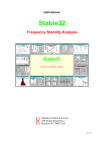
Clock Measurements Using the TimePod 5330A with TimeLab and Stable32 W.J. Riley Hamilton Technical Services Beaufort, SC 29907 USA Introduction This paper describes methods for making clock frequency and phase measurements using a Miles Design TimePod 5330A Programmable Cross Spectrum Analyzer [1, Appendix I] along with its accompanying TimeLab program [2] and the Stable32 stability analysis software package [3]. The TimePod (shown in Figure 1) is an 11” x 5” x 3” module with reference and signal RF inputs, an external power supply and a USB PC interface. It uses four digital receivers to make cross-correlation amplitude and phase measurements that can characterize the stability and purity of an RF source with exceptional resolution and ease. Figure 1. Photograph of the TimePod 5330A Programmable Cross Spectrum Analyzer Measurement Functions The TimePod has three basic measurement functions: 1. Frequency Stability: This function measures Allan deviation and similar statistics with a noise floor in the mid pp1014 region at 1 second. 2. Phase Noise and Jitter: This function measures SSB phase noise and integrated phase jitter with a noise floor of below -170 dBc/Hz at 10 kHz from the carrier. 3. AM Noise: This function measures amplitude noise with a noise floor of about -170 dBc/Hz at 100 kHz from the carrier. Items 1 and 2 are emphasized in this paper since they are used to characterize the frequency stability and phase noise of frequency standards, clocks and oscillators. The instrument can also measure the additive phase noise of a 2-port device. Hardware, Software and Measurement Setup The TimePod, along with its TimeLab software is straightforward to set up and use. The hardware setup requires only connection to its power supply and, after software installation, a USB connection to a modern Windows PC. The software and instrument driver is installed automatically by running a single installation program. TimePod measurements are controlled and examined via the associated TimeLab program. Additional stability analysis can be performed by launching Stable32 from TimeLab. This combination of hardware and software facilitates making state-of-the art clock stability measurements with remarkable simplicity. Note: TimePod *.tim data filenames are shown in red for reference purposes. Operating Principles The TimePod uses advanced digital receiver techniques to make low-noise, high-resolution RF phase measurements, as described in References [4] through [10] and shown for the TimePod in Figure 2. At one 1 extreme, one can simply accept these techniques as easily-used “magic”; at the other extreme, one can delve into the hardware and signal processing details. Most users will opt for an intermediate approach, understanding the basic operating principles and applying them for their measurements. The enabling technologies are high-speed, high-resolution analog-to-digital conversion (ADC) devices that sample the RF reference and signal inputs, fast in-phase and quadrature digital down conversion, low pass filtration, decimation and other digital signal processing, including the arctangent calculation of phase and FFT spectral analysis, along with dual-channel cross-correlation to cancel internal noise. Figure 2. TimePod Hardware and Signal Processing Architecture The digital signal processing performed by the TimePod to obtain phase information is similar to that of the groundbreaking Symmetricom Model 5120A test set described in Reference [6]. The TimePod uses a 78 MHz clock and produces decimated 236 kS/s complex phase data streams for each of the dual signal and reference channels. Those data are then used to compute the cross variance, discrete Fourier transforms and cross spectrum. Phase data are further decimated to selectable 5 to 500 Hz ENBW for analysis. The TimeLab software application provides the user interface to control the instrument and display the measurement results. Operating Procedure An effective way to use TimePod/TimeLab is to locate the instrument in a test area with a network-connected data acquisition and storage PC, and to analyze the data on a separate workstation PC in an office. The lab computer should be fast, while the workstation should have lots of RAM. Multiple instances of TimeLab can be opened on the workstation to display a variety of plots. 2 Noise Floor The TimePod noise floor can be determined by simply applying a coherent signal from the same reasonablystable frequency source to both its reference and signal inputs, preferably via a passive RF power splitter as shown in Figure 3. The Rb oscillator source has a nominal output of +7 dBm so the TimePod signal and reference inputs are driven at only +4 dBm which is below optimum for lowest noise but seems quite satisfactory. Signal Input Rb Osc 10 MHz RF Power Splitter TimePod 5330A USB to PC Reference Figure 3. Setup for Noise Floor Measurement The results of this test (TimeLab_001.tim) are shown below in both the time (Figure 4) and frequency (Figure 5) domains in terms of Allan deviation and phase noise plots for the default 5 ms sampling interval. This performance, 3.17x10⁻¹⁴ at 1-second, is indeed excellent and rivals any such instrumentation available. Figure 4. ADEV Noise Floor Plot 3 Figure 5. L (f) Noise Floor Plot A similar ADEV plot (Figure 6) is obtained after exporting these data to Stable32 (exporting the highbandwidth phase data necessary for a phase noise plot is not supported). Note that the Stable32 data are averaged by a factor of 2 to obtain the same minimum tau dictated by the noise bandwidth and that its maximum tau is deliberately more restricted. Figure 6. Stable32 ADEV Noise Floor Plot 4 The dependence of the TimePod noise floor on the power level of the reference and signal inputs is shown in Figures 7 and 8 for the widest and narrowest measurement bandwidths respectively (TimeLab_066.tim through (TimeLab_071.tim). These data were obtained after amplifying the output of an HP 10811 OCVCXO to +23 dBm, passing it through a 15 MHz low pass filter and optional attenuator and splitting it with a passive RF power divider for the 5330A reference and signal inputs. For the 500 Hz ENBW, there is no significant difference between nominal levels of +20 and +10 dBm but the noise floor is higher for 0 dBm. For the 0.5 Hz ENBW where the noise floor is lower, there is no significant difference at any of the power values, and the 1second ADEV noise floor is only about 1.5x10⁻¹⁴. Figure 7. Noise Floor versus Power for 500 Hz Bandwidth Figure 8. Noise Floor versus Power for 0.5 Hz Bandwidth 5 Sampling Interval and Equivalent Noise Bandwidth The TimePod sampling interval is an important operating parameter because it affects the range of available time domain averaging times, number of data points, practical run duration and noise floor. The sampling interval is set as part of the measurement setup, and the available choices are shown in Table I. Table I. TimePod Operating Parameters Sample Rate Points/Second 2 20 200 (Default) 2000 Sample Interval Seconds 0.5 0.05 0.005 0.0005 Measurement BW (ENBW) Hz 0.5 5 50 500 Minimum Tau Seconds 1 0.1 0.01 0.001 1-Second Noise Floor (Measured) pp1014 1.58 2.35 3.25 5.86 The minimum xDEV tau values shown are those clipped by the equivalent noise bandwidth (ENBW). The observed noise floor is actually better than that deemed typical. The range of sampling rates covers settings appropriate for long-term runs to those for phase noise measurement. Figure 9 shows a composite of coherent noise floor ADEV curves for the various sample rates (TimeLab_012-015.tim). These measured 1 second ADEV noise floor values are shown in Table 1. Lower bandwidth results in lower noise, requires fewer data points, and supports a longer run while having lower resolution and a longer minimum tau. Note that the 30minute 500 Hz BW run acquired 3.6 million data points and a 102 MB file. Figure 9. Composite Noise Floor Plot for Various Sample Rates 6 Measurement Example #1: Two Rubidium Oscillators The first example (TimeLab_011.tim) of using the Time Pod/Lab is to compare two Efratom LPRO-101 rubidium oscillators. The 10 MHz output of Rb1 is applied to the 5330A reference input and that of Rb2 is applied to the signal input via a Mini-Circuits FTB-1-1 RF isolation transformer [12], as shown in Figure 10. The latter was found to reduce AC power line ground loop interference in some cases (as recommended in the TimePod instruction manual). Such interference can show up as ripples in an ADEV plot as well as spurs in a phase noise plot. The manufacturer’s recommendation to power all devices involved in the measurement from a common AC power strip is a good one, and has resulted in phase noise plots with absolutely no power line spurs without RF isolation transformers. Instrument spurs, if any, are very low. Iso Xformer Rb Osc #2 Signal Input 10 MHz Rb Osc #1 TimePod 5330A USB to PC Reference Figure 10. Test Setup for Two Rb Oscillators The high resolution and low noise of the TimePod means that it is able to properly measure the stability of the two rubidium oscillators. Figure 11. Phase Record for Two Rb Oscillators The slope of the Figure 11 phase record shows that the frequency offset between the two rubidium oscillators is 1.09x10⁻¹¹, and the positive slope indicates that the frequency of Rb2 is higher. Figure 12 shows the phase residuals after removal of this linear trend (frequency offset). 7 Figure 12. Phase Residuals for Two Rb Oscillators Figure 13. Frequency Record for Two Rb Oscillators The scale of the Figure 13 fractional frequency plot is expanded to better show the white FM noise; this masks some of the extreme points, including two outliers of around 1.3x10⁻⁹ during a 240 ps phase step. 8 Figure 14. Frequency Stability Plot for Two Rb Oscillators Figure 14 shows that the pair of Rb oscillators has a white FM noise characteristic at a level of 9.1x10⁻¹² at second so it can be inferred that each source has a stability of about 6.4x10⁻¹² at that averaging time. Figure 15. Stable32 Frequency Stability Plot with W FM Noise Fit The Stable32 white FM noise fit between 1 and 100 seconds of Figure 15 shows a combined 1-second stability of 8.90x10⁻¹². This result is in good agreement with other measurements using an analog DMTD clock measuring system. 9 Figure 16. Phase Noise Plot for Two Rb Oscillators The -80 dBc/Hz phase noise shown in Figure 16 at 1 Hz from the 10 MHz carrier corresponds to a white FM noise level of 1x10-11 at 1 second. Most of the spurs are power line related, the strongest being 60 and 120 Hz. The 10 Hz spur is probably from a 10 MHz + 10 Hz offset DDS synthesizer driven by Rb1. Extreme care (RF isolation transformers, double-shielded coax cable, etc.) is required to avoid such interference, and the most effective cures are probably physical separation or a screen room, powering-down or disconnecting the interfering sources, and using a low impedance common ground (including a metallic bench top). The 5330A seems particularly sensitive to power line ground loop interference, and internal RF input isolation transformers with ground-isolated coaxial connectors might be better. Figure 17 shows the same plot with the major spurs suppressed. Figure 17. Phase Noise Plot with Major Spurs Suppressed 10 Measurement Example #2: GPS Disciplined Oscillator versus Rubidium Reference The second Time Pod/Lab example (TimeLab_016.tim) is to measure the stability of a Trimble Thunderbolt GPS disciplined crystal oscillator against Rb1, an Efratom LPRO-101 rubidium oscillator. In the short term, the GPSDO has comparable or better stability than the Rb oscillator. In the medium term, it is quite sensitive to temperature variations so is actively temperature controlled by means of a baseplate heater inside an insulated box. In the long term, the GPSDO is steered by GPS with a 1000 second time constant and therefore serves as a frequency reference for the rubidium frequency standard (RFS) which is syntonized manually by adjusting its C-field. The main purposes of this measurement are therefore to (1) assess the combined short term stability of the GPSDO and RFS, (2) observe the residual environmental sensitivity of the GPSDO, and (3) determine the absolute frequency offset of the RFS. A fairly long 6-hour run is needed for item (2), so a slow 2 sample/second measurement rate is chosen to minimize the data file size. The results of this run are shown in Figures 18-23. The phase record (Figure 18) is essentially linear, indicating an average Rb1 frequency offset of about +1.22x10⁻¹¹ (the sign is reversed because the RFS is connected to the TimePod reference input). The phase residuals (Figure 19) show slow variations of about 25 ns over a period of about 5000 seconds, a frequency excursion on the order of 1x10-11, presumably due to environmental (thermal) disturbances. Figure 18. GPSDO versus Rb1Phase Plot 11 Figure 19. GPSDO versus Rb1Phase Residuals Plot The fractional frequency plots of Figures 20 and 21 (data averaged by x20) show slow excursions of about 2x10-11 p-p with no discernible trend. Figure 20. GPSDO versus Rb1 Fractional Frequency Plot 12 Figure 21. Stable32 GPSDO versus Rb1 Fractional Frequency Plot The frequency stability (Figure 22) is essentially flat at 4x10-12 for averaging times between 1 and 1000 seconds, a surprisingly good result considering that the previous measurement attributed a higher noise to each Rb oscillator. The stability then improves at averaging times longer than the 1000 second loop time constant as GPS disciplining occurs. Ultimately, the combined stability would be limited by the flicker floor of the RFS at about 2x10-13, and the long-term stability would be determined by the RFS aging. Figure 22. GPSDO versus Rb1 Stability Plot 13 The close-in phase noise (Figure 23) of -85 dBc/Hz at 1 Hz has a -10 dB/decade flicker PM noise slope agrees with the 1-second stability. Figure 23. GPSDO versus Rb1 Phase Noise Plot An identical run with Rb2 as the reference source (TimeLab_018.tim) was conducted with essentially identical results. The combined ADEV was also fairly flat between 1 and 1000 seconds, with a higher 1-second ADEV of 6.03x10⁻¹², and the RFS frequency offset was larger, +2.21x10⁻¹¹. Measurement Example #3: Additive Phase Noise of a Distribution Amplifier The TimePod can be used to measure the additive phase noise of an active or passive two-port network with the setup shown in Figure 24. Network Under Test Rb Osc 10 MHz RF Power Splitter Signal Input TimePod 5330A USB to PC Reference Figure 24. Setup to Measure Additive Phase Noise of 2-Port The device under test was pair +7 dBm unity gain distribution amplifiers using LMH6703 wideband op amps that buffer the output of an LPRO rubidium oscillator as shown in Figure 25. The source noise is coherent but the amplifier noise is not, so the setup measures the combined incoherent noise of the two amplifiers, as shown in Figure 26 (TimeLab_020.tim). 14 Signal Input Rb Osc 10 MHz Distribution Amplifiers TimePod 5330A USB to PC Reference Figure 25. Rb Oscillator Distribution Amplifier Phase Noise Test Setup The phase noise plot, which uses the TimeLab spur suppression feature, shows the combined additive noise of the two amplifier channels and should therefore be reduced by 3 dB for one amplifier. There is little or no headroom above the measuring system noise floor at this +7 dBm signal level. Nevertheless, since the distribution amplifier noise is much less than that of the Rb source everywhere (see Figure 18), these amplifiers are fine for this application. Figure 26. Rb Oscillator Distribution Amplifier Phase Noise Plot Measurement Example #4: Efficacy of OCVCXO PLL Clean-Up Loop An example of a TimePod/Lab measurement of an OCVCXO PLL clean-up filter [13] for a rubidium frequency standard (RFS) is shown in Figure 27. The magenta (upper) curve (TimeLab_040.tim) shows the phase noise of an LPRO-101 rubidium measured against an HP 10811 OCVCXO. The 1 Hz phase noise corresponds to a combined 1-second short-term stability slightly better than 1x10-11, as expected for the RFS. That spectrum shows fairly strong spurs at 150 and 300 Hz caused by the RFS internal servo modulation as well as several other weaker ones at higher sideband frequencies. The noise floor is about -155 dBc/Hz. The blue (lower) curve (TimeLab_045.tim) shows the phase noise of the same source and reference but with the Rb signal filtered by the OCVCXO PLL module. Notice that the loop acts as a low-pass filter, preserving the 1 Hz phase noise while eliminating the spurs and lowering the noise floor. 15 Figure 27. RFS Phase Noise With and Without OCVCXO and PLL Clean-up Filter Measurement Example #5: Warm-Up of an Oven Controlled Crystal Oscillator As an example of a rather ordinary frequency measurement, Figure 28 shows the TimePod frequency record during the warm-up of an ovenized crystal oscillator (TimeLab_050.tim). The main point is that there is no problem measuring large frequency offsets; in this case the initial frequency was about -21 ppm and the final frequency was about 10 Hz above 10 MHz. The oscillator was turned on at the start of the TimePod data acquisition. The latter portion of the same record can be used to assess the unit’s phase noise and ADEV stability with high resolution. Figure 28. OCXO Warm-Up Frequency Record Long-Term Measurements As a “personal” clock measuring instrument, the 5330A is not intended primarily for making long-term measurements, which may require a multi-channel system with extensive data archiving capabilities. Nevertheless, the TimePod can be used for that purpose by choosing the minimum 2 samples/second acquisition rate and setting it for a long (e.g., multi-day) run. When collecting only frequency stability data, the data file has a reasonable size of about 4.8 MB per day, which can be saved at any time during the run. A few days of TimePod data reloads quickly into TimeLab, transfers quickly to Stable32, and can then be saved as a 1-second phase data file of about 1.9 MB/day. Further averaging to a longer tau is, of course, possible. Note also that the TimePod *.tim phase data file can be read directly into Stable32 with some minor editing. 16 Temperature Coefficient of Phase The phase stability of the 5330A is specified as less than 10 ps/hour after 2 hours at 5 MHz (presumably after warm up in a temperature-stable environment), but the actual temperature coefficient of phase is not specified. A crude 1-hour test was therefore conducted by allowing the unit to self-heat and, after stabilization, be cooled by a fan to re-stabilize at a lower temperature while observing the phase of a coherent 10 MHz source as shown in Figure 4. The initial temperature was 42.7°C at the top of the TimePod case; after 15 minutes, it was 43.3°C; after 30 minutes the temperature was °C, and the fan was turned on underneath it; 15 minutes later, the temperature had dropped to 32.6°C, and at the end of the 1 hour run it was 32.5°C. The corresponding phase record is shown in Figure 29 (TimeLab_022.tim). The phase changed about -12 ps for a temperature change of -10°C, a very respectable temperature coefficient of 1.2 ps/°C. Figure 29. Phase Record During Temperature Test Input Return Loss The TimePod signal and reference port input return loss was measured between 0.5 to 30 MHz to confirm that it provides a reasonably good match to avoid problems with reflections on the input cables. The results are shown in Figures 30 and 31. Figure 30. TimePod Signal Port Return Loss Figure 31. TimePod Signal Port Return Loss 17 For the signal port, the minimum return loss over the specified 0.5 to 25 MHz range is about 16 dB at 20 MHz, a VSWR of 1.38:1, which is within the specified 1.5:1 specification; it is 23 dB and 1.16:1 at 10 MHz. For the reference port, the minimum return loss over the specified 0.5 to 25 MHz range is about 16 dB at 7.6 MHz, a VSWR of 1.38:1, which is also within the specified 1.5:1 specification; it is 17 dB and 1.35:1 at 10 MHz. Comments The 5330A capability to make time domain measurements at short sampling times (e.g., 1 ms) opens up a new window for those accustomed only to 1-second measurements. That window not only shows source stability in that region, but it also shows how easily those measurements can be affected by power line interference and crosstalk. The TimePod manual discusses those problems, which can be frustrating at first, but they actually help by revealing issues that were previously hidden. Similarly, the 5330A capability to easily and simultaneously make frequency domain phase noise measurements is a great advantage. Most importantly, the TimePod/Lab combination has been completely free of crashes, outliers and other such anomalies. Conclusions The TimePod 5330A and its associated TimeLab software is a remarkably fine instrument for measuring the stability of precision clocks and oscillators. Employing the latest RF and digital signal processing techniques in an effective hardware/software combination, it offers both high performance and ease of use in a small package at an economical price. TimePod is best suited as a personal laboratory or portable clock measuring system, and, when used along with Stable32, is capable of detailed stability measurement and analysis of even the highest performance such devices. I highly recommend it. Acknowledgment The TimePod 5330A Programmable Cross Spectrum Analyzer used for these measurements was provided to Hamilton Technical Services by Mr. John Miles of Miles Design LLC. References 1. TimePod 5330A Programmable Cross Spectrum Analyzer Operation and Service Manual, Revision 1.02, Miles Design LLC, Lake Forest Park, WA 98155, May 20, 2012 (TimePod Version 3.4.7.0 XEM 3005 was used herein) 2. TimeLab, Miles Design LLC, Lake Forest Park, WA 98155 (Version 1.014 of 05/15/12 used herein). 3. Data Sheet, Stable32 Software Package for Frequency Stability Analysis, Hamilton Technical Services, Beaufort, SC 29907, August 2008 (Version 1.59 used herein). 4. J. Grove, J. Hein, J. Retta, P. Schweiger, W. Solbrig, and S.R. Stein, “Direct-Digital Phase-Noise Measurement”, Proceedings of the. IEEE International Frequency Control. Symposium, August 2004, pp. 287-291. 5. S.R. Stein, “The Allan Variance – Challenges and Opportunities”, IEEE Transactions on Ultrasonics, Ferroelectrics and Frequency Control, Volume 57, Issue 3, March 2010, pp. 540-547. 6. S.R. Stein et al. “Comparison of Heterodyne and Direct-Sampling Techniques for Phase-Difference Measurements”, Proceedings of the 2005 NCSL International Workshop and Symposium, 2005 (copy obtained directly from author). 7. E. Rubiola, “The Magic of Cross Correlation in Measurements from DC to Optics”, Proceedings of the 22nd European Frequency and Time Forum, April 2008. , 8. E. Rubiola and F. Vernotte, “The Cross-Spectrum Experimental Method”, arXiv:1003.0113v1 February 27, 2010. 9. G. Paul Landis, Ivan Galysh, and Thomas Petsopolous, “A New Digital Phase Measurement System”, Proceedings of the 33rd Annual Precise Time and Time Interval Meeting, November 2001, pp. 543-552. 18 10. F. L. Walls, S. R. Stein, James E. Gray, and David J. Glaze, “Design Considerations in State-of-the-Art Signal Processing and Phase Noise Measurement System”, Proceedings of the 30th Annual Frequency Control Symposium, June 1976, pp. 269-274. 11. Data Sheet, Model 5120A Phase Noise & Allan Deviation Test Set, Symmetricom, Inc., Boulder, CO 80301. 12. Data Sheet, FTB-1-1 Coaxial RF Transformer, 50 , 0.2-500 MHz, Balanced to Single-Ended, MiniCircuits, Brooklyn, NY 11235. 13. W.J. Riley, “A 10 MHz OCVCXO and PLL Module”, Hamilton Technical Services, Beaufort, SC 29907, June 10, 2012. W.J Riley Hamilton Technical Services File: Clock Measurements Using the TimePod 5330A with TimeLab and Stable32.doc June 8, 2012 Revision D: July 7, 2012 19 Appendix I – TimePod Brochure 20 21