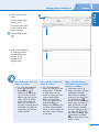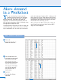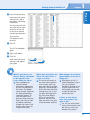
1
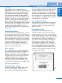
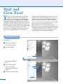
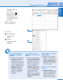
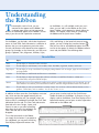
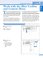
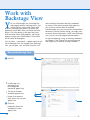
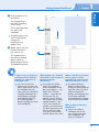
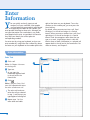
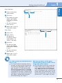
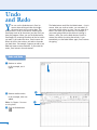
What You Can Do
in Excel
M
numeric information easier. You can use the program
to create worksheets, databases, and charts. Without
a doubt, you could perform the following functions
manually, but you can use Excel to make them easier.
Lay Out a Worksheet
When you sit down to develop a worksheet
with a pencil and ledger paper, you do not
always have all the information to complete the
design and layout of the worksheet. Ideas may
occur to you after you sketch the layout of your
worksheet. After you are finished jotting down
the column headings and the row headings,
you might think of another column or row
that you did not include. If you are working with
pencil and paper, restructuring the layout of a
worksheet can be tedious and time-consuming.
With Excel, you can easily insert columns and
rows as well as move information from one
location to another.
the information in your workbook and instantly
gives you the new answers — in most cases,
without the associated math errors.
TE
RI
AL
icrosoft Excel is one of the world’s most
popular spreadsheet programs. You could
create worksheets on ledger paper and use
a calculator or draw charts on graph paper, but Excel
makes these tasks and others related to managing
GH
TE
D
MA
Organize, Sort, and Filter Lists
You can create tables to organize your data in
lists. For example, you can create inventory lists,
employee lists, customer lists, student grade lists,
and sales records. In Excel, you can add, delete,
sort, search, and display records in the list as
often as required to maintain the list. You can
sort data on the worksheet alphabetically and
numerically in ascending or descending order.
For example, you can sort sales records in
chronological order by dates. You can also use
the AutoFilter feature to quickly find information
that meets a specific criterion or to find the top
or bottom ten values in the list without sorting.
CO
PY
RI
Calculate Numbers
Think about the tasks involved in managing your
checkbook register. You subtract the amount of
each check written and add the deposits to the
running balance. You then use your bank
statement to balance your checkbook, and it is
not at all uncommon to find math errors in your
checkbook. So, you must then recalculate the
numbers in your checkbook register and jot
down the new answers. If you set up an Excel
workbook to do the same tasks, you can use
formulas that subtract checks and add deposits.
You enter the formulas only once and simply
supply the amounts of your checks and deposits,
much as you record them in your checkbook
register. When you change the numbers in the
workbook, Excel uses the formulas to recalculate
4
Getting Started with Excel
Make Editing Changes
To correct a mistake on ledger paper, you have
to use an eraser or you have to reconstruct the
entire worksheet. With Excel, you can overwrite
data in any cell in your worksheet. You can also
quickly delete data in one cell or in a group of
cells. And when you accidentally make mistakes
that overwrite original data while using Excel,
you do not have to retype or reconstruct
information. Instead, you can just restore the
data by using the Undo button.
Check Spelling
You no longer have to manually proofread
your work. When you use Excel’s AutoCorrect
feature, Excel corrects commonly made
mistakes as you type — and you can add your
own personal set of common typos to the list.
In addition, before you print, you can run
spell check to search for misspellings. If you
are a poor typist, this feature enables you to
concentrate on calculating your numbers while
Excel catches spelling errors.
1
with dollar signs, commas, and decimal points.
You can experiment with the settings until the
worksheet appears the way that you want it
and then you can print it. You can boldface,
italicize, and underline data as well as change
fonts and font sizes. Excel also lets you shade
cells, add borders, and apply styles to improve
the appearance of a worksheet.
Preview Before Printing
You can preview your worksheet to see how it
will look when you print it. You can also add
headers and footers and adjust page breaks
before you print.
Chart Numeric Data
Numbers form the foundation of charts.
Manually creating charts is time-consuming
and takes some artistic skill. In Excel, creating
charts is quick and easy. You can track the sales
trends of several products with a chart. You also
can make as many “What if?” projections as
you want in the worksheet by increasing and
decreasing the numbers used in the chart; as
you change the numbers in the worksheet,
Excel instantly updates the chart. Excel’s charts
let you simultaneously view the sales trends
in a picture representation on-screen and the
numbers in the worksheet, making your sales
forecasting more efficient.
Make Formatting Changes
Excel easily enables you to align data in cells;
center column headings across columns;
adjust column width; and display numbers
5
PART I
View Data
When working with a large worksheet on
ledger paper, such as a financial statement, you
might have to use a ruler to compare figures
on a far portion of the worksheet. You might
even find yourself folding the ledger paper to
bring the columns you want to compare close
together. In Excel, you can split the worksheet
into two or four panes to view distant figures
side by side. That way, you can easily see the
effects of asking “What happens when I change
this value?” to project changes. You can also
temporarily hide intermediary columns so
distant figures appear right next to each other
as you work.
chapter
Start and
Close Excel
Y
ou can start the Excel program by using the
Windows Start menu. When you open the
Start menu, the Windows search field appears
at the bottom and the All Programs choice appears
immediately above the search field. Once you select
All Programs, Windows displays folders that contain the
programs installed on your computer. The shortcut to
start Excel appears in the Microsoft Office folder. After
you select Excel from the Microsoft Office folder
several times, it will appear on the Start menu in the
list of recently opened programs. You can select
Microsoft Office Excel 2010 from that list to open the
program. If you use Excel regularly, you may want to
pin Excel to the Start menu or Windows taskbar or
create a shortcut for it so you can open it more quickly.
You can close Excel by using a command in Backstage
view or you can use the Close button in the
upper-right corner of the Excel window. Excel’s
behavior when you close the program depends on the
method you choose to close the program, the number
of workbooks you have open, and whether you have
made changes to any of the open workbooks.
Start and Close Excel
Start Excel
1
Click the Start button.
The Start menu opens.
2
Click All Programs.
2
1
Programs changes to
• All
Back.
3
Click Microsoft Office.
3
4
list of installed
• The
Microsoft Office programs
appears.
4
•
Click Microsoft Excel 2010.
•
6
Getting Started with Excel
chapter
1
The cell pointer ( )
• appears
as you move
PART I
The main window for
Excel opens.
•
the mouse over cells
in the worksheet. You
use the cell pointer to
select cells.
Note: See Chapter 4 for
more on selecting cells.
1
Close Excel
1
Click the File tab.
Backstage view
appears.
2
Click Exit.
Excel closes all open
workbooks.
Does Excel prompt me to
save before closing the
program?
If you have not made any
changes to the workbook,
Excel closes without
prompting you to take any
further action. However, if
you have made changes to
an open workbook, Excel
prompts you to save the
workbook. After you
respond to the prompt,
Excel closes regardless of
whether you save the
workbook.
2
Can I click the X in the
upper-right corner to close
Excel?
Yes. But if you have more
than one workbook open,
Excel closes only the active
workbook instead of the
program. You must click
the X in the upper-right
corner of each open
workbook. When you click
the X while viewing the
last open workbook, both
the workbook and the
program close. Before
Excel closes any workbook
you have changed, Excel
prompts you to save the
workbook.
What happens if I pin Excel
to the taskbar?
A button for Excel always
appears on the Windows
taskbar. To pin Excel to the
taskbar, complete steps 1 to
3, right-click on Microsoft
Excel 2010, and then click
Pin to Start Menu.
How do I create a desktop
shortcut?
To create a desktop
shortcut for Excel, complete
steps 1 to 3, right-click on
Microsoft Excel 2010, click
Send To, and then click
Desktop (Create Shortcut).
7
Understanding
the Excel Screen
E
ach time you open Excel, you see a new
workbook named Book1 that contains three
worksheets.
A Title Bar
Displays the name of the
workbook and the name of
the program.
B Quick Access Toolbar
By default, this contains
buttons that enable you to
save, undo your last action,
and redo your last action.
You can also add buttons
to this toolbar; see Chapter
30 for more.
F Worksheet Tabs
These identify the worksheet on
which you are currently working.
You can switch worksheets by
clicking a worksheet tab.
G Status Bar
This displays Excel’s current
mode, such as Ready or Edit, and
identifies any special keys you
press, such as Caps Lock. The
B
status bar also contains View
buttons that you can use to
switch views and a Zoom control
to help you zoom in or zoom out.
See Chapter 8 for more on views
and zooming.
H Scroll Bars
These enable you to view more
rows and columns.
A
C
D
C Ribbon
Contains most Excel
commands, organized on
tabs. See the section
“Understanding the
Ribbon” for more.
D Formula Bar
Composed of three parts,
the Formula Bar contains
the Name box, buttons
that pertain to entering
data, and the contents of
the currently selected cell.
E Worksheet Area
The place where you enter
information into Excel,
divided into rows and
columns.
8
E
F
H
H
G
Getting Started with Excel
chapter
1
P
PART I
Learn Excel
Terminology
resented next is a series of terms you need to
know as you work with Excel.
Workbook
A workbook is a file in which you store your data.
Think of a workbook as a three-ring binder.
Each workbook contains at least one worksheet,
and a new workbook contains three worksheets,
named Sheet1, Sheet2, and Sheet3. People use
worksheets to organize, manage, and consolidate
data. You can have as many worksheets in a
workbook as your computer’s memory permits.
Worksheet
A worksheet is a grid of columns and rows. Each
Excel workbook contains 1,048,576 rows and
16,384 columns. Each column is labeled with a
letter of the alphabet; the column following
column Z is column AA, followed by AB, and so
on. The last column in any worksheet is column
XFD. Each row is labeled with a number, starting
with row 1 and ending with row 1,048,576.
Cell
A cell is the intersection of a row and a column.
Each cell has a unique name called a cell
address. A cell address is the designation
formed by combining the column and row
names in column/row order. For example, the
cell at the intersection of column A and row 8
is cell A8, and A8 is its cell address.
Range
The term range refers to a group of cells. A range
can be any rectangular set of cells. To identify
a range, you use a combination of two cell
addresses: the address of the cell in the
upper-left corner of the range and the address
of the cell in the lower-right corner of the
range. A colon (:) separates the two cell
addresses. For example, the range A2:C4
includes the cells A2, A3, A4, B2, B3, B4, C2,
C3, and C4.
Formula Bar
The Formula Bar is composed of three parts.
At the left edge of the Formula Bar, the Name
box displays the location of the currently
selected cell.
The Cell Contents area appears on the right
side of the Formula Bar and displays the
information stored in the currently selected cell.
If a cell contains a formula, the formula appears
in the Cell Contents area, and the formula’s
result appears in the active cell. If the active cell
contains a very long entry, you can use
at
the right edge of the Cell Contents area to
expand the size of the area vertically.
Between the Name box and the Cell Contents
area, buttons appear that help you enter
information. Before you start typing in a cell,
only the Function Wizard button ( ) appears,
as described in Part III; you can use this button
to help you enter Excel functions. Once you
start typing, two more buttons appear; click
to accept the entry as it appears in the Cell
Contents area or click
to reject any typing
and return the cell to the way it appeared
before you began typing.
9
Understanding
the Ribbon
o accomplish tasks in Excel, you use
commands that appear on the Ribbon. You
no longer open menus to find commands;
buttons for commands appear on the Ribbon. Do not
worry if you do not find a particular command
T
on the Ribbon; it is still available, and if you use it
often, you can add it to the Ribbon or the Quick
Access Toolbar, which appears by default above the
Ribbon. See Chapter 28 for more on customizing
the Ribbon and the Quick Access Toolbar.
On the Ribbon, you find tabs, which take the place of
menus in Excel 2010. Each tab contains a collection of
buttons that you use to perform a particular action.
On each tab, buttons with related functions appear in
groups. For example, on the Home tab, you find seven
groups: Clipboard, Font, Alignment, Number, Styles,
Cells, and Editing. In the lower-left corner of some
groups, you see a Dialog Box Launcher button ( )
that you can click to see additional options that you
can set for the group. By default, the Ribbon contains
seven tabs, described in the following table.
Tabs on the Ribbon
Tab
Purpose
Home
This tab helps you format and edit a worksheet.
Insert
This tab helps you add elements, such as tables, charts, PivotTables, hyperlinks, headers, and footers.
Page Layout
This tab helps you set up a worksheet for printing by setting elements such as margins, page size and orientation,
and page breaks.
Formulas
This tab helps you add formulas and functions to a worksheet.
Data
This tab helps you import and query data, outline a worksheet, sort and filter information, validate and
consolidate data, and perform What-If analysis.
Review
This tab helps you proof a worksheet for spelling errors and also contains other proofing tools. From this tab, you can
add comments to a worksheet, protect and share a workbook, and track changes that others make to the workbook.
View
This tab helps you view your worksheet in a variety of ways. You can show or hide worksheet elements, such as
gridlines, column letters, and row numbers. You can also zoom in or out.
In addition to these seven tabs, Excel displays contextual
tabs, which are tabs that appear because you are
performing a particular task. For example, when you
select a chart in a workbook, Excel adds the Chart Tools
tab behind the View tab. The Chart Tools tab contains
three tabs of its own: Design, Layout, and
Format. As soon as you select something
other than the chart in the workbook, the
Chart Tools tab and its three subtabs
disappear.
To use the commands on the Ribbon,
you simply click a button. If you prefer to
use a keyboard, you can press the Alt key;
Excel displays keyboard characters that
10
you can press to select tools on the Quick Access
Toolbar and tabs on the Ribbon. If you press a key to
display a tab on the Ribbon, Excel then displays all the
keyboard characters you can press to select a particular
command on the Ribbon tab.
Getting Started with Excel
chapter
1
PART I
Work with the Mini Toolbar
and Context Menu
Y
You will notice, though, that the commands on the
Mini toolbar change when you select pictures,
charts, Clip Art, or SmartArt to reflect the commands
you need when working with these types of objects.
In most cases, the Mini toolbar and the Context
menu contain a combination of the most commonly
used commands available in the Clipboard, Font,
Alignment, and Number groups on the Home tab.
The commands that appear on the Context menu,
also called a shortcut menu, also change depending
on the content of the cells or the type of object with
which you are working. That is, Excel displays only
those commands on the menu that are relevant to
the information in the cells or the type of object you
select; this is how the menu got its name.
ou can use the Mini toolbar and the Context
menu to help you quickly format text without
switching to the Home tab. The Mini toolbar
and the Context menu always appear together when
you right-click on cells that contain text or numbers,
shapes, text boxes, WordArt, pictures, charts, Clip
Art, or SmartArt.
Work with the Mini Toolbar and Context Menu
1
Select a cell or range
of cells.
Note: See Chapter 4 for
more on selecting cells.
1
2
Right-click on the
selection.
•
Mini toolbar and
• The
Context menu appear,
with the Mini toolbar
above the Context
menu.
•
11
Work with
Backstage View
Y
ou can use Backstage view to manage files
and program options. Backstage view is new
to Excel 2010 as well as other Office 2010
products. Backstage view replaces the menu that
appeared in Excel 2007 when you clicked the Office
button. The Office button is also gone from Excel
2010 and other Office 2010 programs; the File tab
appears in place of the Office button in Excel 2010
and all Office 2010 programs.
A list of actions — commands — appears down the left
side of Backstage view. For example, from Backstage
view, you can open, save, and close Excel files. You
also can display information about the workbook
on-screen in Excel when you open Backstage view,
such as file size and the date last modified.
From Backstage view, you can also print and distribute
documents; however, before sharing, you might want
to remove sensitive information. Finally, from Backstage
view, you can set Excel program behavior options.
For more on opening, saving, and closing workbooks,
see Chapter 2. See Chapter 8 for more on printing
and Chapter 29 for more on sharing workbooks.
Work with Backstage View
1
Click File.
1
Backstage view,
• Incommonly
used
file-management
commands appear here.
title of the open
• The
workbook appears here.
that represent
• Buttons
other actions you can take
appear here.
2
Click Info.
about the
• Information
workbook on-screen
appears here.
12
•
•
2
•
•
Getting Started with Excel
1
PART I
3
chapter
•
Click an option in the
left column.
This example shows
the results of clicking
Save & Send.
commands help
• These
you share Excel
3
workbooks.
•
buttons in the
• Clicking
Save & Send column
changes the
information that
appears here.
4
Repeat step 2 until you
find the command
you want to use.
4
This example shows
the results of clicking
Recent, which by
default displays the last
20 workbooks opened.
Is there a way to return to
working in Excel without
making any selections in
Backstage view?
Yes. You can click File
again or you can press Esc.
Either action returns you to
the workbook that was
open when you clicked File
to display Backstage view.
And although you might
be tempted to click Exit,
resist the temptation
because clicking Exit closes
Excel completely.
What happens if I click the
check box at the bottom of
the list of Recent
Workbooks?
When I click Recent, Recent
Places appears on the
far-right side of the screen.
What information is here?
If you click the Quickly
access this number of
Recent Workbooks check
box, Excel displays — just
above Info in the left
column — the names of
the last four files you
opened. You can change
the number from 4 to any
number between 1 and
20. As you increase the
number, you also increase
the space required to view
the list, and Excel adds
scroll bars to the middle
and left sides of the screen.
The Recent Places list
displays locations from
which you recently opened
Excel files. When you click
a Recent Place, Excel
displays the dialog box you
use to open workbooks
and automatically navigates
to the location you clicked.
What is Recover Unsaved
Workbooks?
Excel saves copies of
workbooks you do not
save, and you can open
these workbooks. For
more, see Chapter 2.
13
Enter
Information
Y
ou can quickly and easily type text and
numbers into your worksheet. Most people
use Excel primarily to accomplish math-related
tasks, and supplying text labels for the numbers you
enter provides meaning to those tasks. Although you
can type information into a worksheet in any order,
some people find it easier to type labels first because
they help users identify the correct place for
corresponding numbers.
You enter text by using your keyboard, and you can
enter numbers by using either the number keys above
the letters on your keyboard or the number pad to the
right of the letters on your keyboard. To use the
numbers on the number pad, you must press the
Num Lock key.
By default, when you enter text into a cell, Excel
left-aligns it in the cell and assigns it a General
format. When you enter a number into a cell, Excel
right-aligns it in the cell and assigns it a General
format. Excel also recognizes some dates that you
type; as a result, it right-aligns them in cells and
formats them as dates. Information in a selected cell
appears both in the cell and in the Formula Bar. For
more on formats, see Chapter 3.
Enter Information
Enter Text
1
3
Click a cell.
Note: See Chapter 4 for more
1
•
on selecting cells.
2
Type text.
you type, the
• As
information appears both
•
2
in the cell and in the
Formula Bar.
3
Click
.
Note: If you press Enter, Excel
stores the information but moves
the active cell down one cell.
active cell continues
• The
to be the cell you selected
in step 1, and the text you
typed appears left-aligned.
4
Repeat steps 1 to 3 to
enter other text labels.
14
•
Getting Started with Excel
chapter
1
1
Select a cell and then
type a number.
2
Press Enter.
•
•
number you typed
• The
appears right-aligned
1
PART I
Enter Numbers
in the cell you selected
in step 1.
active cell moves
• The
down one row.
3
Repeat steps 1 and 2 to
enter other numbers.
Enter Dates
Select a cell.
3
Press Enter.
Type a date in
mm-dd-yyyy or
mm/dd/yyyy format
(either dashes (-) or
slashes (/) will work).
•
•
1
2
1
date you typed
• The
appears right-aligned
in the cell you selected
in step 1.
active cell moves
• The
down one row.
4
Repeat steps 1 to 3 to
enter other numbers.
Can I edit or delete the information that I
type in a cell?
Yes. You can edit the information either as
you type it or after you type it by pressing
F2 to switch to Edit mode. To edit as you
type, just press F2. To edit after you type,
click the cell and then press F2. To change
an entry completely, enter new information
as described in this section. To delete all the
information in a cell, select the cell and then
press Delete. To delete both information
and cell formatting, see Chapter 3.
Why does my label in cell A1 appear
truncated but my label in cell B1 seems to
occupy both cells B1 and C1?
The information in both cells exceeds their
column widths. When an empty cell such
as C1 appears beside a cell containing an
overly large entry such as B1, information
seems to occupy both cells. However, Excel
actually stores all the information in cell B1;
look at the Formula Bar as you select cell B1
and then cell C1. See Chapter 5 for more.
15
Undo
and Redo
Y
ou can use the Undo feature in Excel to
recover from editing mistakes that might
otherwise force you to re-enter data. The
Undo feature in Excel is cumulative, meaning that
Excel keeps track of all the actions you take until you
close the program. When you use the Undo feature,
Excel begins by reversing the effects of the last action
you took. If you undo four times, Excel reverses the
effects of the last four actions you took in the order
you took them. For example, suppose you edit a text
label and remove some characters. If you undo the
action, Excel reinserts those characters.
The Redo feature works like the Undo feature — but in
reverse. After you undo an action, you can redo it. If
you undo several actions in a row, you can redo all of
them in the order you undid them. For example, if
you undo typing and then the effects of resizing a
column, when you use the Redo feature, Excel first
restores the effects of resizing the column. If you
immediately use the Redo feature again, Excel restores
the typing.
Undo and Redo
1
Perform an action.
In this example, text is
typed.
1
2
Perform another action.
3
In this example, italics are
added.
Note: See Chapter 3 for more
on using italics.
3
Click the Undo button
( ).
16
2
Getting Started with Excel
1
PART I
reverses the last
• Excel
action.
chapter
4
In this example, Excel
removes italics.
If you click Undo again
in this example, Excel
removes the text.
Click the Redo button
( ).
•
4
reverses the effect
• Excel
of undoing an action
Can I undo more than one
action at a time?
Yes. Click the drop-down
arrow ( ) beside the
Undo button ( ) to
display the list of actions
you can undo. Click the
oldest action you want to
undo, and Excel undoes
all the actions from the
oldest one you select to
the latest, showing you the
worksheet at the point in
time before you took any
of those actions.
•
by adding back your
last one. In this
example, Excel
reapplies italics.
Can I redo more than one
action at a time?
Yes. The Redo feature
works the same way as the
Undo feature. To be able
to redo more than one
action at a time, you must
undo multiple actions
before you redo them.
Then, click
beside the
Redo button ( ) to
display a list of actions you
can redo. Click the oldest
action, and Excel redoes all
the actions from the oldest
to the latest.
Why is the Redo button
unavailable when the Undo
button is available?
Excel keeps track of all
actions you take in all open
workbooks and makes
those actions available to
undo until you close Excel.
The Redo button ( )
button will not be available
unless there are actions to
redo, and actions to redo
do not become available
until you undo an action. If
you then click
to redo
the action you undid, then
becomes unavailable
because there are no more
actions to redo.
17
Move Around
in a Worksheet
Y
ou can use arrow keys to move around a
worksheet, moving the active cell up, down,
left, or right one cell at a time. If you hold
down an arrow key, Excel moves the active cell
repeatedly in the direction designated by the arrow
key. You can also move one screen at a time by using
the Page Up and Page Down keys.
To quickly move to the first or last cell in a range, you
can take advantage of the End key. You use the End
key in combination with the arrow keys to move the
active cell to the top or bottom cell in a column or the
left or right cell in a row. When you press the End key,
Excel displays End Mode on the status bar to alert you
that the active cell will move to the first or last cell in
the direction of the arrow key you use.
When you know the address of the cell in which you
want to work, you can move directly to that cell by
using the Go To dialog box.
Move Around in a Worksheet
1
Click a cell.
makes the cell you
• Excel
clicked the active cell.
•
2
Press the right arrow key.
moves the active cell
• Excel
one column to the right.
You can press any arrow
key to move the active cell
one cell in that direction.
3
•
You can press and hold an
arrow key to repeatedly
move the active cell in
that direction.
Press End.
status bar displays
• The
End Mode.
18
•
Getting Started with Excel
1
PART I
4
chapter
Press the up arrow key.
moves the active
• Excel
cell to the first cell in
•
the column containing
information.
You can press End with
any arrow key to move
to the first or last cell
in the row or column
containing information.
You can press
Ctrl+Home to move
to cell A1.
5
Press F5.
The Go To dialog box
opens.
6
7
Type a cell address.
Click OK.
Excel moves the active
cell to the cell address
you typed.
When I open Excel, I see
Sheet1, Sheet2, and Sheet3
at the bottom of the
screen. What are these?
Every workbook can
contain multiple
worksheets, represented
by tabs at the bottom of
the screen. The default
names for each worksheet
are Sheet followed by a
sequential number. To
view the content of a
particular sheet, click that
sheet’s tab. You can add
and delete worksheets,
change their names, and
move or copy them; see
Chapter 6 for more.
6
7
Where does Excel place the
active cell when I move a
screen at a time?
The active cell remains in
the same relative position
on the screen when you
press the Page Up or Page
Down keys. For example, if
D10 is the active cell while
viewing rows 1 to 27 and
you press the Page Down
key, then Excel displays
D37 as the active cell.
However, the active cell
does not move if you click
in the horizontal scroll bar.
What happens if I click the
Special button in the Go To
dialog box?
Excel opens the Go To
Special dialog box, where
you can set special
conditions for Excel to use
to go to a particular cell.
For example, you can opt
to select all cells that
contain formulas.
Is there an easy way to
move one screen to the
right or left?
Yes. You can click a blank
area in the horizontal scroll
bar that runs across the
bottom of the screen.
19