1
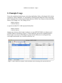
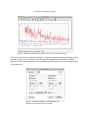
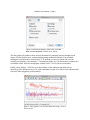
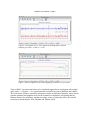
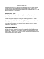
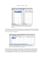
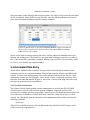
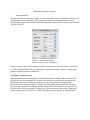
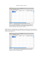
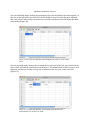
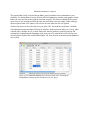
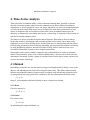
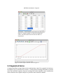
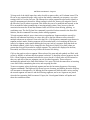
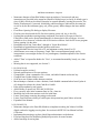
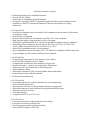
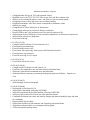
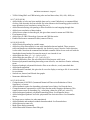
Automated Numerical Time-Series
Evaluation of Varying Sequences Software
Antevs 1.3.0 User Manual
Copyright © 2011-2015 Frederick W. Vollmer
ANTEVS User Manual – Contents
Table of Contents
License
Installation
1.
Introduction
2.
Example Usage
3.
Data Entry
3.1 Data Files
3.2 Tree-Ring Files
3.3 Manual Data Entry
3.4 Automated Data Entry
4.
Time-Series Analysis
4.1 Detrend
4.2 Filter
4.3 Mean
4.4 Data Graph
4.5 Cross-Correlation
4.6 Bin Test
5.
Segments and Missing Data
5.1 Missing Values
5.2 Segmented Series
6.
References
7.
History
ii
ii
1
2
6
6
7
7
9
14
14
16
17
17
17
18
19
20
22
23
ANTEVS User Manual – Page ii
License
ANTEVS is Copyright © 2011-2015 Frederick W. Vollmer. This program is distributed in the hope that
it will be useful, but without any warranty; without even the implied warranty of merchantability or
fitness for a particular purpose.
ANTEVS is free software, however you may not redistribute or post it online without the author's
permission. It may only be distributed as the released compressed file package with this file and other
included files. Any significant usage, such as a resulting presentation or publication, should include the
following two attributions to the program and author:
Rayburn, J.A., and Vollmer, F.W., 2013. ANTEVS: A quantitative varve sequence cross-correlation
technique with examples from the northeastern United States. GFF: Journal of the Geological
Society of Sweden, v. 135, p 282-292.
Vollmer, F.W., 2015. ANTEVS 1.3: Automated numerical time-series evaluation of varying sequences
software. Retrieved from: www.frederickvollmer.com/antevs.
Any reference to the content of the User Manual (this document) may be cited as follows:
Vollmer, F.W., 2015. ANTEVS 1.3: Automated numerical time-series evaluation of varying sequences
software user manual. Retrieved from: www.frederickvollmer.com/antevs.
Installation
On Macintosh OS X, double click the disk image file (.dmg), and drag the Antevs application to your
Applications folder, or other desired location.
On Windows, unzip the zip file (.zip) using the Extract All option, and drag the Antevs folder to any
desired location. The Antevs folder contains the Antevs application (Antevs.exe), and a Resources
folder which is required.
On Linux unpack the gzip file (.tar.gz), and copy the Antevs folder to any desired location. The Antevs
folder contains the Antevs application (antevs), and a Resources folder which is required.
ANTEVS User Manual – Page 1
1. Introduction
Time-series arise in situations where a value is measured through time, generally at discrete
intervals. Annual intervals commonly occur in natural systems due to seasonal variations in
temperature, as displayed in proglacial varves, tree-rings, and glacial ice. Antevs (Automated
Numerical Time-series Evaluation of Varying Sequences) is designed primarily to work with
such natural time-series, but can be applied to other discrete time-series as well. Antevs is
designed to aid in correlation of time-series, where an undated times-series, the unknown, is
compared to a previously dated series, a chronology, to determine if they overlap in time and to
date the unknown series.
Antevs was developed for the correlation of proglacial varve sequences (Rayburn and Vollmer,
2013), however it includes standard techniques for matching tree-ring sequences, and can
convert files between varve and tree-ring formats. It includes routines for reading the Velmex
UniSlide digital readout used for tree-ring measurements. A common problem with natural timeseries is that of missing data, often due to broken cores. Antevs includes interactive procedures to
correlate sequences, such as broken cores, that contain missing values.
Antevs is designed to be user friendly and easy to use, with powerful analytical tools under the
hood. It is designed for ease of use, and undergoes extensive testing by undergraduates working
on research projects in John Rayburn's varve and tree-ring laboratory at SUNY New Paltz
Antevs is developed on Macintosh OS X and is compiled for Macintosh OS X, Windows, and
Linux. Currently testing is done on OS X 10.6, 10.10, Windows XP, Windows 7, and Linux
Ubuntu. User input is appreciated to improve operation on various platforms.
ANTEVS User Manual – Page 2
2. Example Usage
To test the correlation of glacial varve series from the Hudson Valley at Newburgh, NY with the
Connecticut Valley at Hartford, CT, download the following North American Varve Chronology
(NAVC) Normal Curves files from the North American Glacial Varve Project website (data from
Antevs, 1922; Ridge et al., 2012; Ridge, 2012):
HUD29-32AM.txt
CON28-32AM.txt
or open the included TSV (Tab-Separated Value) files:
HUD29-32AM.tsv
CON28-32AM.tsv
Assume one is known and the other is unknown, so open HUD29-32AM as an unknown and
CON28-32AM as a chronology (Figure 1). Select them both, and use the command Analyze >
Data Graph to view the raw data (Figure 2). Note that the differences in scaling and long
wavelength trends makes any correlation difficult to see.
Figure 1. Antevs Data Series Window with an unknown and a chronology file open and selected.
ANTEVS User Manual – Page 3
Figure 2. Data Graph Window showing the two raw varve example data sets.
To detrend and rescale the data select Analyze > Detrend to open the Preferences Dialog , and set
Detrend on, with a 16 term Fourier curve fit, using the Standardized normalization method
(Figure 3). In the View Pane check Detrended data for both Unknown and Chronology (Figure
4), and press OK.
Figure 3. Preference Dialog > Detrend Pane with
Detrend on, and default Fourier settings.
ANTEVS User Manual – Page 4
Figure 4. Preferences Dialog > View Pane with Raw
data and Detended data checked on for display.
The data graph will update to show the data detrended by removing long wavelength trends
using a 16 term Fourier curve, and normalizing using standard deviations of the residuals,
making the correlation more clear (Figure 5). To perform a cross-correlation and view the
resulting correlogram, select Analyze > Correlogram (Figure 6). Use the mouse to examine the r
correlation values. Note the strong spike at offset 0 and r = 0.643, the best correlation.
Finally, select Analyze > Bin Test to see how subsets of the unknown match the known
chronology. The default bin size is 50, with a minimum overlap of 50. Most of the subsets match
with zero offset suggesting a robust match.
Figure 5. Data graphs of raw and detrended data using a 16 term
Fourier series.
ANTEVS User Manual – Page 5
Figure 6. Correlogram for two varve sequences showing spike at the best
matching year with r = 0.643, z = 6.516.
Figure 7. Bin correlogram for varve data suggesting a robust fit at 0 year offset.
Tests on NAVC varve data sets known to be correlated suggest that a correlogram with a single
spike with r >= 0.6 and z >= 6 is a good potential correlation for varves (Rayburn and Vollmer,
2013). However, definitive correlation acceptance criteria are difficult to quantify, rather, Antevs
provides statistical and graphical tools for the evaluation of sequences, recognizing that the
ultimate decision for correlation, whether tree-rings, varves, or other time series, lies with the
researcher (Grissino-Mayer, 2001; Rayburn and Vollmer, 2013).
ANTEVS User Manual – Page 6
3. Data Entry
Antevs can read numerous data file formats, including most common spreadsheet files (e.g.,
Excel, LibreOffice) as described in Section 3.1. A header row in these files is used to describe
the following data. Additionally, data can be entered directly using the Data Edit Window . A third
option is to use automated data collection with the Velmex Unislide digital readout system,
commonly used for tree-ring measurements.
3.1 Data Files
Numerous data file formats are supported, the simplest are spreadsheet (e.g., Excel, LibreOffice)
compatible lists with a header. The default is a simple tab-separated value (TSV), or tab
delimited, format for data, consisting of optional comment lines, a header identifying the data
columns, and rows of data. For example:
// Hudson Valley; Newburgh; NY
// This is a comment
//
Year<tab>Raw<tab>Comment
2900<tab>44.300<tab>
2901<tab>25.500<tab>approximate value only
Headers can include: ID, Year, Raw, Fit, Detrend, Count, and Mean. Count and Mean are special
output headers used when creating a mean chronology. Summer, Winter, Comment (or Note)
headers are also read and written, but are not otherwise used. It is best to avoid commas in
comment lines. The TSV file format is recommended over the space-delimited TXT format, as it
are can be read and written by most spreadsheet programs, and the comment and header lines
provide self-documentation of the content.
A comma-separated value (CSV) format is identical to the TSV format, but uses commas as data
delimiters. Note that commas in data fields can potentially cause problems. This format can be
also read and written by most spreadsheet programs, for example:
// Hudson Valley; Newburgh; NY
// This is a comment
//
Year,Raw,Comment
2900,44.300,
2901,25.500,approximate value only
A space-delimited format (TXT), which is for a single sample and has year or sequence number
(first column), and total thickness as decimal values in centimeters in the second column. If four
columns are detected they are assumed to be year, summer thickness, winter thickness, total
thickness. A TSV format is recommended over this format.
ANTEVS User Manual – Page 7
Three additional formats used by spreadsheet programs such as LibreOffice Calc and Microsoft
Excel are supported: OpenDocument (ODS), Office Open XML (XLSX), and Excel (XLS)
spreadsheet formats. The spreadsheet may have comments at the beginning starting with “//”, and
must have a header line as described above.
3.2 Tree-Ring Files
A number of specialized formats have been developed for tree-ring files, some of which were
based on Fortran punch card formats. Antevs can read and write a number of these, and convert
them into other formats.
A decadal tree-ring raw format (RWL) contains fixed column records with core id, decade or
start year, and thicknesses. Multiple cores per file are supported. Thicknesses are stored as six
digit integers in units of 0.01 mm or 0.001 mm. The 'Precision' command can be used to set the
precision to 2 or 3 places before reading or writing a file (default is 3).
A tree-ring chronology format (CRN) that contains a single composite chronology which is
standardized to a mean value of 1.
3.3 Manual Data Entry
While it is often convenient enter data into a spreadsheet such as Excel or LibreOffice, entering a
new time series directly into Antevs is straightforward. In the main Data Sets Window select the
Unknowns Grid , and then the File > New command. A new time series entitled “untitled” will be
created (Figure 8). Change the title as required, and use the Edit Data command (paper and pencil
icon) to open the Data Edit Window (Figure 9) .
ANTEVS User Manual – Page 8
Figure 8. The Data Series Window after using the File > New
command to create a new series. The series can be renamed as
required.
By default the first year is 1900, edit the starting year as required (this can also be changed later),
and then begin entering data in the Raw column. Each entry advances the year by one and moves
the cursor down one row (Figure 10).
Figure 9. The Data Edit Window after creating a new series. The start year is
given a default value of 1900, edit this as required.
After data has been entered, the Cancel Edits (red X icon) and Accept Edits (green checkmark
icon) commands become available. Use Accept Edits to accept the data, this will update any
currently open graphs. Cancel Edits will revert the data to the previous state last accepted. The
Revert command (blue curved arrow icon) is not currently available because the initial data
ANTEVS User Manual – Page 9
series was empty. When editing a data set opened from a file, Revert will revert to the state when
the file was opened. When finished, accept the edits, close the Edit Data Window , and save the
series from the Data Sets Window using the Save As command.
Figure 10. Manual entry of data in the Data Edit Window , ready to enter data for
the year 1883. Grayed entries can not be edited. The Cancel Edits and Accept
Edits icons are now enabled.
Antevs can be used for editing existing time series, and has additional commands such as for
splitting and joining rows. If the time series start year must be changed, enter the new value in
row 1, and use the Edit > Renumber command. Missing values (Section 5) are entered by “NaN”
(or “nan”), or, by default, any negative number.
3.4 Automated Data Entry
Antevs allows automated data collection using the Velmex Unislide digital readout system,
commonly used for tree-ring measurements. This has been tested on Windows and Macintosh
systems. To collect data measurements, click on the Unknown Grid list and use the File > New
command to create a new file (Figure 8). Select the file, rename it as desired, and select Edit >
Edit Data. In the Data Edit Window (Figure 9), select Edit > Connect (blue plug and socket icon)
and enter the required serial port parameters.
3.4.1 Serial Port Connection
The Velmex Unislide digital readout system communicates via a serial port (RS-232 DB9),
which requires a serial-to-USB converter on most computers. Numerous serial-to-USB
converters are available, and their setups differ. Antevs is set for the default parameters that work
in our laboratory on Windows (COM3, 9600 baud, 8 data bits, 2 stop bits, no party, no flow
control). On a Macintosh open the Terminal from the Applications Utilities folder, and enter the
following command:
ls /dev/tty.*
This will list available serial ports. For the Macintosh using a Prolific PL2303 chip set serial
USB converter the required port is:
ANTEVS User Manual – Page 10
/dev/tty.usbserial
This port works in our laboratory (Figure 11). An open source driver is available for the PL2303
chip set that works on Macintosh, and is included on the Linux Ubuntu distribution. A free
downloadable version from Prolific includes an installation manual (find it using a web search on
“Prolific PL2303”).
Figure 11. Serial port dialog showing
settings for a Macintosh computer,
these may differ on your configuration.
Future versions of Antevs will attempt to connect with other data collection devices. The author
will work with researchers who are attempting to automate their data collection, currently this
must be through a serial port connection.
3.4.2 Data Coordinate Entry
After connecting to the recording device in the Data Edit Window using the Edit > Connect (blue
plug and socket icon) command, the Connect icon indicates a connection has been made, the
Record icon (red circle) has changed from gray to red, and the status has changed from
Disconnected to Connected (Figure 12). Antevs has four modes during automated data entry:
Disconnected, Connected, Initializing, and Recording. These are indicated in the status bar, as
well as by the color of the Record icon (gray, red, yellow, and green respectively). Each mode
change is indicated by an audio cue, a click. User instructions are also given in the status bar.
ANTEVS User Manual – Page 11
Figure 12. The Data Edit Window in Connected mode, after connection with
the recording device. The Connect icon (blue plug and socket) indicates
connection, the Record icon (red circle) has changed from gray to red, and the
status has changed from Disconnected to Connected.
Edit the initial year as required (this can be changed later), and click on the red Record icon to
initialize the device. The mode will change from Connected to Initializing, and the Record icon
becomes orange (Figure 13).
Figure 13. The Data Edit Window in Initializing mode, ready to accept the
coordinate of the start of the data sequence.
ANTEVS User Manual – Page 12
Once in Initializing mode, position the recording device at the beginning of the data sequence, in
this case at the start of the year 1900. The device should be reset to zero at this point, although
this is not critical. When ready, use the device to send the coordinates, this will change the mode
to Recording (Figure 14).
Figure 14. The Data Edit Window in Recording mode, ready to record a data
series.
Once in recording mode, advance the recording device to the end of the first year, in this case the
end of 1900, and send the coordinates from the device. The measurement for the first year is now
displayed, and Antevs is ready to accept the coordinate for the next year, in this case 1901
(Figure 15).
Figure 15. The Data Edit Window in Recording mode after the first
measurement, here for the year 1900.
ANTEVS User Manual – Page 13
The Cancel Edits (red X icon) and Accept Edits (green checkmark icon) commands are now
available. Use Accept Edits to accept the data, this will update any currently open graphs. Cancel
Edits will revert the data to the previous state last accepted. The Revert command (blue curved
arrow icon) is not currently available because the initial data series was empty. When editing a
data set opened from a file, Revert will revert to the state when the file was opened.
Advance the device to the end of the next year, here 1901, and send the coordinates. Continue
with subsequent years until data collection is complete. Antevs gives an audio cue, a beep, when
a decade entry, divisible by 10, is made. Data entry may be paused by selecting Record, and
continued by reinitializing the beginning of the next year to be entered (the end of the last year
entered). When finished, use Accept Edits (Figure 16), then Save As in the Data Series Window to
save to disk.
Figure 16. The Data Edit Window after entering a time series, and using the
Accept Edits command (green checkmark icon, now gray).
ANTEVS User Manual – Page 14
4. Time-Series Analysis
Time-series arise in situations where a value is measured through time, generally at discrete
intervals. In natural systems annual intervals commonly occur due to seasonal variations in
temperature, as seen in proglacial varves, tree-rings, and glacial ice. Antevs is designed primarily
to work with such natural time-series, but can be applied to other discrete time-series as well.
Antevs is designed to aid in correlation of time-series, where an undated times-series, the
unknown, is compared to a previously dated series, a chronology, to determine if they overlap in
time and to date the unknown series.
The analysis in Antevs is broken down into three main parts. Detrending is done to remove
longer term trends or wavelengths, and to rescale the time-series so they can be more easily
compared. A curve is fit to the time-series, and the fitted curve is removed from the data values.
Filtering may optionally be done following detrending, and can potentially enhance correlations
by using neighboring values to smooth local values. Finally, the two time-series are crosscorrelated to determine if a match can be found between them.
Data graphs can be used to visually compare the raw or detrended series, and a correlogram
allows visual evaluation of the cross-correlation. Additionally, a bin test can be done to test the
robustness of the match. Finally, a group of correlated series can be used to create a mean series,
to serve as a master chronology.
4.1 Detrend
Detrending rescales the raw data and removes longer wavelength trends by fitting a curve to the
data set, and adjusting the raw data values using the fitted values. This allows sequences with
different environmental inputs to be more easily correlated, such as distal and proximal varves,
or young and old tree-ring growth. The residuals are the data values minus the fitted values:
ri = y i - ŷ i
where ŷi is the estimate calculated by fitting a curve or function to the data.
4.1.1 Mean
Fits to the mean of y:
ŷi = Σ yi / n
4.1.2 Linear
Fits a linear curve:
ŷ = a + bx
by minimizing the squared residuals in y.
ANTEVS User Manual – Page 15
4.1.3 Quadratic
Fits a quadratic curve:
ŷ = a + bx + cx 2
by minimizing the squared residuals in y.
4.1.4 Cubic
Fits a cubic curve:
ŷ = a + bx + cx 2 + dx3
by minimizing the squared residuals in y.
4.1.5 Exponential
Fits an exponential curve:
ŷ = aebx + c
to the data by minimizing the squared residuals in y using an iterative method. This can be useful
for tree-rings that have a regular decrease in width with age, but can fail in many cases.
4.1.6 Automatic
For cubic, quadratic and linear curve fitting a fit is rejected if a negative thickness is predicted,
and a lower order curve is tried, until the mean is used. For an exponential fit, the curve is
rejected with b > 0 or c < 0, and a linear curve fit is tried. If a linear fit is rejected with b > 0, or a
negative thickness is predicted, the data is fits to the mean value of y. Automatic exponential is a
common choice for some tree-ring data sets (Cook and Holmes, 1986).
4.1.7 Spline
Fits a cubic spline to the raw data. The Stiffness parameter controls the tightness of the curve
(Cook and Peters, 1981).
4.1.8 Fourier
Fits a Fourier series to the raw data. The Low pass frequencies parameter controls the number of
components in the series. This is the default method used for varve analysis, with a default
setting of 16 (Rayburn and Vollmer, 2013).
4.1.9 Method
The Detrend Method sets the method by which the fit curve is used to detrend the raw data.
4.1.9.1 Fit
Displays the fit curve, ŷi.
ANTEVS User Manual – Page 16
4.1.9.2 Residual
The residuals method uses the residuals, subtracting the predicted value, ŷi , from the
data value, yi:
ri = (yi – ŷi)
These are not normalized, so units are in centimeters or millimeters, with a mean of
zero.
4.1.9.3 Standardized
Standardizes, or normalizes, the residuals by dividing by the standard deviation of residuals. The
data is transformed to standard deviations from the fit curve. This allows comparison of differing
series, as it gives unitless numbers with a mean of zero. This is the default method for varve
analysis.
4.1.9.4 Ratio
Uses the ratio method:
y' = (yi / ŷi)
commonly used for tree-rings. This can be biased however, and using residuals is more
robust. Values of ŷi near zero are discarded to avoid divide by zero errors. The mean of
the detrended values will be 1.
4.1.9.5 Ratio Log
Uses the Ratio method (Section 4.1.9.4) and applies a log transform for variance
stabilization after adding a constant of one-sixth of the series mean to each value.
4.2 Filter
Displays the filters dialog. Filters are applied after detrending the data to normalize the data and
potentially emphasize correlations. Normalizing involves smoothing the data by using
neighboring values.
4.2.1 Delta Bar
Smooths using the average of the nearest neighboring data points:
yi' = (yi-1 + yi + yi+1)/3
Rayburn and Vollmer (2013) suggest this filter may help emphasize some varve correlations.
4.2.2 Cubic derivative
Orthogonal cubic first derivative filter. Smooths using the cubic derivative of the nearest
neighboring data points. This filters the data to look for changes in slope of the series using the
first derivative of a local cubic polynomial. The number of terms can be 5, 7, or 9. The 5 term
cubic derivative filter can be particularly effective for correlation.
ANTEVS User Manual – Page 17
4.2.3 Ratio
Smooths using the ratio of current and previous years:
yi' = yi / yi-1
4.2.4 Natural
Logarithmic, or natural, change from previous year to current year (Hollstein):
yi' = ln(yi / yi-1)
4.2.5 Relative
Relative change from previous to current year:
yi' = (yi - yi-1) / yi-1
4.2.6 Log five year
Five year logarithmic smoothing filter (Baillie and Pilcher, 1973):
yi' = ln(5 * xi2) / (xi-2 + xi-1 + xi + xi+1 + xi+2))
4.3 Mean
Calculates a mean master series of all open data series, either chronologies or unknowns. Each
series is detrended before calculating the mean. Before creating a mean master series, in the
Preferences Dialog > Detrend Panel , the Detrend option should be checked, and either
Standardized (recommended) or Ratio methods selected. The detrending rescales the series so
each is weighted equally. The data series are not normalized when calculating the mean, so the
normalize filter setting does not matter.
Note that detrending using the Standardized method gives values with a mean of zero, and
therefore will create negative values. The Treat negative as missing and Display missing as “-9”
options (see Section 5) must be off.
4.4 Data Graph
Graphs unknown and chronology thickness, or normalized thicknesses, versus year. Optionally
plots best fit curves and raw data for unknowns and chronologies. This graph can be used to
segment the time-series if there are gaps or missing data (Section 5).
4.5 Cross-Correlation
Applies the current filters, first detrending then normalizing, and calculates the cross-correlations
and t statistics for each possible match. The default overlap required for a test is 50, this can be
changed in the Preference Dialog > Limits Panel .
ANTEVS User Manual – Page 18
4.6 Bin Test
Sequentially groups the unknown data into bins, similar to bootstrapping, and runs each against
the selected chronology displaying the best correlations based on the t statistic. Used to test the
robustness of the match and to potentially locate missing varves or tree-rings in an unknown. The
bin size can be changed in the Preference Dialog > Limits Panel . The bin size must be larger or
equal to than the minimum overlap.
ANTEVS User Manual – Page 19
5. Segments and Missing Data
A common problem in natural data sets such as varves and tree-rings is missing data points, as
cores or observable varve sequences can be broken or discontinuous. Antevs treats missing data
points as NaN (Not a Number) values, which have no numeric value. There can be any number
of NaN data points in a sequence. In order to deal with this internally and avoid numerical errors,
Antevs uses linear interpolation over the NaN values. This is, for example, the default used by
MatLab to deal with NaN values in numerical analysis.
Breaks can be inserted into the unknown time-series, allowing individual segments of an
unknown time-series to be interactively shifted in time by incrementing or decrementing them.
The segments can be individually compared to the chronology, and slid forward or backwards to
match. Additionally, the cross-correlation can be automatically calculated at each step to test the
strenght of the match.
5.1 Missing Values
Antevs treats missing data points as NaN (Not a Number) values, which have no numeric value,
and there can be any number of NaN data points in a sequence. In order to deal with this
internally and avoid numerical errors, Antevs uses linear interpolation over the NaN values. This
is, for example, the default used by MatLab to deal with NaN values in numerical analysis.
To maintain operability with time series that may contain negative values (such as temperature),
Antevs currently has two settings to control how it deals with NaN values. These are set in the
Preferences Dialog > Options Panel . If Treat negative as missing is checked (by default it is not),
any negative number is treated as a NaN. The second option, Display missing as “-9” , controls
how the NaN is displayed in the Data Edit Window and output files. This is also off by default,
however, a common convention in tree-ring data is to use “-9” to signify a missing value. If that
is important, turn this option on, and “-9” will be displayed instead of “NaN” in the Data Edit
Window, and in saved files. Note, however, that treating negative values as NaN will create
problems when creating a mean series using standardized detrending. Standardized detrending
produces a series with a mean of zero, and will contain negative values.
Figure 17 shows a simple example of a time series with NaN values, and Figure 18 shows the
Data Graph of this series. The three NaN values between 1901 and 1905 are interpolated. NaN
values van be entered in the Data Edit Window , or in input files, as “NaN” (or “nan”), or, if Treat
negative as missing is checked, any negative number.
ANTEVS User Manual – Page 20
Figure 17. Simple example of a time series with NaN
values. The NaN values between 1901 and 1905 are
interpolated.
Figure 18. Data Graph of the time series in Figure 17.
5.2 Segmented Series
A common problem in natural time-series is missing data, caused, for example, by broken or
incomplete cores. As described in Section 5.1, Antevs allows inserting NaN values to break a
series into individual segments, however inserting NaN values manually can be cumbersome.
Antevs therefore uses segment analysis to provide a more interactive method.
ANTEVS User Manual – Page 21
To keep track of the initial input data, and to be able to remove edits, an ID column is used. The
ID can be any sequential integer value, such as the initially estimated year sequence, or a series
starting with 0 or 1 as the first year. The ID must be a unique sequential value used to identify a
specific measurement in that series. When reading in a data file, Antevs will assign the Year to
the ID value if no ID values are present. This allows the year to be modified and restored, as the
ID is not modified when renumbering or inserting missing values. Note, however, that the
association between the ID and the measured value will be lost when deleting, splitting, or
combining rows. The Set ID from Year command is provided for data entered in the Data Edit
Window, use this command if necessary before editing segments.
To begin segment analysis, open a time-series as an unknown. Segment analysis can only be
done on one unknown time-series at a time, this will be the first unknown series selected if
multiple unknowns are selected. Next select the Edit > Edit Segments command to put Antevs in
segment analysis mode. Existing segments will be marked with a circle marking the first year
(start) of a segment, and a square marking the last year (end) of a segment. Note that these are
the default symbols, which can be changed in the Preferences Dialog. If no NaN values are
present the series will be marked as a single segment. The symbols are displayed in the Raw,
Detrended, and Filtered curves, any of these can be used for editing.
Click on the graph to select a segment. When selected, the start and end symbols are filled, with
yellow by default, to indicate that the segment is selected. To break the selected segment, use the
Edit > Break Segment command, and enter the year to break it. A NaN value will be inserted at
that year, and each of the two segments can now be edited separately. These values are
automatically updated in the Data Edit Window if it is open. This has the same effect as inserting
a new NaN value, renumbering the series, and accepting the edits.
To move a segment, select the desired segment and use the Increment Segment or Decrement
Segment commands. The Right and Left arrow keys are shortcuts, and holding down the Shift key
will increment or decrement by 10. Moving the first segment will shift the entire series, moving
the second segment will move it and the following segments, and so on. Segments are joined
when the last separating NaN is removed. If open, the Correlogram Window will update and
show the correlation values.
ANTEVS User Manual – Page 22
6. References
Antevs, E., 1922. The recession of the last ice sheet in New England. American Geographical
Society Research Series 11, p. 1-120.
Baillie, M.G.L., and Pilcher, J.R., 1973. A simple crossdating program fro tree-ring research.
Tree-Ring Bulletin, v. 33, p. 7-14.
Brewer, P., Murphy, D., Jansma, E., 2011. TRiCYCLE: A universal conversion tool for digital
tree-ring data. Tree-Ring Research 67, p.135-144.
Cook, E.R., 1985. A time series analysis approach to tree ring standardization. Ph.D. dissertation,
University of Arizona.
Cook, E.R., and Richard L. Holmes, R.L., 1986. Users manual for program ARSTAN.
Laboratory of Tree-Ring Research, University of Arizona, Tucson, USA.
Cook, E.R. and Peters, K. 1981. The smoothing spline: a new approach to standardizing forest
interior tree-ring width series for dendroclimatic studies. Tree-Ring Bulletin, v. 47, p. 45-53.
Cook, E.R. and Peters, K. 1997. Calculating unbiased tree-ring indices for the study of climatic
and environmental change. The Holocene, v. 7, n. 3, p. 361-370.
Davis, J. C., 1986. Statistics and Data Analysis in Geology, Second Edition. John Wiley & Sons,
New York, USA. 646 p.
Fritts, H.C., Mosimann, J.E., and Bottorff, 1969. A revised computer program for standardizing
tree-ring series. Tree-Ring Bulletin, v. 29, p. 15-20.
Grissino-Mayer, H.D., 2001, Evaluation crossdating accuracy: a manual and tutorial for the
computer program COFECHA. Tree-Ring Research, v. 57, n. 2, p. 205-221.
Holmes, R.L, 1983. Computer-assisted quality control in tree-ring dating and measurement.
Tree-Ring Bulletin, v. 43, p. 69-78.
Melvina, T.M., Brifffaa, K.R., Nicolussib, K., Grabnerc, M., 2007. Time-varying-response
smoothing. Dendrochronologia, v. 25, p. 65-69.
Press, W. H., Teukolsky, S. A., Vetterling, W. T., and Flannery, B. P., 2007. Numerical Recipes:
The Art of Scientific Computing, Third Edition. Cambridge University Press, Cambridge,
UK. 1235 p.
Rayburn, J.A., and Vollmer, F.W., 2013. ANTEVS: A quantitative varve sequence crosscorrelation technique with examples from the northeastern United States. GFF: Journal of the
Geological Society of Sweden, v. 135, p 282-292.
Ridge, J.C., 2012, The North American Glacial Varve Project: (http://eos.tufts.edu/varves),
sponsored by The National Science Foundation and The Department of Earth and Ocean
Sciences at Tufts University, Medford, Massachusetts.
Ridge, J.C., Balco, G., Bayless, R.L., Becks, C.C., Carter, L.B., Dean, J.L., Voytek, E.B, and
Wei, J.H., 2012. The new North American varve chronology: a precise record of southeastern
Laurentide ice sheet deglaciation and climate, 18.2–12.5 kyr bp, and correlations with
Greenland ice core records. American Journal of Science, v. 312, p. 685–722.
Vollmer, F.W., 2015. ANTEVS 1.3.0: Automated Numerical Time-series Evaluation of Varying
Sequences software. Retrieved from: www.frederickvollmer.com/antevs.
ANTEVS User Manual – Page 23
7. History
1.3.0 (2015-06-29)
• Serial Settings, Initialize Read, Split, and Preferences dialogs re-configured for better crossplatform consistency. Additional tooltip help added. TLabel controls replaced with
TStaticText.
• Added “ID” column to provide a unique identifier for each measurement to allow editing of
years without losing track of initial input values. See Section 5. Feature request by Andrew
Breckenridge.
• Added command to set the ID from the Year. This will change the ID to the current year, and
would normally only be done during initial measurements.
• Fixed the reading of spreadsheet files (ods, xls, xlsx) so column order is not important.
• Made “Ratio Log” a separate method option instead of using checkboxes, this uses the Ratio
method followed by log normalization (COFECHA option). A combobox allows separate
methods for unknowns and chronologies.
• Numerous internal changes to preferences code for easier updates.
• Added visual segment editing for missing data and broken cores with 6 new segment analysis
commands, see Section 5.
• New icon.
1.2.1 (2015-01-29)
• Made default for treat negative as NaN to false to avoid problems with mean series when
using standardized detending.
• Fixed bug causing crash when renaming Chronology.
• Fixed widths in initial display of columns.
• Currently line count: 159,471.
1.2.0 (2015-01-07)
• Added StatusBars to MainWindow and DataWindow.
• Replaced Timers with Messages to communicate between windows.
• Replaced StringGrids with DrawGrids to avoid internal data duplication.
• Numerous internal changes for utilizing Messages and DrawGrids, resulting in more
maintainable code for future updates.
• Grayed uneditable cells in grids.
• Fixed LogForm to open in front when Preferences > Options > Display log is checked.
• Added date time string to LogForm, and added left margin.
• Added Unknown and Chronology dates to Correlogram status bar. The correlogram status bar
now contains all information contained in the Log file.
• Fixed 'Save As' command to rename file in MainWindow grids.
• Changed 'Clear' to 'Close' in file close warning dialogs.
• Fixed the extra warning dialog when closing a file modified in the DataWindow.
• Modified to 'Revert' command. In the Data Window, Cancel Edits reverts to the last state
saved with Accept Edits, while Revert returns to the state when the file was opened.
ANTEVS User Manual – Page 24
• Numerous changes to Data Edit Window input procedures. Current mode and user
instructions are provided in the status bar (instead of dialog boxes) to clarify. A default year is
given (1900), which can be edited. Data may be entered manually or using the recorder. The
modes: Disconnected, Connected, Initializing, and Recording are indicated in the status bar,
as well as by the Record button (gray, red, yellow, green). Mode changes also have audible
cues.
• Fixed Error Opening File dialog to display file name.
• Fixed an error that cleared the file list when opening a new ods, xls, or xlsx file.
• Updated the spreadsheet opening/saving component. Previously a file open in Excel or
LibreOffice could not be opened simultaneously in Antevs due to file privileges. It is now
possible to do so, however, with the risk of file version collision. Save the file in one program
before opening it in the other.
• DataWindow tool hint "Insert Row" changed to "Insert Row Before".
• DataWindow Append button switched position with Insert.
• Changed default bin size from 100 to 50, and minimum overlap from 60 to 50.
• Added mouse-over status to Frequency Graph. This is an experimental graph, and its
interpretation is not straight-forward. It is a periodogram, a modulus-squared of the Fourier
transform.
• Added "Time" as input alias header for "Year", to accommodate monthly, hourly, etc., time
series.
• Missing data is now supported, see Section 5.
1.1.0 (2014-10-04)
• Updated to minor version 1.
• Internal modifications to file save routines.
• Changed Edit > Clear command to File > Close, and added Cmd-W accelerator key.
• Changed Auto-Update default to true.
• Grids now save column widths between sessions.
• Moved Analyze > Refresh to View > Refresh, fixed disabled command when Auto-Update is
off, changed accelerator key from Cmd-H to Cmd-R.
• Paint pickers updated to use opacity.
• Added ability to open Excel XLS and XLSX files.
• Fix to correctly save initial comment lines in File > Save As .
• Modified data collection routines to ask for initial date.
• Linux: Fixed image centering bug using work around.
• Linux: Fixed Preference dialog so visible pane always matches panel listbox selection.
• Expanded User Manual.
1.0.6 (2014-02-23)
• Numerous changes to the Data Edit Window to implement reading the Velmex UniSlide
digital readout for logging tree-ring data. See section in ANTEVS User Manual on Data
Collection.
• Implemented messaging to replace global flags and minimize recalculations.
• Fixed and bug that was disallowing multiple open series for some formats.
• Added warnings for saving data.
ANTEVS User Manual – Page 25
•
•
•
•
Disallowed opening series with identical names.
Fixes to File Save dialog.
Added Save As command to Data Edit window.
Changed the name from ANTEVS (Automatic Numerical Time-series Evaluation of Varve
Sequences) to ANTEVS (Automated Numerical Time-series Evaluation of Varying
Sequences).
1.0.5 (2013-04-29)
• Fixed Revert command in data edit window. This command reverts the data to the last time it
was opened or saved.
• Added Select All command.
• Removed depreciated Clear All command, use Select All + Clear commands.
• Made Precision apply to displayed data as well as file output.
• Added ODS (OpenDocument), XLS, and XLSX spreadsheet formats to Save As command.
• Added Export Sets command to save all selected data sets in one TSV, CSV, ODS, XLS,
XLSX, or RWL (decadal) format file. See Brewer et al., 2011.
• Added ODS spreadsheet format to Open command.
• Open command now detects and opens TSV, CSV, ODS files, in addition to RWL format files,
to open multiple sets files created with Export Sets command.
1.0.4 (2013-04-22)
• Grouped graph components in SVG output for easier editing.
• Fixed text vertical alignment in SVG output.
• Changed menu item Save As Vector Graphics to Export SVG.
• Removed Unicode => symbol, not recognized by AI Helvetica.
• Added target CPU and system info to About dialog box.
• Added comment editing.
• Added Split command to split, join and renumber data measurements.
• Removed depreciated Combine command.
• Preference file modifications.
1.0.3 (2013-04-08)
• Fixed floating point error caused if detrend curve exactly equals data.
• Fixed preference button hints.
• Allow opening of Preference dialog without selecting or opening data.
• Added menu options to open Preference dialog Detrend and Filter pages.
• Added fit curve color selection.
• Added About dialog.
• Compiled with FPC 2.6.2, LCL 1.0.8.
1.0.2 (2013-04-01)
• Fixed bug causing freeze when opening Precision dialog.
• Precision now stored in preference file.
• Precision settings moved to Preferences dialog.
• Added ANTEVS header to TXT files.
ANTEVS User Manual – Page 26
•
•
•
•
•
•
•
•
•
•
•
•
Changed default file type to TSV (tab separated values).
Modified Save As for TXT, TSV, CSV files to save Year and Raw columns only.
Added z score, standard deviation, count, and offset to cross-correlation graph.
Changed precision to three places in cross-correlation display.
Displayed maximum t value now always corresponds to maximum r value.
Added p to t graph.
Changed title of 'Filters' dialog box to 'Preferences'.
Changed page selection in preference dialog to combobox.
Detrend, Filters, and View preferences are now saved to preference file.
Added option to turn off display of cross-correlation significance in Preferences Options tab.
Added stroke selection for graph data.
Fixed runs trend bug.
1.0.1 (2013--03-16)
• Compiled with Free Pascal 2.6.0 and Lazarus 1.0.6.
• Fixed missing tick marks bug.
• Fixed tick marks stroke color.
• Fixed vector font export bug, fonts are now filled instead of stroked.
• Fixed incorrect log references.
• Fixed fill color bug in SVG export.
1.0.0 (2012-10-31)
• First official release for review.
0.0.20 (2012-09-18)
• Compiled with Free Pascal 2.6 and Lazarus 1.0.
• Fixed Save As command to save raw data instead of detrended data.
• Added new Save Detrend command saves detrended data.
• Added preliminary frequency spectrum (periodogram) graph, use Window > Fequency to
view.
0.0.19 (2012-04-15)
• Added multiple colors to data graph.
0.0.18 (2012-04-08)
• Recompiled on Free Pascal 2.6.0.
• Added Spline detrending, following COFECHA.
• Added Log transform for the Ratio method, following COFECHA.
• Added csv and tsv data files for both raw data and mean masters.
• Combined file formats into Open and Save As dialogs, and removed multiple Open and Save
As commands.
• Removed Delta bar past filter.
• Added Link checkbox to link unknown and chronology detrend methods.
• Added max and mean labels to correlogram and bin graphs.
• TODO: Interpolate missing values.
ANTEVS User Manual – Page 27
• TODO: Debug RWL and CRN missing value and end data values, 999, -999, -9999, etc.
0.0.17 (2012-02-24)
• Added ability to select and view multiple data sets by control (Windows) or command (Mac)
clicking. Note that only the first selected file in the unknown and chronology grids is used for
most operations (cross correlation, saving files, etc.).
• Added data windowing with panning to allow detailed view and stepping through data.
• Added cross-correlation of data window.
• Added Count column in data edit grid, this gives data counts for means and CRN files.
• Fixed memory leak.
• Added Save As CRN Chronology for mean and CRN data series.
• Enabled Preferences command on Mac (same as Filters).
0.0.16 (2012-02-05)
• Added Fourier detrending for variable terms.
• Added two delta filters mainly for use with Standardize detrend method. These are more
stable and handle zero thicknesses naturally (no division by zero). Note the Cubic derivative
is also stable. Note that the common Ratio method normalize filters do not work well with the
Standardize detrend method, because the mean is zero instead of one.
• Added Delta bar filter: y1' = y1 - (y0+y1+y2)/3.
• Added Delta bar past filter: y3' = y3 - (y0+y1+y2)/3.
• Removed Difference filter, this was identical to Delta bar past with 1 term.
• Removed polynomial smoothing detrending as not effective, was similar to Fourier with many
terms.
• Removed quadratic polynomial derivative filter as not effective, overly smoothed data.
• Added mean toolbutton.
• Added detrend Fit method, this gives the fit curve for display or saving to file. It is not useful
for correlation.
• Stacked raw, detrend, and filtered data graphs.
• Numerous additional fixes.
0.0.15 (2012-02-19)
• Changed name to ANTEVS (Automated Numerical Time-series Evaluation of Varve
Sequences), or Antevs.
• Added automatic option for detrending polynomial curve fitting. See Detrend above.
• Changed automatic exponential to reject linear fits that predict negative thicknesses. This
removes some errors in detrending (e.g., calculating a mean for ny005.rwl, series 22).
• Added orthogonal quadratic polynomial smoothing filters. See Normalize above.
• Added orthogonal quadratic and cubic polynomial first derivative filters. See Normalize
above.
• No longer saves window size when maximized.
• Added residuals and standard residuals detrend methods. See Detrend above.
• Added data series name edit.
• Made Filters dialog nonmodal.
• Added Detrended column to Data Edit grid.
ANTEVS User Manual – Page 28
• Enabled Quit command in Windows.
0.0.14 (2012-02-16)
• Fixed saving of mean files.
• Rewrote handling of zero thicknesses, only used during normalization to avoid division by
zero or log zero.
• Stacked graphs with scales on all curves.
• Fixed update of Data Edit grid when a chronology is viewed.
• Fixed update of main data set grid after editing data.
• Optional runs trend calculation is done simultaneously and viewed on a separate stacked
graph.
• Runs trend algorithm is modified slightly following Corina; an up/down/same =
up/down/same match gets +1, a same = up/down gets +0.5, otherwise no match gets 0.
0.0.13 (2012-02-06)
• Rewrote cross-correlation procedure to minimize potential round off, no change in
functionality.
• Fixed bug in graph frame drawing.
• Fixed bug in exponential fitting, was not fully converging.
• Added y scale labels to data graph for raw data on right. Filtered data scale remains on left.
Grid is drawn for filtered data unless only raw or detrend fit is on.
• Fixed Clear tool button, was not working.
• Fixed two bugs causing random errors in mean calculation.
• Changed menu text from "Cross-Correlation" to "Correlation", no change in functionality.
0.0.12 (2012-02-05)
• Added Zoom commands and controls, including mouse dragging.
• Fixed Accept Edits command in Data Edit window, was not keeping edits.
• Changed Processed to Filtered for clarity.
• Changed Data View to Data Edit.
• Added toolbar to Data Set window.
• Added data names to graphs.
• Fixed y axis scaling error on data graph.
• Added correlogram caption.
• Linked Filter Normalize controls, so changing unknown now changes chronology. Added an
option to turn linking off, but there is no reason for these to differ. May combine in next
version.
• Fixed Save As, was not enabled.
• Added more information in status bar.
0.0.11 (2012-01-28)
• Added graphics buffer to fix slow redraw on Windows.
• Fixed focus loss when closing filters dialog on Windows.
• Fixed divide by zero error
ANTEVS User Manual – Page 29
0.0.10 (2012-01-28)
• Fixed window position xml preferences
• Fixed error reading rwl, 999 entries now excluded as well as -9999
• Fixed data view, was not updating on data grid focus change
• Enabled view detrend as always available
• Fixed error in mean calculation, was not detrending with correct settings
• Added save view options in preferences
• Fixed divide by zero error
0.0.9 (2012-01-25)
• Internal changes for easier maintanence
• Fixed compatibility with OS X 10.5
0.0.8 (2012-01-18)
• Added graph of offset values to bin test correlogram.
• Added color keys for curves on graphs.
• Restored ability to calculate mean chronology.
• Restored option to view log output.
• Fixed bugs in bin test.
• Made auto-refresh optional.
• Added Refresh command and toolbar buttons.
• Fixed label and grid spacings to auto-size.
• Added ability to open CRN files.
• Added ability to detect and open four column TXT files.
• TXT file is checked for non-sequential values.
• Added Open command that uses file extension to determine file type.
• Added quadratic and cubic detrending options.
• Turned off automatic renumbering when editing a file.
• Added Renumber command.
0.0.7 (2012-01-08)
• Completed graphical display of bin test and data display.
• Simplified analyze options.
• Depreciated log test display window.
• Added curve fitting and detrending algorithms.
• Implemented Marquardt non-linear curve fitting.
• Added best-fit curve display to data graph window.
• Redesignated growth correlations as normalize filters, e.g., Natural and Difference.
• Added additional normalize filters, e.g., Log five year and Two year sum.
• Depreciated cross-association (available in Filters Extra tab).
• Depreciated runs analysis (available in Filters Extra tab as SIgn).
• Experimental implementation of area correction algorithm (depreciated).
• Implemented chronology data display.
• Implemented unknown data editing with preview and restore.
• Added minimum thickness value with default of 0.001.
ANTEVS User Manual – Page 30
•
•
•
•
•
Added automatic update of Data View, Data Graph, Bin Test and Correlogram windows.
Created new icon.
Added preference file to remember window locations and sizes.
Added vector graphics SVG output of graphs.
Added PNG, BMG, and JPG bitmap output of graphs.
0.0.6 (2011-12-11)
• Added Graph Window.
• Added Thickness Graph.
• Added Growth Graph.
• Added year offsets to Log Window anaylses to assist in locating matches.
0.0.5 (2011-12-03)
• Added 'Precision' command to set precisions in files to avoid precision loss when converting
varve to tree-ring format.
• Enabled Analyze and Window commands from Log Window.
• Added Mean Growth command.
• Added Growth Correlation command.
• Modified Bin Test to allow setting of additional filtering parameters, including multiple
matches per bin.
• Added desktop icon.
0.0.4 (2011-11-21)
• Rewrote Trend Percentage algoritm.
0.0.3 (2011-11-20)
• Added Normalize.
• Added Normalized Mean.
• Added Cross-Correlation.
• Added Runs Correlation.
• Added Bin Test.
This page intentionally left blank.