1
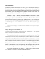
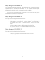
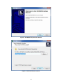
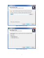
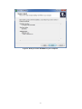
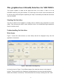
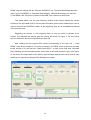
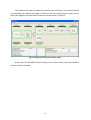
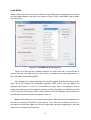
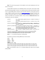
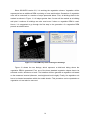
SOLWEIG – A climate design tool
User manual for version 2
Last update: 1st February, 2011
Urban Climate Group
Department of Earth Sciences
University of Gothenburg
Sweden
Table of contents
INTRODUCTION.................................................................................................................... 3
MAJOR CHANGES IN SOLWEIG 1.1............................................................................................................ 3
MAJOR CHANGES IN SOLWEIG 2.0............................................................................................................ 4
MAJOR CHANGES IN SOLWEIG 2.1............................................................................................................ 4
MAJOR CHANGES IN SOLWEIG 2.2............................................................................................................ 4
INSTALLATION ..................................................................................................................... 5
SYSTEM REQUIREMENTS ........................................................................................................................... 5
OTHER APPLICATIONS NEEDED BEFORE INSTALLING THE SOFTWARE........................................ 5
INSTALLING THE INTERFACE.................................................................................................................... 5
THE GRAPHICAL USER-FRIENDLY INTERFACE FOR SOLWEIG.......................... 9
STARTING THE INTERFACE........................................................................................................................ 9
UNDERSTANDING THE INTERFACE ......................................................................................................... 9
Main frame................................................................................................................................................... 9
Load DEMs................................................................................................................................................ 12
Set point of interest in the DEM................................................................................................................. 18
Load-Create SVFs ..................................................................................................................................... 20
Set model parameters................................................................................................................................. 21
Add meteorological data............................................................................................................................ 23
Execute SOLWEIG..................................................................................................................................... 25
Calculate Daily Shading............................................................................................................................ 27
UPCOMING VERSIONS...................................................................................................... 29
VERSION 3.0.................................................................................................................................................. 29
ACRONYMS AND ABBREVIATIONS .............................................................................. 30
REFERENCES ....................................................................................................................... 31
2
Introduction
SOLWEIG is a computer software model which can be used to estimate spatial variations of
3D radiation fluxes and mean radiant temperature (Tmrt) in complex urban settings. This
document describes the computer software and the graphical user-friendly interface that has
been developed for the SOLWEIG model. For detailed description of the model, see
Lindberg et al. (2008) and Lindberg & Grimmond (2010).
SOLWEIG is written in MATLAB programming language. This involves a certain
number of advantages for the aim of this model, as matrices processing are required
continuously, a requirement that MATLAB covers perfectly. Therefore better, fast and
efficient results are obtained. The Graphical user interface is written in Java and makes use
of a runtime engine called the MCR (MATLAB Compiler Runtime), which makes it possible to
run MATLAB application outside the MATLAB environment. The MCR is deployed royaltyfree.
This document will help you to install and run the SOLWEIG model using the Graphical
user interface.
Major changes in SOLWEIG 1.1
Longwave and shortwave radiation fluxes from the four cardinal points is now separated
based on anisotropical Sky View Factor (SVF) images.
The computations time in this new version is much slower than previous version. This
is because a new concept is used to estimate outgoing longwave radiation. In 1.0 the spatial
variations of Lup was only dependent on local shadow patterns on the ground. In 1.1 a new
concept of Ground View Factors has been introduced which is a parameter that is estimated
based on what an instrument measuring Lup actually is seeing based on its height above
ground and shadow patterns. In order to make accurate estimations of GVF, locations of
building walls need to be known. Walls can be found automatically be the SOLWEIG-model.
However, if the User wants to have more control over what are buildings and not, the User
should use the marking tool included in the ‘Create/Edit Vegetation DEM’ (page 12).
A very simple approach taken from Offerle et al. (2003) is used to estimate nocturnal
Ldown. Therefore Tmrt could also be estimated during night in version 1.1.
3
Major changes in SOLWEIG 2.0
A new vegetation scheme is now included. The interface also has a wizard for generating
vegetation data to be included in the calculations. The new vegetation scheme is again
slowing down the calculation but the computation time is still acceptable.
A new improved output section is also incorporated do that the user has more options
on what kind of output that should be generated.
Major changes in SOLWEIG 2.1
Some major (and minor) bugs have been fixed such as:
−
Small changes in the equations for shortwave radiation. The reflected part is
now weighted using a fraction of shadow component instead of sun altitude
angles
−
An error in outgoing shortwave radiation equation have been fixed
−
The generation of bushes in the vegetation DEM process is improved
Major changes in SOLWEIG 2.2
Some major (and minor) bugs have been fixed such as:
−
A major bug regarding the scale of trees and bushes is resolved
4
Installation
This section gives you information on how to install the SOLWEIG graphical user-friendly
Interface on a regular PC.
System requirements
The Interface runs under WINDOWS NT/2000/XP/Vista/7 platforms.
Other applications needed before installing the software
There are a two additional applications that have to be installed on the PC before been able
to run SOLWEIG:
Upgrade (or install) Java Runtime Environment, JRE (version Java 6). This is
easiest made online.
Install the MCR (MATLAB Compiler Runtime 7.13). This can be downloaded
from the Urban Climate Group webpage. If you are using earlier versions of
SOLWEIG, you should keep the corresponding MCR installed on your
computer.
Installing the Interface
Download the executable installation file (SOLWEIG Setup.exe) of the Interface from the
Urban Climate Group webpage and follow the installation procedure as shown below (Figure
1):
Figure 1. Select setup language.
5
Figure 2. SOLWEIG setup welcome window.
Figure 3. Select destination location.
6
Figure 4. Select start menu folder.
Figure 5. Create a desktop icon.
7
Figure 6. Ready to install SOLWEIG on your computer.
8
The graphical user-friendly Interface for SOLWEIG
This section explains in detail all the steps that have to be taken in order to run the
SOLWEIG model by using the Interface. For each step of the model, some screenshots will
be shown along with descriptions explaining the step’s functionality and data that should be
used and loaded.
Starting the Interface
The time it takes for the interface to actually start is relatively long compared to its size
(3Mb). This is because the MCR is also initialized, which is a considerable larger application
than the Interface itself.
Understanding the Interface
Main frame
Figure 7 shows the initial window (or main frame) that will be displayed every time the
application is launched:
Figure 7. Main frame at the beginning
As it can be seen in Figure 7, the different steps of the model are shown in the shape of
buttons. They are sorted in two flowcharts (located between the menu bar and the status
tables at the bottom of the frame). The first flowchart has six steps, starting from the “Load
9
DEMs” step and ending with the “Execute SOLWEIG” one. The second flowchart has three
steps, from “Load DEMs” to “Calculate Daily Shading”. Notice that the steps one and two
(“Load DEMs” and “Set point of interest in the DEM”) are common for both flows.
Two status tables, one for each flowchart, (bottom of the frame) indicate the current
situation of the input data (that is, the files and information that must be loaded by the user in
order to execute the SOLWEIG model). At the beginning, they are all unloaded and marked
with red-cross icons.
Regarding the buttons, in the beginning there is only one which is allowed to be
clicked. This indicates the starting point for running the model. In Figure 7, the only button
which is allowed to be clicked represents the step one.
After loading the first required files (those corresponding to the step one – “Load
DEMs”), step button number 2 “Set point of interest in the DEM”, which is optional, and step
button number 3 for the first flow “Load-Create SVFs”, as well as the final step “Calculate
Daily Shading” for the second flowchart, will be able to be used (marked in grey, see Figure
8). As shown, the status table to the bottom right indicates (with blue-tick icons) that all input
data that are required to calculate Daily Shading are loaded.
Figure 8. Main frame with the second flow ready
10
The Interface will continue enabling the remain steps (buttons) of the model when the
corresponding and required input data is loaded on the active step (marked in grey colour).
When this happens, the main frame will have the shape shown in Figure 9.
Figure 9. Main frame with the first flow ready
In this case, the SOLWEIG model is ready to be run since all the input data related to
the first flowchart is loaded.
11
Load DEMs
When a button from the main frame is clicked, a new dialog pops up with all the functionality
and input data related to one step of the model. In Figure 10 the “Load DEMs” step is shown
in a new dialog.
Figure 10. Load DEMs step at the beginning
Figure 10 shows how the Interface specifies the action that has to be performed in
order to load the input data correctly (this is done by enabling the corresponding button, in
this case called “Load building DEM”).
After loading the corresponding data, the Interface enables all the buttons shown in the
figure above. By clicking the “Create/Edit vegetation DEM” button, two new dialogs are
displayed (see Figures 11 and 12). The location part (right side of the dialog) is used to
locate the model domain at a geographic location on Earth. By default, the Interface provides
a list of cities and their location, which can be edited or removed. Besides, new locations can
be added if the desired city does not appear on the list.
Note: all the edited and new locations that might be added are stored in a separate file
that can be reused by SOLWEIG’s future versions. Thus, there will not exist the need of reedit and/nor re-add them again. We will also appreciate comments suggesting to add new
locations in our default file of locations.
12
Note: The land use map option of the Interface is still under development and is not
active in this version.
A raster DEM is essential for the SOLWEIG model to work and it could consist of both
ground and building heights, but also of only building structures with ground elevation equals
to zero. A raster DEM could be created in almost any GIS software’s. A brief guide on how to
create a DEM in ArcGIS can be found at the Urban Climate Group webpage. By default, the
Interface will allow all types of file extensions in where a building DEM can be stored. In
order for the DEM to be successfully loaded, it has to follow the ERSI ASCII Grid format
(including the order of the headers):
ncols?#
(# = a float number greater than zero = number of columns of
the matrix)
nrows?#
(# = a float number greater than zero = number of rows of the
matrix)
xllcorner or xllcenter?# (# = a positive or negative decimal number = geographic “x”
coordinate of the lower corner of the matrix). Can be either
xllcorner or xllcenter.
yllcorner or yllcenter?# (# = a positive or negative decimal number = geographic “y”
coordinate of the left side of the matrix). Must be yllcorner when
using xllcorner and yllcenter when using xllcenter.
cellsize?#
(# = a positive decimal number, from 0 = size of 1 pixel)
NODATA_value?#
(# = a positive or negative decimal number = the value of no
data)
The matrix of positive and/or negative decimal numbers representing the DEM.
Each row is separated by a new line and each column by a blank character.
The size is the one specified in the “ncols” and “nrows” headers.
Note: (? = 1 or more blank characters, including tabs).
An example of the above building DEM format is shown below:
ncols
350
nrows
350
xllcorner 39250
yllcorner 27993
cellsize
1
NODATA_value -9999
0.723 0.207 0.341 0.408 0.439 0.455 0.463 0.461 0.445 0.409 0.371 0.36 0.347
0.337 0.319 0.312 0.312 0.301 0.297 0.294 0.289 0.285 0.276 0.275 0.268 0.257
0.244 0.199 0.924 0.924 0.923 0.928 0.924 0.931 0.931 0.934 0.935 0.937 0.939
Note: since SOLWEIG version 2.0, it is allowed loading both square and non-square
building DEMs.
13
Since SOLWEIG version 2.0, it is working the vegetation scheme. Vegetation will be
represented as an additional DEM consisting of trees and bushes. Generation of vegetation
units will be executed in a number of steps presented below. First, all buildings have to be
marked as shown in Figure 11. All edges greater than 2 meter will be marked as a building
wall pixel. Locations of buildings are also used even if when no vegetation DEM is used.
Hence, it is suggested to go through the first step in the generation of a vegetation DEM
process as shown below.
Figure 11. Load DEMs step when marking the buildings
Figure 12 shows the two dialogs, which represent a third-level dialog where the
vegetation DEM is generated. First, one of the three standard vegetation shapes has to be
selected: conifer, deciduous or bush. The Interface will then generate a vegetation unit based
on the measures inserted (diameter, tree height and trunk height). Finally, the vegetation unit
has to be located somewhere within the model domain. This procedure can be repeated or a
vegetation unit can also be removed.
14
Figure 12. Load DEMs step when setting the vegetation units
By default, the Interface will allow all types of file extensions in where a vegetation
DEM can be stored. In order to be successfully loaded, it has to follow the following format
(including the order of the headers):
ID
i
ttype
t
dia
d
height
h
trunk
tr
x
x
y
y
build
b
Where all the columns are separated by a tab and:
- i = tree identifier (a round number from 1 to infinity).
- t = tree type (a round number that can only have the three following values: 1 =
Conifer; 2 = Deciduous; 3 = Bush).
- d = tree diameter in meters (a decimal number from 0 to infinity).
- h = tree height in meters (a decimal number from 0 to infinity).
- tr = tree trunk size in meters (a decimal number from 0 to infinity). This value cannot
be equal or greater than the tree height. Besides, the bush tree will always have a
value of 0.0 for this column.
- x = ‘x’ coordinate from the building DEM where the tree is located (a round number
from 1 to the maximum ‘x’ value of the building DEM).
- y = ‘y’ coordinate from the building DEM where the tree is located (a round number
from 1 to the maximum ‘y’ value of the building DEM).
- b = an area that corresponds with a marked building from the building DEM. This
value is automatically assigned by the application the first time the user marks the
buildings. Therefore if new trees are added manually, this value has to be 0.0
(decimal format). On the contrary, if there are marked buildings but not trees, there
will be entries with values 0.0 in all the columns excepting in the “build” one.
15
An example of the above vegetation DEM format is shown below:
ID
0.0
2.0
3.0
4.0
5.0
ttype
0.0
1.0
3.0
2.0
1.0
dia
0.0
10.0
5.0
15.0
5.0
height
0.0
30.0
5.0
20.0
6.0
trunk
0.0
5.0
0.0
5.0
5.0
x
0.0
128.0
182.0
133.0
144.0
y
0.0
133.0
58.0
40.0
234.0
build
16873.0
17307.0
10155.0
23081.0
19425.0
Important: every time a new vegetation file is saved (or loaded) within the interface, a new
vegetation SVF must be created (or loaded) as well (see below).
Figure 13 shows how the “Load DEMs” dialog looks like after both the building and
vegetation DEMs have been loaded.
Figure 13. Load DEMs step when both DEMs are loaded
SOLWEIG will allow re-loading, re-creating or re-selecting all the input data if
neccesary. The only exception is the building DEM, which is the main element of the model.
However, it can be re-loaded by clicking on the button “Load new DEMs” (see Figure 13). By
doing this, SOLWEIG will restart all the elements, so, excepting the meteorological file, the
remain data will have to be loaded, created or selected again.
16
By clicking on the “Close” button, the dialog will be hidden and the Interface will go
back to the main frame. Before clicking on the “Close” button, the geographical location of
the model domain (DEM) should be specified.
17
Set point of interest in the DEM
Figure 14 shows the dialog that pops up when the button “Set point of interest in the DEM” is
clicked on the main frame.
Figure 14. Set point of interest with point set
Clicking on the “Set new point” button will activate the MATLAB window (at the left,
Figure 14), which will show the building DEM and the vegetation on it if there is vegetation
DEM loaded. In order to specify a point of interest, the mouse cursor has to be used to point
the cursor over the shown DEM and then click on the desired area within the map. For this
purpose, the coordinates the cursor is pointing to in real time is shown to facilitate the point’s
selection. After this interaction, the Java window will get the selected coordinate and show it
on its window (“x” and “y” boxes at the top of the Java window). The height is referring to the
centre of gravitation of a standard male but can be altered to any positive value.
The point of interest is a location where more detailed information of the model can be
extracted. The text-file generated includes the following attributes:
year
month
day
hour
altitude
azimuth
Kdirect
year
month of year
day in month
hour of day
altitude of the Sun (in degrees)
azimuth of the Sun (in degrees)
Direct beam solar radiation (calculated of from meteorol. data)
18
Kdiffuse
Kglobal
Kdown
Kup
Knorth
Keast
Ksouth
Kwest
Ldown
Lup
Lnorth
Least
Lsouth
Lwest
Ta
RH
Ea
Esky
Sstr
Tmrt
I0
CI
Gvf
CI_Tg
diffuse component of radiation (calculated of from meteorol. data)
global radiation (from meteorological input data)
downward shortwave radiation
outgoing shortwave radiation
shortwave radiation from north
shortwave radiation from east
shortwave radiation from west
shortwave radiation from south
downward longwave radiation
outgoing longwave radiation
longwave radiation from north
longwave radiation from east
longwave radiation from west
longwave radiation from west
air temperature from meteorol. data
relative humidity from meteorol. data
vapor pressure
sky emissivity
mean radiant flux density
mean radiant temperature
theoretical value of maximum incoming solar radiation
clearness index for Ldown (Based on Crawford and Duchon, 1999)
Ground View Factor
clearness index used for calculating Ta/Ts differences (Based on
Reindl et al. 1990)
The point of interest can be unselected by clicking on the button “Clear current point”.
19
Load-Create SVFs
The Interface can also be used to obtain images of sky view factor values. Figure 15 shows
the dialog that is popped up when the “Load-Create SVFs” button is clicked in the main
frame. This is the most time consuming part of the model execution. The output of the SVF
images generated is again as ESRI ASCII Grids.
Figure 15. Load-Create SVFs when both SVFs are loaded
This step allows loading existing SVFs or creating them if they do not exist. For the
case of creating the building SVFs, there are five SVFs images created for each SVF
generation, one default and one for each four cardinal points per DEM. If vegetation data is
used (vegetaion SVF option), five more SVF images are generated, having a total amount of
ten images. They are all saved in the same zip-file that has to be specified before creating
the images.
In Figure 15, the input data is already loaded; thus, by clicking on “Close” button
(bottom right) the dialog will be hidden and the Interface will go back to the main frame,
which now will have enabled the step buttons number four and five of the first flowchart.
20
Set model parameters
Figure 16 shows the dialog which corresponds to the window that is popped up when the
“Set model parameters” button is clicked in the main frame. It is possible to use the default
values or to specify new values in the right most column. The model parameters are divided
into urban, vegetation, mean radiant temperature (previously known as personal) and
physiological equivalent temperature (PET) parameters.
Note: The vegetation parameters are enabled only if there is a vegetation DEM loaded.
Note: The PET parameters are still under development and are not active in this
version.
21
Figure 16. Set model parameters
22
Add meteorological data
Figure 17 shows the dialog that is popped up when the “Add meteorological data” button is
clicked in the main frame.
Figure 17. Add meteorological data with data loaded.
By default, the Interface will allow all types of file extensions in where the
meteorological data can be stored. In order to be successfully loaded, it has to follow the
following format including the order of the columns. The header names must also be
specified a below:
year
yyyy
month day hour
mm
dd h
Ta
a
RH
b
radG
c
radD
d
radI
e
Where all the columns are separated by a tab and:
- yyyy = a year with 4 digits.
- mm = a month (a round number between 1 and 12, including both).
- dd = a day (a round number between 1 and 31, including both. The values 29, 30 and
31 can appear depending on the chosen month and year, as it is specified in the
Gregorian calendar).
- h = an hour (a round number between 0 and 23, including both).
- a = the air temperature (a positive or negative decimal number).
- b = the relative humidity (a decimal number between 0 and 100, including both).
- c = the global shortwave radiation (a decimal number from -50 to infinity).
- d = the diffuse shortwave radiation (a decimal number from -50 to infinity).
- e = the direct shortwave radiation (a decimal number from -50 to infinity).
23
An example of the above format is shown below:
year
2005
2005
2005
2005
2005
2005
month
10
10
10
10
10
10
day
11
11
11
11
11
11
hour
1
2
7
8
9
11
Ta
12.9
12.6
11.9
12.5
14.3
17.5
RH
92
92
89
86
78
64
radG
0
0
5.1
63.2
172
347.2
radD
0
0
5.1
39.3
59.8
75.5
radI
0
0
0
222.1
499.1
695.7
IMPORTANT! The direct-beam radiation (radI) used as input in the SOLWEIG model is
not the direct shortwave radiation on a horizontal surface but on a surface perpendicular to
the light source. Hence, the relationship between global radiation and the two separate
components are:
radG = radI sin(h) + radD
where h is the sun altitude. Since diffuse and direct components of short wave radiation
is not common data, it is also possible to calculate diffuse and direct shortwave radiation by
ticking the box in Figure 16 Reindl et al. (1990).
24
Execute SOLWEIG
Figure 18 shows the dialog, which pops up when the “Execute SOLWEIG” button is clicked in
the main frame.
By clicking on the “Execute SOLWEIG” button (bottom right), the SOLWEIG model will
be launched. Before that, an output folder must be specified. Besides, there is the possibility
to execute the model without taking into account the vegetation DEM, in case there is one
loaded. This can be useful to compare the results with and without vegetation on the building
DEM.
Since SOLWEIG version 2.0, there is the chance to store the results in two different file
format types: ASCII and TIFF. All the output images options can be selected at one time by
clicking on the button “Select all”. If, on the contrary, they all want to be unselected at one
time, the button “Clear all” will do so.
Note: The outputs related to the PET are disabled since the PET parameters are still
under development and are not active in this version.
If the option “Do not show the temporal images during the execution” is selected, the
results will not be shown on real time.
25
Figure 18. Execute SOLWEIG before executing the model.
26
Calculate Daily Shading
Figure 19 shows the dialog that is popped up when the “Calculate Daily Shading” button is
clicked in the main frame.
Figure 19. Calculate Daily Shading before executing the model
By clicking on the “Calculate Daily Shading” button (bottom right), the shadow patterns
simulation will be launched. Before executing, an output folder must be specified. Besides,
there is the possibility to execute the model without taking into account the vegetation DEM,
in case there is one loaded. This can be useful to compare the results with and without
vegetation on the building DEM.
Since SOLWEIG version 2.0, there is the chance to store the results in two different file
format types: ASCII and TIFF.
27
If the option “Do not show the temporal images during the execution” is selected, the
results will not be shown on real time.
The additional execution inputs is used to specify on what day the shadow patterns
should be generated and in what temporal resolution.
28
Upcoming versions
The SOLWEIG model is in a development process and we are constantly working on
refinement and improvements of the model. Our plans so far are to present these changes in
one major upgrade:
Version 3.0
Two major changes are planned in the upcoming version 3.0. First, a land use scheme will
be incorporated which gives the opportunity to change surface characteristics and separate
between vegetation types more explicit. Second, possibilities to calculate PET (Physiological
Equivalent Temperature) will also be included. The aim is still to improve the surface
temperature parameterization and the temporal resolution. This upgrade will probably be
available first half of 2011.
29
Acronyms and abbreviations
ASCII: American Standard Code for Information Interchange.
DEM: Digital Elevation Model.
MCR: MATLAB Compiler Runtime.
SOLWEIG: SOlar and LongWave Environmental Irradiance Geometry.
SRS: Software Requirements Specification.
SVF: Sky View Factor.
UTC: Coordinated Universal Time.
30
References
Crawford TM, Duchon CE (1999) An improved parameterization for estimating effective
atmospheric emissivity for use in calculating daytime downwelling longwave radiation.
Journal of Applied Meteorology, 38:474–480.
Lindberg, F., Thorsson, S., Holmer, B., 2008. SOLWEIG 1.0 – Modelling spatial variations of
3D radiant fluxes and mean radiant temperature in complex urban settings. International
Journal of Biometeorology (2008) 52:697–713.
Lindberg, F., Grimmond, C. S. B., 2010. The influence of vegetation and building morphology
on mean radiant temperatures in urban areas I - Model development. Manuscript
Offerle B.D., C.S.B. GRIMMOND, T.R. Oke. 2003: Parameterization of net all-wave radiation
for urban areas. Journal of Applied Meteorology, 42, 1157-1173.
Reindl, D. T., Beckman, W. A., Duffie, J. A. 1990. "Diffuse fraction correlation." Solar energy
45(1): 1-7.
31