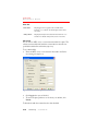
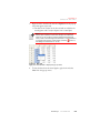
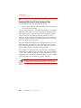
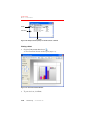
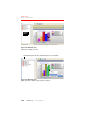
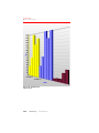
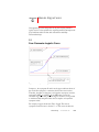
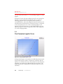
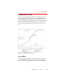
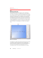
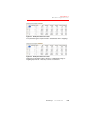
1
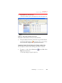
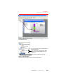
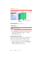
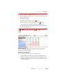
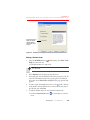
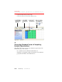
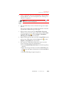
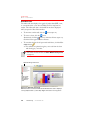
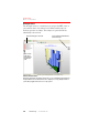
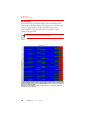
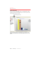
APPENDIX C
MOD
EL
EQUATIONS
C.3
Heteroscedasticity
Fitting nonlinear models to observed data is often complicated by
nonconstant or heterogeneous variability. Heterogeneous variability or
heteroscedasticity occurs in most types of observed data. This is especially
true for biochemical assays where concentration or dose is the predictor
and response is often based on count. Therefore, we can expect that
measurement error varies with respect to the mean. In the Luminex 100
system, MFI (median fluorescence intensity) values are based on bead
counts and vary with the concentration. In this case, we expect the error
in detecting MFI values to increase as concentration increases. This is
best seen in Figure C.3, a residual plot from a Luminex 100 cytokines
assay.
Figure C.3 Residual plot
A residual plot is a graphical representation of how far away an observed
concentration is from its expected value. It plots residuals against
observed concentrations. In Figure C.3, we can see that the deviation of
the observed concentration from the expected value increases as
concentration increases. This means the variability is not constant.
C.4
MasterPlex QT
www.miraibio.com