1
The Institute for Systems Research
ISR Technical Report 2008-16
A
R
ISR develops, applies and teaches advanced methodologies of design and
analysis to solve complex, hierarchical, heterogeneous and dynamic problems of engineering technology and systems for industry and government.
ISR is a permanent institute of the University of Maryland, within the
A. James Clark School of Engineering. It is a graduated National Science
Foundation Engineering Research Center.
www.isr.umd.edu
Graphical User Interface For Automated Biological Cell
Manipulation Tasks
Zachary Cummins
Advisors: Dr. Benjamin Shapiro, Roland Probst
University of Maryland
Institute for Systems Research
Research Experience for Undergraduates 2008
Table of Contents
1 Introduction . . . . . . . . . . . . . . . . . . . . . . . . . . . . . . . . . . . . . . . . . . . . . . . . . . . . . .
1.1 Background . . . . . . . . . . . . . . . . . . . . . . . . . . . . . . . . . . . . . . . . . . . . . . . . . . . . .
..
1.2 Electroosmotic Flow . . . . . . . . . . . . . . . . . . . . . . . . . . . . . . . . . . . . . . . . . . . . . .
..
1.3 Control Devices . . . . . . . . . . . . . . . . . . . . . . . . . . . . . . . . . . . . . . . . . . . . . . . . .
...
1.4 Control System . . . . . . . . . . . . . . . . . . . . . . . . . . . . . . . . . . . . . . . . . . . . . . . . . .
..
1.4.1 Model . . . . . . . . . . . . . . . . . . . . . . . . . . . . . . . . . . . . . . . . . . . . . . . . . . . . . . . . .
.
1.4.2 Algorithm . . . . . . . . . . . . . . . . . . . . . . . . . . . . . . . . . . . . . . . . . . . . . . . . . . . . . .
.
1.4.3 Optical Feedback . . . . . . . . . . . . . . . . . . . . . . . . . . . . . . . . . . . . . . . . . . . . . . . .
.
1.4.4 Accuracy . . . . . . . . . . . . . . . . . . . . . . . . . . . . . . . . . . . . . . . . . . . . . . . . . . . . . . .
.
1.5 Project Goal . . . . . . . . . . . . . . . . . . . . . . . . . . . . . . . . . . . . . . . . . . . . . . . . . . . .
...
1
1
1
2
3
3
3
4
4
4
5
5
5
7
8
8
9
9
10
2 Single Loop Program . . . . . . . . . . . . . . . . . . . . . . . . . . . . . . . . . . . . . . . . . . . . . . . 10
2.1 Existing Code Review . . . . . . . . . . . . . . . . . . . . . . . . . . . . . . . . . . . . . . . . . . . . 11
...
14
2.1.1 Optical Tracking . . . . . . . . . . . . . . . . . . . . . . . . . . . . . . . . . . . . . . . . . . . . . . . . .
.
15
2.1.2 Kalman Filter . . . . . . . . . . . . . . . . . . . . . . . . . . . . . . . . . . . . . . . . . . . . . . . . . . . 15
.
15
2.1.3 Channel Calibration . . . . . . . . . . . . . . . . . . . . . . . . . . . . . . . . . . . . . . . . . . . . . . 15
.
17
2.1.4 Trajectory Manipulation . . . . . . . . . . . . . . . . . . . . . . . . . . . . . . . . . . . . . . . . . . . 17
.
18
2.1.5 Recording . . . . . . . . . . . . . . . . . . . . . . . . . . . . . . . . . . . . . . . . . . . . . . . . . . . . . . 18
.
18
2.2 Approach . . . . . . . . . . . . . . . . . . . . . . . . . . . . . . . . . . . . . . . . . . . . . . . . . . . . . . 18
...
19
2.3 Experiments . . . . . . . . . . . . . . . . . . . . . . . . . . . . . . . . . . . . . . . . . . . . . . . . . . . . 20
...
2.3.1 Eight Channel Device . . . . . . . . . . . . . . . . . . . . . . . . . . . . . . . . . . . . . . . . . . . . . 20
.
2.3.2 Twelve Channel Device . . . . . . . . . . . . . . . . . . . . . . . . . . . . . . . . . . . . . . . . . . .
.
2.4 Conclusion . . . . . . . . . . . . . . . . . . . . . . . . . . . . . . . . . . . . . . . . . . . . . . . . . . . . .
...
i
3 Multiple Loop Program . . . . . . . . . . . . . . . . . . . . . . . . . . . . . . . . . . . . . . . . . . . . .
3.1 Goal . . . . . . . . . . . . . . . . . . . . . . . . . . . . . . . . . . . . . . . . . . . . . . . . . . . . . . . . . .
...
3.2 Approach . . . . . . . . . . . . . . . . . . . . . . . . . . . . . . . . . . . . . . . . . . . . . . . . . . . . . .
...
3.2.1 Optimization . . . . . . . . . . . . . . . . . . . . . . . . . . . . . . . . . . . . . . . . . . . . . . . . . . . .
.
3.2.2 Timers . . . . . . . . . . . . . . . . . . . . . . . . . . . . . . . . . . . . . . . . . . . . . . . . . . . . . . . . .
.
3.2.3 Graphics . . . . . . . . . . . . . . . . . . . . . . . . . . . . . . . . . . . . . . . . . . . . . . . . . . . . . . .
.
3.2.4 Organization . . . . . . . . . . . . . . . . . . . . . . . . . . . . . . . . . . . . . . . . . . . . . . . . . . . .
.
3.2.5 Operation . . . . . . . . . . . . . . . . . . . . . . . . . . . . . . . . . . . . . . . . . . . . . . . . . . . . . .
.
3.3 Experiments . . . . . . . . . . . . . . . . . . . . . . . . . . . . . . . . . . . . . . . . . . . . . . . . . . . .
...
3.3.1 Eight Channel Device . . . . . . . . . . . . . . . . . . . . . . . . . . . . . . . . . . . . . . . . . . . . .
.
3.3.2 Four Channel Device . . . . . . . . . . . . . . . . . . . . . . . . . . . . . . . . . . . . . . . . . . . . .
.
3.4 Conclusion . . . . . . . . . . . . . . . . . . . . . . . . . . . . . . . . . . . . . . . . . . . . . . . . . . . . .
...
4 References . . . . . . . . . . . . . . . . . . . . . . . . . . . . . . . . . . . . . . . . . . . . . . . . . . . . . . . .
A Multiple Loop Program User Manual . . . . . . . . . . . . . . . . . . . . . . . . . . . . . . . . . 21
ii
Table of Figures
1. Electroosmotic flow double layer
2. Control device
3. Eight channel flow modes
4. Particle Tracker window
5. Channel view
6. Thresholded particle image
7. Particle image matrix
8. Labeled particle image matrix
9. Kalman filter results for tracking a single particle
10. Channel calibration
11. Trajectory Manipulation
12. Prepared eight channel device
13. Matrix synthesis
14. Five particles following a square trajectory
15. Five particles following the letters
16. Multiple Loop program window
17. Particle dragging
18. Four particle channel geometry
iii
1
2
3
4
5
6
6
6
7
8
8
10
13
13
14
15
19
19
1 Introduction
1.1 Background
Precise manipulation of particles at a microscopic level can be accomplished by a number
of means with varying degrees of success and benefits. Many biological and pharmaceutical
laboratories employ optical tweezers that use dielectrophoresis to trap and move particles [1].
Optical tweezers can manipulate hundreds of particles at a time in three dimensional space to
within nanometers of each intended position. The advantages of such optical trapping systems
can not be understated, but come at a price. Optical tweezers require lasers and delicate optics
that require significant power and space relative to less accurate and extensive alternatives.
Alternative particle trapping systems have been created as alternatives to optical tweezers
utilizing: electric fields, taking advantage of particles with dielectric properties; magnetic fields,
which manipulate particles with magnets attached to them; and arrays of microelectromechanical
air nozzles that can steer particles along a control surface. These solutions can be executed more
cheaply, and built on a small scale, but lack significant steering capabilities.
The control system described in this section aims to reach some middle ground between
the steering capabilities of optical tweezers and the attractive size and scale of the alternatives.
For a more detailed discussion of the follow introductory descriptions, see [1] and [2].
1.2 Electroosmotic Flow
Figure 1: Electroosmotic flow double layer
1
When a polar fluid, like water, enters a microchannel, an electrical double layer is formed
at the interface between the wall of the channel and the fluid, as shown in Fig. 1. The negatively
charged channel walls of the microchannel attract the positive ions of the fluid, creating a
concentration of positive charges. When an electrical field is applied to the fluid, the fluid of the
double layer is displaced, moving toward the positive cathode end of the applied current. The
displacement of the fluid layer drags the entire fluid along with it, including all the particles in it
regardless of their charge.
The flows created by this effect are predictable and uniform across the channel, making
them ideal for particle control and steering.
1.3 Control Devices
Control devices utilizing EOF are created in a six part process, grouped by two functions:
fabrication and replication. During fabrication, a mold formed by several intersecting
microchannels is formed on a dehydrated silicon wafer. During replication, a silicone polymer,
polydimethylsiloxane (PDMS), is poured over the mold and allowed to solidify. The resulting
device, similar to the one pictured in Fig. 2, can then be placed mold-side down on a glass
microscope slide and filled with deionized water. Voltages applied at each channel create EOF in
each channel.
Figure 2: Control device
2
1.4 Control System
1.4.1 Model
The Navier-Stokes equations model the dynamics of the fluid contained within the
control chamber and microchannels. The electric fields are modeled by Laplace's equation.
Electroosmotic slip velocity boundary conditions are enforced at the floor and ceiling of the
device, while the effects of the channel walls are considered to be negligible.
The resulting governing equation simplifies to V EO = u E , where u is the
electroosmotic mobility of the particle. This equation relates the velocity at any given point in
the flow to the electrical field at that point. Additionally, if the particles themselves are charged
or carry surface charges, they are effected by a process called electrophoresis. Under
electrophoresis, the particle is transported relative to the flow. The velocity due to electrophoresis
is similarly V EP = c E , where c is the electrophoretic mobility. The total velocity for any
given particle, then, is given by V NET =
u
c E . u and c can be determined experimentally,
or obtained from a reference, while E is governed by the voltages applied to the control system.
1.4.2 Algorithm
Each control device is capable of several independent
flow modes. Four of the modes for an eight channel device
are pictured in Fig. 3. In order to achieve a desired velocity
for a given particle, some combination of these modes is
calculated in order to determine the necessary voltage input to
each microchannel.
Individually, each particle in the flow has two degrees
Figure 3: Eight channel flow
modes
3
of freedom in its positioning, x and y coordinates relative to the center of the the control
chamber. This means that a device with odd number, N , modes can control N − 1 ÷ 2
particles.
1.4.3 Optical Feedback
The control algorithm described in 1.4.2 assumes no error in the control model or
uncertainty in the measurement of mobility constants, as well as no sources of noise in the
system response. To account for any errors or uncertainties that may arise in the system, a visual
feedback loop is created using a camera connected between a computer running image
processing software and a microscope used to view the control device. A more detailed
discussion of the optical feedback algorithm is given in section 2.1.2.
1.4.4 Accuracy
The control system is robust in its ability to overcome deficiencies in mobility
measurements, ambient noise, and a relative disregard for the chemical factors that govern
electroosmotic and electrophoretic mobilities for particles.
In general, the accuracy of the system is defined by the resolution of the camera. For
example, each pixel of a 640×480 pixel camera corresponds appoximately to 1 μm error.
1.5 Project Goal
The goal of this project was to develop and refine a graphical user interface (GUI) that
effectively closed the control loop, and gave users the ability to simply and easily interact with a
microchannel device.
To test the efficiency of the control algorithm, the program would be able to create and
run trajectories for particles to follow. To analyze and verify the results, the program would be
able to record experiments in real time. Because of the visual nature of the program, it would
4
also be able to output experiments as videos.
For flexibility in development and distribution, it was desired that MATLAB be the
primary development and running platform.
2 Single Loop Program
2.1 Existing Code Review
The “Single Loop” program was an extension of
work that I had done during the Spring 2008 semester.
During this time, my goal was to take a skeleton program
originally created by Roland Probst and expand it into a
full-featured GUI. This work was primarily done using
previously captured images as a test on the optical
tracking and filtering routines described below. The main
Figure 4: Particle Tracker window
view of this program is pictured in Fig. 4.
The basis for the program was a continuous while loop that would update tracking and
control in each iteration.
2.1.1 Optical Tracking
The optical tracking algorithm uses standard functions provided by the Image Processing
Toolbox included with MATLAB.
5
Figure 5: Channel view
Given a channel image, like that shown in Fig. 5, and the predicted position of a particle,
the optical tracking algorithm extracts the small region of interest (ROI) surrounding the
predicted position, shown as a white outline in Fig. 6. The ROI is converted to black and white,
where any pixel above a certain brightness threshold is given a value of 1, and any value below
is given a value of 0, illustrated in Fig. 7. The brightness threshold is determined by averaging
the intensity of the brightest pixel with the intensity of the dimmest pixel.
Figure 6: Thresholded
particle image
Figure 7: Particle image
matrix
Figure 8: Labeled
particle image matrix
From the resulting black and white image, the position of the particle relative to the ROI
is calculated by averaging the positions of each pixel with an intensity value of 1. The particle's
position with respect to the entire image is then known.
For the event that there are multiple particles present in the same ROI, the bwlabel
6
function is used to find “blobs” of pixels connected to each other. Blobs are identified with a
numeric identifier put in place of pixels with an intensity value of 1. Fig. 8 illustrates the result of
bwlabel when applied to the entire image displayed in Fig. 5. The particle is uniquely
identified by the number 14.
bwlabel does well to distinguish between particles, but in order to determine which
particle is the one of interest, a predictive filter is useful.
2.1.2 Kalman Filter
Measuring particle positions involves some unavoidable uncertainties inherent to both the
imaging and measuring processes. Tracking particles effectively within the camera image is done
with the aid of a Kalman filter that attempts to reduce measurement uncertainties. Additionally,
the filter is able to predict the position of the particle in the next time step. This prediction is then
used by the optical tracking algorithm to determine which particle among several is the correct
particle to measure and subsequently track.
Figure 9: Kalman filter results for tracking a single
particle
7
Fig. 9 illustrates the use of the Kalman filter in the tracking of a single particle. Between
frames 317 and 321, the measurement of the particle undergoes a rapid oscillation in the vertical
direction; the estimated position, by contrast, remains relatively linear. This feature becomes
especially important when particles undergo severe oscillation or rapid changes in direction.
The mathematical derivation and reasoning of the Kalman filter is beyond the scope of
this paper. A more detailed discussion can be found in [3].
2.1.3 Channel Calibration
A key feature of the code previously developed
was the ability to interactively and visually measure and
orient the channel geometry. By visualizing the channel
geometry, users can more easily and accurately line up the
modeled channel geometry of the program with the actual
channel geometry pictured. This is vital for conversion
between the camera's pixel coordinate system, and the
Figure 10: Channel calibration
control model's metric coordinate system.
2.1.4 Trajectory Manipulation
Another key existing feature was the ability to
interactively create and manipulate trajectories using
Bézier curve parameterization [#]. Modeled after Adobe
Photoshop's (Adobe Systems Incorporated, San Jose, CA)
Path tool, users could plot and move points using tools on
the trajectory toolbar. The shaping tool allowed users to
Figure 11: Trajectory manipulation
8
select individual points and modify the curvature around the point.
This type of trajectory manipulation is ideal for on-the-fly particle steering, and provides
the ability to create arbitrarily complex trajectories that would be difficult to create from the
command line or from a script file.
2.1.5 Recording
Recording was a simple matter, but especially important in making Particle Tracker
useful as an experiment tool. At each frame, the recording routine would add relevant program
data structures to a single cumulative recording structure. This structure could then be saved for
later analysis, or played back within the program.
In this early version of the recording code, channel orientation and scaling information
was not saved. This limited the visual usefulness of the recordings to single program sessions
where no changes were made to channel geometry.
2.2 Approach
The first task was to connect the existing program the external devices used to monitor
and control the physical control devices. Integration of the camera into the program was
achieved in three parts:
1. Initializing the camera as a MATLAB videoinput object.
2. Using preview to automatically update the camera image on the display axis at
interval. As a downside, this capped the program control loop frequency at the image
acquisition frequency of the camera, 30 Hz at its fastest.
3. Retrieving the latest image from the camera using getsnapshot.
The second task was to calculate voltages for each device device based on the error
between the measured particle position and the desired particle position. This was easily
9
accomplished because each control model associated with the model also had an associated
voltage calculation function that followed the flow-field matrix inversion scheme described in
[2].
The third task was to send the calculated voltages to the analog voltage output device that
would apply them to a control device. This was achieved in two parts:
1. Initializing the analog output device as a MATLAB analogoutput object.
2. Stopping the object with stop, then queuing data voltages into the device's buffer
using putdata and restarting the object with start.
Once the program was capable of performing these three tasks, it could then be used to
perform experiments, and troubleshoot problems in the code and in the control model's
calculation of voltage.
2.3 Experiments
2.3.1 Eight Channel Device
To visually verify that the program
was correctly calculating and applying
voltages, an eight channel control device,
Fig. 12, was prepared and equalized on
two separate occasions.
During the first experiment, it was
possible to control one particle with
limited success near the center of the
device. When the particle was dragged
Figure 12: Prepared eight channel device
away from the center, its error would
10
gradually increase until it could no longer be held by the controller. In trying to control more
than one particle, all the particles were shot off of their desired positions. During trials where
multiple particles were being controlled it seemed that the wrong channels were being actuated.
A coordinate system conversion error seemed to be the problem. In the existing
conversion code, the device cross section was assumed to be measured along the diameter rather
the radius; thus, conversion was off by a factor of 2. This explained why particles could be held
near the center, and it was thought that a combination of this and poor pressure equalization
caused multiple particle control to fail.
In the second experiment, this correction allowed for one particle to be steered aptly
throughout the control area with little problem. However, when multiple particles were selected,
control became immediately unstable.
2.3.2 Twelve Channel Device
Intertwined with the eight channel experiments were twelve channel device experiments
with Satej Chaudhary that aimed to control a maximum of five particles at a time. These
experiments suffered the same characteristics that plagued the eight channel experiments. Only
one particle could be steered at a time, and multiple particle steering was impossible.
Additionally, pressure equalization was of greater importance in reducing disturbances to the
control device.
The apparent obstacle to multiple particle steering was an error in the code that retrieved
the flow field matrix as well as the code that returned voltages. Both were initially programmed
to synthesize matrices following a pattern of stacking all x components on top of all y
components. The fix was to instead synthesize these matrices by interchanging x and y
components, as shown in Fig. 13.
11
However, the operations performed here are mathematically equivalent. In performing
the above “fix,” the actual error was corrected as a consequence of rethinking the functions in
question.
a.) Correct
b.) Incorrect
vx , 1
e= v y, 1
vx , 2
v y ,2
vx ,1
e= v x , 2
v y, 1
v y ,2
[]
[]
Figure 13: Matrix synthesis
Once corrected, multiple particle tracking became a reality for the twelve channel device.
During early experiments, control of two, three, and four particles was performed with relative
success. Difficulties came in many forms:
1. Pressure flow was very detrimental to the device. Unless the pressure of the channel was
careful equalized and maintained throughout experiments, it was unlikely that the device
would display enough stability to either steer particles or simply hold several in position.
2. Channel actuation would reverse or fail due to changes in system chemistry and ion
buildup. This would occur during long experiments and when voltage was manually
applied to a specific channel for prolonged periods of time.
3. Channels became easily clogged and required thorough cleaning to remove any
significant blockage. 2 micrometer fluorescent beads were originally used for ease in
tracking and visualization, but 1.2 micrometer fluorescent beads were settled on.
4. Program speed, after long experiments, gradually decreased to below the desired control
frequency of 15 Hz.
For these reasons, experiments with the twelve channel device took on a very delicate
dynamic, but eventually proved successful. Several trajectories were planned by Chaudhary in a
12
simplistic form. Each trajectory was a collection of waypoints – points used in linearly
interpolating the complete trajectory – normalized to a radius of 1 unit, and each waypoint was
associated with a time relative to the beginning of the trajectory's start. The number of points in
between assured that the trajectory was correctly updated with the control algorithm at each
update, and were determined by the formula:
Number of points = Control frequency[ Hz ] × Secondsbetween waypoints[ s]
An example of his type of trajectory is a square followed by five particles, shown in Fig.
14. The black line represents the desired trajectory, the red trajectory represents the actual
trajectory of each particle, and the blue outlined square represents the region of interest in which
the particle being controlled was searched for. Note that in the bottom right corner of the square
that accuracy is especially poor. This is due to comparatively poor actuation from one or more of
the channels in the bottom right of the image. Also note that at points along the trajectories that
the actual trajectories seem to loop on themselves. This is due to overshoot caused by time delay;
voltages are being applied for too long, forcing particles passed their desired positions.
Figure 14: Five particles following a square
trajectory
13
Another experiment, shown in Fig. 15, was done using the trajectory tool to form five
letters representing five of the people that have spent time with the project. This was a more
difficult task, and larger errors appeared in letters with more curves in them. Note that the
trajectories do not use the Bézier shaping feature of the trajectory tool. When these curves were
employed, they resulted in velocities too fast to be handled while steering five particles. Instead,
waypoints were put in place to ensure the same linear fit as employed with the trajectories
described above.
Figure 15: Five particles following the letters:
B (Dr. Benjamin Shapiro), S (Satej Chaudhary), M
(Mike Armani), R (Roland Probst), and Z (Zach
Cummins)
2.4 Conclusion
Performing experiments with this program provided many valuable lessons.
Fundamentally, the structure of the program did not lend itself to ease of development, which
was one of the pillars of choosing MATLAB as the development platform to begin with. As
needs changed, the amount of code grew to many thousand lines, which was undesirable for
debugging and distribution.
14
Trajectory creation essentially failed as a tool. Though attractive, it became an
afterthought during the experiment process. When it was used, it was not fully developed to
perform tasks in the experimental setting, and so a supplementary waypoint style of trajectory
plotting took its place. This feature may require functional or experimental necessity and purpose
before it is more aptly developed.
Speed also became an apparent issue during experiments and recording. Control
frequency would drop to 10 Hz in the presence of more than three particles and trajectories. All
extraneous graphic displays were thus disabled or hidden to achieve 15 Hz.
3 Multiple Loop Program
3.1 Goal
Drawing from experiences and
observations accumulated in developing
and using the Single Loop program, I set
out to almost completely rewrite the
program. This program would be a
simplified version of the Single Loop
program, meaning that it would not have
trajectory creation or many graphics. The
focus points of this version of the program
were speed, size, and ease of use.
3.2 Approach
Figure 16: Multiple Loop program window
3.2.1 Optimization
Using the profile function, several time consuming functions were identified and
15
modified for speed:
1. The stop function used to reset the voltage applied to the analog output device took the
most time, subtracting as much as 10 Hz from the control frequency. However, it was
never needed at all.
As long as the voltage output device's sampling buffer did not run out, it is able to
run without stopping. Alternatively, the device can be restarted using start, which did
not require a stop function call beforehand. This was an artifact from older code that
used a different voltage output device.
2. The drawnow function that flushed the MATLAB event queue and redrew all open
figures slowed down the control frequency by a variable amount depending on the
complexity of graphics to be recalculated and displayed at each call.
Removing drawnow also removes the ability to actively use the mouse to interact
with program, so compromises in the design and display of the GUI were made. All
extraneous graphics would be hidden by default.
3. The getsnapshot function used to retrieve the latest frame from the camera for
processing limited the maximum control frequency to the frequency of the camera. At
each call, getsnapshot waits for the frame to be completed before returning control
to MATLAB. The preview function used to display images from the camera operates
in a similar way.
getsnapshot was replaced with peekdata, which simply takes the number
of frames requested from the camera buffer without waiting for a frame to completed.
This means that, when run faster than the camera frequency, a frame may only partially
be current frame. For this application, where small velocities and particles are expected,
16
this alternative is acceptable and does not effect control.
preview was removed in favor manually updating the CData property of the
image object on the display axis with the image retrieved using peekdata. This
achieves the same thing as preview without waiting for camera to finish acquiring
frames.
3.2.2 Timers
To simulate a multi-threaded environment, and free the command line up during program
operation, timer functions were utilized. The timer function allows MATLAB to schedule
function operation, and can be made to continually run in the program background. This was an
ideal solution because videoinput, analogoutput, and all other clocked device objects
provide built in timer functionality.
The camera image would then be automatically updated at a frequency separate and
perhaps different from the control frequency because both would be run in their own timers.
Early tests resulted in frequencies as high as 60 Hz for the videoinput timer, and 100 Hz for
the analogoutput timer.
3.2.3 Graphics
To simplify graphics display, hggroup and hgtransform objects were employed to
group together objects that could be hidden and shown at the same time, or rotated and scaled at
the same time. The hgtransform object is especially useful in creating a virtual representation
of the control device. The control device can be easily modeled using actual or normalized units,
and then scaled, rotated, and centered over the camera image. This simplifies both the display of
data in the channel coordinate system and the conversion between coordinate systems.
Timer functions enabled more extensive use of graphics callbacks to handle mousing
17
events. Where these events were handled during each loop iteration in the Single Loop program,
they are handled using the WindowButtonDragFcn property of the program figure. This reduces
code size and simplifies the way events are thought about.
3.2.4 Organization
Due to the shear size of the Single Loop program, it was thought that organization would
be best handled by organizing structures into classes. Object orientation is not one of MATLAB's
strengths, but the logical organization of functions was attractive.
Instead, as code was being simplified through the other methods described, only the
directory structure of classes was adopted. This meant that functions could be placed in a folder
of the same name with an “@” symbol in front of it. In this folder, another folder entitled
“private” could contain functions only called by the function in the directory above it.
3.2.5 Operation
Program operation was to be as simplistic as possible, following a simple procedure:
1. Match channel geometries.
2. Select and drag particles with the mouse.
3. Record and replay operation.
3.3 Experiments
With the control code having been debugged during the development of the Single Loop
program, experiments on the Muliple Loop program were performed largely to verify that it
worked with the control system, and what, if any, speed benefits there were.
3.3.1 Eight Channel Device
Experiments to test that the program worked with the existing control algorithm were
done first using an eight channel device. This would also verify that the program could be used
18
in related experiments involving nanodots.
With little effort, the eight channel was up
and working. By adjusting the gain on the channel
voltages, accuracy and the speed of the control
device to the motion of the mouse could be easily
increased. Multiple particle control likewise
worked fairly well when simply holding particles
in place. Difficulty did occur in moving these
particles, however.
Figure 17: Particle dragging
3.3.1 Four Channel Device
The four channel device was especially
important to test because it would potentially
serve as a demonstration of the control system's
operation for a Nature Protocols protocol paper.
Unfortunately, a working model of four channel
control was not available for testing. Instead, the
eight channel model was used, using only the
voltages calculated for channel 1 (top), channel 3
(right), channel 5 (bottom), and channel 7 (left).
Figure 18: Four particle channel geometry
This resulted in adequate control of a single particle when the voltage gain was increased.
However, the eight channel flow field matrix is smaller than the control area of the four
channel device. When directly adapted to the actual control area radius of the four channel
19
device, particles must not travel past the boundaries of the flow field matrix. Doing so results in
program error and termination. To account for this, either the flow field matrix must be properly
scaled, or a new model must be extracted and used.
3.4 Conclusion
The Multiple Loop program provides an overall better base for continued development of
the Particle Tracker program. During experiments, the control frequency easily reached 30 Hz,
matching the camera frequency. For faster cameras, this will mean improved control, and the
possibility of increasing the number of particles controlled by juggling between different sets of
particles. As the camera frequency increases, the error measured between a particle's measured
position and its desired position will decrease, and so finer adjustments can be made during each
loop iteration.
A short manual for this program is attached as Appendix B.
4 References
[1] B. Shapiro et al: “Using Feedback Control of Microflows to Independently Steer Multiple
Particles”, IEEE J. Micromech. Systems, vol. 15, no. 4, pp. 945-956, 2006
[2] S. Chaudhary and B. Shapiro: “Arbitrary Steering of Multiple Particles Independently in
an Electro-Osmotically Driven Microfluidic System”, IEEE Trans. Control Systems
Tech., vol. 14, no. 4, pp. 669-680, 2006
[3] Randall L. Eubank: “A Kalman Filter Primer”, CRC Press, 2006
20
Appendix A: Multiple Loop Program User Manual
21
Particle Tracker User Manual
1 Introduction
Particle Tracker is a MATLAB demonstration of the cross channel microfluidic control
device. Users can select particles from live video of the control device, and use the mouse to
drag particles within the control area. Recording and playback functionality allows users to save,
replay, and analyze experiments.
1.1 Requirements
The requirements listed below refer to those used in developing and testing the program.
Other hardware configurations and software versions may work, but are not guaranteed.
1.1.1 Hardware
z
z
z
z
Processor: Intel Pentium 4 3.4 GHz
RAM: 1 GB DDR2
Hard drive: 80 GB WD800JD, 7200 RPM
Video RAM: 256 MB ATI Radeon X600
1.1.2 Software
MATLAB R2007b
c Image Acquisition Toolbox Version 3.0
c Image Processing Toolbox Version 6.0
c Data Acquisition Toolbox Version 2.11
1.2 Installation
To install, extract particletracker.zip into a convenient location.
1.3 Configuration
Particle Tracker uses MATLAB analogoutput and videoinput objects to interface
with the control apparatus. To use a specific device, edit the following files:
z
File
Output
initao.m
analogoutput
updateao.m
No Output
initvid.m
videoinput
updatevid.m
Image
Description
Initializes the analog output device applying
voltages to the control device.
Sends voltages calculated by the control algorithm
to the analog output device.
Initializes the camera viewing the control device.
Returns the latest frame from the camera.
Table 1: Configuration files
Note: Each file contains useful comments and code examples.
22
3 Operation
3.1 Running
1.
In MATLAB, navigate to the directory containing the
Particle Tracker installation. To run the program, simply
run pttool.m from the directory view or command
line. A window similar to that shown in Figure 1 will
appear.
3.2 Calibrating
1.
Select the “Voltage Display On/Off” button on the
toolbar to bring up the channel voltage display.
2.
Manually apply arbitrary voltages to each channel by
typing in voltages in the respective channel text fields
located in the bottom left corner of the display.
Applying a variety of positive and negative voltages to
each channel tests actuation and is useful for visually
locating each channel.
23
3.
In order to calibrate the conversion from Particle
Tracker's pixel coordinate system to the metric
coordinate system of the control algorithm, the pictured
channel geometry must be matched with the modeled
channel geometry provided by the program.
Select the “Channel Geometry” toolbar button to initiate
the channel calibration mode.
4.
To adjust the radius and angular orientation of the
modeled channel geometry, hold the left mouse button
down on the white dot lying in Channel 2 and drag until
a rough estimate of the scale and rotation of the pictured
channel geometry has been reached.
Note:
To only adjust the channel's radius, hold both the left and right
mouse button down on the white dot at the same time while
dragging.
To only adjust the channel's angular orientation, instead hold the
right button down on the white dot while dragging.
5.
To center the modeled channel geometry over the
pictured channel geometry, hold the left mouse button
down on the center of the white cross and drag to the
pictured channel geometry's center.
6.
Repeat steps 4 and 5 until the pictured channel geometry and the modeled channel
geometry overlap.
7.
Exit channel calibration mode by again selecting “Channel Geometry.”
Note: The device may need to be calibrated several times during the course of an experiment as the result of
small movements during channel reservoir refilling or from mechanical vibration applied to the work area.
Repeat the above instructions as necessary.
24
3.3 Manipulating Particles
1.
Enable particle control by selecting “Control On/Off”
from the toolbar.
2.
Choose a particle for control by left mouse clicking the
active camera view.
Two circles will appear, connected by a black line. One
circle displays the desired position of the particle, while
the other displays the actual position of the particle.
The initial desired position is the point clicked by the
mouse.
3.
Initially, a selected particle may exhibit large error with
respect to its desired position. This error may be
attributed to pressure flow or flaws in the device.
To correct this, increase the voltage gain by setting the
“Gain” field on the bottom of the window to a number
higher than displayed.
Note: Setting gain too high will result in overshoot and instability.
If possible, experiment to find the appropriate gain.
4.
Drag the particle within the control area by left mouse
clicking either of a particle's positioning circles, and
dragging the circle in the desired direction.
25
5.
Particles may be deleted from the controller by right
mouse clicking either of a particle's positioning circles.
To delete all particles at once, choose “Release All”
from the “Particles” menu.
To delete all but the number of particles capable of
being controlled, choose “Release Extra” from the
“Particles” menu.
3.4 Recording
3.4.1 Toolbar
The recording toolbar consists of five tools enabling experiments to be recorded and
replayed. These tools do not interfere with the tracking and control of particles, but may slow the
program down when lengthy recordings are in memory.
26
Button
Action
Description
Rewind Resets or restarts playback from the first recorded time step.
Sequentially displays each time step in memory. When a recording
finishes playback, it rewinds to the beginning and replays.
Play
Note: Time steps are not played with respect to the time at which they were
recorded. They are played with respect to the current speed of the Control loop.
This avoids interference with ongoing particle control occurring in the program
background.
Pause
Halts the display on the current time step without returning the
display to the active camera view.
Stop
Returns the display to the active camera view and any existing
trackers still in the control area.
Record
Saves each time step to memory beginning from the initial button
press and ending when Stop is pressed.
Table 2: Recording toolbar
3.4.2 Playback Display
Experiment playback features two useful displays: “Channel Geometry” to give a clearly
defined view of the control device, and “Experiment Data” (time, frequency, voltage, and gain)
for analysis. Each can be toggled on and off by selecting the corresponding entry of the the
“Recording” menu's “Display” sub-menu.
3.4.3 Saving and Loading
Experiment data can be saved to a MATLAB .mat file for analysis by selecting “Save
Recording” from the “Recording” menu. This data can then be loaded at another time by
selecting “Load Recording” from the “Recording” menu.
3.4.4 Saving Video
Playback can be saved as an AVI file by selecting “Export to AVI” from the “Recording”
Menu.
Note: Saving playback to video can take a significant amount of memory. Long experiments may take a long
time or cause program error.
3.4.5 Saving Screenshots
Still images can be saved from playback by selecting “Save Screenshot” from the
“Recording” menu. These images are saved in the png format.
3.4.6 Clearing Experiment Data
Experiments can take up a significant amount of memory, causing the program to slow
down. To release this memory, choose “Clear Recording” from the “Recording” menu.
27