1
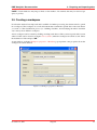
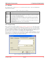
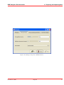
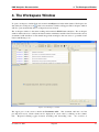
KMX Analytics Documentation
November 4, 2011
Project
Author
Client
Date
KMX Analytics Documentation
R. Argentini, R.P. v.d. Berg
November 4, 2011
Project Code
Document Status
Document Version
Copyright © 2006–2009 Treparel Information Solutions B.V., Delft, The Netherlands.
All Intellectual Property Rights on the content of this document are explicitly reserved by Treparel Information Solutions B.V.
No part of this document may be copied or made public by means of press, photocopy, microfilm audio or videotape or by
whatever means, nor to be stored in an electronic retrieval system without prior written permission by Treparel Information
Solutions B.V.
KMX Analytics Documentation
CONTENTS
Contents
1
Introduction
4
2
Licensing
5
3
Preparing and importing data
3.1 Logging onto KMX Patent Analytics
3.2 Importing from file . . . . . . . . .
3.3 Importing CSV files . . . . . . . . .
3.4 Querying a data service . . . . . . .
3.5 Creating a workspace . . . . . . . .
3.5.1 Metadata . . . . . . . . . .
3.5.2 Text processing . . . . . . .
3.5.3 Text Field Weights . . . . .
3.5.4 SVM Parameters . . . . . .
4
5
6
.
.
.
.
.
.
.
.
.
.
.
.
.
.
.
.
.
.
.
.
.
.
.
.
.
.
.
.
.
.
.
.
.
.
.
.
.
.
.
.
.
.
.
.
.
.
.
.
.
.
.
.
.
.
.
.
.
.
.
.
.
.
.
.
.
.
.
.
.
.
.
.
.
.
.
.
.
.
.
.
.
.
.
.
.
.
.
.
.
.
.
.
.
.
.
.
.
.
.
.
.
.
.
.
.
.
.
.
.
.
.
.
.
.
.
.
.
.
.
.
.
.
.
.
.
.
.
.
.
.
.
.
.
.
.
.
.
.
.
.
.
.
.
.
.
.
.
.
.
.
.
.
.
.
.
.
.
.
.
.
.
.
.
.
.
.
.
.
.
.
.
.
.
.
.
.
.
.
.
.
.
.
.
.
.
.
.
.
.
.
.
.
.
.
.
.
.
.
.
.
.
.
.
.
.
.
.
.
.
.
.
.
.
.
.
.
.
.
.
.
.
.
.
.
.
7
7
7
8
10
14
15
15
16
16
The Workspace Window
4.1 Projection Visualization . . . . . . . . . . .
4.2 Selection . . . . . . . . . . . . . . . . . .
4.3 Searching . . . . . . . . . . . . . . . . . .
4.4 Brushing . . . . . . . . . . . . . . . . . . .
4.4.1 Adding documents to a brush . . .
4.4.2 Removing documents from a brush
4.4.3 Labeling a brush . . . . . . . . . .
4.4.4 Creating a sub-workspace . . . . .
4.4.5 Saving a brush . . . . . . . . . . .
4.4.6 Loading a brush . . . . . . . . . . .
4.4.7 Exporting the brushing legend . . .
4.5 Filtering . . . . . . . . . . . . . . . . . . .
4.5.1 Adding filters . . . . . . . . . . . .
4.5.2 Entering Filter Expressions . . . . .
4.6 Classification . . . . . . . . . . . . . . . .
4.7 Coloring . . . . . . . . . . . . . . . . . . .
.
.
.
.
.
.
.
.
.
.
.
.
.
.
.
.
.
.
.
.
.
.
.
.
.
.
.
.
.
.
.
.
.
.
.
.
.
.
.
.
.
.
.
.
.
.
.
.
.
.
.
.
.
.
.
.
.
.
.
.
.
.
.
.
.
.
.
.
.
.
.
.
.
.
.
.
.
.
.
.
.
.
.
.
.
.
.
.
.
.
.
.
.
.
.
.
.
.
.
.
.
.
.
.
.
.
.
.
.
.
.
.
.
.
.
.
.
.
.
.
.
.
.
.
.
.
.
.
.
.
.
.
.
.
.
.
.
.
.
.
.
.
.
.
.
.
.
.
.
.
.
.
.
.
.
.
.
.
.
.
.
.
.
.
.
.
.
.
.
.
.
.
.
.
.
.
.
.
.
.
.
.
.
.
.
.
.
.
.
.
.
.
.
.
.
.
.
.
.
.
.
.
.
.
.
.
.
.
.
.
.
.
.
.
.
.
.
.
.
.
.
.
.
.
.
.
.
.
.
.
.
.
.
.
.
.
.
.
.
.
.
.
.
.
.
.
.
.
.
.
.
.
.
.
.
.
.
.
.
.
.
.
.
.
.
.
.
.
.
.
.
.
.
.
.
.
.
.
.
.
.
.
.
.
.
.
.
.
.
.
.
.
.
.
.
.
.
.
.
.
.
.
.
.
.
.
.
.
.
.
.
.
.
.
.
.
.
.
.
.
.
.
.
.
.
.
.
.
.
.
.
.
.
.
.
.
.
.
.
.
.
.
.
.
.
.
.
.
.
.
.
.
.
.
.
.
.
.
.
.
.
.
.
.
.
.
.
.
.
.
.
.
.
.
.
.
.
.
.
.
.
.
.
.
18
19
24
24
24
26
28
28
28
29
29
29
29
31
33
34
35
Classification Concepts
5.1 What kind of results can be expected
5.2 Classifying Text Data . . . . . . . .
5.3 Type of classifications . . . . . . . .
5.3.1 Binary classification . . . .
5.3.2 Multi class classification . .
.
.
.
.
.
.
.
.
.
.
.
.
.
.
.
.
.
.
.
.
.
.
.
.
.
.
.
.
.
.
.
.
.
.
.
.
.
.
.
.
.
.
.
.
.
.
.
.
.
.
.
.
.
.
.
.
.
.
.
.
.
.
.
.
.
.
.
.
.
.
.
.
.
.
.
.
.
.
.
.
.
.
.
.
.
.
.
.
.
.
.
.
.
.
.
.
.
.
.
.
.
.
.
.
.
.
.
.
.
.
.
.
.
.
.
.
.
.
.
.
.
.
.
.
.
.
.
.
.
.
.
.
.
.
.
.
.
.
.
.
41
41
41
42
42
42
The classification process
6.1 Session Objects . . . . . . . . . . .
6.2 Performing Binary Classification . .
6.3 Performing compound classification
6.4 Performing Multiclass Classification
6.5 Cross-validation and ROC plot . . .
.
.
.
.
.
.
.
.
.
.
.
.
.
.
.
.
.
.
.
.
.
.
.
.
.
.
.
.
.
.
.
.
.
.
.
.
.
.
.
.
.
.
.
.
.
.
.
.
.
.
.
.
.
.
.
.
.
.
.
.
.
.
.
.
.
.
.
.
.
.
.
.
.
.
.
.
.
.
.
.
.
.
.
.
.
.
.
.
.
.
.
.
.
.
.
.
.
.
.
.
.
.
.
.
.
.
.
.
.
.
.
.
.
.
.
.
.
.
.
.
.
.
.
.
.
.
.
.
.
.
.
.
.
.
.
.
.
.
.
.
43
43
44
48
50
51
November 4, 2011
.
.
.
.
.
.
.
.
.
.
.
.
.
.
.
.
.
.
.
.
.
.
.
.
.
.
.
Treparel
2
KMX Analytics Documentation
6.6
CONTENTS
Parallel Coordinates Visualization . . . . . . . . . . . . . . . . . . . . . . . . . . . . . 52
7
Workflow building classifiers
57
8
Performance metrics explained
8.1 Confusion matrix . . . . . . . . . . . . . . . . . . . . . . . . . . . . . . . . . . . . . .
8.2 Precision and Recall . . . . . . . . . . . . . . . . . . . . . . . . . . . . . . . . . . . .
8.3 Reading ROC plots . . . . . . . . . . . . . . . . . . . . . . . . . . . . . . . . . . . . .
59
59
59
59
Index
November 4, 2011
61
Treparel
3
KMX Analytics Documentation
1. Introduction
1. Introduction
Treparel would like to thank you for choosing our software solution. We are here to serve you as our
valued customer and to make sure the software provides you with the benefits you were looking for. We
appreciate any suggestions and or remarks that you may have to improve our solutions even further.
This document serves as a user manual and look-up reference for users of the Treparel KMX Patent
Analytics SE software. In some of the illustrations in this manual a user-field is visible. These references
are not present in your SE edition and can be safely ignored. SE is a single user application and as such
does not support multiple users.
KMX Patent Analytics is aimed at professionals who need to analyze many text documents.
KMX Patent Analytics consists of three main ingredients. Automated (supervised) categorization, document clustering (unsupervised) and an integrated visualization/analytics environment.
KMX Patent Analytics uses supervised classification that allows an information professional to define
documents of interest based on examples (training data). By using training data the software does not
restrict itself to the use of specific keywords, instead relying on the specified documents to establish a
profile of the categories. The classifier assigns scores to the examined documents that can be used to
establish the relevance of the document to the classification task at hand.
KMX Patent Analytics provides unsupervised clustering techniques to give the user insight into the
structure of the data set itself. This technique is unsupervised and works primarily by comparing the
text statistics of different documents to each other. Documents that are similar are placed near to each
other. This enables the user to discover new classes and potentially relevant document groups.
The result of the supervised and unsupervised analysis are integrated into a rich interactive visualization
environment that combines the power of both supervised and unsupervised algorithms. This enables the
user to take the information obtained from the undirected clustering analysis and use it to select better
training documents for automated text categorization. They can even discover entirely new classes of
documents and use them to define a new category in the classifier with a single click. It also allows the
user to integrate the results of the supervised classification into the clustering analysis, tailoring it to the
task at hand. Interactive exploration delivers information at all levels, from high-level data set overview
to individual document text.
All these components work together to enable the user to learn as much as possible about the data in
the allotted time, discover documents and subclasses of interest and extract them from the data set using
robust and repeatable methods.
We wish you many productive hours with our solutions,
The Treparel Team
Support website: http://treparel.com/uk/about_us/customer_support/
E-mail support: [email protected]
November 4, 2011
Treparel
4
KMX Analytics Documentation
2. Licensing
2. Licensing
KMX Patent Analytics requires a valid license in order to run. The majority of users users install the
application from pre-licensed installation media, and will therefore not need to concern themselved
with licensing details. If you wish to install from unlicensed installer files, or are the administrator for
your organization’s Enterprise Edition installation, this section will give you an overview of the license
management system.
Figure 2.1: The program will not start if the license file is missing or expired.
In order to run KMX Patent Analytics, the user will need a valid license file. The program will not start
if the license file is missing or expired. You should have received a valid license file together with your
program distribution.
Using the License Management button on the license expiration notification, the user can open the
license management interface. The license manager is also available from within the application, by
selecting Help -> License... from the application menu. In the license manager the user can view the
information contained in the current license, if any. The user can also import a new license file if desired,
by using the Import License button. After a new license file has been loaded, the program will shut
down. After the program has been restarted, the new license file will be used.
November 4, 2011
Treparel
5
KMX Analytics Documentation
2. Licensing
Figure 2.2: License management and information.
November 4, 2011
Treparel
6
KMX Analytics Documentation
3. Preparing and importing data
3. Preparing and importing data
3.1 Logging onto KMX Patent Analytics
Start the KMX Patent Analytics program on your system.
First open the KMX application.
The KMX Patent Analytics application opens and you will see the main screen, see figure The main
application screen. Open the root folder to by clicking on the + sign if it is still closed.
Figure 3.1: The main application screen
3.2 Importing from file
To import a data into KMX Patent Analytics using files, an initial data set has to be retrieved from your
data sources. If this is not already the case, the created collection of records must be converted into a
format supported by KMX Patent Analytics.
Supported formats for text import are:
• Microsoft Excel (both XLS and XLSX)
• Comma Separated Values (CSV), see also the section about CSV import in this manual.
• Patbase XML, both at document and family level
• WIPO ST.32 XML
• Medline XML
November 4, 2011
Treparel
7
KMX Analytics Documentation
3. Preparing and importing data
Formats may be unavailable due to licensing restrictions and/or configuration.
Now the file is ready to be imported into KMX Patent Analytics.
The dataset can now be imported by selecting the relevant import option fromt eh file menu. For example, to import a CSV file, select File → Import from file → Excel and CSV.
The system will now ask you where to store the data. Select the position where you want to store the
imported dataset, and click OK.
Figure 3.2: Select a folder
You can first create a new folder by clicking the right mouse button, selecting the folder and then store
the dataset.
Figure 3.3: Create a sub-folder
By clicking the OK button, you start uploading your data set to the KMX server. Once the upload and
processing has completed the dataset will be displayed in the designated location in the Object panel in
the main window with a dataset icon .
The dataset remains accessible from within KMX Patent Analytics until you explicitly request the system
to remove it again by selecting the dataset, right-clicking and selecting delete object. Once uploaded
you can access the dataset at any time and perform classification operations on it.
3.3 Importing CSV files
The importer for comma-separated-values (CSV) files is very comprehensive. It supports multiple character encodings, both in strict and non-strict modes. It supports selection of CSV parameters including
November 4, 2011
Treparel
8
KMX Analytics Documentation
3. Preparing and importing data
Figure 3.4: The CSV importer
November 4, 2011
Treparel
9
KMX Analytics Documentation
3. Preparing and importing data
separator, quoting and escape characters, as well as different quoting rules. These parameters can be
auto-detected. The importer includes an option to skip rows at the start of the file, for example to ignore
a header, and a way to specify which column contains the document identifier. In order to facilitate these
operations, the importer sports a preview pane that shows the way the documents in the set are being
parsed and updates in real time. The importer also includes a verification function that find problems
with the set and helps the user to troubleshoot them.
Under the heading Import Options the user can select basic properties of the file to be imported. The
user can select the character encoding of the specified file. The user can also choose whether this
encoding is to be decoded in a strict manner (invalid characters cause an error) or in a non-strict manner
(invalid characters are replaced with the unicode replacement character, U+FFFD). The user can also
choose to skip additional header rows by starting the import of the CSV file from a different line number.
Finally, the user can select what column contains the unique document identifier.
Under the heading CSV Options the used can select options that affect how the CSV file is to be
decoded. The user can select what character is to be used as a separator. Traditionally, the comma (,)
character is used, but some spreadsheet programs default to the semicolor (;) character. Sometimes the
TAB character is used. A custom separator can be entered. The quoting character is used to delimit
data fields that may contain a separatoor character. There are two main methods of protecting a quote
character in a data field. Double quoting means that two repeated quoting characters in a quoted data
field are treated as a single quoting character apprearing in the data. The quoting character can also
be protected usign an escape character. A common chioce is the backslash () character. The escape
character must then also be used to escape escape characters in the input, resulting in two consecutive
escape characters to represent a single escape character in the input.
A preview pane offer a live view of how the CSV file will be doceded using the current settings. The
number of rows decoded for preview can be selected under the heading Preview Options. Here we can
also refresh the preview pane, forcing a complete re-evaluation of the contents of the file.
3.4 Querying a data service
It is also possible to import a dataset directly from one of the supported databases. To access this
functionality, select File –> Search and Import from the menu.
Using the Database to query control you can choose which database you wish to use to perform your
searches. Additional configuration options relating to access to this database can be set using the Configure button.
The user can enter a query in the query field. The query can be multiple lines and should be specified in
the query syntax that is required by the underlying data source. Using the File menu, the user can load
and save search queries for future use.
Using the Select Columns button, the user can select the columns from the underlying database that will
be imported into KMX Patent Analytics.
The user can preview of the results of the current query. Upon presing the Preview button, the application will retrieve the top matches from the database. The number of results retrieved in preview mode
defaults to 5 and can be adjusted using the input field above the preview pane. The application will also
indicate the total number of documents that match the search query.
Once the user is satisfied with the results of the query, he can press the Import button. This will start
the process of retrieving the result set from the database and importing it into KMX Patent Analytics.
November 4, 2011
Treparel
10
KMX Analytics Documentation
3. Preparing and importing data
Figure 3.5: The Search and Import window.
November 4, 2011
Treparel
11
KMX Analytics Documentation
3. Preparing and importing data
Figure 3.6: The Select Columns window.
November 4, 2011
Treparel
12
KMX Analytics Documentation
3. Preparing and importing data
Figure 3.7: A query and the corresponding preview. The current query select all documents with a
publication date (pd) later than the beginning of the year 2010 that contain the world “bicycle” and
are part of the IPC class B62 (“Land vehicles for travelling otherwise than on rails”)
Figure 3.8: Importing the documents into a KMX Dataset.
November 4, 2011
Treparel
13
KMX Analytics Documentation
3. Preparing and importing data
NOTE: Certain databases may impose limits on the number of documents that may be retrieved per
query or per day.
3.5 Creating a workspace
Now that the data has been imported and is available for further processing, the dataset must be opened
in a workspace. The workspace is a work environment that contains the specific data of the total dataset
you work on. The classification process (i.e. building classifiers, and classifying the whole document
set) is always done within a workspace.
A new workspace can be created by clicking on an imported data set. The system responds with a screen
where a folder can be selected (see figure Select a folder) where the workspace should be stored. Select
the destination folder and press OK.
A new window, see figure Workspace properties - Metadata, pops up where some properties about the
workspace should be entered.
Figure 3.9: Workspace properties - Metadata
November 4, 2011
Treparel
14
KMX Analytics Documentation
3. Preparing and importing data
3.5.1 Metadata
The metadata fields, see table Metadata fields, give the user the option to enter some administrative
details about the workspace.
Table 3.1: Object properties - Metadata
Metadata
field
Name
Constraints
Purpose
Creator
Created at
Notes
Description
This field is mandatory and serves to give the workspace a name.
A free text area where optionally constraints can be added (e.g. dataset used, details
about selection of learning documents)
An optional free text area where the purpose can be described (e.g. project details)
The user that created the object. Automatically assigned by the program, and can not
be modified by a user.
The time and date of creation. Automatically assigned by the program, and can not be
modified by a user.
An optional free text field where a user can add remarks.
3.5.2 Text processing
Here a stoplist can be specified, see figure Workspace Properties - Text Processing.. The stoplist contains
a collection of stop words that will be ignored during the classification processes. For every language,
there is one default list containing stop words. Users can add custom stopwords to the stoplist. You can
also select a specific word stemmer for your language. This setting determines how different forms of
the same word (e.g. “device”/”devices”) are regularized and is language dependent.
The user can choose between presets for both stemming and stoplist for different languages, or he can
modify them to his or her liking. The supported languages are English, Danish, Dutch, Finnish, French,
German, Italian, Norwegian, Portuguese, Spanish and Swedish.
Figure 3.10: Workspace Properties - Text Processing.
November 4, 2011
Treparel
15
KMX Analytics Documentation
3. Preparing and importing data
3.5.3 Text Field Weights
The Text field weights tab, see figure Workspace Properties - Text field weights., allows a user to define
a weight-factor for each of the imported data fields. A weight factor can be specified per field, ranging
from 0 to 10. By default the weight factors are set to 0. At least one text field must have a weight greater
than 0, or no text will be available for performing text mining tasks.
Figure 3.11: Workspace Properties - Text field weights.
3.5.4 SVM Parameters
Here some parameters can be specified, see figure Workspace Properties - SVM Parameters. that have an
effect on the classification engine itself. It is strongly advised to use the default settings since the default
is a general optimum based on elaborate tests. The setting Significant words per document specifies
the maximum number of words per document that are taken into account when building a classifier. The
setting Total significant terms is the total amount of regularized unique terms the classification process
will use.
November 4, 2011
Treparel
16
KMX Analytics Documentation
3. Preparing and importing data
Figure 3.12: Workspace Properties - SVM Parameters.
November 4, 2011
Treparel
17
KMX Analytics Documentation
4. The Workspace Window
4. The Workspace Window
To open a workspace, double-click on its name in the Object tree in the main window. Workspaces are
denoted by the workspace icon . After a few moments a window will appear. The workspace window
will also open automatically after a workspace has been created.
The workspace window is the main working environment in KMX Patent Analytics. The workspace
window enables the user to analyze the dataset under examination and the relation between the various
documents, build classifiers for automated categorization and gives the user access to powerful visualization and filtering tools.
Figure 4.1: Workspace window.
The upper part of the screen contains the Document table. The document table has one line
per imported record. Each column can be displayed in sorted order by clicking on the columntitle. Repeated clicking toggles between ascending and descending order. An overview of
November 4, 2011
Treparel
18
KMX Analytics Documentation
4. The Workspace Window
the columns present in the workspace view can be seen in table Workspace view columns.
Table 4.1: Workspace view columns
Column
name
NAME
column
Label
column
L column
S column
Title
column
Description
The NAME column is the main identifier for the document according to the utilized data
source.
In the label column the user can specify the labels of individual documents. These labels
are subsequently used to drive the classification process. The appearance of the label
column varies depending on the label mode. In binary labelling mode the user can click on
the :guilabel:’+’ (green),:guilabel:’-‘ (red) and :guilabel:’?’ (white) dots to denote
documents that belong to either the positive or negative class, or that should be
disregarded altogether. In free labelling mode the user can type any labels he or she wants.
A drop-down selection will keep track of all past choices and suggest them for ease of
labelling.
If the L column is checked, the document is used as a learning document when creating a
classifier. The column can only be checked for documents that have been assigned a label.
The S column is filled-in by the suggestion system. After each classification round, the
suggestion system offers a suggestion about what documents can best be selected as
learning documents for the next round. These documents are marked in the S column. The
suggestion column is only available during binary classification.
The last column displays the title of the document, or another field that gives a brief
description of the subject. This field is chosen based on the available data in the utilized
data source.
4.1 Projection Visualization
To calculate the projection the user selects Projection → Generate Projection, presses the Generate
button on the toolbar or clicks on the message in the Landscaping tab. This will generate
Projection
a projection based on the default projection settings. In general the user is advised to use the default
settings.
There is an option to manually adjust the settings of the projection algorithms. To show the projection
settings dialog the user has to enable this option in the advanced settings dialog. To open this dialog
select from the main application window Tools → Advanced Settings. Enable Show settings each time
a projection is requested on the Projection tab. This will open the settings dialog as illustrated in
figure Adjust the projection settings. before the program starts the projection generation, allowing the
user to adjust the projection settings.
November 4, 2011
Treparel
19
KMX Analytics Documentation
4. The Workspace Window
Figure 4.2: Adjust the projection settings.
Table Projection settings describes the various projection settings that can be altered.
Table 4.2: Projection settings
Option
Projection
Technique
Calculate tf x
idf
Normalize
feature vectors
Number of
neighbors
Similarity
measure
Description
This option allows the user to choose the projection algorithm that is used.
tf x idf is a statistical measure that evaluates the importance of a term in a
document relative to the entire document corpus. Calculating this measure will
give common words less importance.
This option normalizes the feature vector. Additionally if the option to calculate tf
x idf has been set the net result of these two operation combined will be the ntf-idf
measure; ntf-idf helps prevent a bias towards longer documents and provides more
emphasis on words that occur often in a document.
Determines the number of points that are used to compute the local projection
approximation. Increasing the number of neighbors trades local accuracy for
global accuracy. density estimation layer.
Note: Currently the only similarity measure supported is the Cosine measure. The
cosine measure is one of the more prominent similarity measures and defines the
similarity of documents as the angle or cosine of the angle between two document
vectors. The benefit of this measure is that it does not depend on document length;
documents with the same composition but different term frequency will be treated
as identical.
The number of iterations that will be used in the clustering algorithm.
Number of
iterations
Number of
The number of clusters (control points) will be determined based on the total
clusters
number of documents present in the data by the system. The user has the option to
November
4,
2011
Treparel
(control
alter this number.
points)
20
KMX Analytics Documentation
4. The Workspace Window
Figure 4.3: The workspace window with generated projection
November 4, 2011
Treparel
21
KMX Analytics Documentation
4. The Workspace Window
The user can now examine the landscaping visualization for clusters of similar documents, shown in
the image above. The user can use the mouse to hover over a document and get an annotation pop-up
with the document identifier, the document title and the terms that are most important for that specific
document. The regions in the image with the highest document density are automatically annotated with
the most important terms.
Figure 4.4: Edit annotation
The automatic term annotation can be edited by double-clicking on an annotation or right-clicking on
it and selecting Edit Term Annotation... from the context menu. From the Edit Annotation dialog,
the user can suppress terms, preventing them to be shown in the annotations, using the Remove Term
button. This does not affect the calculation of the projection, it merely hides the term from view. The
hidden items will appear in red. They can be restored using the Restore Term button. By pressing the
Rename Term button the user can edit the terms shown. The new term will appear in blue. The user
must take care not to rename terms into words that are wrong or misleading.
The user can restore the term annotation to its original state by right-clicking on the landscaping view
and selecting Reset Term Annotation Edits from the context menu. The user can also change the
annotation font by right-clicking on the landscaping view and selecting Set Term Annotation Font...
from the context menu.
Once a document has been selected the user can open the document view window by selecting Window
→ Document View or by pressing the Document View
button. The fields viewable in the document
view can be selected or removed by right clicking on the document view window.
The currently selected document, which is the document currently displayed in the Document View is
located at the center of the cross-hair.
In the projection visualization documents are represented by an outer brush glyph and an inner attribute
glyph. When no documents are brushed, the brush glyph is a black circle. If no coloring has been
selected, no attribute glyph is displayed. Clicking the + button in the projection visualization will open
the projection visualization controls:
Here you can determine whether filtered items should be shown as semi-transparent points or completely
omitted. You can also determine whether brush glyphs should be displayed, and what their size should
November 4, 2011
Treparel
22
KMX Analytics Documentation
4. The Workspace Window
Figure 4.5: The document view window.
Figure 4.6: Projection visualization controls.
November 4, 2011
Treparel
23
KMX Analytics Documentation
4. The Workspace Window
be. If coloring is enabled, the same settings can be adjusted for the inner attribute glyphs.
The final slider controls the opacity of the density estimation layer. The density estimation layer
provides a visual clue regarding the concentration of documents for every location on the projection
visualization. When working with the density estimation layer, it is often beneficial to reduce the size of
the brush glyphs or disable them altogether.
Finally, we can use the checkbox labeled Term annotation to toggle the visibility of the automatic term
annotation.
4.2 Selection
The document selection highlights the document under investigation. Single document selection mode is
enabled by default and can be enabled using Brushes → Single or by using the Selection and interaction
toolbar. The currently selected document is displayed in the Document View, is marked with a crosshair in the projection window and with an arrow in the left margin of the documents table.
Figure 4.7: Selection and interaction toolbar
Using the selection and interaction toolbar you can also brush/unbrush the current selection or brush all
documents. You can also switch to one of the brushing tools: the rectangular brush, the circle brush and
the paint brushes. Paint brushes of different sizes can be accessed clicking on the arrow next to the paint
brush icon and selecting the desired size.
4.3 Searching
The workspace window sports in its top-righthand corner a searching interface. Entering a search query
will restrict the documents visible in the document list to the documents that match the search query.
Words that match the search query will be highlighted in the document list if they are visible.
Entering a search query will restrict the documents visible in the document list to the documents that
match the search query. It will also act as a temporary filter for documents in the projection visualization.
Words that match the search query will be highlighted in the document list and in the document view.
The document view will also indicate the location of the matches in the document by placing lines in the
scrollbar.
If there are any matches in columns that are currently hidden from view, the document view will issue a
warning. Clicking on the warning text will show the relevant columns.
4.4 Brushing
The user can now use the created cluster visualization to examine groups of similar documents and select
or reject documents as suitable training documents. To achieve this we use the brushes view, see figure
The brushes view. If the brushes view is not present we can activate it by selecting Window → Brushes
or by pressing the Brushes
button on the toolbar.
November 4, 2011
Treparel
24
KMX Analytics Documentation
4. The Workspace Window
Figure 4.8: Searching in the workspace window
Figure 4.9: Show hidden matches
November 4, 2011
Treparel
25
KMX Analytics Documentation
4. The Workspace Window
Figure 4.10: The brushes view
We can add brushes by pressing the Add brush
button. We can remove brushes by pressing the
Remove brush
button. Brushes are mutually exclusive: a document can only be present in a single
brush and not in multiple brushes at the same time. This means that if a document is added to a brush it
will automatically be removed any other brush it might previously have been added to.
The brushes view consists of four items: brush visibility, color, name and item count. The first item
defines if the brush is visible or not in the landscaping view. Brushes are enabled by default, but the
user has the option to (temporarily) disable a brush by removing the tick in the checkbox. This hides all
documents contained by that specific brush from both the landscaping view and the list of documents on
the landscaping view.
The second item is a little solid square that defines the color that is used for the brush. This color can
be user selected by double clicking on the colored square or by choosing change color from the brush
context menu. The user is then presented with the color selection dialog as shown in figure The color
selection dialog..
Next is the name of the brush; this can be edited by the user by double clicking the name the brush or
by choosing rename brush from the brush context menu.
The number to the right of the brush name is the item count. It shows how many documents are included
in that specific brush. Below the table that contains the brushes the number of items not currently
assigned to a brush is displayed. Using the ... button the user can brush all unbrushed documents.
4.4.1 Adding documents to a brush
Using the brushes we can select groups of documents that we find interesting. First select one of the
brushing modes, e.g. the rectangle brushing mode, mode Brushes → Square or by using the Selection
and interaction toolbar.
Use one of the brushes to mark some items in the dataset window, the dataset view or the projection
visualization. The document will become selected in all views as these views are linked. Figure Brushing
illustrates the process of brushing in the projection view. Here we have used the medium paint brush to
highlight two clusters of documents.
November 4, 2011
Treparel
26
KMX Analytics Documentation
4. The Workspace Window
Figure 4.11: The color selection dialog.
Figure 4.12: Brushing
November 4, 2011
Treparel
27
KMX Analytics Documentation
4. The Workspace Window
We can also add all documents to the current brush by using the Brush all visible documents
button.
When documents are added to a brush, the brush view will automatically be extended with the five most
important terms for the documents contained in that brush.
Figure 4.13: Brush annotation.
4.4.2 Removing documents from a brush
The user can deselect specific documents by holding down the Ctrl button and pressing the left mouse
button on the document that needs to be deselected. Deselecting multiple documents can be performed
by holding down the Ctrl button and by pressing the left mouse button while dragging the mouse
pointer over the documents that need to be unselected.
The user can remove all documents from a brush by selecting the brush and pressing the Clear brush
button or by right clicking on the brush and selecting Clear brush from the context menu.
The user can also remove all documents from all brushes by selecting Clear all brushes from the context
menu.
4.4.3 Labeling a brush
The user can label all documents contained in a brush. To label the documents in a brush the user presses
the Label brush...
button or selects the Label brush... option from the brush’s context menu.
The behavior of this option differs depending on the kind of classifier that is currently set in the Classification tab. For binary classifiers the user can select a label from a choice of positive, negative, ignore
(i.e. do not use these documents) or none (i.e. no label is set). In free classification mode the user can
choose one of the currently assigned labels or create a new one.
4.4.4 Creating a sub-workspace
The user can create a new workspace that includes only the documents present in a brush by pressing
the Create workspace from brush
button or by selecting Create workspace... from the brush’s
context menu. You will be presented with the workspace creation dialogs. At the end of the procedure a
new workspace will be created that only contains the documents present in the brush.
November 4, 2011
Treparel
28
KMX Analytics Documentation
4. The Workspace Window
4.4.5 Saving a brush
Brushes are an easy way for a user to select documents of interest. To retain the work performed to
create a brush, the user can choose to save the documents contained by a brush to a file for later use. To
save a brush right click on the desired brush and choose Save brush.... The user is then prompted to
select a location where the brush can be saved. This creates a <name>.brush file, with the name defined
by the user, containing the accession numbers of the documents contained in the brush.
4.4.6 Loading a brush
The user can choose to load the content of a brush that was saved at a prior time. To load a brush the
user either selects a current brush or creates a new brush and right clicks on the selected brush. From the
context menu select Load brush.... The user is prompted to select a brush file. The items will just be
selected in the color of the brush that was selected to load the brush in. The name of the brush selected
when the user choses to load a brush will be assigned the name of the brush file.
4.4.7 Exporting the brushing legend
As brushing is the ideal tool to highlight sections of the visualization it follows that the user needs some
method to export the meaning of each brush. There are two options to export the current brushes view
legend. Both are selected from the Brushes view context menu.
• Copy all labels to clipboard - Copies the brush legend to the clipboard
• Save all labels - Saves the brush legend to a file
The resulting clipboard image or file will resemble the figure illustrated in figure Brush legend.
Figure 4.14: Brush legend.
4.5 Filtering
The Filter and Query window provides the user with a means to identify interesting areas of the visualization and hide the rest. The Filter and Query window can be enabled by pressing the Filter and Query
button on the toolbar or by selecting Window → Filter and Query.
The resulting Filter and Query window (see figure Filter and Query view.) consists of two tabs. The first
tab contains the Filter Builder, a table based filter editor. The second tab enables the user to specify a
filter using a manual text query.
If filters have been defined, not all documents will be visible when the workspace is opened. If this is
the case, a warning will be shown at the top of the window. By clicking on the warning text, the filters
will be disabled and all documents will be shown. The warning text will be updated to remind the users
that the filters are now disabled.
If filters have been defined (see Filter and Query view.), not all documents will be visible when the
workspace is opened. If this is the case, a warning will be shown at the top of the documents table. By
November 4, 2011
Treparel
29
KMX Analytics Documentation
4. The Workspace Window
Figure 4.15: Filter and Query view.
Figure 4.16: Warning, filters are active.
November 4, 2011
Treparel
30
KMX Analytics Documentation
4. The Workspace Window
clicking on the warning text, the filters will be disabled and all documents will be shown. The warning
text will be updated to remind the users that the filters are now disabled.
Figure 4.17: Warning, filters have been disabled.
4.5.1 Adding filters
Each individual filter consists of three separate fields. When a new filter is created the user must select
the desired values for these three separate fields. The variable field contains all the features columns
present in the data; the user can select the feature by means of drop-down list. Features consisting of
empty numeric columns are removed from the selectable features. The operator field consists of the
operators that can be used in each filter, again by means of drop-down list the user selects the operator needed for the specific filter/query. In table Filter and query operators an overview of supported
operators is provided. The default operator is the ‘CONTAINS’ operator.
Table 4.3: Filter and query operators
Operator
CONTAINS
DOES NOT CONTAIN
EQUAL TO
NOT EQUAL TO
LESS THAN
LESS THAN OR EQUAL TO
GREATER THAN
GREATER THAN OR EQUAL TO
Argument
argument is a single value
argument is a single value
argument is a single value
argument is a single value
argument is a single value, not applicable to strings
argument is a single value, not applicable to strings
argument is a single value, not applicable to strings
argument is a single value, not applicable to strings
The value field contains the value the user wants to filter on. Please note that any filter on strings will
be case insensitive. The filters can be added and removed easily by the Add Filter and Remove Filter
buttons.
The filter is applied immediately when entered, the user will see a reduction of the number of documents
visible in the projection view. The other windows in the landscaping view will also only reflect the filtered documents. Removing a filter will add the previously hidden documents again. Filters on different
variables will be interpreted as logical AND. Filters on identical variables are interpreted as a logical
OR.
November 4, 2011
Treparel
31
KMX Analytics Documentation
4. The Workspace Window
Figure 4.18: Adding a filter.
November 4, 2011
Treparel
32
KMX Analytics Documentation
4. The Workspace Window
4.5.2 Entering Filter Expressions
Figure 4.19: Adding an expression-based query.
Alternatively the user can decide to type (complex) manual queries directly using the expression field.
The field is only enabled if there are no filters currently active.
Queries can be constructed using column names, numeric and string constants (enclosed in single or
double quotes) and the operators listed in table Filter expression operators.
Table 4.4: Filter expression operators
Operator
in
==
!=
<
<=
>
>=
and
or
not
Argument
Set membership or substring
Equality
Inequality
Less than
Less than or equal
Greater than
Greater than or equal
Evaluates to True if both sub-expressions are True.
Evaluates to True if at least one sub-expression is True.
Reverses the truth value of the following sub-expression.
The expression is applied immediately when entered, the user will see a reduction of the number of
documents visible in the projection view. The other windows in the landscaping view will also only
reflect the filtered documents. Removing the expression will add the previously hidden documents
November 4, 2011
Treparel
33
KMX Analytics Documentation
4. The Workspace Window
again.
4.6 Classification
In this section we will present a brief overview of the classification functionality. For a full tutorial,
including compound and multi-class classification and performance estimation, see The classification
process.
Figure 4.20: Labeling the documents.
Documents can be labeled for classification by setting the appropriate label in the Label column. A
check-mark will appear in the corresponding L column, indicating that the document will be used to
create classifiers.
The Classification tab holds all the interface elements required for creating and applying classifiers.
The Label mode control switches between Binary and Free labeling mode. In binary labeling mode
the user can select between Positive (+) and Negative (-) labels, in addition to the ever-present Ignore
(?) and None (+). In free labeling mode the user can type any label of their choosing.
Number to suggest and Sampling level are parameters that control the suggestion system. The setting number to suggest controls how many documents will be suggested. The setting sampling level
determines around what scores the suggested documents will reside.
Pressing the Train classifier button will create a classifier using the labeled documents. If Also classify
after training is selected, the classifier will be immediately applied to the documents in the workspace.
The user can also apply a classifier stored in the User objects or Session objects by selecting it and
pressing the Classify now button.
November 4, 2011
Treparel
34
KMX Analytics Documentation
4. The Workspace Window
Figure 4.21: The classification tab
4.7 Coloring
Coloring provides as an additional means to examine the documents in the projection visualization. This
enables the user to experiment with the documents based on certain traits by means of colormaps. The
colormaps facilitate the search for patterns in the data. The Coloring window can be enabled by pressing
the Coloring
button on the toolbar or by selecting Window → Coloring. The window is illustrated
in figure The coloring window..
The Coloring can be enabled or disabled by means of the Enable coloring by variable value checkmark.
The window consists of three tabs; the first tab shows the variables that can serve as input for the
coloring. Coloring can have three data types: numbers, dates and strings.
The second tab contains the various colormaps that can be used for coloring, see figure Changing colormaps.. Currently there are six colormaps supported; the default colormap is jet. All colormaps
can be viewed in the table Coloring colormaps. Please note that the spectrum colormap is cyclic.
Table 4.5: Coloring colormaps
Name
Colormap
blue/yellow
gray
heat
ice
jet
spectrum
Once a variable has been chosen as input for the colormap a color is assigned to each of the labels, this
can be viewed in the third tab of the coloring widget.
In the case of a numeric column is selected as input variable for the coloring the color labels tab will
remain empty and the variable range is depicted directly in the colormap. The minimum value will be
shown on the left and the maximum value on the right. Values between the minimum and the maximum
November 4, 2011
Treparel
35
KMX Analytics Documentation
4. The Workspace Window
Figure 4.22: The coloring window.
November 4, 2011
Treparel
36
KMX Analytics Documentation
4. The Workspace Window
Figure 4.23: Changing colormaps.
Figure 4.24: An annotated spectrum colormap (minimum value 1.0, maximum value 84.0)
November 4, 2011
Treparel
37
KMX Analytics Documentation
4. The Workspace Window
are mapped to the colormap used for coloring. An example is illustrated in figure, An annotated spectrum
colormap (minimum value 1.0, maximum value 84.0).
Figure 4.25: Color labels
In the case illustrated in figure Color labels, we selected compound classifier and used a spectrum
colormap. This results in five distinct colors for the three classes, the “Other” classification result and
the “(no value)” entry that is not used in this case. The classification result column is an example of a
column that can take a fixed number of distinct values. These are known as nominal variables. Other
examples of nominal variables are the label column and the brush column.
By default it is not possible to employ text columns for coloring, as there is no uniform way to assign
colors to unstructured text. For text columns that contain relatively few distinct values, the users can
enable coloring by selecting Edit → Edit Columns from the menu in the workspace window and selecting
the Enable coloring button for the desired columns. This effectively transforms the column into a
nominal variable, enabling coloring functionality.
If coloring is enabled the way documents are visualized will subtly change. Documents are now represented as dots consisting of an inside (attribute glyph) and an outside (brush glyph). The size of the
inside and outside can be defined by the user by clicking on the + button in the visualization and adjusting the Brush glyph and the Attribute glyph sliders. The moment coloring is removed, the attribute
glyph will be hidden. The dots will only reflect the brush color if brushed, and the default color (black)
otherwise.
As long as coloring is enabled any brushing will be shown on brush glyphs (the outside of the dots, with
black indicating no selection) and a possible colormap will be shown on the attribute glyph (inside of
the dots). An example is depicted in figure Brushing and coloring. In this specific case some documents
November 4, 2011
Treparel
38
KMX Analytics Documentation
4. The Workspace Window
Figure 4.26: Edit columns
are brushed (orange and cyan) and the respective coloring based on the classification score is shown as
a colormap.
November 4, 2011
Treparel
39
KMX Analytics Documentation
4. The Workspace Window
Figure 4.27: Brushing and coloring
November 4, 2011
Treparel
40
KMX Analytics Documentation
5. Classification Concepts
5. Classification Concepts
The classification process is the process where the text mining system is used to cluster an imported set
of documents into some user-defined classes (subjects). In order to let the text mining process work,
the system first has to be trained. To do this, a user has to define a set of learning documents that are
specific for the subject he/she is interested in. The learning documents are always chosen from the
total collection of documents under investigation. When the learning documents have been chosen well,
the system will be able to find similar documents in the data set. For each document, the system will
calculate a similarity score which is an indication of how similar the document is to the chosen set of
learning documents.
The classification set is normally an iterative process, i.e. the learning and selection sequence is performed multiple times until a set of sufficient quality is found.
5.1 What kind of results can be expected
For each category (i.e. subject of interest) the user has to define a training set. Using the information
contained in the training set the system will, using machine learning techniques, determine a model
for discriminating between the designated categories. We call this model a classifier. By applying
this classifier to new (unlabelled) documents we can, in a process known as classification, calculate a
category similarity score for every category. These scores are then used to determine whether a document
is considered to be part of a certain class or not.
The similarity score is no more than a calculated indication. Badly chosen learning sets produce bad
results. So a high score is only an indication of how similar a document is to a chosen collection of
learning documents. That can be something different than the similarity a document has with the subject
a user is interested in.
5.2 Classifying Text Data
The system supports classification of (value-added) text data in combination with presentation and visualization of the classification results.
Three steps are required to classify text data:
1. First a user should collect records from data sources that describe the subjects he/she is interested
in.
2. Next, a classifier must be built. The classifier is built by selecting a small set of learning documents
from the total set of documents. The initial set of learning documents can later be improved by
adding more learning documents whereby the classifier can give improved classification results.
3. In the end, the system should be trained up to a degree where it can classify all remaining documents into the user defined categories. The text mining system implements visualization that
helps a user during the classifier development phase.
November 4, 2011
Treparel
41
KMX Analytics Documentation
5. Classification Concepts
5.3 Type of classifications
The system supports two types of classifications: binary classification and multiclass classification.
5.3.1 Binary classification
This classification method allows for high precision classification.
The binary classification method uses both a set of positive and a set of negative learning documents for
the construction of a classifier. The positive learning documents all describe the subject the user is interested in. The negative learning documents are used to train the system about what kind of information
is not relevant to the task at hand.
Binary classifiers can be assembled into a compound classifier. The compound classifier is used to
automatically classify for each of the assembled binary classifiers.
5.3.2 Multi class classification
This classification method is less precise than the former one.
The multi-class classification process only uses positive learning documents for the construction of a
classifier. For each of the subjects a user is interested in, he/she has to define a certain amount of
learning documents that are specific to the subject. So by scanning through the documents, a user can
assign a class label to a document, where each class label stands for one of the subjects the user is
searching for. Based on the created set of learning documents, the system can find similar ones. Again
a relevance-score gives an indication about how similar a document is to each of the defined classes.
November 4, 2011
Treparel
42
KMX Analytics Documentation
6. The classification process
6. The classification process
The diagram in Appendix I provides a graphical example of a classification process. This process may
be different in your situation. For this example, the diagram indicates all required steps from building a
data set up to exporting the result set.
6.1 Session Objects
Select this tab first before you start classifying. The Session Objects tab holds all temporary classifiers
that are produced during the classification process. Session Objects are temporary. They will remain
available across program sessions, but may vanish without warning as a result of server maintenance.
The Session Objects field is meant for experimenting with classifiers until a classifier with sufficient
quality is created.
Figure 6.1: Manipulating session objects.
Session Objects can be manipulated by first selecting an object, and then click the right-hand mouse
button, see figure Manipulating session objects.. The supported manipulations are listed in table Session
object manipulations.
Table 6.1: Session object manipulations
Option
Save
Object
Rename
Delete
Object
Properties
Description
The classifier is finalized, and is moved from the Session Objects field to a user defined
place in the User Objects field.
The Session Object can be given another name.
The Session Object can be permanently be removed
Properties can be added to the Object
November 4, 2011
Treparel
43
KMX Analytics Documentation
6. The classification process
6.2 Performing Binary Classification
The binary classification process builds a classifier that classifies for one single subject. In order to build
a binary classifier, Label mode - Binary must be selected. By default all labels are empty, indicating
that the document is unlabelled.
The user can click on the + (green) or - (red) circles to denote documents that belong to either the positive
or negative class. These circles can be toggled: pressing a highlighted circle will switch the labelling
off. The user can also select ? (white). This indicates that the document should be disregarded. Use ?
(white) for documents that cannot be labelled or are irrelevant to the task at hand. For an example of
labeling documents for binary classification, see figure Labeling the documents..
When labelling a document a check mark will appear in the L column, indicating this document will be
used for training. The user can deselect the check in the L column to prevent the document from being
used as a learning document.
Figure 6.2: Labeling the documents.
Once all learning documents have been selected, a classifier can be built by selecting Create Classifier.
After some time the newly generated classifier is displayed in the Session Object panel, see figure
Creating and applying the classifier.. If Also classify after training is checked, the classifier will be
applied automatically. You can also apply a classifier manually by selecting the classifier in the Session
objects tab and selecting Classify Now.
The classifier will be used to classify the entire data set. After the classification process finishes, the
Score column will contain the calculated classification scores.
The user can display a histogram of the classification scores, see figure Displaying the frequency distribution., by selecting View → Frequency Distribution Plot from the menu or by pressing the Frequency
button on the toolbar.
Distribution Plot
The whole process can be repeated, i.e. additional learning documents can be selected, a new classifier
can be built from this new selection, and the whole set can be classified again. The system is equipped
with a suggestion system that gives a suggestion about what documents should be chosen as learning
November 4, 2011
Treparel
44
KMX Analytics Documentation
6. The classification process
Figure 6.3: Creating and applying the classifier.
November 4, 2011
Treparel
45
KMX Analytics Documentation
6. The classification process
Figure 6.4: Displaying the frequency distribution.
November 4, 2011
Treparel
46
KMX Analytics Documentation
6. The classification process
documents for the next round, see figure Labeling the documents proposed by the suggestion system..
The user can manually assign class labels (+ or -, or ? if unsure) to these suggested documents.
Figure 6.5: Labeling the documents proposed by the suggestion system.
In figure Labeling the documents proposed by the suggestion system. we can see how the suggestion
system controls can be adjusted. The setting number to suggest controls how many documents will
be suggested. The setting sampling level determines around what scores the suggested documents will
reside.
Figure 6.6: Suggestion system controls.
When the user finds that the classifier is satisfactory, he can save it to the user objects space so the
classifier can be used again in the future and shared with co-workers. To save a classifier, go to Session
objects, right-click the classifier and provide the directory where you want to save it, see figure Saving
a classifier.. Once it is saved, the classifier will disappear from the session objects list and appear in the
icon.
User objects tab, designated by the binary classifier
The final results can now be exported to a spreadsheet containing the original data and additionally a
column for each classification result as well as the result column. Results can be exported by selecting
File → Save Results to CSV or press the Save Results to CSV
button on the toolbar.
The user can choose to export the labels use to a file by selecting File → Export labels or by pressing
the Export labels
button. Likewise importing labels can be done by selecting File → Import labels
or by pressing the Import labels
button. If the user wants to create a new classifier he can reset the
current labels by selecting Edit → Clear labels or by pressing the Clear labels
button.
November 4, 2011
Treparel
47
KMX Analytics Documentation
6. The classification process
Figure 6.7: Saving a classifier.
6.3 Performing compound classification
Figure 6.8: A compound classifier
By constructing and storing multiple binary classifiers in a folder, a compound classifier is created, see
figure A compound classifier. In fact a compound classifier is nothing more than a folder containing
multiple binary classifiers. The advantage however is that a compound classifier can be selected for
classifying data. To do this, simply select the folder where the classifiers are stored and select Classify
Now. The system then automatically executes the classification process for each of the classifiers it finds
in that folder, and presents the classification results in separate columns on the same screen, see figure
Results of a compound classifier.
As can be seen in figure Results of a compound classifier, not only the individual binary classifier results
are shown but also an additional column. This column, bearing the name of the compound classifier
(the folder name), shows the documents that have the highest score relative to a certain cut-off. We
call this column the result column. The cut-off value can be set by selecting View → Result Column
Properties. A dialog with the column properties is shown in figure The result column properties dialog..
If the highest score, relative to the cut-off is the same for more than one classifier, the first classifier in
the compound classifier folder is assigned to the result column.
If all the binary classifiers in a compound classifier score below the cut-off for a document the result
column assigns the ‘Other‘ label to that document. This provides the user with a means to ensure that
only documents with reasonable certainty are assigned an actual label.
The probability distribution for compound classifiers can also be displayed, see figure Frequency distriNovember 4, 2011
Treparel
48
KMX Analytics Documentation
6. The classification process
Figure 6.9: Results of a compound classifier
Figure 6.10: The result column properties dialog.
November 4, 2011
Treparel
49
KMX Analytics Documentation
6. The classification process
bution for a compound classifier.
Figure 6.11: Frequency distribution for a compound classifier.
6.4 Performing Multiclass Classification
Instead of using a binary classifier you can use a multi-class classifier or ‘free’ classifier. The process is
similar to a binary classification but instead of positive and negative labels you can describe your own
labels and you are not limited to two labels. Multi-class classifiers are designated by the multi-class
icon. First change the Label mode in the workspace to Free, see figure Setting the label
classifier
mode to ‘Free’.
Figure 6.12: Setting the label mode to ‘Free’.
You can then assign free-form labels to the documents, see figure Labeling documents for use in a multiclass classifier.. The labels that are used are retained so the user can use previously used labels by select
a label from a dropdown-list, see figure Labeling documents for use in a multi-class classifier.. If the
user decides to edit a label contained in the dropdown-list, all documents currently labeled with that
specific label will be altered to reflect the changes made to that specific label.
November 4, 2011
Treparel
50
KMX Analytics Documentation
6. The classification process
Figure 6.13: Labeling documents for use in a multi-class classifier.
After creating a classifier and running the classification each document is ranked for all labels, see figure
Classification results using a multi-class classifier.. As can be see the multiclass classification also
features a result column and identical to the compound classification the result column properties can be
called by selecting View → Result Column Properties.
Figure 6.14: Classification results using a multi-class classifier.
6.5 Cross-validation and ROC plot
After a binary classification, the classification statistics in the view menu are available. The classification statistics are only available in binary labeling mode. A ROC plot is constructed based on crossvalidation, the user no longer has to define a separate test set. Cross-validation requires at least 10
November 4, 2011
Treparel
51
KMX Analytics Documentation
6. The classification process
labeled training documents, of which at least three positive and three negative.
Binary classification statistics (Precision, Recall, F1 and the ROC plot) are computed on the basis of
n-fold cross-validation, see Appendix II for an explanation of these performance metrics. This means
that the training set is divided into a number (n) of “packages” of approximately equal size. One package
is kept aside while a classifier is built on the documents contained in the other four. The documents in
the hold-out package are classified using this classifier. The process is then repeated for all packages,
yielding classification scores for all documents in the training set. These scores are used to compute the
classification statistics.
We have chosen to implement cross-validation-based performance estimation because it yields reliable
performance estimation without the need to label a test set. The system will create a number of classifiers
and classify all training documents when the classification statistics are requested. This may take a while,
especially when dealing with large training sets.
The default value for the number of packages is five. This number provides a good trade-off between
the number of classifiers that must be created and the quality of the performance estimation. This value
can be adjusted in the advanced settings.
Because the documents are classified using classifiers built on (n-1)/n of the data (4/5ths using the default
n of five), they will have a tendency to lightly under-estimate the performance of the entire classifier.
Also keep in mind that the results depend on the way the packages are assembled. We use a class-based
random sampling method, which means that the results will vary slightly from run to run.
We can obtain the Classification Statistics by selecting View → Classification Statistics from the menu
or by pressing the Classification Statistics
button on the toolbar.
By labeling additional training documents, we can reduce the margin of error in the estimates of the
classification statistics. A large error margin is illustrated in figure Performance metrics with a large
error margin., a small error margin in figure Performance metrics with a small error margin..
6.6 Parallel Coordinates Visualization
In the parallel coordinates window we see the classification scores for the documents for different predefined classes. Each document is a line and the vertical position along an axis represents the degree
of match with the class specified at the bottom of the axis, , see figure Parallel Coordinates: Overlaid.
Some labels might not be readable without readjusting the window. The user can pan and zoom the
visualization using the clickable scrollwheel on the mouse.
The user can change the line opacity in the parallel coordinate plot dialog, see figure Parallel Coordinates: Adjusting Line Opacity. This is particularly useful to show the concentration of item scores in
visualizations with many line segments.
There are a two different views for the parallel coordinate plot. The user can specify the desired view by
selecting Set Tiled View Mode or Set Overlay View Mode from the context menu. The default setting
for the parallel coordinates view is Overlay View Mode, as illustrated in figure Parallel Coordinates:
Overlaid. This view setting draws the brush lines all in front of each other and is especially useful to
compare classes orbrushes in a single view.
The Tiled View Mode places all the brushes side by side. This can be especially useful to see how
various selections (brushes) of the dataset perform in terms of classification scores for certain classes.
November 4, 2011
Treparel
52
KMX Analytics Documentation
6. The classification process
Figure 6.15: Performance metrics with a large error margin.
November 4, 2011
Treparel
53
KMX Analytics Documentation
6. The classification process
Figure 6.16: Performance metrics with a small error margin.
November 4, 2011
Treparel
54
KMX Analytics Documentation
6. The classification process
Figure 6.17: Parallel Coordinates: Overlaid
Figure 6.18: Parallel Coordinates: Adjusting Line Opacity
November 4, 2011
Treparel
55
KMX Analytics Documentation
6. The classification process
Figure 6.19: Parallel Coordinates: Tiled
November 4, 2011
Treparel
56
KMX Analytics Documentation
7. Workflow building classifiers
7. Workflow building classifiers
November 4, 2011
Treparel
57
KMX Analytics Documentation
7. Workflow building classifiers
Figure 7.1: Workflow building classifiers and classify.
November 4, 2011
Treparel
58
KMX Analytics Documentation
8. Performance metrics explained
8. Performance metrics explained
8.1 Confusion matrix
After we create a classifier, we wish to evaluate its performance. We apply the classifier to a set with
known labels and contrast the predicted labels to the actual labels. For the sake of simplicity we will
base our explanation on a binary classifier with a “positive” and a “negative” category.
We distinguish four cases:
• The actual label is Positive, the classification is Positive. We call this a True Positive (TP)
• The actual label is Negative, the classification is Negative. We call this a True Negative (TN)
• The actual label is Positive, the classification is Negative. We call this a False Negative (FN)
• The actual label is Negative, the classification is Positive. We call this a False Positive (FP)
It is customary to represent these results in a confusion matrix, i.e. a matrix with the accurate results
(TP and TN) on the major diagonal.
Predicted Class
Yes
No
FN
Actual Class Yes TP
No
FP
TN
8.2 Precision and Recall
There are a number of metrics that assess classification performance. They can usually be written in
terms of the components of the confusion matrix, TP, FP, TN, FN. A popular metric pair is precision
(P) and recall (R):
P = TP/(TP+FP) = number of correct positive predictions divided by number of positive predictions
R = TP/(TP+FN) = number of correct positive predictions divided by number of positive class documents
The precision measures how many out of the positives found were actual positives. It penalizes for
returning false positives. The recall measures how many out of the actual positives in the set were
found. It penalizes for omitting relevant results, the false negatives.
These measures should be taken in combination, as it is quite easy to improve one at the cost of the other.
In a trivial example, a classifier that classifies everything as positive would be completely unusable. Yet
the recall for such a classifier would be 1.0, as no positive documents were missed. The weighted
harmonic mean of precision and recall is known as the F-measure, which is often used to measure the
performance of a system when a single number is preferred. F = 2 / (1/precision + 1/recall) = 2PR / (P+R)
8.3 Reading ROC plots
The results of a classification can also be measured by a receiver operating characteristic (ROC) curve.
An ROC plot is a graphical plot of the sensitivity vs. 1-specificity for a binary classifier system as its
discrimination threshold is varied. The ROC can also be represented equivalently by plotting the
November 4, 2011
Treparel
59
KMX Analytics Documentation
8. Performance metrics explained
fraction (or rate) of true positives (TPR) vs. the fraction of false positives (FPR).
TPR = TP / (TP+FN) = sensitivity
FPR = FP / (FP+TN) = 1 - specificity
The best possible prediction method would yield in a graph a point in the upper left corner of the ROC
space, i.e. 100% sensitivity (all true positives are found) and 100% specificity (no false positives are
found). A completely random classifier would give a straight line at an angle of 45 degrees from the
horizontal, from bottom left to top right: this is because, as the threshold is raised, equal proportions
of true and false positives would be let in. Results below this no-discrimination line would suggest a
detector that gave wrong results consistently.
November 4, 2011
Treparel
60
KMX Analytics Documentation
INDEX
Index
B
Brushing, 24
C
Classification, 34
Color Maps, 35
Coloring, 34
Confustion Matrix, 59
D
Documents Table, 19
E
TPR, 59
True Negative, 59
True Positive, 59
True Positive Rate, 59
W
Workspace Properties, 14
Workspace Properties: Metadata, 14
Workspace Properties: SVM Parameters, 16
Workspace Properties: Text Field Weights, 15
Workspace Properties: Text Processing Options,
15
Workspace window, 16
Edit Annotation, 22
Edit Columns, 38
F
F-measure, 59
False Negative, 59
False Positive, 59
False Positive Rate, 59
Filter Builder, 31
Filter Expressions, 31
Filtering, 29
FN, 59
FP, 59
FPR, 59
Full Document View, 22
L
Landscaping, 19
P
Precision, 59
Projection settings, 19
Projection Visualization Controls, 22
R
Recall, 59
ROC plot, 59
S
Searching, 24
Selection, 24
T
TN, 59
TP, 59
November 4, 2011
Treparel
61