1
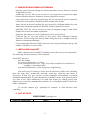
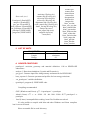
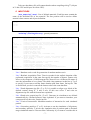
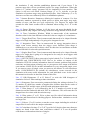
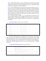
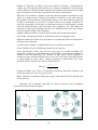
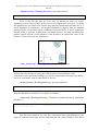
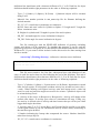
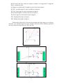
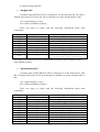
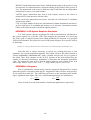
PeneloPET V 1.1
(User Manual)
(2007-06-14)
Nuclear Physics Group
(Complutense University, Madrid)
http://nuclear.fis.ucm.es
-2-
INDICE
0.
MODIFICATIONS FROM LAST VERSION............................................. - 5 -
1.
INSTALLING PeneloPET ....................................................................... - 5 -
2.
LIST OF FILES ....................................................................................... - 5 -
3.
LIST OF UNITS....................................................................................... - 6 -
4.
SOURCE CODE FILES .......................................................................... - 6 -
5.
INPUT FILES .......................................................................................... - 7 -
6.
OUTPUT FILES .................................................................................... - 14 -
7.
EXECUTING PeneloPET...................................................................... - 16 -
APPENDIX 1: How to Read Hits List File Using FORTRAN 77................ - 17 APPENDIX 2: CRYSTAL PIXEL NUMERATION ........................................ - 17 APPENDIX 3: LOR System Response Simulation ................................... - 18 APPENDIX 4: Sinograms ........................................................................... - 18 APPENDIX 5: LOR histogram .................................................................... - 19 -
-3-
-4-
0. MODIFICATIONS FROM LAST VERSION
-
main.inp: some lines have change the format and others are new. Read new format
in Input Files section.
-
scanner.inp: one less line in new version. It is not need now to specify the angle
between adjacent detectors. Read new format in Input Files section.
-
coinc_matrix.inp: in this new optional input file you can specify you own protocol
of detectors in coincidence. Read file format in Input Files section.
-
frame_list.inp: in this new optional file you can specify a different duration for each
frame of the simulated acquisicion. Read file format in Input Files section.
-
SINGLES LIST file can be stored now with all integrated single events. Read
Output Files section for further explanation.
-
image.bin: the number of voxels a dimensions can be specified now.
-
Corrected bug for the total activity of the source when delimited emission
directions. In old version total activity didn’t change but now is weighted with the
fraction of simulated solid angle.
-
Corrected bug that affected to high count rates. Now singles dead-time, pile-up, and
random coincidences is more tested.
1. INSTALLING PeneloPET
Make a directory for PeneloPET installation, place there the zip file and unzip it.
The following directory structure will be obtained:
PeneloPET_directory/
doc/ this manual
scr/ source code directory (*.f files).
work/ working directory. (exe, *.inp). You need to compile first to obtain exe.
/example (*.inp example files)
mat/ material data bases (*.mat, isotope.inp, rangefile.inp).
One useful way of working is create specific directories inside work/ including
there the input files (scanner.inp, main.inp, source.inp, object.inp and others if
neccesary). In that way you can have several simulation environments to perform
simulation independently. To start simulation you should be in the work/ directory but if
you want to use other subdirectory for input and output you should specify that
subdirectory as the first command line parameter. See executing PeneloPET section for
further explanation.
To run the example type “penelopet.exe example” at work directory after
compiling.
2. LIST OF FILES
EXECUTABLE: penelopet.exe
SOURCE CODE (src/)
INPUT
-5-
OUTPUT
Working dir
Source dir (src/)
Penelopet.f (PeneloPET)
analyze.f (PeneloPET)
gen_geo.f (PeneloPET)
beta_espectro.f (PeneloPET)
var_penelopet.f (PeneloPET)
penelope.f (PENELOPE)
pengeom.f (PENELOPE)
main.inp (Working dir)
scanner.inp (Working dir)
object.inp (Working dir)
source.inp (Working dir)
alignments.inp (Working dir)
coinc_matrix.inp (Working dir)
frame_list.inp (Working dir)
isotope.inp (mat/)
mat_names.inp (mat/)
rangefile.inp (mat/)
*.mat (mat/)
scanner.geo
scanner.mat
material.mat
scanner.dat
sinogram.bin
histolor.bin
imagen.bin
histo_row.dat
histo_row_row.dat
histo_timediff.dat
histo_spectro.dat
histo_bodyscat.dat
histo_scatter.dat
histo_emission.dat
histo_range.dat
histo_pair.dat
histo_hits.dat
histo_sino.dat
3. LIST OF UNITS
MAGNITUDE
Time
Length
Energy
UNIT
second, nanosecond
centimeter
eV
4. SOURCE CODE FILES
-
penelopet.f: emission, geometry and material definition. Call to PENELOPE
subroutines.
-
analyze.f : Detection simulation (Crystals and Electronics).
-
gen_geo.f: Generate input files with geometry and materials for PENELOPE.
-
beta_espectro.f: Generate spectrum and profiles for beta energy emissions.
-
var_penelopet.f: variables definition.
-
(penelope.f, pengeom.f): PENELOPE code.
Compiling recommended:
-
GNU (Windows and Linux): g77 –O penelopet.f –o penelopet
-
Absoft (Linux): f77 –s –w –N109 –O3 –h4 –N86 –H100 –lU77 penelopet.f -o
penelopet
-
Intel (Linux): incompatibilities reading *.mat files. Problem not solved.
It’s also posible to compile with Mac and other Windows and Linux compilers
but it’s not well tested.
Place executable file in work/ directory
-6-
Take care that binary file will content headers when compiling with g77 (4 bytes
in 32 bits CPU and 8 bytes in 64 bits CPU).
5. INPUT FILES
“mat_names.inp” (mat/): List of defined materials. Each line must contain the
name of the definition file of one material. The line position will be used to define
material when scanner and objects definition.
water.mat
bgo.mat
lso.mat
nai.mat
.
.
.
“main.inp” (Working directory): general parameters.
12345 54321
[Random number generator seeds]
100 5 F
[Realistic Acquisition Time [sec]; Number of Frames; Read frame_list.inp
F
[Read alignments.inp file]
F
[Read coinc_matrix.inp]
20
[Limit for the number of interactions in each photon]
F T T
[Secundary Particles Simu; Positron Range (T-F); Non-Collinearity (T-F)]
0 180 500 25
[Start&Stop angles [degrees],Steps/cycle, Cycle period [sec]]
100000.
[Lower Energy Window (eV)]
700000.
[Upper Energy Window (eV)]
20
[Coincidence Time Window (ns)]
20
[Trigger Dead Time (ns)]
320
[Integration Time (ns)]
1600
[Singles Dead Time (ns)]
F F F
[HITS LIST, SINGLES LIST, COINCIDENCE LIST]
F
[Write Lor Histogram]
F 127 100 5
[Write Sinogram; radial bins; angular bins; maximum radio]
F 95 95 45 5 5 [Write Image; X Y Z voxels, Transaxial & Axial FOV (cm)]
F
[Hits checking]
F
[Verbose]
F
[Avoid more than 2 singles in coincidence window]
F
[System Response Simulation - LOR]
F
[System Response Simulation - Sinogram]
7 7 7
[Chord points - Transaxial Axial Longitudinal]
2.5 2.2 8.55
[Tranaxial(Pitch times)Axial(Pitch times)Longitudinal(cm)]
3 1000000
[Chord Aperture, Positrons/Point]
-
Line 1 Random seeds: seeds for generation of random numbers serie.
-
Line 2 Realistic Acquisition Time: Time in seconds for the realistic duration of the
performed acquisition. In the same line specify the number of frames. Frames only
affect to the sinogram a LOR histogram files that will use a different file name to
store the information of every frame. The third a last parameter in this line is T or F
to specify if you want to read the frame duration plan from frame_list.inp file. This
is useful when you don’t want all the frames to have the same duration.
-
Line 3 Read alignments.inp file: (T or F). It’s possible to align every block of the
defined scanner along X, Y and Z axis. In this case select T and write an
alignments.inp file with the format later explained.
-
Line 4 Read coinc_matrix.inp file: (T or F). Detectors in coincidences are defined
automatically by a defined protocol later explained. If you want to introduce your
own protocol use the coinc_matrix.inp file.
-
Line 5 Limit of interactions: Maximum number of interaction for each simulated
particle.
-
Line 6 Secondary particles: (T or F): Activate or not the simulation of all primary
and secondary particles. T involve the simulation also of positron path so Positron
range simulation must be F but not Non-Collinearity if you want to consider this in
-7-
the simulation. F only simulate annihilation photons and if you choose T for
positron range this will use predefined profiles for range distribution. When this
option is T, realistic energy spectrum will be simulated for beta particles. This
option is still not well tested. Positron Range: (T or F): Activate or not the
simulation of positron range using predefined profiles. Non-Collinearity: (T or F):
Activate or not the non-collinearity effect for annihilation photons.
-
Line 7 Scanner Rotation: Parameters defining del rotation of scanners. Use four
consecutive numbers separated by blank spaces to define start angle, stop angle,
number of steps, and time per cycle respectively. Use Degrees for angles and
seconds for time. Static scanner will be simulated when writing “0 0 1 0” in this
line.
-
Line 8-9 Energy Window: Indicate in eV the lower and upper thresholds for the
energy window. Only singles with energy inside this energy window will be stored.
-
Line 10 Time Coincidence Window: Width in nanoseconds of the maximum
absolute value for the time difference allowed for the two singles of a coincidence.
-
Line 11 Trigger Dead Time: Time in nanoseconds that needs to be elapsed from the
trigger of a single independently of is going to be integrated or not.
-
Line 12 Integration Time: Time in nanoseconds for energy integration when a
single event occurs starting from the trigger event. Realistic pulse shape is
simulated so try to select also realistic values for this time in concordance with the
rise and fall time for selected crystals detectors.
-
Line 13 Singles Dead Time: Time in nanoseconds that needs to be elapsed from the
trigger of a single that is going to be integrated to be ready for new triggers with
coincidence capabilities.
-
Line 14 LIST OUTPUTS: three consecutive logical valued (T or F). Indicate HITS,
SINGLES and COINCIDENCES LIST files to be written as outputs of the
simulation. HITS file include information about all scanner positions and particle
emissions and interactions allowing user to post-process this output with his/her
own routines. SINGLES file include information for every integrated single event.
If you want to store all single event you must set all detector in self-coincidence
mode. COINCIDENCES file include all coincidences events occurred in the
simulation with some useful information for each individual event. At the end of
this manual are describe in detail the format of this files.
-
Line 15 LOR Histograms: (T or F) Select T to write the LOR histogram of
simulation. Select F when rotating scanner simulation.
-
Line 16 Sinograms: Four consecutive parameter defining the writing selection (T or
F), number of radial bins, number of angular bins, distance between the centre of
the transaxial FOV and the centre of the bin with maximum radial value.
-
Line 17 Write Image: (T or F) followed by the X, Y Z number of voxels in each
dimension and the transaxial and axial FOV in centimeters. This will cause the file
imagen.bin to be written with the emission map.
-
Line 18 Write points: (T or F) Write a plane text file with all information about
emissions and interactions for checking purpose. Perform short simulation to avoid
too large files.
-
Line 19 Verbose: (T or F) Activate or not the screen output including the refresh of
output files for each call to the analyze subroutine.
-
Line 20 Coincidence Sorting: (T or F) If T get rid of all singles when more than two
singles are found in the same time coincidence window. If F sort all possible
coincidences with random selection of singles.
-8-
-
Line 21 LOR system response: (T or F) set simulation for calculation of the system
response for a specific LOR. This comprise the generation of a source.inp file with
a grid of emission points from which probability of detector in a specified LOR will
be obtained. See appendix for further explanation.
-
Line 22 Three following lines are only used when LOR system response is set to T.
First line are three odd number with the number of transaxial, axial and longitudinal
points in the chords. Central point of the chord will be always in the line that join
the geometrical centre of the crystals that conform the LOR. Second line specify the
total width in centimetres in each dimension of the chord. Third line content the
emission aperture for annihilation photons with the LOR as reference direction
(TH1=0, TH2=selected_value. See source.inp file explanation) and the number of
simulated emission from each point.
-
Line 23 Sinogram system response: (T or F) set simulation for calculation of the
system response sinogram based. The biggest difference between this case and the
presented before is that here the probability is for detection in a sinogram bin,
including all LORs that contributes to this bin. This option is not enough tested at
this moment.
“isotope.inp” (mat/): Isotopes emission definitions
--------------------- ISOTOPES ---------------------1
6586.2
9
F18
!ID, Half Life [sec], Z,
B+
249.8E3
1.
!Type Energy Fraction
----------------------------------------------------2
1223.4
6
C11
!ID, Half Life [sec], Z,
B+
385.6E3
1.
!Type Energy Fraction
----------------------------------------------------3
597.9
7
N13
!ID, Half Life [sec], Z,
B+
491.82E3
1.
!Type Energy Fraction
----------------------------------------------------4
122.24
8
O15
!ID, Half Life [sec], Z,
B+
735.28E3
1.
!Type Energy Fraction
----------------------------------------------------5
8.21097E7
11
Na22
!ID, Half Life [sec], Z,
B+
215.54E3
1.
!Type Energy Fraction
G
1274.54E3
1.
-----------------------------------------------------
Name
Name
Name
Name
Name
In this file is defined the list of emitted particles for each isotope. The file starts
with a free line and is followed by the definition of several isotopes. Each isotope
definition includes one first line with the numeration ID, half life in seconds, atomic
mass and isotope name. Next, each emitted particle should include its information in a
different line including type of particle (B+, B- or G for positron, electro and photon
respectively), Emission energy (Q value for B+ and B-) and fraction of emission
occurrence.
“scanner.inp” (Working directory): Scanner definition
------ SCANNER DEFINITION -------------------------------------------------------------2
!Number of Detectors by Ring
1
!Number of Detectors in Coincidence in the same Ring
2
!Number of Rings
1.0
!Gap Between Rings [cm]
10
!Number of transaxial crystals by Detector [COLUMNS]
10
!Number of axial crystals by Detector [ROWS]
2
!Number of crystal layers by Detector
1.0 2 0.2 1 40 1.5
!Length [cm],Mater,Ener resol [fract],Rise&Fall [ns],T Resol [ns]
1.0 3 0.3 1 60 3.0
!One line for each crystal layer
1.0 1.0
!Column&Row Pitch: Distance from center of adjacent crystals [cm]
1.0
!Radio: Center FOV - Center Front of Detector [cm]
----------------------------------------------------------------------------------------
-9-
-
Number of Detectors by Ring: select the number of detector conforming the
scanner ring. The angle between detectors is constant. If simulation of several rings
of these detector is needed include in this line the number of detectors in one of that
rings. All detectors in the same ring will have the same axial position.
-
Detectors in Coincidence: Number of detectors that can produce coincidence events
with every single detector. Include only number of detectors in the same ring but
the program will assume the all equivalents detectors for other different rings will
be also in coincidence. If you have a scanner with an even number of detector in
each ring, the number of detectors in coincidences must be an odd number, starting
with the fronted detector and increasing with contiguous. For odd number of
detectors in each ring this number must be even, starting with the two more fronted
detectors and increasing with contiguous.
-
Number of Rings: number of ring of detectors that will conform the scanner
-
Gap Width: Axial gap separation in centimeters between contiguous rings
-
Material: número de la línea en la que aparece el nombre del fichero del material en
el fichero mat_names.inp
-
Crystals Array: Number of columns and rows of crystal for one detector.
-
Layer: Number of layers of different crystals for one detector.
-
Layer Specification: Write one line for every layer of crystals including five
consecutive parameters with information about length of crystal pixel, number of
material from mat_names.inp file (number of line where desired material is
written), Energy resolution fraction (0-1) at 511 keV peak, Rise time and Fall time
in nanoseconds for pulse shape, timing resolution in nanoseconds. First layer
specified will be closed to the centre of transaxial FOV.
Pulse(t ) =
e
− t / t fall
− e− t / trise
t fall − trise
-
Transversal Pitch: two values in centimetres indicating transaxial (columns) and
axial (rows) pitch size for every pixel crystal.
-
Radio: Distance in centimetres from the centre of the transaxial FOV and the front
of one detector.
Important: All coordinates and shifts are always referred to the coordinates
system represented in the next figure
- 10 -
This figure shows the coordinates system reference and the numeration protocol for rings and block
detectors.
“alignments.inp” (Working directory): general parameters.
0 3 0.5 0.2 0.0 40 !RING BLOCK X Y Z PH
1 7 0.2 0.0 1.0 0
Write in this file one line for every only for blocks you desire to specify
alignment position. Rest of block will be set to zero alignment in each axis. To define
the alignment for one block write first the ring and block numeration and later the X, Y
and Z alignment in centimeters, and angular alignment in degrees from the standard
position. In this case general system coordinates is not used for X, Y and Y alignments.
Instead of that, a reference is taken from each block detector. The only block that have
parallel system reference in the number 0 and all others are rotated the same as the
detector. Z axis is the same for all detectors.
“coinc_matrix.inp” (Working directory): general parameters.
0 0 0 2 !RING1 BLOCK1 RING2 BLOCK2
0 1 0 3
Write in this file one line for every pair of block that are in coincidence. Selfcoincidence can be performed setting every block in coincidence with itself. One block
can be in coincidence with as many block as desired.
“frame_list.inp” (Working directory): general parameters.
40 !Frame Duration (sec)
30
20
Write the duration in seconds of every frame in each line.
“object.inp” (Working directory): Definition of additional objects (phantoms,
shielding...)
------ OBJECT DEFINITION --------------------------------------C 1 0. 0. 0. 0. 1. 1. 0. 0.
¡TYPE MATER XC YC ZC RI RE H [cm] PH_INC TH_INC
!ONE LINE FOR EACH OBJECT
.
.
----------------------------------------------------------------
This file must contain a free first line, subsequent lines with definition of one
object in each line and at least one line indicating the end of the definition. This end of
- 11 -
definition line should start with a character different of S, C or R. Each line for object
definition should include eight parameters in the order as following explained:
-
Type: C (Cylinder), S (Sphere), R (Prism) . Cylindrical objects will be oriented
along Z axis.
-
Material: line number position in mat_names.inp file for filename defining the
desired material
-
XC, YC, ZC: central object coordinates in centimetres
-
RI, RE: Inner and outer radio for Cylinder or Sphere. X Length and Y Length for
Prism. centimetres units.
-
H: Height for cylinder and Z Length for prism. Not used in sphere.
-
PH_INC: Azimuth angle for source inclination in degrees.
-
TH_INC: Polar angle for source inclination in degrees.
The file scanner.geo with the PENELOPE definition of geometry including
scanner and objects will be generated. To visualize the geometry it can be used the
programs gview2d.exe and gview3d.exe that PENELOPE includes and can be used in a
Windows PC. If you want to define inclusive bodies this need to be done starting from
inside to outside.
“source.inp” (Working directory): radioactive emission source definition
------ SOURCE DEFINITION -------------------------------------------------------------C 1E6 F 1 0 0 0 0 1 1 0 0 0 0 0 180 !T A U I X Y Z RI RE H PH_IN TH_IN PH TH TH1 TH2
!ONE LINE FOR EACH SOURCE
.
.
---------------------------------------------------------------------------------------
This file must contain a free first line, subsequent lines with definition of one
source in each line and at least one line indicating the end of the definition. This end of
definition line should start with a character different of S, C, P or R. Each line for object
definition should include eight parameters in the order as following explained:
-
Type: C (Cylinder), S (Sphere) , P (point source) or R (Prism). Important use capital
letter for hot regions. If cold regions (without activity) are needed use lower case c,
s and r. When defining cold regions activity, units and isotope need a value but
won’t be used and emission angles not need to be written. Cylindrical objects will
be oriented along Z axis.
-
A: Activity of the source in Becquerel or Becquerel/cc. Activity will change when
realistic time elapse. If Activity goes close to 0 simulation will stop. If long very
low activity is desired select 0 activity and time between decays will be just a little
bigger than singles dead time.
-
U: Activity units (T or F). T means Bq/cc and F means Bq. Be careful is you define
a cold region because if you use concentration activity will be always referencing to
the total hot region defined.
-
I: Number indicating the Isotope that compounds the source. Number should be
taken from isotope.inp file.
-
XC, YC, ZC: central source coordinates in centimeters
- 12 -
-
RI, RE: Inner and outer radio for Cylinder or Sphere. X Length and Y Length for
Prism. centimeters units.
-
H: Height for cylinder and Z Length for prism. Not used in sphere
-
PH_INC: Azimuth angle for object inclination in degrees.
-
TH_INC: Polar angle for object inclination in degrees.
-
PH: Azimutal angle for emission direction in degrees
-
TH: Polar angle for emission direction in degrees
-
TH1: Starting Polar angle in degrees
-
TH2: Ending Polar angle in degrees
Emission direction will be chosen using azimutal and polar angles as a reference
direction. Any azimutal angle from this reference direction will be randomly generated
but only with polar angles between TH1 and TH2
- 13 -
This figures are a graphical explanation of the emission direction definition. The figure above is a general
case and two figures bellow are two different useful settings.
6. OUTPUT FILES
Output files will be written in the selected working directory
•
“hits.list”:
Is written when HIST LIST is selected to T in the main.inp file. This file is
formed with events of 28 bytes (B) and is refreshed every time storage buffer is full.
2 B = Signed short integer (2 bytes).
4 B = Float real number (4 bytes)
8B = Double precision (8 bytes)
There are 4 different events types:
Angular position (every time the scanner step to a new poisiton):
-1
2B
0
2B
ANG
4B
0
4B
0
4B
0
4B
TIME
8B
-
ANG: angle in degrees for scanner angular position.
-
TIME: elapsed time in seconds from the beginning of acquisition.
Decay location:
0
2B
-
0
2B
X
4B
Y
4B
Z
4B
0
4B
TIME
8B
E
4B
TIME
8B
E
4B
TIME
8B
X, Y, Z: decay location coordinates in centimeters.
Particle emission location:
KPAR
2B
0
2B
X
4B
Y
4B
Z
4B
-
KPAR: 1 for electrons, 2 for photons and 3 for positrons.
-
E: Particle energy in eV.
Hit location:
4
2B
IBODY
2B
X
4B
Y
4B
Z
4B
IBODY: numeration for the body where hit take place. This numeration start
from 1 with ring=0, block=0, layer=0 (see crystal numeration appendix). Every layer of
every block set up an unique body. IBODY numeration start increasing with the layer
inside the same block, the blocks inside the same rings and the rings of blocks
consecutively.
- 14 -
E: particle energy after hit.
•
“singles.list”:
Is written when SINGLES LIST is selected to T in the main.inp file. This file is
formed with events of 15 bytes (B) and is refreshed every time storage buffer is full.
1 B = Signed integer (1 byte)
4 B = Float real number (4 bytes)
There two types of events with the following information about each
coincidence:
Format
(1B)
(4B)
(4B)
(1B)
(1B)
(1B)
(1B)
(1B)
Synchronism Event
ID Event = 0
Scanner Angle (deg)
Acquisition Time (sec)
0
0
0
0
0
(1B)
0
Coincidence Event
ID Event =1
Energy of single
Time stamp (sec)
Column single
Row singl
Layer single
Block single
Ring single
Single type
(1=true, 2=scatter, 3=pile-up, 4=single gamma)
All singles events that follow to one synchronism events have been simulated in the
same angular position.
•
“coincidences.list”:
Is written when COINCIDENCE LIST is selected to T in the main.inp file. This
file is formed with events of 28 bytes (B) and is refreshed every time storage buffer is
full.
1 B = Signed integer (1 byte)
4 B = Float real number (4 bytes)
There two types of events with the following information about each
coincidence:
Format
(1B)
(4B)
(4B)
(4B)
(4B)
(1B)
(1B)
(1B)
(1B)
(1B)
(1B)
(1B)
Synchronism Event
ID Event = 0
Scanner Angle (deg)
Acquisition Time (sec)
0
0
0
0
0
0
0
0
0
Coincidence Event
ID Event =1
Energy of single 1
Energy of single 2
Time difference (sec)
Time stamp for that coincidence (sec)
Column single 1
Row single1
Layer single 1
Block single 1
Ring single 1
Column single 2
Row single 2
- 15 -
(1B)
(1B)
(1B)
0
0
0
(1B)
0
Layer single 2
Block single 2
Ring single 2
Coincidence type
(1=pile-up, 2=self-coincidence, 3=scatter, 4=true, 5=random)
All coincidence events that follow to one synchronism events have been simulated in
the same angular position.
BINARY FILES
-
sinogram.bin -> 3D sinogram (integer*4). See appendix for further explanation.
-
histolor.bin -> LOR histogram (integer*4). See appendix for further explanation.
-
imagen.bin -> map of emissions. 55x55x55 singed long integers (4 bytes). FOV will
bet 70% of the scanner diameter
PLAIN TEXT FILES
-
scanner.mat -> PENELOPE material data base with all the materials used in the
simulation.
-
material.dat -> PENELOPE material summary.
-
scanner.geo -> geometry file for PENELOPET. Use this file to visualize geometry
with gview2d.exe and gview3d.exe programs.
-
scanner.dat -> central coordinates of every pixel crystal and numeration.
-
histo_range.dat -> histogram of the range for each type of particle. Only when
secondary particle simulation.
-
histo_emission.dat -> energy spectrum of emitted particles. Only when secondary
particle simulation.
-
histo_bodyscatt.dat -> number of interaction in each body before or after detection
-
histo_scatter.dat: -> number of singles of coincidences with first scatter at that body
-
histo_sino.dat -> summation of all radial profiles of the sinogram. Only written
when sinogram simulation.
-
histo_timediff.dat -> histogram of the time difference between both singles of the
coincidence.
-
histo_row.dat -> histogram of coincdences with both singles in the same row.
-
histo_row_row.dat -> histrogram of coincidence in the same pair of rows.
-
histo_hits.dat -> number of interactions in detector for singles of coincidences.
-
histo_pair.dat -> number of coincidences in each pair of detectors
-
histo_spectro.dat -> energy spectrum for singles of coincidences.
7. EXECUTING PeneloPET
Here is explained the recommended steps to run a simulation with PeneloPET:
-
Make a list of materials involved in desired simulation. Look for them at
mat_names.inp file and keep the line where are named. If one or some needed
materials are not defined use PENELOPE material program to make new material
files and add their names to the mat_names.inp file and copy the *.mat files to the
PeneloPET directory.
- 16 -
-
Make a list of isotopes involved in desired simulation. Look for them at isotope.inp
file. If one or some needed isotopes are not defined edit this file including all
information as explained before. Positron range simulation will require to add new
isotopes information in the rangefile.dat but at this moment it’s not possible so new
isotopes definition should exclude positron range simulation in main.inp file.
-
Set main.inp file with general parameters for the simulation.
-
Set scanner.inp and object.inp files with the scanner, phantoms and shielding
definition.
-
Set source.inp file with activity source.
-
Start execution program typing the name of executable file (penelopet) and stopping
simulation quick when “CREATING PENELOPE CROSS SECTION
DATABASE...” is showed in the screen. After this, scanner.geo file with the
PENELOPE geometry definition file can be find in the working directory. Open it
using the gview2d.exe and gview3d.exe programs to check the geometry definition.
Also open the imagen.bin file to check emissions distribution.
-
Select in main.inp a realistic time of simulation short enough to simulate only
several thousands of decay process. Run complete simulation and run
cheking_hits.gnu script with gnuplot to visualize the emission and hits in the
simulation. In this way you can check is simulation in running as desired. Also try
to check if statistics output from simulation is compatible with settings.
-
Select now desired time for the simulation in the main.inp file and start running
simulation using executable file from executable directory in command line. If a
working directory different of executable directory will be used the full or relative
path for this directory as first command line argument. Input files should be placed
in the selected working directory but not material definition files (*.mat). All output
file will be written in the selected working directory.
penelopet.exe working_directory
Rendering of scanner and object definition using the gview3d.exe program.
APPENDIX 1: How to Read Hits List File Using FORTRAN 77
OPEN(UNIT=1,FILE=’hits.list’,FORM=’UNFORMATTED’)
READ(1) [INT*2],[INT*2],[REAL*4],[REAL*4],[REAL*4],[REAL*4],[REAL*8]
CLOSE(1)
APPENDIX 2: CRYSTAL PIXEL NUMERATION
-
RING: rings numeration start from 0 in the lower Z coordinate and increases as
increases Z.
- 17 -
-
BLOCK: blocks numeration start from 0 with the block laying in the positive X axis
and increases in counterclockwise direction looking at the scanner from positive Z
axis. The numeration is the same for different rings. Each block has an independent
numeration for layers, rows and columns.
-
LAYER: layers numeration start from 0 with crystals closest to the center of
transaxial FOV and increases with the radio.
-
ROW: axial rows numeration start from 1 with the row with lowest Z coordinate
and increases with Z.
-
COL: For block number 0 the pixel with transaxial column numeration start from 1
at pixel with lowest Y coordinate and increases as Y increases. Numeration in other
blocks is the same but turn to the block angular position.
APPENDIX 3: LOR System Response Simulation
T in LOR system response at main.inp file will set simulation for calculation of
the system response for a specific LOR. This comprise the generation of a source.inp
file with a grid of emission points from which probability of detection in a specified
LOR will be obtained. The protocol to run a LOR system response for a specific LOR is
as following:
penelopet.exe working_dir RING1 BLOCK1 LAYER1 ROW1 COL1 RING2 BLOCK2 LAYER2 ROW2 COL2
Note that here is always necessary to specify the working directory as first
parameter. See crystal numeration appendix. The output will be a file named similar to
“chord_0000000000_0000000000.dat” with 6 columns and one line for every point of
the chord. Three first columns are the (X,Y,Z) location of the point followed by the
number of detected coincidences, probability of detection and normalize probability
value. The output file name will be formed with to digits for each counter in the next
order: ring1, block1, layer1, row1, col1, “_”, ring2, block2, layer2, row2, col2.
APPENDIX 4: Sinograms
Here is explained the format used to write the sinogram. Sinogram file is written
when this option is selected in main.inp file. Angular bins take reference at the positive
X axis and follow until 180º. The radial bin start from 0 to the maximum radio and the
sign is explained in the figure. The size of radial and angular bins are calculated as
2·ρ max
180º
∆ρ =
∆θ =
Nρ −1
Nθ
where Nρ and Nθ are the total number of radial and angular bins respectively.
- 18 -
This figure shows the way for calculating the radial and angular components for the sinogram. On the left
are the reference used for the bin calculation and on the right the sign protocol employed.
Sinograms are written in raw format using singed long integer format (4 bytes)
and the total number of bins is
N b in s = N ρ · Nθ · N rows · N rows
where Nrows is the total number of rows including all the scanner rings and gap interrings regions. The order used for bins is starting for minimum radial, angular and rows
bins and increasing first radial, later angular and finally rows bins. The protocol
employer for oblique sinograms is explained in the following figure
APPENDIX 5: LOR histogram
This file is written when selected in main.inp file. This file will contain the
number of coincidence detected in each LOR. The file is written in raw format using
signed long integers (4 bytes). The order for numbering LOR start with the pair formed
by the crystal (CRYSTAL 1) with the lowest numerations and the crystal (CRYSTAL
2) in coincidence with the first one with lowest numerations. Continue in order with all
CRYSTAL 2 in coincidence with CRYSTAL 1 in the same ring. When finished,
continue with following CRYSTAL 1 and so on until finish all the combinations inside
the same ring. Continue repeating the same process but using all rings combination each
time ordering with ring of CRYSTAL 1 as less significant and ring of CRYSTAL 2 as
- 19 -
more significant The numeration for one crystal increase with the following significant
order: column, row, layer, block.
- 20 -