1
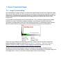
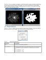
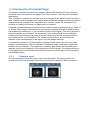
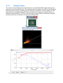
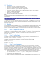
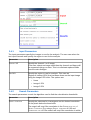
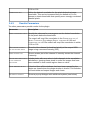
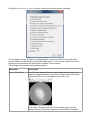
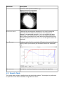
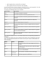
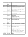
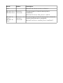
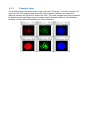
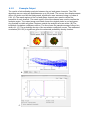
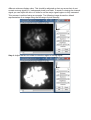
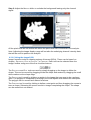
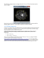
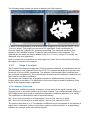
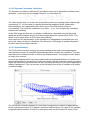
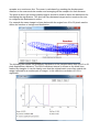
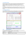
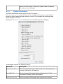
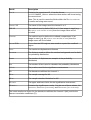
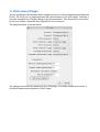
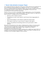
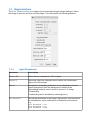
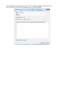
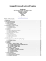
ImageJ Colocalisation Plugins
Alex Herbert
MRC Genome Damage and Stability Centre
School of Life Sciences
University of Sussex
Science Road
Falmer
BN1 9RQ
[email protected]
Table of Contents
1 Introduction........................................................................................................................3
2 Stack Threshold Plugin......................................................................................................4
2.1 Image Thresholding....................................................................................................4
2.2 Plugin Interface...........................................................................................................5
2.2.1 Input Parameters.................................................................................................5
3 Colocalisation Threshold Plugin.........................................................................................6
3.1.1 Example Input......................................................................................................6
3.1.2 Example Output...................................................................................................7
3.2 Features......................................................................................................................8
3.3 Method........................................................................................................................8
3.3.1 Step 1: Regression Analysis................................................................................8
3.3.2 Step 2: Define limits............................................................................................8
3.3.3 Step 3: Iterative search.......................................................................................8
3.4 Plugin Interface...........................................................................................................9
3.4.1 Input Parameters...............................................................................................10
3.4.2 Search Parameters...........................................................................................10
3.4.3 Results Parameters...........................................................................................11
3.5 Results Table............................................................................................................13
4 Confined Displacement Algorithm (CDA) Plugin.............................................................17
4.1.1 Example Input....................................................................................................18
4.1.2 Example Output.................................................................................................19
4.2 Features....................................................................................................................20
4.3 Method......................................................................................................................20
4.3.1 Stage 1: Identify Channel Signal.......................................................................20
4.3.1.1 Using the ImageJ minimum display value.................................................20
4.3.1.2 Using the ImageJ ROI................................................................................22
4.3.1.3 Using an image mask.................................................................................23
4.3.2 Stage 2: Analysis...............................................................................................24
4.3.2.1 Manders Coefficient...................................................................................24
4.3.2.2 Pearson Correlation Coefficient.................................................................25
4.3.2.3 Displacements............................................................................................25
4.3.2.4 Speed Increases........................................................................................27
4.4 Plugin Interface.........................................................................................................27
4.4.1 Input Parameters...............................................................................................27
4.4.2 Displacement Parameters.................................................................................28
4.4.3 Options Parameters..........................................................................................29
4.5 Results Table............................................................................................................30
5 CDA (macro) Plugin.........................................................................................................32
6 Stack Correlation Analyser Plugin...................................................................................33
6.1 Plugin Interface.........................................................................................................33
6.1.1 Input Parameters...............................................................................................33
6.2 Results......................................................................................................................34
6.2.1 Header Record..................................................................................................34
6.2.2 Threshold Record..............................................................................................35
6.2.3 Correlation Record............................................................................................35
7 Stack Colocalisation Analyser Plugin...............................................................................36
7.1 Plugin Interface.........................................................................................................37
7.1.1 Input Parameters...............................................................................................37
7.2 Results Table............................................................................................................38
8 References.......................................................................................................................40
9 Appendix 1: Batch Processing.........................................................................................41
9.1 Step 1: Record the macro.........................................................................................41
9.2 Step 2: Prepare input files........................................................................................41
9.3 Step 3: Process Batch command.............................................................................41
1 Introduction
Digital images can be recorded using different light filters. Each filter records an image
containing only the information from the wavelengths of light that pass through the filter.
This produces an image with multiple channels each representing different light.
Colocalisation analysis is used to determine the amount of an image channel's signal that
occurs in the same location as another channel. If the channels represent specific objects
such as fluorescence tagged proteins, colocalisation analysis will quantify whether the
different objects are found in the same location.
The GDSC Colocalisation plugins provide various tools to perform colocalisation analysis.
The following tools are available:
Stack Threshold
Processes an image stack and applies thresholding to create a
mask for each channel+frame combination. This defines the
signal region of each channel.
Colocalisation
Threshold
Compares two images for correlated pixel intensities. If the two
images are correlated a search is performed to identify the
threshold below which the two images are not correlated.
CDA
Uses the Confined Displacement Algorithm (CDA) to compute the
significance of colocalisation metrics (Manders' coefficient and
correlation coefficient).
Stack Correlation
Analyser
Processes a stack image with multiple channels. Extracts all the
channels and frames and performs:
1. Thresholding to create a mask for each channel+frame
2. All-vs-all channel correlation within the union/intersect of
the channel masks
Stack Colocalisation
Analyser
Processes a stack image with multiple channels. Requires three
channels. Each frame is processed separately. Extracts all the
channels (collating z-stacks) and performs:
1. Thresholding to create a mask for each channel
2. CDA analysis of channel 1-vs-channel 2 within the region
defined by channel 3
The stack analyser plugins can be incorporated into ImageJ macros to allow rapid analysis
of hundreds of images for correlations.
2 Stack Threshold Plugin
2.1 Image Thresholding
An initial stage of image analysis is to determine which pixels contain the important image
data. All the other pixels can then be ignored resulting in faster processing of the image. A
simple way to separate the important pixels is to assign a threshold level to the image. All
pixels below this level are ignored as the background, pixels above the level are the
foreground.
It is possible to automatically set a threshold level. This is done by analysing the image
distribution of pixel intensities (image histogram) and setting a threshold value that
separates a background cluster from the foreground pixels. The following image outlines
the two peaks that are characteristic of a well defined background and foreground.
There are many different thresholding methods. ImageJ also has a built-in threshold
method available using the command IMAGE > ADJUST > THREHOLD... The AUTO THRESHOLD
plugin of Gabrial Landini contains several different methods that you can try (see
http://pacific.mpi-cbg.de/wiki/index.php/Auto_Threshold).
However the threshold methods require the analysis of the image histogram for the
channel that you are thresholding. ImageJ can perform thresholding on a single image or a
3d image stack. It has no method for processing a multi-channel image.
The STACK THRESHOLD plugin can analyse a multi-dimensional image and apply thresholding
to each channel and time frame in the image. The result is presented as a new image
mask. Foreground pixels are white, background pixels are black. An example of an input
and output image are shown below:
2.2 Plugin Interface
The STACK THRESHOLD plugin uses the standard ImageJ plugin dialogue. Select the image to
process and then run the plugin. This will present the following window:
2.2.1
Input Parameters
Parameter
Description
METHOD
Specify the thresholding method
LOG THRESHOLDS
Record the thresholds to the ImageJ log window. A threshold will
be calculated for each combination of timeframe and channel,
e.g:
t1c1 threshold = 778
t1c2 threshold = 617
t1c3 threshold = 2441
3 Colocalisation Threshold Plugin
The positive correlation between two images indicates that the signal in one channel is
observed at the same time as the signal in the other channel. This may have biological
significance.
This correlation is expected to be high when the strength of the signal is both channels is
high. However as the strength of the signal reduces towards background noise it would be
expected that the strength of the correlation also reduces. Under this assumption it is
possible to measure the amount of signal that is correlated.
A method for determining the threshold level for each channel was proposed by Costes, et
al. (2004). Each image is thresholded at its maximum intensity and the correlation below
this threshold is measured (i.e. the correlation for the entire signal). This will be positive if
the two channels are colocated. The threshold is then reduced and the colocalisation
remeasured. By iterating this process a search is performed for the intensity threshold
below which there is no correlation. The fraction of signal above this threshold is a
measure of the colocalisation of the signal in the two image channels.
An exhaustive search for the thresholds is computationally expensive due to the large
number of combinations. The Colocalisation Thresholds plugin computes a regression
between the two channels. This regression is used to approximate the threshold level
required in the second image for a set threshold in the first image. The plugin performs a
converging search for the image thresholds and reports various metrics on the resulting
thresholded images.
3.1.1
Example Input
The following figure shows the input required for the plugin. The input consists of 2
channels of a microscopy image where the channels are stained for different proteins.
3.1.2
Example Output
The results of colocalisation threshold analysis. (A) Combined RGB image showing only
pixels above the threshold levels. The image shows the original channels in red and green;
the blue channel shows colocalised pixels. (B) A plot of channel 1 verses channel 2. The
regression line is plotted along with the threshold level for channel 1 (vertical line) and
channel 2 (horizontal line). (C) Plot of the correlation above (blue) and below (red points)
the threshold level for channel 1 verses the threshold level.
A.
B.
C.
3.2 Features
•
•
•
•
•
•
•
Note
Processes 8-bit and 16-bit greyscale images
Processes 2D and 3D images (i.e. image stacks)
Selection of channel regions using the ImageJ ROI
Calculates threshold value for each image below which there is no correlation
Outputs threshold mask images
Generates a full results table
Efficient convergence algorithm is fast
The plugin presented here is a modification of the original [ColocThreshold] plugin
available from:
http://www.uhnres.utoronto.ca/facilities/wcif/imagej/colour_analysis.htm#6.3
Colocalisation Threshold
The plugin has been altered to add additional features such as support for 16-bit and 3D
images, region selection options, more results output and the new implementation of the
threshold search code.
3.3 Method
The colocalisation threshold plugin uses a heuristic search for the threshold limits for each
channel below which there is no correlation. The search is only performed if there is a
positive correlation between all the pixels in both channels. The method is outlined below.
3.3.1
Step 1: Regression Analysis
A regression is computed between the two channels. This assumes a linear relationship
between the two channels. The value of channel 2 can then be expression as:
ch2 = ch1 * m + c
3.3.2
Step 2: Define limits
The limits for the threshold search are set using the maximum and minimum value of
channel 1. These are named Tmax and Tmin.
Using the linear regression the limits for channel 2 are then defined using:
ch2min = Tmin * m + c
ch2max = Tmax * m + c
3.3.3
Step 3: Iterative search
The search is performed by continuously updating the current threshold for channel 1,
calculating the threshold for channel 2 and the subsequent regression value for all pixels
below the thresholds. The search is convergent in that it only operates between the current
maximum and minimum limit for channel 1. The limits are adjusted based on the results of
each iteration and the current threshold is updated to half way between the two limits.
1. At any point in the algorithm it is known that there is a positive correlation when T =
Tmax. T is then set as Tmin + (Tmax – Tmin) / 2, i.e. halfway between the two limits
2. Calculate the new regression value
3. If the correlation is positive then it is known the threshold must be lowered. T max is
updated to T
4. If the correlation is negative then it is known the threshold must be raised. T min is
updated to T
5. Repeat
The iteration stops when either:
•
The correlation is within the SEARCH TOLERANCE of the CORRELATION LIMIT
•
The distance between Tmax and Tmin is 1, i.e. convergence
•
The MAXIMUM ITERATIONS value is reached
In certain cases the final threshold limit may not have the desired correlation. This is
because convergence or MAXIMUM ITERATIONS occurs during a search where the CORRELATION
LIMIT is not reached. In this case the results are sorted in descending order by the
threshold. The final limit is set as the threshold value which resulted in:
•
The correlation above the threshold being more than the CORRELATION LIMIT
•
The correlation below the threshold is the closest to the target CORRELATION LIMIT
In the event that no results satisfy the criteria then the threshold is set using the lowest
intensity level sampled from channel 1.
The following chart shows how the threshold is updated during a typical search. Initially the
threshold is reduced until the correlation goes below the CORRELATION LIMIT. The threshold is
then raised and subsequently raised/lowered as the correlation alternates around the
CORRELATION LIMIT. In this instance the CORRELATION LIMIT was not obtained and the threshold
converged at 166.
3.4 Plugin Interface
The Colocalisation Threshold plugin interface uses a frame within the ImageJ application.
The plugin has many options but these can be divided into sections controlling parts of the
algorithm. The different sections are shown in the following image and are described
below.
3.4.1
Input Parameters
The input parameters specify the images to use for the analysis. The user can select the
two input channels and specify the region to use for the analysis.
Parameter
Description
CHANNEL 1/2
Specify the channel 1 or 2 image.
If the user selects an image stack then the channel and frame will
be requested during run-time. This is to eliminate optional fields
from the main dialogue
USE ROI
3.4.2
Specify the region to use for analysis. This uses an
Region-of-Interest (ROI) that has been drawn on the input image
using the ImageJ ROI tools. The options are:
•
None
•
Image 1 ROI
•
Image 2 ROI
Search Parameters
The search parameters control the algorithm used to find the colocalisation thresholds.
Parameter
Description
SEARCH TOLERANCE
Specify the tolerance for convergence on the desired correlation
for the pixels below the thresholds.
The search will stop if the correlation is the CORRELATION LIMIT +/SEARCH TOLERANCE. E.g. using a SEARCH TOLERANCE of 0.05 and
CORRELATION LIMIT of 0 the search will stop if the correlation in within
-0.05 to 0.05.
CORRELATION LIMIT
3.4.3
Define the desired correlation for the pixels below the image
thresholds. This can be increased from the default of 0 in an
attempt to obtain thresholds that specifiy more strongly correlated
channel pixels
Results Parameters
The other parameters provide results for the plugin.
Parameter
Description
SHOW COLOCALISED PIXELS Specify the tolerance for convergence on the desired correlation
for the pixels below the thresholds.
The search will stop if the correlation is the CORRELATION LIMIT +/SEARCH TOLERANCE. E.g. using a SEARCH TOLERANCE of 0.05 and
CORRELATION LIMIT of 0 the search will stop if the correlation in within
-0.05 to 0.05.
USE CONSTANT INTENSITY
FOR COLOCALISED PIXELS
SHOW SCATTER PLOT
Show the blue channel (colocalised pixels) of the output RGB
image using a constant intensity (255)
Show a scatter plot of the channel 1 intensity verses the channel
2 intensity
INCLUDE ZERO-ZERO PIXELS Include pixels with zero value in both channels in the correlation
IN THE THRESHOLD
calculations. Ignoring these pixels is useful for images that have
CALCULATION
been masked so that certain regions have no value
CLOSE WINDOWS ON EXIT
If checked then all the windows that have been opened by the
plugin are closed when the plugin window is closed. This includes
the result table and output images and charts.
SET RESULTS OPTIONS
Shows a pop-up dialogue with additional options (see below)
Clicking the SET RESULT OPTIONS checkbox shows the following pop-up dialogue:
The dialogue contains settings for configuring the columns included in the result table.
Further details can be found in the Results Table section. This can be useful if you have
limited screen resolution and would like to disable some columns.
The dialogue also contains the following options:
Parameter
Description
OUTPUT ROIS/MASKS
If an ROI was selected from an input image then this option will
output a cropped duplicate of the input images with all the pixels
outside the ROI (if non rectangular) set to zero, e.g.
In all cases this option will also show a mask image for each
channel where all the pixels above the colocalisation threshold
Parameter
Description
are white, other pixels are black, e.g.
EXHAUSTIVE SEARCH
If selected the convergence algorithm is not used. Instead all
threshold values between the maximum and minimum for
channel 1 are analysed using MAX ITERATIONS to define the step
increments. The final threshold is set as the highest threshold
with a positive correlation for pixels above the threshold and the
closest correlation to the CORRELATION LIMIT for the pixels below the
threshold
PLOT R VALUES
Produce a plot of (a) the correlation (R) values above (solid line)
and (b) below (cross points) the threshold verses the threshold,
e.g.
MAX ITERATIONS
Specify the maximum iterations to use within the algorithm
3.5 Results Table
The results table contains details about the threshold analysis. The analysis is performed
on pixels that have been classified using different criteria:
•
pixel is greater than a set level for one channel
•
pixel is greater than the set levels for both channels
In each case the level can be set using the a threshold of 0 (i.e. count any pixel), 1 (i.e. the
pixel has a value) or the threshold set during the analysis phase.
This allows the following values to be computed:
Result Value
Description
NCH1
The number of pixels in channel 1
NCH1GT0
The number of pixels in channel 1 greater than zero
NCH1GTT
The number of pixels in channel 1 greater than the channel 1
threshold
NCOLOC
The number of pixels where both channels are above the
threshold
SUMCH1
The sum of pixel values in channel 1
SUMCH1GTT
The sum of pixel values in channel 1 greater than the channel 1
threshold
SUMCH1_CH2GT0
The sum of pixel values in channel 1 where channel 2 is greater
than zero
SUMCH1_CH2GTT
The sum of pixel values in channel 1 where channel 2 is greater
than the channel 2 threshold
SUMCH1_COLOC
The sum of pixel values in channel 1 where both channels are
above the threshold
Note: With the exception of NCOLOC all of these values have corresponding equivalents for
Channel 2.
The initial result values are used to compute result metrics that are displayed in the result
table. The following table describes the results and the option used to enable/disable the
result column(s):
Result
Option
Description
IMAGES
-
Contains the titles of the input images used for the
analysis
ROI
-
Contains the ROI that was used to select the region
for the analysis
ZEROZERO
-
Shows whether INCLUDE ZERO-ZERO PIXELS IN THE THRESHOLD
CALCULATION was selected
RTOTAL
PEARSON'S FOR
The Pearson's correlation for the entire image
WHOLE IMAGE
M/B
SHOW
LINEAR
The linear regression coefficients:
Result
Option
Description
REGRESSION
ch2 = ch1 * m + b
SOLUTION
CH1 / CH2 THRESH SHOW
RCOLOC
THRESHOLDS
PEARSON'S FOR
IMAGE ABOVE
The channel thresholds
The Pearson's correlation coefficient for the pixels
above both the channel thresholds
THRESHOLD
R<THRESHOLD
PEARSON'S FOR
IMAGE BELOW
THRESHOLD
M1 / M2
The Pearson's correlation coefficient for the pixels
below both the channel thresholds. This should be
close to the CORRELATION LIMIT
MANDERS ORIGINAL The Manders coefficient for the image
COEFFICIENT
M1 = SUMCH1_CH2GT0 / SUMCH1
(How much of channel 1 intensity occurs where
channel 2 has signal)
TM1
/ TM2
MANDERS USING
THRESHOLD
The Manders coefficient for the pixels above the
channel thresholds
TM1
= SUMCH1_CH2GTT / SUMCH1
(How much of channel 1 intensity occurs where
channel 2 is correlated)
N
NUMBER OF
COLOCALISED
The number of pixels in the analysis region (optionally
excludes the zero-zero pixels)
VOXELS
NZERO
NUMBER OF
COLOCALISED
The number of pixels that are zero for both channel 1
and 2
VOXELS
NCH1GTT
/
NCH2GTT
NUMBER OF
COLOCALISED
The number of pixels that are above the threshold for
channel 1/2
VOXELS
NCOLOC
NUMBER OF
COLOCALISED
The number of pixels that are above the threshold for
both channel 1 and channel 2
VOXELS
% VOL COLOC
% VOLUME
COLOCALISED
The percentage of pixels that are above the
thresholds for both channels:
% VOL COLOC = NCOLOC / TOTALPIXELS
Note that TOTALPIXELS is the total number of pixels in
the analysis region including zero-zero pixels.
%CH1GTT VOL
COLOC /
%CH2GTT VOL
% VOLUME ABOVE
THRESHOLD
COLOCALISED
The percentage of pixels above the channel threshold
that are also above the threshold for the other
channel:
Result
Option
Description
COLOC
%CH1GTT VOL COLOCN = COLOC / NCH1GTT
%CH1 INT COLOC / % INTENSITY
%CH2 INT COLOC COLOCALISED
The percentage of channel intensity that is
colocalised:
%CH1 INT COLOCSUM = CH1_COLOC /
%CH1GTT INT
COLOC /
%CH2GTT INT
COLOC
SUMCH1
% INTENSITY ABOVE The percentage of channel intensity that is above the
THRESHOLD
channel threshold that is colocalised:
COLOCALISED
%CH1GTT INT COLOC = SUMCH1_COLOC / SUMCH1GTT
4 Confined Displacement Algorithm (CDA) Plugin
The Confined Displacement Algorithm (CDA) ImageJ plugin allows the identification of
significant areas of colocalisation within 2D and 3D images.
The quantification of colocalisation is performed in two stages. Stage 1 identifies locations
where the two channels both occur. Stage 2 calculates a measure to quantify the
cooccurrence of the two channels, for example using the percentage of colocated signal or
the correlation between the colocated channels.
However the quantification of colocalisation has no context. This results in subjective
interpretation as to the significance of the value. For example a given colocalisation result
may be very good or very bad depending on the underlying distribution of signal intensity
within the image. In this case the results of many different images can be compared to
provide a context for the result under investigation. However this analysis is also
subjective and it is possible that alternative images are either not available or not
representative.
To solve this issue representative images for comparison can be produced from the
original image. This ensures the total channel intensity is the same. Randomly shuffling the
pixels provides new images but does not maintain a realistic grouping of pixel intensities
characteristic of structural content. Rotating the image in 90 degree intervals or translating
the image with wrapping does maintain the structural content but introduces bias
depending on the nature of the transform, e.g. the centre of the rotation or the angle of the
translation.
A solution to this situation is to perform translations in all directions and at all possible
distances. If the colocalisation measure is calculated for each translation then a probability
density function can be computed that shows how the measure varies with distance. If the
two channels are significantly colocated it would be expected that the original
colocalisation measure would be very different from the colocalisation measure of a highly
shifted image. If there is no true colocalisation then shifting the image will produce
colocalisation scores higher (and lower) than the actual measure.
An additional factor to consider is that the information in the two channels may be located
in only parts of the overall image, for example the nucleus of a cell. Consequently the
translation shifts may move the signal of the channel into an area of the image where it
would never naturally occur. This could result in a false conclusion that the two channels
are colocated in the original image. The solution is to define an area within which the
pixels can be translated. Pixels moving beyond the region are wrapped to re-enter from
the other side. This method thus maintains the underlying image structure. This method is
the principle behind the Confined Displacement Algorithm (CDA) [Ramirez et al].
4.1.1
Example Input
The following figure shows the input required for the CDA plugin. The input consists of 3
channels of a microscopy image where the red and green channels are stained for
different proteins and the blue is stained for DNA. The mask images have been produced
by performing thresholding using the ImageJ default threshold method. Colocalisation
analysis can be performed between any of the channels.
4.1.2
Example Output
The results of colocalisation analysis between the red and green channels. The CDA
algorithm was run using all displacements up to 25 pixels. The scores from displacements
above 15 pixels used as the background; significance was assessed using a p-value of
0.01. (A) The mask regions of the red and green channel were used to define the
presence of each channel. The mask region of the blue channel was used to confine the
analysis region. The output image and mask shows the original pixels in red and green.
Any overlap is visible as yellow. Regions outside the analysis area are white. (B) The
individual correlation coefficients scores. The line shows the sample average using a bin
width of 1. (C) The probability density of the correlation coefficient scores. The measured
correlation (R=0.31) is significant given the estimated probability density function.
A.
B.
C.
4.2 Features
•
•
•
•
•
•
•
•
•
•
•
Note
Processes 8-bit and 16-bit greyscale images
Processes 2D and 3D images (i.e. image stacks)
Selection of channel regions and confined region using: a mask image; an image
minimum display value; or the ImageJ ROI
Optional expansion of confined region to include channel regions
Performs CDA shifts within a configurable radius
Calculates Manders' coefficients and correlation coefficient
Outputs the analysed regions as a new image
Generates a full results table
Saves results text table and images to a directory
Efficient combined-image displacement algorithm is fast
Multi-threading support for extra speed
The plugin presented here is a modification of the original CDA plugin available from the
ImageJ wiki:
http://imagejdocu.tudor.lu/doku.php?
id=plugin:analysis:confined_displacement_algorithm_determines_true_and_random_co
localization_:start
The plugin has been altered to add additional features such as support for 16-bit and 3D
images, additional region selection options, correlation analysis, saving the results to file
and the reimplementation of the core CDA code.
4.3 Method
The CDA plugin provides colocalisation analysis for 2D and 3D images. The process for
using the plugin has two stages: identification of the regions containing the signal in each
channel; and running the CDA analysis.
4.3.1
Stage 1: Identify Channel Signal
To determine if the signal in two channels is colocated the first step is to assign the region
that contains the signal in each channel. Additionally it is possible to define a region of the
image where the signal is expected to occur. This is the Confined region which will be
used within the Confined Displacement Algorithm.
This region assignment process is not performed by the CDA plugin. However the plugin
provides flexibility in that it recognises different methods for defining the signal regions:
•
Using the ImageJ minimum display value
•
Using an ImageJ ROI
•
Using an image mask
Each of these options are described in further detail below:
4.3.1.1 Using the ImageJ minimum display value
ImageJ provides the ability to change the range of pixel values that are displayed on
screen. Any pixel above the maximum display value will be fully saturated, pixels below the
minimum display value will be black.
To change the display range use IMAGE > ADJUST > BRIGHTNESS/CONTRAST. This will display a
small dialogue that has sliders to control the display range. Use the MINIMUM slider to set a
different minimum display value. This should be adjusted so that any areas that do not
contain a strong signal (i.e. background pixels) are black. To assist in viewing the channel
signal you can adjust the MAXIMUM slider to set the major signal regions to fully saturated.
This process is outlined using an example. The following image shows the default
representation of an image using the full range of pixel intensity:
Step 1: Adjust the MAXIMUM slider to view the region of strong signal:
Step 2: Adjust the MINIMUM slider to exclude the background leaving only the channel
signal:
All the pixels that are still visible will define the pixels that will be included in the analysis.
Note: Adjusting the image display range will not alter the underlying channel intensity data
that will be used to perform the analysis.
4.3.1.2 Using the ImageJ ROI
ImageJ contains tools for drawing regions of interest (ROIs). These can be based on
shapes - RECTANGLE, OVAL or POLYGON - or FREEHAND. Each tool can be selected from the
ImageJ toolbar using one of the first 4 toolbar buttons:
The RECTANGLE and OVAL tools are used by simply dragging on the image to define the
shape. This can be moved by dragging inside the shape and resized by dragging the small
white markers at the shape edge.
The POLYGON tool is used by clicking on points in the image that you want to be a polygon
apex. The polygon is completed by clicking in the small square that defined the start point.
The polygon can be moved and resized as above.
The FREEHAND tool is used by clicking to define a start point and then dragging the mouse to
trace a shape. Releasing the mouse results in ImageJ completing the shape. The shape
can be moved but not resized.
The following example shows an image where the FREEHAND ROI tool has been used to
define a region:
Note that since the ROI must be contiguous using this method is not recommended for
defining regions with two or more distinct segments of channel intensity.
4.3.1.3 Using an image mask
A mask is an image of the same dimensions as the original image but with pixel values set
as either foreground or background. This is usually done using a black and white image.
Only the pixels that are not black will be used.
ImageJ provides tools to produce a mask from your original image. This is done by
analysing the image and setting a threshold value for pixels to be included in the
foreground:
•
IMAGE > DUPLICATE...
•
IMAGE > ADJUST > THREHOLD...
There are many different thresholding methods. The AUTO THRESHOLD plugin of Gabrial
Landini contains several that you can try (see
http://pacific.mpi-cbg.de/wiki/index.php/Auto_Threshold). You can apply all the
methods to see which is best for your image. However in most cases the default ImageJ
method or the Otsu method both provide robust and efficient partitioning of the data.
The following image shows the result of applying the Otsu method:
To assist in the thresholding of multi-dimensional images you can use the GDSC > STACK
THRESHOLD plugin. This plugin can process a 5D hyperstack. Each combination of
channel+frame are extracted for separate processing. The threshold method is then
applied to the individual channel Z-stack for each time frame in the sequence. The
methods are the same as those available in the AUTO THRESHOLD plugin. The results are
displayed as a new hyperstack.
Note: In practice it is possible to use any image as a mask. All non-zero pixels will define
the region to include in the analysis.
4.3.2
Stage 2: Analysis
The Confined Displacement Algorithm (CDA) computes measures of colocalisation for the
selected pixels in two channels (CH1 and CH2). The regions that define the channels are
known as ROI1 and ROI2 respectively. This analysis is performed within a defined area
(the confined compartment). The colocalisation measures are the Manders coefficient and
the Pearson correlation coefficient.
The metrics are computed for all possible translations (displacements) of one of the
images within a set radius. The distribution of the scores can be used to determine if the
score of the original image is significant.
4.3.2.1 Manders Coefficient
The Manders coefficient provides a measure of how much of the signal intensity of a
channel occurs in the same location as the other channel. The overlap between ROI1 and
ROI2 defines the region used to calculate the Manders coefficient (Manders et al, 1993).
The coefficient is calculated for each channel as follows:
M1 = Sum of CH1 intensity in overlap region / Sum of CH1 intensity in ROI1
M2 = Sum of CH2 intensity in overlap region / Sum of CH2 intensity in ROI2
The values range from 0 to 1. The Manders coefficient can be interpreted as the fraction of
signal that is colocated. It does not provide a measure of whether there is a dependency
between the strength of the two channel signals.
4.3.2.2 Pearson Correlation Coefficient
The Pearson correlation coefficient (R) provides a measure of dependence between two
quantities, in this case the two image channels. It is calculated as:
The value ranges from +1 in the case of a perfect positive (increasing) linear relationship
(correlation) to −1 in the case of a perfect decreasing (negative) linear relationship
(anticorrelation). As it approaches zero there is less of a relationship (closer to
uncorrelated). The closer the coefficient is to either −1 or 1, the stronger the correlation
between the variables.
In the CDA plugin the Pearson correlation coefficient is calculated using all the pixels
within the confined region and not just those pixels within the overlap of the ROIs. This
allows it to be used when no ROIs have been defined.
Note that since the denominator of the calculation is independent of matched pairs of x
and y this value can be pre-calculated. This allows the CDA plugin to rapidly calculate R
for each shift of the image channels.
4.3.2.3 Displacements
The CDA method involves shifting one image relative to the other and computing the
colocalisation metrics. All possible displacements within a radius are computed. The user
must select the maximum radius to use for the displacements. The plugin provides charts
to help in this process.
Once all the displacements have been performed the resulting distribution of metrics can
then be plotted verses the distance. In the case where the two channels contain colocated
signal the distribution will show a fall off with increasing distance as the metrics approach a
random background. This can be seen in the following chart of the R samples of a weakly
correlated image:
The fall off will eventually plateau at a level that corresponds to random images with the
same underlying structure. The plateau should be defined where the mean of the samples
is approximately constant. To assist in setting this level the plot shows the mean of the
samples as a continuous line. The mean is calculated by rounding the displacement
distance to the nearest whole number and averaging all the samples for each distance.
The point at which the random plateau begins should be used to define the distribution for
calculating the significance. This level will vary between images and so requires the user
to configure the displacement radius.
For example the same image is shown below with the region from 15 to 25 pixels used to
define the random or background distribution:
The following plot shows the probability distribution of the samples taken from the 15 to 25
pixel displacement distance. The 95% confidence interval is shown as the black lines
marked by triangles. It can be clearly seen that the original metric score lies outside the
range expected for a random pair of images. In this case the correlation of 0.31 is
significant.
4.3.2.4 Speed Increases
When using a large radius there may be many thousands of possible displacements. It is
possible to compute a random subset of these displacements to increase speed. The
number of samples can be configured in the plugin options (using the PERMUTATIONS
parameter). However enough samples must be computed to produce an estimate of the
distribution.
The plugin uses multi-threaded code to compute the permutations. The number of threads
can be configured using the ImageJ options (selected from the menu item EDIT > OPTIONS >
MEMORY & THREADS). By default this will be the number of processor cores available on your
computer.
4.4 Plugin Interface
The CDA interface uses a frame within the ImageJ application. The plugin has many
options but these can be divided into sections controlling parts of the algorithm. The
different sections are shown in the following image and are described below.
4.4.1
Input Parameters
The input parameters specify the images to use for the analysis. The user can select the
two input channels and specify the regions to use for the analysis.
Parameter
Description
CHANNEL 1/2
Specify the channel 1 or 2 image.
If the user selects an image stack then the channel and frame will
be requested during run-time. This is to eliminate optional fields
from the main dialogue.
ROI FOR CHANNEL 1/2
Specify the region that contains the image signal for channel 1 or
2.
The methods are described in above in the section titled Stage 1:
Identify Channel Signal.
If [NONE] is selected then only the correlation analysis will be
relevant (since the Manders coefficient will always be 1).
CONFINED COMPARTMENT
Specify the region used to confine the displacements. Only pixels
within this region will be analysed.
The methods are described in above in the section titled Stage 1:
Identify Channel Signal.
INCLUDE ROIS
4.4.2
If this option is selected the confined compartment will be
expanded to contain all the pixels in ROI 1 and 2. Otherwise the
two ROIs will be cropped to the confined compartment. This
allows the user to separately define the confined region but
ensure that all the channels' signal is included in the analysis.
Displacement Parameters
The displacement parameters control the maximum shift applied to one image relative to
the other. Increasing the maximum displacement will increase the number of calculations
required.
Parameter
Description
MAXIMUM RADIAL
The maximum displacement distance
DISPLACEMENT
RANDOM RADIAL
DISPLACEMENT
COMPUTE SUB-RANDOM
SAMPLES
The distance that defines the random sample distribution. The
probability distribution will be calculated using all sample above
this level.
All the samples below the RANDOM RADIAL DISPLACEMENT are not
required for the analysis. However they are useful for determining
the displacement radius since they are plotted in the samples
window.
Use this option if you have configured the RANDOM RADIAL
DISPLACEMENT and are re-running the analysis to produce different
result outputs. This will decrease calculation time.
APPROX NUMBER OF
SAMPLES
BINS FOR HISTOGRAM
The label shows an estimate of the number of displacements that
are required for the analysis. It is possible to reduce the number
of samples by using the PERMUTATIONS parameter in the SET RESULTS
OPTIONS dialog (see below).
The probability distribution is calculated by binning data to
produce a histogram. This parameter sets the number of bins to
use to cover the range. If there are a large number of samples
this value can be increased.
4.4.3
Options Parameters
The other parameters provide options for the CDA plugin.
If CLOSE WINDOWS ON EXIT is checked then all the windows that have been opened by the
plugin are closed when the plugin window is closed. This includes the result table and
output images and charts.
Clicking the SET RESULT OPTIONS checkbox shows the following pop-up dialogue:
The dialogue contains the following settings:
Parameter
Description
SHOW CHANNEL 1/2
Show an image of the signal of channel 1 or 2. This represents
the input data used in the analysis
SHOW ROI 1/2
Show an image of the signal region of channel 1 or 2. This
represents the region used in the analysis
SHOW MERGED CHANNEL
Show a combined RGB image that contains both channels
Parameter
Description
SHOW MERGED ROI
Show a combined RGB image that contains both channel regions
SHOW MERGED CHANNEL
Show a combined RGB image that contains both channels but
with one channel shifted at the maximum displacement (i.e.
representative of a random pair of channels)
MAX DISPLACEMENT
SHOW
MERGED
ROI MAX
DISPLACEMENT
Show a combined RGB image that contains both channel regions
but with one channel shifted at the maximum displacement
SHOW M1/M2/R PLOT
Specify whether to show a plot of the samples for the M1/M2/R
metrics
SHOW M1/M2/R
Specify whether to show a probability distribution for the M1/M2/R
metrics
STATISTICS
SAVE RESULTS
If selected this will cause the results to be saved to a folder in the
RESULTS DIRECTORY. The folder will be named
CDAYYYYMMDD_HHMMSS where the date section will be set using
the current time.
The plugin will save the MERGED CHANNEL and MERGED ROI as
ImageJ TIFF images and the results that are recorded in the
result table in a text file called RESULTS.TXT. These items allow a
user to quickly see the channel data used in the analysis and the
results. This is useful for quickly scanning a history of CDA
analysis. All the other results can be recomputed using the plugin
if necessary
RESULT DIRECTORY
Specify the root directory for the results. If it does not exist then
the plugin will not save any results.
If an invalid directory is entered the plugin will alert the user with
a warning
P-VALUE
Set the p-value used to define the limits for the assessment of
significance. If the score from the unshifted image lies outside of
the probability values defined using this p-value then the result is
labelled as significant
PERMUTATIONS
The number of displacements to compute. If set lower than the
total number possible then a subset will be randomly chosen. Use
this option to speed up the CDA algorithm.
Setting this value to zero causes all permutations to be computed
4.5 Results Table
The results table contains details about the CDA analysis. The table contains the following
information:
Result
Description
EXP. ID
Contains the experiment ID. It has the format
CDAYYYYMMDD_HHMMSS where the date section will be set using
the current time.
Note: This is used to name the folder within the RESULTS DIRECTORY
if results are being auto-saved
CHANNEL 1/2
The name of the image used for channel 1 or 2
ROI 1/2
The method used to define ROI 1 or 2. If an image is used (e.g.
MIN DISPLAY VALUE or USE AS MASK) then the image name will be
included
CONFINED
The method used to define the confined compartment. If an
image is used (e.g. MIN DISPLAY VALUE or USE AS MASK) then the
image name will be included
INCLUDE ROIS
If TRUE then the ROI regions were used to expand the confined
region
D-MAX
The maximum displacement distance
D-RANDOM
The distance used to define the random background used to buld
the probability distribution
SAMPLE
The number of displacement samples in the probability
distribution
BINS
The number of bins used to calculate the probability distribution
P-VALUE
The p-value used for the significance assessment
M1
The Manders coefficient for channel 1
M1 AV
The sample average for M1
M1 SD
The sample standard deviation for M1
M1 LIMITS
The upper and lower limits for the significance assessment
M1 RESULT
Contains the significance results. Can be one of three values: NOT
SIGNIFICANT; SIGNIFICANT (COLOCATED); and SIGNIFICANT (NOT COLOCATED)
The same results are shown for the Manders coefficient for channel 2 (M2) and for the
Pearson correlation coefficient (R).
5 CDA (macro) Plugin
Test for significant colocalisation within images using the Confined Displacement Algorithm
(CDA). The CDA (MACRO) plugin performs the same analysis as the CDA plugin. However it
uses the standard IMAGEJ plugin dialog to get the parameters. This allows it to be recorded
by the IMAGEJ Macro Recorder and supported in IMAGEJ macros.
The plugin interface is shown below:
The options and results are identical to the CDA plugin. For further details see section 4:
Confined Displacement Algorithm (CDA) Plugin.
6 Stack Correlation Analyser Plugin
The analysis of a single image for correlated channels requires definition of the channel
signal region, definition of the region overlap and then analysis of the signal intensity. This
can be a labour intensive task if performed manually. However it is possible to perform all
the steps automatically for a fast initial analysis of multiple channel images.
The STACK CORRELATION ANALYSER automates the search for correlated channels within a
multi-channel image. The plugin extracts all the channels and frames and performs:
•
Thresholding to create a mask for each channel+frame (optionally aggregating the
z-stack)
•
All-vs-all channel correlation (see 4.3.2.2) within the union/intersect of the channel
masks
•
All-vs-all Manders overlap coefficients (see 4.3.2.1) if using the intersect of the
channel masks
For example a 3 channel image will have a correlation analysis performed for 1-vs-2,
1-vs-3 and 2-vs-3 for each frame in the image sequence. For images with a z-stack this
can be performed using the entire stack or for each z-slice individually.
The plugin can be used within the ImageJ scripting tools to rapidly test a large number of
images for correlated channels (see Appendix 1: Batch Processing). This allows the user
to identify the best candidate images for further analysis.
6.1 Plugin Interface
The STACK CORRELATION ANALYSER plugin uses the standard ImageJ plugin dialogue. Select
the image to process and then run the plugin. This will present the following window:
6.1.1
Input Parameters
Parameter
Description
METHOD
Specify the thresholding method to use to identify the channel
signal (foreground) from the background. Details of the
thresholding methods can be found in section 2.1: Image
Thresholding
INTERSECT
If checked then the intersect of the two channel masks will be
used to define the pixels used in the analysis. Otherwise the
union will be used.
If the intersect is used then a Manders overlap coefficient is
calculated for each channel
AGGREGATE Z-STACKS
Combine the z-stack of each channel-frame combination into a
single stack for analysis, i.e. this will perform all-vs-all analysis
between channels using the entire z-stack.
If unchecked then all-vs-all analysis between channels is
performed for each slice of the z-stack
LOG THRESHOLDS
Record the thresholds to the ImageJ log window. A threshold will
be calculated for each combination of timeframe and channel
(and optionally z-slice), e.g:
t1c1z1 threshold = 778
t1c2z1 threshold = 617
t1c3z1 threshold = 2441
SHOW MASK
If selected then the mask image calculated using the thresholds
will be shown, e.g.
This allows the user to check that the mask is selecting the
correct regions for analysis
SUBTRACT THRESHOLD
Subtract the threshold value from each pixel before calculating
the Manders coefficient. The coefficient then represents the
fraction of intensity above the background that overlaps with the
other region
6.2 Results
The STACK CORRELATION ANALYSER writes the results directly to the ImageJ log window.
6.2.1
Header Record
The first line records the threshold method used for the analysis and the name of the input
image, e.g.
Stack correlation (Default) : Y3067s1_04_R3D.tif
6.2.2
Threshold Record
If the LOG THRESHOLDS is selected the plugin records the thresholds for each extracted
channel, e.g.
t1c1z1 threshold = 777
t1c2z1 threshold = 616
t1c3z1 threshold = 2441
6.2.3
Correlation Record
A single line is written for each channel correlation that is calculated. Each line uses a
comma-separated format, e.g.
t1,c1z1,c2z1,1182,12.35%,0.3120,0.9190,0.7818
t1,c1z1,c3z1,2692,28.14%,0.2281,0.9164,0.7854
t1,c2z1,c3z1,1305,13.64%,-0.0233,0.1018,0.9006
The fields of the result entry are described in the following table:
Field
Description
1
The timeframe of the image used for the analysis
2
The first channel and z-slice of the image used for the analysis.
If AGGREGATE Z-STACKS was selected then this will contain only the channel
3
The second channel and z-slice of the image used for the analysis
4
The number of pixels used for the analysis. This is either the union or intersect
of the two channel masks depending on the INTERSECT parameters
5
The percentage area used in the analysis, i.e. the number of pixels used in the
analysis divided by the total number of pixels in the channel
6
The Pearson correlation coefficient for the two channels
7
The Manders overlap coefficient for the first channel. This is only shown if the
intersect of the masks is used
8
The Manders overlap coefficient for the second channel. This is only shown if
the intersect of the masks is used
7 Stack Colocalisation Analyser Plugin
The Confined Displacement Algorithm (CDA) can be used to determine the significance of
the colocalisation measures between two channels. The CDA PLUGIN for ImageJ (see
section 4: Confined Displacement Algorithm (CDA) Plugin) provides a feature rich interface
for configurable analysis of images using the CDA algorithm. This can be a time
consuming task when processing many images.
The STACK COLOCALISATION ANALYSER provides a simple implementation of the CDA algorithm
for fast automated analysis of multi-channel images. The plugin requires an image with at
least 2 channels. The plugin performs the following steps:
•
Selection of the 2 analysis channels
•
Thresholding to create a mask region for each channel+frame (aggregating the
z-stack)
•
Optional thresholding of a third channel to define the analysis region
•
CDA analysis of channel 1 verses channel 2 using the mask regions
•
Analysis using different thresholding methods can be performed in a batch
operation
During the CDA analysis the total number of displacements is limited to increase speed.
This is performed by computing a random subset of all possible displacements. The
subset size can be configured but should be large enough that the sample is
representative of the entire set (e.g. 20%).
The plugin can be used within the ImageJ scripting tools to rapidly test a large number of
images for colocated channels (see Appendix 1: Batch Processing). This allows the user
to identify the best candidate images for further analysis.
7.1 Plugin Interface
The STACK CORRELATION ANALYSER plugin uses the standard ImageJ plugin dialogue. Select
the image to process and then run the plugin. This will present the following window:
7.1.1
Input Parameters
Parameter
Description
CHANNEL 1/2
Select the two channels for CDA analysis
CHANNEL 3
Optionally select the channel used to define the confinement
region for CDA analysis
METHOD
Specify the thresholding method to use to identify the channel
signal (foreground) from the background. Details of the
thresholding methods can be found in section 2.1: Image
Thresholding.
Thresholding can be disabled by selecting [NONE]
LOG THRESHOLDS
Record the thresholds to the ImageJ log window. A threshold will
be calculated for each combination of timeframe and channel,
e.g:
t1c1 threshold = 778
t1c2 threshold = 617
t1c3 threshold = 2441
SHOW MASK
If selected then the mask image calculated using the thresholds
will be shown, e.g.
This allows the user to check that the mask is selecting the
correct regions for analysis
SUBTRACT THRESHOLD
Subtract the threshold value from each pixel before calculating
the Manders coefficient. The coefficient then represents the
fraction of intensity above the background that overlaps with the
other region
PERMUTATIONS
Specify the number of displacements to use for CDA analysis.
This will be a random subset of the entire set of possible
displacements (unless the PERMUTATIONS is greater than the entire
set)
MAXIMUM SHIFT
Set the maximum displacement distance
MINIMUM SHIFT
Set the maximum displacement distance
SIGNIFICANCE
Set the p-value used to calculate significance
7.2 Results Table
The results table contains details about the CDA analysis. The table contains the following
information:
Result
Description
IMAGE
The title of the input image
P
The p-value used to assign significance
METHOD
The threshold method used to generate the mask image
FRAME
The image frame used in the analysis
CH1/2
The two channels used for CDA analysis
CH3
The channel used to define the confined region. If no region was
selected this is set to [None]
N
The number of pixels in the overlap between the channel 1 and 2
mask regions
AREA
The percentage of pixels within the confined region used for
Result
Description
analysis that are inside the overlap between the channel 1 and 2
mask regions
M1/2
The thresholded Manders coefficient for channel 1/2. The
Manders coefficient is calculated as the fraction of intensity in the
channel where the other channel is above the threshold, e.g.
M1 = SUMCH1_CH2GTT / SUMCH1
(How much of channel 1 foreground intensity occurs where
channel 2 is foreground)
SIG
The significance of the Manders coefficient (true/false)
R
The Pearson correlation coefficient calculated using only the
pixels from the overlap between the channel 1 and 2 mask
regions
SIG
The significance of the Pearson correlation coefficient (true/false)
8 References
Costes et al. (2004). Automatic and quantitative measurement of protein-protein
colocalization in live cells. Biophysical Journal, 86, 3993-4003.
Ramirez et al. (2010). Confined Displacement Algorithm Determines True and Random
Colocalization. Journal of Microscopy, 239, 173-183.
E.M.M. Manders, F.J. Verbeek and J.A. Aten. (1993) Measurement of co-localization of
object in dual-colour confocal images. Journal of Microscopy, 169, 375-382.
9 Appendix 1: Batch Processing
ImageJ can automate processing large numbers of image files with a macro in a single
batch process. This can be used to run a plugin on multiple input files.
9.1 Step 1: Record the macro
Open a representative image to be used for the analysis. Test the plugin (or series of
commands) using different parameters and ensure the result is as desired.
Open the ImageJ macro recorder: PLUGINS > MACRO > RECORD...
Run the chosen commands on the image configuring the parameters as required. ImageJ
will record the commands to the Recorder window. For example running the STACK
CORRELATION ANALYSER plugin on an image will produce the following macro command:
run("Stack Correlation Analyser", "method=Default intersect aggregate");
Pressing the CREATE button to generate a new macro and save it for use later. You can test
the macro on a fresh image by using the MACROS > RUN MACRO command from the Macro
window.
9.2 Step 2: Prepare input files
Place all the image files in a single directory. The directory should not contain images that
you do not want to process.
If the macro command modifies the images then you can also create an output directory
that will be used to store the modified images.
9.3 Step 3: PROCESS BATCH command
Open the ImageJ PROCESS BATCH window: PROCESS > BATCH > MACRO...
The PROCESS BATCH window allows you to select an input directory containing all your
images. You can then specify an optional output directory and the format for the output
images.
The dialogue provides the ability to select from common commands which are then
inserted into the text area. You can also open your own macros or paste the code from the
ImageJ macro recorder. The PROCESS button starts the batch processing.
For each image in the input folder ImageJ will open the image, apply the commands, save
the image to the output folder (if present) and then close the image. Any results windows
generated by the plugin commands will remain open.
Note that if you do not specify an output directory then the images will not be saved after
running the command. This is useful if your macro command does not alter the input
images.
The following image shows the PROCESS BATCH window configured to run the STACK
CORRELATION ANALYSER on all the images in the F:\Temp directory.