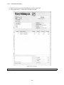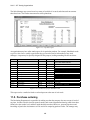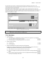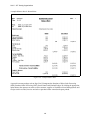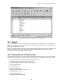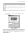
1
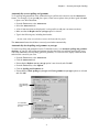
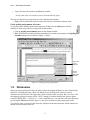
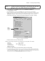
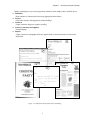
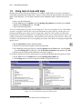
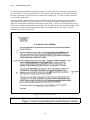
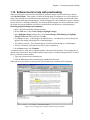
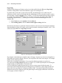
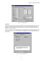
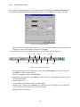
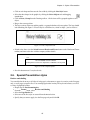
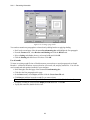
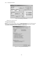
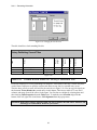
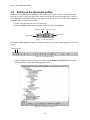
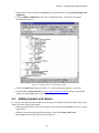
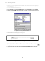
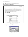
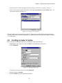
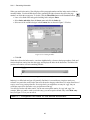
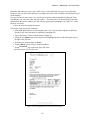
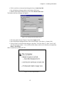
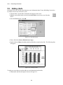
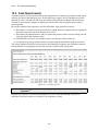
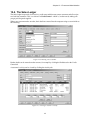
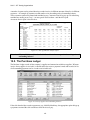
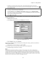
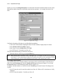
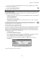
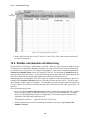
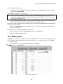
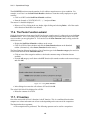
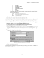
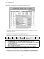
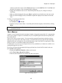
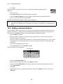
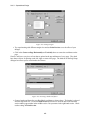
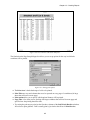
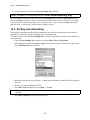
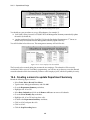
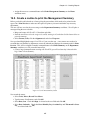
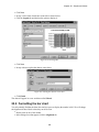
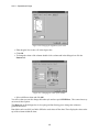
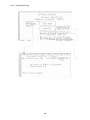
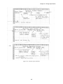
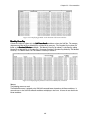
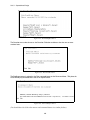
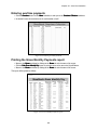
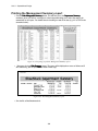
Chapter 20 – Graphs and Charts
Figure 20.11: The modified worksheet
• Highlight cells B2 to M2, B4 to M4 and cells B11 to M11.
• Click the Chart Wizard button and choose to create a column chart.
• In Step 2 click the Series tab and name the series 2000 and 1999 so that the legend is labelled
correctly, as shown below.
Figure 20.12: Naming the series
The series that we wish to plot have been identified correctly. If, however, you wanted to change the data
range that has been selected it is at this point that you have the opportunity to do so. First click the Data
Range tab. Then either mark the range by dragging the pointer on the worksheet, or edit the range in the
dialogue box. To mark a new range, click the icon on the right of the data range. The Chart Wizard will
be reduced to a small box allowing you to mark the data range. Click the icon again to return to the
dialogue box. (See Figure 20.13.)
173