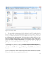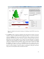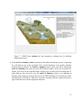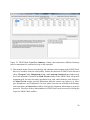
1
QGIS Interface for SWAT (QSWAT) Version 1.2 October 2015 Prepared by: Yihun Dile, R. Srinivasan and Chris George This guide describes QSWAT, which uses the 2012 version of the SWAT model. This version describes QSWAT version 1.2, which needs SWAT Editor version 2012.10.18. 1 QSWAT (QGIS SWAT) Step by Step Setup for the Robit Watershed, Lake Tana basin Ethiopia Contents 1. Environment and Tools Required ........................................................................................... 4 2. Installation............................................................................................................................... 4 3. Structure and Location of Source Data ................................................................................... 6 4. Structure and Location of Output Data ................................................................................... 6 5. Setup for Robit Watershed, Lake Tana Basin ......................................................................... 7 5.1. Watershed Delineation ..................................................................................................... 9 5.2. Create HRUs .................................................................................................................. 18 5.3. SWAT Setup and Run ..................................................................................................... 27 5.4. Output Visualization with QSWAT ................................................................................ 32 5.4.1. Preparing to visualise .................................................................................................. 33 5.4.2. Running visualise ........................................................................................................ 33 5.4.3. Visualisation period..................................................................................................... 33 5.4.4. Static visualisation ...................................................................................................... 33 5.4.5. Animation.................................................................................................................... 37 5.4.6. Plotting ........................................................................................................................ 39 5.5. 6 7 SWAT Output Visualization with SWAT Error Checker ................................................ 44 Appendix I ............................................................................................................................ 49 6.1 Adding tables into SWAT and Project databases............................................................ 49 6.2 Preparing daily climatic data for QSWAT ...................................................................... 53 6.3 Preparing landuse and soil look-up tables ...................................................................... 55 Appendix II – preparing global DEM data for QSWAT ....................................................... 56 7.1 Introduction ................................................................................................................... 56 7.2 Obtaining SRTM DEM data ........................................................................................... 56 7.2.1. 90m data .................................................................................................................. 56 7.2.2. 30m data .................................................................................................................. 56 2 7.3. Clipping the grids ........................................................................................................... 57 7.4. Merging the grids ........................................................................................................... 58 7.5. Reprojecting the grid ...................................................................................................... 59 7.6. Masking a DEM ............................................................................................................. 63 7.7. Large DEMs ................................................................................................................... 66 8 Appendix III: Using a Predefined Watershed and Stream Network ..................................... 69 9 Appendix IV: Installing and Using MPI .............................................................................. 72 9.1 Installing MS-MPI.......................................................................................................... 72 9.2 Configuring QSWAT to use MPI ................................................................................... 73 9.3 Blocking network access ................................................................................................ 73 3 1. Environment and Tools Required Microsoft Windows (any version, as far as we are aware) Microsoft Access, as the interface uses an Access database Text editor (e.g. WordPad, NotePad, NotePad++) that enables you to read and edit ASCII text files. A tool like WinZip that can uncompress.zip files (not needed with recent versions of Windows) System requirements for SWAT Editor Version 2012.10.18 Microsoft Windows XP to 8.1 Microsoft .Net Framework 3.5 Adobe Acrobat Reader Version 7 or higher. Acrobat Reader may be downloaded for free from: http://www.adobe.com/products/acrobat/readstep2.html 2. Installation Install QGIS by running QGIS-OSGeo4W-2.6.1-1-Setup-x86.exe. It can be downloaded from http://qgis.org/downloads/QGIS-OSGeo4W-2.6.1-1-Setup-x86.exe. Use the default folder C:\Program Files\QGIS Brighton as the installation folder, or C:\Program Files (x86)\M QGIS Brighton on a 64-bit machine. Currently you must use the 32-bit version on 64-bit machines. It is also currently necessary to use version 2.6 rather than 2.8. From now on we will use Program Files as a folder name, even though it will be Program Files (x86) on a 64-bit machine. Install SWATEditor 2012 version in its standard place C:\SWAT\SWATEditor. For the SWAT 2012 version, unzip the installation archive swateditor_install_201210_218.zip (or a later version if available from http://swat.tamu.edu/software/arcswat/swateditor/) and double-click on the "setup.exe" program to install the SWAT Editor. This will launch the SWAT Editor install program. Use the default folder C:\SWAT\SWATEditor as the installation folder. The SWATEditor folder will consist of Databases folder, SwatCheck folder, SWATEditorHelp, and other SWAT executables. The database folder consists of SWAT2012 databases which require updating based on user available information (e.g. user soil, weather generator). Refer to Appendix I on how to update a database. Refer to the SWATEditor_Documentation.pdf document in SWATEditorHelp for important information on how to get started with the SWAT Editor. 4 Make sure you have the system requirements listed above for the SWAT Editor to work properly. Failure to have the above system configuration may result in failure to install the SWAT Editor or errors in the SWAT Editor interface. Users can join the user group for any help at https://groups.google.com/forum/#!forum/qswat Figure: SWATEditor installation folder (after installing QSWAT) Install QSWAT by running QSWATinstall1.2.exe or a later version. This adds some files to the SWATEditor: a project database and a reference database in Databases, SWATGraph in the SWATGraph folder, and also stores the TauDEM executables in a new directory C:\SWAT\SWATEditor\TauDEM5Bin. The QGIS plugin QSWAT is put into the user's home directory in .qgis2\python\plugins\QSwat, which we will refer to as the QSWAT directory. The latest version of QSWAT can be downloaded from the SWAT website http://swat.tamu.edu/. 5 3. Structure and Location of Source Data Before starting QGIS, users should prepare their tabular and spatial data according to SWAT requirements. Users can refer to Appendix I on preparing tabular data (e.g. uploading look-up tables into SWAT databases, preparing climatic data, etc). All the spatial data (DEM, land use and soil) should be projected into the same projected coordinate system. Users can refer to Appendix II for preparing global data for QSWAT. Users can also refer to the Arcswat Interface for SWAT2012 User’s Guide (page 11-36) for detailed guidance. The example files used in this manual are available in the QSWAT directory in a directory Example Dataset. This directory contains: A DEM in directory DEM A stream reaches file to burn in to the DEM, in directory RobitStreams An outlet file in directory MainOutlet Landuse and soil maps in directories Landuse and Soil Climate data in directory ClimateRobit Some Excel files for making database tables, and An observed data file observedFlow.csv in directory Observed. Users are recommended to save the example dataset in a folder C:\QSWAT_Projects\Example Dataset during setting up the QSWAT project. 4. Structure and Location of Output Data We will be establishing a project called Demo, say, in a folder C:\ QSWAT_Projects\Robit\Demov1. This will create: 1) In the folder C:\QSWAT_Projects\Robit\Demov1 the project file Demo.qgs and a folder Demo. If we later want to reopen the project Demo.qgs will be the file we look for. The folder Demo is the project folder. 2) A folder C:\ QSWAT_Projects\Robit\Demov1\Demo\Scenarios\Default\TxtInOut that will contain all the SWAT input and output files. 3) A folder C:\ QSWAT_Projects\Robit\Demov1\Demo\Scenarios\Default\TablesIn that may be used by the SWAT Editor. 4) A folder C:\ QSWAT_Projects\Robit\Demov1\Demo\Scenarios\Default\TablesOut that may be used by the SWAT Editor and is used to hold results files from visualisation. 5) A folder C:\ QSWAT_Projects\Robit\Demov1\Demo\Source that will contain copies of our input maps and a number of intermediate maps generated during watershed delineation. 6 6) If we choose to save a SWAT run as Sim1, say, then a folder C:\ QSWAT_Projects\Robit\Demov1\Demo\Scenarios\Sim1 will be created (a copy of C:\ QSWAT_Projects\Robit\Demov1\Demo\Scenarios\Default, including its sub-folders). 7) A folder C:\ QSWAT_Projects\Robit\Demov1\Demo\Watershed with several subfolders 5. Setup for Robit Watershed, Lake Tana Basin 1. Start QGIS and select Plugins menu -> Manage and Install Plugins and find QSWAT. Click its checkbox to install, which takes a few seconds. The SWAT icon will appear in the toolbar. SWAT Figure 1. QGIS with the SWAT icon. 2. Start QSWAT by clicking the SWAT icon. 3. The main QSWAT interface will be displayed. Click the box New Project. 4. A browser will be displayed requesting a name for the new project. Type Demo in the text box labelled File name (under the C:\QSWAT_Projects\Robit\Demov1 folder). See Figure 2. 7 Figure 2: Creating a QSWAT project At this stage all your maps should be prepared in an equal area projection (probably, but not necessarily, UTM1). All the maps should be in the same projection coordinate system. The interface now presents a step-by-step configuration to be followed in order to prepare the SWAT simulation, starting with Step 1 (Figure 3). 1 UTM is not an equal area projection, but is close to being so, and sufficiently close for SWAT to use on most watersheds. 8 Figure 3: Step 1 interface 5. At this stage the project database is created as Demo.mdb in the project folder, and a copy of the SWAT reference database QSWATRef2012.mdb is also created there. Users should update these databases at this stage. These include adding the look-up tables for the land use and soil maps. Refer to Appendix I (at the end of this document) on how to prepare the look-up tables for landuse and soil. Users may also need to extend or replace tables in the copy of the SWAT reference database: again see Appendix I for details. 5.1. Watershed Delineation 6. To start automatic watershed delineation click the Delineate Watershed button. When the prompt box is opened browse to the data source in the dialogue box next to Select DEM. 7. Browse to the C:\ QSWAT_Projects\Example Datase\DEM\srtm_30m folder and open the file hdr.adf. This DEM is an ESRI grid and consists of a number of files. The file called hdr.adf is the one to choose for such a grid. 9 Figure 4. Selecting the DEM 8. The name of the elevation map grid will be displayed in the DEM text box below the Watershed dialogue box. The selected DEM will be copied to the projects Source folder and, if necessary, converted to GeoTiff format (.tif). If your DEM's units are not metres you can select the DEM properties tab and change them. This tab also shows the DEM cell size, cell area, projection system and extent in degrees. Users can burn in using an existing stream network using the option Burn in existing stream network; use a file with the extension *.shp (Figure 5). Check the Burn in existing stream network option and select the file C:\ QSWAT_Projects\Example Datase\RobitStreams\robReach.shp. The delineation form allows you to opt for a predefined watershed and stream network by selecting the Use existing watershed tab. If you are interested in using a predefined watershed and stream network please refer to Appendix III (Using a Predefined Watershed and Stream Network). We will not use MPI, which enables multiprocessing during watershed delineation (see Appendix IV) and so the Number of processes spinbox should be set to 0. 10 Figure 5. Creating stream networks 9. The threshold size for creating subbasins should be set next. It can be set by area, in various units such as sq km or hectares, or by number of cells. If necessary, change the threshold method to use hectares, change the number of hectares to 90, and press Create Streams: the number of cells will be adjusted to the corresponding value (1000). The threshold is the number 11 of cells (or area) required to form a stream: a cell will be made part of a stream if it has at least the threshold number of cells draining into it. Stream reaches are sections of the stream network between significant points, where significant points are stream sources, stream junctions, and inlet, outlet, point source, and reservoir points that we may add later. A subbasin is an area draining into a stream reach. This step creates streams (Figure 6). It also loads the stream burn-in shapefile if selected. Figure 6. Stream networks displayed 10. An inlets/outlets file containing just a main outlet is provided for this example. Check the Use an inlets/outlets shapefile option, and browse to MainOutlet/MainOutlet.shp 11. Users can add outlets, reservoirs, inlets, and point sources by selecting the Draw Inlets/Outlets option. This first asks if you wish to add to the existing inlets/outlets file, or create a new one. Having made this choice, select the type of point to add, and click on the map to place it at the appropriate place. Points need to be placed on the stream network, and you may need to zoom in to place them precisely. Only points within the snap threshold of a stream reach will be counted as points. Click OK to confirm and exit, and Cancel to remove points and exit. If you choose to draw a new file, drawoutlets.shp is created in the Watershed\Shapes folder, which may be used again. See Appendix III for details of the fields needed in an inlets/outlets 12 file. We do not add any additional outlets, reservoirs, inlets, or point sources in this example. Figure 7. Step where Inlets/Outlets are added. 12. If you have several points in your inlets/outlets file you can choose to use just a selection of them. To do this choose the Select Inlets/Outlets option. Hold Ctrl and select the points by dragging the mouse to make a small rectangle around them. Selected points will turn yellow, and a count will be shown at the bottom left of the main window (Figure 8). You only need to use this option if you want to only use a subset of outlets. The default is to use all the points in the outlets file or those drawn. 13 Figure 8. Inlets/outlets selected 13. Clicking Review snapped shows the snapped inlets/outlets, i.e. those within the defined threshold distance. Clicking Create Watershed will create the watersheds after a few minutes (Figure 9). Figure 9. Delineated watersheds 14 14. In QSWAT users can select and merge subbasins. This is especially important in avoiding small subbasins. To merge subbasins, select the option Select subbasins under Merge subbasins. Hold the Ctrl key and click in subbasins you want to select. Selected subbasins will turn yellow, and a count is shown at the bottom left of the dialogue window (Figure 10). Figure 10. Step of merging subbasins. 15. For the sake of this exercise, we will not merge the selected subbasin. Release the Ctrl key and click on the map outside the watershed and the selected subbasin will be unselected. Checking the option of Select small subbasins provides the option to merge subbasins below a certain threshold (i.e. either the area in hectares or a percentage of the mean subbasin area) (Figure 11). For this exercise click the radio button percentage of mean area, and put 25 in the box next to it. Click Select. It will show you subbasins that have an area less than 25% of the mean area. When finished click “Save” to save your selection, or “Cancel” to abandon your selection. You click Merge to perform the merge. Note: You cannot merge a subbasin that has an outlet, inlet, reservoir, or point source. So in this example, the only small subbasin is that nearest the watershed outlet, which cannot be merged, and QSWAT will report this. 15 Figure 11. Subbasins that have an area less than 25% of the mean subbasin area merged to downstream subbasins. 16. Point sources can be added to all the subbasins by checking the option Add point source to each subbasin (Figure 12). You can also add reservoirs to selected subbasins. You then need to click Add. Unlike points added earlier, these extra point sources or reservoirs do not create subbasin boundaries, but are added to existing subbasins, provided they do not already have point sources or reservoirs. Adding point sources to all subbasins is useful if you have several to add. It is quite safe since only those you provide input data for will have any effect in the SWAT simulation. For this example, check the box Add point source to each subbasin, and click Add. This will add point source to each subbasin (Figure 12). 16 Figure 12. Point sources added to each subbasin 17. You need to click OK. This causes the subbasins to be numbered. This step ends watershed delineation, and enables the Create HRUs option (Figure 13). Figure 13. Watershed delineation is completed, and Create HRUs is enabled 17 5.2. Create HRUs 18. Having calculated the basins you needed to calculate the details of the Hydrological Response Units (HRUs) that are used by SWAT. These are divisions of basins into smaller units each of which has a particular soil/landuse (crop)/slope range combination. 19. To do this we click Create HRUs, select C:\QSWAT_Projects\Example Dataset\Landuse\roblandusenew\hdr.adf as the Landuse map, and select Robit_landuses as the Landuse table; select C:\QSWAT_Projects\Example Dataset\ Soil\mowr_soil90\hdr.adf as the Soil map, and select Robit_soils as the Soil table. The last two will take a few seconds as the relevant database tables are read. Select usersoil as the Soil data option. The other soil data options are for watersheds in the USA for which you are using STATSGO, STATSGO2, or SSURGO soil maps. To use STATSGO2 or SSURGO soil maps you will need to download SWAT_US_SSURGO_Soils.mdb from http://swat.tamu.edu/media/63316/SWAT_US_SSURGO_Soils.zip and install it in C:\SWAT\SWATEditor\Databases. No soil lookup table is needed with STATSGO2 or SSURGO. 20. We will form HRUs based on slope as well as landuse and soil. We add an intermediate point for slopes (e.g. 10) to divide HRUs into those with average slopes in the range 0-10% and those with average slopes above 10%. Type 10 in the box and click Insert. The Slope bands box shows the intermediate limit is inserted. To generate the FullHRUs shapefile, click in the check box. 21. To read in the data from the DEM, landuse, soil and slope maps and prepare to calculate HRUs, make sure Read from maps is checked and click Read (Figure 14). This may take a few minutes. There is also an option Read from previous run. This can be used when rerunning the project, provided you have not rerun the delineation step, and not changed the soil or landuse inputs, or the slope bands, to recover information from the project database instead of rereading the grids. Reading from the database is substantially faster. 18 Figure 14: Reading the land use, soil and slope maps 22. After reading the grids you will notice a number of changes to the QSWAT display (Figure 15): A Slope bands map has been created and added. This allows you to see where the areas 19 of the two slope bands selected for this project are located. If no intermediate slope limits are chosen this map is not created. The legends for the landuse map robelandusenew and the soil map mowr_soil90 include the landuse and soil categories from the SWAT database. A shapefile FullHRUs has been created and added. This allows users to see where in each subbasin the potential Hydrological Response Units (HRUs) are physically located. If, for example, we zoom in on subbasin 2, in the Legend panel select (left button) FullHRUs, open its attribute table (right button), set the mouse to Select Feature(s) (QGIS toolbar) and click on the box around the number 2, then we get a view like Figure 16. We see that this potential HRU is composed of several parts, has the landuse AGRL, the soil LVx, and the slope band 0-10. Its area of 172.35 ha is 50.1% of the subbasin. Close the Attribute Table Editor. Generating the FullHRUs shapefile is optional, as it can take some time. A count of the potential HRUs (51 in this example) is displayed whether this file is created or not. Figure 15. After reading grids 20 Figure 16. Viewing a particular HRU 23. Before you continue with HRU definition, if you look at the main QSWAT window you see that a new item Select Report to View is available and you can choose to view just two reports at this point, which are the Elevation and Landuse and Soil reports. The elevation report gives information about how much land is at each elevation from the lowest to the highest, both for the watershed as a whole and for each subbasin (Figure 17). The landuse and soil report lists the landuse, soil and slope-band areas for each subbasin (Figure 18). Figure 17: Elevation report 21 Figure 18. Landuse and soil report 24. At this point you have the options to split landuses, and to exempt landuses, both of which will affect how HRUs are defined. Splitting landuses allows you to define more precise landuses than your landuse map provides. If, say, you know that in this basin 50% of the AGRL (Agricultural land generic) is used for corn, and the other 50% is used for teff, you could split AGRL into 50% CORN and 50% TEFF (Figure 19). It is possible to use the original landuse (here AGRL) as one of the sub-landuses. The percentages are integers and need to sum to 100 for each landuse you split. Split AGRL into 50% CORN and 50% TEFF as shown. Exempting landuses allows us to ensure that a landuse is retained in the HRU calculation even if it falls below the thresholds we will define later. For example, we might decide to exempt the forest landuse FRST (Figure 20). Make this exemption. 22 Figure 19. Splitting a landuse Figure 20. Exempting a landuse 25. Once all the data has been read in and stored, the Single/Multiple HRUs choice is enabled. Dominant landuse, soil, slope and Dominant HRU options provide just one HRU for 23 each subbasin (i.e. option of Single HRU). Dominant landuse, soil, slope chooses the landuse with the biggest area in the subbasin, the soil with the biggest area in the subbasin, and the slope range with the biggest area in the subbasin and uses them for the whole subbasin. Dominant HRU selects the largest of the potential HRUs in each subbasin and makes its landuse, soil and slope range the ones chosen for the whole subbasin. The options with Filter by landuse, soil, slope; Filter by area; and Target number of HRUs create Multiple HRUs. For the Multiple HRUs option, users can exclude HRUs that are insignificant by considering percentage thresholds or area thresholds. The option of Filter by land use, soil and slope, will ignore any potential HRUs for which the landuse, soil or slope is less than the selected threshold. The areas of HRUs that are ignored will be redistributed proportionately amongst those that are retained. The option of Filter by area will ignore HRUs that are below a specified threshold amount (either percent of the subbasin, or area). Finally the option of Target number of HRUs limits the number of HRUs to a user preferred amount (i.e. between the lower limit of one HRU per subbasin and the upper one of retaining all potential HRUs). For this exercise, use the method of Filter by land use, soil and slope and choose the Threshold method of Percent of subbasin. For landuse, the value of 81 as the maximum we can choose indicates that there is a subbasin where the maximum value for a landuse is 81%. If we chose a higher value than 81% we would be trying to ignore all the landuse categories in that subbasin. Hence 81% is the minimum across the subbasins of the maximum landuse percentage in each subbasin. For this exercise, let’s select 10% for landuse, by using the slider or by typing in the box, and click Go. The interface then computes the min-max percentage for a soil as 52%. Select 10 for Soil, click Go. Similarly select 10 for slope. At this stage the user can create HRUs by clicking Create HRUs (Figure 21). The number of HRUs created (54) is reported at the top of the map canvas. 24 Figure 21. Creating multiple HRUs by Filter by land use, soil and slope 26. Create HRUs is now reported as done and the third step is enabled (Figure 22). If you requested a Full HRUs file you will notice that an Actual HRUs file has now been added. This contains the potential HRUs that were retained as actual HRUs (and so typically has some holes representing those that were not retained). This file also shows the numbering of HRUs as well 25 as subbasins. If you open its attribute table you will see in the last column, called HRUGIS, values like 000050001, which indicates that this row is for HRU 1 in subbasin 5. Input files for this HRU (found in the TxtInOut folder) use the HRUGIS value as their base file name. HRUs that were split, those for landuse AGRL, have two HRUGIS values, since they will have two sets of HRU input files, one for CORN and one for TEFF. If you look at the Reports now available you will find that there is an HRUs report that only includes the landuses, soils and slope bands left after HRU selection, and also gives details of the HRUs that have been formed (Figure 23). If you wish to change the HRU thresholds then you can click the Create HRUs button again, change the thresholds and/or the landuses to be split or exempted, and rerun the Create HRUs step. Figure 22. About to do step 3 26 Figure 23. HRUs report 27. It is strongly recommended to save the project (via the file menu of QGIS) at this stage. 5.3. SWAT Setup and Run 28. At this point almost everything is ready to write the SWAT input files and run SWAT. The SWAT Editor assumes that dates are written in the mm/dd/yyyy format. You may need to change to this system on your machine, by opening the Control Panel, selecting Region and setting English (United States) as the format. Otherwise you may get messages about invalid date. Click Edit Inputs and Run SWAT (Figure 22). This executes SWAT Editor (Figure 24). 27 Figure 24. Connecting the Demo project to SWAT databases 29. Click Connect to Databases to connect to the project database and to the SWAT reference database SWATRef2012.mdb. This will be to the local copy if you made one. If it didn't appear you can change it (the second entry in the SWAT Editor form). 30. Now the Write Input Tables will be active. Click the option Weather Stations. This step provides the option to provide the weather generator data, and write the weather data. By clicking the Weather Data Generator tab, users can choose WGEN_Robit. By clicking the different tabs users can write the corresponding weather data. For the Robit Demo project all the climate data are stored in the folder C:\QSWAT_Projects\Example Dataset\ClimateRobit. The ClimateRobit folder consists of station and weather data for rainfall, temperature, solar radiation, relative humidity and wind speed. The text files are prepared according to the SWAT format. Users provide just station information. Using the station information, SWAT Editor will access (and write) the relevant climate data. The station files are pcpRobStation.txt, tmpRobStation.txt, solRobStation.txt, rhumRobStation.txt, and windRobStation.txt for rainfall, temperature, solar radiation, relative humidity, and wind speed respectively. For each tab for rainfall, temperature, etc. check the option for gages rather than simulation and select the appropriate stations file. Click OK. The climate data (which will be accessed by SWAT Editor using station information) are: robpcp.txt, robtmp.txt, robsol.txt, robrhum.txt, and robwind.txt. Click Cancel to close the Weather Data Definition form. 28 31. To write the remaining input tables and files select Write Input Tables -> Write SWAT Input Tables. Click Select All in the list box (Figure 25) and click the Create Tables button. There is a program for estimating the heat units needed for plant growth, using climate data, but it is currently available only for the USA. Since this project is outside the USA, choose the option No. The heat units value appears in the management (*.mgt) files, and you can later edit these values using the SWAT Editor. Also answer No to writing point source, reservoir and inlet information. Writing the database tables can take a few minutes, especially if your simulation covers several years, but it is fast in this case as the weather data is prepared already. A form announces that the tables have been built, where you click OK to acknowledge. If all is well you will see a form (Figure 25) showing that all database tables and files have been written successfully. Click Cancel. Figure 25. About to write the SWAT input files 29 32. Now the user can edit different SWAT databases and simulation conditions (e.g. methods to estimate potential evapotranspiration, stream flow routing, etc). This is also the step where users can implement different management scenarios. 33. To run SWAT click SWAT Simulation -> Run SWAT. Set the time periods to run SWAT (e.g. 01/01/1990 to 12/31/2000), chose Monthly timestep, and NYSKIP (number of years to skip of 3), check the Print Water Quality Output option, and leave the Output File Variables set to All. Select a release version of SWAT.exe, 64-bit if you have a 64-bit machine, else 32-bit. Finally click Setup SWAT Run (figure 26). This step activates Run SWAT. Figure 26. Setting up SWAT Run 34. Click Run SWAT to launch the SWAT executable in a command window (Figure 27). 30 Figure 27: Running SWAT 35. If the run is successful the command window will close and a message box will say that SWAT was run successfully. Click OK. 36. If the run is not successful the command window will stay open with a message telling you to Hit Enter to exit. The release versions of the SWAT executable run faster than the debug versions, but don't provide information on errors, so if you have an error hit enter to close the command window and run SWAT again but with a debug version of SWAT.exe selected. The error message may suggest which SWAT input file needs to be checked, or you may be able to get more information from examining the SWAT source code, but probably you will need to report the problem to the SWAT team. Go to the SWAT support page http://swat.tamu.edu/support/ for advice. Click Cancel to close the SWAT simulation window. 37. If you want to use QSWAT visualisation you need to use Read SWAT Output in the SWAT Simulation menu. Select output.rch, output.sub, output.hru, output.sed, and (if you checked Print Water Quality Output in the Run SWAT form) output.wql, and click Import Files to Database. 38. The SWAT simulations can be saved using the Read SWAT Output option under SWAT Simulation tab. This copies C:\QSWAT_Projects\Robit\Demov1\Demo\Scenarios\Default to C:\QSWAT_Projects\Robit\Demov1\Demo\Scenarios\Sim1 if the user chooses to save as Sim1. If 31 Sim1 already exists it will ask the user to confirm it should be overwritten. Click Cancel to close the SWAT Output form. 39. Set Default Simulation option under SWAT Simulation tab helps to restore the model parameters and its output back to a preferred previous SWAT simulation (i.e. not necessarily only to the default simulation). 40. Manual Calibration helper option under SWAT Simulation is used to calibrate SWAT parameters manually. It can also be used to implement calibrated model parameters for SWAT simulation when automatic model calibration is done outside the QSWAT environment (e.g. using SWAT-CUP). 41. Click Exit to close the SWAT Editor. 5.4. Output Visualization with QSWAT Once SWAT has been run and the output imported, so that there is an output database SWATOutput.mdb in the Scenarios\Default\TablesOut directory of the project, then a button Visualise becomes available in the main QSWAT form. Visualisation allows outputs from SWAT to be visualised graphically by subbasin, reach, or HRU. Figure 28. Main QSWAT form showing Visualization button 32 5.4.1. Preparing to visualise In order to visualise results you have first, of course, to (successfully) run SWAT. Then you have to save your results in the output database. To do this, in the SWAT Editor, use SWAT Simulation → Read SWAT Output to bring up the SWAT Output form. Then check the boxes for the outputs you want to save in the database. QSWAT can display results from output.rch, output.sub, output.hru, output.sed, and output.wql (which only has data if the Print Water Quality Output was checked in the SWAT Editor Run SWAT form). Then click the Import Files to Database button to create (or update) the database. It is a good idea to use the Save Simulation button to save the simulation, having provided a suitable name. Then if you change anything and run SWAT again, the results from the run will still be available. Even if you don't get as far as running SWAT in changes to the project, saving the previous simulation also saves copies of the watershed, streams and actual HRUs shapefiles, which are needed for visualisation, and which may be changed if you rerun watershed delineation or HRU creation. Click Cancel to exit from the SWAT Output form, and Exit from the SWAT Editor. 5.4.2. Running visualise Click Visualise on the main QSWAT form to bring up the Visualise Results form (Figure 29). Here the Choose scenario pull-down menu shows the simulations, or scenarios, that are available: the current Default one, and in this example another called Sim1 that has been saved. Select the one that you wish to display. Then use the Choose SWAT output table to see what tables are available: you will see all or some of hru, rch, sed, sub, and wql (the list depends on the output files you imported into the SWATOutput database). Select one of these. 5.4.3. Visualisation period The start and finish dates shown are initially the start and finish dates of output from the Default scenario. You may choose dates within these if you wish, to shorten the period being visualised. If other scenarios are selected, the dates will be changed if necessary to ensure there is data available for the whole period. 5.4.4. Static visualisation There are three possibilities shown by the tabs for Static data, Animation and Plot. For static data a single summary value is calculated for each subbasin, reach, or HRU and displayed as a map. For animation there is an animated display of the value in each subbasin, reach, or HRU at each time step in the animation. Plot supports the creation and display of plots of selected variables. This section deals with static data; animation and plotting are described in the following sections. Make sure the Static data tab is selected. Static results are created by generating a shapefile, and by default this will be called 33 <table>results.shp (e.g. subresults.shp) and stored in the TablesOut directory of the current scenario. You can leave this default, or change the file name and location as you wish. You may notice files called hrus.shp, rivs.shp, and subs.shp in this directory. Do not choose any of these as your file name: they are copies of the actual HRUs, stream reaches and watershed shapefiles generated by QSWAT, copied into this folder and used as a basis for the results shapefile (and for animation). This is done because these shapefiles may be changed by subsequent runs of QSWAT and not have the same HRUs, stream reaches or subbasins as this run had. You should also avoid naming your results shapefile as animate in the TablesOut directory: this filename is used for animation and such a results shapefile is likely to be overwritten without warning. The pull-down menu in Choose variables contains all the output variables from your chosen table. You can select these one at a time and use the Add button to add them to the box below, or simply click All to get all of them. You can adjust your selection by selecting and using Del to delete ones, or using Clear to delete all of them. Data from all the variables you place in the box will be placed in the results file. You then need to select one of them to be displayed. 34 Figure 29. Visualise results form For each variable, for each subbasin, the output data has a value for each day, month, or year of your simulation (according to what period you chose for the SWAT run). To display the results graphically we need to produce a single value for each variable for each subbasin, and for this we choose a Summary. Summaries available are: Totals: the summary is the total of the values for the variable for the subbasin, reach, or 35 HRU. Daily means: the summary is the daily mean of the total, the total divided by the number of days in the simulation. Monthly means: the summary is the monthly mean of the total, the total divided by the number of months in the simulation. The number of months may be fractional Annual means: the summary is the annual mean of the total, the total divided by the number of years in the simulation. The number of years may be fractional. Maxima: the summary is the maximum value for the variable for the subbasin, reach, or HRU. Minima: the summary is the minimum value for the variable for the subbasin, reach, or HRU. Figure 30. Displaying results When you have loaded the variables you want included into the variables box, selected the one to display (SURQmm for this example), and chosen the summary (annual means), click the Create button. You will be asked to confirm if you are overwriting an existing shapefile. Then the results file will be displayed as shown in Figure 30. The legend shows that we are displaying SURQmm values from the Default simulation. The results layer is given a default colouring using 5 intervals chosen by the Jenks natural breaks algorithm to cover the range of summary values for the variable. You can change the colouring scheme if you wish (right click on the layer entry in the Layers panel, select Properties and then 36 select the Style tab). To display a different variable from the list, select it with the mouse and click Create. To change the summary, select the new one from the pull-down menu and click Create. 5.4.5. Animation To animate, after choosing the scenario and the SWAT output table, select the Animation tab. The Variable pull-down menu contains all the variables from the chosen output table (Figure 31): select one of these. A new animation layer is created in the map canvas, showing the initial values of this variable in the simulation (Figure 32). Here we are animating the PETmm variable in the Sim1 simulation. Note that the range of possible values runs from 90 to 169 (the minimum and maximum values for PETmm for the whole simulation period). You can view the actual initial values for each subbasin by examining the attribute table (right click on the Animate entry in the Layers panel and Open Attribute Table). There are controls to run, pause and rewind the simulation: it steps through daily, monthly or annual time steps according to the reporting period chosen for the simulation. The speed of the animation can be adjusted using the Speed spinbox. You can also investigate the changing values manually, by dragging the slider, or by pressing the left and right arrows on your keyboard. The date (day, month, or year) of each step appears above the slider. The animation is achieved by creating a shapefile animate.shp in the TablesOut folder of the scenario. At each time step the values of the variable are updated and the file redisplayed. Hence this file is being continuously changed. It is regarded as a temporary file and so is not preserved. If you wish to save a view of the animation at a particular moment you can pause the animation and make a copy of this file (remembering to copy the .dbf, .prj, and .shx files as well as the .shp file). 37 Figure 31. Choosing an animation variable. 38 Figure 32. Start animation As with static visualisation, it is possible to change the colouring scheme used (the colour ramp and/or the number of classes): right click on the legend entry, select Properties and then select Style. 5.4.6. Plotting Plotting allows the rapid display of output data as line graphs or histograms, plotting values against time. It is intended to facilitate comparisons of outputs from different scenarios, or different subbasins, reaches, or HRUs, or between simulated and observed values. Plotting is done in two stages, data collection and display. After collection, just before display, data is saved in a comma-separated value (.csv) file. This file can be loaded into tools like Excel to support more extensive analysis than provided by the plotting tool SWATGraph that is supplied with QSWAT. 5.4.6.1. Collecting plot data As with other visualisation options, start by selecting a scenario and SWAT output table. Then reduce the period if you wish. Next you can select an observed data file if you have one (Figure 33). The structure of observed data files is described later. As many plots as you like may be added to the table. You can start by clicking Add plot. This adds a row to the table, and already shows the chosen scenario and table. The Sub (subbasin) 39 field is empty and so is the Variable. This first row is also the currently selected row, and this is important. Whenever we change the scenario, output table, subbasin, HRU or variable settings through their pull-down menus we will immediately change values in the currently selected row. When you have more than one row you can select a row by clicking in it. Whether the HRU setting is available or is set to '-' depends on the table we are using. If it is hru (and we chose a multiple HRU option for the scenario) then we can choose an HRU from the current subbasin. Otherwise HRU is not used and is set to '-'. Suppose we want to compare the main outlet flows from two scenarios, and for both the main outlet subbasin is number 9. Then rch is the appropriate table, and we select this and select 9 as the Subbasin. Finally we select FLOW_OUTcms as the Variable. Now we want to add a second row to the table for the other scenario. A convenient way to do this is the Copy plot button. This copies the current row to a new row, and makes it current. Then all we have to do is choose a new scenario and the second row will be (almost) what we want. The subbasin number is cleared in the new row, to remind us that in a different scenario subbasin numbers might be different. We select the appropriate number, in this case 9 again. It is also possible to move the current row up or down: this just affects the ordering of the plots in the output. To add observed data we select an observed data file, and use the button Add observed. observed is used as the scenario name, '-' is used for Table, Sub, and HRU, and we can select a variable name from the file. 40 Figure 33. Plot screen When we have completed the plot selections we click Plot. This invites us first to choose a .csv file to save the data. We can if we wish later import this into, for example, Excel if we wish to do further manipulations or use Excel’s graphing tools. Once the data is written to the .csv file, SWATGraph is automatically started to display the data graphically: see Figure 34. The data has been displayed as histograms, labelled by months as that 41 was the time interval of our SWAT output. We can change the display to lines using the Chart Type pull-down box and clicking Update Graph. Figure 34 shows a plot of the flow out of subbasin 9 (the main outlet) against the observed data file observedFlow.csv supplied with the Robit example. Note that this file only has data from the beginning of 1993 to the end of 1997, so the finish date needs to be adjusted to 31 December 1997 before clicking Plot. Other SWATGraph options include importing another (similarly created) .csv file, using New File to Plot, and saving the graph to the clipboard, using Copy chart to clipboard, so we can then, for example, paste it into the Paint tool to make an image file. The data from the .csv file is also displayed. The column headings, also shown in the graph legend, take the form Scenario-Table-Number-Variable, where Number is the subbasin number if the table is reach or subbasin, and the hru number if the table is hru. For an observed plot the form is observed-Variable. You can fill in the Chart Title and Y Axis Titles if you wish, and change the X Axis Title. At the bottom of the screen some statistics are displayed. These are correlation coefficients for each pair of plots, and Nash coefficients for each pair of plots where one is observed. Some of these may be meaningless, of course, if for example you choose to plot four things that are really two pairs, but it is quicker as well as simpler to calculate them all than it is to ask the users what they want. 5.4.6.2. How compatible do different scenarios need to be? Obviously, they need to use the same time interval (monthly, daily or yearly). The period is automatically adjusted to include all the scenarios involved (but see below for observed data). You also need to be reasonably confident that the things you want to compare are indeed comparable, so if you are comparing hrus, for example, they should be the same hru in each scenario. But if you are comparing the main outlet reach in each scenario, which gives figures for the whole watershed, it doesn’t matter how the subbasins and hrus in each were selected, or how the subbasins are numbered, as long as you select the main outlet subbasin number for each. 42 Figure 34. SWATGraph 5.4.6.3. Including observed data To include observed data you need to prepare a .csv file, i.e. a text file where each line consists of the same number of items (one or more), separated by commas. The first line should be comma-separated text strings, which will be used as the variables. If the first string is DATE, or Date, or indeed these four letters in any case, it and the data in the first column are ignored. The dates are assumed to be the same as in the SWAT output plots; they are not checked. The data on lines two to the end (apart from ignored dates) should be numeric. 43 Table, Subbasin and HRU boxes in an observed plot row will be unavailable, but you need to choose a Variable. The choices in the Variable pull-down box will be the variables (apart from date) in the first line of the .csv file. 5.5. SWAT Output Visualization with SWAT Error Checker SWAT-Check is a tool that is used to summarize results from SWAT simulations. It can also provide warnings that can help to improve the modeling skills in SWAT. Currently, the program is integrated with the SWAT model and it can be found under the SWAT Simulations tab, and under Read SWAT Output drop-down list. It can also be installed separately. It can be downloaded from the ArcSWAT website: http://swat.tamu.edu/software/swat-check/. SWAT-Check evaluates different processes in the landscape. The following section describes the purposes of some of the tabs in the SWAT-Check program. Each tab has also brief note on the subject it is dealing with. 1) SWAT-Check evaluation can be executed by locating the TxtInOut folder of a particular simulation (Figure 35). Clicking Run SWATCheck button from the SWAT Output form directs to the TxtInOut folder in the Default simulation folder (the Default simulation always saves results from the most recent SWAT run). However, different simulations can be accessed by clicking the folder button in the right of the Project Location (Figure 35). SWATCheck only reads files in the TxtInOut folder. Therefore, it is important to select the TxtInOut folder of a particular simulation that one is interested in (e.g. C:\QSWAT_Projects\Robit\Demov1\Demo\Scenarios\Sim1\TxtInOut). The analysis will be executed by clicking the Examine Model Output button. Besides executing SWAT-Check, the Setup window provides a summary of the simulation details and watershed characteristics. Moreover, the Setup window provides messages and warnings that need to be addressed to improve the model simulation. 44 Button to choose a particular simulation Figure 35. SWAT-Check Setup window showing how to run SWAT-Check for a particular simulation. 2) The Hydrology window in SWAT-Check summarizes the water balance both graphically and numerically. It can be accessed by clicking the Hydrology tab at the top of the SWAT-Check window. As hydrology is the basis for the landscape processes, particular attention should be given to modeling the hydrology right. Therefore, SWAT-Check will be a vital tool in providing a quick summary of the hydrological components and as such aids easy understanding of the system. For example, it provides the ratios of different water balance components. Users can, therefore, compare these values with published literature values, or measured estimates, and have an idea how to improve the model performance in subsequent model calibration processes. Moreover, it gives warnings and suggests methods how to address them (Figure 36). 45 Figure 36. Graphical and numerical summary of hydrology related SWAT results from SWAT-Check. 3) The Sediment window summarizes graphically and numerically the sediment yield in the watershed – both in the upland and in-stream processes (Figure 37). It can be accessed by clicking the Sediment tab at the top of the SWAT-Check window. Sediment loss from the landscape is affected by many factors. Therefore, summaries of sediment related results from SWAT-Check can provide insights on how to improve the model performance in simulating sediment loss in the watershed. For example a quick overview of sediment overestimation could hint to inadequate biomass production, which could be further examined in the land use summary tab (Figure 38). Moreover, the Sediment tab provides warnings when results are outside ranges available in the literature. However, results are watershed specific and one needs to use these warnings as a basis for further re-examination by taking the actual landscape processes in the particular study watershed into context. 46 Figure 37. SWAT-Check sediment tab that summarizes sediment loss for different landscape processes 4) The Land Use Summary window summarizes the different landscape process components for each land use type in the watershed. These include hydrology, water quality, sediment transport and crop growth. The Land Use Summary report can be accessed by clicking the Land Use Summary tab at the top of the SWAT-Check window. In the case of model calibration, users focus on the watershed outlet, and they may overlook processes taking place in minor land use types. In such a case, the Land Use Summary report is very important in showing where things get wrong in the process of SWAT modeling as it summarizes results spatially land use by land use. Moreover, it provides warnings related to a particular land use type so that the users can take appropriate measures. 47 Figure 38. SWAT-Check Land Use Summary window that summarizes different landscape process components for each land use type in the watershed. 5) This manual mainly focuses on hydrology and sediment related outputs of the SWAT-Check. However, in studies related to water quality, besides the functions of SWAT-Check discussed above, Nitrogen Cycle, Phosphorous Cycle, and Landscape Nutrient Loss windows may be of vital importance. Results from Plant Growth window of the SWAT-Check will provide important guide for users who study agricultural crop yield, and/or biomass yield. Moreover, the Plant Growth window provides information about the various crop stresses (e.g. Nitrogen, Phosphorous, and Temperature). In cases where reservoirs are included in the management operations, the Reservoirs window could provide important information on reservoir processes. Therefore, all these functionalities in SWAT-Check can be accessed by clicking the respective SWAT-Check toolbars. 48 6 Appendix I 6.1 Adding tables into SWAT and Project databases Tables need to be added to the project database (Robit_landuses and Robit_soils) and to the local copy of the SWAT reference database. (usersoil and WGEN_Robit). We need to use a new usersoil table in the SWAT reference database. A local copy of this database was made when the project was started, so that changes to it would not affect other projects, and would not be lost if we installed a new version of QSWAT. If you want to change this database and use it in several projects you could instead edit the master copy C:\SWAT\SWATEditor\Databases\SWATRef2012mdb before you create any projects, but remember to reinstate your changes if you install a new version of QSWAT. The tables to be added to the reference database are usersoil, using Example Dataset\usersoil.xlsx, and WGEN_Robit, using Example Dataset\WGEN_Robit.xlsx. Look up tables for landuse and soil maps are placed in the project database (in our case C:\ QSWAT_Projects\Robit\Demov1\Demo\Demo.mdb) not in the SWAT reference database. In our case we need to make tables Robit_landuses, from Example Dataset\Robit_landuses.xlsx, and Robit_soils from Example Dataset\Robit_soils.xlsx. This section shows how tables can be imported from Excel files. Tables may also be imported by other means. In particular they may be imported from comma separated value files or copied directly from other Access databases. We will use as our first example importing WGEN_Robit.xlsx into the copied reference database. WGEN tables define data for simulating weather using a weather generator. They are used by SWAT when observed data is missing (either entirely, or on particular dates). The tables define data for one or more simulated weather stations. The SWAT Editor will assign the same station to all subbasins if there is only one in the table, or find the nearest to each subbasin if there are more than one. You can define a new table in the reference database, as we do here, or replace the dummy data in the existing table WGEN_user. 1. Open the copied reference database in Access. Select External Data -> Excel -> Browse to the folder where the data to be imported is located. 49 Figure 1. Importing data into SWAT database 2. Select the radio button – Import the source data into table in the current database. 3. Follow the wizard - click next three times, and on the fourth step choose the radio button No Primary Key (Figure 2). The table to be appended should have the same format as the table WGEN_US_FirstOrder in the database. 50 Figure 2. Formatting the table similar to the table WGEN_US_FirstOrder Name the table with a name starting WGEN (e.g. WGEN_Robit, Figure 3) Creating the usersoil table in the reference database from Example Dataset\usersoil.xlsx is very similar, except that since there is already a table usersoil you will be asked to confirm that you want to overwrite it. The table must be called usersoil. 51 Figure 3. Naming the table 52 6.2 Preparing daily climatic data for QSWAT 1. The user should initially prepare station information. The station information should be prepared for all the climatic variables for which the user has local data. The header for the table should consist of columns ID (station ID), NAME, LAT (latitude), LONG (longitude) and ELEVATION. Refer to the example dataset in the folder Example Dataset\ClimateRobit, e.g. pcpRobStation.txt. 2. The actual climate data should have the same file name as the station NAME in the station data (e.g. robpcp). The format of the climate data should be as follows: the first line should be the date in the format yyyymmdd followed by the daily climatic data values. Missing values will be replaced by -99. The data format for the precipitation, solar radiation, wind speed and relative humidity is the same. Refer to the example dataset for precipitation data in the folder at Example Dataset\ClimateRobit, e.g. robpcp.txt. The only exception is for minimum temperature and maximum temperature, in which case the minimum temperature and maximum temperature are separated by a comma. Refer to the example dataset for temperature dataset at Example Dataset\ClimateRobit\tmpRobStation.txt. 3. The actual climatic data should be saved in the same folder as the station files. 4. The units for precipitation, temperature, solar radiation, wind speed and relative humidity should be mm, degree centigrade, MJ/m², m/s, and decimal fraction, respectively. 5. For each subbasin, SWAT uses observed climatic data from the closest station. If there is no observed station climatic data, QSWAT will use simulated data using the weather generator. The algorithm used by QSWAT is as follows: for example, suppose there are weather stations with identifiers A, B and C, and tables Apcp, Bpcp, Atmp, Btmp, and Cslr. Then the result will be: For precipitation: subbasins will use measured data from Apcp or Bpcp, according to whether station A or B is closer. For temperature: subbasins will use measured data from Atmp or Btmp, according to whether station A or B is closer. For solar radiation: all subbasins will use measured data from Cslr. For relative humidity: all subbasins will use simulated data. For wind speed: all subbasins will use simulated data. 53 This makes it easy for users to vary climate data if they wish, and to combine measured data from a number of sources. It is even possible to combine simulated and measured data for different subbasins: in the example above, for example, if all the values in Apcp are -99 (missing data), while Bpcp is measured data, then subbasins nearer to station A will use simulated precipitation data and those nearer to B will use measured data. 6. Weather generation When measured data is not available, SWAT uses data simulated by a weather generator program which uses parameters supplied in weather generator files. The SWAT Editor uses a weather generator table, which can contain the parameters for a number of weather stations, each represented by one line in the table. An example weather generator table (WGEN_user) is supplied with SWAT Editor, in the reference database QSWATRef2012.mdb (C:\SWAT\SWATEditor\Databases). You can make your own such table, add it to the SWAT reference database with a name starting with the string WGEN. Use Write InputTables -> Weather Stations, select the Weather Generator Data tab, and then find WGEN_user in the pull-down Locations Table menu. It will then appear in this menu. The SWAT Editor will then allocate to each subbasin the nearest weather generation station from the selected table. There is a weather generation table covering the world available from the SWAT website: http://swat.tamu.edu/media/99082/cfsr_world.zip. Install as explained in the pdf file included in the zip archive, and you will see WGEN_CFSR_World as an option for the Locations Table. 7. Using global data from the SWAT web site The SWAT web site offers global weather data (http://globalweather.tamu.edu/). In the website, you can provide the appropriate Lat and Long values for the bounding box of the study area. If your search with your bounding box provides you no (or very limited) station data, you might try a larger search area. You can acquire climate data that ranges from 1/1/1979 to 7/31/2014. It is good to start at midnight (12.00AM), and also select all five kinds of data. You can receive the climate data both in SWAT files format and CSV files in a zipped folder. It is sufficient to select just the SWAT files. The zipped folder will include pcp.txt, rh.txt, solar.txt, tmp.txt, and wind.txt. These files give details of the weather stations – name, latitude, longitude and elevation. Use Write InputTables -> Weather Stations, select the Rainfall Data tab, make sure the timestep is Daily, and Raingages is checked, navigate to pcp.txt as the Locations Table. Then select the Temperature Data tab, check Climate Stations and navigate to tmp.txt. In similar fashion choose rh.txt, solar.txt, and wind.txt in the Relative Humidity, Solar Radiation, and Wind Speed tabs. Select a WGEN table as described above in the Weather Generator tab, and click 54 OK. The SWAT Editor assigns weather stations or gages to subbasins according to proximity and writes the necessary tables and files. It announces when processing is complete, and you click OK. 6.3 Preparing landuse and soil look-up tables For each landuse or soil map the user has to prepare a table like Robit_landuses or Robit_soils and put it into either C:\SWAT\SWATEditor\Databases\QSWATProj2012.mdb or the project database Demo.mdb in the Demo folder (C:\QSWAT_Projects\Robit\Demov1\Demo). In the first case it will be copied into every new project database, but the user must be careful to keep it and replace it whenever QSWAT is reinstalled. In the second case it will only be used on the particular project. The project database is created by copying QSWATProj2012.mdb to the New Project. Therefore, before Step 1, the user has to add any extra tables that are needed for a particular project. Standard landuse and soil tables, namely global_landuses and global_soils are already included in the project database. These are for use with the global landuse and soil maps available from the WaterBase website on its data page http://www.waterbase.org/download_data.html. If you use these maps then you can use these lookup tables, and the existing tables usersoil, crop, and urban in the reference database are appropriate. The global maps are in latlong projection and will need clipping and reprojecting to your project's projection as described for global DEMs in Appendix II. In the case of a landuse map, the table should have the string landuse in its name. Then it will be offered as an option for a landuse table. It must have the same structure as the table global_landuses in QSWATProj2012.mdb. So it must contain at least the columns LANDUSE_ID (type Long Integer) and SWAT_CODE (type Text). The LANDUSE_ID corresponds to the values in the landuse grid. It is possible that more than one of the LANDUSE_IDs maps to the same SWAT_CODE, where your data makes more distinctions than are supported by SWAT. The SWAT_CODE strings are 4 letters long and all the ones used in your map must be found in a table crop (or a table urban if the SWAT_CODE starts with a ‘U’) found in the SWAT reference database. In the case of a soil map, the table should have the string soil in its name. Then it will be offered as an option for a soil table. You should copy the structure of the table global_soils in QSWATProj2012.mdb. So it must contain at least the columns SOIL_ID (type Long Integer) and SNAM (type Text). The SOIL_ID corresponds to the values in the soil grid. All the SNAM strings you use must be found in a table usersoil found in the SWAT reference database. 55 7 Appendix II – preparing global DEM data for QSWAT 7.1 Introduction You may have your own digital elevation map (DEM) for your watershed, but if you don't this section explains how to obtain and prepare DEM data obtainable free from the web. The techniques for clipping and reprojecting DEMs may also be useful for DEMs from other sources. There are also notes about masking DEMs and about dealing with large DEMs in the final two sub-sections (7.7) that should be of general interest. 7.2 Obtaining SRTM DEM data SRTM (Shuttle Radar Topography Mission) is a good source of DEM data for almost anywhere in the world. It is available at 90 metre and, since the end of 2014, 30 metre resolutions. The first thing to do is to make a note of the extent of the watershed you want to model: the maximum and minimum latitudes and longitudes. Decimal longitudes that are west of the Greenwich meridian should be expressed as negative numbers: if you have a longitude above 180°, subtract 360. Decimal degrees, rather than degrees, minutes and seconds, will be required for clipping later, so convert yours if necessary (just divide the minutes by 60 and round to 1 decimal place) and make a note of them. Choose or create a folder for the maps to be stored. We will refer to this as the map folder. 7.2.1. 90m data You might like to use the less detailed 90m data if your watershed is large or if you are new to QSWAT. Go to http://srtm.csi.cgiar.org/, and select the SRTM Data Search and Download menu item. Then select GeoTiff as the file format. You can now select tiles by selecting Multiple Selection and clicking on them, or by selecting Input Coordinates and entering the extent. Then click Begin Search and on the next page select the Data Download (FTP) or (HTTP) for each of your tiles. You will not need the mask. Each tile comes in a zipped archive file containing a text file with information about SRTM (including citation data) and a .tif file, plus .hdr and .tfw files. Unzip each archive and put the files in the map folder. 7.2.2. 30m data Go to http://earthexplorer.usgs.gov/ and register if it is your first visit, or log on. You won't be able to download anything until you are logged on. Under Coordinates, select Decimal and click Add Coordinate. Enter, the latitude and longitude of one of the 4 corners of the extent. Add the other 3 corners similarly. Then above Enter Search 56 Criteria select the second tab, Data Sets. Find Digital Elevation, click on the plus sign to expand and find SRTM. Expand that and check SRTM 1 Arc-Second Global. Then go straight to the fourth tab, Results. After a few seconds you should see the tiles you need listed. For each one. Click on Download options (the 5th symbol) and then click Download beside GeoTIFF. Save the file, close the Download Options form, and repeat for each of your tiles. Note that the save form says the file is a zipped archive, but its extension is .tif and it is not zipped. Move the .tif files to the map folder. 7.3. Clipping the grids Start QGIS and load the first grid (using Layer → Add Raster Layer, or the corresponding button on the left of the QGIS window). Select Raster → Extraction → Clipper to bring up the Clipper form (Figure 1). Set the grid to the Input file, type <grid_name>_clip_ll as the Output file, check No data value, and enter the appropriate value, which is -32768 for 90m data and -32767 for 30m data2. You can find the appropriate value by right clicking on the entry in the Layers panel, selecting Properties, and selecting the General tab. The no data value is included in the Layer info box. Use Extent as the Clipping mode, and enter the extent you used to download the grids. It is a good idea to widen these somewhat, say by 0.2 of a degree, to make sure there are no problems. x here means longitude and y is latitude. Make a note of the values you use as you may need them again. The extent will be shown as a rectangle on the map canvas, so you can see it is where you expect it to be. Check Load into canvas when finished and click OK. You may get a warning about going outside the raster, which you can ignore if this is what you expected. Don't close the Clipper form, so that you can keep the no data value and extent. Right click on the original, unclipped grid in the Layers panel, select Remove and confirm. You will be left with the clipped portion. Load each of the other grids, and clip in the same way. Remember to change the output file name each time or you will overwrite a previous clip. Close the Clipper form when you have clipped all your grids and checked that the pieces abut to form a rectangle as expected. 2 The value should not matter, as long as it is less than any occurring in the actual data, but if it is different from the existing no data value it can cause problems with the existing value being accepted as an actual data value. 57 Figure 1: Clipper form 7.4. Merging the grids You should have all the clipped grids loaded. Use Raster → Miscellaneous → Merge to open the Merge form (Figure 2). Click the Select button next to Input files and in the next form navigate to the map folder. Hold Ctrl and click on each of the files ending in _clip_ll.tif. Click Open. You will be back in the Merge form. Click Select by Output file, which should return you to the map folder, else navigate to it, choose a suitable name, perhaps ending in dem_ll to remind you what it is, and click Save. Back in the Merge form, check No data value and enter the value you used earlier, e.g. -32768 for 90m, -32767 for 30m. If necessary, check Load into canvas when finished, and click OK. Check the next two messages don't tell you of errors, and click OK to close each of them. 58 Check your merged DEM is OK by removing the visibility of the other layers. If all is well you can Close the Merge form. Figure 2: Merge form 7.5. Reprojecting the grid Our final task is to reproject the merged grid into an “equal area” projection, i.e. one in which each grid cell has the same area. The current lat-long projection is not appropriate because at different latitudes the same amounts of longitude will represent different distances. Universal Transverse Mercator (UTM) is a good general choice for the new projection. It is available 59 almost everywhere, and while not exactly an equal area projection is sufficiently close for most SWAT modelling. We need a suitable UTM zone. We can find the zone from a map like http://www.dmap.co.uk/utmworld.htm, or use the formula (x + 180)/6 rounded up to the next integer, for a reasonably central longitude x in our area. So, for example, if x is -100 the UTM zone will be 80/6, or 13.3, rounded up, to give 14. Then we note whether we are in the northern or southern hemisphere. Use Raster → Projections → Warp (Reproject) to open the Warp (Reproject) form (Figure 4). Select the merged grid as the Input file from the pull-down menu. Click Select next to Output file, navigate if necessary to the map folder, and type in a suitable name, perhaps ending in dem_utm to remind you what it is. Check the Target SRS box and click the Select button beside it to bring up the Select the target SRS form (Figure 3). For zone 14 in the northern hemisphere, for example, we need to find WGS84 / UTM zone 14N. If we have used it recently it will appear in the upper Recently used box. Otherwise we have to find it in the lower box. It will appear under Projected Coordinate Systems rather than Geographic and can be found much closer to the bottom than the top. Note that it has an EPSG number of 32614, while the corresponding zone in the southern hemisphere has an EPSG number of 32714. So if you know the zone and the north or south hemisphere you can calculate the EPSG number. QGIS does not support finding the CRS by EPSG number, however. On the other hand, once you have used it it will appear in the recently used list, making it much quicker next time. Make sure the right zone appears in the Selected CRS box, and click OK. Check No Data values and put in the same no data value, -32768 for 90m, -32767 for 30m. Uncheck Load into canvas when finished: the projection is different from the current lat-long projection and should be viewed in a new QGIS window. TauDEM recommends that DEMs have square cells. Gdalwarp, the tool that we are using to do the reprojection, has a parameter to generate an output grid with a particular resolution, but the QGIS form does not offer this option. We can achieve it, however, by editing the command in the bottom window of the Warp form. To do this, click on the Edit button (the yellow pencil symbol) and include the string -tr 90 90. This is the parameter for 90 metre square cells. If you were using the 30 metre SRTM data you would use the string -tr 30 30. You can put this parameter string before the -of parameter, for example. Don't put it at the end as the final parameter is the output file name. See Figure 4. Do not click the Edit button or it will remove the extra parameter; just click OK to perform the reprojection. You should see a message saying that processing is complete (click OK), and a second one showing the output is created, finishing 60 with 0...10...20...30...40...50...60...70...80...90...100 – done. Click OK to close this. Figure 3: Select the target SRS form 61 Figure 4: Warp (Reproject) form 62 Start a new QGIS instance (leaving the old one in case you find you made an error and need to redo something). Load dem_utm file and check it looks OK. Note that coordinates in the box at the bottom are now shown as metres instead of degrees (you won't recognise the numbers but you will see the difference from the previous instance of QGIS) 3. If all looks well close the previous instance of QGIS. Choose Discard when asked if you want to save the project. 7.6. Masking a DEM QSWAT does not itself provide a facility for masking a DEM, because the capability is already in QGIS. Before showing how to mask, a note about when to do it. Masking, or reducing the area of the DEM to be delineated, is done for two reasons: To reduce the amount of time that delineation takes. To improve the accuracy of delineation. The first reason is much less true now than it was some years ago because of the improved speed of computers. Unless your DEM is very large and detailed it will typically take a few minutes at most to delineate, and as you don't often repeat the process (and QSWAT tries to reduce the amount of recalculation when it is repeated, as well as supporting multi-core processing) reducing the area more than the rough clipping described in this document is not likely to be worth doing. See section for more information about large DEMs. Masking is also dangerous. If after delineation you find that part of your watershed boundary is on the edge of your DEM then it is quite possible that you have excluded some of the watershed, and it will be a good idea to reclip the DEM more generously and run again. So the general advice on masking your DEM is don't do it! The second reason is much more compelling. DEMs are far from perfect representations of the real terrain, and delineation can easily include in the watershed areas which are known to be outside it. In this case, if you have a reliable map of the actual watershed boundary, you can use it to clip the DEM precisely. So we assume you have a good map of the watershed boundary, which we assume is a shapefile with a single shape in it. We further assume it is in the projection of your final DEM: if it is in 3 If you see degrees instead of metres as the coordinates you should open Project → Project Properties and select the CRS tab. If Enable 'on the fly' CRS transformation is checked you are strongly advised to uncheck it. If it is checked then you will not be informed about loading layers with different projections, which can lead to errors in QSWAT. 63 Figure 5: Reprojecting a shapefile some other projection right click on the entry in the Layers panel, select Save as..., and in the next form change the CRS from Layer CRS to Selected CRS, use Browse to find the projection, enter a new file name and click OK (Figure 5). We can now use this boundary shapefile to clip our DEM. Start QGIS, load the projected DEM, and then load the projected watershed shapefile (Figure 6) Check the shape lies within the DEM, or we made a mistake somewhere! 64 Figure 6: Ready to clip DEM with watershed boundary shape Then use Raster → Extraction → Clipper to open the Clipper form (Figure 7). If not already 65 selected, select the dem_utm from the pull-down menu as the input, Click the output Select button, navigate to the map folder, and use perhaps sj_dem_clip_utm as the file name. Set the no data value to that of the DEM, -32768 for the 90m, -32767 for the 30m. Set the Clipping mode to Mask layer and make sure the boundary shapefile is selected Click OK to reproject, and again to clear the completion message. Figure 7: Clipping the DEM by mask Close the clipper form and remove the dem_utm to check that we have a DEM clipped to the shape. 7.7. Large DEMs Some processing times for large DEMs are shown in Table 1. These are not intended to be anything more than indicative: while the number of cells in a DEM is probably the main factor 66 influencing processing time, it is not the only one. DEM sizes are in millions of cells: for example the 100 million DEM has 10000 rows and 10000 columns. You can see the size of your DEM by loading it in QGIS, right clicking the entry in the Layers panel and selecting Properties. The Layer info section under the General tab shows the number of columns and rows. The times in Table 1 are for running from after loading the DEM to the end of stream delineation: this includes the two most long-running TauDEM functions (D8FlowDir and DinfFlowDir). Note that these two functions only need to be rerun if the DEM changes. If you want to change the delineation threshold, or the inlets/outlets, the rerun will be much faster than these times. Where there is a second time in brackets, this is for running without using the Message Passing Interface (MPI), i.e. with a single process. The machines used to obtain these figures are: A. A 32-bit laptop with an Intel T9400 2.53GHz processor with 2 cores and 2 GB of memory. MPI was used with 4 processes. B. A 64-bit PC with an Intel i3 3.3GHz processor with 2 cores, 4 logical processors and 6GB of memory. MPI was used with 8 processes. C. A 64-bit PC with an Intel i7 3.4GHz processor with 4 cores, 8 logical processors and 8GB of memory. MPI was used with 16 processes. See Appendix IV on installing and using MPI.. Machine/ DEM size A B C 100 2100(*) 255(560) 104(450) 25 *(480) 64(140) 28(111) 12 159(205) 28(61) 12(48) 6 42(57) 8 (16) 4 (13) 4 13(22) 3(5) 1(3) 2 7(9) 1(2) 1(2) 1 3(4) 1(1) 1(1) Table 1: Times in minutes for processing large DEMs (sizes in millions of cells) * - run failed There are two conclusions to be drawn from these figures: In this range of DEM sizes the times increase initially linearly with the size of the DEM, 67 but later much more sharply. A DEM of 369 million cells processed on machine C took over 15 hours, much worse than the rough '1 minute per million cells' that you would expect for this machine from the table. Typically 'Not Responding' will appear at the top of the main QGIS window and/or the delineation form. This is a result of the TauDEM processes running in the background but using almost all the CPU resources. Ignore the lack of responsiveness and be patient! MPI only makes a substantial difference when the DEMs are above a few million cells. 68 8 Appendix III: Using a Predefined Watershed and Stream Network The delineation form allows you to opt for a predefined watershed and stream network by selecting the Use existing watershed tab. On this tab you can select the shapefiles containing the watershed and its subbasins (the Watershed shapefile) and the stream network (the Streams shapefile). These files need to have the same projection as the DEM. If you want to use files generated by TauDEM in a previous project, then such files can be found in the Sources subfolder of that project, with names ending wshed.shp and net.shp respectively. It is also possible, but not necessary, to specify an Outlets/Inlets shapefile, and again a file from the previous project may be used. If such a file is not specified, only main outlet(s) from the watershed will be used as main outlets in the new project. You will not be able to mark inlets, but you will later be able to add reservoirs and/or point sources to existing subbasins. The watershed shapefile must be a polygon shapefile (each polygon representing a subbasin) with the following fields: Necessary/Optional Name Type Necessary PolygonID Integer Optional Area Double Optional Subbasin Integer The streams shapefile must be a line shapefile (each line representing a stream reach) with the following fields: Necessary/Optional Name Type Necessary WSNO Integer Necessary LINKNO Integer Necessary DSLINKNO Integer Optional DSNODEID Integer Optional Length Double Optional Drop Double 69 An outlets/inlets shapefile must be a point shapefile with the following fields: Necessary/Optional Name Type Necessary ID Integer Necessary RES Integer Necessary INLET Integer Necessary PTSOURCE Integer Necessary fields must be defined in the original files. Optional fields may or may not be defined originally. With two exceptions defined below, if optional fields are defined, and if the Reuse button is checked then their values will be assumed to be correct and reused. If optional fields are not defined originally, or if the Recalculate button is checked, then they will be defined if necessary, calculated, and the calculated values inserted4. Any file may have other fields defined: these will be ignored. The fields may be in any order. The first exception is the DSNODEID field. This is necessary if an outlets/inlets shapefile is specified, in which case it is assumed to be correct and its non-negative values must refer to ID values in that file. DSNODEID values are never recalculated. The second exception is the Subbasin field in the watershed shapefile. Even if present and Reuse is selected it is checked to have suitable values for the SWAT basin numbers. These must be strictly positive and form a consecutive ascending sequence starting from 1, except for basins which are empty, when the Subbasin values must be zero. If the Subbasin values do not meet these requirements they are recalculated. There are some conditions imposed on the fields. The PolygonID values in the watershed shapefile must be unique, non-negative, and must equal the corresponding WSNO values in the streams shapefile: each subbasin must have exactly one stream reach, and each stream reach must have exactly one subbasin. These two fields provide the connection between the subbasins and the stream reaches. The LINKNO values must also be unique and non-negative (and will typically but not necessarily be the same as the WSNO numbers.). The DSLINKNO (downstream link) values must each be another LINKNO value or -1, where -1 indicates a watershed outlet. Files previously generated by TauDEM will meet all these conditions, and their values may be safely reused. 4 Changes to these files are only made to the copies of the originals in the Source folder of the project. 70 There is also an assumption made about the stream reach shapefile. Each stream reach is a single line, represented as a sequence of points. The first point in the sequence may represent the upstream (source) end and the last represent the downstream (outlet) end, or vice versa. TauDEM creates stream reaches with the first point at the outlet end, but either orientation is accepted by QSWAT. The assumption is that the orientation is the same for all the reaches. The orientation is checked by finding a reach with an upstream or downstream reach where the ends of the reaches are within one dem cell of each other: normally such ends will exactly coincide. The optional fields are (if necessary) calculated as follows: Field Calculation Area The area of the subbasin in square metres. Subbasin For subbasins which are not empty and not upstream of an inlet, a unique number from the contiguous sequence 1 .. n, where n is the number of such subbasins. These will be the subbasin numbers for use by SWAT. For subbasins which are empty or upstream of an inlet, 0. Length The total length in metres of the straight line segments forming the reach. Drop The absolute difference in metres between the elevations of the end points of the reach. Note that if a predefined watershed and stream network is chosen then the length of the stream reach in each subbasin will be used for the maximum flow length in that subbasin. 71 9 Appendix IV: Installing and Using MPI QSWAT uses TauDEM, Terrain Analysis Using Digital Elevation Maps, as the main component for doing watershed delineation. The current version of TauDEM is designed for modern multicore architectures. A multicore CPU has more than one processor: 2, 4, even more. By using an implementation of the Message Passing Interface (MPI), TauDEM can take advantage of multiple cores, splitting tasks into several processes distributed between them, and speeding up calculations. It is also able (provided your machine has enough memory) to process very large DEMs: up to 4GB. The implementation of MPI used by TauDEM is MS-MPI from Microsoft, which is free to download and use. By default MS-MPI is not installed when you install QSWAT: TauDEM will run without it, in "single process" mode. You may obtain and install MS-MPI, and we give some instructions below. Then QSWAT will take advantage of it. There is no point in doing this unless you have a multicore CPU, and probably not much unless you have large DEMs: see Appendix II for some examples of processing times on large DEMs. It is possible the first time you run one of the TauDEM executables after installing MS-MPI that you get a TauDEM error, and in the details you will see Fatal protocol error: check version between Mpiexec.exe, Msmpi.dll, and Smpd.exe. The way to fix this is to remove or make inaccessible the copy of msmpi.dll that is stored with the TauDEM executables in order to enable them to run without MS-MPI. Go to the directory C:\SWAT\SWATEditor\Taudem5Bin and rename msmpi.dll to,say, msmpidll (which is better than removal as you can restore it later if necessary). 9.1 Installing MS-MPI Note that you need to be an administrator to install MS-MPI. Download the MS-MPI installer from http://msdn.microsoft.com/en-us/library/bb524831%28v=vs.85%29.aspx and install it. Restart the machine (otherwise it will not be able to find the executable mpiexec.exe). 72 9.2 On a 32-bit machine there can be a problem installing and running the 2012 version of MS-MPI. If MSMPISetup will not run you need the 2008 version: see below. If the installer runs, after restarting your machine you should check all is OK by opening a command window and running the command mpiexec -help. If there is an error saying that mpiexec is not a valid 32-bit command then download and install the 2008 version of MS-MPI from http://www.microsoft.com/en-gb/download/details.aspx?id=14737. Configuring QSWAT to use MPI On the QSWAT main screen there is a QSWAT parameters button. Clicking this enables users to set the locations of the SWAT Editor (by default C:\SWAT\SWATEditor) and of mpiexec.exe (by default C:\Program Files\Microsoft MPI\Bin). Users should also make sure Use MPI is checked: this is checked by default if the MPI Bin directory exists. Then MPI will be used during watershed delineation provided the Number of processes spinbox in the Delineate watershed form is set to some positive number. This should be left at zero if MPI is not installed. See Appendix II for some example times for large DEMs on different machines with typical settings of the number of processes. 9.3 Blocking network access MS-MPI supports multi-process computations across several machines. So you may get a Windows firewall query as to whether you want to allow the MS-MPI program manager, smpd, access to networks. Since TauDEM only runs multiple processes inside your machine you may Cancel access (unless, of course, you are using MS-MPI for other purposes for which it needs network access). Separate TauDEM executables (D8FlowDir, DInfFlowDir, etc) may also raise the same query, which is annoying - but it only happens the first time you use them! 73 Figure1: Cancelling network access for MPI 74