Download Mech 466

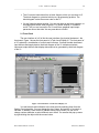
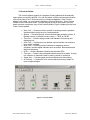
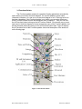
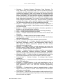
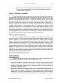
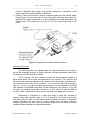
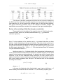
Lab 4. Tank Level Display
57
_____________________________________________________________________________________
Mech 466
Automatic Controls
Lab #4
Introduction to Data Acquisition and LabVIEW
Part 1. Displaying Water Levels in a Tank
LEARNING OBJECTIVE
The objectives of the experiments in this lab are:
¾ Introduce the LabVIEW program development environment as an efficient tool for
data acquisition and process control.
¾ Introduce and apply data acquisition concepts and methodologies.
¾ Build a LabVIEW program that acquires voltage signals corresponding to liquid
heights.
¾ Calibrate the LabVIEW program to display actual liquid heights.
¾ Calculate the resistance of valves based on formulas that model fluid flow
through restrictions and experimental data obtained using the developed
LabVIEW program.
¾ This Lab also serves as an introduction that covers the necessary background
required for Lab # 5 in which the actual control of liquid height is performed.
BACKGROUND
1. What Is LabVIEW?
LabVIEW is short for Laboratory Virtual Instrument Engineering Workbench. It is
a program development environment, much like modern C or BASIC. However,
LabVIEW is different from those development environments in one important respect.
While other programming systems use text-based languages to create lines of code,
LabVIEW uses a graphical programming language, G, to create programs in block
diagram form.
2. How Does LabVIEW Work?
LabVIEW is a general-purpose programming system, but it also includes libraries
of functions and development tools designed specifically for data acquisition and
instrument control. LabVIEW programs are called virtual instruments (VIs) because their
appearance and operation can imitate actual instruments. However, VIs are similar to
the functions of conventional language programs.
A VI consists of an interactive user interface, a data flow diagram that serves as
the source code, and icon connections that allow the VI to be called from higher level
VIs. More specifically, VIs are structured as follows:
¾ The interactive user interface of a VI is called the front panel, because it
simulates the panel of a physical instrument. The front panel can contain
knobs, push buttons, graphs, and other controls and indicators.
Mech 466 Automatic Controls
Laboratory Manual
Lab 4. Tank Level Display
58
_____________________________________________________________________________________
¾ The VI receives instructions from a block diagram, which you construct in G.
The block diagram is a pictorial solution to a programming problem. The
block diagram is also the source code for the VI.
¾ VIs are hierarchical and modular. You can use them as top-level programs, or
as subprograms within other programs. A VI within another VI is called a
subVI. The icon and connector of a VI work like a graphical input/output
parameter list so that other VIs can pass data to a subVI.
2.1 Front Panel
The user interface of a VI is like the user interface of a physical instrument - the
front panel. Figure 1 shows the front panel of a Tank Level Display VI. The front panel of
a VI is primarily a combination of controls and indicators. Controls simulate instrument
input devices and supply data to the block diagram of the VI. Indicators simulate
instrument output devices that display data acquired or generated by the block diagram
of the VI.
Figure 1. Front Panel of a Tank Level Display VI
You add controls and indicators to the front panel by selecting them from the
floating Controls palette. You can change the size, shape, and position of a control or
indicator. In addition, each control or indicator has a pop-up menu you can use to
change various attributes or select different menu items. You access this pop-up menu
by right-clicking the object with the mouse button.
Mech 466 Automatic Controls
Laboratory Manual
Lab 4. Tank Level Display
59
_____________________________________________________________________________________
2.2 Block Diagram
You can switch from the front panel to the block diagram by selecting Windows »
Show Diagram from the menu. The Diagram window holds the block diagram of the VI,
which is the graphical source code of a VI. You construct the block diagram by wiring
together objects that send or receive data, perform specific functions, and control the
flow of execution. Figure 2 shows the block diagram of the Tank Level Display VI. The
diagram shows several primary block diagram program objects - terminals, nodes, and
wires.
When you place a control or indicator on the front panel, a corresponding
terminal appears on the block diagram. You cannot delete a terminal that belongs to a
control or indicator. The terminal disappears only when you delete its control or indicator
on the front panel. The terminal symbols suggest the data type of the control or indicator.
For example, a DBL terminal represents a double-precision, floating-point number; a TF
terminal is a Boolean; an I16 terminal represents a regular, 16-bit integer; and an ABC
terminal represents a string. The Multiply function icon also has terminals. Think of
terminals as entry and exit ports. Terminals that produce data are referred to as data
source terminals and terminals that receive data are data sink terminals.
Figure 2. Block Diagram of the Tank Level Display VI
Nodes are program execution elements. They are analogous to statements,
operators, functions, and subroutines in conventional programming languages. The
Multiply function is one type of node. The G-programming language has an extensive
library of functions for math, comparison, conversion, I/O, and more. Another type of
node is a structure. Structures are graphical representations of the loops and case
statements of traditional programming languages. The G-programming language also
has special nodes for linking to external text-based code and for evaluating text-based
Mech 466 Automatic Controls
Laboratory Manual
Lab 4. Tank Level Display
60
_____________________________________________________________________________________
formulas. You add nodes to the block diagram by selecting them from the floating
Functions palette.
Wires are the data paths between source and sink terminals. You cannot wire a
source terminal to another source, nor can you wire a sink terminal to another sink.
However, you can wire one source to several sinks. Wires are colored according to the
kind of data each wire carries. Blue wires carry integers, orange wires carry floatingpoint numbers, green wires carry Booleans, and pink wires carry strings. To wire from
one terminal to another, select the Wiring tool from the floating Tools palette, click on the
first terminal, move the tool to the second terminal, and click on the second terminal. It
does not matter at which terminal you start. The hot spot of the Wiring tool is the tip of
the unwound wiring segment. When the Wiring tool is over a terminal, the terminal area
blinks, to indicate that clicking connects the wire to that terminal.
Data flow is the principle that governs G program execution. Stated simply, a
node only executes when all data inputs arrive; the node supplies data to all of its output
terminals when it finishes executing; the data immediately passes from source to sink
terminals. Data flow programming contrasts with the control flow method of executing a
conventional program, in which instructions are executed in the sequence in which they
are written. Control flow execution is instruction driven. Data flow execution is datadriven or data-dependent.
2.3 Icon and Connector
When an icon of a VI is placed on the diagram of another VI, it becomes a subVI,
the G equivalent of a subroutine. The controls and indicators of a subVI receive data
from and return data to the diagram of the calling VI. The connector is a set of terminals
that correspond to the subVI controls and indicators. The icon is either the pictorial
representation of the purpose of the VI, or a textual description of the VI or its terminals.
The connector is much like the parameter list of a function call; the connector terminals
act like parameters. Each terminal corresponds to a particular control or indicator on the
front panel. A connector receives data at its input terminals and passes the data to the
subVI code through the subVI controls, or receives the results at its output terminals
from the subVI indicators. Every VI has a default icon displayed in the icon pane in the
upper right corner of the front panel and block diagram windows. Every VI also has a
connector, which you access by choosing Show Connector from the icon pane pop-up
menu on the front panel. When you bring up the connector for the first time, you see a
connector pattern. You can select a different pattern if you want. The connector
generally has one terminal for each control or indicator on the front panel. You can
assign up to 28 terminals. If you anticipate future changes to the VI that might require a
new input or output, leave some extra terminals unconnected.
3. What Are LabVIEW Palettes?
LabVIEW palettes contain various tools and objects used to create and edit the
front panel and block diagram. It is said that the palettes float because you can move
them anywhere you want on the desktop. The three main palettes are the Tools,
Controls and Functions palettes.
Mech 466 Automatic Controls
Laboratory Manual
Lab 4. Tank Level Display
61
_____________________________________________________________________________________
3.1 Tools Palette
LabVIEW uses a floating Tools palette, which you can use to edit and debug VIs.
A tool is a special operating mode of the mouse cursor. You use tools to define the
operation taking place when subsequent mouse clicks are made on the panel or
diagram. You can move this palette anywhere you want, or you can close it temporarily
by clicking the close box. Once closed, you can access it again by selecting Windows »
Show Tools Palette. Figure 3 displays the Tools palette with the following functions.
¾ Automatic Tool Selection —If automatic tool selection is enabled and you
move the cursor over objects on the front panel or block diagram,
LabVIEW automatically selects the corresponding tool from the Tools
palette. You can disable automatic tool selection and select a tool
manually.
¾ Operating tool — Changes the value of a control or selects the text within
a control.
¾ Positioning tool — Positions, resizes, and selects objects.
¾ Labeling tool — Edits text and creates free labels.
¾ Wiring tool — Wires objects together in the block diagram.
¾ Object Pop-up Menu tool — Opens the pop-up menu of an object.
¾ Scrolling tool — Scrolls the window without using the scroll bars.
¾ Breakpoint tool — Sets breakpoints on VIs, functions, loops, sequences,
and cases.
¾ Probe tool — Creates probes on wires.
¾ Color Copy tool — Copies colors for pasting with the Color tool.
¾ Coloring tool — Sets foreground and background colors.
Figure 3. Tools Palette
Mech 466 Automatic Controls
Laboratory Manual
Lab 4. Tank Level Display
62
_____________________________________________________________________________________
3.2 Controls Palette
The Controls palette consists of a graphical, floating palette that automatically
opens when you launch LabVIEW. You use this palette to place controls and indicators
on the front panel of a VI. Each top-level icon contains subpalettes. If the Controls
palette is not visible, you can open the palette by selecting Windows » Show Controls
Palette from the front panel menu. You can also pop up on an open area in the front
panel to access a temporary copy of the Controls palette. Figure 4 displays the top-level
of the Controls palette.
¾ Num Ctrls — Contains numeric controls for entering numeric quantities.
Includes digital controls such as knobs and dials.
¾ Buttons — Contains Boolean controls that simulate switches, buttons. A
Boolean control or indicator has two values — TRUE or FALSE.
¾ Text Ctrls — Contains string controls and indicators for entering and
displaying text.
¾ User Ctrls — Contains any user defined controls that the user wishes to
have readily available.
¾ Num Ctrls — Contains numeric indicators for dispaying numeric
quantities. Includes digital indicators such as meters, thermometers and
tank level indicators
¾ LEDs — Contains Boolean indicators that simulate LEDs.
¾ Text Inds — Contains string and path indicators as well as tables. A string
is a collection of characters used to make up words or sentences.
¾ Graph Inds — Contains graph and chart indicators for data plotting.
¾ All Controls — Contains all of the controls above plus many others for
more complex designs.
Figure 4. Controls Palette
Mech 466 Automatic Controls
Laboratory Manual
Lab 4. Tank Level Display
63
_____________________________________________________________________________________
3.3 Functions Palette
The Functions palette consists of a graphical, floating palette that automatically
opens when you switch to the block diagram. You use this palette to place nodes
(constants, indicators, VIs, and so on) on the block diagram of a VI. Each top-level icon
contains subpalettes. If the Functions palette is not visible, you can select Windows »
Show Functions Palette from the block diagram menu to display it. Then you can click
the All Functions button to bring up the All Functions Palette. You can also pop up on an
open area in the block diagram to access a temporary copy of the Functions palette, and
access the same palette by clicking on the All Functions button there. Figure 5 displays
the all Functions level of the Functions palette. And a brief description of the buttons is
on the flowing page.
Figure 5. All Functions Palette
Mech 466 Automatic Controls
Laboratory Manual
Lab 4. Tank Level Display
64
_____________________________________________________________________________________
¾ Structures — Contains Sequence Structures, Case Structures, For
Loops, While Loops, and Formula Nodes. The icon for each G structure is
a resizeable box with a distinctive border. You can place an object inside
a structure by dragging it inside, or by building the structure around the
object. The Sequence Structure consists of one or more subdiagrams that
execute sequentially. The Case structure executes a subdiagram based
on an input value and is analogous to an if-then-else statement in textbased, programming languages. You use the For Loop and While Loop to
control repetitive operations, either until a specified number of iterations
completes (For Loop) or while a specified condition is true (While Loop).
The Formula Node executes one or more mathematical formulas.
¾ Numeric — Contains functions that perform elementary operations on
numbers like add and multiply. It also contains numeric constants for use
in the block diagram.
¾ Boolean — Contains functions that perform elementary operations on
Booleans. It also contains Boolean constants.
¾ String — Contains functions that work on strings and string formatting.
¾ Array — Contains functions that work on arrays.
¾ Cluster — Contains functions that work on clusters such as Bundle and
Unbundle.
¾ Comparison — Contains functions that compare numbers.
¾ Time & Dialog — Contains functions that work as timers and functions
that display dialog boxes.
¾ File I/O — Contains functions that read/write input/output files.
¾ NI and Instrument I/O — Contains functions that communicate with
input/output instruments, there is a NI Measurements button which is
more specific to National Instruments products that also contains
instrument input/output as well.
¾ Waveform — Contains functions to build waveforms that include the
waveform values, channel information, and timing information, and to set
and retrieve waveform attributes and components.
¾ Analysis — Contains functions to perform waveform measurements,
waveform conditioning, waveform monitoring, waveform generation,
signal processing, point-by-point analysis, and mathematical calculations.
¾ Application Control — Contains functions to programmatically control VIs
and LabVIEW applications on the local computer or across a network.
¾ Communication — Contains functions to exchange data between
applications.
¾ Report Generation — Contains functions to create and manipulate reports
of LabVIEW applications.
¾ Advanced — Contains functions to call code from libraries, such as
dynamic link libraries (DLLs); to manipulate LabVIEW data for use in
other applications; and to call code from text-based programming
languages.
¾ Decorations — Contains items to group or separate objects on a block
diagram with boxes, lines, or arrows. These objects are for decoration
only and do not modify data.
¾ User Libraries — Use the User Libraries palette to add controls and VIs to
the Controls and Functions palettes. By default, the User Libraries palette
does not contain any objects.
Mech 466 Automatic Controls
Laboratory Manual
Lab 4. Tank Level Display
65
_____________________________________________________________________________________
¾ Select a VI — For selecting VIs to be inserted as subVIs in the current VI.
The icon and connector pair of a VI must be defined before it could be
used as a subVI in another VI.
4. How To Get Help In LabVIEW?
The two common help options that you may need are the Help Window and the
Reference Help. Both help options can be accessed from the Help pull-down menu. The
Help Window contains help information for functions, constants, subVIs, controls and
indicators, and dialog box menu items. To display the window, choose Show Context
Help from the Help menu. Move your cursor over the icon of a function, a subVI node, or
a VI icon (including the icon of the VI you have open, shown at the top right of the VI
window) to see the help information. The Help window displays the most commonly
required help information in a condensed format. To access more extensive online
information, select Help » Online Reference. For most block diagram objects, you can
select Online Reference from the pop-up menu of the object. You also can access this
information by pressing the question mark button shown to the left, located at the bottom
of the Help Window. For a more extensive explanation of LabVIEW functionality, refer to
the LabVIEW User Manual or the G Programming Reference Manual.
5. Data Acquisition Systems
The use of LabVIEW software and computer form a portion of a modern data
acquisition system. A data acquisition system, commonly called DAQ system, is a term
normally applied to a microcomputer based measurement sampling and processing
system. The basic form of a data acquisition system is illustrated in Figure 6. A DAQ
system begins with the transducers (in our case pressure transducers mounted on the
bottom of the tanks) that outputs a voltage or current signal in response to the variable of
interest (water pressure). A signal conditioning system contains electronic equipment
designed to supply the source voltage to the transducer, as well as provide filtering and
amplification. The computer contains a DAQ card that provides the necessary analogue
to digital conversion (and/or digital to analogue) and using DAQ software, will perform all
data manipulation, data storage and display.
Data Acquisition System Components
Signal Conditioning
Analogue signals will normally require some type of signal conditioning for the
proper interface with a digital system. These components include:
1. Transducer Excitation: Certain transducers (such as strain gauges) require external
voltages or currents to excite their own circuitry in a process known as transducer
excitation. It is important that the supply voltage provided by the signal conditioner be
stable and relatively noise free.
2. Amplification: Amplification maximizes the use of the available voltage range to
increase the accuracy of the digital signal and to increase the signal-to-noise ratio
(SNR). Although computer DAQ boards will often provide some selectable signal
amplification, it should be remembered that external amplification is often necessary
to minimize the effects of external noise (60 Hz noise for example). Our system
Mech 466 Automatic Controls
Laboratory Manual
Lab 4. Tank Level Display
66
_____________________________________________________________________________________
utilizes a dedicated strain guage card specially designed for wheatstone circuit
based instruments such the pressure transducer.
3. Filtering: Filters are required to remove unwanted signals from the desired signal.
Several types of filters, such as low pass, high pass, and band pass filters, are
installed in the signal conditioning to clean the signal prior to digital processing. The
filtering card in this experiment is set with a cut off (or corner frequency) of 100
Hertz.
Figure 6. Components of a Data Acquisition System
Data Acquisition Card
The data acquisition card located within the computer contains the circuitry to
provide the necessary Analogue to Digital conversion for signal processing. Some of the
key features of a DAQ card are as follows:
A/D Converters: The A/D converter converts the input analogue voltage to a
digital signal which can be read and processed by the computer. The resolution and
accuracy of the conversion depends on the number of bits the voltage is translated into.
The conversion time varies as the resolution, i.e., the more bits required, the longer it
takes (i.e. 10 μsec. for 12 bit conversion versus 20μsec. for 16 bit conversion). The DAQ
card installed in the ME466 computers (IOTech DAQboard 100) utilizes a 12 bit A/D
converter. It is configured to provide a 0 count for –5 volts, 2048 for 0 volts and 4095 for
+5 volts. Table 1 shows the bit counts versus resolution and voltage value of one bit.
Multiplexing: A multiplexer is a switch that allows a single A/D converter to
measure many input channels (often 8, 12 or 16 channels). This switch is normally a
solid state switch to allow for high speed switching between channels. A multiplexed
scheme eliminates the high cost of having multiple A/D converters. However,
multiplexing reduces the rate at which data can be acquired from an individual channel
because multiple channels are scanned sequentially.
Mech 466 Automatic Controls
Laboratory Manual
Lab 4. Tank Level Display
67
_____________________________________________________________________________________
Table 1. Resolution and Accuracy for A/D Conversion
The software (LabVIEW) is designed with drivers that can control the operation of
the DAQ card. Key elements of the data acquistion such as sample rates, number of
input channels, etc. can be selected from software inputs. It should be noted however,
that signal conditioning operations such as the transducer excitation voltages and
amplification are normally done outside of the computer in the signal conditioning box.
Review of the modeling of fluid-flow through a constriction
The general form for the relation of the mass flow rate w of a fluid-flow through a
constriction (valve, orifice, etc.) and the pressure difference (p1 – p2) across this
restriction is given by:
w=
1
( p1 − p 2 )1 / α
R
(1)
Here, R is the resistance of the restriction and α is a constant that takes on values
between 1 and 2 depending on the type of restriction. The most common value of α in
the case of high flow rates through pipes (those having a Reynolds number Re > 105) or
through short constrictions or nozzles is 2. For very slow flows through long pipes where
the flow remains laminar (Re < 1100), α = 1. Flow rates between these two extremes
can yield intermediate values of α.
Note that a value of α = 2 indicates that the flow is proportional to the square root
of the pressure difference and therefore will produce a nonlinear equation. For the initial
stages of control systems analysis and design, it is typically very useful to linearize these
equations so that the well established design techniques for linear systems can be
applied. Linearization involves selecting an operating point and expanding the nonlinear
term to be a small perturbation from that point. The nonlinear term can be expanded
according to the relation
(1 + ε ) β ≅ 1 + βε
(2)
where ε << 1.
In the case of a liquid tank with a liquid height h, area A and no inlet flow win = 0
and a relatively short restriction at the outlet with α = 2, the continuity equation gives
m& = ρAh& = win − wout = − wout
Mech 466 Automatic Controls
(3)
Laboratory Manual
Lab 4. Tank Level Display
68
_____________________________________________________________________________________
The pressure at the entrance of the restriction is given by p1 = ρgh and assuming
ambient pressure outside the restriction p2 = 0, the equation describing the outflow
through the restriction can be written as
wout =
1
ρgh
R
(4)
Combining (3) and (4) gives
ρAh& = −
1
ρgh
R
(5)
Linearization of (5) involves selecting an operating point ho and substituting h = ho + Δh
and h& = Δh / Δt to obtain,
ρA
Δh
1
=−
ρg (ho + Δh)
Δt
R
=−
Since
ρgho ⎛
R
Δh ⎞
⎜⎜1 +
⎟
ho ⎟⎠
⎝
1/ 2
Δh
<< 1 , therefore using (2)
ho
ρA
ρgho
Δh
≅−
R
Δt
⎛
1 Δh ⎞
⎜⎜1 +
⎟
2 ho ⎟⎠
⎝
(6)
Thus the resistance of the restriction can be obtained as
R=−
1
A
gho ⎛
1 Δh ⎞ Δt
⎟
⎜⎜1 +
ρ ⎝ 2 ho ⎟⎠ Δh
(7)
Note that since the height is decreasing, Δh will be negative and R will be a positive
value.
Mech 466 Automatic Controls
Laboratory Manual
Lab 4. Tank Level Display
69
_____________________________________________________________________________________
PROCEDURES: Tank Level Display
This Lab demonstrates how LabVIEW can be used for process monitoring and
control applications. The actual control however is performed in Lab # 5. Figure 7 shows
a schematic for an experimental setup that resembles many real life applications. It
consists of two interconnected tanks that continuously supply two different processes
with two different flow rates.
In this section, you are asked to build the Tank Level Display VI whose front
panel and block diagram are shown in Figures 1 and 2. The purpose of the VI is to
perform the following functions:
¾ To continuously acquire signals from two pressure transducers placed in the
base of two tanks and display the corresponding readings (12-bit unsigned
integer counts).
¾ To convert the acquired counts into voltages and display them.
¾ To convert voltages into liquid heights, display them and monitor their time
response.
Inlet
Valve A
Inlet
Valve B
Tank A
Tank B
Proportional
Control
Valve
Control
Unit
Valve AB
Pressure
Transducer A
Pressure
Transducer B
Process
Valve A
Disturbance
Valve
Process
Valve B
Pump
Figure 7. Schematic of the Tank Level Display and Control Setup.
Mech 466 Automatic Controls
Laboratory Manual
Lab 4. Tank Level Display
70
_____________________________________________________________________________________
Creating the front panel
Begin by considering the front panel shown in Figure 1. It has three digital
indicators for Volts A, Volts B, and Time (sec), two tank level indicators to display the
current liquid levels, a waveform chart that displays the time response of the tanks’
levels, and a stop button to stop acquiring data. Consider the following steps in building
the front panel:
1. Select New VI from the LabVIEW startup screen.
2. Create the three digital indicators: Select Digital Indicator from the Numeric
Indicators (Num Inds) subpalette of the Controls palette. Drag and drop the indicator
on the front panel. Type Volts A inside the label box. Using the positioning tool from
the Tools palette, drag the indicator to the desired location on the front panel. Repeat
the same process to create the other two indicators and label them. Note that each
time you create a new control or indicator, LabVIEW automatically creates the
corresponding terminals in the block diagram.
3. Similarly, create the two tank level indicators by dragging them from the Numeric
subpalette of the Controls palette. Add labels and position the tanks. You can set the
upper limit of the scale of each tank to read 25.0 (inches) by direct typing over the
initial 10.0 upper limit.
4. Create the waveform chart by selecting it from the Graph Indicators (Graph Inds)
subpalette of the Controls palette. Add the chart label, position it and set its y-axis
upper limit. If you right-click on the graph using the mouse, a pop menu will appear
that can allow you to control the functionality and appearance of the chart such as
showing or hiding the graph palette and the x-axis scale. Set the x-axis scale to
AutoScale X, also select the y-axis scale and make sure that there is no check mark
beside AutoScale Y. You can also resize the chart’s legend by dragging its corners
to allow for the two variables.
5. Finally create the stop button by selecting it from the Boolean subpalette of the
Controls palette.
Creating the block diagram
Switch to the block diagram window and note the different terminals that
LabVIEW automatically created corresponding to the front panel objects. Use Figure 2
as a guide for positioning the different terminals in the diagram.
The subVI Get Single Scan.vi is set up to communicate with the data acquisition card
installed in the computer and to perform a single scan on two specified channels to
which the pressure transducers are connected. The Get Single Scan.vi SubVI takes the
device number and the channels to scan as input. The SubVI also returns two double
values corresponding to the read pressure signals. The output from Two Ch Single
Scan.vi subVI are 12-bit unsigned integers ranging from zero to 4095 (largest 12-bit
integer), that are internally converted to a double value in Volts.
The voltages are then converted into liquid heights using two sets of linear conversion
factors each consisting of a slope and an intercept. Use the following steps to build the
block diagram:
Mech 466 Automatic Controls
Laboratory Manual
Lab 4. Tank Level Display
71
_____________________________________________________________________________________
1. Insert the subVI Get Single Scan.vi into the block diagram by choosing Select a VI
from the Functions palette. This subVI has two output terminals and a two input
terminals.
2. Create a new constant for the device input terminal and set the value to 1 by
selecting the Numeric Constant from the Numeric subpalette of the All Functions
palette.
3. Create two channels for measuring by selecting the NI Measurement then selecting
the Data Acquisition subpalettes from the All Functions palette.
4. Right click on one of the channels and select “New Channel”. Make sure the drop
down list box has Analog Input selected then press the next button. Type “Tank A”
for channel name and leave the description blank, then press the next button (if Tank
A is already made create a Tank C for practice). Make sure that Voltage is selected
on the drop down menu, then press the next button, this ensures that the readings
we are getting are Voltage measurements. Now it is asking you to name the units for
this measurement, this is optional, but put Volts in the Units box, and make sure the
minimum and maximum values are set to -5 Volts and +5 Volts respectively, then
press the next button. Make sure that “No scaling” is selected then again press the
next button. It then asks what device you want to use, this allows you to select
between multiple devices on systems that have more than one. Select Dev1, and
set “Which channel…” to 0, and select the analog input mode of “Referenced single
ended”, then click the finish button. Repeat for “Tank B” but make the analog
channel (“Which channel…”) set to 1.
5. Now left click on the first channel and set it to “Tank A” and left click on the second
channel and set it to “Tank B”. Note that you may select “Tank A” or “Tank B” on
both channel tools of the block diagram even though you only setup each once. This
is so that users can just setup the channels once at the beginning and have them
available anywhere in the program.
6. Place two Multiply functions and two Add functions on the block diagram. These are
located in the Numeric subpalette of the Functions palette. All these functions have
two input terminals and one output terminal.
7. Add the two sets of Volts to Inches linear conversion factors with preliminary values
of 1.0, 1.0, 0.0 and 0.0 to the block diagram by selecting Numeric Constant from the
Numeric subpalette of the All Functions palette. Label these constants as slope and
intercept as shown. The values of these conversion factors will be later adjusted.
8. The waveform chart has a single input terminal. For the waveform chart to plot two
variables, the two variables must be “bundeled” together into a cluster using the
Bundle function available in the Cluster subpalette of the All Functions palette. Add a
Bundle function to the block diagram. The Bundle function has two input terminals
and one output terminal.
9. Using the wiring tool found on the Tools palette, wire the terminals of the objects on
the block diagram as shown in Figure 2. To wire from one terminal to another, click
on the first terminal, move the tool to the second terminal, and click on the second
terminal. Remember that it does not matter on which terminal you initiate the wiring.
10. The current status of the block diagram may allow the VI to perform a single data
acquisition operation for the tanks’ level. To perform this operation repeatedly, the
objects in the block diagram must be placed inside a While Loop found in the
Structures subpalette of the Functions palette. The While Loop is a resizable box.
You place the While Loop in the block diagram by clicking with the While Loop icon
in an area above and to the left of all the objects that you want to execute within the
loop then drag out a rectangle while holding down the mouse button. The While Loop
has two terminals, a Boolean input terminal (if symbol is loop executes while input is
Mech 466 Automatic Controls
Laboratory Manual
Lab 4. Tank Level Display
72
_____________________________________________________________________________________
TRUE) and an optional numeric output terminal that outputs the number of times the
loop has executed. NOTE: In the diagram the constants for the device and for the
channels are placed outside of the while loop. Having these constants outside of the
loop has no bearing on how the program operates, but if you were to want those to
be controls so that you could configure which channels are which only on program
start, then it is vital that the controls be outside of the while loop, otherwise during
each loop the program would recheck these controls and set them to what ever the
values are at the time of activation. The stop button HAS to be in the while loop
otherwise it only checks the status of the button once at startup and does not change
the value during execution of the program as it is not asked to.
11. As it stands now, the While Loop would execute as quickly as the computer system
would allow. To control the loop timing, place the Wait Until Next ms Multiple function
located in the Time & Dialog subpalette of the Functions palette inside the loop. This
timing control function has a single input terminal and a single optional output
terminal. It waits until the millisecond timer is a multiple of the specified input value
(in ms) before returning the optional millisecond timer value. Wire a Numeric
Constant of 100.0 (ms) to the input terminal of the timing function.
12. To display the elapsed time since the start of the run, first convert the time step of
the While Loop execution in milliseconds to seconds (by dividing by a 1000.0), then
multiply it by the number of times the loop has executed (i), and finally wire the result
to the Time (sec) digital indicator.
13. To stop acquiring data and exit the While loop, the stop button terminal should be
wired to the Boolean input terminal of the loop. Since the default output value of the
stop button is FALSE and clicking the button will change it into TRUE, the while loop
by default stops on a TRUE condition, thus wiring the button direct to the Boolean
input terminal will stop the program when the stop button is pressed.
14. Select Save from the File menu to save your work on a floppy disk. You can run the
VI by clicking on the Run button on either the front panel or block diagram Toolbars.
Calibrating the VI to find the volts to inches conversion factors
If you run the VI as its stands now, you will find that the displayed tanks’ levels are the
voltage readings and not the actual heights. Selecting appropriate values for the volts to
inches linear conversion factors (slope and intercept) for each of the two pressure
transducers can be accomplished as follows
1. Run the Tank Level Display VI.
2. While Inlet Valve A open and all other valves closed, turn on the pump to fill Tank A
with water to a known height, say 6 inches. Turn the pump off, wait a second then
record the corresponding voltage. (Turning the pump off also reduces the noise in
the voltage reading.)
3. Repeat step 2 for water heights of 8, 10, 12, … , 20 inches.
4. Use the eight data points to plot the height against the voltage for Tank A. The slope
and intercept can then be measured graphically.
5. Close Inlet Valve A, open Inlet valve B and repeat steps 2 – 4 for Tank B.
6. Stop the Tank Level Display VI.
7. Insert the slope and intercept values into the block diagram by typing them over the
1.0, 1.0, 0.0 and 0.0 preliminary values for the conversion factors.
8. Now the Tank Level Display VI is ready to display actual tanks’ levels.
Mech 466 Automatic Controls
Laboratory Manual
Lab 4. Tank Level Display
73
_____________________________________________________________________________________
Finding the resistances of Process Valve A, Process Valve B and Valve AB
In this section you are required to perform the experimental measurements needed to
find the resistances of three valves. Referring to the review section that covers the
modeling of fluid-flow through restrictions, it can be seen that the formula for the
resistance of the outlet flow valve of a tank with no inlet flow depends on the flow speed.
For very slow flows, the constant α in Equation (1) is assumed to equal 1. This yields a
linear flow rate relation involving the valve resistance R in the form
ρAh& = −
1
ρgh
R
and assuming h& = Δh / Δt , we get
R=−
gh Δt
A Δh
Knowing that the inside diameter of both tanks is 5 inches and the outside diameters of
the two pipes that run inside each tank are 1.25 inches and 0.875 inches, use the
following steps to find the resistance of Process Valves A and B:
1. Run the Tank Level Display VI.
2. While Inlet Valve A open and all other valves closed, turn on the pump to fill Tank A
with water. Turn the pump off.
3. Open Process Valve A and let the tank drain.
4. Using the time indicator on the front panel of the Tank Level Display VI, monitor the
height drop from about 20 inches to about 5 inches by recording the time and the
corresponding tank height using 10 seconds time intervals.
5. Use the linear equation for the flow rate through a constriction (α = 1) to graph the
resistance of Process Valve A versus the water height in Tank A.
6. Use a similar procedure to graph the resistance of Process Valve B versus the water
height in Tank B.
The above graphs are based on the assumption of slow laminar flow through the valve.
However, as indicated in the review section, a value of α = 2 is more suitable for high
flow rates and flows through short constrictions such as valves. This yields the nonlinear
relation in Equation (5)
ρAh& = −
1
R
ρgh
which can be linearized by selecting an operating point ho to give
R=−
1
A
gho ⎛
1 Δh ⎞ Δt
⎟
⎜⎜1 +
ρ ⎝ 2 ho ⎟⎠ Δh
Assuming an operating height for the water in tank A to be hAo = 10 inches, use the time
interval that contains this height to find the resistance of Process Valve A based on the
Mech 466 Automatic Controls
Laboratory Manual
Lab 4. Tank Level Display
74
_____________________________________________________________________________________
linearized equation at this operating point. Also find a linearized value for the resistance
of Process Valve B at an operating height of hBo = 7 inches.
To find the resistance of Valve AB at the same operating point hAo = 10 inches and hBo =
7 inches, fill Tank A to an initial height of 12 inches and Tank B to 5 inches. Open Valve
AB and allow Tank A to drain into Tank B. Record the time it takes for Tank A height to
drop from 10.5 inches to 9.5 inches (or Tank B height to rise from 6.5 inches to 7.5
inches). In this case, assuming the water height in Tank A is higher than that in B, the
flow through Valve AB that connects the two tanks A and B can be written as
ρAA
Δh A
Δh B
1
= − ρAB
=−
Δt
Δt
R AB
ρg (h A − hB )
which can be linearized about the operating point hA = hAo + ΔhA and hB = hBo + ΔhB to
give
B
R AB = −
1
AA
g (h Ao − hBo ) ⎛ 1 Δh A − Δh B
⎜1 +
⎜ 2 h −h
ρ
Ao
Bo
⎝
B
⎞ Δt
⎟
⎟ Δh
⎠ A
Report Requirements
1. Have the TA inspect the developed VI and its operation. Include the TA’s comments
on the VI.
2. Comment on any difficulties you encountered in building the VI.
3. Comment on the usefulness and applicability of G programming using LabVIEW.
4. Graph the calibration results. Find the slope and intercept for both graphs. Comment
on the results including any sources of errors.
5. Calculate and graph the valve resistance versus tank heights for both Process
Valves A and B based on the linear assumption. Is this assumption valid? Explain.
6. Using the linearized equations, determine the resistance of the three valves at the
operational points. Compare these values with the corresponding linear case.
Comment on the units of the resistance in each case. Which value of R should be
used in the process control of the tanks? Explain.
Mech 466 Automatic Controls
Laboratory Manual