1
Automatic Control
Systems Toolbox v.3.0
user's manual
automatic control systems toolbox v.3.0 :: user's manual :: © 2000 - 2001 92BROTHERS --- pag.2/20
INDEX
Note on License.............................................................................................................................. 3
Note for TI-92+ and TI-89 Users ..................................................................................................... 3
Used Symbols and Abbreviations: .................................................................................................. 4
What's Automatic Control Systems Toolbox.................................................................................... 5
What it's new in version 3.0............................................................................................................. 5
Installing Automatic Control Systems Toolbox (ACST) v.3.0 ........................................................... 6
The Command Window................................................................................................................... 7
LTI Models ...................................................................................................................................... 8
Command: tf................................................................................................................................................... 8
Command: zpk ............................................................................................................................................... 9
Command: ss ................................................................................................................................................. 9
Command: gain.............................................................................................................................................. 9
Command: mmimo......................................................................................................................................... 9
Command: setdelay ..................................................................................................................................... 10
Command: series ......................................................................................................................................... 11
Command: parallel ....................................................................................................................................... 11
Command: feedback .................................................................................................................................... 12
Analysis in Frequency Domain...................................................................................................... 13
Command: bode........................................................................................................................................... 13
Command: nichols ....................................................................................................................................... 14
Command: nyquist ....................................................................................................................................... 15
Command: margin........................................................................................................................................ 15
Poles and Zeros Analysis.............................................................................................................. 16
Command: rlocus ......................................................................................................................................... 16
Command: zpmap........................................................................................................................................ 16
Analysis in Time Domain: Simulation ............................................................................................ 17
Commands: impulse and step...................................................................................................................... 17
Command: simul .......................................................................................................................................... 18
Elaborating Graphical Results....................................................................................................... 19
Command: ggraph ....................................................................................................................................... 19
Multiple Plots Using PIC Files ...................................................................................................................... 19
Register 92BROTHERS programs..................................................................................... 20
About 92BROTHERS ........................................................................................................ 20
pag.2/20
automatic control systems toolbox v.3.0 :: user's manual :: © 2000 - 2001 92BROTHERS --- pag.3/20
Note on License
Automatic Control System Toolbox Copyright (C) 2000-2001 92BROTHERS - G.Luca Troiani
This program is free software; you can redistribute it and/or modify it under the terms of the GNU General
Public License as published by the Free Software Foundation; either version 2 of the License, or (at your
option) any later version.
This program is distributed in the hope that it will be useful, but WITHOUT ANY WARRANTY; without even
the implied warranty of MERCHANTABILITY or FITNESS FOR A PARTICULAR PURPOSE. See the GNU
General Public License for more details. You should have received a copy of the GNU General Public
License along with this program; if not, write to the Free Software Foundation, Inc., 59 Temple Place, Suite
330, Boston, MA 02111- 1307 USA Full GNU GENERAL PUBLIC LICENSE Version 2, June 1991:
license.txt file
Note for TI-92+ and TI-89 Users
Automatic Control Systems Toolbox v.3.0 was tested on a TI-89 (Hardware version 2.00 Advanced
Mathematics software version 2.05).
Screenshots are captured on a TI-92 (in TI-89 the graphical results and screen messages can look different
case of the smaller screen).
pag.3/20
automatic control systems toolbox v.3.0 :: user's manual :: © 2000 - 2001 92BROTHERS --- pag.4/20
Used Symbols and Abbreviations:
[[•]]
[[•]][i][j]
[•]
[•][i]
<•>
[[SYSTEM]]
LTI
SISO
MIMO
ACST
CW
matrix
element of a matrix placed in row i and column j
array/row vector
element i of the array/row vector
key of TI-92's keyboard
matrix associated to a system [see LTI Models paragraph]
linear time-invariant system
Single Input Single Output system
Multiple Input Multiple Output system
Automatic Control System Toolbox program
Command Window
pag.4/20
automatic control systems toolbox v.3.0 :: user's manual :: © 2000 - 2001 92BROTHERS --- pag.5/20
What's Automatic Control Systems Toolbox
Automatic Control Systems Toolbox (ACST) it's a powerful toolbox to design, analyze and simulate (control)
systems. ACST has powerful tools for:
! systems design by:
! specifying the transfer function;
! specifying poles and zeros of the transfer function;
! specifying the state-space (SS) model;
! specifying MIMO systems using SISO systems
! connecting two MIMO (Multiple Input Multiple Output) systems by:
! series connection;
! parallel connection;
! feedback connection.
! system analysis by:
! Bode plots (MIMO systems);
! Nichols chart (MIMO systems);
! Nyquist diagram (MIMO systems);
! Gain and Phase margins (MIMO systems);
! Root locus (SISO systems);
! Poles-Zeros map (SISO systems);
! systems simulation by:
! step response (MIMO systems);
! impulse response (MIMO systems);
! generic multiple input response (MIMO systems);
! save and modify graphical outputs;
What it's new in version 3.0
!
!
!
!
!
!
new LTI modelling that allow to set the input delay separately by the LTI transfer function to speed up the
analysis of systems;
now you can use auto frequency ranging for bode, nichols and nyquist analysis;
more flexible systems' simulation;
specific command to create MIMO systems using SISO systems;
bugs fixed;
faster;
pag.5/20
automatic control systems toolbox v.3.0 :: user's manual :: © 2000 - 2001 92BROTHERS --- pag.6/20
Installing Automatic Control Systems Toolbox (ACST) v.3.0
To install ACST into your calculator you need:
! software:
! TI-GRAPH LINK software (http://www.ti.com/calc/docs/link.htm);
! acst.zip (http://www.92brothers.net/ or http://web.tiscalinet.it/92brothers/) that must contain:
! acst.92g (for TI-92);
! readme.txt;
! license.txt;
! acst.manual.pdf (this manual);
! hardware:
! Windows/Macintosh
Gray TI-GRAPH LINK cable
! Windows Only
Black TI-GRAPH LINK cable
To install ACST into your calculator must:
1. unzip the acst.zip file into a folder (ex.: ..\desktop\acst)
2. send files from your PC to a TI-92:
! run the TI-Graph link program;
! Open the Link menu and select Send...;
! Select ..\desktop\acst\acst.92g file from the dialog window and click on Add;
! Click on Retain Folder to send the files back to their original folder;
! Click on OK to transmit the files;
3. control that a new fold named acst was created and it contain all listed files:
! acst PRGM
! bode PRGM
! errorms PRGM
! feedback FUNC
! ggraph PRGM
1
! ilaplace, ilapsub, laplace,lapsub
! impulse PRGM
! intro PIC
! invlap FUNC
! kernel PRGM
! laplace FUNC
! margin
! mmimo
! nichols PRGM
! nyquist PRGM
! parallel FUNC
! rlocus PRGM
! series FUNC
! simul PRGM
! step PRGM
! zpmap PRGM
4. ACST v2.2 it's now installed.
1
ilaplace, ilapsub, laplace and lapsub are included as a library and are developed by Lars Frederiksen
pag.6/20
automatic control systems toolbox v.3.0 :: user's manual :: © 2000 - 2001 92BROTHERS --- pag.7/20
The Command Window
The Command Window (CW) allow ACST's users to input their commands and see the result.
The ">>" symbol it's the prompt and it's displayed when ACST it's ready to get commands.
To input a command simply type it and press <ENTER> to run it.
There are two kinds of commands:
! TI-BASIC commands ("=" operator excluded) and user defined commands (function and/or programs);
! ACST commands.
There are two kinds of ACST commands (see next paragraphs to more explains):
! basic commands:
! quit: to quit ACST commands;
! clear: to refresh the command window;
! help: to get quick help on commands (use this manual for full help on commands);
! "=" operator: can be used to assign right values to left values (ex var=expression assign expression
to var);
! ggraph: to run a simple graphic editor to edit graphical results preventively saved;
! control toolbox commands:
! bode: to perform the bode analysis of a SISO or MIMO system;
! feedback: to connect two (SISO and/or MIMO) systems by feedback connection;
! impulse: to simulate the time impulse response of SISO or MIMO systems;
! margin: to evaluate gain and phase margins of SISO or MIMO systems;
! mmimo: to crate MIMO systems using SISO systems;
! nichols: to plot the Nichols chart of a SISO or MIMO system;
! nyquist: to plot the Nyquist diagram of a SISO or MIMO system;
! parallel: to connect two (SISO and/or MIMO) systems by parallel connection;
! rlocus: to plot the root locus of a SISO system;
! tf: to specify the transfer function of a system by numerator and denominator coefficients;
! series: to connect two (SISO and/or MIMO) systems by series connection;
! simul: simulate the time response of SISO or MIMO system to arbitrary inputs;
! step: simulate the time response of SISO or MIMO systems to step input;
! ss: to specify the transfer function of a system by state-space model of a system;
! zpk: to specify the transfer function of a system by zeros and poles of a transfer function;
! zpmap: to map zeros and poles of a SISO system.
Some of this commands can be runned from the HOME window of the calculator, but it's recommended to
run the commands from the ACST Command Window (CW) that perform a control on syntax or convert to
the rigth sintax and suggest you the right syntax or return the error number. Running the commands from the
CW moreover allow ACST Kernel control changes on the mode settings of your calc and the storage of
temporay files into your calculator memory that can occur after a runtime error.
pag.7/20
automatic control systems toolbox v.3.0 :: user's manual :: © 2000 - 2001 92BROTHERS --- pag.8/20
LTI Models
LTI systems are rappresented as a matrix of transfer functions. If the system has M inputs and N outputs the
matrix has N rows and M coluns and [SYSTEM][i,j] it's the transfer function from the input j to the output i.
To define SISO system you can specify:
! the coefficients of numerator and denominator of the transfer function;
! the poles and the zeros of the transfer function;
! the state space model;
(note that you can't specify the transfer function as a function of s as in the older versions. This limit is due to
a new way to stori LTI systems models to have best performaces).
A special SISO system it's the Linear Gain (or Gain). To specify a gain you must specify the gain value.
The corresponding commands are:
! sys = tf([NUM],[DEN]);
! sys = zpk([ZEROS],[POLES],k);
! sys = ss([[A]],[[B]],[[C]],[[D]]);
! sys = gain(GainValue).
To Define MIMO (M inputs and N outputs) system you can:
define M×N SISO systems and combine single systems in a NxM matrix using commamd mmimo.
SISO and MIMO systems support delays:
to specify systems delays there is a specific command: setdelay
SISO and MIMO systems can be interconnected by:
! series interconnection of two systems (SISO and/or MIMO) ;
! parallel interconnection of two systems (SISO and/or MIMO);
! feedback interconnection of two systems (SISO and/or MIMO).
The corresponding commands are:
! sys = series([SYS1],[SYS2],[OUTPUT1],[INPUT2]);
! sys = parallel([SYS1],[SYS2],[INPUT1],[INPUT2],[OUTPUT1],[OUTPUT2]);
! sys = feedback([SYS1],[SYS2],[INPUT1],[OUTPUT1]).
The next pages will show the use of commands
!
!
!
!
!
!
!
!
!
tf
zpk
ss
gain
mmimo
setdelay
series
parallel
feedback
Command: tf
<PURPOSE>
Specify transfer function of SISO system by numerator
and denominator coefficients
<SYNTAX>
sys=tf([NUM],[DEN])
where:
[NUM] and [DEN] are the row vectors of numerator and
denominator coefficients ordered in descending powers of s
(fig.1) exemple of command tf
pag.8/20
automatic control systems toolbox v.3.0 :: user's manual :: © 2000 - 2001 92BROTHERS --- pag.9/20
Command: zpk
<PURPOSE>
Specify transfer function of SISO system by zeros, poles
and gain
<SYNTAX>
sys=zpk([ZEROS],[POLES],k)
where:
! [ZEROS] is the row vector of zeros (set [] if none);
! [POLES] is the row vector of poles (a LTI system must have
at least one pole);
(fig.2) exemple of command zpk
!
k is the gain
Command: ss
<PURPOSE>
Specify transfer function of SISO and MIMO system by
state space model
<SYNTAX>
sys=ss([[A]],[[B]],[[C]],[[D]])
where [[A]],[[B]],[[C]],[[D]] are the matrix of the
system described by:
[X]=[[A]]·[X]+[[B]]·[U]
[Y]=[[C]]·[X]+[[D]]·[U]
(fig.3) exemple of command ss
Setting [[D]]=0 is interpreted as the zero matrix of adequate
dimensions
Command: gain
<PURPOSE>
Specify SISO gain system
<SYNTAX>
g=gain(GainValue)
where:
! g is the name of the gain system
! GainValue it's the value of the gain
Command: mmimo
<PURPOSE>
Generate a MIMO system model using pre-existent SISO
systems ( ! All input delays will be resetted ! )
<SYNTAX>
mimo
it will appear a dialog window (fig.4) that will ask
! the name of new MIMO system
! the number of inputs
! the number of outputs
then you must insert the names of pre-existent SISO systems
from input 1, 2, ... to output 1,2,... (fig.5)
As an exemple we want to create a MIMO systems with two
inputs and two output. We will ask this MIMO system "g". The
transfer function by input j to output i will be asked gij:
! g11 it's the TF from input 1 to output 1
! g12 it's the TF from input 2 to output 1
! g21 it's the TF from input 1 to output 2
! g22 it's the TF from input 2 to output 2
We have to make two step:
1. using tf, zpk or ss commands we define g11,...,g22
2. we run command mmimo (see fig.4-5)
pag.9/20
(fig.4-5) exemple of command mmimo
automatic control systems toolbox v.3.0 :: user's manual :: © 2000 - 2001 92BROTHERS --- pag.10/20
Command: setdelay
<PURPOSE>
Specify input delay(s) of SISO or MIMO systems
<SYNTAX>
setdaly SYS DELAY
where:
! SYS it's the name of an existent SISO or MIMO system
! DELAY is a row vector of inputs delays. DELAYS must have
an element for each input of SYS. If SYS is a SISO system
DELAY can be a number
Example is illustrated in fig.6-7
(fig.6-7) exemple of command setdelay
pag.10/20
automatic control systems toolbox v.3.0 :: user's manual :: © 2000 - 2001 92BROTHERS --- pag.11/20
Command: series
<PURPOSE>
Series Connection of two LTI SISO or MIMO systems ( ! All input delays will be resetted ! )
<SYNTAX>
sersys=series(sys1,sys2,[OUT1],[IN2])
where sersys is the name of the resultant LTI system obtained by series interconnection of sys1 and sys2.
The outputs of sys1 specified by [OUT1] are connected to the inputs of sys2 specified by [IN2] (see fig.8).
(fig.8)
<EXEMPLE>
We have two systems:
! sys1 with three inputs and four outputs and
! sys2 with five inputs and three outputs.
We want to connect sys1 to sys2 in series by connecting outputs 3 and 2 of sys1 with inputs 1 and 4 of
sys2:
from the Command Window we must enter:
sersys=series(sys1,sys2,[3,2],[1,4])
(sys1 and sys2 must be preventively stored in sys1 and sys2 var - ! All input delays will be resetted !).
Command: parallel
<PURPOSE>
Parallel Connection of two LTI SISO or MIMO systems ( ! All input delays will be resetted ! )
<SYNTAX>
parsys=series(sys1,sys2,[IN1],[IN2],[OUT1],[OUT2]) where parsys is the name of the resultant LTI system
obtained by parallel interconnection of sys1 and sys2. The inputs specified by [IN1] and [IN2] are connected
and the outputs specified by [OUT1] and [OUT2] are summed. The resulting system [[parsys]] maps
[u1;u;u2] to [y1;y;y2]. The vectors [IN1] and [IN2] contain indexes into the input vectors of sys1 and sys2,
respectively, and define the input channels v12 and v21 in the diagram. Similarly, the vectors [OUT1] and
[OUT2] contain indexes into the outputs of these two systems, and define the output channels z12 and z21 in
the diagram. (see fig.9)
(fig.9)
<EXEMPLE>
We have two systems:
! sys1 with three inputs and four outputs and
! sys2 with one input and one output.
We want to connect sys1 and sys2 in parallel by connecting input 1 of sys1 with the input 1 of sys2 and by
summing output 3 of sys1 and the output of sys2:
from the Command Window we must enter:
parsys=parallel(sys1,sys2,[1],[1],[3],[1])
or
parsys=parallel(sys1,sys2,1,1,3,1)
(sys1 and sys2 must be preventively stored in sys1 and sys2 var - ! All input delays will be resetted !).
pag.11/20
automatic control systems toolbox v.3.0 :: user's manual :: © 2000 - 2001 92BROTHERS --- pag.12/20
Command: feedback
<PURPOSE>
Feedback Connection of two LTI SISO or MIMO systems ( ! All input delays will be resetted ! )
<SYNTAX>
fbsys=feedback(sys1,sys2,[INPUT],[OUTPUT])
where fbsys is the name of the resultant LTI system obtained by feedback interconnection of sys1 (name or
expression) and sys2. [INPUT] is the vector that contains indices of the input vector of sys1 and specifies
which inputs are involved in the feedback loop, [OUTPUT] specifies which outputs of sys1 are used for
feedback. [INPUT] and sys2 outputs must have matching dimensions, [OUTPUT] and sys2 inputs must have
matching dimensions. [INPUT] contains the indices of v2 ([INPUT][i] it's connected with y0[i]), [OUTPUT]
contains the indices of y2 ([OUTPUT][i] it's connected with v0[i]) (see fig.10).
(fig.10)
<EXEMPLE>
We want to make a system as shown in the next picture (fig.11):
(fig.11)
from the Command Window we must enter:
fbsys=feedback(sys1,sys2,[3,2],[3,4])
(sys1 and sys2 must be preventively stored in sys1 and sys2 var - ! All input delays will be resetted !)
pag.12/20
automatic control systems toolbox v.3.0 :: user's manual :: © 2000 - 2001 92BROTHERS --- pag.13/20
Analysis in Frequency Domain
Analysis of LTI MIMO systems can be performed by:
! Bode Plots: plots the magnitude and phase of the frequency response of LTI systems. Full semilog grid
is also displayed. Bode plots analysis support SISO or MIMO systems, and systems with time delays.
! Nichols Plot: plots the frequency response of an LTI MIMO system and plots it in the Nichols
coordinates. It's also displayed the -3dB curve of the Nichols Chart. Nichols analysis support SISO or
MIMO systems, and systems with time delays.
! Nyquist Plot: plots the Nyquist frequency response of LTI MIMO systems. It's also displayed the (-1,0)
point and the unitary circle. Nyquist analysis support SISO or MIMO systems, and systems with time
delays.
! Gain and Phase margins: calulates the gain margin and the phase margin (and the crossover
frequencyes) of a system. Gain and Phase margins support SISO or MIMO systems, but not support
systems with time delays.
Command: bode
<PURPOSE>
Bode plot of a LTI SISO or MIMO system
<SYNTAX>
bode(SYS,{wmin,wmax}) or bode(SYS)
where:
! SYS it's a the name or the expression of a LTI SISO or MIMO system;
! {wmin,wmax} it's a two elements list that specifies the frequency range of the plot. If it's used the syntax
bode(SYS) wmin and wmax will be setted by the program.
<EXEMPLE>
We want the Bode Plot of G(s) (SISO system:
zeros=[10,10], poles=[0,-1,-1,-10,-5i,5i], gain=1) in the frequency
range of {0.1,100} rad/sec.
After we run the command (fig.12) a pop-up menu will ask what
to plot: MAG plot, PHASE plot or MAG and Phase plot in split
screen mode. In fig.13-14-15 are illustrated the MAG plot, the
Phase plot and MAG and Phase plot in split screen mode
respectively.
After the selected plot it's plotted by the toolbar at
the top you can:
(fig.12) ex. running command bode
! return Command Window (press <F1>);
! change the zoom (press <F2>);
! select plot MAG/Phase type (press <F3>);
! show windows dims (press <F4>+<1>);
! get a point info (press <F4>+<2>);
! save the plot as a PIC file (press <F5>+<1>);
! load a saved PIC file (press <F5>+<2>).
(fig 13-14-15) Bode plots of G(s)
pag.13/20
automatic control systems toolbox v.3.0 :: user's manual :: © 2000 - 2001 92BROTHERS --- pag.14/20
Command: nichols
<PURPOSE>
Nichols plot of a LTI SISO or MIMO system
<SYNTAX>
nichols(SYS,{wmin,wmax}) or nichols(SYS)
where:
! SYS it's a the name or the expression of a LTI SISO or MIMO system;
! {wmin,wmax} it's a two elements list that specifies the frequency range of the plot. If it's used the syntax
bode(SYS) wmin and wmax will be setted by the program.
<EXEMPLE>
We want the Nichols Plot of G(s) (SISO system: zeros=[10,10],
poles=[0,-1,-5], gain=1). We want that the frequency range will
be auto selected
After the Nichols plot it's plotted (fig.17) by the toolbar at the top
you can:
! return Command Window (press <F1>);
! change the zoom (press <F2>);
! select plot MAG/Phase type (press <F3>);
! show windows dims (press <F4>+<1>);
! get a point info (press <F4>+<2>);
(fig.16) ex. running command nichols
! save the plot as a PIC file (press <F5>+<1>);
! load a saved PIC file (press <F5>+<2>).
(fig.17) Nichols plot of G(s)
pag.14/20
automatic control systems toolbox v.3.0 :: user's manual :: © 2000 - 2001 92BROTHERS --- pag.15/20
Command: nyquist
<PURPOSE>
Nyquist plot of a LTI SISO or MIMO system
<SYNTAX>
nyquist(SYS,{wmin,wmax}) or nyquist(SYS)
where:
! SYS it's a the name or the expression of a LTI SISO or MIMO system;
! {wmin,wmax} it's a two elements list that specifies the frequency range of the plot. If it's used the syntax
nyquist(SYS) wmin and wmax will be setted by the program.
<EXEMPLE>
We want the Nyquist Plot of G(s) (SISO system: NUM=2,
DEN=10s+1 with time delay of 2sec) in the frequency range of
{0.001,5} rad/sec. (fig.18).
After the Nyquist plot it's plotted (fig.19) by the toolbar at the top
you can:
! return Command Window (press <F1>);
! change the zoom (press <F2>);
! get a point info (press <F4>);
! ReGraph the plot(press <F5>);
! save the plot as a PIC file (press <F6>+<1>);
! load a saved PIC file (press <F6>+<2>).
(fig.18) ex. running command nyquist
(fig.19) Nyquist plot of G(s)
Command: margin
<PURPOSE>
Evaluate Gain Margin and Phase Margin, return also crossover frequencyes
<SYNTAX>
margin(SYS)
where SYS it's a the name or the expression of a LTI SISO or MIMO system
<EXEMPLE>
We want the Gain Margin (Gm) the Phase Margin (Pm) and the crossover frequencyes (Wcg and Wcp) of
the system G(s) ([ZEROS]=[-10], [POLES]=[-1,-2,-3], Gain=1). See (fig.20) for syntax and result.
(fig.20) exemple of command margin
pag.15/20
automatic control systems toolbox v.3.0 :: user's manual :: © 2000 - 2001 92BROTHERS --- pag.16/20
Poles and Zeros Analysis
To analyze the poles and zeros characteristics of a SISO system are available two commands:
! rlocus
! zpmap
Command: rlocus
rlocus computes the Root Locus of a SISO open-loop system. The root locus gives the closed-loop pole
trajectories as a function of the feedback gain (assuming negative feedback).
pzmap plots the pole-zero map of a SISO system. rlocus and zpmap support only SISO systems without time
delays. Poles are rappresented by ! zeros are rappresented by ", the evolution of poles it's rappresented
by #.
Command: rlocus
<PURPOSE>
Plot the root locus of a SISO system without time delays
<SYNTAX>
rlocus(SYS,{GainMin,GainMax})
or
rlocus(SYS,[SpecificGains])
where SYS is the name (or expression) of the system
under analysis, {GainMin,GainMax} it's the gain interval of study
(a dialog asking how many point plot in the gain interval will
(fig.21) exemple of rlocus command
appear), [SpecificGains] it's a row vector of specific gains (see
the exemple in fig.21)
<EXEMPLE>
We want the root locus of G(s) (SISO system: zeros=[1,3],
poles=[-1,-2,-2-i,-2+i], gain=1) at the specific gains:
[0.05,0.1,0.5,1,5,15,50,100,200,300]
(fig.21).
After the Root Locus is plotted (fig.22) you can
! return to command window (press <F1>) ;
! set zoom factor (press <F2> - see fig.23 for ZoomBox
(fig.22) root locus for G(s)
exemple);
! show plot dimensions (press <F3>);
! ReGraph the root locus (press <F4>);
! save the plot as a PIC file (press <F5>+<1>);
! load a saved PIC file (press <F5>+<2>).
To decide the values of the row vector of specific gains it's
suggested to try little interval and find the most significant gains.
ZoomBox is very helpful to set the most significant area of the
plot.
(fig.23) zoom of (fig.22)
Command: zpmap
<PURPOSE>
Plot the poles and zeros map of a SISO system without time delays. zpmap correspond to rlocus command
with [SpecificGains]=[0]
<SYNTAX>
zpmap(SYS)
where SYS is the name (or expression) of the system under analysis.
<EXEMPLE>
We want the root locus of G(s), the same system used for the exemple of rlocus command (see fig.23-24 for
the resultant plot).
(fig.23) exemple of command zpmap
(fig.24) zpmap for G(s)
pag.16/20
automatic control systems toolbox v.3.0 :: user's manual :: © 2000 - 2001 92BROTHERS --- pag.17/20
Analysis in Time Domain: Simulation
Simulation of LTI MIMO systems can be performed by:
! inpulse: calculates the unit impulse response of a linear system. The impulse response is the response
to a Dirac input d(t ). Inpulse response support SISO or MIMO systems, and systems with time delays.
! step: calculates the unit step response of a linear system. Step response support SISO or MIMO
systems, and systems with time delays.
! simul: simulates the time response of continuous or discrete linear systems to arbitrary (L-transformable)
inputs. Time response support SISO or MIMO systems, and systems with time delays.
Commands: impulse and step
<PURPOSE>
Plot the unit impulse response and unit step response of a linear system SISO or MIMO (time delays
supported)
<SYNTAX>
! impulse(SYS,StopTime)
! step(SYS,StopTime)
where SYS it's the system name (or expression) and StopTime is the maximum time (in seconds) of the
simulation (plot it's from 0 to StopTime sec.)
<EXEMPLE>
We want to study the impulse and step response of G(s) described in (fig.25) for 15 sec.
G(s) can be formed by feedback connection of
G1(s)=1/(s (s+1)) and unitary gain system (fig.26).
Then we can run impulse command and step
command separately (fig26).
(fig.25) G(s)
After plots are plotted (figg.27-28) we can:
! return to command window (press <F1>) ;
! set zoom factor (press <F2>);
! show plot dimensions (press <F3>+<1>);
! trace the plot (press <F3>+<2>);
! save the plot as a PIC file (press <F4>+<1>);
! load a saved PIC file (press <F4>+<2>).
(fig.26) G(s) modelling and commands
(fig.27) impulse response of G(s)
(fig.28) step response of G(s)
pag.17/20
automatic control systems toolbox v.3.0 :: user's manual :: © 2000 - 2001 92BROTHERS --- pag.18/20
Command: simul
<PURPOSE>
Plot the time response of continuous or discrete linear systems to arbitrary (L-transformable) inputs
<SYNTAX>
simul(SYS,[INPUT],StopTime)
where:
! SYS it's the name of system under analysis;
! [INPUT] it's the vector (column) of inputs ([INPUT] must have a row for each imput of SYS - number of
colums of [[SYS]] -). [INPUT] elements must be L-transormable
! StopTime it's the stop time (in seconds) for the simulation.
<EXEMPLE>
We want to study the response of G(s) described in
(fig.29) for 20 sec. G(s) can be formed by feedback
connection of G1(s) and unitary gain system (fig.30).
G1(s) it's a system with two inputs (control input and
noise input) and one output (in the feedback
connection only input 1 is envolved). For G1(s) the
tranfer function from input 1 and the output is:
[[g1]][1,1]=1/(s·(s+1)), the tranfer function from input
2 and the output is: [[g1]][1,2]=1 (fig.30).
(fig.29)
The inputs of global system (G(s)) are:
! control=u(t-1) -- the control input (see fig.31);
! noise=-0.2·u(t-10) -- the noise (see fig.31).
The commands to define inputs and run the
simulation are illustrated in (fig.31).
(fig.31)
After time response it' plotted (fig.32) you can:
! return to command window (press <F1>) ;
! set zoom factor (press <F2>);
! select the output -- MIMO systems (press <F3>);
! show plot dimensions (press <F4>+<1>);
! trace the plot (press <F4>+<2>);
! save the plot as a PIC file (press <F5>+<1>);
! load a saved PIC file (press <F5>+<2>).
(fig.30) G(s) (see fig.29) model
(fig.31) response of G(s)
pag.18/20
automatic control systems toolbox v.3.0 :: user's manual :: © 2000 - 2001 92BROTHERS --- pag.19/20
Elaborating Graphical Results
Command: ggraph
Graphical results (obtained by bode, nyquist, nichols, rlocus, zpmap, impulse, step, simul) stored in PIC
variables (see prev. sections), can be elaborated by a simple graphical application (not so powerful, but a
simple tool that allows to elaborate plots under ACST environment) (see fig.32). To call the graphical tool
from in the CW run the ggraph command (type ggraph and press <ENTER>).
With ggraph tool you can:
! load a saved PIC file (<F1>+<1>);
! save the image in a PIC file (<F1>+<2>);
! insert horizontal line (<F2>+<1>);
! insert vertical line (<F2>+<2>);
! insert point-to-point line (<F2>+<3>);
! insert text (<F2>+<4>);
! undo last (<F2>+<5>);
! undo all (<F2>+<6>);
! save and exit (<F3>+<1>);
! exit without saving (<F3>+<2>).
(fig.32) graphical elaboration of (fig.28)
Multiple Plots Using PIC Files
Graphical commands that return plots (ex.: bode) can save the result in a PIC file and can save current
Zoom Factor. This functionality can used to have multple plots.
Exemple:
G(s) it's paramteric with parameter k:
G(s) =
4500 ⋅ k
s2 + 361 .2 ⋅ s + 4500 ⋅ k
and we want to plot the step response with k=181.2, k=14.5, k=7.248 for 0.05 sec. (see fig.33).
When the plot with k=181.2 it's plotted save the plot in a PIC file
(named -- ex. --xpic) by pressing <F4>+<1> and store the zoom
factor by pressing <F2>+<5>. When the plot with k=14.5 it's
plotted recall the stored zoom by pressing <F2>+<6> and recall
xpic by pressing <F4>+<2> and save the new pic in xpic file by
pressing <F4>+<1>. When the plot with k=7.248 it's plotted recall
the stored zoom by pressing <F2>+<6> and recall xpic by
pressing <F4>+<2> and save the new pic (see fig.34) in xpic file
by pressing <F4>+<1>.
(fig.33)
(fig.34) step response for k∈{181.2,14.5,7.248}
In (fig.35) it's showed the last version of xpic (fig.34) modified
using ggraph tools.
(fig.35) graphical elaboration of (fig.34)
pag.19/20
automatic control systems toolbox v.3.0 :: user's manual :: © 2000 - 2001 92BROTHERS --- pag.20/20
Register 92BROTHERS programs
It's recommended to register your programs -- ABSOLUTELY FREE -- to have information about new
versions, bugs etc. by e-mail
The only data required to register are:
• Name or Nickname
• e-mail address: to send you informative e-mail [e-mail address will not given to third parts]
• program (and version) you want to register
• calculator model
• where the program was downloaded
Note: e-mail sent by 92BROTHERS don't have promotional messages.
To register send the following form at:
http://register.92brothers.net/ or http://web.tiscalinet.it/92brothers/register.htm
About 92BROTHERS
For more info on 92BROTHERS' programs:
http://www.92broters.net/
For other 92BROTHERS' programs:
http://programs.92brothers.net/
or support on 92BROTHERS' programs:
http://support.92brothers.net/
Autors: 92BROTHERS®
www: http://www.92brothers.net/
e-mail: [email protected]
pag.20/20