1
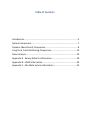
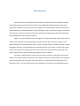
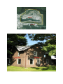
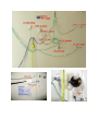
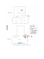
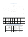
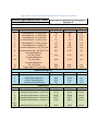
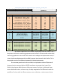
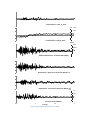
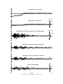
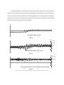
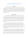
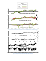
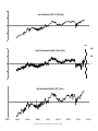
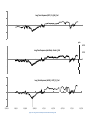
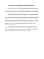
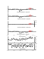
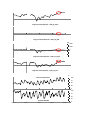
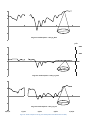
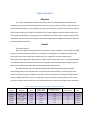
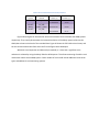
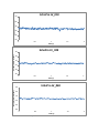
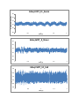
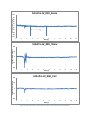
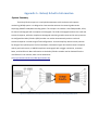
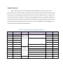
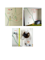
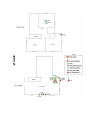
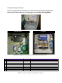
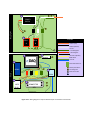
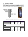
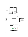
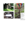
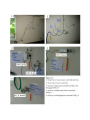
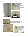
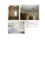
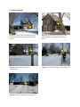
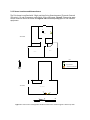
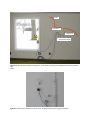
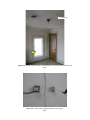
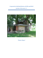
Comparative Field Qualification of ACM and ACSM
Systems at Sycamore, IL
Thomas Koegel
Table of Contents
Introduction ......................................................................................... 3
System Comparison.............................................................................. 7
Dynamic (Burst Event) Comparison ...................................................... 8
Long Term Crack Monitoring Comparison .......................................... 14
Noise Analysis .................................................................................... 24
Appendix A - Kelunji EchoPro Information ......................................... 29
Appendix B - eDAQ Information ......................................................... 33
Appendix C - ēKo Mote System Information ...................................... 42
Introduction
The purpose of this comparative field qualification is to demonstrate the new Kelunji EchoPro
hybrid ACSM system and its performance relative to the eDAQ and eko Motes systems. These three
systems are installed at a test site in Sycamore, IL, adjacent to an active quarry. Data for this report was
collected during a period between March 7, 2011 and May 13, 2011. The analysis includes a comparison
of the long-term results for all three systems and a comparison of the dynamic results and noise levels
for the eDAQ and the Kelunji EchoPro systems.
Figure 1 is an aerial view of the site, and Figure 2 is a view of the exterior of the house with the
exterior walls annotated. These photographs, along with the floor plan in Figure 6, will give a basic
understanding of the site and test house layout. Figure 3 through Figure 5 illustrate the sensor locations
throughout the house. The comparable sensors include the three crack sensors on the first floor shear
crack and the second floor ceiling crack and the two crack sensors on the first floor seam crack. Also,
dynamic data from the internal and exterior geophones will be compared.
This report is organized into five major sections. The first section is a comparison of the three
systems. The second section is the dynamic results from a blast event. The third section is the long term
results of the systems over the period. The fourth section is a comparison of the noise levels on the
eDAQ and EchoPro. The last section contains three appendices, one for each of the deployed systems.
Figure 1: Aerial View of Site with Annotations
Figure 2: Exterior View of Floit Hoise with Annotations
Figure 3: South Exterior Wall with Sensors
Figure 4: Ceiling Crack Bedroom with Sensors
Figure 5: Ceiling Crack Bedroom with KEP sensors
Figure 6: Floit House Floor Plan and Kelunji EchoPro System Layout
System Comparison
Objective
This section will provide important background details about the Kelunji EchoPro ACSM hybrid
system, the eDAQ ACSM system, and the ēKo Motes system deployed at the test house at Sycamore, IL.
In addition, comparisons of the three systems with regard to system properties and sensors will begin to
demonstrate the advantages and disadvantages of the different systems and their independent
capabilities.
Comparative Matrices
The tables below help summarize the key capabilities of each system in an attempt to highlight
their similarities and differences. Table 1 shows system properties and Table 2 shows sensor and
recording properties.
Table 1: Comparison of System Properties of deployed ACM and ACSM systems
System
Battery Type
EchoPro
12 V DC or
regulated
power supply
--
eDAQ
ēKo
Motes
Base station:
110 AC power
Motes:
Self powered
Battery
Life
--
A/D
Converter
24 bit
-5 years
(with
sunlight)
for Motes
Wiring
SoMat
cables
SoMat
cables
None
10 bit
Internet
Communication
Yes
Long Term
Monitoring
Yes
Dynamic
Monitoring
Yes
Yes
Yes
Yes
Yes
Yes
No
Table 2: Comparison of Sensor Properties of deployed ACM and ACSM systems
Sensors
EchoPro
eDAQ
Sampling
12 channels: up
to 1000 Hz
6 channels: up to
2000 Hz
Up to 1000 Hz
ēKo Motes
Every 15 minutes
Channels
12
Type(s)
Displacement: Single
Pole LVDTs
Velocity: Geophones
Trigger
External
or
Internal
Power
Powers sensors
directly
16
Displacement: any
Velocity: any
Temperature &
Humidity: any
Crack: any
Temperature &
Humidity: any
Internal
Separate
power source
required
Internal
Separate
power source
required
Cost
Dynamic (Burst Event) Comparison
Objective
This section will investigate the crack and structural response of the test house at
Sycamore, IL for a specific blast event from May 11, 2011. Triggered data was collected for the
event on both the Kelunji EchoPro hybrid ACSM system and the eDAQ ACSM system. Plots of
the data for corresponding sensors on each system will help graphically compare the two
systems.
Results
The blast event on May 11, 2011 at 11:05 AM triggered the dynamic recording of both
systems. Table 3 below summarizes the event from the Kelunji EchoPro system of sensors. The
largest structural response was .57 inches per second on the first floor exterior mid-wall
geophone. The ground motion excitation had a maximum of .64 inches per second in the radial
direction and about .5 inches per second in both the transverse and vertical directions. From
this raw data, the displacement results were obtained by integrating the velocity data with the 1
milli-second time step. The relative displacement is the difference between the top and bottom
first floor geophones.
Figure 7 and Figure 8 show the time histories of the comparable first floor cracks, the
relative displacement, the displacement of the first floor corner geophones, and the transverse
ground motion for the eDAQ and EchoPro systems respectively. The two systems perform
similarly. They both record similar structural velocity and displacement response, and they both
record similar crack responses. Similarities in the magnitude of the responses are seen by the
comparison of the responses in Table 3 and Table 4. The maximum and minimum values are the
absolute max and min during the duration of the time history, even if there is a step shift.
There is a difference between the shape of each systems response across the seam. The KEP
LVDT returned a step response and the the eDAQ LVDT did not. This difference may be a result of
different locations on the crack or installation differences such as the parallelism of the LVDT body and
target.
Table 3: Summary Table of the Kelunji EchoPro ACSM System for the May 11, 2011 Blast Event
Externally Triggered Dynamic Event - EchoPro
May 11, 2011 11:05 AM
Blast Event at Floit test house near quarry in
Sycamore, IL
Kelunji EchoPro
Channel
Description
Maximum
1
Crack Response – LV_01K_Seam
38
2
Crack Response – LV_02K_Shear
16
3
Crack Response – LV_03K_Null
9
4
Crack Response – LV_04K_IntHor
31
5
Crack Response – LV_05K_IntVert
45
6
Crack Response – LV_06K_Ceil
25
7
Structural Response – HG_07K_Mid
0.47
8
Structural Response - HG_08K_1FUp
0.21
Structural Response 9
HG_09K_1FDwn
0.16
Structural Response –
10
HG_10K_2FUp
0.28
Structural Response –
11
VG_11K_2FCeil
0.00
12
Trigger Signal – LC_12K_Trig
5.05
LARCOR Seismograph
Channel
Description
Maximum
A
Air Blast
0.02
R
Radial Ground Motion
0.62
V
Vertical Ground Motion
0.52
T
Transverse Ground Motion
0.54
Displacement
Channel
Description
Maximum
7
Absolute Displacement - Channel 7
0.064
8
Absolute Displacement - Channel 8
0.019
9
Absolute Displacement - Channel 9
0.025
10
Absolute Displacement - Channel 10
0.017
11
Absolute Displacement - Channel 11
0.000
Ch9 Ch8
Relative Displacement (Ch 9 - Ch8)
0.031
Minimum
-140
-66
-8
-29
-48
-120
-0.57
-0.23
Unit
µ-in
µ-in
µ-in
µ-in
µ-in
µ-in
in/s
in/s
-0.22
in/s
-0.36
in/s
0.00
0.00
in/s
Volts
Minimum
0.02
-0.64
-0.42
-0.5
Unit
Millibars
in/s
in/s
in/s
Minimum
-0.061
-0.019
-0.030
-0.017
0.000
Unit
milli-in
milli-in
milli-in
milli-in
milli-in
-0.035
milli-in
Table 4: Summary Table of the eDAQ ACSM System for the May 11, 2011 Blast Event
Externally Triggered Dynamic Event - eDAQ
5/11/2011 11:05
Channel
9
10
11
12
13
14
15
16
Channel
1
2
3
4
Channel
13
14
15
16
Ch14 Ch13
Blast Event at Floit test house near quarry in
Sycamore, IL
eDAQ - Crack and Velocity Sensors
Description
Maximum
Crack Response - LVDT_9_Shear
63
Crack Response - LVDT_10_Null
26
Crack Response - LVDT_11_Seam
84
Crack Response - LVDT_12_Ceil
122
Structural Response - HG_13_Bottom1
0.23
Structural Response - HG_14_Top1
0.24
Structural Response - HG_15_Top2
0.41
Structural Response - HG_16_Midwall
0.53
eDAQ - External Sensors
Description
Maximum
Radial Ground Motion
0.177933485
Vertical Ground Motion
0.167359581
Transverse Ground Motion
0.197665746
Air Blast
0.00269782
Displacement
Description
Maximum
Absolute Displacement - Channel 13
0.035
Absolute Displacement - Channel 14
0.022
Absolute Displacement - Channel 15
0.022
Absolute Displacement - Channel 16
0.073
Relative Displacement (Ch 14 - Ch13)
0.042
Minimum
-121
-33
-80
-249
-0.18
-0.25
-0.31
-0.63
Unit
µ-in
µ-in
µ-in
µ-in
in/s
in/s
in/s
in/s
Minimum
-0.200018911
-0.191971283
-0.148249314
-0.001940944
Unit
in/s
in/s
in/s
Millibars
Minimum
-0.037
-0.020
-0.022
-0.079
Unit
milli-in
milli-in
milli-in
milli-in
-0.038
milli-in
The relative displacement for the eDAQ is slightly larger than the EchoPro. This is
likely due to the EchoPro monitoring geophones at the corners of an interior wall and the eDAQ
monitoring geophones at the corners of an exterior wall. Looking at the displacement results, it
is clear that the top displacement for the eDAQ is greater than the one for the EchoPro. This is
the probable source of the difference between the relative displacements.
The transverse ground motion for the eDAQ tri-axial geophone is about 50 percent of
the ground motion measured by the LARCOR compliance seismograph that is part of the
EchoPro hybrid system. While there are likely many sources of variation, including soil types,
sensor depth and location, and sensor type, the large magnitude of the difference creates the
possibility of an issue with the different systems, sensor calibration, or other sources of error.
Crack Response - LVDT_11_Seam
µ-in
µ-in
300
300
150
0
Crack Response - LVDT_9_Shear
milli-in
milli-in
0.05
0.05
0.025
0.025
00
Relative Displacement - 1f Interior Wall( 13&14 )
milli-in
0.05
0.025
0
Displacement - Upper Corner SE Exterior Wall Ch. 13
Displacement - Lower Corner SE Exterior Wall Ch. 14
in/s
0.3
0.15
0
0.5
1
Transverse Ground Motion
1.5
Time (s)
Figure 7: May 11, 2011 1105 Dynamic Event - eDAQ
2
Crack Response - LV_01K_Seam
µ-in
µ-in
Crack Response - LV_02K_Shear
200
200
100
100
00
milli-in
milli-in
0.05
0.05
Relative Displacement North Living Room Interior Wall Ch ( 8&9 )
0.025
0.025
00
milli-in
0.05
Displacement - Upper Corner NE Interior Wall Ch. 8
0.025
0
Displacement - Lower Corner NE Interior Wall Ch. 9
in/s
Transverse Ground Motion
1
0.5
0
1
1.5
Time (s)
2
Figure 8: May 11, 2011 1105 Dynamic Event - EchoPro
2.5
Figure 9 illustrates the crack response of each system to the ceiling crack on the second floor
bedroom and the velocity response from the vertical geophone. The response of the crack sensors is
similar across the two systems. However, the vertical geophone is not responding at the magnitude
expected for the event. This is likely an issue inherent to the sensor or its preparation and installation
because the raw data showcases the same problem.
Crack Response (KEP) - LV_06K
1
2
Time (s)
2
3
µ-in
300
150
0
Crack Response (eDAQ) - LVDT_12_Ceil
0.5
1
Time (s)
1.5
2
in/s
0.0003
0.00015
0
Structural Response (KEP) - Vertical Geophone on Bedroom Ceiling
1
1.5
Time (s)
2
Figure 9: May 11, 2011 1105 Dynamic Event - Second Floor Response (Both Systems)
2.5
Long Term Crack Monitoring Comparison
Objective
The following section will describe the crack movements and environmental data for the
period between March 7, 2011 and May 13, 2011 for the three systems (Kelunji EchoPro, eDAQ,
eko Motes) present at the Sycamore, IL test house. The purpose of this is to graphically compare
the long term results from the systems and attempt to describe any discrepancies. Additionally,
a dynamic event from May 11, 2011 will serve as a sample event for comparison of dynamic and
long term crack response.
Long Term Results
Long term response monitoring shows crack movements that occur due to long term
environmental factors such as temperature and humidity. For the best results, sensors must be
continuously monitored over long period of time and return reasonable data. Figure 10 shows
the crack response of all three systems over the entire collection period, and Figure 11 shows
the interior and exterior environmental variations over the same time. Figure 9 and Figure 10
show the response of each individual system for the exterior shear crack and the bedroom
ceiling crack.
The trend that can be extracted from the figures is that as the average temperature
increases, the cracks decrease in size. This makes sense as thermal expansion of the wall
material with increased temperature would serve to reduce the size of the cracks. However, it is
important to note that humidity fluctuations also have a large impact on crack response, though
it is difficult to discern a trend from the figures due to the rapid variation of the exterior
humidity response.
For the most part, the crack sensors measure very similar responses and show peaks and
troughs at the same points in time. However, there are observable deviations between the
sensors at the beginning and end of the shear crack time history and the end of the seam crack
time history. There are several possible explanations for these differences. First, human error in
installation and sensor error in responding to crack movements can the different magnitudes.
Second, the crack gauges monitor different locations on the crack. Therefore, the long term
environmental factors could create strain localizations that vary the impacts at the various
positions of the sensors. Further study could involve multiple LVDT’s on a single system and
crack to help determine what factors influence differences in long term crack response between
sensor locations.
Long Term Response (KEP & eDAQ) - Seam Crack
µ-in 6000
3000
0
Long Term Response (All) - Shear Crack
Long Term Response (All) - Ceiling Crack
2/26/11
3/8/11
3/18/11
3/28/11
4/7/11
4/17/11
4/27/11
5/7/11
5/17/11
Figure 10: Long Term Crack Response for Multiple Systems to Highlight Differences in Response Patterns
°F
100
50
Interior Temperature
0
%
100
50
Interior Humidity
0
External Temperature
External Humidity
2/26/11
3/8/11
3/18/11
3/28/11
4/7/11
4/17/11
4/27/11
Figure 11: Interior and Exterior Temperature and Humidity Fluctuations
5/7/11
5/17/11
Long Term Response (KEP) - LV_02K_Shear
µ-in
6000
Long Term Response (eko Mote) - Node 2_Shear
3000
0
Long Term Response (eDAQ) - LVDT_9_Shear
2/26/11
3/8/11
3/18/11
3/28/11
4/7/11
4/17/11
Figure 12: Long Term Crack Response for Exterior Shear Crack
4/27/11
5/7/11
5/17/11
Long Term Response (KEP) - LV_06K_Ceil
µ-in
6000
Long Term Response (eko Mote) - Node 3_Ceil
3000
0
Long Term Response (eDAQ) - LVDT_12_Ceil
2/26/11
3/8/11
3/18/11
3/28/11
4/7/11
4/17/11
Figure 13: Long Term Crack Response for Bedroom Ceiling Crack
4/27/11
5/7/11
5/17/11
Comparison of Long Term Response with the Sample Blast Event
To compare the magnitude of crack response between the long term environmental variations
and the dynamic response from a blast event, it is important to establish a means of visually comparing
the two. This is complicated by the large differences in the time scale (long term is in terms of days and
months while dynamic response occurs in a matter of seconds).
Figure 14 and Figure 15 shows the long term crack response of the EchoPro and eDAQ systems
respectively with the dynamic event period circled in red. These figures show that there is no large
change in the long term trend of the crack movement during this period. In order to further demonstrate
this, Figure 13 and Figure 14 enlarge the long term response for the three comparable cracks (exterior
seam, exterior shear, bedroom ceiling). Also included in these figures is a representation of the dynamic
response of these cracks during the May 11, 2011 blast event. These dynamic responses are displayed
below the x-axis near the corresponding date and are scaled to about twice their real response
magnitude for viewing purposes
More information on the specifics of the blast event can be found in the dynamic analysis
section of this report. However, it can be concluded that the event, with an maximum ground motion
near .5 or .6 inches per second, does not produce a crack response that is significant when compared to
the magnitude of the long term crack variations due to environmental effects.
Long Term Crack Response - LV_01K_Seam
Long Term Crack Response - LV_02K_Shear
µ-in
4000
2000
0
Long Term Crack Response - LV_05K_IntVert
Long Term Crack Response - LV_06K_Ceil
4/27/11
5/1/11
5/5/11
5/9/11
5/13/11
°F
100
External Temperature
75
50
25
0
%
100
75
50
25
External Humidity
4/27/11
5/1/11
5/5/11
th
0
5/9/11
5/13/11
Figure 14: April 27 – May 13 EchoPro Response with Dynamic Event Data Circled
Long Term Crack Response - LVDT_9_Shear
Long Term Crack Response - LVDT_10_Null
µ-in
4000
2000
0
Long Term Crack Response - LVDT_11_Seam
Long Term Crack Response - LVDT_12_Ceil
°F
100
External Temperature
75
50
25
0
%
100
75
50
25
External Humidity
4/27/11
5/1/11
5/5/11
5/9/11
5/13/11
Figure 15: April 27 - May 13th eDAQ Response with Dynamic Event Data Circled:
0
Long Term Response - LV_01K_Seam
µ-in
4000
Long Term Response - LV_02K_Shear
2000
0
Long Term Response - LV_06K_Ceil
4/27/11
5/1/11
5/5/11
5/9/11
Figure 16: Visual Comparison of Long Term and Dynamic Crack Movements on EchoPro
5/13/11
Long Term Crack Response - LVDT_9_Shear
µ-in
4000
2000
0
Long Term Crack Response - LVDT_11_Seam
Long Term Crack Response - LVDT_12_Ceil
4/27/11
15
5/1/11
5/5/11
5/9/11
Figure 17: Visual Comparison of Long Term and Dynamic Crack Movements on eDAQ
5/13/11
Noise Analysis
Objective
This section will attempt to compare the noise levels for the Kelunji EchoPro and EDAQ crack
monitoring systems based on data obtained from the test house in Sycamore, Illinois. Visual resolution of
a crack monitoring system is constrained by the noise level. Simply put, the lower the noise level relative
to the sensor sensitivity, the higher the resolution of the output. Higher resolution allows smaller crack
movements to be detected, improving the value and performance of the system. For the purpose of this
comparison, the noise levels of the Kelunji crack sensors (LVDTs) and the EDAQ crack sensors (LVDTs) will
be determined from the data.
Results
The results shown in
Table 5 and Table 6 were derived from two events that were recorded on the EchoPro and eDAQ
systems. The noise calculations took four to six random 1-second peak to peak difference samples for
each crack sensor channel from each time history (in the range after the event response) and
determined the average peak to peak noise for a given channel across both events. A standard deviation
is included to show the variation in the noise across samples. Visual estimates were included to ensure
that peak to peak noise estimates were not being distorted by data outliers.
The tables illustrate the noise difference between the EchoPro and eDAQ by grouping the
corresponding sensors with the same color. The results show that the EchoPro, monitoring the same
cracks, has at the very least a 50 percent reduction in the noise level from the eDAQ. The large levels of
noise on eDAQ channel LVDT_12_Ceil is likely due to a sensor problem, as these levels of noise are not
typical for the other sensor channels on the system and does not represent the typical sensor resolution.
Table 5: Noise Level Comparison for EchoPro and eDAQ ACSM systems
System
EchoPro
eDAQ
EchoPro
eDAQ
EchoPro
eDAQ
Channel
LV_01K_Seam
LVDT_11_Seam
LV_02K
LVDT_9_Shear
LV_06K
LVDT_12_Ceil
Type
crack
crack
crack
crack
crack
crack
Peak to Peak
Average Noise
11.39
26.66
10.63
35.28
8.54
83.68
Standard Deviation of
Average Noise
1.21
2.46
1.54
3.14
1.31
3.28
Visual Estimate
10
20
10
25
8
70
unit
µ-inches
µ-inches
µ-inches
µ-inches
µ-inches
µ-inches
Table 6: Noise Level Reduction from eDAQ to EchoPro
System
EchoPro
eDAQ
EchoPro
EDAQ
EchoPro
EDAQ
Channel
LV_01K
LVDT_11_Seam
LV_02K
LVDT_9_Shear
LV_06K
LVDT_12_Ceil
Reduction Peak
to Peak (%)
Reduction Visual
Estimate (%)
57.26825034
50.00
69.87387511
60.00
89.78928096
88.57
Figure 18 and Figure 19 illustrate two-second time histories for the EchoPro and eDAQ systems
respectively. They visually demonstrate the increased resolution of the Kelunji system relative to the
eDAQ due to lower noise levels of the recorded data. Figure 20 shows the full EchoPro time history and
the two second time window from which the first two figures were developed.
With both visual inspection and data analysis methods, it is clear that a significant noise
reduction is achieved by using the Kelunji EchoPro ACSM system. This allows monitoring of smaller crack
movements relative to the eDAQ system. Further studies of noise could include additional crack sensor
types and additional crack monitoring systems.
EchoPro LV_01K
Output (micro-inches)
50
30
10
-10
-30
-50
0
0.5
1.5
2
EchoPro LV_02K
50
Output (micro-inches)
1
Time (s)
30
10
-10
-30
-50
0
0.5
1.5
2
EchoPro LV_06K
50
Output (micro-inches)
1
Time (s)
30
10
-10
-30
-50
0
0.5
1
Time (s)
1.5
Figure 18: Noise Illustration - EchoPro 2 second Time History
2
Edaq LVDT_11_Seam
Output (micro-inches)
50
30
10
-10
-30
-50
0
0.5
1.5
2
1.5
2
1.5
2
Edaq LVDT_9_Shear
50
Output (micro-inches)
1
Time (s)
30
10
-10
-30
-50
0
0.5
Edaq LVDT_12_Ceil
50
Output (micro-inches)
1
Time (s)
30
10
-10
-30
-50
0
0.5
1
Time (s)
Figure 19: Noise Illustration - eDAQ 2 second Time History
EchoPro LV_01K_Seam
Output (micro-inches)
100
80
60
40
20
0
-20
-40
-60
-80
-100
0
1
2
4
5
6
Time (s)
7
8
9
10
11
8
9
10
11
8
9
10
11
EchoPro LV_02K_Shear
100
Output (micro-inches)
3
50
0
-50
-100
0
1
2
3
5
6
Time (s)
7
EchoPro LV_06K_Ceil
100
Output (micro-inches)
4
50
0
-50
-100
0
1
2
3
4
5
6
Time (s)
7
Figure 20: Noise Illustration - EchoPro Full Time History with Annotated 2 Second Window
Appendix A - Kelunji EchoPro Information
-System Summary
The Kelunji EchoPro system is a new hybrid autonomous crack and structural response
monitoring (ACSM) system. It is designed as a low cost alternative to the research grade version
employing SOMAT’s eDAQ data recording system. The concept is to combine a new field portable, 24 bit,
12 channel seismograph with a compliance seismograph. The 24 bit seismograph monitors the crack and
structural response, while the compliance seismograph monitors ground motions and air over pressures.
As configured the Kelunji EchoPro (KEP) recorder can monitor autonomously monitor crack and
structural response in a wide range of field configurations. Cost and simplicity were the main priorities
for design of the hybrid system. The full installation, illustrated in Figure 21includes structural response
velocity and crack sensors, a LARCOR compliance seismograph with a trigger connection, connector
boxes, and the KEP unit. More information on the Kelunji EchoPro recorder can be obtained from the
manufacturer’s user manual, which can be obtained at
(<http://customer.esands.com/index.php?section=45)
Figure 21: Components of the hybrid autonomous crack & structural monitoring (ACSM) system
-Sensor Summary
Table 7 summarizes the sensors installed with the Kelunji EchoPro. The first column is the
EchoPro channel for the given sensor. Columns two and three give the channel name and type of sensor.
Columns four, five, and six give the location of the sensor in the house, what the sensor is used for, and
serial number of the sensor. Figure 22 to Figure 24 are photographs that show completed installation of
sensors on the exterior E-W wall, interior E-W wall, and bedroom ceiling respectively. Figure 25 is a plan
view of the house with the location of all sensors. The sensors unnumbered in those photographs are
associated with other systems of instrumentation.
Table 7: Floit House Sensor Installation Summary
Channel
Channel Name
Sensor
Location
Use
Serial
1
LV_01K_Seam
LVDT –
Exterior E-W Wall
Crack
110890
2
LV_02K_Shear
Displacement
Crack
102241
3
LV_03K_Null
Transducers
Null
110886
4
LV_04K_IntHor
Crack
110885
5
LV_05K_IntVert
Crack
110884
6
LV_06K_Ceil
BR Ceiling
Crack
110887
7
HG_07K_Mid
Geophone –
Exterior E-W Wall
Horizontal
N/A
8
HG_08K_1FUp
Velocity
Interior E-W Wall Upper Corner
Horizontal
N/A
9
HG_09K_1FDwn
Transducer
Interior E-W Wall Lower Corner
Horizontal
N/A
10
HG_10K_2FUp
BR E-W Wall Upper Corner
Horizontal
N/A
11
VG_11K_2FCeil
BR Ceiling
Vertical
N/A
12
LC_12K_Trig
Outside of Exterior East Wall
Trigger
N/A
LARCOR
Interior E-W Wall
Figure 22: Exterior E-W Wall Sensors
Figure 23: Interior E-W Wall Sensors
Figure 24: Bedroom Ceiling Sensors
Figure 25: Plan View of Sensor Locations
Appendix B - eDAQ Information
-System Summary
The following information was included from a report by Charles Dowding and Jeffrey Meissner
titled Sycamore Installation Report. This report and additional reports and information are available at
http://iti.northwestern.edu/acm/publications.html
2.2 SoMat eDAQ System (wired)
The Floit House also has the traditional ACM wired system paradigm equipped with SoMat’s
eDAQ Classic data logger. The system is designed to autonomously monitor ground motion, air
overpressure, structural response, and crack response. The data is stored short term in the
Floit House, transmitted via the Internet connection in the QC house (shown in Figure 2.12),
uploaded to an ITI server, and then broadcast over the web for viewing. The eDAQ is
programmed to collect both data long-term (every hour) and during dynamic events (1000 Hz
sampling) triggered by the triaxial and horizontal geophones.
Figure 2.12 describes the layout of the wired system. The data is transmitted via a Proxim
Tsunami point-to- point wireless network connection back to the Internet connection in the QC
house.
2.2.1 System Enclosure Contents
The wires running back from the sensors to the eDAQ all meet at an enclosure box behind the
stairs in the Floit House. Photos of this enclosure are shown in Figure 2.13 with Table 2.1
describing its contents. Additionally, a wiring diagram of this box is shown in Figure 2.14.
BOTTOM LAYER
TOP LAYER
8
6
3
1
4
7
5
2
Figure 2.13 - Photographs of enclosure with both top and bottom layer contents
No.
Manufacturer / Product
1
SoMat eDAQ Classic
2
Analog Input Break Out Box, modified by ITI
3
MOXA Universal Communicator
4
Xytronix Web Relay
5
Advantantech ADAM Ethernet Switch
6
Radioshack 1.5 amp 13.8 volt DC power supply
7
SOLA Linear Power Supplies
8
Cutler Hammer Circuit Breaker
Model No.
Function
ECPU-HLB
Data Logger with 16 high level analog input channels
1-EHLB-AIBOX-2
16 Channel Board to connect sensors with SoMat jacks
UC-7408
Embedded GNU/Linux computer to buffer data and control communication
X-WR-1R12-1I5-5
Web-based watchdog timer to reset UC necessary
ADAM-6520
5-port Industrial 10/100 Mbps Ethernet Switch
22-508
Provides DC power to non-sensor devices
SCL4D15-DN
Provides low noise, low voltage DC to sensors
WMS1B15
Provides power protection and acts as power switch
Table 2.1 - Contents of Enclosure with description of function
6
BOTTOM
LAYER
POWER
SUPPLY
7
LEGEND
SOLA
A
SOLA
B
110V AC (Ext. Power)
110V AC (Hot)
110V AC (Neutral)
Ground
+ Low Voltage DC
- Low Voltage DC
+DC contlʼd by Relay
8
1
BREAKER
SoMat Cable
Ethernet
3
Power Distribution Pt.
Wire Up Wire Down
MOXA
Grounding Post
TOP
LAYER
5
Ethernet Jack Out
ADAM
4
WEB
RELAY
2
CONNECTOR
BOX
x16 (sensors)
Figure 2.14 - Wiring diagram of top and bottom layers of enclosure in Floit House
2.2.2 Sensor Locations and Nomenclature
The eDAQ has the capability of monitoring 16 channels of which only 12 are occupied in this
installation. Figure 2.15 shows the connector box layout, and Table 2.2 lists the sensors along
with their channel designations and detailed descriptions. Figure 2.16 shows the sensors’
exact locations within the house. Photographs of the sensors are also shown in Figures 2.172.22. Please see Appendix C for calibration sheets for these sensors.
1
9
LVDT
Transverse Geophone
2
10
LVDT
Vertical Geophone
3
11
LVDT
Air Overpressure
4
12
LVDT
5
13
Horizontal
Geophone
6
14
Horizontal
Geophone
7
15
Horizontal Geophone
8
16
Horizontal Geophone
Longitudinal Geophone
Figure 2.15 - Diagram and photograph of SoMat Connector Box and channel designations
Channel
1
2
3
4
5
6
7
8
9
10
11
12
13
14
15
16
Channel Name
Geo_1_L
Geo_2_T
Geo_3_V
4_Air
Sensor
Manufacturer
Model
Serial No.
Triaxial Geophone
(buried)
GeoSonics
N/A
ACM installation
Franklin, WI
Air Overpressure
GeoSonics
3000 Series
NW 3
Vac nt Channels
LVDT_9_Shear
LVDT_10_Null
LVDT_11_Seam
LVDT_12_Ceil
HG_13_Bottom1
HG_14_Top1
HG_15_Top2
HG_16_Midwall
Linear Variable
Differential
Transformer
MacroSensors
DC-750-050
Horizontal Wall
Geophone (wallmounted)
GeoSpace
HS-1-LT 98449
Table 2.2 - Exhaustive description of sensors and channel designation
Old LVDT 5
Old LVDT 6
Vegas recovered A
89735
N/A
L12
BEDROOM 1
2ND FLOOR
STAIRS
BEDROOM 3
BEDROOM 2
H15
6'8"
KEY
Data Logger
Triaxial Geophone
N
LVDT
Horizontal Geophone
Tsunami Transmitter
eDAQ
STAIRS
L
T
1ST FLOOR
LIVING / DINING ROOM
L11
5'7"
5'
H16
L9 5'4"
L10 4'11"
3"
T 1'10"
7'6"
V
H13
H14
4'0"
10'
20'
Figure 2.16 - Exact sensor and equipment locations within house. Measure given is distance up wall
1
2
N
N
3
Figure 2.17 -
Geo_2_T
1 - Southeast corner of
house showing
seismograph (triaxial
geophone) location
Geo_3_T
Geo_1_L
N
2 - View from house of
trench and buried
geophone
3 - Close-up of buried
geophone with
longitudinal axis pointing
north toward the quarry
1
2
Figure 2.20 1 - Overall view of
southeast corner
geophones on first
floor
2 - Close-up of top
geophone monitored
by HG_14
HG_14_Top1
3 - Close-up of bottom
geopohone monitored
by HG_13
3
HG_13_Bottom1
1
Figure 2.21 1 - Overall view of second floor bedroom geophone on south wall
2 - Closer view of geophone below slanted ceiling in top corner
3 - Close-up of top geophone monitored by HG_15
2
3
HG_15_Top2
1
2
3
Figure 2.22 1 - Overall view of ceiling crack from hallway
outside bedroom (looking North)
2 - Closer view of ceiling crack inside bedroom
(looking West)
3 - Close-up of ceiling crack monitored by
LVDT_12
LVDT_12_Ceil
Appendix C - ēKo Mote System Information
-System Summary
The following information was included from a report by Charles Dowding and Jeffrey Meissner
titled Sycamore Installation Report. This report and additional reports and information are available at
http://iti.northwestern.edu/acm/publications.html
2.1 ēKo Mote System (wireless)
The REG installed a wireless sensor network (WSN) to monitor long-term changes in two cracks
at the Floit House in conjunction with temperature and humidity. The WSN in Sycamore is a
multi-hop system that consists of 4 nodes (motes) and a base station at the QC house. Data is
collected from the sensors at the nodes and is then relayed back to the base station. Figure 2.1
shows the location of the nodes within the wireless mesh network. Figures 2.3-2.6 below also
show detailed photographs of the mote locations.
2.1.1 Mote Locations
3
2
Figure 2.2 - Exterior view of southwest corner of
instrumented Floit House, showing where Node 2
is inside.
4
Figure 2.4 - Node 4 as relay point on
telephone pole
0
Figure 2.6 - Node 0 is base station inside QC house
Figure 2.3 - Exterior view of east wall of instrumented Floit House, showing where Node 3 is
inside.
5
Figure 2.5 - Node 5 as relay point on telephone pole
2.1.2 Sensor Locations and Nomenclature
The Floit house is outfitted with 3 high precision String Potentiometers (Firstmark Controls
150 series). S1 and S3 measure cracks, while S2 is a null gauge. Figure 2.7 shows the exact
sensor locations within the house and Figures 2.8-2.11 show photographs of the installed
equipment.
S3
M3
BEDROOM 1
2ND FLOOR
STAIRS
BEDROOM 3
BEDROOM 2
KEY
eKo Mote
String Potentiometer
Temperature & Humidity Probe
N
STAIRS
1ST FLOOR
LIVING / DINING ROOM
5'3"
5'
S1
S2
TH
10'
M2
20'
Figure 2.7 - Exact sensor and equipment locations within house. Measure given is distance up wall
Crack
Crack Sensor
Null Sensor
2
eKoMote
Temperature Probe
Figure 2.8 - Interior view of Node 2 in living room. Crack sensor, null sensor, and temperature probe connected to
eKo
Mote.
Figure 2.9 - Close-up of crack sensor and null sensor. Both instruments are string-potentiometers
Crack Sensor
3
Figure 2.10 - Interior view of Node 3 in upstairs bedroom. Crack sensor connected to eKo
Mote.
Figure 2.11 - Close-up of string-potentiometer across ceiling
crack