1
UNISENSE SENSORTRACE SUITE
SENSORTRACE PHOTO
USER MANUAL
SensorTrace Suite v2.0 User Manual
Copyright © 2013 · Unisense A/S
Version October 2013
SENSORTRACE PHOTO
USER MANUAL
UNISENSE A/S
TABLE OF CONTENTS
SENSORTRACE PHOTO . . . . . . . . . . . . . . . . . . . . . . . . . . . . . . . . . . . . . . . . . . . . . . . . . . . . . . . . . . . . . . . . 1
USER MANUAL . . . . . . . . . . . . . . . . . . . . . . . . . . . . . . . . . . . . . . . . . . . . . . . . . . . . . . . . . . . . . . . . . . . . . . . . 1
CONGRATULATIONS WITH YOUR NEW PRODUCT . . . . . . . . . . . . . . . . . . . . . . . . . . . . . . . . . . . . . . 7
Support, ordering, and contact information
7
WARRANTY AND LIABILITY . . . . . . . . . . . . . . . . . . . . . . . . . . . . . . . . . . . . . . . . . . . . . . . . . . . . . . . . . . . . 8
OVERVIEW . . . . . . . . . . . . . . . . . . . . . . . . . . . . . . . . . . . . . . . . . . . . . . . . . . . . . . . . . . . . . . . . . . . . . . . . . . . . 11
THE LIGHT-DARK SHIFT METHOD . . . . . . . . . . . . . . . . . . . . . . . . . . . . . . . . . . . . . . . . . . . . . . . . . . . . 12
MEASURING SETUP . . . . . . . . . . . . . . . . . . . . . . . . . . . . . . . . . . . . . . . . . . . . . . . . . . . . . . . . . . . . . . . . . . 15
INSTALLING THE SOFTWARE . . . . . . . . . . . . . . . . . . . . . . . . . . . . . . . . . . . . . . . . . . . . . . . . . . . . . . . . 16
GETTING STARTED . . . . . . . . . . . . . . . . . . . . . . . . . . . . . . . . . . . . . . . . . . . . . . . . . . . . . . . . . . . . . . . . . . 17
SENSORTRACE PHOTO INTERFACE . . . . . . . . . . . . . . . . . . . . . . . . . . . . . . . . . . . . . . . . . . . . . . . . . . . 19
SETTINGS TAB . . . . . . . . . . . . . . . . . . . . . . . . . . . . . . . . . . . . . . . . . . . . . . . . . . . . . . . . . . . . . . . . . . . . . . . 20
COMMENTS TAB . . . . . . . . . . . . . . . . . . . . . . . . . . . . . . . . . . . . . . . . . . . . . . . . . . . . . . . . . . . . . . . . . . . . . 22
CALIBRATION TAB . . . . . . . . . . . . . . . . . . . . . . . . . . . . . . . . . . . . . . . . . . . . . . . . . . . . . . . . . . . . . . . . . . . 24
Calibration procedure
Recalibration procedure
Retrieving a calibration
25
26
26
CALIBRATION OF LIGHT SENSOR . . . . . . . . . . . . . . . . . . . . . . . . . . . . . . . . . . . . . . . . . . . . . . . . . . . . 27
THE LIVE DATA GRAPH . . . . . . . . . . . . . . . . . . . . . . . . . . . . . . . . . . . . . . . . . . . . . . . . . . . . . . . . . . . . . . . 28
EXPERIMENT TAB . . . . . . . . . . . . . . . . . . . . . . . . . . . . . . . . . . . . . . . . . . . . . . . . . . . . . . . . . . . . . . . . . . . . 30
Motor control
32
PERFORMING AN EXPERIMENT . . . . . . . . . . . . . . . . . . . . . . . . . . . . . . . . . . . . . . . . . . . . . . . . . . . . . . 33
Settings
Photosynthesis rate measurements
The profile windows
33
34
37
OUTPUT FILE . . . . . . . . . . . . . . . . . . . . . . . . . . . . . . . . . . . . . . . . . . . . . . . . . . . . . . . . . . . . . . . . . . . . . . . . 38
EXPERIMENTAL DATA EXAMPLE . . . . . . . . . . . . . . . . . . . . . . . . . . . . . . . . . . . . . . . . . . . . . . . . . . . . . 40
5
6
CONGRATULATIONS WITH YOUR NEW PRODUCT
Support, ordering, and contact information
If you wish to order additional products or if you encounter any
problems and need scientific/technical assistance, please do not
hesitate to contact our sales and support team. We will respond to
your inquiry within one working day.
E-mail: [email protected]
Unisense A/S
Tueager 1
DK-8200 Aarhus N, Denmark
Tel: +45 8944 9500
Fax: +45 8944 9549
Further documentation and support is available at our website
www.unisense.com.
7
WARRANTY AND LIABILITY
Unisense SensorTrace Suite software is checked and validated
on the operating systems as given in the specification, running
English language settings. It comes with lifetime updates.
Software must be installed under administrator rights. Customer
must ensure PC is fully updated and no conflicting third party
software is installed. Unisense do not warrant compliance with any
other operating systems, language settings or third party software.
For instrumentation and sensors, please refer to our warranty
conditions as given in the document “General Terms of Sale and
Delivery of Unisense A/S” found on www.unisense.com
License agreement
The following terms shall apply to the software provided by
Unisense A/S (“Unisense”) in connection with the simultaneous
sale to you (“Customer”) of a Unisense SensorTrace Suite Software.
All rights, title and interest in the software belong to Unisense.
Unisense grants to the Customer a royalty-free, non-exclusive and
non-transferable license to use the software solely in connection
with the Unisense Product purchased from Unisense simultaneously with the purchase of the software. The Customer undertakes
not to copy, modify, reverse engineer, disassemble or de-compile
all or any part of the software or rent, lease, distribute or sell the
software. The Customer shall, however, be entitled to make one
copy of the software for back-up and recovery purposes for use
solely in connection with the Unisense Products supplied by
Unisense together with the software.
Nothing in this License Agreement or any other agreement
between Unisense and the Customer shall be construed as an
obligation for Unisense to provide to the Customer updates of the
software. This License Agreement shall automatically terminate if
the Customer violates the terms of the license. In case of termination of the license the Customer shall immediately destroy the
software and any copy thereof.
8
THE CUSTOMER TAKES THE SOFTWARE “AS IS.” UNISENSE
MAKES NO WARRANTY OR REPRESENTATION CONCERNING THE
SOFTWARE, AND EXPRESSLY DISCLAIMS ALL OTHER WARRANTIES
AND CONDITIONS, EXPRESS OR IMPLIED, STATUTORY OR
OTHERWISE, OF WHATEVER KIND OR NATURE, INCLUDING BUT
NOT LIMITED TO ANY AND ALL IMPLIED WARRANTIES, INCLUDING
IMPLIED WARRANTIES OF MERCHANTABILITY AND FITNESS FOR A
PARTICULAR PURPOSE.
UNISENSE SHALL NOT BE LIABLE FOR ANY DAMAGES OF ANY KIND,
INCLUDING INCIDENTAL, SPECIAL, PUNITIVE, CONSEQUENTIAL,
AND SIMILAR DAMAGES, INCLUDING, WITHOUT LIMITATION,
LOSS OF PRODUCTION, LOSS OF PROFIT, LOSS OF DATA, LOSS OF
GOODWILL, LOSS OF CONTRACTS, OR BUSINESS INTERRUPTION
This License Agreement and any dispute arising out of or in
relation to this License Agreement shall be governed by and
construed in accordance with the laws of Denmark exclusive of
its choice of law provisions. The venue for any such dispute shall
be the Danish courts provided however that Unisense shall be
entitled to instigate legal proceedings against the Customer
before the courts with jurisdiction over the matter located in a
country where the Customer has a place of business or is incorporated or organized.
9
10
OVERVIEW
SensorTrace Photo - For photosynthetic experiments using the
light-dark switch technique we recommend that you use.
SensorTrace Suite is compatible with all digital Unisense instruments. It supports up to 16 channels with an adjustable logging
frequency of up to 50 samples per second depending on the
Unisense amplifier connected. The program automatically saves
all data in an SQL database and all data can be exported in csv
formatted files for subsequent data analysis.
System requirements:
• A digital Unisense amplifier or A/D-converter unit.
• PC with Windows XP/2ooo/Vista/Windows 7 32
bit/64, Windows 8/8.1
•
min. 200 MB free hard disk space
•
USB port(s)
•
min. screen resolution 1280 x 800
• min. 4 GB RAM
Other programs available in the full SensorTrace Suite:
SensorTrace Profiling - For motor control, activity calculations,
and profiling in 1, 2 or 3 dimensions we recommend that you use.
SensorTrace Logger is the basic data acquisition program from
the Unisense program SensorTrace Suite. It offers timeseries
datalogging and calibration features.
SensorTrace Rate - For microrespiration experiments to measure
the metabolic rates including respiration rates of small aquatic
animals, bacteria or oxygen production of phytoplankton we
recommend that you use.
11
THE LIGHT-DARK SHIFT METHOD
This paragraph gives a short description of the theory on which
the light-dark shift method is based. The tip of an oxygen
microsensor is placed at a certain position r in a photosynthetic
system. It measures at time t the oxygen concentration C(r,t).
The time dependency (i.e. the derivative in time) of the oxygen
concentration can be described by:
∂C
= −T − R + P
∂t
where P is the volumetric gross photosynthesis rate of oxygen
(mol m-3 s-1) and R the volumetric oxygen respiration rate (mol
m-3 s-1), respectively. The volumetric transport rate T represents the changes in oxygen concentration due to transport
phenomena (mol m-3 s-1). The type of transport is dependent
on the specific sample under investigation. It can be due to
advection, convection, or diffusion. The light-dark shift method
works for all types of transport.
For the light-dark shift technique, it is important that the oxygen
concentration reaches a measurable steady state value under a
constant illumination setting. At steady state the above equation
is equal to zero:
∂C
= 0 ⇒ −T − R + P = 0
∂t
If now the illumination is switched off the steady state situation
is disturbed. The photosynthesis rate P is now zero, whereas
transport and respiration rates are assumed to remain unchanged
within the next short time period. Thus, the time dependency
of the oxygen concentration C immediately after the onset of
darkness is given by:
∂C
= −T − R
∂t
12
The latter two equations can be subtracted from each other,
which yield:
P=−
∂C
∂t
Thus, the volumetric gross photosynthesis rate P can be determined by the slope of the oxygen concentration C immediately
after the light-dark shift. This is indicated in the following figure.
Practically, the measurements are realized by moving the
oxygen microsensor tip to the measuring site with the help of
a micromanipulator. The sample of interest is illuminated with
photosynthetically active light of a constant intensity. Steady state
is achieved when the microsensor reading is stable over time. At
this point the illumination is switched off. It is essential that the
switching event is fast (<<100 ms). Hence, just switching off the
light source will usually not work, as most light sources exhibit
an afterglow. Normally, sample shading will be the best method.
This can be done by either blocking the light path manually (e.g.
using a piece of cardboard or aluminium foil) or by applying an
electronic shutter.
13
The computer samples the voltage readings of the microsensor at
a frequency of 10- 50 Hz. The typical sampling interval starts 1-3
seconds before the switching event and stops 2-4 seconds after it.
The time interval before the switching event is used to calculate
an average value of the steady state oxygen concentration. The
volumetric gross photosynthesis rate is obtained by fitting a linear
slope to the data sampled immediately after darkening. The user
has to define the start and end time of the fitting interval relative
to the switching event. Typical values for the fitting interval are
0-0.5 and 0.5-2 seconds for the start and end times, respectively.
As the Photo software has to know exactly when the switching
took place, a light sensor is placed within the light field near the
measuring site. Its signal is used by the computer as a trigger for
the switching event.
14
MEASURING SETUP
In order to realize ligh-dark measurement the following components are required for the experimental setup:
• Fast responding O2 micro-sensor
• Light sensor including amplifier box
• Micromanipulator
• Microsensor Monometer or Multimeter
• Photosynthetic active sample
(i.e.
algae mat, coral)
• Photo software
The microsensor is connected via the LEMO connector to a pA
channel on the front of the meter, while the UNISENSE Light
Sensor box is connected to an analogue input channel at the rear.
The UNISENSE Microsensor Mono- or Multimeter is connected
to a USB-port of the computer. The microsensor is placed in a
micromanipulator that is used to position the sensor tip at the
intended measuring site of the studied sample. The tip of the light
sensor is positioned, i.e. with a lab stand, within the light field, but
placed so that it is not interfering with the path of light towards
the measuring site. Thus, the light sensor signal acts as an exact
indicator for the time of light to dark transition.
15
INSTALLING THE SOFTWARE
Make sure that you are installing having the full administration
rights.
Start the installation program (.exe file) from the CD. Follow the
instructions given by the installation program.
This will install the SensorTrace Suite program including a version
of this manual in the program group “Unisense”. Instrument
drivers and a configuration utility for the A/D-converter will also
be installed. This is called Instacal and will be placed in a program
group called “Measurement Computing”.
To activate the full SensorTrace Suite program and gain access to
Logger+, Profiling, Photo, and Rate enter the License Key supplied
with the installation CD. To access the dialog box for entering the
license key, click on the Enter License Key button in the low right
corner for the main SensorTrace Suite window. Press Activate when
the key is fully entered. Contact [email protected] to purchase a
license key.
16
GETTING STARTED
1. Set the PC power management to Always On. And
make sure that your PC does not enter sleep mode
or stand by during measurements as this will interrupt the connection to the instruments and it will
be necessary to restart the program.
2. Connect all instruments in your set-up to the computer.
3. Start SensorTrace Suite - it is placed in the program
group “Unisense”. The following main program
window appears:
4. Choose either to make a new Photo experiment or
load an old experiment.
a. New Experiment: When a new experiment is
selected, the user is asked to create a new
experiment from the dialog box that appears.
Create the new experiment by naming
experiment and researcher identitiy, followed
by an optional brief experimental description.
17
Finally select an exsisting master experiment or
create a new master experiment, then press the
Create button to create the new experiment.
The master experiment allows the user to
group several sub-experiments e.g. on the
same sample or sample station.
b. Load Experiment: A dialog box appears were
you can choose the experiment that you would
like to open. Press Load when the experiment
is selected. This mode is for working with
old data; settings and parameters cannot be
changed, and new measurements cannot be
started.
18
SENSORTRACE PHOTO INTERFACE
The SensorTrace Photo interface is divided into two main areas.
The upper area is divided into tabs which allow the user to access
different functions of the program.
The lower area, the Live Data, shows the sensor signals and event
marks continuously to provide the user with an overview of
the entire experiment. The Live Data is shown in all tabs of the
program.
In the right side area sensor selection and if available motor
controls are found.
All components will be described in detail on the following pages.
19
SETTINGS TAB
After clicking the Create button in the experiment setup dialog
box, the first tab to appear in the upper area is the Setttings tab.
This tab will display the detected hardware and sensors. In the
Sensors table, various parameters for the sensor(s) can be chosen.
The software will automatically start searching for connected
instruments, i.e. MultiMeters and motor controllers. If no instruments are recognized it is possible to manually repeat the scan.
In the settings window the registered sensor channels are found at
the top. For each sensor channel there are several setting options.
From left to right the user can adjust the following information:
Status of the sensor channel, sensor type, sensor measuring unit,
output range, and sensor name. Furthermore it is possible to add a
short comment for each sensor.
Sensor: Mark the checkboxes for the channel/sensors you want to
view and record signals from
Type: Choose sensor type from the drop-down menu if the default
value is not appropriate.
Unit: Select an appropriate concentration unit for the sensor
signal when calibrated.
20
The Settings tab
shown with all
menus down for an
overview.
Range (V): Select the voltage range for the A/D-converter. Select
the smallest range possible to get the most out of the resolution
of the A/D-converter matching the expected signal range of the
sensors. It is recommended not to select an unnecessary high
range as this may cause a loss in resolution. However the range
should not be chosen so small that the signal gets beyond the
selected range. This will cause the A/D-converter to get saturated.
Name: Write a name describing your sensor (optional).
Comment: Write a comment about your sensor (optional).
Motors
The number of connected motors detected by the program
are shown at the bottom of the window. If a 3-D motorized
micro-manipulator system is used motors Z, X and Y should be
recognized. For a1-D stage only motor stage Z will be identified.
For each motor unit it is possible to adjust the settings for motor
velocity and acceleration before the experiment is started. If
a manual micromanipulator is part of the experiment setup, a
manual motor can be included and the user will be prompted
every time the sensor sould be moved between measurements.
After the sensor and motor settings have been checked and
adjusted accordingly, press the Start Experiment button. The
software will subsequently make several tabs available.
The sensor and A/D converter settings will be saved and more tabs
will appear (Calibration). Note that settings cannot be changed
after starting
21
COMMENTS TAB
The Comments tab allows the user to enter notes and comments
regarding the measurements in the file. Any text that you want to
save with your data (e.g. a general description of your experiment)
can be entered.
Picture may be common between ST Logger, Photo, Rate and Profiler
SensorTrace Photo allows the user to make comments with a
timestamp which will be displayed on both the Live Data graph
and Logger graphs. This enables the user to get a better overview
of the course of an experiment. Pressing Add will add the
comment along with a timestamp from the time the Add button
is pushed.
22
The timestamp can be updated by entering the time manually.
Thus this feature allows the user to either 1) press the Add button
just when observing an unforeseen event and then write the
appropriate text later or 2) write the text first, wait for an expected
event and enter the time when the event occurs.
The events will be listed in the table to the right and an indication
will be displayed in the graph in the Live Data window. During
logging an experiment you can also press the Comments button
and get the below comments dialog box.
In addition to the user-generated comments, the program will
time stamp and show events for instance calibrations.
All comments and events are stored in the internal database file.
23
CALIBRATION TAB
Calibrations are performed in the Calibration tab. The individual
sensor tabs at the top show whether the sensors are calibrated or
not.
Uncalibrated
Calibrated
Choose the sensor tab that you would like to calibrate. The sensor
name, type and calibration unit is shown for each sensor.
The mV signal in the middle is the current raw sensor signal for the
chosen sensor. The sensor signal can also be followed continuously
in the Live Data graph at the bottom of the tab.
24
Calibration procedure
1. Prepare the calibration samples
2. Choose the sensor you want to calibate.
3. Change the concentration in the concentration box
according to the actual calibration solution. For
oxygen an automated procedure to calculate the
atmospheric saturation as a function of temperature and salinity can be invoked by pressing the
button named Calculate O2 Conc.. The below
dialog box will be shown.
4. After entering the correct concentration, add the
calibration point by pressing Add point. Several
points can be added for each concentration.
5. Change to another calibration standard and repeat
points 3-4. It is possible to use several different
standards and make a multi-point calibration to
verify linearity.
6. If a calibration point is not valid (e.g. due to typing
errors) a single point can be cleared by selecting
it with the mouse and pressing Delete Point. All
calibration points can be removed by pressing
Clear all Points.
7. When you are satisfied with your calibration press
Apply calibration. A linear regression will be per-
25
formed based on the calibration, and this regression will form the basis for converting signals to
calibrated values. Values are displayed in the table.
8. Repeat 2-7 for other sensors
The calibration table below the calibration graph shows the
calibrations for the chosen sensor. Each calibration will appear
here with information on calibration number, time of calibration,
linear regression data (slope, intercept and r2) as well as additional
user comments that can be entered directly into the table.
For information on calibration of a specific sensors consult the
sensor manuals
Recalibration procedure
Sensors can be recalibrated at any time during an experiment. The
new calibration applies from the time of calibration onward. To
recalibrate the sensor:
1. Press Clear all points
2. Follow step 1-6 in the Calibration procedure.
All calibration data are stored in the SensorTrace Suite database.
Retrieving a calibration
Pressing Retrieve calibration will retrieve the calibration of the
sensor made the last time the program was running. If you want to
use the retrieved calibration remember to press Apply calibration
after retrieving a calibration.
Note! When retrieving a calibration you are loading an older calibration made previously. Make sure that the retrieved calibration
matches your current sensor in terms of signal size and units, and
that the calibration temperature etc. are still valid.
26
IMPORTANT
When retrieving
a calibration you
will load the last
calibration made
the previous time
the program was
running. Make sure
that the retrieved
calibration
matches your
current sensor in
terms of signal size
and units.
CALIBRATION OF LIGHT SENSOR
During calibration of the light sensor it is recommended that the
sensor is physically placed in the same position that is used for
the actual measurements. Press Set light On during illumination.
Now switch the illumination off and press Set light Off. The actual
voltage readings of the light sensor are shown in the boxes next
to the buttons. The calibration of the light sensor is now activated
by pressing the apply calibration tab. It is recommended to
test that the light trigger will actually capture a change in light
regime during light on-off transitions, by turning the light source
repeatedly on and off a couple of times while observing the status
of the sensor.
The software is pre-programmed to respond to light threshold
values that are somewhat lower/higher that the recorded
calibration values for light on and light off, respectively. It is
further possible to adjust these readings, i.e. the light on value
downwards and the light off value upwards, to further ensure that
the light transition is captured during experiments.
The calibrated light signal is shown as RAW and the value represents the current signal in units of % compared with the set signal
value for light on.
27
THE LIVE DATA GRAPH
The Live Data graph is permanently visible in the lower part of
the SensorTrace Suite interface. It allows the user to view sensor
signals continuously. By default uncalibrated raw sensor signals
are shown but if the Calibrated check box is checked, calibrated
values are plotted (for calibrated sensors). The Live Data holds a
maximum of 1 million datapoints in total. Thus as an example, the
Live Data graph can show 500.000 points for each of two sensors.
You can change the height of the window by dragging its upper
border.
Picture may be common between SensorTrace Logger, Photo, Rate and Profiler
Comments, calibrations points and other events generated by the
user or the program can be seen as colored marks in the Live Data
window. By holding the cursor over the mark the associated text is
displayed next to the mark. For further information on comments
and events see also the section on the Comments tab.
28
X-axis scale
By default the time scale (x-axis) is controlled in the Show last
drop down list, where a number of preset time intervals can be
chosen. To have a look at a certain time span zoom in on this area
by dragging a rectangle with the mouse from the upper left corner
to the lower right corner of the area of interest. The mouse wheel
can also be used. To un-zoom, rigth-click and select Zoom out or
double-click directly on the graph.
By clicking the Pause check box the auto updating is halted and
zooming and scrollinng through the data is easier, especially if
you have selected a fast sampling interval. Data is still logged and
un-checking the Pause will update the graph.
Y-axis scale
By default, the y-axis autoscales to accommodate the maximum
and minimum signals that are shown in the Live Data. The y-axis
scale can be modified by zooming like for the x-axis.
Calibrated/un-calibrated The user can control whether the
graphs show calibrated signals or raw signals for the sensors by
checking the Calibrated checkbox for each graph. If no calibration
has been performed (see Calibration tab section below) and the
checkbox is checked, no signals will be plotted.
Chart legend
At the top of the chart there is a sensor legend showing the graph
colour for the associated sensors and their current signal/concentration value.
Datapoints
The datapoints in the Live Data window can be cleared by pressing
Clear. This will NOT affect the stored data.
29
EXPERIMENT TAB
The main experimental window is used during photosynthesis
rate measurements and is composed of a number of different
elements.
The main display features are:
1. Settings: In this window the experimental settings are pre-adjusted for the photosynthetic rate
measurements.
2. Overview: This window contains two graphs that
summarize the results of the performed experiments by showing the measured steady-state
concentrations and slopes as a function of sample
depth.
3. Measuring: Displays the sensor signals during the
last performed light-dark measurement. The values
for steady-state and slope are shown and the time
interval for calculations can be manually adjusted.
30
4. Sensors and Motors: Contains the elements for sensor and motor control.
31
Motor control
The illustrated box is used for control of the motorized micromanipulator, and hence it is used for exact positioning of the sensor
tip during light-dark experiments.
The shown depth unit is always micrometers. Actual Depth
indicates the current depth position of the microsensor tip. If
you press Goto the microsensor will be moved to a new depth as
set under New Depth. Under Move by step you can press the Up
or Down keys will move the micro-sensor one step up or down,
respectively, as indicated by the set step size. Further control
options are the Set Home tab, which adjusts the current depth
position of the sensor to zero, and the Go Home tab that will bring
the sensor to an already defined zero depth position.
Access to the control of other connected motor stages is obtained
by clicking the Motor X and Motor Y tabs, respectively. Identical
control features are available for these motor stages as described
for Motor Z.
32
PERFORMING AN EXPERIMENT
Settings
Before the actual measurement can be started, some parameters
have to be adjusted in the experimental window. These were
already described in the paragraph “The Light-Dark Shift Method”.
The sampling rate (or sampling frequency) is set in Samples/
sec. The total sampling duration is set in Before switch and After
switch. These parameters define the recorded time interval in
seconds before the switching event and after it, respectively. The
time interval used for the slope fitting is defined in Start and End.
The values are given in seconds relative to the switching event.
Note that the fitting interval can be interactively changed for each
experiment after the measurement has been made (see below).
33
Photosynthesis rate measurements
Now the actual measurement can be started. The oxygen microsensor tip is positioned at the measuring site of the illuminated
sample. The oxygen sensor reading in the “Live data” window has
to be observed until the signal reaches a stable value, which thus
indicates that the system is in a steady-state.
Now click the Measure tab. On the screen the message “Measuring”
will be shown, which indicates that the measurement has started.
After a short time period (as set in “Before switch”) this message
will change to “Turn of the light”, signalling that it is time to darken
the sample. It is important to wait with the switch event for at least
as many seconds as set under “Before switch”, because the trigger
signal of the light sensor can otherwise not be detected.
Keep the sample in the dark until the “Measurement” window is
opened, but not unnecessarily long as an extended darkening
period will prolong the time period before a new steady-state is
reached and the next rate measurement can be made.
34
The Measurement window displays two charts with recorded signal
data for the light sensor and the oxygen sensor during the lightdark transition. The captured data are shown either as calibrated
values or as raw signals. The graph that shows the oxygen data
includes the fitted lines (in thick black) for both steady-state and
slope intervals. Both intervals can be manually adjusted following
the measurement to optimize the curve fit. The “Measurement”
window displays two charts with recorded signal data for the light
sensor and the oxygen sensor during the light-dark transition.
The captured data are shown either as calibrated values or as raw
signals. The right hand graph that shows the oxygen data includes
the fitted lines (in thick black) for both steady-state and slope
intervals. Both intervals can be manually adjusted following the
measurement to optimize the curve fit.
The “Measurement” window displays two charts with recorded
signal data for the light sensor and the oxygen sensor during the
light-dark transition. The captured data are shown either as calibrated values or as raw signals. The right hand graph that shows
the oxygen data includes the fitted lines (in thick black) for both
steady-state and slope intervals. Both intervals can be manually
adjusted following the measurement to optimize the curve fit.
The calculated values for steady-state (µM O2) and slope (µM O2/
ms), including statistical analysis of the data, are shown in the box
next to the graph. These values will be automatically updated
when the interval is adjusted. The R2 of the line fittings is a value
between 0 and 1, and the closer the slopeline is to 1, the better the
fit.
When a measurement has been completed the data is being saved
to the file by clicking the Save button. Alternatively, if the signal
data from the current measurement for some reason should not
be saved, i.e. if Photo did not detect the trigger signal or if the
measured data was of poor quality, the Clear button will erase the
recorded data, and the measurement can be repeated.
35
After the measurement has been saved, the sensor can now be
moved from the current to the next position using the motor
controls, and a new light-dark experiment can be performed.
Depending on the selected step size (i.e. 100µm) this will generate
a data set that at high spatial resolution describes the vertical
distribution of the photosynthetic activity within the analyzed
sample.
36
The profile windows
All measurements that are saved will be displayed in two separate
graphs in the Overview window and these graphs will be updated
gradually as the experiment progresses.
The two graph plots show steady state values and calculated
slopes, respectively, as a function of depth in the sample.
The y-axis refers to the depth position (µm), where the
data points have been acquired. The x-axis refers either
to the either the voltage value or to the calibrated value.
The two plots give the user an overview of the measured distribution of the photosynthetic activity within the studied sample.
From the combined data it is possible to clearly identify where in
the sample that the photosynthetic activity is found.
37
OUTPUT FILE
All saved profiles and text entered and stored in your SensorTrace
Photo program are logged to an internal SensorTrace Suite
database. However all data, including raw data are accessible
through data export in an Microsoft Excel compatible output file
format (CSV) to facilitate processing and graphic representation
of the data. All you need is to make sure that you have a program
that can view or import CSV files. e.g. Microsoft Excel files.
Click the Export button to save data
38
In the below figure an example data file has been loaded into
Microsoft Excel
Please note that a “ . ” is always used as a decimal delimiter.
39
EXPERIMENTAL DATA EXAMPLE
This section gives an example of an experimental data set for
photosynthesis rate measurements obtained using the lightdark-shift method. The measurements were performed in a highly
diverse microbial sediment community with high photosynthetic
activity.
Light – dark shift measurements in photosynthetic microbial mat.
In the exemplified study the photosynthetic rates were measured
over a vertical micro-gradient from 1000µm above the sediment
surface to a depth of 2000µm. Measurements were performed and
at a spatial resolution of 100µm. A fast responding oxygen sensor
with a tip diameter of 50µm and a response time <0.5 seconds was
used.
40
Example of rate measurement performed at 300µm sample depth within the zone with very
high photosynthetic activity.
In the presented study the photosynthetic active zone spanned a
layer about 1 mm wide from the sample surface. The highest rate
of photosynthesis was measured within a 200-400µm deep section
of the sample, and the highest rates of activity coincided with the
depth region where the highest oxygen levels were found.
Summary of the results of the performed light – dark shift measurements in the photosynthetic mat environment.
41
TROUBLESHOOTING
Problem
Possible cause 1
Possible cause 2
Solution
Problem
Possible cause 1
Solution
Possible cause 2
Solution
Instruments not found
You have not connected your digital sensor
instrument or A/D-converter.
An A/D-converter with different bit-resolution
has just been connected
Open the configuration utility (InstaCal). InstaCal
will clear any old A/D-converters not connected
to your system and search for connected
A/D-converters
“Noisy” measurements
Physical vibrations from other appliances on
the table are causing movements of the sensor
resulting in instability of experimental set-up and
disturbances in the measurements.
Remove all unrelated appliances from surfaces in
contact with the experimental set-up and ensure
completely stable conditions for the sample.
Electric noise in the system.
Check that the system is properly grounded.
Connect the Ground connection on your sensor
instrument to a ground source (a waterpipe or
similar). Sometimes it can also help to ground
the meter directly to your measuring set-up
with a wire going from the Ground connection
of the sensor instrument to the liquid you are
measuring in.
If you encounter other problems and need scientific/technical assistance, please contact
[email protected] for online support(we will answer you within one workday)
42
UNISENSE, DENMARK
www.unisense.com · [email protected]