1
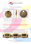
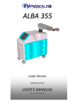
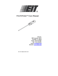
Basics of UV Measurement
PowerView Software® II
UV Radiometer Profiling Software
User’s Guide
For use with EIT® Power Puck® II and
UVICURE Plus® II Profiling Radiometers
UV Technical Support & Sales
EIT Instrument Markets
108 Carpenter Drive, Sterling, VA 20164
Voice: 703-478-0700 • Fax: 703-478-0815
Email: [email protected]
www.eit.com
P/N: IM-0077 Rev A • August 2012 •
UV Calibration & Service
EIT Instrument Markets
22815 Glenn Drive, Suite 104, Sterling, VA 20164
Voice: 703-652-7332 • Fax: 703-652-7340
Email: [email protected]
www.eit.com
PP/Plus 2 Profiler Guide
Page - 1
Table of Contents
Table of Contents
1. Basics of UV Measurement ……
Page 3
2. Collecting Data for use with PowerView Software® II …… Page 8
3. Installing the Software …… Page 13
4. Opening the PowerView Software® II …… Page 15
5. Importing Data from an EIT Radiometer …… Page 17
6. Quick Overview – Four Views of Your Data …… Page 25
7. Basic Navigation and Tools
…… Page 31
8. Using Cursors – Numerical Analysis …… Page 41
9. Setting Thresholds …… Page 48
10. Exporting Data …… Page 50
11. Advanced Analysis & Formatting Tools …… Page 59
12. Appendix A: Commands & Shortcuts …… Page 69
13. Appendix B: EIT UV Bandwidth Response Curves …… Page 70
14. Appendix C: Power Puck® II Profiler and UVICURE® Plus II
Profiler Instrument Specifications …… Page 72
P/N: IM-0077 Rev A • August 2012 •
PP/Plus 2 Profiler Guide
Page - 2
1. The Basics of UV Measurement
Basics of UV Measurement
Congratulations! As a PowerView Software® II user, you have already made a strong commitment to
accurate and reproducible UV measurement by purchasing one of the finest and most popular tools
available. The EIT PowerView Software® II application provides data analysis and file sharing capabilities
for your Power Puck® II Profiler and UVICURE® Plus II Profiler instruments.
This section is intended to be a quick explanation of the basic principles of UV measurement.
Why Should I Measure?
A common mantra in quality control is that “you cannot control what you do not measure.” The best
producers do not haul out their test equipment only when things fail – they monitor the condition of
their process often, and make corrections as they are warranted.
Here are a few reasons to measure the performance of your UV system:
•
•
•
•
•
To avoid costly downtime, rework and scrap due to diminished UV output
As part of an ISO-, or QS- SPC, or other quality assurance program
To optimize your curing process and increase productivity and profits
To communicate more clearly with partners, suppliers and customers
For suppliers - to document a curing process so it can be replicated in the field
What Should I Measure?
When you bake a cake, you care about two variables: oven temperature and cooking time. When you
cure UV materials, you are concerned about three factors: wavelength, power (or irradiance), and
energy (or energy density). Each of these parameters can alter the degree of cure at the surface, at the
substrate, or throughout the material.
Wavelength: The wavelength of a UV light source is determined by the lamp manufacturer, and should
be selected based on the recommendations of your chemistry supplier. Mercury-based lamps such as
arc or microwave sources commonly emit over a broad spectra ranging from 240-450nm. This spectra is
broken down further into bandwidths designated as the UVA, UVB, UVC and UVV bands.
P/N: IM-0077 Rev A • August 2012 •
PP/Plus 2 Profiler Guide
Page - 3
1. The Basics of UV Measurement
The distribution of energy across these bands depends on the design and operation of the lamp, since
additives (such as Iron or Gallium) can alter the spectra and change over time. UV LEDs are also supplied
with output specified at particular wavelengths. Unintended changes in energy within various
bandwidths can adversely affect properties such as surface or “through-cure”.
UVA, UVA2,UVB, UVC, UVV Transmission scan
100
90
80
Normalized %T
70
60
UVV
UVA
UVB
UVC
UVA2
50
40
30
20
EIT Inc.
2/26/09
10
0
230 240 250 260 270 280 290 300 310 320 330 340 350 360 370 380 390 400 410 420 430 440 450 460
wave length
®
®
The bandwidth response of EIT’s Power Puck II and UVICURE Plus II radiometers for each of the
UVA, UVA2 UVB, UVC and UVV bands measurement.
It is not uncommon for the emission of a UV lamp to change with respect to one bandwidth but not
another. This condition can affect your process and can easily be detected by comparing a reference file
with subsequent samples, on a bandwidth-by-bandwidth basis.
Power/Irradiance: Irradiance is the “brightness” of the light source. Irradiance falls off as the square of
the distance as you move away from the light (UV) source, or as the light source output diminishes for
any reason. It is common for some UV lamps to lose irradiance with time, or with frequent cycling of the
lamps. Dirty or damaged reflectors can also reduce irradiance, especially in the shorter wavelengths.
Irradiance is measured in Watts (W/cm2) or milliWatts (mW/cm2) per square centimeter. Although
different in meaning from a technical definition, irradiance is sometimes also called “intensity”.
P/N: IM-0077 Rev A • August 2012 •
PP/Plus 2 Profiler Guide
Page - 4
1. The Basics of UV Measurement
Energy/Energy Density: Irradiance alone is not a sufficient measure of the UV cure process, since
proper curing requires a certain amount of exposure time. Energy density is a measure of how much
power was received over a length of time. If you chart irradiance on a vertical axis against time on the
horizontal axis, energy density is the area under the curve. Although different in meaning from a
technical definition, Energy Density is sometimes also called “dose”. Be sure to communicate in the
same language and terms.
To calculate the area under the curve, your EIT radiometer takes frequent irradiance readings, and then
adds them together. The faster the sample rate, the more accurate the estimate of energy density.
Energy is measured in Joules (J/cm2) or milliJoules (mJ/cm2) per square centimeter.
Power / Irradiance
Peak Irradiance
Time
Energy density is the total amount of energy exposure over time. It is the mathematical
calculation of the area under the irradiance curve. The instrument calculates energy
density by adding many irradiance samples together. The numerical irradiance reported is
the peak irradiance value recorded by the instrument
NOTE: The irradiance value reported by the instrument can vary based on the sample rate of the
instrument and the speed at which the data was collected. More information is presented in Chapter 3.
P/N: IM-0077 Rev A • August 2012 •
PP/Plus 2 Profiler Guide
Page - 5
1. The Basics of UV Measurement
Where Should I Measure?
The EIT Power Puck® II Profiler and UVICURE® Plus II Profiler instruments are designed to be selfcontained, compact instruments that can be placed in the UV process environment. The optical window
on the radiometer should be positioned so that it faces the UV light source in the same location and
orientation as production parts in order to provide the most representative measurement of irradiance
at the part surface.
Note: Your EIT radiometer is a sensitive electronic device and should not be exposed to long, high UV
intensity runs with extremely high temperatures. An over temperature alarm will sound if the internal
temperature of the device goes over 65oC. Modify your data collection procedures to avoid damaging
the instrument if the alarm sounds.
If your instrument is too hot to touch, it is probably too hot to take a reading.
How Often Should I Measure?
Periodic measurement will help you detect problems before they affect your process. You should
establish a regimen that fits your production schedule. Some customers measure once during each
production shift, others once a day, some less often.
You should measure your process each time you make a significant alteration to your curing system,
such as lamp changes, reflector cleaning, lamp repositioning or line speed changes.
EIT also manufactures a number of products that provide continuous measurement of UV irradiance for
those customers who wish to constantly monitor UV output in real-time. These devices do not have the
same accuracy as your data logger, but used in combination with a Power Puck® II Profiler or UVICURE®
Plus II Profiler, provide a powerful combination for both tracking real time changes and gathering
absolute NIST traceable data. Visit the EIT website http://www.eit.com/uv-products/radiometersonline-monitors for more information about online monitoring products.
P/N: IM-0077 Rev A • August 2012 •
PP/Plus 2 Profiler Guide
Page - 6
1. The Basics of UV Measurement
Where Can I Get More Information on UV Measurement?
EIT offers a number of free, helpful publications on various aspects of UV measurement that are
available from its website at http://www.eit.com/uv-products/technical-papers-presentations . We also
have a knowledgeable, fully-trained group of sales representatives worldwide who can offer assistance
and advice. To locate a representative in your region visit:
http://www.eit.com/uv-products/representatives-and-distributors
P/N: IM-0077 Rev A • August 2012 •
PP/Plus 2 Profiler Guide
Page - 7
2. Collecting Data for use with PowerView II
Do I Have the Proper Instrument?
The EIT PowerView Software® II application is compatible with the latest generation of EIT Power Puck®
II Profiler and UVICURE® Plus II Profiler products.
Upgrading Power Puck® II or UVICURE® Plus II units to Profiler units
Power Puck® II or UVICURE® Plus II units in the field with a mini USB connector (top unit in image
below) can be upgraded to a Profiler unit. The upgrade option is not available for Power Puck® II or
UVICURE® Plus II units with a serial port (bottom unit in image below) or for legacy Power Puck or
UVICURE® Plus units.
Mini USB
Serial
The upgrade requires a hardware upgrade that is only available from EIT. The unit must be shipped to
EIT. Please contact EIT or your local representative or distributors for pricing and availability of this
upgrade and the needed hardware change.
The most current and up to date information on shipping an Instrument to EIT can be found on the EIT
website http://www.eit.com/uv-products/customer-service-support under: “UV Support, Calibration
and Service / How to Return a Unit to EIT”
Ship the unit prepaid to:
EIT Instrument Markets
22815 Glenn Drive/Suite 104
Sterling, VA 20164
Be sure to include company information, contact phone, fax and e-mail information in the package.
P/N: IM-0077 Rev A • August 2012 •
PP/Plus 2 Profiler Guide
Page - 8
2. Collecting Data for use with PowerView II
When returning the UV Power Puck® II or UVICURE® P Plus II unit, please return the equipment in the
original (or equivalent) packaging. You will be responsible for damage incurred from inadequate
packaging, if the original packaging is not used. The customer is responsible for insuring the unit during
transportation to EIT Instrument Markets. Please complete a copy of the Service Request Form and
send it with your shipment. This form MUST be completed and sent in with your unit(s).
NOTICE
The PowerView Software® II will not work with earlier generation products. Please check with EIT‘s
technical service department, or with your authorized EIT sales representative if you are unsure of your
hardware compatibility.
At this time the PowerView Software® II recognizes Power Puck® II Profiler and UVICURE® Plus II Profiler
*.tdms files, and the software will not recognize or display *.eit data files created using EIT PowerMAP
devices.
Basic Instrument Layout & Controls
The basic layout and controls for the EIT Power Puck® II Profiler and UVICURE® Plus II Profiler devices are
shown below:
P/N: IM-0077 Rev A • August 2012 •
PP/Plus 2 Profiler Guide
Page - 9
2. Collecting Data for use with PowerView II
Configuring Your Device for the PowerView II
As described in the Basics of UV Measurement, calculating energy density is accomplished by
mathematically summing many irradiance samples together (see Chapter 1). The sampling frequency of
the irradiance data points and calculation method can result in slightly different irradiance values.
In addition to the “Smooth On” and “Smooth Off” settings in the EIT Power Puck® II Profiler and
UVICURE® Plus II instruments, the Profiler version of the instruments has a third option called
“PROFILER” mode. Adjusting your instrument to “PROFILER” mode sets the effective sample rate of the
instrument to 128 samples/second. This is the rate at which the PowerView Software® II calculates the
irradiance and energy density readings from the transferred data. This allows the values calculated by
your radiometer (and shown on the instrument display) to closely match the values calculated by
PowerView Software® II.
For the best match between PowerView II and
the instrument display, select SMOOTH:
PROFILER in SETUP Mode.
To Change The SMOOTH Instrument Setting:
1. Enter the Setup Mode, using the soft button to the left of the display
2. Press and hold for 0.5 second, then release. The Setup screen will display the current settings.
3. Default modes will appear proceeded with an *asterisk.
4. To change selections between SMOOTH ON, SMOOTH OFF and SMOOTH PROFILER, use the down ↓
and right → arrow buttons located under the arrows to scroll in the indicated direction.
5. To change the default selection, first select the line, then the setting on each line.
6. Press the SAVE button to save the setting as the new default. An *asterisk will appear next to the
setting.
7. When the changes are completed, press the EXIT button to return to the default mode.
P/N: IM-0077 Rev A • August 2012 •
PP/Plus 2 Profiler Guide
Page - 10
2. Collecting Data for use with PowerView II
Note: The selected “smooth” mode the user has set in the instrument will be displayed by the
PowerView Software II® program. Note that the time and date that the information was transferred to
the computer is also displayed by PowerView II.
Taking a UV Measurement
The following Procedure appears in the Power UV Power Puck® II and UVICURE® Plus II User’s Manual.
The procedure is reproduced here for convenience, but readers are urged to consult the entire manual
before use. The user’s manual can be found on the EIT website at:
http://www.eit.com/instruments/100200%20PP2HU_revB.pdf
Turning On the Radiometer
Press and Hold the ON / OFF button until the display illuminates. The display will briefly display the
Radiometer Model Name, Serial Number, Software Version, Calibration Date, Range, and Wavelength
Bands installed. The display will then enter the default mode and display the data from the last run
before the unit was turned off.
Turning OFF the Radiometer
Press and Hold the ON / OFF button. A tone will sound. When tone stops, release the button. The unit
turns off.
Entering the RUN MODE
A short press of the “RUN” button clears the memory and puts the unit in the “RUN” mode. The display
shows “RUNNING” after shortly displaying the internal temperature of the unit. Confirm that the unit
displays “RUNNING” before initiating a reading.
Place the radiometer on the belt or object with the optic window looking toward the UV source. The
display and buttons will be facing away from the UV source. When the radiometer exits the curing
chamber, the display will still be flashing “RUNNING”.
CAUTION: Exposing the display to high UV radiation will damage the display.
P/N: IM-0077 Rev A • August 2012 •
PP/Plus 2 Profiler Guide
Page - 11
2. Collecting Data for use with PowerView II
Exiting the RUN MODE
A short press of the “STOP” button (Soft button display bar indicates “STOP” next to the
“ON / OFF” button) will exit the “RUN” mode and will return to the same default mode prior to making
the exposure run, but will display the new value.
P/N: IM-0077 Rev A • August 2012 •
PP/Plus 2 Profiler Guide
Page - 12
3. Installing the PowerView Software® II
Basic Installation Procedure
The EIT PowerView Software® II is digitally signed, and designed to run in a Microsoft Windows
environment and can installed on Windows XP, Windows NT, Windows Vista and Windows 7 platforms.
The system can also be installed on Apple computers that provide a dual boot operating system by
running the program using a Windows operating system.
If you are installing the software from a factory supplied CD-ROM, the CD should automatically launch
the installer utility which will guide you through the PowerView Software® II installation process.
If installing the program from other media, another file location, or in the event that the CD ROM
autorun file does not successfully launch, locate and double click the setup.exe file. Note that as part of
the installation procedure the software will also install needed National Instruments LabVIEW files.
Users on certain secure local area networks may need to consult with their System Administrator for
assistance installing the software.
Windows driver files called INF files associate hardware (such as the Power Puck II Profiler or UVICURE
Plus II Profiler instruments) to the software (PowerView Software II). The INF files are needed to allow
the hardware (instrument) to transfer the collected data files to the software.
During installation, the software will load hardware driver software for the EIT Power Puck II and
UVICURE Plus II Profiler radiometers. The version of Windows on your computer and how it is set will
determine if the INF files are automatically associated with the program.
If your instrument is not automatically recognized when transferring data (Chapter 5), you may need to
do a one-time association of the instrument INF file to the software.
P/N: IM-0077 Rev A • August 2012 •
PP/Plus 2 Profiler Guide
Page - 13
3. Installing the PowerView Software® II
If you are Using Windows XP, the driver file is named PowerPuck2.inf
If you are using Windows NT, Vista or Windows 7, the driver file is named PowerPuck2_vista.inf
Once installed, these files should be located in the c:\Windows\Inf with a copy also located at
c:\Program Files\EIT\PowerView II\data file location as shown below.
The software has been optimized for a minimum display resolution of 1280 x 800. If your display
supports a lower screen resolution, scroll bars are automatically displayed to allow you to scroll to all
parts of the screen.
P/N: IM-0077 Rev A • August 2012 •
PP/Plus 2 Profiler Guide
Page - 14
4. Opening the PowerView Software® II
Starting the PowerView Software® II Application
Once installed, the EIT PowerView Software® II application can be started by clicking on the PowerView
II icon on your desktop, or by selecting it from the Programs menu of your Start Button. From the Start
Button you can select EIT → PowerView II → PowerView II to open the application.
Accessing PowerView from the START Menu
The PowerView II Desktop Icon
Either action should launch the PowerView Software® II application. It may take a minute or two to load
the software package during which time you should see the following welcome screen:
The PowerView II Welcome Screen
P/N: IM-0077 Rev A • August 2012 •
PP/Plus 2 Profiler Guide
Page - 15
4. Opening the PowerView Software® II
Once the software has fully loaded, the main EIT PowerView® II screen should appear. You may need to
adjust your monitor’s display settings so that you can see the entire screen on your monitor. Notice that
there are four “tabs” and the default “Graph by File” view is selected.
The Default PowerView II Graph by File Screen
P/N: IM-0077 Rev A • August 2012 •
PP/Plus 2 Profiler Guide
Page - 16
5. Importing Data from your EIT Radiometer
Importing Data
Data collected by a Power Puck® II Profiler or UVICURE® Plus II Profiler radiometer can be downloaded
from the device and saved on your computer as a data file (with a .tdms extension). This data can then
be viewed, analyzed and exported to other programs such as Microsoft Excel® using the EIT PowerView
Software® II application.
To Download Data from a Power Puck® II Profiler or UVICURE® Plus II Profiler Radiometer:
1. Connect the device to the computer using the factory supplied USB to mini-USB connector. (Note:
The mini-USB cable is a standard cable that is widely available if your cable is lost, misplaced or
damaged. The cable can also be purchased from EIT if desired.
Connecting a Radiometer via the radiometer’s mini-USB connector
2. Turn on the device by depressing the Power on/off button
Depress the Power button to energize the radiometer
P/N: IM-0077 Rev A • August 2012 •
PP/Plus 2 Profiler Guide
Page - 17
5. Importing Data from your EIT Radiometer
3. On the EIT PowerView® II toolbar, select: Device → Read Powerpuck II
Transfer data by selecting → Read Powerpuck II
As you will see throughout this manual, there are often two ways to perform common tasks - one, using
the toolbar as in the example above, and another shortcut method using the right-click button on your
mouse.
Many PowerView II Software features can be
accessed easily by right-clicking when your
mouse is properly positioned on the screen.
To transfer data from your radiometer to the PowerView Software® II program, you can also point your
mouse to the Sample File dropdown menu in the upper right corner of the screen and depress the rightclick button. This will activate a dialog box which contains the Read Powerpuck II option
Transfer data by selecting → Read Powerpuck II from the right-click menu
when the cursor is located in the Sample or Reference File dropdown menu.
P/N: IM-0077 Rev A • August 2012 •
PP/Plus 2 Profiler Guide
Page - 18
5. Importing Data from your EIT Radiometer
4. You should observe the “Reading Data” dialog box while data is being imported from your device into
the EIT PowerView Software® II application.
Reading data from your radiometer does not remove any data from the device, but merely copies the
data into the software for analysis. Your original data is preserved in the instrument until you take a
new reading by entering the RUN mode.
Note: The file structure and storage location for ‘behind the scenes’ files varies significantly for different
versions of Windows. If the PowerView Software® II fails to recognize your EIT radiometer, or
succesfully transfer data, please refer to the PowerView Software® II Troubleshooting Guide available on
the EIT website at: http://www.eit.com/uv-products/technical-product-notes-and-user-manuals
September 2012: Not posted yet: Contact EIT for assistance
P/N: IM-0077 Rev A • August 2012 •
PP/Plus 2 Profiler Guide
Page - 19
5. Importing Data from your EIT Radiometer
Creating Data File Names
You will be prompted to choose or enter a filename and location for the data file. You may use the
factory selected default location, or create a new file folder and location.
Transfer data by selecting → Read Power PUCK II from the right-click menu
when the cursor is located in the Sample or Reference File dropdown menu.
Enter a file name which is useful to you in describing the contents of the data in the file and then select
This procedure will transfer data from your EIT radiometer and create a file for the data in the specified
location.
P/N: IM-0077 Rev A • August 2012 •
PP/Plus 2 Profiler Guide
Page - 20
5. Importing Data from your EIT Radiometer
Data File Shortcuts
Files displayed on the drop down menu are actually shortcuts to the actual files stored in a data folder.
The shortcuts allow easy access to the most recent files used.
The shortcuts are created automatically when the data is transferred from the instrument.
The Data folder which contains your transferred files has the actual data file (*.tdms) and the shortcut
associated with the data file (*.tdms_index). See the groups of files below.
You may choose the default location shown by the software, or can navigate to any directory and folder,
or create a new folder for your data just as you normally would with Windows Explorer.
P/N: IM-0077 Rev A • August 2012 •
PP/Plus 2 Profiler Guide
Page - 21
5. Importing Data from your EIT Radiometer
PowerView Software® II files may be exchanged electronically (Email, USB Stick). The “shortcut” will not
be on your computer and you will need to ‘open’ the file as a sample or reference from either the drop
down menu or by right clicking on the Sample or Reference menu.
Organizing your Data Files
Data files all look pretty much the same to the PowerView Software® II. Neither your radiometer, nor
the PowerView Software® II can tell anything about whether the data is intended to be a reference file
or a sample. It cannot tell you anything about which lamp, or for what product, the data was collected,
or who collected it. So if these details are important to track, proper note taking and data organization
is imperative.
P/N: IM-0077 Rev A • August 2012 •
PP/Plus 2 Profiler Guide
Page - 22
5. Importing Data from your EIT Radiometer
Fortunately the PowerView Software® II provides several tools to help you add notes, and organize your
data files. The note taking capabilities will be described in Chapter 7, but you should first decide how
you want to organize your files. Common choices include:
•
•
•
•
•
•
By UV system type (arc, microwave)
By lamp type (mercury, mercury-iron, etc.)
By system or production line
By date
By customer
By other process or R&D parameter such as the formulation, power supply, substrate type, etc.
Example of standard data transferred to the computer from the instrument
From the Toolbar select Configure → Paths
Launch the Configure Paths window from the Toolbar
This opens the Configure Paths window which will allow you to specify a new folder name, or location
for your data files, and sample and reference shortcuts. You may choose locations that are appropriate
to your work environment and naming conventions by clicking the folder icons.
P/N: IM-0077 Rev A • August 2012 •
PP/Plus 2 Profiler Guide
Page - 23
5. Importing Data from your EIT Radiometer
Change folder names and locations for your files from the Configure Paths window
P/N: IM-0077 Rev A • August 2012 •
PP/Plus 2 Profiler Guide
Page - 24
6. Quick Overview – Four Views of your Data
An Overview – The Four Types of PowerView® II Screens
Once the software has loaded, the main EIT PowerView Software® II screen will appear. You may need
to adjust your monitor’s display settings so that you can see the entire screen on your monitor without
scrolling. (Note: The PowerView Software® II has been optimized for a 16:9 aspect ratio to eliminate the
need to scroll during use, and this setting should be selected when possible.)
When the EIT PowerView Software® II loads, it defaults to the Graph by File screen. This is one of four
ways to view data in PowerView Software® II. The other choices are to Graph by Band, or to display a
Table, choose either Table by File, or Table by Band. Simply select the Tab for the view you wish to use.
These four choices present the same radiometric data in different formats. They make it more
convenient to perform different types of data analysis.
We begin by introducing the basic function and motivation for each of the four views before describing
how to navigate and manipulate these views.
1. The Graph by File Tab
The Graph by File view is ideal for visually comparing two different data files. One of these files is
referred to as a SAMPLE file, and the other file is described as the REFERENCE file.
There is nothing physical that differentiates a sample file from a reference file other than referring to
them by these names. It is common practice however to compare fresh data samples to a benchmark,
or reference set of data that might have been collected when new lamps were installed and the line was
operating perfectly. So, you may wish to give reference files a filename that distinguishes them as
reference data so they can be easily identified.
P/N: IM-0077 Rev A • August 2012 •
PP/Plus 2 Profiler Guide
Page - 25
6. Quick Overview – Four Views of your Data
The screen below shows a typical plot in the Graph by File view. Drop down menus in the upper right
corner allow you to select a sample file and reference file for comparison (although there is nothing that
requires you to actually plot two graphs). You could, and often will want to display only a single plot.
As will be described in much more detail, the numerical calculations performed in this view compare the
radiometer data for the sample file to the reference file.
2. The Table by File Tab
Table by File is a numerical view of the same data used to produce the Graph by File plots. Like Graph
by File, Table by File is used to compare various aspects of two data files, usually a sample and a
reference file.
In Table by File view, as shown in the screen below, numerical data for each file is presented in adjacent
columns. A third column, labelled “Difference” compares the data in the Sample and
P/N: IM-0077 Rev A • August 2012 •
PP/Plus 2 Profiler Guide
Page - 26
6. Quick Overview – Four Views of your Data
Reference file columns, and by convention, compute the difference between the sample and the
reference file (i.e. Reference – Sample = Difference).
The organization of the rows of the Table by File view is determined by the Table View dropdown menu
which can be set to either Parameter view or Bandwidth view.
The Table View dropdown menu
A) Parameter View:
When Parameter view is selected, the rows of the table contain the UV parameters: Power (grouped by
UV band) and Energy (grouped by UV band). Each parameter is presented in both absolute terms (e.g.
mW/cm2 and mJ/cm2) and as Power% and Energy% which reports the percentage difference between
the Sample and the Reference (grouped again by UV band).
Note: If the cursors are turned OFF, (as will be discussed in the Advanced User Tools chapter), the
maximum values for each bandwidth are displayed and used to compute the differences. If the cursors
are turned ON, the values displayed will correspond to the sample and reference cursor locations. The
status of the cursors is indicated on the cursor row near the bottom of the table.
If the dropdown Table View menu is changed to Bandwidth view:
Table by File using Parameter View
P/N: IM-0077 Rev A • August 2012 •
PP/Plus 2 Profiler Guide
Page - 27
6. Quick Overview – Four Views of your Data
B) Band View
In Band view, the same data is arranged differently. In this view, the Sample, Reference and Difference
columns remain the same, but the rows are organized by grouping the parameters (Power level,
Power%, Energy level and Energy%) by Band as shown below. The influence of the cursor status on the
numerical values displayed is the same as it is in Parameter view.
Table by File using Bandwidth View
The Graph by File and Table by File views are motivated by similar questions such as “how do I compare
two radiometers and examine the differences between the two?” The Graph by File and Table by File
views are the most common choice.
3. The Graph by Band Tab
Selecting Graph by Band allows you to compare up to four sources at once within a single selected UV
bandwidth. The plot below illustrates that in this view, each source is represented by a different color
plot making visual comparisons easier. The upper right corner now presents dropdown menus to select
both the bandwidth of interest, and up to four data files.
P/N: IM-0077 Rev A • August 2012 •
PP/Plus 2 Profiler Guide
Page - 28
6. Quick Overview – Four Views of your Data
In addition to the graph, this view also provides a numerical Summary of the data in the lower right
corner of the screen. To select which data files are used for the numeric Summary calculations, use the
Sample File dropdown menu to select from among the four sample files. Note that the file listed in the
top position is used as the Reference file for calculations.
Once again, the status of the cursors (e.g. ON or OFF) will determine whether the numerical data
displayed in the summary and cursors panes is the maximum reading for the Sample file selected
(Cursors OFF), or the Power level at the cursor, and Energy calculated between the cursor locations
(cursors ON).
Here you see a comparison between the (dotted) reference file and (amber) sample file viewed in the
UVA band.
Graph by Band example
4. The Table by Band Tab
The Table by Band tab presents a tabular arrangement of the same data used in the Graph by Band
view. For the band selected (from the upper right dropdown menu), the table presents the measurment
parameters (absolute Power levels, %Power difference, absolute Energy levels, and Energy% difference)
for each Sample compared to the Reference file. These figures appear in the columns of the table.
(Note that the file selected in the top dropdown menu location is designated as the reference file for
comparisons.)
P/N: IM-0077 Rev A • August 2012 •
PP/Plus 2 Profiler Guide
Page - 29
6. Quick Overview – Four Views of your Data
The rows of the table group the data in three different ways that facilitate your analysis: the first group
reports the values for each Sample and the Reference file. The second group of rows reports the
difference in Power and Energy between each Sample and the Reference file. Finally, the third group of
rows provides the difference between each pair of samples. This group also includes some statistical
information useful when you have more than one sample. The software calculates the mean, standard
deviation and variance of each parameter for all of the samples selected.
In the example below, three samples are compared to a reference file. The values for each Sample and
how each compares to the Reference are reported. The Table also indicates that the average Power for
the three samples is about 308.5 mW/cm2, or about 8.4% less than the reference. But thePowerView
Software® II also makes it easy to observe that Sample 1 is lower than both Sample 2 and Sample 3,
while Samples 2 and 3 are much closer in value to each other. This might cause us to question what
process conditions led to the lower values recorded for Sample 1.
Table by Band provides Sample Information, Differences and Statistical Information
P/N: IM-0077 Rev A • August 2012 •
PP/Plus 2 Profiler Guide
Page - 30
7. Basic Navigation & Tools
The EIT PowerView Software® II application has a number of powerful tools for analyzing UV radiometer
data. In this chapter, we begin by describing how to open your data, select which bandwidths to display,
and how to navigate the graphs using the ZOOM control options. We also introduce the Summary
feature obtaining numerical values and comparisons from your datasets.
Opening Your Data Files for Analysis
Once data has been downloaded from an EIT Power Puck® II Profiler or UVICURE® Plus II Profiler, and a
shortcut has been created, these files are accessible within the PowerView Software® II application from
the Sample File and Reference File pull down menus that are located just outside the upper right corner
of the graph.
It is a common practice to create a “reference file”, made when the line is operating under optimum
conditions. This reference file can be used as a benchmark for comparing subsequent samples to verify
that the process is operating properly. It is a good idea to name the reference file so that it can be easily
identified and distinguished from sample data files to avoid confusion.
For example, to open the reference file, click on the dropdown menu and select the desired reference
file by name.
To begin, access data files via the dropdown menus
P/N: IM-0077 Rev A • August 2012 •
PP/Plus 2 Profiler Guide
Page - 31
7. Basic Navigation & Tools
Opening the reference file first, before the sample file, is a good practice since the software will
automatically scale the graph according to the reference data which is usually equal to, or greater than
subsequent samples.
The selected Reference file is displayed on the Graph by File Screen
Now open the sample file by clicking on the appropriate file name in the Sample File pull down menu.
Repeat the selection process for the Sample data File
P/N: IM-0077 Rev A • August 2012 •
PP/Plus 2 Profiler Guide
Page - 32
7. Basic Navigation & Tools
The Sample and Reference Graphs are now both displayed in PowerView Software® II:
The selected Reference and Sample Files are displayed on the graph
Radiometer data is visible in the Information & Notes panes
Note that the software automatically displays the instrument’s display values in the Information & Notes
panes for both the sample and reference files. Along with the recorded data, the software also displays
the devices Serial Number, internal temperature, and other device specific parameters.
P/N: IM-0077 Rev A • August 2012 •
PP/Plus 2 Profiler Guide
Page - 33
7. Basic Navigation & Tools
Editing Sample Information & Notes
Since accurate record keeping and organizing data is of such great importance, we introduce the
Information & Notes editor feature of the PowerView Software® II early in this manual. Some additional
editing tools for note taking are presented in Chapter 11.
The Information & Notes can be edited and annotated by a simple procedure:
1. Right Click while the cursor is positioned within the Information & Notes pane.
Right click in the pane to launch the Edit Notes button
2. Click on the Edit Notes button that appears. This will open an editing window that permits free form
entry of additional information:
The Information & Notes editor screen
P/N: IM-0077 Rev A • August 2012 •
PP/Plus 2 Profiler Guide
Page - 34
7. Basic Navigation & Tools
3. After editing, click OK
The editing window will be closed, and the Sample Information & Notes will be updated.
12.
Example of additional notes and comments added
Selecting which Bands to Display
You can select which UV band(s) to display on sample and/or reference graphs by checking the desired
bands. This makes it easier to focus on wavelength specific features of the data.
Selecting which UV Bands display
P/N: IM-0077 Rev A • August 2012 •
PP/Plus 2 Profiler Guide
Page - 35
7. Basic Navigation & Tools
In the example above, only the UVA band has been selected for both the Sample and Reference. This
will result in the following simplified display which shows only UVA band data:
Only selected bands are plotted in the resulting graph
Using the Zoom Controls
The Zoom tool (identified by a magnifying glass icon) provides several aids to navigating graphs.
Clicking on the Zoom (magnifying glass) icon will reveal several Zoom options.
Several Zoom tools are available for different tasks
P/N: IM-0077 Rev A • August 2012 •
PP/Plus 2 Profiler Guide
Page - 36
7. Basic Navigation & Tools
The Zoom Control options perform the following tasks:
This tool zooms on a user-selected rectangular area. Click on the tool to select it, and then
position the cursor so that it is located at one corner of the desired rectangular area. Press the left
mouse control button to select that corner of the desired area. Then, while continuing to depress the
left mouse button, drag the mouse to the opposite diagonal corner of the desired rectangle. Releasing
the left mouse button will anchor the entire rectangle, and the software will zoom on the selected area.
This tool zooms on a user-selected portion of the graph time line (x-axis). Click on the tool to
select it, and then position the cursor so that it is located at one end of the time period of interest. Press
the left mouse control button to select one extreme of the desired range. Then, while continuing to
depress the left mouse button, drag the mouse to the opposite edge of the range. Release the left
mouse button to zoom on the selected time period of the graph.
This tool zooms on a user-selected portion of the graph y-axis. It is useful for magnifying portions
of the graphs to look at Power (irradiance) detail. Click on the tool to select it, and then position the
cursor so that it is located at one end of the power level of interest. Press the left mouse control button
to select one extreme of the desired range. Then, while continuing to depress the left mouse button,
drag the mouse to the opposite edge of the range. Release the left mouse button to zoom on the
selected irradiance portion of the graph. Note that this expands the Power axis across the entire time
period of the graph.
This tool performs a Zoom Out function. Click on the tool to select it, and then position the
cursor on that portion of the graph you wish to Zoom Out from. Pressing the left click button will zoom
out from the current cursor location in both the X- and Y- direction. Each time the button is clicked, the
magnification will be increased. If the mouse is moved to a new location and pressed, the graph will
Zoom Out from the new location.
P/N: IM-0077 Rev A • August 2012 •
PP/Plus 2 Profiler Guide
Page - 37
7. Basic Navigation & Tools
This tool performs a Zoom In function. Click on the tool to select it, and then position the cursor
on that portion of the graph you wish to Zoom In from. Pressing the left click button will zoom in from
the current cursor location in both the X- and Y- directions. Each time the button is clicked, the
magnification will be decreased. If the mouse is moved to a new location and pressed, the graph will
Zoom In from the new location.
This tool is a Zoom “undo” button. Click on this icon to restore the graph to its default zoom
setting. This button has the same effect as the Zoom All button:
Use the Zoom All or Zoom Undo buttons if you want to quickly restore the graph settings to the default
view.
A slider control, located just below the graph allows the graph to be repositioned from left to right
should portions of interest be out of range in the current display. This is especially useful when the
ZOOM controls are used as will be described in more detail below.
Detail of the Slider Control used to
reposition a Graph on the X-axis
P/N: IM-0077 Rev A • August 2012 •
PP/Plus 2 Profiler Guide
Page - 38
7. Basic Navigation & Tools
Viewing Summary Data
Though the EIT PowerView Software® II provides a number of graphical analysis tools, it is also useful for
analyzing hard numerical data as we introduced in Chapter 6 in describing the Table by File and Table by
Band views.
Numeric data is also summarized in the Graph by File and Graph by Band views. The Summary data
window located in the lower right of the screen is useful in comparing values for the peak irradiance
(Power) and energy density (Energy) between reference and sample readings.
Initially, the Band dropdown menu will display a default N/A value and consequently no data is
displayed. Using the Band dropdown menu, select a measurement band of interest (e.g. UVA, UVB,
UVC, etc.) and the PowerView Software® II will display the appropriate peak irradiance and energy
density values for the sample and/or reference files you have selected. The software will also calculate
the percentage difference in Power and Energy between the sample and the selected reference file.
The Band dropdown menu (with default N/A Status)
Note: The values displayed in the Summary data pane depend upon whether the cursors feature has
been turned on or off. For more information about using cursors, see Chapter 8 below.
With the CURSORS button toggled to the off position, (the default on software startup) the summary
data will display the maximum value for the selected Band. With CURSORS turned ON, (indicated by a
green color) the data displayed will be the Power and Energy values of the selected band at the current
cursor location.
P/N: IM-0077 Rev A • August 2012 •
PP/Plus 2 Profiler Guide
Page - 39
7. Basic Navigation & Tools
The Summary data displayed with a Band (e.g. UVA) selected. Note that Cursors are off
Detail of Summary data for a Reference and Sample file
In this example, the sample is 12.70% lower than the Reference in Power (mW/cm2) and 27.99% lower
than the Reference in Energy (mJ/cm2).
P/N: IM-0077 Rev A • August 2012 •
PP/Plus 2 Profiler Guide
Page - 40
8. Using Cursors – Numerical Analysis
Understanding the Graph Axes
The previous section introduced the basics of displaying graphs and data. Graphs in PowerView
Software® II display Power on the vertical, or Y-axis, and Time along the horizontal, or X-axis.
Graphs in PowerView II present data by plotting Time on the X-axis and Power on the Y-axis
Time begins at 00:00 (minutes: seconds) and corresponds to the time when data logging was initiated.
The graph above shows the data recorded by a Power Puck® II Profiler traveling on a conveyor with two
lamps. The peak of the first lamp is at approximately 2.3 seconds, and the second at approximately 6.8
seconds.
Activating the Cursors
The EIT PowerView Software® II allows you to add positionable cursors that help provide more precise
numerical data from anywhere in the displayed graph. One method of activating the cursor feature is to
click on the Cursors toggle button so that the green indicator is shown. Note that the cursors can only be
activated if a Bandwidth has been selected from the Bandwidth dropdown menu. The cursor will
always display information associated with the bandwidth selected.
The Cursor Toggle Button
P/N: IM-0077 Rev A • August 2012 •
PP/Plus 2 Profiler Guide
Page - 41
8. Using Cursors – Numerical Analysis
This will activate a pair of cursors. We will refer to these as the Left-Hand and Right-Hand cursors.
Two Cursors are Displayed
The cursors can also be activated by right clicking and selecting cursors from the sub-menu provided a
bandwidth has been selected (otherwise the cursors option will not be active).
Cursors can also be activated by right-clicking on the graph when a file is present and a band is selected
Once the cursors have been activated, right clicking on the graph area will present a sub-menu with
various Cursor Control options. Notice how the “Center Cursors” and “Select Cursors” are now activated
Cursor Controls in the sub-menu
P/N: IM-0077 Rev A • August 2012 •
PP/Plus 2 Profiler Guide
Page - 42
8. Using Cursors – Numerical Analysis
The Cursor Positioning, Zoom and Hand icons are all used to help analyze the data. Only one icon may be
“active” at a time. The “active” icon is indicated by a small green “dot” and gray background.
The Cursor Positioning Tool
The Hand Positioning Tool
The Zoom Tool
Positioning the Cursors
Begin by making sure the Cursor Positioning icon is active.
When the mouse hovers near either cursor, a cursor movement icon appears. Press and hold the left
mouse button and drag the cursor to the desired location.
A movement Icon appears when the mouse hovers near a
cursor
Position cursors using your mouse, or entering a numeric value for the time.
P/N: IM-0077 Rev A • August 2012 •
PP/Plus 2 Profiler Guide
Page - 43
8. Using Cursors – Numerical Analysis
The cursor can also be moved by incrementing/decrementing the time associated with the current
cursor position, or by direct numeric entry of a specific time.
Adjust the cursor position by changing the time of its position
This is a useful method of “fine tuning” the cursor position once it has been dragged close to the desired
location.
Cursors and Numeric Data
When the cursor feature is activated, the numeric summary and cursor data depends on the absolute
and the relative position of the two cursors.
The Left-Hand cursor displays Power values (mW/cm2) in the left hand data column, while the righthand cursor displays Power values in the center (Ref.) column.
The Energy value displayed is the Energy in that region of the graph that lies between the two cursors.
This is a useful tool for measuring the Energy of each light source when there are multiple light sources
since the cursors can be positioned to the left and right of each successive peak to measure the Energy
of each individual peak.
But users should take care in interpreting measurements when the cursors are activated by noting the
position of the cursors and that they reflect the intended measurement.
P/N: IM-0077 Rev A • August 2012 •
PP/Plus 2 Profiler Guide
Page - 44
8. Using Cursors – Numerical Analysis
The following example is illustrative of how the cursor data for a Sample is displayed:
Right- Hand
Cursor
Left-Hand
Cursor
00:06.70
In Green
The left hand cursor in green is at 00:06.00 seconds on the x-axis. The irradiance value where the cursor
intersects the profile is 38.960 mW/cm2
In Purple
The right hand cursor in purple is at 00:06.70 seconds on the x-axis. The irradiance value where the
cursor intersects the profile is 180.710 mW/cm2
In Red
The time difference between the two cursors is in red and is 00:00.70 seconds. The Energy Density of
74.943 mJ/cm2 is the Energy Density between the two cursors and under the curve
Superimposing Graphs with the Sync Tool
It is frequently instructive to compare two graphs by superimposing them. This technique makes it
easier to visually compare different features that could be associated with properties of the lamps,
reflectors, or other components. The SYNC PLOTS button is used to overlay two points in the plot area. It
does this by horizontally aligning the Reference and Sample cursors.
P/N: IM-0077 Rev A • August 2012 •
PP/Plus 2 Profiler Guide
Page - 45
8. Using Cursors – Numerical Analysis
To overlay two graphs using the EIT PowerView Software® II application:
1. Position each of the two cursors on corresponding parts of the curve. These two locations will be used
to sync the graphs. For example, a cursor has been located on each of the peaks in the graph below.
Position cursors to the points on each plot that will be superimposed
2. Click on the SYNC PLOTS button
Select Sync Plots to Overlay the cursors
The plots can also be synchronized by right clicking on
the mouse with the cursor on the graph
P/N: IM-0077 Rev A • August 2012 •
PP/Plus 2 Profiler Guide
Page - 46
8. Using Cursors – Numerical Analysis
This action will overlay the two plots at the position of the two cursors as shown below:
The result of Syncing Cursors – overlaid Plots
Note that the Zoom and the Cursor functions can also be accessed by right-clicking while the mouse is
contained in the main graph pane. This will launch a sub-menu of tool choices.
Right Click for the Zoom and Cursor Options Menu
Note the Sync Plots feature can be accessed from this sub menu, as well as an UnSync Plots option.
Selecting UnSync Plots after Syncing Plots returns the files to their orignal state and can be thought of as
having a “reload files” effect on your work.
P/N: IM-0077 Rev A • August 2012 •
PP/Plus 2 Profiler Guide
Page - 47
9. Setting Thresholds
Why Set a Threshold?
A threshold “sets the bar” for what UV measurements the PowerView Software® II will consider for
display and calculations. Readings below the threshold will be disregarded for these purposes.
Sometimes a threshold is used to eliminate stray UV measurements inadvertently recorded by the
instrument (due to poor system shielding for example). Or, setting a threshold can be used if the
instrument reports “negative numbers.” Due to changes in conditions, and instrument variation, it Is
not uncommon to see small negative numbers close to zero in the data. Setting a zero threshold makes
Energy Density calculations more realistic.
How to Set a Threshold
The EIT PowerView Software® II uses NO THRESHOLD as its default. This means all data recorded is used
for display and calculation.
To set a threshold:
1. Turn on the Threshold by clicking the Threshold radio button in the lower right corner of the screen.
By default, thresholds are turned off.
2. The numerical value for the threshold may be entered directly by clicking in the number display pane,
or by incrementing/decrementing the threshold value up/down buttons. Here, a (large) value of 20
mW/cm2 is entered.
Turn on thresholds and enter a numeric value.
P/N: IM-0077 Rev A • August 2012 •
PP/Plus 2 Profiler Guide
Page - 48
9. Setting Thresholds
The Effect of a Threshold
Setting a threshold to disregard radiometer data below the designated value, will reduce the Energy
Density (mJ/cm2) when positive Power values are ignored, and raise the Energy Density when negative
Power values are disregarded.
Consider the following example:
An example of the effect of Threshold level on Energy calculations
In this example, without applying a Threshold, the peak Power is 325.695 mW/cm2 in the UVA band with
total Energy of 368.234 mJ/cm2 (between the two cursors shown).
When a Threshold of 20.000 mW/cm2 is applied, there is no change in the Power level, but the Energy is
reduced to 325.695.
For purposes of illustration, we have depicted the threshold (which is not actually displayed in
PowerView Software® II) by the dashed red line on the sample graph. The effect of the Threshold
control, is to cause all measurments below the dashed line to be eliminated from the Energy
computation.
P/N: IM-0077 Rev A • August 2012 •
PP/Plus 2 Profiler Guide
Page - 49
10. Exporting Graphs, Tables, and Data Sets
Moving Beyond PowerView Software® II
As powerful as the EIT PowerView Software® II application can be, there are times you will want to
export graphs, data tables and even your raw data for use with other programs, perhaps for further
analysis, reporting, or sharing with colleagues and suppliers. The software has tools that allow you to
save graph images, and to export data tables and data sets in standard formats that can be read by
programs like Microsoft Excel® and other statistical software.
Exporting Graphs
Depending on your preference, there are two convenient methods for exporting a PowerView
Software® II graph. The PowerView Software® II program exports the graph as an Image in a standard
file format such as a JPEG graphic file.
1. From the Toolbar, select File → Export Image…
Saving a Graph using from the Toolbar
2. This will launch the Export Front Panel dialog box.
The Export dialog box with Format
and Destination Options
P/N: IM-0077 Rev A • August 2012 •
PP/Plus 2 Profiler Guide
Page - 50
10. Exporting Graphs, Tables, and Data Sets
3. Several file formats are available from the dropdown menu:
Graphs may be saved in several formats
4. The file may be saved either to the Clipboard so it can be cut and pasted into another application, or
saved to a File on your computer. The File command will open Microsoft Explorer to allow you to
choose a location to store the file by selecting the Export Key
Target options for saving graphs
An alternative method of exporting a graph is to Right Click on the graph, launching a sub-menu which
permits you to select Export Graph Image and open a similar Export dialog box.
Right clicking on a graph also
provides a means to export graphs
P/N: IM-0077 Rev A • August 2012 •
PP/Plus 2 Profiler Guide
Page - 51
10. Exporting Graphs, Tables, and Data Sets
Exporting Data Tables
To export data to Microsoft Excel® or other statistical software package, right-click on the data table in
either the Table by File or Table by Bandwidth tabs.
Right click on a Table to open the CSV File save dialog box
This will launch the Export Table to a CSV dialog box where you can select the storage location for the
data file and select a suitable File Name. The CSV (Comma Delimited) format is a common standard
which can be opened by Microsoft Excel® and other statistical analysis programs.
Select a File Name and storage location.
P/N: IM-0077 Rev A • August 2012 •
PP/Plus 2 Profiler Guide
Page - 52
10. Exporting Graphs, Tables, and Data Sets
EIT provides users with access to the raw sample data collected by your radiometer. This data allows
advanced users to create their own graphical and numeric analysis using other software applications.
Since the raw data is stored in a .tdms format, to facilitate access to the data during installation, the
PowerView Software® II installs a utility, developed by National Instruments® used to import .tdms files
into Microsoft Excel®. Once in Excel®, the data can be viewed, manipulated, saved or exported in
another convenient format (e.g. comma delimited, .csv file format). A troubleshooting guide for the
National Instruments TDM importer add-in is available on the EIT website at: http://www.eit.com/uvproducts/technical-product-notes-and-user-manuals
NOTE: It is a good practice to always back up important data to protect against unintended loss when
performing these data handling procedures.
Importing a TDMS File into Excel®
Two methods of opening your data in Excel® are described below - first, by selecting a file and opening
the application, and second from within Excel® itself.
1. Opening Data Files from Within Excel®
Once the PowerView Software® II is properly installed, the TDMS Importer utility should be visible in
Microsoft Excel® as an Add-In program.
®
The TDMS import utility appears as an Excel Add-In
P/N: IM-0077 Rev A • August 2012 •
PP/Plus 2 Profiler Guide
Page - 53
10. Exporting Graphs, Tables, and Data Sets
Clicking on the TDMS installer will open a browser that allows you to select which TDMS file you wish to
open.
Clicking on the Add-In opens a file browser to locate and select the TDMS file of choice
Click on the desired TDMS file and an Excel workbook will open:
The root page of a sample file with summary and device information
P/N: IM-0077 Rev A • August 2012 •
PP/Plus 2 Profiler Guide
Page - 54
10. Exporting Graphs, Tables, and Data Sets
2. Opening Data Files in Excel by Right Clicking on File Names
You can also open your data files in Excel by locating the file and right-clicking.
1. Locate the .TDMS file of interest. You can check the Configure → Paths screen to remind yourself of
the location, or use Microsoft Windows Explorer®. (Reminder: Using descriptive file names make
locating files easier).
The TDMS file icon
Note that you want to import the TDMS file and not the shortcut which will have a TDMS_INDEX file
designation.
2. Right click on the TDMS file name to open the submenu:
Right click to open the sub menu
P/N: IM-0077 Rev A • August 2012 •
PP/Plus 2 Profiler Guide
Page - 55
10. Exporting Graphs, Tables, and Data Sets
3. Choose to open the file from a list.
Choose to select a program from a list
4. Select the Excel® Importer program from the list of applications. You may have the option to check a
box that will ask you if you always want to use this software to open your TDMS files. Selecting this
option makes opening files quicker in the future.
®
Select the Excel Importer from the Programs list
P/N: IM-0077 Rev A • August 2012 •
PP/Plus 2 Profiler Guide
Page - 56
10. Exporting Graphs, Tables, and Data Sets
5. Selecting Excel® Importer will open your data file in Microsoft Excel®.
Working with Radiometric Data in Excel®
Note that there are two Tabs in this new workbook: the root tab which contains summary information
about the sample and data about the instrument used, and a second screen which contains the
radiometric data.
To view the raw data, select the Signals tab at the bottom of the Excel® sheet
Selecting between the root sheet, and the Signals (data) sheet
P/N: IM-0077 Rev A • August 2012 •
PP/Plus 2 Profiler Guide
Page - 57
10. Exporting Graphs, Tables, and Data Sets
The entire dataset is now visible. Each bandwidth recorded is displayed in separate columns. Each row
represents a new reading taken by the instrument. Time must be calculated by starting with the first
data reading and then incrementing each successive reading by the sample rate.
The Signals sheet displays each sample reading in the dataset.
Within Excel you are free to use any of the tools to manipulate, display, and export data or use the data
for calculations. Excel® can export your data in a wide range of other formats including simple delimited
files such as .csv formats which can be used by other applications.
You may observe (as we have shown in this example) negative values close to zero for some readings.
This is due to some slight variation from reading to reading and is not uncommon. The PowerView
Software® II uses zero in place of very small negative values to more accurately calculate energy density.
You should be aware of potential negative values and decide how to treat them in your own
calculations.
P/N: IM-0077 Rev A • August 2012 •
PP/Plus 2 Profiler Guide
Page - 58
11. Advanced Editing & Navigation
Advanced Text Editing: Sample Information & Notes
In Chapter 5 we described that the Sample Information & Notes window contains important
information for record keeping and that the contents can be edited and annotated by a simple
procedure:
1. Right Click while the cursor is positioned within the Information & Notes pane.
Right click in the pane to launch the Edit Notes button
2. Click on the Edit Notes button that appears. This will open an editing window that permits free form
entry of additional information:
The Information & Notes editor screen
P/N: IM-0077 Rev A • August 2012 •
PP/Plus 2 Profiler Guide
Page - 59
11. Advanced Editing & Navigation
3. After editing, click OK
The editing window will be closed, and the Sample Information & Notes will be updated.
User Templates for Faster, More Consistent Notes
For greater uniformity of recordkeeping, and to speed up entering notes, you can recall a stored
template to assist your data entry. The software is supplied with two example templates; a formulator
template and a UV system template. To access these templates, from the toolbar select Configure →
User Template
Opening a stored User Template to simplify adding notes
The stored UV System template
P/N: IM-0077 Rev A • August 2012 •
PP/Plus 2 Profiler Guide
Page - 60
11. Advanced Editing & Navigation
Creating a Custom User Template
Alternatively, the EIT PowerView Software® II application makes it easy to create your own customized
template by entering a new template name. You will be prompted to create a new file.
If you respond Yes, Windows Notepad will open your new text file for editing.
Create a custom template in Notepad
New templates that you create will be saved and appear in the Configure → User Template menu
The custom Template is available for use
Templates are intended to ease text entry by allowing you to cut and paste their contents into the
Information & Notes panes.
P/N: IM-0077 Rev A • August 2012 •
PP/Plus 2 Profiler Guide
Page - 61
11. Advanced Editing & Navigation
Custom Text Entry
Common words, terms and abbreviations are also available for cutting and pasting. The PowerView
Software® II comes with many common terms already loaded, but you can add your own terms, names,
locations, and other free-form text to ease data entry and assure greater consistency.
1. From the main toolbar select Configure → User Text
2. This will open a table of custom terms:
P/N: IM-0077 Rev A • August 2012 •
PP/Plus 2 Profiler Guide
Page - 62
11. Advanced Editing & Navigation
3. Right click on the table to open the editing sub menu:
The User Text sub-menu allows you to accomplish common tasks such as copying, cutting and pasting
text, deleting entries, adding (inserting) new entries, and adding optional descriptions for terms.
The User Text table provides a quick way to annotate your data with commonly used names, locations,
conditions and other terms.
P/N: IM-0077 Rev A • August 2012 •
PP/Plus 2 Profiler Guide
Page - 63
11. Advanced Editing & Navigation
Formatting Numbers
You can alter the way PowerView® II displays numeric data. From the Toolbar, select Configure →
Number Format
Opening the Number Format dialog box
This launches the Number Format dialog box
Select the precision of data and format of negative values
Using the dropdown menus in this dialog box, you can change the precision (number of digits following
the decimal point) used to display Power, Energy and Percentage figures in the display. You can also
choose from several alternative ways to display negative values.
P/N: IM-0077 Rev A • August 2012 •
PP/Plus 2 Profiler Guide
Page - 64
11. Advanced Editing & Navigation
Changing Units of Measurement
From the same Toolbar → Configure selection you may also select → Units
Opening the Units dialog box
This will launch the Configure Units dialog box:
Select the Power, Energy units
Use this dropdown menu to change the units that will be displayed for Power and Energy values. You
can choose between Watts/cm2 and mW/cm2 for Power and between J/cm2 and mJ/cm2 for Energy.
P/N: IM-0077 Rev A • August 2012 •
PP/Plus 2 Profiler Guide
Page - 65
11. Advanced Editing & Navigation
Advanced Formatting of Plots
A number of advanced tools are available for formatting the way graphs are displayed. These tools can
be accessed by right clicking when the mouse is in the small panes that show the color of the trace.
Below is the main attribute menu and the various sub-menus
available for each attribute
These sub-menus provide tools for setting how each curve is
drawn (lines, symbols, connected symbols, bars, shaded bars)
and the attributes of the plot in terms of color, line style and line width.
These attributes are set for each individual curve.
P/N: IM-0077 Rev A • August 2012 •
PP/Plus 2 Profiler Guide
Page - 66
11. Advanced Editing & Navigation
The Bar Plots menu allows you to use various bar styles to show
the area under a curve. For example, here the UVC curve has
a simple bar format:
The Fill command can be used
to apply a solid fill either inside
or outside the graph plots. This
is used to highlight plots.
The Interpolation tool selects how data points are connected. Choices include no connection, straight
lines, X-then-Y, Y-then-X and either vertical or horizontal averaging methods.
P/N: IM-0077 Rev A • August 2012 •
PP/Plus 2 Profiler Guide
Page - 67
11. Advanced Editing & Navigation
Finally, these sub-menus allow you to change the pointer style, and Export the graph to either the
Clipboard or a CSV data file suitable for Microsoft Excel® or other statistical analysis program.
P/N: IM-0077 Rev A • August 2012 •
PP/Plus 2 Profiler Guide
Page - 68
Appendix A – Commands and Shortcuts
1. The Main Toolbar Options
2. Right-Clicking in the Main Window with Different Views
P/N: IM-0077 Rev A • August 2012 •
PP/Plus 2 Profiler Guide
Page - 69
Appendix B – Bandwidth Response Curves
EIT UV Bandwidths
EIT has five different bandwidths choices in the UV region currently available in the Puck instruments.
The five different EIT bandwidths are:
• UVA (320-390 nm)
• UVA2 (380-410 nm)
• UVB (280-320 nm)
• UVC (250-260 nm)
• UVV (395-445 nm)
UVA2 is the most recent EIT bandwidth and it can be used to measure both additive bulbs and UV LED
sources in the 380-410 nm range.
P/N: IM-0077 Rev A • August 2012 •
PP/Plus 2 Profiler Guide
Page - 70
Appendix C – Radiometer Specifications
Product Specifications: Power Puck® II and UVICURE® Plus II Profiler Products
Display
Dynamic Ranges
Easy to Read, Yellow Text on Black Background
Suggested Operating Range UVC
10 mW/cm2 1 W/cm2
Midrange
(1W)
10 mW/cm2
to 1 W/cm2
400-1200
µW/cm2
1-100
mW/cm2
Approximate Start Threshold
UVC
400-1200
µW/cm2
40-120
µW/cm2
Suggested Operating Range:
UVA, UVA2, UVB, UVV
Approximate Start Threshold
UVA, UVA2, UVB, UVV
Standard
Range (10W)
100 mW/cm2
to 10W/cm2
4-12 mW/cm2
Standard Power Puck II
EIT UVA (320-390 nm)
EIT UVB (280-320 nm)
EIT UVC (250-260 nm)
EIT UVV (395-445 nm)
Spectral Ranges
Power Puck® II
Each instrument has 4 EIT
UV bands
Spectral Ranges
UVICURE® Plus II
Each instrument has one
of the EIT UV bands
EIT UVA (320-390 nm)
EIT UVA2 (380-410 nm)
EIT UVB (280-320 nm)
EIT UVC (250-260 nm)
EIT UVV (395-445 nm)
Spatial Response
Approximately Cosine
Accuracy
±10%, ±5% Typical
Low Power
(100 mW)
1-100
mW/cm2
40-120
µW/cm2
1-100
mW/cm2
40-120
µW/cm2
UVA2 Power Puck II
EIT UVA (320-390 nm)
EIT UVA2 (380-410 nm)
EIT UVB (280-320 nm)
EIT UVV (395-445 nm)
o
Operating Temperature
Time-Out Period
0-65 C Maximum Internal Temperature; Tolerates Higher External Temperatures for
Short Duration, Audible Alarm Indicates Over-Temperature Condition. This is more
likely to be a concern on long exposures to high intensity UV sources.
2 Minutes DISPLAY Mode (no key activity).
A No Time-Out mode can be Activated by the EIT Factory
Battery
(2) User-Replaceable AAA Alkaline Cells
Smooth Modes
•
•
•
Sample Rate for Profiling
The Profiler instruments use a fixed sample rate of 128 samples/second for profiling
Smooth ON: Effective Sample rate of 25 samples/second
Smooth OFF: Effective Sample rate of 2048 samples/second
Smooth PROFILER: Effective Sample rate of 128 samples/second
®
Memory Capacity
Battery Life
Dimensions
®
The memory capacity of the Power Puck II and UVICURE Plus II Profilers in Profiler
Mode is sufficient to collect data for all common industrial curing applications with
>100 minutes of collection capacity.
Expected battery life is 15-20 hours
Low Battery symbol displayed at 0.9V
4.60 x 0.50 inches , 117 x 12.7 mm (D x H)
P/N: IM-0077 Rev A • August 2012 •
PP/Plus 2 Profiler Guide
Page - 71
Appendix C – Radiometer Specifications
Weight
10.1 ounces, (289 grams)
Package Material
Aluminum, Stainless-Steel
Carrying Case Weight
9 ounces, 260 grams
Carrying Case Material
Cut Polyurethane Interior, Scuff-Resistant Nylon Cover
Carrying Case Dimensions
10.75 x 3.5 x 7.75 inches, 274 x 89 x 197mm (W x H x D)
Regulatory Statements
NOTE: This equipment has been tested and found to comply with the limits for a Class A digital device,
pursuant to part 15 of the FCC Rules. These limits are designed to provide reasonable protection against
harmful interference when the equipment is operated in a commercial environment. This equipment
generates, uses, and can radiate radio frequency energy and, if not installed and used in accordance with
the instruction manual, may cause harmful interference to radio communications. Operation of this
equipment in a residential area is likely to cause harmful interference in which case the user will be required
to correct the interference at his own expense.
This equipment is a Class A device, suitable for use in all establishments other than domestic and those
directly connected to a low voltage power supply network which supplies buildings used for domestic
purposes.
This equipment is in conformity with the following standards and therefore bears CE marking:
o
o
o
o
IEC 61326-1:2005
EN55011: 1998
EN61000-4-2: 1995, A1: 1998, A2: 2001
EN 61000-4-3: 2002, A1: 2002
Following the provisions of the applicable directives:
o
o
98/34/EEC and amendments
89/336/EEC and amendments.
Designed and manufactured in the USA.
Authorized CE representative in the European Community
Jenton International
Mr. Richard Little
9/10 Ardglen Industrial Estate
Ardglen Road, Whitchurch
Hampshire RG28 7BB
U.K.
Phone: 44-125-689-2194
Fax: 44-125-689-6486
Email: [email protected]
P/N: IM-0077 Rev A • August 2012 •
PP/Plus 2 Profiler Guide
Page - 72