Download ID-2000 Windows Manual

INSTRUCTION MANUAL
ID-2000 Windows
4/96
C o p y r i g h t ( c ) 1 9 9 6
C a m p b e l l S c i e n t i f i c , I n c .
This is a blank page.
PREFACE
COPYRIGHT
No part of this document may be reproduced or transmitted in any form or by any means, electronic or
mechanical, for any purpose, without the express written permission of Interface Design.
 1995, 1996 Interface Design. All rights reserved.
TRADEMARKS
Interface Design, ID-2000, and DataSystem-2000 are trademarks of Interface Design.
All other brand and product names are marks or registered marks of their respective companies.
LIMITATION OF WARRANTY
Interface Design offers no warrants, express or implied, regarding the accuracy, sufficiency, suitability or
merchantability of the software or other materials delivered herewith. Customers have the sole
responsibility for inspecting and testing all products to their satisfaction before using them with important
data. In no event shall Interface Design be liable for direct, indirect, special, incidental, or consequential
damages arising out of the use or inability to use the program or documentation.
CHANGES
Interface Design reserves the right to make changes to this program or documentation without
reservation and without notification to its users. The material in this manual is for information only and is
subject to change without notice.
TECHNICAL SUPPORT
Contact Campbell Scientific for technical support at 435-753-2342.
PRINTING
March 4, 1996
This is a blank page.
2
LIMITED WARRANTY
CAMPBELL SCIENTIFIC, INC. warrants that the magnetic diskette on which the accompanying
computer software is recorded and the documentation provided with it are free from physical
defects in materials and workmanship under normal use. CAMPBELL SCIENTIFIC, INC.
warrants that the computer software itself will perform substantially in accordance with the
specifications set forth in the Operator’s Manual published by CAMPBELL SCIENTIFIC, INC.
CAMPBELL SCIENTIFIC, INC. warrants that the software is compatible with IBM PC/XT/AT and
PS/2 microcomputers and 100% compatible computers only. CAMPBELL SCIENTIFIC, INC. is
not responsible for incompatibility of this software running under any operating system other than
those specified in accompanying data sheets or operator’s manuals.
The above warranties are made for ninety (90) days from the date of original shipment.
CAMPBELL SCIENTIFIC, INC. will replace any magnetic diskette or documentation which proves
defective in materials or workmanship without charge.
CAMPBELL SCIENTIFIC, INC. will either replace or correct any software that does not perform
substantially according to the specifications set forth in the Operator’s Manual with a corrected
copy of the software or corrective code. In the case of significant error in the documentation,
CAMPBELL SCIENTIFIC, INC. will correct errors in the documentation without charge by
providing addenda or substitute pages.
If CAMPBELL SCIENTIFIC, INC. is unable to replace defective documentation or a defective
diskette, or if CAMPBELL SCIENTIFIC, INC. is unable to provide corrected software or corrected
documentation within a reasonable time, CAMPBELL SCIENTIFIC, INC. will either replace the
software with a functionally similar program or refund the purchase price paid for the software.
CAMPBELL SCIENTIFIC, INC. does not warrant that the software will meet licensee’s
requirements of that the software or documentation are error free or that the operation of the
software will be uninterrupted. The warranty does not cover any diskette or documentation which
has been damaged or abused. The software warranty does not cover any software which has
been altered or changed in any way by anyone other than CAMPBELL SCIENTIFIC, INC.
CAMPBELL SCIENTIFIC, INC. is not responsible for problems caused by computer hardware,
computer operating systems or the use of CAMPBELL SCIENTIFIC, INC.’s software with nonCAMPBELL SCIENTIFIC, INC. software.
ALL WARRANTIES OF MERCHANTABILITY AND FITNESS FOR A PARTICULAR PURPOSE
ARE DISCLAIMED AND EXCLUDED. CAMPBELL SCIENTIFIC, INC. SHALL NOT IN ANY
CASE BE LIABLE FOR SPECIAL, INCIDENTAL, CONSEQUENTIAL, INDIRECT, OR OTHER
SIMILAR DAMAGES EVEN IF CAMPBELL SCIENTIFIC HAS BEEN ADVISED OF THE
POSSIBILITY OF SUCH DAMAGES.
CAMPBELL SCIENTIFIC, INC. is not responsible for any costs incurred as result of lost profits or
revenue, loss of use of the software, loss of data, cost of re-creating lost data, the cost of any
substitute program, claims by any party other than licensee, or for other similar costs.
LICENSEE’S SOLE AND EXCLUSIVE REMEDY IS SET FORTH IN THIS LIMITED WARRANTY.
CAMPBELL SCIENTIFIC, INS.’S AGGREGATE LIABILITY ARISING FROM OR RELATING TO
THIS AGREEMENT OR THE SOFTWARE OR DOCUMENTATION (REGARDLESS OF THE
FORM OF ACTION - E.G. CONTRACT, TORT, COMPUTER MALPRACTICE, FRAUD AND/OR
OTHERWISE) IS LIMITED TO THE PURCHASE PRICE PAID BY THE LICENSEE.
LICENSE FOR USE
This software is protected by both the United States copyright law and international copyright
treaty provisions. You may copy it onto a computer to be used and you may make archival
copies of the software for the sole purpose of backing-up CAMPBELL SCIENTIFIC, INC.
software and protecting your investment from loss. All copyright notices and labeling must be left
intact.
This software may be used by any number of people, and may be freely moved from one
computer location to another, so long as there is not a possibility of it being used at one location
while it’s being used at another. The software, under the terms of this license, cannot be used by
two different people in two different places at the same time.
ID-2000 WINDOWS USER’S MANUAL
TABLE OF CONTENTS
PDF viewers note: These page numbers refer to the printed version of this document. Use
the Adobe Acrobat® bookmarks tab for links to specific sections.
ID-2000 WINDOWS INTRODUCTION
I.1
Welcome ................................................................................................................................. I-1
I.2
Getting Started ........................................................................................................................ I-1
1.
THE BASICS
1.1
Toolbar Buttons...................................................................................................................... 1-3
1.2
Status Bar .............................................................................................................................. 1-5
1.3
Quick Tour.............................................................................................................................. 1-5
2.
PLOT TEMPLATE VIEW
2.1
“On” Group ............................................................................................................................. 2-3
2.2
“Data File” Group ................................................................................................................... 2-3
2.3
2.3.1
2.3.2
2.3.3
“Parameter Selection” Group................................................................................................. 2-4
Selecting Parameters ...................................................................................................... 2-5
Derivatives and Integrals................................................................................................. 2-5
Editing Scales.................................................................................................................. 2-6
2.4
“Auto Scale” Group ................................................................................................................ 2-7
2.5
“Smoothing” Group ................................................................................................................ 2-7
2.6
“Primary File” Group .............................................................................................................. 2-8
2.7
“Plot Type” Group .................................................................................................................. 2-8
2.8
“Plot Title” Group.................................................................................................................. 2-10
3.
PLOT VIEW
3.1
3.1.1
3.1.2
Zooming ................................................................................................................................. 3-2
Zoom In ........................................................................................................................... 3-2
Zoom Out......................................................................................................................... 3-6
3.2
Panning .................................................................................................................................. 3-6
3.3
Plot Notes............................................................................................................................... 3-7
3.4
Copy Plot................................................................................................................................ 3-9
3.5
Export Plot.............................................................................................................................. 3-9
3.6
Statistics................................................................................................................................. 3-9
3.7
Save and Recall Plot............................................................................................................ 3-10
3.8
Data Track Rollup ................................................................................................................ 3-12
3.9
Data Markers ....................................................................................................................... 3-13
3.10
Reference Time ................................................................................................................... 3-13
I
TABLE OF CONTENTS
4.
FFT VIEW.................................................................................................................................. 4-1
5.
CALCULATED PARAMETERS
5.1
5.1.1
5.1.2
5.2
6.
Editing/Creating...................................................................................................................... 5-2
Deleting ........................................................................................................................... 5-2
Entering an Equation ....................................................................................................... 5-2
Mathematical Functions ......................................................................................................... 5-3
IMPORT/EXPORT
6.1
6.1.1
Importing Data........................................................................................................................ 6-1
Using the ASCII Text Import............................................................................................ 6-2
6.2
Parameter Names.................................................................................................................. 6-4
6.3
Exporting Data ....................................................................................................................... 6-5
6.4
6.4.1
7.
Data File Formats .................................................................................................................. 6-7
Data File Format.............................................................................................................. 6-7
PREFERENCES
7.1
7.1.1
7.1.2
7.1.3
7.1.4
Plotting References................................................................................................................ 7-1
Time Format .................................................................................................................... 7-1
Miscellaneous.................................................................................................................. 7-4
Display Items ................................................................................................................... 7-4
Performance .................................................................................................................... 7-6
7.2
FFT Preferences .................................................................................................................... 7-7
7.3
General Preferences.............................................................................................................. 7-8
7.4
Printing Preferences .............................................................................................................. 7-9
7.5
Fonts Preferences.................................................................................................................. 7-9
7.6
Colors Preferences .............................................................................................................. 7-11
8.
TROUBLESHOOTING .......................................................................................................... 8-1
INDEX .............................................................................................................................................. IDX-1
II
ID-2000 WINDOWS INTRODUCTION
I.1 WELCOME
Welcome to ID-2000 for Windows! ID-2000 has
always represented Interface Design’s
commitment to providing powerful yet easy to
use software for the data acquisition and
analysis industry. ID-2000 is designed to be a
very useful yet powerful tool for your data
analysis needs.
Until now, ID-2000 was only available as a DOS
application and as such it was bound by
memory limitations and other restrictions
created by DOS itself. ID-2000 Windows
breaks free of these restrictions allowing more
effective and creative features to be
implemented in order to make data analysis
even easier and more powerful than before.
•
Provide report quality annotated plots and
capabilities for inserting plots into other
Windows applications.
ID-2000 is a Windows 3.1 application and
utilizes many of the latest programming
techniques (such as a toolbar with “tool tips”) to
make operation fast and easy. ID-2000 may
also be run using Windows 95 although it is not
a 32 bit Windows 95 application.
ID-2000 will run using the standard Windows
3.1 VGA resolution. However, it is
recommended that you use SuperVGA (800 x
600 or higher) and 256 colors if possible in
order to see the plotted data more clearly.
I.2 GETTING STARTED
Many data analysis packages today are
designed to be an “everything to everybody”
product. Unfortunately most of these are either
so generic that they do not do anything
particularly well or so complex that you get
frustrated and do not use them. ID-2000 breaks
this mold by being very simple and easy to use
while providing powerful tools to help you
analyze data like never before.
You’re probably anxious to get started using
ID-2000 to analyze your data. We recommend
that you follow these steps :
The primary goals of ID-2000 Windows are
simple:
2. Install ID-2000 Windows on your hard disk
using the SETUP.EXE program found on
the original diskette.
•
•
Provide an easy to use, simplistic user
interface for analyzing time-based data
(continuous sampled data).
Provide fast and flexible data graphing with
multiple plot types for both small and huge
data files (up to 512 parameters and
gigabyte files).
•
Allow you to view all the details in your data
by multi-level zooming.
•
Provide data manipulation through
calculated parameters, data smoothing,
derivatives, integrals, and FFTs.
•
Provide basic frequency analysis features
such as Amplitude Spectrum and Power
Spectrum plots with various FFT sizes and
data windowing types.
1. Install Microsoft Windows Version 3.1 or
Microsoft Windows 95 (both purchased
separately) and learn how to use it. Do not
attempt to install or use ID-2000 Windows until
you are comfortable using Microsoft Windows.
3. Review Chapter 1 which contains a brief
tour of some basic functions in ID-2000.
NOTE: The figures shown in this Help file
are actual ID-2000 screens that were
captured while running under Windows 95.
If you are using ID-2000 under Windows 3.1
there may be slight discrepancies between
what you see on your display and the
figures in this manual. However, the
differences should be only in the
appearance of the window’s border
(controlled by Windows itself) and various
dialog controls such as check boxes that
use an “X” instead of a “√”.
This is a blank page.
I-1
ID-2000 WINDOWS INTRODUCTION
I-2
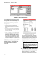
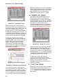
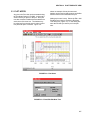
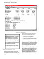
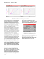
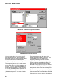
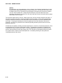
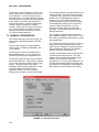
SECTION 1. THE BASICS
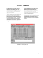
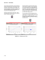
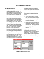
ID-2000 Windows uses a single window to
display one of three different views - Plot
Template, Plot, and FFT. Figure 1-1 shows a
sample Plot Template view that will produce a
single Strip-Chart style plot of the parameter
“Signal_0” versus “Time”.
The Plot Template view is used to define what
parameters you wish to plot and how they
should be plotted. When you start ID-2000 the
Plot Template view is what initially appears in
the ID-2000 application window. You use this
view to select data files, select parameters,
enable/disable plotting features, import/export
data files, and access ID-2000 configuration
settings.
The Plot Template view is essentially a large
dialog box that fills the entire application
window. It contains many different controls
such as buttons, check boxes, radio buttons,
etc. A complete description of the Plot
Template view features and functions can be
found in the following chapters.
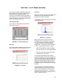
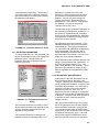
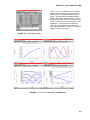
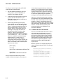
The second view is the Plot view which contains
the actual graphs that you defined in the Plot
Template. Figure 1-2 is a sample Plot view
based upon the settings in the Plot Template in
Figure 1-1.
FIGURE 1-1. Plot Template View
1-1
SECTION 1. THE BASICS
FIGURE 1-2. Plot View
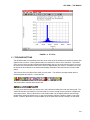
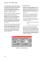
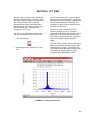
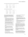
The third and last view is the FFT view which is
displayed in Figure 1-3. This view is used to
display an Amplitude Spectrum or Power
Spectrum plot of selected data. These plots
identify either the amplitude or power
associated with discrete frequencies within the
data. You can control the number of data points
used in calculating the FFT as well as the type
of data windowing you wish to use through the
1-2
Options - Preferences menu. Complete
descriptions of FFT features and procedures
are covered in the following chapters.
All three views share the same application
window and therefore only one may be visible at
any give time. The menus and toolbar buttons
will enable and disable automatically based
upon which view is currently active.
SECTION 1. THE BASICS
FIGURE 1-3. FFT View
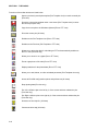
1.1 TOOLBAR BUTTONS
The ID-2000 toolbar is immediately below the menu at the top of the window and consists of buttons with
graphical icons on them. Clicking these buttons is a shortcut for various menu selections. The toolbar
uses “tool tips” which are little reminders that automatically pop up next to the mouse cursor if you move
the mouse over a toolbar button and leave it there for approximately one second. In addition to tool tips
the status bar at the bottom of the window also displays information about the function of each toolbar
button.
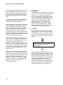
There are two sizes of toolbars from which you may select. The default is the large toolbar which is
used throughout this Help file. It looks like this:
The small toolbar is similar and looks like this:
You may select which toolbar you wish to use in the Preferences dialog box under the General tab. The
small toolbar button is primarily for VGA users that do not have enough screen resolution to display the
entire large toolbar. Some of the buttons on the small toolbar may be slightly different from the large
toolbar button simply because there is no way to successfully reduce the button’s graphic on the large
toolbar. However, the buttons on both toolbars are in the same order and the “tool tips” are the same.
1-3
SECTION 1. THE BASICS
Functions of the toolbar buttons are listed below:
Opens a previously saved plot template (Plot Template view) or recalls a saved plot
(Plot view)
Saves the current plot template under a new name (Plot Template view) or saves
the current plot (Plot view)
Copy the current plot to the Windows clipboard (Plot or FFT view)
Prints the current plot (All views)
Switches to the Plot Template view (Plot or FFT view)
Switches to the Plot view (Plot Template or FFT view)
Allows you to select the data for calculating an FFT and automatically switches to
the FFT view (Plot view only)
Allows you to zoom in on a graph (Plot or FFT view)
Zooms a graph out to full scale (Plot or FFT view)
Displays statistics for the plotted data (Plot or FFT view)
Allows you to add, delete, or edit a calculated parameter (Plot Template view only)
Access all ID-2000 configuration options and preferences (All views)
Stops plotting data (Plot view only)
Pan Left - shifts the plot to the left by ½ of the screen and then redraws the plot.
(Plot view only)
Pan Right - shifts the plot to the right by ½ of the screen and then redraws the plot.
(Plot view only)
Accesses on-line Help file. (All views)
Context sensitive help (All views)
1-4
SECTION 1. THE BASICS
1.2 STATUS BAR
The status bar at the bottom of the screen
contains four panes.
The first pane is used to display information
regarding the status of ID-2000 or instructions
for you to follow.
The second and third panes will display the
coordinates of the mouse cursor when you
move the mouse inside one of the graphs that
are plotted. The coordinates displayed in these
panes are in the units of the graph in which the
mouse cursor is currently located. It is not the
actual data value but simply the cursor location.
The fourth and last pane displays the current
time of day. Clicking on this pane toggles to
display either the current date or current time.
1.3 QUICK TOUR
Let’s take a quick tour of how to define a plot in
the Plot Template view and then look at the
actual plot in the Plot view. We will be using
one of the sample data files that is included with
ID-2000 so you do not have to worry about
converting any data files.
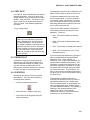
To begin, let’s start ID-2000 by clicking on the
ID-2000 icon which looks like this:
(If you already have ID-2000 running then just
continue with the next step.)
You should see the “splash” screen with
copyright information followed by the Plot
Template view (Figure 1-1). If you do not see
the Plot Template view and see a file selection
dialog box instead, that’s OK. Just skip down a
step to where we select the primary file.
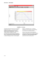
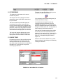
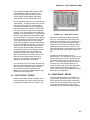
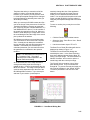
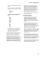
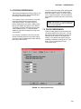
Once the Plot Template view becomes visible
we want to select a new template which will
default all of the settings for us. Select the File New menu item which will display the Select
Data File or Template dialog box shown in
Figure 1-4.
Select the file named “realdata.idw” by either
double clicking it or by clicking on it followed by
clicking the OK button.
FIGURE 1-4. Select Data File or Template
1-5
SECTION 1. THE BASICS
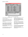
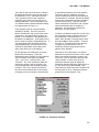
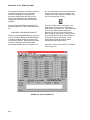
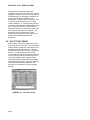
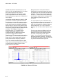
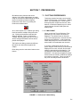
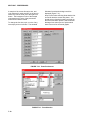
FIGURE 1-5. Plot Template of REALDATA.IDW
The Plot Template view should change to look
similar to that in Figure 1-5.
Now let’s make a Strip Chart plot. We will have
two strips (or graphs) on our plot. The first
graph will be “ExhaustTemp” parameter versus
“Time”. The second one will be “FanSpeed”
versus “Time”.
If you look at Figure 1-5 you will see groups or
columns labeled “On”, “Data File”, “Parameter
Selection”, “Auto Scale”, and “Smoothing”.
There are eight rows of items in each group.
Each row represents one graph or strip. We
want to plot two strips so we will be working with
the first two rows only.
Look at the first row in Figure 1-5. The boxes in
the “On” group are called “check boxes” and
allow you to turn a feature on or off by
1-6
“checking” or “unchecking” the box. The box is
checked when it contains either an “X” or “√”
inside. To check or uncheck it just click the
mouse in it which will toggle it back and forth.
We want to turn the first graph on so check the
box on the first row now.
Continue across on the first row to the group
labeled “Data File”. The button label should say
Primary. This button is used to specify what
data file (other than the primary file) you wish to
use. We won’t change this now but will discuss
it later in the manual.
The next group is labeled “Parameter Selection”
and contains a column of buttons under the “X”
label and another column under the “Y” label.
The names on these buttons are the
parameters that are selected for the X-axis and
Y-axis of your plot.
SECTION 1. THE BASICS
The button on the first row under the X label in
the Parameter Selection group should already
be defaulted to “Time”. We want to use the
“Time” parameter but let’s pick a different
parameter just to show you how easy it is to
change parameters. Click on this button now.
You should see the Parameter Selection dialog
box appear shown in Figure 1-6.
In this dialog box are all of the parameters
available for plotting. The list on the left is
labeled “Parameters” and is a list of the actual
parameters in the data file that is going to be
plotted. In our example it is the parameters in
the data file “realdata.idw”. At the bottom of the
list is a check box labeled “Alphabetical Sort”. If
you check this box the parameter list will be
sorted alphabetically. If this check box is not
checked the parameters will be listed in the
same order as they are in the data file.
On the right side of the dialog box is a group
labeled “Std. Parameters”. These are
parameters that are available for every data file.
The four buttons in the group are labeled:
“Time”, “Ref. Time”, “Scan_Number”, and
“Scanrate”. The “Time” parameter (which we
are going to select) is just as it sounds - the
time in seconds since the first data point was
recorded. “Ref. Time” represents reference
time which we will discuss later in the manual
but simply put it is the number of seconds from
a user-defined reference point in the data file.
The “Scan_Number” parameter is just the
number of data points since the first data point.
The last button is “Scanrate” which is the speed
at which the current data point was recorded in
Hz (scans per second). There are also two
check boxes labeled “Derivative” and “Integral”
which plots the derivative or integral of a
parameter. We will discuss integrals and
derivatives in a later chapter.
To select a parameter simply click on one of the
Std. Parameter buttons or double click one of
the parameters in the parameter list. Let’s
select “Scan_Number” so simply have to click
the button labeled “Scan_Number”. That’s all
there is to it. This takes you back to the Plot
Template view and the button in the X Parameter Selection group should now be
labeled “Scan_Number”.
Now that you know how easy it is to select a
parameter let’s go back and select “Time” again
which is the actual parameter we want to use
for our plot. Click on the button that now says
“Scan_Number” on the first row of the XParameter Selection group to display the
Parameter Selection dialog box again (Figure 16). Now click on the button labeled “Time”.
This returns you back to the Plot Template view
and the button in the X - Parameter Selection
group should now be labeled “Time” .
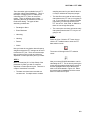
FIGURE 1-6. Parameter Selection
1-7
SECTION 1. THE BASICS
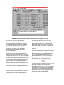
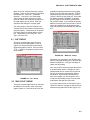
FIGURE 1-7. Plot Template view of ExhaustTemp and FanSpeed vs. Time
OK, now let’s pick our Y-axis parameter “ExhaustTemp”. Picking the Y-axis parameter
works just like the X-axis parameter. Click on
the button in the first row under the Y label in
the Parameter Selection group. This causes
the Parameter Selection List dialog box in
Figure 1-6 to re-appear. Now look in the
Parameters list and select the parameter
named “ExhaustTemp”.
Just one more thing to check. Look down
toward the lower portion of the window to find
the row labeled “Plot Type”. Make sure the
radio button labeled “Strip-Chart” has a dot in it
which means that it is selected. If another plot
type is selected then just click on Strip-Chart to
select it.
That’s all there is to selecting parameters for
plotting! Now let’s do the second strip. Go down
to the second row and “turn on” the second graph
by checking the check box in the “On” column just
like the first row. The X-axis parameter button on
the second row should already be labeled “Time”
so go on over to the Y-axis parameter button.
Click this button to display the Parameter
Selection dialog and select the parameter named
“FanSpeed” in the Parameter List. Verify that the
button label in the Plot Template view has now
changed to FanSpeed.
Now we are ready to see what this plot looks
like. Find the toolbar button and click it to
switch to the Plot view. You can also do the
same thing by selecting the View - Switch to
Plot menu item or by pressing the F3 key.
Look in the group labeled “Auto Scale” and
make sure both boxes are checked for the first
two rows. Now look at the “Smoothing” group
and make sure both buttons are labeled OFF
for the first two rows.
1-8
The Plot Template should now look like Figure 1-7.
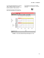
You should see a plot similar to Figure 1-8. The
top strip is a graph of our first parameter,
ExhaustTemp versus Time. The second strip is
FanSpeed versus Time. On Strip-Chart plots
there is only one X-axis which is located at the
very bottom of the plot. All graphs are plotted
against the same X-axis parameter.
SECTION 1. THE BASICS
If you have a printer attached to your computer
and it is installed in Windows you may try
printing by simply clicking on the printer toolbar
button or via the File - Print menu item.
Plot Template by clicking the Plot-Template
toolbar button or the View-Switch to Template
menu item.
Now that you know how to make a plot let’s
make a more interesting one. Go back to the
FIGURE 1-8. Plot view of ExhaustTemp and FanSpeed vs. Time
1-9
SECTION 1. THE BASICS
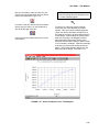
We are now going to make an X-Y plot of
“FanSpeed” versus “TurbineSpeed”. We will
only be plotting one graph this time so turn off
the second graph (remove the check on the
second row in the “On” group). Change the Xaxis parameter on the first graph to
“FanSpeed”. (Click on the first button under the
X column and then select the “FanSpeed”
parameter in the Parameter Selection dialog.)
Now change the Y-axis parameter to
“TurbineSpeed”. The last thing we need to do is
to change the plot type from Strip-Chart to X-Y.
(Just click on the “X-Y” radio button on the Plot
Type row.)
Your Plot Template window should look like
Figure 1-9.
FIGURE 1-9. Plot Template for FanSpeed versus TurbineSpeed
1-10
SECTION 1. THE BASICS
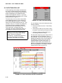
Now you are ready to make your first X-Y plot.
Click on the Plot toolbar button and you should
see the plot displayed in Figure 1-10.
Let’s have a little fun and use the Zoom feature.
We are going to zoom in on the small blob of
data at the top right of the plot.
Click on the Zoom toolbar button to turn on the
zoom feature.
NOTE: When in “zoom” mode the mouse
cursor will change from the standard arrow
to a small magnifying glass.
To zoom in on a plot you draw a rectangle
around the part of the data that you want to
expand. Once you have the magnifying glass
cursor click the mouse where you want one of
the rectangle corners to be and HOLD down the
mouse button. While holding the mouse button
down you are going to be dragging a rubberband rectangle along with the mouse cursor.
Move the mouse until the data you want to zoom
in on is inside the rectangle. When the rectangle
is the size you desire then release the mouse
button. The plot will redraw to display only the
data inside the rectangle. See Figure 1-11.
FIGURE 1-10. Plot for FanSpeed versus TurbineSpeed
1-11
SECTION 1. THE BASICS
Of course the actual scales of your plot may be
different depending upon exactly what rectangle
you drew. That’s all there is to zooming. You
can try zooming in even closer on the blob if you
want to by repeating the same procedure. In
fact, ID-2000 will let you keep zooming until you
only have a few data points to plot!
Now let’s zoom back out to full scale. This is
very simple since all you have to do is click the
Zoom Full Scale toolbar button:
That concludes our quick tour through a few
basic features of ID-2000. Pretty easy wasn’t
it? You can always use the sample data files
(REALDATA, 48CHAN, and SINE4FFT) when
you want to explore the many features of ID2000. In fact, these three data files are used
throughout this manual in illustrations so that
you can follow along if you like.
You can return to the Plot Template view by
clicking the Plot Template toolbar button or the
View - Switch to Template menu item. To exit
ID-2000 click on the File - Exit menu item or
access the Windows system menu to close the
ID-2000 window.
FIGURE 1-11. Zooming an X-Y Plot
1-12
SECTION 2. PLOT TEMPLATE VIEW
In the previous chapter we briefly looked at the
three different “views” that are available in the
ID-2000 Windows application window. To
review, only one window is used by ID-2000. In
that window you can “view” three different types
of things but only one of them can be viewed at
a time. These three “views” are:
FFT View
This view is similar to the Plot view except that it
displays an FFT plot (amplitude or power
spectrum) for frequency analysis.
This chapter discusses the features found in the
Plot Template view.
Plot Template View
In this view you tell ID-2000 what you want to
plot and how to plot it.
FIGURE 2-3. FFT View
FIGURE 2-1. Plot Template View
Plot View
As its name implies it displays the actual graphs
that you defined in the Plot Template view.
Before getting into the details of the Plot
Template view let’s discuss the plot template
file. The information contained in the Plot
Template view is stored in an ID-2000 plot
template file. Template files use an extension
of “.IDT”. These template files are used to:
•
Start ID-2000 with the same plot settings
that you used when you last exited ID-2000.
•
Provide a method for saving multiple plot
settings that can be reused.
The template file IDWIN.IDT is the default
template and always contains the settings from
your last ID-2000 session. When ID-2000 exits
it saves the current plot settings in IDWIN.IDT.
When you start ID-2000 the settings stored in
IDWIN.IDT are automatically loaded so that
everything is just like it was when you last used
ID-2000.
FIGURE 2-2. Plot View
You may save the plot template settings to
another template file at any time by selecting
the File - Save Template As menu item and
entering the desired file name. You can then
load these saved settings by selecting the File Open Template menu item.
2-1
SECTION 2. PLOT TEMPLATE VIEW
The template file feature in ID-2000 is useful for
maintaining multiple types of plot settings.
Instead of changing all of the graph and
parameter settings back and forth you can
simply save templates for the standard plot
settings you desire and just load the desired
template.
You can switch back to the Plot Template view
from any of the other views by clicking on the
toolbar button or the View-Plot Template menu
item or by pressing the F3 key.
You may also start ID-2000 by specifying the
desired template file on the command line such
as:
The Plot Template view is essentially a very
large dialog box with buttons, check boxes,
radio buttons, and edit boxes. All of these items
work like any other Windows application.
Normally you will use the left mouse button
when clicking on these items. However, some
items offer special functions when clicking on
them with the right mouse button. Items
utilizing both left and right buttons will be
identified throughout this manual.
IDWIN.EXE C:\ID2000W\MYTEMP.IDT
When you start ID-2000 Windows by clicking on
its icon in Program Manager, ID-2000 attempts
to load the template settings you used during
your last work session. After checking to make
sure all the settings are still valid ID-2000
automatically displays the Plot Template view.
Let’s take a close up look at the Plot Template
view in Figure 2-4.
FIGURE 2-4. Plot Template View
2-2
SECTION 2. PLOT TEMPLATE VIEW
Many of the Plot Template items are grouped
together. There are five of these groups which
are labeled “On”, “Data File”, “Parameter
Selection”, “Auto Scale”, and “Smoothing”.
These groups all have eight rows of check
boxes or buttons in them which correspond to
the eight graphs you can define. Each row
represents the settings for a single graph.
The lower portion of the Plot Template view
contains various items that are not specifically
grouped together. These items do not pertain
to a single graph but instead affect the entire
plot. These items are “Primary File”, “Plot
Type”, and “Plot Title”.
probably be plotting parameters on the graphs
that all come from the same data file. ID-2000
simplifies this procedure by having you load a
“primary” data file for the entire plot. If the Data
File button is labeled “PRIMARY” it indicates
that the graph will use whatever primary data
file you have loaded. If you change the primary
data file for the plot (we’ll tell you how to do that
later in this chapter) then all graphs that were
using the primary file automatically are changed
too!
2.1 “ON” GROUP
This group contains eight check boxes for
turning each of the eight graphs on and off
(Figure 2-5). Clicking the left mouse buttons
toggles the graph on and off. If the box has a
“X” or “√” inside it, the graph is turned on and
will be plotted.
FIGURE 2-6. “Data File” Group
Sometimes you may want to use different data
files for each graph allowing you to analyze data
between multiple files. This type of analysis is
called multi-file plotting.
FIGURE 2-5. “On” Group
Let’s say you were looking at temperatures from
a remote weather station. Perhaps you have
separate data files for several 24 hour periods
and you would like to compare them against
one another. By selecting a different file for
each of the graphs you can compare or even
overlay the data making it easy to see how the
temperature changed from day to day.
2.2 “DATA FILE” GROUP
This group contains eight buttons for selecting
the data file to be used for each of the eight
graphs (Figure 2-6). Most of the time you will
If you click (using the left mouse button) on the
“Data File” button for a graph you will see the file
selection dialog that looks like this (Figure 2-7):
2-3
SECTION 2. PLOT TEMPLATE VIEW
FIGURE 2-7. Data File Selection Dialog
This is a standard Windows file selection dialog
box except that a button has been added in the
lower right corner labeled “Use Primary”.
There are three types of files you may select
from Figure 2-7:
1. Primary - If you want to use the plot’s
primary file simply click the “Use Primary”
button.
2. Secondary - If you wish to use an ID-2000
file for this graph other than the primary file
select the desired file.
3. Import - If you want to select a data file that
is not an ID-2000 data file you first need to
select the type of file desired you wish to
import in the “List Files of Type” drop down
box and then select the desired file. (Refer
to the Import/Export section of this manual
for additional information on importing files.)
Using the right mouse button to click on a graph
“Data File” button is a short cut method of
viewing information on that data file. You can
alternately use the File - Data File Info menu
item to view information on any data file.
(Figure 2-8).
FIGURE 2-8. Data File Info
The information on the data file is displayed in
ID-2000’s TextPad utility. This utility is similar to
the Windows Notepad program that allows you
to view and save text files. The CUT, COPY,
and PASTE functions in TextPad allow you to
manipulate the information as desired including
copying/pasting it into other applications.
NOTE: The data file information is in a
temporary file which will automatically be
deleted upon closing the TextPad utility. If
you want to keep this file you must save it
under a new name.
2.3 “PARAMETER SELECTION” GROUP
There are two columns of buttons in this group
(Figure 2-9). The first column is labeled “X” and
the second is labeled “Y”. These buttons
represent each graph’s X-axis parameter and
2-4
SECTION 2. PLOT TEMPLATE VIEW
Y-axis parameter respectively. These buttons
are used to either select a different parameter
(left mouse button) or to edit the plot scales for
the parameter (right button).
parameters. However, there are a few
differences. When selecting an X parameter
the derivative and integral check boxes are
disabled. You may not plot a derivative or
integral on the X axis. When selecting a Y
parameter the “Time” and “Ref. Time” buttons
are disabled. You may not plot time or
reference time on the Y axis.
The list inside the group labeled “Parameters” is
the actual list of parameters for the data file. If
the check box “Alphabetical Sort” is enabled
then the list is sorted alphabetically. Otherwise,
the parameters are listed in the same order as
they are found in the data file.
FIGURE 2-9. “Parameter Selection” Group
2.3.1 SELECTING PARAMETERS
To change either the X or Y axis parameter use
the left mouse button to click on the appropriate
parameter button. This will display the
Parameter Selection List dialog box shown
below in Figure 2-10.
Any parameters enclosed in brackets “[ ]” are
calculated parameters and are not part of the
original data file. These are parameters that
you can create in ID-2000 which are appended
to the original data. You may add, edit, or
delete calculated parameters which will be
discussed later in this manual. You may never
modify any of the original parameters.
On the right side of the Parameter Selection List
dialog is a group labeled “Std. Parameters”. In
this group are buttons labeled “Time”, “Ref.
Time”, Scan_Number”, and “Scanrate”. These
parameters are available for plotting on any
data file regardless of what parameters it may
contain.
2.3.2 DERIVATIVES AND INTEGRALS
FIGURE 2-10. Parameter Selection List
Dialog
The Parameter Selection List contains a list of
all parameters contained in the data file as well
as some “standard” parameters which are
available for every data file.
The Parameter Selection List dialog box is
basically the same for selecting either X or Y
At the bottom of the “Std. Parameters” list are
two check boxes labeled “Derivative” and
“Integral”. Checking one of these boxes allows
you to plot either the derivative or integral of one
of the data file parameters. You cannot plot a
derivative or integral of one of the standard
parameters (Time, Ref. Time, etc.). A
derivative is the rate of change for a parameter
relative to time or how fast the parameter value
is changing. A integral is sort of the opposite of
a derivative in that it is the total amount of
change over time.
Let’s say you had a data file of a race car and
one of the parameters in the file was “SPEED”
which represents car speed in miles per hour.
You could plot the derivative of SPEED which
would show you the acceleration of the car (how
the speed is changing over time). You could
also plot the integral of SPEED which would
show you how many miles the car was driven.
2-5
SECTION 2. PLOT TEMPLATE VIEW
To select a parameter from the Parameter List
either double click on the parameter or highlight
the parameter (by clicking once on it) and then
click the OK button. Make sure that the
derivative and integral boxes are checked (or
unchecked) appropriately before selecting the
parameter. To select one of the Std.
Parameters simply click its button.
When you select X-axis parameters for multiple
graphs it is important to remember that all
graphs plotted must have the same X
parameter. Let’s say you wanted to plot four
parameters versus “Time” on a strip chart plot.
You would need to make sure that all four
graphs that are going to be plotted have “Time”
as their X-axis parameter. If one of them has a
different X-axis parameter you will receive an
error message when you attempt to switch to
the Plot view.
This does not mean that all eight graphs have to
have the same parameter selection in the Plot
Template. Only the graphs that are “turned on”
have to have the same parameter. You may
want to set up many different graphs initially but
only turn on the one you want to look at first.
When you are finished analyzing that graph
then you simply turn it off and turn on the next
graph you want to plot.
2.3.3 EDITING SCALES
Most of the time you will probably want ID-2000
to handle the parameter scaling for you.
However, you can manually scale a graph using
the Edit Scales dialog shown in Figure 2-11. In
this dialog you can also specify the section of
data to be plotted if you do not want the entire
file plotted.
If you click on one of the parameter buttons in
the Parameter Selection group (Figure 2-9)
using the right mouse button you are able to
edit scaling information for that parameter.
The Edit Scales dialog box shown in Figure 211 allows you to edit two items that affect how
the parameter is plotted:
•
The minimum and maximum graph
scales.
•
The section of data you wish to plot.
On the left of the dialog is a group labeled
“Parameter Scaling”. Inside this group are
fields in which you can enter the MIN and MAX
scaling values. You can click on the Full Scale
button to default the MIN and MAX to full scale
values based upon data file header information.
You can also update all eight graphs in the Plot
Template to use these scales by checking the
“Set scales for all graphs”.
FIGURE 2-11. Edit Scales Dialog
2-6
SECTION 2. PLOT TEMPLATE VIEW
If you change the MIN or MAX scale ID-2000
will automatically switch the graph over to
manual scaling so that it will use your scale
values instead of automatically calculating
scales based upon the plotted data values.
On the right of the dialog box is a group labeled
“Data Subset”. This group allows you to control
how much of the data file is actually plotted.
Let’s take an example of a very large data file
that was recorded at a scanrate of 1000 (1000
scans per second) for 1000 seconds (about 16
minutes). This data file would have 1,000,000
readings of every parameter in it. Obviously this
would be a big data file and would take a while
to plot the entire file. Perhaps you have already
looked at the data or know from the comments
in the data file that the part you are primarily
interested in looking at is only the data between
the time of 450 and 475 seconds. You could of
course plot all 1000 seconds of data and then
zoom in on the section between 450 and 475
but that would mean you would have to wait for
all 1,000,000 data points to be plotted first.
Instead you could enter a value in the “Time
Start” field of 450 and “Time Stop” field of 475
which would only plot the data for those 25
seconds. This would be much faster than
waiting for the entire file to be plotted.
If you press the “Full Time” button the start and
stop times will be defaulted to the entire length
of the data file so that every point is plotted.
You may also check the “Set times for all
graphs” box if you want all eight graphs to use
the same start and stop times.
2.4 “AUTO SCALE” GROUP
Farther to the right in the Plot Template view is
a group labeled “Auto Scale” with two columns
of check boxes labeled X and Y (Figure 2-12).
FIGURE 2-12. “Auto Scale” Group
By default, ID-2000 automatically scales the
plots you create based upon the value of the
data that is being plotted. With autoscaling you
never have to worry about having a plot with
scales of 0 and 10 when the parameter being
plotted only varies between 0.5 and 0.75. ID2000 will calculate the best scales to use so that
the parameter takes up the largest part of the
plot.
Sometimes it is advantageous to turn
autoscaling off. This may be the case if you are
printing many plots from various data files and
you want the scales on all the plots to be the
same. To turn autoscaling off remove the X in
the check box under the appropriate X or Y
column and then right click on the appropriate
Parameter Selection button to type in your
scales. (See the previous paragraph on how to
edit scales for a parameter.)
2.5 “SMOOTHING” GROUP
To the far right side of the Plot Template is a
group labeled “Smoothing” (Figure 2-13). Like
the Parameter Selection group it contains two
columns of buttons labeled X and Y that allow
you to specify what amount (if any) of data
smoothing is to be used when plotting a graph.
2-7
SECTION 2. PLOT TEMPLATE VIEW
Because all graphs use a common X parameter
when plotted all graphs must also use the same
level of X parameter smoothing. If you change
the smoothing level for one X parameter it
automatically changes them for all graphs.
2.6 “PRIMARY FILE” GROUP
FIGURE 2-13. “Smoothing” Group
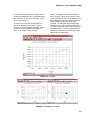
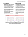
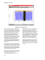
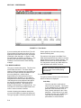
Data smoothing uses a “running” average
technique to smooth out the small bumps and
variations in data that was recorded. There are
four levels of data smoothing: off, small,
medium, and large. These levels correspond to
averaging the current data point with 0, 3, 7, or
11 data points before AND after it. Figure 2-14
shows an example of a Strip-Chart plot of the
same parameter with and without smoothing.
The top is the original unsmoothed data
corresponding to the derivative of FanSpeed in
REALDATA.IDW. The lower trace is the same
derivative with a small level of smoothing
applied. Any time you plot a smoothed
parameter an “(S)” will appear beside the
parameter label and a legend is included at the
bottom of the plot identifying that “(S)” means
the parameter is smoothed.
Although not visibly grouped together as the
previous groups, the Primary File group is
nonetheless a group consisting of one button
and informational text (Figure 2-15). This group
displays the name of the current primary file on
the button. To the right of the button is
information about the file such as what rate its
data was recorded at, the starting date/time of
the recording, and the length of the recording.
FIGURE 2-15. “Primary File” Group
As described previously, the primary data file is
the default data file used for all graphs. You
may manually select a “secondary” data file for
a single graph if desired but all graphs default to
using the primary file. If you change the primary
file all graphs that are using the primary file are
automatically updated with the new file.
Like the buttons in the Data File group
previously discussed, the primary data file
button allows you to either select a new primary
data file (left mouse button) or displays
information about the current primary data file
(right mouse button).
FIGURE 2-14. Smoothed and Unsmoothed
You can see from Figure 2-14 that in some
cases data smoothing can substantially improve
the readability of a graph. However, caution
should be used when smoothing data because
you are not plotting the original recorded data you are plotting a running average of the data.
2-8
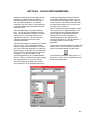
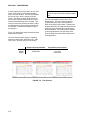
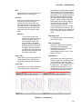
2.7 “PLOT TYPE” GROUP
This group is also not visibly marked as a group
but contains four radio buttons labeled: “X-Y”,
“X-Y-Y”, “Strip Chart”, and “Multi-Plot” (Figure 216). To change plot types simply click the plot
type desired.
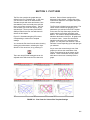
SECTION 2. PLOT TEMPLATE VIEW
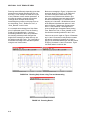
The X-Y, X-Y-Y, and Multi-Plot are somewhat
similar in that they produce a single graph with
either a single or multiple data traces on the
graph. The Strip Chart plot contains multiple
graphs - each with a single data trace. The X-Y
plot uses only one X-axis and Y-axis parameter.
The X-Y-Y plot uses one X-axis and two Y-axis
parameters. The Strip Chart and Multi-Plot
uses one X-axis parameter and from one to
eight Y-axis parameters. Figure 2-17 illustrates
samples of all four plot types.
FIGURE 2-16. “Plot Type” Group
FIGURE 2-17. X-Y, X-Y-Y, Strip Chart, and Multi-Plot
2-9
SECTION 2. PLOT TEMPLATE VIEW
Any parameter (except derivatives and
integrals) may be used for the X-axis on all four
plot types. However, you must use the same Xaxis parameter for each graph or data trace on
the plot types that allow multiple Y-axis
parameters. Typically Time or Reference Time
is used for the X-axis parameter on a Strip
Chart or Multi-Plot. X-Y plots typically plot two
recorded or calculated parameters against each
other. However, there is no restriction as to
parameter selection except as previously noted
with regard to derivatives and integrals. Any
parameter may be plotted as the Y-axis
parameter(s) except Time or Reference Time
which are only available as an X-axis
parameter.
2.8 “PLOT TITLE” GROUP
At the bottom of the Plot Template view is the
final group labeled “Plot Title”. This is actually a
single edit field containing the plot title that is to
be displayed at the top of the plot. This title
defaults to the comments (if any) in the primary
data file. To change the title just click the
mouse inside the edit box and type the new title.
You may use up to three lines for the plot title.
Once you change the title, changes will be
saved with the plot template and used instead
of the data file comments. However, changing
the primary file will erase the plot title and
default to the comments for the new primary
data file.
FIGURE 2-18. “Plot Title” Group
2-10
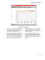
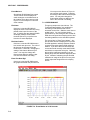
SECTION 3. PLOT VIEW
The Plot view contains the graphs that you
defined in the Plot Template view. In this view
you can zoom in and out on data sections,
annotate the plot with notes and leaders, view
data statistics, save and recall plots, send the
plot to your printer, and much more. The Plot
view is where you will do the majority of your
data analysis. There are many tools that ID2000 provides for the Plot view which we will
discuss in this chapter.
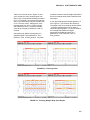
Figure 3-1 illustrates samples of Plot views
corresponding to various Plot Template
settings.
You access the Plot view from the other views by
clicking the toolbar button, selecting the ViewSwitch To Plot menu item, or by pressing F3.
There are many ID-2000 settings that can be
adjusted which affect how the Plot view looks
and acts. Some of these settings will be
discussed in this chapter. Please refer to the
Preferences chapter for a complete description
of these settings.
The Plot view is divided into several areas. The
center section contains the graph(s) of the
parameters you selected in the Plot Template.
In the case of a Strip Chart style plot the first
graph is at the top and the last graph at the
bottom. The X-axis is always horizontal and is
labeled at the bottom of the plot. All graphs use
a common X-axis. Y-axes are vertical and
labeled on either the left or right side of the
graphs. You may have one common Y-axis or
individual Y-axes depending upon what plot type
you selected.
As you move the mouse through one of the
graphs you will see the coordinates of the
cursor on the status bar at the bottom of the
window. These coordinates are only visible
while the mouse cursor is actually inside a
graph.
FIGURE 3-1. Plot Views for Various Plot Template Settings
3-1
SECTION 3. PLOT TEMPLATE VIEW
If you have enabled the Data Track feature from
the Plotting Preferences dialog box or via the
View - Track Rollup menu item you will also see
a small “rollup” dialog that displays the actual
data values as you move the mouse through a
graph.
The mouse cursor coordinates and Data Track
coordinates (if enabled) are always available
any time the mouse enters a graph.
Delta coordinates are substituted for the mouse
cursor coordinates on the status bar any time
you click and drag the mouse while inside a
graph. These coordinates give you the delta X
and delta Y distances from the anchor point
which you set when you initially clicked the
mouse. As long as you keep the mouse button
down delta coordinates will be displayed on the
status bar. Releasing the mouse button reverts
back to normal mouse coordinates.
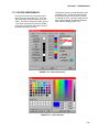
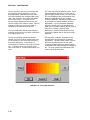
ID-2000 offers a unique feature called the “color
map”. This is a small stripe across the top of
each graph if you are plotting Time, Reference
Time, or Scan-Number as the X-axis
parameter. The color map may look sort of like
a rainbow or a “color wash” that goes from one
color to another. The purpose of the color map
is to provide you a quick visual cue as to where
the minimums and maximums of the Y-axis
parameter occur.
The colors in the color map correspond to the
value of the Y-axis parameter data. If the color
map is defined to go from red to yellow then red
would correspond to the lowest data value and
yellow to the highest data value for the Y-axis
parameter. A palette of 100 colors is created
for the color map. You may change the colors,
disable, or enable the color map in the
Preferences dialog box.
3-2
3.1 ZOOMING
Zooming allows you to magnify a section of data
(“zoom in”) or to view more of the entire data file
(“zoom out”). To “zoom in” you control the
amount of magnification by drawing a rectangle
around the data that you want to magnify. To
“zoom out” you select one of the preset levels of
200% (scales are doubled), 500% (scales
increased by factor of 5), 1000% (scales
increased by factor of 10), or FULL (resets
scales to full scales from data file). There is
also “zoom previous” which either zooms in or
out to the settings you previously used.
3.1.1 ZOOM IN
You may want to magnify a particular section of
data so that you can see it better. Zooming in
with ID-2000 is very easy. To enter the “zoom
in” mode you may either select the View - Zoom
In menu item or click on the “Zoom In” toolbar
button.
NOTE: “Zoom In” mode is denoted by the
mouse cursor changing to a small
magnifying glass.
Like many Windows applications, you zoom in
with ID-2000 by drawing a rectangle around the
part of the graph(s) you wish to magnify. This is
done by clicking the mouse at a corner of the
rectangle and dragging the mouse (which drags
a rectangle anchored at the point where you
clicked) to the opposite corner. When you
release the mouse button at the opposite corner
the plot will automatically redraw using scales
associated with the area you just defined.
SECTION 3. PLOT TEMPLATE VIEW
Let’s review the example from Chapter 1 where
we plotted FanSpeed versus TurbineSpeed and
then zoomed in on a portion of the data. Figure
3-2 is our original plot.
To zoom in on the section of data at the top
right of the graph you first enter the “Zoom”
mode by any of the methods described. When
the mouse cursor changes to a magnifying
glass we are ready to begin zooming.
Imagine a rectangle around the data that you
want to magnify. Move the mouse to a corner
of that rectangle and click the left mouse button.
While holding the mouse button down drag the
mouse toward the opposite corner of the
rectangle. A rubber band style rectangle will
follow the mouse. When the mouse is where
you want the opposite corner to be then release
the mouse button. Figure 3-3 shows what you
should see just before you release the mouse
button and the resulting plot.
FIGURE 3-2. X-Y Plot
FIGURE 3-3. Zooming an X-Y Plot
3-3
SECTION 3. PLOT TEMPLATE VIEW
Zooming reacts differently depending upon what
parameters are plotted and what plot type you
are using. In our example we used an X-Y plot
of one parameter versus another parameter. In
this case the resulting zoomed plot used the
rectangle which we drew while zooming.
Autoscaling has no affect on this plot since we
are not plotting “Time”, “Reference Time”, or
“Scan_Number” on the X-axis.
If our example were changed to a Strip Chart
plot of a parameter versus Time the zooming
would work a little differently. If we have
autoscaling enabled for the Y-axis parameter
the resulting zoomed plot will disregard the
height of the rectangle you draw and only use
the width to scale the X-axis. The Y-axis will be
autoscaled according to the data that is plotted
using the new X-axis scales.
Both zoom rectangles in Figure 3-4 produce the
same plot shown in Figure 3-5. ID-2000 used
our zoom rectangles in both cases to only
define the time period that we wished to plot.
Our zoom rectangles were both approximately
the same width starting at 1.7 seconds and
stopping at 2.9 seconds. ID-2000 then looked
at the data and calculated the optimum Y-axis
scale for Signal_5 based upon its data values
from 1.7 to 2.9 seconds. The height of the
zoom rectangles are disregarded when plotting
Time, Reference Time, or Scan_Number on the
X-axis with autoscaling enabled for the Y-axis.
If we were to zoom in again on Figure 3-5 between
say 2.2 and 2.5 seconds it really would not matter
how tall our rectangle is because the Y-axis is
going to be autoscaled based upon the data values
of Signal_5 between 2.2 and 2.5 seconds. Figure
3-6 shows what it would look like.
FIGURE 3-4. Zooming Strip Charts using Time and Autoscaling
FIGURE 3-5. Zooming Result
3-4
SECTION 3. PLOT TEMPLATE VIEW
Take a look at the left view in Figure 3-6 and
you’ll see that our zoom rectangle goes from
about 2.2 to 2.5 seconds horizontally and about
0.5 to 1.75 vertically. Now look at the right view
and you will see that the new plot is scaled from
2.2 to 2.5 for the X-axis. Although our zoom
rectangle went from 0.5 to 1.75 the new plot
was scaled from 0.8 to 1.6 which is the data
value range of Signal_5 between 2.2 and 2.5
seconds.
Autoscaling only affects zooming when it is
enabled and the X-axis parameter is Time,
Reference Time, or Scan_Number. Any other
conditions results in both the height and width of
the zoom rectangle being used to determine the
new scales.
If your Strip Chart plot has multiple graphs on it
as in Figure 3-7 you still zoom the same way.
The height of the zoom rectangle doesn’t matter
- in fact the rectangle doesn’t even have to
extend through all graphs. It is only the width of
the rectangle that matters as long as
autoscaling is enabled and the X-axis
parameter is Time, Reference Time, or
Scan_Number.
FIGURE 3-6. Zooming Closer
FIGURE 3-7. Zooming Multiple Strip Chart Graphs
3-5
SECTION 3. PLOT TEMPLATE VIEW
Even though our zoom rectangle did not extend
into the Signal_15 graph it was zoomed anyway.
500% - Same as 1000% except a factor of
5 is used.
If you are confused as to when the height of the
zoom rectangle is used then remember these
two rules.
200% - Same as 1000% except a factor of
2 is used.
•
Zoom rectangle height is NOT used when:
The only “zoom out” toolbar button is which
zooms out to full scale.
The Y-axis autoscaling is enabled AND
the X-axis parameter is “Time”,
“Reference Time”, or “Scan_Number”.
•
Zoom rectangle height IS used when:
The Y-axis autoscaling is disabled OR
the X-axis parameter is NOT “Time”,
“Reference Time”, or “Scan_Number”.
3.1.2 ZOOM OUT
After you have zoomed in on a section of data
you may decide that you need to look at a
different section of data. Depending upon how
closely you zoomed in the current data section,
the desired data section may not be visible.
Somehow you need to get back to the main plot
displaying all the data so that you can then
zoom in on the desired data.
There are several ways to zoom out. You could
go back to the Plot Template view and then
recreate the plot but that would be time
consuming and awkward. ID-2000 can zoom
out directly from the Plot view. If you click on
the View - Zoom Out menu item you will see a
sub-menu of items labeled:
Previous - Zooms in or out to the previous
zoom settings you used.
Full - Zooms out to full scale. All scales are
reset to the absolute minimum and
maximum contained in the data file. All
Time-Start and Time-Stop values are reset
to the full length of the data file.
1000% - Increases both X and Y scales by
a factor of 10. If the X-axis parameter is
Time, Reference Time, or Scan_Number
then Time-Start and Time-Stop are also
increased by a factor of 10.
3-6
Immediately after selecting the menu item or
clicking the toolbar button the plot will be
redrawn with the new scales.
NOTE: You may also want to consider
using the Save Plot and Recall Plot feature
when zooming. These features allow you to
save and recall multiple plot settings without
having to actually redraw the data.
Consider an example of a large data file
that takes more than a few seconds to plot.
Every time you zoom out to full scale the
entire plot has to be redrawn. If you do this
many times during a session you could
waste a lot of time just redrawing in order to
zoom in on a section of data. If you use the
Save Plot feature as soon as the plot is first
drawn then you are saving a picture of the
plot along with all the necessary information
ID-2000 needs. When you are ready to
zoom out to full scale you can simply recall
it with the Recall Plot feature which paints
the picture back on the screen and resets
all the information to the settings associated
with the full plot. This can be much faster
than redrawing the plot. Refer to the Save
Plot and Recall Plot sections later in this
manual for more information on these
features.
3.2 PANNING
Panning allows you to shift a zoomed plot either
left or right so that you can view data on either
side. Panning is only active in the Plot view and
only if you have zoomed in on a graph.
Clicking on one of the Pan buttons shifts the
current plot left or right by 50%.
SECTION 3. PLOT TEMPLATE VIEW
3.3 PLOT NOTES
Any plot in the Plot view can be annotated using
the Plot Notes feature in ID-2000. A plot note is
a text box that you place on the plot. Each plot
note also contains 4 leaders that are attached to
each corner of the text box. The leaders may
be pulled out from the plot note in order to point
to a particular point of interest. Figure 3-8
shows an example of how plot notes and
leaders can be used so that someone unfamiliar
with the data can still understand the plot.
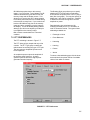
Adding a plot note is easy. Select the Edit - Add
Plot Note menu item to access the Plot Note
Text dialog box (Figure 3-9). In this dialog box
enter the text that you want to put in the plot
note.
FIGURE 3-8. Plot Notes
FIGURE 3-9. Enter/Edit Plot Note Text
3-7
SECTION 3. PLOT TEMPLATE VIEW
The text in a plot note is displayed as a single
line of text. You cannot split a plot note into
multiple lines. While there is no limit to the
number of characters you can use in a plot note
the most effective notes are very brief and
limited only a few words.
current location. If you click in an invalid
location the plot note placing operation will be
aborted.
NOTE: As the cursor indicates, the plot
note’s anchor point is at the intersection of
the small cross-hair in the cursor. This
point will be the upper left, center or right
depending upon the alignment selected for
the plot note.
You may select whether to use left, center, or
right alignment for locating the plot note by
selecting the appropriate type in the “Alignment”
box. Each plot note may use its own alignment.
In the Plot Note Text dialog you may also
change the style used for ALL plot notes. You
may select whether or not to have a box drawn
around each plot note. (The color of the box
can be set in the Preferences dialog). You may
also select whether or not to erase the graph
behind the plot note. Keep in mind that any
Style changes affect all plot notes. These style
settings may also be changed via the
Preferences dialog.
The mouse cursor will change to one of these
cursors (depending upon the alignment you
chose) when you have completed entering the
plot note text and clicked the OK button
indicating that you may now specify the location
for the plot note.
A plot note is located by its anchor point. The
anchor point depends upon the selected
alignment. “Left” uses the upper left corner of
the text box as an anchor. “Center” uses the
top center point of the text box. “Right” uses
the top right corner of the text box. This anchor
point MUST fall inside a graph - it cannot be
located above the top graph or below the
bottom graph. However, the plot note itself may
extend outside the graph.
To select the location of the plot note simply
move the mouse to the desired location and
click the left mouse button.
If you are locating the plot note and move
outside the graphs, the cursor will change
indicating that it may not be placed at the
3-8
Once a plot note is located on the plot you may
move, edit, or delete it. To select the plot note,
click the mouse button inside its text box. You
will see four handles at either the corners of the
text box or the ends of the leaders (if any).
To move a plot note you must select it, then
drag the plot note to the new location. The end
of any plot note leaders will remain stationary
and stretch to connect to the new plot note
location.
You can move a plot note leader by clicking in
the leader’s handle and dragging it to the new
location. If you want to delete the leader simply
drag it back inside the text box.
To delete an individual plot note you must select
it and then press the delete key or select the
Edit - Delete Plot Note menu item. You may
delete all plot notes by selecting the Edit Delete ALL Plot Notes menu item.
To edit the plot note you must select it and then
select the Edit - Edit Plot Note menu item.
It is important to understand the life span of a
plot note.
•
All plot notes are deleted when you return to
the Plot Template view.
•
If you zoom in so that the plot note’s upper
left corner is not visible the plot note will be
automatically deleted.
•
If you zoom in so that the end of a leader is
invalid the leader will be deleted (if the plot
note is at a valid location it will remain
without the leader).
SECTION 3. PLOT TEMPLATE VIEW
3.4 COPY PLOT
It is simple to insert an ID-2000 plot into another
Windows application. Once you have the plot
created click the “Copy” toolbar button or select
the Edit - Copy menu item. This places a copy
of the current plot on the Windows clipboard.
Then just “paste” it into whatever application
you desire.
“Copy” toolbar button
NOTE: If you have the color map feature
enabled you may find that the colors are
fewer or different when you paste the plot
into other applications. This is common if
your display is capable of 256 colors but the
application only uses 16 colors. Should you
find this condition to exist you can disable
the color map feature in the Preferences
dialog box, recreate the plot, and then copy
it to the clipboard.
3.5 EXPORT PLOT
In addition to copying the current plot to the
clipboard you can export the current plot to a
device independent bitmap file (.BMP). Once
your plot has been created select the File Export menu item which allows you to enter the
file name you wish to save the plot under.
3.6 STATISTICS
ID-2000 can provide quick access to plotted
data statistics. There are three methods of
accessing these statistics:
•
Click the statistics toolbar button:
•
Select the View - Statistics menu item
•
Click inside one of the graphs using the
right mouse button
The statistical information will be displayed in ID2000’s TextPad utility as shown in Figure 3-10.
The statistics displayed are only for the data
that is actually plotted. If you have zoomed in
on a section of data or specified a Time-Start
and Time-Stop that resulted in only part of the
data being plotted then the statistics will not be
for the entire length of the file.
There are four basic statistics calculated for
each plotted parameter including the X-axis
parameter. These are:
•
MIN - The minimum data point that was
plotted
•
MAX - The maximum data point that was
plotted
•
AVG - The average of all data points plotted
•
SUM - The “area under the curve” for all
data points plotted
If you access the Data Statistics by clicking the
right mouse button inside a graph AND the
graph has “Time”, “Scan_Number”, or
“Reference Time” as the X-axis parameter you
will find additional statistical information. This
information consists of the data values for ALL
parameters (regardless of whether or not they
are plotted) that correspond to the point where
you clicked the mouse. This is makes it very
easy to check values of multiple parameters at
any given time or point in the file without having
to plot each one.
The statistical information is stored in a
temporary file named IDSTATS.TXT which is
automatically loaded into the TextPad utility.
This file will automatically be deleted when you
have completed viewing the statistics unless
you have disabled this feature. The enabling or
disabling of the automatic deletion of the
statistics file is done via the General
Preferences dialog box. (See the section on
Preferences for more information.)
3-9
SECTION 3. PLOT TEMPLATE VIEW
FIGURE 3-10. Data Statistics
NOTE: When you request to view statistics
ID-2000 asks Windows to load and run the
TextPad utility program which automatically
loads the IDSTATS.TXT file. If you have
multiple applications active or minimal
system resources Windows may not be
able to run the TextPad utility (or any other
application). Should this occur you will be
notified via an error message. You may be
able to close other applications in order to
free up Windows resources that will allow
the TextPad utility to be loaded.
It is also important that you exit TextPad
instead of just switching back to ID-2000
which leaves TextPad still running and
active.
3.7 SAVE AND RECALL PLOT
We briefly described the save and recall plot
feature during our discussion on zooming. The
3-10
primary reason for using these features is to
save you time by eliminating the need to:
•
Redraw a plot of a large data file
•
Create a plot template to match a specific
plot’s characteristics.
As we discussed in the zooming section you
can use the save and recall feature to make
zooming more efficient. Without this feature ID2000 would have to redraw the plot every time
you zoomed out to full scale which could be
time consuming on large data files.
There is another benefit of this feature.
Consider the case where you are analyzing a
plot and think that you are finished with it. You
switch back to the Plot Template view, load a
different file, and make some other plots.
Suddenly you realize that you need to look at
that first plot again. If you did not save that plot
then you would have to go back to the Plot
SECTION 3. PLOT TEMPLATE VIEW
Template view and try to remember all of the
settings in order to recreate that initial plot.
However, if you saved it you only have to recall
it. All the plot template settings will be changed
back automatically to what they were when you
saved the plot initially.
When you save a plot ID-2000 creates two files one for the image of the plot and one for the Plot
Template information necessary to create the
plot. These two files are named IDWSAVED.T??
and IDWSAVED.B?? where ?? is the number of
the saved plot ranging from 00 to 99. When you
decide to recall the plot you simply select it from
the recall dialog box and the image of the saved
plot is painted in the window.
ID-2000 does not delete any saved plots when
you exit ID-2000 or return to the Plot Template
view. A saved plot can always be recalled as
long its data file(s) still exist and parameters are
available. If the saved plot is based upon a
calculated parameter you must make sure that
the parameter is not deleted or the equation
modified.
NOTE: The IDWSAVED files are placed in
the “Temporary Path”. This path is
defaulted to the location specified in the
General Preferences dialog
As we discussed one of the major benefits of
saving and recalling a plot is not having to
redraw the plot. In some circumstances the plot
MUST be redrawn. The image of the plot that is
saved is strictly dependent upon the size of the
ID-2000 application window. If you save a plot
and later in your session (or subsequent
sessions) change the size of the application
window then the saved plot image does not
match your new window size and becomes
invalid. You can still recall the plot but since the
image is invalid ID-2000 is forced to redraw it
using the plot template settings that were saved
with it.
To save or recall a plot you may do one of the
following:
•
Click the Recall or Save toolbar buttons.
•
Select the View - Save Plot or View - Recall
Plot menu item.
•
Use the accelerator keys of F5 or F6.
The Save Plot or Recall Plot dialog will then be
displayed as shown in Figure 3-11.
The Save Plot and Recall Plot dialogs are
essentially the same. In the Save Plot dialog
there is an additional button labeled “New” for
saving a new plot image. The second button is
labeled “Overwrite” and is used to replace a
saved image with the current plot image.
The “Saved” list box contains a list of all the
plots already saved. They are numbered 0
through 99. To preview a saved plot image you
only need to highlight it in the “Saved” list box.
To recall a plot select it and click the “Load”
button.
FIGURE 3-11. Save/Recall Dialog Box
3-11
SECTION 3. PLOT TEMPLATE VIEW
3.8 DATA TRACK ROLLUP
At the beginning of this chapter we discussed
the various coordinates that can be displayed.
The mouse cursor coordinates (either actual or
delta) are displayed on the status bar at the
bottom of the application window. If you have
enabled data tracking you will also see a “rollup”
dialog as shown in Figure 3-12.
The track rollup can be moved to any location
on the Windows screen (it is not restricted to
the ID-2000 application window). In its upper
right corner is a button with an arrow on it. This
is used to “roll up” or “roll down” the dialog box.
The upper left corner contains a Windows
system menu button that allows you to close,
roll up and down, or arrange the rollup.
“Arranging” the rollup automatically rolls it up
and locates it at the top left of the Plot view.
NOTE: If you are using Windows 95 you
may want to turn off the “Center Dialog
Boxes” feature in the Desktop Preferences. If enabled this feature will
force the rollup dialog to be initially
displayed in the center of your display.
FIGURE 3-12. Data Track Rollup Dialog
You can display or remove the data track rollup
by three methods:
•
Check or uncheck the View - Track Rollup
menu item
•
If the rollup is visible you may close it using
its system menu button at the top left corner
•
Check or uncheck the Data Track box in
the Plotting Preferences dialog.
The data track rollup may only be active if the Xaxis parameter is Time, Reference Time, or
Scan_Number. When active and rolled down, it
displays the data point value of each graph’s Yaxis parameter for the point in time or scan
number pointed to by the mouse cursor. In
addition to these values, small markers are
placed on each graph identifying the data point
that is being displayed. An example of these
markers can be seen in Figure 3-13.
FIGURE 3-13. Data Track Rollup and Data Track Markers
3-12
SECTION 3. PLOT TEMPLATE VIEW
3.9 DATA MARKERS
3.10 REFERENCE TIME
ID-2000 provides the capability of marking data
traces to assist you in distinguishing them on
monochrome displays or printers. These
markers consist of a small square with a
number in it that is displayed periodically along
a data trace. Each data trace uses a different
number which is also included in the Y-axis
parameter title for reference.
One of the powerful features in ID-2000 is the
capability to overlay data from different files. In
order to plot parameters in multiple files versus
time you must be able to synchronize the files in
time. Selecting the “Reference Time”
parameter instead of “Time” for the X-axis
parameter allows you to plot data versus time
by using a reference time instead of actual time.
Data markers are only available for Multi-Plot
and X-Y-Y plots where multiple data traces are
plotted on a common graph.
In order to use the reference time feature, you
must select a point in each data file that will be
assigned a reference time of “0.0” seconds.
Data prior to that point will be considered to
have negative time and points following will
have positive time. This technique allows you to
synchronize multiple data files at their 0.0
reference time points so that you can perform
data trending.
Data markers may be enabled or disabled via
the View - Data Marker menu item or the
Plotting Preferences dialog.
Figure 3-14 is an example of a Multi-Plot with
and without data markers enabled.
FIGURE 3-14. Multi-Plot with and without Data Markers
3-13
SECTION 3. PLOT TEMPLATE VIEW
FIGURE 3-15. Reference Time Synchronizes Files
Figure 3-15 shows plots of the same parameter
from three different files. The plot on the left
simply plots the data versus actual time. The
result is that it is difficult to compare the traces
because they are not synchronized. The plot on
the right uses Reference Time for the X-axis
parameter. The 0.0 reference time point was
set for each of the data files so that
synchronization occurred at a specific location
where the engine’s RPM began to accelerate.
You only need to set the reference time for a
data file once. The location of the 0.0 reference
point is stored in the file’s header section and is
available for every parameter (including
calculated parameters). You may change the
0.0 reference time location as often as desired
although typically you only need to set it once.
To set the 0.0 reference time location you need
to plot one or more parameters versus either
Time or Reference Time. You may use any plot
type desired when plotting a single file. If you
wish to plot multiple files you may only use the
X-Y and Strip Chart plot types so that only one
data file is on each graph. The point where you
want to establish the 0.0 reference time location
must be visible on one or more of the graphs
plotted. You may wish to zoom in closer on the
data in order to more accurately locate where
you want the reference time location to be.
Once you are ready to tell ID-2000 where to
place the 0.0 reference time point select the
Edit - Reference Time menu item. You will then
be asked to “point” to a graph (containing a
parameter from the data file in which you wish
to set a new reference time location). Click the
mouse (left button) on the desired graph at the
3-14
point you wish to establish as the new 0.0
reference time location. The dialog box shown
in Figure 3-16 will then be displayed to let you
edit and verify the location of the 0.0 point.
FIGURE 3-16. Edit Reference Time
Repeat this process for every data file that you
will be using in you multiple file plot.
Remember, you only need to do this once as
the 0.0 reference time location remains in the
data file header section for future use.
SECTION 4. FFT VIEW
ID-2000 makes no claims to be a full featured
frequency analysis product. However, it does
offer basic frequency analysis capabilities in the
form of Amplitude Spectrum and Power
Spectrum plots for those users that need to
periodically look at the frequency response of
their time-based data. These plots are
displayed in the FFT view.
The FFT view is very similar to the Plot view. It
can only be accessed from the Plot view by:
•
•
FFT toolbar button:
Selecting the View - Switch to FFT menu
item
The FFT view shares many common features
with the Plot View including cursor coordinates,
data tracking, zooming, statistics, copying a plot
to the Windows clipboard, and printing. For
information on these common features refer to
the chapter on Plot View.
For those of you not familiar with FFTs or
frequency analysis, an FFT is a complex
mathematical calculation performed on a set of
data points. The result of the calculation is a
set of values corresponding to the amplitude or
power of the signal at discrete frequency
ranges.
Figure 4-1 shows a Power Spectrum plot which
displays the amplitude the signal produced for
various frequency ranges. The tall bar in the
middle indicates that the largest amplitude was
concentrated at a single frequency range
corresponding to approximately 156Hz.
FIGURE 4-1. Power Spectrum Plot
4-1
SECTION 4. FFT VIEW
ID-2000 calculates FFTs based upon 64, 128,
256, 512, 1024, or 4096 data points. You select
the number of points to use in the FFT
Preferences dialog box. The number of data
points is important because it directly affects
how many frequency ranges can be determined
for the signal.
Let’s take an example where we specify a 1024
point section of data for a parameter where all
the points were recorded at a constant scanrate
of 1000/second. An FFT calculation on these
points would result in the amplitude (Amplitude
Spectrum plot) or power (Power Spectrum plot)
for each of 512 frequencies (half the number of
data points) ranging from 0Hz to 500Hz (half the
scanrate). The number of frequencies
determined by an FFT is always half the
number of data points in the FFT. The
minimum frequency is always 0Hz and the
maximum is always half the scanrate.
Therefore, an FFT using a small number of data
points results in a coarse frequency resolution
where an FFT using a large number of data
points produces a fine frequency resolution.
Both plots have an X-axis scale of 0Hz to
500Hz (half our scanrate) because this scale is
only based upon the rate at which the data was
recorded - not the number of data points used
for the FFT. However, this scale is divided up
into frequency ranges equal to exactly one half
of the number of points used in the FFT
calculation.
For our 64 point FFT plot on the left we have
only 32 frequencies ranges to represent the full
range from 0Hz to 500Hz. This means that
each one corresponds to a frequency range of
approximately 500 / 32 = 15.6 Hz (half the
recording rate / half the number of points in the
FFT).
The plot on the right used 4096 points for the
FFT calculation so we can break our 0Hz to
500Hz up into many more frequency ranges
with each corresponding to 500 / 2048 =
0.24Hz. You can visibly tell the difference by
the width of the bars in the plots. The left plot
has fairly wide bars while the plot on the left has
very thin bars that look like single lines.
Figure 4-2 contains Amplitude Spectrum plots
of the exact same data using both the minimum
(64) and maximum (4096) number of data
points for the FFT calculation.
FIGURE 4-2. Effects of FFT sizes
4-2
SECTION 4. FFT VIEW
There is another option available for the FFT
calculation called “Data Windowing”. This is a
technique of modifying the FFT data prior to
calculating the FFT in order to accent the
results. There are different types of data
windowing that may be selected from the FFT
Preferences dialog. The types of data
windowing available are:
•
Rectangle or None
•
Exact Blackman
•
Hamming
•
Hanning
sampling was used in your data file there is
no way to calculate the frequency ranges.
•
The data file must contain at least as many
data points as the FFT size you are going to
use. If your data file only contains 500 data
points then you obviously cannot use an
FFT size of 512, 1024, 2048, or 4096 since
there are not enough data points.
•
The current plot must have at least as many
data points plotted as the FFT size you are
going to use.
STEP 2
•
Parzen
•
Welch
Now you know the very basics about frequency
analysis and how the FFT settings can be used
to affect the FFT plot. There are several steps
that you have to take in order to produce an
Amplitude or Power Spectrum plot of your data.
Select the View - Switch to FFT menu item or
click the FFT toolbar button to enter the FFT
data selection mode.
The cursor will change to the FFT selection
cursor:
STEP 1
Make a normal plot (X-Y or Strip Chart) of the
parameter for which you wish to create an
Amplitude or Power Spectrum plot. There are a
couple of restrictions to consider.
•
The data must have been recorded at a
constant rate. If multiple rates or random
Now you must tell ID-2000 what data to use for
calculating the FFT. This is done by moving the
mouse into the graph and placing the mouse so
that the highlighted area covers the data you
wish to use as illustrated in Figure 4-3. When
the desired data is highlighted click the mouse
button to create the FFT plot.
4-3
SECTION 4. FFT VIEW
FIGURE 4-3. Selecting FFT Data
There are several options that may be set via
the FFT Preferences dialog including plot type,
FFT size, data windowing type, use of decibels,
and plot style. For more information refer to the
section on ID-2000 Preferences. You may
modify the FFT plot without going back to the
Plot view and reselecting the FFT data by
simply changing these options in the FFT
Preferences. For example, if you currently have
a 1024 point Amplitude Spectrum plot you can
easily switch to a 512 point Power Spectrum
plot using decibels and any type of data
windowing by selecting the appropriate options
in the FFT Preferences dialog. The FFT view
will automatically redraw to accommodate the
new options.
If you change the FFT size in the FFT view ID2000 attempts to keep the data section used for
FFT calculation “centered” about the same point
as the current FFT. This is no problem if you
select a smaller FFT size. However, selecting a
larger FFT size could result in the center point
of the FFT data having to be shifted.
If the current center data point is less than one
half the FFT size from the beginning of the file it
will be shifted forward to the point
corresponding with half the FFT size. The
4-4
entire data section used for calculating the FFT
will be set as the first FFT size data points.
Consider as an example a 1024 point FFT
centered about the 1500th data point in the file.
Now assume the FFT size were changed to
4096. The 1500th point could no longer be the
center of a 4096 point FFT since it is too close
to the beginning of the file. Therefore it would
automatically be moved to the 2048th point
which would correspond to the FFT data
ranging from the first to the 4096th data point.
A similar condition exists if the current center
data point is less than one half the FFT size
from the end of the file. In this case it will be
shifted backward to the point corresponding to
file’s total number of data points minus half the
FFT size.
SECTION 5. CALCULATED PARAMETERS
In addition to plotting any of the original data file
parameters, ID-2000 standard parameters, or
derivatives/integrals you can also create and
plot “calculated” parameters. A calculated
parameter is just as it sounds - a parameter that
is calculated based upon an equation and other
parameter values.
Calculated parameters are powerful analysis
tools. You can easily plot parameters such as
ratios, multiple parameter averages, normalized
parameters, etc. even though they were not
originally in the data file. You can even have
calculated parameters based upon other
calculated parameters.
Calculated parameters are created by an equation
which you enter. The resulting data from the
equation is appended to the data file. Therefore,
you can plot calculated parameters over and over
without having to recalculate all of its values each
time because the values actually become part of
the data file. You can add, delete, or edit
calculated parameters in any ID-2000 Windows
data file. There is a maximum parameter (original
plus calculated) limit of 512 for any data file.
or standard mathematical functions. Besides
the standard mathematical operators you may
use functions such as ABS(), SIN(), COS(), etc.
in your equations. All equations are saved with
the data file which allows you to review or edit
the equations at a later time.
Once a calculated parameter is added to a data
file it is treated like an original parameter. The
only difference is that calculated parameters
may be deleted from the data file while the
original data can never be changed. All
calculated parameters are displayed in the
Parameter Selection List in square brackets “[ ]”
to distinguish them from the original
parameters.
To access the Calculated Parameters dialog either
select the Edit - Calc. Parameters menu item or
click the calculated parameter toolbar button.
The Calculated Parameters dialog (Figure 5-1)
allows you to create new parameters and edit or
delete existing parameters.
Calculated parameter equations may contain
other parameters, other calculated parameters,
FIGURE 5-1. Calculated Parameters Dialog Box
5-1
SECTION 5. CALCULATED PARAMETERS
5.1 EDITING/CREATING
To create a new calculated parameter click the
“New” button which activates the “Name” edit
box. Use this box to enter the name for the new
calculated parameter.
((TurbineSpeed^0.5)+Throttle/ABS(PressRatio))
*(ExhaustTemp/1080.98)^2
Equations must not exceed 180 characters in
length.
There are restrictions on what you may name a
parameter. For detailed information on these
restrictions please refer to the chapter on
Importing. The following is a brief summary of
these restrictions:
•
It may be up to 15 characters in length.
•
It must start with a letter.
•
It must contain ONLY letters, numbers, and
the underscore character _.
•
It must NOT contain spaces.
•
It may consist of both upper and lower case
letters.
•
It may not be the same as one of ID-2000s
standard parameters (regardless of case):
•
It may not be the same as one of ID-2000
mathematical functions (regardless of case):
•
It may also be useful to use upper and
lower case character combinations for
parameter names as in EngineSpeed,
OilPressure, ExhaustTemp, etc.
To edit an existing calculated parameter in the
Existing Parameters list, highlight it and click the
“Edit” button. You may also double click the
parameter to edit it.
5.1.1 DELETING
To delete an existing calculated parameter in
the Existing Parameters list highlight it and click
the “Delete” button.
5.1.2 ENTERING AN EQUATION
Calculated parameter equations may contain
any parameter in the Existing Parameters list
including other calculated parameters,
mathematical operators, and/or mathematical
functions. The following is a sample equation
that uses parameters, operators, and
mathematical functions.
5-2
NOTE: If your equation is longer than 180
characters you may be able to break it up
into multiple sub equations and then
combine them together for a final calculated
parameter.
Equations are case sensitive. In the sample
equation above notice that some parameters
use both upper and lower case characters. You
must enter a parameter or math function
precisely or ID-2000 will report it as a missing
parameter.
Equations may use any of the standard math
operators:
•
+
Addition
•
-
Subtraction
•
*
Multiplication
•
/
Division
•
^
Raise to power
•
( ) Parenthesis
ID-2000 provides many mathematical functions
that may also be used in an equation. These
functions are listed on the following pages.
You can manually enter or modify the equation
using the Equation edit box. You may also
double click on any parameter in the Existing
Parameters list or Math Functions list which will
cause it to be pasted into the equation at the
current location.
When the equation is complete you may check
it for errors by clicking the “Check” button. If
any errors are found ID-2000 will display the
error so that you may correct the equation.
If errors such as ‘division by zero’ or ‘argument
too large’ occur during the calculation of a
calculated parameter, a message will be
displayed at the end of the process identifying
SECTION 5. CALCULATED PARAMETERS
the error. Should such an error occur, a value
equal to that entered in the Error Value edit box
will be substituted for the values that could not
be calculated. The default Error Value is 99,999,999.0 but may be changed to any value
desired.
NOTE: You may specify any value you
wish for the Error Value. However, you
should use a value that would NEVER be
possible to avoid future confusion as to
whether a data point represents a true value
or a calculation error.
5.2 MATHEMATICAL FUNCTIONS
Mathematical functions can be used in the
equation of a calculated parameter.
Mathematical functions have the form of:
FUNCTION(argument)
where ‘FUNCTION’ is the name of the
mathematical function (i.e. - ABS, COS, SIN,
etc.) immediately followed by a left parenthesis
and no spaces. The function argument may
consist of any combination of parameters,
operands and/or other functions. The argument
must always be followed by a matching right
parenthesis. The following is a list of
mathematical functions you may use when
entering a calculated parameter:
COSH(n)
Calculates the hyperbolic cosine of n where n
must be a value less than 712 and greater than
-712.
LOG(n)
Calculates the log base 10 of n where n must
be a value greater than 0.0.
LN(n)
Calculates the natural log of n where n must be
a value greater than 0.0.
SIN(n)
Calculates the sine of n where n must be a
value less than 134219000.0 and greater than 134219000.0.
SINH(n)
Calculates the hyperbolic sine of n where n
must be a value less than 712 and greater than
-712.
TAN(n)
Calculates the tangent of n where n must be a
value less than 134219000.0 and greater than 134219000.0
TANH(n)
ABS(n)
Calculates the hyperbolic tangent of n.
Finds the absolute value for n.
All mathematical functions use only upper case
characters. When using them in an equation be
sure to enter them just as they appear in the
Math Functions list box.
ACOS(n)
Calculates the arccossine of n where n must be
a value less than 1.0 and greater than -1.0.
ASIN(n)
Calculates the arcsine of n where n must be a
value less than 1.0 and greater than -1.0.
ATAN(n)
Calculates the arctangent of n.
COS(n)
Calculates the cosine of n where n must be a
value less than 134219000.0 and greater than 134219000.0
5-3
SECTION 5. CALCULATED PARAMETERS
This is a blank page.
5-4
SECTION 6. IMPORT/EXPORT
6.1 IMPORTING DATA
ID-2000 includes data import utilities for ASCII
data files as well as files produced by
specialized data acquisition equipment. To
import a data file you may either select the File Import menu item or click the “Import” button
when selecting a Primary or Secondary data
file.
There are virtually an unlimited number of file
formats in which data may be stored. As a
result you may find that ID-2000 is unable to
directly import your data. Most data producing
programs include the ability to export data to
other data formats such as ASCII, DADiSP, etc.
Even if your original data file is not directly
supported by ID-2000 you may be able to export
the data using the software that originally
created it to a format that is supported by ID2000. You should also contact Interface Design
to find out if an import program has already
been written for your specific file format.
There are two methods for importing a data file
into ID-2000. You may select the File - Import
menu item or simply click on either the primary
file button or a graph’s data file button in the
Plot Template View window. The file selection
dialog box will appear as shown in Figure 6-1.
In the bottom left corner of the dialog is a drop
down list labeled “List Files of Type:”. If you
click on the drop down arrow you will see a list
of all “built-in” file imports. They include imports
for data files from previous ID-2000 DOS
versions, ASCII text, and various specialized
formats produced by different data acquisition
equipment.
If you are unable to produce a data file in a
format supported by ID-2000 you have two
options.
•
You can write your own file conversion
utility. This chapter contains a complete
description of the ID-2000 file format.
However, writing a file conversion utility is
not a trivial matter and requires significant
programming experience.
•
Contact Interface Design about having a
custom import utility written for you on a
contractual basis. This is often faster and
more cost effective than trying to write a
conversion program yourself. Contact the
Interface Design sales department for more
information.
Any custom import utility can be added to the
“List Files of Type” drop down list in the file
selection dialog. This allows you to
automatically execute your import utility from
within ID-2000. Your import utility will be
executed with two command line arguments.
The first argument is the name of your data file
you wish to import. The second argument is the
name of the new ID-2000 Windows file you wish
to create.
FIGURE 6-1. Select Data File For Import
6-1
SECTION 6. IMPORT/EXPORT
To add your custom import utility to ID-2000
follow the steps outlined below:
1. Use the Windows Notepad or other text
editing utility to load the IDWIN.INI file
located in you Windows directory.
2. Locate the [User Import] section of the file.
If you do not have this section in your
IDWIN.INI file then add it as a new line at
the bottom of the file.
3. On the line(s) below the [User Import]
section is where you will add your custom
import utilities. The line should begin with
“User1=“ (without the quotation marks) for
the first custom import, “User2=“ for the
second, “User3=“ for the third and so on.
Following the equal sign should be the
description you wish to see in the drop
down list. Place a comma after the
description and then the data file extension
of your data files (i.e. - *.dat). If you wish to
search for multiple file extensions simply
separate them by a semi-colon (i.e. *.dat;*.txt;*.prn;*.csv). Place another
comma after the file extension and then the
full path name of your custom import utility.
Here is an example of two custom imports
that have been added:
[User Import]
User1=My
Import,*.dat,C:\ID2OOOW\CUSTOM1.EXE
User2=Your
Import,*.dat,C:\ID2000W\YOUR.EXE
Keep in mind that ID-2000 merely sends a
request to Windows asking it to execute your
6-2
custom import program when you select your
data file. If your system does not have enough
resources to simultaneously run your custom
import program then the request is denied by
Windows. Should this happen you may be able
to close other applications you might have
running to free additional Windows resources.
When your custom import program activates,
remember that it is running simultaneously with
ID-2000. This means that you should exit your
program (or have it automatically terminate)
when you are finished with it instead of leaving it
active and merely switching back to the ID-2000
window. This will allow any memory and
resources used by your application to be
returned to Windows.
6.1.1 USING THE ASCII TEXT IMPORT
There is no standard ASCII file format. ASCII
only implies that text characters are used
instead of binary formatted data. As a result,
there are an infinite number of ASCII formats
that may be encountered. Fortunately, most
data acquisition programs that produce ASCII
files follow some general guidelines. These
guidelines are used by the ID-2000 ASCII
import feature.
Below is a portion of a sample ASCII file that
may be imported using the ASCII Text file type
in ID-2000.
Pressure1,Pressure2,Pressure3,..
psia,psia,psia,...
0.021999,0.047987,0.077953,...
0.032995,0.071957,0.116842,...
0.043988,0.095898,0.155626,...
0.054977,0.1198,0.19427,...
0.06596,0.143655,0.232738,...
SECTION 6. IMPORT/EXPORT
Here is another sample of the same file but using another ASCII format.
Pressure1
psia
0.021999
0.032995
0.043988
0.054977
0.06596
Pressure2
psia
0.047987
0.071957
0.095898
0.1198
0.143655
Pressure3
psia
0.077953
0.116842
0.155626
0.19427
0.232738
...
...
...
...
...
...
...
“Pressure3”
“psia”
0.077953
0.116842
0.155626
0.19427
0.232738
...
...
...
...
...
...
...
And still another format of the same file
“Pressure1”
“psia”
0.021999
0.032995
0.043988
0.054977
0.06596
“Pressure2”
“psia”
0.047987
0.071957
0.095898
0.1198
0.143655
As you can see from the above examples there
truly are many different formats that can be
used to store data. Therefore ID-2000 makes
some basic restrictions on the formats that can
be imported.
•
The data must be in column format. That
means that each line of data must contain
one value for each parameter. The result is
that data for the first channel is the first
number one each line. The second channel
is the second number, and so on.
must be on the line(s) immediately before
the first line of data.
•
Parameter names and units may be
enclosed in quotation marks.
•
Parameter names must conform to the ID2000 parameter naming restrictions. (Refer
to the Parameter Names section later in this
chapter).
•
There can be any number of header lines at
the beginning of the file provided that none
begin with a numerical value.
All data in the file must be recorded at a
single constant rate.
•
White space (spaces and tabs) are ignored.
This means you can have any number of
spaces or tabs separating the data.
•
•
Each line must end with a carriage return
character followed by a linefeed character.
•
Each line must contain the same number of
values.
•
Each line of data must begin with a
numerical value. It can of course have
white space characters since they are
ignored.
Some import types may require you to enter
additional information in order to complete the
import procedure. The “Enter File Information”
dialog box allows you to specify the starting
date/time and recording rate as well as edit the
names and units used for the imported
parameters.
•
Each value on a line must be separated by
a space, tab, and/or comma. Multiple
spaces and tabs may be used between
values although only one comma may be
placed between values.
•
There are no blank lines.
•
The parameter names and units for the
data are optional. If they are included they
Depending upon what information could be
determined from the import file, some of the
items in the “Enter File Information” dialog box
may disabled.
Most of the time you only need to enter
additional information when importing an ASCII
file or other imports that are missing necessary
information such as the recording date/time,
recording rate, or parameter name information.
6-3
SECTION 6. IMPORT/EXPORT
Figure 6-2 displays the “Enter File Information”
dialog box.
FIGURE 6-2. Import File Information
FIGURE 6-3. Edit Parameter Names
The date and time are defaulted to the file
creation date of the import data file. You should
change this to reflect the precise time/date of
the first data point in the file. You must enter
the date/time in the following format:
YYYY-MM-DD HH:MM:SS
as in 1993-09-14 19:43:22 which represents
September 14, 1993 at 7:43:22 p.m.
The scanrate may be entered as either the
number of scans/second or seconds/scan.
Check the box that corresponds to the value
entered for the scanrate.
You may edit the parameter names by clicking
on the “Edit Names” button which displays the
“Edit Parameter Names” dialog box displayed in
Figure 6-3.
6-4
6.2 PARAMETER NAMES
When importing certain types of data files or
creating calculated parameters you will need to
create a parameter name. So that your new
parameter name does not conflict with any ID2000 processes you must follow several
guidelines when determining a parameter
name.
•
It may be up to 15 characters in length.
•
It must start with a letter.
•
It must contain ONLY letters, numbers, and
the underscore character “_”.
•
It must NOT contain spaces.
SECTION 6. IMPORT/EXPORT
•
It may consist of both upper and lower case
letters.
•
It may not be the same as one of ID-2000s
standard parameters (regardless of case):
Time
Scan_Number
Scanrate.
•
It may not be the same as one of ID-2000
mathematical functions (regardless of
case):
ABS
ACOS
ASIN
ATAN
COS
COSH
LOG
LN
SIN
SINH
TAN
TANH
•
It may also be useful to use upper and
lower case character combinations for
parameter names as in EngineSpeed,
OilPressure, ExhaustTemp, etc.
If you have entered an invalid name (or one is
included in a data file being imported) the
Invalid Name dialog box will be displayed.
ID-2000 keeps track of parameter name
substitutions that you have previously used and
will attempt to default the same substitution. As
in the figure above a parameter using the
restricted name of “Time” must be changed. In
the “Enter new name” field the new name of
“MegadacTime” is defaulted because that was
previously used for a parameter originally
named “Time”. ID-2000 stores all the name
substitutions you use from the Invalid Name
dialog in the IDWIN.INI file under Name
Substitutions. You may of course enter any
name desired for a parameter with an invalid
name. Doing so will simply update the
IDWIN.INI file with the new name you select.
You may optionally include units for any, all, or
none of the parameters.
6.3 EXPORTING DATA
Any ID-2000 data file may be exported as
another ID-2000 file, an ASCII text file, or
DADiSP file. ID-2000 also allows you to
perform a partial export by specifying which
parameters and what section of data you wish
to export.
To export a data file select the File - Export
menu item from the Plot Template view. The
standard file selection dialog box will be
displayed so that you can select which ID-2000
Windows data file you wish to export. The
default is the current primary data file.
After selecting which file to export the file export
dialog box is displayed for selecting what type of
file format you wish to export and the name of
the exported file. Figure 6-4 shows the file
export dialog box.
In the bottom left corner of the dialog is a drop
down list labeled “List Files of Type:”. If you
click on the drop down arrow you will see a list
of all export file formats. They include ID2000 Windows (used for partial exports to another ID2000 file), ASCII Column, and DADiSP.
After selecting the export file format the Export
Data Selection dialog box is displayed to allow
you to select various export options.
6-5
SECTION 6. IMPORT/EXPORT
FIGURE 6-4. Select Export Type and File Name
FIGURE 6-5. Export Data Selection
You may export all or only a portion of an ID2000 Windows data file. After selecting the
data file to export, the export file format, and the
export file name the Export Data Selection
dialog box is displayed as shown in Figure 6-5.
The parameter list on the left is used to select
the parameters you wish to include in the
export. The default is all of the parameters are
exported. You may use the “All” and “None” to
quickly select or de-select all of the parameters
or you may individually click on a parameter to
turn it on/off. You may also check the
“Alphabetical Sort” box if you prefer to list the
parameters in alphabetical order.
6-6
The Data Subset group in the upper right is
used to specify a subset of the entire file. The
Time Start and Time Stop default to the
beginning and ending of the file which will
export all the data for each selected parameter.
Figure 6-3 shows these fields with values of 0.
and 4.49 which represent the entire length of
the data file being exported. If you only wanted
to export data between 1.0 and 2.0 seconds you
would simply edit the Time Start field and Time
Stop field to show 1.0 and 2.0 respectively.
The Time Data group is only available for ASCII
Column exports and is not applicable to ID-2000
Windows or DADiSP exports. For ASCII
Column exports you may optionally include time
SECTION 6. IMPORT/EXPORT
as an exported parameters by checking the
“Include Time” box. If time is exported it will be
the first parameter and labeled “TIME” with a
units label of “sec”. You may also select what
type of format should be used for the time data.
“As Seconds” produces a floating point number
corresponding to the elapsed time in seconds
since the first data point. “As Time Of Day”
produces a string value formatted as YYYYMM-DD HH:MM:SS.SSS. An example of this
format would be:
1995-12-01 18:05:45.289
which represents December 1, 1995 at
6:05:45pm with 0.289 fractional seconds.
6.4 DATA FILE FORMATS
Most data that is recorded by some type of
instrument such as a data logger, analog to
digital converter, etc. is stored in what we will
refer to as a “by scan” format. This means that
the data is stored in the following pattern:
Param0 - Param1 - Param2 - ... - ParamN Param0 - Param1 - Param2 - ... - ParamN
where Param0 represents the value of the first
parameter and ParamN is the value of the last
parameter. One reading of each parameter is
called a “scan” of data. Therefore a “by scan”
format consists of the first scan of data followed
by the second scan followed by the third scan
and so on.
This format is very inefficient for plotting large
data files. The reason is simple. Consider as
an example a large data file with 10 parameters
in it and 100,000 scans (readings of each
parameter). If you want to plot the first
parameter you would need to open the data file,
read one number, skip nine numbers, read one
number, skip nine numbers, etc. until all
100,000 values for the first parameter were
read. You could alternately read every number
in the file (all 1,000,000 numbers) and throw
away 90% of them only keeping the first
parameter values (10%). Either way is very
inefficient and slow.
ID-2000 uses what we will refer to as a “by
parameter” file format. This simply means that
all the data for the first parameter is sequential
in the file and can be read as one continuous
data block. In our example the first 100,000
numbers would all be Param0 data. The next
100,000 numbers would be all Param1 data.
And so on. This is much more efficient for
plotting since a parameter can be plotted by
reading just that parameter’s data without
having to skip numbers or throw away
unneeded numbers.
Unfortunately, the “by parameter” format is not
efficient for real-time recording so most data
loggers and data acquisition equipment use the
“by scan” format instead. Therefore most data
files must be imported or converted to the ID2000 format in order to plot them.
6.4.1 DATA FILE FORMAT
The ID-2000 data file format is listed here for
informational purposes only in order to assist
you should you decide to write your own file
conversion. Many of the terms used to describe
the file format is technical and associated with
the C programming language constructs.
NOTE: Unless you are experienced in C
programming it is not advisable to attempt
to create a file conversion utility yourself.
Interface Design personnel will only explain
the format and will make no attempt to help
you actually write a conversion program
unless you wish to do so on a contractual
basis. For more information on C language
data types refer to your C compiler manual.
The ID-2000 Windows file format consists of a
file header followed by all the data for the first
parameter, then the second parameter, etc.
This header is placed at the beginning of the
data file and contains necessary information
such as the number of channels, number of
scans, parameter names, recording rate, etc.
6-7
SECTION 6. IMPORT/EXPORT
TYPE
string
SIZE
12 + NULL
unsigned integer
string
string
string
long integer
2
60 + NULL
60 + NULL
60 + NULL
4
unsigned integer
2
unsigned integer
unsigned long integer
byte
2
4
1
unsigned integer
2
struct RATES
struct CHAN
unsigned integer
unsigned long integer
double
see NOTE 2
see NOTE 3
2
4 * number of
event markers
8
byte
1
DESCRIPTION
ID-2000 data file signature. Must be “IDWIN 1.0” space
padded to 12 characters followed by a NULL byte
Must be equal to 0
First line of data file comments
Second line of data file comments
Third line of data file comments
Recording start time in seconds since midnight (00:00:00),
January 1, 1970, Universal Coordinated Time
Number of parameters including calculated parameters but not
including TIME if it is a recorded parameter
Number of calculated parameters
Number data scans (one reading of each parameter is a scan)
0 if time is calculated by following rate information
1 if time data is included in the file. See NOTE 1
Number of scanrates (0 if time data included in file or >0 if time
is to be calculated)
Data structure containing recording rate information
Data structure containing parameter information
Number of event markers
Scan numbers of event markers
Reference time in delta seconds from beginning of test. See
NOTE 4
0 = single precision data (4 bytes)
1 = double precision data (8 bytes)
NOTE 1:
The time corresponding to each data point can either be calculated based upon the recording
rate and the time of day for the first data point or actual time data can be stored in the data file.
The most efficient method of handling time is for ID-2000 to calculate it. In order to do this the
data must have been recorded using one of the following methods:
•
All data was recorded using a single constant rate throughout the data file.
•
All parameters were recorded at the same rate for any give scan but the rate changed
one or more times during the data file.
If the data was not recorded using one of these methods then time data must be contained in
the data file. The time data must start at 0.0 seconds and continually increase through the file.
6-8
SECTION 6. IMPORT/EXPORT
NOTE 2:
If time data is included in the data file this structure array will not be present. If time is to be
calculated then the rate information must be contained in an array of the following C language
structures:
struct RATES
{
unsigned long
4 bytes
Scan number where rate changed.
First rate must be set with a scan
number of 0.
double
8 bytes
Rate in seconds/scan.
(Remember that a scan is one
reading of every parameter)
}[number of scanrates]
The RATES structure array, as well as all ID-2000 structures, are packed on 2 byte boundaries
for performance.
If your data file was recorded at a single constant rate you would use a value of 1 for the number
of rates and the RATES structure would contain just one entry for the two elements.
Now assume that your data file was recorded with the rate being changed three times during the
recording. It started out at 100 scans per second (0.01). At scan number 1150 the rate was
changed to 1000 scans per second (0.001). And finally at scan number 6750 the rate was
changed to 10 scans per second (0.1). The RATES structure array would be filled out as
follows:
ARRAY ENTRY
0
1
2
SCAN NUMBER
0
1150
6750
RATE
0.01
0.001
0.1
NOTE 3:
The parameter information is contained in the following array of C language structures:
struct CHAN
{
string
15 + NULL
string
15 + NULL
double
8
double
8
}[ number of parameters]
Name of parameter
Parameter units
Minimum data value for this parameter
Maximum data value for this parameter
6-9
SECTION 6. IMPORT/EXPORT
NOTE 4:
ID-2000 allows you to plot parameters versus “reference” time instead of standard time in order
to synchronize multiple data files about a common data event. The reference time value in the
file header is the time (in seconds from the beginning of the data) for the point that you wish to
use as a reference data point. Initially this point should be set as 0.0 which refers to the
beginning of the data file. However, the user may modify the reference time point which updates
this variable in the file header.
This ends the header section of the file. What comes next in the file is actual parameter data values. If
time data is included in the file it is placed immediately after the header. If time is being calculated by
using the scanrate information then the data values for the first parameter is placed immediately after
the header. Following the last data point of the first parameter is the first data point of the second
parameter. All values of a parameter are included sequentially followed by all the values of the next
parameter and so on.
ID-2000 has the capability of adding calculated parameters to a data file. All calculated parameter values
are appended to the end of the original data in the file. The parameter information is included in the
CHAN structure array located in the header. Calculated parameters are placed in the data file like the
data for other parameters except that it begins with a 181 character null terminated string that contains
the equation used to create the calculated parameter. Immediately following this string starts the
calculated parameter data values.
6-10
SECTION 7. PREFERENCES
ID-2000 has many features that can be
adjusted. All of these adjustments are made
using the Preferences tabbed dialog box which
may be accessed by either the Options Preferences menu item or by clicking the
Preferences toolbar button:
7.1 PLOTTING PREFERENCES
As it’s name implies it is a “tabbed” type dialog
box that combines multiple dialog boxes into
one. Clicking the desired tab activates the
dialog for that tab. Figure 7-1 depicts the
“Plotting” tab dialog that allows you to control
various settings associated with how data is
plotted and displayed.
7.1.1 TIME FORMAT
The Preferences dialog contains six different
tabs which are described throughout this
chapter.
Each dialog uses the same three buttons at the
bottom.
This dialog contains four basic control groups
named “Time Format”, “Performance”, “Display
Items”, and “Miscellaneous”. Inside each of
these groups are multiple check boxes, radio
buttons, or edit boxes that allow you to control
various aspects of how ID-2000 plots and
displays data.
When you plot the Time or Reference Time
parameter you can control how the time is
displayed. The default format is “Seconds
(0.0)”, which displays time in seconds from the
beginning of the data file. In this format time
would always begin at 0.0 and increase to the
total number of seconds data was recorded.
If you have a particularly long file you may
prefer using the “24hr Clock (0.0)” format which
displays time in hours, minutes, and seconds
relative to the beginning of the data file. The
first data point’s time would be displayed as
00:00:00.0. If the total time displayed exceeds
24 hours then the format is modified to displays
the number of days also. This is not “time of
day” time and always starts at 00:00:00.0.
FIGURE 7-1. Preferences Tabbed Dialog
7-1
SECTION 7. PREFERENCES
In some instances you may desire to use “24hr
Clock (Time Of Day)” format which displays
time in a multi-line label. The first line contains
the time of day in hours, minutes, seconds
format. This does not begin at 00:00:00.0 as
the previous format but the actual time of day
when the data file began to be recorded. The
next line of the label contains the date in either
month/day/year or day/month/year format (see
the General - Preferences description later in
this chapter).
Figure 7-2 displays the same plot with the three
different time formats.
NOTE: You cannot use the 24hr Clock
(Time Of Day) format when plotting multiple
files.
There are two additional items in the Time
Format group. The first of these is labeled
“Elapsed Seconds” and is only available in
either of the 24hr Clock formats. Enabling the
“Elapsed Seconds” will insert the same label as
produced by the Seconds (0.0) format above
the normal labels. If this feature were enabled
on the example above using the 24hr Clock
(Time Of Day) format the first tick label would
be changed from:
The time formats used in Figure 7-2 starting
with the far left plot are “Seconds (0.0)”, “24hr
Clock (0.0)”, and 24hr Clock (Time Of Day).
Line 1
Line 2
Line 3
Elapsed Seconds disabled
17:16:00
02/06/1996
Elapsed Seconds enabled
0.0
17:16:00
02/06/1996
FIGURE 7-2. Time Formats
7-2
SECTION 7. PREFERENCES
FIGURE 7-3. Elapsed Seconds
The purpose of the Elapsed Seconds feature is
to also provide elapsed time which is used for
other features in ID-2000 such as specifying the
Time-Start/Stop, reference time, etc.
plotting long data files that span a great deal of
time. The “Time Marker” feature allows you to
easily locate daily, weekly, monthly, and annual
sections of the data.
The second additional feature is labeled “Time
Marker”. This feature places a small triangular
mark at periodic intervals on the X-axis that
correspond to the interval selected (Day, Week,
Month, or Year). Figure 4 shows an example of
this feature. This can be very useful when
If you are plotting with the 24hr Clock (0.0)
format the markers are placed at the selected
interval relative to the first data point. Let’s say
you have selected “Day” for the interval then
there would be a mark at 24 hours, 48 hours, 72
hours, etc.
7-3
SECTION 7. PREFERENCES
FIGURE 7-4. Time Marker
If you are plotting with the 24hr Clock (Time Of
Day) format then the marks would be 24 hours
apart but the first mark would occur at midnight
following the first data point. In Figure 7-4 the
first point starts at 15:49:34 on February 1. The
first time mark would be located at midnight
February 2 and time marks at each following
midnight.
Scatter graph and is useful when plotting
historical trending data.
The last item in this group is the Data Trace
Width which specifies the line width to use when
plotting data (not used for Scatter graphs). The
default is for the line to be one pixel in width.
You may select or specify any width desired to
make the data traces thicker or thinner.
7.1.2 MISCELLANEOUS
This group contains three items. The first is the
Quick Graph check box. The Quick Graph
feature is useful for plotting very large data files.
With Quick Graph checked, ID-2000 does not
plot every data point. Instead it plots
approximately four data points per pixel of
horizontal screen resolution. If your graph is
400 pixels across then ID-2000 would only plot
1600 data points evenly dispersed throughout
the data file regardless of how many points
were actually in the file. This allows you to
display a representation of a graph quickly. You
may then turn off the Quick Graph feature and
zoom in closer on areas of interest.
Instead of drawing lines between data points
you can tell ID-2000 to just draw the data point.
This type of graph is commonly referred to as a
7-4
NOTE: Selecting a width greater than 1
pixel can result in decreased plotting
performance.
7.1.3 DISPLAY ITEMS
This group contains numerous check boxes that
affect how the plot is displayed.
Color Map:
The color map is the multi-colored
stripe at the top of graphs. This feature
is only available for X-Y and Strip Chart
plots with Time, Reference Time, or
Scan_Number selected for the X-axis
parameter. Check this box if you wish
to display the color map. Disabling the
color map can increase plotting
performance in some instances.
SECTION 7. PREFERENCES
Grid:
Check this box if you wish to display the
background grid on each graph.
Plot Title:
At the top of the plot is space reserved
for three lines of text that may be
entered in the Plot Title group in the
Plot Template view. If you do not have
a plot title or prefer to not display it you
can disable this feature which will also
make more room on the plot for each
graph.
would always want this feature enabled.
However, there may be circumstances
where disabling the Y-Axis title might be
advantageous. An example would be a
Multi-Plot where the same parameter
from eight different data files is being
plotted . With this feature enabled the
plotted parameter would be displayed
eight times for the Y-Axis title. This is
not only redundant but could
unnecessarily clutter the plot. A better
solution would be to turn off the Y-Axis
title and use a plot note or modified Plot
Title to identify the plotted parameter’s
name.
Centered:
To the right of the Plot Title
check box is another check box
labeled “Centered” which is
only available if the Plot Title
box is checked. The default
alignment for the plot title is left
aligned along the far left side of
the graph. If the Centered box
is checked then each line of the
plot title will be center aligned at
the middle of the graph.
X-Axis Title:
Parameter Units:
To display parameter units in the graph
axes check this box.
Data Track Rollup:
If this box is checked, the data track
rollup dialog will be displayed
immediately in the Plot or FFT view.
This feature may also be
enabled/disabled via the View - Track
Rollup menu item.
Data Markers:
Check this box if you wish to display the
X-axis parameter title. Normally you
would always want this feature enabled.
Y-Axis Title:
Check this box if you wish to display the
Y-axis parameter title. Normally you
Data markers are small squares with
numbers inside that are placed directly
over the data on a graph at several
locations to assist you in distinguishing
the data traces. This feature is only
available for the plot types of X-Y-Y
and Multi-Plot. Figure 7-5 illustrates a
plot with and without data markers.
FIGURE 7-5. Data Markers
7-5
SECTION 7. PREFERENCES
Event Markers:
Specialized ID-2000 data files contain
“events” which can be displayed as
small rectangles on the data traces at
the location where the event occurred.
Figure 7-6 is an example of a file with
event markers.
File Name:
If this box is checked ID-2000 will
display the name of the file that is being
plotted at the lower left corner of the
plot. If multiple files are plotted ID-2000
will display “Multiple Files Plotted”.
Uncheck this box if you prefer not to
have the file name displayed.
Plot Note Outline:
If this box is checked ID-2000 draws a
box around each plot note. The color of
the box may be changed using the
Preferences - Colors tab. Changing the
setting of this feature affects all plot
notes. You may also change this
feature when editing or adding a plot
note in the Plot Note Text dialog.
Erase Plot Note Bgd:
If this box is checked ID-2000 erases
the graph underneath the plot note text.
You may turn this feature off if you do
not want the graph erased. Changing
the setting of this feature affects all plot
notes. You may also change this
feature when editing or adding a plot
note in the Plot Note Text dialog.
7.1.4 PERFORMANCE
This group contains two check boxes. The
“Calculate Data Statistics” box enables the
calculating of data statistics that can be
accessed via the View - Statistics menu item or
toolbar button. You can increase plotting
performance by unchecking this box so that ID2000 does not spend time keeping track of and
calculating statistics on the data that is plotted.
The second box is “Data Trace Update”. Any
time another window is displayed on top of the
ID-2000 application window, Windows sends a
command requesting that ID-2000 redraw its
window. If you are in the Plot view when this
occurs this would normally mean that ID-2000
would have to redraw the entire plot. Obviously
this would be inefficient especially if you are
plotting large data files that take significant time
to plot. Instead of redrawing the plot ID-2000
maintains an image of the plot in memory and
simply copies that image back to the display
screen.
FIGURE 7-6. Event Marker at 31.54 Seconds
7-6
SECTION 7. PREFERENCES
ID-2000 always plots data on this memory
image. If you check the “Trace Update” box ID2000 will simultaneously plot data on both the
memory image and the display screen. This
allows you to see the plot as it is being created
but reduces performance due to ID-2000 having
to draw twice as many lines. If you uncheck the
box then ID-2000 will only plot on the memory
image and at its completion copy the image to
the display. This is the fastest plotting method
although you will not see anything until the plot
is completed on the memory image.
The Drawing Style group allows you to specify
whether the FFT plot should be made using
lines between the points (like a non-FFT plot) or
bars (like a bar graph). You may also specify to
display the Y-axis values in decibels. A decibel
is defined as 20 times the log base 10 of the
amplitude or power.
Both of these controls default to a checked
condition.
•
Rectangle or None
•
Exact Blackman
The FFT tab dialog is shown in Figure 7-7.
•
Hamming
The FFT dialog is fairly simple with only a few
controls. The FFT Type group contains two
radio buttons for selecting the type of FFT plot.
The two types are Amplitude Spectrum and
Power Spectrum.
•
Hanning
•
Parzen
•
Welch
7.2 FFT PREFERENCES
An amplitude spectrum plots the amplitude of
the signal at each frequency. A power
spectrum plots the amount of signal power
generated at each frequency.
Data windowing is a technique used for
modifying the data prior to FFT calculation in
order to accent the results. The types of data
windowing available are:
To select a data windowing type click the down
arrow which will drop down the list of available
choices from which to choose.
FIGURE 7-7. FFT Preferences
7-7
SECTION 7. PREFERENCES
The last item in the FFT dialog is the FFT size
which is the number of data points used for the
FFT calculation. You may choose from 64 to
4096 data points. To select a different size click
the down arrow to drop down the list of available
sizes. Keep in mind when selecting the FFT
size that your data file must have at least that
number of points recorded at a constant
scanrate. While large FFT sizes can produce
more precise frequency resolution a smaller
size may be sufficient and allow you to view
FFT plots on smaller data files.
7.3 GENERAL PREFERENCES
The General tab dialog is shown in Figure 7-8
and is used to adjust miscellaneous ID-2000
features.
There are three groups of controls labeled
“Date Format”, “ToolBar and StatusBar”, and
“File Locations”.
The first group is used to tell ID-2000 how it
should display dates. You may select from
Month/Day/Year (default) or Day/Month/Year.
The second group allows you to turn on/off the
toolbar and status bar. If the toolbar is enabled
you can also select from either a small or large
toolbar. The large toolbar is the default
although in lower resolution displays (i.e. VGA)
not all the toolbar buttons will fit in the
application window. For lower resolution
displays you may wish to use the small toolbar.
The last group specifies two path locations to be
used by ID-2000. These two paths are labeled
“Templates” and “Temp Files”. Both of these
default to the ID-2000 application directory.
However, if you have installed ID-2000 on a
server that does not give you write permission
for the application directory you must specify
another location for these files. You may
specify any location where you have write
privileges. The locations may be the same or
different directories.
The “Template” location is where the default
plot template, IDWIN.IDT, will be stored. This is
also used as the default location when you save
plot template files.
The “Temp Files” location is used for any of the
temporary files that ID-2000 needs to create
while running. Examples of temporary files are
those produced for displaying data statistics,
data file information, saved plots, etc.
ID-2000 normally deletes all the temporary files
it creates except saved plot files. The data
statistics file is normally deleted after viewing.
However, you may wish to retain this
information file. You can control whether or not
ID-2000 automatically deletes the statistics file
by checking or unchecking the “Delete stats file
after viewing” box at the bottom of the dialog.
FIGURE 7-8. General Preferences
7-8
SECTION 7. PREFERENCES
7.4 PRINTING PREFERENCES
The printing tab displays the dialog in Figure 7-9
and controls how colors should be printed and
the margins used when printing.
If your printer is not a color printer you may wish
to have ID-2000 always use monochrome
colors when printing. This has no effect on
what is displayed on your screen. Most printers
that are not capable of printing in color will use
a “dithering” process to simulate colors by print
various shades of gray. To eliminate these
shades of gray select “Always print using mono
color scheme”.
If your printer is capable of color and you wish
to have ID-2000 print plots in the colors exactly
as you have them displayed then select “Always
print using current colors”.
You can control the margin when printing plots
by entering values for the four margin fields.
Enter the margin in inches. If you are using 81/2 X 11 paper and want a 1/2 inch margin all
around then you would enter 0.5 in each of the
fields.
NOTE: Do not enter 7.5 for the right margin
as this would mean you want 7.5 inches of
space on the right side.
7.5 FONTS PREFERENCES
There are many parts of a plot for which you
can specify what font is to be used. You can
also specify what font should be used for the
status bar at the bottom of the application
window. All of these fonts may be any font
available to Windows including all True Type
fonts. Figure 7-8 displays the Fonts
Preferences dialog.
FIGURE 7-9. Printing Preferences
7-9
SECTION 7. PREFERENCES
A sample of the current font style, size, and
color selected for each text item on the plot (or
status bar) can be found just to the right of its
button. The background color of the sample
corresponds to the color of the plot section
where the text will be located.
To change the font size, style, or color of any
item simply click on its button. The standard
Windows font selection dialog box will be
displayed (Figure 7-11).
Keep in mind when selecting fonts that the font
is used for both the screen and printer. You
should select a font that is easily read both on
the screen and when printed. Also remember
that large fonts take up a lot of space which
leave less room for the actual graphs.
FIGURE 7-10. Fonts Preferences
FIGURE 7-11. Font Selection
7-10
SECTION 7. PREFERENCES
7.6 COLORS PREFERENCES
Like the fonts, there are numerous items for
which you may change the color. There are
also pre-defined color schemes that you can
select. The Colors Preferences dialog (Figure
7-12) allows you to specify colors for virtually
every item on the plot as well as the colors of
the data traces and color map.
The first two groups are labeled Graph Colors
and Data Colors. These two groups contain
many items and their current color selection.
To change the color of an item simply click its
button which displays the standard Windows
color selection dialog (Figure 7-13).
FIGURE 7-12. Colors Preferences
FIGURE 7-13. Color Selection
7-11
SECTION 7. PREFERENCES
You do not have to use any color scheme and
may manually specify each item’s color as
described above. Alternately you may select
one of the standard color schemes listed in the
“Std. Color Schemes” group which will default
all the colors for you. To choose a color
scheme simply highlight the desired one and
click the “Apply Color Scheme” button. This will
change the colors for every item to what is
specified by the selected color scheme.
The Color Map button activates the dialog for
selecting what color(s) to use when creating the
color map (Figure 7-14).
The color map uses 100 different colors. These
colors will appear differently on a 256 color or
higher display (SVGA) versus a 16 color (VGA).
The colors displayed also are dependent upon
what other applications you are currently
running in Windows. Windows provides access
to one single color palette between all active
applications. If you have another application
that has locked its colors into the palette ID2000 may not be able to display the full range of
100 colors. However, when the other
application is closed ID-2000 should have full
access to the palette and all 100 colors will be
displayed.
The color map dialog contains two buttons
labeled From and To which represent the color
for the minimum Y-axis value and maximum Yaxis value respectively. In the center is a
representation of what the color map would look
like. To change one or both of these colors
click on the From or To button and select a new
color.
The last group is labeled “Transparent” and
represents the color that will be considered
“transparent”. ID-2000 needs to have a unique
solid color specified which it can use when
overlaying multiple images so that the images
on the bottom will “show through” the images on
top. The color specified as transparent must
not be used for anything else.
FIGURE 7-14. Color Map Selection
7-12
SECTION 8. TROUBLESHOOTING
The following is a list of some of the more
commonly asked questions regarding ID-2000
features and procedures. Solutions and hints
for each are provided. It is recommended that
you look through these questions prior to calling
Technical Support to see if your particular
question has already been answered.
“I have a very large data file but I only want
to look at a small piece of it and do not want
to wait for the entire graph to be displayed.
How can I do this?”
There are two common ways to only display a
small portion of a data file. The first method is to
access the Edit Scales dialog and enter values
for Time Start and Time Stop if you know the
starting and stopping points you wish to plot. ID2000 will only plot data starting at the data point
corresponding to Time Start and stop plotting at
the data point corresponding to Time Stop.
A second method is to use the Quick Graph
feature which draws a quick representation of
the graph by only plotting selected data points.
Turn the quick graph feature on in the Plotting
Preferences dialog then go ahead and plot the
entire graph. When the graph has finished
plotting then turn off the Quick Graph feature
and zoom in on the section of data desired.
“I am manually scaling my graphs but the
scales are not the same as what I entered in
the Edit Scales dialog. What is wrong?”
There are conditions when ID-2000 will not use
the exact scaling numbers that you specify for
manual scaling. This is because ID-2000 will
not use non-standard scales. These types of
scales have grid intervals of an abnormal
number such as 3, 6, 7, 9, etc. or scales that
would result in partial grids being used at either
the top or bottom of the graph. ID-2000 uses
only intervals that are easy to read such as 1, 2,
5, etc. and always uses whole grids.
For example, let’s say you request scales of 3
for the min and 97 for the max. ID-2000 will not
produce a plot where the minimum scale is 3
and the maximum scale is 97. Instead, it will
calculate the closest min and max that could be
used and still produce standardized grid
intervals. In this example it would substitute
values of 0 and 100 in order to eliminate the
non-standard scales you requested.
“What is an integral and how does it work?”
If you plot an integral of a parameter you are
actually plotting the running total of the amount
of change in the parameter over time.
Let’s say that you have a data file of a race car
and one of the parameters in the file is Speed
which is speed of the car in miles per hour.
Now assume that you want to make a plot of the
distance the car travels over time but you don’t
have any Distance parameter in the file. By
using the integral feature in ID-2000 you can still
make the desired plot.
Without getting too complicated, think of plotting
the Speed parameter against Time. Now draw
small rectangles that are one second wide with
the bottom of the rectangle at 0 and the top at
the velocity value for that particular second. If
you do this for every second in the data file you
would have something similar to a bar chart
where the bars are touching each other. If you
added up the areas of each rectangle you would
have the distance traveled.
This is how the integral values of a parameter
are calculated. What you see on the screen is
the cumulative total of these areas at any given
point which in our example would represent
distance.
“How do derivatives work in ID-2000 and
why do they look so ”noisy"?"
The derivative of a parameter represents how
fast a parameter is changing over time. This is
the opposite of an integral which represents the
total amount of change over time. In our
previous example involving integration we
integrated the Speed parameter in order to
obtain distance that a car travels. If you plot the
derivative of the Speed parameter you obtain
the car’s acceleration. Or in other words, the
derivative of the Speed parameter is how fast
the car’s speed is changing which is
acceleration.
8-1
SECTION 8. TROUBLESHOOTING
The reason that the derivative of a parameter
may look “noisy” is because of the method used
in producing the original data. If the data was
recorded using an Analog to Digital Converter,
what may look like a smooth curve is actually a
series of very small stair steps. If you zoom in
very close on any parameter you may be able to
see these steps in some of the parameters.
When you calculate a derivative of a parameter
with all these tiny stair steps the result may not
be a smooth line but a shading effect that
oscillates between zero and some value.
To reduce this effect and provide a smoother
derivative calculation you can enable the
Smoothing feature for the parameter. With
Smoothing enabled the stair steps in the data
are smoothed out using a running average
technique prior to calculating the derivative.
This results in less oscillation in the derivative
values.
You should start with the lowest amount of
smoothing and see if that is enough to “clean
up” the derivative. If necessary then increase
the amount of smoothing.
WARNING: You must be aware that
smoothing alters the data values which are
plotted (or used for derivative calculations).
Although the original data in the file is never
changed the resulting plot of a smoothed
parameter may no longer be an accurate
representation of the original data and
therefore smoothing should be done with
caution. To see if smoothing is acceptable,
plot the smoothed and unsmoothed
parameter on a Multi-Plot so that you can
see exactly how the data is changed.
“I already have data files but there is no
import for my file format in ID-2000. How
can I convert them?”
ID-2000 provides importing capabilities for
numerous file formats and allows you to add
custom import utilities. For a complete
description of these refer to the Importing Data.
If the program that generated the data files
offers a DADiSP or ASCII file format you may
be able to export the data from that program
into one of those formats which can then be
imported into ID-2000.
8-2
Otherwise, you will need to create a custom import
utility. Interface Design can create it for you for a
nominal charge. Contact Interface Design for
more information on creating custom imports.
“I can’t tell which parameter is which on a
Multi-Plot or X-Y-Y when I print it on my
black and white printer?”
ID-2000 has a Data Markers feature that can be
enabled which will “mark” each of the data
traces. Refer to the Plotting Preferences
section of this manual for more information.
“ID-2000 always starts with the same plot
settings that I used last time. Can I save
multiple settings and just load those
settings when I need to change? Can I have
ID-2000 start with different settings?”
ID-2000 uses plot template files which contain
all the plot settings, data files, parameter
information, etc. These settings are stored in a
plot template file which uses an IDT extension.
The default plot template file is IDWIN.IDT
which contains the settings when you last used
ID-2000.
You can create a plot template at any time by
accessing the File - Save Template As menu
item. To load the settings from a template
simply select the File - Open Template menu
item. You may also specify a template file on
the ID-2000 command line as in “IDWIN.EXE
C:\ID2000W\MYOTHER.IDT” which will
automatically load the specified template.
Plot template files are only used to change the
current plot settings when they are loaded. The
plot templates are immediately closed after the
plot settings have been updated. The plot
template will not be changed by any subsequent
plot changes you make. In order to update a
plot template with the current settings you must
re-save it.
“I am color blind (or partially color blind) and
can’t see some of the colors in ID-2000?”
Actually, this question is not as uncommon as
you might think. A great many people are either
partially or totally color blind and just can’t
distinguish the difference between some colors.
SECTION 8. TROUBLESHOOTING
You can change any of the plotting colors in ID2000 through the Color Preferences dialog box.
There are preset color schemes available from
which you can choose or you can change the
color of individual items.
“The data in my file was not recorded at a
constant rate. Can ID-2000 still import it?
ID-2000 is capable of using data files with
multiple recording rates and files that include
actual time data. However, the current import
functions do not support this. In order to import
data with multiple or variable rates you must
create a custom import utility.
“The Y-axis labels look different (or they are
not rotated) when I print to my HP LaserJet II
printer.”
Some printers such as the HP LaserJet II have
some unique quirks that can cause unexpected
results when printing a plot. The HP LaserJet II
ALWAYS prints non-rotated text at 300DPI
regardless of the resolution you actually select
in the Windows Print Setup dialog. This results
in crisp looking text for everything except the Yaxis labels which are rotated 90 degrees and
printed as graphics instead of text. To make
matters worse the LaserJet II does not support
rotated text AT ALL at low resolutions.
“I am adding plot notes and leaders to my
plot but I keep losing them. What is
happening?”
The only solution when printing to these printers
is to always print at their maximum resolution or
turn off the Y-axis labels and use plot notes to
annotate the graphs accordingly.
Plot notes and leaders should be the very last
thing you do before printing, saving, or
exporting. If you zoom or pan a plot so that the
anchor point of a plot note or leader is not
visible it will be automatically deleted.
“I am running ID-2000 under Windows 95
and every time I try to stretch the size of the
application window the plot redraws.”
“I made an Amplitude Spectrum (or Power
Spectrum) plot but wish to use a different
data windowing or FFT size. Do I have to
start all over?”
No, ID-2000 allows you to simply click on a
different data window type or FFT size and the
plot will automatically be redrawn.
If you have installed Microsoft Plus! for
Windows 95 there is a setting that affects how
windows are resized. Access the Properties
feature for the display (right click on the desktop
and select Properties). Click on the Plus! tab
and check the setting for “Show windows
contents while dragging”. If this feature is
checked it will cause ID-2000 to constantly
redraw the plot while you are resizing the
window. To eliminate this behavior simply
uncheck this feature.
8-3
SECTION 8. TROUBLESHOOTING
This is a blank page.
8-4
INDEX
calculated parameters
creating new
deleting
editing
equations
errors
math functions
names
color map
colors
selecting
colors, schemes
coordinates
cursor
data
delta
data file
information
data file formats
ID-2000
data markers
data trace update
data trace width
data track rollup
event markers
exporting
data files
plots
FFT
amplitude spectrum
data windowing
decibels
lines/bars
power spectrum
selecting data
size
FFT view
fonts
color
selecting
status bar
grid
importing
data files
installation
menu
Multi-Plot
panning
parameter names
5-1
5-2
5-2
5-2
5-2
5-2
5-3
5-2
3-2, 7-4, 7-12
7-11
7-12
3-2
3-2
3-2
2-4, 2-8
6-7
3-13
7-6
7-4
3-2, 3-12, 7-5
7-6
6-5
3-9
4-1
7-7
4-3, 7-7
7-7
7-7
7-7
4-3
4-2, 4-4, 7-8
1-2, 4-1
7-10
7-9, 7-10
7-9
7-5
6-1
I-1
1-2
2-8
3-6
6-4
parameters
autoscale
2-7
calculated, See calculated parameters
derivatives
2-8
scaling - autoscale
1-8
scaling - min/max
2-6
scaling - start/stop time
2-7
selecting
1-6, 2-4
smoothing
2-7
units
7-5
parameters
2-3
performance
settings
7-6
plot notes
3-7
adding
3-7
deleting
3-8
moving
3-8
plot template view
1-1, 2-1
plot title
2-10, 7-5
editing
2-10
plot type
selecting
1-8, 2-8
plot view
1-1, 3-1
plots
copying to clipboard
3-9
exporting, See exporting plots
recalling
3-6, 3-10, 3-11
saving
3-6, 3-10, 3-11
preferences
3-1, 7-1
colors
3-2, 7-11
FFT
4-4, 7-7
fonts
7-9
general
7-8
plotting
7-1
printing
7-9
primary file
selecting
1-5, 1-6, 2-3, 2-8
printing
margins
7-9
use of color
7-9
quick graph
7-4
reference time
1-7, 3-13, 6-10
scatter graph
7-4
secondary file
selecting
2-3
splash screen
1-5
starting ID-2000
1-5
statistics
3-9, 7-6
status bar
1-5
cursor coordinates
1-5
time/date
1-5
Strip Chart plot
1-6, 2-8
IDX-1
INDEX
TextPad
time format
toolbar
buttons
tool tips
turning a graph on/off
Windows 95
X-Y plot
X-Y-Y plot
zooming
in
out
previous
with autoscale
IDX-2
2-4
7-1
1-2, 1-3
1-4
1-3
1-6, 2-3
3-12, 8-3
2-8
2-8
3-2
1-11, 3-2
1-12, 3-6
3-6
3-4, 3-5
This is a blank page.
Campbell Scientific Companies
Campbell Scientific, Inc. (CSI)
815 West 1800 North
Logan, Utah 84321
UNITED STATES
www.campbellsci.com
[email protected]
Campbell Scientific Africa Pty. Ltd. (CSAf)
PO Box 2450
Somerset West 7129
SOUTH AFRICA
www.csafrica.co.za
[email protected]
Campbell Scientific Australia Pty. Ltd. (CSA)
PO Box 444
Thuringowa Central
QLD 4812 AUSTRALIA
www.campbellsci.com.au
[email protected]
Campbell Scientific do Brazil Ltda. (CSB)
Rua Luisa Crapsi Orsi, 15 Butantã
CEP: 005543-000 São Paulo SP BRAZIL
www.campbellsci.com.br
[email protected]
Campbell Scientific Canada Corp. (CSC)
11564 - 149th Street NW
Edmonton, Alberta T5M 1W7
CANADA
www.campbellsci.ca
[email protected]
Campbell Scientific Ltd. (CSL)
Campbell Park
80 Hathern Road
Shepshed, Loughborough LE12 9GX
UNITED KINGDOM
www.campbellsci.co.uk
[email protected]
Campbell Scientific Ltd. (France)
Miniparc du Verger - Bat. H
1, rue de Terre Neuve - Les Ulis
91967 COURTABOEUF CEDEX
FRANCE
www.campbellsci.fr
[email protected]
Campbell Scientific Spain, S. L.
Psg. Font 14, local 8
08013 Barcelona
SPAIN
www.campbellsci.es
[email protected]
Please visit www.campbellsci.com to obtain contact information for your local US or International representative.