Download introduction to the R Project for Statistical Computing

5
R graphics
R provides a rich environment for statistical visualisation [28]. There are
two graphics systems: the base system (in the graphics package, loaded
by default when R starts) and the trellis system (in the lattice package).
R graphics are highly customizable; see each method’s help page for details and (for base graphics) the help page for graphics parameters: ?par.
Except for casual use, it’s best to create a script (§3.5) with the graphics
commands; this can then be edited, and it also provides a way to produce
the exact same graph later.
Multiple graphs can be placed in the same window for display or printing;
see §5.4, and several graphics windows can be opened at the same time;
see §5.3.
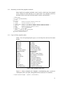
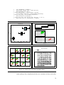
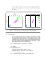
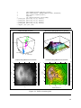
To get a quick appreciation of R graphics, run the demostration programs:
> demo(graphics)
> demo(image)
> demo(lattice)
5.1
Base graphics
A technical introduction to base graphics is given in Chapter 12 of [36].
Here we give an example of building up a sophisticated plot step-by-step,
starting with the defaults and customizing.
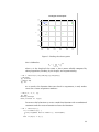
The example is a scatter plot of petal length vs. width from the iris data
set. A default scatterplot of two variables is produced by the plot.default
method, which is automatically used by the generic plot command if two
equal-length vectors are given as arguments:
> data(iris)
> str(iris)
`data.frame': 150 obs. of 5 variables:
$ Sepal.Length: num 5.1 4.9 4.7 4.6 5 5.4 4.6 5 4.4 4.9 ...
$ Sepal.Width : num 3.5 3 3.2 3.1 3.6 3.9 3.4 3.4 2.9 3.1 ...
$ Petal.Length: num 1.4 1.4 1.3 1.5 1.4 1.7 1.4 1.5 1.4 1.5 ...
$ Petal.Width : num 0.2 0.2 0.2 0.2 0.2 0.4 0.3 0.2 0.2 0.1 ...
$ Species
: Factor w/ 3 levels "setosa","versicolor",..: 1 1 1 1 1 1 1 ...
> attach(iris)
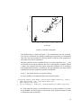
> plot(Petal.Length, Petal.Width)
In this form, the x- and y-axes are given by the first and second arguments,
respectively. The same plot can be produced using a formula §4.17 showing the dependence, in which case the y-axis is given as the dependent
variable on the left-hand side of the formula:
> plot(Petal.Width ~ Petal.Length)
69