1
Manual Desimp Polca game The third phase of the Polca game is an individual reflection, based on the experiences during the Polca game and a simulation of a Polca system. This manual describes some aspects of the software tool used for the simulation. Only the functions and windows that need to be used and understood for the Polca system simulation will be described. More specifically, this manual will not describe the simulation model nor provide details on the modelling tool. Readers that are interested in writing their own simulation programs or in using the tool can consider reading the Desimp User's manual version 2.0.2. The structure of this manual is as follows. Section 1 describes the basics of a discrete event simulation of a system. Section 2 discusses the Polca model and its characteristics. Section 3 is the main section. It discusses the user interface of the simulation system and explains how relevant information can be obtained from the various windows. Section 4 ends with describing how the form should be used to report the results of your simulation. 1 DESIMP: Discrete Event SIMulation in delphi Pascal Simulation is an important tool for resolving design and evaluation problems in the area of Decision and Management Sciences. It aims at imitating and observing the behaviour of a system over time. DESIMP is a discrete event simulation tool. A discrete event simulation describes the behaviour of a system over time according to events that occur at specific moments in time and have effect on the system state. An example of an event is the arrival of an order. This event will initiate one or more processes (for example, order acceptance, purchasing, engineering, production, delivery, et cetera) and therefore lead to several actions of one or more actors. These actions belong to processes, and DESIMP describes the behaviour of systems according to the sequence of activities or decisions within such processes. In general, the occurrence of such events depends on external factors that can not be influenced by the actors. Such events are often modelled as if they originate from random processes, i.e. the probability or duration of their occurrence is described using probability distributions. A simulation tool can be used to experiment with different settings of parameters of a system. The effect of a specific set of parameters can be compared with another set of parameters. We will denote this as two experiments with different parameter settings. In order to compare the effect of the different parameter settings, statistical analysis has to be applied. DESIMP provides some elementary statistics on various performance measures that can be related to inputs, processes, and resources. Multiple replications with different starting values of the random number generator result in different and statistically independent measures of the same performance indicator, which enables the user to provide statements about the accuracy of the expected values of the performance measures of the simulated system. DESIMP consists of a library of routines that can be called in a Delphi program. The simulation model has to be described using a basic template. Within this template, several 1 calls are made to routines in the DESIMP library, which results in a Delphi program executable that can be run on any windows computer. For the Polca game, students will only have to execute such an executable, which means that simulation modelling will not be required in the Polca game. Therefore, this manual will focus on the interface of running a simulation experiment. DESIMP has been developed by Evert Jan Stokking, Faculty of Economics of the University of Groningen. For the Polca game, he released a new version of DESIMP, 2.05, which enables the use of an animation screen in the simulation tool. We will explain this animation screen in detail in section 3. 2 Characteristics of the Polca simulation model The Polca simulation model consists of several independent processes that interact: The arrival of new orders is simulated in an order generator process. This Order generator process determines the number of orders that will arrive simultaneously, the arrival time of this new batch of orders, and the routing of the orders. Order The various experiments apply different settings for this process, i.e. o constant or random interarrival time o low or high number of orders arriving simultaneously (batch size) o constant or random number of orders arriving simultaneously (demand variation low or high) o constant or random number of cells to visit in a routing (productmix variation low or high) The order process describes the sequence of activities of an order in the system. After it has been generated and the specific routing has been determined, the order waits until it is allowed to start (time authorization and a Polca card available), next it awaits until processing is started, next it awaits until it is transported to the next cell in the routing and then this sub process will be repeated until the last cell in the routing has been visited. Performance measures that relate to the process of an order: • The total throughput time of the order is the difference between the completion time and the arrival time in the system. • The shop floor throughput time is the difference between the completion time and the moment the order has started processing in the first cell. • The number of orders in the system reports the number of simultaneously active orders in the system. This is the sum of the Work In Process (WIP) and the order pool. • The number of finished orders is a count used for determining the average throughput times of the orders. • The order waiting time in cell x measures the time an order waits in cell x from the moment of arriving in this cell and being authorized with respect to the starting time until the moment of being selected by the cell. So it includes the waiting time for the required Polca and for capacity in cell x. 2 Cell Each cell is described using a cyclical process. A cell can either await an order or be busy. It is busy if it is processing or setting up for an order, or if it faces a breakdown. Performance measures that relate to the process of a cell: • Observations of the time a cell is not busy result in a utilization rate smaller than 1 and a positive value for the % time cell X not utilized. Note that in order for this measure to be accurate, sufficient observations of idle periods have to be made (see section 3 on results). The higher the utilization rate, the less observations encountered, which may make it necessary to use a longer run length (simulated period). • Cell x waiting time measures the length of each period cell x is idle. • The number of waiting orders in cell x is a count that can be used to determine the WIP in cell x (the average number of orders in process in this cell should be added to this measure to obtain the WIP). If a cell is free and several orders are authorized to start and awaiting processing in this cell, it has to choose what order should be processed first. Polca The experimental settings with respect to the cell are. o selection rule used (longest waiting time (default) or minimal set-up time) o occurrence of breakdowns (yes/no) Each polca is also described as a cyclical process. A polca either awaits an order in the fist cell of its loop, or it is connected to an order. Transport times are zero in the simulated polca system, so other states of a polca card (i.e. awaiting transport or in transport to the originating cell) do not consume time. When a polca is connected to an order, it visits both the originating cell and the destination cell before it is released from the order. Performance measures that relate to the process of a polca: • The number of free polca’s x->y in cell x shows how many polca’s are on average available in the originating cell. The report also shows how many of the available polca’s in this loop have actually been used. • For polca’s that have started circulating, the time they are not attached to an order is observed and reported in polca x->y waiting time in cell x. • The polca x->y laptime measures the cycle time of a polca, i.e. the time that passes after being attached to an order until the moment of being attached to another order. This cycle time is used in the formula for determining the number of polca’s. The number of polca’s in a loop is an experimental factor in the simulation model. For ease of use, all loops apply the same number of polca’s during the simulation. However, this is a simplification and no theoretical reason exists for using the same number of polca’s in different loops. Hence, one of the experimental settings is the: o number of polca’s in each loop 3 The Polca system that is simulated resembles the situation at the polca game layout, although there are some small modifications. Figure 1 shows the animation screen for the simulated system with two polca’s in each loop. We will use this figure to explain the production system that is being simulated. Figure 1 Simulated production system at time 0 The production system consists of six cells. Every order has to visit the first cell A (orange). Next (a subset of) cells B, C, and D have to be visited. Finally, all orders visit cell E and F. Cell A is the only cell that might have to be set up for an order. At time 0, the cell is not set up for any order, so the first order that is selected (order 4) is located in a set up position. The border of this circle is yellow coloured, which indicates that cell A is currently being set up for orders that will visit the yellow coloured cell B after being processed in cell A. The processing time in cell A is two time units, as each circle represents one time unit. Cell B has no set up, but each job faces an identical processing time of 4 units. The same holds true for cell C. Cell D even has a processing time of 5 units. Note however that cells B, C, and D are not visited by each order, as the routings of the orders differ with respect to the subset of cells B, C, and D that have to be visited. A cell can only process one order at a time. So a cell needs to complete the whole sequence of processing steps before another job can be started in the same cell. This completes the description of the simulated polca system and the characteristics of the simulation model. The next section will describe the user interface and animation screen in detail and discuss the interpretation of the results. 4 3 Simulating a Polca system with DESIMP Nestor provides a compressed file SIMULATE.ZIP that encloses four files that should be saved in the same folder. These four files are: • DesimpNestor.exe • SimModel.pas • Desimp.ini • DESIMPManualChapter1_7.pdf The first file is the executable file of DESIMP. This version allows only for experimenting with a model that already has been build and that is described in SimModel.pas. You will have to start DESIMP by clicking on the executable file. The first screen that you will see is shown in Figure 2, except for the red crosses that are inserted to draw your attention to the functionality that has been eliminated from your version. Please do not use these menu choices or buttons. Figure 2 DESIMP opening window The opening window contains three main parts. On top, you find the menu and toolbar. The toolbar buttons Run and Step have a keyboard shortcut F9 and F8 respectively, as shown in Figure 3. Figure 3 Keyboard short cuts revealed through the menu The left panel contains the various views of the simulation process. The upper part does not function, but would normally open an existing simulation model for editing and compiling. The lower part is being used in the simulation assignment. It shows eight views / windows that will be explained shortly. One of them is currently selected, namely the Experiment view. We will discuss all views, starting with the first one: Compiled Source. 5 View: Compiled Source Figure 4 Compiled Source view Compiled Source contains a view of the simulation model that is being used. In case of the Polca simulation, this model is difficult to understand without a thorough knowledge of Delphi Object Pascal and Desimp. Therefore the Compiled Source shows only a short non-technical description of the model. It describes the processes according to the sequential steps that have to be taken. Note that comments are inserted after the // sign. Readers that would like to take a view of the complete simulation model are invited to send an e-mail to [email protected] . 6 View: Experiment Figure 5 Experiment view Figure 5 shows the experiment view after the button Run or Step has been pressed. Here the initial settings of the experiment are being determined. Before pressing the Run or Step button, the number of replications can be selected from a predetermined number of choices in the list box field. If each time a different seed of the random generator is used, then a high number of replications will lead to improved reliability of the results. The reason is that the statistical analysis assumes independence of the results from each replication. If exactly the same seed is entered, the results of the two replications will be identical as well. The seed can be changed, but you can also accept the suggested number. After pressing the Run or Step button, several questions are asked with respect to the experimental factors that were introduced in section 2. The first question is shown in Figure 5 and concerns the number of polca’s in a loop. The suggested number (20) can be accepted by pressing the Enter key, but you can also input another integer number between 1 and 20. Please see the experimental design specified on your form for the inputs you have to provide. Six other questions will be asked, after which the simulation starts running. In the experiment view, you can only see the progress of the simulation on the status bar left. The numbers on the status bar indicate the replication number (1) and the simulated time (126). 7 View: Trace Figure 6 Part of the trace view The trace of a discrete simulation system shows the chronological sequence of activities that are being performed by all objects in the system. It can be used for verification, but is not necessary to understand the contents of this screen for the simulation of the polca system. Let’s take a look at the information on the screen. If Trace is selected in the left panel, the toolbar changes as well. The button Trace seems pressed, which means that the results of the trace are stored in a text field. This is rather resource-consuming, even if you do not present the contents of the trace on the open window. So if you do not need the information of the trace anymore, release the trace button on the toolbar. The first column of the trace window shows a unique activity number. The second column shows the simulation time (154). At time 154 several activities are being performed. Order39 decides to wait in the input queue of cell 5. Cell 5 might be busy with another order at this moment in time. Cell 2 has waited zero time units upon an order and decides to select order44, attaches the required Polca card and holds this order and polca one time unit till time 155. By pressing the Step (F8) button, the trace will proceed to the first event after the current time. All activities that are being performed at this moment in time will be listed in the trace view. By pressing SHIFT-F8, the simulation will proceed with a single activity. Pressing Run (F9) will lead to a fast scrolling view. 8 View: Event List, Queues, Warnings Figure 7 Event list view The next three views are mainly useful during design and testing of a simulation model. Note that the Trace button on the toolbar has not yet been released. Apparently the user has forgotten to do so or the data in the trace view has to be gathered in the background. The event list shows all events that are already known to occur in future. At time 154 we know that one time unit later several objects will have to perform one or more activities. Cells 1-5 all have to perform event 21, animation1 event 3, and at time 161 new orders will be generated. A specific event that will always be listed in this window is the MainObject. This is the controller of the simulation system and will terminate all activities at the specified moment in time (800000). Because of a persistent bug in the system, it is not recommended to simulate until time 800000. Please pause your simulation on an earlier moment by pressing the yellow PAUSE button in the toolbar and report the results. The Queues view shows the contents of the various queues in the simulation system. It will be quite difficult for most of you to understand this view, so for further explanation we refer to the User's manual of DESIMP that is included in the zip file SIMULATE.ZIP. The Warnings view shows errors and warnings for the designer and/or user of the simulation system. Most of the time you will see an empty screen. 9 View: Report Figure 8 Reports view The Report window contains all statistical data on the simulation experiment. The first two rows mention the model and time of running the simulation. The next 7 rows describe the experimental settings in this experiment. The Report continuous with the current replication number. Data from this replication is gathered and based on these data the performance measures will be modified. The seed for the random number generator in this replication is also described. Finally three sections appear where the results and other data will be presented. The first section describes the results, i.e. the performance measures. The next section provides information on the skewness of the distribution of the results. The last section provides information to validate the random number generator in the simulation experiment. All three sections will be illustrated using a figure. 10 Figure 9 Report section Results (1) The first section (Results) shows in the first column the title of a performance measure. Next it shows the number of observations (Obs) during the simulation run. Note that the various performance measures have different numbers of observations. The first measure (total throughput time) has 708 observations, similar to the number of finished orders. The reason is that each finished order contributes to the performance measure total throughput time. However, the number of orders in the system (i.e. the WIP) has been observed already 963 times. Each state change leads to a new measurement, so this performance measure changes more frequently. Min and Max show the range of the performance measure in this experiment, Mean the average value of the measure. The column +/- shows the reliability of the mean, based on the number of completed replications in this experiment. It describes a 95% confidence interval around the estimated mean. The probability that the true mean will be in this interval is 95%. The last column shows the mean total per replication, i.e. Obs*Mean divided by the number of replications. 11 You can determine the confidence interval of several performance measures by hand. The following formulas can be used: Let µ Xi : true (unknown) mean value of the performance measure in this experiment : value of the performance measure in replication i n : total number of replications performed in this experiment X (n ) : average value of the performance measure, based on n replications σ2 : (unknown) variance of sample mean X (∞) S 2 (n ) : unbiased estimate of σ 2 , based on n replications Then X (n ) = S 2 (n ) = 1 n n ∑ Xi i =1 1 n −1 n ∑ ( X i − X (n ) ) 2 i =1 And the ± 95% confidence interval of µ is: S 2 (n) S 2 (n ) X (n )-2 , X (n )+2 n n The confidence interval of the true mean provides information on the accuracy of the estimate X ( n ) of the true mean, and this accuracy increases with the number of replications n. Note that the unbiased estimate of the variance of the distribution of the performance measure value in different replications is not necessarily decreasing in n. Figure 10 Report section Results (2) The reports on Polca's and cells will be discussed in detail. Figure 10 shows that the number of free Polca's that circulate in loop 3->5 (cell C->E) was on average 1.40987. This amount of Polca's 3->5 is on average decoupled from an order and waiting to be attached to a new order in cell 3. The Min and Max column show that a situation has occurred where the bin in cell 3 was completely empty (0 free Polca's) as well as a situation that the bin contained two cards. The latter situation reflects the initial situation, as the Polca simulation starts with all available Polca cards in the bin in the originating cell. The average waiting time of a (used) Polca card in the bin in cell 3 was 15.1978 time units. The longest waiting time encountered by a Polca card was 70 time units. The lap time of a Polca 3->5 is on average 6.4 time units. The minimum time was 6 units, which is exactly the sum of processing times in cell 3 and 5. The maximum was 8 time units, so apparently no long waiting times are to be expected for orders in cell 5. 12 Figure 11 Report section Results (3) The order waiting time in cell 5 is shown in Figure 11. Our idea was correct: the order waiting time in cell 5 was on average 0.2 time units and the longest waiting time encountered was 2 time units. In the latter situation, probably two orders from different originating cells entered cell 5 at the same moment in time, while no orders were queued in cell 5. One of them had to wait the total processing time in cell 5, which makes the maximal order waiting time in cell 5 equal to 2 time units. The utilization of cell 5 can be calculated as (100%-% Time cell 5 not utilized) = 56.197% This estimate is based on 1262 observations of cell 5 either becoming idle or leaving the idle state. Such a high number of observations makes the estimate rather reliable. Cell 5 has on average waited 1.8 time units before a new set of orders was processed. The longest waiting time was 11 time units. This completes our discussion of the results section of the report view. Figure 12 Report section Distribution of results The section Distribution of results provides percentile estimates of the performance measures. Imagine that all observations of the specific performance measure were sorted. The columns represent the maximum value of the performance measure in the subset of observations mentioned. For example, 90% of the finished orders encountered a total throughput time of 48 or less. Hence, (100-90)% had a total throughput time above 48. Finally, the section Distribution presents the drawings from probability distribution functions. This report is excluded from your simulation experiments. 13 View: Animation Figure 13 Animation screen The last view that is available in DESIMP 2.05 is the animation view. This view has been added specifically for enabling an animated view of the Polca game layout during the simulation run. It has to be activated by pressing the TRACE button of the top menu. The reason is that it is quite time consuming for the computer to generate and update this view. We will describe several parts of this screen in detail. Note that the basic layout of the cells already has been described in Figure 1 on page 4. First, we will focus on the lower right side of the animation screen. There we find a list of orders that have been generated but not yet released to cell A. The routing of the orders has randomly been determined, and by chance or policy 9 of the 10 unreleased orders have to visit cell C immediately after cell A. Cell A is busy with order 848, which number is shown on an orange-yellow Polca between the input circle and the three output circles. The other cells will also show the processed order with the attached Polca('s) between these circles. Cell B has no orders in progress nor any order waiting. Cell C has an order in progress (831), which will go to cell D afterwards. C has also an order waiting (834). This order has to wait on capacity in C, but also on an available Polca card from the next cell. What cell will it have to visit after cell C? This can be seen on the plan board at the lower left site of the animation screen. The plan board lists all orders and shows in the last column the remaining routing after the current cell has been visited. Order 834 is shown to be generated on time 2912.00, has 14 a status of awaiting Polca authorization (it has currently only one Polca attached), and has to visit cells 4, 5, and 6 (i.e. D, E, and F) afterwards. Now we know that order 834 will have to wait for a 3-> 5 (green->blue) Polca card. There are two of these cards circulating. One of them is attached to order 831 currently processed on cell C. The other is attached to order 829 in the input circle in cell D. The latter one is allowed to start and just awaits a decision of cell D to start processing this order. Cell D has almost finished processing of order 842, and the status Allowed to start indicates that for the waiting order a Polca card 4->5 is available. This card is shown to be waiting in the output circle in cell D. If no number is mentioned on the card, the Polca is free and waits in the originating cell. Finally, some basic performance indicators are shown at the bottom right of the animation screen. Total throughput time, shop floor throughput time and number of finished orders. See page 2 for a description of these measures. If the number of Polca's is equal to the maximum number of Polca's (i.e. 20), then the animation screen will not show any Polca at all. This situation can be considered as an unconstrained system, where orders never have to wait before the required Polca becomes available. This completes our description of the DESIMP user interface for the Polca simulation game. Further details and explanations can be fund in the User's Manual DESIMP. 15 4 Reporting the results of your simulation The individual reflections on the Polca game should be accompanied by a description of the experiments you performed using DESIMP. Seven experimental factors have been introduced on page 2: 1. constant or random interarrival time 2. low or high number of orders arriving simultaneously (batch size) 3. constant or random number of orders arriving simultaneously (demand variation low or high) 4. constant or random number of cells to visit in a routing (productmix variation low or high) 5. selection rule used (longest waiting time (default) or minimal set-up time) 6. occurrence of breakdowns (yes/no) 7. number of polca’s in each loop Every student has to experiment with the last factor, in combination with a specific set of choices for factors 1-6. The specific set of choices for your experiment depends on your research design. The main results to be reported are total throughput time and shop floor throughput time. Experiments with a small number of Polca's in each loop might result in a non-stable system, i.e., a system with on average an infinite number of orders in the order pool. Measuring such a system is useless, as increasing the length of a simulation run will logically result in a larger total throughput time measure. Therefore you have to investigate during the simulation run whether the results are still useful. Both the Report and Animation screen can provide you with information on the length of the order pool. You do not need to simulate the experiment with all numbers of Polca's between 1 and 20. Just start at 1 and continue to 2, 3, 4, 5. If you have seen a significant difference in the performance between the last two numbers, you should continue, otherwise you may quit. Note that for unstable systems you do not need to gather data. Please report only the facts that have lead you to decide that it is probably an unstable system. It is often wise to report the length of a simulation run (time when run has been paused and report generated). You may decide on your own how long you simulate, depending on the number of observations of the various measures. Please note the number of observations that determine the utilization of the cells! This should be more than 100 for each cell. To give you an idea how long you should simulate: more than 2000 time units, less than 800000 time units. The number of replications of a similar experiment with a different seed of the random number generator should be sufficient for statistically significance of the outcomes, and to determine confidence intervals for the mean total throughput time and mean shop floor throughput time in your experiment. These intervals should be reported as well. 16