1
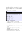
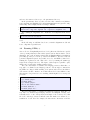
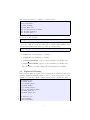
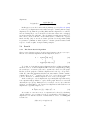
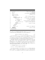
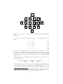
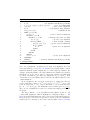
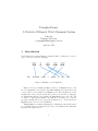
TsinghuaAligner:
A Statistical Bilingual Word Alignment System
Yang Liu
Tsinghua University
[email protected]
April 22, 2015
1
Introduction
Word alignment is a natural language task that aims to identify the correspondence between words in two languages.
The
zongtong
zai
niuyue
fabiao
jianghua
总统
在
纽约
发表
讲话
President
made
a
speech
at
New York
Figure 1: Example of word alignment.
Figure 1 shows a (romanized) Chinese sentence, an English sentence, and
the word alignment between them. The links highlighted in blue indicate the
correspondence between Chinese and English words. Word alignment is a challenging task because both the lexical choices and word orders in two languages
are significantly different. For example, the English function words “the” and
“a” have no counterparts in Chinese. In addition, a verb phrase (e.g., “made a
speech”) is usually followed by a prepositional phrase (e.g., “at New York”) in
English but the order is reversed in Chinese.
TsinghuaAligner is statistical bilingual word alignment system that takes a
set of parallel sentences as input and produces word alignment automatically.
It has the following features:
1
1. Language independence. The system is language independent and can
be used for any language pairs.
2. Extensibility. Our system is based on log-linear models, which are capable of incorporating arbitrary information sources as features. Therefore,
the system is highly extensible. It is possible to design and include new
features to capture the characteristics of specific languages.
3. Supervised learning. Provided with manually annotated parallel corpus, the system is able to learn to minimize the difference between its
alignment and the manual alignment.
4. Unsupervised learning. The system is also capable of learning from
unlabeled data automatically and delivers pretty good performance.
5. Structural constraints. TsinghuaAligner supports a variety of structural constraints such as many-to-many, ITG, and block ITG. These constraints prove to be effective in modeling the structural divergence between
natural languages.
6. Link posterior probabilities. The system is capable of producing the
posterior probability for each link in alignments to indicate the confidence
that two words are aligned.
2
Installation
2.1
System Requirements
TsinghuaAligner supports Linux i686 and Mac OSX. You need to install the
following free third-party software to build TsinghuaAligner:
1. GIZA++. It can be downloaded at https://code.google.com/p/giza-pp/;
2. g++ version 4.6.3 or higher;
3. Python version 2.7.3;
4. JRE 1.6 or higher (optional, only used for the visualization tool AlignViz).
2.2
Installing TshinghuaAligner
Here is a brief guide on how to install TsinghuaAligner.
2.2.1
Step 1: Unpacking
Unpack the package using the following command.
1
tar xvfz TsinghuaAligner.tar.gz
2
2.2.2
Step 2: Compiling
Entering the TsinghuaAligner directory, you may find five folders (code, doc,
example, GUI, and scripts) and one script file (install.sh). The code folder includes the source code, the doc folder includes the documentation, the
example folder contains example data, the GUI folder contains the visualization
tool AlignViz, and the scripts folder includes Python scripts for training the
system.
First, change the mode of the installing script.
1
chmod +x install.sh
Then, install the system by running the script.
1
./install.sh
If everything goes well, you should see the following information.
1
2
3
4
5
6
7
8
9
10
Creating a directory to store binary executables ... done!
Compiling TsinghuaAligner ... done!
Compiling waEval ... done!
Compiling convertNBestListFormat ... done!
Compiling genIni ... done!
Compiling mergeNBestList ... done!
Compiling optimizeAER ... done!
Chmoding genNoise ... done!
Compiling trainer ... done!
Chomoding scripts ... done!
11
12
The system is installed successfully.
The script creates a folder bin to place all binary executables:
1. TsinghuaAligner: the main component of the system that produces
word alignment for parallel corpora;
2. optimizeAER: the main component for supervised training;
3. trainer: the main component for unsupervised training;
4. convertNBestListFormat: converting n-best list format for supervised
training;
5. genIni: generating configuration files for supervised training;
6. megerNBestList: merging n-best lists of multiple iterations for supervised learning;
7. genNoise.py: generating noises for unsupervised learning;
8. waEval: evaluating the system in terms of alignment error rate.
3
2.2.3
Step 3: Compiling GIZA++
TsinghuaAligner takes the translation probabilities derived from GIZA++ as
the central feature in the log-linear model. As a result, GIZA++ needs to be
properly installed to run our system. Please visit https://code.google.com/p/gizapp/ to download GIZA++ and compile it according to its user manual.
After installing GIZA++, copy the following binary executables to the bin
folder:
1. GIZA++: the main component for training IBM models;
2. mkcls: training word classes on monolingual corpus;
3. plain2snt.out: converting plain files to the snt format;
4. snt2cooc.out: collecting co-occurrence statistics.
Note that there should be 12 binary executables in the bin folder if the
system is properly installed.
2.2.4
Step 4: Locating the Executables
Training TsinghuaAligner is mainly done by using the Python scripts in the
scripts folder. You need to enable these scripts to locate the binary executables
by modifying the root_dir variable in each script.
For example, you may change line 7 of the GIZA.py script
1
1
root_dir = ’’
to
root_dir = ’/User/Jack/TsinghuaAligner’
Note that /User/Jack/TsinghuaAligner is the directory where TsinghuaAligner is installed. You may use the command pwd to get the full path name
of the root directory.
Do the same to the other two Python scripts supervisedTraining.py and
unsupervisedTraining.py and complete the installation.
3
User Guide
3.1
Quick Start
To quickly know how TsinghuaAligner works, you may take the following steps.
First, download the model.ce.tar.gz file from the system website 1 , which
is a Chinese-English model that can be directly used by TsinghuaAligner. Unpack the file
1
tar xvfz model.ce.tar.gz
1 http://nlp.csai.tsinghua.edu.cn/˜ly/systems/TsinghuaAligner/TsinghuaAligner.html
4
and move the model.ce directory to the quickstart directory.
In the quickstart directory, there are three files: chinese.txt (Chinese
text), english.txt (English text), and TsinghuaAligner.ini (system configuration file). Then, simply run the following command:
1
2
1
TsinghuaAligner --ini-file TsinghuaAligner.ini --src-file
chinese.txt --trg-file english.txt --agt-file alignment.txt
The resulting file alignment.txt contains the word alignment in the Moses
format
0-0 1-2 2-3 3-5 4-7 5-8 6-9
where 0-0 denotes that the first Chinese word is aligned to the first English
word.
In the following, we will introduce how to train the alignment models and
how to align unseen parallel text.
3.2
Running GIZA++
As noted before, TsinghuaAligner is based on log-linear models that are capable
of incorporating arbitrary features that capture various characteristics of word
alignment. One of the most important feature in TsinghuaAligner is translation
probability product (see Section 5) derived from GIZA++, the state-of-the-art
generative alignment system. As a result, we need to run GIZA++ first before
training the log-linear models. This can be done by running the GIZA++.py
script in the scripts directory. The input of this script is a parallel corpus,
which can be found in the example/trnset folder.
The source file trnset.f contains source-language sentences. Each line corresponds to a tokenized source-language sentence. We strongly recommend using UTF-8 encoding for all the training, development, and test sets. In addition,
each sentence should contain no more than 100 words because GIZA++ usually truncates long sentences before training, which might lead to unexpected
problems.
1
2
3
4
5
6
7
wo
wo
ni
ni
wo
ta
ta
xihuan dushu .
ye xihuan yinyue .
xihuan dushu .
ye xihuan yinyue .
he ni dou xihuan dushu .
xihuan dushu ma ?
xihuan yinyue ma ?
The target file trnset.e contains target-language sentences. Each line corresponds to a tokenized target-language sentence. For English, lowering cases
is usually used to reduce data sparseness and improve the accuracy. Note that
the source and target sentences with the same line number are assumed to be
translations of each other. For example, the first sentence in trnset.f and the
5
first sentence in trnset.e constitute a parallel sentence.
1
2
3
4
5
6
7
i like reading .
i also like music .
you like reading .
you like music too .
both you and me like reading .
does he like reading ?
does he like music ?
To run GIZA++, simply use the GIZA.py script in the scripts folder with
the two above files as input.
1
GIZA.py trnset.f trnset.e
GIZA++ training usually takes a long time, especially for large parallel
corpora (i.e., millions of sentence pairs). We recommend using nohup to keep
executing the training script after you exit from a shell prompt.
1
nohup GIZA.py trnset.f trnset.e &
When GIZA++ training is complete, there should be four resulting files:
1. source.vcb: source-language vocabulary;
2. target.vcb: target-language vocabulary;
3. source target.tTable: source-to-target translation probability table;
4. target source.tTable: target-to-source translation probability table.
These files will be used in both supervised and unsupervised training.
3.3
Supervised Training
In supervised training, we require a set of parallel sentences annotated with goldstandard alignment manually, which we refer to as the development set. The
example development set in the example/devset folder contains three files.
1
2
3
4
5
6
7
8
==> devset.f <==
wo xihuan dushu .
wo ye xihuan yinyue .
ni xihuan dushu .
ni ye xihuan yinyue .
wo he ni dou xihuan dushu .
ta xihuan dushu ma ?
ta xihuan yinyue ma ?
9
10
11
12
==> devset.e <==
i like reading .
i also like music .
6
13
14
15
16
17
you like reading .
you like music too .
both you and me like reading .
does he like reading ?
does he like music ?
18
19
20
21
22
23
24
25
26
==> devset.wa <==
1:1/1 2:2/1 3:3/1
1:1/1 2:2/1 3:3/1
1:1/1 2:2/1 3:3/1
1:1/1 2:4/1 3:2/1
1:4/1 2:3/1 3:2/1
1:2/1 2:3/1 3:4/1
1:2/1 2:3/1 3:4/1
4:4/1
4:4/1
4:4/1
4:3/1
4:1/1
4:1/0
4:1/0
5:5/1
5:5/1
5:5/1 6:6/1
5:5/1
5:5/1
The source and target files are similar to the training set. 2 The goldstandard file devset.wa contains manual annotations. “1:1/1” denotes a sure
link that connects the first source word and the first target word. This usually
happens for content words such as “yinyue” and “music”. In contrast, “4:1/0”
denotes a possible link that connects the fourth source word (e.g., “ma”) and
the first English word (e.g., “does”). Function words are usually aligned as
possible links.
Our supervised trainer relies on the development set to learn the parameters
of log-linear models. The arguments of the supervisedTraining.py in the
scripts folder are listed as follows:
1
2
3
4
5
6
7
8
9
10
11
Usage: supervisedTraining [--help] ...
Required arguments:
--src-vcb-file <file>
--trg-vcb-file <file>
--s2t-ttable-file <file>
--t2s-ttable-file <file>
--dev-src-file <file>
--dev-trg-file <file>
--dev-agt-file <file>
Optional arguments:
--iter-limit [1, +00)
12
13
--nbest-list-size [1, +00)
14
15
--beam-size [1, +00)
16
17
--structural-constraint {0, 1, 2}
18
19
source vocabulary
target vocabulary
source-to-target TTable
target-to-source TTable
devset source file
devset target file
devset alignment file
MERT iteration limit
(default: 10)
n-best list size
(default: 100)
beam size
(default: 1)
structural constraint
0: arbitrary
1: ITG
2 For simplicity, the source and target files in the training and development sets are the
same. In practice, training sets are usually much larger than development sets.
7
20
21
22
--enable-prepruning {0, 1}
23
24
25
26
--prepruning-threshold (-00, +00)
27
28
--help
2: BITG
(default: 0)
enable prepruning
0: disable
1: enable
(default: 0)
prepruning threshold
(default: 0)
prints this message
We distinguish between required and optional arguments. Required arguments must be explicitly specified when running the supervisedTraining.py
script. The 7 required arguments are all files, including the resulting files from
GIZA++ and the development set. Optional arguments include
1. iteration limit: limit on minimum error rate training iterations. The
default value is 10.
2. n-best list size: n-best list size. The default value is 100.
3. beam size: beam size of the search algorithm. The default value is 1.
4. structural constraint: TsinghuaAligner supports three kinds of structural constraints: arbitrary, ITG, and block ITG. The default value is
0.
5. enabling prepruning: prepruning is a technique that improves the aligning speed by constraining the search space. The default value is 0.
6. prepruning threshold: The threshold for prepruning. The default value
is 0.
You need not specify optional arguments in running the script unless you
want to change the default setting. An example command for supervised training is
1
2
3
4
supervisedTraining.py --src-vcb-file source.vcb --trg-vcb-file
target.vcb --s2t-ttable-file source_target.tTable --t2s-ttable
-file target_source.tTable --dev-src-file dev.f --dev-trg-file
dev.e --dev-agt-file dev.wa
The resulting file is a configuration file TsinghuaAligner.ini for the aligner.
1
2
3
4
5
# knowledge sources
[source vocabulary file]
[target vocabulary file]
[source-to-target TTable
[target-to-source TTable
source.vcb
target.vcb
file] source_target.tTable
file] target_source.tTable
6
7
# feature weights
8
8
9
10
11
12
13
14
15
16
17
18
19
20
21
22
23
[translation probability product feature weight] 0.0504511
[link count feature weight] -0.0661723
[relative position absolute distance feature weight] -0.264923
[cross count feature weight] -0.0588821
[mono neighbor count feature weight] -0.137836
[swap neighbor count feature weight] -0.049596
[source linked word count feature weight] -0.00257702
[target linked word count feature weight] -0.0229796
[source maximal fertility feature weight] -0.072508
[target maximal fertility feature weight] -0.0126342
[source sibling distance feature weight] -0.072326
[target sibling distance feature weight] 0.0100039
[one-to-one link count feature weight] -0.0212899
[one-to-many link count feature weight] -0.0310621
[many-to-one link count feature weight] 0.0334263
[many-to-many link count feature weight] 0.0933321
24
25
26
# search setting
[beam size] 1
27
28
29
30
31
32
# structural constraint
# 0: arbitrary
# 1: ITG
# 2: BITG
[structural constraint] 0
33
34
35
36
# speed-up setting
[enable pre-pruning] 0
[pre-pruning threshold] 0.0
We will explain the configuration file in detail in Section 3.5.
3.4
Unsupervised Training
As manual annotation is labor intensive, it is appealing to directly learn the
feature weights from unlabled data.
Our unsupervised trainer unsupervisedTraining.py in the scripts folder
only uses the training set for parameter estimation.
1
2
3
4
5
6
7
8
Usage: unsupervisedTraining [--help] ...
Required arguments:
--src-file <file>
source file
--trg-file <file>
target file
--src-vcb-file <file>
source vocabulary
--trg-vcb-file <file>
target vocabulary
--s2t-ttable-file <file>
source-to-target TTable
--t2s-ttable-file <file>
target-to-source TTable
9
9
10
11
12
13
14
15
16
17
18
19
20
21
22
23
24
25
26
27
28
29
30
31
32
33
34
35
Optional arguments:
--training-corpus-size [1, +00)
training corpus size
(default: 10)
--sent-length-limit [1, +00)
sentence length limit
(default: 100)
--shuffle {0, 1}
shuffling words randomly
(default: 1)
--replace {0, 1}
replacing words randomly
(default: 0)
--insert {0, 1}
inserting words randomly
(default: 0)
--delete {0, 1}
deleting words randomly
(default: 0)
--beam-size [1, +00)
beam size
(default: 5)
--sample-size [1, +00)
sample size
(default: 10)
--sgd-iter-limit [1, +00)
SGD iteration limit
(default: 100)
--sgd-converge-threshold (0, +00) SGD convergence threshold
(default: 0.01)
--sgd-converge-limit [1, +00)
SGD convergence limit
(default: 3)
--sgd-lr-numerator (0, +00)
SGD learning rate numerator
(default: 1.0)
--sgd-lr-denominator (0, +00)
SGD learning rate denominator
(default: 1.0)
The optional arguments include
1. training corpus size: the number of training examples used for training.
It turns out our unsupervised trainer works pretty well only using a small
number of training examples. The default value is 10;
2. sentence length limit: the maximal length of sentences in the training
corpus. The default value is 100;
3. shuffle: our unsupervised training algorithm is based on a contrastive
learning approach, which differentiates the observed examples from noises.
Turning this option on will generate noisy examples by shuffling words.
The default value is 1;
4. replace: generating noises by replacing words randomly. The default
value is 0;
5. insert: generating noises by replacing words randomly. The default value
is 0;
10
6. delete: generating noises by inserting words randomly. The default value
is 0;
7. beam size: beam size for the search algorithm. The default value is 5;
8. sample size: sample size for top-n sampling that approximates the expectations of features. The default value is 10;
9. SGD iteration limit: we use stochastic gradient descent for optimization. This argument specifies the limit on SGD iterations. The default
value is 100;
10. SGD convergence threshold: the threshold for judging convergence in
SGD. The default value is 0.01;
11. SGD convergence limit: the limit for judging convergence in SGD. The
default value is 3;
12. SGD learning rate numerator: the numerator for computing learning
rate in SGD. The default value is 1.0;
13. SGD learning rate denominator: the denominator for computing
learning rate in SGD. The default value is 1.0.
An example command for unsupervised training is
1
2
3
4
unsupervisedTraining.py --src-file trnset.f --trg-file trnset.e
--src-vcb-file source.vcb --trg-vcb-file target.vcb --s2t
-ttable-file source_target.tTable --t2s-ttable-file target
_source.tTable
The resulting file of unsupervised training is also a configuration file
TsinghuaAligner.ini for the aligner.
3.5
Aligning Unseen Parallel Corpus
TsinghuaAligner takes a configuration file TsinghuaAligner.ini as input:
1
2
3
4
5
# knowledge sources
[source vocabulary file]
[target vocabulary file]
[source-to-target TTable
[target-to-source TTable
source.vcb
target.vcb
file] source_target.tTable
file] target_source.tTable
6
7
8
9
10
11
12
# feature weights
[translation probability product feature weight] 0.0504511
[link count feature weight] -0.0661723
[relative position absolute distance feature weight] -0.264923
[cross count feature weight] -0.0588821
[mono neighbor count feature weight] -0.137836
11
13
14
15
16
17
18
19
20
21
22
23
[swap neighbor count feature weight] -0.049596
[source linked word count feature weight] -0.00257702
[target linked word count feature weight] -0.0229796
[source maximal fertility feature weight] -0.072508
[target maximal fertility feature weight] -0.0126342
[source sibling distance feature weight] -0.072326
[target sibling distance feature weight] 0.0100039
[one-to-one link count feature weight] -0.0212899
[one-to-many link count feature weight] -0.0310621
[many-to-one link count feature weight] 0.0334263
[many-to-many link count feature weight] 0.0933321
24
25
26
# search setting
[beam size] 1
27
28
29
30
31
32
# structural constraint
# 0: arbitrary
# 1: ITG
# 2: BITG
[structural constraint] 0
33
34
35
36
# speed-up setting
[enable pre-pruning] 1
[pre-pruning threshold] 0.0
Lines 1-5 show the knowledge sources used by the aligner, which are source
and target vocabularies and translation probability tables in two directions generated by GIZA++. Lines 7-23 specify the feature weights of the log-linear
model. We use 16 features in TsinghuaAligner. Other parameters in the configuration file are related to the search algorithm. We strongly recommend
enabling pre-pruning to improve the aligning speed by an order of magnitude
without sacrificing accuracy significantly.
The default structural constraint used in search is “arbitrary”. You may try
other constraint such as “ITG” by modifying the configuration file as follows
1
2
3
4
5
# structural constraint
# 0: arbitrary
# 1: ITG
# 2: BITG
[structural constraint] 1
The aligner itself in the bin folder is easy to use.
1
2
3
4
5
Usage: TsinghuaAligner [--help] ...
Required arguments:
--ini-file <ini_file>
initialization file
--src-file <src_file>
source file
--trg-file <trg_file>
target file
12
6
7
8
9
--agt-file <agt_file>
Optional arguments:
--nbest-list [1, +00)
--verbose {0, 1}
10
11
12
--posterior {0, 1}
13
14
--help
alignment file
n-best list size (default: 1)
displays run-time information
* 0: document level (default)
* 1: sentence level
outputs posterior link probabilities
(default: 0)
prints this message to STDOUT
There are two optional arguments:
1. n-best list size: n-best list size. The default value is 1.
2. verbose: display run-time information. The default value is 0.
3. posterior: output posterior link probabilities. The default value is 0.
Suppose we have unseen source and target sentences as follows
1
2
3
==> source.txt <==
ta he wo dou xihuan yinyue .
ni he ta dou xihuan dushu .
4
5
6
7
==> target.txt <==
both he and i like music .
both he and you like reading .
Let’s run the aligner to produce alignment for the sentences.
1
2
TsinghuaAligner --ini-file TsinghuaAligner.ini --src-file
source.txt --trg-file target.txt --agt-file alignment.txt
The resulting file alignment.txt is in the Moses format:
1
2
1-0 2-3 3-2 4-4 5-5 6-6
0-3 3-2 4-4 5-5 6-6
where “1-0” denotes that the second source word is aligned to the first target
word. Note that the subscript of the first word is 0 rather than 1.
Sometimes, we are interested in how well two words are aligned. TsinghuaAligner is able to output link posterior probabilities to indicate the degree of alignedness. This can be simply done by turning the posterior option on:
1
2
3
1
2
3
TsinghuaAligner --ini-file TsinghuaAligner.ini --src-file
source.txt --trg-file target.txt --agt-file alignment.txt
--posterior 1
The result file is as follows.
4-4/0.997164 5-5/0.981469 6-6/0.941433 2-3/0.868177 3-2/0.570701
1-0/0.476397 2-0/0.090127
4-4/0.996101 5-5/0.976339 6-6/0.919651 3-2/0.777563 0-3/0.646714
13
4
1-0/0.415113
Note that each link is assigned a probability within [0, 1] to indicate the confidence the two words are aligned. The resulting file just contains sets of links
collected from the aligning process and do not form reasonable alignments. You
must specify a threshold to prune unlikely links and get high-quality alignments.
3.6
Visualization
We provide a visualization tool called AlignViz to display the alignment results,
which is located in the GUI folder. The input of AlignViz are three files.
1
2
3
==> source.txt <==
ta he wo dou xihuan yinyue .
ni he ta dou xihuan dushu .
4
5
6
7
==> target.txt <==
both he and i like music .
both he and you like reading .
8
9
10
11
==> alignment.txt <==
0-1 1-2 2-3 3-0 4-4 5-5 6-6
0-3 1-2 2-1 3-0 4-4 5-5 6-6
To launch AlignViz, simply use the following command
1
java -jar AlignViz.jar
The aligned sentence pair is shown in Figure 2.
Figure 2: Visualization of word alignment.
14
3.7
Evaluation
To evaluate our system, we need a test set to calculate alignment error rate
(AER). The test set in the example/tstset folder is
1
2
3
==> tstset.f <==
ta he wo dou xihuan yinyue .
ni he ta dou xihuan dushu .
4
5
6
7
==> tstset.e <==
both he and i like music .
both he and you like reading .
8
9
10
11
==> tstset.wa <==
1:2/1 2:3/1 3:4/1 4:1/1 5:5/1 6:6/1
1:2/1 2:3/1 3:4/1 4:1/1 5:5/1 6:6/1
Now, let’s run the aligner to produce alignment for the test set.
1
2
TsinghuaAligner --ini-file TsinghuaAligner.ini --src-file
tstset.f --trg-file tstset.e --agt-file alignment.txt
The resulting file alignment.txt is in the Moses format:
1
2
1
1
2
1-0 2-3 3-2 4-4 5-5 6-6
0-3 3-2 4-4 5-5 6-6
Finally, you may run the waEval program in the bin folder to calculate the
AER score:
waEval tstset.wa alignment.txt
The evaluation result is shown as follows.
(1) 3 3 6 6 -> 0.5
(2) 2 2 5 6 -> 0.636364
3
4
5
6
7
[total
[total
[total
[total
matched sure] 5
matched possible] 5
actual] 11
sure] 12
8
9
10
11
[Precision] 0.454545
[Recall] 0.416667
[AER] 0.565217
12
13
14
15
Top 10 wrong predictions:
(2) 0.636364
(1) 0.5
waEval outputs not only the overall AER score but also the AER score for
each sentence pair. It lists the top-10 wrong sentence pairs to facilitate error
15
analysis.
4
Additional Datasets
In the TsinghuaAligner.tar.gz package, we only offer toy training, development, and test sets for showing how to use the system. In practice, you need
large training corpus and manually annotated development and test sets for
running the system.
We offer the following additional Chinese-English datasets for FREE on our
system website: 3
1. model.ce.tar.gz: the model files (see Section 3.1) are trained by GIZA++
on millions of Chinese-English sentence pairs. Note that all Chinese words are composed of halfwidth characters and all English words are lower
cased.
2. Chinese-English training set: the training set comprises parallel corpora from the United Nations website (UN) and the Hong Kong Government website (HK). The UK part contains 43K sentence pairs and the HK
part contains 630K sentence pairs.
3. Chinese-English evaluation set: the evaluation set comprises two parts: the development set (450 sentences) and the test set (450 sentences).
Note that we use the UTF-8 encoding for all Chinese and English files.
5
Tutorial
5.1
Log-Linear Models for Word Alignment
TsinghuaAligner originates from our early work on introducing log-linear models
into word alignment (Liu et al., 2005). Given a source language sentence f =
f1 , . . . , fj , . . . , fJ and a target language sentence e = e1 , . . . , ei , . . . , eI , we define
a link l = (j, i) to exist if fj and ei are translations (or part of a translation)
of one another. Then, an alignment is defined as a subset of the Cartesian
product of the word positions:
a ⊆ {(j, i) : j = 1, . . . , J; i = 1, . . . , I}
(1)
Note that the above definition allows for arbitrary alignments while IBM models
impose the many-to-one constraint (Brown et al., 1993).
In supervised learning, the log-linear model for word alignment is given by
exp(θ · h(f , e, a)
0
a0 exp(θ · h(f , e, a ))
P (a|f , e) = P
3 http://nlp.csai.tsinghua.edu.cn/˜ly/systems/TsinghuaAligner/TsinghuaAligner.html
16
(2)
where h(·) ∈ RK×1 is a real-valued vector of feature functions that capture the
characteristics of bilingual word alignment and θ ∈ RK×1 is the corresponding
feature weights.
In unsupervised learning, the latent-variable log-linear model for word alignment is defined as
X
P (f , e) =
P (f , e, a)
(3)
a
=
X
a
exp(θ · h(f , e, a)
P P P
0 0
0
f0
e0
a0 exp(θ · h(f , e , a ))
(4)
The major advantage of log-linear models is to define useful features that
capture various characteristics of word alignments. The features used in TsinghuaAligner mostly derive from (Liu et al., 2010).
5.1.1
Translation Probability Product
To determine the correspondence of words in two languages, word-to-word translation probabilities are always the most important knowledge source. To model
a symmetric alignment, a straightforward way is to compute the product of the
translation probabilities of each link in two directions.
For example, suppose that there is an alignment {1, 2} for a source language
sentence f1 f2 and a target language sentence e1 e2 ; the translation probability
product is
t(e2 |f1 ) × t(f1 |e2 )
where t(e|f ) is the probability that f is translated to e and t(f |e) is the probability that e is translated to f , respectively.
Unfortunately, the underlying model is biased: the more links added, the
smaller the product will be. For example, if we add a link (2, 2) to the current
alignment and obtain a new alignment {(1, 2), (2, 2)}, the resulting product will
decrease after being multiplied with t(e2 |f2 ) × t(f2 |e2 ):
t(e2 |f1 ) × t(f1 |e2 ) × t(e2 |f2 ) × t(f2 |e2 )
The problem results from the absence of empty cepts. Following Brown
et al. (1993), a cept in an alignment is either a single source word or it is empty.
They assign cepts to positions in the source sentence and reserve position zero for
the empty cept. All unaligned target target words are assumed to be “aligned”
to the empty cept. For example, in the current example alignment {(1, 2)}, the
unaligned target word e1 is said to be “aligned” to the empty cept f0 . As our
model is symmetric, we use f0 to denote the empty cept on the source side and
e0 to denote the empty cept on the target side, respectively.
If we take empty cepts into account, the product for {(1, 2)} can be rewritten
as
t(e2 |f1 ) × t(f1 |e2 ) × t(e1 |f0 ) × t(f2 |e0 )
17
Similarly, the product for {(1, 2), (2, 2)} now becomes
t(e2 |f1 ) × t(f1 |e2 ) × t(e2 |f2 ) × t(f2 |e2 ) × t(e1 |f0 )
Similarly, the new product for {(1, 2), (2, 2)} now becomes
t(e2 |f1 ) × t(f1 |e2 ) × t(e2 |f2 ) × t(f2 |e2 ) × t(e1 |f0 )
Note that after adding the link (2, 2), the new product still has more factors
than the old product. However, the new product is not necessarily always
smaller than the old one. In this case, the new product divided by the old
product is
t(e2 |f2 ) × t(f2 |e2 )
t(f2 |e0 )
Whether a new product increases or not depends on actual translation probabilities.4
Depending on whether aligned or not, we divide the words in a sentence pair
into two categories: aligned and unaligned. For each aligned word, we use
translation probabilities conditioned on its counterpart in two directions (i.e.,
t(ei |fj ) and t(fj |ei )). For each unaligned word, we use translation probabilities
conditioned on empty cepts on the other side in two directions (i.e., t(ei |f0 ) and
t(fj |e0 )).
Formally, the feature function for translation probability product is given
by5
X
htpp (f , e, a) =
log t(ei |fj ) + log t(fj |ei ) +
(j,i)∈a
J
X
log δ(ψj , 0) × t(fj |e0 ) + 1 − δ(ψj , 0) +
j=1
I
X
log δ(φi , 0) × t(ei |f0 ) + 1 − δ(φi , 0)
(5)
i=1
where δ(x, y) is the Kronecker function, which is 1 if x = y and 0 otherwise. We
define the fertility of a source word fj as the number of aligned target words:
X
ψj =
δ(j 0 , j)
(6)
(j 0 ,i)∈a
4 Even though we take empty cepts into account, the bias problem still exists because the
product will decrease by adding new links if there are no unaligned words. For example,
the product will go down if we further add a link (1, 1) to {(1, 2), (2, 2)} as all source words
are aligned. This might not be a bad bias because reference alignments usually do not have
all words aligned and contain too many links. Although translation probability product is
degenerate as a generative model, the bias problem can be alleviated when this feature is
combined with other features such as link count (see Section 4.1.2).
5 We use the logarithmic form of translation probability product to avoid manipulating very
small numbers (e.g., 4.3 × e−100 ) just for practical reasons.
18
Table 1: Calculating feature values of translation probability product for a
source sentence f1 f2 and a target sentence e1 e2 .
alignment
feature value
{}
log t(e1 |f0 ) · t(e2 |f0 ) · t(f1 |e0 ) · t(f2 |e0 )
{(1, 2)}
log t(e1 |f0 ) · t(e2 |f1 ) · t(f1 |e2 ) · t(f2 |e0 )
{(1, 2), (2, 2)} log t(e1 |f0 ) · t(e2 |f1 ) · t(e2 |f2 ) · t(f1 |e2 ) · t(f2 |e2 )
Similarly, the fertility of a target word ei is the number of aligned source
words:
X
φi =
δ(i0 , i)
(7)
(j,i0 )∈a
For example, as only one English word President is aligned to the first Chinese word zongtong in Figure 1, the fertility of zongtong is ψ1 = 1. Similarly, the
fertility of the third Chinese word niuyue is ψ3 = 2 because there are two aligned
English words. The fertility of the first English word The is φ1 = 0. Obviously,
the words with zero fertilities (e.g., The and a in Figure 1) are unaligned.
In Eq. (5), the first term calculates the product of aligned words, the second
term deals with unaligned source words, and the third term deals with unaligned
target words. Table 1 shows the feature values for some word alignments.
For efficiency, we need to calculate the difference of feature values instead
of the values themselves, which we call feature gain. The feature gain for
translation probability product is 6
gtpp (f , e, a, j, i) = log t(ei |fj ) + log t(fj |ei ) −
log δ(ψj , 0) × t(fj |e0 ) + 1 − δ(ψj , 0) −
log δ(φi , 0) × t(ei |f0 ) + 1 − δ(φi , 0)
(8)
where ψj and φi are the fertilities before adding the link (j, i).
Although this feature is symmetric, we obtain the translation probabilities
t(f |e) and t(e|f ) by training the IBM models using GIZA++ (Och and Ney,
2003).
5.1.2
Link Count
Given a source sentence with J words and a target sentence with I words, there
are J × I possible links. However, the actual number of links in a reference
alignment is usually far less. For example, there are only 6 links in Figure 1
although the maximum is 5 × 8 = 40. The number of links has an important
effect on alignment quality because more links result in higher recall while less
links result in higher precision. A good trade-off between recall and precision
usually results from a reasonable number of links. Using the number of links as a
6 For clarity, we use g
tpp (f , e, a, j, i) instead of gtpp (f , e, a, l) because j and i appear in the
equation.
19
feature could also alleviate the bias problem posed by the translation probability
product feature (see Section 4.1.1). A negative weight of the link count feature
often leads to less links while a positive weight favors more links.
Formally, the feature function of link count is
hlc (f , e, a) = |a|
(9)
glc (f , e, a, l) = 1
(10)
where |a| is the cardinality of a (i.e., the number of links in a).
5.1.3
Relative Position Absolute Distance
The difference between word orders in two languages can be captured by calculating the relative position absolute distance (Taskar et al., 2005):
X j
i hrpad (f , e, a) =
− J
I
(j,i)∈a
j
i grpad (f , e, a, j, i) = − J
I
5.1.4
(11)
(12)
Cross Count
Due to the diversity of natural languages, word orders between two languages
are usually different. For example, subject-verb-object (SVO) languages such as
Chinese and English often put an object after a verb while subject-object-verb
(SOV) languages such as Japanese and Turkish often put an object before a
verb. Even between SVO languages such as Chinese and English, word orders
could be quite different too. In Figure 1, while zai is the second Chinese word,
its counterpart at is the sixth English word. Meanwhile, the fourth Chinese word
fabiao is aligned to the third English word made before at. We say that there
is a cross between the two links (2, 6) and (4, 3) because (2 − 4) × (6 − 3) < 0.
In Figure 1, there are six crosses, reflecting the significant structural divergence
between Chinese and English. As a result, we could use the number of crosses
in alignments to capture the divergence of word orders between two languages.
Formally, the feature function of cross count is given by
X X
hcc (f , e, a) =
J(j − j 0 ) × (i − i0 ) < 0K
(13)
(j,i)∈a (j 0 ,i0 )∈a
gcc (f , e, a, j, i) =
X
J(j − j 0 ) × (i − i0 ) < 0K
(14)
(j 0 ,i0 )∈a
where JexprK is an indicator function that takes a boolean expression expr as
the argument:
1 if expr is true
JexprK =
(15)
0 otherwise
20
5.1.5
Neighbor Count
Moore (2005) finds that word alignments between closely-related languages tend
to be approximately monotonic. Even for distantly-related languages, the number of crossing links is far less than chance since phrases tend to be translated as
contiguous chunks. In Figure 1, the dark points are positioned approximately in
parallel with the diagonal line, indicating that the alignment is approximately
monotonic.
To capture such monotonicity, we follow Lacoste-Julien et al. (2006) to encourage strictly monotonic alignments by adding bonus for a pair of links (j, i)
and (j 0 , i0 ) such that
j − j 0 = 1 ∧ i − i0 = 1
In Figure 1, there is one such link pair: (2, 6) and (3, 7). We call them
monotonic neighbors.
Formally, the feature function of neighbor count is given by
X X
hnc (f , e, a) =
Jj − j 0 = 1 ∧ i − i0 = 1K
(16)
(j,i)∈a (j 0 ,i0 )∈a
gnc (f , e, a, j, i) =
X
Jj − j 0 = 1 ∧ i − i0 = 1K
(17)
(j 0 ,i0 )∈a
TsinghuaAligner also uses swapping neighbors in a similar way:
j − j 0 = 1 ∧ i − i0 = −1
5.1.6
Linked Word Count
We observe that there should not be too many unaligned words in good alignments. For example, there are only two unaligned words on the target side in
Figure 1: The and a. Unaligned words are usually function words that have
little lexical meaning but instead serve to express grammatical relationships
with other words or specify the attitude or mood of the speaker. To control the
number of unaligned words, we follow Moore et al. (2006) to introduce a linked
word count feature that simply counts the number of aligned words:
hlwc (f , e, a) =
J
X
I
X
Jφi > 0K
(18)
glwc (f , e, a, j, i) = δ(ψj , 0) + δ(φi , 0)
(19)
j=1
Jψj > 0K +
i=1
where ψj and φi are the fertilities before adding l.
TsinghuaAligner separates the two terms in the above two equations to distinguish between source linked word count and target linked word count.
5.1.7
Maximal Fertility
To control the maximal number of source words aligned to the same target word
and vice versa, we introduce the maximal fertility feature:
21
hmf (f , e, a) = max{ψj } + max{φi }
j
i
(20)
It is not straightforward to calculate the feature gain. In practice, TsinghuaAligner maintains the positions of maximal fertilities and calculates the
feature gain without checking all links. TsinghuaAligner distinguishes between
source maximal fertility and target maximal fertility.
5.1.8
Sibling Distance
In word alignments, there are usually several words connected the same word
on the other side. For example, in Figure 1, two English words New and York
are aligned to one Chinese word niuyue. We call the words aligned to the same
word on the other side siblings. A word often tends to produce a series of
words in another language that belong together, while others tend to produce a
series of words that should be separate. To model this tendency, we introduce
a feature that sums up the distances between siblings.
Formally, we use ωj,k to denote the position of the k-th target word aligned
to a source word fj and use πi,k to denote the position of the k-th source word
aligned to a target word ei . Obviously, ωj,k+1 is always greater than ωj,k by
definition.
As New and York are siblings, we define the distance between them is ω3,2 −
ω3,1 − 1 = 0. The distance sum of fj can be efficiently calculated as
ωj,ψj − ωj,1 − ψj + 1 if ψj > 1
∆(j, ψj ) =
(21)
0
otherwise
Accordingly, the distance sum of ei is
πi,φi − πi,1 − φi + 1
∇(i, φi ) =
0
if φi > 1
otherwise
(22)
Formally, the feature function of sibling distance is given by
hsd (f , e, a) =
J
X
∆(j, ψj ) +
j=1
I
X
∇(i, φi )
(23)
i=1
The corresponding feature gain is
gsd (f , e, a, j, i)
=
∆(j, ψj + 1) − ∆(j, ψj ) +
∇(i, φi + 1) − ∇(i, φi )
(24)
where ψj and φi are the fertilities before adding the link (j, i).
TsinghuaAligner distinguishes between source sibling distance and target sibling distance.
22
5.1.9
Link Type Count
Due to the different fertilities of words, there are different types of links. For
instance, one-to-one links indicate that one source word (e.g., zongtong) is translated into exactly one target word (e.g., President) while many-to-many links
exist for phrase-to-phrase translation. The distribution of link types differs for
different language pairs. For example, one-to-one links occur more frequently
in closely-related language pairs (e.g., French-English) while one-to-many links
are more common in distantly-related language pairs (e.g., Chinese-English). To
capture the distribution of link types independent of languages, we use features
to count different types of links.
Following Moore (2005), we divide links in an alignment into four categories:
1. one-to-one links, in which neither the source nor the target word participates in other links;
2. one-to-many links, in which only the source word participates in other
links;
3. many-to-one links, in which only the target word participates in other
links;
4. many-to-many links, in which both the source and target words participate in other links.
In Figure 1, (1, 2), (2, 6), (4, 3), and (5, 5) are one-to-one links and others
are one-to-many links.
As a result, we introduce four features:
X
ho2o (f , e, a) =
Jψj = 1 ∧ φi = 1K
(25)
(j,i)∈a
X
ho2m (f , e, a) =
Jψj > 1 ∧ φi = 1K
(26)
Jψj = 1 ∧ φi > 1K
(27)
Jψj > 1 ∧ φi > 1K
(28)
(j,i)∈a
X
hm2o (f , e, a) =
(j,i)∈a
X
hm2m (f , e, a) =
(j,i)∈a
Their feature gains cannot be calculated in a straightforward way because
the addition of a link might change the link types of its siblings on both the
source and target sides. Please refer to Liu et al. (2010) for the algorithm to
calculate the four feature gains.
5.2
Supervised Training
In supervised training, we are given the gold-standard alignments for the parallel
corpus. Using the minimum error rate training (MERT) algorithm (Och, 2003),
training log-linear models actually reduces to training linear models.
23
Table 2: Example feature values and error scores.
feature values
candidate
AER
h1 h2 h3
a1
-85 4
10
0.21
a2
-89 3
12
0.20
-93 6
11
0.22
a3
Suppose we have three candidate alignments: a1 , a2 , and a3 . Their error
scores are 0.21, 0.20, and 0.22, respectively. Therefore, a2 is the best candidate
alignment, a1 is the second best, and a3 is the third best. We use three features
to score each candidate. Table 2 lists the feature values for each candidate.
If the set of feature weights is {1.0, 1.0, 1.0}, the linear model scores of the
three candidates are −71, −74, and −76, respectively. While reference alignment
considers a2 as the best candidate, a1 has the maximal model score. This is
unpleasant because the model fails to agree with the reference. If we change
the feature weights to {1.0, −2.0, 2.0}, the model scores become −73, −71, and
−83, respectively. Now, the model chooses a2 as the best candidate correctly.
If a set of feature weights manages to make model predictions agree with reference alignments in training examples, we would expect the model will achieve
good alignment quality on unseen data as well. To do this, the MERT algorithm
can be used to find feature weights that minimize error scores on a representative
hand-aligned training corpus.
Given a reference alignment r and a candidate alignment a , we use a loss
function E(r, a) to measure alignment performance. Note that E(r, a) can be
any error function. Given a bilingual corpus hf1S , eS1 i with a reference alignment
(s)
(s)
r(s) and a set of M different candidate alignments C(s) = {a1 . . . aM } for
each sentence pair hf (s) , e(s) i, our goal is to find a set of feature weights θ̂ that
minimizes the overall loss on the training corpus:
θ̂
=
X
S
E(r(s) , â(f (s) , e(s) ; θ))
argmin
θ
=
X
S X
M
(s)
(s)
(s) (s)
(s)
argmin
E(r , am )δ â(f , e ; θ), am
θ
(29)
s=1
(30)
s=1 m=1
where â(f (s) , e(s) ; θ) is the best candidate alignment produced by the linear
model:
(s) (s)
(s) (s)
â(f , e ; θ) = argmax θ · h(f , e , a)
(31)
a
The basic idea of MERT is to optimize only one parameter (i.e., feature
weight) each time and keep all other parameters fixed. This process runs iteratively over M parameters until the overall loss on the training corpus will not
decrease. Please refer to (Liu et al., 2010) for more details.
24
5.3
5.3.1
Unsupervised Training
Unsupervised Learning of Log-Linear Models
To allow for unsupervised word alignment with arbitrary features, latent-variable
log-linear models have been studied in recent years (Berg-Kirkpatrick et al.,
2010; Dyer et al., 2011, 2013). Let x = hf , ei be a pair of source and target sentences and y be the word alignment. A latent-variable log-linear model
parametrized by a real-valued vector θ ∈ RK×1 is given by
X
P (x; θ) =
P (x, y; θ)
(32)
y∈Y(x)
P
y∈Y(x)
=
exp(θ · h(x, y))
Z(θ)
(33)
where h(·) ∈ RK×1 is a feature vector and Z(θ) is a partition function for
normalization:
X X
Z(θ) =
exp(θ · h(x, y))
(34)
x∈X y∈Y(x)
We use X to denote all possible pairs of source and target strings and Y(x)
to denote the set of all possible alignments for a sentence pair x. Given a set
of training examples {x(i) }Ii=1 , the standard training objective is to find the
parameter that maximizes the log-likelihood of the training set:
(
)
θ∗
=
argmax L(θ)
(35)
θ
(
=
argmax
log
θ
)
(i)
P (x ; θ)
(36)
i=1
(
=
I
Y
argmax
θ
I
X
i=1
X
log
exp(θ · h(x(i) , y))
y∈Y(x(i) )
)
− log Z(θ)
(37)
Standard numerical optimization methods such as L-BFGS and Stochastic
Gradient Descent (SGD) require to calculate the partial derivative of the loglikelihood L(θ) with respect to the k-th feature weight θk
=
∂L(θ)
∂θk
I
X X
P (y|x(i) ; θ)hk (x(i) , y)
i=1 y∈Y(x(i) )
25
Figure 3: (a) An observed (romanized) Chinese sentence, an English sentence,
and the word alignment between them; (b) a noisy training example derived
from (a) by randomly permutating and substituting words. As the training
data only consists of sentence pairs, word alignment serves as a latent variable
in the log-linear model. In our approach, the latent-variable log-linear model is
expected to assign higher probabilities to observed training examples than to
noisy examples.
−
X X
P (x, y; θ)hk (x, y)
(38)
x∈X y∈Y(x)
=
I
X
Ey|x(i) ;θ [hk (x(i) , y)] − Ex,y;θ [hk (x, y)]
(39)
i=1
As there are exponentially many sentences and alignments, the two expectations in Eq. (8) are intractable to calculate for non-local features that are critical
for measuring the fertility and non-monotonicity of alignment (Liu et al., 2010).
Consequently, existing approaches have to use only local features to allow dynamic programming algorithms to calculate expectations efficiently on lattices
(Dyer et al., 2011). Therefore, how to calculate the expectations of non-local
features accurately and efficiently remains a major challenge for unsupervised
word alignment.
5.3.2
Contrastive Learning with Top-n Sampling
Instead of maximizing the log-likelihood of the observed training data, we propose a contrastive approach to unsupervised learning of log-linear models (Liu
and Sun, 2015).
For example, given an observed training example as shown in Figure 3(a),
it is possible to generate a noisy example as shown in Figure 3(b) by randomly
shuffling and substituting words on both sides. Intuitively, we expect that the
probability of the observed example is higher than that of the noisy example.
This is called contrastive learning, which has been advocated by a number of
authors.
More formally, let x̃ be a noisy training example derived from an observed
example x. Our training data is composed of pairs of observed and noisy examples: D = {hx(i) , x̃(i) i}Ii=1 . The training objective is to maximize the difference
26
of probabilities between observed and noisy training examples:
θ∗
(
=
)
argmax J(θ)
(40)
θ
(
=
argmax
log
θ
argmax
θ
I
X
log
i=1
)
(41)
P (x̃(i) )
i=1
(
=
I
Y
P (x(i) )
X
exp(θ · h(x(i) , y))
y∈Y(x(i) )
)
X
− log
(i)
exp(θ · h(x̃ , y))
y∈Y(x̃(i) )
(42)
Accordingly, the partial derivative of J(θ) with respect to the k-th feature
weight θk is given by
=
∂J(θ)
∂θk
I
X X
P (y|x(i) ; θ)hk (x(i) , y)
i=1 y∈Y(x(i) )
−
X
P (y|x̃(i) ; θ)hk (x̃(i) , y)
(43)
y∈Y(x̃(i) )
=
I
X
Ey|x(i) ;θ [hk (x(i) , y)] − Ey|x̃(i) ;θ [hk (x̃(i) , y)]
i=1
(44)
The key difference is that our approach cancels out the partition function
Z(θ), which poses the major computational challenge in unsupervised learning
of log-linear models. However, it is still intractable to calculate the expectation
with respect to the posterior distribution Ey|x;θ [h(x, y)] for non-local features
due to the exponential search space. One possible solution is to use Gibbs
sampling to draw samples from the posterior distribution P (y|x; θ) (DeNero
et al., 2008). But the Gibbs sampler usually runs for a long time to converge to
the equilibrium distribution.
Fortunately, by definition, only alignments with highest probabilities play a
central role in calculating expectations. If the probability mass of the log-linear
model for word alignment is concentrated on a small number of alignments, it
will be efficient and accurate to only use most likely alignments to approximate
the expectation.
Figure 4 plots the distributions of log-linear models parametrized by 1,000
random feature weight vectors. We used all the 16 features. The true distribu27
probability
1.0
0.9
0.8
0.7
0.6
0.5
0.4
0.3
0.2
0.1
0.0
0 1 2 3 4 5 6 7 8 9 10 11 12 13 14 15 16
the n-th best alignment
Figure 4: Distributions of log-linear models for alignment on short sentences (≤
4 words).
tions were calculated by enumerating all possible alignments for short Chinese
and English sentences (≤ 4 words). We find that top-5 alignments usually account for over 99% of the probability mass.
More importantly, we also tried various sentence lengths, language pairs, and
feature groups and found this concentration property to hold consistently. One
possible reason is that the exponential function enlarges the differences between
variables dramatically (i.e., a > b ⇒ exp(a) exp(b)).
Therefore, we propose to approximate the expectation using most likely
alignments:
Ey|x;θ [hk (x, y)]
X
=
P (y|x; θ)hk (x, y)
(45)
y∈Y(x)
P
=
y∈Y(x)
exp(θ · h(x, y))hk (x, y)
P
y0 ∈Y(x)
P
≈
y∈N (x;θ)
P
exp(θ · h(x, y0 ))
exp(θ · h(x, y))hk (x, y)
y0 ∈N (x;θ)
exp(θ · h(x, y0 ))
(46)
(47)
where N (x; θ) ⊆ Y(x) contains the most likely alignments depending on θ:
∀y1 ∈ N (x; θ), ∀y2 ∈ Y(x)\N (x; θ) :
θ · h(x, y1 ) > θ · h(x, y2 )
(48)
Let the cardinality of N (x; θ) be n. We refer to Eq. (47) as top-n sampling because the approximate posterior distribution is normalized over top-n
28
alignments:
exp(θ · h(x, y))
0
y0 ∈N (x) exp(θ · h(x, y ))
PN (y|x; θ) = P
(49)
In this paper, we use the beam search algorithm proposed by Liu et al. (2010)
to retrieve top-n alignments from the full search space. Starting with an empty
alignment, the algorithm keeps adding links until the alignment score will not
increase. During the process, local and non-local feature values can be calculated
in an incremental way efficiently. The algorithm generally runs in O(bl2 m2 )
time, where b is the beam size. As it is intractable to calculate the objective
function in Eq. (42), we use the stochastic gradient descent algorithm (SGD)
for parameter optimization, which requires to calculate partial derivatives with
respect to feature weights on single training examples.
5.4
5.4.1
Search
The Beam Search Algorithm
Given a source language sentence f and a target language sentence e, we try to
find the best candidate alignment with the highest model score:
â = argmax P (f , e, a)
(50)
a
= argmax θ · h(f , e, a)
(51)
a
To do this, we begin with an empty alignment and keep adding new links until the model score of current alignment will not increase. Graphically speaking,
the search space of a sentence pair can be organized as a directed acyclic graph.
Each node in the graph is a candidate alignment and each edge corresponds to
a link. We define that alignments that have the same number of links constitute
a level. There are 2J×I possible nodes and J × I + 1 levels in a graph. Our
goal is to find the node with the highest model score in a search graph.
As the search space of word alignment is exponential (although enumerable),
it is computationally prohibitive to explore all the graph. Instead, we can search
efficiently in a greedy way. During the above search process, we expect that the
addition of a single link l to the current best alignment a will result in a new
alignment a ∪ {l} with a higher score:
θ · h(f , e, a ∪ {l}) − h(f , e, a) > 0
(52)
As a result, we can remove most of computational overhead by calculating
only the difference of scores instead of the scores themselves. The difference of
alignment scores with the addition of a link, which we refer to as a link gain,
is defined as
G(f , e, a, l) = θ · g(f , e, a, l)
29
(53)
Algorithm 1 A beam search algorithm for word alignment
1: procedure Align(f , e)
2:
open ← ∅
. a list of active alignments
3:
N ←∅
. n-best list
4:
a←∅
. begin with an empty alignment
5:
Add(open, a, β, b)
. initialize the list
6:
while open 6= ∅ do
7:
closed ← ∅
. a list of promising alignments
8:
for all a ∈ open do
9:
for all l ∈ J × I − a do
. enumerate all possible new links
10:
a0 ← a ∪ {l}
. produce a new alignment
11:
g ← Gain(f , e, a, l)
. compute the link gain
12:
if g > 0 then
. ensure that the score will increase
13:
Add(closed, a0 , β, b)
. update promising alignments
14:
end if
15:
Add(N , a0 , 0, n)
. update n-best list
16:
end for
17:
end for
18:
open ← closed
. update active alignments
19:
end while
20:
return N
. return n-best list
21: end procedure
where g(f , e, a, l) is a feature gain vector, which is a vector of the incrementals
of feature value after adding a link l to the current alignment a:
g(f , e, a, l) = h(f , e, a ∪ {l}) − h(f , e, a)
(54)
In our experiments, we use a beam search algorithm that is more general
than the above greedy algorithm. In the greedy algorithm, we retain at most
one candidate in each level of the space graph while traversing top-down. In
the beam search algorithm, we retain at most b candidates at each level.
Algorithm 1 shows the beam search algorithm. The input is a source language sentence f and a target language sentence e (line 1). The algorithm
maintains a list of active alignments open (line 2) and an n-best list N (line 3).
The aligning process begins with an empty alignment a (line 4) and the procedure Add(open, a, β, b) adds a to open. The procedure prunes search space by
discarding any alignment that has a score worse than:
1. β multiplied with the best score in the list, or
2. the score of b-th best alignment in the list.
For each iteration (line 6), we use a list closed to store promising alignments
that have higher scores than current alignment. For every possible link l (line
9), we produce a new alignment a0 (line 10) and calculate the link gain G by
30
Figure 5: An ITG derivation for a Chinese-English sentence pair.
calling the procedure Gain(f , e, a, l). If a0 has a higher score (line 12), it is
added to closed (line 13). We also update N to keep the top n alignments
explored during the search (line 15). The n-best list will be used in training
feature weights by MERT. This process iterates until there are no promising
alignments. The theoretical running time of this algorithm is O(bJ 2 I 2 ).
5.4.2
Pre-Pruning
In Algorithm 1, enumerating all possible new links (line 9) leads to the major
computational overhead and can be replaced by pre-pruning. Given an alignment a ∈ open to be extended, we define C ⊆ J × I − a as the candidate link
set. Instead of enumerating all possible candidates, pre-pruning only considers
the highly likely candidates:
n
o
C = (j, i)| log t(ei |fj ) − log t(ei |f0 ) + log t(fj |ei ) − log t(fj |e0 ) > γ
(55)
where γ is a pre-pruning threshold to balance the search accuracy and efficiency.
The default value of γ is 0 in TsinghuaAligner.
Experiments show that pre-pruning dramatically improves the aligning speed
by an order of magnitude without sacrificing accuracy significantly.
5.4.3
The ITG and Block ITG Constraints
One major challenge in word alignment is modeling the permutations of words
between source and target sentences. Due to the diversity of natural languages,
the word orders of source and target sentences are usually quite different, especially for distantly-related language pairs such as Chinese and English. Inversion transduction grammar (ITG) (Wu, 1997) is a synchronous grammar for
synchronous parsing of source and target language sentences. It builds a synchronous parse tree that indicates the correspondence as well as permutation
31
a1
a6
a2
a3
a4
a5
a7
a8
a9
a10
a12
a13
a14
a15
a11
a16
Figure 6: The search space of word alignment. ITG alignments are highlighted
by shading.
of blocks (i.e., consecutive word sequences) based on the following production
rules:
X
→ [X X]
(56)
X
→
(57)
X
→ f /e
(58)
X
→ f /
(59)
X
→ /e
(60)
hX Xi
where X is a non-terminal, f is a source word, e is a target word, and is
an empty word. While rule (57) merges two blocks in a monotone order, rule
(58) merges in an inverted order. Rules (59) − (61) are responsible for aligning
source and target words. Figure 5 shows an ITG derivation for a Chinese-English
sentence pair.
The decision rule of finding the Viterbi alignment â for a sentence pair
hf0J , eI0 i is given by 7
n Y
o
Y
Y
â = argmax
p(fj , ei ) ×
p(fj , ) ×
p(, ei )
(61)
a
(j,i)∈a
j ∈a
/
i∈a
/
Traditionally, this can be done in O(n6 ) time using bilingual parsing Wu (1997).
We extend a beam search algorithm shown in Algorithm 1 to search for
Viterbi ITG word alignments (Li et al., 2012). Figure 6 illustrates the search
7 For simplicity, we assume the distribution for the binary rules X → [X X] and X → hX Xi
is uniform. Xiong et al. (2006) propose a maximal entropy model to distinguish between two
merging options based on lexical evidence. We leave this for future work.
32
Algorithm 2 A beam search algorithm for ITG alignment.
1: procedure AlignItg(f , e)
2:
â → ∅
. the alignment with highest probability
3:
L → {(j, i) : p(fj , ei ) > p(f , ) × p(, e)}
. a set of promising links
4:
open ← ∅
. a list of active alignments
5:
a←∅
. begin with an empty alignment
6:
Add(open, a, β, b)
. initialize the list
7:
while open 6= ∅ do
8:
closed ← ∅
. a list of expanded alignments
9:
for all a ∈ open do
10:
for all l ∈ L − a do
. enumerate all possible new links
11:
a0 ← a ∪ {l}
. produce a new alignment
12:
if Itg(a0 ) then
. ensure the ITG constraint
13:
Add(closed, a0 , β, b)
. update expanded alignments
14:
if a0 > â then
15:
â = a0
. update the best alignment
16:
end if
17:
end if
18:
end for
19:
end for
20:
open ← closed
. update active alignments
21:
end while
22:
return â
. return the alignment with highest probability
23: end procedure
space of word alignment. Starting from an empty word alignment, the beam
search algorithm proposed by Liu et al. (2010) keeps add single links to current
alignments until all expanded alignments do not have higher probabilities. For
example, adding single links to the empty alignment a1 results in four expanded
alignments: a2 , a3 , a4 , and a5 . Suppose only a3 has a higher probability than
a1 . Then, expanding a3 gives three new alignments: a7 , a9 , and a11 . If all
of them have lower probabilities than a3 , then the algorithm returns a3 as the
optimal alignment.
From a graphical point of view, the search space is organized as a directed
acyclic graph that consists of 2J×I nodes and J × I × 2J×I−1 edges. The
nodes are divided into J × I + 1 layers. The number of nodes in the kth layer
J×I (k = 0, . . . , J × I) is J×I
.
k . The maximum of layer width is given by b J×I
2 c
The goal of word alignment is to find a node that has the highest probability in
the graph.
The major difference of our algorithm from Algorithm 1 is that we only
consider ITG alignments, which is highlighted by shading in Figure 5. Wu
(1997) shows that ITG alignments only account for 0.1% in the full search space.
The percentage is even lower for long sentences. As the worst-case running time
is O(bn4 ) (b is a beam size) for the beam search algorithm of Liu et al. (2010),
33
8
7
Islamabad
6
at
5
Musharraf
4
with
3
meeting
2
a
1
held
step
1
2
3
4
5
6
7
8
9
10
11
12
13
operation
S
S
S
RM
S
S
RM
RI
S
S
RM
RI
RM
stack
[0, 1, 0,
[0, 1, 0,
[0, 1, 0,
[0, 1, 0,
[0, 1, 0,
[0, 1, 0,
[0, 1, 0,
[0, 1, 0,
[0, 1, 0,
[0, 1, 0,
[0, 1, 0,
[0, 1, 0,
[0, 8, 0,
1]
1]
1]
1]
1]
1]
1]
1]
1]
1]
1]
1]
8]
[1,
[1,
[1,
[1,
[1,
[1,
[1,
[1,
[1,
[1,
[1,
2,
2,
3,
3,
3,
3,
5,
5,
5,
5,
8,
6,
6,
6,
6,
6,
6,
4,
4,
4,
4,
1,
7]
7]
8]
8]
8]
8]
8]
8]
8]
8]
8]
了
6
7
会谈
5
举行
4
穆沙拉夫
3
与
2
伊斯兰堡
1
在
0
他
0
He
8
[2, 3, 7, 8]
[3, 4, 4, 5]
[3, 4, 4, 5] [4, 5, 5, 6]
[3, 5, 4, 6]
[5, 7, 1, 3]
[5, 7, 1, 3] [7, 8, 3, 4]
[5, 8, 1, 4]
Figure 7: A shift-reduce algorithm for judging ITG alignment. The algorithm
scans links from left to right on the source side. Each link (j, i) is treated as an
atomic block [j − 1, j, i − 1, i]. Three operators are defined: S (shift a block),
RM (merge two blocks in a monotone order), and RI (merge two blocks in an
inverted order). The algorithm runs in a reduce-eager manner: merge blocks
as soon as possible. Unaligned words are attached to the left nearest aligned
words (e.g., [5, 7, 1, 3] in step 9).
this can be reduced to O(bn3 ) for the beam search algorithm that searches for
ITG word alignment. 8
Algorithm 2 shows the beam search algorithm for ITG alignment. The best
8 If
the Viterbi alignment is a full alignment (e.g., a16 ) and the beam size is 1,
nodes will be explored. Apparently, this can hardly happen in practice. For
ITG alignments, however, our algorithm can reach at most the min(J, I)-th layer because
ITG only allows for one-to-one links.
(J×I)×(J×I+1)
2
34
alignment is set to empty at the beginning (line 2). The algorithm collects
promising links L before alignment expansion (line 3). By promising, we mean
that adding a link will increase the probability of current alignment.
For each alignment, the algorithm calls a procedure Itg(a) to verify whether
it is an ITG alignment or not (line 12). We use a shift-reduce algorithm for ITG
verification. As shown in Figure 7, the shift-reduce algorithm scans links from
left to right on the source side. Each link (j, i) is treated as an atomic block
[j − 1, j, i − 1, i]. The algorithm maintains a stack of blocks, on which three
operators are defined:
1. S: shift a block into the stack;
2. RM : merge two blocks in a monotone order;
3. RI : merge two blocks in an inverted order.
The algorithm runs in a reduce-eager manner: merge blocks as soon as
possible. Unaligned words are attached to the left nearest aligned words deterministically. The alignment satisfies the ITG constraint if and only if the
algorithm manages to find a block corresponding to the input sentence pair.
The shift-reduce algorithm runs in linear time. 9
At each level, the algorithm at most retains b alignments (line 13). As
ITG only allows for one-to-one links, the beam search algorithm runs for at
most min(J, I) iterations (lines 7-21). Therefore, the running time of our beam
search algorithm is O(bn3 ).
Similarly, TsinghuaAligner also supports the block ITG constraint as described in (Haghighi et al., 2009).
5.4.4
Link Posterior Probabilities
Sometimes, we are interested in the confidence of aligning a specific word pair
rather than the overall word alignment. To do so, we define link posterior
probability as
P (l|f , e)
=
X
a
=
P (a|f , e) × Jl ∈ aK
h
i
Ea|f ,e Jl ∈ aK
(62)
(63)
This is especially useful for building bilingual lexicons and inducing weighted
alignment matrices (Liu et al., 2009).
However, due to the exponential search space of word alignment, it is intractable to calculate the posteriors exactly using log-linear model models. Alternatively, TsinghuaAligner resorts to an approximate approach:
9 In practice, the algorithm can be even more efficient by recording the sequence of blocks
in each hypothesis without unaligned word attachment. Therefore, block merging needs not
to start from scratch for each hypothesis.
35
P
P (l|f , e) ≈
P
≈
P (a|f , e) × Jl ∈ aK
P
a∈E P (a|f , e)
(64)
exp(θ · h(f , e, a)) × Jl ∈ aK
P
a∈E exp(θ · h(f , e, a))
(65)
a∈E
a∈E
where E is the explored search space (i.e., the set of nodes visited in the search
graph) during the aligning process.
References
Berg-Kirkpatrick, T., Bouchard-Cot̂é, A., DeNero, J., and Klein, D. (2010).
Painless unsupervised learning with features. In Proceedings of NAACL 2010.
Brown, P. F., Pietra, V. J. D., Pietra, S. A. D., and Mercer, R. L. (1993).
The mathematics of statistical machine translation: parameter estimation.
Computational Linguistics.
DeNero, J., Bouchard-Cot̂é, A., and Klein, D. (2008). Sampling alignment
structure under a bayesian translation model. In Proceedings of EMNLP
2008.
Dyer, C., Chahuneau, V., and Smith, N. A. (2013). A simple, fast, and effective
reparameterization of ibm model 2. In Proceedings of NAACL 2013.
Dyer, C., Clark, J. H., Lavie, A., and Smith, N. A. (2011). Unsupervised word
alignment with arbitrary features. In Proceedings of ACL 2011.
Haghighi, A., Blitzer, J., DeNero, J., and Klein, D. (2009). Better word alignments with supervised itg models. In Proceedings of ACL 2009.
Lacoste-Julien, S., Taskar, B., Klein, D., and Jordan, M. I. (2006). Word alignment via quadratic assignment. In Proceedings of HLT-NAACL 2007, pages
112–119, New York City, USA.
Li, P., Liu, Y., and Sun, M. (2012). A beam search algorithm for itg word
alignment. In Proceedings of COLING 2012.
Liu, Y., Liu, Q., and Lin, S. (2005). Log-linear models for word alignment. In
Proceedings of ACL 2005.
Liu, Y., Liu, Q., and Lin, S. (2010). Discriminative word alignment by linear
modeling. Computational Linguistics.
Liu, Y. and Sun, M. (2015). Contrastive unsupervised word alignment with
non-local features. In Proceedings of AAAI 2015.
Liu, Y., Xia, T., Xiao, X., and Liu, Q. (2009). Weighted alignment matrices for
statistical machine translation. In Proceedings of EMNLP 2009.
36
Moore, R. C. (2005). A discriminative framework for bilingual word alignment. In Proceedings of HLT-EMNLP 2005, pages 81–88, Vancouver, British
Columbia, Canada.
Moore, R. C., Yih, W.-t., and Bode, A. (2006). Improved discriminative bilingual word alignment. In Proceedings of COLING-ACL 2006, pages 513–520,
Sydney, Australia.
Och, F. J. (2003). Minimum error rate training in statistical machine translation.
In Proceedings of ACL 2003, pages 160–167, Sapporo, Japan.
Och, F. J. and Ney, H. (2003). A systematic comparison of various statistical
alignment models. Computational Linguistics, 29(1):19–51.
Taskar, B., Lacoste-Julien, S., and Klein, D. (2005). A discriminative matching
approach to word alignment. In Proceedings of HLT-EMNLP 2005, pages
73–80, Vancouver, British Columbia, Canada.
Wu, D. (1997). Stochastic inversion transduction grammars and bilingual parsing of parallel corpora. Computational Linguistics.
Xiong, D., Liu, Q., and Lin, S. (2006). Maximum entropy based phrase reordering model for statistical machine translation. In Proceedings of ACL
2006.
37