Download Signal Processing Toolset Reference Manual

Chapter 10
Digital Filter Banks
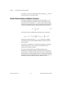
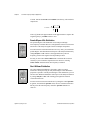
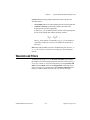
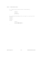
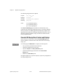
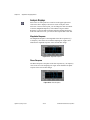
Equation 10-12 implies that for orthogonal wavelets and filter banks
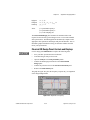
H0 ( z ) = z
–N
–1
G0 ( z )
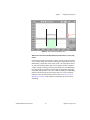
where you use the relation in Equation 10-3. Consequently, Equation 10-7
can be written as
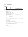
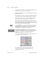
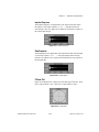
P0 ( z ) = z
–N
–1
G 0 ( z )G 0 ( z )
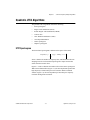
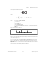
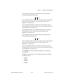
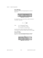
If
–1
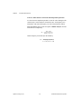
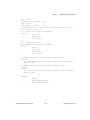
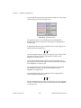
G 0 ( z )G 0 ( z ) = P ( z )
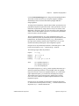
then
jω
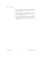
P( e ) =
N
∑
n = –N
p [ n ]e
– jωn
N
=
∑ g0 [ n ]e
– jωn
2
(10-13)
n=0
which implies that P(z) is non-negative.
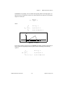
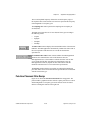
Similar to biorthogonal cases, the selection of P0(z) in orthogonal cases is
dominated by maximum flat and equiripple halfband filters. However,
because of constraints imposed by Equation 10-13, P0(z) must be the
time-shifted non-negative function P(z). Although the maximum flat filter
in Equation 10-9 ensures this requirement, special care must be taken when
P0(z) is an equiripple halfband filter.
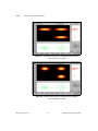
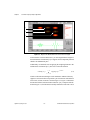
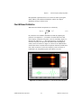
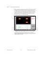
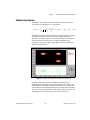
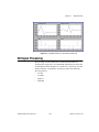
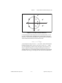
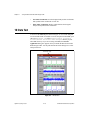
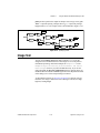
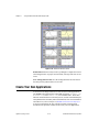
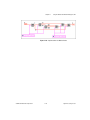
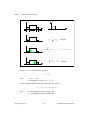
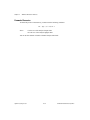
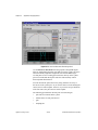
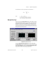
Figure 10-8 plots the third-order Daubechies filter banks and wavelets. It is
derived from the same maximum flat filter as that depicted in Figure 10-5.
In this case, however, G0(z) contains three zeros at ω = π and all zeros inside
the unit circle, therefore possessing minimum phase. Because of the
orthogonality, its dual filter bank has the same convergence property.
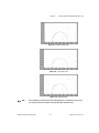
Compared to the B-spline cases in Figures 10-6 and 10-7, the third-order
Daubechies wavelet and scaling function is not as smooth as that of G0(z)
and G1(z) (refer to Figure 10-6) but is much smoother than that of H0(z) and
H1(z) (refer to Figure 10-7).
Signal Processing Toolset
10-10
© National Instruments Corporation