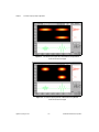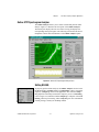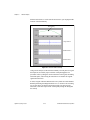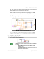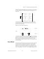
1
Signal Processing Toolset Reference Manual Signal Processing Toolset January 1999 Edition Part Number 322142A-01 Internet Support E-mail: [email protected] FTP Site: ftp.natinst.com Web Address: http://www.natinst.com Bulletin Board Support BBS United States: 512 794 5422 BBS United Kingdom: 01635 551422 BBS France: 01 48 65 15 59 Fax-on-Demand Support 512 418 1111 Telephone Support (USA) Tel: 512 795 8248 Fax: 512 794 5678 International Offices Australia 03 9879 5166, Austria 0662 45 79 90 0, Belgium 02 757 00 20, Brazil 011 288 3336, Canada (Ontario) 905 785 0085, Canada (Québec) 514 694 8521, Denmark 45 76 26 00, Finland 09 725 725 11, France 01 48 14 24 24, Germany 089 741 31 30, Hong Kong 2645 3186, Israel 03 6120092, Italy 02 413091, Japan 03 5472 2970, Korea 02 596 7456, Mexico 5 520 2635, Netherlands 0348 433466, Norway 32 84 84 00, Singapore 2265886, Spain 91 640 0085, Sweden 08 730 49 70, Switzerland 056 200 51 51, Taiwan 02 377 1200, United Kingdom 01635 523545 National Instruments Corporate Headquarters 6504 Bridge Point Parkway Austin, Texas 78730-5039 USA Tel: 512 794 0100 © Copyright 1993, 1998 National Instruments Corporation. All rights reserved. Important Information Warranty The media on which you receive National Instruments software are warranted not to fail to execute programming instructions, due to defects in materials and workmanship, for a period of 90 days from date of shipment, as evidenced by receipts or other documentation. National Instruments will, at its option, repair or replace software media that do not execute programming instructions if National Instruments receives notice of such defects during the warranty period. National Instruments does not warrant that the operation of the software shall be uninterrupted or error free. A Return Material Authorization (RMA) number must be obtained from the factory and clearly marked on the outside of the package before any equipment will be accepted for warranty work. National Instruments will pay the shipping costs of returning to the owner parts which are covered by warranty. National Instruments believes that the information in this manual is accurate. The document has been carefully reviewed for technical accuracy. In the event that technical or typographical errors exist, National Instruments reserves the right to make changes to subsequent editions of this document without prior notice to holders of this edition. The reader should consult National Instruments if errors are suspected. In no event shall National Instruments be liable for any damages arising out of or related to this document or the information contained in it. EXCEPT AS SPECIFIED HEREIN, NATIONAL INSTRUMENTS MAKES NO WARRANTIES, EXPRESS OR IMPLIED, AND SPECIFICALLY DISCLAIMS ANY WARRANTY OF MERCHANTABILITY OR FITNESS FOR A PARTICULAR PURPOSE. CUSTOMER’S RIGHT TO RECOVER DAMAGES CAUSED BY FAULT OR NEGLIGENCE ON THE PART OF NATIONAL INSTRUMENTS SHALL BE LIMITED TO THE AMOUNT THERETOFORE PAID BY THE CUSTOMER. NATIONAL INSTRUMENTS WILL NOT BE LIABLE FOR DAMAGES RESULTING FROM LOSS OF DATA, PROFITS, USE OF PRODUCTS, OR INCIDENTAL OR CONSEQUENTIAL DAMAGES, EVEN IF ADVISED OF THE POSSIBILITY THEREOF. This limitation of the liability of National Instruments will apply regardless of the form of action, whether in contract or tort, including negligence. Any action against National Instruments must be brought within one year after the cause of action accrues. National Instruments shall not be liable for any delay in performance due to causes beyond its reasonable control. The warranty provided herein does not cover damages, defects, malfunctions, or service failures caused by owner’s failure to follow the National Instruments installation, operation, or maintenance instructions; owner’s modification of the product; owner’s abuse, misuse, or negligent acts; and power failure or surges, fire, flood, accident, actions of third parties, or other events outside reasonable control. Copyright Under the copyright laws, this publication may not be reproduced or transmitted in any form, electronic or mechanical, including photocopying, recording, storing in an information retrieval system, or translating, in whole or in part, without the prior written consent of National Instruments Corporation. Trademarks CVI™, LabVIEW™, natinst.com™, National Instruments™, and NI-DAQ™ are trademarks of National Instruments Corporation. Product names referenced in this document are trademarks or trade names of their respective companies. WARNING REGARDING MEDICAL AND CLINICAL USE OF NATIONAL INSTRUMENTS PRODUCTS National Instruments products are not designed with components and testing intended to ensure a level of reliability suitable for use in treatment and diagnosis of humans. Applications of National Instruments products involving medical or clinical treatment can create a potential for accidental injury caused by product failure, or by errors on the part of the user or application designer. Any use or application of National Instruments products for or involving medical or clinical treatment must be performed by properly trained and qualified medical personnel, and all traditional medical safeguards, equipment, and procedures that are appropriate in the particular situation to prevent serious injury or death should always continue to be used when National Instruments products are being used. National Instruments products are NOT intended to be a substitute for any form of established process, procedure, or equipment used to monitor or safeguard human health and safety in medical or clinical treatment. Contents About This Manual Organization of This Manual .........................................................................................xix Part I—Joint Time-Frequency Analysis Toolkit .............................................xix Part II—Wavelet and Filter Bank Design Toolkit...........................................xix Part III—Super-Resolution Spectral Analysis Toolkit....................................xx Part IV—Digital Filter Design Toolkit............................................................xxi Part V—Third-Octave Analysis Toolkit .........................................................xxi Part VI—VirtualBench-DSA...........................................................................xxii Conventions Used in This Manual.................................................................................xxii Related Documentation..................................................................................................xxiii Customer Communication .............................................................................................xxiii Chapter 1 Signal Processing Toolset Overview Signal Processing Toolset ..............................................................................................1-1 Joint Time-Frequency Analysis Toolkit ........................................................................1-1 Wavelet and Filter Bank Design Toolkit .......................................................................1-2 Super-Resolution Spectral Analysis Toolkit..................................................................1-2 Digital Filter Design Toolkit..........................................................................................1-2 Third-Octave Analysis Toolkit ......................................................................................1-3 VirtualBench-DSA.........................................................................................................1-3 System Requirements ....................................................................................................1-4 Installation .....................................................................................................................1-4 PART I Joint Time-Frequency Analysis Toolkit Chapter 2 The Need for Joint Time-Frequency Analysis Review of the Classical Fourier Transform ...................................................................2-1 The Need for JTFA ........................................................................................................2-4 Basic Approaches to JTFA ............................................................................................2-6 © National Instruments Corporation v Signal Processing Toolset Contents Chapter 3 Joint Time-Frequency Analysis Algorithms Linear JTFA Algorithms ............................................................................................... 3-1 Gabor Expansion and STFT............................................................................ 3-1 Adaptive Representation and Adaptive Transform......................................... 3-2 Quadratic JTFA Algorithms .......................................................................................... 3-3 STFT Spectrogram .......................................................................................... 3-3 Wigner–Ville Distribution and Pseudo Wigner–Ville Distribution................ 3-5 Cohen’s Class.................................................................................................. 3-8 Choi–Williams Distribution............................................................................ 3-9 Cone-Shaped Distribution............................................................................... 3-10 Gabor Spectrogram ......................................................................................... 3-11 Adaptive Spectrogram..................................................................................... 3-13 Chapter 4 Joint Time-Frequency Analysis VIs Adaptive Transform....................................................................................................... 4-1 Inverse Adaptive Transform.......................................................................................... 4-2 Short-Time Fourier Transform ...................................................................................... 4-3 Gabor Expansion ........................................................................................................... 4-4 2D STFT........................................................................................................................ 4-4 2D Gabor Expansion ..................................................................................................... 4-6 Fast Dual........................................................................................................................ 4-7 Normalized Gaussian Window Function....................................................................... 4-8 Adaptive Spectrogram ................................................................................................... 4-9 Cohen’s Class ................................................................................................................ 4-10 CWD (Choi–Williams Distribution) ............................................................................. 4-10 Cone-Shaped Distribution ............................................................................................. 4-11 STFT Spectrogram ........................................................................................................ 4-12 PWVD (Pseudo Wigner–Ville Distribution)................................................................. 4-13 Gabor Spectrogram (Gabor Expansion-Based Spectrogram)........................................ 4-14 Time-Frequency Distribution Series ............................................................................. 4-15 Chapter 5 Joint Time-Frequency Analysis Applications Linear Algorithm Examples .......................................................................................... 5-1 Denoise............................................................................................................ 5-1 Image Analysis................................................................................................ 5-3 Time-Dependent Spectrum Analysis Examples............................................................ 5-6 Online STFT Spectrogram Analyzer .............................................................. 5-7 Setting NI-DAQ................................................................................ 5-7 Signal Processing Toolset vi © National Instruments Corporation Contents Setting the Analysis Window............................................................5-8 Acquiring Data..................................................................................5-8 Saving Data .......................................................................................5-8 Offline Joint Time-Frequency Analyzer .........................................................5-8 Changing Spectrogram Display ........................................................5-9 Inputting Data ...................................................................................5-10 Saving Results...................................................................................5-10 Switching Between Conventional Power and Instantaneous Spectrum...........................................................5-10 Frequency Zooming ..........................................................................5-11 Applying the Pre-Emphasis Filter.....................................................5-11 Setting Time Parameters ...................................................................5-12 Selecting the JTFA Method ..............................................................5-12 STFT Spectrogram .............................................................5-12 Gabor Spectrogram.............................................................5-13 Adaptive Spectrogram ........................................................5-13 Pseudo Wigner–Ville Distribution .....................................5-14 Choi–Williams Distribution ...............................................5-14 Cone-Shaped Distribution ..................................................5-15 Chapter 6 Frequently Asked Questions Chapter 7 JTFA References Chapter 8 JTFA Error Codes PART II Wavelet and Filter Bank Design Toolkit Chapter 9 Wavelet Analysis History of Wavelet Analysis..........................................................................................9-1 Conventional Fourier Transform.....................................................................9-1 Innovative Wavelet Analysis...........................................................................9-3 Wavelet Analysis vs. Fourier Analysis..........................................................................9-7 © National Instruments Corporation vii Signal Processing Toolset Contents Applications of Wavelet Analysis ................................................................................. 9-9 Discontinuity Detection .................................................................................. 9-9 Multiscale Analysis......................................................................................... 9-11 Detrend............................................................................................................ 9-12 Denoise............................................................................................................ 9-13 Performance Issues........................................................................................................ 9-13 Chapter 10 Digital Filter Banks Two-Channel Perfect Reconstruction Filter Banks....................................................... 10-1 Biorthogonal Filter Banks............................................................................... 10-4 Orthogonal Filter Banks.................................................................................. 10-9 2D Signal Processing..................................................................................................... 10-11 Chapter 11 Using the Wavelet and Filter Bank Design Toolkit Wavelet and Filter Bank Design.................................................................................... 11-1 Design Panel.................................................................................................................. 11-6 Designing Wavelets and Filter Banks ........................................................................... 11-7 1D Data Test.................................................................................................................. 11-10 Image Test ..................................................................................................................... 11-13 Wavelets and Filters ...................................................................................................... 11-15 Create Your Own Applications ..................................................................................... 11-16 Wavelet Packet Analysis................................................................................. 11-17 Online Testing Panel ....................................................................................... 11-18 Chapter 12 WFBD Toolkit Function Reference LabVIEW VI Applications............................................................................................ 12-1 LabWindows/CVI Applications .................................................................................... 12-17 Calling WFBD Functions in LabWindows/CVI ............................................. 12-17 WFBD Instrument Driver ............................................................................... 12-17 AllocCoeffWFBD............................................................................. 12-19 Analysis2DArraySize ....................................................................... 12-20 AnalysisFilterBank ........................................................................... 12-22 AnalysisFilterBank2D ...................................................................... 12-24 DecimationFilter ............................................................................... 12-29 FreeCoeffWFBD .............................................................................. 12-33 InterpolationFilter ............................................................................. 12-34 ReadCoeffWFBD ............................................................................. 12-37 Synthesis2DArraySize...................................................................... 12-38 Signal Processing Toolset viii © National Instruments Corporation Contents SynthesisFilterBank ..........................................................................12-40 SynthesisFilterBank2D .....................................................................12-43 Windows Applications...................................................................................................12-47 Chapter 13 Wavelet References Chapter 14 Wavelet Error Codes PART III Super-Resolution Spectral Analysis Toolkit Chapter 15 Introduction to Model-Based Frequency Analysis The Need for Model-Based Frequency Analysis...........................................................15-1 Applying Model-Based Method Properly......................................................................15-6 When to Use This Software ...........................................................................................15-8 Chapter 16 Model-Based Frequency Analysis Algorithms Models, Power Spectra, and Damped Sinusoids ...........................................................16-1 ARMA, MA, and AR Models .........................................................................16-1 Model Coefficients and Power Spectra ...........................................................16-3 AR Model and Damped Sinusoids ..................................................................16-4 Algorithms for Super-Resolution Spectral Analysis and Parameter Estimation ...........16-5 Covariance Method .........................................................................................16-5 Principle Component Auto-Regressive Method..............................................16-6 Prony’s Method ...............................................................................................16-7 Matrix Pencil Method......................................................................................16-8 Minimum Description Length .........................................................................16-8 Chapter 17 Super-Resolution Spectral Analysis and Parameter Estimation VIs Covariance Method........................................................................................................17-1 Covariance Power Spectrum..........................................................................................17-2 PCAR Method................................................................................................................17-3 PCAR Power Spectrum .................................................................................................17-4 © National Instruments Corporation ix Signal Processing Toolset Contents Prony’s Method ............................................................................................................. 17-5 Matrix Pencil Method.................................................................................................... 17-6 Minimum Description Length ....................................................................................... 17-7 Chapter 18 Applying Super-Resolution Spectral Analysis and Parameter Estimation Sampling Frequency...................................................................................................... 18-2 Select Test Data............................................................................................................. 18-2 The Upper Bound AR Order ......................................................................................... 18-3 FFT-Based Methods ...................................................................................................... 18-3 Selection of Super-Resolution Spectra Algorithms....................................................... 18-4 Estimation of Damped Sinusoids .................................................................................. 18-4 Synthetic Data ............................................................................................................... 18-5 Chapter 19 Super-Resolution Spectral Analysis References PART IV Digital Filter Design Toolkit Chapter 20 Digital Filter Design Application Main Menu .................................................................................................................... 20-2 Opening the Filter Design Panels.................................................................... 20-3 Directly Loading a Filter Specification File ................................................... 20-3 Editing the DFD Preferences .......................................................................... 20-3 Quitting the DFD Application......................................................................... 20-3 Digital Filter Design Panels........................................................................................... 20-3 Common Controls and Features...................................................................... 20-4 Using the DFD Menu ....................................................................... 20-4 Saving Filter Specifications ............................................... 20-4 Loading Filter Specifications ............................................. 20-5 Saving Filter Coefficients................................................... 20-5 Analyzing Filter Designs.................................................... 20-6 DAQ and Filter Real-World Testing.................................. 20-6 Simulated DAQ and Filter Testing..................................... 20-6 Transferring Filter Designs ................................................ 20-6 Returning to the Main Menu .............................................. 20-7 Panning and Zooming Options ......................................................... 20-7 Graph Cursors................................................................................... 20-9 Signal Processing Toolset x © National Instruments Corporation Contents Classical IIR Filter Design ..............................................................................20-9 Classical IIR Design Panel Controls and Displays ...........................20-11 Classical FIR Design .......................................................................................20-14 Classical FIR Design Panel Controls and Displays ..........................20-16 Pole-Zero Placement Filter Design .................................................................20-19 Pole-Zero Placement Panel Controls and Displays...........................20-21 Arbitrary FIR Design.......................................................................................20-25 Arbitrary FIR Filter Design Panel Controls and Displays ................20-26 Analysis of Filter Design Panel.......................................................................20-30 Analysis Displays..............................................................................20-32 Magnitude Response...........................................................20-32 Phase Response...................................................................20-32 Impulse Response ...............................................................20-33 Step Response.....................................................................20-33 Z-Plane Plot ........................................................................20-33 H(z) for IIR Filters..............................................................20-34 H(z) for FIR Filters.............................................................20-34 DAQ and Filter Panel ......................................................................................20-35 Chapter 21 IIR and FIR Implementation Infinite Impulse Response Filters ..................................................................................21-11 Cascade-Form IIR Filtering.............................................................................21-12 Finite Impulse Response Filters.....................................................................................21-14 Format of the Filter-Coefficient Text Files....................................................................21-14 FIR-Coefficient File Format............................................................................21-14 IIR Coefficient File Format .............................................................................21-16 Chapter 22 Using Your Coefficient Designs with DFD Utilities LabVIEW DFD Utilities ................................................................................................22-1 Read DFD Coefficients ...................................................................................22-2 DFD Filter .......................................................................................................22-3 LabWindows/CVI Utilities ............................................................................................22-4 The DFD Instrument Driver ............................................................................22-4 Using the DFD Instrument Driver...................................................................22-4 AllocCoeffDFD ...............................................................................................22-5 ReadCoeffDFD................................................................................................22-6 FreeCoeffDFD.................................................................................................22-7 FilterDFD ........................................................................................................22-8 Windows DLL DFD Utilities ........................................................................................22-9 © National Instruments Corporation xi Signal Processing Toolset Contents Chapter 23 DFD References PART V Third-Octave Analysis Toolkit Chapter 24 Overview of the Third-Octave Analysis Toolkit Description of an Octave Analyzer ............................................................................... 24-1 Introduction to the Third-Octave Analysis Toolkit ....................................................... 24-2 Chapter 25 Operating the Third-Octave Analyzer Setting Up the Third-Octave Analyzer ......................................................................... 25-1 Running the Third-Octave Analyzer ............................................................................. 25-5 Chapter 26 Third-Octave Analysis Design Algorithm Description................................................................................................... 26-1 Multistage Decimation Techniques............................................................................... 26-2 Internal Data Averaging ................................................................................................ 26-5 Specifications of the Third-Octave Analysis Toolkit.................................................... 26-6 Chapter 27 Third Octave Filters VI Third-Octave Filters VI ................................................................................................. 27-1 Chapter 28 Building Windows Applications for Third-Octave Analysis Third-Octave Analysis Applications in LabWindows/CVI .......................................... 28-1 Third-Octave Analysis Instrument Driver ...................................................... 28-1 Running Third-Octave Analysis Applications in LabWindows/CVI ............. 28-3 Third-Octave Analysis Applications in Windows......................................................... 28-4 Third-Octave Analysis Applications in Visual Basic.................................................... 28-4 Chapter 29 Third-Octave References Signal Processing Toolset xii © National Instruments Corporation Contents Chapter 30 Third-Octave Error Codes PART VI VirtualBench-DSA Chapter 31 VirtualBench-DSA Launching VirtualBench-DSA ......................................................................................31-1 Front Panel Features ......................................................................................................31-1 Computations Panel Features.........................................................................................31-5 Acquiring and Measuring Signals..................................................................................31-7 Working with Waveforms .............................................................................................31-10 Making Precise Measurements Using Markers...............................................31-10 Loading Reference Waveforms.......................................................................31-10 Saving Reference Waveforms .........................................................................31-11 Generating Reports for Use with Other Applications .....................................31-12 Appendix A Customer Communication Glossary Index Figures Figure 2-1. Figure 2-2. Figure 2-3. Figure 2-4. Figure 2-5. Figure 2-6. Basis Functions Used for Fourier Transform ........................................2-2 Seismic Signal .......................................................................................2-2 ECG Signal............................................................................................2-3 Speech Signal ........................................................................................2-3 Ionized Impulse Signal..........................................................................2-5 Reconstructed Signal.............................................................................2-5 Figure 3-1. STFT-Based Spectrogram with a Narrowband Hanning Window for the Three-Tone Test Signal .............................................................3-4 STFT-Based Spectrogram with a Wideband Hanning Window for the Three-Tone Test Signal .............................................................3-4 Wigner–Ville Distribution for the Three-Tone Test Signal ..................3-6 Figure 3-2. Figure 3-3. © National Instruments Corporation xiii Signal Processing Toolset Contents Figure 3-4. Figure 3-5. Figure 3-6. Figure 3-7. Figure 3-8. Figure 3-9. Pseudo Wigner–Ville Distribution with Gaussian Window w[m] for the Three-Tone Test Signal ............................................................. 3-7 Pseudo Wigner–Ville Distribution for the Three-Tone Test Signal ..... 3-8 Choi–Williams Distribution (a = 1) for the Three-Tone Test Signal.... 3-9 Cone-Shaped Distribution (a = 1) for the Three-Tone Test Signal ...... 3-10 Gabor Spectrogram (Order Four) for the Three-Tone Test Signal ....... 3-12 Adaptive Spectrogram for the Three-Tone Test Signal ........................ 3-13 Figure 5-1. Figure 5-2. Figure 5-3. Figure 5-4. Figure 5-5. Figure 5-6. Figure 5-7. Gabor Expansion-Based Denoise ......................................................... 5-3 2D STFT for Image Analysis................................................................ 5-4 Subimage Frequency Contents ............................................................. 5-4 2D STFT for the Image Analysis in Figure 5-2 .................................... 5-6 Online STFT Spectrogram Analyzer Panel .......................................... 5-7 Offline Joint Time-Frequency Analyzer ............................................... 5-9 Instantaneous Spectrum Display .......................................................... 5-11 Figure 6-1. Figure 6-2. STFT Spectrogram (Hanning Window)................................................ 6-4 Gabor Spectrogram (Order Four).......................................................... 6-5 Figure 9-1. Figure 9-2. Figure 9-3. Figure 9-4. Figure 9-5. Figure 9-6. Figure 9-7. Figure 9-8. Figure 9-9. Figure 9-10. Sum of Two Truncated Sine Waveforms.............................................. 9-2 Wavelet ................................................................................................. 9-4 Wavelet Analysis .................................................................................. 9-6 Short-Time Fourier Transform Sampling Grid..................................... 9-7 Wavelet Transform Sampling Grid....................................................... 9-8 Comparison of Transform Processes .................................................... 9-9 Detection of Discontinuity .................................................................... 9-10 Multiscale Analysis............................................................................... 9-11 Detrend.................................................................................................. 9-12 Denoise ................................................................................................. 9-13 Figure 10-1. Figure 10-2. Two-Channel Filter Bank ..................................................................... 10-1 Relationship of Two-Channel PR Filter Banks and Wavelet Transform......................................................................... 10-2 Figure 10-3. Filter Bank and Wavelet Transform Coefficients ................................. 10-3 Figure 10-4. Halfband Filter ...................................................................................... 10-6 Figure 10-5. Zeros Distribution for (1 – z –1)6Q(z).................................................... 10-7 Figure 10-6. B-Spline Filter Bank ............................................................................. 10-7 Figure 10-7. Dual B-Spline Filter Bank .................................................................... 10-8 Figure 10-8. Third-Order Daubechies Filter Banks and Wavelets ............................ 10-11 Figure 10-9. 2D Signal Processing ............................................................................ 10-12 Figure 10-10. 2D Image Decomposition ..................................................................... 10-13 Signal Processing Toolset xiv © National Instruments Corporation Contents Figure 11-1. Figure 11-2. Figure 11-3. Figure 11-4. Figure 11-5. Figure 11-6. Figure 11-7. Figure 11-8. Figure 11-9. Figure 11-10. Figure 11-11. Figure 11-12. Figure 11-13. Figure 11-14. Figure 11-15. Design Procedure for Wavelets and Filter Banks .................................11-2 Non-Negative Equiripple Halfband Filter .............................................11-3 Minimum Phase Filter ...........................................................................11-5 Linear Phase Filter.................................................................................11-5 Orthogonal Filter ...................................................................................11-5 Design Panel..........................................................................................11-6 Equiripple Filter ....................................................................................11-8 1D Test Panel ........................................................................................11-10 DAQ Setup Panel ..................................................................................11-12 Specifying a Path...................................................................................11-13 Image Test Panel ...................................................................................11-14 Wavelets and Filters Panel ....................................................................11-16 Full Path of a Three-Level Perfect Reconstruction Tree.......................11-17 Wavelet Packet ......................................................................................11-18 Implementation of a Wavelet Packet.....................................................11-19 Figure 12-1. Figure 12-2. Figure 12-3. Figure 12-4. Figure 12-5. Zero Padding .........................................................................................12-3 Symmetric Extension ............................................................................12-4 Filtering Operation ................................................................................12-12 Two-Channel Perfect Reconstruction System.......................................12-13 Signal Interpolated by 2 ........................................................................12-15 Figure 15-1. Figure 15-2. Figure 15-3. Figure 15-4. Figure 15-5. Figure 15-6. Figure 15-7. Figure 15-8. Figure 15-9. 50 Samples for a Sum of Two Sinusoids ..............................................15-2 FFT-Based Power Spectra Based on 50 Samples .................................15-2 Two Sinusoids with 15 Samples ...........................................................15-3 FFT-Based Power Spectra Based on 15 Samples .................................15-3 Super-Resolution Power Spectra Based on 15 Samples .......................15-3 Damped Sinusoids.................................................................................15-4 FFT-Based Power Spectra for Damped Sinusoids ................................15-5 Parameter Estimation by Matrix Pencil Method ...................................15-5 Super-Resolution Power Spectra with Order 10 for Sum Of Two Sinusoids....................................................................15-6 Figure 17-1. Real and Complex Covariance VIs .......................................................17-1 Figure 18-1. Figure 18-2. Figure 18-3. Figure 18-4. Figure 18-5. Figure 18-6. Super-Resolution and Modal Panel.......................................................18-1 Waveform of Test Sample.....................................................................18-2 FFT-Based Methods ..............................................................................18-3 Super-Resolution Spectra ......................................................................18-4 Estimation of Damped Sinusoids ..........................................................18-4 Synthetic Data Panel .............................................................................18-5 © National Instruments Corporation xv Signal Processing Toolset Contents Figure 20-1. Figure 20-2. Figure 20-3. Figure 20-4. Figure 20-5. Figure 20-6. Figure 20-7. Figure 20-8. Figure 20-9. Figure 20-10. Figure 20-11. Figure 20-12. Figure 20-13. Figure 20-14. Figure 20-15. Figure 20-16. Figure 20-17. Figure 20-18. Figure 20-19. Figure 20-20. Figure 20-21. Figure 20-22. Figure 20-23. Figure 20-24. Figure 20-25. Figure 20-26. Figure 20-27. Figure 20-28. Figure 20-29. Figure 20-30. Figure 20-31. Figure 20-32. Figure 20-33. Conceptual Overview of the Digital Filter Design Toolkit .................. 20-2 DFD Main Menu Panel ......................................................................... 20-2 DFD Pop-Up Menu............................................................................... 20-4 Example of Graph Palette ..................................................................... 20-7 Zoom Tool Pop-Up Menu..................................................................... 20-8 Example of Two Cursors on a Graph ................................................... 20-9 Classical IIR Design Panel.................................................................... 20-9 Magnitude vs Frequency....................................................................... 20-11 Text Entry Portion of Design Panel ...................................................... 20-12 Classical FIR Design Panel................................................................... 20-14 Frequency Response Magnitude ........................................................... 20-17 Text-Based Interface ............................................................................. 20-18 Pole-Zero Placement Filter Design Panel ............................................. 20-20 Z-Plane Plot of Filter Poles and Zeros .................................................. 20-21 Array of Zeros in Rectangular Coordinates .......................................... 20-22 Array of Poles in Rectangular Coordinates .......................................... 20-23 Array of Zeros and Poles in Polar Coordinates .................................... 20-23 Magnitude vs Frequency....................................................................... 20-24 Arbitrary FIR Design Panel .................................................................. 20-25 Desired and Actual Magnitude Response ............................................. 20-26 Selected Points Indicator....................................................................... 20-27 Array of Frequency-Magnitude Points ................................................. 20-28 Additional Controls for Arbitrary FIR Design Panel............................ 20-29 Analysis of Filter Design Panel ............................................................ 20-31 Magnitude Response ............................................................................. 20-32 Phase Response ..................................................................................... 20-32 Impulse Response ................................................................................. 20-33 Step Response ....................................................................................... 20-33 Z-Plane Plot .......................................................................................... 20-33 H(z) for IIR Filters................................................................................. 20-34 H(z) for FIR Filters................................................................................ 20-34 DAQ and Filter Panel............................................................................ 20-35 Switching Displays ............................................................................... 20-36 Figure 21-1. Figure 21-2. Figure 21-3. Cascaded Filter Stages .......................................................................... 21-12 Direct Form Structure ........................................................................... 21-13 Direct Form II Structure........................................................................ 21-13 Figure 25-1. Figure 25-2. Figure 25-3. Figure 25-4. Third-Octave Analyzer Setup Dialog Box............................................ 25-2 Internal Data Averaging # Dialog Box ................................................. 25-5 Four-Channel Third-Octave Analyzer Panel ........................................ 25-6 One-Channel Third-Octave Analyzer Panel with Reference Signal..... 25-8 Signal Processing Toolset xvi © National Instruments Corporation Contents Figure 26-1. Figure 26-2. Multistage Third-Octave Analyzer Design Using FFT .........................26-4 Internal Data Averaging Procedure.......................................................26-5 Figure 31-1. Figure 31-2. Figure 31-3. Figure 31-4. Figure 31-5. Figure 31-6. Figure 31-7. Figure 31-8. Figure 31-9. Figure 31-10. Front Panel of VirtualBench-DSA ........................................................31-1 VirtualBench-DSA Status Display........................................................31-5 VirtualBench-DSA Marker Display......................................................31-5 Computations Panel...............................................................................31-5 Hardware Tab of DSA Settings Dialog Box .........................................31-7 Acquisition Tab of DSA Settings Dialog Box ......................................31-8 Triggering Tab of DSA Settings Dialog Box........................................31-9 Load Reference Waveforms Dialog Box ..............................................31-11 Save Reference Waveforms Dialog Box...............................................31-12 Generate Report Dialog Box .................................................................31-13 Tables Table 5-1. Guidelines for Choosing Analysis Window..........................................5-13 Table 6-1. Quadratic JTFA Algorithms..................................................................6-2 Table 8-1. JTFA Error Codes ................................................................................8-1 Table 11-1. Filter Comparison..................................................................................11-4 Table 14-1. LabVIEW VI and LabWindows/CVI Function Error Codes ...............14-1 Table 15-1. Table 15-2. Damped Sinusoids.................................................................................15-4 FFT, JTFA, Wavelets, and Model-Based Methods...............................15-7 Table 18-1. Default Sinusoid Parameters .................................................................18-6 Table 20-1. Table 20-2. Suggested Specification Filename Extensions .....................................20-5 Filter Specification Transfers ...............................................................20-7 Table 21-1. Table 21-2. FIR-Coefficient Text Files and Descriptions .......................................21-5 IIR-Coefficient Text Files and Descriptions ........................................21-6 Table 24-1. Filter Bands for ANSI S1.11 ................................................................24-2 Table 26-1. Third-Octave Analyzer Sampling Rates, ANSI Bands, and Center Frequencies .........................................................................26-2 Table 26-2. Different Sampling Frequencies ..........................................................26-3 © National Instruments Corporation xvii Signal Processing Toolset About This Manual Organization of This Manual The Signal Processing Toolset Reference Manual is divided into six sections and is organized as follows: • Chapter 1, Signal Processing Toolset Overview, provides an overview of the Signal Processing Toolset components, system requirements, and installation instructions. Part I—Joint Time-Frequency Analysis Toolkit • Chapter 2, The Need for Joint Time-Frequency Analysis, explains the need for and the approaches to joint time-frequency analysis (JTFA). • Chapter 3, Joint Time-Frequency Analysis Algorithms, describes the algorithms the JTFA VIs use. The JTFA algorithms implemented in this package fall into two categories: linear and quadratic. • Chapter 4, Joint Time-Frequency Analysis VIs, describes the JTFA VIs. • Chapter 5, Joint Time-Frequency Analysis Applications, introduces some JTFA applications. Because JTFA is relatively new, it is less known among practicing engineers and scientists, unlike the well-known Fourier analysis. The examples in this chapter reveal only the potential of JTFA. The power of JTFA has not been fully explored. These examples can help you learn and apply JTFA to your applications. • Chapter 6, Frequently Asked Questions, addresses some questions JTFA users frequently ask. • Chapter 7, JTFA References, lists reference material that contains more information on the theory and algorithms implemented in the JTFA toolkit. • Chapter 8, JTFA Error Codes, lists the error codes the JTFA VIs return. Part II—Wavelet and Filter Bank Design Toolkit • © National Instruments Corporation Chapter 9, Wavelet Analysis, describes the history of wavelet analysis, compares Fourier transform and wavelet analysis, and describes some applications of wavelet analysis. xix Signal Processing Toolset About This Manual • Chapter 10, Digital Filter Banks, describes the design of two-channel perfect reconstruction filter banks and defines the types of filter banks used with wavelet analysis. • Chapter 11, Using the Wavelet and Filter Bank Design Toolkit, describes the architecture of the Wavelet and Filter Bank Design (WFBD) toolkit, lists the design procedures, and describes some applications you can create with the WFBD toolkit • Chapter 12, WFBD Toolkit Function Reference, describes the VIs in the WFBD toolkit, the instrument driver for LabWindows/CVI, and the functions in the DLLs. • Chapter 13, Wavelet References, lists reference material that contains more information on the theory and algorithms implemented in the WFBD toolkit. • Chapter 14, Wavelet Error Codes, lists the error codes LabVIEW VIs and LabWindows/CVI functions return, including the error number and a description. Part III—Super-Resolution Spectral Analysis Toolkit Signal Processing Toolset • Chapter 15, Introduction to Model-Based Frequency Analysis, introduces the basic concepts of model-based frequency analysis. • Chapter 16, Model-Based Frequency Analysis Algorithms, outlines the theoretical background of model-based frequency analysis and describes the relationship among the model coefficients, the power spectra, and the parameters of damped sinusoids. • Chapter 17, Super-Resolution Spectral Analysis and Parameter Estimation VIs, describes VIs used to perform super-resolution and parameter estimation. Each algorithm included has two forms: one for real and the other for complex-valued samples. The real VIs work only for real-valued data sets, and the complex VIs work for both real and complex samples. • Chapter 18, Applying Super-Resolution Spectral Analysis and Parameter Estimation, describes a comprehensive testing example application included with the Super-Resolution Spectral Analysis toolkit. This example software is designed to help you learn about model-based analysis. • Chapter 19, Super-Resolution Spectral Analysis References, lists reference material that contains more information on the theory and algorithms implemented in the Super-Resolution Spectral Analysis toolkit. xx © National Instruments Corporation About This Manual Part IV—Digital Filter Design Toolkit • Chapter 20, Digital Filter Design Application, describes the DFD application you use to design infinite impulse response (IIR) and finite impulse response (FIR) digital filters. • Chapter 21, IIR and FIR Implementation, describes the filter implementation equations for IIR and FIR filtering and the format of the IIR and FIR filter coefficient files. • Chapter 22, Using Your Coefficient Designs with DFD Utilities, describes the DFD utilities you use for filtering applications. • Chapter 23, DFD References, lists reference material that contains more information on the theory and algorithms implemented in the DFD toolkit. Part V—Third-Octave Analysis Toolkit • Chapter 24, Overview of the Third-Octave Analysis Toolkit, explains how you can use this program. The Third-Octave Analysis toolkit can act as a stand-alone application or as an add-on toolkit for LabVIEW. The toolkit also provides the instrument driver for LabWindows/CVI users and dynamic link libraries for Windows users. • Chapter 25, Operating the Third-Octave Analyzer, describes the Third-Octave Analyzer application and explains the program features. • Chapter 26, Third-Octave Analysis Design, describes the design specifications and algorithms of the Third-Octave Analysis toolkit. • Chapter 27, Third-Octave Filters VI, describes the Third-Octave Filters VI and its parameters. • Chapter 28, Building Windows Applications for Third-Octave Analysis, describes how to build a third-octave analysis application under Windows 95/NT. • Chapter 29, Third-Octave References, lists reference material that contains more information on the theory and algorithms implemented in the Third-Octave Analysis toolkit. • Chapter 30, Third-Octave Error Codes, lists the error codes returned by the Third-Octave Filters VI and the C function ThirdOctave_Analyzer(). © National Instruments Corporation xxi Signal Processing Toolset About This Manual Part VI—VirtualBench-DSA • Chapter 31, VirtualBench-DSA, explains the VirtualBench-DSA features and how to acquire and measure signals with the DSA. • Appendix A, Customer Communication, contains forms you can use to request help from National Instruments or to comment on our products and manuals. • The Glossary contains an alphabetical list and description of terms used in this manual, including abbreviations, acronyms, metric prefixes, mnemonics, and symbols. • The Index contains an alphabetical list of key terms and topics in this manual, including the page where you can find each one. Conventions Used in This Manual The following conventions are used in this manual: <> Angle brackets enclose the name of a key on the keyboard—for example, <shift>. Angle brackets containing numbers separated by an ellipsis represent a range of values associated with a bit or signal name—for example, DBIO<3..0>. » The » symbol leads you through nested menu items and dialog box options to a final action. The sequence File»Page Setup»Options»Substitute Fonts directs you to pull down the File menu, select the Page Setup item, select Options, and finally select the Substitute Fonts option from the last dialog box. This icon to the left of bold italicized text denotes a note, which alerts you to important information. bold Bold text denotes the names of menus, menu items, parameters, dialog boxes, dialog box buttons or options, icons, windows, Windows 95 tabs, panels, controls, or LEDs. Matrices are in uppercase bold letters. Vectors are in lowercase bold letters. bold italic Bold italic text denotes a note. italic Italic text denotes variables, elements of a matrix, emphasis, a cross reference, or an introduction to a key concept. This font also denotes text from which you supply the appropriate word or value. Signal Processing Toolset xxii © National Instruments Corporation About This Manual monospace Text in this font denotes text or characters that you should enter from the keyboard, sections of code, programming examples, and syntax examples. This font is also used for the proper names of disk drives, paths, directories, programs, subprograms, subroutines, device names, functions, operations, variables, filenames and extensions, and for statements and comments taken from programs. monospace italic Italic text in this font denotes that you must enter the appropriate words or values in the place of these items. Related Documentation The following documents contain information that you might find helpful as you read this manual: • G Programming Reference Manual • LabVIEW Online Reference • LabVIEW User Manual • LabWindows/CVI User Manual Customer Communication National Instruments wants to receive your comments on our products and manuals. We are interested in the applications you develop with our products, and we want to help if you have problems with them. To make it easy for you to contact us, this manual contains comment and configuration forms for you to complete. These forms are in Appendix A, Customer Communication, at the end of this manual. © National Instruments Corporation xxiii Signal Processing Toolset 1 OVERVIEW Signal Processing Toolset Overview This chapter provides an overview of the Signal Processing Toolset components, system requirements, and installation instructions. For more information about each component, refer to the corresponding part of this manual. Signal Processing Toolset The Signal Processing Toolset contains the Joint Time-Frequency Analysis toolkit, the Wavelet and Filter Bank Design toolkit, the Super-Resolution Spectral Analysis toolkit, the Digital Filter Design toolkit, the Third-Octave Analysis toolkit, and the VirtualBench-DSA. This software performs various specialized signal processing tasks, such as finding the power spectrum of a signal, representing signals in the joint time-frequency domain, and interactively designing digital filters and wavelets. You can use the Signal Processing Toolset with programming environments such as LabVIEW, LabWindows/CVI, or Microsoft Visual Basic. The diverse applications for the toolset include acoustics, radar, sonar, seismology, remote sensing, instrumentation, and vibration analysis. Joint Time-Frequency Analysis Toolkit Using the Joint Time-Frequency Analysis toolkit, you can enhance computer-based signal processing on nonstationary signals. Applications include speech processing, sound analysis, sonar, radar, machine testing, vibration analysis, and dynamic signal monitoring. The Joint Time-Frequency Analysis toolkit provides several algorithms for applications in which the frequency content of a signal varies with time. These algorithms include the award-winning and patented Gabor spectrogram, the Wigner-Ville distribution, the Choi–Williams © National Instruments Corporation 1-1 Signal Processing Toolset Chapter 1 Signal Processing Toolset Overview distribution, the short-time Fourier transform, the cone-shaped distribution, and the adaptive spectrogram. Wavelet and Filter Bank Design Toolkit The Wavelet and Filter Bank Design toolkit provides an intuitive and interactive interface for designing wavelet transforms and filter banks. You can use wavelets for feature extraction and data compression. By interactively selecting a wavelet prototype (equiripple or maxflat) and different finite impulse response combinations, you easily can find the best wavelet or filter bank for your application. As you design the wavelets, you can apply them to 1D and 2D signals (images) and immediately see the effect of the design on your signal. The Wavelet and Filter Bank Design toolkit is extremely powerful for signals that have short time duration and wide frequency bandwidth. Super-Resolution Spectral Analysis Toolkit Several applications use a model-based signal analysis method when the number of data samples is limited. The Super-Resolution Spectral Analysis toolkit contains a standalone application you can use to test algorithms such as covariance, the Prony’s method, the principle component auto-regression, and the matrix pencil method for model-based analysis. Some of these methods have previously not been commercially available. Besides directly using the built-in test panel, you also can use VIs to construct your own applications in LabVIEW. This toolkit can be used to perform high-resolution spectral analysis and parameter estimation. These parameters include the amplitude, phase, damping factor, and frequency of damped sinusoids. You can use the toolkit for other applications such as linear prediction, signal synthesis, data compression, and system identification. You can use these tools in diverse applications such as biomedicine, economics, geophysics, noise and vibration, and speech analysis. Digital Filter Design Toolkit The Digital Filter Design toolkit provides a general-purpose design tool for signal conditioning, control systems, digital signal processing, and virtual instrument applications. Using the Digital Filter Design toolkit, you can design bandpass, bandstop, lowpass, and highpass filters, and filters with Signal Processing Toolset 1-2 © National Instruments Corporation Chapter 1 Signal Processing Toolset Overview an arbitrary magnitude response. Use the powerful graphical user interface to design finite impulse response and infinite impulse response filters. You design filters by interactively editing the magnitude response graph or the pole-zero plot in the z-plane. You test your design online with a built-in function generator, and you analyze the filter using the step and impulse responses, magnitude and phase responses, and pole-zero plot. When you complete your design, you can save the filter coefficients to a file for use in other applications. Third-Octave Analysis Toolkit Scientists and engineers in the fields of acoustics and vibration use the Third-Octave Analysis toolkit to determine the spectral energy contained in a specific set of third-octave bands. With the Third-Octave Analysis toolkit, you can measure sound, vibration, and noise signals quickly and easily. Third-octave analysis applications include vibration tests of machines, architectural acoustics, power measurements, and appliance testing. The Third-Octave Analysis toolkit conforms to ANSI Standard S1.11-1986 and features an easy-to-use graphical user interface for third-octave analysis and data acquisition. You can choose from one to four input channels, each with its own windowing, weighting, and averaging capabilities. You can compare the results of third-octave analysis on the signal from each channel to those of a reference signal you have analyzed previously. VirtualBench-DSA Use the VirtualBench-DSA (Dynamic Signal Analyzer) to acquire signals and measure the power spectrum, harmonic content, amplitude spectrum, cross-power spectrum, frequency response, coherence, and impulse response. You also can use the VirtualBench-DSA as a low-frequency oscilloscope to view signals separately in the time and frequency domains simultaneously. With the VirtualBench-DSA, you gain the functionality of simultaneously analyzing signals on two channels. VirtualBench-DSA also provides markers for measuring the total harmonic distortion. © National Instruments Corporation 1-3 Signal Processing Toolset Chapter 1 Signal Processing Toolset Overview System Requirements You must use the Third-Octave Analysis toolkit with one of the National Instruments data acquisition devices. The Third-Octave Analysis toolkit can analyze signals correctly only when the signal does not have any aliasing. You should use a device that has a built-in anti-aliasing filter. The National Instruments Dynamic Signal Acquisition boards have these built-in filters. Installation Complete the following steps to install the Signal Processing Toolset: 1. Insert the CD of the Signal Processing Toolset into your CD-ROM drive and double-click setup.exe. 2. Follow the instructions on your screen. Once you have completed the on-screen installation instructions, you are ready to run the toolkits in the Signal Processing Toolset. Signal Processing Toolset 1-4 © National Instruments Corporation Part I Joint Time-Frequency Analysis Toolkit This section of the manual describes the Joint Time-Frequency Analysis (JTFA) toolkit. • Chapter 2, The Need for Joint Time-Frequency Analysis, explains the need for and the approaches to joint time-frequency analysis (JTFA). • Chapter 3, Joint Time-Frequency Analysis Algorithms, describes the algorithms the JTFA VIs use. The JTFA algorithms implemented in this package fall into two categories: linear and quadratic. • Chapter 4, Joint Time-Frequency Analysis VIs, describes the JTFA VIs. • Chapter 5, Joint Time-Frequency Analysis Applications, introduces some JTFA applications. Because JTFA is relatively new, it is less known among practicing engineers and scientists, unlike the well-known Fourier analysis. The examples in this chapter reveal only the potential of JTFA. The power of JTFA has not been fully explored. These examples can help you learn and apply JTFA to your applications. • Chapter 6, Frequently Asked Questions, addresses some questions JTFA users frequently ask. • Chapter 7, JTFA References, lists reference material that contains more information on the theory and algorithms implemented in the JTFA toolkit. • Chapter 8, JTFA Error Codes, lists the error codes the JTFA VIs return. © National Instruments Corporation I-1 Signal Processing Toolset 2 The Need for Joint Time-Frequency Analysis This chapter explains the need for and the approaches to joint time-frequency analysis (JTFA). Review of the Classical Fourier Transform From a mathematical point of view, you can describe a given signal in many different ways. For instance, you can write the signal as a function of time, which shows how the signal amplitude changes over time. Alternatively, you can write the signal as a function of frequency, which tells us how frequently the amplitude changes. The bridge between time and frequency representations is the Fourier transform, first introduced by Jean Baptiste Joseph Fourier in 1807. During the study of heat propagation and diffusion, Fourier found that a series of harmonically related sinusoids was useful in representing the temperature distribution throughout a body. Later he claimed that any periodic signal could be represented by such a series and any aperiodic signal could be represented as a weighted integral of sinusoids.1 By the 1820s, Fourier’s revolutionary claims were proved mathematically by S.D. Poisson, A.L. Cauchy, and P.L. Dirichlet. Since then, the Fourier transform has become one of the most important signal analysis methods. By applying the Fourier transformation, you easily can decompose any signal as a weighted sum of sinusoid functions as shown in Figure 2-1. Consequently, you can process either the signal time waveform or its corresponding set of sinusoid functions, depending on which form is more convenient. In addition to being linear, the Fourier transform provides a feasible way of computing the power spectrum for a signal. Because the power spectrum usually has a simpler pattern than the time waveform, it 1 Fourier’s original paper was never published because of J.L. Lagrange’s vehement objections. Lagrange, an important mathematician during that time, argued that trigonometric series were of very limited use. © National Instruments Corporation 2-1 Signal Processing Toolset Chapter 2 The Need for Joint Time-Frequency Analysis often serves as the fingerprint of the analyzed signal. In signal processing, you often want to represent certain attributes of the signal explicitly. Figure 2-1. Basis Functions Used for Fourier Transform Although the Fourier transform has been widely recognized in many disciplines, it possesses certain disadvantages that prevent its use in many important applications. Figures 2-2 and 2-3 depict two common signals: seismic and ECG (electrocardiogram). Unlike the sinusoid functions used as the basis of the Fourier transform that extend over the entire time domain (refer to Figure 2-1), the seismic signal lives only for a very short period, and the ECG signal basically consists of isolated bursts. Using the Fourier series to represent those signals, you need an infinite number of sinusoid functions that can cancel each other to achieve the near-zero points. Therefore, the classical Fourier series cannot economically represent these applications. Figure 2-2. Seismic Signal Signal Processing Toolset 2-2 © National Instruments Corporation Chapter 2 The Need for Joint Time-Frequency Analysis Figure 2-3. ECG Signal As mentioned earlier, another important application of the Fourier transform is spectral analysis. Figure 2-4 illustrates a word, hood, spoken by a 5-year-old boy. The bottom plot depicts the time waveform. The upper-right plot depicts the conventional power spectrum. The conventional power spectrum shows that the word hood contains three main frequency tones. However, the power spectrum alone does not clearly indicate how those frequencies evolve over time. Obviously, the frequency tones of a speech signal are not constant. Despite the fact that the frequency contents of most signals change with time, the classical Fourier theory allows us to analyze a signal only in the time domain or in the frequency domain. Figure 2-4. Speech Signal © National Instruments Corporation 2-3 Signal Processing Toolset Chapter 2 The Need for Joint Time-Frequency Analysis The Need for JTFA The large plot of Figure 2-4 is a time-dependent spectrum that plots the energy of the signal as a function of both time and frequency. As shown, the time-dependent spectrum clearly reveals the pattern of the formants. From the formants, you can see how the frequency changes. The relative brightness levels of the plot show the intensity of the frequencies. In this example, the JTFA helps illustrate the mechanism of human speech. Another important motivation for applying JTFA is the detection of noise-corrupted signals. In general, random noise tends to spread evenly across the time and frequency domains. However, the signal usually concentrates in a relatively short time period or a narrow frequency band. If you convert the noise-corrupted signal to the joint time-frequency domain, you can substantially improve the local (or regional) Signal-to-Noise Ratio (SNR). Figure 2-5 depicts the impulse signal the U.S. Department of Energy ALEXIS/BLACKBEARD satellite received.1 After passing through dispersive media, such as the ionosphere, the impulse signal becomes the nonlinear chirp signal. As shown in Figure 2-5, random noise dominates both the time waveform and the power spectrum. Neither indicate the existence of the impulse signal. However, from the time-dependent spectrum, you can immediately identify the presence of the chirp-type signal that arches across the joint time-frequency domain. The horizontal lines correspond to radio carrier signals that basically remain unchanged over time. 1 Data courtesy of Non-Proliferation and International Security Division, Los Alamos National Laboratory. Signal Processing Toolset 2-4 © National Instruments Corporation Chapter 2 The Need for Joint Time-Frequency Analysis Figure 2-5. Ionized Impulse Signal Based on the joint time-frequency representation, you can further mask the desired signal, as shown in the top plot in Figure 2-6. You then can apply the inverse transformation to recover the noiseless time waveform. The lower plot of Figure 2-6 illustrates the noisy and reconstructed signals. When the SNR is very low, as with many satellite signals, JTFA might offer the only opportunity to detect the signal of interest. Figure 2-6. Reconstructed Signal © National Instruments Corporation 2-5 Signal Processing Toolset Chapter 2 The Need for Joint Time-Frequency Analysis Basic Approaches to JTFA The development of JTFA began more than a half century ago. The most straightforward approach of characterizing the frequency of a signal as a function of time was to divide the signal into several blocks that could be overlapped. Then, the Fourier transform was applied to each block of data to indicate the frequency contents of each. This process has become known as the short-time Fourier transform (STFT) and roughly reflects how frequency contents change over time. The size of the blocks determines the time accuracy. The smaller the block, the better the time resolution. However, frequency resolution is inversely proportional to the size of a block. While the small block yields good time resolution, it also deteriorates the frequency resolution and vice versa. Traditionally, this phenomena is known as the window effect. From the concept of expansion and series, Dennis Gabor,1 a Hungarian-born British physicist, suggested expanding a signal into a set of weighted frequency modulated Gaussian functions. Because the Gaussian function is concentrated in both the time and frequency domains, the weights describe the signal behavior in local time and frequency. The resulting presentation is known as the Gabor expansion. In fact, you can consider the Gabor expansion the inverse of the STFT. However, this inverse relationship was not clear during Gabor’s lifetime and not well understood until the 1980s. At present, both the theory and implementation of the Gabor expansion and STFT are mature enough to apply to real application problems. As the linear JTFA develops, the quadratic JTFA (time-dependent spectrum) attracts great attention. The simplest time-dependent spectrum is the square of the STFT, which was named the STFT-based spectrogram or the STFT spectrogram. As mentioned earlier, the STFT spectrogram suffers from the window effect. A more elegant method is the Wigner–Ville Distribution (WVD), which originally was developed in the context of quantum mechanics by Hungarian-born American physicist Eugene P. Wigner.2 The WVD has high resolution and many other useful properties for signal analysis, but it suffers from crossterm interference. To reduce crossterm interference, you can use two proven algorithms: Cohen’s class and the Gabor expansion-based spectrogram (also known as the Gabor spectrogram). Scientists at National Instruments developed 1 2 In 1970, Gabor (1900–1979) was awarded the Nobel Prize in Physics for his discovery of the principles of holography. Wigner’s pioneering application of group theory to an atomic nucleus established a method for discovering and applying the principles of symmetry to the behavior of physical phenomena. In 1963, he was awarded the Nobel Prize in Physics. Signal Processing Toolset 2-6 © National Instruments Corporation Chapter 2 The Need for Joint Time-Frequency Analysis the Gabor spectrogram in the early 1990s. Based on the conventional Gabor expansion and the WVD, the adaptive representation-based spectrogram—the adaptive spectrogram—also was introduced by scientists at National Instruments. Unlike the linear JTFA method, the quadratic JTFA method is not unique. This toolkit contains the following quadratic algorithms: • adaptive spectrogram • Cohen’s class • – Choi–Williams distribution – cone-shaped distribution – STFT spectrogram – WVD Gabor spectrogram Which method should you use? Often, the choice is application dependent. Through these methods, you can process the signals that the conventional Fourier transform cannot handle. © National Instruments Corporation 2-7 Signal Processing Toolset 3 Joint Time-Frequency Analysis Algorithms This chapter describes the algorithms the joint time-frequency analysis (JTFA) VIs use. The JTFA algorithms implemented in this package fall into two categories: linear and quadratic. For more information on a particular algorithm, consult Qian’s (1996) and Cohen’s (1995) works. Linear JTFA Algorithms Linear JTFA includes the following methods: • Gabor expansion, considered the inverse short-time Fourier transform (STFT) • STFT, used for computing the Gabor coefficients • adaptive representation, considered the inverse adaptive transform • adaptive transform Gabor Expansion and STFT The Gabor expansion represents a signal s[i] as the weighted sum of the frequency-modulated and time-shifted function h[i]: s[i] = N–1 ∑ ∑ Cm, n h [ i – m∆M ]e j2πni ⁄ N (3-1) m n=0 where the Gabor coefficients Cm,n are computed by the STFT C m, n = STFT [ m∆M, n ] = ∑ s [ i ]γ∗ [ i – m∆M ]e – j 2πni ⁄ N i=0 where N denotes the number of frequency bins, and ∆M denotes the time sampling interval. You can use any function as γ[i], as long as its dual function h[i] exists. For the perfect reconstruction, the oversampling rate, N/∆M, must be greater than or equal to one. For a given h[i] or γ[i], use the FastDual VI to compute the corresponding dual function. © National Instruments Corporation 3-1 Signal Processing Toolset Chapter 3 Joint Time-Frequency Analysis Algorithms If the STFT is not used for computing the Gabor coefficient Cm,n, there are no restrictions for γ[i] or the ratio N/∆M. Adaptive Representation and Adaptive Transform In the Gabor expansion, the elementary functions h[i-m∆M]e j2πni/N are time-shifted and frequency-modulated versions of the single prototype function h[i]. Refer to Equation 3-1. To better match the analyzed signal, the adaptive representation was developed to decompose the signal s[i] as a sum of weighted linear adaptive chirp modulated Gaussian functions: s[i] = D–1 ∑ Ak hk [ i ] (3-2) k=0 where the linear chirp modulated Gaussian function hk[i] is defined by 2 hk [ i ] = ( αk π ) – 0.25 β [ i – ik ] 2 exp – ------------------ + j 2πf k [ i – ik ] + ----k- [ i – i k ] 2 2α k which has four-tuple parameters (αk , ik , fk , βk ). Therefore, the adaptive representation is more flexible than the elementary function used in the Gabor expansion. The parameter D in Equation 3-2 denotes the total number of elementary functions used by hk[i]. Ak is the weight of each individual hk[i], as computed by the adaptive transform. Scientists at National Instruments and Mallat and Zhang (1993) independently developed the adaptive representation, also known as the matching pursuit. The adaptive methods in this toolkit were implemented with the adaptive oriented orthogonal projective decomposition algorithm. The source code for this algorithm was developed by Professor Qinye Yin and Zhifang Ni at Xi’an Jiaotong University, China (Yin 1997). Signal Processing Toolset 3-2 © National Instruments Corporation Chapter 3 Joint Time-Frequency Analysis Algorithms Quadratic JTFA Algorithms The quadratic JTFA algorithms include the following: • STFT spectrogram • Wigner–Ville distribution (WVD) • Pseudo Wigner–Ville distribution (PWVD) • Cohen’s class • Choi–Williams distribution (CWD) • cone-shaped distribution • Gabor spectrogram • adaptive spectrogram STFT Spectrogram The STFT-based spectrogram is defined as the square of the STFT: SP [ m∆M, n ] = ∑ s [ i ]γ [ i – m∆M ]e – j 2πni ⁄ N 2 i=0 where N denotes the number of frequency bins, and ∆M denotes the time sampling interval. The STFT-based spectrogram is simple and fast but suffers from the window effect. Figures 3-1 and 3-2 illustrate the window effect of the STFT spectrogram. With a narrowband window (Figure 3-1), the time-dependent spectrum has high frequency resolution but poor time resolution. With a wideband window (Figure 3-2), the time-dependent spectrum has poor frequency resolution but high time resolution. © National Instruments Corporation 3-3 Signal Processing Toolset Chapter 3 Joint Time-Frequency Analysis Algorithms Figure 3-1. STFT-Based Spectrogram with a Narrowband Hanning Window for the Three-Tone Test Signal Figure 3-2. STFT-Based Spectrogram with a Wideband Hanning Window for the Three-Tone Test Signal Signal Processing Toolset 3-4 © National Instruments Corporation Chapter 3 Joint Time-Frequency Analysis Algorithms Wigner–Ville Distribution and Pseudo Wigner–Ville Distribution For a signal s[i], the Wigner–Ville distribution is WVD [ i, k ] = L⁄2 ∑ R [ i, m ]e – j2πkm ⁄ L m = –L ⁄ 2 where the function R[i,m] is the instantaneous correlation given by1 R [ i, m ] = z [ i + m ]z∗ [ i – m ] The WVD can also be computed by WVD [ i, k ] = L⁄2 ∑ ℜ [ i, m ]e j2πkm ⁄ L m = –L ⁄ 2 where ℜ [ i, m ] = Z [ i + m ]Z ∗ [ i – m ] Z[k] denotes the Fourier transform of z[i] The Wigner–Ville distribution is simple and fast. It has the best joint time-frequency resolution of all known quadratic JTFA algorithms. However, if the analyzed signal contains more than one component, the WVD method suffers from crossterm interference. Figure 3-3 depicts the WVD of the three-tone test signal. Three real signal terms are centered at (0.03 sec, 400 Hz), (0.09 sec, 100 Hz), and (0.09 sec, 400 Hz). Three crossterms exist, labeled as 1, 2, and 3 in Figure 3-3. Autoterms at (0.03 sec, 400 Hz) and (0.09 sec, 400 Hz), which have different time centers, cause crossterm 1. Autoterms at (0.09 sec, 100 Hz) and (0.09 sec, 400 Hz), which have different frequency centers, cause crossterm 3. Autoterms at (0.03 sec, 400 Hz) and (0.09 sec, 100 Hz) create crossterm 2. The crossterm reflects the correlation between a pair of corresponding autoterms, always sits halfway between two corresponding autoterms, and oscillates frequently. Although its magnitude can be very large, its average usually is limited. 1 z[i] is the analytical or interpolated form of s[i]. See Qian (1996) for more details. © National Instruments Corporation 3-5 Signal Processing Toolset Chapter 3 Joint Time-Frequency Analysis Algorithms 1 2 3 Figure 3-3. Wigner–Ville Distribution for the Three-Tone Test Signal To alleviate the crossterm interference, you can assign different weights to the instantaneous correlation R[i,m] to suppress the less important parts and enhance the fundamental parts. Traditionally, two methods exist for applying the weighting function to the instantaneous correlation R[i,m]. The first is in the time domain: PWVD [ i, k ] = L⁄2 ∑ w [ m ]R [ i, m ]e – j2πkm ⁄ L (3-3) m = –L ⁄ 2 which is called the Pseudo Wigner–Ville distribution. PWVD effectively suppresses crossterms that correspond to a pair of autoterms with different time centers, such as crossterms 1 and 2 in Figure 3-3. Figure 3-4 illustrates the PWVD with the Gaussian window function w[m]. Compared with the WVD in Figure 3-3, the PWVD successfully eliminates crossterms 1 and 2. Signal Processing Toolset 3-6 © National Instruments Corporation Chapter 3 Joint Time-Frequency Analysis Algorithms Figure 3-4. Pseudo Wigner–Ville Distribution with Gaussian Window w[m] for the Three-Tone Test Signal In the second method, you assign weights to the instantaneous correlation R[i,m] in the frequency domain: WVD [ i, k ] = L⁄2 ∑ H [ m ]ℜ [ i, m ]e j2πkm ⁄ L (3-4) m = –L ⁄ 2 This weighting function effectively suppresses crossterms that correspond to a pair of autoterms with different frequencies, such as crossterms 2 and 3 in Figure 3-3. Figure 3-5 illustrates the PWVD with the Gaussian window function H[m]. Compared with the WVD in Figure 3-3, the PWVD successfully eliminates crossterms 2 and 3. © National Instruments Corporation 3-7 Signal Processing Toolset Chapter 3 Joint Time-Frequency Analysis Algorithms Figure 3-5. Pseudo Wigner–Ville Distribution for the Three-Tone Test Signal Notice that Equation 3-4 is equivalent to L⁄2 ∑ PWVD [ i, k ] = m = –L ⁄ 2 h [ n ]R [ i – n, m ] e – j2πkm ⁄ L ∑ n (3-5) where h[n] is the inverse Fourier transform of H[m] in Equation 3-4. Cohen’s Class Because the crossterm highly oscillates in the joint time-frequency domain, another intuitive way of reducing the crossterm interference is to perform 2D filtering to the Wigner–Ville distribution. The result can be described as C [ i, k ] = L⁄2 ∑ ∑n Φ [ n, m ]R [ i – n, m ]e – j2πkm ⁄ L (3-6) m = –L ⁄ 2 where Φ[i,m] denotes the kernel function. Notice that the window functions w[m] in Equation 3-3 and h[m] in Equation 3-5 are special cases of Φ[i,m] in Equation 3-6. In 1966, Leon Cohen developed the representation C[i,k] in Equation 3-6, so it is traditionally known as Cohen’s class. Compared with the PWVD in Equation 3-3 or 3-5, the Cohen’s class method is more general and flexible. Signal Processing Toolset 3-8 © National Instruments Corporation Chapter 3 Joint Time-Frequency Analysis Algorithms Most quadratic equations known so far, such as the STFT spectrogram, WVD, PWVD, Choi–Williams distribution, and the cone-shaped distribution, belong to Cohen’s class. Choi–Williams Distribution When the kernel function in Equation 3-6 is defined by Φ [ i, m ] = α – αi -------------e 4πm 2 2 2 ⁄ ( 4m ) (3-7) the yield is the Choi–Williams distribution (CWD). By adjusting the parameter α in Equation 3-7, you balance crossterm interference and time-frequency resolution. The greater α, the less smoothing. Figure 3-6 illustrates the CWD for α = 1. The CWD effectively can suppress the crossterm caused by two autoterms with different time and frequency centers, such as crossterm 2 in Figure 3-3. However, the CWD method cannot reduce those crossterms that correspond to autoterms with the same time center (crossterm 3) or the same frequency center (crossterm 1). Furthermore, the computation speed of the CWD is very slow. Figure 3-6. Choi–Williams Distribution (α = 1) for the Three-Tone Test Signal © National Instruments Corporation 3-9 Signal Processing Toolset Chapter 3 Joint Time-Frequency Analysis Algorithms Cone-Shaped Distribution When the kernel function in Equation 3-6 is defined by αm2 – ---------Φ [ i, m ] = e c for i < m otherwise 0 (3-8) the yield is the cone-shaped distribution. In this toolkit, the constant c is set to 500. By adjusting the parameter α in Equation 3-8, you can balance crossterm interference and time-frequency resolution. The greater α, the less smoothing. Figure 3-7 illustrates the cone-shaped distribution for α = 1. The cone-shaped distribution effectively suppresses crossterms 2 and 3 from Figure 3-3, but it cannot reduce the crossterms that correspond to autoterms with the same frequency center (crossterm 1). The cone-shaped distribution is faster than the CWD method. Figure 3-7. Cone-Shaped Distribution (α = 1) for the Three-Tone Test Signal Signal Processing Toolset 3-10 © National Instruments Corporation Chapter 3 Joint Time-Frequency Analysis Algorithms Gabor Spectrogram In addition to applying the Pseudo Wigner–Ville distribution window method, you can apply the Gabor expansion to a signal to identify the significance of each term to the signal’s energy at point [i, k]. You can then preserve those terms that have major contributions at point [i, k] and remove those terms that have a negligible influence on the signal’s energy. Because it is a Gabor expansion-based spectrogram, the resulting method is the Gabor spectrogram. The Gabor spectrogram is defined by GS D [ i, k ] = ∑ m – m′ + n – n′ ≤ D C m, n C m′, n′ WVD h, h′ [ i, k ] where WVDh,h'[i,k] denotes the cross WVD of frequency-modulated Gaussian functions. The order of the Gabor spectrogram, D, controls the degree of smoothing. For D = 0, GS0[i,k] is non-negative and similar to the STFT spectrogram. As D goes to infinity, the Gabor spectrogram converges to the WVD. A lower order Gabor spectrogram has less crossterm interference but lower resolution. A higher order Gabor spectrogram has better resolution but more crossterms. Moreover, the higher the order, the longer the computation time. For best results, choose an order of three to five. The Gabor spectrogram has better resolution than the STFT spectrogram and much less crossterm interference than the cone-shaped, Choi–Williams, or Wigner–Ville distributions. © National Instruments Corporation 3-11 Signal Processing Toolset Chapter 3 Joint Time-Frequency Analysis Algorithms Figure 3-8 illustrates the fourth-order Gabor spectrogram for the three-tone test signal. It possesses high time-frequency resolution and does not have the crossterm interference that appears in the cone-shaped, Choi–Williams, or Wigner–Ville distributions. The computational speed of the fourth-order Gabor spectrogram is slower than the STFT spectrogram and WVD but faster than the CWD or cone-shaped distribution. Figure 3-8. Gabor Spectrogram (Order Four) for the Three-Tone Test Signal Scientists at National Instruments developed the Gabor spectrogram method, winning the EDS (Electronic Design News) 1992 Software Award and the 1993 R&D 100 award. Signal Processing Toolset 3-12 © National Instruments Corporation Chapter 3 Joint Time-Frequency Analysis Algorithms Adaptive Spectrogram The adaptive spectrogram method is an adaptive representation-based spectrogram (refer to Equation 3-2) computed by AS [ i, n ] = 2 D–1 ∑ k=0 2 [ i – ik ] 2 2 2 - – ( 2π ) α k [ n – f k – β k ( i – i k ) ] A k exp – -----------------αk (3-9) The adaptive spectrogram achieves the best joint time-frequency resolution if the analyzed signal is a sum of linear chirp modulated Gaussian functions. For example, Figure 3-9 shows that the adaptive spectrogram effectively describes the three-tone test signal. Unfortunately, the computation speed of the adaptive spectrogram increases exponentially with the analyzed data size. Figure 3-9. Adaptive Spectrogram for the Three-Tone Test Signal Scientists at National Instruments and Mallat and Zhang (1993) independently developed the adaptive representation, also known as the matching pursuit. The adaptive methods in this toolkit were implemented with the adaptive oriented orthogonal projective decomposition algorithm. The source code for this algorithm was developed by Professor Qinye Yin and Zhifang Ni at Xi’an Jiaotong University, China (Yin 1997). © National Instruments Corporation 3-13 Signal Processing Toolset 4 Joint Time-Frequency Analysis VIs This chapter describes the JTFA VIs. Adaptive Transform Computes the coefficients of the adaptive representation. x[i] is the time waveform, either a real-valued or analytical signal. # of Terms determines the maximum number of elementary functions used for the adaptive representation. The more elementary functions, the more accurate the presentation. However, computation time increases as the number of elementary functions increases. A[k] is a 1D array that indicates the weight of each elementary function hk[i]. parameters is a 2D array that indicates four-tuple parameters of elementary functions hk[i]: 2 hk [ i ] = ( αk π ) © National Instruments Corporation – 0.25 β [ i – ik ] 2 exp – ------------------ + j 2πf k [ i – i k ] + ----k- [ i – i k ] 2 2α k 4-1 (4-1) Signal Processing Toolset Chapter 4 Joint Time-Frequency Analysis VIs Column Parameter kth Elementary Function 0 ik time center 1 ak variance 2 2πf k range: [0, 2π ] normalized center frequency 3 βk frequency changing rate residual (MSE) indicates the mean square error (MSE) of the signal x[i] and the adaptive representation. The MSE reduces as the number of elementary functions increases. error indicates a JTFA VI error. Refer to Chapter 8, JTFA Error Codes, for a list of JTFA error codes and their descriptions. Inverse Adaptive Transform Reconstructs the time waveform based on the adaptive representation. Analytical Signal? determines if the reconstructed signal is an analytical signal. A[k] is a 1D array that indicates the weight of each elementary function hk[i]. parameters is a 2D array that indicates the four-tuple parameters of the elementary function hk[i] from Equation 4-1. Signal Processing Toolset Column Parameter kth Elementary Function 0 ik time center 1 ak variance 2 2πf k range: [0, 2π ] normalized center frequency 3 βk frequency changing rate 4-2 © National Instruments Corporation Chapter 4 Joint Time-Frequency Analysis VIs signal length controls the length of the reconstructed signal. y[i] is the reconstructed time waveform. error indicates a JTFA VI error. Refer to Chapter 8, JTFA Error Codes, for a list of JTFA error codes and their descriptions. Short-Time Fourier Transform Computes the Gabor coefficients of the 1D Gabor expansion, or the Gabor transform. x[i] is the time waveform, either a real-valued or general complex signal. r[i] is the analysis window function. dM is the Gabor time sampling interval. The length of the analysis function r[i] must be evenly divisible by dM. # of frequency bins determines the number of columns of C[m][n]. It must be a power of two. C[m][n] is the Gabor coefficient. error indicates a JTFA VI error. Refer to Chapter 8, JTFA Error Codes, for a list of JTFA error codes and their descriptions. © National Instruments Corporation 4-3 Signal Processing Toolset Chapter 4 Joint Time-Frequency Analysis VIs Gabor Expansion Represents a signal s[i] as the weighted sum of the frequency modulated function h[i]. complex? determines if the reconstructed signal is a complex value. C[m][n] is the Gabor coefficient. h[i] is the synthesis window function. dM is the Gabor time sampling interval. The length of the synthesis function h[i] must be evenly divisible by dM. signal length controls the length of the reconstructed signal. y[i] is the reconstructed time waveform. error indicates a JTFA VI error. Refer to Chapter 8, JTFA Error Codes, for a list of JTFA error codes and their descriptions. 2D STFT Computes the Gabor coefficients of a 2D signal Gabor expansion. Signal Processing Toolset 4-4 © National Instruments Corporation Chapter 4 Joint Time-Frequency Analysis VIs x[i][k] is a 2D signal. analysis 1 is the cluster for the analysis window function of the row. r1[i] is the analysis function for the row of x[i][k]. dM1 is the Gabor time sampling interval. The length of the analysis function r1[i] must be evenly divisible by dM1. N1 determines the number of elements for the second index n1 of the Gabor coefficients. It must be a power of two. analysis 2 is the cluster for the analysis window function of the column. r2[k] is the analysis window function for the column of x[i][k]. dM2 is the Gabor time sampling interval. The length of the analysis function r2[i] must be evenly divisible by dM2. N2 determines the number of elements for the fourth index n2 of the Gabor coefficients. It must be a power of two. C[m1][n1][m2][n2] is the Gabor coefficient. error indicates a JTFA VI error. Refer to Chapter 8, JTFA Error Codes, for a list of JTFA error codes and their descriptions. © National Instruments Corporation 4-5 Signal Processing Toolset Chapter 4 Joint Time-Frequency Analysis VIs 2D Gabor Expansion Computes the Gabor expansion for a 2D signal. C[m1][n1][m2][n2] is the Gabor coefficient. synthesis 1 is the cluster for the synthesis window function of the row. h1[i] is the synthesis function for the row of x[i][k]. dM1 is the Gabor time sampling interval. The length of the analysis function h1[i] must be evenly divisible by dM1. rows determines the number of elements for the second index n1 of the Gabor coefficients. It must be a power of two. synthesis 2 is the cluster for the analysis window function of the column. Signal Processing Toolset 4-6 © National Instruments Corporation Chapter 4 Joint Time-Frequency Analysis VIs h2[k] is the synthesis window function for the column of x[i][k]. dM2 is the Gabor time sampling interval. The length of the synthesis function h2[i] must be evenly divisible by dM2. cols determines the number of elements for the fourth index n2 of the Gabor coefficients. It must be a power of two. y[i][k] is the reconstructed 2D signal. error indicates a JTFA VI error. Refer to Chapter 8, JTFA Error Codes, for a list of JTFA error codes and their descriptions. Fast Dual Computes the dual function of a given function h[i]. Lengths of signal and h[i] are the same? (T) determines if lengths of the signal and the window function h[i] are the same. If the length of h[i] is the same as the analyzed signal, the dual function solution of the given function h[i] is much broader. However, if the length of the signal is very long, the dual function solution might not be realistic. h[i] is the analysis or synthesis window function. dM is the Gabor time sampling interval. The length of h[i] must be evenly divisible by dM. # of frequency bins controls the number of frequency bins of the resulting STFT and Gabor expansion. It must be a power of two. The length of h[i] must be evenly divisible by # of frequency bins. The ratio of # of frequency bins to dM is the oversampling rate. For stable reconstruction, the oversampling rate must be greater than or equal to one: the number of frequency bins oversampling = ------------------------------------------------------------------------------- ≥ 1 dM © National Instruments Corporation 4-7 Signal Processing Toolset Chapter 4 Joint Time-Frequency Analysis VIs r[i] is the dual function of h[i]. r[i] and h[i] constitute a pair of analysis and synthesis functions for the STFT (Gabor transform) and Gabor expansion (considered the inverse Gabor transform). error indicates a JTFA VI error. Refer to Chapter 8, JTFA Error Codes, for a list of JTFA error codes and their descriptions (–20083 no solution; 20001 rank deficiency). Normalized Gaussian Window Function Computes the unit energy Gaussian window function defined by 2 ( i – t0 ) – -----------------2 2 –1 ⁄ 4 2σ y [ i ] = ( πσ ) (4-2) e which is optimally concentrated in time and frequency domains simultaneously. # of samples determines the length of the normalized Gaussian window function y[i]. center point determines the center point t0 in Equation 4-2. var determines the variance of the normalized Gaussian function σ2 in Equation 4-2. If the Normalized Gaussian Window Function VI is used for the STFT or Gabor expansion, the variance is the number of frequency bins 2 σ = ------------------------------------------------------------------------------- × dM 2π In this case, the MSE of the dual function is minimum, as computed by the Fast DualVI and the Normalized Gaussian Window Function VI. The resulting representation is known as the orthogonal-like Gabor expansion. y[i] is the resulting normalized Gaussian window function. error indicates a JTFA VI error. Refer to Chapter 8, JTFA Error Codes, for a list of JTFA error codes and their descriptions. Signal Processing Toolset 4-8 © National Instruments Corporation Chapter 4 Joint Time-Frequency Analysis VIs Adaptive Spectrogram Computes the adaptive representation-based spectrogram. x[i] is the time waveform, either a real-valued or analytical signal. # of Terms determines the maximum number of elementary functions used for the adaptive representation. The more elementary functions, the more accurate the presentation. Unfortunately, computation time increases as the number of elementary functions increases. # of rows determines the maximum number of rows of the spectrogram p[i][k]. # of frequency bins determines the number of columns of the spectrogram p[i][k] by number of frequency bins number of columns = --------------------------------------------------------------------- + 1 2 (4-3) # of frequency bins must be a power of two. p[i][k] is the adaptive spectrogram. residual indicates the mean square error of the signal x[i] and the adaptive representation. The MSE reduces as the number of elementary functions increases. error indicates a JTFA VI error. Refer to Chapter 8, JTFA Error Codes, for a list of JTFA error codes and their descriptions. © National Instruments Corporation 4-9 Signal Processing Toolset Chapter 4 Joint Time-Frequency Analysis VIs Cohen’s Class Computes the general Cohen’s class. Analytical Signal? determines whether the signal to process is an analytical signal. x[i] is the time waveform. kernel function is the first quarter of a user-defined 2D kernel function. The number of rows of the kernel function determines the number of distinct frequencies (the number of columns) of the spectrogram p[i][k]. It must be a power of two. # of rows determines the maximum number of rows of the spectrogram p[i][k]. p[i][k] is the Cohen’s class. error indicates a JTFA VI error. Refer to Chapter 8, JTFA Error Codes, for a list of JTFA error codes and their descriptions. CWD (Choi–Williams Distribution) Computes the Choi–Williams distribution. Analytical Signal? determines whether the signal to process is an analytical signal. x[i] is the time waveform. Signal Processing Toolset 4-10 © National Instruments Corporation Chapter 4 Joint Time-Frequency Analysis VIs parameter controls the resolution and crossterm interference. parameter must be greater than zero. Decreasing parameter suppresses the crossterm interference in the resulting spectrogram. Unfortunately, decreasing parameter also reduces the resolution. # of rows determines the maximum number of rows of the spectrogram p[i][k]. # of frequency bins determines the number of columns of the spectrogram p[i][k] by number of frequency bins number of columns = --------------------------------------------------------------------2 (4-4) # of frequency bins must be a power of two. p[i][k] is the Choi–Williams distribution. error indicates a JTFA VI error. Refer to Chapter 8, JTFA Error Codes, for a list of JTFA error codes and their descriptions. Cone-Shaped Distribution Computes the cone-shaped kernel distribution. Analytical Signal? determines whether to process the analytical signal. x[i] is the time waveform. parameter controls the resolution and crossterm interference. parameter must be greater than zero. Decreasing parameter suppresses the crossterm interference in the resulting spectrogram. Unfortunately, decreasing parameter also reduces the resolution. # of rows determines the maximum number of rows of the spectrogram p[i][k]. © National Instruments Corporation 4-11 Signal Processing Toolset Chapter 4 Joint Time-Frequency Analysis VIs # of frequency bins determines the number of columns of the spectrogram p[i][k] from Equation 4-4. It must be a power of two. p[i][k] is the cone-shaped distribution. error indicates a JTFA VI error. Refer to Chapter 8, JTFA Error Codes, for a list of JTFA error codes and their descriptions. STFT Spectrogram Computes the STFT-based spectrogram. x[i] is the time waveform. r[i] is the analysis window function. # of rows determines the maximum number of rows of the spectrogram p[i][k]. # of frequency bins determines the number of columns of the spectrogram p[i][k] from Equation 4-3. It must be a power of two. p[i][k] is the STFT spectrogram. error indicates a JTFA VI error. Refer to Chapter 8, JTFA Error Codes, for a list of JTFA error codes and their descriptions. Signal Processing Toolset 4-12 © National Instruments Corporation Chapter 4 Joint Time-Frequency Analysis VIs PWVD (Pseudo Wigner–Ville Distribution) Computes the windowed Wigner–Ville distribution. Analytical Signal? determines whether to process the analytical signal. x[i] is the time waveform. Gauss window var controls the resolution and crossterm interference. It must be greater than zero. The greater the variance, the better the resolution but the more severe the interference. The opposite is also true. This process suppresses only those crossterms that correspond to two autoterms with different time centers. # of rows determines the maximum number of rows of the spectrogram p[i][k]. # of frequency bins determines the number of columns of the spectrogram p[i][k] from Equation 4-4. It must be a power of two. p[i][k] is the pseudo Wigner–Ville distribution. error indicates a JTFA VI error. Refer to Chapter 8, JTFA Error Codes, for a list of JTFA error codes and their descriptions. © National Instruments Corporation 4-13 Signal Processing Toolset Chapter 4 Joint Time-Frequency Analysis VIs Gabor Spectrogram (Gabor Expansion-Based Spectrogram) Computes the Gabor expansion-based spectrogram with given analysis functions. basis selects the analysis and synthesis functions used for the Gabor spectrogram. Three types of functions are provided: wideband, mediumband, and narrowband. The default is mediumband. x[i] is the time waveform, either a real-valued or complex signal. order balances the resolution and crossterm interference. order must be greater than or equal to zero. The greater the order, the better the resolution but the more severe the interference. The opposite is also true. When order is set to zero, the Gabor spectrogram is non-negative. As order increases, the Gabor spectrogram converges to the Wigner–Ville distribution. Computation time is related to the order. The higher the order, the longer the computation time. For most applications, choose an order between three and five. # of rows determines the maximum number of rows of the spectrogram p[i][k]. tolerance controls the precision of the resulting Gabor spectrogram. The smaller the tolerance, the more computation time required. The default value is 10–2. p[i][k] is the Gabor spectrogram. error indicates a JTFA VI error. Refer to Chapter 8, JTFA Error Codes, for a list of JTFA error codes and their descriptions. Signal Processing Toolset 4-14 © National Instruments Corporation Chapter 4 Joint Time-Frequency Analysis VIs Time-Frequency Distribution Series Computes the Gabor expansion-based spectrogram, which is the engine of the GaborSpectrogram VI. order balances the resolution and crossterm interference. order must be greater than or equal to zero. The greater the order, the better the resolution but the more severe the interference. The opposite is also true. When order is set to zero, the Gabor spectrogram is non-negative. As order increases, the Gabor spectrogram converges to the Wigner–Ville distribution. Computing time is related to order. The higher the order, the longer the computation time. For most applications, choose an order between three and five. x[i] is the time waveform, either a real-valued or complex signal. r[i] is the analysis function. r[i] must be the dual function of the normalized Gaussian function in Equation 4-2. dM is the Gabor time sampling interval. The length of the analysis function r[i] must be evenly divisible by dM. # of frequency bins controls the number of columns of p[i][k]. When the analyzed signal x[i] is a real value, the number of columns of p[i][k] is determined by Equation 4-3. When x[i] is complex, the number of columns of p[i][k] is equal to # of frequency bins. The # of frequency bins must be a power of two. The length of the analysis function r[i] must be evenly divisible by # of frequency bins. The ratio of # of frequency bins to dM is the oversampling rate, which must be greater than or equal to 1: the number of frequency bins oversampling = ------------------------------------------------------------------------------- ≥ 1 dM © National Instruments Corporation 4-15 Signal Processing Toolset Chapter 4 Joint Time-Frequency Analysis VIs tolerance controls the precision of the resulting Gabor spectrogram. The smaller the tolerance, the more computation time required. The default value is 10–2. # of rows determines the maximum number of rows of the spectrogram p[i][k]. p[i][k] is the Gabor spectrogram. error indicates a JTFA VI error. Refer to Chapter 8, JTFA Error Codes, for a list of JTFA error codes and their descriptions. Signal Processing Toolset 4-16 © National Instruments Corporation Joint Time-Frequency Analysis Applications 5 This chapter introduces some JTFA applications. Because JTFA is relatively new, it is less known among practicing engineers and scientists, unlike the well-known Fourier analysis. The examples in this chapter reveal only the potential of JTFA. The power of JTFA has not been fully explored. These examples can help you learn and apply JTFA to your applications. Unlike the traditional analysis in which you can analyze a signal only in the time domain or frequency domain, JTFA defines a signal in the joint time and frequency domain. Consequently, you can better understand and process the signal in which you are interested. The examples in this chapter demonstrate VIs based on linear or quadratic algorithms. You can find all examples in Examples.llb in the Examples\Signal Processing Toolset\Joint Time Frequency Analysis directory in your LabVIEW directory. You can run the application by selecting Start»Programs»National Instruments Signal Processing Toolset»Joint Time-Frequency Analyzer. Linear Algorithm Examples The following two linear algorithm examples demonstrate noise reduction (denoise) and image analysis. Denoise Noise reduction is a powerful JTFA application. In general, random noise evenly distributes over the entire joint time-frequency domain because it is not limited to a short time period or narrow frequency band. A signal’s joint time-frequency representation always concentrates in a relatively small region. As a result, the regional Signal-to-Noise Ratio (SNR) in the joint time-frequency domain can be much higher than that in either the time or the frequency domain. In other words, the noise-corrupted signal is easier to recognize in the joint time-frequency domain. After identifying the © National Instruments Corporation 5-1 Signal Processing Toolset Chapter 5 Joint Time-Frequency Analysis Applications signal component, you can apply a mask to filter the signal components and take the inverse transform to obtain the noise-free time waveform. Figure 5-1 illustrates the Gabor expansion-based denoise example. By adjusting the noise control knob, you vary the noise level. In Figure 5-1, the original SNR is –0.37 db. From examining the time waveform, power spectrum, and Gabor coefficients, you might notice that the signal is much easier to recognize from the Gabor coefficients than from either the time waveform or from the spectrum. The following procedure describes the Gabor expansion-based denoise process: Signal Processing Toolset 1. Take the STFT with respect to the noise signal x[n]. 2. Mask the signal STFT (or Gabor coefficients) from the joint time-frequency domain. 3. To get the noise-reduced time waveform x1[n], compute the Gabor expansion of the signal’s Gabor coefficients obtained in step 2. 4. Repeat steps 1 through 3. The number of iterations depends on the original SNR. The lower the SNR, the more iterations. 5-2 © National Instruments Corporation Chapter 5 Joint Time-Frequency Analysis Applications Figure 5-1. Gabor Expansion-Based Denoise In this example, there are three iterations. The resulting SNR is 10.52 db. The bottom plot depicts the time waveform-based on the prominent Gabor coefficients selected from the joint time-frequency domain. Notice an improvement of approximately 11 db—an impossible improvement using traditional techniques. Scientists at National Instruments and Hughes Aircraft jointly developed this iterative denoise method. Image Analysis By applying the 2D STFT method, you can decompose a 2D image into several subimages, as shown in Figure 5-2. Figure 5-3 describes the corresponding frequency contents of each subimage. If you adjust the analysis window functions, you can have each subimage represent only the information in which you are interested. © National Instruments Corporation 5-3 Signal Processing Toolset Chapter 5 Joint Time-Frequency Analysis Applications high frequency Figure 5-2. 2D STFT for Image Analysis high frequency Figure 5-3. Subimage Frequency Contents Signal Processing Toolset 5-4 © National Instruments Corporation Chapter 5 Joint Time-Frequency Analysis Applications Figure 5-4 illustrates the 2D STFT VI used for the image analysis plotted in Figure 5-2. In this example, the row analysis window, r1[i], and column analysis function, r2[i], are the same. Moreover, N1 = N2 = 4 and dM1 = dM2 = 2. In other words, the oversampling rate is 2. The relationship between the analysis windows and the resulting subimage is determined as follows: • The ratio of the number of rows (between the original image and the new image) is equal to the oversampling rate N1/dM1. In this example, 2. • The number of vertical subimages is equal to N1. • The ratio of the number of columns (between the original image and the new image) is equal to the oversampling rate N2/dM2. In this example, 2. • The number of horizontal subimages is equal to N2. • The total number of subimages is equal to the product of the number of vertical subimages and the number of horizontal subimages. In this example, 16. © National Instruments Corporation 5-5 Signal Processing Toolset Chapter 5 Joint Time-Frequency Analysis Applications Figure 5-4. 2D STFT for the Image Analysis in Figure 5-2 Time-Dependent Spectrum Analysis Examples A primary motivation of JTFA is to discover how the power spectrum of a signal changes over time. While classical algorithms such as the square of the Fourier transform indicate only the average of a signal’s power spectrum, JTFA algorithms allow you to examine the instantaneous spectrum. Consequently, you have a better understanding of the nature of the signal in which you are interested. For your convenience, this toolkit provides a comprehensive combination of online and offline joint time-frequency analyzers. Using these analyzers, you can perform rather sophisticated time-dependent spectrum analysis. Because each algorithm has advantages and disadvantages, you should select an algorithm based on the application. The simplest and fastest algorithm is the STFT spectrogram, which is suitable for online analysis. If the frequency contents of a signal change rapidly, consider one of the other algorithms included in this toolkit. Signal Processing Toolset 5-6 © National Instruments Corporation Chapter 5 Joint Time-Frequency Analysis Applications Online STFT Spectrogram Analyzer The Online Analyzer allows you to collect real data and perform online analysis. Figure 5-5 illustrates the front panel of the Online Analyzer. The bottom plot displays the time waveform. The top plot displays the corresponding STFT spectrogram. The following sections describe how to manipulate controls and read indicators on the Online Analyzer panel. Figure 5-5. Online STFT Spectrogram Analyzer Panel Setting NI-DAQ To properly preform online analysis, the Online Analyzer needs to know the device number, channel number, and input limits. Choose a sampling frequency (samp freq.) based on the application. The maximum samp freq. depends on the DAQ card and the computer you use. scan backlog (refer to Figure 5-5) indicates whether samp freq. is adequate. If the scan backlog value keeps increasing, reduce samp freq. For more information on DAQ settings, consult your NI-DAQ manual. © National Instruments Corporation 5-7 Signal Processing Toolset Chapter 5 Joint Time-Frequency Analysis Applications Setting the Analysis Window You can choose one of four types of windows: rectangular, Blackman, Hamming, or Hanning. The maximum window length is 512. Acquiring Data To start collecting data with NI-DAQ, set the left switch to Acquire. scan backlog (refer to Figure 5-5) indicates whether the system can keep up with the incoming samples. You must move the right switch to Capture Data to preserve the acquired data. Saving Data To save data, you must move the right switch to Capture Data, as explained in the previous section. The indicator # of points in memory displays the number of data points in memory. When you toggle Capture Data to Stop, # of points in memory is replaced by the indicator total # of points saved, which displays the total number data points saved in memory. The captured data remains in temporary memory until you stop acquiring data. When you finish collecting data, a dialog box prompts you to save the data to a text file. If you select Discard, the memory is cleared, and the data is lost. If you select Yes, the data in memory is saved to a text file you designate. Offline Joint Time-Frequency Analyzer If the signal’s frequency contents change rapidly, the STFT spectrogram is not adequate, and you need an Offline Analyzer, such as the one shown in Figure 5-6. The bottom plot illustrates the time waveform of the analyzed signal. The plot on the right displays the classical power spectrum or instantaneous spectrum. The upper-left plot shows the spectrogram (time-dependent spectrum). Signal Processing Toolset 5-8 © National Instruments Corporation Chapter 5 Joint Time-Frequency Analysis Applications Figure 5-6. Offline Joint Time-Frequency Analyzer Because it demonstrates each quadratic JTFA algorithm included in this toolkit, the Offline Analyzer helps you select the algorithm that best fits your application. Note This instrument was designed for demonstration purposes only. For most real applications, you need to build your own JTFA instrument using the VIs included in this toolkit. The following sections explain how to manipulate controls and read indicators in the Offline Analyzer. Changing Spectrogram Display There are three options for the spectrogram display. By clicking the cursor button, you turn the cursor on and off. By moving the linear/db switch, you select linear or db display. By moving the color-gray switch, you control the color table of the spectrogram. © National Instruments Corporation 5-9 Signal Processing Toolset Chapter 5 Joint Time-Frequency Analysis Applications Inputting Data Click the Read Data button to select the data file that you want to analyze. The data file must be a 1D text file. If the file contains x-index, remove it with any word processor before you analyze the data. The << and >> buttons move you to the previous or next block of data, respectively. Saving Results By selecting Save Result, you can save any displayed data, such as the time waveform, power spectrum, and spectrogram, as a text file. All spectrograms display only the non-negative points. The Offline Analyzer automatically truncates negative points to zero. If you use log scale, the displayed spectrogram is further normalized. However, real spectrograms, except for the STFT and the adaptive spectrograms, might contain negative values. Save Result saves the real spectrogram without truncating or normalizing. Switching Between Conventional Power and Instantaneous Spectrum Select spectrum to switch the spectrum display between a conventional power spectrum and an instantaneous spectrum. When you select instant spectrum, as shown in Figure 5-7, the cursor controls the time instant. A group of indicators below the spectrum displays the cursor position. Signal Processing Toolset 5-10 © National Instruments Corporation Chapter 5 Joint Time-Frequency Analysis Applications Figure 5-7. Instantaneous Spectrum Display Frequency Zooming The control fs determines the frequency range to display. The highest frequency is equal to fs ⁄ 2 . By using the freq. zoom control, you can examine the signal in the frequency domain. The frequency range displayed is equal to fs ⁄ (2 × zoom factor). The maximum zoom factor is limited to 16, so the smallest frequency range is fs ⁄ 32 . The f0 parameter determines the start frequency to display and must be greater than or equal to zero. Moreover, f0 + fs ⁄ ( 2 × zoom factor ) < fs ⁄ 2. If f0 is out of the valid range, the selection is ignored. Applying the Pre-Emphasis Filter Click the pre-emph button to apply the pre-emphasis filter to the import signal. The pre-emphasis filter suppresses DC and enhances high-frequency components. As the factor control increases, the DC remaining decreases. The factor control ranges from 0 to 1. © National Instruments Corporation 5-11 Signal Processing Toolset Chapter 5 Joint Time-Frequency Analysis Applications Setting Time Parameters Time parameters allow you to process the part of signal in which you are most interested. t0 controls the start point of the analyzed signal. If t0 is out of range, it reverts to zero. The block length control determines the length of the signal to process. If block length is larger than the signal length, it is ignored. Selecting the JTFA Method Use the method control to specify any of the following quadratic JTFA algorithms the Offline Analyzer contains: Note • STFT spectrogram • Gabor spectrogram • adaptive spectrogram • Pseudo Wigner–Ville distribution • Choi–Williams distribution • cone-shaped distribution Generally, you should start with the STFT spectrogram because it is fast and simple. STFT Spectrogram To run the STFT spectrogram, you need to input values for window selector and window length. The Offline Analyzer provides four window types: rectangular, Blackman, Hamming, and Hanning. window length must be less than 256. If you enter a length greater than 256, the length automatically truncates to 256. The longer the window, the higher the frequency resolution but the poorer the time resolution and vice versa. Consider the long window as narrowband and the short window as wideband. Adjust the window length and type such that the resulting STFT spectrogram achieves the best compromise between time and frequency resolution. You can use the resulting window length as a reference for the Gabor spectrogram. Refer to the following Gabor Spectrogram section for more information. If you cannot achieve satisfactory resolution with the STFT spectrogram, try the Gabor spectrogram or one of the other methods explained later in this chapter. Signal Processing Toolset 5-12 © National Instruments Corporation Chapter 5 Joint Time-Frequency Analysis Applications Gabor Spectrogram If the time-frequency resolution of the STFT spectrogram is not satisfactory, try the Gabor spectrogram next. This method requires more computation time than the STFT spectrogram, but the Gabor spectrogram has better time-frequency resolution. To process the Gabor spectrogram, you need to set the order and analysis window parameters. order controls the resolution and crossterm interference. The higher the order, the better the time-frequency resolution. As the order goes to infinity, the Gabor spectrogram converges to the Wigner–Ville distribution. Notice that as the order increases, crossterms become more obvious. Furthermore, computation time is proportional to the order selected. Set order from three to five to achieve the best compromise between resolution and crossterm interference. In general, the Gabor spectrogram is less sensitive to window length than the STFT spectrogram. Hence, there are only three analysis window selections: wideband, mediumband, and narrowband. If you adjusted the window length using the STFT method, use that value to determine which analysis window you should select for the Gabor spectrogram, as shown in Table 5-1. Table 5-1. Guidelines for Choosing Analysis Window STFT Spectrogram Window Length Analysis Window for Gabor Spectrogram 1–32 wideband 33–96 mediumband 96–256 narrowband Adaptive Spectrogram If you can consider a signal as the sum of linear chirp functions with different Gaussian envelopes, use the adaptive spectrogram to achieve the best time-frequency resolution. # of terms determines the number of linear chirp functions used to approximate the analyzed signal. The more elementary the linear chirp functions, the more accurate the approximation and the smaller the residual. Unfortunately, the more elementary functions you specify, the longer the computation time. Usually, you should start with a small number © National Instruments Corporation 5-13 Signal Processing Toolset Chapter 5 Joint Time-Frequency Analysis Applications of terms. Increase # of terms until residual is satisfactory. The residual is computed as ∑n s [ n ] – a [ n ] 2 residual = ---------------------------------------2 ∑ s[n] n where a[n] denotes the approximation. If the approximation is equal to the original signal s[n], residual reduces to zero. Pseudo Wigner–Ville Distribution The pseudo Wigner–Ville distribution is fast and provides high time-frequency resolution. However, it might suffer from serious crossterm interference if the analyzed signal consists of multiple components. You can lessen the crossterm interference two ways. First, you can take the pseudo Wigner–Ville distribution with respect to the analytical function by setting analytic? to ON. However, this approach destroys the low frequency portion of the signal’s time-dependent spectrum. Second, you can reduce Gauss window var to eliminate the crossterm caused by a pair of autoterms separated in time. However, reducing Gauss window var deteriorates time-frequency resolution. Choi–Williams Distribution The Choi–Williams distribution is designed to reduce crossterm interference while preserving as many useful Wigner–Ville distribution properties as possible. Like the pseudo Wigner–Ville distribution, you can take the Choi–Williams distribution with respect to the analytical function by setting analytic? to ON. The resulting spectrogram has reduced crossterm interference. You also can lessen crossterm interference by setting the control paramet. In general, the smaller the paramet value, the less crossterm interference but the poorer the time-frequency resolution. paramet defaults to a value of 1. Signal Processing Toolset 5-14 © National Instruments Corporation Chapter 5 Joint Time-Frequency Analysis Applications Cone-Shaped Distribution The cone-shaped distribution is another type of time-dependent spectrum designed to reduce crossterm interference. Like the pseudo Wigner–Ville distribution and the Choi–Williams distribution, you also can take the cone-shaped distribution with respect to the analytical function by setting analytic? to ON. The resulting spectrogram has reduced crossterm interference. You also can lessen crossterm interference by setting the control paramet. In general, the smaller the paramet value, the less crossterm interference but the poorer the time-frequency resolution. paramet defaults to a value of 1. © National Instruments Corporation 5-15 Signal Processing Toolset Frequently Asked Questions 6 This chapter addresses some questions JTFA users frequently ask. What Is the Difference between Linear and Quadratic JTFA Methods? This package includes both linear and quadratic methods. Linear transforms include the following methods: • Gabor expansion, considered the inverse short-time Fourier transform (STFT) • STFT, used for computing the Gabor coefficients • adaptive representation, considered the inverse adaptive transform • adaptive transform The quadratic JTFA algorithms include the following: • STFT spectrogram • Wigner–Ville distribution (WVD) • Pseudo Wigner–Ville distribution (PWVD) • Cohen’s class • Choi–Williams distribution (CWD) • cone-shaped distribution • Gabor spectrogram • adaptive spectrogram If you consider the linear JTFA as the evolution of the conventional Fourier transform, the quadratic JTFA is the counterpart of the standard power spectrum. The difference between linear and quadratic methods is that you can invert the linear transform. As with the fast-Fourier transform, you can reconstruct the original signal based on the Gabor coefficients. The linear transform is suitable for signal processing, such as time-varying filtering. In general, the quadratic form is not reversible. You cannot restore the original time waveform from the time-dependent spectrum. However, the quadratic JTFA describes the energy distribution of the signal in the joint time-frequency domain, which is useful for signal analysis. © National Instruments Corporation 6-1 Signal Processing Toolset Chapter 6 Frequently Asked Questions Which Quadratic JTFA Algorithms Should I Use? Each quadratic JTFA algorithm has advantages and disadvantages. You should select a particular algorithm based on the application. Generally speaking, no algorithm is superior to all others in all applications. Table 6-1 summarizes the advantages and disadvantages of all quadratic algorithms provided in this package. Table 6-1. Quadratic JTFA Algorithms Resolution and Crossterm Description Method adaptive spectrogram extremely high resolution when a signal is made up of linear chirps Speed slow no crossterms non-negative CWD less crossterm than PWVD very slow cone-shaped distribution less crossterm interference than PWVD or CWD slow Gabor spectrogram good resolution moderate robust minor crossterms PWVD extremely high resolution for a few types of signals fast severe crossterms STFT spectrogram poor resolution fast robust non-negative If the frequency contents of the analyzed signal do not change rapidly, try the STFT spectrogram first. You can apply a relatively long window function to obtain a good frequency resolution with tolerable time resolution deterioration. Because the STFT spectrogram is fast, it is suitable for online analysis. Signal Processing Toolset 6-2 © National Instruments Corporation Chapter 6 Frequently Asked Questions The other algorithms generally have better joint time and frequency resolution than the STFT spectrogram, but they require more computation time, which is suitable for offline analysis only. If you need a higher resolution, use the third- or fourth-order Gabor spectrogram to reduce crossterm interference and achieve faster processing speeds. National Instruments recommends that you use the following procedure when analyzing a signal: 1. Begin with the STFT and determine which analysis window is best: wideband, mediumband, or narrowband. 2. Use STFT if you are satisfied with the results. If not, continue with step 3. 3. Try the Gabor spectrogram if the STFT does not produce satisfactory results. Regardless of the analysis window used, the Gabor spectrogram converges to the Wigner-Ville distribution as the order increases. If the order is low, the type of analysis window influences the Gabor spectrogram, although the effect is not as large as that on the STFT. Select your Gabor spectrogram analysis window based on the window information obtained in step 1. 4. Increase the order until the crossterm interference becomes obvious. For most applications, an order of three to five should be adequate. 5. Reduce the data block length and increase the freq. zoom to examine detailed features. Can I Measure a Signal’s Energy in the Joint Time-Frequency Domain Point-to-Point? This question addresses a fundamental issue in the joint time-frequency analysis area. Except for a few special cases, the answer is no. As far as scientists are aware, no algorithm can meaningfully measure a signal’s energy point-to-point in the joint time-frequency domain. Roughly speaking, the result P(t,w) of all quadratic JTFA algorithms indicates a certain type of weighted average energy near the point (t, f ). Some algorithms take an average over a larger area, such as the STFT spectrogram. In this case, the time-frequency resolution is poor, but it is always greater than or equal to zero. Some methods cause heavy weights on a small number of points, such as the high-order Gabor spectrogram, which yields better time-frequency resolution. In this case, some points might approach negativity, which is not acceptable for certain applications. In short, every algorithm has advantages and disadvantages. © National Instruments Corporation 6-3 Signal Processing Toolset Chapter 6 Frequently Asked Questions As an example, Figure 6-1 shows an STFT spectrogram with a test signal that contains 10 sine cycles at 10 Hz. Although the signal starts at t = 1 s and ends at t = 2 s, the STFT spectrogram clearly shows something before t = 1 s and after t = 2 s, as indicated by the arrows. Moreover, the time-dependent spectrum indicates that the signal does not contain only 10 Hz but that it possesses a certain bandwidth. Figure 6-1. STFT Spectrogram (Hanning Window) By applying other methods, you can substantially suppress the energy outside 1 s to 2 s and 10 Hz, thereby achieving a near point-to-point measurement. Figure 6-2, shows the Gabor spectrogram. As shown, most of the signal’s energy is between 1 s to 2 s and 10 Hz. The higher the order, the higher the concentration and the closer you come to achieving a point-to-point measurement. On the other hand, the higher order Gabor spectrogram produces negative values, which might be difficult to accept from the classical energy definition point of view. Moreover, the Gabor spectrogram generally requires more computation time than the STFT spectrogram. Signal Processing Toolset 6-4 © National Instruments Corporation Chapter 6 Frequently Asked Questions Figure 6-2. Gabor Spectrogram (Order Four) What Can I Do If the Time-Dependent Spectrum Shows a Line Only at DC? If the analyzed signal is non-negative, such as an ECG or the stock index, or if it contains a large DC offset, the resulting time-dependent spectrum is dominated by a single line in the vicinity of DC. You might not be able to see more interesting frequency patterns. To suppress the DC component, you have to apply certain types of preprocessing. However, the methods for removing the DC components (or detrending) are application dependent. No general method works in all cases. Common techniques of detrending include lowpass filtering and curve fitting. However, a more promising technique is the wavelet transform. Refer to Part II, Wavelet and Filter Bank Design Toolkit, of this manual for information on wavelet-based detrending. © National Instruments Corporation 6-5 Signal Processing Toolset Chapter 6 Frequently Asked Questions Can I Use Other Software to Plot the Time-Dependent Spectrum? Yes. Save the time-dependent spectrum to a text file. The resulting text file contains only Z values and does not retain the time- and frequency-axis information. The time and frequency axis can be determined as follows. While t0 and f0 are shown on the front panel of Offline Analyzer, the time increment ∆t is computed by time span ∆t = -----------------------------------------number of rows and the frequency increment ∆f is determined by sampling frequency ∆f = -------------------------------------------------------2 × zoom factor × 128 Signal Processing Toolset 6-6 © National Instruments Corporation 7 JTFA References This chapter lists reference material that contains more information on the theory and algorithms implemented in the JTFA toolkit. Choi, H., and W. J. Williams. “Improved time-frequency representation of multicomponent signals using exponential kernels.” IEEE Trans. Acoustics, Speech, Signal Processing vol. 37.6 (1989):862–871. Cohen, L. “Generalized phase-space distribution functions.” J. Math. Phys. vol. 7 (1966):781–806. Cohen, L. “Time-frequency distribution: A review.” Proc. IEEE vol. 77.7 (1989):941–981. Cohen, L. Time-frequency analysis. Englewood Cliffs, N.J.: Prentice-Hall, 1995. Mallat, S., and Z. Zhang. “Matching Pursuits with Time-Frequency Dictionaries,” IEEE Trans. Signal Process. vol. 41.12 (1993): 3397–3415. Qian, S., and J. M. Morris. “Wigner distribution decomposition and crossterm deleted representation.” Signal Processing vol. 25.2 (1992):125–144. Qian, S., and D. Chen. “Discrete Gabor transform.” IEEE Trans. Signal Processing vol. 41.7 (1993):2429–2439. Qian, S., and D. Chen. “Decomposition of the Wigner-Ville distribution and time-frequency distribution series.” IEEE Trans. Signal Processing vol. 42.10 (1994):2836–2841. Qian, S., and D. Chen. Joint time-frequency analysis. Englewood Cliffs, N.J.: Prentice-Hall, 1996. Wexler, J., and S. Raz. “Discrete Gabor expansions.” Signal Processing vol. 21.3 (1990):207–221. © National Instruments Corporation 7-1 Signal Processing Toolset Chapter 7 JTFA References Yin, Q., Z. Ni, S. Qian, and D. Chen. “Adaptive oriented orthogonal projective decomposition.” Journal of Electronics (Chinese) vol. 25.4 (1997):52–58. Xia, X. G., and S. Qian. “An iterative algorithm for time-varying filtering in the discrete Gabor transform domain.” Submitted to IEEE Trans. on Signal Processing. Zhao, Y., L. E. Atlas, and R. J. Marks. “The use of cone-shaped kernels for generalized time-frequency representations of nonstationary signals.” IEEE Trans. Acoustics, Speech, Signal Processing vol. 38.7 (1990):1084 –1091. Signal Processing Toolset 7-2 © National Instruments Corporation 8 JTFA Error Codes This chapter lists the error codes the JTFA VIs return. Table 8-1. JTFA Error Codes Code –2080 Error Name Description GabordMErr The Gabor time sampling interval is not evenly divided by the window length. The oversampling rate N/dM is less than one. –2081 GaborNErr The number of frequency bins is not a power of two. The number of frequency bins is not evenly divided by the window length. The oversampling rate N/dM is less than one. –2082 GaborOversamplErr The oversampling rate N/dM is less than one. –2083 JTFANoSolutionErr The dual function does not exist. –2084 JTFAWindowErr The window length is not an integral multiple of the number of frequency bins N. –2085 JTFAParametErr The order of the Gabor spectrogram is less than zero. The number of terms of the adaptive transform is less than zero. –2086 JTFATimeSamplErr The Gabor coefficient array is empty. –2087 JTFAHilbertErr The sample length is not equal to the length of the corresponding Hilbert transform. –2088 JTFADecimatErr The time decimation is greater than the sample length. RankDeficient The matrix is near ill condition. 2001 © National Instruments Corporation 8-1 Signal Processing Toolset Part II Wavelet and Filter Bank Design Toolkit This section of the manual describes the Wavelet and Filter Bank Design toolkit. • Chapter 9, Wavelet Analysis, describes the history of wavelet analysis, compares Fourier transform and wavelet analysis, and describes some applications of wavelet analysis. • Chapter 10, Digital Filter Banks, describes the design of two-channel perfect reconstruction filter banks and defines the types of filter banks used with wavelet analysis. • Chapter 11, Using the Wavelet and Filter Bank Design Toolkit, describes the architecture of the Wavelet and Filter Bank Design (WFBD) toolkit, lists the design procedures, and describes some applications you can create with the WFBD toolkit. • Chapter 12, WFBD Toolkit Function Reference, describes the VIs in the WFBD toolkit, the instrument driver for LabWindows/CVI, and the functions in the DLLs. • Chapter 13, Wavelet References, lists reference material that contains more information on the theory and algorithms implemented in the WFBD toolkit. • Chapter 14, Wavelet Error Codes, lists the error codes LabVIEW VIs and LabWindows/CVI functions return, including the error number and a description. © National Instruments Corporation II-1 Signal Processing Toolset 9 Wavelet Analysis This chapter describes the history of wavelet analysis, compares Fourier transform and wavelet analysis, and describes some applications of wavelet analysis. History of Wavelet Analysis Although Alfred Haar first mentioned the term wavelet in a 1909 thesis, the idea of wavelet analysis did not receive much attention until the late 1970s. Since then, wavelet analysis has been studied thoroughly and applied successfully in many areas. Some people think current wavelet analysis is no more than the recasting and unifying of existing theories and techniques. Nevertheless, the breadth of applications for wavelet analysis is more expansive than ever was anticipated. Conventional Fourier Transform The development of wavelet analysis originally was motivated by the desire to overcome the drawbacks of traditional Fourier analysis and short-time Fourier transform (STFT) processes. Fourier transform characterizes the frequency behaviors of a signal but not how the frequencies change over time. STFT, or windowed Fourier transform, simultaneously characterizes a signal in time and frequency. You can encounter a problem because the signal time and frequency resolutions are fixed once you select the type of window. However, signals encountered in nature always have a long time period at low frequency and a short time period at high frequency. This suggests that the window should have high time resolution at high frequency. To understand the fundamentals of wavelet analysis, start with an artificial example. © National Instruments Corporation 9-1 Signal Processing Toolset Chapter 9 Wavelet Analysis Figure 9-1 shows a signal s(t) that consists of two truncated sine waveforms. The first waveform spans 0 second to 1 second, and the second waveform spans 1 second to 1.5 seconds. In other words, the frequency of s(t) is 1 Hz for 0 ≤ t < 1 and 2 Hz for 1 ≤ t < 1.5. s(t) 2 0.5 0.0 1.5 t 1.0 Figure 9-1. Sum of Two Truncated Sine Waveforms When describing frequency behavior, you traditionally compare s(t) with a group of harmonically related complex sinusoidal functions, such as exp{j2πkt/T}. Here, the term harmonically related complex sinusoidal functions refers to the sets of periodic sinusoidal functions with fundamental frequencies that are all multiples of a single positive frequency 2π/T. You accomplish the comparison process with the following correlation (or inner product) operation: ak = ∫ s ( t )e k∗ ( t ) dt = T 2πk ( ) exp – j ---------t dt T ∫s t T where ak is the Fourier coefficient and * denotes a complex conjugate. The magnitude of ak indicates the degree of similarity between the signal s(t) and the elementary function exp{j2πkt/T}. If this quantity is large, it indicates a high degree of correlation between s(t) and exp{j2πkt/T}. If this quantity is almost 0, it indicates a low degree of correlation between s(t) and exp{j2πkt/T}. Therefore, you can consider ak as the measure of similarity between the signal s(t) and each complex sinusoidal function exp{ j2πkt/T}. Because exp{j2πkt/T} represents a distinct frequency 2πk/T (a frequency tick mark), the Fourier coefficient ak indicates the amount of signal present at the frequency 2πk/T. In Figure 9-1, s(t) consists of two truncated sine waveforms. The inner product of such truncated signal and pure sine waveforms, which extends from minus infinity to plus infinity, never vanishes. In other words, ak is not zero for all k. However, the dominant ak, with the largest magnitude, Signal Processing Toolset 9-2 © National Instruments Corporation Chapter 9 Wavelet Analysis corresponds to 1 Hz and 2 Hz elementary functions. This indicates that the primary components of s(t) are 1 Hz and 2 Hz signals. However, it is unclear, based on ak alone, when the 1 Hz or the 2 Hz components exist in time. There are many ways of building the frequency tick marks to measure the frequency behavior of a signal. By using complex sinusoidal functions, not only can you analyze signals but you also can reconstruct the original signal with the Fourier coefficient ak. For example, you can write s(t) in terms of the sum of complex sinusoidal functions, according to the following formula, traditionally known as Fourier expansion: s(t) = ∞ ∑ ak ek ( t ) k = –∞ = ∞ 2πt -k ∑ ak exp j ------T k = –∞ (9-1) where ak is the Fourier coefficient and 2πk/T is the frequency tick mark. In this equation, because ak is not zero for all k, you must use an infinite number of complex sinusoidal functions in Equation 9-1 to restore s(t) in Figure 9-1. Innovative Wavelet Analysis Looking at s(t) more closely, you find that to determine the frequency contents of s(t), you need information regarding only one cycle, such as the time span of one cycle. With this information, you can compute the frequency with the following formula: 1 frequency = ---------------------------------------------------time span of one cycle According to this equation, the higher the frequency, the shorter the time span. Therefore, instead of using infinitely long complex sinusoidal functions, you can use only one cycle of a sinusoidal waveform, or a © National Instruments Corporation 9-3 Signal Processing Toolset Chapter 9 Wavelet Analysis wavelet, to measure s(t). The wavelet ψ(t) used to measure s(t) is one cycle of sinusoidal waveform, as shown in Figure 9-2. 2 m⁄2 m ψ( 2 t) frequency spectrum 2 m=1 f t 0 0.5 2 1 m=0 t f 1 0 1 Figure 9-2. Wavelet Because ψ(t) spans 1 second, consider the frequency of ψ(t) to be 1 Hz. As in the case of Fourier analysis, you can achieve the comparison process with the following correlation (or inner product) operation: W m, n = ∫ s ( t )ψ m, n ( t ) dt (9-2) T where Wm,n denotes the wavelet transform coefficients and ψm,n(t) are the elementary functions of the wavelet transform. However, the structure of the elementary functions ψm,n(t) differs from the Fourier transformations, which are the dilated and shifted versions of ψ(t): ψ m, n ( t ) = 2 m⁄2 m ψ ( 2 ( t – n2 –m )) (9-3) where m and n are integers. Signal Processing Toolset 9-4 © National Instruments Corporation Chapter 9 Wavelet Analysis By increasing n, you shift ψm,n(t) forward in time. By increasing m, you compress the time duration and thereby increase the center frequency and frequency bandwidth of ψ(t) (Qian and Chen 1996). You can consider the parameter m as the scale factor and 2–m as the sampling step. Therefore, the shorter the time duration, the smaller the time sampling step, and vice versa. Assuming the center frequency of ψ(t) is ω0, the center frequency of ψm,n(t) would be 2mω0. Consequently, you systematically can adjust the scale factor m to achieve different frequency tick marks to measure the signal frequency contents. In other words, as the scale factor m increases, the center frequency and bandwidth of the wavelet increases 2m. Figure 9-3 depicts the wavelet transform procedure. First, let m = n = 0 by aligning ψ(t) and s(t) at t = 0. As in Equation 9-3, compare ψ(t) with s(t) for 0 ≤ t < 1. You obtain W0,0 = 1. Shift ψ(t) to the next second (let n = 1) and compare it with s(t) for 1 ≤ t < 2. You obtain W0,1 = 0. Compress ψ(t) into 0 second to 0.5 seconds (let m = 1) and repeat the previous operations with the time-shift step 0.5. You obtain the following results, also displayed in the shaded table of Figure 9-3: W 1, 0 = 0 © National Instruments Corporation W 1, 1 = 0 9-5 W 1, 2 = 1 W 1, 3 = 0 Signal Processing Toolset Chapter 9 Wavelet Analysis 0 2 sec 1 0 0 0 1 2 Hz 2ψ 2 t – n--- 2 Ψ(t – n) 1 1 0 0 1 Hz 2 Wm,n s(t) 2 1.5 0.5 0 t 1.0 s ( t ) = ψ ( t ) + 2ψ 2 t – 1 --- 2 Two Basis Functions Figure 9-3. Wavelet Analysis You can continue to compress ψ(t) by increasing the scale factor m and reducing the time-shift step 2–m to test s(t). This procedure is called wavelet transform. ψ(t) is called the mother wavelet because the different wavelets used to measure s(t) are the dilated and shifted versions of this wavelet. The results of each comparison, Wm,n , are named wavelet coefficients. The index m and n are the scale and time indicators, respectively, which describe the signal behavior in the joint time-scale domain. As shown in Figure 9-5, you easily can convert the scale into frequency. Hence, Wm,n also can be considered the signal representation in joint time and frequency domain. In the example in Figure 9-3, by checking the wavelet coefficients, you know that for 0 ≤ t < 1 the frequency of s(t) is 1 Hz and for 1 ≤ t < 1.5 the frequency of s(t) is 2 Hz. Unlike Fourier analysis, wavelet transform not only indicates what frequencies the signal s(t) contains but also indicates when these frequencies occur. Moreover, the wavelet coefficients Wm,n of a real-valued signal s(t) are always real as long as you choose real-valued ψ(t). Compared to Fourier expansion, you usually can use fewer wavelet functions to Signal Processing Toolset 9-6 © National Instruments Corporation Chapter 9 Wavelet Analysis represent the signal s(t). In the example in Figure 9-3, s(t) can be completely represented by two terms, whereas an infinite number of complex sinusoidal functions would be needed in the case of Fourier expansion. Wavelet Analysis vs. Fourier Analysis You can apply short-time Fourier transform to characterize a signal in both the time and frequency domains simultaneously. However, you also can use wavelet analysis to perform the same function because of its similarity to STFT. You compute both by the correlation (or inner product) operation, but the main difference lies in how you build the elementary functions. For STFT, the elementary functions used to test the signal are time-shifted, frequency-modulated single window functions, all with some envelope. Because this modulation does not change the time or frequency resolutions (Qian and Chen 1996), the time and frequency resolutions of the elementary functions employed in STFT are constant. Figure 9-4 illustrates the sampling grid for the STFT. frequency time Figure 9-4. Short-Time Fourier Transform Sampling Grid For wavelet transform, increasing the scale parameter m reduces the width of the wavelets. The time resolution of the wavelets improves, and the frequency resolution becomes worse as m becomes larger. Because of this, wavelet analysis has good time resolution at high frequencies and good frequency resolution at low frequencies. © National Instruments Corporation 9-7 Signal Processing Toolset Chapter 9 Wavelet Analysis Figure 9-5 illustrates the sampling grid for wavelet transform. Suppose that the center frequency and bandwidth of the mother wavelet ψ(t) are ω0 and ∆ω, respectively. The center frequency and bandwidth of ψ(2mt) are 2mω0 and 2m∆ω. Although the time and frequency resolutions change at different scales m, the ratio between bandwidth and center frequency remains constant. Therefore, wavelet analysis is also called constant Q analysis, where Q = center frequency/bandwidth. 22ω0 better time resolution better frequency resolution frequency 2ω0 ω0 time Figure 9-5. Wavelet Transform Sampling Grid Wavelet transform is closely related to both conventional Fourier transform and short-time Fourier transform. As shown in Figure 9-6, all these transform processes employ the same mathematical tool, the correlation operation or inner product, to compare the signal s(t) to the elementary function bα(t). The difference lies in the structure of the elementary functions {eα(t)}. In some cases, wavelet analysis is more natural because the signals always have a long time cycle at low frequency and a short time cycle at high frequency. Signal Processing Toolset 9-8 © National Instruments Corporation Chapter 9 inner product t) e α( = ∫ Wavelet Analysis s ( t )e α∗ ( t ) dt Fourier Transform kt j2π { p ex / T} Windowed FT eα(t) = h(t)exp{j2πkt/T} eα ( t) = 2 –m/2 ψ(2 m (t – Wavelet Transform n2 –m )) Figure 9-6. Comparison of Transform Processes Applications of Wavelet Analysis You can use wavelet analysis for a variety of functions, including detecting the discontinuity of a signal, looking at a signal from different scales, removing the trend of a signal, suppressing noise, and compressing data. Discontinuity Detection Wavelet analysis detects signal discontinuity, such as jumps, spikes, and other non-smooth features. Ridding signals of noise is often much easier to identify in the wavelet domain than in the original domain For example, the top plot of Figure 9-7 illustrates a signal s(k) made up of two exponential functions. The turning point or the discontinuity of the first derivative is at k = 500. The remaining plots are wavelet coefficients with © National Instruments Corporation 9-9 Signal Processing Toolset Chapter 9 Wavelet Analysis different scale factors m. As the scale factor increases, you can pinpoint the location of the discontinuity. Discontinuity Large Scale m Medial Scale m Small Scale m Figure 9-7. Detection of Discontinuity Using wavelet analysis to detect the discontinuity or break point of a signal has helped to successfully repair scratches in old phonographs. The procedure works by taking the wavelet transform on the signal, smoothing unwanted spikes, and inverting the transform to reconstruct the original signal minus the noise. In 1889, an agent of Thomas Edison used a wax cylinder to record Johannes Brahms performing his Hungarian Dance No. 1 in G minor. The recording was so poor that it was hard to discern the melody. By using wavelet transform, researchers improved the sound quality enough to distinguish the melody. Signal Processing Toolset 9-10 © National Instruments Corporation Chapter 9 Wavelet Analysis Multiscale Analysis Using wavelet analysis, you also can look at a signal from different scales, commonly called multiscale analysis. Wavelet transform-based multiscale analysis helps you better understand the signal and provides a useful tool for selectively discarding undesired components, such as noise and trend, that corrupt the original signals. Figure 9-8 illustrates a multiscale analysis of an S&P 500 stock index during the years 1947 through 1993. The top plot displays a monthly S&P 500 index while the last plot describes the long-term trend of the stock movement. The remaining two plots display the short term fluctuation of the stock, at different levels, during this time. To better characterize the fluctuation that reflects the short-term behavior of the stock, you must remove the trend. To do this, first adjust the wavelet decomposition level until you obtain a desired trend. Then, set the corresponding wavelet coefficients to zero and reconstruct the original samples minus the trend. S&P 500 Index Long-Term Trend Figure 9-8. Multiscale Analysis © National Instruments Corporation 9-11 Signal Processing Toolset Chapter 9 Wavelet Analysis Detrend One of the most important issues in the application of joint time-frequency analysis is how to remove the trend. In most applications, the trend is often less interesting. It attaches to a strong DC component in the frequency spectrum and thereby blocks many other important signal features. Traditional detrend techniques usually remove the trend by lowpass filtering, which blurs sharp features in the underlying signal. Wavelet-based detrend is somewhat superior to this process because it better preserves the important features of the original signal. Figures 9-9 and 9-8 illustrate the same S&P 500 stock index information, but Figure 9-9 shows it as a joint time-frequency analysis. The top plot illustrates the S&P 500 stock index and its corresponding long-term trend (smooth curve). The center plot displays the residue between the original data and the trend, reflecting the short-term fluctuation. The bottom plot displays the joint time and frequency behavior of the residue. It shows that over the past 50 years, a four-year cycle dominates the S&P 500 index, which agrees with most economists assertions. Long-Term Trend Residue Frequency time (1947 – 1993) Four-year Cycle Figure 9-9. Detrend Signal Processing Toolset 9-12 © National Instruments Corporation Chapter 9 Wavelet Analysis Denoise Unlike conventional Fourier transform, which uses only one basis function, wavelet transform provides an infinite number of mother wavelets to select. Consequently, you can select the wavelets that best match the signal. Once the wavelets match the signal, you can use a few wavelet basis to approximate the signal and achieve denoise. Figure 9-10 illustrates one of the most successful applications of wavelet analysis—denoise. This application works by first taking the wavelet transform of the signal, setting the coefficients below a certain threshold to zero, and finally inverting the transform to reconstruct the original signal. The resulting signal has less noise interference if the threshold is set properly. Refer to Donoho (1995) for more information about wavelet transform-based denoising. Although Figure 9-10 uses only 25 percent of the data, the reconstruction preserves all important features contained in the original image. The left image is transformed into the wavelet basis with 75 percent of the wavelet components set to zero (those of smallest magnitude). The right image is reconstructed from the remaining 25 percent wavelet components. Original Image Reconstruction Figure 9-10. Denoise Performance Issues Although wavelet analysis possesses many attractive features, its numerical implementation is not as straightforward as its counterparts, such as conventional Fourier transform and short-time Fourier transform. The difficulty arises from the following two aspects: • © National Instruments Corporation In order to reconstruct the original signal, the selection of the mother wavelet ψ(t) is not arbitrary. Although any function can be used in Equation 9-2, you sometimes cannot restore the original signal based on the resulting wavelet coefficients Wm,n. ψ(t) is a valid or qualified 9-13 Signal Processing Toolset Chapter 9 Wavelet Analysis wavelet only if you can reconstruct the original signal from its corresponding wavelet coefficients. The selection of the qualified wavelet is subject to certain restrictions. On the other hand, it is not unique. Unlike the case of conventional Fourier transform, in which the basis functions must be complex sinusoidal functions, you can select from an infinite number of mother wavelet functions. Therefore, the biggest issue of applying wavelet analysis is how to choose a desired mother wavelet ψ(t). It is generally agreed that the success of the application of wavelet transform depends on the selection of a proper wavelet function. • Because the scale factor m could go from negative infinity to positive infinity, it is impossible to make the time index of the wavelet function, 2m(t – n2–m), an integer number simply by digitizing t as i∆t, where ∆t denotes the time sampling interval. This problem prohibits us from using digital computers to evaluate wavelet transform. Fortunately, researchers discovered a relationship between wavelet transform and the perfect reconstruction filter bank, a form of digital filter banks. You can implement wavelet transform with specific types of digital filter banks known as two-channel perfect reconstruction filter banks. Chapter 10, Digital Filter Banks, describes the basics of two-channel perfect reconstruction filter banks and the types of digital filter banks used with wavelet analysis. Signal Processing Toolset 9-14 © National Instruments Corporation 10 Digital Filter Banks This chapter describes the design of two-channel perfect reconstruction filter banks and defines the types of filter banks used with wavelet analysis. Two-Channel Perfect Reconstruction Filter Banks Two-channel perfect reconstruction (PR) filter banks were recognized as useful in signal processing for a long time, particularly after their close relationship with wavelet transform was discovered. Since then, it has become a common technique for computing wavelet transform. Figure 10-1 illustrates a typical two-channel filter bank system. The signal X(z) is first filtered by a filter bank constituted by G0(z) and G1(z). Y 1( z ) Y1(z) 2 G0(z) Processing Ξ(ζ) G1(z) 2 H1(z) 2 X (z) + H0(z) 2 Y0(z) Y0 ( z ) Figure 10-1. Two-Channel Filter Bank Note For a finite impulse response (FIR) digital filter g[n], the z-transform is defined as G(z) = N ∑ g [ n ]z n=0 –n = G (e jω ) = G(ω) = N ∑ g [ n ]e – jωn n=0 where N denotes the filter order. Consequently, the filter length is equal to N + 1. Clearly, w = 0 is equivalent to z = 1. w = p is equivalent to z = –1. That is, G(0) and G(p) in the frequency domain correspond to G(1) and G(–1) in the z-domain. The outputs of G0(z) and G1(z) are downsampled by 2 to obtain Y0(z) and Y1(z). After some processing, the modified signals are upsampled and filtered by another filter bank constituted by H0(z) and H1(z). If no © National Instruments Corporation 10-1 Signal Processing Toolset Chapter 10 Digital Filter Banks processing takes place between the two filter banks (Y0(z) and Y1(z) are not altered), the sum of outputs of H0(z) and H1(z) is identical to the original signal X(z), except for the time delay. Such a system is commonly referred to as two-channel PR filter banks. G0(z) and G1(z) form an analysis filter bank, whereas H0(z) and H1(z) form a synthesis filter bank. Note G(z) and H(z) can be interchanged. For instance, you can use H0(z) and H1(z) for analysis and G0(z) and G1(z) for synthesis. H0(z) and H1(z) are usually considered as the dual of G0(z) and G1(z), and vice versa. Traditionally, G0(z) and H0(z) are lowpass filters, while G1(z) and H1(z) are highpass filters, where the subscripts 0 and 1 represent lowpass and highpass filters, respectively. Because the two-channel PR filter banks process Y0(z) and Y1(z) at half the sampling rate of the original signal X(z), they attract many signal processing applications. If you assume the following convention: G1(z) 2 G0(z) 2 then the relationship between two-channel PR filter banks and wavelet transform can be illustrated by Figure 10-2. wm,n wm – 1,n wm – 2,n wm – k,n ψ(t) φ(t) Figure 10-2. Relationship of Two-Channel PR Filter Banks and Wavelet Transform Signal Processing Toolset 10-2 © National Instruments Corporation Chapter 10 Digital Filter Banks It has been proved (Qian and Chen 1996) that under certain conditions, two-channel PR filter banks are related to wavelet transform in two ways: • The impulse response of the lowpass filters converges to the scaling function φ(t). Once you obtain φ(t), you can compute the mother wavelet function ψ(t) by highpass φ(t), as shown in Figure 10-2. • The outputs of each of the highpass filters are approximations of the wavelet transform. You can accomplish wavelet transform with a tree of two-channel PR filter banks. The selection of a desirable mother wavelet becomes the design of two-channel PR filter banks. Figure 10-3 illustrates the relationship of filter banks and wavelet transform coefficients. frequency filter banks time Figure 10-3. Filter Bank and Wavelet Transform Coefficients The following sections describe the design fundamentals for two types of two-channel PR filter banks: biorthogonal and orthogonal. In most equations, only results are given without justifications. You can find mathematical treatments in the related references listed in Chapter 13, Wavelet References. © National Instruments Corporation 10-3 Signal Processing Toolset Chapter 10 Digital Filter Banks Biorthogonal Filter Banks Refer to Figure 10-1. You can define (Strang and Nguyen 1995; Vaidyanathan 1993) the output of the low-channel as ˆ 1 Y 0 ( z ) = --- H 0 ( z ) [ G 0 ( z )X ( z ) + G 0 ( – z )X ( – z ) ] 2 Similarly, you can define the output of the up-channel as ˆ 1 Y 1 ( z ) = --- H 1 ( z ) [ G 1 ( z )X ( z ) + G 1 ( – z )X ( – z ) ] 2 Add them together to obtain 1 1--[ H 0 ( z )G 0 ( z ) + H 1 ( z )G 1 ( z ) ]X ( z ) + --- [ H 0 ( z )G 0 ( – z ) + H 1 ( z )G 1 ( – z ) ] X ( – z ) 2 2 (10-1) One term involves X(z), and the other involves X(–z). For perfect reconstruction, the term with X(–z), traditionally called the alias term, must be zero. To achieve this, you want H 0 ( z )G 0 ( – z ) + H 1 ( z )G 1 ( – z ) = 0 (10-2) which you accomplish by letting H0 ( z ) = G1 ( –z ) H1 ( z ) = –G0 ( –z ) and (10-3) The relationship in Equation 10-3 implies that you can obtain h0[n] by alternating the sign of g1[n]: n h0 [ n ] = ( –1 ) g1 [ n ] Similarly h1 [ n ] = ( –1 ) n+1 g0 [ n ] (10-4) Therefore, g1[n] and h1[n] are the highpass filters if g0[n] and h0[n] are the lowpass filters. For perfect reconstruction, you also want the first term in Signal Processing Toolset 10-4 © National Instruments Corporation Chapter 10 Digital Filter Banks Equation 10-1, called the distortion term, to be a constant or a pure time delay. For example H 0 ( z )G 0 ( z ) + H 1 ( z )G 1 ( z ) = 2z –l (10-5) where l denotes a time delay. If you satisfy both Equations 10-2 and 10-5, the output of the two-channel filter bank in Figure 10-1 is a delayed version of the input signal: –l ˆ X( z) = z X( z) However, there remains a problem computing G0(z) and G1(z) [or H0(z) and H1(z)]. Once you determine G0(z) and G1(z), you can find the rest of the filters with Equation 10-3. You also can write Equation 10-3 as G1 ( z ) = H0 ( –z ) and H1 ( z ) = –G0 ( –z ) Substituting it into Equation 10-5 yields G 0 ( z )H 0 ( z ) – G 0 ( – z )H 0 ( – z ) = P 0 ( z ) – P 0 ( – z ) = 2z –l (10-6) where P0(z) denotes the product of two lowpass filters, G0(z) and H0(z): P 0 ( z ) = G 0 ( z )H 0 ( z ) (10-7) Equation 10-6 indicates that all odd terms of the product of two lowpass filters, G0(z) and H0(z), must be zero except for order l, where l must be odd. But, even order terms are arbitrary. You can summarize these observations by the following formula: 0 p0 [ n ] = 2 arbitrary n odd and n ≠ l n=l n even (10-8) This reduces the design of two-channel PR filter banks to two steps: 1. Design a filter P0(z) that satisfies Equation 10-8. 2. Factorize P0(z) into G0(z) and H0(z). Then use Equation 10-3 to compute G1(z) and H1(z). © National Instruments Corporation 10-5 Signal Processing Toolset Chapter 10 Digital Filter Banks The following two types of filters are frequently used for P0(z): • an equiripple halfband filter (Vaidyanathan and Nguyen 1987) • a maximum flat filter In the first filter, the halfband refers to a filter in which ωs + ωp = π, where ωs and ωp denote the passband and stopband frequencies, respectively, as in Figure 10-4. P(ω) 0 ωp ωs π/2 π ω Figure 10-4. Halfband Filter The second filter is the maximum flat filter with a form according to the following formula: – 1 2p P0 ( z ) = ( 1 + z ) Q ( z ) (10-9) which has 2p zeros at z = –1 or ω = π. If you limit the order of the polynomial Q(z) to 2p – 2, then Q(z) is unique. Note The maximum flat filter here differs from the Butterworth filter. The low-frequency asymptote of the Butterworth filter is a constant. The maximum flat filter is not. In all cases, the product of lowpass filter P0(z) is a type I filter: p0 [ n ] = p0 [ N – n ] N even where N denotes the filter order. Consequently, the number of coefficients p0[n] is odd, N + 1. Signal Processing Toolset 10-6 © National Instruments Corporation Chapter 10 Digital Filter Banks Figure 10-5 plots the zeros distribution of a maximum flat filter P0(z) for p = 3. Figure 10-5. Zeros Distribution for (1 – z –1)6Q(z) There are six zeros at ω = π. In this case, the order of the unique polynomial Q(z) is four, which contributes another four zeros (not on the unit circle). If you let three zeros at ω = π go to G0(z) according to the formula –1 3 G0 ( z ) = ( 1 + z ) and the rest of the zeros go to H0(z), you obtain B-spline filter banks. The coefficients of g0[n] and g1[n] and the corresponding scaling function and mother wavelet are plotted in Figure 10-6. Both the scaling function and mother wavelet generated by g0[n] and g1[n] are smooth. Figure 10-6. B-Spline Filter Bank © National Instruments Corporation 10-7 Signal Processing Toolset Chapter 10 Digital Filter Banks Figure 10-7 depicts the dual filter bank, h0[n] and h1[n], and corresponding scaling function and mother wavelet. You also can use h0[n] and h1[n] for analysis. In Figure 10-7, the tree filter banks constituted by h0[n] and h1[n] do not converge. Figure 10-7. Dual B-Spline Filter Bank You must remember that two-channel PR filter banks do not necessarily correspond to the wavelet transform. The wavelet transformations are special cases of two-channel PR filter banks. The conditions of two-channel PR filter banks are more moderate than those for the wavelet transform. Finally, the analysis filter banks and synthesis filter banks presented in this section are orthogonal to each other: ∑n gi [ n – 2k ]hi [ n ] = δ(k) (10-10) and ∑n gi [ n – 2k ] hl [ n ] = 0 Signal Processing Toolset 10-8 i ≠ l, ∀k © National Instruments Corporation Chapter 10 Digital Filter Banks The filters banks that satisfy Equation 10-10 are traditionally called biorthogonal filter bank. In addition to Equation 10-10, if the analysis filter banks also satisfy the following equations: ∑n gi [ n – 2k ]gi [ n ] = δ(k) (10-11) and ∑n gi [ n – 2k ] gl [ n ] = 0 i ≠ l, ∀k the resulting filter banks are called orthogonal filter bank. Orthogonal filter banks are special cases of biorthogonal filter banks. Orthogonal Filter Banks As shown in the preceding section, once you determine P0(z), the product of two lowpass filters, you must factorize P0(z) into G0(z) and H0(z). The combinations of zeros are not unique. Different combinations lead to different filter banks. Sometimes G0(z) and G1(z) work well, but H0(z) and H1(z) might not (refer to Figure 10-6 and Figure 10-7). One way to make this process easier is to limit the selections into a subset. The most effective approach is to require G0(z) and G1(z), and thereby H0(z) and H1(z), to be orthogonal, as described by Equation 10-11. These constraints reduce the filter banks design to one filter design. Once you select G0(z), you easily can find all other filters. The constraints imposed by Equation 10-11 not only guarantee that both filter banks have the same performance but these constraints also provide other advantages. For example, many applications demonstrate that the lack of orthogonality complicates quantization and bit allocation between bands, eliminating the conservation of energy. To achieve Equation 10-11, let G1 ( z ) = –z –N –1 G0 ( –z ) (10-12) which implies that g1[n] is the alternating flip of g0[n] ( g 1 [ 0 ], g 1 [ 1 ], g 1 [ 2 ], … ) = ( g 0 [ N ], – g 0 [ N – 1 ], g 0 [ N – 2 ], … ) © National Instruments Corporation 10-9 Signal Processing Toolset Chapter 10 Digital Filter Banks Equation 10-12 implies that for orthogonal wavelets and filter banks H0 ( z ) = z –N –1 G0 ( z ) where you use the relation in Equation 10-3. Consequently, Equation 10-7 can be written as P0 ( z ) = z –N –1 G 0 ( z )G 0 ( z ) If –1 G 0 ( z )G 0 ( z ) = P ( z ) then jω P( e ) = N ∑ n = –N p [ n ]e – jωn N = ∑ g0 [ n ]e – jωn 2 (10-13) n=0 which implies that P(z) is non-negative. Similar to biorthogonal cases, the selection of P0(z) in orthogonal cases is dominated by maximum flat and equiripple halfband filters. However, because of constraints imposed by Equation 10-13, P0(z) must be the time-shifted non-negative function P(z). Although the maximum flat filter in Equation 10-9 ensures this requirement, special care must be taken when P0(z) is an equiripple halfband filter. Figure 10-8 plots the third-order Daubechies filter banks and wavelets. It is derived from the same maximum flat filter as that depicted in Figure 10-5. In this case, however, G0(z) contains three zeros at ω = π and all zeros inside the unit circle, therefore possessing minimum phase. Because of the orthogonality, its dual filter bank has the same convergence property. Compared to the B-spline cases in Figures 10-6 and 10-7, the third-order Daubechies wavelet and scaling function is not as smooth as that of G0(z) and G1(z) (refer to Figure 10-6) but is much smoother than that of H0(z) and H1(z) (refer to Figure 10-7). Signal Processing Toolset 10-10 © National Instruments Corporation Chapter 10 Digital Filter Banks Figure 10-8. Third-Order Daubechies Filter Banks and Wavelets 2D Signal Processing The preceding sections introduced two-channel PR filter banks for 1D signal processing. In fact, two-channel PR filter banks also can be used for 2D signals as shown in Figure 10-9. In this case, you process rows first and then columns. Consequently, one 2D array splits to the following four 2D sub-arrays: • low-low • low-high • high-low • high-high © National Instruments Corporation 10-11 Signal Processing Toolset Chapter 10 Digital Filter Banks Each sub-array is a quarter the size of the original 2D signal. columns rows G1(z) G1(z) 2 high-high G0(z) 2 high-low G1(z) 2 low-high G0(z) 2 low-low 2 G0(z) 2 Figure 10-9. 2D Signal Processing Figure 10-10 illustrates 2D image decomposition by two-channel PR filter banks. In this case, the original 128-by-128 2D array is decomposed into four 64-by-64 sub-arrays. The total size of the four sub-arrays is the same as the original 2D array. For example, the total number of elements in the four sub-arrays is 16,384, which equals 128 × 128. However, if the filters are selected properly, you can make sub-arrays such that the majority elements are small enough to be neglected. Consequently, you can use a fraction of the entire wavelet transform coefficients to recover the original image and thereby achieve data compression. In this example, you use the largest 25 percent wavelet transform coefficients to rebuild the original image. Among them, the majority (93.22 percent) are from the low-low sub-array. The remaining three sub-arrays contain limited information. If you repeat the wavelet transform to the low-low sub-array, you can reduce the compression rate further. Signal Processing Toolset 10-12 © National Instruments Corporation Chapter 10 Digital Filter Banks lowlow lowhigh highlow highhigh Figure 10-10. 2D Image Decomposition © National Instruments Corporation 10-13 Signal Processing Toolset Using the Wavelet and Filter Bank Design Toolkit 11 This chapter describes the architecture of the Wavelet and Filter Bank Design (WFBD) toolkit, lists the design procedures, and describes some applications you can create with the WFBD toolkit. This chapter also describes how to use the WFBD toolkit to design a desired wavelet and filter bank. Although you can use it without understanding the fundamentals of wavelets and filter banks introduced in the previous two chapters, for the best results, National Instruments highly recommends that you review those chapters before you run the WFBD toolkit. You can run the application by selecting Start»Programs» National Instruments Signal Processing Toolset»Wavelet and Filter Bank Designer. Wavelet and Filter Bank Design Figure 11-1 lists the choices of wavelets and filter banks available in the WFBD toolkit. The design of wavelets and filter banks contains the following three steps: 1. Determine the type of wavelet and filter banks, orthogonal or biorthogonal. 2. Select the type of filters based on the product P0(z) of the two lowpass filters, G0(z) and H0(z). 3. Factorize P0(z) into G0(z) and H0(z). © National Instruments Corporation 11-1 Signal Processing Toolset Chapter 11 Using the Wavelet and Filter Bank Design Toolkit Step 1 Step 2 Step 3 Product of Lowpass Factorization P0(z) = G0(z)H0(z) B-spline –1 k G0 ( z ) = ( 1 + z ) – 1 2p – k H0 ( z ) = ( 1 + z ) Maximum Flat Q(z) Linear Phase G0(z) has to contain both – 1 2p (1 + z ) Q(z) zero zi and its reciprocal 1/zi Arbitrary Linear Phase G0(z) has to contain both Biorthogonal General Equiripple zero zi and its reciprocal 1/zi Arbitrary Linear Phase G0(z) has to contain both Positive Equiripple jω P(e ) ≥ 0 zero zi and its reciprocal 1/z Minimum Phase (Daubechies) G0(z) contains all zeros |zi|<1 Maximum Flat – 1 2p Orthogonal zi → G0 ( z ) ( 1 ⁄ zi ) → H0 ( z ) i Arbitrary (1 + z ) Q(z) Arbitrary Minimum Phase G0(z) contains all zeros |zi|<1 Positive Equiripple jω P(e ) ≥ 0 Arbitrary Figure 11-1. Design Procedure for Wavelets and Filter Banks Because all filters in the WFBD toolkit act as real-valued finite impulse response (FIR) filters, the zeros of P0(z), G0(z), and H0(z) are symmetrical in the z-plane. This implies that for any zero zi, there always exists zi*, if zi is complex (refer to Figure 11-2). You need to deal only with half of the z-plane. Once you select zi, the program automatically includes its complex conjugate zi*. Signal Processing Toolset 11-2 © National Instruments Corporation Chapter 11 Using the Wavelet and Filter Bank Design Toolkit 1 ---z1 1 ---z2 z1 z2 –1 z 2∗ 1 z 1∗ 1 ------z 2∗ 1 ------z 1∗ Figure 11-2. Non-Negative Equiripple Halfband Filter For both orthogonal and biorthogonal wavelets and filter banks, you can use either maximum flat or equiripple filters for the product of lowpass filters P0(z). The maximum flat filters have good frequency attenuation but wider transition band. Because the filter has the form – 1 2p P0 ( z ) = ( 1 + z ) Q ( z ) you can impose as many zeros at ω = π as you like. On the other hand, the halfband equiripple filters can have only a pair of zeros at ω = π, which gives the equiripple type filters slower convergence rates. However, it is easier to balance the frequency attenuation and transition band for an equiripple filter. For a given transition band, the attenuation is proportional to the filter order of P0(z). The larger the order, the better the attenuation. © National Instruments Corporation 11-3 Signal Processing Toolset Chapter 11 Using the Wavelet and Filter Bank Design Toolkit Once you determine P0(z), you must factorize it into the lowpass filters, G0(z) and H0(z). The combination of zeros is not unique. Table 11-1 summarizes some important filter combinations. Figures 11-3 through 11-5 plot the zeros distribution. Table 11-1. Filter Comparison Filter Zeros Property Figure Real complex conjugate symmetrical easy to implement 11-2 Minimum Phase z i ≤ 1 for all i (on or inside of unit circle) important for control systems 11-3 desirable for image processing 11-4 analysis and synthesis have the same performance 11-5 all zeros have to be on or inside of the unit circle Linear Phase must contain both zi and its reciprocal 1/zi the pair of reciprocals must be in the same filter Orthogonal cannot have zi and its reciprocal 1/zi simultaneously zi and its reciprocal have to be in the separated filters, contradictory to linear phase Signal Processing Toolset convenient for bit allocation and quantization error control not linear phase even length (N odd) 11-4 © National Instruments Corporation Chapter 11 Using the Wavelet and Filter Bank Design Toolkit Figure 11-3. Minimum Phase Filter Figure 11-4. Linear Phase Filter Figure 11-5. Orthogonal Filter Note The conditions for linear phase and orthogonality are contradictory. In general, you cannot achieve linear phase and orthogonality simultaneously. © National Instruments Corporation 11-5 Signal Processing Toolset Chapter 11 Using the Wavelet and Filter Bank Design Toolkit Design Panel If you use LabVIEW with the WFBD toolkit, you design your wavelets and filter banks by using the Design Panel. To access the Design Panel, open WaveMain.llb and open Design Panel. This VI opens the panel shown in Figure 11-6. If you do not have LabVIEW, run wfbd.exe. The first panel to appear is the Design Panel. Use the Design Panel to complete the three steps in the following Designing Wavelets and Filter Banks section. Refer to Chapter 10, Digital Filter Banks, for background information on wavelets and filter banks. Step 1: Type of Filter Banks Frequency Response of G0(z) and G1(z) Step 2: Type of P0(z) Step 3: Type of G0(z) Zero Distribution of G0(z) and H0(z) x: G0(z) o: H0(z) Figure 11-6. Design Panel Signal Processing Toolset 11-6 © National Instruments Corporation Chapter 11 Using the Wavelet and Filter Bank Design Toolkit Designing Wavelets and Filter Banks The three steps in designing wavelets and filter banks are as follows: 1. Select the type of filter bank. You can select from two types of wavelets and filter banks: orthogonal and biorthogonal. You can design orthogonal filters and wavelets easily because they involve fewer parameters, but the filter banks cannot be linear phase. 2. Find the product P0(z). P0(z) denotes the product of G0(z) and H0(z): P0(z) = G0(z)H0(z) Note In the WFBD toolkit, G denotes an analysis filter, and H denotes a synthesis filter. The subscript 0 denotes a lowpass filter, and 1 denotes a highpass filter. In orthogonal filter banks, P0(z) can be either maximum flat or positive equiripple. In biorthogonal filter banks, P0(z) can be maximum flat, general equiripple, or positive equiripple. The maximum flat filter differs from the Butterworth filter and has the following form: – 1 2p P0 ( z ) = ( 1 + z ) Q ( z ) The parameter p is controlled by the zero pairs at π control. Q(z) is a 2p – 2 order polynomial, which you can uniquely determine if p is decided. Therefore, the total number of coefficients of P0(z) is 4p – 1. The equiripple is further divided into the general equiripple and positive equiripple filters. However, you can select only general equiripple filters for biorthogonal filter banks. Although both are halfband filters (the sum of the normalized passband and stopband frequencies equals 0.5), the Fourier transform of the positive equiripple filter p0[n] is always real and non-negative. There are © National Instruments Corporation 11-7 Signal Processing Toolset Chapter 11 Using the Wavelet and Filter Bank Design Toolkit two parameters associated with equiripple filters, the # of taps and normalized passband frequency as illustrated in Figure 11-7. Must Be Less Than 0.5 Must Be 4 p – 1, p = 2,3,... Figure 11-7. Equiripple Filter The # of taps control displays the number of coefficients of P0(z). Because P0(z) is a type I FIR filter, the length of P0(z) must be 4p – 1, where p = 2,3,.... The passband control displays the normalized cutoff frequency of P0(z), which must be less than 0.5. 3. Factorize P0(z) into G0(z) and H0(z). The plot in the lower half of the Design Panel in Figure 11-6 displays the zeros distribution of P0(z). Because all the zeros are symmetrical with respect to x-axis, only the upper half of the plane is displayed. The selection of G0(z) and H0(z) is to group different zeros. The blue circle represents the zeros in G0(z), and the red cross represents the zeros in H0(z). To select a zero, place the cursor on the zero that you want to choose and click the left mouse button. This switches the zeros from G0(z) to H0(z) and vice versa. All the zeros go to either G0(z) or H0(z). The plot in the upper half of the panel displays the frequency response of filters G0(z) and G1(z). G1(z) is the sign-alternated version of H0(z). Therefore, G1(z) must be a highpass filter if H0(z) is a lowpass filter. If two zeros are too close to choose, use the Zoom Tool palette, located in the lower right corner of the Design Panel to zoom in on the zeros until you can identify the zeros. For maximum flat filters, there are Signal Processing Toolset 11-8 © National Instruments Corporation Chapter 11 Using the Wavelet and Filter Bank Design Toolkit multiple zeros at z = 0. Use the zeros at π control to determine how many zeros at z = 0 go to G0(z). For the given P0(z), you have the following four choices for G0(z) and H0(z): • Linear Phase—Any zero and its reciprocal must belong to the same filter. • Minimum Phase—G0(z) contains all the zeros inside the unit circle. When P0(z) is maximum flat and G0(z) is minimum phase, the resulting wavelets are traditionally named Daubechies wavelets. • B-Spline—Only available when the filter is biorthogonal and maximum flat. In this case –1 k G0 ( z ) = ( 1 + z ) – 1 2p – k H0 ( z ) = ( 1 + z ) Q(z) where k is decided by the zeros at π control. p is decided by the zeros at π control, as mentioned earlier. • Arbitrary—No specific constraints. Once you decide the type of G0(z) and H0(z), the program automatically computes the constraints. For example, once you select a zero, its reciprocal automatically is included if you choose G0(z) for linear phase. All possible design combinations provided by this panel are summarized in Figure 11-1. The Design Panel also provides other utilities. You can access these utilities from the Menu control. • Show Wavelets invokes the Wavelets and Filters panel. Use this panel to display the mother wavelet, scaling functions, and the filter coefficients. • Save Design… saves the design information in a binary file. • Load Design… loads a saved design information file. © National Instruments Corporation 11-9 Signal Processing Toolset Chapter 11 Using the Wavelet and Filter Bank Design Toolkit • Save Filter Coefficients saves the designed analysis filter coefficients and synthesis filter coefficients in a text file. • Show Filter Coefficients displays a table that lists the designed analysis and synthesis filter coefficients. 1D Data Test You can use the 1D Test panel shown in Figure 11-8 to test the designed wavelet and filter bank for 1D data. To access the panel in LabVIEW, open 1D Test in Examples.llb in the Examples\Signal Processing Toolset\Wavelet and Filter Bank Designer directory in your LabVIEW directory. If you are not using LabVIEW, the Wavelet Application dialog box appears when you launch the Wavelet and Filter Bank Design toolkit. Use the pull-down menu in this dialog box to select and open 1D Test. Extension Type Figure 11-8. 1D Test Panel Signal Processing Toolset 11-10 © National Instruments Corporation Chapter 11 Using the Wavelet and Filter Bank Design Toolkit The following sections describe the controls on the 1D_Test panel. Extension Type determines the padding method for the data. You have the following choices: • zero padding adds zeros at the beginning and end of the original data. • symmetric extension symmetrically adds the input data at the beginning and end of the original data. In both cases, you can add the number of points at the beginning and the end of the original data with the following formula: Np – 1 Ng + Nh -------------- = ------------------–1 2 2 where Np is the number of coefficients of P0(z), Ng is the number of coefficients of filter G0(z), and Nh is the number of coefficients of filter H0(z). Display shows either a time waveform or a histogram. Data provides the following choices: • Read from file reads 1D input data from a text file. • Acquire Data uses the data acquisition board specified in the DAQ Setup panel to acquire a block of data and then analyze it. You must run the DAQ Setup panel before you acquire any data. © National Instruments Corporation 11-11 Signal Processing Toolset Chapter 11 Using the Wavelet and Filter Bank Design Toolkit • DAQ Setup invokes the DAQ Setup panel, shown in Figure 11-9. Use this panel to configure your data acquisition board. Figure 11-9. DAQ Setup Panel Usually, you need to configure only the following parameters: Note – device indicates which DAQ board you are using to acquire data. – channel indicates which channel on your DAQ board you are using to acquire data. You can specify only one channel. – sampling rate indicates how fast you sample your data. – # of samples indicates how many samples to acquire. – The Acquire Data to a File button acquires a block of data and saves it to a text file. The remaining parameters on the DAQ Setup panel are for advanced data acquisition users. Refer to the LabVIEW Data Acquisition Basics Manual from National Instruments for more information about these parameters. Signal Processing Toolset 11-12 © National Instruments Corporation Chapter 11 Using the Wavelet and Filter Bank Design Toolkit path specifies a path for the output for that plot. You can type in any path. While 0 represents passing a lowpass filter G0(z), 1 represents passing a highpass filter G1(z). An example of this is demonstrated in Figure 11-10. 1 G1(z) 2 01 G1(z) G0(z) 2 2 0 G0(z) 001 G1(z) 2 G0(z) 2 2 00 000 Figure 11-10. Specifying a Path Image Test You can use the Image Test panel shown in Figure 11-11 to test the designed wavelet and filter bank for a 2D image. To access the panel in LabVIEW, open Image Test Panel examples in Examples.llb in the Examples\Signal Processing Toolset\Wavelet and Filter Bank Designer directory in your LabVIEW directory. If you are not using LabVIEW, the Wavelet Application dialog box appears when you launch the Wavelet and Filter Bank Design toolkit. Use the pull-down menu in this dialog box to select and open Image Test Panel. As introduced in Chapter 10, Digital Filter Banks, by applying wavelet transform, one image is broken into four subimages: low-low, low-high, high-low, and high-high. © National Instruments Corporation 11-13 Signal Processing Toolset Chapter 11 Using the Wavelet and Filter Bank Design Toolkit Percentage of Data Used from Sub-Images low-low low-high high-low high-high Figure 11-11. Image Test Panel The following sections describe the controls on the Image Test panel. Data Usage (%) displays the percentage of the wavelet coefficients from each of the subimages used to restore the image. In Figure 11-11, the original image size is 353 × 148, or 52,244, data samples. The reconstruction uses 25 percent of the largest wavelet transform coefficients: 25 percent of 52,244, or 13,061 samples. Among these samples, 93.05 percent are from the low-low subimage (12,147 coefficients), 6.23 percent are from the low-high subimage (814 coefficients), and 0.85 percent are from the high-low subimage (111 coefficients). None are from the high-high subimage. Remaining Data displays your choice for the percentage of the largest data from the four subimages, which is used for the reconstruction. Signal Processing Toolset 11-14 © National Instruments Corporation Chapter 11 Using the Wavelet and Filter Bank Design Toolkit extension determines the padding method for the data. You have the following choices: • zero padding adds zeros at the beginning and end of the original data. • symmetric extension symmetrically adds the input data at the beginning and end of the original data. In both cases, you can add the number of points at the beginning and the end of the original data with the following formula: Ng + Nh Np – 1 -------------- = ------------------–1 2 2 where Np is the number of coefficients of P0(z), Ng is the number of coefficients of filter G0(z), and Nh is the number of coefficients of filter H0(z). Data reads a 2D spreadsheet text file or standard image file, such as a.tif or .bmp file. Be sure to choose the correct data type when reading the data file. Wavelets and Filters As illustrated in Figure 11-12, the Wavelets and Filters panel displays the mother wavelet and scaling functions and the filter coefficients G0(z), G1(z), H0(z), and H1(z). You access this panel by selecting Wavelet and Filters from the Menu control of the Design Panel. Filter banks do not always converge to a wavelet function. The Wavelets and Filters panel helps you examine whether the filter bank you selected converges. © National Instruments Corporation 11-15 Signal Processing Toolset Chapter 11 Using the Wavelet and Filter Bank Design Toolkit Figure 11-12. Wavelets and Filters Panel Refinement defines how many levels to go through to compute the wavelet and scaling function. A proper wavelet usually converges after four or five levels. Save Scaling and Wavelets saves the scaling functions and wavelets for the analysis and synthesis filters in a text file. Create Your Own Applications You can save all design results as text files for use in other applications. The WFBD toolkit includes three LabVIEW VI libraries, WaveMain.llb, Wavesubs.llb, and Wavemisc.llb, for LabVIEW users. These three libraries contain the basic wavelet analysis VIs, such as 1D and 2D analysis and synthesis filters and many other useful functions. For more information about these VIs, refer to Chapter 12, WFBD Toolkit Function Reference. You can test the design not only with the two built-in testing panels described in the previous sections but also from your own applications. Signal Processing Toolset 11-16 © National Instruments Corporation Chapter 11 Using the Wavelet and Filter Bank Design Toolkit This section introduces a few applications that you can develop with the help of this toolkit. You can create all the examples described in this section with or without LabVIEW because you always can incorporate the filter bank coefficients into your applications from previously saved text files. Wavelet Packet Analysis The preceding sections introduce wavelet analysis in which the signal is continuously decomposed in the lowpass path, similar to the path shown in Figure 10-2, Relationship of Two-Channel PR Filter Banks and Wavelet Transform, in Chapter 10, Digital Filter Banks. You also can apply other decomposition schemes to the signal and still maintain the perfect reconstruction. Figure 11-13 illustrates the full path for a three-level decomposition. 11 1 111 110 101 10 01 100 011 010 001 0 00 000 Figure 11-13. Full Path of a Three-Level Perfect Reconstruction Tree © National Instruments Corporation 11-17 Signal Processing Toolset Chapter 11 Using the Wavelet and Filter Bank Design Toolkit For example, you can decompose the signal X as 0, 100, 101, and 11, then use those coefficients to reconstruct the original signal by the synthesis filter banks as shown in Figure 11-14. 11 1 101 10 X(z) X(z) 100 0 Figure 11-14. Wavelet Packet Although you do not follow the ordinary wavelet decomposition scheme discussed in the earlier chapters in this case, you can still fully recover the original signal X if the coefficients are not altered. This generalized wavelet decomposition is called a wavelet packet, which offers a wider range of possibilities for signal processing. The path is completely determined by your application. One common method is to check each node of the decomposition tree and quantify the information. Then, continue to decompose those nodes that contain more information. Such technique is traditionally called an entropy-based criterion. Online Testing Panel To assist you with testing your own applications, the main design panel saves the filter coefficients as the following global variables in the Wavelet Global VI: • Analysis Filter Coefficients—Contains coefficients G0(z) and G1(z). • Synthesis Filter Coefficients—Contains coefficients H0(z) and H1(z). These variables simultaneously change as you change the design. If you incorporate those parameters into your own application, you can see the effect of the different design. Figure 11-15 illustrates how LabVIEW uses these two parameters to implement a wavelet packet similar to the one displayed in Figure 11-14. Signal Processing Toolset 11-18 © National Instruments Corporation Chapter 11 Using the Wavelet and Filter Bank Design Toolkit Figure 11-15. Implementation of a Wavelet Packet © National Instruments Corporation 11-19 Signal Processing Toolset 12 WFBD Toolkit Function Reference This chapter describes the VIs in the WFBD toolkit, the instrument driver for LabWindows/CVI, and the functions in the DLLs. LabVIEW VI Applications This section contains the VIs you can use when operating the WFBD toolkit with LabVIEW. Analysis Filter Bank VI This VI computes the outputs of an analysis filter bank. x[i] is the input data array. Analysis Filter Bank contains the analysis filter bank coefficients. Lowpass contains the lowpass analysis filter coefficients G0. Highpass contains the highpass analysis filter coefficients G1. extension decides the initial condition Xi and final condition Xf. extension has two options: 0: zero padding changes all the initial conditions and final conditions to zeros. 1: symmetric extension extends signal x[i] symmetrically as the initial condition and final condition. © National Instruments Corporation 12-1 Signal Processing Toolset Chapter 12 WFBD Toolkit Function Reference perfect reconstruction? determines if the results can be reconstructed. y1 is the output of analysis highpass filter. y0 is the output of analysis lowpass filter. error. Refer to Chapter 14, Wavelet Error Codes, for a description of the error. The VI performs the following operation: X G1(z) 2 Y1 G0(z) 2 Y0 If you define input as x[i] and outputs as y0 and y1, then n g0 y0 n = ∑ x1 2n + i g n g0 – i i=1 n g1 y1 m = ∑ x1 2n + i g1 n g1 – i i=1 where Signal Processing Toolset n = 0,1,...ny0 – 1, m = 0,1,...ny1 – 1 ny0 is the length of output y0, ny0 = ceil((nx + ng1 – 1)/2) ny1 is the length of output y1, ny1 = ceil((nx + ng0 – 1)/2) nx is the size of input array x[i] ng0 is the size of G0 ng1 is the size of G1 G0 is the analysis lowpass filter coefficients G1 is the analysis highpass filter coefficients X1 is the input signal x[i] plus the initial condition Xi and final condition Xf, which is decided by the selection of extension 12-2 © National Instruments Corporation Chapter 12 WFBD Toolkit Function Reference If extension is zero padding, zeros are added at the beginning and the end of x[i]. Figure 12-1 shows how the VI constructs X1 in this case. All the elements in Xi and Xf are zeros and the lengths of Xi and Xf are n g0 + n g1 n p = --------------------- – 1 2 That is 0 ≤ n ≤ np – 1 0 x1 n = x n – np 0 np ≤ n ≤ np + nx – 1 n p + n x ≤ n ≤ 2n p + n x – 1 X1 X Xi Xf Figure 12-1. Zero Padding If you select symmetric extension for your extension, input x[i] is extended symmetrically at the first point at the beginning and the last point at the end, according to the following equation: x np – n x1 n = x n – np x nx – [ n – ( nx + np ) ] – 2 © National Instruments Corporation 12-3 0 ≤ n ≤ np – 1 np ≤ n ≤ np + nx – 1 n p + n x ≤ n ≤ 2n p + n x – 1 Signal Processing Toolset Chapter 12 WFBD Toolkit Function Reference Figure 12-2 shows how the VI constructs X1 in this case. The lengths of Xi and Xf are the same as in the zero padding case. X1 X Xi Xf Figure 12-2. Symmetric Extension If you want to construct Xi and Xf in a different way, you can open the diagram of this VI and modify it, making sure the lengths of Xi and Xf are equal to np. After constructing X1, this VI computes outputs y0 and y1 the same way as the outputs in the Decimation Filter VI. Refer to the Decimation Filter VI in this chapter to learn how to compute y0 and y1. Synthesis Filter Bank VI This VI computes the outputs of a synthesis filter bank. y1[i] is the input data array for the synthesis highpass filter, often the output from the analysis highpass filter. y0[i] is the input data array for the synthesis lowpass filter, often the output from the analysis lowpass filter. Synthesis Filter Bank contains the synthesis filter coefficients. Lowpass contains the lowpass synthesis filter coefficients. Highpass contains the highpass synthesis filter coefficients. Signal Processing Toolset 12-4 © National Instruments Corporation Chapter 12 WFBD Toolkit Function Reference x[i] is the output from the synthesis filter bank. error. Refer to Chapter 14, Wavelet Error Codes, for a description of the error. The VI performs the following operation: Y1 2 H1(z) Y0 2 H0(z) X The output x[i] can be described by n h0 ⁄ 2 – 1 xn = ∑ i=0 where Note n h1 ⁄ 2 – 1 y0 n + i h0 n h0 – 2i + ∑ i=0 y1 n + i h1 n h1 – 2i n = 0,1,...L – 1 L is the size of output x[i] L = 2ny0 – nh0 + 1 or L = 2ny1 – nh1 + 1 The lengths of y0[i] and y1[i] must satisfy 2ny0 – nh0 = 2ny1 – nh0. If your inputs y0[i] and y1[i] are the outputs from the same analysis filter bank, this condition is satisfied automatically. H0 is the synthesis lowpass filter coefficients, where nh0 is the size of H0 H1 is the synthesis highpass filter coefficients, where nh0 is the size of H1 Refer to the Interpolation Filter VI in this chapter for more information about this operation. 2D Analysis Filter Bank VI This VI computes the outputs of a 2D image passing through an analysis filter bank. © National Instruments Corporation 12-5 Signal Processing Toolset Chapter 12 WFBD Toolkit Function Reference When a 2D image passes an analysis filter bank, it is broken into four sub-images. Refer to Chapter 10, Digital Filter Banks, for more information about computing the four sub-images. perfect reconstruction? determines if the results can be reconstructed. x[m][n] contains 2D input image data. Analysis Filter Bank contains the analysis filter bank coefficients. Lowpass contains the lowpass analysis filter coefficients. Highpass contains the highpass analysis filter coefficients. extension decides the initial condition and final condition. extension has two options: 0: zero padding changes all the initial conditions and final conditions to zeros. 1: symmetric extension extends signal X symmetrically as the initial condition and final condition. Refer to the Analysis Filter Bank VI for more information about how to add data in these two cases. Low_Low contains the output of the first subimage from the analysis filter bank. Low_High contains the output of the second subimage from the analysis filter bank. High_Low contains the output of the third subimage from the analysis filter bank. High_High contains the output of the fourth subimage from the analysis filter bank. error. Refer to Chapter 14, Wavelet Error Codes, for a description of the error. Signal Processing Toolset 12-6 © National Instruments Corporation Chapter 12 WFBD Toolkit Function Reference 2D Analysis Filter Bank for I16 VI This VI computes the outputs of a 2D image passing through an analysis filter bank. When a 2D image passes an analysis filter bank, it is broken into four sub-images. Refer to Chapter 10, Digital Filter Banks, for more information about computing the four sub-images. perfect reconstruction? determines if the results can be reconstructed. x[m][n] contains 2D input image data. Analysis Filter Coefficients contains the analysis filter bank coefficients. Lowpass contains the lowpass analysis filter coefficients. Highpass contains the highpass analysis filter coefficients. extension decides the initial condition and final condition. extension has two options: 0: zero padding changes all the initial conditions and final conditions to zeros. 1: symmetric extension extends signal X symmetrically as the initial condition and final condition. Refer to the Analysis Filter Bank VI for more information about how to add data in these two cases. Low_Low contains the output of the first subimage from the analysis filter bank. Low_High contains the output of the second subimage from the analysis filter bank. High_Low contains the output of the third subimage from the analysis filter bank. © National Instruments Corporation 12-7 Signal Processing Toolset Chapter 12 WFBD Toolkit Function Reference High_High contains the output of the fourth subimage from the analysis filter bank. error. Refer to Chapter 14, Wavelet Error Codes, for a description of the error. 2D Synthesis Filter Bank VI This VI computes the 2D output of a synthesis filter bank. It reconstructs the four subimages into the original image, if the four images are the outputs from the same 2D Analysis Filter Bank VI. Synthesis Filter Bank contains the synthesis filters coefficients. Lowpass contains the lowpass synthesis filter coefficients. Highpass contains the highpass synthesis filter coefficients. Low_Low contains the first subimage from the analysis filter bank. Low_High contains the second subimage from the analysis filter bank. High_Low contains the third subimage from the analysis filter bank. High_High contains the fourth subimage from the analysis filter bank. y[m][n] is the reconstructed X image of the signal. error. Refer to Chapter 14, Wavelet Error Codes, for a description of the error. Signal Processing Toolset 12-8 © National Instruments Corporation Chapter 12 WFBD Toolkit Function Reference 2D Synthesis Filter Bank for I16 VI This VI computes the 2D output of a synthesis filter bank. It reconstructs the four subimages into the original image, if the four images are the outputs from the same 2D Analysis Filter Bank VI. Synthesis Filter Coefficients contains the synthesis filters coefficients. Lowpass contains the lowpass synthesis filter coefficients. Highpass contains the highpass synthesis filter coefficients. Low_Low contains the first subimage from the analysis filter bank. Low_High contains the second subimage from the analysis filter bank. High_Low contains the third subimage from the analysis filter bank. High_High contains the fourth subimage from the analysis filter bank. Output is the reconstructed X image of the signal. error. Refer to Chapter 14, Wavelet Error Codes, for a description of the error. © National Instruments Corporation 12-9 Signal Processing Toolset Chapter 12 WFBD Toolkit Function Reference Decimation Filter VI This VI performs a decimation filter. decimate factor indicates the data reduction rate in the y[i] array. Only every Mth point of the output from filter G is kept in the y[i] array. initial condition contains the initial condition of the x[i]. x[i] contains the input signal. final condition contains the final condition of the x[i]. h[n] contains the filter coefficients. y[i] contains the output array. error. Refer to Chapter 14, Wavelet Error Codes, for a description of the error. This VI performs the following operation: X G(z) M Y That is ng yi = ∑ x1 Mi + k g n g – k i = 0, 1…ceil ( ( L – n g + 1 ) ⁄ M ) k=1 Signal Processing Toolset 12-10 © National Instruments Corporation Chapter 12 where nx is the size of X G are the h[n] ng is the size of G Y is the y[i] array M is the decimate factor X1 is initial condition plus x[i] plus final condition, according to the following formula: xi i x1 i = x i – n xi xf i – n xi – nx where WFBD Toolkit Function Reference i = 0, 1…n xi – 1 i = n xi, n xi + 1…n xi + n x – 1 i = n xi + n x …n xi + n x + n xf – 1 Xi is the array of initial condition nxi is the size of Xi xfi is the array of final condition nxf is the size of Xf The operation is illustrated in Figure 12-3. The VI performs a regular finite impulse response filtering or convolution followed by a decimation factor of M. The first plot in Figure 12-3 shows the signal of X1. © National Instruments Corporation 12-11 Signal Processing Toolset Chapter 12 WFBD Toolkit Function Reference X1 Xi G X Xf ng – 1 y 0' = ∑ x1 g i ng – i first point i=0 ng – 1 y n' = ∑ x1 n + i g ng – i n = 1, …L – n g – 2 i=0 ng – 1 y' L – 1 = ∑ x1 L – ng + i gng – i last point i=0 Figure 12-3. Filtering Operation In Figure 12-3, Y is the decimation version of Y' y n = y' Mn where n = 0,1...L – 1/M L is the length of X1, where L = nxi + nx + nxf For the two-channel PR filter banks, the requirement for nxi and nxf is n xi = n xf = ( n g0 + n g1 ) ⁄ ( 2 – 1 ) where Signal Processing Toolset ng0 is the length of the analysis lowpass filter ng1 is the length of the analysis highpass filter 12-12 © National Instruments Corporation Chapter 12 WFBD Toolkit Function Reference If nxi and nxf meet the above condition, using the Decimation Filter VI and the Interpolation Filter VIs produces a perfect reconstructed signal with no delay. Figure 12-4 shows how to build a two-channel perfect reconstruction system using the Decimation Filter VI and the Interpolation Filter VIs. The x[i] and y[i] arrays are the same. In this example, the initial condition and final condition arrays are constructed as zero padding. You can construct any values in initial condition and final condition as long as the sizes meet the requirements previously mentioned. If these requirements are met, you receive the same y[i] as x[i]. 2-channel analysis 2-channel synthesis filter bank filter bank Figure 12-4. Two-Channel Perfect Reconstruction System This VI is a subVI of the 2-Channel Analysis Filter Bank VI, which limits the initial condition and final condition to two cases: zero padding and symmetric extension. Truncated Decimation Filter VI This VI performs a truncated decimation filter. extension decides the initial condition and final condition. extension has two options: 0: zero padding changes all the initial conditions and final conditions to zeros. 1: symmetric extension extends signal x[i] symmetrically as the initial condition and final condition. © National Instruments Corporation 12-13 Signal Processing Toolset Chapter 12 WFBD Toolkit Function Reference Refer to the Analysis Filter Bank VI for more information about how to add data in these two cases. x[i] contains the input signal. h[k] contains the filter coefficients. decimate factor indicates the data reduction rate in the y[i] array. Only every Mth point of the output from filter G is kept in the y[i] array. y[i] contains the output array. error. Refer to Chapter 14, Wavelet Error Codes, for a description of the error. Interpolation Filter VI This VI performs an interpolation filter. Input contains the input signal. Filter Coefficients contains the filter coefficients. interpolation factor indicates the number of zeros to add among the Input data points. L – 1 zeros are inserted among each data point of the Input array before the filtering operation. Output contains the output array. error. Refer to Chapter 14, Wavelet Error Codes, for a description of the error. Signal Processing Toolset 12-14 © National Instruments Corporation Chapter 12 WFBD Toolkit Function Reference This VI performs the following operation: X L H(z) Y X1 That is nh – 1 yi = ∑ x1 i + k gnh – k i = 0, 1…Ln x – n h + 1 k=0 where H is the array of Filter Coefficients nh is the size of H Y is the Output array L is the interpolation factor X1 is the interpolated Input, that is, you insert L – 1 zeros among each point of Input data Figure 12-5 shows the case when L = 2. L=2 Figure 12-5. Signal Interpolated by 2 From X1 to Y is a regular finite impulse response filtering or convolution. The operation is the same as shown in Figure 12-3. If you set the proper length of the initial condition and final condition in the Decimation Filter VI, when building a two-channel filter bank using the Decimation Filter VI and the Interpolation Filter VI, you can get a perfect reconstructed signal with no delay, as shown in Figure 12-4. This VI is a subVI of the 2-Channel Synthesis Filter Bank VI. © National Instruments Corporation 12-15 Signal Processing Toolset Chapter 12 WFBD Toolkit Function Reference Mother Wavelet and Scaling Function VI This VI computes the mother wavelet and scaling function of a filter bank. For a detailed description of the mother wavelet and scaling function, refer to Figure 10-2, Relationship of Two-Channel PR Filter Banks and Wavelet Transform, in Chapter 10, Digital Filter Banks. Filter Bank Coefficients contains the filter bank coefficients. Lowpass contains the lowpass filter coefficients. Highpass contains the highpass filter coefficients. refinement indicates how many levels of lowpass filters to go through to calculate the Mother Wavelet and Scaling Function. Scaling Function. Refer to Figure 10-2, Relationship of Two-Channel PR Filter Banks and Wavelet Transform, in Chapter 10, Digital Filter Banks. Mother Wavelet. Refer to Figure 9-3, Wavelet Analysis, in Chapter 9, Wavelet Analysis. dt indicates the time duration between two points in the Mother Wavelet and Scaling Function outputs. error. Refer to Chapter 14, Wavelet Error Codes, for a description of the error. Signal Processing Toolset 12-16 © National Instruments Corporation Chapter 12 WFBD Toolkit Function Reference LabWindows/CVI Applications This section describes the LabWindows/CVI utilities you can use with the WFBD toolkit. Calling WFBD Functions in LabWindows/CVI Add the wfbd32.fp to your project to call any functions in the instrument driver in your C code. You can find wfdb32.fp under the CVI Support\instr subdirectory of your installation directory. wfbd32.fp needs import library wfbd32.lib in the same directory to run correctly. wfbd32.lib calls wfbd32.dll, which is installed in the Libraries subdirectory of your installation directory. LabWindows/CVI complier is compatible with four commonly used C extensions: • Visual C/C++ • Symantec C/C++ • Borland C/C++ • Watcom C/C++ The installer automatically detects which extension LabWindows/CVI supports and installs the correct import library wfbd32.lib. If you later change LabWindows/CVI to a different extension, you need to copy the right import library wfbd32.lib to the same directory as wfbd32.fp. You can find four different import libraries under windll\lib subdirectory of your installation directory. For examples of how to call these functions, check the directory CVI Support\examples subdirectory of your installation directory. WFBD Instrument Driver The Wavelet and Filter Bank Design toolkit provides an instrument driver, wfbd.fp, for LabWindows/CVI developers using the Windows 95/NT platform. You can find this file in the CVI Support\instr subdirectory of your installation directory. The following are the function prototypes in the instrument driver. typedef struct { double *Lowpass; /* pointer to lowpass filter coefficients */ long nl; /* number of coefficients in Lowpass */ double *Highpass; /* pointer to the lowpass filter coefficients */ long nh; /* number of coefficients in Lowpass */ }FilterBankStruct, *FilterBankPtr; © National Instruments Corporation 12-17 Signal Processing Toolset Chapter 12 WFBD Toolkit Function Reference long status = AnalysisFilterBank(double x[], long nx, FilterBankPtr AnalysisFilters, long padtype, double y0[], long ny0, double y1[], long ny1); long status = SynthesisFilterBank(double y0[], long ny0, double y1[], long ny1, FilterBankPtr SynthesisFilters, double x[], long nx); long status = DecimationFilter(double x[], long nx, double coef[], long ncoef, double init[], long ni, double final[], long nf, long decfact, double y[], long ny); long status = InterpolationFilter(double x[], long nx, double coef[], long nf, long interfact, double y[], long ny); long status = AnalysisFilterBank2D(void *x, long rows, long cols, FilterBankPtr AnalysisFilters, long padtype, void* low_low, void* low_high, void* high_low, void* high_high, long outsize[]); long status = Analysis2DArraySize(long xrows, long xcols, long nl, long nh, long nsize[8]); long status = SynthesisFilterBank2D(void* low_low, void* low_high, void* high_low, void* high_high, long insize[], FilterBankPtr SynthesisFilters, void *x, long xrows, long xcols); long status = Synthesis2DArraySize(long nsize[8], long nl, long nh, long *rows, long *cols); FilterBankPtr fptr = AllocCoeffWFBD(void); long status = ReadCoeffWFBD(char coeffPath[], FilterBankPtr AnalysisFilter, FilterBankPtr SynthesisFilter); long err = FreeCoeffWFBD(FilterBankPtr fptr); Signal Processing Toolset 12-18 © National Instruments Corporation Chapter 12 WFBD Toolkit Function Reference AllocCoeffWFBD FilterBankPtr fptr = AllocCoeffWFBD(void); Use this function to allocate the WFBD filter bank coefficients structure. You must call this function once to properly allocate the WFBD filter coefficients structure. Return Value Name fptr © National Instruments Corporation Type Description FilterBankPtr Pointer to allocated filter bank structure. 12-19 Signal Processing Toolset Chapter 12 WFBD Toolkit Function Reference Analysis2DArraySize long status = Analysis2DArraySize(long xrows, long xcols, long nl, long nh, long nsize[8]); Computes the sizes of four output arrays for AnalysisFilterBank2D. Call this function to compute the sizes for four arrays before calling AnalysisFilterBank2D. Parameters Input Name Type Description xrows long integer The row size of 2D input array x. xcols long integer The column size of 2D input array x. nl long integer The size of lowpass filter in the analysis filter bank. nh long integer The size of highpass filter in the analysis filter bank. Signal Processing Toolset 12-20 © National Instruments Corporation Chapter 12 WFBD Toolkit Function Reference Output Name nsize Type Description long-integer array The array contains all the size information of four output arrays in AnalysisFilterBank2D. The array size of nsize must be 8. Assume the four arrays are low_low, low_high, high_low, and high_high, then nsize[0]: the number of rows of array low_low nsize[1]: the number of columns of array low_low nsize[2]: the number of rows of array low_high nsize[3]: the number of columns of array low_high nsize[4]: the number of rows of array high_low nsize[5]: the number of columns of array high_low nsize[6]: the number of rows of array high_high nsize[7]: the number of columns of array high_high Return Value Name status © National Instruments Corporation Type Description integer Refer to Chapter 14, Wavelet Error Codes, for a description of the error. 12-21 Signal Processing Toolset Chapter 12 WFBD Toolkit Function Reference AnalysisFilterBank long status = AnalysisFilterBank(double x[], long nx, FilterBankPtr AnalysisFilters, long padtype, double y0[], long ny0, double y1[], long ny1); Computes the outputs of a 2-channel analysis filter bank. It performs the same operation as the 2-Channel Filter Bank VI. Refer to the description about that VI for more information. Parameters Input Name Type Description x double-precision array The input data array. nx long integer The size of input array x. AnalysisFilters FilterBankPtr The structure holding the analysis filter bank coefficients. padtype long integer The type of padding used at the beginning and the end of the input data: 0: zero padding 1: symmetric extension ny0 long integer The array size of y0. It must be ceil((nx + nh – 1) / 2). nh is the size of the highpass filter in AnalysisFilters. ny1 long integer The array size of y1. It must be ceil((nx + nl – 1) / 2). nl is the size of the lowpass filter in AnalysisFilters. Output Name Type Description y0 double-precision array The output from the analysis lowpass filter. y1 double-precision array The output from the analysis highpass filter. Signal Processing Toolset 12-22 © National Instruments Corporation Chapter 12 WFBD Toolkit Function Reference Return Value Name Type status integer Description Refer to Chapter 14, Wavelet Error Codes, for a description of the error. Example /* Example 1: How to call function AnalysisFilterBank */ include “wfbd.h” FilterBankPtr anaptr, synptr; double *x,*y0,*y1; long err,nx,ny0,ny1; anaptr = AllocCoeffWFBD(); /* allocate filter bank structure */ if(!anaptr) return; synptr = AllocCoeffWFBD(); if(!synptr) { free(anaptr); return; } err = ReadCoeffWFBD(“coef.dat”,anaptr,synptr); /* Read filter bank coefficients */ if(err) goto errend; nx = 128; x = (double*)malloc(nx*sizeof(double)); if(!x) goto errend; Chirp (nx, 1.0, 0.0, 0.5, x); ny0 = ceil(0.5*(nx+anaptr->nh-1));/* Compute the size of output array */ y0 = (double*)malloc(ny0*sizeof(double)); if(!y0) goto errend; ny1 = ceil(0.5*(nx+anaptr->nl-1)); y1 = (double*)malloc(ny1*sizeof(double)); if(!y1) { free(y0); goto errend; } err = AnalysisFilterBank(x,nx,anaptr,0,y0,ny0,y1,ny1); errend: free(x); FreeCoeffWFBD(anaptr); FreeCoeffWFBD(synptr); } © National Instruments Corporation 12-23 Signal Processing Toolset Chapter 12 WFBD Toolkit Function Reference AnalysisFilterBank2D long status = AnalysisFilterBank2D(void *x, long rows, long cols, FilterBankPtr AnalysisFilters, long padtype, void* low_low, void* low_high, void* high_low, void* high_high, long outsize[]); Computes the output from an analysis filter bank of a 2D signal. It performs the same operation as in the 2D Analysis Filter Bank VI. Refer to the description for that VI for more information. Parameters Input Name Type Description x double-precision 2D array The input 2D data array. rows long integer The number of rows of input array x. cols long integer The number of columns of input array x. AnalysisFilters FilterBankPtr The structure that holds the analysis filter bank coefficients. padtype long integer The type of padding used at the beginning and the end of the input data: 0: zero padding 1: symmetric extension Signal Processing Toolset 12-24 © National Instruments Corporation Chapter 12 Name outsize Type WFBD Toolkit Function Reference Description long integer array Contains the size information for four output arrays. Call the Analysis2DArraySize function to compute this array. outsize[0]: the number of rows of array low_low; it must be ceil((rows + nh – 1) / 2). outsize[1]: the number of columns of array low_low; it must be ceil((cols + nh – 1) / 2). outsize[2]: the number of rows of array low_high; it must be ceil((rows + nl – 1) / 2). outsize[3]: the number of columns of array low_high; it must be ceil((cols + nh – 1) / 2). outsize[4]: the number of rows of array high_low; it must be ceil((rows + nh – 1) / 2). outsize[5]: the number of columns of array high_low; it must be ceil((cols + nl – 1) / 2). outsize[6]: the number of rows of array high_high; it must be ceil((rows + nl – 1) / 2). outsize[7]: the number of columns of array high_high; it must be ceil((cols + nl – 1) / 2). For all equations, nl is the size of the lowpass filters, and nh is the size of the highpass filters in the Analysis Filters. © National Instruments Corporation 12-25 Signal Processing Toolset Chapter 12 WFBD Toolkit Function Reference Name Type Description outsize[5]: the number of columns of array high_low; it must be ceil((cols + nl – 1) / 2). outsize[6]: the number of rows of array high_high; it must be ceil((rows + nl – 1) / 2). outsize[7]: the number of columns of array high_high; it must be ceil((cols + nl – 1) / 2). For all equations, nl is the size of the lowpass filters, and nh is the size of the highpass filters in the Analysis Filters. Output Name Type Description low_low double-precision 2D array The upper left subimage from the analysis filter bank. low_high double-precision 2D array The upper right subimage from the analysis filter bank. high_low double-precision 2D array The lower left subimage from the analysis filter bank. high_high double-precision 2D array The lower right subimage from the analysis filter bank. Return Value Name status Signal Processing Toolset Type Description integer Refer to Chapter 14, Wavelet Error Codes, for a description of the error. 12-26 © National Instruments Corporation Chapter 12 WFBD Toolkit Function Reference Example /* Example 2: How to call function AnalysisFilterBank2D #include “wfbd.h” FilterBankPtr anaptr, synptr; double *x,*ll,*lh,*hl,*hh; long err,rows,cols,nsize[8]; anaptr = AllocCoeffWFBD(); if(!anaptr) return; synptr = AllocCoeffWFBD(); if(!synptr) { free(anaptr); return; } */ /* allocate filter bank structure */ err = ReadCoeffWFBD(“coef.dat”,anaptr,synptr); coefficients */ if(err) goto errend; rows = 128; cols = 256; x = (double*)malloc(rows*cols*sizeof(double)); if(!x) goto errend; /* Read filter bank /* compute the size of output arrays */ err = Analysis2DArraySize(rows,cols,anaptr->nl,anaptr->nh,nsize); if(err) goto errend; /* Allocate memory for the output arrays*/ ll = (double*)malloc(nsize[0]*nsize[1]*sizeof(double)); if(!ll) goto errend; lh = (double*)malloc(nsize[2]*nsize[3]*sizeof(double)); if(!lh) { free(ll); goto errend; } hl = (double*)malloc(nsize[4]*nsize[5]*sizeof(double)); if(!hl) { free(ll); free(lh); goto errend; } © National Instruments Corporation 12-27 Signal Processing Toolset Chapter 12 WFBD Toolkit Function Reference hh = (double*)malloc(nsize[6]*nsize[7]*sizeof(double)); if(!hh) { free(ll); free(lh); free(hl); goto errend; } err = AnalysisFilterBank2D(x,rows,cols,anaptr,0,ll,lh,hl,hh,nsize); free(ll); free(lh); free(hl); free(hh); errend: free(x); FreeCoeffWFBD(anaptr); FreeCoeffWFBD(synptr); } Signal Processing Toolset 12-28 © National Instruments Corporation Chapter 12 WFBD Toolkit Function Reference DecimationFilter long status = DecimationFilter(double x[], long nx, double coef[], long ncoef, double init[], long ni, double final[], long nf, long decfact, double y[], long ny); Performs a decimation filtering. It performs the same operation as the Decimation Filter VI. Refer to the description for that VI for more information. Parameters Input Name Type Description x double-precision array The input data array. nx long integer The size of input array x. coef double-precision array The array of filter coefficients. ncoef long integer The size of array coef. init double-precision array The initial condition of the input data. ni long integer The size of array init. final double-precision array The final condition of the input data. nf long integer The size of array final. decfact long integer The decimation factor. ny long integer The size of output array y; it must be ceil((nx + ni + nf – ncoef + 1 ) ⁄ decfact ) . Output Name y © National Instruments Corporation Type Description double-precision array 12-29 The output from the decimation filter. Signal Processing Toolset Chapter 12 WFBD Toolkit Function Reference Return Value Name status Type Description integer Refer to Chapter 14, Wavelet Error Codes, for a description of the error. Example /* Example 3: How to build 2-channel analysis filter bank using DecimationFilter */ #include “wfbd.h” FilterBankPtr anaptr, synptr; double *x,*y0,*y1,*init,*final, *xtmp; long err,nx,ny0,ny1,nl,nh,npad,i; anaptr = AllocCoeffWFBD(); if(!anaptr) return; synptr = AllocCoeffWFBD(); if(!synptr) { free(anaptr); return; } /* allocate filter bank structure */ err = ReadCoeffWFBD(“coef.dat”,anaptr,synptr); coefficients */ if(err) goto errend; /* Read filter bank nl = anaptr->nl; nh = anaptr->nh; x = (double*)malloc(nx*sizeof(double)); if(!x) goto errend; npad = (nl+nh)/2-1; /* Compute the size of initial and final condition arrays */ init = (double*) malloc(npad*sizeof(double)); if(!init) goto errend; final = (double*) malloc(npad*sizeof(double)); if(!final) { free(init); goto errend; } /* Initialize the initial and final condition arrays to zeros. You can initialize these two arrays to different values based on your requirements. */ Signal Processing Toolset 12-30 © National Instruments Corporation Chapter 12 WFBD Toolkit Function Reference xtmp = init; for(i=npad;i--;) *xtmp++ = 0.0; xtmp = final; for(i=npad;i--;) *xtmp++ = 0.0; /* Compute the size of output arrays and allocate memory for them */ ny0 = ceil(0.5*(nx+nh-1)); y0 = (double*)malloc(ny0*sizeof(double)); if(!y0) { free(init); free(final); goto errend; } ny1 = ceil(0.5*(nx+nl-1)); y1 = (double*)malloc(ny1*sizeof(double)); if(!y1) { free(y0); free(init); free(final); goto errend; } /* Compute the output from the analysis lowpass filter */ if(nl>0) err = DecimationFilter(x,nx,anaptr->Lowpass,nl,init,npad,final, npad,2,y0,ny0); /* Compute the output from the analysis highpass filter */ if(!err) { if(nh>0) err = DecimationFilter(x,nx,anaptr->Highpass,nh,init,npad,final, npad,2,y1,ny1); } errend: free(x); FreeCoeffWFBD(anaptr); FreeCoeffWFBD(synptr); } © National Instruments Corporation 12-31 Signal Processing Toolset Chapter 12 WFBD Toolkit Function Reference Parameter Discussion To obtain the perfect reconstruction, you must meet the following condition: ni = nf = ( nl + nh ) ⁄ 2 – 1 where nl is the size of the analysis lowpass filter nh is the size of the analysis highpass filter You can use this function to build a 2-channel analysis filter bank. Signal Processing Toolset 12-32 © National Instruments Corporation Chapter 12 WFBD Toolkit Function Reference FreeCoeffWFBD long err = FreeCoeffWFBD(FilterBankPtr fptr); Use this function to free the WFBD filter bank coefficients structure and all of its coefficients arrays. Parameters Input Name fptr Type Description FilterBankPtr Pointer to allocated filter bank structure. Return Value Name err © National Instruments Corporation Type Description integer Refer to Chapter 14, Wavelet Error Codes, for a description of the error. 12-33 Signal Processing Toolset Chapter 12 WFBD Toolkit Function Reference InterpolationFilter long status = InterpolationFilter(double x[], long nx, double coef[], long nf, long interfact, double y[], long ny); Performs an interpolation filter. It performs the same operation as the Interpolation Filter VI. Refer to the description for that VI for more information. You can use this function to build a 2-channel synthesis filter bank. Parameters Input Name Type Description x double-precision array The input data array. nx long integer The size of input array x. coef double-precision array The array of filter coefficients. nf long integer The size of array coef. interfact long integer The interpolation factor. ny long integer The size of output array y; it must be nx × interfact – nf + 1. Output Name y Type Description double-precision array The output from the interpolation filter. Return Value Name status Signal Processing Toolset Type Description integer Refer to Chapter 14, Wavelet Error Codes, for a description of the error. 12-34 © National Instruments Corporation Chapter 12 WFBD Toolkit Function Reference Example /* Example 4: How to build 2-channel synthesis filter bank using InterpolationFilter */ #include “wfbd.h” test() { FilterBankPtr anaptr, synptr; double *x,*y0,*y1,*tmp,*x0; long err,nx,ny0,ny1,nl,nh,npad,i; anaptr = AllocCoeffWFBD(); /* allocate filter bank structure */ if(!anaptr) return; synptr = AllocCoeffWFBD(); if(!synptr) { free(anaptr); return; } err = ReadCoeffWFBD(“coef.dat”,anaptr,synptr); /* Read filter bank coefficients */ if(err) goto errend; nl = anaptr->nl; nh = anaptr->nh; x = (double*)malloc(nx*sizeof(double)); if(!x) goto errend; /* Compute the size of output arrays and allocate memory for them */ ny0 = ceil(0.5*(nx+anaptr->nh-1)); y0 = (double*)malloc(ny0*sizeof(double)); if(!y0) goto errend; ny1 = ceil(0.5*(nx+anaptr->nl-1)); y1 = (double*)malloc(ny1*sizeof(double)); if(!y1) { free(y0); goto errend; } err = AnalysisFilterBank(x,nx,anaptr,0,y0,ny0,y1,ny1); if(err) { free(y0); free(y1); goto errend; } © National Instruments Corporation 12-35 Signal Processing Toolset Chapter 12 WFBD Toolkit Function Reference /* Allocate memory for the output of synthesis filter bank */ x0 = (double*)malloc(nx*sizeof(double)); if(!x0) { free(y0); free(y1); goto errend; } tmp = (double*)malloc(nx*sizeof(double)); if(!tmp) { free(y0); free(y1); free(x0); goto errend; } /* Compute the output from synthesis lowpass filter */ err=InterpolationFilter(y0,ny0,synptr->Lowpass,synptr->nl,2,x0,nx); if(err) { free(tmp); return (err); } /* Compute the output from synthesis highpass filter */ err=InterpolationFilter(y1,ny1,synptr->Highpass,synptr->nh,2,tmp,nx; if(err) { free(tmp); return (err); } /* Compute the output from the synthesis filter bank */ for(i=0;i<nx;i++) x0[i] += tmp[i]; errend: free(x); FreeCoeffWFBD(anaptr); FreeCoeffWFBD(synptr); } Signal Processing Toolset 12-36 © National Instruments Corporation Chapter 12 WFBD Toolkit Function Reference ReadCoeffWFBD long status = ReadCoeffWFBD(char coeffPath[], FilterBankPtr AnalysisFilter, FilterBankPtr SynthesisFilter); Reads the analysis and synthesis filter bank coefficients from a text file.You must call AllocCoeffWFBD to allocate filter bank structures for both analysis filter banks and synthesis filter banks. The text file is created by using WFBD.exe. Parameters Input Name coeffPath Type Path char array The path of the text file to read. Output Name Type Path AnalysisFilter FilterBankPtr The structure that holds the analysis filter bank coefficients. If this pointer is set to NULL, the function does not read the analysis filter bank coefficients. SynthesisFilter FilterBankPtr The structure that holds the synthesis filter bank coefficients. If this pointer is set to NULL, the function does not read the synthesis filter bank coefficients. Return Value Name status © National Instruments Corporation Type Description integer Refer to Chapter 14, Wavelet Error Codes, for a description of the error. 12-37 Signal Processing Toolset Chapter 12 WFBD Toolkit Function Reference Synthesis2DArraySize long status = Synthesis2DArraySize(long nsize[8], long nl, long nh, long *rows, long *cols); Computes the size of the 2D output array for SynthesisFilterBank2D. Call this function to compute the sizes for the output array before calling SynthesisFilterBank2D. Parameters Input Name nsize Type Description long integer array The array contains all the size information of four input arrays for the SynthesisFilterBank2D. The array size of nsize must be 8. Assume the four input arrays are low_low, low_high, high_low, and high_high, then nsize[0]: the number of rows of array low_low nsize[1]: the number of columns of array low_low nsize[2]: the number of rows of array low_high nsize[3]: the number of columns of array low_high nsize[4]: the number of rows of array high_low nsize[5]: the number of columns of array high_low nsize[6]: the number of rows of array high_high nsize[7]: the number of columns of array high_high Signal Processing Toolset 12-38 © National Instruments Corporation Chapter 12 Name Type WFBD Toolkit Function Reference Description nl long integer The size of lowpass filter in the synthesis filter bank. nh long integer The size of highpass filter in the synthesis filter bank. Output Name Type Description rows long integer The row size of the 2D output array for SynthesisFilterBank2D. cols long integer The column size of the 2D output array for SynthesisFilterBank2D. Return Value Name status © National Instruments Corporation Type Description integer Refer to Chapter 14, Wavelet Error Codes, for a description of the error. 12-39 Signal Processing Toolset Chapter 12 WFBD Toolkit Function Reference SynthesisFilterBank long status = SynthesisFilterBank(double y0[], long ny0, double y1[], long ny1, FilterBankPtr SynthesisFilters, double x[], long nx); Computes the output of a 2-channel synthesis filter bank. It performs the same operation as in the 2-Channel Synthesis Filter Bank VI. Refer to the description for that VI for more information. 2 × ny0 – nl + 1 = 2 × ny1 – nh + 1 Parameters Input Name Type Description y0 double-precision array The input data array for the synthesis lowpass filter. ny0 long integer The size of input array y0. y1 double-precision array The input data array for the synthesis highpass filter. ny1 long integer The size of input array y1. SynthesisFilters FilterBankPtr The structure that holds the synthesis filter bank coefficients. nx long integer The array size of x. It must be 2 × ny0 – nl + 1 = 2 × ny1 – nh + 1 . The values of ny0, ny1, nl, and nh must meet the above condition. n1 is the size of lowpass filter in SynthesisFilters. nh is the size of highpass filter in SynthesisFilters. Output Name x Signal Processing Toolset Type Description double-precision array 12-40 The output from the synthesis filter bank. © National Instruments Corporation Chapter 12 WFBD Toolkit Function Reference Return Value Name status Type Description integer Refer to Chapter 14, Wavelet Error Codes, for a description of the error. Example /* Example 5: How to call function SynthesisFilterBank */ #include “wfbd.h” FilterBankPtr anaptr, synptr; double *x,*y0,*y1,*x0; long err,nx,ny0,ny1; anaptr = AllocCoeffWFBD(); if(!anaptr) return; synptr = AllocCoeffWFBD(); if(!synptr) { free(anaptr); return; } /* allocate filter bank structure */ err = ReadCoeffWFBD(“coef.dat”,anaptr,synptr); coefficients */ if(err) goto errend; nx = 128; x = (double*)malloc(nx*sizeof(double)); if(!x) goto errend; Chirp (nx, 1.0, 0.0, 0.5, x); /* Read filter bank ny0 = ceil(0.5*(nx+anaptr->nh-1));/* Compute the size of output array */ y0 = (double*)malloc(ny0*sizeof(double)); if(!y0) goto errend; ny1 = ceil(0.5*(nx+anaptr->nl-1)); y1 = (double*)malloc(ny1*sizeof(double)); if(!y1) { free(y0); goto errend; } err=AnalysisFilterBank(x,nx,anaptr,0,y0,ny0,y1,ny1); © National Instruments Corporation 12-41 Signal Processing Toolset Chapter 12 WFBD Toolkit Function Reference /* Allocate memory for the output of synthesis filter bank */ x0 = (double*)malloc(nx*sizeof(double)); if(!x0) { free(y0); free(y1); goto errend; } err = SynthesisFilterBank(y0,ny0,y1,ny1,synptr,x0,nx); /* x0 and x should be the same value */ free(x0); errend: free(x); FreeCoeffWFBD(anaptr); FreeCoeffWFBD(synptr); } Signal Processing Toolset 12-42 © National Instruments Corporation Chapter 12 WFBD Toolkit Function Reference SynthesisFilterBank2D long status = SynthesisFilterBank2D(void* low_low, void* low_high, void* high_low, void* high_high, long insize[], FilterBankPtr SynthesisFilters, void *x, long xrows, long xcols); Computes the output from a synthesis filter bank of a 2D signal. Parameters Input Name Type Description low_low double-precision 2D array The upper left subimage from the analysis filter bank. low_high double-precision 2D array The upper right subimage from the analysis filter bank. high_low double-precision 2D array The lower left subimage from the analysis filter bank. high_high double-precision 2D array The lower right subimage from the analysis filter bank. © National Instruments Corporation 12-43 Signal Processing Toolset Chapter 12 WFBD Toolkit Function Reference Name insize Type Description long integer array Contains the size information for all four input arrays: outsize[0]: the number of rows of array low_low outsize[1]: the number of columns of array low_low outsize[2]: the number of rows of array low_high outsize[3]: the number of columns of array low_high outsize[4]: the number of rows of array high_low outsize[5]: the number of columns of array high_low outsize[6]: the number of rows of array high_high outsize[7]: the number of columns of array high_high SynthesisFilters FilterBankPtr The structure that holds the synthesis filter bank coefficients. xrows long integer The row size of output array x. Call the function Synthesis2DArraySize to compute xrows. xcols long integer The column size of output array x. Call the function Synthesis2DArraySize to compute xcols. Output Name x Signal Processing Toolset Type Description double-precision 2D array 12-44 The output from the synthesis filter bank. © National Instruments Corporation Chapter 12 WFBD Toolkit Function Reference Return Value Name status Type Description integer Refer to Chapter 14, Wavelet Error Codes, for a description of the error. Example /* Example 6: How to call function SynthesisFilterBank2D */ #include “wfbd.h” FilterBankPtr anaptr, synptr; double *x,*ll,*lh,*hl,*hh,*x0; long err,rows,cols,nsize[8],x0rows, x0cols; anaptr = AllocCoeffWFBD(); if(!anaptr) return; synptr = AllocCoeffWFBD(); if(!synptr) { free(anaptr); return; } /* allocate filter bank structure */ err = ReadCoeffWFBD(“coef.dat”,anaptr,synptr); coefficients */ if(err) goto errend; rows = 128; cols = 256; x = (double*)malloc(rows*cols*sizeof(double)); if(!x) goto errend; /* Read filter bank /* compute the size of output arrays */ err = Analysis2DArraySize(rows,cols,anaptr->nl,anaptr->nh,nsize); if(err) goto errend; /* Allocate memory for the output arrays */ ll = (double*)malloc(nsize[0]*nsize[1]*sizeof(double)); if(!ll) goto errend; lh = (double*)malloc(nsize[2]*nsize[3]*sizeof(double)); if(!lh) { free(ll); goto errend; } hl = (double*)malloc(nsize[4]*nsize[5]*sizeof(double)); if(!hl) { free(ll); free(lh); goto errend; © National Instruments Corporation 12-45 Signal Processing Toolset Chapter 12 WFBD Toolkit Function Reference } hh = (double*)malloc(nsize[6]*nsize[7]*sizeof(double)); if(!hh) { free(ll); free(lh); free(hl); goto errend; } err = AnalysisFilterBank2D(x,rows,cols,anaptr,0,ll,lh,hl,hh,nsize); if(err){ free(ll); free(lh); free(hl); free(hh); goto errend; } /* Compute the size of 2D output from the synthesis filter bank */ Synthesis2DArraySize(nsize,synptr->nl,synptr->nh,&x0rows,&x0cols); /* Allocate 2D output for the synthesis filter bank */ x0 = (double*)malloc(x0rows*x0cols*sizeof(double)); if(!hh) { free(ll); free(lh); free(hl); free(hh); goto errend; } err=SynthesisFilterBank2D(ll,lh,hl,hh,nsize,synptr,x0,x0rows,x0cols; free(ll); free(lh); free(hl); free(hh); free(x0); errend: free(x); FreeCoeffWFBD(anaptr); FreeCoeffWFBD(synptr); } Signal Processing Toolset 12-46 © National Instruments Corporation Chapter 12 WFBD Toolkit Function Reference Windows Applications The WFBD toolkit provides a 32-bit dynamic link library (DLL), wfbd32.dll, for all Windows platforms users. The DLL is located in the Libraries subdirectory of your installation directory. Four import libraries for different compilers also are provided: • Microsoft Visual C/C++ • Borland C/C++ • Watcom C/C++ • Symantec C/C++ You can find these four import libraries under the Libraries subdirectory of your installation directory. The functions in the DLL are the same as for LabWindows/CVI. Refer to the previous WFBD Instrument Driver section for the function descriptions. Call these functions the same way in your code as you call any functions in DLLs. © National Instruments Corporation 12-47 Signal Processing Toolset Wavelet References 13 This chapter lists reference material that contains more information on the theory and algorithms implemented in the WFBD toolkit. Crochiere, R. E., and L. R. Rabiner. Multirate Digital Signal Processing. Englewood Cliffs, N.J.: Prentice-Hall, 1983. Donoho, D. L. “De-noise by soft thresholding.” IEEE Transactions Information Theory vol. 3.41 (1995): 613–627. Qian, S., and D. Chen. Joint Time-Frequency Analysis. Upper Saddle River, N.J.: Prentice-Hall, 1996. Strang, G., and T. Nguyen. Wavelets and Filter Banks. Wellesley, MA: Wellesley-Cambridge Press, 1995. Vaidyanathan, P.P. Multirate Systems and Filter Banks, Englewood Cliffs, N.J.: Prentice-Hall, 1993. Vaidyanathan, P.P., and T. Nguyen. “A ‘Trick’ for the Design of FIR Half-Band Filters.” IEEE Transactions on Circuits and Systems vol. 3 (March 1987): 297–300. © National Instruments Corporation 13-1 Signal Processing Toolset Wavelet Error Codes 14 This chapter lists the error codes LabVIEW VIs and LabWindows/CVI functions return, including the error number and a description. Each VI returns an error code that indicates whether the function was performed successfully. Table 14-1. LabVIEW VI and LabWindows/CVI Function Error Codes Code 0 Name Description NoErr No error; the call was successful. –20001 OutOfMemErr There is not enough memory left to perform the specified routine. –20002 EqSamplesErr The input sequences must be the same size. –20003 SamplesGTZeroErr The number of samples must be greater than zero. –20004 SamplesGEZeroErr The number of samples must be greater than or equal to zero. –20005 SamplesGEOneErr The number of samples must be greater than or equal to one. –20008 ArraySizeErr The input arrays do not contain the correct number of data values for this VI. –20009 PowerOfTwoErr The size of the input array must be a power of two: size = 2m, 0 < m < 23. –20012 CyclesErr The number of cycles must be greater than zero and less than or equal to the number of samples. –20020 NyquistErr The cutoff frequency, fc, must meet the condition 0 ≤ fc ≤ fs/2 –20021 OrderGTZeroErr The order must be greater than zero. –20031 EqRplDesignErr The filter cannot be designed with the specified input values. © National Instruments Corporation 14-1 Signal Processing Toolset Chapter 14 Wavelet Error Codes Table 14-1. LabVIEW VI and LabWindows/CVI Function Error Codes (Continued) Code Name Description –20033 EvenSizeErr The number of coefficients must be odd for this filter. –20034 OddSizeErr The number of coefficients must be even for this filter. –20038 IntervalsErr The number of intervals must be greater than zero. –20039 MatrixMulErr The number of columns in the first matrix is not equal to the number of rows in the second matrix or vector. –20040 SquareMatrixErr The input matrix must be a square matrix. –20041 SingularMatrixErr The system of equations cannot be solved because the input matrix is singular. –20062 MaxIterErr The maximum iterations have been exceeded. –20065 ZeroVectorErr The vector cannot be zero. Signal Processing Toolset 14-2 © National Instruments Corporation Part III Super-Resolution Spectral Analysis Toolkit This section of the manual describes the Super-Resolution Spectral Analysis toolkit. • Chapter 15, Introduction to Model-Based Frequency Analysis, introduces the basic concepts of model-based frequency analysis. • Chapter 16, Model-Based Frequency Analysis Algorithms, outlines the theoretical background of model-based frequency analysis and describes the relationship among the model coefficients, the power spectra, and the parameters of damped sinusoids. • Chapter 17, Super-Resolution Spectral Analysis and Parameter Estimation VIs, describes VIs used to perform super-resolution and parameter estimation. Each algorithm included has two forms: one for real and the other for complex-valued samples. The real VIs work only for real-valued data sets, and the complex VIs work for both real and complex samples. • Chapter 18, Applying Super-Resolution Spectral Analysis and Parameter Estimation, describes a comprehensive testing example application included with the Super-Resolution Spectral Analysis toolkit. This example software is designed to help you learn about model-based analysis. • Chapter 19, Super-Resolution Spectral Analysis References, lists reference material that contains more information on the theory and algorithms implemented in the Super-Resolution Spectral Analysis toolkit. © National Instruments Corporation III-1 Signal Processing Toolset Introduction to Model-Based Frequency Analysis 15 This chapter introduces the basic concepts of model-based frequency analysis. Spectral analysis usually consists of two methods: non–model-based methods, such as the fast Fourier transform (FFT)-based methods, and model-based methods. Compared to the FFT-based approach, the model-based method needs fewer data samples and is more accurate if the model fits the analyzed data samples well. Employing the model-based method, you not only can obtain super-resolution power spectra with a small data set, but you also can estimate the parameters of damped sinusoids. The model-based method is an important alternative to classical FFT-based methods in many frequency analysis applications. The Need for Model-Based Frequency Analysis Spectrum is a variant of the Latin word specter, meaning image or ghostly apparition. Sir Isaac Newton first used the term in 1671 to describe the band of light colors. Since then, the spectrum was generalized for arbitrary signals, and it characterizes the frequency behavior of a signal. Spectral analysis answers such questions as “Does most of the power of the signal reside at low or high frequencies?” or “Are there resonances?” As one might expect, spectral analysis finds wide use in such diverse fields as biomedicine, economics, geophysics, noise and vibration, radar, sonar, speech, and other areas in which signals of unknown or of questionable origin are of interest. Examining spectra or performing spectral analysis, you can often discover some important features of signals that are not obvious in the time waveform of the signal. Over the last 30 years, a primary tool for spectral analysis has been the FFT. However, the frequency resolution of the FFT-based methods is bounded by the number of data samples. The relationship of the number of samples and frequency resolution can be quantified by sampling frequency ∆f = ----------------------------------------------------number of samples © National Instruments Corporation 15-1 (15-1) Signal Processing Toolset Chapter 15 Introduction to Model-Based Frequency Analysis where ∆f denotes the frequency resolution, which characterizes the minimum difference between two sinusoids that can be distinguished. Obviously, for a given sampling frequency, the more the samples, the higher the frequency resolution. Figure 15-1 illustrates a sum of two sinusoids. The frequencies of these two sinusoids are 0.11 Hz and 0.13 Hz, respectively. To separate those two sinusoids, the frequency resolution ∆f has to be less than or equal to 0.02 Hz. Assume that the sampling frequency is 1 Hz. Based on Equation 15-1, you need at least 50 samples. Figure 15-2 depicts the FFT-based power spectra: one employs the rectangular window and the other the Hamming window. As long as you have enough samples, either window is able to separate the two sinusoids. Figure 15-1. 50 Samples for a Sum of Two Sinusoids Figure 15-2. FFT-Based Power Spectra Based on 50 Samples In many applications, however, the number of data samples is limited. The shortness of the record might be a result of a genuine lack of data, as in the seismic patterns of an erupting volcano, or a result of an artificially imposed restriction necessary to ensure that the spectral characteristics of a signal do not change over the duration of the data record, as in speech processing. When the data record is small, scientists often think that the frequency resolution of FFT-based power spectra is not adequate. For example, reduce the number of data samples to 15. Figure 15-3 shows the 15-sample data record. The resulting FFT-based power spectra are Signal Processing Toolset 15-2 © National Instruments Corporation Chapter 15 Introduction to Model-Based Frequency Analysis plotted in Figure 15-4. In this case, neither one yields the frequency resolution high enough to resolve those two close sinusoids. Figure 15-3. Two Sinusoids with 15 Samples Figure 15-4. FFT-Based Power Spectra Based on 15 Samples An alternative is the model-based method. By employing model-based analysis techniques, you can achieve super-resolution spectra. Once you assume a suitable signal model and determine its coefficients, you are presumably able to predict the missing data based on the given finite data set. When you use the model-based method, it is as if you have an infinite number of data samples. Thus, you can substantially improve the frequency resolution. Figure 15-5 depicts two model-based super-resolution power spectra for the sinusoids in Figure 15-3. Figure 15-5. Super-Resolution Power Spectra Based on 15 Samples © National Instruments Corporation 15-3 Signal Processing Toolset Chapter 15 Introduction to Model-Based Frequency Analysis Although the FFT-based methods need at least 50 samples, the model-based super-resolution power spectra detect two sinusoids satisfactorily with only 15 samples. Another important application of model-based methods is to estimate the parameters of damped sinusoids, such as the amplitude, phase, damping factor, and frequency. You can compute the signal frequency and phase by applying the FFT, if the number of data samples is large enough. However, there is no clue about the signal damping behavior. In nature, the signal amplitude often changes with time, gradually decreasing or increasing until blowing out. The damping behavior is an important aspect of the signal that indicates whether the corresponding system is stable. Figure 15-6 depicts a sum of two damped sinusoids, in which the sampling frequency is 1 Hz. Figure 15-6. Damped Sinusoids Table 15-1 lists the corresponding parameters, and Figure 15-7 plots the resulting FFT-based power spectra. Applying FFT-based methods provides no way to tell the complete information about the two damped sinusoids. Table 15-1. Damped Sinusoids Signal Processing Toolset Signal Amplitude phase (rad) damping factor frequency (Hz) signal 1 1.0 0.20 –0.10 0.13 signal 2 1.0 0.10 –0.20 0.11 15-4 © National Instruments Corporation Chapter 15 Introduction to Model-Based Frequency Analysis Figure 15-7. FFT-Based Power Spectra for Damped Sinusoids Figure 15-8 illustrates the estimated result by a model-based algorithm, the matrix pencil algorithm. Notice that a real signal produces two imaginary symmetrical complex sinusoids. The lower left of Figure 15-8 indicates that there are a total of four complex sinusoids for the samples shown in Figure 15-6. Figure 15-8 also lists the parameters of the components with positive frequencies that match Table 15-1 perfectly. The amplitude of the complex sinusoids is half that of the corresponding real sinusoid. Figure 15-8. Parameter Estimation by Matrix Pencil Method The precision of the FFT-based methods is accurate only at frequencies that are integer multiples of the frequency increment1: sampling frequency ----------------------------------------------------------number of FFT points (15-2) There is no such limitation for the model-based methods. Therefore the model-based methods are much more accurate than that of the FFT-based techniques. 1 The number of samples in Equation 15-1 and the number of FFT points in Equation 15-2 might not be equal. For a given number of data samples, you always are able to increase the number of FFT points simply by zero-padding. Increasing the number of FFT points reduces the frequency increment but does not improve the ability of resolving two close sinusoids. © National Instruments Corporation 15-5 Signal Processing Toolset Chapter 15 Introduction to Model-Based Frequency Analysis Besides the super-resolution power spectra, model-based analyses are also fundamental in many other signal processing applications, such as • linear prediction (for example, linear predict code) • signal synthesis • data compression (for example, speech compression) • system identification Although the focus of this section of the manual is on frequency analysis, the main engines (signal model estimation) provided in this software easily can be tailored for many other applications, such as those listed in the previous paragraph. Applying Model-Based Method Properly As mentioned in the preceding section, using model-based methods can achieve super-resolution power spectra with a limited number of data samples or estimate the parameters of damped sinusoids. For best results, however, there are several things to consider. For example, the signal has to be a certain type of time series. For example, it should be able to be generated by the recursive difference equation p x[ n] = – ∑ ak x [ n – k ] + w [ n ] (15-3) k=1 where w[n] denotes the error. Moreover, you need to select the order of the model correctly. Otherwise, you might obtain an incorrect spectrum or parameter estimate. Figure 15-9 is the plot of super-resolution power spectra for the sum of two sinusoids in Figure 15-3 computed by the same model-based methods as that in Figure 15-5. Figure 15-9. Super-Resolution Power Spectra with Order 10 for Sum Of Two Sinusoids Signal Processing Toolset 15-6 © National Instruments Corporation Chapter 15 Introduction to Model-Based Frequency Analysis Instead of choosing order four, here the order is artificially increased to 10. Consequently, in addition to the four real components, several spurious peaks appear that do not actually exist. Blindly applying model-based techniques does not lead to a good estimation. The good estimation relies on a proper selection of the signal model as well as the model order. The rest of this section of the manual deals with this central topic. One reason for using a few samples to perform frequency analysis is to ensure that the spectral characteristics of a signal do not change over the duration of the data record. This is also a primary motivation of developing the joint time-frequency analysis (JTFA) and wavelet transform. At this point, a natural question might be, “Which technique is the best?” The answer is that each method has advantages and disadvantages. None is superior to all others in every application. Table 15-2 compares model-based methods with FFT, JTFA, and wavelets. There is no assumption about the analyzed signal for FFT, JTFA, and wavelet analysis, whereas the model-based methods work only for certain type of signals. Moreover, the performance of model-based frequency analysis is quite sensitive to noise, though there are some variations for different algorithms. For example, the principle component auto-regressive (PCAR) method in Figure 15-5 has better noise immunization than that of the covariance method. Table 15-2. FFT, JTFA, Wavelets, and Model-Based Methods Signal Model Stationary Data Length Frequency Resolution Noise Sensitivity FFT arbitrary yes long low moderate fast JTFA arbitrary no long low low moderate Wavelets arbitrary no long constant Q low fast Model-based not arbitrary no short high high slow Method Speed Finally, the computation of the super-resolution power spectra is much more expensive than that of FFT, JTFA, and wavelet transform. When the number of data samples is more than a few hundred, it is no longer appropriate to use model-based methods because of the computation time involved and numerical inaccuracies that might result. © National Instruments Corporation 15-7 Signal Processing Toolset Chapter 15 Introduction to Model-Based Frequency Analysis When to Use This Software This software contains VIs for several effective model-based analysis methods. Some of them, such as the matrix pencil method, have previously not been commercially available. Using these VIs, you can build your own applications to perform super-resolution spectral analysis and parameter estimation. In addition, there is also a comprehensive test panel to assist those who are not familiar with model-based frequency analysis. Refer to Chapter 16, Model-Based Frequency Analysis Algorithms, and Chapter 17, Super-Resolution Spectral Analysis and Parameter Estimation VIs, for more information about the algorithm. Signal Processing Toolset 15-8 © National Instruments Corporation 16 Model-Based Frequency Analysis Algorithms This chapter outlines the theoretical background of model-based frequency analysis and describes the relationship among the model coefficients, the power spectra, and the parameters of damped sinusoids. In most cases, only the conclusions are presented without justification. For more information, refer to Kay (1987) and Marple, Jr. (1987). Models, Power Spectra, and Damped Sinusoids This section introduces the signal models used for model-based frequency analysis and explains the relationship among the model coefficients, the power spectra, and the parameters of damped sinusoids. ARMA, MA, and AR Models As mentioned previously, model-based frequency analysis is suitable only for certain types of data. In general, it has to be generated by exciting a linear shift-invariant causal pole-zero filter (rational transfer function) with white noise. In other words, the data sample x[n] has to fit the following model: p x[ n] = – q ∑ ak x [ n – k ] + ∑ k=1 bm w [ n – m ] for 0 ≤ n < N (16-1) m=0 where b0 = 1 and w[n] is the white noise with zero mean and variance σ2. Equation 16-1 is traditionally called the auto-regressive and moving average (ARMA) model. There are two special cases of Equation 16-1, one is ak = 0 for all k. Consequently, it reduces to q x[n] = ∑ bm w [ n – m ] for 0 ≤ n < N (16-2) m=0 © National Instruments Corporation 16-1 Signal Processing Toolset Chapter 16 Model-Based Frequency Analysis Algorithms which is called a moving average (MA) model. The second is bm = 0 for m > 0. In this case, the ARMA model in Equation 16-1 becomes p x[ n] = – ∑ ak x [ n – k ] + w [ n ] for 0 ≤ n < N (16-3) k=1 which is called an auto-regressive (AR) model. According to Equation 16-3, you can use currently known data samples to predict the future data with error w[n]. Let the predicted data be x̂ [ n ] , then p x̂ [ n ] = – ∑ ak x [ n – k ] for p ≤ n < N (16-4) k=1 or x[ p – 1 ] x[ p] … x[ N – 2 ] x[ p – 2 ] x[ p – 1 ] … x[ N – 1 ] … … … … x[0] x[1] … x[N – p + 1] a1 x̂ [ p ] x̂ = – [p + 1] … … x̂ [ N – 1 ] ap a2 (16-5) which is named a forward prediction. Alternatively, there is a backward prediction, explained later in this chapter. The AR, MA, and ARMA models cover a wide range of signals in nature. In most applications, you confidently can apply model-based methods for frequency analysis. Usually, you can choose the appropriate model based on physical modeling. In practice, you might not know which of the given models is best for the problem at hand. An important result from the Wold decomposition and Kolmogorov theorems is that any AR or ARMA process can be represented by an MA process of possibly infinite order. Likewise, any MA or ARMA process can be represented by an AR process of possibly infinite order. Refer to Kolmogorov (1941) and Wold (1954) for more information. If you choose the wrong model among the three, you might still obtain a reasonable approximation by using a high enough model order. The next task is determining the model order. As shown in the previous chapter, the wrong model order might lead to an incorrect result. To select the right order, you need some knowledge about the signal. Each complex Signal Processing Toolset 16-2 © National Instruments Corporation Chapter 16 Model-Based Frequency Analysis Algorithms sinusoid component counts as one order. Each real sinusoid component generates two complex sinusoids that correspond to two orders. If you are not sure what order you should use, you can estimate it with the minimum description length algorithm introduced later in this chapter. Because AR-based algorithms have been better understood and are more popular than their counterparts, the rest of this section of the manual limits the discussion to AR-based methods. Model Coefficients and Power Spectra Taking the z-transform of Equation 16-1 yields a rational transfer function: q ∑ 1+ bm z –m m=1 ( z )- = -----------------------------------= H(z) ---------X( z) = B p A( z) –k 1 + ∑ ak z (16-6) k=1 It can be proved that the power spectrum P(f) is P(z) evaluated along the unit circle, where B ( z )B∗ ( 1 ⁄ z∗ ) 2 2 P ( z ) = H ( z )H∗ ( 1 ⁄ z∗ )σ = -----------------------------------σ A ( z )A∗ ( 1 ⁄ z∗ ) (16-7) where * denotes the complex conjugate. For the AR model, the power spectrum is 2 σ P ( f ) = ----------------------------------------------p 1+ ∑ ak e – j 2πfk (16-8) 2 k=1 which implies that once you compute the coefficients ak of the AR model, you readily can obtain the power spectrum by taking the reciprocal of the fast Fourier transform (FFT) of ak. If A(z) is the z-transform of the coefficients ak as shown in Equation 16-6, it can be shown that A∗ ( 1 ⁄ z∗ ) = 1 + p ∑ ( ak )∗ z k k=1 © National Instruments Corporation 16-3 Signal Processing Toolset Chapter 16 Model-Based Frequency Analysis Algorithms While A(z)X(z) forms the forward prediction, A*(1/z*)X(z) constitutes a backward prediction: p ∑ ( a k )∗ x [ n + k ] x̂ [ n ] = – for 0 ≤ n < N (16-9) k=1 which uses future data to predict the data that was sampled at p steps before. The formula in Equation 16-9 of the backward prediction can be written as x[1] x[2] … x[N – p] x[2] x[3] … x[N – p + 1] … … … … ( a 1 )∗ x[p] x̂ [ 0 ] x [ p + 1 ] ( a 2 )∗ = – x̂ [ 1 ] … … … x [ N – 1 ] ( a )∗ x̂ [ N – p – 1 ] p (16-10) The forward and backward predictions in Equation 16-8 are interchangeable. For instance, let p A(z) = 1 + ∑ ak z –k p A(z) = 1 + or k=0 ∑ ( a k )∗ z k (16-11) k=0 The resulting P(z) in Equation 16-7 are the same. AR Model and Damped Sinusoids Damped sinusoids are common in applications such as noise and vibration. Many natural phenomena can be formulated as a linear combination of damped sinusoids: p p x[n] = ∑ Ck exp { ( αk + j2πfk )n } = ∑ Ck ( zk ) n for 0 ≤ n < N (16-12) k=1 k=1 where the parameter αk indicates the damping factor and Ck denotes the complex amplitudes. Equation 16-12 also can be written in matrix form as ( z1 ) 0 ( z1 ) 1 … ( z1 ) Signal Processing Toolset ( z2 ) 0 ( z2 ) 1 … N–1 … ( zp ) 0 … ( zp ) 1 …… ( z2 ) N–1 16-4 … ( zp ) N–1 C1 x[ 0] x[ 1] = … … x[N – 1] Cp C2 (16-13) © National Instruments Corporation Chapter 16 Model-Based Frequency Analysis Algorithms where the matrix of the time-indexed z elements has a Vandermonde structure. At first glance, Equation 16-12 does not seem to belong to any of the models described by Equations 16-1, 16-2, and 16-3. However, it is closely related to the AR model in Equation 16-31. In 1795, Baron de Prony discovered that zk in Equation 16-12 actually are roots of the polynomial p A(z) = 1 + ∑ ak z –k p = ∏ ( 1 – zk z –1 ) (16-14) k=1 k=1 where ak are nothing more than the coefficients of the regular AR model in Equation 16-3. Consequently, the procedure of finding the damped sinusoids parameters is to first compute the AR coefficients ak. Then, solve the polynomial in Equation 16-14 to determine zk. Finally, the solution of the linear system in Equation 16-13 gives the complex amplitudes Ck. Algorithms for Super-Resolution Spectral Analysis and Parameter Estimation This section briefly introduces the algorithms included in the Super-Resolution Spectral Analysis toolkit. The covariance and PCAR methods are used to compute super-resolution power spectra. The matrix pencil and Prony’s methods are applied mainly for parameter estimation. The minimum description length algorithm is used to estimate the number of complex sinusoids. Covariance Method Assume that the future data is estimated by the forward prediction (Equations 16-4 and 16-5). The covariance method computes the coefficients ak such that the error between x[n] and x̂ [ n ] is minimized: N–1 min a k ∑ x [ n ] – x̂ [ n ] 2 n=p 1 Prony developed this method 13 years before the Fourier transform was introduced. © National Instruments Corporation 16-5 Signal Processing Toolset Chapter 16 Model-Based Frequency Analysis Algorithms In Equation 16-5, the optimal coefficients ak are simply the solution of the linear system of x[ p – 1] x[ p] … x[ N – 2] x[ p – 2 ] x[ p – 1 ] … x[ N – 1 ] … … … … x[0] x[1] … x[N – p + 1] a1 x[ p] = – x[ p + 1 ] … … x[ N – 1] ap a2 The covariance method is simple, but it is sensitive to noise. Principle Component Auto-Regressive Method The covariance method only minimizes the error between x[n] and x̂ [ n ] for p ≤ n < N (that is, N – p points), even though there are N samples of x[n]. The PCAR method formulates the linear system as Xf a = – xf Xb xb (16-15) where a denotes the data vector a = a1 a2 … ap T x f and x b denote the right side vectors of the forward prediction in Equation 16-5 and backward prediction in Equation 16-10, respectively. You also can write this as xf = x[ p] x[ p + 1 ] … x[N – 1 ] x[0 ] x[1 ] … x[N – p – 1 ] xb Signal Processing Toolset 16-6 T © National Instruments Corporation Chapter 16 Model-Based Frequency Analysis Algorithms Similarly, the matrices Xf and Xb are the left side matrices of the forward prediction in Equation 16-5 and backward prediction in Equation 16-10, respectively: Xf Xb x[ p – 1 ] x[ p] … = x[ N – 2 ] x[ 1] x[ 2] … x[ N – p ] x[p – 2 ] x[p – 1 ] … x[N – 1 ] x[2 ] x[3 ] … x[N – p + 1 ] … … … … … … … … x[0 ] x[1 ] … x[ N – p + 1 ] x[ p] x[ p + 1] … x[ N – 1 ] Consequently, the linear system in Equation 16-15 uses forward and backward prediction information. In this manner, you obtain extra data points and average more errors. Moreover, you solve for the coefficients by L a = vi vi ∑ ---λi 1 T T X x (16-16) i=1 where X≡ Xf Xb and x ≡ xf xb (16-17) λ i denote the L largest eigenvalues of the matrix X. v i are L corresponding eigenvectors. The parameter L represents the number of complex sinusoids. Because you use only L principle components in Equation 16-16, the results obtained by PCAR are much less sensitive to noise than that of the covariance method. Prony’s Method This method estimates the parameters of damped sinusoids. First, apply the covariance method to compute the AR coefficients ak. Then, find the complex roots zk of the polynomial in Equation 16-14. The phase of zk indicates the frequency, and the amplitude is the damping factor. Finally, insert zk into Equation 16-13 to solve Ck. The amplitude and phase of the © National Instruments Corporation 16-7 Signal Processing Toolset Chapter 16 Model-Based Frequency Analysis Algorithms sinusoid component zk are equal to the amplitude and phase of Ck, respectively. Matrix Pencil Method This is a modified Prony’s method that is faster and less sensitive to noise than Prony’s method. However, the derivation is more involved. Refer to Hua and Sarkar (1990) for more information. Minimum Description Length This algorithm determines the number of sinusoids, n, by 2 min n { N ln σ + 3n ln N } where σ2 is an estimation of the noise variance and N is the number of data samples. The optimal value n can be used as the AR order p for the covariance method or the number of complex sinusoids L for PCAR and matrix pencil methods. Signal Processing Toolset 16-8 © National Instruments Corporation Super-Resolution Spectral Analysis and Parameter Estimation VIs 17 This chapter describes VIs used to perform super-resolution and parameter estimation. Each algorithm included has two forms: one for real and the other for complex-valued samples. The real VIs work only for real-valued data sets, and the complex VIs work for both real and complex samples. Using a complex VI on the real-valued samples is at least two times slower than using the real VIs. As shown in Figure 17-1, the real and complex VIs have, except for the data type of the input array x[n], the same inputs and outputs. The icons for the complex VIs include the letter C in the upper left corner. This chapter includes only the VIs for real-valued samples. You can find descriptions of error codes in Appendix B, Error Codes, of the LabVIEW Function and VI Reference Manual. Figure 17-1. Real and Complex Covariance VIs Covariance Method Computes the AR coefficients and the corresponding roots by the covariance method. x[n] is the time waveform. AR order determines the order of the auto-regressive model. The selection of the AR order is crucial and directly affects the accuracy of the © National Instruments Corporation 17-1 Signal Processing Toolset Chapter 17 Super-Resolution Spectral Analysis and Parameter Estimation VIs estimation. However, you can apply the MDL.vi to estimate the AR order if you are not sure what the order should be. AR coefficients gives an array of auto-regressive model coefficients. roots gives an array of polynomial roots that are complex numbers in general. noise estimation indicates the covariance of the Gaussian white noise. Covariance Power Spectrum Computes the covariance method-based power spectrum. x[n] is the time waveform. AR order determines the order of the auto-regressive model. The selection of the AR order is crucial and directly affects the accuracy of the estimation. However, you can apply the MDL.vi to estimate the AR order if you are not sure what the order should be. sampling frequency controls the sampling frequency. The default value is 1 Hz. XY Graph gives parameters for the plot of the power spectrum. x0 indicates the lower bound of the frequency range, which is fixed at –fs/2, where fs denotes the sampling frequency. ∆x indicates the frequency increment. Signal Processing Toolset 17-2 © National Instruments Corporation Chapter 17 Super-Resolution Spectral Analysis and Parameter Estimation VIs y[n] indicates the estimated power spectrum in the log scale. The number of frequency points is fixed at 2,048. The peak value is normalized to 0 db. noise estimation indicates the Gaussian white noise covariance. PCAR Method Computes the AR coefficients and the corresponding roots by the principle components auto-regressive (PCAR) method. Compared to the covariance method, the PCAR is less sensitive to noise but needs more computing time. x[n] is the time waveform. AR order determines the order of the auto-regressive model, which has to be bigger than or equal to the number of complex sinusoids. For a good frequency estimation, a higher order is recommended. Usually, AR order is at least two times larger than the number of complex sinusoids. # of complex sinusoids determines the number of sinusoids. Notice that a real sinusoid generates two complex sinusoids. The parameter of # of complex sinusoids is crucial and directly affects the accuracy of the resulting estimation. However, you can apply the MDL.vi to estimate this parameter if you are not sure how many sinusoids exist. AR coefficients gives an array of auto-regressive model coefficients. roots gives an array of polynomial roots that are complex numbers in general. © National Instruments Corporation 17-3 Signal Processing Toolset Chapter 17 Super-Resolution Spectral Analysis and Parameter Estimation VIs PCAR Power Spectrum Computes the PCAR method-based power spectrum. Compared to the covariance-based spectrum estimator, this algorithm is less sensitive to noise but needs more computing time. x[n] is the time waveform. AR order determines the order of the auto-regressive model, which has to be bigger than or equal to the number of complex sinusoids. For a good frequency estimation, a higher order is recommended. Usually, AR order is at least two times larger than the number of complex sinusoids. # of complex sinusoids determines the number of sinusoids. Notice that a real sinusoid generates two complex sinusoids. The parameter of # of complex sinusoids is crucial and directly affects the accuracy of the resulting estimation. However, you can apply the MDL.vi to estimate this parameter if you are not sure how many sinusoids exist. sampling frequency controls the sampling frequency. The default value is 1 Hz. positive frequency? When it is true, the VI provides only amplitudes, phases, and frequencies associated with the positive frequency components. XY Graph gives parameters for the plot of the power spectrum. x0 indicates the lower bound of the frequency range, which is fixed at –fs/2, where fs denotes the sampling frequency. ∆x indicates the frequency increment. Signal Processing Toolset 17-4 © National Instruments Corporation Chapter 17 Super-Resolution Spectral Analysis and Parameter Estimation VIs y[n] indicates the estimated power spectrum in the log scale. The number of frequency points is fixed at 2,048. The peak value is normalized to 0 db. amplitude gives an array of amplitudes. phase gives an array of phases. frequency gives an array of frequencies. noise estimation indicates the covariance of the Gaussian white noise. Prony’s Method Applies the Prony’s method to estimate the parameters of exponentially damped sinusoids. The parameters include amplitudes, phases, damping factors, and frequencies. positive frequency? When it is true, the VI provides only amplitudes, phases, and frequencies associated with the positive frequency components. x[n] is the time waveform. # of complex sinusoids determines the number of sinusoids. Notice that a real sinusoid generates two complex sinusoids. The parameter of # of complex sinusoids is crucial and directly affects the accuracy of the resulting estimation. However, you can apply the MDL.vi to estimate this parameter if you are not sure how many sinusoids exist. sampling frequency controls the sampling frequency. The default value is 1 Hz. amplitude gives an array of amplitudes. © National Instruments Corporation 17-5 Signal Processing Toolset Chapter 17 Super-Resolution Spectral Analysis and Parameter Estimation VIs phase gives an array of phases. damping factor gives an array of exponential damping factors. frequency gives an array of frequencies. Matrix Pencil Method Applies the matrix pencil method to estimate parameters of exponentially damped sinusoids. The parameters include amplitudes, phases, damping factors, and frequencies. Compared to Prony’s method, this method in general is faster and less sensitive to noise. x[n] is the time waveform. AR order determines the order of the auto-regressive model, which has to be bigger than or equal to the number of complex sinusoids. For a good frequency estimation, a higher order is recommended. Usually, AR order is at least two times larger than the number of complex sinusoids. # of complex sinusoids determines the number of sinusoids. Notice that a real sinusoid generates two complex sinusoids. The parameter of # of complex sinusoids is crucial and directly affects the accuracy of the resulting estimation. However, you can apply the MDL.vi to estimate this parameter if you are not sure how many sinusoids exist. sampling frequency controls the sampling frequency. The default value is 1 Hz. positive frequency? When it is true, the VI provides only amplitudes, phases, and frequencies associated with the positive frequency components. noise indicates the Gaussian white noise covariance. Signal Processing Toolset 17-6 © National Instruments Corporation Chapter 17 Super-Resolution Spectral Analysis and Parameter Estimation VIs amplitude gives an array of amplitudes. phase gives an array of phases. damping factor gives an array of exponential damping factors. frequency gives an array of frequencies. Minimum Description Length Estimates the order of the AR model. When PCAR or matrix pencil methods are used, the output of this VI also can be used to estimate the number of sinusoids. For PCAR or matrix pencil methods, the order of the AR model is usually set at least two times larger than the number of sinusoids. x[n] is the time waveform. largest order determines the upper bound of AR orders. A larger upper bound gives more choices for the optimal AR order. The upper bound cannot be bigger than the number of samples x[n]. Moreover, the bigger the upper bound, the longer the computing time. optimal AR order gives the estimated order of the AR model. © National Instruments Corporation 17-7 Signal Processing Toolset Applying Super-Resolution Spectral Analysis and Parameter Estimation 18 This chapter describes a comprehensive testing example application included with the Super-Resolution Spectral Analysis toolkit. This example software is designed to help you learn about model-based analysis. This software runs with or without LabVIEW. By using this comprehensive testing software, you can try different algorithms for the data samples without programming. You can run the application by selecting Start»Programs»National Instruments Signal Processing Toolset»Super-Resolution Spectral Analyzer. Figure 18-1. Super-Resolution and Modal Panel © National Instruments Corporation 18-1 Signal Processing Toolset Chapter 18 Applying Super-Resolution Spectral Analysis and Parameter Estimation Figure 18-1 illustrates the main panel of the testing software, which contains the following three major plots: • The upper-left plot is the waveform of the test sample. • The upper-right plot is the FFT-based spectrum. • The lower-right plot is the model-based super-resolution spectrum. The table in the lower-left portion of the panel lists the parameters associated with each damped sinusoid. The following sections describe how to use this built-in software. Sampling Frequency The control, fs (sampling frequency), located below the time waveform plot shown in Figure 18-2 determines the sampling frequency. The default value is 1 Hz. Figure 18-2. Waveform of Test Sample Select Test Data The Select Test Data ring control, shown in Figure 18-2, is located in the upper left of the panel and provides two choices: input data from built-in Synthetic Data panel or from a text file. If you are a first-time user, start with the Synthetic Data, which gives you a better idea of how to properly apply the model-based analysis. Once you select the input data from Synthetic Data, the Synthetic Data panel automatically opens. Signal Processing Toolset 18-2 © National Instruments Corporation Chapter 18 Applying Super-Resolution Spectral Analysis and Parameter Estimation The Upper Bound AR Order One of the most important efforts for effectively applying the model-based analysis is the proper choice of the order of the AR model. Usually, each complex sinusoid counts as one order, and each real-valued sinusoid counts as two orders. Unfortunately, in many cases, you might not know how many sinusoids the sample contains. To help you to determine the order of the AR model, this testing software uses the maximum description length algorithm to estimate the order of the AR model for the sample data. To automatically estimate the order of AR model, however, you need to define the upper bound of the order. The control of the upper bound AR order is below the time waveform, as shown in Figure 18-2. The larger the upper bound you select, the more precise the result. However, the larger the upper bound, the longer the computing time. The upper bound should be two to three times larger than the real order but cannot be larger than the number of samples. FFT-Based Methods This comprehensive testing software provides the following four types of windows for FFT-based spectrum: Blackman, Hamming, Hanning, and Rectangular. The window type control is above the plot of the FFT-based spectrum, as shown in Figure 18-3. Figure 18-3. FFT-Based Methods © National Instruments Corporation 18-3 Signal Processing Toolset Chapter 18 Applying Super-Resolution Spectral Analysis and Parameter Estimation Selection of Super-Resolution Spectra Algorithms The testing software contains two types of super-resolution spectra algorithms: covariance and principle component auto-regressive (PCAR) methods. You can select either type by using the ring control located above the super-resolution spectra plot, as shown in Figure 18-4. Figure 18-4. Super-Resolution Spectra The PCAR method is less sensitive to noise than that of the covariance method, but it requires more computing time and memory space. Estimation of Damped Sinusoids The built-in test software provides two types of methods, Prony’s method and matrix pencil, to estimate the parameters associated with damped sinusoids. As shown in Figure 18-5, the complex sinusoids indicator shows the estimated number of complex sinusoids the test samples contain. The sum of two complex sinusoids produces one real-valued sinusoid. The 2D array indicates corresponding parameters for each positive frequency sinusoid, such as amplitude, phase, damping factor, and frequency. Although Prony’s method has been known for many years, the matrix pencil method is more accurate and computationally economical. Figure 18-5. Estimation of Damped Sinusoids Signal Processing Toolset 18-4 © National Instruments Corporation Chapter 18 Applying Super-Resolution Spectral Analysis and Parameter Estimation Synthetic Data Figure 18-6 illustrates the Synthetic Data panel that generates samples that contain two damped sinusoids corrupted with Gaussian white noise. Figure 18-6. Synthetic Data Panel The damped sinusoid has the following form: s [ n ] = Ae where – an cos ( 2πfn + θ ) A is the real-valued amplitude a is the real-valued damping factor f is the frequency θ is the phase The parameter number of samples determines the size of the data set. The model-based analysis heavily uses matrix computation, which is computationally expensive. National Instruments highly recommends that you limit the number of samples to less than a few hundred because of the computing time and memory space considerations. As shown in Figure 18-6, you can adjust the intensity of the additive Gaussian white noise by using the Gaussian white noise control. As mentioned in Chapter 15, Introduction to Model-Based Frequency Analysis, the results of model-based analysis are sensitive to the intensity © National Instruments Corporation 18-5 Signal Processing Toolset Chapter 18 Applying Super-Resolution Spectral Analysis and Parameter Estimation and type of noise. The performance of model-based analysis deteriorates substantially as the intensity of noise increases or the noise is other than Gaussian white noise. Once you click the Quit button or change the set of the Select Test Data ring control in the main panel, the Synthetic Data panel automatically disappears. The default value of number of samples is 50. Table 18-1 lists the default sinusoid parameters. Table 18-1. Default Sinusoid Parameters Sinusoid Amplitude Phase Damping Factor Frequency sinusoid 1 1.0 0.0 0.0 0.11 Hz sinusoid 2 1.0 0.0 0.0 0.13 Hz When number of samples is 50, you can see that both FFT-based and model-based methods separate two different frequencies well. If you reduce number of samples to 25, only model-based spectra are able to tell the difference between two frequencies. For FFT-based spectra, you cannot distinguish two different frequencies, no matter what kind of windows you apply. If you change the noise intensity, you can see that the performance of the PCAR method is much less sensitive to the noise than the covariance method. You also can vary the set of phase, amplitude, and damping factor to see how the estimation results change. In general, the matrix pencil method is more accurate and computationally efficient than Prony’s method. Signal Processing Toolset 18-6 © National Instruments Corporation Super-Resolution Spectral Analysis References 19 This chapter lists reference material that contains more information on the theory and algorithms implemented in the Super-Resolution Spectral Analysis toolkit. Hua, Y., and T. K. Sarkar. “Matrix Pencil Method for Estimating Parameters of Exponentially Damped/Undamped Sinusoids in Noise.” IEEE Transaction on Acoustic, Speech, and Signal Processing vol. 38.5 (1990): 814–824. Kay, S. M. Modern Spectral Estimation. Englewood Cliffs, N.J.: Prentice-Hall, 1987. Kolmogorov, A. N. “Interpolation and Extrapolation von Stationaren Zufalligen Folgen.” Bull. Acad. Sci. USSR., Ser. Math. vol. 5 (1941): 3–14. Marple, Jr., S. L. Digital Spectral Analysis with Applications. Englewood Cliffs, N.J.: Prentice-Hall, 1987. Wold, H. Stationary Time Series. Uppsala, Sweden: Almqvist and Wiksell, 1938, republished 1954. © National Instruments Corporation 19-1 Signal Processing Toolset Part IV Digital Filter Design Toolkit This section of the manual describes the Digital Filter Design (DFD) toolkit. • Chapter 20, Digital Filter Design Application, describes the DFD application you use to design infinite impulse response (IIR) and finite impulse response (FIR) digital filters. • Chapter 21, IIR and FIR Implementation, describes the filter implementation equations for IIR and FIR filtering and the format of the IIR and FIR filter coefficient files. • Chapter 22, Using Your Coefficient Designs with DFD Utilities, describes the DFD utilities you use for filtering applications. • Chapter 23, DFD References, lists reference material that contains more information on the theory and algorithms implemented in the DFD toolkit. © National Instruments Corporation IV-1 Signal Processing Toolset Digital Filter Design Application 20 This chapter describes the Digital Filter Design (DFD) application you use to design infinite impulse response (IIR) and finite impulse response (FIR) digital filters. The DFD application provides complete filter design and analysis tools you can use to design digital filters to meet your precise filter specifications. You can design your IIR and FIR filters graphically, review filter responses interactively, save your filter design work, and load your design work from previous sessions. You can save digital filter coefficients for later implementation from within LabVIEW and LabWindows/CVI. Also, you can call Windows DFD dynamic link libraries (DLLs) from other applications, or other applications can load the filter coefficient files directly. This section of this manual includes all required filter coefficient forms and implementation equations. If you have a National Instruments data acquisition (DAQ) device, you can perform real-world filter testing in the DFD application. You can view the time waveforms or the spectra of the input signal and the filtered signal while you simultaneously redesign your digital filters. © National Instruments Corporation 20-1 Signal Processing Toolset Chapter 20 Digital Filter Design Application Figure 20-1 illustrates the interaction between the DFD toolkit and related applications. Digital Filter Design Application Save Load Filter Specification Files LabVIEW Data Acquisition and Filtering Save Filter Coefficient Files LabWindows/CVI Windows DLL Figure 20-1. Conceptual Overview of the Digital Filter Design Toolkit Main Menu You can run the application by selecting Start»Programs»National Instruments Signal Processing Toolset»Digital Filter Designer. When you launch the DFD application, a panel displays the main available options. Figure 20-2 shows the Main Menu panel. Figure 20-2. DFD Main Menu Panel Signal Processing Toolset 20-2 © National Instruments Corporation Chapter 20 Digital Filter Design Application Opening the Filter Design Panels From the Main Menu panel, you can open any of the four digital filter design panels: Classical IIR Filter Design, Classical FIR Filter Design, Pole-Zero Placement, and Arbitrary FIR Filter Design. For more information about each design panel, refer to the Digital Filter Design Panels section later in this chapter. Directly Loading a Filter Specification File You also can load a previously designed filter specification file directly from the Main Menu panel. When you click the Load Spec… button, the DFD application prompts you to select the filter specification file that you saved during previous design work. After you select the file, you can open the appropriate design panel for that specification file. You then can resume work on an ongoing design project. Editing the DFD Preferences To customize your DFD application preferences, click the Preferences… button on the Main Menu panel. You can edit your DFD application preferences for future design sessions. Quitting the DFD Application Click the Quit button on the Main Menu panel to quit the DFD application. Digital Filter Design Panels When you double-click one of the four design selections in the Main Menu panel, the DFD application loads and runs the selected design panel. You can use these design panels to design IIR or FIR filters, save your design work and filter coefficients, or load previous filter designs. After designing your filter, you can move from the design panels to the Analysis of Filter Design panel to view various frequency domain and time domain filter responses. You can save these responses to text files for use in other applications. You also can perform real-world testing of your filter designs by moving to the DAQ and Filter panel, which performs data acquisition and filtering in parallel with your filter designing. © National Instruments Corporation 20-3 Signal Processing Toolset Chapter 20 Digital Filter Design Application Common Controls and Features The following sections describe the controls and features of the DFD application. Using the DFD Menu All four filter design panels, the Analysis of Filter Design panel, and the DAQ and Filter panel have a DFD pop-up menu from which you can select a number of options. Figure 20-3 shows the DFD pop-up menu for the Classical IIR Design panel. The following sections describe each DFD Menu option. Figure 20-3. DFD Pop-Up Menu Saving Filter Specifications To save all your specifications for the present filter design panel, select DFD Menu»Save Spec…. The DFD application prompts you for the name of the filter specification file to save. National Instruments suggests that you name your spec files appropriately for a given filter design. For example, if you design a lowpass IIR filter, name the file lowpass.iir or lowp1.iir if this design is the first of many lowpass IIR designs. Table 20-1 lists suggested filename extensions for the four filter design panels. These names have no effect on how the DFD application interprets the file contents. Signal Processing Toolset 20-4 © National Instruments Corporation Chapter 20 Digital Filter Design Application Table 20-1. Suggested Specification Filename Extensions Design Panel Filename Classical IIR Design filename.iir Classical FIR Design filename.fir Pole-Zero Placement filename.pz Arbitrary FIR Design filename.arb Loading Filter Specifications To load a filter specification file into the present filter design panel, select DFD Menu»Load Spec…. The DFD application prompts you for the location of the filter specification file to load. If the selected spec file is the same type design as the present design panel, the DFD application loads the specification from the selected file into the present design panel for viewing, editing, or analysis. If you designed the selected spec file in a different design panel than the present panel, the DFD application prompts you to open the appropriate design panel for that specification file. For example, if you are using the Pole-Zero Placement panel and you load a specification file saved in the Classical FIR Design panel, the DFD application prompts you to open the Classical FIR Design panel to resume work on the loaded filter specifications. Saving Filter Coefficients Select DFD Menu»Save Coeff… to save your filter coefficients to a file. The DFD application first prompts you for the format of the coefficient file. You can select text format or log format. Select text format to view or print the coefficient file or to use the coefficients in other non-LabVIEW filtering applications. Select log format for LabVIEW-only filtering applications. However, LabVIEW filtering utilities read both text-formatted and log-formatted coefficient files. After you select the format of the coefficient file, the DFD application prompts you for the name of the filter coefficient file to save. Name your coefficient files appropriately for a given filter design. For example, if you save bandpass IIR filter coefficients, name the file bpiir.txt or bpiir.log, depending on the coefficient file type. © National Instruments Corporation 20-5 Signal Processing Toolset Chapter 20 Digital Filter Design Application Analyzing Filter Designs To analyze your filter design, choose DFD Menu»Analysis. The DFD application loads and runs the Analysis of Filter Design panel. From this analysis panel, you can view the filter magnitude response, phase response, impulse response, step response, and pole-zero plot. You also can view and print full-screen plots of each response. From the full-screen views, you can save the analysis results to a text file. DAQ and Filter Real-World Testing If you have a National Instruments DAQ device, you can test the present filter design on real-world signals by choosing DFD Menu»DAQ and Filter. The DFD application loads and runs the DAQ and Filter panel. From this panel, you can configure your DAQ device and then acquire real signals. The acquired data passes through the currently designed filter, and the DFD application plots the input and output waveforms and spectrums. Simulated DAQ and Filter Testing You also can test your filter designs using a built-in simulated function generator. Choose DFD Menu»DAQ and Filter and configure the DAQ source to simulated DAQ. You then can click the Function Generator button on the DAQ and Filter panel to view and edit settings that include signal type, frequency, amplitude, and noise level. Transferring Filter Designs You can transfer some filter design specifications from one design panel to another. For example, you can configure your passband and stopband requirements while you design an FIR filter and find the IIR filter that meets your design specifications. Not all design panels can share specifications. Table 20-2 shows the transfers you can perform and the corresponding DFD Menu options. Signal Processing Toolset 20-6 © National Instruments Corporation Chapter 20 Digital Filter Design Application Table 20-2. Filter Specification Transfers Design Transfer DFD Menu Option Filter specs from the Classical IIR to Classical FIR Xfer Classical FIR Filter specs from the Classical FIR to Classical IIR Xfer Classical IIR Poles and zeros from Classical IIR to Pole-Zero Placement Xfer Pole Zero Returning to the Main Menu To return to the Main Menu panel, choose DFD Menu»Main Menu. Panning and Zooming Options Any graph you drop onto the front panel includes the graph palette. This palette has controls for panning (scrolling the display area of a graph) and for zooming in and out of sections of the graph. Many DFD graphs include the graph palette. Figure 20-4 illustrates a graph with its accompanying graph palette. Graph Palette Figure 20-4. Example of Graph Palette When you click the Autoscale X button, the DFD application autoscales the x-data of the graph. When you click the Autoscale Y button, the DFD application autoscales the y-data of the graph. If you want the graph to autoscale either of the scales continuously, click the lock switch to lock autoscaling. © National Instruments Corporation 20-7 Signal Processing Toolset Chapter 20 Digital Filter Design Application The Scale Format buttons give you run-time control over the format of the x-scale and y-scale markers. You use the remaining three buttons to control the operation mode for the graph. The plus or crosshatch indicates that you are in standard operate mode. In operate mode, you can click in the graph to move cursors around. When you click the Panning Tool, you switch to a mode in which you can scroll the visible data by clicking and dragging sections of the graph. When you click the Zoom Tool, you can zoom in on a section of the graph by dragging a selection rectangle around that section. If you click the Zoom Tool, a pop-up menu opens in which you can choose other methods of zooming. Figure 20-5 shows this menu. Figure 20-5. Zoom Tool Pop-Up Menu The Zoom Tool pop-up menu contains the following buttons: Zoom by rectangle. Zoom by rectangle, with zooming restricted to x-data. The y-scale remains unchanged. Zoom by rectangle, with zooming restricted to y-data. The z-scale remains unchanged. Undo last zoom. Resets the graph to its previous setting. Zoom in about a point. If you click and hold the mouse button on a specific point, the graph continuously zooms in until you release the mouse button. Shift-click to zoom in the opposite direction. Zoom out about a point. If you click and hold the mouse button on a specific point, the graph continuously zooms out until you release the mouse button. Shift-click to zoom in the opposite direction. Signal Processing Toolset 20-8 © National Instruments Corporation Chapter 20 Digital Filter Design Application Graph Cursors Figure 20-6 shows two cursors on a graph. You can move a cursor on a graph or chart by dragging it with the Operating Tool. Cursors Figure 20-6. Example of Two Cursors on a Graph You also can click the direction diamonds on the cursor movement control to move all cursors selected in the specified direction. You select cursors by moving them on the graph with the Operating Tool. Classical IIR Filter Design Figure 20-7 shows the Classical IIR Design panel. This panel includes a graphical interface with the Magnitude vs Frequency cursors and plot on the left side and a text-based interface with digital controls on the right side. Figure 20-7. Classical IIR Design Panel © National Instruments Corporation 20-9 Signal Processing Toolset Chapter 20 Digital Filter Design Application Use this panel to design classical IIR digital filters. These filters include the classic types (lowpass, highpass, bandpass, and bandstop) and the classic designs (Butterworth, Chebyshev, Inverse Chebyshev, and Elliptic). To design classical IIR filters, adjust the filter specifications. The passband and stopband requirements define a filter specification. You can define these requirements by using either text entry or the cursors in the Magnitude vs Frequency graph. As you use the mouse to click and drag the cursors, the text entries update. Likewise, as you enter new specifications in the text entries, the cursors update. The lower passband frequency (fp1), upper passband frequency (fp2), and the passband response (Gp) define the passband specification. For the bandpass filter, the passband ranges from fp1 to fp2. The passband is the region in the frequency domain with a response near 1.0. Gp is the minimum allowable passband gain or filter magnitude response. In Figure 20-7, the passband is specified as having a minimum gain of –5 dB between the frequencies of fp1 = 1900 Hz and fp2 = 2600 Hz. The following ranges define the passband: 0 ≤ f ≤ fp 1 lowpass highpass fp 1 ≤ f ≤ f samp ⁄ 2 bandpass fp 1 ≤ f ≤ fp 2 bandstop 0 ≤ f ≤ fp 1 , fp 2 ≤ f ≤ f samp ⁄ 2 where fp1 is passband frequency 1 fp2 is passband frequency 2 fsamp is the sampling rate The lower stopband frequencies ( fs1 and fs2 ) and the stopband attenuation (Gs) define the stopband specification. For the bandpass filter, the stopband ranges from 0.0 (DC) to the lower stopband frequency ( fs1) and from the upper stopband frequency ( fs2 ) to half of the sampling rate (Nyquist rate). The stopband is the region in the frequency domain with a response near 0.0. Gs is the minimum acceptable stopband attenuation or filter magnitude response. In Figure 20-7, the stopband specification has a minimum attenuation of –40 dB between the frequencies of 0 and fs1 = 1500 Hz and between the frequencies of fs2 = 3000 Hz and 4000 Hz. The following ranges define the stopband: lowpass Signal Processing Toolset fs 1 ≤ f ≤ f samp ⁄ 2 20-10 © National Instruments Corporation Chapter 20 highpass bandpass bandstop 0 ≤ f ≤ fs 1 0 ≤ f ≤ fs 1 , fs 2 ≤ f ≤ f samp ⁄ 2 fs 1 ≤ f ≤ 2 where fs1 is passband frequency 1 fs2 is passband frequency 2 fsamp is the sampling rate Digital Filter Design Application The Classical IIR Design panel estimates the minimum filter order required for the selected type and design to meet or exceed the modified filter specifications. The DFD application automatically computes other appropriate filter parameters and designs and plots the IIR filter. You see immediate graphical feedback to help you determine whether the filter meets your specifications. Classical IIR Design Panel Controls and Displays Use the design panel DFD Menu to complete the following tasks: • Save your filter specifications and coefficients. • Load filter designs from previous work. • Open the Analysis or the DAQ and Filter panels. • Transfer the IIR design specifications to the Classical FIR Design panel. • Transfer the poles and zeros to the Pole-Zero Placement panel. • Return to the Main Menu panel. The graph in Figure 20-8 plots the frequency response H( f ) as magnitude of the designed digital filter. Figure 20-8. Magnitude vs Frequency © National Instruments Corporation 20-11 Signal Processing Toolset Chapter 20 Digital Filter Design Application The magnitude (y-axis) is in linear or decibel units, depending on how you set the button in the upper-left corner of the graph. The frequency (x-axis) is in hertz. The full scale ranges from 0.0 to Nyquist (half the sampling rate). By moving the blue cursor lines or crosshairs, you control the passband response (horizontal lines) and the passband frequencies (vertical lines). By moving the red cursor lines, you control the stopband attenuation (horizontal lines) and the stopband frequencies (vertical lines). These cursors represent the filter design specifications for the selected classical IIR filter. In the passband, the filter has a gain greater than or equal to the specified passband response. In the stopband, the filter has a gain less than or equal to the specified stopband attenuation. Use the linear/dB button to control the display units (linear or dB) of all magnitude and gain controls and displays. These controls and displays include Magnitude vs Frequency plot (y-axis), passband response, stopband attenuation, and tracking cursor magnitude. The frequency and magnitude indicators display the location of the tracking transparent square cursor. This cursor is locked to the frequency response H( f ), so moving this cursor updates the frequency and magnitude digital displays with data points from H( f ). You can enter the complete filter specifications using the text entry portion of the design panel as shown in Figure 20-9. Figure 20-9. Text Entry Portion of Design Panel The passband response is the minimum gain in the passband. The horizontal blue cursor line represents this response in the Magnitude vs Frequency plot. Signal Processing Toolset 20-12 © National Instruments Corporation Chapter 20 Digital Filter Design Application In the passband, the filter gain is guaranteed to be at least as high as the specified passband response (Gp): H ( f ) ≥ Gp The first passband frequency defines one frequency edge of the passband. The first vertical blue cursor line represents this frequency in the Magnitude vs Frequency plot. The second passband frequency defines the second frequency edge of the passband. The second vertical blue cursor line represents this frequency in the Magnitude vs Frequency plot. The stopband attenuation is the minimum attenuation in the stopband. The horizontal red cursor line represents this attenuation in the Magnitude vs Frequency plot. In the stopband, the filter gain is guaranteed to be no higher than the specified stopband attenuation (Gs): H ( f ) ≤ Gs The first stopband frequency defines one frequency edge of the stopband. The first vertical red cursor line represents this frequency in the Magnitude vs Frequency plot. The second stopband frequency defines the second frequency edge of the stopband. The second vertical red cursor line represents this frequency in the Magnitude vs Frequency plot. The sampling rate control specifies the sampling rate in samples per second (hertz). The type control specifies one of four classical filter types according to the following values: • lowpass • highpass • bandpass • bandstop © National Instruments Corporation 20-13 Signal Processing Toolset Chapter 20 Digital Filter Design Application The design control specifies one of four classical filter design algorithms according to the following values: • Butterworth • Chebyshev • Inverse Chebyshev • Elliptic The filter order indicator displays the estimated filter order of the classical IIR filter. The DFD application automatically estimates the filter order as the lowest possible order that meets or exceeds the desired filter specifications. The message window displays errors that occur during the IIR design procedure. These errors occur when the filter specifications are inconsistent with the chosen filter type. Classical FIR Design Figure 20-10 shows the Classical FIR Design panel. This panel functions similarly to the Classical IIR Design panel. The panel includes a graphical interface with the Magnitude vs Frequency cursors and plot on the left side and a text-based interface with digital controls on the right side. Figure 20-10. Classical FIR Design Panel Signal Processing Toolset 20-14 © National Instruments Corporation Chapter 20 Digital Filter Design Application Use the Classical FIR Design panel to design classical FIR digital filters. These filters include the classic types (lowpass, highpass, bandpass, and bandstop) and use the Parks-McClellan equiripple FIR filter design algorithm. To design classical FIR filters, adjust the desired filter specifications. The passband and stopband requirements define a filter specification. You can define these requirements by using either text entry or the cursors in the Magnitude vs Frequency graph. As you use the mouse to click and drag the cursors, the text entries update. Likewise, as you enter new specifications in the text entries, the cursors update. The lower passband frequency (fp1), upper passband frequency (fp2), and the passband response (Gp) define the passband specification. For the bandpass filter, the passband ranges from fp1 to fp2. The passband is the region in the frequency domain with a response near 1.0. Gp is the minimum allowable passband gain or filter magnitude response. In Figure 20-10, the passband specification is a minimum gain of –5 dB between the frequencies of fp1 = 1900 Hz and fp2 = 2600 Hz. The following ranges define the passband: lowpass highpass bandpass bandstop 0 ≤ f ≤ fp 1 fp 1 ≤ f ≤ f samp ⁄ 2 fp 1 ≤ f ≤ fp 2 0 ≤ f ≤ fp 1 , fp 2 ≤ f ≤ f samp ⁄ 2 where fp1 is passband frequency 1 fp2 is passband frequency 2 fsamp is the sampling rate The stopband frequencies (fs1 and fs2) and the stopband attenuation (Gs) define the stopband specification. For the bandpass filter, the stopband ranges from 0.0 (DC) to the lower stopband frequency (fs1) and from the upper stopband frequency (fs2) to half of the sampling rate (Nyquist). The stopband is the region in the frequency domain with a response near 0.0. Gs is the minimum acceptable stopband attenuation or filter magnitude response. In Figure 20-10, the stopband specification has a minimum attenuation of –40 dB between the frequencies of 0 and fs1 = 1500 Hz and between the frequencies of fs2 = 3000 Hz and 4000 Hz. © National Instruments Corporation 20-15 Signal Processing Toolset Chapter 20 Digital Filter Design Application The following ranges define the stopband: lowpass highpass bandpass bandstop fs 1 ≤ f ≤ f samp ⁄ 2 0 ≤ f ≤ fs 1 0 ≤ f ≤ fs 1 , fs 2 ≤ f ≤ f samp ⁄ 2 fs 1 ≤ f ≤ 2 where fs1 is passband frequency 1 fs2 is passband frequency 2 fpsamp is the sampling rate The Classical FIR Design panel estimates the minimal filter order required for the selected type and design to meet or exceed the modified filter specifications. The DFD application automatically computes other appropriate filter parameters and designs and plots the FIR filter. You see immediate graphical feedback to help you determine whether the filter meets your specifications. Classical FIR Design Panel Controls and Displays These controls are similar to those in the Classical IIR Design panel, with two additions: a minimize filter order button and an error message display box. Use the design panel DFD Menu to complete the following tasks: • Save your filter specifications and coefficients. • Load filter designs from previous work. • Open the Analysis or the DAQ and Filter panels. • Transfer the FIR design specifications to the Classical IIR Design panel. • Return to the Main Menu panel. The graph in Figure 20-11 plots the frequency response H(f) magnitude of the designed digital filter. Signal Processing Toolset 20-16 © National Instruments Corporation Chapter 20 Digital Filter Design Application Figure 20-11. Frequency Response Magnitude The magnitude (y-axis) is in linear or decibel units, depending on how you set the button in the upper-left corner of the graph. The frequency (x-axis) is in hertz. The full scale ranges from 0.0 to Nyquist (half the sampling rate). By moving the blue cursor lines or crosshairs, you control the passband response (horizontal lines) and the passband frequencies (vertical lines). By moving the red cursor lines, you control the stopband attenuation (horizontal lines) and the stopband frequencies (vertical lines). These cursors represent the filter design specifications for the selected classical FIR filter. In the passband, the filter has a gain greater than or equal to the specified passband response. In the stopband, the filter has a gain less than or equal to the specified stopband attenuation. Use the linear/dB button to control the display units (linear or dB) of all magnitude and gain controls and displays. These controls and displays include Magnitude vs Frequency plot (y-axis), passband response, stopband attenuation, and tracking cursor magnitude. The frequency and magnitude indicators display the location of the tracking transparent square cursor. This cursor is locked to the frequency response H( f ), so moving this cursor updates the frequency and magnitude digital displays with data points from H( f ). © National Instruments Corporation 20-17 Signal Processing Toolset Chapter 20 Digital Filter Design Application You can enter the complete filter specifications using the text entry portion of the design panel as shown in Figure 20-12. Figure 20-12. Text-Based Interface The passband response is the minimum gain in the passband. The horizontal blue cursor line represents this response in the Magnitude vs Frequency plot. In the passband, the filter gain is guaranteed to be at least as high as the specified passband response (Gp): H ( f ) ≥ Gp The first passband frequency defines one frequency edge of the passband. The first vertical blue cursor line represents this frequency in the Magnitude vs Frequency plot. The second passband frequency defines the second frequency edge of the passband. The second vertical blue cursor line represents this frequency in the Magnitude vs Frequency plot. The stopband attenuation is the minimum attenuation in the stopband. The horizontal red cursor line represents this attenuation in the Magnitude vs Frequency plot. In the stopband, the filter gain is guaranteed to be no higher than the specified stopband attenuation (Gs): H ( f ) ≤ Gs The first stopband frequency defines one frequency edge of the stopband. The first vertical red cursor line represents this frequency in the Magnitude vs Frequency plot. Signal Processing Toolset 20-18 © National Instruments Corporation Chapter 20 Digital Filter Design Application The second stopband frequency defines the second frequency edge of the stopband. The second vertical red cursor line represents this frequency in the Magnitude vs Frequency plot. The sampling rate control specifies the sampling rate in samples per second (hertz). The type control specifies one of four classical filter types according to the following values: • lowpass • highpass • bandpass • bandstop The filter order indicator displays the estimated filter order of the classical FIR filter. The DFD application automatically estimates the filter order as the lowest possible order that meets or exceeds the desired filter specifications. The minimize filter order button controls whether the DFD application minimizes the estimated filter order. If this button is OFF, the DFD application uses a fast formula to estimate the filter order to meet or exceed the desired filter specifications. If this button is ON, the DFD application iteratively adjusts the filter order until it finds the minimum order that meets or exceeds the filter specifications. The message window displays errors that occur during the FIR design procedure. These errors occur when the filter specifications are inconsistent with the chosen filter type. Pole-Zero Placement Filter Design Figure 20-13 shows the Pole-Zero Placement filter design panel. The panel includes a graphical interface with the z-plane pole and zero cursors and the Magnitude vs Frequency plot on the left side and a text-based interface with digital controls on the right side. © National Instruments Corporation 20-19 Signal Processing Toolset Chapter 20 Digital Filter Design Application Figure 20-13. Pole-Zero Placement Filter Design Panel Use the Pole-Zero Placement filter design panel to design IIR digital filters by manipulating the filter poles and zeros in the z-plane. The poles and zeros initially might have originated from classical IIR designs. Use this panel to move existing poles and zeros directly on the z-plane plot. You can add and delete poles and zeros and accurately control their important characteristics. You can describe the poles and zeros by using either the text entry or the cursors in the z-plane plot. As you use the mouse to click and drag the cursors, the text entries update. Likewise, as you enter new specifications in the text entries, the pole and zero cursors update. The following specifications describe pole-zero filter designs: Signal Processing Toolset • pole and zero locations in the z-plane • characteristics of each pole and zero • gain • sampling rate 20-20 © National Instruments Corporation Chapter 20 Digital Filter Design Application Any change in these parameters corresponds to a change in the filter coefficients. The DFD application matches the poles and zeros and creates stable second-order stages for IIR filter coefficients. The DFD application then uses these coefficients to compute the filter magnitude response. For immediate graphical feedback to your pole-zero filter designs, the Magnitude vs Frequency plot updates automatically when you change the poles or zeros. Pole-Zero Placement Panel Controls and Displays Use the design panel DFD Menu to complete the following tasks: • Save your filter specifications and coefficients. • Load filter designs from previous work. • Open the Analysis or the DAQ and Filter panels. • Return to the Main Menu panel. Figure 20-14 shows the z-plane plot of the filtered poles and zeros. You can move each pole (red ×) anywhere within the unit circle along and above the x-axis. You can move each zero (blue o) anywhere along and above the x-axis. Figure 20-14. Z-Plane Plot of Filter Poles and Zeros Click the delete selected button to delete the selected pole or zero. Click poles and zeros to select them. Click the add pole button to add a pole to the z-plane. The new pole is located at the origin. Click the add zero button to add a zero to the z-plane. The new zero is located at the origin. © National Instruments Corporation 20-21 Signal Processing Toolset Chapter 20 Digital Filter Design Application The coordinates control specifies how the DFD application displays the poles and zeros, either in rectangular or polar coordinates. Figure 20-15 shows the array of zeros in rectangular coordinates. The complex value of each zero represents its rectangular position on the z-plane. The integer 3 in the upper-left box is the index of the displayed zero. By changing this index value, you can display a particular zero of the array of zeros. When you select a particular zero in the z-plane plot, the DFD application sets the index value of the array to the selected zero. Figure 20-15. Array of Zeros in Rectangular Coordinates If you select the real checkbox, the zero becomes purely real and is limited to real-axis movement. When you select the lp checkbox, the zero has linear phase. If the zero is not real or on the unit circle, the DFD application matches it with another zero at a radius of 1/r, where r is the radius of the original zero. The radius is the distance from the origin. Linear phase zeros are important in linear phase FIR filters. If your z-plane plot contains only zeros, and all the zeros have linear phase, the FIR filter you designed has an overall linear phase response. If you select the uc checkbox, the zero is forced to be located on the unit circle (radius of 1.0) and is limited to movement along the unit circle. The order text entry is the order of the zero or the number of actual zeros at this location in the z-plane. An Mth-order zero at z = b has a z-transform of H(z) = (z – b) M Figure 20-16 shows the array of poles in rectangular coordinates. The complex value of each pole represents its rectangular position on the z-plane. The integer 0 in the upper-left box is the index of the displayed pole. By changing this index value, you can display a particular pole of the Signal Processing Toolset 20-22 © National Instruments Corporation Chapter 20 Digital Filter Design Application array of poles. When you select a particular pole in the z-plane plot, the DFD application sets the index value of the array to the selected pole. Figure 20-16. Array of Poles in Rectangular Coordinates Only one special characteristic applies to poles— whether they are real. If you select the real checkbox, the pole becomes purely real and is limited to real-axis movement. The order text entry specifies the pole order or the number of actual poles at this location in the z-plane. An Mth-order pole at z = a has a z-transform of H(z) = (z – a) –M If you change the coordinates to polar coordinates, the DFD application displays the poles and zeros in polar coordinates as shown in Figure 20-17. Figure 20-17. Array of Zeros and Poles in Polar Coordinates © National Instruments Corporation 20-23 Signal Processing Toolset Chapter 20 Digital Filter Design Application The graph in Figure 20-18 plots the frequency response H( f ) magnitude of the designed digital filter. Figure 20-18. Magnitude vs Frequency The magnitude (y-axis) is in linear or decibel units, depending on how you set the button in the upper-left corner of the graph. The frequency (x-axis) is in hertz. The full scale ranges from 0.0 to Nyquist (half the sampling rate). The sampling rate control specifies the sampling rate in samples per second (hertz). The gain control specifies the gain constant for the designed filter. Increasing this gain increases the overall gain of the designed filter. Setting the normalize button to Normalize On adjusts the filter gain so that the maximum response is 1.0 (0 dB). If you set this button to Normalize On, you cannot adjust the gain control manually. Setting the normalize button to Normalize Off allows you to manually adjust the gain control but does not guarantee a maximum response of 1.0. Signal Processing Toolset 20-24 © National Instruments Corporation Chapter 20 Digital Filter Design Application Arbitrary FIR Design Figure 20-19 shows the Arbitrary FIR Design panel. The panel includes a graphical interface with the Magnitude vs Frequency cursors and plot on the left side and a text-based interface with digital controls on the right side. Figure 20-19. Arbitrary FIR Design Panel Use this panel to design arbitrary-magnitude FIR digital filters. Enter or modify the array magnitude response points (frequency and magnitude). From these points, the DFD application forms a desired magnitude response that covers the entire frequency range from 0.0 to Nyquist (half the sampling rate). The DFD application then processes this desired response, along with the filter order, and uses the Parks-McClellan algorithm to design an optimal equiripple FIR filter. The Parks-McClellan algorithm minimizes the difference between the desired and actual filter response across the entire frequency range. To design arbitrary-magnitude FIR filters, enter or modify the desired frequency-magnitude points and choose an interpolation type to generate © National Instruments Corporation 20-25 Signal Processing Toolset Chapter 20 Digital Filter Design Application the desired response between your specified points. The DFD application automatically designs and plots the equiripple FIR filter. You see immediate graphical feedback to help you determine whether the filter meets your specifications. Arbitrary FIR Filter Design Panel Controls and Displays Use the design panel DFD Menu to complete the following tasks: • Save your filter specifications and coefficients. • Load filter designs from previous work. • Open the Analysis or the DAQ and Filter panels. • Return to the Main Menu panel. The graph in Figure 20-20 plots the desired and actual magnitude response of the designed FIR filter. Figure 20-20. Desired and Actual Magnitude Response The magnitude (y-axis) is in linear or decibel units, depending on how you set the button in the upper-left corner of the graph. The frequency (x-axis) is in hertz. The full scale ranges from 0.0 to Nyquist (half the sampling rate). Use the linear/dB button to control the display units (linear or dB) of all magnitude and gain controls and displays. These controls and displays include Magnitude vs Frequency plot (y-axis), passband response, stopband attenuation, and tracking cursor magnitude. Signal Processing Toolset 20-26 © National Instruments Corporation Chapter 20 Digital Filter Design Application The # points control specifies the number of frequency-magnitude points the DFD application uses to create the desired filter magnitude response. Reducing this number deletes points from the end of the frequency-magnitude array. Increasing this number inserts the additional number of points to the right of the selected point. Set the multiple select button to ON to select more than one frequency-magnitude point on the response graph. Clicking a selected point removes that point from the selection list. The interpolation control selects the type of interpolation the DFD application uses to generate the desired response from the array of frequency-magnitude points. Choose linear interp to create flat filters (lowpass, highpass, bandpass, and bandstop). Choose spline interp to create smoothly varying filters. Click the ins button to insert a frequency-magnitude point between the selected point and the next point. If the selected point is the last point in the frequency-magnitude array, the DFD application inserts the new point between the last two points of the array. The DFD application inserts new points halfway along the line connecting the two outer points. Click the del button to delete the selected frequency-magnitude points. The DFD application deletes all selected points. The selected points indicator displays the selected frequency-magnitude points as shown in Figure 20-21. You can select points on the Arbitrary Magnitude Response graph by clicking the point. You also can select points directly from the frequency-magnitude array by clicking the circle to the right of each point as shown in Figure 20-22. Figure 20-21. Selected Points Indicator © National Instruments Corporation 20-27 Signal Processing Toolset Chapter 20 Digital Filter Design Application Figure 20-22 displays the array of frequency-magnitude points the DFD application uses to construct the desired filter magnitude response. The DFD application forms the desired filter response by interpolating between these points. Figure 20-22. Array of Frequency-Magnitude Points The frequency of each point is in hertz, and the magnitude is in linear or decibel units of gain, depending on the setting of the button in the upper-left corner of the Arbitrary Magnitude Response graph. You can select points in this array by clicking in the circle to the right of each point. You then can delete the selected points by clicking the del button. You can move selected points by clicking the desired direction diamonds in the cursor movement control in the lower-right corner of the Arbitrary Magnitude Response graph. The filter order control specifies the total number of coefficients in the digital FIR filter. The ripple indicator displays the largest absolute error (linear) between the desired and actual filter responses. The message window displays errors that occurred during the FIR design procedure. Signal Processing Toolset 20-28 © National Instruments Corporation Chapter 20 Digital Filter Design Application Select the locked frequencies checkbox, as shown in Figure 20-23, to lock the present frequency values of the frequency-magnitude points. If you select this checkbox, you can alter only the magnitude or y value of the frequency-magnitude points. Figure 20-23. Additional Controls for Arbitrary FIR Design Panel Select the uniform spacing checkbox to space the frequency values of the frequency-magnitude points. The DFD application spaces the frequency-magnitude points uniformly from 0.0 to half the sampling rate, inclusive. Select the sort by frequency checkbox to sort the frequency-magnitude points in both the response graph and the array according to ascending frequency. The value of each frequency-magnitude point remains unchanged. Only the order of the points can change. © National Instruments Corporation 20-29 Signal Processing Toolset Chapter 20 Digital Filter Design Application Select the import from file checkbox to import frequency-magnitude points from a text file. The imported file format consists of the following tab-delimited columns: 1st line: 2nd line: 3rd line: 4th line: . . . last line: sampling rate frequency 1 frequency 2 frequency 3 . . . last frequency dB/linear setting (0 for linear, 1 for dB) magnitude 1 magnitude 2 magnitude 3 . . . last magnitude For example, a file with five frequency-magnitude points appears as 8000.0 1 0.0 –60.0 1000.0 –40.0 2000.0 –20.0 3000.0 0.0 4000.0 –60.0 The sampling rate control specifies the sampling rate in samples per second (hertz). Analysis of Filter Design Panel Figure 20-24 shows the Analysis of Filter Design panel. Use this panel to complete the following tasks: Signal Processing Toolset • View the filter magnitude response, phase response, impulse response, step response, and pole-zero plot. • View and print full-screen plots of each response. • In the full-screen views, save the analysis results to text files. 20-30 © National Instruments Corporation Chapter 20 Digital Filter Design Application Figure 20-24. Analysis of Filter Design Panel If you select DFD Menu»Analysis from a filter design panel, the Analysis of Filter Design panel uses that particular filter design to compute the various filter responses. You also can analyze any of the four filter designs from the Design Analyzed ring control. The Analysis of Filter Design panel uses the filter parameters from the selected filter design. Use the DFD Menu to load filter designs from previous work, open the DAQ and Filter panel, go to the selected filter design panel, or return to the Main Menu panel. Use the Design Analyzed control to select the filter control to analyze. If you continue to modify the same filter design that the DFD application is analyzing, the application recomputes all filter responses. © National Instruments Corporation 20-31 Signal Processing Toolset Chapter 20 Digital Filter Design Application Analysis Displays Each of the five filter plots has a zoom box in the upper-right corner. Click in this box to display a full-screen version of the plot. In the full-screen versions of these plots, you can change the units from linear to decibel (Magnitude Response), from radians to degrees (Phase Response), or from seconds to samples (Impulse and Step Responses). From each full-screen view, you can save the response data to text files. Magnitude Response The Magnitude Response is the magnitude of the filter response H( f ) as frequency varies from zero to half the sampling rate. Figure 20-25 illustrates the magnitude response of the selected filter design. Figure 20-25. Magnitude Response Phase Response The Phase Response is the phase of the filter response H( f ) as frequency varies from zero to the sampling rate. Figure 20-26 illustrates the phase response of the selected filter design. Figure 20-26. Phase Response Signal Processing Toolset 20-32 © National Instruments Corporation Chapter 20 Digital Filter Design Application Impulse Response The Impulse Response of a digital filter is the output of the filter when the input is a unit sample sequence (1, 0, 0, …). The input before the unity sample is also zero. Figure 20-27 illustrates the impulse response of the selected filter design. Figure 20-27. Impulse Response Step Response The Step Response of a digital filter is the output of the filter when the input is a unit step sequence (1, 1, 1, …). The input samples before the step sequence are defined as zero. Figure 20-28 illustrates the step response of the designed filter. Figure 20-28. Step Response Z-Plane Plot Figure 20-29 illustrates the z-plane plot of the filter poles and zeros. Each pole is represented by a red ×. Each zero is represented by a blue o. Figure 20-29. Z-Plane Plot © National Instruments Corporation 20-33 Signal Processing Toolset Chapter 20 Digital Filter Design Application H(z) for IIR Filters H(z) is the z-transform of the designed digital filter, as shown in Figure 20-30. Figure 20-30. H(z) for IIR Filters For an IIR filter, H(z) can be represented by a product of fractions of second-order z-polynomials: H(z) = Ns k=1 where Nk ( z ) ∏ ------------D (z) k N k ( z ) is the numerator for stage k D k ( z ) is the denominator for stage k N s is the number of second-order stages You can view the N(z) and D(z) polynomials for other stages by incrementing the index shown in the upper-left side of the H(z) display. H(z) for FIR Filters H(z) is the z-transform of the designed digital filter, as shown in Figure 20-31. You can scroll through H(z) using the scroll bar. Figure 20-31. H(z) for FIR Filters Signal Processing Toolset 20-34 © National Instruments Corporation Chapter 20 Digital Filter Design Application –1 For an FIR filter, H(z) can be represented as a polynomial in z : H(z) = order – 1 ∑ hj z –j j=0 where j = 0, 1, …, order – 1 h j represents the FIR filter coefficients order is the number of FIR coefficients DAQ and Filter Panel Figure 20-32 shows the DAQ and Filter panel. Use this panel if you have a National Instruments DAQ device and you want to see how the current filter design performs on real-world signals or if you want to check the performance of your filter with a simulated signal. In this panel, you can configure your DAQ device and acquire real signals. The acquired data passes through the designed filter, and the DFD application plots the input and output waveforms and spectrums. Figure 20-32. DAQ and Filter Panel If you select DFD Menu»DAQ and Filter from a filter design panel, the DAQ and Filter panel uses that particular set of filter coefficients when filtering the acquired signals. You also can use any of the four filter designs from the Filter Design ring control. The DAQ and Filter panel uses the filter parameters from the selected design specifications. © National Instruments Corporation 20-35 Signal Processing Toolset Chapter 20 Digital Filter Design Application Use the DFD Menu to load and test filter designs from previous work, open the Analysis of Filter Design panel, go to the selected filter design panel, or return to the Main Menu panel. Use the Filter Design control to designate the filter design to use in filtering the acquired signal. From the DFD Menu select Go to Design to load and run the corresponding filter design panel. Use the on/off switch to control whether you want the DFD to acquire blocks continuously or on demand. Set the switch to on to continuously acquire blocks of data. Set the switch to off to acquire when the Acquire Once button is clicked. Click the DAQ Setup button to change the data acquisition settings such as the device number, number of samples to acquire, triggering parameters, or sampling rate. You also can set the source to either DAQ Device or Simulated DAQ. If you configure the source to Simulated DAQ, a built-in simulated function generator provides signals to the DAQ and Filter panel. From the DAQ and Filter panel, click the Function Generator button to view and edit settings including signal type, frequency, amplitude, and noise level. To change the view of a response plot, use the ring control above the plot. Select either Time Waveform or Spectrum for the input acquired signal or the filtered signal. Figure 20-33 shows an example of switching displays for the spectrum of both the input and filtered signals. Figure 20-33. Switching Displays The actual sampling rate appears in an indicator at the lower-left side of the DAQ and Filter panel. Signal Processing Toolset 20-36 © National Instruments Corporation 21 IIR and FIR Implementation This chapter describes the filter implementation equations for IIR and FIR filtering and the format of the IIR and FIR filter coefficient files. Infinite Impulse Response Filters Infinite impulse response (IIR) filters are digital filters with impulse responses that theoretically can be infinite in length (duration). The general difference equation characterizing IIR filters is 1 y i = ----- a0 Nb – 1 ∑ j=0 Na – 1 bj xi – j – ∑ay k i–k k=1 (21-1) where Nb is the number of forward coefficients (bj) and Na is the number of reverse coefficients (ak). In most IIR filter designs, coefficient a0 is 1. The output sample at the present sample index i consists of the sum of scaled present and past inputs (xi and xi – j when j ≠ 0) and scaled past outputs (yi – k). The response of the general IIR filter to an impulse (x0 = 1 and xi = 0 for all i ≠ 0) is called the impulse response of the filter. The impulse response of the filter described by Equation 21-1 has an infinite length for nonzero coefficients. In practical filter applications, however, the impulse response of stable IIR filters decays to near zero in a finite number of samples. The advantage of digital IIR filters over finite impulse response (FIR) filters is that IIR filters usually require fewer coefficients to perform similar filtering operations. Therefore, IIR filters execute much faster and do not require extra memory because they execute in place. The disadvantage of IIR filters is that the phase response is nonlinear. If the application does not require phase information, such as simple signal monitoring, IIR filters might be appropriate. Use FIR filters for applications that require linear phase responses. © National Instruments Corporation 21-1 Signal Processing Toolset Chapter 21 IIR and FIR Implementation IIR filters are also known as recursive filters or autoregressive moving-average (ARMA) filters. Refer to Chapter 23, DFD References, for additional references for information about this topic. Cascade-Form IIR Filtering Filters implemented using the structure Equation 21-1 defines directly are known as direct form IIR filters. Direct form implementations often are sensitive to errors introduced by coefficient quantization and by computational precision limits. Additionally, a filter designed to be stable can become unstable with increasing coefficient length, which is proportional to filter order. You can obtain a less-sensitive structure by dividing the direct form transfer function into lower order sections, or filter stages. The direct form transfer function of the filter given by Equation 21-1 (with a0 = 1) can be written as a ratio of z transforms: –( N – 1 ) –1 b0 + b1 z + … + b Nb – 1 z b H ( z ) = --------------------------------------------------------------------------–( N – 1 ) –1 1 + a 1 z + … + a Na – 1 z a (21-2) By factoring Equation 21-2 into second-order sections, the transfer function of the filter becomes a product of second-order filter functions: H(z) = Ns –1 ∏ –2 b 0k + b 1k z + b 2k z ------------------------------------------------–1 –2 k = 1 1 + a 1k z + a 2k z (21-3) where N s = N a ⁄ 2 is the largest integer less than or equal to N a ⁄ 2 and Na ≥ Nb. This new filter structure can be described as a cascade of second-order filters, as shown in Figure 21-1. x [ i] o Stage 1 Stage 2 ••• Stage Ns o y [ i] Figure 21-1. Cascaded Filter Stages You can implement each second-order stage using the direct form filter equations: y [ i ] = b0 x [ i ] + b1 x [ i – 1 ] + b2 x [ i – 2 ] – a1 y [ i – 1 ] – a2 y [ i – 2 ] Signal Processing Toolset 21-2 © National Instruments Corporation Chapter 21 IIR and FIR Implementation The illustration in Figure 21-2 shows the graphical representation of these direct form equations. b0 x [i] + y [i] + –1 z –1 z a b1 – 1 + + z–1 z –1 b2 a – 2 Figure 21-2. Direct Form Structure For each stage, you must maintain two past inputs (x[i – 1], x[i – 2]) and two past outputs (y[i – 1], y[i – 2]). A more efficient implementation of each second-order stage is known as the direct form II. You can implement each second-order stage using the direct form II filter equations: s [ i ] = x [ i ] – a1 s [ i – 1 ] – a2 s [ i – 2 ] y [ i ] = b0 s [ i ] + b1 s [ i – 1 ] + b2 s [ i – 2 ] The illustration in Figure 21-3 shows the graphical representation of these direct form II equations. s [i] x[i] b0 + + y[i] z–1 b1 -a1 + + z–1 -a 2 b2 Figure 21-3. Direct Form II Structure © National Instruments Corporation 21-3 Signal Processing Toolset Chapter 21 IIR and FIR Implementation Finite Impulse Response Filters FIR filters are digital filters with finite impulse responses. FIR filters are also known as nonrecursive filters, convolution filters, or moving-average (MA) filters because you can express the output of an FIR filter as a finite convolution: n–1 yi = ∑h (21-4) k xi – k k=0 where xi represents the input sequence to be filtered, yi represents the output filtered sequence, and hk represents the FIR filter coefficients. FIR filters have the following characteristics: • They can be designed to have linear phase by ensuring coefficient symmetry. • They are always stable. • You can perform the filtering function using the convolution. A delay generally is associated with the output sequence: n–1 delay = -----------2 where n is the number of FIR filter coefficients. You design FIR filters by approximating a specified desired-frequency response of a discrete-time system. The most common techniques approximate the desired-magnitude response while maintaining a linear phase response. Format of the Filter-Coefficient Text Files When you save your filter coefficients to a text file, the DFD application generates a readable text file that contains all the information you need to implement the designed FIR or IIR digital filter. This section describes the format for both FIR and IIR filter-coefficient files. FIR-Coefficient File Format Table 21-1 provides example FIR-coefficient text files and descriptions. You can implement the FIR filter using Equation 21-4 directly. Signal Processing Toolset 21-4 © National Instruments Corporation Chapter 21 IIR and FIR Implementation Table 21-1. FIR-Coefficient Text Files and Descriptions Coefficient File Example Description FIR filter coefficients type of file Sampling rate sampling rate label 8.000000E+3 sampling rate in Hz N filter order label 22 filter order h[0..21] coefficients label 6.350871E–3 1st coefficient, h[0] –8.833535E–3 2nd coefficient, h[1] –2.847674E–2 . 4.626607E–2 . 4.103986E–2 . –1.114579E–1 –1.412791E–2 1.810791E–1 –5.984635E–2 –2.002337E–1 1.516199E–1 1.516199E–1 –2.002337E–1 –5.984635E–2 1.810791E–1 –1.412791E–2 –1.114579E–1 4.103986E–2 © National Instruments Corporation 21-5 Signal Processing Toolset Chapter 21 IIR and FIR Implementation Table 21-1. FIR-Coefficient Text Files and Descriptions (Continued) Coefficient File Example Description 4.626607E–2 . –2.847674E–2 . –8.833535E–3 . 6.350871E–3 last coefficient, h[N – 1] IIR Coefficient File Format IIR coefficient files are slightly more complex than FIR coefficient files. IIR filters usually are described by two sets of coefficients, a and b coefficients. A total of M × S a coefficients and (M + 1) × S b coefficients exist, where M is the stage order (usually 2) and S is the number of stages. An IIR filter with three second-order stages has two a coefficients per stage for a total of six a coefficients and three b coefficients per stage for a total of nine b coefficients. You can implement the IIR filter in cascade stages by using Equation 21-1 (maintaining two past inputs and two past outputs for each stage) or by using the direct form II equations (maintaining two past internal states). Table 21-2 provides example IIR-coefficient text files and descriptions. Table 21-2. IIR-Coefficient Text Files and Descriptions Coefficient File Example Signal Processing Toolset Description IIR filter coefficients coefficient type Sampling rate sampling rate label 8.000000E+3 sampling rate in Hz Stage order stage order label 2 order of each stage Number of stages number of stages label 3 number of stages a coefficients a coefficients label 6 number of coefficients 21-6 © National Instruments Corporation Chapter 21 IIR and FIR Implementation Table 21-2. IIR-Coefficient Text Files and Descriptions (Continued) Coefficient File Example © National Instruments Corporation Description 3.801467E–1 a1 for stage 1 8.754090E–1 a2 for stage 1 –1.021050E–1 a1 for stage 2 9.492741E–1 a2 for stage 2 8.460304E–1 a1 for stage 3 9.450986E–1 a2 for stage 3 b coefficients b coefficients label 9 number of b coefficients 1.514603E–2 b0 for stage 1 0.000000E+0 b1 for stage 1 1.514603E–2 b2 for stage 1 1.000000E+0 b0 for stage 2 6.618322E–1 b1 for stage 2 1.000000E+0 b2 for stage 2 1.000000E+0 b0 for stage 3 1.276187E+0 b1 for stage 3 1.000000E+0 b2 for stage 3 21-7 Signal Processing Toolset Using Your Coefficient Designs with DFD Utilities 22 This chapter describes the DFD utilities you use for filtering applications. LabVIEW DFD Utilities This section contains descriptions of the DFD utilities you can use within your LabVIEW applications to read DFD filter coefficient files and filter your data using the coefficients. The two DFD utility virtual instruments (VIs) are Read DFD Coefficients and DFD Filter. To use these VIs, connect the file path of your coefficient file to Read DFD Coefficients. Connect the output Coefficient Cluster to DFD Filter, along with your input signal. Once this sequence is followed and the VIs have executed, your filtered data is available at the DFD Filter output Filtered X. © National Instruments Corporation 22-1 Signal Processing Toolset Chapter 22 Using Your Coefficient Designs with DFD Utilities Read DFD Coefficients Reads the DFD filter coefficient files and returns the coefficient data in a DFD coefficient cluster. You can use the DFD Filter VI to filter your signals using the DFD coefficient. coefficient file path is the LabVIEW path to the DFD coefficient file. This file can be in log or text-file format. If coefficient file path is empty, you can select a coefficient file from an open file dialog. Coefficient Cluster is the cluster of coefficient information read from the coefficient file. The Coefficient Cluster contains the following parameters: coefficient type is either 0 (IIR) or 1 (FIR). sampling rate is the sampling rate in hertz. IIR Filter Cluster is the cascade IIR filter cluster. h(n) contains the FIR filter coefficients. new file path is the file path to the coefficient file read. If coefficient file path is empty, the new file path contains the path to the file selected from the open file dialog. file error is set to TRUE if an error has occurred while reading or interpreting the coefficient file. Signal Processing Toolset 22-2 © National Instruments Corporation Chapter 22 Using Your Coefficient Designs with DFD Utilities DFD Filter Filters the input array X using the DFD coefficient cluster. Use the Read DFD Coefficients VI to read your DFD coefficient files and properly initialize the input Coefficient Cluster. X contains the array of input samples to filter. Coefficient Cluster is the cluster of coefficient information read from the coefficient file. The Coefficient Cluster contains the following parameters: coefficient type is either 0 (IIR) or 1 (FIR). sampling rate is the sampling rate in hertz. IIR Filter Cluster is the cascade IIR filter cluster. h(n) specifies the FIR filter coefficients. init/cont (init:F) controls the initialization of the internal filter states. When init/cont (init:F) is FALSE (default), the internal states are initialized to zero. When init/cont (init:F) is TRUE, the internal filter states are initialized to the final filter states from the previous call to this instance of this VI. To filter a large data sequence that has been split into smaller blocks, set this control to FALSE for the first block and to TRUE for continuous filtering of all remaining blocks. Filtered X is the array of filtered output samples. error is the error code returned from the filtering VIs. You can wire this output to the Find First Error VI to produce an error cluster. Then you can wire this cluster to the Simple Error Handler VI or the General Error Handler VI for an immediate report on any errors. You can find descriptions of error codes in Appendix B, Error Codes, of the LabVIEW Function and VI Reference Manual. © National Instruments Corporation 22-3 Signal Processing Toolset Chapter 22 Using Your Coefficient Designs with DFD Utilities LabWindows/CVI Utilities This section contains descriptions of the DFD utilities you can use within your LabWindows/CVI applications to read DFD filter coefficient files and filter your data using the coefficients. The DFD Instrument Driver The DFD toolkit provides a LabWindows/CVI instrument driver file named DFDUTILS.FP. You can find this file in the CVI Support\instr subdirectory of your Digital Filter Design installation directory. The DFD utility functions contained in the instrument driver DFDUTILS.FP use a filter coefficient structure that holds the filter coefficients. The header file DFDUTILS.H contains this filter structure and the four DFD utility function prototypes: #define intnum long #define floatnum double typedef struct { intnum type; /* type of filter (1p,hp,bp,bs) */ intnum order; /* order of filter */ intnum reset; /* 0 - don't reset, 1- reset */ intnum a; /* number of a coefficients */ floatnum *a; /* pointer to a coefficients */ intnum nb; /* number of b coefficients */ floatnum *b; /* pointer to b coefficients */ intnum ns; /* number of internal states */ floatnum *s; /* pointer to internal state array */ } FilterStruct, *FilterPtr; FilterPtr AllocCoeffDFD (void); long ReadCoeffDFD (char coeffPath[], FilterPtr filterCoefficients, double *samplingrate); long FilterDFD (double inputArray[], long n, FilterPtr filterCoefficients, double outputArray[]); long FreeCoeffDFD (FilterPtr filterCoefficients); Using the DFD Instrument Driver Add the DFDUTILS.FP to your project and DFDUTILS.H to your source code. Now you can call the DFD utility functions in your C code. An example called DFDXMPL.PRJ in the CVI Support\example subdirectory shows you how to call the DFD utility functions. Signal Processing Toolset 22-4 © National Instruments Corporation Chapter 22 Using Your Coefficient Designs with DFD Utilities AllocCoeffDFD FilterPtr fptr = AllocCoeffDFD (void); Purpose Allocates and clears the DFD filter coefficient structure. You must call this function once to allocate the DFD filter coefficient structure properly. Return Value Name fptr © National Instruments Corporation Type Description FilterPtr Pointer allocated to filter structure. 22-5 Signal Processing Toolset Chapter 22 Using Your Coefficient Designs with DFD Utilities ReadCoeffDFD long err = ReadCoeffDFD (char coeffPath[], FilterPtr filterCoefficients, double *samplingRate); Purpose Reads your DFD filter coefficient file. You must call AllocCoeffDFD once before calling this function. Parameters Input Name coeffPath Type Description character array Pathname of DFD-coefficient file. Output Name Type Description filterCoefficients FilterPtr Pointer to filter-coefficient structure. samplingRate double Pointer to sampling rate. Return Value Name err Signal Processing Toolset Type Description long integer Error code. 22-6 © National Instruments Corporation Chapter 22 Using Your Coefficient Designs with DFD Utilities FreeCoeffDFD long err = FreeCoeffDFD (FilterPtr filterCoefficients); Purpose Frees the DFD filter coefficient structure and all its coefficient arrays. Parameters Input Name filterCoefficients Type Description FilterPtr Pointer to filter-coefficient structure. Return Value Name err © National Instruments Corporation Type Description long integer Error code. 22-7 Signal Processing Toolset Chapter 22 Using Your Coefficient Designs with DFD Utilities FilterDFD long err = FilterDFD (double inputArray[], long n, FilterPtr filterCoefficients, double outputArray[]); Purpose Filters the input samples using the DFD filter coefficients. You must call AllocCoeffDFD and ReadCoeffDFD once before calling this function. You can use this function to filter blocks of one continuous sequence of input samples. The input state of the filter is maintained using the DFD filter coefficient structure. The number of output samples equals the number of input samples (n). Parameters Input Name Type Description inputArray double array Input array of unfiltered samples. n long integer Number of elements in input array. filterCoefficients FilterPtr Pointer to filter-coefficient structure. Output Name Type outputArray double array Description Output array of filtered samples that must be at least as large as inputArray. Return Value Name err Signal Processing Toolset Type Description long integer Error code. 22-8 © National Instruments Corporation Chapter 22 Using Your Coefficient Designs with DFD Utilities Windows DLL DFD Utilities This section contains descriptions of the DFD utilities you can use from within your Windows 95/NT applications to read DFD filter coefficient files and to filter your data using the coefficients. When you install the DFD toolkit, a 32-bit DLL named DFD32.DLL is installed for Windows 95/NT users. This DLL is located in the Libraries subdirectory of your installation directory, along with the header file Dfdutils.h. The DFD DLL and header file have the following function prototypes: FilterPtr AllocCoeffDFD (void); long ReadCoeffDFD (char coeffPath[], FilterPtr filterCoefficients, double *samplingrate); long FreeCoeffDFD (FilterPtr filterCoefficients); long FilterDFD (double inputArray[], long n, FilterPtr filterCoefficients, double outputArray[]); Refer to the descriptions for each function and its parameters in the previous section, LabWindows/CVI Utilities. Call these functions in your code the same way you call other DLL functions. The DFD toolkit also provides an example for Visual Basic 4.0 that shows you how to call the DFD utility functions. The source code is in the DFDUTILS\WINSRC\EXAMPLE\VB subdirectory of your installation directory. © National Instruments Corporation 22-9 Signal Processing Toolset 23 DFD References This chapter lists reference material that contains more information on the theory and algorithms implemented in the DFD toolkit. Jackson, L. B. Digital Filters and Signal Processing. Boston: Kluwer, 1986. Oppenheim, A. V., and R. W. Schafer. Discrete-Time Signal Processing. Englewood Cliffs, N.J.: Prentice-Hall, 1989. Parks, T. W., and C. S. Burrus. Digital Filter Design. New York: John Wiley & Sons, Inc., 1987. Parks, T. W., and J. H. McClellan. “A Program for the Design of Linear Phase Finite Impulse Response Filters.” IEEE Trans. Audio Electroacoustics vol. AU-20.3 (Aug. 1972a): 195–199. Parks, T. W., and J. H. McClellan. “Chebyshev Approximation for Nonrecursive Digital Filters with Linear Phase.” IEEE Trans. Circuit Theory vol. CT- 19 (March 1972a): 189–194. Williams, A. B., and F. J. Taylor. Electronic Filter Design Handbook. New York: McGraw-Hill, 1988. © National Instruments Corporation 23-1 Signal Processing Toolset Part V Third-Octave Analysis Toolkit This section of the manual describes the Third-Octave Analysis toolkit. • Chapter 24, Overview of the Third-Octave Analysis Toolkit, explains how you can use this program. The Third-Octave Analysis toolkit can act as a stand-alone application or as an add-on toolkit for LabVIEW. The toolkit also provides the instrument driver for LabWindows/CVI users and dynamic link libraries for Windows users. • Chapter 25, Operating the Third-Octave Analyzer, describes the Third-Octave Analyzer application and explains the program features. • Chapter 26, Third-Octave Analysis Design, describes the design specifications and algorithms of the Third-Octave Analysis toolkit. • Chapter 27, Third-Octave Filters VI, describes the Third-Octave Filters VI and its parameters. • Chapter 28, Building Windows Applications for Third-Octave Analysis, describes how to build a third-octave analysis application under Windows 95/NT. • Chapter 29, Third-Octave References, lists reference material that contains more information on the theory and algorithms implemented in the Third-Octave Analysis toolkit. • Chapter 30, Third-Octave Error Codes, lists the error codes returned by the Third-Octave Filters VI and the C function ThirdOctave_Analyzer(). © National Instruments Corporation V-1 Signal Processing Toolset Overview of the Third-Octave Analysis Toolkit 24 This chapter explains how you can use this program. The Third-Octave Analysis toolkit can act as a stand-alone application or as an add-on toolkit for LabVIEW. The toolkit also provides the instrument driver for LabWindows/CVI users and dynamic link libraries (DLLs) for Windows users. Description of an Octave Analyzer An octave analyzer is a parallel-connected filter bank with a set number of filters. Each filter is tuned to a special frequency band and has a designated center frequency and bandwidth. The following formula determines the center frequencies of a pair of two adjacent filters: fi + 1 b --------- = 2 fi where fi is the designated center frequency in the ith filter band and fi+1 is the designated center frequency of the next higher band. The parameter b is the bandwidth designator for the particular octave analyzer of interest. Therefore, b = 1 for an octave analyzer, b = 1/3 for a one-third octave analyzer (also called a third-octave analyzer), b = 1/6 for a one-sixth octave analyzer, and so on. Notice that the following equation also is expressed in b octaves, often: f i + 1 - = b log 2 ------- fi where log2 represents the base 2 logarithm. In the case of a third-octave analyzer, the center frequencies of any two adjacent filters are related by a factor of 21/3, or one-third of an octave. © National Instruments Corporation 24-1 Signal Processing Toolset Chapter 24 Overview of the Third-Octave Analysis Toolkit Introduction to the Third-Octave Analysis Toolkit Third-octave analysis is a special type of octave analysis widely used in acoustical analysis and audio signal processing. You can use the Third-Octave Analysis toolkit to analyze stationary acoustic and audio signals. Because the frequency contents and average properties of a stationary signal do not vary with time, the spectrum of the signal also does not change over time. For example, the speech waveform of a conversation or the noise from a vehicle roughly can be regarded as a stationary signal over a short time interval. You should not use the Third-Octave Analysis toolkit with transient signals. The Third-Octave Analysis toolkit meets the conditions for Order 3, Type 3-D, one-third octave filters as defined in the ANSI S1.11-1986 standard. Table 24-1 shows the filter band center frequencies in hertz as defined by this standard. You can see in this table that the center frequency increases at a logarithmic rate. For a given filter in the filter bank, the bandwidth of the filter is determined by 2–1/6(21/3 – 1)(fm), where fm is the designated center frequency. Because fm increases logarithmically, the bandwidth also increases logarithmically. Table 24-1. Filter Bands for ANSI S1.11 Signal Processing Toolset ANSI Band Number Center Frequency (Hz) 1/3 Octave 7 5 8 6.3 9 8 Data is out of the dynamic range of the analyzer. 10 10 –70.4 11 12.5 –63.4 12 16 –56.7 13 20 –50.5 14 25 – 44.7 15 31.5 –39.4 16 40 –34.6 24-2 A-weighting (dB) (Factor to mimic human hearing) © National Instruments Corporation Chapter 24 Overview of the Third-Octave Analysis Toolkit Table 24-1. Filter Bands for ANSI S1.11 (Continued) © National Instruments Corporation ANSI Band Number Center Frequency (Hz) 1/3 Octave A-weighting (dB) (Factor to mimic human hearing) 17 50 –30.3 18 63 –26.2 19 80 –22.5 20 100 –19.1 21 125 –16.1 22 160 –13.4 23 200 –10.9 24 250 –8.6 25 315 –6.6 26 400 – 4.8 27 500 –3.2 28 630 –1.9 29 800 – 0.8 30 1000 0 31 1250 +0.6 32 1600 +1.0 33 2000 +1.2 34 2500 +1.3 35 3150 +1.2 36 4000 +1.0 37 5000 +0.5 38 6300 – 0.1 39 8000 –1.1 40 10000 –2.5 24-3 Signal Processing Toolset Chapter 24 Overview of the Third-Octave Analysis Toolkit Table 24-1. Filter Bands for ANSI S1.11 (Continued) ANSI Band Number Center Frequency (Hz) 1/3 Octave A-weighting (dB) (Factor to mimic human hearing) 41 12500 – 4.3 42 16000 –6.6 43 20000 –9.3 The Third-Octave Analyzer uses 1000 Hz as its reference frequency. The following paragraphs describe how the analyzer calculates its center frequencies. Define an array as CF. CF = {20, 25, 31.5, 40, 50, 63, 80, 100, 125, 160, 200, 250, 315, 400, 500, 630, 800, 1000, 1250, 1600, 2000, 2500, 3150, 4000, 5000, 6300, 8000, 10000, 12500, 16000, 20000} If the sampling rate is 51200 Hz, the center frequencies are the same as in Table 24-1 from ANSI Band number 13 to 43. Thus, from 20 Hz to 20000 Hz is the same as the array CF. If the sampling rate is fs, define ∆f = fs/51200, then the ith center frequency is CF[i]∆f, where CF[i] is the ith element in the array CF. Signal Processing Toolset 24-4 © National Instruments Corporation Operating the Third-Octave Analyzer 25 This chapter describes the Third-Octave Analyzer application and explains the program features. For information on the analyzer algorithm, refer to Chapter 26, Third-Octave Analysis Design. Setting Up the Third-Octave Analyzer In Windows 95/NT, first configure your data acquisition (DAQ) device using the NI-DAQ Configuration Utility. Run the application by selecting Start»Programs»National Instruments Signal Processing Toolset» Third-Octave Analyzer or by launching LabVIEW and opening the Third-Octave Analyzer.vi found in octave.llb. The analyzer opens a Setup panel, as shown in Figure 25-1. © National Instruments Corporation 25-1 Signal Processing Toolset Chapter 25 Operating the Third-Octave Analyzer Figure 25-1. Third-Octave Analyzer Setup Dialog Box The following paragraphs describe the Setup front panel parameters and buttons that you can customize for your application: device assigns an identification number to your device. In Windows, you assign this number to your device when you run the NI-DAQ Configuration Utility. sampling rate designates the rate at which your device samples. The Third-Octave Analyzer offers three sampling rates: 12.8 kHz, 25.6 kHz, and 51.2 kHz. The corresponding data frequency ranges analyzed are 5 Hz–5 kHz, 10 Hz–10 kHz, and 20 Hz–20 kHz. data blocks to average indicates the number of data blocks the analyzer averages before the final display. The analyzer acquires M data points each time for each channel, where M = 54,280 if FFT size = 512 and M = 28,680 if FFT size = 256. After it analyzes the data block, the analyzer acquires another M-point data block and analyzes it. The Third-Octave Analyzer repeats this process the number of times that you have designated in this parameter. The final power output is the average of the power output from each block. Notice that the analyzer does not continuously acquire the data block, which should be satisfactory for stationary signals. Signal Processing Toolset 25-2 © National Instruments Corporation Chapter 25 Operating the Third-Octave Analyzer Channel # indicates which channels you want to acquire data from and analyze. You can choose up to four channels, and the Channel # can be the same in every control. Each channel has a checkbox. If you do not need to use a channel, click inside the box until the check disappears to disable all the parameters associated with that channel. Window Type selects one of four commonly used windows (rectangular, Blackman, Hamming, or Hanning) for each channel. The window reduces the truncation effect. The Window Type parameter defaults to the Hanning window. Average Type indicates what type of average the analyzer uses to average the data block. The two types of possible averages are linear or exponential averaging. The analyzer defaults to linear averaging. If data blocks to average is Q, then S p ( k ) is the instantaneous power output of data block p, and the averaged power output after the number of Q data blocks is S Q ( k ) . The following formula defines the linear averaging, also called true or additive averaging: 1 S Q ( k ) = ---Q Q–1 ∑ Sp ( k ) p=0 The following is the formula for exponential averaging, also referred to as discount or RC averaging: S p ( k ) = ( 1 – α )S p – 1 ( k ) + αS p ( k ) 1where α = --and 0 < α < 1 Q Weighting designates the weighting types. The human sense of hearing responds differently to different frequencies and does not perceive sound equally. Choosing A-Weighting tells the analyzers to mimic human hearing responses to acoustical signals. Refer to Table 24-1, Filter Bands for ANSI S1.11, in Chapter 24, Overview of the Third-Octave Analysis Toolkit, for a list of default A-Weighting values incorporated in the analyzer. You also can choose no weighting and custom weighting. When you choose custom weighting, you must read your weighting file. This file is a spreadsheet file with two columns, where the first column is 31 center frequencies and the second column is 31 corresponding weighting values. An example of a weighting file is aweight.dat in the TestData subdirectory. Make sure the weighting value corresponds © National Instruments Corporation 25-3 Signal Processing Toolset Chapter 25 Operating the Third-Octave Analyzer correctly to the right frequency. The analyzer adds the weighting value to the final power value before displaying it. View Weighting displays a table that shows all the weighting values at each frequency for each channel. FFT size is the size used to compute fast Fourier transform (FFT) internally. It has two options: 512 and 256. Using 512-point FFT gives more accurate results but takes twice the memory and runs slower than using 256-point FFT. FFT size defaults to 512. Internal Data Averaging indicates the input data in one block that needs averaging. A block of data that is acquired each time is just enough for computing the outputs of the first 10 third-octave filters in the lower frequencies, but it is more than enough for computing the outputs of the 21 higher frequency bands. This parameter controls how to compute the power in the 21 third-octave filters in the highest frequencies. There are three Internal Data Averaging parameter options. • no averaging means the analyzer uses only the minimum points of the data to compute the octave outputs in the 21 highest frequency bands and throws all the rest of the data away. If your signal is almost stationary, use this option. • complete averaging means the analyzer uses all the data points to compute the octave outputs in the 21 highest frequency bands. No data is thrown away. This option results in a slower execution time, so you should select it when the signal is not completely stationary. • custom averaging allows you to choose other internal averaging settings. The no averaging and complete averaging are the two extreme cases of the Internal Data Averaging. When you choose custom averaging, an edit button appears to the right of the Internal Data Averaging control. When you click the Edit button, the Set Internal Averaging # dialog box appears, as shown in Figure 25-2. Signal Processing Toolset 25-4 © National Instruments Corporation Chapter 25 Operating the Third-Octave Analyzer Figure 25-2. Internal Data Averaging # Dialog Box Internal Average Times indicates the number of blocks of data to average in the higher frequency bands. The first number in the control should be in the range of 1–150. The second number should be in the range of 1–15. The lower bound on both controls (1) corresponds to no averaging and the upper bound (150 for the first control and 15 for the second control) is complete averaging. Any number in between these two numbers is partial averaging. The more the averaging, the slower the execution time. Refer to the Internal Data Averaging section in Chapter 26, Third-Octave Analysis Design, for more information. Click OK to accept the new internal average settings or Cancel to go back to the original setting. Running the Third-Octave Analyzer When you finish setting all the parameters in the Setup dialog box, click the Done button. Then, the analyzer begins to acquire data, performs third-octave analysis, and displays the power results on the front panel. The analyzer shows both the power values and the corresponding center frequencies. The Third-Octave Analyzer displays the graphs only for the channels you choose. Figure 25-3 shows a four-channel analyzer panel. Only one, two, or three graphs appear if you choose only one, two, or three channels. © National Instruments Corporation 25-5 Signal Processing Toolset Chapter 25 Operating the Third-Octave Analyzer You can use the Operating Tool to position the cursors, shown as thin vertical lines with an asterisk in each channel chart in Figure 25-3. Move the cursors left and right to display the power value in each band. Two indicators show the center frequency of each band and the corresponding power value. Center Frequency Power Value Cursor Figure 25-3. Four-Channel Third-Octave Analyzer Panel The following sections define the several control buttons on the Third-Octave Analyzer front panel that you can select to perform functions. Setup opens the Setup dialog box. Acquire acquires and analyzes a block of data. The analyzer does not start acquiring data until you click this button. Signal Processing Toolset 25-6 © National Instruments Corporation Chapter 25 Operating the Third-Octave Analyzer Use the control to the left of the Acquire button to acquire your data in Single or Continuous mode. When you select Single, every time you click the Acquire button, the analyzer acquires and analyzes a new data block. When you choose Continuous, the analyzer starts to acquire and analyze data when you click the Acquire button. When one block of data finishes, the analyzer acquires the next block of data and analyzes it. This process continues until you click the Stop Acquire button. The Acquire button, which is shown in Figure 25-3, becomes the Stop Acquire button during an acquisition. Amplitude Table shows a table with all 31 bands of output power values for each channel. Save saves the 31 bands of power values to a file in a spreadsheet format where each column represents 31 bands of power value for each channel. This button saves the power amplitude as well as some status information, such as channel numbers, window type, average type, and weighting values. Recall recalls a file that contains previously saved status and data. If the current status differs from the recalled status, the analyzer loads the recalled status and displays the recalled results. When you acquire a new data block, the analyzer still uses the recalled status until you click the Setup button again. Quit stops the analyzer. Reference makes the analyzer prompt you to load your reference file, which should be the same file format to which you save your data. The analyzer plots the reference on the same graph with the power value. When you have the reference signal, each plot has two more indicators that show the value of reference and the difference of reference with the actual power value at each frequency band. Clear Reference clears the reference signal for the analyzer. © National Instruments Corporation 25-7 Signal Processing Toolset Chapter 25 Operating the Third-Octave Analyzer Figure 25-4 is the front panel for one channel with a reference signal. The indicator box in the bottom left corner of the analyzer shows the status of the analyzer. In Figure 25-4, the status of this VI is idle. Power Value Reference Value Difference of Power Value with Reference Value Figure 25-4. One-Channel Third-Octave Analyzer Panel with Reference Signal Signal Processing Toolset 25-8 © National Instruments Corporation Third-Octave Analysis Design 26 This chapter describes the design specifications and algorithms of the Third-Octave Analysis toolkit. ANSI Standard S1.11 defines clear specifications for octave band filters. Octave band filters can be either passive or active analog filters that operate on continuous-time signals or analog and digital filters that operate on discrete-time signals. Traditional octave analyzers typically use analog filters, but newer analyzers most often use digital filters. Digital octave filters are designed in several ways. A set of bandpass filters (usually infinite impulse response filters) can be designed directly from the time domain at different center frequencies and bandwidths. In particular, ANSI S1.11 uses Butterworth filters to define the order and attenuation of the octave filters. Digital octave filters also can be designed in the frequency domain using the fast Fourier transform (FFT). Many instrument manufacturers use a spectrum analyzer to synthesize the octave analyzer. The Third-Octave Analysis toolkit also follows this approach. Algorithm Description In the frequency domain approach to octave analysis, you first collect a block of data. Then you apply the FFT to the data to obtain the spectral information. Because the spectral information appears in a discrete format, several discrete spectral values, or bins, are weighted and then summed to obtain the power for each of the 31 filters. You can obtain these same results by using a third-octave filter. The number of bins used for each octave filter varies depending on the center frequency of the octave filter. Typically, higher frequencies require more bins than lower frequencies. © National Instruments Corporation 26-1 Signal Processing Toolset Chapter 26 Third-Octave Analysis Design Table 26-1 shows the three possible sampling rates the Third-Octave Analyzer uses. Each sampling rate covers 31 ANSI third-octave bands, as listed in Table 24-1, Filter Bands for ANSI S1.11, in Chapter 24, Overview of the Third-Octave Analysis Toolkit. Table 26-1. Third-Octave Analyzer Sampling Rates, ANSI Bands, and Center Frequencies Sampling Rate ANSI Band Center Frequencies 12.8 kHz 7–37 5 Hz–5 kHz 25.6 kHz 10– 40 10 Hz–10 kHz 51.2 kHz 13– 43 20 Hz–20 kHz Multistage Decimation Techniques Given an N-point FFT and a sampling frequency fs, you can find the frequency resolution by using the following formula: ---f = fs N Assume you have selected fs = 12.8 kHz for N = 512. Therefore 12.8 kHz f = ----------------------- = 0.025 kHz = 25 Hz 512 A 25 Hz frequency resolution is sufficient for higher frequency bands but not for lower frequency bands. For example, the center frequencies for ANSI bands 7 and 8 are only 1.3 Hz apart. Therefore, you must reduce f for lower frequency bands. You can reduce f by increasing N or by reducing the sampling frequency fs. Increasing N dramatically increases the time needed to compute the FFT and makes the Third-Octave Analyzer impractical. Therefore, you should reduce the sampling frequency for lower frequency bands. Most data acquisition devices have a limited choice of sampling frequencies. At any given time, only one sampling frequency is chosen. The hardware sampling frequency should be selected according to the highest center frequency that you analyze, as shown in Table 26-1. Signal Processing Toolset 26-2 © National Instruments Corporation Chapter 26 Third-Octave Analysis Design After you select the hardware sampling rate, the Third-Octave Analyzer uses a lowpass filter to remove unwanted high frequencies and then takes every 10th data point to lower the sampling frequency. This process is called decimation. For example, a 100-point data block would contain only 10 points after decimation. Table 26-2 shows how different sampling rates apply to the different third-octave filters. Table 26-2 also shows the frequency resolution in each group, assuming that you used a 512-point FFT size. Table 26-2. Different Sampling Frequencies Group Sampling Frequencies Group 3 (first 10 filters) ANSI 7–16 fs = 128 Hz ∆f = 0.25 Hz ANSI 10–19 fs = 256 Hz ∆f = 0.5 Hz ANSI 13–22 fs = 512 Hz ∆f = 1 Hz Group 2 (middle 10 filters) ANSI 17–26 fs = 1.28 kHz ∆f = 2.5 Hz ANSI 20–29 fs = 2.56 kHz ∆f = 5 Hz ANSI 23–32 fs = 5.12 kHz ∆f = 10 Hz Group 1 (last 11 filters) ANSI 27–37 fs = 12.8 kHz ∆f = 25 Hz ANSI 30–40 fs = 25.6 kHz ∆f = 50 Hz ANSI 33–43 fs = 51.2 kHz ∆f = 100 Hz The frequencies in Group 1 are actual hardware sampling rates, and the other groups show rates obtained by using the decimation technique. The filters in Group 2 have one-tenth the sampling rate of those in Group 1, and the filters in Group 3 have one-tenth the sampling rate of the Group 2 filters. By reducing the sampling frequency in this way, there is enough frequency resolution for all the octave filters. The size of the FFT, N, remains fixed at 512 points. When you run the analyzer, it gathers 51,200 data points at the higher frequencies and computes a 512-point FFT. The analyzer modifies the frequency data from the FFT according to a predetermined weighting function to obtain the output of the 11 third-octave filters in Group 1. The analyzer then decimates the data block to get the data at the next lower sampling frequency and computes the second 512-point FFT. Finally, it decimates the data block again to get the data at the lowest frequencies and computes © National Instruments Corporation 26-3 Signal Processing Toolset Chapter 26 Third-Octave Analysis Design the third 512-point FFT. In this way, the analyzer obtains and displays 31 bands of power output. Figure 26-1 shows this design procedure. Σf ΣΣ 20Hz 10:1 decimate 25Hz Σf 2 2 512-point FFT 160Hz 10 Weighting Functions Lowpass Filter 200Hz 250Hz Σf Σf Σf 2 2 Display 2 512-point FFT 10:1 decimate 1.6kHz 10 Weighting Functions Lowpass Filter 2.0kHz Input A/D 2.5kHz Σf Σf Σf 2 2 2 512-point FFT 20kHz 11 Weighting Functions Σf 2 Figure 26-1. Multistage Third-Octave Analyzer Design Using FFT With the analyzer, you also can choose to have 256-point FFT. This is not as accurate as using 512-point FFT, but it requires less memory and runs faster. If you choose to use 256-point FFT, the analyzer acquires a total of 28,680 points. Signal Processing Toolset 26-4 © National Instruments Corporation Chapter 26 Third-Octave Analysis Design Internal Data Averaging Figure 26-2 shows a diagram of how internal data points are used in each processing stage. M Stage 1 (overlapping case) ∆N ∆N N N N decimate M/10 Stage 2 (non-overlapping case) ∆N N N N decimate N Figure 26-2. Internal Data Averaging Procedure As described previously, there are three filter groups. The original M points are acquired by hardware (M = 54280 if N = 512 and M = 28680 if N = 256). The decimation filters are successively applied to obtain approximate M/10 points and M/100 points in the second and third stages. In the first stage, there are roughly 100 blocks of data. In the second stage, there are approximately 10 blocks of data, each is N points. Thus, averaging is applicable in the first and second stages. The last stage has exactly N points. Therefore, no average is available at this stage. The Internal Data Averaging array controls the number of averaging blocks in each stage. The first element controls the first stage, and the second element controls the second stage. Assuming the value of one element in the array is set to j, then ∆N = M/j is the distance between the two adjacent N-point blocks. Total number of j N-point blocks are averaged at that stage. When ∆N < N, the averaging is overlapping data averaging as illustrated in Stage 1 of Figure 26-2. When ∆N ≥ N, the averaging is non-overlapping data averaging, as illustrated in Stage 2 of Figure 26-2. © National Instruments Corporation 26-5 Signal Processing Toolset Chapter 26 Third-Octave Analysis Design For example, if M = 54280 and N = 512, the first element in Internal Data Averaging is set to 150, and ∆N = 54280/150 = 362. Therefore, 512 – 362 = 150, so about 30 percent of the data is overlapping. For the second stage, if the second element in Internal Data Averaging is set to 15, then ∆N = 5400/15 = 360. Now there is also 512 – 360 = 152. Again, about 30 percent of the data is overlapping. In most applications, 30 percent of overlapping data is sufficient for spectral analysis. Therefore, 150 and 15 are used as the default settings for the Internal Data Averaging array as the complete averaging case in the analyzer. They are also the upper bound values for the array elements. In the case of no averaging in the analyzer, the values of both elements in the array are set to 1. The more data blocks that are averaged, the longer it takes to compute the data. If the signal is almost stationary, no averaging is needed. If the signal is not almost stationary, some averaging is needed. Specifications of the Third-Octave Analysis Toolkit You set the hardware sampling frequencies at 51.2 kHz, 25.6 kHz, and 12.8 kHz using the Setup panel. Each band filter satisfies Order 3, Type 3-D (where D is the sub-type designator) as defined in the ANSI S1.11-1986 standard. These filters are defined as follows: • Signal Processing Toolset Order 3—Each filter in the filter bank has attenuation characteristics equal to or exceeding the third-order Butterworth filters, except in the passband ripples. The original Third-Octave Analyzer is defined using the analog Butterworth filter, which has a flat frequency response in the passband range. The S1.11-1986 accepts the use of a digital filter in the Third-Octave Analyzer. Therefore, passband ripples are also acceptable. 26-6 © National Instruments Corporation Chapter 26 • • Note Third-Octave Analysis Design Type 3—The Type 3-D filter meets the following ANSI standards: – 200 millibels for peak-to-valley ripple – 100 millibels for reference passband attenuation – 30 millibels for linearity – 41 millibels for white noise bandwidth error The stopband attenuation is > 65 dB. The Sub-Type Designator D, in Type 3-D, means that there are > 100 millibels for composite bandwidth error. © National Instruments Corporation 26-7 Signal Processing Toolset Third-Octave Filters VI 27 This chapter describes the Third-Octave Filters VI and its parameters. Third-Octave Filters VI This VI is the main VI the Third-Octave Analyzer calls. It computes the outputs of 31 third-octave filters from the data applied at the Input X. block size determines the FFT size that is used to compute the third-octave outputs. This parameter has two options: 256 or 512. Selecting a size of 512 gives more accurate results but takes more memory and runs slower than selecting a size of 256. The block size parameter defaults to 512. Input X is the input data array. The size of this input must be 28680 if block size = 256 or 54280 if block size = 512. sampling rate is the sampling rate of Input X. This parameter determines the frequency range that is being analyzed. Assuming sampling rate is fs, i = fs ⁄ 12800 , fl is the lower bound of the frequency range, and fh is the upper bound of the frequency range, then fl = i × 5 Hz , fh = i × 5000 Hz . For example, if fs = 25600 Hz, then i = 2, the frequency range is 10 Hz–10000 Hz. The recommended fs should be chosen from 12800 Hz, 25600 Hz, or 51200 Hz. The corresponding frequencies ranges are 5 Hz–5000 Hz, 10 Hz–10000 Hz, and 20 Hz–20000 Hz. The sampling rate parameter defaults to 12800 Hz. © National Instruments Corporation 27-1 Signal Processing Toolset Chapter 27 Third-Octave Filters VI window type is the type of window that applies to the Input X. You can choose from the following four options: rectangular, Hamming, Hanning, or Blackman. The window type parameter defaults to Hanning. Average Number indicates the number of blocks of data to average in the higher frequency bands. This is a two-element array. The first number should be in the range of 1–150, and the second number should be in the range of 1–15. The lower bound corresponds to no averaging. The upper bound corresponds to complete averaging. Any number in between corresponds to partial averaging. The more the averaging, the slower the execution time. Refer to the Internal Data Averaging section in Chapter 26, Third-Octave Analysis Design, for more information. Note This control also is referred to as Internal Average Times in Figure 25-2, Internal Data Averaging # Dialog Box. Band Power contains the power outputs of the 31 third-octave filters. Center Frequency contains the center frequencies of the 31 third-octave filters. Refer to the Introduction to the Third-Octave Analysis Toolkit section in Chapter 24, Overview of the Third-Octave Analysis Toolkit, for information on how to compute the center frequencies. error. Refer to Chapter 30, Third-Octave Error Codes, for a list of error codes. Signal Processing Toolset 27-2 © National Instruments Corporation Building Windows Applications for Third-Octave Analysis 28 This chapter describes how to build a third-octave analysis application under Windows 95/NT. Third-Octave Analysis Applications in LabWindows/CVI This section describes the instrument driver for LabWindows/CVI included with the Third Octave Analysis toolkit and provides information on running third-octave analysis applications in LabWindows/CVI. Third-Octave Analysis Instrument Driver The Third-Octave Analysis toolkit provides an instrument driver, octave.fp, for LabWindows/CVI users. You can find this file in the CVI Support\instr subdirectory of your installation directory. The following is the prototype for the instrument driver. long status = ThirdOctave_Analyzer(double input[], long nx, double fs, long winType, long FFTSize, long avgNum[2], double Power[31], double CenterFreq[31], long outputNum); © National Instruments Corporation 28-1 Signal Processing Toolset Chapter 28 Building Windows Applications for Third-Octave Analysis Parameters Input Name Type Description input double array Input data array. nx long integer Size of the input data array. fs double integer Sampling rate of input. winType long integer Type of window that applies to the input array. FFTSize long integer FFT size used to compute the third-octave outputs, which can be only 256 or 512. avgNum long array Internal averaging information. outputNum long integer Size of output arrays, which must be 31. Power double array Outputs of the 31 third-octave filters. CenterFreq double array Center frequencies of the 31 third-octave filters. Output Name Type Description Power double array Outputs of the 31 third-octave filters. CenterFreq double array Center frequencies of the 31 third-octave filters. Return Value Name status Type long integer Description Refer to Chapter 30, Third-Octave Error Codes, for a list of error codes. Parameter Discussion input is the input data array. The size of input must be 28680 if FFTSize = 256 and must be 54280 if FFTSize = 512. nx is the array size of input. The size of nx must be 28680 if FFTSize = 256 and must be 54280 if FFTSize = 512. Signal Processing Toolset 28-2 © National Instruments Corporation Chapter 28 Building Windows Applications for Third-Octave Analysis fs is the sampling rate of input. This parameter determines the frequency range that is being analyzed. Assuming i = fs/12800, fl is the lower bound of the frequency range, and fh is the high bound of the frequency range, then fl = i × 5 Hz , fh = i × 5000 Hz . For example, if fs = 25600 Hz, then i = 2, the frequency range is 10 Hz to 10000 Hz. The recommended fs should be chosen from 12800 Hz, 25600 Hz, or 51200 Hz. The corresponding frequencies ranges are 5 Hz–5000 Hz, 10 Hz–10000 Hz, and 20 Hz–20000 Hz. winType is the type of window that applies to the input array. You can choose from the following four options: rectangular, Hamming, Hanning, or Blackman. FFTSize is the FFT size that is used to compute the third-octave outputs. It can be only 256 or 512. Using 512-point FFT gives more accurate results but takes more memory and runs slower than using 256-point FFT. avgNum indicates the number of blocks of data to average in the higher frequency bands. This is a two-element array. The first number should be in the range of 1–150, and the second number should be in the range of 1–15. The lower bound corresponds to no averaging. The upper bound corresponds to complete averaging. Any number in between corresponds to partial averaging. No averaging is used for almost stationary signals, and complete averaging is used for signals that are not almost stationary. The more the averaging, the slower the execution time. Refer to the Internal Data Averaging section in Chapter 26, Third-Octave Analysis Design, for more information. outputNum is the size of output arrays of Power and CenterFreq, which must be 31. Power is an array that contains the outputs of the 31 third-octave filters. It is not in the dB format. CenterFreq is an array that contains the center frequencies of the 31 third-octave filters. Refer to the Introduction to the Third-Octave Analysis Toolkit section in Chapter 24, Overview of the Third-Octave Analysis Toolkit, for information on how the center frequencies are computed. Running Third-Octave Analysis Applications in LabWindows/CVI Add the octave.fp to your project and call the ThirdOctave_Analyzer function in your C code. Depending on the CVI compatibility mode that you selected (Borland, Msvc, Symantec, or Watcom) during your CVI installation, you must copy the appropriate Octave.obj file from the CVI Support\instr\win32\ folder to the CVI Support\instr folder. For an example of how to call this function, open CVI Support\example\oct_exam.prj. © National Instruments Corporation 28-3 Signal Processing Toolset Chapter 28 Building Windows Applications for Third-Octave Analysis Third-Octave Analysis Applications in Windows The Third-Octave Analysis toolkit provides a 32-bit dynamic link library (DLL), octave32.dll, for Windows 95/NT users. This DLL is located in the Libraries subdirectory of your installation directory. The function prototype in this DLLs is: long ThirdOctave_Analyzer(double *input, long nx, double fs, long winType, long FFTSize, long avgNum[2], double Power[31], double CenterFreq[31], long outputNum); The meanings of the parameters are the same as for the instrument driver for LabWindows/CVI. Refer to the previous Third-Octave Analysis Instrument Driver section for the parameter descriptions. Call this function the same way in your code as you call any function in DLLs. Third-Octave Analysis Applications in Visual Basic The Third-Octave Analysis toolkit also provides an example for Visual Basic that shows you how to call the ThirdOctave_Analyzer function. You can find the source codes in the Libraries\Example\VisualBasic subdirectory of your installation directory. For Windows 95/NT, copy octave32.dll from the Libraries folder to your Windows\System folder. Signal Processing Toolset 28-4 © National Instruments Corporation Third-Octave References 29 This chapter lists reference material that contains more information on the theory and algorithms implemented in the Third-Octave Analysis toolkit. American National Standards Institute. ANSI S1.11-1986: Specification for octave-band and fractional-octave-band analog and digital filters. New York: Acoustical Society of America, 1986. Randall, R.B. Frequency Analysis. Nærum, Denmark: Brüel & Kjær, 1987. © National Instruments Corporation 29-1 Signal Processing Toolset Third-Octave Error Codes 30 This chapter lists the error codes returned by the Third-Octave Filters VI and the C function ThirdOctave_Analyzer(). Code Name Description –20001 OutofMemErr There is not enough memory left. –20070 SamplingRateErr The sampling rate is not correct. –20071 ArraySizeErr The size of one of the arrays is not correct. © National Instruments Corporation 30-1 Signal Processing Toolset Part VI VirtualBench-DSA This section of the manual describes the VirtualBench dynamic signal analyzer (DSA). • © National Instruments Corporation Chapter 31, VirtualBench-DSA, explains the VirtualBench-DSA features and how to acquire and measure signals with the DSA. VI-1 Signal Processing Toolset 31 VirtualBench-DSA This chapter explains the VirtualBench dynamic signal analyzer (DSA) features and how to acquire and measure signals with the DSA. Launching VirtualBench-DSA You can launch VirtualBench-DSA by selecting Start»Programs» National Instruments Signal Processing Toolset»VirtualBench-DSA. Front Panel Features This section explains the features of the VirtualBench-DSA front panel, shown in Figure 31-1. Measurement Displays Display 1 Controls Display Settings Display 2 Controls Main Control Bar Figure 31-1. Front Panel of VirtualBench-DSA © National Instruments Corporation 31-1 Signal Processing Toolset Chapter 31 VirtualBench-DSA The Display Settings provide individual control of the measurements VirtualBench-DSA performs on Display 1 and 2. You can switch between Display 1 and 2 by clicking on the left and right arrow buttons above the display settings control. Use the Channel Select control to select which channel (A or B) to display. Use the Function control to select which function to perform on the selected channel. Functions include single-channel measurements (time waveform, amplitude spectrum, and power spectrum) and dual-channel measurements (coherence, cross power spectrum, frequency response, and impulse response). VirtualBench-DSA performs the function on the selected channel for single-channel measurements and on channels A and B for dual-channel measurements. Use the Magnitude/Phase Mode control to determine whether the magnitude or phase result of the selected function is displayed. The time waveform, power spectrum, coherence, and impulse response functions do not have a phase result. Use the Magnitude Unit control to set the unit for the magnitude result of the selected function. These units include Vrms, Vpk, Vrms2, Vpk2, Vrms/rtHz, Vpk/rtHz, Vrms2/Hz, and Vpk2/Hz. Dual-channel measurements like coherence and frequency response are not expressed in units. As a result, no unit appears on the measurement display. Furthermore, if you select an inappropriate unit for a function, VirtualBench-DSA overrides the selection and chooses the correct units. Use the Log/Linear Mode control to select linear or decibel (dB) modes for the y-axis of the magnitude display. If you select dB mode, VirtualBench-DSA uses dBV(rms) or dBVpk for the display for amplitude, auto power, and cross power spectra where the reference is 1 Vrms or 1 Vpk, respectively. dB is used for the amplitude spectrum because it is already a ratio. Coherence, impulse response, and time waveform are never shown in dB. If dBm is selected, the reference is 0.78 V for amplitude, power, and cross power spectrums. Use the Phase Unit control to select the unit (degrees or radians) for the phase result of the selected function. The time waveform, power spectrum, coherence, and impulse response functions do not have a phase result. Use the Markers control to turn markers on and off for the selected display. Options are Off, Dual, and Harmonic. Refer to the Making Signal Processing Toolset 31-2 © National Instruments Corporation Chapter 31 VirtualBench-DSA Precise Measurements Using Markers section in this chapter for more information. The Display 1/Display 2 controls change the marker positions and display attributes of the respective displays. Use the Marker button to precisely control the position of markers 1 and 2 (m1 and m2). You can select either marker by clicking the middle button. The marker that appears on the middle button is the marker you can move with the left and right arrow buttons. Refer to the Making Precise Measurements Using Markers section in this chapter for more information about markers. Use the Legend control to display the trace attributes of each channel. Pop up on a trace in the legend to see a menu of the following trace attributes: • Common Plots configures a plot for a preset combination of point, line, and fill styles in one step. A variety of preset options exist. • Point Style, Line Style, and Line Width contains different display styles you can choose to distinguish your traces. Your printer might not be able to print hairlines. • Bar Plots options are vertical bars, horizontal bars, or no bars at all. • Fill Baseline sets which baseline to fill. Zero fills from the trace to a baseline generated at zero. Infinity fills from the trace to the positive edge of the graph. Infinity fills from the trace to the negative edge of the graph. With the last option, you can set a specific trace of the strip chart to fill. • Interpolation options are X or Y Stepwise, No, or Linear interpolation. • Color sets the color for the trace. The foreground color determines the color for the point if you select a point style. The background color determines the color for the line if you select interpolation. Use the following Palette controls to change the display of each channel: © National Instruments Corporation • X-axis Autoscale autoscales the x-axis of the display once. You can enable x-axis autoscaling permanently by clicking the switch to the left of this button. • X-axis Formatting accesses the Format, Precision, and Mapping Mode of the x-axis. With Format, you select notation for the axis. Some options are Octal, Decimal, and Hexadecimal. 31-3 Signal Processing Toolset Chapter 31 VirtualBench-DSA Precision controls the number of digits after the decimal. Mapping Mode controls whether the data is displayed using a linear or logarithmic scale. • Zoom Mode accesses different types of zooming, which include zoom by rectangle, zoom in about a point, zoom out about a point, and undo zoom. • Standard Mode changes the mode of the display from zoom or pan to standard mode. • Y-axis Autoscale autoscales the y-axis of the display once. You can enable y-axis autoscaling permanently by clicking the switch to the left of this button. • Y-axis Formatting accesses the Format, Precision, and Mapping Mode of the y-axis. With Format, you select notation for the axis. Some options are Octal, Decimal, and Hexadecimal. Precision controls the number of digits after the decimal. Mapping Mode controls whether the data is displayed using a linear or logarithmic scale. • Pan Mode changes the display to pan mode so you can scroll the data on the display by clicking on and dragging on the display. Use the following Main Control Bar buttons to acquire data and information: Run starts or stops continuous data acquisition. If you enabled averaging, you can stop data acquisition by clicking on the Run button to clear the averaging buffers. Use the Pause button to stop data acquisition without clearing the averaging buffers. Single acquires a single frame of data. Pause pauses the acquisition in progress. If you enabled averaging, stopping data acquisition using the Pause button retains the averaging buffers. Using the Run button to stop data acquisition clears the averaging buffers Trigger Timeout turns yellow when a trigger does not occur within the time period the trigger timeout specifies in the Trigger Configuration dialog box. Signal Processing Toolset 31-4 © National Instruments Corporation Chapter 31 VirtualBench-DSA Use the Measurement Displays to show measurements, reference waveforms, and markers for marker measurements. • The Status Display indicator shows important information about the window type and averaging used and the state of the source output, as shown in Figure 31-2. Figure 31-2. VirtualBench-DSA Status Display • The Marker Display indicator shows the location of the m1 and m2 markers, as shown in Figure 31-3. The Marker Display also shows the difference between the m1 and m2 markers. Figure 31-3. VirtualBench-DSA Marker Display Computations Panel Features This section explains the features of the Windows»Computations panel, shown in Figure 31-4. With the Computations panel, you can make several different computations on one or two channels while simultaneously acquiring data in the Measurements panel. To select the channels to make computations on, click one or both of the Channel Select controls at the top of the panel. Figure 31-4. Computations Panel © National Instruments Corporation 31-5 Signal Processing Toolset Chapter 31 VirtualBench-DSA Use the Channel Select ring controls to select the channel or reference waveform on which to perform computations. The Power Estimate indicator shows the calculated power estimate in Vrms2 and dB(V). The power estimate is the sum of the total power in the frequency bins between and including the start and end frequency, inclusive. For dB(V), 1 Vrms2 = 0 dB. The AC Estimate and DC Estimate indicators show the calculated AC signal level in Vrms and dB and the calculated DC signal level in Volts. Use the # of Harmonics for THD control to set the number of harmonics to detect for total harmonic distortion (THD) and harmonic computation. The computations are independent of the panel displays. There is no relation between the harmonic markers on the display and the number of harmonics computed here. The Harmonic Frequencies and Amplitudes indicator displays the frequencies and amplitudes for the selected channels. • Hz displays the frequency of the harmonic. • Vrms displays the amplitude in Vrms of the harmonic. • dB displays the amplitude in dB(V) of the harmonic. (For dB(V), 1 Vrms = 0 dB). The THD (Total Harmonic Distortion) indicator displays 2 2 ( fundamental amplitude ) + ( harmonic amplitudes ) ------------------------------------------------------------------------------------------------------------------------------( fundamental amplitude ) 2 The THD + Noise indicator shows the THD plus noise calculation in percentage and dB. For best results, use the 7-term Blackman-Harris window when measuring THD + Noise. THD + Noise also measures the Signal-to-Noise Ratio when the input signal is a pure tone (single frequency sinusoid). Signal Processing Toolset 31-6 © National Instruments Corporation Chapter 31 VirtualBench-DSA Acquiring and Measuring Signals You can start acquiring and measuring signals with VirtualBench-DSA by following these steps: 1. Connect a signal to the Channel 0 or 1 input of your DAQ device. Refer to the user manual of your DAQ device for more information. 2. Configure the DSA. a. Select Edit»Settings on the front panel. b. Select the Hardware tab from the DSA Settings dialog box, shown in Figure 31-5. Figure 31-5. Hardware Tab of DSA Settings Dialog Box © National Instruments Corporation c. Select the device that you want to use for the data acquisition. The device must be successfully configured in the NI-DAQ Configuration Utility to appear in the Device list. d. Set Channel A or B to Channel 0 or 1, depending on where you connected the signal in step 1. e. Change the input Voltage Range to reflect the upper and lower bounds of your signal (in volts). 31-7 Signal Processing Toolset Chapter 31 VirtualBench-DSA f. Click on the Acquisition tab in the DSA Settings dialog box, shown in Figure 31-6. Figure 31-6. Acquisition Tab of DSA Settings Dialog Box Signal Processing Toolset g. Set the Frame Size control to 1024 for VirtualBench-DSA to analyze data in blocks of 1024 points. h. Select a Sample Rate that is at least twice the maximum frequency that you are trying to measure. i. Select the Averaging Type as Off and Window Type as None (Uniform). j. Click on the Triggering tab in the DSA Settings dialog box, shown in Figure 31-7. 31-8 © National Instruments Corporation Chapter 31 VirtualBench-DSA Figure 31-7. Triggering Tab of DSA Settings Dialog Box k. Set the Trigger Type to None. This setting puts the acquisition in free-run mode. l. Click on OK. 3. Use the left or right arrow buttons to change the display indicator to Display 1 in the Display Settings control on the front panel. 4. Select Channel A or B (depending on where you connected your signal) in the channel selector of the display settings control. 5. On the front panel, select Time Waveform in the Function selector of the Display Settings control. Set the mode to magnitude, the units to vrms, and the scale to linear. 6. Select Markers Off in the Markers section. 7. Use the left or right arrow buttons to change the display indicator to Display 2 in the Display Settings control on the front panel. 8. Set the Channel Selector to the same channel you used in step 4. 9. On the front panel, select Pwr Spectrum in the Function selector of the Display Settings control. Set the mode to magnitude, the units to vrms, and the scale to dB. 10. Click on the Single button. VirtualBench-DSA displays a single frame of data. The Time Waveform is on Display 1, and the Power Spectrum is on Display 2. If no data is visible, click on the y-axis Autoscale © National Instruments Corporation 31-9 Signal Processing Toolset Chapter 31 VirtualBench-DSA button (the button with the y and up/down arrows) in the Palette control. Check your signal connections if data is still not visible. 11. Click on Run. VirtualBench-DSA continuously acquires and displays frames of data. 12. Click on Run again to stop acquisition. Working with Waveforms This section explains how to make precise measurements using markers and shows you how to load, save, and clear waveforms. It also describes how to generate reports with other applications. Making Precise Measurements Using Markers VirtualBench-DSA provides dual or harmonic markers that you can use on the measurement displays of the front panel to make precise measurements. 1. Set up VirtualBench-DSA to display a waveform in one of the measurement displays. 2. Select Dual or Harmonic Markers from the Display Settings control to turn on markers on the display. 3. Move the cursors on the display by dragging them with the mouse or use the Marker control for fine positioning. With Harmonic Markers, you can move only marker m1. Markers m2, m3, and so on appear automatically at the second, third, and so on harmonic frequency. Marker m1 is considered the fundamental frequency. With Dual Markers, you can move both m1 and m2. You can use the Marker display to determine the exact positions of markers m1 and m2 and the distance between them on the x-axis and y-axis. Loading Reference Waveforms Waveforms that you have saved to disk are called reference waveforms. They can be loaded into either measurement display of the front panel. To do so, complete the following steps: Signal Processing Toolset 1. Click on Run or Single to stop data acquisition. 2. Select File»Load Reference Waves. 3. Select the name of the reference waveform file. Click OK. 31-10 © National Instruments Corporation Chapter 31 4. VirtualBench-DSA Select a measurement display for each reference waveform in the file in the Load Reference Waveforms dialog box, as shown in Figure 31-8. Notice that you can load only one reference waveform into a measurement display. Figure 31-8. Load Reference Waveforms Dialog Box Wave indicates the order of the reference waveforms in the file. Waveform Name indicates the name of the reference waveform when it was saved. Use the Load to control to select in which front panel display to load the reference waveform. Comments shows the comments saved in the file. Username shows the user name saved in the file. When you finish entering your information, click OK. 5. Click Single or Run to display newly acquired data with the reference waveform. Saving Reference Waveforms Acquired data in either measurement display of the front panel that you save to disk is called a reference waveform. To save a reference waveform, complete the following steps: 1. Click Run or Single to stop acquisition. 2. Select File»Save Reference Waves. © National Instruments Corporation 31-11 Signal Processing Toolset Chapter 31 VirtualBench-DSA 3. Select the measurement display(s) where the data to save resides in the Save Reference Waveforms dialog box, as shown in Figure 31-9. Figure 31-9. Save Reference Waveforms Dialog Box Use the Save? checkboxes to save the waveform in the display of the front panel you select. Waveform Name indicates the names for the reference waveforms being saved. Comments saves the information you provide with the reference waveforms for future reference. Username saves a user name with the reference waveforms for future reference. Name the reference waveforms and click OK. 4. In the File dialog box, enter the name of the reference waveform file and select the location to store the file. Click OK. Generating Reports for Use with Other Applications VirtualBench-DSA can generate reports in a tab-delimited ASCII report format that other applications can use. To generate this type of report for your acquired data, reference waveforms, and computations, complete the following steps: Signal Processing Toolset 1. If VirtualBench-DSA is running, click Run or Single to stop data acquisition. 2. Select File»Generate Report. 31-12 © National Instruments Corporation Chapter 31 3. VirtualBench-DSA Select the measurement display with the waveforms to save in the Generate Report dialog box, as shown in Figure 31-10. Name the waveforms. Figure 31-10. Generate Report Dialog Box Use the Save? checkboxes to save the waveforms in the front panel displays you select. Name sets names for the waveforms you are saving. Use the Save Computations? checkboxes to save the computations for the waveforms you are saving. Username saves a user name with the waveforms for future reference. Comments saves user-provided information with the waveforms for future reference. 4. Select the channels and reference waveforms that have computations you want to save. Click OK. 5. In the File dialog box, enter the name of the report file and select the location to store the file. Click OK. Waveform data that you save with the Generate Report option cannot be loaded as a reference waveform. To load a waveform as a reference waveform, you must use the Save Reference Waveform options to load the waveform. © National Instruments Corporation 31-13 Signal Processing Toolset Customer Communication A For your convenience, this appendix contains forms to help you gather the information necessary to help us solve your technical problems and a form you can use to comment on the product documentation. When you contact us, we need the information on the Technical Support Form and the configuration form, if your manual contains one, about your system configuration to answer your questions as quickly as possible. National Instruments has technical assistance through electronic, fax, and telephone systems to quickly provide the information you need. Our electronic services include a bulletin board service, an FTP site, a fax-on-demand system, and e-mail support. If you have a hardware or software problem, first try the electronic support systems. If the information available on these systems does not answer your questions, we offer fax and telephone support through our technical support centers, which are staffed by applications engineers. Electronic Services Bulletin Board Support National Instruments has BBS and FTP sites dedicated for 24-hour support with a collection of files and documents to answer most common customer questions. From these sites, you can also download the latest instrument drivers, updates, and example programs. For recorded instructions on how to use the bulletin board and FTP services and for BBS automated information, call 512 795 6990. You can access these services at: United States: 512 794 5422 Up to 14,400 baud, 8 data bits, 1 stop bit, no parity United Kingdom: 01635 551422 Up to 9,600 baud, 8 data bits, 1 stop bit, no parity France: 01 48 65 15 59 Up to 9,600 baud, 8 data bits, 1 stop bit, no parity FTP Support To access our FTP site, log on to our Internet host, ftp.natinst.com, as anonymous and use your Internet address, such as [email protected], as your password. The support files and documents are located in the /support directories. © National Instruments Corporation A-1 Signal Processing Toolset Fax-on-Demand Support Fax-on-Demand is a 24-hour information retrieval system containing a library of documents on a wide range of technical information. You can access Fax-on-Demand from a touch-tone telephone at 512 418 1111. E-Mail Support (Currently USA Only) You can submit technical support questions to the applications engineering team through e-mail at the Internet address listed below. Remember to include your name, address, and phone number so we can contact you with solutions and suggestions. [email protected] Telephone and Fax Support National Instruments has branch offices all over the world. Use the list below to find the technical support number for your country. If there is no National Instruments office in your country, contact the source from which you purchased your software to obtain support. Country Telephone Fax Australia Austria Belgium Brazil Canada (Ontario) Canada (Québec) Denmark Finland France Germany Hong Kong Israel Italy Japan Korea Mexico Netherlands Norway Singapore Spain Sweden Switzerland Taiwan United Kingdom United States 03 9879 5166 0662 45 79 90 0 02 757 00 20 011 288 3336 905 785 0085 514 694 8521 45 76 26 00 09 725 725 11 01 48 14 24 24 089 741 31 30 2645 3186 03 6120092 02 413091 03 5472 2970 02 596 7456 5 520 2635 0348 433466 32 84 84 00 2265886 91 640 0085 08 730 49 70 056 200 51 51 02 377 1200 01635 523545 512 795 8248 03 9879 6277 0662 45 79 90 19 02 757 03 11 011 288 8528 905 785 0086 514 694 4399 45 76 26 02 09 725 725 55 01 48 14 24 14 089 714 60 35 2686 8505 03 6120095 02 41309215 03 5472 2977 02 596 7455 5 520 3282 0348 430673 32 84 86 00 2265887 91 640 0533 08 730 43 70 056 200 51 55 02 737 4644 01635 523154 512 794 5678 Signal Processing Toolset A-2 © National Instruments Corporation Technical Support Form Photocopy this form and update it each time you make changes to your software or hardware, and use the completed copy of this form as a reference for your current configuration. Completing this form accurately before contacting National Instruments for technical support helps our applications engineers answer your questions more efficiently. If you are using any National Instruments hardware or software products related to this problem, include the configuration forms from their user manuals. Include additional pages if necessary. Name __________________________________________________________________________ Company _______________________________________________________________________ Address ________________________________________________________________________ _______________________________________________________________________________ Fax ( ___ ) ________________Phone ( ___ ) __________________________________________ Computer brand____________ Model ___________________ Processor_____________________ Operating system (include version number) ____________________________________________ Clock speed ______MHz RAM _____MB Mouse ___yes ___no Display adapter __________________________ Other adapters installed _______________________________________ Hard disk capacity _____MB Brand_________________________________________________ Instruments used _________________________________________________________________ _______________________________________________________________________________ National Instruments hardware product model _____________ Revision ____________________ Configuration ___________________________________________________________________ National Instruments software product ___________________ Version _____________________ Configuration ___________________________________________________________________ The problem is: __________________________________________________________________ _______________________________________________________________________________ _______________________________________________________________________________ _______________________________________________________________________________ _______________________________________________________________________________ List any error messages: ___________________________________________________________ _______________________________________________________________________________ _______________________________________________________________________________ The following steps reproduce the problem: ___________________________________________ _______________________________________________________________________________ _______________________________________________________________________________ _______________________________________________________________________________ _______________________________________________________________________________ Signal Processing Toolset Hardware and Software Configuration Form Record the settings and revisions of your hardware and software on the line to the right of each item. Complete a new copy of this form each time you revise your software or hardware configuration, and use this form as a reference for your current configuration. Completing this form accurately before contacting National Instruments for technical support helps our applications engineers answer your questions more efficiently. National Instruments Products Hardware revision _______________________________________________________________ Interrupt level of hardware _________________________________________________________ DMA channels of hardware ________________________________________________________ Base I/O address of hardware _______________________________________________________ Programming choice _____________________________________________________________ National Instruments software ______________________________________________________ Other boards in system ____________________________________________________________ Base I/O address of other boards ____________________________________________________ DMA channels of other boards _____________________________________________________ Interrupt level of other boards ______________________________________________________ Other Products Computer make and model ________________________________________________________ Microprocessor __________________________________________________________________ Clock frequency or speed __________________________________________________________ Type of video board installed _______________________________________________________ Operating system version __________________________________________________________ Operating system mode ___________________________________________________________ Programming language ___________________________________________________________ Programming language version _____________________________________________________ Other boards in system ____________________________________________________________ Base I/O address of other boards ____________________________________________________ DMA channels of other boards _____________________________________________________ Interrupt level of other boards ______________________________________________________ Documentation Comment Form National Instruments encourages you to comment on the documentation supplied with our products. This information helps us provide quality products to meet your needs. Title: Signal Processing Toolset Reference Manual Edition Date: January 1999 Part Number: 322142A-01 Please comment on the completeness, clarity, and organization of the manual. _______________________________________________________________________________ _______________________________________________________________________________ _______________________________________________________________________________ _______________________________________________________________________________ _______________________________________________________________________________ _______________________________________________________________________________ _______________________________________________________________________________ If you find errors in the manual, please record the page numbers and describe the errors. _______________________________________________________________________________ _______________________________________________________________________________ _______________________________________________________________________________ _______________________________________________________________________________ _______________________________________________________________________________ _______________________________________________________________________________ _______________________________________________________________________________ Thank you for your help. Name _________________________________________________________________________ Title __________________________________________________________________________ Company _______________________________________________________________________ Address ________________________________________________________________________ _______________________________________________________________________________ E-Mail Address __________________________________________________________________ Phone ( ___ ) __________________________ Fax ( ___ ) ________________________________ Mail to: Technical Publications National Instruments Corporation 6504 Bridge Point Parkway Austin, Texas 78730-5039 Fax to: Technical Publications National Instruments Corporation 512 794 5678 Glossary Numbers/Symbols % Percent. ∞ Infinity. π Pi. 1D One-dimensional. 2D Two-dimensional. A A/D Analog/digital. alias term An image term in the frequency domain. alternating flip For a periodic sequence g[n] with a period N, the sequence (–1)ng[N – n] is considered as alternating flip of g[n]. analysis filter bank A filter bank that converts a signal from time domain into wavelet domain. ANSI American National Standards Institute. ANSI S1.11-1986 Specifications for octave-band and fractional-octave-band analog and digital filters. array Ordered, indexed set of data elements of the same type. ASCII American Standard Code for Information Interchange. © National Instruments Corporation G-1 Signal Processing Toolset Glossary B basis A core or fundamental function. biorthogonal filter bank A filter bank in which analysis and synthesis filter banks are orthogonal to each other. block diagram Pictorial description or representation of a program or algorithm. In G, the block diagram is the source code for the VI. It consists of executable icons called nodes as well as wires that carry data between the nodes. Boolean controls and indicators Front panel objects used to manipulate and display Boolean (TRUE or FALSE) data. Several styles are available, such as switches, buttons, and LEDs. Butterworth filter A special kind of filter in which the low-frequency asymptope is a constant. C chart See scope chart, strip chart, and sweep chart. checkbox Small square box in a dialog box that can be selected or cleared. Check boxes generally are associated with multiple options that can be set. More than one check box can be selected. CIN See code interface node. cluster Set of ordered, unindexed data elements of any data type including numeric, Boolean, string, array, or cluster. The elements must be all controls or all indicators. code interface node CIN. Special block diagram node through which you can link conventional, text-based code to a VI. constant Q analysis Analysis where the ratio between the center frequency and frequency bandwidth is constant. continuous run Execution mode in which a VI is run repeatedly until the operator stops it. You enable it by clicking the Continuous Run button. Signal Processing Toolset G-2 © National Instruments Corporation Glossary control Front panel object for entering data to a VI interactively or to a subVI programmatically. CWD Choi–Williams distribution. D DAQ See data acquisition. data acquisition DAQ. Process of acquiring data, typically from A/D or digital input plug-in boards. data type Format for information. In BridgeVIEW, acceptable data types for tag configuration are analog, discrete, bit array, and string. In LabVIEW, acceptable data types for most functions are numeric, array, string, and cluster. datalog file File that stores data as a sequence of records of a single, arbitrary data type that you specify when you create the file. While all the records in a datalog file must be of a single type, that type can be complex; for instance, you can specify that each record is a cluster containing a string, a number, and an array. Daubechies wavelet and filter bank Wavelet and filter bank that has a maximum number of zeros at π. The wavelet and filter bank was initially developed by Ingrid Daubechies. dB Decibels. A logarithmic unit for measuring ratios of amplitude levels. If the amplitudes are specified in terms of power, then 1 dB = 10 × log 10 ( P ⁄ Pr ) where P is the measured power and Pr is the reference power. If the amplitudes are specified in terms of voltage, then 1 dB = 20 × log 10 ( V ⁄ Vr ) where V is the measured voltage and Vr is the reference voltage. decimation filter The output of the filter does not preserve all points. denoise Remove the noise from the original signal. developer See system developer. DFD Digital Filter Design. DFT Discrete Fourier transform. DGT Discrete Gabor transform. © National Instruments Corporation G-3 Signal Processing Toolset Glossary dialog box Window that appears when an application needs further information to carry out a command. distortion term A term that causes distortion in a filter output. DLL Dynamic link library. DSA Dynamic signal acquisition. DSP Digital signal processing. E equiripple filter A filter with equiripples in the passband and stopband. error message Indication of a software or hardware malfunction, or an unacceptable data entry attempt. F FFT Fast Fourier transform, an efficient and fast method for calculating the discrete Fourier transform. The number of samples is usually constrained to be a power of 2. The fast Fourier transform (or the discrete Fourier transform) determines the amplitude and phase of frequency components present in a time domain digital signal. filter bank A group of filters. finite impulse response filter A filter without feedback and containing only zeros in the z-domain. FIR Finite impulse response. formula node Node that executes formulas you enter as text. Formula nodes are especially useful for lengthy formulas that would be cumbersome to build in block diagram form. frame Segment of time domain data. Signal Processing Toolset G-4 © National Instruments Corporation Glossary front panel Interactive user interface of a VI. Modeled after the front panel of physical instruments, it is composed of switches, slides, meters, graphs, charts, gauges, LEDs, or other controls or indicators. function Built-in execution element, comparable to an operator, function, or statement in a conventional language. G G Graphical programming language used to develop LabVIEW and BridgeVIEW applications. global variable Non-reentrant subVI with local memory that uses an uninitialized shift register to store data from one execution to the next. The memory of copies of these subVIs is shared and thus can be used to pass global data between them. GPIB General Purpose Interface Bus. Common name for the communications interface system defined in ANSI/IEEE Standard 488.1-1987 and ANSI/IEEE Standard 488.2-1987. H halfband filter A filter with a cut-off frequency at a half of the frequency band. Help Online instructions that explain how to use a Windows application. The Help menu displays specific Help topics. Pressing <F1> displays a list of Help topics. Help window Special window that displays the names and locations of the terminals for a function or subVI, the description of controls and indicators, the values of universal constants, and descriptions and data types of control attributes. Hz Hertz. Cycles per second. © National Instruments Corporation G-5 Signal Processing Toolset Glossary I I/O Input/output. Transfer of data to or from a computer system involving communications channels, operator input devices, and/or data acquisition and control interfaces. icon Graphical representation of a node on a block diagram. IEEE Institute for Electrical and Electronic Engineers. IIR filters Infinite impulse response filters. image compression Using only part of the data to recover the original image. indicator Front panel object that displays output. inner product A mathematical operation used to test the difference between two functions. J JTFA Joint time-frequency analysis. L LabVIEW Laboratory Virtual Instrument Engineering Workbench. Program development application based on the programming language G used commonly for test and measurement purposes. local variable Variable that enables you to read or write to one of the controls or indicators on the front panel of your VI. M matrix Two-dimensional array. maximum flat filter A type I filter that has a maximum number of zeros at π. MB Megabytes of memory. mother wavelet An elementary wavelet. Signal Processing Toolset G-6 © National Instruments Corporation Glossary multicomponent signal A signal containing significant energy concentrated around more than one distinct and separate frequency. multiscale analysis Analyzing a signal in several different scales. N node Program execution element. Nodes are analogous to statements, operators, functions, and subroutines in conventional programming languages. In a block diagram, nodes include functions, structures, and subVIs. nonstationary signal Signal whose frequency content changes within a captured frame. numeric controls and indicators Front panel objects used to manipulate and display or input and output numeric data. Nyquist rate Half the sampling rate. O object Generic term for any item on the front panel or block diagram, including controls, nodes, wires, and imported pictures. octave Interval between two frequencies, one of which is twice the other. For example, frequencies of 250 Hz and 500 Hz are one octave apart, as are frequencies of 1 kHz and 2 kHz. Refer to third-octave. orthogonal filter bank A filter bank where both the analysis and synthesis filter banks are orthogonal to themselves. It is a special case of biorthogonal filter banks. oversampling rate Ratio between the number of Gabor coefficients and the number of test samples. P plot Graphical representation of an array of data shown either in a graph or a chart. pop up To call a special menu by right-clicking (Windows) or command-clicking (Macintosh) an object. © National Instruments Corporation G-7 Signal Processing Toolset Glossary pop-up menu Menu accessed by right-clicking (Windows) or command-clicking (Macintosh) an object. Menu options pertain to that object. preemphasis Filtering before processing. PWVD Pseudo Wigner–Ville Distribution. R reentrant execution Mode in which calls to multiple instances of a subVI can execute in parallel with distinct and separate data storage. representation Subtype of the numeric data type. Representations include signed and unsigned byte, word, and long integers, as well as single-, double-, and extended-precision floating-point numbers, both real and complex. S sampling rate Rate at which a continuous waveform is digitized. scope chart Numeric indicator modeled on the operation of an oscilloscope. signal discontinuity The point where the first derivative does not exist. spectral changes Changes in the frequency content of a signal. spectral leakage Phenomenon whereby the measured spectral energy appears to leak from one frequency into other frequencies. It occurs when a sampled waveform does not contain an integral number of cycles over the time period during which it was sampled. The technique used to reduce spectral leakage is to multiply the time-domain waveform by “window” function. Refer to window. spectrogram A display of the energy distribution of a signal with one axis being time and the other being frequency. STFT Short-time Fourier transform. string controls and indicators Front panel objects used to manipulate and display or input and output text. strip chart Numeric plotting indicator modeled after a paper strip chart recorder, which scrolls as it plots data. Signal Processing Toolset G-8 © National Instruments Corporation Glossary subVI VI used in the block diagram of another VI. It is comparable to a subroutine. sweep chart Numeric indicator modeled on the operation of an oscilloscope. It is similar to a scope chart, except that a line sweeps across the display to separate old data from new data. synthesis filter bank A filter bank that transfers a signal from the wavelet domain into the time domain. system developer Creator of the application software to be executed. T temporal Of or relating to time domain. third-octave Ratio between two frequencies, equal to 21 ⁄ 3 . Refer to octave. two-dimensional Having two dimensions, such as an array with both rows and columns. type I filter The filter coefficients are symmetric among the middle point V VI See virtual instrument. VI library Special file that contains a collection of related VIs for a specific use. virtual instrument VI. Program in the graphical programming language G; so-called because it models the appearance and function of a physical instrument. Virtual Instrument Software Architecture Single interface library for controlling GPIB, VXI, RS-232, and other types of instruments. W waveform chart Indicator that plots data points at a certain rate. wavelet A transform using wavelet as the elementary functions. wavelet-based detrend A method of detrend, which is achieved by wavelet transform. © National Instruments Corporation G-9 Signal Processing Toolset Glossary window Technique used to reduce spectral leakage by multiplying the time-domain waveform by a “window” function. The process of windowing reduces the amplitudes of discontinuities at the edges of a waveform, thereby reducing spectral leakage. If the waveform contains an integral number of cycles, there is no spectral leakage. Refer to spectral leakage. WVD Wigner–Ville Distribution. Signal Processing Toolset G-10 © National Instruments Corporation Index Numbers Arbitrary FIR Design panel. See Digital Filter Design (DFD) application. ARMA (auto-regressive and moving average) model, 16-1 to 16-3 ARMA filters. See IIR filters. auto-regressive (AR) model. See AR (auto-regressive) model. 1D data test, Wavelet and Filter Bank Design toolkit, 11-10 to 11-13 2D Analysis Filter Bank for I16 VI, 12-7 to 12-8 2D Analysis Filter Bank VI, 12-5 to 12-6 2D Gabor Expansion VI, 4-6 to 4-7 2D signal processing, 10-11 to 10-13 2D STFT VI, 4-4 to 4-5 2D Synthesis Filter Bank for I16 VI, 12-9 2D Synthesis Filter Bank VI, 12-8 B biorthogonal filter banks, 10-4 to 10-9 B-spline filter banks, 10-7 to 10-8 halfband filter (figure), 10-6 maximum flat filter, 10-6 to 10-7 zeros distribution for maximum flat filter (figure), 10-7 bulletin board support, A-1 A adaptive representation algorithm, 3-2 adaptive spectrogram description, 3-13 historical background, 2-7 Offline Joint Time-Frequency Analyzer application, 5-13 to 5-14 Adaptive Spectrogram VI, 4-9 adaptive transform algorithm, 3-2 Adaptive Transform VI, 4-1 to 4-2 AllocCoeffDFD function, 22-5 AllocCoeffWFBD function, 12-19 Analysis Filter Bank VI, 12-1 to 12-4 Analysis of Filter Design panel. See Digital Filter Design (DFD) application. Analysis2DArraySize function, 12-20 to 12-21 AnalysisFilterBank function, 12-22 to 12-23 AnalysisFilterBank2D function, 12-24 to 12-28 AR (auto-regressive) model, 16-1 to 16-3 coefficients and power spectra, 16-3 to 16-4 damped sinusoids and, 16-4 to 16-5 description, 16-1 to 16-3 principle component auto-regressive method, 16-6 to 16-7 selecting upper bound AR order, 18-3 © National Instruments Corporation C cascade-form IIR filtering, 21-2 to 21-3 Choi–Williams distribution CWD (Choi–Williams distribution) VI, 4-10 to 4-11 description, 3-9 Offline Joint Time-Frequency Analyzer application, 5-14 three-tone test signal (figure), 3-9 Classical FIR Filter Design panel. See Digital Filter Design (DFD) application. Classical IIR Filter Design panel. See Digital Filter Design (DFD) application. Cohen’s class description, 3-8 to 3-9 historical background, 2-6 Cohen’s Class VI, 4-10 Computations panel, VirtualBench-DSA, 31-5 to 31-6 I-1 Signal Processing Toolset Index biorthogonal filter banks, 10-4 to 10-9 orthogonal filter banks, 10-9 to 10-11 relationship with wavelet transform, 10-2 to 10-3 two-channel filter bank (figure), 10-1 Digital Filter Design (DFD) application, 20-1 to 20-36 Analysis of Filter Design panel, 20-30 to 20-35 analysis displays, 20-32 to 20-35 Design Analyzed control, 20-31 DFD Menu, 20-31 H(z) for FIR Filters display, 20-34 to 20-35 H(z) for IIR Filters display, 20-34 illustration, 20-31 Impulse Response display, 20-33 Magnitude Response display, 20-32 Phase Response display, 20-32 Step Response display, 20-33 Z-Plane Plot display, 20-33 Arbitrary FIR Design panel, 20-25 to 20-30 # points control, 20-27 del button, 20-27 DFD Menu, 20-26 filter order control, 20-28 illustration, 20-25 import from file checkbox, 20-30 ins button, 20-27 interpolation control, 20-27 linear/dB button, 20-26 locked frequencies checkbox, 20-29 message window, 20-28 multiple select button, 20-27 ripple indicator, 20-28 sampling rate control, 20-30 selected points indicator, 20-27 to 20-28 cone-shaped distribution description, 3-10 Offline Joint Time-Frequency Analyzer application, 5-15 three-tone test signal (figure), 3-10 Cone-Shaped Distribution VI, 4-11 to 4-12 covariance method, 16-5 to 16-6 Covariance Method VI, 17-1 to 17-2 Covariance Power Spectrum VI, 17-2 to 17-3 customer communication, xxiii, A-1 to A-2 CWD (Choi–Williams distribution) VI, 4-10 to 4-11 D damped sinusoids AR model and, 16-4 to 16-5 estimating with model-based frequency analysis, 15-4 to 15-5 estimating with Super-Resolution Spectral Analyzer, 18-4 DAQ and Filter panel. See Digital Filter Design (DFD) application. Decimation Filter VI, 12-10 to 12-13 DecimationFilter function, 12-29 to 12-32 denoise application linear JTFA algorithm, 5-1 to 5-3 wavelet analysis, 9-13 designing wavelets and filter banks. See Wavelet and Filter Bank Design toolkit. detrend application, wavelet analysis, 9-12 DFD Filter VI, 22-3 DFD instrument driver, 22-4 DFD Menu. See Digital Filter Design (DFD) application. digital filter banks, 10-1 to 10-13. See also Wavelet and Filter Bank Design toolkit. 2D signal processing, 10-11 to 10-13 two-channel perfect reconstruction filter banks, 10-1 to 10-11 Signal Processing Toolset I-2 © National Instruments Corporation Index filter specification transfers (table), 20-7 loading filter specifications, 20-5 returning to Main Menu, 20-7 saving filter coefficients, 20-5 saving filter specifications, 20-4 to 20-5 simulated DAQ and filter testing, 20-6 suggested specification filename extensions (table), 20-5 transferring filter designs, 20-6 to 20-7 graph cursors, 20-9 Main Menu panel, 20-2 to 20-3 directly loading filter specification files, 20-3 editing preferences, 20-3 opening filter design panels, 20-3 quitting application, 20-3 overview, 20-1 to 20-2 panning and zooming options, 20-7 to 20-8 Pole-Zero Placement filter design panel, 20-19 to 20-24 add pole button, 20-21 add zero button, 20-21 controls and displays, 20-21 to 20-24 coordinates control, 20-22 to 20-24 delete selected button, 20-21 DFD Menu, 20-21 gain control, 20-24 illustration, 20-20 sampling rate control, 20-24 specifications for pole-zero filter designs, 20-20 to 20-21 Digital Filter Design (DFD) utilities, 22-1 to 22-9 LabVIEW DFD utilities, 22-1 to 22-3 DFD Filter, 22-3 Read DFD Coefficients, 22-2 sort by frequency checkbox, 20-29 uniform spacing checkbox, 20-29 Classical FIR Filter Design panel, 20-14 to 20-19 controls and displays, 20-16 to 20-19 DFD Menu, 20-16 to 20-17 filter order indicator, 20-19 frequency and magnitude indicators, 20-17 to 20-19 linear d/B button, 20-17 message window, 20-19 minimize filter order button, 20-19 sampling rate control, 20-19 type control, 20-19 using, 20-14 to 20-16 Classical IIR Filter Design panel, 20-9 to 20-14 controls and displays, 20-11 to 20-14 design control, 20-14 DFD Menu, 20-11 to 20-12 filter order indicator, 20-14 frequency and magnitude indicators, 20-12 to 20-13 linear/dB button, 20-12 sampling rate control, 20-13 type control, 20-13 using, 20-9 to 20-11 common controls and features, 20-4 to 20-9 DAQ and Filter panel, 20-35 to 20-36 DAQ Setup button, 20-36 DFD Menu, 20-36 Filter Design control, 20-36 illustration, 20-35 on/off switch, 20-36 sampling rate indicator, 20-36 DFD Menu, 20-4 to 20-7 analyzing filter designs, 20-6 DAQ and filter real-world testing, 20-6 © National Instruments Corporation I-3 Signal Processing Toolset Index filter banks. See digital filter banks; Wavelet and Filter Bank Design toolkit. FilterDFD function, 22-8 finite impulse response filters. See FIR filters. FIR filters. See also Digital Filter Design (DFD) application. characteristics, 21-4 FIR-coefficient file format, 21-4 to 21-6 Fourier transform, 2-1 to 2-3. See also STFT (short-time Fourier transform). basis functions (figure), 2-2 definition, 2-1 spectral analysis example (figure), 2-3 uses, 2-1 to 2-2 wavelet analysis vs., 9-7 to 9-9 comparison of transform processes (figure), 9-9 history of, 9-1 to 9-3 short-time Fourier transform sampling grid (figure), 9-7 wavelet transform sampling grid (figure), 9-8 FreeCoeffDFD function, 22-7 FreeCoeffWFBD function, 12-33 frequency analysis. See model-based frequency analysis. FTP support, A-1 LabWindows/CVI utilities, 22-4 to 22-8 AllocCoeffDFD, 22-5 DFD instrument driver, 22-4 FilterDFD, 22-8 FreeCoeffDFD, 22-7 ReadCoeffDFD, 22-6 Windows DLL DFD utilities, 22-9 Digital Filter Design toolkit overview, 1-2 to 1-3 reference materials, 23-1 discontinuity detection application, wavelet analysis, 9-9 to 9-10 documentation conventions used in manual, xxii-xxiii organization of manual, xix-xxii related documentation, xxiii E electronic support services, A-1 to A-2 e-mail support, A-2 error codes joint time-frequency analysis (JTFA), 8-1 Third-Octave Analysis toolkit, 30-1 Wavelet and Filter Bank Design toolkit, 14-1 to 14-2 F G Fast Dual VI, 4-7 to 4-8 fast Fourier transform compared with model-based frequency analysis, 15-1 to 15-6 comparison of FFT, JTFA, wavelets, and model-based methods (table), 15-7 windows for FFT-based spectrum in Super-Resolution Spectral Analyzer, 18-3 fax and telephone support numbers, A-2 Fax-on-Demand support, A-2 Signal Processing Toolset Gabor expansion historical background, 2-6 linear JTFA algorithm, 3-1 STFT in computation of, 3-1 to 3-2 Gabor Expansion VI, 4-4 2D Gabor Expansion VI, 4-6 to 4-7 Gabor spectrogram description, 3-11 to 3-12 fourth order, for three-tone test signal (figure), 3-12 I-4 © National Instruments Corporation Index Choi–Williams distribution, 3-9 Cohen’s class, 3-8 to 3-9 cone-shaped distribution, 3-10 Gabor spectrogram, 3-11 to 3-12 STFT spectrogram, 3-3 to 3-4 Wigner–Ville distribution and Pseudo Wigner–Ville distribution, 3-5 to 3-8 joint time-frequency analysis applications, 5-1 to 5-15 linear algorithm examples, 5-1 to 5-6 denoise, 5-1 to 5-3 image analysis, 5-3 to 5-6 time-dependent spectrum analysis examples, 5-6 to 5-15 Offline Joint Time-Frequency Analyzer, 5-8 to 5-15 Online STFT Spectrogram Analyzer, 5-7 to 5-8 joint time-frequency analysis (JTFA) basic approaches to, 2-6 to 2-7 classical Fourier transform review, 2-1 to 2-3 comparison of FFT, JTFA, wavelets, and model-based methods (table), 15-7 error codes, 8-1 frequently asked questions, 6-1 to 6-6 choosing an algorithm, 6-2 to 6-3 difference between linear and quadratic methods, 6-1 point-to-point measurements, 6-3 to 6-5 saving time-dependent spectrum for analysis with other software, 6-6 suppressing DC component, 6-5 need for, 2-4 to 2-5 reference materials, 7-1 to 7-2 uses for, 2-4 to 2-5 joint time-frequency analysis (JTFA) VIs, 4-1 to 4-16 2D Gabor Expansion, 4-6 to 4-7 guidelines for choosing analysis window (table), 5-13 historical background, 2-6 to 2-7 Offline Joint Time-Frequency Analyzer application, 5-12 Gabor Spectrogram VI, 4-14 Gaussian Window Function VI, Normalized, 4-8 I IIR filters, 21-1 to 21-3. See also Digital Filter Design (DFD) application. advantages and disadvantages, 21-1 cascade-form IIR filtering, 21-2 to 21-3 IIR coefficient file format, 21-6 to 21-7 image analysis JTFA application, 5-3 to 5-6 Image Test panel, Wavelet and Filter Bank Design toolkit, 11-13 to 11-15 infinite impulse response filters. See IIR filters. installation, Signal Processing Toolset, 1-4 internal data averaging, Third-Octave Analysis toolkit, 26-5 to 26-6 Interpolation Filter VI, 12-14 to 12-15 InterpolationFilter function, 12-34 to 12-36 Inverse Adaptive Transform VI, 4-2 to 4-3 J joint time-frequency analysis algorithms, 3-1 to 3-13 choosing an algorithm, 6-2 to 6-3 differences between linear and quadratic methods, 6-1 linear algorithms, 3-1 to 3-2 adaptive representation and adaptive transform, 3-2 Gabor expansion and STFT, 3-1 to 3-2 quadratic algorithms, 3-3 to 3-13 adaptive spectrogram, 3-13 © National Instruments Corporation I-5 Signal Processing Toolset Index L 2D STFT, 4-4 to 4-5 Adaptive Spectrogram, 4-9 Adaptive Transform, 4-1 to 4-2 Cohen’s Class, 4-10 Cone-Shaped Distribution, 4-11 to 4-12 CWD (Choi–Williams distribution), 4-10 to 4-11 Fast Dual, 4-7 to 4-8 Gabor Expansion, 4-4 Gabor Spectrogram, 4-14 Inverse Adaptive Transform, 4-2 to 4-3 Normalized Gaussian Window Function, 4-8 PWVD (Pseudo Wigner–Ville distribution), 4-13 Short-Time Transform, 4-3 STFT Spectrogram, 4-12 Time-Frequency Distribution Series, 4-15 to 4-16 Joint Time-Frequency Analysis toolkit, overview, 1-1 to 1-2 Joint Time-Frequency Analyzer, Offline adaptive spectrogram, 5-13 to 5-14 applying pre-emphasis filter, 5-11 changing spectrogram display, 5-9 Choi–Williams distribution, 5-14 cone-shaped distribution, 5-15 frequency zooming, 5-11 Gabor spectrogram, 5-13 illustration, 5-9 inputting data, 5-10 Pseudo Wigner–Ville distribution, 5-14 saving results, 5-10 selecting JTFA method, 5-12 setting time parameters, 5-12 STFT spectrogram, 5-12 switching between conventional power and instantaneous spectrum, 5-10 to 5-11 Signal Processing Toolset LabVIEW DFD utilities, 22-1 to 22-3 DFD Filter, 22-3 Read DFD Coefficients, 22-2 LabVIEW VI applications, 12-1 to 12-16 2D Analysis Filter Bank VI, 12-5 to 12-6 2D Synthesis Filter Bank for I16 VI, 12-9 2D Synthesis Filter Bank VI, 12-8 Analysis Filter Bank VI, 12-1 to 12-4 Decimation Filter VI, 12-10 to 12-13 Interpolation Filter VI, 12-14 to 12-15 Mother Wavelet and Scaling Function VI, 12-16 Synthesis Filter Bank VI, 12-4 to 12-5 Truncated Decimation Filter VI, 12-13 to 12-14 LabWindows/CVI applications, 12-17 to 12-46 AllocCoeffWFBD function, 12-19 Analysis2DArraySize function, 12-20 to 12-21 AnalysisFilterBank function, 12-22 to 12-23 AnalysisFilterBank2D function, 12-24 to 12-28 calling WFBD functions, 12-17 DecimationFilter function, 12-29 to 12-32 FreeCoeffWFBD function, 12-33 InterpolationFilter function, 12-34 to 12-36 ReadCoeffWFBD function, 12-37 Synthesis2DArraySize function, 12-38 to 12-39 SynthesisFilterBank function, 12-40 to 12-42 SynthesisFilterBank2D function, 12-43 to 12-46 WFBD instrument driver function prototypes, 12-17 to 12-18 LabWindows/CVI DFD utilities, 22-4 to 22-8 AllocCoeffDFD, 22-5 I-6 © National Instruments Corporation Index ARMA, MA, and AR models, 16-1 to 16-3 compared with fast Fourier transform, 15-1 to 15-6 estimating parameters of damped sinusoids, 15-4 to 15-5 model coefficients and power spectra, 16-3 to 16-4 uses for, 15-1 to 15-6 Mother Wavelet and Scaling Function VI, 12-16 moving average (MA) model, 16-1 multiscale analysis application, wavelet analysis, 9-11 multistage decimation techniques, Third-Octave Analysis toolkit, 26-2 to 26-4 DFD instrument driver, 22-4 FilterDFD, 22-8 FreeCoeffDFD, 22-7 ReadCoeffDFD, 22-6 linear JTFA algorithms, 3-1 to 3-2 adaptive representation and adaptive transform, 3-2 examples, 5-1 to 5-6 denoise, 5-1 to 5-3 image analysis, 5-3 to 5-6 Gabor expansion and STFT, 3-1 to 3-2 M MA filters. See FIR filters. MA (moving average) model, 16-1 manual. See documentation. matching pursuit, 3-2 matrix pencil method, 16-8 Matrix Pencil Method VI, 17-6 to 17-7 minimum description length algorithm, 16-8 Minimum Description Length VI, 17-7 model-based frequency analysis, 15-1 to 15-8. See also super-resolution spectral analysis and parameter estimation. algorithms, 16-5 to 16-8 covariance method, 16-5 to 16-6 matrix pencil method, 16-8 minimum description length, 16-8 principle component auto-regressive method, 16-6 to 16-7 Prony’s method, 16-7 applications comparison of FFT, JTFA, wavelets, and model-based methods (table), 15-7 proper use of, 15-6 to 15-7 types of, 15-6 AR model and damped sinusoids, 16-4 to 16-5 © National Instruments Corporation N noise reduction JTFA application (denoise), 5-1 to 5-3 Normalized Gaussian Window Function VI, 4-8 O octave analyzer, 24-1. See also Third-Octave Analyzer. Offline Joint Time-Frequency Analyzer, 5-8 to 5-15 adaptive spectrogram, 5-13 to 5-14 applying pre-emphasis filter, 5-11 changing spectrogram display, 5-9 Choi–Williams distribution, 5-14 cone-shaped distribution, 5-15 frequency zooming, 5-11 Gabor spectrogram, 5-13 illustration, 5-9 inputting data, 5-10 Pseudo Wigner–Ville distribution, 5-14 saving results, 5-10 selecting JTFA method, 5-12 I-7 Signal Processing Toolset Index Offline Joint Time-Frequency Analyzer application, 5-12 to 5-15 STFT spectrogram, 3-3 to 3-4 Wigner–Ville distribution and Pseudo Wigner–Ville distribution, 3-5 to 3-8 setting time parameters, 5-12 STFT spectrogram, 5-12 switching between conventional power and instantaneous spectrum, 5-10 to 5-11 1D data test, Wavelet and Filter Bank Design toolkit, 11-10 to 11-13 Online STFT Spectrogram Analyzer, 5-7 to 5-8 orthogonal filter banks, 10-9 to 10-11 R Read DFD Coefficients VI, 22-2 ReadCoeffDFD function, 22-6 ReadCoeffWFBD function, 12-37 reference waveforms loading, 31-10 to 31-11 saving, 31-11 to 31-12 P PCAR Method VI, 17-3 PCAR Power Spectrum VI, 17-4 to 17-5 Pole-Zero Placement filter design panel. See Digital Filter Design (DFD) application. power spectra and model coefficients, 16-3 to 16-4 pre-emphasis filter, Offline Joint Time-Frequency Analyzer application, 5-11 principle component auto-regressive method, 16-6 to 16-7 Prony’s method, 16-7 Prony’s Method VI, 17-5 to 17-6 Pseudo Wigner–Ville distribution description, 3-6 to 3-8 with Gaussian window for three-tone test signal (figure), 3-7 Offline Joint Time-Frequency Analyzer application, 5-14 PWVD VI, 4-13 three-tone test signal (figure), 3-8 S short-time Fourier transform. See STFT (short-time Fourier transform). Short-Time Transform VI, 4-3 Signal Processing Toolset components, 1-1 to 1-3 installation, 1-4 overview, 1-1 system requirements, 1-4 spectrum analysis. See model-based frequency analysis; Super-Resolution Spectral Analysis toolkit. spectrum analysis applications. See time-dependent spectrum analysis examples. spectrum display, switching between conventional power and instantaneous spectrum, 5-10 to 5-11 STFT (short-time Fourier transform) computation of Gabor expansion, 3-1 to 3-2 historical background, 2-6 Short-Time Fourier Transform VI, 4-3 wavelet analysis vs., 9-7 to 9-9 comparison of transform processes (figure), 9-9 Q quadratic JTFA algorithms, 3-3 to 3-13 adaptive spectrogram, 3-13 Choi–Williams distribution, 3-9 Cohen’s class, 3-8 to 3-9 cone-shaped distribution, 3-10 Gabor spectrogram, 3-11 to 3-12 Signal Processing Toolset I-8 © National Instruments Corporation Index Synthesis2DArraySize function, 12-38 to 12-39 SynthesisFilterBank function, 12-40 to 12-42 SynthesisFilterBank2D function, 12-43 to 12-46 system requirements for Signal Processing Toolset, 1-4 short-time Fourier transform sampling grid (figure), 9-7 wavelet transform sampling grid (figure), 9-8 STFT spectrogram, 3-3 to 3-4 description, 3-3 historical background, 2-6 Offline Joint Time-Frequency Analyzer application, 5-12 window effect (figures), 3-4 STFT Spectrogram VI, 4-12 2D STFT VI, 4-4 to 4-5 super-resolution spectral analysis and parameter estimation testing example application, 18-1 to 18-6 algorithm selection, 18-4 estimation of damped sinusoids, 18-4 FFT-based methods, 18-3 main panel (figure), 18-1 sampling frequency control, 18-2 Select Test Data ring control, 18-2 synthetic data, 18-5 to 18-6 upper bound AR order, 18-3 VIs Covariance Method VI, 17-1 to 17-2 Covariance Power Spectrum VI, 17-2 to 17-3 Matrix Pencil Method VI, 17-6 to 17-7 Minimum Description Length VI, 17-7 PCAR Method VI, 17-3 PCAR Power Spectrum VI, 17-4 to 17-5 Prony’s Method VI, 17-5 to 17-6 Super-Resolution Spectral Analysis toolkit. See also model-based frequency analysis. overview, 1-2 reference materials, 19-1 when to use, 15-8 Synthesis Filter Bank VI, 12-4 to 12-5 © National Instruments Corporation T technical support, A-1 to A-2 telephone and fax support numbers, A-2 Third-Octave Analysis applications, 28-1 to 28-4 LabWindows/CVI, 28-1 to 28-3 running applications, 28-3 Third-Octave Analysis instrument driver, 28-1 to 28-3 Visual Basic, 28-4 Windows 95/NT, 28-4 Third-Octave Analysis instrument driver, 28-1 to 28-3 Third-Octave Analysis toolkit algorithm description, 26-1 to 26-2 calculation of center frequencies, 24-4 error codes, 30-1 filter band center frequencies for ANSI S1.11 (table), 24-2 to 24-4 internal data averaging, 26-5 to 26-6 multistage decimation techniques, 26-2 to 26-4 formula for frequency resolution, 26-2 sampling frequencies (table), 26-3 using FFT (figure), 26-4 octave analyzer description, 24-1 overview, 1-3, 24-2 reference materials, 29-1 sampling rates, ANSI bands, and center frequencies (table), 26-2 specifications, 26-6 to 26-7 I-9 Signal Processing Toolset Index two-channel perfect reconstruction filter banks, 10-1 to 10-11 biorthogonal filter banks, 10-4 to 10-9 orthogonal filter banks, 10-9 to 10-11 relationship with wavelet transform, 10-2 to 10-3 two-channel filter bank (figure), 10-1 2D Analysis Filter Bank for I16 VI, 12-7 to 12-8 2D Analysis Filter Bank VI, 12-5 to 12-6 2D Gabor Expansion VI, 4-6 to 4-7 2D signal processing, 10-11 to 10-13 2D STFT VI, 4-4 to 4-5 2D Synthesis Filter Bank for I16 VI, 12-9 2D Synthesis Filter Bank VI, 12-8 Third-Octave Analyzer front panel Acquire button, 25-6 to 25-7 Amplitude Table button, 25-7 Clear Reference button, 25-7 illustration, 25-6 one channel panel with reference signal (figure), 25-8 Quit button, 25-7 Recall button, 25-7 Reference button, 25-7 Save button, 25-7 Setup button, 25-6 running, 25-5 to 25-8 Setup dialog box, 25-1 to 25-5 Average Type control, 25-3 Channel # control, 25-3 data blocks to average control, 25-2 device control, 25-2 FFT size control, 25-4 illustration, 25-2 Internal Data Averaging control, 25-4 Internal Data Averaging dialog box, 25-5 sampling rate control, 25-2 View Weighting button, 25-4 Weighting control, 25-3 to 25-4 Window Type control, 25-3 Third-Octave Filters VI, 27-1 to 27-2 time-dependent spectrum analysis examples, 5-6 to 5-15 Offline Joint Time-Frequency Analyzer, 5-8 to 5-15 Online STFT Spectrogram Analyzer, 5-7 to 5-8 Time-Frequency Distribution Series VI, 4-15 to 4-16 Truncated Decimation Filter VI, 12-13 to 12-14 Signal Processing Toolset V VirtualBench-DSA, 31-1 to 31-13 acquiring and measuring signals, 31-7 to 31-10 Acquisitions tab of DSA Settings dialog box (figure), 31-8 Hardware tab of DSA Settings dialog box (figure), 31-7 Triggering tab of DSA Settings dialog box (figure), 31-9 Computations panel, 31-5 to 31-6 # of Harmonics for THD control, 31-6 AC Estimate indicator, 31-6 Channel Select ring controls, 31-6 DC Estimate indicator, 31-6 Harmonic Frequencies and Amplitudes indicator, 31-6 illustration, 31-5 Power Estimate indicator, 31-6 THD + Noise indicator, 31-6 THD indicator, 31-6 front panel, 31-1 to 31-5 Channel Select control, 31-2 I-10 © National Instruments Corporation Index loading reference waveforms, 31-10 to 31-11 precise measurements using markers, 31-10 saving reference waveforms, 31-11 to 31-12 wavelet analysis, 9-1 to 9-14 applications of, 9-9 to 9-13 denoise, 9-13 detrend, 9-12 discontinuity detection, 9-9 to 9-10 multiscale analysis, 9-11 compared with Fourier analysis, 9-7 to 9-9 compared with Fourier transform comparison of transform processes (figure), 9-9 short-time Fourier transform sampling grid (figure), 9-7 wavelet transform sampling grid (figure), 9-8 comparison of FFT, JTFA, wavelets, and model-based methods (table), 15-7 fundamentals of, 9-1 to 9-3 history of, 9-1 to 9-7 innovative analysis, 9-3 to 9-7 overcoming Fourier analysis drawbacks, 9-1 to 9-3 performance issues, 9-13 to 9-14 Wavelet and Filter Bank Design toolkit. See also digital filter banks; wavelet analysis. creating applications, 11-16 to 11-19 online testing panel, 11-18 to 11-19 wavelet packet analysis, 11-17 to 11-18 design considerations, 11-1 to 11-5 design steps, 11-1 to 11-2 filter combinations (table), 11-4 linear phase filter (figure), 11-5 minimum phase filter (figure), 11-5 Display 1/Display 2 controls, 31-3 Display Settings, 31-2 Function control, 31-2 illustration, 31-1 Legend control, 31-3 Log/Linear Mode control, 31-2 Magnitude Unit control, 31-2 Magnitude/Phase Mode control, 31-2 Main Control Bar buttons, 31-4 Marker button, 31-3 Marker Display indicator, 31-5 Markers control, 31-2 Measurement Displays, 31-5 Palette controls, 31-3 to 31-4 Pause button, 31-4 Phase Unit control, 31-2 Run button, 31-4 Single button, 31-4 Status Display indicator, 31-5 Trigger Timeout indicator, 31-4 launching, 31-1 overview, 1-3 waveforms, 31-10 to 31-13 generating reports for use in other applications, 31-12 to 31-13 loading reference waveforms, 31-10 to 31-11 precise measurements using markers, 31-10 saving reference waveforms, 31-11 to 31-12 Visual Basic Third-Octave Analysis applications, 28-4 W waveforms, in VirtualBench-DSA, 31-10 to 31-13 generating reports for use in other applications, 31-12 to 31-13 © National Instruments Corporation I-11 Signal Processing Toolset Index calling WFBD functions, 12-17 DecimationFilter function, 12-29 to 12-32 FreeCoeffWFBD function, 12-33 InterpolationFilter function, 12-34 to 12-36 ReadCoeffWFBD function, 12-37 Synthesis2DArraySize function, 12-38 to 12-39 SynthesisFilterBank function, 12-40 to 12-42 SynthesisFilterBank2D function, 12-43 to 12-46 WFBD instrument driver function prototypes, 12-17 to 12-18 1D Test panel, 11-10 to 11-13 overview, 1-2 reference materials, 13-1 Wavelets and Filters panel, 11-15 to 11-16 Windows applications, 12-47 WFBD toolkit. See Wavelet and Filter Bank Design toolkit. Wigner–Ville distribution (WVD). See also Pseudo Wigner–Ville distribution. description, 3-5 to 3-6 historical background, 2-6 window effect, 2-6 Windows applications Third-Octave Analysis applications, 28-4 Wavelet and Filter Bank Design toolkit, 12-47 Windows DLL DFD utilities, 22-9 orthogonal and biorthogonal filters, 11-3 orthogonal filter (figure), 11-5 Design Panel, 11-6 designing wavelets and filter banks, 11-7 to 11-10 equiripple filter (figure), 11-8 factorizing P0(z) into G0(z) and H0(z), 11-8 to 11-9 finding product P0(z), 11-7 to 11-8 selecting filter type, 11-7 utilities available on Menu control, 11-9 to 11-10 error codes, 14-1 to 14-2 Image Test panel, 11-13 to 11-15 LabVIEW VI applications, 12-1 to 12-16 2D Analysis Filter Bank for I16 VI, 12-7 2D Analysis Filter Bank VI, 12-5 to 12-6 2D Synthesis Filter Bank for I16 VI, 12-9 2D Synthesis Filter Bank VI, 12-8 Analysis Filter Bank VI, 12-1 to 12-4 Decimation Filter VI, 12-10 to 12-13 Interpolation Filter VI, 12-14 to 12-15 Mother Wavelet and Scaling Function VI, 12-16 Synthesis Filter Bank VI, 12-4 to 12-5 Truncated Decimation Filter VI, 12-13 to 12-14 LabWindows/CVI applications, 12-17 to 12-46 AllocCoeffWFBD function, 12-19 Analysis2DArraySize function, 12-20 to 12-21 AnalysisFilterBank function, 12-22 to 12-23 AnalysisFilterBank2D function, 12-24 to 12-28 Signal Processing Toolset I-12 © National Instruments Corporation