Download 0.2 - Ibiblio

Lessons In Industrial Instrumentation
By Tony R. Kuphaldt
Version 0.2 – Released September 29, 2008
i
c 2008, Tony R. Kuphaldt
°
This book is licensed under the Creative Commons Attribution License, version 3.0. To view a
copy of this license, turn to page 631. The terms and conditions of this license allow for free copying,
distribution, and/or modification of all licensed works by the general public.
Revision history1
• Version 0.1 – July to September 2008 (initial development)
• Version 0.2 – released September 29, 2008 for Fall quarter student use
1 Version numbers ending in odd digits are developmental (e.g. 0.7, 1.23, 4.5), with only the latest revision made
accessible to the public. Version numbers ending in even digits (e.g. 0.6, 1.0, 2.14) are considered “public-release”
and will be archived. Version numbers beginning with zero (e.g. 0.1, 0.2, etc.) represent incomplete editions lacking
major chapters or topic coverage.
ii
Contents
Preface
3
1 Physics
1.1 Terms and Definitions . . . . . . . . . . . . . . . . . . . . . . . . . . .
1.2 Metric prefixes . . . . . . . . . . . . . . . . . . . . . . . . . . . . . . .
1.3 Unit conversions and physical constants . . . . . . . . . . . . . . . . .
1.3.1 Conversion formulae for temperature . . . . . . . . . . . . . . .
1.3.2 Conversion factors for distance . . . . . . . . . . . . . . . . . .
1.3.3 Conversion factors for volume . . . . . . . . . . . . . . . . . . .
1.3.4 Conversion factors for velocity . . . . . . . . . . . . . . . . . .
1.3.5 Conversion factors for mass . . . . . . . . . . . . . . . . . . . .
1.3.6 Conversion factors for force . . . . . . . . . . . . . . . . . . . .
1.3.7 Conversion factors for area . . . . . . . . . . . . . . . . . . . .
1.3.8 Conversion factors for pressure (either all gauge or all absolute)
1.3.9 Conversion factors for pressure (absolute pressure units only) .
1.3.10 Conversion factors for energy or work . . . . . . . . . . . . . .
1.3.11 Conversion factors for power . . . . . . . . . . . . . . . . . . .
1.3.12 Terrestrial constants . . . . . . . . . . . . . . . . . . . . . . . .
1.3.13 Properties of water . . . . . . . . . . . . . . . . . . . . . . . . .
1.3.14 Properties of dry air at sea level . . . . . . . . . . . . . . . . .
1.3.15 Miscellaneous physical constants . . . . . . . . . . . . . . . . .
1.3.16 Weight densities of common materials . . . . . . . . . . . . . .
1.4 Dimensional analysis . . . . . . . . . . . . . . . . . . . . . . . . . . . .
1.5 The International System of Units . . . . . . . . . . . . . . . . . . . .
1.6 Conservation Laws . . . . . . . . . . . . . . . . . . . . . . . . . . . . .
1.7 Classical mechanics . . . . . . . . . . . . . . . . . . . . . . . . . . . . .
1.7.1 Newton’s Laws of Motion . . . . . . . . . . . . . . . . . . . . .
1.7.2 Work and Energy . . . . . . . . . . . . . . . . . . . . . . . . . .
1.7.3 Mechanical springs . . . . . . . . . . . . . . . . . . . . . . . . .
1.8 Fluid mechanics . . . . . . . . . . . . . . . . . . . . . . . . . . . . . . .
1.8.1 Pressure . . . . . . . . . . . . . . . . . . . . . . . . . . . . . . .
1.8.2 Pascal’s Principle and hydrostatic pressure . . . . . . . . . . .
1.8.3 Fluid density expressions . . . . . . . . . . . . . . . . . . . . .
1.8.4 Manometers . . . . . . . . . . . . . . . . . . . . . . . . . . . . .
iii
.
.
.
.
.
.
.
.
.
.
.
.
.
.
.
.
.
.
.
.
.
.
.
.
.
.
.
.
.
.
.
.
.
.
.
.
.
.
.
.
.
.
.
.
.
.
.
.
.
.
.
.
.
.
.
.
.
.
.
.
.
.
.
.
.
.
.
.
.
.
.
.
.
.
.
.
.
.
.
.
.
.
.
.
.
.
.
.
.
.
.
.
.
.
.
.
.
.
.
.
.
.
.
.
.
.
.
.
.
.
.
.
.
.
.
.
.
.
.
.
.
.
.
.
.
.
.
.
.
.
.
.
.
.
.
.
.
.
.
.
.
.
.
.
.
.
.
.
.
.
.
.
.
.
.
.
.
.
.
.
.
.
.
.
.
.
.
.
.
.
.
.
.
.
.
.
.
.
.
.
.
.
.
.
.
.
.
.
.
.
.
.
.
.
.
.
.
.
.
.
.
.
.
.
.
.
.
.
.
.
.
.
.
.
.
.
.
.
.
.
.
.
.
.
.
.
.
.
.
.
.
.
.
.
.
.
.
.
.
.
.
.
.
.
.
.
.
.
7
8
9
10
13
13
13
13
13
13
13
13
14
14
14
14
15
15
15
16
18
19
20
20
21
22
25
27
28
33
38
40
iv
CONTENTS
1.8.5
1.8.6
1.8.7
1.8.8
1.8.9
1.8.10
1.8.11
1.8.12
1.8.13
1.8.14
Systems of pressure measurement
Buoyancy . . . . . . . . . . . . .
Gas Laws . . . . . . . . . . . . .
Fluid viscosity . . . . . . . . . .
Reynolds number . . . . . . . . .
Law of Continuity . . . . . . . .
Viscous flow . . . . . . . . . . . .
Bernoulli’s equation . . . . . . .
Torricelli’s equation . . . . . . .
Flow through a venturi tube . .
.
.
.
.
.
.
.
.
.
.
.
.
.
.
.
.
.
.
.
.
.
.
.
.
.
.
.
.
.
.
.
.
.
.
.
.
.
.
.
.
.
.
.
.
.
.
.
.
.
.
.
.
.
.
.
.
.
.
.
.
.
.
.
.
.
.
.
.
.
.
.
.
.
.
.
.
.
.
.
.
.
.
.
.
.
.
.
.
.
.
.
.
.
.
.
.
.
.
.
.
.
.
.
.
.
.
.
.
.
.
.
.
.
.
.
.
.
.
.
.
.
.
.
.
.
.
.
.
.
.
.
.
.
.
.
.
.
.
.
.
.
.
.
.
.
.
.
.
.
.
.
.
.
.
.
.
.
.
.
.
.
.
.
.
.
.
.
.
.
.
.
.
.
.
.
.
.
.
.
.
.
.
.
.
.
.
.
.
.
.
.
.
.
.
.
.
.
.
.
.
.
.
.
.
.
.
.
.
.
.
.
.
.
.
.
.
.
.
.
.
.
.
.
.
.
.
.
.
.
.
.
.
.
.
.
.
.
.
.
.
.
.
.
.
.
.
.
.
.
.
43
45
47
49
51
53
54
55
57
58
.
.
.
.
.
.
.
.
.
.
.
.
.
.
.
.
.
.
.
.
.
.
.
.
.
.
.
.
.
.
.
.
.
.
.
.
.
.
.
.
.
.
.
.
.
.
.
.
.
.
.
.
.
.
.
.
.
.
.
.
.
.
.
.
.
.
.
.
.
.
.
.
.
.
.
.
.
.
.
.
.
.
.
.
.
.
.
.
.
.
.
.
.
.
.
.
.
.
.
.
.
.
.
.
.
.
.
.
.
.
.
.
.
.
.
.
.
.
.
.
.
.
.
.
.
.
.
.
.
.
.
.
.
.
.
.
.
.
.
.
.
.
.
.
.
.
.
.
.
.
.
.
.
.
.
.
.
.
.
.
.
.
.
.
.
.
.
.
.
.
.
.
.
.
.
.
.
.
.
.
.
.
61
61
62
63
64
65
68
69
3 DC electricity
3.1 Electrical voltage . . . . . . . . . . . . .
3.2 Electrical current . . . . . . . . . . . . .
3.2.1 Electron versus conventional flow
3.3 Electrical resistance and Ohm’s Law . .
3.4 Series versus parallel circuits . . . . . .
3.5 Kirchhoff’s Laws . . . . . . . . . . . . .
3.6 Electrical sources and loads . . . . . . .
3.7 Resistors . . . . . . . . . . . . . . . . . .
3.8 Bridge circuits . . . . . . . . . . . . . .
3.8.1 Component measurement . . . .
3.8.2 Sensor signal conditioning . . . .
3.9 Capacitors . . . . . . . . . . . . . . . . .
3.10 Inductors . . . . . . . . . . . . . . . . .
.
.
.
.
.
.
.
.
.
.
.
.
.
.
.
.
.
.
.
.
.
.
.
.
.
.
.
.
.
.
.
.
.
.
.
.
.
.
.
.
.
.
.
.
.
.
.
.
.
.
.
.
.
.
.
.
.
.
.
.
.
.
.
.
.
.
.
.
.
.
.
.
.
.
.
.
.
.
.
.
.
.
.
.
.
.
.
.
.
.
.
.
.
.
.
.
.
.
.
.
.
.
.
.
.
.
.
.
.
.
.
.
.
.
.
.
.
.
.
.
.
.
.
.
.
.
.
.
.
.
.
.
.
.
.
.
.
.
.
.
.
.
.
.
.
.
.
.
.
.
.
.
.
.
.
.
.
.
.
.
.
.
.
.
.
.
.
.
.
.
.
.
.
.
.
.
.
.
.
.
.
.
.
.
.
.
.
.
.
.
.
.
.
.
.
.
.
.
.
.
.
.
.
.
.
.
.
.
.
.
.
.
.
.
.
.
.
.
.
.
.
.
.
.
.
.
.
.
.
.
.
.
.
.
.
.
.
.
.
.
.
.
.
.
.
.
.
.
.
.
.
.
.
.
.
.
.
.
.
.
.
.
.
.
.
.
.
.
.
.
.
.
.
.
.
.
.
.
.
.
.
.
.
.
.
.
.
.
.
.
.
.
.
.
.
.
.
.
.
.
.
.
.
.
.
.
.
.
.
.
.
.
.
.
.
.
.
.
.
.
.
.
.
.
.
73
74
79
82
87
90
94
98
99
100
101
103
108
110
4 AC
4.1
4.2
4.3
4.4
.
.
.
.
.
.
.
.
.
.
.
.
.
.
.
.
.
.
.
.
.
.
.
.
.
.
.
.
.
.
.
.
.
.
.
.
.
.
.
.
.
.
.
.
.
.
.
.
.
.
.
.
.
.
.
.
.
.
.
.
.
.
.
.
.
.
.
.
.
.
.
.
.
.
.
.
.
.
.
.
.
.
.
.
.
.
.
.
.
.
.
.
.
.
.
.
.
.
.
.
113
114
117
117
118
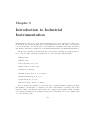
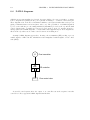
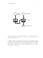
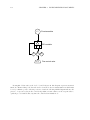
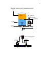
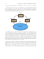
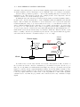
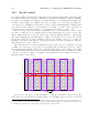
5 Introduction to Industrial Instrumentation
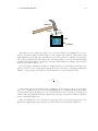
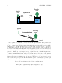
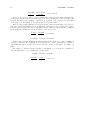
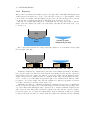
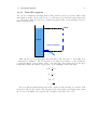
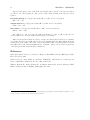
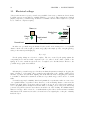
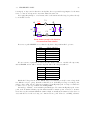
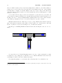
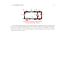
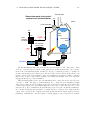
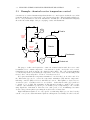
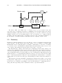
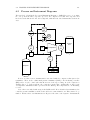
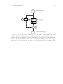
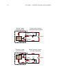
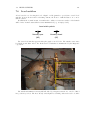
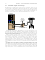
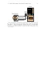
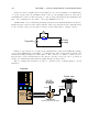
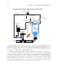
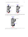
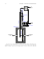
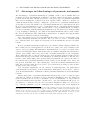
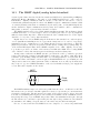
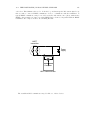
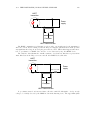
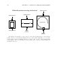
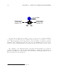
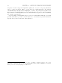
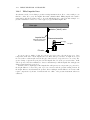
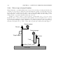
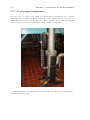
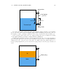
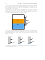
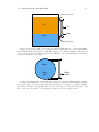
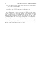
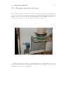
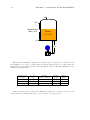
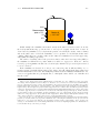
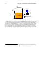
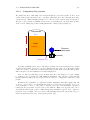
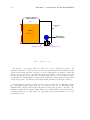
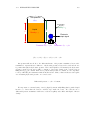
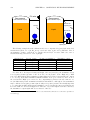
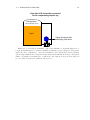
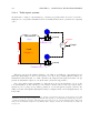
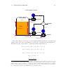
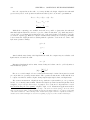
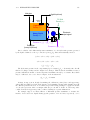
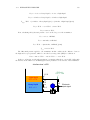
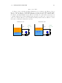
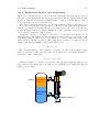
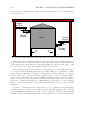
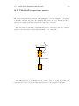
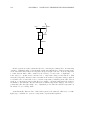
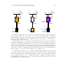
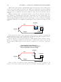
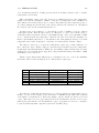
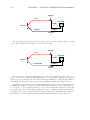
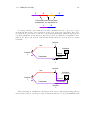
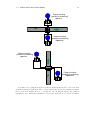
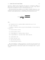
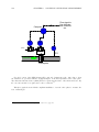
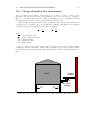
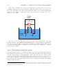
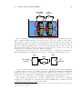
5.1 Example: boiler water level control system . . .
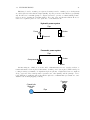
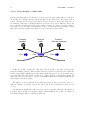
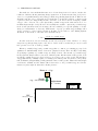
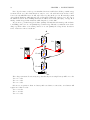
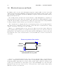
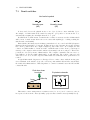
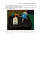
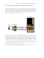
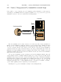
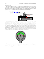
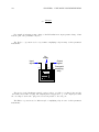
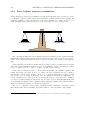
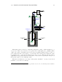
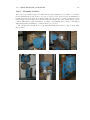
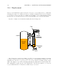
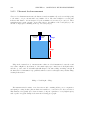
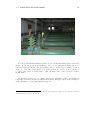
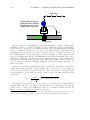
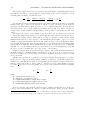
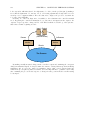
5.2 Example: wastewater disinfection . . . . . . . .
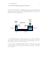
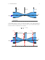
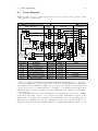
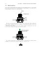
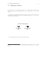
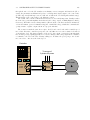
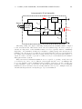
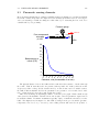
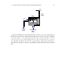
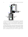
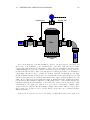
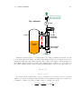
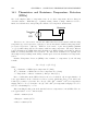
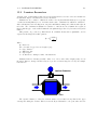
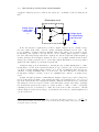
5.3 Example: chemical reactor temperature control
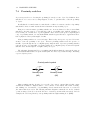
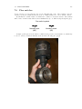
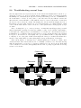
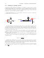
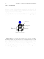
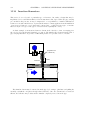
5.4 Other types of instruments . . . . . . . . . . .
.
.
.
.
.
.
.
.
.
.
.
.
.
.
.
.
.
.
.
.
.
.
.
.
.
.
.
.
.
.
.
.
.
.
.
.
.
.
.
.
.
.
.
.
.
.
.
.
.
.
.
.
.
.
.
.
.
.
.
.
.
.
.
.
.
.
.
.
.
.
.
.
.
.
.
.
.
.
.
.
.
.
.
.
129
132
137
139
141
2 Chemistry
2.1 Terms and Definitions . . . .
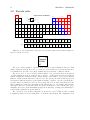
2.2 Periodic table . . . . . . . . .
2.3 Molecular quantities . . . . .
2.4 Stoichiometry . . . . . . . . .
2.5 Energy in chemical reactions
2.6 Ions in liquid solutions . . . .
2.7 pH . . . . . . . . . . . . . . .
.
.
.
.
.
.
.
.
.
.
.
.
.
.
.
.
.
.
.
.
.
.
.
.
.
.
.
.
.
.
.
.
.
.
.
electricity
RMS quantities . . . . . . . . . . . . .
Resistance, Reactance, and Impedance
Series and parallel circuits . . . . . . .
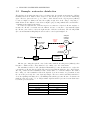
Phasor mathematics . . . . . . . . . .
.
.
.
.
CONTENTS
5.5
v
Summary . . . . . . . . . . . . . . . . . . . . . . . . . . . . . . . . . . . . . . . . . . 146
6 Instrumentation documents
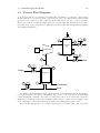
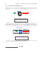
6.1 Process Flow Diagrams . . . . . . . . . . . . . . . . . .
6.2 Process and Instrument Diagrams . . . . . . . . . . . .
6.3 Loop diagrams . . . . . . . . . . . . . . . . . . . . . . .
6.4 SAMA diagrams . . . . . . . . . . . . . . . . . . . . . .
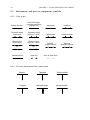
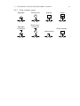
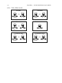
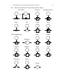
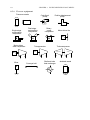
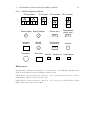
6.5 Instrument and process equipment symbols . . . . . . .
6.5.1 Line types . . . . . . . . . . . . . . . . . . . . . .
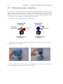
6.5.2 Process/Instrument line connections . . . . . . .
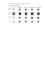
6.5.3 Instrument bubbles . . . . . . . . . . . . . . . . .
6.5.4 Process valve types . . . . . . . . . . . . . . . . .
6.5.5 Valve actuator types . . . . . . . . . . . . . . . .
6.5.6 Valve failure mode . . . . . . . . . . . . . . . . .
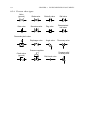
6.5.7 Flow measurement devices (flowing left-to-right)
6.5.8 Process equipment . . . . . . . . . . . . . . . . .
6.5.9 SAMA diagram symbols . . . . . . . . . . . . . .
.
.
.
.
.
.
.
.
.
.
.
.
.
.
.
.
.
.
.
.
.
.
.
.
.
.
.
.
.
.
.
.
.
.
.
.
.
.
.
.
.
.
.
.
.
.
.
.
.
.
.
.
.
.
.
.
.
.
.
.
.
.
.
.
.
.
.
.
.
.
.
.
.
.
.
.
.
.
.
.
.
.
.
.
.
.
.
.
.
.
.
.
.
.
.
.
.
.
.
.
.
.
.
.
.
.
.
.
.
.
.
.
.
.
.
.
.
.
.
.
.
.
.
.
.
.
.
.
.
.
.
.
.
.
.
.
.
.
.
.
.
.
.
.
.
.
.
.
.
.
.
.
.
.
.
.
.
.
.
.
.
.
.
.
.
.
.
.
.
.
.
.
.
.
.
.
.
.
.
.
.
.
.
.
.
.
.
.
.
.
.
.
.
.
.
.
.
.
.
.
.
.
.
.
.
.
.
.
.
.
.
.
.
.
.
.
.
.
.
.
.
.
.
.
147
149
151
153
156
160
160
160
161
162
163
164
165
166
167
7 Discrete process measurement
7.1 “Normal” status of a switch .
7.2 Hand switches . . . . . . . . .
7.3 Limit switches . . . . . . . .
7.4 Proximity switches . . . . . .
7.5 Pressure switches . . . . . . .
7.6 Level switches . . . . . . . . .
7.7 Temperature switches . . . .
7.8 Flow switches . . . . . . . . .
.
.
.
.
.
.
.
.
.
.
.
.
.
.
.
.
.
.
.
.
.
.
.
.
.
.
.
.
.
.
.
.
.
.
.
.
.
.
.
.
.
.
.
.
.
.
.
.
.
.
.
.
.
.
.
.
.
.
.
.
.
.
.
.
.
.
.
.
.
.
.
.
.
.
.
.
.
.
.
.
.
.
.
.
.
.
.
.
.
.
.
.
.
.
.
.
.
.
.
.
.
.
.
.
.
.
.
.
.
.
.
.
.
.
.
.
.
.
.
.
.
.
.
.
.
.
.
.
169
170
172
173
175
179
181
183
185
. . . .
. . . .
. . . .
. . . .
. . . .
. . . .
signal
. . . .
. . . .
. . . .
. . . .
. . . .
.
.
.
.
.
.
.
.
.
.
.
.
.
.
.
.
.
.
.
.
.
.
.
.
.
.
.
.
.
.
.
.
.
.
.
.
.
.
.
.
.
.
.
.
.
.
.
.
.
.
.
.
.
.
.
.
.
.
.
.
.
.
.
.
.
.
.
.
.
.
.
.
.
.
.
.
.
.
.
.
.
.
.
.
.
.
.
.
.
.
.
.
.
.
.
.
.
.
.
.
.
.
.
.
.
.
.
.
.
.
.
.
.
.
.
.
.
.
.
.
.
.
.
.
.
.
.
.
.
.
.
.
187
187
190
190
191
191
192
192
193
196
198
200
202
.
.
.
.
.
.
.
.
.
.
.
.
.
.
.
.
.
.
.
.
.
.
.
.
.
.
.
.
.
.
.
.
.
.
.
.
.
.
.
.
.
.
.
.
.
.
.
.
.
.
.
.
.
.
.
.
.
.
.
.
.
.
.
.
.
.
.
.
.
.
.
.
.
.
.
.
.
.
.
.
.
.
.
.
.
.
.
.
.
.
.
.
.
.
.
.
.
.
.
.
.
.
.
.
.
.
.
.
.
.
.
.
.
.
.
.
.
.
.
.
8 Analog electronic instrumentation
8.1 4 to 20 mA analog current signals . . . . . . . . . . . . . .
8.2 Relating 4 to 20 mA signals to instrument variables . . .
8.2.1 Example calculation: controller output to valve . .
8.2.2 Example calculation: flow transmitter . . . . . . .
8.2.3 Example calculation: temperature transmitter . .
8.2.4 Example calculation: pH transmitter . . . . . . . .
8.2.5 Example calculation: reverse-acting I/P transducer
8.2.6 Graphical interpretation of signal ranges . . . . . .
8.3 Controller output current loops . . . . . . . . . . . . . . .
8.4 4-wire (“self-powered”) transmitter current loops . . . . .
8.5 2-wire (“loop-powered”) transmitter current loops . . . .
8.6 Troubleshooting current loops . . . . . . . . . . . . . . . .
vi
CONTENTS
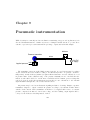
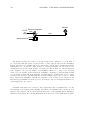
9 Pneumatic instrumentation
9.1 Pneumatic sensing elements . . . . . . . . . . . . . . . .
9.2 Self-balancing pneumatic instrument principles . . . . .
9.3 Pilot valves and pneumatic amplifying relays . . . . . .
9.4 Analogy to opamp circuits . . . . . . . . . . . . . . . . .
9.5 Analysis of a practical pneumatic instrument . . . . . .
9.6 Proper care and feeding of pneumatic instruments . . .
9.7 Advantages and disadvantages of pneumatic instruments
.
.
.
.
.
.
.
.
.
.
.
.
.
.
.
.
.
.
.
.
.
.
.
.
.
.
.
.
.
.
.
.
.
.
.
.
.
.
.
.
.
.
.
.
.
.
.
.
.
.
.
.
.
.
.
.
.
.
.
.
.
.
.
.
.
.
.
.
.
.
.
.
.
.
.
.
.
.
.
.
.
.
.
.
.
.
.
.
.
.
.
.
.
.
.
.
.
.
.
.
.
.
.
.
.
.
.
.
.
.
.
.
209
213
216
220
228
237
242
243
10 Digital electronic instrumentation
10.1 The HART digital/analog hybrid standard .
10.1.1 HART multidrop mode . . . . . . .
10.1.2 HART multi-variable transmitters .
10.2 Fieldbus standards . . . . . . . . . . . . . .
10.3 Wireless instrumentation . . . . . . . . . . .
.
.
.
.
.
.
.
.
.
.
.
.
.
.
.
.
.
.
.
.
.
.
.
.
.
.
.
.
.
.
.
.
.
.
.
.
.
.
.
.
.
.
.
.
.
.
.
.
.
.
.
.
.
.
.
.
.
.
.
.
.
.
.
.
.
.
.
.
.
.
.
.
.
.
.
.
.
.
.
.
245
246
252
253
254
255
11 Instrument calibration
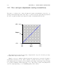
11.1 The meaning of calibration . . . . . . . . . . . . . . . . .
11.2 Zero and span adjustments (analog transmitters) . . . . .
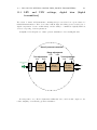
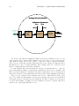
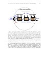
11.3 LRV and URV settings, digital trim (digital transmitters)
11.4 Calibration procedures . . . . . . . . . . . . . . . . . . . .
11.4.1 Linear instruments . . . . . . . . . . . . . . . . . .
11.4.2 Nonlinear instruments . . . . . . . . . . . . . . . .
11.4.3 Discrete instruments . . . . . . . . . . . . . . . . .
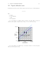
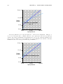
11.5 Typical calibration errors . . . . . . . . . . . . . . . . . .
11.5.1 As-found and as-left documentation . . . . . . . .
11.5.2 Up-tests and Down-tests . . . . . . . . . . . . . . .
11.6 NIST traceability . . . . . . . . . . . . . . . . . . . . . . .
11.7 Instrument turndown . . . . . . . . . . . . . . . . . . . . .
11.8 Practical calibration standards . . . . . . . . . . . . . . .
11.8.1 Electrical standards . . . . . . . . . . . . . . . . .
11.8.2 Temperature standards . . . . . . . . . . . . . . .
11.8.3 Pressure standards . . . . . . . . . . . . . . . . . .
11.8.4 Flow standards . . . . . . . . . . . . . . . . . . . .
11.8.5 Analytical standards . . . . . . . . . . . . . . . . .
.
.
.
.
.
.
.
.
.
.
.
.
.
.
.
.
.
.
.
.
.
.
.
.
.
.
.
.
.
.
.
.
.
.
.
.
.
.
.
.
.
.
.
.
.
.
.
.
.
.
.
.
.
.
.
.
.
.
.
.
.
.
.
.
.
.
.
.
.
.
.
.
.
.
.
.
.
.
.
.
.
.
.
.
.
.
.
.
.
.
.
.
.
.
.
.
.
.
.
.
.
.
.
.
.
.
.
.
.
.
.
.
.
.
.
.
.
.
.
.
.
.
.
.
.
.
.
.
.
.
.
.
.
.
.
.
.
.
.
.
.
.
.
.
.
.
.
.
.
.
.
.
.
.
.
.
.
.
.
.
.
.
.
.
.
.
.
.
.
.
.
.
.
.
.
.
.
.
.
.
.
.
.
.
.
.
.
.
.
.
.
.
.
.
.
.
.
.
.
.
.
.
.
.
.
.
.
.
.
.
.
.
.
.
.
.
.
.
.
.
.
.
.
.
.
.
.
.
.
.
.
.
.
.
.
.
.
.
.
.
.
.
.
.
.
.
.
.
.
.
.
.
.
.
.
.
.
.
.
.
.
.
.
.
.
.
.
.
.
.
257
257
258
261
265
265
265
266
267
270
270
271
271
272
273
275
278
284
285
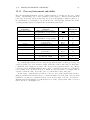
12 Continuous pressure measurement
12.1 Manometers . . . . . . . . . . . . . . . . . .
12.2 Mechanical pressure elements . . . . . . . .
12.3 Electrical pressure elements . . . . . . . . .
12.3.1 Piezoresistive (strain gauge) sensors
12.3.2 Differential capacitance sensors . . .
12.3.3 Resonant element sensors . . . . . .
12.3.4 Mechanical adaptations . . . . . . .
12.4 Force-balance pressure transmitters . . . . .
12.5 Differential pressure transmitters . . . . . .
.
.
.
.
.
.
.
.
.
.
.
.
.
.
.
.
.
.
.
.
.
.
.
.
.
.
.
.
.
.
.
.
.
.
.
.
.
.
.
.
.
.
.
.
.
.
.
.
.
.
.
.
.
.
.
.
.
.
.
.
.
.
.
.
.
.
.
.
.
.
.
.
.
.
.
.
.
.
.
.
.
.
.
.
.
.
.
.
.
.
.
.
.
.
.
.
.
.
.
.
.
.
.
.
.
.
.
.
.
.
.
.
.
.
.
.
.
.
.
.
.
.
.
.
.
.
.
.
.
.
.
.
.
.
.
289
290
295
299
300
303
308
311
312
316
.
.
.
.
.
.
.
.
.
.
.
.
.
.
.
.
.
.
.
.
.
.
.
.
.
.
.
.
.
.
.
.
.
.
.
.
.
.
.
.
.
.
.
.
.
.
.
.
.
.
.
.
.
.
.
.
.
.
.
.
.
.
.
.
.
.
.
.
.
.
.
.
.
.
.
.
.
.
.
.
.
.
.
.
.
.
.
.
.
.
.
.
.
.
.
.
.
.
.
.
.
.
.
.
.
.
.
CONTENTS
12.6 Pressure sensor accessories . . . . . . .
12.6.1 Valve manifolds . . . . . . . . .
12.6.2 Bleed fittings . . . . . . . . . .
12.6.3 Pressure pulsation dampening .
12.6.4 Remote and chemical seals . .
12.6.5 Filled impulse lines . . . . . . .
12.6.6 Purged impulse lines . . . . . .
12.6.7 Heat-traced impulse lines . . .
12.6.8 Water traps and pigtail siphons
12.6.9 Mounting brackets . . . . . . .
12.7 Process/instrument suitability . . . . .
vii
.
.
.
.
.
.
.
.
.
.
.
.
.
.
.
.
.
.
.
.
.
.
.
.
.
.
.
.
.
.
.
.
.
.
.
.
.
.
.
.
.
.
.
.
.
.
.
.
.
.
.
.
.
.
.
.
.
.
.
.
.
.
.
.
.
.
.
.
.
.
.
.
.
.
.
.
.
.
.
.
.
.
.
.
.
.
.
.
.
.
.
.
.
.
.
.
.
.
.
.
.
.
.
.
.
.
.
.
.
.
.
.
.
.
.
.
.
.
.
.
.
.
.
.
.
.
.
.
.
.
.
.
.
.
.
.
.
.
.
.
.
.
.
.
.
.
.
.
.
.
.
.
.
.
.
.
.
.
.
.
.
.
.
.
.
.
.
.
.
.
.
.
.
.
.
.
.
.
.
.
.
.
.
.
.
.
.
.
.
.
.
.
.
.
.
.
.
.
.
.
.
.
.
.
.
.
.
.
.
.
.
.
.
.
.
.
.
.
.
.
.
.
.
.
.
.
.
.
.
.
.
.
.
.
.
.
.
.
.
.
.
.
.
.
.
.
.
.
.
.
.
.
.
.
.
.
.
.
.
.
.
.
.
.
.
.
.
.
.
.
.
.
.
.
.
.
.
.
.
.
.
.
.
.
.
.
321
322
326
327
330
337
338
340
342
343
344
13 Continuous level measurement
13.1 Level gauges (sightglasses) . . . . . . . . . . . . .
13.2 Float . . . . . . . . . . . . . . . . . . . . . . . . .
13.3 Hydrostatic pressure . . . . . . . . . . . . . . . .
13.3.1 Bubbler systems . . . . . . . . . . . . . .
13.3.2 Transmitter suppression and elevation . .
13.3.3 Compensated leg systems . . . . . . . . .
13.3.4 Tank expert systems . . . . . . . . . . . .
13.3.5 Hydrostatic interface level measurement .
13.4 Displacement . . . . . . . . . . . . . . . . . . . .
13.4.1 Displacement interface level measurement
13.5 Echo . . . . . . . . . . . . . . . . . . . . . . . . .
13.5.1 Ultrasonic level measurement . . . . . . .
13.5.2 Radar level measurement . . . . . . . . .
13.6 Laser level measurement . . . . . . . . . . . . . .
13.7 Weight . . . . . . . . . . . . . . . . . . . . . . . .
13.8 Capacitive . . . . . . . . . . . . . . . . . . . . . .
13.9 Radiation . . . . . . . . . . . . . . . . . . . . . .
13.10Level sensor accessories . . . . . . . . . . . . . .
13.11Process/instrument suitability . . . . . . . . . . .
.
.
.
.
.
.
.
.
.
.
.
.
.
.
.
.
.
.
.
.
.
.
.
.
.
.
.
.
.
.
.
.
.
.
.
.
.
.
.
.
.
.
.
.
.
.
.
.
.
.
.
.
.
.
.
.
.
.
.
.
.
.
.
.
.
.
.
.
.
.
.
.
.
.
.
.
.
.
.
.
.
.
.
.
.
.
.
.
.
.
.
.
.
.
.
.
.
.
.
.
.
.
.
.
.
.
.
.
.
.
.
.
.
.
.
.
.
.
.
.
.
.
.
.
.
.
.
.
.
.
.
.
.
.
.
.
.
.
.
.
.
.
.
.
.
.
.
.
.
.
.
.
.
.
.
.
.
.
.
.
.
.
.
.
.
.
.
.
.
.
.
.
.
.
.
.
.
.
.
.
.
.
.
.
.
.
.
.
.
.
.
.
.
.
.
.
.
.
.
.
.
.
.
.
.
.
.
.
.
.
.
.
.
.
.
.
.
.
.
.
.
.
.
.
.
.
.
.
.
.
.
.
.
.
.
.
.
.
.
.
.
.
.
.
.
.
.
.
.
.
.
.
.
.
.
.
.
.
.
.
.
.
.
.
.
.
.
.
.
.
.
.
.
.
.
.
.
.
.
.
.
.
.
.
.
.
.
.
.
.
.
.
.
.
.
.
.
.
.
.
.
.
.
.
.
.
.
.
.
.
.
.
.
.
.
.
.
.
.
.
.
.
.
.
.
.
.
.
.
.
.
.
.
.
.
.
.
.
.
.
.
.
.
.
.
.
.
.
.
.
.
.
.
.
.
.
.
.
.
.
.
.
.
.
.
.
.
.
.
.
.
.
.
.
.
.
.
.
.
.
347
348
352
357
361
363
367
372
376
382
387
389
390
395
402
403
406
408
409
412
.
.
.
.
.
.
.
415
417
419
422
427
435
437
441
14 Continuous temperature measurement
14.1 Bi-metal temperature sensors . . . . . . . . . . . . . . . . .
14.2 Filled-bulb temperature sensors . . . . . . . . . . . . . . . .
14.3 Thermistors and Resistance Temperature Detectors (RTDs)
14.4 Thermocouples . . . . . . . . . . . . . . . . . . . . . . . . .
14.5 Optical temperature sensing . . . . . . . . . . . . . . . . . .
14.6 Temperature sensor accessories . . . . . . . . . . . . . . . .
14.7 Process/instrument suitability . . . . . . . . . . . . . . . . .
.
.
.
.
.
.
.
.
.
.
.
.
.
.
.
.
.
.
.
.
.
.
.
.
.
.
.
.
.
.
.
.
.
.
.
.
.
.
.
.
.
.
.
.
.
.
.
.
.
.
.
.
.
.
.
.
.
.
.
.
.
.
.
.
.
.
.
.
.
.
.
.
.
.
.
.
.
.
.
.
.
.
.
.
.
.
.
.
.
.
.
viii
CONTENTS
15 Continuous fluid flow measurement
15.1 Pressure-based flowmeters . . . . . . . . .
15.1.1 Venturi tubes and basic principles
15.1.2 Orifice plates . . . . . . . . . . . .
15.1.3 Other differential producers . . . .
15.1.4 Proper installation . . . . . . . . .
15.1.5 High-accuracy flow measurement .
15.1.6 Equation summary . . . . . . . . .
15.2 Laminar flowmeters . . . . . . . . . . . .
15.3 Variable-area flowmeters . . . . . . . . . .
15.4 Velocity-based flowmeters . . . . . . . . .
15.4.1 Turbine flowmeters . . . . . . . . .
15.4.2 Vortex flowmeters . . . . . . . . .
15.4.3 Magnetic flowmeters . . . . . . . .
15.4.4 Ultrasonic flowmeters . . . . . . .
15.5 Inertia-based (true mass) flowmeters . . .
15.5.1 Coriolis flowmeters . . . . . . . . .
15.6 Thermal-based (mass) flowmeters . . . . .
15.7 Positive displacement flowmeters . . . . .
15.8 Weighfeeders . . . . . . . . . . . . . . . .
15.9 Change-of-quantity flow measurement . .
15.10Insertion flowmeters . . . . . . . . . . . .
15.11Process/instrument suitability . . . . . . .
.
.
.
.
.
.
.
.
.
.
.
.
.
.
.
.
.
.
.
.
.
.
.
.
.
.
.
.
.
.
.
.
.
.
.
.
.
.
.
.
.
.
.
.
.
.
.
.
.
.
.
.
.
.
.
.
.
.
.
.
.
.
.
.
.
.
.
.
.
.
.
.
.
.
.
.
.
.
.
.
.
.
.
.
.
.
.
.
.
.
.
.
.
.
.
.
.
.
.
.
.
.
.
.
.
.
.
.
.
.
.
.
.
.
.
.
.
.
.
.
.
.
.
.
.
.
.
.
.
.
.
.
.
.
.
.
.
.
.
.
.
.
.
.
.
.
.
.
.
.
.
.
.
.
.
.
.
.
.
.
.
.
.
.
.
.
.
.
.
.
.
.
.
.
.
.
.
.
.
.
.
.
.
.
.
.
.
.
.
.
.
.
.
.
.
.
.
.
.
.
.
.
.
.
.
.
.
.
.
.
.
.
.
.
.
.
.
.
.
.
.
.
.
.
.
.
.
.
.
.
.
.
.
.
.
.
.
.
.
.
.
.
.
.
.
.
.
.
.
.
.
.
.
.
.
.
.
.
.
.
.
.
.
.
.
.
.
.
.
.
.
.
.
.
.
.
.
.
.
.
.
.
.
.
.
.
.
.
.
.
.
.
.
.
.
.
.
.
.
.
.
.
.
.
.
.
.
.
.
.
.
.
.
.
.
.
.
.
.
.
.
.
.
.
.
.
.
.
.
.
.
.
.
.
.
.
.
.
.
.
.
.
.
.
.
.
.
.
.
.
.
.
.
.
.
.
.
.
.
.
.
.
.
.
.
.
.
.
.
.
.
.
.
.
.
.
.
.
.
.
.
.
.
.
.
.
.
.
.
.
.
.
.
.
.
.
.
.
.
.
.
.
.
.
.
.
.
.
.
.
.
.
.
.
.
.
.
.
.
.
.
.
.
.
.
.
.
.
.
.
.
.
.
.
.
.
.
.
.
.
.
.
.
.
.
.
.
.
.
.
.
.
.
.
.
.
.
.
.
.
.
.
.
.
.
.
.
.
.
.
.
.
.
.
.
.
.
.
.
.
.
.
.
.
.
.
.
.
.
.
.
.
.
.
.
.
.
.
.
.
.
.
.
.
.
.
.
.
.
.
.
.
.
.
.
.
.
.
.
.
.
.
.
.
.
.
.
.
443
444
449
458
467
473
477
483
485
487
495
496
501
505
512
514
515
524
527
528
529
532
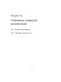
537
16 Continuous analytical measurement
16.1 Density measurement . . . . . . . . . . . . . .
16.2 Turbidity measurement . . . . . . . . . . . .
16.3 Conductivity measurement . . . . . . . . . .
16.3.1 Dissociation and ionization in aqueous
16.3.2 Two-electrode conductivity probes . .
16.3.3 Four-electrode conductivity probes . .
16.3.4 Electrodeless conductivity probes . . .
16.4 pH measurement . . . . . . . . . . . . . . . .
16.4.1 Colorimetric pH measurement . . . . .
16.4.2 Potentiometric pH measurement . . .
16.5 Chromatography . . . . . . . . . . . . . . . .
. . . . . .
. . . . . .
. . . . . .
solutions
. . . . . .
. . . . . .
. . . . . .
. . . . . .
. . . . . .
. . . . . .
. . . . . .
.
.
.
.
.
.
.
.
.
.
.
.
.
.
.
.
.
.
.
.
.
.
.
.
.
.
.
.
.
.
.
.
.
.
.
.
.
.
.
.
.
.
.
.
.
.
.
.
.
.
.
.
.
.
.
.
.
.
.
.
.
.
.
.
.
.
.
.
.
.
.
.
.
.
.
.
.
.
.
.
.
.
.
.
.
.
.
.
.
.
.
.
.
.
.
.
.
.
.
.
.
.
.
.
.
.
.
.
.
.
.
.
.
.
.
.
.
.
.
.
.
.
.
.
.
.
.
.
.
.
.
.
.
.
.
.
.
.
.
.
.
.
.
.
.
.
.
.
.
.
.
.
.
.
.
.
.
.
.
.
.
.
.
.
.
.
.
.
.
.
.
.
.
.
.
.
541
541
541
542
542
543
544
546
549
549
550
561
17 Signal characterization
17.1 Flow measurement in open channels
17.2 Liquid volume measurement . . . . .
17.3 Radiative temperature measurement
17.4 Analytical measurements . . . . . .
.
.
.
.
.
.
.
.
.
.
.
.
.
.
.
.
.
.
.
.
.
.
.
.
.
.
.
.
.
.
.
.
.
.
.
.
.
.
.
.
.
.
.
.
.
.
.
.
.
.
.
.
.
.
.
.
.
.
.
.
.
.
.
.
.
.
.
.
573
581
583
591
592
.
.
.
.
.
.
.
.
.
.
.
.
.
.
.
.
.
.
.
.
.
.
.
.
.
.
.
.
.
.
.
.
.
.
.
.
.
.
.
.
CONTENTS
18 Continuous feedback control
18.1 Basic feedback control principles
18.2 On/off control . . . . . . . . . . .
18.3 Proportional-only control . . . .
18.4 Proportional-only offset . . . . .
18.5 Integral (reset) control . . . . . .
18.6 Derivative (rate) control . . . . .
18.7 PID controller tuning . . . . . .
1
.
.
.
.
.
.
.
.
.
.
.
.
.
.
.
.
.
.
.
.
.
.
.
.
.
.
.
.
.
.
.
.
.
.
.
.
.
.
.
.
.
.
.
.
.
.
.
.
.
.
.
.
.
.
.
.
.
.
.
.
.
.
.
.
.
.
.
.
.
.
.
.
.
.
.
.
.
.
.
.
.
.
.
.
.
.
.
.
.
.
.
.
.
.
.
.
.
.
.
.
.
.
.
.
.
.
.
.
.
.
.
.
.
.
.
.
.
.
.
.
.
.
.
.
.
.
.
.
.
.
.
.
.
.
.
.
.
.
.
.
.
.
.
.
.
.
.
.
.
.
.
.
.
.
.
.
.
.
.
.
.
.
.
.
.
.
.
.
.
.
.
.
.
.
.
.
.
.
.
.
.
.
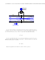
A Doctor Strangeflow, or how I learned to relax and love Reynolds numbers
.
.
.
.
.
.
.
.
.
.
.
.
.
.
.
.
.
.
.
.
.
595
596
602
604
608
611
614
616
621
B Creative Commons Attribution License
631
B.1 A simple explanation of your rights . . . . . . . . . . . . . . . . . . . . . . . . . . . . 632
B.2 Legal code . . . . . . . . . . . . . . . . . . . . . . . . . . . . . . . . . . . . . . . . . . 633
2
CONTENTS
Preface
I did not want to write this book . . . honestly.
My first book project began in 1998, titled Lessons In Electric Circuits, and I didn’t call “quit”
until six volumes and five years later. Even then, it was not complete, but being an open-source
project it gained traction on the internet to the point where other people took over its development
and it grew fine without me. The impetus for writing this first tome was a general dissatisfaction
with available electronics textbooks. Plenty of textbooks exist to describe things, but few really
explain things well for students, and the field of electronics is no exception. I wanted my book(s)
to be different, and so they were. No one told me how time-consuming it was going to be to write
them, though!
The next few years’ worth of my spare time went to developing a set of question-and-answer
worksheets designed to teach electronics theory in a Socratic, active-engagement style. This project
proved quite successful in my professional life as an instructor of electronics. In the summer of 2006,
my job changed from teaching electronics to teaching industrial instrumentation, and I decided to
continue the Socratic mode of instruction with another set of question-and-answer worksheets.
However, the field of industrial instrumentation is not as well-represented as general electronics,
and thus the array of available textbooks is not as vast. I began to re-discover the drudgery of
trying to teach with inadequate texts as source material. The basis of my active teaching style was
that students would spend time researching the material on their own, then engage in Socratic-style
discussion with me on the subject matter when they arrived for class. This teaching technique
functions in direct proportion to the quality and quantity of the source material at the students’
disposal. Despite much searching, I was unable to find a textbook that adequately addressed my
students’ learning needs. Many textbooks I found were written in a shallow, “math-phobic” style
that was well below the level I intended to teach to. Some reference books I found contained great
information, but were often written for degreed engineers with lots of Laplace transforms and other
mathematical techniques that were well above the level I intended to teach to. Few on either side of
the spectrum actually made an effort to explain certain concepts that students generally struggle to
understand. I needed a text that gave good, practical information and theoretical coverage at the
same time.
In a futile effort to provide my students with enough information to study outside of class, I
scoured the internet for free tutorials written by others. While some manufacturer’s tutorials were
nearly perfect for my needs, others were just as shallow as the textbooks I had found, and/or were
little more than sales brochures. I found myself starting to write my own tutorials on specific topics
to “plug the gaps,” but then another problem arose: it became troublesome for students to navigate
through dozens of tutorials in an effort to find the information they needed in their studies. What
3
4
CONTENTS
my students really needed was a book, not a smorgasbord of tutorials.
So here I am again, writing another textbook. This time around I have the advantage of wisdom
gained from the first textbook project. For this project, I will not:
• . . . attempt to maintain a parallel book in HTML markup (for direct viewing on the internet).
I had to go to the trouble of inventing my own markup language last time in an effort to have
multiple format versions of the book from the same source code. Instead, this time I will use
stock LATEXas the source code format and regular Adobe PDF format for the final output,
which anyone may read thanks to its ubiquity.
• . . . use a GNU GPL-style copyleft license. Instead, I will use the Creative Commons
Attribution-only license, which makes things a lot easier for anyone wishing to incorporate my
work into derivative works. My interest is maximum flexibility for those who may adapt my
material to their own needs, not the imposition of certain philosophical ideals.
• . . . start from a conceptual state of “ground zero.” I will assume the reader has certain
familiarity with electronics and mathematics, which I will build on. If a reader finds they need
to learn more about electronics, they should go read Lessons In Electric Circuits.
• . . . avoid using calculus to help explain certain concepts. Not all my readers will understand
these parts, and so I will be sure to explain what I can without using calculus. However,
I want to give my more mathematically adept students an opportunity to see the power of
calculus applied to instrumentation where appropriate. By occasionally applying calculus and
explaining my steps, I also hope this text will serve as a practical guide for students who might
wish to learn calculus, so they can see its utility and function in a context that interests them.
There do exist many fine references on the subject of industrial instrumentation. I only wish I
could condense their best parts into a single volume for my students. Being able to do so would
certainly save me from having to write my own! Listed here are some of the best books I can
recommend for those wishing to explore instrumentation outside of my own presentation:
• Handbook of Instrumentation and Controls, by Howard P. Kallen. Perhaps the best-written
textbook on general instrumentation I have ever encountered. Too bad it’s long out of print
– my copy dates 1961. Like most American textbooks written during the years immediately
following Sputnik, it is a masterpiece of practical content and conceptual clarity.
• Industrial Instrumentation Fundamentals, by Austin E. Fribance. Another great post-Sputnik
textbook – my copy dates 1962.
• Instrumentation for Process Measurement and Control, by Normal A. Anderson. An inspiring
effort by someone who knows the art of teaching as well as the craft of instrumentation. Too
bad the content doesn’t seem to have been updated since 1980.
• Instrument Engineers’ Handbook series (Volumes I, II, and III), edited by Béla Lipták. By far
my favorite modern references on the subject. Unfortunately, there is a fair amount of material
within that lies well beyond my students’ grasp (Laplace transforms, etc.), and the volumes
are incredibly bulky and expensive (1000+ pages, at a cost of nearly $200.00 apiece!). These
texts also lack some of the basic content my students do need, and I don’t have the heart to
tell them to buy yet another textbook to fill the gaps.
CONTENTS
5
• Practically anything written by Francis Greg Shinskey.
Whether or not I achieve my goal of writing a better textbook is a judgment left for others to
make. One decided advantage my book will have over all the others is its openness. If you don’t like
anything you see in these pages, you have the right to modify it at will! Delete content, add content,
modify content – it’s all fair in this game we call “open source.” My only condition is declared in the
Creative Commons Attribution License: that you give me credit for my original authorship. What
you do with it beyond that is wholly up to you. This way, perhaps I can spare someone else from
having to write their own textbook from scratch!
6
CONTENTS
Chapter 1
Physics
7
8
1.1
CHAPTER 1. PHYSICS
Terms and Definitions
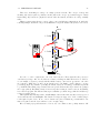
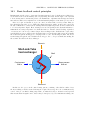
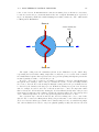
Mass (m) is the opposition that an object has to acceleration (changes in velocity). Weight is
the force (F ) imposed on a mass by a gravitational field. Mass is an intrinsic property of an
object, regardless of the environment. Weight, on the other hand, depends on the strength of the
gravitational field in which the object resides. A 20 kilogram slug of metal has the exact same mass
whether it rests on Earth or in the zero-gravity environment of outer space. However, the weight
of that mass depends on gravity: zero weight in outer space (where there is no gravity to act upon
it), some weight on Earth, and a much greater amount of weight on the planet Jupiter (due to the
much stronger gravitational field).
Since mass is the opposition of an object to changes in velocity (acceleration), it stands to reason
that force, mass, and acceleration for any particular object are directly related to one another:
F = ma
Where,
F = Force in newtons (metric) or pounds (British)
m = Mass in kilograms (metric) or slugs (British)
a = Acceleration in meters per second squared (metric) or feet per second squared (British)
If the force in question is the weight of the object, then the acceleration (a) in question is the
acceleration constant of the gravitational field where the object resides. For Earth at sea level,
agravity is approximately 9.8 meters per second squared, or 32 feet per second squared. Earth’s
gravitational acceleration constant is usually represented in equations by the variable letter g instead
of the more generic a.
Since acceleration is nothing more than the rate of velocity change with respect to time, the
force/mass equation may be expressed using the calculus notation of the first derivative:
F =m
dv
dt
Where,
F = Force in newtons (metric) or pounds (British)
m = Mass in kilograms (metric) or slugs (British)
v = Velocity in meters per second (metric) or feet per second (British)
t = Time in seconds
Since velocity is nothing more than the rate of position change with respect to time, the
force/mass equation may be expressed using the calculus notation of the second derivative
(acceleration being the derivative of velocity, which in turn is the derivative of position):
F =m
d2 x
dt2
Where,
F = Force in newtons (metric) or pounds (British)
m = Mass in kilograms (metric) or slugs (British)
x = Position in meters (metric) or feet (British)
t = Time in seconds
1.2. METRIC PREFIXES
9
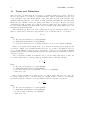
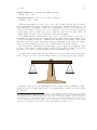
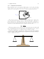
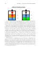
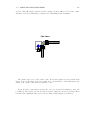
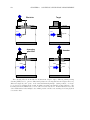
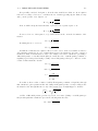
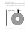
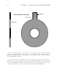
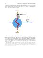
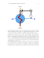
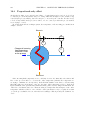
Mass density (ρ) for any substance is the proportion of mass to volume. Weight density (γ) for
any substance is the proportion of weight to volume.
Just as weight and mass are related to each other by gravitational acceleration, weight density
and mass density are also related to each other by gravity:
Fweight = mg
γ = ρg
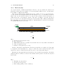
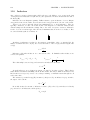
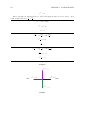
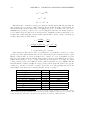
1.2
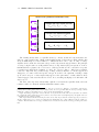
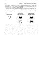
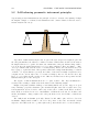
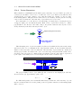
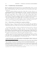
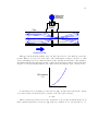
Weight and Mass
Weight density and Mass density
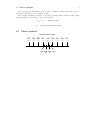
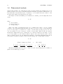
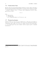
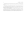
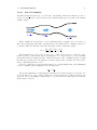
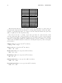
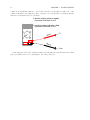
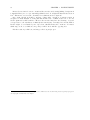
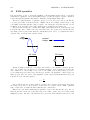
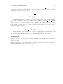
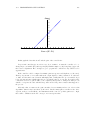
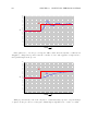
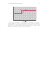
Metric prefixes
METRIC PREFIX SCALE
T
tera
1012
G
M
giga mega
109
106
k
kilo
103
(none)
100
m
µ
milli micro
10-3 10-6
102 101 10-1 10-2
hecto deca deci centi
h
da
d
c
n
nano
10-9
p
pico
10-12
10
CHAPTER 1. PHYSICS
1.3
Unit conversions and physical constants
Converting between disparate units of measurement is the bane of many science students. The
problem is worse for students of industrial instrumentation in the United States of America, who
must work with British (“Customary”) units such as the pound, the foot, the gallon, etc. Worldwide adoption of the metric system would go a long way toward alleviating this problem, but until
then it is important for students of instrumentation to master the art of unit conversions 1 .
It is possible to convert from one unit of measurement to another by use of tables designed
expressly for this purpose. Such tables usually have a column of units on the left-hand side and an
identical row of units along the top, whereby one can look up the conversion factor to multiply by
to convert from any listed unit to any other listed unit. While such tables are undeniably simple to
use, they are practically impossible to memorize.
The goal of this section is to provide you with a more powerful technique for unit conversion,
which lends itself much better to memorization of conversion factors. This way, you will be able to
convert between many common units of measurement while memorizing only a handful of essential
conversion factors.
I like to call this the unity fraction technique. It involves setting up the original quantity as
a fraction, then multiplying by a series of fractions having physical values of unity (1) so that by
multiplication the original value does not change, but the units do. Let’s take for example the
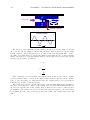
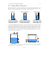
conversion of quarts into gallons, an example of a fluid volume conversion:
35 qt = ??? gal
Now, most people know there are four quarts in one gallon, and so it is tempting to simply
divide the number 35 by four to arrive at the proper number of gallons. However, the purpose of
this example is to show you how the technique of unity fractions works, not to get an answer to a
problem. First, we set up the original quantity as a fraction, in this case a fraction with 1 as the
denominator:
35 qt
1
Next, we multiply this fraction by another fraction having a physical value of unity, or 1. This
means a fraction comprised of equal measures in the numerator and denominator, but with different
units of measurement, arranged in such a way that the undesired unit cancels out leaving only the
desired unit(s). In this particular example, we wish to cancel out quarts and end up with gallons,
so we must arrange a fraction consisting of quarts and gallons having equal quantities in numerator
and denominator, such that quarts will cancel and gallons will remain:
µ
¶µ
¶
1 gal
35 qt
1
4 qt
1 An
interesting point to make here is that the United States did get something right when they designed their
monetary system of dollars and cents. This is essentially a metric system of measurement, with 100 cents per
dollar. The founders of the USA wisely decided to avoid the utterly confusing denominations of the British, with
their pounds, pence, farthings, shillings, etc. The denominations of penny, dime, dollar, and eagle ($10 gold coin)
comprised a simple power-of-ten system for money. Credit goes to France for first adopting a metric system of general
weights and measures as their national standard.
1.3. UNIT CONVERSIONS AND PHYSICAL CONSTANTS
11
Now we see how the unit of “quarts” cancels from the numerator of the first fraction and the
denominator of the second (“unity”) fraction, leaving only the unit of “gallons” left standing:
¶µ
¶
µ
1 gal
35 qt
= 8.75 gal
1
4 qt
The reason this conversion technique is so powerful is that it allows one to do a large range of
unit conversions while memorizing the smallest possible set of conversion factors.
Here is a set of six equal volumes, each one expressed in a different unit of measurement:
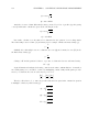
1 gallon (gal) = 231.0 cubic inches (in3 ) = 4 quarts (qt) = 8 pints (pt) = 128 fluid ounces (fl. oz.)
= 3.7854 liters (l)
Since all six of these quantities are physically equal, it is possible to build a “unity fraction” out
of any two, to use in converting any of the represented volume units into any of the other represented
volume units. Shown here are a few different volume unit conversion problems, using unity fractions
built only from these factors:
40 gallons converted into fluid ounces:
¶µ
¶
µ
128 fl. oz
40 gal
= 5120 fl. oz
1
1 gal
5.5 pints converted into cubic inches:
µ
¶µ
¶
5.5 pt
231 in3
= 158.8 in3
1
8 pt
1170 liters converted into quarts:
µ
1170 l
1
¶µ
4 qt
3.7854 l
¶
= 1236 qt
By contrast, if we were to try to memorize a 6 × 6 table giving conversion factors between any
two of six volume units, we would have to commit 30 different conversion factors to memory! Clearly,
the ability to set up “unity fractions” is a much more memory-efficient and practical approach.
But what if we wished to convert to a unit of volume measurement other than the six shown in
the long equality? For instance, what if we wished to convert 5.5 pints into cubic feet instead of
cubic inches? Since cubic feet is not a unit represented in the long string of quantities, what do we
do?
We do know of another equality between inches and feet, though. Everyone should know that
there are 12 inches in 1 foot. All we need to do is set up another unity fraction in the original
problem to convert cubic inches into cubic feet:
5.5 pints converted into cubic feet (our first attempt! ):
µ
¶µ
¶µ
¶
5.5 pt
231 in3
1 ft
= ???
1
8 pt
12 in
12
CHAPTER 1. PHYSICS
1 ft
Unfortunately, this will not give us the result we seek. Even though 12
in is a valid unity fraction,
it does not completely cancel out the unit of inches. What we need is a unity fraction relating cubic
1 ft
feet to cubic inches. We can get this, though, simply by cubing the 12
in unity fraction:
5.5 pints converted into cubic feet (our second attempt! ):
µ
5.5 pt
1
¶µ
231 in3
8 pt
¶µ
1 ft
12 in
¶3
Distributing the third power to the interior terms of the last unity fraction:
µ
¶µ
¶µ 3 3 ¶
5.5 pt
231 in3
1 ft
1
8 pt
123 in3
Calculating the values of 13 and 123 inside the last unity fraction, then canceling units and
solving:
¶µ
¶µ
¶
µ
231 in3
1 ft3
5.5 pt
= 0.0919 ft3
1
8 pt
1728 in3
Once again, this unit conversion technique shows its power by minimizing the number of
conversion factors we must memorize. We need not memorize how many cubic inches are in a
cubic foot, or how many square inches are in a square foot, if we know how many linear inches are in
a linear foot and we simply let the fractions “tell” us whether a power is needed for unit cancellation.
A major caveat to this method of converting units is that the units must be directly proportional
to one another, since this multiplicative conversion method is really nothing more than an exercise
in mathematical proportions. Here are some examples (but not an exhaustive list!) of conversions
that cannot be performed using the “unity fraction” method:
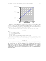
• Absolute / Gauge pressures, because one scale is offset from the other by 14.7 PSI (atmospheric
pressure).
• Celsius / Fahrenheit, because one scale is offset from the other by 32 degrees.
• Wire diameter / gauge number, because gauge numbers grow smaller as wire diameter grows
larger (inverse proportion rather than direct) and because there is no proportion relating the
two.
• Power / decibels, because the relationship is logarithmic rather than proportional.
The following subsections give sets of physically equal quantities, which may be used to create
unity fractions for unit conversion problems. Note that only those quantities shown in the same line
(separated by = symbols) are truly equal to each other, not quantities appearing in different lines!
1.3. UNIT CONVERSIONS AND PHYSICAL CONSTANTS
1.3.1
13
Conversion formulae for temperature
• o F = (o C)(9/5) + 32
• o C = (o F - 32)(5/9)
• o R = o F + 459.67
• K = o C + 273.15
1.3.2
1
1
1
1
Conversion factors for distance
inch (in) = 2.540000 centimeter (cm)
foot (ft) = 12 inches (in)
yard (yd) = 3 feet (ft)
mile (mi) = 5280 feet (ft)
1.3.3
Conversion factors for volume
1 gallon (gal) = 231.0 cubic inches (in3 ) = 4 quarts (qt) = 8 pints (pt) = 128 fluid ounces (fl. oz.)
= 3.7854 liters (l)
1 milliliter (ml) = 1 cubic centimeter (cm3 )
1.3.4
Conversion factors for velocity
1 mile per hour (mi/h) = 88 feet per minute (ft/m) = 1.46667 feet per second (ft/s) = 1.60934
kilometer per hour (km/h) = 0.44704 meter per second (m/s) = 0.868976 knot (knot – international)
1.3.5
Conversion factors for mass
1 pound (lbm) = 0.45359 kilogram (kg) = 0.031081 slugs
1.3.6
Conversion factors for force
1 pound-force (lbf) = 4.44822 newton (N)
1.3.7
Conversion factors for area
1 acre = 43560 square feet (ft2 ) = 4840 square yards (yd2 ) = 4046.86 square meters (m2 )
1.3.8
Conversion factors for pressure (either all gauge or all absolute)
1 pound per square inch (PSI) = 2.03603 inches of mercury (in. Hg) = 27.6807 inches of water (in.
W.C.) = 6.894757 kilo-pascals (kPa)
14
CHAPTER 1. PHYSICS
1.3.9
Conversion factors for pressure (absolute pressure units only)
1 atmosphere (Atm) = 14.7 pounds per square inch absolute (PSIA) = 760 millimeters of mercury
absolute (mmHgA) = 760 torr (torr) = 1.01325 bar (bar)
1.3.10
Conversion factors for energy or work
1 British thermal unit (Btu – “International Table”) = 251.996 calories (cal – “International Table”)
= 1055.06 joules (J) = 1055.06 watt-seconds (W-s) = 0.293071 watt-hour (W-hr) = 1.05506 x 10 10
ergs (erg) = 778.169 foot-pound-force (ft-lbf)
1.3.11
Conversion factors for power
1 horsepower (hp – 550 ft-lbf/s) = 745.7 watts (W) = 2544.43 British thermal units per hour
(Btu/hr) = 0.0760181 boiler horsepower (hp – boiler)
1.3.12
Terrestrial constants
Acceleration of gravity at sea level = 9.806650 meters per second per second (m/s 2 ) = 32.1740 feet
per second per second (ft/s2 )
Atmospheric pressure = 14.7 pounds per square inch absolute (PSIA) = 760 millimeters of mercury
absolute (mmHgA) = 760 torr (torr) = 1.01325 bar (bar)
Atmospheric gas concentrations:
• Nitrogen = 78.084 %
• Oxygen = 20.946 %
• Argon = 0.934 %
• Carbon Dioxide (CO2 ) = 0.033 %
• Neon = 18.18 ppm
• Helium = 5.24 ppm
• Methane (CH4 ) = 2 ppm
• Krypton = 1.14 ppm
• Hydrogen = 0.5 ppm
• Nitrous Oxide (N2 O) = 0.5 ppm
• Xenon = 0.087 ppm
1.3. UNIT CONVERSIONS AND PHYSICAL CONSTANTS
1.3.13
15
Properties of water
Freezing point at sea level = 32o F = 0o C
Boiling point at sea level = 212o F = 100o C
Density of water at 4o C = 1000 kg/m3 = 1 g/cm3 = 1 kg/liter = 62.428 lb/ft3 = 1.951 slugs/ft3
Specific heat of water at 14o C = 1.00002 calories/g·o C = 1 BTU/lb·o F = 4.1869 joules/g·o C
Specific heat of ice ≈ 0.5 calories/g·o C
Specific heat of steam ≈ 0.48 calories/g·o C
Absolute viscosity of water at 20o C = 1.0019 centipoise (cp) = 0.0010019 Pascal-seconds (Pa·s)
Surface tension of water (in contact with air) at 18o C = 73.05 dynes/cm
pH of pure water at 25o C = 7.0 (pH scale = 0 to 14 )
1.3.14
Properties of dry air at sea level
Density of dry air at 20o C and 760 torr = 1.204 mg/cm3 = 1.204 kg/m3 = 0.075 lb/ft3 = 0.00235
slugs/ft3
Absolute viscosity of dry air at 20o C and 760 torr = 0.018 centipoise (cp) = 1.8 × 10−5 Pascalseconds (Pa·s)
1.3.15
Miscellaneous physical constants
Speed of light in a vacuum (c) = 2.9979 × 108 meters per second (m/s) = 186,281 miles per second
(mi/s)
Avogadro’s number (NA ) = 6.0220 × 1023 per mole (mol−1 )
Electronic charge (e) = 1.6022 × 10−19 Coulomb (C)
Faraday constant (F ) = 9.6485 × 104 Coulombs per mole (C/mol)
Boltzmann’s constant (k) = 1.3807 × 10−23 joules per Kelvin (J/K)
Stefan-Boltzmann constant (σ) = 5.6703 × 10−8 Watts per square meter-Kelvin4 (W/m2 ·K4 )
Molar gas constant (R) = 8.3144 joules per mole-Kelvin (J/mol-K)
Note: all physical constants listed here were derived (rounded to the fifth significant digit) from
values given on page F-198 of the CRC Handbook of Chemistry and Physics, 64th edition.
16
CHAPTER 1. PHYSICS
1.3.16
Weight densities of common materials
All density figures approximate for samples at standard temperature and pressure.
Liquids:
• Gasoline: γ = 41 lb/ft3 to 43 lb/ft3
• Naphtha, petroleum: γ = 41.5 lb/ft3
• Acetone: γ = 49.4 lb/ft3
• Ethanol (ethyl alcohol): γ = 49.4 lb/ft3
• Methanol (methyl alcohol): γ = 50.5 lb/ft3
• Kerosene: γ = 51.2 lb/ft3
• Toluene: γ = 54.1 lb/ft3
• Benzene: γ = 56.1 lb/ft3
• Olive oil: γ = 57.3 lb/ft3
• Coconut oil: γ = 57.7 lb/ft3
• Linseed oil (boiled): γ = 58.8 lb/ft3
• Castor oil: γ = 60.5 lb/ft3
• Sea water: γ = 63.99 lb/ft3
• Milk: γ = 64.2 lb/ft3 to 64.6 lb/ft3
• Ethylene glycol (ethanediol): γ = 69.22 lb/ft3
• Glycerin: γ = 78.6 lb/ft3
• Mercury: γ = 849 lb/ft3
Solids:
• Balsa wood: γ = 7 lb/ft3 to 9 lb/ft3
• Cork: γ = 14 lb/ft3 to 16 lb/ft3
• Maple wood: γ = 39 lb/ft3 to 47 lb/ft3
• Ice: γ = 57.2 lb/ft3
• Tar: γ = 66 lb/ft3
• Rubber (soft): γ = 69 lb/ft3
• Rubber (hard): γ = 74 lb/ft3
1.3. UNIT CONVERSIONS AND PHYSICAL CONSTANTS
• Calcium: γ = 96.763 lb/ft3
• Sugar: γ = 99 lb/ft3
• Magnesium: γ = 108.50 lb/ft3
• Beryllium: γ = 115.37 lb/ft3
• Rock salt: γ = 136 lb/ft3
• Quartz: γ = 165 lb/ft3
• Cement (set): γ = 170 lb/ft3 to 190 lb/ft3
• Carbon (diamond): γ = 196.65 lb/ft3 to 220.37 lb/ft3
• Chromium: γ = 448.86 lb/ft3
• Iron: γ = 490.68 lb/ft3
• Brass: γ = 524.4 lb/ft3
• Copper: γ = 559.36 lb/ft3
• Molybdenum: γ = 638.01 lb/ft3
• Lead: γ = 708.56 lb/ft3
• Gold: γ = 1178.6 lb/ft3
17
18
1.4
CHAPTER 1. PHYSICS
Dimensional analysis
An interesting parallel to the “unity fraction” unit conversion technique is something referred to in
physics as dimensional analysis. Performing dimensional analysis on a physics formula means to set
it up with units of measurement in place of variables, to see how units cancel and combine to form
the appropriate unit(s) of measurement for the result.
For example, let’s take the familiar power formula used to calculate power in a simple DC electric
circuit:
P = IV
Where,
P = Power (watts)
I = Current (amperes)
V = Voltage (volts)
Each of the units of measurement in the above formula (watt, ampere, volt) are actually
comprised of more fundamental physical units. One watt of power is one joule of energy transferred
per second. One ampere of current is one coulomb of electric charge moving by per second. One
volt of potential is one joule of energy per coulomb of electric charge. When we write the equation
showing these units in their proper orientations, we see that the result (power in watts, or joules
per second) actually does agree with the units for amperes and volts because the unit of electric
charge (coulombs) cancels out. In dimensional analysis we customarily distinguish unit symbols
from variables by using non-italicized letters and surrounding each one with square brackets:
P = IV
[Watts] = [Amperes] × [Volts]
·
¸ ·
¸ ·
¸
Coulombs
Joules
Joules
=
×
Seconds
Seconds
Coulombs
or
[W] = [A][V]
or
· ¸ · ¸· ¸
J
C
J
=
s
s
C
Dimensional analysis gives us a way to “check our work” when setting up new formulae for
physics- and chemistry-type problems.
1.5. THE INTERNATIONAL SYSTEM OF UNITS
1.5
19
The International System of Units
The very purpose of physics is to quantitatively describe and explain the physical world in as few
terms as possible. This principle extends to units of measurement as well, which is why we usually
find different units used in science actually defined in terms of more fundamental units. The watt,
for example, is one joule of energy transferred per second of time. The joule, in turn, is defined in
terms of three base units, the kilogram, the meter, and the second:
[J] =
[kg][m2 ]
[s2 ]
Within the metric system of measurements, an international standard exists for which units
are considered fundamental and which are considered “derived” from the fundamental units. The
modern standard is called SI, which stands for Système International. This standard recognizes
seven fundamental, or base units, from which all others are derived2 :
Physical quantity
Length
Mass
Time
Electric current
Temperature
Amount of substance
Luminous intensity
SI unit
meter
kilogram
second
ampere
kelvin
mole
candela
SI symbol
m
kg
s
A
K
mol
cd
An older standard existed for base units, in which the centimeter, gram, and second comprised
the first three base units. This standard is referred to as the cgs system, in contrast to the SI
system3 . You will still encounter some derived cgs units used in instrumentation, including the poise
and the stokes (both used to express fluid viscosity). Then of course we have the British engineering
system which uses such wonderful4 units as feet, pounds, and (thankfully) seconds. Despite the fact
that the majority of the world uses the metric (SI) system for weights and measures, the British
system is sometimes referred to as the Customary system.
2 The only exception to this rule being units of measurement for angles, over which there has not yet been full
agreement whether the unit of the radian (and its solid counterpart, the steradian) is a base unit or a derived unit.
3 The older name for the SI system was “MKS,” representing meters, kilograms, and seconds.
4 I’m noting my sarcasm here, just in case you are immune to my odd sense of humor.
20
1.6
CHAPTER 1. PHYSICS
Conservation Laws
The Law of Mass Conservation states that matter can neither be created nor destroyed. The Law of
Energy Conservation states that energy can neither be created nor destroyed. However, both mass
and energy may change forms, and even change into one another in the case of nuclear phenomena.
Conversion of mass into energy, or of energy into mass, is quantitatively described by Albert
Einstein’s famous equation:
E = mc2
Where,
E = Energy (joules)
m = Mass (kilograms)
c = Speed of light (approximately 3 × 108 meters per second)
1.7
Classical mechanics
Classical mechanics (often called Newtonian mechanics in honor of Isaac Newton) deal with forces
and motions of objects in common circumstances. The vast majority of instrumentation applications
deals with this realm of physics. Two other areas of physics, relativistic and quantum, will not
be covered in this chapter because their domains lie outside the typical experience of industrial
instrumentation5 .
5 Relativistic physics deals with phenomena arising as objects travel near the velocity of light. Quantum physics
deals with phenomena at the atomic level. Neither is germane to the vast majority of industrial instrument
applications.
1.7. CLASSICAL MECHANICS
1.7.1
21
Newton’s Laws of Motion
These laws were formulated by the great mathematician and physicist Isaac Newton (1642-1727).
Much of Newton’s thought was inspired by the work of an individual who died the same year Newton
was born, Galileo Galilei (1564-1642).
1. An object at rest tends to stay at rest; an object in motion tends to stay in motion
2. The acceleration of an object is directly proportional to the net force acting upon it and
inversely proportional to the object’s mass
3. Forces between objects always exist in equal and opposite pairs
Newton’s first law may be thought of as the law of inertia, because it describes the property of
inertia that all objects having mass exhibit: resistance to change in velocity.
Newton’s second law is the verbal equivalent of the force/mass/acceleration formula: F = ma
Newton’s third law describes how forces always exist in pairs between two objects. The rotating
blades of a helicopter, for example, exert a downward force on the air (accelerating the air), but the
air in turn exerts an upward force on the helicopter (suspending it in flight). These two forces are
equal in magnitude but opposite in direction. Such is always the case when forces exist between
objects.
22
CHAPTER 1. PHYSICS
1.7.2
Work and Energy
Work is the expenditure of energy resulting from exerting a force over a parallel displacement
(motion)6 :
W = Fx
Where,
W = Work, in joules (metric) or foot-pounds (English)
F = Force doing the work, in newtons (metric) or pounds (English)
x = Displacement over which the work was done, in meters (metric) or feet (English)
Potential energy is energy existing in a stored state, having the potential to do useful work. If we
perform work in lifting a mass vertically against the pull of earth’s gravity, we store potential energy
which may later be released by allowing the mass to return to its previous altitude. The equation
for potential energy in this case is just a special form of the work equation (W = F x), where work is
now expressed as potential energy (W = Ep ), force is now expressed as a weight caused by gravity
acting on a mass (F = mg), and displacement is now expressed as a height (x = h):
W = Fx
Ep = mgh
Where,
Ep = Potential energy in joules (metric) or foot-pounds (British)
m = Mass of object in kilograms (metric) or slugs (British)
g = Acceleration of gravity in meters per second squared (metric) or feet per second squared
(British)
h = Height of lift in meters (metric) or feet (British)
Kinetic energy is energy in motion. The kinetic energy of a moving mass is equal to:
Ek =
1
mv 2
2
Where,
Ek = Potential energy in joules (metric) or foot-pounds (British)
m = Mass of object in kilograms (metric) or slugs (British)
v = Velocity of mass in meters per second (metric) or feet per second (British)
The Law of Energy Conservation is extremely useful in projectile mechanics problems, where
we typically assume a projectile loses no energy and gains no energy in its flight. The velocity of
6 Technically, the best way to express work resulting from force and displacement is in the form of a vector dot~ ·~
product: W = F
x. The result of a dot product is always a scalar quantity (neither work nor energy possesses a
direction, so it cannot be a vector), and the result is the same magnitude as a scalar product only if the two vectors
are pointed in the same direction.
1.7. CLASSICAL MECHANICS
23
a projectile, therefore, depends on its height above the ground, because the sum of potential and
kinetic energies must remain constant:
Ep + Ek = constant
In free-fall problems, where the only source of energy for a projectile is its initial height, the
initial potential energy must be equal to the final kinetic energy:
Ep (initial) = Ek (final)
1
mv 2
2 f
We can see from this equation that mass cancels out of both sides, leaving us with this simpler
form:
mghi =
1 2
v
2 f
It also leads to the paradoxical conclusion that the mass of a free-falling object is irrelevant to
its velocity. That is, both a heavy object and a light object in free fall will hit the ground with
the same velocity, and fall for the same amount of time, if released from the same height under the
influence of the same gravity7 .
ghi =
Dimensional analysis confirms the common nature of energy whether in the form of potential,
kinetic, or even mass (as described by Einstein’s equation). First, we will set these three energy
equations next to each other for comparison of their variables:
Ep = mgh
Ek =
Potential energy due to elevation
1
mv 2
2
E = mc2
Kinetic energy due to velocity
Mass-to-energy equivalence
Next, we will dimensionally analyze them using standard SI metric units (kilogram, meter,
second). Following the SI convention, mass (m) is always expressed in kilograms [kg], distance (h)
in meters [m], and time (t) in seconds [s]. This means velocity (v, or c for the velocity of light) in
the SI system will be expressed in meters per second [m/s] and acceleration (a, or g for gravitational
acceleration) in meters per second squared [m/s2 ]:
hmi
[kg][m2 ]
=
[kg]
[m]
[s2 ]
s2
h m i2
[kg][m2 ]
=
[kg]
[s2 ]
s
Potential energy due to elevation
Kinetic energy due to velocity
7 In practice, we usually see heavy objects fall faster than light objects due to the resistance of air. Energy losses
due to air friction nullify our assumption of constant total energy during free-fall. Energy lost due to air friction never
translates to velocity, and so the heavier object ends up hitting the ground faster (and sooner) because it had much
more energy than the light object did to start.
24
CHAPTER 1. PHYSICS
h m i2
[kg][m2 ]
= [kg]
2
[s ]
s
Mass-to-energy equivalence
In all three cases, the unit for energy is the same: kilogram-meter squared per second squared.
This is the fundamental definition of a “joule” of energy, and it is the same result given by all three
formulae.
1.7. CLASSICAL MECHANICS
1.7.3
25
Mechanical springs
Many instruments make use of springs to translate force into motion, or visa-versa. The basic “Ohm’s
Law” equation for a mechanical spring relating applied force to spring motion (displacement) is called
Hooke’s Law 8 :
F = −kx
Where,
F = Force generated by the spring in newtons (metric) or pounds (English)
k = Constant of elasticity, or “spring constant” in newtons per meter (metric) or pounds per
foot (English)
x = Displacement of spring in meters (metric) or feet (English)
Hooke’s Law is a linear function, just like Ohm’s Law is a linear function: doubling the
displacement (either tension or compression) doubles the spring’s force. At least this is how springs
behave when they are displaced a small percentage of their total length. If you displace a spring
more substantially, the spring material will become strained beyond its elastic limit and either yield
(permanently deform) or fail (break).
The amount of potential energy stored in a tensed spring may be predicted using calculus. We
know that potential energy stored in a spring is the same as the amount of work done on the spring,
and work is equal to the product of force and displacement (assuming parallel lines of action for
both):
Ep = F x
Thus, the amount of work done on a spring is the force applied to the spring (F = kx) multiplied
by the displacement (x). The problem is, the force applied to a spring varies with displacement
and therefore is not constant as we compress or stretch the spring. Thus, in order to calculate the
amount of potential energy stored in the spring (Ep = F x), we must calculate the amount of energy
stored
R over infinitesimal amounts of displacement (F dx, or kx dx) and then add those bits of energy
up ( ) to arrive at a total:
Z
Ep = kx dx
We may evaluate this integral using the power rule (x is raised to the power of 1 in the integrand):
Ep =
1 2
kx + E0
2
Where,
Ep = Energy stored in the spring in joules (metric) or foot-pounds (English)
k = Constant of elasticity, or “spring constant” in newtons per meter (metric) or pounds per
foot (English)
8 Hooke’s Law may be written as F = kx without the negative sign, in which case the force (F ) is the force applied
on the spring from an external source. Here, the negative sign represents the spring’s reaction force to being displaced
(the restoring force). A spring’s reaction force always opposes the direction of displacement: compress a spring, and
it pushes back on you; stretch a spring, and it pulls back. A negative sign is the mathematically symbolic way of
expressing the opposing direction of a vector.
26
CHAPTER 1. PHYSICS
x = Displacement of spring in meters (metric) or feet (English)
E0 = The constant of integration, representing the amount of energy initially stored in the spring
prior to our displacement of it
For example, if we take a very large spring with a constant k equal to 60 pounds per foot and
displace it by 4 feet, we will store 480 foot-pounds of potential energy in that spring (i.e. we will do
480 foot-pounds of work on the spring).
Graphing the force-displacement function on a graph yields a straight line (as we would expect,
because Hooke’s Law is a linear function). The area accumulated underneath this line from 0 feet
to 4 feet represents the integration of that function over the interval of 0 to 4 feet, and thus the
amount of potential energy stored in the spring:
400
300
Force
(pounds)
(F)
200
100
Work = 480 foot-pounds
0
1
2
3
4
5
6
Displacement (x)
(feet)
Note how the geometric interpretation of the shaded area on the graph exactly equals the result
predicted by the equation Ep = 12 kx2 : the area of a triangle is one-half times the base times the
height. One-half times 4 feet times 240 pounds is 480 foot-pounds.
1.8. FLUID MECHANICS
1.8
27
Fluid mechanics
A fluid is any substance having the ability to flow : to freely change shape and move under the
influence of a motivating force. Fluid motion may be analyzed on a microscopic level, treating each
fluid molecule as an individual projectile body. This approach can be extraordinarily tedious on a
practical level, but still useful as a simple model of fluid motion.
Some fluid properties are accurately predicted by this model, especially predictions dealing with
potential and kinetic energies. However, the ability of a fluid’s molecules to independently move give
it unique properties that solids do not possess. One of these properties is the ability to effortlessly
transfer pressure, defined as force applied over area.
28
1.8.1
CHAPTER 1. PHYSICS
Pressure
The common phases of matter are solid, liquid, and gas. Liquids and gases are fundamentally distinct
from solids in their intrinsic inability to maintain a fixed shape. In other words, liquids and gases
tend to fill whatever solid containers they are held in. Similarly, both liquids and gases both have
the ability to flow, which is why they are collectively called fluids.
Due to their lack of definite shape, fluids tend to disperse any force applied to them. This stands
in marked contrast to solids, which tend to transfer force with the direction unchanged. Take for
example the force transferred by a nail, from a hammer to a piece of wood:
Hammer
Force
exerted
on nail
Nail
Wood
Force
exerted
on wood
The impact of the hammer’s blow is directed straight through the solid nail into the wood below.
Nothing surprising here. But now consider what a fluid would do when subjected to the same
hammer blow:
1.8. FLUID MECHANICS
29
Hammer
Force
exerted
on piston
Piston
Force
exerted
on cylinder
walls
Fluid
Cylinder
Given the freedom of a fluid’s molecules to move about, the impact of the hammer blow becomes
directed everywhere against the inside surface of the container (the cylinder). This is true for all
fluids: liquids and gases alike. The only difference between the behavior of a liquid and a gas in the
same scenario is that the gas will compress (i.e. the piston will move down as the hammer struck
it), whereas the liquid will not compress (i.e. the piston will remain in its resting position). Gases
yield under pressure, liquids do not.
It is very useful to quantify force applied to a fluid in terms of force per unit area, since the force
applied to a fluid becomes evenly dispersed in all directions to the surface containing it. This is the
definition of pressure (P ): how much force (F ) is distributed across how much area (A).
P =
F
A
In the metric system, the standard unit of pressure is the Pascal (Pa), defined as one Newton
(N) of force per square meter (m2 ) of area. In the English system of measurement, the standard unit
of pressure is the PSI : pounds (lb) of force per square inch (in2 ) of area. Pressure is often expressed
in units of kilo-pascals (kPa) when metric units are used because one pascal is a rather low pressure
in most engineering applications.
The even distribution of force throughout a fluid has some very practical applications. One
application of this principle is the hydraulic lift, which functions somewhat like a fluid lever:
30
CHAPTER 1. PHYSICS
Resulting
force
Applied
force
Hydraulic lift
Small
piston
Large
piston
Fluid
Applied
force
Lever and fulcrum
Resulting
force
Leve
r
Fulcrum
Ground
Force applied to the small piston creates a pressure throughout the fluid. That pressure exerts
a greater force on the large piston than what is exerted on the small piston, by a factor equal to
the ratio of piston areas. If the large piston has five times the area of the small piston, force will be
multiplied by five. Just like with the lever, however, there must be a trade-off so we do not violate
the Conservation of Energy. The trade-off for increased force is decreased distance, whether in the
lever system or in the hydraulic lift system. If the large piston generates a force five times greater
than what was input at the small piston, it will move only one-fifth the distance that the small
piston does. In this way, energy in equals energy out (remember that work, which is equivalent to
energy, is calculated by multiplying force by parallel distance traveled).
For those familiar with electricity, what you see here in either the lever system or the hydraulic
lift is analogous to a transformer : we can step AC voltage up, but only by reducing AC current.
Being a passive device, a transformer cannot boost power. Therefore, power out can never be greater
than power in, and given a perfectly efficient transformer, power out will always be precisely equal
to power in:
Power = (Voltage in)(Current in) = (Voltage out)(Current out)
Work = (Force in)(Distance in) = (Force out)(Distance out)
1.8. FLUID MECHANICS
31
Fluid may be used to transfer power just as electricity is used to transfer power. Such systems
are called hydraulic if the fluid is a liquid (usually oil), and pneumatic if the fluid is a gas (usually
air). In either case, a machine (pump or compressor) is used to generate a continuous fluid pressure,
pipes are used to transfer the pressurized fluid to the point of use, and then the fluid is allowed to
exert a force against a piston or a set of pistons to do mechanical work:
Hydraulic power system
Pipe
Cylinder
Pump
Reservoir
Piston
Pneumatic power system
Pipe
Cylinder
Compressor
Piston
An interesting use of fluid we see in the field of instrumentation is as a signaling medium, to
transfer information between places rather than to transfer power between places. This is analogous
to using electricity to transmit voice signals in telephone systems, or digital data between computers
along copper wire. Here, fluid pressure represents some other quantity, and the principle of force
being distributed equally throughout the fluid is exploited to transmit that representation to some
distant location, through piping or tubing:
Pressure
gauge
Closed bulb
filled with
fluid
Pipe
32
CHAPTER 1. PHYSICS
This illustration shows a simple temperature-measuring system called a filled bulb, where an
enclosed bulb filled with fluid is exposed to a temperature that we wish to measure. Heat causes the
fluid pressure to increase, which is sent to the gauge far away through the pipe, and registered at
the gauge. The purpose of the fluid here is two-fold: first to sense temperature, and second to relay
this temperature measurement a long distance away to the gauge. The principle of even pressure
distribution allows the fluid to act as a signal medium to convey the information (bulb temperature)
to a distant location.
1.8. FLUID MECHANICS
1.8.2
33
Pascal’s Principle and hydrostatic pressure
We learned earlier that fluids tend to evenly distribute the force applied to them. This tendency is
known as Pascal’s principle, and it is the fundamental principle upon which fluid power and fluid
signaling systems function. In the example of a hydraulic lift given earlier, we assume that the
pressure throughout the fluid pathway is equal:
Resulting
force
(1350 lbs)
Applied
force
(150 lbs)
Hydraulic lift
Small
piston
(3 in2)
Pressure =
50 PSI
Large
piston
(27 in2)
Fluid
Pressure =
50 PSI
Pressure =
50 PSI
Pressure =
50 PSI
The key assumption we make here is that the only force we need to consider on the fluid is the
force exerted on the small piston (150 pounds). If this is truly the only force acting on the fluid,
then it will likewise be the only source of fluid pressure, and pressure will simply be equal to force
divided by area (150 pounds ÷ 3 square inches = 50 PSI).
However, when we are dealing with tall columns of fluid, and/or dense fluids, there is another
force we must consider: the weight of the fluid itself. Suppose we took a cubic foot of water which
weighs approximately 62.4 pounds, and poured it into a tall, vertical tube with a cross-sectional
area of 1 square inch:
34
CHAPTER 1. PHYSICS
Water column
weight = 62.4 lbs
Cross-sectional
tube area = 1 in2
Pressure gauge
62.4 PSI
Naturally, we would expect the pressure measured at the bottom of this tall tube to be 62.4
pounds per square inch, since the entire column of water (weighing 62.4 pounds) has its weight
supported by one square inch of area.
If we placed another pressure gauge mid-way up the tube, though, how much pressure would it
register? At first you might be inclined to say 62.4 PSI as well, because you learned earlier in this
lesson that fluids naturally distribute force throughout their bulk. However, in this case the pressure
is not the same mid-way up the column as it is at the bottom:
1.8. FLUID MECHANICS
35
Water column
weight = 62.4 lbs
Pressure gauge
(Half-way up)
Cross-sectional
tube area = 1 in2
31.2 PSI
Pressure gauge
62.4 PSI
The reason for this apparent discrepancy is that the source of pressure in this fluid system comes
from the weight of the water column itself. Half-way up the column, the water only experiences half
the total weight (31.2 pounds), and so the pressure is half of what it is at the very bottom. We never
dealt with this effect before, because we assumed the force exerted by the piston in the hydraulic
lift was so large that it “swamped” the weight of the fluid itself. Here, with our very tall column
of water (144 feet tall!), the effect of gravity upon the water’s mass is quite substantial. Indeed,
without a piston to exert an external force on the water, weight is the only source of force we have
to consider when calculating pressure.
An interesting fact about pressure generated by a column of fluid is that the width or shape of
the containing vessel is irrelevant: the height of the fluid column is the only dimension we need to
consider. Examine the following tube shapes, all connected at the bottom:
3
feet
36
CHAPTER 1. PHYSICS
Since the force of fluid weight is generated only along the axis of gravitational attraction (straight
down), that is the only axis of measurement important in determining “hydrostatic” fluid pressure.
The fixed relationship between the vertical height of a water column and pressure is such that
sometimes water column height is used as a unit of measurement for pressure. That is, instead of
saying “30 PSI,” we could just as correctly quantify that same pressure as 830.4 inches of water
(”W.C. or ”H2 O), the conversion factor being approximately 27.68 inches of vertical water column
per PSI.
As one might guess, the density of the fluid in a vertical column has a significant impact on
the hydrostatic pressure that column generates. A liquid twice as dense as water, for example, will
produce twice the pressure for a given column height. For example, a column of this liquid (twice
as dense as water) 14 inches high will produce a pressure at the bottom equal to 28 inches of water
(28 ”W.C.), or just over 1 PSI. An extreme example is liquid mercury, which is over 13.5 times as
dense as water. Due to its exceptional density and ready availability, the height of a mercury column
is also used as a standard unit of pressure measurement. For instance, 25 PSI could be expressed
as 50.9 inches of mercury (”Hg), the conversion factor being approximately 2.036 inches of vertical
mercury column per PSI.
The mathematical relationship between vertical liquid height and hydrostatic pressure is quite
simple, and may be expressed by either of the following formulae:
P = ρgh
P = γh
Where,
P = Hydrostatic pressure in units of weight per square area unit: Pascals (N/m 2 ) or lb/ft2
ρ = Mass density of liquid in kilograms per cubic meter (metric) or slugs per cubic foot (British)
g = Acceleration of gravity (9.8 meters per second squared or 32 feet per second squared)
γ = Weight density of liquid in newtons per cubic meter (metric) or pounds per cubic foot
(British)
h = Vertical height of liquid column
Dimensional analysis vindicates these formulae in their calculation of hydrostatic pressure.
Taking the second formula as an example:
P = γh
·
¸ · ¸· ¸
lb
ft
lb
2 =
3
1
ft
ft
As you can see, the unit of “feet” in the height term cancels out one of the “feet” units in the
denominator of the density term, leaving an answer for pressure in units of pounds per square foot.
If one wished to set up the problem so that the answer presented in a more common pressure unit
such as pounds per square inch, both the liquid density and height would have to be expressed in
appropriate units (pounds per cubic inch and inches, respectively).
1.8. FLUID MECHANICS
37
Applying this to a realistic problem, consider the case of a tank filled with 8 feet (vertical) of
castor oil, having a weight density of 60.5 pounds per cubic foot. This is how we would set up the
formula to calculate for hydrostatic pressure at the bottom of the tank:
P = γh
P =
µ
60.5 lb
ft3
¶
(8 ft)
484 lb
ft2
If we wished to convert this result into a more common unit such as PSI (pounds per square
inch), we could do so using an appropriate fraction of conversion units:
¶
¶µ
µ
1 ft2
484 lb
P =
144 in2
ft2
P =
P =
3.36 lb
= 3.36 PSI
in2
38
1.8.3
CHAPTER 1. PHYSICS
Fluid density expressions
Fluid density is commonly expressed as a ratio in comparison to pure water at standard
temperature9 . This ratio is known as specific gravity. For example, the specific gravity of glycerin
may be determined by dividing the density of glycerin by the density of water:
Specific gravity of any liquid =
Dliquid
Dwater
3
Specific gravity of glycerin =
Dglycerin
78.6 lb/ft
=
3 = 1.26
Dwater
62.4 lb/ft
As with all ratios, specific gravity is a unitless quantity. Note how the identical units of pounds
per cubic foot cancel out of both numerator and denominator, to leave a quotient with no unit at
all.
Industry-specific units of measurement do exist for expressing the relative density of a fluid. These
units of measurement all begin with the word “degree” much the same as for units of temperature
measurement. They are as follows:
The mathematical relationships between each of these “degree” units of density versus specific
gravity10 is as follows:
Degrees API =
141.5
− 131.5
Specific gravity
Degrees Twaddell = 200 × (Specific gravity − 1)
Two different formulae exist for the calculation of degrees Baumé, depending on whether the
liquid in question is heavier or lighter than water. For lighter-than-water liquids:
140
− 130
Specific gravity
Note that pure water would measure 10o Baumé on the light scale. As liquid density decreases,
the light Baumé value increases. For heavier-than-water liquids:
Degrees Baumé (light) =
145
Specific gravity
Note that pure water would measure 0o Baumé on the heavy scale. As liquid density increases,
the heavy Baumé value increases. Just to make things confusing, there are different standards for the
heavy Baumé scale. Instead of the constant value 145 shown in the above equation (used throughout
the United States of America), an older Dutch standard used the same formula with a constant value
of 144. The Gerlach heavy Baumé scale uses a constant value of 146.78:
Degrees Baumé (heavy) = 145 −
Degrees Baumé (heavy, old Dutch) = 144 −
144
Specific gravity
9 Usually, this standard temperature is 4 degrees Celsius, the point of maximum density for water. However,
sometimes the specific gravity of a fluid will be expressed in relation to the density of water at some other temperature.
10 For each of these calculations, specific gravity is defined as the ratio of the liquid’s density at 60 degrees Fahrenheit
to the density of pure water, also at 60 degrees Fahrenheit.
1.8. FLUID MECHANICS
Degrees Baumé (heavy, Gerlach scale) = 146.78 −
39
146.78
Specific gravity
There exists a seemingly endless array of “degree” scales used to express liquid density, scattered
throughout the pages of history. For the measurement of sugar concentrations in the food industries,
the unit of degrees Balling was invented. This scale was later revised to become the unit of degrees
Brix, which directly corresponds to the percent concentration of sugar in the liquid. The density of
tanning liquor may be measured in degrees Bark. Milk density may be measured in degrees Soxhlet.
Vegetable oil density (and in older times, the density of oil extracted from sperm whales) may be
measured in degrees Oleo.
40
1.8.4
CHAPTER 1. PHYSICS
Manometers
Expressing fluid pressure in terms of a vertical liquid column makes perfect sense when we use a very
simple kind of motion-balance pressure instrument called a manometer. A manometer is nothing
more than a piece of clear (glass or plastic) tubing filled with a liquid of known density, situated
next to a scale for measuring distance. The most basic form of manometer is the U-tube manometer,
shown here:
U-tube manometer
(vented)
(vented)
(vented)
Applied
pressure
h
Height
difference
Pressure is read on the scale as the difference in height (h) between the two liquid columns. One
nice feature of a manometer is that it really cannot become “uncalibrated” so long as the fluid is
pure and the assembly is maintained in an upright position. If the fluid used is water, the manometer
may be filled and emptied at will, and even rolled up for storage if the tubes are made of flexible
plastic.
We may build even more sensitive manometers by purposely inclining one or more of the tubes,
so that distance read along the tube length is a fractional proportion of distance measured along
the vertical:
Inclined manometer
1.8. FLUID MECHANICS
41
This way, a greater motion of liquid is required to generate the same hydrostatic pressure (vertical
liquid displacement) than in an upright manometer, making the inclined manometer more sensitive.
If even more sensitivity is desired, we may build something called a micromanometer, consisting
of a gas bubble trapped in a clear horizontal tube between two large vertical manometer chambers:
A simple micromanometer
air
bubble
Scale
Pressure applied to the top of either vertical chamber will cause the vertical liquid columns to
shift just the same as any U-tube manometer. However, the bubble trapped in the clear horizontal
tube will move much further than the vertical displacement of either liquid column, owing to the
huge difference in cross-sectional area between the vertical chambers and the horizontal tube. This
amplification of motion makes the micromanometer exceptionally sensitive to small pressures.
A common form of manometer seen in calibration laboratories is the well type, consisting of a
single vertical tube and a relatively large reservoir (called the “well”) acting as the second column:
"Well" manometer
Applied
pressure
Scale
Well
Due to the well’s much larger cross-sectional area, liquid motion inside of it is negligible compared
to the motion of liquid inside the clear viewing tube. For all practical purposes, the only liquid motion
is inside the smaller tube. Thus, the well manometer provides an easier means of reading pressure:
42
CHAPTER 1. PHYSICS
no longer does one have to measure the difference of height between two liquid columns, only the
height of a single column.
1.8. FLUID MECHANICS
1.8.5
43
Systems of pressure measurement
Pressure measurement is often a relative thing. What we mean when we say there is 35 PSI of air
pressure in an inflated car tire is that the pressure inside the tire is 35 pounds per square inch greater
than the surrounding, ambient air pressure. It is a fact that we live and breathe in a pressurized
environment. Just as a vertical column of liquid generates a hydrostatic pressure, so does a vertical
column of gas. If the column of gas is very tall, the pressure generated by it will be substantial
enough to measure. Such is the case with Earth’s atmosphere, the pressure at sea level caused by
the weight of the atmosphere is approximately 14.7 PSI.
You and I do not perceive this constant air pressure around us because the pressure inside our
bodies is equal to the pressure outside our bodies. Thus our skin, which serves as a differential
pressure-sensing diaphragm, detects no difference of pressure between the inside and outside of our
bodies. The only time the Earth’s air pressure becomes perceptible to us is if we rapidly ascend or
descend in a vehicle, where the pressure inside our bodies does not have time to equalize with the
pressure outside, and we feel the force of that differential pressure on our eardrums.
If we wish to speak of a fluid pressure in terms of how it compares to a perfect vacuum (absolute
zero pressure), we specify it in terms of absolute units. For example, when I said earlier that the
atmospheric pressure at sea level was 14.7 PSI, what I really meant is that it is 14.7 PSIA (pounds
per square inch absolute), meaning 14.7 pounds per square inch greater than a perfect vacuum.
When I said earlier that the air pressure inside an inflated car tire was 35 PSI, what I really meant
is that it was 35 PSIG (pounds per square inch gauge), meaning 35 pounds per square inch greater
than ambient air pressure. When units of pressure measurement are specified without a “G” or “A”
suffix, it is usually (but not always!) assumed that gauge pressure (relative to ambient pressure) is
meant.
This offset of 14.7 PSI between absolute and gauge pressures can be confusing if we must convert
between different pressure units. Suppose we wished to express the tire pressure of 35 PSIG in
units of inches of water column (”W.C.). If we stay in the gauge-pressure scale, all we have to do is
multiply by 27.68:
35 PSI 27.68 ”W.C.
×
= 968.8 ”W.C.
1
1 PSI
Note how the fractions have been arranged to facilitate cancellation of units. The “PSI” unit
in the numerator of the first fraction cancels with the “PSI” unit in the denominator of the second
fraction, leaving inches of water column (”W.C.) as the only unit standing. Multiplying the first
fraction (35 PSI over 1) by the second fraction (27.68 ”W.C. over 1 PSI) is “legal” to do since the
second fraction has a physical value of unity (1): being that 27.68 inches of water column is the
same physical pressure as 1 PSI, the second fraction is really the number “1” in disguise. As we
know, multiplying any quantity by unity does not change its value, so the result of 968.8 ”W.C. we
get has the exact same physical meaning as the original figure of 35 PSI.
If, however, we wished to express the car’s tire pressure in terms of inches of water column
absolute (in reference to a perfect vacuum), we would have to include the 14.7 PSI offset in our
calculation, and do the conversion in two steps:
35 PSIG + 14.7 PSI = 49.7 PSIA
44
CHAPTER 1. PHYSICS
49.7 PSIA 27.68 ”W.C.A
×
= 1375.7 ”W.C.A
1
1 PSIA
The proportion between inches of water column and pounds per square inch is still the same
(27.68) in the absolute scale as it is in the gauge scale. The only difference is that we included the
14.7 PSI offset in the very beginning to express the tire’s pressure on the absolute scale rather than
on the gauge scale. From then on, all conversions were in absolute units.
There are some pressure units that are always in absolute terms. One is the unit of atmospheres, 1
atmosphere being 14.7 PSIA. There is no such thing as “atmospheres gauge” pressure. For example,
if we were given a pressure as being 4.5 atmospheres and we wanted to convert that into pounds per
square inch gauge (PSIG), the conversion would be a two-step process:
4.5 atm 14.7 PSIA
×
= 66.15 PSIA
1
1 atm
66.15 PSIA − 14.7 PSI = 51.45 PSIG
Another unit of pressure measurement that is always absolute is the torr, equal to 1 millimeter
of mercury column absolute (mmHgA). 0 torr is absolute zero, equal to 0 atmospheres, 0 PSIA, or
-14.7 PSIG. Atmospheric pressure at sea level is 760 torr, equal to 1 atmosphere, 14.7 PSIA, or 0
PSIG.
If we wished to convert the car tire’s pressure of 35 PSIG into torr, we would once again have to
offset the initial value to get everything into absolute terms.
35 PSIG + 14.7 PSI = 49.7 PSIA
760 torr
49.7 PSIA
×
= 2569.5 torr
1
14.7 PSIA
1.8. FLUID MECHANICS
1.8.6
45
Buoyancy
When a solid body is immersed in a fluid, it displaces an equal volume of that fluid. This displacement
of fluid generates an upward force on the object called the buoyant force. The magnitude of this
force is equal to the weight of the fluid displaced by the solid body, and it is always directed exactly
opposite the line of gravitational attraction. This is known as Archimedes’ Principle.
Buoyant force is what makes ships float. A ship sinks into the water just enough so that the
weight of the water displaced is equal to the total weight of the ship and all it holds (cargo, crew,
food, fuel, etc.):
Ship
Amount of water
displaced by the ship
Water
If we could somehow measure the weight of that water displaced, we would find it exactly equals
the dry weight of the ship:
Scale
tons
Scale
tons
Archimedes’ Principle also explains why hot-air balloons and helium aircraft float. By filling a
large enclosure with a gas that is less dense than the surrounding air, that enclosure experiences
an upward (buoyant) force equal to the difference between the weight of the air displaced and the
weight of the gas enclosed. If this buoyant force equals the weight of the craft and all it holds (cargo,
crew, food, fuel, etc.), it will exhibit an apparent weight of zero, which means it will float. If the
buoyant force exceeds the weight of the craft, the resultant force will cause an upward acceleration
according to Newton’s Second Law of motion (F = ma).
Submarines also make use of Archimedes’ Principle, adjusting their buoyancy by adjusting the
amount of water held by ballast tanks on the hull. Positive buoyancy is achieved by “blowing” water
out of the ballast tanks with high-pressure compressed air, so that the submarine weighs less (but
still occupies the same hull volume and therefore displaces the same amount of water). Negative
buoyancy is achieved by “flooding” the ballast tanks so that the submarine weighs more. Neutral
buoyancy is when the buoyant force exactly equals the weight of the submarine and the remaining
46
CHAPTER 1. PHYSICS
water stored in the ballast tanks, so that the submarine is able to “hover” in the water with no
vertical acceleration or deceleration.
An interesting application of Archimedes’ Principle is the quantitative determination of an
object’s density by submersion in a liquid. For instance, copper is 8.96 times as dense as water,
with a mass of 8.96 grams per cubic centimeter (8.96 g/cm3 ) as opposed to water at 1.00 gram per
cubic centimeter (1.00 g/cm3 ). If we had a sample of pure, solid copper exactly 1 cubic centimeter
in volume, it would have a mass of 8.96 grams. Completely submerged in pure water, this same
sample of solid copper would appear to have a mass of only 7.96 grams, because it would experience
a buoyant force equivalent to the mass of water it displaces (1 cubic centimeter = 1 gram of water).
Thus, we see that the difference between the dry mass (mass measured in air) and the wet mass
(mass measured when completely submerged in water) is the mass of the water displaced. Dividing
the sample’s dry mass by this mass difference (dry − wet mass) yields the ratio between the sample’s
mass and the mass of an equivalent volume of water, which is the very definition of specific gravity.
The same calculation yields a quantity for specific gravity if weights instead of masses are used,
since weight is nothing more than mass multiplied by the acceleration of gravity (F weight = mg),
and the constant g cancels out of both numerator and denominator:
Specific Gravity =
Dry weight
mdry g
mdry
=
=
mdry − mwet
mdry g − mwet g
Dry weight − Wet weight
1.8. FLUID MECHANICS
1.8.7
47
Gas Laws
The Ideal Gas Law relates pressure, volume, molecular quantity, and temperature of an ideal gas
together in one neat mathematical expression:
P V = nRT
Where,
P = Absolute pressure (atmospheres)
V = Volume (liters)
n = Gas quantity (moles)
R = Universal gas constant (0.0821 L · atm / mol · K)
T = Absolute temperature (K)
An alternative form of the Ideal Gas Law uses the number of actual gas molecules (N ) instead
of the number of moles of molecules (n):
P V = N kT
Where,
P = Absolute pressure (atmospheres)
V = Volume (liters)
N = Gas quantity (moles)
k = Boltzmann’s constant (1.38 × 10−23 J / K)
T = Absolute temperature (K)
Although no gas in real life is ideal, the Ideal Gas Law is a close approximation for conditions of
modest gas density, and no phase changes (gas turning into liquid or visa-versa).
Since the molecular quantity of an enclosed gas is constant, and the universal gas constant must
be constant, the Ideal Gas Law may be written as a proportionality instead of an equation:
PV ∝ T
Several “gas laws” are derived from this Ideal Gas Law. They are as follows:
P V = Constant
V ∝T
P ∝T
Boyle’s Law (assuming constant temperature T )
Charles’s Law (assuming constant pressure P )
Gay-Lussac’s Law (assuming constant volume V )
You will see these laws referenced in explanations where the specified quantity is constant (or
very nearly constant).
48
CHAPTER 1. PHYSICS
For non-ideal conditions, the “Real” Gas Law formula incorporates a corrected term for the
compressibility of the gas:
P V = ZnRT
Where,
P = Absolute pressure (atmospheres)
V = Volume (liters)
Z = Gas compressibility factor (unitless)
n = Gas quantity (moles)
R = Universal gas constant (0.0821 L · atm / mol · K)
T = Absolute temperature (K)
The compressibility factor for an ideal gas is unity (Z = 1), making the Ideal Gas Law a limiting
case of the Real Gas Law. Real gases have compressibility factors less than unity (< 1).
1.8. FLUID MECHANICS
1.8.8
49
Fluid viscosity
Viscosity is a measure of a fluid’s internal friction. The more “viscous” a fluid is, the “thicker” it is
when stirred. Clean water is an example of a low-viscosity liquid, while honey at room temperature
is an example of a high-viscosity liquid.
There are two different ways to quantify the viscosity of a fluid: absolute viscosity and kinematic
viscosity. Absolute viscosity (symbolized by the Greek symbol “eta” η, or sometimes by the Greek
symbol “mu” µ), also known as dynamic viscosity, is a direct relation between stress placed on
a fluid and its rate of deformation (or shear). The textbook definition of absolute viscosity is
based on a model of two flat plates moving past each other with a film of fluid separating them.
The relationship between the shear stress applied to this fluid film (force divided by area) and the
velocity/film thickness ratio is viscosity:
Force
plate
F
Velocity
v
Fluid
(stationary)
L
plate
η=
FL
Av
Where,
η = Absolute viscosity (pascal-seconds)
F = Force (newtons)
L = Film thickness (meters) – typically much less than 1 meter for any realistic demonstration!
A = Plate area (square meters)
v = Relative velocity (meters per second)
Another common unit of measurement for absolute viscosity is the poise, with 1 poise being equal
to 0.1 pascal-seconds. Both units are too large for common use, and so absolute viscosity is often
expressed in centipoise. Water has an absolute viscosity of very nearly 1.000 centipoise.
Kinematic viscosity (symbolized by the Greek letter “nu” ν) includes an assessment of the fluid’s
density in addition to all the above factors. It is calculated as the quotient of absolute viscosity and
mass density:
ν=
Where,
ν = Kinematic viscosity (stokes)
η = Absolute viscosity (poises)
ρ = Mass density (grams per cubic centimeter)
η
ρ
50
CHAPTER 1. PHYSICS
As with the unit of poise, the unit of stokes is too large for convenient use, so kinematic viscosities
are often expressed in units of centistokes. Water has an absolute viscosity of very nearly 1.000
centistokes.
The mechanism of viscosity in liquids is inter-molecular cohesion. Since this cohesive force is
overcome with increasing temperature, most liquids tend to become “thinner” (less viscous) as they
heat up. The mechanism of viscosity in gases, however, is inter-molecular collisions. Since these
collisions increase in frequency and intensity with increasing temperature, gases tend to become
“thicker” (more viscous) as they heat up.
As a ratio of stress to strain (applied force to yielding velocity), viscosity is often constant for
a given fluid at a given temperature. Interesting exceptions exist, though. Fluids whose viscosities
change with applied stress, and/or over time with all other factors constant, are referred to as nonNewtonian fluids. A simple example of a non-Newtonian fluid is cornstarch mixed with water, which
“solidifies” under increasing stress then returns to a liquid state when the stress is removed.
1.8. FLUID MECHANICS
1.8.9
51
Reynolds number
Viscous flow is when friction forces dominate the behavior of a moving fluid, typically in cases where
viscosity (internal fluid friction) is great. Inviscid flow, by contrast, is where friction within a moving
fluid is negligible. The Reynolds number of a fluid is a dimensionless quantity expressing the ratio
between a moving fluid’s momentum and its viscosity.
A couple of formulae for calculating Reynolds number of a flow are shown here:
Re =
DV ρ
µ
Where,
Re = Reynolds number (unitless)
D = Diameter of pipe, (meters)
V = Average velocity of fluid (meters per second)
ρ = Mass density of fluid (kilograms per cubic meter)
µ = Absolute viscosity of fluid (Pascal-seconds)
Re =
(3160)Gf Q
Dµ
Where,
Re = Reynolds number (unitless)
Gf = Specific gravity of liquid (unitless)
Q = Flow rate (gallons per minute)
D = Diameter of pipe (inches)
µ = Absolute viscosity of fluid (centipoise)
The Reynolds number of a fluid stream may be used to qualitatively predict whether the flow
regime will be laminar or turbulent. Low Reynolds number values predict laminar flow, where fluid
molecules move in straight “stream-line” paths, and fluid velocity near the center of the pipe is
substantially greater than near the pipe walls:
Laminar flow
pipe wall
Velocity
"profile"
Fluid flow
pipe wall
High Reynolds number values predict turbulent flow, where individual molecule motion is chaotic
on a microscopic scale, and fluid velocities across the face of the flow profile are similar:
52
CHAPTER 1. PHYSICS
Turbulent flow
pipe wall
Velocity
"profile"
Fluid flow
pipe wall
A generally accepted rule-of-thumb is that Reynolds number values less than 10,000 will probably
be laminar, while values in excess of 10,000 will probably be turbulent. There is no definite threshold
value for all fluids and piping configurations, though.
1.8. FLUID MECHANICS
1.8.10
53
Law of Continuity
Any fluid moving through a pipe obeys the Law of Continuity, which states that the product of
average velocity (v), pipe cross-sectional area (A), and fluid density (ρ) for a given flow stream must
remain constant:
ρ1A1v1
ρ2A2v2
ρ3A3v3
Fluid continuity is an expression of a more fundamental law of physics: the Conservation of
Mass. If we assign appropriate units of measurement to the variables in the continuity equation, we
see that the units cancel in such a way that only units of mass per unit time remain:
·
¸· 2¸h i · ¸
kg
m
kg
m
ρAv =
=
3
m
1
s
s
This means that in order for the product ρAv to differ between any two points in a pipe,
mass would have to mysteriously appear and disappear. So long as the pipe does not leak, this
is impossible without violating the Law of Mass Conservation. The continuity principle for fluid
through a pipe is analogous to the principle of current being the same everywhere in a series circuit,
and for equivalently the same reason.
We refer to a fluid as incompressible if its density does not substantially change. For this limiting
case, the continuity equation simplifies to the following form:
A1 v 1 = A 2 v 2
The practical implication of this principle is that fluid velocity is inversely proportional to the
cross-sectional area of a pipe. That is, fluid slows down when the pipe’s diameter expands, and
visa-versa. We see this principle easily in nature: deep rivers run slow, while rapids are relatively
shallow (and/or narrow).
54
1.8.11
CHAPTER 1. PHYSICS
Viscous flow
The pressure dropped by a slow-moving, viscous fluid through a pipe is described by the HagenPoiseuille equation. This equation applies only for conditions of low Reynolds number; i.e. when
viscous forces are the dominant restraint to fluid motion through the pipe, and turbulence is
nonexistent:
¶
µ
∆P D4
Q=k
µL
Where,
Q = Flow rate (gallons per minute)
k = Unit conversion factor = 7.86 ×105
∆P = Pressure drop (inches of water column)
D = Pipe diameter (inches)
µ = Liquid viscosity (centipoise) – this is a temperature-dependent variable!
L = Length of pipe section (inches)
1.8. FLUID MECHANICS
1.8.12
55
Bernoulli’s equation
Bernoulli’s equation is an expression of the Law of Energy Conservation for an inviscid fluid stream,
named after Daniel Bernoulli11 . It states that the sum total energy at any point in a passive fluid
stream (i.e. no pumps or other energy-imparting machines in the flow path) must be constant. Two
versions of the equation are shown here:
v2 ρ
v12 ρ
+ P1 = z2 ρg + 2 + P2
2
2
z1 ρg +
z1 +
v12
P1
v2
P2
+
= z2 + 2 +
2g
γ
2g
γ
Where,
z = Height of fluid (from a common reference point, usually ground level)
ρ = Mass density of fluid
γ = Weight density of fluid (γ = ρg)
g = Acceleration of gravity
v = Velocity of fluid
P = Pressure of fluid
Each of the three terms in Bernoulli’s equation is an expression of a different kind of energy,
commonly referred to as head :
zρg
Elevation head
v2 ρ
2
Velocity head
P
Pressure head
Elevation and Pressure heads are potential forms of energy, while Velocity head is a kinetic form
of energy. Note how the elevation and velocity head terms so closely resemble the formulae for
potential and kinetic energy of solid objects:
Ep = mgh
Potential energy formula
1
mv 2
Kinetic energy formula
2
It is very important to maintain consistent units of measurement when using Bernoulli’s equation!
Each of the three energy terms (elevation, velocity, and pressure) must possess the exact same units
if they are to add appropriately12 . Here is an example of dimensional analysis applied to the first
version of Bernoulli’s equation (using British units):
Ek =
11 According to Ven Te Chow in Open Channel Hydraulics, who quotes from Hunter Rouse and Simon Ince’s work
History of Hydraulics, Bernoulli’s equation was first formulated by the great mathematician Leonhard Euler and made
popular by Julius Weisbach, not by Daniel Bernoulli himself.
12 Surely you’ve heard the expression, “Apples and Oranges don’t add up.” Well, pounds per square inch and
pounds per square foot don’t add up either!
56
CHAPTER 1. PHYSICS
v2 ρ
+P
2
¸
·
¸ · ¸ · ¸2 ·
¸ · ¸ ·
ft
slug
slug
ft
lb
slug
+
[ft]
+
=
s2
s
ft · s2
ft3
ft3
ft2
zρg +
As you can see, both the first and second terms of the equation (elevation and velocity heads)
bear the same unit of slugs per foot-second squared after all the “feet” are canceled. The third term
(pressure head) does not appear as though its units agree with the other two terms, until you realize
that the unit definition of a “pound” is a slug of mass multiplied by the acceleration of gravity in
feet per second squared, following Newton’s Second Law of motion (F = ma):
· ¸
ft
[lb] = [slug] 2
s
Once we make this substitution into the pressure head term, the units are revealed to be the
same as the other two terms, slugs per foot-second squared:
h i

ft
·
¸
· ¸
slug
s2 
slug
lb

=
=
ft · s2
ft2
ft2
In order for our British units to be consistent here, we must use feet for elevation, slugs per
cubic foot for mass density, feet per second squared for acceleration, feet per second for velocity,
and pounds per square foot for pressure. If one wished to use the more common pressure unit of
PSI (pounds per square inch) with Bernoulli’s equation instead of PSF (pounds per square foot),
all the other units would have to change accordingly: elevation in inches, mass density in slugs per
cubic inch, acceleration in inches per second squared, and velocity in inches per second.
Just for fun, we can try dimensional analysis on the second version of Bernoulli’s equation, this
time using metric units:
P
v2
+
2g
γ
h
i

" £ ¤2 #
N
m
2
m
[m] + £ sm ¤ +  h i  = [m]
N
s2
m3
z+
Here, we see that all three terms end up being cast in simple units of meters. That is, the fluid’s
elevation, velocity, and pressure heads are all expressed as simple elevations. In order for our metric
units to be consistent here, we must use meters for elevation, meters per second for velocity, meters
per second squared for acceleration, pascals (newtons per square meter ) for pressure, and newtons
per cubic meter for weight density.
1.8. FLUID MECHANICS
1.8.13
57
Torricelli’s equation
The velocity of a liquid stream exiting from a nozzle, pressured solely by a vertical column of that
same liquid, is equal to the free-fall velocity of a solid mass dropped from the same height as the
top of the liquid column. In both cases, potential energy (in the form of vertical height) converts to
kinetic energy (motion):
Mass
Liquid
(same velocities)
v
v
This was discovered by Evangelista Torricelli almost 100 years prior to Bernoulli’s more
comprehensive formulation. The velocity may be determined by solving for v after setting the
potential and kinetic energy formulae equal to each other (since all potential energy at the upper
height must translate into kinetic energy at the bottom, assuming no frictional losses):
mgh =
gh =
1
mv 2
2
1 2
v
2
2gh = v 2
v=
p
2gh
Note how mass (m) simply disappears from the equation, neatly canceling on both sides. This
means the nozzle velocity depends only on height, not the mass density of the liquid. It also means
the velocity of the falling object depends only on height, not the mass of the object.
58
1.8.14
CHAPTER 1. PHYSICS
Flow through a venturi tube
If an incompressible fluid moves through a venturi tube (a tube purposefully built to be narrow in
the middle), the continuity principle tells us the fluid velocity must increase through the narrow
portion. This increase in velocity causes kinetic energy to increase at that point. If the tube is
level with the earth, there is negligible difference in elevation (z) between different points of the
tube’s centerline, which means elevation head remains constant. According to the Law of Energy
Conservation, some other form of energy must decrease to account for the increase in kinetic energy.
This other form is the pressure head, which decreases at the throat of the venturi:
Pressure
(greatest)
Flow
Pressure
(least)
Flow
Pressure
(less than upstream)
Flow
Ideally, the pressure downstream of the narrow throat should be the same as the pressure
upstream, assuming equal pipe diameters upstream and down. However, in practice the downstream
pressure gauge will show slightly less pressure than the upstream gauge due to some inevitable energy
loss as the fluid passed through the venturi. Some of this loss is due to fluid friction against the
walls of the tube, and some is due to viscous losses within the fluid driven by turbulent fluid motion
at the high-velocity throat passage.
The difference between upstream and downstream pressure is called permanent pressure loss,
while the difference in pressure between the narrow throat and downstream is called pressure
recovery.
If we install vertical sight-tubes called piezometers along a horizontal venturi tube, the differences
in pressure will be shown by the heights of liquid columns within the tubes. Here, we assume an
ideal (inviscid) liquid with no permanent pressure loss:
1.8. FLUID MECHANICS
59
Piezometer
Piezometer
Piezometer
CL
Flow
Ground level
If we add three more piezometers to the venturi tube assembly, each one equipped with its own
Pitot tube facing upstream to “catch” the velocity of the fluid, we see that total energy is indeed
conserved at every point in the system. Here, each of the “heads” represented in Bernoulli’s equation
are shown in relation to the different piezometer heights:
z+
P
v2
+
= (constant)
2g
γ
v12/2g
v32/2g
energy line
v22/2g
P1/γ
P3/γ
P2/γ
CL
Flow
z1
z2
z3
60
CHAPTER 1. PHYSICS
A more realistic scenario would show the influence of energy lost in the system due to friction.
Here, the total energy is seen to decrease as a result of friction:
energy line
v12/2g
v32/2g
2
P1/γ
v2 /2g
P3/γ
P2/γ
CL
Flow
z1
z2
z3
References
Chow, Ven Te., Open-Channel Hydraulics, McGraw-Hill Book Company, Inc., New York, NY, 1959.
Giancoli, Douglas C., Physics for Scientists & Engineers, Third Edition, Prentice Hall, Upper Saddle
River, New Jersey, 2000.
Lipták, Béla G., Instrument Engineers’ Handbook – Process Measurement and Analysis Volume I,
Fourth Edition, CRC Press, New York, NY, 2003.
Miller, Richard W., Flow Measurement Engineering Handbook, Second Edition, McGraw-Hill
Publishing Company, New York, NY, 1989.
Rouse, Hunter, Characteristics of Laminar and Turbulent Flow (video), Iowa Institute of Hydraulic
Research, University of Iowa.
Shapiro, Ascher H., Pressure Fields and Fluid Acceleration (video), Massachusetts Institute of
Technology, Educational Services Incorporated, 1962.
Vennard, John K., Elementary Fluid Mechanics, 3rd Edition, John Wiley & Sons, Inc., New York,
NY, 1954.
Weast, Robert C.; Astel, Melvin J.; and Beyer, William H., CRC Handbook of Chemistry and
Physics, 64th Edition, CRC Press, Inc., Boca Raton, FL, 1984.
Chapter 2
Chemistry
2.1
Terms and Definitions
• Atom: the smallest unit of matter that may be isolated by chemical means.
• Element: a substance composed of atoms all sharing the same number of protons in their
nuclei.
• Particle: a part of an atom, separable from the other portions only by levels of energy far in
excess of chemical reactions.
• Molecule: the smallest unit of matter composed of two or more atoms joined by electron
interaction in a fixed ratio. The smallest unit of a compound.
• Ion: an atom or molecule that is not electrically balanced.
• Compound : a substance composed of identical molecules.
• Mixture: a substance composed of different atoms or molecules.
61
62
CHAPTER 2. CHEMISTRY
2.2
Periodic table
H
1
Hydrogen
1.00794
Metalloids
1s1
Li
Lithium
6.941
2s1
Symbol
3 Be
4
Beryllium
9.012182
K
19
Potassium
39.0983
Name
2s2
Electron
configuration
Na
11 Mg
12
Sodium Magnesium
22.989768 24.3050
3s1
He
2
Helium
4.00260
Periodic Table of the Elements
4s1
Atomic number
B
Atomic mass
(averaged according to
occurence on earth)
2p1
C
6 N
7
Carbon
Nitrogen
12.011
14.0067
2p2
2p3
1s2
O
8 F
9 Ne
10
Oxygen
Fluorine
Neon
15.9994
18.9984
20.179
2p4
2p5
2p6
Al
13 Si
14 P
15 S
16 Cl
17 Ar
18
Aluminum
Silicon Phosphorus Sulfur
Chlorine
Argon
26.9815
28.0855
30.9738
32.06
35.453
39.948
Metals
3s2
5
Boron
10.81
Nonmetals
3p1
3p2
3p3
3p4
3p5
3p6
20 Sc
21 Ti
22 V
23 Cr
24 Mn
25 Fe
26 Co
27 Ni
28 Cu
29 Zn
30 Ga
31 Ge
32 As
33 Se
34 Br
35 Kr
36
K
19 Ca
Scandium Titanium
Vanadium Chromium Manganese
Iron
Cobalt
Nickel
Copper
Zinc
Gallium Germanium Arsenic
Selenium Bromine
Krypton
Potassium Calcium
40.078
44.955910
47.88
50.9415
51.9961
54.93805
55.847
58.93320
58.69
63.546
65.39
69.723
72.61
74.92159
78.96
79.904
83.80
39.0983
4s1
4s2
3d14s2
3d24s2
3d34s2
3d54s1
3d54s2
3d64s2
3d74s2
3d84s2
3d104s1
3d104s2
4p1
4p2
4p3
4p4
4p5
4p6
Rb
37 Sr
38 Y
39 Zr
40 Nb
41 Mo
42 Tc
43 Ru
44 Rh
45 Pd
46 Ag
47 Cd
48 In
49 Sn
50 Sb
51 Te
52 I
53 Xe
54
Rubidium Strontium
Yttrium
Zirconium Niobium Molybdenum Technetium Ruthenium Rhodium
Palladium
Silver
Cadmium
Indium
Tin
Antimony Tellurium
Iodine
Xenon
85.4678
87.62
88.90585
91.224
92.90638
95.94
(98)
101.07
102.90550
106.42
107.8682
112.411
114.82
118.710
121.75
127.60
126.905
131.30
5s1
5s2
4d15s2
4d25s2
4d45s1
4d55s1
4d55s2
4d75s1
4d85s1
4d105s0
4d105s1
4d105s2
5p1
5p2
5p3
5p4
5p5
5p6
Cs
55 Ba
56
57 - 71
Hf
72 Ta
73 W
74 Re
75 Os
76 Ir
77 Pt
78 Au
79 Hg
80 Tl
81 Pb
82 Bi
83 Po
84 At
85 Rn
86
Cesium
Barium
Lanthanide Hafnium
Tantalum Tungsten Rhenium
Osmium
Iridium
Platinum
Gold
Mercury
Thallium
Lead
Bismuth
Polonium Astatine
Radon
series
132.90543
137.327
178.49
180.9479
183.85
186.207
190.2
192.22
195.08
196.96654
200.59
204.3833
207.2
208.98037
(209)
(210)
(222)
6s1
6s2
Fr
87 Ra
88
Francium
Radium
(223)
(226)
7s1
5d26s2
89 - 103
Actinide
series
7s2
Lanthanide
series
Unq
5d46s2
105 Unh
5d56s2
106 Uns
Unnilhexium
(261)
(262)
(263)
6d27s2
6d37s2
6d47s2
5d66s2
107
5d76s2
108
5d96s1
5d106s1
5d106s2
6p1
6p2
6p3
6p4
6p5
6p6
109
Unnilseptium
(262)
La
57 Ce
58 Pr
59 Nd
60 Pm
61 Sm
62 Eu
63 Gd
64 Tb
65 Dy
66 Ho
67 Er
68 Tm
69 Yb
70 Lu
71
Lanthanum Cerium Praseodymium Neodymium Promethium Samarium Europium Gadolinium Terbium Dysprosium Holmium
Erbium
Thulium
Ytterbium
Lutetium
138.9055
140.115 140.90765
144.24
(145)
150.36
151.965
157.25
158.92534
162.50
164.93032
167.26
168.93421
173.04
174.967
5d16s2
Actinide
series
5d36s2
104 Unp
Unnilquadium Unnilpentium
4f15d16s2
4f36s2
4f46s2
4f56s2
4f66s2
4f76s2
4f75d16s2
4f96s2
4f106s2
4f116s2
4f126s2
4f136s2
4f146s2
4f145d16s2
Ac
89 Th
90 Pa
91 U
92 Np
93 Pu
94 Am
95 Cm
96 Bk
97 Cf
98 Es
99 Fm
100 Md
101 No
102 Lr
103
Actinium
Thorium Protactinium Uranium Neptunium Plutonium Americium
Curium
Berkelium Californium Einsteinium Fermium Mendelevium Nobelium Lawrencium
(227)
232.0381 231.03588 238.0289
(237)
(244)
(243)
(247)
(247)
(251)
(252)
(257)
(258)
(259)
(260)
6d17s2
6d27s2
5f26d17s2
5f36d17s2
5f46d17s2
5f66d07s2
5f76d07s2
5f76d17s2
5f96d07s2
5f106d07s2
5f116d07s2
5f126d07s2
5f136d07s2
6d07s2
6d17s2
Attributes of each element may be interpreted in each table entry as such. In this example, we
have the element Potassium:
K
19
Potassium
39.0983
4s1
The atomic number (number of protons in the nucleus of each Potassium atom) is 19. This
number defines the element. If we were to somehow to add or subtract protons from the nucleus of
a Potassium atom, it would cease being Potassium and transmutate into a different element.
The atomic mass or atomic weight (combined number of protons and neutron in the nucleus
of each Potassium atom) is 39. Neutrons may be added to or taken away from an atom’s nucleus
without changing its elemental identity. Atoms with the same number of protons but different
numbers of neutrons in the nucleus are called isotopes. Isotopes have the same chemical properties,
but may have different nuclear properties (such as stability – whether or not the atom is likely to
spontaneously decay, which we refer to as radioactivity). The periodic table entry shows an atomic
mass of slightly more than 39 for Potassium because different isotopes of Potassium exist in nature.
The table’s entries for atomic mass reflect the relative abundances of each element’s isotopes as
naturally found on the earth. Individually, though, the atomic mass of a single atom will always be
a whole number (just like the atomic number).
The outer-most electron shell configuration is shown here as 4s1 , telling us that a neutral
Potassium atom has 1 electron residing in the “s” subshell of the 4th shell. The configuration of an
2.3. MOLECULAR QUANTITIES
63
atom’s electrons in the outermost different shells and subshells determines its chemical properties
(i.e. its tendency to bond with other atoms to form molecules).
2.3
Molecular quantities
Sample sizes of chemical substances are often measured in moles. One mole of a substance is defined
as a sample having 6.022 × 1023 (Avogadro’s number ) molecules1 . An elemental sample’s mass is
equal to its molecular quantity in moles multiplied by the element’s atomic mass in amu (atomic
mass units). For example, 2.00 moles of naturally-occurring Potassium will have a mass of 78.2
grams.
When referring to liquid solutions, the concentration of a solute is often expressed as a molarity,
defined as the number of moles of solute per liter of solution. Molarity is usually symbolized by an
italicized capital letter M. It is important to bear in mind that the volume used to calculate molarity
is that of the total solution (solute plus solvent) and not the solvent alone.
Suppose we had a solution of salt-water, comprised of 33.1 grams of table salt thoroughly mixed
with pure water to make a total volume of 1.39 liters. In order to calculate the molarity of this
solution, we first need to determine the equivalence between moles of salt and grams of salt. Since
table salt is sodium chloride (NaCl), and we know the atomic masses of both sodium (23.0 amu)
and chlorine (35.5 amu), we may easily calculate the mass of one mole of salt:
1 mole of NaCl = 23.0 g + 35.5 g = 58.5 g
We may use this equivalence as a unity fraction to help us convert the number of grams of salt
per unit volume of solution into a molarity (moles of salt molecules per liter):
¶µ
¶
µ
1 mol
mol
33.1 g
= 0.407 M
= 0.407
1.39 l
58.5 g
l
1 Truth be told, a “mole” is 6.022 × 1023 of literally any discrete entities. There is nothing wrong with measuring
the amount of eggs in the world using the unit of the mole. Think of “mole” as a really big dozen!
64
2.4
CHAPTER 2. CHEMISTRY
Stoichiometry
Stoichiometry is the balancing of atoms in a chemical equation. It is an expression of the Law of
Mass Conservation, in that elements are neither created nor destroyed in a chemical reaction. Thus,
the numbers and types of atoms in a reaction product sample must be the same as the numbers and
types of atoms in the reactants which reacted to produce it. For example:
CH4 + 2O2 → CO2 + 2H2 O
Reactants
Carbon = 1 × 1
Hydrogen = 1 × 4
Oxygen = 2 × 2
Reaction products
Carbon = 1 × 1
Hydrogen = 2 × 2
Oxygen = (1 × 2) + (2 × 1)
As you can see in this example, every single atom entering the reaction is accounted for in the
reaction products. The only exception to this rule is in nuclear reactions where elements transmutate.
No such transmutation occurs in any mere chemical reaction, and so we may safely assume equal
numbers and types of atoms before and after any chemical reaction. Chemical reactions strictly
involve re-organization of molecular bonds, with electrons as the constituent particles comprising
those bonds. Nuclear reactions involve the re-organization of atomic nuclei (protons, neutrons, etc.),
with far greater energy levels associated.
2.5. ENERGY IN CHEMICAL REACTIONS
2.5
65
Energy in chemical reactions
A chemical reaction that results in the net release of energy is called exothermic. Conversely, a
chemical reaction that requires a net input of energy to occur is called endothermic. The relationship
between chemical reactions and energy exchange is correlated with the breaking or making of
chemical bonds. Atoms bonded together represent a lower state of total energy than those same
atoms existing separately, all other factors being equal. Thus, when separate atoms join together to
form a molecule, they go from a high state of energy to a low state of energy, releasing the difference
in energy in some form (heat, light, etc.). Conversely, an input of energy is required to break that
chemical and force the atoms to separate.
An example of this is the strong bond between two atoms of hydrogen (H) and one atom of oxygen
(O), to form water (H2 O). When hydrogen and oxygen atoms bond together to form water, they
release energy. This, by definition, is an exothermic reaction, but we know it better as combustion:
hydrogen is flammable in the presence of oxygen.
A reversal of this reaction occurs when water is subjected to an electrical current, breaking water
molecules up into hydrogen and oxygen gas molecules. This process of forced separation requires
a substantial input of energy to accomplish, which by definition makes it an endothermic reaction.
Specifically, the use of electricity to cause a chemical reaction is called electrolysis.
Energy storage and release is the purpose of the so-called “hydrogen economy” where hydrogen
is a medium of energy distribution. The reasoning behind a hydrogen economy is that different
sources of energy will be used to separate hydrogen from oxygen in water, then that hydrogen will
be transported to points of use and consumed as a fuel, releasing energy. All the energy released by
the hydrogen at the point of use comes from the energy sources tapped to separate the hydrogen
from oxygen in water. Thus, the purpose of hydrogen in a hydrogen economy is to function as an
energy storage and transport medium. The fundamental principle at work here is the energy stored
in chemical bonds: invested in the separation of hydrogen from oxygen, and later returned in the
re-combination of hydrogen and oxygen back into water.
The fact that hydrogen and oxygen as separate gases possess potential energy does not mean
they are guaranteed to spontaneously combust when brought together. By analogy, just because
rocks sitting on a hillside possess potential energy (by virtue of being elevated above the hill’s base)
does not means all rocks in the world spontaneously roll downhill. Some rocks need a push to get
started because they are caught on a ledge or resting in a hole. Likewise, many exothermic reactions
require an initial investment of energy before they can proceed. In the case of hydrogen and oxygen,
what is generally needed is a spark to initiate the reaction. This initial requirement of input energy
is called the activation energy of the reaction.
Activation energy may be shown in graphical form. For an exothermic reaction, it appears as a
“hill” that must be climbed before the total energy can fall to a lower (than original) level:
66
CHAPTER 2. CHEMISTRY
Exothermic reaction
Potential
energy
Activation energy
Before
reaction
Energy released
by reaction
After
reaction
Time
For an endothermic reaction, activation energy is much greater, a part of which never returns
but is stored in the reaction products as potential energy:
Endothermic reaction
Potential
energy
Activation energy
Energy stored
by reaction
Before
reaction
Time
After
reaction
A catalyst is a substance that works to minimize activation energy in a chemical reaction without
being altered by the reaction itself. Catalysts are popularly used in industry to accelerate both
exothermic and endothermic reactions, reducing the gross amount of energy that must be initially
input to a process to make a reaction occur. A common example of a catalyst is the catalytic
2.5. ENERGY IN CHEMICAL REACTIONS
67
converter installed in the exhaust pipe of an automobile engine, helping to reduce oxidize unburnt
fuel molecules and certain combustion products such as carbon monoxide (CO) to compounds which
are not as polluting. Without a catalytic converter, the exhaust gas temperature is not hot enough
to overcome the activation energy of these reactions, and so they will not occur (at least not at the
rate necessary to make a significant difference). The presence of the catalyst allows the reactions to
take place at standard exhaust temperatures.
The effect of a catalyst on activation energy may be shown by the following graphs, the dashedline curve showing the energy progression with a catalyst and the solid-line curve showing the
reaction progressing without the benefit of a catalyst:
Exothermic reaction
Potential
energy
Activation energy
(with catalyst)
Before
reaction
Time
Endothermic reaction
Energy released
by reaction
After
reaction
Potential
energy
Activation energy
(with catalyst)
Before
reaction
Time
Energy stored
by reaction
After
reaction
68
2.6
CHAPTER 2. CHEMISTRY
Ions in liquid solutions
Many liquid substances undergo a process whereby their constituent molecules split into positively
and negatively charged ion pairs. Liquid ionic compounds split into ions completely or nearly
completely, while only a small percentage of the molecules in a liquid covalent compound split into
ions. The process of neutral molecules separating into ion pairs is called dissociation when it happens
in ionic compounds, and ionization when it happens to covalent compounds.
Molten salt (NaCl) is an example of the former, while pure water (H2 O) is an example of the
latter. The large presence of ions in molten salt explains why it is a good conductor of electricity,
while the comparative lack of ions in pure water explains why it is often considered an insulator. In
fact, the electrical conductivity of a liquid substance is the definitive test of whether it is an ionic
or a covalent (“molecular”) substance.
Pure water ionizes into positive hydrogen ions2 (H+ ) and negative hydroxyl ions (OH− ). At
room temperature, the concentration of hydrogen and hydroxyl ions in a sample of pure water is
quite small: a molarity of 10−7 M (moles per liter) each.
Given the fact that pure water has a mass of 1 kilogram (1000 grams) per liter, and one mole
of pure water has a mass of 18 grams, we must conclude that there are approximately 55.56 moles
of water molecules in one liter (55.56 M ). If only 10−7 moles of those molecules ionize at room
temperature, that represents an extremely small percentage of the total:
10−7 M
= 0.0000000018 = 0.00000018% = 0.0018 ppm (parts per million)
55.56 M
It is not difficult to see why pure water is such a poor conductor of electricity. With so few
ions available to act as charge carriers, the water is practically an insulator. The vast majority of
water molecules remain un-ionized and therefore cannot transport electric charges from one point
to another.
The molarity of both hydrogen and hydroxyl ions in a pure water sample increases with increasing
temperature. For example, at 60o C, the molarity of hydrogen and hydroxyl ions increases to 3.1 ×
10−7 M , which is still only 0.0056 parts per million, but definitely larger than the concentration at
room temperature (25o C).
2 Actually, the more common form of positive ion in water is hydronium: H O+ , but we often simply refer to the
3
positive half of an ionized water molecule as hydrogen (H+ ).
2.7. PH
2.7
69
pH
Hydrogen ion activity in aqueous (water-based) solutions is a very important parameter for a wide
variety of industrial processes. Hydrogen ions are always measured on a logarithmic scale, and
referred to as pH.
Free hydrogen ions (H+ ) are rare in a liquid solution, and are more often found attached to
whole water molecules to form a positive ion called hydronium (H3 O+ ). However, process control
professionals usually refer to these positive ions simply as “hydrogen” even though the truth is a bit
more complicated.
pH is mathematically defined as the negative common logarithm of hydrogen ion activity in a
solution. Hydrogen ion activity is expressed as a molarity (number of moles of active ions per liter
of solution), with “pH” being the unit of measurement for the logarithmic result:
pH = − log[H+ ]
For example, an aqueous solution with an active hydrogen concentration of 0.00044 M has a pH
value of 3.36 pH.
Water is a covalent compound, and so there is little separation of water molecules in liquid form.
Most of the water molecules remain as whole molecules (H2 O) while a very small percentage ionize
into positive hydrogen ions (H+ ) and negative hydroxyl ions (OH− ). The mathematical product
of hydrogen and hydroxyl ion molarity in water is known as the ionization constant (K w ), and its
value varies with temperature.
At 25 degrees Celsius (room temperature), the value of Kw is 1.0 × 10−14 . Since each one of
the water molecules that does ionize in this absolutely pure water sample separates into exactly one
hydrogen ion (H+ ) and one hydroxyl ion (OH− ), the molarities of hydrogen and hydroxyl ions must
be equal to each other. The equality between hydrogen and hydroxyl ions in a pure water sample
means that pure water is neutral, and that the molarity of hydrogen ions is equal to the square root
of Kw :
[H+ ] =
p
Kw =
p
1.0 × 10−14 = 1.0 × 10−7 M
Since we know pH is defined as the negative logarithm of hydrogen ion activity, and we can be
assured all hydrogen ions present in the solution will be “active” since there are no other positive
ions to interfere with them, the pH value for water at 25 degrees Celsius is:
pH of pure water at 25o C = − log(1.0 × 10−7 M ) = 7.0 pH
As the temperature of a pure water sample changes, the ionization constant changes as well.
Increasing temperature causes more of the water molecules to ionize, resulting in a larger K w value.
The following table shows Kw values for pure water at different temperatures:
70
CHAPTER 2. CHEMISTRY
Temperature
0o C
5o C
10o C
15o C
20o C
25o C
30o C
35o C
40o C
45o C
50o C
55o C
60o C
KW
1.139 × 10−15
1.846 × 10−15
2.920 × 10−15
4.505 × 10−15
6.809 × 10−15
1.008 × 10−14
1.469 × 10−14
2.089 × 10−14
2.919 × 10−14
4.018 × 10−14
5.474 × 10−14
7.296 × 10−14
9.614 × 10−14
This means that while any pure water sample is neutral (an equal number of positive hydrogen
ions and negative hydroxyl ions), the pH value does change with temperature, and is only equal to
7.0 pH at one particular temperature: 25o C. Based on the Kw values shown in the table, pure water
will be 6.51 pH at 60o C and 7.47 pH at freezing.
If we add an electrolyte to a sample of pure water, (at least some of) the molecules of that
electrolyte will separate into positive and negative ions. If the positive ion of the electrolyte happens
to be a hydrogen ion (H+ ), we call that electrolyte an acid. If the negative ion of the electrolyte
happens to be a hydroxyl ion (OH− ), we call that electrolyte a caustic, or alkaline, or base. Some
common acidic and alkaline substances are listed here, showing their respective positive and negative
ions in solution:
Sulfuric acid is an acid (produces H+ in solution)
H2 SO4 → 2H+ + SO4 2−
Nitric acid is an acid (produces H+ in solution)
HNO3 → H+ + NO3 −
Hydrocyanic acid is an acid (produces H+ in solution)
HCN → H+ + CN−
Hydrofluoric acid is an acid (produces H+ in solution)
HF → H+ + F−
Lithium hydroxide is a caustic (produces OH− in solution)
LiOH → Li+ + OH−
Potassium hydroxide is a caustic (produces OH− in solution)
KOH → K+ + OH−
2.7. PH
71
Sodium hydroxide is a caustic (produces OH− in solution)
NaOH → Na+ + OH−
Calcium hydroxide is a caustic (produces OH− in solution)
Ca(OH)2 → Ca2+ + 2OH−
When an acid substance is added to water, some of the acid molecules dissociate into positive
hydrogen ions (H+ ) and negative ions (the type of negative ions depending on what type of acid
it is). This increases the molarity of hydrogen ions (the number of moles of H + ions per liter of
solution). The addition of hydrogen ions to the solution also decreases the molarity of hydroxyl
ions (the number of moles of OH− ions per liter of solution) because some of the water’s OH− ions
combine with the acid’s H+ ions to form deionized water molecules (H2 O).
If an alkaline substance (otherwise known as a caustic, or a base) is added to water, some of
the alkaline molecules dissociate into negative hydroxyl ions (OH− ) and positive ions (the type of
positive ions depending on what type of alkaline it is). This increases the molarity of OH − ions in
the solution, as well as decreases the molarity of hydrogen ions (again, because some of the caustic’s
OH− ions combine with the water’s H+ ions to form deionized water molecules, H2 O).
The result of this complementary effect (increasing one type of water ion, decreasing the other)
keeps the overall ionization constant relatively constant, at least for dilute solutions. In other words,
the addition of an acid or a caustic may change [H+ ], but it has little effect on Kw .
A simple way to envision this effect is to think of a laboratory balance scale, balancing the
number of hydrogen ions in a solution against the number of hydroxyl ions in the same solution:
[ H+ ]
[ OH- ]
When the solution is pure water, this imaginary scale is balanced (neutral), with [H + ] = [OH− ].
Adding an acid to the solution tips the scale one way, while adding a caustic to the solution tips it
the other way3 .
3 It
should be noted that the solution never becomes electrically imbalanced with the addition of an acid or caustic.
It is merely the balance of hydrogen to hydroxyl ions we are referring to here. The net electrical charge for the
solution should still be zero after the addition of an acid or caustic, because while the balance of hydrogen to hydroxyl
ions does change, that electrical charge imbalance is made up by the other ions resulting from the addition of the
electrolyte (anions for acids, cations for caustics). The end result is still one negative ion for every positive ion (equal
and opposite charge numbers) in the solution no matter what substance(s) we dissolve into it.
72
CHAPTER 2. CHEMISTRY
If an electrolyte has no effect on the hydrogen and hydroxyl ion activity of an aqueous solution,
we call it a salt. The following is a list of some common salts, showing their respective ions in
solution:
Potassium chloride is a salt (produces neither H+ nor OH− nor O2− in solution)
KCl → K+ + Cl−
Sodium chloride is a salt (produces neither H+ nor OH− nor O2− in solution)
NaCl → Na+ + Cl−
Zinc sulfate is a salt (produces neither H+ nor OH− nor O2− in solution)
ZnSO4 → Zn+ + SO4 −
The addition of a salt to an aqueous solution should have no effect on pH, because the ions
created neither add to nor take away from the hydrogen ion activity4 .
When both an acid and caustic are added to an aqueous solution, their tendency is to neutralize
one another, the hydrogen ions liberated by the acid combining (and canceling) with the hydroxyl
ions liberated by the caustic. The result of a perfectly balanced mix of acid and caustic is deionized
water (H2 O) and a salt. Such neutralizations are exothermic, owing to the decreased energy states
of the hydrogen and hydroxyl ions after combination.
References
Giancoli, Douglas C., Physics for Scientists & Engineers, Third Edition, Prentice Hall, Upper Saddle
River, New Jersey, 2000.
Weast, Robert C.; Astel, Melvin J.; and Beyer, William H., CRC Handbook of Chemistry and
Physics, 64th Edition, CRC Press, Inc., Boca Raton, FL, 1984.
Whitten, Kenneth W.; Gailey, Kenneth D.; and Davis, Raymond E., General Chemistry, Third
Edition, Saunders College Publishing, Philadelphia, PA, 1988.
4 Exceptions do exist for strong concentrations, where hydrogen ions may be present in solution yet unable to react
because of being “crowded out” by other ions in the solution.
Chapter 3
DC electricity
73
74
3.1
CHAPTER 3. DC ELECTRICITY
Electrical voltage
Voltage is the amount of specific potential energy available between two points in an electric circuit.
Potential energy is energy that is potentially available to do work. Looking at this from a classical
physics perspective, potential energy is what we accumulate when we lift a weight above ground
level, or when we compress a spring:
Wall
Mass (m)
Spring
Elastic force
(kx)
Weight
(mg)
Height raised
(h)
Distance
compressed
(x)
Ground level
In either case, potential energy is calculated by the work done in exerting a force over a parallel
distance. In the case of the weight, potential energy (Ep ) is the simple product of weight (gravity g
acting on the mass m) and height (h):
Ep = mgh
For the spring, things are a bit more complex. The force exerted by the spring against the
compressing motion increases with compression (F = kx, where k is the elastic constant of the
spring). It does not remain steady as the force of weight does for the lifted mass. Therefore, the
potential energy equation is nonlinear:
Ep =
1 2
kx
2
Releasing the potential energy stored in these mechanical systems is as simple as dropping the
mass, or letting go of the spring. The potential energy will return to the original condition (zero)
when the objects are at rest in their original positions. If either the mass or the spring were attached
to a machine to harness the return-motion, that stored potential energy could be used to do useful
tasks.
Potential energy may be similarly defined and quantified for any situation where we exert a force
over a parallel distance, regardless of where that force or the motivating distance comes from. For
instance, the static cling you experience when you pull a cotton sock out of a dryer is an example of
a force. By pulling that sock away from another article of clothing, you are doing work, and storing
potential energy in the tension between that sock and the rest of the clothing. In a similar manner,
that stored energy could be released to do useful tasks if we placed the sock in some kind of machine
that harnessed the return motion as the sock went back to its original place on the pile of laundry
inside the dryer.
3.1. ELECTRICAL VOLTAGE
75
If we make use of non-mechanical means to move electric charge from one location to another, the
result is no different. Moving attracting charges apart from one another means doing work (a force
exerted over a parallel distance) and storing potential energy in that physical tension. When we use
chemical reactions to move electrons from one metal plate to another in a solution, or when we spin
a generator and electro-magnetically motivate electrons to seek other locations, we impart potential
energy to those electrons. We could express this potential energy in the same unit as we do for
mechanical systems (the Joule). However, it is actually more useful to express the potential energy
in an electric system in terms of how many joules are available per a specific quantity of electric
charge (a certain number of electrons). This measure of specific potential energy is simply called
electric potential or voltage, and we measure it in units of Volts, in honor of the Italian physicist
Alessandro Volta, inventor of the first electrochemical battery.
1 Volt =
1 Joule of potential energy
1 Coulomb of electric charge
In other words, if we forced 1 Coulomb’s worth of electrons (6.24 × 1018 of them, to be exact)
away from a positively-charged place, and did one Joule’s worth of work in the process, we would
have generated one Volt of electric potential.
Electric potential (voltage) and potential energy share a common, yet confusing property: both
quantities are fundamentally relative between two physical locations. There is really no such thing
as specifying a quantity of potential energy at a single location. The amount of potential energy
in any system is always relative between two different points. If I lift a mass off the ground, I can
specify its potential energy, but only in relation to its former position on the ground. The amount of
energy that mass is potentially capable of releasing by free-fall depends on how far it could possibly
fall. To illustrate, imagine lifting a 1 kilogram mass 1 meter off the ground. That 1-kilo mass weighs
9.8 Newtons on Earth, and the distance lifted was 1 meter, so the potential energy stored in the
mass is 9.8 joules, right? Consider the following scenario:
Mass (m = 1 kg)
Weight
(mg = 9.8 Newtons)
Height raised
(h = 1 meter)
Table
0.5 meters
tall
Cliff
300 meters to bottom
76
CHAPTER 3. DC ELECTRICITY
If we drop the mass over the spot we first lifted it from, it will release all the potential energy
we invested in it: 9.8 joules. But what if we carry it over to the table and release it there? Since
now it can only fall half a meter, it will only release 4.9 joules in the process. How much potential
energy did the mass have while suspended above that table? What if we carry it over to the edge of
the cliff and release it there? Falling 301 meters, it will release 2.95 kilojoules (kJ) of energy. How
much potential energy did the mass have while suspended over the cliff?
As you can see, potential energy is a relative quantity. We must know the mass’s position relative
to its falling point before we can quantify its potential energy. Likewise, we must know an electric
charge’s position relative to its return point before we can quantify the voltage it has. Consider a
series of batteries connected as shown:
A
1.5 volts
VBC
V
B
A
V
A
VBD
OFF
A
V
COM
A
V
A
OFF
A
1.5 volts
COM
C
1.5 volts
D
The voltage as measured between any two points directly across a single battery will be 1.5 volts:
VAB = 1.5 volts
VBC = 1.5 volts
VCD = 1.5 volts
If, however, we span more than one battery with our voltmeter connections, our voltmeter will
register more than 1.5 volts:
VAC = 3.0 volts
VBD = 3.0 volts
VAD = 4.5 volts
3.1. ELECTRICAL VOLTAGE
77
There is no such thing as “voltage” at a single point in a circuit. The concept of voltage has
meaning only between pairs of points in a circuit, just as the concept of potential energy for a mass
has meaning only between two physical locations: where the mass is, and where it could potentially
fall to.
Things get interesting when we connect voltage sources in different configurations. Consider the
following example, identical to the previous illustration except the middle battery has been reversed:
A
1.5 volts
VBC
B
VBD
V
A
V
A
OFF
V
A
V
A
OFF
A
A
COM
1.5 volts
COM
C
1.5 volts
D
Note the “+” and “-” signs next to the ends of the batteries. These signs show the polarity of
each battery’s voltage. Also note how the two voltmeter readings are different from before. Here we
see an example of negative potential with the middle battery connected in opposition to the other
two batteries. While the top and bottom batteries are both “lifting” electric charges to greater
potential (going from point D to point A), the middle battery is decreasing potential from point C
to point B. It’s like taking a step forward, then a step back, then another step forward. Or, perhaps
more appropriately, like lifting a mass 1.5 meters up, then setting it down 1.5 meters, then lifting
it 1.5 meters up again. The first and last steps accumulate potential energy, while the middle step
releases potential energy.
This explains why it is important to install multiple batteries the same way into battery-powered
devices such as radios and flashlights. The batteries’ voltages are supposed to add to a make a larger
total required by the device. If one or more batteries are placed backwards, potential will be lost
instead of gained, and the device will not receive enough voltage.
Here we must pay special attention to how we use our voltmeter, since polarity matters. All
78
CHAPTER 3. DC ELECTRICITY
voltmeters are standardized with two colors for the test leads: red and black. To make sense of the
voltmeter’s indication, especially the positive or negative sign of the indication, we must understand
what the red and black test lead colors mean:
A positive reading indicates a gain
in potential from black to red.
A negative reading indicates a loss
in potential from black to red.
V
A
)
(Red
V
To
A
OFF
A
COM
(Blac
k)
From
Connecting these test leads to different points in a circuit will tell you whether there is potential
gain or potential loss from one point (black) to the other point (red).
3.2. ELECTRICAL CURRENT
3.2
79
Electrical current
Current is the name we give to the motion of electric charges from a point of high potential to a
point of low potential. All we need to form an electric current is a source of potential (voltage)
and some electric charges that are free to move between the poles of that potential. For instance, if
we connected a battery to two metal plates, we would create an electric field between those plates,
analogous to a gravitational field except that it only acts on electrically charged objects, while
gravity acts on anything with mass. A free charge placed between those plates would “fall” toward
one of the plates just as a mass would fall toward a larger mass:
Gravitational field
Metal plate
Mass
Negative charge
Electric field
Earth
-
+
Metal plate
An electric charge will "fall" in an electric field
just as a mass will fall in a gravitational field.
Some substances, most notably metals, have very mobile electrons. That is, the outer (valence)
electrons are very easily dislodged from the parent atoms to drift to and fro throughout the material.
In fact, the electrons of metals are so free that physicists sometimes refer to the structure of a metal
as atoms floating in a “sea of electrons”. The electrons are almost fluid in their mobility throughout
a solid metal object, and this property of metals may be exploited to form definite pathways for
electric currents.
If the poles of a voltage source are joined by a continuous path of metal, the free electrons within
that metal will drift toward the positive pole (electrons having a negative charge, opposite charges
attracting one another):
80
CHAPTER 3. DC ELECTRICITY
Direction of
electron motion
inside metal
-
+
If the source of this voltage is continually replenished by chemical energy, mechanical energy, or
some other form of energy, the free electrons will continually loop around this circular path. We call
this unbroken path an electric circuit.
We typically measure the amount of current in a circuit by the unit of amperes, or amps for
short (named in honor of the French physicist André Ampère. One ampere of current is equal to one
coulomb of electric charge (6.24 × 1018 electrons) moving past a point in a circuit for every second
of time.
Like masses falling toward a source of gravity, these electrons continually “fall” toward the
positive pole of a voltage source. After arriving at that source, the energy imparted by that source
“lifts” the electrons to a higher potential state where they once again “fall down” to the positive
pole through the circuit.
Like rising and falling masses in a gravitational field, these electrons act as carriers of energy
within the electric field of the circuit. This is very useful, as we can use them to convey energy
from one place to another, using metal wires as conduits for this energy. This is the basic idea
behind electric power systems: a source of power (a generator ) is turned by some mechanical engine
(windmill, water turbine, steam engine, etc.), creating an electric potential. This potential is then
used to motivate free electrons inside the metal wires to drift in a common direction. The electron
drift is conveyed in a circuit through long wires, where they can do useful work at a load device such
as an electric motor, light bulb, or heater.
(Turned by an engine)
Generator
Motor
Current
Current
Wire
Wire
(Turns a conveyor belt
or other mechanical load)
3.2. ELECTRICAL CURRENT
81
Given the proper metal alloys, the friction that electrons experience within the metal wires may
be made very small, allowing nearly all the energy to be expended at the load (motor), with very little
wasted along the path (wires). This makes electricity the most efficient means of energy transport
known.
The electric currents common in electric power lines may range from hundreds to thousands of
amperes. The currents conveyed through power receptacles in your home typically are no more
than 15 or 20 amperes. The currents in the small battery-powered circuits you will build are even
less: fractions of an ampere. For this reason, we commonly use the metric prefix milli (one onethousandth) to express these small currents. For instance, 10 milliamperes is 0.010 amperes, and
500 milliamperes is one-half of an ampere.
82
3.2.1
CHAPTER 3. DC ELECTRICITY
Electron versus conventional flow
When Benjamin Franklin advanced his single-fluid theory of electricity, he defined “positive” and
“negative” as the surplus and deficiency of electric charge, respectively. These labels were largely
arbitrary, as Mr. Franklin had no means of identifying the actual nature of electric charge carriers
with the primitive test equipment and laboratory techniques of his day. As luck would have it,
his hypothesis was precisely opposite of the truth for metallic conductors, where electrons are the
dominant charge carrier.
This means that in an electric circuit consisting of a battery and a light bulb, electrons slowly
move from the negative side of the battery, through the metal wires, through the light bulb, and on
to the positive side of the battery as such:
+
Direction of electron flow
Unfortunately, scientists and engineers had grown accustomed to Franklin’s false hypothesis long
before the true nature of electric current in metallic conductors was discovered. Their preferred
notation was to show electric current flowing from the positive pole of a source, through the load,
returning to the negative pole of the source:
+
Direction of conventional flow
This relationship between voltage polarity marks and conventional flow current makes more
intuitive sense than electron flow notation, because it is reminiscent of fluid pressure and flow
direction:
3.2. ELECTRICAL CURRENT
83
Conventional flow current notation
Voltage
source
Light
bulb
Conventional flow current notation
Fluid motion
Pump
Valve
Fluid motion
If we take the “+” sign to represent more pressure and the “-” sign to represent less pressure,
it makes perfect sense that fluid should move from the high-pressure (discharge) port of the pump
through the hydraulic “circuit” and back to the low-pressure (suction) port of the pump. It also
makes perfect sense that the upstream side of the valve (a fluid restriction) will have a greater
pressure than the downstream side of the valve. In other words, conventional flow notation best
honors Mr. Franklin’s original intent of modeling current as though it were a fluid, even though he
was later proven to be mistaken in the case of metallic conductors where electrons are the dominant
charge carrier.
This convention was so well-established in the electrical engineering realm that it held sway
despite the discovery of electrons. Engineers, who create the symbols used to represent the electronic
devices they invent, consistently chose to draw arrows in the direction of conventional flow rather
than electron flow. In each of the following symbols, the arrow heads point in the direction that
positive charge carriers would move (opposite the direction that electrons actually move):
84
CHAPTER 3. DC ELECTRICITY
NPN bipolar
transistor
N-channel
IGBT
PNP bipolar
transistor
P-channel
IGBT
Diode
Unijunction
transistor
SCR
Current
source
This stands in contrast to electronics technicians, who historically have been taught using electron
flow notation. I remember sitting in a technical school classroom being told by my teacher to always
imagine the electrons moving against the arrows of the devices, and wondering why it mattered.
It is truly a sad situation when the members of two branches within the same field do not agree
on something as fundamental as the convention used to denote flow in diagrams. It is even worse
when people within the field argue over which convention is best. So long as one is consistent with
their convention and with their thinking, it does not matter! Many fine technologists may be found
on either side of this “fence,” and some are adept enough to switch between both without getting
confused.
For what it’s worth, I personally prefer conventional flow notation. The only objective arguments
I have in favor of this preference are as follows:
• Conventional flow notation makes more intuitive sense to someone familiar with fluid systems
(as all instrument technicians need to be!).
• Conventional flow notation matches all device arrows; no need to “go against the arrow” when
tracing current in a schematic diagram.
• Conventional flow notation is consistent with the “right-hand rule” for vector cross products
(which are essential for understanding electromagnetics at advanced academic levels). The
so-called “left-hand rule” taught to students learning electron flow notation is mathematically
wrong, and must be un-learned if the student ever progresses to the engineering level in his or
her studies.
• Conventional flow notation is the standard for modern manufacturers’ documentation
(reference manuals, troubleshooting guides, datasheets, etc.)1 .
1 I have yet to read a document of any kind written by an equipment manufacturer that uses electron flow notation,
and this is after scrutinizing literally hundreds of documents looking for this exact detail! For the record, though, most
technical documents do not bother to draw a direction for current at all, leaving it to the imagination of the reader
instead. It is only when a direction must be drawn that one sees a strong preference in industry for conventional flow
notation.
3.2. ELECTRICAL CURRENT
85
• Conventional flow notation makes sense of the descriptive terms sourcing and sinking.
This last point merits further investigation. The terms “sourcing” and “sinking” are often used
in the study of digital electronics to describe the direction of current in a switching circuit. A circuit
that “sources” current to a load is one where the direction of conventional flow points outward from
the sourcing circuit to the load device.
For example, here are two schematic diagrams showing two different kinds of electronic proximity
switch. The first switch sinks current in from the LED through its output terminal, through its
transistor, and down to ground. The second switch sources current from the positive supply terminal
through its transistor and out to the LED through its output terminal (note the direction of the
thick arrow near the output screw terminal in each circuit):
"Sinking" output
proximity switch
Current "sinks" down to
ground through the switch
+V
Output
LED
+ 24VDC
−
Sensor
circuit
Ground
Switch "sources" current
out to the load device
"Sourcing" output
proximity switch
+V
Sensor
circuit
Output
LED
+ 24VDC
−
Ground
These terms simply make no sense when viewed from the perspective of electron flow notation.
If you were to actually trace the directions of the electrons, you would find that a device “sourcing”
current has electrons flowing into its connection terminal, while a device “sinking” current sends
electrons out to another device where they travel (up) to a point of more positive potential.
86
CHAPTER 3. DC ELECTRICITY
In fact, the association between conventional flow notation and sourcing/sinking descriptions is
so firm that I have yet to see a professionally published textbook on digital circuits that uses electron
flow2 . This is true even for textbooks written for technicians and not engineers!
Once again, though, it should be understood that either convention of current notation is
adequate for circuit analysis. I dearly wish this horrible state of affairs would come to an end,
but the plain fact is that it will not. Electron flow notation may have the advantage of greater
correspondence to the actual state of affairs (in the vast majority of circuits), but conventional flow
has the weight of over a hundred years of precedent, cultural inertia, and convenience. No matter
which way you choose to think, at some point you will be faced with the opposing view.
Pick the notation you like best, and may you live long and prosper.
2 If by chance I have missed anyone’s digital textbook that does use electron flow, please accept my apologies. I
can only speak of what I have seen myself.
3.3. ELECTRICAL RESISTANCE AND OHM’S LAW
3.3
87
Electrical resistance and Ohm’s Law
To review, voltage is the measure of potential energy available to electric charges. Current is the
uniform drifting of electric charges in response to a voltage. We can have a voltage without having
a current, but we cannot have a current without first having a voltage to motivate it 3 . Current
without voltage would be equivalent to motion without a motivating force.
When electric charges move through a material such as metal, they will naturally encounter some
friction, just as fluid moving through a pipe will inevitably encounter friction 4 . We have a name for
this friction to electrical charge motion: resistance. Like voltage and current, resistance has its own
special unit of measurement: the ohm, named in honor of the German physicist Georg Simon Ohm.
At this point it would be good to summarize and compare the symbols and units we use for
voltage, current, and resistance:
Quantity
Voltage
Current
Resistance
Algebraic symbol
V (or E)
I
R
Unit
Volt
Ampere (or Amp)
Ohm
Unit abbreviation
V
A
Ω
Ohm defined resistance as the mathematical ratio between applied voltage and resulting current:
R=
V
I
Verbally expressed, resistance is how much voltage it takes to force a certain rate of current
through a conductive material. Many materials have relatively stable resistances, while others do
not. Devices called resistors are sold which are manufactured to possess a very precise amount of
resistance, for the purpose of limiting current in circuits (among other things).
Here is an example of Ohm’s Law in action: calculate the amount of current in a circuit with a
voltage source of 25 V and a total resistance of 3500 Ω. Taking 25 volts and dividing by 3500 ohms,
you should arrive at a result of 0.007143 amperes, or 7.143 milliamperes (7.143 mA).
One of the most challenging aspect of Ohm’s Law is remembering to keep all variables in context.
This is a common problem for many students when studying physics as well: none of the equations
learned in a physics class will yield the correct results unless all the variables relate to the same
object or situation. For instance, it would make no sense to try to calculate the kinetic energy of a
moving object (E = 21 mv 2 ) by taking the mass of one object (m) and multiplying it by the square of
the velocity of some other object (v 2 ). Likewise, with Ohm’s Law, we must make sure the voltage,
current, and resistance values we are using all relate to the same portion of the same circuit.
If the circuit in question has only one source of voltage, one resistance, and one path for current,
there cannot be any mix-ups. Expressing the previous example in a schematic diagram:
3 Except
4 Except
in the noteworthy case of superconductivity, a phenomenon occurring at extremely low temperatures.
in the noteworthy case of superfluidity, another phenomenon occurring at extremely low temperatures.
88
CHAPTER 3. DC ELECTRICITY
Current
7.143 mA
wire
+
25 V − Voltage
source
Resistor
3500 Ω
wire
7.143 mA
Current
Note: arrows point in the direction of electron motion
However, if we look at a more complex circuit, we encounter the potential for mix-ups:
R1
3500 Ω
R2
1500 Ω
+
25 V −
Which resistance do we use to calculate current in this circuit? Do we divide our 25 volts by
3500 ohms like we did last time, or do we divide it by 1500 ohms, or something entirely different?
The answer to this question lies in the identification of voltages and currents. We know that the 25
volt potential will be impressed across the total of the two resistances R 1 and R2 , and since there is
only one path for current they must share the same current. Thus, we actually have three voltages
(V1 , V2 , and Vtotal ), three resistances (R1 , R2 , and Rtotal ), and only one current (I):
3.3. ELECTRICAL RESISTANCE AND OHM’S LAW
89
I
V1
R1
3500 Ω
V2
R2
1500 Ω
+
25 V − Vtotal
I
Note: arrows point in the direction of electron motion
Manipulating the Ohm’s Law equation originally given (R =
three equations for this circuit:
V
I
) to solve for V , we end up with
Vtotal = IRtotal = I(R1 + R2 )
V1 = IR1
V2 = IR2
Thus, the current in this circuit is 5 milliamps (5 mA), the voltage across resistor R 1 is 17.5
volts, and the voltage across resistor R2 is 7.5 volts.
90
3.4
CHAPTER 3. DC ELECTRICITY
Series versus parallel circuits
In addition to Ohm’s Law, we have a whole set of rules describing how voltages, currents, and
resistances relate in circuits comprised of multiple resistors. These rules fall evenly into two
categories: series circuits and parallel circuits. The two circuit types are shown here, with squares
representing any type of two-terminal electrical component:
Series circuit
Parallel circuit
(One path for current)
Equipotential points
Equipotential points
The defining characteristic of a series electrical circuit is that it has just one path for current.
This means there can be only one value for current anywhere in the circuit, the exact same current
for all components at any given time5 . The principle of current being the same everywhere in a
series circuit is actually an expression of a more fundamental law of physics: the Conservation of
Charge, which states that electric charge cannot be created or destroyed. In order for current to
have different values at different points in a series circuit indefinitely, electric charge would have to
somehow appear and disappear to account for greater rates of charge flow in some areas than in
others. It would be the equivalent of having different rates of water flow at different locations along
one length of pipe6 .
Series circuits are defined by having only one path for current, and this means the steady-state
current in a series circuit must be the same at all points of that circuit. It also means that the sum
of all voltages dropped by load devices must equal the sum total of all source voltages, and that the
total resistance of the circuit will be the sum of all individual resistances:
5 Interesting exceptions do exist to this rule, but only on very short time scales, such as in cases where we examine
the a transient (pulse) signal nanosecond by nanosecond, and/or when very high-frequency AC signals exist over
comparatively long conductor lengths.
6 Those exceptional cases mentioned earlier in the footnote are possible only because electric charge may be
temporarily stored and released by a property called capacitance. Even then, the law of charge conservation is
not violated because the stored charges re-emerge as current at later times. This is analogous to pouring water into
a bucket: just because water is poured into a bucket but no water leaves the bucket does not mean that water is
magically disappearing! It is merely being stored, and can re-emerge at a later time.
3.4. SERIES VERSUS PARALLEL CIRCUITS
91
Series circuit (resistors connected in-line)
V1
R1
Voltages add up to equal the total
Vtotal = V1 + V2 + . . . + Vn
V2
R2
Current is the same throughout
Itotal = I1 = I2 = . . . = In
V3
R3
Resistances add up to equal the total
V4
R4
Rtotal = R1 + R2 + . . . + Rn
The defining characteristic of a parallel circuit, by contrast, is that all components share the
same two equipotential points. “Equipotential” simply means “at the same potential” which points
along an uninterrupted conductor must be7 . This means there can be only one value of voltage
anywhere in the circuit, the exact same voltage for all components at any given time 8 . The principle
of voltage being the same across all parallel-connected components is (also) an expression of a more
fundamental law of physics: the Conservation of Energy, in this case the conservation of specific
potential energy which is the definition of voltage. In order for voltage to differ between parallelconnected components, the potential energy of charge carriers would have to somehow appear and
disappear to account for lesser and greater voltages. It would be the equivalent of having a “high
spots” and “low spots” of water mysteriously appear on the quiet surface of a lake, which we know
cannot happen because water has the freedom to move, meaning any high spots would rush to fill
any low spots9 .
The sum of all component currents must equal the total current in a parallel circuit, and total
resistance will be less than the smallest individual resistance value:
7 An ideal conductor has no resistance, and so there is no reason for a difference of potential to exist along a
pathway where nothing stands in the way of charge motion. If ever a potential difference developed, charge carriers
within the conductor would simply move to new locations and neutralize the potential.
8 Again, interesting exceptions do exist to this rule on very short time scales, such as in cases where we examine
the a transient (pulse) signal nanosecond by nanosecond, and/or when very high-frequency AC signals exist over
comparatively long conductor lengths.
9 The exceptional cases mentioned in the previous footnote exist only because the electrical property of inductance
allows potential energy to be stored in a magnetic field, manifesting as a voltage different along the length of a
conductor. Even then, the law of energy conservation is not violated because the stored energy re-emerges at a later
time.
92
CHAPTER 3. DC ELECTRICITY
Parallel circuit (resistors connected across each other)
R1
I1
Voltage is the same throughout
Vtotal = V1 = V2 = . . . = Vn
R2
Currents add up to equal the total
I2
R3
I3
Itotal = I1 + I2 + . . . + In
Resistances diminish to equal the total
R4
Rtotal = (R1-1 + R2-1 + . . . + Rn-1)-1
I4
The rule for calculating total resistance in a parallel circuit perplexes many students with its
weird compound reciprocal notation. There is a more intuitive way to understand this rule, and it
involves a different quantity called conductance, symbolized by the letter G.
Conductance is defined as the reciprocal of resistance; that is, a measure of how easily electrical
charge carriers may move through a substance. If the electrical resistance of an object doubles, then
it now has half the conductance it did before:
1
R
It should be intuitively apparent that conductances add in parallel circuits. That is, the total
amount of conductance for a parallel circuit must be the sum total of all individual conductances,
because the addition of more conductive pathways must make it easier overall for charge carriers to
move through the circuit. Thus,
G=
Gtotal = G1 + G2 + · · · + Gn
The formula shown here should be familiar to you. It has the same form as the total resistance
formula for series circuits. Just as resistances add in series (more series resistance makes the overall
resistance to current increase), conductances add in parallel (more conductive branches makes the
overall conductance increase).
Knowing that resistance is the reciprocal of conductance, we may substitute R1 for G wherever
we see it in the conductance equation:
1
1
1
1
=
+
+ ··· +
Rtotal
R1
R2
Rn
Now, to solve for Rtotal , we need to reciprocate both sides:
3.4. SERIES VERSUS PARALLEL CIRCUITS
Rtotal =
1
R1
+
93
1
R2
1
+ ··· +
1
Rn
For both series and parallel circuits, total power dissipated by all load devices is equal to the
total power delivered by all source devices. The configuration of a circuit is irrelevant to the balance
between power supplied and power lost, because this balance is an expression of the Law of Energy
Conservation.
94
3.5
CHAPTER 3. DC ELECTRICITY
Kirchhoff ’s Laws
Two extremely important principles in electric circuits were codified by Gustav Robert Kirchhoff in
the year 1847, known as Kirchhoff ’s Laws. His two laws refer to voltages and currents in electric
circuits, respectively.
Kirchhoff’s Voltage Law states that the algebraic sum of all voltages in a closed loop is equal to
zero. Another way to state this law is to say that for every rise in potential there must be an equal
fall, if we begin at any point in a circuit and travel in a loop back to that same starting point.
An analogy for visualizing Kirchhoff’s Voltage Law is hiking up a mountain. Suppose we start
at the base of a mountain and hike to an altitude of 5,000 feet to set up camp for an overnight stay.
Then, the next day we set off from camp and hike further up another 3,500 feet. Deciding we’ve
climbed high enough for two days, we set up camp again and stay the night. The next day we hike
down 6,200 feet to a third location and camp once gain. On the fourth day we hike back to our
original starting point at the base of the mountain. We can summarize our hiking adventure as a
series of rises and falls like this:
C
y2
3
Da
D
ay
1
Day
B
A
Day
4
Day
Day 1
Day 2
Day 3
Day 4
(Total)
D
Path
AB
BC
CD
DA
ABCDA
Altitude gain/loss
+5,000 feet
+3,500 feet
-6,200 feet
-2,300 feet
0 feet
Of course, no one would brag to their friends that they spent four days hiking a total altitude
of 0 feet, so people generally speak in terms of the highest point reached: in this case 8,500 feet.
However, if we track each day’s gain or loss in algebraic terms (maintaining the mathematical sign,
either positive or negative), we see that the end sum is zero (and indeed must always be zero) if we
finish at our starting point.
If we view this scenario from the perspective of potential energy as we lift a constant mass from
point to point, we would conclude that we were doing work on that mass (i.e. investing energy in
it by lifting it higher) on days 1 and 2, but letting the mass do work on us (i.e. releasing energy by
3.5. KIRCHHOFF’S LAWS
95
lowering it) on days 3 and 4. After the four-day hike, the net potential energy imparted to the mass
is zero, because it ends up at the exact same altitude it started at.
Let’s apply this principle to a real circuit, where total current and all voltage drops have already
been calculated for us:
1 kΩ
7V
4 mA
E
+
−
A
1 kΩ
4V
2V
1 kΩ
5V
1.5 kΩ
+
−
B
6V
C
D
Arrow shows current in the direction
of conventional flow notation
If we trace a path ABCDEA, we see that the algebraic voltage sum in this loop is zero:
Path
AB
BC
CD
DE
EA
ABCDEA
Voltage gain/loss
- 4 volts
- 6 volts
+ 5 volts
- 2 volts
+ 7 volts
0 volts
We can even trace a path that does not follow the circuit conductors or include all components,
such as EDCBE, and we will see that the algebraic sum of all voltages is still zero:
Path
ED
DC
CB
BE
EDCBE
Voltage gain/loss
+ 2 volts
- 5 volts
+ 6 volts
- 3 volts
0 volts
Kirchhoff’s Voltage Law is often a difficult subject for students, precisely because voltage itself
is a difficult concept to grasp. Remember that there is no such thing as voltage at a single point;
rather, voltage exists only as a differential quantity. To intelligently speak of voltage, we must refer
to either a loss or gain of potential between two points.
Our analogy of altitude on a mountain is particularly apt. We cannot intelligently speak of some
point on the mountain as having a specific altitude unless we assume a point of reference to measure
from. If we say the mountain summit is 9,200 feet high, we usually mean 9,200 feet higher than sea
level, with the level of the sea being our common reference point. However, our hiking adventure
96
CHAPTER 3. DC ELECTRICITY
where we climbed 8,500 feet in two days did not imply that we climbed to an absolute altitude of
8,500 feet above sea level. Since I never specified the sea-level altitude at the base of the mountain,
it is impossible to calculate our absolute altitude at the end of day 2. All you can tell from the
data given is that we climbed 8,500 feet above the mountain base, wherever that happens to be with
reference to sea level.
So it is with electrical voltage as well: most circuits have a point labeled as ground where all
other voltages are referenced. In DC-powered circuits, this ground point is often the negative pole of
the DC power source10 . Voltage is fundamentally a quantity relative between two points: a measure
of how much potential has increased or decreased moving from one point to another.
Kirchhoff’s Current Law is a much easier concept to grasp. This law states that the algebraic
sum of all currents at a junction point (called a node) is equal to zero. Another way to state this
law is to say that for every electron entering a node, one must exit somewhere.
An analogy for visualizing Kirchhoff’s Current Law is water flowing into and out of a “tee”
fitting:
300 GPM
230 GPM
70 GPM
So long as there are no leaks in this piping system, every drop of water entering the tee must
be balanced by a drop exiting the tee. For there to be a continuous mis-match between flow rates
would imply a violation of the Law of Mass Conservation.
Let’s apply this principle to a real circuit, where all currents have been calculated for us:
10 But not always! There do exist positive-ground systems, particularly in telephone circuits and in some early
automobile electrical systems.
3.5. KIRCHHOFF’S LAWS
7V
4 mA
4 mA
+
−
A
97
E
2 mA
2 mA
4 mA
1 kΩ
2 mA
1 kΩ
1 kΩ
5V
1.5 kΩ
+
−
B
4 mA
C
4 mA
D
2 mA
Arrows show currents in the direction
of conventional flow notation
At nodes where just two wires connect (such as points A, B, and C), the amount of current going
in to the node exactly equals the amount of current going out (4 mA, in each case). At nodes where
three wires join (such as points D and E), we see one large current and two smaller currents (one
4 mA current versus two 2 mA currents), with the directions such that the sum of the two smaller
currents form the larger current.
98
3.6
CHAPTER 3. DC ELECTRICITY
Electrical sources and loads
By definition, and source is a device that inputs energy into a system, while a load is a device that
extracts energy from a system. Examples of typical electrical sources include generators, photovoltaic
cells, thermopiles, and primary-cell batteries. Examples of typical electrical loads include resistors,
lamps, and electric motors.
In a working circuit, electrical sources and loads may be easily distinguished by comparison of
their current directions and voltage drop polarities. An electrical source always manifests a voltage
polarity in a direction that assists the direction of charge flow. An electrical source always manifests
a voltage polarity in a direction that opposes the direction of charge flow.
The convention used to designate direction of current (charge flow) becomes very important here.
Since there are two commonly accepted notations – electron flow and “conventional” flow, exactly
opposite of each other – it is easy to become confused.
First we see a diagram showing a source and a load, using electron flow notation. Electrons,
being negatively charged particles, are repelled by the negative (-) poles of both source and load,
and attracted to the positive (+) poles of both source and load. The difference between source and
load is that the source device motivates the flow of electrons while the load device resists the flow
of electrons:
Shown using electron flow notation
Source
Generator
+
−
Load
Resistor
Electrons are repelled by the (-) poles
and attracted to the (+) poles
Next we see a diagram showing the same source and load, this time using “conventional” flow
notation to designate the direction of current. Here we must imagine positively-charged carriers
moving through the wires instead of electrons. These positive charge carriers are repelled by any
positive (+) pole and attracted to any negative (-) pole. Viewed in this light, we see the exact same
principle at work: the source device is seen to motivate the flow of these positive charge carriers
while the load device resists the flow:
3.7. RESISTORS
99
Shown using conventional flow notation
Source
Generator
Load
+
−
Resistor
Positive charge carriers are repelled by the
(+) poles and attracted to the (-) poles
In later sections, we encounter devices with the ability to act as sources and loads at different
times. Both capacitors (see section 3.9 starting on page 108) and inductors (see section 3.10 starting
on page 110) have the ability to temporarily contribute to and extract energy from electrical circuits,
both having the ability to act as energy storage devices.
3.7
Resistors
Resistance is dissipative opposition to the flow of charge carriers. All conductors (except
superconductors) possess some electrical resistance. The relationship between voltage, current, and
resistance is known as Ohm’s Law :
V = IR
Conductance (G) is the reciprocal of resistance:
G=
1
R
Resistors are devices expressly designed and manufactured to possess electrical resistance. They
are constructed of a partially conductive material such as carbon or metal alloy. Resistors have power
dissipation ratings as well as resistance ratings. Here are some schematic symbols for resistors:
The amount of power dissipated by a resistance may be calculated as a function of either voltage
or current, and is known as Joule’s Law :
P = IV
P =
V2
R
P = I 2R
100
3.8
CHAPTER 3. DC ELECTRICITY
Bridge circuits
A bridge circuit is basically a pair of voltage dividers where the circuit output is taken as the
difference in potential between the two dividers. Bridge circuits may be drawn in schematic form in
an H-shape or in a diamond shape, although the diamond configuration is more common:
Vexcitation +
−
Vexcitation +
−
Voutput
R2
R4
R3
R1
R3
R1
Voutput
R2
R4
The voltage source powering the bridge circuit is called the excitation source. This source may
be DC or AC depending on the application of the bridge circuit. The components comprising the
bridge need not be resistors, either: capacitors, inductors, lengths of wire, sensing elements, and
other component forms are possible, depending on the application.
Two major applications exist for bridge circuits, which will be explained in the following
subsections.
3.8. BRIDGE CIRCUITS
3.8.1
101
Component measurement
Bridge circuits may be used to test components. In this capacity, one of the “arms” of the bridge
circuit is comprised of the component under test, while at least one of the other “arms” is made
adjustable. The common Wheatstone bridge circuit for resistance measurement is shown here:
Radjust
R1
Vexcitation +
−
Galvanometer
R2
Rspecimen
Fixed resistors R1 and R2 are of precisely known value and high precision. Variable resistor
Radjust has a labeled knob allowing for a person to adjust and read its value to a high degree of
precision. When the ratio of the variable resistance to the specimen resistance equals the ratio of
the two fixed resistors, the sensitive galvanometer will register exactly zero volts regardless of the
excitation source’s value. This is called a balanced condition for the bridge circuit:
Radjust
R1
=
R2
Rspecimen
When the two resistance ratios are equal, the voltage drops across the respective resistances will
also be equal. Kirchhoff’s Voltage Law declares that the voltage differential between two equal and
opposite voltage drops must be zero, accounting for the meter’s indication of balance.
It would not be inappropriate to relate this to the operation of a laboratory balance-beam scale,
comparing a specimen of unknown mass against a set of known masses. In either case, the instrument
is merely comparing an unknown quantity against an (adjustable) known quantity, indicating a
condition of equality between the two:
102
CHAPTER 3. DC ELECTRICITY
Many legacy instruments were designed around the concept of a self-balancing bridge circuit,
where an electric servo motor drove a potentiometer to achieve a balanced condition against the
voltage produced by some process sensor. Analog electronic paper chart recorders often used this
principle. Almost all pneumatic process instruments use this principle to translate the force of a
sensing element into a variable air pressure.
Modern bridge circuits are mostly used in laboratories for extremely precise component
measurements. Very rarely will you encounter a Wheatstone bridge circuit used in the process
industries.
3.8. BRIDGE CIRCUITS
3.8.2
103
Sensor signal conditioning
A different application for bridge circuits is to convert the output of an electrical sensor into a
voltage signal representing some physical measurement. This is by far the most popular use of
bridge measurement circuits in industry, and here we see the same circuit used in an entirely different
manner from that of the balanced Wheatstone bridge circuit.
R3
R1
Vexcitation +
−
Voutput
R2
Rsensor
Voutput
Here, the bridge will be balanced only when Rsensor is at one particular resistance value. Unlike
the Wheatstone bridge, which serves to measure a component’s value when the circuit is balanced,
this bridge circuit will probably spend most of its life in an unbalanced condition. The output
voltage changes as a function of sensor resistance, which makes that voltage a reflection of the
sensor’s physical condition. In the above circuit, we see that the output voltage increases (positive
on the top wire, negative on the bottom wire) as the resistance of Rsensor increases.
One of the most common applications for this kind of bridge circuit is in strain measurement,
where the mechanical strain of an object is converted into an electrical signal. The sensor used here
is a device known as a strain gauge: a folded wire designed to stretch and compress with the object
under test, altering its electrical resistance accordingly.
104
CHAPTER 3. DC ELECTRICITY
Test specimen
R1
R2
V
Vexcitation
R3
Strain
gauge
When the specimen is stretched along its long axis, the metal wires in the strain gauge stretch
with it, increasing their length and decreasing their cross-sectional area, both of which work to
increase the wire’s electrical resistance. This stretching is microscopic in scale, but the resistance
change is measurable and repeatable within the specimen’s elastic limit. In the above circuit example,
stretching the specimen will cause the voltmeter to read upscale (as defined by the polarity marks).
Compressing the specimen along its long axis has the opposite effect, decreasing the strain gauge
resistance and driving the meter downscale.
Strain gauges are used to precisely measure the strain (stretching or compressing motion)
of mechanical elements. One application for strain gauges is the measurement of strain on
machinery components, such as the frame components of an automobile or airplane undergoing
design development testing. Another application is in the measurement of force in a device called
a load cell. A “load cell” is comprised of one or more strain gauges bonded to the surface of a
metal structure having precisely known elastic properties. This metal structure will stretch and
compress very precisely with applied force, as though it were an extremely stiff spring. The strain
gauges bonded to this structure measure the strain, translating applied force into electrical resistance
changes.
You can see what a load cell looks like in the following photograph:
3.8. BRIDGE CIRCUITS
105
Strain gauges are not the only dynamic element applicable to bridge circuits. In fact, any
resistance-based sensor may be used in a bridge circuit to translate a physical measurement into
an electrical (voltage) signal. Thermistors (changing resistance with temperature) and photocells
(changing resistance with light exposure) are just two alternatives to strain gauges.
It should be noted that the amount of voltage output by this bridge circuit depends both on the
amount of resistance change of the sensor and the value of the excitation source. This dependency
on source voltage value is a major difference between a sensing bridge circuit and a Wheatstone
(balanced) bridge circuit. In a perfectly balanced bridge, the excitation voltage is irrelevant: the
output voltage is zero no matter what source voltage value you use. In an unbalanced bridge circuit,
however, source voltage value matters! For this reason, these bridge circuits are often rated in terms
of how many millivolts of output they produce per volt of excitation per unit of physical measurement
(microns of strain, newtons of stress, etc.).
An interesting feature of a sensing bridge circuit is its ability to cancel out unwanted variables.
In the case of a strain gauge, for example, mechanical strain is not the only variable affecting gauge
resistance. Temperature also affects gauge resistance. Since we do not wish our strain gauge to also
act as a thermometer (which would make measurements very uncertain – how would we differentiate
the effects of changing temperature from the effects of changing strain?), we must find some way to
nullify resistance changes due solely to temperature, such that our bridge circuit will respond only
to changes in strain. The solution is to creatively use a “dummy” strain gauge as another arm of
the bridge:
106
CHAPTER 3. DC ELECTRICITY
R1
A
R2
V
B
Strain
gauge
"Dummy"
gauge
The “dummy” gauge is attached to the specimen in such a way that it maintains the same
temperature as the active strain gauge, yet experiences no strain. Thus, any difference in gauge
resistances must be due solely to specimen strain. The differential nature of the bridge circuit
naturally translates the differential resistance of the two gauges into one voltage signal representing
strain.
If thermistors are used instead of strain gauges, this circuit becomes a differential temperature
sensor. Differential temperature sensing circuits are used in solar heating control systems, to detect
when the solar collector is hotter than the room or heat storage mass being heated.
Sensing bridge circuits may have more than one active “arm” as well. The examples you have
seen so far in this section have all been quarter-active bridge circuits. It is possible, however, to
incorporate more than one sensor into the same bridge circuit. So long as the sensors’ resistance
changes are coordinated, their combined effect will be to increase the sensitivity (and often the
linearity as well) of the measurement.
For example, full-active bridge circuits are sometimes built out of four strain gauges, where each
strain gauge comprises one arm of the bridge. Two of the strain gauges must compress and the
other two must stretch under the application of the same mechanical force, in order that the bridge
will become unbalanced with strain:
3.8. BRIDGE CIRCUITS
Gauge 1
Tension
Test specimen
107
FORCE
Gauge 4
Gauge 3
Gauge 2
Gaug
e2
Gauge 3
Compression
Gauge 1
Gaug
e4
Not only does a full-active bridge circuit provide greater sensitivity and linearity than a quarteractive bridge, but it also naturally provides temperature compensation without the need for
“dummy” strain gauges, since the resistances of all four strain gauges will change by the same
proportion if the specimen temperature changes.
108
CHAPTER 3. DC ELECTRICITY
3.9
Capacitors
Any two electrical conductors separated by an insulating medium possess the characteristic called
capacitance: the ability to store energy in the form of an electric field. Capacitance is symbolized
by the capital letter C and is measured in the unit of the Farad (F). The relationship between
capacitance, stored electric charge (Q), and voltage (V ) is as follows:
Q = CV
For example, a capacitance having a value of 33 microfarads charged to a voltage of 5 volts would
store an electric charge of 165 microcoulombs.
Capacitance is a non-dissipative quantity. Unlike resistance, a pure capacitance does not dissipate
energy in the form of heat; rather, it stores and releases energy from and to the rest of the circuit.
Capacitors are devices expressly designed and manufactured to possess capacitance. They are
constructed of a “sandwich” of conductive plates separated by an insulating dielectric. Capacitors
have voltage ratings as well as capacitance ratings. Here are some schematic symbols for capacitors:
Nonpolarized
Polarized
A capacitor’s capacitance is related to the electric permittivity of the dielectric material
(symbolized by the Greek letter “epsilon,” ²), the cross-sectional area of the overlapping plates
(A), and the distance separating the plates (d):
C=
²A
d
Capacitance adds when capacitors are connected in parallel. It diminishes when capacitors are
connected in series:
Cparallel = C1 + C2 + · · · Cn
Cseries =
1
C1
+
1
C2
1
+ ··· +
1
Cn
The relationship between voltage and current for a capacitor is as follows:
I=C
dV
dt
As such, capacitors oppose changes in voltage over time by creating a current. This behavior
makes capacitors useful for stabilizing voltage in DC circuits. One way to think of a capacitor
3.9. CAPACITORS
109
in a DC circuit is as a temporary voltage source, always “wanting” to maintain voltage across its
terminals at the same value.
The amount of potential energy (Ep , in units of joules) stored by a capacitor is proportional to
the square of the voltage:
1
CV 2
2
In an AC circuit, the amount of capacitive reactance (XC ) offered by a capacitor is inversely
proportional to both capacitance and frequency:
Ep =
XC =
1
2πf C
110
CHAPTER 3. DC ELECTRICITY
3.10
Inductors
Any conductor possesses a characteristic called inductance: the ability to store energy in the form
of a magnetic field. Inductance is symbolized by the capital letter L and is measured in the unit of
the Henry (H).
Inductance is a non-dissipative quantity. Unlike resistance, a pure inductance does not dissipate
energy in the form of heat; rather, it stores and releases energy from and to the rest of the circuit.
Inductors are devices expressly designed and manufactured to possess inductance. They are
typically constructed of a wire coil wound around a ferromagnetic core material. Inductors have
current ratings as well as inductance ratings. Due to the effect of magnetic saturation, inductance
tends to decrease as current approaches the rated maximum value in an iron-core inductor. Here
are some schematic symbols for inductors:
An inductor’s inductance is related to the magnetic permeability of the core material (µ), the
number of turns in the wire coil (N ), the cross-sectional area of the coil (A), and the length of the
coil (l):
µN 2 A
l
Inductance adds when inductors are connected in series. It diminishes when inductors are
connected in parallel:
L=
Lseries = L1 + L2 + · · · Ln
Lparallel =
1
L1
+
1
L2
1
+ ··· +
1
Ln
The relationship between voltage and current for an inductor is as follows:
dI
dt
As such, inductors oppose changes in current over time by dropping a voltage. This behavior
makes inductors useful for stabilizing current in DC circuits. One way to think of an inductor in a
DC circuit is as a temporary current source, always “wanting” to maintain current through its coil
at the same value.
The amount of potential energy (Ep , in units of joules) stored by an inductor is proportional to
the square of the current:
V =L
1 2
LI
2
In an AC circuit, the amount of inductive reactance (XL ) offered by an inductor is directly
proportional to both inductance and frequency:
Ep =
XL = 2πf L
3.10. INDUCTORS
111
References
Boylestad, Robert L., Introductory Circuit Analysis, 9th Edition, Prentice Hall, Upper Saddle River,
New Jersey, 2000.
112
CHAPTER 3. DC ELECTRICITY
Chapter 4
AC electricity
113
114
4.1
CHAPTER 4. AC ELECTRICITY
RMS quantities
It is often useful to be able to express the amplitude of an AC quantity such as voltage or current in
terms that are equivalent to direct current (DC). Doing so provides an “apples-to-apples” comparison
between AC and DC quantities that makes comparative circuit analysis much easier.
The most popular standard of equivalence is based on work and power, and we call this the
root-mean-square value of an AC waveform, or RMS for short. For example, an AC voltage of 120
volts “RMS” means that this AC voltage is capable of producing the exact same amount of power
(in Watts) at an electrical load as a 120 volt DC source powering the exact same load.
The problem is exactly how to calculate this “RMS” value if all we know about the AC waveform
is its peak value. If we compare a sine wave and a DC “wave” side by side, it is clear that the sine
wave must peak at a greater value than the constant DC level in order to be equivalent in terms of
doing the same work in the same amount of time:
peak
voltage
constant
voltage
AC circuit
DC circuit
+
−
R
R
At first, it might seem like the correct approach would be to use calculus to integrate the sine
wave over one-half of a cycle (from 0 to π radians) and figure out how much area is under the
curve. This is close, but not fully correct. You see, the ability of an electrical voltage to produce
a power dissipation at a resistor is not directly proportional to the magnitude of that voltage, but
rather proportional to the square of the magnitude of that voltage! In mathematical terms, power
is predicted by the following equation:
P =
V2
R
If we double the amount of voltage applied to a resistor, the power increases four-fold. If we triple
the voltage, the power goes up by a factor of nine! If we are to figure out the “RMS” equivalent
value of a sine wave, we must take this nonlinearity into consideration.
First let us begin with a mathematical equivalence between the DC and AC cases. On one
hand, the amount of work done by the DC voltage source will be equal to the power of that circuit
multiplied by time. The unit of measurement for power is the Watt, which is defined as 1 Joule
4.1. RMS QUANTITIES
115
of work per second. So, multiplying the steady power rate in a DC circuit by the time we keep it
powered will result in an answer of joules (total energy dissipated by the resistor):
µ 2¶
V
t
Work =
R
On the other hand, the amount of work done by a sine-wave-shaped AC voltage is equal to the
square of the sine function divided by resistance, integrated over a specified time period. In other
words, we will use the calculus process of integration to calculate the area underneath the function
sin2 t rather than under the function sin t. Since the interval from 0 to π will encompass the essence
of the sine wave’s shape, this will be our integration interval:
Work =
Z
π
0
sin2 t
dt
R
Setting these two equations equal to each other (since we want the amount of work in each case
to be equal), and making sure the DC side of the equation has π for the amount of time (being the
same interval as the AC side), we get this:
µ 2¶
Z π
sin2 t
V
π=
dt
R
R
0
First, we know that R is a constant value, and so we may move it out of the integrand:
µ 2¶
Z
V
1 π 2
sin t dt
π=
R
R 0
Multiplying both sides of the equation by R eliminates it completely. This should make intuitive
sense, as our RMS equivalent value for a voltage is defined strictly by the ability to produce the
same amount of power as the same value of DC voltage for any resistance value. Therefore the
actual value of resistance (R) should not matter, and it should come as no surprise that it falls out:
Z π
V 2π =
sin2 t dt
0
Now, we may simplify the integrand by substituting the half-angle equivalence for the sin 2 t
function
Z π
1 − cos 2t
V 2π =
dt
2
0
Factoring one-half out of the integrand and moving it outside (because it’s a constant):
Z
1 π
V 2π =
1 − cos 2t dt
2 0
We may write this as the difference between two integrals, treating each term in the integrand
as its own integration problem:
¶
µZ π
Z π
1
2
V π=
1 dt −
cos 2t dt
2
0
0
116
CHAPTER 4. AC ELECTRICITY
The second integral may be solved simply by using substitution, with u = 2t, du = 2 dt, and
dt = du
2 :
µZ π
¶
Z π
1
cos u
V 2π =
du
1 dt −
2
2
0
0
Moving the one-half outside the second integrand:
µZ π
¶
Z
1 π
1
2
1 dt −
V π=
cos u du
2
2 0
0
Finally, now we can integrate the silly thing:
µ
¶
1
1
π
π
[t]0 − [sin 2t]0
V 2π =
2
2
µ
¶
1
1
[π − 0] − [sin 2π − sin 0]
V 2π =
2
2
¶
µ
1
1
[π − 0] − [0 − 0]
V 2π =
2
2
V 2π =
1
(π − 0)
2
V 2π =
1
π
2
We can see that π cancels out of both sides:
1
2
Taking the square root of both sides, we arrive at our final answer:
V2 =
1
V =√
2
So, for a sinusoidal voltage with a peak value of 1 volt, the DC equivalent or “RMS” voltage
value would be √12 volts, or approximately 0.707 volts. In other words, a sinusoidal voltage of 1 volt
peak will produce just as much power dissipation at a resistor as a steady DC battery voltage of
0.7071 volts applied to that same resistor. Therefore, this 1 volt peak sine wave may be properly
called a 0.7071 volt RMS sine wave, or a 0.7071 volt “DC equivalent” sine wave.
This factor for sinusoidal voltages is quite useful in electrical power system calculations, where
the wave-shape of the voltage is nearly always sinusoidal (or very close). In your home, for example,
the voltage available at any wall receptacle is 120 volts RMS, which translates to 169.7 volts peak.
Electricians and electronics technicians often memorize the √12 conversion factor without realizing
it only applies to sinusoidal voltage and current waveforms. If we are dealing with a non-sinusoidal
wave-shape, the conversion factor between peak and RMS will be different! The mathematical
procedure for obtaining the conversion factor will be identical, though: integrate the wave-shape’s
function (squared) over an interval sufficiently long to capture the essence of the shape, and set that
equal to V 2 times that same interval span.
4.2. RESISTANCE, REACTANCE, AND IMPEDANCE
4.2
117
Resistance, Reactance, and Impedance
Resistance (R) is the dissipative opposition to an electric current, analogous to friction encountered
by a moving object. Reactance (X) is the opposition to an electric current resulting from energy
storage within circuit components, analogous to inertia of a moving object. Impedance (Z) is the
combined total opposition to an electric current.
Reactance comes in two opposing types: capacitive (XC ) and inductive (XL ). Each one is a
function of frequency (f ) in an AC circuit:
XC =
4.3
1
2πf C
XL = 2πf L
Series and parallel circuits
Impedance in a series circuit is the orthogonal sum of resistance and reactance:
q
Z = R2 + (XL2 − XC2 )
Equivalent series and parallel circuits are circuits that have the exact same total impedance
as one another, one with series-connected resistance and reactance, and the other with parallelconnected resistance and reactance. The resistance and reactance values of equivalent series and
parallel circuits may be expressed in terms of those circuits’ total impedance:
Rseries
Rparallel
Xparallel
Xseries
If the total impedance of one circuit (either series or parallel) is known, the component values of
the equivalent circuit may be found by algebraically manipulating these equations and solving for
the desired R and X values:
Z 2 = Rseries Rparallel
Z 2 = Xseries Xparallel
118
4.4
CHAPTER 4. AC ELECTRICITY
Phasor mathematics
Something every beginning trigonometry student learns (or should learn) is how a sine wave is
derived from the polar plot of a circle:
π/2
π
0
3π/2
π/2
0
π
3π/2
2π
This translation from circular motion to a lengthwise plot has special significance to electrical
circuits, because the circular diagram represents how alternating current (AC) is generated by a
rotating machines, while the lengthwise plot shows how AC is generally displayed on a measuring
instrument. The principle of an AC generator is that a magnet is rotated on a shaft past stationary
coils of wire. When these wire coils experience the changing magnetic field produced by the rotating
magnet, a sinusoidal voltage will be induced in the coils.
V0
coil
coil
S
N magnet
vcoil
vcoil
θ
0
π/2
π
3π/2
2π
-V0
vcoil = V0 cos θ
While sine and cosine wave graphs are quite descriptive, there is another type of graph that is
even more descriptive for AC circuits: the so-called crank diagram. A “crank diagram” represents
4.4. PHASOR MATHEMATICS
119
the sinusoidal wave not as a plot of instantaneous amplitude versus time, but rather as a plot of
peak amplitude versus generator shaft angle. This is basically the polar-circular plot seen earlier,
which beginning trigonometry students often see near the beginning of their studies:
π/2
π
0
Direction of
vector rotation
3π/2
By representing a sinusoidal voltage as a rotating vector instead of a graph over time, it is easier
to see how multiple waveforms will interact with each other. Quite often in alternating-current (AC)
circuits, we must deal with voltage waveforms that add with one another by virtue of their sources
being connected in series. This sinusoidal addition becomes confusing if the two waveforms are not
perfectly in step, which is often the case. However, out-of-step sinusoids are easy to represent and
easy to sum when drawn as vectors in a crank diagram. Consider the following example, showing
two sinusoidal waveforms, 60 degrees ( π3 radians) out of step with each other:
120
CHAPTER 4. AC ELECTRICITY
π/2
A
B
B
π/3
phase
shift
π
A
3π/2
0
0
π/2
π/3
phase
shift
π
3π/2
2π
Graphically computing the sum of these two waves would be quite difficult in the standard graph
(right-hand side), but it is as easy as stacking vectors tip-to-tail in the crank diagram:
π/2
A+
π
A
B
B
0
3π/2
The length of the dashed-line vector A + B (radius of the dashed-line circle) represents the
amplitude of the resultant sum waveform, while the phase shift is represented by the angles between
4.4. PHASOR MATHEMATICS
121
this new vector and the original vectors A and B.
This is all well and good, but we need to have a symbolic means of representing this same
information if we are to do any real math with AC voltages and currents. There is one way to do
this, if we take the leap of labeling the axes of the “crank diagram” as the axes of a complex plane
(real and imaginary numbers):
+imaginary
B
-real
+real
A
-imaginary
If we do this, we may symbolically represent each vector as a complex number. For example,
vector B in the above diagram could be represented as the complex number x + jy (using j as the
symbol for an imaginary quantity instead of i so as to not confuse it with current):
+imaginary
B
-real
θ
x
jy
+real
-imaginary
Alternatively, we could express this complex quantity in polar form as an amplitude (B) and an
angle (Θ), using the cosine and sine functions to translate this amplitude and angle into rectangular
122
CHAPTER 4. AC ELECTRICITY
terms:
B(cos Θ + j sin Θ)
This is where things get really elegant. As you may recall, Euler’s Relation relates complex
exponential functions to trigonometric functions as such:
ejΘ = cos Θ + j sin Θ
With this critical piece of information, we have a truly elegant way to express all the information
contained in the crank-diagram vector, in the form of an exponential term:
BejΘ
In other words, this AC voltage, which is really a sinusoidal function over time, may be symbolized
as a constant amplitude B (representing the peak voltage of the waveform) multiplied by a complex
exponential (ejΘ ). What makes this representation really nice is that the complex exponential
obeys all the mathematical laws we associate with real exponentials, including the differentiation
and integration rules of calculus. This makes math operations much easier to deal with than if we
had to represent AC voltages as trigonometric functions.
Credit for this mathematical application goes to Charles Proteus Steinmetz, the brilliant electrical
engineer (1865-1923). At the time, Steinmetz simply referred to this representation of AC waveforms
as vectors. Now, we assign them the unique name of phasors so as to not confuse them with other
types of vectors. The term “phasor” is quite appropriate, because the angle of a phasor (Θ) represents
the phase shift between that waveform and a reference waveform.
The notation has become so popular in electrical theory that even students who have never been
introduced to Euler’s Relation use them. In this case the notation is altered to make it easier to
understand. Instead of writing BejΘ , the mathematically innocent electronics student would write
B 6 Θ.
However, the real purpose of phasors is to make difficult math easier, so this is what we will
explore now. Consider the problem of defining electrical opposition to current in an AC circuit.
In DC (direct-current) circuits, resistance (R) is defined by Ohm’s Law as being the ratio between
voltage (V ) and current (I):
V
I
There are some electrical components, though, which do not obey Ohm’s Law. Capacitors and
inductors are two outstanding examples. The fundamental reason why these two components do not
follow Ohm’s Law is because they do not dissipate energy like resistances do. Rather than dissipate
energy (in the form of heat and/or light), capacitors and inductors store and release energy from and
to the circuit in which they are connected. The contrast between resistors and these components
is remarkably similar to the contrast between friction and inertia in mechanical systems. Whether
pushing a flat-bottom box across a floor or pushing a heavy wheeled cart across a floor, work is
required to get the object moving. However, the flat-bottom box will immediately stop when you
stop pushing it, while the wheeled cart will continue to coast because it has kinetic energy stored in
it.
R=
4.4. PHASOR MATHEMATICS
123
The relationships between voltage and current for capacitors (C) and inductors (L) are as follows:
dV
dI
V =L
dt
dt
Expressed verbally, capacitors pass electric current proportional to how quickly the voltage across
them changes over time. Conversely, inductors produce a voltage drop proportional to how quickly
current through them changes over time. The symmetry here is beautiful: capacitors, which store
energy in an electric field, oppose changes in voltage. Inductors, which store energy in a magnetic
field, oppose changes in current.
When either type of component is placed in an AC circuit, and subjected to sinusoidal voltages
and currents, it will appear to have a “resistance.” Given the amplitude of the circuit voltage and
the frequency of oscillation (how rapidly the waveforms alternate over time), each type of component
will only pass so much current. It would be nice, then, to be able to express the opposition each
of these components offers to alternating current in the same way we express the resistance of a
resistor in ohms (Ω). To do this, we will have to figure out a way to take the above equations and
manipulate them to express each component’s behavior as a ratio of VI . I will begin this process by
using regular trigonometric functions to represent AC waveforms, then after seeing how ugly this
gets I will switch to using phasors and you will see how much easier the math becomes.
I=C
Let’s start with the capacitor. Suppose we impress an AC voltage across a capacitor as such:
AC voltage
source
V = sin ωt
C
Capacitor
It is common practice to represent the angle of an AC signal as the product ωt rather than as
a static angle Θ, with ω representing the angular velocity of the circuit in radians per second. If a
circuit has a ω equal to 2π, it means the generator shaft is making one full rotation every second.
Multiplying ω by time t will give the generator’s shaft position at that point in time. For example,
in the United States our AC power grid operates at 60 cycles per second, or 60 revolutions of our
ideal generator every second. This translates into an angular velocity ω of 120π radians per second,
or approximately 377 radians per second.
We know that the capacitor’s relationship between voltage and current is as follows:
dV
dt
Therefore, we may substitute the expression for voltage in this circuit into the equation and use
calculus to differentiate it with respect to time:
I=C
I=C
d
(sin ωt)
dt
I = ωC(cos ωt)
124
CHAPTER 4. AC ELECTRICITY
The ratio of
V
I
(the opposition to electric current, analogous to resistance R) will then be:
sin ωt
V
=
I
ωC cos ωt
1
V
=
tan ωt
I
ωC
This might look simple enough, until you realize that the ratio VI will become undefined for
certain values of t, notably π2 and 3π
2 . If we look at a time-domain plot of voltage and current for
a capacitor, it becomes clear why this is. There are points in time where voltage is maximum and
current is zero:
V
I
Max. voltage,
zero current
Max. voltage,
zero current
Max. voltage,
zero current
Max. voltage,
zero current
At these instantaneous points in time, it truly does appear as if the “resistance” of the capacitor
is undefined (infinite), with multiple incidents of maximum voltage and zero current. However, this
does not capture the essence of what we are trying to do: relate the peak amplitude of the voltage
with the peak amplitude of the current, to see what the ratio of these two peaks are. The ratio
calculated here utterly fails because those peaks never happen at the same time.
One way around this problem is to express the voltage as a complex quantity rather than as a
scalar quantity. In other words, we use the sine and cosine functions to represent what this wave
is doing, just like we used the “crank diagram” to represent the voltage as a rotating vector. By
doing this, we can represent the waveforms as static amplitudes (vector lengths) rather than as
instantaneous quantities that alternately peak and dip over time. The problem with this approach
is that the math gets a lot tougher:
I=C
dV
dt
I=C
V = cos ωt + j sin ωt
d
(cos ωt + j sin ωt)
dt
I = C(−ω sin ωt + jω cos ωt)
4.4. PHASOR MATHEMATICS
125
I = ωC(− sin ωt + j cos ωt)
V
cos ωt + j sin ωt
=
I
ωC(− sin ωt + j cos ωt)
The final result is so ugly no one would want to use it. We may have succeeded in obtaining a
ratio of V to I that doesn’t blow up at certain values of t, but it provides no practical insight into
what the capacitor will really do when placed in the circuit.
Phasors to the rescue! Instead of representing the source voltage as a sum of trig functions
(V = cos ωt + j sin ωt), we will use Euler’s Relation to represent it as a complex exponential and
differentiate from there:
I=C
dV
dt
V = ejωt
I=C
d ¡ jωt ¢
e
dt
I = jωCejωt
V
ejωt
=
I
jωCejωt
1
V
=
I
jωC
V
1
= −j
I
ωC
Note how the exponential term completely drops out of the equation, leaving us with a clean
ratio strictly in terms of capacitance (C), angular velocity (ω), and of course j. This is the power
of phasors: it transforms an ugly math problem into something trivial by comparison.
Another detail of phasor math that is both beautiful and practical is the famous expression
of Euler’s Relation, the one all math teachers love because it directly relates several fundamental
constants in one elegant equation:
eiπ = −1
If you understand that this equation is nothing more than the fuller version of Euler’s Relation
with Θ set to the value of π, you may draw a few more practical insights from it:
eiΘ = cos Θ + i sin Θ
eiπ = cos π + i sin π
eiπ = −1 + i0
126
CHAPTER 4. AC ELECTRICITY
eiπ = −1
After seeing this, the natural question to ask is what happens when we set Θ equal to other,
common angles such as 0, π2 , or 3π
2 ?
ei0 = cos 0 + i sin 0
ei0 = 1 + i0
ei0 = 1
π
ei 2 = cos
³π´
2
+ i sin
³π´
2
π
ei 2 = 0 + i1
π
ei 2 = i
e
i 3π
2
µ
= cos
ei
3π
2
3π
2
ei
¶
+ i sin
µ
3π
2
¶
= 0 − i1
3π
2
= −i
We may show all the equivalencies on the complex plane, as unit vectors:
+imaginary
eiπ/2 = i
eiπ = -1
ei0 = 1
-real
+real
ei3π/2 = -i
-imaginary
4.4. PHASOR MATHEMATICS
127
Going back to the result we got for the capacitor’s opposition to current ( VI ), we see that we can
express the −i term (or −j term, as it is more commonly written in electronics work) as a complex
exponential and gain a little more insight:
1
V
= −j
I
ωC
³
´ 1
j3π
V
= e 2
I
ωC
What this means is that the capacitor’s opposition to current takes the form of a phasor pointing
π
down on the complex plane. In other words, it is a phasor with a fixed angle ( 3π
2 , or − 2 radians)
rather than rotating around the origin like all the voltage and current phasors do. In electric circuit
theory, there is a special name we give to such a quantity, being a ratio of voltage to current,
but possessing a complex value. We call this quantity impedance rather than resistance, and we
symbolize it using the letter Z.
When we do this, we arrive at a new form of Ohm’s Law for AC circuits:
V
V
V = IZ
I=
I
Z
With all quantities expressed in the form of phasors, we may apply nearly all the rules of DC
circuits (Ohm’s Law, Kirchhoff’s Laws, etc.) to AC circuits. What was old is new again!
Z=
References
Boylestad, Robert L., Introductory Circuit Analysis, 9th Edition, Prentice Hall, Upper Saddle River,
New Jersey, 2000.
Steinmetz, Charles P., Theory and Calculation of Alternating Current Phenomena, Third Edition,
McGraw Publishing Company, New York, NY, 1900.
128
CHAPTER 4. AC ELECTRICITY
Chapter 5
Introduction to Industrial
Instrumentation
Instrumentation is the science of automated measurement and control. Applications of this science
abound in modern research, industry, and everyday living. From automobile engine control systems
to home thermostats to aircraft autopilots to the manufacture of pharmaceutical drugs, automation
surrounds us. This chapter explains some of the fundamental principles of industrial instrumentation.
The first step, naturally, is measurement. If we can’t measure something, it is really pointless to
try to control it. This “something” usually takes one of the following forms in industry:
• Fluid pressure
• Fluid flow rate
• The temperature of an object
• Fluid volume stored in a vessel
• Chemical concentration
• Machine position, motion, or acceleration
• Physical dimension(s) of an object
• Count (inventory) of objects
• Electrical voltage, current, or resistance
Once we measure the quantity we are interested in, we usually transmit a signal representing
this quantity to an indicating or computing device where either human or automated action then
takes place. If the controlling action is automated, the computer sends a signal to a final controlling
device which then influences the quantity being measured. This final control device usually takes
one of the following forms:
129
130
CHAPTER 5. INTRODUCTION TO INDUSTRIAL INSTRUMENTATION
• Control valve (for throttling the flow rate of a fluid)
• Electric motor
• Electric heater
Both the measurement device and the final control device connect to some physical system which
we call the process. To show this as a general block diagram:
Decides
Controller
Senses
Influences
Measuring
device
Final control
device
Reacts
The Process
The common home thermostat is an example of a measurement and control system, with the
home’s internal air temperature being the “process” under control. In this example, the thermostat
usually serves two functions: sensing and control, while the home’s heater adds heat to the home
to increase temperature, and/or the home’s air conditioner extracts heat from the home to decrease
temperature. The job of this control system is to maintain air temperature at some comfortable
level, with the heater or air conditioner taking action to correct temperature if it strays too far from
the desired value (called the setpoint).
Industrial measurement and control systems have their own unique terms and standards, which is
the primary focus of this lesson. Here are some common instrumentation terms and their definitions:
Process: The physical system we are attempting to control or measure. Examples: water filtration
system, molten metal casting system, steam boiler, oil refinery unit, power generation unit.
Process Variable, or PV: The specific quantity we are measuring in a process. Examples: pressure,
level, temperature, flow, electrical conductivity, pH, position, speed, vibration.
Setpoint, or SP: The value at which we desire the process variable to be maintained at. In other
words, the “target” value of the process variable.
131
Primary Sensing Element, or PSE: A device that directly senses the process variable and
translates that sensed quantity into an analog representation (electrical voltage, current, resistance;
mechanical force, motion, etc.). Examples: thermocouple, thermistor, bourdon tube, microphone,
potentiometer, electrochemical cell, accelerometer.
Transducer: A device that converts one standardized instrumentation signal into another
standardized instrumentation signal, and/or performs some sort of processing on that signal.
Examples: I/P converter (converts 4-20 mA electric signal into 3-15 PSI pneumatic signal), P/I
converter (converts 3-15 PSI pneumatic signal into 4-20 mA electric signal), square-root extractor
(calculates the square root of the input signal).
Note: in general science parlance, a “transducer” is any device that converts one form of energy
into another, such as a microphone or a thermocouple. In industrial instrumentation, however, we
generally use “primary sensing element” to describe this concept and reserve the word “transducer”
to specifically refer to a conversion device for standardized instrumentation signals.
Transmitter: A device that translates the signal produced by a primary sensing element (PSE) into
a standardized instrumentation signal such as 3-15 PSI air pressure, 4-20 mA DC electric current,
Fieldbus digital signal packet, etc., which may then be conveyed to an indicating device, a controlling
device, or both.
Lower- and Upper-range values, abbreviated LRV and URV, respectively: the values of process
measurement deemed to be 0% and 100% of a transmitter’s calibrated range. For example, if a
temperature transmitter is calibrated to measured a range of temperature starting at 300 degrees
Celsius and ending at 500 degrees Celsius, 300 degrees would be the LRV and 500 degrees the URV.
Controller: A device that receives a process variable (PV) signal from a primary sensing element
(PSE) or transmitter, compares that signal to the desired value for that process variable (called the
setpoint), and calculates an appropriate output signal value to be sent to a final control element
(FCE) such as an electric motor or control valve.
Final Control Element, or FCE: A device that receives the signal from a controller to directly
influence the process. Examples: variable-speed electric motor, control valve, electric heater.
Automatic mode: When the controller generates an output signal based on the relationship of
process variable (PV) to the setpoint (SP).
Manual mode: When the controller’s decision-making ability is bypassed to let a human operator
directly determine the output signal sent to the final control element.
Now I will show you some practical examples of measurement and control systems so you can
get a better idea of these fundamental concepts.
132
5.1
CHAPTER 5. INTRODUCTION TO INDUSTRIAL INSTRUMENTATION
Example: boiler water level control system
Steam boilers are very common in industry, principally because steam power is so useful. Common
uses for steam in industry include doing mechanical work (e.g. a steam engine moving some sort
of machine), heating, producing vacuums (through the use of “steam eductors”), and augmenting
chemical processes (e.g. reforming of natural gas into hydrogen and carbon dioxide).
The process of converting water into steam is quite simple: heat up the water until it boils.
Anyone who has ever boiled a pot of water for cooking knows how this process works. Making
steam continuously, however, is a little more complicated. The fundamental variable to measure
and control in a continuous boiler is the level of water in the “steam drum” (the upper vessel in a
water-tube boiler). In order to safely and efficiently produce a continuous flow of steam, we must
ensure the steam drum never runs too low on water, or too high. If there is not enough water in
the drum, the water tubes may run dry and burn through from the heat of the fire. If there is too
much water in the drum, liquid water may be carried along with the flow of steam, causing problems
downstream.
In this next illustration, you can see the essential elements of a water level control system,
showing transmitter, controller, and control valve:
5.1. EXAMPLE: BOILER WATER LEVEL CONTROL SYSTEM
133
Exhaust stack
Steam drum water level control
system for an industrial boiler
A.S.
Steam
Level transmitter
LT
Steam drum
water
A.S.
LIC
Level
Indicating
Controller
SP
PV
Riser
tubes
3-15 PSI
measurement
signal
Downcomer
tubes
Air-operated
control valve
Mud drum
Bu
rn
er
3-15 PSI
control
signal
Feedwater
The first instrument in this control system is the level transmitter, or “LT”. The purpose of this
device is to sense the water level in the steam drum and report that measurement to the controller
in the form of an instrument signal. In this case, the type of signal is pneumatic: a variable air
pressure sent through metal or plastic tubes. The greater the water level in the drum, the more air
pressure output by the level transmitter. Since the transmitter is pneumatic, it must be supplied
with a source of clean, compressed air on which to run. This is the meaning of the “A.S.” tube (Air
Supply) entering the top of the transmitter.
This pneumatic signal is sent to the next instrument in the control system, the level indicating
controller, or “LIC”. The purpose of this instrument is to compare the level transmitter’s signal
with a setpoint value entered by a human operator (the desired water level in the steam drum). The
controller then generates an output signal telling the control valve to either introduce more or less
water into the boiler to maintain the steam drum water level at setpoint. As with the transmitter,
the controller in this system is pneumatic, operating entirely on compressed air. This means the
output of the controller is also a variable air pressure signal, just like the signal output by the level
transmitter. Naturally, the controller requires a constant supply of clean, compressed air on which
134
CHAPTER 5. INTRODUCTION TO INDUSTRIAL INSTRUMENTATION
to run, which explains the “A.S.” (Air Supply) tube connecting to it.
The last instrument in this control system is the control valve, being operated directly by the air
pressure signal generated by the controller. This particular control valve uses a large diaphragm to
convert the air pressure signal into a mechanical force to move the valve open and closed. A large
spring inside the valve mechanism provides the force necessary to return the valve to its normal
position, while the force generated by the air pressure on the diaphragm works against the spring
to move the valve the other direction.
When the controller is placed in the “automatic” mode, it will move the control valve to whatever
position it needs to be in order to maintain a constant steam drum water level. The phrase “whatever
position it needs to be” suggests that the relationship between the controller output signal, the
process variable signal (PV), and the setpoint (SP) can be quite complex. If the controller senses a
water level above setpoint, it will take whatever action is necessary to bring that level back down
to setpoint. Conversely, if the controller senses a water level below setpoint, it will take whatever
action is necessary to bring that level up to setpoint. What this means in a practical sense is that
the controller’s output signal (equating to valve position) is just as much a function of process load
(i.e. how much steam is being used from the boiler) as it is a function of setpoint.
Consider a situation where the steam demand from the boiler is very low. If there isn’t much
steam being drawn off the boiler, this means there will be little water boiled into steam and therefore
little need for additional feedwater to be pumped into the boiler. Therefore, in this situation, one
would expect the control valve to hover near the fully-closed position, allowing just enough water
into the boiler to keep the steam drum water level at setpoint.
If, however, there is great demand for steam from this boiler, the rate of evaporation will be
much higher. This means the control system will have to add feedwater to the boiler at a much
greater flow rate in order to maintain the steam drum water level at setpoint. In this situation we
would expect to see the control valve much closer to being fully-open as the control system “works
harder” to maintain a constant water level in the steam drum.
A human operator running this boiler has the option of placing the controller into “manual”
mode. In this mode, the control valve position is under direct control of the human operator,
with the controller essentially ignoring the signal sent from the water level transmitter. Being an
indicating controller, the controller faceplate will still show how much water is in the steam drum,
but it is now the human operator’s sole responsibility to move the control valve to the appropriate
position to hold water level at setpoint.
Manual mode is useful to the human operator(s) during start-up and shut-down conditions. It is
also useful to the instrument technician for troubleshooting a mis-behaving control system. When a
controller is in automatic mode, the output signal (sent to the control valve) changes in response to
the process variable (PV) and setpoint (SP) values. Changes in the control valve position, in turn,
naturally affect the process variable signal through the physical relationships of the process. What
we have here is a situation where causality is uncertain. If we see the process variable changing
erratically over time, does this mean we have a faulty transmitter (outputting an erratic signal), or
does it mean the controller output is erratic (causing the control valve to shift position unnecessarily),
or does it mean the steam demand is fluctuating and causing the water level to vary as a result?
So long as the controller remains in automatic mode, we can never be completely sure what is
causing what to happen, because the chain of causality is actually a loop, with everything affecting
everything else in the system.
5.1. EXAMPLE: BOILER WATER LEVEL CONTROL SYSTEM
135
A simple way to diagnose such a problem is to place the controller in manual mode. Now the
output signal to the control valve will be fixed at whatever level the human operator or technician
sets it to. If we see the process variable signal suddenly stabilize, we know the problem has something
to do with the controller output. If we see the process variable signal suddenly become even more
erratic once we place the controller in manual mode, we know the controller was actually trying to
do its job properly in automatic mode and the cause of the problem lies within the process itself.
As was mentioned before, this is an example of a pneumatic (compressed air) control system,
where all the instruments operate on compressed air, and use compressed air as the signaling medium.
Pneumatic instrumentation is an old technology, dating back many decades. While most modern
instruments are electronic in nature, pneumatic instruments still find application within industry.
The most common industry standard for pneumatic pressure signals is 3 to 15 PSI, with 3 PSI
representing low end-of-scale and 15 PSI representing high end-of-scale. The following table shows
the meaning of different signal pressures are they relate to the level transmitter’s output:
Transmitter air signal pressure
3 PSI
6 PSI
9 PSI
12 PSI
15 PSI
Steam drum water level
0% (Empty)
25%
50%
75%
100% (Full)
Likewise, the controller’s pneumatic output signal to the control valve uses the same 3 to 15 PSI
standard to command different valve positions:
Controller output signal pressure
3 PSI
6 PSI
9 PSI
12 PSI
15 PSI
Control valve position
0% open (Fully shut)
25% open
50% open
75% open
100% (Fully open)
It should be noted the previously shown transmitter calibration table assumes the transmitter
measures the full range of water level possible in the drum. Usually, this is not the case. Instead,
the transmitter will be calibrated so that it only senses a narrow range of water level near the middle
of the drum. Thus, 3 PSI (0%) will not represent an empty drum, and neither will 15 PSI (100%)
represent a completely full drum. Calibrating the transmitter like this helps avoid the possibility of
actually running the drum completely empty or completely full in the case of an operator incorrectly
setting the setpoint value near either extreme end of the measurement scale.
An example table showing this kind of realistic transmitter calibration is shown here:
136
CHAPTER 5. INTRODUCTION TO INDUSTRIAL INSTRUMENTATION
Transmitter air signal pressure
3 PSI
6 PSI
9 PSI
12 PSI
15 PSI
Actual steam drum water level
40%
45%
50%
55%
60%
5.2. EXAMPLE: WASTEWATER DISINFECTION
5.2
137
Example: wastewater disinfection
The final step in treating wastewater before releasing it into the natural environment is to kill any
harmful bacteria in it. This is called disinfection, and chlorine gas is a very effective disinfecting
agent. However, just as it is not good to mix too little chlorine in the outgoing water (effluent)
because we might not disinfect the water thoroughly enough, there is also danger of injecting too
much chlorine in the effluent because then we might begin poisoning animals and beneficial microorganisms in the natural environment.
To ensure the right amount of chlorine injection, we must use a dissolved chlorine analyzer to
measure the chlorine concentration in the effluent, and use a controller to automatically adjust
the chlorine control valve to inject the right amount of chlorine at all times. The following P&ID
(Process and Instrument Diagram) shows how such a control system might look:
Analytical
indicating
controller
Chlorine supply
4-20 mA
control
signal
AIC
Motor-operated
control valve
M
4-20 mA
measurement
signal
Analytical
transmitter
Cl2
AT
Contact
chamber
Influent
SP
Effluent
Mixer
Chlorine gas coming through the control valve mixes with the incoming water (influent), then
has time to disinfect in the contact chamber before exiting out to the environment.
The transmitter is labeled “AT” (Analytical Transmitter) because its function is to analyze the
concentration of chlorine dissolved in the water and transmit this information to the control system.
The “Cl2 ” written near the transmitter bubble declares this to be a chlorine analyzer. The dashed
line coming out of the transmitter tells us the signal is electronic in nature, not pneumatic as was
the case in the previous (boiler control system) example. The most common and likely standard for
electronic signaling in industry is 4 to 20 milliamps DC, which represents chlorine concentration in
much the same way as the 3 to 15 PSI pneumatic signal standard represented steam drum water
level in the previous system:
Transmitter signal current
4 mA
8 mA
12 mA
16 mA
20 mA
Chlorine concentration
0% (no chlorine)
25%
50%
75%
100% (Full concentration)
138
CHAPTER 5. INTRODUCTION TO INDUSTRIAL INSTRUMENTATION
The controller is labeled “AIC” because it is an Analytical Indicating Controller. Controllers are
always designated by the process variable they are charged with controlling, in this case the chlorine
analysis of the effluent. “Indicating” means there is some form of display that a human operator or
technician can read showing the chlorine concentration. “SP” refers to the setpoint value entered by
the operator, which the controller tries to maintain by adjusting the position of the chlorine injection
valve.
A dashed line going from the controller to the valve indicates another electronic signal, most likely
4 to 20 mA DC again. Just as with the 3 to 15 PSI pneumatic signal standard in the pneumatic
boiler control system, the amount of electric current in this signal path directly relates to a certain
valve position:
Controller output signal current
4 mA
8 mA
12 mA
16 mA
20 mA
Control valve position
0% open (Fully shut)
25% open
50% open
75% open
100% (Fully open)
Note: it is possible, and in some cases even preferable, to have either a transmitter or a control
valve that responds in reverse fashion to an instrument signal such as 3 to 15 PSI or 4 to 20 milliamps.
For example, this valve could have been set up to be wide open at 4 mA and fully shut at 20 mA.
The main point to recognize here is that both the process variable sensed by the transmitter and
the position of the control valve are proportionately represented by an analog signal.
The letter “M” inside the control valve bubble tells us this is a motor-actuated valve. Instead
of using compressed air pushing against a spring-loaded diaphragm as was the case in the boiler
control system, this valve is actuated by an electric motor turning a gear-reduction mechanism. The
gear reduction mechanism allows slow motion of the control valve stem even though the motor spins
at a fast rate. A special electronic control circuit inside the valve actuator modulates electric power
to the electric motor in order to ensure the valve position accurately matches the signal sent by the
controller. In effect, this is another control system in itself, controlling valve position according to a
“setpoint” signal sent by another device (in this case, the AIT controller which is telling the valve
what position to go to).
5.3. EXAMPLE: CHEMICAL REACTOR TEMPERATURE CONTROL
5.3
139
Example: chemical reactor temperature control
Sometimes we see a mix of instrument signal standards in one control system. Such is the case for this
particular chemical reactor temperature control system, where three different signal standards are
used to convey information between the instruments. A P&ID (Process and Instrument Diagram)
shows the inter-relationships of the process piping, vessels, and instruments:
TV
Feed in
3-15 PSI
control
signal
Steam
SP
I
/P
TY
4-20 mA
control
signal
Reactor
TIC
Condensate
A.S.
Fieldbus (digital)
measurement
signal
TT
Product out
The purpose of this control system is to ensure the chemical solution inside the reactor vessel
is maintained at a constant temperature. A steam-heated “jacket” envelops the reactor vessel,
transferring heat from the steam into the chemical solution inside. The control system maintains
a constant temperature by measuring the temperature of the reactor vessel, and throttling steam
from a boiler to the steam jacket to add more or less heat as needed.
We begin as usual with the temperature transmitter, located near the bottom of the vessel. Note
the different line type used to connect the temperature transmitter (TT) with the temperatureindicating controller (TIC): solid dots with lines in between. This signifies a digital electronic
instrument signal – sometimes referred to as a fieldbus – rather than an analog type (such as 4
to 20 mA or 3 to 15 PSI). The transmitter in this system is actually a computer, and so is the
controller. The transmitter reports the process variable (reactor temperature) to the controller
using digital bits of information. Here there is no analog scale of 4 to 20 milliamps, but rather
electric voltage/current pulses representing the 0 and 1 states of binary data.
Digital instrument signals are not only capable of transferring simple process data, but they
can also convey device status information (such as self-diagnostic test results). In other words, the
140
CHAPTER 5. INTRODUCTION TO INDUSTRIAL INSTRUMENTATION
digital signal coming from this transmitter not only tells the controller how hot the reactor is, but
it can also tell the controller how well the transmitter is functioning!
The dashed line exiting the controller shows it to be analog electronic: most likely 4 to 20
milliamps DC. This electronic signal does not go directly to the control valve, however. It passes
through a device labeled “TY”, which is a transducer to convert the 4 to 20 mA electronic signal
into a 3 to 15 PSI pneumatic signal which then actuates the valve. In essence, this signal transducer
acts as an electrically-controlled air pressure regulator, taking the supply air pressure (usually 20 to
25 PSI) and regulating it down to a level commanded by the controller’s electronic output signal.
At the temperature control valve (TV) the 3 to 15 PSI pneumatic pressure signal applies a force
on a diaphragm to move the valve mechanism against the restraining force of a large spring. The
construction and operation of this valve is the same as for the feedwater valve in the pneumatic
boiler water control system.
5.4. OTHER TYPES OF INSTRUMENTS
5.4
141
Other types of instruments
So far we have just looked at instruments that sense, control, and influence process variables.
Transmitters, controllers, and control valves are respective examples of each instrument type.
However, other instruments exist to perform useful functions for us.
One common “auxiliary” instrument is the indicator, the purpose of which is to provide a humanreadable indication of an instrument signal. Quite often process transmitters are not equipped with
readouts for whatever variable they measure: they just transmit a standard instrument signal (3 to
15 PSI, 4 to 20 mA, etc.) to another device. An indicator gives a human operator a convenient
way of seeing what the output of the transmitter is without having to connect test equipment
(pressure gauge for 3-15 PSI, ammeter for 4-20 mA) and perform conversion calculations. Moreover,
indicators may be located far from their respective transmitters, providing readouts in locations
more convenient than the location of the transmitter itself. An example where remote indication
would be practical is shown here, in a nuclear reactor temperature measurement system:
Temperature
indicator
Temperature
transmitter
4-20 mA signal
TI
TT
Concrete wall
Nuclear
reactor
No human can survive inside the concrete-walled containment vessel when the nuclear reactor
is operating, due to the strong radiation flux around the reactor. The temperature transmitter is
built to withstand the radiation, though, and it transmits a 4 to 20 milliamp electronic signal to an
142
CHAPTER 5. INTRODUCTION TO INDUSTRIAL INSTRUMENTATION
indicating recorder located outside of the containment building where it is safe for a human operator
to be. There is nothing preventing us from connecting multiple indicators, at multiple locations,
to the same 4 to 20 milliamp signal wires coming from the temperature transmitter. This allows
us to display the reactor temperature in as many locations as we desire, since there is no absolute
limitation on how far we may conduct a DC milliamp signal along copper wires.
Another common “auxiliary” instrument is the recorder (sometimes specifically referred to as a
chart recorder or a trend recorder ), the purpose of which is to draw a graph of process variable(s)
over time. Recorders usually have indications built into them for showing the instantaneous value
of the instrument signal(s) simultaneously with the historical values, and for this reason are usually
designated as indicating recorders. A temperature indicating recorder for the nuclear reactor system
shown previously would be designated as a “TIR” accordingly.
Recorders are extremely helpful for troubleshooting process control problems. This is especially
true when the recorder is configured to record not just the process variable, but also the controller’s
setpoint and output variables as well. Here is an example of a typical “trend” showing the
relationship between process variable, setpoint, and controller output in automatic mode, as graphed
by a recorder:
100
95
90
85
80
75
70
65
60
%
PV
55
50
45
SP
40
35
30
25
Output
20
15
10
5
0
Time
Here, the setpoint (SP) appears as a perfectly straight (red) line, the process variable as a slightly
bumpy (blue) line, and the controller output as a very bumpy (purple) line. We can see from this
trend that the controller is doing exactly what it should: holding the process variable value close to
setpoint, manipulating the final control element as far as necessary to do so. The erratic appearance
of the output signal is not really a problem, contrary to most peoples’ first impression. The fact
that the process variable never deviates significantly from the setpoint tells us the control system is
operating quite well. What accounts for the erratic controller output, then? Variations in process
load. As other variables in the process vary, the controller is forced to compensate for these variations
in order that the process variable does not drift from setpoint. Now, maybe this does indicate a
problem somewhere else in the process, but there is certainly no problem in this control system.
5.4. OTHER TYPES OF INSTRUMENTS
143
Recorders become powerful diagnostic tools when coupled with the controller’s manual control
mode. By placing a controller in “manual” mode and allowing direct human control over the final
control element (valve, motor, heater), we can tell a lot about a process. Here is an example of a
trend recording for a process in manual mode, where the process variable response is seen graphed
in relation to the controller output as that output is increased and decreased in steps:
100
95
90
85
80
75
70
65
60
%
55
50
PV
45
40
35
30
25
Output
20
15
10
5
0
Time
Notice the time delay between when the output signal is “stepped” to a new value and when
the process variable responds to the change. This sort of delay is generally not good for a control
system. Imagine trying to steer an automobile whose front wheels respond to your input at the
steering wheel only after a 5-second delay! This would be a very challenging car to drive, because
the steering is grossly delayed. The same problem plagues any industrial control system with a time
lag between the final control element and the transmitter. Typical causes of this problem include
transport delay (where there is a physical delay resulting from transit time of a process medium
from the point of control to the point of measurement) and mechanical problems in the final control
element.
This next example shows another type of problem revealed by a trend recording during manualmode testing:
144
CHAPTER 5. INTRODUCTION TO INDUSTRIAL INSTRUMENTATION
100
95
90
85
80
75
70
65
60
%
55
50
PV
45
40
35
30
Output
25
20
15
10
5
0
Time
Here, we see the process quickly responding to all step-changes in controller output except for
those involving a change in direction. This problem is usually caused by mechanical friction in the
final control element (e.g. sticky valve stem packing in a pneumatically-actuated control valve), and
is analogous to “loose” steering in an automobile, where the driver must turn the steering wheel a
little bit extra after reversing steering direction. Anyone who has ever driven an old farm tractor
knows what this phenomenon is like, and how it detrimentally affects one’s ability to steer the tractor
in a straight line.
Another type of instrument commonly seen in measurement and control systems is the process
switch. The purpose of a switch is to turn on and off with varying process conditions. Usually,
switches are used to activate alarms to alert human operators to take special action. In other
situations, switches are directly used as control devices. The following P&ID of a compressed air
control system shows both uses of process switches:
5.4. OTHER TYPES OF INSTRUMENTS
145
PSH
PAH
PSHH
PSL
Compressor
M
Filter
Blowdown
The “PSH” (pressure switch, high) activates when the air pressure inside the vessel reaches its
high control point. The “PSL” (pressure switch, low ) activates when the air pressure inside the
vessel drops down to its low control point. Both switches feed discrete (on/off) electrical signals to
a logic control device (signified by the diamond) which then controls the starting and stopping of
the electric motor-driven air compressor.
Another switch in this system labeled “PSHH” (pressure switch, high-high) activates only if
the air pressure inside the vessel exceeds a level beyond the high shut-off point of the high pressure
control switch (PSH). If this switch activates, something has gone wrong with the compressor control
system, and the high pressure alarm (PAH, or pressure alarm, high) activates to notify a human
operator.
All three switches in this air compressor control system are directly actuated by the air pressure
in the vessel. In other words these are process-sensing switches. It is possible to build switch devices
that interpret standardized instrumentation signals such as 3 to 15 PSI (pneumatic) or 4 to 20
milliamps (analog electronic), which allows us to build on/off control systems and alarms for any
type of process variable we can measure with a transmitter. For example, the chlorine wastewater
disinfection system shown earlier may be equipped with a couple of alarm switches to alert an
operator if the chlorine concentration ever exceeds pre-determined high or low limits:
146
CHAPTER 5. INTRODUCTION TO INDUSTRIAL INSTRUMENTATION
Chlorine supply
AIC
SP
M
AAL
AAH
Contact
chamber
Influent
Cl2
AT
Effluent
Mixer
The labels “AAL” and “AAH” refer to analytical alarm low and analytical alarm high,
respectively. Since both alarms work off the 4 to 20 milliamp electronic signal output by the chlorine
analytical transmitter (AT) rather than directly sensing the process, their construction is greatly
simplified. If these were process-sensing switches, each one would have to be equipped with the
capability of directly sensing chlorine concentration. In other words, each switch would have to be
its own chlorine concentration analyzer, with all the inherent complexity of such a device!
5.5
Summary
Instrument technicians maintain the safe and efficient operation of industrial measurement and
control systems. As this chapter shows, this requires a broad command of technical skill.
Instrumentation is more than just physics or chemistry or mathematics or electronics or mechanics
or control theory alone. An instrument technician must understand all these subject areas to some
degree, and more importantly how these knowledge areas relate to each other.
The all-inclusiveness of this profession makes it very challenging and interesting. Adding to the
challenge is the continual introduction of new technologies. The advent of new technologies, however,
does not necessarily relegate legacy technologies to the scrap heap. It is quite common to find stateof-the-art instruments in the very same facility as decades-old instruments; digital fieldbus networks
running alongside 3 to 15 PSI pneumatic signal tubes; microprocessor-based sensors mounted right
next to old mercury tilt-switches. Thus, the competent instrument technician must be comfortable
working with both old and new technologies, understanding the relative merits and weaknesses of
each.
This is why the most important skill for an instrument technician is the ability to teach oneself.
It is impossible to fully prepare for a career like this with any amount of preparatory schooling. The
profession is so broad and the responsibility so great, and the landscape so continuously subject to
change, that life-long learning for the technician is a matter of professional survival.
Chapter 6
Instrumentation documents
Every technical discipline has its own standardized way(s) of making descriptive diagrams, and
instrumentation is no exception. The scope of instrumentation is so broad, however, that no one
form of diagram is sufficient to capture all we might need to represent. This chapter will discuss
three different types of instrumentation diagrams:
• Process Flow Diagrams (PFDs)
• Process and Instrument diagrams (P&IDs)
• Loop diagrams
• SAMA diagrams
At the highest level, the instrument technician is interested in the interconnections of process
vessels, pipes, and flow paths of process fluids. The proper form of diagram to represent the “big
picture” of a process is called a process flow diagram. Individual instruments are sparsely represented
in a PFD, because the focus of the diagram is the process itself.
At the lowest level, the instrument technician is interested in the interconnections of individual
instruments, including all the wire numbers, terminal numbers, cable types, instrument calibration
ranges, etc. The proper form of diagram for this level of fine detail is called a loop diagram. Here,
the process vessels and piping are sparsely represented, because the focus of the diagram is the
instruments themselves.
Process and instrument diagrams (P&IDs) lie somewhere in the middle between process flow
diagrams and loop diagrams. A P&ID shows the layout of all relevant process vessels, pipes, and
machinery, but with instruments superimposed on the diagram showing what gets measured and
what gets controlled. Here, one can view the flow of the process as well as the “flow” of information
between instruments measuring and controlling the process.
SAMA diagrams are used for an entirely different purpose: to document the strategy of a control
system. In a SAMA diagram, emphasis is placed on the algorithms used to control a process, as
opposed to piping, wiring, or instrument connections. These diagrams are commonly found within
the power generation industry, but are sometimes used in other industries as well.
147
148
CHAPTER 6. INSTRUMENTATION DOCUMENTS
An instrument technician must often switch between different diagrams when troubleshooting a
complex control system. There is simply too much detail for any one diagram to show everything.
Even if the page were large enough, a “show everything” diagram would be so chock-full of details
that it would be difficult to follow any one line of details you happened to be interested in at any
particular time. The narrowing of scope with the progression from PFD to loop diagram may be
visualized as a process of “zooming in,” as though one were viewing a process through the lens of
a microscope at different powers. First you begin with a PFD or P&ID to get an overview of the
process, to see how the major components interact. Then, once you have identified which instrument
“loop” you need to investigate, you go to the appropriate loop diagram to see the interconnection
details of that instrument system so you know where to connect your test equipment and what
signals you expect to find when you do.
Another analogy for this progression of documents is a map, or more precisely, a globe, an
atlas, and a city street map. The globe gives you the “big picture” of the Earth, countries, and
major cities. An atlas allows you to “zoom in” to see details of particular provinces, states, and
principalities, and the routes of travel connecting them all. A city map shows you major and minor
roads, canals, alleyways, and perhaps even some addresses in order for you to find your way to a
particular destination. It would be impractical to have a globe large enough to show you all the
details of every city! Furthermore, a globe comprehensive enough to show you all these details
would have to be updated very frequently to keep up with all cities’ road changes. There is a certain
economy inherent to the omission of fine details, both in ease of use and in ease of maintenance.
6.1. PROCESS FLOW DIAGRAMS
6.1
149
Process Flow Diagrams
To show a practical process example, let’s examine three diagrams for a compressor control system.
In this fictitious process, water is being evaporated from a process solution under partial vacuum
(provided by the compressor). The compressor then transports the vapors to a “knockout drum”
where some of them condense into liquid form. As a typical PFD, this diagram shows the major
interconnections of process vessels and equipment, but omits details such as instrument signal lines
and auxiliary instruments:
PV
TI
PT
Knockout
drum
Compressor
M
LG
LT
LV
FT
Water
TV
TT
Steam
Evaporator
LV
LI
Condensate
Brine
One might guess the instrument interconnections based on the instruments’ labels. For instance,
a good guess would be that the level transmitter (LT) on the bottom of the knockout drum might
send the signal that eventually controls the level valve (LV) on the bottom of that same vessel. One
might also guess that the temperature transmitter (TT) on the top of the evaporator might be part
of the temperature control system that lets steam into the heating jacket of that vessel.
Based on this diagram alone, one would be hard-pressed to determine what control system, if
150
CHAPTER 6. INSTRUMENTATION DOCUMENTS
any, controls the compressor itself. All the PFD shows relating directly to the compressor is a flow
transmitter (FT) on the suction line. This level of uncertainty is perfectly acceptable for a PFD,
because its purpose is merely to show the general flow of the process itself, and only a bare minimum
of control instrumentation.
6.2. PROCESS AND INSTRUMENT DIAGRAMS
6.2
151
Process and Instrument Diagrams
The next level of detail is the Process and Instrument Diagram, or P&ID. Here, we see a “zooming
in” of scope from the whole evaporator process to the compressor as a unit. The evaporator and
knockout vessels almost fade into the background, with their associated instruments absent from
view:
PDT
42
FIC
42
FV
42
Knockout
drum
FT
42
M
Compressor
TT
43
TT
41
Evaporator
TIR
TIR
41
43
Now we see there is more instrumentation associated with the compressor than just a flow
transmitter. There is also a differential pressure transmitter (PDT), a flow indicating controller
(FIC), and a “recycle” control valve that allows some of the vapor coming out of the compressor’s
discharge line to go back around into the compressor’s suction line. Additionally, we have a pair
of temperature transmitters that report suction and discharge line temperatures to an indicating
recorder.
Some other noteworthy details emerge in the P&ID as well. We see that the flow transmitter, flow
controller, pressure transmitter, and flow valve all bear a common number: 42. This common “loop
number” indicates these four instruments are all part of the same control system. An instrument
152
CHAPTER 6. INSTRUMENTATION DOCUMENTS
with any other loop number is part of a different control system, measuring and/or controlling some
other function in the process. Examples of this include the two temperature transmitters and their
respective recorders, bearing the loop numbers 41 and 43.
Please note the differences in the instrument “bubbles” as shown on this P&ID. Some of the
bubbles are just open circles, where others have lines going through the middle. Each of these
symbols has meaning according to the ISA (Instrumentation, Systems, and Automation society)
standard:
Field-mounted
Panel-mounted
(main control room)
Panel-mounted
(auxiliary location)
Front of panel
Front of panel
Rear of panel
Rear of panel
The type of “bubble” used for each instrument tells us something about its location. This,
obviously, is quite important when working in a facility with many thousands of instruments scattered
over acres of facility area, structures, and buildings.
The rectangular box enclosing both temperature recorders shows they are part of the same
physical instrument. In other words, this indicates there is really only one temperature recorder
instrument, and that it plots both suction and discharge temperatures (most likely on the same
trend graph). This suggests that each bubble may not necessarily represent a discrete, physical
instrument, but rather an instrument function that may reside in a multi-function device.
Details we do not see on this P&ID include cable types, wire numbers, terminal blocks, junction
boxes, instrument calibration ranges, failure modes, power sources, and the like. To examine this
level of detail, we must go to the loop diagram we are interested in.
6.3. LOOP DIAGRAMS
6.3
153
Loop diagrams
Finally, we arrive at the loop diagram (sometimes called a loop sheet) for the compressor surge
control system (loop number 42):
Loop Diagram: Compressor surge control
Date:
Field
panel
Field process area
JB
30
0-200 PSID
PDT
42
+
-
Red
8
CBL21
4-20 mA
CBL24
9
Blk
Panel rear
PR1
Blk
10
I
4-20 mA
P
Compressor
FY
42b
+
S
FV 42
FE
42
FT
42
11
12
CBL22
CBL23
Blk
0-1500 SCFM
Tag number
1
Red
2
Red
PR2
Blk
13
Blk
Description
2
4
Blk
Red
60 Hz
ES 120VAC
Blk
4
1
FIC
42
3
CBL26
3
0-1500 SCFM
5
6
L1
5
L2
G
6
AS 20 PSI
4-20 mA
-
CBL25
G
L2
Red
+
Panel front
Red
JB
1
Red
April 1, 2003
L1
14
15
Red
PR3
Blk
16
7
+
8
-
FY
42a
+
-
CBL27
ES 120VAC
60 Hz
9
Input cal.
Output cal.
0-100 "WC
FE 42
Venturi tube
0-1500 SCFM
FT 42
Suction flow transmitter
0-100 "WC
4-20 mA
FY 42a
Square root extractor
4-20 mA
4-20 mA
FY 42b
Current-to-pressure converter
4-20 mA
3-15 PSI
FV 42
Anti-surge control valve
3-15 PSI
100%-0%
PDT 42
Differential pressure transmitter
0-200 PSI
20-4 mA
FIC 42
Anti-surge controller
4-20 mA
4-20 mA
Notes
Air-to-close
Reverse action
Here we see that the P&ID didn’t show us all the instruments in this control “loop.” Not only do
we have two transmitters, a controller, and a valve; we also have two signal transducers. Transducer
42a modifies the flow transmitter’s signal before it goes into the controller, and transducer 42b
converts the electronic 4 to 20 mA signal into a pneumatic 3 to 15 PSI air pressure signal. Each
instrument “bubble” in a loop diagram represents an individual device, with its own terminals for
connecting wires.
Note that dashed lines now represent individual copper wires instead of whole cables. Terminal
blocks where these wires connect to are represented by squares with numbers in them. Cable
numbers, wire colors, junction block numbers, panel identification, and even grounding points are
all shown in loop diagrams. The only type of diagram at a lower level of abstraction than a loop
diagram would be an electronic schematic diagram for an individual instrument, which of course
154
CHAPTER 6. INSTRUMENTATION DOCUMENTS
would only show details pertaining to that one instrument. Thus, the loop diagram is the most
detailed form of diagram for a control system as a whole, and thus it must contain all details
omitted by PFDs and P&IDs alike.
To the novice it may seem excessive to include such trivia as wire colors in a loop diagram. To
the experienced instrument technician who has had to work on systems lacking such documented
detail, this information is highly valued. The more detail you put into a loop diagram, the easier
it makes the inevitable job of maintaining that system at some later date. When a loop diagram
shows you exactly what wire color to expect at exactly what point in an instrumentation system,
and exactly what terminal that wire should connect to, it becomes much easier to proceed with any
troubleshooting, calibration, or upgrade task.
An interesting detail seen on this loop diagram is an entry specifying “input calibration” and
“output calibration” for each and every instrument in the system. This is actually a very important
concept to keep in mind when troubleshooting a complex instrumentation system: every instrument
has at least one input and at least one output, with some sort of mathematical relationship between
the two. Diagnosing where a problem lies within a measurement or control system often reduces
to testing various instruments to see if their output responses appropriately match their input
conditions.
For example, one way to test the flow transmitter in this system would be to subject it to a
number of different pressures within its range (specified in the diagram as 0 to 100 inches of water
column differential) and seeing whether or not the current signal output by the transmitter was
consistently proportional to the applied pressure (e.g. 4 mA at 0 inches pressure, 20 mA at 100
inches pressure, 12 mA at 50 inches pressure, etc.).
Given the fact that a calibration error or malfunction in any one of these instruments can cause
a problem for the control system as a whole, it is nice to know there is a way to determine which
instrument is to blame and which instruments are not. This general principle holds true regardless
of the instrument’s type or technology. You can use the same input-versus-output test procedure to
verify the proper operation of a pneumatic (3 to 15 PSI) level transmitter or an analog electronic
(4 to 20 mA) flow transmitter or a digital (fieldbus) temperature transmitter alike. Each and every
instrument has an input and an output, and there is always a predictable (and testable) correlation
from one to the other.
Another interesting detail seen on this loop diagram is the action of each instrument. You will
notice a box and arrow (pointing either up or down) next to each instrument bubble. An “up” arrow
(↑) represents a direct-acting instrument: one whose output signal increases as the input stimulus
increases. A “down” arrow (↓) represents a reverse-acting instrument: one whose output signal
decreases as the input stimulus increases. All the instruments in this loop are direct-acting with the
exception of the pressure differential transmitter PDT-42:
0-200 PSID
PDT
42
+
-
6.3. LOOP DIAGRAMS
155
Here, the “down” arrow tells us the transmitter will output a full-range signal (20 mA) when it
senses zero differential pressure, and a 0% signal (4 mA) when sensing a full 200 PSI differential.
While this calibration may seem confusing and unwarranted, it serves a definite purpose in this
particular control system. Since the transmitter’s current signal decreases as pressure increases, and
the controller must be correspondingly configured, a decreasing current signal will be interpreted
by the controller as a high differential pressure. If any wire connection fails in the 4-20 mA current
loop for that transmitter, the resulting 0 mA signal will be naturally “seen” by the controller as
a pressure over-range condition. This is considered dangerous in a compressor system because it
predicts a condition of surge. Thus, the controller will naturally take action to prevent surge by
commanding the anti-surge control valve to open, because it “thinks” the compressor is about to
surge. In other words, the transmitter is intentionally calibrated to be reverse-acting so that any
break in the signal wiring will naturally bring the system to its safest condition.
156
6.4
CHAPTER 6. INSTRUMENTATION DOCUMENTS
SAMA diagrams
SAMA is an acronym standing for Scientific Apparatus Makers Association, referring to a unique
form of diagram used primary in the power generation industry to document control strategies.
These diagrams focus on the flow of information within a control system rather than on the process
piping or instrument interconnections (wires, tubes, etc.). The general flow of a SAMA diagram is
top-to-bottom, with the process sensing instrument (transmitter) located at the top and the final
control element (valve or variable-speed motor) located at the bottom. No attempt is made to
arrange symbols in a SAMA diagram to correlate with actual equipment layout: these diagrams are
all about the algorithms used to make control decisions, and nothing more.
A sample SAMA diagram appears here, showing a flow transmitter (FT) sending a process
variable signal to a PID controller, which then sends a manipulated variable signal to a flow control
valve (FCV):
FT
Flow transmitter
PID controller
P
I D
FCV
Flow control valve
A cascaded control system, where the output of one controller acts as the setpoint for another
controller to follow, appears in SAMA diagram form like this:
6.4. SAMA DIAGRAMS
LT
157
Level
transmitter
FT
Flow transmitter
PID controller
P
I D
P
I D
FCV
Flow control valve
In this case, the primary controller senses the level in a vessel, commanding the secondary (flow)
controller to maintain the necessary amount of flow either in or out of the vessel as needed to
maintain level at some setpoint.
SAMA diagrams may show varying degrees of detail about the control strategies they document.
For example, you may see the auto/manual controls represented as separate entities in a SAMA
diagram, apart from the basic PID controller function. In the following example, we see a transfer
block (T) and two manual adjustment blocks (A) providing a human operator the ability to
separately adjust the controller’s setpoint and output (manipulated) variables, and to transfer
between automatic and manual modes:
158
CHAPTER 6. INSTRUMENTATION DOCUMENTS
FT
Flow transmitter
PID controller
P
A
I D
T
FCV
A
Flow control valve
Rectangular blocks such as the ∆, P, I, and D shown in this diagram represent automatic
functions. Diamond-shaped blocks such as the A and T blocks are manual functions which must
be set by a human operator. Showing even more detail, the following SAMA diagram indicates the
presence of setpoint tracking in the controller algorithm, a feature that forces the setpoint value to
equal the process variable value any time the controller is in manual mode:
6.4. SAMA DIAGRAMS
159
FT
A
Flow transmitter
T
PID controller
P
I D
T
FCV
A
Flow control valve
Here we see a new type of line: dashed instead of solid. This too has meaning in the world
of SAMA diagrams. Solid lines represent analog (continuously variable) signals such as process
variable, setpoint, and manipulated variable. Dashed lines represent discrete (on/off) signal paths,
in this case the auto/manual state of the controller commanding the PID algorithm to get its setpoint
either from the operator’s input (A) or from the process variable input (the flow transmitter: FT).
160
6.5
6.5.1
CHAPTER 6. INSTRUMENTATION DOCUMENTS
Instrument and process equipment symbols
Line types
Process flow line
Instrument supply
or process connection
(impulse line)
Waveguide
Undefined
Pneumatic signal
(continuous)
Pneumatic signal
(discrete -- on/off)
Capillary tube
Hydraulic signal
Electric signal
(continuous)
Electric signal
(discrete -- on/off)
Data link
(system internal)
Data link
(between systems)
(or)
(or)
Mechanical link
Radio link
6.5.2
Sonic or other wave
Process/Instrument line connections
Generic
Flanged
Threaded
Socket welded
Heat/cool traced
(direct) Welded
6.5. INSTRUMENT AND PROCESS EQUIPMENT SYMBOLS
6.5.3
Instrument bubbles
Field mounted
Discrete
instruments
Shared
instruments
Computer
function
Logic
161
Main control panel
front-mounted
Main control panel
rear-mounted
Auxiliary control panel
front-mounted
Auxiliary control panel
rear-mounted
162
CHAPTER 6. INSTRUMENTATION DOCUMENTS
6.5.4
Process valve types
Valve
(generic)
Globe valve
Gate valve
Saunders valve
Butterfly valve
Ball valve
Plug valve
Characterized
ball valve
Pneumatic pinch valve
Diaphragm valve
Angle valve
Three-way valve
Pressure regulator
Check valve
(generic)
Pressure relief
or safety valve
Ball check valve
6.5. INSTRUMENT AND PROCESS EQUIPMENT SYMBOLS
6.5.5
163
Valve actuator types
Diaphragm
Diaphragm
w/ hand jack
Electric motor
Solenoid
M
S
Piston
Electric motor
w/ hand jack
Electro-hydraulic
M
Hand (manual)
E
/H
164
6.5.6
CHAPTER 6. INSTRUMENTATION DOCUMENTS
Valve failure mode
Fail open
Fail closed
(or)
(or)
FO
FC
Fail locked
Fail indeterminate
(or)
FL
Fail last/drift open
Fail last/drift closed
(or)
(or)
FL/DO
FL/DC
6.5. INSTRUMENT AND PROCESS EQUIPMENT SYMBOLS
6.5.7
165
Flow measurement devices (flowing left-to-right)
Orifice plate
Pitot tube
Averging pitot tubes
Turbine
Target
Vortex
Coriolis
Wedge
V-cone
(or)
Flume
Weir
Positive displacement
Rotameter
Ultrasonic
Magnetic
M
Flow nozzle
Venturi
Generic
FE
166
CHAPTER 6. INSTRUMENTATION DOCUMENTS
6.5.8
Process equipment
Pressure vessels
Single-stage
reciprocating
compressor
Centrifugal
pump
Dual-stage
reciprocating
compressor
Positive-displacement
pump
Rotary
screw
compressor
Motor-driven fan
M
Motor-driven
axial compressor
Turbogenerator
M
G
Mixer
M
Conveyor belt
Turbocompressor
Compressor
Shell-and-tube
heat exchanger
Turbine
Jacketed vessel
6.5. INSTRUMENT AND PROCESS EQUIPMENT SYMBOLS
6.5.9
167
SAMA diagram symbols
PID controllers
P
I D
K ∫
PI controller
d
P
dt
D-PI controller
PD-I controller
D
P D
I
P
Manual adjust Manual transfer
I
I
Control valve
Characterized
control valve
A
T
FCV
f(x)
Automatic
function
Manual
function
Control valve
w/ positioner
Indicator
FCV
I
Transmitter
Time delay
t
Summer
Σ
Square root
Characterizer
f(x)
References
Instrumentation, Systems, and Automation Society Standards, 5.1-1984 (R1992), Instrumentation
Symbols and Identification, Research Triangle Park, NC, 1984.
Lipták, Béla G., Instrument Engineers’ Handbook – Process Measurement and Analysis Volume I,
Fourth Edition, CRC Press, New York, NY, 2003.
Lipták, Béla G., Instrument Engineers’ Handbook – Process Software and Digital Networks, Third
Edition, CRC Press, New York, NY, 2002.
168
CHAPTER 6. INSTRUMENTATION DOCUMENTS
Chapter 7
Discrete process measurement
The word “discrete” means individual or distinct. In engineering, a “discrete” variable or
measurement refers to a true-or-false condition. Thus, a discrete sensor is one that is only able
to indicate whether the measured variable is above or below a specified setpoint.
Discrete sensors typically take the form of switches, built to “trip” when the measured quantity
either exceeds or falls below a specified value. These devices are less sophisticated than so-called
continuous sensors capable of reporting an analog value, but they are quite useful in industry.
Many different types of discrete sensors exist, detecting variables such as position, fluid pressure,
material level, temperature, and fluid flow rate. The output of a discrete sensor is typically electrical
in nature, whether it be an active voltage signal or just resistive continuity between two terminals
on the device.
169
170
7.1
CHAPTER 7. DISCRETE PROCESS MEASUREMENT
“Normal” status of a switch
Perhaps the most confusing aspect of discrete sensors is the definition of a sensor’s normal status.
Electrical switch contacts are typically classified as either normally-open or normally-closed, referring
to the open or closed status of the contacts under “normal” conditions. But what exactly defines
“normal” for a switch? The answer is not complex, but it is often misunderstood.
The “normal” status for a switch is the status its electrical contacts are in under a condition of
minimum physical stimulus. For a momentary-contact pushbutton switch, this would be the status
of the switch contact when it is not being pressed. The “normal” status of any switch is the way
it is drawn in an electrical schematic. For instance, the following diagram shows a normally-open
pushbutton switch controlling a lamp on a 120 volt AC circuit (the “hot” and “neutral” poles of the
AC power source labeled L1 and L2, respectively):
L2
L1
Switch
Lamp
Normally-open contacts
We can tell this switch is a normally-open (NO) switch because it is drawn in an open position.
The lamp will energize only if someone presses the switch, holding its normally-open contacts in the
“closed” position. Normally-open switch contacts are sometimes referred to in the electrical industry
as form-A contacts.
If we had used a normally-closed pushbutton switch instead, the behavior would be exactly
opposite. The lamp would energize if the switch was left alone, but it would turn off if anyone
pressed the switch. Normally-closed switch contacts are sometimes referred to in the electrical
industry as form-B contacts. :
L2
L1
Switch
Lamp
Normally-closed contacts
This seems rather simple, don’t you think? What could possibly be confusing about the “normal”
status of a switch? The confusion becomes evident, though, when you consider the case of a different
kind of discrete sensor such as a flow switch.
A flow switch is built to detect fluid flow through a pipe. In a schematic diagram, the switch
symbol appears to be a toggle switch with a “flag” hanging below. The schematic diagram, of course,
only shows the circuitry and not the pipe where the switch is physically mounted:
7.1. “NORMAL” STATUS OF A SWITCH
171
A low coolant flow alarm circuit
L1
L2
Alarm
lamp
Flow switch
This particular flow switch is used to trigger an alarm light if coolant flow through the pipe ever
falls to a dangerously low level, and the contacts are normally-closed as evidenced by the closed
status in the diagram. Here is where things get confusing: even though this switch is designated as
“normally-closed,” it will spend most of its lifetime being held in the open status by the presence of
adequate coolant flow through the pipe. Only when the flow through the pipe slows down enough
will this switch return to its “normal” status (remember, the condition of minimum stimulus? ) and
conduct electrical power to the lamp. In other words, the “normal” status of this switch (closed) is
actually an abnormal status for the process it is sensing (low flow)!
Students often wonder why process switch contacts are labeled according to this convention of
“minimum stimulus” instead of according to the typical status of the process in which the switch
is used. The answer to this question is that the manufacturer of the sensor has no idea whatsoever
as to your intended use. The manufacturer of the switch does not know and does not care whether
you intend to use their flow switch as a low-flow alarm or as a high-flow alarm. In other words, the
manufacturer cannot predict what the typical status of your process will be, and so the definition
of “normal” status for the switch must be founded on some common criterion unrelated to your
particular application. That common criterion is the status of minimum stimulus: when the sensor
is exposed to the least amount of stimulation from the process it senses.
Here is a listing of “normal” definitions for various discrete sensor types:
• Hand switch: no one pressing the switch
• Limit switch: target not contacting the switch
• Proximity switch: target far away
• Pressure switch: low pressure (or even a vacuum)
• Level switch: low level (empty)
• Temperature switch: low temperature (cold)
• Flow switch: low flow rate (fluid stopped)
These are the conditions represented by the switch statuses shown in a schematic diagram.
These may very well not be the statuses of the switches when they are exposed to typical operating
conditions in the process.
172
7.2
CHAPTER 7. DISCRETE PROCESS MEASUREMENT
Hand switches
A hand switch is exactly what the name implies: an electrical switch actuated by a person’s hand
motion. These may take the form of toggle, pushbutton, rotary, pull-chain, etc. A common form of
industrial pushbutton switch looks something like this:
Button
Threaded neck
Base
NC terminal
NC terminal
NO terminal
NO terminal
The threaded neck inserts through a hole cut into a metal or plastic panel, with a matching nut
to hold it in place. Thus, the button faces the human operator(s) while the switch contacts reside
on the other side of the panel.
When pressed, the downward motion of the actuator breaks the electrical bridge between the
two NC contacts, forming a new bridge between the NO contacts:
Switch in the actuated
(pressed) state
NC terminal
NC terminal
NO terminal
NO terminal
The schematic diagram symbol for this type of switch looks much like the real thing, with the
normally-closed contact set on top and the normally-open contact set below:
7.3. LIMIT SWITCHES
7.3
173
Limit switches
Limit switch symbols
Normally-open
(NO)
Normally-closed
(NC)
A limit switch detects the physical motion of an object by direct contact with that object.
An example of a limit switch is the switch detecting the open position of an automobile door,
automatically energizing the cabin light when the door opens.
Recall that the “normal” status of a switch is the condition of minimum stimulus. A limit switch
will be in its “normal” status when it is not in contact with anything (i.e. nothing touching the
switch actuator mechanism).
Limit switches find many uses in industry, particular in robotic control and CNC (Computer
Numerical Control) machine tool systems. In many motion-control systems, the moving elements
have “home” positions where the computer assigns a position value of zero. For example, the axis
controls on a CNC machine tool such as a lathe or mill all return to their “home” positions upon
start-up, so the computer can know with confidence the starting locations of each piece. These home
positions are detected by means of limit switches. The computer commands each servo motor to
travel fully in one direction until a limit switch on each axis trips. The position counter for each
axis resets to zero as soon as the respective limit switch detects that the home position has been
reached.
A typical limit switch design uses a roller-tipped lever to make contact with the moving part.
Screw terminals on the switch body provide connection points with the NC and NO contacts inside
the switch. Most limit switches of this design share a “common” terminal between the NC and NO
contacts like this:
Push lever down
to actuate
Roller tip
r
Leve
Com NC
Equivalent schematic
Com
NC
NO
NO
This switch contact arrangement is sometimes referred to as a form-C contact set, since it
incorporates both a form-A contact (normally-open) as well as a form-B contact (normally-closed).
174
CHAPTER 7. DISCRETE PROCESS MEASUREMENT
7.4. PROXIMITY SWITCHES
7.4
175
Proximity switches
A proximity switch is one detecting the proximity (closeness) of some object. By definition, these
switches are non-contact sensors, using magnetic, electric, or optical means to sense the proximity
of objects.
Recall that the “normal” status of a switch is the condition of minimum stimulus. A proximity
switch will be in its “normal” status when it is distant from any actuating object.
Being non-contact in nature, proximity switches are often used instead of direct-contact limit
switches for the same purpose of detecting the position of a machine part, with the advantage of
never wearing out over time due to repeated physical contact. However, the greater complexity (and
cost) of a proximity switch over a mechanical limit switch relegates their use to applications where
lack of physical contact yields tangible benefits.
Most proximity switches are active in design. That is, they incorporate a powered electronic
circuit to sense the proximity of an object. Inductive proximity switches sense the presence of
metallic objects through the use of a high-frequency magnetic field. Capacitive proximity switches
sense the presence of non-metallic objects through the use of a high-frequency electric field. Optical
switches detect the interruption of a light beam by an object.
The schematic diagram symbol for a proximity switch with mechanical contacts is the same as
for a mechanical limit switch, except the switch symbol is enclosed by a diamond shape, indicating
a powered (active) device:
Proximity switch symbols
prox
Normally-open
(NO)
prox
Normally-closed
(NC)
Many proximity switches, though, do not provide “dry contact” outputs. Instead, their output
elements are transistors configured either to source current or sink current. The terms “sourcing”
and “sinking” are best understood by visualizing electric current in the direction of conventional
flow rather than electron flow. The following schematic diagrams contrast the two modes of switch
operation, using red arrows to show the direction of current (conventional flow notation). In both
examples, the load being driven by each proximity switch is a light-emitting diode (LED):
176
CHAPTER 7. DISCRETE PROCESS MEASUREMENT
"Sinking" output
proximity switch
Current "sinks" down to
ground through the switch
+V
Output
LED
+ 24VDC
−
Sensor
circuit
Ground
"Sourcing" output
proximity switch
Switch "sources" current
out to the load device
+V
Sensor
circuit
Output
Ground
LED
+ 24VDC
−
7.4. PROXIMITY SWITCHES
177
This switch detects the passing of teeth on the chain sprocket, generating a slow square-wave
electrical signal as the sprocket rotates. Such a switch may be used as a rotational speed sensor
178
CHAPTER 7. DISCRETE PROCESS MEASUREMENT
(sprocket speed proportional to signal frequency) or as a broken chain sensor (when sensing the
rotation of the driven sprocket):
7.5. PRESSURE SWITCHES
7.5
179
Pressure switches
A pressure switch is one detecting the presence of fluid pressure. Pressure switches often use
diaphragms or bellows as the pressure-sensing element, the motion of which actuates one or more
switch contacts.
Recall that the “normal” status of a switch is the condition of minimum stimulus. A pressure
switch will be in its “normal” status when it senses minimum pressure (e.g. no applied pressure, or
in some cases a vacuum condition)1 .
Pressure switch symbols
Normally-open
(NO)
Normally-closed
(NC)
The following photograph shows two pressure switches sensing the same fluid pressure as an
electronic pressure transmitter (the device on the far left):
1 If the trip setting of a pressure switch is below atmospheric pressure, then it will be “actuated” at atmospheric
pressure and in its “normal” status only when the pressure falls below that trip point (i.e. a vacuum).
180
CHAPTER 7. DISCRETE PROCESS MEASUREMENT
In this photograph, we see a pressure switch actuated by differential pressure (the difference in
fluid pressure sensed between two ports):
The electrical switch element is located underneath the blue cover, while the diaphragm pressure
element is located within the grey metal housing. The net force exerted on the diaphragm by the
two fluid pressures varies in magnitude and direction with the magnitude of those pressures. If
the two fluid pressures are precisely equal, the diaphragm experiences no net force (zero differential
pressure).
7.6. LEVEL SWITCHES
7.6
181
Level switches
A level switch is one detecting the level of liquid or solid (granules or powder) in a vessel. Level
switches often use floats as the level-sensing element, the motion of which actuates one or more
switch contacts.
Recall that the “normal” status of a switch is the condition of minimum stimulus. A level switch
will be in its “normal” status when it senses minimum level (e.g. an empty vessel).
Level switch symbols
Normally-open
(NO)
Normally-closed
(NC)
Two water level switches appear in this photograph of an old boiler. The switches sense water
level in the steam drum of the boiler. Both water level switches are manufactured by the Magnetrol
corporation:
The switch mechanism is a mercury tilt bulb, tilted by a magnet’s attraction to a steel rod lifted
into position by a float. The float directly senses liquid level, which positions the steel rod either
182
CHAPTER 7. DISCRETE PROCESS MEASUREMENT
closer to or further away from the magnet. If the rod comes close enough to the magnet, the mercury
bottle will tilt and change the switch’s electrical status.
This level switch uses a metal tuning fork structure to detect the presence of a liquid or solid
(powder or granules) in a vessel:
An electronic circuit continuously excites the tuning fork, causing it to mechanically vibrate.
When the prongs of the fork contact anything with substantial mass, the resonant frequency of
the structure dramatically decreases. The circuit detects this change and indicates the presence of
material contacting the fork.
7.7. TEMPERATURE SWITCHES
7.7
183
Temperature switches
A temperature switch is one detecting the temperature of an object. Temperature switches often use
bimetallic strips as the pressure-sensing element, the motion of which actuates one or more switch
contacts.
Recall that the “normal” status of a switch is the condition of minimum stimulus. A temperature
switch will be in its “normal” status when it senses minimum temperature (i.e. cold, in some cases
a condition colder than ambient)2 .
Temperature switch symbols
Normally-open
(NO)
Normally-closed
(NC)
The following photograph shows a temperature-actuated switch:
2 If the trip setting of a temperature switch is below ambient temperature, then it will be “actuated” at ambient
temperature and in its “normal” status only when the temperature falls below that trip point (i.e. colder than
ambient).
184
CHAPTER 7. DISCRETE PROCESS MEASUREMENT
7.8. FLOW SWITCHES
7.8
185
Flow switches
A flow switch is one detecting the flow of some fluid through a pipe. Flow switches often use
“paddles” as the flow-sensing element, the motion of which actuates one or more switch contacts.
Recall that the “normal” status of a switch is the condition of minimum stimulus. A flow switch
will be in its “normal” status when it senses minimum flow (i.e. no fluid moving through the pipe).
Flow switch symbols
Normally-open
(NO)
Normally-closed
(NC)
A simple paddle placed in the midst of a fluid stream generates a mechanical force which may
be used to actuate a switch mechanism, as shown in the following photograph:
186
CHAPTER 7. DISCRETE PROCESS MEASUREMENT
Chapter 8
Analog electronic instrumentation
8.1
4 to 20 mA analog current signals
The most popular form of signal transmission used in modern industrial instrumentation systems
(as of this writing) is the 4 to 20 milliamp DC standard. This is an analog signal standard, meaning
that the electric current is used to proportionately represent measurements or command signals.
Typically, a 4 milliamp current value represents 0% of scale, a 20 milliamp current value represents
100% of scale, and any current value in between 4 and 20 milliamps represents a commensurate
percentage in between 0% and 100%.
For example, if we were to calibrate a 4-20 mA temperature transmitter for a measurement range
of 50 to 250 degrees C, we could relate the current and measured temperature values on a graph like
this:
187
188
CHAPTER 8. ANALOG ELECTRONIC INSTRUMENTATION
250
240
230
220
210
200
190
180
170
Measured 160
temperature 150
(oC)
140
130
120
110
100
90
80
70
60
50
4
5
6
7
8
9 10 11 12 13 14 15 16 17 18 19 20
DC current signal (mA)
This is not unlike the pneumatic instrument signal standard or 3 to 15 pounds per square
inch (PSI), where a varying air pressure signal represents some process measurement in an analog
(proportional) fashion.
DC current signals are also used in control systems to command the positioning of a final control
element, such as a control valve or a variable-speed motor drive (VSD). In these cases, the milliamp
value does not directly represent a process measurement, but rather how the degree to which the
final control element influences the process. Typically (but not always!), 4 milliamps commands a
closed (shut) control valve or a stopped motor, while 20 milliamps commands a wide-open valve or
a motor running at full speed.
8.1. 4 TO 20 MA ANALOG CURRENT SIGNALS
189
Thus, most industrial control systems use at least two different 4-20 mA signals: one to represent
the process variable (PV) and one to represent the command signal to the final control element (the
“manipulated variable” or MV):
Decides
4-20 mA
PV signal
PV
input
Controller
Senses
MV
output
4-20 mA
MV signal
Influences
Measuring
device
Final control
device
Reacts
The Process
The relationship between these two signals depends entirely on the response of the controller.
There is no reason to ever expect the two current signals to be equal, for they represent entirely
different things. In fact, if the controller is reverse-acting, it is entirely normal for the two current
signals to be inversely related: as the PV signal increases going to a reverse-acting controller, the
output signal will decrease. If the controller is placed into “manual” mode by a human operator,
the output signal will have no automatic relation to the PV signal at all, instead being entirely
determined by the operator’s whim.
190
CHAPTER 8. ANALOG ELECTRONIC INSTRUMENTATION
8.2
Relating 4 to 20 mA signals to instrument variables
Calculating the equivalent milliamp value for any given percentage of signal range is quite easy.
Given the linear relationship between signal percentage and milliamps, the equation takes the form
of the standard slope-intercept line equation y = mx + b. Here, y is the equivalent current in
milliamps, x is the desired percentage of signal, m is the span of the 4-20 mA range (16 mA), and
b is the offset value, or the “live zero” of 4 mA:
³ x ´
+ (4 mA)
current = (16 mA)
100%
This equation form is identical to the one used to calculate pneumatic instrument signal pressures
(the 3 to 15 PSI standard):
³ x ´
pressure = (12 PSI)
+ (3 PSI)
100%
The same mathematical relationship holds for any linear measurement range. Given a percentage
of range x, the measured variable is equal to:
³ x ´
+ (LRV)
measured variable = (Span)
100%
Some practical examples of calculations between milliamp current values and process variable
values follow:
8.2.1
Example calculation: controller output to valve
An electronic loop controller outputs a signal of 8.55 mA to a direct-responding control valve (where
4 mA is shut and 20 mA is wide open). How far open should the control valve be at this MV signal
level?
We must convert the milliamp signal value into a percentage of valve travel. This means
determining the percentage value of the 8.55 mA signal on the 4-20 mA range. First, we need
to manipulate the percentage-milliamp formula to solve for percentage (x):
³ x ´
+ (4 mA) = current
(16 mA)
100%
³ x ´
(16 mA)
= current − (4 mA)
100%
x
current − (4 mA)
=
100%
(16 mA)
µ
¶
current − (4 mA)
x=
100%
(16 mA)
Next, we plug in the 8.55 mA signal value and solve for x:
8.2. RELATING 4 TO 20 MA SIGNALS TO INSTRUMENT VARIABLES
x=
µ
8.55 mA − (4 mA)
(16 mA)
¶
191
100%
x = 28.4%
Therefore, the control valve should be 28.4 % open when the MV signal is at a value of 8.55 mA.
8.2.2
Example calculation: flow transmitter
A flow transmitter is ranged 0 to 350 gallons per minute, 4-20 mA output, direct-responding.
Calculate the current signal value at a flow rate of 204 GPM.
First, we convert the flow value of 204 GPM into a percentage of range. This is a simple matter
of division, since the flow measurement range is zero-based:
204 GPM
= 0.583 = 58.3%
350 GPM
Next, we take this percentage value and translate it into a milliamp value using the formula
previously shown:
³ x ´
+ (4 mA) = current
(16 mA)
100%
¶
µ
58.3%
+ (4 mA) = 13.3 mA
(16 mA)
100%
Therefore, the transmitter should output a PV signal of 13.3 mA at a flow rate of 204 GPM.
8.2.3
Example calculation: temperature transmitter
A pneumatic temperature transmitter is ranged 50 to 140 degrees Fahrenheit and has a 3-15 PSI
output signal. Calculate the pneumatic output pressure if the temperature is 79 degrees Fahrenheit.
First, we convert the temperature value of 79 degrees into a percentage of range based on the
knowledge of the temperature range span (140 degrees − 50 degrees = 90 degrees) and lower-range
value (LRV = 50 degrees). We may do so by manipulating the general formula for any linear
measurement to solve for x:
³ x ´
measured variable = (Span)
+ (LRV)
100%
³ x ´
measured variable − (LRV) = (Span)
100%
measured variable − (LRV)
x
=
(Span)
100%
µ
¶
measured variable − (LRV)
x=
100%
(Span)
192
CHAPTER 8. ANALOG ELECTRONIC INSTRUMENTATION
x=
µ
79o F − 50o F
90o F
¶
100%
x = 32.2%
Next, we take this percentage value and translate it into a pneumatic pressure value using the
formula previously shown:
³ x ´
(12 PSI)
+ (3 PSI) = pressure
100%
µ
¶
32.2%
(12 PSI)
+ (3 PSI) = 6.87 PSI
100%
Therefore, the transmitter should output a PV signal of 6.87 PSI at a temperature of 79 o F.
8.2.4
Example calculation: pH transmitter
A pH transmitter has a calibrated range of 4 pH to 10 pH, with a 4-20 mA output signal. Calculate
the pH sensed by the transmitter if its output signal is 11.3 mA.
First, we must convert the milliamp value into a percentage. Following the same technique we
used for the control valve problem:
µ
¶
current − (4 mA)
100% = percent of range
(16 mA)
¶
µ
11.3 mA − (4 mA)
100% = 0.456 = 45.6%
(16 mA)
Next, we take this percentage value and translate it into a pH value, given the transmitter’s
measurement span of 6 pH (10 pH − 4 pH)and offset of 4 pH:
³ x ´
(10 pH)
+ (4 pH) = pH value
100%
µ
¶
45.6%
(10 pH)
+ (4 pH) = 8.56 pH
100%
Therefore, the transmitter’s 11.3 mA output signal reflects a measured pH value of 8.56 pH.
8.2.5
Example calculation: reverse-acting I/P transducer signal
A current-to-pressure transducer is used to convert a 4-20 mA electronic signal into a 3-15 PSI
pneumatic signal. This particular transducer is configured for reverse action instead of direct,
meaning that its pressure output at 4 mA should be 15 PSI and its pressure output at 20 mA should
be 3 PSI. Calculate the necessary current signal value to produce an output pressure of 12.7 PSI.
Reverse-acting instruments are still linear, and therefore still follow the slope-intercept line
formula y = mx + b. The only differences are a negative slope and a different intercept value.
8.2. RELATING 4 TO 20 MA SIGNALS TO INSTRUMENT VARIABLES
193
Instead of y = 16x + 4 as is the case for direct-acting instruments, this reverse-acting instrument
follows the linear equation y = −16x + 20:
³ x ´
+ (20 mA) = current
(−16 mA)
100%
First, we need to to convert the pressure signal value of 12.7 PSI into a percentage of 3-15 PSI
range. We will manipulate the percentage-pressure formula to solve for x:
³ x ´
+ (3 PSI) = pressure
(12 PSI)
100%
³ x ´
(12 PSI)
= pressure − (3 PSI)
100%
pressure − (3 PSI)
x
=
100%
(12 PSI)
µ
¶
pressure − (3 PSI)
x=
100%
(12 PSI)
Next, we plug in the 12.7 PSI signal value and solve for x:
µ
¶
12.7 PSI − (3 PSI)
x=
100%
(12 PSI)
x = 80.8%
This tells us that 12.7 PSI represents 80.8 % of the 3-15 PSI signal range. Plugging this percentage
value into our modified (negative-slope) percentage-current formula will tell us how much current is
necessary to generate this 12.7 PSI pneumatic output:
³ x ´
+ (20 mA) = current
(−16 mA)
100%
µ
¶
80.8%
(−16 mA)
+ (20 mA) = 7.07 mA
100%
Therefore, a current signal of 7.07 mA is necessary to drive the output of this reverse-acting I/P
transducer to a pressure of 12.7 PSI.
8.2.6
Graphical interpretation of signal ranges
A helpful illustration for students in understanding analog signal ranges is to consider the signal
range to be expressed as a length on a number line. For example, the common 4-20 mA analog
current signal range would appear as such:
4 mA
8 mA
12 mA
0%
25%
50%
16 mA
75%
20 mA
100%
194
CHAPTER 8. ANALOG ELECTRONIC INSTRUMENTATION
If one were to ask the percentage corresponding to a 14.4 mA signal on a 4-20 mA range, it
would be as simple as determining the length of a line segment stretching from the 4 mA mark to
the 14.4 mA mark:
14.4 mA
4 mA
8 mA
12 mA
0%
25%
50%
16 mA
75%
20 mA
100%
10.4 mA length
16 mA span
As a percentage, this thick line is 10.4 mA long (the distance between 14.4 mA and 4 mA) over
a total (possible) length of 16 mA (the total span between 20 mA and 4 mA). Thus:
¶
µ
14.4 mA − 4 mA
100%
Percentage =
20 mA − 4 mA
Percentage = 65%
This same “number line” approach may be used to visualize any conversion from one analog scale
to another. Consider the case of an electronic pressure transmitter calibrated to a pressure range of
-5 to +25 PSI, having an (obsolete) current signal output range of 10 to 50 mA. The appropriate
current signal value for an applied pressure of +12 PSI would be represented on the number line as
such:
+12 PSI
-5 PSI
10 mA
+2.5 PSI +10 PSI
20 mA
30 mA
+17.5 PSI +25 PSI
40 mA
50 mA
Proportion:
17 PSI length
? mA length
17 PSI
? mA
=
30 PSI 40 mA
30 PSI span
40 mA span
Finding the “length” of this line segment in units of milliamps is as simple as setting up a
proportion between the length of the line in units of PSI over the total (span) in PSI, to the length
of the line in units of mA over the total (span) in mA:
8.2. RELATING 4 TO 20 MA SIGNALS TO INSTRUMENT VARIABLES
195
17 PSI
? mA
=
30 PSI
40 mA
Solving for the unknown (?) current by cross-multiplication and division yields a value of 22.67
mA. Of course, this value of 22.67 mA only tells us the length of the line segment on the number
line; it does not directly tell us the current signal value. To find that, we must add the “live zero”
offset of 10 mA, for a final result of 32.67 mA.
+12 PSI
-5 PSI
10 mA
+2.5 PSI +10 PSI
20 mA
30 mA
+17.5 PSI +25 PSI
40 mA
50 mA
32.67 mA
Thus, an applied pressure of +12 PSI to this transmitter should result in a 32.67 mA output
signal.
196
8.3
CHAPTER 8. ANALOG ELECTRONIC INSTRUMENTATION
Controller output current loops
The simplest form of 4-20 mA current loop is the type used to represent the output of a process
controller, sending a command signal to a final control element. Here, the controller both supplies
the electrical power and regulates the DC current to the final control element, which acts as an
electrical load. To illustrate, consider the example of a controller sending a 4-20 mA signal to an
I/P (current-to-pressure) signal converter, which then pneumatically drives a control valve:
Controller
PV
Control valve
SP
20 PSI
instrument
air supply
Out
A
air tubing
/M
air tubing
I
Dependent
current
source
/P
2-wire cable
Transducer
(Current-to-Pressure converter)
This particular controller has two digital displays, one for process variable (PV) and one for
setpoint (SP), with a bargraph for displaying the output value (Out). One pushbutton provides
the operator with a way to switch between Automatic and Manual modes (A/M), while two other
pushbuttons provide means to decrement and increment either the setpoint value (in Automatic
mode) or the Output value (in Manual mode).
Inside the controller, a dependent current source provides the 4-20 mA DC current signal to
the I/P transducer. Like all current sources, its purpose is to maintain current in the “loop”
circuit regardless of circuit resistance or any external voltage sources. Unlike a constant current
source, a “dependent” current source (represented by a diamond shape instead of a circle shape)
varies its current value according to the dictates of some external stimulus. In this case, either the
mathematical function of the controller (Automatic mode) or the arbitrary setting of the human
operator (Manual mode) tells the current source how much DC current it should maintain in the
circuit.
For example, if the operator happened to switch the controller into Manual mode and set the
output value at 50%, the proper amount of DC current for this signal percentage would be 12 mA
(exactly half-way between 4 mA and 20 mA). If everything is working properly, the current in the
“loop” circuit to the I/P transducer should remain exactly at 12 mA regardless of slight changes
in wire resistance, I/P coil resistance, or anything else: the current source inside the controller will
“fight” as hard as it has to in order to maintain this set amount of current. This current, as it flows
8.3. CONTROLLER OUTPUT CURRENT LOOPS
197
through the wire coil of the I/P transducer mechanism, creates a magnetic field inside the I/P to
actuate the pneumatic mechanism and produce a 9 PSI pressure signal output to the control valve
(9 PSI being exactly half-way between 3 PSI and 15 PSI in the 3-15 PSI signal standard range).
This should move the control valve to the half-way position.
The details of the controller’s internal current source are not terribly important. Usually, it takes
the form of an operational amplifier circuit driven by the voltage output of a DAC (Digital-to-Analog
Converter). The DAC converts a binary number (either from the controller’s automatic calculations,
or from the human operator’s manual setting) into a small DC voltage, which then commands the
op-amp circuit to regulate output current at a proportional value.
The scenario is much the same if we replace the I/P and control valve with a variable-speed
motor drive. From the controller’s perspective, the only difference it sees is a resistive load instead
of an inductive load. The input resistance of the motor drive circuit converts the 4-20 mA signal
into an analog voltage signal (typically 1-5 V, but not always). This voltage signal then constitutes
a command to the rest of the drive circuitry, telling it to modulate the power going to the electric
motor in order to drive it at the desired speed:
Controller
PV
To source of
3-phase AC power
SP
Out
A
/M
Input
Dependent
current
source
Two-wire cable
Output
Motor
drive
DC motor
198
8.4
CHAPTER 8. ANALOG ELECTRONIC INSTRUMENTATION
4-wire (“self-powered”) transmitter current loops
DC electric current signals may also be used to communicate process measurement information from
transmitters to controllers, indicators, recorders, alarms, and other input devices. The simplest form
of 4-20 mA measurement loop is one where the transmitter has two terminals for the 4-20 mA signal
wires to connect, and two more terminals where a power source connects. These transmitters are
called “4-wire” or self-powered. The current signal from the transmitter connects to the process
variable input terminals of the controller to complete the loop:
Controller
PV
SP
Out
Power
source
4-wire transmitter
A
/M
2-wire cable
Voltage-sensing
analog-to-digital
converter
Typically, process controllers are not equipped to directly accept milliamp input signals, but
rather voltage signals. For this reason we must connect a precision resistor across the input terminals
to convert the 4-20 mA signal into a standardized analog voltage signal that the controller can
understand. A voltage signal range of 1 to 5 volts is standard, although some models of controller
use different voltage ranges and therefore require different precision resistor values. If the voltage
range is 1-5 volts and the current range is 4-20 mA, the precision resistor value must be 250 ohms.
Since this is a digital controller, the input voltage at the controller terminals is interpreted by
an analog-to-digital converter (ADC) circuit, which converts the measured voltage into a digital
number that the controller’s microprocessor can work with.
In some installations, the transmitter power is supplied through additional wires in the cable
from a power source located in the same panel as the controller:
8.4. 4-WIRE (“SELF-POWERED”) TRANSMITTER CURRENT LOOPS
199
Controller
PV
SP
Power
source
4-wire transmitter
Out
A
/M
4-wire cable
Voltage-sensing
analog-to-digital
converter
The obvious disadvantage of this scheme is the requirement of two more conductors in the cable.
More conductors means the cable will be larger-diameter and more expensive for a given length.
Cables with more conductors will require larger electrical conduit to fit in to, and all field wiring
panels will have to contain more terminal blocks to marshal the additional conductors. If no suitable
electrical power source exists at the transmitter location, though, a 4-wire cable is necessary to service
a 4-wire transmitter.
200
CHAPTER 8. ANALOG ELECTRONIC INSTRUMENTATION
8.5
2-wire (“loop-powered”) transmitter current loops
It is possible to convey electrical power and communicate analog information over the same two
wires using 4 to 20 milliamps DC, if we design the transmitter to be loop-powered. A loop-powered
transmitter connects to a process controller in the following manner:
Controller
PV
Power
source
SP
2-wire transmitter
Out
A
/M
2-wire cable
Voltage-sensing
analog-to-digital
converter
Here, the transmitter is not really a current source in the sense that a 4-wire transmitter is.
Instead, a 2-wire transmitter’s circuitry is designed to act as a current regulator, limiting current in
the series loop to a value representing the process measurement, while relying on a remote source
of power to motivate current to flow. Please note the direction of the arrow in the transmitter’s
dependent current source symbol, and how it relates to the voltage polarity marks. Refer back to the
illustration of a 4-wire transmitter circuit for comparison. The current “source” in this loop-powered
transmitter actually behaves as an electrical load, while the current source in the 4-wire transmitter
functions as a true electrical source.
A loop-powered transmitter gets its operating power from the minimum terminal voltage and
current available at its two terminals. With the typical source voltage being 24 volts DC, and the
maximum voltage dropped across the controller’s 250 ohm resistor being 5 volts DC, the transmitter
should always have at least 19 volts available at its terminals. Given the lower end of the 4-20 mA
signal range, the transmitter should always have at least 4 mA of current to run on. Thus, the
transmitter will always have a certain minimum amount of electrical power available on which to
operate, while regulating current to signal the process measurement.
Internally, the loop-powered transmitter circuitry looks something like this:
8.5. 2-WIRE (“LOOP-POWERED”) TRANSMITTER CURRENT LOOPS
201
Loop-powered 4-20 mA transmitter
< 4 mA
Out
+V
Sensor
circuitry
Gnd
Gnd
Rbias
Sensing
and scaling
+
Out
Voltage
regulator
In
Rlimit
+V
Additional
current
(as needed)
Op-amp
Rfeedback
−
Gnd
(ground)
Rsense
All sensing, scaling, and output conditioning circuitry inside the transmitter must be designed
to run on less then 4 mA of DC current, and at a modest terminal voltage. In order to create loop
currents exceeding 4 mA – as the transmitter must do in order to span the entire 4 to 20 milliamp
signal range – the transmitter circuitry uses a transistor to shunt (bypass) extra current from one
terminal to the other as needed to make the total current indicative of the process measurement.
For example, if the transmitter’s internal operating current is only 3.8 mA, and it must regulate loop
current at a value of 16 mA to represent a condition of 75% process measurement, the transistor
will bypass 12.2 mA of current.
Early current-based industrial transmitters were not capable of operating on such low levels
of electrical power, and so used a different current signal standard: 10 to 50 milliamps DC.
Loop power supplies for these transmitters ranged upwards of 90 volts to provide enough power
for the transmitter. Safety concerns made the 10-50 mA standard unsuitable for some industrial
installations, and modern microelectronic circuitry with its reduced power consumption made the
4-20 mA standard practical for nearly all types of process transmitters.
202
8.6
CHAPTER 8. ANALOG ELECTRONIC INSTRUMENTATION
Troubleshooting current loops
Since the signal of interest is represented by an electric current in an instrumentation current “loop”
circuit, the obvious tool to use for troubleshooting is a multimeter capable of accurately measuring
DC milliamperes. Unfortunately, though, there is a major disadvantage to the use of a milliammeter:
the circuit must be “broken” at some point to connect the meter in series with the current, and
this means the current will fall to 0 mA until the meter is connected (then fall to 0 mA when
the meter is removed from the circuit). Interrupting the current means interrupting the flow of
information conveyed by that current, be it a process measurement or a command signal to a final
control element. This will have adverse effects on a control system unless certain preparatory steps
are taken.
Before “breaking the loop” to connect your meter, one must first warn all appropriate personnel
that the signal will be interrupted at least twice, falling to a value of -25% each time. If the signal to
be interrupted is coming from a process transmitter to a controller, the controller should be placed
in Manual mode so it will not cause an upset in the process (by moving the final control element
in response to the sudden loss of PV signal). Also, process alarms should be temporarily disabled
so that they do not cause panic. If this current signal also drives process shutdown alarms, these
should be temporarily disabled so that nothing shuts down upon interruption of the signal.
If the current signal to be interrupted is a command signal from a controller to a final control
element, the final control element either needs to be manually overridden so as to hold a fixed setting
while the signal varies, or it needs to be bypasses completely by some other device(s). If the final
control element is a control valve, this typically takes the form of opening a bypass valve and closing
at least one block valve:
Control valve
Block valve
Block valve
Bypass valve
8.6. TROUBLESHOOTING CURRENT LOOPS
203
Since the manually-operated bypass valve now performs the job that the automatic control valve
used to, a human operator must remain posted at the bypass valve to carefully throttle it and
maintain control of the process.
From this we see that the seemingly simple task of connecting a milliammeter in series with a
4-20 mA current signal harbors certain risks and can be labor-intensive. Better ways must exist,
no?
One better way to measure a 4-20 mA signal without interrupting it is to do so magnetically,
using a clamp-on milliammeter. Modern Hall-effect sensors are sensitive and accurate enough to
now monitor the weak magnetic fields created by the passage of small DC currents in wires. Thus,
a clamp-on milliammeter is very simple and non-intrusive to use. Not all technicians have access
to these wonderful test instruments, though, and even if they do there are certain precautions one
must take to ensure their indications will not be thrown into error by external magnetic fields.
Another way to measure a 4-20 mA signal without interrupting it involves the use of a rectifying
diode, originally installed in the loop circuit when it was commissioned. The diode may be placed
anywhere in series within the loop in such a way that it will be forward-biased. During normal
operation, the diode will drop approximately 0.7 volts, as is typical for any silicon rectifying diode
when forward biased. The following schematic diagram shows such a diode installed in a 2-wire
transmitter loop circuit:
Transmitter
≈ 0.7 V
Power
supply
If someone connects a milliammeter in parallel with this diode, however, the very low input
resistance of the ammeters “shorts past” the diode and prevents any substantial voltage drop from
forming across it. Without the necessary forward voltage drop, the diode effectively turns off and
conducts 0 mA, leaving the entire loop current to pass through the ammeter:
All current goes through
the milliammeter!
mA
Transmitter
≈ 0.0 V
Power
supply
When the milliammeter is disconnected, the requisite 0.7 volt drop appears to turn on the diode,
and all loop current flows through the diode again. At no time is the loop current ever interrupted,
which means a technician may take current measurements this way and never have to worry about
generating false process variable indications, setting off alarms, or upsetting the process.
204
CHAPTER 8. ANALOG ELECTRONIC INSTRUMENTATION
Such a diode may be installed at the nearest junction box, between terminals on a terminal strip,
or even incorporated into the transmitter itself. Some process transmitters have an extra pair of
terminals labeled “Test” for this exact purpose. A diode is already installed in the transmitter, and
these “test” terminals serve as points to connect the milliammeter across.
A similar method for non-invasively measuring current in a 4-20 mA instrumentation circuit is to
install a precision resistor in series. If the resistance value is precisely known, the technician merely
needs to measure voltage across it with a voltmeter and use Ohm’s Law to calculate current:
V
Transmitter
Power
supply
V = IR
If neither component (diode nor resistor) is pre-installed in the circuit, and if a Hall-effect (clampon) precision milliammeter is unavailable, a technician may still perform useful troubleshooting
measurements using nothing but a DC voltmeter. Here, however, one must be careful of how to
interpret these voltage measurements, for they may not directly correspond to the loop current as
was the case with measurements taken in parallel with the precision resistor.
Take for example this 4-20 mA loop where a controller sends a command signal to an I/P
transducer:
Controller
PV
Control valve
SP
20 PSI
instrument
air supply
Out
A
air tubing
/M
air tubing
I
Dependent
current
source
/P
2-wire cable
Transducer
(Current-to-Pressure converter)
8.6. TROUBLESHOOTING CURRENT LOOPS
205
There is no standardized resistance value for I/P transducer coils, and so the amount of voltage
dropped across the I/P terminals for any given amount of loop current will be unique for every
different model of I/P. The Fisher model 567 I/P transducer built for 4-20 mA signals has a nominal
coil resistance of 176 ohms. Thus, we would expect to see a voltage drop of approximately 0.7
volts at 4 mA and a drop of approximately 3.5 volts at 20 mA across the I/P terminals. Since the
controller output terminals are directly in parallel with the I/P terminals, we would expect to see
approximately the same voltage there as well (slightly greater due to wire resistance). The lack of
known precision in the I/P coil resistance makes it difficult to tell exactly how much current is in
the loop for any given voltage measurement we take with a voltmeter. However, if we do know the
approximate coil resistance of the I/P, we can at least obtain an estimate of loop current, which is
usually good enough for diagnostic purposes.
If the I/P coil resistance is completely unknown, voltage measurements become useless for
quantitative determination of loop current. Voltage measurements would be useful only for
qualitatively determining loop continuity (i.e. whether there is a break in the wiring between the
controller and I/P).
Another example for consideration is this loop-powered 4-20 mA transmitter and controller
circuit, where the controller supplies DC power for the loop:
Controller
PV
SP
Out
2-wire transmitter
A
/M
+V
26 VDC
2-wire cable
250 Ω
Voltage-sensing
analog-to-digital
converter
It is very common to find controllers with their own built-in loop power supplies, due to the
popularity of loop-powered (2-wire) 4-20 mA transmitters. If we know the transmitter requires a
DC voltage source somewhere in the circuit to power it up, it makes sense to include one in the
controller, right?
The only voltage measurement that directly and accurately correlates to loop current is the
voltage directly across the 250 ohm precision resistor. A loop current of 4 mA will yield a voltage
drop of 1 volt, 12 mA will drop 3 volts, 20 mA will drop 5 volts, etc.
A voltage measurement across the transmitter terminals will show us the difference in voltage
between the 26 volt power supply and the voltage dropped across the 250 ohm resistor. In other
206
CHAPTER 8. ANALOG ELECTRONIC INSTRUMENTATION
words, the transmitter’s terminal voltage is simply what is left over from the source voltage of 26
volts after subtracting the resistor’s voltage drop. This makes the transmitter terminal voltage
inversely proportional to loop current: the transmitter sees approximately 25 volts at 4 mA loop
current (0% signal) and approximately 21 volts at 20 mA loop current (100% signal).
The use of the word “approximate” is very intentional here, for loop power supplies are usually
non-regulated. In other words, the “26 volt” rating is approximate and subject to change! One of
the advantages of the loop-powered transmitter circuit is that the source voltage is largely irrelevant,
so long as it exceeds the minimum value necessary to ensure adequate power to the transmitter. If
the source voltage drifts for any reason, it will have no impact on the measurement signal at all,
because the transmitter is built as a current regulator, regulating current in the loop to whatever
value represents the process measurement, regardless of slight changes in loop source voltage, wire
resistance, etc. This rejection of power supply voltage changes means that the loop power supply
need not be regulated, and so in practice it rarely is.
This brings us to a common problem in loop-powered 4-20 mA transmitter circuits: maintaining
sufficient operating voltage at the transmitter terminals. Recall that a loop-powered transmitter
relies on the voltage dropped across its terminals (combined with a current of less than 4 mA) to
power its internal workings. This means the terminal voltage must not be allowed to dip below a
certain minimum value, or else the transmitter will not have enough electrical power to continue its
normal operation. This makes it possible to “starve” the transmitter of voltage if the loop power
supply voltage is insufficient, and/or if the loop resistance is excessive.
To illustrate how this can be a problem, consider the following 4-20 mA measurement loop, where
the controller supplies only 20 volts DC to power the loop, and an indicator is included in the circuit
to provide operators with field-located indication of the transmitter’s measurement:
Controller
PV
Indicator
SP
Out
250 Ω
A
/M
2-wire transmitter
+V
20 VDC
2-wire cable
250 Ω
Voltage-sensing
analog-to-digital
converter
The indicator contains its own 250 ohm resistor to provide a 1-5 volt signal for the meter
mechanism to sense. This means the total loop resistance is now 500 ohms (plus any wire resistance).
At full current (20 mA), this total resistance will drop (at least) 10 volts, leaving 10 volts or less
8.6. TROUBLESHOOTING CURRENT LOOPS
207
at the transmitter terminals to power the transmitter’s internal workings. 10 volts may not be
enough for the transmitter to successfully operate, though. The Rosemount model 3051 pressure
transmitter, for example, requires a minimum of 10.5 volts at the terminals to operate.
However, the transmitter will operate just fine at lower loop current levels. When the loop
current is only 4 mA, for example, the combined voltage drop across the two 250 ohm resistors will
be only 2 volts, leaving about 18 volts at the transmitter terminals: more than enough for practically
any model of 4-20 mA loop-powered transmitter to successfully operate. Thus, the problem of
insufficient supply voltage only manifests itself when the process measurement nears 100% of range.
This could be a difficult problem to diagnose, since it appears only during certain process conditions.
A technician looking only for wiring faults (loose connections, corroded terminals, etc.) would never
find the problem.
When a loop-powered transmitter is starved of voltage, its behavior becomes erratic. This is
especially true of “smart” transmitters with built-in microprocessor circuitry. If the terminal voltage
dips below the required minimum, the microprocessor circuit shuts down. When the circuit shuts
down, the current draw decreases accordingly. This causes the terminal voltage to rise again, at
which point the microprocessor has enough voltage to start up. As the microprocessor “boots” back
up again, it increases loop current to reflect the near-100% process measurement. This causes the
terminal voltage to sag, which subsequently causes the microprocessor to shut down again. The
result is a slow on/off cycling of the transmitter’s current, which makes the process controller think
the process variable is surging wildly. The problem disappears, though, as soon as the process
measurement decreases enough that the transmitter is allowed enough terminal voltage to operate
normally.
208
CHAPTER 8. ANALOG ELECTRONIC INSTRUMENTATION
Chapter 9
Pneumatic instrumentation
While electricity is commonly used as a medium for transferring energy across long distances, it is
also used in instrumentation to transfer information. A simple 4-20 mA current “loop” uses direct
current to represent a process measurement in percentage of span, such as in this example:
Indicator
Pressure transmitter
wires
Applied pressure
tube
H
+ 24 VDC
− supply
L
The transmitter senses an applied fluid pressure from the process being measured, regulates
electric current in the series circuit according to its calibration (4 mA = no pressure ; 20 mA =
full pressure), and the indicator (ammeter) registers this measurement on a scale calibrated to read
in pressure units. If the calibrated range of the pressure transmitter is 0 to 250 PSI, then the
indicator’s scale will be labeled to read from 0 to 250 PSI as well. No human operator reading that
scale need worry about how the measurement gets from the process to the indicator – the 4-20 mA
signal medium is transparent to the end-user as it should be.
Air pressure may be used as an alternative signaling medium to electricity. Imagine a pressure
transmitter designed to output a variable air pressure according to its calibration rather than a
variable electric current. Such a transmitter would have to be supplied with a source of constantpressure compressed air instead of an electric voltage, and the resulting output signal would be
conveyed to the indicator via tubing instead of wires:
209
210
CHAPTER 9. PNEUMATIC INSTRUMENTATION
Indicator
20 PSI
air
supply
Applied pressure
Pressure transmitter
tube
supply
output
tube
H
tube
L
The indicator in this case would be a special pressure gauge, calibrated to read in units of
process pressure although actuated by the pressure of clean compressed air from the transmitter
instead of directly by process fluid. The most common range of air pressure for industrial pneumatic
instruments is 3 to 15 PSI. An output pressure of 3 PSI represents the low end of the process
measurement scale and an output pressure of 15 PSI represents the high end of the measurement
scale. Applied to the previous example of a transmitter calibrated to a range of 0 to 250 PSI,
a lack of process pressure would result in the transmitter outputting a 3 PSI air signal and full
process pressure would result in an air signal of 15 PSI. The face of this special “receiver” gauge
would be labeled from 0 to 250 PSI, while the actual mechanism would operate on the 3 to 15 PSI
range output by the transmitter. Just like the 4-20 mA loop, the end-user need not know how the
information gets transmitted from the process to the indicator. The 3-15 PSI signal medium is once
again transparent to the operator.
Pneumatic temperature, flow, and level control systems have all been manufactured to use the
same principle of 3-15 PSI air pressure signaling. In each case, the transmitter and controller are both
supplied clean compressed air at some nominal pressure (20 to 25 PSI, usually) and the instrument
signals travel via tubing. The following illustrations show what some of these applications look like:
211
Biodiesel "wash column" temperature control
Wash water
in
Washed
biodiesel out
Biodiesel
In
Out
Water
Foxboro model 12A
temperature transmitter
Instrument air
supply (20 PSI)
Foxboro model 43 AP
controller
Supply
Condensate
out
Element
Out
Unwashed
feed in
Spent wash
water out
Control
valve
Steam
Flow controller
tubing
PV
SP
Flow control system
Flow control valve
Flow transmitter
20 PSI
supply
H
L
tubing
Flow
Orifice plate
212
CHAPTER 9. PNEUMATIC INSTRUMENTATION
Two-element boiler steam drum level control
Square-root extractor
tubing
tubing
FY
Exhaust stack
Flow transmitter
A.S.
A.S.
FT
Steam
Level transmitter
LT
Steam drum
A.S.
20 PSI supply
tubing
Riser
tubes
Level controller
SP
Boiler
tubing
PV
tubing
Downcomer
tubes
Feedwater
control valve
Mud drum
LY
Bu
rn
er
Σ
tubing
Feedwater
Instruments functioning on compressed air, and process measurement signals transmitted as air
pressures through long runs of metal tubing, was the norm for industrial instrumentation prior to
the advent of reliable electronics. In honor of this paradigm, instrument technicians were often
referred to as instrument mechanics, for these air-powered devices were mechanically complex and
in frequent need of adjustment to maintain high accuracy.
Pneumatic instruments still find wide application in industry, although it is increasingly rare to
encounter completely pneumatic control loops. One of the most common applications for pneumatic
control system components is control valve actuation, where pneumatic technology still dominates.
Not only is compressed air used to create the actuation force in many control valve mechanisms, it is
still often the signal medium employed to command the valve’s position. Quite often this pneumatic
signal originates from a device called an I/P transducer, or current-to-pressure converter, taking a
4-20 mA control signal from the output of an electronic controller and translating that information
as a pneumatic 3-15 PSI signal to the control valve’s positioner or actuator.
9.1. PNEUMATIC SENSING ELEMENTS
9.1
213
Pneumatic sensing elements
Most pneumatic instruments use a simple but highly sensitive mechanism for converting mechanical
motion into variable air pressure: the baffle-and-nozzle assembly (sometimes referred to as a flapperand-nozzle assembly). A baffle is nothing more than a flat object obstructing the flow of air out of
a small nozzle by close proximity:
Pressure gauge
Clearance
From compressed
air supply
(20 PSI)
Orifice
Nozzle
Baffle
20
18
16
14
12
Backpressure at
10
nozzle (PSI)
8
6
4
2
0
0
1 2
3
4
5
6
7
8
9 10
Clearance, mils (thousandths of an inch)
The physical distance between the baffle and the nozzle alters the resistance of air flow through
the nozzle. This in turn affects the air pressure built up inside the nozzle (called the nozzle
backpressure). Like a voltage divider circuit formed by one fixed resistor and one variable resistor,
the baffle/nozzle mechanism “divides” the pneumatic source pressure to a lower value based on the
ratio of restrictiveness between the nozzle and the fixed orifice.
This crude assemblage is surprisingly sensitive, as shown by the graph. With a small enough
orifice, just a few thousandths of an inch of motion is enough to drive the pneumatic output between
its saturation limits. Pneumatic transmitters typically employ a small sheet-metal lever as the
baffle. The slightest motion imparted to this baffle by changes in the process variable (pressure,
temperature, flow, level, etc.) detected by some sensing element will cause the air pressure to
214
CHAPTER 9. PNEUMATIC INSTRUMENTATION
change in response.
The principle behind the operation of a baffle/nozzle mechanism is often used directly in qualitycontrol work, checking for proper dimensioning of machined metal parts. Take for instance this
shaft diameter checker, using air to determine whether or not a machined shaft inserted by a human
operator is of the proper diameter after being manufactured on an assembly line:
From compressed
air supply
(20 PSI)
Orifice
Pressure gauge
Test jig
Clearance
Machined metal shaft
If the shaft diameter is too small, there will be excessive clearance between the shaft and the
inside diameter of the test jig, causing less air pressure to register on the gauge. Conversely, if
the shaft diameter is too large, the clearance will be less and the gauge will register a greater air
pressure because the flow of air will be obstructed by the reduced clearance. The exact pressure is
of no particular consequence to the quality-control operator reading the gauge. What does matter
is that the pressure falls within an acceptable range, reflecting proper manufacturing tolerances for
the shaft. In fact, just like the 3-15 PSI “receiver gauges” used as pneumatic instrument indicators,
the face of this pressure gauge might very well lack pressure units (such as kPa or PSI), but rather
be labeled with a colored band showing acceptable limits of mechanical fit:
Good
(reje
ct)
ct)
(reje
This is another example of the analogue nature of pneumatic pressure signals: the pressure
registered by this gauge represents a completely different variable, in this case the mechanical fit of
the shaft to the test jig.
9.1. PNEUMATIC SENSING ELEMENTS
215
Although it is possible to construct a pneumatic instrument consisting only of a baffle/nozzle
mechanism, this is rarely done. Usually the baffle/nozzle mechanism is but one of several components
that comprise a “balancing” mechanism in a pneumatic instrument. It is this concept of selfbalancing that we will study next.
216
9.2
CHAPTER 9. PNEUMATIC INSTRUMENTATION
Self-balancing pneumatic instrument principles
A great many precision instruments use the principle of balance to measure some quantity. Perhaps
the simplest example of a balance-based instrument is the common balance-beam scale used to
measure mass in a laboratory:
A specimen of unknown mass is placed in one pan of the scale, and precise weights are placed in
the other pan until the scale achieves a condition of balance. When balance is achieved, the mass of
the sample is known to be equal to the sum total of mass in the other pan. An interesting detail to
note about the scale itself is that it has no need of routine calibration. There is nothing to “drift”
out of spec which would cause the scale to read inaccurately. In fact, the scale itself doesn’t even
have a gauge to register the mass of the specimen: all it has is a single mark indicating a condition
of balance. To express this more precisely, the balance beam scale is actually a differential mass
comparison device, and it only needs to be accurate at a single point: zero. In other words, it only
has to be correct when it tells you there is zero difference in mass between the specimen and the
standard masses piled on the other pan.
The elegance of this mechanism allows it to be quite accurate. The only real limitation to
accuracy is the certainty to which we know the masses of the balancing weights.
Imagine being tasked with the challenge of automating this laboratory scale. Suppose we grew
weary of having to pay a lab technician to place standard weights on the scale to balance it for every
new measurement, and we decided to find a way for the scale to balance itself. Where would we
start? Well, we would need some sort of mechanism to tell when the scale was out of balance, and
another mechanism to change weight on the other pan whenever an out-of-balance condition was
detected.
The baffle/nozzle mechanism previously discussed would suffice quite well as a detection
mechanism. Simply attach a baffle to the end of the pointer on the scale, and attach a nozzle
adjacent to the baffle at the “zero” position (where the pointer should come to a rest at balance):
9.2. SELF-BALANCING PNEUMATIC INSTRUMENT PRINCIPLES
217
Gauge
Tube
Nozzle
Air supply
Orifice
Now we have a highly sensitive means of indicating when the scale is balanced, but we still have
not yet achieved full automation. The scale cannot balance itself, at least not yet.
What if, instead of using precise, machined, brass weights placed on the other pan to counter the
mass of the specimen, we used a pneumatically-actuated force generator operated by the backpressure
of the nozzle? An example of such a “force generator” is a bellows: a device made of thin sheet metal
with circular corrugations in it, so that it looks like the bellows fabric on an accordion. Pneumatic
pressure applied to the interior of the bellows causes it to elongate. If the metal of the bellows is
flexible enough so it does not naturally restrain the motion of expansion, the force generated by the
expansion of the bellows will almost exactly equal that predicted by the force-pressure-area equation:
Force
Force = Pressure × Area
Bellows
F = PA
Applied pressure
If the bellows’ expansion is externally restrained so it does not stretch appreciably – and therefore
the metal never gets the opportunity to act as a restraining spring – the force exerted by the bellows
on that restraining object will exactly equal the pneumatic pressure multiplied by the cross-sectional
area of the bellows’ end.
218
CHAPTER 9. PNEUMATIC INSTRUMENTATION
Applying this to the problem of the self-balancing laboratory scale, imagine fixing a bellows to
the frame of the scale so that it presses downward on the pan where the brass weights normally go,
then connecting the bellows to the nozzle backpressure:
Bellows
Tube
Nozzle
Air supply
Orifice
Now the scale will self-balance. When mass is added to the left-hand pan, the pointer (baffle) will
move ever so slightly toward the nozzle until enough backpressure builds up behind the nozzle to make
the bellows exert the proper amount of balancing force and bring the pointer back (very close) to
its original balanced condition. This balancing action is entirely automatic: the nozzle backpressure
adjusts to whatever it needs to be in order to keep the pointer at the balanced position, applying or
venting pressure to the bellows as needed to keep the system in a condition of equilibrium. What
we have created is a negative feedback system, where the output of the system (nozzle backpressure)
continuously adjusts to match and balance the input (the applied mass).
This is all well and good, but how does this help us determine the mass of the specimen in the
left-hand pan? What good is this self-balancing scale if we cannot read the balancing force? All we
have achieved so far is to make the scale self-balancing. The next step is making the balancing force
readable to a human operator.
Before we add the final piece to this automated scale, it is worthwhile to reflect on what has been
done so far. By adding the baffle/nozzle and bellows mechanisms to the scale, we have abolished
the need for brass weights and instead have substituted air pressure. In effect, the scale translates
the specimen’s mass into a proportional, analogue, air pressure. What we really need is a way to
now translate that air pressure into a human-readable indication of mass.
The solution is simple: add the pressure gauge back to the system. The gauge will register air
pressure, but this time the air pressure will be proportionately equivalent to specimen mass. In
honor of this proportionality, we may label the face of the pressure gauge in units of grams (mass)
instead of PSI or kPa (pressure):
9.2. SELF-BALANCING PNEUMATIC INSTRUMENT PRINCIPLES
219
Gauge
Bellows
Tube
Nozzle
Air supply
Orifice
Although it may seem as though we are done with the task of fully automating the laboratory
scale, we can go a step further. Building this pneumatic negative-feedback balancing system provides
us with a capability the old manually-operated scale never had: remote indication. There is no reason
why the indicating gauge must be located near the scale. Nothing prevents us from locating the
receiver gauge some distance from the scale, and using long lengths of tubing to connect the two:
Gauge
A long ways away
Bellows
Tube
Nozzle
Air supply
Orifice
By equipping the scale with a pneumatic self-balancing apparatus, we have turned it into a
pneumatic mass transmitter, capable of relaying the mass measurement in pneumatic, analog form
to an indicating gauge far away. This is the basic force-balance principle used in most pneumatic
industrial transmitters to convert some process measurement into a 3-15 PSI pneumatic signal.
220
9.3
CHAPTER 9. PNEUMATIC INSTRUMENTATION
Pilot valves and pneumatic amplifying relays
Self-balancing mechanisms such as the fictitious pneumatic laboratory scale in the previous section
are most accurate when the imbalance detection mechanism is most sensitive. In other words, the
more aggressively the baffle/nozzle mechanism responds to slight out-of-balance conditions, the more
precise will be the relationship between measured variable (mass) and output signal (air pressure to
the gauge).
A plain baffle/nozzle mechanism may be made extremely sensitive by reducing the size of the
orifice. However, a problem caused by decreasing orifice size is a corresponding decrease in the
nozzle’s ability to provide increasing backpressure to fill a bellows of significant volume. In other
words, a smaller orifice will result in greater sensitivity to baffle motion, but it also limits the air flow
rate available to fill the bellows, which makes the system slower to respond. Another disadvantage of
smaller orifices is that they become more susceptible to plugging due to impurities in the compressed
air.
An alternative technique to making the baffle/nozzle mechanism more sensitive is to amplify its
output pressure using some other pneumatic device. This is analogous to increasing the sensitivity
of a voltage-generating electrical detector by passing its output voltage signal through an electronic
amplifier. Small changes in detector output become bigger changes in amplifier output which then
causes our self-balancing system to be even more precise.
What we need, then, is a pneumatic amplifier: a mechanism to amplify small changes in air
pressure and convert them into larger changes in air pressure. In essence, we need to find a pneumatic
equivalent of the electronic transistor : a device that lets one signal control another.
First, let us analyze the following pneumatic mechanism and its electrical analogue (as shown on
the right):
9.3. PILOT VALVES AND PNEUMATIC AMPLIFYING RELAYS
Pneumatic mechanism
221
Equivalent electrical circuit
Compressed
air supply
+V
Output pressure
orifice
Vout
se
at
se
(vent)
at
plug
(vent)
Control rod
moves up
and down
As the control rod is moved up and down by an outside force, the distance between the plug
and the seat changes. This changes the amount of resistance experienced by the escaping air,
thus causing the pressure gauge to register varying amounts of pressure. There is little functional
difference between this mechanism and a baffle/nozzle mechanism. Both work on the principle of one
variable restriction and one fixed restriction (the orifice) “dividing” the pressure of the compressed
air source to some lesser value.
The sensitivity of this pneumatic mechanism may be improved by extending the control rod and
adding a second plug/seat assembly. The resulting mechanism, with dual plugs and seats, is known
as a pneumatic pilot valve. An illustration of a pilot valve is shown here, along with its electrical
analogue (on the right):
222
CHAPTER 9. PNEUMATIC INSTRUMENTATION
Pneumatic pilot valve
Compressed
air supply
Equivalent electrical circuit
+V
Output pressure
plug
Control
knob
Vout
se
at
se
(vent)
at
plug
(vent)
Control rod
moves up
and down
As the control rod is moved up and down, both variable restrictions change in complementary
fashion. As one restriction opens up, the other pinches shut. The combination of two restrictions
changing in opposite direction results in a much more aggressive change in output pressure as
registered by the gauge.
A similar design of pilot valve reverses the directions of the two plugs and seats. The only
operational difference between this pilot valve and the previous design is an inverse relationship
between control rod motion and pressure:
9.3. PILOT VALVES AND PNEUMATIC AMPLIFYING RELAYS
Pneumatic pilot valve
Compressed
air supply
223
Equivalent electrical circuit
+V
Output pressure
Control
knob
(vent)
Vout
(vent)
Control rod
moves up
and down
At this point, all we’ve managed to accomplish is build a better baffle/nozzle mechanism. We
still do not yet have a pneumatic equivalent of an electronic transistor. To accomplish that, we must
have some way of allowing an air pressure signal to control the motion of a pilot valve’s control rod.
This is possible with the addition of a diaphragm, as shown in this illustration:
224
CHAPTER 9. PNEUMATIC INSTRUMENTATION
Compressed
air supply
Output pressure
(vent)
diaphragm
Input pressure
The diaphragm is nothing more than a thin disk of sheet metal, upon which an incoming air
pressure signal presses. Force on the diaphragm is a simple function of signal pressure (P ) and
diaphragm area (A), as described by the standard force-pressure-area equation:
F = PA
If the diaphragm is taut, the elasticity of the metal allows it to also function as a spring. This
allows the force to translate into displacement (motion), forming a definite relationship between
applied air pressure and control rod position. Thus, the applied air pressure input will exert control
over the output pressure. The addition of an actuating mechanism to the pilot valve turns it into a
pneumatic relay, which is the pneumatic equivalent of the electronic transistor we were looking for.
It is easy to see how the input air signal exerts control over the output air signal in these two
illustrations:
9.3. PILOT VALVES AND PNEUMATIC AMPLIFYING RELAYS
Compressed
air supply
225
Compressed
air supply
(High) output pressure
(Low) output pressure
(vent)
(vent)
diaphragm
diaphragm
(High) input pressure
(Low) input pressure
Since there is a direct relationship between input pressure and output pressure in this pneumatic
relay, we classify it as a direct-acting relay. If we were to add an actuating diaphragm to the first
pilot valve design, we would have a reverse-acting relay as shown here:
Compressed
air supply
Output pressure
plug
se
at
se
at
plug
(vent)
diaphragm
Input pressure
The gain (A) of any pneumatic relay is defined just the same as the gain of any electronic
amplifier circuit, the ratio of output change to input change:
226
CHAPTER 9. PNEUMATIC INSTRUMENTATION
A=
∆Output
∆Input
For example, if an input pressure change of ∆2 PSI results in an output pressure change of ∆12
PSI, the gain of the pneumatic relay is 6.
The Foxboro corporation used a very sensitive amplifying relay in many of their pneumatic
instruments:
Air
supply
Input
signal
Output
signal
input
supply
(vent)
leaf spring
ball
Pneumatic
amplifying
relay
stem valve
diaphragm
The motion of the diaphragm actuated a pair of valves: one with a cone-shaped plug and the
other with a metal ball for a plug. The ball-plug allowed supply air to go to the output port, while
the cone-shaped “stem valve” plug vented excess air pressure to the vent port.
The Fisher corporation used a different style of amplifying relay in some of their pneumatic
instruments:
9.3. PILOT VALVES AND PNEUMATIC AMPLIFYING RELAYS
227
Baffle
Nozzle
Relay
Input
signal
Vent
Output
signal
Compressed
air
supply
The gain of this Fisher relay was much less than that of the Foxboro relay, since output pressure in
the Fisher relay was allowed to act against input pressure by exerting force on a sizable diaphragm.
The movable vent seat in the Fisher relay made this design a “non-bleeding” type, meaning it
possessed the ability to close both supply and vent valves at the same time, allowing it to hold an
output air pressure between saturation limits without bleeding a substantial amount of compressed
air to atmosphere through the vent. The Foxboro relay design, by contrast, was a “bleeding type,”
whose ball and stem valves could never close simultaneously, and thus would always bleed some
compressed air to atmosphere so long as the output pressure remained somewhere between saturation
limits.
228
9.4
CHAPTER 9. PNEUMATIC INSTRUMENTATION
Analogy to opamp circuits
Self-balancing pneumatic instrument mechanisms are very similar to negative-feedback operational
amplifier circuits, in that negative feedback is used to generate an output signal in precise proportion
to an input signal. This section compares simple operational amplifier (“opamp”) circuits with
analogous pneumatic mechanisms for the purpose of illustrating how negative feedback works, and
learning how to generally analyze pneumatic mechanisms.
In the following illustration, we see an opamp with no feedback (open loop), next to a baffle/nozzle
mechanism with no feedback (open loop):
Pout
+V
xin
Clearance
−
Vin
+
Air supply
Orifice
Nozzle
Vout
Baffle
-V
For each system there is an input and an output. For the opamp, input and output are both
electrical (voltage) signals: Vin is the differential voltage between the two input terminals, and Vout
is the single-ended voltage measured between the output terminal and ground. For the baffle/nozzle,
the input is the physical gap between the baffle and nozzle (xin ) while the output is the backpressure
indicated by the pressure gauge (Pout ).
Both systems have very large gains. Operational amplifier open-loop gains typically exceed
200,000 (over 100 dB), and we have already seen how just a few thousandths of an inch of baffle
motion is enough to drive the backpressure of a nozzle nearly to its limits (supply pressure and
atmospheric pressure, respectively).
Gain is always defined as the ratio between output and input for a system. Mathematically, it is
the quotient of output change and input change, with “change” represented by the triangular Greek
capital-letter delta:
Gain = A =
∆Output
∆Input
Normally, gain is a unitless ratio. We can easily see this for the opamp circuit, since both output
and input are voltages, any unit of measurement for voltage would cancel in the quotient, leaving a
unitless quantity. This is not so evident in the baffle/nozzle system, with the output represented in
units of pressure and the input represented in units of distance.
If we were to add a bellows to the baffle/nozzle mechanism, we would have a system that inputs
and outputs fluid pressure, allowing us to more formally define the gain of the system as a unitless
out
ratio of ∆P
∆Pin :
9.4. ANALOGY TO OPAMP CIRCUITS
229
Pout
Orifice
Nozzle
Air supply
Pin
Baffle
The general effect of negative feedback is to decrease the gain of a system, and also make that
system’s response more linear over the operating range. This is not an easy concept to grasp,
however, and so we will explore the effect of adding negative feedback in detail for both systems.
The simplest expression of negative feedback is a condition of 100% negative feedback, where the
whole strength of the output signal gets “fed back” to the amplification system in degenerative
fashion. For an opamp, this simply means connecting the output terminal directly to the inverting
input terminal:
+V
−
Vin
+
Vout
-V
We call this “negative” or “degenerative” feedback because its effect is counteractive in nature.
If the output voltage rises too high, the effect of feeding this signal to the inverting input will be to
bring the output voltage back down again. Likewise, if the output voltage is too low, the inverting
input will sense this and act to bring it back up again. Self-correction typifies the very nature of
negative feedback.
Having connected the inverting input directly to the output of the opamp leaves us with the
noninverting terminal as the sole remaining input. Thus, our input voltage signal is a groundreferenced voltage just like the output. The voltage gain of this circuit is unity (1), meaning that
the output will assume whatever voltage level is present at the input, within the limits of the opamp’s
power supply. If we were to send a voltage signal of 5 volts to the noninverting terminal of this
opamp circuit, it would output 5 volts, provided that the power supply exceeds 5 volts in potential
from ground.
Let’s analyze exactly why this happens. First, we will start with the equation representing the
open-loop output of an opamp, as a function of its differential input voltage:
Vout = AOL (Vin(+) − Vin(−) )
230
CHAPTER 9. PNEUMATIC INSTRUMENTATION
As stated before, the open-loop voltage gain of an opamp is typically very large (A OL = 200,000
or more!). Connecting the opamp’s output to the inverting input terminal simplifies the equation:
Vout may be substituted for Vin(−) , and Vin(+) simply becomes Vin since it is now the only remaining
input. Reducing the equation to the two variables of Vout and Vin and a constant (AOL ) allows us to
) as a function of the opamp’s internal voltage gain (AOL ). The
solve for overall voltage gain ( VVout
in
following sequence of algebraic manipulations shows how this is done:
Vout = AOL (Vin − Vout )
Vout = AOL Vin − AOL Vout
AOL Vout + Vout = AOL Vin
Vout (AOL + 1) = AOL Vin
Overall gain =
AOL
Vout
=
Vin
AOL + 1
If we assume an internal opamp gain of 200,000, the overall gain will be very nearly equal to
unity (0.999995). Moreover, this near-unity gain will remain quite stable despite large changes in
the opamp’s internal (open-loop) gain. The following table shows the effect of major A OL changes
on overall voltage gain (AV ):
AOL
Internal gain
100,000
200,000
300,000
500,000
1,000,000
AV
Overall gain
0.99999
0.999995
0.999997
0.999998
0.999999
Note how an order of magnitude change1 in AOL (from 100,000 to 1,000,000) results is a miniscule
change in overall voltage gain (from 0.99999 to 0.999999). Negative feedback clearly has a stabilizing
effect on the closed-loop gain of the opamp circuit, which is the primary reason it finds such wide
application in engineered systems. It was this effect that led Harold Black in the late 1920’s to apply
negative feedback to the design of very stable telephone amplifier circuits.
If we subject our negative feedback opamp circuit to a constant input voltage of exactly 5 volts,
we may expand the table to show the effect of changing open-loop gain on the output voltage, and
also the differential voltage appearing between the opamp’s two input terminals:
1 An “order of magnitude” is nothing more than a ten-fold change. Do you want to sound like you’re really smart
and impress those around you? Just start comparing ordinary differences in terms of orders of magnitude. “Hey dude,
that last snowboarder’s jump was an order of magnitude higher than the one before!” “Whoa, that’s some big air .
. .” Just don’t make the mistake of using decibels in the same way (“Whoa dude, that last jump was at least 10 dB
higher than the one before!”) – you don’t want people to think you’re a nerd.
9.4. ANALOGY TO OPAMP CIRCUITS
AOL
Internal gain
100,000
200,000
300,000
500,000
1,000,000
AV
Overall gain
0.99999
0.999995
0.999997
0.999998
0.999999
231
Vout
Output voltage
4.99995
4.999975
4.99998
4.99999
4.999995
Vin(+) − Vin(−)
Differential input voltage
0.00005
0.000025
0.00002
0.00001
0.000005
With such extremely high open-loop voltage gains, it hardly requires any difference in voltage
between the two input terminals to generate the necessary output voltage to balance the input.
Thus, Vout = Vin for all practical purposes.
One of the “simplifying assumptions” electronics technicians and engineers make when analyzing
opamp circuits is that the differential input voltage in any negative feedback circuit is zero. As we
see in the above table, this assumption is very nearly true. Following this assumption to its logical
consequence allows us to predict the output voltage of any negative feedback opamp circuit quite
simply. For example:
+V
−
Vdiff = 0 µV
Vin = 5 volts
+
Vout = 5 volts
-V
If we simply assume there will be no difference of voltage between the two input terminals of the
opamp with negative feedback in effect, we may conclude that the output voltage is exactly equal to
the input voltage, since that is what must happen in order for the two input terminals to see equal
potentials.
Now let us apply similar techniques to the analysis of a pneumatic baffle/nozzle mechanism.
Suppose we arrange a pair of identical bellows in opposition to one another on a force beam, so that
any difference in force output by the two bellows will push the baffle either closer to the nozzle or
further away from it:
232
CHAPTER 9. PNEUMATIC INSTRUMENTATION
Pout
Air supply
Pout
Pin
Feedback
bellows
Input
bellows
Pivot
It should be clear that the left-hand bellows, which experiences the same pressure (P out ) as the
pressure gauge, introduces negative feedback into the system. If the output pressure happens to
rise too high, the baffle will be pushed away from the nozzle by the force of the feedback bellows,
causing backpressure to decrease and stabilize. Likewise, if the output pressure happens to go too
low, the baffle will move closer to the nozzle and cause the backpressure to rise again. Once again
we see the defining characteristic of negative feedback in action: its self-correcting nature works to
counteract any change in output conditions.
As we have seen already, the baffle/nozzle is exceptionally sensitive to motion. Only a few
thousandths of an inch of motion is sufficient to saturate the nozzle backpressure at either extreme
(supply air pressure or zero, depending on which direction the baffle moves). This is analogous to the
differential inputs of an operational amplifier, which only need to see a few microvolts of potential
difference to saturate the amplifier’s output.
Introducing negative feedback to the opamp led to a condition where the differential input voltage
was held to (nearly) zero. In fact, this potential is so small that we safely considered it zero for
the purpose of more easily analyzing the output response of the system. We may make the exact
same “simplifying assumption” for the pneumatic mechanism: we will assume the baffle/nozzle gap
remains constant in order to more easily determine the output pressure response to an input pressure.
If we simply assume the baffle/nozzle gap cannot change with negative feedback in effect, we may
conclude that the output pressure is exactly equal to the input pressure for the pneumatic system
shown, since that is what must happen in order for the two pressures to generate exactly opposing
forces so that the baffle will not move from its original position.
The analytical technique of assuming perfect balance in a negative feedback system works just
as well for more complicated systems. Consider the following opamp circuit:
9.4. ANALOGY TO OPAMP CIRCUITS
233
R
R
+V
−
Vdiff = 0 µV
Vin
Vout
+
-V
Here, negative feedback occurs through a voltage divider from the output terminal to the inverting
input terminal, so that only one-half of the output voltage gets “fed back” degeneratively. If we
follow our simplifying assumption that perfect balance (zero difference of voltage) will be achieved
between the two opamp input terminals due to the balancing action of negative feedback, we are
led to the conclusion that Vout must be exactly twice the magnitude of Vin . In other words, the
output voltage must increase to twice the value of the input voltage in order for the divided feedback
signal to exactly equal the input signal. Thus, feeding back half the output voltage yields an overall
voltage gain of two.
If we make the same (analogous) change to the pneumatic system, we see the same effect:
Pout
Air supply
Pin
Small bellows
Area = 1/2 A
Large bellows
Area = A
Pivot
Here, the feedback bellows has been made smaller (exactly half the surface area of the input
bellows). This results in half the amount of force applied to the force beam for the same amount
of pressure. If we follow our simplifying assumption that perfect balance (zero baffle motion) will
be achieved due to the balancing action of negative feedback, we are led to the conclusion that P out
must be exactly twice the magnitude of Pin . In other words, the output pressure must increase to
twice the value of the input pressure in order for the divided feedback force to exactly equal the
input force and prevent the baffle from moving. Thus, our pneumatic mechanism has a pressure
gain of two, just like the opamp circuit with divided feedback.
234
CHAPTER 9. PNEUMATIC INSTRUMENTATION
We could have achieved the same effect by moving the feedback bellows to a lower position on
the force beam instead of changing its surface area:
Pout
Air supply
Pin
Pivot
This arrangement effectively reduces the feedback force by placing the feedback bellows at a
mechanical disadvantage to the input bellows. If the distance between the feedback bellows tip and
the force beam pivot is exactly half the distance between the input bellows tip and the force beam
pivot, the effective force ratio will be one-half.
Pneumatic instruments built such that bellows’ forces directly oppose one another in the same
line of action to constrain the motion of a beam are known as “force balance” systems. Instruments
built such that bellows’ forces oppose one another through different lever lengths (such as in the
last system) are technically known as “moment balance” systems, referencing the moment arm
lengths through which the bellows’ forces act to balance each other. However, one will often find
that “moment balance” instruments are commonly referred to as “force balance” because the two
principles are so similar.
An entirely different classification of pneumatic instrument is known as motion balance. The
same “simplifying assumption” of zero baffle/nozzle gap motion holds true for the analysis of these
mechanisms as well:
Pout
Pin
Air supply
In this mechanism there is no fixed pivot for the beam. Instead, the beam hangs between the
ends of two bellows units, affixed by pivoting links. As input pressure increases, the input bellows
9.4. ANALOGY TO OPAMP CIRCUITS
235
expands outward, attempting to push the beam closer to the nozzle. However, if we follow our
assumption that negative feedback holds the nozzle gap constant, we see that the feedback bellows
must expand the same amount, and thus (if it has the same area and spring characteristics as the
input bellows) the output pressure must equal the input pressure:
Pout
Pin
Air supply
We call this a motion balance system instead of a force balance system because we see two
motions canceling each other out to maintain a constant nozzle gap instead of two forces canceling
each other out to maintain a constant nozzle gap.
The gain of a motion-balance pneumatic instrument may be changed by altering the bellows-tonozzle distance so that one of the two bellows has more effect than the other. For instance, this
system has a gain of 2, since the feedback bellows must move twice as far as the input bellows in
order to maintain a constant nozzle gap:
Pout
Pin
Air supply
Force-balance (and moment-balance) instruments are generally considered more accurate than
motion-balance instruments because motion-balance instruments rely on the pressure elements
(bellows, diaphragms, or bourdon tubes) possessing predictable spring characteristics. Since pressure
must accurately translate to motion in a motion-balance system, there must be a predictable
relationship between pressure and motion in order for the instrument to maintain accuracy. If
anything happens to affect this pressure/motion relationship such as metal fatigue or temperature
change, the instrument’s calibration will drift. Since there is negligible motion in a force-balance
system, pressure element spring characteristics are irrelevant to the operation of these devices, and
their calibrations remain more stable over time.
Both force- and motion-balance pneumatic instruments are usually equipped with an amplifying
236
CHAPTER 9. PNEUMATIC INSTRUMENTATION
relay between the nozzle backpressure chamber and the feedback bellows. The purpose of an
amplifying relay in a self-balancing pneumatic system is the same as the purpose of providing
an operational amplifier with an extremely high open-loop voltage gain: the more internal gain
the system has, the closer to ideal the “balancing” effect will be. In other words, our “simplifying
assumption” of zero baffle/nozzle gap change will be closer to the truth in a system where the nozzle
pressure gets amplified before going to the feedback bellows:
Air supply
Pout
Supply
Input
Amplifying
relay
Output
Pin
Pivot
Thus, adding a relay to a self-balancing pneumatic system is analogous to increasing the openloop voltage gain of an opamp (AOL ) by several-fold: it makes the overall gain closer to ideal. The
overall gain of the system, though, is dictated by the ratio of bellows leverage on the force beam,
just like the overall gain of a negative-feedback opamp circuit is dictated by the feedback network
and not by the opamp’s internal (open-loop) voltage gain.
9.5. ANALYSIS OF A PRACTICAL PNEUMATIC INSTRUMENT
9.5
237
Analysis of a practical pneumatic instrument
Perhaps one of the most popular pneumatic industrial instruments ever manufactured is the Foxboro
model 13 differential pressure transmitter. A photograph of one with the cover removed is shown
here:
The following is a functional illustration of this instrument:
238
CHAPTER 9. PNEUMATIC INSTRUMENTATION
Relay
Air
supply
Baffle
Nozzle
Flexure
Force bar
Range bar
Range wheel
Bellows
Output
signal
Zero screw
Capsule
Diaphragm seal
High pressure
input
Flexure
Low pressure
input
Part of the reason for this instrument’s popularity is the extreme utility of differential pressure
transmitters in general. A “DP cell” may be used to measure pressure, vacuum, pressure differential,
liquid level, liquid or gas flow, and even liquid density. A reason for this particular differential
9.5. ANALYSIS OF A PRACTICAL PNEUMATIC INSTRUMENT
239
transmitter’s popularity is excellent design: the Foxboro model 13 transmitter is rugged, easy to
calibrate, and quite accurate.
Like so many pneumatic instruments, the model 13 transmitter uses the force-balance (more
precisely, the motion-balance) principle whereby any shift in position is sensed by a detector (the
baffle/nozzle assembly) and immediately corrected through negative feedback to restore equilibrium.
As a result, the output air pressure signal becomes an analogue of the differential process fluid
pressure sensed by the diaphragm capsule. In the following photograph you can see my index finger
pointing to the baffle/nozzle mechanism at the top of the transmitter:
Let’s analyze the behavior of this transmitter step-by-step as it senses an increasing pressure
on the “High pressure” input port. As the pressure here increases, the large diaphragm capsule is
forced to the right. The same effect would occur if the pressure on the “Low pressure” input port
were to decrease. This is a differential pressure transmitter, so what it responds to is changes in
pressure difference between the two input ports.
This resultant motion of the capsule tugs on the thin flexure connecting it to the force bar. The
force bar pivots at the fulcrum (where the small diaphragm seal is located) in a counter-clockwise
rotation, tugging the flexure at the top of the force bar. This motion causes the range bar to also
pivot at its fulcrum (the sharp-edged “range wheel”), moving the baffle closer to the nozzle.
As the baffle approaches the nozzle, air flow through the nozzle becomes more restricted,
accumulating backpressure in the nozzle. This backpressure increase is greatly amplified in the
relay, which sends an increasing air pressure signal both to the output line and to the bellows at the
bottom of the range bar. Increasing pneumatic pressure in the bellows causes it to push harder on
the bottom of the range bar, counterbalancing the initial motion and returning the range bar (and
force bar) to their near-original positions.
Calibration of this instrument is accomplished through two adjustments: the zero screw and
the range wheel. The zero screw simply adds tension to the bottom of the range bar, pulling it in
such a direction as to collapse the bellows as the zero screw is turned clockwise. This action pushes
240
CHAPTER 9. PNEUMATIC INSTRUMENTATION
the baffle closer to the nozzle and tends to increase air pressure to the bellows as the system seeks
equilibrium. If a technician turns the range wheel, the lever ratio of the range bar changes, affecting
the ratio of force bar force to bellows force. The following photograph shows the range bar and
range wheel of the instrument:
As in all instruments, the zero adjustment works by adding or subtracting a quantity, while the
span adjustment works by multiplying or dividing a quantity. In the Foxboro model 13 pneumatic
transmitter, the quantity in question is force. The zero screw adds or subtracts force to the
mechanical system by tensioning a spring, while the range wheel multiplies or divides force in the
9.5. ANALYSIS OF A PRACTICAL PNEUMATIC INSTRUMENT
system by changing the mechanical advantage (force ratio) of a lever.
241
242
9.6
CHAPTER 9. PNEUMATIC INSTRUMENTATION
Proper care and feeding of pneumatic instruments
Perhaps the most important rule to obey when using pneumatic instruments is to maintain clean
and dry instrument air. Compressed air containing dirt, rust, oil, water, or other contaminants will
cause operational problems for pneumatic instruments. First and foremost is the concern that tiny
orifices and nozzles inside the pneumatic mechanisms will clog over time. Clogged orifices tend to
result in decreased output pressure, while clogged nozzles tend to result in increased output pressure.
In either case, the “first aid” repair is to pass a welding torch tip cleaner through the plugged hole
to break loose the residue or debris plugging it.
Moisture in compressed air tends to corrode metal parts inside pneumatic mechanisms. This
corrosion may break loose to form debris that plugs orifices and nozzles, or it may simply eat
through thin diaphragms and bellows until air leaks develop. Grossly excessive moisture will cause
erratic operation as “plugs” of liquid travel through thin tubes, orifices, and nozzles designed only
for air passage.
A common mistake made when installing pneumatic instruments is to connect them to a generalservice (“utility”) compressed air supply instead of a dedicated instrument-service compressed air
system. Utility air systems are designed to supply air tools and large air-powered actuators with
pneumatic power. These high-flow compressed air systems are often seeded with antifreeze and/or
lubricating chemicals to prolong the operating life of the piping and air-consuming devices, but
the same liquids will wreak havoc on sensitive instrumentation. Instrument air supplies should be
sourced by their own dedicated air compressor(s), complete with automatic air-dryer equipment,
and distributed through stainless steel, copper, or plastic tubing (never black iron or galvanized iron
pipe!).
The worst example of moisture in an instrument air system I have ever witnessed is an event
that happened at an oil refinery where I worked as an instrument technician. Someone on the
operations staff decided they would use 100 PSI instrument air to purge a process pipe filled with
acid. Unfortunately, the acid pressure in the process pipe exceeded 100 PSI, and as a result acid
flushed backward into the instrument air system. Within days most of the pneumatic instruments
in that section of the refinery failed due to accelerated corrosion of brass and aluminum components
inside the instruments. The total failure of multiple instruments over such a short time could have
easily resulted in a disaster, but fortunately the crisis was minimal. Once the first couple of faulty
instruments were disassembled after removal, the cause of failure became evident and the technicians
took action to purge the lines of acid before too many more instruments suffered the same fate.
Pneumatic instruments must be fed compressed air of the proper pressure as well. Just like
electronic circuits which require power supply voltages within specified limits, pneumatic instruments
do not operate well if their air supply pressure is too low or too high. If the supply pressure is too
low, the instrument cannot generate a full-scale output signal. If the supply pressure is too high,
internal failure may result from ruptured diaphragms, seals, or bellows. Many pneumatic instruments
are equipped with their own local pressure regulators directly attached to ensure each instrument
receives the correct pressure despite pressure fluctuations in the supply line.
Another “killer” of pneumatic instruments is mechanical vibration. These are precision
mechanical devices, so they do not generally respond well to repeated shaking. At the very least,
calibration adjustments may loosen and shift, causing the instrument’s accuracy to suffer. At worst,
actual failure may result from component breakage2 .
2 Having
said this, pneumatic instruments can be remarkably rugged devices. I once worked on a field-mounted
9.7. ADVANTAGES AND DISADVANTAGES OF PNEUMATIC INSTRUMENTS
9.7
243
Advantages and disadvantages of pneumatic instruments
The disadvantages of pneumatic instruments are painfully evident to anyone familiar with both
pneumatic and electronic instruments. Sensitivity to vibration, changes in temperature, mounting
position, and the like affect calibration accuracy to a far greater degree for pneumatic instruments
than electronic instruments. Compressed air is an expensive utility – much more expensive per
equivalent watt-hour than electricity – making the operational cost of pneumatic instruments far
greater than electronic. The installed cost of pneumatic instruments can be quite high as well, given
the need for special (stainless steel, copper, or tough plastic) tubes to carry supply air and pneumatic
signals to distant locations. The volume of air tubes used to convey pneumatic signals over distances
acts as a low-pass filter, naturally damping the instrument’s response and thereby reducing its ability
to respond quickly to changing process conditions. Pneumatic instruments cannot be made “smart”
like electronic instruments, either. With all these disadvantages, one might wonder why pneumatic
instruments are still used at all in modern industry.
Part of the answer is legacy. For an industrial facility built decades ago, it makes little sense
to replace instruments that still work just fine. The cost of labor to remove old tubing, install
new conduit and wires, and configure new (expensive) electronic instruments often is not worth the
benefits.
However, pneumatic instruments actually enjoy some definite technical advantages which secure
their continued use in certain applications even in the 21st century. One decided advantage is the
intrinsic safety of pneumatic field instruments. Instruments that do not run on electricity cannot
generate electrical sparks. This is of utmost importance in “classified” industrial environments where
explosive gases, liquids, dusts, and powders exist. Pneumatic instruments are also self-purging.
Their continual bleeding of compressed air from vent ports in pneumatic relays and nozzles acts as a
natural clean-air purge for the inside of the instrument, preventing the intrusion of dust and vapor
from the outside with a slight positive pressure inside the instrument case. It is not uncommon to
find a field-mounted pneumatic instrument encrusted with corrosion and filth on the outside, but
factory-clean on the inside due to this continual purge of clean air. Pneumatic instruments mounted
inside larger enclosures with other devices tend to protect them all by providing a positive-pressure
air purge for the entire enclosure.
Some pneumatic instruments can also function in high-temperature and high-radiation
environments that would damage electronic instruments. Although it is often possible to “harden”
electronic field instruments to such harsh conditions, pneumatic instruments are practically immune
by nature.
An interesting feature of pneumatic instruments is that they may operate on compressed gases
other than air. This is an advantage in remote natural gas installations, where the natural gas
itself is sometimes used as a source of pneumatic “power” for instruments. So long as there is
compressed natural gas in the pipeline to measure and to control, the instruments will operate. No
air compressor or electrical power source is needed in these installations. What is needed, however,
is good filtering equipment to prevent contaminants in the natural gas (dirt, debris, liquids) from
pneumatic controller attached to the same support as a badly cavitating control valve. The vibrations of the control
valve transferred to the controller through the support, causing the baffle to hammer repeatedly against the nozzle
until the nozzle’s tip had been worn down to a flattened shape. Remarkably, the only indication of this problem
was the fact the controller was having some difficulty maintaining setpoint. Other than that, it seemed to operate
adequately! I doubt any electronic device would have fared as well, unless completely “potted” in epoxy.
244
CHAPTER 9. PNEUMATIC INSTRUMENTATION
causing problems within the sensitive instrument mechanisms.
References
Patrick, Dale R. and Patrick, Steven R., Pneumatic Instrumentation, Delmar Publishers, Inc.,
Albany, NY, 1993.
Chapter 10
Digital electronic instrumentation
245
246
10.1
CHAPTER 10. DIGITAL ELECTRONIC INSTRUMENTATION
The HART digital/analog hybrid standard
A technological advance introduced in the late 1980’s was HART, an acronym standing for Highway
Addressable Remote Transmitter. The purpose of the HART standard was to create a way for
instruments to digitally communicate with one another over the same two wires used to convey a
4-20 mA analog instrument signal. In other words, HART is a hybrid communication standard, with
one variable (channel) of information communicated by the analog value of a 4-20 mA DC signal, and
another channel for digital communication whereby many other variables could be communicated
using pulses of current to represent binary bit values of 0 and 1.
The HART standard was developed with existing installations in mind. The medium for digital
communication had to be robust enough to travel over twisted-pair cables of very long length and
unknown characteristic impedance. This meant that the data communication rate for the digital
data had to be very slow, even by 1980’s standards.
Digital data is encoded in HART using the Bell 202 modem standard: two audio-frequency
“tones” (1200 Hz and 2200 Hz) are used to represent the binary states of “1” and “0,” respectively,
transmitted at a rate of 1200 bits per second. This is known as frequency-shift keying, or FSK. The
physical representation of these two frequencies is an AC current of 1 mA peak-to-peak superimposed
on the 4-20 mA DC signal. Thus, when a HART-compatible device “talks” digitally on a two-wire
loop circuit, it produces tone bursts of AC current at 1.2 kHz and 2.2kHz. The receiving HART
device “listens” for these AC current frequencies and interprets them as binary bits.
An important consideration in HART current loops is that the total loop resistance (precision
resistor values plus wire resistance) must fall within a certain range: 250 ohms to 1100 ohms. Most
4-20 mA loops (containing a single 250 ohm resistor for converting 4-20 mA to 1-5 V) measure in at
just over 250 ohms total resistance, and work quite well with HART. Even loops containing two 250
ohm precision resistors meet this requirement. Where technicians often encounter problems is when
they set up a loop-powered HART transmitter on the test bench with a lab-style power supply and
no 250 ohm resistor anywhere in the circuit:
HART
transmitter
Power
supply
The HART transmitter may be modeled as two parallel current sources: one DC and one AC. The
DC current source provides the 4-20 mA regulation necessary to represent the process measurement
as an analog current value. The AC current source turns on and off as necessary to “inject” the 1 mA
P-P audio-tone HART signal along the two wires. Inside the transmitter is also a HART modem for
interpreting AC voltage tones as HART data packets. Thus, data transmission takes place through
the AC current source, and data reception takes place through a voltage-sensitive modem, all inside
the transmitter, all “talking” along the same two wires that carry the DC 4-20 mA signal.
For ease of connection in the field, HART devices are designed to be connected in parallel with
10.1. THE HART DIGITAL/ANALOG HYBRID STANDARD
247
each other. This eliminates the need to break the loop and interrupt the DC current signal every
time we wish to connect a HART communicator device to communicate with the transmitter. A
typical HART communicator may be modeled as another AC current source (along with another
HART voltage-sensitive modem for receiving HART data). Connected in parallel with the HART
transmitter, the complete circuit looks something like this:
HART
transmitter
Power
supply
Computer
HART communicator
The actual hand-held communicator may look like one of these devices:
248
CHAPTER 10. DIGITAL ELECTRONIC INSTRUMENTATION
With all these sources in the same circuit, it is advisable to use the Superposition Theorem
for analysis. This involves “turning off” all but one source at a time to see what the effect is for
each source, then superimposing the results to see what all the sources do when all are working
simultaneously.
We really only need to consider the effects of either AC current source to see what the problem is
in this circuit with no loop resistance. Consider the situation where the transmitter is sending HART
data to the communicator. The AC current source inside the transmitter will be active, injecting its 1
mA P-P audio-tone signal onto the two wires of the circuit. To apply the Superposition Theorem, we
replace all the other sources with their own equivalent internal resistances (voltage sources become
“shorts,” and current sources become “opens”):
10.1. THE HART DIGITAL/ANALOG HYBRID STANDARD
249
HART
transmitter
Power
supply
Computer
HART communicator
The HART communicator is “listening” for those audio tone signals sent by the transmitter’s
AC source, but it “hears” nothing because the DC power supply’s equivalent short-circuit prevents
any significant AC voltage from developing across the two wires. This is what happens when there
is no loop resistance: no HART device is able to receive data sent by any other HART device.
The solution to this dilemma is to install a resistance of at least 250 ohms but not greater than
1100 ohms between the DC power source and all other HART devices, like this:
HART
transmitter
Power
supply
250 < R < 1100
Computer
HART communicator
Loop resistance must be at least 250 ohms to allow the 1 mA P-P AC signal to develop enough
voltage to be reliably detected by the HART modem in the listening device. The upper limit (1100
250
CHAPTER 10. DIGITAL ELECTRONIC INSTRUMENTATION
ohms) is not a function of HART communication so much as it is a function of the DC voltage
drop, and the need to maintain a minimum DC terminal voltage at the transmitter for its own
operation. If there is too much loop resistance, the transmitter will become “starved” of voltage and
act erratically. In fact, 1100 ohms of loop resistance may even be excessive if the DC power supply
voltage is too low!
Loop resistance is also necessary for the HART transmitter to receive data signals transmitted
by the HART communicator. If we analyze the circuit when the HART communicator’s current
source is active, we get this result:
HART
transmitter
Power
supply
250 < R < 1100
Computer
HART communicator
Without the loop resistance in place, the DC power supply would “short out” the communicator’s
AC current signal just as effectively as it shorted out the transmitter’s AC current signal. The
presence of a loop resistor in the circuit provides a place for an AC voltage to develop in response
to the AC current injected by the communicator. This AC voltage (across the loop resistor) is seen
in the diagram as being directly in parallel with the transmitter, where its internal HART modem
receives the audio tones and processes the data packets.
Generally manufacturer instructions recommend that HART communicator devices be connected
in parallel with the HART field instrument, as shown in the above schematic diagrams. However, it
is also perfectly valid to connect the communicator device directly in parallel with the loop resistor
like this:
10.1. THE HART DIGITAL/ANALOG HYBRID STANDARD
251
HART
transmitter
Power
supply
250 < R < 1100
Computer
HART communicator
Connected directly in parallel with the loop resistor, the communicator is able to receive
transmissions from the HART transmitter just fine, as the DC power source acts as a dead short to
the AC current HART signal and passes it through to the transmitter.
This is nice to know, as it is often easier to achieve an alligator-clip connection across the leads
of a resistor than it is to clip in parallel with the loop wires when at a terminal strip or at the
controller end of the loop circuit.
HART technology has given a new lease on the venerable 4-20 mA analog instrumentation signal
standard. It has allowed new features and capabilities to be added on to existing analog signal loops
without having to upgrade wiring or change all instruments in the loop. Some of the features of
HART are listed here:
• Diagnostic data may be transmitted by the field device (self-test results, out-of-limit alarms,
preventative maintenance alerts, etc.)
• Field instruments may be re-ranged remotely through the use of HART communicators
• Technicians may use HART communicators to force field instruments into different “manual”
modes for diagnostic purposes (e.g. forcing a transmitter to output a fixed current so as
to check calibration of other loop components, manually stroking a valve equipped with a
HART-capable positioner)
• Field instruments may be programmed with identification data (e.g.
corresponding to plant-wide instrument loop documentation)
tag numbers
252
CHAPTER 10. DIGITAL ELECTRONIC INSTRUMENTATION
10.1.1
HART multidrop mode
The HART standard also supports a mode of operation that is totally digital, and capable of
supporting multiple HART instruments on the same pair of wires. This is known as multidrop
mode.
Every HART instrument has an address number, which is typically set to a value of zero (0). A
network address is a number used to distinguish one device from another on a broadcast network,
so messages broadcast across the network may be directed to specific destinations. When a HART
instrument operates in digital/analog hybrid mode, where it must have its own dedicated wire pair
for communicating the 4-20 mA DC signal between it and an indicator or controller, there is no
need for a digital address. An address becomes necessary only when multiple devices are connected
to the same network wiring, and there arises a need to digitally distinguish one device from another
on the same network.
This is a functionality the designers of HART intended from the beginning, although it is
frequently unused in industry. Multiple HART instruments may be connected directly in parallel
with one another along the same wire pair, and information exchanged between those instruments
and a host system, if the HART address numbers are set to non-zero values (between 1 and 15):
HART communicator
or PC w/ HART modem
DC
power +
−
supply
H
L
Address 4
H
L
Address 13
H
L
Address 10
H
L
Address 5
Setting an instrument’s HART address to a non-zero value is all that is necessary to engage
multidrop mode. The address numbers themselves are irrelevant, as long as they fall within the
range of 1 to 15 and are unique to that network.
The major disadvantage of using HART instruments in multidrop mode is its slow speed.
Due to HART’s slow data rate (1200 bits per second), it may take several seconds to access a
particular instrument’s data on a multidropped network. For some applications such as temperature
measurement, this slow response time may be acceptable. For inherently faster processes such as
liquid flow control, it would not be nearly fast enough to provide up-to-date information for the
control system to act upon.
10.1. THE HART DIGITAL/ANALOG HYBRID STANDARD
10.1.2
253
HART multi-variable transmitters
Some “smart” instruments have the ability to report multiple process variables. A good example
of this is Coriolis-effect flowmeters, which by their very nature simultaneously measure the density,
flow rate, and temperature of the fluid passing through them. A single pair of wires can only convey
one 4-20 mA analog signal, but that same pair of wires may convey multiple digital signals encoded
in the HART protocol. Digital signal transmission is required to realize the full capability of such
“multi-variable” transmitters.
If the host system receiving the transmitter’s signal(s) is HART-ready, it may digitally poll the
transmitters for all variables. If, however, the host system does not “talk” using the HART protocol,
some other means must be found to “decode” the wealth of digital data coming from the multivariable transmitter. One such device is Rosemount’s model 333 HART “Tri-Loop” demultiplexer
shown in the following photograph:
This device polls the multi-variable transmitter and converts up to three HART variables into
independent 4-20 mA analog output signals, which any suitable analog indicator or controller device
may receive.
It should be noted that the same caveat applicable to multidrop HART systems (i.e. slow
speed) applies to HART polling of multi-variable transmitters. HART is a relatively slow digital
bus standard, and as such it should never be considered for applications demanding quick response.
In applications where speed is not a concern, however, it is a very practical solution for acquiring
multiple channels of data over a single pair of wires.
254
CHAPTER 10. DIGITAL ELECTRONIC INSTRUMENTATION
10.2
Fieldbus standards
The general definition of a fieldbus is any digital network designed to interconnect field-located
instruments. By this definition, HART multidrop is a type of industrial fieldbus. However, HART is
too slow to function as a practical fieldbus for many applications, so other fieldbus standards exist.
Here is a list showing many popular fieldbus standards:
• FOUNDATION Fieldbus
• Profibus PA
• Profibus DP
• Profibus FMS
• Modbus
• AS-I
• CANbus
• ControlNET
• DeviceNet
• BACnet
The utility of digital “fieldbus” instruments becomes apparent through the host system these
instruments are connected to (typically a distributed control system, or DCS ). Fieldbus-aware host
systems usually have means to provide instrument information (including diagnostics) in very easyto-navigate formats. For example, the following screenshot shows the field instrument devices
connected to a small-scale DCS used in an educational lab. Each instrument appears as an icon,
which may be explored further simply by pointing-and-clicking with the mouse 1 :
1 The
host system in this case is an Emerson DeltaV DCS, and the device manager software is Emerson AMS.
10.3. WIRELESS INSTRUMENTATION
10.3
255
Wireless instrumentation
At the time of this writing, several manufacturers have developed radio-based process transmitters
capable of establishing “mesh” networks with each other for the exchange and relaying of digital
information. These transmitters are battery-powered, which means they have no need for field wiring:
simply connect them to the process! No clear “winner” has emerged as the technical standard for
wireless data exchange in a process environment, however. Such technology has the potential to
revolutionize the industry so long as the problems of data security and operational reliability may
be adequately addressed.
256
CHAPTER 10. DIGITAL ELECTRONIC INSTRUMENTATION
References
HART Communications, Technical Information L452 EN; SAMSON AG
Chapter 11
Instrument calibration
11.1
The meaning of calibration
Every instrument has at least one input and one output. For a pressure sensor, the input would be
some fluid pressure and the output would (most likely) be an electronic signal. For a loop indicator,
the input would be a 4-20 mA current signal and the output would be a human-readable display.
For a variable-speed motor drive, the input would be an electronic signal and the output would be
electric power to the motor.
To calibrate an instrument means to check and adjust (if necessary) its response so that the
output accurately corresponds to its input throughout a specified range. In order to do this, one
must expose the instrument to an actual input stimulus of precisely known quantity. For a pressure
gauge, indicator, or transmitter, this would mean subjecting the pressure instrument to known fluid
pressures and comparing the instrument response against those known pressure quantities. One
cannot perform a true calibration without comparing an instrument’s response to known stimuli.
To range an instrument means to set the lower and upper range values so that it responds with
the desired sensitivity to changes in input. For example, a pressure transmitter set to a range of 0
to 200 PSI could be re-ranged to respond on a scale of 0 to 150 PSI.
In analog instruments, re-ranging could (usually) only be accomplished by re-calibration, since
the same adjustments were used to achieve both purposes. In digital instruments, calibration and
ranging are typically separate adjustments, so it is important to know the difference.
257
258
11.2
CHAPTER 11. INSTRUMENT CALIBRATION
Zero and span adjustments (analog transmitters)
The purpose of calibration is to ensure the input and output of an instrument correspond to one
another predictably throughout the entire range of operation. We may express this expectation in
the form of a graph, showing how the input and output of an instrument should relate:
URV 100%
Output
50%
LRV
0%
0%
LRV
50%
Input
100%
URV
This graph shows how any given percentage of input should correspond to the same percentage
of output, all the way from 0% to 100%.
Things become more complicated when the input and output axes are represented by units of
measurement other than “percent.” Take for instance a pressure transmitter, a device designed to
sense a fluid pressure and output an electronic signal corresponding to that pressure. Here is a graph
for a pressure transmitter with an input range of 0 to 100 pounds per square inch (PSI) and an
electronic output signal range of 4 to 20 milliamps (mA) electric current:
11.2. ZERO AND SPAN ADJUSTMENTS (ANALOG TRANSMITTERS)
259
URV 20 mA
Output 12 mA
current
LRV
4 mA
0 mA
0 PSI
LRV
50 PSI
Input pressure
100 PSI
URV
Although the graph is still linear, zero pressure does not equate to zero current. This is called
a live zero, because the 0% point of measurement (0 PSI fluid pressure) corresponds to a non-zero
(“live”) electronic signal. 0 PSI pressure may be the LRV (Lower Range Value) of the transmitter’s
input, but the LRV of the transmitter’s output is 4 mA, not 0 mA.
Any linear, mathematical function may be expressed in “slope-intercept” equation form:
y = mx + b
Where,
y = Vertical position on graph
x = Horizontal position on graph
m = Slope of line
b = Point of intersection between the line and the vertical (y) axis
This instrument’s calibration is no different. If we let x represent the input pressure in units
of PSI and y represent the output current in units of milliamps, we may write an equation for this
instrument as follows:
y = 0.16x + 4
On the actual instrument (the pressure transmitter), there are two adjustments which let us
match the instrument’s behavior to the ideal equation. One adjustment is called the zero while
the other is called the span. These two adjustments correspond exactly to the b and m terms of
the linear function, respectively: the “zero” adjustment shifts the instrument’s function vertically
on the graph, while the “span” adjustment changes the slope of the function on the graph. By
adjusting both zero and span, we may set the instrument for any range of measurement within the
manufacturer’s limits.
260
CHAPTER 11. INSTRUMENT CALIBRATION
It should be noted that for most analog instruments, these two adjustments are interactive. That
is, adjusting one has an effect on the other. Specifically, changes made to the span adjustment almost
always alter the instrument’s zero point. An instrument with interactive zero and span adjustments
requires much more effort to accurately calibrate, as one must switch back and forth between the
lower- and upper-range points repeatedly to adjust for accuracy.
11.3. LRV AND URV SETTINGS, DIGITAL TRIM (DIGITAL TRANSMITTERS)
11.3
LRV and URV
transmitters)
settings,
digital
trim
261
(digital
The advent of “smart” field instruments containing microprocessors has been a great advance for
industrial instrumentation. These devices have built-in diagnostic ability, greater accuracy (due to
digital compensation of sensor nonlinearities), and the ability to communicate digitally with host
devices for reporting of various parameters.
A simplified block diagram of a “smart” pressure transmitter looks something like this:
"Smart" pressure transmitter
Range adjustments
LRV
URV
Trim adjustments
Low
High
Sensor
Apply pressure
here
Analog-toDigital
Converter
(ADC)
Trim adjustments
Low
High
Microprocessor
Digital-to
Analog
Converter
4-20 mA
(DAC)
It is important to note all the adjustments within this device, and how this compares to the
relative simplicity of an all-analog pressure transmitter:
262
CHAPTER 11. INSTRUMENT CALIBRATION
Analog pressure transmitter
Calibration adjustments
Zero
Span
(Bias)
Sensor
Apply pressure
here
Low-pass
filter
circuit
(Gain)
Amplifier
Driver
circuit
4-20 mA
Note how the only calibration adjustments available in the analog transmitter are the “zero” and
“span” settings. Not so with the smart transmitter! Not only can we set lower- and upper-range
values (LRV and URV), but it is also possible to calibrate the analog-to-digital and digital-toanalog converter circuits independently! What this means for the calibration technician is that a
full calibration procedure on a smart transmitter will potentially require more work and a greater
number of adjustments than an all-analog transmitter!
A common mistake made among students and experienced technicians alike is to confuse the
range settings (LRV and URV) for actual calibration adjustments. Just because you digitally set the
LRV of a pressure transmitter to 0.00 PSI and the URV to 100.00 PSI does not necessarily mean it
will register accurately at points within that range! The following example will illustrate this fallacy.
Suppose we have a smart pressure transmitter ranged for 0 to 100 PSI with an analog output
range of 4 to 20 mA, but this transmitter’s pressure sensor is fatigued from years of use such that an
actual applied pressure of 100 PSI generates a signal that the analog-to-digital converter interprets
as only 96 PSI. Assuming everything else in the transmitter is in perfect condition, with perfect
calibration, the output signal will still be in error:
11.3. LRV AND URV SETTINGS, DIGITAL TRIM (DIGITAL TRANSMITTERS)
263
"Smart" pressure transmitter
Range adjustments
LRV
0
PSI
Trim adjustments
96 PSI Low
High
(equivalent)
URV
100 PSI Trim adjustments
Low
High
analog signal
Analog-toDigital
Converter
Sensor
100 PSI
applied
pressure
(ADC)
Error!
Microprocessor
96.00 PSI
digital value
19.36 mA
digital value
Digital-to
Analog
Converter
19.36 mA
(DAC)
As the saying goes, “a chain is only as strong as its weakest link.” Here we see how the
calibration of a sophisticated pressure transmitter may be corrupted despite perfect calibration
of both analog/digital converter circuits, and perfect range settings in the microprocessor. The
microprocessor “thinks” the applied pressure is only 96 PSI, and it responds accordingly with a
19.36 mA output signal. The only way anyone would ever know this transmitter was inaccurate at
100 PSI is to actually apply a known value of 100 PSI fluid pressure to the sensor and note the
incorrect response. The lesson here should be clear: digitally setting a smart instrument’s LRV and
URV points does not constitute a legitimate calibration of the instrument.
For this reason, smart instruments always provide a means to perform what is called a digital trim
on both the ADC and DAC circuits, to ensure the microprocessor “sees” the correct representation
of the applied stimulus and to ensure the microprocessor’s output signal gets accurately converted
into a DC current, respectively.
I have witnessed some technicians use the LRV and URV settings in a manner not unlike the
zero and span adjustments on an analog transmitter to correct errors such as this. Following this
methodology, we would have to set the URV of the fatigued transmitter to 96 PSI instead of 100
PSI, so that an applied pressure of 100 PSI would give us the 20 mA output signal we desire. In
other words, we would let the microprocessor “think” it was only seeing 96 PSI, then skew the URV
so that it output the correct signal anyway. Such an approach will work to an extent, but any digital
264
CHAPTER 11. INSTRUMENT CALIBRATION
queries to the transmitter (e.g. using a digital-over-analog protocol such as HART) will result in
conflicting information, as the current signal represents full scale (100 PSI) while the digital register
inside the transmitter shows 96 PSI. The only comprehensive solution to this problem is to “trim”
the analog-to-digital converter so that the transmitter’s microprocessor “knows” the actual pressure
value applied to the sensor.
Once digital trims have been performed on both input and output converters, of course, the
technician is free to re-range the microprocessor as many times as desired without re-calibration.
This capability is particularly useful when re-ranging is desired for special conditions, such as process
start-up and shut-down when certain process variables drift into uncommon regions. An instrument
technician may use a hand-held digital “communicator” device to re-set the LRV and URV range
values to whatever new values are desired by operations staff without having to re-check calibration
by applying known physical stimuli to the instrument. So long as the ADC and DAC trims are
both fine, the overall accuracy of the instrument will still be good with the new range. With analog
instruments, the only way to switch to a different measurement range was to change the zero and
span adjustments, which necessitated the re-application of physical stimuli to the device (a full recalibration). Here and here alone we see where calibration is not necessary for a smart instrument. If
overall measurement accuracy must be verified, however, there is no substitute for an actual physical
calibration, and this entails both ADC and DAC “trim” procedures for a smart instrument.
11.4. CALIBRATION PROCEDURES
11.4
Calibration procedures
11.4.1
Linear instruments
265
The simplest calibration procedure for a linear instrument is the so-called zero-and-span method.
The method is as follows:
1. Apply the lower-range value stimulus to the instrument, wait for it to stabilize
2. Move the “zero” adjustment until the instrument registers accurately at this point
3. Apply the upper-range value stimulus to the instrument, wait for it to stabilize
4. Move the “span” adjustment until the instrument registers accurately at this point
5. Repeat steps 1 through 4 as necessary to achieve good accuracy at both ends of the range
An improvement over this crude procedure is to check the instrument’s response at several points
between the lower- and upper-range values. A common example of this is the so-called five-point
calibration where the instrument is checked at 0% (LRV), 25%, 50%, 75%, and 100% (URV) of
range. A variation on this theme is to check at the five points of 10%, 25%, 50%, 75%, and 90%,
while still making zero and span adjustments at 0% and 100%. Regardless of the specific percentage
points chosen for checking, the goal is to ensure that minimum accuracy is maintained at all points
along the scale, so that the instrument’s response may be trusted when placed into service.
Yet another improvement over the basic five-point test is to check the instrument’s response
at five calibration points decreasing as well as increasing. Such tests are often referred to as Updown calibrations. The purpose of such a test is to determine if the instrument has any significant
hysteresis: a lack of responsiveness to a change in direction.
Some linear instruments provide a means to adjust linearity. This adjustment should be moved
only if absolutely necessary! Quite often, these linearity adjustments are very sensitive, and prone
to over-adjustment by zealous fingers. The linearity adjustment of an instrument should be changed
only if the required accuracy cannot be achieved across the full range of the instrument. Otherwise,
it is advisable to adjust the zero and span controls to “split” the error between the highest and
lowest points on the scale, and leave linearity alone.
11.4.2
Nonlinear instruments
The calibration of inherently nonlinear instruments is much more challenging than for linear
instruments. No longer are two adjustments (zero and span) sufficient, because more than two
points are necessary to define a curve.
Examples of nonlinear instruments include expanded-scale electrical meters, square root
characterizers, and position-characterized control valves.
Every nonlinear instrument will have its own recommended calibration procedure, so I will defer
you to the manufacturer’s literature for your specific instrument. I will, however, offer one piece
of advice. When calibrating a nonlinear instrument, document all the adjustments you make (e.g.
how many turns on each calibration screw) just in case you find the need to “re-set” the instrument
back to its original condition. More than once I have struggled to calibrate a nonlinear instrument
only to find myself further away from good calibration than where I originally started. In times like
these, it is good to know you can always reverse your steps and start over!
266
11.4.3
CHAPTER 11. INSTRUMENT CALIBRATION
Discrete instruments
The word “discrete” means individual or distinct. In engineering, a “discrete” variable or
measurement refers to a true-or-false condition. Thus, a discrete sensor is one that is only able
to indicate whether the measured variable is above or below a specified setpoint.
Examples of discrete instruments are process switches designed to turn on and off at certain
values. A pressure switch, for example, used to turn an air compressor on if the air pressure ever
falls below 85 PSI, is an example of a discrete instrument.
Discrete instruments need regular calibration just like continuous instruments. Most discrete
instruments have but one calibration adjustment: the set-point or trip-point. Some process switches
have two adjustments: the set-point as well as a deadband adjustment. The purpose of a deadband
adjustment is to provide an adjustable buffer range that must be traversed before the switch changes
state. To use our 85 PSI low air pressure switch as an example, the set-point would be 85 PSI, but
if the deadband were 5 PSI it would mean the switch would not change state until the pressure rose
above 90 PSI (85 PSI + 5 PSI).
When calibrating a discrete instrument, you must be sure to check the accuracy of the set-point
in the proper direction of stimulus change. For our air pressure switch example, this would mean
checking to see that the switch changed states at 85 PSI falling, not 85 PSI rising. If it were not for
the existence of deadband, it would not matter which way the applied pressure changed during the
calibration test. However, deadband will always be present in a discrete instrument, whether that
deadband is adjustable or not. Given a deadband of 5 PSI for this example switch, the difference
between verifying a change of state at 85 PSI falling versus 85 PSI rising would mean the difference
between the air compressor turning on if the pressure fell below 85 PSI versus turning on if the
pressure fell below 80 PSI.
A procedure to efficiently calibrate a discrete instrument without too many trial-and-error
attempts is to set the stimulus at the desired value (e.g. 85 PSI for our hypothetical low-pressure
switch) and then move the set-point adjustment in the opposite direction as the intended direction
of the stimulus (in this case, increasing the set-point value until the switch changes states). The
basis for this technique is the realization that most comparison mechanisms cannot tell the difference
between a rising process variable and a falling setpoint (or visa-versa). Thus, a falling pressure may
be simulated by a rising set-point adjustment. You should still perform an actual changing-stimulus
test to ensure the instrument responds properly under realistic circumstances, but this “trick” will
help you achieve good calibration in less time.
11.5. TYPICAL CALIBRATION ERRORS
11.5
267
Typical calibration errors
Recall that the slope-intercept form of a linear equation describes the response of a linear instrument:
y = mx + b
Where,
y = Output
m = Span adjustment
x = Input
b = Zero adjustment
A zero shift calibration error shifts the function vertically on the graph. This error affects all
calibration points equally, creating the same percentage of error across the entire range:
20 mA
12 mA
Output
current
The effect of a zero shift
y = mx + b
4 mA
0 mA
0 PSI
50 PSI
Input pressure
100 PSI
A span shift calibration error shifts the slope of the function. This error’s effect is unequal at
different points throughout the range:
268
CHAPTER 11. INSTRUMENT CALIBRATION
20 mA
12 mA
Output
current
The effect of a span shift
y = mx + b
4 mA
0 mA
0 PSI
50 PSI
Input pressure
100 PSI
A linearity calibration error causes the function to deviate from a straight line. This type of
error does not directly relate to a shift in either zero (b) or span (m) because the slope-intercept
equation only describes straight lines. If an instrument does not provide a linearity adjustment, the
best you can do for this type of error is “split the error” between high and low extremes, so that the
maximum absolute error at any point in the range is minimized:
20 mA
12 mA
Output
current
The effect of a linearity error
4 mA
0 mA
0 PSI
50 PSI
Input pressure
100 PSI
11.5. TYPICAL CALIBRATION ERRORS
269
A hysteresis calibration error occurs when the instrument responds differently to an increasing
input compared to a decreasing input. The only way to detect this type of error is to do an up-down
calibration test, checking for instrument response at the same calibration points going down as going
up:
20 mA
12 mA
Output
current
The effect of a hysteresis error
(note the arrows showing direction of motion)
4 mA
0 mA
0 PSI
50 PSI
Input pressure
100 PSI
Hysteresis errors are almost always caused by mechanical friction on some moving element
(and/or a loose coupling between mechanical elements) such as bourdon tubes, bellows, diaphragms,
pivots, levers, or gear sets. Flexible metal strips called flexures – which are designed to serve as
frictionless pivot points in mechanical instruments – may also cause hysteresis errors if cracked or
bent.
In practice, most calibration errors are some combination of zero, span, linearity, and hysteresis
problems.
270
11.5.1
CHAPTER 11. INSTRUMENT CALIBRATION
As-found and as-left documentation
An important principle in calibration practice is to document every instrument’s calibration as it
was found and as it was left after adjustments were made. The purpose for documenting both
conditions is so that data is available to calculate instrument drift over time. If only one of these
conditions is documented during each calibration event, it will be difficult to determine how well an
instrument is holding its calibration over long periods of time. Excessive drift is often an indicator
of impending failure, which is vital for any program of predictive maintenance or quality control.
Typically, the format for documenting both As-Found and As-Left data is a simple table showing
the points of calibration, the ideal instrument responses, the actual instrument responses, and the
calculated error at each point. The following table is an example for a pressure transmitter with a
range of 0 to 200 PSI over a five-point scale:
Percent
of range
0%
25%
50%
75%
100%
11.5.2
Input
pressure
0 PSI
50 PSI
100 PSI
150 PSI
200 PSI
Output current
(ideal)
4.00 mA
8.00 mA
12.00 mA
16.00 mA
20.00 mA
Output current
(measured)
Error
(percent of span)
Up-tests and Down-tests
It is not uncommon for calibration tables to show multiple calibration points going up as well as
going down, for the purpose of documenting hysteresis and deadband errors. Note the following
example, showing a transmitter with a maximum hysteresis of 0.313 % (the offending data points
are shown in bold-faced type):
Percent
of range
0%
25% ↑
50% ↑
75% ↑
100% ↑
75% ↓
50% ↓
25% ↓
0% ↓
Input
pressure
0 PSI
50 PSI
100 PSI
150 PSI
200 PSI
150 PSI
100 PSI
50 PSI
0 PSI
Output current
(ideal)
4.00 mA
8.00 mA
12.00 mA
16.00 mA
20.00 mA
16.00 mA
12.00 mA
8.00 mA
4.00 mA
Output current
(measured)
3.99 mA
7.98 mA
11.99 mA
15.99 mA
20.00 mA
16.01 mA
12.02 mA
8.03 mA
4.01 mA
Error
(percent of span)
-0.0625 %
-0.125 %
-0.0625 %
-0.0625 %
0%
+0.0625 %
+0.125 %
+0.188 %
+0.0625 %
In the course of performing such a directional calibration test, it is important not to overshoot
any of the test points. If you do happen to overshoot a test point in setting up one of the input
conditions for the instrument, simply “back up” the test stimulus and re-approach the test point
from the same direction as before. Unless each test point’s value is approached from the proper
direction, the data cannot be used to determine hysteresis/deadband error.
11.6. NIST TRACEABILITY
11.6
271
NIST traceability
As defined previously, calibration means the comparison and adjustment (if necessary) of an
instrument’s response to a stimulus of precisely known quantity, to ensure operational accuracy.
In order to perform a calibration, one must be reasonably sure that the physical quantity used to
stimulate the instrument is accurate in itself. For example, if I try calibrating a pressure gauge to
read accurately at an applied pressure of 200 PSI, I must be reasonably sure that the pressure I am
using to stimulate the gauge is actually 200 PSI. If it is not 200 PSI, then all I am doing is adjusting
the pressure gauge to register 200 PSI when in fact it is sensing something different.
Ultimately, this is a philosophical question of epistemology: how do we know what is true?
There are no easy answers here, but teams of scientists and engineers known as metrologists devote
their professional lives to the study of calibration standards to ensure we have access to the best
approximation of “truth” for our calibration purposes. Metrology is the science of measurement,
and the central repository of expertise on this science within the United States of America is the
National Institute of Standards and Technology, or the NIST (formerly known as the National Bureau
of Standards, or NBS ).
Experts at the NIST work to ensure we have means of tracing measurement accuracy back to
intrinsic standards, which are quantities inherently fixed (as far as anyone knows). The vibrational
frequency of an isolated cesium atom when stimulated by radio energy, for example, is an intrinsic
standard used for the measurement of time (forming the basis of the so-called atomic clock ). So far
as anyone knows, this frequency is fixed in nature and cannot vary. Intrinsic standards therefore
serve as absolute references which we may calibrate certain instruments against.
The machinery necessary to replicate intrinsic standards for practical use are quite expensive and
usually delicate. This means the average metrologist (let alone the average industrial instrument
technician) simply will never have access to one. In order for these intrinsic standards to be useful
within the industrial world, we use them to calibrate other instruments, which are used to calibrate
other instruments, and so on until we arrive at the instrument we intend to calibrate for field service in
a process. So long as this “chain” of instruments is calibrated against each other regularly enough to
ensure good accuracy at the end-point, we may calibrate our field instruments with confidence. The
documented confidence is known as NIST traceability: that the accuracy of the field instrument we
calibrate is ultimately ensured by a trail of documentation leading to intrinsic standards maintained
by the NIST.
11.7
Instrument turndown
An important performance parameter for transmitter instruments is something often referred to as
turndown or rangedown. “Turndown” is defined as the ratio of maximum allowable span to the
minimum allowable span for a particular instrument.
Suppose a pressure transmitter has a maximum calibration range of 0 to 300 pounds per square
inch (PSI), and a turndown of 20:1. This means that a technician may adjust the span anywhere
between 300 PSI and 15 PSI. This is important to know in order to select the proper transmitter
for any given measurement application. The odds of you finding a transmitter with just the perfect
factory-calibrated range for your measurement application may be quite small, meaning you will
have to adjust its range to fit your needs. The turndown ratio tells you how far you will be able to
practically adjust your instrument’s range.
272
11.8
CHAPTER 11. INSTRUMENT CALIBRATION
Practical calibration standards
Within the context of a calibration shop environment, where accurate calibrations are important
yet intrinsic standards are not readily accessible, we must do what we can to maintain a workable
degree of accuracy in the calibration equipment used to calibrate field instruments.
It is important that the degree of uncertainty in the accuracy of a test instrument is significantly
less than the degree of uncertainty we hope to achieve in the instruments we calibrate. Otherwise,
calibration becomes an exercise in futility. This ratio of uncertainties is called the Test Uncertainty
Ratio, or TUR. A good rule-of-thumb is to maintain a TUR of at least 4:1 (ideally 10:1 or better),
the test equipment being many times more accurate (less uncertain) than the field instruments we
calibrate with them.
I have personally witnessed the confusion and wasted time that results from trying to calibrate a
field instrument to a tighter tolerance than what the calibrating equipment is capable of. In one case,
an instrument technician attempted to calibrate a pneumatic pressure transmitter to a tolerance of
+/- 0.5% of span using a test gauge that was only good for +/- 1% of the same span. This poor
technician kept going back and forth, adjusting zero and span over and over again, trying to stay
within the stated specification of 0.5%. After giving up, he tested the test gauges by comparing
three of them, one against the other. When it was realized no two test gauges would agree with
each other to within the tolerance he was trying to achieve in calibrating the transmitter, it became
clear what the problem was.
The lesson to be learned here is to always ensure the equipment used to calibrate industrial
instruments is reliably accurate (enough). No piece of test equipment will ever be perfectly accurate,
but perfection is not what we need. Our goal is to be accurate enough that the final calibration will
be reliable within specified boundaries.
The next few subsections describe various standards used in instrument shops to calibrate
industrial instruments.
11.8. PRACTICAL CALIBRATION STANDARDS
11.8.1
273
Electrical standards
Electrical calibration equipment – used to calibrate instruments measuring voltage, current, and
resistance – must be periodically calibrated against higher-tier standards maintained by outside
laboratories. In years past, instrument shops would often maintain their own standard cell batteries
(often called Weston cells) as a primary voltage reference. These special-purpose batteries produced
1.0183 volts DC at room temperature with low uncertainty and drift, but were sensitive to vibration
and non-trivial to actually use. Now, electronic voltage references have all but displaced standard
cells in calibration shops and laboratories, but these references must be checked and adjusted for
drift in order to maintain their NIST traceability.
One enormous benefit of electronic calibration references is that they are able to generate
accurate currents and resistances in addition to voltage (and not just voltage at one fixed value,
either!). Modern electronic references are digitally-controlled as well, which lends themselves well
to automated testing in assembly-line environments, and/or programmed multi-point calibrations
with automatic documentation of as-found and as-left calibration data.
If a shop cannot afford one of these versatile references for benchtop calibration use, an acceptable
alternative in some cases is to purchase a high-accuracy multimeter and equip the calibration bench
with adjustable voltage, current, and resistance sources. These sources will be simultaneously
connected to the high-accuracy multimeter and the instrument under test, and adjusted until the
high-accuracy meter registers the desired value. The measurement shown by the instrument under
test is then compared against the reference meter and adjusted until matching (to within the required
tolerance). The following illustration shows how a high-accuracy voltmeter could be used to calibrate
a handheld voltmeter in this fashion:
Handheld multimeter
High-accuracy (benchtop) multimeter
V
V
V
V A Ω
A
V
OFF
A
Com
A
COM
Variable voltage source
Terminal
block
Coarse
Fine
274
CHAPTER 11. INSTRUMENT CALIBRATION
It should be noted that the variable voltage source shown in this test arrangement need not be
sophisticated. It simply needs to be variable (to allow precise adjustment until the high-accuracy
voltmeter registers the desired voltage value) and stable (so that the adjustment does not drift
appreciably over time).
11.8. PRACTICAL CALIBRATION STANDARDS
11.8.2
275
Temperature standards
The most common technologies for industrial temperature measurement are electronic in nature:
RTDs and thermocouples. As such, the standards used to calibrate such devices are the same
standards used to calibrate electrical instruments such as digital multimeters (DMMs).
However, there are some temperature-measuring instruments that are not electrical in nature.
This category includes bimetallic thermometers, filled-bulb temperature systems, and optical
pyrometers. In order to calibrate these types of instruments, we must accurately create the
calibration temperatures in the instrument shop.
A time-honored standard for low-temperature industrial calibrations is water, specifically the
freezing and boiling points of water. Pure water at sea level (full atmospheric pressure) freezes at
32 degrees Fahrenheit (0 degrees Celsius) and boils at 212 degrees Fahrenheit (100 degrees Celsius).
In fact, the Celsius temperature scale is defined by these two points of phase change for water at
sea level1 .
To use water as a temperature calibration standard, simply prepare a vessel for one of two
conditions: thermal equilibrium at freezing or thermal equilibrium at boiling. “Thermal equilibrium”
in this context simply means equal temperature throughout the mixed-phase sample. In the case of
freezing, this means a well-mixed sample of solid ice and liquid water. In the case of boiling, this
means a pot of water at a steady boil (vaporous steam and liquid water in direct contact). What
you are trying to achieve here is ample contact between the two phases (either solid and liquid; or
liquid and vapor) to eliminate hot or cold spots.
One major disadvantage of using phase changes to produce accurate temperatures in the shop is
the limited availability of temperatures. With water at sea level, the only calibration standards you
can create is 0 degrees Celsius and 100 degrees Celsius. If you need to create some other temperature
for calibration purposes, you either need to find a suitable material with a phase change happening
at that temperature (good luck!) or you need to find a finely adjustable temperature source and use
an accurate thermometer to compare your instrument under test against. This scenario is analogous
to the use of a high-accuracy voltmeter and an adjustable voltage source to calibrate a voltage
instrument.
Laboratory-grade thermometers are relatively easy to secure. Variable temperature sources
suitable for calibration use include oil bath and sand bath calibrators. These devices are exactly
what they sound like: small pots filled with either oil or sand, containing an electric heating element
and a temperature control system using a laboratory-grade (NIST-traceable) thermal sensor. In the
case of sand baths, a small amount of compressed air is introduced at the bottom of the vessel to
“fluidize” the sand so that the grains move around much like the molecules of a liquid, helping the
system reach thermal equilibrium. To use a bath-type calibrator, place the temperature instrument
to be calibrated so that the sensing element dips into the bath, then wait for the bath to reach the
desired temperature.
An oil bath temperature calibrator is shown in the following photograph, with sockets to accept
seven temperature probes into the heated oil reservoir:
1 The Celsius scale used to be called the Centigrade scale, which literally means “100 steps.” I personally prefer
“Centigrade” to “Celsius” because it actually describes something about the unit of measurement. In the same vein,
I also prefer the older label “Cycles Per Second” (cps) to “Hertz” as the unit of measurement for frequency. You may
have noticed by now that the instrumentation world does not yield to my opinions, much to my chagrin.
276
CHAPTER 11. INSTRUMENT CALIBRATION
Dry-block temperature calibrators also exist for creating accurate calibration temperatures in the
instrument shop environment. Instead of a fluid (or fluidized powder) bath as the thermal medium,
these devices use metal blocks with blind (dead-end) holes drilled for the insertion of temperaturesensing instruments.
An inexpensive dry-block temperature calibrator intended for bench-top service is shown in this
photograph:
11.8. PRACTICAL CALIBRATION STANDARDS
277
Optical temperature instruments require a different sort of calibration tool: one that emits
radiation equivalent to that of the process object at certain specified temperatures. This type of
calibration tool is called a blackbody calibrator, having a target area where the optical instrument
may be aimed. Like oil and sand bath calibrators, a blackbody calibrator relies on an internal
temperature sensing element as a reference, to control the optical emissions of the blackbody target
at any specified temperature within a practical range.
278
CHAPTER 11. INSTRUMENT CALIBRATION
11.8.3
Pressure standards
In order to accurately calibrate a pressure instrument in a shop environment, we must create fluid
pressures of known magnitude against which we compare the instrument being calibrated. As with
other types of physical calibrations, our choices of instruments falls into two broad categories: devices
that inherently produce known pressures versus devices that accurately measure pressures created
by some (other) adjustable source.
A deadweight tester (sometimes referred to as a dead-test calibrator) is an example in the former
category. These devices create accurately known pressures by means of precise masses and pistons
of precise area:
Deadweight tester
Mass
Gauge to be
calibrated
Primary piston
Oil or water Secondary piston
After connecting the gauge (or other pressure instrument) to be calibrated, the technician adjusts
the secondary piston to cause the primary piston to lift off its resting position and be suspended
by oil pressure alone. So long as the mass placed on the primary piston is precisely known, Earth’s
gravitational field is constant, and the piston is perfectly vertical, the fluid pressure applied to the
instrument under test must be equal to the value described by the following equation:
P =
F
A
Where,
P = Fluid pressure
F = Force exerted by the action of gravity on the mass (Fweight = mg)
A = Area of piston
The primary piston area, of course, is precisely set at the time of the deadweight tester’s
manufacture and does not change appreciably throughout the life of the device.
A very simple deadweight tester unit appears in the next photograph, mounted to a yellow
wooden base:
11.8. PRACTICAL CALIBRATION STANDARDS
279
When sufficient pressure has been accumulated inside the tester to overcome the weight on the
piston, the piston rises off its rest and “floats” on the pressurized oil, as shown in this close-up
photograph:
280
CHAPTER 11. INSTRUMENT CALIBRATION
A common operating practice for any deadweight tester is to gently spin the mass during testing
so that the primary piston continually rotates within its cylinder. Any motion will prevent static
friction from taking hold, helping to ensure the only force on the primary piston is the force of the
fluid within the deadweight tester.
Most modern deadweight testers include extra features such as hand pumps and bleed valves in
addition to secondary pistons, to facilitate both rapid and precise operation. The next photograph
shows a newer deadweight tester, with these extra features:
There is also such a thing as a pneumatic deadweight tester. In these devices, a constant flow of
gas such as compressed air or bottled nitrogen vents through a bleed port operated by the primary
piston. The piston moves as necessary to maintain just enough gas pressure inside the unit to
suspend the mass(es) against gravity. This gas pressure passes on to the instrument under test, just
as liquid pressure in a hydraulic deadweight tester passes to the test instrument for comparison:
11.8. PRACTICAL CALIBRATION STANDARDS
281
Pneumatic deadweight tester
Mass
Gauge to be
calibrated
Primary piston
Bleed
From gas
source
Restriction
In fact, the construction and operation of a pneumatic deadweight tester is quite similar to a
self-balancing (force-balance) pneumatic instrument mechanism with a baffle/nozzle assembly. A
moving element opens or closes a variable restriction downstream of a fixed restriction to generate
a varying pressure. In this case, that pressure directly operates the bleed vent to self-regulate gas
pressure at whatever value is necessary to suspend the mass against gravity.
Deadweight testers (both hydraulic and pneumatic) lend themselves well to relatively high
pressures, owing to the practical limitations of mass and piston area. You could use a deadweight
tester to calibrate a 100 PSI pressure gauge used for measuring water mains pressure, for example,
but you could not use a deadweight tester to calibrate a 0 to 1 ”W.C. (zero to one inch water column)
pressure gauge used to measure draft pressure in a furnace flue.
For low-pressure calibrations, the simple manometer is a much more practical standard.
Manometers, of course, do not generate pressure on their own. In order to use a manometer to
calibrate a pressure instrument, you must connect both devices to a source of variable fluid pressure,
typically instrument air through a precision pressure regulator:
282
CHAPTER 11. INSTRUMENT CALIBRATION
Gauge to be
calibrated
Precision
pressure
regulator
h
Manometer
From air
source
The difference in liquid column heights (h) within the manometer shows the pressure applied to
the gauge. As with the deadweight tester, the accuracy of this pressure measurement is bound by
just a few physical constants, none of which are liable to spurious change. So long as the manometer’s
liquid density is precisely known, Earth’s gravitational field is constant, and the manometer tubes
are perfectly vertical, the fluid pressure indicated by the manometer must be equal to the value
described by the following equation (two different forms given):
P = ρgh
(or)
P = γh
Where,
P = Fluid pressure
ρ = Mass density of fluid
γ = Weight density of fluid
g = Acceleration of gravity
h = Height difference between manometer liquid columns
Of course, with pressure-measuring test instruments of suitable accuracy (preferably NISTtraceable), the same sort of calibration jig may be used for virtually any desired range of pressures:
11.8. PRACTICAL CALIBRATION STANDARDS
Gauge to be
calibrated
283
Precision
pressure
regulator
Electronic
test
gauge
From air
source
When the electronic test gauge is designed for very low pressures (inches of water column), they
are sometimes referred to as electronic manometers.
Instrument calibrations performed in the field (i.e. in locations near or at the intended point
of use rather than in a professionally-equipped shop) are almost always done this way: a pressuregenerating source is connected to both the instrument under test and a trusted calibration gauge
(“test gauge”), and the two indications are compared at several points along the calibrated range.
Test equipment suitable for field pressure calibrations include slack-tube manometers made from
flexible plastic tubing hung from any available anchor point near eye level, and test gauges typically
of the helical bourdon tube variety. Portable electronic test gauges are also available for field use,
many with built-in hand pumps for generating precise air pressures.
A noteworthy example of a pneumatic pressure calibrator for field use was a device manufactured
by the Wallace & Tiernan corporation, affectionately called a Wally box by at least one generation
of instrument technicians. A “Wally box” consisted of a large dial pressure gauge (several inches
in diameter) with a multi-turn needle and a very fine scale, connected to a network of valves and
regulators which were used to set different air pressures from any common compressed air source.
The entire mechanism was housed in an impact-resistance case for ruggedness. One of the many
nice features of this calibration instrument was a selector valve allowing the technician to switch
between two different pressures output by independent pressure regulators. Once the two pressure
regulator values were set to the instrument’s lower- and upper-range values (LRV and URV), it was
possible to switch back and forth between those two pressures at will, making the task of adjusting
an analog instrument with interactive zero and span adjustments much easier than it would have
been to precisely adjust a single pressure regulator again and again.
284
CHAPTER 11. INSTRUMENT CALIBRATION
11.8.4
Flow standards
Most forms of continuous flow measurement are inferential; that is, we measure flow indirectly by
measuring some other variable (such as pressure, voltage, or frequency) directly. With this in mind,
we may usually achieve reasonable calibration accuracy simply by calibrating the primary sensor
and replacing the flow element (if inspection proves necessary). In the case of an orifice plate used to
measure fluid flow rate, this would mean calibrating the differential pressure transmitter to measure
pressure accurately and replacing the orifice plate if it shows signs of wear.
In some cases, though, direct validation of flow measurement accuracy is needed. Most techniques
of flow rate validation take the form of measuring accumulated fluid volume over time. This may
prove to be complicated, especially if the fluids in question are hazardous in any way, and/or the
flow rates are large, and/or the fluid is a gas or vapor.
For simple validation of liquid flow rates, the flow may be diverted from its normal path in
the process and into a container where either accumulated volume or accumulated weight may be
measured over time. If the rate of flow into this container is constant, the accumulated volume (or
weight) should increase linearly over time. The actual flow rate may then be calculated by dividing
the change in volume (∆V ) by the time interval over which the change in volume was measured
(∆t). The resulting quotient is the average flow rate between those two points in time, which is an
approximation of instantaneous flow rate:
∆V
= Average flow
∆t
∆V
dV
≈
= Instantaneous flow
∆t
dt
If a suitable vessel exists in the process with level-measuring capability (e.g. a liquid storage
vessel equipped with a level transmitter), you may apply the same mathematical technique: use
that vessel as an accumulator for the flow in question, tracking the accumulated (or lost) volume
over time and then calculating ∆V
∆t . The accuracy of this technique rests on some additional factors,
though:
• The accuracy of the level transmitter (as a volume measuring instrument!)
• The ability to ensure only one flow path in or out of that vessel
The first condition listed here places significant limitations on the flow calibration accuracy one
can achieve with this method. In essence, you are using the level instrument as the “test gauge” for
the flow instrument, so it needs to be high-accuracy in order to achieve even reasonable accuracy
for the flowmeter being calibrated.
A more sophisticated approach for direct flow validation is the use of a device called a flow
prover. A “flow prover” is a precision piston-and-cylinder mechanism used to precisely measure a
quantity of liquid over time. Process flow is diverted through the prover, moving the piston over
time. Sensors on the prover mechanism detect when the piston has reached certain positions, and
time measurements taken at those different positions enable the calculation of average flow ( ∆V
∆t ).
11.8. PRACTICAL CALIBRATION STANDARDS
11.8.5
285
Analytical standards
An analyzer measures intrinsic properties of a substance sample such as its density, chemical content,
or purity. Whereas the other types of instruments discussed in this chapter measure quantities
incidental to the composition of a substance (pressure, level, temperature, and flow rate), an analyzer
measures something related to the nature of substance being processed.
As previously defined, to calibrate an instrument means to check and adjust (if necessary) its
response so that the output accurately corresponds to its input throughout a specified range. In
order to do this, one must expose the instrument to an actual input stimulus of precisely known
quantity. This is no different for an analytical instrument. In order to calibrate an analyzer, we
must exposed it to known quantities of substances with the desired range of properties (density,
chemical composition, etc.).
A classic example of this is the calibration of a pH analyzer. pH is the measurement of hydrogen
ion activity in an aqueous solution. The standard range of measurement is 0 pH to 14 pH, the
number representing a negative power of 10 approximately describing the hydrogen ion molarity of
the solution (how many moles of active hydrogen ions per liter of solution) 2 .
The pH of a solution is typically measured with a pair of special electrodes immersed in the
solution, which generate a voltage proportional to the pH of the solution. In order to calibrate
a pH instrument, you must have a sample of liquid solution with a known pH value. For pH
instrumentation, such calibration solutions are called buffers, because they are specially formulated
to maintain stable pH values even in the face of (slight levels of) contamination.
pH buffers may be purchased in liquid form or in powder form. Liquid buffer solutions may be
used directly out of the bottle, while powdered buffers must be dissolved in appropriate quantities
of de-ionized water to generate a solution ready for calibration use. Pre-mixed liquid buffers are
convenient to use, but have a fairly limited shelf life. Powdered buffer capsules are generally superior
for long-term storage, and also enjoy the advantage of occupying less storage space in their dry state
than a liquid buffer solution. The following photograph shows a few 7.00 pH (+/- 0.02 pH) buffer
capsules ready to be mixed with water to form a usable buffer solution:
2 For example, a solution with a pH value of 4.7 has a concentration of 10 −4.7 moles of active hydrogen ions per
liter. For more information on “moles” and solution concentration, see section 2.3, beginning on page 63.
286
CHAPTER 11. INSTRUMENT CALIBRATION
After preparing the buffer solution in a cup, the pH probe is inserted into the buffer solution and
given time to stabilize. One stabilized, the pH instrument may be adjusted to register the proper
pH value. Buffer solutions should not be exposed to ambient air for any longer than necessary
(especially alkaline buffers such as 10.0 pH) due to contamination3 . Pre-mixed liquid buffer storage
containers should be capped immediately after pouring into working cups. Used buffer solution
should be discarded rather than re-used at a later date.
Analyzers designed to measure the concentration of certain gases in air must be calibrated
in a similar manner. Oxygen analyzers, for example, used to measure the concentration of free
oxygen in the exhaust gases of furnaces, engines, and other combustion processes must be calibrated
against known standards of oxygen concentration. An oxygen analyzer designed to measure oxygen
concentration over a range of ambient (20.9% oxygen) to 0% oxygen may be calibrated with ambient
air as one of the standard values4 , and a sample of pure nitrogen gas (containing 0% oxygen) as the
3 Carbon dioxide gas in ambient air will cause carbonic acid to form in an aqueous solution. This has an especially
rapid effect on high-pH (alkaline) buffers.
4 It is assumed that the concentration of oxygen in ambient air is a stable enough quantity to serve as a calibration
standard for most industrial applications. It is certainly an accessible standard!
11.8. PRACTICAL CALIBRATION STANDARDS
287
other standard value. An oxygen analyzer intended for the measurement of oxygen concentrations in
excess of ambient air would require a different standard, most likely a sample of 100% pure oxygen,
as a calibration reference.
An analyzer designed to measure the concentration of hydrogen sulfide (H 2 S), a toxic gas
produced by anaerobic bacterial decomposition of organic matter, will require a sample of gas with
a precisely known concentration of hydrogen sulfide mixed in it as a calibration reference. A typical
reference gas concentration might be 25 or 50 parts per million (ppm). Gas mixtures with such
precise concentration values as this may be purchased from chemical laboratories for the purpose of
calibrating concentration analyzers, and are often referred to as span gases because they are used
to set the span of analyzer instruments.
Analytical instruments are generally subject to greater drifting over time than instruments
that measure incidental quantities such as pressure, level, temperature, or flow rate. It is
not uncommon for instrument technicians to be tasked with daily calibration checks of certain
instruments responsible for monitoring atmospheric or water emissions at industrial facilities. For
this reason, it is often practical to equip such critical analyzers with self-calibration systems. A
self-calibration system is a system of solenoid (electrically controlled on-off) valves and reference gas
bottles set up in such a way that a computer is able to switch the analyzer off-line and subject it to
standard reference gases on a regular schedule to check calibration. Many analyzers are programmed
to automatically calibrate themselves against these reference gases, thus eliminating tedious work
for the instrument technician. A typical self-calibration system for a gas analyzer might look like
this:
288
CHAPTER 11. INSTRUMENT CALIBRATION
S
Process line
S
Span
gas
Sample
block valve
Shutoff
valve
S
Filter
In
Zero
gas
Gas analyzer
Sample
bypass valve
Out
Output signal
S
Alarm signal
Vents
The gas analyzer is equipped with its own auto-calibration controls and programming, allowing it
to periodically shut off the process sample and switch to known reference gases for “zero” and “span”
calibration checks. If these checks indicate excessive drift or any other questionable results, the
analyzer has the ability to flag a maintenance alarm to alert an instrument technician to a potential
problem that may require servicing. This sort of self-calibration and self-diagnostic capability saves
the instrument technician from having to spend substantial time running manual calibration checks,
yet alerts the technician if anything is in need of actual repair. Barring any component failures within
this system, the only maintenance this system will need is periodic replacement of the calibration
gas bottles.
References
Calibration: Philosophy In Practice, Second Edition, Fluke Corporation, Everett, WA, 1994.
Lipták, Béla G., Instrument Engineers’ Handbook – Process Measurement and Analysis Volume I,
Fourth Edition, CRC Press, New York, NY, 2003.
Chapter 12
Continuous pressure measurement
In many ways, pressure is the primary variable for a wide range of process measurements. Many
types of industrial measurements are actually inferred from pressure, such as:
• Flow (measuring the pressure dropped across a restriction)
• Liquid level (measuring the pressure created by a vertical liquid column)
• Liquid density (measuring the pressure difference across a fixed-height liquid column)
• Weight (hydraulic load cell)
Even temperature may be inferred from pressure measurement, as in the case of a fluid-filled
chamber where fluid pressure and fluid temperature are directly related. As such, pressure is a very
important quantity to measure, and measure accurately. This section describes different technologies
for the measurement of pressure.
289
290
12.1
CHAPTER 12. CONTINUOUS PRESSURE MEASUREMENT
Manometers
A very simple device used to measure pressure is the manometer : a fluid-filled tube where an applied
gas pressure causes the fluid height to shift proportionately. This is why pressure is often measured
in units of liquid height (e.g. inches of water, inches of mercury). As you can see, a manometer is
fundamentally an instrument of differential pressure measurement, indicating the difference between
two pressures by a shift in liquid column height:
U-tube manometer
Applied
pressure
(greater)
Transparent
tube allows
liquid columns
to be seen
Applied
pressure
(lesser)
Head
Liquid
Liquid column height in a manometer should always be interpreted at the centerline of the liquid
column, regardless of the shape of the liquid’s meniscus (the curved air/liquid interface):
12.1. MANOMETERS
291
Read here
Read here
CL
CL
Manometers come in a variety of forms, the most common being the U-tube, well (sometimes
called a cistern), raised well, and inclined :
,
U-tube manometer
"Well" manometer
(vented)
(vented)
Applied
pressure
Applied
pressure
Well
292
CHAPTER 12. CONTINUOUS PRESSURE MEASUREMENT
"Raised well" manometer
"Raised-well" inclined manometer
Pressure
input
(vented)
Well
Well
U-tube manometers are very inexpensive, and are generally made from clear plastic (see the lefthand photo). Cistern-style manometers are the norm for calibration bench work, and are typically
constructed from metal cisterns and glass tubes (see the right-hand photo):
12.1. MANOMETERS
293
Inclined manometers are used to measure very low pressures, owing to their exceptional sensitivity
(note the fractional scale for inches of water column in the following photograph, extending from 0
to 1.5 inches on the scale, reading left to right):
294
CHAPTER 12. CONTINUOUS PRESSURE MEASUREMENT
Note that venting one side of a manometer is standard practice when using is as a gauge pressure
indicator (responding to pressure in excess of atmospheric). Both pressure ports will be used if the
manometer is applied to the measurement of differential pressure, just as in the case of the U-tube
manometer first shown in this section. Absolute pressure may also be measured by a manometer, if
one of the pressure ports connects to a sealed vacuum chamber. This is how a mercury barometer
is constructed for the measurement of absolute ambient air pressure: by sealing off one side of a
manometer and removing all the air in that side, so that the applied (atmospheric) pressure is always
compared against a vacuum.
Manometers incorporating a “well” have the advantage of single-point reading: one need only
compare the height of one liquid column, not the difference in height between two liquid columns.
The cross-sectional area of the liquid column in the well is so much greater than that within the
transparent manometer tube that the change in height within the well is usually negligible. In cases
where the difference is significant, the spacing between divisions on the manometer scale may be
skewed to compensate1 .
Inclined manometers enjoy the advantage of increased sensitivity.
Since manometers
fundamentally operate on the principle of pressure balanced by liquid height, and this liquid height is
always measured parallel to the line of gravitational pull (perfectly vertical), inclining the manometer
tube means that liquid must travel further along the tube to generate the same change in (purely)
vertical height than it would in a vertical manometer tube. Thus, an inclined manometer tube causes
an amplification in liquid motion for a given amount of pressure change, allowing measurements of
greater resolution.
1 If
you are having difficulty understanding this concept, imagine a simple U-tube manometer where one of the tubes
is opaque, and therefore one of the two liquid columns cannot be seen. In order to be able to measure pressure just
by looking at one liquid column height, we would have to make a custom scale where every inch of height registered
as two inches of water column pressure, because for each inch of height change in the liquid column we can see, the
liquid column we can’t see also changes by an inch. A scale custom-made for a well-type manometer is just the same
concept, only without such dramatic skewing of scales.
12.2. MECHANICAL PRESSURE ELEMENTS
12.2
295
Mechanical pressure elements
Mechanical pressure-sensing elements include the bellows, the diaphragm, and the bourdon tube. Each
of these devices converts a fluid pressure into a force. If unrestrained, the natural elastic properties
of the element will produce a motion proportional to the applied pressure.
Force
Force
Bourdon tube
Bellows
Applied pressure
Force
Diaphragm
Applied
pressure
Applied
pressure
Bellows resemble an accordion constructed from metal instead of fabric. Increasing pressure
inside a bellows unit causes it to elongate. A diaphragm is nothing more than a thin disk of material
which bows outward under the influence of a fluid pressure. Many diaphragms are constructed from
metal, which gives them spring-like qualities. Some diaphragms are intentionally constructed out
of materials with little strength, such that there is negligible spring effect. These are called slack
diaphragms, and they are used in conjunction with external mechanisms that produce the necessary
restraining force to prevent damage from applied pressure. Bourdon tubes are made of spring-like
metal alloys bent into a circular shape. Under the influence of internal pressure, a bourdon tube
“tries” to straighten out into its original shape before being bent at the time of manufacture.
Most pressure gauges use a bourdon tube as their pressure-sensing element. Most pressure
transmitters use a diaphragm as their pressure-sensing element. Bourdon tubes may be made in
spiral or helical forms for greater motion (and therefore greater gauge resolution). A typical C-tube
bourdon tube pressure gauge mechanism is shown in the following illustration:
296
CHAPTER 12. CONTINUOUS PRESSURE MEASUREMENT
Pressure gauge
mechanism
Bourdon
tube
Pinion gear
Lin
k
Sector gear
(dots shown
are pivot points)
Pointer
Applied
pressure
A photograph of a C-tube pressure gauge mechanism reveals the physical construction of such a
pressure gauge:
12.2. MECHANICAL PRESSURE ELEMENTS
297
It should be noted that bellows, diaphragms, and bourdon tubes alike may all be used to measure
differential and/or absolute pressure in addition to gauge pressure. All that is needed for these other
functionalities is to subject the other side of each pressure-sensing element to either another applied
pressure (in the case of differential measurement) or to a vacuum chamber (in the case of absolute
pressure measurement):
298
CHAPTER 12. CONTINUOUS PRESSURE MEASUREMENT
Differential pressure sensing mechanisms
Applied pressure
Applied pressure
Applied pressure
Bourdon tube
Applied pressure
Applied
pressure
Applied
pressure
The challenge in doing this, of course, is how to extract the mechanical motion of the pressuresensing element to an external mechanism (such as a pointer) while maintaining a good pressure
seal. In gauge pressure mechanisms, this is no problem because one side of the pressure-sensing
element must be exposed to atmospheric pressure anyway, and so that side is always available for
mechanical connection.
12.3. ELECTRICAL PRESSURE ELEMENTS
12.3
299
Electrical pressure elements
Several different technologies exist for the conversion of fluid pressure into an electrical signal
response. These technologies form the basis of electronic pressure transmitters: devices designed
to measure fluid pressure and transmit that information via electrical signals such as the 4-20 mA
analog standard, or in digital form such as HART or FOUNDATION Fieldbus.
A brief survey of electronic pressure transmitters in contemporary2 use reveals a diverse
representation of electrical pressure-sensing elements:
Manufacturer
ABB/Bailey
ABB/Bailey
Foxboro
Honeywell
Rosemount
Rosemount
Rosemount
Yokogawa
2 As
of this writing, 2008.
Model
PTSD
PTSP
IDP10
ST3000
1151
3051
3095
EJX series
Pressure sensor technology
Differential reluctance
Piezoresistive (strain gauge)
Piezoresistive (strain gauge)
Piezoresistive (strain gauge)
Differential capacitance
Differential capacitance
Differential capacitance
Mechanical resonance
300
12.3.1
CHAPTER 12. CONTINUOUS PRESSURE MEASUREMENT
Piezoresistive (strain gauge) sensors
Piezoresistive means “pressure-sensitive resistance,” or a resistance that changes value with applied
pressure. The strain gauge is a classic example of a piezoresistive element:
Test specimen
R1
R2
V
Vexcitation
R3
Strain
gauge
As the test specimen is stretched or compressed by the application of force, the conductors of
the strain gauge are similarly deformed. Electrical resistance of any conductor is proportional to the
ratio of length over cross-sectional area (R ∝ Al ), which means that tensile deformation (stretching)
will increase electrical resistance by simultaneously increasing length and decreasing cross-sectional
area while compressive deformation (squishing) will decrease electrical resistance by simultaneously
decreasing length and increasing cross-sectional area.
Attaching a strain gauge to a diaphragm results in a device that changes resistance with applied
pressure. Pressure forces the diaphragm to deform, which in turn causes the strain gauge to change
resistance. By measuring this change in resistance, we can infer the amount of pressure applied to
the diaphragm.
The classic strain gauge system represented in the previous illustration is made of metal (both
the test specimen and the strain gauge itself). Within its elastic limits, many metals exhibit good
spring characteristics. Metals, however, are subject to fatigue over repeated cycles of strain (tension
and compression), and they will begin to “flow” if strained beyond their elastic limit. This is a
common source of error in metallic piezoresistive pressure instruments: if overpressured, they tend
to lose accuracy due to damage of the spring and strain gauge elements. 3
Modern manufacturing techniques have made possible the construction of strain gauges made
of silicon instead of metal. Silicon exhibits very linear spring characteristics over its narrow range
of motion, and a high resistance to fatigue. When a silicon strain gauge is over-stressed, it fails
3 For a simple demonstration of metal fatigue and metal “flow,” simply take a metal paper clip and repeatedly bend
it back and forth until you feel the metal wire weaken. Gentle force applied to the paper clip will cause it to deform
in such a way that it returns to its original shape when the force is removed. Greater force, however, will exceed the
paper clip’s elastic limit, causing permanent deformation and also altering the spring characteristics of the clip.
12.3. ELECTRICAL PRESSURE ELEMENTS
301
completely rather than “flows” as is the case with metal strain gauges. This is generally considered
a better result, as it clearly indicates the need for sensor replacement (whereas a metallic strain
sensor may give the false impression of continued function after an over-stress event).
Thus, most modern piezoresistive-based pressure instruments use silicon strain gauge elements
to sense deformation of a diaphragm due to applied fluid pressure. A simplified illustration of a
diaphragm / strain gauge pressure sensor is shown here:
Diaphragm
Strain gauge
Applied
pressure
In some designs, a single silicon wafer serves as both the diaphragm and the strain gauge so
as to fully exploit the excellent mechanical properties of silicon (high linearity and low fatigue).
However, silicon is not chemically compatible with many process fluids, and so pressure must be
transferred to the silicon diaphragm/sensor via a non-reactive fill fluid (commonly a silicone-based
or fluorocarbon-based liquid). A metal isolating diaphragm transfers process fluid pressure to the
fill fluid. Another simplified illustration shows how this works:
Silicon diaphragm/
strain gauge
Fill fuid
Metal isolating diaphragm
Rigid housing
Applied
pressure
The isolating diaphragm is designed to be much more flexible (less rigid) than the silicon
diaphragm, because its purpose is to seamlessly transfer fluid pressure from the process fluid to
302
CHAPTER 12. CONTINUOUS PRESSURE MEASUREMENT
the fill fluid, not to act as a spring element. In this way, the silicon sensor experiences the same
pressure that it would if it were directly exposed to the process fluid, without having to contact the
process fluid.
An example of a pressure instrument utilizing a silicon strain gauge element is the Foxboro model
IDP10 differential pressure transmitter, shown in the following photograph:
12.3. ELECTRICAL PRESSURE ELEMENTS
12.3.2
303
Differential capacitance sensors
Another common electrical pressure sensor design works on the principle of differential capacitance.
In this design, the sensing element is a taut metal diaphragm located equidistant between two
stationary metal surfaces, forming a complementary pair of capacitances. An electrically insulating
fill fluid (usually a liquid silicone compound) transfers motion from the isolating diaphragms to the
sensing diaphragm, and also doubles as an effective dielectric for the two capacitors:
Output terminals
Solid insulation
Pressure
Isolating
diaphragm
Pressure
Silicone Sensing
fill fluid diaphragm
Isolating
diaphragm
Any difference of pressure across the cell will cause the diaphragm to flex in the direction of least
pressure. Since capacitance between conductors is inversely proportional to the distance separating
them, this causes capacitance on the low-pressure side to increase and capacitance on the highpressure side to decrease:
304
CHAPTER 12. CONTINUOUS PRESSURE MEASUREMENT
Output terminals
Solid insulation
High
Pressure
Isolating
diaphragm
C
C
Low
Pressure
Isolating
diaphragm
A capacitance detector circuit connected to this cell uses a high-frequency AC excitation signal
to measure the different in capacitance between the two halves, translating that into a DC signal
which ultimately becomes the signal output by the instrument representing pressure.
These pressure sensors are highly accurate, stable, and rugged. The solid frame bounds the
motion of the two isolating diaphragms such that the sensing diaphragm cannot move past its
elastic limit. This gives the differential capacitance excellent resistance to overpressure damage.
A classic example of a pressure instrument based on the differential capacitance sensor is the
Rosemount model 1151 differential pressure transmitter, shown in assembled form in the following
photograph:
12.3. ELECTRICAL PRESSURE ELEMENTS
305
By removing four bolts from the transmitter, we are able to remove two flanges from the pressure
capsule, exposing the isolating diaphragms to plain view:
A close-up photograph shows the construction of one of the isolating diaphragms, which unlike
306
CHAPTER 12. CONTINUOUS PRESSURE MEASUREMENT
the sensing diaphragm is designed to be very flexible. The concentric corrugations in the metal
of the diaphragm allow it to easily flex with applied pressure, transmitting process fluid pressure
through the silicone fill fluid to the taut sensing diaphragm inside the differential capacitance cell:
The differential capacitance sensor inherently measures differences in pressure applied between
its two sides. In keeping with this functionality, this pressure instrument has two threaded ports
into which fluid pressure may be applied. A later section in this chapter will elaborate on the utility
of differential pressure transmitters (section 12.5 beginning on page 316).
All the electronic circuitry necessary for converting the sensor’s differential capacitance into an
electronic signal representing pressure is housed in the blue-colored structure above the capsule and
flanges.
A more modern realization of the differential capacitance pressure-sensing principle is the
Rosemount model 3051 differential pressure transmitter:
12.3. ELECTRICAL PRESSURE ELEMENTS
307
Just like the older model, this instrument has two ports through which fluid pressure may be
applied to the sensor. The sensor, in turn, responds only to the difference in pressure between the
ports.
The differential capacitance sensor construction is more complex in this particular pressure
instrument, with the plane of the sensing diaphragm lying perpendicular to the plane of the two
isolating diaphragms. This “coplanar” design is far more compact than the older style of sensor,
with general engineering advances providing much improved resolution and accuracy.
308
12.3.3
CHAPTER 12. CONTINUOUS PRESSURE MEASUREMENT
Resonant element sensors
As any guitarist, violinist, or other stringed-instrument musician can tell you, the natural frequency
of a tensed string increases with tension. This, in fact, is how stringed instruments are tuned: the
tension on each string is precisely adjusted to achieve the desired resonant frequency.
Mathematically, the resonant frequency of a string may be described by the following formula:
1
f=
2L
s
FT
µ
Where,
f = Fundamental resonant frequency of string (Hertz)
L = String length (meters)
FT = String tension (newtons)
µ = Unit mass of string (kilograms per meter)
It stands to reason, then, that a string may serve as a force sensor. All that is needed to complete
the sensor is an oscillator circuit to keep the string vibrating at its resonant frequency, and that
frequency becomes an indication of tension (force). If the force stems from pressure applied to some
sensing element such as a bellows or diaphragm, the string’s resonant frequency will indicate fluid
pressure. A proof-of-concept device based on this principle might look like this:
Diaphragm
Magnet
Oscillator
circuit
String
Applied pressure
The Foxboro company pioneered this concept in an early resonant wire design of pressure
transmitter. Later, the Yokogawa corporation of Japan applied the concept to a pair of micromachined4 silicon resonator structures, which became the basis for their successful line of “DPharp”
pressure transmitters. A photograph of a Yokogawa model EJA110 pressure transmitter with this
technology is seen here:
4 This
is an example of a micro-electro-mechanical system, or MEMS.
12.3. ELECTRICAL PRESSURE ELEMENTS
309
Even when disassembled, the transmitter does not look much different from the more common
differential capacitance sensor design. Process pressure enters through ports in two flanges, presses
against a pair of isolating diaphragms, transferring motion to the sensing diaphragm where the
resonant elements change frequency with diaphragm strain:
310
CHAPTER 12. CONTINUOUS PRESSURE MEASUREMENT
The important design differences are hidden from view, inside the sensing capsule. Functionally,
though, this transmitter is much the same as its differential-capacitance cousin.
An interesting advantage of the resonant element pressure sensor is that the sensor signal is very
easy to digitize. The vibration of each resonant element is sensed by the electronics package as an AC
frequency. Any frequency signal may be easily “counted” over a given span of time and converted to
a binary digital representation. Quartz crystal electronic oscillators are extremely precise, providing
the stable frequency reference necessary for comparison in any frequency-based instrument.
In the Yokogawa “DPharp” design, the two resonant elements oscillate at a nominal frequency
of 90 kHz. As the sensing diaphragm deforms with applied differential pressure, one resonator
experiences tension while the other experiences compression, causing the frequency of the former to
shift up and the latter to shift down (as much as +/- 20 kHz). The signal conditioning electronics
inside the transmitter measures this difference in resonator frequency to infer applied pressure.
12.3. ELECTRICAL PRESSURE ELEMENTS
12.3.4
311
Mechanical adaptations
Most modern electronic pressure sensors convert very small diaphragm motions into electrical signals
through the use of sensitive motion-sensing techniques (strain gauge sensors, differential capacitance
cells, etc.). Diaphragms made from elastic materials behave as springs, but circular diaphragms
exhibit very nonlinear behavior when significantly stretched unlike classic spring designs such as
coil and leaf springs which exhibit linear behavior over a wide range of motion. Therefore, in
order to yield a linear response to pressure, a diaphragm-based pressure sensor must be designed in
such a way that the diaphragm stretches very little over the normal range of operation. Limiting
the displacement of a diaphragm necessitates highly sensitive motion-detection techniques such as
strain gauge sensors, differential capacitance cells, and mechanical resonance sensors to convert that
diaphragm’s very slight motion into an electronic signal.
An alternative approach to electronic pressure measurement is to use mechanical pressuresensing elements with more linear pressure-displacement characteristics – such as bourdon tubes
and spring-loaded bellows – and then detect the large-scale motion of the pressure element using
a less-sophisticated electrical motion-sensing device such as a potentiometer, LVDT, or Hall Effect
sensor. In other words, we take the sort of mechanism commonly found in a direct-reading pressure
gauge and attach it to a potentiometer (or similar device) to derive an electrical signal from the
pressure measurement.
This alternative approach is undeniably simpler and less expensive to manufacture than the
more sophisticated approaches used with diaphragm-based pressure instruments, but is prone to
greater inaccuracies. Even bourdon tubes and bellows are not perfectly linear spring elements, and
the substantial motions involved with using such pressure elements introduces the possibility of
hysteresis errors (where the instrument does not respond accurately during reversals of pressure,
where the mechanism changes direction of motion) due to mechanism friction, and deadband errors
due to backlash (looseness) in mechanical connections.
You are likely to encounter this sort of pressure instrument design in direct-reading gauges
equipped with electronic transmitting capability. An instrument manufacturer will take a proven
product line of pressure gauge and add a motion-sensing device to it that generates an electric
signal proportional to mechanical movement inside the gauge, resulting in an inexpensive pressure
transmitter that happens to double as a direct-reading pressure gauge.
312
12.4
CHAPTER 12. CONTINUOUS PRESSURE MEASUREMENT
Force-balance pressure transmitters
An important legacy technology for all kinds of continuous measurement is the self-balancing system.
A “self-balance” system continuously balances an adjustable quantity against a sensed quantity, the
adjustable quantity becoming an indication of the sensed quantity once balance is achieved. A
common manual-balance system is the type of scale used in laboratories to measure mass:
Known masses
Unknown mass
Here, the unknown mass is the sensed quantity, and the known masses are the adjustable quantity.
A human lab technician applies as many masses to the left-hand side of the scale as needed to achieve
balance, then counts up the sum total of those masses to determine the quantity of the unknown
mass.
Such a system is perfectly linear, which is why these balance scales are popularly used for scientific
work. The scale mechanism itself is the very model of simplicity, and the only thing the pointer
needs to accurately sense is a condition of balance (equality between masses).
If the task of balancing is given to an automatic mechanism, the adjustable quantity will
continuously change and adapt as needed to balance the sensed quantity, thereby becoming a
representation of that sensed quantity. In the case of pressure instruments, pressure is easily
converted into force by acting on the surface area of a sensing element such as a diaphragm or a
bellows. A balancing force may be generated to exactly cancel the process pressure’s force, making a
force-balance pressure instrument. Like the laboratory balance scale, an industrial instrument built
on the principle of balancing a sensed quantity with an adjustable quantity will be inherently linear,
which is a tremendous advantage for measurement purposes.
Here, we see a diagram of a force-balance pneumatic pressure transmitter 5 , balancing a sensed
differential pressure with an adjustable air pressure which becomes a pneumatic output signal:
5 Based
on the design of Foxboro’s popular model 13A pneumatic “DP cell” differential pressure transmitter.
12.4. FORCE-BALANCE PRESSURE TRANSMITTERS
Relay
313
Air
supply
Baffle
Nozzle
Force
(sensed)
Force
(adjustable)
Flexure
Force bar
Range bar
Range wheel
(fulcrum)
Force
(adjustable)
Bellows
Output
signal
Zero screw
Capsule
Diaphragm seal
(fulcrum)
High pressure
input
Flexure
Low pressure
input
Force
(sensed)
Differential pressure is sensed by a liquid-filled diaphragm “capsule,” which transmits force to
a “force bar.” If the force bar moves out of position due to this applied force, a highly sensitive
“baffle” and “nozzle” mechanism senses it and causes a pneumatic amplifier (called a “relay”) to
send a different amount of air pressure to a bellows unit. The bellows presses against the “range
bar” which pivots to counter-act the initial motion of the force bar. When the system returns to
equilibrium, the air pressure inside the bellows will be a direct, linear representation of the process
fluid pressure applied to the diaphragm capsule.
With minor modifications to the design of this pressure transmitter6 , we may convert it from
pneumatic to electronic force-balancing:
6 Very
loosely based on the design of Foxboro’s popular E13 electronic “DP cell” differential pressure transmitter.
314
CHAPTER 12. CONTINUOUS PRESSURE MEASUREMENT
Amplifier
Balance
sensor
Force
(sensed)
Force
(adjustable)
Flexure
Force bar
Range bar
Range wheel
(fulcrum)
Force
(adjustable)
Force coil
10-50 mA
output signal
Zero screw
Capsule
Diaphragm seal
(fulcrum)
High pressure
input
Flexure
Low pressure
input
Force
(sensed)
Differential pressure is sensed by the same type of liquid-filled diaphragm capsule, which transmits
force to the force bar. If the force bar moves out of position due to this applied force, a highly sensitive
electromagnetic sensor detects it and causes an electronic amplifier to send a different amount of
electric current to a force coil. The force coil presses against the range bar which pivots to counteract the initial motion of the force bar. When the system returns to equilibrium, the milliampere
current through the force coil will be a direct, linear representation of the process fluid pressure
applied to the diaphragm capsule.
A distinct advantage of force-balance pressure instruments (besides their inherent linearity) is
the constraining of sensing element motion. Unlike a modern diaphragm-based pressure transmitter
which relies on the spring characteristics of the diaphragm to convert pressure into force and then
into motion (displacement) which is sensed and converted into an electronic signal, a force-balance
transmitter works best when the diaphragm is slack and has no spring characteristics at all. Balance
with the force of the process fluid pressure is achieved by the application of either an adjustable
air pressure or an adjustable electric current, not by the natural tensing of a spring element. This
makes a force-balance instrument far less susceptible to errors due to metal fatigue or any other
12.4. FORCE-BALANCE PRESSURE TRANSMITTERS
315
degradation of spring characteristics.
Unfortunately, force-balance instruments have significant disadvantages as well. Force-balance
mechanisms tend to be bulky7 , and they translate external vibration into inertial force which adds
“noise” to the output signal. Also, the amount of electrical power necessary to provide adequate
balancing force in an electronic force-balance transmitter is such that it is nearly impossible to limit
below the level necessary to ensure intrinsic safety (protection against the accidental ignition of
explosive atmospheres by limiting the amount of energy the instrument could possibly discharge
into a spark).
7 One instrument technician I encountered referred to the Foxboro E13 differential pressure transmitter as “pig
iron” after having to hoist it by hand to the top of a distillation tower.
316
CHAPTER 12. CONTINUOUS PRESSURE MEASUREMENT
12.5
Differential pressure transmitters
One of the most common, and most useful, pressure measuring instruments in industry is the
differential pressure transmitter. This device senses the difference in pressure between two ports and
outputs a signal representing that pressure in relation to a calibrated range. Differential pressure
transmitters may be based on any of the previously discussed pressure-sensing technologies, so this
section discusses practical application rather than internal workings.
Differential pressure transmitters look something like this:
Pneumatic DP
transmitter
Electronic DP
transmitter
Wires
Force-balance
mechanism
Air signal out
Electronics
Air supply
H
L
Diaphragm capsule
assembly
H
L
Diaphragm capsule
assembly
Two models of electronic differential pressure transmitter are shown here, the Rosemount model
1151 (left) and model 3051 (right):
Two more models of electronic differential pressure transmitter are shown in the next photograph,
the Yokogawa EJA110 (left) and the Foxboro IDP10 (right):
12.5. DIFFERENTIAL PRESSURE TRANSMITTERS
317
Regardless of make or model, every differential pressure (“DP”, “d/p”, or ∆P) 8 transmitter has
two pressure ports to sense different process fluid pressures. One of these ports is labeled “high”
and the other is labeled “low”. This labeling does not necessarily mean that the “high” port must
always be at a greater pressure than the “low” port. What these labels represent is the effect that
a pressure at that point will have on the output signal.
The concept of differential pressure instrument port labeling is very similar to the “inverting”
and “noninverting” labels applied to operational amplifier input terminals:
Inverting
−
Noninverting
+
The “+” and “-” symbols do not imply polarity of the input voltage(s). It is not as though the
“+” input must be more positive than the “-” input. These symbols merely represent the different
effects on the output signal that each input has. An increasing voltage applied to the “+” input
drives the op-amp’s output positive, while an increasing voltage applied to the “-” input drives the
op-amp’s output negative. In a similar manner, an increasing pressure applied to the “high” port
of a DP transmitter will drive the output signal to a greater level (up), while an increasing pressure
applied to the “low” port of a DP transmitter will drive the output signal to a lesser level (down):
8 As far as I have been able to determine, the labels “D/P” and “DP cell” were originally trademarks of the Foxboro
Company. Those particular transmitter models became so popular that the term “DP cell” came to be applied to
nearly all makes and models of differential pressure transmitter, much like the trademark “Vise-Grip” is often used
to describe any self-locking pliers, or “Band-Aid” is often used to describe any form of self-adhesive bandage.
318
CHAPTER 12. CONTINUOUS PRESSURE MEASUREMENT
4-20 mA signal
Pressure here
drives output
toward 20 mA
H
High
side
L
Pressure here
drives output
toward 4 mA
Low
side
We can use metal or plastic tubes (or pipes) to connect one or more ports of a pressure transmitter
to points in a process. These tubes are commonly called impulse lines, or gauge lines, or sensing
lines 9 . This is equivalent to the test wires used to connect a voltmeter to points in a circuit for
measuring voltage. Typically, these tubes are connected to the transmitter and to the process by
means of compression fittings which allow for relatively easy disconnection and reconnection of tubes.
The combination of two differential pressure ports makes the DP transmitter very versatile as
a pressure-measuring device. We may use the DP transmitter to measure an actual difference of
pressure across a fluid device such as a filter. Here, the amount of differential pressure across the
filter represents how clogged the filter is:
9 Also
called impulse tubes, gauge tubes, or sensing tubes.
12.5. DIFFERENTIAL PRESSURE TRANSMITTERS
Impulse line
H
319
L
Impulse line
Filter
Note how the high side of the DP transmitter connects to the upstream side of the filter, and
the low side of the transmitter to the downstream side of the filter. This way, increased filter
clogging will result in an increased transmitter output. Since the transmitter’s internal pressuresensing diaphragm only responds to differences in pressure between the “high” and “low” ports, the
pressure in the filter and pipe relative to the atmosphere is completely irrelevant to the transmitter’s
output signal. The filter could be operating at a pressure of 10 PSI or 10,000 PSI: the only thing
the DP transmitter measures is the pressure drop across the filter. If the upstream side is at 10 PSI
and the downstream side is at 9 PSI, the differential pressure will be 1 PSI (sometimes labeled as
PSID, “D” for differential ). If the upstream pressure is 10,000 PSI and the downstream pressure
is 9,999 PSI, the DP transmitter will still see a differential pressure of just 1 PSID. Likewise, the
technician calibrating the DP transmitter on the workbench could use a precise air pressure of just
1 PSI (applied to the “high” port, with the “low” port vented to atmosphere) to simulate either
of these real-world conditions. The DP transmitter simply cannot tell the difference between these
three scenarios, nor should it be able to tell the difference if its purpose is to exclusively measure
differential pressure.
In the world of electronics, we refer to the ability of a differential voltage sensor (such as an
320
CHAPTER 12. CONTINUOUS PRESSURE MEASUREMENT
operational amplifier) to sense small differences in voltage while ignoring large potentials measured
with reference to ground by the phrase common-mode rejection. An ideal operational amplifier
completely ignores the amount of voltage common to both input terminals, responding only to the
difference in voltage between those terminals. This is precisely what a well-designed differential
pressure instrument does, except with fluid pressure instead of electrical voltage. A differential
pressure instrument all but ignores gauge pressure common to both ports, while responding only to
differences in pressure between those two ports.
A vivid example of this may be inferred from the nameplate of a Foxboro model 13A differential
pressure transmitter, shown in this photograph:
This nameplate tells us that the transmitter has a calibrated differential pressure range of 50”
H2 O (50 inches water column, which is only about 1.8 PSI). However, the nameplate also tells us
that the transmitter has a maximum working pressure (MWP) of 1500 PSI. “Working pressure”
refers to the amount of gauge pressure common to each port, not the differential pressure between
ports. Taking these figures at face value means this transmitter will register zero (no differential
pressure) even if the gauge pressure applied equally to both ports is a full 1500 PSI! In other words,
this differential pressure transmitter will reject up to 1500 PSI of gauge pressure, and respond only
to small differences in pressure between the ports (1.8 PSI differential being enough to stimulate the
transmitter to full scale output).
12.6. PRESSURE SENSOR ACCESSORIES
12.6
321
Pressure sensor accessories
Multiple accessories exist for pressure-sensing devices to function optimally in challenging process
environments. Sometimes, we must use special accessories to protect the pressure instrument against
hazards of certain process fluids. One such hazard is pressure pulsation, for example at the discharge
of a piston-type (positive-displacement) high-pressure pump. Pulsating pressure can quickly damage
mechanical sensors such as bourdon tubes, either by wear of the mechanism transferring pressure
element motion to an indicating needle, and/or fatigue of the metal element itself.
322
12.6.1
CHAPTER 12. CONTINUOUS PRESSURE MEASUREMENT
Valve manifolds
An important accessory to the differential pressure transmitter is the three-valve manifold. This
device incorporates three manual valves to isolate and equalize pressure from the process to the
transmitter, for maintenance and calibration purposes.
The following illustration shows the three valves comprising a three-valve manifold (within the
dotted-line box), as well as a fourth valve called a “bleed” valve used to vent trapped fluid pressure
to atmosphere:
Bleed valve
H
L
Equalizing valve
Block valve
Block valve
Impulse lines to process . . .
While this illustration shows the three valves as separate devices, connected together and to
the transmitter by tubing, three-valve manifolds are more commonly manufactured as monolithic
devices: the three valves cast together into one block of metal, attaching to the pressure transmitter
by way of a flanged face with O-ring seals. Bleed valves are most commonly found as separate
devices threaded into one or more of the ports on the transmitter’s diaphragm chambers.
The following photograph shows a three-valve manifold bolted to a Honeywell model ST3000
differential pressure transmitter. A bleed valve fitting may be seen inserted into the upper port on
the nearest diaphragm capsule flange:
12.6. PRESSURE SENSOR ACCESSORIES
323
In normal operation, the two block valves are left open so that process fluid pressure may reach
the transmitter. The equalizing valve is left tightly shut so that no fluid can pass between the “high”
and “low” pressure sides. To isolate the transmitter from the process for maintenance, one must first
close the block valves, then open the equalizing valve to ensure the transmitter “sees” no differential
pressure. The “bleed” valve is opened at the very last step to relieve pent-up fluid pressure within
the manifold and transmitter chambers:
Normal operation
H
L
Removed from service
H
L
Shut
Shut
Open
Open
Open
Open
Shut
Shut
A variation on this theme is the five-valve manifold, shown in this illustration:
324
CHAPTER 12. CONTINUOUS PRESSURE MEASUREMENT
H
L
Equalizing valve
Equalizing valve
Block valve
Block valve
Bleed valve
To process
To process
To atmosphere
(or safe location elsewhere)
Manifold valve positions for normal operation and maintenance are as follows:
Normal operation
H
Shut
Shut
Open
L
Removed from service
H
Shut
Open
Open
Open
Shut
L
Open
Shut
It is critically important that the equalizing valve(s) never be open while both block valves
are open! Doing so will allow process fluid to flow through the equalizing valve(s) from the highpressure side of the process to the low-pressure side of the process. If the impulse tubes connecting
the manifold to the process are intentionally filled with a fill fluid (such as glycerin, to displace
process water from entering the impulse tubes; or water in a steam system), this fill fluid will be
lost. Also, if the process fluid is dangerously hot or radioactive, a combination of open equalizing
and block valves will let that dangerous fluid reach the transmitter and manifold, possibly causing
damage or creating a personal hazard. Speaking from personal experience, I once made this mistake
on a differential pressure transmitter connected to a steam system, causing hot steam to flow through
the manifold and overheat the equalizing valve so that it seized open and could not be shut again!
The only way I was able to stop the flow of hot steam through the manifold was to locate and shut
12.6. PRESSURE SENSOR ACCESSORIES
325
a sliding-gate hand valve between the impulse tube and the process pipe. Fortunately, this cast iron
valve was not damaged by the heat and was still able to shut off the flow.
Pressure transmitter valve manifolds also come in single block-and-bleed configurations, for gauge
pressure applications. Here, the “low” pressure port of the transmitter is vented to atmosphere, with
only the “high” pressure port connected to the impulse line:
H
L
Block valve
Bleed valve
Impulse line to process . . .
The following photograph shows a bank of eight pressure transmitters, seven out of the eight being
equipped with a single block-and-bleed manifold. The eighth transmitter (bottom row, second-from
left) sports a 5-valve manifold:
326
CHAPTER 12. CONTINUOUS PRESSURE MEASUREMENT
12.6.2
Bleed fittings
Before removing a pressure transmitter from live service, the technician must “bleed” stored fluid
pressure to atmosphere in order to achieve a zero energy state prior to disconnecting the transmitter
from the impulse lines. Some valve manifolds provide a bleed valve for doing just this, but
many do not10 . An inexpensive and common accessory for pressure-sensing instruments (especially
transmitters) is the bleed valve fitting, installed on the instrument as a discrete device. The most
common bleed fitting is equipped with 1/4 inch male NPT pipe threads, for installation into one
of the 1/4 inch NPT threaded pipe holes typically provided on pressure transmitter flanges. The
bleed is operated with a small wrench, loosening a ball-tipped plug off its seat to allow process
fluid to escape through a small vent hole in the side of the fitting. The following photographs show
close-up views of a bleed fitting both assembled (left) and with the plug fully extracted from the
fitting (right). The bleed hole may be clearly seen in both photographs:
When installed directly on the flanges of a pressure instrument, these bleed valves may be used
to bleed unwanted fluids from the pressure chambers, for example bleeding air bubbles from an
instrument intended to sense water pressure, or bleeding condensed water out of an instrument
intended to sense compressed air pressure.
The following photographs show bleed fittings installed two different ways on the side of a pressure
transmitter flange, one way to bleed gas out of a liquid process (located on top) and the other way
to bleed liquid out of a gas process (located on bottom):
10 The
standard 3-valve manifold, for instance, does not provide a bleed valve – only block and equalizing valves.
12.6. PRESSURE SENSOR ACCESSORIES
12.6.3
327
Pressure pulsation dampening
A simple way to mitigate the effects of pulsation on a pressure gauge is to fill the inside of the
gauge with a viscous liquid such as glycerin or oil. The inherent friction of this fill liquid has a
“shock-absorber” quality which dampens the gauge mechanism’s motion and helps protect against
damage from pulsations or from external vibration. This method is ineffectual for high-amplitude
pulsations, though.
A more sophisticated method for dampening pulsations seen by a pressure instrument is called a
snubber, and it consists of a fluid restriction placed between with the pressure sensor and the process.
The simplest example of a snubber is a simple needle valve (an adjustable valve designed for low
flow rates) placed in a mid-open position, restricting fluid flow in and out of a pressure gauge:
Pressure gauge
Needle valve
(partially open)
Pipe
At first, the placement of a throttling valve between the process and a pressure-measuring
instrument seems rather strange, because there should not be any continuous flow in or out of
the gauge for such a valve to throttle! However, a pulsing pressure causes a small amount of
alternating flow in and out of the pressure instrument, owing to the expansion and contraction of
the mechanical pressure-sensing element (bellows, diaphragm, or bourdon tube). The needle valve
provides a restriction for this flow which, when combined with the fluid capacitance of the pressure
instrument, combine to form a low-pass filter of sorts. By impeding the flow of fluid in and out
of the pressure instrument, that instrument is prevented from “seeing” the high and low peaks
of the pulsating pressure. Instead, the instrument registers a much steadier pressure over time.
An electrical analogy for a pressure snubber is an RC low-pass filter circuit “dampening” voltage
pulsations from reaching a voltmeter:
328
CHAPTER 12. CONTINUOUS PRESSURE MEASUREMENT
Voltmeter needle
vibrates with AC
"pulsations"
"Pulsing" voltage
source (DC + AC)
+
−
Low-pass filter
"Pulsing" voltage
source (DC + AC)
Voltmeter needle
no longer
vibrates
+
−
One potential problem with the needle valve idea is that the small orifice inside the valve may
plug up over time with debris or deposits from dirty process fluid. This, of course, would be bad
because if that valve were to ever completely plug, the pressure instrument would stop responding
to any changes in process pressure at all, or perhaps just become too slow in responding to major
changes.
A solution to this problem is to fill the pressure sensor mechanism with a clean liquid (called a fill
fluid ), then transfer pressure from the process fluid to the fill fluid (and then to the pressure-sensing
element) using a slack diaphragm or some other membrane:
Pressure gauge
Needle valve
(partially open)
Isolating diaphragm
Pipe
In order for the fill fluid and isolating diaphragm to work effectively, there cannot be any gas
bubbles in the fill fluid – it must be a “solid” hydraulic system from the diaphragm to the sensing
element. The presence of gas bubbles means that the fill fluid is compressible, which means the
12.6. PRESSURE SENSOR ACCESSORIES
329
isolating diaphragm may have to move more than necessary to transfer pressure to the instrument’s
sensing element. This will introduce pressure measurement errors if the isolating diaphragm begins to
tense from excessive motion (and thereby oppose some process fluid pressure from fully transferring to
the fill fluid), or hit a “stop” point where it cannot move any further (thereby preventing any further
transfer of pressure from process fluid to fill fluid)11 . For this reason, isolating diaphragm systems
for pressure instruments are usually “packed” with fill fluid at the point and time of manufacture,
then sealed in such a way that they cannot be opened for any form of maintenance. Consequently,
any fill fluid leak in such a system immediately ruins it.
11 This concept will be immediately familiar to anyone who has ever had to “bleed” air bubbles out of an automobile
brake system. With air bubbles in the system, the brake pedal has a “spongy” feel when depressed, and much
pedal motion is required to achieve adequate braking force. After bleeding all air out of the brake fluid tubes, the
pedal motion feels much more “solid” than before, with minimal motion required to achieve adequate braking force.
Imagine the brake pedal being the isolating diaphragm, and the brake pads being the pressure sensing element inside
the instrument. If enough gas bubbles exist in the tubes, the brake pedal might stop against the floor when fully
pressed, preventing full force from ever reaching the brake pads! Likewise, if the isolating diaphragm hits a hard
motion limit due to gas bubbles in the fill fluid, the sensing element will not experience full process pressure!
330
12.6.4
CHAPTER 12. CONTINUOUS PRESSURE MEASUREMENT
Remote and chemical seals
Isolating diaphragms have merit even in scenarios where pressure pulsations are not a problem.
Consider the case of a food-processing system where we must remotely measure pressure inside a
mixing vessel:
Wall
Pressure gauge
Vessel
Tube
The presence of the tube connecting the vessel to the pressure gauge poses a hygiene problem.
Stagnant process fluid (in this case, some liquid food product) inside the tube can support microbial
growth, which will eventually contaminate the vessel no matter how well or how often the vessel is
cleaned. Even automated Clean-In-Place and Steam-In-Place (CIP and SIP, respectively) protocols
where the vessel is chemically purged between batches cannot prevent this problem because the
cleaning agents never purge the entire length of the tubing (ultimately, to the bourdon tube or other
sensing element inside the gauge).
Here, we see a valid application of an isolating diaphragm and fill fluid. If we mount an isolating
diaphragm to the vessel in such a way that the process fluid directly contacts the diaphragm,
sealed fill fluid will be the only material inside the tubing carrying that pressure to the instrument.
Furthermore, the isolating diaphragm will be directly exposed to the vessel interior, and therefore
cleaned with every CIP cycle. Thus, the problem of microbial contamination is completely avoided:
12.6. PRESSURE SENSOR ACCESSORIES
331
Wall
Pressure gauge
Vessel
Isolating
diaphragm
Capillary tubing
(with fill fluid)
Such systems are often referred to as remote seals, and they are available on a number of different
pressure instruments including gauges, transmitters, and switches. If the purpose of an isolating
diaphragm and fill fluid is to protect the sensitive instrument from corrosive or otherwise harsh
chemicals, it is often referred to as a chemical seal.
The following photograph shows a pressure gauge equipped with a chemical seal diaphragm.
Note that the chemical seal on this particular gauge is close-coupled to the gauge, since the only
goal here is protection of the gauge from harsh process fluids, not the ability to remotely mount the
gauge:
332
CHAPTER 12. CONTINUOUS PRESSURE MEASUREMENT
A view facing the bottom of the flange reveals the thin metal isolating diaphragm which keeps
process fluid from entering the gauge mechanism. Only inert fill fluid occupies the space between
this diaphragm and the gauge’s bourdon tube:
12.6. PRESSURE SENSOR ACCESSORIES
333
The only difference between this chemical-seal gauge and a remote-seal gauge is that a remoteseal gauge uses a length of very small-diameter tubing called capillary tubing to transfer fill fluid
pressure from the sealing diaphragm to the gauge mechanism.
Direct-reading gauges are not the only type of pressure instrument that may benefit from having
remote seals. Electronic pressure transmitters are also manufactured with remote seals for the same
reasons: protection of the transmitter sensor from harsh process fluid, or prevention of “dead-end”
tube lengths where organic process fluid would stagnate and harbor microbial growths. The following
photograph shows a pressure transmitter equipped with a remote sealing diaphragm. The capillary
tube is protected by a coiled metal (“armor”) sheath:
A close-up view of the sealing diaphragm shows its corrugated design, allowing the metal to
easily flex and transfer pressure to the fill fluid within the capillary tubing:
Just like the isolating diaphragms of the pressure-sensing capsule, these remote diaphragms need
only transfer process fluid pressure to the fill fluid and (ultimately) to the taut sensing diaphragm
inside the instrument. Therefore, these diaphragms perform their function best if they are designed
334
CHAPTER 12. CONTINUOUS PRESSURE MEASUREMENT
to easily flex. This allows the taut sensing diaphragm to provide the vast majority of the opposing
force to the fluid pressure, as though it were the only spring element in the fluid system.
The connection point between the capillary tube and the transmitter’s sensor capsule is labeled
with a warning never to disassemble, since doing so would allow air to enter the filled system (or fill
fluid to escape from the system) and thereby ruin its accuracy:
In order for a remote seal system to work, the hydraulic “connection” between the sealing
diaphragm and the pressure-sensing element must be completely gas-free so that there will be a
“solid” transfer of motion from one end to the other.
A potential problem with using remote diaphragms is the hydrostatic pressure generated by the
fill fluid if the pressure instrument is located far away (vertically) from the process connection point.
For example, a pressure gauge located far below the vessel it connects to will register a greater
pressure than what is actually inside the vessel, because the vessel’s pressure adds to the hydrostatic
pressure caused by the liquid in the tubing:
12.6. PRESSURE SENSOR ACCESSORIES
335
Vessel
Pressure = Pprocess
0 to 50 PSI
Isolating
diaphragm
Tube
(with fill fluid)
Pelevation = ρgh = γh
Elevation = 4.86 PSI
(h)
Pressure = Pprocess + Pelevation
Pressure gauge
4.86 to 54.86 PSI
(calibrated range)
This pressure may be calculated by the formula ρgh or γh where ρ is the mass density of the fill
liquid or γ is the weight density of the fill liquid. For example, a 12 foot capillary tube height filled
with a fill liquid having a weight density of 58.3 lb/ft3 will generate an elevation pressure of almost
700 lb/ft2 , or 4.86 PSI. If the pressure instrument is located below the process connection point,
this 4.86 PSI offset must be incorporated into the instrument’s calibration range. If we desire this
pressure instrument to accurately measure a process pressure range of 0 to 50 PSI, we would have
to calibrate it for an actual range of 4.86 to 54.86 PSI.
The reverse problem exists where the pressure instrument is located higher than the process
connection: here the instrument will register a lower pressure than what is actually inside the
vessel, offset by the amount predicted by the hydrostatic pressure formulae ρgh or γh.
In all fairness, this problem is not limited to remote seal systems – even non-isolated systems
where the tubing is filled with process liquid will exhibit this offset error. However, in filled-capillary
systems a vertical offset is guaranteed to produce a pressure offset because fill fluids are always liquid,
and liquids generate pressure in direct proportion to the vertical height of the liquid column (and
to the density of that liquid).
A similar problem unique to isolated-fill pressure instruments is measurement error caused by
336
CHAPTER 12. CONTINUOUS PRESSURE MEASUREMENT
temperature extremes. Suppose the liquid-filled capillary tube of a remote seal pressure instrument
comes too near a hot steam pipe, furnace, or some other source of high temperature. The expansion
of the fill fluid may cause the isolation diaphragm to extend to the point where it begins to tense
and add a pressure to the fill fluid above and beyond that of the process fluid. Cold temperatures
may wreak havoc with filled capillary tubes as well, if the fill fluid congeals or even freezes such that
it no longer flows as it should.
Proper mounting of the instrument and proper selection of the fill fluid12 will help to avoid such
problems. All in all, the potential for trouble with remote- and chemical-seal pressure instruments
is greatly offset by their benefits in the right applications.
12 Most pressure instrument manufacturers offer a range of fill fluids for different applications.
Not only is
temperature a consideration in the selection of the right fill fluid, but also potential contamination of or reaction
with the process if the isolating diaphragm ever suffers a leak!
12.6. PRESSURE SENSOR ACCESSORIES
12.6.5
337
Filled impulse lines
An alternate method for isolating a pressure-sensing instrument from direct contact with process
fluid is to either fill or purge the impulse lines with a harmless fluid. Filling impulse tubes with a
static fluid works when gravity is able to keep the fill fluid in place, such as in this example of a
pressure transmitter connected to a water pipe by a glycerin-filled impulse line:
Water pipe
Isolation ("block") valve
Impulse line
(filled with glycerin which
is denser than water)
Pressure transmitter
Air supply
...
H
PV signal
L
Fill valve
A reason someone might do this is for freeze protection, since glycerin freezes at a lower
temperature than water. If the impulse line were filled with process water, it might freeze solid
in cold weather conditions (the water in the pipe cannot freeze so long as it is forced to flow). The
greater density of glycerin keeps it placed in the impulse line, below the process water line. A fill
valve is provided near the transmitter so that a technician may re-fill the impulse line with glycerin
(using a hand pump) if ever needed.
As with a remote diaphragm, a filled impulse line will generate its own pressure proportional to
the height difference between the point of process connection and the pressure-sensing element. If
the height difference is substantial, the pressure offset resulting from this difference in elevation will
require compensation by means of an intentional “zero shift” of the pressure instrument when it is
calibrated.
338
12.6.6
CHAPTER 12. CONTINUOUS PRESSURE MEASUREMENT
Purged impulse lines
Continuous purge of an impulse line is an option when the line is prone to plugging. Consider this
example, where pressure is measured at the bottom of a sedimentation vessel:
Sedimentation tank
Pressure transmitter
Air supply
...
H
PV signal
L
Impulse line
Purge
water supply
Sludge drainage
valve
Purge valve
Check valve
A continuous flow of clean water enters through a “purge valve” and flows through the impulse
line, keeping it clear of sediment while still allowing the pressure instrument to sense pressure at
12.6. PRESSURE SENSOR ACCESSORIES
339
the bottom of the vessel. A check valve guards against reverse flow through the purge line, in case
process fluid pressure ever exceeds purge supply pressure. Purged systems are very useful, but a few
details are necessary to consider before deciding to implement such a strategy:
• How reliable is the supply of purge fluid? If this stops for any reason, the impulse line may
plug!
• Is the purge fluid supply pressure guaranteed to exceed the process pressure at all times, for
proper direction of purge flow?
• What options exist for purge fluids that will not adversely react with the process?
• What options exist for purge fluids that will not contaminate the process?
• How expensive will it be to maintain this constant flow of purge fluid into the process?
Also, it is important to limit the flow of purge fluid to a rate that will not create a falsely high
pressure measurement due to restrictive pressure drop across the length of the impulse line, yet flow
freely enough to achieve the goal of plug prevention. In many installations, a visual flow indicator
is installed in the purge line to facilitate optimum purge flow adjustment. Such flow indicators are
also helpful for troubleshooting, as they will indicate if anything happens to stop the purge flow.
In the previous example, the purge fluid was clean water. Many options exist for purge fluids
other than water, though. Gases such as air, nitrogen, or carbon dioxide are often used in purged
systems, for both gas and liquid process applications.
Purged impulse lines, just like filled lines and diaphragm-isolated lines, will generate hydrostatic
pressure with vertical height. If the purge fluid is a liquid, this elevation-dependent pressure may be
an offset to include in the instrument’s calibration. If the purge fluid is a gas (such as air), however,
any height difference may be ignored because the density of the gas is negligible.
340
12.6.7
CHAPTER 12. CONTINUOUS PRESSURE MEASUREMENT
Heat-traced impulse lines
If impulse lines are filled with liquid, there may exist a possibility for that liquid to freeze in coldweather conditions. This possibility depends, of course, on the type of liquid filling the impulse lines
and how cold the weather gets in that geographic location.
One safeguard against impulse line freezing is to trace the impulse lines with some form of
active heating medium, steam and electrical being the most common. “Steam tracing” consists of a
copper tube carrying low-pressure steam, bundled alongside one or more impulse tubes, enclosed in
a thermally insulating jacket.
Water pipe
Isolation ("block") valve
15 PSI
steam supply
Steam-traced
impulse tube
Pressure gauge
Steam "trap"
Vent
Steam flows through the shutoff valve, through the tube in the insulated bundle, transferring
heat to the impulse tube as it flows past. Cooled steam condenses into water and collects in the
steam trap device located at the lowest elevation on the steam trace line. When the water level
builds up to a certain level inside the trap, a float-operated valve opens to vent the water. This
allows more steam to flow into the tracing tube, keeping the impulse line continually heated.
The steam trap naturally acts as a sort of thermostat as well, even though it only senses condensed
water level and not temperature. The rate at which steam condenses into water depends on how
cold the impulse tube is. The colder the impulse tube (caused by colder ambient conditions), the
more heat energy drawn from the steam, and consequently the faster condensation rate of steam
into water. This means water will accumulate faster in the steam trap, which means it will “blow
down” more often. More frequent blow-down events means a greater flow rate of steam into the
tracing tube, which adds more heat to the tubing bundle and raises its temperature. Thus, the
system is naturally regulating, with its own negative feedback loop to maintain bundle temperature
at a relatively stable point13 .
13 In fact, after you become accustomed to the regular “popping” and “hissing” sounds of steam traps blowing
down, you can interpret the blow-down frequency as a crude ambient temperature thermometer! Steam traps seldom
12.6. PRESSURE SENSOR ACCESSORIES
341
Steam traps are not infallible, being susceptible to freezing (in very cold weather) and sticking
open (wasting steam by venting it directly to atmosphere). However, they are generally reliable
devices, capable of adding tremendous amounts of heat to impulse tubing for protection against
freezing.
Electrically traced impulse lines are an alternative solution for cold-weather problems. The
“tracing” used is a twin-wire cable (sometimes called heat tape) that acts as a resistive heater.
When power is applied, the cable heats up, thus imparting thermal energy to the impulse tubing it
is bundled with.
Heat tape may be self-regulating, or controlled with an external thermostat. Self-regulating heat
tape exhibits an electrical resistance that varies with temperature, automatically self-regulating its
own temperature without the need for external controls.
Both steam and electrical heat tracing are used to protect instruments themselves from cold
weather freezing, not just the impulse lines. In these applications it is important to remember that
only the liquid-filled portions of the instrument need freeze protection, not the electronics portions!
blow down during warm weather, but their “popping” is much more regular (one every minute or less) when ambient
temperatures drop well below the freezing point of water.
342
12.6.8
CHAPTER 12. CONTINUOUS PRESSURE MEASUREMENT
Water traps and pigtail siphons
Many industrial processes utilize high-pressure steam for direct heating, performing mechanical work,
combustion control, and as a chemical reactant. Measuring the pressure of steam is important both
for its end-point use and its generation (in a boiler). One problem with doing this is the relatively
high temperature of steam at the pressures common in industry, which can cause damage to the
sensing element of a pressure instrument if directly connected.
A simple yet effective solution to this problem is to intentionally create a “low” spot in the
impulse line where condensed steam (water) will accumulate and act as a liquid barrier to prevent
hot steam from reaching the pressure instrument. The principle is much the same as a plumber’s
trap used underneath sinks, creating a liquid seal to prevent noxious gases from entering a home
from the sewer system. A loop of tube or pipe called a pigtail siphon achieves the same purpose:
Pressure gauge
Fill valve
Pressure gauge
"Pigtail" siphon
Fill valve
"Trap"
Isolation ("block") valve
Steam pipe
12.6. PRESSURE SENSOR ACCESSORIES
12.6.9
343
Mounting brackets
An accessory specifically designed for differential pressure transmitters, but useful for other fieldmounted instruments as well, is the 2 inch pipe mounting bracket. Such a bracket is manufactured
from heavy-gauge sheet metal and equipped with a U-bolt designed to clamp around any 2 inch
black iron pipe. Holes stamped in the bracket match mounting bolts on the capsule flanges of most
common differential pressure transmitters, providing a mechanically stable means of attaching a
differential pressure transmitter to a framework in a process area.
The following photographs show several different instruments mounted to pipe sections using
these brackets:
344
12.7
CHAPTER 12. CONTINUOUS PRESSURE MEASUREMENT
Process/instrument suitability
On a fundamental level, pressure is universal. Regardless of the fluid in question; liquid or gas, hot
or cold, corrosive or inert, pressure is nothing more than the amount of force exerted by that fluid
over a unit area:
P =
F
A
It should come as no surprise, then, that the common mechanical sensing elements for measuring
pressure (bellows, diaphragm, bourdon tube, etc.) are equally applicable to all fluid pressure
measurement applications, at least in principle. It is normally a matter of proper material selection
and element strength (material thickness) to make a pressure instrument suitable for any range of
process fluids.
Fill fluids used in pressure instruments – whether it be the dielectric liquid inside a differential
capacitance sensor, the fill liquid of a remote or chemical seal system, or liquid used to fill a vertical
section of impulse tubing – must be chosen so as to not adversely react with or contaminate the
process.
Pure oxygen processes require that no system component have traces of hydrocarbon fluids
present. While oxygen itself is not explosive, it greatly accelerates the combustion and explosive
potential of any flammable substance. Therefore, a pressure gauge calibrated using oil as the working
fluid in a deadweight tester would definitely not be suitable for pure oxygen service! The same may
be said for a differential pressure transmitter with a hydrocarbon-based fill inside its pressure-sensing
capsule14 .
Pharmaceutical, medical, and food manufacturing processes require strict purity and the ability
to disinfect all elements in the process system at will. Stagnant lines are not allowed in such
processes, as microbe cultures may flourish in such “dead end” piping. Remote seals are very
helpful in overcoming this problem, but the fill fluids used in remote systems must be chosen so that
a leak in the isolating diaphragm will not contaminate the process.
Manometers, of course, are rather limited in their application, as their operation depends
on direct contact between process fluid and manometer liquid. In the early days of industrial
instrumentation, liquid mercury was a very common medium for process manometers, and it was
not unusual to see a mercury manometer used in direct contact with a process fluid such as oil or
water to provide pressure indication:
14 Although this fluid would not normally contact pure oxygen in the process, it could if the isolating diaphragm
inside the transmitter were to ever leak.
12.7. PROCESS/INSTRUMENT SUITABILITY
345
Water pipe
Isolation ("block") valve
(vent)
Float
Scale
Water
Mercury
Mercury
h
Range tube
Thankfully, those days are gone. Mercury (chemical symbol “Hg”) is a toxic metal and therefore
hazardous to work with. Calibration of these manometers was also challenging due to the column
height of the process liquid in the impulse line and the range tube. When the process fluid is a gas,
the difference in mercury column height directly translates to sensed pressure by the hydrostatic
pressure formula P = ρgh or P = γh. When the process fluid is a liquid, though, the shifting of
mercury columns also creates a change in height of the process liquid column, which means the
indicated pressure is a function of the height difference (h) and the difference in density between
the process liquid and mercury. Consequently, the indications provided by mercury manometers in
liquid pressure applications were subject to correction according to process liquid density.
346
CHAPTER 12. CONTINUOUS PRESSURE MEASUREMENT
References
Beckerath, Alexander von; Eberlein, Anselm; Julien, Hermann; Kersten, Peter; and Kreutzer,
Jochem, WIKA-Handbook, Pressure and Temperature Measurement, WIKA Alexander Wiegand
GmbH & Co., Klingenberg, Germany, 1995.
“Digital Sensor Technology” (PowerPoint slideshow presentation), Yokogawa Corporation of
America.
Fribance, Austin E., Industrial Instrumentation Fundamentals, McGraw-Hill Book Company, New
York, NY, 1962.
Kallen, Howard P., Handbook of Instrumentation and Controls, McGraw-Hill Book Company, Inc.,
New York, NY, 1961.
Lipták, Béla G., Instrument Engineers’ Handbook – Process Measurement and Analysis Volume I,
Fourth Edition, CRC Press, New York, NY, 2003.
Patrick, Dale R. and Patrick, Steven R., Pneumatic Instrumentation, Delmar Publishers, Inc.,
Albany, NY, 1993.
Technical Note: “Rosemount 1199 Fill Fluid Specifications”, Rosemount, Emerson Process
Management, 2005.
Chapter 13
Continuous level measurement
Many industrial processes require the accurate measurement of fluid or solid (powder, granule,
etc.) height within a vessel. Some process vessels hold a stratified combination of fluids, naturally
separated into different layers by virtue of differing densities, where the height of the interface point
between liquid layers is of interest.
A wide variety of technologies exist to measure the level of substances in a vessel, each exploiting
a different principle of physics. This chapter explores the major level-measurement technologies in
current use.
347
348
13.1
CHAPTER 13. CONTINUOUS LEVEL MEASUREMENT
Level gauges (sightglasses)
The level gauge, or sightglass is to liquid level measurement as manometers are to pressure
measurement: a very simple and effective technology for direct visual indication of process level.
In its simplest form, a level gauge is nothing more than a clear tube through which process liquid
may be seen. The following photograph shows a simple example of a sightglass:
A functional diagram of a sightglass shows how it visually represents the level of liquid inside a
vessel such as a storage tank:
13.1. LEVEL GAUGES (SIGHTGLASSES)
349
gauge valve
Level gauge
(glass tube)
Liquid column
Liquid column
Process liquid
gauge valve
Level gauge valves exist to allow replacement of the glass tube without emptying or depressurizing
the process vessel. These valves are usually equipped with flow-limiting devices in the event of a
tube rupture, so that too much process fluid does not escape even when the valves are fully open.
Some level gauges called reflex gauges are equipped with special optics to facilitate the viewing
of clear liquids, which is problematic for simple glass-tube sightglasses.
As simple and apparently trouble-free as level gauges may seem, there are special circumstances
where they will register incorrectly. One such circumstance is in the presence of a lighter liquid layer
existing between the connection ports of the gauge. If a lighter (less dense) liquid exists above a
heavier (denser) liquid in the process vessel, the level gauge may not show the proper interface, if
at all:
Oil
Water
Water (only)
350
CHAPTER 13. CONTINUOUS LEVEL MEASUREMENT
Here we see how a column of water in the sightglass shows less (total) level than the combination
of water and oil inside the process vessel. Since the oil lies between the two level gauge ports into
the vessel (sometimes called nozzles), it cannot enter the sightglass tube, and therefore the level
gauge will continue to show just water.
If by chance some oil does find its way into the sightglass tube – either by the interface level
dropping below the lower nozzle or the total level rising above the upper nozzle – the oil/water
interface shown inside the level gauge may not continue to reflect the true interface inside the vessel
once the interface and total levels return to their previous positions:
Oil
Oil
Water
Water
In effect, the level gauge and vessel together form a U-tube manometer. So long as the pressures
from each liquid column are the same, the columns balance each other. The problem is, many
different liquid-liquid interface columns can have the same hydrostatic pressure without being
identical to one another:
Oil
Water
Oil
Oil
Water
Water
The only way to ensure proper two-part liquid interface level indication in a sightglass is to keep
both ports (nozzles) submerged:
13.1. LEVEL GAUGES (SIGHTGLASSES)
351
Nozzle is submerged
Oil
Oil
Water
Water
Nozzle is submerged
Another troublesome scenario for level gauges is when the liquid inside the vessel is substantially
hotter than the liquid in the gauge, causing the densities to be different. This is commonly seen
on boiler level gauges, where the water inside the sightglass cools off substantially from its former
temperature inside the boiler drum:
Steam
Water
(hot)
Water
(cold)
Looking at the sightglass as a U-tube manometer again, we see that unequal-height liquid columns
may indeed balance each other’s hydrostatic pressures if the two columns are comprised of liquids
with different densities. The weight density of water is 62.4 lb/ft3 at standard temperature, but
may be as low as only 36 lb/ft3 at temperatures common for power generation boilers.
352
CHAPTER 13. CONTINUOUS LEVEL MEASUREMENT
13.2
Float
Perhaps the simplest form of solid or liquid level measurement is with a float: a device that rides on
the surface of the fluid or solid within the storage vessel. The float itself must be of substantially
lesser density than the substance of interest, and it must not corrode or otherwise react with the
substance.
Floats may be used for manual “gauging” of level, as illustrated here:
Person
Tape
Float
A person lowers a float down into a storage vessel using a flexible measuring tape, until the tape
goes slack due to the float coming to rest on the material surface. At that point, the person notes
the length indicated on the tape (reading off the lip of the vessel access hole).
Obviously, this method of level measurement is tedious and may pose risk to the person
conducting the measurement. If the vessel is pressurized, this method is simply not applicable.
If we automate the person’s function using a small winch controlled by a computer – having
the computer automatically lower the float down to the material surface and measure the amount
of cable played out at each measurement cycle – we may achieve better results without human
intervention. Such a level gauge may be enclosed in such a way to allow pressurization of the vessel,
too:
13.2. FLOAT
353
Computer
control
Cable
Float
A simpler version of this technique uses a spring-reel to constantly tension the cable holding the
float, so that the float continuously rides on the surface of the liquid in the vessel 1 :
Spring-loaded
cable reel
Pulley
Cable
Float
Pulley
Cable
Float
Spring-loaded
cable reel
The following photograph shows the “measurement head” of a spring-reel tape-and-float liquid
level transmitter, with the vertical pipe housing the tape on its way to the top of the storage tank
where it will turn 180 degrees via two pulleys and attach to the float inside the tank:
1 A spring-loaded cable float only works with liquid level measurement, while a retracting float will measure liquids
and solids with equal ease. The reason for this limitation is simple: a float that always contacts the material surface
is likely to become buried if the material in question is a solid (powder or granules), which must be fed into the vessel
from above.
354
CHAPTER 13. CONTINUOUS LEVEL MEASUREMENT
The spring reel’s angular position may be measured by a multi-turn potentiometer or a rotary
encoder (located inside the “head” unit), then converted to an electronic signal for transmission to a
remote display, control, and/or recording system. Such systems are used extensively for measurement
of water and fuel in storage tanks.
If the liquid inside the vessel is subject to turbulence, guide wires may be necessary to keep the
float cable in a vertical orientation:
13.2. FLOAT
355
Guide wire
The guide wires are anchored to the floor and roof of the vessel, passing through ring lugs on
the float to keep it from straying laterally.
One of the potential disadvantages of tape-and-float level measurement systems is fouling of the
tape (and guide wires) if the substance is sticky or unclean.
A variation on the theme of float level measurement is to place a small float inside the tube of a
sightglass-style level gauge:
Float
Process liquid
Level gauge
The float’s position inside the tube may be readily detected by ultrasonic waves, magnetic sensors
or any other applicable means. Locating the float inside a tube eliminates the need for guide wires
or a sophisticated tape retraction or tensioning system. If no visual indication is necessary, the
level gauge tube may be constructed out of metal instead of glass, greatly reducing the risk of
356
CHAPTER 13. CONTINUOUS LEVEL MEASUREMENT
tube breakage. All the problems inherent to sightglasses, however, still apply to this form of float
instrument.
13.3. HYDROSTATIC PRESSURE
13.3
357
Hydrostatic pressure
A vertical column of fluid exerts a pressure due to the column’s weight. The relationship between
column height and fluid pressure at the bottom of the column is constant for any particular fluid
(density) regardless of vessel width or shape.
This principle makes it possible to infer the height of liquid in a vessel by measuring the pressure
generated at the bottom:
Water
Water
Water
Same pressure!
The mathematical relationship between liquid column height and pressure is as follows:
P = ρgh
P = γh
Where,
P = Hydrostatic pressure
ρ = Mass density of fluid in kilograms per cubic meter (metric) or slugs per cubic foot (British)
g = Acceleration of gravity
γ = Weight density of fluid in newtons per cubic meter (metric) or pounds per cubic foot (British)
h = Height of vertical fluid column above point of pressure measurement
For example, the pressure generated by a column of oil 12 feet high having a weight density (γ)
of 40 pounds per cubic foot is:
P = γh
P =
µ
12 ft
1
P =
¶µ
40 lb
ft3
480 lb
ft2
¶
358
CHAPTER 13. CONTINUOUS LEVEL MEASUREMENT
Note the cancellation of units, resulting in a pressure value of 480 pounds per square foot (PSF).
To convert into the more common pressure unit of pounds per square inch, we may multiply by the
proportion of square feet to square inches, eliminating the unit of square feet by cancellation and
leaving square inches in the denominator:
P =
µ
480 lb
ft2
¶µ
12 ft2
122 in2
¶
P =
µ
480 lb
ft2
¶µ
1 ft2
144 in2
¶
3.33 lb
= 3.33 PSI
in2
Thus, a pressure gauge attached to the bottom of the vessel holding a 12 foot column of this oil
would register 3.33 PSI. It is possible to customize the scale on the gauge to read directly in feet of
oil (height) instead of PSI, for convenience of the operator who must periodically read the gauge.
Since the mathematical relationship between oil height and pressure is both linear and direct, the
gauge’s indication will always be proportional to height.
Any type of pressure-sensing instrument may be used as a liquid level transmitter by means of
this principle. In the following photograph, you see a Rosemount model 1151 pressure transmitter
being used to measure the height of colored water inside a clear plastic tube:
P =
The critically important factor in liquid level measurement using hydrostatic pressure is liquid
density. One must accurately know the liquid’s density in order to have any hope of measuring
that liquid’s level using hydrostatic pressure, since density is an integral part of the height/pressure
relationship (P = ρgh and P = γh). Having an accurate assessment of liquid density also implies that
density must remain relatively constant despite other changes in the process. If the liquid density
is subject to random variation, the accuracy of any hydrostatic pressure-based level instrument will
correspondingly vary.
It should be noted, though, that changes in liquid density will have absolutely no effect on
hydrostatic measurement of liquid mass, so long as the vessel has a constant cross-sectional area
throughout its entire height. A simple thought experiment proves this: imagine a vessel partially
full of liquid, with a pressure transmitter attached to the bottom to measure hydrostatic pressure.
13.3. HYDROSTATIC PRESSURE
359
Now imagine the temperature of that liquid increasing, so that its volume expands and has a lower
density than before. Assuming no addition or loss of liquid to or from the vessel, any increase in
liquid level will be strictly due to volume expansion (density decrease). Liquid level inside this vessel
will rise, but the transmitter will sense the exact same hydrostatic pressure as before, since the rise
in level is precisely countered by the decrease in density (if h increases by the same factor that γ
decreases, then P = γh must remain the same!). In other words, hydrostatic pressure is seen to
be a direct indication of the liquid mass contained within the vessel, regardless of changes in liquid
density.
Differential pressure transmitters are the most common pressure-sensing device used in this
capacity to infer liquid level within a vessel. In the hypothetical case of the oil vessel just considered,
the transmitter would connect to the vessel in this manner (with the high side toward the process
and the low side vented to atmosphere):
Oil
Transmitter
Electronic
output signal
H
L
(vented)
Impulse tube
Connected as such, the differential pressure transmitter functions as a gauge pressure transmitter,
responding to hydrostatic pressure exceeding ambient (atmospheric) pressure. As liquid level
increases, the hydrostatic pressure applied to the “high” side of the differential pressure transmitter
also increases, driving the transmitter’s output signal higher.
Some pressure-sensing instruments are built specifically for hydrostatic measurement of liquid
level in vessels, doing away with impulse tubing altogether in favor of a special kind of sealing
diaphragm that protrudes slightly into the vessel through a flanged pipe entry (commonly called a
nozzle). A photograph of such a level transmitter is shown here:
360
CHAPTER 13. CONTINUOUS LEVEL MEASUREMENT
The calibration table for a transmitter close-coupled to the bottom of an oil storage tank would
be as follows, assuming a zero to twelve foot measurement range for oil height, an oil density of 40
pounds per cubic foot, and a 4-20 mA transmitter output signal range:
Oil level
0 ft
3 ft
6 ft
9 ft
12 ft
Percent of range
0%
25 %
50 %
75 %
100 %
Hydrostatic pressure
0 PSI
0.833 PSI
1.67 PSI
2.50 PSI
3.33 PSI
Transmitter output
4 mA
8 mA
12 mA
16 mA
20 mA
13.3. HYDROSTATIC PRESSURE
13.3.1
361
Bubbler systems
An interesting variation on this theme of direct hydrostatic pressure measurement is the use of a
purge gas to measure hydrostatic pressure in a liquid-containing vessel. This eliminates the need for
direct contact of the process liquid against the pressure-sensing element, which can be advantageous
if the process liquid is corrosive.
Such systems are often called bubble tube or dip tube systems, the former name being
appropriately descriptive for the way purge gas bubbles out the end of the tube as it is submerged
in process liquid. A key detail of a bubble tube system is to provide a means of limiting gas flow
through the tube, so that the purge gas backpressure properly reflects hydrostatic pressure at the
end of the tube with no additional pressure due to frictional losses along the length of the tube.
Most bubble tube systems, therefore, are provided with some means of monitoring purge gas flow,
typically with a rotameter or with a sightfeed bubbler :
Purge supply
Purge supply
Pressure
regulator
Pressure
regulator
Needle
valve
Needle
valve
Rotameter
Sight feed bubbler
dip
tube
dip
tube
H
bubbles
L
H
L
bubbles
If the purge gas flow is not too great, gas pressure measured anywhere in the tube system
downstream of the needle valve will be equal to the hydrostatic pressure of the process liquid at
the bottom of the tube where the gas escapes. In other words, the purge gas acts to transmit the
liquid’s hydrostatic pressure to some remote point where a pressure-sensing instrument is located.
A general rule-of-thumb is to limit purge gas flow to the point where you can easily count individual
bubbles exiting the bubble tube (or inside the sightfeed bubbler if one is provided on the system).
As with all purged systems, certain criteria must be met for successful operation. Listed here
are a few pertinent questions to consider for a bubble tube system:
• How reliable is the supply of purge fluid? If this stops for any reason, the level measurement
may be in error!
362
CHAPTER 13. CONTINUOUS LEVEL MEASUREMENT
• Is the purge fluid supply pressure guaranteed to exceed the hydrostatic pressure at all times,
to ensure continuous purging (bubbling)?
• What options exist for purge gases that will not adversely react with the process?
• What options exist for purge gases that will not contaminate the process?
• How expensive will it be to maintain this constant flow of purge gas into the process?
One measurement artifact of a bubble tube system is a slight variation in pressure each time a
new bubble breaks away from the end of the tube. The amount of pressure variation is approximately
equal to the hydrostatic pressure of process fluid at a height equal to the diameter of the bubble,
which in turn will be approximately equal to the diameter of the bubble tube. For example, a
1/4 inch diameter dip tube will experience pressure oscillations with a peak-to-peak amplitude of
approximately 1/4 inch elevation of process liquid. The frequency of this pressure oscillation, of
course, will be equal to the rate at which individual bubbles escape out the end of the dip tube.
Usually, this is a small variation when considered in the context of the measured liquid height in
the vessel. A pressure oscillation of approximately 1/4 inch compared to a measurement range of 0
to 10 feet, for example, is only about 0.2% of span. Modern pressure transmitters have the ability
to “filter” or “dampen” pressure variations over time, which is a useful feature for minimizing the
effect such a pressure variation will have on system performance.
13.3. HYDROSTATIC PRESSURE
13.3.2
363
Transmitter suppression and elevation
A very common scenario for liquid level measurement is where the pressure-sensing instrument is
not located at the same level as the 0% measurement point. The following photograph shows an
example of this, where a Rosemount model 3051 differential pressure transmitter is being used to
sense hydrostatic pressure of colored water inside a (clear) vertical plastic tube:
Consider the example of a pressure sensor measuring the level of liquid ethanol in a storage
tank. The measurement range for liquid height in this ethanol storage tank is 0 to 40 feet, but the
transmitter is located 30 feet below the tank:
364
CHAPTER 13. CONTINUOUS LEVEL MEASUREMENT
(vent)
100%
Measurement
span = 40 ft
Ethanol
γ = 49.3 lb/ft3
0%
30 ft
L
H
This means the transmitter’s impulse line contains a 30-foot elevation head of ethanol, so that
the transmitter “sees” 30 feet of ethanol when the tank is empty and 70 feet of ethanol when the
tank is full. A 3-point calibration table for this instrument would look like this, assuming a 4 to 20
mA DC output signal range:
Ethanol level
in tank
0 ft
20 ft
40 ft
Percent of
range
0%
50 %
100 %
Pressure
(inches of water)
284 ”W.C.
474 ”W.C.
663 ”W.C.
Pressure
(PSI)
10.3 PSI
17.1 PSI
24.0 PSI
Output
(mA)
4 mA
12 mA
20 mA
Another common scenario is where the transmitter is mounted at or near the vessel’s bottom,
but the desired level measurement range does not extend to the vessel bottom:
13.3. HYDROSTATIC PRESSURE
365
(vent)
100%
Measurement
span = 5 ft
0%
Castor oil
γ = 60.5 lb/ft3
4 ft
H
L
In this example, the transmitter is mounted exactly at the same level as the vessel bottom, but
the level measurement range goes from 4 feet to 9 feet (a 5 foot span). At the level of castor oil
deemed 0%, the transmitter “sees” a hydrostatic pressure of 1.68 PSI (46.5 inches of water column)
and at the 100% castor oil level the transmitter “sees” a pressure of 3.78 PSI (105 inches water
column). Thus, these two pressure values would define the transmitter’s lower and upper range
values (LRV and URV), respectively.
The term for describing either of the previous scenarios, where the lower range value (LRV) of
the transmitter’s calibration is a positive number, is called zero suppression 2 . If the zero offset is
reversed (e.g. the transmitter mounted at a location higher than the 0% process level), it is referred
to as zero elevation 3 .
If the transmitter is elevated above the process connection point, it will most likely “see” a
negative pressure (vacuum) with an empty vessel owing to the pull of liquid in the line leading down
from the instrument to the vessel. It is vitally important in elevated transmitter installations to use
a remote seal rather than an open impulse line, so that liquid cannot dribble out of this line and
into the vessel4 :
2 Or
alternatively, zero depression.
is some disagreement among instrumentation professionals as to the definitions of these two terms.
According to Béla G. Lipták’s Instrument Engineers’ Handbook, Process Measurement and Analysis (Fourth Edition,
page 67), “suppressed zero range” refers to the transmitter being located below the 0% level (the LRV being a positive
pressure value), while “suppression,” “suppressed range,” and “suppressed span” mean exactly the opposite (LRV is a
negative value). The Yokogawa Corporation defines “suppression” as a condition where the LRV is a positive pressure
(“Autolevel” Application Note), as does the Michael MacBeth in his CANDU Instrumentation & Control course (lesson
1, module 4, page 12), Foxboro’s technical notes on bubble tube installations (pages 4 through 7), and Rosemount’s
product manual for their 1151 Alphaline pressure transmitter (page 3-7). Interestingly, the Rosemount document
defines “zero range suppression” as synonymous with “suppression,” which disagrees with Lipták’s distinction. My
advice: draw a picture if you want the other person to clearly understand what you mean!
4 As you are about to see, the calibration of an elevated transmitter depends on us knowing how much hydrostatic
pressure (or vacuum, in this case) is generated within the tube connecting the transmitter to the process vessel. If
liquid were to ever escape from this tube, the hydrostatic pressure would be unpredictable, and so would be the
accuracy of our transmitter as a level-measuring instrument. A remote seal diaphragm guarantees no fill fluid will be
lost if and when the process vessel goes empty.
3 There
366
CHAPTER 13. CONTINUOUS LEVEL MEASUREMENT
(vent)
100%
H
Measurement
span = 11 ft
L
Sea water
γ = 64.0 lb/ft3
6 ft
Capillary tube with
fill fluid γ = 58.3 lb/ft3
0%
Remote seal
In this example, we see a remote seal system with a fill fluid having a density of 58.3 lb/ft 3 , and
a process level measurement range of 0 to 11 feet of sea water (density = 64 lb/ft 3 ). The transmitter
elevation is 6 feet, which means it will “see” a vacuum of -2.43 PSI (-67.2 inches of water column)
when the vessel is completely empty. This, of course, will be the transmitter’s calibrated lower range
value (LRV). The upper range value (URV) will be the pressure “seen” with 11 feet of sea water in
the vessel. This much sea water will contribute an additional 4.89 PSI of hydrostatic pressure at the
level of the remote seal diaphragm, causing the transmitter to experience a pressure of +2.46 PSI 5 .
5 The sea water’s positive pressure at the remote seal diaphragm adds to the negative pressure already generated
by the downward length of the capillary tube’s fill fluid (-2.43 PSI), which explains why the transmitter only “sees”
2.46 PSI of pressure at the 100% full mark.
13.3. HYDROSTATIC PRESSURE
13.3.3
367
Compensated leg systems
The simple and direct relationship between liquid height in a vessel and pressure at the bottom
of that vessel is ruined if another source of pressure exists inside the vessel other than hydrostatic
(elevation head). This is virtually guaranteed to be the case if the vessel in question is unvented.
Any gas or vapor pressure accumulation in an enclosed vessel will add to the hydrostatic pressure
at the bottom, causing any pressure-sensing instrument to falsely register a high level:
Gas pressure
(Pgas)
Liquid
h
Density = γ
Electronic
output signal
H
L
(vented)
Pressure = Pgas + γh
A pressure transmitter has no way of “knowing” how much of the sensed pressure is due to liquid
elevation and how much of it is due to pressure existing in the vapor space above the liquid. Unless
a way can be found to compensate for any non-hydrostatic pressure in the vessel, this extra pressure
will be interpreted by the transmitter as additional liquid level.
Moreover, this error will change as gas pressure inside the vessel changes, so it cannot simply
be “calibrated out” by a static zero shift within the instrument. The only way to hydrostatically
measure liquid level inside an enclosed (non-vented) vessel is to continuously compensate for gas
pressure.
Fortunately, the capabilities of a differential pressure transmitter make this a simple task. All
we need to do is connect a second impulse line (called a compensating leg), from the “Low” port
of the transmitter to the top of the vessel, so that the “Low” side of the transmitter experiences
nothing but the gas pressure enclosed by the vessel, while the “High” side experiences the sum of
gas and hydrostatic pressures. Since a differential pressure transmitter responds only to differences
in pressure between “High” and “Low” sides, it will naturally subtract the gas pressure (P gas ) to
yield a measurement based solely on hydrostatic pressure (γh):
368
CHAPTER 13. CONTINUOUS LEVEL MEASUREMENT
Gas pressure
(Pgas)
Compensating
leg
Liquid
h
Density = γ
Electronic
output signal
H
Pressure = Pgas + γh
L
Pressure = Pgas
(Pgas + γh) − Pgas = γh
The amount of gas pressure inside the vessel now becomes completely irrelevant to the
transmitter’s indication, because its effect is canceled at the differential pressure instrument’s sensing
element. If gas pressure inside the vessel were to increase while liquid level remained constant, the
pressure sensed at both ports of the differential pressure transmitter would increase by the exact
same amount, with the pressure difference between the “high” and “low” ports remaining absolutely
constant with the constant liquid level. This means the instrument’s output signal is a representation
of hydrostatic pressure only, which represents liquid height (assuming a known liquid density γ).
Unfortunately, it is common for enclosed vessels to hold condensible vapors, which may over time
fill a compensating leg full of liquid. If the tube connecting the “Low” side of a differential pressure
transmitter fills completely with a liquid, this will add a hydrostatic pressure to that side of the
transmitter, causing another calibration shift. This wet leg condition makes level measurement more
complicated than a dry leg condition where the only pressure sensed by the transmitter’s “Low” side
is gas pressure (Pgas ):
13.3. HYDROSTATIC PRESSURE
369
Gas pressure
(Pgas)
Compensating
leg (wet)
Density = γ2
Liquid
h1
Density = γ1
h2
Electronic
output signal
H
Pressure = Pgas + γ1h1
L
Pressure = Pgas + γ2h2
(Pgas + γ1 h1 ) − (Pgas + γ2 h2 ) = γ1 h1 − γ2 h2
Gas pressure still cancels due to the differential nature of the pressure transmitter, but now the
transmitter’s output indicates a difference of hydrostatic pressures between the vessel and the wet
leg, rather than just the hydrostatic pressure of the vessel’s liquid level. Fortunately, the hydrostatic
pressure generated by the wet leg will be constant, so long as the density of the condensed vapors
filling that leg (γ2 ) is constant. If the wet leg’s hydrostatic pressure is constant, we can compensate
for it by calibrating the transmitter with an intentional zero shift, so that it indicates as though it
were measuring hydrostatic pressure on a vented vessel.
Differential pressure = γ1 h1 − Constant
We may ensure a constant density of wet leg liquid by intentionally filling that leg with a liquid
known to be denser than the densest condensed vapor inside the vessel. We could also use a
differential pressure transmitter with remote seals and capillary tubes filled with liquid of known
density:
370
CHAPTER 13. CONTINUOUS LEVEL MEASUREMENT
Fill valve
Gas pressure
Gas pressure
(with condensible vapors)
(with condensible vapors)
Remote seal
Wet leg
Liquid
Capillary tube
Liquid
H
Remote seal
H
L
L
Capillary tube
The following example shows the calibration table for a compensated-leg (wet) hydrostatic level
measurement system, for a gasoline storage vessel and water as the wet leg fill fluid. Here, I
am assuming a density of 41.0 lb/ft3 for gasoline and 62.4 lb/ft3 for water, with a 0 to 10 foot
measurement range and an 11 foot wet leg height:
Gasoline level
0 ft
2.5 ft
5 ft
7.5 ft
10 ft
Percent of range
0%
25 %
50 %
75 %
100 %
Pressure at transmitter
-4.77 PSI
-4.05 PSI
-3.34 PSI
-2.63 PSI
-1.92 PSI
Transmitter output
4 mA
8 mA
12 mA
16 mA
20 mA
Note that due to the superior density and height of the wet (water) leg, the transmitter always
sees a negative pressure (pressure on the “Low” side exceeds pressure on the “High” side). With
some older differential pressure transmitter designs, this was a problem. Consequently, it is common
to see “wet leg” hydrostatic transmitters installed with the “Low” port connected to the bottom of
the vessel and the “High” port connected to the compensating leg. In fact, it is still common to see
modern differential pressure transmitters installed in this manner6 , although modern transmitters
may be calibrated for negative pressures just as easily as for positive pressures. It is vitally important
to recognize that any differential pressure transmitter connected as such (for any reason) will respond
in reverse fashion to increases in liquid level. That is to say, as the liquid level in the vessel rises,
the transmitter’s output signal will decrease instead of increase:
6 Sometimes this is done out of habit, other times because instrument technicians do not know the capabilities of
new technology.
13.3. HYDROSTATIC PRESSURE
371
High side of DP transmitter connected
to the compensating impulse leg
Gas pressure
(with condensible vapors)
Liquid
Signal decreases with
increasing liquid level!
L
H
Either way of connecting the transmitter to the vessel will suffice for measuring liquid level, so
long as the instrumentation receiving the transmitter’s signal is properly configured to interpret the
signal. The choice of which way to connect the transmitter to the vessel should be driven by fail-safe
system design, which means to design the measurement system such that the most probably system
failures – including broken signal wires – result in the control system “seeing” the most dangerous
process condition and therefore taking the safest action.
372
CHAPTER 13. CONTINUOUS LEVEL MEASUREMENT
13.3.4
Tank expert systems
An alternative to using a compensating leg to subtract gas pressure inside an enclosed vessel is to
simply use a second pressure transmitter and electronically subtract the two pressures in a computing
device:
Gas pressure
H
L
(vented)
(Pgas)
Subtraction
B
Pressure = Pgas
LY
Height
A
Liquid
h
A-B
Density = γ
H
L
(vented)
Pressure = Pgas + γh
This approach enjoys the distinct advantage of avoiding a potentially wet compensating leg, but
suffers the disadvantages of extra cost and greater error due to the potential calibration drift of two
transmitters rather than just one. Such a system is also impractical in applications where the gas
pressure is substantial compared to the hydrostatic (elevation head) pressure 7 .
If we add a third pressure transmitter to this system, located a known distance (x) above the
bottom transmitter, we have all the pieces necessary for what is called a tank expert system. These
systems are used on large storage tanks operating at or near atmospheric pressure, and have the
ability to measure infer liquid height, liquid density, total liquid volume, and total liquid mass stored
in the tank:
7 This is due to limited transmitter resolution. Imagine an application where the elevation head was 10 PSI
(maximum) yet the vapor space pressure was 200 PSI. The majority of each transmitter’s working range would be
“consumed” measuring gas pressure, with hydrostatic head being a mere 5% of the measurement range. This would
make precise measurement of liquid level very difficult, akin to trying to measure the sound intensity of a whisper in
a noisy room.
13.3. HYDROSTATIC PRESSURE
373
A "tank expert" system
Ptop
Gas pressure
H
L
(vented)
(Pgas)
Pressure = Pgas
LY
Pmiddle
Liquid
h
h-x
Pbottom
Density = γ
H
x
Height
L
(vented)
H
L
(vented)
Pressure = Pgas + γ(h - x)
Pressure = Pgas + γh
The pressure difference between the bottom and middle transmitters will change only if the liquid
density changes8 , since the two transmitters are separated by a known and fixed height difference.
This allows the level computer (LY) to continuously calculate liquid density (γ):
Pbottom − Pmiddle = (Pgas + γh) − [Pgas + γ(h − x)]
Pbottom − Pmiddle = Pgas + γh − Pgas − γ(h − x)
Pbottom − Pmiddle = Pgas + γh − Pgas − γh + γx)
Pbottom − Pmiddle = γx
Pbottom − Pmiddle
=γ
x
8 Assuming the liquid level is equal to or greater than x. Otherwise, the pressure difference between P
bottom and
Pmiddle will depend on liquid density and liquid height. However, this condition is easy to check: the level computer
simply checks to see if Pmiddle and Ptop are unequal. If so, then the computer knows the liquid level exceeds x and it
is safe to calculate density. If not, and Pmiddle registers the same as Ptop , the computer knows those two transmitters
are both registering gas pressure only, and it knows to stop calculating density.
374
CHAPTER 13. CONTINUOUS LEVEL MEASUREMENT
Once the computer knows the value of γ, it may calculate the height of liquid in the tank with
great accuracy based on the pressure measurements taken by the bottom and top transmitters:
Pbottom − Ptop = (Pgas + γh) − Pgas
Pbottom − Ptop = γh
Pbottom − Ptop
=h
γ
With all the computing power available in the LY, it is possible to characterize the tank such
that this height measurement converts to a precise volume measurement 9 (V ), which may then be
converted into a total mass (m) measurement based on the mass density of the liquid (ρ) and the
acceleration of gravity (g). First, the computer calculates mass density based on the proportionality
between mass and weight (shown here starting with the equivalence between the two forms of the
hydrostatic pressure formula):
ρgh = γh
ρg = γ
ρ=
γ
g
Armed with the mass density of the liquid inside the tank, the computer may now calculate total
liquid mass stored inside the tank:
m = ρV
Dimensional analysis shows how units of mass density and volume cancel to yield only units of
mass in this last equation:
·
¸
kg £ 3 ¤
[kg] =
m
m3
Here we see a vivid example of how several measurements may be inferred from just a few actual
process (in this case, pressure) measurements. Three pressure measurements on this tank allow us
to compute four inferred variables: liquid density, liquid height, liquid volume, and liquid mass.
The accurate measurement of liquids in storage tanks is not just useful for process operations,
but also for conducting business affairs. Whether the liquid represents raw material purchased from
a supplier, or a processed product ready to be pumped out to a customer, both parties have a vested
interest in knowing the exact quantity of liquid bought or sold. Measurement applications such as
9 The details of this math depend entirely on the shape of the tank. For vertical cylinders – the most common
shape for vented storage tanks – volume and height are related by the simple formula V = πr 2 h where r is the radius
of the tank’s circular base. Other tank shapes and orientations may require much more sophisticated formulae to
calculate stored volume from height. See section 17.2, beginning on page 583, for more details on this subject.
13.3. HYDROSTATIC PRESSURE
375
this are known as custody transfer, because they represent the transfer of custody (ownership) of a
substance exchanged in a business agreement. It is common for both buyer and seller to operate and
maintain their own custody transfer instrumentation, and to compare the instruments’ readings for
concurrence within a mutually agreed margin of error.
376
13.3.5
CHAPTER 13. CONTINUOUS LEVEL MEASUREMENT
Hydrostatic interface level measurement
Hydrostatic pressure sensors may be used to detect the level of a liquid-liquid interface, if and
only if the total height of liquid sensed by the instrument is fixed. A single hydrostatic-based level
instrument cannot discern between a changing interface level and a changing total level, so the latter
must be fixed in order to measure the former.
One way of fixing total liquid height is to equip the vessel with an overflow pipe, and ensure
that drain flow is always less than incoming flow (so that some flow must always go through the
overflow pipe). This strategy naturally lends itself to separation processes, where a mixture of light
and heavy liquids are separated by their differing densities:
Inlet pipe
h2
h1
Light liquid
Density = γ2
Overflow
pipe
(light liquid out)
Interface
Electronic
output signal
Heavy liquid
Density = γ1
H
L
(vented)
Pressure = γ1h1 + γ2h2
Drain pipe
(heavy liquid out)
Here we see a practical application for liquid-liquid interface level measurement. If the goal is to
separate two liquids of differing densities from one another, we need only the light liquid to exit out
the overflow pipe and only the heavy liquid to exit out the drain pipe. This means we must control
the interface level to stay between those two piping points on the vessel. If the interface drifts too
far up, heavy liquid will be carried out the overflow pipe; and if we let the interface drift too far
down, light liquid will flow out of the drain pipe. The first step in controlling any process variable
is to measure that variable, and so here we are faced with the necessity of measuring the interface
point between the light and heavy liquids.
Another way of fixing the total height seen by the transmitter is to use a compensating leg located
at a point on the vessel always lower than the total liquid height. In this example, a transmitter
with remote seals is used:
13.3. HYDROSTATIC PRESSURE
377
Inlet pipe
(light liquid out)
Fill fluid
Density =γ4
Floating
pump
Light liquid
Density = γ2
h3
h2
h4
Heavy liquid
Density = γ1
h1
H
Electronic
output signal
L
Pressure = γ1h1 + γ2h2 + γ2h3
Drain pipe
(heavy liquid out)
Pressure = γ4h4 + γ2h3
Since both sides of the differential pressure transmitter “see” the hydrostatic pressure generated
by the liquid column above the top connection point (γ2 h3 ), this term is naturally canceled:
(γ1 h1 + γ2 h2 + γ2 h3 ) − (γ4 h4 + γ2 h3 )
γ 1 h1 + γ 2 h2 + γ 2 h3 − γ 4 h4 − γ 2 h3
γ 1 h1 + γ 2 h2 − γ 4 h4
The hydrostatic pressure in the compensating leg is constant (γ4 h4 = Constant), since the fill
fluid never changes density and the height never changes. This means the transmitter’s sensed
pressure will differ from that of an uncompensated transmitter merely by a constant offset, which
may be “calibrated out” so as to have no impact on the measurement:
γ1 h1 + γ2 h2 − Constant
At first, it may seem as though determining the calibration points (lower- and upper-range
values: LRV and URV) for a hydrostatic interface level transmitter is impossibly daunting given all
the different pressures involved. A recommended problem-solving technique to apply here is that
of a thought experiment, where we imagine what the process will “look like” at lower-range value
condition and at the upper-range value condition, drawing two separate illustrations.
For example, suppose we must calibrate a differential pressure transmitter to measure the
interface level between two liquids having specific gravities of 1.1 and 0.78, respectively, over a
378
CHAPTER 13. CONTINUOUS LEVEL MEASUREMENT
span of 3 feet. The transmitter is equipped with remote seals, each containing a halocarbon fill fluid
with a specific gravity of 1.09. The physical layout of the system is as follows:
Fill fluid
S.G. = 1.09
1.5 ft
Light liquid
S.G. = 0.78
URV
3 ft
Heavy liquid
S.G. = 1.1
9 ft
LRV
4.5 ft
H
Electronic
output signal
L
As the first step in our “thought experiment,” we imagine what the process would look like with
the interface at the LRV level, calculating hydrostatic pressures seen at each side of the transmitter:
Interface level = LRV
Fill fluid
S.G. = 1.09
1.5 ft
Light liquid
S.G. = 0.78
URV
3 ft
9 ft
LRV
Heavy liquid
S.G. = 1.1
4.5 ft
H
Electronic
output signal
L
We know from our previous exploration of this setup that any hydrostatic pressure resulting from
liquid level above the top remote seal location is irrelevant to the transmitter, since it is “seen” on
both sides of the transmitter and thus cancels out. All we must do, then, is calculate hydrostatic
pressures as though the total liquid level stopped at that upper diaphragm connection point.
First, calculating the hydrostatic pressure “seen” at the high port of the transmitter 10 :
10 Here I will calculate all hydrostatic pressures in units of inches water column. This is relatively easy because we
have been given the specific gravities of each liquid, which make it easy to translate actual liquid column height into
column heights of pure water.
13.3. HYDROSTATIC PRESSURE
379
Phigh = 4.5 feet of heavy liquid + 4.5 feet of light liquid
Phigh = 54 inches of heavy liquid + 54 inches of light liquid
Phigh ”W.C. = (54 inches of heavy liquid )(1.1) + (54 inches of light liquid )(0.78)
Phigh ”W.C. = 59.4 ”W.C. + 42.12 ”W.C.
Phigh = 101.52 ”W.C.
Next, calculating the hydrostatic pressure “seen” at the low port of the transmitter:
Plow = 9 feet of fill fluid
Plow = 108 inches of fill fluid
Plow ”W.C. = (108 inches of fill fluid )(1.09)
Plow = 117.72 ”W.C.
The differential pressure applied to the transmitter in this condition is the difference between
the high and low port pressures, which becomes the lower range value (LRV) for calibration:
PLRV = 101.52 ”W.C. − 117.72 ”W.C. = −16.2 ”W.C.
As the second step in our “thought experiment,” we imagine what the process would look like with
the interface at the URV level, calculating hydrostatic pressures seen at each side of the transmitter:
Interface level = URV
Fill fluid
S.G. = 1.09
1.5 ft
Light liquid
S.G. = 0.78
URV
3 ft
Heavy liquid
S.G. = 1.1
9 ft
LRV
4.5 ft
H
L
Electronic
output signal
380
CHAPTER 13. CONTINUOUS LEVEL MEASUREMENT
Phigh = 7.5 feet of heavy liquid + 1.5 feet of light liquid
Phigh = 90 inches of heavy liquid + 18 inches of light liquid
Phigh ”W.C. = (90 inches of heavy liquid )(1.1) + (18 inches of light liquid )(0.78)
Phigh ”W.C. = 99 ”W.C. + 14.04 ”W.C.
Phigh = 113.04 ”W.C.
The hydrostatic pressure of the compensating leg is exactly the same as it was before: 9 feet of
fill fluid having a specific gravity of 1.09, which means there is no need to calculate it again. It will
still be 117.72 inches of water column. Thus, the differential pressure at the URV point is:
PU RV = 113.04 ”W.C. − 117.72 ”W.C. = −4.68 ”W.C.
Using these two pressure values and some interpolation, we may generate a 5-point calibration
table (assuming a 4-20 mA transmitter output signal range) for this interface level measurement
system:
Interface level
4.5 ft
5.25 ft
6 ft
6.75 ft
7.5 ft
Percent of range
0%
25 %
50 %
75 %
100 %
Pressure at transmitter
-16.2 ”W.C.
-13.32 ”W.C.
-10.44 ”W.C.
-7.56 ”W.C.
-4.68 ”W.C.
Transmitter output
4 mA
8 mA
12 mA
16 mA
20 mA
When the time comes to bench-calibrate this instrument in the shop, the easiest way to do so
will be to set the two remote diaphragms on the workbench (at the same level), then apply 16.2 to
4.68 inches of water column pressure to the low remote seal diaphragm with the other diaphragm
at atmospheric pressure to simulate the desired range of negative differential pressures 11 .
The more mathematically inclined reader will notice that the span of this instrument (URV −
LRV) is equal to the span of the interface level (3 feet, or 36 inches) multiplied by the difference in
specific gravities (1.1 − 0.78):
Span in ”W.C. = (36 inches)(1.1 − 0.78)
11 Remember that a differential pressure instrument cannot “tell the difference” between a positive pressure applied
to the low side, an equal vacuum applied to the high side, or an equivalent difference of two positive pressures with
the low side’s pressure exceeding the high side’s pressure. Simulating the exact process pressures experienced in the
field to a transmitter on a workbench would be exceedingly complicated, so we “cheat” by simplifying the calibration
setup and applying the equivalent difference of pressure only to the “low” side.
13.3. HYDROSTATIC PRESSURE
381
Span = 11.52 ”W.C.
Looking at our two “thought experiment” illustrations, we see that the only difference between
the two scenarios is the type of liquid filling that 3-foot region between the LRV and URV marks.
Therefore, the only difference between the transmitter’s pressures in those two conditions will be
the difference in height multiplied by the difference in density. Not only is this an easy way for us
to quickly calculate the necessary transmitter span, but it also is a way for us to check our previous
work: we see that the difference between the LRV and URV pressures is indeed a difference of 11.52
inches water column just as this method predicts.
Interface level = LRV
Interface level = URV
Fill fluid
S.G. = 1.09
1.5 ft
Light liquid
S.G. = 0.78
Light liquid
S.G. = 0.78
URV
URV
3 ft
3 ft
9 ft
Heavy liquid
S.G. = 1.1
LRV
Heavy liquid
S.G. = 1.1
Fill fluid
S.G. = 1.09
1.5 ft
4.5 ft
H
L
9 ft
LRV
4.5 ft
H
L
382
CHAPTER 13. CONTINUOUS LEVEL MEASUREMENT
13.4
Displacement
Displacer level instruments exploit Archimedes’ Principle to detect liquid level by continuously
measuring the weight of a rod immersed in the process liquid. As liquid level increases, the displacer
rod experiences a greater buoyant force, making it appear lighter to the sensing instrument, which
interprets the loss of weight as an increase in level and transmits a proportional output signal.
In practice a displacer level instrument usually takes the following form:
Cap
Block
valves
Process
liquid
displacer
Vessel
Weightmeasuring
mechanism
Displacer
"cage"
Drain
valve
The following photograph shows a Fisher “LevelTrol” model pneumatic transmitter measuring
condensate level in a knockout drum for natural gas service. The instrument itself appears on the
right-hand side of the photo, topped by a grey-colored “head” with two pneumatic pressure gauges
visible. The displacer “cage” is the vertical pipe immediately behind and below the head unit. Note
that a sightglass level gauge appears on the left-hand side of the knockout chamber (or condensate
boot) for visual indication of condensate level inside the process vessel:
13.4. DISPLACEMENT
383
Two photos of a disassembled LevelTrol displacer instrument appear here, showing how the
displacer fits inside the cage pipe:
384
CHAPTER 13. CONTINUOUS LEVEL MEASUREMENT
The cage pipe is coupled to the process vessel through two block valves, allowing isolation from
the process. A drain valve allows the cage to be emptied of process liquid for instrument service
and zero calibration. Full-range calibration may be done by flooding the cage with process liquid (a
wet calibration), or by suspending the displacer with a string and precise scale (a dry calibration),
pulling upward on the displacer at just the right amount to simulate buoyancy at 100% liquid level:
13.4. DISPLACEMENT
385
Pull up on string
until scale registers
the desired force
"Dry" calibration
Scale
valves
shut
Process
liquid
displacer
Vessel
Weightmeasuring
mechanism
Liquid drained
out of cage
valve open
Calculation of this buoyant force is a simple matter. According to Archimedes’ Principle, buoyant
force is always equal to the weight of the fluid volume displaced. In the case of a displacer-based level
instrument at full range, this usually means the entire volume of the displacer element is submerged
in the liquid. Simply calculate the volume of the displacer (if it is a cylinder, V = πr 2 l, where r is
the cylinder radius and l is the cylinder length) and multiply that volume by the weight density (γ):
Fbuoyant = γV
Fbuoyant = γπr 2 l
For example, if the weight density of the process fluid is 57.3 pounds per cubic foot and the
displacer is a cylinder measuring 3 inches in diameter and 24 inches in length, the necessary force
to simulate a condition of buoyancy at full level may be calculated as follows:
γ=
µ
57.3 lb
ft3
¶µ
1 ft3
123 in3
¶
= 0.0332
lb
in3
386
CHAPTER 13. CONTINUOUS LEVEL MEASUREMENT
V = πr 2 l = π(1.5 in)2 (24 in) = 169.6 in3
Fbuoyant = γV =
µ
lb
0.0332 3
in
¶
¡
¢
169.6 in3 = 5.63 lb
Note how important it is to maintain consistency of units! The liquid density was given in units
of pounds per cubic foot and the displacer dimensions in inches, which would have caused serious
problems without a conversion between feet and inches. In my example work, I opted to convert
density into units of pounds per cubic inch, but I could have just as easily converted the displacer
dimensions into feet to arrive at a displacer volume in units of cubic feet.
13.4. DISPLACEMENT
13.4.1
387
Displacement interface level measurement
Displacer level instruments may be used to measure liquid-liquid interfaces just the same as
hydrostatic pressure instruments. One important requirement is that the displacer always be fully
submerged. If this rule is violated, the instrument will not be able to “tell” the difference between
a low (total) liquid level and a low interface level.
If the displacer instrument has its own “cage,” it is important that both pipes connecting the cage
to the process vessel (sometimes called “nozzles”) be submerged. This ensures the liquid interface
inside the cage matches the interface inside the vessel. If the upper nozzle ever goes dry, the same
problem can happen with a caged displacer instrument as with a “sightglass” level gauge (see page
350 for a detailed explanation of this problem.).
Calculating buoyant force on a displacer element due to a combination of two liquids is not as
difficult as it may sound. Archimedes’ Principle still holds: that buoyant force is equal to the weight
of the fluid(s) displaced. All we need to do is calculate the combined weights and volumes of the
displaced liquids to calculate buoyant force. For a single liquid, buoyant force is equal to the weight
density of that liquid (γ) multiplied by the volume displaced (V ):
Fbuoyant = γV
For a two-liquid interface, the buoyant force is equal to the sum of the two liquid weights
displaced, each liquid weight term being equal to the weight density of that liquid multiplied by
the displaced volume of that liquid:
Fbuoyant = γ1 V1 + γ2 V2
Vessel
Light liquid
Density = γ2
displacer
Assuming a displacer of constant cross-sectional area throughout its length, the volume for each
liquid’s displacement is simply equal to the same area (πr 2 ) multiplied by the length of the displacer
submerged in that liquid:
l2
l1
Heavy liquid
Density = γ1
Displacer area = πr2
388
CHAPTER 13. CONTINUOUS LEVEL MEASUREMENT
Fbuoyant = γ1 πr2 l1 + γ2 πr2 l2
Since the area (πr 2 ) is common to both buoyancy terms in this equation, we may factor it out
for simplicity’s sake:
Fbuoyant = πr2 (γ1 l1 + γ2 l2 )
Calculating the LRV buoyant force is as simple as setting l1 equal to zero and l2 equal to the
displacer length (L):
Fbuoyant (LRV) = πr 2 γ2 L
Calculating the URV buoyant force is as simple as setting l2 equal to zero and l1 equal to the
displacer length (L):
Fbuoyant (URV) = πr 2 γ1 L
The buoyancy for any measurement percentage between the LRV (0%) and URV (100%) may
be calculated by interpolation. Sample calculations are shown below for a displacer instrument
measuring the interface level between two liquids having specific gravities of 0.850 and 1.10, with a
displacer length of 30 inches and a displacer diameter of 2.75 inches (radius = 1.375 inches):
¶
µ
lb
lb
lb
γ1 = 62.4 3 (1.10) = 68.6 3 = 0.0397 3
in
ft
ft
¶
µ
lb
lb
lb
γ2 = 62.4 3 (0.85) = 53.0 3 = 0.0307 3
in
ft
ft
µ
¶
lb
2
Fbuoyant (LRV) = π(1.375 in) 0.0307 3 (30 in) = 5.47 lb
in
µ
¶
lb
Fbuoyant (URV) = π(1.375 in)2 0.0397 3 (30 in) = 7.08 lb
in
Interface level (inches)
0
7.5
15
22.5
30
Buoyant force (pounds)
5.47
5.87
6.27
6.68
7.08
13.5. ECHO
13.5
389
Echo
A completely different way of measuring liquid level in vessels is to bounce a traveling wave off the
surface of the liquid – typically from a location at the top of the vessel – using the time-of-flight for
the waves as an indicator of distance, and therefore an indicator of liquid height inside the vessel.
Echo-based level instruments enjoy the distinct advantage of immunity to changes in liquid density,
a factor crucial to the accurate calibration of hydrostatic and displacement level instruments. In
this regard, they are quite comparable with float-based level measurement systems.
The single most important factor to the accuracy of an echo-based level instrument is the speed
at which the wave travels en route to the liquid surface and back. This wave propagation speed
is as fundamental to the accuracy of an echo instrument as liquid density is to the accuracy of
a hydrostatic or displacer instrument. So long as this velocity is known and stable, good level
measurement accuracy is generally easy to achieve.
From a historical perspective, hydrostatic and displacement level instruments have a richer
pedigree. These instruments are simpler in nature than echo-based instruments, and were
practical long before the advent of modern electronic technology. Echo-based instruments require
precision timing and wave-shaping circuitry, plus sensitive (and rugged!) transceiver elements,
demanding a much higher level of technology. However, modern electronic design and instrument
manufacturing practices are making echo-based level instruments more and more practical for
industrial applications. At the time of this writing (2008), it is common practice in some industries
to replace old displacer level instruments with guided-wave radar instruments, even in demanding
applications operating at high pressures12 .
Liquid-liquid interfaces may also be measured with some types of echo-based level instruments,
most commonly guided-wave radar.
Echo-based level instruments may be “fooled” by layers of foam resting on top of the liquid, and
the liquid-to-liquid interface detection models may have difficulty detecting non-distinct interfaces
(such as emulsions). Irregular structures residing within the vapor space of a vessel (such as access
portals, mixer paddles and shafts, ladders, etc.) may wreak havoc with echo-based level instruments
by casting false echoes back to the instrument, although this problem may be mitigated by installing
guide tubes for the waves to travel in, or using wave probes as in the cases of guided-wave radar
instruments. Liquid streams pouring in to the vessel through the vapor space may similarly cause
problems for an echo instrument. Additionally, all echo-based instruments have dead zones where
liquid level is too close to the transceiver to be accurately measured or even detected (the echo
time-of-flight being too short for the receiving electronics to distinguish from the incident pulse).
12 My own experience with this trend is within the oil refining industry, where legacy displacer instruments (typically
Fisher brand “LevelTrol” units) are being replaced with new guided-wave radar transmitters, both for single-liquid
and liquid-liquid interface applications.
390
13.5.1
CHAPTER 13. CONTINUOUS LEVEL MEASUREMENT
Ultrasonic level measurement
Ultrasonic level instruments measure the distance from the transmitter (located at some high point)
to the surface of a process material located further below. The time-of-flight for a sound pulse
indicates this distance, and is interpreted by the transmitter electronics as process level. These
transmitters may output a signal corresponding either to the fullness of the vessel (fillage) or the
amount of empty space remaining at the top of a vessel (ullage).
Transmitted
sound
Received
sound
Ullage
Fillage
Ullage is the “natural” mode of measurement for this sort of level instrument, because the sound
wave’s time-of-flight is a direct function of how much empty space exists between the liquid surface
and the top of the vessel. Total tank height will always be the sum of fillage and ullage, though. If
the ultrasonic level transmitter is programmed with the vessel’s total height, it may calculate fillage
via simple subtraction:
Fillage = Total height − Ullage
The instrument itself consists of an electronics module containing all the power, computation,
and signal processing circuits; plus an ultrasonic transducer to send and receive the sound waves.
This transducer is typically piezoelectric in nature, being the equivalent of a very high-frequency
audio speaker. A typical example is shown in the following photograph:
13.5. ECHO
391
If the ultrasonic transducer is rugged enough, and the process vessel sufficiently free of sludge
and other sound-dampening materials accumulating at the vessel bottom, the transducer may be
mounted at the bottom of the vessel, bouncing sound waves off the liquid surface through the liquid
itself rather than through the vapor space:
392
CHAPTER 13. CONTINUOUS LEVEL MEASUREMENT
Ullage
Transmitted
sound
Received
sound
Fillage
This arrangement makes fillage the natural measurement, and ullage a derived measurement
(calculated by subtraction from total vessel height).
Ullage = Total height − Fillage
Whether the ultrasonic transducer is mounted above or below the liquid level, the principle of
detection is any significant difference in material density. If the detection interface is between a gas
and a liquid, the abrupt change in density is enough to create a strong reflected signal. However, it
is possible for foam and floating solids to also cause echos when the transducer is above-mounted,
which may or may not be desirable depending on the application13 .
Ultrasonic level instruments enjoy the advantage of being able to measure the height of solid
materials such as powders and grains stored in vessels, not just liquids. Certain challenges unique
to these level measurement applications include low material density (not causing strong reflections)
and uneven profiles (causing reflections to be scattered laterally instead of straight back to the
ultrasonic instrument. A classic problem encountered when measuring the level of a powdered or
granular material in a vessel is the angle of repose formed by the material as a result of being fed
into the vessel at one point:
13 If the goal is to only detect the liquid, then reflections from foam or solids would be bad. However, if the goal of
measuring level is to prevent a vessel from overflowing, it is good to measure anything floating on the liquid surface!
13.5. ECHO
393
Feed chute
Angle of repose
This angled surface is difficult for an ultrasonic device to detect because it tends to scatter the
sound waves laterally instead of reflecting them strongly back toward the instrument. However, even
if the scattering problem is not significant, there still remains the problem of interpretation: what
is the instrument actually measuring? The detected level near the vessel wall will certainly register
less than at the center, but the level detected mid-way between the vessel wall and vessel center
may not be an accurate average of those two heights. Moreover, this angle may decrease over time
if mechanical vibrations cause the material to “flow” and tumble from center to edge.
In fact, the angle will probably reverse itself if the vessel empties from a center-located chute:
Outlet
For this reason, solids storage measurement applications demanding high accuracy generally use
other techniques, such as weight-based measurement (see section 13.7 for more information).
394
CHAPTER 13. CONTINUOUS LEVEL MEASUREMENT
Since the speed of sound is so important to accurate distance calculations for ultrasonic
instruments, some ultrasonic level instruments are equipped with temperature sensors to measure
the temperature of the fluid through which the sound waves travel. A formula programmed into
the transmitter calculates the speed of sound based on temperature, so that the instrument may
continuously compensate for changes in sound velocity rooted in temperature changes, and therefore
maintain superior accuracy over a wide range of ambient conditions. In the vast majority of
ultrasonic level transmitter installations (where the instrument is mounted above the liquid level
such that the sound waves travel through air, bounce off liquid, and travel back through air), it
is the speed of sound through air that matters. The speed of sound through liquid is irrelevant
in these applications, since most of the acoustic energy reflects off the liquid surface and therefore
never travels through it.
13.5. ECHO
13.5.2
395
Radar level measurement
Radar 14 level instruments measure the distance from the transmitter (located at some high point)
to the surface of a process material located further below in much the same way as ultrasonic
transmitters. The fundamental difference between a radar instrument and an ultrasonic instrument is
the use of radio waves instead of sound waves. Radio waves are electromagnetic in nature (comprised
of alternating electric and magnetic fields), and very high frequency (in the microwave frequency
range – GHz). Sound waves are mechanical vibrations (transmitted from molecule to molecule in a
fluid or solid substance) and of much lower frequency (tens or hundreds of kilohertz – still too high
for a human being to detect as a tone) than radio waves.
Some radar level instruments use waveguide “probes” to guide the radio waves into the process
liquid while others send radio waves out through open space to reflect off the process material.
The instruments using waveguides are called guided-wave radar instruments, whereas the radar
instruments relying on open space for signal propagation are called non-contact radar. The
differences between these two varieties of radar instruments is shown in the following illustration:
Non-contact radar
liquid level measurement
Radio
waves
Guided-wave radar
liquid level measurement
Probe
Radio
waves
Non-contact radar transmitters are always mounted on the top side of a storage vessel. Modern
radar transmitters are quite compact, as this photograph shows:
14 “Radar” is an acronym: RAdio Detection And Ranging. First used as a method for detecting enemy ships and
aircraft at long distances over the ocean in World War II, this technology is used for detecting the presence, distance,
and/or speed of objects in a wide variety of applications.
396
CHAPTER 13. CONTINUOUS LEVEL MEASUREMENT
Probes used in guided-wave radar instruments may be single metal rods, parallel pairs of metal
rods, or a coaxial metal rod-and-tube structure. Single-rod probes radiate the most energy, whereas
coaxial probes do the best job guiding the microwave energy to the liquid interface and back.
However, single-rod probes are much more tolerant of process fouling, where sticky masses of viscous
liquid and/or solid matter cling to the probe. Such fouling deposits may cause radio energy reflections
of sufficient magnitude to be misinterpreted by the radar instrument as a liquid level.
Non-contact radar instruments rely on an antenna to direct microwave energy into the vessel,
and to receive the echo (return) energy. These antennae must be kept clean and dry, which may be
a problem if the liquid being measured emits condensible vapors. For this reason, non-contact radar
instruments are often separated from the vessel interior by means of a dielectric window (made of
some substance that is relatively “transparent” to radio waves yet acts as an effective vapor barrier):
13.5. ECHO
397
Non-contact radar
liquid level measurement
Dielectric window
Radio
waves
Radio waves travel at the velocity of light15 , 2.9979 ×108 meters per second in a perfect vacuum.
The velocity of a radio wave through space depends on the dielectric permittivity (symbolized by
the Greek letter “epsilon,” ²) of that space. A formula relating wave velocity to relative permittivity
(the ratio of a substance’s permittivity to that of a perfect vacuum, symbolized as ² r and sometimes
called the dielectric constant of the substance) and the velocity of light in a perfect vacuum (c) is
shown here16 :
c
v=√
²r
The relative permittivity of air at standard pressure and temperature is very nearly unity (1).
The permittivity of any gas is a function of both pressure and temperature, as shown by the following
formula:
²r = 1 + (²ref − 1)
P Tref
Pref T
Where,
²r = Relative permittivity of a gas at a given pressure (P ) and temperature (T )
15 In actuality, both radio waves and light waves are electromagnetic in nature. The only difference between the
two is frequency: while the radio waves used in radar systems are classified as “microwaves” with frequencies in the
gigahertz (GHz) region, visible light waves range in the hundred of terahertz (THz)!
16 This formula assumes lossless conditions: that none of the wave’s energy is converted to heat while traveling
through the dielectric. For many situations, this is true enough to assume.
398
CHAPTER 13. CONTINUOUS LEVEL MEASUREMENT
²ref = Relative permittivity of the same gas at standard pressure (Pref ) and temperature (Tref )
P = Absolute pressure of gas (bars)
Pref = Absolute pressure of gas under standard conditions (≈ 1 bar)
T = Absolute temperature of gas (Kelvin)
Tref = Absolute temperature of gas under standard conditions (≈ 273 K)
If a radio wave encounters a sudden change in dielectric permittivity, some of that wave’s energy
will be reflected in the form of another wave traveling the opposite direction. In other words, the
wave will “echo” when it reaches a discontinuity. This is the basis of all radar devices:
Radar transceiver
(Air)
εr1 ≈ 1
Pincident
Preflected
Pforward
(Water)
εr2 ≈ 80
This same principle explains reflected signals in copper transmission lines as well. If anything
happens along the length of a transmission line to cause a discontinuity (a sudden change in
characteristic impedance), a portion of the signal’s power will be reflected back to the source. In a
transmission line, continuities may be formed by pinches, breaks, or short-circuits. In a radar level
measurement system, any sudden change in permittivity is a discontinuity that will reflect some of
the radio energy back to the source.
The ratio of reflected power to incident (transmitted) power at any interface of materials is called
the power reflection factor (R). This may be expressed as a unitless ratio, or more often as a decibel
figure. The relationship between dielectric permittivity and reflection factor is as follows:
¡√
R = ¡√
²r2 −
²r2 +
√
²r1
√
²r1
¢2
¢2
Where,
R = Power reflection factor at interface, as a unitless ratio
²r1 = Relative permittivity (dielectric constant) of the first medium
13.5. ECHO
399
²r2 = Relative permittivity (dielectric constant) of the second medium
The fraction of incident power transmitted through the interface (Pf orward ) is, of course, the
mathematical complement of the power reflection factor: 1 − R.
For situations where the first medium is air or some other low-permittivity gas, the formula
simplifies to the following form (with ²r being the relative permittivity of the reflecting substance):
¡√
¢2
²r − 1
R = ¡√
¢2
²r + 1
In the previous illustration, the two media were air (²r ≈ 1) and water (²r ≈ 80) – a nearly ideal
scenario for strong signal reflection. Given these relative permittivity values, the power reflection
factor has a value of 0.638 (63.8%), or -1.95 dB. This means that well over half the incident power
gets reflected by the air/water interface, with the remaining 0.362 (36.2%) of the wave’s power
making it through the air-water interface and propagating into water. If the liquid in question is
gasoline rather than water (having a rather low relative permittivity value of approximately 2), the
power reflection ratio will only be 0.0294 (2.94%) or -15.3 dB, with the vast majority of the wave’s
power successfully penetrating the air-gasoline interface.
The longer version of the power reflection factor formula suggests liquid-liquid interfaces should
be detectable using radar, and indeed they are. All that is needed is a sufficiently large difference in
relative permittivity between the two liquids to create a strong enough echo to reliably detect.
Liquid-liquid interface level measurement with radar works best when the upper liquid has a
substantially lesser permittivity value than the lower liquid17 . A layer of hydrocarbon oil on top of
water (or any aqueous solution such as an acid or a caustic) is a good candidate for guided-wave
radar level measurement. An example of a liquid-liquid interface that would be very difficult for a
radar instrument to detect is water (²r ≈ 80) above glycerin (²r ≈ 42). If the radar instrument uses
a digital network protocol to communicate information with a host system (such as HART or any
number of “fieldbus” standards), it may perform as a multi-variable transmitter, transmitting both
the interface level measurement and the total liquid level measurement simultaneously.
One reason why a lesser-² fluid above a greater-² fluid is easier to detect than the inverse is due
to the necessity of the signal having to travel through a gas-liquid interface above the liquid-liquid
interface. With gases and vapors having such small ² values, the signal would have to pass through
the gas-liquid interface first in order to reach the liquid-liquid interface. This gas-liquid interface,
having the greatest difference in ² values of any interface within the vessel, will be most reflective
to radio energy in both directions. Thus, only a small portion of the incident wave will ever reach
the liquid-liquid interface, and a similarly small portion of the wave reflected off the liquid-liquid
interface (which itself is a fraction of the forward wave power that made it through the gas-liquid
interface on its way down) will ever make it through the gas-liquid interface on its way back up to
the instrument. The situation is much improved if the ² values of the two liquid layers are inverted,
as shown in this hypothetical comparison (all calculations18 assume no power dissipation along the
way, only reflection at the interfaces):
17 Rosemount’s “Replacing Displacers with Guided Wave Radar” technical note states that the difference in dielectric
constant between the upper and lower liquids must be at least 10.
18 R = 0.5285 for the 1/40 interface; R = 0.02944 for the 40/80 interface; and R = 0.6382 for the 1/80 interface.
400
CHAPTER 13. CONTINUOUS LEVEL MEASUREMENT
Signal power strengths en route and
reflected off of the liquid-liquid interface
100%
0.655%
ε=1
47.15%
1.388%
ε = 40
ε = 80
100%
0.385%
ε=1
36.18%
1.065%
ε = 80
ε = 40
As you can see in the illustration, the difference in power received back at the instrument is
nearly two to one, just from the upper liquid having the lesser of two identical ² values. Of course,
in real life you do not have the luxury of choosing which liquid will go on top of the other, but you
do have the luxury to choose the appropriate liquid-liquid interface level measurement technology,
and as you can see here certain orientations of ² values are less detectable with radar than others.
Another factor working against radar as a liquid-liquid interface measurement technology for
interfaces where the upper liquid has a greater dielectric constant is that fact that many high-²
liquids are aqueous in nature, and water readily dissipates microwave energy. This fact is exploited
in microwave ovens, where microwave radiation excites water molecules in the food, dissipating
energy in the form of heat. For a radar-based level measurement system consisting of gas/vapor
over water over some other (heavier) liquid, the echo signal will be extremely weak because the
signal must pass through the “lossy” water layer twice before it returns to the radar instrument.
Radio energy losses are important to consider in radar level instrumentation, even when the
detected interface is simply gas (or vapor) over liquid. The power reflection factor formula only
predicts the ratio of reflected power to incident power at an interface of substances. Just because an
air-water interface reflects 63.8% of the incident power does not mean 63.8% of the incident power
will actually return to the transceiver antenna! Any dissipative losses between the transceiver and
the interface(s) of concern will weaken the radio signal, to the point where it may become difficult
to distinguish from noise.
Another important factor in maximizing reflected power is the degree to which the microwaves
spread out on their way to the liquid interface(s) and back to the transceiver. Guided-wave radar
instruments receive a far greater percentage of their transmitted power than non-contact radar
instruments because the metal rod(s) used to guide the microwave signal pulses help prevent the
waves from spreading (and therefore weakening) throughout the liquids as they propagate. In other
words, the metal rod(s) function as a transmission line to direct and focus the microwave energy,
ensuring a straight path from the instrument into the liquid, and a straight echo return path from the
liquid back to the instrument. This is why guided-wave radar is the only practical radar technology
for measuring liquid-liquid interfaces.
13.5. ECHO
401
A critically important factor in accurate level measurement using radar instruments is that
the relative permittivity of the upper substance(s) (all media between the radar instrument and
the interface of interest) be accurately known. The reason for this is rooted in the dependence
of electromagnetic wave propagation velocity to relative permittivity. Recalling the wave velocity
formula shown earlier:
c
v=√
²r
Where,
v = Velocity of electromagnetic wave through a particular substance
c = Velocity of light in a perfect vacuum (≈ 3 × 108 meters per second)
²r = Relative permittivity (dielectric constant) of the substance
In the case of a single-liquid application where nothing but gas or vapor exists above the liquid,
the permittivity of that gas or vapor must be precisely known. In the case of a two-liquid interface
with gas or vapor above, the relative permittivities of both gas and upper liquids must be accurately
known in order to accurately measure the liquid-liquid interface. Changes in dielectric constant
value of the medium or media through which the microwaves must travel and echo will cause the
microwave radiation to propagate at different velocities. Since all radar measurement is based on
time-of-flight through the media separating the radar transceiver from the echo interface, changes
in wave velocity through this media will affect the amount of time required for the wave to travel
from the transceiver to the echo interface, and reflect back to the transceiver. Therefore, changes in
dielectric constant directly affect the accuracy of any radar level measurement.
Factors influencing the dielectric constant of gases include pressure and temperature, which
means the accuracy of a radar level instrument will vary as gas pressure and/or gas temperature vary!
Whether or not this variation is substantial enough to consider for any application depends on the
desired measurement accuracy and the degree of permittivity change from one pressure/temperature
extreme to another. In no case should a radar instrument be considered for any level measurement
application unless the dielectric constant value(s) of the upper media are precisely known. This is
analogous to the dependence on liquid density that hydrostatic level instruments face. It is futile to
attempt level measurement based on hydrostatic pressure if liquid density is unknown, and it is just
as futile to attempt level measurement based on radar if the dielectric constants are unknown 19 .
As with ultrasonic level instruments, radar level instruments have the ability to measure the
level of solid substances in vessels (e.g. powders and granules). The same caveat of repose angle
applicable to ultrasonic level measurement (see page 392), however, is a factor for radar measurement
as well. When the particulate solid is not very dense (i.e. much air between particles), the dielectric
constant may be rather low, making the material surface more difficult to detect.
19 For vented-tank level measurement applications where air is the only substance above the point of interest, the
relative permittivity is so close to a value of 1 that there is little need for further consideration on this point. Where
the relative permittivity of fluids becomes a problem for radar is in high-pressure (non-air) gas applications and
liquid-liquid interface applications, especially where the upper substance composition is subject to change.
402
13.6
CHAPTER 13. CONTINUOUS LEVEL MEASUREMENT
Laser level measurement
The least-common form of echo-based level measurement is laser, which uses pulses of laser light
reflected off the surface of a liquid to detect the liquid level. Perhaps the most limiting factor
with laser measurement is the necessity of having a sufficiently reflective surface for the laser light
to “echo” off of. Many liquids are not reflective enough for this to be a practical measurement
technique, and the presence of dust or thick vapors in the space between the laser and the liquid
will disperse the light, weakening the light signal and making the level more difficult to detect.
However, lasers have been applied with great success in measuring distances between objects.
Applications of this technology include motion control on large machines, where a laser points at a
moving reflector, the laser’s electronics calculating distance to the reflector based on the amount of
time it takes for the laser “echo” to return. The advent of mass-produced, precision electronics has
made this technology practical and affordable for many applications. At the time of this writing
(2008), it is even possible for the average American consumer to purchase laser “tape measures” for
use in building construction!
13.7. WEIGHT
13.7
403
Weight
Weight-based level instruments sense process level in a vessel by directly measuring the weight of
the vessel. If the vessel’s empty weight (tare weight) is known, process weight becomes a simple
calculation of total weight minus tare weight. Obviously, weight-based level sensors can measure
both liquid and solid materials, and they have the benefit of providing inherently linear mass storage
measurement20 . Load cells (strain gauges bonded to a steel element of precisely known modulus) are
typically the primary sensing element of choice for detecting vessel weight. As the vessel’s weight
changes, the load cells compress or relax on a microscopic scale, causing the strain gauges inside to
change resistance. These small changes in electrical resistance become a direct indication of vessel
weight.
The following photograph shows three bins, each one supported by pillars equipped with load
cells near their bases:
One very important caveat for weight-based level instruments is to isolate the vessel from any
external mechanical stresses generated by pipes or machinery. The following illustration shows a
typical installation for a weight-based measurement system, where all pipes attaching to the vessel do
20 Regardless of the vessel’s shape or internal structure, the measurement provided by a weight-sensing system is
based on the true mass of the stored material. Unlike height-based level measurement technologies (float, ultrasonic,
radar, etc.), no characterization will ever be necessary to convert a measurement of height into a measurement of
volume.
404
CHAPTER 13. CONTINUOUS LEVEL MEASUREMENT
so through flexible couplings, and the weight of the pipes themselves is borne by outside structures
through pipe hangers:
Support
structure
Hanger
Pipe
Flexible
coupling
Support
structure
Vessel
Hanger
Pipe
Load
cell
Load
cell
Flexible
coupling
Stress relief is very important because any forces acting upon the storage vessel will be interpreted
by the load cells as more or less material stored in the vessel. The only way to ensure that the load
cell’s measurement is a direct indication of material held inside the vessel is to ensure that no other
forces act upon the vessel except the gravitational weight of the material.
An interesting problem associated with load cell measurement of vessel weight arises if there
are ever electric currents traveling through the load cell(s). This is not a normal state of affairs,
but it can happen if maintenance workers incorrectly attach arc welding equipment to the support
structure of the vessel, or if certain electrical equipment mounted on the vessel such as lights or
motors develop ground faults. The electronic amplifier circuits interpreting a load cell’s resistance
will detect voltage drops created by such currents, interpreting them as changes in load cell resistance
and therefore as changes in material level. Sufficiently large currents may even cause permanent
damage to load cells, as is often the case when the currents in question are generated by arc welding
equipment.
A variation on this theme is the so-called hydraulic load cell which is a piston-and-cylinder
mechanism designed to translate vessel weight directly into hydraulic (liquid) pressure. A normal
pressure transmitter then measures the pressure developed by the load cell and reports it as material
weight stored in the vessel. Hydraulic load cells completely bypass the electrical problems associated
13.7. WEIGHT
405
with resistive load cells, but are more difficult to network for the calculation of total weight (using
multiple cells to measure the weight of a large vessel).
406
13.8
CHAPTER 13. CONTINUOUS LEVEL MEASUREMENT
Capacitive
Capacitive level instruments measure electrical capacitance of a conductive rod inserted vertically
into a process vessel. As process level increases, capacitance increases between the rod and the vessel
walls, causing the instrument to output a greater signal.
The basic principle behind capacitive level instruments is the capacitance equation:
C=
²A
d
Where,
C = Capacitance
² = Permittivity of dielectric (insulating) material between plates
A = Overlapping area of plates
d = Distance separating plates
The amount of capacitance exhibited between a metal rod inserted into the vessel and the metal
walls of that vessel will vary only with changes in permittivity (²), area (A), or distance (d). Since
A is constant (the interior surface area of the vessel is fixed, as is the area of the rod once installed),
only changes in ² or d can affect the probe’s capacitance.
Capacitive level probes come in two basic varieties: one for conductive liquids and one for nonconductive liquids. If the liquid in the vessel is conductive, it cannot be used as the dielectric
(insulating) medium of a capacitor. Consequently, capacitive level probes designed for conductive
liquids are coated with plastic or some other dielectric substance, so that the metal probe forms one
plate of the capacitor and the conductive liquid forms the other:
Probe
Metal vessel
Vapor
Terminals
Dielectric
sheath
Liquid
(conductive)
In this style of capacitive level probe, the variable is distance (d), since the conductive liquid
essentially acts to bring the vessel wall electrically closer to the probe. This means total capacitance
13.8. CAPACITIVE
407
will be greatest when the vessel is full (effective distance d is at a minimum), and least when the
vessel is empty.
If the liquid is non-conductive, it may be used as the dielectric itself, with the metal wall of the
storage vessel forming the second capacitor plate:
Probe
Metal vessel
Terminals
Vapor
Liquid
(dielectric)
In this style of capacitive level probe, the variable is permittivity (²), provided the liquid has
a substantially greater permittivity than the vapor space above the liquid. This means total
capacitance will be greatest when the vessel is full (average permittivity ² is at a maximum), and
least when the vessel is empty.
Permittivity of the process substance is a critical variable in the non-conductive style of
capacitance level probe, and so good accuracy may be obtained with this kind of instrument only
if the process permittivity is accurately known. A clever way to ensure good level measurement
accuracy when the process permittivity is not stable over time is to equip the instrument with a
special compensating probe (sometimes called a composition probe) below the LRV point in the vessel
that will always be submerged in liquid. Since this compensating probe is always immersed, and
always experiences the same A and d dimensions, its capacitance is purely a function of the liquid’s
permittivity (²). This gives the instrument a way to continuously measure process permittivity,
which it then uses to calculate level based on the capacitance of the main probe. The inclusion of
a compensating probe to measure and compensate for changes in liquid permittivity is analogous
to the inclusion of a third pressure transmitter in a hydrostatic tank expert system to continuously
measure and compensate for liquid density. It is a way to correct for changes in the one remaining
system variable that is not related to changes in liquid level.
Capacitive level instruments may be used to measure the level of solids (powders and granules)
in addition to liquids. In these applications, and solid substance is almost always non-conductive,
and therefore the permittivity of the substance becomes a factor in measurement accuracy. This
408
CHAPTER 13. CONTINUOUS LEVEL MEASUREMENT
can be problematic, as moisture content variations in the solid may greatly affect permittivity, as
can variations in granule size. They are not known for great accuracy, though, primarily due to
sensitivity to changes in process permittivity and errors caused by stray capacitance in probe cables.
13.9
Radiation
Certain types of nuclear radiation easily penetrates the walls of industrial vessels, but is attenuated
by traveling through the bulk of material stored within those vessels. By placing a radioactive source
on one side of the vessel and measuring the radiation making it through to the other side of the
vessel, an approximate indication of level within that vessel may be obtained.
The three most common forms of nuclear radiation are alpha particles (α), beta particles (β),
and gamma rays (γ). Alpha particles are helium nuclei (2 protons bound together with 2 neutrons)
ejected at high velocity from the nuclei of certain decaying atoms. They are easy to detect, but have
very little penetrating power and so are not used for industrial level measurement. Beta particles are
electrons21 ejected at high velocity from the nuclei of certain decaying atoms. Like alpha particles,
though, they have little penetrating power and so are not used for industrial level measurement.
Gamma rays, on the other hand, are electromagnetic in nature (like X-rays and light waves) and
have great penetrating power. This form of radiation is the most common used in industrial level
measurement.
One of the most effective methods of shielding against gamma ray radiation is with very
dense substances such as lead or concrete. This is why the source boxes holding gamma-emitting
radioactive pellets are lined with lead, so that the radiation escapes only in the direction intended:
lead
source
Radiation
These “sources” may be locked out for testing and maintenance by moving a lever that hinges
a lead shutter over the “window” of the box. This lead shutter acts as an on/off switch for the
radioactive source. The lever actuating the shutter typically has provisions for lockout/tagout so
that a maintenance person may place a padlock on the lever and prevent anyone else from “turning
on” the source during maintenance.
The accuracy of radiation-based level instruments varies with the stability of process fluid density,
vessel wall coating, source decay rates, and detector drift. Given these error variables and the
additional need for NRC (Nuclear Regulatory Commission) licensing to operate such instruments at
an industrial facility, radiation instruments are typically used where no other instrument can possibly
function. Examples include the level measurement of highly corrosive or toxic process fluids where
penetrations into the vessel must be minimized and where piping requirements make weight-based
measurement impractical, as well as processes where the internal conditions of the vessel are too
violent for any instrument to survive (e.g. delayed coking vessels in the oil refining industry).
21 Beta particles are not orbital electrons, but rather than product of elementary particle decay in an atom’s nucleus.
These electrons are spontaneously generated and subsequently ejected from the nucleus of the atom.
13.10. LEVEL SENSOR ACCESSORIES
13.10
409
Level sensor accessories
Disturbances in the liquid tend to complicate liquid level measurement. These disturbances may
result from liquid introduced into a vessel above the liquid level (splashing into the liquid’s surface),
the rotation of agitator paddles, and/or turbulent flows from mixing pumps. Any source of
turbulence for the liquid surface (or liquid-liquid interface) is especially problematic for echo-type
level sensors, which only sense interfaces between vapors and liquids, or liquids and liquids.
If it is not possible to eliminate disturbances inside the process vessel, a relatively simple accessory
one may add to the process vessel is a vertical length of pipe called a stilling well. To understand
the principle of a stilling well, first consider the application of a hydraulic oil reservoir where we
wish to continuously measure oil level. The oil flow in and out of this reservoir will cause problems
for the displacer element:
LT
"choppy" liquid surface
Turbulence will impose vertical
oscillations on the displacer
Oil flow will impose a
lateral force on the displacer
Flow
Flow
A section of vertical pipe installed in the reservoir around the displacer will serve as a shield to
all the turbulence in the rest of the reservoir. The displacer element will no longer be subject to
a horizontal blast of oil entering the reservoir, nor any wave action to make it bob up and down.
This section of pipe quiets, or stills, the oil surrounding the displacer, making it easier to measure
oil level:
LT
Stilling well (pipe)
Flow
Flow
410
CHAPTER 13. CONTINUOUS LEVEL MEASUREMENT
Stilling wells may be used in conjunction with many types of level instruments: floats, displacers,
ultrasonic, radar, and laser to name a few. If the process application necessitates liquid-liquid
interface measurement, however, the stilling well must be properly installed to ensure the interface
level inside the well match the interface levels in the rest of the vessel. Consider this example of
using a stilling well in conjunction with a tape-and-float system for interface measurement:
Yes!
No!
Tape
Tape
Stilling
well
Stilling
well
Float
Interface
Float
Interface
In the left-hand installation where the stilling well is completely submerged, the interface levels
will always match. In the right-hand installation where the top of the stilling well extends above
the total liquid level, however, the two levels may not always match:
13.10. LEVEL SENSOR ACCESSORIES
411
. . . or . . .
The problem here is analogous to what we see with sightglass-style level gauges: interfaces may
be reliably indicated if and only if both ends of the sightglass are submerged (see page 350 for an
illustrated description of the problem).
If it is not possible or practical to ensure complete submersion of the stilling well, an alternative
technique is to drill holes or cut slots in the well to allow interface levels to equalize inside and
outside of the well tube:
412
CHAPTER 13. CONTINUOUS LEVEL MEASUREMENT
Stilling well
Slots cut into
stilling well tube
Such equalization ports are commonly found as a standard design feature on coaxial probes for
guided-wave radar level transmitters, where the outer tube of the coaxial transmission line acts as
a sort of stilling well for the fluid. Coaxial probes are typically chosen for liquid-liquid interface
radar measurement applications because they do the best job of preventing dispersion of the radio
energy22 , but the “stilling well” property of a coaxial probe practically necessitates these equalization
ports to ensure the interface level within the probe always matches the interface level in the rest of
the vessel.
13.11
Process/instrument suitability
22 So much of the incident power is lost as the radar signal partially reflects off the gas-liquid interface, then the
liquid-liquid interface, then again through the gas-liquid interface on its return trip to the instrument that every care
must be taken to ensure optimum received signal strength. While twin-lead probes have been applied in liquid-liquid
interface measurement service, the coaxial probe design is still the best for maintaining radar signal integrity.
13.11. PROCESS/INSTRUMENT SUITABILITY
413
References
“Autolevel” Application Note AN 01C22A01-01E, Yokogawa Electric Corporation, 2006.
“Boiler Drum Level Transmitter Calibration”, application data sheet 00800-0100-3055, Rosemount,
Inc., Chanhassen, MN, 2001.
Brumbi, Detlef, Fundamentals of Radar Technology for Level Gauging, 4th Edition, Krohne
Messtechnik GmbH & Co. KG, Duisburg, Germany, 2003.
“Bubble Tube Installations For Liquid Level, Density, and Interface Measurements”, document MI
020-328, The Foxboro Company, Foxboro, MA, 1988.
Fribance, Austin E., Industrial Instrumentation Fundamentals, McGraw-Hill Book Company, New
York, NY, 1962.
Kallen, Howard P., Handbook of Instrumentation and Controls, McGraw-Hill Book Company, Inc.,
New York, NY, 1961.
“Level Measurement Technology: Radar”, document 00816-0100-3209, revision AA, Rosemount,
Inc., Chanhassen, MN, 1999.
Lipták, Béla G., Instrument Engineers’ Handbook – Process Measurement and Analysis Volume I,
Fourth Edition, CRC Press, New York, NY, 2003.
MacBeth, Michael, IAEA CANDU Instrumentation & Control Course, SNERDI, Shanghai, 1998.
“Model 1151 Alphaline Pressure Transmitters”, product manual 00809-0100-4360, revision AA,
Rosemount, Inc., Chanhassen, MN, 1997.
“Replacing Displacers with Guided Wave Radar”, technical note 3300 2 02 CA, Rosemount, Inc.,
Chanhassen, MN, 2003.
414
CHAPTER 13. CONTINUOUS LEVEL MEASUREMENT
Chapter 14
Continuous temperature
measurement
Temperature is the measure of average molecular kinetic energy within a substance. The concept
is easiest to understand for gases under low pressure, where gas molecules randomly shuffle about.
The average kinetic (motional) energy of these gas molecules defines temperature for that quantity
of gas. There is even a formula expressing the relationship between average kinetic energy (E k ) and
temperature (T ) for a monatomic (single-atom molecule) gas:
Ek =
3kT
2
Where,
Ek = Average kinetic energy of the gas molecules (joules)
k = Boltzmann’s constant (1.38 × 10−23 joules/Kelvin)
T = Absolute temperature of gas (Kelvin)
Thermal energy is a different concept: the quantity of total kinetic energy for this random
molecular motion. If the average kinetic energy is defined as 3kT
2 , then the total kinetic energy for
all the molecules in a monatomic gas must be this quantity times the total number of molecules (N )
in the gas sample:
3N kT
2
This may be equivalently expressed in terms of the number of moles of gas rather than the
number of molecules (a staggeringly large number for any realistic sample):
Ethermal =
Ethermal =
3nRT
2
Where,
Ethermal = Total thermal energy for a gas sample (joules)
n = Quantity of gas in the sample (moles)
R = Ideal gas constant (8.315 joules per mole-Kelvin)
415
416
CHAPTER 14. CONTINUOUS TEMPERATURE MEASUREMENT
T = Absolute temperature of gas (Kelvin)
Heat is defined as the exchange of thermal energy from one sample to another, by way of
conduction (direct contact), convention (transfer via a moving fluid), or radiation (emitted energy);
although you will often find the terms thermal energy and heat used interchangeably.
Temperature is a more easily detected quantity than heat. There are many different ways to
measure temperature, from a simple glass-bulb mercury thermometer to sophisticated infra-red
optical sensor systems. Like all other areas of measurement, there is no single technology that
is best for all applications. Each temperature-measurement technique has its own strengths and
weaknesses. One responsibility of the instrument technician is to know these pros and cons so as
to choose the best technology for the application, and this knowledge is best obtained through
understanding the operational principles of each technology.
14.1. BI-METAL TEMPERATURE SENSORS
14.1
417
Bi-metal temperature sensors
Solids tend to expand when heated. The amount that a solid sample will expand with increased
temperature depends on the size of the sample, the material it is made of, and the amount of
temperature rise. The following formula relates linear expansion to temperature change:
l = l0 (1 + α∆T )
Where,
l = Length of material after heating
l0 = Original length of material
α = Coefficient of linear expansion
∆T = Change in temperature
Here are some typical values of α for common metals:
• Aluminum = 25 × 10−6 per degree C
• Copper = 16.6 × 10−6 per degree C
• Iron = 12 × 10−6 per degree C
• Tin = 20 × 10−6 per degree C
• Titanium = 8.5 × 10−6 per degree C
As you can see, the values for α are quite small. This means the amount of expansion (or
contraction) for modest temperature changes are almost too small to see unless the sample size (l 0 )
is huge. We can readily see the effects of thermal expansion in structures such as bridges, where
expansion joints must be incorporated into the design to prevent serious problems due to changes
in ambient temperature. However, for a sample the size of your hand the change in length from a
cold day to a warm day will be microscopic.
One way to amplify the motion resulting from thermal expansion is to bond two strips of dissimilar
metals together, such as copper and iron. If we were to take two equally-sized strips of copper and
iron, lay them side-by-side, and then heat both of them to a higher temperature, we would see the
copper strip lengthen slightly more than the iron strip:
copper
Expansion
iron
If we bond these two strips of metal together, this differential growth will result in a bending
motion that greatly exceeds the linear expansion. This device is called a bi-metal strip:
Bending
copper
iron
418
CHAPTER 14. CONTINUOUS TEMPERATURE MEASUREMENT
This bending motion is significant enough to drive a pointer mechanism, activate an
electromechanical switch, or perform any number of other mechanical tasks, making this a very
simple and useful primary sensing element for temperature.
If a bi-metallic strip is twisted over a long length, it will tend to un-twist as it heats up. This
twisting motion may be used to directly drive the needle of a temperature gauge. This is the
operating principle of the temperature gauge shown in the following photograph:
14.2. FILLED-BULB TEMPERATURE SENSORS
14.2
419
Filled-bulb temperature sensors
Filled-bulb systems exploit the principle of fluid expansion to measure temperature. If a fluid is
enclosed in a sealed system and then heated, the molecules in that fluid will exert a greater pressure
on the walls of the enclosing vessel. By measuring this pressure, and/or by allowing the fluid to
expand under constant pressure, we may infer the temperature of the fluid.
Class I and Class V systems use a liquid fill fluid (class V is mercury). Here, the volumetric
expansion of the liquid drives an indicating mechanism to show temperature:
Pivot
Pointer
Liquid
Scale
Bellows
Class I or Class V
Liquid
Bulb
Class III systems use a gas fill fluid instead of liquid. Here, the change in pressure with
temperature (as described by the Ideal Gas Law) allows us to sense the bulb’s temperature:
420
CHAPTER 14. CONTINUOUS TEMPERATURE MEASUREMENT
Pivot
Pointer
Gas
Scale
Bellows
Class III
Gas
Bulb
In these systems, it is quite critical that the tube connecting the sensing bulb to the indicating
element be of minimal volume, so that the fluid expansion is primarily due to changes in temperature
at the bulb rather than changes in temperature along the length of the tube. It is also important
to realize that the fluid volume contained by the bellows (or bourdon tube or diaphragm . . .)
is also subject to expansion and contraction due to temperature changes at the indicator. This
means the temperature indication varies somewhat as the indicator temperature changes, which is
not desirable, since we intend the device to measure temperature (exclusively) at the bulb. Various
methods of compensation exist for this effect (for example, a bi-metal spring inside the indicator
mechanism to automatically offset the indication as ambient temperature changes), but it may be
permanently offset through a simple “zero” adjustment provided that the ambient temperature at
the indicator does not change much.
A fundamentally different class of filled-bulb system is the Class II, which uses a volatile
liquid/vapor combination to generate a temperature-dependent fluid expansion:
14.2. FILLED-BULB TEMPERATURE SENSORS
Pivot
Pointer
Volatile
liquid
Scale
Pivot
Bellows
Pointer
Vapor
421
Scale
Pivot
Bellows
Pointer
Scale
Bellows
Nonvolatile
liquid
Class IIA
Class IIB
Class IID
Vapor
Vapor
Volatile
liquid
Vapor
Bulb
Bulb
Volatile
liquid
Volatile liquid
Bulb
Nonvolatile
liquid
Given that the liquid and vapor are in direct contact with each other, the pressure in the system
will be precisely equal to the saturated vapor pressure at the vapor/liquid interface. This makes
the Class II system sensitive to temperature only at the bulb and nowhere else along the system’s
volume. Because of this phenomenon, a Class II filled-bulb system requires no compensation for
temperature changes at the indicator.
Class II systems do have one notable idiosyncrasy, though: they have a tendency to switch from
Class IIA to Class IIB when the temperature of the sensing bulb crosses the ambient temperature at
the indicator. Simply put, the liquid tends to seek the colder portion of a Class II system while the
vapor tends to seek the warmer portion. This causes problems when the indicator and sensing bulb
exchange identities as warmer/colder. The rush of liquid up (or down) the capillary tubing as the
system tries to reach a new equilibrium causes intermittent measurement errors. Class II filled-bulb
systems designed to operate in either IIA or IIB mode are classified as IIC.
One calibration problem common to all systems with liquid-filled capillary tubes is an offset in
temperature measurement due to hydrostatic pressure (or suction) resulting from a different in height
between the measurement bulb and the indicator. This represents a “zero” shift in calibration, which
may be permanently offset by a “zero” adjustment at the time of installation. Class III (gas-filled)
and Class IIB (vapor-filled) systems, of course, suffer no such problem because there is no liquid in
the capillary tube to generate a pressure.
422
CHAPTER 14. CONTINUOUS TEMPERATURE MEASUREMENT
14.3
Thermistors and Resistance Temperature Detectors
(RTDs)
One of the simplest classes of temperature sensor is one where temperature effects a change in
electrical resistance. With this type of primary sensing element, a simple ohmmeter is able to
function as a thermometer, interpreting the resistance as a temperature measurement:
Ohmmeter
Thermistor
or
RTD
Thermistors are devices made of metal oxide which either increase in resistance with increasing
temperature (a positive temperature coefficient) or decrease in resistance with increasing temperature
(a negative temperature coefficient). RTDs are devices made of pure metal (usually platinum
or copper) which always increase in resistance with increasing temperature. The major different
between thermistors and RTDs is linearity: thermistors are highly sensitive and nonlinear, whereas
RTDs are relatively insensitive but very linear. For this reason, thermistors are typically used
where high accuracy is unimportant. Many consumer-grade devices use thermistors for temperature
sensors.
Resistive Temperature Detectors (RTDs) relate resistance to temperature by the following
formula:
RT = Rref [1 + α(T − Tref )]
Where,
RT = Resistance of RTD at given temperature T (ohms)
Rref = Resistance of RTD at the reference temperature Tref (ohms)
α = Temperature coefficient of resistance (ohms per ohm/degree)
Due to nonlinearities in the RTD’s behavior, the above formula is only an approximation. A
better approximation is the Callendar-van Dusen formula, which introduces second, third, and
fourth-degree terms for a better fit: RT = Rref (1 + AT + BT 2 − 100CT 3 + CT 4 ) for temperatures
ranging -200o C < T < 0o C and RT = Rref (1 + AT + BT 2 ) for temperatures ranging 0o C < T <
661o C, both assuming Tref = 0o C.
Water’s melting/freezing point is the standard reference temperature for most RTDs. Here are
some typical values of α for common metals:
• Nickel = 0.00672 Ω/Ωo C
• Tungsten = 0.0045 Ω/Ωo C
• Silver = 0.0041 Ω/Ωo C
14.3. THERMISTORS AND RESISTANCE TEMPERATURE DETECTORS (RTDS)
423
• Gold = 0.0040 Ω/Ωo C
• Platinum = 0.00392 Ω/Ωo C
• Copper = 0.0038 Ω/Ωo C
100 Ω is a very common reference resistance (Rref ) for industrial RTDs. 1000 Ω is another
common reference resistance. Compared to thermistors with their tens or even hundreds of thousands
of ohms’ nominal resistance, an RTD’s resistance is comparatively small. This can cause problems
with measurement, since the wires connecting an RTD to its ohmmeter possess their own resistance,
which will be a more substantial percentage of the total circuit resistance than for a thermistor.
The following schematic diagrams show the relative effects of 2 ohms total wire resistance on a
thermistor circuit and on an RTD circuit:
Rwire = 1 Ω
Thermistor
Rref = 50k Ω
Rwire = 1 Ω
Rwire = 1 Ω
RTD
Rref = 100 Ω
Rwire = 1 Ω
Ohmmeter
Rtotal = 50,002 Ω
Ohmmeter
Rtotal = 102 Ω
Clearly, wire resistance is more problematic for low-resistance RTDs than for high-resistance
thermistors. In the RTD circuit, wire resistance counts for 1.96% of the total circuit resistance. In
the thermistor circuit, the same 2 ohms of wire resistance counts for only 0.004% of the total circuit
resistance. The thermistor’s huge reference resistance value “swamps” 1 the wire resistance to the
point that the latter becomes insignificant by comparison.
In HVAC (Heating, Ventilation, and Air Conditioning) systems, where the temperature
measurement range is relatively narrow, the nonlinearity of thermistors is not a serious concern
and their relative immunity to wire resistance is a decided advantage over RTDs. In industrial
temperature measurement applications where the temperature ranges are usually much wider, the
1 “Swamping” is the term given to the overshadowing of one effect by another. Here, the normal resistance of the
high-value RTD greatly overshadows any wire resistance, such that wire resistance becomes negligible.
424
CHAPTER 14. CONTINUOUS TEMPERATURE MEASUREMENT
nonlinearity of thermistors is a significant problem, so we must find a way to deal with the (lesser)
problem of wire resistance.
A very old electrical technique known as the Kelvin or four-wire method is a practical solution
for this problem. Commonly employed to make precise resistance measurements for scientific
experiments in laboratory conditions, the four-wire technique uses four wires to connect the
resistance under test (in this case, the RTD) to the measuring instrument:
Rwire = 1 Ω
Rwire = 1 Ω
RTD
Rref = 100 Ω
Rwire = 1 Ω
Voltmeter
Current
source
Rwire = 1 Ω
Current is supplied to the RTD from a current source, whose job it is to precisely regulate
current regardless of circuit resistance. A voltmeter measures the voltage dropped across the RTD,
and Ohm’s Law is used to calculate the resistance of the RTD (R = VI ).
None of the wire resistances are consequential in this circuit. The two wires carrying current to the
RTD will drop some voltage along their length, but this is of no concern because the voltmeter only
“sees” the voltage dropped across the RTD. The two wires connecting the voltmeter to the RTD have
resistance, but drop negligible voltage because the voltmeter draws so little current through them
(remember an ideal voltmeters has infinite input impedance, and modern semiconductor-amplified
voltmeters have impedances of several mega-ohms or more).
The only disadvantage of the four-wire method is the sheer number of wires necessary. Four
wires per RTD can add up to a sizeable wire count when many different RTDs are involved on the
same process. Wires cost money, and occupy expensive conduit, so there are situations where the
four-wire method is a burden.
A compromise between two-wire and four-wire RTD connections is the three-wire connection,
which looks like this:
14.3. THERMISTORS AND RESISTANCE TEMPERATURE DETECTORS (RTDS)
425
Rwire = 1 Ω
Voltmeter B
Rwire = 1 Ω
RTD
Rref = 100 Ω
Rwire = 1 Ω
Voltmeter A
Current
source
In a three-wire RTD circuit, voltmeter “A” measures the voltage dropped across the RTD (plus
the voltage dropped across the bottom current-carrying wire). Voltmeter “B” measures just the
voltage dropped across the top current-carrying wire. Assuming both current-carrying wires will have
(very nearly) the same resistance, subtracting the indication of voltmeter “B” from the indication
given by voltmeter “A” yields the voltage dropped across the RTD.
VRT D = Vmeter(A) − Vmeter(B)
Of course, real RTD instruments do not typically employ direct-indicating voltmeters. Most
often, the voltage-measuring element is an analog-to-digital converter (ADC) which sends a digital
output to a microprocessor for processing and signal output and/or display. Analog electronic RTD
instruments have also been built, using operational amplifiers to convert the RTD’s voltage drop into
a standard instrument output signal, such as 4-20 mA DC. The voltmeters shown in the previous
diagrams serve only to illustrate the basic concepts.
One problem inherent to both thermistors and RTD’s is self-heating. In order to measure the
resistance of either device, we must pass an electric current through it. Unfortunately, this results
in the generation of heat at the resistance according to Joule’s Law:
P = I 2R
This dissipated power causes the thermistor or RTD to increase in temperature beyond its
surrounding environment, introducing a positive measurement error. The effect may be minimized
by limiting excitation current to a bare minimum, but this results in less voltage dropped across
the device. The smaller the developed voltage, the more sensitive the voltage-measuring instrument
must be to accurately sense the condition of the resistive element. Furthermore, a decreased signal
voltage means we will have a decreased signal-to-noise ratio, all other factors being equal.
One clever way to circumvent the self-heating problem without diminishing excitation current
to the point of uselessness is to pulse current through the resistive sensor and digitally sample the
voltage only during those brief time periods while the thermistor or RTD is powered. This technique
works well when we are able to tolerate slow sample rates from our temperature instrument, which
426
CHAPTER 14. CONTINUOUS TEMPERATURE MEASUREMENT
is often the case because most temperature measurement applications are slow-changing by nature.
The pulsed-current technique enjoys the further advantage of reducing power consumption for the
instrument, an important factor in battery-powered temperature measurement applications.
14.4. THERMOCOUPLES
14.4
427
Thermocouples
When two dissimilar metal wires are joined together at one end, a voltage is produced at the other
end that is approximately proportional to temperature. That is to say, the junction of two different
metals behaves like a temperature-sensitive battery. This form of electrical temperature sensor is
called a thermocouple:
Iron (Fe) wire
Junction
Voltage
Copper (Cu) wire
This phenomenon provides us with a simple and direct way to electrically infer temperature:
simply measure the voltage produced by the junction, and you can tell the temperature of that
junction. And it would be that simple, if it were not for an unavoidable consequence of electric
circuits: when we connect any kind of electrical instrument the iron and copper wires, we inevitably
produce another junction of dissimilar metals. The following schematic shows this fact.
Iron
Junction
J2
Voltmeter
Copper
Junction
J1
Copper
Copper
Junction
J3
Junction J1 is a junction of iron and copper – two dissimilar metals – which will generate a voltage
related to temperature. Note that junction J2 , which is necessary for the simple fact that we must
somehow connect our copper-wired voltmeter to the iron wire, is also a dissimilar-metal junction
which will generate a voltage related to temperature. Note also how the polarity of junction J 2
stands opposed to the polarity of junction J1 (iron = positive ; copper = negative). A third junction
(J3 ) also exists between wires, but it is of no consequence because it is a junction of two identical
metals which does not generate a temperature-dependent voltage at all.
The presence of this second voltage-generating junction (J2 ) helps explain why the voltmeter
registers 0 volts when the entire system is at room temperature: any voltage generated by the ironcopper junctions will be equal in magnitude and opposite in polarity, resulting in a net (series-total)
voltage of zero. It is only when the two junctions J1 and J2 are at different temperatures that the
voltmeter registers any voltage at all.
428
CHAPTER 14. CONTINUOUS TEMPERATURE MEASUREMENT
Thus, thermocouple systems are fundamentally differential temperature sensors. That is, they
provide an electrical output proportional to the difference in temperature between two different
points. For this reason, the wire junction we use to measure the temperature of interest is called the
measurement junction while the other junction (which we cannot get rid of) is called the reference
junction.
Multiple techniques exist to deal with the influence of the reference junction’s temperature.
One technique is to physically fix the temperature of that junction at some constant value so it is
always stable. This way, any changes in measured voltage must be due to changes in temperature
at the measurement junction, since the reference junction has been rendered incapable of changing
temperature. This may be accomplished by immersing the reference junction in a bath of ice and
water:
Iron
Junction
J2
Voltmeter
ice/water
bath
Junction
J1
Copper
Copper
In fact, this is how thermocouple temperature/voltage tables are referenced: describing the
amount of voltage produced for given temperatures at the measurement junction with the reference
junction held at the freezing point of water (0 o C = 32 o F).
However, this is not a very practical solution for dealing with the reference junction’s voltage.
Instead, we could apply an additional electrical circuit to counter-act the voltage produced by the
reference junction. This is called a reference junction compensation or cold junction compensation
circuit:
Compensating for the effects of J2
using a ‘‘reference junction compensation’’
circuit to generate a counter-voltage
Iron
Junction
J2
Voltmeter
Vrjc
Junction
J1
Copper
Copper
Please note that “cold junction” is just a synonymous label for “reference junction.” In
fact the “cold” reference junction may very well be at a warmer temperature than the so-called
14.4. THERMOCOUPLES
429
“hot” measurement junction! Nothing prevents anyone from using a thermocouple to measure
temperatures below freezing.
This compensating voltage source (Vrjc in the above schematic) uses some other temperaturesensing device such as a thermistor or RTD to sense the local temperature at the terminal block
where junction J2 is formed, and produce a counter-voltage that is precisely equal and opposite to
J2 ’s voltage. Having canceled the effect of the reference junction, the voltmeter now only registers
the voltage produced by the measurement junction J1 .
At first it may seem pointless to go through the trouble of building a reference junction
compensation circuit. After all, why bother to do this just to be able to use a thermocouple to
accurately measure temperature, when we could simply use this “other” device (thermistor, RTD,
etc.) to directly measure the temperature of interest? In other words, isn’t the usefulness of a
thermocouple invalidated if we have to go through the trouble of integrating another type of electrical
temperature sensor in the circuit just to compensate for an idiosyncrasy of thermocouples?
The answer to this very good question is that thermocouples enjoy certain advantages over
these other sensor types. Thermocouples are extremely rugged and have far greater temperaturemeasurement ranges than thermistors, RTDs, and other primary sensing elements. However, if the
application does not demand extreme ruggedness or large measurement ranges, a thermistor or RTD
would likely be the better choice.
Thermocouples exist in many different types, each with its own color codes for the dissimilarmetal wires. Here is a table showing the more common thermocouple types:
Type
T
J
E
K
S
B
Positive wire
copper (blue)
iron (white)
chromel (violet)
chromel (yellow)
Pt90% - Rh10% (black)
Pt70% - Rh30% (black)
Negative wire
constantan (red)
constantan (red)
constantan (red)
alumel (red)
Platinum (red)
Pt94% - Rh6% (red)
Temperature range
-300 to 700 o F
32 to 1400 o F
32 to 1600 o F
32 to 2300 o F
32 to 2700 o F
32 to 3380 o F
It is critical to realize that the phenomenon of a “reference junction” is an inevitable effect of
having to close the electric circuit loop in a circuit made of dissimilar metals. This is true regardless
of the number of metals involved. In the last example, only two metals were involved: iron and
copper. This formed one iron-copper junction (J1 ) at the measurement end and one iron-copper
junction (J2 ) at the indicator end. Recall that the copper-copper junction J3 was of no consequence
because its identical metallic composition generates no thermal voltage:
430
CHAPTER 14. CONTINUOUS TEMPERATURE MEASUREMENT
Iron
Junction
J2
Voltmeter
Copper
Junction
J1
Copper
Copper
Junction
J3
The same thing happens when we form a thermocouple out of two metals, neither one being
copper. Take for instance this example of a type J thermocouple:
Iron
Junction
J2
Voltmeter
Copper
Junction
J1
Constantan
Copper
Junction
J3
Here we have three voltage-generating junctions: J1 of iron and constantan, J2 of iron and copper,
and J3 of copper and constantan which just happens to be the metallic combination for a type T
thermocouple. Upon first inspection it would seem we have a much more complex situation than we
did with just two metals (iron and copper), but in actuality the situation is as simple as before.
A principle we apply in thermocouple circuit analysis called the Law of Intermediate Metals helps
us simplify the situation. According to this law, intermediate metals in a series of junctions are of
no consequence to the overall (net) voltage so long as those intermediate junctions are all at the
same temperature. Representing this pictorially, the net effect of having four different metals (A, B,
C, and D) joined together in series is the same as just having the first and last metal in that series
(A and D) joined with one junction, if all intermediate junctions are at the same temperature:
14.4. THERMOCOUPLES
431
A
B
C
D
If all junctions are at the same
temperature, it is equivalent to . . .
A
D
In our Type J thermocouple circuit where iron and constantan both join to copper, we see copper
as an intermediate metal so long as junctions J2 and J3 are at the same temperature. Since those
two junctions are located next to each other on the indicating instrument, identical temperature is a
reasonable assumption, and we may treat junctions J2 and J3 as a single iron-constantan reference
junction. In other words, the Law of Intermediate Metals tells us we can treat these two circuits
identically:
Iron
Junction
J2
Voltmeter
Junction
J1
Copper
Constantan
Copper
Junction
J3
Iron
Junction
J2
Voltmeter
(made of constantan wire)
Junction
J1
Constantan
Constantan
Constantan
(no voltage)
Junction
J3
The practical import of all this is we can always treat the reference junction(s) as a single junction
made from the same two metal types as the measurement junction, so long as all dissimilar metal
432
CHAPTER 14. CONTINUOUS TEMPERATURE MEASUREMENT
junctions at the reference location are of equal temperature.
This fact is extremely important in the age of semiconductor circuitry, where the connection of
a thermocouple to an electronic amplifier involves many different junctions, from the thermocouple
wires to the amplifier’s silicon. Here we see a multitude of reference junctions, inevitably formed by
the necessary connections from thermocouple wire to the silicon substrate inside the amplifier chip:
Iron
brass
J2
copper
J4
kovar
lead/tin
J6
J8
gold
J10
J12
J1
Constantan
J3
brass
copper
J5
kovar
lead/tin
J7
J13
gold
J9
silicon +
silicon −
J11
It should be obvious that each complementary junction pair cancels if each pair is at the same
temperature (e.g. gold-silicon junction J12 cancels with silicon-gold junction J13 because they
generate the exact same amount of voltage with opposing polarities). The Law of Intermediate
Metals goes one step further by telling us junctions J2 through J13 taken together in series are of
the same effect as a single reference junction of iron and constantan. Automatic reference junction
compensation is as simple as counter-acting the voltage produced by this equivalent iron-constantan
junction at whatever temperature junctions J2 through J13 happen to be at.
Previously, it was suggested this automatic compensation could be accomplished by intentionally
inserting a temperature-dependent voltage source in series with the circuit, oriented in such a way
as to oppose the reference junction’s voltage:
Compensating for the effects of J2
using a ‘‘reference junction compensation’’
circuit to generate a counter-voltage
Iron
Junction
J2
Voltmeter
Vrjc
Junction
J1
Copper
Copper
This technique is known as hardware compensation. A stand-alone circuit designed to do this
is sometimes called an ice point, because it electrically accomplishes the same thing as physically
placing the reference junction(s) in a bath of ice-water.
14.4. THERMOCOUPLES
433
A more modern technique for reference junction compensation is called software compensation.
This is applicable only where the indicating device is microprocessor-based, and where an additional
analog input channel exists.
Compensating for the effects of J2
using a second input channel to sense
ambient temperature and correcting
mathematically in the computer
Junction Copper
J2
Copper
Junction
J1
Display
ADC
µP
RTD or
thermistor
ADC
DAC
4-20 mA
output
Instead of canceling the effect of the reference junction electrically, we can cancel the effect
mathematically inside the microprocessor. Perhaps the greatest advantage of software compensation
is flexibility. Being able to re-program the compensation function means we may use this device with
different thermocouple types. With hardware-based compensation (an “ice point” circuit), re-wiring
or replacement is necessary to accommodate different thermocouple types.
Another consideration for thermocouples is burnout detection. The most common failure mode
for thermocouples is to fail open, otherwise known as “burning out.” An open thermocouple is
problematic for any voltage-measuring instrument with high input impedance because the lack of a
complete circuit on the input makes it possible for electrical noise from surrounding sources (power
lines, electric motors, variable-frequency motor drives) to be detected by the instrument and falsely
interpreted as a wildly varying temperature.
For this reason it is prudent to design into the thermocouple instrument some provision for
generating a consistent state in the absence of a complete circuit. This is called the burnout mode
of a thermocouple instrument.
Burnout
mode
switch
Voltmeter
mV
Lo
Hi
+
−
The resistor in this circuit provides a path for current in the event of an open thermocouple.
434
CHAPTER 14. CONTINUOUS TEMPERATURE MEASUREMENT
It is sized in the mega-ohm range so that its effect is minimal during normal operation when the
thermocouple circuit is complete. Only when the thermocouple fails open will the miniscule current
through the resistor have any substantial effect on the voltmeter’s indication. The SPDT switch
provides a selectable burnout mode: in the event of a burnt-out thermocouple, we can configure the
meter to either read high temperature (sourced by the instrument’s internal milli-voltage source) or
low temperature (grounded), depending on what failure mode we deem safest for the application.
14.5. OPTICAL TEMPERATURE SENSING
14.5
435
Optical temperature sensing
Virtually any mass above absolute zero temperature will emit electromagnetic radiation (photons,
or light) as a function of that temperature. The Stefan-Boltzmann Law of radiated energy tells us
that the rate of heat lost by radiant emission from a hot object is proportional to the fourth power
of the absolute temperature:
dQ
= eσAT 4
dt
Where,
dQ
dt = Radiant heat loss rate (watts)
e = Emissivity factor (unitless)
σ = Stefan-Boltzmann constant (5.67 × 10−8 W / m2 · K4 )
A = Surface area (square meters)
T = Absolute temperature (Kelvin)
This phenomenon provides us a way to infer an object’s absolute temperature by sensing the
radiation it emits. Such a measurement technique holds obvious advantages, perhaps the greatest
being the lack of need for direct contact to the process with a sensing element such as an RTD or
thermocouple.
Using an array of radiation sensors it is possible to build a thermal imager, providing a graphic
display of objects in its view according to their temperatures. Each object is artificially colored in
the display on a chromatic scale that varies with temperature, hot objects typically registering as
red tones and cold objects typically registering as blue tones. Thermal imaging is very useful in
the electric power distribution industry, where technicians can check power line insulators and other
objects at elevated potential for “hot spots” without having to make physical contact with those
objects. Thermal imaging is also useful in performing “energy audits” of buildings and other heated
structures, providing a means of revealing points of heat escape through walls, windows, and roofs.
Perhaps the main disadvantage of optical temperature sensors is their inaccuracy. The emissivity
factor (e) in the Stefan-Boltzmann equation varies with the composition of a substance, but beyond
that there are several other factors (surface finish, shape, etc.) that affect the amount of radiation
an optical sensor will receive from an object. For this reason, emissivity is not a very practical way
to gauge the effectiveness of an optical temperature sensor. Instead, a more comprehensive measure
of an object’s “thermal-optical measureability” is emittance.
A perfect emitter of thermal radiation is known as a blackbody. Emittance for a blackbody is
unity (1), while emittance figures for any real object is a value between 1 and 0. The only certain way
to know the emittance of an object is to test that object’s thermal radiation at a known temperature.
This assumes we have the ability to measure that object’s temperature by direct contact, which of
course renders void one of the major purposes of optical thermometry: to be able to measure an
object’s temperature without having to touch it. Not all hope is lost for optical techniques, though.
All we have to do is obtain an emittance value for that object one time, and then we may calibrate
an optical temperature sensor for that object’s particular emittance so as to measure its temperature
in the future without contact.
Beyond the issue of emittance, other idiosyncrasies plague optical techniques as well. Objects
also have the ability to reflect and transmit radiation from other bodies, which taints the accuracy
of any optical device sensing the radiation from that body. An example of the former is trying to
436
CHAPTER 14. CONTINUOUS TEMPERATURE MEASUREMENT
measure the temperature of a silver mirror using an optical pyrometer: the radiation received by the
pyrometer is mostly from other objects, merely reflected by the mirror. An example of the latter is
trying to measure the temperature of a gas or a clear liquid, and instead primarily measuring the
temperature of a solid object in the background (through the gas or liquid).
Nevertheless, optical techniques for measuring temperature have been and will continue to be
useful in specific applications where other, contact-based techniques are impractical.
14.6. TEMPERATURE SENSOR ACCESSORIES
14.6
437
Temperature sensor accessories
One of the most important accessories for any temperature-sensing element is a pressure-tight sheath
known as a thermowell. This may be thought of as a thermally conductive protrusion into a process
vessel or pipe that allows a temperature-sensitive instrument to detect process temperature without
opening a hole in the vessel or pipe. Thermowells are critically important for installations where
the temperature element (RTD, thermocouple, thermometer, etc.) must be replaceable without
de-pressurizing the process.
Thermowells may be made out of any material that is thermally conductive, pressure-tight, and
not chemically reactive with the process. A simple diagram showing a thermowell in use with a
temperature gauge is shown here:
o
Thermometer
C
Compression
fitting
Pipe wall
Pipe wall
Thermowell
Process fluid
Pipe wall
If the temperature gauge is removed for service or replacement, the thermowell maintains pressure
integrity of the pipe (no process fluid leaking out, and no air leaking in):
438
CHAPTER 14. CONTINUOUS TEMPERATURE MEASUREMENT
C
Pipe wall
o
Thermometer
(removed from process)
Pipe wall
Thermowell
Process fluid
Pipe wall
Photographs of a real (stainless steel) thermowell are shown here, the left-hand photo showing the
entire length of the thermowell, and the right-hand photo showing the end where the temperaturesensing device is inserted:
A photo of a complete RTD assembly (connection head, RTD, and thermowell) appears in the
14.6. TEMPERATURE SENSOR ACCESSORIES
439
next photograph:
Another photo shows an RTD installed in a thermowell on the side of a commercial freezer, using
a Rosemount model 3044C temperature transmitter to output a 4-20 mA signal to an operator
display:
440
CHAPTER 14. CONTINUOUS TEMPERATURE MEASUREMENT
As useful as thermowells are, they are not without their caveats. First and foremost is the firstorder time lag they add to the temperature measurement system by virtue of their mass and specific
heat value. It should be intuitively obvious that one or more pounds of metal will not heat up and
cool down as fast as a few ounces’ worth of RTD or thermocouple, and therefore that the presence
of a thermowell will decrease the response time of any temperature-sensing element.
A potential problem with thermowells is incorrect installation of the temperature-sensing element.
The element must be inserted with full contact at the bottom of the thermowell’s blind hole. If any air
gap is allows to exist between the end of the temperature element and the bottom of the thermowell’s
hole, this will add a second time lag to the measurement system2 . Some thermowells include a spring
clip in the bottom of the blind hole to help maintain constant metal-to-metal contact between the
sensing element and the thermowell wall.
2 The air gap acts as a thermal resistance while the mass of the element itself acts as a thermal capacitance. Thus,
the inclusion of an air gap forms a thermal “RC time constant” delay network secondary to the thermal delay incurred
by the thermowell.
14.7. PROCESS/INSTRUMENT SUITABILITY
14.7
441
Process/instrument suitability
The primary consideration for selecting a proper temperature sensing element for any application is
the expected temperature range. Mechanical (bi-metal) and filled-system temperature sensors are
limited to relatively low process temperatures, and cannot relay signals very far from the point of
measurement.
Thermocouples are by far the most rugged and wide-ranging of the contact-type temperature
sensors. Accuracies vary with thermocouple type and installation quality.
RTDs are more fragile than thermocouples, but they require no reference compensation and are
inherently more linear.
Optical sensors lack the ability to measure temperature of fluids inside vessels unless a transparent
window is provided in the vessel for light emissions to reach the sensor. Otherwise, the best an optical
sensor can do is report the skin temperature of a vessel. For monitoring surface temperatures of solid
objects, especially objects that would be impractical or even dangerous to contact (e.g. electrical
insulators on high-voltage power lines), optical sensors are the only appropriate solution.
Chemical reactivity is a concern for contact-type sensors. If the sensing element is held inside
a thermowell, that thermowell must be selected for minimum reaction with the process fluid(s).
Bare thermocouples are particularly vulnerable to chemical reactions given the nature of most
thermocouple metals (iron, nickel, copper, etc.), and must be carefully chosen for the particular
process chemistry to avoid reliability problems later.
References
Beckerath, Alexander von; Eberlein, Anselm; Julien, Hermann; Kersten, Peter; and Kreutzer,
Jochem, WIKA-Handbook, Pressure and Temperature Measurement, WIKA Alexander Wiegand
GmbH & Co., Klingenberg, Germany, 1995.
Fribance, Austin E., Industrial Instrumentation Fundamentals, McGraw-Hill Book Company, New
York, NY, 1962.
Irwin, J. David, The Industrial Electronics Handbook, CRC Press, Boca Raton, FL, 1997.
Kallen, Howard P., Handbook of Instrumentation and Controls, McGraw-Hill Book Company, Inc.,
New York, NY, 1961.
Lipták, Béla G., Instrument Engineers’ Handbook – Process Measurement and Analysis Volume I,
Fourth Edition, CRC Press, New York, NY, 2003.
442
CHAPTER 14. CONTINUOUS TEMPERATURE MEASUREMENT
Chapter 15
Continuous fluid flow measurement
Fluid flow may be measured volumetrically or by mass. Volumetric flow is expressed in volume
units (e.g. gallons, liters, cubic inches) per unit time. Mass flow is expressed in mass units (slugs,
kilograms, pounds-mass) per unit time.
Liquids are essentially incompressible: that is, they do not easily yield in volume to applied
pressure. Gases and vapors, however, easily change volume under the influence of changing pressure.
In other words, a gas will yield to an increasing pressure by decreasing in volume as the gas molecules
are forced closer together. This makes volumetric flow measurement more complex for gases than for
liquids. To begin, we must agree on how to standardize volumetric measurement for a gas, when the
volume is so easily subject to change. We can do this by agreeing on standard “base-line” pressures
and temperatures under which a particular gas volume is specified.
For example, a gas flow rate of 900 SCFM (Standard Cubic Feet per Minute) refers to 900 cubic
feet of gas flowing per minute of time, if that gas flowstream were subjected to atmospheric pressure
at 70o F (British units). The actual volume of gas moving through that pipe each minute under
pressurized conditions will likely occupy far less than 900 cubic feet, due to physical compression
(reduction of volume resulting from increased pressure) of the gas. However, the unit of “standard”
cubic feet per minute gives people a common frame of reference.
443
444
15.1
CHAPTER 15. CONTINUOUS FLUID FLOW MEASUREMENT
Pressure-based flowmeters
All masses require force to accelerate (we can also think of this in terms of the mass generating a
reaction force as a result of being accelerated). This is quantitatively expressed by Newton’s Second
Law of Motion:
Force
(F)
Acceleration
(a)
Mass
(m)
Newton’s Second Law formula
F = ma
All fluids possess mass, and therefore require force to accelerate just like solid masses. If we
consider a quantity of fluid confined inside a pipe1 , with that fluid quantity having a mass equal to
its volume multiplied by its mass density (m = ρV , where ρ is the fluid’s mass per unit volume), the
force required to accelerate that fluid “plug” would be calculated just the same as for a solid mass:
A volume of fluid
Pipe
Force (F)
Acceleration (a)
Mass
(m = ρV)
Newton’s Second Law formula
F = ma
F = ρVa
Since this accelerating force is applied on the cross-sectional area of the fluid plug, we may express
it as a pressure, the definition of pressure being force per unit area:
F = ρV a
F
V
=ρ a
A
A
1 Sometimes
referred to as a plug of fluid.
15.1. PRESSURE-BASED FLOWMETERS
445
P =ρ
V
a
A
Since the rules of algebra required we divide both sides of the force equation by area, it left us
with a fraction of volume over area ( VA ) on the right-hand side of the equation. This fraction has a
physical meaning, since we know the volume of a cylinder divided by the area of its circular face is
simply the length of that cylinder:
P =ρ
V
a
A
P = ρla
When we apply this to the illustration of the fluid mass, it makes sense: the pressure described
by the equation is actually a differential 2 pressure drop from one side of the fluid mass to the other,
with the length variable (l) describing the spacing between the differential pressure ports:
Length (l)
Pipe
Mass
(m = ρV)
Acceleration (a)
Pressure drop
(P)
This tells us we can accelerate a “plug” of fluid by applying a difference of pressure across its
length. The amount of pressure we apply will be in direct proportion to the density of the fluid and
its rate of acceleration. Conversely, we may measure a fluid’s rate of acceleration by measuring the
pressure developed across a distance over which it accelerates.
We may easily force a fluid to accelerate by altering its natural flow path. The difference of
pressure generated by this acceleration will indirectly indicate the rate of acceleration. Since the
acceleration we see from a change in flow path is a direct function of how fast the fluid was originally
moving, the acceleration (and therefore the pressure drop) indirectly indicates fluid flow rate.
A very common way to cause linear acceleration in a moving fluid is to pass the fluid through a
constriction in the pipe, thereby increasing its velocity (remember that the definition of acceleration
is a change in velocity). The following illustrations show several devices used to linearly accelerate
moving fluids when placed in pipes, with differential pressure transmitters connected to measure the
pressure drop resulting from this acceleration:
2 What really matters in Newton’s Second Law equation is the resultant force causing the acceleration. This is the
vector sum of all forces acting on the mass. Likewise, what really matters in this scenario is the resultant pressure
acting on the fluid plug, and this resultant pressure is the difference of pressure between one face of the plug and the
other, since those two pressures will be acting in direct opposition to each other.
446
CHAPTER 15. CONTINUOUS FLUID FLOW MEASUREMENT
Venturi tube
H
L
Flow
Flow
H
L
Flow nozzle
H
Pipe wall
Flange
Flange
Flange
Flange
V-cone
L
Pipe wall
Stud
Nut
Orifice plate
Nut
Segmental wedge
H
L
Orifice plate
H
L
Pipe wall
Flow
Pipe wall
Flange
Flange
Stud
Nut
Nut
Another way we may accelerate a fluid is to force it to turn a corner through a pipe fitting called
15.1. PRESSURE-BASED FLOWMETERS
447
an elbow. This will generate radial acceleration, causing a pressure difference between the outside
and inside of the elbow which may be measured by a differential pressure transmitter:
Pipe elbow
H
L
The pressure tap located on the outside of the elbow’s turn registers a greater pressure than
the tap located on the inside of the elbow’s turn, due to the inertial force of the fluid’s mass being
“flung” to the outside of the turn as it rounds the corner.
Yet another way to cause fluid acceleration is to force it to decelerate by bringing a portion of it
to a full stop. The pressure generated by this deceleration (called the stagnation pressure) tells us
how fast it was originally flowing. A few devices working on this principle are shown here:
448
CHAPTER 15. CONTINUOUS FLUID FLOW MEASUREMENT
Pitot tube
L
Target
H
Forcemeasuring
mechanism
Pipe wall
Pipe wall
Flow
Pipe wall
Pipe wall
Flow
Drag disk
Hole
Pipe wall
L
H
Pipe wall
Averaging
pitot tube
Pipe wall
Pipe wall
H
Annubar
Pipe wall
Pipe wall
Holes
Holes
Flow
L
Divider
(internal)
Holes
Flow
Pipe wall
Pipe wall
The following subsections in this flow measurement chapter explore different primary sensing
elements (PSE’s) used to generate differential pressure in a moving fluid stream. Despite their very
different designs, they all operate on the same fundamental principle: causing a fluid to accelerate
(or decelerate) by changing its flow path, and thus generating a measurable pressure difference. The
following subsection will introduce a device called a venturi tube used to measure fluid flow rates, and
derive mathematical relationships between fluid pressure and flow rate starting from basic physical
conservation laws.
15.1. PRESSURE-BASED FLOWMETERS
15.1.1
449
Venturi tubes and basic principles
The standard example used to demonstrate pressure change in a fluid stream is the venturi tube: a
pipe purposefully narrowed to create a region of low pressure. If the fluid going through the venturi
tube is a liquid under relatively low pressure, we may vividly show the pressure at different points
in the tube by means of piezometers, which are transparent tubes allowing us to view liquid column
heights. The greater the height of liquid column in the piezometer, the greater the pressure at that
point in the flowstream:
CL
Flow
Point 1
Point 2
Point 3
Ground level
As indicated by the piezometer liquid heights, pressure at the constriction (point 2) is the least,
while pressures at the wide portions of the venturi tube (points 1 and 3) are the greatest. This is a
counter-intuitive result, but it has a firm grounding in the physics of mass and energy conservation.
If we assume no energy is added (by a pump) or lost (due to friction) as fluid travels through this
pipe, then the Law of Energy Conservation describes a situation where the fluid’s energy must remain
constant at all points in the pipe as it travels through. If we assume no fluid joins this flowstream
from another pipe, or is lost from this pipe through any leaks, then the Law of Mass Conservation
describes a situation where the fluid’s mass flow rate must remain constant at all points in the pipe
as it travels through.
So long as fluid density remains fairly constant3 , fluid velocity must increase as the cross-sectional
area of the pipe decreases, as described by the Law of Continuity (see section 1.8.10 on page 53 for
more details on this concept):
A 1 v1 = A 2 v2
3 This is a very sound assumption for liquids, and a fair assumption for gases when pressure changes through the
venturi tube are modest.
450
CHAPTER 15. CONTINUOUS FLUID FLOW MEASUREMENT
Rearranging variables in this equation to place velocities in terms of areas, we get the following
result:
A1
v2
=
v1
A2
This equation tells us that the ratio of fluid velocity between the narrow throat (point 2) and the
wide mouth (point 1) of the pipe is the same ratio as the mouth’s area to the throat’s area. So, if
the mouth of the pipe had an area 5 times as great as the area of the throat, then we would expect
the fluid velocity in the throat to be 5 times as great as the velocity at the mouth. Simply put, the
narrow throat causes the fluid to accelerate from a lower velocity to a higher velocity.
We know from our study of energy in physics that kinetic energy is proportional to the square
of a mass’s velocity (Ek = 12 mv 2 ). If we know the fluid molecules increase velocity as they travel
through the venturi tube’s throat, we may safely conclude that those molecules’ kinetic energies must
increase as well. However, we also know that the total energy at any point in the fluid stream must
remain constant, because no energy is added to or taken away from the stream in this simple fluid
system. Therefore, if kinetic energy increases at the throat, potential energy must correspondingly
decrease to keep the total amount of energy constant at any point in the fluid.
Potential energy may be manifest as height above ground, or as pressure in a fluid system. Since
this venturi tube is level with the ground, there cannot be a height change to account for a change in
potential energy. Therefore, there must be a change of pressure (P ) as the fluid travels through the
venturi throat. The Laws of Mass and Energy Conservation invariably lead us to this conclusion:
fluid pressure must decrease as it travels through the narrow throat of the venturi tube 4 .
Conservation of energy at different points in a fluid stream is neatly expressed in Bernoulli’s
Equation as a constant sum of elevation, pressure, and velocity “heads” (see section 1.8.12 on page
55 for more details on this concept):
z1 ρg +
v12 ρ
v2 ρ
+ P1 = z2 ρg + 2 + P2
2
2
Where,
z = Height of fluid (from a common reference point, usually ground level)
ρ = Mass density of fluid
g = Acceleration of gravity
v = Velocity of fluid
P = Pressure of fluid
We will use Bernoulli’s equation to develop a precise mathematical relationship between pressure
and flow rate in a venturi tube. To simplify our task, we will hold to the following assumptions for
our venturi tube system:
• No energy lost or gained in the venturi tube (all energy is conserved)
• No mass lost or gained in the venturi tube (all mass is conserved)
• Fluid is incompressible
4 To see a graphical relationship between fluid acceleration and fluid pressures in a venturi tube, examine the
illustration found on page 627.
15.1. PRESSURE-BASED FLOWMETERS
451
• Venturi tube centerline is level (no height changes to consider)
Applying the last two assumptions to Bernoulli’s equation, we see that the “elevation head” term
drops out of both sides, since z, ρ, and g are equal at all points in the system:
v2 ρ
v12 ρ
+ P1 = 2 + P2
2
2
Now we will algebraically re-arrange this equation to show pressures at points 1 and 2 in terms
of velocities at points 1 and 2:
v22 ρ v12 ρ
−
= P1 − P2
2
2
Factoring
ρ
2
out of the velocity head terms:
ρ 2
(v − v12 ) = P1 − P2
2 2
The Continuity equation shows us the relationship between velocities v 1 and v2 and the areas at
those points in the venturi tube, assuming constant density (ρ):
A 1 v1 = A 2 v2
Specifically, we need to re-arrange this equation to define v1 in terms of v2 so we may substitute
into Bernoulli’s equation:
µ ¶
A2
v1 =
v2
A1
Performing the algebraic substitution:
ρ 2
(v −
2 2
·µ
A2
A1
¶
µ
A2
A1
¶2
v2
¸2
) = P 1 − P2
Distributing the “square” power:
ρ 2
(v −
2 2
v22 ) = P1 − P2
Factoring v22 out of the outer parentheses set:
ρv22
(1 −
2
µ
A2
A1
¶2
) = P 1 − P2
Solving for v2 , step by step:
ρv22
2


=
1−
1
³
A2
A1


´2  (P1 − P2 )
452
CHAPTER 15. CONTINUOUS FLUID FLOW MEASUREMENT


ρv22 = 2 
v22


= 2
v2 =
√
1−
1−
2r
1
³
A2
A1
1
³
A2
A1
1−
1
³


´2  (P1 − P2 )


´2 
A2
A1
´2
µ
P1 − P 2
ρ
s
¶
P1 − P 2
ρ
The result shows us how to solve for fluid velocity at the venturi throat (v 2 ) based on a difference
of pressure measured between the mouth and the throat (P1 − P2 ). We are only one step away from
a volumetric flow equation here, and that is to convert velocity (v) into flow rate (Q). Velocity is
expressed in units of length per time (feet or meters per second or minute), while volumetric flow
is expressed in units of volume per time (cubic feet or cubic meters per second or minute). Simply
multiplying throat velocity (v2 ) by throat area (A2 ) will give us the result we seek:
General flow/area/velocity relationship:
Q = Av
Equation for throat velocity:
v2 =
√
2r
1−
1
³
A2
A1
´2
s
P1 − P 2
ρ
Multiplying both sides of the equation by throat area:
A 2 v2 =
√
2A2 r
1−
1
³
A2
A1
´2
s
P1 − P 2
ρ
Now we have an equation solving for volumetric flow:
s
√
1
P1 − P 2
Q = 2A2 r
³ ´2
ρ
A2
1− A
1
Please note how many constants we have in this equation. For any given venturi tube, the mouth
and throat areas (A1 and A2 ) will be fixed. This means the majority of this rather long equation
are constant for any particular venturi tube, and therefore do not change with pressure, density, or
flow rate. Knowing this, we may re-write the equation as a simple proportionality:
15.1. PRESSURE-BASED FLOWMETERS
Q∝
453
s
P1 − P 2
ρ
To make this a more precise mathematical statement, we may insert a constant of proportionality
(k) and once more have a true equation to work with:
s
P1 − P 2
Q=k
ρ
The value of k depends, of course, on the physical dimensions of the venturi mouth and throat.
A practical advantage to using a constant of proportionality is that we may adjust the value of k as
necessary to account for factors other than just venturi tube geometry. One very important factor
to consider is units of measurement. If the value of k is determined strictly by tube geometry, then
the units used to express volumetric flow rate must correspond to the units used to express pressures
and fluid density. For example, Q will be in units of cubic feet per second only if we insert pressure
values P1 and P2 in units of pounds per square foot and mass density in units of slugs per cubic
feet! If we wish to use more convenient units of measurement such as inches of water column for
pressure and specific gravity (unitless) for density, the volumetric flow value produced by the raw
equation will not be in any useful unit.
However, if we know the differential pressure produced by any particular venturi tube with any
particular fluid density at a specified flow rate, we may calculate the k value necessary to characterize
that venturi tube for any other condition using those units. For example, if we know a particular
venturi tube develops 45 inches of water column differential pressure at a flow rate of 180 gallons
per minute of water (specific gravity = 1), we may plug these values into the equation and solve for
k:
s
P1 − P 2
Q=k
ρ
r
45
180 = k
1
180
k = q = 26.83
45
1
Now that we know a value of 26.83 for k will yield gallons per minute of liquid flow through
this venturi tube given pressure in inches of water column and density as a specific gravity, we may
readily predict the flow rate through this tube for any other pressure drop we might happen to
measure:
s
·
¸
[”W.C.]
gal
= 26.83
m
Specific gravity
60 inches of water column differential pressure generated by a flow of water (specific gravity =
1) in this particular venturi tube gives us the following flow rate:
454
CHAPTER 15. CONTINUOUS FLUID FLOW MEASUREMENT
Q = 26.83
r
60
1
Q = 207.8 GPM
110 inches of water column differential pressure generated by a flow of gasoline (specific gravity
= 0.657) in this same venturi tube gives us the following flow rate:
r
110
Q = 26.83
0.657
Q = 347 GPM
If we wish to calculate mass flow instead of volumetric flow, the equation does not change much.
The relationship between volume (V ) and mass (m) for a sample of fluid is its mass density (ρ):
ρ=
m
V
Similarly, the relationship between a volumetric flow rate (Q) and a mass flow rate (W ) is also
the fluid’s mass density (ρ):
ρ=
W
Q
Solving for W in this equation leads us to a product of volumetric flow rate and mass density:
W = ρQ
A quick dimensional analysis check using common metric units confirms this fact. A mass flow
rate in kilograms per second will be obtained by multiplying a mass density in kilograms per cubic
meter by a volumetric flow rate in cubic meters per second:
· ¸ ·
¸· 3¸
kg
kg
m
=
s
m3
s
Therefore, all we have to do to turn our general volumetric flow equation into a mass flow equation
is multiply both sides by fluid density (ρ):
s
P1 − P 2
Q=k
ρ
s
P1 − P 2
ρQ = kρ
ρ
s
P1 − P 2
W = kρ
ρ
15.1. PRESSURE-BASED FLOWMETERS
455
It is generally considered “inelegant” to show the same variable more than once in an equation
if it is not necessary, so let’s try to consolidate the two densities (ρ) using algebra. First, we may
write ρ as the product of two square-roots:
s
P1 − P 2
√ √
W =k ρ ρ
ρ
Next, we will break up the last radical into a quotient of two separate square roots:
√
√ √ P1 − P2
W =k ρ ρ
√
ρ
Now we see how one of the square-rooted ρ terms cancels out the one in the denominator of the
fraction:
√ p
W = k ρ P1 − P 2
Re-writing the two roots as one:
W =k
p
ρ(P1 − P2 )
As with the volumetric flow equation, all we need in order to arrive at a suitable k value for
any particular venturi tube is a set of values taken from a real venturi tube in service, expressed
in whatever units of measurement we desire. For example, if we had a venturi tube generating a
differential pressure of 2.30 kilo-Pascals (kPa) at a mass flow rate of 500 kilograms per minute of
naphtha (a petroleum product having a density of 0.665 kilograms per liter), we could solve for the
k value of this venturi tube as such:
p
W = k ρ(P1 − P2 )
500 = k
p
(0.665)(2.3)
k=p
500
(0.665)(2.3)
k = 404
Now that we know a value of 404 for k will yield kilograms per minute of liquid flow through
this venturi tube given pressure in kPa and density in kilograms per liter, we may readily predict
the mass flow rate through this tube for any other pressure drop we might happen to measure:
s· ¸
· ¸
kg
kg
= 404
[kPa]
m
l
6.1 kPa of differential pressure generated by a flow of sea water (density = 1.03 kilograms per
liter) in this particular venturi tube gives us the following mass flow rate:
p
W = 404 (1.03)(6.1)
456
CHAPTER 15. CONTINUOUS FLUID FLOW MEASUREMENT
W = 1012
kg
m
It should be apparent by now that the relationship between flow rate (whether it be volumetric
or mass) and differential pressure is non-linear: a doubling of flow rate will not result in a doubling
of differential pressure. Rather, a doubling of flow rate will result in a quadrupling of differential
pressure.
This quadratic relationship between flow and pressure drop due to fluid acceleration requires
us to mathematically “condition” or “characterize” the pressure signal sensed by the differential
pressure instrument in order to arrive at an expressed value for flow rate. The customary solution
to this problem is to incorporate a “square root” function between the transmitter and the flow
indicator, as shown in the following diagram:
Differential
pressure
instrument
Characterizer
wires
H
Indicating
gauge
wires
L
Orifice
Pipe
Vena contracta
Direction of flow
In the days of pneumatic instrumentation, this square-root function was performed in a separate
device called a square root extractor. The Foxboro corporation model 557 pneumatic square root
extractor was a classic example of this technology5 :
5 Despite the impressive craftsmanship and engineering that went into the design of pneumatic square root
extractors, their obsolescence is mourned by no one. These devices were notoriously difficult to set up and calibrate
accurately, especially as they aged.
15.1. PRESSURE-BASED FLOWMETERS
457
The modern solution is to incorporate digital square-root computation either in the indicator or
in the transmitter itself.
458
15.1.2
CHAPTER 15. CONTINUOUS FLUID FLOW MEASUREMENT
Orifice plates
Of all the pressure-based flow elements in existence, the most common is the orifice plate. This is
simply a metal plate with a hole in the middle for fluid to flow through. Orifice plates are typically
sandwiched between two flanges of a pipe joint, allowing for easy installation and removal:
Orifice plate
Nut
Nut
Stud
Flange
Pipe wall
Flange
vena contracta
(point of maximum constriction)
Pipe wall
Flange
Flange
Stud
Nut
Nut
The point where the fluid flow profile constricts to a minimum cross-sectional area after flowing
through the orifice is called the vena contracta, and it is the area of minimum fluid pressure. The
vena contracta corresponds to the narrow throat of a venturi tube.
The simplest design of orifice plate is the square-edged, concentric orifice. This type of orifice
plate is manufactured by machining a precise, straight hole in the middle of a thin metal plate.
Looking at a side view of a square-edged concentric orifice plate reveals sharp edges (90 o corners)
at the hole:
15.1. PRESSURE-BASED FLOWMETERS
459
"Paddle"
Square-edged, concentric orifice plate
Label
(front view)
(side view)
Sharp edge
Square-edged orifice plates may be installed in either direction, since the orifice plate “appears”
exactly the same from either direction of fluid approach. In fact, this allows square-edged orifice
plates to be used for measuring bidirectional flow rates (where the fluid flow direction reverses itself
from time to time). A text label printed on the “paddle” of any orifice plate customarily identifies
the upstream side of that plate, but in the case of the square-edged orifice plate it does not matter.
The purpose of having a square edge on the hole in an orifice plate is to minimize contact with
the fast-moving moving fluid stream going through the hole. Ideally, this edge will be knife-sharp.
If the orifice plate is relatively thick (1/8 or an inch or more), it may be necessary to bevel the
downstream side of the hole to further minimize contact with the fluid stream:
460
CHAPTER 15. CONTINUOUS FLUID FLOW MEASUREMENT
Square-edged, concentric orifice plate
with downstream bevel
(front view)
"Paddle"
Label
(side view)
Looking at the side-view of this orifice plate, the intended direction of flow is left-to-right, with
the sharp edge facing the incoming fluid stream and the bevel providing a non-contact outlet for
the fluid. Beveled orifice plates are obviously uni-directional, and must be installed with the paddle
text facing upstream.
Other square-edged orifice plates exist to address conditions where gas bubbles or solid particles
may be present in liquid flows, or where liquid droplets or solid particles may be present in gas flows.
The first of this type is called the eccentric orifice plate, where the hole is located off-center to allow
the undesired portions of the fluid to pass through the orifice rather than build up on the upstream
face:
15.1. PRESSURE-BASED FLOWMETERS
461
"Paddle"
Square-edged, eccentric orifice plate
Label
(front view)
(side view)
For gas flows, the hole should be offset downward, so that any liquid droplets or solid particles
may easily pass through. For liquid flows, the hole should be offset upward to allow gas bubbles to
pass through and offset downward to allow heavy solids to pass through.
The second off-center orifice plate type is called the segmental orifice plate, where the hole is not
circular but rather just a segment of a concentric circle:
462
CHAPTER 15. CONTINUOUS FLUID FLOW MEASUREMENT
"Paddle"
Square-edged, segmental orifice plate
Label
(front view)
(side view)
As with the eccentric orifice plate design, the segmental hole should be offset downward in gas
flow applications and either upward or downward in liquid flow applications depending on the type
of undesired material(s) in the flowstream.
Some orifice plates employ non-square-edged holes for the purpose of improving performance at
low Reynolds number6 values, where the effects of fluid viscosity are more apparent. These orifice
plate types employ rounded- or conical-entrance holes in an effort to minimize the effects of fluid
viscosity. Experiments have shown that decreased Reynolds number causes the flowstream to not
contract as much when traveling through an orifice, thus limiting fluid acceleration and decreasing the
amount of differential pressure produced by the orifice plate. However, experiments have also shown
that decreased Reynolds number in a venturi-type flow element causes an increase in differential
pressure due to the effects of friction against the entrance cone walls. By manufacturing an orifice
plate in such a way that the hole exhibits “venturi-like” properties (i.e. a dull edge where the fastmoving fluid stream has more contact with the plate), these two effects tend to cancel each other,
6 To
read more about the concept of Reynolds number, refer to section 1.8.9 beginning on page 51.
15.1. PRESSURE-BASED FLOWMETERS
463
resulting in an orifice plate that maintains consistent accuracy at lower flow rates and/or higher
viscosities than the simple square-edged orifice.
Two common non-square-edge orifice plate designs are the quadrant-edge and conic-entrance
orifices. The quadrant-edge is shown first:
"Paddle"
Quadrant-edge orifice plate
Label
(front view)
(side view)
The conical-entrance orifice plate looks like a beveled square-edge orifice plate installed
backwards, with flow entering the conical side and exiting the square-edged side:
464
CHAPTER 15. CONTINUOUS FLUID FLOW MEASUREMENT
"Paddle"
Conical-entrance orifice plate
Label
(front view)
(side view)
Here, is it vitally important to pay attention to the paddle’s text label. This is the only sure
indication of which direction an orifice plate needs to be installed. One can easily imagine an
instrument technician mistaking a conical-entrance orifice plate for a square-edged, beveled orifice
plate and installing it backward!
Several standards exist for pressure tap locations. Ideally, the upstream pressure tap will detect
fluid pressure at a point of minimum velocity, and the downstream tap will detect pressure at the
vena contracta (maximum velocity). In reality, this ideal is never perfectly achieved. An overview
of the most popular tap locations for orifice plates is shown in the following illustration:
15.1. PRESSURE-BASED FLOWMETERS
465
Flange taps
Pipe
threads
Vena contracta taps
1D
Orifice plate
Orifice plate
Pipe
threads
Pipe
threads
Flange
Pipe wall
vena contracta
vena contracta
(point of maximum constriction)
(point of maximum constriction)
Pipe wall
Pipe wall
Flange
Flange
Flange
Flange
Stud
Nut
Stud
Nut
Nut
Radius taps
Corner taps
1
/2D
1D
Nut
Pipe
threads
Pipe
threads
Orifice plate
Pipe
threads
Flange
Pipe wall
Pipe wall
vena contracta
(point of maximum constriction)
vena contracta
(point of maximum constriction)
Pipe wall
Pipe wall
Flange
Pipe wall
Flange
Flange
Stud
Nut
Stud
Nut
Nut
Pipe taps or
2.5D
Flange
Nut
Full-flow taps
8D
Flange taps are the most popular tap location in the United States. Flanges may be manufactured
with tap holes pre-drilled and finished before the flange is even welded to the pipe, making this a
very convenient pressure tap configuration. Most of the other tap configurations require drilling into
the pipe after installation, which is not only labor-intensive, but may possibly weaken the pipe at
the locations of the tap holes.
Corner taps must be used on small pipe diameters, where the vena contracta is so close to the
downstream face of the orifice plate that a downstream flange tap would sense pressure in the highly
turbulent region (too far downstream). Corner taps obviously require special (i.e. expensive) flange
fittings, which is why they tend to be used only when necessary.
466
CHAPTER 15. CONTINUOUS FLUID FLOW MEASUREMENT
Care should be taken to avoid measuring downstream pressure in the highly turbulent region
following the vena contracta. This is why the pipe tap (also known as full-flow tap) standard calls
for a downstream tap location eight pipe diameters away from the orifice: to give the flow stream
room to stabilize for more consistent pressure readings7 .
Wherever the taps are located, it is vitally important that the tap holes be flush with the inside
wall of the pipe or flange. Even the smallest recess or burr left from drilling will cause measurement
errors.
For relatively low flow rates, an alternative arrangement is the integral orifice plate. This is
where a small orifice plate is physically attached to the differential pressure-sensing element so that
no impulse lines are needed. A photograph of an integral orifice plate and transmitter is shown here:
7 What this means is that a “pipe tap” installation is actually measuring permanent pressure loss, which also
happens to scale with the square of flow rate because the primary mechanism for energy loss in turbulent flow
conditions is the translation of linear velocity to angular (swirling) velocity in the form of eddies. This kinetic energy
is eventually dissipated in the form of heat as the eddies eventually succumb to viscosity.
15.1. PRESSURE-BASED FLOWMETERS
15.1.3
467
Other differential producers
Other pressure-based flow elements exist as alternatives to the orifice plate. The Pitot tube, for
example, senses pressure as the fluid stagnates (comes to a complete stop) against the open end of
a forward-facing tube. A shortcoming of the classic single-tube Pitot assembly is sensitivity to fluid
velocity at just one point in the pipe, so a more common form of Pitot tube seen in industry is the
averaging Pitot tube consisting of several stagnation holes sensing velocity at multiple points across
the width of the flow:
Pitot tube
L
H
L
Pipe wall
Pipe wall
H
Averaging
pitot tube
Pipe wall
Pipe wall
Holes
Flow
Flow
Hole
Pipe wall
Pipe wall
A variation on the latter theme is the Annubar flow element, a trade name of the Dieterich
Standard corporation. An “Annubar” is an averaging pitot tube consolidating high and low pressuresensing ports in a single probe assembly:
468
CHAPTER 15. CONTINUOUS FLUID FLOW MEASUREMENT
H
L
Annubar
Pipe wall
Pipe wall
Holes
Divider
(internal)
Holes
Flow
Pipe wall
A less sophisticated realization of the stagnation principle is the target flow sensor, consisting of
15.1. PRESSURE-BASED FLOWMETERS
469
a blunt “paddle” (or “drag disk”) inserted into the flowstream. The force exerted on this paddle
by the moving fluid is sensed by a special transmitter mechanism, which then outputs a signal
corresponding to flow rate (proportional to the square of fluid velocity, just like an orifice plate):
Forcemeasuring
Target
mechanism
Pipe wall
Pipe wall
Flow
Drag disk
Pipe wall
The classic venturi tube pioneered by Clemens Herschel in 1887 has been adapted in a variety
of forms broadly classified as flow tubes. All flow tubes work on the same principle: developing a
differential pressure by channeling fluid flow from a wide tube to a narrow tube. The differ from the
classic venturi only in construction details. Examples of flow tube designs include the Dall tube,
Lo-Loss flow tube, Gentile or Bethlehem flow tube, and the B.I.F. Universal Venturi.
Another variation on the venturi theme is called a flow nozzle, designed to be clamped between
the faces of two pipe flanges in a manner similar to an orifice plate. The goal here is to achieve
simplicity of installation approximating that of an orifice plate while improving performance (less
permanent pressure loss) over orifice plates:
470
CHAPTER 15. CONTINUOUS FLUID FLOW MEASUREMENT
H
L
1
/2 D
1D
Flow nozzle
Pipe wall
Flange
Flange
Flange
Flange
Pipe wall
Stud
Nut
Nut
Two more variations on the venturi theme are the V-cone and Segmental wedge flow elements.
The V-cone (or “venturi cone,” a trade name of the McCrometer division of the Danaher corporation)
may be thought of as a venturi tube in reverse: instead of narrowing the tube’s diameter to cause
fluid acceleration, fluid must flow around a cone-shaped obstruction placed in the middle of the tube.
The tube’s effective area will be reduced by the presence of this cone, causing fluid to accelerate
through the restriction just as it would through the throat of a classic venturi tube:
H
L
V-cone
This cone is hollow, with a pressure-sensing port on the downstream side allowing for easy
detection of fluid pressure near the vena contracta. Upstream pressure is sensed by another port in
15.1. PRESSURE-BASED FLOWMETERS
471
the pipe wall upstream of the cone. The following photograph shows a V-cone flow tube, cut away
for demonstration purposes:
Segmental wedge elements are special pipe sections with wedge-shaped restrictions built in. These
devices, albeit crude, are useful for measuring the flow rates of slurries, especially when pressure is
sensed by the transmitter through remote-seal diaphragms (to eliminate the possibility of impulse
tube plugging):
Segmental wedge
H
Flow
L
472
CHAPTER 15. CONTINUOUS FLUID FLOW MEASUREMENT
Finally, the lowly pipe elbow may be pressed into service as a flow-measuring element, since fluid
turning a corner in the elbow experiences radial acceleration and therefore generates a differential
pressure along the axis of acceleration:
Pipe elbow
H
L
Pipe elbows should be considered for flow measurement only as a last resort. Their inaccuracies
tend to be extreme, owing to the non-precise construction of most pipe elbows and the relatively
weak differential pressures generated8 .
8 The fact that a pipe elbow generates small differential pressure is an accuracy concern because other sources of
pressure become larger by comparison. Noise generated by fluid turbulence in the elbow, for example, becomes a
significant portion of the pressure sensed by the transmitter when the differential pressure is so low (i.e. the signal-tonoise ratio becomes smaller). Errors caused by differences in elbow tap elevation and different impulse line fill fluids,
for example, become more significant as well.
15.1. PRESSURE-BASED FLOWMETERS
15.1.4
473
Proper installation
Perhaps the most common way in which the flow measurement accuracy of any flowmeter becomes
compromised is incorrect installation, and pressure-based flowmeters are no exception to this rule.
The following list shows some of the details one must consider in installing a pressure-based flowmeter
element:
• Necessary upstream and downstream straight-pipe lengths
• Beta ratio
• Impulse tube tap locations
• Tap finish
• Transmitter location in relation to the pipe
Sharp turns in piping networks introduce large-scale turbulence into the flowstream. Elbows,
tees, valves, fans, and pumps are some of the most common causes of large-scale turbulence in
piping systems. When the natural flow path of a fluid is disturbed by such a device, the velocity
profile of that fluid will become asymmetrical; e.g. the velocity gradient from one wall boundary
of the pipe to the other will not be orderly. Large eddies in the flowstream (called swirl ) will be
present. This may cause problems for pressure-based flow elements which rely on linear acceleration
(change in velocity in one dimension) to measure fluid flow rate. If the flow profile is distorted
enough, the acceleration detected at the element may be too great or too little, and therefore not
properly represent the full fluid flowstream9 .
Large-scale disturbances
pipe wall
swirl
Fluid flow
swirl
pipe wall
Velocity profile
Even disturbances located downstream of the flow element impact measurement accuracy (albeit
not as much as upstream disturbances). Unfortunately, both upstream and downstream flow
disturbances are unavoidable on all but the simplest fluid systems. This means we must devise
ways to stabilize a flowstream’s velocity profile near the flow element in order to achieve accurate
measurements of flow rate. A very simple and effective way to stabilize a flow profile is to provide
adequate lengths of straight pipe ahead of (and behind) the flow element. Given enough time, even
the most chaotic flowstream will “settle down” to a symmetrical profile all on its own. The following
9 L.K. Spink mentions in his book Principles and Practice of Flow Meter Engineering that certain tests have shown
flow measurement errors induced from severe disturbances as far as 60 to 100 pipe diameters upstream of the primary
flow element!
474
CHAPTER 15. CONTINUOUS FLUID FLOW MEASUREMENT
illustration shows the effect of a pipe elbow on a flowstream, and how the velocity profile returns to
a normal (symmetrical) form after traveling through a sufficient length of straight pipe:
Straight pipe length
pipe wall
Fluid flow
pipe wall
Velocity profile
(asymmetrical)
Velocity profile
(still somewhat asymmetrical)
Velocity profile
(symmetrical)
Recommendations for minimum upstream and downstream straight-pipe lengths vary
significantly with the nature of the turbulent disturbance, piping geometry, and flow element. As
a general rule, elements having a smaller beta ratio (ratio of throat diameter d to pipe diameter
D) are more tolerant of disturbances, with profiled flow (e.g. venturi tubes, flow tubes) having the
greatest tolerance10 . Ultimately, you should consult the flow element manufacturer’s documentation
for a more detailed recommendation appropriate to any specific application.
In applications where sufficient straight-run pipe lengths are impractical, another option exists
for “taming” turbulence generated by piping disturbances. Devices called flow conditioners may be
installed upstream of the flow element to help the flow profile achieve symmetry in a far shorter
distance than simple straight pipe could do alone. Flow conditioners take the form of a series of
tubes or vanes installed inside the pipe, parallel to the direction of flow. These tubes or vanes force
the fluid molecules to travel in straighter paths, thus stabilizing the flowstream prior to entering a
flow element:
Flow conditioner
pipe wall
pipe wall
Velocity profile
(asymmetrical)
Velocity profile
(symmetrical)
Another common source of trouble for pressure-based flowmeters is improper transmitter
location. Here, the type of process fluid flow being measured dictates how the pressure-sensing
instrument should be located in relation to the pipe. For gas and vapor flows, it is important that
no stray liquid droplets collect in the impulse lines leading to the transmitter, lest a vertical liquid
column begin to collect in those lines and generate an error-producing pressure. For liquid flows, it is
important that no gas bubbles collect in the impulse lines, or else those bubbles may displace liquid
from the lines and thereby cause unequal vertical liquid columns, which would (again) generate an
error-producing differential pressure.
In order to let gravity do the work of preventing these problems, we must locate the transmitter
above the pipe for gas flow applications and below the pipe for liquid flow applications:
10 However, there are disadvantages to using small-beta elements, one of them being increased permanent pressure
loss which usually translates to increased operating costs due to energy loss.
15.1. PRESSURE-BASED FLOWMETERS
475
Proper mounting
position for measuring
gas flow
H
L
Pipe
Flow
Proper mounting
position for measuring
liquid flow
H
Flow
Proper mounting
position for measuring
gas flow
L
L
Pipe
H
Proper mounting
position for measuring
liquid flow
H
L
Condensible vapor applications (such as steam flow measurement) should be treated the same
as liquid measurement applications. Here, condensed liquid will collect in the transmitter’s impulse
lines so long as the impulse lines are cooler than the vapor flowing through the pipe (which is
typically the case). Placing the transmitter below the pipe allows vapors to condense and fill the
476
CHAPTER 15. CONTINUOUS FLUID FLOW MEASUREMENT
impulse lines with liquid (condensate), which then acts as a natural seal protecting the transmitter
from exposure to hot process vapors.
In such applications it is important for the technician to pre-fill both impulse lines with condensed
liquid prior to placing the flowmeter into service. “Tee” fittings with removable plugs or fill valves
are provided to do this. Failure to pre-fill the impulse lines will likely result in measurement errors
during initial operation, as condensed vapors will inevitably fill the impulse lines at slightly different
rates and cause a difference in vertical liquid column heights within those lines.
If tap holes must be drilled into the pipe (or flanges) at the process site, great care must be
taken to properly drill and de-burr the holes. A pressure-sensing tap hole should be flush with the
inner pipe wall, with no rough edges or burrs to create turbulence. Also, there should be no reliefs
or countersinking near the hole on the inside of the pipe. Even small irregularities at the tap holes
may generate surprisingly large flow-measurement errors.
15.1. PRESSURE-BASED FLOWMETERS
15.1.5
477
High-accuracy flow measurement
Many assumptions were made in formulating flow equations from physical conservation laws. Suffice
it to say, the flow formulae you have seen so far in this chapter are only approximations of reality.
Orifice plates are some of the worst offenders in this regard, since the fluid encounters such abrupt
changes in geometry passing through the orifice. Venturi tubes are nearly ideal, since the machined
contours of the tube ensure gradual changes in fluid pressure and minimize turbulence.
However, in the real world we must often do the best we can with imperfect technologies. Orifice
plates, despite being less than perfect as flow-sensing elements, are convenient and economical to
install in flanged pipes. Orifice plates are also the easiest type of flow element to replace in the event
of damage or routine servicing. In applications such as custody transfer, where the flow of fluid
represents product being bought and sold, flow measurement accuracy is paramount. It is therefore
important to figure out how to coax the most accuracy from the common orifice plate in order that
we may measure fluid flows both accurately and economically.
If we compare the true flow rate through a pressure-generating primary sensing element
against the theoretical flow rate predicted by an idealized equation, we may notice a substantial
discrepancy11 . Causes of this discrepancy include, but are not limited to:
• Energy losses due to turbulence and viscosity
• Energy losses due to friction against the pipe and element surfaces
• Uneven flow profile, especially at low Reynolds numbers
• Fluid compressibility
• Thermal expansion (or contraction) of the element
• Non-ideal pressure tap location(s)
The ratio between true flow rate and theoretical flow rate for any measured amount of differential
pressure is known as the discharge coefficient of the flow-sensing element, symbolized by the variable
C. Since a value of 1 represents a theoretical ideal, the actual value of C for any real pressuregenerating flow element will be less than 1:
C=
True flow
Theoretical flow
For gas and vapor flows, true flow rate deviates even more from the theoretical (ideal) flow value
than liquids do, for reasons that have to do with the compressible nature of gases and vapors. A gas
expansion factor (Y ) may be calculated for any flow element by comparing its discharge coefficient
for gases against its discharge coefficient for liquids. As with the discharge coefficient, values of Y
for any real pressure-generating element will be less than 1:
Y =
Cgas
Cliquid
11 Richard W. Miller, in his book Flow Measurement Engineering Handbook, states that venturi tubes may come
within 1 to 3 percent of ideal, while a square-edged orifice plate may perform as poorly as only 60 percent of theoretical!
478
CHAPTER 15. CONTINUOUS FLUID FLOW MEASUREMENT
´
True gas flow
Theoretical gas flow
´
Y =³
True liquid flow
Theoretical liquid flow
Incorporating these factors into the ideal volumetric flow equation developed on page 452, we
arrive at the following formulation:
s
√
CY A2
P1 − P 2
Q = 2r
³ ´2
ρ
A2
1− A
1
³
If we wished, we could even √
add another factor to account for any necessary unit conversions
(N ), getting rid of the constant 2 in the process:
s
P1 − P 2
CY A2
Q=Nr
³ ´2
ρ
A2
1− A
1
Sadly, neither the discharge coefficient (C) nor the gas expansion factor (Y ) will remain constant
across the entire measurement range of any given flow element. These variables are subject to some
change with flow rate, which further complicates the task of accurately inferring flow rate from
differential pressure measurement. However, if we know the values of C and Y for typical flow
conditions, we may achieve good accuracy most of the time.
Likewise, the fact that C and Y change with flow places limits on the accuracy obtainable with
the “proportionality constant” formulae seen earlier. Whether we are measuring volumetric or mass
flow rate, the k factor calculated at one particular flow condition will not hold constant for all flow
conditions:
s
P1 − P 2
Q=k
ρ
p
W = k ρ(P1 − P2 )
This means after we have calculated a value for k based on a particular flow condition, we can
only trust the results of the equation for flow conditions not too different from the one we used to
calculate k.
As you can see in both flow equations, the density of the fluid (ρ) is an important factor. If
fluid density is relatively stable, we may treat ρ as a constant, incorporating its value into the
proportionality factor (k) to make the two formulae even simpler:
p
Q = k Q P1 − P 2
W = kW
p
P1 − P 2
However, if fluid density is subject to change over time, we will need some means to continually
calculate ρ so that our inferred flow measurement will remain accurate. Variable fluid density is a
15.1. PRESSURE-BASED FLOWMETERS
479
typical state of affairs in gas flow measurement, since all gases are compressible by definition. A
simple change in static gas pressure within the pipe is all that is needed to make ρ change, which in
turn affects the relationship between flow rate and differential pressure drop.
The American Gas Association (AGA) provides a formula for calculating volumetric flow of any
gas using orifice plates in their #3 Report, compensating for changes in gas pressure and temperature.
A variation of that formula is shown here (consistent with previous forms in this section):
CY A2
Q=Nr
³ ´2
A2
1− A
1
s
Zs P1 (P1 − P2 )
Gf Zf 1 T
Where,
Q = Volumetric flow rate (e.g. gallons per minute, standard cubic feet per second)
N = Unit conversion factor
C = Discharge coefficient (accounts for energy losses, Reynolds number corrections, pressure tap
locations, etc.)
A1 = Cross-sectional area of mouth
A2 = Cross-sectional area of throat
Zs = Compressibility factor of gas under standard conditions
Zf 1 = Compressibility factor of gas under flowing conditions, upstream
Gf = Specific gravity of gas
T = Absolute temperature of gas
P1 = Upstream pressure (absolute)
P2 = Downstream pressure (absolute)
This equation implies the continuous measurement of gas pressure (P 1 ) and temperature (T )
inside the pipe, in addition to the differential pressure produced by the orifice plate (P 1 − P2 ).
These measurements may be taken by three separate devices, their signals routed to a gas flow
computer:
480
CHAPTER 15. CONTINUOUS FLUID FLOW MEASUREMENT
Flow signal to
flow indicator,
flow controller,
etc.
Computer
FY
PT
L
PDT
H
H
L
(vent)
TT
RTD
Gas flow
Orifice plate
Note the location of the RTD (thermowell), positioned downstream of the orifice plate so that
the turbulence it generates will have negligible impact on the fluid dynamics at the orifice plate.
The American Gas Association (AGA) allows for upstream placement of the thermowell, but only
if located at least three feet upstream of a flow conditioner12 .
This photograph shows an AGA3-compliant installation of several orifice plates to measure the
flow of natural gas:
12 Specified
in Part 2 of the AGA Report #3, section 2.6.5, page 22.
15.1. PRESSURE-BASED FLOWMETERS
481
Note the special transmitter manifolds, built to accept both the differential pressure and absolute
pressure (Rosemount model 3051) transmitters. Also note the quick-change fittings (the ribbed
cast-iron housings) holding the orifice plates (which cannot be directly seen), to facilitate convenient
change-out of the orifice plates which is periodically necessary due to wear. It is not unheard of
to replace orifice plates on a daily basis to ensure the sharp orifice edges necessary for accurate
measurement13 .
An alternative strategy is to use a single multi-variable transmitter capable of measuring gas
temperature as well as both static and differential pressures. This approach enjoys the advantage of
simpler installation over the multi-instrument approach:
13 This is especially true in the gas exploration industry, where natural gas coming out of the earth is laden with a
substantial amount of sand, rocks, and grit.
482
CHAPTER 15. CONTINUOUS FLUID FLOW MEASUREMENT
Digital bus
Multivariable transmitter
(measures static pressure,
differential pressure, and
temperature in one unit)
UT
H
L
RTD
Gas flow
Orifice plate
The Rosemount model 3095MV and Yokogawa model EJX910 are examples of multi-variable
transmitters designed to perform compensated gas flow measurement, equipped with multiple
pressure sensors, a connection port for an RTD temperature sensor, and sufficient digital computing
power to continuously calculate flow rate based on the AGA equation. Such multi-variable
transmitters may provide an analog output for computed flow rate, or a digital output where all
three primary variables and the computed flow rate may be transmitted to a host system (as shown
in the previous illustration). The Yokogawa EJX910A provides an interesting signal output option:
a digital pulse signal, where each pulse represents a specific quantity (either volume or mass) of fluid.
The frequency of this pulse train represents flow rate, while the total number of pulses counted over
a period of time represents the total amount of fluid that has passed through the orifice plate over
that amount of time.
Liquid flow measurement applications may also benefit from compensation, because liquid
density changes with temperature. Static pressure is not a concern here, because liquids are
considered incompressible for all practical purposes14 . Thus, the formula for compensated liquid
flow measurement does not include any terms for static pressure, just differential pressure and
temperature:
q
CY A2
Q=Nr
(P1 − P2 )[1 + kT (T − Tref )]
³ ´
1−
A2
A1
2
The constant kT shown in the above equation is the proportionality factor for liquid expansion
with increasing temperature. The difference in temperature between the measured condition (T )
and the reference condition (Tref ) multiplied by this factor determines how much less dense the
liquid is compared to its density at the reference temperature.
14 Liquids can and do compress, the measurement of their “compressibility” being what is called the bulk modulus.
However, this compressibility is too slight to be of any consequence in most flow measurement applications.
15.1. PRESSURE-BASED FLOWMETERS
15.1.6
483
Equation summary
Volumetric flow rate (Q):
CY A2
Q=Nr
³ ´2
A2
1− A
1
s
P1 − P 2
ρf
Mass flow rate (W ):
W =Nr
CY A2
³ ´2
A2
1− A
1
q
ρf (P1 − P2 )
Where,
Q = Volumetric flow rate (e.g. gallons per minute, flowing cubic feet per second)
W = Mass flow rate (e.g. kilograms per second, slugs per minute)
N = Unit conversion factor
C = Discharge coefficient (accounts for energy losses, Reynolds number corrections, pressure tap
locations, etc.)
Y = Gas expansion factor (Y = 1 for liquids)
A1 = Cross-sectional area of mouth
A2 = Cross-sectional area of throat
ρf = Fluid density at flowing conditions (actual temperature and pressure at the element)
The beta ratio (β) of a differential-producing element is the ratio of throat diameter to mouth
d
diameter (β = D
). This is the primary factor determining acceleration as the fluid increases velocity
entering the constricted throat of a flow element (venturi tube, orifice plate, wedge, etc.). The
following expression is often called the velocity of approach factor (commonly symbolized as E v ),
because it relates the velocity of the fluid through the constriction to the velocity of the fluid as it
approaches the flow element:
Ev = p
1
1 − β4
= Velocity of approach factor
This same velocity approach factor may be expressed in terms of mouth and throat areas (A 1
and A2 , respectively):
Ev = r
1−
1
³
A2
A1
´2 = Velocity of approach factor
When computing the volumetric flow of a gas in standard volume units (e.g. SCFM), the
equation becomes much more complex than the simple (flowing) volumetric rate equation. Any
equation computing flow in standard units must predict the effective expansion of the gas if it were
to transition from flowing conditions (the actual pressure and temperature it experiences flowing
through the pipe) to standard conditions (one atmosphere pressure at 60 degrees Fahrenheit). The
484
CHAPTER 15. CONTINUOUS FLUID FLOW MEASUREMENT
compensated gas flow measurement equation published by the American Gas Association (AGA
Report #3) in 1992 for orifice plates with flange taps calculates this expansion to standard conditions
with a series of factors accounting for flowing and standard (“base”) conditions, in addition to the
more common factors such as velocity of approach and gas expansion. Most of these factors are
represented in the AGA3 equation by different variables beginning with the letter F :
Q = Fn (Fc + Fsl )Y Fpb Ftb Ftf Fgr Fpv
Where,
p
hW Pf 1
Q = Volumetric flow rate (standard cubic feet per hour – SCFH)
Fn = Numeric conversion factor (accounts for certain numeric constants, unit-conversion
coefficients, and the velocity of approach factor Ev )
Fc = Orifice calculation factor (a polynomial function of the orifice plate’s β ratio and Reynolds
number), appropriate for flange taps
Fsl = Slope factor (another polynomial function of the orifice plate’s β ratio and Reynolds
number), appropriate for flange taps
Fc + Fsl = Cd = Discharge coefficient, appropriate for flange taps
Y = Gas expansion factor (a function of β, differential pressure, static pressure, and specific
heats)
Fpb = Base pressure factor =
14.73 PSI
,
Pb
Ftb = Base temperature factor =
with pressure in PSIA (absolute)
Tb
519.67 ,
Ftf = Flowing temperature factor =
q
with temperature in degrees Rankine
519.67
Tf ,
with temperature in degrees Rankine
q
Fgr = Real gas relative density factor = G1r
q
Fpv = Supercompressibility factor = ZZfb1
hW = Differential pressure produced by orifice plate (inches water column)
Pf 1 = Flowing pressure of gas at the upstream tap (PSI absolute)
15.2. LAMINAR FLOWMETERS
15.2
485
Laminar flowmeters
A unique form of differential pressure-based flow measurement deserves its own section in this flow
measurement chapter, and that is the laminar flowmeter.
Laminar flow is a condition of fluid motion where viscous (internal fluid friction) forces greatly
overshadow inertial (kinetic) forces. A flowstream in a state of laminar flow exhibits no turbulence,
with each fluid molecule traveling in its own path, with limited mixing and collisions with adjacent
molecules. The dominant mechanism for resistance to fluid motion in a laminar flow regime is
friction with the pipe or tube walls. Laminar flow is qualitatively predicted by low values of Reynolds
number.
This pressure drop created by fluid friction in a laminar flowstream is quantifiable, and is
expressed in the Hagen-Poiseuille equation:
Q=k
µ
∆P D4
µL
¶
Where,
Q = Flow rate
∆P = Pressure dropped across a length of pipe
D = Pipe diameter
µ = Fluid viscosity
L = Pipe length
k = Coefficient accounting for units of measurement
Laminar flowmeter elements generally consist of one or more tubes whose length greatly exceeds
the inside diameter, arranged in such a way as to produce a slow-moving flow velocity. An example
is shown here:
Laminar flowmeter
H
L
Tubes
The expanded diameter of the flow element ensures a lower fluid velocity than in the pipes
entering and exiting the element. This decreases the Reynolds number to the point where the flow
486
CHAPTER 15. CONTINUOUS FLUID FLOW MEASUREMENT
regime exhibits laminar behavior. The large number of small-diameter tubes packed in the wide area
of the element provide adequate wall surface area for the fluid’s viscosity to act upon, creating an
overall pressure drop from inlet to outlet which is measured by the differential pressure transmitter.
This pressure drop is permanent (no recovery of pressure downstream) because the mechanism of
pressure drop is friction: total dissipation (loss) of energy in the form of heat.
Another common form of laminar flow element is simply a coiled capillary tube: a long tube
with a very small inside diameter. The small inside diameter of such a tube makes wall-boundary
effects dominant, such that the flow regime will remain laminar over a wide range of flow rates. The
extremely restrictive nature of a capillary tube, of course, limits the use of such flow elements to very
low flow rates such as those encountered in the sampling networks of certain analytical instruments.
A unique advantage of the laminar flowmeter is its linear relationship between flow rate and
developed pressure drop. It is the only pressure-based flow measurement device for filled pipes
that exhibits a linear pressure/flow relationship. This means no “square-root” characterization
is necessary to obtain linear flow measurements with a laminar flowmeter. The big disadvantage
of this meter type is its dependence on fluid viscosity, which in turn is strongly influenced by
fluid temperature. Thus, all laminar flowmeters require temperature compensation in order to
derive accurate measurements, and some even use temperature control systems to force the fluid’s
temperature to be constant as it moves through the element15 .
Laminar flow elements find their widest application inside pneumatic instruments, where a linear
pressure/flow relationship is highly advantageous (behaving like a “resistor” for instrument air flow)
and the viscosity of the fluid (instrument air) is relatively constant. Pneumatic controllers, for
instance, use laminar restrictors as part of the derivative and integral calculation modules, the
combination of “resistance” from the restrictor and “capacitance” from volume chambers forming a
sort of pneumatic time-constant (τ ) network.
15 This includes elaborate oil-bath systems where the laminar flow element is submerged in a temperature-controlled
oil bath, the purpose of which is to hold temperature inside the laminar element constant despite sudden changes in
the measured fluid’s temperature.
15.3. VARIABLE-AREA FLOWMETERS
15.3
487
Variable-area flowmeters
An Variable-area flowmeter is one where the fluid must pass through a restriction whose area
increases with flow rate. The simplest example of a variable-area flowmeter is the rotameter, which
uses a solid object (called a plummet or float) as a flow indicator, suspended in the midst of a
tapered tube:
Pipe
Flow
Clear, tapered
glass tube
Scale
Plummet, or
"float"
Flow
Stop
Pipe
As fluid flows upward through the tube, a pressure differential develops across the plummet. This
pressure differential, acting on the effective area of the plummet body, develops an upward force
(F = P
A ). If this force exceeds the weight of the plummet, the plummet moves up. As the plummet
moves further up in the tapered tube, the area between the plummet and the tube walls (through
which the fluid must travel) grows larger. This increased flowing area allows the fluid to make it past
the plummet without having to accelerate as much, thereby developing less pressure drop across the
plummet’s body. At some point, the flowing area reaches a point where the pressure-induced force
on the plummet body exactly matches the weight of the plummet. This is the point in the tube
where the plummet stops moving, indicating flow rate by it position relative to a scale mounted (or
etched) on the outside of the tube.
The following rotameter uses a spherical plummet, suspended in a flow tube machined from a
solid block of clear plastic. An adjustable valve at the bottom of the rotameter provides a means
for adjusting gas flow:
488
CHAPTER 15. CONTINUOUS FLUID FLOW MEASUREMENT
The same basic flow equation used for pressure-based flow elements holds true for rotameters as
well:
s
P1 − P 2
Q=k
ρ
However, the difference in this application is that the value of the radicand is constant, since the
pressure difference will remain constant16 and the fluid density will likely remain constant as well.
Thus, k will change in proportion to Q. The only variable within k relevant to plummet position is
the flowing area between the plummet and the tube walls.
Most rotameters are indicating devices only. They may be equipped to transmit flow information
electronically by adding sensors to detect the plummet’s position in the tube, but this is not common
practice.
16 If we know that the plummet’s weight will remain constant, its area will remain constant, and that the force
generated by the pressure drop will always be in equilibrium with the plummet’s weight for any steady flow rate, then
the relationship F = P
dictates a constant pressure. Thus, we may classify the rotameter as a constant-pressure,
A
variable-area flowmeter. This stands in contrast to devices such as orifice plates, which are variable-pressure, constantarea.
15.3. VARIABLE-AREA FLOWMETERS
489
Rotameters are very commonly used as purge flow indicators for pressure and level measurement
systems requiring a constant flow of purge fluid (see pages 338 and 361 for examples). Such
rotameters are usually equipped with hand-adjustable needle valves for manual regulation of purge
fluid flow rate.
A very different style of variable-area flowmeter is used extensively to measure flow rate through
open channels, such as irrigation ditches. If an obstruction is placed within a channel, any liquid
flowing through the channel must rise on the upstream side of the obstruction. By measuring this
liquid level rise, it is possible to infer the rate of liquid flow past the obstruction.
The first form of open-channel flowmeter is the weir, which is nothing more than a dam
obstructing passage of liquid through the channel. Three styles of weir are shown in the following
illustration; the rectangular, Cippoletti, and V-notch:
Ch
an
Ch
an
ne
l
Weir
Rectangular
Ch
an
ne
l
Weir
Cippoletti
ne
l
Weir
V-notch
A rectangular weir has a notch of simple rectangular shape, as the name implies. A Cippoletti
weir is much like a rectangular weir, except that the vertical sides of the notch have a 4:1 slope
(rise of 4, run of 1; approximately a 14 degree angle from vertical). A V-notch weir has a triangular
notch, customarily measuring either 60 or 90 degrees.
The following photograph shows water flowing through a Cippoletti weir:
At a condition of zero flow through the channel, the liquid level will be at or below the crest
(lowest point on the opening) of the weir. As liquid begins to flow through the channel, it must spill
over the crest of the weir in order to get past the weir and continue downstream in the channel. In
order for this to happen, the level of the liquid upstream of the weir must rise above the weir’s crest
490
CHAPTER 15. CONTINUOUS FLUID FLOW MEASUREMENT
height. This height of liquid upstream of the weir represents a hydrostatic pressure, much the same
as liquid heights in piezometer tubes represent pressures in a liquid flowstream through an enclosed
pipe (see page 59 for examples of this). The height of liquid above the crest of a weir is analogous
to the pressure differential generated by an orifice plate. As liquid flow is increased even more, a
greater pressure (head) will be generated upstream of the weir, forcing the liquid level to rise. This
effectively increases the cross-sectional area of the weir’s “throat” as a taller stream of liquid exits
the notch of the weir17 .
Greater level upstream
of the weir
Zero flow
Liquid spilling
over weir crest
Effective notch area
Effective notch area
Zero flow
Some flow
More flow
This dependence of notch area on flow rate creates a very different relationship between flow rate
and liquid height (measured above the crest) than the relationship between flow rate and differential
pressure in an orifice plate:
Q = 3.33(L − 0.2H)H 1.5
Q = 3.367LH 1.5
Rectangular weir
Cippoletti weir
17 Orifice plates are variable-pressure, constant-area flowmeters. Rotameters are constant-pressure, variable-area
flowmeters. Weirs are variable-pressure, variable-area flowmeters. As one might expect, the mathematical functions
describing each of these flowmeter types is unique!
15.3. VARIABLE-AREA FLOWMETERS
µ
θ
Q = 2.48 tan
2
491
¶
H 2.5
V-notch weir
Where,
Q = Volumetric flow rate (cubic feet per second – CFS)
L = Width of crest (feet)
θ = V-notch angle (degrees)
H = Head (feet)
As you can see from a comparison of characteristic flow equations between these three types of
weirs, the shape of the weir’s notch has a dramatic effect on the mathematical relationship between
flow rate and head (liquid level upstream of the weir, measured above the crest height). This implies
that it is possible to create almost any characteristic equation we might like just by carefully shaping
the weir’s notch in some custom form. A good example of this is the so-called proportional or Sutro
weir:
This weir design is not used very often, due to its inherently weak structure and tendency to clog
with debris.
A variation on the theme of a weir is another open-channel device called a flume. If weirs may
be thought of as open-channel orifice plates, then flumes may be thought of as open-channel venturi
tubes:
492
CHAPTER 15. CONTINUOUS FLUID FLOW MEASUREMENT
Like weirs, flumes generate upstream liquid level height changes indicative of flow rate. One of
the most common flume design is the Parshall flume, named after its inventor R.L. Parshall when
it was developed in the year 1920.
The following formulae relate head (upstream liquid height) to flow rate for free-flowing Parshall
flumes18 :
Q = 0.992H 1.547
3-inch wide throat Parshall flume
Q = 2.06H 1.58
6-inch wide throat Parshall flume
Q = 3.07H 1.53
9-inch wide throat Parshall flume
Q = 4LH 1.53
1-foot to 8-foot wide throat Parshall flume
Q = (3.6875L + 2.5)H 1.53
10-foot to 50-foot wide throat Parshall flume
Where,
Q = Volumetric flow rate (cubic feet per second – CFS)
L = Width of flume throat (feet)
H = Head (feet)
Flumes are generally less accurate than weirs, but they do enjoy the advantage of being inherently
self-cleaning. If the liquid stream being measured is drainage- or waste-water, a substantial amount
of solid debris may be present in the flow that could cause repeated clogging problems for weirs. In
such applications, flumes are often the more practical flow element for the task (and more accurate
over the long term as well, since even the finest weir will not register accuracy once it becomes fouled
by debris).
Once a weir or flume has been installed in an open channel to measure the flow of liquid, some
method must be employed to sense upstream liquid level and translate this level measurement into
18 It is also possible to operate a Parshall flume in fully submerged mode, where liquid level must be measured at
both the upstream and throat sections of the flume. Correction factors must be applied to these equations if the flume
is submerged.
15.3. VARIABLE-AREA FLOWMETERS
493
a flow measurement. Perhaps the most common technology for weir/flume level sensing is ultrasonic
(see section 13.5.1, page number 390, for more information on how this technology works). Ultrasonic
level sensors are completely non-contact, which means they cannot become fouled by the process
liquid (or debris in the process liquid). However, they may be “fooled” by foam or debris floating
on top of the liquid, as well as waves on the liquid surface.
The following photograph shows a Parshall flume measuring effluent flow from a municipal sewage
treatment plant, with an ultrasonic transducer mounted above the middle of the flume to detect
water level flowing through:
Once the liquid level is successfully measured, a computing device is used to translate that
level measurement into a suitable flow measurement (and in some cases even integrate that flow
measurement with respect to time to arrive at a value forRtotal liquid volume passed through the
element, in accordance with the calculus relationship V = Q dt + C).
A technique for providing a clean and “quiet” (still) liquid surface to measure the level of is
called a stilling well. This is an open-top chamber connected to the weir/flume channel by a pipe,
so that the liquid level in the stilling well matches the liquid level in the channel. The following
illustration shows a stilling well connected to a weir/flume channel, with the direction of liquid flow
in the channel being perpendicular to the page (i.e. either coming toward your eyes or going away
from your eyes):
494
CHAPTER 15. CONTINUOUS FLUID FLOW MEASUREMENT
FT
ultrasonic
Water in weir/flume
channel
To discourage plugging of the passageway connecting the stilling well to the channel, a small
flow rate of clean water may be introduced into the well. This forms a constant purge flow into the
channel, flushing out debris that might otherwise find its way into the connecting passageway to
plug it up. Note how the purge water enters the stilling well through a submerged tube, so it does
not cause splashing on the water’s surface inside the well which could cause measurement problems
for the ultrasonic sensor:
FT
ultrasonic
Valve
Water in weir/flume
channel
Sediment flushed out of passageway
Water
supply
15.4. VELOCITY-BASED FLOWMETERS
15.4
495
Velocity-based flowmeters
The Law of Continuity for fluids states that the product of mass density (ρ), cross-sectional pipe
area (A) and average velocity (v) must remain constant through any continuous length of pipe:
ρ1A1v1
ρ2A2v2
ρ3A3v3
If the density of the fluid is not subject to change as it travels through the pipe (a very good
assumption for liquids), we may simplify the Law of Continuity by eliminating the density terms
from the equation:
A 1 v1 = A 2 v2
The product of cross-sectional pipe area and average fluid velocity is the volumetric flow rate of
the fluid through the pipe (Q = Av). This tells us that fluid velocity will be directly proportional
to volumetric flow rate given a known cross-sectional area and a constant density for the fluid
flowstream. Any device able to directly measure fluid velocity is therefore capable of inferring
volumetric flow rate of fluid in a pipe. This is the basis for velocity-based flowmeter designs.
496
15.4.1
CHAPTER 15. CONTINUOUS FLUID FLOW MEASUREMENT
Turbine flowmeters
Turbine flowmeters use a free-spinning turbine wheel to measure fluid velocity, much like a miniature
windmill installed in the flow stream. The fundamental design goal of a turbine flowmeter is to make
the turbine element as free-spinning as possible, so that no torque is required to sustain the turbine’s
rotation. If this goal is achieved, the turbine blades will achieve a rotating (tip) speed that equalizes
with the linear velocity of the fluid:
Cable
Turbine blades
Sensor
Tube wall
Turbine wheel
(side view)
Turbine shaft
Fluid flow
Direction of
wheel rotation
Tube wall
A cut-away demonstration model of a turbine flowmeter is shown in the following photograph.
The blade sensor may be seen protruding from the top of the flowtube, just above the turbine wheel:
15.4. VELOCITY-BASED FLOWMETERS
497
Note the sets of “flow conditioner” vanes immediately before and after the turbine wheel in the
photograph. As one might expect, turbine flowmeters are very sensitive to swirl in the process fluid
flowstream. In order to achieve high accuracy, the flow profile must not be swirling in the vicinity
of the turbine, lest the turbine wheel spin faster or slower than it should to represent the velocity
of a straight-flowing fluid.
Each blade on the turbine acts as an inclined plane for the fluid molecules as they pass by. The
angle of the blades determines the ratio of tip speed to fluid velocity19 .
Turbine speed may be transmitted to an indicator mechanically by means of cables and/or gears,
electronically by means of magnetic sensor using a “pickup” coil to generating voltage pulses as the
turbine blades rotate underneath, or even optically in some applications by reflecting light off the
specific locations on the turbine wheel (the light pulses conveyed to and from the wheel via fiberoptic cables). Pickup coils are preferred over mechanical cables or gears for the simple reason of
less resistance to rotation. Cables and gears always present some degree of friction to the turbine’s
rotation, causing the flowmeter to register less flow than there actually is. Magnetic pickup sensors,
however, are frictionless.
The rotational speed of the turbine wheel directly relates to fluid velocity, which is proportional
to volumetric flow rate. If a magnetic pickup is used to detect the turbine blades as they pass by the
sensor, the frequency of the AC voltage signal output by the sensor relates directly to fluid velocity
(and volumetric flow).
19 For instance, a blade angle of 45 degrees would make blade tip speed equal to fluid velocity. A blade angle of only
30 degrees (from the turbine shaft centerline) would result in a blade tip speed of about one-half fluid velocity.
498
CHAPTER 15. CONTINUOUS FLUID FLOW MEASUREMENT
Since volumetric flow and pickup coil output frequency are directly proportional to each other,
we may express this relationship in the form of an equation:
f = kQ
Where,
f = Frequency of output signal (Hz)
Q = Volumetric flow rate (e.g. gallons per second)
k = “K” factor of the turbine element (e.g. pulses per gallon)
Dimensional analysis confirms the validity of this equation. Using units of GPS (gallons per
second) and pulses per gallon, we see that the product of these two quantities is indeed pulses per
second (equivalent to cycles per second, or Hz):
¸ ·
¸·
¸
·
Pulses gal
Pulses
=
s
gal
s
Using algebra to solve for flow (Q), we see that it is the quotient of frequency and K factor that
yields a volumetric flow rate for a turbine flowmeter:
f
k
If pickup signal frequency directly represents volumetric flow rate, then the total number of
pulses accumulated in any given time span will represent the amount of fluid volume passed through
the turbine meter over that same time span. We may express this algebraically as the product of
average flow rate (Q), average frequency (f ), K factor, and time:
Q=
ft
k
A more sophisticated way of calculating total volume passed through a turbine meter requires
calculus, representing total volume as the time-integral of instantaneous signal frequency and K
factor over a period of time from t = 0 to t = T :
V = Qt =
V =
Z
T
Q dt
0
or
V =
Z
T
0
f
dt
k
We may achieve approximately the same result simply by using a digital counter circuit to
totalize pulses output by the pickup coil and a microprocessor to calculate volume in whatever unit
of measurement we deem appropriate.
As with the orifice plate flow element, standards have been drafted for the use of turbine
flowmeters as precision measuring instruments in gas flow applications, particularly the custody
transfer20 of natural gas. The American Gas Association has published a standard called the Report
#7 specifying the installation of turbine flowmeters for high-accuracy gas flow measurement, along
20 “Custody transfer” refers to measurement applications where a product is exchanging ownership. In other words,
someone is selling, and someone else is buying, quantities of fluid as part of a business transaction. It is not difficult to
understand why accuracy is important in such applications, as both parties have a vested interest in a fair exchange.
15.4. VELOCITY-BASED FLOWMETERS
499
with the associated mathematics for precisely calculating flow rate based on turbine speed, gas
pressure, and gas temperature.
The following photograph shows three AGA7-compliant installations of turbine flowmeters for
measuring the flow rate of natural gas:
Note the pressure-sensing and temperature-sensing instrumentation installed in the pipe,
reporting gas pressure and gas temperature to a flow-calculating computer (along with turbine
pulse frequency) for the calculation of natural gas flow rate. Less-critical applications may use a
“compensated” turbine flowmeter that mechanically performs the same pressure- and temperaturecompensation functions on turbine speed to achieve true gas flow measurement, as shown in the
following photograph:
500
CHAPTER 15. CONTINUOUS FLUID FLOW MEASUREMENT
The particular flowmeter shown in the above photograph uses a filled-bulb temperature sensor
(note the coiled, armored capillary tube connecting the flowmeter to the bulb) and shows total gas
flow by a series of pointers, rather than gas flow rate.
15.4. VELOCITY-BASED FLOWMETERS
15.4.2
501
Vortex flowmeters
When a fluid moves with high Reynolds number past a stationary object (a “bluff body”), there is
a tendency for the fluid to form vortices on either side of the object. Each vortex will form, then
detach from the object and continue to move with the flowing gas or liquid, one side at a time
in alternating fashion. This phenomenon is known as vortex shedding, and the pattern of moving
vortices carried downstream of the stationary object is known as a vortex street.
It is commonplace to see the effects of vortex shedding on a windy day by observing the motion
of flagpoles, light poles, and tall smokestacks. Each of these objects has a tendency to oscillate
perpendicular to the direction of the wind, owing to the pressure variations caused by the vortices
as they alternately form and break away from the object:
Flagpole (looking down from above)
Wind
Side-to-side motion
of the flagpole
This alternating series of vortices was studied by Vincenc Strouhal in the late nineteenth century
and later by Theodore von Kármán in the early twentieth century. It was determined that the
distance between successive vortices downstream of the stationary object is relatively constant, and
directly proportional to the width of the object, for a wide range of Reynolds number values. If we
view these vortices as crests of a continuous wave, the distance between vortices may be represented
by the symbol customarily reserved for wavelength: the Greek letter “lambda” (λ).
Fluid flow
d
λ
The proportionality between object width (d) and vortex street wavelength (λ) is called the
Strouhal number (S), approximately equal to 0.17:
d
0.17
If a differential pressure sensor is installed immediately downstream of the stationary object in
such an orientation that it detects the passing vortices as pressure variations, an alternating signal
will be detected:
λS = d
λ≈
502
CHAPTER 15. CONTINUOUS FLUID FLOW MEASUREMENT
Fluid flow
d
λ
Pressure sensor
Pressure signal
Time
The frequency of this alternating pressure signal is directly proportional to fluid velocity past
the object, since the wavelength is constant. This follows the classic frequency-velocity-wavelength
formula common to all traveling waves (λf = v). Since we know the wavelength will be equal to
the bluff body’s width divided by the Strouhal number (approximately 0.17), we may substitute
this into the frequency-velocity-wavelength formula to solve for fluid velocity (v) in terms of signal
frequency (f ) and bluff body width (d).
v = λf
v=
d
f
0.17
v=
df
0.17
Thus, a stationary object and pressure sensor installed in the middle of a pipe section constitute
a form of flowmeter called a vortex flowmeter. Like a turbine flowmeter with an electronic “pickup”
sensor to detect the passage of rotating turbine blades, the output frequency of a vortex flowmeter
is linearly proportional to volumetric flow rate.
The pressure sensors used in vortex flowmeters are not standard differential pressure transmitters,
since the vortex frequency is too high to be successfully detected by such bulky instruments. Instead,
the sensors are typically piezoelectric crystals. These pressure sensors need not be calibrated, since
the amplitude of the pressure waves detected is irrelevant. Only the frequency of the waves matter
for measuring flow rate, and so nearly any pressure sensor with a fast enough response time will
suffice.
15.4. VELOCITY-BASED FLOWMETERS
503
Like turbine meters, the relationship between sensor frequency (f ) and volumetric flow rate
(Q) may be expressed as a proportionality, with the letter k used to represent the constant of
proportionality for any particular flowmeter:
f = kQ
Where,
f = Frequency of output signal (Hz)
Q = Volumetric flow rate (e.g. gallons per second)
k = “K” factor of the vortex shedding flowtube (e.g. pulses per gallon)
This means that vortex flowmeters, like electronic turbine meters, each have a particular “K
factor” relating the number of pulses generated per unit volume passed through the meter 21 .
Counting the total number of pulses over a certain time span yields total fluid volume passed
through the meter over that same time span, making the vortex flowmeter readily adaptable for
“totalizing” fluid volume just like turbine meters.
Since vortex flowmeters have no moving parts, they do not suffer the problems of wear and
lubrication facing turbine meters. There is no moving element to “coast” as in a turbine flowmeter
if fluid flow suddenly stops, which means vortex flowmeters are better suited to measuring erratic
flows.
The following photograph shows a vortex flow transmitter manufactured by Rosemount:
The next two photographs show close-up views of the flowtube assembly, front (left) and rear
(right):
21 This K factor is empirically determined for each flowmeter by the manufacturer using water as the test fluid (a
factory “wet-calibration”), to ensure optimum accuracy.
504
CHAPTER 15. CONTINUOUS FLUID FLOW MEASUREMENT
15.4. VELOCITY-BASED FLOWMETERS
15.4.3
505
Magnetic flowmeters
When an electrical conductor moves perpendicular to a magnetic field, a voltage is induced in
that conductor perpendicular to both the magnetic flux lines and the direction of motion. This
phenomenon is known as electromagnetic induction, and it is the basic principle upon which all
electro-mechanical generators operate.
In a generator mechanism, the conductor in question is typically a coil (or set of coils) made
of copper wire. However, there is no reason the conductor must be made of copper wire. Any
electrically conductive substance in motion is sufficient to electromagnetically induce a voltage, even
if that substance is a liquid (or a gas22 ).
Consider water flowing through a pipe, with a magnetic field passing perpendicularly through
the pipe:
S
Pipe
Magnet
N
Fl
ow
Wire
Wire
S
Magnet
N
The direction of liquid flow cuts perpendicularly through the lines of magnetic flux, generating a
voltage along an axis perpendicular to both. Metal electrodes opposite each other in the pipe wall
intercept this voltage, making it readable to an electronic circuit.
A voltage induced by the linear motion of a conductor through a magnetic field is called
motional EMF, the magnitude of which is predicted by the following formula (assuming perfect
perpendicularity between the direction of velocity, the orientation of the magnetic flux lines, and
the axis of voltage measurement):
22 Technically,
a gas must be super-heated into a plasma state before it is able to conduct electricity.
506
CHAPTER 15. CONTINUOUS FLUID FLOW MEASUREMENT
E = Blv
Where,
E = Motional EMF (volts)
B = Magnetic flux density (Tesla)
l = Length of conductor passing through the magnetic field (meters)
v = Velocity of conductor (meters per second)
Assuming a fixed magnetic field strength (constant B) and an electrode spacing equal to the
fixed diameter of the pipe (constant l = d), the only variable capable of influencing the magnitude
of induced voltage is velocity (v). In our example, v is not the velocity of a wire segment, but rather
the average velocity of the liquid flowstream (v). Since we see that this voltage will be proportional
to average fluid velocity, it must also be proportional to volumetric flow rate, since volumetric flow
rate is also proportional to average fluid velocity23 . Thus, what we have here is a type of flowmeter
based on electromagnetic induction. These flowmeters are commonly known as magnetic flowmeters
or simply mag-flow meters.
We may state the relationship between volumetric flow rate (Q) and motional EMF (E) more
precisely by algebraic substitution. First, we will write the formula relating volumetric flow to
average velocity, and then manipulate it to solve for average velocity:
Q = Av
Q
=v
A
Next, we re-state the motional EMF equation, and then substitute Q
A for v to arrive at an equation
relating motional EMF to volumetric flow rate (Q), magnetic flux density (B), pipe diameter (d),
and pipe area (A):
E = Bdv
E = Bd
Q
A
BdQ
A
Since we know this is a circular pipe, we know that area and diameter are directly related to
2
each other by the formula A = πd4 . Thus, we may substitute this definition for area into the last
equation, to arrive at a formula with one less variable (only d, instead of both d and A):
E=
E=
BdQ
πd2
4
23 This is an application of the transitive property in mathematics: if two quantities are both equal to a common
third quantity, they must also be equal to each other. This property applies to proportionalities as well as equalities:
if two quantities are proportional to a common third quantity, they must also be proportional to each other.
15.4. VELOCITY-BASED FLOWMETERS
E=
507
BdQ 4
1 πd2
4BQ
πd
If we wish to have a formula defining flow rate Q in terms of motional EMF (E), we may simply
manipulate the last equation to solve for Q:
E=
πdE
4B
This formula will successfully predict flow rate only for absolutely perfect circumstances. In order
to compensate for inevitable imperfections, a “proportionality constant” (k) is usually included in
the formula24 :
Q=
πdE
4B
Note the linearity of this equation. Nowhere do we encounter a power, root, or other nonlinear mathematical function in the equation for a magnetic flowmeter. This means no special
characterization is required to calculate volumetric flow rate.
A few conditions must be met for this formula to successfully infer volumetric flow rate from
induced voltage:
Q=k
• The liquid must be a reasonably good conductor of electricity
• Both electrodes must contact the liquid
• The pipe must be completely filled with liquid
• The flowtube must be properly grounded to avoid errors caused by stray electric currents in
the liquid
The first condition is met by careful consideration of the process liquid prior to installation.
Magnetic flowmeter manufacturers will specify the minimum conductivity value of the liquid to be
measured. The second and third conditions are met by correct installation of the magnetic flowtube
in the pipe. The installation must be done in such a way as to guarantee full flooding of the flowtube
(no gas pockets). The flowtube is usually installed with electrodes across from each other horizontally
(never vertically!) so that even a momentary gas bubble will not break electrical contact between
an electrode tip and the liquid flowstream.
Electrical conductivity of the process liquid must meet a certain minimum value, but that is
all. It is surprising to some technicians that changes in liquid conductivity have little to no effect
on flow measurement accuracy. It is not as though a doubling of liquid conductivity will result
in a doubling of induced voltage! Motional EMF is strictly a function of physical dimensions,
magnetic field strength, and fluid velocity. Liquids with poor conductivity simply present a greater
electrical resistance in the voltage-measuring circuit, but this is of little consequence because the
input impedance of the detection circuitry is phenomenally high. Common fluid types that will
24 The
colloquial term in the United States for this sort of thing is fudge factor.
508
CHAPTER 15. CONTINUOUS FLUID FLOW MEASUREMENT
not work with magnetic flowmeters include deionized water (e.g. steam boiler feedwater, ultrapure
water for pharmaceutical and semiconductor manufacturing) and oils.
Proper grounding of the flowtube is very important for magnetic flowmeters. The motional
EMF generated by most liquid flowstreams is very weak (1 millivolt or less!), and therefore may
be easily overshadowed by noise voltage present as a result of stray electric currents in the piping
and/or liquid. To combat this problem, magnetic flowmeters are usually equipped to shunt stray
electric currents around the flowtube so that the only voltage intercepted by the electrodes will be
the motional EMF produced by liquid flow. The following photograph shows a Rosemount model
8700 magnetic flowtube, with braided-wire grounding straps clearly visible:
Note how both grounding straps attach to a common junction point on the flowtube housing.
This common junction point should also be bonded to a functional earth ground when the flowtube
is installed in the process line. On this particular flowtube you can see a stainless steel grounding
ring on the face of the near flange, connected to one of the braided grounding straps. An identical
grounding ring lays on the other flange, but it is not clearly visible in this photograph. These rings
provide points of electrical contact with the liquid in installations where the pipe is made of plastic,
15.4. VELOCITY-BASED FLOWMETERS
509
or where the pipe is metal but lined with a plastic material for corrosion resistance.
Magnetic flowmeters are fairly tolerant of swirl and other large-scale turbulent fluid behavior.
They do not require the long straight-runs of pipe upstream and downstream that orifice plates do,
which is a great advantage in many piping systems.
Some magnetic flowmeters have their signal conditioning electronics located integral to the
flowtube assembly. A couple of examples are shown here (a pair of small Endress+Hauser flowmeters
on the left and a large Toshiba flowmeter on the right):
Other magnetic flowmeters have separate electronics and flowtube assemblies, connected together
by shielded cable. In these installations, the electronics assembly is referred to as the flow transmitter
(FT) and the flowtube as the flow element (FE):
510
CHAPTER 15. CONTINUOUS FLUID FLOW MEASUREMENT
While in theory a permanent magnet should be able to provide the necessary magnetic flux for
a magnetic flowmeter to function, this is almost never done in practice. The reason for this has to
do with a phenomenon called polarization which occurs when a DC voltage is impressed across a
liquid containing ions (electrically charged molecules). Ionic polarization would soon interfere with
detection of the motional EMF if a magnetic flowmeter were to use a constant magnetic flux such
as that produced by a permanent magnet. A simple solution to this problem is to alternate the
polarity of the magnetic field, so that the motional EMF polarity also alternates and never gives the
fluid ions enough time to polarize.
This is why magnetic flowmeter tubes almost always use electromagnet coils to generate the
magnetic flux necessary for induction to occur. A photograph of a Foxboro magnetic flowtube with
one of the protective covers removed shows these wire coils clearly (in blue):
Perhaps the simplest form of coil excitation is when the coil is energized by 60 Hz AC power
taken from the line power source. Since motional EMF is proportional to fluid velocity and to the
flux density of the magnetic field, the induced voltage for such a coil will be a sine wave whose
amplitude varies with volumetric flow rate.
Unfortunately, if there is any stray electric current traveling through the liquid to produce
erroneous voltage drops between the electrodes, chances are it will be 60 Hz AC as well. With
the coil energized by 60 Hz AC, any such noise voltage may be falsely interpreted as fluid flow
because the sensor electronics has no way to distinguish between 60 Hz noise in the fluid and a 60
Hz motional EMF caused by fluid flow.
A more sophisticated solution to this problem uses a pulsed excitation power source for the
flowtube coils. This is called DC excitation by magnetic flowmeter manufacturers, which is a bit
15.4. VELOCITY-BASED FLOWMETERS
511
misleading because these “DC” excitation signals often reverse polarity, appearing more like an AC
square wave on an oscilloscope display. The motional EMF for one of these flowmeters will bear the
same waveshape, with amplitude once again being the indicator of volumetric flow rate. The sensor
electronics can more easily reject any AC noise voltage because the frequency and waveshape of the
noise (60 Hz, sinusoidal) will not match that of the flow-induced motional EMF signal.
512
15.4.4
CHAPTER 15. CONTINUOUS FLUID FLOW MEASUREMENT
Ultrasonic flowmeters
Ultrasonic flowmeters measure fluid velocity by passing high-frequency sound waves along the fluid
flow path. Fluid motion influences the propagation of these sound waves, which may then be
measured to infer fluid velocity. Two major sub-types of ultrasonic flowmeters exist: Doppler and
transit-time. Both types of ultrasonic flowmeter work by transmitting a high-frequency sound wave
into the fluid stream (the incident pulse) and analyzing the received pulse.
re
Fluid flow
fle
ct
in
ed
ci
de
nt
Doppler flowmeters exploit the Doppler effect, which is the shifting of frequency resulting from
waves emitted by or reflected by a moving object. Doppler flowmeters bounce sound waves off
of bubbles or particulate material in the flow stream, measure the frequency shift, and infer fluid
velocity.
If the reflected wave returns from a bubble that is advancing toward the flowmeter sensor, the
reflected frequency will be greater than the incident frequency. If the flow reverses direction and the
reflected wave returns from a bubble that is traveling away from the sensor, the reflected frequency
will be less than the incident frequency.
Doppler-effect ultrasonic flowmeters obviously require flowstream containing bubbles or
particulate matter. In many applications this is a normal state of affairs (municipal wastewater,
for example). However, some process fluids are simply too clean and too homogeneous to reflect
sound waves. In such applications, a different sort of ultrasonic velocity detection technique must
be applied.
Transit-time flowmeters, sometimes called counterpropagation flowmeters, use a pair of opposed
sensors to measure the time difference between a sound pulse traveling with the fluid flow versus a
sound pulse traveling against the fluid flow. Since the motion of fluid tends to carry a sound wave
along, the sound pulse transmitted downstream will make the journey faster than a sound pulse
transmitted upstream:
do
w
Fluid flow
ns
tre
am
513
up
st
re
am
15.4. VELOCITY-BASED FLOWMETERS
In this flowmeter design, a clean fluid with no solid impurities is essential for good signal
transmission.
One potential problem with the transit-time flowmeter is being able to measure the true average
fluid velocity when the flow profile changes with Reynolds number. If just one ultrasonic “beam” is
used to probe the fluid velocity, the path this beam takes will likely see a different velocity profile
as the flow rate changes (and the Reynolds number changes along with it). Recall the difference
in fluid velocity profiles between low Reynolds number flows (left) and high Reynolds number flows
(right):
Laminar flow
Turbulent flow
pipe wall
pipe wall
Velocity
"profile"
Fluid flow
pipe wall
Velocity
"profile"
Fluid flow
pipe wall
A popular way to mitigate this problem is to use multiple sensor pairs, sending acoustic signals
along multiple paths through the fluid (i.e. a multipath ultrasonic flowmeter), and to average the
resulting velocity measurements. Dual-beam flowmeters have been in use for well over a decade, and
one manufacturer even has a five beam ultrasonic flowmeter model which they claim maintains an
accuracy of +/- 0.15% through the laminar-to-turbulent flow regime transition 25 .
Some modern ultrasonic flowmeters have the ability to switch back and forth between Doppler
and transit-time (counterpropagation) modes, automatically adapting to the fluid being sensed. This
capability enhances the suitability of ultrasonic flowmeters to a wider range of process applications.
Ultrasonic flowmeters are adversely affected by swirl and other large-scale fluid disturbances,
and as such may require substantial lengths of straight pipe upstream and downstream of the
measurement flowtube to stabilize the flow profile.
Advances in ultrasonic flow measurement technology have reached a point where it is now feasible
to consider ultrasonic flowmeters for custody transfer measurement of natural gas. The American
Gas Association has released a report specifying the use of multipath ultrasonic flowmeters in this
capacity (Report #9).
25 See page 10 of Friedrich Hofmann’s Fundamentals of Ultrasonic Flow Measurement for industrial applications
paper.
514
CHAPTER 15. CONTINUOUS FLUID FLOW MEASUREMENT
A unique advantage to ultrasonic flow measurement is the ability to measure flow through
the use of temporary clamp-on sensors rather than a specialized flowtube with built-in ultrasonic
transducers. While clamp-on sensors are not without their share of problems 26 , they constitute an
excellent solution for certain flow measurement applications.
15.5
Inertia-based (true mass) flowmeters
Flowmeters based on true mass measurement ignore fluid density, outputting a signal directly (and
linearly) proportional to mass flow rate. These are quite useful in the chemical industries, where
stoichiometric ratios must be accurately maintained.
26 Most notably, the problem of achieving good acoustic coupling with the pipe wall so that signal transmission to
the fluid and signal reception back to the sensor may be optimized.
15.5. INERTIA-BASED (TRUE MASS) FLOWMETERS
15.5.1
515
Coriolis flowmeters
In physics, certain types of forces are classified as fictitious or pseudoforces because they only appear
to exist when viewed from an accelerating perspective (called a non-inertial reference frame). The
feeling you get in your stomach when you accelerate either up or down in an elevator, or when riding
a roller-coaster at an amusement park, feels like a force acting against your body when it is really
nothing more than the reaction of your body’s inertia to being accelerated by the vehicle you are
in. The real force is the force of the vehicle against your body, causing it to accelerate. What you
perceive is merely a reaction to that force, and not the primary cause of your discomfort as it might
appear to be.
Centrifugal force is another example of a “pseudoforce” because although it may appear to be
a real force acting on any rotating object, it is in fact nothing more than an inertial reaction.
Centrifugal force is a common experience to any child who has ever played on a “merry-go-round:”
that perception of a force drawing you away from the center of rotation, toward the rim. The real
force acting on any rotating object is toward the center of rotation (a centripetal force) which is
necessary to make the object radially accelerate toward a center point rather than travel in a straight
line as it normally would without any forces acting upon it. When viewed from the perspective of
the spinning object, however, it would seem there is a force drawing the object away from the center
(a centrifugal force).
Yet another example of a “pseudoforce” is the Coriolis force, more complicated than centrifugal
force, arising from motion perpendicular to the axis of rotation in a non-inertial reference frame.
The example of a merry-go-round works to illustrate Coriolis force as well: imagine sitting at the
center of a spinning merry-go-round, holding a ball. If you gently toss the ball away from you and
watch the trajectory of the ball, you will notice it curve rather than travel away in a straight line. In
reality, the ball is traveling in a straight line (as viewed from an observer standing on the ground),
but from your perspective on the merry-go-round, it appears to be deflected by an invisible force
which we call the Coriolis force.
In order to generate a Coriolis force, we must have a mass moving at a velocity perpendicular to
an axis of rotation:
Axis of rotation
Coriolis force
vector
Apparent trajectory
of the ball (as viewed
from the rotating platform)
Ball
516
CHAPTER 15. CONTINUOUS FLUID FLOW MEASUREMENT
The magnitude of this force is predicted by the following vector equation 27 :
~ × ~v 0 m
F~c = −2Ω
Where,
F~c = Coriolis force vector
~ = Angular velocity (rotation) vector
Ω
~v 0 = Velocity vector as viewed from the rotating reference frame
m = Mass of the object
If we replace the ball with a fluid moving through a tube, and we introduce a rotation vector
by tilting that tube around a stationary axis (a fulcrum), a Coriolis force develops on the tube in
such a way as to oppose the direction of rotation just like the Coriolis force opposed the direction
of rotation of the rotating platform in the previous illustration:
Fluid motion
Tube
Coriolis force
vector
Axis of rotation
To phrase this in anthropomorphic terms, the fluid “fights” against this rotation because it
“wants” to keep traveling in a straight line. For any given rotational velocity, the amount of “fight”
will be directly proportional to the product of fluid velocity and fluid mass. In other words, the
magnitude of the Coriolis force will be in direct proportion to the fluid’s mass flow rate. This is the
basis of a Coriolis mass flowmeter.
As you might guess, it can be difficult to engineer a tubing system capable of spinning in circles
while carrying a flowstream of pressurized fluid. To bypass the practical difficulties of building
a spinning tube system, Coriolis flowmeters are instead built on the principle of a flexible tube
that oscillates back and forth, producing the same effect in an intermittent fashion rather than
continuously. The effect is not unlike wiggling a hose side to side as it carries a stream of water:
27 This is an example of a vector cross-product where all three vectors are perpendicular to each other, and the
directions follow the right-hand rule.
15.5. INERTIA-BASED (TRUE MASS) FLOWMETERS
517
Fulcrum
(elbow)
Motion of hand
Arc of rotation
W
at
er
Coriolis force
(This illustration is from a vertical view,
looking down. The Coriolis force acts
laterally, bending the hose to the side.)
Fl
ui
d
We cannot build a Coriolis flowmeter exactly like the water hose illustration shown above unless
we are willing to let the process fluid exit the tubing, so a common Coriolis flowmeter design uses
a U-shaped tube that redirects the fluid flow back to the center of rotation. The curved end of the
flexible U-tube is forced to shake back and forth while the tube ends anchor to a stationary manifold:
Fl
ui
d
Shaking
motion
The two parallel tubes will experience opposite Coriolis forces as the U-tube assembly shakes up
and down, causing the U-bend to twist. As mass flow rate through the tube increases, so does the
degree of twisting. By monitoring the amplitude of this twisting motion, we may infer the mass flow
rate of the fluid passing through the tube:
ui
Fl
Fl
ui
d
CHAPTER 15. CONTINUOUS FLUID FLOW MEASUREMENT
d
518
ui
d
Shaking
motion
Fl
Fl
ui
d
Shaking
motion
End view
End view
Fl
ui
d
Fl
ui
d
In order to reduce the amount of vibration generated by a Coriolis flowmeter, and more
importantly to reduce the effect any external vibrations may have on the flowmeter, two identical Utubes are built next to each other and shaken in complementary fashion (always moving in opposite
directions)28 . Tube twist is measured as relative motion from one tube to the next, not as motion
between the tube and the stationary housing of the flowmeter. This (ideally) eliminates the effect
of any common-mode vibrations on the inferred flow measurement:
28 For those readers with an automotive bent, this is the same principle applied in opposed-cylinder engines (e.g.
Porsche “boxer” air-cooled 6-cylinder engine, Volkswagen air-cooled 4-cylinder engine, BMW air-cooled motorcycle
twin engine, Citroen 2CV 2-cylinder engine, Subaru 4- and 6-cylinder opposed engines, etc.). Opposite piston pairs are
always 180o out of phase for the purpose of maintaining mechanical balance: both moving away from the crankshaft
or both moving toward the crankshaft, at any given time.
15.5. INERTIA-BASED (TRUE MASS) FLOWMETERS
519
Great care is taken by the manufacturer to ensure the two tubes are as close to identical as
possible: not only are their physical characteristics precisely matched, but the fluid flow is split very
evenly between the tubes29 so their respective Coriolis forces should be identical in magnitude.
A photograph of a Rosemount (Micro-Motion) U-tube Coriolis flowmeter demonstration unit
shows the U-shaped tubes (one tube is directly above the other in this picture, so you cannot tell
there are actually two U-tubes):
A closer inspection of this flowmeter shows that there are actually two U-tubes, one positioned
directly above the other, shaken in complementary directions by a common electromagnetic force
coil:
29 An alternative to splitting the flow is to plumb the tubes in series so they must share the exact same flow rate,
like series-connected resistors sharing the exact same amount of electrical current.
520
CHAPTER 15. CONTINUOUS FLUID FLOW MEASUREMENT
Two magnetic displacement sensors monitor the relative motions of the tubes and transmit
signals to an electronics module for digital processing. One of those sensor coils may be seen in
the previous photograph. Both the force coil and the sensor coil are nothing more than permanent
magnets surrounded by movable copper wire coils. The main difference between the force coil and
the sensor coil is that the force coil is powered by an AC signal to impart a vibratory force to the
tubes, whereas the sensor coils are both unpowered so they can detect tube motion by generating AC
voltages to be sensed by the electronics module. The force coil is shown in the left-hand photograph,
while one of the two sensor coils appears in the right-hand photograph:
Advances in sensor technology and signal processing have allowed the construction of Coriolis
flowmeters employing straighter tubes than the U-tube unit previously illustrated and photographed.
Straighter tubes are advantageous for reasons of reduced plugging potential and the ability to easily
drain all liquids out of the flowmeter when needed.
15.5. INERTIA-BASED (TRUE MASS) FLOWMETERS
521
The tubes of a Coriolis flowmeter are not just conduits for fluid flow, they are also precision spring
elements. As such, it is important to precisely know the spring constant value of these tubes so that
the Coriolis force may be inferred from tube displacement (i.e. how far the tubes twist). Every
Coriolis flow element is factory-tested to determine the flow tubes’ mechanical properties, then the
electronic transmitter is programmed with the various constant values describing those properties.
The following photograph shows a close-up view of the nameplate on a Rosemount (Micro-Motion)
Coriolis mass flowmeter, showing the physical constant values determined for that specific flowtube
assembly at the time of manufacture:
Coriolis flowmeters are equipped with RTD temperature sensors to continuously monitor the
process fluid temperature. Fluid temperature is important to know because it affects certain
properties of the tubes (e.g. spring constant, diameter, and length). The temperature indication is
usually accessible as an auxiliary output, which means a Coriolis flowmeter may double as a (very
expensive!) temperature transmitter.
Another variable is measured and (potentially) transmitted by a Coriolis flowmeter, and this
variable is fluid density. The tubes within a Coriolis flowmeter are shaken at their mechanical
resonant frequency to maximize their shaking motion with the least amount of applied power to
the force coil possible. The electronics module continuously varies the force coil’s AC excitation
frequency to maintain mechanical resonance. This resonant frequency happens to change with
process fluid density, since the effective mass of the fluid-filled tubes changes with process fluid
density30 , and mass is one of the variables influencing the resonant frequency of any physical object.
30 If you consider each tube as a container with a fixed volume capacity, a change in fluid density (e.g. pounds per
cubic foot) must result in a change of weight for each tube.
522
CHAPTER 15. CONTINUOUS FLUID FLOW MEASUREMENT
Note the “mass” term in the following formula, describing the resonant frequency of a tensed string:
1
f=
2L
s
FT
µ
Where,
f = Fundamental resonant frequency of string (Hertz)
L = String length (meters)
FT = String tension (newtons)
µ = Unit mass of string (kilograms per meter)
This means fluid density, along with fluid temperature, is another variable measured by a Coriolis
flowmeter. The ability to simultaneously measure these three variables (mass flow rate, temperature,
and density) makes the Coriolis flowmeter a very versatile instrument indeed. This is especially true
when the flowmeter in question communicates digitally using a “fieldbus” standard rather than an
analog 4-20 mA signal. Fieldbus communication allows multiple variables to be transmitted by the
device to the host system (and/or to other devices on the same fieldbus network), allowing the
Coriolis flowmeter to do the job of three instruments!
An example of a Coriolis mass flowmeter being used as a multi-variable transmitter appears in
the following photographs. Note the instrument tag labels in the close-up photograph (FT, TT, and
DT), documenting its use as a flow transmitter, temperature transmitter, and density transmitter,
respectively:
Even though a Coriolis flowmeter inherently measures mass flow rate, the continuous
measurement of fluid density allows the meter to calculate volumetric flow rate if this is the preferred
means of expressing fluid flow. The relationship between mass flow (W ), volumetric flow (Q), and
mass density (ρ) is quite simple:
W = ρQ
Q=
W
ρ
All the flowmeter’s computer must do to output a volumetric flow measurement is take the
mass flow measurement value and divide that by the fluid’s measured density. A simple exercise in
15.5. INERTIA-BASED (TRUE MASS) FLOWMETERS
523
dimensional analysis (performed with metric units of measurement) validates this concept for both
forms of the equation shown above:
h i
kg
· 3¸
¸· 3¸
· ¸ ·
s
kg
m
m
kg
=
=h i
kg
s
m3
s
s
m3
Coriolis mass flowmeters are very accurate and dependable. They are also completely immune
to swirl and other fluid disturbances, which means they may be located nearly anywhere in a
piping system with no need at all for straight-run pipe lengths upstream or downstream of the
meter. Their natural ability to measure true mass flow, along with their characteristic linearity
and accuracy, makes them ideally suited for custody transfer applications (where the flow of fluid
represents product being bought and sold). Perhaps the greatest disadvantage of Coriolis flowmeters
is their high initial cost, especially for large pipe sizes.
524
15.6
CHAPTER 15. CONTINUOUS FLUID FLOW MEASUREMENT
Thermal-based (mass) flowmeters
Wind chill is a phenomenon common to nearly everyone who has ever lived in a cold environment.
When the ambient air temperature is substantially colder than the temperature of your body, heat
will transfer from your body to the surrounding air. If there is no breeze to move air past your body,
the air molecules immediately surrounding your body will begin to warm up as they absorb heat
from your body, which will then decrease the rate of heat loss. However, if there is even a slight
breeze of air moving past your body, your body will come into contact with more cool (unheated)
air molecules than it would otherwise, causing a greater rate of heat loss. Thus, your perception of
the surrounding temperature will be cooler than if there were no breeze.
We may exploit this principle to measure mass flow rate, by placing a heated object in the midst
of a fluid flowstream, and measuring how much heat the flowing fluid convects away from the heated
object. The “wind chill” experienced by that heated object is a function of true mass flow rate (and
not just volumetric flow rate) because the mechanism of heat loss is the rate at which fluid molecules
contact the heated object, with each of those molecules having a definite mass.
The simplest form of thermal mass flowmeter is the hot-wire anemometer, used to measure air
speed. This flowmeter consists of a metal wire through which an electric current is passed to heat
it up. An electric circuit monitors the resistance of this wire (which is directly proportional to wire
temperature because most metals have a definite temperature coefficient of resistance). If air speed
past the wire increases, more heat will be drawn away from the wire and cause its temperature to
drop. The circuit senses this temperature change and compensates by increasing current through
the wire to bring its temperature back up to setpoint. The amount of current sent through the wire
becomes a representation of mass air flow rate past the wire.
Most mass air flow sensors used in automotive engine control applications employ this principle.
It is important for engine control computers to measure mass air flow and not just volumetric air
flow because it is important to maintain proper air/fuel ratio even if the air density changes due
to changes in altitude. In other words, the computer needs to know how many air molecules are
entering the engine per second in order to properly meter the correct amount of fuel into the engine
for complete and efficient combustion. The “hot wire” mass air flow sensor is simple and inexpensive
to produce in quantity, which is why it finds common use in automotive applications.
Industrial thermal mass flowmeters usually consist of a specially designed “flowtube” with two
temperature sensors inside: one that is heated and one that is unheated. The heated sensor acts
as the mass flow sensor (cooling down as flow rate increases) while the unheated sensor serves to
compensate for the “ambient” temperature of the process fluid. A typical thermal mass flowtube
appears in the following diagrams (note the swirl vanes in the close-up photograph, designed to
introduce large-scale turbulence into the flowstream to maximize the convective cooling effect of the
fluid against the heated sensor element):
15.6. THERMAL-BASED (MASS) FLOWMETERS
525
The simple construction of thermal mass flowmeters allows them to be manufactured in very
small sizes. The following photograph shows a small device that is not only a mass flow meter, but
also a mass flow controller with its own built-in throttling valve mechanism and control electronics.
To give you a sense of scale, the tube fittings seen on the left- and right-hand sides of this device
are 1/4 inch, making this photograph nearly full-size:
526
CHAPTER 15. CONTINUOUS FLUID FLOW MEASUREMENT
An important factor in the calibration of a thermal mass flowmeter is the specific heat of the
process fluid. “Specific heat” is a measure of the amount of heat energy needed to change the
temperature of a standard quantity of substance by some specified amount 31 . Some substances have
much greater specific heat values than others, meaning those substances have the ability to absorb
(or release) a lot of heat energy without experiencing a great temperature change. Fluids with high
specific heat values make good coolants, because they are able to remove much heat energy from
hot objects without experiencing great increases in temperature themselves. Since thermal mass
flowmeters work on the principle of convective cooling, this means a fluid having a high specific heat
value will elicit a greater response from a thermal mass flowmeter than the exact same mass flow
rate of a fluid having a lesser specific heat value (i.e. a fluid that is not as good of a coolant).
This means we must know the specific heat value of whatever fluid we plan to measure with a
thermal mass flowmeter, and we must be assured its specific heat value will remain constant. For
this reason, thermal mass flowmeters are not suitable for measuring the flow rates of fluid streams
whose chemical composition is likely to change over time. This limitation is analogous to that of
a pressure sensor used to hydrostatically measure the level of liquid in a vessel: in order for this
level-measurement technique to be accurate, we must know the density of the liquid and also be
assured that density will be constant over time.
example, the specific heat of water is 1.00 kcal / kg · Co , meaning that the addition of 1000 calories of heat
energy is required to raise the temperature of 1 kilogram of water by 1 degree Celsius, or that we must remove 1000
calories of heat energy to cool that same quantity of water by 1 degree Celsius. Ethyl alcohol, by contrast, has a
specific heat value of only 0.58 kcal / kg · Co , meaning it is almost twice as easy to warm up or cool down as water
(little more than half the energy required to heat or cool water needs to be transferred to heat or cool the same mass
quantity of ethyl alcohol by the same amount of temperature).
31 For
15.7. POSITIVE DISPLACEMENT FLOWMETERS
15.7
527
Positive displacement flowmeters
A positive displacement flowmeter is a cyclic mechanism built to pass a fixed volume of fluid through
with every cycle. Many positive displacement flowmeters are rotary in nature, meaning each shaft
revolution represents a certain volume of fluid has passed through the meter.
Positive displacement flowmeters have been the traditional choice for residential and commercial
natural gas flow and water flow measurement in the United States (a simple application of custody
transfer flow measurement, where the fluid being measured is a commodity bought and sold). The
cyclic nature of a positive displacement meter lends itself well to total gas quantity measurement
(and not just flow rate), as the mechanism may be coupled to a mechanical counter which is read by
utility personnel on a monthly basis. A rotary gas flowmeter is shown in the following photograph.
Note the odometer-style numerical display on the left-hand end of the meter, totalizing gas usage
over time:
Positive displacement flowmeters rely on moving parts to shuttle quantities of fluid through them,
and these moving parts must effectively seal against each other to prevent leakage past the mechanism
(which will result in the instrument indicating less fluid passing through than there actually is). The
finely-machined construction of a positive displacement flowmeter will suffer damage from grit or
other abrasive materials present in the fluid, which means these flowmeters are applicable only
to clean fluid flowstreams. Even with clean fluid flowing through, the mechanisms are subject to
wear and accumulating inaccuracies over time. However, there is really nothing more definitive for
measuring volumetric flow rate than an instrument built to measure individual volumes of fluid with
each mechanical cycle. As one might guess, these instruments are completely immune to swirl and
528
CHAPTER 15. CONTINUOUS FLUID FLOW MEASUREMENT
other large-scale fluid turbulence, and may be installed nearly anywhere in a piping system (no need
for long sections of straight-length pipe upstream or downstream). Positive displacement flowmeters
are also very linear, since mechanism cycles are directly proportional to fluid volume.
15.8
Weighfeeders
A completely different kind of flowmeter is the weighfeeder, used to measure the flow of solid material
such as powders and grains. One of the most common weighfeeder designs consists of a conveyor
belt with a section supported by rollers coupled to one or more load cells, such that a fixed length
of the belt is continuously weighed:
Material from
storage bin
Feed chute
Solid powder or granules
Load cell
Belt motion
M
To process
Motor
The load cell measures the weight of a fixed-length belt section, yielding a figure of material
weight per linear distance on the belt. A tachometer (speed sensor) measures the speed of the belt.
The product of these two variables is the mass flow rate of solid material “through” the weighfeeder:
W =
FS
d
Where,
W = Mass flow rate (e.g. pounds per second)
F = Force of gravity acting on the weighed belt section (e.g. pounds)
S = Belt speed (e.g. feet per second)
d = Length of weighed belt section (e.g. feet)
15.9. CHANGE-OF-QUANTITY FLOW MEASUREMENT
15.9
529
Change-of-quantity flow measurement
Flow, by definition, is the passage of material from one location to another over time. So far
this chapter has explored technologies for measuring flow rate en route from source to destination.
However, a completely different method exists for measuring flow rates: measuring how much
material has either departed or arrived at the terminal locations over time.
Mathematically, we may express flow as a ratio of quantity to time. Whether it is volumetric flow
or mass flow we are referring to, the concept is the same: quantity of material moved per quantity
of time. We may express average flow rates as ratios of changes:
W =
∆m
∆t
Q=
∆V
∆t
Where,
W = Average mass flow rate
Q = Average volumetric flow rate
∆m = Change in mass
∆V = Change in volume
∆t = Change in time
Suppose a water storage vessel is equipped with load cells to precisely measure weight (which is
directly proportional to mass with constant gravity). Assuming only one pipe entering or exiting
the vessel, any flow of water through that pipe will result in the vessel’s total weight changing over
time:
Support
structure
Vessel
Hanger
Pipe
Load
cell
Load
cell
Flexible
coupling
530
CHAPTER 15. CONTINUOUS FLUID FLOW MEASUREMENT
If the measured mass of this vessel decreased from 74,688 kilograms to 70,100 kilograms between
4:05 AM and 4:07 AM, we could say that the average mass flow rate of water leaving the vessel is
2,294 kilograms per minute over that time span.
W =
∆m
70100 kg − 74688 kg
−4588 kg
kg
=
=
= 2294
∆t
4:07 − 4:05
2 min
min
Note that this average flow measurement may be determined without any flowmeter of any kind
installed in the pipe to intercept the water flow. All the concerns of flowmeters studied thus far
(turbulence, Reynolds number, fluid properties, etc.) are completely irrelevant. We may measure
practically any flow rate we desire simply by measuring stored weight (or volume) over time. A
computer may do this calculation automatically for us if we wish, on practically any time scale
desired.
Now suppose the practice of determining average flow rates every two minutes was considered
too infrequent. Imagine that operations personnel require flow data calculated and displayed more
often than just 30 times an hour. All we must do to achieve better time resolution is take weight
(mass) measurements more often. Of course, each mass-change interval will be expected to be less
with more frequent measurements, but the amount of time we divide by in each calculation will be
proportionally smaller as well. If the flow rate happens to be absolutely steady, we may sample mass
as frequently as we might like and we will still arrive at the same flow rate value as before (sampling
mass just once every two minutes). If, however, the flow rate is not steady, sampling more often will
allow us to better see the immediate “ups” and “downs” of flow behavior.
Imagine now that we had our hypothetical “flow computer” take weight (mass) measurements at
an infinitely fast pace: an infinite number of samples per second. Now, we are no longer averaging
flow rates over finite periods of time; instead we would be calculating instantaneous flow rate at any
given point in time.
Calculus has a special form of symbology to represent such hypothetical scenarios: we replace
the Greek letter “delta” (∆, meaning “change”) with the roman letter “d” (meaning differential ).
A simple way of picturing the meaning of “d” is to think of it as meaning an infinitesimal interval of
whatever variable follows the “d” in the equation32 . When we set up two differentials in a quotient,
we call the dd fraction a derivative. Re-writing our average flow rate equations in derivative (calculus)
form:
W =
dm
dt
Q=
dV
dt
Where,
W = Instantaneous mass flow rate
Q = Instantaneous volumetric flow rate
dm = Infinitesimal (infinitely small) change in mass
dV = Infinitesimal (infinitely small) change in volume
dt = Infinitesimal (infinitely small) change in time
We need not dream of hypothetical computers capable of infinite calculations per second in order
to derive a flow measurement from a mass (or volume) measurement. Analog electronic circuitry
32 While this may seem like a very informal definition of differential, it is actually rooted in a field of mathematics
called nonstandard analysis, and closely compares with the conceptual notions envisioned by calculus’ founders.
15.9. CHANGE-OF-QUANTITY FLOW MEASUREMENT
531
exploits the natural properties of resistors and capacitors to essentially do this very thing in real
time33 :
Differentiator circuit
C
Voltage signal
in from mass
transmitter
m
R
−
+
Voltage signal
out representing
mass flow rate
dm
dt
In the vast majority of applications you will see digital computers used to calculate average
flow rates rather than analog electronic circuits calculating instantaneous flow rates. The
broad capabilities of digital computers virtually ensures they will be used somewhere in the
measurement/control system, so the rationale is to use the existing digital computer to calculate
flow rates (albeit imperfectly) rather than complicate the system design with additional (analog)
circuitry. As fast as modern digital computers are able to process simple calculations such as these
anyway, there is little practical reason to prefer analog signal differentiation except in specialized
applications where high speed performance is paramount.
Perhaps the single greatest disadvantage to inferring flow rate by differentiating mass or volume
measurements over time is the requirement that the storage vessel have but one flow path in and
out. If the vessel has multiple paths for liquid to move in and out (simultaneously), any flow rate
calculated on change-in-quantity will be a net flow rate only. It is impossible to use this flow
measurement technique to measure one flow out of multiple flows common to one liquid storage
vessel.
A simple “thought experiment” confirms this fact. Imagine a water storage vessel receiving a flow
rate in at 200 gallons per minute. Next, imagine that same vessel emptying water out of a second
pipe at the exact same flow rate: 200 gallons per minute. With the exact same flow rate both entering
and exiting the vessel, the water level in the vessel will remain constant. Any change-of-quantity
flow measurement system would register zero change in mass or volume over time, consequently
calculating a flow rate of absolutely zero. Truly, the net flow rate for this vessel is zero, but this
tells us nothing about the flow in each pipe, except that those flow rates are equal in magnitude and
opposite in direction.
be precise, the equation describing the function of this analog differentiator circuit is: V out = −RC dVdtin . The
negative sign is an artifact of the circuit design – being essentially an inverting amplifier with negative gain – and not
an essential element of the math.
33 To
532
15.10
CHAPTER 15. CONTINUOUS FLUID FLOW MEASUREMENT
Insertion flowmeters
This section does not describe a particular type of flowmeter, but rather a design that may be
implemented for several different kinds of flow measurement technologies. When the pipe carrying
process fluid is large in size, it may be impractical or cost-prohibitive to install a full-diameter
flowmeter to measure fluid flow rate. A practical alternative for many applications is the installation
of an insertion flowmeter: a probe that may be inserted into or extracted from a pipe, to measure
fluid velocity in one region of the pipe’s cross-sectional area (usually the center).
A classic example of an insertion flowmeter element is the Annubar, a form of averaging pitot
tube pioneered by the Dieterich Standard corporation. The Annubar flow element is inserted into a
pipe carrying fluid where it generates a differential pressure for a pressure sensor to measure:
L
Compression nut
("Gland" nut)
H
Handle
Ball valve
Pipe wall
Pipe wall
Flow
Pipe wall
The Annubar element may be extracted from the pipe by loosening a “gland nut” and pulling the
assembly out until the end passes through a hand ball valve. Once the element has been extracted
this far, the ball valve may be shut and the Annubar completely removed from the pipe:
15.10. INSERTION FLOWMETERS
533
Loosen this nut to
extract the Annubar
Ball valve
Close this ball valve
when the Annubar is clear
Pipe wall
Pipe wall
Flow
Pipe wall
Other flowmeter technologies manufactured in insertion form include vortex, turbine, and thermal
mass. If the flow-detection element is compact rather than distributed, care must be taken to ensure
correct positioning within the pipe. Since flow profiles are never completely flat, any insertion meter
element will register a greater flow rate at the center of the pipe than near the walls. Wherever the
insertion element is placed in the pipe diameter, that placement must remain consistent through
repeated extractions and re-insertions or else the effective calibration of the insertion flowmeter will
change every time it is removed and re-inserted into the pipe. Care must also be taken to insert the
flowmeter so that the flow element points directly upstream, and not at an angle.
A unique advantage of insertion instruments is that they may be installed in an operating pipe
by using specialized hot-tapping equipment. A “hot tap” is a procedure whereby a safe penetration
is made into a pipe while the pipe is carrying fluid under pressure. The first step in a hot-tapping
operation is to weld a “saddle tee” fitting on the side of the pipe:
534
CHAPTER 15. CONTINUOUS FLUID FLOW MEASUREMENT
Weld
Weld
Fluid
Next, a ball valve is bolted onto the saddle tee flange. This ball valve will be used to isolate the
insertion instrument from the fluid pressure inside the pipe:
Ball valve
Fluid
A special hot-tapping drill is then bolted to the open end of the ball valve. This drill uses a
high-pressure seal to contain fluid pressure inside the drill chamber as a motor spins the drill bit.
The ball valve is opened, then the drill bit is advanced toward the pipe wall where it cuts a hole
into the pipe. Fluid pressure rushes into the empty chamber of the ball valve and hot-tapping drill
as soon as the pipe wall is breached:
15.10. INSERTION FLOWMETERS
535
High-pressure seals
Hot-tapping
drill motor
Ball valve
(open)
Drill bit
Fluid
Once the hole has been completely drilled, the bit is extracted and the ball valve shut to allow
removal of the hot-tapping drill:
536
CHAPTER 15. CONTINUOUS FLUID FLOW MEASUREMENT
Hot-tapping
drill motor
Ball valve
(shut)
Fluid
Now there is a flanged and isolated connection into the “hot” pipe, through which an insertion
flowmeter (or other instrument/device) may be installed.
Hot-tapping is a technical skill, with many safety concerns specific to different process fluids,
pipe types, and process applications. This brief introduction to the technique is not intended to be
instructional, but merely informational.
15.11. PROCESS/INSTRUMENT SUITABILITY
15.11
537
Process/instrument suitability
Every flow-measuring instrument exploits a physical principle to measure the flow rate of fluid
stream. Understanding each of these principles as they apply to different flow-measurement
technologies is the first and most important step in properly applying a suitable technology to
the measurement of a particular process stream flow rate. The following table lists the specific
operating principles exploited by different flow measurement technologies:
Flow measurement
technology
Differential pressure
Laminar
Weirs & flumes
Turbine (velocity)
Vortex
Magnetic
Ultrasonic
Coriolis
Turbine (mass)
Thermal
Positive displacement
Operating
principle
Fluid mass self-acceleration,
potential-kinetic energy exchange
Viscous fluid friction
Fluid mass self-acceleration,
potential-kinetic energy exchange
Fluid velocity spinning
a vaned wheel
von Kármán effect
Electromagnetic induction
Sound wave time-of-flight
Fluid inertia,
Coriolis effect
Fluid inertia
Convective cooling,
specific heat of fluid
Movement of fixed volumes
Linearity
√
Bidirectional
∆P
linear
(some)
yes
Hn
no
linear
linear
linear
linear
yes
no
yes
yes
linear
linear
yes
(some)
linear
linear
no
(some)
A potentially important factor in choosing an appropriate flowmeter technology is energy loss
caused by pressure drop. Some flowmeter designs, such as the common orifice plate, are inexpensive
to install but carry a high price in terms of the energy lost in permanent pressure drop. Energy
costs money, and so industrial facilities would be wise to consider the long-term cost of a flowmeter
before settling on the one that is cheapest to install. It could very well be, for example, that an
expensive venturi tube will cost less after years of operation than a cheap orifice plate.
In this regard, certain flowmeters stand above the rest: those with obstructionless flowtubes.
Magnetic and ultrasonic flowmeters have no obstructions whatsoever in the path of the flow. This
translates to (nearly) zero permanent pressure loss along the length of the tube, and therefore.
Thermal mass and straight-tube Coriolis flowmeters are nearly obstructionless, while vortex and
turbine meters are only slightly worse.
538
CHAPTER 15. CONTINUOUS FLUID FLOW MEASUREMENT
References
AGA Report No. 3 – Orifice metering of natural gas and other related hydrocarbon fluids,
Part 1 (General Equations and Uncertainty Guidelines), Catalog number XQ9017, American Gas
Association and American Petroleum Institute, Washington D.C., Third Edition October 1990,
Second Printing June 2003.
AGA Report No. 3 – Orifice metering of natural gas and other related hydrocarbon fluids, Part 2
(Specification and Installation Requirements), Catalog number XQ0002, American Gas Association
and American Petroleum Institute, Washington D.C., Fourth Edition April 2000, Second Printing
June 2003.
AGA Report No. 3 – Orifice metering of natural gas and other related hydrocarbon fluids, Part
3 (Natural Gas Applications), Catalog number XQ9210, American Gas Association and American
Petroleum Institute, Washington D.C., Third Edition August 1992, Second Printing June 2003.
AGA Report No. 3 – Orifice metering of natural gas and other related hydrocarbon fluids,
Part 4 (Background, Development, Implementation Procedure, and Subroutine Documentation for
Empirical Flange-Tapped Discharge Coefficient Equation), Catalog number XQ9211, American Gas
Association and American Petroleum Institute, Washington D.C., Third Edition October 1992,
Second Printing August 1995, Third Printing June 2003.
Chow, Ven Te., Open-Channel Hydraulics, McGraw-Hill Book Company, Inc., New York, NY, 1959.
“Flow Measurement User Manual”, Form Number A6043, Part Number D301224X012, Emerson
Process Management, 2005.
Fribance, Austin E., Industrial Instrumentation Fundamentals, McGraw-Hill Book Company, New
York, NY, 1962.
General Specifications: “EJX910A Multivariable Transmitter”, Document GS 01C25R01-01E, 5th
edition, Yokogawa Electric Corporation, Tokyo, Japan, 2005.
Giancoli, Douglas C., Physics for Scientists & Engineers, Third Edition, Prentice Hall, Upper Saddle
River, New Jersey, 2000.
Hofmann, Friedrich, Fundamentals of Ultrasonic Flow Measurement for industrial applications,
Krohne Messtechnik GmbH & Co. KG, Duisburg, Germany, 2000.
Hofmann, Friedrich, Fundamental Principles of Electromagnetic Flow Measurement, 3rd Edition,
Krohne Messtechnik GmbH & Co. KG, Duisburg, Germany, 2003.
Kallen, Howard P., Handbook of Instrumentation and Controls, McGraw-Hill Book Company, Inc.,
New York, NY, 1961.
Keisler, H. Jerome, Elementary Calculus – An Infinitesimal Approach, Second Edition, University
of Wisconsin, 2000.
15.11. PROCESS/INSTRUMENT SUITABILITY
539
Lipták, Béla G., Instrument Engineers’ Handbook – Process Measurement and Analysis Volume I,
Fourth Edition, CRC Press, New York, NY, 2003.
Miller, Richard W., Flow Measurement Engineering Handbook, Second Edition, McGraw-Hill
Publishing Company, New York, NY, 1989.
Price, James F., A Coriolis Tutorial, version 3.3, Woods Hole Oceanographic Institution, Woods
Hole, MA, 2006.
Spink, L. K., Principles and Practice of Flow Meter Engineering, Ninth Edition, The Foxboro
Company, Foxboro, MA, 1967.
Vennard, John K., Elementary Fluid Mechanics, 3rd Edition, John Wiley & Sons, Inc., New York,
NY, 1954.
540
CHAPTER 15. CONTINUOUS FLUID FLOW MEASUREMENT
Chapter 16
Continuous analytical
measurement
16.1
Density measurement
16.2
Turbidity measurement
541
542
16.3
CHAPTER 16. CONTINUOUS ANALYTICAL MEASUREMENT
Conductivity measurement
Electrical conductivity in metals is the result of free electrons drifting within a “lattice” of atomic
nuclei comprising the metal object. When a voltage is applied across two points of a metal object,
these free electrons immediately drift toward the positive pole (anode) and away from the negative
pole (cathode).
Electrical conductivity in liquids is another matter entirely. Here, the charge carriers are ions:
electrically imbalanced atoms or molecules that are free to drift because they are not “locked” into
a lattice structure as is the case with solid substances. The degree of electrical conductivity of any
liquid is therefore dependent on the ion density of the solution (how many ions freely exist per
unit volume of liquid). When a voltage is applied across two points of a liquid solution, negative
ions will drift toward the positive pole (anode) and positive ions will drift toward the negative pole
(cathode). In honor of this directional drifting, negative ions are sometimes called anions (attracted
to the anode), while positive ions are sometimes called cations (attracted to the cathode).
Electrical conductivity in gases is much the same: ions are the charge carriers. However, with
gases at room temperature, ionic activity is virtually nonexistent. A gas must be superheated into
a plasma state before substantial ions exist which can support an electric current.
16.3.1
Dissociation and ionization in aqueous solutions
Pure water is a very poor conductor of electricity. Some water molecules will “ionize” into unbalanced
halves (instead of H2 O, you will find some negatively charged hydroxyl ions (OH− ) and some
positively charged hydrogen ions1 (H+ ), but the percentage is extremely small at room temperature.
Any substance that enhances electrical conductivity when dissolved in water is called an
electrolyte. This enhancement of conductivity occurs due to the molecules of the electrolyte
separating into positive and negative ions, which are then free to serve as electrical charge carriers.
If the electrolyte in question is an ionically-bonded compound2 (table salt is a common example), the
ions forming that compound naturally separate in solution, and this separation is called dissociation.
If the electrolyte in question is a covalently-bonded compound3 (hydrogen chloride is an example),
the separation of those molecules into positive and negative ions is called ionization.
Both dissociation and ionization refer to the separation of formerly joined atoms upon entering a
solution. The difference between these terms is the type of substance that splits: “dissociation” refers
to the division of ionic compounds (such as table salt), while “ionization” refers to covalent-bonded
(molecular) compounds such as HCl which are not ionic in their pure state.
Ionic impurities added to water (such as salts and metals) immediately dissociate and become
available to act as charge carriers. Thus, the measure of a water sample’s electrical conductivity is
1 Truth be told, free hydrogen ions are extremely rare in an aqueous solution. You are far more likely to find them
bound to normal water molecules to form positive hydronium ions (H3 O+ ). For simplicity’s sake, though, professional
literature often refers to these positive ions as “hydrogen” ions and even represent them symbolically as H + .
2 Ionic compounds are formed when oppositely charged atomic ions bind together by mutual attraction. The
distinguishing characteristic of an ionic compound is that it is a conductor of electricity in its pure, liquid state. That
is, it readily separates into anions and cations all by itself. Even in its solid form, an ionic compound is already
ionized, with its constituent atoms held together by an imbalance of electric charge. Being in a liquid state simply
gives those atoms the physical mobility needed to dissociate.
3 Covalent compounds are formed when neutral atoms bind together by the sharing of valence electrons. Such
compounds are not good conductors of electricity in their pure, liquid states.
16.3. CONDUCTIVITY MEASUREMENT
543
a fair estimate of ionic impurity concentration. Conductivity is therefore an important analytical
measurement for certain water purity applications, such as the treatment of boiler feedwater, and
the preparation of high-purity water used for semiconductor manufacturing.
It should be noted that conductivity measurement is a very non-specific form of analytical
measurement. The conductivity of a liquid solution is a gross indication of its ionic content, but it
tells us nothing specific about the type or types of ions present in the solution. Therefore, conductivity
measurement is meaningful only when we have prior knowledge of the particular ionic species present
in the solution (or when the purpose is to eliminate all ions in the solution such as in the case of
ultra-pure water treatment, in which case we do not care about types of ions because our ideal goal
is zero conductivity).
16.3.2
Two-electrode conductivity probes
Conductivity is measured by an electric current passed through the solution. The most primitive
form of conductivity sensor (sometimes referred to as a conductivity cell ) consists of two metal
electrodes inserted in the solution, connected to a circuit designed to measure conductance (G), the
reciprocal of resistance ( R1 ):
+
−
Voltage
source Ammeter
V
A
I
G=
I
V
Distance = d
Sample
liquid
Area = A
The conductance measured by this instrument is a function of plate geometry (surface area and
distance of separation) as well as the ionic activity of the solution. A simple increase in separation
distance between the probe electrodes will result in a decreased conductance measurement (increased
resistance R) even if the liquid solution’s ionic properties do not change. Therefore, conductance
(G) is not particularly useful as an expression of liquid conductivity.
The mathematical relationship between conductance (G), plate area (A), plate distance (d), and
the actual conductivity of the liquid (k) is expressed in the following equation 4 :
G=k
A
d
4 This equation bears a striking similarity to the equation for resistance of metal wire: R = ρ l , where l is the
A
length of a wire sample, A is the cross-sectional area of the wire, and ρ is the specific resistance of the wire metal.
544
CHAPTER 16. CONTINUOUS ANALYTICAL MEASUREMENT
Where,
G = Conductance, in Siemens (S)
k = Specific conductivity of liquid, in Siemens per centimeter (S/cm)
A = Electrode area (each), in square centimeters (cm2 )
d = Electrode separation distance, in centimeters (cm)
The unit of Siemens per centimeter may seem odd at first, but it is necessary to account for all
the units present in the variables of the equation. A simple dimensional analysis proves this:
·
¸
S [cm2 ]
[S] =
cm [cm]
For any particular conductivity cell, the geometry may be expressed as a ratio of separation
distance to plate area, usually symbolized by the lower-case Greek letter Theta (θ), and always
expressed in the unit of inverse centimeters (cm−1 ):
d
A
Re-writing the conductance equation using θ instead of A and d, we see that conductance is the
quotient of conductivity k and the cell constant θ:
θ=
G=
k
θ
Where,
G = Conductance, in Siemens (S)
k = Specific conductivity of liquid, in Siemens per centimeter (S/cm)
θ = Cell constant, in inverse centimeters (cm−1 )
Manipulating this equation to solve for conductivity (k) given electrical conductance (G) and
cell constant (Θ), we have the following result:
k = Gθ
Two-electrode conductivity cells are not very practical in real applications, because mineral
and metal ions attracted to the electrodes tend to “plate” the electrodes over time forming solid,
insulating barriers on the electrodes. While this “electroplating” action may be substantially reduced
by using AC instead of DC5 to excite the sensing circuit, it is usually not enough. Over time, the
conductive barriers formed by ions bonded to the electrode surfaces will create calibration errors by
making the instrument “think” the liquid is less conductive than it actually is.
16.3.3
Four-electrode conductivity probes
A very old electrical technique known as the Kelvin or four-wire resistance-measuring method is a
practical solution for this problem. Commonly employed to make precise resistance measurements
5 The use of alternating current forces the ions to switch directions of travel many times per second, thus reducing
the chance they have of bonding to the metal electrodes.
16.3. CONDUCTIVITY MEASUREMENT
545
for scientific experiments in laboratory conditions, as well as measuring the electrical resistance of
strain gauges and other resistive sensors, the four-wire technique uses four conductors to connect
the resistance under test to the measuring instrument:
4-wire ohmmeter
clip
4-wire cable
I
Rspecimen
V
(wire resistance)
clip
Rspecimen =
Voltmeter indication
Current source
Only the outer two conductors carry substantial current. The inner two conductors connecting
the voltmeter to the test specimen carry negligible current (due to the voltmeter’s extremely high
input impedance) and therefore drop negligible voltage along their lengths. Voltage dropped across
the current-carrying (outer) wires is irrelevant, since that voltage drop is never detected by the
voltmeter.
Since the voltmeter only measures voltage dropped across the specimen (the resistor under test),
and not the test resistance plus wiring resistance, the resulting resistance measurement is much
more accurate. In the case of conductivity measurement, it is not wire resistance that we care to
ignore, but rather the added resistance caused by plating of the electrodes. By using four electrodes
instead of two, we are able to measure voltage dropped across a length of liquid solution only, and
completely ignore the resistive effects of electrode plating:
Current
source
I
Voltmeter
V
Sample
liquid
546
CHAPTER 16. CONTINUOUS ANALYTICAL MEASUREMENT
In the 4-wire conductivity cell, any electrode plating will merely burden the current source by
causing it to output a greater voltage, but it will not affect the amount of voltage detected by the two
inner electrodes as that electric current passes through the liquid. Some conductivity instruments
employ a second voltmeter to measure the voltage dropped between the “excitation” electrodes, to
indicate electrode fouling:
Current
source
I
(Second) voltmeter
V
Voltmeter
V
Sample
liquid
Any form of electrode fouling will cause this secondary voltage measurement to rise, thus
providing an indicator that instrument technicians may use for predictive maintenance (telling them
when the probes need cleaning or replacement). Meanwhile, the primary voltmeter will do its job
of accurately measuring liquid conductivity so long as the current source is still able to output its
normal amount of current.
16.3.4
Electrodeless conductivity probes
An entirely different design of conductivity cell called electrodeless uses electromagnetic induction
rather than direct electrical contact to detect the conductivity of the liquid solution. This cell design
enjoys the distinct advantage of virtual immunity to fouling6 , since there is no direct electrical contact
between the measurement circuit and the liquid solution. Instead of using two or four electrodes
inserted into the solution for conductivity measurement, this cell uses two toroidal inductors (one to
induce an AC voltage in the liquid solution, and the other to measure the strength of the resulting
current through the solution):
6 Toroidal conductivity sensors may suffer calibration errors if the fouling is so bad that the hole becomes choked
off with sludge, but this is an extreme condition. These sensors are far more tolerant to fouling than any form of
contact-type (electrode) conductivity cell.
16.3. CONDUCTIVITY MEASUREMENT
547
AC voltage
source
AC
voltmeter
V
Current
Magnetic
flux
Since toroidal magnetic cores do an excellent job of containing their own magnetic fields, there
will be negligible mutual inductance between the two wire coils. The only way a voltage will be
induced in the secondary coil is if there is an AC current passing through the center of that coil,
through the liquid itself. The primary coil is ideally situated to induce such a current in the solution.
The more conductive the liquid solution, the more current will pass through the center of both coils
(through the liquid), thus producing a greater induced voltage at the secondary coil. Secondary coil
voltage therefore is directly proportional to liquid conductivity7 .
The equivalent electrical circuit for a toroidal conductivity probe looks like a pair of transformers,
with the liquid acting as a resistive path for current to connect the two transformers together:
wire
liquid
wire
AC voltage
source
AC
V voltmeter
wire
liquid
wire
Toroidal conductivity cells are whenever possible, due to their ruggedness and virtual immunity
to fouling. However, they are not sensitive enough for conductivity measurement in high-purity
applications such as boiler feedwater treatment and ultra-pure water treatment necessary for
pharmaceutical and semiconductor manufacturing. As always, the manufacturer’s specifications
are the best source of information for conductivity cell applicability in any particular process.
The following photograph shows a toroidal conductivity probe along with a conductivity
transmitter (to both display the conductivity measurement in millisiemens per centimeter and also
transmit the measurement as a 4-20 mA analog signal):
7 Note that this is opposite the behavior of a direct-contact conductivity cell, which produces less voltage as the
liquid becomes more conductive.
548
CHAPTER 16. CONTINUOUS ANALYTICAL MEASUREMENT
16.4. PH MEASUREMENT
16.4
549
pH measurement
pH is the measurement of the hydrogen ion activity in a liquid solution. It is one of the most common
forms of analytical measurement in industry, because pH has a great effect on the outcome of many
chemical processes. Food processing, water treatment, pharmaceutical production, steam generation
(thermal power plants), and alcohol manufacturing are just some of the industries making extensive
use of pH measurement (and control). pH is also a significant factor in the corrosion of metal pipes
and vessels carrying aqueous (water-based) solutions, so pH measurement and control is important
in the life-extension of these capital investments.
In order to understand pH measurement, you must first understand the chemistry of pH. Please
refer to section 2.7 beginning on page 69 for a theoretical introduction to pH.
16.4.1
Colorimetric pH measurement
One of the simplest ways to measure the pH of a solution is by color. Certain specific chemicals
dissolved in an aqueous solution will change color if the pH value of that solution falls within a
certain range. Litmus paper is a common laboratory application of this principle, where a colorchanging chemical substance infused on a paper strip changes color when dipped in the solution.
Comparing the final color of the litmus paper to a reference chart yields an approximate pH value
for the solution.
A natural example of this phenomenon is well-know to flower gardeners, who recognize that
hydrangea blossoms change color with the pH value of the soil. In essence, these plants act as
organic litmus indicators8 . This hydrangea plant indicates acidic soil by the violet color of its
blossoms:
8 Truth be told, the color of a hydrangea blossom is only indirectly determined by soil pH. Soil pH affects the plant’s
uptake of aluminum, which is the direct cause of color change. Interesting, the pH-color relationship of a hydrangea
plant is exactly opposite that of common laboratory litmus paper: red litmus paper indicates an acidic solution while
blue litmus paper indicates an alkaline solution; whereas red hydrangea blossoms indicate alkaline soil while blue (or
violet) hydrangea blossoms indicate acidic soil.
550
CHAPTER 16. CONTINUOUS ANALYTICAL MEASUREMENT
16.4.2
Potentiometric pH measurement
Color-change is a common pH test method used for manual laboratory analyses, but it is not wellsuited to continuous process measurement. By far the most common pH measurement method in
use is electrochemical : special pH-sensitive electrodes inserted into an aqueous solution will generate
a voltage dependent upon the pH value of that solution.
Like all other potentiometric (voltage-based) analytical measurements, electrochemical pH
measurement is based on the Nernst equation, which describes the electrical potential generated
by a difference in ionic concentration between two different solutions separated by an ion-permeable
membrane:
RT
ln
V =
nF
µ
C1
C2
¶
Where,
V = Voltage produced across membrane due to ion exchange, in volts (V)
R = Universal gas constant (8.315 J/mol·K)
T = Absolute temperature, in Kelvin (K)
n = Number of electrons transferred per ion exchanged (unitless)
F = Faraday constant, in coulombs per mole (96,485 C/mol e− )
C1 = Concentration of ion in measured solution, in moles per liter of solution (M )
C2 = Concentration of ion in reference solution (on other side of membrane), in moles per liter
of solution (M )
We may also write the Nernst equation using of common logarithms instead of natural logarithms,
which is usually how we see it written in the context of pH measurement:
V =
2.303RT
log
nF
µ
C1
C2
¶
In the case of pH measurement, the Nernst equation describes the amount of electrical voltage
developed across a special glass membrane due to hydrogen ion exchange between the process liquid
solution and a buffer solution inside the bulb formulated to maintain a constant pH value of 7.0 pH.
Special pH-measurement electrodes are manufactured with a closed end made of this glass, with the
buffer solution contained within the glass bulb:
16.4. PH MEASUREMENT
551
wire connection point
Measurement
electrode
glass body
seal
silver
wire
- +
+ + + -
Bulb filled with
silver chloride
+ potassium chloride
tip
"buffer" solution
+
+
(7.0 pH)
+
+
+ + + + + - - - -
Very thin glass bulb,
Voltage produced
across thickness of
glass membrane
Any concentration of hydrogen ions in the process solution differing from the hydrogen ion
concentration in the buffer solution ([H+ ] = 1 × 10−7 M ) will cause a voltage to develop across the
thickness of the glass. Thus, a standard pH measurement electrode produces no potential when the
process solution’s pH value is exactly 7.0 pH (equal in hydrogen ion activity to the buffer solution
trapped within the bulb).
Actually measuring this voltage, however, presents a bit of a problem: while we have a convenient
electrical connection to the solution inside the glass bulb, we do not have any place to connect the
552
CHAPTER 16. CONTINUOUS ANALYTICAL MEASUREMENT
other terminal of a sensitive voltmeter to the solution outside the bulb 9 . In order to establish a
complete circuit from the glass membrane to the voltmeter, we must create a zero-potential electrical
junction with the process solution. To do this, we use another special electrode called a reference
electrode:
wire connection point
Reference
electrode
Glass or plastic body
silver
wire
Filled with
potassium chloride
"buffer" solution
silver chloride
tip
Porous junction
Together, the measurement and reference electrodes provide a voltage-generating element
sensitive to the pH value of whatever solution they are submerged in:
9 Remember
that voltage is always measured between two points!
16.4. PH MEASUREMENT
553
pH
meter
Measurement
electrode
(Voltmeter)
Reference
electrode
Solution
The most common configuration for modern pH probe sets is what is called a combination
electrode, which combines both the glass measurement electrode and the porous reference electrode
in a single unit. This photograph shows a typical industrial combination pH electrode:
The red-colored plastic cap on the right-hand end of this combination electrode covers and
protects a gold-plated coaxial electrical connector, to which the voltage-sensitive pH indicator (or
transmitter) attaches.
554
CHAPTER 16. CONTINUOUS ANALYTICAL MEASUREMENT
Another model of pH probe appears in the next photograph. Here, there is no protective plastic
cap covering the probe connector, allowing a view of the gold-plated connector bars:
A close-up photograph of the probe tip reveals the glass measurement bulb, a weep hole for
process liquid to enter the reference electrode assembly (internal to the white plastic probe body),
and a metal solution ground electrode:
16.4. PH MEASUREMENT
555
It is extremely important to always keep the glass electrode wet. Its proper operation depends
on complete hydration of the glass, which allows hydrogen ions to penetrate the glass and develop
the Nernst potential. The probes shown in these photographs are shown in a dry state only because
they have already exhausted their useful lives and cannot be damaged any further by dehydration.
The process of hydration – so essential to the working of the glass electrode – is also a mechanism
of wear. Layers of glass “slough” off over time if continuously hydrated, which means that glass pH
electrodes have a limited life whether they are being used to measure the pH of a process solution
(continuously wet) or if they are being stored on a shelf (maintained in a wet state by a small
quantity of potassium hydroxide held close to the glass probe by a liquid-tight cap). It is therefore
impossible to extend the shelf life of a glass pH electrode indefinitely.
The voltage produced by the measurement electrode (glass membrane) is quite modest. A
calculation for voltage produced by a measurement electrode immersed in a 6.0 pH solution shows
this. First, we must calculate hydrogen ion concentration (activity) for a 6.0 pH solution, based on
the definition of pH being the negative logarithm of hydrogen ion molarity:
pH = − log[H+ ]
6.0 = − log[H+ ]
−6.0 = log[H+ ]
556
CHAPTER 16. CONTINUOUS ANALYTICAL MEASUREMENT
10−6.0 = 10log[H
+
]
10−6.0 = H+
H+ = 1 × 10−6 M
This tells us the concentration of hydrogen ions in the 6.0 pH solution (which is practically the
same as hydrogen ion activity for dilute solutions). We know that the buffer solution inside the
glass measurement bulb has a stable value of 7.0 pH (hydrogen ion concentration of 1 × 10 −7 M , or
0.0000001 moles per liter), so all we need to do now is plug these values in to the Nernst equation to
see how much voltage the glass electrode should generate. Assuming a solution temperature of 25 o
C (298.15 K), and knowing that n in the Nernst equation will be equal to 1 (since each hydrogen
ion has a single-value electrical charge):
µ ¶
2.303RT
C1
V =
log
nF
C2
µ
¶
1 × 10−6 M
(2.303)(8.315)(298.15)
log
V =
(1)(96485)
1 × 10−7 M
V = (59.17 mV) log 10 = 59.17 mV
If the measured solution had a value of 7.0 pH instead of 6.0 pH, there would be no voltage
generated across the glass membrane since the two solutions’ hydrogen ion activities would be equal.
Having a solution with one decade (ten times more: exactly one “order of magnitude”) greater
hydrogen ions activity than the internal buffer solution produces 59.17 millivolts at 25 degrees
Celsius. If the pH were to drop to 5.0 (two units away from 7.0 instead of one unit), the output
voltage would be double: 118.3 millivolts. If the solution’s pH value were more alkaline than the
internal buffer (for example, 8.0 pH), the voltage generated at the glass bulb would be the opposite
polarity (e.g. 8.0 pH = -59.17 mV ; 9.0 pH = -118.3 mV, etc.). The following table shows the
relationship between hydrogen ion activity, pH value, and probe voltage 10 :
Hydrogen ion activity
1 × 10−3 M = 0.001 M
1 × 10−4 M = 0.0001 M
1 × 10−5 M = 0.00001 M
1 × 10−6 M = 0.000001 M
1 × 10−7 M = 0.0000001 M
1 × 10−8 M = 0.00000001 M
1 × 10−9 M = 0.000000001 M
1 × 10−10 M = 0.0000000001 M
1 × 10−11 M = 0.00000000001 M
pH value
3.0 pH
4.0 pH
5.0 pH
6.0 pH
7.0 pH
8.0 pH
9.0 pH
10.0 pH
11.0 pH
Probe voltage (at 25o C)
236.7 mV
177.5 mV
118.3 mV
59.17 mV
0 mV
-59.17 mV
-118.3 mV
-177.5 mV
-236.7 mV
10 The mathematical sign of probe voltage is arbitrary. It depends entirely on whether we consider the reference
(buffer) solution’s hydrogen ion activity to be C1 or C2 in the equation. Which ever way we choose to calculate this
voltage, though, the polarity will be opposite for acidic pH values as compared to alkaline pH values
16.4. PH MEASUREMENT
557
This numerical progression is reminiscent of the Richter scale used to measure earthquake
magnitudes, where each ten-fold (decade) multiplication of power is represented by one more
increment on the scale (e.g. a 6.0 Richter earthquake is ten times more powerful than a 5.0 Richter
earthquake). The logarithmic nature of the Nernst equation means that pH probes – and in fact
all potentiometric sensors based on the same dynamic of voltage produced by ion exchange across a
membrane – have astounding rangeability: they are capable of representing a wide range of conditions
with a modest signal voltage span.
Of course, the disadvantage of high rangeability is the potential for large pH measurement errors
if the voltage detection within the pH instrument is even just a little bit inaccurate. The problem is
made even worse by the fact that the voltage measurement circuit has an extremely high impedance
due to the presence of the glass membrane11 . The pH instrument measuring the voltage produced
by a pH probe assembly must have an input impedance that is orders of magnitude greater yet,
or else the probe’s voltage signal will become “loaded down” by the voltmeter and not register
accurately. Fortunately, modern operational amplifier circuits with field-effect transistor input stages
are sufficient for this task12 :
Equivalent electrical circuit of a pH probe and instrument
pH probe assembly
Rglass
Cable
pH instrument
250 MΩ
VpH
+
−
Rinput
Rref
1012 Ω
+
V
-
1 kΩ
The voltage sensed by the pH instrument very nearly
equals VpH because (Rglass + Rref) << Rinput
Even if we use a high-input-impedance pH instrument to sense the voltage output by the pH
probe assembly, we may still encounter a problem created by the impedance of the glass electrode: an
RC time constant created by the parasitic capacitance of the probe cable connecting the electrodes
to the sensing instrument. The longer this cable is, the worse the problem becomes due to increased
capacitance:
11 Glass is a very good insulator of electricity. With a thin layer of glass being an essential part of the sensor circuit,
the typical impedance of that circuit will lie in the range of hundreds of mega-ohms!
12 Operational amplifier circuits with field-effect transistor inputs may easily achieve input impedances in the teraohm range (1 × 1012 Ω).
558
CHAPTER 16. CONTINUOUS ANALYTICAL MEASUREMENT
pH probe assembly
Rglass
Cable
pH instrument
250 MΩ
VpH
+
−
Rinput
Rref
Cparasitic
1012 Ω
+
V
-
1 kΩ
This time constant value may be significant if the cable is long and/or the probe resistance is
abnormally large. Assuming a combined (measurement and reference) electrode resistance of 700
MΩ and a 30 foot length of RG-58U coaxial cable (at 28.5 pF capacitance per foot), the time constant
will be:
τ = RC
¡
¢
τ = (700 × 106 Ω) (28.5 × 10−12 F/ft)(30 ft)
τ = (700 × 106 Ω)(8.55 × 10−10 F)
τ = 0.599 seconds
Considering the simple approximation of 5 time constants being the time necessary for a firstorder system such as this to achieve within 1% of its final value after a step-change, this means
a sudden change in voltage at the pH probe caused by a sudden change in pH will not be fully
registered by the pH instrument until almost 3 seconds after the event has passed!
It may seem impossible for a cable with capacitance measured in picofarads to generate a time
constant easily within the range of human perception, but it is indeed reasonable when you consider
the exceptionally large resistance value of a glass pH measurement electrode. For this reason, and
also for the purpose of limiting the reception of external electrical “noise,” it is best to keep the
cable length between pH probe and instrument as short as possible.
When short cable lengths are simply not practical, a preamplifier module may be connected
between the pH probe assembly and the pH instrument. Such a device is essentially a unity-gain
(gain = 1) amplifier designed to “repeat” the weak voltage output of the pH probe assembly in
a much stronger (i.e. lower-impedance) form so that the effects of cable capacitance will not be
as severe. A unity-gain operational amplifier “voltage buffer” circuit illustrates the concept of a
preamplifier:
16.4. PH MEASUREMENT
559
+V
pH probe assembly
VpH
Rglass
−
250 MΩ
+
+
−
Rref
Cable
Preamp
pH instrument
Rinput
1012 Ω
+
V
-
1 kΩ
The preamplifier does not boost the probes’ voltage output at all. Rather, it serves to decrease
the impedance (the Thévenin equivalent resistance) of the probes by providing a low-resistance
(relatively high-current capacity) voltage output to drive the cable and pH instrument. By providing
a voltage gain of 1, and a very large current gain, the preamplifier practically eliminates RC time
constant problems caused by cable capacitance, and also helps reduce the effect of induced electrical
noise. As a consequence, the practical cable length limit is extended by orders of magnitude.
Referring back to the Nernst equation, we see that temperature plays a role in determining
the amount of voltage generated by the glass electrode membrane. The calculations we performed
earlier predicting the amount of voltage produced by different solution pH values all assumed the
same temperature: 25 degrees Celsius (298.15 Kelvin). If the solution is not at room temperature,
however, the voltage output by the pH probe will not be 59.17 millivolts per pH unit. For example,
if a glass measurement electrode is immersed in a solution having a pH value of 6.0 pH at 70 degrees
Celsius (343.15 Kelvin), the voltage generated by that glass membrane will be 68.11 mV rather
than 59.17 mV as it would be at 25 degrees Celsius. That is to say, the slope of the pH-to-voltage
function will be 68.11 millivolts per pH unit rather than 59.17 millivolts per pH unit as it was at
room temperature.
In order for a pH instrument to accurately infer a solution’s pH value from the voltage generated
by a glass electrode, it must “know” the expected slope of the Nernst equation. Since the only
variable in the Nernst equation beside the two ion concentration values (C 1 and C2 ) is temperature
(T ), a simple temperature measurement will provide the pH instrument the information it needs to
function accurately. For this reason, many pH instruments are constructed to accept an RTD input
for solution temperature sensing, and many pH probe assemblies have built-in RTD temperature
sensors ready to sense solution temperature.
The slope of a pH instrument is generally set by performing a two-point calibration using buffer
solutions as the pH calibration standard. A buffer solution is a specially formulated solution that
maintains a stable pH value even under conditions of slight contamination. For more information
on pH buffer solutions, see section 11.8.5 on page 285. The pH probe assembly is inserted into a
cup containing a buffer solution of known pH value, then the pH instrument is “standardized” to
560
CHAPTER 16. CONTINUOUS ANALYTICAL MEASUREMENT
that pH value13 . After standardizing at the first calibration point, the pH probe is removed from
the buffer, rinsed, then placed into another cup containing a second buffer with a different pH value.
After another stabilization period, the pH instrument is standardized to this second pH value.
It only takes two points to define a line, so these two buffer measurements are all that is required
by a pH instrument to define the linear transfer function relating probe voltage to solution pH:
2
3
4
pH
4.02 pH buffer
m
V/
5
55
.8
6
op
e
=
pH 7
Sl
8
Isopotential point
9
10.06 pH buffer
10
11
12
-300
-240
-180
-120
-60
0
60
120
180
240
300
Probe voltage (mV)
-165 mV
172 mV
Most modern pH instruments will display the calculated slope value after calibration. This value
should (ideally) be 59.17 millivolts per pH unit at 25 degrees Celsius, but it will likely be a bit less
than this. The voltage-generating ability of a glass electrode decays with age, so a low slope value
may indicate a probe in need of replacement.
Another informative feature of the voltage/pH transfer function graph is the location of the
isopotential point: that point on the graph corresponding to 0 voltage. In theory, this point should
correspond to a pH value of 7.0 pH. However, if there exist stray potentials in the pH measurement
circuit – for example, voltage differences caused by ion mobility problems in the porous junction of
the reference electrode – this point will be shifted. A quick way to check the isopotential point of
any calibrated pH instrument is to short the input terminals together (forcing V input to be equal to
0 millivolts) and note the pH indication on the instrument’s display.
When calibrating a pH instrument, you should choose buffers that most closely “bracket” the
expected range of pH measurement in the process. The most common buffer pH values are 4, 7, and
10 (nominal). For example, if you expect to measure pH values in the process ranging between 7.5
and 9, you should calibrate that pH instrument using 7 and 10 buffers.
13 With all modern pH instruments being digital in design, this standardization process usually entails pressing a
pushbutton on the faceplate of the instrument to “tell” it that the probe is stabilized in the buffer solution.
16.5. CHROMATOGRAPHY
16.5
561
Chromatography
Imagine a major marathon race, where hundreds of runners gather in one place to compete. When
the starting gun is fired, all the runners begin running the race, starting from the same location (the
starting line) at the same time. As the race progresses, the faster runners distance themselves from
the slower runners, resulting in a dispersion of runners along the race course over time.
Now imagine a marathon race where certain runners share the exact same running speeds.
Suppose a group of runners in this marathon all run at exactly 8 miles per hour (MPH), while
another group of runners in the race run at exactly 6 miles per hour, and another group runs at
exactly 5 miles per hour. What would happen to these three groups of runners over time, supposing
they all begin the race at the same location and at the exact same time?
As you can probably imagine, the runners within each speed group will stay with each other
throughout the race, with the three groups becoming further spread apart over time. The first of
these three groups to cross the finish line will be the 8 MPH runners, followed by the 6 MPH runners
a bit later, and then followed by the 5 MPH runners after that. To an observer at the very start of
the race, it would be difficult to tell exactly how many 6 MPH runners there were in the crowd, but
to an observer at the finish line with a stop watch, it would be very easy to tell how many 6 MPH
runners competed in the race (by counting how many runners crossed the finish line at the exact
time corresponding to a speed of 6 MPH).
Now imagine a mixture of chemicals in a fluid state traveling through a very small-diameter
“capillary” tube filled with an inert, porous material such as sand. Some of those fluid molecules
will find it easier to progress down the length of the tube than others, with similar molecules sharing
similar propagation speeds. Thus, a small sample of that chemical mixture injected into such a
capillary tube, and carried along the tube by a continuous flow of solvent (gas or liquid), will
tend to separate into its constituent components over time just like the crowd of marathon runners
separate over time according to running speed. A detector placed at the outlet of the capillary tube,
configured to detect any chemical different from the solvent, will indicate the different components
exiting the tube at different times. If the “running speed” of each chemical component is known
from prior tests, this device may be used to identify the composition of the original chemical mix
(and even how much of each component was present in the injected sample).
This is the essence of chromatography: the technique of chemical separation by time-delayed
travel down the length of a stationary medium (called a column). In chromatography, the chemical
solution traveling down the column is called the mobile phase, while the solid and/or liquid substance
residing within the column is called the stationary phase. Chromatography was first applied to
chemical analysis by a Russian botanist named Tswett, who was interested in separating mixtures
of plant pigments. The colorful bands left behind in the stationary phase by the separated pigments
gave rise to the name “chromatography,” which literally means “color writing.”
Modern chemists often apply chromatographic techniques in the laboratory to purify chemical
samples, and/or to measure the concentrations of different chemical substances within mixtures.
Some of these techniques are manual (such as in the case of thin-layer chromatography, where liquid
solvents carry liquid chemical components along a flat plate covered with an inert coating such
as alumina, and the positions of the chemical drops after time distinguishes one component from
another). Other techniques are automated, with machines called chromatographs performing the
timed analysis of chemical travel through tightly-packed tubular columns.
562
CHAPTER 16. CONTINUOUS ANALYTICAL MEASUREMENT
Thin-layer chromatography
Step 1
Step 2
Step 3
"Plate"
Beaker
Solvent "wicks"
up the plate
Solvent
= Sample
spot
= Component "A"
= Component "B"
= Component "A"
= Component "B"
As solvent wicks up the surface of the plate, it carries along with it all
components of the sample spot. Each component travels at a different
speed, separating the components along the plate over time.
The simplest forms of chromatography reveal the chemical composition of the analyzed mixture
as residue retained by the stationary phase. In the case of thin-layer chromatography, the different
liquid components of the mobile phase remain embedded in the stationary phase at distinct locations
after sufficient “developing” time. The same is true in paper-strip chromatography where a simple
strip of filter paper serves as the stationary phase through which the mobile phase (liquid sample
and solvent) travels: the different components of the sample remain in the paper as residue, their
relative positions along the paper’s length indicating their extent of travel during the test period.
If the components have different colors, the result will be a stratified pattern of colors on the paper
strip14 .
Most chromatography techniques, however, allow the sample to completely wash through a
packed column, relying on a detector at the end of the column to indicate when each component
has exited the column. A simplified schematic of a process gas chromatograph (GC) shows how this
type of analyzer functions:
14 This effect is particularly striking when paper-strip chromatography is used to analyze the composition of ink. It
is really quite amazing to see how many different colors are contained in plain “black” ink!
16.5. CHROMATOGRAPHY
563
Sample in
Pressure regulator
Sample valve
Column
Detector
Vent
Shutoff valve
Carrier gas
supply
Sample out
Programmable
controller
(for gas chromatographs only)
The sample valve periodically injects a very precise quantity of sample into the entrance of the
column tube and then shuts off to allow the constant-flow carrier gas to wash this sample through the
length of the column tube. Each component of the sample travels through the column at different
rates, exiting the column at different times. All the detector needs to do is be able to tell the
difference between pure carrier gas and carrier gas mixed with anything else (components of the
sample).
Several different detector designs exist for process gas chromatographs. The two most common
are the flame ionization detector (FID) and the thermal conductivity detector (TCD). All detectors
exploit some physical difference between the solutes (sample components dissolved within the carrier
gas) and the carrier gas itself which acts as a gaseous solvent.
Flame ionization detectors work on the principle of ions liberated in the combustion of the sample
components. A permanent flame (usually fueled by hydrogen gas which produces negligible ions in
combustion) serves to ionize any gas molecules exiting the chromatograph column that are not
carrier gas. Common carrier gases used with FID sensors are helium and nitrogen. Gas molecules
containing carbon easily ionize during combustion, which makes the FID sensor well-suited for GC
analysis in the petrochemical industries, where hydrocarbon content analysis is the most common
form of analytical measurement15 .
Thermal conductivity detectors work on the principle of heat transfer by convection (gas cooling).
Recall the dependence of a thermal mass flowmeter’s calibration on the specific heat value of the gas
being measured16 . This dependence upon specific heat meant that we needed to know the specific
heat value of the gas whose flow we intend to measure, or else the flowmeter’s calibration would be
15 In fact, FID sensors are sometimes referred to as carbon counters, since their response is almost directly
proportional to the number of carbon atoms passing through the flame.
16 See section 15.6, on page 526. The greater the specific heat value of a gas, the more heat energy it can carry away
from a hot object through convection, all other factors being equal.
564
CHAPTER 16. CONTINUOUS ANALYTICAL MEASUREMENT
in jeopardy. Here, in the context of chromatograph detectors, we exploit the impact specific heat
value has on thermal convection, using this principle to detect compositional change for a constantflow gas rate. The temperature change of a heated RTD or thermistor caused by exposure to a
gas mixture with changing specific heat value indicates when a new sample component exits the
chromatograph column.
If we plot the response of the detector on a graph, we see a pattern of peaks, each one
indicating the departure of a component “group” exiting the column. This graph is typically called
a chromatogram:
1 = First component to exit column
5 = Last component to exit column
Detector signal
1
3
2
4
5
Time
Narrow peaks represent compact bunches of molecules all exiting the column at nearly the same
time. Wide peaks represent more diffuse groupings of similar (or identical) molecules. In this
chromatogram, you can see that components 4 and 5 are not clearly differentiated over time. Better
separation may be achieved by altering the sample volume, carrier gas flow rate, type of carrier gas,
column packing material, and/or column temperature.
If the relative propagation speeds of each component is known in advance, the chromatogram
peaks may be used to identify the presence (and quantities of) those components. The quantity
of each component present in the original sample may be determined by applying the calculus
technique of integration to each chromatogram peak, calculating the area underneath each curve.
The vertical axis represents detector signal, which is proportional to component concentration 17
17 Detector response also varies substantially with the type of substance being detected, and not just its
concentration. A flame ionization detector (FID), for instance, yields different responses for a given mass flow rate of
butane (C4 H10 ) than it does for the same mass flow rate of methane (CH4 ), due to the differing carbon count per
mass ratios of the two compounds. This means the same raw signal from an FID sensor generated by a concentration
of butane versus a concentration of methane actually represents different concentrations of butane versus methane
16.5. CHROMATOGRAPHY
565
which is proportional to flow rate given a fixed carrier flow rate. This means the height of each peak
represents mass flow rate of each component (W , in units of micrograms per minute, or some similar
units). The horizontal axis represents time, so therefore the integral (sum of infinitesimal products)
of the detector signal over the time interval for any specific peak (time t1 to t2 ) represents a mass
quantity that has passed through the column. In simplified terms, a mass flow rate (micrograms per
minute) multiplied by a time interval (minutes) equals mass in micrograms:
Z t2
m=
W dt
t1
Where,
m = Mass of sample component in micrograms
W = Instantaneous mass flow rate of sample component in micrograms per minute
t = Time in minutes (t1 and t2 are the interval times between which total mass is calculated)
W
(µg / min)
Detector signal
This mathematical relationship may be seen in graphical form by shading the area underneath
the peak of a chromatogram:
Area accumulated under the curve
represents the total mass of that
component passed through the
detector between times t1 and t2
t1
t2
(µg)
Time
(min)
Since process chromatographs have the ability to independently analyze the quantities of multiple
components in a chemical sample, these instruments are inherently multi-variable. A single analog
in the carrier. The inconsistent response of a chromatograph detector to different sampled components is not as
troubling a problem as one might think, though. Since the chromatograph column does a good job separating each
component from the other over time, we may program the computer to re-calibrate itself for each component at the
specific time(s) each component is expected to exit the column. So long as we know in advance the characteristic
detector response for each expected compound separated by the chromatograph, we may easily compensate for those
variations in real time so that the chromatogram consistently and accurately represents component concentrations
over the entire analysis cycle.
566
CHAPTER 16. CONTINUOUS ANALYTICAL MEASUREMENT
output signal (e.g. 4-20 mA) would only be able to transmit information about the concentration
of any one component (any one peak) in the chromatogram. This is perfectly adequate if only one
component concentration is worth knowing about in the process18 , but some form of multi-channel
digital (or multiple analog outputs) transmission is necessary to make full use of a chromatograph’s
ability.
All modern chromatographs are “smart” instruments, containing one or more digital computers
which execute the calculations necessary to derive precise measurements from chromatogram data.
The computational power of modern chromatographs may be used to further analyze the process
sample, beyond simple determinations of concentration or quantity. Examples of more abstract
analyses include approximate octane value of gasoline (based on the relative concentrations of several
components), or the heating value of natural gas (based on the relative concentrations of methane,
ethane, propane, butane, carbon dioxide, helium, etc. in a sample of natural gas). The following
photograph shows a gas chromatograph (GC) fulfilling precisely this purpose: the determination of
heating value for natural gas19 .
18 It is not uncommon to find chromatographs used in processes to measure the concentration of a single chemical
component, even though the device is capable of measuring the concentrations of multiple components in that process
stream. In those cases, chromatography is (or was at the time of installation) the most practical analytical technique
to use for quantitative detection of that substance. Why else use an inherently multi-variable analyzer when you could
have used a different, single-variable technology that was single-variable? By analogy, it is possible to use a Coriolis
flowmeter to measure nothing but fluid density, even though such a device is fully capable of measuring fluid density
and mass flow rate and temperature.
19 Since the heat of combustion is well-known for various components of natural gas (methane, ethane, propane, etc.),
all the chromatograph computer needs to do is multiply the different heat values by their respective concentrations
in the gas flowstream, then average the total heat value per unit volume (or mass) of natural gas.
16.5. CHROMATOGRAPHY
567
This particular GC is used by a natural gas distribution company as part of its pricing system.
The heating value of the natural gas is used as data to calculate the selling price of the natural gas
(dollars per standard cubic foot), so that the customers pay only for the actual benefit of the gas
(i.e. its ability to function as a fuel) and not just volumetric or mass quantity.
Although the column cannot be seen in the photograph of the GC, several high-pressure steel
“bottles” may be seen in the background holding carrier gas used to wash the natural gas sample
through the column. A typical gas chromatograph column appears in the next photograph. It is
nothing more than a stainless-steel tube packed with an inert, porous filling material:
568
CHAPTER 16. CONTINUOUS ANALYTICAL MEASUREMENT
This particular GC column is 28 feet long, with an outside diameter of only 1/8 inch (the tube’s
inside diameter is even less than that). Column geometry and packing material vary greatly with
application. The many choices intrinsic to column design are best left to specialists in the field of
chromatography, not the average technician or even the average process engineer.
Arguably, the most important component of a process gas chromatograph is the sample valve.
Its purpose is to inject the exact same sample quantity into the column at the beginning of each
cycle. A common form of sample valve uses a rotating element to switch port connections between
the sample gas stream, carrier gas stream, and column:
16.5. CHROMATOGRAPHY
569
Position 1
Position 2
Port
Fluid path
Port
Slot
Rotor
Fluid path
Rotor
Slot
Tube
Tube
Three slots connect three pairs of ports together. When the rotary valve actuates, the port
connections switch, redirecting gas flows.
Connected to a sample stream, carrier stream, and column, the rotary sample valve operates in
two different modes. The first mode is a “loading” position where the sample stream flows through
a short length of tubing (called a sample loop) and exits to a waste discharge port, while the carrier
gas flows through the column to wash the last sample through. The second mode is a “sampling”
position where the volume of sample gas held in the sample loop tubing gets injected into the column
by a flow of carrier gas behind it:
570
CHAPTER 16. CONTINUOUS ANALYTICAL MEASUREMENT
Sample loop
Loading position
Sample in
To column
To waste
Carrier gas
Sample loop
Sampling position
Sample in
To column
To waste
Carrier gas
The purpose of the sample loop tube is to act as a holding reservoir for a fixed volume of sample
gas. When the sample valve switches to the sample position, the carrier gas will flush the contents of
the sample loop into the front of the column. This valve configuration guarantees that the injected
sample volume does not vary with inevitable variations in sample valve actuation time. The sample
valve need only remain in the “sampling” position long enough to completely flush the sample loop
tube, and the proper volume of injected sample gas is guaranteed.
While in the loading position, the stream of gas sampled from the process continuously fills the
sample loop and then exits to a waste port. This may seem unnecessary but it is in fact essential for
practical sampling operation. The volume of process gas injected into the chromatograph column
during each cycle is so small (typically measured in units of microliters!) that a continuous flow of
sample gas to waste is necessary to purge the impulse line connecting the analyzer to the process,
which in turn is necessary for the analyzer to obtain analyses of current conditions. If it were not
for the continuous flow of sample to waste, it would take a very long time for a sample of process
16.5. CHROMATOGRAPHY
571
gas to make its way through the long impulse tube to the analyzer to be sampled!
Process pipe
Block valve
Impulse line
length
Sample conditioning
(cooling, heating, filtering)
Waste
(to vent, flare, or
other safe location)
Process
chromatograph
Signal output(s)
Even with continuous flow in the impulse line, process chromatographs exhibit substantial dead
time in their analyses for the simple reason of having to wait for the next sample to progress through
the entire length of the column. It is the basic nature of a chromatograph to separate components
of a chemical stream over time, and so a certain amount of dead time will be inevitable. However,
dead time in any measuring instrument is an undesirable quality. Dead time in a feedback control
loop is especially bad, as it greatly increases the chances of instability.
One way to reduce the dead time of a chromatograph is to alter some of its operating parameters
during the analysis cycle in such a way that it speeds up the progress of the mobile phase during
periods of time where slowness of elution is not as important for fine separation of components. The
flow rate of the mobile phase may be altered, the temperature of the column may be ramped up or
down, and even different columns may be switched into the mobile phase stream. In chromatography,
we refer to this on-line alteration of parameters as programming. Temperature programming is an
especially popular feature of process gas chromatographs, due to the direct effect temperature has
on the viscosity of a flowing gas20 . Carefully altering the operating temperature of a GC column
while a sample washes through it is an excellent way to optimize the separation and time delay
properties of a column, effectively realizing the high separation properties of a long column with the
reduced dead time of a much shorter column.
20 Whereas most liquids decrease in viscosity as temperature rises, gases increase in viscosity as they get hotter.
Since the flow regime through a chromatograph column is most definitely laminar and not turbulent, viscosity has a
great effect on flow rate.
572
CHAPTER 16. CONTINUOUS ANALYTICAL MEASUREMENT
References
Boylestad, Robert L., Introductory Circuit Analysis, 9th Edition, Prentice Hall, Upper Saddle River,
New Jersey, 2000.
Fribance, Austin E., Industrial Instrumentation Fundamentals, McGraw-Hill Book Company, New
York, NY, 1962.
Kohlmann, Frederick J., What Is pH, And How Is It Measured?, Hach Company, 2003.
Lavigne, John R., Instrumentation Applications for the Pulp and Paper Industry, Miller Freeman
Publications, Foxboro, MA, 1979.
Lipták, Béla G., Instrument Engineers’ Handbook – Process Measurement and Analysis Volume I,
Fourth Edition, CRC Press, New York, NY, 2003.
Novak, Joe, What Is Conductivity, And How Is It Measured?, Hach Company, 2003.
Sadar, Michael J., Turbidity Science, Technical Information Series – Booklet No. 11, Hach Company,
1998.
Scott, Raymond P.W., Gas Chromatography, Library4Science, LLC, 2003.
Scott, Raymond P.W., Gas Chromatography Detectors, Library4Science, LLC, 2003.
Scott, Raymond P.W., Liquid Chromatography, Library4Science, LLC, 2003.
Scott, Raymond P.W., Liquid Chromatography Detectors, Library4Science, LLC, 2003.
Scott, Raymond P.W., Principles and Practice of Chromatography, Library4Science, LLC, 2003.
Sherman, R.E.; Rhodes, L.J., Analytical Instrumentation: practical guides for measurement and
control, ISA, Research Triangle Park, NC, 1996.
Shinskey, Francis G., pH and pION Control in Process and Waste Streams, John Wiley & Sons, New
York, NY, 1973.
Theory and Practice of pH Measurement, PN 44-6033, Rosemount Analytical, 1999.
Chapter 17
Signal characterization
Mathematics is full of complementary principles and symmetry. Perhaps nowhere is this more
evident than with inverse functions: functions that “un-do” one another when put together. A few
examples of inverse functions are shown in the following table:
f −1 (x)
Subtraction
Division
Root
Logarithm
Integral
f (x)
Addition
Multiplication
Power
Exponential
Derivative
Inverse functions are vital to master if one hopes to be able to manipulate algebraic (literal)
expressions. For example, to solve for time (t) in this exponential formula, you must know that the
natural logarithm function directly “un-does” the exponential ex . This is the only way to “unravel”
the equation and get t isolated by itself on one side of the equals sign:
V = 12e−t
Divide both sides by 12
V
= e−t
12
Take the natural logarithm of both sides
ln
µ
V
12
¶
¡ ¢
= ln e−t
The natural logarithm “cancels out” the exponential
573
574
CHAPTER 17. SIGNAL CHARACTERIZATION
ln
µ
V
12
¶
= −t
Multiply both sides by negative one
− ln
µ
V
12
¶
=t
In industry there exist a great many practical problems where inverse functions play a similar
role. Just as inverse functions are useful for manipulating literal expressions in algebra, they are also
useful in inferring measurements of things we cannot directly measure. Many continuous industrial
measurements are inferential in nature, meaning that we actually measure some other variable in
order to quantify the variable of interest. More often than not, the relationship between the primary
variable and the inferred variable is nonlinear, necessitating some form of mathematical processing
to complete the inferential measurement.
Take for instance the problem of measuring fluid flow through a pipe. To the layperson, this
may seem to be a trivial problem. However there is no practical way to directly and continuously
measure the flow rate of a fluid, especially when we cannot allow the fluid in question to become
exposed to the atmosphere (e.g. when the liquid or gas in question is toxic, flammable, under high
pressure, or any combination thereof).
One standard way to measure the flow rate of a fluid through a pipe is to intentionally place a
restriction in the path of the fluid, and measure the pressure drop across that restriction. The most
common form of intentional restriction used for this purpose is a thin plate of metal with a hole
precisely machined in the center, called an orifice plate. A side view of the orifice plate assembly
and pressure-measuring instrument looks like this:
575
Differential
pressure
instrument
H
L
Orifice
Pipe
Vena contracta
Direction of flow
This approach should make intuitive sense: the faster the flow rate of the fluid, the greater the
pressure difference developed across the orifice. The actual physics of this process has to do with
energy exchanging between potential and kinetic forms, but that is incidental to this discussion.
The mathematically interesting characteristic of this flow measurement technique is its nonlinearity.
Pressure does not rise linearly with flow rate; rather, it increases with the square of the flow rate:
Diff. pressure
(P)
Flow (Q)
To write this as a proportionality, we relate flow rate (Q) to pressure (P ) as follows (the constant
k accounts for unit conversions and the geometries of the orifice plate and pipe):
P = kQ2
This is a practical problem for us because our intent is to use pressure measurement (P ) as an
indirect (inferred) indication of flow rate (Q). If the two variables are not directly related to one
576
CHAPTER 17. SIGNAL CHARACTERIZATION
another, we will not be able to regard one as being directly representative of the other. To make
this problem more clear to see, imagine a pressure gauge connected across the restriction, with the
face of the gauge labeled in percent:
Face of pressure gauge, calibrated to
read in percent of full flow rate
40
45 50 55
60
35
65
30
70
25
75
20
80
15
Percent of
full flow
10
85
90
5
95
0
100
Consider a pressure gauge such as the one shown above, registering 20 percent on a linear scale
at some amount of flow through the pipe. What will happen if the flow rate through that pipe
suddenly doubles? An operator or technician looking at the gauge ought to see a new reading of 40
percent, if indeed the gauge is supposed to indicate flow rate. However, this will not happen. Since
the pressure dropped across the orifice in the pipe increases with the square of flow rate, a doubling
of flow rate will actually cause the pressure gauge reading to quadruple! In other words, it will go
from reading 20% to reading 80%, which is definitely not an accurate indication of the flow increase.
A couple of simple solutions exist for addressing this problem. One is to re-label the pressure
gauge with a “square root” scale. Examine this photograph of a 3-15 PSI receiver gauge having
both linear and square-root scales:
577
Now, a doubling of fluid flow rate still results in a quadrupling of needle motion, but due to the
nonlinear scale this translates into a simple doubling of indicated flow, which is precisely what we
need for this to function as an accurate flow indicator.
If the differential pressure instrument outputs a 4-20 mA analog electronic signal instead of a
3-15 PSI pneumatic signal, we may apply the same “nonlinear scale” treatment to any current meter
and achieve the same result:
578
CHAPTER 17. SIGNAL CHARACTERIZATION
Another simple solution is to use a nonlinear manometer, with a curved viewing tube 1 :
Pressure
input
Curved manometer
Pressure
input
The scale positioned alongside the curved viewing tube will be linear, with equal spacings between
division marks along its entire length. The vertical height of the liquid column translates pressure
into varying degrees of movement along the axis of the tube by the tube’s curvature. Literally, any
inverse function desired may be “encoded” into this manometer by fashioning the viewing tube into
the desired (custom) shape without any need to print a nonlinear scale.
1 This solution works best for measuring the flow rate of gases, not liquids, since the manometer obviously must use
a liquid of its own to indicate pressure, and mixing or other interference between the process liquid and the manometer
liquid could be problematic.
579
Shown here is a photograph of an actual curved-tube manometer. This particular specimen does
not have a scale reading in units of flow, but it certainly could if it had the correct curve for a
square-root characterization:
A more sophisticated solution to the “square root problem” is to use a computer to manipulate
the signal coming from the differential pressure instrument so that the characterized signal becomes a
direct, linear representation of flow. In other words, the computer square-roots the pressure sensor’s
signal in order that the final signal becomes a direct representation of fluid flow rate:
580
CHAPTER 17. SIGNAL CHARACTERIZATION
Differential
pressure
instrument
Characterizer
wires
H
Indicating
gauge
wires
L
Orifice
Pipe
Vena contracta
Direction of flow
Both solutions achieve their goal by mathematically “un-doing” the nonlinear (square) function
intrinsic to the physics of the orifice plate with a complementary (inverse) function. This intentional
compounding of inverse functions is sometimes called linearization, because it has the overall effect
of making the output of the instrument system a direct proportion of the input:
Output = k(Input)
Fluid flow rate measurement in pipes is not the only application where we find nonlinearities
complicating the task of measurement. Several other applications exhibit similar challenges:
• Liquid flow measurement in open channels (over weirs)
• Liquid level measurement in non-cylindrical vessels
• Temperature measurement by radiated energy
• Chemical composition measurement
The following sections will describe the mathematics behind each of these measurement
applications.
17.1. FLOW MEASUREMENT IN OPEN CHANNELS
17.1
581
Flow measurement in open channels
Measuring the flow rate of liquid through an open channel is not unlike measuring the flow rate of a
liquid through a closed pipe: one of the more common methods for doing so is to place a restriction
in the path of the liquid flow and then measure the “pressure” dropped across that restriction. The
easiest way to do this is to install a low “dam” in the middle of the channel, then measure the height
of the liquid upstream of the dam as a way to infer flow rate. This dam is technically referred to as
a weir, and three styles of weir are commonly used:
Different styles of weirs for measuring open-channel liquid flow
Ch
an
Ch
an
ne
l
Weir
Rectangular
Ch
an
ne
l
ne
l
Weir
Weir
Cippoletti
V-notch
Another type of open-channel restriction used to measure liquid flow is called a flume. An
illustration of a Parshall flume is shown here:
Weirs and flumes may be thought of being somewhat like “orifice plates” and “venturi tubes,”
respectively, for open-channel liquid flow. Like an orifice plate, a weir or a flume generates a
differential pressure that varies with the flow rate through it. However, this is where the similarities
end. Exposing the fluid stream to atmospheric pressure means the differential pressure caused
by the flow rate manifests itself as a difference in liquid height at different points in the channel.
Thus, weirs and flumes allow the indirect measurement of liquid flow by sensing liquid height. An
interesting feature of weirs and flumes is that although they are nonlinear primary sensing elements,
their nonlinearity is quite different from that of an orifice.
Note the following transfer functions for different weirs and flumes, relating the rate of liquid
flow through the device (Q) to the level of liquid rise upstream of the device (called “head”, or H):
582
CHAPTER 17. SIGNAL CHARACTERIZATION
¶
µ
5
Θ
H2
Q = 2.48 tan
2
3
Q = 3.367LH 2
Q = 0.992H 1.547
Q = 3.07H 1.53
V-notch weir
Cippoletti weir
3-inch wide throat Parshall flume
9-inch wide throat Parshall flume
Where,
Q = Volumetric flow rate (cubic feet per second – CFS)
L = Width of notch crest or throat width (feet)
Θ = V-notch angle (degrees)
H = Head (feet)
It is important to note these functions provide answers for flow rate (Q) with head (H) being
the independent variable. In other words, they will tell us how much liquid is flowing given a certain
head. In the course of calibrating the head-measuring instruments that infer flow rate, however, it
is important to know the inverse transfer function: how much head there will be for any given value
of flow. Here, algebraic manipulation becomes important to the technician. For example, here is
the solution for H in the function for a Cippoletti weir:
3
Q = 3.367LH 2
Dividing both sides of the equation by 3.367 and L:
3
Q
= H2
3.367L
3
root of both sides:
2
r
Q
3/2
=H
3.367L
√
This in itself may be problematic, as some calculators do not have an x y function. In cases such
as this, it is helpful to remember that a root is nothing more than an inverse power. Therefore, we
could re-write the final form of the equation using a 32 power instead of a 23 root:
Taking the
µ
Q
3.367L
¶ 32
=H
17.2. LIQUID VOLUME MEASUREMENT
17.2
583
Liquid volume measurement
When businesses use large vessels to store liquids, it is useful to know how much liquid is stored in
each vessel. A variety of technologies exist to measure stored liquid. Hydrostatic pressure, radar,
ultrasonic, and tape-and-float are just a few of the more common technologies:
Hydrostatic
Radar or Ultrasonic
Liquid
Liquid
Liquid
Radio or sound waves
bounced off the liquid surface
determine how far away the
liquid is from the sensor
Float riding on liquid
surface moves a metal
cable or "tape," which
directly registers level
Pressure sensor infers
liquid level by measuring
static pressure developed
by the liquid ‘‘head’’
Tape-and-Float
These liquid measuring technologies share a common trait: they measure the quantity of liquid
in the vessel by measuring liquid height. If the vessel in question has a constant cross-sectional area
throughout its working height (e.g. a vertical cylinder), then liquid height will directly correspond
to liquid volume. However, if the vessel in question does not have a constant cross-sectional area
throughout its height, the relationship between liquid height and liquid volume will not be linear.
For example, there is a world of difference between the height/volume functions for a vertical
cylinder versus a horizontal cylinder:
r
V
h
h
r
V
The volume function for a vertical cylinder is a simple matter of geometry – height (h) multiplied
by the cylinder’s cross-sectional area (πr 2 ):
V = πr 2 h
584
CHAPTER 17. SIGNAL CHARACTERIZATION
Calculating the volume of a horizontal cylinder as a function of liquid height (h) is a far more
complicated matter, because the cross-sectional area is also a function of height. For this, we need
to apply calculus.
First, we begin with the mathematical definition of a circle, then graphically represent a partial
area of that circle as a series of very thin rectangles:
-r h-r
y
+r
h
x2 + y2 = r2
r
A
x
dx
In this sketch, I show the circle “filling” from left to right rather than from bottom to top. I have
done this strictly out of mathematical convention, where the x (horizontal) axis is the independent
variable. No matter how the circle gets filled, the relationship of area (A) to fill distance (h) will be
the same.
If x2 + y 2 = r2 (the mathematical definition of a circle), then the area of each rectangular “slice”
comprising the accumulated area between −r and h − r is equal to 2y dx. In other words, the total
accumulated area between −r and h − r is:
A=
Now, writing y in terms of r and x (y =
integrand:
A=2
Z
Z
h−r
2y dx
−r
√
r2 − x2 ) and moving the constant “2” outside the
h−r
−r
p
r2 − x2 dx
Consulting a table of integrals, we find this solution for the general form:
Z p
³u´
up 2
a2
a2 − u2 du =
a − u2 +
+C
sin−1
2
2
a
17.2. LIQUID VOLUME MEASUREMENT
585
Applying this solution to our particular integral . . .
A=2
A=2
·µ
· p
³ x ´¸h−r
x
r2
sin−1
r 2 − x2 +
2
2
r −r
(h − r) p 2
r2
(h − r)
sin−1
r − (h − r)2 +
2
2
r
A=2
·µ
¶
−
µ
r2
−r
−r p 2
sin−1
r − (−r)2 +
2
2
r
(h − r) p 2
(h − r)
r2
sin−1
r − (h2 − 2hr + r 2 ) +
2
2
r
A=2
·µ
r2
(h − r) p
(h − r)
2hr − h2 +
sin−1
2
2
r
·
A = (h − r)
p
2hr −
h2
2
+ r sin
−1
¶
¶
−
−
µ
µ
−r √
r2 −π
0+
2
2 2
−πr2
4
(h − r) πr2
+
r
2
¶¸
¶¸
¶¸
¸
Knowing that the stored liquid volume in the horizontal tank will be this area multiplied by the
constant length (L) of the tank, our formula for volume is as follows:
·
V = L (h − r)
p
2hr −
h2
2
+ r sin
−1
(h − r) πr2
+
r
2
¸
As you can see, the result is far from simple. Any instrumentation system tasked with the
inference of stored liquid volume by measurement of liquid height in a horizontal cylinder must
somehow apply this formula on a continuous basis. This is a prime example of how digital computer
technology is essential to certain continuous measurement applications!
Spherical vessels, such as those used to store liquefied natural gas (LNG) and butane, present a
similar challenge. The height/volume function is nonlinear because the cross-sectional area of the
vessel changes with height.
Calculus provides a way for us to derive an equation solving for stored volume (V ) with height (h)
as the independent variable. We begin in a similar manner to the last problem with the mathematical
definition of a circle, except now we consider the filling of a sphere with a series of thin, circular
disks:
586
CHAPTER 17. SIGNAL CHARACTERIZATION
y
-r h-r
+r
h
x2 + y2 = r2
r
V
(disks)
x
dx
If x2 + y 2 = r2 (the mathematical definition of a circle), then the volume of each circular disk
comprising the accumulated volume between −r and h − r is equal to πy 2 dx. In other words, the
total accumulated area between −r and h − r is:
V =
Z
h−r
πy 2 dx
−r
√
Now, writing y in terms of r and x (y =
integrand:
V =π
Z
h−r
−r
r2 − x2 ) and moving the constant π outside the
³p
r 2 − x2
´2
dx
Immediately we see how the square and the square-root cancel one another, leaving us with a
fairly simple integrand:
V =π
Z
h−r
−r
r2 − x2 dx
We may write this as the difference of two integrals:
! Ã Z
à Z
h−r
2
r dx − π
V = π
−r
h−r
2
x dx
−r
!
Since r is a constant, the left-hand integral is simply πr 2 x. The right-hand integral is solvable
by the power rule:
17.2. LIQUID VOLUME MEASUREMENT
V = πr
2
587
h−r
[x]−r
x3
− π
3
·
¸h−r
−r
·
¸
(h − r)3
(−r)3
V = πr 2 [(h − r) − (−r)] − π
−π
3
3
V = πr 2 [h − r + r] −
V = πhr 2 −
¤
π£
(h − r)3 − (−r)3
3
¤
π£ 3
(h − 2h2 r + hr 2 − h2 r + 2hr 2 − r3 ) + r 3
3
V = πhr 2 −
¤
π£ 3
h − 3h2 r + 3hr 2
3
V = πhr 2 −
πh3
+ πh2 r − πhr 2
3
V =−
πh3
+ πh2 r
3
V = πh2 r −
πh3
3
V = πh2 (r −
h
)
3
This function will “un-do” the inherent height/volume nonlinearity of a spherical vessel, allowing
a height measurement to translate directly into a volume measurement. A “characterizing” function
such as this is typically executed in a digital computer connected to the level sensor, or sometimes
in a computer chip within the sensor device itself.
An interesting alternative to a formal equation for linearizing the level measurement signal is to
use something called a multi-segment characterizer function, also implemented in a digital computer.
This is an example of what mathematicians call a piecewise function: a function made up of line
segments. Multi-segment characterizer functions may be programmed to emulate virtually any
continuous function, with reasonable accuracy:
588
CHAPTER 17. SIGNAL CHARACTERIZATION
Continuous characterizing function
Piecewise characterizing function
Full
Full
V
V
Empty
Empty
0
h
D
h
0
D
The computer correlates the input signal (height measurement, h) to a point on this piecewise
function, linearly interpolating between the nearest pair of programmed coordinate points. The
number of points available for multi-point characterizers varies between ten and one hundred 2
depending on the desired accuracy and the available computing power.
Although true fans of math might blanch at the idea of approximating an inverse function for level
measurement using a piecewise approach rather than simply implementing the correct continuous
function, the multi-point characterizer technique does have certain practical advantages. For one,
it is readily adaptable to any shape of vessel, no matter how strange. Take for instance this vessel,
made of separate cylindrical sections welded together:
D
h
Liquid
h
0
Empty
V
Full
Here, the vessel’s very own height/volume function is fundamentally piecewise, and so nothing
but a piecewise characterizing function could possibly linearize the level measurement into a volume
measurement!
2 There is no theoretical limit to the number of points in a digital computer’s characterizer function given sufficient
processing power and memory. There is, however, a limit to the patience of the human programmer who must encode
all the necessary x, y data points defining this function. Most of the piecewise characterizing functions I have seen
available in digital instrumentation systems provide 10 to 20 (x, y) coordinate points to define the function. Fewer
than 10 coordinate points risks excessive interpolation errors, and more than 20 would just be tedious to set up.
17.2. LIQUID VOLUME MEASUREMENT
589
Consider also the case of a spherical vessel with odd-shaped objects welded to the vessel walls,
and/or inserted into the vessel’s interior:
D
h
The volumetric space occupied by these structures will introduce all kinds of discontinuities into
the transfer function, and so once again we have a case where a continuous characterizing function
cannot properly linearize the level signal into a volume measurement. Here, only a piecewise function
will suffice.
To best generate the coordinate points for a proper multi-point characterizer function, one must
collect data on the storage vessel in the form of a strapping table. This entails emptying the vessel
completely, then filling it with measured quantities of liquid, one sample at a time, and taking level
readings:
Introduced liquid volume
150 gallons
300 gallons
450 gallons
600 gallons
750 gallons
Measured liquid level
2.46 feet
4.72 feet
5.8 feet
(etc., etc.)
(etc., etc.)
Each of these paired numbers would constitute the coordinates to be programmed into the
characterizer function computer by the instrument technician or engineer:
600
500
400
V
(gallons) 300
200
100
0
0 1
2 3 4
h (feet)
5
6
590
CHAPTER 17. SIGNAL CHARACTERIZATION
Many “smart” level transmitter instruments have enough computational power to perform the
level-to-volume characterization directly, so as to transmit a signal corresponding directly to liquid
volume rather than just liquid level. This eliminates the need for an external “level computer”
to perform the necessary characterization. The following screenshot was taken from a personal
computer running configuration software for a radar level transmitter3 , showing the strapping table
data point fields where a technician or engineer would program the vessel’s level-versus-volume
piecewise function:
This configuration window actually shows more than just a strapping table. It also shows the
option of calculating volume for different vessel shapes (vertical cylinder is the option selected here)
including horizontal cylinder and sphere. In order to use the strapping table option, the user would
have to select “Strapping Table” from the list of Tank Types. Otherwise, the level transmitter’s
computer will attempt to calculate volume from an ideal tank shape.
3 The configuration software is Emerson’s AMS, running on an engineering workstation in a DeltaV control system
network. The radar level transmitter is a Rosemount model 3301 (guided-wave) unit.
17.3. RADIATIVE TEMPERATURE MEASUREMENT
17.3
591
Radiative temperature measurement
Temperature measurement devices may be classified into two broad types: contact and noncontact. Contact-type temperature sensors detect temperature by directly touching the material
to be measured, and there are several varieties in this category. Non-contact temperature sensors
work by detecting light emitted by hot objects.
Energy radiated in the form of electromagnetic waves (photons, or light) relates to object
temperature by an equation known as the Stefan-Boltzmann equation, which tells us the rate of
heat lost by radiant emission from a hot object is proportional to the fourth power of its absolute
temperature:
P = eσAT 4
Where,
P = Radiated energy power (watts)
e = Emissivity factor (unitless)
σ = Stefan-Boltzmann constant (5.67 × 10−8 W / m2 · K4 )
A = Surface area (square meters)
T = Absolute temperature (Kelvin)
Solving for temperature (T ) involves the use of the fourth root, to “un-do” the fourth power
function inherent to the original function:
r
P
4
T =
eσA
Any optical temperature sensor measuring the emitted power (P ) must “characterize” the power
measurement using the above equation to arrive at an inferred temperature. This characterization
is typically performed inside the temperature sensor by a microcomputer.
592
CHAPTER 17. SIGNAL CHARACTERIZATION
17.4
Analytical measurements
A great many chemical composition measurements may be made indirectly by means of electricity,
if those measurements are related to the concentration of ions (electrically charged molecules). Such
measurements include:
• pH of an aqueous solution
• Oxygen concentration in air
• Ammonia concentration in air
• Lead concentration in water
The basic principle works like this: two different chemical samples are placed in close proximity
to each other, separated only by an ion-selective membrane able to pass the ion of interest. As the
ion activity attempts to reach equilibrium through the membrane, an electrical voltage is produced
across that membrane. If we measure the voltage produced, we can infer the relative activity of the
ions on either side of the membrane.
Not surprisingly, the function relating ion activity to the voltage generated is nonlinear. The
standard equation describing the relationship between ionic activity on both sides of the membrane
and the voltage produced is called the Nernst equation:
V =
RT
ln
nF
µ
a1
a2
¶
Where,
V = Electrical voltage produced across membrane due to ion exchange (volts)
R = Universal gas constant (8.315 J/mol·K)
T = Absolute temperature (Kelvin)
n = Number of electrons transferred per ion exchanged (unitless)
F = Faraday constant (96,485 coulombs per mole)
a1 = Activity of ion in measured sample
a2 = Activity of ion in reference sample (on other side of membrane)
A practical application for this technology is in the measurement of oxygen concentration in
the flue gas of a large industrial burner, such as what might be used to heat up water to generate
steam. The measurement of oxygen concentration in the exhaust of a combustion heater (or boiler)
is very important both for maximizing fuel efficiency and for minimizing pollution (specifically,
the production of NOx molecules). Ideally, a burner’s exhaust gas will contain no oxygen, having
consumed it all in the process of combustion with a perfect stoichiometric mix of fuel and air. In
practice, the exhaust gas of an efficiently-controlled burner will be somewhere near 2%, as opposed
to the normal 21% of ambient air.
One way to measure the oxygen content of hot exhaust is to use a high-temperature zirconium
oxide detector. This detector is made of a “sandwich” of platinum electrodes on either side of a
solid zirconium oxide electrolyte. One side of this electrochemical cell is exposed to the exhaust gas
(process), while the other side is exposed to heated air which serves as a reference:
17.4. ANALYTICAL MEASUREMENTS
593
Vcell
(inside furnace)
Platinum electrode
Reference gas (air)
ZrO2 ceramic
Process gas
(ambient atmosphere)
Platinum electrode
The electrical voltage generated by this “sandwich” of zirconium and platinum is sent to an
electronic amplifier circuit, and then to a microcomputer which applies an inverse function to the
measured voltage in order to arrive at an inferred measurement for oxygen concentration. This
type of chemical analysis is called potentiometric, since it measures (“metric”) based on an electrical
voltage (“potential”).
The Nernst equation is an interesting one to unravel, to solve for ion activity in the sample (a 1 )
given voltage (V ):
µ ¶
a1
RT
ln
V =
nF
a2
Multiplying both sides by nF :
nF V = RT ln
µ
a1
a2
¶
Dividing both sides by RT :
nF V
= ln
RT
µ
a1
a2
¶
Applying the rule that the difference of logs is equal to the log of the quotient:
nF V
= ln a1 − ln a2
RT
594
CHAPTER 17. SIGNAL CHARACTERIZATION
Adding ln a2 to both sides:
nF V
+ ln a2 = ln a1
RT
Making both sides of the equation a power of e:
e
nF V
RT
+ln a2
= eln a1
Canceling the natural log and exponential functions on the right-hand side:
e
nF V
RT
+ln a2
= a1
In most cases, the ionic activity of a2 will be relatively constant, and so ln a2 will be relatively
constant as well. With this in mind, we may simplify the equation further, using k as our constant
value:
Substituting k for ln a2 :
e
nF V
RT
+k
= a1
Applying the rule that the sum of exponents is the product of powers:
ek e
nF V
RT
= a1
If k is constant, then ek will be constant as well (calling the new constant C):
Ce
nF V
RT
= a1
Analytical instruments based on potentiometry must evaluate this inverse function to “undo” the
Nernst equation to arrive at an inferred measurement of ion activity in the sample given the small
voltage produced by the sensing membrane. These instruments typically have temperature sensors
as well built in to the sensing membrane assembly, since it is apparent that temperature (T ) also
plays a role in the generation of this voltage. Once again, this mathematical function is typically
evaluated in a microprocessor.
References
Lipták, Béla G., Instrument Engineers’ Handbook – Process Measurement and Analysis Volume I,
Fourth Edition, CRC Press, New York, NY, 2003.
Stewart, James, Calculus: concepts and contexts, 2nd Edition, Brooks/Cole, Pacific Grove, CA,
2001.
Chapter 18
Continuous feedback control
595
596
18.1
CHAPTER 18. CONTINUOUS FEEDBACK CONTROL
Basic feedback control principles
Instrumentation is the science of automated measurement and control. Applications of this science
abound in modern research, industry, and everyday living. From automobile engine control systems
to home thermostats to aircraft autopilots to the manufacture of pharmaceutical drugs, automation
surrounds us. This section explains some of the fundamental principles of automatic process control.
Before we begin our discussion on process control, we must define a few key terms. First, we
have what is known as the process. This is the physical system we wish to monitor and control. For
the sake of illustration, consider a heat exchanger that uses high-temperature steam to transfer heat
to a lower-temperature liquid. Heat exchangers are used frequently in the chemical industries to
maintain the necessary temperature of a chemical solution, so that the desired blending, separation,
or reactions can occur. A very common design of heat exchanger is the “shell-and-tube” style, where
a metal shell serves as a conduit for the chemical solution to flow through, while a network of smaller
tubes runs through the heating space, carrying steam or some other heating medium. The hotter
steam flowing through the tubes transfers heat energy to the cooler process fluid surrounding the
tubes, inside the shell of the heat exchanger:
Steam in
Shell-and-Tube
heat exchanger
Shell
Cool process
fluid in
Warm process
fluid out
Tube
Steam out
In this case, the process is the entire heating system, consisting of the fluid we wish to heat,
the heat exchanger, and the steam delivering the required heat energy. In order to maintain steady
control of the process fluid’s exiting temperature, we must find a way to measure it and represent
that measurement in signal form so that it may be interpreted by other instruments taking some
18.1. BASIC FEEDBACK CONTROL PRINCIPLES
597
form of control action. In instrumentation terms, the measuring device is known as a transmitter,
because it transmits the process measurement in the form of a signal. Transmitters are represented
in process diagrams by small circles with identifying letters inside, in this case, “TT,” which stands
for Temperature Transmitter:
Steam in
"Process Variable" (PV)
signal
TT
Steam out
The signal coming from the transmitter (shown in the illustration by the dashed line),
representing the heated fluid’s exiting temperature, is called the process variable. Like a variable
in a mathematical equation that represents some story-problem quantity, this signal represents the
measured quantity we wish to control in the process.
In order to exert control over the process variable, we must have some way of altering fluid flow
through the heat exchanger, either of the process fluid, the steam, or both. Generally, it makes
more sense to alter the flow of the heating medium (the steam), and let the process fluid flow rate
be dictated by the demands of the larger process. If this heat exchanger were part of an oil refinery
unit, for example, it would be far better to throttle steam flow to control oil temperature rather
than to throttle the oil flow itself, since altering the oil’s flow will undoubtedly affect other processes
upstream and downstream of the exchanger. Ideally, the exchanger will act as a device that provides
even, consistent temperature oil out, for any given temperature and flow-rate of oil in.
One convenient way to throttle steam flow into the heat exchanger is to use a control valve
(labeled “TV” because it is a Temperature Valve). In general terms, a control valve is known as a
final control element. Other types of final control elements exist (servo motors, variable-flow pumps,
and other mechanical devices used to vary some physical quantity at will), but valves are the most
598
CHAPTER 18. CONTINUOUS FEEDBACK CONTROL
common, and probably the simplest to understand. With a final control element in place, the steam
flow becomes known as the manipulated variable, because it is the quantity we will manipulate in
order to gain control over the process variable:
Steam in
Control signal
TV
TT
Steam out
Valves come in a wide variety of sizes and styles. Some valves are hand-operated: that is, they
have a “wheel” or other form of manual control that may be moved to “pinch off” or “open up”
the flow passage through the pipe. Other valves come equipped with signal receivers and positioner
devices, which move the valve mechanism to various positions at the command of a signal (usually
an electrical signal, like the type output by transmitter instruments). This feature allows for remote
control, so that a human operator or computer device may exert control over the manipulated
variable from a distance.
This brings us to the final, and most critical, component of the heat exchanger temperature
control system: the controller. This is a device designed to interpret the transmitter’s process
variable signal and decide how far open the control valve needs to be in order to maintain that
process variable at the desired value.
18.1. BASIC FEEDBACK CONTROL PRINCIPLES
599
Steam in
TC
TV
TT
Steam out
Here, the circle with the letters “TC” in the center represents the controller. Those letters
stand for Temperature Controller, since the process variable being controlled is the process fluid’s
temperature. Usually, the controller consists of a computer making automatic decisions to open and
close the valve as necessary to stabilize the process variable at some predetermined setpoint.
Note that the controller’s circle has a solid line going through the center of it, while the
transmitter and control valve circles are open. An open circle represents a field-mounted device
according to the ISA standard for instrumentation symbols, and a single solid line through the
middle of a circle tells us the device is located on the front of a control panel in a main control room
location. So, even though the diagram might appear as though these three instruments are located
close to one another, they in fact may be quite far apart. Both the transmitter and the valve must
be located near the heat exchanger (out in the “field” area rather than inside a building), but the
controller may be located a long distance away where human operators can adjust the setpoint from
inside a safe and secure control room.
These elements comprise the essentials of a feedback control system: the process (the system
to be controlled), the process variable (the specific quantity to be measured and controlled), the
transmitter (the device used to measure the process variable and output a corresponding signal),
the controller (the device that decides what to do to bring the process variable as close to setpoint as
possible), the final control element (the device that directly exerts control over the process), and the
600
CHAPTER 18. CONTINUOUS FEEDBACK CONTROL
manipulated variable (the quantity to be directly altered to effect control over the process variable).
Feedback control may be viewed as a sort of information “loop,” from the transmitter (measuring
the process variable), to the controller, to the final control element, and through the process itself,
back to the transmitter. Ideally, a process control “loop” not only holds the process variable at a
steady level (the setpoint), but also maintains control over the process variable given changes in
setpoint, and even changes in other variables of the process:
Decides
Controller
Senses
Influences
Measuring
device
Final control
device
Reacts
The Process
For example, if we were to raise the temperature setpoint in the heat exchanger process, the
controller would automatically call for more steam flow by opening the control valve, thus introducing
more heat energy into the process, thus raising the temperature to the new setpoint level. If
the process fluid flow rate (an uncontrolled, or wild variable) were to suddenly increase, the heat
exchanger outlet temperature would fall due to the physics of heat transfer, but once this drop was
detected by the transmitter and reported to the controller, the controller would automatically call
for additional steam flow to compensate for the temperature drop, thus bringing the process variable
back in agreement with the setpoint. Ideally, a well-designed and well-tuned control loop will sense
and compensate for any change in the process or in the setpoint, the end result being a process
variable value that always holds steady at the setpoint value.
Many types of processes lend themselves to feedback control. Consider an aircraft autopilot
system, keeping an airplane on a steady course heading: reading the plane’s heading (process
variable) from an electronic compass and using the rudder as a final control element to change
the plane’s “yaw.” An automobile’s “cruise control” is another example of a feedback control
system, with the process variable being the car’s velocity, and the final control element being
the engine’s throttle. Steam boilers with automatic pressure controls, electrical generators with
18.1. BASIC FEEDBACK CONTROL PRINCIPLES
601
automatic voltage and frequency controls, and water pumping systems with automatic flow controls
are further examples of how feedback may be used to maintain control over certain process variables.
Modern technology makes it possible to control nearly anything that may be measured in an
industrial process. This extends beyond the pale of simple pressure, level, temperature, and flow
variables to include even certain chemical properties.
In municipal water and wastewater treatment systems, numerous chemical quantities must be
measured and controlled automatically to ensure maximum health and minimum environmental
impact. Take for instance the chlorination of treated wastewater, before it leaves the wastewater
treatment facility into a large body of water such as a river, bay, or ocean. Chlorine is added to the
water to kill any residual bacteria so that they do not consume oxygen in the body of water they
are released to. Too little chlorine added, and not enough bacteria are killed, resulting in a high
biological oxygen demand or BOD in the water which will asphyxiate the fish swimming in it. Too
much chlorine added, and the chlorine itself poses a hazard to marine life. Thus, the chlorine content
must be carefully controlled at a particular setpoint, and the control system must take aggressive
action if the dissolved chlorine concentration strays too low or too high:
Analytical
indicating
controller
Chlorine supply
4-20 mA
control
signal
AIC
Motor-operated
control valve
M
4-20 mA
measurement
signal
Analytical
transmitter
Contact
chamber
Influent
SP
Cl2
AT
Effluent
Mixer
Now that we have seen the basic elements of a feedback control system, we will concentrate on
the algorithms used in the controller to maintain a process variable at setpoint. For the scope of
this topic, an “algorithm” is a mathematical relationship between the process variable and setpoint
inputs of a controller, and the output (manipulated variable). Control algorithms determine how the
manipulated variable quantity is deduced from PV and SP inputs, and range from the elementary
to the very complex. In the most common form of control algorithm, the so-called “PID” algorithm,
calculus is used to determine the proper final control element action for any combination of input
signals.
602
18.2
CHAPTER 18. CONTINUOUS FEEDBACK CONTROL
On/off control
Once while working as an instrument technician in a large manufacturing facility, a mechanic asked
me what it was that I did. I began to explain my job, which was essentially to calibrate, maintain,
troubleshoot, document, and modify (as needed) all automatic control systems in the facility. The
mechanic seemed puzzled as I explained the task of “tuning” loop controllers, especially those
controllers used to maintain the temperature of large, gas-fired industrial furnaces holding many
tons of molten metal. “Why does a controller have to be ‘tuned’ ?” he asked. “All a controller does
is turn the burner on when the metal’s too cold, and turn it off when it becomes too hot!”
In its most basic form, the mechanic’s assessment of the control system was correct: to turn
the burner on when the process variable (molten metal temperature) drops below setpoint, and
turn it off when it rises above setpoint. However, the actual algorithm is much more complex than
that, finely adjusting the burner intensity according to the amount of error between PV and SP,
the amount of time the error has accumulated, and the rate-of-change of the error over time. In
his limited observation of the furnace controllers, though, he had noticed nothing more than the
full-on/full-off action of the controller.
The technical term for a control algorithm that merely checks for the process variable exceeding
or falling below setpoint is on/off control. In colloquial terms, it is known as bang-bang control,
since the manipulated variable output of the controller rapidly switches between fully “on” and fully
“off” with no intermediate state. Control systems this crude usually provide very imprecise control
of the process variable. Consider our example of the shell-and-tube heat exchanger, if we were to
implement simple on/off control1 :
100
Output
95
90
85
80
75
70
65
60
%
USP
55
50
45
40
PV
LSP
35
30
25
20
15
10
5
0
Time
As you can see, the degree of control is rather poor. The process variable “cycles” between the
upper and lower setpoints (USP and LSP) without ever stabilizing at the setpoint, because that
1 To be precise, this form of on/off control is known as differential gap because there are two setpoints with a gap
in between. While on/off control is possible with a single setpoint (FCE on when below setpoint and off when above),
it is usually not practical due to the frequent cycling of the final control element.
18.2. ON/OFF CONTROL
603
would require the steam valve to be position somewhere between fully closed and fully open.
This simple control algorithm may be adequate for temperature control in a house, but not for a
sensitive chemical process! Can you imagine what it would be like if an automobile’s cruise control
system relied on this algorithm? Not only is the lack of precision a problem, but the frequent
cycling of the final control element may contribute to premature failure due to mechanical wear.
In the heat exchanger scenario, thermal cycling (hot-cold-hot-cold) will cause metal fatigue in the
tubes, resulting in a shortened service life. Furthermore, every excursion of the process variable
above setpoint is wasted energy, because the process fluid is being heated to a greater temperature
than what is necessary.
Clearly, the only practical answer to this dilemma is a control algorithm able to proportion the
final control element rather than just operate it at zero or full effect (the control valve fully closed
or fully open). This, in its simplest form, is called proportional control.
604
CHAPTER 18. CONTINUOUS FEEDBACK CONTROL
18.3
Proportional-only control
Here is where math starts to enter the algorithm: a proportional controller calculates the difference
between the process variable signal and the setpoint signal, and calls it the error. This is a measure
of how far off the process is deviating from its setpoint, and may be calculated as SP-PV or as PVSP, depending on whether or not the controller has to produce an increasing output signal to cause
an increase in the process variable, or output a decreasing signal to do the same thing. This choice
in how we subtract determines whether the controller will be reverse-acting or direct-acting. The
direction of action required of the controller is determined by the nature of the process, transmitter,
and final control element. In this case, we are assuming that an increasing output signal sent to the
valve results in increased steam flow, and consequently higher temperature, so our algorithm will
need to be reverse-acting (i.e. an increase in measured temperature results in a decrease in output
signal; error calculated as SP-PV). This error signal is then multiplied by a constant value called the
gain, which is programmed into the controller. The resulting figure, plus a “bias” quantity, becomes
the output signal sent to the valve to proportion it:
m = Kp e + b
Where,
m = Controller output
e = Error (difference between PV and SP)
Kp = Proportional gain
b = Bias
If this equation appears to resemble the standard slope-intercept form of linear equation
(y = mx + b), it is more than coincidence. Often, the response of a proportional controller is
shown graphically as a line, the slope of the line representing gain and the y-intercept of the line
representing the output bias point, or what value the output signal will be when there is zero error
(PV precisely equals SP):
18.3. PROPORTIONAL-ONLY CONTROL
605
Output
+100
+90
+80
+70
+60
+50
+40
+30
+20
+10
-100
-90
-80
-70
-60
-50
-40
-30
-20
-10
0
+10
+20
+30
+40
+50
+60
+70
+80
+90
+100
Error = (SP - PV)
In this graph the bias value is 50% and the gain of the controller is 1.
Proportional controllers give us a choice as to how “sensitive” we want the controller to be to
changes in process variable (PV) and setpoint (SP). With the simple on/off (“bang-bang”) approach,
there was no adjustment. Here, though, we get to program the controller for any desired level of
aggressiveness.
If the controller could be configured for infinite gain, its response would duplicate on/off control.
That is, any amount of error will result in the output signal becoming “saturated” at either 0%
or 100%, and the final control element will simply turn on fully when the process variable drops
below setpoint and turn off fully when the process variable rises above setpoint. Conversely, if the
controller is set for zero gain, it will become completely unresponsive to changes in either process
variable or setpoint: the valve will hold its position at the bias point no matter what happens to
the process.
Obviously, then, we must set the gain somewhere between infinity and zero in order for this
algorithm to function any better than on/off control. Just how much gain a controller needs to have
depends on the process and all the other instruments in the control loop. If the gain is set too high,
there will be oscillations as the PV converges on a new setpoint value:
606
CHAPTER 18. CONTINUOUS FEEDBACK CONTROL
100
95
90
85
PV
80
75
SP
70
65
60
%
55
50
45
40
35
30
25
20
15
10
5
0
Time
If the gain is set too low, the process response will be stable under steady-state conditions, but
“sluggish” to changes in setpoint because the controller does not take aggressive enough action to
cause quick changes in the process:
100
95
90
85
80
75
SP
70
65
60
%
PV
55
50
45
40
35
30
25
20
15
10
5
0
Time
With proportional-only control, the only way to obtain fast-acting response to setpoint changes
or “upsets” in the process is to set the gain constant high enough that some “overshoot” results:
18.3. PROPORTIONAL-ONLY CONTROL
607
100
95
90
85
80
75
PV
SP
70
65
60
%
55
50
45
40
35
30
25
20
15
10
5
0
Time
As with on/off control, instances of overshoot (the process variable rising above setpoint) and
undershoot (drifting below setpoint) are generally undesirable, and for the same reasons. Ideally, the
controller will be able to respond in such a way that the process variable is made equal to setpoint as
quickly as the process dynamics will allow, yet with no substantial overshoot or undershoot. With
plain proportional control, however, this ideal goal is nearly impossible.
608
18.4
CHAPTER 18. CONTINUOUS FEEDBACK CONTROL
Proportional-only offset
Another shortcoming of proportional control has to do with changes in process load. A “load” in
a controlled process is any variable subject to change which has an impact on the variable being
controlled (the process variable), but is not subject to correction by the controller. In other words,
a “load” is any variable in the process we cannot or do not control, yet affects the process variable
we are trying to control.
In our hypothetical heat exchanger system, the temperature of the incoming process fluid is an
example of a load:
Steam in
TC
TV
Changes in incoming
feed temperature
constitute a "load"
on the process
TT
Steam out
If the incoming fluid temperature were to suddenly decrease, the immediate effect this would
have on the process would be to decrease the outlet temperature (which is the temperature we
are trying to maintain at a steady value). It should make intuitive sense that a colder incoming
fluid will require more heat input to raise it to the same outlet temperature as before. If the heat
input remains the same (at least in the immediate future), this colder incoming flow must make the
outlet flow colder than it was before. Thus, incoming feed temperature has an impact on the outlet
temperature whether we like it or not, and the control system has no way to regulate how warm
or cold the process fluid is before it enters the heat exchanger. This is precisely the definition of a
“load.”
18.4. PROPORTIONAL-ONLY OFFSET
609
Of course, it is the job of the controller to counteract any tendency for the outlet temperature
to stray from setpoint, but as we shall soon see this cannot be perfectly achieved with proportional
control alone.
Let us carefully analyze the scenario of sudden inlet fluid temperature decrease to see how
a proportional controller would respond. Imagine that previous to this sudden drop in feed
temperature, the controller was controlling outlet temperature exactly at setpoint (PV = SP) and
everything was stable. Recall that the equation for a proportional controller is as follows:
m = Kp e + b
Where,
m = Controller output
e = Error (difference between PV and SP)
Kp = Proportional gain
b = Bias
We know that a decrease in feed temperature will result in consequent a decrease of outlet
temperature with all other factors remaining the same. From the equation we can see that a
decrease in process variable (PV) will cause the Output value in the proportional controller equation
to increase. This means a wider-open steam valve, admitting more heating steam into the heat
exchanger.
All this is good, as we would expect the controller to call for more steam as the outlet temperature
drops. But will this action be enough to bring the outlet temperature back up to setpoint where it
was prior to the load change? Unfortunately it will not, although the reason for this may not be
evident upon first inspection.
In order to prove that the PV will never go back to SP as long as the incoming feed temperature
has dropped, let us imagine for a moment that somehow it did. According to the proportional
controller equation, this would mean that the steam valve would resume its old pre-load-change
position, only letting through the original flow rate of steam to heat the process fluid. Obviously, if
the incoming process fluid is colder than before, and the flow rate is unchanged, the same amount
of heat input (from steam) will result in a colder outlet temperature. In other words, if the steam
valve goes back to its old position, the outlet temperature will fall just as it did when the incoming
flow suddenly became colder. This tells us the controller cannot bring the outlet temperature back
up to setpoint by proportional action alone.
What will happen is that the controller’s output will increase with falling outlet temperature,
until there is enough steam flow admitted to the heat exchanger to prevent the temperature from
falling any further. But in order to maintain this greater flow rate of steam (for greater heating
effect), an error must develop between PV and SP. In other words, the process variable (temperature)
must fall a bit in order for the controller to call for more steam, in order that the process variable
does not fall any further than this.
This necessary error between PV and SP is called proportional-only offset, sometimes less formally
known as droop. The amount of droop depends on how severe the load change is, and how aggressive
the controller responds (i.e. how much gain it has). The term “droop” is very misleading, as it
is possible for the error to develop the other way (i.e. the PV might rise above SP due to a load
change!). Imagine the opposite load-change scenario, where the incoming feed temperature suddenly
rises instead of falls. If the controller was controlling exactly at setpoint before this upset, the final
610
CHAPTER 18. CONTINUOUS FEEDBACK CONTROL
result will be an outlet temperature that settles at some point above setpoint, enough so that the
controller is able to pinch the steam valve far enough closed to stop any further rise in temperature.
We can minimize proportional-only offset by increasing controller gain. This makes the controller
more “aggressive” so that it moves the control valve further for any given change in PV or SP. Thus,
not as much error needs to develop between PV and SP to move the valve to any new position it
needs to go. However, too much gain and the control system will begin to oscillate just like a crude
on/off controller.
If we are limited in how much gain we can program in to the controller, how do we minimize
this offset? One way is for a human operator to periodically place the controller in manual mode
and move the control valve just a little bit more so that the PV once again reaches SP, then place
the controller back into automatic mode. In essence this technique adjusts the “Bias” term of
the controller equation. The disadvantage of this technique is rather obvious: it requires frequent
human intervention. What’s the point of having an automation system that needs periodic human
intervention to maintain setpoint?
A more sophisticated method for eliminating proportional-only offset is to add a different control
action to the controller: one that takes action based on the amount of error between PV and SP
and the amount of time that error has existed. We call this control mode integral, or reset. This
will be the subject of the next section.
18.5. INTEGRAL (RESET) CONTROL
18.5
611
Integral (reset) control
Integration is a calculus principle, but don’t let the word “calculus” scare you. You are probably
already familiar with the concept of numerical integration even though you may have never heard
of the term before.
Calculus is a form of mathematics that deals with changing variables, and how rates of change
relate between different variables. When we “integrate” a variable with respect to time, what we
are doing is accumulating that variable’s value as time progresses. Perhaps the simplest example
of this is a vehicle odometer, which accumulates the total distance traveled by the vehicle over a
certain time period. This stands in contrast to a speedometer, which indicates how far the vehicle
is traveling per unit of time.
Imagine a car moving along at exactly 30 miles per hour. How far will this vehicle travel after 1
hour of driving this speed? Obviously, it will travel 30 miles. Now, how far will this vehicle travel
if it continues for another 2 hours at the exact same speed? Obviously, it will travel 60 more miles,
for a total distance of 90 miles since it began moving. If the car’s speed is a constant, calculating
total distance traveled is a simple matter of multiplying that speed by the travel time.
The odometer mechanism that keeps track of the mileage traveled by the car may be thought of
as integrating the speed of the car with respect to time. In essence, it is multiplying speed times
time continuously to keep a running total of how far the car has gone. When the car is traveling
at a high speed, the odometer “integrates” at a faster rate. When the car is traveling slowly, the
odometer “integrates” slowly.
If the car travels in reverse, the odometer will decrement (count down) rather than increment
(count up) because it sees a negative quantity for speed2 . The rate at which the odometer decrements
depends on how fast the car travels in reverse. When the car is stopped (zero speed), the odometer
holds its reading and neither increments nor decrements.
Now imagine how this concept might apply to a process controller. Integration is provided
either by a mechanism (in the case of a pneumatic controller), an op-amp circuit (in the case of an
analog electronic controller), or by a microprocessor running a digital integration algorithm. The
variable being integrated is error (the difference between PV and SP). Thus the integral mode of
the controller ramps the output either up or down over time, the direction of ramping determined
by the sign of the error (PV greater or less than SP), and the rate of ramping determined by the
magnitude of the error (how far away PV is from SP).
If proportional action is where the error tells the output how far to move, integral action is where
the error tells the output how fast to move. One might think of integral as being how “impatient”
the controller is, with integral action constantly ramping the output as far as it needs to go in order
to eliminate error. Once the error is zero (PV = SP), of course, the integral action stops ramping,
leaving the controller output (valve position) at its last value just like a stopped car’s odometer
holds a constant value.
If we add an integral term to the controller equation, we get something that looks like this:
Z
m = Kp e + Ki e dt + b
2 At least the old-fashioned mechanical odometers would. Some new cars use a pulse detector on the driveshaft
which cannot tell the difference between forward and reverse, and therefore their odometers always increment. Shades
of Ferris Bueller’s Day Off.
612
CHAPTER 18. CONTINUOUS FEEDBACK CONTROL
Where,
m = Controller output
e = Error (difference between PV and SP)
Kp = Proportional gain
Ki = Integral gain
t = Time
b = Bias
R The most confusing portion of this equation for those new to calculus is the part that says
“ e dt”. The integration symbol (looks like an elongated letter “S”) tells us the controller will
accumulate (“sum”) multiple products of error (e) over tiny slices of time (dt). Quite literally, the
controller multiplies error by time (for very short segments of time) and continuously adds up all
those products to contribute to the output signal which then drives the control valve (or other final
control element).
To see how this works in a practical sense, let’s imagine how a proportional + integral controller
would respond to the scenario of a heat exchanger whose inlet temperature suddenly dropped. As
we saw with proportional-only control, an inevitable offset occurs between PV and SP with changes
in load, because an error must develop if the controller is to generate the different output signal
value necessary to halt further change in PV.
Once this error develops, though, integral action begins to work. Over time, a larger and larger
quantity accumulates in the integral mechanism (or register) of the controller because an error
persists over time. That accumulated value adds to the controller’s output, driving the steam control
valve further and further open. This, of course, adds heat at a faster rate to the heat exchanger,
which causes the outlet temperature to rise. As the temperature re-approaches setpoint, the error
becomes smaller and thus the integral action proceeds at a slower rate (like a car’s odometer ticking
by at a slower rate when the car’s speed decreases). So long as the PV is below SP (the outlet
temperature is still too cool), the controller will continue to integrate upwards, driving the control
valve further and further open. Only when the PV rises to exactly meet SP does integral action
finally rest, holding the valve at a steady position.
Integral is a highly effective mode of process control. In fact, some processes respond so well
to integral controller action that it is possible to operate the control loop on integral action alone,
without proportional. Typically, though, process controllers are designed to operate as proportionalonly (P), proportional plus integral (PI).
Just as too much proportional gain will cause a process control system to oscillate, too much
integral gain will also cause oscillation. If the integration happens at too fast a rate, the controller’s
output will “saturate” either high or low before the process variable can make it back to setpoint.
Once this happens, the only condition that will “unwind” the accumulated integral quantity is for
an error to develop of the opposite sign, and remain that way long enough for a canceling quantity
to accumulate. Thus, the PV must cross over the SP, guaranteeing at least another half-cycle of
oscillation.
A similar problem called reset windup (or integral windup) happens when external conditions
make it impossible for the controller to hold the process variable equal to setpoint. Imagine what
would happen in the heat exchanger system if the steam boiler suddenly stopped producing steam.
As outlet temperature dropped, the controller’s proportional action would open up the control valve
18.5. INTEGRAL (RESET) CONTROL
613
in a futile effort to raise temperature. If and when steam service is restored, proportional action
would just move the valve back to its original position as the process variable returned to its original
value (before the boiler died). This is how a proportional-only controller would respond to a steam
“outage”: nice and predictably. If the controller had integral action, however, a much worse condition
would result. All the time spent with the outlet temperature below setpoint causes the controller’s
integral term to “wind up” in a futile attempt to admit more steam to the heat exchanger. This
accumulated quantity can only be un-done by the process variable rising above setpoint for an equal
error-time product, which means when the steam supply resumes, the temperature will rise well
above setpoint until the integral action finally “unwinds” and brings the control valve back to a sane
position again.
Various techniques exist to manage integral windup. Controllers may be built with limits to
restrict how far the integral term can accumulate under adverse conditions. In some controllers,
integral action may be turned off completely if the error exceeds a certain value. The surest fix for
integral windup is human operator intervention, by placing the controller in manual mode. This
typically resets the integral accumulator to a value of zero and loads a new value into the bias term
of the equation to set the valve position wherever the operator decides. Operators usually wait until
the process variable has returned at or near setpoint before releasing the controller into automatic
mode again.
While it might appear that operator intervention is again a problem to be avoided (as it was
in the case of having to correct for proportional-only offset), it is noteworthy to consider that
the conditions leading to integral windup usually occur only during shut-down conditions. It is
customary for human operators to run the process manually anyway during a shutdown, and so the
switch to manual mode is something they would do anyway and the potential problem of windup
often never manifests itself.
614
18.6
CHAPTER 18. CONTINUOUS FEEDBACK CONTROL
Derivative (rate) control
The final facet of PID control is the “D” term, which stands for derivative. This is a calculus
concept like integral, except most people consider it easier to understand. Simply put, derivative is
the expression of a variable’s rate-of-change with respect to another variable. Finding the derivative
of a function (differentiation) is the inverse operation of integration. With integration, we calculated
accumulated value of some variable’s product with time. With derivative, we calculate the ratio of a
variable’s change per unit of time. Whereas integration is fundamentally a multiplicative operation
(products), differentiation always involves division (ratios).
A controller with derivative (or rate) action looks at how fast the process variable changes per
unit of time, and takes action proportional to that rate of change. In contrast to integral (reset)
action which represents the “impatience” of the controller, derivative (rate) action represents the
“cautious” side of the controller.
If the process variable starts to change at a high rate of speed, the job of derivative action is to
move the control valve in such a direction as to counteract this rapid change, and thereby moderate
the speed at which the process variable changes.
What this will do is make the controller “cautious” with regard to rapid changes in process
variable. If the process variable is headed toward the setpoint value at a rapid rate, the derivative
term of the equation will diminish the output signal, thus slowing tempering the control response
and slowing the process variable’s approach toward setpoint. To use an automotive analogy, it is
as if a driver, driving a very heavy vehicle, preemptively applies the brakes to slow the vehicle’s
approach to an intersection, knowing that the vehicle doesn’t “stop on a dime.” The heavier the
vehicle, the sooner a wise driver will apply the brakes, to avoid “overshoot” beyond the stop sign
and into the intersection.
If we modify the controller equation to incorporate differentiation, it will look something like
this:
Z
de
m = Kp e + Ki e dt + Kd + b
dt
Where,
m = Controller output
e = Error (difference between PV and SP)
Kp = Proportional gain
Ki = Integral gain
Kd = Derivative gain
t = Time
b = Bias
The de
dt term of the equation expresses the rate of change of error (e) over time (t). The lower-case
letter “d” symbols represent the calculus concept of differentials which may be thought of in this
context as very tiny increments of the following variables. In other words, de
dt refers to the ratio
of a very small change in error (de) over a very small increment of time (dt). On a graph, this is
interpreted as the slope of a curve at a specific point (slope being defined as rise over run).
It should be mentioned that derivative mode should be used with caution. Since it acts on rates
of change, derivative action will “go crazy” if it sees substantial noise in the PV signal. Even small
amounts of noise possess extremely large rates of change (defined as percent PV change per minute
18.6. DERIVATIVE (RATE) CONTROL
615
of time) owing to the relatively high frequency of noise compared to the timescale of physical process
changes.
616
18.7
CHAPTER 18. CONTINUOUS FEEDBACK CONTROL
PID controller tuning
So far we have seen three different controller actions which may be applied to stabilize an automated
process: proportional, integral, and derivative, or PID. The relative effect of each action in a controller
may be set by the instrument technician, by adjusting the values of Kp , Ki , and Kd . The act of
adjusting these three gain values to achieve optimum control stability is called tuning.
In a mechanical (pneumatic) PID controller, these constants are typically adjusted by manually
moving fulcrum positions and needle valve positions. In analog electronic PID controllers,
potentiometers and switch-selectable capacitors typically control the gain settings. Digital electronic
controllers, of course, are simply programmed with direct numerical values for K p , Ki , and Kd .
A very unfortunate source of confusion in the world of PID controllers is different units for
expressing P, I, and D constants. Beginning with proportional, we have two ways of expressing
the “aggressiveness” of the controller: gain and proportional band. Gain is exactly what you might
expect it to be if you have an electronics background: a direct ratio of output change to input
change. For a proportional-only controller, a gain of 2 means that a 10% change in error results in a
20% change in output signal. The other way of expressing proportional action, called “proportional
band” defines the controller’s aggressiveness in terms of how much input change is necessary (in
units of percent) to produce a full-scale (100%) change in output signal. Thus, a gain of 2 would be
expressed as a proportional band of 50%. A gain of 5 would be equivalent to a proportional band
of 20%. A gain of 0.4 is the same as a proportional band of 250%. These are just two different
(reciprocal) ways of saying the same thing.
Integral isn’t any better. We have two (reciprocal, again) ways of expressing how fast a controller
will ramp its output (integrate) given a constant input error. The first way is in units of time, usually
minutes or seconds. An integral-only controller with a tuning constant value of 2 minutes and a
constant error (difference between SP and PV) of 10% will ramp the output at a constant rate of 10%
every 2 minutes, or 5% per minute. Often, we find integral action included with proportional in the
same controller, and so the integral constant is sometimes expressed in minutes per repeat instead of
just minutes, referring to how many minutes the integral action will “repeat” proportional’s action.
Thus, a PI controller with a proportional gain of 1, an integral constant of 5 minutes per repeat,
and a constant error of 10% will take 5 minutes to ramp the output 10% (or 2% per minute). The
same controller with twice the proportional gain will only take 2.5 minutes to ramp the output the
same amount (4% per minute) if the algorithm is such that proportional gain influences both P and
I terms (which is quite common). One could also express that controller’s integral action as 0.2
repeats per minute instead of 5 minutes per repeat, just to be confusing.
Derivative is the most consistent tuning parameter of them all, always being expressed directly
in units of time, usually minutes or seconds. A controller with a derivative time setting of 2 minutes
will generate an output offset of 10% if it sees the error changing at a steady rate of 5% per minute.
That is, unless the proportional gain of the controller also affects derivative action, in which case
the amount of offset introduced by derivative action will be multiplied by the gain value.
Oh, but the fun doesn’t end here. In addition to having multiple units of measurement to express
PID settings, we also have multiple algorithms for calculating the controller output. The version
I’ve been showing you thus far in this section is called the parallel algorithm, with the P, I, and D
terms all separate:
18.7. PID CONTROLLER TUNING
m = Kp e + Ki
617
Z
e dt + Kd
de
+b
dt
If only things were always this simple! As luck would have it, the best algorithm for tuning real
processes (called the ISA algorithm) uses Kp as a multiplier for all three terms, and so the resulting
equation looks different:
¶
µ
Z
de
+b
m = Kp e + Ki e dt + Kd
dt
Back in the days when pneumatic controllers were the norm, it was expensive to build PID
controllers to implement either of these two equations, and so an equation form better suited for
mechanical design became popular. Known as the “series” PID algorithm, its equation looks like
this:
¶
µ
¶µ
Z
d
m = Kp e + Ki e dt
+b
1 + Kd
dt
Even though pneumatic and analog electronic PID controllers are mostly obsolete, we still see
the old “series” algorithm implemented in some modern digital controllers for the sake of direct
interchangeability. This way, someone can upgrade their old control system and use the exact same
P, I, and D tuning constants in the new controller to control the process just as well.
Just in case you thought things still weren’t complicated enough, we have even more variations
on PID control algorithms to consider. Some controllers calculate the derivative term on error, while
others calculate it on process variable alone. The difference in response between these two controller
types is revealed when a human operator makes a setpoint change: the PV-based derivative controller
does nothing, while the error-based derivative controller makes a sudden “jump” in its output value.
Furthermore, many digital electronic controllers calculate the PID equation based on changes in
PV rather than the absolute value of PV. This is known as the velocity algorithm, as opposed to
the position algorithm. The difference between these two variations of PID control becomes evident
when one changes the gain setting: the velocity algorithm controller does nothing, while the position
algorithm controller makes a sudden “jump” in its output value.
Most digital electronic controllers also have provision for process variable filtering, the purpose of
which is to dampen unwanted noise from the PV signal. Over-enthusiastic use of filtering, however,
can cause major problems with PID control. Too much filtering, and the PID algorithm does not
see the “real-time” value of the PV, and consequently will begin to control a sluggish version of the
PV instead of the real PV.
There is much that may be said about controller tuning. The first and most significant point
to be made about tuning is this: don’t, unless you know what you are doing. Poor control caused
by improper tuning is very wasteful of product and energy in a manufacturing operation, and can
even be dangerous to operations if too unstable. Far too many control loops run erratically because
someone decided to mess with the controller’s PID settings when they did not understand how or
why to do so.
When a formerly robust control system gets “out of tune,” the cause is almost always due
to problems in the process or field instrumentation. Unfortunately, what a lot of good-intended
technicians do is go straight to the controller and try adjusting the P, I, and D settings because it
618
CHAPTER 18. CONTINUOUS FEEDBACK CONTROL
looks easy and it will make them look really smart to be able to fix the problem just by making a
few technical adjustments. No amount of P, I, or D setting adjustments, though, will correct for
actual process or equipment failures. The real solution is to diagnose the process to determine the
root cause of the instability.
Ironically, one of the best diagnostic tools available to the technician is the controller’s manual
mode. By placing the controller in manual mode, we “disconnect” the input from the output so the
output no longer responds to changes in PV or SP. This breaks the feedback loop of the system so
that it has a definite beginning and end:
Input Output
Senses
Controller
(manual mode)
Measuring
device
Influences
Final control
device
Reacts
The Process
By making carefully measured changes in the controller’s output and examining the consequent
changes in transmitter signal, one may determine the existence of many different problems including
transmitter and process noise, improper transmitter ranges, final control element hysteresis,
variations in process gain, lag times, dead times, and other impediments to optimum control. Only
after examining the process and its response to changes in valve position should controller tuning
be attempted.
18.7. PID CONTROLLER TUNING
619
References
Lavigne, John R., Instrumentation Applications for the Pulp and Paper Industry, The Foxboro
Company, Foxboro, MA, 1979.
Lipták, Béla G., Instrument Engineers’ Handbook – Process Control Volume II, Third Edition, CRC
Press, Boca Raton, FL, 1999.
Shinskey, Francis G., Energy Conservation through Control, Academic Press, New York, NY, 1978.
Shinskey, Francis G., Process-Control Systems – Application / Design / Adjustment, Second Edition,
McGraw-Hill Book Company, New York, NY, 1979.
St. Clair, David W., Controller Tuning and Control Loop Performance, a primer, Straight-Line
Control Company, Newark, DE, 1989.
620
CHAPTER 18. CONTINUOUS FEEDBACK CONTROL
Appendix A
Doctor Strangeflow, or how I
learned to relax and love Reynolds
numbers
Of all the non-analytical (non-chemistry) process measurements students encounter in their
Instrumentation training, flow measurement is one of the most mysterious. Where else would we have
to take the square root of a transmitter signal just to measure a process variable in the simplest case?
Since flow measurement is so vital to many industries, it cannot go untouched in an Instrumentation
curriculum. Students must learn how to measure flow, and how to do it accurately. The fact that it
is a fundamentally complex thing, however, often leads to oversimplification in the classroom. Such
was definitely the case in my own education, and it lead to a number of misunderstandings that
were corrected after a lapse of 15 years, in a sudden “Aha!” moment that I now wish to share with
you.
The orifice plate is to flow measurement what a thermocouple is to temperature measurement:
an inexpensive yet effective primary sensing element. The concept is disarmingly simple. Place a
restriction in a pipe, then measure the resulting pressure drop (∆P ) across that restriction to infer
flow rate. You may have already seen a diagram such as the following, illustrating how an orifice
plate works:
621
622APPENDIX A. DOCTOR STRANGEFLOW, OR HOW I LEARNED TO RELAX AND LOVE REYNOLDS NUMBERS
Differential
pressure
instrument
H
L
Orifice
Pipe
Vena contracta
Direction of flow
Now, the really weird thing about measuring flow this way is that the resulting ∆P signal does
not linearly correspond to flow rate. Double the flow rate, and the ∆P quadruples. Triple the flow
rate and the ∆P increases by a factor of nine. To express this relationship mathematically:
Q2 ∝ ∆P
In other words, differential pressure across an orifice plate (∆P ) is proportional to the square of
the flow rate (Q2 ). To be more precise, we may include a coefficient (k) with a precise value that
turns the proportionality into an equality:
Q2 = k(∆P )
Expressed in graphical form, the function looks like one-half of a parabola:
623
Diff. pressure
(∆P)
Flow (Q)
To obtain a linear flow measurement signal from the differential pressure instrument’s output
signal, we must “square root” that signal, either with a computer inside the transmitter, with
a computer inside the receiving instrument, or a separate computing instrument (a “square root
extractor”). We may see mathematically how this yields a value for flow rate (Q), following from
our original equation:
Q2 = k(∆P )
p
Q2 =
Q=
p
k(∆P )
p
k(∆P )
. . . substituting a new coefficient value k 1 . . .
√
Q = k ∆P
Students are taught that the differential pressure develops as a consequence of energy conservation
in the flowing liquid stream. As the liquid enters a constriction, its velocity must increase to account
for the same volumetric rate through a reduced area. This results in kinetic energy increasing, which
must be accompanied by a corresponding decrease in potential energy (i.e. pressure) to conserve
total fluid energy. Pressure measurements taken in a venturi pipe confirm this:
1 Since we get to choose whatever k value we need to make this an equality, we don’t have to keep k inside the
radicand, and so you will usually see the equation written as it is shown in the last step with k outside the radicand.
624APPENDIX A. DOCTOR STRANGEFLOW, OR HOW I LEARNED TO RELAX AND LOVE REYNOLDS NUMBERS
High pressure
High pressure
Low pressure
Flow
Flow
Flow
High velocity
Low velocity
Low velocity
In all honesty, this did not make sense to me when I heard this. My “common sense” told me
the fluid pressure would increase as it became crammed into the constriction, not decrease. Even
more, “common sense” told me that whatever pressure was lost through the constriction would never
be regained, contrary to the pressure indication of the gauge furthest downstream. Accepting this
principle was an act of faith on my part, putting preconceived notions aside for something new. A
leap of faith, however, is not the same as a leap in understanding. I believed what I was told, but I
really didn’t understand why it was true.
The problem intensified when my teacher showed a more detailed flow equation. This new
equation contained a term for fluid density (ρ):
Q=k
s
∆P
ρ
What this equation showed us is that orifice plate flow measurement depended on density. If
the fluid density changed, our instrument calibration would have to change in order to maintain
good accuracy of measurement. Something disturbed me about this equation, though, so I raised
my hand. The subsequent exchange between me and my teacher went something like this:
Me: What about viscosity?
Teacher: What?
Me: Doesn’t fluid viscosity have an effect on flow measurement, just like density?
Teacher: You don’t see a variable for viscosity in the equation, do you?
Me: Well, no, but it’s got to have some effect on flow measurement!
Teacher: How come?
Me: Imagine clean water flowing through a venturi, or through the hole of an orifice plate.
At a certain flow rate, a certain amount of ∆P will develop across the orifice. Now imagine
625
that same orifice flowing an equal rate of liquid honey: approximately the same density as
water, but much thicker. Wouldn’t the increased “thickness,” or viscosity, of the honey result
in more friction through the orifice, and thus more of a pressure drop than what the water
would create?
Teacher: I’m sure viscosity has some effect, but it must be minimal since it isn’t in the
equation.
Me: Then why is honey so hard to suck through a straw?
Teacher: Come again?
Me: A straw is a narrow pipe, similar to the throat of a venturi or the hole of an orifice,
right? The difference in pressure between the suction in my mouth and the atmosphere is
the ∆P across that orifice. The result is flow through the straw. If viscosity is of such little
effect, then why is liquid honey so much harder to suck through a straw than water? The
pressure is the same, the density is about the same, then why isn’t the flow rate the same
according to the equation you just gave us?
Teacher: In industry, we usually don’t measure fluids as thick as honey, and so it’s safe to
ignore viscosity in the flow equation . . .
My teacher’s smokescreen – that thick fluid flow streams were rare in industry – did nothing to
alleviate my confusion. Despite my ignorance of the industrial world, I could very easily imagine
liquids that were more viscous than water, honey or no honey. Somewhere, somehow, someone had
to be measuring the flow rate of such liquids, and there the effects of viscosity on orifice ∆P must
be apparent. Surely my teacher knew this. But then why did the flow equation not have a variable
for viscosity in it? How could this parameter be unimportant? Like most students, though, I could
see that arguing would get me nowhere and it was better for my grade to just go along with what
the teacher said than to press for answers he couldn’t give. In other words, I swept my doubts under
the carpet of “learning” and made a leap of faith.
After that, we studied different types of orifice plates, different types of pressure tap locations,
and other inferential primary sensing elements (annubars, target meters, pipe elbows, etc.). They
all worked on Bernoulli’s principle of decreased pressure through a restriction, and they all required
square root extraction of the pressure signal to obtain a linearized flow measurement. In fact, this
became the sole criterion for determining whether or not we needed square root extraction on the
signal: did the flow measurement originate from a differential pressure instrument? If so, then we
needed to “square root” the signal. If not, we didn’t. A neat and clean distinction, separating ∆P based flow measurements from all the others (magnetic, vortex shedding, Coriolis effect, thermal,
etc.). Nice, clean, simple, neat, and only 95% correct, as I was to discover later.
Fast-forward fifteen years. I was now a teacher in a technical college, teaching Instrumentation
to students just like myself a decade and a half ago. It was my first time preparing to teach flow
measurement, and so I brushed up on my knowledge by consulting one of the best technical references
I could get my hands on: Béla Lipták’s Process Measurement and Analysis, third edition. Part of
the Instrument Engineers’ Handbook series, this wonderful work was to be our primary text as we
626APPENDIX A. DOCTOR STRANGEFLOW, OR HOW I LEARNED TO RELAX AND LOVE REYNOLDS NUMBERS
explored the world of process measurement during the 2002-2003 academic year.
It was in reading this book that I had an epiphany. Section 2.8 of the text discussed a type of
flowmeter I had never seen or heard of before: the laminar flowmeter. As I read this section of
the book, my jaw hit the floor. Here was a differential-pressure-based flowmeter that was linear!
That is, there was no square root extraction required at all to convert the ∆P measurement into a
flow measurement. Furthermore, its operation was based on some weird equation called the HagenPoiseuille Law rather than Bernoulli’s Law.
Early in the section’s discussion of this flowmeter, a couple of paragraphs explained the meaning
of something called Reynolds number of a flow stream, and how this was critically important to
laminar flowmeters. Now, I had heard of Reynolds number before when I worked in industry, but I
never knew what it meant. All I knew is that it had something to do with the selection of flowmeter
types: one must know the Reynolds number of a fluid before one could properly select which type
of flow-measuring instrument to use in a particular application. Since this determination typically
fell within the domain of instrument engineers and not instrument technicians (as I was), I gave
myself permission to remain ignorant about it and blissfully went on my way. Little did I know that
Reynolds number held the key to understanding my “honey-through-a-straw” question of years ago,
as well as comprehending (not just believing) how orifice plates actually worked.
According to Lipták, laminar flowmeters were effective only for low Reynolds numbers, typically
below 1200. Cross-referencing the orifice plate section of the same book told me that Reynolds
numbers for typical orifice-plate flow streams were much greater (10,000 or higher). Furthermore,
the orifice plate section contained an insightful passage on page 152 which I will now quote here.
Italicized words indicate my own emphasis, locating the exact points of my “Aha!” moments:
The basic equations of flow assume that the velocity of flow is uniform across a given
cross-section. In practice, flow velocity at any cross section approaches zero in the boundary
layer adjacent to the pipe wall, and varies across the diameter. This flow velocity profile has a
significant effect on the relationship between flow velocity and pressure difference developed in
a head meter. In 1883, Sir Osborne Reynolds, an English scientist, presented a paper before
the Royal Society, proposing a single, dimensionless ratio now known as Reynolds number,
as a criterion to describe this phenomenon. This number, Re, is expressed as
Re =
V Dρ
µ
where V is velocity, D is diameter, ρ is density, and µ is absolute viscosity. Reynolds number
expresses the ratio of inertial forces to viscous forces. At a very low Reynolds number, viscous
forces predominate, and the inertial forces have little effect. Pressure difference approaches
direct proportionality to average flow velocity and to viscosity. At high Reynolds numbers,
inertial forces predominate and viscous drag effects become negligible.
What the second paragraph is saying is that for slow-moving, viscous fluids (such as honey in a
straw), the forces of friction (fluid “dragging” against the pipe walls) are far greater than the forces
of inertia (fluid momentum). This means that the pressure difference required to move such a fluid
through a pipe primarily works to overcome the friction of that fluid against the walls of the pipe.
For most industrial flows, where the flow velocities are fast and the fluids have little viscosity (like
clean water), flow through an orifice plate is assumed to be frictionless. Thus, the pressure dropped
across a constriction is not the result of friction between the fluid and the pipe, but rather it is
a consequence of having to accelerate the fluid from a low velocity to a high velocity through the
narrow orifice.
627
My mistake, years ago, was in assuming that water flowing through an orifice generated
substantial friction, and that this is what created the ∆P across an orifice plate. This is what
my “common sense” told me. In my mind, I imagined the water having to rub past the walls of
the pipe, past the face of the orifice plate, and through the constriction of the orifice at a very high
speed, in order to make it through to the other side. I memorized what my teacher told us about
energy exchange and how pressure had to drop as velocity increased, but I never really internalized
it because I still held to my faulty assumption of friction being the dominant mechanism of pressure
drop in an orifice plate. In other words, while I could parrot the doctrine of kinetic and potential
energy exchange, I was still thinking in terms of friction, which is a totally different phenomenon.
The difference between these two phenomena is the difference between energy exchanged and energy
dissipated. To use an electrical analogy, it is the difference between reactance (X) and resistance (R).
Incidentally, many electronics students experience the same confusion when they study reactance,
mistakenly thinking it is the same thing as resistance where in reality it is quite different in terms
of energy, but that is a subject for another essay!
In a frictionless flow stream, fluid pressure decreases as fluid velocity increases in order to conserve
energy. Another way to think of this is that a pressure differential must develop in order to provide
the “push” needed to accelerate the fluid from a low speed to a high speed. Conversely, as the fluid
slows back down after having passed through the constriction, a reverse pressure differential must
develop in order to provide the “push” needed for that deceleration:
Direction of "push"
Direction of "push"
∆P
∆P
High
High
Acceleration
Deceleration
Low
Flow
Flow
Flow
High velocity
Low velocity
Low velocity
A moving mass does not simply slow down on its own! There must be some opposing force to
decelerate a mass from a high speed to a low speed. This is where the pressure recovery downstream
of the orifice plate comes from. If the pressure differential across an orifice plate originated primarily
from friction, as I mistakenly assumed when I first learned about orifice plates, then there would be
no reason for the pressure to ever recover downstream of the constriction. The presence of friction
means energy lost, not energy exchanged. Although both inertia and friction are capable of creating
pressure drops, the lasting effects of these two different phenomena are definitely not the same.
There is a quadratic (“square”) relationship between velocity and differential pressure precisely
because there is a quadratic relationship between velocity and kinetic energy as all first-quarter
physics students learn (Ek = 12 mv 2 ). This is why ∆P increases with the square of flow rate (Q2 )
628APPENDIX A. DOCTOR STRANGEFLOW, OR HOW I LEARNED TO RELAX AND LOVE REYNOLDS NUMBERS
and why we must “square-root” the ∆P signal to obtain a flow measurement. This is also why fluid
density is so important in the orifice-plate flow equation. The denser a fluid is, the more work will be
required to accelerate it through a constriction, resulting in greater ∆P , all other conditions being
equal:
s
∆P
(Our old friend, the “orifice plate” equation)
Q=k
ρ
This equation is only accurate, however, when fluid friction is negligible: when the viscosity
of the fluid is so low and/or its speed is so high that the effects of potential and kinetic energy
exchange completely overshadow2 the effects of friction against the pipe walls and against the orifice
plate. This is indeed the case for most industrial flow applications, and so this is what students first
study as they learn how flow is measured. Unfortunately, this is often the only equation two-year
Instrumentation students study with regard to flow measurement.
In situations where Reynolds number is low, fluid friction becomes the dominant factor and
the standard “orifice plate” equation no longer applies. Here, the ∆P generated by a viscous
fluid moving through a pipe really does depend primarily on how “thick” the fluid is. And, just like
electrons moving through a resistor in an electric circuit, the pressure drop across the area of friction
is directly proportional to the rate of flow (∆P ∝ Q for fluids, V ∝ I for electrons). This is why
laminar flowmeters – which work only when Reynolds number is low – yield a nice linear relationship
between ∆P and flow rate and therefore do not require square root extraction of the ∆P signal.
These flowmeters do, however, require temperature compensation (and even temperature control
in some cases) because flow measurement accuracy depends on fluid viscosity, and fluid viscosity
varies according to temperature. The Hagen-Poiseuille equation describing flow rate and differential
pressure for laminar flow (low Re) is shown here for comparison:
¶
µ
∆P D4
Q=k
µL
Where,
Q = Flow rate (gallons per minute)
k = Unit conversion factor = 7.86 ×105
∆P = Pressure drop (inches of water column)
D = Pipe diameter (inches)
µ = Liquid viscosity (centipoise) – this is a temperature-dependent variable!
L = Length of pipe section (inches)
Note that if the pipe dimensions and fluid viscosity are held constant, the relationship between
flow and differential pressure is a direct proportion:
Q ∝ ∆P
2 In
engineering, this goes by the romantic name of swamping. We say that the overshadowing effect “swamps” out
all others because of its vastly superior magnitude, and so it is safe (not to mention simpler!) to ignore the smaller
effect(s). The most elegant cases of “swamping” are when an engineer intentionally designs a system so that the
desired effect is many times greater than the undesired effect(s), thereby forcing the system to behave more like the
ideal. This application of swamping is prevalent in electrical engineering, where resistors are often added to circuits
for the purpose of overshadowing the effects of stray (undesirable) resistance in wiring and components.
629
In reality, there is no such thing as a frictionless flow (excepting superfluidic cases such as
Helium II which are well outside the bounds of normal experience), just as there is no such thing as
a massless flow (no inertia). In normal applications there will always be both effects at work. By
not considering fluid friction for high Reynolds numbers and not considering fluid density for low
Reynolds numbers, engineers draw simplified models of reality which allow us to more easily measure
fluid flow. As in so many other areas of study, we exchange accuracy for simplicity, precision for
convenience. Problems arise when we forget that we’ve made this Faustian exchange and wander
into areas where our simplistic models are no longer accurate.
Perhaps the most practical upshot of all this for students of Instrumentation is to realize exactly
why and how orifice plates work. Bernoulli’s equation does not include any considerations of friction.
To the contrary, we must assume the fluid to be completely frictionless in order for the concept to
make sense. This explains several things:
• There is little permanent pressure drop across an orifice: most of the pressure lost at the vena
contracta is regained further on downstream as the fluid returns to its original (slow) speed.
Permanent pressure drop will occur only where there is energy lost through the constriction,
such as in cases where fluid friction is substantial. Where the fluid is frictionless there is no
mechanism in an orifice to dissipate energy, and so with no energy lost there must be full
pressure recovery as the fluid returns to its original speed.
• Pressure tap location makes a difference: to ensure that the downstream tap is actually sensing
the pressure at a point where the fluid is moving significantly faster than upstream (the “vena
contracta”), and not just anywhere downstream of the orifice. If the pressure drop were due
to friction alone, it would be permanent and the downstream tap location would not be as
critical.
• Standard orifice plates have knife-edges on their upstream sides: to minimize contact area
(friction points) with the high-speed flow.
• Care must be taken to ensure Reynolds number is high enough to permit the use of an orifice
plate: if not, the linear Q/∆P relationship for viscous flow will assert itself along with the
quadratic potential/kinetic energy relationship, causing the overall Q/∆P relationship to be
polynomial rather than purely quadratic, and thereby corrupting the measurement accuracy.
• Sufficient upstream pipe length is needed to condition flow for orifice plate measurement, not
to make it “laminar” as is popularly (and wrongly) believed, but to allow natural turbulence
to “flatten” the flow profile for uniform velocity. Laminar flow is something that only happens
when viscous forces overshadow inertial forces (e.g. flow at low Reynolds numbers), and is
totally different from the fully developed turbulent flow that orifice plates need for accurate
measurement.
In a more general sense, the lesson we should learn here is that blind faith is no substitute for
understanding, and that a sense of confusion or disagreement during the learning process is a sign
of one or more misconceptions in need of correction. If you find yourself disagreeing with what you
are being taught, either you are making a mistake and/or your teacher is. Pursuing your questions
to their logical end is the key to discovery, while making a leap of faith (simply believing what you
are told) is an act of avoidance: escaping the discomfort of confusion and uncertainty at the expense
of a deeper learning experience. This is an exchange no student should feel they have to make.
630APPENDIX A. DOCTOR STRANGEFLOW, OR HOW I LEARNED TO RELAX AND LOVE REYNOLDS NUMBERS
References
Lipták, Béla G., Instrument Engineers’ Handbook – Process Measurement and Analysis Volume I,
Third Edition, CRC Press, New York, NY.
Appendix B
Creative Commons Attribution
License
631
632
APPENDIX B. CREATIVE COMMONS ATTRIBUTION LICENSE
B.1
A simple explanation of your rights
This is an “open-source” textbook, meaning that the digital files used to create the final form (PDF,
printed paper, or other) are freely available for your perusal, reproduction, distribution, and even
modification. These files reside at the following website:
http://openbookproject.net/books/socratic/sinst/book/
The Creative Commons Attribution license grants you (the recipient), as well as anyone who
might receive my work from you, the right to freely use it. This license also grants you (and others)
the right to modify my work, so long as you properly credit my original authorship. My work
is copyrighted under United States law, but this license grants everyone else in the world certain
freedoms that are not customarily available under full copyright. This means no one needs to ask
my permission, or pay any royalties to me, in order to read, copy, distribute, publish, or otherwise
use this book.
If you choose to modify my work, you will have made what legal professionals refer to as a
derivative work. The Creative Commons license broadly groups derivative works under the term
adaptations. In simple terms, the fundamental restriction placed on you when you do this is that you
must properly credit me for the portions of your adaptation that are my original work. Otherwise,
you may treat your adaptation the same way you would treat a completely original work of your
own. This means you are legally permitted to enjoy full copyright protection for your adaptation,
up to and including exclusive rights of reproduction and distribution. In other words, this license
does not bind your derivative work under the same terms and conditions that I used to release my
original work.
The practical upshot of this is that you may modify my work and re-publish it as you would any
other book, with the full legal right to demand royalties, restrict distributions, etc. This does not
compromise the freedom of my original work, because that is still available to everyone under the
terms and conditions of the Attribution license1 . It does, however, protect the investment(s) you
make in creating the adaptation by allowing you to release the adaptation under whatever terms
you see fit (so long as those terms comply with current intellectual property laws, of course).
In summary, the following “legalese” is actually a very good thing for you, the reader of my book.
It grants you permission to do so much more with this text than what you would be legally allowed
to do with any other (traditionally copyrighted) book. It also opens the door to open collaborative
development, so that it might grow into something far better than what I alone could create.
1 You cannot pass my original work to anyone else under different terms or conditions than the Attribution license.
That is called sublicensing, and the Attribution license forbids it. In fact, any re-distribution of my original work
must come with a notice to the Attribution license, so anyone receiving the book through you knows their rights.
B.2. LEGAL CODE
B.2
633
Legal code
THE WORK (AS DEFINED BELOW) IS PROVIDED UNDER THE TERMS OF THIS
CREATIVE COMMONS PUBLIC LICENSE (“CCPL” OR “LICENSE”). THE WORK IS
PROTECTED BY COPYRIGHT AND/OR OTHER APPLICABLE LAW. ANY USE OF THE
WORK OTHER THAN AS AUTHORIZED UNDER THIS LICENSE OR COPYRIGHT LAW IS
PROHIBITED.
BY EXERCISING ANY RIGHTS TO THE WORK PROVIDED HERE, YOU ACCEPT AND
AGREE TO BE BOUND BY THE TERMS OF THIS LICENSE. TO THE EXTENT THIS
LICENSE MAY BE CONSIDERED TO BE A CONTRACT, THE LICENSOR GRANTS YOU
THE RIGHTS CONTAINED HERE IN CONSIDERATION OF YOUR ACCEPTANCE OF SUCH
TERMS AND CONDITIONS.
1. Definitions
1. “Adaptation” means a work based upon the Work, or upon the Work and other pre-existing
works, such as a translation, adaptation, derivative work, arrangement of music or other alterations
of a literary or artistic work, or phonogram or performance and includes cinematographic adaptations
or any other form in which the Work may be recast, transformed, or adapted including in any form
recognizably derived from the original, except that a work that constitutes a Collection will not
be considered an Adaptation for the purpose of this License. For the avoidance of doubt, where
the Work is a musical work, performance or phonogram, the synchronization of the Work in timedrelation with a moving image (“synching”) will be considered an Adaptation for the purpose of this
License.
2. “Collection” means a collection of literary or artistic works, such as encyclopedias and
anthologies, or performances, phonograms or broadcasts, or other works or subject matter other
than works listed in Section 1(f) below, which, by reason of the selection and arrangement of their
contents, constitute intellectual creations, in which the Work is included in its entirety in unmodified
form along with one or more other contributions, each constituting separate and independent works
in themselves, which together are assembled into a collective whole. A work that constitutes a
Collection will not be considered an Adaptation (as defined above) for the purposes of this License.
3. “Distribute” means to make available to the public the original and copies of the Work or
Adaptation, as appropriate, through sale or other transfer of ownership.
4. “Licensor” means the individual, individuals, entity or entities that offer(s) the Work under
the terms of this License.
5. “Original Author” means, in the case of a literary or artistic work, the individual, individuals,
entity or entities who created the Work or if no individual or entity can be identified, the publisher;
and in addition (i) in the case of a performance the actors, singers, musicians, dancers, and other
persons who act, sing, deliver, declaim, play in, interpret or otherwise perform literary or artistic
works or expressions of folklore; (ii) in the case of a phonogram the producer being the person or
legal entity who first fixes the sounds of a performance or other sounds; and, (iii) in the case of
broadcasts, the organization that transmits the broadcast.
6. “Work” means the literary and/or artistic work offered under the terms of this License
including without limitation any production in the literary, scientific and artistic domain, whatever
may be the mode or form of its expression including digital form, such as a book, pamphlet and
other writing; a lecture, address, sermon or other work of the same nature; a dramatic or dramaticomusical work; a choreographic work or entertainment in dumb show; a musical composition with
634
APPENDIX B. CREATIVE COMMONS ATTRIBUTION LICENSE
or without words; a cinematographic work to which are assimilated works expressed by a process
analogous to cinematography; a work of drawing, painting, architecture, sculpture, engraving or
lithography; a photographic work to which are assimilated works expressed by a process analogous
to photography; a work of applied art; an illustration, map, plan, sketch or three-dimensional work
relative to geography, topography, architecture or science; a performance; a broadcast; a phonogram;
a compilation of data to the extent it is protected as a copyrightable work; or a work performed by
a variety or circus performer to the extent it is not otherwise considered a literary or artistic work.
7. “You” means an individual or entity exercising rights under this License who has not previously
violated the terms of this License with respect to the Work, or who has received express permission
from the Licensor to exercise rights under this License despite a previous violation.
8. “Publicly Perform” means to perform public recitations of the Work and to communicate to
the public those public recitations, by any means or process, including by wire or wireless means
or public digital performances; to make available to the public Works in such a way that members
of the public may access these Works from a place and at a place individually chosen by them; to
perform the Work to the public by any means or process and the communication to the public of the
performances of the Work, including by public digital performance; to broadcast and rebroadcast
the Work by any means including signs, sounds or images.
9. “Reproduce” means to make copies of the Work by any means including without limitation by
sound or visual recordings and the right of fixation and reproducing fixations of the Work, including
storage of a protected performance or phonogram in digital form or other electronic medium.
2. Fair Dealing Rights. Nothing in this License is intended to reduce, limit, or restrict any
uses free from copyright or rights arising from limitations or exceptions that are provided for in
connection with the copyright protection under copyright law or other applicable laws.
3. License Grant. Subject to the terms and conditions of this License, Licensor hereby grants
You a worldwide, royalty-free, non-exclusive, perpetual (for the duration of the applicable copyright)
license to exercise the rights in the Work as stated below:
1. to Reproduce the Work, to incorporate the Work into one or more Collections, and to
Reproduce the Work as incorporated in the Collections;
2. to create and Reproduce Adaptations provided that any such Adaptation, including any
translation in any medium, takes reasonable steps to clearly label, demarcate or otherwise identify
that changes were made to the original Work. For example, a translation could be marked “The
original work was translated from English to Spanish,” or a modification could indicate “The original
work has been modified.”;
3. to Distribute and Publicly Perform the Work including as incorporated in Collections; and,
4. to Distribute and Publicly Perform Adaptations.
5. For the avoidance of doubt:
1. Non-waivable Compulsory License Schemes. In those jurisdictions in which the right to
collect royalties through any statutory or compulsory licensing scheme cannot be waived, the Licensor
reserves the exclusive right to collect such royalties for any exercise by You of the rights granted
under this License;
2. Waivable Compulsory License Schemes. In those jurisdictions in which the right to collect
royalties through any statutory or compulsory licensing scheme can be waived, the Licensor waives
the exclusive right to collect such royalties for any exercise by You of the rights granted under this
License; and,
B.2. LEGAL CODE
635
3. Voluntary License Schemes. The Licensor waives the right to collect royalties, whether
individually or, in the event that the Licensor is a member of a collecting society that administers
voluntary licensing schemes, via that society, from any exercise by You of the rights granted under
this License.
The above rights may be exercised in all media and formats whether now known or hereafter
devised. The above rights include the right to make such modifications as are technically necessary
to exercise the rights in other media and formats. Subject to Section 8(f), all rights not expressly
granted by Licensor are hereby reserved.
4. Restrictions. The license granted in Section 3 above is expressly made subject to and limited
by the following restrictions:
1. You may Distribute or Publicly Perform the Work only under the terms of this License. You
must include a copy of, or the Uniform Resource Identifier (URI) for, this License with every copy of
the Work You Distribute or Publicly Perform. You may not offer or impose any terms on the Work
that restrict the terms of this License or the ability of the recipient of the Work to exercise the rights
granted to that recipient under the terms of the License. You may not sublicense the Work. You
must keep intact all notices that refer to this License and to the disclaimer of warranties with every
copy of the Work You Distribute or Publicly Perform. When You Distribute or Publicly Perform
the Work, You may not impose any effective technological measures on the Work that restrict the
ability of a recipient of the Work from You to exercise the rights granted to that recipient under
the terms of the License. This Section 4(a) applies to the Work as incorporated in a Collection,
but this does not require the Collection apart from the Work itself to be made subject to the terms
of this License. If You create a Collection, upon notice from any Licensor You must, to the extent
practicable, remove from the Collection any credit as required by Section 4(b), as requested. If You
create an Adaptation, upon notice from any Licensor You must, to the extent practicable, remove
from the Adaptation any credit as required by Section 4(b), as requested.
2. If You Distribute, or Publicly Perform the Work or any Adaptations or Collections, You
must, unless a request has been made pursuant to Section 4(a), keep intact all copyright notices
for the Work and provide, reasonable to the medium or means You are utilizing: (i) the name of
the Original Author (or pseudonym, if applicable) if supplied, and/or if the Original Author and/or
Licensor designate another party or parties (e.g., a sponsor institute, publishing entity, journal)
for attribution (“Attribution Parties”) in Licensor’s copyright notice, terms of service or by other
reasonable means, the name of such party or parties; (ii) the title of the Work if supplied; (iii)
to the extent reasonably practicable, the URI, if any, that Licensor specifies to be associated with
the Work, unless such URI does not refer to the copyright notice or licensing information for the
Work; and (iv) , consistent with Section 3(b), in the case of an Adaptation, a credit identifying the
use of the Work in the Adaptation (e.g., “French translation of the Work by Original Author,” or
“Screenplay based on original Work by Original Author”). The credit required by this Section 4 (b)
may be implemented in any reasonable manner; provided, however, that in the case of a Adaptation
or Collection, at a minimum such credit will appear, if a credit for all contributing authors of the
Adaptation or Collection appears, then as part of these credits and in a manner at least as prominent
as the credits for the other contributing authors. For the avoidance of doubt, You may only use the
credit required by this Section for the purpose of attribution in the manner set out above and, by
exercising Your rights under this License, You may not implicitly or explicitly assert or imply any
connection with, sponsorship or endorsement by the Original Author, Licensor and/or Attribution
Parties, as appropriate, of You or Your use of the Work, without the separate, express prior written
636
APPENDIX B. CREATIVE COMMONS ATTRIBUTION LICENSE
permission of the Original Author, Licensor and/or Attribution Parties.
3. Except as otherwise agreed in writing by the Licensor or as may be otherwise permitted
by applicable law, if You Reproduce, Distribute or Publicly Perform the Work either by itself or
as part of any Adaptations or Collections, You must not distort, mutilate, modify or take other
derogatory action in relation to the Work which would be prejudicial to the Original Author’s honor
or reputation. Licensor agrees that in those jurisdictions (e.g. Japan), in which any exercise of
the right granted in Section 3(b) of this License (the right to make Adaptations) would be deemed
to be a distortion, mutilation, modification or other derogatory action prejudicial to the Original
Author’s honor and reputation, the Licensor will waive or not assert, as appropriate, this Section,
to the fullest extent permitted by the applicable national law, to enable You to reasonably exercise
Your right under Section 3(b) of this License (right to make Adaptations) but not otherwise.
5. Representations, Warranties and Disclaimer
UNLESS
OTHERWISE
MUTUALLY
AGREED
TO BY THE PARTIES IN WRITING, LICENSOR OFFERS THE WORK AS-IS AND MAKES
NO REPRESENTATIONS OR WARRANTIES OF ANY KIND CONCERNING THE WORK,
EXPRESS, IMPLIED, STATUTORY OR OTHERWISE, INCLUDING, WITHOUT LIMITATION,
WARRANTIES OF TITLE, MERCHANTIBILITY, FITNESS FOR A PARTICULAR PURPOSE,
NONINFRINGEMENT, OR THE ABSENCE OF LATENT OR OTHER DEFECTS, ACCURACY,
OR THE PRESENCE OF ABSENCE OF ERRORS, WHETHER OR NOT DISCOVERABLE.
SOME JURISDICTIONS DO NOT ALLOW THE EXCLUSION OF IMPLIED WARRANTIES,
SO SUCH EXCLUSION MAY NOT APPLY TO YOU.
6. Limitation on Liability. EXCEPT TO THE EXTENT REQUIRED BY APPLICABLE
LAW, IN NO EVENT WILL LICENSOR BE LIABLE TO YOU ON ANY LEGAL THEORY FOR
ANY SPECIAL, INCIDENTAL, CONSEQUENTIAL, PUNITIVE OR EXEMPLARY DAMAGES
ARISING OUT OF THIS LICENSE OR THE USE OF THE WORK, EVEN IF LICENSOR HAS
BEEN ADVISED OF THE POSSIBILITY OF SUCH DAMAGES.
7. Termination
1. This License and the rights granted hereunder will terminate automatically upon any breach
by You of the terms of this License. Individuals or entities who have received Adaptations or
Collections from You under this License, however, will not have their licenses terminated provided
such individuals or entities remain in full compliance with those licenses. Sections 1, 2, 5, 6, 7, and
8 will survive any termination of this License.
2. Subject to the above terms and conditions, the license granted here is perpetual (for the
duration of the applicable copyright in the Work). Notwithstanding the above, Licensor reserves
the right to release the Work under different license terms or to stop distributing the Work at any
time; provided, however that any such election will not serve to withdraw this License (or any other
license that has been, or is required to be, granted under the terms of this License), and this License
will continue in full force and effect unless terminated as stated above.
8. Miscellaneous
1. Each time You Distribute or Publicly Perform the Work or a Collection, the Licensor offers
to the recipient a license to the Work on the same terms and conditions as the license granted to
You under this License.
B.2. LEGAL CODE
637
2. Each time You Distribute or Publicly Perform an Adaptation, Licensor offers to the recipient
a license to the original Work on the same terms and conditions as the license granted to You under
this License.
3. If any provision of this License is invalid or unenforceable under applicable law, it shall not
affect the validity or enforceability of the remainder of the terms of this License, and without further
action by the parties to this agreement, such provision shall be reformed to the minimum extent
necessary to make such provision valid and enforceable.
4. No term or provision of this License shall be deemed waived and no breach consented to unless
such waiver or consent shall be in writing and signed by the party to be charged with such waiver
or consent.
5. This License constitutes the entire agreement between the parties with respect to the Work
licensed here. There are no understandings, agreements or representations with respect to the Work
not specified here. Licensor shall not be bound by any additional provisions that may appear in any
communication from You. This License may not be modified without the mutual written agreement
of the Licensor and You.
6. The rights granted under, and the subject matter referenced, in this License were drafted
utilizing the terminology of the Berne Convention for the Protection of Literary and Artistic Works
(as amended on September 28, 1979), the Rome Convention of 1961, the WIPO Copyright Treaty
of 1996, the WIPO Performances and Phonograms Treaty of 1996 and the Universal Copyright
Convention (as revised on July 24, 1971). These rights and subject matter take effect in the relevant
jurisdiction in which the License terms are sought to be enforced according to the corresponding
provisions of the implementation of those treaty provisions in the applicable national law. If the
standard suite of rights granted under applicable copyright law includes additional rights not granted
under this License, such additional rights are deemed to be included in the License; this License is
not intended to restrict the license of any rights under applicable law.
Creative Commons Notice
Creative Commons is not a party to this License, and makes no warranty whatsoever in
connection with the Work. Creative Commons will not be liable to You or any party on any legal
theory for any damages whatsoever, including without limitation any general, special, incidental or
consequential damages arising in connection to this license. Notwithstanding the foregoing two (2)
sentences, if Creative Commons has expressly identified itself as the Licensor hereunder, it shall have
all rights and obligations of Licensor.
Except for the limited purpose of indicating to the public that the Work is licensed under the
CCPL, Creative Commons does not authorize the use by either party of the trademark “Creative
Commons” or any related trademark or logo of Creative Commons without the prior written consent
of Creative Commons. Any permitted use will be in compliance with Creative Commons’ thencurrent trademark usage guidelines, as may be published on its website or otherwise made available
upon request from time to time. For the avoidance of doubt, this trademark restriction does not
form part of this License.
Creative Commons may be contacted at http://creativecommons.org/
Index
Atomic clock, 271
Atomic mass, 62
Atomic number, 62
Atomic weight, 62
Automatic mode, 131
Averaging Pitot tube, 467
Avogadro’s number, 63
j operator, 121
10 to 50 mA, 201
3 to 15 PSI, 210
3-valve manifold, 322
4 to 20 mA, 187, 209
4-wire resistance measurement circuit, 424,
545
4-wire transmitter, 198
5-point calibration, 265
5-valve manifold, 323
B.I.F. Universal Venturi tube, 469
Backpressure, nozzle, 213
Baffle, 213
Balance beam scale, 216
Balling, degrees, 39
Bang-bang control, 602
Bark, degrees, 39
Barometer, 294
Base, 70, 71
Base unit, 19
Baumé, degrees, 38
Bellows, 217, 295
Bernoulli’s equation, 55, 450
Bernoulli, Daniel, 55
Beta ratio of flow element, 483
Bethlehem flow tube, 469
Bi-metal strip, 417
Biological oxygen demand, 601
Blackbody, 435
Blackbody calibrator, 277
Bleed valve fitting, 326
Bluff body, 501
BOD, 601
Boiling point of water, 275
Bourdon tube, 295
Boyle’s Law, 47
Bridge circuit, 100
Brix, degrees, 39
Bubble tube, 361
Absolute pressure, 43, 294
Absolute viscosity, 49
AC excitation, magnetic flowmeter, 510
Acid, 70, 71
Activation energy, 65
Address, 252
AGA Report #3, 479, 484
AGA Report #7, 499
AGA Report #9, 513
Algorithm, 601
Algorithm, control, 156
Alkaline, 70, 71
American Gas Association, 479, 484, 499, 513
Ampère, André, 80
Ampere, 80
Analyzer, 285
Angle of repose, 392
Anion, 542
Annubar, 467, 532
Anode, 542
API, degrees, 38
Archimedes’ Principle, 45, 385
As-found calibration, 270
As-left calibration, 270
Atmospheres, 44
Atom, 61
638
INDEX
Buffer solution, 285, 550, 560
Buoyancy, 45, 385
Buoyant test of density, 46
Burnout, thermocouple, 433
Calibration, 257, 285
Calibration gas, 287
Capacitance, 108
Capacitor, 108
Capillary tube, 333, 486
Cathode, 542
Cation, 542
Caustic, 70, 71
Celsius, 275
Centigrade, 275
Centrifugal force, 515
Centripetal force, 515
cgs, 19
Charles’s Law, 47
Chart recorder, 142
Chemical seal, 331
Chemical versus nuclear reaction, 64
Chromatogram, 564
Chromatography, 561
CIP, 330
Cippoletti weir, 489, 582
Cistern manometer, 291
Clamp-on milliammeter, 203
Class I filled system, 419
Class II filled system, 420
Class III filled system, 419
Class V filled system, 419
Clean-In-Place, 330
Cold junction compensation, 428
Cold junction, thermocouple, 429
Column, chromatograph, 561
Combination electrode, 553
Combustion, 65
Common-mode rejection, 320
Compensating leg, 367
Complex number, 121
Compound, 61
Compressibility, 48
Compression fitting, 318
Condensate boot, 382
Conductance, 92, 99
639
Conductivity cell, 543
Conductivity sensor, 543
Conical-entrance orifice plate, 463
Conservation of Electric Charge, 90
Conservation of Energy, 20, 23, 30, 55, 91, 93,
449
Conservation of Mass, 20, 53, 64, 96, 449
Constant of proportionality, 453
Control algorithm, 601
Controller, 131
Controller gain, 604
Conventional flow, 175
Coriolis force, 515
Coriolis mass flowmeter, 516
Corner taps (orifice plate), 465
Coulomb, 75, 80
Counterpropagation ultrasonic flowmeter, 512
cps, 275
Crank diagram, 119
Crest, weir, 490
Current, 79, 80
Curved manometer, 578
Custody transfer, 375, 477, 499, 523, 527
Cycles per second, 275
Dall flow tube, 469
DC excitation, magnetic flowmeter, 511
Dead-test unit, 278
Deadweight tester, 278
Deadweight tester, pneumatic, 280
Degrees API, 38
Degrees Balling, 39
Degrees Bark, 39
Degrees Baumé, 38
Degrees Brix, 39
Degrees Oleo, 39
Degrees Soxhlet, 39
Degrees Twaddell, 38
Density, influence on hydrostatic level
measurement accuracy, 358
Dependent current source, 196
Derivative control, 614
Derivative notation, calculus, 530
Derived unit, 19
Diaphragm, 223, 295
Diaphragm, isolating, 301, 303, 306, 330
640
Dielectric constant, 397
Dielectric constant, influence on radar level
measurement accuracy, 401
Differential, 614
Differential capacitance pressure sensor, 303
Differential notation, calculus, 530
Differential pressure, 43, 294
Differential temperature sensing circuit, 106
Differentiation, applied to capacitive voltage
and current, 123
Digital multimeter, 275
Dimensional analysis, 18, 23, 37
Diode, in current loop circuit, 203
Dip tube, 361
Direct-acting controller, 604
Direct-acting pneumatic relay, 225
Direct-acting transmitter, 154
Discharge coefficient, 477
Discrete, 169, 266
Displacement, 45
Displacer level instrument, 382
Dissociation, 542
DMM, 275
Doppler effect, 512
Doppler ultrasonic flowmeter, 512
DP cell, 239
Drift, 270
Droop, 610
Dry leg, 368
Dry-block temperature calibrator, 276
Eccentric orifice plate, 460
Einstein, Albert, 20
Electrical heat tracing, 341
Electrodeless conductivity cell, 546
Electrolysis, 65
Electromagnetic induction, 505
Electron flow, 175
Electron shell configuration, 63
Electronic manometer, 283
Element, 61
Emerson AMS software, 254, 590
Emerson DeltaV control system, 254, 590
Emissivity, thermal, 435
Emittance, thermal, 435
Endothermic, 65
INDEX
Endress+Hauser magnetic flowmeter, 509
Equivalent circuits, series and parallel AC, 117
Error, controller, 604, 611
Euler’s relation, 122
Excitation source, for bridge circuit, 100
Exothermic, 65
Farad, 108
Feedback control system, 600
Fieldbus, 139, 254
Fill fluid, 301, 303, 306, 325, 328, 419
Fillage, 390
Filled bulb, 32, 419
Filled impulse line, 337
Filtering, 617
Final Control Element, 131
First Law of Motion, 21
Fisher “LevelTrol” displacer instrument, 382
Five-point calibration, 265
Five-valve manifold, 323
Flame ionization detector, GC, 563
Flange taps (orifice plate), 465
Flapper, 213
Flexure, 269
Float level measurement, 352
Flow conditioner, 474
Flow prover, 284
Flow switch, 185
Flow tube, 469
Flow-straightening vanes, 474
Fluid, 27, 28
Flume, 491, 581
Force balance system, 234, 312
Form-A contact, 170
Form-B contact, 170
Form-C contact, 173
Foxboro magnetic flowtube, 510
Foxboro
model
13 differential pressure transmitter,
239
Foxboro model 557 pneumatic square root
extractor, 457
Foxboro model IDP10 differential pressure
transmitter, 302, 316
Freezing point of water, 275
Frequency shift keying, 246
INDEX
FSK, 246
Full-active bridge circuit, 106
Full-flow taps (orifice plates), 466
Function, inverse, 573
Function, piecewise, 587
Gain, controller, 604, 616
Galilei, Galileo, 21
Gas, 28
Gas expansion factor, 477
Gas Laws, 47
Gas, calibration, 287
Gas, span, 287
Gauge line, 318
Gauge pressure, 43, 294
Gauge tube, 318
Gay-Lussac’s Law, 47
Generator, 80
Gentile flow tube, 469
Gerlach scale, 38
Ground, 96
Grounding, magnetic flowmeters, 509
Guided wave radar, 395
Hagen-Poiseuille equation, 54, 485, 628
Hall Effect sensor, 311
Hand switch, 172
HART multidrop mode, 252
Head (fluid), 55
Heat exchanger, 596
Heat tape, 341
Heat tracing, 340
Helical bourdon tube, 283, 295
Henry, 110
Herschel, Clemens, 469
Hertz, 275
Hot-tapping, 533
Hot-wire anemometer, 524
HVAC, 424
Hydration, pH electrode, 555
Hydraulic, 31
Hydraulic lift, 29
Hydraulic load cell, 405
Hydrogen economy, 65
Hydrogen ion, 68, 69, 542
Hydronium ion, 68, 69, 542
641
Hydrostatic pressure, 36
Hydroxyl ion, 68, 69, 542
Hysteresis, 265
I/P transducer, 204, 212
Ice point, thermocouple, 432
Ideal Gas Law, 47
Ideal PID algorithm, 617
Impedance, 117, 127
Impulse line, 318
Impulse tube, 318, 325
Inches of mercury, 36
Inches of water column, 36
Inclined manometer, 40, 291
Indicator, 141
Inductance, 110
Inductor, 110
Inferential measurement, 284, 289, 374, 574
Inferred variable, 374, 574
Instrument tube bundle, 340
Integral control, 611
Integral orifice plate, 466
Integral windup, 613
Integration, applied to RMS waveform value,
115
Interactive zero and span adjustments, 260,
283
Interface level measurement, 347
Intrinsic safety, 315
Intrinsic standard, 271
Inverse function, 573
Inviscid flow, 51
Ion, 61
Ion-selective membrane, 592
Ionization, 542
ISA PID algorithm, 617
Isolating diaphragm, 301, 303, 306, 330
Isopotential point, pH, 560
Isotope, 62
Joule, 75
Joule’s Law, 99
KCL, 96
Kelvin resistance measurement, 424, 545
Kinematic viscosity, 49
642
Kinetic energy, 22
Kirchhoff’s Current Law, 96
Kirchhoff’s Voltage Law, 94
Knockout drum, 382
KVL, 94
Laminar flow, 52, 54, 628
Laminar flowmeter, 485
Law of Continuity (fluids), 53, 449, 495
Law of Intermediate Metals, thermocouple
circuits, 430
Level gauge, 348
Level switch, 181
Limit switch, 173
Linearity error, 268
Linearization, 580
Liquid, 28
Liquid interface detection with radar, 399
Live zero, 259
Lo-Loss flow tube, 469
Load, 80, 608
Load cell, 104, 403
Load cell, hydraulic, 405
Load versus source, 98
Loop-powered transmitter, 200
Lower range value, 131, 259, 262, 283
LRV, 131, 259, 262, 283
LVDT, 311
Magnetic flowmeter, 506
Magnetrol liquid level switch, 181
Manifold, pressure transmitter, 322, 323
Manipulated variable, 598
Manometer, 40, 281, 290
Manometer, cistern, 291
Manometer, inclined, 40, 291
Manometer, nonlinear, 578
Manometer, raised well, 291
Manometer, slack tube, 283
Manometer, U-tube, 291
Manometer, well, 291
Manual mode, 131
Mass density, 9
Mass flow, 443
Maximum working pressure, 320
Measurement electrode, 550
INDEX
Measurement junction, thermocouple, 428
MEMS, 308
Meniscus, 290
Mercury, 345
Mercury barometer, 294
Metal fatigue, 300
Metrology, 271
Micromanometer, 41
Minutes per repeat, 616
Mixture, 61
Mobile phase, 561
Molarity, 63, 285
Mole, 63
Molecule, 61
Moment balance system, 234
Motion balance system, 234
Motional EMF, 505
Multi-segment characterizer, 587
Multi-variable transmitter, 253, 399, 481, 522,
566
Multidrop, HART, 252
Multipath ultrasonic flowmeter, 513
MWP, 320
NBS, 271
Needle valve, 327
Nernst equation, 550, 556, 592
Newton, Isaac, 21
NIST, 271
Non-bleeding pneumatic relay, 227
Non-contact radar, 395
Non-inertial reference frame, 515
Non-Newtonian fluid, 50
Nonlinear manometer, 578
NOx emissions, 592
Nozzle, 213
Nuclear versus chemical reaction, 64
Ohm, 87
Ohm’s Law, 99
Ohm, Georg Simon, 87
Oil bath temperature calibrator, 275
Oleo, degrees, 39
On-off control, 602
Order of magnitude, 230
Orifice plate, 458, 574
INDEX
Orifice plate, concentric, 459
Orifice plate, conical entrance, 463
Orifice plate, eccentric, 460
Orifice plate, integral, 466
Orifice plate, quadrant edge, 463
Orifice plate, segmental, 461
Orifice plate, square-edged, 459
Oxygen control, burner, 592
Parallel PID algorithm, 616
Parshall flume, 581
Particle, 61
Parts per million, 287
Pascal, 29
Pascal’s principle, 33
Periodic table of the elements, 62
Permanent pressure loss, 58
Permittivity, 108
Permittivity, relative, 397
pH, 69, 285
Phase change, 275
Phasor, 122
Pickup coil, 497
Piecewise function, 587
Piezometer, 449
Pigtail siphon, 342
Pilot valve, 221
Pipe elbow flow element, 472
Pipe hanger, 404
Pipe taps (orifice plate), 466
Pitot tube, 467
Pneumatic, 31
Pneumatic “resistor”, 486
Pneumatic control system, 135
Pneumatic deadweight tester, 280
Pneumatic relay, 224
Poise, 49
Polarity, 77
Position PID algorithm, 617
Potential energy, 22, 74
Power reflection factor, 398
Powers and roots, 582
ppm, 287
Preamplifier, pH probe, 558
Predictive maintenance, 270
Pressure, 27, 29, 344
643
Pressure gauge mechanism, typical, 295
Pressure recovery, 58
Pressure snubber, 327
Pressure switch, 179
Pressure, absolute, 43
Pressure, differential, 43
Pressure, gauge, 43
Pressure, hydrostatic, 36
Pressure-based flowmeters, 444
Primary sensing element, 131
Process, 130, 596
Process switch, 144
Process variable, 130, 597
Programming, chromatograph, 571
Projectile physics, 23
Proportional band, controller, 616
Proportional control, 603
Proportional weir, 491
Proportional-only offset, 610
Proximity switch, 175
Purge flow rate, 339, 361
Purged impulse line, 339
Quadrant-edge orifice plate, 463
Quarter-active bridge circuit, 106
Radar detection of liquid interfaces, 399
Radar level instrument, 395
Radioactivity, 62
Raised well manometer, 291
Range wheel, 239
Rangeability, 557
Rangedown, 271
Ranging, 257
Rate control, 614
Reactance, 117
Real Gas Law, 48
Receiver gauge, 214
Recorder, 142
Rectangular weir, 489
Reference electrode, 552
Reference junction compensation, 428
Reference junction, thermocouple, 428
Reflection factor, 398
Relative permittivity, 397
644
Relative permittivity, influence on radar level
measurement accuracy, 401
Remote seal, 331
Repeats per minute, 616
Repose, angle of, 392
Reset control, 611
Reset windup, 613
Resistance, 87, 99, 117
Resistor, 99
Resonant wire pressure sensor, 308
Reverse-acting controller, 604
Reverse-acting pneumatic relay, 225
Reverse-acting transmitter, 154
Reynolds number, 51
Richter scale, 557
Roots and powers, 582
Rosemount Micro-Motion Coriolis mass
flowmeter, 519
Rosemount model 1151 differential pressure
transmitter, 304, 316, 358
Rosemount model 3051 differential pressure
transmitter, 207, 306, 316, 363, 481
Rosemount model 3095MV multi-variable
transmitter, 482
Rosemount model 3301 guided-wave radar
transmitter, 590
Rosemount model 8700 magnetic flowmeter,
509
Rotameter, 361, 487
RTD, 275, 422
Salt, 72
SAMA diagram, 156
Sand bath temperature calibrator, 275
Second Law of Motion, 21, 45
Segmental orifice plate, 461
Segmental wedge, 471
Self-balancing bridge, 102
Self-balancing system, 218, 312
Self-powered transmitter, 198
Sensing line, 318
Sensing tube, 318
Series PID algorithm, 617
Setpoint, 130, 599
Setpoint tracking, 158
Shelf life, pH electrode, 555
INDEX
Sightfeed bubbler, 361
Sightglass, 348
Silicon resonator pressure sensor, 308
Sinking output switch, 175
SIP, 330
Slack diaphragm, 295
Slack-tube manometer, 283
Slope, pH instrument, 559
Smart instrument, 261
Smart transmitter, 207
Snubber, pressure, 327
Solid, 28
Sonic level instrument, 390
Source versus load, 98
Sourcing output switch, 175
Soxhlet, degrees, 39
Span adjustment, 259
Span gas, 287
Span shift, 267
Specific gravity, 38, 46
Specific heat, 526
Spiral bourdon tube, 295
Square root characterizer, 456, 579, 623, 625,
628
Square root extractor, 457
Square root scale, 576
Square-edged concentric orifice plate, 459
Stagnation pressure, 447
Standard cell, 273
Stationary phase, 561
Steam jacket, 139
Steam tracing, 340
Steam trap, 340
Steam-In-Place, 330
Stefan-Boltzmann equation, 591
Stefan-Boltzmann Law, 435
Steinmetz, Charles Proteus, 122
Stem valve, 226
Stilling well, 409, 493
Stoichiometry, 64
Stokes, 50
Strain gauge, 103, 300
Strapping table, 589
Strouhal number, 501
Strouhal, Vincenc, 501
Superconductivity, 87
INDEX
Superfluidity, 87
Sutro weir, 491
Swamping, 423, 628
Switch, 169
Switch, process, 144
Système International, 19
Tank expert system, 372
Tape-and-float level measurement, 354
Tare weight, 403
Target flow element, 469
Temperature switch, 183
Temperature, defined for a gas, 415
Test Uncertainty Ratio, 272
Thermal conductivity detector, GC, 564
Thermal energy, 415
Thermal imager, 435
Thermal mass flowmeter, 524
Thermistor, 422
Thermocouple, 275, 427
Thermocouple burnout detection, 433
Thermowell, 437
Thin-layer chromatography, 561
Third Law of Motion, 21
Three-valve manifold, 322
Toroidal conductivity cell, 546
Torr, 44
Torricelli, Evangelista, 57
Toshiba magnetic flowmeter, 509
Transducer, 131
Transit-time ultrasonic flowmeter, 512
Transmitter, 131
Trap, 342
Trap, steam, 340
Trend recorder, 142
Tuning, controller, 616
TUR, 272
Turbine flow element, 496
Turbulent flow, 52
Turndown, 271
Twaddell, degrees, 38
U-tube manometer, 291
Ullage, 390
Ultrasonic flowmeter, 512
Ultrasonic level instrument, 390
645
Unit conversions, 10
Unity fraction, 10
Up-down calibration test, 265
Upper range value, 131, 262, 283
URV, 131, 262, 283
V-cone flow element, 470
V-notch weir, 489
Variable-area flowmeter, 487
Velocity of approach factor, 483
Velocity PID algorithm, 617
Vena contracta, 458, 622
Venturi tube, 58, 449
Viscosity, 49
Viscosity, absolute, 49
Viscosity, kinematic, 49
Viscosity, temperature dependence, 50
Viscous flow, 51
Volt, 75
Volta, Alessandro, 75
Voltage, 74
Volumetric flow, 443
von Kármán, Theodore, 501
Vortex flowmeter, 502
Vortex street, 501
Wallace & Tiernan, 283
Wally box, 283
Wastewater disinfection, 137, 601
Weighfeeder, 528
Weight density, 9
Weight-based level instrument, 403
Weir, 489, 581
Well manometer, 291
Weston cell, 273
Wet leg, 368
Wild variable, 600
Wind-up, controller, 613
Work, 75
Yokogawa DPharp pressure transmitter, 308
Yokogawa model EJA110 differential pressure
transmitter, 308, 316
Zero adjustment, 259
Zero energy state, 326
646
Zero shift, 267
Zirconium oxide, 592
INDEX