Download PATH ANALYSIS FOR PROCESS TROUBLESHOOTING Biao

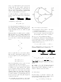
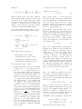
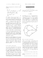
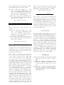
PATH ANALYSIS FOR PROCESS
TROUBLESHOOTING
Biao Huang ∗,1 Nina Thornhill ∗∗ Sirish Shah ∗
Dave Shook ∗∗∗
∗
Dept. of Chemical and Materials Engg., University of Alberta,
Edmonton, AB, Canada, T6G 2G6
∗∗
Department of Electronic and Electrical Engg., University of
College London, London, U.K. WC1E 7JE
∗∗∗
Matrikon Inc., Edmonton, AB, Canada, T5J 3N4
Abstract: In this paper, a model-free data-driven approach to process troubleshooting
is proposed. The method is simple and can handle both univariate and multivariate
processes. The only information needed for such an analysis is the data. The objective
is to identify possible source of variability/oscillation from all interacting variables.
To achieve this objective, a model-free method known as path analysis is used. In this
paper, we will summarize the theory and algorithms developed for such an analysis.
An industrial case study is presented to demonstrate the feasibility of the proposed
method.
Keywords: Process monitoring, troubleshooting, data mining, path analysis
1. INTRODUCTION
If a control loop has no potential to improve
performance by tuning the controller, then one
obvious choice is to trace the source of the upset
and reduce the disturbances/oscillations in the
source. One therefore has to search for, among
many loops which interact with the loop of concern, the source of the disturbances/oscillations.
This can be a forbidding task for a large scale
process without an appropriate analysis tool. The
method of path analysis was developed by the
geneticist to explain causal relations in population
genetics (Johnson and Wichern, 1982). The goal of
path analysis is to provide plausible explanations
of observed correlations by constructing models of
cause-and-effect relations variables. In this study
we will explore this method further and develop
it for process troubleshooting applications.
2. PATH DIAGRAM
2.1 What is path analysis?
The concept of path analysis is explained in this
subsection according to (Johnson and Wichern,
1
Corresponding author; [email protected]
1982). For a more comprehensive discussion on
the path analysis method, readers are referred
to (Johnson and Wichern, 1982) and references
therein.
It is well known that a significant correlation
between two variables does not imply a causal
relationship. For example, the variation in both
variables may be introduced by a third variable.
Or one of the two variables may affect the second
variable through a third variable or many other
variables.
When one variable X1 precedes another variable
X2 in time, it may be postulated that X1 causes
X2 . The relation can be represented, in the path
analysis, as X1 → X2 . Taking into account the
error ε2 , the path diagram may be presented as
X1
X2
ε2
The diagram may be written as a linear model
X 2 = β0 + β1 X 1 + 2
where X1 is considered to be a causal variable
that is not influenced by other variables. The
notion of a causal relation between X1 and X2
requires that all other possible causal factors
be ruled out. Statistically, we specify that X1
and ε2 be uncorrelated, where ε2 represents the
collective effect of all unmeasured variables that
could conceivably influence X1 and X2 .
To offset the influence of variable units, the regression equation is written in the standardized
form as
X2 − µ2
σ11 X1 − µ1
σεε ε2
= β1
( √
)+
√
√
σ22
σ22
σ11
σ22 σεε
or written in a compact form:
Z2 = p21 Z1 + p2ε ε
Note that all variables including the error ε2 now
have the same variance of 1 and mean of 0. The
error ε also has a coefficient. The parameters, p,
in the standardized model, are defined as path
coefficients.
Mathematically, it is equally logical to postulate
that X2 causes X1 or to postulate a third model
that includes a common factor. In the latter case
the correlation between X1 and X2 is spurious and
not a cause-effect correlation. The path diagram
is now
ε2
F3
ε1
Fig. 1. An example of path analysis
(2) A straight arrow is also drawn to each output
variable from its residual.
(3) A curved, double-headed arrow is drawn between each pair of input (exogenous) variables thought to have nonzero correlation.
The above procedure is illustrated in Fig. 1.
To calculate the coefficients for the path diagram,
we use standardized variable, i.e. all variables have
mean 0 and variance 1. If a regression model of
original variables is given by
X2
X1
where we again allow for errors in the relationship. In terms of standardized variables, the linear model implied by the path diagram above
becomes
Y = β0 + β1 X 1 + β2 X 2 + · · · + β r X r + ε
Then a (multivariate) regression model of the
normalized variables can be constructed as
√
√
σ11 X1 − µ1
σ22 X2 − µ2
Y − µY
= β1 √
( √
) + β2 √
( √
)+
√
σY Y
σY Y
σ11
σY Y
σ22
√
√
σrr Xr − µr
σεε
ε
( √
)+ √
(√
)
· · · + βr √
σY Y
σrr
σY Y
σεε
or
Ys = pY 1 Z1 + pY 2 Z2 + · · · + pY r Zr + pY ε εs (1)
Z1 = p13 F3 + p1ε1 ε1
Z2 = p23 F3 + p1ε2 ε2
where the standardized errors ε1 and ε2 are uncorrelated with each other and with F3 .
A distinction is made between variables that are
not influenced by other variables in the system
(exogenous/input variables) and those variables
that are affected by others (endogenous/output
variables). With each of the latter output variables is associated a residual. Certain conventions
govern the drawing of a path diagram. Directed
arrows represent a path. The path diagram is
constructed as follows.
(1) A straight arrow is drawn to each output
(endogenous) variable from each of its source.
√
√
The coefficients, pY k = βk σkk / σY Y and pY ε =
√
√
σεε / σY Y are the path coefficients or the direct
effects.
An example of the path diagram is shown in
Fig. 1, where pY 1 , pY 2 , pY 3 , pY ε are the path coefficients (direct effect coefficients); ρij is the correlation coefficient between Xi and Xj .
2.2 Path analysis
It is interesting to see that the correlation coefficient between Y and Xi can be constructed from
the path diagram. This is shown below.
ρY Xi = Corr(Y, Xi ) = Cov(Ys , Zi )
2.3 Asymptotic property of path analysis
Using (1),
r
r
Cov(Ys , Zi ) = Cov(
pY j Zj , Zi ) =
pY i ρij
j=1
j=1
Consider a model given by
y = aT X 1 + e
(2)
which is weighted sum of the path coefficients.
This correlation may be interpreted as the total
effects from Xi to Y through all possible paths,
and therefore this total effect is nothing but the
correlation coefficient between Xi and Y . The
difference between the direct effect and correlation
coefficient is evident through this analysis.
where y is the variable of concern (output variable), X1 is an input variable that directly affects
y, and e is a disturbance variable that is independent of X1 . The problem of interest is to isolate
the source variables X1 from a group of input
(plausible source) variables. That is, to isolate X1
from a set of input variables, X.
Another interesting fact is the variance decomposition. Note that the following equation exists:
Among this set of input variables, some are also
affected by the same source X1 and therefore a
strong correlation apparently exists between these
variables and y as well; the remaining variables are
irrelevant to y. Accordingly we partition X into
X1 , X2 and X3 . X2 is the set of input variables
that are directly affected by X1 and described by
the following model
r
pY i Zi + pY ε ε)
1 = V ar(Ys ) = V ar(
i=1
=
=
r r
i=1 k=1
r
p2Y i
i=1
pY i ρik pY k + p2Y ε
+2
r
r−1
pY i ρik pY k + p2Y ε
i=1 k=i+1
= vd + vi + vu
This equation may be interpreted as
(Total variance of the output)
= (Contribution from direct effects)
+(Contribution from indirect effects)
+(Contribution from unknown source)
Two useful indices can be defined:
• Completeness index of the selected variables
is defined as γc = vd + vi which is bounded
from 0 to 1. γc = 0 indicates that the selected input (independent/exogenous) variables have no effect at all on the output (dependent/endogenous) variables, while γc = 1
indicates that the selected input variables
are complete and explain all variability in
the output variables. γc = 0.5 indicates that
50% variance of the output variables can
be explained by the selected input variables.
Therefore, γc ≈ 0.5 or γc < 0.5 is a typical indication that additional input variables may
need to be selected for a meaningful analysis.
• Significance index of the direct effect is de|vi |
. γd = 1 indicates that
fined as γd = 1 − |v
d|
all effects are from the direct path, the input
variables are mutually independent and the
source of variability can be identified easily.
Therefore, γd < 0.5 is typical indication that
the source of the variability may not be isolated even though the selected input variables are sufficient to explain the variability
in the output.
X2 = F X1 + ε
(3)
where F is a coefficient matrix of an appropriate
dimension and ε with Cov(ε) = 0 is a disturbance
variable vector. The posed condition Cov(ε) = 0
ensures X2 not to include any variable that is
exactly the same as one of the variables in X1
or a linear combination of X1 . Physically, this
tells us that we should not include any two or
more input variables, which are exactly the same
or have exact linear relationship, into the input
variables. Numerically, this condition will avoid
the collinearity problem in regression analysis. X3
is a set of input variables that do not affect y and
may be represented by the following model
X3 = v
(4)
where v is a disturbance variable vector and is
independent of both X1 and X2 . In addition, e, ε
and v are mutually independent. Now suppose we
build a model of y by including all possible input
variables as the input:
yˆ = l1T X1 + l2T X2 + l3T X3
(5)
where l1 , l2 and l3 are model coefficients of appropriate dimension. All variables, y, X1 , X2 and
X3 have been normalized, namely EX1 X1T = I,
EX2 X2T = I, EX3 X3T = I. Using model (5), one
would like to know if the estimated model can
converge to the true model (2) in the limit.
Substituting eqns (3) and (4) into eqn.(5) yields
yˆ = l1T X1 + l2T (F X1 + ε) + l3T X3
= (l1T + l2T F )X1 + l2T ε + l3T X3
Subtracting eqn.(2) by eqn.(6) yields
(6)
y − yˆ = (a − l1 − F T l2 )T X1 − l2T ε − l3T X3 + e
Table 1. Correlation coefficients
(7)
Taking mean square value on both sides of eqn.(7)
results in
E(y − yˆ)2
(8)
= (a − l1 − F T l2 )T E[X1 X1T ](a − l1 − F T l2 )
+l3T E[X3 X3T ]l3 + l2T EεεT l2 + EeeT
x1
x2
x3
y
x1
1
0.76
0.91
0.94
x2
x3
y
1
0.72
0.77
1
0.83
1
that it is the real source of the variation in y. The
two indices can be calculated as
= (a − l1 − F T l2 )T (a − l1 − F T l2 )
γc = 0.89
+l3T l3 + l2T EεεT l2 + Ee2
γd = 0.90
≥ Ee2
(9)
The equality is achieved if and only if l1 = a,
l2 = 0 and l3 = 0. The minimum of E(y − yˆ)2 is
achieved in the limit by least squares. Therefore,
the least squares estimation can asymptotically
converge to the true model (2) even though a
number of redundant/irrelevant variables have
been included in the model. The implication of
this result is that if X1 is the source of the
variability in y among all selected input variables,
then this source can be correctly identified by
checking the estimated coefficients of all input
variables. The one which is statistically nonzero is
likely to be the sources of variability. Other input
variables (with zero coefficients), although they
are also correlated with y, are in fact the response
to X1 but not the source of y, and can therefore
be ruled out through this analysis. One potential
problem in the calculation is the collinearity of the
input variables. If two or more of input variables
are highly correlated, then the regression analysis
may fail. In this case, PCA/PLS based regression
analysis may be applied.
Obviously, the path analysis proposed so far is
limited to steady state analysis. Process dynamics
such as time delay may affect the result if the disturbances are relatively fast. Thus, the algorithm
discussed so far can only be applied to trace slow
disturbances. Extension to dynamic application
such as for oscillation detection will be discussed
in the next section.
2.4 An example on path analysis
The following example illustrates the path analysis method. Four variables, x1 , x2 , x3 and y are
used for analysis where y is the quality variable of
the concern (output variable). All four variables
are highly correlated with the correlation coefficients shown in Table 1 (the last row of the table).
According to this simple correlation analysis all
input variables seem to have a strong correlation
with y (with the minimum correlation coefficient
0.77). However, the path analysis shown in Fig.2
clearly distinguishes x1 from others and indicates
Both numbers are close to 1, indicating that the
selected variables are able to explain most of the
variability in y and the source of the variability
can be easily identified. γc = 0.89 also indicates
that 89% variability in y can be explained by the
selected variables and γd = 0.90 indicates that
the direct effect dominates the indirect effect and
therefore it is fairly easy to isolate the source of
the variability.
Fig. 2. An example of path analysis
If there are a large number of variables involved in
the analysis, the graphic representation may not
be efficient. The direct effect table can be constructed which lists the direct effect coefficients.
For example, the direct effect of the path analysis
figure shown in Fig.2 can be equally represented
by Table 2. Another table is known as total effect
table which shows the total effect from a input
variable to the output variable by combining direct effect and indirect effect. For example, the
total effect from x1 to y, according to Fig.2, can
be calculated as
0.97 + 0.76 × 0.15 + 0.91 × (−0.16) = 0.94
while the total effect from x2 to y can be calculated as
0.15 + 0.76 × 0.97 + 0.73 × (−0.16) = 0.77
The total effect from this analysis is given in Table 3, which is exactly the same as the correlation
coefficients between the input variables and the
output variable y as has been discussed above.
Table 2. Direct effect table
y
x1
0.97
x2
0.15
x3
-0.16
ε
0.33
Table 3. Total effect table
y
x1
0.94
x2
0.77
x3
0.83
ε
0.33
3. APPLICATION OF PATH ANALYSIS FOR
OSCILLATION DETECTION
One of the most important applications of the
path analysis is for oscillation detection and tracing the source of the oscillation. Oscillation is a
dynamic behavior of the process and is determined
by its amplitude, frequency and phase. While the
amplitude and frequency can be captured by the
static path analysis, the phase lag or time delay
clearly nullifies the static approach.
For oscillation detection or tracing the oscillation,
one is not interested in finding the phase information of the oscillation as long as the frequency
of the oscillation is captured. Autocovariance or
spectrum of a time series captures the oscillation
characteristics including amplitude and frequency
but is independent of the phase. Therefore, applying the path analysis to the autocovariance of
data will circumvent the problem of phase lag or
time delay.
Thornhill et al. (2001)(Thornhill et al., 2001a)
have presented a MATLAB function to calculate
filtered autocovariance and spectrum of time series. The same algorithm is used here for dynamic path analysis. A set of data (courtesy of
a SE Asian refinery) has been used for oscillation
detection in Thornhill et al. (2001)(Thornhill et
al., 2001b). The same set of data is revisited by
applying the path analysis to the autocovariance
of the data. The process diagram is shown in
Fig.3.
Fig. 3. Schematic of process and control volumes
Table 4. Summary of indices
Tag 11
Tag 34
γc
0.98
0.85
γd
0.94
0.36
have an identical shape as Tag 20. Path analysis
yields the following results:
(1) The completeness index and significance index are calculated and shown in Tab4: The
first column of the table shows that Tag 19
and 20 can explain most variability of Tag 11
and 34. The second column shows that the
source of Tag 11’s variability can be easily
identified while the source of Tag 34 variability may not be isolated easily.
(2) The direct effect table is shown in Tab.5. The
Table 5. Direct effect table
Tag 11
Tag 34
Tag 19
0.92
0.26
Tag 20
0.07
0.71
ε
0.14
0.25
The question is to trace the source of the oscillations. The path analysis is applied to the autocovariance of the data to search for the source,
which constitutes the following five steps:
first column clearly indicates that Tag 19 is
the source of Tag 11. The second column
shows that Tag 20 is possibly the main contributor to Tag 34 but Tag 19 also has a considerable contribution. Therefore, a unique
source of Tag 34 can not be identified.
Step 1: Draw a control volume around PSA unit
(see Fig.3 for control volume 1). Tag 11 and 34 as
output variables; Tag 19 and 20 as input variables.
Tag 3 is not an independent input as it is found to
Step 2: Draw a control volume around Reformer
(see Fig.3 for control volume 2). Tag 19 and 20 as
output; Tag 29, 30, 31, 34 as inputs. In this step,
we will analyze Tag 19 only. The analysis with Tag
20 as output will be performed in the next step.
Path analysis yields the following results:
(1) The two indices are calculated as γc = 0.93
and γd = 0.92. These results indicate that
most of the variability in Tag 19 can be explained by the selected inputs and in addition
the source can be easily identified.
(2) The direct effect table is summarized in
Tab.6. This result clearly indicates that Tag
34 is the source of Tag 19.
Table 6. Direct effect table
Tag 19
Tag 29
0.04
Tag 30
0.06
Tag 31
0.03
Tag 34
0.93
ε
0.26
Step 3: Continuation of Step 2 with Tag 20 as
output.
(1) The two indices are calculated as γc = 0.94
and γd = 0.97. These results indicate that
most of the variability in Tag 20 can be
explained by the selected inputs and the
source can be easily identified.
(2) The direct effect table is summarized in
Tab.7. This result clearly shows that Tag 34
is the source of Tag 20.
Table 7. Direct effect table
Tag 20
Tag 29
-0.02
Tag 30
0.03
Tag 31
0.01
Tag 34
0.95
ε
0.25
Comments: Step 2 and 3 indicate that Tag 34 is
actually the source of both Tag 19 and 20. This
result explains why Tag 34 can not find its source
from Tag 19 or 20 in Step 1.
Step 4: Draw a control volume around the whole
process as shown in the flowchart (see Fig.3 for
control volume 3). Tag 11 is the output (Tag
34 is a recycle stream and not an output); Tag
23, 25, 26, 27, 35, 36, 37, 30, 31 are the inputs.
Some inputs such as light naphtha flow rate is
not available and has not been included in the
analysis. Path analysis yields the following result
shown in Table 8. Due to the space limit, direct
path coefficients with small values are omitted
from the table. The two indices γc = 0.96 and
γd = 0.90 indicate that the selected inputs are
sufficient to explain the output variability and the
source of the variability can be easily identified.
The direct path coefficient from Tag 25 to Tag
11 clearly shows that Tag 25 is the source of the
oscillation in Tag 11. Combining with the results
obtained in previous steps, now the question is
which one of Tag 25 and Tag 34 is the source of
the oscillation. If there is no recycle from Tag 34
to Tag 25, then the result obtained in this step
clearly shows that Tag 25 is the real source and
Tag 34 is actually a response to Tag 25. However,
if there is a recycle from Tag 34 to Tag 25, then
Tag 34 could be the source, a result obtained in
Thornhill et al.(2001)(Thornhill et al., 2001b).
Table 8. Direct effect table
Tag 11
γc
0.96
γd
0.90
Tag 25
1.0
ε
0.20
Step 5: Draw a control volume around Feed unit,
Feed vaporizer/superheater unit and Reformer
feed pre-heat unit (see Fig.3 for control volume 4).
Tag 29 is taken as output; Tag 23, 25, 26, 35, 36,
37, 27 as inputs. Path analysis yields γc = 0.37,
the selected input variables are not sufficient to
explain the variability in Tag 29. Therefore, the
source of the Tag 29 oscillation can not be identified from the given tags.
4. CONCLUSIONS
In this paper the path analysis is proposed for
process troubleshooting by tracing the source of
variability/oscillation. Path analysis is similar to
correlation analysis in terms of its simplicity but
it provides a directional correlation information.
That is, a correlation analysis reveals all possible correlation between two variables, direct and
indirect, while path analysis reports the direct
relation of two variables. It is shown in this paper
that path analysis can be used to trace the source
of process variability. The result has also been
extended to tracing the oscillation by applying
the path analysis to autocovariance data. An industrial case study is presented to illustrate the
effectiveness of the proposed algorithms.
5. REFERENCES
Johnson, R.A. and D.W. Wichern (1982). Applied
Multivariate Statistical Analysis. PrenticeHall.
Thornhill, N., B. Huang and H. Zhang (2001a).
Detection of multiple oscillations in control
loops. To appear in Journal of Process Control.
Thornhill, N.F., S.L. Shah and B. Huang (2001b).
Detection of distributed oscillations and rootcause diagnosis. In: Proceedings of CHEMAS.
Cheju Island, Korea.