Download dev PDF - Read the Docs

Jumos
Main Documentation
Release 0.1
Guillaume Fraux
May 27, 2015
Contents
1
Installation
2
User manual
2.1 Package overview . . . . . . . . . . . . . . . . . . . . .
Simulation flow . . . . . . . . . . . . . . . . . . . . . .
Simulation example . . . . . . . . . . . . . . . . . . . .
Main types . . . . . . . . . . . . . . . . . . . . . . . .
2.2 Universes . . . . . . . . . . . . . . . . . . . . . . . . .
UnitCell . . . . . . . . . . . . . . . . . . . . . . . . . .
Topology . . . . . . . . . . . . . . . . . . . . . . . . .
Frame . . . . . . . . . . . . . . . . . . . . . . . . . . .
Interactions . . . . . . . . . . . . . . . . . . . . . . . .
Potentials . . . . . . . . . . . . . . . . . . . . . . . . .
Universe type . . . . . . . . . . . . . . . . . . . . .
Loading initial configurations from files . . . . . . . . .
2.3 Simulations . . . . . . . . . . . . . . . . . . . . . . . .
Propagator . . . . . . . . . . . . . . . . . . . . . . . . .
Molecular Dynamics . . . . . . . . . . . . . . . . . . .
Computing values of interest . . . . . . . . . . . . . . .
Exporting values of interest . . . . . . . . . . . . . . . .
Simulation type . . . . . . . . . . . . . . . . . . . .
2.4 Utilities . . . . . . . . . . . . . . . . . . . . . . . . . .
Internal units . . . . . . . . . . . . . . . . . . . . . . .
Interaction with others units systems . . . . . . . . . . .
Periodic boundary conditions and distances computations
Trajectories . . . . . . . . . . . . . . . . . . . . . . . .
Array3D . . . . . . . . . . . . . . . . . . . . . . . . . .
3
2
.
.
.
.
.
.
.
.
.
.
.
.
.
.
.
.
.
.
.
.
.
.
.
.
2
2
2
4
5
5
5
7
8
9
9
11
12
12
12
12
15
17
18
18
18
19
19
20
22
Extending Jumos
3.1 Extending Jumos . . . . . . . . . . . . . . . . . . . . . . . . . . . . . . . . . . . . . . . . . . .
22
22
.
.
.
.
.
.
.
.
.
.
.
.
.
.
.
.
.
.
.
.
.
.
.
.
.
.
.
.
.
.
.
.
.
.
.
.
.
.
.
.
.
.
.
.
.
.
.
.
.
.
.
.
.
.
.
.
.
.
.
.
.
.
.
.
.
.
.
.
.
.
.
.
.
.
.
.
.
.
.
.
.
.
.
.
.
.
.
.
.
.
.
.
.
.
.
.
.
.
.
.
.
.
.
.
.
.
.
.
.
.
.
.
.
.
.
.
.
.
.
.
.
.
.
.
.
.
.
.
.
.
.
.
.
.
.
.
.
.
.
.
.
.
.
.
.
.
.
.
.
.
.
.
.
.
.
.
.
.
.
.
.
.
.
.
.
.
.
.
.
.
.
.
.
.
.
.
.
.
.
.
.
.
.
.
.
.
.
.
.
.
.
.
.
.
.
.
.
.
.
.
.
.
.
.
.
.
.
.
.
.
.
.
.
.
.
.
.
.
.
.
.
.
.
.
.
.
.
.
.
.
.
.
.
.
.
.
.
.
.
.
.
.
.
.
.
.
.
.
.
.
.
.
.
.
.
.
.
.
.
.
.
.
.
.
.
.
.
.
.
.
.
.
.
.
.
.
.
.
.
.
.
.
.
.
.
.
.
.
.
.
.
.
.
.
.
.
.
.
.
.
.
.
.
.
.
.
.
.
.
.
.
.
.
.
.
.
.
.
.
.
.
.
.
.
.
.
.
.
.
.
.
.
.
.
.
.
.
.
.
.
.
.
.
.
.
.
.
.
.
.
.
.
.
.
.
.
.
.
.
.
.
.
.
.
.
.
.
.
.
.
.
.
.
.
.
.
.
.
.
.
.
.
.
.
.
.
.
.
.
.
.
.
.
.
.
.
.
.
.
.
.
.
.
.
.
.
.
.
.
.
.
.
.
.
.
.
.
.
.
.
.
.
.
.
.
.
.
.
.
.
.
.
.
.
.
.
.
.
.
.
.
.
.
.
.
.
.
.
.
.
.
.
.
.
.
.
.
.
.
.
.
.
.
.
.
.
.
.
.
.
.
.
.
.
.
.
.
.
.
.
.
.
.
.
.
.
.
.
.
.
.
.
.
.
.
.
.
.
.
.
.
.
.
.
Defining a new potential . . . . . . . . . . . . . . . . . . . . . . . . . . . . . . . . . . . . . . .
Algorithms for all simulations . . . . . . . . . . . . . . . . . . . . . . . . . . . . . . . . . . . .
Algorithms for molecular dynamics . . . . . . . . . . . . . . . . . . . . . . . . . . . . . . . . .
25paragraph*.147
25paragraph*.153
26paragraph*.155
22
24
25
Jumos is a package for molecular simulations written using the Julia language. It provides a set of customisable
blocks for running molecular simulations, and developing novel algorithm for each part of a simulation. Every algorithm (potential computation, long range interactions, pair lists computing, outputs, etc.) can easily be
customised.
Note: This package is in a very alpha stage, and still in heavy developement. Breaking changes can occurs in the
API without any notice at any time.
This documentation is divided in two parts: first come the user manual, starting by some explanation about usal
algorithms in simulations (page 2) and an example (page 4) of how we can use Jumos to run a molecular dynamic
simulation. The second part is the developer documentation, exposing the internal of Jumos, and how we can use
them to programm new algorithms.
1 Installation
Jumos uses the 0.4 prerelease version of Julia, and can be installed at julia prompt with the Pkg.add("Jumos")
command. You also can run the unit tests with the Pkg.test("Jumos") command.
2 User manual
2.1 Package overview
This section is a guide to get started with molecular simulations in Jumos. It contains explanations about the how
to define and run a basic simulation.
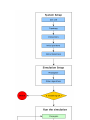
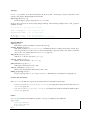
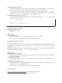
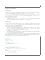
Simulation flow
In every molecular simulation, the main steps are roughly the same. We start by setting the simulated system:
positions of the particles, maybe velocities, atomic types, potential to use between the atoms, etc. Secondly, we
have to choose the simulation type and setup the propagator and the analysis algorithms.
Then we can run the simulation for a given number of steps nsteps. During the run, the propagator can be
a Newton integrator for Molecular Dynamics, a MonteCarlo propagator for MonteCarlo simulation, a Gradient
descent for energy minimization, etc. Other algorithms can be added to the simulation, in order to perform live
analysis of the simulation or to output data.
All this is summarised in the figure Simulation flow in Jumos (page 3).
All the steps in the process of running a simulation are described below.
System setup
The system will contain all the physical informations about what we are simulating. In Jumos, a system is represented by the Universe (page 11) type. It should at least contain data about the simulation cell (page 5), the system
topology (page 8), the initial particles coordinates and the interactions (page 9) between the particles.
Simulation setup
During the simulation, the system will be propagated by a propagator (page 12): MolecularDynamics,
MonteCarlo, Minimization are examples of propagators. Other algorithms can take place here, either
algorithms to compute thermodynamic properties or algorithms to modify the behaviour of the simulation.
Running the simulation
The simulation run is the main part of the simulation, and consist in three main steps:
• Use the propagator to genrerate an update in the particles positions;
• Compute thermodynamical properties of the system;
• Output data to file for later analysis.
Simulation example
In Jumos, one run simulations by writting specials Julia scripts. A primer intoduction to the Julia language can be
found here, if needed.
Lennard-Jones fluid
Here is a simple simulation script for running a simulation of a Lennard-Jones fluid at 300𝐾.
1
#!/usr/bin/env julia
2
3
4
# Loading the Jumos module before anything else
using Jumos
5
6
7
# Molecular Dynamics with 1.0fs timestep
sim = Simulation(:MD, 1.0)
8
9
10
11
12
13
# Create a cubic cell with a width of 10A
cell = UnitCell(10.0)
# Read a topology from a file
topology = Topology("lennard-jones.xyz")
# Create an universe from the cell and the topology
14
15
16
17
18
universe = Universe(cell, topology)
positions_from_file!(universe, "lennard-jones.xyz")
# Initialize random velocities at 300K
create_velocities!(universe, 300)
19
20
21
# Add Lennard-Jones interactions between He atoms
add_interaction!(universe, LennardJones(0.8, 2.0), "He", "He")
22
23
24
25
26
27
# You can either bind algorithms to variables ...
out_trajectory = TrajectoryOutput("LJ-trajectory.xyz", 1)
push!(sim, out_trajectory)
# ... or create them directly in function call
push!(sim, EnergyOutput("LJ-energy.dat", 10))
28
29
propagate!(sim, universe, 5000)
30
31
32
# Simulation scripts are normal Julia scripts !
println("All done")
Each simulation script should start by the using Jumos directive. This imports the module and the exported
names in the current scope.
Then, in this script, we create two main objects: a simulation (page 18), and an universe (page 11). The topology
and the original positions for the universe are read from the same file, as an .xyz file contains topological
information (mainly the atomics names) and coordinates. The velocities are then initialized from a Boltzmann
distribution at 300K.
The only interaction — a Lennard-Jones (page 10) interaction — is also added to the universe before the run. The
next lines add some outputs to the simulation, namely a trajectory and an energy output. Finally, the simulation
runs for 5000 steps.
Other example
Some other examples scripts can be found in the example folder in Jumos’ source tree. To go there, use the julia
prompt:
julia> Pkg.dir("Jumos")
"~/.julia/v0.4/Jumos"
julia>; cd $ans/examples
~/.julia/v0.4/Jumos/examples
Main types
Jumos is organised around two main types: the Universe hold data about the system we are simulating; and the
Simulation type hold data about the algorithms we should use for the simulation.
Universe
The Universe type contains data. It is built around four other basic types:
• The Topology (page 8) contains data about the atomic organisation, i.e. the particles, bonds, angles and
dihedral angles in the system;
• The UnitCell (page 5) contains data about the bounding box of the simulation;
• The Interactions (page 9) type contains data about the potentials (page 9) to use for the atoms in the system;
• The Frame (page 8) type contains raw data about the positions and maybe velocities of the particles in the
system;
Simulation
The Simulation type contains algorithms. The progagator (page 12) algorithm is the one responsible for
propagating the Universe along the simulation. It also contains some analysis algorithms (called compute
(page 15) in Jumos); and some output (page 17) algorithms, to save data during the simulation run.
2.2 Universes
UnitCell
A simulation cell (UnitCell type) is the virtual container in which all the particles of a simulation move. The
UnitCell type is parametrized by the celltype. There are three different types of simulation cells:
• Infinite cells (InfiniteCell) do not have any boundaries. Any move is allowed inside these cells;
• Orthorombic cells (OrthorombicCell) have up to three independent lenghts; all the angles of the cell
are set to 90° (𝜋/2 radians)
• Triclinic cells (TriclinicCell) have 6 independent parameters: 3 lenghts and 3 angles.
Creating simulation cell
UnitCell(A[, B, C, alpha, beta, gamma, celltype ])
Creates an unit cell. If no celltype parameter is given, this function tries to guess the cell type using the
following behavior: if all the angles are equals to 𝜋/2, then the cell is an OrthorombicCell; else, it is a
TriclinicCell.
If no value is given for alpha, beta, gamma, they are set to 𝜋/2. If no value is given for B, C, they
are set to be equal to A. This creates a cubic cell. If no value is given for A, a cell with lenghts of 0 Angström
and 𝜋/2 angles is constructed.
julia> UnitCell() # Without parameters
OrthorombicCell
Lenghts: 0.0, 0.0, 0.0
julia> UnitCell(10.) # With one lenght
OrthorombicCell
Lenghts: 10.0, 10.0, 10.0
julia> UnitCell(10., 12, 15) # With three lenghts
OrthorombicCell
Lenghts: 10.0, 12.0, 15.0
julia> UnitCell(10, 10, 10, pi/2, pi/3, pi/5) # With lenghts and angles
TriclinicCell
Lenghts: 10.0, 10.0, 10.0
Angles: 1.5707963267948966, 1.0471975511965976, 0.6283185307179586
julia> UnitCell(InfiniteCell) # With type
InfiniteCell
julia> UnitCell(10., 12, 15, TriclinicCell) # with lenghts and type
TriclinicCell
Lenghts: 10.0, 12.0, 15.0
Angles: 1.5707963267948966, 1.5707963267948966, 1.5707963267948966
UnitCell(u::Vector[, v::Vector, celltype ])
If the size matches, this function expands the vectors and returns the corresponding cell.
julia> u = [10, 20, 30]
3-element Array{Int64,1}:
10
20
30
julia> UnitCell(u)
OrthorombicCell
Lenghts: 10.0, 20.0, 30.0
Indexing simulation cell
You can access the cell size and angles either directly, or by integer indexing.
getindex(b::UnitCell, i::Int)
Calling b[i] will return the corresponding length or angle : for i in [1:3], you get the ith lenght, and
for i in [4:6], you get [avoid get] the angles.
In case of intense use of such indexing, direct field access should be more efficient. The internal fields of a
cell are : the three lenghts a, b, c, and the three angles alpha, beta, gamma.
Boundary conditions and cells
Only fully periodic boundary conditions are implemented for now. This means that if a particle crosses the
boundary at some step, it will be wrapped up and will appear at the opposite boundary.
Distances and cells
The distance between two particles depends on the cell type. In all cases, the minimal image convention is used:
the distance between two particles is the minimal distance between all the images of theses particles. This is
explicited in the Periodic boundary conditions and distances computations (page 19) part of this documentation.
Topology
The Topology type creates the link between human-readable and computer-readable information about the
system. Humans prefer to use string labels for molecules and atoms, whereas a computer will only uses integers.
Atom type
An Atom instance is a representation of a type of particle in the system. It is paramerized by an AtomType,
which can be one of:
• Element : an element in the perdiodic classification;
• DummyAtom : a dummy atom, for particles without interactions;
• CorseGrain : corse-grain particle, for corse-grain simulations;
• UnknownAtom : All the other kind of particles.
You can access the following fields for all atoms:
• label::Symbol : the atom name;
• mass : the atom mass;
• charge : the atom charge;
• properties::Dict{String, Any} : any other property: dipolar moment, etc.;
Atom([label, type ])
Creates an atom with the label label. If type is provided, it is used as the Atom type. Else, a type is
guessed according to the following procedure: if the label is in the periodic classification, the the atom is
an Element. Else, it is a CorseGrain atom.
julia> Atom()
"Atom{UnknownAtom}"
julia> Atom("He")
"Atom{Element} He"
julia> Atom("CH4")
"Atom{CorseGrain} CH4"
julia> Atom("Zn", DummyAtom)
"Atom{DummyAtom} Zn"
mass(label::Symbol)
Try to guess the mass associated with an element, from the periodic table data. If no value could be found,
the 0.0 value is returned.
mass(atom::Atom)
Return the atomic mass if it was set, or call the function mass(atom.label).
Topology
A Topology instance stores all the information about the system : atomic types, atomic composition of the
system, bonds, angles, dihedral agnles and molecules.
Topology([natoms = 0 ])
Create an empty topology with space for natoms atoms.
Atoms in the system can be accesed using integer indexing. The following example shows a few operations
available on atoms:
# topology is a Topology with 10 atoms
atom = topology[3] # Get a specific atom
println(atom.label) # Get the atom label
atom.mass = 42.9
topology[5] = atom
# Set the atom mass
# Set the 5th atom of the topology
Topology functions
size(topology)
This function returns the number of atoms in the topology.
atomic_masses(topology)
This function returns a Vector{Float64} containing the masses of all the atoms in the system. If no
mass was provided, it uses the ATOMIC_MASSES dictionnary to guess the values. If no value is found, the
mass is set to 0.0. All the values are in internal units (page 18).
add_atom!(topology, atom)
Add the atom Atom to the end of topology.
remove_atom!(topology, i)
Remove the atom at index i in topology.
add_liaison!(topology, i, j)
Add a liaison between the atoms i and j.
remove_liaison!(topology, i, j)
Remove any existing liaison between the atoms i and j.
dummy_topology(natoms)
Create a topology with natoms of type DummyAtom. This function exist mainly for testing purposes.
Periodic table information
The Universes module also exports two dictonaries that store information about atoms:
• ATOMIC_MASSES is a Dict{String, Float64} associating atoms symbols and atomic masses, in
internal units (page 18) ;
• VDW_RADIUS is a Dict{String, Integer} associating atoms symbols and Van der Waals radii, in
internal units (page 18).
Frame
A Frame object holds the data which is specific to one step of a simulation. It is defined as:
type Frame
positions::Array3D
velocities::Array3D
step::Integer
end
i.e. it contains information about the current step, the current positions, and possibly the current velocities. If there
is no velocity information, the velocities Array3D (page 22) is a 0-sized array.
The Frame type have the following constructor:
Frame([natom=0 ])
Creates a frame with space for natoms particles.
Interactions
The interaction type contains informations about which potentials (page 9) the simulation should use for
the atoms in the system. This type is not intended to be manupulated directly, but rather through the
add_interaction!() (page 9) function.
add_interaction!(universe, potential, atoms...[; computation=:auto; kwargs...])
Add an interaction between the atoms atomic types, using the potential potential function (page 10)
in the universe.
This function accept many keywords arguments to tweak the potential computation methode (page 11) used
to effectively compute the potential. The main keyword is computation which default to :auto. It can
be set to other values to choose another computation method than the default one.
julia> # Setup an universe with four atoms: two He and one Ar
julia> top = Topology();
julia> add_atom!(top, Atom("He")); add_atom!(top, Atom("He"));
julia> add_atom!(top, Atom("Ar")); add_atom!(top, Atom("Ar"));
julia> universe = Universe(UnitCell(), top);
# Use default values for everything
julia> add_interaction!(universe, LennardJones(0.23, 2.2), "He", "He")
# Set the cutoff to 7.5 A
julia> add_interaction!(universe, LennardJones(0.3, 2.5), "He", "Ar", cutoff=7.5)
# Use table computation with 3000 points, and a maximum distance of 5A
julia> add_interaction!(universe, Harmonic(40, 3.3), "Ar", "Ar", computation=:table, numpoint
Using non-default computation
By default, the computation algorithm is automatically determined by the potential function type.
ShortRangePotential are computed with CutoffComputation, and all other potentials are computed
by DirectComputation. If we want to use another computation algorithm, this can be done by providing a
computation keyword to the add_interaction! function. The following values are allowed:
• :direct to use a DirectComputation;
• :cutoff to use a CutoffComputation. The cutoff can be specified with the cutoff keyword argument;
• :table‘ to use a TableComputation. The table size can be specified with the numpoints keyword
argument, and the maximum distance with the rmax keyword argument.
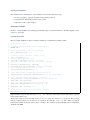
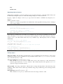
Potentials
In order to compute the energy or the forces acting on a particle, two informations are needed : a potential energy
function, and a computation algorithm. The potential function is a description of the variations of the potential
with the particles positions, and a potential computation is a way to compute the values of this potential function.
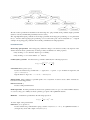
The following image shows the all the potentials functions types currently available in Jumos.
We can see these potentials are classified as four main categories: pair potentials, bond potentials, angles potentials
(between 3 atoms) and dihedral potentials (between 4 atoms).
The only implemented pair potentials are short-range potentials. Short-range pair potentials go to zero faster than
the 1/𝑟3 function, and long-range pair potentials go to zero at the same speed or more slowly than 1/𝑟3 . A typical
example of long-range pair potential is the Coulomb potential between charged particles.
Potential functions
Short-range pair potential Short-range pair potential are subtypes of PairPotential. They only depends on the
distance between the two particles they are acting on. They should have two main properties:
• They should go to zero when the distance goes to infinity;
• They should go to zero faster than the 1/𝑟3 function.
Lennard-Jones potential A Lennard-Jones potential is defined by the following expression:
(︂(︁ )︁
)︂
𝜎 12 (︁ 𝜎 )︁6
−
𝑉 (𝑟) = 4𝜖
𝑟
𝑟
LennardJones(epsilon, sigma)
Creates a Lennard-Jones potential with 𝜎 = sigma, and 𝜖 = epsilon. sigma should be in angstroms, and
epsilon in 𝑘𝐽/𝑚𝑜𝑙.
Typical values for Argon are: 𝜎 = 3.35 𝐴, 𝜖 = 0.96 𝑘𝐽/𝑚𝑜𝑙
Null potential This potential is a potential equal to zero everywhere. It can be used to define “interactions”
between non interacting particles.
NullPotential()
Creates a null potential instance.
Bonded potential Bonded potentials acts between two particles, but does no go to zero with an infinite distance.
A contrario, they goes to infinity as the two particles goes apart of the equilibirum distance.
Harmonic An harmonic potential have the following expression:
𝑉 (𝑟) =
1
𝑘(⃗𝑟 − ⃗𝑟0 )2 − 𝐷0
2
𝐷0 is the depth of the potential well.
Harmonic(k, r0, depth=0.0)
Creates an harmonic potential with a spring constant of k (in 𝑘𝐽.𝑚𝑜𝑙−1 .𝐴−2 ), an equilibrium distance 𝑟0
(in angstroms); and a well’s depth of 𝐷0 (in 𝑘𝐽/𝑚𝑜𝑙).
Potential computation
As stated at the begiging of this section, we need two informations to compute interactions between particles: a
potential function, and a potential computation. The potential compuatation algorithms come in four flavors:
• The DirectComputation is only a small wrapper on the top of the potential functions, and directly
calls the potential function methods for energy and force evaluations.
• The CutoffComputation is used for short range potentials. All interactions at a longer distance than
the cutoff distance are set to zero. The default cutoff is 12 𝐴, and this can be changed by passing a cutoff
keyword argument to the add_interaction function. With this computation, the energy is shifted so
that their is a continuity in the energy at the cutoff distance.
• The TableComputation use table lookup to extrapolate the potential energy and the forces at a given
point. This saves computation time at the cost of accuracy. This algorithm is parametrized by an integer, the
size of the undelying array. Increases in this size will result in more accuracy, at the cost of more memory
usage. The default size is 2000 points — which corresponds to roughly 15kb. TableComputation has
also a maximum distance for computations, rmax. For any bigger distances, the TableComputation
will returns a null energy and null forces. So TableComputation can only be used if you are sure that
the particles will never be at a greater distance than rmax.
• The LongRangeComputation is not implemented yet.
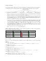
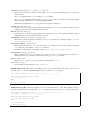
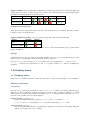
Which computation for which potential ? Not all computation algorithms are suitable for all potential functions. The usable associations are in the table below.
Function
DirectComputation
CutoffComputation
TableComputation
ShortRangePotential
BondedPotential
AnglePotential
DihedralPotential
Universe type
The Universe type contains data about a simulation. In order to build an universe, you can use the following
functions.
Universe(cell, topology)
Create a new universe with the simulation cell (page 5) cell and the Topology (page 8) topology.
setframe!(universe, frame)
Set the Frame (page 8) of universe to frame.
setcell!(universe, cell)
Set the simulation cell (page 5) of universe to cell.
setcell!(universe[, celltype ], paremeters...)
Set the simulation cell (page 5) of universe to UnitCell(parameters..., celltype).
add_atom!(u::Universe, atom::Atom)
Add the Atom (page 7) atom to the universe topology.
add_liaison!(u::Universe, atom_i::Atom, atom_j::Atom)
Add a liaison between the atoms at indexes i and j in the universe topology.
remove_atom!(u::Universe, index)
Remove the atom at index i in the universe topology.
remove_liaison!(u::Universe, atom_i::Atom, atom_j::Atom)
Remove any liaison between the atoms at indexes i and j in the universe topology.
The add_interaction!() (page 9) function is already documented in the Interactions section of this
document.
Loading initial configurations from files
It is often usefull to load initial configurations from files, instead of building it by hand. The Trajectories (page 20)
module provides functionalities for this.
2.3 Simulations
The simulation module contains types representing algorithms. The main type is the Simulation (page 18) type,
which is parametrized by a Propagator (page 12). This propagator will determine which kind of simulation we
are running: Molecular Dynamics (page 12); Monte-Carlo; energy minimization; etc.
Note: Only molecular dynamic is implemented in Jumos for now, but at least Monte-Carlo and energetic optimization should follow. If you are interested in implementing such methods, please signal yourself in the Gihtub
issues list.
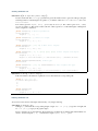
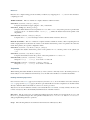
Propagator
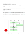
Molecular Dynamics
Fig. 2: Flow of algorithms in MolecularDynamics propagator
MolecularDynamics(timestep)
Creates an empty molecular dynamic simulation using a Velocity-Verlet integrator with the specified
timestep.
Without any thermostat (page 13) or barostat (page 14), this performs a NVE integration of the system.
MolecularDynamics(::Integrator)
Creates an empty simulation with the specified integrator (page 13).
Time integration
An integrator is an algorithm responsible for updating the positions and the velocities of the current frame (page 8)
of the simulation (page 18).
Verlet integrators Verlet integrators are based on Taylor expensions of Newton’s second law. They provide a
simple way to integrate the movement, and conserve the energy if a sufficently small timestep is used. Assuming
the absence of barostat and thermostat, they provide a NVE integration.
type Verlet
The Verlet algorithm is described here for example. The main constructor for this integrator is
Verlet(timestep), where timestep is the timestep in femtosecond.
type VelocityVerlet
The velocity-Verlet algorithm is descibed extensively in the literature, for example in this webpages. The
main constructor for this integrator is VelocityVerlet(timestep), where timestep is the integration timestep in femtosecond. This is the default integration algorithm in Jumos.
Force computation
The NaiveForceComputer algorithm computes the forces by iterating over all the pairs of atoms, and calling
the appropriate interaction potential. This algorithm is the default in Jumos.
Controlling the simulation
While running a simulation, we often want to have control over some simulation parameters: the temperature, the
pressure, . . . This is the goal of the Control algorithms.
Such algorithms are subtypes of Control, and can be added to a simulation using the add_control()
(page 15) function:
Controlling the temperature: Thermostats Various algorithms are available to control the temperature of a
simulation and perform pseudo NVT simulations. The following thermostating algorithms are currently implemented:
type VelocityRescaleThermostat
The velocity rescale algorithm controls the temperature by rescaling all the velocities when the temperature
differs exceedingly from the desired temperature.
The constructor takes two parameters: the desired temperature and a tolerance interval. If the absolute
difference between the current temperature and the desired temperature is larger than the tolerance, this
algorithm rescales the velocities.
sim = MolecularDynamic(2.0)
# This sets the temperature to 300K, with a tolerance of 50K
thermostat = VelocityRescaleThermostat(300, 50)
add_control(sim, thermostat)
type BerendsenThermostat
The berendsen thermostat sets the simulation temperature by exponentially relaxing to a desired temperature. A more complete description of this algorithm can be found in the original article 1 .
The constructor takes as parameters the desired temperature, and the coupling parameter, expressed in
simulation timestep units. A coupling parameter of 100, will give a coupling time of 150 𝑓 𝑠 if the simulation
timestep is 1.5 𝑓 𝑠, and a coupling time of 200 𝑓 𝑠 if the timestep is 2.0 𝑓 𝑠.
BerendsenThermostat(T [, coupling ])
Creates a Berendsen thermostat at the temperature T with a coupling parameter of coupling. The default
values for coupling is 100.
sim = MolecularDynamic(2.0)
# This sets the temperature to 300K
thermostat = BerendsenThermostat(300)
add_control(sim, thermostat)
Controlling the pressure: Barostats
type BerendsenBarostat
TODO
Other controls
type WrapParticles
This control wraps the positions of all the particles inside the unit cell (page 5).
This control is present by default in the molecular dynamic simulations.
Checking the simulation consistency
Molecular dynamic is usually a garbage in, garbage out set of algorithms. The numeric and physical issues are
not caught by the algorithm themselves, and the physical (and chemical) consistency of the simulation should be
checked often.
In Jumos, this is achieved by the Check algorithms, which are presented in this section. Checking algorithms can
be added to a simulation by using the add_check() (page 15) function.
Existing checks
type GlobalVelocityIsNull
This algorithm checks if the global velocity (the total moment of inertia) is null for the current simulation.
The absolute tolerance is 10−5 𝐴/𝑓 𝑠.
type TotalForceIsNull
This algorithm checks if the sum of the forces is null for the current simulation. The absolute tolerance is
10−5 𝑢𝑚𝑎 · 𝐴/𝑓 𝑠2 .
type AllPositionsAreDefined
This algorithm checks is all the positions and all the velocities are defined numbers, i.e. if all the values are
not infinity or the NaN (not a number) values.
This algorithm is used by default by all the molecular dynamic simulation.
Default algorithms
Default algorithms for molecular dynamic are presented in the following table:
1
H.J.C. Berendsen, et al. J. Chem Phys 81, 3684 (1984); doi: 10.1063/1.448118
Simulation step
Integration
Forces computation
Control
Check
Default algorithms
Velocity-Verlet (page 13)
Naive computation (page 13)
Wrap particles in the box (page 14)
All positions are defined (page 14)
Functions for algorithms selection
The six following functions are used to to select specific algorithms for the simulation. They allow to add and
change all the algorithms, even in the middle of a run.
set_integrator(sim, integrator)
Sets the simulation integrator to integrator.
Usage example:
# Creates the integrator directly in the function
set_integrator(sim, Verlet(2.5))
# Binds the integrator to a variable if you want to change a parameter
integrator = Verlet(0.5)
set_integrator(sim, integrator)
run!(sim, 300)
# Run with a 0.5 fs timestep
integrator.timestep = 1.5
run!(sim, 3000) # Run with a 1.5 fs timestep
set_forces_computation(sim, forces_computer)
Sets the simulation algorithm for forces computation to forces_computer.
add_check(sim, check)
Adds a check (page 14) to the simulation check list and issues a warning if the check is already present.
Usage example:
# Note the parentheses, needed to instanciate the new check.
add_check(sim, AllPositionsAreDefined())
add_control(sim, control)
Adds a control (page 13) algorithm to the simulation list. If the control algorithm is already present, a
warning is issued.
Usage example:
add_control(sim, RescaleVelocities(300, 100))
Computing values of interest
To compute physical values from a simulation, we can use algorithms represented by subtypes of Compute and
associate these algorithms to a simulation.
Users don’t usualy need to use these compute algorithms directly, as the output algorithms (see Exporting values
of interest (page 17)) set the needed computations by themself.
Computed values can have various usages: they may be used in outputs (page 17), or in controls (page 13).
The data is shared between algorithms using the Universe.data field. This field is a dictionnary associating
symbols and any kind of value.
This page of documentation presents the implemented computations. Each computation can be associated with a
specific simulation (page 18) using the push! function.
push!(simulation, compute)
Adds a compute (page 15) algorithm to the simulation list. If the algorithm is already present, a warning is
issued. Usage example:
sim = Simulation(:md, 1.0) # Create a simulation
# Do not forget the parentheses to instanciate the computation
push!(sim, MyCompute())
propagate!(sim, universe, 5000)
# You can access the last computed value in the sim.data dictionnary
universe.data[:my_compute]
You can also call directly any instance of MyCompute:
universe = Universe() # Create an universe
# ...
compute = MyCompute() # Instanciate the compute
value = compute(universe) # Compute the value
The following paragraphs sums up the implemented computations, giving for each algorithm the return value (for
direct calling), and the associated keys in Universe.data.
Energy related values
type TemperatureCompute
Computes the temperature of the universe.
Key: :temperature
Return value: The current frame temperature.
type EnergyCompute
Computes the potential, kinetic and total energy of the current simulation step.
Keys: :E_kinetic, :E_potential, :E_total
Return value: A tuple containing the kinetic, potential and total energy.
energy = EnergyCompute()
# unpacking the tuple
E_kinetic, E_potential, E_total = energy(universe)
# accessing the tuple values
E = energy(sim)
E_kinetic = E[1]
E_potential = E[2]
E_total = E[3]
Volume
type VolumeCompute
Computes the volume of the current unit cell (page 5).
Key: :volume
Return value: The current cell volume
Pressure
type PressureCompute
TODO
Key:
Return value:
Exporting values of interest
While running a simulation, some basic analysis can be performed and writen to a data file. Further analysis can
be differed by writing the trajectory to a file, and running existing tools on these trajectories.
In Jumos, outputs are subtypes of the Output type, and can be added to a simulation by using the push!
function.
push!(simulation, output)
Adds an output (page 17) algorithm to the simulation list. If the algorithm is already present, a warning is
issued. Usage example:
sim = Simulation(:md, 1.0)
# Direct addition
push!(sim, TrajectoryOutput("mytraj.xyz"))
# Binding the output to a variable
out = TrajectoryOutput("mytraj-2.xyz", 5)
push!(sim, out)
Each output is by default writen to the disk at every simulation step. To speed-up the simulation run and remove
useless information, a write frequency can be used as the last parameter of each output constructor. If this frequency is set to n, the values will be writen only every n simulaton steps. This frequency can also be changed
dynamically:
# Frequency is set to 1 by default
traj_out = TrajectoryOutput("mytraj.xyz")
add_output(sim, traj_out)
propagate!(sim, universe, 300) # 300 steps will be writen
# Set frequency to 50
traj_out.frequency = OutputFrequency(50)
propagate!(sim, universe, 500) # 10 steps will be writen
Existing outputs
Trajectory output The first thing one might want to save in a simulation run is the trajectory of the system.
Such trajectory can be used for visualisation, storage and further analysis. The TrajectoryOutput provide a
way to write this trajectory to a file.
TrajectoryOutput(filename[, frequency = 1 ])
This construct a TrajectoryOutput which can be used to write a trajectory to a file. The trajectory
format is guessed from the filename extension. This format must have write capacities, see the list
(page 22) of supported formats in Jumos.
Energy output The energy output write to a file the values of energy and temperature for the current step of the
simulation. Values writen are the current step, the kinetic energy, the potential energy, the total energy and the
temperature.
EnergyOutput(filename[, frequency = 1 ])
This construct a EnergyOutput which can be used to the energy evolution to a file.
Defining a new output
Adding a new output with custom values, can be done either by using a custom output or by subtyping (page 24)
the Output type to define a new output. The the former wayis to be prefered when adding a one-shot output, and
the latter when adding an output which will be re-used.
Custom output The CustomOutput type provide a way to build specific output. The data to be writen
should be computed (page 15) before the output by adding the specific algorithms to the current simulation. These
computation algorithm set a value in the MolecularDynamic.data dictionairy, which can be accessed during
the output step. See the computation algorithms (page 15) page for a list of keys.
CustomOutput(filename, values[, frequency = 1; header=”“ ])
This create a CustomOutput to be writen to the file filename. The values is a vector of symbols,
these symbols being the keys of the Universe.data dictionary. The header string will be writen on
the top of the output file, and can contains some metadata.
Usage example:
sim = Simulation(:md, 1.0)
# TemperatureCompute register a :temperature key
push!(sim, TemperatureCompute())
temperature_output = CustomOutput("Sim-Temp.dat", [:temperature], header="# step
push!(sim, temperature_output)
Simulation type
In Jumos, simulations are first-class citizen, i.e. objects bound to variables.
Simulation(propagator::Propagator)
Create a simulation with the specified propagator.
Simulation(propagator::Symbol, args...)
Create a simulation with a propagator (page 12) which type is given by the propagator symbol. The
args are passed to the propagator constructor.
If propagator takes one of the :MD, :md and :moleculardynamics values, a MolecularDynamics
(page 12) propagator is created.
2.4 Utilities
This part of the documentation give some information about basic algebrical types used in Jumos.
Internal units
Jumos uses a set of internal units, converting back and forth to these units when needed. Conversion from SI units
is always supported. Parenthesis indicate planned conversion that is not implemented yet.
T/K")
Quantity
Distances
Time
Velocities
Mass
Temperature
Energy
Force
Pressure
Charge
Internal unit
Ångtröm (𝐴)
Femptosecond (𝑓 𝑠)
Ångtröm/Femptosecond (𝐴/𝑓 𝑠)
Unified atomic mass (𝑢 or 𝐷𝑎)
Kelvin (𝐾)
Kilo-Joule/Mole (𝑘𝐽/𝑚𝑜𝑙)
Kilo-Joule/(Mole-Ångtröm) 𝑘𝐽/(𝑚𝑜𝑙𝐴)
𝑏𝑎𝑟
Multiples of 𝑒 = 1.602176487 10−19 𝐶
Supported conversions
(bohr)
𝑔/𝑚𝑜𝑙
(𝑒𝑉 ), (𝑅𝑦), (𝑘𝑐𝑎𝑙/𝑚𝑜𝑙)
(𝑎𝑡𝑚)
Interaction with others units systems
Jumos uses it’s own unit system, and do not track the units in the code. All the interaction with units is based on
the SIUnits package. We can convert from and to internal representation using the following functions :
internal(value::SIQuantity)
Converts a value with unit to its internal representation.
julia> internal(2m)
1.9999999999999996e10
# Distance
julia> internal(3kg*m/s^2)
7.17017208413002e-14
# Force
with_unit(value::Number, target_unit::SIUnit)
Converts an internal value to its value in the International System. You shall note that units are not tracked
in the code, so you can convert a position to a pressure. And all the results are returned in the main SI unit,
without considering any power-of-ten prefix.
This may leads to strange results like:
julia> with_unit(45, mJ)
188280.0 kg m²/s²
julia> with_unit(45, J)
188280.0 kg m²/s²
This behaviour will be corrected in future versions.
Periodic boundary conditions and distances computations
The PBC module offers utilities for distance computations using periodic boundary conditions.
Minimal images
These functions take a vector and wrap it inside a cell (page 5), by finding the minimal vector fitting inside the
cell.
minimal_image(vect, cell::UnitCell)
Wraps the vect vector inside the cell unit cell. vect can be a Vector (i.e. a 1D array), or a view from
an Array3D (page 22). This function returns the wrapped vector.
minimal_image!(vect, cell::UnitCell)
Wraps vect inside of cell, and stores the result in vect.
minimal_image!(A::Matrix, cell::UnitCell)
If A is a 3xN Array, wraps each one of the columns in the cell. The result is stored in A. If A is not a 3xN
array, this throws an error.
Distances
Distances are computed using periodic boundary conditions, by wrapping the ⃗𝑟𝑖 − ⃗𝑟𝑗 vector in the cell before
computing its norm.
Within one Frame This set of functions computes distances within one frame.
distance(ref::Frame, i::Integer, j::Integer)
Computes the distance between particles i and j in the frame.
distance_array(ref::Frame[, result ])
Computes all the distances between particles in frame. The result array can be passed as a pre-allocated
storage for the 𝑁 × 𝑁 distances matrix. result[i, j] will be the distance between the particle i and
the particle j.
distance3d(ref::Frame, i::Integer, j::Integer)
Computes the ⃗𝑟𝑖 − ⃗𝑟𝑗 vector and wraps it in the cell. This function returns a 3D vector.
Between two Frames This set of functions computes distances within two frames, either computing the how
much a single particle moved between two frames or the distance between the position of a particle i in a reference
frame and a particle j in a specific configuration frame.
distance(ref::Frame, conf::Frame, i::Integer, j::Integer)
Computes the distance between the position of the particle i in ref, and the position of the particle j in
conf
distance(ref::Frame, conf::Frame, i::Integer)
Computes the distance between the position of the same particle i in ref and conf.
distance3d(ref::Frame, conf::Frame, i::Integer)
Wraps the ref[i] - conf[i] vector in the ref unit cell.
distance3d(ref::Frame, conf::Frame, i::Integer, j::Integer)
Wraps the ref[i] - conf[i] vector in the ref unit cell.
Trajectories
When running molecular simulations, the trajectory of the system is commonly saved to the disk in prevision of
future analysis or new simulations run. The Trajectories module offers facilities to read and write this files.
Reading and writing trajectories
One can read or write frames (page 8) from a trajectory. In order to do so, more information is needed : namely an
unit cell (page 5) and a topology (page 8). Both are optional, but allow for better computations. Some file formats
already contain this kind of informations so there is no need to provide it.
Trajectories can exist in differents formats: text formats like the XYZ format, or binary formats. In Jumos, the
format of a trajectory file is automatically determined based on the file extension.
Base types The two basic types for reading and writing trajectories in files are respectively the Reader and
the Writer parametrised types. For each specific format, there is a FormatWriter and/or FormatReader
subtype implementing the basic operations.
Usage The following functions are defined for the interactions with trajectory files.
opentraj(filename[, mode=”r”, topology=”“, kwargs... ])
Opens a trajectory file for reading or writing. The filename extension determines the format (page 22)
of the trajectory.
The mode argument can be "r" for reading or "w" for writing.
The topology argument can be the path to a Topology (page 8) file, if you want to use atomic names with
trajectories files in which there is no topological informations.
All the keyword arguments kwargs are passed to the specific constructors.
Reader(filename[, kwargs... ])
Creates a Reader object, by passing the keywords arguments kwargs to the specific constructor. This is
equivalent to use the opentraj function with "r" mode.
Writer(filename[, kwargs... ])
Creates a Writer object, by passing the keywords arguments kwargs to the specific constructor. This is
equivalent to use the opentraj function with "w" mode.
eachframe(::Reader [range::Range, start=first_step])
This function creates an [interator] interface to a Reader, allowing for constructions like for frame
in eachframe(reader).
read_next_frame!(::Reader, frame)
Reads the next frame from Reader, and stores it into frame. Raises an error in case of failure, and returns
true if there are other frames to read, false otherwise.
This function can be used in constructions such as while read_next_frame!(traj).
read_frame!(::Reader, step, frame)
Reads a frame at the step step from the Reader, and stores it into frame. Raises an error in the case of
failure and returns true if there is a frame after the step step, false otherwise.
write(::Writer, frame)
Writes the Frame (page 8) frame to the file associated with the Writer.
close(trajectory_file)
Closes the file associated with a Reader or a Writer.
Reading frames from a file Here is an example of how you can read frames from a file. In the Reader
constructor, the cell keyword argument will be used to construct an UnitCell (page 5).
traj_reader = Reader("filename.xyz", cell=[10., 10., 10.])
for frame in eachframe(traj_reader)
# Do stuff here
end
close(traj_reader)
Writing frames in a file Here is an example of how you can write frames to a file. This example converts a
trajectory from a file format to another. The topology keyword is used to read a Topology (page 8) from a file.
traj_reader = Reader("filename-in.nc", topology="topology.xyz")
traj_writer = Writer("filename-out.xyz")
for frame in eachframe(traj_reader)
write(traj_writer, frame)
end
close(traj_writer)
close(traj_reader)
Supported formats The following table summarizes the formats supported by Jumos, giving the reading and
writing capacities of Jumos, as well as the presence or absence of the unit cell and the topology information in the
files. The last column indicates the accepted keywords.
Format
Extension
Read
Write
Cell
Topology
Keywords
XYZ
.xyz
cell
Amber NetCDF
.nc
topology
Readind and writing topologies
Topologies can also be represented and stored in files. Some functions allow to read directly these files, but there
is usally no need to use them directely.
Supported formats for topology Topology reading supports the formats in the following table.
Format
Reading ?
Writing ?
XYZ
LAMMPS data file
If you want to write a toplogy to a file, the best way for now is to create a frame with this topology, and write this
frame to an XYZ file.
Array3D
3-dimensionals vectors are very common in molecular simulations. The Array3D type implements arrays of this
kind of vectors, provinding all the usual operations between its components.
If A is an Array3D and i an integer, A[i] is a 3-dimensional vector implementing +, - between vector, .+,
.-, .*, */ between vectors and scalars; dot and cross products, and the unit! function, normalizing its
argument.
3 Extending Jumos
3.1 Extending Jumos
In this section, you will find and how to extend Jumos base types to add more fucntionalities to your simulations.
Defining a new potential
User potential
The easier way to define a new potential is to create UserPotential instances, providing potential and force
functions. To add a potential, for example an harmonic potential, we have to define two functions, a potential
function and a force function. These functions should take a Float64 value (the distance) and return a Float64
(the value of the potential or the force at this distance).
UserPotential(potential, force)
Creates an UserPotential instance, using the potential and force functions.
potential and force should take a Float64 parameter and return a Float64 value.
UserPotential(potential)
Creates an UserPotential instance by automatically computing the force function using a finite difference
method, as provided by the Calculus package.
Here is an example of the user potential usage:
# potential function
f(x) = 6*(x-3.)^2 - .5
# force function
g(x) = -12.*x + 36.
# Create a potential instance
my_harmonic_potential = UserPotential(f, g)
# One can also create a potential whithout providing a funtion for the force,
# at the cost of a less effective computation.
my_harmonic_2 = UserPotential(f)
force(my_harmonic_2, 3.3) == force(my_harmonic_potential, 3.3)
# false
isapprox(force(my_harmonic_2, 3.3), force(my_harmonic_potential, 3.3))
# true
Subtyping PotentialFunction
A more efficient way to use custom potential is to subtype the either PairPotential, BondedPotential,
AnglePotential or DihedralPotential, according to the new potential from.
For example, we are goning to define a Lennard-Jones potential using an other function:
𝑉 (𝑟) =
𝐵
𝐴
− 6
12
𝑟
𝑟
This is obviously a ShortRangePotential, so we are going to subtype this potential function.
To define a new potential, we need to add methods to two functions: call and force. It is necessary to import these
two functions in the current scope before extending them. Potentials should be declared as immutable, this
allow for optimizations in the code generation.
# import the functions to extend
import Base: call
import Jumos: force
immutable LennardJones2 <: PairPotential
A::Float64
B::Float64
end
# potential function
function call(pot::LennardJones2, r::Real)
return pot.A/(r^12) - pot.B/(r^6)
end
# force function
function force(pot::LennardJones2, r::Real)
return 12 * pot.A/(r^13) - 6 * pot.B/(r^7)
end
The above example can the be used like this:
# Add a LennardJones2 interaction to an universe
universe = Universe(...)
add_interaction!(universe, LennardJones2(4.5, 5.3), "He", "He")
# Directly compute values
pot = LennardJones2(4.5, 5.3)
pot(3.3) # value of the potential at r=3.3
force(pot, 8.12) # value of the force at r=8.12
Algorithms for all simulations
Computing values
Algorithms to compute properties from a simulation are called Compute in Jumos. They all act by taking an
Universe (page 11) as parameter, and then setting a value in the Universe.data dictionary.
To add a new compute algorithm (we will call it MyCompute), we have to subtype
Jumos.Simulations.BaseCompute and provide specialised implementation for the Base.call
function; with the following signature:
Base.call(::Compute, ::Universe)
This function can set a Universe.data entry with a Symbol key to store the computed value. This
value can be anything, but basic types (scalars, arrays, etc.) are to be prefered.
Outputing values
An other way to create a custom output is to subtype Output. The subtyped type must have at least one field:
frequency::OutputFrequency, which is responsible for selecting the write frequency of this output. Two
functions can be overloaded to set the output behaviour.
Base.write(::Output, context::Dict{Symbol, Any})
Write the ouptut. This function will be called every n simulation steps according to the frequency field.
The context parameter contains all the values set up by the computation algorithms (page 15), and a
special key :frame refering to the current simulation frame (page 8).
Jumos.setup(::Output, ::Simulation)
This function is called once, at the begining of a simulation run. It should do some setup job, like adding
the needed computations algorithms to the simulation.
As an example, let’s build a custom output writing the x position of the first atom of the simulation at each step.
This position will be taken from the frame, so no specific computation algorithm is needed here. But this position
will be writen in bohr, so some conversion from Angstroms will be needed.
# File FirstX.jl
using Jumos
import Base.write
import Jumos.setup
type FirstX <: Output
file::IOStream
frequency::OutputFrequency
end
# Default values constructor
function FirstX(filename, frequency=1)
file = open(filename, "w")
return FirstX(file, OutputFrequency(frequency))
end
function write(out::FirstX, context::Dict)
frame = context[:frame]
x = frame.positions[1][1]
x = x/0.529 # Converting to bohr
write(out.file, "$x \n")
end
# Not needed here
# function setup(::FirstX, ::Simulation)
This type can be used like this:
using Jumos
require("FirstX.jl")
sim = Simulation(:md, 1.0)
# ...
push!(sim, FirstX("The-first-x-file.dat"))
Algorithms for molecular dynamics
Writing a new integrator
To create a new integrator, you have to subtype the Integrator type, and provide the call method, with the
following signature: call(::Integrator, ::MolecularDynamic).
The integrator is responsible for calling the getforces!(::MolecularDynamics, ::Universe) function when the MolecularDynamics.forces field needs to be updated. It should update the two Array3D
(page 22): Universe.frame.positions and Universe.frame.velocities with appropriate values.
The Universe.masses field is a Vector{Float64} containing the particles masses. Any other required
information should be stored in the new Integrator subtype.
Computing the forces
To create a new force computation algorithm, you have to subtype ForcesComputer, and provide the method
call(::ForcesComputer, ::Universe, forces::Array3D).
This method should fill the forces array with the forces acting on each particles: forces[i] should
be the 3D vector of forces acting on the atom i. In order to do this, the algorithm can use the
Universe.frame.posistions and Universe.frame.velocities arrays.
Potentials to use for the atoms can be optained throught the following functions:
pairs(::Interactions, i, j)
Get a Vector{PairPotential} of interactions betweens atoms i and j.
bonds(::Interactions, i, j)
Get a Vector{BondPotential} of interactions betweens atoms i and j.
angles(::Interactions, i, j, k)
Get a Vector{AnglePotential} of interactions betweens atoms i and j and k.
dihedrals(::Interactions, i, j, k, m)
Get a Vector{DihedralPotential} of interactions betweens atoms i, j, k and m.
Adding new checks
Adding a new check algorithm is as simple as subtyping Check and extending the call(::Check,
::Universe, ::MolecularDynamic) method. This method should throw an exception of type
CheckError if the checked condition is not fullfiled.
type CheckError
Customs exception providing a specific error message for simulation checking.
julia> throw(CheckError("This is a message"))
ERROR: Error in simulation :
This is a message
in __text at no file (repeats 3 times)
Adding new controls
To add a new type of control to a simulation, the main way is to subtype Control, and provide two specialised
methods: call(::Control, ::Universe) and the optional setup(::Control, ::Simulation).
The call method should contain the algorithm inplementation, and the setup method is called once at each
simulation start. It should be used to add add some computation algorithm (page 15) to the simulation, as needed.
Index
A
add_atom
() (built-in function), 11
add_check() (built-in function), 15
add_control() (built-in function), 15
add_interaction
() (built-in function), 9
add_liaison
() (built-in function), 11
angles() (built-in function), 25
Atom() (built-in function), 7
atomic_masses() (built-in function), 8
() (built-in function), 19
minimal_image() (built-in function), 19
MolecularDynamics() (built-in function), 12, 13
N
NullPotential() (built-in function), 10
O
opentraj() (built-in function), 20
P
pairs() (built-in function), 25
B
R
BerendsenThermostat() (built-in function), 14
bonds() (built-in function), 25
read_frame
() (built-in function), 21
read_next_frame
() (built-in function), 21
Reader() (built-in function), 21
remove_atom
() (built-in function), 11
remove_liaison
() (built-in function), 12
C
close() (built-in function), 21
CustomOutput() (built-in function), 18
D
dihedrals() (built-in function), 25
distance() (built-in function), 20
distance3d() (built-in function), 20
distance_array() (built-in function), 20
dummy_topology() (built-in function), 8
E
eachframe() (built-in function), 21
EnergyOutput() (built-in function), 17
F
Frame() (built-in function), 9
G
S
set_forces_computation() (built-in function), 15
set_integrator() (built-in function), 15
setcell
() (built-in function), 11
setframe
() (built-in function), 11
Simulation() (built-in function), 18
size() (built-in function), 8
T
getindex() (built-in function), 6
Topology() (built-in function), 8
TrajectoryOutput() (built-in function), 17
H
U
Harmonic() (built-in function), 10
UnitCell() (built-in function), 6
Universe() (built-in function), 11
UserPotential() (built-in function), 22
I
internal() (built-in function), 19
W
J
with_unit() (built-in function), 19
write() (built-in function), 21
Writer() (built-in function), 21
Jumos.setup() (built-in function), 24
L
LennardJones() (built-in function), 10
M
mass() (built-in function), 7
minimal_image
28