Download Custom WaveView User Guide

Custom WaveView User
Guide
Version F-2011.09-SP1, December 2011
Copyright Notice and Proprietary Information
Copyright © 2011 Synopsys, Inc. All rights reserved. This software and documentation contain confidential and proprietary
information that is the property of Synopsys, Inc. The software and documentation are furnished under a license agreement and
may be used or copied only in accordance with the terms of the license agreement. No part of the software and documentation may
be reproduced, transmitted, or translated, in any form or by any means, electronic, mechanical, manual, optical, or otherwise, without
prior written permission of Synopsys, Inc., or as expressly provided by the license agreement.
Right to Copy Documentation
The license agreement with Synopsys permits licensee to make copies of the documentation for its internal use only.
Each copy shall include all copyrights, trademarks, service marks, and proprietary rights notices, if any. Licensee must
assign sequential numbers to all copies. These copies shall contain the following legend on the cover page:
“This document is duplicated with the permission of Synopsys, Inc., for the exclusive use of
__________________________________________ and its employees. This is copy number __________.”
Destination Control Statement
All technical data contained in this publication is subject to the export control laws of the United States of America.
Disclosure to nationals of other countries contrary to United States law is prohibited. It is the reader’s responsibility to
determine the applicable regulations and to comply with them.
Disclaimer
SYNOPSYS, INC., AND ITS LICENSORS MAKE NO WARRANTY OF ANY KIND, EXPRESS OR IMPLIED, WITH
REGARD TO THIS MATERIAL, INCLUDING, BUT NOT LIMITED TO, THE IMPLIED WARRANTIES OF
MERCHANTABILITY AND FITNESS FOR A PARTICULAR PURPOSE.
Registered Trademarks (®)
Synopsys, AEON, AMPS, Astro, Behavior Extracting Synthesis Technology, Cadabra, CATS, Certify, CHIPit, CoMET,
Confirma, CODE V, Design Compiler, DesignSphere, DesignWare, Eclypse, EMBED-IT!, Formality, Galaxy Custom
Designer, Global Synthesis, HAPS, HapsTrak, HDL Analyst, HSIM, HSPICE, Identify, Leda, LightTools, MAST, METeor,
ModelTools, NanoSim, NOVeA, OpenVera, ORA, PathMill, Physical Compiler, PrimeTime, SCOPE, Simply Better
Results, SiVL, SNUG, SolvNet, Sonic Focus, STAR Memory System, Syndicated, Synplicity, the Synplicity logo, Synplify,
Synplify Pro, Synthesis Constraints Optimization Environment, TetraMAX, UMRBus, VCS, Vera, and YIELDirector are
registered trademarks of Synopsys, Inc.
Trademarks (™)
AFGen, Apollo, ARC, ASAP, Astro-Rail, Astro-Xtalk, Aurora, AvanWaves, BEST, Columbia, Columbia-CE, Cosmos,
CosmosLE, CosmosScope, CRITIC, CustomExplorer, CustomSim, DC Expert, DC Professional, DC Ultra, Design
Analyzer, Design Vision, DesignerHDL, DesignPower, DFTMAX, Direct Silicon Access, Discovery, Encore, EPIC, Galaxy,
HANEX, HDL Compiler, Hercules, Hierarchical Optimization Technology, High-performance ASIC Prototyping System,
HSIMplus, i-Virtual Stepper, IICE, in-Sync, iN-Tandem, Intelli, Jupiter, Jupiter-DP, JupiterXT, JupiterXT-ASIC, Liberty,
Libra-Passport, Library Compiler, Macro-PLUS, Magellan, Mars, Mars-Rail, Mars-Xtalk, Milkyway, ModelSource, Module
Compiler, MultiPoint, ORAengineering, Physical Analyst, Planet, Planet-PL, Polaris, Power Compiler, Raphael,
RippledMixer, Saturn, Scirocco, Scirocco-i, SiWare, Star-RCXT, Star-SimXT, StarRC, System Compiler, System
Designer, Taurus, TotalRecall, TSUPREM-4, VCSi, VHDL Compiler, VMC, and Worksheet Buffer are trademarks of
Synopsys, Inc.
Service Marks (sm)
MAP-in, SVP Café, and TAP-in are service marks of Synopsys, Inc.
SystemC is a trademark of the Open SystemC Initiative and is used under license.
ARM and AMBA are registered trademarks of ARM Limited.
Saber is a registered trademark of SabreMark Limited Partnership and is used under license.
All other product or company names may be trademarks of their respective owners.
ii
Custom WaveView User Guide
F-2011.09-SP1
Contents
1.
2.
3.
Introduction to Custom WaveView . . . . . . . . . . . . . . . . . . . . . . . . . . . . . . . .
1
Supported Platforms and Operating Systems . . . . . . . . . . . . . . . . . . . . . . . . .
1
Installing Custom WaveView . . . . . . . . . . . . . . . . . . . . . . . . . . . . . . . . . . . . . .
1
Using Private Color Maps . . . . . . . . . . . . . . . . . . . . . . . . . . . . . . . . . . . . . . . .
2
Getting Started. . . . . . . . . . . . . . . . . . . . . . . . . . . . . . . . . . . . . . . . . . . . . . . .
3
Starting Custom WaveView . . . . . . . . . . . . . . . . . . . . . . . . . . . . . . . . . . . . . . .
3
Setting Environment Variables . . . . . . . . . . . . . . . . . . . . . . . . . . . . . . . . .
5
Application Overview . . . . . . . . . . . . . . . . . . . . . . . . . . . . . . . . . . . . . . . . . . . .
6
GUI Conventions . . . . . . . . . . . . . . . . . . . . . . . . . . . . . . . . . . . . . . . . . . . . . . .
8
Using Mouse Buttons . . . . . . . . . . . . . . . . . . . . . . . . . . . . . . . . . . . . . . . .
8
Selecting Browser Items . . . . . . . . . . . . . . . . . . . . . . . . . . . . . . . . . . . . .
8
Drag-and-Drop Operations. . . . . . . . . . . . . . . . . . . . . . . . . . . . . . . . . . . .
9
Numerical Values . . . . . . . . . . . . . . . . . . . . . . . . . . . . . . . . . . . . . . . . . . .
9
Terminating the Application . . . . . . . . . . . . . . . . . . . . . . . . . . . . . . . . . . . . . . .
9
Changing the Default Log File Directory . . . . . . . . . . . . . . . . . . . . . . . . . . . . .
10
Using the Waveview Window . . . . . . . . . . . . . . . . . . . . . . . . . . . . . . . . . . . .
11
Displaying Waveview Windows . . . . . . . . . . . . . . . . . . . . . . . . . . . . . . . . . . . .
12
Stack Mode . . . . . . . . . . . . . . . . . . . . . . . . . . . . . . . . . . . . . . . . . . . . . . .
12
Row and Column Mode . . . . . . . . . . . . . . . . . . . . . . . . . . . . . . . . . . . . . .
14
Vertical Row and Column Mode. . . . . . . . . . . . . . . . . . . . . . . . . . . . . . . .
14
Horizontal Row and Column Mode . . . . . . . . . . . . . . . . . . . . . . . . . . . . .
14
Tiled Row and Column Mode. . . . . . . . . . . . . . . . . . . . . . . . . . . . . . . . . .
15
Adding New Waveviews . . . . . . . . . . . . . . . . . . . . . . . . . . . . . . . . . . . . . . . . . .
15
Docking and Undocking Waveviews . . . . . . . . . . . . . . . . . . . . . . . . . . . . . . . .
15
The Active Waveview . . . . . . . . . . . . . . . . . . . . . . . . . . . . . . . . . . . . . . . . . . . .
16
Refreshing Waveviews. . . . . . . . . . . . . . . . . . . . . . . . . . . . . . . . . . . . . . . . . . .
16
Deleting Waveviews . . . . . . . . . . . . . . . . . . . . . . . . . . . . . . . . . . . . . . . . . . . . .
16
iii
Contents
4.
5.
iv
Renaming Waveviews . . . . . . . . . . . . . . . . . . . . . . . . . . . . . . . . . . . . . . . . . . .
16
Undoing Waveview Operations . . . . . . . . . . . . . . . . . . . . . . . . . . . . . . . . . . . .
17
Toggling the Hierarchy and Signal Browser Displays. . . . . . . . . . . . . . . . . . . .
17
Displaying Waveview Titles . . . . . . . . . . . . . . . . . . . . . . . . . . . . . . . . . . . . . . .
17
Clearing Waveview Contents . . . . . . . . . . . . . . . . . . . . . . . . . . . . . . . . . . . . . .
17
Changing the Order of Tabbed Waveviews . . . . . . . . . . . . . . . . . . . . . . . . . . .
17
Synchronizing Waveviews . . . . . . . . . . . . . . . . . . . . . . . . . . . . . . . . . . . . . . . .
18
Dumping the Waveview Contents . . . . . . . . . . . . . . . . . . . . . . . . . . . . . . . . . .
18
Toggling the Console Window Display . . . . . . . . . . . . . . . . . . . . . . . . . . . . . . .
18
Loading and Displaying Waveforms . . . . . . . . . . . . . . . . . . . . . . . . . . . . . .
19
Opening Waveform Files . . . . . . . . . . . . . . . . . . . . . . . . . . . . . . . . . . . . . . . . .
19
Using the Output View Browser . . . . . . . . . . . . . . . . . . . . . . . . . . . . . . . . . . . .
21
Filtering Signals . . . . . . . . . . . . . . . . . . . . . . . . . . . . . . . . . . . . . . . . . . . . . . . .
26
Displaying Signals . . . . . . . . . . . . . . . . . . . . . . . . . . . . . . . . . . . . . . . . . . . . . .
27
Updating Waveforms . . . . . . . . . . . . . . . . . . . . . . . . . . . . . . . . . . . . . . . . . . . .
27
Waveform Marching (Automatic Update) . . . . . . . . . . . . . . . . . . . . . . . . .
28
Clearing Waveforms. . . . . . . . . . . . . . . . . . . . . . . . . . . . . . . . . . . . . . . . . . . . .
28
Grouping Waveform Files . . . . . . . . . . . . . . . . . . . . . . . . . . . . . . . . . . . . . . . .
28
Adding Waveform Files to the Bookmark List . . . . . . . . . . . . . . . . . . . . . . . . .
30
Finding Signals . . . . . . . . . . . . . . . . . . . . . . . . . . . . . . . . . . . . . . . . . . . . . . . .
30
File Format Support. . . . . . . . . . . . . . . . . . . . . . . . . . . . . . . . . . . . . . . . . . . .
33
Supported Formats . . . . . . . . . . . . . . . . . . . . . . . . . . . . . . . . . . . . . . . . . . . . .
34
Reading Compressed Waveform Files (UNIX Only) . . . . . . . . . . . . . . . . . . . .
34
Synopsys WDF Format . . . . . . . . . . . . . . . . . . . . . . . . . . . . . . . . . . . . . . . . . .
35
Importing .err* Error Files . . . . . . . . . . . . . . . . . . . . . . . . . . . . . . . . . . . . . . . .
35
Converting Existing Output Files . . . . . . . . . . . . . . . . . . . . . . . . . . . . . . . . . . .
35
Lossless Compression . . . . . . . . . . . . . . . . . . . . . . . . . . . . . . . . . . . . . . .
36
Lossy Compression . . . . . . . . . . . . . . . . . . . . . . . . . . . . . . . . . . . . . . . . .
36
WDF Data Reduction . . . . . . . . . . . . . . . . . . . . . . . . . . . . . . . . . . . . . . . . . . . .
36
Contents
6.
Direct WDF Output from Synopsys HSIM . . . . . . . . . . . . . . . . . . . . . . . . . . . .
37
Required Netlist Parameters . . . . . . . . . . . . . . . . . . . . . . . . . . . . . . . . . .
37
Direct WDF Output from Synopsys NanoSim . . . . . . . . . . . . . . . . . . . . . . . . .
37
Specifying WDF as the Default in .epicrc . . . . . . . . . . . . . . . . . . . . . . . . .
38
-out Command-Line Options . . . . . . . . . . . . . . . . . . . . . . . . . . . . . . . . . .
38
*NanoSim cfg Command . . . . . . . . . . . . . . . . . . . . . . . . . . . . . . . . . . . . .
38
Configuration Command . . . . . . . . . . . . . . . . . . . . . . . . . . . . . . . . . . . . .
39
Direct WDF output from Cadence Spectre or UltraSim . . . . . . . . . . . . . . . . . .
39
Direct WDF output from Cadence Verilog-XL/NC-Verilog . . . . . . . . . . . . . . . .
39
Reading Textual Data. . . . . . . . . . . . . . . . . . . . . . . . . . . . . . . . . . . . . . . . . . . .
40
Tabulated Data in Real Numbers . . . . . . . . . . . . . . . . . . . . . . . . . . . . . . .
40
Tabulated Data in Complex Numbers. . . . . . . . . . . . . . . . . . . . . . . . . . . .
41
2-Dimension Sweep Data in Real Numbers. . . . . . . . . . . . . . . . . . . . . . .
42
2-Dimension Sweep Data in Complex Numbers . . . . . . . . . . . . . . . . . . .
43
Measured Data without Name Header. . . . . . . . . . . . . . . . . . . . . . . . . . .
44
SPICE PWL sources . . . . . . . . . . . . . . . . . . . . . . . . . . . . . . . . . . . . . . . .
44
Loading Multiple Files in Virtuoso . . . . . . . . . . . . . . . . . . . . . . . . . . . . . . . . . .
45
Virtuoso dcOp Parametric Analysis . . . . . . . . . . . . . . . . . . . . . . . . . . . . .
45
Special Note for the ELDO COU Format . . . . . . . . . . . . . . . . . . . . . . . . . . . . .
45
Special Note for the ADMS/ELDO WDB Format . . . . . . . . . . . . . . . . . . . . . . .
46
Special Note for the PSF Format . . . . . . . . . . . . . . . . . . . . . . . . . . . . . . . . . . .
46
Special Note for the WDF and fsdb Formats . . . . . . . . . . . . . . . . . . . . . . . . . .
47
Displaying Waveforms. . . . . . . . . . . . . . . . . . . . . . . . . . . . . . . . . . . . . . . . . .
49
X-Y Panel. . . . . . . . . . . . . . . . . . . . . . . . . . . . . . . . . . . . . . . . . . . . . . . . . . . . .
49
Logic Panel . . . . . . . . . . . . . . . . . . . . . . . . . . . . . . . . . . . . . . . . . . . . . . . . . . .
50
Mnemonic Mapping for Bus Signals . . . . . . . . . . . . . . . . . . . . . . . . . . . .
50
Smith Chart Panel . . . . . . . . . . . . . . . . . . . . . . . . . . . . . . . . . . . . . . . . . . . . . .
51
Polar Plot Panel . . . . . . . . . . . . . . . . . . . . . . . . . . . . . . . . . . . . . . . . . . . . . . . .
52
3-D Sweep Panel . . . . . . . . . . . . . . . . . . . . . . . . . . . . . . . . . . . . . . . . . . . . . . .
52
2-D Sweep Panel . . . . . . . . . . . . . . . . . . . . . . . . . . . . . . . . . . . . . . . . . . . . . . .
52
Displaying Multi-trace Waveforms . . . . . . . . . . . . . . . . . . . . . . . . . . . . . .
53
Eye Diagram Panel . . . . . . . . . . . . . . . . . . . . . . . . . . . . . . . . . . . . . . . . . . . . .
54
Histogram Panel. . . . . . . . . . . . . . . . . . . . . . . . . . . . . . . . . . . . . . . . . . . . . . . .
54
v
Contents
7.
vi
Separator Panel . . . . . . . . . . . . . . . . . . . . . . . . . . . . . . . . . . . . . . . . . . . . . . . .
54
Changing the X-axis Variable. . . . . . . . . . . . . . . . . . . . . . . . . . . . . . . . . . . . . .
55
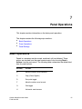
Panel Operations . . . . . . . . . . . . . . . . . . . . . . . . . . . . . . . . . . . . . . . . . . . . . .
57
Basic Operations . . . . . . . . . . . . . . . . . . . . . . . . . . . . . . . . . . . . . . . . . . . . . . .
57
Selecting Panels . . . . . . . . . . . . . . . . . . . . . . . . . . . . . . . . . . . . . . . . . . .
58
Moving or Copying Panels . . . . . . . . . . . . . . . . . . . . . . . . . . . . . . . . . . . .
59
Deleting Panels . . . . . . . . . . . . . . . . . . . . . . . . . . . . . . . . . . . . . . . . . . . .
59
Pasting Deleted Panels . . . . . . . . . . . . . . . . . . . . . . . . . . . . . . . . . . . . . .
59
Grouping Panels . . . . . . . . . . . . . . . . . . . . . . . . . . . . . . . . . . . . . . . . . . .
59
Ungrouping Panels. . . . . . . . . . . . . . . . . . . . . . . . . . . . . . . . . . . . . . . . . .
60
Zoom Operations . . . . . . . . . . . . . . . . . . . . . . . . . . . . . . . . . . . . . . . . . . . . . . .
60
X/Y (Box) Zoom . . . . . . . . . . . . . . . . . . . . . . . . . . . . . . . . . . . . . . . . . . . .
61
X Zoom. . . . . . . . . . . . . . . . . . . . . . . . . . . . . . . . . . . . . . . . . . . . . . . . . . .
61
Y Zoom. . . . . . . . . . . . . . . . . . . . . . . . . . . . . . . . . . . . . . . . . . . . . . . . . . .
61
X Zoom to Fit . . . . . . . . . . . . . . . . . . . . . . . . . . . . . . . . . . . . . . . . . . . . . .
61
Y Zoom to Fit . . . . . . . . . . . . . . . . . . . . . . . . . . . . . . . . . . . . . . . . . . . . . .
62
Un-zoom. . . . . . . . . . . . . . . . . . . . . . . . . . . . . . . . . . . . . . . . . . . . . . . . . .
62
Undo or Redo Zoom. . . . . . . . . . . . . . . . . . . . . . . . . . . . . . . . . . . . . . . . .
62
Using Sliders in Zoomed Panels . . . . . . . . . . . . . . . . . . . . . . . . . . . . . . .
62
Setting Zoom Ranges Manually . . . . . . . . . . . . . . . . . . . . . . . . . . . . . . . .
62
Panel Settings . . . . . . . . . . . . . . . . . . . . . . . . . . . . . . . . . . . . . . . . . . . . . . . . .
63
Displaying Data Points . . . . . . . . . . . . . . . . . . . . . . . . . . . . . . . . . . . . . . .
63
Controlling the Grid . . . . . . . . . . . . . . . . . . . . . . . . . . . . . . . . . . . . . . . . .
64
Adjusting Logarithmic Scales . . . . . . . . . . . . . . . . . . . . . . . . . . . . . . . . . .
64
Using Fixed X-axis (or Y-axis) Full Scale . . . . . . . . . . . . . . . . . . . . . . . . .
64
Changing Axis Font Size . . . . . . . . . . . . . . . . . . . . . . . . . . . . . . . . . . . . .
65
Dual Y-axes . . . . . . . . . . . . . . . . . . . . . . . . . . . . . . . . . . . . . . . . . . . . . . .
65
Setting Axis Attributes . . . . . . . . . . . . . . . . . . . . . . . . . . . . . . . . . . . . . . .
65
Adjusting Panel Height . . . . . . . . . . . . . . . . . . . . . . . . . . . . . . . . . . . . . . .
66
Fitting Panels to Full Window Height . . . . . . . . . . . . . . . . . . . . . . . . . . . .
66
Setting Vector Radix. . . . . . . . . . . . . . . . . . . . . . . . . . . . . . . . . . . . . . . . .
67
Setting Vector Length. . . . . . . . . . . . . . . . . . . . . . . . . . . . . . . . . . . . . . . .
67
Setting Waveform Display Preferences . . . . . . . . . . . . . . . . . . . . . . . . . .
67
Setting the Plot Mode for Complex Signals . . . . . . . . . . . . . . . . . . . . . . .
67
Setting Panel Attributes . . . . . . . . . . . . . . . . . . . . . . . . . . . . . . . . . . . . . .
68
Contents
8.
9.
Waveform Operations . . . . . . . . . . . . . . . . . . . . . . . . . . . . . . . . . . . . . . . . . .
69
Working with Signals and Waveforms . . . . . . . . . . . . . . . . . . . . . . . . . . . . . . .
69
Highlighting Waveforms . . . . . . . . . . . . . . . . . . . . . . . . . . . . . . . . . . . . . .
69
Ungrouping Highlighted Waveforms. . . . . . . . . . . . . . . . . . . . . . . . . . . . .
70
Grouping Highlighted Waveforms . . . . . . . . . . . . . . . . . . . . . . . . . . . . . .
70
Deleting Highlighted Waveforms . . . . . . . . . . . . . . . . . . . . . . . . . . . . . . .
70
Finding the Source of a Waveform . . . . . . . . . . . . . . . . . . . . . . . . . . . . . .
70
Getting Signal Information . . . . . . . . . . . . . . . . . . . . . . . . . . . . . . . . . . . .
70
Adding Signal Alias . . . . . . . . . . . . . . . . . . . . . . . . . . . . . . . . . . . . . . . . .
71
Scanning Waveforms . . . . . . . . . . . . . . . . . . . . . . . . . . . . . . . . . . . . . . . .
71
Scan Configuration. . . . . . . . . . . . . . . . . . . . . . . . . . . . . . . . . . . . . . . . . .
71
Waveform Color Schemes . . . . . . . . . . . . . . . . . . . . . . . . . . . . . . . . . . . . . . . .
72
Local Mode. . . . . . . . . . . . . . . . . . . . . . . . . . . . . . . . . . . . . . . . . . . . . . . .
72
Global Mode (default). . . . . . . . . . . . . . . . . . . . . . . . . . . . . . . . . . . . . . . .
72
Custom Waveform Colors . . . . . . . . . . . . . . . . . . . . . . . . . . . . . . . . . . . . . . . .
72
Modifying Waveform Attributes . . . . . . . . . . . . . . . . . . . . . . . . . . . . . . . . . . . .
73
Adding Text Labels. . . . . . . . . . . . . . . . . . . . . . . . . . . . . . . . . . . . . . . . . . . . . .
73
Measurements . . . . . . . . . . . . . . . . . . . . . . . . . . . . . . . . . . . . . . . . . . . . . . . .
75
Working with Cursors. . . . . . . . . . . . . . . . . . . . . . . . . . . . . . . . . . . . . . . . . . . .
75
Adding Cursors . . . . . . . . . . . . . . . . . . . . . . . . . . . . . . . . . . . . . . . . . . . .
75
The Active Cursor . . . . . . . . . . . . . . . . . . . . . . . . . . . . . . . . . . . . . . . . . .
76
Moving a Cursor. . . . . . . . . . . . . . . . . . . . . . . . . . . . . . . . . . . . . . . . . . . .
76
Jumping Cursors . . . . . . . . . . . . . . . . . . . . . . . . . . . . . . . . . . . . . . . . . . .
76
Locking Pairs of Cursors . . . . . . . . . . . . . . . . . . . . . . . . . . . . . . . . . . . . .
77
Horizontal Cursors . . . . . . . . . . . . . . . . . . . . . . . . . . . . . . . . . . . . . . . . . .
77
Cursors in Smith Charts and Polar Plots . . . . . . . . . . . . . . . . . . . . . . . . .
78
Cursors in 2-D Sweep Panels . . . . . . . . . . . . . . . . . . . . . . . . . . . . . . . . .
78
Cursors in 3-D Sweep Panels . . . . . . . . . . . . . . . . . . . . . . . . . . . . . . . . .
78
Deleting Cursors . . . . . . . . . . . . . . . . . . . . . . . . . . . . . . . . . . . . . . . . . . .
78
Working with Monitors . . . . . . . . . . . . . . . . . . . . . . . . . . . . . . . . . . . . . . . . . . .
79
Adding Monitors . . . . . . . . . . . . . . . . . . . . . . . . . . . . . . . . . . . . . . . . . . . .
80
Deleting Monitors . . . . . . . . . . . . . . . . . . . . . . . . . . . . . . . . . . . . . . . . . . .
80
Reconfiguring Monitors . . . . . . . . . . . . . . . . . . . . . . . . . . . . . . . . . . . . . .
80
Linking Monitors to Cursors . . . . . . . . . . . . . . . . . . . . . . . . . . . . . . . . . . .
80
Using the Measurement Tool . . . . . . . . . . . . . . . . . . . . . . . . . . . . . . . . . . . . . .
81
vii
Contents
viii
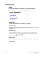
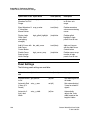
Supported Measurements . . . . . . . . . . . . . . . . . . . . . . . . . . . . . . . . . . . .
General Measurements . . . . . . . . . . . . . . . . . . . . . . . . . . . . . . . . . .
Time Domain Measurements . . . . . . . . . . . . . . . . . . . . . . . . . . . . . .
Frequency Domain Measurements . . . . . . . . . . . . . . . . . . . . . . . . .
Statistical Measurements . . . . . . . . . . . . . . . . . . . . . . . . . . . . . . . . .
Level Measurements . . . . . . . . . . . . . . . . . . . . . . . . . . . . . . . . . . . .
S Domain Measurements. . . . . . . . . . . . . . . . . . . . . . . . . . . . . . . . .
RF Measurements . . . . . . . . . . . . . . . . . . . . . . . . . . . . . . . . . . . . . .
81
84
87
97
99
102
104
104
Adding or Removing Measurement Favorites . . . . . . . . . . . . . . . . . . . . .
105
Setting the Precision of Measurements . . . . . . . . . . . . . . . . . . . . . . . . . .
106
Exporting Measurements . . . . . . . . . . . . . . . . . . . . . . . . . . . . . . . . . . . . .
106
10. Multi-Trace Sweep Waveforms . . . . . . . . . . . . . . . . . . . . . . . . . . . . . . . . . . .
109
Reading Multi-Trace Data . . . . . . . . . . . . . . . . . . . . . . . . . . . . . . . . . . . . . . . .
109
Loading Multi-File PSF Sweep Analysis Result . . . . . . . . . . . . . . . . . . . . . . . .
110
Creating a File Set from Multiple Files . . . . . . . . . . . . . . . . . . . . . . . . . . . . . . .
110
Displaying Multi-Trace Signals . . . . . . . . . . . . . . . . . . . . . . . . . . . . . . . . . . . . .
110
Breaking Multi-Trace Signals . . . . . . . . . . . . . . . . . . . . . . . . . . . . . . . . . . . . . .
111
Calculating Waveforms for Multi-Trace Signals . . . . . . . . . . . . . . . . . . . . . . . .
111
Selecting the Sweeping Parameter . . . . . . . . . . . . . . . . . . . . . . . . . . . . . . . . .
112
Filtering Multi-Trace Waveforms. . . . . . . . . . . . . . . . . . . . . . . . . . . . . . . . . . . .
112
Using Multi-Trace Signals as X-Axes . . . . . . . . . . . . . . . . . . . . . . . . . . . . . . . .
113
Viewing or Modifying Sweep Signal Attributes. . . . . . . . . . . . . . . . . . . . . . . . .
113
11. Eye Diagrams . . . . . . . . . . . . . . . . . . . . . . . . . . . . . . . . . . . . . . . . . . . . . . . . .
115
Unfolding Eye Diagrams . . . . . . . . . . . . . . . . . . . . . . . . . . . . . . . . . . . . . . . . .
115
Tracing Waveform Points in Eye Diagrams . . . . . . . . . . . . . . . . . . . . . . . . . . .
116
Configuring Eye Diagrams . . . . . . . . . . . . . . . . . . . . . . . . . . . . . . . . . . . . . . . .
116
Generating Jitter Histograms . . . . . . . . . . . . . . . . . . . . . . . . . . . . . . . . . . . . . .
117
Automatic Eye Measurement . . . . . . . . . . . . . . . . . . . . . . . . . . . . . . . . . . . . . .
117
Adding User-Defined Masks . . . . . . . . . . . . . . . . . . . . . . . . . . . . . . . . . . . . . .
118
Mask File Syntax . . . . . . . . . . . . . . . . . . . . . . . . . . . . . . . . . . . . . . . . . . .
118
Incorporating Mask Files . . . . . . . . . . . . . . . . . . . . . . . . . . . . . . . . . . . . .
On UNIX Platforms. . . . . . . . . . . . . . . . . . . . . . . . . . . . . . . . . . . . . .
On Windows 95/98 Platforms . . . . . . . . . . . . . . . . . . . . . . . . . . . . . .
118
118
119
Contents
On Windows NT Platforms . . . . . . . . . . . . . . . . . . . . . . . . . . . . . . . .
On Windows XP/2000 Platforms . . . . . . . . . . . . . . . . . . . . . . . . . . .
On Windows Me Platforms. . . . . . . . . . . . . . . . . . . . . . . . . . . . . . . .
119
119
119
Mask File Example. . . . . . . . . . . . . . . . . . . . . . . . . . . . . . . . . . . . . . . . . .
119
12. Using the Equation Builder. . . . . . . . . . . . . . . . . . . . . . . . . . . . . . . . . . . . . .
123
Adding Signals to the Equation Builder . . . . . . . . . . . . . . . . . . . . . . . . . . . . . .
123
Assigning Aliases to Equations . . . . . . . . . . . . . . . . . . . . . . . . . . . . . . . . . . . .
124
Viewing the Result Stack . . . . . . . . . . . . . . . . . . . . . . . . . . . . . . . . . . . . . . . . .
124
Adding .MEASURE Statements to Expressions . . . . . . . . . . . . . . . . . . . . . . .
125
Defining Macros . . . . . . . . . . . . . . . . . . . . . . . . . . . . . . . . . . . . . . . . . . . . . . . .
125
Modifying Equations. . . . . . . . . . . . . . . . . . . . . . . . . . . . . . . . . . . . . . . . . . . . .
126
Calculating Multi-trace Waveforms . . . . . . . . . . . . . . . . . . . . . . . . . . . . . . . . .
126
Special Note Regarding FFT/DFT . . . . . . . . . . . . . . . . . . . . . . . . . . . . . . . . . .
126
Supported Equation Builder Functions . . . . . . . . . . . . . . . . . . . . . . . . . . . . . .
127
Supported Operators . . . . . . . . . . . . . . . . . . . . . . . . . . . . . . . . . . . . . . . .
127
Supported Mathematic Functions . . . . . . . . . . . . . . . . . . . . . . . . . . . . . .
128
Supported RF Functions . . . . . . . . . . . . . . . . . . . . . . . . . . . . . . . . . . . . .
129
Supported Logic Operations . . . . . . . . . . . . . . . . . . . . . . . . . . . . . . . . . .
130
Supported Waveform Functions. . . . . . . . . . . . . . . . . . . . . . . . . . . . . . . .
131
Supported Measurement Functions. . . . . . . . . . . . . . . . . . . . . . . . . . . . .
135
13. Waveform Post Processing. . . . . . . . . . . . . . . . . . . . . . . . . . . . . . . . . . . . . .
143
FFT/DFT Conversion . . . . . . . . . . . . . . . . . . . . . . . . . . . . . . . . . . . . . . . . . . . .
143
Viewing the Spectrum Panel . . . . . . . . . . . . . . . . . . . . . . . . . . . . . . . . . .
146
Calculating SNR/THD Using FFT. . . . . . . . . . . . . . . . . . . . . . . . . . . . . . .
146
FFT of Complex Signals. . . . . . . . . . . . . . . . . . . . . . . . . . . . . . . . . . . . . .
147
Changing the FFT Axes Scale . . . . . . . . . . . . . . . . . . . . . . . . . . . . . . . . .
147
A to D Conversion . . . . . . . . . . . . . . . . . . . . . . . . . . . . . . . . . . . . . . . . . . . . . .
147
Single-Bit A/D Conversion . . . . . . . . . . . . . . . . . . . . . . . . . . . . . . . . . . . .
148
Multi-Bit A/D Conversion . . . . . . . . . . . . . . . . . . . . . . . . . . . . . . . . . . . . .
148
D to A Conversion . . . . . . . . . . . . . . . . . . . . . . . . . . . . . . . . . . . . . . . . . . . . . .
150
Applying .MEASURE Commands . . . . . . . . . . . . . . . . . . . . . . . . . . . . . . . . . .
150
Reducing Data Points . . . . . . . . . . . . . . . . . . . . . . . . . . . . . . . . . . . . . . . . . . .
152
ix
Contents
x
Generating Parametric Plots . . . . . . . . . . . . . . . . . . . . . . . . . . . . . . . . . . . . . .
153
Built-in Parametric Tool for HSPICE .ALTER Simulations . . . . . . . . . . . .
153
Jitter-vs-Time Tool . . . . . . . . . . . . . . . . . . . . . . . . . . . . . . . . . . . . . . . . . . . . . .
153
Selecting Reference Signals . . . . . . . . . . . . . . . . . . . . . . . . . . . . . . . . . .
154
Specifying the Target Signal. . . . . . . . . . . . . . . . . . . . . . . . . . . . . . . . . . .
154
Selecting Reference Edges . . . . . . . . . . . . . . . . . . . . . . . . . . . . . . . . . . .
154
Target Signal Edges . . . . . . . . . . . . . . . . . . . . . . . . . . . . . . . . . . . . . . . . .
154
Jitter Types . . . . . . . . . . . . . . . . . . . . . . . . . . . . . . . . . . . . . . . . . . . . . . . .
155
Jitter Output Options . . . . . . . . . . . . . . . . . . . . . . . . . . . . . . . . . . . . . . . .
155
Exporting Waveform Data . . . . . . . . . . . . . . . . . . . . . . . . . . . . . . . . . . . . . . . .
156
Comparing Waveforms . . . . . . . . . . . . . . . . . . . . . . . . . . . . . . . . . . . . . . . . . .
156
Comparing Waveforms in Batch Mode. . . . . . . . . . . . . . . . . . . . . . . . . . .
157
Sampling and Converting Waveform Data . . . . . . . . . . . . . . . . . . . . . . . .
158
Creating a Waveform Compare Control File . . . . . . . . . . . . . . . . . . . . . .
158
Adding Comments . . . . . . . . . . . . . . . . . . . . . . . . . . . . . . . . . . . . . . . . . .
158
Defining Parameters. . . . . . . . . . . . . . . . . . . . . . . . . . . . . . . . . . . . . . . . .
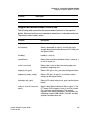
a2d_threshold. . . . . . . . . . . . . . . . . . . . . . . . . . . . . . . . . . . . . . . . . .
bus . . . . . . . . . . . . . . . . . . . . . . . . . . . . . . . . . . . . . . . . . . . . . . . . . .
delay . . . . . . . . . . . . . . . . . . . . . . . . . . . . . . . . . . . . . . . . . . . . . . . . .
file_path . . . . . . . . . . . . . . . . . . . . . . . . . . . . . . . . . . . . . . . . . . . . . .
ignorex . . . . . . . . . . . . . . . . . . . . . . . . . . . . . . . . . . . . . . . . . . . . . . .
ignorez . . . . . . . . . . . . . . . . . . . . . . . . . . . . . . . . . . . . . . . . . . . . . . .
map . . . . . . . . . . . . . . . . . . . . . . . . . . . . . . . . . . . . . . . . . . . . . . . . .
mapfile, map_hier. . . . . . . . . . . . . . . . . . . . . . . . . . . . . . . . . . . . . . .
match_type. . . . . . . . . . . . . . . . . . . . . . . . . . . . . . . . . . . . . . . . . . . .
mean_range . . . . . . . . . . . . . . . . . . . . . . . . . . . . . . . . . . . . . . . . . . .
mean_step . . . . . . . . . . . . . . . . . . . . . . . . . . . . . . . . . . . . . . . . . . . .
mean_tol. . . . . . . . . . . . . . . . . . . . . . . . . . . . . . . . . . . . . . . . . . . . . .
ref_clock . . . . . . . . . . . . . . . . . . . . . . . . . . . . . . . . . . . . . . . . . . . . . .
report_style . . . . . . . . . . . . . . . . . . . . . . . . . . . . . . . . . . . . . . . . . . .
report_type . . . . . . . . . . . . . . . . . . . . . . . . . . . . . . . . . . . . . . . . . . . .
signal . . . . . . . . . . . . . . . . . . . . . . . . . . . . . . . . . . . . . . . . . . . . . . . .
start, stop, step. . . . . . . . . . . . . . . . . . . . . . . . . . . . . . . . . . . . . . . . .
t_tol. . . . . . . . . . . . . . . . . . . . . . . . . . . . . . . . . . . . . . . . . . . . . . . . . .
v_abstol, i_abstol, v_reltol, i_reltol . . . . . . . . . . . . . . . . . . . . . . . . . .
when. . . . . . . . . . . . . . . . . . . . . . . . . . . . . . . . . . . . . . . . . . . . . . . . .
x_absmgn. . . . . . . . . . . . . . . . . . . . . . . . . . . . . . . . . . . . . . . . . . . . .
x_chkrange. . . . . . . . . . . . . . . . . . . . . . . . . . . . . . . . . . . . . . . . . . . .
159
160
160
160
160
160
160
161
161
161
162
162
162
162
163
163
163
163
163
164
164
164
164
Controlling X- and Z-Level Constraints . . . . . . . . . . . . . . . . . . . . . . . . . .
165
Defining Aliases . . . . . . . . . . . . . . . . . . . . . . . . . . . . . . . . . . . . . . . . . . . .
165
Defining Rules . . . . . . . . . . . . . . . . . . . . . . . . . . . . . . . . . . . . . . . . . . . . .
166
Contents
Checking Waveforms . . . . . . . . . . . . . . . . . . . . . . . . . . . . . . . . . . . . . . . .
167
Waveform Check Example . . . . . . . . . . . . . . . . . . . . . . . . . . . . . . . . . . . .
168
Checking Waveform Monotonicity . . . . . . . . . . . . . . . . . . . . . . . . . . . . . .
168
Checking Waveform Bounds . . . . . . . . . . . . . . . . . . . . . . . . . . . . . . . . . .
169
Checking the Waveform Envelope . . . . . . . . . . . . . . . . . . . . . . . . . . . . . .
169
Rules Section Example . . . . . . . . . . . . . . . . . . . . . . . . . . . . . . . . . . . . . .
169
Saving Waveform Comparison Results . . . . . . . . . . . . . . . . . . . . . . . . . .
170
Converting Signals to the Time Domain . . . . . . . . . . . . . . . . . . . . . . . . . . . . .
170
Back-Annotating Signals to CustomExplorer . . . . . . . . . . . . . . . . . . . . . . . . . .
171
14. Using the PWL Editor . . . . . . . . . . . . . . . . . . . . . . . . . . . . . . . . . . . . . . . . . .
173
File Operations. . . . . . . . . . . . . . . . . . . . . . . . . . . . . . . . . . . . . . . . . . . . . . . . .
173
Source Operations . . . . . . . . . . . . . . . . . . . . . . . . . . . . . . . . . . . . . . . . . . . . . .
174
Point Operations . . . . . . . . . . . . . . . . . . . . . . . . . . . . . . . . . . . . . . . . . . . . . . .
174
15. Using the ADC Toolbox . . . . . . . . . . . . . . . . . . . . . . . . . . . . . . . . . . . . . . . . .
177
Generic Versus Coherent ADC Toolbox. . . . . . . . . . . . . . . . . . . . . . . . . . . . . .
177
Overview of the ADC ToolBox . . . . . . . . . . . . . . . . . . . . . . . . . . . . . . . . . . . . .
178
Input Signal of ADC Toolbox . . . . . . . . . . . . . . . . . . . . . . . . . . . . . . . . . . . . . .
178
DC DNL/INL Analysis. . . . . . . . . . . . . . . . . . . . . . . . . . . . . . . . . . . . . . . . . . . .
179
Sine Input . . . . . . . . . . . . . . . . . . . . . . . . . . . . . . . . . . . . . . . . . . . . . . . . .
180
Ramp Input. . . . . . . . . . . . . . . . . . . . . . . . . . . . . . . . . . . . . . . . . . . . . . . .
180
Number of Sample Points and INL/DNL. . . . . . . . . . . . . . . . . . . . . . . . . .
180
Sampling Frequency and INL/DNL. . . . . . . . . . . . . . . . . . . . . . . . . . . . . .
181
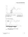
AC Analysis: Coherent Sampling Versus Window Sampling . . . . . . . . . . . . . .
181
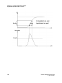
Coherent Sampling . . . . . . . . . . . . . . . . . . . . . . . . . . . . . . . . . . . . . . . . .
181
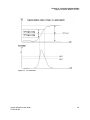
Window Sampling . . . . . . . . . . . . . . . . . . . . . . . . . . . . . . . . . . . . . . . . . .
183
Exporting the DNL/INL/FFT Results as Waveform Data . . . . . . . . . . . . . . . . .
184
Saving or Loading an Analysis Setup . . . . . . . . . . . . . . . . . . . . . . . . . . . . . . .
184
ADC Toolbox Display Controls . . . . . . . . . . . . . . . . . . . . . . . . . . . . . . . . . . . . .
184
Sampled Signal Window . . . . . . . . . . . . . . . . . . . . . . . . . . . . . . . . . . . . .
184
Histogram, DNL, and INL Windows . . . . . . . . . . . . . . . . . . . . . . . . . . . . .
185
Power Spectrum (Sine Input Only). . . . . . . . . . . . . . . . . . . . . . . . . . . . . .
185
AC Dynamic Characteristics . . . . . . . . . . . . . . . . . . . . . . . . . . . . . . . . . . . . . .
186
xi
Contents
xii
DC Static Characteristics . . . . . . . . . . . . . . . . . . . . . . . . . . . . . . . . . . . . . . . . .
186
Running Batch-mode ADC Analyses . . . . . . . . . . . . . . . . . . . . . . . . . . . . . . . .
187
16. Using the Coherent Sample Only (CSO) ADC Toolbox . . . . . . . . . . . . . . .
189
Input Signal Requirements. . . . . . . . . . . . . . . . . . . . . . . . . . . . . . . . . . . . . . . .
189
Preparing the Input Waveform . . . . . . . . . . . . . . . . . . . . . . . . . . . . . . . . . . . . .
189
Sampling the Input Waveform . . . . . . . . . . . . . . . . . . . . . . . . . . . . . . . . . . . . .
191
Preparing Test Benches for the CSO ADC Toolbox . . . . . . . . . . . . . . . . . . . . .
191
Input Signal Strength . . . . . . . . . . . . . . . . . . . . . . . . . . . . . . . . . . . . . . . .
192
Input Sine Wave Frequency . . . . . . . . . . . . . . . . . . . . . . . . . . . . . . . . . . .
192
CSO ADC Toolbox User Interface . . . . . . . . . . . . . . . . . . . . . . . . . . . . . . . . . .
192
Input Parameters . . . . . . . . . . . . . . . . . . . . . . . . . . . . . . . . . . . . . . . . . . . . . . .
192
Selecting Sampling Parameters. . . . . . . . . . . . . . . . . . . . . . . . . . . . . . . . . . . .
195
Sine Input . . . . . . . . . . . . . . . . . . . . . . . . . . . . . . . . . . . . . . . . . . . . . . . . .
195
Ramp Input. . . . . . . . . . . . . . . . . . . . . . . . . . . . . . . . . . . . . . . . . . . . . . . .
195
Exporting DNL/INL/FFT Results as Waveform Data . . . . . . . . . . . . . . . . . . . .
196
Saving or Loading an Analysis Setup . . . . . . . . . . . . . . . . . . . . . . . . . . . . . . .
196
ADC Toolbox Display Controls . . . . . . . . . . . . . . . . . . . . . . . . . . . . . . . . . . . . .
196
Sampled Signal Window . . . . . . . . . . . . . . . . . . . . . . . . . . . . . . . . . . . . .
196
Histogram, DNL, and INL Windows . . . . . . . . . . . . . . . . . . . . . . . . . . . . .
197
Power Spectrum (Sine Input Only). . . . . . . . . . . . . . . . . . . . . . . . . . . . . .
197
AC Dynamic Characteristics . . . . . . . . . . . . . . . . . . . . . . . . . . . . . . . . . . . . . .
198
DC static Characteristics . . . . . . . . . . . . . . . . . . . . . . . . . . . . . . . . . . . . . . . . .
198
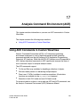
17. Analysis Command Environment (ACE) . . . . . . . . . . . . . . . . . . . . . . . . . . .
199
Using ACE Commands in Custom WaveView . . . . . . . . . . . . . . . . . . . . . . . . .
199
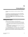
18. Printing Waveforms . . . . . . . . . . . . . . . . . . . . . . . . . . . . . . . . . . . . . . . . . . . .
201
PostScript Print Layout. . . . . . . . . . . . . . . . . . . . . . . . . . . . . . . . . . . . . . . . . . .
201
Printing on UNIX Platforms . . . . . . . . . . . . . . . . . . . . . . . . . . . . . . . . . . . . . . .
202
Printing on Windows Platforms . . . . . . . . . . . . . . . . . . . . . . . . . . . . . . . . . . . .
202
Contents
19. Advanced Controls . . . . . . . . . . . . . . . . . . . . . . . . . . . . . . . . . . . . . . . . . . . .
203
Saving and Restoring Job Sessions . . . . . . . . . . . . . . . . . . . . . . . . . . . . . . . .
203
Saving a Job Session. . . . . . . . . . . . . . . . . . . . . . . . . . . . . . . . . . . . . . . .
203
Restoring a Job Session . . . . . . . . . . . . . . . . . . . . . . . . . . . . . . . . . . . . .
204
Loading Setup from Other Viewer Tools . . . . . . . . . . . . . . . . . . . . . . . . .
204
Customizing Bind Keys . . . . . . . . . . . . . . . . . . . . . . . . . . . . . . . . . . . . . . . . . .
204
Bindkey Functions . . . . . . . . . . . . . . . . . . . . . . . . . . . . . . . . . . . . . . . . . . . . . .
205
Top Menu-operated Bind Key Functions . . . . . . . . . . . . . . . . . . . . . . . . .
205
Waveview Toolbar Bind Key Functions. . . . . . . . . . . . . . . . . . . . . . . . . . .
209
Other Bind Key Functions . . . . . . . . . . . . . . . . . . . . . . . . . . . . . . . . . . . .
210
Preference Settings . . . . . . . . . . . . . . . . . . . . . . . . . . . . . . . . . . . . . . . . . . . . .
212
Configuring Custom WaveView Manually . . . . . . . . . . . . . . . . . . . . . . . . . . . .
212
Customizing File Browser Filters . . . . . . . . . . . . . . . . . . . . . . . . . . . . . . . . . . .
213
Configuring "Send To" in the Windows Environment . . . . . . . . . . . . . . . . . . . .
214
20. Troubleshooting . . . . . . . . . . . . . . . . . . . . . . . . . . . . . . . . . . . . . . . . . . . . . . .
215
Linux Platforms . . . . . . . . . . . . . . . . . . . . . . . . . . . . . . . . . . . . . . . . . . . . . . . .
215
Screen Refresh . . . . . . . . . . . . . . . . . . . . . . . . . . . . . . . . . . . . . . . . . . . .
215
Alternative Methods for Backing-store Setup . . . . . . . . . . . . . . . . . . . . . .
Locate the XServers File . . . . . . . . . . . . . . . . . . . . . . . . . . . . . . . . .
Enable Backing-store for Your Xserver . . . . . . . . . . . . . . . . . . . . . .
Restart Your Xserver to Enable the Changes. . . . . . . . . . . . . . . . . .
216
216
216
217
With GNOME . . . . . . . . . . . . . . . . . . . . . . . . . . . . . . . . . . . . . . . . . . . . . .
217
Program Crashes During Startup on Linux Platforms . . . . . . . . . . . . . . .
217
X-Window Font Warnings . . . . . . . . . . . . . . . . . . . . . . . . . . . . . . . . . . . . . . . .
217
XmTextField Font Warning. . . . . . . . . . . . . . . . . . . . . . . . . . . . . . . . . . . . . . . .
218
Cannot Change Flexlm License File . . . . . . . . . . . . . . . . . . . . . . . . . . . . . . . .
219
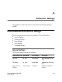
Preference Settings . . . . . . . . . . . . . . . . . . . . . . . . . . . . . . . . . . . . . . . . . . . .
221
Custom WaveView Preference Settings . . . . . . . . . . . . . . . . . . . . . . . . . . . . .
221
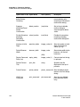
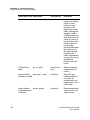
General Settings . . . . . . . . . . . . . . . . . . . . . . . . . . . . . . . . . . . . . . . . . . .
221
A.
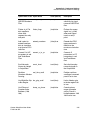
Waveview Settings . . . . . . . . . . . . . . . . . . . . . . . . . . . . . . . . . . . . . . . . . .
223
Panel Settings . . . . . . . . . . . . . . . . . . . . . . . . . . . . . . . . . . . . . . . . . . . . .
226
Signal Settings . . . . . . . . . . . . . . . . . . . . . . . . . . . . . . . . . . . . . . . . . . . . .
229
xiii
Contents
xiv
Color Settings. . . . . . . . . . . . . . . . . . . . . . . . . . . . . . . . . . . . . . . . . . . . . .
231
Threshold Settings . . . . . . . . . . . . . . . . . . . . . . . . . . . . . . . . . . . . . . . . . .
232
Index . . . . . . . . . . . . . . . . . . . . . . . . . . . . . . . . . . . . . . . . . . . . . . . . . . . . . . . . . . . .
235
1
1
Introduction to Custom WaveView
This chapter contains introductory information for Custom WaveView.
Custom WaveView is a graphical waveform viewing and analysis program for
analog/mixed-signal IC design simulations, which can help you to use
simulation tools more effectively with:
■
High-performance waveforms database I/O to access large amount of
simulation data efficiently.
■
Extensive mixed-signal display functions and analysis capabilities to extract
design parameters from simulation result.
Supported Platforms and Operating Systems
See the CustomExplorer and Custom WaveView Release Notes for information
on the latest supported platforms and operating systems. The release notes
are available on SolvNet (http://www.solvnet.com/) in the Download Center.
Installing Custom WaveView
See the CustomExplorer and Custom WaveView Installation Guide for
installation information, which is available from
http://www.synopsys.com/install.
Custom WaveView User Guide
F-2011.09-SP1
1
Chapter 1: Introduction to Custom WaveView
Using Private Color Maps
Using Private Color Maps
On X Windows platforms, Custom WaveView automatically searches for usable
colors from the shared public color resource. A private color map is usually not
needed even if you have color-intensive applications such as a web browser
running. Should Custom WaveView fail to obtain the needed color resource,
you can force the use of private color map with the -priv option. Using a
private colormap ensures proper color display when the mouse pointer moves
into any of the Custom WaveView windows.
2
Custom WaveView User Guide
F-2011.09-SP1
2
Getting Started
2
This chapter provides information on how to invoke and use Custom WaveView.
This chapter contains the following major sections:
■
Starting Custom WaveView
■
Application Overview
■
GUI Conventions
■
Terminating the Application
■
Changing the Default Log File Directory
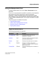
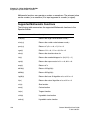
Starting Custom WaveView
Before starting Custom WaveView, consider any environment options you
might want to set. See Setting Environment Variables for more information.
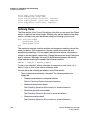
On UNIX and Linux platforms, enter cx -w or wv at the command line to start
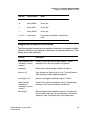
Custom WaveView.
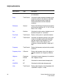
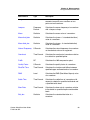
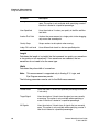
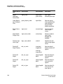
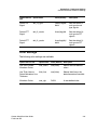
The following command-line options are available:
Option
Action
-ace_perl_gui
Starts ACE Perl in GUI mode.
-ace_perl_no_gui
Starts ACE Perl in batch mode.
-ace_no_gui
Starts an ACE Tcl script in batch mode.
-ace_gui
Starts an ACE Tcl script in GUI mode.
Custom WaveView User Guide
F-2011.09-SP1
3
Chapter 2: Getting Started
Starting Custom WaveView
4
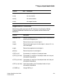
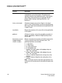
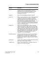
Option
Action
-m
Opens the ACE command console and shell.
-h
Help message.
-c
Batch mode WDF conversion (see -r, -ri, -rv, -w).
-compare rule_file
[out_file] [-x sx_file]
Batch mode waveform comparison.
-display host:screen
Starts 'wv' by displaying the window to host.
-v
Reports software revision.
-priv
Enables a private colormap.
-k
Quick start without the greeting window.
-load
Preloads waveform data to memory. fsdb and NPX-SDIF files
cannot be preloaded. Just the sweep results from tr0 and NW
files can be preloaded.
-r mode
Performs a reduction for WDF conversion.
0:default, loss-less, 1:medium reduction, 2:high reduction
(see -c).
-replay_delay time
Sets the delay time in milliseconds when replaying a log file.
-ri itol
Reduction current tolerance (see -c, -r).
-rv vtol
Reduction voltage tolerance (see -c, -r).
-spxrc pref_file
Starts Custom WaveView using the preference settings
specified in the pref_file.
-x session_file
Loads a session file.
-y session_file
Applies a session file to existing waveform files.
file1, file2, …
Loads waveform files.
-64
Invokes the 64-bit binaries for Sun, HP, and Linux platforms.
Custom WaveView User Guide
F-2011.09-SP1
Chapter 2: Getting Started
Starting Custom WaveView
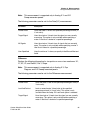
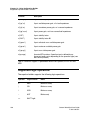
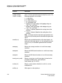
Setting Environment Variables
When starting Custom WaveView, you might want to set one or more of the
following environment variables:
■
SW_SX_QUEUE_LIC (not supported on Windows platforms)
Set to 1 to enable Synopsys license queuing. Flexlm license queuing is not
yet supported.
■
SW_SX_FAST_COU
Set to 1 to enable the fast COU file reader. Defaulted to 0. Fast COU reader
reads multi-run COU files much faster.
■
SW_SX_FAST_JWDB
Set to 1 to enable the fast WDB file reader. Defaulted to 1. Fast WDB reader
does not require the Java server.
■
SW_SX_HELP (UNIX only)
Points to the directory that contains the Custom WaveView online help.
■
SW_SX_INIT
Defines the location of the spxinit file for top menu customization.
■
SW_SX_INIT_DIR
Defines the Custom WaveView initial startup directory.
■
SW_SX_LOG_DIR (UNIX only)
Defines the output directory for the log file sxcmd.log. Default location is the
current working directory.
■
SW_SX_MASKFILE
Points to user-defined mask files for eye diagrams.
■
SW_SX_ORG_ADC
Set to 1 to use the old version of the ADC Toolbox.
■
SW_LIC_TIMEOUT
Sets the amount of time that Custom Waveview holds on to a license when
idle. Once the set time is expired, a dialog asks you to either reclaim the
license or exit and save the session. The minimum value is 30 (minutes).
■
SW_SX_TK_LIB
Custom WaveView User Guide
F-2011.09-SP1
5
Chapter 2: Getting Started
Application Overview
Points to the Tk runtime library for running ACE
■
SW_SX_TMP_DIR (UNIX only)
Points to the temporary directory for reading a compressed (gzipped)
waveform file. Default directory for temporary uncompressed files is the
current working directory.
■
SW_SX_USE_AMAP (UNIX only)
Set to 1 to use the map files in the Artist amap/ directory to map signal
names.
■
SW_WLF_READER
Points to the wlf2sx executable for reading the ModelSim WLF format.
■
SX_HOME (UNIX only)
Defines the Custom WaveView home directory. Custom WaveView
searches for the .spxrc file in $SX_HOME if SX_HOME is defined.
■
SW_SX_64
Set to 1 to point to the 64-bit binaries.
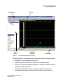
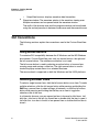
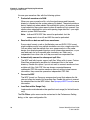
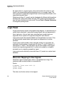
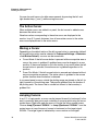
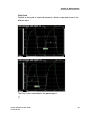
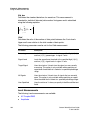
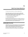
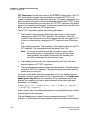
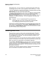
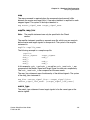
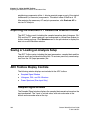
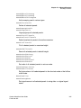
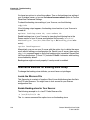
Application Overview
The following figure shows the Custom WaveView main window.
6
Custom WaveView User Guide
F-2011.09-SP1
Chapter 2: Getting Started
Application Overview
Main Menu
Toolbar
Browser
Area
Figure 1
Waveview
Window
Status Bar
Custom WaveView main window
The main window is comprised of the following parts and associated functions:
■
Main Menu: The top application menu bar.
■
Toolbar: The toolbar shortcuts to some of the top menu entries.
■
Status bar: The status bar reports progress of operations such as waveform
loading and signal searching.
■
Browser area: The Browser area contains the Output View browser
including the top hierarchy browser and the bottom signal list window.
Custom WaveView User Guide
F-2011.09-SP1
7
Chapter 2: Getting Started
GUI Conventions
•
■
OutputView browser: displays waveform data hierarchies.
Waveview window: The waveview window is the waveform viewing area.
Multiple waveviews can be opened inside the waveview window.
The width of the browser area and the waveview window can be adjusted
using the vertical pane bar in between the Browser and the waveview area.
GUI Conventions
The following sections explain the conventions used in the Custom WaveView
GUI.
Using Mouse Buttons
To maximize GUI compatibility between the X-Windows and the MS-Windows
environment, Custom WaveView uses only two mouse buttons: the right and
the left mouse buttons. The middle mouse button is not used.
The left mouse button is used in selecting an action button, a browser item,
zooming range and moving a slider bar. The right mouse button is used to
invoke the popup context menu for a selected item/area.
The mouse wheel is supported on both the Windows and the UNIX platforms.
Selecting Browser Items
To select a single browser item, click the left mouse button on an item. To make
multiple selections, click the left mouse button while pressing and holding the
Shift key a second item to select all items in between, or click the left mouse
button while pressing and holding the Ctrl key on an item to toggle the
selection state of the item.
In a hierarchy browser, you can expand an item to browse its child items. Left
click the + icon box to the left of a closed item or double-click the item to open it.
Left click the - icon box to the left of an opened item or double-click the item to
close it.
8
Custom WaveView User Guide
F-2011.09-SP1
Chapter 2: Getting Started
Terminating the Application
Drag-and-Drop Operations
Items from the OutputView browser can be dragged and dropped to waveview
windows. Items can be dragged and dropped inside or between the waveview
windows.
To start a drag-and-drop operation, hold down the left mouse button over an
item, drag it over to a drop-site and release the button to complete the
operation. If the dragged item is a member of a multiple selection set, all
selected items are involved in the drag-and-drop operation.
Numerical Values
All GUI dialog fields accept values in the scientific number format (1.00E+02) or
numbers with scale unit such as nano (n) and micro (u).
The following scale units are supported:
■
T - 1E12
■
G - 1E9
■
M (upper case) - 1E6
■
MEG - 1E6
■
x - 1E6
■
k - 1E3
■
m (lower case) - 1E-3
■
u - 1E-6
■
n - 1E-9
■
p - 1E-12
■
f - 1E-15
Terminating the Application
To exit Custom WaveView, select File > Exit from the top menu. Press Q in any
waveview window to exit the application.
Custom WaveView User Guide
F-2011.09-SP1
9
Chapter 2: Getting Started
Changing the Default Log File Directory
Changing the Default Log File Directory
Custom WaveView by default outputs log files in the working directory. Use the
SW_SX_LOG_DIR environment variable if you want to save the log file to a
different directory.
10
Custom WaveView User Guide
F-2011.09-SP1
3
3
Using the Waveview Window
This chapter contains information on how to use the waveview window.
The waveview window is the waveform display area in Custom WaveView. Left
click over the corresponding tab area of a waveview to bring it to foreground.
Custom WaveView User Guide
F-2011.09-SP1
11
Chapter 3: Using the Waveview Window
Displaying Waveview Windows
Displaying Waveview Windows
A waveview window can have one or more non-overlapping Panels. Panels in a
waveview can be arranged in two modes: vertical stack or independent row/
column. In the vertical stack mode, panels stack top down and share a
common horizontal axis. In the independent row/column mode, panels are
arranged from left to right in a row. Panels in the row/column mode are
independent from each other. A small icon at the upper-right corner of the
waveview indicates the waveview orientation.
The following display modes are available:
■
Stack Mode
■
Row and Column Mode
■
Vertical Row and Column Mode
■
Horizontal Row and Column Mode
■
Tiled Row and Column Mode
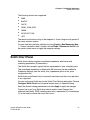
Stack Mode
To view waveviews in vertical stack mode, right-click a waveview tab and
choose Stack Layout from the menu that opens. Custom WaveView displays
waveviews in this mode by default.
12
Custom WaveView User Guide
F-2011.09-SP1
Chapter 3: Using the Waveview Window
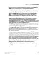
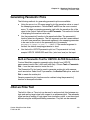
Displaying Waveview Windows
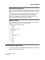
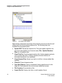
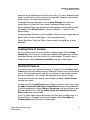
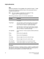
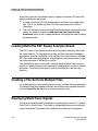
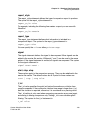
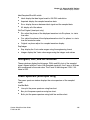
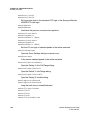
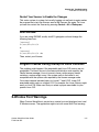
Figure 2 shows the vertical layout display.
Control
Buttons
Vertical
Slider
Vertical axis
Name
Column
Panel
Slider
Name-Monitor
Divider
Monitor-Panel
Divider
Monitor
Column
Horizontal
Slider
Figure 2
Horizontal
Axis
The Vertical Stack mode
The vertical layout has the following display components:
■
Control Buttons: Provides shortcuts to some of the commonly-used
waveview functions.
■
Vertical Slider: Panes zoomed waveforms vertically. It is not displayed for
logic panels.
■
Vertical Axis: The vertical axis of a panel. For a logic panel, it displays the
vector width and radix.
■
Panel Slider: Panes the entire panel stack vertically when the waveview
height is too small to show all panels. Mouse wheel can be used to scroll this
slidebar.
■
Horizontal Axis: The common x-axis of all panels, which appears at both the
top and the bottom of a vertical waveview.
■
Horizontal Slider: this slide bar is used to pane zoomed waves horizontally.
■
Monitor Column: Displays waveform or cursor related values. Multiple
monitors can be added. A horizontal slide bar at the bottom scrolls long
value strings horizontally.
■
Monitor-Panel Divider: Defines the left boundary of the waveform plotting
area. Left-click and drag over the divider to resize the width of monitor
columns.
Custom WaveView User Guide
F-2011.09-SP1
13
Chapter 3: Using the Waveview Window
Displaying Waveview Windows
■
Name-Monitor Divider: Defines the border between the name and monitor
area. Left-click and drag the divider to resize the width of name and monitor
columns.
■
Name Column: Displays waveform names. A vertical slide bar scrolls name
list vertically. A slide bar at the bottom scrolls long name strings horizontally.
Row and Column Mode
To view waveviews in row and column mode, right-click a waveview tab and
choose Row/Column Layout from the menu that opens.
Vertical Row and Column Mode
To view waveviews in vertical row and column mode, right-click a waveview tab
and choose Single Column Layout from the menu that opens.
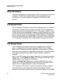
Horizontal Row and Column Mode
To view waveviews in horizontal row and column mode, right-click a waveview
tab and choose Single Row Layout from the menu that opens.
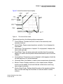
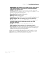
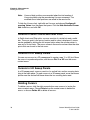
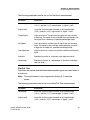
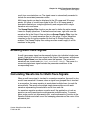
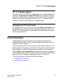
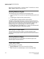
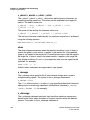
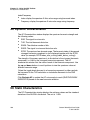
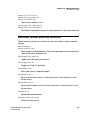
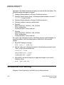
Figure 3 shows the independent row and column display.
Name Column
Measurement Column
Top Panel
Border
Figure 3
14
Horizontal Row and Column mode
Custom WaveView User Guide
F-2011.09-SP1
Chapter 3: Using the Waveview Window
Adding New Waveviews
Panels in the independent row/column layout are arranged in a similar way to
the Vertical Stack mode, except for the following differences and additional
display components:
■
Name column: The name column is located at the top of each panel. The
vertical and horizontal slide bars can be used to scroll long list or long name
strings.
■
Monitor column: The monitor column is at the top of each panel. A horizontal
slide bar at the bottom scrolls long value strings horizontally.
■
Top Panel border: The top border can be moved to redefine the top
boundary of the waveform plotting area. Drag the divider and move it
vertically to resize name/monitor height.
Each waveview window is associated with a waveview context menu that can
be invoked from the upper right corner of the window, or from the WaveView tab
area. Choose an item from the waveview context menu to rename, delete or
refresh a waveview, or edit the waveview title.
Tiled Row and Column Mode
To view waveviews in tiled row and column mode, right-click a waveview tab
and choose Tile Row/Column Layout from the menu that opens.
Adding New Waveviews
Custom WaveView opens an empty waveview initially when the application
starts. To add more waveviews into the Wave window, click the New Waveview
toolbar button or select the top menu WaveView > New. The newly-created
waveview is placed on the top of the waveview stack.
Docking and Undocking Waveviews
Overlapping (docked) waveviews in the WaveView window can be undocked
into individual pop-up windows. Choose WaveView > Dock/Undock from the
main menu to toggle all waveviews between the docked and undocked modes.
All waveviews must be docked or undocked together. Custom WaveView does
not allow WaveViews to be docked or undocked individually.
Custom WaveView User Guide
F-2011.09-SP1
15
Chapter 3: Using the Waveview Window
The Active Waveview
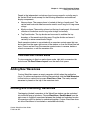
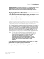
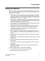
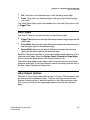
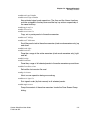
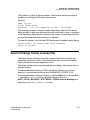
Waveviews can also be docked or undocked using the waveview docking
control button located at the top of each individual waveview window.
Figure 4
Waveview docking control button
The Active Waveview
In the dock mode, the top Waveview is considered the active Waveview. In the
undock mode, the topmost Waveview or the selected Waveview is the active
Waveview. Select a Waveview window from the top menu WaveView > Select,
or click the left mouse button over the window frame or tab. The selected
Waveview becomes the active waveview.
Refreshing Waveviews
Select the top menu Waveview > Refresh to refresh the display content of the
active waveview.
Deleting Waveviews
To delete the active waveview, click the Delete Waveview toolbar button or
choose WaveView > Delete from the main menu. Choose WaveView > Delete
All to delete all waveviews.
Renaming Waveviews
Choose WaveView > Rename from the main menu to rename the active
waveview. To rename a waveview directly, right-click the name tab area (or the
upper right corner) of a waveview and select Rename WaveView.
16
Custom WaveView User Guide
F-2011.09-SP1
Chapter 3: Using the Waveview Window
Undoing Waveview Operations
Undoing Waveview Operations
To undo a waveview operation, choose WaveView > Undo to undo the
previous waveview operation. You can undo object insertions and deletions;
axis, radix, and display settings; and zoom operations. Some waveview
operations, such as adding or deleting a waveview or relocating a signal,
cannot be undone.
Toggling the Hierarchy and Signal Browser Displays
To toggle the Hierarchy and Signal Browser displays, choose WaveView >
Hide/Show Browser from the main menu bar or press Ctrl-H on your
keyboard.
Displaying Waveview Titles
To hide or display the title of a waveview, right-click a waveview tab and choose
either Show Title or Hide Title from the menu that opens.
Clearing Waveview Contents
To clear the contents of a waveview window, right-click inside a waveview and
choose Clear Waveview from the menu that opens.
Changing the Order of Tabbed Waveviews
If you have multiple waveviews open at the same time, you can change the
order of those waveviews by moving the associated tabs left or right.
To change the order of tabbed waveviews, right click the tab of the waveview
you want to move, and choose Move to Left or Move to Right and 1 tab, 2
tab, 3 tab, 4 tab, or 5 tab.
Custom WaveView User Guide
F-2011.09-SP1
17
Chapter 3: Using the Waveview Window
Synchronizing Waveviews
Synchronizing Waveviews
A stack-mode waveview can be synchronized with other stack-mode
waveviews. Cursors and the X-axis of a synchronized waveview are updated
automatically when the X-axis display range or the active cursor location
changes in other synchronized waveviews. Choose WaveView > Sync/
Unsync to toggle the sync state of the active waveview, or choose WaveView >
Sync/Unsync All to toggle the sync states of all waveviews.
Dumping the Waveview Contents
All waveforms in a waveview can be included when performing a screen dump,
even if the waveforms are scrolled above or below the currently visible portion
of the waveview window.
To include all off-screen waveforms, choose WaveView > Dump Screen from
the main menu. Click the Use Maximum WaveView Height check box, and
click OK.
On Microsoft platforms, you can copy and paste the waveview contents to any
application that has access to the clipboard. To copy the screen bitmap of a
waveview window to the clipboard, choose Copy to Clipboard from the
WaveView context menu. To export a waveview in the vector-based Windows
EMF (Enhanced Meta File) format, choose Screen Dump to EMF.
On UNIX platforms, you can dump the waveview contents to the JPEG, PNG,
or EMF formats. Choose Dump Screen from the waveview context menu to
dump the display content.
Toggling the Console Window Display
To toggle the display of the Console window, choose WaveView > Hide/Show
Console from the main menu bar.
18
Custom WaveView User Guide
F-2011.09-SP1
4
Loading and Displaying Waveforms
4
This chapter contains information on how to load and display waveform files.
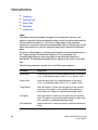
This chapter contains the following major sections:
■
Opening Waveform Files
■
Using the Output View Browser
■
Displaying Signals
■
Filtering Signals
■
Displaying Signals
■
Updating Waveforms
■
Clearing Waveforms
■
Grouping Waveform Files
■
Adding Waveform Files to the Bookmark List
■
Finding Signals
Opening Waveform Files
Custom WaveView automatically detects waveform format when a file is open.
To load a waveform file, click the Import Waveform File toolbar button or
choose File > Import Waveform File.
Select a waveform data file (or multiple files) and click OK to open the selected
waveform files, or click Apply to load more files without closing the dialog
window.
Custom WaveView User Guide
F-2011.09-SP1
19
Chapter 4: Loading and Displaying Waveforms
Opening Waveform Files
You can open waveform files with the following options:
■
Preload all waveforms to RAM
When you open a waveform file, only the signal names and hierarchy
directory is loaded into the system memory by default. The actual waveform
data is loaded only when needed. By enabling this option, all waveform data
is preloaded into the system memory when a waveform file is opened. Use
caution when selecting this option and opening large data files—you might
exhaust system RAM resources.
Note: fsdb and NPX-SDIF files cannot be preloaded. Just the
sweep results from tr0 and NW files can be preloaded.
■
Read multi-run data as multi-trace waveforms
Some output formats, such as the Berkeley raw and ELDO COU format,
might combine results from multiple simulation runs into a single output file.
You can either load the multiple runs as a sweep analysis of the same
design, thus displaying each signal as a multi-trace sweep waveform, or you
can read each run as a separate alter simulation run. Each run is
independent from other runs as if they are read from separated files.
■
Automatically connect to subsequent split files
The WDF and fsdb formats support split files. When a file is open, Custom
WaveView automatically searches for subsequent files in the same
directory. Disable this option if you do not want to connect waveforms from
multiple split files. Split PSF files are always connected because
subsequent PSF files contain waveform data only without signal names
information; they cannot be opened as independent PSF files.
■
Convert to WDF
The WDF format is a Synopsys compression format that reduces the file
size and offers fast access for large data files. Enable this option to convert
the selected files into the WDF format. See Synopsys WDF Format for more
information.
■
Load Data within Range Only
Load waveform data based on the specified x-axis range (for limited formats
only).
The File Filters option menu can be customized in the Preferences Setting
dialog, or the .spxrc configuration file.
20
Custom WaveView User Guide
F-2011.09-SP1
Chapter 4: Loading and Displaying Waveforms
Using the Output View Browser
Clicking Home resets the directory path to the working directory—the directory
in which the program started, for example.
Note:
Most application controls (except toolbar and main menu) are still
functional during a waveform loading session. This feature allows
tool operations in parallel to a lengthy waveform loading process.
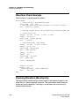
Waveform files can be also loaded from command line as arguments. The
usage is:
wv wdf1 wdf2 wdf3 …
To load multiple output files in different sub-directories, (a directory structure
commonly seen in Cadence Artist environment), click Apply to load files from
different directories or load files from the command line as:
wv */*.tran
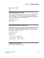
Using the Output View Browser
Once a waveform file is loaded, its signal name directory is displayed
hierarchically in the Output View browser.
The Output View browser consists of an upper hierarchy browser and a lower
signal list window. The lower list window displays signals under the selected
hierarchy in the upper browser. Only one item can be selected in the upper
hierarchy browser, while multiple signals can be selected in the signal windows
for drag-and-drop operations.
To distinguish waveform data with the same file names from different
directories, in the root entries of the upper Output View hierarchy browser,
directory paths of loaded waveform files are displayed using directory prefix DX
where X is the sequential index of different directories. To find out the original
full paths of directory entries, select from the main menu File > Show
Directory Table to display the table that maps directory identifiers to full file
paths.
Custom WaveView User Guide
F-2011.09-SP1
21
Chapter 4: Loading and Displaying Waveforms
Using the Output View Browser
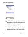
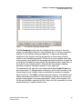
Figure 5
The output view window
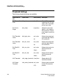
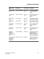
Right-clicking a filename in the Output View hierarchy browser invokes the wdf
context menu for the associated waveform file. The following items are
available from the context menu:
22
■
Update WDF: Reload the waveform file. The same update operation can
also be invoked globally from the main menu (File > Update Waveform
Files) for all waveform files.
■
Close This File: Close the target waveform file. A dialog appears and asks
you to confirm the action. Closing a waveform file also removes all
associated waveforms from waveviews.
■
Close Selected Files: Select from the list of all files to close multiple files
together.
■
Close All: Close all waveform files.
■
Open New Browser: Open a standalone floating signal browser for the
target file. Each waveform file can have one standalone browser.
■
File Grouping: Group waveform files.
■
Create File Set: Create a link file for a multi-member file set.
Custom WaveView User Guide
F-2011.09-SP1
Chapter 4: Loading and Displaying Waveforms
Using the Output View Browser
■
Sweep Display Filter: Appears only with sweep result files. Allows users to
select the active traces for the drag-and-drop and double-click display
operations from the Output View.
■
2nd Sweep Variable: Appears only with sweep result files. Defines the
default 2nd sweeping variable for the parametric() function and Plot Y vs X2
function for cursors in a 2d-sweep panel.
■
Show/Hide Title: Show/hide the title of a file.
■
Edit Title: Edit the title text of a file.
■
Apply Measure: Apply HSPICE .MEASURE commands (batch application).
■
HSPICE Measure Tool: Start interactive HSPICE measurement tool.
■
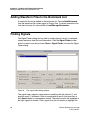
Plot Graph: Some formats (such as ELDO COU) contain display layout
information. Select this item to extract the information and display
waveforms accordingly.
■
Add Bookmark: Add the waveform file to the bookmark list.
■
WDF Properties: Display properties of the selected waveform file.
■
Hierarchy Filter: Set a filter for the children of the node. When any hierarchy
node is filtered out, "more with filter off" is displayed with the hierarchy to
indicate that some nodes are currently hidden.
If multiple files are loaded, to allow simultaneous signal browsing on these
multiple target files, the Open New Browser context menu function opens
multiple signal browsers for each waveform file respectively.
Custom WaveView User Guide
F-2011.09-SP1
23
Chapter 4: Loading and Displaying Waveforms
Using the Output View Browser
Figure 6
Stand-alone floating signal browser
Right-clicking items in the Output View lower signal list window invokes the
signal context menu. The following items are available from the signal context
menu:
24
■
Signal Filter: Select this item to filter the items in the browser based on their
voltage/current type, hierarchy scope, alias name, or name pattern.
■
Show Signal: Switch the signal list between all signals or filtered signals.
■
Name Preference: Switch among the original database name, net name
only by stripping off hierarchy path, or a user-defined alias.
■
Name Sorting: Switch among no sort, alphabetic sort, sort by name length,
then alphabetically, or V()/I() signals first.
■
Signal "NAME": Edit an alias, add to the equation of equation builder, use
as the X-axis-variable, delete (for selected derived signals), modify (for a
derived equation), or Display/Export dcop values from Spectre parametric
analyses.
Custom WaveView User Guide
F-2011.09-SP1
Chapter 4: Loading and Displaying Waveforms
Using the Output View Browser
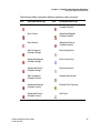
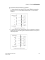
The following tables summarize different waveform types and icons:
Icon
Analog Waveform Type
Icon
Analog Waveform Type
Real Voltage
(Real,Imaginary)
Complex Generic
Real Current
(Magnitude,Degree)
Complex Generic
Real Generic
(Magnitude,Phase)
Complex Generic
(Real,Imaginary)
Complex Voltage
Real Voltage Alias
(Magnitude,Degree)
Complex Voltage
Real Current Alias
(Magnitude,Phase)
Complex Voltage
Real Analog Alias
(Real,Imaginary)
Complex Current
Sweeping Parameter
(Magnitude,Degree)
Complex Current
Derived Data Top Level
(Magnitude,Phase)
Complex Current
Wire Type
Custom WaveView User Guide
F-2011.09-SP1
25
Chapter 4: Loading and Displaying Waveforms
Filtering Signals
Icon
Icon
Digital Waveform Type
Icon
Digital Waveform Type
Logic Integer
Logic Register
Logic Supply
Logic Alias
Logic Parameter
Logic Variable
Logic Wire
(Magnitude,Phase)
Complex Generic
Icon Type
Icon
Icon Type
Waveform Data File (no signal
displayed, not linked)
Generic signal alias name
Linked Waveform Data File
(linked wto netlist)
Voltage signal alias name
Data file with some of its
signals displayed
Current signal alias name
An old data file that has been
overridden by new result
Logic signal alias name
Filtering Signals
To filter the list of signals in the Signal Browser, enter the name or name pattern
of the signal name you want to find into the Filter text box, which is just below
26
Custom WaveView User Guide
F-2011.09-SP1
Chapter 4: Loading and Displaying Waveforms
Displaying Signals
the Signal Browser. Any signals that do not match those characters are filtered
from the list.
Displaying Signals
Signals from the Output View browser can be loaded into a waveview with the
drag-and-drop operation. If a hierarchy (or file) entry is dragged from the upper
hierarchy browser of Output View, all signals in the selected hierarchy level (or
a file) are loaded. If a signal (or multiple signals) is dragged from the signal list
window of Output View, only the selected signals are loaded. Double-click
action can also be used in the lower signal window to add an individual signal.
Depending on the signals being dragged, drop hints appear when signals are
dragged over a waveview area. If the waveview is empty, hint boxes indicate
available initial waveview modes. If the waveview contains existing panels,
insertion hint or drop-in box indicates the drop location.
If any signal from a waveform file is being displayed in a waveview window, the
file icon changes, and the signal name is displayed in blue.
Updating Waveforms
Custom WaveView supports reading growing waveform data files during a
simulation job. Click the Update Waveforms toolbar button or choose File >
Update Waveform Files to update all displayed and derived signals.
If you restart a new simulation to override the old waveform data file, the update
function automatically detects recreated data files and prompts you to select
between keeping the old result or updating to new result.
If you keep the old data file, only the signals that are loaded are available from
the old data file (because the old file is overwritten). An old data file is indicated
by its blue file icon. To update an old data file to the new result, right-click the
file in the Output View Browser and choose Update WDF from the context
menu.
To display signals from both the new and the old data file, choose to keep the
old result. Custom WaveView keeps the old result file and automatically opens
the new data file.
Custom WaveView User Guide
F-2011.09-SP1
27
Chapter 4: Loading and Displaying Waveforms
Clearing Waveforms
If you need to update the WDF signal list, you can right-click the name of a file
in the Output View browser and choose Reload WDF Signal List from the
menu that appears.
Waveform Marching (Automatic Update)
To automatically update waveforms from a running simulation job, choose File
> Waveform Marching … from the main menu. Enter the desired update
interval and the abort trial limit and click the Start button to start waveform
marching. Automatic update is stopped if the waveform file is not growing after
the retrial limit. The automatic update function can be manually stopped at
anytime by clicking the Stop button in the same dialog window.
If the automatic waveform marching is enabled, it is indicated with an icon in the
main application toolbar.
Clearing Waveforms
To clear all currently displayed waveforms, right-click on a waveform and
choose Clear Waveforms from the menu that opens. All displayed waveforms
are cleared.
Grouping Waveform Files
Multiple waveform files can be collected into a group. When signals are loaded
from a member in the grouped waveform files, Custom WaveView automatically
loads the same signals from other waveform files in the same group.
The grouping function is useful for loading signals from corner/alter simulations
that usually involve multiple output files. To group multiple waveform files,
choose File Grouping from the wdf context menu. The Waveform File
Grouping dialog appears.
Select waveform files in the list to group/ungroup them. For waveform formats
that have associated sweeping parameters (such as the COU and the PSF
format), click Select… to filter files based on their parameter value conditions.
28
Custom WaveView User Guide
F-2011.09-SP1
Chapter 4: Loading and Displaying Waveforms
Grouping Waveform Files
Figure 7
The waveform grouping dialog window
The File Grouping function only ties multiple files into a group. It does not
assign any parameter condition to each individual file. As a result, parametric
analysis is not possible on these grouped files. To add corner parameter
conditions to files, the files must be grouped into a file set using a link file
(similar to the runObjFile approach). The link file not only specifies which files
to be grouped, it also defines the associated parameter conditions for each file
in the group. Grouped files using the link file are processed as a single file as if
the result is from a sweep analysis. Since the link file provides sweeping
parameter conditions, parametric analysis is also supported.
To create the link file, right-click a file name and choose Create File Set from
the context menu. To add parameter conditions to a file, enter the value in the
(name=value) format, multiple values are delimited by comma (for example,
temp=0,vdd=3.3). Click Add to add the parameter values to a file and the new
values are indicated in the file list. Note that each of the files in a file set must
have the same number of the same parameters. Finally, enter the path to the
link file and click Ok to create the link file. Once a link file is generated, it can be
opened directly as a regular waveform file.
Custom WaveView User Guide
F-2011.09-SP1
29
Chapter 4: Loading and Displaying Waveforms
Adding Waveform Files to the Bookmark List
Adding Waveform Files to the Bookmark List
A waveform file can be added to the bookmark list. Choose Add Bookmark
from the waveform file context menu in Output View. To reload a waveform file
from the bookmark list, choose File > Load/Manage Bookmarks.
Finding Signals
The Signal Finder dialog can be used to search signals from all (or selected)
loaded waveform data files and hierarchies. Click the Signal Finder toolbar
button or select from the top menu Tools > Signal Finder to invoke the Signal
Finder dialog.
Figure 8
The signal finder dialog window
The signal finder supports name patterns matching with the asterisk (*) and
question mark (?) wildcards. Enter a search pattern and hit the return key or
click Search button to commence a search. The search results are displayed in
the right signal list window. Click a signal from the list window to highlight the
30
Custom WaveView User Guide
F-2011.09-SP1
Chapter 4: Loading and Displaying Waveforms
Finding Signals
signal source in the OutputView browser. Drag-and-drop operations are also
supported from the signal finder result window into any waveview window. You
can sort the results alphabetically by clicking the A-Z Sort and Z-A Sort
buttons.
The search target signals can be refined to Voltage/Current signals only or All
Signals by clicking one of the Type Filter option radio buttons. To limit the
search to a file or a hierarchy level, select the corresponding entry from the left
file/hierarchy browser. If the Selected Level Only option is selected, the target
signals are those in the selected hierarchy/file only. If the Include Sub Levels
option is selected, the target signals are those in and below the selected
hierarchy/file.
On UNIX platforms, select the Multiple Selection option to select multiple
hierarchy entries as the search target.
The All and the None buttons are used to select/de-select all items in the right
signal list window for the drag-and-drop operations.
Click Plot Overlap or Plot Stack to plot selected signals from the result
window in overlap or stack mode.
The Case Sensitive option controls the signal name case sensitivity, while the
Net Name Only and the Full Hier Name options control which part of the
signal names to be used in the search process.
The Show Hierarchy, Show Filename, and Show Path+Filename options
can be used to control the name appearance in the search result browser.
Custom WaveView User Guide
F-2011.09-SP1
31
Chapter 4: Loading and Displaying Waveforms
Finding Signals
32
Custom WaveView User Guide
F-2011.09-SP1
5
File Format Support
5
This chapter contains information on the supported file formats.
This chapter contains the following major sections:
■
Supported Formats
■
Reading Compressed Waveform Files (UNIX Only)
■
Synopsys WDF Format
■
Importing .err* Error Files
■
Converting Existing Output Files
■
WDF Data Reduction
■
Direct WDF Output from Synopsys HSIM
■
Direct WDF Output from Synopsys NanoSim
■
Direct WDF output from Cadence Spectre or UltraSim
■
Direct WDF output from Cadence Verilog-XL/NC-Verilog
■
Reading Textual Data
■
Loading Multiple Files in Virtuoso
■
Special Note for the ELDO COU Format
■
Special Note for the ADMS/ELDO WDB Format
■
Special Note for the PSF Format
■
Special Note for the WDF and fsdb Formats
Custom WaveView User Guide
F-2011.09-SP1
33
Chapter 5: File Format Support
Supported Formats
Supported Formats
Custom WaveView supports the following waveform formats:
■
Cadence Spectre PSF, WSF (binary/ASCII), runObjFile
■
Cadence PSPICE DAT (binary), Allegro SIM (ASCII)
■
Verilog VCD (ASCII), ModelSim WLF (binary)
■
Synopsys HSPICE tr0, sw0, ac0, mt0, hb0, nw0, mc0, mct0, listing file
(Binary/ASCII)
■
Synopsys StarSim wdb, wv, xp (binary)
■
Synopsys HSIM/NanoSim/XA wdb (binary)
■
Synopsys HSIM/NanoSim/TimeMill/Powermill out ,vector, .mt file (ASCII)
■
Synopsys Saber AI/PL (binary/ASCII)
■
Synopsys VCS/Magellan/DVE VPD (binary)
■
Synopsys XA .err, .errz, and .errt files
■
Mentor Graphics ELDO/ADMS COU, WDB (binary), AdiT TR0/TB0.
■
SPICE3/SmartSpice raw format (binary/ASCII)
■
Agilent ADS .ds format (binary), TouchStone S-parameters (ASCII)
■
CSDF (Common Simulation Data Format) (ASCII)
■
Novas fsdb files (binary, v4.3)
■
Text file, CSV (comma separated values) format
■
Other in-house simulator formats (SDIF, MICS, TI-punch)
■
Synopsys WDF format (binary)
■
Binary scope data (Tektronix, Agilent, Lecroy)
■
IBIS models, Synopsys Liberty® files
Reading Compressed Waveform Files (UNIX Only)
On UNIX platforms only, compressed (.Z) or gzipped (.gz) waveform files can
be directly open in Custom WaveView. The tar.gz waveform files are not
readable directly since a tar file can potentially contain multiple files.
34
Custom WaveView User Guide
F-2011.09-SP1
Chapter 5: File Format Support
Synopsys WDF Format
By default the current working directory is used as the temporary directory to
store the decompressed files. Decompressed files are automatically cleaned
up when a the compressed file is closed in WaveView. Set the
SW_SX_TMP_DIR environment variable to redirect the temporary directory to a
different location.
Synopsys WDF Format
The WDF (Waveform Data File) format is a Synopsys proprietary waveform
storage format. The WDF format not only compresses analog and logic
waveform data, it also facilitates fast waveform access for large data files. The
compression scheme can be lossy or loss-less (default). Waveform data files in
other formats can be converted into WDF files on demand.
The WDF format is directly supported by a number of simulators including
HSIM, NanoSim, UltraSim, Spectre, AMS-Designer, and TimeMill/PowerMill.
You can extract signal files as a group. For example, you can create the
following Tcl script file to extract signal files:
set f1 [sx_open_sim_file_read ./group.grp]
sx_current_sim_file $f1
set sig [sx_signal x1]
set sig2 [sx_signal x2]
set f2 [sx_open_sim_file_write ./save2d.wdf]
sx_save_signal $f2 "$sig $sig2"
sx_close_sim_file $f2
sx_close_sim_file $f1
Importing .err* Error Files
To open an .err file, choose File > Import .err File from the main menu bar.
The errors are displayed in the .err File viewer dialog box.
Converting Existing Output Files
One or more output files can be converted (in batch mode) to Synopsys WDF
files using the -c command-line option.
Custom WaveView User Guide
F-2011.09-SP1
35
Chapter 5: File Format Support
WDF Data Reduction
Lossless Compression
With lossless compression, all original simulation output data points are
preserved.
wv -c file1 file2 … filen
Lossy Compression
You can use the -r command-line option to turn on data reduction for the
compression process. Use -r 1 for moderate reduction or -r 2 for a more
aggressive reduction.
wv -c -r (1 or 2) <-rv 0.001> <-ri 10n>
WDF Data Reduction
The data reduction option removes redundant data points from straight
waveform segments based on user-specified error tolerances. Data points are
removed if the error between the original data points and the reduced PWL
segments are smaller than the user-specified tolerance. The following figure
depicts the scheme used in WDF data reduction.
max. error tolerance
Bad reduced segment if
point A is also removed.
error > tolerance
OK reduced segment
error
A
Original
Segments
Points Removed
Figure 9
36
WDF data reduction scheme
Custom WaveView User Guide
F-2011.09-SP1
Chapter 5: File Format Support
Direct WDF Output from Synopsys HSIM
The moderate reduction setting keeps at least 1 point out of four (4) original
data points, while the more aggressive reduction mode keeps 1 out of ten (10)
points. The -rv and -ri options are used to specify the reduction tolerance for
voltage (or generic) waveforms and current waveforms respectively. The default
setting is 5mV for voltage waveform and 1nA for current waveforms.
Direct WDF Output from Synopsys HSIM
In order to generate output files in the Synopsys WDF format using HSIM, you
need to execute HSIM in association with the dynamic runtime library
libWDF.so. If you are running HSIM 2.0, the runtime library is included with
HSIM release. If you are running HSIM 1.3, please contact your HSIM vendor
to get a copy of the runtime library.
Required Netlist Parameters
HSIM uses two netlist parameters to specify the output format: HSIMOUTPUT
and HSIMCOILIB. HSIMOUTPUT specifies the format type, while HSIMCOILIB
specifies the path to the dynamic runtime library used to generate the output.
To create output files in the Synopsys WDF format, add the following
parameters to your netlist. The parameter HSIMCOILIB setting can be omitted
if the runtime library is in the same directory with HSIM binary.
.PARAM HSIMOUTPUT=WDF
.PARAM HSIMCOILIB=<full_path_to_libWDF.so>
Example:
param HSIMOUTPUT=WDF
param HSIMCOILIB=/usr/local/lib/libWDF.so
Direct WDF Output from Synopsys NanoSim
The libwdf.so runtime library is required to generate the Synopsys WDF output
directly from NanoSim.
Custom WaveView User Guide
F-2011.09-SP1
37
Chapter 5: File Format Support
Direct WDF Output from Synopsys NanoSim
You can customize your simulation environment with one of the following ways
to select the WDF format as your output format:
■
Specifying WDF as the Default in .epicrc
■
-out Command-Line Options
■
*NanoSim cfg Command
■
Configuration Command
Specifying WDF as the Default in .epicrc
To configure WDF as the default output format, add (or modify) the following
commands in your .epicrc environment file:
print_format:wdf
output_postfix:wdf
output_custom_library_name:libwdf.so
output_custom_library_path:/path/to/libwdf.so
The .epicrc file is located in your home directory, your current working directory,
or the installation directory, as defined by $EPIC_HOME.
-out Command-Line Options
To configure WDF locally as the output format for a simulation job, add the
following options to your command line:
-out wdf
-outpostfix wdf
-outclname libwdf.so
-outclpath /path/to/libwdf.so
Only the -out option is necessary. The -outpostfix, -outclname, -outclpath
options are not required. Their default value is wdf, libwdf.so, and ./,
respectively.
*NanoSim cfg Command
To configure WDF as the output format for a design, add the following comment
line in your SPICE netlist file:
38
Custom WaveView User Guide
F-2011.09-SP1
Chapter 5: File Format Support
Direct WDF output from Cadence Spectre or UltraSim
*Nanosim cfg="set_print_format for=wdf lib_name=libwdf.so path=/
path/to/libwdf.so postfix=wdf
The command needs to be added in a single comment line. Default value for
lib_name, path and postfix is libwdf.so, ./, and wdf, respectively.
Configuration Command
Use the set_print_format configuration command directly to specify WDF
as the output format. For example:
set_print_format for=wdf lib_name=libwdf.so path=/path/to/
libwdf.so postfix=wdf
Default value for lib_name, path, and postfix is libwdf.so, ./, and wdf,
respectively.
Direct WDF output from Cadence Spectre or UltraSim
Add the following netlist command to generate WDF files from UltraSim (6.0 or
newer revision):
.usim_opt
wf_format=wdf
Add the following option to a Spectre netlist to output WDF files directly from
Spectre (5.1.41 or newer revision):
options rawfmt=wdf
Direct WDF output from Cadence Verilog-XL/NC-Verilog
Runtime library libvpi.so is required to generate Synopsys's WDF output
directly from Cadence Verilog-XL/NC-Verilog simulators. Please contact
Synopsys support to get a copy of the runtime library.
Make sure that the directory path to the runtime library libvpi.so is included in
the LD_LIBRARY_PATH environment variable.
Custom WaveView User Guide
F-2011.09-SP1
39
Chapter 5: File Format Support
Reading Textual Data
The following WDF system tasks can be used in Verilog initial blocks to control
the WDF output:
System Task
Description
$wdf_open("output_filename")
$wdf_open is used to specify the output file name.
$wdf_probe(list of modules)
$wdf_probe is used to enable WDF dump for the
specified modules.
$wdf_close()
$wdf_close is used to close the open WDF file.
Reading Textual Data
Custom WaveView supports data input in regular text format. Scaling factors
(e.g. 1ns) and scientific formats (e.g. 1.0e-9) are both supported in the textual
data files.
To distinguish Custom WaveView text data files from regular text files, the first
line of a text data file is reserved for the format specification and must appear in
the following form, where format-type is the format type keyword:
#format format-type
Lines beginning with a number sign (#) are treated as comments.
The following sections describe how to prepare textual input for
■
Tabulated Data in Real Numbers
■
Tabulated Data in Complex Numbers
■
2-Dimension Sweep Data in Real Numbers
■
2-Dimension Sweep Data in Complex Numbers
■
Measured Data without Name Header
■
SPICE PWL sources
Tabulated Data in Real Numbers
Syntax:
#format table
40
Custom WaveView User Guide
F-2011.09-SP1
Chapter 5: File Format Support
Reading Textual Data
xvar signal1 signal2 ....
valuex value1 value2 ...
...
xvar and signaln are variable names and valuen are numeric values. As a
special-case exception, the first line can be omitted if the name of xvar is
TIME.
Example 1:
#format table
VGATE Ichannel
0.0 0.0
1.0 1u
2.0 5u
3.0 5.2u
...
Example 2:
Custom WaveView can recognize the following data file without the #format
line:
TIME V(1) V(2)
0.0 5.0 2.5
1n 4.8 2.6
...
If the data file does not contain the x-value column, (commonly seen in
measurement data), add keyword #dataonly to the #format line. Custom
WaveView reader automatically assigns a 0-based row index as the x-axis
value.
If the signal names are embedded in the last '#' comment line before the actual
waveform data values, add keyword #cmt_name to the format line.
Tabulated Data in Complex Numbers
Format for complex numbers in (real, imaginary) form.
Syntax:
#format complex-ri
xvar signal1 signal2 ....
valuex value1-real value1-imag value2-real value2-imag ...
...
Format for complex numbers in (magnitude, angle [0-360]) form.
Custom WaveView User Guide
F-2011.09-SP1
41
Chapter 5: File Format Support
Reading Textual Data
Syntax:
#format complex-ma
xvar signal1 signal2 ....
valuex value1-mag value1-angle value2-mag value2-angle ...
...
Format for complex numbers in (magnitude, phase [0-2 ]) form:
Syntax:
#format complex-mp
xvar signal1 signal2 ....
valuex value1-mag value1-phase value2-mag value2-phase ...
...
Example:
#format complex-ri
Freq vout
100meg 0.0 0.0
200meg 1.0 0.1
300meg 1.1 0.2
400meg 1.4 0.4
...
2-Dimension Sweep Data in Real Numbers
Syntax:
#format 2dsweep xvar2
xvar signal1 signal2 ....
#sweep value1-x2
valuex value1 value2 ...
...
#sweep value2-x2
valuex value1 value2 ...
...
where xvar2 is the name of the second sweep variable.
Example:
42
Custom WaveView User Guide
F-2011.09-SP1
Chapter 5: File Format Support
Reading Textual Data
#format 2dsweep vgs
VDS Ichannel
#sweep 0.0
0.0 0.0
1.0 1u
2.0 5u
3.0 5.2u
#sweep 0.1
0.0 0.0
1.0 2u
2.0 6u
3.0 6.2u
...
2-Dimension Sweep Data in Complex Numbers
Format for complex numbers in (real, imaginary) form
Syntax:
#format 2dsweep-ri xvar2
#sweep value1-x2
xvar signal1 signal2 ....
valuex
value1-real value1-imag value2-real value2-imag ...
...
#sweep value2-x2
xvar signal1 signal2 ....
valuex value1-real value1-imag value2-real value2-imag ...
...
Format for complex numbers in (magnitude, angle [0-360]) form.
Syntax:
#format 2dsweep-ma xvar2
#sweep value1-x2
xvar signal1 signal2 ....
valuex value1-real value1-imag value2-real value2-imag ...
...
#sweep value2-x2
xvar signal1 signal2 ....
valuex value1-real value1-imag value2-real value2-imag ...
...
Format for complex numbers in (magnitude, phase [0-2 ]) form.
Custom WaveView User Guide
F-2011.09-SP1
43
Chapter 5: File Format Support
Reading Textual Data
Syntax:
#format 2dsweep-mp xvar2
#sweep value1-x2
xvar signal1 signal2 ....
valuex value1-real value1-imag value2-real value2-imag ...
...
#sweep value2-x2
xvar signal1 signal2 ....
valuex value1-real value1-imag value2-real value2-imag ...
...
Example:
#format 2dsweep-ma temp
freq gain
#sweep 50
100meg 1.0 0
200meg 1.0 90
300meg 1.1 120
400meg 1.4 150
#sweep 75
100meg 1.0 0
200meg 1.0 80
300meg 1.2 110
400meg 1.3 140
...
Measured Data without Name Header
To import text measure data that does not have name header line or the x-axis
value column, choose File > Import Text/PWL Data from the main menu bar.
The Text/PWL Data Table window opens.
Select the desired options and click Ok to load the data file.
Note:
When you open a Touchstone or SC0 file, the Z and Y
parameters from the S parameters are generated and listed in
the signal list.
SPICE PWL sources
To import SPICE PWL sources into Custom WaveView, click the top menu File
> Import Text/PWL Data… to open the Text/PWL Data Table dialog window.
44
Custom WaveView User Guide
F-2011.09-SP1
Chapter 5: File Format Support
Loading Multiple Files in Virtuoso
Choose the SPIEC PWL Source Data option and click Ok to load the data file.
The SPICE PWL sources must not use any variable parameters.
Loading Multiple Files in Virtuoso
Parametric simulations in the Virtuoso environment can generate multiple
output files in multiple directories. The locations and associated sweeping
variables of these files can be found in the runObjFile log file.
The runObjFile can be opened directly in WaveView to access these waveform
files.
Virtuoso dcOp Parametric Analysis
A dcOp analysis from a Virtuoso parametric run can also generate multiple
result files. Each of these corner files contains a single-point operating point
result for each device parameter. A special function is added in the Output View
signal browser context menu to display or export these single-point values
together with their sweeping variable conditions. Right-click a signal in the
signal browser, and choose Signal ’NAME’ > Display Values or Signal
’NAME’ > Export Values.
Special Note for the ELDO COU Format
The COU format from ELDO simulator can contain multiple simulation runs.
Before loading a COU file, COU reader in Custom WaveView needs to scan the
entire file in order to determine how many runs the COU file contains.
For very large COU files, the detection process might take very long time since
the reader has to sequentially examine all data in the COU files.
To speed up this COU file loading process, Custom WaveView has an
alternative built-in search algorithm that can cut the file loading time
significantly. To invoke the fast read option, set the SW_SX_FAST_COU
environment variable to any value in your shell (ex. setenv
SW_SX_FAST_COU). Due to the nature of the COU format, the fast search
algorithm has a trade-off that might potentially determine the number of runs of
a COU file incorrectly. Although the possibility if very low, the user can always
Custom WaveView User Guide
F-2011.09-SP1
45
Chapter 5: File Format Support
Special Note for the ADMS/ELDO WDB Format
choose to disable the fast search algorithm by unset the environment variable
with (unsetenv SW_SX_FAST_COU).
Special Note for the ADMS/ELDO WDB Format
Custom WaveView by default uses a built-in WDB file reader to load data from
WDB files generated by ADMS and ELDO. However, for small amount of
simulation waveform data, the WDB writer in these simulators might buffer
waveform data in the WDB Java server without writing them to a disk file. To
work around this problem, you can take one of the following actions:
1. For ELDO, set the -isaving option to a smaller value to force more frequent
incremental saving to disk files. The file size specified in the -isaving option
is in MB. For ADMS, set the JwdbSpillThreshold option in $HOME/
.vams_setup to a smaller value to lower the buffer size.
2. Enter setenv SW_SX_JWDB_API 1 at the command line to use the
vendor-provided WDB API to load data directly from the Java WDB server.
The API + Java WDB server operation, however, can be very slow for large
WDB files.
Special Note for the PSF Format
PSF format assigns a unit for each signal in a simulation output file. For noise
analysis, in order to display different waveforms using proper scales, signals
with V^2/Hz unit are automatically converted to V/sqrt(Hz) by taking the square
root of the loaded value during the waveform loading process.
The PSF format splits large output data (> 2GB) into multiple 2GB PSF files.
The subsequent PSF files are hidden in the same directory (for example, the
hidden file name starts with a period). Custom WaveView automatically looks
for the subsequent files in the same directory and loads waveform data from
these files.
46
Custom WaveView User Guide
F-2011.09-SP1
Chapter 5: File Format Support
Special Note for the WDF and fsdb Formats
Special Note for the WDF and fsdb Formats
The WDF and the fsdb format both support split files. When Custom WaveView
opens a WDF or fsdb file, it automatically looks for subsequent files in the same
directory. For example, if the loaded file is output.wdf, Custom WaveView
automatically looks for output.wdf.1. If the output file is output.fsdb.1, Custom
WaveView looks for output.fsdb.2. If you do not want to load the subsequent
split files, disable the Automatically connect to subsequent split files option
in the Loading Waveform Files dialog window.
Custom WaveView User Guide
F-2011.09-SP1
47
Chapter 5: File Format Support
Special Note for the WDF and fsdb Formats
48
Custom WaveView User Guide
F-2011.09-SP1
6
6
Displaying Waveforms
This chapter contains information on how to display different types of
waveforms.
Panels are created automatically when signals are dropped into a waveview
window. Default panel type is selected based on the signal type. To manually
add a specific type of panel into the active waveview window, choose Panel >
New from the main menu.
The following panel types are available:
■
X-Y Panel
■
Logic Panel
■
Smith Chart Panel
■
Polar Plot Panel
■
3-D Sweep Panel
■
2-D Sweep Panel
■
Eye Diagram Panel
■
Histogram Panel
■
Separator Panel
X-Y Panel
An X-Y panel is designed to display analog waveforms. It is the only panel type
that is allowed in both vertical stack and row/column waveviews. The X-Y panel
accepts signals that are represented in (valuex,valuey) pairs, ( (x,y) data points,
for example), where valuex can be the default sweeping variable of a signal, or
Custom WaveView User Guide
F-2011.09-SP1
49
Chapter 6: Displaying Waveforms
Logic Panel
the signal value of a regular signal; valuey can be either the value of a realsignal or the magnitude/phase/real/imaginary part of a complex signal. The
zoom operation is supported along both axes, and the logarithmic scale is also
supported along both axes.
Waveforms in linear X-Y panels can be displayed with different plotting options
including PWL (piece-wise-linear) line-type, PWC (piece-wise-constant) linetype, bar chart and data-point only mode. Choose Panel > Display Preference
to change the plotting mode.
Logic Panel
A logic panel displays signals using digital timing diagram. It is permitted only in
vertical stack waveviews. Logic panels accept signals that are represented in
(time, logic) pairs. Various logic states including logic strength levels are
supported. Zoom operation is supported along the x-axis direction.
Logic panels cannot be manually added from the application top menu. They
are automatically created when logic signals are dropped into a vertical
waveview.
Current vector width (number of bits) and radix setting of a logic panel are
indicated in the left column of each panel (B: binary, O: octal, D: decimal, H:
Hex-decimal, A: ASCII). The width digits are red color-coded for bus signals
formed from originally separated bits, or yellow color-coded for a single bit
extracted from an originally grouped bus signal.
Logic panels can be arbitrarily mixed with linear X-Y panels in a vertical stack
waveview.
Mnemonic Mapping for Bus Signals
WaveView supports mapping bus values to pre-defined text strings. The
translation table can be provided in an external file.
Syntax:
# comment lines start with '#'
value1 name1
value2 name2
…
The values are the bus values to be mapped.
50
Custom WaveView User Guide
F-2011.09-SP1
Chapter 6: Displaying Waveforms
Smith Chart Panel
The following formats are supported:
■
2400
■
0xAF32
■
'hAF32
■
'b1001_0100_0101
■
'd2400
■
'b110110111100
■
'o371
The names are the text strings to be mapped to. A text string must be quoted if
the name contains spaces.
You can load the translation table by choosing Config > Bus Mnemonic Map
…. Once a translation table is loaded, choose Radix > Mnemonic On/Off from
the panel context menu to toggle the mapping settings.
Smith Chart Panel
Smith charts display complex normalized impedance, admittance and
scattering parameters (S-parameters).
The Smith chart accepts signals that are represented in (real, complex) pairs.
The normalized impedance is defaulted at 50 ohms and can be modified in
Preference Settings (see the smith_char_impedance option in the .spxrc
configuration file).
Smith charts are allowed only in horizontal waveviews and the zoom operation
is not supported.
You can configure a Smith chart in the Smith Chart Settings dialog box. Choose
Configure Smith Chart from the panel context menu to open the dialog.
Enter the desired setting preferences and click Apply to apply the changes.
Cursors (up to two) in a Smith chart can be used to trace Gamma (the
reflection coefficient), SWR (standing wave ratio), impedance (Z) or admittance
(Y) at the location where the cursor hairs cross.
Custom WaveView User Guide
F-2011.09-SP1
51
Chapter 6: Displaying Waveforms
Polar Plot Panel
Polar Plot Panel
Polar plots display data on a complex plane. They are allowed only in horizontal
waveviews. The Polar plot accepts signals that are represented in (real,
complex) pairs. The zoom operation is supported only along the radial
direction.
3-D Sweep Panel
The 3-D Sweep panel displays 2-dimensional sweeping data on a 3-dimension
coordinate. It is allowed only in horizontal waveviews. The 3-D Sweep panel
accepts signals that are represented in ((x1, x2), value) pairs, where x1 and x2
are the first and second independent sweeping variable respectively, and value
can be either the value of a real signal or the magnitude/phase/real/imaginary
part of a complex signal. The viewing angles of the 3-dimension coordinate can
be interactively adjusted from the two sliders in the panel. The zoom operation
is not supported. Logarithmic scale is supported only along the vertical axis.
2-D Sweep Panel
The 2-D Sweep panel displays 2-dimensional sweeping data on a flat X-Y
plane. It is allowed only in horizontal waveviews. Similar to the 3-D Sweep
panel, the 2-D Sweep panel accepts signals that are represented in ((x1, x2),
value) pairs. Zoom operation is supported along both axes. Logarithmic scale is
also supported along both axes (the x1 direction and the y direction, for
example).
Both 2-D and 3-D sweep panels support sweep filters that display the selected
sweep traces. Choose Sweep Line Filter from the panel context menu, and
highlight traces in the Sweep Line Filter dialog.
Enable the Display Trace Value option to display value label next to each
sweep trace. If a 2D/3D sweep panel contains more than one signal, the first
signal or the first highlighted signal is used as the filter target.
In 2-D sweep plot, the min/max Y-value bounds and the average Y-value of a
multi-trace signal can be automatically extracted (for example, waveform
envelop from statistical simulation result). To invoke this function, choose Find
52
Custom WaveView User Guide
F-2011.09-SP1
Chapter 6: Displaying Waveforms
2-D Sweep Panel
Envelope Bound from the panel context menu of a 2-D sweep panel. Custom
WaveView scans all data points from all traces and creates three new
waveforms representing the min/max bounds and the average waveform.
Displaying Multi-trace Waveforms
A multi-trace signal contains multiple waveform traces. Each trace has a set of
associated sweeping parameters (or sub X-variables). For example:
Trace1: Temp=0 Vdd=3.3
Trace 2: Temp=0 Vdd=5
Trace 3: Temp=100 Vdd=3.3
Trace 3: Temp=100 Vdd=5
By default, a multi-trace signal is plotted with respect to its main independent
sweeping variable (time, for example). In this case, the sweep line filter function
in a 2D-sweep panel can used to selectively display some of the traces.
The 2D-sweep panel also supports plotting a multi-trace signal with respect to
one of its sweeping parameters. To change the default X-axis of a 2D-sweep
panel to a sub X-variable, choose Change X Variable from the panel context
menu. Drag and drop a sweeping parameter from the Output View browser to
the Setting X Variable dialog window. Choose Sweep Line Filter from the
panel context menu to open the Sub X-Variable Plotting Filter dialog window.
Note:
The filter setup is different between using the default X-axis and
sub X-Variable X-axis. This is because in the sub X-Variable plot
mode, based on the selected sub X-variable, the number of
traces might vary depending on the number of unique
combinations among other sweeping parameters. Custom
WaveView automatically finds out the number of traces, and
sorts the order of the sub X-Variable values to display
waveforms.
A multi-trace signal must have equal number of points in each of its original
traces in order to be plotted in the sub X-variable mode.
The current version of Custom WaveView does not support plotting a multitrace signal with respect to another multi-trace signal.
Custom WaveView User Guide
F-2011.09-SP1
53
Chapter 6: Displaying Waveforms
Eye Diagram Panel
Eye Diagram Panel
The Eye diagram panel is allowed only in horizontal waveviews, although more
than one eye diagram with differing triggers can be plotted on a single panel.
Please see Configuring Eye Diagrams for detailed descriptions on how to use
the Eye Diagram functions in Custom WaveView.
Histogram Panel
The Histogram panel can be placed in horizontal waveviews only. To create a
Histogram, an empty Histogram panel must created first by choosing Panel >
New > Histogram from the main menu. Signals can then be dragged from the
Output View browser and dropped into the Histogram.
A histogram plots an individual histogram for each signal in the panel. The
average value and standard deviation can be annotated on top of each
histogram and the number of bins and data bounds can be reconfigured.
Custom WaveView can also calculate the distribution percentages of regions
divided by user-defined markers from the histogram mean center.
To reconfigure a Histogram, use the Histogram Settings Dialog by choosing
Configure Histogram from the panel context menu. Choose Show Average
Line to enable the average bar. By default, the histogram plots. Choose Show
Single Histogram of all Signals to plot a single histogram of all signals in the
panel. Click the Show normal distribution curve check box to display the
normal distribution curve over the histogram.
Separator Panel
The Separator panel can be used to assign panel groups. All panels after a
separator panel and before the next separator panel are considered a panel
group. A group name can be assigned to a separator panel. Right-click a
separator panel, and choose Edit Label to modify name. Use the left "+"/"-"
icon in a separator panel to expand/collapse the panels in a panel group.
54
Custom WaveView User Guide
F-2011.09-SP1
Chapter 6: Displaying Waveforms
Changing the X-axis Variable
Changing the X-axis Variable
By default, signals in X-Y panels are plotted with respect to their internal X
variables defined in the original waveform data file. The X variable can be
replaced with a signal so that other signals are plotted as functions of the
selected signal.
In a vertical waveview, if the waveview contains no logic panel, you can assign
a signal as the common X variable so that all signals are plotted against the
selected X variable. In a horizontal waveview, the same operation can be
applied individually to all selected X-Y panels.
To select a signal as the new X variable, choose Axes > X Variable from the
main menu to open the Setting X Variable dialog window.
With the dialog open, right click a signal in the Output View signal list window
and choose Use as X Variable. The drag-and-drop operation is also supported
from the Output View browser to the Setting X Variable dialog window. The
name of the newly selected signal is entered in the read-only X Variable dialog
window. Click Apply to apply the change to an active vertical waveview or all
the selected panels in an active horizontal waveview.
To restore to signals' internal X variables, select the Use Internal X Variable
option in the dialog and click Apply.
The drag-and-drop operation can be also used to set the X variable. Drag a
signal from the Output View browser and drop it in the lower X-axis of a stack
waveview, or the X-axis of a X-Y panel in a row/column waveview.
Custom WaveView User Guide
F-2011.09-SP1
55
Chapter 6: Displaying Waveforms
Changing the X-axis Variable
56
Custom WaveView User Guide
F-2011.09-SP1
7
7
Panel Operations
This chapter contains information on the basic panel operations.
This chapter contains the following major sections:
■
Basic Operations
■
Zoom Operations
■
Panel Settings
Basic Operations
Panels in a waveview can be moved, combined, split and deleted. These
actions are invoked from the panel context menu or by choosing Panel >
Actions from the main menu. The following table summarizes the default bind
keys for panel actions:
Bind Key
Function
B
Move the active cursor backward
C
Copy (Panel, Signals)
D
Data point toggle
F
Move the active cursor forward
G
Grid toggle
H
Horizontal zoom/unzoom
Custom WaveView User Guide
F-2011.09-SP1
57
Chapter 7: Panel Operations
Basic Operations
Bind Key
Function
N
Scan forward
P
Scan backward
Q
Quit
S
Signal select/highlight
T
Fit/unfit panel height to full window height
V
Vertical zoom/unzoom
X
Unzoom (reset)
Z
Box zoom/unzoom
Delete or
Backspace
Delete panel/signal
Esc
Deselect all panels
Up Arrow
Scroll up a waveview
Down Arrow Scroll down a waveview
Selecting Panels
Panels can be selected (highlighted) for further actions. To select a panel, left
click over the name/monitor area of a panel. Selected panels appear with their
name area background highlighted in gray. Multiple panels can be Shiftselected or Ctrl-selected.
To select all panels in a waveview, choose Panel > Select All from the main
menu. To deselect all panels, choose Panel > Unselect All from the main
menu.
You can also use the Panel Select control button to toggle between the SelectAll and the Unselect-All operations.
58
Custom WaveView User Guide
F-2011.09-SP1
Chapter 7: Panel Operations
Basic Operations
Moving or Copying Panels
To move or copy a panel, click and hold the left mouse button on a name or
value area of a panel. Drag the panel to a new location and release the mouse
button. If the source panel is selected, all selected panels are moved/copied.
During the dragging process, a drop hint appears to indicate the drop location.
Panels can be moved/copied from a waveview window to another waveview
window. Use the preference settings to select between the Move and the Copy
operations. Panels can also be copied and pasted using the corresponding
menu entries in the panel context menu.
Deleting Panels
To delete a panel, choose Cut from the panel context menu. If the target panel
is selected, all selected panels are deleted.
The panel delete action can also be invoked from the Delete control button.
Pasting Deleted Panels
Deleted panels can be pasted back to any waveviews by choosing Paste from
the panel context menu. The deleted panels are always pasted after the current
panel in which the mouse pointer resides.
Grouping Panels
Selected panels can be grouped into one panel. Choose Group from the panel
context menu or Panel > Actions > Group from the main menu.
If the grouped panels are in a logic panel type, a new bus signal is formed. The
Bus Configuration dialog allows you to configure the bus signal.
Panel grouping action can also be invoked from the Panel Group control button.
Custom WaveView User Guide
F-2011.09-SP1
59
Chapter 7: Panel Operations
Zoom Operations
Ungrouping Panels
Signals inside a panel can be split so that each signal is placed into a new
panel. Choose Ungroup from the panel context menu or Panel > Actions >
Ungroup from the main menu.
Panel ungroup action can also be invoked from the Panel Split control button.
Zoom Operations
Zoom operations are supported in the following panel types:
■
X/Y zoom in X-Y, 2D-Sweep and Eye-diagram panels
■
X zoom in logic panels
■
Radial zoom in Polar Coordinate panels
Depending on the default action type of the left mouse button in a waveview
(default left mouse button action can be selected in Preference Settings >
Waveview > Left Button Default), the zoom operation is invoked with:
■
Cursor mode: You can invoke the zoom operation by first arming a waveview
into the zoom mode. Click the zoom control button to activate the zoom
mode.
■
Zoom mode: The zoom operation automatically starts when you hold down
and drag the left mouse button inside a waveform.
Default Bind Key: Press the Z key to arm the zoom mode and release it to
unarm.
If the left mouse button is defaulted to cursor operations (see Bindkey
Functions), continue clicking the zoom control button cycles the zoom mode in
the following order: X/Y zoom ( ), X zoom ( ), Y zoom ( ), no zoom ( ). The
current zoom mode is indicated with the different icons of the zoom control
button. If the left mouse button is defaulted to zoom operations, continue
clicking the zoom control button cycles the zoom mode among X/Y zoom ( ), X
zoom ( ) and Y zoom ( ).
60
Custom WaveView User Guide
F-2011.09-SP1
Chapter 7: Panel Operations
Zoom Operations
X/Y (Box) Zoom
With a waveview armed in the X/Y zoom mode, click and hold the left mouse
button at a corner of the area to be zoomed in and drag the mouse pointer to
the diagonally opposite corner of the zoom area. Release the button to stop
zooming.
If you arm the X/Y-zoom operation of a waveview with the Z bind key, releasing
the Z bind key without any zoom action results in a 2x zoom out. The same 2x
zoom out action can also be invoked using the Zoom Out control button.
X Zoom
With the zoom control button in X-zoom mode, indicated by zoom control
button. Hold down the left mouse button and drag the mouse pointer along the
horizontal direction to define the X-zoom range.
Default Bind Key: Press the H key to arm the horizontal zoom operation.
If you arm the X-zoom operation of a waveview with the H bind key, releasing
the H bind key without any zoom action results in a 2x x-axis zoom out.
Y Zoom
With the zoom control button in Y-zoom mode, indicated by zoom control
button. Hold down the left mouse button and drag the mouse pointer along the
vertical direction to define the Y-zoom range.
Default Bind Key: Press the V key to arm the vertical zoom operation.
If you arm the Y-zoom operation of a waveview with the V bind key, releasing
the V bind key without any zoom action results in a 2x y-axis zoom out.
X Zoom to Fit
Select one or more panels, and press the I bind key. The zoom to fit is applied
to the selected panel axes. If no panel is selected, the zoom to fit is applied to
all panels.
Custom WaveView User Guide
F-2011.09-SP1
61
Chapter 7: Panel Operations
Zoom Operations
Y Zoom to Fit
Select one or more panels, and press the Y bind key. The zoom to fit is applied
to the selected panel axes. If no panel is selected, the zoom to fit is applied to
all panels.
Un-zoom
To restore all selected panels to their full plotting ranges, click the un-zoom
control button.
Default Bind Key: X
Undo or Redo Zoom
The undo/redo zoom functions allow you to traverse up/down a zoom operation
sequence. Use the undo-zoom function to undo a zoom step and redo-zoom
function to redo a zoom operation.
Default bind keys: U for undo-zoom, R for redo-zoom.
Using Sliders in Zoomed Panels
In a zoomed panel (X-Y, logic or 2D-Sweep), the zoomed area can be
interactively shifted using the horizontal and vertical slide bars. The waveview
is redrawn at real time when the slide bar is moved. This graphic intensive
operation can become noticeably slow especially when you work from a remote
host.
The real-time screen redraw can be disabled for the slide bar to avoid the slow
graphic operation. To disable real-time redraw, disable the Real-time
waveview scroll option in Preference Settings > Waveview. With the realtime waveview scroll disabled, only the grid rulers are interactively redrawn
during slide bar movement.
Setting Zoom Ranges Manually
The zoom operations can be also performed by manually specifying the X-axis
and Y-axis ranges. Choose Axes > Axes Range > Set Zoom from the main
62
Custom WaveView User Guide
F-2011.09-SP1
Chapter 7: Panel Operations
Panel Settings
menu, and enter the zoom range parameters. Then click Ok to set the zoom
level on all panels or selected panels of the active waveview. Note that the Y
ranges are in db (or db10) if the target panel Y-axis is in db (or db10) scale.
Panel Settings
The following panel settings are available:
■
Displaying Data Points
■
Controlling the Grid
■
Adjusting Logarithmic Scales
■
Using Fixed X-axis (or Y-axis) Full Scale
■
Changing Axis Font Size
■
Dual Y-axes
■
Adjusting Panel Height
■
Fitting Panels to Full Window Height
■
Setting Vector Radix
■
Setting Vector Length
■
Setting Waveform Display Preferences
■
Setting the Plot Mode for Complex Signals
■
Setting Panel Attributes
Displaying Data Points
Custom WaveView displays waveform by plotting piece-wise-linear (PWL) lines
between data points. To display the actual data points, click the Data Point
control button to toggle on/off the data point markers.
Default bind key: D.
Custom WaveView User Guide
F-2011.09-SP1
63
Chapter 7: Panel Operations
Panel Settings
Controlling the Grid
You can toggle the grids of selected panels on or off with the Grid control
button.
Grid settings are toggled through the X-Y grid; X-grid only; Y-grid only; and No
grid cycle.
Default bind key: G.
You can also choose Axes > Grid from the main menu to turn X/Y grids on or
off directly.
Grids parameters of XY panels can be redefined. Choose Grid Settings from
the panel context menu or Axes > Grid > User Settings from the main menu to
open the Grid Settings Dialog.
User-defined grids start from the Start value and repeat over the Step interval
in both directions away from the start point.
Adjusting Logarithmic Scales
The X-Y, 2D-Sweep, and 3D-Sweep panels support the logarithmic scales.
Choose Axes > X-Log Setting or Axes > Y-Log Setting from the main menu
to switch X/Y-axis of all selected panels among: linear, logarithmic, db20, and
db10 modes. Axis scales can be also changed directly using the axis context
menu by right clicking over the X/Y axis in a panel.
Logarithmic Y-axis has a range limit of six decades. If a linear Y-axis ranges
from a negative minimum to a positive maximum, three decades are allocated
for the positive and negative half respectively with the negative part coded in
different color.
Using Fixed X-axis (or Y-axis) Full Scale
Fixed plotting ranges can be assigned to the X-axis of X-Y panels. Choose
Axes > X/Y Full Scale > Set X Full Scale from the main menu and enter the Xaxis range parameters. Click Ok to apply the change to selected panels of the
active waveview. The default Y-axis range can be changed by choosing Axes >
X/Y Full Scale > Default Y Full Scale from the main menu.
64
Custom WaveView User Guide
F-2011.09-SP1
Chapter 7: Panel Operations
Panel Settings
Changing Axis Font Size
Choose Axes > Axis Font and either Normal or Large from the Custom
Waveview menu bar to change the font size.
Dual Y-axes
Dual Y-axes are supported in X-Y and the 2D-sweep panels. To display (or
disable) the 2nd Y-axis in a X-Y panel, choose Dual Axis > Show/Hide Right
Axis from the panel context menu. Choose Dual Axis > I-Signals to Right
Axis to display all current signals of a panel using the right axis. Arbitrary
signals can be also attached to (or detached from) the right axis by choosing
Signal "Name" > Right/Left Axis. Signals that are attached to the right axis
are indicated with the icons in front of the signal names.
Setting Axis Attributes
To set axis attributes:
1. Double-click on an axis.
The Axis Attributes window opens.
2. Choose an axis from the Axis menu.
All axes in the active waveview window are available.
3. Click one of the zoom level buttons to change the display:
•
Zoom In increases magnification to show detail.
•
Zoom to Fit displays the maximum number of data points to show the
entire range of a signal. The entire range is determined by the minimum
and maximum values entered in the Full Scale Range text boxes at the
bottom of the Axis Attributes window.
4. Enter values for the zoom level in the Min and Max text boxes.
These values specify the range you want to display.
5. (Optional) Click the Use Waveform Range check box to specify the range
of a signal, and enter the Min and Max values for that range.
6. (Optional) Click the Grid On check box to display the grid for the selected
axes.
Custom WaveView User Guide
F-2011.09-SP1
65
Chapter 7: Panel Operations
Panel Settings
You can click the Auto Grid check box and enter Start and Stop values for
the gridding. You can only turn this option off for linear axes.
7. Choose the axis label font size from the Font menu.
Normal and Large font sizes are available.
8. Choose an axis type from the Type menu.
Axis types include Linear, Log, dB20, dB20, dB10, and dBm10.
9. Click Apply to save your changes.
Adjusting Panel Height
Panel heights in a vertical stack waveview are calculated automatically based
on the following preference settings:
■
Maximum number of visible panels
■
Minimum X-Y panel height
You can adjust the height of a panel by dragging the bottom edge of the left Yaxis area. If the panel in action is a selected panel, the height of all selected
panels is changed. To restore selected panels to their default auto height,
choose Panel > Height > Default.
Individual panel height adjustment is available for analog panels only. To adjust
the height of all logic panels, change the value of Logic Panel Height in the
preference settings.
Fitting Panels to Full Window Height
In a vertical stack waveview, height of selected panels can be automatically
adjusted to fit to the full window height. Choose Panel > Height > Fit to fit all
selected panels to the total window height, or use the default bind key 'T' to
toggle selected panels between fit and unfit modes. If the selected panels are
separated into multiple groups, each group is fitted respectively. If there are too
many panels in a group and the panel height becomes too small, the height is
limited to the user-defined minimum height.
Choose Panel > Height > Fit All to fit all panels of a waveview to the total
window height.
66
Custom WaveView User Guide
F-2011.09-SP1
Chapter 7: Panel Operations
Panel Settings
Setting Vector Radix
Logic vector values by default are displayed in binary. The following radix
selections are supported:
■
binary
■
octal
■
decimal
■
hex-decimal
■
ASCII
Select from the top menu Panel > Radix to select a radix setting for all selected
panels. You can also choose Radix from the panel context menu to select a
radix setting for the panel in action.
Setting Vector Length
Logic vector values by default are displayed in their shortest possible form.
Select from the top menu Panel > Display Preference > Full Logic Value to
display vector values in full length.
Setting Waveform Display Preferences
Analog signals can be displayed as PWL, PWC, Bar, or Data Point Only
waveforms. Choose Panel > Display Preference from the main menu to select
preferred display mode of a panel.
Setting the Plot Mode for Complex Signals
When complex signals are plotted on non-complex panels (X-Y, 2D-sweep, and
3D-sweep), the signals are by default plotted using the magnitude value of the
complex data. You can switch it to the phase, real part, or imaginary part of the
complex data.
Choose Plot Complex from the panel context menu to select the preferred
complex setting. All signals inside a panel are plotted using the same complex
Custom WaveView User Guide
F-2011.09-SP1
67
Chapter 7: Panel Operations
Panel Settings
mode. The following icons are placed before the signal names to indicate the
current complex mode:
■
■
(no icon) real-value waveform
magnitude
■
phase
■
real part
■
imaginary part
■
group delay
To configure how complex signals should be displayed, choose Config >
Preferences > Panel tab and select the preferred Default AC Signal Display
setting. The following settings are available:
■
Complex: Displays a single waveform using the magnitude value of the
complex signal.
■
M/P: Displays the magnitude and the phase of a complex signal respectively
in two panels in stack mode.
■
R/I: Displays the real part and the imaginary part of a complex signal
respectively in two panels in stack mode.
■
M+P: Displays the magnitude and the phase of a complex signal in the same
panel.
Setting Panel Attributes
To set the attributes for a panel, right-click a panel and choose Attributes from
the menu that opens. The Panel Attributes window opens with the options for
the type of panel (analog, digital, or bus).
68
Custom WaveView User Guide
F-2011.09-SP1
8
Waveform Operations
8
This chapter contains information on how to work with and modify waveforms.
This chapter contains the following major sections:
■
Working with Signals and Waveforms
■
Waveform Color Schemes
■
Custom Waveform Colors
■
Modifying Waveform Attributes
■
Adding Text Labels
Working with Signals and Waveforms
Signals in a panel can be deleted, highlighted, or re-paneled. These actions
can be invoked from the signal context menu by right-clicking the name or
monitor area of a panel with the Signal Mode control button armed. Without
arming the signal mode control button, right-clicking the same area opens the
panel context menu.
The signal mode control button is red when armed.
Default Bind Key: Press the S key to arm the signal mode and release it to
unarm.
Highlighting Waveforms
With the signal check control button armed, left-click the name of a signal to
toggle its highlight state on and off.
Custom WaveView User Guide
F-2011.09-SP1
69
Chapter 8: Waveform Operations
Working with Signals and Waveforms
You can also toggle signals highlight by left-clicking the waveforms, which
toggles the highlight states of all signals that intersect the mouse pointer.
Ungrouping Highlighted Waveforms
Right-click a highlighted signal, and choose Ungroup from the signal context
menu to split each of the highlighted signals into a new panel.
Grouping Highlighted Waveforms
Right-click a highlighted signal, and choose Group from the signal context
menu to group all highlighted signals into a new panel.
Deleting Highlighted Waveforms
Right-click a highlighted signal and choose Cut from the signal context menu to
delete all highlighted signals.
You can also move highlighted signals in a panel with a drag-and-drop
operation. With the signal mode control button armed, follow the steps in
(Moving/Copying panels) to move highlighted signals between panels or
waveviews.
Finding the Source of a Waveform
Right-click the name of a signal, and choose Source of "Signal" from the
signal context menu to highlight its source location in the Output View signal
browser. Note that only the Output View signal browser is used to show the
signal source. The floating browsers of individual files, if open, are not used to
show the signal source.
Getting Signal Information
To view the name, file ID, and full path of a signal, move your mouse pointer
over the name of a signal. The signal information is displayed in the button
status bar.
70
Custom WaveView User Guide
F-2011.09-SP1
Chapter 8: Waveform Operations
Working with Signals and Waveforms
Adding Signal Alias
Alias names can be added to signals in waveview windows. To define a new
alias to a signal, choose Signal "name" > Edit Alias from the signal context
menu. Enter an alias name, and click Ok to set the alias. To reset the name of a
signal to its original name, follow the same sequence and enable the Use
Original Signal Name option to reset the signal name.
Scanning Waveforms
Once signals are loaded onto a waveview. You can scan signals from the same
files using the Scan control buttons. This feature can be used to compare
signals from different data files.
Clicking the right arrow button advances signals from all selected panels to
their corresponding next signals from the same waveform data files. Clicking
the left arrow scans signals in the reverse direction.
Please note that scanning signals might require reloading data if the next/
previous signals are not currently loaded. To speed up the scan process by
avoiding data reloading, you might choose to load all waveform data to memory
when waveform data files are initially opened (see Opening Waveform Files).
Default Bind Key: N (next) or P (previous).
Scan Configuration
You can configure the scan function into two different modes:
■
Direct Scan: With the Direct mode, Custom WaveView scans signals
according to their order in the waveform data file.
■
Smart Scan: In the Smart mode, with a master waveform data file selected,
Custom WaveView scans signals from the master waveform data file
according to their order in the file, while automatically searches other
waveform data files for signals with matched names.
To reconfigure the current scan settings, choose Config > Scan Settings…
from the main menu, or click the Scan Config toolbar button to open the ScanControl Settings dialog window.
Custom WaveView User Guide
F-2011.09-SP1
71
Chapter 8: Waveform Operations
Waveform Color Schemes
Select a scan mode and a master file and click Apply to make the change. The
Lock Scope option controls if the scan is limited within the current hierarchy
scope.
Waveform Color Schemes
Custom WaveView provides two default waveform color schemes. Both
methods repetitively assign eight (8) different colors to waveforms.
Local Mode
With the local mode, waveform colors start from the first color for each panel.
Colors are then sequentially assigned to subsequent waveforms in a panel.
Depending on the order of waveforms in a panel, waveform colors might
change while they are moved. You can set the local mode by choosing
Preference Settings > Waveview > Cycle Color By and selecting the Panel
mode.
Global Mode (default)
With the global mode, waveform colors start from the first color for each
waveview. Colors are then sequentially assigned to each waveform in a
waveview. The assigned colors stay with waveforms regardless of their
locations even when they are moved to a different waveview. To select the
global mode, choose Preference Settings > Waveview > Cycle Color By,
and select the Waveview mode.
Custom Waveform Colors
Default waveform color choices can be added or deleted in Preference
Settings > Colors. Up to 16 colors can be assigned as the default colors for
waveforms.
72
Custom WaveView User Guide
F-2011.09-SP1
Chapter 8: Waveform Operations
Modifying Waveform Attributes
Modifying Waveform Attributes
To modify waveform attributes for a waveform:
1. Double-click the signal name of the waveform, or right-click the signal name
and choose Signal ’<signal_name>’ > Attributes from the menu that
opens.
The Waveform Attributes dialog box opens.
2. Choose a signal from the Signal menu to which the attributes are applied.
3. Change any of the following waveform display attributes:
•
Line Color
•
Line Width
•
Dash Type
•
Marker Shape
4. For analog signals, change the following attributes as necessary:
•
Display Preference
•
Hide Signal
•
Axis (left or right)
5. For digital signals, change the following attributes as necessary:
•
Display Preference and type
•
Mnemonic On
•
Radix
6. For analog or digital signals, enter the marker frequency, which changes the
display frequency of the data point markers.
7. (Optional) Click the Turn on Alias check box to change the alias of a signal.
8. Click Apply to save your changes.
Adding Text Labels
Text remarks can be added to a waveview window. Click the Text Remark
control button to open the Remark Text dialog window.
Custom WaveView User Guide
F-2011.09-SP1
73
Chapter 8: Waveform Operations
Adding Text Labels
The label function supports multi-line text. Use the backslash character (\) to
break a text label into multiple lines.
A text remark can be moved within a waveview window. Left-click and drag a
remark box to move the text label. Release the mouse button at a new location
to reposition the text remark.
Text remarks can be anchored to a (x,y) value point in a waveview. An
anchored text remark moves with waveforms when a waveview is panned. Two
font sizes are available: small and large.
To delete a text remark, right-click the text box to invoke the text remark context
menu. Choose Delete Remark to delete the remark or Delete All Remarks to
delete all text remarks in the waveview.
74
Custom WaveView User Guide
F-2011.09-SP1
9
Measurements
9
This chapter contains information on using cursors and measurements.
Custom WaveView provides the following ways to measure waveforms:
■
Cursors: Used to trace waveform values. Unlimited cursors can be added.
See Working with Cursors for more information.
■
Monitors: Used to monitor global waveform properties such as minimum,
maximum, average, RMS, and peak-to-peak values. Monitors can be
associated with cursors to trace waveform values such as derivative and
difference, or associated with the viewing ranges to display local minimum,
maximum, average, RMS, and peak-to-peak values. See Working with
Monitors for more information.
■
Measurements in the Measurement Tool: Used to make interactive
measurements on a waveform or between different waveforms. Various
measure types are available including rise/fall time, frequency, width, and
jitter. See Using the Measurement Tool for more information.
Working with Cursors
Cursors are used to trace waveform related values. Multiple cursors can be
added to a panel. The X-axis position of a cursor is indicated underneath the
cursor hair.
Adding Cursors
To add a cursor, choose Add Cursor from the panel context menu. A cursor
can also be created using the Add-Cursor control button.
Custom WaveView User Guide
F-2011.09-SP1
75
Chapter 9: Measurements
Working with Cursors
You can also add cursors for delta measurements by pressing the left- and
right-bracket keys ( [ and ] ) while moving the cursor.
The Active Cursor
When multiple cursors are added to a panel, the last moved or added cursor
becomes the active cursor.
Waveform values corresponding to the active cursor are displayed in the
monitor. In an X-Y panel, distances from all non-active cursors to the active
cursor are displayed next to the active cursor.
Moving a Cursor
Depending on the default action of the left mouse button in a waveview (default
left mouse button action can be selected in Preference Settings > Waveview
> Left Button Default), a cursor can be moved with:
■
Cursor Mode: If the left mouse button is pressed with mouse pointer near a
cursor, the cursor is grabbed. A grabbed cursor can be dragged to a new
position. If the mouse pointer is not in the vicinity of any cursor when the left
mouse button is pressed, the active cursor is grabbed regardless of its
position.
■
Zoom-First Mode: If the left mouse button is pressed and released without
any mouse pointer movement. The active cursor is grabbed to the mouse
pointer location when the button is released.
In a zoomed panel, cursors outside the plotting range are placed on the left (or
right) boundary of the plotting area. They can be grabbed from the borders of
the plotting area. The cursor that is outside but closest to the boundary is
grabbed first.
Jumping Cursors
In an X-Y or logic panels, a cursor can be jumped forward (or backward) to the
next (or previous) data point, peak, switching or crossing point using the cursor
context menu. Right-click near the cursor to invoke the cursor context menu.
Choose Jump (F)orward "SIGNAL" or Jump (B)ackward "SIGNAL" from the
context menu to jump the cursor forward or backward on the target signal
SIGNAL. The target signal is indicated by a cross marker on the signal
76
Custom WaveView User Guide
F-2011.09-SP1
Chapter 9: Measurements
Working with Cursors
waveform at the intercept point with the cursor hair. To select a different target
signal, move the cursor near a waveform (along the Y direction) and the cross
marker snaps to the new target waveform.
To change the jump parameters, choose Jump Settings from the cursor
context menu to invoke the Cursor Jump Parameters dialog window.
Enter a preferred jump type and associated parameters and click Ok to make
the change. Click Set as Default to save the settings in ~/.spxlast as the
default setting.
For digital panels, the cursor can be jumped to the next value change, the next
match value, the next rise/fall edge, or the user-defined time.
Default Bind Keys: Press the F key to jump forward, and the B key to jump
backward.
Locking Pairs of Cursors
A pair of vertical cursors can be locked to a fixed distance. Choose Setup
Locked Pair from the cursor context menu. Specify the target cursor and the
preferred distance to lock two cursors at a fixed distance. To unlock a pair of
locked cursors, choose Release Locked Pair from the context menu.
Horizontal Cursors
Horizontal cursors are supported in analog X-Y panels. Choose Switch to HCursor from the cursor context menu to change a vertical cursor to a horizontal
cursor. The horizontal cursors trace the x-axis values of the nearest intersect
point with waveforms. The x-values are displayed in the monitor column.
To add a horizontal cursor directly, choose Axes > Cursor > Add H-Cursor
from the main menu.
You can also click the Add Cursor control button to add an H-cursor by setting
the Add H-Cursor with Add Cursor Control Button option in the preferences.
To set this preference, choose Config > Preferences from the main menu and
click the WaveView tab. Click the Add H-Cursor with Add Cursor Control
Button check box, and click OK.
In an X-Y panel, labels can be annotated to all the signal crossing points of a
horizontal cursor. To enable crossing value labels, choose Configure HCrossing Values from the cursor context menu.
Custom WaveView User Guide
F-2011.09-SP1
77
Chapter 9: Measurements
Working with Cursors
Note:
H-cursor label positions are recorded when the total number of
H-crossing labels stay the same during H-cursor movement. The
modified cursor label positions are saved in the session file.
To hide the H-cursor hair, right-click an H-cursor and choose Configure Hcrossing Values from the menu that opens. Click the Hide Horizontal Cursor
Hair check box, and click OK.
Cursors in Smith Charts and Polar Plots
In Smith charts and Polar plots, a cursor consists of a circle hair and a radial
hair. The cross point is the cursor location and its value is displayed. A cursor
can be grabbed by clicking the left mouse button when the mouse pointer is
near any of its two hairs. The cursor values in the monitor column trace the data
points that are closest to the hair cross.
Cursors in 2-D Sweep Panels
You can use a cursor in a 2D-sweep panel to create a new 'Y vs X2' plot. Move
the cursor to a preferred position, and choose Plot Y vs X2 from the cursor
context menu.
Cursors in 3-D Sweep Panels
In a 3D-sweep panel, a cursor consists of a vertical hair, and two crossing hairs
lying in the base plane. To grab a cursor in a 3D-sweep panel, move the mouse
pointer near the vertical hair base where the two crossing hairs meet.
Deleting Cursors
To delete a cursor, click the right mouse button near a cursor to invoke the
cursor context menu. Choose Delete from the context menu to delete the
cursor, or choose Delete All to delete all cursors.
78
Custom WaveView User Guide
F-2011.09-SP1
Chapter 9: Measurements
Working with Monitors
Working with Monitors
Monitors are used to trace waveform related values. Multiple monitors can be
added to vertical waveviews, or panels in horizontal. The following monitors for
analog panels are available:
■
Cursor value (Y=): Traces waveform values that correspond to the current
active cursor position. Logarithmic value is displayed if the corresponding
panel has logarithmic Y-axis. To display the logarithmic of a negative value
x, the format -<log(abs(x))> is used.
■
Derivative (S=): Traces waveform derivative values that correspond to the
current active cursor position. Derivative of logarithmic values is displayed if
the corresponding panel has logarithmic Y-axis.
■
1/Derivative (1/S=): Traces the reciprocal of waveform derivative values that
correspond to the current active cursor position.
■
Delta value (D=): Displays difference between (1) waveform values that
correspond to the active cursor position and (2) waveform values that
correspond to the other cursor. Delta value is available only when a
waveview (or panel) has two cursors.
■
Cursor Average (A=): Displays waveform average between the cursors.
Cursor average value is available only when a waveview (or panel) has two
cursors.
■
Minimum (MIN=): Displays waveform minimum values over full or zoomed
signal range.
■
Maximum (MAX=): Displays waveform maximum values over full or zoomed
signal range.
■
PP (PP=): Displays waveform peak-to-peak values over full or zoomed
signal range.
■
Average (AVG=): Displays waveform average values over full or zoomed
signal range.
■
RMS (RMS=): Displays waveform root mean square values over full or
zoomed signal range.
The following radix options for logic panels are available:
■
Use Panel Setting: Uses the panel default radix setting.
■
Binary: Displays logic values in binary radix.
Custom WaveView User Guide
F-2011.09-SP1
79
Chapter 9: Measurements
Working with Monitors
■
Octal: displays logic values with octal radix.
■
Decimal: Displays logic values in decimal numbers.
■
Hex-decimal: Displays logic value with hex-decimal radix.
■
ASCII: Decodes logic vector into ASCII text.
Adding Monitors
If a vertical waveview (or a panel in a horizontal waveview) has no existing
monitor in the cursor value type, a cursor value type monitor is automatically
added when a cursor is created.
To add a new monitor, click the Monitor control button to open the Monitor
Settings dialog window. Select the preferred settings, and click Ok to create the
monitor.
Deleting Monitors
To delete a monitor, right-click a monitor, and choose Delete Monitor from the
context menu that appears.
Reconfiguring Monitors
To reconfigure a monitor, right click a monitor, and choose Configure Monitor
from the context menu that appears. In the Monitor Setting dialog box that
opens, reconfigure the monitor and click Ok to make the change.
Linking Monitors to Cursors
To link a monitor to a selected cursor, right-click a monitor and choose Link
Cursor from the context menu that appears. In Cursor Selection dialog window
that opens, link any desired monitors to cursors.
80
Custom WaveView User Guide
F-2011.09-SP1
Chapter 9: Measurements
Using the Measurement Tool
Using the Measurement Tool
To access the Measurement Tool, choose Tools > Measurement from the
main menu.
Once one or more measurements are added to a waveview, you can drag those
measurements with the left mouse button to take the measurement
interactively. If a panel has multiple signals and you want perform a Width,
Slew, Frequency, or Duty-Cycle measurement, the default measurement target
is the first selected (highlighted) signal. The first signal is the default if no signal
is selected.
The following topics are available in this section:
■
Supported Measurements
■
Adding or Removing Measurement Favorites
■
Setting the Precision of Measurements
■
Exporting Measurements
Supported Measurements
The following measurements are supported:
Measurement
Type
Description
AC Coupled RMS
Level
Calculates the RMS value of the AC
component of a waveform.
Amplitude
Level
Calculates the difference between the topline
and baseline reference levels.
Baseline
Level
Calculates the baseline level of a waveform.
Cpk
Statistics
Calculates an indicator of the process
capability for a waveform relative to specified
upper and lower limits.
Damping Ratio
S Domain
Calculates the damping ratio of a waveform as
-real/mag.
Custom WaveView User Guide
F-2011.09-SP1
81
Chapter 9: Measurements
Using the Measurement Tool
82
Measurement
Type
Description
Data(X,Y)
General
Displays the X-axis and Y-axis values of a point
on a waveform.
Delay
Time Domain
Calculates the delay between the edges of two
waveforms relative to the default or specified
topline and baseline levels for both the
measured waveform and the reference
waveform.
Difference
General
Displays the following information for two points
on one or two waveforms: X1, Y1; X2, Y2; and
Delta X, Del Y, Slope.
Dpu
Statistics
Calculates the total number of defects per unit
based on the points in a waveform.
Duty Cycle
Time Domain
Displays a duty cycle of a periodic waveform.
F VS T
Time Domain
Calculates all frequency, period, or duty cycle
values for the edges crossing the threshold,
and then creates new Frequency vs. time,
Period vs. time, or Duty Cycle vs. time
waveforms using the specified X range and Y
level.
Frequency
Time Domain
Displays the frequency and period of a periodic
waveform.
Frequency Value
S Domain
Displays the frequency value at the point of a
complex waveform on a Nyquist (or Nichols)
plot.
Highpass
Frequency
Domain
Calculates the corner frequency of a waveform
with a highpass shape.
IP2
RF
Calculates the second order intercept point.
IP3/SFDR
RF
Calculates the third order intercept point.
Jitter
Time Domain
Displays the histogram of crossing edges with
a specified X range or Y range.
Custom WaveView User Guide
F-2011.09-SP1
Chapter 9: Measurements
Using the Measurement Tool
Measurement
Type
Description
Length
General
Calculates the length of a straight line that
connects two points on a waveform or two
points on two waveforms.
Lowpass
Frequency
Domain
Calculates the corner frequency of a waveform
with a lowpass shape.
Mean
Statistics
Calculates the mean value of a waveform.
Mean+3std_dev
Statistics
Calculates the (mean + 3 standard deviation)
value of a waveform.
Mean-3std_dev
Statistics
Calculates the (mean - 3 standard deviation)
value of a waveform.
Natural Frequency
S Domain
Calculates the natural frequency of a waveform
as the absolute value of an argument.
Overshoot
Time Domain
Calculates the overshoot of a waveform relative
to a default or specified topline.
P1dB
RF
Calculates the 1dB compression point.
Quality Factor
S Domain
Calculates the quality factor of a waveform.
Rise/Fall Time
Time Domain
Calculates the risetime and falltime between
specified upper and lower levels of a waveform.
RMS
Level
Calculates the RMS (Root Mean Square) value
of a waveform.
Settle Time
Time Domain
Calculates the settle time of a waveform with
respect to a default or specified settle level and
a specified settle band.
Slew Rate
Time Domain
Calculates the slew rate of a waveform relative
to the default or specified topline and baseline
levels.
Std_dev
Statistics
Calculates the standard deviation of a
waveform.
Custom WaveView User Guide
F-2011.09-SP1
83
Chapter 9: Measurements
Using the Measurement Tool
Measurement
Type
Description
Stopband
Frequency
Domain
Calculates the stopband, low, high, or center
frequency level or the level at which the
measurement is calculated for a stopbandshaped waveform.
Topline
Level
Calculates the topline level of a waveform.
Undershoot
Time Domain
Calculates the undershoot of a waveform
relative to a default or specified baseline level.
Width
General
Calculates the pulse width of a waveform.
Y Diff
General
Displays the Delta Y at a X value between two
points on two waveforms.
Y Range
General
Displays the following information for a
waveform: Waveform name, peak-to-peak Y
range; Minimum Y value, Maximum Y value;
and Average Y value, RMS value.
Yield
Statistics
Calculates the ratio of the number of data
points between the Y-axis levels Upper and
Lower relative to the total number of data
points.
General Measurements
The following general measurements are available:
■
Data(X,Y)
■
Difference
■
Length
■
Width
■
Y Diff
■
Y Range
Data(X,Y)
Displays the X-axis and Y-axis values of a point on a waveform.
84
Custom WaveView User Guide
F-2011.09-SP1
Chapter 9: Measurements
Using the Measurement Tool
Note:
This measurement is supported only in Analog X-Y and 2-D
Sweep waveview panels.
The following parameters can be set for the Data(X,Y) measurement:
Parameter
Description
Locked Level
Locks the meter Y level at the specified percentage or level (in
Y-axis units).
Target Signal
Uses the min/max Y levels from the signal you are currently
measuring. This option is only available when specifying a
meter Y level that is locked at a specified percentage.
All Signals
Uses the min/max Y levels from all signals that are currently
open. This option is only available when specifying a meter Y
level that is locked at a specified percentage.
User Specified
Uses the min/max Y values you specify in the Min and Max text
fields.
Difference
Displays the following information for two points on one or two waveforms: X1,
Y1; X2, Y2; and Delta X, Del Y, Slope.
Note:
This measurement is supported only in Analog X-Y, Eye
Diagram, and 2-D Sweep waveview panels.
The following parameters can be set for the Difference measurement:
Parameter
Description
Locked Level
Locks the meter Y level at the specified percentage or level (in
Y-axis units).
Lock 2nd Point at
Locks a second meter Y-level point at the specified
percentage or level (in Y-axis units). This option is only
available when the Indep. P2 Lock Level option is selected.
Target Signal
Uses the min/max Y levels from the signal you are currently
measuring. This option is only available when specifying a
meter Y level that is locked at a specified percentage.
Custom WaveView User Guide
F-2011.09-SP1
85
Chapter 9: Measurements
Using the Measurement Tool
Parameter
Description
All Signals
Uses the min/max Y levels from all signals that are currently
open. This option is only available when specifying a meter Y
level that is locked at a specified percentage.
User Specified
Uses the min/max Y values you specify in the Min and Max
text fields.
Anchor First Point
Anchors the measurement at a single point; further dragging
only moves the second point.
Gravity Snap
Snaps anchors to data points when moving.
Indep. P2 Lock Level
Uses different lock levels for the two specified points.
Length
Calculates the length of a straight line that connects two points on a waveform
or two points on two waveforms. If two waveforms are selected, the two
waveforms do not need to be the same type.
Width
Calculates the pulse width of a waveform.
Note:
This measurement is supported only in Analog X-Y, Login, and
Eye Diagram waveview panels.
The following parameters can be set for the Width measurement:
86
Parameter
Description
Locked Level
Locks the meter Y level at the specified percentage or level (in
Y-axis units).
Target Signal
Uses the min/max Y levels from the signal you are currently
measuring. This option is only available when specifying a
meter Y level that is locked at a specified percentage.
All Signals
Uses the min/max Y levels from all signals that are currently
open. This option is only available when specifying a meter Y
level that is locked at a specified percentage.
Custom WaveView User Guide
F-2011.09-SP1
Chapter 9: Measurements
Using the Measurement Tool
Parameter
Description
User Specified
Uses the min/max Y values you specify in the Min and Max text
fields.
Y Diff
Displays the Delta Y at a X value between two points on two waveforms.
Note:
This measurement is supported only in Analog X-Y waveview
panels.
Y Range
Displays the following information for a waveform:
■
Waveform name
■
Peak-to-Peak Y range
■
Minimum Y value
■
Maximum Y value
■
Average Y value
■
RMS value
Note:
This measurement is supported only in Analog X-Y waveview
panels.
Specifying the Measure over Zoomed X-Range option measures the zoomed
area that is currently displayed on screen. If this option is not specified, the
whole waveform is measured even if the waveform is zoomed and some of the
X-range is not visible.
Time Domain Measurements
The following General measurements are available:
■
Delay
■
Duty Cycle
■
F VS T
■
Frequency
■
Jitter
Custom WaveView User Guide
F-2011.09-SP1
87
Chapter 9: Measurements
Using the Measurement Tool
■
Overshoot
■
Rise/Fall Time
■
Settle Time
■
Slew Rate
■
Undershoot
Delay
Calculates the delay between the edges of two waveforms relative to the
default or specified topline and baseline levels for both the measured waveform
and the reference waveform. The rising or falling edge on the reference
waveform is assumed to cause the corresponding (rising or falling) edge on the
measured waveform so that the reference edge occurs before the measured
edge.
All rising or falling edges for the measured waveform are determined based on
the Trigger setting in the Measure dialog box. From each edge, the
corresponding previously-occurring edge on the reference waveform is
determined. The difference between the two edges on the X-axis is the delay
time.
The following parameters can be set for the Delay measurement:
88
Parameter
Description
Percentage
Locks the delay level at the specified percentages for the signal
( L(%) ) and reference signal ( Ref. L(%) ). In signal Y units.
Signal Level
Locks the delay level at the specified levels for the signal
( L(V) ) and reference signal ( Ref. L(V) ). In signal Y units.
Target Signal
Uses the min/max Y levels from the signal you are currently
measuring. This option is only available when specifying a
delay level that is locked at a specified percentage range.
All Signals
Uses the min/max Y levels from all signals that are currently
open. This option is only available when specifying a delay level
that is locked at a specified percentage range.
User Specified
Uses the min/max Y values you specify in the Min and Max text
fields.
Custom WaveView User Guide
F-2011.09-SP1
Chapter 9: Measurements
Using the Measurement Tool
Duty Cycle
Displays a duty cycle of a periodic waveform, which is measured in one of two
different ways:
The Duty Cycle is calculated as the percentage of:
t1
----t
Custom WaveView User Guide
F-2011.09-SP1
89
Chapter 9: Measurements
Using the Measurement Tool
Note:
This measurement is supported only in Analog X-Y and Login
waveview panels.
The following parameters can be set for the Duty Cycle measurement:
Parameter
Description
Locked Level
Locks the meter Y level at the specified percentage or level (in
Y-axis units).
Target Signal
Uses the min/max Y levels from the signal you are currently
measuring. This option is only available when specifying a
meter Y level that is locked at a specified percentage.
All Signals
Uses the min/max Y levels from all signals that are currently
open. This option is only available when specifying a meter Y
level that is locked at a specified percentage.
User Specified
Uses the min/max Y values you specify in the Min and Max text
fields.
F VS T
Calculates all frequency, period, or duty cycle values for the edges crossing the
threshold, and then create new Frequency vs. time, Period vs. time, or Duty
Cycle vs. time waveforms using the specified X range and Y level.
Note:
This measurement is supported only in Analog X-Y waveview
panels.
The following parameters can be set for the F VS T measurement:
90
Parameter
Description
Locked Level
Locks the meter Y level at the specified percentage or level (in
Y-axis units).
Target Signal
Uses the min/max Y levels from the signal you are currently
measuring. This option is only available when specifying a
meter Y level that is locked at a specified percentage.
Custom WaveView User Guide
F-2011.09-SP1
Chapter 9: Measurements
Using the Measurement Tool
Parameter
Description
All Signals
Uses the min/max Y levels from all signals that are currently
open. This option is only available when specifying a meter Y
level that is locked at a specified percentage.
User Specified
Uses the min/max Y values you specify in the Min and Max text
fields.
Delta-P vs T Plot
Plots the delta period versus time. This option is available by
right-clicking your mouse and choosing Delta-P vs T Plot from
the menu that opens.
Frequency
Displays the frequency and period of a periodic waveform. The period is
calculated as the difference in time between two consecutive edges of the
same polarity of a waveform. The frequency is calculated as:
1 ---------------period
Note:
This measurement is supported only in Analog X-Y and Login
waveview panels.
The following parameters can be set for the Frequency measurement:
Parameter
Description
Locked Level
Locks the meter Y level at the specified percentage or level (in
Y-axis units).
Target Signal
Uses the min/max Y levels from the signal you are currently
measuring. This option is only available when specifying a
meter Y level that is locked at a specified percentage.
All Signals
Uses the min/max Y levels from all signals that are currently
open. This option is only available when specifying a meter Y
level that is locked at a specified percentage.
User Specified
Uses the min/max Y values you specify in the Min and Max text
fields.
Custom WaveView User Guide
F-2011.09-SP1
91
Chapter 9: Measurements
Using the Measurement Tool
Jitter
Displays the histogram of crossing edges with a specified X range or Y range.
You must click the right mouse button menu on the measurement meter to
complete the measurement.
Note:
This measurement is supported only in Analog X-Y, Eye
Diagram, and 2-D Sweep waveview panels.
The following parameters can be set for the Jitter measurement:
Parameter
Description
Locked Level
Locks the meter Y level at the specified percentage or level (in
Y-axis units).
Target Signal
Uses the min/max Y levels from the signal you are currently
measuring. This option is only available when specifying a
meter Y level that is locked at a specified percentage.
All Signals
Uses the min/max Y levels from all signals that are currently
open. This option is only available when specifying a meter Y
level that is locked at a specified percentage.
User Specified
Uses the min/max Y values you specify in the Min and Max text
fields.
Rising
Measures the rising edge jitter.
Falling
Measures the falling edge jitter.
H-Crossing
Measures edges that cross the horizontal range.
V-Crossing
Measures edges that cross the vertical range.
New WaveView
Plots the jitter histogram on a new waveview window.
Active WaveView
Plots the jitter histogram on the active waveview window.
Overshoot
Calculates the overshoot of a waveform relative to a default or specified topline.
The overshoot is calculated as the difference between the maximum point on
the waveform and the specified (or calculated) Topline value.
92
Custom WaveView User Guide
F-2011.09-SP1
Chapter 9: Measurements
Using the Measurement Tool
The following parameters can be set for the Overshoot measurement:
Parameter
Description
Percentage
Locks the rise/fall margin threshold at the specified high
( H(%) ) and low ( L(%) ) percentages. In signal Y units.
Signal Level
Locks the rise/fall margin threshold at the specified high
( H(V) ) and low ( L(V) ) signal levels. In signal Y units.
Target Signal
Uses the min/max Y levels from the signal you are currently
measuring. This option is only available when specifying a rise/
fall margin that is locked at a specified percentage range.
All Signals
Uses the min/max Y levels from all signals that are currently
open. This option is only available when specifying a rise/fall
margin that is locked at a specified percentage range.
User Specified
Uses the min/max Y values you specify in the Min and Max text
fields.
Absolute
Specifies the result as "maximum value-high level value."
Percentage
Specifies the result as a percentage of "absolute value/(high
level-low level)."
Rise/Fall Time
Calculates the risetime and falltime between specified upper and lower levels of
a waveform.
Note:
This measurement is only supported in Analog X-Y waveview
panels.
The following parameters can be set for the Rise/Fall Time measurement:
Parameter
Description
Percentage
Locks the rise/fall margin threshold at the specified high
( H(%) ) and low ( L(%) ) percentages. In signal Y units.
Signal Level
Locks the rise/fall margin threshold at the specified high
( H(V) ) and low ( L(V) ) signal levels. In signal Y units.
Custom WaveView User Guide
F-2011.09-SP1
93
Chapter 9: Measurements
Using the Measurement Tool
Parameter
Description
Target Signal
Uses the min/max Y levels from the signal you are currently
measuring. This option is only available when specifying a rise/
fall margin that is locked at a specified percentage range.
All Signals
Uses the min/max Y levels from all signals that are currently
open. This option is only available when specifying a rise/fall
margin that is locked at a specified percentage range.
User Specified
Uses the min/max Y values you specify in the Min and Max text
fields.
Settle Time
Calculates the settle time of a waveform with respect to a default or specified
settle level and a specified settle band. The settle time is calculated by
searching the waveform from right to left to find the first point that is outside of
the settle band. The time that the waveform leaves the settle band is used as
the settle time.
The following parameters can be set for the Settle Time measurement:
94
Parameter
Description
Percentage
Locks the settle level at the specified percentage level
( Level(%) ). In signal Y units.
Signal Level
Locks the settle level at the specified signal level ( Level(V) ). In
signal Y units.
Target Signal
Uses the min/max Y levels from the signal you are currently
measuring. This option is only available when specifying a
settle level that is locked at a specified percentage range.
All Signals
Uses the min/max Y levels from all signals that are currently
open. This option is only available when specifying a settle level
that is locked at a specified percentage range.
User Specified
Uses the min/max Y values you specify in the Min and Max text
fields.
Custom WaveView User Guide
F-2011.09-SP1
Chapter 9: Measurements
Using the Measurement Tool
Parameter
Description
% of SettleLevel
Calculates the band value as the specified band value
percentage multiplied by the settle level (for example,
5*settle_level).
% of PeaktoPeak
Calculates the band value as the specified band value
percentage multiplied by the peak to peak range of the signal
(for example, 5*peak_to_peak_range).
Absolute
Calculates the band value as the specified value (in signal Y
units).
Slew Rate
Calculates the slew rate of a waveform relative to the default or specified
topline and baseline levels.
Note:
This measurement is only supported in Analog X-Y waveview
panels.
The slew rate is calculated using the difference between the upper and lower
levels of a waveform divided by the risetime or falltime of the edge. You can
select the upper and lower levels as a percentage of the topline or baseline.
The following parameters can be set for the Slew Rate measurement:
Parameter
Description
Percentage
Locks the rise/fall margin threshold at the specified high
( H(%) ) and low ( L(%) ) percentages. In signal Y units.
Signal Level
Locks the rise/fall margin threshold at the specified high
( H(V) ) and low ( L(V) ) signal levels. In signal Y units.
Target Signal
Uses the min/max Y levels from the signal you are currently
measuring. This option is only available when specifying a rise/
fall margin that is locked at a specified percentage range.
All Signals
Uses the min/max Y levels from all signals that are currently
open. This option is only available when specifying a rise/fall
margin that is locked at a specified percentage range.
Custom WaveView User Guide
F-2011.09-SP1
95
Chapter 9: Measurements
Using the Measurement Tool
Parameter
Description
User Specified
Uses the min/max Y values you specify in the Min and Max text
fields.
Undershoot
Calculates the undershoot of a waveform relative to a default or specified
baseline level. The undershoot is calculated as the difference between the
minimum point on the waveform and the specified (or calculated) Baseline
value.
The following parameters can be set for the Undershoot measurement:
96
Parameter
Description
Percentage
Locks the rise/fall margin threshold at the specified high
( H(%) ) and low ( L(%) ) percentages. In signal Y units.
Signal Level
Locks the rise/fall margin threshold at the specified high
( H(V) ) and low ( L(V) ) signal levels. In signal Y units.
Target Signal
Uses the min/max Y levels from the signal you are currently
measuring. This option is only available when specifying a rise/
fall margin that is locked at a specified percentage range.
All Signals
Uses the min/max Y levels from all signals that are currently
open. This option is only available when specifying a rise/fall
margin that is locked at a specified percentage range.
User Specified
Uses the min/max Y values you specify in the Min and Max text
fields.
Absolute
Specifies the result as "maximum value-high level value."
Percentage
Specifies the result as a percentage of "absolute value/(high
level-low level)."
Custom WaveView User Guide
F-2011.09-SP1
Chapter 9: Measurements
Using the Measurement Tool
Frequency Domain Measurements
The following Frequency Domain measurements are available:
■
Highpass
■
Lowpass
■
Stopband
Highpass
Calculates the corner frequency of a waveform with a highpass shape. The
highpass measurement is calculated relative to a default offset or a specified
topline and a specified offset.
The corner frequency is calculated by searching from the right to the left until
the waveform first falls below the measurement level, which is determined by
the specified offset value (from the topline).
The following parameters can be set for the Highpass measurement:
Parameter
Description
Percentage
Locks the topline at the specified percentage ( Topline(%) ). In
signal Y units.
Signal Level
Locks the topline at the specified signal level (Topline). In signal
Y units.
Target Signal
Uses the min/max Y levels from the signal you are currently
measuring. This option is only available when specifying a
topline that is locked at a specified percentage range.
All Signals
Uses the min/max Y levels from all signals that are currently
open. This option is only available when specifying a topline
that is locked at a specified percentage range.
User Specified
Uses the min/max Y values you specify in the Min and Max text
fields.
Offset
Specifies the offset in Y-axis units.
Custom WaveView User Guide
F-2011.09-SP1
97
Chapter 9: Measurements
Using the Measurement Tool
Lowpass
Calculates the corner frequency of a waveform with a lowpass shape. The
lowpass measurement is calculated relative to a default or specified topline and
a specified offset.
The corner frequency is calculated by searching from the left to the right until
the waveform first falls below the measurement level, which is determined by
the specified offset value (from the topline).
The following parameters can be set for the Lowpass measurement:
Parameter
Description
Percentage
Locks the topline at the specified percentage ( Topline(%) ). In
signal Y units.
Signal Level
Locks the topline at the specified signal level (Topline). In signal
Y units.
Target Signal
Uses the min/max Y levels from the signal you are currently
measuring. This option is only available when specifying a
topline that is locked at a specified percentage range.
All Signals
Uses the min/max Y levels from all signals that are currently
open. This option is only available when specifying a topline
that is locked at a specified percentage range.
User Specified
Uses the min/max Y values you specify in the Min and Max text
fields.
Offset
Specifies the offset in Y-axis units.
Stopband
Calculates the stopband, low, high, or center frequency level or the level at
which the measurement is calculated for a stopband-shaped waveform. This
measurement is calculated relative to a default or specified topline level and a
specified offset:
fcenter = square root of (flow*fhigh)
quality factor = fcenter/bandwidth
98
Custom WaveView User Guide
F-2011.09-SP1
Chapter 9: Measurements
Using the Measurement Tool
The following parameters can be set for the Stopband measurement:
Parameter
Description
Percentage
Locks the topline at the specified percentage ( Topline(%) ). In
signal Y units.
Signal Level
Locks the topline at the specified signal level (Topline). In signal
Y units.
Target Signal
Uses the min/max Y levels from the signal you are currently
measuring. This option is only available when specifying a
topline that is locked at a specified percentage range.
All Signals
Uses the min/max Y levels from all signals that are currently
open. This option is only available when specifying a topline
that is locked at a specified percentage range.
User Specified
Uses the min/max Y values you specify in the Min and Max text
fields.
Offset
Specifies the offset in Y-axis units.
Statistical Measurements
The following Statistical measurements are available:
■
Cpk
■
Dpu
■
Mean
■
Mean+3std_dev
■
Mean-3std_dev
■
Std_dev
■
Yield
Cpk
Calculates an indicator of the process capability for a waveform relative to
specified upper and lower limits. Cpk is calculated using the following equation:
Custom WaveView User Guide
F-2011.09-SP1
99
Chapter 9: Measurements
Using the Measurement Tool
upper
– mean------------------------------3 ( std_dev )
or
mean
– lower------------------------------3 ( std_dev )
In this calculation, mean represents the mean value of the scatter plot, upper
and lower represent the specification limits you specify, and std_dev
represents the standard deviations of the scatter plot. When both the uppermean and lower-mean values are provided, the smaller result of these two
calculations is displayed as the measurement.
The following parameters can be set for the Cpk measurement:
Parameter
Description
Percentage
Locks the upper/lower threshold at the specified high ( H(%) )
and low ( L(%) ) percentages. In signal Y units.
Signal Level
Locks the upper/lower threshold at the specified high ( H(V) )
and low ( L(V) ) signal levels. In signal Y units.
Target Signal
Uses the min/max Y levels from the signal you are currently
measuring. This option is only available when specifying an
upper/lower threshold that is locked at a specified percentage
range.
All Signals
Uses the min/max Y levels from all signals that are currently
open. This option is only available when specifying an upper/
lower threshold that is locked at a specified percentage range.
User Specified
Uses the min/max Y values you specify in the Min and Max text
fields.
Dpu
Calculates the total number of defects per unit based on the points in a
waveform. Given one or both of an upper and lower specification limit, the Dpu
is calculated as the area under a normal distribution that falls outside the
specification limit(s). The mean and standard deviation of the normal
distribution are equal to the mean and standard deviation of the points in the
waveform.
100
Custom WaveView User Guide
F-2011.09-SP1
Chapter 9: Measurements
Using the Measurement Tool
The following parameters can be set for the Dpu measurement:
Parameter
Description
Percentage
Locks the upper/lower threshold at the specified high ( H(%) )
and low ( L(%) ) percentages. In signal Y units.
Signal Level
Locks the upper/lower threshold at the specified high ( H(V) )
and low ( L(V) ) signal levels. In signal Y units.
Target Signal
Uses the min/max Y levels from the signal you are currently
measuring. This option is only available when specifying an
upper/lower threshold that is locked at a specified percentage
range.
All Signals
Uses the min/max Y levels from all signals that are currently
open. This option is only available when specifying an upper/
lower threshold that is locked at a specified percentage range.
User Specified
Uses the min/max Y values you specify in the Min and Max text
fields.
Mean
Calculates the mean value of a waveform, which is calculated using the
following equation:
N
1
---N
∑ Wj
j=1
In this calculation, N is the number of points, and array Wj contains the
individual points of the waveform.
Mean+3std_dev
Calculates the (mean + 3 standard deviation) value of a waveform.
Mean-3std_dev
Calculates the (mean - 3 standard deviation) value of a waveform.
Custom WaveView User Guide
F-2011.09-SP1
101
Chapter 9: Measurements
Using the Measurement Tool
Std_dev
Calculates the standard deviation of a waveform. This measurement is
intended for statistical (discrete) data such as histograms and is calculated
using the following equation:
1--2
N
1 -----------N–1
∑ ( Wj – w )
2
j=1
Yield
Calculates the ratio of the number of data points between the Y-axis levels
Upper and Lower relative to the total number of data points.
The following parameters can be set for the Yield measurement:
Parameter
Description
Percentage
Locks the upper/lower threshold at the specified high ( H(%) )
and low ( L(%) ) percentages. In signal Y units.
Signal Level
Locks the upper/lower threshold at the specified high ( H(V) )
and low ( L(V) ) signal levels. In signal Y units.
Target Signal
Uses the min/max Y levels from the signal you are currently
measuring. This option is only available when specifying an
upper/lower threshold that is locked at a specified percentage
range.
All Signals
Uses the min/max Y levels from all signals that are currently
open. This option is only available when specifying an upper/
lower threshold that is locked at a specified percentage range.
User Specified
Uses the min/max Y values you specify in the Min and Max text
fields.
Level Measurements
The following Level measurements are available:
102
■
AC Coupled RMS
■
Amplitude
Custom WaveView User Guide
F-2011.09-SP1
Chapter 9: Measurements
Using the Measurement Tool
■
Baseline
■
RMS
■
Topline
AC Coupled RMS
Calculates the RMS value of the AC component of a waveform. the AC couples
RMS is calculated using the following equation:
x2
1
2
---------------------( w – w ) dx
∫
( x2 – x1 )
1--2
x1
In this calculation, w represents the waveform and is its average value. The x1
and x2 values are the starting and ending points for the waveform. Add in WV
as an option for the AC Coupled measurement.
Amplitude
Calculates the difference between the topline and baseline reference levels.
Baseline
Calculates the baseline level of a waveform.
Note:
This measurement is automatically calculated when enabled.
RMS
Calculates the RMS (Root Mean Square) value of a waveform using the
following equation:
x2
1
2
---------------------( W dx )
∫
( x2 – x1 )
1--2
x1
In this calculation, W represents the waveform, and x1 and x2 represent the
starting and ending points.
Custom WaveView User Guide
F-2011.09-SP1
103
Chapter 9: Measurements
Using the Measurement Tool
Topline
Calculates the topline level of a waveform. The topline is automatically
calculated using the probability density histogram method.
S Domain Measurements
The following S Domain measurements are available:
■
Damping Ratio
■
Frequency Value
■
Natural Frequency
■
Quality Factor
Damping Ratio
Calculates the damping ratio of a waveform as -real/mag.
Frequency Value
Displays the frequency value at the point of a complex waveform on a Nyquist
(or Nichols) plot.
Natural Frequency
Calculates the natural frequency of a waveform as the absolute value of an
argument. The natural frequency is calculated using the following equation:
natural frequency =
2
2
( real + imag )
Quality Factor
Calculates the quality factor of a waveform. This measurement is calculated as:
1
---------------------------------------2 ( damping ratio )
104
Custom WaveView User Guide
F-2011.09-SP1
Chapter 9: Measurements
Using the Measurement Tool
RF Measurements
The following RF measurements are available:
■
P1dB
■
IP2
■
IP3/SFDR
P1dB
Calculates the 1dB compression point.
IP2
Calculates the second order intercept point.
IP3/SFDR
Calculates the third order intercept point.
The following parameters can be set for the IP3/SFDR measurement:
Parameter
Description
Calculate SFDR
Specifies that IP3 is calculated as well as SFDR.
Use INTEGRATED_NF Specifies the Integrated Noise Figure to be used for the
SFDR calculation.
Noise Figure (dB)
Specifies the Noise Figure in decibels (dB).
SN ratio (dB)
Specifies the signal-to-noise ratio in decibels (dB).
Band width (dB)
Specifies the system Bandwidth in decibels (dB). This
parameter is not available when "Use INTEGRATED_NF" is
selected.
Integrated NF (dB)
Specifies the Integrated Noise Figure in decibels (dB). This
parameter is not available when "Use INTEGRATED_NF" is
selected.
Custom WaveView User Guide
F-2011.09-SP1
105
Chapter 9: Measurements
Using the Measurement Tool
Adding or Removing Measurement Favorites
In the Favorites tab, you can choose from several measurement you use most
often.
To add a measurement to the list of favorites:
1. Click the All tab.
The available measurement categories and corresponding measurement
appear.
2. Click a measurement.
3. Click the Favorite button at the bottom of the Measurement Tool window.
The selected measurement is saved as a favorite and is included as one of
the measurements you can choose from the Favorite tab.
To remove a measurement from the favorite measurement list:
1. Click the Favorite tab.
The current measurement favorites are displayed at the top of the
Measurement Tool window.
2. Click a measurement.
3. Click the Remove button at the bottom of the Measurement Tool window.
The selected measurement is removed from the list of favorite
measurements you can choose from the Favorite tab.
Setting the Precision of Measurements
To change the precision of measurements, choose Config > Preferences, and
click on the General tab. Enter a value in the Number of Valid Digits text box.
Exporting Measurements
When you perform a measurement on a waveform, the measurement can be
exported to the following equivalent forms:
106
■
Equivalent HSPICE .MEASURE statements
■
Tcl ACE sx_equation statements
■
Equation builder equations
Custom WaveView User Guide
F-2011.09-SP1
Chapter 9: Measurements
Using the Measurement Tool
To directly export a measurement to the Equation Builder, right-click a
measurement and choose Meter to Eqn from the context menu. The
equivalent measurement equation and the result are displayed in the equation
builder.
To export all measurements on a waveview window, right-click a measurement
and choose Meter Export. Use the Dynamic Meter Export dialog box to select
which meters to be exported and the preferred export type. Only the following
types of measurements can be exported:
■
Rise/Fall time
■
Width/Frequency
■
Difference
■
Y-Difference
■
Y-Range
In the Dynamic Meter Export dialog window, you can define the export name of
individual measurements, enable/disable a meter in the list, control how to
count the number of switch edges, and define the precision for the exported
values.
For HSPICE Measure and ACE Tcl export modes, the path of the output file
must be specified.
Custom WaveView User Guide
F-2011.09-SP1
107
Chapter 9: Measurements
Using the Measurement Tool
108
Custom WaveView User Guide
F-2011.09-SP1
10
Multi-Trace Sweep Waveforms
10
This chapter contains information on multi-trace sweep waveforms.
A typical analog signal from a circuit simulator contains a single trace of
waveform data representing the full span of a single simulation run. Many
simulators, however, generate a single output file for multiple simulation runs at
different simulation conditions/parameters. Examples include:
■
sw0, ac0, and tr0 files from HSPICE (Synopsys)
■
COU files from ELDO (Mentor Graphics)
■
PL files from Saber (Synopsys)
Each signal in these files contains multiple traces from different simulation runs.
Custom WaveView reads these multiple traces as a single signal and displays
them in several different ways. The following sections describe how you can
manipulate these multi-trace signals using different panels.
Reading Multi-Trace Data
HSPICE/Saber (Synopsys) parametric analyses can result in multi-trace sweep
output files. These files have the same file extension as those from the regular
simulation runs. But a single signal from these sweep result file actually
consists of multiple traces representing results from different runs.
ELDO (Mentor Graphics) parametric analysis also stores output in a similar
way and result in multi-trace COU files. Different from the HSPICE/Saber
Custom WaveView User Guide
F-2011.09-SP1
109
Chapter 10: Multi-Trace Sweep Waveforms
Loading Multi-File PSF Sweep Analysis Result
output files, there are two different ways to read a multi-trace COU files (also
applied to Berkeley raw format):
■
A single multi-trace COU file can be read as multiple virtual single-trace
files. This is the default way that COU files are processed in Custom
WaveView.
■
The COU file can be read as a single file with each signal containing multiple
traces. You need to enable the read multi-run data as multi-trace
waveforms option in the Loading Waveform File dialog box before loading
the waveform file.
Loading Multi-File PSF Sweep Analysis Result
The PSF format stores sweep analysis result in multiple waveform files under
the same directory. To load these result files and their associated sweeping
parameters, open the runObjFile or the logFile in the output directory. Multiple
PSF files under the sweep analysis output directory are processed as a single
file under the name of runObjFile or logFile.
The runObjFile is also used to open Cadence Spectre Monte Carlo analysis
results or Cadence Analog Artist parametric sweep analysis results in multiple
directories. For Analog Artist results, open the runObjFile in the main psf/
directory.
Creating a File Set from Multiple Files
If a sweep analysis is done externally using script, multiple files are generated.
To combine these files together with their associated corner variable conditions,
use the Create File Set function in Grouping waveform files.
Displaying Multi-Trace Signals
A multi-trace waveform can be displayed in regular panels such as X-Y panels,
Polar Plots or Smith Charts. The signal is automatically broken into individual
traces. Each trace is assigned with a different color and used to represent
110
Custom WaveView User Guide
F-2011.09-SP1
Chapter 10: Multi-Trace Sweep Waveforms
Breaking Multi-Trace Signals
result from one simulation run. The signal name is automatically amended to
include the associated parameter values.
Multi-trace signals can be also displayed in the 2D-sweep and 3D-sweep
panels. All traces of a multi-trace signal in the 2D or 3D-sweep panel is
operated collectively as a single signal entity and assigned with a single
waveform color and name.
The Sweep Display Filter function can be used to define the active sweep
traces for display operations. To define the active traces, right click over the
waveform file in the Output View and choose Sweep Display Filter from the
context menu. For sweep waveform files in a file group, Custom WaveView
searches for the first group member file that has its Sweep Display filter
enabled. The Sweep Display filter settings are then used to apply to all file
members in the group.
Breaking Multi-Trace Signals
A multi-trace sweep signal can be manually broken into individual single-trace
signals. Right-click a multi-trace signal in the Output View browser, and choose
Break Signal-Name from the context menu that appears. The converted
waveforms are stored under derived waveforms.TRACE . The name of a
converted single-trace signal includes the parameter conditions of the
corresponding trace.
Calculating Waveforms for Multi-Trace Signals
When a multi-trace signal is involved in a waveform equation, the result is also
a multi-trace waveform. However, when a signal from grouped files is involved
in an equation, the same equation is recalculated multiple times for each file
automatically. The results are multiple single-trace waveforms with each
waveform representing the calculation result from each file.
If a waveform equation produces a scalar result, the application of such an
equation on multi-trace signals would generate multiple scalars. To convert
these scalar results into a parametric plot, use the parametric() function in the
Equation Builder and select one of the sweeping parameter as the x-axis of the
parametric plot.
Custom WaveView User Guide
F-2011.09-SP1
111
Chapter 10: Multi-Trace Sweep Waveforms
Selecting the Sweeping Parameter
Note:
An equation can only involve multi-trace signals that have the
same number of traces and the same sweeping parameter
conditions.
Selecting the Sweeping Parameter
A multi-trace signal can contain multiple parameters for each trace. The
following table shows a typical example:
Trace Index
Temperature
Vdd
Trace 1
10
5
Trace 2
100
5
Trace 3
10
4.8
Trace 4
100
4.8
You can selected the active sweeping parameter by right-clicking the sweep
result file in the Output View browser and choosing X2 Parameter from context
menu that appears. The active sweeping parameter is used in the Y vs X2
conversion in a 2D-sweep panel and equation calculation of the parametric()
function.
Filtering Multi-Trace Waveforms
A multi-trace signal contains multiple waveform traces. Each trace has a set of
associated sweeping parameters (or sub X-variables). For example:
Trace
Trace
Trace
Trace
1:
2:
3:
4:
Temp=0 Vdd=3.3
Temp=0 Vdd=5
Temp=100 Vdd=3.3
Temp=100 Vdd=5
By default, a multi-trace signal is plotted with respect to its primary independent
sweeping variable (time, for example). In this case, you can choose Sweep line
filter from the context menu in a 2D-sweep panel to display selected traces.
112
Custom WaveView User Guide
F-2011.09-SP1
Chapter 10: Multi-Trace Sweep Waveforms
Using Multi-Trace Signals as X-Axes
The 2D-sweep panel also supports plotting a multi-trace signal with respect to
sweeping parameters other than the primary variable (sub X-variable). To
change the default X-axis of a 2D-sweep panel to a sub X-variable, choose
Change X Variable from the panel context menu. Drag and drop a sweeping
parameter (type P) from the Output View browser to the Setting X Variable
dialog window.
When a 2D-sweep panel is set up to plot waveforms against a sub X-variable,
choosing Sweep Line Filter from the panel context menu opens the Sub XVariable Plotting Filter dialog window.
That the filter setup is different between using the default X-axis and sub XVariable X-axis. This is because in the sub X-Variable plot mode, based on the
selected sub X-variable, the number of traces can vary depending on the
number of unique combinations among other sweeping parameters. Custom
WaveView automatically finds out the number of traces, and sorts the order of
the sub X-Variable values to display waveforms.
Note:
A multi-trace signal must have equal number of points in each of
its original traces in order to be plotted in the sub X-variable
mode.
Using Multi-Trace Signals as X-Axes
The current version of Custom WaveView does not support plotting a multitrace signal with respect to another multi-trace signal.
Viewing or Modifying Sweep Signal Attributes
To view or modify sweep signal attributes for an XY panel:
1. Right-click on an XY panel, and choose Sweep Attributes from the menu
that opens.
The Sweep Attributes dialog box opens.
2. Choose a panel from the Panel menu.
Panels are identified by the number of rows or column they contain. The
default is All.
Custom WaveView User Guide
F-2011.09-SP1
113
Chapter 10: Multi-Trace Sweep Waveforms
Viewing or Modifying Sweep Signal Attributes
3. Choose a signal from the Signal menu for which you want to change sweep
attributes.
4. Choose a color for the sweeps from the Color menu.
Rainbow is selected by default.
5. Click the check box in the Show column of the sweep table for each trace
you want to show in a sweep.
The traces displayed in the panel are selected by default. When you move
your cursor over the data in the parameter table, the line is highlighted in the
corresponding panel. Any changes that you make are saved as they occur.
You can click the Show All or Hide All buttons at the bottom of the Sweep
Attributes dialog box to show or hide all traces, respectively.
6. (Optional) Click the Apply other signals with the same parameter check
box to sync the attribute settings with other signals.
7. Click Close when you are finished.
114
Custom WaveView User Guide
F-2011.09-SP1
11
Eye Diagrams
11
This chapter contains information on how to create and manipulate eye
diagrams.
To use the Eye diagram, create an empty Eye diagram panel by choosing
Panel > New > Eye Diagram from the main menu. Signals are then dragged
from the Output View browser and dropped into the Eye diagram. The Eye
diagram by default displays signals in the folded mode.
A folded Eye diagram partitions signals into continuous intervals that are then
overlapped to form the Eye diagram. The interval width can be user-specified
or automatically determined.
Zoom operations are supported in both folded and unfolded eye diagrams.
The shift parameter is used to controls the alignment of a folded Eye diagram.
A slider at the lower left corner of the Eye diagram panel allows users to
interactively change the shift setting.
Unfolding Eye Diagrams
An Eye diagram can be unfolded by choosing Unfold Eye from the panel
context menu. The unfolded Eye diagram displays the original signals and the
corresponding intervals highlighted in red box at the top.
Similar to an oscilloscope, the Eye diagram also accepts a signal as an external
trigger to construct the folded Eye diagram. To specify the external trigger
signal, drag the signal from the Output View browser and drop it into the lower
right corner of an Eye diagram panel. A hint box highlights the drop location for
the external trigger signal.
Custom WaveView User Guide
F-2011.09-SP1
115
Chapter 11: Eye Diagrams
Tracing Waveform Points in Eye Diagrams
Tracing Waveform Points in Eye Diagrams
You can use cursors in an eye diagram to trace a waveform point location in the
unfolded eye. Choose Trace from the cursor context menu of the
corresponding eye diagram location. Cursors are jumped to the corresponding
location when the eye is unfolded.
Configuring Eye Diagrams
You can change eye diagram parameters from the Eye Diagram Settings dialog
window. Choose Configure Eye from the panel context menu to open the
dialog.
Eye width is automatically determined if the Auto-Width option is checked. You
can manually set the width/frequency by disabling the Auto-Width option. In
Auto-Width mode, an eye diagram always uses the first signal in the panel to
determine the eye width.
The Trigger Period option sets the eye trigger period. By default, the trigger
period is the same as the eye diagram UI width. Other available options include
0.5UI, External Trigger, and User-defined.
For externally triggered eye diagrams, the trigger levels and edges can be also
configured. The Auto-Level option uses the average magnitude of the external
trigger signal as the trigger level.
The Filter Settings configuration tab is used to exclude unwanted time period
when forming an eye diagram. Two filtering modes are supported: In the Index
Range mode, use the Starting Window and Number of Windows settings to
select the range. In the Time Range mode, use the Start Time and Stop Time
settings.
A mask can be superimposed to the folded eye diagram as timing specification.
Mask type and parameters can be selected from the mask configuration tab.
User-defined masks can be added using mask files.
The mask can be displayed on top of the eye diagram waveforms if the Show
Mask on Top of Waveforms option is selected.
Cursors in a folded eye diagram trace the eye fuss (eye height/width) or the
envelops of the eye pattern. Select the desired Eye fuss values and eight
envelop measurements (upper/lower/left/right by outer/inner) from the cursor
116
Custom WaveView User Guide
F-2011.09-SP1
Chapter 11: Eye Diagrams
Generating Jitter Histograms
context menu. If a cursor is selected to trace the eye envelope, the cursor is
automatically moved to their corresponding unfolded positions when the eye
diagram is unfolded.
Eye diagram settings can be copied and pasted between multiple eye
diagrams; right-click an eye diagram and choose either Copy Settings or
Paste Settings from the context menu.
Generating Jitter Histograms
Cursors are normally used in Eye Diagrams to trace the eye envelope or fuss.
They can be also used to produce jitter histograms from the eye envelope
pattern. To create the jitter histograms, move a cursor and position its
horizontal hair at a preferred level. Click the right mouse button on a cursor to
open the cursor context menu and choose View Histogram.
Custom WaveView automatically samples the time (the offset into a folded eye
window) of each cross-point between the horizontal hair and the eye waveform,
and creates histograms for the two areas.
The generated histograms display the jitter distributions of the two crosssection areas.
Automatic Eye Measurement
The Automatic Eye Measurement tool can take eye opening or aperture
measurement on an eye diagram. Choose Measure Eye from the panel
context menu to open this measurement function.
The measurement results are displayed on top of the eye diagrams. Choose
Clear Measure from the panel context menu to clear the measure results.
The same eye measurement functions are also available as ACE functions for
batch mode measurements. Refer to the Analysis Command Environment
Reference (ACE) Reference Manual for details.
Custom WaveView User Guide
F-2011.09-SP1
117
Chapter 11: Eye Diagrams
Adding User-Defined Masks
Adding User-Defined Masks
A mask is an abstract reference overlaid in eye diagrams to qualify signals
timing integrity. Custom WaveView provides two built-in masks: a standard
mask for common near-end timing specifications and the IEEE802.3 mask. You
can add your own mask definitions using mask files as well.
Mask File Syntax
A mask file can contain one or multiple mask definitions. A mask consists of
multiple segments that are lines plotted between adjacent points from a node
list. Each mask definition is organized in the following format:
mask "maskname" direct|normalized
"nodename", X, Y
<newpath>
"nodename", X, Y
…
The keyword mask starts a new mask definition, which must be followed by a
quoted mask name and then a type keyword (direct or normalized) that
specifies the mask type. The words mask, direct, normalized, and
newpath are reserved keywords.
Each node in the list consists of a quoted node name, the X value of the node
and the Y value of the node. For a direct type mask, X is the x value into an eye
window, and Y is the y value of the node. For a normalized type mask, X and Y
values denote a node position as fractions into the eye window. X=0 (Y=0) is on
the left (bottom) window edge and X=1 (Y=1) is on the right (top) window edge.
A newpath keyword breaks line strokes and starts a new drawing stroke.
Incorporating Mask Files
Custom WaveView uses the SW_SX_MASKFILE environment variable as a
pointer to the user mask files.
On UNIX Platforms
setenv SW_SX_MASKFILE file1:file2:filen
118
Custom WaveView User Guide
F-2011.09-SP1
Chapter 11: Eye Diagrams
Adding User-Defined Masks
file1…filen are the path to the mask files. A column (:) is placed between
file paths.
On Windows 95/98 Platforms
Open a MSDOS window and edit AUTOEXEC.BAT in the top directory of your
boot hard-drive (C:\, for example). Add the following line to the
AUTOEXEC.BAT file:
SET SW_SX_MASKFILE=file1;file2;filen
The file names are separated by semi-column (;) instead of column (:) because
Windows uses column (:) as a drive delimiter.
On Windows NT Platforms
Open the Control Panel and double-click the System icon. Once you see the
System Properties dialog box, select the Environment Variables tab. Add the
SW_SX_MASKFILE environment variable as described in On Windows 95/98
Platforms.
On Windows XP/2000 Platforms
Open the Control Panel and double-click the System icon. Once you see the
System Properties dialog box, select the Advanced tab and click the
Environment Variables button. Add the SW_SX_MASKFILE environment
variable as described in On Windows 95/98 Platforms.
On Windows Me Platforms
Click Start, choose Run..., and then enter msconfig.exe and click OK to run the
msconfig.exe program. Click the Environment tab and enter SW_SX_MASKFILE
as a new environment variable. Make sure that the box before
SW_SX_MASKFILE is checked to enable the environment variable.
Custom WaveView reads these mask files at initialization time and expands the
mask menu in the Eye Configuration dialog with the user-defined masks.
Mask File Example
The following mask example defines an IEEE802.3 mask as shown in
Figure 10.
Custom WaveView User Guide
F-2011.09-SP1
119
Chapter 11: Eye Diagrams
Adding User-Defined Masks
Figure 10
120
The IEEE802.3 mask
Custom WaveView User Guide
F-2011.09-SP1
Chapter 11: Eye Diagrams
Adding User-Defined Masks
mask "IEEE802.3" direct
"A", 0.0n, 0.0
"C", 15.0n, 0.4
"D", 25.0n, 0.55
"E", 32.0n, 0.45
"F", 42.0n, 0.0
"G", 57.0n,-1.0
"T",110.0n,-1.0
"V",110.0n,-0.7
"S",111.0n,-0.15
"R",108.0n, 0.0
"Q",111.0n, 0.15
"P",110.0n, 0.75
"O",100.0n, 0.4
"N", 85.0n, 1.0
"B", 15.0n, 1.0
"A", 0.0n, 0.0
newpath
"H", 48.0n, 0.7
"I", 67.0n, 0.6
"J", 92.0n, 0.0
"K", 74.0n,-0.55
"L", 73.0n,-0.55
"M", 58.0n, 0.0
"H", 48.0n, 0.7
newpath
"U",100.0n,-0.3
"W", 90.0n,-0.7
"V",110.0n,-0.7
"U",100.0n,-0.3
Custom WaveView User Guide
F-2011.09-SP1
121
Chapter 11: Eye Diagrams
Adding User-Defined Masks
122
Custom WaveView User Guide
F-2011.09-SP1
12
12
Using the Equation Builder
This chapter contains information on using the equation builder.
The equation builder in Custom WaveView facilitates multi-file mixed-signal
waveform operations and measurement. Choose Tools > Equation Builder
from the main menu or the Equation Builder toolbar button to start the
equation builder.
The equation builder can generate output as scalar measurement results, new
waveform data, text output tables, or user-defined input equations. You can
type input equations into the equation editor or construct them by dragging and
dropping from the Output View signal browser.
The following topics are available for the Equation Builder:
■
Adding Signals to the Equation Builder
■
Assigning Aliases to Equations
■
Viewing the Result Stack
■
Defining Macros
■
Modifying Equations
■
Calculating Multi-trace Waveforms
■
Special Note Regarding FFT/DFT
■
Supported Equation Builder Functions
Adding Signals to the Equation Builder
To add a signal to the equation, drag-and-drop the signal from the Output View
browser into the equation builder window, or right-click signal in the Output
Custom WaveView User Guide
F-2011.09-SP1
123
Chapter 12: Using the Equation Builder
Assigning Aliases to Equations
View browser and choose Add "SIGNAL" To Equation from the context menu
that appears.
Signals can be also typed into the equation field in the following format, where
file_index is the zero-based sequential index of the waveform data file which
contains the signal 'signal_name':
'file_index|signal_name'
If file_index is omitted, the first matched signal from all waveform files is used.
If an equation is required to find a signal using case-sensitive name search,
use the wave() function to access the signal. For example:
wave('I(Vdd)')
The equation builder accepts numbers in scientific or scale format (eg. 1.0e-12,
10n, 0.23m).
Assigning Aliases to Equations
To assign a name to an equation, start the equation with the NAME= prefix. For
example:
POWER='0|I(VDD)' * '0|VDD'
The equation can be referred to in subsequent operations using this alias
name.
Viewing the Result Stack
The result stack below the equation builder keypad displays results from
previous calculations in the order they were entered. By default the result stack
displays the first equation on the top of the stack, click the Reverse toggle
button to reverse this order so the latest result is displayed on the top of the
result stack.
To recall a previously entered equation, click the equation in the result stack.
Items in the result stack can be deleted or cleared using the Delete and the
Clear buttons. Click the Save button to save the result stack (sequence) in the
ACE format. Saved results can be restored using the Load button, or choosing
124
Custom WaveView User Guide
F-2011.09-SP1
Chapter 12: Using the Equation Builder
Adding .MEASURE Statements to Expressions
File > Run ACE Program… from the main menu. To change the alias name of
an equation output, click the Name button to modify the name.
Adding .MEASURE Statements to Expressions
To add a .MEASURE statement to an expression:
1. Ensure the Equation Builder is open (Tools > Equation Builder).
2. Click the Measure tab.
The .MEASURE options are displayed.
3. Enter information for any needed .MEASURE options.
See the HSPICE Reference Manual: Commands and Control Options for
further information on the .MEASURE statement.
4. Click the green arrow to save your changes.
Defining Macros
To define a macro:
1. Ensure the Equation Builder is open (Tools > Equation Builder).
The Equation Builder opens.
2. Click the Macro tab.
The Macro tab page is displayed.
3. Click the Input macro definition here text, and enter the definition
for the macro in the text box.
Custom WaveView supports macro definitions with an arbitrary number of
input arguments. For example:
FNEW(a,b) = a*b - 2 PI=3.1415
4. Enter a name for the macro in the Name (Args) column for the macro you
are creating.
5. Press Enter.
The macro is created.
Custom WaveView User Guide
F-2011.09-SP1
125
Chapter 12: Using the Equation Builder
Modifying Equations
Macro definitions can be imported or exported by clicking the Load and Save
buttons.
Modifying Equations
To modify an equation, choose Signal "Name" > Modify from the Output View
context menu. Choose Signal "Name" > Edit Alias from the Output View
context menu to rename the equation to a new alias name.
Calculating Multi-trace Waveforms
The equation builder supports operations on multi-trace sweep waveform data.
Multi-trace waveforms are generated from parametric sweep analysis. An
individual trace in a multi-trace waveform is usually associated with a set of
parameters.
When applying an equation to a multi-trace waveform, the equation builder
operation is automatically repeated to every trace. As a result, multiple
waveforms are generated from the operation.
For scalar measurement, a new measure-vs-trace signal is generated. The
parametric() function can then be applied to the new measure-vs-trace
signal to plot the measure result vs a selected parameter. For example:
AVG=mean('I(VDD') parametric(AVG,TEMP)
or
parametric(mean('I(VDD)',TEMP)
Special Note Regarding FFT/DFT
Before release 2005.4, the FFT/DFT function in Custom WaveView uses ejwt
for forward FFT calculation and e-jwt for inversed Fourier transform (IFT)
calculation. However, this convention differs from the ones used in SPICE
simulators. From 2005.4, the complex conjugate has been reversed between
the FFT and IFT; for example, e-jwt is now used for FFT and ejwt for IFT.
126
Custom WaveView User Guide
F-2011.09-SP1
Chapter 12: Using the Equation Builder
Supported Equation Builder Functions
For applications that need to combine a transfer function (tf) from an AC
simulation to the Custom WaveView FFT result, the following modification is
required for 2005.3 and earlier versions:
complex(real("tf"),-imag("tf")) * fft(….)
This modification is not required with version 2005.4 and later.
Supported Equation Builder Functions
The following equation builder functions and operators are supported:
■
Supported Operators
■
Supported Mathematic Functions
■
Supported RF Functions
■
Supported Logic Operations
■
Supported Waveform Functions
■
Supported Measurement Functions
Supported Operators
The following table summarizes the operators that the equation builder
supports.
Operator/Function
Alias
Description
+
Addition operator
-
Subtraction operator
*
Multiplication operator
/
Division operator
^
**
Power operator
?
Ternary operator
%
Integer operator
Custom WaveView User Guide
F-2011.09-SP1
127
Chapter 12: Using the Equation Builder
Supported Equation Builder Functions
Mathematic functions can operate on scalars or waveforms. The returned value
can be a scalar (or a waveform) if its input argument is a scalar (or signal).
Supported Mathematic Functions
The following table summarizes the supported Mathematic functions in the
Equation Builder.
Function
128
Alias
Description
max(x,y)
Returns the larger value between x and y
min(x,y)
Returns the smaller value between x and y
pwr(x,y)
Returns x**y if x >= 0, -x**y if x < 0
sgn(x)
Returns 1 if x > 0, -1 if x < 0, 0 if x = 0
abs(x)
Returns the absolute value of x
int(x)
Returns the rounded integer of x. (int(-1.2) = -1)
sqrt(x)
Returns the square root of x if x >= 0, 0 if x < 0
exp(x)
Returns e**x
db10(x)
Returns 10*log10(x)
db20(x)
Returns 20*log10(x)
log10(x)
Returns the base-10 logarithm of x, or 0 if x < 0
ln(x)
Returns the natural logarithm of x, or 0 if x < 0
sin(x)
Sine function
cos(x)
Cosine function
tan(x)
Tangent function
sinh(x)
Hyperbolic sine function
cosh(x)
Hyperbolic cosine function
Custom WaveView User Guide
F-2011.09-SP1
Chapter 12: Using the Equation Builder
Supported Equation Builder Functions
Function
Alias
Description
tanh(x)
Hyperbolic tangent function
asin(x)
Arc sine function
acos(x)
Arc cosine function
atan(x)
Arc tangent function
Supported RF Functions
The following table summaries the RF functions in the Equation Builder.
Complex mathematic functions can also operate on both scalars and
waveforms.
Function
Description
complex(v1,v2)
Returns a complex scalar (or waveform) with v1 as the real part
and v2 as the imaginary part
real(v)
Returns the real part of scalar/signal v
imag(v)
Returns the imaginary part of scalar/signal v, returns 0 if v is a
real scalar/signal
mag(v)
Returns the magnitude of scalar/signal v
phase(v)
Returns the phase of scalar/signal v
rf("SP",p1,p2)
S-parameter, p1 and p2 are 1-based port index
rf("ZP",p1,p2,<z0>)
Z-parameter, p1 and p2 are 1-based port index. z0 is the port
characteristic impedance
rf("YP",p1,p2,<z0>)
Y-parameter, p1 and p2 are 1-based port index. z0 is the port
characteristic impedance
rf("HP",p1,p2,<z0>) 2-port H-parameter, p1/p2 1-based port index. z0: port
characteristic impedance
rf("VSWR",p1)
Custom WaveView User Guide
F-2011.09-SP1
Voltage SWR at p1
129
Chapter 12: Using the Equation Builder
Supported Equation Builder Functions
Function
Description
rf("ZM",p1)
Z-parameter at port p1 with all other ports matched
rf("ga",zl)
2-port available power gain, zl is load impedance
rf("gt",zs)
2-port transducer power gain, zs is source impedance
rf("gp",zs,zl)
2-port power gain, zs/zl are source/load impedance
rf("KF")
2-port stability factor
rf("B1F")
2-port stability factor B1
rf("gumx")
2-port unilateral max. available power gain
rf("gmax")
2-port maximum available power gain
rf("gmsg")
2-port max. stable power gain
rf(op,args)
Assorted RF functions, Operation type is defined by op.
Argument length varies depending on the operation type (see
the summary below).
The RF functions support S-parameter result from Spectre, ELDO-RF and
ADS.
Supported Logic Operations
The equation builder supports the following logic operations.
130
Operator
Logic Function
Notes
&
AND
Bitwise or unary
|
OR
Bitwise or unary
^
XOR
Bitwise or unary
~
NOT
Bitwise only
>>
SHIFT right
Custom WaveView User Guide
F-2011.09-SP1
Chapter 12: Using the Equation Builder
Supported Equation Builder Functions
Operator
Logic Function
Notes
<<
SHIFT left
~&
Unary NAND
Unary only
~|
Unary NOR
Unary only
~^
Unary XNOR
Unary only
’b ’o ’d ’h
Logic values
For example, 16'b0100 a 16-bit binary
value
Supported Waveform Functions
The following table summarizes the waveform functions in the equation builder.
Waveform functions must operate on waveforms (or derived waveforms). They
always return new waveforms.
Function
Description
a2d(s,low,high,<bits>,
<timestep>,<xstart>,
<xstop>)
Converts the s signal from analog to digital. The bits,
timestep, xstart, and xstart options are optional.
average(s)
Returns the running average waveform of signal s
clip(s,x1,x2)
Clips waveform of signal s from x1 to x2. The clip() function
adds data points on the clipped boundaries.
crossings(s1,s2)
Returns crossing points between signal s1 and s2.
d2a(s,low,high,
<glitchspan>,
<timestep>,<xstart>,
<xstop>)
Converts the s signal from digital to analog. The glitchspan,
timestep, xstart, and xstart options are optional.
derivative(s)
Returns the derivative waveform of signal s. For end points,
only two points are used. For non-end points, a three-point
scheme is used. The current point is the middle point.
Custom WaveView User Guide
F-2011.09-SP1
131
Chapter 12: Using the Equation Builder
Supported Equation Builder Functions
Function
Description
fft(s,x1,x2,n,win)
Returns the FFT result of signal s. Signal s is evenly PWC
sampled from x1 to x2 for n points. The optional win
argument specifies the windowing function. Valid window
type strings (case insensitive) are: rectangle, Bartlett,
parzen, welch, hanning, hamming, Blackman, and
blackharris.
fvst(s,y,xstart,xend)
Calculates frequeny versus time. Signal s is the input
signal, y is the y threshold level, and xstart and xend sepcify
the x range. If both xstart and xend are not specified, the full
x range is used.
func(Sy,Sx)
Returns the waveform of Sy versus Sx for the specified Sy
an Sx signals.
gdelay(s)
AC domain function, returns the groupdelay waveform of
signal s. groupdelay is defined as d(phase)/d(w) where
w=2*pi*freq.
hold_times(s,rs,cp,yt,
sigedge,refedge,
<xstart>,<xstop>)
Returns a waveform that contains all hold time data points.
X values represent when the hold times occur. The
following arguments are available:
■
s: signal data
rs: Clock signal
■
cp: Clock period time
■
yt: Y-threshold value
■
sigedge: Data signal edge, valid sigedge string are:
"rise", "fall", and "both"
■
refedge: Clock signal edge, valid refedge string are:
"rise", "fall", and "both"
■
<xstart>: (Optional) Specifies the starting time of the
measure
■
<xstop>: (Optional) Specifies the ending time of the
measure
Note: If the input value for the clock signal period is 0 or
smaller than 0, the clock period is calculated using the clock
signal.
■
132
Custom WaveView User Guide
F-2011.09-SP1
Chapter 12: Using the Equation Builder
Supported Equation Builder Functions
Function
Description
ift(s,fund,h)
Returns the IFT (inversed Fourier transform) time-domain
waveform of the input frequency-domain spectrum s.
Argument fund is the fundamental frequency, h is the
maximum harmonic index to be included in the IFT
computation. (h=0 for DC)
integral(s)
Returns the running integral waveform of signal s.
join(s1,s2)
Returns a joined waveform of s1 and s2. Depending on the
starting x-axis value of the two signals, join() always
appends the waveform that has greater starting x-axis
value to the one with a smaller x-axis starting value. If s1
and s2 overlap, the overlapped portion of the later
waveform is removed before joining. Reversed sweep data
(x-start > x-stop) from s1 and s2 is reordered into forward
sweep in the joined waveform.
median(s,w)
Returns the smoothed waveform of signal s using the
median-value method. For every data point in the original
signal s, the median-value method sorts the values of the
original data point and w points before and after the original
point. The median value of the sorted result is then used to
replace the original data value. Advantage: no new value
that is different from the original data point values is
introduced in the smoothing process.
parametric(m,parm)
Returns the parametric plots of measure m vs sweeping
parameter parm. If the optional parm argument is not
defined or cannot be found in the associated sweeping
parameters of m, sequential sweep trace index is used as
the plot x-axis.
repeat(s,p,n)
Creates a new waveform by repeating the period (p) of the
given signal number of cycle (n) times.
sample(s,x,p,n)
Returns a new waveform that is a sampled waveform of
signal s from x at step p for n times
Custom WaveView User Guide
F-2011.09-SP1
133
Chapter 12: Using the Equation Builder
Supported Equation Builder Functions
Function
Description
setup_times(s,rs,cp,yt, Returns a waveform that contains all setup time data
sigedge,refedge,
points. X values represent when the setup times occur. The
<xstart>,<xstop>)
following arguments are available:
■
s: signal data
rs: Clock signal
■
cp: Clock period time
■
yt: Y-threshold value
■
sigedge: Data signal edge, valid sigedge string are:
"rise", "fall", and "both"
■
refedge: Clock signal edge, valid refedge string are:
"rise", "fall", and "both"
■
<xstart>: (Optional) Specifies the starting time of the
measure
■
<xstop>: (Optional) Specifies the ending time of the
measure
Note: If the input value for the clock signal period is 0 or
smaller than 0, the clock period is calculated using the clock
signal.
■
134
smooth(s,w)
Returns the smoothed waveform of the input signal s. for
each point of the input signal s at x, the average value from
(x-w) to (x+w) is calculated to generated the smoothed
output
sweepavg
Returns the average waveform of a multi-trace sweep
waveform.
sweepmax
Returns the MAX bound waveform of a multi-trace sweep
waveform.
sweepmin
Returns the MIN bound waveform of a multi-trace sweep
waveform.
trace(s,parm_cond)
Returns a trace from a multi-trace signal s based on the
parameter condition parm_cond (example.
trace("sweep_sig","A=1:B=2")
xscale(s,xf)
Returns a new waveform identical to s with its x-scale
multiplied by xf.
xshift(s,xv)
Shifts signal s to the right by xv
Custom WaveView User Guide
F-2011.09-SP1
Chapter 12: Using the Equation Builder
Supported Equation Builder Functions
Function
Description
xval(s)
Returns the x-axis value of signal s.
Supported Measurement Functions
The following table summaries the measurement functions in the equation
builder. Measure functions must operate on waveforms (or derived waveforms).
They always return scalar values.
Function
Description
avgfreq(s,x1,x2)
Returns the average frequency of s from x1 to x2
bw(s,bound)
Returns bandwidth of signal s at which the signal
strength drops below bound-db from its DC value (see
the figures below).
bw3db(s)
bw3db(s) = bw(s,3)
correlation(s)
Returns the correlation coefficient of the Y values of s
vs. the X values of s.
cross(s,v,n,xstart)
Returns the x value of the nth crossing edge over
threshold v beginning at x1.
dcgain(s,min_gain)
Returns DC gain at min_gain (see the figures below).
dcgamos(s,output_swing)
Returns DC gain, of signal s, at maximum output
swing (see the figures below).
dcswing(s,min_gain)
Returns DC output swing at min_gain (see the figures
below).
enb(s,x1,x2,n,fin<,fmax,win,
deci>)
Returns the Effective Number of Bits of signal s. The
FFT evenly PWC samples s from x1 to x2 for n points.
Fin is the input signal frequency. The optional
argument fmax sets the band limit, win specifies the
windowing function ENB=(SNR-1.76)/6.02, and deci
specifies the decimation rate.
Custom WaveView User Guide
F-2011.09-SP1
135
Chapter 12: Using the Equation Builder
Supported Equation Builder Functions
136
Function
Description
falltime(s,high,low,xstart)
Returns the time difference of signal s from the high
threshold crossing to the low threshold crossing
beginning at x1 (see the figures below).
falltrig(s,v,n)
Returns the x value of the nth falling edge over
threshold v
gain_m(s)
Returns the gain margin of signal s
gain1_f(s)
Returns the frequency of signal s at which the signal's
magnitude is 0db (1)
gbp(s,bound)
Returns gain-bandwidth product of signal s at which
the signal strength drops below bound-db from its DC
value (see the figures below).
integ(s,x1,x2)
Returns the integral value of signal s from x1 to x2
mean(s,x1,x2)
Returns the mean value of signal s from x1 to x2
overshoot(s,low,high)
Returns the overshoot of signal s, in fraction of (highlow). i.e. (max(signal) - high)/(high-low) (see the
figures below).
paramvalue(p)
Returns the value of parameter p. This is used mainly
with multi-trace waveforms to extract the sweeping
parameter value. The returned value varies from trace
to trace in a multi-trace sweeping signal.
phase_m(s)
Returns the phase margin of signal s
risetime(s,low,high,xstart)
Returns the time difference of signal s from low
threshold crossing to high threshold crossing
beginning at x1 (see the figures below).
risetrig(s,v,n)
Returns the x value of the nth rising edge over
threshold v
rmsval(s,x1,x2)
Returns the RMS value of signal s from x1 to x2
settling_t(signal,xstart,xstop,
percentage,<xend>)
Returns the settling time of the signal (see the figures
below). When xend is specified, the function
calculates the settle time in a sub-window waveform.
Custom WaveView User Guide
F-2011.09-SP1
Chapter 12: Using the Equation Builder
Supported Equation Builder Functions
Function
Description
slewrate(s,initv,finalv)
Returns the slew rate, of signal s, from threshold initv
crossing to threshold finalv crossing (see the figures
below).
slope(s,x)
Returns the slope value of signal s at x
sndr(s,x1,x2,n,fin<,fmax,win,
deci>)
Returns the signal to noise-and-distortion ratio in db of
signal s. The FFT evenly PWC samples s from x1 to
x2 for n points. Fin is the input signal frequency. The
optional argument fmax sets the band limit, win
specifies the windowing function, and deci specifies
the decimation rate.
snr(s,x1,x2,n,fin<,fmax,win,
deci>)
Returns the signal-to-noise ratio in db of signal s. The
FFT evenly PWC samples s from x1 to x2 for n points.
Fin is the input signal frequency. The optional
argument fmax defines the band limit, win specifies
the windowing function, and deci specifies the
decimation rate.. Valid window type strings (case
insensitive) are: rectangle, bartlett, parzen, welch,
hanning, hamming, blackman, and blackharris.
snr_f(s,sf,st,nf,nt)
Returns the signal-to-noise ratio in dB of waveform s,
which is the resulting waveform of an FFT. The sf and
st arguments define the signal range around each
harmonic, and the nf and nt arguments define the
noise range around each harmonic.
stddev(s)
Returns the standard deviation of the Y values of the
input signal s. X value of s is discarded.
thd(s,x1,x2,n,fin<,fmax,win,
ish,deci>)
Returns the total harmonic distortion in db of signal s.
The FFT evenly PWC samples s from x1 to x2 for n
points. Fin is the input signal frequency. The optional
argument fmax sets the band limit, win specifies the
windowing function, ish specifies the maximum
harmonic index flag, and deci specifies the decimation
rate.
variance(s)
Returns the variance of the Y values of the input signal
s. X value of s is discarded.
Custom WaveView User Guide
F-2011.09-SP1
137
Chapter 12: Using the Equation Builder
Supported Equation Builder Functions
Function
Description
xmax(s)
Returns the maximum value in the x-axis range of a
given signal.
xmin(s)
Returns the minimum value in the x-axis range of a
given signal.
ymax(s,x1,x2)
Returns the maximum y value of signal s between x1
and x2
ymin(s,x1,x2)
Returns the minimum y value of signal s between x1
and x2
yvalue(s,x)
Returns the y value of signal s at x
The following figures illustrate the implementation of the measurement
functions.
138
Custom WaveView User Guide
F-2011.09-SP1
Chapter 12: Using the Equation Builder
Supported Equation Builder Functions
Figure 11
Time-domain functions
Custom WaveView User Guide
F-2011.09-SP1
139
Chapter 12: Using the Equation Builder
Supported Equation Builder Functions
140
Custom WaveView User Guide
F-2011.09-SP1
Chapter 12: Using the Equation Builder
Supported Equation Builder Functions
Figure 12
DC functions
Custom WaveView User Guide
F-2011.09-SP1
141
Chapter 12: Using the Equation Builder
Supported Equation Builder Functions
Figure 13
142
AC functions
Custom WaveView User Guide
F-2011.09-SP1
13
Waveform Post Processing
13
This chapter contains information on post processing waveform data.
Custom WaveView provides the following post-processing functions:
■
FFT/DFT Conversion
■
A to D Conversion
■
D to A Conversion
■
Applying .MEASURE Commands
■
Generating Parametric Plots
■
Reducing Data Points
■
Jitter-vs-Time Tool
■
Exporting Waveform Data
■
Comparing Waveforms
■
Converting Signals to the Time Domain
All derived data are stored in a special type of waveform data file, which is
added to the file list in the Output View hierarchy browser.
FFT/DFT Conversion
FFT and DFT operations are used to convert time-domain signals into their
frequency-domain spectrum representation. The FFT/DFT operations can be
performed on waveforms in the X-Y panels only.
Custom WaveView supports FFT/DFT operation using various windowing
functions. The FFT/DFT dialog box can be invoked by choosing Tools > FFT/
Custom WaveView User Guide
F-2011.09-SP1
143
Chapter 13: Waveform Post Processing
FFT/DFT Conversion
DFT Conversion from the main menu or the FFT/DFT toolbar button. The FFT/
DFT dialog window accepts input parameters and applies DFT/FFT to all
signals in selected panels of the active waveview. If no panel is selected in the
active waveview, all signals in the active waveview become the FFT/DFT target.
If the active waveview has only one panel, the FFT/DFT operation is by default
applied to all waveforms in the panel. If the active waveview has more than one
panel, you need to select the FFT target panels.
The FFT/DFT algorithm requires the following parameters:
■
The number of sample points: Determines the number of time-domain
sample points used for FFT/DFT operation. This number is internally
rounded to the next power of two that is greater than the user input for FFT.
A slow run time warning is displayed for DFT operations over 1024 points.
OR
The sampling frequency: The frequency of the sampling signal for the FFT/
DFT operation. The sampling rate must be greater than 1 hz.
Note: If you have a defined time range, you need to specify either
the number points or sampling rate. If you do not have a time
range specified, the number of points and the sampling rate
are used to determine the start and stop times.
■
The sampling window start time: Determines the start time of the timedomain window for FFT/DFT conversion.
■
The sampling window end time: Determines the end time of the time-domain
window for FFT/DFT conversion. The specified window end time must be
greater than its start time.
You must choose which three input parameters are in use. Deselect an input
parameter using the toggle switch in front of the parameter. If the Enable zeropadding after stop time option is selected, all four parameters need to be
entered, the sampling stop time is adjusted based on the other three input
parameters. For example:
window_end_time < window_start_time + number_of_samples *
(1/sampling_frequency)
Evenly spaced zeros are padded between the user specified end time and the
one calculated by the waveview.
Click the Check button to check the input parameters before a FFT/DFT
operation. It automatically fills the unspecific value and modifies the end time if
144
Custom WaveView User Guide
F-2011.09-SP1
Chapter 13: Waveform Post Processing
FFT/DFT Conversion
necessary when four sampling parameters are specified. Use the Save and
Load buttons to save and load FFT input parameters respectively.
To enter the start and stop time based on the frequency of the input signal,
enter the input signal frequency in the Input Signal Frequency field and click
Apply to calculate the start/stop time.
Select the Signed value option to sample a logic signal using signed bus
value. FFT tool uses PWC sampling if the FFT target is a PWC analog
waveform or logic waveform. PWL sampling is used if the target is a PWL
analog waveform.
Window functions can be applied for the FFT/DFT operation. If a window
function is selected, the waveform data are multiplied with the selected
windowing function before the FFT/DFT operation. No window function is used
if the Rectangle window type is selected. The gaussian and the kaiser-bessel
window types require the additional Alpha parameter.
The FFT/DFT output can be normalized against the waveform DC component
or a user-defined value in Magnitude Normalization. All harmonic components
are displayed in reference to the reference.
If the Suppress DC before FFT/DFT option is selected, the dc component is
excluded from the target waveforms in the FFT/DFT operation. This is to
minimize the error introduced by those signal with large DC component and
very small AC magnitudes.
The Output Frequency range settings specify the range of FFT/DFT spectrums
for display or text output. The fmin and fmax value define the output spectrum
range of interest. Specifying frequency of interest only displays or outputs the
multiple of this frequency harmonic; all other harmonics are omitted.
The FFT/DFT results can be displayed in a regular X-Y panel or in a spectrum
panel. User can also send the results to either a text window or text file for
further processing. Y-axis scale is automatically set as db for the FFT/DFT plot.
Select the Display Sampled Waveform option to display the time-domain
sampled waveform, including the effect of the windowing function.
The FFT result can be displayed in a regular X-Y panel, or a special spectrum
panel, or into text window or file. See Viewing the Spectrum Panel for more
information.
Custom WaveView User Guide
F-2011.09-SP1
145
Chapter 13: Waveform Post Processing
FFT/DFT Conversion
Viewing the Spectrum Panel
The spectrum panel displays spectrum magnitude of harmonic components at
different frequencies. Choose Plot Complex from the context menu to change
the value to the phase, real, or imaginary part of the complex data.
The Spectrum panel uses bar chart by default to display waveforms. You can
change it to a line chart by choosing Configure Spectrum from the panel
context menu.
Cursors in the Spectrum panel report waveform values based on the current
complex plot mode. Instead of using piece-wise-linear (PWL) interpolation, the
piece-wise-constant (PWC) value is used within each spectrum interval.
Calculating SNR/THD Using FFT
To calculate and display the total harmonic distortion (THD), signal to noise
ratio (SNR), signal to noise and distortion ratio (SNDR) and effective number of
bits (ENB) of the target signals, select the Evaluate SNR/THD/SNDR/ENB
option. The result is displayed in the text window or the text output file.
For SNR/THD/SNDR/ENOB calculation, windowing function is usually used if
the sample range does not cover integer cycles of the input signal. However,
the time-domain windowing functions also spread the original harmonics of the
input signal spectrum into multiple spectrum components. To accommodate the
spreading effect, an additional parameter (Bin Size) is required to describe
how many spectral components, on each side of a harmonic frequency, should
be included as the power of the harmonic.
Specify the cut-off frequency for the noise components in the Band Limit field.
This value affects the SNR/SNDR/ENOB calculation. Set to 0 if no band limit is
used.
Note:
146
To include counting floor components when calculating SNR/
SNDR, enable the Count floor noise components in SNR/
SNDR calculation option, which is available in the Preferences
(Config > Preferences > Threshold Tab).
Custom WaveView User Guide
F-2011.09-SP1
Chapter 13: Waveform Post Processing
A to D Conversion
FFT of Complex Signals
If the input signal of FFT/DFT is a complex signal, non-symmetric spectrum is
generated. The Suppress DC before FFT/DFT option is ignored if the input
signal is in complex values. To prepare a complex input signal from transient
analysis (for RF-mixer applications), use the complex() equation builder
function to combine two real signals into a complex signal.
Changing the FFT Axes Scale
To change the scale of the X- and Y-axis, choose Config > Preferences from
the main menu bar, and click the Panel tab. Select the desired scales in the
Default FFT X/Y Scale section, and click OK. These preferences are saved in
the .spxrc preference file.
A to D Conversion
Analog waveforms can be converted to logic waveforms based on userspecified threshold values. The conversion procedure can be applied only to
waveforms in the X-Y panels.
If the active waveview has only one panel, the A/D conversion operation is by
default applied to all waveforms in this panel. If the active waveview has more
than one panel, you need to select panels for the A/D conversion operation.
Choose Tools > A to D Conversion to invoke the A/D conversion operation or
click the A to D toolbar button. The A/D Conversion Parameters dialog opens
and prompts you to accept the specified parameters for conversion.
This section contains information on the following topics:
■
Single-Bit A/D Conversion
■
Multi-Bit A/D Conversion
Custom WaveView User Guide
F-2011.09-SP1
147
Chapter 13: Waveform Post Processing
A to D Conversion
Single-Bit A/D Conversion
Analog waveforms can be converted to single-bit logic waveforms in one of two
ways:
■
With a single threshold defined, data points above the threshold level are
converted to logic H, and those below to logic L.
■
With two thresholds defined, all points above the high threshold level are
converted to logic H. While all points below the low threshold level are
converted to logic L. All other points in between are converted to logic X.
The converted waveforms are displayed in logic panels. Since logic panels are
allowed only in vertical waveviews, a new vertical waveview is automatically
created if the current active waveview is in horizontal mode.
The two-threshold conversion requires that a signal stays long enough in the X
region (region between the high and low thresholds) in order to generate an X
state in the converted logic waveform. The minimum duration requirement is
defined by the rise (fall) slew if the signal level moves from below (above) the
low (high) threshold level. The rise and fall slews are defined using the
d2a_rise_slew and d2a_fall_slew configuration options.
The default settings for the A to D operation can be specified in Preference
Settings > Conversion.
Multi-Bit A/D Conversion
With multi-bit A/D conversion, analog waveforms are converted to multi-bit logic
signals. The quantization thresholds are determined automatically based on
the number of bits and user-specified lower/upper bounds.
148
Custom WaveView User Guide
F-2011.09-SP1
Chapter 13: Waveform Post Processing
A to D Conversion
Two quantization threshold schemes are available:
■
Y = (upper_bound - lower_bound)/(2^bit_counnt): Maintains asymmetric
partitions as (Y+Y/2) for the largest codeword and Y/2 for the smallest
codeword.
■
Y = (upper_bound - lower_bound)/(2^bit_count -1): Maintains a symmetric
partition as Y/2 for both the largest and smallest codewords. This option is
selected by default.
Custom WaveView User Guide
F-2011.09-SP1
149
Chapter 13: Waveform Post Processing
D to A Conversion
D to A Conversion
Logic waveforms can be converted into analog waveforms based on userspecified analog levels. D/A conversion can be applied only to waveforms in the
logic panels.
If the active waveview has only one panel, the D/A conversion operation is by
default applied to all waveforms in this panel. If the active waveview has more
than one panel, you need to select panels for the D/A conversion operation.
Choose Tools > D to A Conversion from the main menu to invoke the D/A
conversion operation or click the D to A toolbar button. The D/A Conversion
Parameters dialog appears to accept parameters for the conversion operation.
Both single-bit and multi-bit D/A conversions are supported. Analog levels for
multi-bit D/A conversion are determined based on rules. Enter the analog
voltage levels for the low and high logic states.
There are two modes for D2A sampling: fixed rate sampling and value
transition sampling. With the value transition sampling, the D-to-A conversion is
completed only at the time when the input digital signal changes its value.
X and Z states can be converted to low or high voltage levels based on user
preferences.
Click the Extend to Full Display Range button to extend the x-axis range to
the current full x-axis display range for each converted analog waveforms, even
if the original logic data has an x-axis range that is shorter than the full range.
Rising and falling slews of the converted analog waveforms can be specified in
Preference Settings > Conversion, or using the d2a_rise_slew and
d2a_fall_slew configuration options.
Applying .MEASURE Commands
Custom WaveView allows users to apply the .MEASURE statements in a Spice
netlist, or apply a set of .MEASURE commands extracted from the netlist (the
extraction capability is available in CustomExplorer only), to the simulation
output file.
150
Custom WaveView User Guide
F-2011.09-SP1
Chapter 13: Waveform Post Processing
Applying .MEASURE Commands
By applying the .MEASURE commands, WaveView users can:
■
Take additional measurements on the target signals available in the
simulation files without re-running simulation.
■
Re-apply .MEASURE to different simulation output files.
■
Speed up simulation job by running simulation without the .MEASURE
statements in the input netlist. (Simulation usually takes longer and uses
more memory when the netlist contains .MEASURE statements.)
The following HSPICE .MEASURE commands are supported:
■
.MEASURE <TRAN|AC|DC> meas_name
+ AVG|RMS|PP|MIN|MAX|INTEG signal
+ <FROM=start_time TO=start_time>
■
.MEASURE <TRAN|AC|DC>meas_name
+ TRIG signal_1 VAL=value TD=delay RISE|FALL|CROSS=index
+ TARG signal_2 VAL=value TD=delay RISE|FALL|CROSS=index
■
.MEASURE <TRAN|AC|DC> meas_name
+ WHEN signal_1 = signal_2 TD=delay
+ RISE|FALL|CROSS=index
■
.MEASURE <TRAN|AC|DC> meas_name
+ WHEN signal_1 = value TD=delay RISE|FALL|CROSS=index
■
.MEASURE <TRAN|AC|DC> meas_name FIND
+ WHEN signal_1 = signal_2 TD=delay
+ RISE|FALL|CROSS=index
■
.MEASURE <TRAN|AC|DC> meas_name FIND signal_3
+ WHEN signal_1 = value TD=delay RISE|FALL|CROSS=index
■
.MEASURE <TRAN|AC|DC> meas_name FIND
+ AT=time
■
.MEASURE <TRAN|AC|DC> meas_name DERIVATIVE
+ WHEN signal_1 = signal_2 TD=delay
+ RISE|FALL|CROSS=index
■
.MEASURE <TRAN|AC|DC> meas_name DERIVATIVE signal_3
+ WHEN signal_1 = value TD=delay RISE|FALL|CROSS=index
■
.MEASURE <TRAN|AC|DC> meas_name DERIVATIVE
+ AT=time
■
.MEASURE <TRAN|AC|DC> meas_name param('equation')
Custom WaveView User Guide
F-2011.09-SP1
signal_3
signal_1
signal_3
signal_1
151
Chapter 13: Waveform Post Processing
Reducing Data Points
The signals in the .MEASURE can be (1) a voltage signal such as V(N1) (2) a
current signal such as I1(R1) or (3) an equation, such as PAR('V(1) + 2*V(2)')
.MEASURE statements in a netlist can be applied to a waveform file by choosing
Apply Measure from the OutputView context menu.
In the Apply Measure dialog box, enter values for the Measure Command File
and Measurement Result text boxes for the measurement results. The
Measure Command File can be a complete netlist with embedded .MEASURE
statements, or a netlist file that has .MEASURE statements only without the
actual circuit part.
Note:
Since the .MEASURE command input file is processed as a
SPICE netlist file, the first line of the input file is always ignored.
Any .MEASURE command in the first line is ignored.
Alternatively, the HSPICE Measurement Tool can be used to perform the same
measurement tasks interactively. Choose Tools > HSPICE Measure Tool from
the main menu or HSPICE Measure Tool from the wdf context menu to invoke
the HSPICE Measurement dialog window.
Reducing Data Points
Piecewise-linear waveforms often contain redundant data points. The data
point reduction function allows users to remove redundant data points based
on user-specified error tolerance. The same data reduction scheme is also
used in WDF data reduction.
If the active waveview has only one panel, the reduction operation is by default
applied to all waveforms in this panel. If the active waveview has more than one
panel, you need to first select panels for the reduction operation.
Choose Tools > Data Reduction from the main menu to invoke the data point
reduction operation or click the Data Reduction button in the toolbar. The Data
Reduction Parameters dialog appears, and the parameters are acquired for the
data reduction operation.
Click Ok to start the data reduction operation. Waveforms with reduced data
points are created in new panels in the same waveview.
152
Custom WaveView User Guide
F-2011.09-SP1
Chapter 13: Waveform Post Processing
Generating Parametric Plots
Generating Parametric Plots
The following methods for generating parametric plots are available:
■
Using the cursor in a 2D-sweep panel to plot the waveform value vs one of
the sweeping parameters. Choose Plot Y vs X2 from the cursor context
menu. To select a sweeping parameter, right click the waveform file of the
signal in the Output View and choose X2 Parameter. This method is limited
to displaying the waveform value only.
■
Use the parametric() function in the equation builder. The parametric()
function takes two arguments. The first argument must be a measurement
of a multi-trace waveform; the second argument is the sweeping parameter
to be used as the x-axis in the parametric plot (for example,
parametric(mean("v(out)"),"TEMP"). If the second argument is
omitted, the default sweeping parameter is used.
■
Use the built-in HSPICE parametric plot tool. The parametric tool only
accepts HSPICE .MEASURE result files (.mtx/.msx/.max) as the input.
Built-in Parametric Tool for HSPICE .ALTER Simulations
Custom WaveView supports parametric plots directly from HSPICE
measurement results files (.mt0/.ms0/.ma0 files). Choose Tools > Parametric
Plot… from the main menu to invoke the tool.
The Parametric Plot tool can be used to generate scatter plot with measure
result annotation. Select the X/Y parameters, the Scatter Plot option, and click
Plot to create the scatter plot.
Generic parametric plot functions can be realized using the parametric()
function in the equation builder.
Jitter-vs-Time Tool
The built-in Jitter-vs-Time tool can be used to analyze clock jitter between any
logic and analog target signal with respect to a reference signal. The reference
signal can be an analog or logic signal from simulation output, or an idea signal
defined using the width/period/delay parameters. The jitter can be measure
Custom WaveView User Guide
F-2011.09-SP1
153
Chapter 13: Waveform Post Processing
Jitter-vs-Time Tool
against the rise and fall edges of a reference signal. To invoke the tool, choose
Tools > Jitter vs. Time from the main menu.
Selecting Reference Signals
The reference signal can be selected from the following sources:
■
User-defined Ideal Clock: an ideal clock signal defined by delay, period, and
width.
■
A Digital Signal: a digital simulation output waveform.
■
An Analog Signal: an analog simulation output waveform.
The Digital or Analog Signal field requires an external waveform that can be
specified in the External Signal field. Drag and drop the external signal from the
output view browser to the input field. If an analog reference signal is used,
threshold value for the rise and fall edges also need to be specified.
If the Display Reference Clock Signal option is selected, the reference signal
is shown together with the jitter-vs-time output waveform.
Specifying the Target Signal
The target signal can be either a digital or an analog simulation output
waveform. The analog target waveform requires the rise/fall threshold values to
be specified.
Selecting Reference Edges
User can select the rise, fall or both edges of the reference signal as the
reference edge for the jitter evaluation.
Target Signal Edges
The following options are available:
154
■
Same as Reference: Finds rise-to-rise and fall-to-fall jitters.
■
Rise: Finds jitter from reference edge to only the rising target edge.
Custom WaveView User Guide
F-2011.09-SP1
Chapter 13: Waveform Post Processing
Jitter-vs-Time Tool
■
Fall: Finds jitter from reference edge to only the falling target edge.
■
Cross: Finds jitter from reference edge to the next target switching edge
(rise or fall).
The Target Signal Edge options are enabled only if the Jitter Type option is set
to Trigger Time.
Jitter Types
The Jitter vs Time tool can evaluate jitter for the following types:
■
Trigger Time: Measures the edge differences between trigger edge and the
signal edge.
■
Pulse Width: Measures the pulse differences between the reference signal
and the target signal at the reference edge.
■
Period Width: Measures the period differences between the reference
signal and the target signal at the reference edge.
By default, WaveView searches for target signal edges in both directions from a
reference switch edge. Select the Always Search Forward for Target Edge
option to force the target search in the forward direction only.
The default target edge search range is half of the clock period at the current
reference clock cycle. To limit the maximum search time range, enter the limit in
the Max. Target Edge Search Range field.
Jitter Output Options
The Jitter vs Time result is displayed in a linear X-Y panel. PWL waveforms and
bar charts are the available plot types. The jitter value sign can be selected
between forward-positive or backward-positive. In the forward positive mode,
jitter values are positive if the target edge appears later than the reference
edge.
Custom WaveView User Guide
F-2011.09-SP1
155
Chapter 13: Waveform Post Processing
Exporting Waveform Data
Exporting Waveform Data
To export waveform data, choose File > Export Waveform Data from the main
menu bar and select a file in which to save the waveform data. Confirm your
output file path to open the Waveform Export Parameters dialog box.
Waveform data in the active waveview can be saved using several different
formats. The following formats are supported:
Format
Description
Tabulated data list
You can save analog waveforms using the tabulated format.
Logic waveforms cannot be saved using the tabulated format.
SPICE piecewiselinear (PWL)
source
You can save both analog and logic waveforms using the SPICE
PWL format.
WDF format
Synopsys WDF compressed format.
VCD
VCD file with analog support.
M-File
Matlab file.
By default, Custom WaveView only exports waveforms in selected panels using
the X-axis step of the very first signal. Click Export Waveforms in All Panels
to export waveforms in all panels.
For tabulated output format, click Use Fixed Step and enter the step size to
export waveforms in fixed user-defined step. The Waveforms/Page option
controls the number of waveforms per row. Selecting the Suppress X-axis
column option hides the x-axis in the table output. Selecting the Hex Logic
Values option changes the binary logic output values to hexidecimal values.
Comparing Waveforms
The following sections are included:
156
■
Comparing Waveforms in Batch Mode
■
Creating a Waveform Compare Control File
Custom WaveView User Guide
F-2011.09-SP1
Chapter 13: Waveform Post Processing
Comparing Waveforms
■
Adding Comments
■
Defining Parameters
■
Controlling X- and Z-Level Constraints
■
Defining Aliases
■
Defining Rules
■
Saving Waveform Comparison Results
Comparing Waveforms in Batch Mode
Note:
This function requires a full CustomExplorer license.
The batch mode sample-based waveform compare function compares mixedsignal waveforms between multiple target waveform files and a golden master
waveform file. The comparison rules are defined in a check rule file that is used
to control the comparison process.
To compare waveforms in batch mode using the Waveform Compare utility:
1. Review the general rules that apply when comparing waveforms.
See Sampling and Converting Waveform Data for more information.
2. Create a check rule file if you want to compare signals and generate reports
of any differences that exist.
See Creating a Waveform Compare Control File for more information.
3. Use the following syntax at the command line to start a comparison:
wv -compare rule_file [out_file] [-x sx_file]
The out_file is the output file name. If you do not specify a name, the
comparison result is displayed directly in the standard output. The
-x sx_file syntax generates a Custom WaveView session file, which you
can load into Custom WaveView to view the comparison results.
During comparison, if any errors occur due to unlocated or mismatched signals,
a list of the mismatched signals are saved in a mismatch.txt file.
Custom WaveView User Guide
F-2011.09-SP1
157
Chapter 13: Waveform Post Processing
Comparing Waveforms
Sampling and Converting Waveform Data
The following general rules apply when comparing waveforms:
■
If a logic bus signal has different width (number of bits) between the master
and the target file, only the less significant bits of the longer bus value are
compared with the shorter bus value.
■
Multiple signals are compared sequentially during the comparison process.
■
Analog waveforms are compared based on the final V/I tolerance that is
evaluated from user-defined tolerance values as:
tolerance = MAX(abstol, reltol*master_waveform_value)
■
A signal must exist in both the master and one of the target files for the
comparison to take place.
■
If one of the signals from the master file and the target file is a logic signal,
logic comparison is used to compare the two signals.
■
For analog waveforms, voltage tolerance is used if master and target signals
are not both current type.
Creating a Waveform Compare Control File
Before the waveforms are compared, create a check rule file to compare
signals and generate reports of any differences that exist.
The check rule file must include the following items:
■
Path to the master file and the target files.
■
Names of signals to compare and name mapping information if the signal
names are different between the master file and the target files.
■
Start, stop, delay, and step values for the comparison to take place.
Adding Comments
When adding comments, ensure each line begins with a semicolon (;).
158
Custom WaveView User Guide
F-2011.09-SP1
Chapter 13: Waveform Post Processing
Comparing Waveforms
Defining Parameters
You can define parameters to control the waveform compare and checks. Any
parameters defined outside of the Rule and Check sections are treated as
global parameters. Any locally defined parameters inside of the Rule and
Check sections supersede defined global parameters.
The following parameters are available:
■
a2d_threshold
■
bus
■
delay
■
file_path
■
ignorex
■
ignorez
■
map
■
mapfile, map_hier
■
match_type
■
mean_range
■
mean_step
■
mean_tol
■
ref_clock
■
report_style
■
report_type
■
signal
■
start, stop, step
■
t_tol
■
v_abstol, i_abstol, v_reltol, i_reltol
■
when
■
x_absmgn
■
x_chkrange
Custom WaveView User Guide
F-2011.09-SP1
159
Chapter 13: Waveform Post Processing
Comparing Waveforms
a2d_threshold
The a2d_threshold value applies to both the master and the target files. It
describes the voltage threshold value for converting an analog signal to a
digital signal. The value can be redefined in the master or target file section.
The default value is 1.5. Syntax for the a2d_threshold value is:
a2d_threshold value
bus
The bus statement describes how a master logic bus value should be
interpreted when compared to an analog target signal. The keywords used in
the bus statement are (1) scale: specifies the scaling factor from the decimal
bus value (2) signed/unsigned: specifies if the bus value is signed or unsigned.
(3) pwc/pwl: specifies if PWC or PWL interpolation should be used for value in
between two bus value transitions. The syntax of the bus statement is:
bus bus_signal_name scale=value unsigned pwc
delay
The delay value applies to both the master and the target files. It describes the
shift amount of x-axis value the user prefers to add to the original waveforms.
The value can be redefined in the master or target file section. Positive delay
value implies shifting the waveform toward the positive x-axis direction. The
default value is zero. Syntax for the delay parameter is:
delay value
file_path
The master file section must start with the master statement. The syntax for the
master statement is:
master file_path
ignorex
The ignorex statement ignores x states during comparison.
ignorez
The ignorez statement ignores z states during comparison.
160
Custom WaveView User Guide
F-2011.09-SP1
Chapter 13: Waveform Post Processing
Comparing Waveforms
map
The map command is required when the compared signal name(s) differ
between the master and target file(s). One map statement is required for each
mapped signal. The syntax of the map statement is:
map master_signal_name target_signal_name
mapfile, map_hier
Note:
The mapfile statement can only be specified in the Check
section.
The mapfile statement specifies a separate map file, which you can create to
define master and target signals for comparison. The syntax of the mapfile
statement is:
mapfile <mapfile_name>
The following example is a sample map file:
;mapfile1
;Master_SigName
node_1
node_3
node_5
node_6
Target_SigName
node_2
node_5
node_7
In this example, node_1 and node_2, as well as node_6 and node_7, are
compared as the Master Signal and Target Signal for each pair, respectively.
The node_3 and node_5 are compared as the same name.
The map_hier statement maps the hierarchy of the defined signals. The syntax
of the map_hier statement is:
map_hier <master_signal_hier> <target_signal_hier>
<master_signal_leaf_name> [<target_signal_leaf_name>]
match_type
The match_type statement forces target signals to be the same type as the
master signals.
Custom WaveView User Guide
F-2011.09-SP1
161
Chapter 13: Waveform Post Processing
Comparing Waveforms
mean_range
The mean_range statement performs a mean comparison for a derived set of
waveforms based on the defined starting and stopping range values. The
syntax for the mean_range statement is:
mean_range start stop
When a mean check is enabled, the mean version waveforms are first created
for the master and target signals. Using the mean check does not affect the
time points used for the check. If the time value falls in one of the mean_range
periods, the mean waveforms are used instead of the original waveforms.
Multiple mean_range statements can exist in a single check section.
mean_step
The mean_step statement samples waveforms and performs mean
comparisons based on the defined step value. The syntax for the mean_step
statement is:
mean_step step_value
The default value is 1ns. Mean comparisons are enabled as long as the
mean_tol statement appears in the rule section.
mean_tol
The mean_tol statement performs a mean comparison based on the defined
tolerance value. The syntax for the mean_tol statement is:
mean_tol value
The default value is 0.01.
ref_clock
A reference trigger clock signal can be used to determine the x-axis locations
the comparison takes place. Two statements are required to define the
reference trigger clock. Their syntax are:
ref_clock signal_name rise|fall|crossref_threshold value
The reference clock signal can be a logic or analog signal. For an analog
reference signal, the ref_threshold value also needs to be defined. If the
ref_threshold statement is omitted, the a2d_threshold value is used as the
default. If ref_clock is defined in the rule file, the stop/start/step values are
ignored.
162
Custom WaveView User Guide
F-2011.09-SP1
Chapter 13: Waveform Post Processing
Comparing Waveforms
report_style
The report_style statement defines the type of comparison report to produce.
The syntax for the report_style statement is:
report_style value
For example, including the following line creates a report you can use with
NanoSim:
report_style nanosim
report_type
The report_type statement defines what information is included in a
comparison report. The syntax for the report_type statement is:
report_type value
You can specify the value as either point or range.
signal
The signal statement defines the signal to be compared. More signals can be
added in the master file section. Wildcards (* and ?) can be used in the name
pattern. If the signal statement is omitted, all signals are compared. The syntax
for the signal statement is:
signal name1 name2 …
start, stop, step
These values apply to the comparison process. They can be redefined in the
master file section. The default values are 0. Syntax for these values are:
start | stop | step value
t_tol
The t_tol value specifies the point just before the continuous violation time
range is exceeded. If the continuous violation time range is larger than t_tol,
then the violation is reported; otherwise, it is considered as a passing result.
The t_tol setting is only used when comparing one master versus one target,
and analog to analog comparison only. Setting t_tol to zero disables glitch
filtering. The syntax for the t_tol statement is:
t_tol value
Custom WaveView User Guide
F-2011.09-SP1
163
Chapter 13: Waveform Post Processing
Comparing Waveforms
v_abstol, i_abstol, v_reltol, i_reltol
The v_abstol, i_abstol, v_reltol, i_reltol values define the error tolerances for
comparing analog waveforms. The values can be redefined in the target file
section. The default values are:
v_abstol = 50uv, i_abstol = 1nA, v_reltol = 0.001,
i_reltol = 0.01
The syntax for the settings the tolerance values are:
v_abstol | i_abstol | v_reltol | i_reltol value
The final error tolerance used internally for waveform comparison is evaluated
using the following equation
MAX(ABS(abstol),reltol*ABS(master_v))
when
The when statement executes when the specified condition is met. If when is
used in the global or rule section, it applies to the master file. If the specified
signal is not located in the master file, CustomExplorer tries to find the signal in
the target file. If when is used in the check section, it applies to the target file.
Only simple conditions (!= and ==) are supported, and only one signal can be
specified. For example:
when "v(b) !=
1"
Arbitrary when statements are supported for logic signals.
x_absmgn
The x_absmgn value specifies the X axis tolerance margin and is used to
compare analog signals. The syntax for the x_absmgn statement is:
x_absmgn value
The value without a plus (+) or minus (-) sign specifies bidirectional tolerance.
Adding a plus or minus sign specifies a unidirectional tolerance (x_absmgn
+5n or x_absmgn -3n, for example).
x_chkrange
The x_chkrange statement performs logic transition waveform comparisons
based on the value, which searches for a signal transition within the defined
window. The syntax for the x_chkrange statement is:
164
Custom WaveView User Guide
F-2011.09-SP1
Chapter 13: Waveform Post Processing
Comparing Waveforms
x_chkrange value
The value without a plus (+) or minus (-) sign specifies bidirectional checking.
Adding a plus or minus sign specifies unidirectional checking (x_chkrange
+5n or x_chkrange -5n, for example).
Note:
The x_chkrange statement can be used in both rule and check
sections when comparing digital signal transitions.
Controlling X- and Z-Level Constraints
X- and Z-level constraints change depending on the way you use some
waveform comparison statements.
For example, when you use use_sim_step and x_chkrange, the following Xand Z-level constraints are applied:
■
The X and Z states remain as is and are compared. This is the default
behavior.
The default X and Z states change in the following manner if you use the
following commands as described:
•
setx 0: Sets X-states to “Low” for comparison.
•
setx -1: Sets X-states to the previously known state for comparison.
•
setx 1: Sets X-states to “HIGH” for comparison.
•
setz 0: Sets Z-states to “Low” for comparison.
•
setz -1: Sets Z-states to the previously known state for comparison.
•
setz 1: Sets Z-states to “HIGH” for comparison.
Note:
Using the ignorex or ignorex statements with the x_chkrange
statement could produce unwanted results.
Defining Aliases
Aliases define values that can be later referenced in the Rule and the Check
sections of the control file. For example, you can define the following aliases to
substitute a reference string in a control file:
Custom WaveView User Guide
F-2011.09-SP1
165
Chapter 13: Waveform Post Processing
Comparing Waveforms
alias
alias
alias
alias
alias
small_step "step=200ps"
medium_step "step=.5ns"
initial_period "start=0ns, stop=5ns"
stable_period "start=5ns, stop=16n"
end_period "start=16ns, stop=20n"
Defining Rules
The Rule section of the Control File defines rules that you can use in the Check
section to perform the actual checks. Multiple rules can be defined in the Rule
section, and each rule must be defined using the following syntax format:
rule rule_name begin
parm1=parm1_value
parm2=parm2_value
end
The waveform compare function samples and compares waveform data at the
steps you define. Each comparison rule can contain one master file and
comparison parameters. You can specify absolute and relative tolerances for
voltage or current signals, respectively. Voltage tolerances are used if the signal
type is unknown. Warnings are issued if the difference between the master
signal and the target signal exceeds the following condition:
abstol + reltol * master_signal
To use a “one-direction” relative tolerance for comparison, add a plus (+) or
minus (-) sign in front of the relative tolerance value.
You can define the following parameters in the Rule section:
Type of check represented by a keyword. The following checks are
supported:
•
Sample-based waveform compare function.
See for Checking Waveformsmore information.
•
Waveform monotonicity check.
See Checking Waveform Monotonicity for more information.
•
Waveform absolute bound check.
See Checking Waveform Bounds for more information.
•
Waveform envelop check.
See Checking Waveform Monotonicity for more information.
166
Custom WaveView User Guide
F-2011.09-SP1
Chapter 13: Waveform Post Processing
Comparing Waveforms
■
Comparison sampling step (overwrites global definition)
■
Master file definition
■
Check parameters such as tolerances and boundaries.
For example, v_abstol, v_reltol, i_abstol, and i_reltol overwrites the defaults
and Global definitions.
Note:
Aliases can be used in comparison sampling steps and tolerance
or boundary check parameters.
Checking Waveforms
The Waveform Compare Utility checks the rules specified in the check section
sequentially on the specified target(s), time range, and signal list. Checking
parameters can be redefined to and apply to the subsequent checks in the
check section. The check is performed sequentially on all rules specified in the
Check section and reports the violations for each check.
You can specify the following parameters in the Check section:
■
Target file(s).
Multiple target files can be delimited by spaces or commas. For example:
target
■
"t1.dat t2.dat"
Check start/stop time (x-axis) range.
The time_range statement defines the check start and stop times.
■
Target signals.
Signal names can contain the asterisk (*) or question mark (?) wildcards.
For example:
signal
■
"*"
The rule to use.
A predefined rule must be specified for each check. For example:
rule
"initial_v_check"
Custom WaveView User Guide
F-2011.09-SP1
167
Chapter 13: Waveform Post Processing
Comparing Waveforms
Waveform Check Example
The following is a sample waveform check:
check begin
;; value can be a pre-defined alias
time_range "0ns, 6ns"
;; the rule must have been defined in the rule section
rule "initial_v_check"
;; missing target files are automatically removed from the
;; target file list
target "t1.dat, t2.dat, t3.dat, t4.dat"
signal "s1,s2,s3"
time_range stable_period
rule "v_check"
;; check different time range
target "t1.dat, t2.dat, t3.dat"
signal "s1,s2,s3"
time_range end_period
rule "last_master"
target "t1.dat"
signal "s1"
time_range "5n,15n"
rule "mono_chk"
;rule
"bound_chk"
target "t1.dat"
signal "s1"
; varcond_target "VDD=5:TEMP=100"
rule
"env_chk"
end
Checking Waveform Monotonicity
The monotonicity check function screens each of the specified signals in the
target file for Y-value magnitude inversion. The monotonicity check does not
require any input parameter. A warning is issued when the monotonicity is
reversed and restored.
168
Custom WaveView User Guide
F-2011.09-SP1
Chapter 13: Waveform Post Processing
Comparing Waveforms
rule mono_chk begin
monotonicity_check
end
Checking Waveform Bounds
The bound check function screens every data point of the specified signals in
the target file against the absolute lower and upper bounds defined in the
upper_bound and lower_bound statements. A warning message is issued
for each data point that exists outside of the bounds.
rule bound_chk begin
upper_bound 6.2
lower_bound 0.5
end
Checking the Waveform Envelope
The envelope check function screens every data point of the specified signals
in the target file against the two 'bounding' signals defined in the bound_sig1
and bound_sig2 statements. A warning message is issued for each data
point that exists outside of the bounds.
rule env_chk begin
master gold1.dat
bound_sig1 s1
bound_sig2 s2
; master_sig1 sweep1.dat
; master_sig2 sweep2.dat
; varcond_sig1 "VDD=5:TEMP=0"
; varcond_sig2 "VDD=5:TEMP=100"
end
Rules Section Example
The following is a sample rules section:
Custom WaveView User Guide
F-2011.09-SP1
169
Chapter 13: Waveform Post Processing
Converting Signals to the Time Domain
rule initial_v_check begin
master gold1.dat
step
small_step
v_tolerance 1mv
v_reltol
+0.01
end
rule v_check begin
master gold2.dat
step
.1ns
v_tolerance 1mv
;
delay 1ns
v_reltol
-0.01
end
If a waveform compare rule contains no master file, the previous master file in
the check sequence is used. For example:
rule last_master begin
step .2ns
v_tolerance 2mv
end
Saving Waveform Comparison Results
Waveform comparison results can be saved in a session file with the violated
intervals highlighted by adding the -x session_file option to the sx -compare
command. The operating system and CustomExplorer version information is
also included in this file. You can load the session file into Custom WaveView
for further analysis.
Converting Signals to the Time Domain
To convert a signal to the time domain:
1. Right-click a plotted signal name in the waveview panel.
2. Choose Signal ’<name>’ > To Time Domain from the context menu that
appears. The Convert to Time Domain dialog box opens.
3. Enter values (in seconds) for the x_Start, x_End, and x_Interval fields.
4. Click Ok to convert the signal to the time domain. The new time domain data
is plotted to the waveview window.
170
Custom WaveView User Guide
F-2011.09-SP1
Chapter 13: Waveform Post Processing
Back-Annotating Signals to CustomExplorer
Back-Annotating Signals to CustomExplorer
Note:
A CustomExplorer license is required for this feature.
To back-annotate a signal to CustomExplorer, right-click the name of a signal
and choose Signal ’<signal_name>’ > Back Annotate to DesignView from
the menu that opens.
Custom WaveView User Guide
F-2011.09-SP1
171
Chapter 13: Waveform Post Processing
Back-Annotating Signals to CustomExplorer
172
Custom WaveView User Guide
F-2011.09-SP1
14
Using the PWL Editor
14
This chapter contains information on how to use the PWL Source Editor.
The PWL Source Editor is used to construct SPICE PWL input stimuli for circuit
simulations. The editor supports interactive editing functions via direct point
dragging. Multiple sources can be edited or overlapped simultaneously. You
can store the edit result in the text PWL storage files (.pwl) or exported to
SPICE netlist files.
The command buttons are grouped into three groups:
■
File Operations
■
Source Operations
■
Point Operations
File Operations
Open a pre-stored PWL editing task with the Open button. Save an editing task
with the Save button. The save function automatically appends file extension
.pwl to the user-specified filename if the .pwl extension is not used. Click the
Check button to check errors in the PWL sources such as overlapping time
points.
Click Close to close the PWL editor window. All PWL sources are not removed
when the PWL editor window is closed.
Custom WaveView User Guide
F-2011.09-SP1
173
Chapter 14: Using the PWL Editor
Source Operations
Source Operations
Click the Add New Source button to add a single PWL source or a bus pattern
that contains multiple PWL sources. For bus pattern, the usage of high or low
levels, cycle time, rise time, and fall time are indicated in the following figure.
For example:
Figure 14
Timing parameters of a bus pattern
The source list window keeps a list of all PWL sources. The selected PWL
source is the active source highlighted with thick line. Click Modify a Source to
modify the name and parameters of the active source. Click Display Source to
toggle the active source on and off.
Delete the active source with the Delete a Source button, or clear all sources
with the Delete All button.
Point Operations
A newly added source has five points. Click the left mouse button on a point to
select the point as the active point. You can insert a new point after the current
active point using the Insert a Point button, or insert a pattern using the Insert
Pattern button. A point can also be directly added with the Time and Value text
fields and the Add button. The newly added point becomes the active point
highlighted with a solid box. With multiple points in a source, click the Next or
the Prev button to jump the active point of a source.
174
Custom WaveView User Guide
F-2011.09-SP1
Chapter 14: Using the PWL Editor
Point Operations
To shift the entire PWL pattern forward or backward after the active point, click
the Shift Pattern button, and drag the active point horizontally to shift the
pattern. For example:
Figure 15
A shifting PWL pattern
The Time and Value fields are updated when a new active point is selected. To
modify the values of the active point, enter new values and click the Modify
button to make the change. You can also change the values of any point by
dragging it directly with the left mouse button. Dragging a point also selects it
as the active point.
Click the Delete a Point button to delete the active point.
To assist point placement, snap functions can be enabled along the horizontal
and vertical direction. Enter the preferred snap distance and check the
corresponding option button to enable the snap function.
To zoom in an area, press and hold the left mouse button and move the mouse
pointer to select the zoom area. Click the Zoomout button to zoom out or the
Full button to reset to full viewing range.
Custom WaveView User Guide
F-2011.09-SP1
175
Chapter 14: Using the PWL Editor
Point Operations
176
Custom WaveView User Guide
F-2011.09-SP1
15
Using the ADC Toolbox
15
This chapter contains information on how to use the ADC Toolbox.
The ADC Toolbox is a built-in tool for detailed performance analysis of A-to-D
converter designs. Based on simulation output waveform data or measured
data, the ADC Toolbox reports the following performance merits:
■
DC static characteristics - Histogram, INL/DNL min/max values and their
standard deviations.
■
AC dynamic characteristics - noise parameters SNR, THD, SNDR, SFDR
and ENOB and the frequency-domain power spectrum.
To open the ADC Toolbox, choose Tools > ADC Toolbox… from the main
menu. Simplified SNR/THD/SNDR/ENOB calculation functions, for sine input
signals, are also provided in the FFT dialog and the equation builder.
Generic Versus Coherent ADC Toolbox
Before Custom WaveView version 2004.4, the ADC Toolbox only supports the
Coherent sampling method for sine input waveform and the input waveform
have their signal amplitude in code values (signal values range from 0 to 2N-1,
where N is the number of bits of the design).
From release 2004.4, a new generic ADC Toolbox is introduced. The new ADC
toolbox accepts input signal in arbitrary amplitude, and a more generic Window
sampling method is added to eliminate the need to sample the input sine
waveform over integer cycles, which is a requirement of the Coherent sampling
method.
To use the original Coherent-only ADC Toolbox, set the SW_SX_ORG_ADC
environment variable to 1 in your shell:
Custom WaveView User Guide
F-2011.09-SP1
177
Chapter 15: Using the ADC Toolbox
Overview of the ADC ToolBox
setenv SW_SX_ORG_ADC 1
Without setting the SW_SX_ORG_ADC environment variable, the new generic
ADC Toolbox is invoked as the default mode.
The new generic ADC Toolbox also allows the AC and the DC analysis be
carried out separately.
Overview of the ADC ToolBox
The ADC Toolbox window is divided into three tabs: the Input Parameters tab,
DC Analysis Result tab, and AC Analysis Result tab.
The Input Parameter tab acquires input parameters from users for an ADC
analysis task. The input parameters are divided into four categories: General
input signal properties and data sampling parameters, DC analysis parameters,
AC analysis parameters, and AC Coherent sampling parameters.
The DC Analysis Result tab displays sampled waveform and DC result
including histogram, DNL and INL plots/distribution.
The AC Analysis Result tab displays the FFT spectrum of the sine input
waveform and AC figure of merits including SNR/THD/SNDR/SFDR/ENOB.
Input Signal of ADC Toolbox
The ADC Toolbox accepts the following input signals:
■
Sine: Both AC FFT analysis and INL/DNL analysis are available for the sine
input type.
■
Ramp: Only the INL/DNL analysis is available for the ramp input type.
The input signal of the ADC Toolbox can be an analog signal with arbitrary
amplitude ranges, or a digital bus signal representing the digital output code of
an ADC design. For digital bus input signal, the bus signal must be displayed in
a waveview panel. Drag an analog a signal from the Output View, or a bus
signal from a panel to the Signal field in the ADC Toolbox.
The input signal is sampled based on one group of the following three sampling
parameters: Start Time, Stop Time, and number of points, or Start Time,
178
Custom WaveView User Guide
F-2011.09-SP1
Chapter 15: Using the ADC Toolbox
DC DNL/INL Analysis
Sampling Frequency (Fs), and number of points. When the stop time is used (in
the first group), the last sample point is at:
stop_time - (stop_time - start_time)/number_of_points
For sine input type, the input frequency (Fin) also needs to be specified.
For measured data that was sampled at known Fs, the data (x,y) value pair can
use integer index as the x values. If this is the case, select the Measured data
option and the ADC Toolbox processes the input as if the data is sampled at Fs.
When the Measured Data option is selected, the Start T/P value is the starting
index (0-based) of the measured data.
If you have a measurement data with only single column, i.e. the data is
measured at fixed known sampling rate so the data file does not contain x-axis
sample time information. Edit the file header to add:
#format table
name_of_data
measure data 1
measure data 2
…..
data_only
With the keywords in the header line, Custom WaveView can load such a text
data file as a regular waveform file and automatically assign integer index to the
X-axis. You can then apply the Measured Data option and use the
measurement data in the ADC Toolbox.
DC DNL/INL Analysis
To calculate DNL/INL, an analog input signal is first scaled into full code range
based on the Code Range parameters in the DC Input Parameters section. If
the Number of Bits value is used, the ADC Toolbox assumes that the input
signal covers full code range from 0 to 2N-1. If the User-defined Code Range
option is selected, the ADC Toolbox assumes that the input signal swings from
the Min code value to the Max code value. Digital input bus signal is not subject
to this amplitude scaling, instead the bus direct code values are used.
If the analog input signal value is already converted to the A/D converter output
bus values, select the Signal Value=Output Code option.
Because the ADC Toolbox always automatically scales the analog input signal,
PWL sampling is always used in sampling analog input signal.
Custom WaveView User Guide
F-2011.09-SP1
179
Chapter 15: Using the ADC Toolbox
DC DNL/INL Analysis
After entering the necessary DC analysis parameters, click Evaluate DC to
carry out a DC analysis.
Sine Input
For sine input signal, based on the sampled data and the Fin parameters, the
ADC Toolbox needs to find the ideal sine wave in order to calculate INL and
DNL. The ADC Toolbox uses two methods to calculate the ideal sine waveform:
■
FFT fitting: if the input sine waveform data is not clipped. The amplitude and
phase of the strongest FFT spectrum component of the input sine signal is
used as the ideal sine waveform.
■
LMS (least-mean-square) fitting: if the input sine waveform data is clipped.
(often seen with measure data), the ADC Toolbox uses the sample data
within the Clip-Min and Clip-Max code values, and LMS fitting method to find
the original ideal sine waveform. The offset and the amplitude of the fitted
ideal sine waveform is displayed in the Sampled Data plot.
With the LMS fitting, since the clipped sampled data might be heavily distorted,
FFT AC analysis is disabled.
Ramp Input
For the ramp input type, ADC Toolbox always assumes that the ideal ramp
signal evenly covers the full code range. Based on this assumption, multiple
complete cycles of ramp (up or/and down) are accepted.
Number of Sample Points and INL/DNL
In order to produce meaningful INL/DNL result, the number of sample points
must be large enough so that there is at least one sample point in each code
value. For example, for a 10-bit design, ramp input, at least 1024 points (210)
sample points are needed. Sine input type needs even more points because
the sample points do not distribute evenly over different code values.
Since the ADC Toolbox scales the original analog input signal and uses PWL
method to sample the scaled input signal, it is the user's responsibility to make
sure that the measurement/simulation generates enough true data points at
each code value.
180
Custom WaveView User Guide
F-2011.09-SP1
Chapter 15: Using the ADC Toolbox
AC Analysis: Coherent Sampling Versus Window Sampling
Sampling Frequency and INL/DNL
For sine input type, if multiple periods of the input sine waveform are sampled,
the sampling frequency Fs and input frequency Fin must be carefully selected
to avoid sampling the same code values in each period. For example, if a 5MHz
input sine waveform (6-bit) is sampled at 40MHz over 128 cycles, the 8
sampled code values from each cycle are always the same. As a result, only 8
out of the 64 code values are available in the sampled data. If Fin is at
4.99MHz, with the sampling frequency, the sampled data has different code
values from cycle to cycle, and the INL/DNL result would be more meaningful.
AC Analysis: Coherent Sampling Versus Window
Sampling
With the sine input type, the ADC Toolbox supports FFT AC analysis using two
different types of sampling method:
■
Coherent Sampling
■
Window Sampling
Coherent Sampling
With coherent sampling, exact integer multiple cycles (FinNUM) of the input
sine wave are sampled. The sampled data are then sorted into a single cycle of
sine wave before performing the dynamic performance analysis using FFT.
Advantages of the coherent sampling method include:
■
It allows an input signal at higher frequency to be sampled using a lower
sampling rate. In the real world, physical measurement equipment might
sometimes have limited sampling performance to meet the Nyquist criterion
required by the bandwidth of the input signal.
■
Harmonics and noise are readily separated in the power spectrum using
coherent sampling.
■
FFT windowing functions are not required because integer cycles of the
input signal are sampled.
Custom WaveView User Guide
F-2011.09-SP1
181
Chapter 15: Using the ADC Toolbox
AC Analysis: Coherent Sampling Versus Window Sampling
Figure 16
Coherent sine wave sampling
However, coherent sampling method does require the exact frequency (Fin) of
the input sine wave to be known prior to running an ADC simulation. To use the
coherent sampling method in the ADC Toolbox, you need to enter the preferred
Precision, the estimated Fin and Fclk, and Sample Pts. Then, click Evaluate
AC to find out the exact values for Fin.
Figure 16 is a coherent sampling example with FinNUM = 3, N=32. Coherent
sampling requires that N x Fclk = FinNUM x Fin. In order to sort sampled points
of multiple cycles into a single sine wave cycle, N and FinNUM should not have
any common factor. Since N is always power of 2, an odd number for FinNUM
is always a valid choice. In the ADC Toolbox, the FinNUM value can be
automatically determined based on user-defined Fin and Fclk values.
182
Custom WaveView User Guide
F-2011.09-SP1
Chapter 15: Using the ADC Toolbox
AC Analysis: Coherent Sampling Versus Window Sampling
As depicted in the above graph, the power spectrum of the sorted sine wave is
also a sorted version of the original multi-cycle sine waveform's power
spectrum.
The sorted single-cycle sine wave is sometime also referred to as the unfolded
sine wave.
Refer to the next chapter for how to enter parameters for Coherent Sample.
Window Sampling
The window sampling method does not require integer number of cycles of the
input sine signal to be sampled. However, to overcome the spectral leakage
problem from not sampling over an integer cycles of the input waveform, a FFT
windowing function is required. Figure 17 shows the FFT spectrum of a
4.99MHz sine signal sampled over 127.75 cycles at 40MHz.
Figure 17
FFT spectrum with window functions
As depicted in the above spectrum, the power at the fundamental frequency
(4.99MHz) gets spread into neighboring spectral components due to spectral
leakage. For this reason, a binsize parameter is required to include all
Custom WaveView User Guide
F-2011.09-SP1
183
Chapter 15: Using the ADC Toolbox
Exporting the DNL/INL/FFT Results as Waveform Data
neighboring components within +/- binsize spectral range as part of the original
fundamental (or harmonic) components. The default value of BinSize is 10.
After entering the necessary AC analysis parameters, click Evaluate AC to
start an AC analysis.
Exporting the DNL/INL/FFT Results as Waveform Data
The ADC Toolbox result, including the sampled waveform data, histogram, INL/
DNL and the FFT power spectrum, can be exported to a WaveView window for
further viewing purpose. Click Waveform next to the plot window to display the
data into a new WaveView window.
Saving or Loading an Analysis Setup
The ADC Toolbox setup, including the input parameters, sampled data and the
analysis result can be saved into data files. To restore a previously saved setup,
load from the .INI (Input parameter) file.
ADC Toolbox Display Controls
The following window displays are included in the ADC toolbox:
■
Sampled Signal Window
■
Histogram, DNL, and INL Windows
■
Power Spectrum (Sine Input Only)
Sampled Signal Window
The Sampled Signal window displays the sampled data waveform based on the
input parameters. The Y-axis is in code value, with min-code value at the
bottom and max-code value at the top.
184
Custom WaveView User Guide
F-2011.09-SP1
Chapter 15: Using the ADC Toolbox
ADC Toolbox Display Controls
Ideal/Acquired/Error/All switch:
■
Ideal: display the ideal signal used for INL/DNL calculation.
■
Acquired: display the sampled waveform data.
■
Error: display the error between ideal signal and the sampled data.
■
All: display all of the above.
Sin/Cos/Original (sine input only):
■
Sin: adjust the phase of the displayed waveform into Sin phase, i.e. starts
from zero.
■
Cos: adjust the phase of the displayed waveform into Cos phase, i.e. starts
from the maximum value.
■
Original: no phase adjust for sampled waveform display.
Exp/Integer
■
Exp: display the Y-axis value ranges using the engineering format
■
Integer: display the Y-axis value ranges using the integer code values
Histogram, DNL, and INL Windows
Theses windows display the histogram, DNLb and INL plots of the sampled
signal. Aligned with the Y-axis of the Sampled signal plot, the Y-axes of all three
plots correspond to the code value. The X-axis is the histogram / DNL / INL
value in LSB.
Power Spectrum (Sine Input Only)
The power spectrum window displays the noise spectrum of the sampled
signal.
Line/Bar/Both
■
Line: plot the power spectrum using line chart.
■
Bar: plot the power spectrum using bar chart.
■
Both: plot the power spectrum using both line and bar chart.
Custom WaveView User Guide
F-2011.09-SP1
185
Chapter 15: Using the ADC Toolbox
AC Dynamic Characteristics
Index/Frequency
■
Index: display the spectrum X-Axis value range using harmonic index.
■
Frequency: display the spectrum X-axis value range using frequency.
AC Dynamic Characteristics
The AC Characteristics window displays the spectrum harmonic strength and
the following values:
■
SNR: The signal-to-noise ratio.
■
THD: The total harmonic distortion.
■
ENOB: The effective number of bits.
■
SNDR: The signal to noise and distortion ratio.
■
SFDR: The spurious free dynamic range. The harmonic index of the second
strongest harmonic component is also displayed together with the SFDR
value (for example, SFDR index_after_sorting (index_before_sorting)).
The strength of the power spectrum is in db relative to the strongest harmonic
component, i.e. 0 db for the strongest harmonic component. The AC
characteristic window lists the value of each of the harmonic component. Use
the up and down buttons to scroll up/down to view the spectrum values at
different harmonic range.
Select the toggle check box next to a harmonic component to either exclude
the harmonic for the THD calculation or include the harmonic for the SNR
calculation.
Click Evaluate AC to update the AC noise analysis result (SNR/THD/ENOB/
SNDR/SFDR) based on the new harmonic selection.
DC Static Characteristics
The DC Characteristics window displays the min/max values and the standard
deviation of the INL/DNL distribution. The unit is 1 LSB.
186
Custom WaveView User Guide
F-2011.09-SP1
Chapter 15: Using the ADC Toolbox
Running Batch-mode ADC Analyses
Running Batch-mode ADC Analyses
ADC Toolbox analysis can be run in batch mode with the -adcin, -adcout,
-adcwdf and -adccsv command line option. The usage is:
wv -adcin adc.INI -adcout out_sw -adcwdf wdf_sw
The adc.INI is a previously saved .INI file, out_sw is the _ (underscore)
delimited type switch that controls the output text files; wdf_sw is the _
(underscore) delimited type switch that controls the output WDF waveform files.
The -adccsv option sets the output text file in the CSV (comma separated
values) format.
One of the -adcout and -adcwdf options must be specified or the batch mode
operation is aborted. Supported type strings are INL, DNL, FFT, TLA, HIS, IND,
ALL and DAT (-adcout only). FFT and TLA have no effect on ramp input signals.
For example:
wv -adcin adc.INI -adcout
INL_DNL
-adcwdf
TLA_FFT -
adccsv
Custom WaveView User Guide
F-2011.09-SP1
187
Chapter 15: Using the ADC Toolbox
Running Batch-mode ADC Analyses
188
Custom WaveView User Guide
F-2011.09-SP1
16
16
Using the Coherent Sample Only (CSO) ADC
Toolbox
This chapter contains information on how to use the CSO ADC Toolbox.
To start the ADC Toolbox in the CSO mode, set the SW_SX_ORG_ADC shell
environment variable.
Input Signal Requirements
The input waveform for the CSO ADC Toolbox must have its signal strength in
integer code values (for example, 0 to 63 for a 6-bit ADC). Run a simulation on
an ADC design first and then convert the ADC output codes into an acceptable
waveform.
Preparing the Input Waveform
As depicted in the flow chart below, the following steps demonstrate how to use
Custom WaveView to convert the simulated ADC output code (in analog
waveforms) to an acceptable input signal for the CSO ADC Toolbox.
Custom WaveView User Guide
F-2011.09-SP1
189
Chapter 16: Using the Coherent Sample Only (CSO) ADC Toolbox
Preparing the Input Waveform
Figure 18
Preparing an input signal for the ADC toolbox
To convert the simulated ADC output code to an acceptable input signal for the
CSO ADC Toolbox:
1. Identify the analog output waveforms that represent the ADC output code,
for example "ad0" to "ad5" for a 6-bit design.
2. Display these signals in a waveview window and then highlight them by
highlighting the panel(s) these signals reside in.
3. Use the A/D converter tool in the Custom WaveView single-bit mode to
convert each of the highlighted analog waveforms to a digital waveform.
Name the converted digital waveforms "AD0" - "AD5", and ensure proper
threshold value is used for this A to D conversion step.
4. Group the converted logic signal "AD0" - "AD5" into a digital bus signal.
Make sure that the signals are ordered (sorted) correctly so "AD5" is the
MSB and "AD0" is the LSB.
5. Rename the grouped bus signal to "AD". You can use this logic bus signal
directly as the input to the ADC Toolbox, or you can continue to Step 6.
To use the logic bus signal as the input, the bus signal must be displayed in
a waveview window, and you must drag and drop the logic bus signal from
the display panel.
6. Use the D/A convertor tool in Custom WaveView to convert the grouped
converted digital bus "AD", in multi-bit mode, into an analog waveform.
7. Ensure the Use logic bus value option is selected so that the converted
waveform has strength in code value.
190
Custom WaveView User Guide
F-2011.09-SP1
Chapter 16: Using the Coherent Sample Only (CSO) ADC Toolbox
Sampling the Input Waveform
8. Rename the final analog waveform "ad".
The analog waveform "ad" is now ready for use with the ADC Toolbox. Skip
Step 1 to Step 3 if your simulator generates logic output waveforms directly.
If your simulator directly generates a logic bus waveform, skip Step 1 to
Step 5.
To specify the input signal, drag and drop the converted analog signal from the
Output View browser to the Signal field in the ADC Toolbox.
Sampling the Input Waveform
The CSO ADC Toolbox samples the input signal waveform based on the
following equation:
N ⋅ Fin = FinNUM ⋅ Fclk
where
■
N is the number of sampling points (power of 2)
■
Fin is the input frequency
■
FinNUM is the total number of cycles of a sine signal input used for coherent
sampling.
■
Fclk is the sampling frequency
Note:
N and FinNUM must not have any common factors.
For sine wave input, the number of sample points N must to be power of 2
because FFT is used internally to calculate the ADC dynamic performance. It is
important to choose N large enough to produce at least one sample point for
each output code value. In the ADC Toolbox, PWC sampling is always used to
sample the input signal waveform.
Preparing Test Benches for the CSO ADC Toolbox
To maximize the effectiveness of the CSO ADC Toolbox, the following
guidelines can be used to prepare the input test tone for simulating an ADC
design.
Custom WaveView User Guide
F-2011.09-SP1
191
Chapter 16: Using the Coherent Sample Only (CSO) ADC Toolbox
CSO ADC Toolbox User Interface
Input Signal Strength
For both ramp and sine input type, the ideal input signal strength should drive
the ADC output over a full swing output code from 0 to 2^BIT-1, where BIT is
the number of bits. On the other hand, the input signal should not be too strong
and therefore over drive the ADC outside its operating range. Proper input
signal strength results in more accurate INL/DNL analysis result.
Input Sine Wave Frequency
In general, depending on the speed performance of the ADC design, the input
test tone's frequency should be low enough so that the digital output does not
skip codes. (i.e. all output codes should be exercised by the input test tone.).
For coherent sine wave sampling, the exact input test tone frequency Fin must
be determined before running the ADC simulation.
CSO ADC Toolbox User Interface
The CSO ADC Toolbox accepts user input parameters and generates graphic
and textual analysis report.
After completing an analysis based on user input parameters, the CSO ADC
Toolbox allows you to perform the following actions:
■
Display analysis results in regular waveview windows
■
Export analysis result to text files
■
Save/load the analysis parameters setup
Input Parameters
The following table summaries the input parameters required by the CSO ADC
Toolbox.
192
Input Signal Type
Sine
Ramp
Start Time
mandatory
mandatory
Custom WaveView User Guide
F-2011.09-SP1
Chapter 16: Using the Coherent Sample Only (CSO) ADC Toolbox
Input Parameters
Input Signal Type
Sine
Ramp
Precision
mandatory
not required
Decimation
mandatory
not required
Sample Points
mandatory
mandatory
Fclk User
mandatory
mandatory
Fin User
mandatory
not required
Fin #
optional
not required
Fclk
optional
not required
Fin
optional
not required
Bits
mandatory
mandatory
THD
mandatory
not required
SNR
mandatory
not required
■
Start Time: The time at which the ADC Toolbox starts sampling the input
signal.
■
Precision: number of digits after the decimal point for the internal Fclk, Fin
and Fin# calculation. For the sine wave coherent sampling method, small
error in Fclk and Fin can result in inaccurate analysis result. If the Use user
Fclk/Fin option is not selected, the ADC Toolbox re-calculates the precise
values internally for Fclk, Fin and Fin#.
■
Decimation: Integer decimation-in-time. Default is 1. The decimation is used
to mimic the sampling speed limitation of real measurement equipment by
slowing down the sampling clock by the integer decimation factor. The
actual sampling clock frequency is Fclk/decimation. When the ADC Toolbox
is used on simulation data, the value should be set to 1.
■
Sample Points: Number of sample point. Since the ADC Toolbox uses FFT
for noise analysis, the number of sample points must be power of 2.
■
Fclk user: The frequency of the sampling clock.
■
Fin user: The frequency of the input sine wave. Ignored for ramp input.
Custom WaveView User Guide
F-2011.09-SP1
193
Chapter 16: Using the Coherent Sample Only (CSO) ADC Toolbox
Input Parameters
■
FinNUM: The total integer number of cycles of input sine signal for coherent
sampling. Required only when the Use user Fclk/Fin option is selected. It
is otherwise calculated internally based on other input parameters. Ignored
for ramp input.
Note: If the Use user Fclk/Fin option is selected, the Fclk-user
value is used directly as the sampling frequency for acquiring
data from the input signal. The input data is sampled for a
total span of Sample-points / Fclk-user. If the Use user Fclk/
Fin option is not selected, the ADC Toolbox uses Precision,
Fin-User, Fclk-User, Sample Points, and Decimation to
calculate the precise internal Fclk, Fin, and FinNUM. In this
case, you only need to provide approximate Fclk and Fin
values. The final internally calculated Fclk, Fin, and FinNUM
values are displayed in corresponding fields.
■
Bits/Min/Max: Number of bits of the AD converter design, and the minimal
and maximal code value (MIN/MAX). The MIN/MAX values, instead of the
Bits value, are used if the Use Code Value Range option is selected. If the
Use Code Value Range option is not selected, the Bits value is used and
the code value is assumed to range from 0 to 2^Bits - 1. Any sampled code
values that are outside this range are clipped at the MIN/MAX values.
■
THD: The highest harmonic order that is included as harmonic for the total
harmonic distortion calculation.
■
SNR: The highest harmonic order that is excluded from noise for the signal
to noise ratio calculation.
■
Indexed Data: If the input data has been sampled at a fixed rate without the
x-axis time information for each of the data points (for example,
measurement data), select this option and the ADC Toolbox assumes that
the data is sampled at Fclk.
After entering all the required input parameters and the options, click
Evaluate to complete the analysis.
194
Custom WaveView User Guide
F-2011.09-SP1
Chapter 16: Using the Coherent Sample Only (CSO) ADC Toolbox
Selecting Sampling Parameters
Selecting Sampling Parameters
The following sampling parameters are available:
■
Sine Input
■
Ramp Input
Sine Input
To select a sine input sampling parameter:
1. Select the Sine option.
2. Enter a Sample Pts value.
3. If the Use user Fclk/Fin option is selected, enter proper Fclk, Fin and
FinNUM values. These values are used directly by the waveform sampling
process.
4. If the Use user Fclk/Fin option is selected, enter proper Fclk, Fin and
FinNUM values. These values are used directly by the waveform sampling
process.
5. If the Use user Fclk/Fin option is not selected, enter the preferred Precision
value and estimated Fclk, Fin values. The FinNUM value and the exact Fclk
and Fin values are calculated automatically.
6. Select the Sort Sampled Points option to view the unfolded power
spectrum of the sorted sampled waveform, or de-select the Sort Sampled
Points option to view the folded power spectrum of the unsorted sampled
waveform. You need to click Evaluate every time the Sort Sampled Points
option is changed.
Ramp Input
Select the Ramp option and enter the Start, Sample-Pts, and Fclk values.
Custom WaveView User Guide
F-2011.09-SP1
195
Chapter 16: Using the Coherent Sample Only (CSO) ADC Toolbox
Exporting DNL/INL/FFT Results as Waveform Data
Exporting DNL/INL/FFT Results as Waveform Data
The ADC Toolbox result, including the sampled waveform data, histogram, INL/
DNL and the FFT power spectrum, can be exported to a WaveView window for
further viewing purpose. Select the preferred data type switches in the ADC
Toolbox and click Waveform to display the data into a new WaveView window.
Saving or Loading an Analysis Setup
The ADC Toolbox setup, including the input parameters, sampled data and the
analysis result can be saved into data files. To restore a previously saved setup,
load from the .INI (Input parameter) file.
ADC Toolbox Display Controls
The following ADC toolbox display controls are available:
■
Sampled Signal Window
■
Histogram, DNL, and INL Windows
■
Power Spectrum (Sine Input Only)
Sampled Signal Window
The Sampled Signal window displays the sampled data waveform based on the
input parameters. The Y-axis is in code value, with min-code value at the
bottom and max-code value at the top.
Ideal/Acquired/Error/All switch:
196
■
Ideal: display the ideal signal used for INL/DNL calculation.
■
Acquired: display the sampled waveform data.
■
Error: display the error between ideal signal and the sampled data.
■
All: display all of the above.
Custom WaveView User Guide
F-2011.09-SP1
Chapter 16: Using the Coherent Sample Only (CSO) ADC Toolbox
ADC Toolbox Display Controls
Sin/Cos/Original (sine input only)
■
Sin: adjust the phase of the displayed waveform into Sin phase, i.e. starts
from zero.
■
Cos: adjust the phase of the displayed waveform into Cos phase, i.e. starts
from the maximum value.
■
Original: no phase adjust for sampled waveform display.
Exp/Integer
■
Exp: display the Y-axis value ranges using the engineering format
■
Integer: display the Y-axis value ranges using the integer code values
Histogram, DNL, and INL Windows
Theses windows display the histogram, DNL, and INL plots of the sampled
signal. Aligned with the Y-axis of the Sampled Signal plot, the Y-axes of all three
plots correspond to the code value. The X-axis is the histogram / DNL / INL
value in LSB.
Power Spectrum (Sine Input Only)
The power spectrum window displays the noise spectrum of the sampled
signal.
Line/Bar/Both
■
Line: plot the power spectrum using line chart.
■
Bar: plot the power spectrum using bar chart.
■
Both: plot the power spectrum using both line and bar chart.
Index/Frequency
■
Index: display the spectrum X-Axis value range using harmonic index
■
Frequency: display the spectrum X-axis value range using frequency.
Custom WaveView User Guide
F-2011.09-SP1
197
Chapter 16: Using the Coherent Sample Only (CSO) ADC Toolbox
AC Dynamic Characteristics
AC Dynamic Characteristics
The AC Characteristics window displays the spectrum harmonic strength and
the following values:
■
SNR: the signal-to-noise ratio
■
THD: the total harmonic distortion
■
ENOB: the effective number of bits
■
SNDR: the signal to noise and distortion ratio
■
SFDR: the spurious free dynamic range. The harmonic index of the second
strongest harmonic component is also displayed together with the SFDR
value (for example, SFDR index_after_sorting (index_before_sorting)).
The strength of the power spectrum is in db relative to the strongest harmonic
component (for example, 0 db for the strongest harmonic component). The AC
characteristic window lists the value of each of the harmonic component. Use
the up or down buttons to scroll up/down to view the spectrum values at
different harmonic range. Select the toggle check box next to a harmonic
component to exclude the harmonic for the THD calculation or include the
harmonic for the SNR calculation.
Click Evaluate to update the AC noise analysis result (SNR/THD/ENOB/
SNDR/SFDR) based on the new harmonic selection.
DC static Characteristics
The DC Characteristics window displays the min/max values and the standard
deviation of the INL/DNL distribution. The value is in LSB units.
198
Custom WaveView User Guide
F-2011.09-SP1
17
17
Analysis Command Environment (ACE)
This chapter contains information on you can use ACE commands in Custom
WaveView.
This chapter contains the following major sections:
■
Using ACE Commands in Custom WaveView
Using ACE Commands in Custom WaveView
Analysis Command Environment (ACE) is a Tcl-based programming
environment comprised of a set of high-level waveform data operating
commands evolved from the old Synopsys APX (Application Programming
Extension) API functions. While the old APX API functions are still supported in
ACE, the new high-level commands in ACE significantly increase the ease of
use to construct scripts for complex analysis needs.
The ACE commands support:
■
Tcl list and Perl array variables for handling a collection of objects.
■
Wild card name pattern for referencing multiple objects.
■
Direct use of Tcl/Perl variables in waveform equations. All calculator
functions are available for the sx_equation command.
■
Execution in both GUI mode and non-GUI batch mode.
For more information on how to set up and use ACE and ACE commands, see
the Analysis Command Environment (ACE) Reference Manual.
Custom WaveView User Guide
F-2011.09-SP1
199
Chapter 17: Analysis Command Environment (ACE)
Using ACE Commands in Custom WaveView
200
Custom WaveView User Guide
F-2011.09-SP1
18
Printing Waveforms
18
This chapter contains information on how to print waveforms on different
platforms.
On UNIX platforms, Custom WaveView supports printout in the PostScript
format only. To submit a print job, click toolbar button or choose File > Print
from the main menu to open the Print Setup window.
The print target is defaulted to the current active waveview, which can be
changed by clicking Change. Select your preferred settings and click Print to
submit the print job.
PostScript Print Layout
Multiple print options are supported for the PostScript printout:
■
Print only the active Waveview to a single page as shown on the screen.
■
Print all signals in the active Waveview using the display height. Multiple
pages might be needed if the Waveview has signals that are scrolled out of
the view.
■
Print all Waveview's in a single page, multi-column layout. The user can
choose the number of columns preferred.
■
Print all Waveview's, each in a single page, as shown on the screen display.
Select the Color PostScript option if your printer supports color PostScript.
The default print setup is black/white in landscape orientation. The default
printer device and user-defined print command can be predefined in the .spxrc
file.
Custom WaveView User Guide
F-2011.09-SP1
201
Chapter 18: Printing Waveforms
Printing on UNIX Platforms
Printing on UNIX Platforms
On UNIX platforms, the Print Setup dialog window supports print out to different
paper sizes and printers. Printer names can be predefined in the Printer
Devices field of the Preference Settings dialog. Multiple printer names are
delimited by semicolon (;). Selected paper size and printer device are saved in
$HOME/.spxlast when the application is closed. The stored values are
automatically used as the default when the application starts again. If the
PRINTER environment variable is defined in you UNIX shell, it is always used
as the default printer.
Printing on Windows Platforms
On MS Windows platforms, in additional to the PostScript print-to-file option,
Custom WaveView also supports printout to all installed printers except line
printers. PostScript format is supported as a file output option only. Click toolbar
button or choose File > Print from the main menu to open the MS Windows
version of Print Setup dialog. Select preferred options and click Continue to
select a printer device, or select the path for the PostScript output file.
202
Custom WaveView User Guide
F-2011.09-SP1
19
19
Advanced Controls
This chapter contains information on how to use Custom Waveview advanced
controls.
This chapter contains the following major sections:
■
Saving and Restoring Job Sessions
■
Customizing Bind Keys
■
Bindkey Functions
■
Preference Settings
■
Configuring Custom WaveView Manually
■
Customizing File Browser Filters
■
Configuring "Send To" in the Windows Environment
Saving and Restoring Job Sessions
Custom WaveView provides save/restore functions for users to save/retrieve a
job session to/from a session file. The session file has a default file extension of
.sx.
Saving a Job Session
To save your current session, click the Save Session toolbar button or choose
Setup > Save Session from the main menu.
The Save Session dialog box appears to accept the session file path. Select or
enter the file in which to save your current job session.
Custom WaveView User Guide
F-2011.09-SP1
203
Chapter 19: Advanced Controls
Customizing Bind Keys
Restoring a Job Session
To load from a session file, click the Load Session toolbar button or choose
Setup > Load Session from the main menu.
The Load Session dialog appears. Accept the session file path, and select or
enter the file from which to restore your job session.
A session file can be also loaded from the command line with the -x option.
For example:
wv -x setup_file
If the Apply to existing waveform files option is not enabled, the session
loader restores signal selection/layout using the waveform data files specified
in the session file. If you prefer to apply the saved signal selection/layout to
other loaded waveform data files in the application, enable the Apply to
existing waveform files option. Select the preferred waveform data file for
each restore target using the Waveform Source Dialog.
Use the -y option to apply session setup on different waveform data files from
the command line. Usage of the -y option is:
wv -y setup_file file1 file2 … filen
Select the Suppress popup warning messages option to disable session
loading warning messages (missing signals, for example).
Loading Setup from Other Viewer Tools
Custom WaveView supports loading setup files from nWave (rc files) and Xelga
(swd files). To load a setup file, choose File > Load RC Files from the main
menu.
Customizing Bind Keys
Bind key settings can be customized for key action in the waveview windows.
Custom WaveView allows key bindings on keys: 'A' to 'Z', '0' - '9', CTRL-A to
CTRL-Z, CTRL-0 to CTRL-9, ESC, Delete, Backspace, Up-Arrow and DownArrow. To customize the bind key settings, choose Setup > Key Bindings from
the main menu to open the BindKey Setting dialog.
204
Custom WaveView User Guide
F-2011.09-SP1
Chapter 19: Advanced Controls
Bindkey Functions
Except for the five function keys (ESC, Delete, Backspace, UP, and DOWN), a
key-down action and a key-up action can be associated with each key.
The available actions can be categorized into the following types:
■
menuFunctionName: Equivalent to the top menu actions.
■
wctrlFunctionName: Equivalent to the waveview control button actions.
■
wcmdFunctionName: Special waveview command actions.
The Bind-Key dialog automatically flags warnings if the selected action is not
allowed for a key event. Select your auto-repeat and action preferences and
click Apply to apply the change or click Save to apply and save the change.
Key binding settings are saved in $HOME/.spxkey on UNIX platforms, or the
Windows Registry on Windows platforms.
Bindkey Functions
The following bind key functions are available:
■
Top Menu-operated Bind Key Functions
■
Waveview Toolbar Bind Key Functions
■
Other Bind Key Functions
Top Menu-operated Bind Key Functions
These functions can be also invoked from the top menu. The current bind key
setting is indicated at the right end in the associated menu box.
menuLoadWaveformFiles
Open the Open: Waveform Files dialog.
menuUpdateAll
Update all loaded waveform files.
menuPrintWV
Open the Print Setup dialog.
menuExportWV
Open the Waveform Export Parameters dialog.
Custom WaveView User Guide
F-2011.09-SP1
205
Chapter 19: Advanced Controls
Bindkey Functions
menuAbortLoading
Abort the current waveform file loading process.
menuShowDirTable
Open the Directory/File Table dialog.
menuQuitApp
Terminate the current Custom WaveView process.
menuLoadSession
Open the Load Session dialog.
menuSaveSession
Open the Save Session dialog.
menuNewWaveView
Add a new waveview window.
menuUndoWaveView
Undo the previous waveview operation.
menuDeleteWaveView
Delete the active waveview window.
menuDeleteAllWaveView
Delete all waveview windows.
menuRenameWaveView
Rename the active waveview window.
menuRefreshWaveView
Refresh the content of the active waveview.
menuToggleWVDocking
Toggle waveview between dock/undock modes.
menuToggleBrowser
Show/hide the signal browser.
menuAddPanelLinear
menuAddPanelSmith
menuAddPanelPolar
menuAddPanelEyeDiagram
206
Custom WaveView User Guide
F-2011.09-SP1
Chapter 19: Advanced Controls
Bindkey Functions
menuAddPanel2Dsweep
menuAddPanel3Dsweep
menuAddPanelHistogram
Add an empty panel in various types.
menuDeletePanels
Delete all selected panels.
menuUngroupPanels
menuGroupPanels
Ungroup/group all selected panels.
menuSelectAllPanels
menuUnselectAllPanels
Select/unselect all panels in the active waveview.
menuFitAllPanels
Fit all selected panels to waveview height.
menuDefHAllPanels
Reset all selected panels to default height.
menuSetRadixBinary
menuSetRadixOctal
menuSetRadixHex
menuSetRadixDecimal
menuSetRadixASCII
Set radix of all selected panels to various mode.
menuShowShortVector
menuShowFullVector
Set logic values of all selected panels to the shortest mode or the full bus
width mode.
MenuShowAlias
menuShowOrgName
Set signal names in all selected panels to using alias or original signal
name.
Custom WaveView User Guide
F-2011.09-SP1
207
Chapter 19: Advanced Controls
Bindkey Functions
menuSetStyleVCD
menuSetStyleRTF
Set logic value style to the standard VCD logic or the Synopsys/Nassda
HANEX RTF-style logic.
menuUndoZoom
menuRedoZoom
Undo/redo the previous zoom/unzoom operation.
menuSetLinearXAxis
menuSetLogXAxis
menuSetDBXAxis (db20)
menuSetLinearYAxis
menuSetLogYAxis
menuSetDBYAxis (db20)
Set the X/Y axis type of selected panels in the active waveview.
menuSetZoomRange
Open the Zoom Settings dialog for manual zoom.
menuResetZoom
Fully unzoom selected panels in the active waveview.
menuConfigSelectedYAxis
Open the Setting Y Axis Full Range dialog.
menuConfigYAxisDefault
Open the Default Y Axis Range dialog.
menuConfigXAxisVariable
Open the Setting X Variable dialog.
menuJumpCursorForward
menuJumpCursorBackward
Jump the main cursor forward/backward.
menuCallSignalFinder
menuCallFFT
menuCallD2A
menuCallA2D
menuCallDataReduction
208
Custom WaveView User Guide
F-2011.09-SP1
Chapter 19: Advanced Controls
Bindkey Functions
menuCallCalculator
menuCallDynamicMeter
menuCallPWLEditor
Open various analysis tools.
menuShowSelectedSignals
menuHideSelectedSignals
Show/hide all highlighted signals in selected panels of the active waveview.
Waveview Toolbar Bind Key Functions
These functions can be also invoked from the mini toolbar in each waveview
window.
wbtnScanNext
wbtnScanPrevious
Scan signals in selected panels of the active waveview to the next/previous
signal in the same waveform file.
wbtnToggleDataPoints
Toggle on/off the data point markers.
wbtnToggleGrids
Toggle on/off the X/Y grid lines.
wbtnAddCursor
Add a new cursor in selected panels.
wbtnAddCursorL
Move a left waveform cursor to the closest point on the waveform to the
mouse cursor.
wbtnAddCursorR
Move a right waveform cursor to the closest point on the waveform to the
mouse cursor.
wbtnDelete
Delete the selected panels.
wbtnSwitchMainCursor
Switch the main cursor.
Custom WaveView User Guide
F-2011.09-SP1
209
Chapter 19: Advanced Controls
Bindkey Functions
wbtnAddMonitor
Add a new monitor.
wbtnAddTextLabel
Add a text label.
Other Bind Key Functions
These functions can be invoked only via bind keys.
wcmdCopyLastDMeter
Make a copy of the last dynamic meter added in a waveview.
wcmdRepeatScript
Repeat the last ACE script executed.
wcmdTogglePanelFit
Toggle all selected panels in the active waveview between fit/default panel
height.
wcmdToggleSyncMode
Toggle the active waveview between sync/unsync modes.
wcmdArmBoxZoom
wcmdUnarmBoxZoom
Key-activated box-zoom operations. The Arm and the Unarm functions must
be assigned to the key-down and the key/-up actions respectively of the
same bind key.
wcmdArmVertZoom
wcmdUnarmVertZoom
Key-activated vertical zoom operations. The Arm and the Unarm functions
must be assigned to the key-down and the key/-up actions respectively of
the same bind key.
wcmdArmHorzZoom
wcmdUnarmHorzZoom
Key-activated horizontal zoom operations. The Arm and the Unarm
functions must be assigned to the key-down and the key/-up actions
respectively of the same bind key.
210
Custom WaveView User Guide
F-2011.09-SP1
Chapter 19: Advanced Controls
Bindkey Functions
wcmdArmSignalMode
wcmdUnarmSignalMode
Key-activated signal mode operations. The Arm and the Unarm functions
must be assigned to the key-down and the key/-up actions respectively of
the same bind key.
wcmdCopyPanels
wcmdCutPanels
wcmdPastePanels
Copy, cut or paste panels in the active waveview.
wcmdScrollWVUp
wcmdScrollWVDown
Scroll the panel stack in the active waveview (stack-mode waveview only) up
and down.
wcmdXPanRight
wcmdXPanLeft
Pane the x-range in the active waveview (stack-mode waveview only) right
and left.
wcmdYPanUp
wcmdYPanDown
Pane the y-range of all selected panels in the active waveview up and down.
wcmdReloadSession
Reload the last session file used.
wcmdQuitZoom
Abort a zoom operation during mouse drag.
wcmdSortSignals
Sort signals order (by their names) in all selected panels.
wcmdDumpScreen
Dump the content of the active waveview. Invoke the Save Screen Dump
dialog.
Custom WaveView User Guide
F-2011.09-SP1
211
Chapter 19: Advanced Controls
Preference Settings
wcmdJumpCursorBackward
wcmdJumpCursorForward
wcmdResetZoom
wcmdUndoZoom
wcmdRedoZoom
These functions are duplicates of the same 'menu' bind key functions. They
are kept only for backward compatibility.
Preference Settings
You can configure Custom WaveView with the Preferences. Click the
Preferences toolbar button or choose Config > Preferences from the main
menu to open the Preference Settings.
The configuration entries are organized into five groups: General, Waveview,
Panel, Colors, and Threshold. Configurable items of each group are placed
inside a separated dialog tab.
Click Apply to apply your changes, or Save to apply and save the changes.
A detailed description of each configurable option is described in Custom
WaveView Preference Settings.
Configuring Custom WaveView Manually
You can configure Custom WaveView by modifying:
■
The .spxrc configuration file for UNIX platforms.
■
The Windows Registry for MS-Windows platforms.
The configuration settings are used to initialize Custom WaveView.
The configuration file must be named .spxrc. Custom WaveView reads the
configuration file from three different locations in the following order:
212
■
$(SX_HOME)/.spxrc (if SX_HOME is defined)
■
$(HOME)/.spxrc (if HOME is defined)
■
current_working_directory/.spxrc
Custom WaveView User Guide
F-2011.09-SP1
Chapter 19: Advanced Controls
Customizing File Browser Filters
SX_HOME is a user-defined environment variable; HOME is a shell variable which
defaults to a user's home directory.
Configuration settings from current_working_directory/.spxrc have
the highest priority. Settings read first are overridden by those read later in the
sequence.
On a Windows platforms, preference settings are automatically updated into
Windows Registry when you click Save in the Preference Settings dialog
(Preferences settings). If manual editing is necessary, run regedit from a MSDOS prompt and modify settings in the following location:
HKEY_CURRENT_USER\Software\Sandwork Design\Custom WaveView
Please see Appendix A on page 221 for the list of setting options.
Customizing File Browser Filters
The file filter option menu in the file loading dialog window can be customized
to add your own filter patterns. To customize the menu:
1. Choose Config > Preferences from the main menu bar.
The Preference Settings window opens.
2. Click the General tab.
3. Specify a waveform filter from the Waveform File Filter preference menu.
You can choose to filter All Files or Waveform Files.
4. (Optional) Click New to create a new filter pattern, then enter your own filter
pattern using the following format:
pattern_label:filter_pattern
The pattern_label is a character string, which is displayed in the filter
option menu, and filter_pattern is the actual string pattern used for
name filtering. Multiple filter patterns are delimited by vertical bar (|). For
example:
Spice3 output:*.raw|*.out
Multiple filter option menu pattern entries are delimited by a semicolon (;).
For example:
Spice3 output:*.raw ; Spice listing:*.out
Custom WaveView User Guide
F-2011.09-SP1
213
Chapter 19: Advanced Controls
Configuring "Send To" in the Windows Environment
If the filter_label field is omitted in an entry, the filter_pattern is
used as the display string in the filter option menu.
5. Click OK or Apply-save to save your changes.
To delete a custom filter, select the filter from the Waveform File Filter menu
and click Delete.
Configuring "Send To" in the Windows Environment
In the Windows O/S environment, Custom WaveView can be added to the
Send To application list to support direct import of waveform files or the Custom
WaveView session files using the Send To context menu.
To add Custom WaveView to the Send To application list, choose Start > Run
from the main desktop screen and enter sendto to open the SendTo folder.
To support reading waveform files using the Send To menu, add a short cut in
the SendTo folder to the Custom WaveView executable. The executable can be
found at C:/Program Files/Sandwork Design/CustomWaveView
version/wv.exe.
To support reading session files using the Send To menu, add a short cut in the
SendTo folder to the Custom WaveView executable. Make sure that the -x
option is appended to the end in the Target field in the shortcut property. The
shortcut should be renamed to reflect the purpose of the Send To shortcut
("WV Session", for example).
214
Custom WaveView User Guide
F-2011.09-SP1
20
Troubleshooting
20
This chapter contains information on troubleshooting topics.
This chapter contains the following major sections:
■
Linux Platforms
■
X-Window Font Warnings
■
XmTextField Font Warning
■
Cannot Change Flexlm License File
Linux Platforms
The following troubleshooting categories are available for Linux platforms:
■
Screen Refresh
■
Alternative Methods for Backing-store Setup
■
With GNOME
■
Program Crashes During Startup on Linux Platforms
Screen Refresh
When running in Linux 7.0 or higher, waveview screen content is not refreshed
after being blocked by other windows.
The problem is related to the backing store setting of your X server. Waveview
windows in Custom WaveView rely on the backing store function of X server to
refresh screen content.
Custom WaveView User Guide
F-2011.09-SP1
215
Chapter 20: Troubleshooting
Linux Platforms
You have two options to solve this problem: Turn on the backing store setting of
your X-window server, or turn on the internal screen refresh option in Custom
WaveView Preference Settings.
To check the backing store setting of your X server, run the following:
xdpyinfo
If the following output appears, the backing store function of your X server is
turned off:
options: backing-store NO, save-unders NO
Enable backing store of your X server by inserting the following line in the
Screen section of your X server configuration file (normally /etc/X11/
XF86Config or /etc/X11/XF86Config-4, but backing_store also
works):
Option "backingstore"
Alternatively, you can run your X server with the option +bs to obtain the same
result without editing your configuration file. Restart your X server, then run the
xdpyinfo command again to verify that backing store is enabled. Recent Red
Hat Linux distributions (7.0 and 7.1) include XFree86 4.x binaries with backing
store disabled by default.
Backingstore might not work properly if overlay mode is enabled.
Alternative Methods for Backing-store Setup
To change the backing-store attribute, you must have root privileges.
Locate the XServers File
This file can be in a variety of locations. Most Linux distributions place the file in
/etc/X11/xdm/Xservers. You might have to look around for your Xserver
configuration files.
Enable Backing-store for Your Xserver
The following example is of a /var/X11/xdm/Xservers file:
:0 /usr/bin/X11/X +bs
The +bs server command-line option turns on the backing store.
216
Custom WaveView User Guide
F-2011.09-SP1
Chapter 20: Troubleshooting
X-Window Font Warnings
Restart Your Xserver to Enable the Changes
This varies system to system, but usually logging out and back in again makes
the program that starts the Xserver read in the Xservers file again. On Linux
you can also restart the Xserver by pressing Control + Alt + Backspace.
With GNOME
If you are using GNOME, modify /etc/X11/gdm/gdm.conf and change the
following lines from:
[servers]
0=/usr/bin/X11/X
to
[servers]
0=/usr/bin/X11/X +bs
Then, restart your Xserver.
Program Crashes During Startup on Linux Platforms
This problem might happen if the executable and Linux O/S version are not
compatible. The crash occurs in the license initialization code used by the
Flexlm license manager. Linux is known to have a wide range of kernel
variations; crashes might occur if the system calls in the kernel is not
compatible with the system calls required by the license manager code.
Our current release includes binary for Linux6, 7 and 8 O/S. Lower O/S
executable might crash on a higher O/S. For example, the Linux 6 binary might
crash on Linux 7/8. Make sure that you select a proper executable for your
specific Linux O/S.
X-Window Font Warnings
When Custom WaveView is started on a remote host and displayed on a local
X-Windows server. The application might start with some Motif Font warning
Custom WaveView User Guide
F-2011.09-SP1
217
Chapter 20: Troubleshooting
XmTextField Font Warning
messages if the default character set cannot be found on the local display. The
following warning messages are typical:
■
Warning: Missing charsets in String to FontSet conversion
■
Warning: Cannot convert string "-dt-interface system-medium-r-normal-l*-**-*-*-*-*-*-*" to type FontSet
■
Warning: Missing charsets in String to FontSet conversion
■
Warning: Unable to load any usable fontset
■
Warning:
Name: FONTLIST_DEFAULT_TAG_STRING
Class: XmRendition
Conversion failed. Cannot load font.
■
Warning:
Name: FONTLIST_DEFAULT_TAG_STRING
Class: XmRendition
Conversion failed. Cannot load font.
As a result, text messages in some of the dialog windows might disappear. To
solve this problem, follow the steps below to modify the X font resource
settings.
1. Save the X setting by running:
xrdb -query >
xrdb_org
2. Edit file "xrdb_org" to change the values of the following resources to use
"fixed" (or 9x15) as the default font:
*FontList: fixed
*buttonFontList: fixed
*labelFontList: fixed
*textFontList: fixed
3. After editing, run the following line to apply the change to your local XWindows server:
xrdb -load xrdb_org
XmTextField Font Warning
Symptom: Cannot type text in "text field" entry in dialog windows.
218
Custom WaveView User Guide
F-2011.09-SP1
Chapter 20: Troubleshooting
Cannot Change Flexlm License File
This problem is a Motif X-Server problem. The following warning message is
issued in a non-English X-Windows environment.
Warning:
Name: td_text
Class: XmTextField
Character '\123' not supported in font.
Discarded.
This warning message is usually issued multiple times when the file loading
dialog window (or any other dialog window with a text field) is open. In the case
of the file loading dialog window, file name text string is not automatically filled
into the File Name field when a file entry is selected.
To solve this problem, the following UNIX environment variables need to be set:
setenv LANG C (or setenv LANG en_US.iso88591)
setenv LC_CTYPE C
Cannot Change Flexlm License File
The Flexlm license manager stores the location of the license file after the
application successfully starts. The stored license file is used as the default
license file the next time the application starts.
The stored setting needs to be removed when installing a new license file to a
different location.
To remove the default setting on UNIX, edit the file .flexlmrc in your home
directory to remove the line starting with SANDWORK_LICENSE_FILE.
To remove the default setting on Windows, click the Start button, choose Run
…, and enter regedit to edit the Windows Registry. Browse to
HKEY_LOCAL_MACHINE > SOFTWARE > FLEXlm License Manager and
delete the SANDWORK_LICENSE_FILE entry.
Custom WaveView User Guide
F-2011.09-SP1
219
Chapter 20: Troubleshooting
Cannot Change Flexlm License File
220
Custom WaveView User Guide
F-2011.09-SP1
A
A
Preference Settings
This appendix contains information on the Custom WaveView preference
settings.
Custom WaveView Preference Settings
The following preference settings are available for Custom WaveView:
■
General Settings
■
Waveview Settings
■
Panel Settings
■
Color Settings
■
Threshold Settings
General Settings
The following general settings are available:
Option Name in GUI Option Name
Value (Default)
Description
GUI Font
gui_font
(small)/large
Sets preferred GUI font
size.
GUI Colors
gui_color
(bright)/dark
Select default GUI color
tone.
Show Console
Window
show_console
true/(false)
Displays the Console
window.
Custom WaveView User Guide
F-2011.09-SP1
221
Appendix A: Preference Settings
Custom WaveView Preference Settings
Option Name in GUI Option Name
Value (Default)
Automatic OKbutton Pointer
Centering
okbtn_autocenter true/(false)
Set to true to enable
mouse pointer autocentering on OK button in
confirmation dialog.
Suppress
WaveView/Panel
Delete
Confirmation
delete_confirm
(true)/false
Set to false to disable
confirm dialog for
waveview/panel delete
action.
Disable Waveform reload_confirm
Marching
Reloading
Confirmation
true/(false)
Disables the waveform
marching reloading
confirmation dialog box.
Number of Valid
Digits
precision_digits
integer_value (3)
Sets the number of valid
digits for all numeric
values. ([3,10]).
Default Browser
Width
browser_width
integer_value
Sets window width for the
browsers. (All five left
browsers).
(250)
222
Description
Replay Command
Delay (ms)
replay_delay
integer_value (1)
Controls how fast the log
is replayed.
Default Printout
Title
print_title
string
Specifies the title
displayed at the top of
printouts.
Printer Devices
printer_device
printer_name (null) Sets the default printer
device in the Print Setup
dialog.
UNIX Print
Command
print_command
print command
Sets the user-defined
print command (UNIX
only).
Custom WaveView User Guide
F-2011.09-SP1
Appendix A: Preference Settings
Custom WaveView Preference Settings
Option Name in GUI Option Name
Value (Default)
Description
Waveform File
Filter
"label:pattern"
Adds a user-defined filter
pattern to the WDF
loading dialog. This
option can be used
multiple times to add
multiple filter patterns.
wdf_fsb_filter
Waveview Settings
The following waveview settings are available:
Option Name in GUI Option Name
Value (Default)
Description
WaveView
Background
waveview_background (black)/white
Sets the waveview
background color.
Grid Brightness
grid_brightness
(normal)/low
Sets the background
grid brightness for
waveviews.
Cycle Color Per
cycle_color_by
panel/waveview/ Selects color cycle
(panelwaveview) mode. In the panel
mode, the default line
color restarts at color
0 for each panel.
Custom WaveView User Guide
F-2011.09-SP1
223
Appendix A: Preference Settings
Custom WaveView Preference Settings
224
Option Name in GUI Option Name
Value (Default)
Description
Left Button Default left_button_action
(zoom)/cursor
Sets default action
for left mouse button
(LMB). In zoom
mode, box-zoom
operation is the
default action when
LMB is pressed and
dragged. If LMB is
released without any
drag action, the main
cursor (if it exists) is
moved to the mouse
pointer location. In
cursor mode,
pressing LMB moves
the main cursor to
the pointer location.
In both modes, if
LMB is pressed near
a cursor, the cursor is
grabbed and
becomes the main
cursor.
XY-Panel Drop
Mode
(hvsel)/vonly/
honly
Selects the default
orientation for XYpanels.
Always Preload
load_data_at_open
Waveforms to RAM
true/(false)
Sets WDF data
loading schedule. If
set to true, all
waveform data are
loaded when a file is
initially open.
Always Remove
remove_dupsig
Duplicated Signals
in tr0 Files
true/(false)
Removes duplicated
signal names in the
signal browser.
init_xy_mode
Custom WaveView User Guide
F-2011.09-SP1
Appendix A: Preference Settings
Custom WaveView Preference Settings
Option Name in GUI Option Name
Value (Default)
Description
Case Sensitive
case_sens_tro
HSPICE Waveform
Files
(false)/true
Specifies case
sensitivity for signal
names in HSPICE tr0
files.
Flatten ai_pl File
data segments
when each
segment has only
one point
(true)/false
Flattens the sweep
signal in ai_pl files
when each signal
trace has only 1
point.
Add a point to
extend_waveform
extend waveform
data to simulation
max time for EPIC
fsdb files
(false)/true
Extends the EPICtype waveforms in
fsdb file to the
maximum simulation
time.
Convert S to Y/Z
parameters in sc0
and TouchStone
Files
convert_s_to_yz
(true)/false
Converts S
parameters to Y/Z
parameters in sc0
and TouchStone
files.
Sort Hierarchy
Names by Length
in OutputView
smart_hsort
true/(false)
Sorts the hierarchy
names by length in
the OutputView.
Realtime
real_time_scroll
Waveform Window
Panning
(true)/false
Enables real-time
scrolling of a zoomed
panel if set to true.
Limit Side-Bar Grip bar_grip_scroll
to Bar Region
true/(false)
Limits slide-bar grip
to the bar region if set
to true.
Limit Phase of
Complex Value
Between (-180,
180)
(true)/false
Controls phase
range of complex
values. Phase is
limited between -180/
180 if set to true.
Custom WaveView User Guide
F-2011.09-SP1
flatten_flags
clamp_ac_phase
225
Appendix A: Preference Settings
Custom WaveView Preference Settings
Option Name in GUI Option Name
Value (Default)
Description
Extend Signal
auto_x_extend
Waveform to Fill X
Range
true/(false)
Extends waveforms
to fill the x-axis
range.
Show Waveform X- snap_marker
Y Value Near
Mouse Pointer
true/(false)
Enables waveform
values mouse tracing
cursor.
Display Logic
Glitch (timeoverlapping
changes)
(true)/false
Enables glitch
highlight in logic
panels if set to true.
Add H-Cursor with btn_add_cursor
Add-Cursor
Control Button
true/(false)
Adds an H-cursor
with the Add Cursor
Control button
Enable Cursor
Snap to Logic
Value Change
(true)/false
Enables cursor snap
function in logic
panels if set to true.
logic_glitch_highlight
logic_cursor_snap
Panel Settings
The following panel settings are available:
Option Name in
GUI
226
Option Name
Value (Default)
Description
Set Grid Default grid_default
to Off
(on)/off
Sets default grid on/
off mode.
Automatic Dual auto_y_axes
Y-Axes (X-Y
Panels)
on/(off)
Sets automatic dual
Y-axes for mixed I/V
signals.
Automtaic YAxis Label
Width
(off)/on
Automatically
adjusts the Y-axis
width based on the
length of lables.
auto_y_width
Custom WaveView User Guide
F-2011.09-SP1
Appendix A: Preference Settings
Custom WaveView Preference Settings
Option Name in
GUI
Option Name
Value (Default)
Description
(false)/true
Displays the Y-axis
unit labels on a
waveview.
(on)/off
Enables panel
height autoadjustment for nonlogic panels in
vertical waveviews.
Hide Dividers
hide_panel_div
Between
Stacked Panels
(false)/true
Hides the dividing
lines between
panels in stack
mode.
Max. # of Visible max_visible_panels
Panels
integer_value (0)
Sets the maximum
number of visible
XY panels of
vertical stack
waveviews.
Minimum
Analog Panel
Height
min_panel_height
integer_value (20)
Sets minimum
height for non-logic
panels (in screen
pixels) in vertical
waveviews.
[20,1000].
Analog Panel
Height
analog_panel_height
integer_value (120)
Sets analog panel
height for non-autoheight-fit mode.
Logic Panel
Height
logic_panel_height
integer_value (24)
Sets logic panel
height.
Display Y-Axis
Unit Label
Automatically
Fit Analog
Panels to
Waveview
Height
stack_auto_fit
Row/Column
default_panels_perrow integer_value (4)
Mode Default
Panels Per Row
Custom WaveView User Guide
F-2011.09-SP1
Specifies the default
number of panels
per row in row/
column mode.
227
Appendix A: Preference Settings
Custom WaveView Preference Settings
Option Name in
GUI
228
Option Name
Value (Default)
Description
Row/Column
horz_panel_height
Mode Minimum
Panel Height
integer_value (80)
Specifies the
minimum panel
height in row/
column mode.
Default
Histogram Bin
Size
default_hist_binsize
integer_value 1(0)
Sets the default bin
size of histograms.
Signals Per
Panel (d-n-d)
lines_per_panel
integer_value (0)
Sets number of lines
per panel for signal
allocation after the
initial signal dragand-drop
operations. The
default setting 0
causes all signals to
be placed in one
new panel.
Maximum Log
Scale Span in
Decades
max_log_span
(12)
Defines maximum
log scale span in
decades.
Smith Chart
Characteristic
Impedance
smith_char_impedance real_value
(50.0)
Sets the default
characteristic
impedance of Smith
charts.
Custom WaveView User Guide
F-2011.09-SP1
Appendix A: Preference Settings
Custom WaveView Preference Settings
Signal Settings
The following signal settings are available:
Option Name in
GUI
Option Name
Value (Default)
Description
Synchronize
Signal Alias
Between
Browser and
Display
sync_alias
(true)/false
Synchronizes the
signal name alias
between the signal
browser and the
name column in the
canvas.
Add Brackets [ ] alias_bracket
for Signal Alias
Names
(true)/false
Adds bracket to
user-defined signal
alias name.
Always Name
Sweep Family
Signals as
Individual
Traces
sweep_expand
(user)/always
Treats the sweep
signal lines as
individual or a family
of lines.
Flatten Single
Point Sweep
Signals on 2D
Panel
flatten_single_point_sweep (true)/false
Flattens sweep
signals that have
only 1 point in each
trace when plotting
on a 2D panel.
Display Signal signame_popup
Name in Popup
true/(false)
Enables signal
name popup tooltip.
Signal Name
Width/
Adjustment
signame_align
(left)/right/
maxlen
Specifies how the
width of a name
column is displayed
in a waveview.
Signal Name
Content
signal_name
nameonly/
(name+file)/
name+path
Sets signal name
mode in signal
name column.
Custom WaveView User Guide
F-2011.09-SP1
229
Appendix A: Preference Settings
Custom WaveView Preference Settings
Option Name in
GUI
Option Name
Value (Default)
Description
Signal
Hierarchy/
Name Order
signal_path
name+path/
(path+name)
Sets signal
hierarchy path style.
Order Signals
from Grouped
Files
group_display_order
signal/(file)
Sets the signals
(from grouped files)
order during the
drag-and-drop
display operations.
Signal Name
Font
signal_font
(normal)/large
Controls the font
size of signal
names.
Signal Mode
Drag-n-Drop
signal_dnd_mode
(move)/copy
Moves or copies a
signal when
dragged and
dropped.
Default Logic
Value Type
logic_style_default
(vcd)/rtf
Specifies the text
style for logic signal
values.
Default AC
Signal Display
def_ac_stack
(complex)/
magphase/
Sets the default
display mode for AC
signals.
realimag/
mag+phase
230
Default AC
Signal
def_acx_type
(linear)/log/db/
db10
Sets the default Xaxis type for AC
signals.
Default AC
Signal
def_acy_type
(linear)/log/db/
db10
Sets the default Yaxis type for AC
signals.
Default TR
Signal
def_trx_type
(linear)/log/db/
db10
Sets the default Xaxis type for real
type signals.
Custom WaveView User Guide
F-2011.09-SP1
Appendix A: Preference Settings
Custom WaveView Preference Settings
Option Name in
GUI
Option Name
Value (Default)
Description
Default TR
Signal
det_try_type
(linear)/log/db/
db10
Sets the default Yaxis type for real
type signals.
Default FFT
Signal
def_fft_xscale
linear/(log)/db
Sets the default Xaxis type for FFT
signals.
Default FFT
Signal
def_fft_yscale
linear/log/(db)/
db10
Sets the default Yaxis type for FFT
signals.
Color Settings
The following color settings are available:
Option Name in GUI
Option Name
Value (Default)
Description
Use User-Defined
Waveform Colors
user_colors
true/(false)
Selects the user-defined
colors.
Use Think Lines as
Default Waveform Line
Thickness
thick_line
true/(false)
Selects thick line as the
default waveform line width.
Waveform Colors
user_rgb
R:G:B
A user-defined color.
Custom WaveView User Guide
F-2011.09-SP1
231
Appendix A: Preference Settings
Custom WaveView Preference Settings
Threshold Settings
The following threshold settings are available:
Option Name in
GUI
Option Name
Value (Default)
Description
D2A Convert X
State
d2a_xtol
(true)/false
Selects D/A conversion
method for the X/Z logic
states. X/Z is converted
to low if set to true.
D2A X-Axis
Range
d2a_fullext
(true)/false
Selects the converted
signals' x-axis range for
D/A conversion. Current
panel range is used of set
to true.
D2A Threshold
Levels
d2a_high_value
real_value
Defines the analog level
of the high logic state for
D/A conversion.
(5)
D2A Threshold
Levels
d2a_low_value
real_value
(0)
D2A Rise/Fall
Time
d2a_rise_slew
real_value
(10ps)
D2A Rise/Fall
Time
d2a_fall_slew
real_value
(10ps)
Defines the rise slew for
the D/A conversion
process.
Defines the fall slew for
the D/A conversion
process.
A2D Threshold
a2d_single_threshold (true)/false
Selects default A/D
conversion method.
A2D Center
Threshold
a2d_center_threshold real_value
Defines center threshold
for the A/D conversion
process.
(2.5)
232
Defines the analog level
of the low logic state for
D/A conversion.
Custom WaveView User Guide
F-2011.09-SP1
Appendix A: Preference Settings
Custom WaveView Preference Settings
Option Name in
GUI
Option Name
Value (Default)
Description
A2D Threshold
Levels
a2d_high_threshold
Real_value
(4.0)
Defines high threshold
for the A/D conversion
process.
A2D Threshold
Levels
a2d_low_threshold
real_value
(1.0)
Defines low threshold for
the A/D conversion
process.
Meter Default
Levels
dm_high_logic
real_value
(3.3)
Sets the default high logic
level for dynamic meters.
Meter Default
Levels
dm_low_logic
real_value
(0.0)
Sets the default low logic
level for dynamic meters
Meter Default
Margins (%)
dm_high_margin
real_value
(90.0)
Sets the default high slew
margin for dynamic
meters.
Meter Default
Margins (%)
dm_low_margin
real_value
(10.0)
Sets the default low slew
margin for dynamic
meters.
(false)/true
Specifies if the level and
margin values for
dynamic meters depend
on the axis scale (for
example, dB, log, linear).
SNR_inc_floor_noise (false)/true
Counts the floor noise
components in SNR and
SNDR calculations.
Meter level/
SX_DM_DMScale
margin scale
changes
according to panel
scale
Count floor noise
components in
SNR/SNDR
calculation
Custom WaveView User Guide
F-2011.09-SP1
233
Appendix A: Preference Settings
Custom WaveView Preference Settings
234
Custom WaveView User Guide
F-2011.09-SP1
Index
Numerics
2-D sweep panel 52
3-D sweep panel 52
A
AC analysis, in the ADC toolbox 181
AC coupled RMS measurement 103
ACE commands
using 199
ADC toolbox
AC analysis 181
coherent sampling 181
window sampling 183
AC dynamic characteristics 186, 198
analysis setup
loading 196
saving 196
batch-mode analyses, running 187
coherent sample only, invoking 189
DC static characteristics 186, 198
display controls 196
DNL 197
histogram 197
INL 197
power spectrum 197
sampled signal window 196
displays
DNL windows 185
histogram windows 185
INL windows 185
power spectrum 185
sampled signal window 184
DNL analysis
frequency sampling in 181
performing 179
results, exporting 196
sample points in 180
sine input 180
dynamic characteristics, AC 198
FFT results, exporting 196
generic versus coherent sampling 177
INL analysis
frequency sampling in 181
performing 179
results, exporting 196
sample points in 180
sine input 180
input signals, accepted 178
invoking 177
overview 178
ramp input 180
results, explorting as waveform data 184
sampling parameters
ramp input 195
selecting 195
sine input 195
setup 184
static characteristics, DC 198
ADMS file format 46
aliases, assigning to equations 124
amplitude measurement 103
analog to digital
multi-bit waveforms, converting 148
single-bit waveforms, converting 148
waveforms, converting 147
aperture, measuring in eye diagrams 117
attributes, modifying waveform 73
B
baseline measurement 103
batch mode waveform compare 157
bind keys
customizing 204
functions 205
other 210
top-menu operated 205
waveview toolbar 209
bitmap graphic file, saving from waveviews 18
bookmarks, adding 30
browser items, selecting 8
bus signals, mnemonic mapping for 50
235
Index
C
C
color maps, private 2
color schemes, for waveforms 72
commands
ACE, using in SpiceExplorer 199
.MEASURE, applying 150
complex signals
FFT of 147
setting plot mode for 67
cpk measurement 99
CSO ADC toolbox
input parameters 192
input signal requirements 189
input waveforms
preparing 189
sampling 191
invoking 189
test benches
input signal strength 192
input sine wave frequency 192
preparing 191
user interface 192
cursors
active, definition of 76
adding 75
deleting 78
horizontal 77
in 2-D sweep panels 78
in 3-D sweep panels 78
in polar charts 78
in smith charts 78
jumping 76
linking from monitors 80
locking pairs of 77
moving 76
D
damping ratio measurement 104
data points
displaying in panels 63
reducing 152
data, reading multi-trace 109
data(x,y) measurement 84
default log file directory, changing 10
delay measurement 88
DFT calculation, special note for 126
DFT conversion 143
236
difference measurement 85
digital to analog waveforms, converting 150
display preferences, setting for panels 67
dpu measurement 100
drag-n-drop, basic operation 9
dual y-axes, using in panels 65
duty cycle measurement 89
dynamic meters
exporting measurements from 106
precision, setting 106
E
ELDO COU file format 45
ELDO WDB file format 46
EMF files, saving from waveviews 18
environment variables
setting 3
SW_QUEUE_LIC 5
SW_SX_FAST_COU 5
SW_SX_FAST_JWDB 5
SW_SX_HELP 5
SW_SX_INIT 5
SW_SX_INIT_DIR 5
SW_SX_LOG_DIR 5, 10
SW_SX_MASKFILE 5
SW_SX_ORG_ADC 5
SW_SX_TIMEOUT 5
SW_SX_TK_LIB 5
SW_SX_TMP_DIR 6
SW_SX_USE_AMAP 6
SW_WLF_READER 6
SX_HOME 6
equation builder
aliases, assigning to equations 124
DFT, special note for 126
equations, modifying 126
FFT, special note for 126
functions, supported 127
logic operations, supported 130
macros, defining 125
measurement functions, supported 135
multi-trace waveforms, calculating 126
opening 123
operators, supported 127
result stack, viewing 124
RF functions, supported 129
signals, adding 123
Index
F
waveform functions, supported 131
waveforms, calculating multi-trace 126
equations
assigning aliases to 124
modifying 126
exporting waveform data 156
eye diagrams
configuring 116
creating 115
jitter historgrams, generating from 117
measuring 117
panel 54
unfolding 115
waveform points, tracing in 116
F
FFT
calculating 126
converting 143
file browser filters, customizing 213
file formats
ADMS 46
ELDO COU 45
ELDO WDB 46
fsdb 47
PSF 46
supported 34
WDF 47
file grouping 28
file sets
creating from multiple-file sweep analyses 110
creating general 29
fixed x-axis full scale, using in panels 64
Flexlm license file, cannot change 219
formats, supported 34
frequency domain measurements 97
frequency measurement 91
frequency value measurement 104
frequency versus time measurement 90
fsdb file format 47
functions
measurement, supported 135
supported in equation builder 127
waveform, supported 131
H
height
adjusting in panels 66
fitting to full in panels 66
highpass measurement 97
histogram panel 54
horizontal cursors, switching to 77
horizontal row and column mode 14
I
importing waveforms 19
input signal strength, in CSO ADC toolbox 192
input sine wave frequency, in CSO
ADC toolbox 192
inputting textual data 40
installing SpiceExplorer 1
installing WaveView Analyzer 1
IP2 measurement 105
IP3/SFDR measurement 105
J
jitter histograms, generating from eye diagrams 117
jitter measurement 92
jitter versus time tool
invoking 153
output options 155
reference edges, selecting 154
reference signals, selecting 154
target signal, specifying 154
types of evaluations 155
job sessions
loading setup from other viewer tools 204
restoring 204
saving 203
L
length measurement 86
level measurements 102
log file directory, changing default 10
logarithmic scales, controlling in panels 64
logic operations, supported in equation builder 130
logic panel 50
lowpass measurement 98
M
macros, defining in equation builder 125
237
Index
N
mask files
example 119
incorporating 118
syntax 118
user-defined, adding 118
mean measurement 101
mean+3std_dev measurement 101
mean-3std_dev measurement 101
.MEASURE commands
applying 150
measurements
AC coupled RMS 103
amplitude 103
baseline 103
cpk 99
damping ratio 104
data(x,y) 84
delay 88
difference 85
dpu 100
duty cycle 89
favorites
adding 105
removing 105
frequency 91
frequency domain 97
frequency value 104
frequency versus time 90
functions, supported in equation builder 135
general 84
highpass 97
IP2 105
IP3/SFDR 105
jitter 92
length 86
level 102
list of supported 81
lowpass 98
mean 101
mean+3std_dev 101
mean-3std_dev 101
natural frequency 104
overshoot 92
P1dB 104
quality factor 104
rise/fall time 93
RMS 103
S domain 104
238
settle time 94
slew rate 95
statistical 99
std_dev 102
stopband 98
time domain 87
topline 103
undershoot 96
y diff 87
y range 87
yield 102
mnemonic mapping for bus signals 50
monitors
adding 80
deleting 80
linking to cursors 80
list of supported 79
reconfiguring 80
mouse buttons, using in SpiceExplorer 8
multi-file PSF sweep analyses, loading 110
multi-trace data, reading 109
multi-trace signals
breaking 111
displaying 110
sweeping parameter, selecting 112
waveforms, calculating for 111
waveforms, filtering 112
x-axis, using as 113
multi-trace waveforms
calculating 126
displaying 53
N
natural frequency measurement 104
numerical values, supported scale units 9
O
operators, supported in equation builder 127
output files, loading into Virtruoso 45
output view browser
2nd sweeping variable, defining 23
bookmarks, adding 23
dragging and dropping items from 9
extracting display layout information 23
file paths, showing full 21
files
closing all in 22
Index
P
closing selected in 22
grouping 22
HSPICE measure tool, starting 23
introduction 21
.MEASURE commands, applying 23
multi-member file set, creating 22
opening new 22
signals
displaying 27
filtering 24
name sorting method 24
switching name display 24
viewing all or filtered 24
sweep display filter 23
title
editing 23
hiding 23
showing 23
waveforms, reloading 22
WDF properties, displaying 23
overshoot measurement 92
P
P1dB measurement 104
panels
2-D sweep 52
3-D sweep 52
basic operations 57
copying 59
data points, displaying 63
deleted panels, pasting 59
deleting 59
dual y-axes, using 65
eye diagram 54
fixed x-axis full scale, using 64
grid, controlling 64
grouping 59
height
adjusting 66
fitting to full 66
histogram 54
introduction to 49
logarithmic scales, controlling 64
logic 50
moving 59
plot mode, setting for complex signals 67
polar plot 52
selecting 58
separator 54
settings 63
smith chart 51
ungrouping 60
un-zooming 62
vector length, setting 67
vector radix, setting 67
waveform display preferences, setting 67
x zoom 61
x-y 49
x-axis variable, changing 55
y zoom 61
zooming
in or out 60
in x/y mode 61
ranges, setting manually 62
redoing 62
undoing 62
using sliders for 62
parameters
sweeping, selecting 112
parametric plots
for HSPICE .ALTER simulations 153
generating 153
piecewise-linear waveforms, reducing data
points in 152
platforms, supported 1
plots
generating parametric 153
parametric for HSPICE .ALTER simulations 153
polar plot panel 52
PostScript layout, printing in 201
preferences
for WaveView Analyzer 221
color 231
general 221
panel 226
signal 229
threshold 232
waveview 223
setting 212
vector length 67
waveform display 67
printing waveforms 201
private color maps, using 2
PSF file format 46
PSF sweep analyses, loading multi-file 110
PWL source editor
239
Index
Q
files
checking for errors 173
closing 173
exporting 173
opening 173
patterns
inserting 174
shifting 175
points
deleting 175
inserting 174
sources
adding new 174
deleting 174
displaying 174
modifying 174
using 173
Q
quality factor measurement 104
R
ramp input parameters, selecting in
ADC toolbox 195
reference edges, specifying for jitter
versus time 154
result stack, viewing 124
RF functions, supported in equation builder 129
rise/fall time measurement 93
RMS measurement 103
S
S domain measurements 104
sampling parameters, selecting in ADC toolbox 195
scale units, supported 9
screen bitmap, saving from waveviews 18
separator panel 54
settle time measurement 94
signal finder, invoking 30
signals
adding to equation builder 123
aliases, adding 71
bus, mnemonic mapping for 50
complex, FFT of 147
displaying 27
filtering 26
240
filtering in output view 24
finding 30
input, accepted in ADC toolbox 178
multi-trace
breaking 111
displaying 110
filtering 112
sweeping parameter, selecting 112
waveforms, calculating for 111
x-axis, using as 113
reference, selecting for jitter versus time 154
target edges, specifying for jitter versus time 154
target, specifying for jitter versus time 154
time domain, converting to 170
updating
automatically 28
manually 27
sine input parameters, selecting in
ADC toolbox 195
slew rate measurement 95
smith chart panel 51
SNR, calculating using FFT 146
source, finding for waveform 70
spectrum panel, viewing 146
SpiceExplorer
closing 9
installing 1
invoking 3
supported platforms 1
statistical measurements 99
std_dev measurement 102
stopband measurement 98
SW_QUEUE_LIC 5
SW_SX_FAST_COU 5
SW_SX_FAST_JWDB 5
SW_SX_HELP 5
SW_SX_INIT 5
SW_SX_INIT_DIR 5
SW_SX_LOG_DIR 5, 10
SW_SX_MASKFILE 5
SW_SX_ORG_ADC 5
SW_SX_TIMEOUT 5
SW_SX_TK_LIB 5
SW_SX_TMP_DIR 6
SW_SX_USE_AMAP 6
SW_WLF_READER 6
Index
T
sweep analyses, creating a file set from multiple
110
SX_HOME 6
syntax
for mask files 118
T
text labels, adding to waveforms 73
textual data, reading 40
THD, calculating using FFT 146
time domain
coverting signals to 170
measurements 87
topline measurement 103
troubleshooting
cannot change license file 219
on Linux platforms 215
backing-store setup 216
crashes at startup 217
GNOME 217
screen refresh 215
on x windows platforms
font warnings 217
XmTextField font warning 218
U
undershoot measurement 96
UNIX platforms, printing on 202
un-zooming 62
V
vector length, setting in panels 67
vector radix, setting in panels 67
vector-based graphic file, saving from waveviews
18
vertical row and column mode 14
vertical stack mode 12
Virtuoso, loading multiple output files into 45
W
waveform files
compressed, reading 34
WDF 35
converting files to 35
converting with lossless compression 36
converting with lossy compression 36
data reduction 36
from NC-Verilog 39
from Spectre 39
from UltraSim 39
from Verilog-XL 39
generating from HSIM 37
generating from NanoSim 37
waveform marching 28
waveforms
adding to bookmarks 30
analog to digital
converting 147
multi-bit, converting 148
single bit, converting 148
attributes, modifying 73
clearing 28
color schemes 72
global mode 72
local mode 72
colors, custom 72
comparing
in batch mode 157
data, exporting 156
deleting highlighted 70
digital to analog, converting 150
display preferences, setting for panels 67
DNL/INL/FFT results, exporting data from ADC
toolbox 184
functions, supported in equation builder 131
grouping 28
grouping highlighted 70
highlighted 69
deleting 70
grouping 70
ungrouping 70
importing 19
on Windows using "send to" 214
loading
connecting split files 20
converting to WDF 20
pre-loading to RAM 20
reading multiple simulation run data 20
within specified x-axis range 20
multi-trace
calculating 126
displaying 53
opening 19
piecewise-linear
241
Index
X
reducing data points 152
post-processing
complex signals, FFT of 147
DFT conversion 143
FFT conversion 143
SNR, calculating using FFT 146
spectrum panel, viewing 146
THD, calculating using FFT 146
printing 201
on UNIX platforms 202
on Windows platforms 202
PostScript layout 201
scanning 71
configuration 71
source of, finding 70
text labels, adding 73
ungrouping highlighted 70
updating
automatically 28
manually 27
WaveView Analyzer
closing 9
configuring manually 212
installing 1
invoking 3
supported platforms 1
waveviews
active 16
adding new 15
alias names, adding to signals in 71
changing tabbed order 17
changing titles 17
contents, clearing 17
deleting 16
docking 15
horizontal row and column mode 14
introduction 12
refreshing the display 16
renaming 16
saving screen bitmap from 18
selecting 16
synchronizing 18
text labels, adding 73
undocking 15
undoing operations in 17
updating automatically 28
updating manually 27
242
vertical row and column mode 14
vertical stack mode 12
WDF files 35
converting to 35
converting with lossless compression 36
converting with lossy compression 36
data reduction 36
from NC-Verilog 39
from Spectre 39
from UltraSim 39
from Verilog-XL 39
generating from HSIM 37
generating from NanoSim 37
special note for 47
Windows platforms
configuring "send to" 214
printing on 202
X
x zoom 61
x-axis variable, changing in x-y panels 55
x-y mode, zooming in 61
x-y panel 49
x-axis variable, changing 55
Y
y diff measurement 87
y range measurement 87
y zoom 61
yield measurement 102
Z
zooming
in panels 60
in x-y mode 61
redoing 62
undoing 62
un-zooming 62
x-zoom 61
y-zoom 61
zoom ranges, setting manually 62
zoomed panels, using sliders in 62