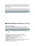
1
Biomedical Genomics
Workbench
APPLICATION BASED MANUAL
Manual for
Biomedical Genomics Workbench 2.5.1
Windows, Mac OS X and Linux
October 15, 2015
This software is for research purposes only.
CLC bio, a QIAGEN Company
Silkeborgvej 2
Prismet
DK-8000 Aarhus C
Denmark
Contents
I
Introduction
6
1 Welcome to Biomedical Genomics Workbench
1.1
Introduction to Biomedical Genomics Workbench . . . . . . . . . . . . . . . . .
7
1.2
Available documentation . . . . . . . . . . . . . . . . . . . . . . . . . . . . . . .
8
1.3
The material covered by this manual . . . . . . . . . . . . . . . . . . . . . . . .
8
1.4
We welcome your comments and suggestions . . . . . . . . . . . . . . . . . . .
8
1.5
Contact information . . . . . . . . . . . . . . . . . . . . . . . . . . . . . . . . .
8
2 Introduction to user interface, workflows, and tracks
II
7
10
2.1
The start screen . . . . . . . . . . . . . . . . . . . . . . . . . . . . . . . . . . .
10
2.2
The user interface . . . . . . . . . . . . . . . . . . . . . . . . . . . . . . . . . .
13
2.3
Workflows - an overview . . . . . . . . . . . . . . . . . . . . . . . . . . . . . . .
15
2.4
The track format . . . . . . . . . . . . . . . . . . . . . . . . . . . . . . . . . . .
17
Applications - ready-to-use workflows
27
3 Ready-to-Use Workflows descriptions and guidelines
28
3.1
General Workflow . . . . . . . . . . . . . . . . . . . . . . . . . . . . . . . . . .
28
3.2
Somatic Cancer . . . . . . . . . . . . . . . . . . . . . . . . . . . . . . . . . . .
29
3.3
Hereditary Disease
29
. . . . . . . . . . . . . . . . . . . . . . . . . . . . . . . . .
4 Getting started
36
4.1
Reference data . . . . . . . . . . . . . . . . . . . . . . . . . . . . . . . . . . . .
36
4.2
Create new folder . . . . . . . . . . . . . . . . . . . . . . . . . . . . . . . . . .
45
4.3
Import sequencing data . . . . . . . . . . . . . . . . . . . . . . . . . . . . . . .
47
4.4
Prepare sequencing data . . . . . . . . . . . . . . . . . . . . . . . . . . . . . .
48
3
CONTENTS
4
5 Whole genome sequencing (WGS)
5.1
General Workflows (WGS) . . . . . . . . . . . . . . . . . . . . . . . . . . . . . .
61
5.2
Somatic Cancer (WGS)
. . . . . . . . . . . . . . . . . . . . . . . . . . . . . . .
69
5.3
Hereditary Disease (WGS) . . . . . . . . . . . . . . . . . . . . . . . . . . . . . .
81
6 Whole exome sequencing (WES)
100
6.1
General Workflows (WES) . . . . . . . . . . . . . . . . . . . . . . . . . . . . . . 101
6.2
Somatic Cancer (WES) . . . . . . . . . . . . . . . . . . . . . . . . . . . . . . . . 110
6.3
Hereditary Disease (WES) . . . . . . . . . . . . . . . . . . . . . . . . . . . . . . 133
7 Targeted amplicon sequencing (TAS)
160
7.1
General Workflows (TAS)
. . . . . . . . . . . . . . . . . . . . . . . . . . . . . . 161
7.2
Somatic Cancer (TAS) . . . . . . . . . . . . . . . . . . . . . . . . . . . . . . . . 169
7.3
Hereditary Disease (TAS) . . . . . . . . . . . . . . . . . . . . . . . . . . . . . . 192
8 Whole Transcriptome Sequencing (WTS)
III
60
219
8.1
Analysis of multiple samples . . . . . . . . . . . . . . . . . . . . . . . . . . . . 220
8.2
Annotate Variants (WTS) . . . . . . . . . . . . . . . . . . . . . . . . . . . . . . . 221
8.3
Compare variants in DNA and RNA . . . . . . . . . . . . . . . . . . . . . . . . . 225
8.4
Identify Candidate Variants and Genes from Tumor Normal Pair . . . . . . . . . . 230
8.5
Identify variants and add expression values . . . . . . . . . . . . . . . . . . . . 235
8.6
Identify and Annotate Differentially Expressed Genes and Pathways . . . . . . . 239
Customized data analysis
243
9 How to edit application workflows
244
9.1
Introduction to customized data analysis . . . . . . . . . . . . . . . . . . . . . . 244
9.2
How to edit preinstalled workflows . . . . . . . . . . . . . . . . . . . . . . . . . 244
10 Using data from other workbenches
247
10.1 Open outputs from other workbenches . . . . . . . . . . . . . . . . . . . . . . . 247
CONTENTS
IV
Plugins
5
248
11 Plugins
249
V
250
Appendix
A Reference data overview
251
B Mini dictionary
256
Bibliography
257
VI
258
Index
Part I
Introduction
6
Chapter 1
Welcome to Biomedical Genomics
Workbench
Contents
1.1
Introduction to Biomedical Genomics Workbench . . . . . . . . . . . . . . .
7
1.2
Available documentation . . . . . . . . . . . . . . . . . . . . . . . . . . . . .
8
1.3
1.4
The material covered by this manual . . . . . . . . . . . . . . . . . . . . . . .
We welcome your comments and suggestions . . . . . . . . . . . . . . . . .
8
8
1.5
Contact information . . . . . . . . . . . . . . . . . . . . . . . . . . . . . . . .
8
Welcome to Biomedical Genomics Workbench 2.5.1 -- a software package supporting your daily
bioinformatics work.
High throughput sequencing is currently revolutionizing both the cancer research and diagnostics
areas. Since the introduction of "next generation sequencing" (NGS) technologies, the field has
quickly moved forward, with rapid improvements in sequencing capacity and the time required for
data production. As a result, in many studies the sequencing process is no longer the bottleneck.
The bottleneck now is the bioinformatic analysis of the data.
Biomedical Genomics Workbench has been developed to address the bioinformatic bottleneck by
offering automated workflows that cover all steps from the initial data processing and quality
assurance through data analyses, annotation, and reporting.
1.1
Introduction to Biomedical Genomics Workbench
Biomedical Genomics Workbench has been developed specifically for cancer research.
A core part of the Biomedical Genomics Workbench is the ready-to-use workflows that are bundled
with reference data. Workflows have been developed for the following applications:
• Whole Genome Sequencing
• Whole exome Sequencing
• Targeted Amplicon Sequencing
7
CHAPTER 1. WELCOME TO BIOMEDICAL GENOMICS WORKBENCH
1.2
8
Available documentation
The documentation for Biomedical Genomics Workbench can be found here: http://www.
clcbio.com/support/downloads/#manuals.
Two manuals are available for Biomedical Genomics Workbench:
• The Biomedical Genomics Workbench application based manual. This relatively short
manual gives a basic introduction to Biomedical Genomics Workbench, which includes a
section on how to get started, as well as describing how to use the different ready-to-use
workflows for analysis of different types of sequencing data.
• The Biomedical Genomics Workbench reference manual. This comprehensive manual
explains the features and functionalities of the Biomedical Genomics Workbench in detail.
If you would like to use a CLC Server, there are two additional manuals that are relevant:
• The CLC Server administrator manual. This manual is for server administrators and
describes how to install and manage CLC Servers.
• CLC Server end user manual. This manual is for the users of the CLC Server. In this manual
you can find a description of how to use a CLC Server from a CLC Workbench.
1.3
The material covered by this manual
This usermanual provides introductory material on how to work with the software, including the
import and initial handling of data and a guide to the data types and user interface. Its main
focus is to provide guidance on how to use the workflows that come with the software.
Also included is an appendix where there is a table listing the available reference data as well as
a small dictionary of terminology used in the Biomedical Genomics Workbench. The dictionary is
not exhaustive, but we hope it will serve as a useful reference, especially for new users.
For comprehensive descriptions of the features and functionalities of the individual tools, please
refer to the Biomedical Genomics Workbench reference manual.
1.4
We welcome your comments and suggestions
We aim to provide user-friendly software for important analyses, such as identifying inherited
disease traits and identifying somatic mutations that underlie this complex disease. To this end,
we continuously develop our bioinformatic platform, expand the collection of research tools, and
extend our documentation resources. We welcome comments or suggestions you have. These
help us greatly in further developing and improving our software. Comments and suggestions
can be submitted directly from within the software using the menu option: Biomedical Genomics
Workbench:
Help | Contact Support
1.5
Contact information
The Biomedical Genomics Workbench is developed by:
CHAPTER 1. WELCOME TO BIOMEDICAL GENOMICS WORKBENCH
9
QIAGEN Aarhus
Silkeborgvej 2
Prismet
8000 Aarhus C
Denmark
http://www.clcbio.com
http://www.qiagenbioinformatics.com
VAT no.: DK 28 30 50 87
Email: [email protected]
Telephone: +45 70 22 32 44
If you have questions or comments regarding the program, you can contact us through the support team as described here: http://www.clcsupport.com/clcgenomicsworkbench/
current/index.php?manual=Getting_help.html.
Chapter 2
Introduction to user interface, workflows,
and tracks
Contents
2.1
The start screen . . . . . . . . . . . . . . . . . . . . . . . . . . . . . . . . . .
2.1.1
10
The getting started table . . . . . . . . . . . . . . . . . . . . . . . . . .
10
2.1.2
Import of example data . . . . . . . . . . . . . . . . . . . . . . . . . . .
2.2
The user interface . . . . . . . . . . . . . . . . . . . . . . . . . . . . . . . . .
12
13
2.2.1
The Toolbox . . . . . . . . . . . . . . . . . . . . . . . . . . . . . . . . .
14
2.3
Workflows - an overview . . . . . . . . . . . . . . . . . . . . . . . . . . . . .
15
2.4
The track format
. . . . . . . . . . . . . . . . . . . . . . . . . . . . . . . . .
17
2.4.1
Track types . . . . . . . . . . . . . . . . . . . . . . . . . . . . . . . . . .
17
2.4.2
The Genome Browser . . . . . . . . . . . . . . . . . . . . . . . . . . . .
17
This section introduces the Biomedical Genomics Workbench general features and functionalities,
including the user interface and a general introduction to workflows and tracks. The information
in this chapter underpins that of later chapters and is highly recommended for new users of
the Workbench. You can find more detailed information in the Biomedical Genomics Workbench reference manual, which can be found online at http://www.clcbio.com/support/
downloads/#manuals.
2.1
The start screen
When you start up the Biomedical Genomics Workbench, you should see an image like the one in
figure 2.1. The information in the left hand panes will differ, depending on what data you already
have available and any plugins you may have installed.
2.1.1
The getting started table
When no data has been opened for viewing, a table is visible in the View Area of the Workbench.
This table provides links to sections of the application based user manual, and is thus a simple
and fast way to access information about using the Biomedical Genomics Workbench.
10
CHAPTER 2. INTRODUCTION TO USER INTERFACE, WORKFLOWS, AND TRACKS
11
Figure 2.1: The Biomedical Genomics Workbench start up window.
Currently Biomedical Genomics Workbench can be used to analyze DNA sequencing data. Analysis
of RNA sequencing data is planned for a future release.
In this section, we take a closer look at the table in the viewing area (figure 2.2).
Figure 2.2: The table in the Biomedical Genomics Workbench, visible when no datasets have
been opened for viewing, provides links so that you can quickly navigate to relevant sections of the
application based manual. To the right hand side of the table, the "Getting Started" and "Explore
and Learn" areas provide links to more general information resources that you may find useful.
Summary stages in data analysis are listed at the left side of the table: Data Preparation, Data
Analysis, Interpretation, and Data Analysis and Interpretation. Click on the text in the table to
CHAPTER 2. INTRODUCTION TO USER INTERFACE, WORKFLOWS, AND TRACKS
12
open the relevant section in the application based manual.
The recommended way to use the table is to start at the top and click on one of the "Whole
genome", "Whole exome", or "Targeted" tabs found under the big "DNA" label if you are working
on DNA-seq data. This acts to select the relevant application area. This done, when you click on
a link within the "DNA" section of the table, you will be directed to the section in the application
based manual about that topic, for example, "Annotate Variants" that applies to that particular
application area, for example, "Whole genome analysis". Likewise, if you work on RNA-seq data,
you can find relevant manual entries with the links provided under the big "RNA" label.
To the right side of the table is a box with two sections; "Getting started" and "Explore
and learn". The "Getting started" area contains links to: the Tutorials (http://http://
qiagenbioinformatics.com/products/biomedical-genomics-workbench/), Full-length
application based manual (PDF), and Full-length reference manual (PDF) (http://www.
clcbio.com/support/downloads/#manuals). The "Explore and Learn" section provides
links to different sections of the application based manual as well as a link to a web page where
you can download example data.
Finally, the Download example data provides links to two different example data sets. This is
described in section 2.1.2
2.1.2
Import of example data
It might be easier to understand the logic of the program by trying to do simple operations on
existing data. Therefore Biomedical Genomics Workbench includes an example data set.
If you would like to download the example data you have three options:
1. You can click Download Example Data in the start up table that is visible in the Biomedical
Genomics Workbench when no datasets have been opened for viewing. This will take you
to http://www.clcbio.com/support/downloads/#data where you can choose to
download two different example datasets that can be used for the following purposes:
• Variant identification in a tumor sample. This dataset is taken from a larger whole
exome dataset and includes data from a small fraction of chromosome 5 (Example_data_tumor.zip).
• Identification of somatic variants in a tumor sample using the matched normal sample
for removal of germline variants. This is matched tumor and normal samples from
chromosome 22 from a whole exome dataset (Example_data_tumor_normal.zip).
2. You can also go to directly to http://www.clcbio.com/support/downloads/#data
and download the example data from there.
3. Finally, you can use these links to get the data:
http://download.clcbio.com/testdata/cancer/current/Example_data_tumor.
zip or
http://download.clcbio.com/testdata/cancer/current/Example_data_tumor_
normal.zip
When you have downloaded the data from the website, you need to import them into the
Biomedical Genomics Workbench. How to import data is described in section 4.3.
CHAPTER 2. INTRODUCTION TO USER INTERFACE, WORKFLOWS, AND TRACKS
2.2
13
The user interface
The Biomedical Genomics Workbench user interface includes the Toolbox, Navigation Area, Menu
Bar, Toolbar, Side Panel, View Area, View Tools, and Status Bar (figure 2.3).
Figure 2.3: At the top you find the Menu Bar and under that, the Toolbar. The Navigation Area
is on the left. Here, you can view and organize your data, and from here, you can open data to
view, select it for launching in applications. Saved data will appear within this area. The Toolbox
is available in two locations in the Workbench. One is in a tab of the pane below the Navigation
Area. The other is via the menu system. The Toolbox is where Workflows and most tools that play a
role in your data analysis are launched from. When opened, datasets are shown in the View Area
along with a Side Panel appears that allows you to customize the viewing options and also navigate
to specific areas of the data. At the bottom of a data view on the right, are the View Tools that
can be used for panning, zooming and selection of specific regions. At the bottom on the left are
icons allowing to view data in a different way, for example look at a table view of the data or view
the history of actions taken on that dataset. The Status Bar in the lower right corner indicates the
location of a selection you have made or where the mouse pointer is pointing to within a dataset
with co-ordinates, such as a track or sequence.
After a dataset is opened, for example by double-clicking on an item in one of the folders visible
in the Navigation Area, the user interface will look similar to that shown in figure 2.3. Each
dataset in the View Area will have an associated Side Panel, Status Bar, and a set of View
Tools.
The Side Panel, Status Bar, and View Area are only visible when data are open for viewing. When
no datasets are open, the view is like that in figure 2.1.
To learn more about the specific areas and functionalities of the user interface, please refer
to the Biomedical Genomics Workbench reference manual, which can be found here: http:
CHAPTER 2. INTRODUCTION TO USER INTERFACE, WORKFLOWS, AND TRACKS
14
//www.clcbio.com/support/downloads/#manuals.
2.2.1
The Toolbox
Here, we focus on organization of the Toolbox. The first to note is the top level folders and their
associated icons (see figure 2.4).
Figure 2.4: The top level folders of the Toolbox are divided into two main categories; the "Ready-toUse Workflows" and the "Tools". The elements under the folders of the "Tools" section can be used
for manual analysis or used for editing existing workflows and building your own workflows.
The toolbox contains two different categories of tools:1) the Ready-to-Use Workflows, which can
be used to run complete analyses, and 2) Tools, containing many individual tools that can be
used for analysis by themselves, or can be used to build workflows from, or which can be added
to existing workflows to expand their functionality. The name of the folders in the Ready-to-use
workflows section reflect the type of analysis the workflows in that folder are designed for. See
figure 2.5).
Manual data analysis, that is, execution of individual analysis steps, can be performed using
the tools contained in the Tools section. Full analyses can be run this way, or such tools can
be used upstream or downstream of workflow-based data analyses. The tools that relevant for
CHAPTER 2. INTRODUCTION TO USER INTERFACE, WORKFLOWS, AND TRACKS
15
Figure 2.5: Each application type has its own set of ready-to-use workflows.
different types of data analysis will vary depending on the questions being asked of the data. In
section 2.3 we will use diagrams and examples to illustrate how different tools and workflows
can be used for data analysis.
For a detailed description of the individual tools we refer to the Biomedical Genomics Workbench
reference manual (http://www.clcbio.com/support/downloads/#manuals).
2.3
Workflows - an overview
Biomedical Genomics Workbench offers a number of analysis workflows, also referred to here as
CHAPTER 2. INTRODUCTION TO USER INTERFACE, WORKFLOWS, AND TRACKS
16
the pre-installed ready-to-use workflows, which include all the necessary steps for a particular
analysis, from the initial quality checking and trimming of the reads to the final reporting of the
results, for example, the disease causing mutations detected in an analysis. The workflows are
easy to use and just require the sequence data as input. You may need to provide additional
information relevant to your data and analysis to run a given workflow, for example adapter trim
lists for trimming sequences, or, when performing "Targeted Amplicon Sequencing", a description
of the sequenced regions.
Irrespective of the type of sequencing data you wish to analyze, there are only few steps necessary
before the identified variants are available for your inspection. A schematic representation of the
flow that an analysis could take is shown in figure 2.6.
Figure 2.6: A basic example of the flow of steps for a sequencing data analysis. The data is
first imported into the Workbench. Then it should be prepared for analysis. Here, a ready-to-use
workflow labeled workflow 1 is used for this. It runs quality control and trimming steps. After
inspection of the quality and trimming reports, the trimmed data are used as input for another
ready-to-use workflow, called workflow 2 in this figure. This is where the data analysis is carried
out. Here, workflow choices associated with variant detection are shown. Additional analyses
can be performed downsteam of this if desired. Downstream analysis could involve using another
ready-to-use workflow or could involve running individual tools from the Tools section of the Toolbox.
The ready-to-use workflows to run, and how many of them to run depend on the type of data you
have and the analysis you wish to perform. For example, overlapping paired data involves other
considerations than single or non-overlapping paired data. Different workflows will be relevant
CHAPTER 2. INTRODUCTION TO USER INTERFACE, WORKFLOWS, AND TRACKS
17
if your aim is to detect variants or annotate variants with information from other databases.
Typically you will need to run two or three workflows to complete a full analysis that includes
preparation of the raw data.
Figure 2.7 shows some of the ready-to-use workflows that are available for each application.
Irrespective of the application type, the first step involves preparation of the raw data. The
ready-to-use workflow to choose to launch the data preparation depends on the type of data
being analyzed. For example, the "Prepare Overlapping Raw Data" workflow is designed to handle
reads with overlapping pairs, whereas the "Prepare Raw Data" workflow is for read sets without
overlapping pairs. The initial data preparation step involves quality control and trimming of the
reads.
2.4
The track format
The Biomedical Genomics Workbench provides a built-in Genome Browser. This view allows
the reference sequenced to be displayed together with other data provided in a so-called track
format. One of the big advantages of using tracks is that they allow visualization, comparison,
and analysis of genome-scale studies, with all the information tied to genomic positions. A central
coordinate-system, provided by a reference genome, makes it possible to view and compare
different datasets together in a Genome Browser view. Of course, each track can be viewed
individually if desired.
2.4.1
Track types
Several different track types are available. To make it easier to recognize the different track types
in the Navigation Area and in the View Area, each track type is associated with a specific icon:
• Coverage graph (
• Read mapping (
)
)
• Reference genome sequence (
• Annotation track (
)
• Genome browser view (
)
• Variants from variant calling (
• Expression track (
)
)
• Differentially expressed genes (
2.4.2
)
)
The Genome Browser
The Genome Browser view is a collection of tracks. Each track in a Genome Browser view is tied
to the same underlying genomic co-ordinate set, making visualization and comparison of different
results and data types simple and intuitive.
Annotations and variant information are provided together with the human reference genome via
our Data Management. Datasets, e.g. in GFF of VCF format, from resources not provided for
CHAPTER 2. INTRODUCTION TO USER INTERFACE, WORKFLOWS, AND TRACKS
18
Figure 2.7: The available pre-installed ready-to-use workflows for the individual application types.
download by Biomedical Genomics Workbench can be imported into the Navigation Area using the
import option found in the toolbar:
Toolbar | Import (
) | Tracks
To illustrate this a Genome Browser view is shown in figure 2.8 to figure 2.13. It consists of
the following tracks, all tied to the human hg19 reference: genomic sequence, gene, coding
sequence (CDS), a read mapping, and variants. In figure 2.8 we have used the zoom tools to
zoom all the way in on a SNV that is found in a coding region.
CHAPTER 2. INTRODUCTION TO USER INTERFACE, WORKFLOWS, AND TRACKS
19
Figure 2.8: A Genome Browser view with a genomic sequence track, a gene track, a coding
sequence (CDS) track, a read mapping track, and a variant track.
A Genome Browser view like the one shown in figure 2.8, allows for a complete overview of reads
mapped to a reference and identified variants. You can see how many reads and variants you
have, and you can compare them to the complete human genome, genes and coding regions.
How to zoom in a Genome Browser view
One way to zoom in to take a closer look at the reads and variants is to use the zoom tools.
These are located in the lower right corner of the view area (see figure 2.9). Click and hold
down the mouse button for a second or two on the relevant icon. This can be either an arrow
or a magnifying glass. By clicking the magnifying glass icon, three icons will appear. These can
be used for zooming in, zooming out, or panning. The different zoom options are described in
detail in the Biomedical Genomics Workbench reference manual in the section entitled "Zoom
and selection in View Area".
Figure 2.9: Click and hold down the mouse button for a second or two on the mangnifying glass
icon until additional icons appear. Select the arrow to activate the "selection" tool. This can be
used to select user-defined regions.
An quick and easy way to zoom in on a particular region is to first use the selection tool, which
is activated by clicking on the arrow shown in figure 2.9). You can then select specific regions
by clicking on the relevant point in the track and, keeping the mouse button depressed, dragging
across the area that you wish to zoom in on. This selects the region. Once selected, you can use
CHAPTER 2. INTRODUCTION TO USER INTERFACE, WORKFLOWS, AND TRACKS
20
the "Zoom to selection" tool (shown in figure 2.10) to zoom in on the selected region.
It is also possible to zoom in just using the mouse: hold down the "Alt" key while scrolling with
the mouse wheel. This zooms in (or out) on the region that is in focus in the View Area.
Figure 2.10: The "Zoom to selection" tool can be used to zoom in on a selected region. Next to the
"Zoom to selection" icon you can find the "Zoom to fit" icon that can be used to zoom all the way
out. The "Zoom slider" on the left side of the "Zoom to selection" can also be used to zoom in and
out.
When clicking on the "Zoom to selection" icon, you will zoom in on the region that you have
selected, and you will be able to see more and more details as you zoom in. This is shown in
figure 2.11 and figure 2.12.
In figure 2.12 the presence of SNVs can be seen in the variant track and an overview of the
mapping at that region in the mapping can be focused on.
To expand the depth of the reads track to view more details of the reads in a specific region,
simply place the mouse cursor near the bottom of the left side of the genome Browser view,
where the track names are, hold down the mouse and drag downwards. This is illustrated in
the lower left side of figure 2.12. Here, the blue line with the arrow under it (within a red circle)
illustrates where you would place the mouse cursor to be able to expand the depth of the track.
In this figure, the four bases in the genomic reference sequence can be discerned via the color
coding. The color codes for each of the bases are: A=red, C=blue, G=yellow, and T=green.
Particular SNVs can also be discerned at this zoom level. The color of the reads indicates
whether a read is part of an intact pair (blue), is a single read or a member of a broken pair
mapped in the forward direction relative to the reference (green), or a single read or a member
of a broken pair mapped in the reverse direction relative to the reference (red). Reads that could
map equally well to other locations in the reference are colored yellow.
Figure 2.13 shows the view after zooming in on one specific SNV. By looking at the other tracks
at that point, we can see that this SNV is found in a gene. The tooltip, which comes up with
the mouse cursor hovers over the SNV in the variant track reveals that this is a heterozygous
mutation occurring in 29 out of 447 reads. Full details about the variants in a track are shown in
the table view of the track, as described in the next section.
How to open a table in split view The table view of a track provides the details of the information
that is presented in the track itself. It is often useful to view the table at the same time as the
track, this is done by opening the table in a split view.
From an individual track open in the Viewing area of the Workbench, this can be done by
depressing the Ctrl key and clicking using the mouse on the small icon of a table at the bottom
of the view.
From a genome Browser view open in the Viewing area, the table view of a particular track can
be opened in a split view by double-clicking on the track name in the list. This is shown in
figure 2.14.
The table and the track are linked, which means that clicking on a particular row in the table
brings that position into focus in the Genome Browser view. For example, if you wished to jump
CHAPTER 2. INTRODUCTION TO USER INTERFACE, WORKFLOWS, AND TRACKS
21
Figure 2.11: When zooming in on a selected region more and more details become visible. In this
image, the individual genes are visible. To distinguish the individual exons, you would have to zoom
in a bit further.
to a particular SNV in the Genome Browser view, you could click on the row in the variant track
table. This is shown in figure 2.15.
Add tracks to a Genome Browser view
The most simple way to add a track to the Genome Browser view is simply to locate the file in the
Navigation Area, click on the file while holding down the mouse key and drag it into the genome
Browser view in the View Area. When you drop the file in the Genome Browser view, the track
will be added to the Genome Browser view (figure 2.16).
Note! After having added a new track to the Genome Browser view, an asterisk has appeared on
the Genome Browser view tab. This indicates that the Genome Browser view must be saved if
you wish to keep the track that has been added.
CHAPTER 2. INTRODUCTION TO USER INTERFACE, WORKFLOWS, AND TRACKS
Figure 2.12: Zooming in reveals more details in all tracks.
22
CHAPTER 2. INTRODUCTION TO USER INTERFACE, WORKFLOWS, AND TRACKS
23
Figure 2.13: We have now zoomed in on one specific SNV that is found in a coding region. By
holding the mouse over the variant, a tooltip will appear that provide further information about the
specific variant. In this case we have found a heterozygous SNV. The normal base at this position
is G but in some of the reads you will see a "T". Actually you can only see one "T" in the reads,
but if you look in the stacked reads, which are those in the color mass where you cannot see each
individual read represented, there are four green lines (read box) indicating that there are Ts at this
position in more reads. When holding the mouse over an individual SNV, as highlighted in the red
circle, a tooltip will appear with information about the SNV. This tooltip informs us that 29 Ts are
observed in the 447 reads covering this particular position. When hovering the mouse cursor over
a particular base in the reference track, the genomic position for this base is shown, as highlighted
with a red arrow here.
CHAPTER 2. INTRODUCTION TO USER INTERFACE, WORKFLOWS, AND TRACKS
24
Figure 2.14: Double-click on the track name in the left side of the view area to open the table
view shown in split view. When opening a track directly from the genome browser view, the table
and track are linked. Hence, when selecting a row in the table by clicking on this row, this specific
position in the track will be brought into focus.
CHAPTER 2. INTRODUCTION TO USER INTERFACE, WORKFLOWS, AND TRACKS
25
Figure 2.15: When you click on an entry in the table this position will automatically be brought into
focus. Here, a row with information about an MNV, which is variant consisting of two or more SNVs,
was clicked on. This brought the location of that MNV into focus in the graphical view. To jump
directly to a detailed view of a position, zoom the graphical view to the desired level first and then
click on the row in the table view.
CHAPTER 2. INTRODUCTION TO USER INTERFACE, WORKFLOWS, AND TRACKS
26
Figure 2.16: The conservation score track has been added to the Genome Browser view by dragging
the track from the Navigation Area into the Genome Browser view in the View Area.
Part II
Applications - ready-to-use workflows
27
Chapter 3
Ready-to-Use Workflows descriptions and
guidelines
Contents
3.1
General Workflow . . . . . . . . . . . . . . . . . . . . . . . . . . . . . . . . .
28
3.2
Somatic Cancer . . . . . . . . . . . . . . . . . . . . . . . . . . . . . . . . . .
29
3.3
Hereditary Disease . . . . . . . . . . . . . . . . . . . . . . . . . . . . . . . .
29
Biomedical Genomics Workbench contains several ready-to-use workflows that support analysis of
cancer data, but also analysis of hereditary diseases and other conditions that are best studied
using family analysis.
The workflows are specific to the type of data used as input: Whole Genome Sequencing (WGS),
Whole Exome Sequencing (WES), Targeted Amplicon Sequencing (TAS) and Whole Transcriptome
Sequencing (WTS). For each of the first three categories, WGS, WES, and TAS, workflows exist
that can be used for general identification and annotation of variants irrespective of disease,
these workflows are found in a folder called General Analysis. In folders called Somatic Cancer,
you can find workflows that are specific for cancer research. Finally, you will find a folder under
each of the WGS, WES, and TAS applications, that is labeled Hereditary Disease. The workflows
found in this folder can be used for studying variants that cause rare diseases or hereditary
diseases (HD).
The ready-to-use workflows found under each of the first three applications have similar names
(with the only difference that "WGS", "WES", or "TAS", or have been added after the name).
However, some of the workflows have been tailored to the individual applications with parameter
settings that have been adjusted to fit e.g. the expected differences in coverage between the
different application types. We therefore recommend that you use the ready-to-use workflow that
is found under the relevant application heading.
3.1
General Workflow
The General workflows are universal workflows in the sense that they can be used independently
of the disease that is being studied. Two workflows exist in this category:
28
CHAPTER 3. READY-TO-USE WORKFLOWS DESCRIPTIONS AND GUIDELINES
29
• Annotate Variants: Annotates variants with gene names, conservation scores, amino acid
changes, and information from clinically relevant databases.
• Identify Known Variants in One Sample: Maps sequencing reads and looks for the presence
or absence of user-specified variants in the mapping.
3.2
Somatic Cancer
The Somatic Cancer ready-to-use workflows are workflows that have been tailored to cancer
research. In this category it is possible to find e.g. workflows that can compare variants in
matched tumor normal pairs. The workflows found in the Somatic Cancer category, use the "Low
Frequency Variant Detection" for variant calling. The advantages of using this variant caller when
analyzing cancer data are that 1) it does not take ploidy into consideration, and 2) it is particularly
good at picking up low frequency variants in contrast to the other variant callers.
The workflows that are available in this category are:
• Filter Somatic Variants: Removes variants outside the target region (only targeted experiments) and common variants present in publicly available databases. Annotates with gene
names, conservation scores, and information from clinically relevant databases.
• Identify Somatic Variants from Tumor Normal Pair: Removes germline variants by referring
to the control sample read mapping, removes variants outside the target region (in case of
a targeted experiment), and annotates with gene names, conservation scores, amino acid
changes, and information from clinically relevant databases.
• Identify Variants: Calls variants in the mapped and locally realigned reads, removes false
positives and, in case of a targeted experiment, removes variants outside the targeted
region. Variant calling is performed with the Low Frequency Variant Detection tool.
3.3
Hereditary Disease
The third category found under each of the three applications WGS, WES, and TAS are the
Hereditary Disease workflows that have been developed to support identification of disease
causing mutations in families.
Hereditary diseases can be non-cancer related diseases, such as inherited heart diseases or
familial hypercholesterolemia, or it can be inherited cancers such as hereditary colorectal cancer
or hereditary breast cancer. In addition to the hereditary diseases, family analysis can help
researchers identify rare disease causing mutations that can be:
• a new mutation, also known as a de novo mutation, that is only present in a child and not
in any of the parents
• a combination of events that occur in the same gene but at different positions in each of
the parents, which is not disease causing by itself in either of the parents, but when both
variants are found in a child, it becomes disease causing; this type of variant is known as
a compound heterozygous variant.
CHAPTER 3. READY-TO-USE WORKFLOWS DESCRIPTIONS AND GUIDELINES
30
A range of different workflows exist in this category that have been optimized for different
purposes. In the current version of the Biomedical Genomics Workbench we offer workflows
tailored to two family sizes, 1) a classical "Trio", consisting of a mother, father, and an affected
child (the proband), and 2) a "Family of Four", which is mother, father, affected child, and either
a sibling (in the workflows that detects rare diseases) or another affected family member (in the
workflows that detect inherited diseases), that can be any affected relative such as a sibling,
grand parent or the like. The workflows use the "Fixed Ploidy Variant Detection" tool, which is
a variant caller that has been designed to call variants in samples with known ploidy from read
mapping data. Workflows designed to detect rare variants can both pick up de novo variants as
well as compound heterozygous variants. In addition to the Trio and Family of Four workflows,
additional workflows exist that have been designed to pick up variants that are inherited from
either the mother or the father.
The available workflows in this category are:
• Filter Causal Variants: Removes variants outside the target region (only targeted experiments) and common variants present in publicly available databases. Annotates with gene
names, conservation scores, and information from clinically relevant databases.
• Identify Causal Inherited Variants in a Family of Four: Identifies putative disease causing
inherited variants by creating a list of variants present in all three affected individuals and
subtracting all variants in the unaffected individual. The workflow includes a back-check for
all family members.
• Identify Causal Inherited Variants in a Trio: Identifies putative disease causing inherited
variants by creating a list of variants present in both affected individuals and subtracting
all variants in the unaffected individual. The workflow includes a back-check for all family
members
• Identify Rare Disease Causing Mutations in a Family of Four: Identifies de novo and compound
heterozygous variants from an extended family of four, where the fourth individual is not
affected.
• Identify Rare Disease Causing Mutations in a Trio: Identifies de novo and compound
heterozygous variants from a Trio. The workflow includes a back-check for all family
members.
• Identify Variants (HD): Calls variants in the mapped and locally realigned reads, removes
false positives and, in case of a targeted experiment, removes variants outside the targeted
region. Variant calling is performed with the Fixed Ploidy Variant Detection tool.
Although each workflow design to analyze Hereditary Diseases is specific to the data used or the
type of analysis, they share several tools and steps:
Below you can find a general description for how to run a workflow in the category "Hereditary
diseases". In some workflows, such as the "Filter Causal Variants" workflows you will be asked
about a variant track as input. Other workflows start with specifying a reads track. This is the
case for all workflows that starts with "Identify Variants.." in the name.
Note that in case of workflows annotating variants using databases available for more than one
population, you can select the population that matches best the population your samples are
CHAPTER 3. READY-TO-USE WORKFLOWS DESCRIPTIONS AND GUIDELINES
31
derived from. This will be done in the wizard for populations from the 1000 Genomes Project,
while Hapmap populations are specified with the Data Management ( ) function before starting
the workflows (see section 4.1.4).
Select the variant track (figure 3.1)
The panel in the left side of the wizard shows the kind of input that should be provided.
Select by double-clicking on the variant track name or click once on the file and then click
on the arrow pointing to the right side in the middle of the wizard.
Figure 3.1: Select the variant track from which you would like to filter somatic variants.
Specify the sequencing reads for each family member (figure 3.2).
The sequencing reads from the different family members are specified one at a time in the
appropriate window. The panel in the left side of the wizard shows the kind of input that
should be provided. Select by double-clicking on the reads file name or click once on the
file and then on the arrow pointing to the right side in the middle of the wizard.
Figure 3.2: Specify the sequencing reads for the appropriate family member.
Specify the targeted region file (figure 3.3).
The targeted region file is a file that specifies which regions have been sequenced, when
working with whole exome sequencing or targeted amplicon sequencing data. This file is
something that you must provide yourself, as this file depends on the technology used
for sequencing. You can obtain the targeted regions file from the vendor of your targeted
sequencing reagents.
Specify the affected child's gender for the Trio analysis (figure 3.4).
Some workflows contains a Trio Analysis and thus take the gender of the proband into
account.
Specify the parameters for the Fixed Ploidy Variant Detection tool (figure 3.5).
CHAPTER 3. READY-TO-USE WORKFLOWS DESCRIPTIONS AND GUIDELINES
32
Figure 3.3: Select the targeted region file you used for sequencing.
Figure 3.4: Specify the proband's gender.
The parameters used by the Fixed Ploidy Variant Detection tool can be adjusted. We have
optimized the parameters to the individual analyses, but you may want to tweak some of
the parameters to fit your particular sequencing data. A good starting point could be to run
an analysis with the default settings.
Figure 3.5: Specify the parameters for the Fixed Ploidy Variant Detection tool.
The parameters that can be set are:
• Required variant probability is the minimum probability value of the 'variant site'
required for the variant to be called. Note that it is not the minimum value of the
probability of the individual variant. For the Fixed Ploidy Variant detector, if a variant
site - and not the variant itself - passes the variant probability threshold, then the
variant with the highest probability at that site will be reported even if the probability
of that particular variant might be less than the threshold. For example if the required
variant probability is set to 0.9 then the individual probability of the variant called
might be less than 0.9 as long as the probability of the entire variant site is greater
than 0.9.
CHAPTER 3. READY-TO-USE WORKFLOWS DESCRIPTIONS AND GUIDELINES
33
• Ignore broken pairs: When ticked, reads from broken pairs are ignored. Broken pairs
may arise for a number of reasons, one being erroneous mapping of the reads. In
general, variants based on broken pair reads are likely to be less reliable, so ignoring
them may reduce the number of spurious variants called. However, broken pairs may
also arise for biological reasons (e.g. due to structural variants) and if they are ignored
some true variants may go undetected. Please note that ignored broken pair reads will
not be considered for any non-specific match filters.
• Minimum coverage: Only variants in regions covered by at least this many reads are
called.
• Minimum count: Only variants that are present in at least this many reads are called.
• Minimum frequency: Only variants that are present at least at the specified frequency
(calculated as 'count'/'coverage') are called.
For more information about the tool, see http://clcsupport.com/biomedicalgenomicsworkben
current/index.php?manual=Fixed_Ploidy_Variant_Detection.html.
Specify the parameters for the QC for Target Sequencing tool (figure 3.6).
When working with targeted data (WES or TAS data), quality checks for the targeted
sequencing is included in the workflows. Again, you can choose to use the default settings,
or you can choose to adjust the parameters.
Figure 3.6: Specify the parameters for the QC for Target Sequencing tool.
The parameters that can be set are:
• Minimum coverage provides the length of each target region that has at least this
coverage.
• Ignore non-specific matches: reads that are non-specifically mapped will be ignored.
• Ignore broken pairs: reads that belong to broken pairs will be ignored.
When asked for it, specify the targeted regions track (figure 3.7).
For more information about the tool, see http://clcsupport.com/biomedicalgenomicsworkben
current/index.php?manual=QC_Target_Sequencing.html.
Map Reads to a reference (figure 3.8).
For this tool, the Autodetect paired distances settings is switched off in all Targeted
Amplicon Sequencing workflows.
CHAPTER 3. READY-TO-USE WORKFLOWS DESCRIPTIONS AND GUIDELINES
34
Figure 3.7: Specify the parameters for the QC for Target Sequencing tool.
Figure 3.8: Specify the parameters for the QC for Target Sequencing tool.
Specify the target region for the Indels and Structural Variants tool (figure 3.9).
The targeted region file is a file that specifies which regions have been sequenced when
working with whole exome sequencing or targeted amplicon sequencing data. This file is
something that you must provide yourself, as this file depends on the technology used
for sequencing. You can obtain the targeted regions file from the vendor of your targeted
sequencing reagents.
Figure 3.9: Specify the parameters for the Indels and Structural Variants tool.
Specify the relevant 1000 Genomes populations (figure 3.10)
Note: this window will appear in workflows that annotate variants with information from
the 1000 Genomes project, unless you have already selected the relevant populations of
interest in your reference data management prior to running the workflow.
Some wizard window will be called Add Information from 1000 Genomes Project or Remove
Variants found in the 1000 Genomes Project. Specify the 1000 Genomes population that
should be used to add or filter out variants found in the 1000 Genomes project. This can
be done using the drop-down list found in this wizard step. Please note that the populations
CHAPTER 3. READY-TO-USE WORKFLOWS DESCRIPTIONS AND GUIDELINES
35
Figure 3.10: Select the relevant 1000 Genomes population(s).
available from the drop-down list can be specified with the Data Management (
found in the top right corner of the Workbench (see section 4.1.4).
) function
Specify the relevant Hapmap populations (figure 3.11)
Note: this window will appear in workflows that annotate variants with information from the
Hapmap project, unless you have already selected the relevant populations of interest in
your reference data management prior to running the workflow.
Figure 3.11: Select the relevant Hapmap population(s).
Some wizard window will be called Add Information from the Hapmap project or Remove
Variants found in Hapmap. Specify the Hapmap population that should be used to add or
filter out variants found in the Hapmap project. This can be done using the drop-down list
found in this wizard step. Please note that the populations available from the drop-down
list can be specified with the Data Management ( ) function found in the top right corner
of the Workbench (see section 4.1.4).
Chapter 4
Getting started
Contents
4.1
Reference data . . . . . . . . . . . . . . . . . . . . . . . . . . . . . . . . . .
4.1.1
The Workbench Reference data location . . . . . . . . . . . . . . . . . .
4.1.2
Space requirements . . . . . . . . . . . . . . . . . . . . . . . . . . . . .
37
4.1.3
Where reference data is downloaded from . . . . . . . . . . . . . . . . .
38
4.1.4
Download and configure reference data . . . . . . . . . . . . . . . . . .
38
37
4.1.5
Troubleshooting reference data downloads . . . . . . . . . . . . . . . . .
45
4.2
Create new folder . . . . . . . . . . . . . . . . . . . . . . . . . . . . . . . . .
45
4.3
Import sequencing data . . . . . . . . . . . . . . . . . . . . . . . . . . . . . .
47
4.3.1
4.4
How to import data . . . . . . . . . . . . . . . . . . . . . . . . . . . . .
48
Prepare sequencing data . . . . . . . . . . . . . . . . . . . . . . . . . . . . .
48
4.4.1
Choosing between Prepare Raw Data and Prepare Overlapping Raw Data
workflows . . . . . . . . . . . . . . . . . . . . . . . . . . . . . . . . . .
49
4.4.2
Import adapter trim list . . . . . . . . . . . . . . . . . . . . . . . . . . .
50
4.4.3
How to run the Prepare Overlapping Raw Data ready-to-use workflow . . .
51
4.4.4
How to run the Prepare Raw Data ready-to-use workflow . . . . . . . . . .
54
4.4.5
Output from the Prepare Overlapping Raw Data and Prepare Raw Data
workflows . . . . . . . . . . . . . . . . . . . . . . . . . . . . . . . . . .
56
How to check the output reports . . . . . . . . . . . . . . . . . . . . . .
57
4.4.6
4.1
36
Reference data
The ready-to-use workflows rely on the presence of particular reference datasets. This reference
data must be downloaded and configured before these workflows can be used. The tools in
the Workbench make it easy to download the necessary data such that the workflows can find
and use it. This section covers the download and configurations needed to make available the
reference data relevant to the Biomedical Genomics Workbench, including the human, mouse and
rat genomes, annotations and variants made available by a variety of databases.
36
CHAPTER 4. GETTING STARTED
4.1.1
37
The Workbench Reference data location
Reference data must be stored in a folder called CLC_References. When the Biomedical Genomics
Workbench is installed, such a folder is created on your file system under your home area. This
folder is specified within the Workbench as a reference location.
You can specify a different location to download reference data to. This is recommended if you
do not have enough space in the area the Workbench designates as the reference data location
by default. To change the reference data location from within the Navigation Area:
Right-click on the folder "CLC_References" | Choose "Location" | Choose "Specify
Reference Location"
The new folder will also be called CLC_References, but will be located where you specify.
In more detail, this action results in the following:
• A folder called CLC_References is created in the location you specified, if a folder of this
name did not already exist.
• The Workbench sets this new location as the place to download reference data to and the
place the ready-to-use workflows should look for reference data.
This action does not:
• Remove the old CLC_References folder.
• Remove the contents of the old CLC_References folder, such as previously downloaded
data.
If you have previously downloaded data into the CLC_References folder with the old location, you
will need to use standard system tools to delete this folder and/or its contents. If you would
like to keep the reference data from the old location, you can move it, using standard system
tools, into the new CLC_References folder that you just specified. This would save you needing
to download it again.
Note! If you run out of space, and realize that the CLC_References should be stored somewhere
else, you can do this by choosing a new location, then manually moving the already downloaded
files to that new location, and restarting the workbench. The "downloaded references" file will
then be updated with all the new references.
4.1.2
Space requirements
The total size of the complete reference data set you can download is approximately 200 GB1 .
The amount of time it will take to download this amount of data depends on your network
connection. It can take several hours, or longer on slower connections.
For reference, in August, 2015, the maximum size of each individual reference data file for Homo
sapiens was approximately:
1
Size as estimated in August, 2015
CHAPTER 4. GETTING STARTED
Database
1000 Genomes
CDS
ClinVar
PhastConc
Cytogenic
Ideogram
dbSNP
dbSNP Common
Genes
Gene Ontology
HapMap
mRNA
Sequence
Target Regions
Target Primers
4.1.3
38
Size
8 GB
56 MB
140 MB
6 GB
80 KB
71 GB
3 GB
6 MB
45 MB
3 GB
75 MB
700 MB
1 MB
7 MB
Where reference data is downloaded from
Reference data must be downloaded and configured manually before you can start using the
ready-to-use workflows in the Biomedical Genomics Workbench. You only have to do this
once. When all necessary reference data have been downloaded and configured, you will be
automatically notified whenever updated reference data are available.
Data is provided by QIAGEN and the Workbench is configured to download from QIAGEN by default.
The location to download the data from can be seen in
Edit | Preferences | Advanced
as shown in figure 4.1.
Unless you are in the special circumstance that your system administrator has decided to mirror
this data locally and wishes you to use that mirror of the data, you should not change this setting.
4.1.4
Download and configure reference data
The first time you open Biomedical Genomics Workbench you will be presented with the dialog
box shown in figure 4.2, which informs you that data are available for download either to the
local or server CLC_References repository. If you check the "Never show this dialog again"
then subsequently you will only be presented with the dialog box when updated versions of the
reference data are available.
Click on the button labeled Yes. This will take you to the wizard shown in figure 4.3.
This wizard can also be accessed from the upper right corner of the Biomedical Genomics
Workbench by clicking on Data Management ( ) (figure 4.4).
The "Manage Reference Data" wizard gives access to all the reference data that are used in the
ready-to-use workflows and in the tutorials. From the wizard you can download and configure the
reference data.
In the upper part of the wizard you can find two tiles called "QIAGEN Reference Data Library" (
and "Custom Reference Data Sets" ( ).
)
CHAPTER 4. GETTING STARTED
39
Figure 4.1: The location where reference data is downloaded from can be seen in the Workbench
Preferences. Generally this should not be altered except in the special case that the data from
QIAGEN is being mirrored locally.
Figure 4.2: Notification that new versions of the reference data are available.
On the left hand side, you can use the drop-down menu to choose where you want to manage the
reference data. If you choose "Locally", the Download, Delete and Apply buttons will work on the
local reference data. If you choose "On Server" (only available if you are connected to the server),
the buttons will work on the reference data on the server you are connected to(figure 4.5).
You can also check how much free space is available for the Reference folder on your local
disk or on the server. The drop-down menu also allows you to check which datasets have been
downloaded locally or on the server. You can see this in the left panel of the reference data
manager.
When on the "QIAGEN Reference Data Library" tile, we can see the list of all available references
data under 4 headers: Reference Data Sets, Reference Data Elements, Tutorial Reference
Data Sets and Tutorial Reference Data Elements. Two icons indicate whether you have already
downloaded your data in your Reference folder ( ) or not ( ).
CHAPTER 4. GETTING STARTED
40
Figure 4.3: The Manage Reference Data wizard gives access to the reference data that are required
to be able to run the ready-to-use workflows.
Figure 4.4: Click on the button labeled "Data management" to open the "Manage Reference Data"
dialog where you can download and configure the reference data that are necessary to be able to
run the ready-to-use-workflows.
Figure 4.5: Reference data can be available locally or on the server.
When selecting a reference set or an element, the window on the right show the size of the
folder as well as some complementary information about the reference database. For Reference
Data Sets, a table recapitulates the elements included in the set with their version number and
respective size, as well as a list of the workflows affected by the set.
Here is the list of the Reference Data Sets and their approximate size: Reference Data Sets
• hg38 96 GB with Ensembl v81, dbSNP v142, ClinVar 20150901
• hg38 88 GB with Ensembl v80, dbSNP v142, ClinVar 20150629
• hg19 63 GB with Ensembl v74, dbSNP v138, ClinVar 20131203
• QIAGEN Gene Reads Panels hg19 8 MB with Ensembl v74
• Mouse 15 GB with Ensembl v80
• Rat 5.5 GB with Ensembl v79
Tutorial Reference Data Sets
• chr 5 of hg19 4.5 GB for use with the Identification of Variants in a Tumor Sample tutorial
CHAPTER 4. GETTING STARTED
41
• chr 14 of hg19 2.3 GB for use with the Copy Number Variant Detection tutorial
• chr 17 of hg19 2 GB for use with the RNA-Seq Analysis of Human Breast Cancer Data
tutorial
• chr 21 of hg19 1 GB for use with the ChIP Sequencing tutorial
• chr 22 of hg19 1 GB for use with the Identification of Somatic Variants in a Matched
Tumor-Normal Pair tutorial
Each Reference Data Set is made of a compilation of Reference Data Elements. Downloading
sets will automatically download the elements the set is made of, but you can also download
elements individually under the Reference Data Elements folder. Note that data for hg19 is
available for the whole genome as well as for individual chromosome 5, 14, 17, 21 and 22.
• For homo sapiens
Sequence hg38
Sequence hg19 (whole genome and chromosome specific)
dbSNP 142
dbSNP 138 (whole genome and chromosome specific)
dbSNP Common 142
dbSNP Common 138 (whole genome and chromosome specific)
Hapmap phase_3_ensembl_v80, Hapmap phase_3 (whole genome and chromosome
specific)
Genes ensembl_v80, ensembl_v73, ensembl_v74 (whole genome and chromosome
specific)
Conservation Scores PhastCons hg38
Conservation Scores PhastCons hg19 (whole genome and chromosome specific)
ClinVar 20150629 and 20130930 (whole genome and chromosome specific), 20131203
(whole genome and chromosome specific)
1000 Genomes Project phase_3 and phase_1 (whole genome and chromosome
specific)
Gene Ontology 20150630 and 20131027 (whole genome and chromosome specific)
CDS ensembl_v80 and ensembl_v74 (whole genome and chromosome specific)
mRNA ensembl_v80 and ensembl_v74 (whole genome and chromosome specific)
Target Regions qiagen_v2.01_hg38, Target Regions qiagen_v2.01 (whole genome and
chromosome specific) and qiagen_v2 (whole genome and chromosome specific)
Target Primers qiagen_v2.01_hg38, qiagen_v2.01 (whole genome and chromosome
specific), qiagen_v2 (whole genome and chromosome specific)
• For mus musculus
CDS ensemb_v80
Conservation Scores Phastcons mm 10
CHAPTER 4. GETTING STARTED
42
dbSNP ensembl_v80
Gene Ontology 20150630
Genes ensembl_v80
mRNA ensembl_v80
Sequence ensemble_v80
• For rattus norvegicus
CDS ensemb_v79
Conservation Scores Phastcons Rnor_5.0
dbSNP ensembl_v79
Gene Ontology 20150630
Genes ensembl_v79
mRNA ensembl_v79
Sequence ensemble_v79
Data that has not been downloaded yet is represented by a plus icon ( ). Select the set
or element you would like to download, and click on the Download button. Once the data is
downloading, the Download button fades out and you can check the progress of the downloading
in the Processes tab below the toolbox (figure 4.6).
Figure 4.6: Click on the info button to see the legal notice and license information.
Once the reference data has been downloaded, the set or element is marked with a check icon
( ).
If you have finished downloading the appropriate Reference Data Set, click on the button labeled
Apply and the workflows will automatically be configured with all the relevant reference data
available. The information in the "Applied" column in the right panel of the reference data manager
describes whether the dataset has been applied to the location specified in the drop-down menu.
For example, a "Yes" in the "Applied" column when the drop-down menu is set to "On Server"
means that the given data will be used from the server, when the affected workflows are run.
This will be the case even if you choose execute the workflow locally (i.e. in the workbench). If
CHAPTER 4. GETTING STARTED
43
the "Applied" column contains "Yes" when the drop-down menu is set to "Locally", this means
the given data will be used from the local reference folder, when the affected workflows are run.
This means that you will not be able to execute these workflows on the server (figure 4.7).
Figure 4.7: Check where your reference data is applied by looking at the column "Applied" in the
data set description.
For references like the "1000 Genomes Project" and "HapMap" databases which contain more
than one reference data file, the workflow will initially be configured with all the populations
being available and you will be able to specify which reference data to use in the workflow wizard
directly.
But you can also modify a pre-existing Reference Data Set to contain only the population you want
to work with. In the Data Management wizard, select the Reference Data Set you are interested
in, click on Create Custom Set. Select the version of the 1000 genomes or Hapmap database
you wish to work with (figure 4.8).
A pop-up window will open where you can select the population you want to work with. Alternatively,
click on the option "custom" in lieu of version and choose from the CLC_References folder the
population of your choice (figure 4.9).
Three letter codes are used to specify the population that the different reference data origin
from (e.g. ASW = American's of African Ancestry in SW USA). For the phase 3 HapMap population codes, please see http://www.sanger.ac.uk/resources/downloads/human/
hapmap3.html and for the 1000 Genomes Project see http://www.ensembl.org/Help/
Faq?id=328.
The Delete button allows user to delete locally installed reference data, whereas only administrators are capable of deleting reference data installed on the server. This can be used if you
CHAPTER 4. GETTING STARTED
44
Figure 4.8: Select the version of the 1000 genomes or Hapmap database you want to work with,
or select the option "custom".
Figure 4.9: Select the version of the 1000 genomes or Hapmap database you want to work with,
or select the option "custom".
suspect that a downloaded reference is corrupt, and needs to be re-downloaded, or if you need
to clean up space, e.g. locally.
Note: Custom reference data sets specific to the workbench on which they are created, and will
not appear in other workbenches connected to the same server.
At the bottom of the wizard you can find:
• A button "Help" button that links to the section in the Biomedical Genomics Workbench
reference manual that describes the "Manage Reference Data" button.
• A Create Custom Set ... button that allows you to create your own set of reference data from
an existing data Sets. Clicking on this button will open a window (figure 4.10) where you
can edit the name of the data set, the organism it represents, the chromosomal extension,
and the annotation types used. For each type of reference, a drop-down menu allows you
to choose from the different versions available, as well as from a custom database. This
is useful when you have your own version of the reference data that you have imported in
CHAPTER 4. GETTING STARTED
45
the workbench and that you would like to use rather than the currently available Reference
Data Sets. The customs data sets are saved under the Custom Reference Data Sets tile.
Do not forget to click on the button Apply if you wish to use this set for your workflows.
Figure 4.10: Select the reference data elements you want to add to you custom reference data set.
• A button labeled "Close". Click on this to close the wizard.
4.1.5
Troubleshooting reference data downloads
Network connection errors can occur when downloading reference data. If this happens, you can
try to resume the download from the Process tile when the network connection has been restored
(see figure 4.11). Alternatively, you can simply press stop to cancel the download process and
clean up any temporary data.
Figure 4.11: It is possible to resume the download of data if you have encountered e.g. network
connection errors.
4.2
Create new folder
To get started you need some data to work with. However, before looking into how you can
import your data into the Biomedical Genomics Workbench we will first create a new folder in the
CHAPTER 4. GETTING STARTED
46
Navigation area that can be used to hold all data that are relevant for the analysis you are about
to perform. You can see how to do this in figure 4.12.
Figure 4.12: Click on the Create Folder icon (or use the tool labeled "New" in the toolbar) to create
a new folder. Provide a name that will make it easy to keep track of your data.
The folder that you have just created will be placed in the CLC_Data location as shown in
figure 4.13.
Figure 4.13: The folder that you have just created will be placed in the CLC_Data location.
CHAPTER 4. GETTING STARTED
4.3
47
Import sequencing data
We are now ready to start importing the data. The simplistic diagram shown in figure 4.14 will be
used throughout the rest of the manual to provide an overview as we step by step move through
the different steps from data import to analysis of your sequencing data.
Figure 4.14: The first thing to do is to import your sequencing data.
Below you can find a short guide on how to import data into the Biomedical Genomics Workbench.
If you wish to learn more about the import options in the Biomedical Genomics Workbench, you
can find a more detailed description in the Biomedical Genomics Workbench reference manual
(http://www.clcbio.com/support/downloads/#manuals).
CHAPTER 4. GETTING STARTED
4.3.1
48
How to import data
1. Use the Import tool in the toolbar (see figure 4.15) to import your sequencing data into the
Biomedical Genomics Workbench.
Figure 4.15: Click on the tool labeled "Import" in the toolbar to import data. Select importer
according to the data type you wish to import.
2. Click on one of the import options e.g. "Illumina". This will make a wizard appear as shown
in figure 4.16.
3. Locate and select the files to import. Note that you can select all sequence files and import
them simultaneously. If you take a closer look at the different options in this wizard, you
can see that it is possible to choose different import options. We recommend to import
data with the standard settings. If you wish to make your own adjustments, you can find
further details about the import options in the Biomedical Genomics Workbench reference
manual (http://www.clcbio.com/support/downloads/#manuals).
4. Click on the button labeled Next. This will take you to the next wizard step (see figure 4.17).
5. Choose the default settings to save the sequence data and click on the button labeled
Next. This will take you to the wizard step shown in figure 4.18.
6. Locate the folder in the Navigation Area that you have created for the purpose.
7. Click on the button labeled Finish. It can take some seconds or even minutes before all
data have been imported and saved.
4.4
Prepare sequencing data
The first thing to do after data import is to check the quality of the sequencing reads and perform
the necessary trimming. This applies no matter whether you are working with Whole Genome
Sequencing, Whole Exome Sequencing, Targeted Amplicon Sequencing or Whole Transcriptome
Sequencing. In the toolbox you can choose between the two different ready-to-use workflows for
data preparation that are shown in the "Run workflow 1" box in figure 4.19.
CHAPTER 4. GETTING STARTED
49
Figure 4.16: Locate and select the files to import. Tick "Paired reads" if you, as in this example,
are importing paired reads.
4.4.1
Choosing between Prepare Raw Data and Prepare Overlapping Raw Data
workflows
The Preparing Raw Data ready-to-use workflows are universal and can be used for all applications; Whole Genome Sequencing, Exome Sequencing, and Targeted Amplicon Sequencing.
But many whole genome sequencing, exome sequencing using capture technology, and targeted
amplicon sequencing strategies produce overlapping reads. Downstream stages of the Biomedical Genomics Workbench (e.g. variant calling) take the frequencies of observed alleles into
consideration as well as the forward-reverse strand balance. When merging overlapping reads
these two parameters will be affected: 1) the frequency of observed alleles in overlapping regions
will be corrected (a variant found both on the forward and the reverse read of the same fragment
should only be counted once), and 2) in the merged fragments the information on forward-reverse
strand origin has become meaningless. These effects have to be taken into consideration when
filtering variants on these statistics. As the forward-reverse strand balance statistic is used as a
variant filter (i.e. the Read direction filter), we recommend using the "Prepare Overlapping Raw
Data" workflow on targeted amplicon sequencing data with overlapping read sequencing strategy,
whereas we recommend the "Prepare Raw Data" workflow for other sequencing protocols (e.g.
whole genome sequencing, whole exome-sequencing, also if making use of overlapping read
sequencing).
CHAPTER 4. GETTING STARTED
50
Figure 4.17: You now have the option to choose whether you wish to open or save the imported
reads. If you select to open the reads, they will not be saved unless you do it manually at a later
point. Select "Save" and click on the button labeled "Next".
Figure 4.18: Locate the folder in the Navigation Area that you have just created and save your
imported reads in the folder.
4.4.2
Import adapter trim list
One important part of the preparation of raw data is adapter trimming. To be able to trim off
the adaptors, an adapter trim list is required. To obtain this file you will have to get in contact
with the vendor and ask them to send this adapter trim list file to you. When an adapter trim
list has been supplied by the vendor of the enrichment kit and sequencing machine, it must be
formatted as a .xls, .xlsx or .csv list and imported into the Biomedical Genomics Workbench. The
adapter trim list can be imported by clicking on the button labeled "Import" in the Toolbar. Select
standard import (figure 4.20) and find the adapter trim list you want to import.
Select "Trim adapter list" (.xls, .xlsx/.csv)" in the "Files of type" drop-down list in the Import
wizard. Click on the button labeled Next and select where you wish to save the adapter
trim list. You can also create your own adapter trim list (see http://clcsupport.com/
biomedicalgenomicsworkbench/current/index.php?manual=Adapter_trimming.html.
CHAPTER 4. GETTING STARTED
51
Figure 4.19: Two ready-to-use workflows are available for data preparation; "Prepare Overlapping
Raw Data" and "Prepare Raw data".
4.4.3
How to run the Prepare Overlapping Raw Data ready-to-use workflow
If your sequencing reads contain overlapping pairs you can use the "Prepare Overlapping Raw
Data" ready-to-use workflow for preparation of your sequences before you proceed to data
analysis such as variant calling.
1. Go to the toolbox and double-click on the "Prepare Overlapping Raw Data" ready-to-use
workflow (figure 4.21).
This will open the wizard shown in figure 4.22 where you can select the reads that you wish
to prepare for further analyses.
There are three ways you can prepare your data: you can run them through the workflow one
sample at the time, or you can select several samples and prepare them simultaneously,
or finally you can run them in batch mode (recommended if your data are found in separate
folders). If you use batch mode, you will get an individual report for every single sample,
whereas you will get one combined report for all samples if you do not run in batch mode.
To run several samples at once, select multiple samples from the left hand side list and
use the small arrow pointing to the right side in the middle of the wizard to send them to
"Selected elements" in the right side of the wizard. To run the samples in "Batch" mode,
CHAPTER 4. GETTING STARTED
52
Figure 4.20: After you have identified the trim list that you want to import, select "Trim adapter list
(.xls, .xlsx/.csv)" in the "Files of type" drop-down list in the Import wizard.
Figure 4.21: The ready-to-use workflows are found in the toolbox.
Figure 4.22: Select the sequencing raw data that should be prepared for further analysis. At this
step you can also choose to prepare several reads in batch mode.
tick "Batch" at the bottom of the wizard as shown in figure 4.22 and select the folder that
holds the data you wish to analyze.
When you have selected the sample(s) you want to prepare, click on the button labeled
Next.
CHAPTER 4. GETTING STARTED
53
2. As part of the data preparation, the sequences are trimmed. In the wizard shown in
figure 4.23 you can specify different trimming parameters and select the adapter trim list
that should be used for adapter trimming by clicking on the folder icon ( ).
Figure 4.23: Select your adapter trim list. You can use the default trim parameters or adjust them
if necessary.
3. Click on the button labeled Next. This will take you to the next wizard step (figure 4.24).
Figure 4.24: Check the settings and save your results.
At this step you get the chance to check the selected settings by clicking on the button
labeled Preview All Parameters (figure 4.25).
In the Preview All Parameters wizard you can only check the settings, and if you wish to
make changes you have to use the Previous button from the wizard to edit parameters in
the relevant windows. At the bottom of the wizard there are two buttons regarding export
functions; one button allows specification of the export format, and the other button (the
CHAPTER 4. GETTING STARTED
54
Figure 4.25: In this wizard you can check the parameter settings. It is also possible to export the
settings to a file format that can be specified using the "Export to" drop-down list.
one labeled "Export Parameters") allows specification of the export destination. When
selecting an export location, you will export the analysis parameter settings that were
specified for this specific experiment.
4. Click on the button labeled OK to go back to the previous wizard step and choose Save.
Note! If you choose to open the results, the results will not be saved automatically. You
can always save the results at a later point.
4.4.4
How to run the Prepare Raw Data ready-to-use workflow
If you have sequencing reads without overlapping pairs, you can use the "Prepare Raw Data"
ready-to-use workflow for preparation of your sequences before you proceed to data analysis such
as variant calling.
1. Go to the toolbox and double-click on the "Prepare Raw Data" ready-to-use workflow
(figure 4.26).
Figure 4.26: The ready-to-use workflows are found in the toolbox.
This will open the wizard shown in figure 4.27 where you can select the reads that you wish
to prepare for further analyses.
CHAPTER 4. GETTING STARTED
55
Figure 4.27: Select the sequencing raw data that you wish to prepare before further analysis. At
this step you can also choose whether you wish to prepare several reads in batch mode.
There are three ways you can prepare your data: you can run them through the workflow one
sample at the time, or you can select several samples and prepare them simultaneously,
or finally you can run them in batch mode (recommended if your data are found in separate
folders). If you use batch mode, you will get an individual report for every single sample,
whereas you will get one combined report for all samples if you do not run in batch mode.
To run several samples at once, select multiple samples from the left hand side list and
use the small arrow pointing to the right side in the middle of the wizard to send them to
"Selected elements" in the right side of the wizard. To run the samples in "Batch" mode,
tick "Batch" at the bottom of the wizard as shown in figure 4.22 and select the folder that
holds the data you wish to analyze.
2. When you have selected the sample(s) you want to prepare, click on the button labeled
Next.
As part of the data preparation, the sequences are trimmed. In the next wizard (figure 4.28)
you can specify different trimming parameters and select the adapter trim list that should
be used for adapter trimming by clicking on the folder icon ( ). To obtain this file you will
have to get in contact with the vendor and ask them to send this adapter trim list file to you.
The adapter trim list has been supplied by the vendor of the enrichment kit and sequencing
machine. See section 4.4.2 for a description of how to import the adapter trim list.
3. Click on the button labeled Next, which will take you to the next wizard (figure 4.29).
If you click on the button labeled Preview All Parameters you get the chance to check the
selected settings. If you wish to make changes you have to use the Previous button from
the wizard to edit parameters in the relevant windows.
The settings can be exported with the two buttons found at the bottom of this wizard; one
button allows specification of the export format, and the other button (the one labeled
"Export Parameters") allows specification of the export destination. When selecting an
export location, you will export the analysis parameter settings that were specified for this
specific experiment.
4. Click on the button labeled OK to go back to the previous wizard and choose Save.
CHAPTER 4. GETTING STARTED
56
Figure 4.28: Select your adapter trim list. You can use the default trim parameters or adjust them
if necessary.
Figure 4.29: Check the settings and save your results.
4.4.5
Output from the Prepare Overlapping Raw Data and Prepare Raw Data workflows
Different outputs are generated from the "Prepare Overlapping Raw Data" and "Prepare Raw
Data" workflows.
Prepare Overlapping Raw Data. Performs quality control and trimming of the sequencing reads
and merging of overlapping read pairs and generates five different outputs:
1. QC graphic report. The report should be checked by the user.
2. QC supplementary report. The report should be checked by the user.
3. Trimming report (the trimmed sequences are automatically used as input in the merging of
paired reads step). The report should be checked by the user.
4. Merged reads output. Use as input together with the "Not merged reads output" in the next
ready-to-use workflow (e.g. "Identify Variants WES").
CHAPTER 4. GETTING STARTED
57
5. Not merged reads output. These should be used as input together with the "Merged reads
output" in the next ready-to-use workflow (e.g. "Identify Variants WES").
Prepare Raw Data. Performs quality control and trimming of the sequencing reads and generates
five different outputs:
1. QC graphic report. The report should be checked by the user.
2. QC supplementary report. The report should be checked by the user.
3. Trimming report. The report should be checked by the user.
4. Trimmed sequences output. Use as input together with the "Trimmed sequences (broken
pairs) output" in the next ready-to-use workflow (e.g. "Identify Variants WES").
5. Trimmed sequences (broken pairs) output. Use as input together with the "Trimmed
sequences output" in the next ready-to-use workflow (e.g. "Identify Variants WES").
4.4.6
How to check the output reports
Three different reports are generated, and all of these should be inspected in order to determine
whether the quality of the sequencing reads and the trimming is acceptable. We are now at the
"Inspect results" step in figure 4.30. The interpretation of the reports is not always completely
straightforward, but as you gain experience it becomes easier.
Graphical QC Report
• 1 Summary
• 2 Per-sequence analysis: Lengths distribution; GC-content; Ambiguous base-content;
Quality distribution
• 3 Per-base analysis: Coverage; Nucleotide distributions; GC-content; Ambiguous basecontent; Quality distribution
• 4 Over-representation analyses: Enriched 5mers; Sequence duplication levels; Duplicated
sequences
Supplementary QC Report
• 1 Summary
• 2 Per-sequence analysis: Lengths distribution; GC-content; Ambiguous base-content;
Quality distribution
• 3 Per-base analysis: Coverage; Nucleotide distributions; GC-content; Ambiguous basecontent; Quality distribution
• 4 Over-representation analyses: Enriched 5mers; Sequence duplication levels; Duplicated
sequences
CHAPTER 4. GETTING STARTED
58
Figure 4.30: Inspect the quality and trimming reports and determine whether you can proceed with
the data analysis or if you have to resequence some of the samples.
For a detailed description of the QC reports and indication on how to interpret the different values, see http://clcsupport.com/biomedicalgenomicsworkbench/current/
index.php?manual=Report_contents.html.
If you can accept the read quality you can now proceed to the next step and use the prepared
reads output as input in the next ready-to-use workflow. If the quality of your reads is poor and
cannot be accepted for further analysis, the best solution to the problem is to go back to start
and resequence the sample.
You are now ready to perform the actual analysis of your sequencing data (see figure 4.31).
CHAPTER 4. GETTING STARTED
59
Figure 4.31: Use the prepared data as input in the relevant ready-to-use workflow, which we here
for the sake of simplicity call "Workflow 2".
Chapter 5
Whole genome sequencing (WGS)
Contents
5.1
5.2
5.3
General Workflows (WGS) . . . . . . . . . . . . . . . . . . . . . . . . . . . .
61
5.1.1
Annotate Variants (WGS) . . . . . . . . . . . . . . . . . . . . . . . . . .
61
5.1.2
Identify Known Variants in One Sample (WGS) . . . . . . . . . . . . . . .
65
Somatic Cancer (WGS) . . . . . . . . . . . . . . . . . . . . . . . . . . . . . .
69
5.2.1
Filter Somatic Variants (WGS) . . . . . . . . . . . . . . . . . . . . . . . .
69
5.2.2
Identify Somatic Variants from Tumor Normal Pair (WGS) . . . . . . . . .
74
5.2.3
Identify Variants (WGS) . . . . . . . . . . . . . . . . . . . . . . . . . . .
77
Hereditary Disease (WGS) . . . . . . . . . . . . . . . . . . . . . . . . . . . .
81
5.3.1
Filter Causal Variants (WGS-HD) . . . . . . . . . . . . . . . . . . . . . .
81
5.3.2
Identify Causal Inherited Variants in Family of Four (WGS) . . . . . . . . .
84
5.3.3
Identify Causal Inherited Variants in Trio (WGS) . . . . . . . . . . . . . .
87
5.3.4
Identify Rare Disease Causing Mutations in Family of Four (WGS) . . . .
90
5.3.5
5.3.6
Identify Rare Disease Causing Mutations in Trio (WGS) . . . . . . . . . .
Identify Variants (WGS-HD) . . . . . . . . . . . . . . . . . . . . . . . . .
94
97
The most comprehensive sequencing method is whole genome sequencing that allows for
identification of genetic variations and somatic mutations across the entire human genome. This
type of sequencing encompasses both chromosomal and mitochondrial DNA. The advantage of
sequencing the entire genome is that not only the protein-coding regions are sequenced, but
information is also provided for regulatory and non-protein-coding regions.
Eleven ready-to-use workflows are available for analysis of whole genome sequencing data
(figure 5.1). The concept of the pre-installed ready-to-use workflows is that read data are used
as input in one end of the workflow and in the other end of the workflow you get a track based
genome browser view and a table with all the identified variants, which may or may not have been
subjected to different kinds of filtering and/or annotation.
In this chapter we will discuss what the individual ready-to-use workflows can be used for and go
through step by step how to run the workflows.
Note! Often you will have to prepare data with one of the two Preparing Raw Data workflows
described in section 4.4 before you proceed to Automatic analysis of sequencing data (WGS).
60
CHAPTER 5. WHOLE GENOME SEQUENCING (WGS)
61
Figure 5.1: The eleven workflows available for analyzing whole genome sequencing data.
5.1
5.1.1
General Workflows (WGS)
Annotate Variants (WGS)
Using a variant track ( ) (e.g. the output from the Identify Variants ready-to-use workflow) the
Annotate Variants (WGS) ready-to-use workflow runs an internal workflow that adds the following
annotations to the variant track:
• Gene names Adds names of genes whenever a variant is found within a known gene.
• mRNA Adds names of mRNA whenever a variant is found within a known transcript.
• CDS Adds names of CDS whenever a variant is found within a coding sequence.
• Amino acid changes Adds information about amino acid changes caused by the variants.
• Information from ClinVar Adds information about the relationships between human variations and their clinical significance.
• Information from dbSNP Adds information from the "Single Nucleotide Polymorphism
Database", which is a general catalog of genome variation, including SNPs, multinucleotide
polymorphisms (MNPs), insertions and deletions (InDels), and short tandem repeats (STRs).
• PhastCons Conservation scores The conservation scores, in this case generated from
a multiple alignment with a number of vertebrates, describe the level of nucleotide
conservation in the region around each variant.
How to run the Annotate Variants (WGS) workflow
1. Go to the toolbox and select the Annotate Variants (WGS) workflow. In the first wizard
step, select the input variant track (figure 5.2).
2. Click on the button labeled Next. The only parameter that should be specified by the
user is which 1000 Genomes population you use (figure 5.3). This can be done using the
CHAPTER 5. WHOLE GENOME SEQUENCING (WGS)
62
Figure 5.2: Select the variant track to annotate.
drop-down list found in this wizard step. Please note that the populations available from
the drop-down list can be specified with the Data Management ( ) function found in the
top right corner of the Workbench (see section 4.1.4).
Figure 5.3: Select the relevant 1000 Genomes population(s).
3. Click on the button labeled Next to go to the last wizard step (figure 5.4).
Figure 5.4: Check the settings and save your results.
In this wizard step you can check the selected settings by clicking on the button labeled
Preview All Parameters. In the Preview All Parameters wizard you can only check the
settings, and if you wish to make changes you have to use the Previous button from the
wizard to edit parameters in the relevant windows.
CHAPTER 5. WHOLE GENOME SEQUENCING (WGS)
63
4. Choose to Save your results and click on the button labeled Finish.
Output from the Annotate Variants (WGS) workflow
Two types of output are generated:
1. Annotated Variants ( ) Annotation track showing the variants. Hold the mouse over one
of the variants or right-clicking on the variant. A tooltip will appear with detailed information
about the variant.
2. Genome Browser View Annotated Variants ( ) A collection of tracks presented together.
Shows the annotated variants track together with the human reference sequence, genes,
transcripts, coding regions, and variants detected in dbSNP, ClinVar, 1000 Genomes, and
PhastCons conservation scores (see figure 5.5).
Figure 5.5: The output from the Annotate Variants ready-to-use workflow is a genome browser view
(a track list) containing individual tracks for all added annotations.
Note! Please be aware, that if you delete the annotated variant track, this track will also
disappear from the genome browser view.
It is possible to add tracks to the Genome Browser View such as mapped sequencing reads as
well as other tracks. This can be done by dragging the track directly from the Navigation Area to
the Genome Browser View.
CHAPTER 5. WHOLE GENOME SEQUENCING (WGS)
64
If you double-click on the name of the annotated variant track in the left hand side of the Genome
Browser View, a table that includes all variants and the added information/annotations will open
(see figure 5.6). The table and the Genome Browser View are linked; if you click on an entry in
the table, this particular position in the genome will automatically be brought into focus in the
Genome Browser View.
Figure 5.6: The output from the Annotate Variants ready-to-use workflow is a genome browser view
(a track list). The information is also available in table view. Click on the small table icon to open
the table view. If you hold down the "Ctrl" key while clicking on the table icon, you will open a split
view showing both the genome browser view and the table view.
You may be met with a warning as shown in figure 5.7. This is simply a warning telling you that it
may take some time to create the table if you are working with tracks containing large amounts
of annotations. Please note that in case none of the variants are present in ClinVar or dbSNP,
the corresponding annotation column headers are missing from the result.
Figure 5.7: Warning that appears when you work with tracks containing many annotations.
Adding information from other sources may help you identify interesting candidate variants for
further research. E.g. common genetic variants (present in the HapMap database) or variants
known to play a role in drug response or other clinical relevant phenotypes (present in the ClinVar
database) can easily be identified. Further, variants not found in the ClinVar database, can be
prioritized based on amino acid changes in case the variant causes changes on the amino acid
level.
CHAPTER 5. WHOLE GENOME SEQUENCING (WGS)
65
A high conservation level between different vertebrates or mammals in the region containing the
variant can also be used to give a hint about whether a given variant is found in a region with an
important functional role. If you would like to use the conservation scores to identify interesting
variants, we recommend that variants with a conservation score of more than 0.9 (PhastCons
score) are prioritized over variants with lower conservation scores.
It is possible to filter variants based on their annotations. This type of filtering can be facilitated
using the table filter found at the top part of the table. If you are performing multiple experiments
where you would like to use the exact same filter criteria, you can create a filter that can be
saved and reused. To do this:
Toolbox | Identify Candidate Variants (
) | Create Filter Criteria (
)
This tool can be used to specify the filter and the Annotate Variants workflow should be
extended by the Identify Candidate Tool (configured with the Filter Criterion). The Biomedical
Genomics Workbench reference manual has a chapter that describes this in detail (http:
//www.clcbio.com/support/downloads/#manuals, see chapter: "Workflows" for more
information on how pre-installed workflows can be extended and/or edited).
Note! Sometimes the databases (e.g. dbSNP) are updated with a newer version, or maybe you
have your own version of the database. In such cases you may wish to change one of the used
databases. This can be done with "Data Management" function, which is described in section
4.1.4.
5.1.2
Identify Known Variants in One Sample (WGS)
The Identify Known Variants in One Sample (WGS) ready-to-use workflow is a combined data
analysis and interpretation ready-to-use workflow.
It should be used to identify known variants, specified by the user (e.g. known breast cancer
associated variants), for their presence or absence in a sample.
Please note that the ready-to-use workflow will not identify new variants.
The Identify Known Variants in One Sample (WGS) ready-to-use workflow maps the sequencing
reads to a human genome sequence and does a local realignment of the mapped reads to
improve the subsequent variant detection. In the next step, only variants specified by the user
are identified and annotated in the newly generated read mapping.
Import your known variants
To make an import into the Biomedical Genomics Workbench, you should have your variants in
GVF format (http://www.sequenceontology.org/resources/gvf.html) or VCF format
(http://ga4gh.org/#/fileformats-team).
Please use the Tracks import as part of the Import tool in the toolbar to import your file into the
Biomedical Genomics Workbench.
How to run the Identify Known Variants in One Sample (WGS) workflow
1. Go to the toolbox and double-click on
CHAPTER 5. WHOLE GENOME SEQUENCING (WGS)
66
Toolbox | Ready-to-Use Workflows | Whole Genome Sequencing ( ) | General
Workflows (WGS) | Identify Known Variants from One Sample (WGS) ( )
2. This will open the wizard step shown in figure 5.8 where you can select the reads of the
sample that should be tested for presence or absence of your known variants.
Figure 5.8: Select the sequencing reads from the sample you would like to test for your known
variants.
If several samples from different folders should be analyzed, the tool has to be run in batch
mode. This is done by selecting "Batch" and specifying the folders that hold the data you
wish to analyse.
Click on the button labeled Next.
3. In the next wizard step, select the file containing the known variants you want to identify in
the read mapping (figure 5.9).
Figure 5.9: Specify the track with the known variants that should be identified.
The parameters that can be set are:
• Minimum coverage The minimum number of reads that covers the position of the
variant, which is required to set "Sufficient Coverage" to YES.
• Detection frequency The minimum allele frequency that is required to annotate a
variant as being present in the sample. The same threshold will also be used to
determine if a variant is homozygous or heterozygous. In case the most frequent
alternative allele at the position of the considered variant has a frequency of less than
this value, the zygosity of the considered variant will be reported as being homozygous.
The parameter "Detection Frequency" will be used in the calculation twice. First, it will report
in the result if a variant has been detected (observed frequency > specified frequency) or
not (observed frequency <= specified frequency). Moreover, it will determine if a variant
CHAPTER 5. WHOLE GENOME SEQUENCING (WGS)
67
should be labeled as heterozygous (frequency of another allele identified at a position of a
variant in the alignment > specified frequency) or homozygous (frequency of all other alleles
identified at a position of a variant in the alignment < specified frequency).
Click on the button labeled Next.
4. In the last wizard step (figure 5.10) you can check the selected settings by clicking on the
button labeled Preview All Parameters.
Figure 5.10: Check the settings and save your results.
At the bottom of this wizard there are two buttons regarding export functions: one button
allows specification of the export format, and the other button (the one labeled "Export
Parameters") allows specification of the export destination. When selecting an export
location, you will export the analysis parameter settings that were specified for this specific
experiment.
5. Click on the button labeled OK to go back to the previous dialog box and choose Save.
Note! If you choose to open the results, the results will not be saved automatically. You
can always save the results at a later point.
Output from the Identify Known Variants in One Sample (WGS) workflow
The Identify Known Variants in One Sample (WGS) tool produces four different output types.
1. Read Mapping Report ( ) The report consists of a number of tables and graphs that in
different ways provide information about the mapped reads.
2. Read Mapping ( ) The mapped sequencing reads. The reads are shown in different
colors depending on their orientation, whether they are single reads or paired reads,
and whether they map unambiguously. For the color codes please see the description of sequence colors in the CLC Genomics Workbench manual that can be found
here: http://www.clcsupport.com/clcgenomicsworkbench/current/index.
php?manual=View_settings_in_Side_Panel.html.
3. Variants Detected in Detail ( ) Annotation track showing the known variants. Like
the "Overview Variants Detected" table, this table provides information about the known
variants. Four columns starting with the sample name and followed by "Read Mapping
coverage", "Read Mapping detection", "Read Mapping frequency", and "Read Mapping
zygosity" provides the overview of whether or not the known variants have been detected in
CHAPTER 5. WHOLE GENOME SEQUENCING (WGS)
68
the sequencing reads, as well as detailed information about the Most Frequent Alternative
Allele (labeled MFAA).
4. Genome Browser View Identify Known Variants ( ) A collection of tracks presented
together. Shows the annotated variants track together with the human reference sequence,
genes, transcripts, coding regions, target regions coverage, the mapped reads, the overview
of the detected variants, and the variants detected in detail.
It is a good idea to start looking at the mapping report to see whether the coverage is sufficient
in the regions of interest (e.g. > 30 ). Please also check that at least 90% of the reads are
mapped to the human reference sequence.
When this has been done you can open the Genome Browser View file (see 5.11).
The Genome Browser View includes the overview track of known variants and the detailed result
track in the context to the human reference sequence, genes, transcripts, coding regions,
targeted regions, and mapped sequencing reads.
Figure 5.11: Genome Browser View that allows inspection of the identified variants in the context
of the human genome and external databases.
Finally, a track with conservation scores has been added to be able to see the level of nucleotide
conservation (from a multiple alignment with many vertebrates) in the region around each variant.
By double clicking on one of the annotated variant tracks in the Genome Browser View, a table
will be shown that includes all variants and the added information/annotations (see 5.12).
Note We do not recommend that any of the produced files are deleted individually as some of
them are linked to other outputs. Please always delete all of them at the same time.
CHAPTER 5. WHOLE GENOME SEQUENCING (WGS)
69
Figure 5.12: Genome Browser View with an open overview variant track with information about if
the variant has been detected or not, the identified zygosity, if the coverage was sufficient at this
position and the observed allele frequency.
5.2
5.2.1
Somatic Cancer (WGS)
Filter Somatic Variants (WGS)
If you are analyzing a list of variants that have been detected in a tumor or blood sample
where no control sample is available from the same patient, you can use the Filter Somatic
Variants (WGS) ready-to-use workflow to identify potential somatic variants. The purpose of this
ready-to-use workflow is to use publicly available (or your own) databases, with common variants
in a population, to extract potential somatic variants whenever no control/normal sample from
the same patient is available.
The Filter Somatic Variants (WGS) ready-to-use workflow accepts variant tracks ( ) (e.g. the
output from the Identify Variants ready-to-use workflow) as input. Variants that are identical to the
human reference sequence are first filtered away and then variants found in the Common dbSNP,
1000 Genomes Project, and HapMap databases are deleted. Variants in those databases are
assumed to not contain relevant somatic variants.
Please note that this tool will likely also remove inherited cancer variants that are present at a
CHAPTER 5. WHOLE GENOME SEQUENCING (WGS)
70
low percentage in a population.
Next, the remaining somatic variants are annotated with gene names, amino acid changes,
conservation scores and information from ClinVar (known variants with medical impact) and
dbSNP (all known variants).
How to run the Filter Somatic Variants (WGS) workflow
To run the Filter Somatic Variants (WGS) tool, go to:
Toolbox | Ready-to-Use Workflows | Whole Genome Sequencing (
Cancer ( ) | Filter Somatic Variants ( )
) | Somatic
1. Double-click on the Filter Somatic Variants (WGS) tool to start the analysis. If you are
connected to a server, you will first be asked where you would like to run the analysis.
2. Next, you will be asked to select the variant track you would like to use for filtering somatic
variants. The panel in the left side of the wizard shows the kind of input that should be
provided (figure 5.13). Select by double-clicking on the reads file name or clicking once on
the file and then clicking on the arrow pointing to the right side in the middle of the wizard.
Figure 5.13: Select the variant track from which you would like to filter somatic variants.
Click on the button labeled Next.
3. In the next step you will be asked to specify which of the 1000 Genomes populations that
should be used for annotation (figure 5.14).
Click on the button labeled Next.
4. The next wizard step will once again allow you to specify the 1000 Genomes population
that should be used, this time for filtering out variants found in the 1000 Genomes project
(figure 5.15).
Click on the button labeled Next.
5. The next wizard step (figure 5.16) concerns removal of variants found in the HapMap
database. Select the population you would like to use from the drop-down list. Please
note that the populations available from the drop-down list can be specified with the Data
Management ( ) function found in the top right corner of the Workbench (see section
4.1.4).
CHAPTER 5. WHOLE GENOME SEQUENCING (WGS)
71
Figure 5.14: Specify which 1000 Genomes population to use for annotation.
Figure 5.15: Specify which 1000 Genomes population to use for filtering out known variants.
Figure 5.16: Specify which HapMap population to use for filtering out known variants.
6. Click on the button labeled Next to go to the last wizard step (shown in figure 5.17).
Pressing the button Preview All Parameters allows you to preview all parameters. At this
step you can only view the parameters, it is not possible to make any changes. Choose to
save the results and click on the button labeled Finish.
Output from the Filter Somatic Variants (WGS) workflow
Two types of output are generated:
1. Somatic Candidate Variants Track that holds the variant data. This track is also included
in the Genome Browser View. If you hold down the Ctrl key (Cmd on Mac) while clicking on
the table icon in the lower left side of the View Area, you can open the table view in split
CHAPTER 5. WHOLE GENOME SEQUENCING (WGS)
72
Figure 5.17: Check the selected parametes by pressing "Preview All Parameters".
view. The table and the variant track are linked together, and when you click on a row in
the table, the track view will automatically bring this position into focus.
2. Genome Browser View Filter Somatic Variants A collection of tracks presented together.
Shows the somatic candidate variants together with the human reference sequence,
genes, transcripts, coding regions, and variants detected in ClinVar, 1000 Genomes, and
the PhastCons conservation scores (see figure 5.18).
Figure 5.18: The Genome Browser View showing the annotated somatic variants together with a
range of other tracks.
CHAPTER 5. WHOLE GENOME SEQUENCING (WGS)
73
The track with the conservation scores allows you to see the level of nucleotide conservation
(from a multiple alignment with many vertebrates) in the region around each variant. Mapped
sequencing reads as well as other tracks can be easily added to the Genome Browser View.
If you click on the annotated variant track in the Genome Browser View, a table will be shown
that includes all variants and the added information/annotations. This is shown in figure 5.19.
Figure 5.19: The Genome Browser View showing the annotated somatic variants together with a
range of other tracks.
Adding information from other sources may help you identify interesting candidate variants for
further research. E.g. common genetic variants (present in the HapMap database) or variants
known to play a role in drug response or other clinical relevant phenotypes (present in the ClinVar
database) can easily be identified. Further, variants not found in the ClinVar databases, can be
prioritized based on amino acid changes in case the variant causes changes on the amino acid
level.
A high conservation level, between different vertebrates or mammals, in the region containing the
variant, can also be used to give a hint about whether a given variant is found in a region with an
important functional role. If you would like to use the conservation scores to identify interesting
variants, we recommend that variants with a conservation score of more than 0.9 (PhastCons
score) is prioritized over variants with lower conservation scores.
It is possible to filter variants based on their annotations. This type of filtering can be facilitated
using the table filter found at the top part of the table. If you are performing multiple experiments
where you would like to use the exact same filter criteria, you can create a filter that can be
saved and reused. To do this:
Toolbox | Identify Candidate Variants (
) | Create Filter Criteria (
)
CHAPTER 5. WHOLE GENOME SEQUENCING (WGS)
74
This tool can be used to specify the filter and the Annotate Variants workflow should be
extended by the Identify Candidate Tool (configured with the Filter Criterion). The Biomedical
Genomics Workbench reference manual has a chapter that describes this in detail (http:
//www.clcbio.com/support/downloads/#manuals, see chapter: "Workflows" for more
information on how pre-installed workflows can be extended and/or edited).
Note! Sometimes the databases (e.g. dbSNP) are updated with a newer version, or maybe you
have your own version of the database. In such cases you may wish to change one of the used
databases. This can be done with "Data Management" function, which is described in section
4.1.4.
5.2.2
Identify Somatic Variants from Tumor Normal Pair (WGS)
The Identify Somatic Variants from Tumor Normal Pair (WGS) ready-to-use workflow can be used
to identify potential somatic variants in a tumor sample when you also have a normal/control
sample from the same patient.
When running the Identify Somatic Variants from Tumor Normal Pair (WGS) the reads are mapped
and the variants identified. An internal workflow removes germline variants that are found in the
mapped reads of the normal/control sample and variants outside the target region are removed
as they are likely to be false positives due to non-specific mapping of sequencing reads. Next,
remaining variants are annotated with gene names, amino acid changes, conservation scores
and information from clinically relevant databases like ClinVar (variants with clinically relevant
association). Finally, information from dbSNP is added to see which of the detected variants have
been observed before and which are completely new.
How to run the Identify Somatic Variants from Tumor Normal Pair (WGS) workflow
To run the Identify Somatic Variants from Tumor Normal Pair (WGS) tool, go to:
Toolbox | Ready-to-Use Workflows | Whole Genome Sequencing ( ) | Somatic
Cancer ( ) | Identify Somatic Variants from Tumor Normal Pair (WGS) ( )
1. Go to the toolbox and double-click on the Identify Somatic Variants from Tumor Normal
Pair (WGS) ready-to-use workflow. This will open the wizard shown in figure 5.20 where you
can select the tumor sample reads.
Figure 5.20: Select the tumor sample reads.
When you have selected the tumor sample reads click on the button labeled Next.
CHAPTER 5. WHOLE GENOME SEQUENCING (WGS)
75
2. In the next wizard step (figure 5.21), please specify the normal sample reads.
Figure 5.21: Select the normal sample reads.
3. Click on the button labeled Next to go to the next wizard step (figure 5.22).
Figure 5.22: Specify the settings for the variant detection.
In this wizard step you can adjust the settings used for variant detection. For a description of the different parameters that can be adjusted in the variant detection
step, we refer to the description of the Low Frequency Variant Detection tool in
the Biomedical Genomics Workbench user manual (http://www.clcsupport.com/
biomedicalgenomicsworkbench/current/index.php?manual=Low_Frequency_
Variant_Detection.html). If you click on "Locked Settings", you will be able to see
all parameters used for variant detection in the ready-to-use workflow.
4. Click on the button labeled Next to go to the step where you can adjust the settings for
removal of germline variants (figure 5.23).
Click on the button labeled Next.
CHAPTER 5. WHOLE GENOME SEQUENCING (WGS)
76
Figure 5.23: Specify setting for removal of germline variants.
5. In the next wizard step you can check the selected settings by clicking on the button labeled
Preview All Parameters (figure 5.24).
Figure 5.24: Check the parameters and save the results.
In the Preview All Parameters wizard you can only check the settings, and if you wish to
make changes you have to use the Previous button from the wizard to edit parameters in
the relevant windows. At the bottom of this wizard there are two buttons regarding export
functions; one button allows specification of the export format, and the other button (the
one labeled "Export Parameters") allows specification of the export destination. When
selecting an export location, you will export the analysis parameter settings that were
specified for this specific experiment.
6. Click on the button labeled OK to go back to the previous wizard step and choose Save.
Note! If you choose to open the results, the results will not be saved automatically. You
can always save the results at a later point.
Output from the Identify Somatic Variants from Tumor Normal Pair (WGS) workflow
Six different outputs are generated:
1. Read Mapping Tumor (
) The mapped sequencing reads for the tumor sample. The
CHAPTER 5. WHOLE GENOME SEQUENCING (WGS)
77
reads are shown in different colors depending on their orientation, whether they are single
reads or paired reads, and whether they map unambiguously. For the color codes please
see the description of sequence colors in the CLC Genomics Workbench manual that can
be found here: http://www.clcsupport.com/clcgenomicsworkbench/current/
index.php?manual=View_settings_in_Side_Panel.html.
2. Read Mapping Normal ( ) The mapped sequencing reads for the normal sample. The
reads are shown in different colors depending on their orientation, whether they are single
reads or paired reads, and whether they map unambiguously. For the color codes please
see the description of sequence colors in the CLC Genomics Workbench manual that can
be found here: http://www.clcsupport.com/clcgenomicsworkbench/current/
index.php?manual=View_settings_in_Side_Panel.html.
3. Mapping Report Tumor ( ) The report consists of a number of tables and graphs that in
different ways provide information about the mapped reads from the tumor sample.
4. Mapping Report Normal ( ) The report consists of a number of tables and graphs that in
different ways provide information about the mapped reads from the normal sample.
5. Annotated Somatic Variants ( ) A variant track holding the identified and annotated
somatic variants. The variants can be shown in track format or in table format. When
holding the mouse over the detected variants in the Genome Browser view a tooltip appears
with information about the individual variants. You will have to zoom in on the variants to
be able to see the detailed tooltip.
6. Genome Browser View Tumor Normal Comparison ( ) A collection of tracks presented
together. Shows the annotated variants track together with the human reference sequence,
genes, transcripts, coding regions, the mapped reads for both normal and tumor, the
annotated somatic variants, information from the ClinVar database, and finally a track
showing the conservation score (see figure 5.25).
5.2.3
Identify Variants (WGS)
The Identify Variants (WGS) tool takes sequencing reads as input and returns identified variants
in a Genome Browser View.
The tool runs an internal workflow that first maps the sequencing reads to the human reference
sequence. Next, it runs a local realignment that is used to improve the variant detection
that comes after the local realignment. Two different variant callers are used; the Low
Frequency Variant Detection tool that is used to call small insertions, deletions, SNVs, MNV,
and replacements, and the "InDel and Structural Variants" caller that calls larger insertions,
deletions, translocations, and replacements. By the end of the variant detection, variants that
have been detected by the Low Frequency Variant Detection caller with an average base quality
smaller than 20 are filtered away.
A detailed mapping report is created to inspect the overall coverage and mapping specificity in
the targeted regions.
How to run the Identify Variants (WGS) workflow
To run the Identify Variants (WGS) workflow, go to:
CHAPTER 5. WHOLE GENOME SEQUENCING (WGS)
78
Figure 5.25: The Genome Browser View presents all the different data tracks together and makes
it easy to compare different tracks.
Toolbox | Ready-to-Use Workflows | Whole Genome Sequencing (
Cancer ( ) | Identify Variants (WGS) ( )
) | Somatic
1. Select the sequencing reads from the sample that should be analyzed (figure 5.26).
Select all sequencing reads from your sample. If several samples should be analyzed, the
tool has to be run in batch mode. To do this, tick "Batch" at the bottom of the wizard and
select the folder that holds the data you wish to analyze.
If you have your sequencing data in separate folders, you should choose to run the analysis
in batch mode.
When you have selected the sample(s) that you want to prepare, click on the button labeled
Next.
2. In the next wizard step (figure 5.27) you can specify the parameters for variant detection.
3. Click on the button labeled Next. This will take you to the next wizard step (figure 5.28).
CHAPTER 5. WHOLE GENOME SEQUENCING (WGS)
79
Figure 5.26: Please select all sequencing reads from the sample to be analyzed.
Figure 5.27: The next thing to do is to specify the parameters that should be used to detect
variants.
In this wizard you can check the selected settings by clicking on the button labeled Preview
All Parameters.
In the Preview All Parameters wizard you can only check the settings, and if you wish to
make changes you have to use the Previous button from the wizard to edit parameters in
the relevant windows. At the bottom of this wizard there are two buttons regarding export
functions; one button allows specification of the export format, and the other button (the
one labeled "Export Parameters") allows specification of the export destination. When
selecting an export location, you will export the analysis parameter settings that were
specified for this specific experiment.
4. Click on the button labeled OK to go back to the previous wizard and choose Save.
Note! If you choose to open the results, the results will not be saved automatically. You
can always save the results at a later point.
CHAPTER 5. WHOLE GENOME SEQUENCING (WGS)
80
Figure 5.28: Check the settings and save your results.
Output from the Identify Variants (WGS) workflow
The Identify Variants (WGS) tool produces six different types of output:
1. Structural Variants ( ) Variant track showing the structural variants; insertions, deletions,
replacements. Hold the mouse over one of the variants or right-clicking on the variant. A
tooltip will appear with detailed information about the variant. The structural variants can
also be viewed in table format by switching to the table view. This is done by pressing the
table icon found in the lower left corner of the View Area.
2. Structural Variant Report ( ) The report consists of a number of tables and graphs that
in different ways provide information about the structural variants.
3. Read Mapping ( ) The mapped sequencing reads. The reads are shown in different
colors depending on their orientation, whether they are single reads or paired reads,
and whether they map unambiguously. For the color codes please see the description of sequence colors in the CLC Genomics Workbench manual that can be found
here: http://www.clcsupport.com/clcgenomicsworkbench/current/index.
php?manual=View_settings_in_Side_Panel.html.
4. Read Mapping Report ( ) The report consists of a number of tables and graphs that in
different ways provide information about the mapped reads.
5. Structural Variants ( ) A variant track holding the identified variants. The variants can
be shown in track format or in table format. When holding the mouse over the detected
variants in the Genome Browser view a tooltip appears with information about the individual
variants. You will have to zoom in on the variants to be able to see the detailed tooltip.
6. Genome Browser View Identify Variants ( ) A collection of tracks presented together.
Shows the annotated variants track together with the human reference sequence, genes,
transcripts, coding regions, the mapped reads, the identified variants, and the structural
variants (see figure 5.5).
Before looking at the identified variants, we recommend that you first take a look at the mapping
report to see whether the coverage is sufficient in the regions of interest (e.g. > 30 ). Furthermore,
CHAPTER 5. WHOLE GENOME SEQUENCING (WGS)
81
please check that at least 90% of the reads map to the human reference sequence. In case of a
targeted experiment, please also check that the majority of reads map to the targeted region.
Next, open the Genome Browser View file (see figure 5.29).
The Genome Browser View lists the track of the identified variants in context to the human
reference sequence, genes, transcripts, coding regions, and mapped sequencing reads.
Figure 5.29: The Genome Browser View allows easy inspection of the identified smaller variants,
larger insertions and deletions, and structural variants in the context of the human genome.
By double-clicking on the InDel variant track in the Genome Browser View, a table will be shown
that lists all identified larger insertions and deletions (see figure 5.30).
In case you would like to change the reference sequence used for read mapping or the human
genes, please use the "Data Management" (see section 4.1.4).
5.3
5.3.1
Hereditary Disease (WGS)
Filter Causal Variants (WGS-HD)
If you are analyzing a list of variants, you can use the Filter Causal Variants (WGS-HD) ready-touse workflow to remove variants that are outside the target region, as well as common variants
present in publicly available databases. The workflow will annotate the remaining variants with
gene names, conservation scores, and information from clinically relevant databases.
The Filter Causal Variants (WGS-HD) ready-to-use workflow accepts variants tracks files.
How to run the Filter Causal Variants (WGS-HD) workflow
To run the Filter Causal Variants (WGS-HD) workflow, go to:
CHAPTER 5. WHOLE GENOME SEQUENCING (WGS)
82
Figure 5.30: This figure shows a Genome Browser View with an open track table. The table allows
deeper inspection of the identified variants.
Toolbox | Ready-to-Use Workflows | Whole Genome Sequencing (
Disease ( ) | Filter Causal Variants (WGS-HD) ( )
) | Hereditary
1. Double-click on the Filter Causal Variants (WGS-HD) tool to start the analysis. If you are
connected to a server, you will first be asked where you would like to run the analysis.
2. Select the variant track you want to use for filtering causal variants (figure 5.31).
The panel in the left side of the wizard shows the kind of input that should be provided.
Select by double-clicking on the variant track name or click once on the file and then click
on the arrow pointing to the right side in the middle of the wizard.
3. Specify which of the 1000 Genomes populations that should be used for annotation
(figure 5.32).
4. Specify the 1000 Genomes population that should be used for filtering out variants found
in the 1000 Genomes project. This can be done using the drop-down list found in this wizard
step. Please note that the populations available from the drop-down list can be specified
with the Data Management ( ) function found in the top right corner of the Workbench
(see section 4.1.4).
5. Specify the Hapmap populations that should be used for filtering out variants found in
Hapmap (figure 7.54).
CHAPTER 5. WHOLE GENOME SEQUENCING (WGS)
83
Figure 5.31: Select the variant track from which you would like to filter somatic variants.
Figure 5.32: Select the relevant 1000 Genomes population(s).
This can be done using the drop-down list found in this wizard step. Please note that the
populations available from the drop-down list can be specified with the Data Management
( ) function found in the top right corner of the Workbench (see section 4.1.4).
Figure 5.33: Select the relevant Hapmap population(s).
6. Pressing the button Preview All Parameters allows you to preview all parameters. At this
step you can only view the parameters, it is not possible to make any changes. Choose to
save the results and click on the button labeled Finish.
CHAPTER 5. WHOLE GENOME SEQUENCING (WGS)
84
Output from the Filter Causal Variants (WGS-HD) workflow
Three types of output are generated:
• An Amino Acid Track
• A Genome Browser View
• A Filtered Variant Track
5.3.2
Identify Causal Inherited Variants in Family of Four (WGS)
As the name of the workflow implies, you can use the Identify Causal Inherited Variants in a
Family of Four (WGS) ready-to-use workflow to identify inherited causal variants in a family of
four. The family relationship can be a child, a mother, a father and one additional affected family
member where, in addition to the child (the proband) one of the parents are affected and one
additional family member is affected. The fourth family member can be any related and affected
family member such as a sibling, grand parent, uncle or the like.
The Identify Causal Inherited Variants in a Family of Four (WGS) ready-to-use workflow accepts
sequencing reads as input from each of the four family members.
How to run the Identify Causal Inherited Variants in a Family of Four (WGS) workflow
This section recapitulates the steps you need to take to start the workflow, each item corresponding to a different wizard windows. For more information on the specific tools used in this
workflow, see section 3.3.
To run the Identify Causal Inherited Variants in a Family of Four (WGS) workflow, go to:
Toolbox | Ready-to-Use Workflows | Whole Genome Sequencing ( ) | Hereditary
Disease ( ) | Identify Causal Inherited Variants in a Family of Four (WGS) ( )
1. Double-click on the Identify Causal Inherited Variants in a Family of Four (WGS) tool to
start the analysis. If you are connected to a server, you will first be asked where you would
like to run the analysis.
2. Select the sequencing reads from the affected family member (figure 5.34).
The sequencing reads from the different family members are specified one at a time in the
appropriate window. The panel in the left side of the wizard shows the kind of input that
should be provided. Select by double-clicking on the reads file name or click once on the
file and then on the arrow pointing to the right side in the middle of the wizard.
3. Select the sequencing reads from the unaffected parent.
4. Select the sequencing reads from the affected parent.
5. Select the sequencing reads from the affected child.
6. Specify the parameters for the Fixed Ploidy Variant Detection tool for the affected family
member (figure 5.35).
CHAPTER 5. WHOLE GENOME SEQUENCING (WGS)
85
Figure 5.34: Specify the sequencing reads for the appropriate family member.
The parameters used by the Fixed Ploidy Variant Detection tool can be adjusted. We have
optimized the parameters to the individual analyses, but you may want to tweak some of
the parameters to fit your particular sequencing data. A good starting point could be to run
an analysis with the default settings.
Figure 5.35: Specify the parameters for the Fixed Ploidy Variant Detection tool.
The parameters that can be set are:
• Required variant probability is the minimum probability value of the 'variant site'
required for the variant to be called. Note that it is not the minimum value of the
probability of the individual variant. For the Fixed Ploidy Variant detector, if a variant
site - and not the variant itself - passes the variant probability threshold, then the
variant with the highest probability at that site will be reported even if the probability
of that particular variant might be less than the threshold. For example if the required
variant probability is set to 0.9 then the individual probability of the variant called
might be less than 0.9 as long as the probability of the entire variant site is greater
than 0.9.
• Ignore broken pairs: When ticked, reads from broken pairs are ignored. Broken pairs
may arise for a number of reasons, one being erroneous mapping of the reads. In
general, variants based on broken pair reads are likely to be less reliable, so ignoring
them may reduce the number of spurious variants called. However, broken pairs may
also arise for biological reasons (e.g. due to structural variants) and if they are ignored
some true variants may go undetected. Please note that ignored broken pair reads will
not be considered for any non-specific match filters.
• Minimum coverage: Only variants in regions covered by at least this many reads are
called.
• Minimum count: Only variants that are present in at least this many reads are called.
CHAPTER 5. WHOLE GENOME SEQUENCING (WGS)
86
• Minimum frequency: Only variants that are present at least at the specified frequency
(calculated as 'count'/'coverage') are called.
For more information about the tool, see http://clcsupport.com/biomedicalgenomicsworkben
current/index.php?manual=Fixed_Ploidy_Variant_Detection.html.
7. Specify the Hapmap populations that should be used for filtering out variants found in
Hapmap (figure 5.36).
This can be done using the drop-down list found in this wizard step. Please note that the
populations available from the drop-down list can be specified with the Data Management
( ) function found in the top right corner of the Workbench (see section 4.1.4).
Figure 5.36: Select the relevant Hapmap population(s).
8. Specify the parameters for the Fixed Ploidy Variant Detection tool for the unaffected
parent.
9. Specify the parameters for the Fixed Ploidy Variant Detection tool for the affected parent.
10. Specify the parameters for the Fixed Ploidy Variant Detection tool for the affected child.
11. Pressing the button Preview All Parameters allows you to preview all parameters. At this
step you can only view the parameters and it is not possible to make any changes. Choose
to save the results and click on the button labeled Finish.
Output from the Identify Causal Inherited Variants in a Family of Four (WGS) workflow
Five types of output are generated:
• Reads Tracks One for each family member. The reads mapped to the reference sequence.
• Variants in ... One track for each family member. The variants identified in each of the
family members. The variant track can be opened in table view to see all information about
the variants.
CHAPTER 5. WHOLE GENOME SEQUENCING (WGS)
87
• Putative Causal Variants in Child The putative disease-causing variants identified in the
child. The variant track can be opened in table view to see all information about the
variants.
• Gene List with Putative Causal Variants Gene track with the identified putative causal
variants in the child. The gene track can be opened in table view to see the gene names.
• Target Region Coverage Report One for each family member. The report consists of a
number of tables and graphs that in different ways provide information about the mapped
reads from each sample.
• Target Region Coverage One track for each individual. When opened in table format, it is
possible to see a range of different information about the targeted regions, such as target
region length, read count, and base count.
• An Amino Acid Track Shows the consequences of the variants at the amino acid level in
the context of the original amino acid sequence. A variant introducing a stop mutation is
illustrated with a red amino acid.
• Genome Browser View This is a collection of tracks shown together in a view that makes
it easy to compare information from the individual tracks, such as compare the identified
putative causal variants with the read mappings and information from databases.
5.3.3
Identify Causal Inherited Variants in Trio (WGS)
The Identify Causal Inherited Variants in a Trio (WGS) ready-to-use workflow identifies putative
disease causing inherited variants by creating a list of variants present in both affected individuals
and subtracting all variants in the unaffected individual. The workflow includes a back-check for
all family members
The Identify Causal Inherited Variants in a Trio (WGS) ready-to-use workflow accepts sequencing
reads as input.
How to run the Identify Causal Inherited Variants in a Trio (WGS) workflow
This section recapitulates the steps you need to take to start the workflow, each item corresponding to a different wizard windows. For more information on the specific tools used in this
workflow, see section 3.3.
To run the Identify Causal Inherited Variants in a Trio (WGS) workflow, go to:
Toolbox | Ready-to-Use Workflows | Whole Genome Sequencing ( ) | Hereditary
Disease ( ) | Identify Causal Inherited Variants in a Trio (WGS) ( )
1. Double-click on the Identify Causal Inherited Variants in a Trio (WGS) tool to start the
analysis. If you are connected to a server, you will first be asked where you would like to
run the analysis.
2. Select the sequencing reads from the affected parent (figure 5.37).
The sequencing reads from the different family members are specified one at a time in the
appropriate window. The panel in the left side of the wizard shows the kind of input that
CHAPTER 5. WHOLE GENOME SEQUENCING (WGS)
88
Figure 5.37: Specify the sequencing reads for the appropriate family member.
should be provided. Select by double-clicking on the reads file name or click once on the
file and then on the arrow pointing to the right side in the middle of the wizard.
3. Select the reads for the unaffected parent.
4. Select the reads for the affected child.
5. Specify the parameters for the Fixed Ploidy Variant Detection tool for the affected parent
(figure 5.38).
The parameters used by the Fixed Ploidy Variant Detection tool can be adjusted. We have
optimized the parameters to the individual analyses, but you may want to tweak some of
the parameters to fit your particular sequencing data. A good starting point could be to run
an analysis with the default settings.
Figure 5.38: Specify the parameters for the Fixed Ploidy Variant Detection tool.
The parameters that can be set are:
• Required variant probability is the minimum probability value of the 'variant site'
required for the variant to be called. Note that it is not the minimum value of the
probability of the individual variant. For the Fixed Ploidy Variant detector, if a variant
site - and not the variant itself - passes the variant probability threshold, then the
variant with the highest probability at that site will be reported even if the probability
of that particular variant might be less than the threshold. For example if the required
variant probability is set to 0.9 then the individual probability of the variant called
might be less than 0.9 as long as the probability of the entire variant site is greater
than 0.9.
• Ignore broken pairs: When ticked, reads from broken pairs are ignored. Broken pairs
may arise for a number of reasons, one being erroneous mapping of the reads. In
general, variants based on broken pair reads are likely to be less reliable, so ignoring
CHAPTER 5. WHOLE GENOME SEQUENCING (WGS)
89
them may reduce the number of spurious variants called. However, broken pairs may
also arise for biological reasons (e.g. due to structural variants) and if they are ignored
some true variants may go undetected. Please note that ignored broken pair reads will
not be considered for any non-specific match filters.
• Minimum coverage: Only variants in regions covered by at least this many reads are
called.
• Minimum count: Only variants that are present in at least this many reads are called.
• Minimum frequency: Only variants that are present at least at the specified frequency
(calculated as 'count'/'coverage') are called.
For more information about the tool, see http://clcsupport.com/biomedicalgenomicsworkben
current/index.php?manual=Fixed_Ploidy_Variant_Detection.html.
6. Specify the Hapmap populations that should be used for filtering out variants found in
Hapmap (figure 5.39).
This can be done using the drop-down list found in this wizard step. Please note that the
populations available from the drop-down list can be specified with the Data Management
( ) function found in the top right corner of the Workbench (see section 4.1.4).
Figure 5.39: Select the relevant Hapmap population(s).
7. Specify the parameters for the Fixed Ploidy Variant Detection tool for the unaffected
parent.
8. Specify the parameters for the Fixed Ploidy Variant Detection tool for the affected child.
9. Pressing the button Preview All Parameters allows you to preview all parameters. At this
step you can only view the parameters and it is not possible to make any changes. Choose
to save the results and click on the button labeled Finish.
CHAPTER 5. WHOLE GENOME SEQUENCING (WGS)
90
Output from the Identify Causal Inherited Variants in a Trio (WGS) workflow
Five types of output are generated:
• Reads Tracks One for each family member. The reads mapped to the reference sequence.
• Variants in ... One track for each family member. The variants identified in each of the
family members. The variant track can be opened in table view to see all information about
the variants.
• Putative Causal Variants in Child The putative disease-causing variants identified in the
child. The variant track can be opened in table view to see all information about the
variants.
• Gene List with Putative Causal Variants Gene track with the identified putative causal
variants in the child. The gene track can be opened in table view to see the gene names.
• An Amino Acid Track Shows the consequences of the variants at the amino acid level in
the context of the original amino acid sequence. A variant introducing a stop mutation is
illustrated with a red amino acid.
• Genome Browser View This is a collection of tracks shown together in a view that makes
it easy to compare information from the individual tracks, such as compare the identified
variants with the read mappings and information from databases.
5.3.4
Identify Rare Disease Causing Mutations in Family of Four (WGS)
You can use the Identify Rare Disease Causing Mutations in a Family of Four (WGS) ready-to-use
workflow to identifie de novo and compound heterozygous variants from an extended family of
four, where the fourth individual is not affected.
The Identify Rare Disease Causing Mutations in a Family of Four (WGS) ready-to-use workflow
accepts sequencing reads as input.
How to run the Identify Rare Disease Causing Mutations in a Family of Four (WGS) workflow
This section recapitulates the steps you need to take to start the workflow, each item corresponding to a different wizard windows. For more information on the specific tools used in this
workflow, see section 3.3.
To run the Identify Rare Disease Causing Mutations in a Family of Four (WGS) workflow, go to:
Toolbox | Ready-to-Use Workflows | Whole Genome Sequencing ( ) | Hereditary
Disease ( ) | Identify Rare Disease Causing Mutations in a Family of Four (WGS
( )
1. Double-click on the Identify Rare Disease Causing Mutations in a Family of Four (WGS)
tool to start the analysis. If you are connected to a server, you will first be asked where you
would like to run the analysis.
2. Select the sequencing reads from the unaffected sibling (figure 5.40).
CHAPTER 5. WHOLE GENOME SEQUENCING (WGS)
91
The sequencing reads from the different family members are specified one at a time in the
appropriate window. The panel in the left side of the wizard shows the kind of input that
should be provided. Select by double-clicking on the reads file name or click once on the
file and then on the arrow pointing to the right side in the middle of the wizard.
Figure 5.40: Specify the sequencing reads for the appropriate family member.
3. Select the sequencing reads from the affected child.
4. Select the sequencing reads from the mother.
5. Select the sequencing reads from the father.
6. Specify the parameters for the Fixed Ploidy Variant Detection tool for the unaffected
sibling (figure 5.41).
The parameters used by the Fixed Ploidy Variant Detection tool can be adjusted. We have
optimized the parameters to the individual analyses, but you may want to tweak some of
the parameters to fit your particular sequencing data. A good starting point could be to run
an analysis with the default settings.
Figure 5.41: Specify the parameters for the Fixed Ploidy Variant Detection tool.
The parameters that can be set are:
• Required variant probability is the minimum probability value of the 'variant site'
required for the variant to be called. Note that it is not the minimum value of the
probability of the individual variant. For the Fixed Ploidy Variant detector, if a variant
site - and not the variant itself - passes the variant probability threshold, then the
variant with the highest probability at that site will be reported even if the probability
of that particular variant might be less than the threshold. For example if the required
variant probability is set to 0.9 then the individual probability of the variant called
might be less than 0.9 as long as the probability of the entire variant site is greater
than 0.9.
CHAPTER 5. WHOLE GENOME SEQUENCING (WGS)
92
• Ignore broken pairs: When ticked, reads from broken pairs are ignored. Broken pairs
may arise for a number of reasons, one being erroneous mapping of the reads. In
general, variants based on broken pair reads are likely to be less reliable, so ignoring
them may reduce the number of spurious variants called. However, broken pairs may
also arise for biological reasons (e.g. due to structural variants) and if they are ignored
some true variants may go undetected. Please note that ignored broken pair reads will
not be considered for any non-specific match filters.
• Minimum coverage: Only variants in regions covered by at least this many reads are
called.
• Minimum count: Only variants that are present in at least this many reads are called.
• Minimum frequency: Only variants that are present at least at the specified frequency
(calculated as 'count'/'coverage') are called.
For more information about the tool, see http://clcsupport.com/biomedicalgenomicsworkben
current/index.php?manual=Fixed_Ploidy_Variant_Detection.html.
7. Specify the affected child's gender (figure 5.42)
Figure 5.42: Specify the proband's gender.
8. Specify the Hapmap populations that should be used for filtering out variants found in
Hapmap for the mother (figure 5.43).
This can be done using the drop-down list found in this wizard step. Please note that the
populations available from the drop-down list can be specified with the Data Management
( ) function found in the top right corner of the Workbench (see section 4.1.4).
9. Specify the Hapmap populations that should be used for filtering out variants found in
Hapmap for the father.
10. Specify the Hapmap populations that should be used for filtering out variants found in
Hapmap from the de novo assembly.
11. Specify the Fixed Ploidy Variant Detection settings that should be used for the for the
affected child.
12. Specify the Fixed Ploidy Variant Detection settings that should be used for the for the
mother.
13. Specify the Fixed Ploidy Variant Detection settings that should be used for the for the
father.
CHAPTER 5. WHOLE GENOME SEQUENCING (WGS)
93
Figure 5.43: Select the relevant Hapmap population(s).
14. Pressing the button Preview All Parameters allows you to preview all parameters. At this
step you can only view the parameters and it is not possible to make any changes. Choose
to save the results and click on the button labeled Finish.
Output from the Rare Disease Causing Mutations in a Family of Four (WGS) workflow
Eleven types of output are generated:
• Read Mapping One for each family member. The reads mapped to the reference sequence.
• Filtered Variant Track One for each family member. The variants identified in each of the
family members. The variant track can be opened in table view to see all information about
the variants.
• Read Mapping Report One for each family member. The report consists of a number of
tables and graphs that in different ways provide information about the mapped reads from
each sample.
• De novo variants Variant track showing de novo variants in the proband. The variant track
can be opened in table view to see all information about the variants.
• Recessive variants Variant track showing recessive variants in the proband. The variant
track can be opened in table view to see all information about the variants.
• Identified Compound Heterozygous Genes Proband Gene track with the identified putative
compound heterozygous Variants in the proband. The gene track can be opened in table
view to see the gene names.
• Gene List with de novo Variants Gene track with the identified putative compound heterozygous Variants in the proband. The gene track can be opened in table view to see the gene
names.
CHAPTER 5. WHOLE GENOME SEQUENCING (WGS)
94
• Gene List with recessive Variants Gene track with the identified recessive variants in the
proband. The gene track can be opened in table view to see the gene names.
• Genome Browser View This is a collection of tracks shown together in a view that makes
it easy to compare information from the individual tracks, such as compare the identified
variants with the read mappings and information from databases.
• De novo Mutations Amino Acid Track
• Recessive Variants Amino Acid Track
5.3.5
Identify Rare Disease Causing Mutations in Trio (WGS)
The Identify Rare Disease Causing Mutations in a Trio (WGS) identifies de novo and compound
heterozygous variants from a Trio. The workflow includes a back-check for all family members.
The Identify Rare Disease Causing Mutations in a Trio (WGS) ready-to-use workflow accepts
sequencing reads as input.
How to run the Identify Rare Disease Causing Mutations in a Trio (WGS) workflow
This section recapitulates the steps you need to take to start the workflow, each item corresponding to a different wizard windows. For more information on the specific tools used in this
workflow, see section 3.3.
To run the Identify Rare Disease Causing Mutations in a Trio (WGS) workflow, go to:
Toolbox | Ready-to-Use Workflows | Whole Genome Sequencing ( ) | Hereditary
Disease ( ) | Identify Rare Disease Causing Mutations in a Trio (WGS ( )
1. Double-click on the Identify Rare Disease Causing Mutations in a Trio (WGS) tool to start
the analysis. If you are connected to a server, you will first be asked where you would like
to run the analysis.
2. Select the sequencing reads from the father (figure 5.44).
The sequencing reads from the different family members are specified one at a time in the
appropriate window. The panel in the left side of the wizard shows the kind of input that
should be provided. Select by double-clicking on the reads file name or click once on the
file and then on the arrow pointing to the right side in the middle of the wizard.
Figure 5.44: Specify the sequencing reads for the appropriate family member.
3. Select the sequencing reads from the mother.
CHAPTER 5. WHOLE GENOME SEQUENCING (WGS)
95
4. Select the sequencing reads from the affected child.
5. Specify the parameters for the Fixed Ploidy Variant Detection tool for the mother (figure 5.45).
The parameters used by the Fixed Ploidy Variant Detection tool can be adjusted. We have
optimized the parameters to the individual analyses, but you may want to tweak some of
the parameters to fit your particular sequencing data. A good starting point could be to run
an analysis with the default settings.
Figure 5.45: Specify the parameters for the Fixed Ploidy Variant Detection tool.
The parameters that can be set are:
• Required variant probability is the minimum probability value of the 'variant site'
required for the variant to be called. Note that it is not the minimum value of the
probability of the individual variant. For the Fixed Ploidy Variant detector, if a variant
site - and not the variant itself - passes the variant probability threshold, then the
variant with the highest probability at that site will be reported even if the probability
of that particular variant might be less than the threshold. For example if the required
variant probability is set to 0.9 then the individual probability of the variant called
might be less than 0.9 as long as the probability of the entire variant site is greater
than 0.9.
• Ignore broken pairs: When ticked, reads from broken pairs are ignored. Broken pairs
may arise for a number of reasons, one being erroneous mapping of the reads. In
general, variants based on broken pair reads are likely to be less reliable, so ignoring
them may reduce the number of spurious variants called. However, broken pairs may
also arise for biological reasons (e.g. due to structural variants) and if they are ignored
some true variants may go undetected. Please note that ignored broken pair reads will
not be considered for any non-specific match filters.
• Minimum coverage: Only variants in regions covered by at least this many reads are
called.
• Minimum count: Only variants that are present in at least this many reads are called.
• Minimum frequency: Only variants that are present at least at the specified frequency
(calculated as 'count'/'coverage') are called.
For more information about the tool, see http://clcsupport.com/biomedicalgenomicsworkben
current/index.php?manual=Fixed_Ploidy_Variant_Detection.html.
6. Specify the affected child's gender (figure 5.46).
CHAPTER 5. WHOLE GENOME SEQUENCING (WGS)
96
Some workflows take the gender into account. When asked for it, provide the gender of the
child (the proband).
Figure 5.46: Specify the proband's gender.
7. Specify the Hapmap populations that should be used for filtering out variants found in
Hapmap for the father (figure 5.47).
This can be done using the drop-down list found in this wizard step. Please note that the
populations available from the drop-down list can be specified with the Data Management
( ) function found in the top right corner of the Workbench (see section 4.1.4).
Figure 5.47: Select the relevant Hapmap population(s).
8. Specify the Hapmap populations that should be used for filtering out variants found in
Hapmap for the mother.
9. Specify the Hapmap populations that should be used for filtering out variants found in
Hapmap from the de novo assembly.
10. Set up the parameters for the Fixed Ploidy Variant Detection tool for the affected child.
11. Set up the parameters for the Fixed Ploidy Variant Detection tool for the father.
CHAPTER 5. WHOLE GENOME SEQUENCING (WGS)
97
12. Pressing the button Preview All Parameters allows you to preview all parameters. At this
step you can only view the parameters and it is not possible to make any changes. Choose
to save the results and click on the button labeled Finish.
Output from the Rare Disease Causing Mutations in a Trio (WGS) workflow
Eleven types of output are generated:
• Read Mapping One for each family member. The reads mapped to the reference sequence.
• Filtered Variant Tracks One for each family member. The variants identified in each of the
family members. The variant track can be opened in table view to see all information about
the variants.
• Read Mapping Report One for each family member. The report consists of a number of
tables and graphs that in different ways provide information about the mapped reads from
each sample.
• De novo variants Filtered variant track showing de novo variants in the proband. The variant
track can be opened in table view to see all information about the variants.
• Recessive variants Filtered variant track showing recessive variants in the proband. The
variant track can be opened in table view to see all information about the variants.
• Gene List with Putative Causal Variants Proband Gene track with the identified putative
compound heterozygous Variants in the proband. The gene track can be opened in table
view to see the gene names.
• Gene List with recessive Variants Gene track with the identified recessive variants in the
proband. The gene track can be opened in table view to see the gene names.
• Identified Compound Heterozygous Genes Proband Gene track with the identified putative
compound heterozygous Variants in the proband. The gene track can be opened in table
view to see the gene names.
• Genome Browser View This is a collection of tracks shown together in a view that makes
it easy to compare information from the individual tracks, such as compare the identified
variants with the read mappings and information from databases.
• De novo Mutations Amino Acid Track
• Recessive Variants Amino Acid Track
5.3.6
Identify Variants (WGS-HD)
You can use the Identify Variants (WGS-HD) ready-to-use workflow to call variants in the mapped
and locally realigned reads. The workflow removes false positives and, in case of a targeted
experiment, removes variants outside the targeted region. Variant calling is performed with the
Fixed Ploidy Variant Detection tool.
The Identify Variants (WGS-HD) ready-to-use workflow accepts sequencing reads as input.
CHAPTER 5. WHOLE GENOME SEQUENCING (WGS)
98
How to run the Identify Variants (WGS-HD) workflow
This section recapitulates the steps you need to take to start the workflow, each item corresponding to a different wizard windows. For more information on the specific tools used in this
workflow, see section 3.3.
To run the Identify Variants (WGS-HD) workflow, go to:
Toolbox | Ready-to-Use Workflows | Whole Genome Sequencing (
Disease ( ) | Identify Variants (WGS-HD) ( )
) | Hereditary
1. Double-click on the Identify Variants (WGS-HD) tool to start the analysis. If you are
connected to a server, you will first be asked where you would like to run the analysis.
2. Select the sequencing reads you want to analyze (figure 5.48). The panel in the left side of
the wizard shows the kind of input that should be provided. Select by double-clicking on the
reads file name or click once on the file and then on the arrow pointing to the right side in
the middle of the wizard.
Figure 5.48: Specify the sequencing reads for the appropriate family member.
3. Specify the parameters for the Fixed Ploidy Variant Detection tool, including a target region
file (figure 5.49).
The parameters used by the Fixed Ploidy Variant Detection tool can be adjusted. We have
optimized the parameters to the individual analyses, but you may want to tweak some of
the parameters to fit your particular sequencing data. A good starting point could be to run
an analysis with the default settings.
Figure 5.49: Specify the parameters for the Fixed Ploidy Variant Detection tool.
The parameters that can be set are:
• Required variant probability is the minimum probability value of the 'variant site'
required for the variant to be called. Note that it is not the minimum value of the
CHAPTER 5. WHOLE GENOME SEQUENCING (WGS)
99
probability of the individual variant. For the Fixed Ploidy Variant detector, if a variant
site - and not the variant itself - passes the variant probability threshold, then the
variant with the highest probability at that site will be reported even if the probability
of that particular variant might be less than the threshold. For example if the required
variant probability is set to 0.9 then the individual probability of the variant called
might be less than 0.9 as long as the probability of the entire variant site is greater
than 0.9.
• Ignore broken pairs: When ticked, reads from broken pairs are ignored. Broken pairs
may arise for a number of reasons, one being erroneous mapping of the reads. In
general, variants based on broken pair reads are likely to be less reliable, so ignoring
them may reduce the number of spurious variants called. However, broken pairs may
also arise for biological reasons (e.g. due to structural variants) and if they are ignored
some true variants may go undetected. Please note that ignored broken pair reads will
not be considered for any non-specific match filters.
• Minimum coverage: Only variants in regions covered by at least this many reads are
called.
• Minimum count: Only variants that are present in at least this many reads are called.
• Minimum frequency: Only variants that are present at least at the specified frequency
(calculated as 'count'/'coverage') are called.
For more information about the tool, see http://clcsupport.com/biomedicalgenomicsworkben
current/index.php?manual=Fixed_Ploidy_Variant_Detection.html.
4. Pressing the button Preview All Parameters allows you to preview all parameters. At this
step you can only view the parameters, it is not possible to make any changes. Choose to
save the results and click on the button labeled Finish.
Output from the Identify Variants (WGS-HD) workflow
Six types of output are generated:
• A Structural Variants
• A Structural Variants Report
• A Reads Track Read Mapping
• A Filtered Variant Track Identified variants
• A Read Mapping Report
• A Genome Browser View
Chapter 6
Whole exome sequencing (WES)
Contents
6.1
6.2
6.3
General Workflows (WES)
. . . . . . . . . . . . . . . . . . . . . . . . . . . . 101
6.1.1
Annotate Variants (WES) . . . . . . . . . . . . . . . . . . . . . . . . . . 101
6.1.2
Identify Known Variants in One Sample (WES) . . . . . . . . . . . . . . . 105
Somatic Cancer (WES) . . . . . . . . . . . . . . . . . . . . . . . . . . . . . . 110
6.2.1
Filter Somatic Variants (WES) . . . . . . . . . . . . . . . . . . . . . . . . 110
6.2.2
Identify Somatic Variants from Tumor Normal Pair (WES) . . . . . . . . . 116
6.2.3
Identify Variants (WES) . . . . . . . . . . . . . . . . . . . . . . . . . . . 121
6.2.4
Identify and Annotate Variants (WES) . . . . . . . . . . . . . . . . . . . . 126
Hereditary Disease (WES) . . . . . . . . . . . . . . . . . . . . . . . . . . . . 133
6.3.1
Filter Causal Variants (WES-HD) . . . . . . . . . . . . . . . . . . . . . . . 133
6.3.2
Identify Causal Inherited Variants in Family of Four (WES) . . . . . . . . . 135
6.3.3
Identify Causal Inherited Variants in Trio (WES) . . . . . . . . . . . . . . 139
6.3.4
6.3.5
Identify Rare Disease Causing Mutations in Family of Four (WES) . . . . . 143
Identify Rare Disease Causing Mutations in Trio (WES) . . . . . . . . . . 148
6.3.6
Identify Variants (WES-HD) . . . . . . . . . . . . . . . . . . . . . . . . . 152
6.3.7
Identify and Annotate Variants (WES-HD) . . . . . . . . . . . . . . . . . . 155
The protein coding part of the human genome accounts for around 1 % of the genome and
consists of around 180,000 exons covering an area of 30 megabases (Mb) [Ng et al., 2009].
By targeting sequencing to only the protein coding parts of the genome, exome sequencing is a
cost efficient way of generating sequencing data that is believed to harbor the vast majority of
the disease-causing mutations [Choi et al., 2009].
Thirteen ready-to-use workflows are available for analysis of whole genome sequencing data
(figure 6.1). The concept of the pre-installed ready-to-use workflows is that read data are used
as input in one end of the workflow and in the other end of the workflow you get a track based
genome browser view and a table with all the identified variants, which may or may not have been
subjected to different kinds of filtering and/or annotation.
In this chapter we will discuss what the individual ready-to-use workflows can be used for and go
through step by step how to run the workflows.
100
CHAPTER 6. WHOLE EXOME SEQUENCING (WES)
101
Figure 6.1: The eleven workflows available for analyzing whole exome sequencing data.
Note! Often you will have to prepare data with one of the two Preparing Raw Data workflows
described in section 4.4 before you proceed to Analysis of sequencing data (WES).
6.1
6.1.1
General Workflows (WES)
Annotate Variants (WES)
Using a variant track ( ) (e.g. the output from the Identify Variants ready-to-use workflow) the
Annotate Variants (WES) ready-to-use workflow runs an internal workflow that adds the following
annotations to the variant track:
• Gene names Adds names of genes whenever a variant is found within a known gene.
• mRNA Adds names of mRNA whenever a variant is found within a known transcript.
• CDS Adds names of CDS whenever a variant is found within a coding sequence.
• Amino acid changes Adds information about amino acid changes caused by the variants.
• Information from ClinVar Adds information about the relationships between human variations and their clinical significance.
• Information from dbSNP Adds information from the "Single Nucleotide Polymorphism
Database", which is a general catalog of genome variation, including SNPs, multinucleotide
polymorphisms (MNPs), insertions and deletions (InDels), and short tandem repeats (STRs).
• PhastCons Conservation scores The conservation scores, in this case generated from
a multiple alignment with a number of vertebrates, describe the level of nucleotide
conservation in the region around each variant.
CHAPTER 6. WHOLE EXOME SEQUENCING (WES)
102
How to run the Annotate Variants (WES) workflow
1. Go to the toolbox and select the Annotate Variants (WES) workflow. In the first wizard
step, select the input variant track (figure 6.2).
Figure 6.2: Select the variant track to annotate.
2. Click on the button labeled Next. The only parameter that should be specified by the user is
which 1000 Genomes population yo use (figure 6.3). This can be done using the drop-down
list found in this wizard step. Please note that the populations available from the drop-down
list can be specified with the Data Management ( ) function found in the top right corner
of the Workbench (see section 4.1.4).
Figure 6.3: Select the relevant 1000 Genomes population(s).
3. Click on the button labeled Next to go to the last wizard step (figure 6.4).
In this wizard step you can check the selected settings by clicking on the button labeled
Preview All Parameters. In the Preview All Parameters wizard you can only check the
settings, and if you wish to make changes you have to use the Previous button from the
wizard to edit parameters in the relevant windows.
4. Choose to Save your results and click on the button labeled Finish.
Output from the Annotate Variants (WES) workflow
Two types of output are generated:
1. Annotated Variants (
) Annotation track showing the variants. Hold the mouse over one
CHAPTER 6. WHOLE EXOME SEQUENCING (WES)
103
Figure 6.4: Check the settings and save your results.
of the variants or right-clicking on the variant. A tooltip will appear with detailed information
about the variant.
2. Genome Browser View Annotated Variants ( ) A collection of tracks presented together.
Shows the annotated variants track together with the human reference sequence, genes,
transcripts, coding regions, and variants detected in dbSNP, ClinVar, 1000 Genomes, and
PhastCons conservation scores (see figure 6.5).
Note! Please be aware, that if you delete the annotated variant track, this track will also
disappear from the genome browser view.
It is possible to add tracks to the Genome Browser View such as mapped sequencing reads as
well as other tracks. This can be done by dragging the track directly from the Navigation Area to
the Genome Browser View.
If you double-click on the name of the annotated variant track in the left hand side of the Genome
Browser View, a table that includes all variants and the added information/annotations will open
(see figure 6.6). The table and the Genome Browser View are linked; if you click on an entry in
the table, this particular position in the genome will automatically be brought into focus in the
Genome Browser View.
You may be met with a warning as shown in figure 6.7. This is simply a warning telling you that it
may take some time to create the table if you are working with tracks containing large amounts
of annotations. Please note that in case none of the variants are present in ClinVar or dbSNP,
the corresponding annotation column headers are missing from the result.
Adding information from other sources may help you identify interesting candidate variants for
further research. E.g. common genetic variants (present in the HapMap database) or variants
known to play a role in drug response or other clinical relevant phenotypes (present in the ClinVar
database) can easily be identified. Further, variants not found in the ClinVar database, can be
prioritized based on amino acid changes in case the variant causes changes on the amino acid
level.
A high conservation level between different vertebrates or mammals, in the region containing the
variant, can also be used to give a hint about whether a given variant is found in a region with an
important functional role. If you would like to use the conservation scores to identify interesting
variants, we recommend that variants with a conservation score of more than 0.9 (PhastCons
CHAPTER 6. WHOLE EXOME SEQUENCING (WES)
104
Figure 6.5: The output from the Annotate Variants ready-to-use workflow is a genome browser view
(a track list) containing individual tracks for all added annotations.
score) is prioritized over variants with lower conservation scores.
It is possible to filter variants based on their annotations. This type of filtering can be facilitated
using the table filter found at the top part of the table. If you are performing multiple experiments
where you would like to use the exact same filter criteria, you can create a filter that can be
saved and reused. To do this:
Toolbox | Identify Candidate Variants (
) | Create Filter Criteria (
)
This tool can be used to specify the filter and the Annotate Variants workflow should be
extended by the Identify Candidate Tool (configured with the Filter Criterion). The Biomedical
Genomics Workbench reference manual has a chapter that describes this in detail (http:
//www.clcbio.com/support/downloads/#manuals, see chapter: "Workflows" for more
information on how pre-installed workflows can be extended and/or edited).
Note! Sometimes the databases (e.g. dbSNP) are updated with a newer version, or maybe you
have your own version of the database. In such cases you may wish to change one of the used
databases. This can be done with "Data Management" function, which is described in section
CHAPTER 6. WHOLE EXOME SEQUENCING (WES)
105
Figure 6.6: The output from the Annotate Variants ready-to-use workflow is a genome browser view
(a track list). The information is also available in table view. Click on the small table icon to open
the table view. If you hold down the "Ctrl" key while clicking on the table icon, you will open a split
view showing both the genome browser view and the table view.
Figure 6.7: Warning that appears when you work with tracks containing many annotations.
4.1.4.
6.1.2
Identify Known Variants in One Sample (WES)
The Identify Known Variants in One Sample (WES) ready-to-use workflow is a combined data
analysis and interpretation ready-to-use workflow.
It should be used to identify known variants specified by the user (e.g. known breast cancer
associated variants) for their presence or absence in a sample.
Please note that the ready-to-use workflow will not identify new variants.
The Identify Known Variants in One Sample (WES) ready-to-use workflow maps the sequencing
reads to a human genome sequence and does a local realignment of the mapped reads to
improve the subsequent variant detection. In the next step, only variants specified by the user
are identified and annotated in the newly generated read mapping.
CHAPTER 6. WHOLE EXOME SEQUENCING (WES)
106
Import your known variants
To make an import into the Biomedical Genomics Workbench, you should have your variants in
GVF format (http://www.sequenceontology.org/resources/gvf.html or VCF format
http://ga4gh.org/#/fileformats-team).
Please use the Tracks import as part of the Import tool in the toolbar to import your file into the
Biomedical Genomics Workbench.
Import your targeted regions
A file with the genomic regions targeted by the amplicon or hybridization kit will be provided by
the vendor. To obtain this file you will have to get in contact with the vendor and ask them to
send this target regions file to you. You will get it in either .bed or .gff format.
Please use the Tracks import as part of the Import tool in the toolbar to import your file into the
Biomedical Genomics Workbench.
How to run the Identify Known Variants in One Sample (WES) workflow
1. Go to the toolbox and double-click on
Toolbox | Ready-to-Use Workflows | Whole Exome Sequencing ( ) | General
Workflows (WES) | Identify Known Variants from One Sample (WES) ( )
2. This will open the wizard step shown in figure 6.8 where you can select the reads of the
sample that should be tested for presence or absence of your known variants.
Figure 6.8: Select the sequencing reads from the sample you would like to test for your known
variants.
If several samples from different folders should be analyzed, the tool has to be run in batch
mode. This is done by selecting "Batch" and specifying the folders that hold the data you
wish to analyse.
Click on the button labeled Next.
3. Specify the target region for the Indels and Structural Variants tool (figure 6.9). This step
is optional and will speed the completion time of the workflow by running the tool only on
the selected target regions. If you do not have a targeted region file to provide, simply click
Next.
4. Specify the parameters for the QC for Target Sequencing tool (figure 6.10).
CHAPTER 6. WHOLE EXOME SEQUENCING (WES)
107
Figure 6.9: Specify the targeted region file for the Indels and Structural Variants tool.
When working with targeted data (WES or TAS data), quality checks for the targeted
sequencing is included in the workflows. This step is not optional, and you need to specify
the targeted regions file adapted to the sequencing technology you used. Choose to use
the default settings or to adjust the parameters.
Figure 6.10: Specify the parameters for the QC for Target Sequencing tool.
The parameters that can be set are:
• Minimum coverage provides the length of each target region that has at least this
coverage.
• Ignore non-specific matches: reads that are non-specifically mapped will be ignored.
• Ignore broken pairs: reads that belong to broken pairs will be ignored.
For more information about the tool, see http://clcsupport.com/biomedicalgenomicsworkben
current/index.php?manual=QC_Target_Sequencing.html.
5. Click on the button labeled Next and specify the track with the known variants that should
be identified in your sample (figure 6.11).
Figure 6.11: Specify the track with the known variants that should be identified.
The parameters that can be set are:
CHAPTER 6. WHOLE EXOME SEQUENCING (WES)
108
• Minimum coverage The minimum number of reads that covers the position of the
variant, which is required to set "Sufficient Coverage" to YES.
• Detection frequency The minimum allele frequency that is required to annotate a
variant as being present in the sample. The same threshold will also be used to
determine if a variant is homozygous or heterozygous. In case the most frequent
alternative allele at the position of the considered variant has a frequency of less than
this value, the zygosity of the considered variant will be reported as being homozygous.
The parameter "Detection Frequency" will be used in the calculation twice. First, it will report
in the result if a variant has been detected (observed frequency > specified frequency) or
not (observed frequency <= specified frequency). Moreover, it will determine if a variant
should be labeled as heterozygous (frequency of another allele identified at a position of a
variant in the alignment > specified frequency) or homozygous (frequency of all other alleles
identified at a position of a variant in the alignment < specified frequency).
Click on the button labeled Next.
6. In the last wizard step (figure 6.12)you can check the selected settings by clicking on the
button labeled Preview All Parameters.
Figure 6.12: Check the settings and save your results.
At the bottom of this wizard there are two buttons regarding export functions; one button
allows specification of the export format, and the other button (the one labeled "Export
Parameters") allows specification of the export destination.
7. Click on the button labeled OK to go back to the previous dialog box and choose to Save
your results.
Note! If you choose to open the results, the results will not be saved automatically. You
can always save the results at a later point.
Output from the Identify Known Variants in One Sample (WES)
The Identify Known Variants in One Sample (WES) tool produces five different output types:
• Read Mapping ( ) The mapped sequencing reads. The reads are shown in different
colors depending on their orientation, whether they are single reads or paired reads,
CHAPTER 6. WHOLE EXOME SEQUENCING (WES)
109
and whether they map unambiguously. For the color codes please see the description of sequence colors in the CLC Genomics Workbench manual that can be found
here: http://www.clcsupport.com/clcgenomicsworkbench/current/index.
php?manual=View_settings_in_Side_Panel.html.
• Target Regions Coverage ( ) A track showing the targeted regions. The table view
provides information about the targeted regions such as target region length, coverage,
regions without coverage, and GC content.
• Target Regions Coverage Report ( ) The report consists of a number of tables and graphs
that in different ways show e.g. the number, length, and coverage of the target regions and
provides information about the read count per GC%.
• Variants Detected in Detail ( ) Annotation track showing the known variants. Like
the "Overview Variants Detected" table, this table provides information about the known
variants. Four columns starting with the sample name and followed by "Read Mapping
coverage", "Read Mapping detection", "Read Mapping frequency", and "Read Mapping
zygosity" provides the overview of whether or not the known variants have been detected in
the sequencing reads, as well as detailed information about the Most Frequent Alternative
Allele (labeled MFAA).
• Genome Browser View Identify Known Variants ( ) A collection of tracks presented
together. Shows the annotated variants track together with the human reference sequence,
genes, transcripts, coding regions, target regions coverage, the mapped reads, the overview
of the detected variants, and the variants detected in detail.
It is a good idea to start looking at the Target Regions Coverage Report to see whether the
coverage is sufficient in the regions of interest (e.g. > 30 ). Please also check that at least 90%
of the reads are mapped to the human reference sequence. In case of a targeted experiment,
we also recommend that you check that the majority of the reads are mapping to the targeted
region.
When you have inspected the target regions coverage report you can open the Genome Browser
View Identify Known Variants file (see 6.13).
The Genome Browser View includes an overview track of the known variants and a detailed result
track presented in the context of the human reference sequence, genes, transcripts, coding
regions, targeted regions, and mapped sequencing reads.
Finally, a track with conservation scores has been added to be able to see the level of nucleotide
conservation (from a multiple alignment with many vertebrates) in the region around each variant.
By double clicking on one of the annotated variant tracks in the Genome Browser View, a table
will be shown that includes all variants and the added information/annotations (see 6.14).
Note We do not recommend that any of the produced files are deleted individually as some of
them are linked to other outputs. Please always delete all of them at the same time.
CHAPTER 6. WHOLE EXOME SEQUENCING (WES)
110
Figure 6.13: Genome Browser View that allows inspection of the identified variants in the context
of the human genome and external databases.
6.2
6.2.1
Somatic Cancer (WES)
Filter Somatic Variants (WES)
If you are analyzing a list of variants that have been detected in a tumor or blood sample
where no control sample is available from the same patient, you can use the Filter Somatic
Variants (WES) ready-to-use workflow to identify potential somatic variants. The purpose of this
ready-to-use workflow is to use publicly available (or your own) databases, with common variants
in a population, to extract potential somatic variants whenever no control/normal sample from
the same patient is available.
The Filter Somatic Variants (WES) ready-to-use workflow accepts variant tracks ( ) (e.g. the
output from the Identify Variants ready-to-use workflow) as input. In cases with heterozygous
variants, the reference allele is first filtered away, then variants outside the targeted region are
removed, and lastly, variants found in the Common dbSNP, 1000 Genomes Project, and HapMap
databases are deleted. Variants in those databases are assumed to not contain relevant somatic
variants.
Please note that this tool will likely also remove inherited cancer variants that are present at a
low percentage in a population.
Next, the remaining somatic variants are annotated with gene names, amino acid changes,
conservation scores and information from ClinVar (known variants with medical impact) and
dbSNP (all known variants).
How to run the Filter Somatic Variants (WES) workflow
To run the Filter Somatic Variants (WES) tool, go to:
CHAPTER 6. WHOLE EXOME SEQUENCING (WES)
111
Figure 6.14: Genome Browser View with an open overview variant track with information about if
the variant has been detected or not, the identified zygosity, if the coverage was sufficient at this
position and the observed allele frequency.
Toolbox | Ready-to-Use Workflows | Whole Exome Sequencing (
( ) | Filter Somatic Variants ( )
) | Somatic Cancer
1. Double-click on the Filter Somatic Variants tool to start the analysis. If you are connected
to a server, you will first be asked where you would like to run the analysis.
2. Next, you will be asked to select the variant track you would like to use for filtering somatic
variants. The panel in the left side of the wizard shows the kind of input that should be
provided (figure 6.15). Select by double-clicking on the reads file name or clicking once on
the file and then clicking on the arrow pointing to the right side in the middle of the wizard.
Click on the button labeled Next.
3. In the next step you will be asked to specify which of the 1000 Genomes populations that
should be used for annotation (figure 6.16).
Click on the button labeled Next.
4. In this wizard step, you are asked to supply a track containing the targeted regions
(figure 6.17). Select the track by clicking on the folder icon ( ) in the wizard.
Click on the button labeled Next.
CHAPTER 6. WHOLE EXOME SEQUENCING (WES)
112
Figure 6.15: Select the variant track from which you would like to filter somatic variants.
Figure 6.16: Specify which 1000 Genomes population to use for annotation.
Figure 6.17: Select your target regions track.
5. The next wizard step will once again allow you to specify the 1000 Genomes population
that should be used, this time for filtering out variants found in the 1000 Genomes project
(figure 6.18).
Click on the button labeled Next.
6. The next wizard step (figure 6.19) concerns removal of variants found in the HapMap
database. Select the population you would like to use from the drop-down list. Please
note that the populations available from the drop-down list can be specified with the Data
Management ( ) function found in the top right corner of the Workbench (see section
4.1.4).
7. Click on the button labeled Next to go to the last wizard step (shown in figure 6.20).
Pressing the button Preview All Parameters allows you to preview all parameters. At this
CHAPTER 6. WHOLE EXOME SEQUENCING (WES)
113
Figure 6.18: Specify which 1000 Genomes population to use for filtering out known variants.
Figure 6.19: Specify which HapMap population to use for filtering out known variants.
Figure 6.20: Check the selected parametes by pressing "Preview All Parameters".
step you can only view the parameters, it is not possible to make any changes. Choose to
save the results and click on the button labeled Finish.
Output from the Filter Somatic Variants (WES) workflow
Two types of output are generated:
• Somatic Candidate Variants Track that holds the variant data. This track is also included
in the Genome Browser View. If you hold down the Ctrl key (Cmd on Mac) while clicking on
CHAPTER 6. WHOLE EXOME SEQUENCING (WES)
114
the table icon in the lower left side of the View Area, you can open the table view in split
view. The table and the variant track are linked together, and when you click on a row in
the table, the track view will automatically bring this position into focus.
• Genome Browser View Filter Somatic Variants A collection of tracks presented together.
Shows the somatic candidate variants together with the human reference sequence,
genes, transcripts, coding regions, and variants detected in ClinVar, 1000 Genomes, and
the PhastCons conservation scores (see figure 6.21).
Figure 6.21: The Genome Browser View showing the annotated somatic variants together with a
range of other tracks.
To see the level of nucleotide conservation (from a multiple alignment with many vertebrates)
in the region around each variant, a track with conservation scores is added as well. Mapped
sequencing reads as well as other tracks can be easily added to this Genome Browser View. By
double clicking on the annotated variant track in the Genome Browser View, a table will be shown
that includes all variants and the added information/annotations (see figure 6.22).
Adding information from other sources may help you identify interesting candidate variants for
further research. E.g. common genetic variants (present in the HapMap database) or variants
known to play a role in drug response or other clinical relevant phenotypes (present in the ClinVar
database) can easily be identified. Further, variants not found in the ClinVar database, can be
prioritized based on amino acid changes in case the variant causes changes on the amino acid
level.
CHAPTER 6. WHOLE EXOME SEQUENCING (WES)
115
Figure 6.22: The Genome Browser View showing the annotated somatic variants together with a
range of other tracks.
A high conservation level, between different vertebrates or mammals, in the region containing the
variant, can also be used to give a hint about whether a given variant is found in a region with an
important functional role. If you would like to use the conservation scores to identify interesting
variants, we recommend that variants with a conservation score of more than 0.9 (PhastCons
score) is prioritized over variants with lower conservation scores.
It is possible to filter variants based on their annotations. This type of filtering can be facilitated
using the table filter found at the top part of the table. If you are performing multiple experiments
where you would like to use the exact same filter criteria, you can create a filter that can be
saved and reused. To do this:
Toolbox | Identify Candidate Variants (
) | Create Filter Criteria (
)
This tool can be used to specify the filter and the Annotate Variants workflow should be
extended by the Identify Candidate Tool (configured with the Filter Criterion). The Biomedical
Genomics Workbench reference manual has a chapter that describes this in detail (http:
//www.clcbio.com/support/downloads/#manuals, see chapter: "Workflows" for more
information on how pre-installed workflows can be extended and/or edited).
Note! Sometimes the databases (e.g. dbSNP) are updated with a newer version, or maybe you
have your own version of the database. In such cases you may wish to change one of the used
databases. This can be done with "Data Management" function, which is described in section
4.1.4.
CHAPTER 6. WHOLE EXOME SEQUENCING (WES)
6.2.2
116
Identify Somatic Variants from Tumor Normal Pair (WES)
The Identify Somatic Variants from Tumor Normal Pair (WES) ready-to-use workflow can be used
to identify potential somatic variants in a tumor sample when you also have a normal/control
sample from the same patient.
When running the Identify Somatic Variants from Tumor Normal Pair (WES) the reads are mapped
and the variants identified. An internal workflow removes germline variants that are found in the
mapped reads of the normal/control sample and variants outside the target region are removed
as they are likely to be false positives due to non-specific mapping of sequencing reads. Next,
remaining variants are annotated with gene names, amino acid changes, conservation scores
and information from clinically relevant databases like ClinVar (variants with clinically relevant
association). Finally, information from dbSNP is added to see which of the detected variants have
been observed before and which are completely new.
Import your targeted regions
A file with the genomic regions targeted by the amplicon or hybridization kit is available from the
vendor of the enrichment kit and sequencing machine. To obtain this file you will have to get in
contact with the vendor and ask them to send this target regions file to you. You will get the file
in either .bed or .gff format.
To import the file:
Go to the toolbar | Import (
) | Tracks (
)
How to run the Identify Somatic Variants from Tumor Normal Pair (WES)
1. Go to the toolbox and double-click on the Identify Somatic Variants from Tumor Normal
Pair (WES) ready-to-use workflow. This will open the wizard shown in figure 6.23 where you
can select the tumor sample reads.
Figure 6.23: Select the tumor sample reads.
When you have selected the tumor sample reads click on the button labeled Next.
2. In the next wizard step (figure 6.24), please specify the normal sample reads.
CHAPTER 6. WHOLE EXOME SEQUENCING (WES)
117
Figure 6.24: Select the normal sample reads.
3. When you have selected the sample(s) you wish to analyze, click on the button labeled
Next. This step allow you to restrict the calling of InDels and structural variants to the
targeted regions (figure 6.25).
Figure 6.25: Specify the target regions track.
4. Click on the button labeled Next to go to the next wizard step (figure 6.26).
Figure 6.26: Specify the settings for the variant detection.
CHAPTER 6. WHOLE EXOME SEQUENCING (WES)
118
5. Click on the button labeled Next, which will take you to the next wizard step (figure 6.27).
In this wizard step you can select your target regions track to be used for reporting the
performance of the targeted re-sequencing experiment for the tumor sample.
Figure 6.27: Select your target region track.
6. Click on the button labeled Next to specify the target regions track to be used in the
"Remove Variants Outside Targeted Regions" step (figure 6.28). The targeted region track
should be the same as the track you selected in the previous wizard step. Variants found
outside the targeted regions will not be included in the output that is generated with the
ready-to-use workflow.
Click on the button labeled Next.
Figure 6.28: Select your target region track.
7. Click on the button labeled Next to go to the step where you can adjust the settings for
removal of germline variants (figure 6.29).
8. Click on the button labeled Next and once again select the target region track (the same
track as you have already selected in previous wizard steps). (figure 6.30).
In the next wizard step you must once again select your target regions track. This time
you specify the track to be used for quality control of the targeted sequencing as this tool
reports the performance (enrichment and specificity) of a targeted re-sequencing experiment
(figure 6.31).
In the next wizard step you can check the selected settings by clicking on the button labeled
Preview All Parameters (figure 6.32).
CHAPTER 6. WHOLE EXOME SEQUENCING (WES)
119
Figure 6.29: Specify setting for removal of germline variants.
Figure 6.30: Select target region track.
In the Preview All Parameters wizard you can only check the settings, and if you wish to
make changes you have to use the Previous button from the wizard to edit parameters in
the relevant windows. At the bottom of this wizard there are two buttons regarding export
functions; one button allows specification of the export format, and the other button (the
one labeled "Export Parameters") allows specification of the export destination. When
selecting an export location, you will export the analysis parameter settings that were
specified for this specific experiment.
9. Click on the button labeled OK to go back to the previous wizard step and choose Save.
Note! If you choose to open the results, the results will not be saved automatically. You
can always save the results at a later point.
Identify Somatic Variants from Tumor Normal Pair (WES)
Eight different outputs are generated:
1. Read Mapping Normal ( ) The mapped sequencing reads for the normal sample. The
reads are shown in different colors depending on their orientation, whether they are single
CHAPTER 6. WHOLE EXOME SEQUENCING (WES)
120
Figure 6.31: Select the target regions track.
Figure 6.32: Check the parameters and save the results.
reads or paired reads, and whether they map unambiguously. For the color codes please
see the description of sequence colors in the CLC Genomics Workbench manual that can
be found here: http://www.clcsupport.com/clcgenomicsworkbench/current/
index.php?manual=View_settings_in_Side_Panel.html
2. Read Mapping Tumor ( ) The mapped sequencing reads for the tumor sample. The
reads are shown in different colors depending on their orientation, whether they are single
reads or paired reads, and whether they map unambiguously. For the color codes please
see the description of sequence colors in the CLC Genomics Workbench manual that can
be found here: http://www.clcsupport.com/clcgenomicsworkbench/current/
index.php?manual@@EQUALS@@View_settings_in_Side_Panel.html.
3. Target Region Coverage Report Normal ( ) The report consists of a number of tables and
graphs that in different ways provide information about the mapped reads from the normal
CHAPTER 6. WHOLE EXOME SEQUENCING (WES)
121
sample.
4. Target Region Coverage Tumor ( ) A track showing the targeted regions. The table view
provides information about the targeted regions such as target region length, coverage,
regions without coverage, and GC content.
5. Target Region Coverage Report Tumor ( ) The report consists of a number of tables and
graphs that in different ways provide information about the mapped reads from the tumor
sample.
6. Variants ( ) A variant track holding the identified variants that are found in the targeted
resions. The variants can be shown in track format or in table format. When holding
the mouse over the detected variants in the Genome Browser view a tooltip appears with
information about the individual variants. You will have to zoom in on the variants to be
able to see the detailed tooltip.
7. Annotated Somatic Variants ( ) A variant track holding the identified and annotated
somatic variants. The variants can be shown in track format or in table format. When
holding the mouse over the detected variants in the Genome Browser view a tooltip appears
with information about the individual variants. You will have to zoom in on the variants to
be able to see the detailed tooltip.
8. Genome Browser View Tumor Normal Comparison ( ) A collection of tracks presented
together. Shows the annotated variants track together with the human reference sequence,
genes, transcripts, coding regions, the mapped reads for both normal and tumor, the
annotated somatic variants, information from the ClinVar database, and finally a track
showing the conservation score (see figure 6.33).
6.2.3
Identify Variants (WES)
The Identify Variants (WES) tool takes sequencing reads as input and returns identified variants
as part of a Genome Browser View.
The tool runs an internal workflow, which starts with mapping the sequencing reads to the human
reference sequence. Then it runs a local realignment to improve the variant detection, which is
run afterwards. At the end, variants with an average base quality smaller than 20 are filtered
away.
In addition, a targeted region report is created to inspect the overall coverage and mapping
specificity in the targeted regions.
Import your targeted regions
A file with the genomic regions targeted by the amplicon or hybridization kit will be provided by
the vendor. To obtain this file you will have to get in contact with the vendor and ask them to
send this target regions file to you. You will get it in either .bed or .gff format.
Please use the Tracks import as part of the Import tool in the toolbar to import your file into the
Biomedical Genomics Workbench.
CHAPTER 6. WHOLE EXOME SEQUENCING (WES)
122
Figure 6.33: The Genome Browser View presents all the different data tracks together and makes
it easy to compare different tracks.
How to run the Identify Variants (WES) workflow
To run the Identify Variants (WES) workflow, go to:
Toolbox | Ready-to-Use Workflows | Whole Exome Sequencing (
( ) | Identify Variants (WES) ( )
) | Somatic Cancer
1. Select the sequencing reads from the sample that should be analyzed (figure 6.34).
Figure 6.34: Please select all sequencing reads from the sample to be analyzed.
Select all sequencing reads from your sample. If several samples should be analyzed, the
CHAPTER 6. WHOLE EXOME SEQUENCING (WES)
123
tool has to be run in batch mode. This is done by selecting "Batch" (tick "Batch" at the
bottom of the wizard as shown in figure 6.42) and select the folder that holds the data you
wish to analyze. If you have your sequencing data in separate folders, you should choose
to run the analysis in batch mode.
When you have selected the sample(s) you wish to prepare, click on the button labeled
Next.
2. In this wizard you can restrict calling of InDels and structural variants to the targeted regions
by specifying the track with the targeted regions from the experiment (figure 6.35).
Figure 6.35: Select the track with the targeted regions from your experiment.
3. In the next wizard step (figure 6.36) you have to specify the track with the targeted regions
from the experiment. You can also specify the minimum read coverage, which should be
present in the targeted regions.
Figure 6.36: Select the track with the targeted regions from your experiment.
4. Click on the button labeled Next, which will take you to the next wizard step (figure 6.37).
In this wizard you can specify the parameter for detecting variants.
5. Click on the button labeled Next, which will take you to the next wizard step (figure 6.38).
6. Click on the button labeled Next to go to the last wizard step (figure 6.39).
In this wizard you get the chance to check the selected settings by clicking on the button
labeled Preview All Parameters. In the Preview All Parameters wizard step you can
only check the settings, and if you wish to make changes you have to use the Previous
button from the wizard to edit parameters in the relevant windows. At the bottom of this
CHAPTER 6. WHOLE EXOME SEQUENCING (WES)
124
Figure 6.37: Please specify the parameters for variant detection.
Figure 6.38: Select the targeted region track. Variants found outside the targeted region will be
removed.
wizard there are two buttons regarding export functions; one button allows specification
of the export format, and the other button (the one labeled "Export Parameters") allows
specification of the export destination. When selecting an export location, you will export
the analysis parameter settings that were specified for this specific experiment.
7. Click on the button labeled OK to go back to the previous wizard step and choose Save.
Note! If you choose to open the results, the results will not be saved automatically. You
can always save the results at a later point.
Output from the Identify Variants (WES) workflow
The Identify Variants (WES) tool produces six different types of output:
1. Read Mapping (
) The mapped sequencing reads. The reads are shown in different
CHAPTER 6. WHOLE EXOME SEQUENCING (WES)
125
Figure 6.39: Choose to save the results. In this wizard step you get the chance to preview the
settings used in the ready-to-use workflow.
colors depending on their orientation, whether they are single reads or paired reads,
and whether they map unambiguously. For the color codes please see the description of sequence colors in the CLC Genomics Workbench manual that can be found
here: http://www.clcsupport.com/clcgenomicsworkbench/current/index.
php?manual=View_settings_in_Side_Panel.html.
2. Target Regions Coverage ( ) The target regions coverage track shows the coverage of the
targeted regions. Detailed information about coverage and read count can be found in the
table format, which can be opened by pressing the table icon found in the lower left corner
of the View Area.
3. Target Regions Coverage Report ( ) The report consists of a number of tables and graphs
that in different ways provide information about the targeted regions.
4. Identified Variants ( ) A variant track holding the identified variants. The variants can
be shown in track format or in table format. When holding the mouse over the detected
variants in the Genome Browser view a tooltip appears with information about the individual
variants. You will have to zoom in on the variants to be able to see the detailed tooltip.
5. Genome Browser View Identify Variants ( ) A collection of tracks presented together.
Shows the annotated variants track together with the human reference sequence, genes,
transcripts, coding regions, the mapped reads, the identified variants, and the structural
variants (see figure 6.5).
It is important that you do not delete any of the produced files individually as some of the outputs
are linked to other outputs. If you would like to delete the outputs, please always delete all of
them at the same time.
Please have first a look at the mapping report to see if the coverage is sufficient in regions of
interest (e.g. > 30 ). Furthermore, please check that at least 90% of reads are mapped to the
human reference sequence. In case of a targeted experiment, please also check that the majority
of reads are mapping to the targeted region.
Afterwards please open the Genome Browser View file (see 6.40).
The Genome Browser View includes the track of identified variants in context to the human
reference sequence, genes, transcripts, coding regions, targeted regions and mapped sequencing
CHAPTER 6. WHOLE EXOME SEQUENCING (WES)
126
reads.
Figure 6.40: The Genome Browser View allows you to inspect the identified variants in the context
of the human genome.
By double clicking on the variant track in the Genome Browser View, a table will be shown which
includes information about all identified variants (see 6.41).
In case you like to change the reference sequence used for mapping as well as the human genes,
please use the "Data Management".
6.2.4
Identify and Annotate Variants (WES)
The Identify and Annotate Variants (WES) tool should be used to identify and annotate variants
in one sample. The tool consists of a workflow that is a combination of the Identify Variants and
the Annotate Variants workflows.
The tool runs an internal workflow, which starts with mapping the sequencing reads to the human
reference sequence. Then it runs a local realignment to improve the variant detection, which
is run afterwards. After the variants have been detected, they are annotated with gene names,
amino acid changes, conservation scores, information from clinically relevant variants present
in the ClinVar database, and information from common variants present in the common dbSNP,
HapMap, and 1000 Genomes database. Furthermore, a detailed mapping report or a targeted
region report (whole exome and targeted amplicon analysis) is created to inspect the overall
coverage and mapping specificity.
Import your targeted regions
A file with the genomic regions targeted by the amplicon or hybridization kit is available from the
vendor of the enrichment kit and sequencing machine. To obtain this file you will have to get in
contact with the vendor and ask them to send this target regions file to you. You will get the file
in either .bed or .gff format.
CHAPTER 6. WHOLE EXOME SEQUENCING (WES)
127
Figure 6.41: Genome Browser View with an open track table to inspect identified variants more
closely in the context of the human genome.
To import the file:
Go to the toolbar | Import (
) | Tracks (
)
How to run the Identify and Annotate Variants (WES) workflow
To run the Identify and Annotate Variants (WES) workflow, go to:
Toolbox | Ready-to-Use Workflows | Whole Exome Sequencing (
( ) | Identify and Annotate Variants (WES) ( )
) | Somatic Cancer
1. Double-click on the Identify and Annotate Variants (WES) tool to start the analysis. If you
are connected to a server, you will first be asked where you would like to run the analysis.
Click on the button labeled Next.
2. You can select the sequencing reads from the sample that should be analyzed.
If several samples should be analyzed, the tool has to be run in batch mode. This is done
by selecting "Batch" (tick "Batch" at the bottom of the wizard as shown in figure 6.42) and
select the folder that holds the data you wish to analyse. If you have your sequencing data
in separate folders, you should choose to run the analysis in batch mode.
CHAPTER 6. WHOLE EXOME SEQUENCING (WES)
128
Figure 6.42: Please select all sequencing reads from the sample to be analyzed.
When you have selected the sample(s) you wish to prepare, click on the button labeled
Next.
3. In the next wizard step (figure 6.43) you can select the population from the 1000 Genomes
project that you would like to use for annotation.
Figure 6.43: Select the population from the 1000 Genomes project that you would like to use for
annotation.
4. In the next wizard (figure 6.44) you can select the target region track and specify the
minimum read coverage that should be present in the targeted regions.
Figure 6.44: Select the track with targeted regions from your experiment.
5. Click on the button labeled Next, which will take you to the next wizard step (figure 6.45). In this dialog, you have to specify the parameters for the variant detection.
CHAPTER 6. WHOLE EXOME SEQUENCING (WES)
129
For a description of the different parameters that can be adjusted in the variant detection step, we refer to the description of the Low Frequency Variant Detection tool
in the Biomedical Genomics Workbench user manual (http://www.clcsupport.com/
biomedicalgenomicsworkbench/current/index.php?manual=Low_Frequency_
Variant_Detection.html). If you click on "Locked Settings", you will be able to see
all parameters used for variant detection in the ready-to-use workflow.
Figure 6.45: Specify the parameters for variant calling.
6. Click on the button labeled Next, which will take you to the next wizard step (figure 6.46). In
this dialog you can specify the target regions track. The variants found outside the targeted
region will be removed at this step in the workflow.
Figure 6.46: In this wizard step you can specify the target regions track. Variants found outside
these regions will be removed.
7. Click on the button labeled Next, which will take you to the next wizard step (figure 6.47).
Once again, select the relevant population from the 1000 Genomes project. This will add
information from the 1000 Genomes project to your variants.
CHAPTER 6. WHOLE EXOME SEQUENCING (WES)
130
Figure 6.47: Select the relevant population from the 1000 Genomes project. This will add
information from the 1000 Genomes project to your variants.
8. Click on the button labeled Next, which will take you to the next wizard step (figure 6.48). At
this step you can select a population from the HapMap database. This will add information
from the Hapmap database to your variants.
Figure 6.48: Select a population from the HapMap database. This will add information from the
Hapmap database to your variants.
9. In this wizard step (figure 6.49) you get the chance to check the selected settings by clicking
on the button labeled Preview All Parameters. In the Preview All Parameters wizard you
can only check the settings, and if you wish to make changes you have to use the Previous
button from the wizard to edit parameters in the relevant windows.
10. Choose to Save your results and press Finish.
Note! If you choose to open the results, the results will not be saved automatically. You
can always save the results at a later point.
Output from the Identify and Annotate Variants (WES) workflow
The Identify and Annotate Variants (WES) tool produces several outputs.
Please do not delete any of the produced files alone as some of them are linked to other outputs.
Please always delete all of them at the same time.
CHAPTER 6. WHOLE EXOME SEQUENCING (WES)
131
Figure 6.49: Check the settings and save your results.
A good place to start is to take a look at the mapping report to see whether the coverage is
sufficient in the regions of interest (e.g. > 30 ). Furthermore, please check that at least 90%
of the reads are mapped to the human reference sequence. In case of a targeted experiment,
please also check that the majority of the reads are mapping to the targeted region.
Next, open the Genome Browser View file (see figure 6.50).
The Genome Browser View includes a track of the identified annotated variants in context to
the human reference sequence, genes, transcripts, coding regions, targeted regions, mapped
sequencing reads, clinically relevant variants in the ClinVar database as well as common variants
in common dbSNP, HapMap, and 1000 Genomes databases.
Figure 6.50: Genome Browser View to inspect identified variants in the context of the human
genome and external databases.
To see the level of nucleotide conservation (from a multiple alignment with many vertebrates) in
CHAPTER 6. WHOLE EXOME SEQUENCING (WES)
132
the region around each variant, a track with conservation scores is added as well.
By double-clicking on the annotated variant track in the Genome Browser View, a table will be
shown that includes all variants and the added information/annotations (see figure 6.51).
Figure 6.51: Genome Browser View with an open track table to inspect identified somatic variants
more closely in the context of the human genome and external databases.
The added information will help you to identify candidate variants for further research. For example
can common genetic variants (present in the HapMap database) or variants known to play a role
in drug response or other clinical relevant phenotypes (present in the ClinVar database) easily be
seen.
Not identified variants in ClinVar, can for example be prioritized based on amino acid changes (do
they cause any changes on the amino acid level?). A high conservation level on the position of
the variant between many vertebrates or mammals can also be a hint that this region could have
an important functional role and variants with a conservation score of more than 0.9 (PhastCons
score) should be prioritized higher. A further filtering of the variants based on their annotations
can be facilitated using the table filter on top of the table.
If you wish to always apply the same filter criteria, the Create new Filter Criteria tool should
be used to specify this filter and the Identify and Annotate Variants (WES) workflow should be
extended by the Identify Candidate Tool (configured with the Filter Criterion). See the reference
manual for more information on how preinstalled workflows can be edited.
Please note that in case none of the variants are present in ClinVar or dbSNP, the corresponding
annotation column headers are missing from the result.
In case you like to change the databases as well as the used database version, please use the
"Data Management".
CHAPTER 6. WHOLE EXOME SEQUENCING (WES)
6.3
133
Hereditary Disease (WES)
6.3.1
Filter Causal Variants (WES-HD)
If you are analyzing a list of variants, you can use the Filter Causal Variants (WES-HD) ready-touse workflow to remove variants that are outside the target region, as well as common variants
present in publicly available databases. The workflow will annotate the remaining variants with
gene names, conservation scores, and information from clinically relevant databases.
The Filter Causal Variants (WES-HD) ready-to-use workflow accepts variants tracks files.
How to run the Filter Causal Variants (WES-HD) workflow
To run the Filter Causal Variants (WES-HD) workflow, go to:
Toolbox | Ready-to-Use Workflows | Whole Exome Sequencing (
Disease ( ) | Filter Causal Variants (WES -HD) ( )
) | Hereditary
1. Double-click on the Filter Somatic Variants (WES-HD) tool to start the analysis. If you are
connected to a server, you will first be asked where you would like to run the analysis.
2. Select the variant track you want to use for filtering causal variants (figure 6.52).
The panel in the left side of the wizard shows the kind of input that should be provided.
Select by double-clicking on the variant track name or click once on the file and then click
on the arrow pointing to the right side in the middle of the wizard.
Figure 6.52: Select the variant track from which you would like to filter somatic variants.
3. Specify which of the 1000 Genomes populations should be used for annotation (figure 6.53).
Figure 6.53: Select the relevant 1000 Genomes population(s).
CHAPTER 6. WHOLE EXOME SEQUENCING (WES)
134
4. Specify the 1000 Genomes population that should be used for filtering out variants found
in the 1000 Genomes project. This can be done using the drop-down list found in this wizard
step. Please note that the populations available from the drop-down list can be specified
with the Data Management ( ) function found in the top right corner of the Workbench
(see section 4.1.4).
5. Specify the Hapmap populations that should be used for filtering out variants found in
Hapmap (figure 6.54).
This can be done using the drop-down list found in this wizard step. Please note that the
populations available from the drop-down list can be specified with the Data Management
( ) function found in the top right corner of the Workbench (see section 4.1.4).
Figure 6.54: Select the relevant Hapmap population(s).
6. Pressing the button Preview All Parameters allows you to preview all parameters. At this
step you can only view the parameters, it is not possible to make any changes. Choose to
save the results and click on the button labeled Finish.
Output from the Filter Causal Variants (WES-HD) workflow
Three types of output are generated:
• An Amino Acid Track Shows the consequences of the variants at the amino acid level in
the context of the original amino acid sequence. A variant introducing a stop mutation is
illustrated with a red amino acid.
• A Genome Browser View
• A Filtered Variant Track
CHAPTER 6. WHOLE EXOME SEQUENCING (WES)
6.3.2
135
Identify Causal Inherited Variants in Family of Four (WES)
As the name of the workflow implies, you can use the Identify Causal Inherited Variants in a
Family of Four (WES) ready-to-use workflow to identify inherited causal variants in a family of
four. The family relationship can be a child, a mother, a father and one additional affected family
member where, in addition to the child (the proband) one of the parents are affected and one
additional family member is affected. The fourth family member can be any related and affected
family member such as a sibling, grand parent, uncle or the like.
The Identify Causal Inherited Variants in a Family of Four (WES) ready-to-use workflow accepts
sequencing reads as input from each of the four family members.
How to run the Identify Causal Inherited Variants in a Family of Four (WES) workflow
This section recapitulates the steps you need to take to start the workflow, each item corresponding to a different wizard windows. For more information on the specific tools used in this
workflow, see section 3.3.
To run the Identify Causal Inherited Variants in a Family of Four (WES) workflow, go to:
Toolbox | Ready-to-Use Workflows | Whole Exome Sequencing ( ) | Hereditary
Disease ( ) | Identify Causal Inherited Variants in a Family of Four (WES) ( )
1. Double-click on the Identify Causal Inherited Variants in a Family of Four (WES) tool to
start the analysis. If you are connected to a server, you will first be asked where you would
like to run the analysis.
2. Select the sequencing reads from the affected family member (figure 6.55).
The sequencing reads from the different family members are specified one at a time in the
appropriate window. The panel in the left side of the wizard shows the kind of input that
should be provided. Select by double-clicking on the reads file name or click once on the
file and then on the arrow pointing to the right side in the middle of the wizard.
Figure 6.55: Specify the sequencing reads for the appropriate family member.
3. Select the sequencing reads from the unaffected parent.
4. Select the sequencing reads from the affected parent.
5. Select the targeted region file (figure 6.56).
The targeted region file is a file that specifies which regions have been sequenced, when
working with whole exome sequencing or targeted amplicon sequencing data. This file is
something that you must provide yourself, as this file depends on the technology used
CHAPTER 6. WHOLE EXOME SEQUENCING (WES)
136
for sequencing. You can obtain the targeted regions file from the vendor of your targeted
sequencing reagents.
Figure 6.56: Select the targeted region file you used for sequencing.
6. Select the sequencing reads from for the affected child.
7. Specify the Hapmap populations that should be used for filtering out variants found in
Hapmap (figure 6.57).
This can be done using the drop-down list found in this wizard step. Please note that the
populations available from the drop-down list can be specified with the Data Management
( ) function found in the top right corner of the Workbench (see section 4.1.4).
Figure 6.57: Select the relevant Hapmap population(s).
8. Specify the parameters for the Fixed Ploidy Variant Detection tool for the affected family
member (figure 6.58).
The parameters used by the Fixed Ploidy Variant Detection tool can be adjusted. We have
optimized the parameters to the individual analyses, but you may want to tweak some of
the parameters to fit your particular sequencing data. A good starting point could be to run
an analysis with the default settings.
The parameters that can be set are:
CHAPTER 6. WHOLE EXOME SEQUENCING (WES)
137
Figure 6.58: Specify the parameters for the Fixed Ploidy Variant Detection tool.
• Required variant probability is the minimum probability value of the 'variant site'
required for the variant to be called. Note that it is not the minimum value of the
probability of the individual variant. For the Fixed Ploidy Variant detector, if a variant
site - and not the variant itself - passes the variant probability threshold, then the
variant with the highest probability at that site will be reported even if the probability
of that particular variant might be less than the threshold. For example if the required
variant probability is set to 0.9 then the individual probability of the variant called
might be less than 0.9 as long as the probability of the entire variant site is greater
than 0.9.
• Ignore broken pairs: When ticked, reads from broken pairs are ignored. Broken pairs
may arise for a number of reasons, one being erroneous mapping of the reads. In
general, variants based on broken pair reads are likely to be less reliable, so ignoring
them may reduce the number of spurious variants called. However, broken pairs may
also arise for biological reasons (e.g. due to structural variants) and if they are ignored
some true variants may go undetected. Please note that ignored broken pair reads will
not be considered for any non-specific match filters.
• Minimum coverage: Only variants in regions covered by at least this many reads are
called.
• Minimum count: Only variants that are present in at least this many reads are called.
• Minimum frequency: Only variants that are present at least at the specified frequency
(calculated as 'count'/'coverage') are called.
For more information about the tool, see http://clcsupport.com/biomedicalgenomicsworkben
current/index.php?manual=Fixed_Ploidy_Variant_Detection.html.
9. Specify the parameters for the QC for Target Sequencing tool for the affected family
member (figure 6.59).
When working with targeted data (WES or TAS data), quality checks for the targeted
sequencing is included in the workflows. Again, you can choose to use the default settings,
or you can choose to adjust the parameters.
The parameters that can be set are:
• Minimum coverage provides the length of each target region that has at least this
coverage.
• Ignore non-specific matches: reads that are non-specifically mapped will be ignored.
CHAPTER 6. WHOLE EXOME SEQUENCING (WES)
138
Figure 6.59: Specify the parameters for the QC for Target Sequencing tool.
• Ignore broken pairs: reads that belong to broken pairs will be ignored.
10. Specify the parameters for the QC for Target Sequencing tool for the affected child.
11. Specify the parameters for the QC for Target Sequencing tool for the unaffected parent.
12. Specify the parameters for the QC for Target Sequencing tool for the affected parent.
13. Specify the parameters for the Fixed Ploidy Variant Detection tool for the unaffected
parent
14. Specify the parameters for the Fixed Ploidy Variant Detection tool for the affected parent
15. Specify the parameters for the Fixed Ploidy Variant Detection tool for the the proband
16. Pressing the button Preview All Parameters allows you to preview all parameters. At this
step you can only view the parameters and it is not possible to make any changes. Choose
to save the results and click on the button labeled Finish.
Output from the Identify Causal Inherited Variants in a Family of Four (WES) workflow
Six types of output are generated:
• Reads Tracks One for each family member. The reads mapped to the reference sequence.
• Variants in ... One track for each family member. The variants identified in each of the
family members. The variant track can be opened in table view to see all information about
the variants.
• Putative Causal Variants in Child The putative disease-causing variants identified in the
child. The variant track can be opened in table view to see all information about the
variants.
• Gene List with Putative Causal Variants Gene track with the identified putative causal
variants in the child. The gene track can be opened in table view to see the gene names.
• Target Region Coverage Report One for each family member. The report consists of a
number of tables and graphs that in different ways provide information about the mapped
reads from each sample.
CHAPTER 6. WHOLE EXOME SEQUENCING (WES)
139
• Target Region Coverage One track for each individual. When opened in table format, it is
possible to see a range of different information about the targeted regions, such as target
region length, read count, and base count.
• An Amino Acid Track Shows the consequences of the variants at the amino acid level in
the context of the original amino acid sequence. A variant introducing a stop mutation is
illustrated with a red amino acid.
• Genome Browser View This is a collection of tracks shown together in a view that makes
it easy to compare information from the individual tracks, such as compare the identified
variants with the read mappings and information from databases.
6.3.3
Identify Causal Inherited Variants in Trio (WES)
The Identify Causal Inherited Variants in a Trio (WES) ready-to-use workflow identifies putative
disease causing inherited variants by creating a list of variants present in both affected individuals
and subtracting all variants in the unaffected individual. The workflow includes a back-check for
all family members
The Identify Causal Inherited Variants in a Trio (WES) ready-to-use workflow accepts sequencing
reads as input.
How to run the Identify Causal Inherited Variants in a Trio (WES) workflow
This section recapitulates the steps you need to take to start the workflow, each item corresponding to a different wizard windows. For more information on the specific tools used in this
workflow, see section 3.3.
To run the Identify Causal Inherited Variants in a Trio (WES) workflow, go to:
Toolbox | Ready-to-Use Workflows | Whole Exome Sequencing ( ) | Hereditary
Disease ( ) | Identify Causal Inherited Variants in a Trio (WES) ( )
1. Double-click on the Identify Causal Inherited Variants in a Trio (WES) tool to start the
analysis. If you are connected to a server, you will first be asked where you would like to
run the analysis.
2. Select the sequencing reads from the unaffected parent (figure 6.60).
The sequencing reads from the different family members are specified one at a time in the
appropriate window. The panel in the left side of the wizard shows the kind of input that
should be provided. Select by double-clicking on the reads file name or click once on the
file and then on the arrow pointing to the right side in the middle of the wizard.
3. Select the sequencing reads for the affected parent.
4. Select the targeted region file (figure 6.61).
The targeted region file is a file that specifies which regions have been sequenced, when
working with whole exome sequencing or targeted amplicon sequencing data. This file is
something that you must provide yourself, as this file depends on the technology used
for sequencing. You can obtain the targeted regions file from the vendor of your targeted
sequencing reagents.
CHAPTER 6. WHOLE EXOME SEQUENCING (WES)
140
Figure 6.60: Specify the sequencing reads for the appropriate family member.
Figure 6.61: Select the targeted region file you used for sequencing.
5. Select the reads for the affected child.
6. Specify the Hapmap populations that should be used for filtering out variants found in
Hapmap (figure 6.62).
This can be done using the drop-down list found in this wizard step. Please note that the
populations available from the drop-down list can be specified with the Data Management
( ) function found in the top right corner of the Workbench (see section 4.1.4).
Figure 6.62: Select the relevant Hapmap population(s).
CHAPTER 6. WHOLE EXOME SEQUENCING (WES)
141
7. Specify the parameters for the QC for Target Sequencing tool for the affected child
(figure 6.63).
When working with targeted data (WES or TAS data), quality checks for the targeted
sequencing is included in the workflows. Again, you can choose to use the default settings,
or you can choose to adjust the parameters.
Figure 6.63: Specify the parameters for the QC for Target Sequencing tool.
The parameters that can be set are:
• Minimum coverage provides the length of each target region that has at least this
coverage.
• Ignore non-specific matches: reads that are non-specifically mapped will be ignored.
• Ignore broken pairs: reads that belong to broken pairs will be ignored.
8. Specify the parameters for the QC for Target Sequencing tool for the unaffected parent.
9. Specify the parameters for the QC for Target Sequencing tool for the affected parent.
10. Specify the parameters for the Fixed Ploidy Variant Detection tool for the unaffected
parent (figure 6.64).
The parameters used by the Fixed Ploidy Variant Detection tool can be adjusted. We have
optimized the parameters to the individual analyses, but you may want to tweak some of
the parameters to fit your particular sequencing data. A good starting point could be to run
an analysis with the default settings.
Figure 6.64: Specify the parameters for the Fixed Ploidy Variant Detection tool.
The parameters that can be set are:
CHAPTER 6. WHOLE EXOME SEQUENCING (WES)
142
• Required variant probability is the minimum probability value of the 'variant site'
required for the variant to be called. Note that it is not the minimum value of the
probability of the individual variant. For the Fixed Ploidy Variant detector, if a variant
site - and not the variant itself - passes the variant probability threshold, then the
variant with the highest probability at that site will be reported even if the probability
of that particular variant might be less than the threshold. For example if the required
variant probability is set to 0.9 then the individual probability of the variant called
might be less than 0.9 as long as the probability of the entire variant site is greater
than 0.9.
• Ignore broken pairs: When ticked, reads from broken pairs are ignored. Broken pairs
may arise for a number of reasons, one being erroneous mapping of the reads. In
general, variants based on broken pair reads are likely to be less reliable, so ignoring
them may reduce the number of spurious variants called. However, broken pairs may
also arise for biological reasons (e.g. due to structural variants) and if they are ignored
some true variants may go undetected. Please note that ignored broken pair reads will
not be considered for any non-specific match filters.
• Minimum coverage: Only variants in regions covered by at least this many reads are
called.
• Minimum count: Only variants that are present in at least this many reads are called.
• Minimum frequency: Only variants that are present at least at the specified frequency
(calculated as 'count'/'coverage') are called.
For more information about the tool, see http://clcsupport.com/biomedicalgenomicsworkben
current/index.php?manual=Fixed_Ploidy_Variant_Detection.html.
11. Specify the parameters for the Fixed Ploidy Variant Detection tool for the affected parent.
12. Specify the parameters for the Fixed Ploidy Variant Detection tool for the affected child.
13. Pressing the button Preview All Parameters allows you to preview all parameters. At this
step you can only view the parameters and it is not possible to make any changes. Choose
to save the results and click on the button labeled Finish.
Output from the Identify Causal Inherited Variants in a Trio (WES) workflow
Six types of output are generated:
• Reads Tracks One for each family member. The reads mapped to the reference sequence.
• Variants in ... One track for each family member. The variants identified in each of the
family members. The variant track can be opened in table view to see all information about
the variants.
• Putative Causal Variants in Child The putative disease-causing variants identified in the
child. The variant track can be opened in table view to see all information about the
variants.
• Gene List with Putative Causal Variants Gene track with the identified putative causal
variants in the child. The gene track can be opened in table view to see the gene names.
CHAPTER 6. WHOLE EXOME SEQUENCING (WES)
143
• Target Region Coverage Report One for each family member. The report consists of a
number of tables and graphs that in different ways provide information about the mapped
reads from each sample.
• Target Region Coverage One track for each individual. When opened in table format, it is
possible to see a range of different information about the targeted regions, such as target
region length, read count, and base count.
• An Amino Acid Track Shows the consequences of the variants at the amino acid level in
the context of the original amino acid sequence. A variant introducing a stop mutation is
illustrated with a red amino acid.
• Genome Browser View This is a collection of tracks shown together in a view that makes
it easy to compare information from the individual tracks, such as compare the identified
variants with the read mappings and information from databases.
6.3.4
Identify Rare Disease Causing Mutations in Family of Four (WES)
You can use the Identify Rare Disease Causing Mutations in a Family of Four (WES) ready-to-use
workflow to identifie de novo and compound heterozygous variants from an extended family of
four, where the fourth individual is not affected.
The Identify Rare Disease Causing Mutations in a Family of Four (WES) ready-to-use workflow
accepts sequencing reads as input.
How to run the Identify Rare Disease Causing Mutations in a Family of Four (WES) workflow
This section recapitulates the steps you need to take to start the workflow, each item corresponding to a different wizard windows. For more information on the specific tools used in this
workflow, see section 3.3.
To run the Identify Rare Disease Causing Mutations in a Family of Four (WES) workflow, go to:
Toolbox | Ready-to-Use Workflows | Whole Exome Sequencing ( ) | Hereditary
Disease ( ) | Identify Rare Disease Causing Mutations in a Family of Four (WGS
( )
1. Double-click on the Identify Rare Disease Causing Mutations in a Family of Four (WES)
tool to start the analysis. If you are connected to a server, you will first be asked where you
would like to run the analysis.
2. Select the targeted region file (figure 6.65).
The targeted region file is a file that specifies which regions have been sequenced, when
working with whole exome sequencing or targeted amplicon sequencing data. This file is
something that you must provide yourself, as this file depends on the technology used
for sequencing. You can obtain the targeted regions file from the vendor of your targeted
sequencing reagents.
3. Select the sequencing reads from the unaffected sibling (figure 6.66).
The sequencing reads from the different family members are specified one at a time in the
appropriate window. The panel in the left side of the wizard shows the kind of input that
CHAPTER 6. WHOLE EXOME SEQUENCING (WES)
144
Figure 6.65: Select the targeted region file you used for sequencing.
should be provided. Select by double-clicking on the reads file name or click once on the
file and then on the arrow pointing to the right side in the middle of the wizard.
Figure 6.66: Specify the sequencing reads for the appropriate family member.
4. Select the sequencing reads from for the affected child.
5. Select the sequencing reads from the mother.
6. Select the sequencing reads from the father.
7. Specify the affected child's gender (figure 6.67).
Figure 6.67: Specify the proband's gender.
8. Specify the Hapmap populations that should be used for filtering out variants found in
Hapmap for the mother (figure 6.68).
This can be done using the drop-down list found in this wizard step. Please note that the
populations available from the drop-down list can be specified with the Data Management
( ) function found in the top right corner of the Workbench (see section 4.1.4).
9. Specify the Hapmap populations that should be used for filtering out variants found in
Hapmap for the father.
CHAPTER 6. WHOLE EXOME SEQUENCING (WES)
145
Figure 6.68: Select the relevant Hapmap population(s).
10. Specify the Hapmap populations that should be used for filtering out variants found in
Hapmap from the de novo assembly.
11. Specify the parameters for the Fixed Ploidy Variant Detection tool for the affected child
(figure 6.69).
The parameters used by the Fixed Ploidy Variant Detection tool can be adjusted. We have
optimized the parameters to the individual analyses, but you may want to tweak some of
the parameters to fit your particular sequencing data. A good starting point could be to run
an analysis with the default settings.
Figure 6.69: Specify the parameters for the Fixed Ploidy Variant Detection tool.
The parameters that can be set are:
• Required variant probability is the minimum probability value of the 'variant site'
required for the variant to be called. Note that it is not the minimum value of the
probability of the individual variant. For the Fixed Ploidy Variant detector, if a variant
site - and not the variant itself - passes the variant probability threshold, then the
variant with the highest probability at that site will be reported even if the probability
CHAPTER 6. WHOLE EXOME SEQUENCING (WES)
146
of that particular variant might be less than the threshold. For example if the required
variant probability is set to 0.9 then the individual probability of the variant called
might be less than 0.9 as long as the probability of the entire variant site is greater
than 0.9.
• Ignore broken pairs: When ticked, reads from broken pairs are ignored. Broken pairs
may arise for a number of reasons, one being erroneous mapping of the reads. In
general, variants based on broken pair reads are likely to be less reliable, so ignoring
them may reduce the number of spurious variants called. However, broken pairs may
also arise for biological reasons (e.g. due to structural variants) and if they are ignored
some true variants may go undetected. Please note that ignored broken pair reads will
not be considered for any non-specific match filters.
• Minimum coverage: Only variants in regions covered by at least this many reads are
called.
• Minimum count: Only variants that are present in at least this many reads are called.
• Minimum frequency: Only variants that are present at least at the specified frequency
(calculated as 'count'/'coverage') are called.
For more information about the tool, see http://clcsupport.com/biomedicalgenomicsworkben
current/index.php?manual=Fixed_Ploidy_Variant_Detection.html.
12. Specify the parameters for the Fixed Ploidy Variant Detection tool for the father.
13. Specify the parameters for the Fixed Ploidy Variant Detection tool for the sibling.
14. Specify the parameters for the Fixed Ploidy Variant Detection tool for the mother.
15. Specify the parameters for the QC for Target Sequencing tool for the father (figure 6.70).
When working with targeted data (WES or TAS data), quality checks for the targeted
sequencing is included in the workflows. Again, you can choose to use the default settings,
or you can choose to adjust the parameters.
Figure 6.70: Specify the parameters for the QC for Target Sequencing tool.
The parameters that can be set are:
• Minimum coverage provides the length of each target region that has at least this
coverage.
• Ignore non-specific matches: reads that are non-specifically mapped will be ignored.
• Ignore broken pairs: reads that belong to broken pairs will be ignored.
CHAPTER 6. WHOLE EXOME SEQUENCING (WES)
147
16. Specify the parameters for the QC for Target Sequencing tool for the mother.
17. Specify the parameters for the QC for Target Sequencing tool for the sibling.
18. Specify the parameters for the QC for Target Sequencing tool for the affected child.
19. Pressing the button Preview All Parameters allows you to preview all parameters. At this
step you can only view the parameters and it is not possible to make any changes. Choose
to save the results and click on the button labeled Finish.
Output from the Identify Rare Disease Causing Mutations in a Family of Four (WES) workflow
Twelve different types of output are generated:
• Reads Mapping One for each family member. The reads mapped to the reference sequence.
• Variant Tracks One for each family member. The variants identified in each of the family
members. The variant track can be opened in table view to see all information about the
variants.
• Target Region Coverage One track for each individual. When opened in table format, it is
possible to see a range of different information about the targeted regions, such as target
region length, read count, and base count.
• Target Region Coverage Report One for each family member. The report consists of a
number of tables and graphs that in different ways provide information about the mapped
reads from each sample.
• Identified Compound Heterozygous Genes Proband Gene track with the identified putative
compound heterozygous Variants in the proband. The gene track can be opened in table
view to see the gene names.
• Gene List with de novo Variants Gene track with the identified putative compound heterozygous Variants in the proband. The gene track can be opened in table view to see the gene
names.
• Gene List with recessive Variants Gene track with the identified recessive variants in the
proband. The gene track can be opened in table view to see the gene names.
• De novo variants Variant track showing de novo variants in the proband. The variant track
can be opened in table view to see all information about the variants.
• Recessive variants Variant track showing recessive variants in the proband. The variant
track can be opened in table view to see all information about the variants.
• De novo Mutations Amino Acid Track
• Recessive Variants Amino Acid Track
• Genome Browser View This is a collection of tracks shown together in a view that makes
it easy to compare information from the individual tracks, such as compare the identified
variants with the read mappings and information from databases.
CHAPTER 6. WHOLE EXOME SEQUENCING (WES)
6.3.5
148
Identify Rare Disease Causing Mutations in Trio (WES)
The Identify Rare Disease Causing Mutations in a Trio (WES) identifies de novo and compound
heterozygous variants from a Trio. The workflow includes a back-check for all family members.
The Identify Rare Disease Causing Mutations in a Trio (WES) ready-to-use workflow accepts
sequencing reads as input.
How to run the Identify Rare Disease Causing Mutations in a Trio (WES) workflow
This section recapitulates the steps you need to take to start the workflow, each item corresponding to a different wizard windows. For more information on the specific tools used in this
workflow, see section 3.3.
To run the Identify Rare Disease Causing Mutations in a Trio (WES) workflow, go to:
Toolbox | Ready-to-Use Workflows | Whole Exome Sequencing ( ) | Hereditary
Disease ( ) | Identify Rare Disease Causing Mutations in a Trio (WES ( )
1. Double-click on the Identify Rare Disease Causing Mutations in a Trio (WES) tool to start
the analysis. If you are connected to a server, you will first be asked where you would like
to run the analysis.
2. Select the sequencing reads from the father (figure 6.71).
The sequencing reads from the different family members are specified one at a time in the
appropriate window. The panel in the left side of the wizard shows the kind of input that
should be provided. Select by double-clicking on the reads file name or click once on the
file and then on the arrow pointing to the right side in the middle of the wizard.
Figure 6.71: Specify the sequencing reads for the appropriate family member.
3. Select the sequencing reads from the mother.
4. Select the targeted region file (figure 6.72).
The targeted region file is a file that specifies which regions have been sequenced, when
working with whole exome sequencing or targeted amplicon sequencing data. This file is
something that you must provide yourself, as this file depends on the technology used
for sequencing. You can obtain the targeted regions file from the vendor of your targeted
sequencing reagents.
5. Select the sequencing reads from the affected child.
6. Specify the affected child's gender (figure 6.73).
CHAPTER 6. WHOLE EXOME SEQUENCING (WES)
149
Figure 6.72: Select the targeted region file you used for sequencing.
Figure 6.73: Specify the proband's gender.
7. Specify the Hapmap populations that should be used for filtering out variants found in
Hapmap for the father (figure 6.74).
This can be done using the drop-down list found in this wizard step. Please note that the
populations available from the drop-down list can be specified with the Data Management
( ) function found in the top right corner of the Workbench (see section 4.1.4).
Figure 6.74: Select the relevant Hapmap population(s).
8. Specify the Hapmap populations that should be used for filtering out variants found in
CHAPTER 6. WHOLE EXOME SEQUENCING (WES)
150
Hapmap for the mother.
9. Specify the Hapmap populations that should be used for filtering out variants found in
Hapmap from the de novo assembly.
10. Specify the parameters for the QC for Target Sequencing tool for the affected child
(figure 6.75).
When working with targeted data, quality checks for the targeted sequencing is included in
the workflows. Again, you can choose to use the default settings, or you can choose to
adjust the parameters.
Figure 6.75: Specify the parameters for the QC for Target Sequencing tool.
The parameters that can be set are:
• Minimum coverage provides the length of each target region that has at least this
coverage.
• Ignore non-specific matches: reads that are non-specifically mapped will be ignored.
• Ignore broken pairs: reads that belong to broken pairs will be ignored.
11. Specify the parameters for the QC for Target Sequencing tool for the father.
12. Specify the parameters for the QC for Target Sequencing tool for the mother.
13. Specify the parameters for the Fixed Ploidy Variant Detection tool for the mother (figure 6.76).
The parameters used by the Fixed Ploidy Variant Detection tool can be adjusted. We have
optimized the parameters to the individual analyses, but you may want to tweak some of
the parameters to fit your particular sequencing data. A good starting point could be to run
an analysis with the default settings.
The parameters that can be set are:
• Required variant probability is the minimum probability value of the 'variant site'
required for the variant to be called. Note that it is not the minimum value of the
probability of the individual variant. For the Fixed Ploidy Variant detector, if a variant
site - and not the variant itself - passes the variant probability threshold, then the
variant with the highest probability at that site will be reported even if the probability
of that particular variant might be less than the threshold. For example if the required
variant probability is set to 0.9 then the individual probability of the variant called
might be less than 0.9 as long as the probability of the entire variant site is greater
than 0.9.
CHAPTER 6. WHOLE EXOME SEQUENCING (WES)
151
Figure 6.76: Specify the parameters for the Fixed Ploidy Variant Detection tool.
• Ignore broken pairs: When ticked, reads from broken pairs are ignored. Broken pairs
may arise for a number of reasons, one being erroneous mapping of the reads. In
general, variants based on broken pair reads are likely to be less reliable, so ignoring
them may reduce the number of spurious variants called. However, broken pairs may
also arise for biological reasons (e.g. due to structural variants) and if they are ignored
some true variants may go undetected. Please note that ignored broken pair reads will
not be considered for any non-specific match filters.
• Minimum coverage: Only variants in regions covered by at least this many reads are
called.
• Minimum count: Only variants that are present in at least this many reads are called.
• Minimum frequency: Only variants that are present at least at the specified frequency
(calculated as 'count'/'coverage') are called.
For more information about the tool, see http://clcsupport.com/biomedicalgenomicsworkben
current/index.php?manual=Fixed_Ploidy_Variant_Detection.html.
14. Specify the parameters for the Fixed Ploidy Variant Detection tool for the affected child.
15. Specify the parameters for the Fixed Ploidy Variant Detection tool for the father.
16. Pressing the button Preview All Parameters allows you to preview all parameters. At this
step you can only view the parameters and it is not possible to make any changes. Choose
to save the results and click on the button labeled Finish.
Output from the Rare Disease Causing Mutations in a Trio (WES) workflow
Twelve different types of output are generated:
• Reads Tracks One for each family member. The reads mapped to the reference sequence.
• Variant Tracks One for each family member. The variants identified in each of the family
members. The variant track can be opened in table view to see all information about the
variants.
• De novo variants Variant track showing de novo variants in the proband. The variant track
can be opened in table view to see all information about the variants.
CHAPTER 6. WHOLE EXOME SEQUENCING (WES)
152
• Recessive variants Variant track showing recessive variants in the proband. The variant
track can be opened in table view to see all information about the variants.
• Identified Compound Heterozygous Genes Proband Gene track with the identified putative
compound heterozygous Variants in the proband. The gene track can be opened in table
view to see the gene names.
• Gene List with de novo Variants Gene track with the identified putative compound heterozygous Variants in the proband. The gene track can be opened in table view to see the gene
names.
• Gene List with recessive Variants Gene track with the identified recessive variants in the
proband. The gene track can be opened in table view to see the gene names.
• Target Region Coverage Report One for each family member. The report consists of a
number of tables and graphs that in different ways provide information about the mapped
reads from each sample.
• Target Region Coverage One track for each individual. When opened in table format, it is
possible to see a range of different information about the targeted regions, such as target
region length, read count, and base count.
• Genome Browser View This is a collection of tracks shown together in a view that makes
it easy to compare information from the individual tracks, such as compare the identified
variants with the read mappings and information from databases.
• De novo Mutations Amino Acid Track
• Recessive Variants Amino Acid Track
6.3.6
Identify Variants (WES-HD)
You can use the Identify Variants (WES-HD) ready-to-use workflow to call variants in the mapped
and locally realigned reads. The workflow removes false positives and, in case of a targeted
experiment, removes variants outside the targeted region. Variant calling is performed with the
Fixed Ploidy Variant Detection tool.
The Identify Variants (WES-HD) ready-to-use workflow accepts sequencing reads as input.
How to run the Identify Variants (WES-HD) workflow
This section recapitulates the steps you need to take to start the workflow, each item corresponding to a different wizard windows. For more information on the specific tools used in this
workflow, see section 3.3.
To run the Identify Variants (WES-HD) workflow, go to:
Toolbox | Ready-to-Use Workflows | Whole Exome Sequencing (
Disease ( ) | Identify Variants (WES-HD) ( )
) | Hereditary
1. Double-click on the Identify Variants (WES-HD) tool to start the analysis. If you are
connected to a server, you will first be asked where you would like to run the analysis.
CHAPTER 6. WHOLE EXOME SEQUENCING (WES)
153
2. Select the sequencing reads you want to analyze (figure 6.77). The panel in the left side of
the wizard shows the kind of input that should be provided. Select by double-clicking on the
reads file name or click once on the file and then on the arrow pointing to the right side in
the middle of the wizard.
Figure 6.77: Specify the sequencing reads for the appropriate family member.
3. Specify a target region file for the Indels and Structural Variants tool (figure 6.78).
The targeted region file is a file that specifies which regions have been sequenced, when
working with whole exome sequencing or targeted amplicon sequencing data. This file is
something that you must provide yourself, as this file depends on the technology used
for sequencing. You can obtain the targeted regions file from the vendor of your targeted
sequencing reagents.
Figure 6.78: Specify the parameters for the Indels and Structural Variants tool.
4. Specify the parameters for the QC for Target Sequencing tool, including a Target region file
(figure 6.79).
When working with targeted data (WES or TAS data), quality checks for the targeted
sequencing is included in the workflows. Again, you can choose to use the default settings,
or you can choose to adjust the parameters.
The parameters that can be set are:
• Minimum coverage provides the length of each target region that has at least this
coverage.
• Ignore non-specific matches: reads that are non-specifically mapped will be ignored.
• Ignore broken pairs: reads that belong to broken pairs will be ignored.
For more information about the tool, see http://clcsupport.com/biomedicalgenomicsworkben
current/index.php?manual=QC_Target_Sequencing.html.
item Specify the parameters for the Fixed Ploidy Variant Detection tool (figure 6.80).
CHAPTER 6. WHOLE EXOME SEQUENCING (WES)
154
Figure 6.79: Specify the parameters for the QC for Target Sequencing tool.
The parameters used by the Fixed Ploidy Variant Detection tool can be adjusted. We have
optimized the parameters to the individual analyses, but you may want to tweak some of
the parameters to fit your particular sequencing data. A good starting point could be to run
an analysis with the default settings.
Figure 6.80: Specify the parameters for the Fixed Ploidy Variant Detection tool.
The parameters that can be set are:
• Required variant probability is the minimum probability value of the 'variant site'
required for the variant to be called. Note that it is not the minimum value of the
probability of the individual variant. For the Fixed Ploidy Variant detector, if a variant
site - and not the variant itself - passes the variant probability threshold, then the
variant with the highest probability at that site will be reported even if the probability
of that particular variant might be less than the threshold. For example if the required
variant probability is set to 0.9 then the individual probability of the variant called
might be less than 0.9 as long as the probability of the entire variant site is greater
than 0.9.
• Ignore broken pairs: When ticked, reads from broken pairs are ignored. Broken pairs
may arise for a number of reasons, one being erroneous mapping of the reads. In
general, variants based on broken pair reads are likely to be less reliable, so ignoring
them may reduce the number of spurious variants called. However, broken pairs may
also arise for biological reasons (e.g. due to structural variants) and if they are ignored
some true variants may go undetected. Please note that ignored broken pair reads will
not be considered for any non-specific match filters.
• Minimum coverage: Only variants in regions covered by at least this many reads are
called.
CHAPTER 6. WHOLE EXOME SEQUENCING (WES)
155
• Minimum count: Only variants that are present in at least this many reads are called.
• Minimum frequency: Only variants that are present at least at the specified frequency
(calculated as 'count'/'coverage') are called.
For more information about the tool, see http://clcsupport.com/biomedicalgenomicsworkben
current/index.php?manual=Fixed_Ploidy_Variant_Detection.html.
5. Pressing the button Preview All Parameters allows you to preview all parameters. At this
step you can only view the parameters, it is not possible to make any changes. Choose to
save the results and click on the button labeled Finish.
Output from the Identify Variants (WES-HD) workflow
Four types of output are generated:
• A Reads Track Read Mapping
• A Filtered Variant Track Identified variants
• A Coverage Report
• A Per-region Statistics Track
6.3.7
Identify and Annotate Variants (WES-HD)
The Identify and Annotate Variants (WES-HD) tool should be used to identify and annotate
variants in one sample. The tool consists of a workflow that is a combination of the Identify
Variants and the Annotate Variants workflows.
The tool runs an internal workflow, which starts with mapping the sequencing reads to the human
reference sequence. Then it runs a local realignment to improve the variant detection, which
is run afterwards. After the variants have been detected, they are annotated with gene names,
amino acid changes, conservation scores, information from clinically relevant variants present
in the ClinVar database, and information from common variants present in the common dbSNP,
HapMap, and 1000 Genomes database. Furthermore, a targeted region report is created to
inspect the overall coverage and mapping specificity.
How to run the Identify and Annotate Variants (WES-HD) workflow
This section recapitulates the steps you need to take to start the workflow, each item corresponding to a different wizard windows. For more information on the specific tools used in this
workflow, see section 3.3.
To run the Identify and Annotate Variants (WES-HD) workflow, go to:
Toolbox | Ready-to-Use Workflows | Whole Exome Sequencing (
Disease ( ) | Identify and Annotate Variants (WES-HD) ( )
) | Hereditary
1. Double-click on the Identify and Annotate Variants (WES-HD) tool to start the analysis.
If you are connected to a server, you will first be asked where you would like to run the
analysis.
CHAPTER 6. WHOLE EXOME SEQUENCING (WES)
156
2. Select the sequencing reads you want to analyze (figure 6.81). The panel in the left side of
the wizard shows the kind of input that should be provided. Select by double-clicking on the
reads file name or click once on the file and then on the arrow pointing to the right side in
the middle of the wizard.
Figure 6.81: Specify the sequencing reads for the appropriate family member.
3. Specify which 1000 Genomes population you would like to use (figure 6.82).
Figure 6.82: Select the relevant 1000 Genomes population(s).
4. Specify a target region file for the Indels and Structural Variants tool. (figure 6.83).
The targeted region file is a file that specifies which regions have been sequenced, when
working with whole exome sequencing or targeted amplicon sequencing data. This file is
something that you must provide yourself, as this file depends on the technology used
for sequencing. You can obtain the targeted regions file from the vendor of your targeted
sequencing reagents.
Figure 6.83: Specify the parameters for the Indels and Structural Variants tool.
5. Specify the parameters for the QC for Target Sequencing tool, including a target region file
(figure 6.84).
The parameters that can be set are:
CHAPTER 6. WHOLE EXOME SEQUENCING (WES)
157
Figure 6.84: Specify the parameters for the QC for Target Sequencing tool.
• Minimum coverage provides the length of each target region that has at least this
coverage.
• Ignore non-specific matches: reads that are non-specifically mapped will be ignored.
• Ignore broken pairs: reads that belong to broken pairs will be ignored.
For more information about the tool, see http://clcsupport.com/biomedicalgenomicsworkben
current/index.php?manual=QC_Target_Sequencing.html.
6. Specify the Fixed Ploidy Variant Detection settings, including a target region file (figure 6.85).
The parameters used by the Fixed Ploidy Variant Detection tool can be adjusted. We have
optimized the parameters to the individual analyses, but you may want to tweak some of
the parameters to fit your particular sequencing data. A good starting point could be to run
an analysis with the default settings.
Figure 6.85: Specify the parameters for the Fixed Ploidy Variant Detection tool.
The parameters that can be set are:
• Required variant probability is the minimum probability value of the 'variant site'
required for the variant to be called. Note that it is not the minimum value of the
probability of the individual variant. For the Fixed Ploidy Variant detector, if a variant
site - and not the variant itself - passes the variant probability threshold, then the
variant with the highest probability at that site will be reported even if the probability
of that particular variant might be less than the threshold. For example if the required
variant probability is set to 0.9 then the individual probability of the variant called
CHAPTER 6. WHOLE EXOME SEQUENCING (WES)
•
•
•
•
158
might be less than 0.9 as long as the probability of the entire variant site is greater
than 0.9.
Ignore broken pairs: When ticked, reads from broken pairs are ignored. Broken pairs
may arise for a number of reasons, one being erroneous mapping of the reads. In
general, variants based on broken pair reads are likely to be less reliable, so ignoring
them may reduce the number of spurious variants called. However, broken pairs may
also arise for biological reasons (e.g. due to structural variants) and if they are ignored
some true variants may go undetected. Please note that ignored broken pair reads will
not be considered for any non-specific match filters.
Minimum coverage: Only variants in regions covered by at least this many reads are
called.
Minimum count: Only variants that are present in at least this many reads are called.
Minimum frequency: Only variants that are present at least at the specified frequency
(calculated as 'count'/'coverage') are called.
For more information about the tool, see http://clcsupport.com/biomedicalgenomicsworkben
current/index.php?manual=Fixed_Ploidy_Variant_Detection.html.
7. Specify a targeted region file to remove variants outside of this region. (figure 6.86)
Figure 6.86: Select the targeted region file you used for sequencing.
8. Specify the 1000 Genomes population that should be used to add information on variants
found in the 1000 Genomes project. This can be done using the drop-down list found in
this wizard step. Please note that the populations available from the drop-down list can
be specified with the Data Management ( ) function found in the top right corner of the
Workbench (see section 4.1.4).
9. Specify the Hapmap population that should be used to add information on variants found
in the Hapmap project. This can be done using the drop-down list found in this wizard step.
Please note that the populations available from the drop-down list can be specified with
the Data Management ( ) function found in the top right corner of the Workbench (see
section 4.1.4).
10. Pressing the button Preview All Parameters allows you to preview all parameters. At this
step you can only view the parameters, it is not possible to make any changes. Choose to
save the results and click on the button labeled Finish.
Output from the Identify and Annotate Variants (WES-HD) workflow
Six types of output are generated:
CHAPTER 6. WHOLE EXOME SEQUENCING (WES)
159
• A 1 Reads Track
• A 1 Coverage Report Read Mapping
• A 1 Per-region Statistics Track
• A Filtered Variant Track Annotated variants
• An Amino Acid Track Shows the consequences of the variants at the amino acid level in
the context of the original amino acid sequence. A variant introducing a stop mutation is
illustrated with a red amino acid.
• A Genome Browser View
Chapter 7
Targeted amplicon sequencing (TAS)
Contents
7.1
General Workflows (TAS) . . . . . . . . . . . . . . . . . . . . . . . .
7.1.1
Annotate Variants (TAS) . . . . . . . . . . . . . . . . . . . . . .
7.1.2
Identify Known Variants in One Sample (TAS) . . . . . . . . . .
7.2
Somatic Cancer (TAS) . . . . . . . . . . . . . . . . . . . . . . . . .
7.2.1
Filter Somatic Variants (TAS) . . . . . . . . . . . . . . . . . . .
7.2.2
Identify Somatic Variants from Tumor Normal Pair (TAS) . . . . .
7.2.3
Identify Variants (TAS) . . . . . . . . . . . . . . . . . . . . . . .
7.2.4
Identify and Annotate Variants (TAS) . . . . . . . . . . . . . . .
7.3
Hereditary Disease (TAS) . . . . . . . . . . . . . . . . . . . . . . . .
7.3.1
Filter Causal Variants (TAS-HD) . . . . . . . . . . . . . . . . . .
7.3.2
Identify Causal Inherited Variants in Family of Four (TAS) . . . .
7.3.3
Identify Causal Inherited Variants in Trio (TAS) . . . . . . . . . .
7.3.4
Identify Rare Disease Causing Mutations in Family of Four (TAS)
7.3.5
Identify Rare Disease Causing Mutations in Trio (TAS) . . . . . .
7.3.6
Identify Variants (TAS-HD) . . . . . . . . . . . . . . . . . . . . .
7.3.7
Identify and Annotate Variants (TAS-HD) . . . . . . . . . . . . .
.
.
.
.
.
.
.
.
.
.
.
.
.
.
.
.
.
.
.
.
.
.
.
.
.
.
.
.
.
.
.
.
.
.
.
.
.
.
.
.
.
.
.
.
.
.
.
.
.
.
.
.
.
.
.
.
.
.
.
.
.
.
.
.
.
.
.
.
.
.
.
.
.
.
.
.
.
.
.
.
161
161
165
169
169
175
181
185
192
192
194
198
202
207
212
214
Targeted sequencing, also known as "targeted resequencing" or "amplicon sequencing" is
a focused approach to genome sequencing with only selected areas of the genome being
sequenced. In cancer research and diagnostics, targeted sequencing is usually based on
sequencing panels that target a number of known cancer-associated genes.
Thirteen ready-to-use workflows are available for analysis of targeted amplicon sequencing data
(figure 7.1). The concept of the pre-installed ready-to-use workflows is that read data are used
as input in one end of the workflow and in the other end of the workflow you get a track based
genome browser view and a table with all the identified variants, which may or may not have been
subjected to different kinds of filtering and/or annotation.
In this chapter we will discuss what the individual ready-to-use workflows can be used for and go
through step by step how to run the workflows.
Note! Often you will have to prepare data with one of the two Preparing Raw Data workflows
described in section 4.4 before you proceed to Automatic analysis of sequencing data (TAS).
160
CHAPTER 7. TARGETED AMPLICON SEQUENCING (TAS)
161
Figure 7.1: The eleven workflows available for analyzing targeted amplicon sequencing data.
7.1
7.1.1
General Workflows (TAS)
Annotate Variants (TAS)
Using a variant track ( ) (e.g. the output from the Identify Variants ready-to-use workflow)
the Annotate Variants (WGS) ready-to-use workflow runs an "internal" workflow that adds the
following annotations to the variant track:
• Gene names Adds names of genes whenever a variant is found within a known gene.
• mRNA Adds names of mRNA whenever a variant is found within a known transcript.
• CDS Adds names of CDS whenever a variant is found within a coding sequence.
• Amino acid changes Adds information about amino acid changes caused by the variants.
• Information from ClinVar Adds information about the relationships between human variations and their clinical significance.
• Information from dbSNP Adds information from the "Single Nucleotide Polymorphism
Database", which is a general catalog of genome variation, including SNPs, multinucleotide
polymorphisms (MNPs), insertions and deletions (InDels), and short tandem repeats (STRs).
• PhastCons Conservation scores The conservation scores, in this case generated from
a multiple alignment with a number of vertebrates, describe the level of nucleotide
conservation in the region around each variant.
How to run the Annotate Variants (TAS) workflow
1. Go to the toolbox and select the Annotate Variants (TAS) workflow. In the first wizard step,
select the input variant track (figure 7.2).
CHAPTER 7. TARGETED AMPLICON SEQUENCING (TAS)
162
Figure 7.2: Select the variant track to annotate.
2. Click on the button labeled Next. The only parameter that should be specified by the
user is which 1000 Genomes population you use (figure 7.3). This can be done using the
drop-down list found in this wizard step. Please note that the populations available from
the drop-down list can be specified with the Data Management ( ) function found in the
top right corner of the Workbench (see section 4.1.4).
Figure 7.3: Select the relevant 1000 Genomes population(s).
3. Click on the button labeled Next to go to the last wizard step (figure 7.4).
Figure 7.4: Check the settings and save your results.
In this wizard step you can check the selected settings by clicking on the button labeled
Preview All Parameters. In the Preview All Parameters wizard you can only check the
settings, and if you wish to make changes you have to use the Previous button from the
wizard to edit parameters in the relevant windows.
CHAPTER 7. TARGETED AMPLICON SEQUENCING (TAS)
163
4. Choose to Save your results and click on the button labeled Finish.
Output from the Annotate Variants (TAS) workflow
Two types of output are generated:
1. Annotated Variants ( ) Annotation track showing the variants. Hold the mouse over one
of the variants or right-clicking on the variant. A tooltip will appear with detailed information
about the variant.
2. Genome Browser View Annotated Variants ( ) A collection of tracks presented together.
Shows the annotated variants track together with the human reference sequence, genes,
transcripts, coding regions, and variants detected in dbSNP, ClinVar, 1000 Genomes, and
PhastCons conservation scores (see figure 7.5).
Figure 7.5: The output from the Annotate Variants ready-to-use workflow is a genome browser view
(a track list) containing individual tracks for all added annotations.
Note! Please be aware, that if you delete the annotated variant track, this track will also
disappear from the genome browser view.
CHAPTER 7. TARGETED AMPLICON SEQUENCING (TAS)
164
It is possible to add tracks to the Genome Browser View such as mapped sequencing reads as
well as other tracks. This can be done by dragging the track directly from the Navigation Area to
the Genome Browser View.
If you double-click on the name of the annotated variant track in the left hand side of the Genome
Browser View, a table that includes all variants and the added information/annotations will open
(see figure 7.6). The table and the Genome Browser View are linked; if you click on an entry in
the table, this particular position in the genome will automatically be brought into focus in the
Genome Browser View.
Figure 7.6: The output from the Annotate Variants ready-to-use workflow is a genome browser view
(a track list). The information is also available in table view. Click on the small table icon to open
the table view. If you hold down the "Ctrl" key while clicking on the table icon, you will open a split
view showing both the genome browser view and the table view.
You may be met with a warning as shown in figure 7.7. This is simply a warning telling you that it
may take some time to create the table if you are working with tracks containing large amounts
of annotations. Please note that in case none of the variants are present in ClinVar or dbSNP,
the corresponding annotation column headers are missing from the result.
Figure 7.7: Warning that appears when you work with tracks containing many annotations.
Adding information from other sources may help you identify interesting candidate variants for
further research. E.g. common genetic variants (present in the HapMap database) or variants
CHAPTER 7. TARGETED AMPLICON SEQUENCING (TAS)
165
known to play a role in drug response or other clinical relevant phenotypes (present in the ClinVar
database) can easily be identified. Further, variants not found in the ClinVar database, can be
prioritized based on amino acid changes in case the variant causes changes on the amino acid
level.
A high conservation level between different vertebrates or mammals, in the region containing the
variant, can also be used to give a hint about whether a given variant is found in a region with an
important functional role. If you would like to use the conservation scores to identify interesting
variants, we recommend that variants with a conservation score of more than 0.9 (PhastCons
score) is prioritized over variants with lower conservation scores.
It is possible to filter variants based on their annotations. This type of filtering can be facilitated
using the table filter found at the top part of the table. If you are performing multiple experiments
where you would like to use the exact same filter criteria, you can create a filter that can be
saved and reused. To do this:
Toolbox | Identify Candidate Variants (
) | Create Filter Criteria (
)
This tool can be used to specify the filter and the Annotate Variants workflow should be
extended by the Identify Candidate Tool (configured with the Filter Criterion). The Biomedical
Genomics Workbench reference manual has a chapter that describes this in detail (http:
//www.clcbio.com/support/downloads/#manuals, see chapter: "Workflows" for more
information on how pre-installed workflows can be extended and/or edited).
Note! Sometimes the databases (e.g. dbSNP) are updated with a newer version, or maybe you
have your own version of the database. In such cases you may wish to change one of the used
databases. This can be done with "Data Management" function, which is described in section
4.1.4.
7.1.2
Identify Known Variants in One Sample (TAS)
The Identify Known Variants in One Sample (TAS ready-to-use workflow is a combined data
analysis and interpretation ready-to-use workflow.
It should be used to identify known variants, specified by the user (e.g. known breast cancer
associated variants), for their presence or absence in a sample.
Please note that the ready-to-use workflow will not identify new variants.
The Identify Known Variants in One Sample (TAS) ready-to-use workflow maps the sequencing
reads to a human genome sequence and does a local realignment of the mapped reads to
improve the subsequent variant detection. In the next step, only variants specified by the user
are identified and annotated in the newly generated read mapping.
Import your known variants
To make an import into the Biomedical Genomics Workbench, you should have your variants in
GVF format (http://www.sequenceontology.org/resources/gvf.html or VCF format
http://ga4gh.org/#/fileformats-team).
Please use the Tracks import as part of the Import tool in the toolbar to import your file into the
Biomedical Genomics Workbench.
CHAPTER 7. TARGETED AMPLICON SEQUENCING (TAS)
166
Import your targeted regions
A file with the genomic regions targeted by the amplicon or hybridization kit will be provided by
the vendor. To obtain this file you will have to get in contact with the vendor and ask them to
send this target regions file to you. You will get it in either .bed or .gff format.
Please use the Tracks import as part of the Import tool in the toolbar to import your file into the
Biomedical Genomics Workbench.
How to run the Identify Known Variants in One Sample (TAS) workflow
1. Go to the toolbox and double-click on
Toolbox | Ready-to-Use Workflows | Targeted Amplicon Sequencing Sequencing
( ) | General Workflows (TAS) | Identify Known Variants from One Sample (TAS)
( )
2. This will open the wizard step shown in figure 7.8 where you can select the reads of the
sample, which should be tested for presence or absence of your known variants.
Figure 7.8: Select the sequencing reads from the sample you would like to test for your known
variants.
If several samples from different folders should be analyzed, the tool has to be run in batch
mode. This is done by selecting "Batch" and spcifying the folders that hold the data you
wish to analyse.
Click on the button labeled Next.
3. Specify the target region for the Indels and Structural Variants tool (figure 7.9). This step
is optional and will speed the completion time of the workflow by running the tool only on
the selected target regions. If you do not have a targeted region file to provide, simply click
Next.
4. Specify the parameters for the QC for Target Sequencing tool (figure 7.10).
When working with targeted data (WES or TAS data), quality checks for the targeted
sequencing is included in the workflows. This step is not optional, and you need to specify
the targeted regions file adapted to the sequencing technology you used. Choose to use
the default settings or to adjust the parameters.
The parameters that can be set are:
• Minimum coverage provides the length of each target region that has at least this
coverage.
CHAPTER 7. TARGETED AMPLICON SEQUENCING (TAS)
167
Figure 7.9: Specify the targeted region file for the Indels and Structural Variants tool.
Figure 7.10: Specify the parameters for the QC for Target Sequencing tool.
• Ignore non-specific matches: reads that are non-specifically mapped will be ignored.
• Ignore broken pairs: reads that belong to broken pairs will be ignored.
For more information about the tool, see http://clcsupport.com/biomedicalgenomicsworkben
current/index.php?manual=QC_Target_Sequencing.html.
5. Click on the button labeled Next and specify the track with the known variants that should
be identified in your sample (figure 7.11).
Figure 7.11: Specify the track with the known variants that should be identified.
The parameters that can be set are:
• Minimum coverage The minimum number of reads that covers the position of the
variant, which is required to set "Sufficient Coverage" to YES.
• Detection frequency The minimum allele frequency that is required to annotate a
variant as being present in the sample. The same threshold will also be used to
CHAPTER 7. TARGETED AMPLICON SEQUENCING (TAS)
168
determine if a variant is homozygous or heterozygous. In case the most frequent
alternative allele at the position of the considered variant has a frequency of less than
this value, the zygosity of the considered variant will be reported as being homozygous.
The parameter "Detection Frequency" will be used in the calculation twice. First, it will report
in the result if a variant has been detected (observed frequency > specified frequency) or
not (observed frequency <= specified frequency). Moreover, it will determine if a variant
should be labeled as heterozygous (frequency of another allele identified at a position of a
variant in the alignment > specified frequency) or homozygous (frequency of all other alleles
identified at a position of a variant in the alignment < specified frequency).
Click on the button labeled Next.
6. In the last wizard step (figure 7.12)you can check the selected settings by clicking on the
button labeled Preview All Parameters.
Figure 7.12: Check the settings and save your results.
At the bottom of this wizard there are two buttons regarding export functions; one button
allows specification of the export format, and the other button (the one labeled "Export
Parameters") allows specification of the export destination.
7. Click on the button labeled OK to go back to the previous dialog box and choose to Save
your results.
Note! If you choose to open the results, the results will not be saved automatically. You
can always save the results at a later point.
Output from the Identify Known Variants in One Sample (TAS)
The Identify Known Variants in One Sample (TAS) tool produces five different output types:
1. Read Mapping ( ) The mapped sequencing reads. The reads are shown in different
colors depending on their orientation, whether they are single reads or paired reads,
and whether they map unambiguously. For the color codes please see the description of sequence colors in the CLC Genomics Workbench manual that can be found
here: http://www.clcsupport.com/clcgenomicsworkbench/current/index.
php?manual=View_settings_in_Side_Panel.html.
2. Target Regions Coverage ( ) A track showing the targeted regions. The table view
provides information about the targeted regions such as target region length, coverage,
regions without coverage, and GC content.
CHAPTER 7. TARGETED AMPLICON SEQUENCING (TAS)
169
3. Target Regions Coverage Report ( ) The report consists of a number of tables and graphs
that in different ways show e.g. the number, length, and coverage of the target regions and
provides information about the read count per GC%.
4. Variants Detected in Detail ( ) Annotation track showing the known variants. Like
the "Overview Variants Detected" table, this table provides information about the known
variants. Four columns starting with the sample name and followed by "Read Mapping
coverage", "Read Mapping detection", "Read Mapping frequency", and "Read Mapping
zygosity" provides the overview of whether or not the known variants have been detected in
the sequencing reads, as well as detailed information about the Most Frequent Alternative
Allele (labeled MFAA).
5. Genome Browser View Identify Known Variants ( ) A collection of tracks presented
together. Shows the annotated variants track together with the human reference sequence,
genes, transcripts, coding regions, target regions coverage, the mapped reads, the overview
of the detected variants, and the variants detected in detail.
It is a good idea to start looking at the Target Regions Coverage Report to see whether the
coverage is sufficient in the regions of interest (e.g. > 30 ). Please also check that at least 90%
of the reads are mapped to the human reference sequence. In case of a targeted experiment,
we also recommend that you check that the majority of the reads are mapping to the targeted
region.
When you have inspected the target regions coverage report you can open the Genome Browser
View Identify Known Variants file (see 7.13).
The Genome Browser View includes an overview track of the known variants and a detailed result
track presented in the context of the human reference sequence, genes, transcripts, coding
regions, targeted regions, and mapped sequencing reads.
Finally, a track with conservation scores has been added to be able to see the level of nucleotide
conservation (from a multiple alignment with many vertebrates) in the region around each variant.
By double clicking on one of the annotated variant tracks in the Genome Browser View, a table
will be shown that includes all variants and the added information/annotations (see 7.14).
Note We do not recommend that any of the produced files are deleted individually as some of
them are linked to other outputs. Please always delete all of them at the same time.
7.2
7.2.1
Somatic Cancer (TAS)
Filter Somatic Variants (TAS)
If you are analyzing a list of variants that have been detected in a tumor or blood sample
where no control sample is available from the same patient, you can use the Filter Somatic
Variants (TAS) ready-to-use workflow to identify potential somatic variants. The purpose of this
ready-to-use workflow is to use publicly available (or your own) databases, with common variants
in a population, to extract potential somatic variants whenever no control/normal sample from
the same patient is available.
The Filter Somatic Variants (TAS) ready-to-use workflow accepts variant tracks ( ) (e.g. the
output from the Identify Variants ready-to-use workflow) as input. Variants that are identical to the
CHAPTER 7. TARGETED AMPLICON SEQUENCING (TAS)
170
Figure 7.13: Genome Browser View that allows inspection of the identified variants in the context
of the human genome and external databases.
human reference sequence are first filtered away, then variants outside the targeted region are
removed, and lastly, variants found in the Common dbSNP, 1000 Genomes Project, and HapMap
databases are deleted. Variants in those databases are assumed to not contain relevant somatic
variants.
Please note that this tool will likely also remove inherited cancer variants that are present at a
low percentage in a population.
Next, the remaining somatic variants are annotated with gene names, amino acid changes,
conservation scores and information from ClinVar (known variants with medical impact) and
dbSNP (all known variants).
How to run the Filter Somatic Variants (TAS) workflow
To run the Filter Somatic Variants (TAS) tool, go to:
Toolbox | Ready-to-Use Workflows | Targeted Amplicon Sequencing (
Cancer ( ) | Filter Somatic Variants ( )
) | Somatic
1. Double-click on the Filter Somatic Variants (TAS) tool to start the analysis. If you are
connected to a server, you will first be asked where you would like to run the analysis.
2. Next, you will be asked to select the variant track you would like to use for filtering somatic
variants. The panel in the left side of the wizard shows the kind of input that should be
provided (figure 7.15). Select by double-clicking on the reads file name or clicking once on
the file and then clicking on the arrow pointing to the right side in the middle of the wizard.
Click on the button labeled Next.
CHAPTER 7. TARGETED AMPLICON SEQUENCING (TAS)
171
Figure 7.14: Genome Browser View with an open overview variant track with information about if
the variant has been detected or not, the identified zygosity, if the coverage was sufficient at this
position and the observed allele frequency.
3. In the next step you will be asked to specify which of the 1000 Genomes populations that
should be used for annotation (figure 7.16).
Click on the button labeled Next.
4. In this wizard step, you are asked to supply a track containing the targeted regions
(figure 7.17). Select the track by clicking on the folder icon ( ) in the wizard.
Click on the button labeled Next.
5. The next wizard step will once again allow you to specify the 1000 Genomes population
that should be used, this time for filtering out variants found in the 1000 Genomes project
(figure 7.18).
Click on the button labeled Next.
6. The next wizard step (figure 7.19) concerns removal of variants found in the HapMap
database. Select the population you would like to use from the drop-down list. Please
CHAPTER 7. TARGETED AMPLICON SEQUENCING (TAS)
172
Figure 7.15: Select the variant track from which you would like to filter somatic variants.
Figure 7.16: Specify which 1000 Genomes population to use for annotation.
Figure 7.17: Select your target regions track.
note that the populations available from the drop-down list can be specified with the Data
Management ( ) function found in the top right corner of the Workbench (see section
4.1.4).
7. Click on the button labeled Next to go to the last wizard step (shown in figure 7.20).
Pressing the button Preview All Parameters allows you to preview all parameters. At this
step you can only view the parameters, it is not possible to make any changes. Choose to
save the results and click on the button labeled Finish.
Output from the Filter Somatic Variants (TAS) workflow
Two types of output are generated:
1. Somatic Candidate Variants Track that holds the variant data. This track is also included
CHAPTER 7. TARGETED AMPLICON SEQUENCING (TAS)
173
Figure 7.18: Specify which 1000 Genomes population to use for filtering out known variants.
Figure 7.19: Specify which HapMap population to use for filtering out known variants.
Figure 7.20: Check the selected parametes by pressing "Preview All Parameters".
in the Genome Browser View. If you hold down the Ctrl key (Cmd on Mac) while clicking on
the table icon in the lower left side of the View Area, you can open the table view in split
view. The table and the variant track are linked together, and when you click on a row in
the table, the track view will automatically bring this position into focus.
2. Genome Browser View Filter Somatic Variants A collection of tracks presented together.
Shows the somatic candidate variants together with the human reference sequence,
genes, transcripts, coding regions, and variants detected in ClinVar, 1000 Genomes, and
the PhastCons conservation scores (see figure 7.21).
CHAPTER 7. TARGETED AMPLICON SEQUENCING (TAS)
174
Figure 7.21: The Genome Browser View showing the annotated somatic variants together with a
range of other tracks.
To see the level of nucleotide conservation (from a multiple alignment with many vertebrates)
in the region around each variant, a track with conservation scores is added as well. Mapped
sequencing reads as well as other tracks can be easily added to this Genome Browser View. By
double clicking on the annotated variant track in the Genome Browser View, a table will be shown
that includes all variants and the added information/annotations (see figure 7.22).
Adding information from other sources may help you identify interesting candidate variants for
further research. E.g. common genetic variants (present in the HapMap database) or variants
known to play a role in drug response or other clinical relevant phenotypes (present in the ClinVar
database) can easily be identified. Further, variants not found in the ClinVar databases, can be
prioritized based on amino acid changes in case the variant causes changes on the amino acid
level.
A high conservation level between different vertebrates or mammals, in the region containing the
variant, can also be used to give a hint about whether a given variant is found in a region with an
important functional role. If you would like to use the conservation scores to identify interesting
variants, we recommend that variants with a conservation score of more than 0.9 (PhastCons
score) is prioritized over variants with lower conservation scores.
It is possible to filter variants based on their annotations. This type of filtering can be facilitated
using the table filter found at the top part of the table. If you are performing multiple experiments
where you would like to use the exact same filter criteria, you can create a filter that can be
saved and reused. To do this:
Toolbox | Identify Candidate Variants (
) | Create Filter Criteria (
)
CHAPTER 7. TARGETED AMPLICON SEQUENCING (TAS)
175
Figure 7.22: The Genome Browser View showing the annotated somatic variants together with a
range of other tracks.
This tool can be used to specify the filter and the Annotate Variants workflow should be
extended by the Identify Candidate Tool (configured with the Filter Criterion). The Biomedical
Genomics Workbench reference manual has a chapter that describes this in detail (http:
//www.clcbio.com/support/downloads/#manuals, see chapter: "Workflows" for more
information on how pre-installed workflows can be extended and/or edited).
Note! Sometimes the databases (e.g. dbSNP) are updated with a newer version, or maybe you
have your own version of the database. In such cases you may wish to change one of the used
databases. This can be done with "Data Management" function, which is described in section
4.1.4.
7.2.2
Identify Somatic Variants from Tumor Normal Pair (TAS)
The Identify Somatic Variants from Tumor Normal Pair (TAS) ready-to-use workflow can be used
to identify potential somatic variants in a tumor sample when you also have a normal/control
sample from the same patient.
When running the Identify Somatic Variants from Tumor Normal Pair (TAS) the reads are mapped
and the variants identified. An internal workflow removes germline variants that are found in the
mapped reads of the normal/control sample and variants outside the target region are removed
as they are likely to be false positives due to non-specific mapping of sequencing reads. Next,
remaining variants are annotated with gene names, amino acid changes, conservation scores
and information from clinically relevant databases like ClinVar (variants with clinically relevant
association). Finally, information from dbSNP is added to see which of the detected variants have
been observed before and which are completely new.
CHAPTER 7. TARGETED AMPLICON SEQUENCING (TAS)
176
Import your targeted regions
A file with the genomic regions targeted by the amplicon or hybridization kit is available from the
vendor of the enrichment kit and sequencing machine. To obtain this file you will have to get in
contact with the vendor and ask them to send this target regions file to you. You will get the file
in either .bed or .gff format.
To import the file:
Go to the toolbar | Import (
) | Tracks (
)
How to run the Identify Somatic Variants from Tumor Normal Pair (TAS) workflow
1. Go to the toolbox and double-click on the Identify Somatic Variants from Tumor Normal
Pair (TAS) ready-to-use workflow. This will open the wizard shown in figure 7.23 where you
can select the tumor sample reads.
Figure 7.23: Select the tumor sample reads.
When you have selected the tumor sample reads click on the button labeled Next.
2. In the next wizard step (figure 7.24), please specify the normal sample reads.
Figure 7.24: Select the normal sample reads.
3. When you have selected the sample(s) you wish to analyze, click on the button labeled
Next. This step allow you to restrict the calling of InDels and structural variants to the
targeted regions (figure 7.25).
4. Click on the button labeled Next to go to the next wizard step (figure 7.26).
CHAPTER 7. TARGETED AMPLICON SEQUENCING (TAS)
177
Figure 7.25: Specify the target regions track.
Figure 7.26: Specify the settings for the variant detection.
5. Click on the button labeled Next, which will take you to the next wizard step (figure 7.27).
In this wizard step you can select your target regions track to be used for reporting the
performance of the targeted re-sequencing experiment for the tumor sample.
Figure 7.27: Select your target region track.
6. Click on the button labeled Next to specify the target regions track to be used in the
"Remove Variants Outside Targeted Regions" step (figure 7.28). The targeted region track
should be the same as the track you selected in the previous wizard step. Variants found
outside the targeted regions will not be included in the output that is generated with the
ready-to-use workflow.
Click on the button labeled Next.
7. Click on the button labeled Next to go to the step where you can adjust the settings for
removal of germline variants (figure 7.29).
CHAPTER 7. TARGETED AMPLICON SEQUENCING (TAS)
178
Figure 7.28: Select your target region track.
Figure 7.29: Specify setting for removal of germline variants.
8. Click on the button labeled Next and once again select the target region track (the same
track as you have already selected in previous wizard steps). (figure 7.30).
In the next wizard step you must once again select your target regions track. This time
you specify the track to be used for quality control of the targeted sequencing as this tool
reports the performance (enrichment and specificity) of a targeted re-sequencing experiment
(figure 7.31).
In the next wizard step you can check the selected settings by clicking on the button labeled
Preview All Parameters (figure 7.32).
In the Preview All Parameters wizard you can only check the settings, and if you wish to
make changes you have to use the Previous button from the wizard to edit parameters in
the relevant windows. At the bottom of this wizard there are two buttons regarding export
functions; one button allows specification of the export format, and the other button (the
CHAPTER 7. TARGETED AMPLICON SEQUENCING (TAS)
179
Figure 7.30: Select target region track.
Figure 7.31: Select the target regions track.
one labeled "Export Parameters") allows specification of the export destination. When
selecting an export location, you will export the analysis parameter settings that were
specified for this specific experiment.
9. Click on the button labeled OK to go back to the previous wizard step and choose Save.
Note! If you choose to open the results, the results will not be saved automatically. You
can always save the results at a later point.
Output from the Identify Somatic Variants from Tumor Normal Pair (TAS) workflow
Eight different outputs are generated:
• Read Mapping Normal ( ) The mapped sequencing reads for the normal sample. The
reads are shown in different colors depending on their orientation, whether they are single
CHAPTER 7. TARGETED AMPLICON SEQUENCING (TAS)
180
Figure 7.32: Check the parameters and save the results.
reads or paired reads, and whether they map unambiguously. For the color codes please
see the description of sequence colors in the CLC Genomics Workbench manual that can
be found here: http://www.clcsupport.com/clcgenomicsworkbench/current/
index.php?manual=View_settings_in_Side_Panel.html
• Read Mapping Tumor ( ) The mapped sequencing reads for the tumor sample. The
reads are shown in different colors depending on their orientation, whether they are single
reads or paired reads, and whether they map unambiguously. For the color codes please
see the description of sequence colors in the CLC Genomics Workbench manual that can
be found here: http://www.clcsupport.com/clcgenomicsworkbench/current/
index.php?manual@@EQUALS@@View_settings_in_Side_Panel.html.
• Target Region Coverage Report Normal ( ) The report consists of a number of tables and
graphs that in different ways provide information about the mapped reads from the normal
sample.
• Target Region Coverage Tumor ( ) A track showing the targeted regions. The table view
provides information about the targeted regions such as target region length, coverage,
regions without coverage, and GC content.
• Target Region Coverage Report Tumor ( ) The report consists of a number of tables and
graphs that in different ways provide information about the mapped reads from the tumor
sample.
• Variants ( ) A variant track holding the identified variants that are found in the targeted
regions. The variants can be shown in track format or in table format. When holding
the mouse over the detected variants in the Genome Browser view a tooltip appears with
information about the individual variants. You will have to zoom in on the variants to be
able to see the detailed tooltip.
• Annotated Somatic Variants ( ) A variant track holding the identified and annotated
somatic variants. The variants can be shown in track format or in table format. When
CHAPTER 7. TARGETED AMPLICON SEQUENCING (TAS)
181
holding the mouse over the detected variants in the Genome Browser view a tooltip appears
with information about the individual variants. You will have to zoom in on the variants to
be able to see the detailed tooltip.
• Genome Browser View Tumor Normal Comparison ( ) A collection of tracks presented
together. Shows the annotated variants track together with the human reference sequence,
genes, transcripts, coding regions, the mapped reads for both normal and tumor, the
annotated somatic variants, information from the ClinVar database, and finally a track
showing the conservation score (see figure 7.33).
Figure 7.33: The Genome Browser View presents all the different data tracks together and makes
it easy to compare different tracks.
7.2.3
Identify Variants (TAS)
The Identify Variants (TAS) tool takes sequencing reads as input and returns identified variants
as part of a Genome Browser View.
The tool runs an internal workflow, which starts with mapping the sequencing reads to the human
reference sequence. Then it runs a local realignment to improve the variant detection, which is
run afterwards. At the end, variants with an average base quality smaller than 20 are filtered
away.
In addition, a targeted region report is created to inspect the overall coverage and mapping
specificity in the targeted regions.
CHAPTER 7. TARGETED AMPLICON SEQUENCING (TAS)
182
Import your targeted regions
A file with the genomic regions targeted by the amplicon or hybridization kit will be provided by
the vendor. To obtain this file you will have to get in contact with the vendor and ask them to
send this target regions file to you. You will get it in either .bed or .gff format.
Please use the Tracks import as part of the Import tool in the toolbar to import your file into the
Biomedical Genomics Workbench.
How to run the Identify Variants (TAS) workflow
To run the Identify Variants (TAS) workflow, go to:
Toolbox | Ready-to-Use Workflows | Targeted Amplicon Sequencing Sequencing
( ) | Hereditary Disease ( ) | Identify Variants (TAS ( )
1. Select the sequencing reads from the sample that should be analyzed (figure 7.34).
Figure 7.34: Please select all sequencing reads from the sample to be analyzed.
Select all sequencing reads from your sample. If several samples should be analyzed, the
tool has to be run in batch mode. This is done by selecting "Batch" (tick "Batch" at the
bottom of the wizard as shown in figure 7.42) and select the folder that holds the data you
wish to analyze. If you have your sequencing data in separate folders, you should choose
to run the analysis in batch mode.
When you have selected the sample(s) you wish to prepare, click on the button labeled
Next.
2. In this wizard you can restrict calling of InDels and structural variants to the targeted regions
by specifying the track with the targeted regions from the experiment (figure 7.35).
3. In the next wizard step (figure 7.36) you have to specify the track with the targeted regions
from the experiment. You can also specify the minimum read coverage, which should be
present in the targeted regions.
4. Click on the button labeled Next, which will take you to the next wizard step (figure 7.37).
In this wizard you can specify the parameter for detecting variants.
5. Click on the button labeled Next, which will take you to the next wizard step (figure 7.38).
CHAPTER 7. TARGETED AMPLICON SEQUENCING (TAS)
183
Figure 7.35: Select the track with the targeted regions from your experiment.
Figure 7.36: Select the track with the targeted regions from your experiment.
Figure 7.37: Please specify the parameters for variant detection.
6. Click on the button labeled Next to go to the last wizard step (figure 7.39).
In this wizard you get the chance to check the selected settings by clicking on the button
labeled Preview All Parameters. In the Preview All Parameters wizard step you can
only check the settings, and if you wish to make changes you have to use the Previous
button from the wizard to edit parameters in the relevant windows. At the bottom of this
wizard there are two buttons regarding export functions; one button allows specification
CHAPTER 7. TARGETED AMPLICON SEQUENCING (TAS)
184
Figure 7.38: Select the targeted region track. Variants found outside the targeted region will be
removed.
Figure 7.39: Choose to save the results. In this wizard step you get the chance to preview the
settings used in the ready-to-use workflow.
of the export format, and the other button (the one labeled "Export Parameters") allows
specification of the export destination. When selecting an export location, you will export
the analysis parameter settings that were specified for this specific experiment.
7. Click on the button labeled OK to go back to the previous wizard step and choose Save.
Note! If you choose to open the results, the results will not be saved automatically. You
can always save the results at a later point.
Output from the Identify Variants (TAS) workflow
The Identify Variants (TAS) tool produces six different types of output:
• Read Mapping ( ) The mapped sequencing reads. The reads are shown in different
colors depending on their orientation, whether they are single reads or paired reads,
and whether they map unambiguously. For the color codes please see the description of sequence colors in the CLC Genomics Workbench manual that can be found
here: http://www.clcsupport.com/clcgenomicsworkbench/current/index.
php?manual=View_settings_in_Side_Panel.html.
CHAPTER 7. TARGETED AMPLICON SEQUENCING (TAS)
185
• Target Regions Coverage ( ) The target regions coverage track shows the coverage of the
targeted regions. Detailed information about coverage and read count can be found in the
table format, which can be opened by pressing the table icon found in the lower left corner
of the View Area.
• Target Regions Coverage Report ( ) The report consists of a number of tables and graphs
that in different ways provide information about the targeted regions.
• Identified Variants ( ) A variant track holding the identified variants. The variants can
be shown in track format or in table format. When holding the mouse over the detected
variants in the Genome Browser view a tooltip appears with information about the individual
variants. You will have to zoom in on the variants to be able to see the detailed tooltip.
• Genome Browser View Identify Variants ( ) A collection of tracks presented together.
Shows the annotated variants track together with the human reference sequence, genes,
transcripts, coding regions, the mapped reads, the identified variants, and the structural
variants (see figure 7.5).
It is important that you do not delete any of the produced files individually as some of the outputs
are linked to other outputs. If you would like to delete the outputs, please always delete all of
them at the same time.
Please have first a look at the mapping report to see if the coverage is sufficient in regions of
interest (e.g. > 30 ). Furthermore, please check that at least 90% of reads are mapped to the
human reference sequence. In case of a targeted experiment, please also check that the majority
of reads are mapping to the targeted region.
Afterwards please open the Genome Browser View file (see 7.40).
The Genome Browser View includes the track of identified variants in context to the human
reference sequence, genes, transcripts, coding regions, targeted regions and mapped sequencing
reads.
By double clicking on the variant track in the Genome Browser View, a table will be shown which
includes information about all identified variants (see 7.41).
In case you like to change the reference sequence used for mapping as well as the human genes,
please use the "Data Management".
7.2.4
Identify and Annotate Variants (TAS)
The Identify and Annotate Variants (TAS) tool should be used to identify and annotate variants
in one sample. The tool consists of a workflow that is a combination of the Identify Variants and
the Annotate Variants workflows.
The tool runs an internal workflow, which starts with mapping the sequencing reads to the human
reference sequence. Then it runs a local realignment to improve the variant detection, which
is run afterwards. After the variants have been detected, they are annotated with gene names,
amino acid changes, conservation scores, information from clinically relevant variants present
in the ClinVar database, and information from common variants present in the common dbSNP,
HapMap, and 1000 Genomes database. Furthermore, a detailed mapping report or a targeted
region report (whole exome and targeted amplicon analysis) is created to inspect the overall
coverage and mapping specificity.
CHAPTER 7. TARGETED AMPLICON SEQUENCING (TAS)
186
Figure 7.40: The Genome Browser View allows you to inspect the identified variants in the context
of the human genome.
Import your targeted regions
A file with the genomic regions targeted by the amplicon or hybridization kit is available from the
vendor of the enrichment kit and sequencing machine. To obtain this file you will have to get in
contact with the vendor and ask them to send this target regions file to you. You will get the file
in either .bed or .gff format.
To import the file:
Go to the toolbar | Import (
) | Tracks (
)
How to run the Identify and Annotate Variants (TAS) workflow
To run the Identify and Annotate Variants (TAS) workflow, go to:
Toolbox | Ready-to-Use Workflows | Targeted Amplicon Sequencing Sequencing
( ) | Somatic Cancer ( ) | Identify and annotate Variants (TAS) ( )
1. Double-click on the Identify and Annotate Variants (TAS) tool to start the analysis. If you
are connected to a server, you will first be asked where you would like to run the analysis.
Click on the button labeled Next.
2. This will open the wizard shown in figure 7.42 where you can select the sequencing reads
from the sample that should be analyzed.
If several samples should be analyzed, the tool has to be run in batch mode. This is done
by selecting "Batch" (tick "Batch" at the bottom of the wizard as shown in figure 7.42) and
CHAPTER 7. TARGETED AMPLICON SEQUENCING (TAS)
187
Figure 7.41: Genome Browser View with an open track table to inspect identified variants more
closely in the context of the human genome.
Figure 7.42: Please select all sequencing reads from the sample to be analyzed.
select the folder that holds the data you wish to analyse. If you have your sequencing data
in separate folders, you should choose to run the analysis in batch mode.
When you have selected the sample(s) you wish to prepare, click on the button labeled
Next.
3. In the next wizard step (figure 7.43) you can select the population from the 1000 Genomes
project that you would like to use for annotation.
4. In the next wizard (figure 7.44) you can select the target region track and specify the
CHAPTER 7. TARGETED AMPLICON SEQUENCING (TAS)
188
Figure 7.43: Select the population from the 1000 Genomes project that you would like to use for
annotation.
minimum read coverage that should be present in the targeted regions.
Figure 7.44: Select the track with targeted regions from your experiment.
5. Click on the button labeled Next, which will take you to the next wizard step (figure 7.45). In this dialog, you have to specify the parameters for the variant detection.
For a description of the different parameters that can be adjusted in the variant detection step, we refer to the description of the Low Frequency Variant Detection tool
in the Biomedical Genomics Workbench user manual (http://www.clcsupport.com/
biomedicalgenomicsworkbench/current/index.php?manual=Low_Frequency_
Variant_Detection.html). If you click on "Locked Settings", you will be able to see
all parameters used for variant detection in the ready-to-use workflow.
6. Click on the button labeled Next, which will take you to the next wizard step (figure 7.46). In
this dialog you can specify the target regions track. The variants found outside the targeted
region will be removed at this step in the workflow.
7. Click on the button labeled Next, which will take you to the next wizard step (figure 7.47).
Once again, select the relevant population from the 1000 Genomes project. This will add
information from the 1000 Genomes project to your variants.
8. Click on the button labeled Next, which will take you to the next wizard step (figure 7.48). At
this step you can select a population from the HapMap database. This will add information
from the Hapmap database to your variants.
9. In this wizard step (figure 7.49) you get the chance to check the selected settings by clicking
on the button labeled Preview All Parameters. In the Preview All Parameters wizard you
CHAPTER 7. TARGETED AMPLICON SEQUENCING (TAS)
189
Figure 7.45: Specify the parameters for variant calling.
Figure 7.46: In this wizard step you can specify the target regions track. Variants found outside
these regions will be removed.
can only check the settings, and if you wish to make changes you have to use the Previous
button from the wizard to edit parameters in the relevant windows.
10. Choose to Save your results and press Finish.
Note! If you choose to open the results, the results will not be saved automatically. You
can always save the results at a later point.
Output from the Identify and Annotate Variants (TAS) workflow
The Identify and Annotate Variants (TAS) tool produces several outputs.
Please do not delete any of the produced files alone as some of them are linked to other outputs.
Please always delete all of them at the same time.
A good place to start is to take a look at the mapping report to see whether the coverage is
sufficient in the regions of interest (e.g. > 30 ). Furthermore, please check that at least 90%
CHAPTER 7. TARGETED AMPLICON SEQUENCING (TAS)
190
Figure 7.47: Select the relevant population from the 1000 Genomes project. This will add
information from the 1000 Genomes project to your variants.
Figure 7.48: Select a population from the HapMap database. This will add information from the
Hapmap database to your variants.
Figure 7.49: Check the settings and save your results.
of the reads are mapped to the human reference sequence. In case of a targeted experiment,
please also check that the majority of the reads are mapping to the targeted region.
Next, open the Genome Browser View file (see figure 7.50).
The Genome Browser View includes a track of the identified annotated variants in context to
CHAPTER 7. TARGETED AMPLICON SEQUENCING (TAS)
191
the human reference sequence, genes, transcripts, coding regions, targeted regions, mapped
sequencing reads, clinically relevant variants in the ClinVar database as well as common variants
in common dbSNP, HapMap, and 1000 Genomes databases.
Figure 7.50: Genome Browser View to inspect identified variants in the context of the human
genome and external databases.
To see the level of nucleotide conservation (from a multiple alignment with many vertebrates) in
the region around each variant, a track with conservation scores is added as well.
By double-clicking on the annotated variant track in the Genome Browser View, a table will be
shown that includes all variants and the added information/annotations (see figure 7.51).
The added information will help you to identify candidate variants for further research. For example
can common genetic variants (present in the HapMap database) or variants known to play a role
in drug response or other clinical relevant phenotypes (present in the ClinVar database) easily be
seen.
Not identified variants in ClinVar, can for example be prioritized based on amino acid changes (do
they cause any changes on the amino acid level?). A high conservation level on the position of
the variant between many vertebrates or mammals can also be a hint that this region could have
an important functional role and variants with a conservation score of more than 0.9 (PhastCons
score) should be prioritized higher. A further filtering of the variants based on their annotations
can be facilitated using the table filter on top of the table.
If you wish to always apply the same filter criteria, the "Create new Filter Criteria" tool should be
used to specify this filter and the "Identify and Annotate" workflow should be extended by the
"Identify Candidate Tool" (configured with the Filter Criterion). See the reference manual for more
information on how preinstalled workflows can be edited.
Please note that in case none of the variants are present in ClinVar or dbSNP, the corresponding
annotation column headers are missing from the result.
In case you like to change the databases as well as the used database version, please use the
CHAPTER 7. TARGETED AMPLICON SEQUENCING (TAS)
192
Figure 7.51: Genome Browser View with an open track table to inspect identified somatic variants
more closely in the context of the human genome and external databases.
"Data Management".
7.3
Hereditary Disease (TAS)
7.3.1
Filter Causal Variants (TAS-HD)
If you are analyzing a list of variants, you can use the Filter Causal Variants (TAS-HD) ready-touse workflow to remove variants that are outside the target region, as well as common variants
present in publicly available databases. The workflow will annotate the remaining variants with
gene names, conservation scores, and information from clinically relevant databases.
The Filter Causal Variants (TAS-HD) ready-to-use workflow accepts variants tracks files as input
files.
How to run the Filter Causal Variants (TAS-HD) workflow
To run the Filter Causal Variants (TAS-HD)) workflow, go to:
Toolbox | Ready-to-Use Workflows | Targeted Amplicon Sequencing Sequencing
( ) | Hereditary Disease ( ) | Filter Candidate Variants (TAS - HD) ( )
1. Double-click on the Filter Causal Variants (TAS-HD) tool to start the analysis. If you are
connected to a server, you will first be asked where you would like to run the analysis.
2. Select the variant track you want to use for filtering causal variants (figure 7.52). The
panel in the left side of the wizard shows the kind of input that should be provided. Select
by double-clicking on the variant track name or click once on the file and then click on the
arrow pointing to the right side in the middle of the wizard.
CHAPTER 7. TARGETED AMPLICON SEQUENCING (TAS)
193
Figure 7.52: Select the variant track from which you would like to filter somatic variants.
3. Specify which of the 1000 Genomes populations that should be used for annotation
(figure 7.53).
Figure 7.53: Select the relevant 1000 Genomes population(s).
4. Specify the 1000 Genomes population that should be used for filtering out variants found
in the 1000 Genomes project. This can be done using the drop-down list found in this wizard
step. Please note that the populations available from the drop-down list can be specified
with the Data Management ( ) function found in the top right corner of the Workbench
(see section 4.1.4).
5. Specify the Hapmap populations that should be used for filtering out variants found in
Hapmap (figure 7.54).
This can be done using the drop-down list found in this wizard step. Please note that the
populations available from the drop-down list can be specified with the Data Management
( ) function found in the top right corner of the Workbench (see section 4.1.4).
6. Pressing the button Preview All Parameters allows you to preview all parameters. At this
step you can only view the parameters, it is not possible to make any changes. Choose to
save the results and click on the button labeled Finish.
Output from the Filter Causal Variants (TAS-HD) workflow
Three types of output are generated:
• An Amino Acid Track Shows the consequences of the variants at the amino acid level in
the context of the original amino acid sequence. A variant introducing a stop mutation is
illustrated with a red amino acid.
CHAPTER 7. TARGETED AMPLICON SEQUENCING (TAS)
194
Figure 7.54: Select the relevant Hapmap population(s).
• A Genome Browser View
• A Filtered Variant Track
7.3.2
Identify Causal Inherited Variants in Family of Four (TAS)
As the name of the workflow implies, you can use the Identify Causal Inherited Variants in a
Family of Four (TAS) ready-to-use workflow to identify inherited causal variants in a family of
four. The family relationship can be a child, a mother, a father and one additional affected family
member where, in addition to the child (the proband) one of the parents are affected and one
additional family member is affected. The fourth family member can be any related and affected
family member such as a sibling, grand parent, uncle or the like.
The Identify Causal Inherited Variants in a Family of Four (TAS) ready-to-use workflow accepts
sequencing reads as input from each of the four family members.
How to run the Identify Causal Inherited Variants in a Family of Four (TAS) workflow
This section recapitulates the steps you need to take to start the workflow, each item corresponding to a different wizard windows. For more information on the specific tools used in this
workflow, see section 3.3.
To run the Identify Causal Inherited Variants in a Family of Four (TAS) workflow, go to:
Toolbox | Ready-to-Use Workflows | Targeted Amplicon Sequencing Sequencing
( ) | Hereditary Disease ( ) | Identify Causal Inherited Variants in a Family of
Four (TAS) ( )
1. Double-click on the Identify Causal Inherited Variants in a Family of Four (TAS) tool to
start the analysis. If you are connected to a server, you will first be asked where you would
CHAPTER 7. TARGETED AMPLICON SEQUENCING (TAS)
195
like to run the analysis.
2. Select the sequencing reads from the affected family member (figure 7.55).
The sequencing reads from the different family members are specified one at a time in the
appropriate window. The panel in the left side of the wizard shows the kind of input that
should be provided. Select by double-clicking on the reads file name or click once on the
file and then on the arrow pointing to the right side in the middle of the wizard.
Figure 7.55: Specify the sequencing reads for the appropriate family member.
3. Select the sequencing reads from the unaffected parent.
4. Select the sequencing reads from the affected parent.
5. Select the targeted region file (figure 7.56).
The targeted region file is a file that specifies which regions have been sequenced, when
working with whole exome sequencing or targeted amplicon sequencing data. This file is
something that you must provide yourself, as this file depends on the technology used
for sequencing. You can obtain the targeted regions file from the vendor of your targeted
sequencing reagents.
Figure 7.56: Select the targeted region file you used for sequencing.
6. Select the reads for the affected child.
7. Specify the Hapmap populations that should be used for filtering out variants found in
Hapmap (figure 7.57).
This can be done using the drop-down list found in this wizard step. Please note that the
populations available from the drop-down list can be specified with the Data Management
( ) function found in the top right corner of the Workbench (see section 4.1.4).
8. Specify the parameters for the Fixed Ploidy Variant Detection tool for the affected family
member (figure 7.58).
CHAPTER 7. TARGETED AMPLICON SEQUENCING (TAS)
196
Figure 7.57: Select the relevant Hapmap population(s).
The parameters used by the Fixed Ploidy Variant Detection tool can be adjusted. We have
optimized the parameters to the individual analyses, but you may want to tweak some of
the parameters to fit your particular sequencing data. A good starting point could be to run
an analysis with the default settings.
Figure 7.58: Specify the parameters for the Fixed Ploidy Variant Detection tool.
The parameters that can be set are:
• Required variant probability is the minimum probability value of the 'variant site'
required for the variant to be called. Note that it is not the minimum value of the
probability of the individual variant. For the Fixed Ploidy Variant detector, if a variant
site - and not the variant itself - passes the variant probability threshold, then the
variant with the highest probability at that site will be reported even if the probability
of that particular variant might be less than the threshold. For example if the required
variant probability is set to 0.9 then the individual probability of the variant called
might be less than 0.9 as long as the probability of the entire variant site is greater
than 0.9.
• Ignore broken pairs: When ticked, reads from broken pairs are ignored. Broken pairs
CHAPTER 7. TARGETED AMPLICON SEQUENCING (TAS)
197
may arise for a number of reasons, one being erroneous mapping of the reads. In
general, variants based on broken pair reads are likely to be less reliable, so ignoring
them may reduce the number of spurious variants called. However, broken pairs may
also arise for biological reasons (e.g. due to structural variants) and if they are ignored
some true variants may go undetected. Please note that ignored broken pair reads will
not be considered for any non-specific match filters.
• Minimum coverage: Only variants in regions covered by at least this many reads are
called.
• Minimum count: Only variants that are present in at least this many reads are called.
• Minimum frequency: Only variants that are present at least at the specified frequency
(calculated as 'count'/'coverage') are called.
For more information about the tool, see http://clcsupport.com/biomedicalgenomicsworkben
current/index.php?manual=Fixed_Ploidy_Variant_Detection.html.
9. Specify the parameters for the QC for Target Sequencing tool for the affected family
member (figure 7.59).
When working with targeted data (WES or TAS data), quality checks for the targeted
sequencing is included in the workflows. Again, you can choose to use the default settings,
or you can choose to adjust the parameters.
Figure 7.59: Specify the parameters for the QC for Target Sequencing tool.
The parameters that can be set are:
• Minimum coverage provides the length of each target region that has at least this
coverage.
• Ignore non-specific matches: reads that are non-specifically mapped will be ignored.
• Ignore broken pairs: reads that belong to broken pairs will be ignored.
For more information about the tool, see http://clcsupport.com/biomedicalgenomicsworkben
current/index.php?manual=QC_Target_Sequencing.html.
10. Specify the parameters for the QC for Target Sequencing tool for the affected child.
11. Specify the parameters for the QC for Target Sequencing tool for the unaffected parent.
12. Specify the parameters for the QC for Target Sequencing tool for the affected parent.
13. Specify the parameters for the Fixed Ploidy Variant Detection tool for the unaffected
parent.
CHAPTER 7. TARGETED AMPLICON SEQUENCING (TAS)
198
14. Specify the parameters for the Fixed Ploidy Variant Detection tool for the affected parent.
15. Specify the parameters for the Fixed Ploidy Variant Detection tool for the affected child.
16. Pressing the button Preview All Parameters allows you to preview all parameters. At this
step you can only view the parameters and it is not possible to make any changes. Choose
to save the results and click on the button labeled Finish.
Output from the Identify Causal Inherited Variants in a Family of Four (TAS) workflow
Six types of output are generated:
• Reads Tracks One for each family member. The reads mapped to the reference sequence.
• Variants in ... One track for each family member. The variants identified in each of the
family members. The variant track can be opened in table view to see all information about
the variants.
• Putative Causal Variants in Child The putative disease-causing variants identified in the
child. The variant track can be opened in table view to see all information about the
variants.
• Gene List with Putative Causal Variants Gene track with the identified putative causal
variants in the child. The gene track can be opened in table view to see the gene names.
• Target Region Coverage Report One for each family member. The report consists of a
number of tables and graphs that in different ways provide information about the mapped
reads from each sample.
• Target Region Coverage One track for each individual. When opened in table format, it is
possible to see a range of different information about the targeted regions, such as target
region length, read count, and base count.
• An Amino Acid Track Shows the consequences of the variants at the amino acid level in
the context of the original amino acid sequence. A variant introducing a stop mutation is
illustrated with a red amino acid.
• Genome Browser View This is a collection of tracks shown together in a view that makes
it easy to compare information from the individual tracks, such as compare the identified
variants with the read mappings and information from databases.
7.3.3
Identify Causal Inherited Variants in Trio (TAS)
The Identify Causal Inherited Variants in a Trio (TAS) ready-to-use workflow identifies putative
disease causing inherited variants by creating a list of variants present in both affected individuals
and subtracting all variants in the unaffected individual. The workflow includes a back-check for
all family members
The Identify Causal Inherited Variants in a Trio (TAS) ready-to-use workflow accepts sequencing
reads as input.
CHAPTER 7. TARGETED AMPLICON SEQUENCING (TAS)
199
How to run the Identify Causal Inherited Variants in a Trio (TAS) workflow
This section recapitulates the steps you need to take to start the workflow, each item corresponding to a different wizard windows. For more information on the specific tools used in this
workflow, see section 3.3.
To run the Identify Causal Inherited Variants in a Trio (TAS) workflow, go to:
Toolbox | Ready-to-Use Workflows | Targeted Amplicon Sequencing Sequencing
( ) | Hereditary Disease ( ) | Identify Causal Inherited Variants in a Trio (TAS)
( )
1. Double-click on the Identify Causal Inherited Variants in a Trio (TAS) tool to start the
analysis. If you are connected to a server, you will first be asked where you would like to
run the analysis.
2. Select the sequencing reads from the unaffected parent (figure 7.60).
The sequencing reads from the different family members are specified one at a time in the
appropriate window. The panel in the left side of the wizard shows the kind of input that
should be provided. Select by double-clicking on the reads file name or click once on the
file and then on the arrow pointing to the right side in the middle of the wizard.
Figure 7.60: Specify the sequencing reads for the appropriate family member.
3. Select the reads for the affected parent.
4. Select the targeted region file (figure 7.61).
The targeted region file is a file that specifies which regions have been sequenced, when
working with whole exome sequencing or targeted amplicon sequencing data. This file is
something that you must provide yourself, as this file depends on the technology used
for sequencing. You can obtain the targeted regions file from the vendor of your targeted
sequencing reagents.
5. Select the reads for the affected child.
6. Specify the Hapmap populations that should be used for filtering out variants found in
Hapmap (figure 7.62).
This can be done using the drop-down list found in this wizard step. Please note that the
populations available from the drop-down list can be specified with the Data Management
( ) function found in the top right corner of the Workbench (see section 4.1.4).
7. Specify the parameters for the QC for Target Sequencing tool for the affected child
(figure 7.63).
CHAPTER 7. TARGETED AMPLICON SEQUENCING (TAS)
200
Figure 7.61: Select the targeted region file you used for sequencing.
Figure 7.62: Select the relevant Hapmap population(s).
When working with targeted data (WES or TAS data), quality checks for the targeted
sequencing is included in the workflows. Again, you can choose to use the default settings,
or you can choose to adjust the parameters.
Figure 7.63: Specify the parameters for the QC for Target Sequencing tool.
The parameters that can be set are:
• Minimum coverage provides the length of each target region that has at least this
coverage.
CHAPTER 7. TARGETED AMPLICON SEQUENCING (TAS)
201
• Ignore non-specific matches: reads that are non-specifically mapped will be ignored.
• Ignore broken pairs: reads that belong to broken pairs will be ignored.
8. Specify the parameters for the QC for Target Sequencing tool for the unaffected parent.
9. Specify the parameters for the QC for Target Sequencing tool for the affected parent.
10. Specify the parameters for the Fixed Ploidy Variant Detection tool for the unaffected
parent (figure 7.64).
The parameters used by the Fixed Ploidy Variant Detection tool can be adjusted. We have
optimized the parameters to the individual analyses, but you may want to tweak some of
the parameters to fit your particular sequencing data. A good starting point could be to run
an analysis with the default settings.
Figure 7.64: Specify the parameters for the Fixed Ploidy Variant Detection tool.
The parameters that can be set are:
• Required variant probability is the minimum probability value of the 'variant site'
required for the variant to be called. Note that it is not the minimum value of the
probability of the individual variant. For the Fixed Ploidy Variant detector, if a variant
site - and not the variant itself - passes the variant probability threshold, then the
variant with the highest probability at that site will be reported even if the probability
of that particular variant might be less than the threshold. For example if the required
variant probability is set to 0.9 then the individual probability of the variant called
might be less than 0.9 as long as the probability of the entire variant site is greater
than 0.9.
• Ignore broken pairs: When ticked, reads from broken pairs are ignored. Broken pairs
may arise for a number of reasons, one being erroneous mapping of the reads. In
general, variants based on broken pair reads are likely to be less reliable, so ignoring
them may reduce the number of spurious variants called. However, broken pairs may
also arise for biological reasons (e.g. due to structural variants) and if they are ignored
some true variants may go undetected. Please note that ignored broken pair reads will
not be considered for any non-specific match filters.
• Minimum coverage: Only variants in regions covered by at least this many reads are
called.
• Minimum count: Only variants that are present in at least this many reads are called.
• Minimum frequency: Only variants that are present at least at the specified frequency
(calculated as 'count'/'coverage') are called.
CHAPTER 7. TARGETED AMPLICON SEQUENCING (TAS)
202
For more information about the tool, see http://clcsupport.com/biomedicalgenomicsworkben
current/index.php?manual=Fixed_Ploidy_Variant_Detection.html.
11. Specify the parameters for the Fixed Ploidy Variant Detection tool for the affected parent.
12. Specify the parameters for the Fixed Ploidy Variant Detection tool for the proband.
13. Pressing the button Preview All Parameters allows you to preview all parameters. At this
step you can only view the parameters and it is not possible to make any changes. Choose
to save the results and click on the button labeled Finish.
Output from the Identify Causal Inherited Variants in a Trio (TAS) workflow
Six types of output are generated:
• Reads Tracks One for each family member. The reads mapped to the reference sequence.
• Variants in ... One track for each family member. The variants identified in each of the
family members. The variant track can be opened in table view to see all information about
the variants.
• Putative Causal Variants in Child The putative disease-causing variants identified in the
child. The variant track can be opened in table view to see all information about the
variants.
• Gene List with Putative Causal Variants Gene track with the identified putative causal
variants in the child. The gene track can be opened in table view to see the gene names.
• Target Region Coverage Report One for each family member. The report consists of a
number of tables and graphs that in different ways provide information about the mapped
reads from each sample.
• Target Region Coverage One track for each individual. When opened in table format, it is
possible to see a range of different information about the targeted regions, such as target
region length, read count, and base count.
• An Amino Acid Track Shows the consequences of the variants at the amino acid level in
the context of the original amino acid sequence. A variant introducing a stop mutation is
illustrated with a red amino acid.
• Genome Browser View This is a collection of tracks shown together in a view that makes
it easy to compare information from the individual tracks, such as compare the identified
variants with the read mappings and information from databases.
7.3.4
Identify Rare Disease Causing Mutations in Family of Four (TAS)
You can use the Identify Rare Disease Causing Mutations in a Family of Four (TAS) ready-to-use
workflow to identifie de novo and compound heterozygous variants from an extended family of
four, where the fourth individual is not affected.
The Identify Rare Disease Causing Mutations in a Family of Four (TAS) ready-to-use workflow
accepts sequencing reads as input.
CHAPTER 7. TARGETED AMPLICON SEQUENCING (TAS)
203
How to run the Identify Rare Disease Causing Mutations in a Family of Four (TAS) workflow
This section recapitulates the steps you need to take to start the workflow, each item corresponding to a different wizard windows. For more information on the specific tools used in this
workflow, see section 3.3.
To run the Identify Rare Disease Causing Mutations in a Family of Four (TAS) workflow, go to:
Toolbox | Ready-to-Use Workflows | Targeted Amplicon Sequencing Sequencing
( ) | Hereditary Disease ( ) | Identify Rare Disease Causing Mutations in a Family
of Four (WGS ( )
1. Double-click on the Identify Rare Disease Causing Mutations in a Family of Four (TAS)
tool to start the analysis. If you are connected to a server, you will first be asked where you
would like to run the analysis.
2. Select the targeted region file (figure 7.65).
The targeted region file is a file that specifies which regions have been sequenced, when
working with whole exome sequencing or targeted amplicon sequencing data. This file is
something that you must provide yourself, as this file depends on the technology used
for sequencing. You can obtain the targeted regions file from the vendor of your targeted
sequencing reagents.
Figure 7.65: Select the targeted region file you used for sequencing.
3. Select the sequencing reads from the unaffected sibling (figure 7.66).
The sequencing reads from the different family members are specified one at a time in the
appropriate window. The panel in the left side of the wizard shows the kind of input that
should be provided. Select by double-clicking on the reads file name or click once on the
file and then on the arrow pointing to the right side in the middle of the wizard.
Figure 7.66: Specify the sequencing reads for the appropriate family member.
CHAPTER 7. TARGETED AMPLICON SEQUENCING (TAS)
204
4. Select the sequencing reads from for the father.
5. Select the sequencing reads from the mother.
6. Select the sequencing reads from the affected child.
7. Specify the Hapmap populations that should be used for filtering out variants found in
Hapmap for the de novo assembly (figure 7.67).
This can be done using the drop-down list found in this wizard step. Please note that the
populations available from the drop-down list can be specified with the Data Management
( ) function found in the top right corner of the Workbench (see section 4.1.4).
Figure 7.67: Select the relevant Hapmap population(s).
8. Specify the affected child's gender (figure 7.68).
Figure 7.68: Specify the proband's gender.
9. Specify the Hapmap populations that should be used for filtering out variants found in
Hapmap for the father.
10. Specify the Hapmap populations that should be used for filtering out variants found in
Hapmap from the mother.
CHAPTER 7. TARGETED AMPLICON SEQUENCING (TAS)
205
11. Specify the parameters for the QC for Target Sequencing tool for the sibling (figure 7.69).
When working with targeted data (WES or TAS data), quality checks for the targeted
sequencing is included in the workflows. Again, you can choose to use the default settings,
or you can choose to adjust the parameters.
Figure 7.69: Specify the parameters for the QC for Target Sequencing tool.
The parameters that can be set are:
• Minimum coverage provides the length of each target region that has at least this
coverage.
• Ignore non-specific matches: reads that are non-specifically mapped will be ignored.
• Ignore broken pairs: reads that belong to broken pairs will be ignored.
12. Specify the parameters for the QC for Target Sequencing tool for the father.
13. Specify the parameters for the QC for Target Sequencing tool for the mother.
14. Specify the parameters for the Fixed Ploidy Variant Detection tool for the sibling (figure 7.70).
The parameters used by the Fixed Ploidy Variant Detection tool can be adjusted. We have
optimized the parameters to the individual analyses, but you may want to tweak some of
the parameters to fit your particular sequencing data. A good starting point could be to run
an analysis with the default settings.
Figure 7.70: Specify the parameters for the Fixed Ploidy Variant Detection tool.
The parameters that can be set are:
• Required variant probability is the minimum probability value of the 'variant site'
required for the variant to be called. Note that it is not the minimum value of the
CHAPTER 7. TARGETED AMPLICON SEQUENCING (TAS)
206
probability of the individual variant. For the Fixed Ploidy Variant detector, if a variant
site - and not the variant itself - passes the variant probability threshold, then the
variant with the highest probability at that site will be reported even if the probability
of that particular variant might be less than the threshold. For example if the required
variant probability is set to 0.9 then the individual probability of the variant called
might be less than 0.9 as long as the probability of the entire variant site is greater
than 0.9.
• Ignore broken pairs: When ticked, reads from broken pairs are ignored. Broken pairs
may arise for a number of reasons, one being erroneous mapping of the reads. In
general, variants based on broken pair reads are likely to be less reliable, so ignoring
them may reduce the number of spurious variants called. However, broken pairs may
also arise for biological reasons (e.g. due to structural variants) and if they are ignored
some true variants may go undetected. Please note that ignored broken pair reads will
not be considered for any non-specific match filters.
• Minimum coverage: Only variants in regions covered by at least this many reads are
called.
• Minimum count: Only variants that are present in at least this many reads are called.
• Minimum frequency: Only variants that are present at least at the specified frequency
(calculated as 'count'/'coverage') are called.
For more information about the tool, see http://clcsupport.com/biomedicalgenomicsworkben
current/index.php?manual=Fixed_Ploidy_Variant_Detection.html.
15. Specify the parameters for the Fixed Ploidy Variant Detection tool for the father.
16. Specify the parameters for the Fixed Ploidy Variant Detection tool for the mother.
17. Specify the parameters for the Fixed Ploidy Variant Detection tool for the affected child.
18. Specify the parameters for the QC for Target Sequencing tool for the affected child.
19. Pressing the button Preview All Parameters allows you to preview all parameters. At this
step you can only view the parameters and it is not possible to make any changes. Choose
to save the results and click on the button labeled Finish.
Output from the Identify Rare Disease Causing Mutations in a Family of Four (TAS) workflow
Twelve different types of output are generated:
• Reads Mapping One for each family member. The reads mapped to the reference sequence.
• Variant Tracks One for each family member. The variants identified in each of the family
members. The variant track can be opened in table view to see all information about the
variants.
• Target Region Coverage One track for each individual. When opened in table format, it is
possible to see a range of different information about the targeted regions, such as target
region length, read count, and base count.
CHAPTER 7. TARGETED AMPLICON SEQUENCING (TAS)
207
• Target Region Coverage Report One for each family member. The report consists of a
number of tables and graphs that in different ways provide information about the mapped
reads from each sample.
• Identified Compound Heterozygous Genes Proband Gene track with the identified putative
compound heterozygous Variants in the proband. The gene track can be opened in table
view to see the gene names.
• Gene List with de novo Variants Gene track with the identified putative compound heterozygous Variants in the proband. The gene track can be opened in table view to see the gene
names.
• Gene List with recessive Variants Gene track with the identified recessive variants in the
proband. The gene track can be opened in table view to see the gene names.
• De novo variants Variant track showing de novo variants in the proband. The variant track
can be opened in table view to see all information about the variants.
• Recessive variants Variant track showing recessive variants in the proband. The variant
track can be opened in table view to see all information about the variants.
• De novo Mutations Amino Acid Track
• Recessive Variants Amino Acid Track
• Genome Browser View This is a collection of tracks shown together in a view that makes
it easy to compare information from the individual tracks, such as compare the identified
variants with the read mappings and information from databases.
7.3.5
Identify Rare Disease Causing Mutations in Trio (TAS)
The Identify Rare Disease Causing Mutations in a Trio (TAS) identifies de novo and compound
heterozygous variants from a Trio. The workflow includes a back-check for all family members.
The Identify Rare Disease Causing Mutations in a Trio (TAS) ready-to-use workflow accepts
sequencing reads as input.
How to run the Identify Rare Disease Causing Mutations in a Trio (TAS) workflow
This section recapitulates the steps you need to take to start the workflow, each item corresponding to a different wizard windows. For more information on the specific tools used in this
workflow, see section 3.3.
To run the Identify Rare Disease Causing Mutations in a Trio (TAS) workflow, go to:
Toolbox | Ready-to-Use Workflows | Targeted Amplicon Sequencing Sequencing
( ) | Hereditary Disease ( ) | Identify Rare Disease Causing Mutations in a Trio
(TAS ( )
1. Double-click on the Identify Rare Disease Causing Mutations in a Trio (TAS) tool to start
the analysis. If you are connected to a server, you will first be asked where you would like
to run the analysis.
CHAPTER 7. TARGETED AMPLICON SEQUENCING (TAS)
208
2. Select the sequencing reads from the father (figure 7.71).
The sequencing reads from the different family members are specified one at a time in the
appropriate window. The panel in the left side of the wizard shows the kind of input that
should be provided. Select by double-clicking on the reads file name or click once on the
file and then on the arrow pointing to the right side in the middle of the wizard.
Figure 7.71: Specify the sequencing reads for the appropriate family member.
3. Select the sequencing reads from the mother.
4. You then need to select the targeted region file (figure 7.72).
The targeted region file is a file that specifies which regions have been sequenced, when
working with whole exome sequencing or targeted amplicon sequencing data. This file is
something that you must provide yourself, as this file depends on the technology used
for sequencing. You can obtain the targeted regions file from the vendor of your targeted
sequencing reagents.
Figure 7.72: Select the targeted region file you used for sequencing.
5. Select the sequencing reads from the affected child.
6. Specify the affected child's gender for the Trio analysis (figure 7.73).
7. Specify the Hapmap populations that should be used for filtering out variants found in
Hapmap for the father (figure 7.74).
This can be done using the drop-down list found in this wizard step. Please note that the
populations available from the drop-down list can be specified with the Data Management
( ) function found in the top right corner of the Workbench (see section 4.1.4).
8. Specify the Hapmap populations that should be used for filtering out variants found in
Hapmap for the mother.
9. Specify the Hapmap populations that should be used for filtering out variants found in
Hapmap from the de novo assembly.
CHAPTER 7. TARGETED AMPLICON SEQUENCING (TAS)
209
Figure 7.73: Specify the proband's gender.
Figure 7.74: Select the relevant Hapmap population(s).
10. Specify the parameters for the QC for Target Sequencing tool for the affected child
(figure 7.75).
When working with targeted data (WES or TAS data), quality checks for the targeted
sequencing is included in the workflows. Again, you can choose to use the default settings,
or you can choose to adjust the parameters.
Figure 7.75: Specify the parameters for the QC for Target Sequencing tool.
The parameters that can be set are:
CHAPTER 7. TARGETED AMPLICON SEQUENCING (TAS)
210
• Minimum coverage provides the length of each target region that has at least this
coverage.
• Ignore non-specific matches: reads that are non-specifically mapped will be ignored.
• Ignore broken pairs: reads that belong to broken pairs will be ignored.
11. Specify the parameters for the QC for Target Sequencing tool for the father.
12. Specify the parameters for the QC for Target Sequencing tool for the mother.
13. Specify the parameters for the Fixed Ploidy Variant Detection tool for the mother (figure 7.76).
The parameters used by the Fixed Ploidy Variant Detection tool can be adjusted. We have
optimized the parameters to the individual analyses, but you may want to tweak some of
the parameters to fit your particular sequencing data. A good starting point could be to run
an analysis with the default settings.
Figure 7.76: Specify the parameters for the Fixed Ploidy Variant Detection tool.
The parameters that can be set are:
• Required variant probability is the minimum probability value of the 'variant site'
required for the variant to be called. Note that it is not the minimum value of the
probability of the individual variant. For the Fixed Ploidy Variant detector, if a variant
site - and not the variant itself - passes the variant probability threshold, then the
variant with the highest probability at that site will be reported even if the probability
of that particular variant might be less than the threshold. For example if the required
variant probability is set to 0.9 then the individual probability of the variant called
might be less than 0.9 as long as the probability of the entire variant site is greater
than 0.9.
• Ignore broken pairs: When ticked, reads from broken pairs are ignored. Broken pairs
may arise for a number of reasons, one being erroneous mapping of the reads. In
general, variants based on broken pair reads are likely to be less reliable, so ignoring
them may reduce the number of spurious variants called. However, broken pairs may
also arise for biological reasons (e.g. due to structural variants) and if they are ignored
some true variants may go undetected. Please note that ignored broken pair reads will
not be considered for any non-specific match filters.
• Minimum coverage: Only variants in regions covered by at least this many reads are
called.
• Minimum count: Only variants that are present in at least this many reads are called.
CHAPTER 7. TARGETED AMPLICON SEQUENCING (TAS)
211
• Minimum frequency: Only variants that are present at least at the specified frequency
(calculated as 'count'/'coverage') are called.
For more information about the tool, see http://clcsupport.com/biomedicalgenomicsworkben
current/index.php?manual=Fixed_Ploidy_Variant_Detection.html.
14. Specify the parameters for the Fixed Ploidy Variant Detection tool for the affected child.
15. Specify the parameters for the Fixed Ploidy Variant Detection tool for the father.
16. Pressing the button Preview All Parameters allows you to preview all parameters. At this
step you can only view the parameters and it is not possible to make any changes. Choose
to save the results and click on the button labeled Finish.
Output from the Rare Disease Causing Mutations in a Trio (TAS) workflow
Twelve different types of output are generated:
• Reads Tracks One for each family member. The reads mapped to the reference sequence.
• Variant Tracks One for each family member. The variants identified in each of the family
members. The variant track can be opened in table view to see all information about the
variants.
• De novo variants Variant track showing de novo variants in the proband. The variant track
can be opened in table view to see all information about the variants.
• Recessive variants Variant track showing recessive variants in the proband. The variant
track can be opened in table view to see all information about the variants.
• Identified Compound Heterozygous Genes Proband Gene track with the identified putative
compound heterozygous Variants in the proband. The gene track can be opened in table
view to see the gene names.
• Gene List with de novo Variants Gene track with the identified putative compound heterozygous Variants in the proband. The gene track can be opened in table view to see the gene
names.
• Gene List with recessive Variants Gene track with the identified recessive variants in the
proband. The gene track can be opened in table view to see the gene names.
• Target Region Coverage Report One for each family member. The report consists of a
number of tables and graphs that in different ways provide information about the mapped
reads from each sample.
• Target Region Coverage One track for each individual. When opened in table format, it is
possible to see a range of different information about the targeted regions, such as target
region length, read count, and base count.
• Genome Browser View This is a collection of tracks shown together in a view that makes
it easy to compare information from the individual tracks, such as compare the identified
variants with the read mappings and information from databases.
• De novo Mutations Amino Acid Track
• Recessive Variants Amino Acid Track
CHAPTER 7. TARGETED AMPLICON SEQUENCING (TAS)
7.3.6
212
Identify Variants (TAS-HD)
You can use the Identify Variants (TAS-HD) ready-to-use workflow to call variants in the mapped
and locally realigned reads. The workflow removes false positives and, in case of a targeted
experiment, removes variants outside the targeted region. Variant calling is performed with the
Fixed Ploidy Variant Detection tool.
The Identify Variants (TA-HD) ready-to-use workflow accepts sequencing reads as input.
How to run the Identify Variants (TAS-HD) workflow
This section recapitulates the steps you need to take to start the workflow, each item corresponding to a different wizard windows. For more information on the specific tools used in this
workflow, see section 3.3.
To run the Identify Variants (TAS-HD) workflow, go to:
Toolbox | Ready-to-Use Workflows | Targeted Amplicon Sequencing Sequencing
( ) | Hereditary Disease ( ) | Identify Variants (TAS-HD ( )
1. Double-click on the Identify Variants (TAS-HD) tool to start the analysis. If you are
connected to a server, you will first be asked where you would like to run the analysis.
2. Select the sequencing reads you want to analyze (figure 7.77). The panel in the left side of
the wizard shows the kind of input that should be provided. Select by double-clicking on the
reads file name or click once on the file and then on the arrow pointing to the right side in
the middle of the wizard.
Figure 7.77: Specify the sequencing reads for the appropriate family member.
3. Specify a target region file for the Indels and Structural Variants tool (figure 7.78).
The targeted region file is a file that specifies which regions have been sequenced, when
working with whole exome sequencing or targeted amplicon sequencing data. This file is
something that you must provide yourself, as this file depends on the technology used
for sequencing. You can obtain the targeted regions file from the vendor of your targeted
sequencing reagents.
4. Specify the parameters for the QC for Target Sequencing tool, including a target region file
(figure 7.79).
When working with targeted data (WES or TAS data), quality checks for the targeted
sequencing is included in the workflows. Again, you can choose to use the default settings,
or you can choose to adjust the parameters.
The parameters that can be set are:
CHAPTER 7. TARGETED AMPLICON SEQUENCING (TAS)
213
Figure 7.78: Specify the parameters for the Indels and Structural Variants tool.
• Minimum coverage provides the length of each target region that has at least this
coverage.
• Ignore non-specific matches: reads that are non-specifically mapped will be ignored.
• Ignore broken pairs: reads that belong to broken pairs will be ignored.
Figure 7.79: Specify the parameters for the QC for Target Sequencing tool.
For more information about the tool, see http://clcsupport.com/biomedicalgenomicsworkben
current/index.php?manual=QC_Target_Sequencing.html.
5. Specify the parameters for the Fixed Ploidy Variant Detection tool, including a target region
file (figure 7.80).
The parameters used by the Fixed Ploidy Variant Detection tool can be adjusted. We have
optimized the parameters to the individual analyses, but you may want to tweak some of
the parameters to fit your particular sequencing data. A good starting point could be to run
an analysis with the default settings.
The parameters that can be set are:
• Required variant probability is the minimum probability value of the 'variant site'
required for the variant to be called. Note that it is not the minimum value of the
probability of the individual variant. For the Fixed Ploidy Variant detector, if a variant
site - and not the variant itself - passes the variant probability threshold, then the
variant with the highest probability at that site will be reported even if the probability
of that particular variant might be less than the threshold. For example if the required
variant probability is set to 0.9 then the individual probability of the variant called
might be less than 0.9 as long as the probability of the entire variant site is greater
than 0.9.
CHAPTER 7. TARGETED AMPLICON SEQUENCING (TAS)
214
Figure 7.80: Specify the parameters for the Fixed Ploidy Variant Detection tool.
• Ignore broken pairs: When ticked, reads from broken pairs are ignored. Broken pairs
may arise for a number of reasons, one being erroneous mapping of the reads. In
general, variants based on broken pair reads are likely to be less reliable, so ignoring
them may reduce the number of spurious variants called. However, broken pairs may
also arise for biological reasons (e.g. due to structural variants) and if they are ignored
some true variants may go undetected. Please note that ignored broken pair reads will
not be considered for any non-specific match filters.
• Minimum coverage: Only variants in regions covered by at least this many reads are
called.
• Minimum count: Only variants that are present in at least this many reads are called.
• Minimum frequency: Only variants that are present at least at the specified frequency
(calculated as 'count'/'coverage') are called.
For more information about the tool, see http://clcsupport.com/biomedicalgenomicsworkben
current/index.php?manual=Fixed_Ploidy_Variant_Detection.html.
6. Pressing the button Preview All Parameters allows you to preview all parameters. At this
step you can only view the parameters, it is not possible to make any changes. Choose to
save the results and click on the button labeled Finish.
Output from the Identify Variants (TAS-HD) workflow
Four types of output are generated:
• A Reads Track Read Mapping
• A Filtered Variant Track Identified variants
• A Coverage Report
• A Per-region Statistics Track
7.3.7
Identify and Annotate Variants (TAS-HD)
The Identify and Annotate Variants (TAS) tool should be used to identify and annotate variants
in one sample. The tool consists of a workflow that is a combination of the Identify Variants and
the Annotate Variants workflows.
CHAPTER 7. TARGETED AMPLICON SEQUENCING (TAS)
215
The tool runs an internal workflow, which starts with mapping the sequencing reads to the human
reference sequence. Then it runs a local realignment to improve the variant detection, which
is run afterwards. After the variants have been detected, they are annotated with gene names,
amino acid changes, conservation scores, information from clinically relevant variants present
in the ClinVar database, and information from common variants present in the common dbSNP,
HapMap, and 1000 Genomes database. Furthermore, a targeted region report is created to
inspect the overall coverage and mapping specificity.
The difference between Identify and Annotate Variants (TAS-HD) and (WES-HD) is that the
Autodetect paired distances has been switched off in Map Reads to Reference tool for the TAS
workflows.
How to run the Identify and Annotate Variants (TAS-HD) workflow
This section recapitulates the steps you need to take to start the workflow, each item corresponding to a different wizard windows. For more information on the specific tools used in this
workflow, see section 3.3.
To run the Identify and Annotate Variants (TAS-HD) workflow, go to:
Toolbox | Ready-to-Use Workflows | Targeted Amplicon Sequencing Sequencing
( ) | Hereditary Disease ( ) | Identify and Annotate Variants ( )
1. Double-click on the Identify and Annotate Variants (TAS-HD) tool to start the analysis.
If you are connected to a server, you will first be asked where you would like to run the
analysis.
2. Select the sequencing reads you want to analyze (figure 7.81). The panel in the left side of
the wizard shows the kind of input that should be provided. Select by double-clicking on the
reads file name or click once on the file and then on the arrow pointing to the right side in
the middle of the wizard.
Figure 7.81: Specify the sequencing reads for the appropriate family member.
3. Specify which 1000 Genomes population you would like to use (figure 7.82).
4. Specify a target region file for the Indels and Structural Variants tool. (figure 7.83).
The targeted region file is a file that specifies which regions have been sequenced, when
working with whole exome sequencing or targeted amplicon sequencing data. This file is
something that you must provide yourself, as this file depends on the technology used
for sequencing. You can obtain the targeted regions file from the vendor of your targeted
sequencing reagents.
CHAPTER 7. TARGETED AMPLICON SEQUENCING (TAS)
216
Figure 7.82: Select the relevant 1000 Genomes population(s).
Figure 7.83: Specify the parameters for the Indels and Structural Variants tool.
5. Specify the parameters for the QC for Target Sequencing tool, including a target region file
(figure 7.84).
Figure 7.84: Specify the parameters for the QC for Target Sequencing tool.
The parameters that can be set are:
• Minimum coverage provides the length of each target region that has at least this
coverage.
• Ignore non-specific matches: reads that are non-specifically mapped will be ignored.
• Ignore broken pairs: reads that belong to broken pairs will be ignored.
For more information about the tool, see http://clcsupport.com/biomedicalgenomicsworkben
current/index.php?manual=QC_Target_Sequencing.html.
6. Specify the Fixed Ploidy Variant Detection settings, including a target region file (figure 7.85).
CHAPTER 7. TARGETED AMPLICON SEQUENCING (TAS)
217
The parameters used by the Fixed Ploidy Variant Detection tool can be adjusted. We have
optimized the parameters to the individual analyses, but you may want to tweak some of
the parameters to fit your particular sequencing data. A good starting point could be to run
an analysis with the default settings.
Figure 7.85: Specify the parameters for the Fixed Ploidy Variant Detection tool.
The parameters that can be set are:
• Required variant probability is the minimum probability value of the 'variant site'
required for the variant to be called. Note that it is not the minimum value of the
probability of the individual variant. For the Fixed Ploidy Variant detector, if a variant
site - and not the variant itself - passes the variant probability threshold, then the
variant with the highest probability at that site will be reported even if the probability
of that particular variant might be less than the threshold. For example if the required
variant probability is set to 0.9 then the individual probability of the variant called
might be less than 0.9 as long as the probability of the entire variant site is greater
than 0.9.
• Ignore broken pairs: When ticked, reads from broken pairs are ignored. Broken pairs
may arise for a number of reasons, one being erroneous mapping of the reads. In
general, variants based on broken pair reads are likely to be less reliable, so ignoring
them may reduce the number of spurious variants called. However, broken pairs may
also arise for biological reasons (e.g. due to structural variants) and if they are ignored
some true variants may go undetected. Please note that ignored broken pair reads will
not be considered for any non-specific match filters.
• Minimum coverage: Only variants in regions covered by at least this many reads are
called.
• Minimum count: Only variants that are present in at least this many reads are called.
• Minimum frequency: Only variants that are present at least at the specified frequency
(calculated as 'count'/'coverage') are called.
For more information about the tool, see http://clcsupport.com/biomedicalgenomicsworkben
current/index.php?manual=Fixed_Ploidy_Variant_Detection.html.
7. Specify a targeted region file to remove variants outside of this region. (figure 7.86)
8. Specify the 1000 Genomes population that should be used to add information on variants
found in the 1000 Genomes project. This can be done using the drop-down list found in
this wizard step. Please note that the populations available from the drop-down list can
CHAPTER 7. TARGETED AMPLICON SEQUENCING (TAS)
218
Figure 7.86: Select the targeted region file you used for sequencing.
be specified with the Data Management (
Workbench (see section 4.1.4).
) function found in the top right corner of the
9. Specify the Hapmap population that should be used to add information on variants found
in the Hapmap project. This can be done using the drop-down list found in this wizard step.
Please note that the populations available from the drop-down list can be specified with
the Data Management ( ) function found in the top right corner of the Workbench (see
section 4.1.4).
10. Pressing the button Preview All Parameters allows you to preview all parameters. At this
step you can only view the parameters, it is not possible to make any changes. Choose to
save the results and click on the button labeled Finish.
Output from the Identify and Annotate Variants (TAS-HD) workflow
Six types of output are generated:
• A Reads Track
• A Coverage Report Read Mapping
• A Per-region Statistics Track
• A Filtered Variant Track Annotated variants
• An Amino Acid Track Shows the consequences of the variants at the amino acid level in
the context of the original amino acid sequence. A variant introducing a stop mutation is
illustrated with a red amino acid.
• A Genome Browser View
Chapter 8
Whole Transcriptome Sequencing (WTS)
Contents
8.1
8.2
8.3
8.4
8.5
8.6
Analysis of multiple samples . . . . . . . . . . . . . . . . . . . . . .
Annotate Variants (WTS) . . . . . . . . . . . . . . . . . . . . . . . .
Compare variants in DNA and RNA . . . . . . . . . . . . . . . . . . .
Identify Candidate Variants and Genes from Tumor Normal Pair . . .
Identify variants and add expression values . . . . . . . . . . . . . .
Identify and Annotate Differentially Expressed Genes and Pathways
.
.
.
.
.
.
.
.
.
.
.
.
.
.
.
.
.
.
.
.
.
.
.
.
.
.
.
.
.
.
220
221
225
230
235
239
The technologies originally developed for next-generation DNA sequencing can also be applied to
deep sequencing of the transcriptome. This is done through cDNA sequencing and is called RNA
sequencing or simply RNA-seq.
One of the key advantages of RNA-seq is that the method is independent of prior knowledge
of the corresponding genomic sequences and therefore can be used to identify transcripts
from unannotated genes, novel splicing isoforms, and gene-fusion transcripts [Wang et al.,
2009, Martin and Wang, 2011]. Another strength is that it opens up for studies of transcriptomic
complexities such as deciphering allele-specific transcription by the use of SNPs present in the
transcribed regions [Heap et al., 2010].
RNA-seq-based transcriptomic studies have the potential to increase the overall understanding of
the transcriptome. However, the key to get access to the hidden information and be able to make
a meaningful interpretation of the sequencing data highly relies on the downstream bioinformatic
analysis.
In this chapter we will first discuss the initial steps in the data analysis that lie upstream of
the analysis using ready-to-use workflows. Next, we will look at what the individual ready-to-use
workflows can be used for and go through step by step how to run the workflows.
The Biomedical Genomics Workbench offers a range of different tools for RNA-seq analysis.
Currently 5 different ready-to-use workflows for 3 different species (human ( ), mouse ( ) and
rat ( )) are available for analysis of RNA-seq data:
• Annotate Variants (WTS)
• Compare Variants in DNA and RNA
219
CHAPTER 8. WHOLE TRANSCRIPTOME SEQUENCING (WTS)
220
• Identify Candidate Variants and Genes from Tumor Normal Pair
• Identify Variants and Add Expression Values
• Identify and Annotate Differentially Expressed Genes and Pathways
The ready-to-use workflows can be found in the toolbox under Whole Transcriptome Sequencing
as shown in figure 8.1.
Figure 8.1: The RNA-seq ready-to-use workflows.
Note! Often you will have to prepare data with one of the two Preparing Raw Data workflows
described in section 4.4 before you proceed to the analysis of the sequencing data RNA-Seq.
Note! Make sure that you have selected the references corresponding to the species you will be
working with. To check and potentially change which Reference Data Set is currently in use, click
on the Data Management ( ) button in the top right corner of the Workbench, and click apply to
the appropriate data set (Hg38, Hg19, Mouse or Rat). If you are given an error message about
missing a reference data element when starting a workflow, you can delete and re-download the
missing reference element or set.
Also note that in case of workflows annotating variants using databases available for more than
one population, you can select the population that matches best the population your samples
are derived from. This will be done in the wizard for populations from the 1000 Genomes Project,
while Hapmap populations can be specified with the Data Management ( ) function before
starting the workflows (see section 4.1.4).
8.1
Analysis of multiple samples
To analyze differential expression in multiple samples, you need to tell the workbench how the
samples are related. This is done by setting up an experiment. The tool that can be used to do
this can be found here:
Toolbox | Tools | Transcriptomics Analysis (
)| Set Up Experiment (
)
The output from the tool is an experiment, which essentially is a set of samples that are grouped.
When setting up the experiment, you define the relationship between the samples. This makes it
CHAPTER 8. WHOLE TRANSCRIPTOME SEQUENCING (WTS)
221
possible to do statistical analysis to investigate the differential expression between the groups.
The experiment is also used to accumulate calculations like t-tests and clustering because this
information is closely related to the grouping of the samples.
How to set up an experiment is described in detail in the Biomedical Genomics Workbench
reference manual under "Setting up an experiment" in Chapter "Transcriptomics Analysis".
8.2
Annotate Variants (WTS)
Using a variant track ( ) (e.g. the output from the Identify Variants and Add Expression Values
ready-to-use workflow) the Annotate Variants (WGS) ready-to-use workflow runs an "internal"
workflow that adds the following annotations to the variant track:
• Gene names Adds names of genes whenever a variant is found within a known gene.
• mRNA Adds names of mRNA whenever a variant is found within a known transcript.
• CDS Adds names of CDS whenever a variant is found within a coding sequence.
• Amino acid changes Adds information about amino acid changes caused by the variants.
• Information from ClinVar Adds information about the relationships between human variations and their clinical significance.
• Information from dbSNP Adds information from the "Single Nucleotide Polymorphism
Database", which is a general catalog of genome variation, including SNPs, multinucleotide
polymorphisms (MNPs), insertions and deletions (InDels), and short tandem repeats (STRs).
• PhastCons Conservation scores The conservation scores, in this case generated from
a multiple alignment with a number of vertebrates, describe the level of nucleotide
conservation in the region around each variant.
1. Go to the toolbox and select the Annotate Variants (WTS) workflow. In the first wizard
step, select the input variant track (figure 8.2).
Figure 8.2: Select the variant track to annotate.
2. Click on the button labeled Next. If you are using the workflow from the Human folder, you
should specify which 1000 Genomes population yo use (figure 8.3). This can be done using
CHAPTER 8. WHOLE TRANSCRIPTOME SEQUENCING (WTS)
222
the drop-down list found in this wizard step. Please note that the populations available from
the drop-down list can be specified with the Data Management ( ) function found in the
top right corner of the Workbench (see section 4.1.4).
Figure 8.3: Select the relevant 1000 Genomes population(s).
3. Click on the button labeled Next to go to the last wizard step (figure 8.4).
Figure 8.4: Check the settings and save your results.
In this wizard step you can check the selected settings by clicking on the button labeled
Preview All Parameters. In the Preview All Parameters wizard you can only check the
settings, it is not possible to make any changes at this point.
4. Choose to Save your results and click on the button labeled Finish.
Two types of output are generated:
1. Annotated Variants ( ) Annotation track showing the variants. Hold the mouse over one
of the variants or right-clicking on the variant. A tooltip will appear with detailed information
about the variant.
2. Genome Browser View Annotated Variants ( ) A collection of tracks presented together.
Shows the annotated variants track together with the human reference sequence, genes,
transcripts, coding regions, and variants detected in dbSNP, ClinVar, 1000 Genomes, and
PhastCons conservation scores (see figure 8.5).
CHAPTER 8. WHOLE TRANSCRIPTOME SEQUENCING (WTS)
223
Figure 8.5: The output from the Annotate Variants ready-to-use workflow is a genome browser view
(a track list) containing individual tracks for all added annotations.
Note! Please be aware that if you delete the annotated variant track, this track will also disappear
from the genome browser view.
It is possible to add tracks to the Genome Browser View such as mapped sequencing reads as
well as other tracks. This can be done by dragging the track directly from the Navigation Area to
the Genome Browser View.
If you double-click on the name of the annotated variant track in the left hand side of the Genome
Browser View, a table that includes all variants and the added information/annotations will open
(see figure 8.6). The table and the Genome Browser View are linked; if you click on an entry in
the table, this particular position in the genome will automatically be brought into focus in the
Genome Browser View.
CHAPTER 8. WHOLE TRANSCRIPTOME SEQUENCING (WTS)
224
Figure 8.6: The output from the Annotate Variants ready-to-use workflow is a genome browser view
(a track list). The information is also available in table view. Click on the small table icon to open
the table view. If you hold down the "Ctrl" key while clicking on the table icon, you will open a split
view showing both the genome browser view and the table view.
You may be met with a warning as shown in figure 8.7. This is simply a warning telling you that it
may take some time to create the table if you are working with tracks containing large amounts
of annotations. Please note that in case none of the variants are present in ClinVar or dbSNP,
the corresponding annotation column headers are missing from the result.
Figure 8.7: Warning that appears when you work with tracks containing many annotations.
Adding information from other sources may help you identify interesting candidate variants for
further research. E.g. known common genetic variants (present in the HapMap database) or
variants known to play a role in drug response or other clinical relevant phenotypes (present in
the ClinVar database) can easily be identified. Further, variants not found in the ClinVar database,
can be prioritized based on amino acid changes in case the variant causes changes on the amino
acid level.
CHAPTER 8. WHOLE TRANSCRIPTOME SEQUENCING (WTS)
225
A high conservation level between different vertebrates or mammals, in the region containing the
variant, can also be used to give a hint about whether a given variant is found in a region with an
important functional role. If you would like to use the conservation scores to identify interesting
variants, we recommend that variants with a conservation score of more than 0.9 (PhastCons
score) is prioritized over variants with lower conservation scores.
It is possible to filter variants based on their annotations. This type of filtering can be facilitated
using the table filter found at the top part of the table. If you are performing multiple experiments
where you would like to use the exact same filter criteria, you can create a filter that can be
saved and reused. To do this:
Toolbox | Identify Candidate Variants (
) | Create Filter Criteria (
)
This tool can be used to specify the filter and the Annotate Variants workflow should be
extended by the Identify Candidate Tool (configured with the Filter Criterion). The Biomedical
Genomics Workbench reference manual has a chapter that describes this in detail (http:
//www.clcbio.com/support/downloads/#manuals, see chapter: "Workflows" for more
information on how pre-installed workflows can be extended and/or edited).
Note! Sometimes the databases (e.g. dbSNP) are updated with a newer version, or maybe you
have your own version of the database. In such cases you may wish to change one of the used
databases. This can be done with "Data Management" function, which is described in section
4.1.4.
8.3
Compare variants in DNA and RNA
Integrated analysis of genomic and transcriptomic sequencing data is a powerful tool that can
help increase our current understanding of human genomic variants. The Compare variants
in DNA and RNA ready-to-use workflow identifies variants in DNA and RNA and studies the
relationship between the identified genomic and transcriptomic variants.
To run the ready-to-use workflow:
Toolbox | Ready-to-Use Workflows | Whole Transcriptome Sequencing (
( ), Mouse ( ) or Rat ( )) | Compare variants in DNA and RNA ( )
) | (Human
1. Double-click on the Compare variants in DNA and RNA ready-to-use workflow to start the
analysis. If you are connected to a server, you will first be asked where you would like to
run the analysis. Click on the button labeled Next.
2. Select the DNA reads that you would like to analyze (figure 8.8). To select the DNA reads,
double-click on the reads file name or click once on the file and then on the arrow pointing
to the right side in the middle of the wizard. Click on the button labeled Next.
3. Select now the RNA reads to analyze (see figure 8.9).
4. Specify a target region for the analysis of the RNA sample with the Indels and Structural
Variants tool (figure 8.10).
The targeted region file is a file that specifies which regions have been sequenced. This file
is something that you must provide yourself, as this file depends on the technology used
for sequencing. You can obtain the targeted regions file from the vendor of your targeted
sequencing reagents.
CHAPTER 8. WHOLE TRANSCRIPTOME SEQUENCING (WTS)
226
Figure 8.8: Select the DNA reads to analyze.
Figure 8.9: Select the RNA reads to analyze.
Figure 8.10: Specify the target region for the Indels and Structural Variants tool.
5. Set the parameters for the Low Frequency Variant Detection step for your RNA sample (see
figure 8.11). For a description of the different parameters that can be adjusted in the variant
detection step, see http://clcsupport.com/biomedicalgenomicsworkbench/
current/index.php?manual=Low_Frequency_Variant_Detection.html. If you
click on "Locked Settings", you will be able to see all parameters used for variant detection
in the ready-to-use workflow.
6. If you are working with the workflow from the Human folder, specify here the relevant 1000
Genomes population for your RNA sample from the drop-down list (see figure 8.12). Choose
the population that matches best the population your samples are derived from.
Under "Locked settings" you can see that "Automatically join adjacent MNVs and SNVs"
CHAPTER 8. WHOLE TRANSCRIPTOME SEQUENCING (WTS)
227
Figure 8.11: Specify the parametes for transcriptomic variant detection.
has been selected. The reason for this is that many databases do not report a succession
of SNVs as one MNV as is the case for the Biomedical Genomics Workbench, and as a
consequence it is not possible to directly compare variants called with Biomedical Genomics
Workbench with these databases. In order to support filtering against these databases
anyway, the option to Automatically join adjacent MNVs and SNVs is enabled. This means
that an MNV in the experimental data will get an exact match, if a set of SNVs and MNVs
in the database can be combined to provide the same allele.
Note! This assumes that SNVs and MNVs in the track of known variants represent the
same allele, although there is no evidence for this in the track of known variants.
Figure 8.12: Select the relevant population from the drop-down list.
CHAPTER 8. WHOLE TRANSCRIPTOME SEQUENCING (WTS)
228
7. Repeat the 2 previous steps (or 3 if you are working with the workflow from the human
folder) to specify the target region, set the parameters for the Low Frequency Variant
Detection the DNA sample - and potentially the population from the 1000 Genomes Project
- that characterizes best your DNA sample.
8. Click on the button labeled Next to go to the result handling step (figure 8.13).
Figure 8.13: Select the relevant population from the drop-down list.
Pressing the button Preview All Parameters allows you to preview all parameters. At
this step you can only view the parameters, it is not possible to make any changes (see
figure 8.14). Choose to save the results and click on the button labeled Finish.
9. Press OK, specify where to save the results, and then click on the button labeled Finish to
run the analysis.
Nine different output are generated:
1. A DNA Read Mapping and a RNA Read Mapping ( ) The mapped DNA or RNA sequencing
reads. The sequencing reads are shown in different colors depending on their orientation,
whether they are single reads or paired reads, and whether they map unambiguously.
For the color codes please see the description in (see http://www.clcsupport.com/
biomedicalgenomicsworkbench/current/index.php?manual=View_settings_
in_Side_Panel.html).
2. A DNA Mapping Report and a RNA Mapping Report ( ) This report contains information
about the reads, reference, transcripts, and statistics. This is explained in more detail in
the Biomedical Genomics Workbench reference manual in section RNA-Seq report (http://
clcsupport.com/biomedicalgenomicsworkbench/current/index.php?manual=
RNA_Seq_report.html).
3. An RNA Gene Expression ( ) A track showing gene expression annotations. Hold the
mouse over or right-clicking on the track. If you have zoomed in to nucleotide level, a tooltip
will appear with information about e.g. gene name and expression values.
CHAPTER 8. WHOLE TRANSCRIPTOME SEQUENCING (WTS)
229
Figure 8.14: Preview all parameters. At this step it is not possible to introduce any changes, it is
only possible to view the settings.
4. An RNA Transcript Expression ( ) A track showing transcript expression annotations.
Hold the mouse over or right-clicking on the track. A tooltip will appear with information
about e.g. gene name and expression values.
5. A Filtered Variant Track with All Variants Found in DNA or RNA (
variants that have been detected in either RNA, DNA or both.
) This track shows all
6. A Filtered Variant Track with Variants Found in Both DNA and RNA ( ) This track shows
only the variants that are present in both DNA and RNA. With the table icon ( ) found in
the lower left part of the View Area it is possible to switch to table view. The table view
provides details about the variants such as type, zygosity, and information from a range of
different databases.
7. A Genome Browser View Variants Found in DNA and RNA ( ) A collection of tracks
presented together. Shows the annotated variants track together with the human reference
sequence, genes, transcripts, coding regions, and variants detected in ClinVar and dbSNP
(see figure 8.15).
The three most important tracks generated are the Variants found in both DNA and RNA track,
All variants found in DNA or RNA track, and the Genome Browser View. The Genome Browser
View makes it easy to get an overview in the context of a reference sequence, and compare
variant and expression tracks with information from different databases. The two other tracks
(Variants found in both DNA and RNA track and All variants found in DNA or RNA track) provides
detailed information about the detected variants when opened in table view.
CHAPTER 8. WHOLE TRANSCRIPTOME SEQUENCING (WTS)
230
Figure 8.15: The genome browser view makes it easy to compare a range of different data.
8.4
Identify Candidate Variants and Genes from Tumor Normal Pair
The Identify Candidate Variants and Genes from Tumor Normal Pair tool identifies somatic
variants and differentially expressed genes in a tumor normal pair. One tumor normal pair can
be compared at the time. If you would like to compare more than one pair you must repeat the
analysis with the next tumor normal pair.
CHAPTER 8. WHOLE TRANSCRIPTOME SEQUENCING (WTS)
231
To run the ready-to-use workflow:
Toolbox | Ready-to-Use Workflows | Whole Transcriptome Sequencing ( ) | (Human
( ), Mouse ( ) or Rat ( )) | Identify Candidate Variants and Genes from Tumor
Normal Pair ( )
1. Double-click on the Identify Candidate Variants and Genes from Tumor Normal Pair tool to
start the analysis. If you are connected to a server, you will first be asked where you would
like to run the analysis.
2. Specify the RNA-seq reads from the normal sample. The panel in the left side of the wizard
shows the kind of input that should be provided (figure 8.16). Select by double-clicking on
the reads file name or clicking once on the file and then clicking on the arrow pointing to
the right side in the middle of the wizard. Click on the button labeled Next.
Figure 8.16: Select the RNA-seq reads from the normal sample.
3. In the next step you will be asked to select the RNA-seq reads from the tumor sample (see
figure 8.17).
Figure 8.17: Select the RNA-seq reads from the tumor sample.
4. In the next wizard step (figure 8.18) you can adjust the settings for the Create fold change
track tool. This tool calculates for each transcript or gene the ratio between the expression
values in the normal and the tumor sample. It becomes then possible to filter on fold
changes and expression values, which makes it easy to identify differentially expressed transcripts or genes. The parameters that can be adjusted in this wizard step are described in detail in the Biomedical Genomics Workbench user manual (see http://clcsupport.com/
CHAPTER 8. WHOLE TRANSCRIPTOME SEQUENCING (WTS)
232
biomedicalgenomicsworkbench/current/index.php?manual=Create_fold_change_
track.html).
Figure 8.18: Specify the parameters for variant calling.
5. Specify in the next 2 windows a target region for the analysis of the Normal sample with
the Indels and Structural Variants tool first for the Normal sample, followed by the Tumor
sample (figure 8.19).
The targeted region file is a file that specifies which regions have been sequenced. This file
is something that you must provide yourself, as this file depends on the technology used
for sequencing. You can obtain the targeted regions file from the vendor of your targeted
sequencing reagents.
Figure 8.19: Specify the target region for the Indels and Structural Variants tool.
6. Set the parameters for the Low Frequency Variant Detection step (see figure 8.20). For
a description of the different parameters that can be adjusted in the variant detection
step, see http://clcsupport.com/biomedicalgenomicsworkbench/current/
index.php?manual=Low_Frequency_Variant_Detection.html.
If you click on "Locked Settings", you will be able to see all parameters used for variant
detection in the ready-to-use workflow.
7. The next wizard step (figure 8.21) concerns removal of germline variants. You are asked to
supply the number of reads in the control data set that should support the variant allele in
order to include it as a match. All the variants where at least this number of control reads
show the particular allele will be filtered away in the result track.
8. Click on the button labeled Next to go to the last wizard step (shown in figure 8.22).
CHAPTER 8. WHOLE TRANSCRIPTOME SEQUENCING (WTS)
233
Figure 8.20: Specify the parameters for variant calling.
Figure 8.21: Specify the number of reads to use as cutoff for removal of germline variants.
Pressing the button Preview All Parameters allows you to preview all parameters. At
this step you can only view the parameters, it is not possible to make any changes (see
figure 8.23). Choose to save the results and click on the button labeled Finish.
Thirteen types of output are generated:
1. Gene Expression Normal and Gene Expression Tumor ( ) A track showing gene expression
annotations. Hold the mouse over or right-clicking on the track. A tooltip will appear with
information about e.g. gene name and gene expression values.
2. Transcript Expression Normal and Transcript Expression Tumor ( ) A track showing
transcript expression annotations. Hold the mouse over or right-clicking on the track. A
tooltip will appear with information about e.g. gene name and transcript expression values.
CHAPTER 8. WHOLE TRANSCRIPTOME SEQUENCING (WTS)
234
Figure 8.22: Check the selected parametes by pressing "Preview All Parameters".
Figure 8.23: Preview all parameters. At this step it is not possible to introduce any changes, it is
only possible to view the settings.
3. RNA-Seq Mapping Report Normal and RNA-Seq Mapping Report Tumor ( ) This report contains information about the reads, reference, transcripts, and statistics. This is
explained in more detail in the Biomedical Genomics Workbench reference manual in section RNA-Seq report (http://clcsupport.com/biomedicalgenomicsworkbench/
current/index.php?manual=RNA_Seq_report.html).
4. Read Mapping Normal and Read Mapping Tumor ( ) The mapped RNA-seq reads. The
RNA-seq reads are shown in different colors depending on their orientation, whether
they are single reads or paired reads, and whether they map unambiguously. For
the color codes please see the description in (see http://www.clcsupport.com/
biomedicalgenomicsworkbench/current/index.php?manual=View_settings_
in_Side_Panel.html).
5. Differentially Expressed Genes file ( ) A track showing the differentially expressed
genes. The table view provides information about fold change, difference in expression,
the maximum expression (observed in either the case or the control), the expression in the
case, and the expression in the control.
6. Variant Calling Report Tumor ( ) Report showing error rates for quality categories, quality
of examined sites, and estimated frequencies of actual to called bases for different quality
CHAPTER 8. WHOLE TRANSCRIPTOME SEQUENCING (WTS)
235
score ranges.
7. Annotated Somatic Variants with Expression Values ( ) A variant track showing the
somatic variants. When mousing over a variant, a tooltip will appear with information about
the variant.
8. Amino Acid Track
9. Genome Browser View RNA-Seq Tumor_Normal Comparison ( ) A collection of tracks
presented together. Shows the annotated variants track together with the human reference
sequence, genes, transcripts, coding regions, and variants detected in ClinVar and dbSNP
(see figure 8.24).
Figure 8.24: The Genome Browser View is a collection of a number of tracks. The Genome Browser
View makes it easy to compare the different tracks. Each track kan be opened individually by
double-clicking on the track name in the left side of the View Area.
8.5
Identify variants and add expression values
The Identify Variants and Add Expression Values ready-to-use workflows can be used to identify
novel and known mutations in RNA-seq data, automatically map, quantify, and annotate the
CHAPTER 8. WHOLE TRANSCRIPTOME SEQUENCING (WTS)
236
transcriptomes, and compare the mutational patterns in the samples with the expression values
of the corresponding transcripts and genes.
To run the ready-to-use workflow:
Toolbox | Ready-to-Use Workflows | Whole Transcriptome Sequencing ( ) | (Human
( ), Mouse ( ) or Rat ( )) | Identify Variants and Add Expression Values ( )
1. Double-click on the Identify Variants and Add Expression Values tool to start the analysis.
If you are connected to a server, you will first be asked, where you would like to run the
analysis.
2. Specify the RNA-seq reads to analyze. The reads can be selected by double-clicking on the
reads file name or clicking once on the file and then clicking on the arrow pointing to the
right side in the middle of the wizard (figure 8.25).
Figure 8.25: Select the sequencing reads to analyze.
Click on the button labeled Next.
3. Specify a target region for the Indels and Structural Variants tool (figure 8.26).
The targeted region file is a file that specifies which regions have been sequenced. This file
is something that you must provide yourself, as this file depends on the technology used
for sequencing. You can obtain the targeted regions file from the vendor of your targeted
sequencing reagents.
Figure 8.26: Specify the target region for the Indels and Structural Variants tool.
4. Set the parameters for the Low Frequency Variant Detection step (see figure 8.27). For
a description of the different parameters that can be adjusted in the variant detection
CHAPTER 8. WHOLE TRANSCRIPTOME SEQUENCING (WTS)
237
step, see http://clcsupport.com/biomedicalgenomicsworkbench/current/
index.php?manual=Low_Frequency_Variant_Detection.html. If you click on
"Locked Settings", you will be able to see all parameters used for variant detection in the
ready-to-use workflow.
Figure 8.27: Specify the parametes for transcriptomic variant detection.
5. If you are working with the workflow from the Human folder, specify here the relevant 1000
Genomes population from the drop-down list (see figure 8.28). Choose the population that
matches best the population your samples are derived from.
Under "Locked settings" you can see that "Automatically join adjacent MNVs and SNVs"
has been selected. The reason for this is that many databases do not report a succession
of SNVs as one MNV as is the case for the Biomedical Genomics Workbench, and as a
consequence it is not possible to directly compare variants called with Biomedical Genomics
Workbench with these databases. In order to support filtering against these databases
anyway, the option to Automatically join adjacent MNVs and SNVs is enabled. This means
that an MNV in the experimental data will get an exact match, if a set of SNVs and MNVs
in the database can be combined to provide the same allele.
Note! This assumes that SNVs and MNVs in the track of known variants represent the
same allele, although there is no evidence for this in the track of known variants.
6. Click on the button labeled Next to go to the last wizard step (shown in figure 8.29).
Pressing the button Preview All Parameters allows you to preview all parameters. At
this step you can only view the parameters, it is not possible to make any changes (see
figure 8.30). Choose to save the results and click on the button labeled Finish.
Seven different output types are generated:
CHAPTER 8. WHOLE TRANSCRIPTOME SEQUENCING (WTS)
238
Figure 8.28: Select the relevant population from the drop-down list.
Figure 8.29: Check the selected parametes by pressing "Preview All Parameters".
1. Gene expression ( ) A track showing gene expression annotations. Hold the mouse over
or right-clicking on the track. A tooltip will appear with information about e.g. gene name
and expression values.
2. Transcript expression ( ) A track showing transcript expression annotations. Hold the
mouse over or right-clicking on the track. A tooltip will appear with information about e.g.
gene name and expression values.
3. RNA-Seq Mapping Report ( ) This report contains information about the reads, reference,
transcripts, and statistics. This is explained in more detail in the Biomedical Genomics
Workbench reference manual in section RNA-Seq report (http://clcsupport.com/
biomedicalgenomicsworkbench/current/index.php?manual=RNA_Seq_report.
html).
4. Read Mapping ( ) The mapped RNA-seq reads. The RNA-seq reads are shown in different
colors depending on their orientation, whether they are single reads or paired reads, and
whether they map unambiguously. For the color codes please see the description in
(see http://www.clcsupport.com/biomedicalgenomicsworkbench/current/
index.php?manual=View_settings_in_Side_Panel.html).
5. Annotated Variants with Expression Values ( ) Annotation track showing the variants.
Hold the mouse over one of the variants or right-clicking on the variant. A tooltip will appear
with detailed information about the variant.
6. RNA-Seq Genome Browser View ( ) A collection of tracks presented together. Shows the
annotated variants track together with the human reference sequence, genes, transcripts,
coding regions, and variants detected in ClinVar and dbSNP (see figure 8.15).
CHAPTER 8. WHOLE TRANSCRIPTOME SEQUENCING (WTS)
239
Figure 8.30: Preview all parameters. At this step it is not possible to introduce any changes, it is
only possible to view the settings.
7. Log (
8.6
) A log of the workflow execution.
Identify and Annotate Differentially Expressed Genes and Pathways
The Identify and Annotate Differentially Expressed Genes and Pathways compares the gene
expression in different groups of samples using an empirical analysis and performs a gene
ontology (GO) enrichment analysis on the differentially expressed genes to identify affected
pathways.
To run the ready-to-use workflow:
Toolbox | Ready-to-Use Workflows | Whole Transcriptome Sequencing ( ) | (Human
( ), Mouse ( ) or Rat ( )) | Identify and Annotate Differentially Expressed Genes
and Pathways ( )
1. Double-click on the Identify and Annotate Differentially Expressed Genes and Pathways
ready-to-use workflow to start the analysis. If you are connected to a server, you will first
be asked where you would like to run the analysis. Next, you will be asked to select the
experiment to analyze (figure 8.31). To select an experiment ( ), double-click on the
experiment file name or click once on the file and then on the arrow pointing to the right
side in the middle of the wizard. Click on the button labeled Next.
2. In the next wizard step you can specify the parameters to be used for extraction of
differentially expressed genes.
Configurable Parameters
CHAPTER 8. WHOLE TRANSCRIPTOME SEQUENCING (WTS)
240
Figure 8.31: Select the experiment to analyze.
• Type of p-value This drop-down menu allows you to select between raw and corrected p-values. For a description of these, please see the Transcriptomics Chapter, section "Corrected p-values" in the CLC Genomics Workbench manual that
can be found here: http://www.clcsupport.com/clcgenomicsworkbench/
current/index.php?manual=Corrected_p_values.html. Only the types of
p-values available for the given statistical analysis will be present in the drop-down
menu.
• Maximum p-value In this input field, you can enter the maximum allowed p-value, as
a number between 0 and 1. If you do not want any filtering based on p-value, enter 1.
• Minimum fold-change value You can also specify the minimum allowed fold-change
value as a number greater than zero. If you do not want any filtering based on
fold-change, enter 0.
Figure 8.32: Select the parameters for extraction of differentially expressed genes.
3. Click on the button labeled Next to go to the next step where you can choose the gene
ontology type you wish to use.
4. In the next step you can choose to preview the settings and save the results (see
figure 8.34).
5. Click on the button labeled "Preview All Parameters" if you would like to preview the
settings. The parameters settings can be viewed but not edited in this view.
6. Press OK, specify where to save the results, and then click on the button labeled Finish to
run the analysis.
CHAPTER 8. WHOLE TRANSCRIPTOME SEQUENCING (WTS)
241
Figure 8.33: Select which gene ontology type to use.
Figure 8.34: The results handling step.
Three different types of output are generated:
1. Annotated Differentially Expressed Genes ( ) This is an annotation track that gives
access to the expression values and other information. This information can be accessed
in two different ways:
• Hold the mouse over or right-clicking on the track. A tooltip will appear with information
about e.g. gene name, results of statistical tests, expression values, and GO
information.
• Open the track in table format by clicking on the table icon in the lower left side of the
View Area.
2. Enriched Gene Groups and Pathways ( ) A table showing the results of the GO enrichment
analysis. The table includes GO terms, a description of the affected function/pathway,
the number of genes in each function/pathway, the number of affected genes within the
function/pathway, and p-values.
3. Genome Browser View Differentially Expressed Genes and Pathways ( ) A collection of
tracks presented together. Shows the human reference sequence, annotation tracks for
genes, coding regions, transcripts, and expression comparison with GO information, and a
conservation score track (see figure 8.35).
CHAPTER 8. WHOLE TRANSCRIPTOME SEQUENCING (WTS)
242
Figure 8.35: The genome browser view allows comparison of the expression comparison tracks
with the reference sequence and different annotation tracks.
Part III
Customized data analysis
243
Chapter 9
How to edit application workflows
Contents
9.1
9.1
Introduction to customized data analysis . . . . . . . . . . . . . . . . . . . . 244
9.2
How to edit preinstalled workflows
. . . . . . . . . . . . . . . . . . . . . . . 244
Introduction to customized data analysis
Biomedical Genomics Workbench offers a range of different tools that can be used for customized
data analysis. The vast majority of the tools are workflow enabled, which means that the tools can
be connected and used in customized workflows. The Biomedical Genomics Workbench reference
manual has a chapter that describes this in detail (http://www.clcbio.com/support/
downloads/#manuals, chapter: "Workflows").
9.2
How to edit preinstalled workflows
An important feature of the Biomedical Genomics Workbench is the possibility to add, delete,
and replace tools in the preinstalled workflows (the tools found in the "Application" folder of the
toolbox). Moreover, parameter settings can be unlocked or locked with different values.
The edited workflow can be installed in the Biomedical Genomics Workbench and Genomics
Server as well as distributed between your collaborators.
When would it be relevant to edit a preinstalled workflow?
Example 1
You have an in-house database with common variants identified in people from your local region.
You have imported the database variants as a track and would like to use this database for
filtering out common variants instead of using HapMap, 1000 Genomes data and common
dbSNP.
Hence, what you would like to do is to modify the "Filter Somatic Variants" workflow and replace
the tools "Add Information from HapMap", "Add Information from 1000 Genomes project" and
"Add Information from common dbSNP" with "Add Information from External Databases".
244
CHAPTER 9. HOW TO EDIT APPLICATION WORKFLOWS
245
Example 2
You would like to only see the known cancer associated variants and non synonymous variants
in the result.
You have used the "Create New Filter Criteria" tool to create a new filter criterion and would
like to extend the "Identify Somatic Variants from Tumor Normal Pair" to include the "Identify
Candidate Variants" tool at the end.
How can I edit a workflow
Click on Workflows -> Create new Workflow in the upper right side corner of the workbench
(figure 9.1).
Figure 9.1: Click on Create new Workflow.
Next, drag and drop the preinstalled workflow that you would like to modify, from the toolbox to
the opened Workflow Editor (figure 9.2). You can now see the underlying workflow. If you right
click on the View Area and click "Layout", the layout will be adjusted.
You will see that at this point you do not have any input associated with the workflow. Please
add an input at the top of the workflow by right-clicking on the first tool in the workflow.
Figure 9.2: Drag and drop the presintalled workflow in the workflow editor.
CHAPTER 9. HOW TO EDIT APPLICATION WORKFLOWS
246
You can remove tools, connections, or drag and drop new tools from the toolbox into the workflow
editor.
How can I install the edited workflow and where will it be in the toolbox
After you have finished editing your workflow, make sure that the validation of the workflow was
successful and save your workflow design file.
Then click on the button labeled Installation. This will open the wizard in figure 9.3
Figure 9.3: The "Create Installer" wizard to be used for workflow installation.
After you have added your details; your name, institution, workflow name and a description of the
workflow, please click on the button labeled Next. This will open the wizard shown in figure 9.4
Figure 9.4: The second "Create Installer" wizard step.
The installed workflow will appear in the "Workflow" folder in the toolbox.
Chapter 10
Using data from other workbenches
Contents
10.1 Open outputs from other workbenches . . . . . . . . . . . . . . . . . . . . . 247
10.1
Open outputs from other workbenches
Please note that if you also have access to CLC Genomics Workbench, CLC Main Workbench,
or CLC Sequence Viewer you may have generated different types of output that you would like
to view in the Biomedical Genomics Workbench. All types of output that have been created in
CLC Genomics Workbench, CLC Main Workbench, or CLC Sequence Viewer can be opened in
the Biomedical Genomics Workbench. This means that you are capable of opening certain output
types that cannot be generated from within the Biomedical Genomics Workbench. In such cases
we refer to our other manuals e.g. the CLC Genomics Workbench manual that can be found here:
http://www.clcbio.com/support/downloads/#manuals for further information about
the output types that are not described in the Biomedical Genomics Workbench manual.
Output files from other workbenches can be imported as described in section 4.3.1 using
Standard Import.
247
Part IV
Plugins
248
Chapter 11
Plugins
The Biomedical Genomics Workbench can be upgraded and customized by installing plugins. This
can be done by clicking on the button labeled "Plugins" in the upper right corner of the Biomedical
Genomics Workbench (figure 11.1.
Figure 11.1: Click on the button labeled "Plugins" to download plugins.
The plugins that are available for Biomedical Genomics Workbench are:
• Advanced Peak Shape Tools Plugin
• Batch Rename
• Biobase Genome Trax Annotate
• Biobase Genome Trax Download
• Duplicate Mapped Reads Removal
•
• Shannon Human Splicing Pipeline
• Shannon Human Splicing Pipeline Client
You can find a detailed description of how to download and install plugins in the Biomedical Genomics Workbench reference manual in chapter Introduction to Biomedical Genomics
Workbench section Plugins.
249
Part V
Appendix
250
Appendix A
Reference data overview
Human hg19
• Human reference sequence, ENSEMBL
ftp://ftp.ensembl.org/pub/current_fasta/homo_sapiens/dna/
Chromosomes 1-22, X, Y and M human reference DNA sequence GRCh37(HG19)
• Human genes, coding sequences and transcripts, ENSEMBL
ftp://ftp.ensembl.org/pub/current_gtf/homo_sapiens/
All annotated protein coding genes for human reference sequence GRCh37(HG19). The
annotation was done by ENSEMBL and includes annotations from RefSeq, CCDS as well as
ENSEMBL itself.
• HapMap variants, ENSEMBL
ftp://ftp.ensembl.org/pub/current_variation/gvf/homo_sapiens/
The goal of the International HapMap Project is to develop a haplotype map of the human
genome, the HapMap, which will describe the common patterns of human DNA sequence
variation (for more information about HapMap see http://hapmap.ncbi.nlm.nih.
gov/). Please note that there are 12 different files (tracks) to be downloaded (one file for
each population). It is recommended that you configure your workflows with the file from
this population that best matches the ethnicity of the patient from which the sample was
taken. You can find more about the population codes, which are part of the filename here:
http://www.sanger.ac.uk/resources/downloads/human/hapmap3.html
• Variants found by the 1000 Genomes Project, ENSEMBL
ftp://ftp.ensembl.org/pub/current_variation/gvf/homo_sapiens/
The 1000 Genomes Project Phase 1 created an integrated map of genetic variations from
1092 human genomes [ et al., 2012]. Please note that there are 4 different files (tracks)
to be downloaded (one file for each population). It is recommended that you configure your
workflows with the file from the population that bests matches the ethnicity of patient from
which the sample was taken. You can learn more about the population codes that are part
of the filename here: http://www.1000genomes.org/.
• dbSNP variants, UCSC
http://hgdownload.soe.ucsc.edu/goldenPath/hg19/database/snp138.txt.
gz
251
APPENDIX A. REFERENCE DATA OVERVIEW
252
Human variants present in the Single Nucleotide Polymorphism Database (dbSNP), which includes smaller insertions, deletions, replacements, SNPs and MNVs. Please note that most
variants in dbSNP are not validated and everybody can submit data to dbSNP. The collection
of variants includes clinical relevant as well as common variants. Please note that the url
must be modified according to what you would like to download - e.g. if you are interested in
snp141Common.txt.gz, "138" in the url should be replaced with "141Common" (for a
full list see http://hgdownload.soe.ucsc.edu/goldenPath/hg19/database/).
• dbSNP common variants, UCSC
http://hgdownload.soe.ucsc.edu/goldenPath/hg19/database/snp138Common.
txt.gz
Uniquely mapped variants that appear in at least 1% of the population or are 100% nonreference. Please note that the url must be modified according to what you would like
to download - e.g. if you are interested in snp141Common.txt.gz, "138" in the url
should be replaced with "141" (for a full list see http://hgdownload.soe.ucsc.edu/
goldenPath/hg19/database/)
• ClinVar database variants, NCBI
http://www.ncbi.nlm.nih.gov/clinvar/docs/maintenance_use/
ClinVar is designed to provide a freely accessible, public archive of reports of the relationships among human variations and phenotypes, with supporting evidence.
• PhastCons Conservation Scores, UCSC
http://hgdownload.soe.ucsc.edu/goldenPath/hg19/phastCons100way/hg19.
100way.phastCons/
Conservation track of UCSC from a multiple alignments of 100 species and measurements
of evolutionary conservation using the phastCons algorithm from the PHAST package.
• Human Gene Ontology (GO slim) file, EBI
http://www.ebi.ac.uk/QuickGO/GMultiTerm
Gene Ontology file in slim format (only high level GO terms annotated) for the GO categories
Molecular Function, Biological Process and Cellular Component annotated on human
genes. The file was made using the QuickGO tool from the EBI (http://www.ebi.ac.
uk/QuickGO/ GMultiTerm).
• target primers and target regions QIAGEN_v2
https://www.qiagen.com/dk/shop/sample-technologies/dna-sample-technologies/
genomic-dna/generead-dnaseq-gene-panels-v2/
These primers and regions are defined and provided for by QIAGEN GeneRead DNAseq
Targeted Panels V2.
Human hg38
• Human reference sequence, ENSEMBL
ftp://ftp.ensembl.org/pub/release-80/fasta/homo_sapiens/dna/
The file Homo_sapiens.GRCh38.dna.toplevel.fa.gz has chromosomal sequences
along with several scaffolds. The scaffolds were removed in the workbench.
• Human genes, coding sequences and transcripts, ENSEMBL
ftp://ftp.ensembl.org/pub/release-80/gtf/homo_sapiens/
filename: Homo_sapiens.GRCh38.80.gtf.gz
APPENDIX A. REFERENCE DATA OVERVIEW
253
• HapMap variants, ENSEMBL
ftp://ftp.ensembl.org/pub/release-80/variation/gvf/homo_sapiens/
The goal of the International HapMap Project is to develop a haplotype map of the human
genome, the HapMap, which will describe the common patterns of human DNA sequence
variation (for more information about HapMap see http://hapmap.ncbi.nlm.nih.
gov/). Please note that there are 12 different files (tracks) to be downloaded (one file for
each population). It is recommended that you configure your workflows with the file from
this population that best matches the ethnicity of the patient from which the sample was
taken. You can find more about the population codes, which are part of the filename here:
http://www.sanger.ac.uk/resources/downloads/human/hapmap3.html
• Variants found by the 1000 Genomes Project, ENSEMBL
ftp://ftp.ensembl.org/pub/release-80/variation/gvf/homo_sapiens/
The 1000 Genomes Project Phase 1 created an integrated map of genetic variations from
1092 human genomes [ et al., 2012]. Please note that there are 4 different files (tracks)
to be downloaded (one file for each population). It is recommended that you configure your
workflows with the file from the population that bests matches the ethnicity of patient from
which the sample was taken. You can learn more about the population codes that are part
of the filename here: http://www.1000genomes.org/.
• dbSNP variants, UCSC
http://hgdownload.soe.ucsc.edu/goldenPath/hg38/database/
Human variants present in the Single Nucleotide Polymorphism Database (dbSNP), which
includes smaller insertions, deletions, replacements, SNPs and MNVs. Please note that
most variants in dbSNP are not validated and everybody can submit data to dbSNP. The
collection of variants includes clinical relevant as well as common variants. filename:
snp142.txt.gz
• dbSNP common variants, UCSC
http://hgdownload.soe.ucsc.edu/goldenPath/hg38/database/
Uniquely mapped variants that appear in at least 1% of the population or are 100%
non-reference. filename: snp142Common.txt.gz
• ClinVar database variants, NCBI
ftp://ftp.ncbi.nlm.nih.gov/pub/clinvar/vcf_GRCh38/
ClinVar is designed to provide a freely accessible, public archive of reports of the relationships among human variations and phenotypes, with supporting evidence. filename:
clinvar_20150629.vcf
• PhastCons Conservation Scores, UCSC
http://hgdownload.cse.ucsc.edu/goldenPath/hg38/phastCons20way/
Conservation track of UCSC from a multiple alignments of 100 species and measurements
of evolutionary conservation using the phastCons algorithm from the PHAST package.
filename: hg38.phastCons20way.wigFix
• Human Gene Ontology (GO slim) file, EBI
http://www.ebi.ac.uk/QuickGO/GMultiTerm
Gene Ontology file in slim format (only high level GO terms annotated) for the GO categories
Molecular Function, Biological Process and Cellular Component annotated on human
genes. The file was made using the QuickGO tool from the EBI (http://www.ebi.ac.
uk/QuickGO/ GMultiTerm).
APPENDIX A. REFERENCE DATA OVERVIEW
254
• target primers and target regions QIAGEN_v2
https://www.qiagen.com/dk/shop/sample-technologies/dna-sample-technologies/
genomic-dna/generead-dnaseq-gene-panels-v2/
These primers and regions are defined and provided for by QIAGEN GeneRead DNAseq
Targeted Panels V2.
Mouse Mm10
• Mouse reference sequence, ENSEMBL
ftp://ftp.ensembl.org/pub/release-80/fasta/mus_musculus/dna/
The file Mus_musculus.GRCm38.dna_sm.toplevel.fa.gz has chromosomal sequences along with several scaffolds. The scaffolds were removed in the workbench.
• Mouse genes, coding sequences and transcripts, ENSEMBL
ftp://ftp.ensembl.org/pub/release-80/gtf/mus_musculus/
filename: Mus_musculus.GRCm38.80.gtf.gz
• dbSNP variants, ENSEMBL
ftp://ftp.ensembl.org/pub/release-80/variation/gvf/mus_musculus/
filename: Mus_musculus.gvf.gz
• PhastCons Conservation Scores, UCSC
http://hgdownload.cse.ucsc.edu/goldenPath/mm10/phastCons60way/mm10.
60way.phastCons/
Each chromosome has a separate wigfix file. Each needs to be downloaded (22 files)
and then combined to make single wigfix file before importing in workbench. filename:
*.phastCons60way.wigFix.gz
• Mouse Gene Ontology (GO slim) file, EBI
http://www.ebi.ac.uk/QuickGO/GMultiTerm
Gene Ontology file in slim format (only high level GO terms annotated) for the GO categories
Molecular Function, Biological Process and Cellular Component annotated on mouse
genes. The file was made using the QuickGO tool from the EBI (http://www.ebi.ac.
uk/QuickGO/ GMultiTerm).
Rat Rnor5.0
• Rat reference sequence, ENSEMBL
ftp://ftp.ensembl.org/pub/release-79/fasta/rattus_norvegicus/dna/
The file Rattus_norvegicus.Rnor_5.0.dna.toplevel.fa.gz has chromosomal
sequences along with several scaffolds. The scaffolds were removed in the workbench.
• Rat genes, coding sequences and transcripts, ENSEMBL
ftp://ftp.ensembl.org/pub/release-79/gtf/rattus_norvegicus
filename: Rattus_norvegicus.Rnor_5.0.79.gtf.gz
• dbSNP variants, ENSEMBL
ftp://ftp.ensembl.org/pub/release-79/variation/gvf/rattus_norvegicus/
filename: Rattus_norvegicus.gvf.gz
APPENDIX A. REFERENCE DATA OVERVIEW
255
• PhastCons Conservation Scores, UCSC
http://hgdownload.cse.ucsc.edu/goldenPath/rn5/phastCons13way/
Each chromosome has a separate wigfix file. Each needs to be downloaded (22 files)
and then combined to make single wigfix file before importing in workbench. filename:
phastCons13way.wigFix.gz
• Rat Gene Ontology (GO slim) file, EBI
http://www.ebi.ac.uk/QuickGO/GMultiTerm
Gene Ontology file in slim format (only high level GO terms annotated) for the GO categories
Molecular Function, Biological Process and Cellular Component annotated on mouse
genes. The file was made using the QuickGO tool from the EBI (http://www.ebi.ac.
uk/QuickGO/ GMultiTerm).
Appendix B
Mini dictionary
Application
Automated workflow
Navigation area
Ready-to-use workflow
Side Panel
Status Bar
Tool
Toolbox
Track
View Area
View Tools
Description
Type of analysis (Whole Genome Sequencing, Wole Exome
Sequencing, Targeted Amplicon Sequencing, RNA-seq)
A workflow consisting of several tools that have been built
together and only requires few inputs from the user
The area in the left side of the Biomedical Genomics Workbench that holds the data
Pre-installed automated workflow consisting of several tools
that have been built together and only requires few inputs
from the user
The Side Panel, shown to the right of all views that are
opened in Biomedical Genomics Workbench allows you to
change the way the content of a view is displayed
The Status Bar is located at the bottom of all views. The
left side of the bar shows whether the computer is making
calculations or whether it is idle. The right side of the bar
indicates the range of the selection of a sequence.
In the Biomedical Genomics Workbench this term is used
about both single tools and ready-to-use workflows
The area in the lower left side of the Biomedical Genomics
Workbench that holds the tools
Data is presented in track format (=genome browser view)
in the Biomedical Genomics Workbench
The area in the middle of the Biomedical Genomics Workbench. This is where you can visualize your results and work
with your data
The area in the lower right part of the View Area. Here you
can find tools for zooming, panning, and selection of data
256
Bibliography
[ et al., 2012] , . G. P. C., Abecasis, G. R., Auton, A., Brooks, L. D., DePristo, M. A., Durbin,
R. M., Handsaker, R. E., Kang, H. M., Marth, G. T., and McVean, G. A. (2012). An integrated
map of genetic variation from 1,092 human genomes. Nature, 491(7422):56--65.
[Choi et al., 2009] Choi, M., Scholl, U. I., Ji, W., Liu, T., Tikhonova, I. R., Zumbo, P., Nayir, A.,
Bakkaloglu, A., Özen, S., Sanjad, S., Nelson-Williams, C., Farhi, A., Mane, S., and Lifton, R. P.
(2009). Genetic diagnosis by whole exome capture and massively parallel DNA sequencing.
Proc Natl Acad Sci U S A, 106(45):19096--19101.
[Heap et al., 2010] Heap, G. A., Yang, J. H. M., Downes, K., Healy, B. C., Hunt, K. A., Bockett,
N., Franke, L., Dubois, P. C., Mein, C. A., Dobson, R. J., Albert, T. J., Rodesch, M. J., Clayton,
D. G., Todd, J. A., van Heel, D. A., and Plagnol, V. (2010). Genome-wide analysis of allelic
expression imbalance in human primary cells by high-throughput transcriptome resequencing.
Hum Mol Genet, 19(1):122--134.
[Martin and Wang, 2011] Martin, J. A. and Wang, Z. (2011). Next-generation transcriptome
assembly. Nat Rev Genet, 12(10):671--682.
[Ng et al., 2009] Ng, S. B., Turner, E. H., Robertson, P. D., Flygare, S. D., Bigham, A. W., Lee,
C., Shaffer, T., Wong, M., Bhattacharjee, A., Eichler, E. E., Bamshad, M., Nickerson, D. A.,
and Shendure, J. (2009). Targeted capture and massively parallel sequencing of 12 human
exomes. Nature, 461(7261):272--276.
[Wang et al., 2009] Wang, Z., Gerstein, M., and Snyder, M. (2009). RNA-Seq: a revolutionary
tool for transcriptomics. Nat Rev Genet, 10(1):57--63.
257
Part VI
Index
258
Index
Annotate
Annotate
Annotate
Annotate
Variants
Variants
Variants
Variants
(TAS), 161
(WES), 101
(WGS), 61
(WTS), 221
Bibliography, 257
Compare variants in DNA and RNA, 225
Compare variants, in DNA and RNA, 225
Configure reference data, 38
Contact information, 8
Create new folder, 45
Customized data analysis, 244
Download reference data, 38
Edit preinstalled workflows, 244
Example data, import, 12
Filter
Filter
Filter
Filter
Filter
Filter
Causal Variants (TAS-HD), 192
Causal Variants (WESHD), 133
Causal Variants (WGS-HD), 81
Somatic Variants (TAS), 169
Somatic Variants (WES), 110
Somatic Variants (WGS), 69
Identify Causal Inherited Variants in Trio (WES),
139
Identify Causal Inherited Variants in Trio (WGS),
87
Identify Known Variants in One Sample (TAS),
165
Identify Known Variants in One Sample (WES),
105
Identify Known Variants in One Sample (WGS),
65
Identify Rare Disease Causing Mutations in
Family of Four (TAS), 202
Identify Rare Disease Causing Mutations in
Family of Four (WES), 143
Identify Rare Disease Causing Mutations in
Family of Four (WGS), 90
Identify Rare Disease Causing Mutations in Trio
(TAS), 207
Identify Rare Disease Causing Mutations in Trio
(WES), 148
Identify Rare Disease Causing Mutations in Trio
(WGS), 94
Identify Somatic Variants from Tumor Normal
Pair (TAS), 175
Identify Somatic Variants from Tumor Normal
Pair (WES), 116
Identify Somatic Variants from Tumor Normal
Pair (WGS), 74
Identify Variants (TAS), 181
Identify Variants (TAS-HD), 212
Identify Variants (WES), 121
Identify Variants (WES-HD), 152
Identify Variants (WGS), 77
Identify Variants (WGS-HD), 97
Identify variants and add expression values,
235
Import data, 47
Identify and annotate differentially expressed
genes, 239
Identify and Annotate Variants (TAS), 185
Identify and Annotate Variants (TAS-HD), 214
Identify and Annotate Variants (WES), 126
Identify and Annotate Variants (WES-HD), 155
Identify candidate variants and genes from tumor normal pair, 230
Identify Causal Inherited Variants in Family of
Four (TAS), 194
Identify Causal Inherited Variants in Family of
Four (WES), 135
Identify Causal Inherited Variants in Family of
Four (WGS), 84
Menu Bar, illustration, 13
Identify Causal Inherited Variants in Trio (TAS),
198
Navigation Area
259
INDEX
illustration, 13
Reference data, 36
Configure, 38
Download, 38
References, 257
RNA-seq analysis, Identify variants and add expression values, 235
RNA-seq, differentially expressed genes and
pathways, 239
RNA-seq, identify candidate variants and differentially expressed genes, 230
Status Bar
illustration, 13
Toolbar
illustration, 13
Toolbox
illustration, 13
User interface, 13
View Area
illustration, 13
260