Download Performance Simulation of Multicast for Small Conferences

Performance Simulation of
Multicast for Small Conferences
Diplomarbeit
der Philosophisch-naturwissenschaftlichen Fakultät
der Universität Bern
vorgelegt von:
Stefan Egger
2002
Leiter der Arbeit:
Prof. Dr. Torsten Braun
Forschungsgruppe Rechnernetze und Verteilte Systeme (RVS)
Institut für Informatik und angewandte Mathematik
Abstract
Many new Internet applications require the transmission of data from a sender to multiple receivers. Unfortunately the IP Multicast technology used today suffers from scalability
problems, especially when used for small and sparse groups. Multicast for Small Conferences is a novel approach aimed at providing more efficent support for audio conferences
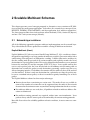
and other small group applications. This thesis contains a detailed explanation of the MSC
concept and describes an implementation of MSC capable end systems and routers in the
ns-2 network simulation software. Furthermore, a performance simulation based on realworld data is presented, including the analysis of several different combinations of MSC
end systems and routers. The results of the simulations are discussed and condensed into
conclusions highlighting the potential of Multicast for Small Conferences as a possible replacement of IP Multicast for small group applications.
Contents
1 Introduction
1
2 Scalable Multicast Schemes
2.1 Network-layer solutions . . . . . . . . . . . . . . . . . . . . . . . . . . . . . . .
2.2 End system multicast . . . . . . . . . . . . . . . . . . . . . . . . . . . . . . . . .
3
3
7
3 Multicast for Small Conferences
3.1 The MSC concept . . . . . . . . . . . . .
3.2 MSC capable routers and end systems .
3.2.1 End systems . . . . . . . . . . . .
3.2.2 MSC header handling for routers
3.3 Comparison with Xcast . . . . . . . . . .
3.4 Problems . . . . . . . . . . . . . . . . . .
3.5 Routing overhead . . . . . . . . . . . . .
.
.
.
.
.
.
.
.
.
.
.
.
.
.
.
.
.
.
.
.
.
.
.
.
.
.
.
.
.
.
.
.
.
.
.
.
.
.
.
.
.
.
.
.
.
.
.
.
.
.
.
.
.
.
.
.
.
.
.
.
.
.
.
.
.
.
.
.
.
.
.
.
.
.
.
.
.
.
.
.
.
.
.
.
.
.
.
.
.
.
.
.
.
.
.
.
.
.
.
.
.
.
.
.
.
.
.
.
.
.
.
.
.
.
.
.
.
.
.
.
.
.
.
.
.
.
.
.
.
.
.
.
.
.
.
.
.
.
.
.
10
10
10
10
12
14
14
15
4 The Network Simulation Software: ns-2
4.1 Choosing a network simulator . . . . . . . .
4.2 Protocols, packet headers and packets in ns-2
4.3 Network components . . . . . . . . . . . . . .
4.4 Routing in ns-2 . . . . . . . . . . . . . . . . .
4.5 Unicast and multicast in ns-2 . . . . . . . . .
4.6 Tracing in ns-2 . . . . . . . . . . . . . . . . . .
4.6.1 Ns-2 tracefiles . . . . . . . . . . . . . .
4.6.2 Nam . . . . . . . . . . . . . . . . . . .
.
.
.
.
.
.
.
.
.
.
.
.
.
.
.
.
.
.
.
.
.
.
.
.
.
.
.
.
.
.
.
.
.
.
.
.
.
.
.
.
.
.
.
.
.
.
.
.
.
.
.
.
.
.
.
.
.
.
.
.
.
.
.
.
.
.
.
.
.
.
.
.
.
.
.
.
.
.
.
.
.
.
.
.
.
.
.
.
.
.
.
.
.
.
.
.
.
.
.
.
.
.
.
.
.
.
.
.
.
.
.
.
.
.
.
.
.
.
.
.
.
.
.
.
.
.
.
.
.
.
.
.
.
.
.
.
.
.
.
.
.
.
.
.
.
.
.
.
.
.
.
.
16
16
17
17
19
20
22
22
22
5 MSC Implementation in ns-2
5.1 Modifications and adaptions . . . . . . .
5.2 The MSC protocol in ns-2 . . . . . . . .
5.3 Implementing end system MSC in ns-2 .
5.3.1 The MSCAgent class . . . . . . .
5.3.2 MSCAgent internals . . . . . . .
5.3.3 Example . . . . . . . . . . . . . .
5.3.4 The NaiveAgent class . . . . . .
5.4 Implementing MSC capable routers . .
5.4.1 The MSCRouter class . . . . . . .
5.4.2 MSCRouter internals . . . . . . .
5.4.3 Example . . . . . . . . . . . . . .
5.4.4 The EMSCRouter class . . . . . .
.
.
.
.
.
.
.
.
.
.
.
.
.
.
.
.
.
.
.
.
.
.
.
.
.
.
.
.
.
.
.
.
.
.
.
.
.
.
.
.
.
.
.
.
.
.
.
.
.
.
.
.
.
.
.
.
.
.
.
.
.
.
.
.
.
.
.
.
.
.
.
.
.
.
.
.
.
.
.
.
.
.
.
.
.
.
.
.
.
.
.
.
.
.
.
.
.
.
.
.
.
.
.
.
.
.
.
.
.
.
.
.
.
.
.
.
.
.
.
.
.
.
.
.
.
.
.
.
.
.
.
.
.
.
.
.
.
.
.
.
.
.
.
.
.
.
.
.
.
.
.
.
.
.
.
.
.
.
.
.
.
.
.
.
.
.
.
.
.
.
.
.
.
.
.
.
.
.
.
.
.
.
.
.
.
.
.
.
.
.
.
.
.
.
.
.
.
.
.
.
.
.
.
.
.
.
.
.
.
.
.
.
.
.
.
.
.
.
.
.
.
.
.
.
.
.
.
.
24
24
25
26
26
26
27
29
30
30
30
31
32
i
.
.
.
.
.
.
.
.
.
.
.
.
.
.
.
.
.
.
.
.
.
.
.
.
.
.
.
.
.
.
.
.
.
.
.
.
.
.
.
.
.
.
.
.
.
.
.
.
.
.
Contents
5.5
5.6
5.4.5 EMSCRouter internals . .
5.4.6 Example . . . . . . . . . .
MSC component tracing features
Running MSC simulations . . . .
6 Simulation Topology
6.1 Introduction . . . . . . . .
6.2 Backbone networks . . . .
6.3 End systems . . . . . . . .
6.4 Real-world data and ns-2 .
.
.
.
.
.
.
.
.
.
.
.
.
.
.
.
.
.
.
.
.
.
.
.
.
.
.
.
.
.
.
.
.
.
.
.
.
.
.
.
.
.
.
.
.
.
.
.
.
.
.
.
.
.
.
.
.
.
.
.
.
.
.
.
.
.
.
.
.
.
.
.
.
.
.
.
.
.
.
.
.
.
.
.
.
.
.
.
.
.
.
.
.
.
.
.
.
.
.
.
.
.
.
.
.
32
32
34
36
.
.
.
.
.
.
.
.
.
.
.
.
.
.
.
.
.
.
.
.
.
.
.
.
.
.
.
.
.
.
.
.
.
.
.
.
.
.
.
.
.
.
.
.
.
.
.
.
.
.
.
.
.
.
.
.
.
.
.
.
.
.
.
.
.
.
.
.
.
.
.
.
.
.
.
.
.
.
.
.
.
.
.
.
.
.
.
.
.
.
.
.
.
.
.
.
.
.
.
.
.
.
.
.
.
.
.
.
38
38
38
39
40
7 Simulation Setup
7.1 Simulation parameters . . . . . .
7.1.1 Group size . . . . . . . . .
7.1.2 Clustering . . . . . . . . .
7.1.3 MSC router functionality
7.2 Packets . . . . . . . . . . . . . . .
7.3 Metrics . . . . . . . . . . . . . . .
.
.
.
.
.
.
.
.
.
.
.
.
.
.
.
.
.
.
.
.
.
.
.
.
.
.
.
.
.
.
.
.
.
.
.
.
.
.
.
.
.
.
.
.
.
.
.
.
.
.
.
.
.
.
.
.
.
.
.
.
.
.
.
.
.
.
.
.
.
.
.
.
.
.
.
.
.
.
.
.
.
.
.
.
.
.
.
.
.
.
.
.
.
.
.
.
.
.
.
.
.
.
.
.
.
.
.
.
.
.
.
.
.
.
.
.
.
.
.
.
.
.
.
.
.
.
.
.
.
.
.
.
.
.
.
.
.
.
.
.
.
.
.
.
.
.
.
.
.
.
.
.
.
.
.
.
45
45
45
45
46
48
50
.
.
.
.
.
51
51
51
53
54
57
.
.
.
.
.
.
.
.
.
59
59
59
60
60
61
61
62
62
63
8 Results
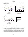
8.1 Average delays . . . . .
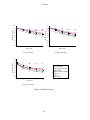
8.2 Maximum delays . . . .
8.3 Bandwidth consumption
8.4 Backbone usage . . . . .
8.5 Summary . . . . . . . . .
.
.
.
.
.
.
.
.
.
.
.
.
.
.
.
.
.
.
.
.
.
.
.
.
.
.
.
.
.
.
.
.
.
.
.
.
.
.
.
.
.
.
.
.
.
.
.
.
.
.
.
.
.
.
.
.
.
.
.
.
.
.
9 Performance Evaluation
9.1 Native multicast . . . . . . . . . . . . . . .
9.2 Naive unicast . . . . . . . . . . . . . . . .
9.3 End system MSC . . . . . . . . . . . . . .
9.4 Full-scale MSC . . . . . . . . . . . . . . . .
9.5 MSC at backbone interlinks . . . . . . . .
9.6 EMSC at backbone interlinks . . . . . . .
9.7 MSC SIX . . . . . . . . . . . . . . . . . . .
9.8 EMSC SIX . . . . . . . . . . . . . . . . . .
9.9 Comparison of MSC and native multicast
.
.
.
.
.
.
.
.
.
.
.
.
.
.
.
.
.
.
.
.
.
.
.
.
.
.
.
.
.
.
.
.
.
.
.
.
.
.
.
.
.
.
.
.
.
.
.
.
.
.
.
.
.
.
.
.
.
.
.
.
.
.
.
.
.
.
.
.
.
.
.
.
.
.
.
.
.
.
.
.
.
.
.
.
.
.
.
.
.
.
.
.
.
.
.
.
.
.
.
.
.
.
.
.
.
.
.
.
.
.
.
.
.
.
.
.
.
.
.
.
.
.
.
.
.
.
.
.
.
.
.
.
.
.
.
.
.
.
.
.
.
.
.
.
.
.
.
.
.
.
.
.
.
.
.
.
.
.
.
.
.
.
.
.
.
.
.
.
.
.
.
.
.
.
.
.
.
.
.
.
.
.
.
.
.
.
.
.
.
.
.
.
.
.
.
.
.
.
.
.
.
.
.
.
.
.
.
.
.
.
.
.
.
.
.
.
.
.
.
.
.
.
.
.
.
.
.
.
.
.
.
.
.
.
.
.
.
.
.
.
.
.
.
.
.
.
.
.
.
.
.
.
.
.
.
.
.
.
.
.
.
.
.
.
.
.
.
.
.
.
.
.
.
.
.
.
.
.
.
.
10 Summary
64
11 Outlook
66
Glossary
67
Bibliography
69
ii
1 Introduction
The increasing popularity of the Internet in the last few years not only led to a massive increase in the number of users, but also pushed the development of many new technologies
which in turn widen the range of applications available. Most of the widely-used traditional
Internet applications, such as web browsers and email, operate between one sender and one
receiver, i.e. they use unicast (point-to-point) connections. However, many new applications
require one or more sources to synchronously serve multiple receivers. Examples are the
communication of stock quotes to brokers and audio (or video) conferencing. Naively, this
could be implemented as a number of unicast connections maintained between the source(s)
and the receivers. However, this is a very inefficient approach: a sender transmitting to a
group of ten receivers would have to transmit the same data ten times. This puts needless
strain on the network infrastructure and consumes a lot of precious bandwidth. Also, such
a configuration requires the sender to keep track of receivers as they join or leave a session.
Unsurprisingly, a more efficient technology has already been developed: IP Multicast. In IP
Multicast, each session (i.e. each group of senders and receivers) is identified by a multicast
group address, and traffic is delivered to all members by the network infrastructure. The
sender does not need to maintain a list of receivers, as the receivers can join and leave multicast groups at their discretion. Also, a host may be a member of more than one group at
a time and does not need to be a member of a group to send datagrams to it. The network
infrastructure, in particular the routers, are responsible that a transmission reaches all group
members. In order to do that, each router maintains routing table entries for all multicast
groups affecting it. The routers also make sure that only one copy of a multicast message
will pass over any link in the network, and copies of the message will be made only where
paths diverge at a router. There are two kinds of groups: permanent and transient. Permanent groups have a well-known, administratively assigned IP address. Those multicast
addresses that are not reserved for permanent groups are available for dynamic assignments
to transient groups which exist only as long as they have members [18, 10].
As the Internet more and more replaces traditional telecommunication networks, it seems
very promising to also use IP Multicast to simplify audio conferencing, which is complex
to set up and very inefficient regarding bandwidth usage when conventional technology
is used. To support a conference, the IP terminals and gateways serving the conferencing
participants can join a common multicast group and exchange traffic via IP Multicast. This
avoids the multiple transport of the same traffic over the backbone networks that is seen in
traditional telephone conferences based on Multipoint Control Units (MCUs).
Unfortunately, IP Multicast does not scale well for (many) small groups such as in audio
conference scenarios. The problem is that the multicast routing entries within routers cannot
be aggregated such as unicast routing entries. While leading unicast address prefixes can
be used for routing entry aggregation, multicast address selection can be arbitrary so that
multicast addresses with similar prefixes do not necessarily have any relation to each other
1
1 Introduction
such as common multicast delivery trees. The scalability problem is even worse since multicast routing entries do not only consist of the destination address but may even include a
source address. This means that a backbone router needs to maintain a multicast routing entry for each global multicast address (or each source address, multicast address pair even
if this multicast group consists of a few members only [6]. As new small group applications
are becoming more and more popular, the routing table sizes are increasing massively. This
not only makes routers more expensive (given the high prices of router memory), but also
deteriorates the performance of these devices. Hence it is not surprising that several proposals addressing this problem have arised recently [30, 29]. There are basically two different
approaches: One idea is two move the multicast functionality up to the application layer,
simplifying the underlying network. Other concepts favor network-layer solutions enhancing or replacing IP Multicast.
This document introduces both approaches: In the first part of chapter 2, Explicit Multicast
(Xcast), Recursive Unicast Tree Multicast (REUNITE), Explicitly Requested Single-source
Multicast (EXPRESS), Distributed Core Multicast (DCM) and the Host Multicast Tree Protocol (HMTP) are presented; all five are network-layer solutions. Multicast concepts using
the application layer are presented in section 2.2. These include three infrastructure-reliant
approaches (CANs, Scattercast, Bayeux), plus Narada. As the title suggests this thesis focuses on MSC - explained in detail in chapter 3 - and presents a performance study based
on simulation results. Consequently, chapter 4 provides an introduction to the ns-2 network
simulator and its most important features, while chapter 5 gives an in-depth explanation of
an MSC implementation in ns-2. In the subsequent two chapters (6 and 7), the simulation
topology and the simulation setup are presented. The simulation results are discussed on
a per-parameter basis in chapter 8, while the performance of the different configurations is
discussed in chapter 9. Chapter 10 presents a number of conclusions based on the simulation
results, with the final chapter providing a short description of possible future work. This is
followed by a glossary and the bibliography at the end of the document.
2
2 Scalable Multicast Schemes
This chapter presents several concepts proposed as alternatives to or extensions of IP Multicast, mainly for small group applications. It describes five network layer concepts (Xcast,
REUNITE, EXPRESS, DCM and HMTP) and four application level multicast approaches.
The latter group includes three infra-structure reliant methods (CANs, Scattercast, Bayeux)
and one “real” end systems concept (Narada).
2.1
Network-layer solutions
All of the following approaches propose multicast implementations on the network layer.
They either define an all-new protocol or extend the existing IP Multicast mechanism.
Explicit Multicast (Xcast)
Explicit Multicast [31] (the successor of Small Group Multicast [5, 4]) is a multicast scheme
designed for supporting a very large number of multicast sessions as present in audio/video
conferencing, network games or collaborative working. It differs from native multicast in
that the sending node keeps track of all session members and explicitly encodes the list of
destinations in a special packet header. This newly defined header introduces a new protocol
between the network (IP) and the transport (UDP/TCP) layer. Xcast capable routers that
receive such a packet parse the Xcast header and use the ordinary unicast routing table to
determine how to route the packet to each destination, generating a packet copy for every
affected outgoing interface. Each address list contains only the addresses that can be reached
via that interface. If there is only one destination for a particular next hop, the packet may
be sent as a standard unicast packet, as there is no multicast gain by formatting it as an Xcast
packet.
The Explicit Multicast scheme has three major advantages:
Routers do not have to maintain per session state. This makes Xcast very scalable in
terms of the number of sessions that can be supported since the nodes in the network
do no need to disseminate or store any multicast routing information for these sessions.
No multicast addresses are used; thus, all problems related to multicast address allocation are eliminated.
No multicast routing protocols are required, neither intra- nor interdomain. Xcast
packets always take the correct path as determined by the unciast routing protocols.
But while Xcast solves the scalability problems of native multicast, it creates some new complexity:
3
2 Scalable Multicast Schemes
Xcast introduces a new protocol and a new protocol ID in the IP header, and the new
protocol header increases the packet overhead. Also, header processing for router becomes more complex, as additional routing table lookups are necessary.
For smooth deployment, Xcast tunnels have to be set up between Xcast capable routers.
Xcast does not rely on established multicast mechanism, making it difficult to allow native multicast receivers to join a multicast group. Although gateways that translate IP
Multicast packets into Xcast packets can be deployed, the problem remains that those
gateways have to synchronize themselves in order to make sure that the same IP Multicast addess is being used for the same set of receivers or multicast group respectively.
Recursive Unicast Tree Multicast (REUNITE)
REUNITE [27] is a multicast scheme that completely avoids the use of IP multicast addresses
and instead relies on unicast addresses both for group identification and packet forwarding.
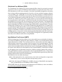
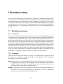
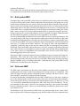
The REUNITE approach has been designed specifically for sparse multicast groups and is
based on an important observation: When the members of a multicast group are distributed
sparsly in a network, the data delivery tree of the group is likely to have a large number of
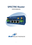
non-branching routers or routers that have only one downstream router. This is illustrated
by the authors of [27] with the tree shown in Figure 2.1, which shows a forwarding tree from
Carnegie Mellon University to 15 U.S. sites.
CMU
R9
R7
R8
R10
R11
R12
R13
R14
R15
R2
R4
R6
R1
R3
R5
Figure 2.1: A multicast forwarding tree from CMU to 15 U.S. sites (taken from [27]).
Consequently, REUNITE aims at exonerating the non-branching routers. The key idea is
to use recursive unicast to implement multicast service. For each group, REUNITE builds
a delivery tree rooted at a specifically designated node (usually the source) called root. A
multicast group is identified by the root’s IP address and a port number. The forwarding
tree is then set up and maintained by control messages sent by the source and the receivers.
Each REUNITE router maintains a Multicast Forwarding Table (MFT) that contains an entry
for every multicast group whose data delivery tree branches at the router. In addition to the
MFT, each REUNITE capable router maintains another table called the Multicast Control Table (MCT). The MCT contains an entry for every group whose multicast delivery tree passes
4
2 Scalable Multicast Schemes
but does not branch at the router. This is not equivalent to the concept of native multicast,
since an MCT lookup is only necessary when processing control messages; during normal
packet forwarding, only MFT lookups need to be performed. REUNITE has a number of
advantages over IP Multicast:
Only the routers at branching points are required to keep multicast forwarding state of
the group. In effect, REUNITE removes unnecessary forwarding state by converting it
into control path state. This results in enhanced scalability, especially in large networks
with many small groups.
REUNITE is incrementally deployable. Since all packets have unicast addresses, a
router that does not implement the new protocol just forwards the packets as if they
were unicast packets.
Since REUNITE does not require every router to process protocol control messages,
a router that is overloaded can decline making further MFT entries and let other upstream routers process the relevant messages. This results in a load balancing capability (even though the forwarding tree may become less efficient).
Using REUNITE gateways, it is possible to retain native multicast in local networks. Since
REUNITE does not use class D addresses at all, the gateways may even use different IP multicast addresses in their respective local networks.
The performance evaluation of REUNITE presented in [27] is based on several ns-2 simulations (ns-2 is presented in chapter 4). However, only the link stress (i.e. the number of
identical packets sent over a link) has been analysed. With many REUNITE capable routers
in the network, the value is very low (close to one). In contrast, link stress values of up to 12
were observed in scenarios with up to 64 receivers and no REUNITE routers.
Explicitly Requested Single-Source Multicast (EXPRESS)
In contrast to Xcast and REUNITE, EXPRESS [15] does not want replace IP multicast. Instead, it provides an extension which introduces means for access control and charging
mechanisms. EXPRESS uses the concept of multicast channels. A channel is a datagramm
delivery service identified by the sender’ source address and a channel destination address.
These destination addresses are specially allocated class D addresses and allow each host in
the Internet to source up to 16 million channels (since a session is identified by the source
and the channel ID). This is an advantage over IP multicast, where address allocation has to
be coordinated Internet-wide.
EXPRESS also introduces a new service function called count, which can be used to collect
information such as the number of receivers a channel serves or the number of links in the
delivery tree. This type of information is useful for charging models.
In terms of packet forwarding, EXPRESS behaves like conventional IP Multicast. ECMP, the
management protocol of EXPESS, sets up forwarding entries in the routers forwarding tables
like other multicast protocols do. Therefore, the problem of increasing routing table sizes is
not addressed.
5
2 Scalable Multicast Schemes
Distributed Core Multicast (DCM)
The Distributed Core Multicast [3] routing protocol differs from the previously presented
approaches in that it replaces IP Multicast in the backbone networks but retains native multicast for delivery in the access networks. It has been specifically designed to scale better
than existing multicast routing protocols when there are many multicast groups with only
a few members each. DCM relies on an overlay network created by so-called Distributed
Core Routers (DCRs). The DCRs are located at the edge of the backbone networks and act as
access points for data from senders inside their area (i.e. an access network) to receivers outside this area. Multicast packets from senders inside are sent towards the local DCR either
by encapsulation or source routing. A DCR also forwards the multicast data received from
the backbone to receivers in the area it belongs to, using native multicast. The Membership
Distribution Protocol (MDP) runs between the DCRs serving the same range of multicast addresses and allows the DCRs to learn about other DCRs that have group members. Also, the
Distributed Core Routers run a special data distribution protocol that tries to optimize the
use of backbone bandwidth and does not require the non-DCR backbone routers to perform
multicast routing. The performance evaluation of DCM presented in [3] is based on ns-2 (see
chapter 4) simulations. It indicates that DCM can massively reduce the routing table size for
backbone routers, as they only need to maintain membership information for a small number of MDP control multicast groups. Also, the DCRs’ routing tables are significantly smaller
than those of a backbone router when using PIM-SM 1 .
Host Multicast Tree Protocol (HMTP)
While the advantages of multicast delivery over unicast delivery are undeniable, the deployment of the IP Multicast protocol has been limited to “islands” of network domains under
single administrative control. These islands need to be connected by manually configured
tunnels to form a static overlay network, which is expensive to set up and maintain. The goal
of Host Multicast [32] is to dynamically connect IP Multicast islands using UDP tunnels. To
achieve this, one member host in each island is elected as the Designated Member (DM) for
the island. Each DM runs the Host Multicast Tree Protocol (HMTP), which allows the DMs
to self-organize into a bi-directional shared tree. Multicast packets produced by sender inside an IP Multicast island are intercepted by the Designated Member hosts, encapsulated
into UDP packets and forwarded along the tree. Receiving DMs decapsulate the packet and
multicast them in their respective local domains.
Host Multicast has two major advantages:
It is fully deployable in the current internet, since it does not depend on cooperation
from routers, servers, tunnel end-points and operating systems.
It takes advantage of IP Multicast’s scalability (in terms of bandwidth consumption),
since it automatically uses IP Multicast where available.
While HMTP helps the development and deployment of IP Multicast, it does not address
any of the latter’s problems mentioned in chapter 1.
1
Protocol Independent Multicast - Sparse Mode
6
2 Scalable Multicast Schemes
2.2
End system multicast
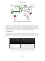
While the concepts presented in the previous sections try to overcome the problems of IP
Multicast by improving the network layer with new router functionality and/or new protocols, there is also a different approach: end system multicast. The idea is to migrate the
multicast service to higher levels, thereby simplifying the underlying network model. Thus,
the problems that plague IP Multicast (group management, routing) are either eliminated or
mitigated due to application-level intelligence. However, the key concern with such a model
is the associated performance penalty. In particular, an overlay approach to multicast, however efficient, cannot perform as well as IP Multicast. It is impossible to completely prevent
multiple overlay edges from traversing the same physical link and thus some redundant
traffic on physical links is unavoidable. Further, communication between end systems involves traversing other end systems, potentially increasing latency [16].
A number of end system/application-level multicast concepts as well as their respective performance characteristics are presented in the following sections. The CAN, Scattercast and
Bayeux approaches are infra-structure-reliant in the sense that they use an overlay network
not only consisting of the end systems in a specific multicast group, but requiring some permanently deployed, group-independent functionality in the network (e.g. a certain router
feature or routing protocol). In contrast, the Narada concept is a “real” end system multicast approach, using only the end systems that are members of a certain multicast group for
transmissions for that group.
Content-Addressable Networks (CAN)
A Content-Addressable Network [23] is a self-organizing application-level network whose
constituent nodes can be thought of as forming a virtual d-dimensional Cartesian coordinate
space. Every node in a CAN “owns” a portion of the total space. CANs are scalable, faulttolerant and completely distributed. The authors of Application-level multicast using CANs
[24] argue that
assuming the deployment of a CAN-like infrastructure in the network, CAN-based
multicast is trivially simple to achieve.
CAN-based multicast can scale to very large group sizes without restricting the service
model to a single-source.
no multicast routing protocol is required, since routing is inherent in CANs.
The simulation-based performance evaluation of multicast using CANs presented [24] indicates that with physical (IP-level) delays of up to 100ms the actual delay in the applicationlevel network can easily reach 300ms, with single values up to 600ms. Thus, it is unlikely
that this approach could be used for delay-sensitive applications such as audio or video conferences. However, multicast using CANs could be ideal for less demanding services that
need to support very large group sizes.
Scattercast
Scattercast [7], also an application-level approach, relies on a collection of strategically placed
network agents (ScatterCast proXies, SCX) that collaboratively provide the multicast service
7
2 Scalable Multicast Schemes
for a session. Agents organize themselves into an overlay network of unicast connections
and build data distribution trees on top of this overlay structure. Clients locate a nearby
agent and tap into the multicast session via that agent. Native multicast mechanism are
used for communication between the client(s) and the proxies, while the proxies exchange
data using unicast connections and a special protocol called Gossamer.
The simulations performed by the authors of Scattercast show that the end-to-end delays are
1.35-2.35 those of native unicast, with a typical value of 1.65. This cost ratio increases when
more SCXs are introduced (due to the additional overhead), but it remains well below 2 even
with 350 SCX involved. This should make Scattercast suitable for many applications. Also,
the Gossamer protocol used for SCX interaction significantly reduces the link stress (the
number of duplicate packets sent over a link) compared to naive unicast, where one packet
copy per receiver is created. However, bandwidth consumption has not been analyzed.
Bayeux
Bayeux [34] uses a prefix-based routing scheme that it inherits from an existing applicationlevel routing protocol called Tapestry [33], a wide-area location and routing architecture. On
top of Tapestry, Bayeux provides a simple protocol that organizes the multicast receivers
into a distribution tree rooted at the source. Tapestry itself guarantees good scalability and
provides multiple paths to every destination, thus enabling application-specific protocols
for fast failover and recovery. Unlike most other application-level multicast systems, not all
nodes of the Tapestry overlay network are Bayeux multicast receivers. This use of dedicated
infrastructure server nodes provides better optimization of the multicast tree.
The performance evaluation presented by the authors uses a topology of 50’000 nodes and
simulated multicast groups with 4’096 members. The results show that the end-to-end delays increase by a factor of up to 6; this indicates that Bayeux cannot support delay-sensitive
applications such as audio or video conferences (unless the underlying physical network has
a very low latency). The advantages of Bayeux are the support for very large groups and its
fault-handling, the latter also allowing reliable service, a feature unique to Bayeux.
Narada
Narada [16] is a “real” end system multicast protocol in the sense that it does require any
infrastructure support (i.e. pre-deployed network functionality). It constructs an overlay
structure among participating end systems in a self-organizing and fully distributed manner.
The construction of the overlay is performed in a two-step process. First, an arbitrary connected subgraph of the Complete Virtual Graph (CVG) is created. In a second step, Narada
constructs reverse shortest path spanning trees of the mesh, each tree rooted at the corresponding source; this is done using well-known algorithms. Since the overlay construction
mechanism of Narada is self-organizing and self-improving, Narada is robust to the failure of end systems and to dynamic changes of group membership. Unlike Xcast and MSC,
Narada can also support large multicast groups. This is confirmed by the performance evaluation presented in [16], which is based on simulations with topologies of up to 1’070 nodes
and multicast groups of up to 256 members. In a group with 128 members, the delay between 90% of pairs of members increases by a factor of at most 4 compared to the unicast
delay between them. For a group of 13 members the same value is 1.5. Thus, Narada seems
to be a viable solution for supporting small multicast groups. In terms of bandwidth con-
8
2 Scalable Multicast Schemes
sumption, Narada performs significantly worse than native multicast. For the previously
mentioned 128-member group, Narada consumes 80% more bandwidth than IP Multicast.
However, this is about a 20% saving compared to naive unicast. With larger group size, the
performance of Narada relative to native multicast improves. Also, link stress (i.e. the number of identical packets sent over a link) is massively lower with Narada than with naive
unicast.
Unfortunately the data of the performance evaluation of Narada presented in [16] is not
directly comparable to the data of the MSC simulations performed as part of this thesis.
Narada was developed to replace native multicast for a wide range of applications and can
also support large groups. Consequently, the performance evaluation has been performed
with very large simulation topologies (up to 1’070 nodes) and different multicast group sizes,
ranging from 13 to 256 members. In contrast, Multicast for Small Conferences only is an
alternative to native multicast in (very) small groups. Thus, the performance simulations
presented in chapter 7 are run with groups of 4 to 20 hosts only. Also, a completely different
topology is used. The NRU (Normalized Resource Usage) values of the two simulations can
be used to illustrate their incompatibility. While the Narada simulations have a maximum
NRU of 2.1 for naive unicast, the same value is 3.7 in the MSC simulations, despite massively
smaller group sizes, which should result in less packet copies.
9
3 Multicast for Small Conferences
This chapter contains an in-depth description of the Multicast for Small Conferences concept
and explains the functionality of MSC end systems and routers. Also included are a comparison between MSC and Xcast as well as a short discussion of possible problems affecting
Multicast for Small Conferences. The last section covers the aspect of increased routing complexity.
3.1
The MSC concept
The Multicast for Small Conferences [6] concept aims at solving the scalability problem of
native multicast while at the same time avoiding the problems of an Xcast-like approach. A
first difference is that MSC is proposed as a concept for multicast packet delivery in the Internet backbone only, while existing intra-domain multicast routing mechanism can remain
in use for regional or access networks. Also, instead of introducing a new protocol, MSC
relies solely on the existing IPv6 [26] protocol, in particular on the IPv6 routing header. In
the Multicast for Small Conferences concept, the unicast address of each receiver is stored in
each packet. The address of the receiver closest to the sender is used as the IP destination
address, while the other addresses are carried in the routing header. The group’s multicast
address should ideally be stored in the routing header as well. However, according to the
IPv6 specification [26], multicast addresses must not appear in a routing header of type 0, or
in the IPv6 destination address field of a packet carrying a routing header of type 0. There
are two solutions to overcome this limitation. The first solution is compatible with all current IPv6 routers, while the second solution is recommended for long-term usage. While in
the first solution the multicast address is carried in a newly defined IPv6 destination option,
in the second solution it is carried at the end of an also newly defined type 1 IPv6 routing
header.
3.2
3.2.1
MSC capable routers and end systems
End systems
MSC sender
An MSC routing header is generated by a sender that is either an MSC terminal or an MSC
gateway. The MSC gateways have the task of supporting end systems not capable of MSC
and/or IPv6 by “translating” the transmission, using native multicast in the local network.
In any case the sender creates a unicast address list of all group members and puts the nearest one in the IPv6 destination address. All other member addresses are put into the MSC
routing header, preferably ordered by the distance from the sender. If the sender detects
10
3 Multicast for Small Conferences
that members have to be reached via different outgoing interfaces, a packet for each affected
interface is generated with the list of members that can be reached via this interface. This
means that a sender divides the address list into N parts and sends N copies of the packet to
the N generated lists.
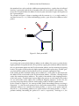
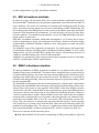
The example in Figure 3.1 shows a topology with five routers (R1-R5), a single sender (S)
and four receivers (D1-D4). When transmitting a packet, S puts all receiver addresses in the
packet.
D1
D2
D4
D3
D2
D4
D3
R2
R3
R5
R4
D4 D3 D2 D1
R1
D4
S
D3
D4
Figure 3.1: End system MSC
Receiving end systems
A receiving end system which finds its address in the address list creates a packet for the
higher protocols encapsulated in the IPv6 packet by copying the multicast address found in
the new destination option into the IPv6 destination address and by removing the routing
header. This packet is delivered to the higher protocol for further processing. An MSC gateway forwards the packet to local multicast receivers using the appropriate scope.
If the routing header contained further unicast addresses, a new packet is generated with
the address of the nearest node in the IPv6 destination address. As before, a routing header
carries the remaining unicast addresses. The packet is forwarded via the outgoing interface
of the end system. A multi-homed system might also generate several copies of the packet
if it can reach nodes of the address list via different outgoing interfaces. In this case, the
receiving end system behaves like the sender of the packet or an MSC capable router.
In the example in Figure 3.1, the concept of MSC packet forwarding between receiving is
illustrated. D1 is the first end system to receive the packet transmitted by S. Detecting that
additional addresses are carried in the routing header, D2 creates a new packet copy addressed to D2; the remaining addresses are again carried in the routing header. D2 and D3
perform similarly, forwarding the packet to D2 and D3 respectively. Arriving at D4, the
11
3 Multicast for Small Conferences
packet’s routing header is empty (apart from the group’s multicast address), and thus no
packet forwarding is required from the part of D4.
3.2.2
MSC header handling for routers
Non-MSC routers
A router that does not understand the MSC header forwards the packet towards the address
specified in the IPv6 destination field.
MSC capable routers
MSC capable routers read the addresses from the IP destination field and the routing header
and determine the outgoing interface for each destination. They then duplicate the packet
for each involved link. Each packet contains only the unicast addresses that can be reached
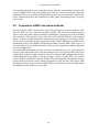
via that interface plus the multicast address identifying the group. This is the MSC functionality proposed in [6]; in this document, this concept is denoted standard MSC.
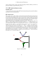
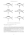
Figure 3.2 illustrates the standard MSC procedure for routers. The setup is the same as in
Figure 3.1, with S sending a packet to the group members D1-D4. All five routers (R1-R5)
are considered MSC capable. On receiving the packet sent by S, R1 performs routing table
lookups for all four addresses carried therein, detecting that D1 and D2 are reached via R2,
while the other two receivers are reached via R5. Thus, R1 produces two packet copies,
each one containing only the relevant addresses. R2 and R5 perform the same operation
on the packets they receive, thus optimizing the packet delivery. In this scenario, no packet
forwarding between end systems is necessary. If, for example, R2 had not been MSC capable, then the packet created by R1 would have been delivered to R3, which would have
forwarded it to D4 as shown in Figure 3.1.
D2
D2
D1
D1
R2
D2
R3
D1
D4 D3 D2 D1
S
R1
D4
D3
R5
R4
D4
D3
D3
Figure 3.2: Standard MSC
12
D4
3 Multicast for Small Conferences
Enhanced MSC
A possible improvement of the standard MSC concept involves the use of topology information, which can for example be obtained from a link state routing protocol such as OSPF.
1 The first MSC capable router that handles an MSC packet after it enters a certain network
domain determines the egress router (i.e. the router where the packet leaves the domain)
for the destination address and all addresses listed in the routing header. A packet is then
created for each involved egress router. Thus, packet forwarding between destinations connected to the same network can be eliminated. On the downside, multiple MSC packets may
be sent over the same link, if two or more egress routers are reached via the same outgoing
interface. In this document, this advanced concept is denoted enhanced MSC.
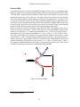
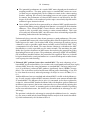
Figure 3.3 illustrates packet forwarding using enhanced MSC. The toplogy is the same as
that of the previous two figures. Again, all five routers are considered MSC capable; additionaly, we assume that R1-R5 form a network domain. As R1 receives the packet sent by S,
it determines the egress router for all addresses: R2 for D1 and D2, R5 for D3 and R4 for D4.
Thus, three packet copies are created, each carrying only the addresses reached via a certain
egress router. R4 and R5 do not need to perform any special action, as the packets they encounter only carry a single address. However, in contrast to the standard MSC concept, two
packets with identical payload were sent over the R1 R5 link. R2 detects that D1 and D2
are reached via different interfaces and creates a packet copy for each receiver. This part of
the MSC functionality is identical in standard and enhanced MSC.
D2
D2
D1
D1
D2
R2
R3
R5
R4
D3
D4
D1
D4 D3 D2 D1
S
R1
D4
D3
Figure 3.3: Enhanced MSC
1
Open Shortest Path First
13
3 Multicast for Small Conferences
3.3
Comparison with Xcast
Although MSC is based on ideas similar to XCast, there are significant differences:
MSC avoids introducing a new protocol and instead relies solely on IPv6.
MSC requires no tunneling between gateways, as routers without MSC functionality
can simply forward the packet according to the IPv6 destination address. This also
simplifies a gradual deployment of MSC in the network.
MSC uses unicast forwarding in the backbone; multicast routing can be retained in
local networks using MSC gateways.
MSC allows applications to use native IP Multicast. Gateways only need to insert an
MSC routing header instead of doing complete address mapping as in Xcast. Therefore
the same multicast address can be used at different sites without the need for synchronizing the gateways.
These items are an indication that Multicast for Small Conferences is less complex to introduce and use than Explicit Multicast.
3.4
Problems
Multicast for Small Conferences suffers from the following problems [6]:
The IPv6 routing header creates overhead that is increasing with the group size. This
might be a problem for audio applications, where the packets are usually relatively
short. Severe complications might emerge in wireless networks. The overhead problem can be solved by gateways serving as MSC receivers and forwarding the received
packets via native IPv6 Multicast to the other receivers after discarding the routing
header.
MSC is an IPv6 only solution and requires the MSC routers and gateways to support
IPv6; solutions such as IP options have to be found to support IPv4 end systems.
All senders need to know the IPv6 unicast address of the group members. This problem can be solved by a group control protocol by which the MSC receivers announce
conference group membership to each other. This information might be distributed
within session descriptions of the Session Announcement Protocol (SAP) by which session descriptions are distributed over a well-known multicast address. The integration
of SDP and MSC is discussed in [6].
MSC introduces additional complexity to the routing process, an aspect which is discussed in the next section.
The problem of increased bandwidth consumption due to the routing header is discussed as
part of the performance evaluation in chapter 9.
14
3 Multicast for Small Conferences
3.5
Routing overhead
As pointed out in the introduction, native multicast is not suitable for supporting a large
number of small multicast groups. The reason is that each router that is part of a forwarding tree has one or more routing table entries for each multicast group. This increases the
routing table size, since the multicast addresses cannot be aggregated. Multicast for Small
Conferences and other approaches exonerate the routers by explicitly carrying the receiver’s
unicast addresses in each packet, which eliminates the need for routers to maintain any information about multicast groups. While this reduces the routing table size, it increases the
complexity of the routing process: When handling an IP Multicast packet, the router has to
scan the routing table for all entries with that address (determining the affected outgoing interfaces) and produce the appropriate number of packet copies. But when encountering an
MSC (or Xcast) packet, the router has to perform multiple lookups, one for each unicast address carried in the packet. Furthermore, the router cannot simply create a packet copy per
outgoing interface. Instead, it has to make sure that each packet only contains the addresses
that can be reached via a certain interface, i.e. the router has to modify the routing header.
While the additional routing table lookups should only marginally affect the router’s overall
performance, the additional header handling and packet copying may be more problematic,
even though the address/interface sorting mechanism is relatively simple to implement [2].
However, MSC and Xcast will in any case put less strain on the router than a naive unicast
approach would.
15
4 The Network Simulation Software: ns-2
Chapter 4 gives an insight into the network simulation software used for this project. It
consists of an overview of ns-2’s capabilities as well as descriptions of some specific features that were relevant for the implementation of MSC. The latter category includes aspects
such as protocols, packets and packet headers, end system simulation as well as unicast and
multicast routing mechanisms.
4.1
Choosing a network simulator
There are quite a number of network simulators available today. However, not all of these
have been able to establish a good reputation within the research community, and of those
who have, most are expensive (e.g. Opnet [21]). In contrast, ns-2 is freely available, and this
has certainly been one of the reasons why it has become the de facto standard network simulator for academic research. The software package, developed by the Information Sciences
Institute (ISI) of the University of Southern California (USC) as part of the Virtual Internet
Testbed (VINT) [19] since 1995, has some major advantages:
documentation Ns-2 has an extensive user manual ( 350 pages) which is maintained by
the developers and updated regularly. Furthermore, there are a number of tutorials
available for new users [14, 8].
large number of users Since ns-2 is widely used in academic research there are a lot of
people working on and with the simulator worldwide. Their knowledge is brought
together and shared through a mailing list with a huge searchable archive.
specialized modules Ns-2 supports the simulation of a large number of technologies and
procedures, including LANs, mobile networking, satellite networking and ad-hoc networking.
Unfortunately, ns-2 also has a number of deficiencies:
mixed coding in OTcl/C++ The developers of ns-2 tried to achieve a fast iteration time
while at the same maintaining a good run-time performance. The result was the use
of a combined OTcl/C++ framework. This in fact yields the envisaged result, but on
the downside the simulator source code tends to be complicated and difficult to understand.
documentation As mentioned above, ns-2 has an extensive documentation covering almost
all aspects of the simulator. But despite being updated regularly the documentation is
not up to date in all parts, which complicates things for developers. Furthermore, there
are very few comments in the code, making program analysis even more difficult.
16
4 The Network Simulation Software: ns-2
structure The structure of ns-2 isn’t logical in all parts. While there are components like
packets, links and queues, there is no such thing as a router. Instead, the router functionality is implemented in a number of internal components (see section 5.4 for details), which makes changes to ns-2’s routing mechanisms rather difficult.
Overall, it can be said that ns-2 is relatively easy to use as long as existing modules can be
used. However, the development of new components is rather complex and time-consuming.
This is particularly true for the implementation of functionality inside the network (e.g.
routers).
4.2
Protocols, packet headers and packets in ns-2
When talking about packets in ns-2, it is important to distinguish between the packet that is
simulated (i.e. a real-world packet) and the simulator’s internal packet representation. The
difference can easily be illustrated by looking at a packet at network level, for example from
an audio transmission. In reality, such a packet could consist of an IP header, followed by
UDP and RTP headers and the payload (the actual audio data). In the simulator, the packet
has these four parts as well, but it also features all other packet (or protocol) headers which
ns-2 supports, e.g. TCP, Ping, MAC etc, even though they’re not all used. Also, each ns2 packet has a so-called common header, which contains important simulator information
such as the simulated packet size (in the example: length of IP, UDP and RTP headers plus
payload length), the packet type, a unique packet ID assigned by the simulator and a timestamp field used to measure queueing delays.
Furthermore, ns-2’s packet headers for specific protocols do not necessarily correspond to
the protocol headers defined in RFCs. For example, ns-2’s IPv4 header just consists of the
destination address, the source address and a TTL field. Everything else (such as ToS, header
checksum, options etc.) has been left out. However, additional fields may be added to any
header if the need arises.
Since ns-2.1b8 - the version used for the simulations in this thesis - does not explicitly support IPv6 and in particular does not provide the means for supporting a routing header, an
MSC packet header was introduced to simulate the relevant fields as well as to store additional information needed for the simulation (original sender, sending time). This new
header structure will be described in detail in section 5.2.
4.3
Network components
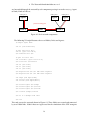
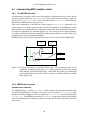
In ns-2, a simulation is set up by creating a network out of components provided by the software. There are three major components: Nodes, Links and Agents. Nodes represent hosts
or routers in a network. By connecting Nodes with Links, a network topology is formed.
Agents represent endpoints where network-layer packets are constructed or consumed; they
are also used used for the implementation of protocols at various layers. Ns-2 has a variety
of Agents for different protocols. Some Agents are both sender and receiver, while others
are specialized on a single function. For the simulation of MSC capable end systems a new
ns-2 Agent has been developed; it is described in section 5.3. Agents are attached to Nodes
and identified by an address consisting of the Node’s ID and a port number. A Node can be
connected to one or more Links and host zero or more Agents. During a simulation, packets
17
4 The Network Simulation Software: ns-2
are forwarded through the network by each component passing it on to the next, e.g. Agent
to Node, Node to Link etc.
node 0 port 0
node 2 port 0
node 2 port 1
Agent
Agent
Agent
packet forwarding path
Node 0
Link
Node 1
Link
Node 2
Figure 4.1: Ns-2 network components
The following Tcl script illustrates the use of Nodes, Links and Agents:
# simple agent demo
set ns [new Simulator]
# open nam trace file
set nf [open out.nam w]
$ns namtrace-all $nf
# open ns trace file
set tracefile [open trace.ns w]
$ns trace-all $tracefile
set n0 [$ns node]
set n1 [$ns node]
set n2 [$ns node]
$ns duplex-link $n0 $n1 1Mb 10ms DropTail
$ns duplex-link $n1 $n2 1Mb 10ms DropTail
set udp0 [new Agent/UDP]
set null2a [new Agent/Null]
set null2b [new Agent/Null]
$ns attach-agent $n0 $udp0
$ns attach-agent $n2 $null2a
$ns attach-agent $n2 $null2b
$ns connect $udp0 $null2b
$ns at 0.1 "$udp0 send 100"
$ns run
This code creates the network shown in Figure 4.1. Three Nodes are created and connected
by two 1 Mbit links. Node 0 hosts an Agent used for the simulation of the UDP transport
18
4 The Network Simulation Software: ns-2
protocol, while Node 1 does not have any Agents, i.e. it is acting as a router only. Two
NullAgents are attached to Node 2. Attached to ports 0 and 1 respectively they both act as
traffic sinks, as they simply discard any incoming packets. The simulator schedules a “send”
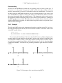
event for the UDP Agent for simulation time 0.1. Thus, at this time the UDP Agent will send
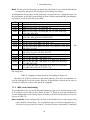
a data packet addressed to Node 2 Port 1. The results of this simulation are shown in Figure
4.2.
0
1
2
0
(a)
1
2
(b)
Figure 4.2: Nam output for the script listed above. (More information about Nam is provided
in section 4.6.2.) The UDP protocol Agent on Node 0 sends a packet addressed
to one of the Agents on Node 2. This packet is forwarded by the Node and Link
components to the receiver, which discards it.
4.4
Routing in ns-2
Unfortunately, there’s no such thing as a router in ns-2. Instead, router functionality is implemented in different parts of the node. The routing tables are maintained by a routing object
in the Simulator (class RouteLogic) and, in case of dynamic routing, in the Nodes (class
rtObject). Furthermore, there are routing agents which implement the different routing
protocols supported by the simulation software.
Inside the Node, packet forwarding is performed by classifier objects (described in chapter
5 of the ns Manual [20]). Classifiers are components with a single entry for packets and one
or more outputs. They analyse incoming packets and pass them on to the next downstream
object, which can be another classifer, a link or an agent (Figures 4.3 and 4.4).
NS-2 provides several types of classifiers:
Address classifiers examine a packets destination field and are used primarily for unicast
packet forwarding. The Port classifier is also an address classifier; it is used for forwarding a packet to the correct receiving Agent on a Node.
Multicast classifiers are installed at the nodes if a simulation uses multicast. These components basically have the same functionality as address classifiers, forwarding packets
according to their source and destination addresses. However, they use Replicator
objects to forward multiple packet copies if necessary.
Replicators are special classifiers since they do not analyse the packets: A Replicator just
sends copies of a packet to all outputs.
Multipath classifiers do not examine any packet fields. Incoming packets are forwarded to
the current slot, and all outputs are served in a round-robin fashion. This can be used
to simulate a router which has multiple routes to a destination and would like to use
them simultaneously.
19
4 The Network Simulation Software: ns-2
Hash classifiers are used when packets should be forwarded according to one or more
packet fields (eg. flow id, source address).
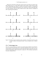
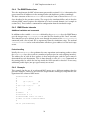
Each Node in ns-2 has a predefined structure of classifiers, shown in Figures 4.3 and 4.4. The
Node class provides a method insert-entry which allows the user to install additional
classifiers at the node entry, i.e. any incoming packet will first be handled by the newly
installed object. This functionality is used to “transform” nodes into MSC capable routers,
as a newly created MSC classifier is installed at the selected nodes (for details see section 5.4
and Figure 5.2).
Agent
Agent
Node
Port Classifier
Link
Link
Address Classifier
Figure 4.3: The internal structure of a standard ns-2 unicast Node. Any incoming packet is
first handled by an address classifier which checks the destination field of the
packet. If the packet is addressed to another Node, it is forwarded to the appropriate link. Otherwise a port classifier forwards the packet to the specified
Agent.
4.5
Unicast and multicast in ns-2
For simulations that rely only on unicast, a simulator instance is invoked using the new
Simulator command. Each unicast node created by this instance has a very simple predefined classifier structure, consisting mainly of an address classificator that forwards incoming packets either to an Agent installed on the node or an outgoing link (Figure 4.3).
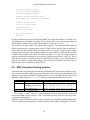
In order to use multicast mechanisms, multicast has to be explicitly enabled when instantiating the simulator, using the new Simulator -multicast on command. Thus, nodes
will be created with additional classifiers and replicators for multicast forwarding (Figure
4.4). Furthermore, a multicast routing protocol has to be specified and configured in the simulation script. In the 2.1b8 version of ns-2, two kinds of multicast protocols are supported
[20]:
Dense Mode (DM) DM.tcl is an implementation of a dense-mode-like protocol. Depending on the value of DM class variable CacheMissMode it can run in one of two modes.
20
4 The Network Simulation Software: ns-2
Agent
Agent
Node
Unicast classifier
Port classifier
Link
G1
Link
Switch
Multicast classifier
Replicators
G2
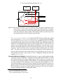
Figure 4.4: The internal structure of an ns-2 multicast Node. The first element in the classifier chain is a switch which separates unicast and multicast traffic. The multicast classifier determines the correct outgoing interfaces from the group address,
while the replicators simply produce the required number of packet copies and
forward them to the receivers (Agents and/or Links)
If CacheMissMode is set to pimdm (default), PIM-DM 1 like forwarding rules will be
used. Alternatively, CacheMissMode can be set to dvmrp (loosely based on DVMRP 2 ).
The main difference between these two modes is that DVMRP maintains parent-child
relationships among nodes to reduce the number of links over which data packets are
broadcast. The implementation works on point-to-point links as well as LANs and
adapts to the network dynamics (links going up and down). Any node that receives
data for a particular group for which it has no downstream receivers, sends a prune
upstream. A prune message causes the upstream node to initiate prune state at that
node. The prune state prevents that node from sending data for that group downstream to the node that sent the original prune message while the state is active. The
time duration for which a prune state is active is configured through the DM class
variable PruneTimeout.
Centralized Multicast (CtrMcast) Centralized multicast is a sparse mode implementation
of multicast similar to PIM-SM3 . A Rendezvous Point (RP) rooted shared tree is built
for a multicast group. The actual sending of prune, join messages etc. to set up state at
the nodes is not simulated (unlike in Dense Mode!). A centralized computation agent
is used to compute the forwarding trees and set up multicast forwarding state, S, G
at the relevant nodes as new receivers join a group. Data packets from the senders to a
group are unicast to the RP. Note that data packets from the senders are unicast to the
RP even if there are no receivers for the group. By concept, the RP sends the multicast
packet to all group members, including the sender.
1
Protocol Independent Multicast - Dense Mode
Distance Vector Multicast Routing Protocol
3
Protocol Independent Multicast - Sparse Mode
2
21
4 The Network Simulation Software: ns-2
4.6
Tracing in ns-2
4.6.1
Ns-2 tracefiles
The network simulator supports the collection simulation data in a tracefile. However, the
user has to explicitly enable this feature by indicating the tracefile name and instructing the
simulator to produce the relevant output. The necessary two lines of code can for example be
found in the simulation script of section 4.3. Ns-2 records each individual packet as it arrives,
departs, or is dropped at a link or queue. Unfortunately, the tracefile format is somewhat
unelegant. As an example, the tracefile output of the Agent demo script from page 18 is
listed below:
+
r
+
r
0.1 0 1 udp 172 ------- 0 0.0 2.1 0 0
0.1 0 1 udp 172 ------- 0 0.0 2.1 0 0
0.111376 0 1 udp 172 ------- 0 0.0 2.1
0.111376 1 2 udp 172 ------- 0 0.0 2.1
0.111376 1 2 udp 172 ------- 0 0.0 2.1
0.122752 1 2 udp 172 ------- 0 0.0 2.1
0
0
0
0
0
0
0
0
The events recorded in this context are packet enqueueing (+) and dequeueing (-) as well as
packet arrival (r). For each event information such as current simulation time, packet source
and destination address, packet type and size are written to the tracefile.
4.6.2
Nam
Nam (a part of the ns-2 distribution) is a Tcl/Tk based animation tool for viewing network
simulation traces and real world packet tracedata. The design theory behind Nam was to
create an animator that is able to read large animation data sets and be extensible enough
so that it could be used in different network visualization situations. Under this constraint
Nam was designed to read simple animation event commands from a large trace file. In
order to handle large animation data sets a miminum of information is kept in memory.
Event commands are kept in the file and reread from the file whenever necessary.
The first step to use Nam is to produce the trace file (not to be confused with the previously
described ns-2 tracefile!). The trace file contains topology information, e.g. nodes, links, as
well as packet traces and is structured similiar to the ns-2 trace file. The MSC tracefile of the
simulation script from section 5.3.3 is shown below.
V
A
A
n
n
n
l
l
+
h
r
+
h
r
-t
-t
-t
-t
-t
-t
-t
-t
-t
-t
-t
-t
-t
-t
-t
-t
* -v 1.0a5 -a 0
* -n 1 -p 0 -o 0xffffffff -c 31 -a 1
* -h 1 -m 2147483647 -s 0
* -a 0 -s 0 -S UP -v circle -c black -i black
* -a 1 -s 1 -S UP -v circle -c black -i black
* -a 2 -s 2 -S UP -v circle -c black -i black
* -s 0 -d 1 -S UP -r 1000000 -D 0.01 -c black
* -s 1 -d 2 -S UP -r 1000000 -D 0.01 -c black
0.1 -s 0 -d 1 -p udp -e 172 -c 0 -i 0 -a 0 -x
0.1 -s 0 -d 1 -p udp -e 172 -c 0 -i 0 -a 0 -x
0.1 -s 0 -d 1 -p udp -e 172 -c 0 -i 0 -a 0 -x
0.111376 -s 0 -d 1 -p udp -e 172 -c 0 -i 0 -a
0.111376 -s 1 -d 2 -p udp -e 172 -c 0 -i 0 -a
0.111376 -s 1 -d 2 -p udp -e 172 -c 0 -i 0 -a
0.111376 -s 1 -d 2 -p udp -e 172 -c 0 -i 0 -a
0.122752 -s 1 -d 2 -p udp -e 172 -c 0 -i 0 -a
22
-o
-o
{0.0
{0.0
{0.0
0 -x
0 -x
0 -x
0 -x
0 -x
2.1 0 ------- null}
2.1 0 ------- null}
2.1 -1 ------- null}
{0.0 2.1 0 ------- null}
{0.0 2.1 0 ------- null}
{0.0 2.1 0 ------- null}
{0.0 2.1 -1 ------- null}
{0.0 2.1 0 ------- null}
4 The Network Simulation Software: ns-2
The events listed in the lower part of this tracefile (+, -, h,r) are similar to those of the ns
tracefile shown in the previous section. In the first part of the Nam tracefile, the simulation
topology and layout are recorded (n and l events). A detailed description of the Nam tracefile can be found in the ns manual [20].
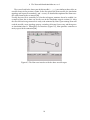
Usually, the trace file is created by ns-2; for that to happen, namtrace has to be enabled. An
example of how this is done can also be seen in the simulation script in section 4.3. After
the trace file has been generated it is ready to be animated by Nam. Upon startup, Nam will
read the tracefile, create topology, pop up a window, do layout if necessary, and then pause
at (simulation) time 0. Through its user interface (Figure 4.5), Nam provides control over
many aspects of the animation [20].
Figure 4.5: The Nam user interface with the above tracefile open.
23
5 MSC Implementation in ns-2
The following sections explain the necessary changes in existing ns-2 code and provide detailed descriptions of the newly created components that are used to simulate MSC capable
end systems and routers. Example simulation scripts are provided to demonstrate the configuration and usage of these components. Guidelines for setting up faultless simulation
scripts are also included.
5.1
Modifications and adaptions
The work on this thesis was performed with version 2.1 Beta 8 of the ns-2 software. This
section contains a list of modifications and additions necessary to simulate Multicast for
Small Conferences.
Modifications of existing files
The following list contains the names of all files that had to be modified as well as a brief
description of the changes. For further information refer to the specific sections (where applicable).
packet.h/.cc The copy() function was moved from packet.h to packet.cc to avoid
dependency problems. Furthermore, the copy() function was modified for correct
copying of the MSC routing header.
route.h/.cc A new command setRouteEntry was implemented in the class RouteLogic
and the method compute routes() was modified. Both changes were necessary to
make it possible to manually alter ns-2’s default routing table. This feature is required
when reproducing real-world networks in the simulator (see chapter 6).
udp.h/.cc The UdpAgent class was enhanced to support the transmission of single packets
of user-defined size. This feature is used when evaluating the performance of native
multicast. Also, support for MSC trace files was included in the UdpAgent class.
ns-route.tcl A new procedure named distance was created. The function uses routing
table information to calculate the distance (number of hops) between two nodes. It is
used by MSC components for distance ordering of addresses in an MSC address list.
ns-node.tcl This class features a new procedure named insert-mscr which is used for
the installation of the MSCRouter component.
ns-default.tcl A new line was inserted to set the packetSize default value for the MSC
packet type.
24
5 MSC Implementation in ns-2
New files
The following C++ files were added to ns-2 in order to simulate Multicast for Small Conferences:
msc hdr.h This file defines the MSC packet header used in ns-2.
msc.h/.cc Define the MSCAgent and the NaiveAgent classes.
mscrouter.cc A new ns-2 classifier which is used for MSC router simulation.
emscrouter.cc Another ns-2 classifier, used for the simulation of enhanced MSC.
Obviously all new files had to be included into the Makefile.
No new Tcl files have been created.
5.2
The MSC protocol in ns-2
Since ns-2.1b8 does not directly support the simulation of IP Version 6 and specifically provides no support for the simulation of a variable size routing header, a new packet header
structure was introduced (file msc hdr.h). This creates a new packet type MSC which is
linked to the MSCAgent class, i.e. each packet allocated by such an Agent will be of this
type. Also, every MSC packet will have an initial size of 204 bytes, as this value is stored in
the file ns-default.tcl as the default overall packet length. This value is based on the
assumption of sending audio data over RTP, UDP and IP; details are discussed in section 7.2.
As has already been briefly explained in section 4.2, the simulator distinguishes between its
internal packet header and the actual (simulated) packet consisting of packet headers and
payload. Also, the structure of the internal packet (protocol) headers do not necessarily reflect the fields of the actual protocol.
The newly defined MSC packet header defines the following fields:
vector ns addr t * otherRecvs The IPv6 routing header is simulated with a vector from
the Standard Template Library. This variable stores a pointer to this vector. The actual address list carried in a routing header cannot be stored in the MSC packet header
since ns-2 only supports fixed size headers (i.e. the header size is set at compilation
time).
double sendTime When an MSCAgent (MSC end system) sends a packet it will store the
simulation time in this variable. Calculation of the difference between the simulation
time on packet arrival and the value stored in this variable allows to determine the
enroute time of a packet. This feature is used for the performance analysis. The timestamp (ts ) field in the common header cannot be used for this purpose since it is used
specifically for measurement of queueing delays and thus is altered every time the
packet enters or leaves a queue.
ns addr t origin Whenever an MSCAgent allocates a new MSC packet it will store its own
address in this field. Receiving agents use this information to determine the original
sender of a packet. The src field of the ns-2 IP header cannot be used for this purpose
since every Agent that receives and re-sends a packet has to modify it (otherwise multicast protocols that use the source address for packet forwarding might get confused).
This field is also used to collect information used for the performance evaluation.
25
5 MSC Implementation in ns-2
int lastttl In order to determine the bandwidth used in MSC simulations it is necessary to
know the number of hops a packet has travelled since last encountering an MSC component (router or end system). Since it is unwise to alter the IP TTL field, each MSC
host or router stores the current IP TTL in this field. The next receiver then determines
the number of links the packet travelled by calculating the difference of the two fields.
It is important to realize that these fields do not correspond to the MSC specification; instead, they are used internally by the simulator. In particular, the size of this packet header
(pointer double ns addr t) is not used to determine the simulated packet size (but the
number of elements stored in the otherRecvs variable is). Details about the difference
between the simulated packet and ns-2’s internal representation have been discussed in section 4.2, while the simulated packet size is explained in section 7.2.
Note that the multicast group address, which would normally be carried at the end of the
IPv6 routing header, is not stored in the MSC header, since it is not required for the simulations. However, the 16 bytes consumed by the group address as well as the 16 bytes used by
the routing header (overhead) in which it is carried are taken into account when calculating
the packet size, i.e. they are included in the default packet size.
5.3
5.3.1
Implementing end system MSC in ns-2
The MSCAgent class
The MSCAgent class is used to simulate the behavior of MSC capable end systems. The
functionality of these is described in Chapter 3.2. Outgoing packets must contain the list of
receivers in the routing header, while incoming packets have to be handed over to higher
level protocols as well as forwarded to the next receivers (if any). Since packet processing
in upper layers is not relevant for this performance simulation, the MSCAgent is basically
a network (IP) layer Agent. As proposed in Chapter 10.6.1 of the ns manual [20], Agent is
used as the base class.
MSCAgent commands
The following commands are supported for use from the simulation script:
addDestination This command is given with a list of Agents (addresses). The MSCAgent
adds these addresses to its internal list of destinations.
send On invocation of this command the MSCAgent creates a new packet which carries all
receivers specified in the internal address list (the first address is copied to the destination field, the others are carried in the routing header).
An example of how MSCAgents and their commands are used can be found in section 5.3.3.
5.3.2
MSCAgent internals
Sending packets
When the send command is issued, the sendmsg method in the class MSCAgent is invoked.
This function allocates a new packet from the Simulator, which already fills in a few fields
26
5 MSC Implementation in ns-2
in the common header and in the IP header. The most important of these are ptype (packet
type), size (packet size in bytes), src (source address) and dst (destination address). For
the MSCAgents, packet type will be MSC, packet size is 204 bytes (the default value set in
ns-default.tcl), and the source address is the node on which the Agent is installed.
The destination field will be empty unless a connect command has been issued or the
MSCAgent has joined a multicast group. Once the MSCAgent can access the packet, it will
replace any preset destination address with the first address in its internal address list (which
contains the addresses of all receivers and is ordered by distance). The rest of the destination
addresses are stored in the vector of the MSC header (simulating the IPv6 routing header).
After saving the sending time in the common header the packet is forwarded to the next
network element by invoking the send method of the Agent superclass Connector.
Receiving packets
An MSCAgent receives a packet when its recv method is invoked by the network component that is forwarding the packet. First, the MSCAgent checks the packet type; normally,
any packet routed to the MSCAgent should have packet type MSC. Therefore packets of all
other types are simply discarded. For MSC packets, the delay is calculated from the sending
time stored in the MSC header and the actual simulation time. The MSCAgent then checks
the size of the simulated routing header. If the vector is not empty, the first entry is moved
to the packet destination field, the source address is updated, and the packet is re-sent. No
other fields of the packet are changed - packet ID and send time remain unchanged, which
is important for tracing. Should the vector be empty (i.e. no more receivers) the packet is
discarded.
5.3.3
Example
This is a sample Tcl script which shows the usage of MSCAgent. Note that issuing a connect command to the Agents is not necessary (and actually useless) since the destination
address is inserted into the IP header based on the group information provided through the
addDestination command.
#
#
#
#
#
#
#
#
#
#
#
MSC end system demo
(2)
(5)
|
|
(0)---(1)---(3)---(4)---(6)
sender:
0
receivers: 2 5 6
set ns [new Simulator]
# open nam trace file
set nf [open out.nam w]
$ns namtrace-all $nf
27
5 MSC Implementation in ns-2
# use a "normal" ns trace file as well:
set tracefile [open trace.ns w]
$ns trace-all $tracefile
proc finish {} {
global ns nf tracefile
$ns flush-trace
close $nf
close $tracefile
exec nam out.nam &
exit
}
# create nodes
set n0 [$ns node]
set n1 [$ns node]
set n2 [$ns node]
set n3 [$ns node]
set n4 [$ns node]
set n5 [$ns node]
set n6 [$ns node]
# create links
$ns duplex-link
$ns duplex-link
$ns duplex-link
$ns duplex-link
$ns duplex-link
$ns duplex-link
$n0
$n1
$n1
$n3
$n4
$n4
$n1
$n2
$n3
$n4
$n5
$n6
1Mb
1Mb
1Mb
1Mb
1Mb
1Mb
10ms
10ms
10ms
10ms
10ms
10ms
DropTail
DropTail
DropTail
DropTail
DropTail
DropTail
# setup MSC end systems
set msc0 [new Agent/MSCAgent]
$ns attach-agent $n0 $msc0
set msc2 [new Agent/MSCAgent]
$ns attach-agent $n2 $msc2
set msc5 [new Agent/MSCAgent]
$ns attach-agent $n5 $msc5
set msc6 [new Agent/MSCAgent]
$ns attach-agent $n6 $msc6
# define the MSC multicast group
$msc0 addDestination $msc2 $msc5 $msc6
# send a single packet
$ns at 0.1 "$msc0 send"
# end simulation
$ns at 1.0 "finish"
# run the simulation
$ns run
28
5 MSC Implementation in ns-2
Running the simulation in Nam shows that the packet travels from one member of the
MSC group to the next, i.e. from node 0 to Node 2, then to node 5, finally arriving at node
6 with a considerable delay (Figure 5.1). However, the routers on nodes 1, 3 and 4 did not
have to provide any multicast functionality. Since each link has a delay of 10 milliseconds
(set in the simulation script), the delay is 20ms for node 2, 60ms for node 5 and 80ms for
node 6 (ignoring queueing delays).
2
0
2
5
1
3
4
6
0
1
(a)
2
5
1
3
4
6
0
3
4
6
4
6
0
5
1
3
4
6
(f)
2
2
5
1
3
2
5
(e)
0
6
(d)
2
1
4
5
1
(c)
0
3
(b)
2
0
5
3
4
6
0
(g)
5
1
3
4
6
(h)
Figure 5.1: The Nam output created by the above simulation. After Node 0 sends the packet
to Node 2 (a)-(b) it is forwarded to Node 5 (c)-(f) and finally arrives at Node 6
(g)-(h).
5.3.4
The NaiveAgent class
This class extends the MSCAgent, but does not actually implement Multicast for Small Conferences. Instead, the NaiveAgent class is used for the simulation of naive unicast, where a
sender produces a packet copy for each recipient. The NaiveAgent supports the same commands as an MSCAgent and also maintains an address list. The two Agents only differ in
the packet sending behavior.
29
5 MSC Implementation in ns-2
5.4
5.4.1
Implementing MSC capable routers
The MSCRouter class
As mentioned in section 4.4, MSC router functionality is implemented in ns-2 with a special
classifier, implemented in the MSCRouter class. The structure of this classifier is quite similar to the ns-2 Replicator class, which also inherits from Classifier. But unlike the
Replicator the MSCRouter has only one exit.
After such a component is installed on a node using the insert-mscr command, every
packet arriving at an MSC enhanced node will first be handled by the MSCRouter (unless
other modules are installed from the simulation script) and is then forwarded to the classifier structure defined by the simulator (Figure 5.2). This concept has the major advantage
of making the MSC functionality completely independent from the rest of the Node (e.g.
attached Agents, Links and routing modules).
MSCRouters provide no special functionality to the ns-2 user and need no configuration.
Agent
Agent
Node
Port Classifier
MSCR
Link
Link
Address Classifier
Figure 5.2: The internal structure of an MSC Router node. Each incoming packet is first
handled by the MSC classifier (class mscr) which performs the necessary routing
table lookups and packet duplications. Afterwards the packet(s) are forwarded
to the existing classifer structure. MSC can also be used with a multicast-enabled
Node (Figure 4.4).
5.4.2
MSCRouter internals
Variables and commands
The MSCRouter has a variable hostNodeID which contains the identification of the node
on which the MSCRouter is installed. The value is set by issuing the set-hostNode command with the ID as argument, which is done by the install-mscr procedure (defined in
ns-node.tcl). The MSCRouters needs the hostNodeID to perform routing table lookups,
since the simulator does not maintain a private routing table for each node when static routing is used.
30
5 MSC Implementation in ns-2
Packet handling
The first test the MSCRouter performs on an incoming packet is for the packet type. If
it is not MSC (i.e. the packet is not part of an MSC session, but rather another unicast or
multicast transmission), the packet is forwarded without any modification. On arrival of
an MSC packet the MSCRouter checks the size of the routing header. If this value is not
zero, the MSCRouter performs a routing table lookup on all destination addresses listed in
the packet (destination field and routing header). This information is then used to create
the appropriate number of outgoing packets, each with the relevant addresses, according to
the MSC specification (see 3.2.2). The address lists are sorted by distance from the node on
which the MSCRouter is installed. All other fields in the packet headers except for the source
address remain unchanged.
5.4.3
Example
The effect of an MSC router can be demonstrated using the script from section 5.3.3 as a basis.
Inserting the following lines directly after the creation of the nodes “transforms” nodes 1 and
4 into MSC-capable routers:
# MSC router
$n1 insert-mscr "" [new Classifier/MSCRouter] 0
$n4 insert-mscr "" [new Classifier/MSCRouter] 0
The analysis with Nam (Figure 5.3) shows that the MSC router on Node 1 duplicates the
incoming packet (b) and sends one copy to node 2 and one copy to Node 3. Similarly, Node
4 sends packets to Nodes 5 and 6 (c). The delay from the sender to host 2 is still the same as
in the previous example (about 20ms), while the delay to hosts 5 and 6 is only about 40ms
(compared to 60-80ms). This indicates the potential performance gain achievable with MSC
routers.
2
0
1
2
5
3
4
6
0
(a)
2
0
1
1
5
3
(b)
5
3
4
6
(c)
Figure 5.3: Nam output of the simulation using MSCRs.
31
4
6
5 MSC Implementation in ns-2
5.4.4
The EMSCRouter class
This class implements the MSC enhancement presented in section 3.2.2, i.e. it determines the
egress router for all addresses in the routing header and duplicates packets accordingly.
The basic structure of the EMSCRouter class is exactly the same as that of the MSCRouter
class described in the previous section. The usage in the simulator differs only in that the
enhanced MSC router requires the definition of a local network domain (see example in
section 5.4.6). Thus it offers a command for configuration from the simulation script.
5.4.5
EMSCRouter internals
Additional variables and commands
In addition to the variable hostNodeID defined by the MSCRouter class, the EMSCRouter
uses the integer array localDomainIDs to store the IDs of nodes of the ”local” network.
This domain has to be defined by the user through invocation of the setLocalDomain
command (with a list of node IDs as arguments) from the simulation script. The method
isInLocalDomain can be used to determine whether a given address is in the local scope
or not.
Packet handling
Initally, the EMSCRouter class performs the same operations on incoming packets as does
the MSCRouter class; this results in a number of packets (one for each outgoing interface).
The address list of each of these packets is then analysed again, and the egress router is
determined for each destination. This is done through a series of lookup commands on
the routing table, by which the last hop inside the local network is detected. If necessary,
additional packet copies (one per egress router) are created.
5.4.6
Example
This example for the use of an enhanced MSC router uses a different topology than the
previous examples. However, the rest of the script remains unchanged, except for the configuration of the enhanced MSC router.
#
#
#
#
#
#
#
#
#
#
#
#
#
#
Enhanced MSC demo
(3)---(4)--\
(6)
|
(5)--<
(0)---(1)---(2)--/
(7)
|
(8)
sender:
0
receivers: 6 7 8
enhanced MSC router on node 1
nodes 1-5 form a network domain
set ns [new Simulator]
32
5 MSC Implementation in ns-2
# open nam trace file
set nf [open out.nam w]
$ns namtrace-all $nf
# use a "normal" ns trace file as well:
set tracefile [open trace.ns w]
$ns trace-all $tracefile
proc finish {} {
global ns nf tracefile
global ns nf
$ns flush-trace
close $nf
close $tracefile
exec nam out.nam &
exit
}
# create nodes
set n0 [$ns node]
set n1 [$ns node]
set n2 [$ns node]
set n3 [$ns node]
set n4 [$ns node]
set n5 [$ns node]
set n6 [$ns node]
set n7 [$ns node]
set n8 [$ns node]
# EMSC router
set emscrouter [new Classifier/EMSCRouter]
$emscrouter setLocalDomain $n1 $n2 $n3 $n4 $n5
$n1 insert-mscr "" $emscrouter 0
# create links
$ns duplex-link
$ns duplex-link
$ns duplex-link
$ns duplex-link
$ns duplex-link
$ns duplex-link
$ns duplex-link
$ns duplex-link
$ns duplex-link
$n0
$n1
$n1
$n2
$n2
$n3
$n4
$n5
$n5
$n1
$n2
$n3
$n5
$n8
$n4
$n5
$n6
$n7
1Mb
1Mb
1Mb
1Mb
1Mb
1Mb
1Mb
1Mb
1Mb
10ms
10ms
10ms
10ms
10ms
10ms
10ms
10ms
10ms
DropTail
DropTail
DropTail
DropTail
DropTail
DropTail
DropTail
DropTail
DropTail
# setup MSC end systems
set msc0 [new Agent/MSCAgent]
$ns attach-agent $n0 $msc0
set msc6 [new Agent/MSCAgent]
$ns attach-agent $n6 $msc6
set msc7 [new Agent/MSCAgent]
33
5 MSC Implementation in ns-2
$ns attach-agent $n7 $msc7
set msc8 [new Agent/MSCAgent]
$ns attach-agent $n8 $msc8
# define the MSC multicast group
$msc0 addDestination $msc6 $msc7 $msc8
# send a single packet
$ns at 0.1 "$msc0 send"
# end simulation
$ns at 1.0 "finish"
# run the simulation
$ns run
In order to illustrate the concept of enhanced MSC we assume that Nodes 1 to 5 form a network domain (e.g. a backbone network). The rest of the nodes act as end systems connected
to that domain. Node 0 is the sender, while Nodes 6, 7 and 8 are receivers.
The analysis with Nam (Figure 5.4) shows what happens. The enhanced MSC router on
Node 1 determines the outgoing egress routers: Node 2 for the host on Node 8 and Node 5
for the other two destinations. Thus, two packet copies are created: A packet with an empty
routing header (except for the multicast address) is sent to Node 6, while the other packet
is addressed to Node 7 and carries the address of Node 8 as well. The effect is that two
packets with identical payload are sent across the link between Nodes 1 and 2 (b). This is
offset by the fact that no packet will travel from Node 6 to Node 2, since no forwarding is
necessary (c). However, packet forwarding is necessary between Nodes 5 and 6, because no
MSC router has been installed on Node 5 (d)-(f).
5.5
MSC component tracing features
Since Nam does not provide the functionality to automatically analyse data and the ns tracefile is a bit inconvenient, MSC components implement their own tracing functionality. The
concept is very simple: each MSC component writes events to an MSC tracefile (which is an
ordinary textfile) named msctrace.ns. Each host and router records certain events:
component
MSCAgent
MSCRouter
event
packet arrival
sending (new packet)
forwarding (after recv)
packet forwarding
tracefile line
MSCA node
MSCA node
MSCA node
MSCR node
recv
send
fwrd
fwrd
from
delay
to
size
to
size
to
size
The node , from and to values stand for the IDs of the host node, source and
destination addresses respectively. size , also an integer value, is the size (in bytes) of the
sent or forwarded packet.
While the events listed above can be used to record the course of MSC handling and for delay
analysis, additional functionality is needed to analyse bandwidth consumption. Therefore,
34
5 MSC Implementation in ns-2
3
3
4
4
6
0
1
6
0
5
1
5
2
2
7
7
8
8
(a)
(b)
3
3
4
4
6
0
1
6
0
5
1
5
2
2
7
7
8
8
(c)
(d)
3
3
4
4
6
0
1
6
0
5
2
1
5
2
7
7
8
8
(e)
(f)
Figure 5.4: The Nam output of the EMSCR example script.
all MSC components also support the special bwcs event:
MSCX bwcs
consumption
The consumption value is calculated by each MSC component receiving an MSC packet
by multiplying the size (in bytes) of the incoming packet with the number of links used since
the last MSC component handled the packet. The links are counted by calculating the difference between the packet’s (IP) TTL field and the value stored in the lastttl value stored
in the MSC header. Each MSC host or router updates this field by copying the actual TTL
value before forwarding a packet.
In order to simplify the analysis of the reference scenarios using native multicast, the UdpAgent class was enhanced to support the same tracing features as the MSCAgent class (including the bwcs event). The same is obviously true for the NaiveAgent class, as it extends
35
5 MSC Implementation in ns-2
the MSCAgent class. Shown below is the MSC tracefile written by the MSC components
when executing the simulation script from section 5.4.6.
MSCA
MSCX
MSCR
MSCR
MSCA
MSCX
MSCA
MSCX
MSCA
MSCA
MSCX
5.6
0
1
1
1
8
8
6
6
6
7
7
send
bwcs
fwrd
fwrd
recv
bwcs
recv
bwcs
fwrd
recv
bwcs
8 236
236
8 204
6 220
0 35.152000
408
0 48.800000
660
7 204
0 72.064000
408
Running MSC simulations
Ns-2 simulations involving MSC components can be set up and run like any other simulation
by defining the necessary installations and events in a Tcl file. To avoid problems during the
initialization, the following structure should be used (with or without MSC components
involved):
Simulator instantiation
Node definitions
Classifiers instantiation and installation of MSCRouters and any other user-defined classifiers
Link definitions
Multicast protocols initialization and configuration of multicast protocols
Agents instantiation, configuration and installation of MSC(G)Agents and other Agents
Routing changes setRouteEntry, addRoute and deleteRoute commands
Events scheduling of simulation events
Maintaining this sequence is important for a number of reasons:
The classifiers are installed inside the nodes, therefore these have to be defined first.
The links are connected to classifiers, and therefore all classifiers have to be installed
before the links are defined.
Multicast protocol configuration requires topology information; therefore nodes and
links have to be defined at the time multicast protocols are introduced.
Routing changes can only take effect after all nodes and links are set up. The influence
of routing changes on the multicast protocol configuration does not have any implications, as the multicast protocols re-calculate the relevant parameters automatically
when the routing table is modified.
36
5 MSC Implementation in ns-2
MSCAgents and MSCRouters impose no special restrictions on the user and can be combined with other ns-2 components.
37
6 Simulation Topology
This chapter focuses on the simulation model used for the performance evaluation of Multicast for Small Conferences. It first describes the key dea before presenting the real-world
networks and end systems used to build the simulation topology. The last section discusses
the integration of real-world data in the network simulation software.
6.1
Introduction
The major goal of this thesis was to use the new ns-2 components for a basic performance
study of the Multicast for Small Conferences protocol. Since choosing an appropriate topology is critical for useful results, it makes sence to base the simulation on real-world information. Since MSC has particularly been developed for use in backbones, basing the simulation
scenarios on information from actual Internet backbone networks was the obvious thing to
do. While this provided the structure for the “backbone” of the simulation topology it was
still necessary to add a number of nodes to simulate the end systems. For the simulations in
this project, this role is played by web servers of universities connecting to the Internet via
the selected backbone networks. Using the web servers (i.e. the host that responds to queries
for www.universityname.edu) makes sense since well-known names can be used and no
special information (IP addresses or hostnames) is required. Furthermore, the delay between
the web server and any other host in the university networks should be negligible.
6.2
Backbone networks
In order to reproduce the characteristics of the real-world topologies in the simulation software it is vital to choose networks about which a lot of information is available. This comprises the structure (topology) of the network as well as data about bandwidth, delays and
routing. Since information from universities and research institutions is more easily available than data from commercial networks, the simulation topology for this thesis is based
on data from a number of (academic) research networks.
The following backbone networks (or parts of them) were used to set up the simulation
topology:
The Pan-European Gigabit Research Network (Géant)
Géant is a four-year project, set up by a Consortium of 27 European national research and
education networks (NRENs), with Dante [9] as its co-ordinating partner. Co-funded by the
European Commission as part of its Framework V Programme, its goal was the improvement of the previous generation of pan-European research network, TEN-155, by creating
38
6 Simulation Topology
a backbone at Gigabit speeds. It connects over 3’000 research and education institutions
in over 30 countries and connects to several research networks in other world regions [13]
(Figure 6.1).
The Italian Academic and Research Network (Garr)
Garr (Gruppo per l’Armonizzazione delle Reti della Ricerca - Research Networks Harmonisation Group) is composed by all subjects representing the Italian Academic and Scientific
Research Community. A major part of its mission is to provide interconnection with other
European and worldwide research networks and with the Internet [12] (Figure 6.2).
Abilene
Abilene is a high-performance network developed by the University Corporation for Advanced Internet Development (UCAID). It connects regional network aggregation points
in the United States, called GigaPoPs, to support the work of Internet2 [17] universities as
they develop advanced Internet applications. Abilene connects to other high-performance
research networks [1] (Figure 6.3).
Swiss Academic & Research Network (Switch)
The Switch foundation was established in 1987 by the Swiss Confederation and the eight
university cantons to promote modern methods of data transmission and to set up and run
an academic and research network in Switzerland. All Swiss universities and some R&D
institutions are connected to the Internet via the SWITCHlan backbone [28].
German Research Network (DFN/G-WiN)
DFN [11] is the computer-based communication infrastructure for science, research and education in Germany. G-WiN is the core of the DFN infrastructure and employs state-of-the-art
optical fibre technology. DFN also offers high performance connections to other networks,
in particular Abilene and Géant [11].
6.3
End systems
The web servers to serve as end systems were selected from the large number of universities
and reseach institutions connecting to the Internet via the backbone networks listed in the
previous section. The goals were
a) to have at least one end system per backbone router
b) to have enough end systems to allow simulations with groups of up to 20 hosts
c) to have a distribution of end systems which allows simulations with different degrees
of clustering.
Furthermore, the web servers of the selected institutions had to allow (i.e. respond to) ping
and traceroute commands; otherwise delay measurements (described in section 6.4) would
39
6 Simulation Topology
have been impossible.
The end systems used to set up the simulation topology are listed in Table 6.1.
6.4
Real-world data and ns-2
Network topology and bandwidth information for all the networks listed in section 6.2 are
available from their respective websites. However, it was necessary to manually obtain information about the routing inside these networks as well as to measure the delays on the
backbone links and from the backbone routers to the connected end systems.
In order to get a somewhat realistic picture of the delays, a large number of ping and
traceroute measurements were performed from looking glasses in the backbone networks and the end systems. To avoid distortions caused by the changing loads during a
day, all data was collected on a single weekday (Tuesday, February 19, 2002) between 1500
and 1800 MET1 . Thus, the networks in Europe as well as those in North America should
show representative delays.
Due to the large number of traceroute commands performed it was possible to get at
least three measurements on each backbone link. In the traceroute outputs, the relevant
hosts were identified and the round-trip time between them was calculated. For most links,
the different measurements yielded very similiar results (i.e. differences of less than 2 ms).
Where this was not the case, particularly in the GARR network additional measurements
were performed to permit the calculation of a useful delay value. Averaging all round-trip
times and asssuming delay = rtt/2 , the delay was established for each link in the (simplified)
topology. The traceroute data also provided routing information which is used to adjust ns2’s default routing in the simulation topology.
The simulation topology in ns-2 was set up according to the topology maps available from
the websites of the selected research networks. To avoid needless overhead, the end system
nodes are directly connected to the next backbone router node. In reality, a number of hosts
usually lay inbetween the two (gateways etc), but they can be left out in this context as they
are not relevant for the simulation. The delay on the direct link just incorporates the overall
delay between the end system and the backbone access point. The resulting ns-2 topology,
consisting of 78 nodes and 89 links, is shown in figure 6.4.
The routing differences between the real-world networks (observed with traceroute) and
ns-2’s default routing were offset by adding a number of setRouteEntry commands (newly
defined in route.cc) to the simulation script. Using setRouteEntry it is possibly to alter
the simulator’s global routing table at runtime from the simulation script.
1
MET: Mid European Time, i.e. UTC+1
40
6 Simulation Topology
City/Region
Bern
Geneva
Munich
Hamburg
St. Etienne
Oslo
Stockholm
Iceland
Torino
Genova
Milano
Padua
Trieste
Bologna
Firenze
Pisa
Perugia
Roma
Frascati
Aquila
Cagliari
Napoli
Bari
Cosenza
Catania
Palermo
Berkeley
Stanford
Irvine, CA
San Diego
Los Angeles
Riverside
Santa Barbara
Anchorage
Seattle
Dallas
Maryland
Princeton
Pittsburgh
Cinncinnati
Wisconsin
Iowa
Eugene, OR
Tucson
College St. TX
Florida
New York
Buffalo
Washington
New York
New York
Boston
Abbr
BRN
GVA
MUC
HAM
STE
OSL
STO
REK
TO
GE
MI
PD
TS
BO
FI
PI
PG
RM
FR
AQ
CA
NA
BA
CS
CT
PA
JBK
SFO
IRV
SAN
LAX
RIV
SBA
ANC
SEA
DFW
BWI
PCT
PIT
CVG
WIS
IOW
EUG
TUS
CLL
MIA
NYC
BUF
DCA
ALB
BGM
BOS
webserver URL
www.unibe.ch
www.unige.ch
www.tu-muenchen.de
www.tu-hamburg.de
www.univ-st-etienne.fr
www.uio.no
www.kth.se
www.hi.is
www.unito.it
www.unige.it
www.unimi.it
www.unipd.it
www.units.it
www.unibo.it
www.unifi.it
www.unipi.it
www.unipg.it
www.uniroma1.it
www.mporzio.astro.it
www.univaq.it
www.unica.it
www.unina.it
www.uniba.it
www.unical.it
www.unict.it
www.unipa.it
www.berkeley.edu
www.stanford.edu
www.uci.edu
www.scsd.edu
www.ucla.edu
www.ucr.edu
www.ucsb.edu
www.uaa.alaska.edu
www.washington.edu
www.utdallas.edu
www.umd.edu
www.princton.edu
www.cmu.edu
www.cu.edu
www.wisc.edu
www.iastate.edu
www.uoregon.edu
www.arizona.edu
www.tamu.edu
www.ufl.edu
www.columbia.edu
www.buffalo.edu
www.gwu.edu
www.albany.edu
www.binghamton.edu
www.mit.edu
Institution
University of Bern
University of Geneva
Technische Universität München
Technische Universität Hamburg
Université Jean Monnet
University of Oslo
Royal Institute of Technology
University of Iceland
University of Torino
University of Genova
University of Milano
University of Padova
University of Trieste
University of Bologna
University of Firenze
University of Pisa
University of Perugia
University of Roma
Rome Astronomical Observatory
University of L’Aquila
University of Cagliari
University of Napoli
University of Bari
University of Calabria
University of Catania
University of Palerma
UCAL Berkeley
Stanford University
UCAL Irvine
Supercomputing Center
UCAL Los Angeles
UCAL Riverside
UCAL Santa Barbara
University of Alaska, Anchorage
University of Washington
University of Texas, Dallas
University of Maryland
Princeton University
Carnegie Mellon University
University of Cinncinnati
University of Wisconsin-Madison
Iowa State University
University of Oregon
University of Arizona
Texas A&M University
University of Florida
Columbia University NYC
University of Buffalo, NY
George Washington University
NY State University
NY State University
Massachusetts Institute of Technology
Table 6.1: The evaluated end systems; the topology is shown in Figure 6.4.
41
6 Simulation Topology
Figure 6.1: Géant topology map
42
6 Simulation Topology
Figure 6.2: Garr topology map
43
6 Simulation Topology
Figure 6.3: Abilene topology map
ANC
EUG
TUS
IOW
STO
REK
PIT
WIS
OSL
HAM
HAM
SEA
CLE
IND
SEA
DEN
KCK
BUF
NYC
JBK
JSV
IAH
DE
MUC
NYC
UK
ALB
BRN
DCA
FR
PCT
ZRH
GVA
CH
SAN
SBA
BRN
GVA
STE
BWI
IRV
FRA
DCA
ATL
SFO
RIV
BOS
BGM
LAX
SE
CVG
DFW
CLL
MI
MIA
CS
LAX
CT
TS
NA
TO
GE
NA
ABILENE
PA
RM
RM
GÉANT
FR
SWITCH
CA
DFN
BO
GARR
FI
BO
Figure 6.4: The ns-2 simulation topology.
44
IT
MI
7 Simulation Setup
The goal of the simulations was to evaluate the performance of Multicast for Small Conferences against native multicast mechanisms. In order to obtain information about MSC’s
sensitivity to group size and clustering, a number of different setups (sets of end systems)
were defined. All of these were used with several different MSC configurations as well as
native multicast and naive unicast. The simulations are based on the idea of using MSC for
an audio conference, i.e. with relatively small packet sizes (see 7.2) and a limited tolerance
to delays.
7.1
7.1.1
Simulation parameters
Group size
Group size is probably the most obvious parameter to use. Theoretically, this parameter
is expected to have a significant effect on the overall performance of the MSC protocol in
terms of delay and bandwidth usage, particularly when end system MSC is used, i.e. the
packet is forwarded from one receiver to the next. However, the influence of the group size
on the delay can be expected to be reduced with the introduction of MSC capable routers.
The amount of additional bandwidth consumption caused by larger groups due to the larger
routing header obviously depends on the clustering (i.e. the spatial locality of the group). In
the scenarios of this performance simulation, five different group sizes are used: 4, 8, 12, 16
and 20. On the lower end, four makes sense because it is almost the smallest possible group.
At the same time a formation of 16 or 20 hosts can hardly be called a small conference and
should thus be suitable for testing the performance limit of the MSC protocol.
7.1.2
Clustering
Clustering denotes the spatial locality of a group. The stronger the clustering, the closer
the members of a conference are together (in the network topology). Three strengths of
clustering were used in the simulation:
None In these scenarios an even distribution of the involved hosts over the whole simulation topology was envisaged. For small group sizes this means one to two hosts per
backbone network. In environments with a larger number of end systems the idea was
to have no more than one host per backbone router.
Strong In simulations with strong clustering the end systems are divided into two to four
clusters of two to five hosts (depending on the group size). A cluster is a number of
end systems connecting to the same backbone router.
45
7 Simulation Setup
Weak The idea of weak clustering is to choose the end systems in a way that the distribution
is somewhere inbetween the two degrees of clustering listed above.
As mentioned in the previous section, clustering is expected to have a significant impact on
the performance of the MSC protocol both in terms of delay and bandwidth consumption,
especially in scenarios with end system MSC.
CL
None
None
None
None
GS
4
8
12
16
None
20
Weak
Weak
Weak
Weak
4
8
12
16
Weak
20
Strong
Strong
Strong
Strong
4
8
12
16
Strong
20
Hosts
BRN, FI, OSL, DFW
BRN, FI, OSL, DFW, CS, HAM, JBK, PIT
BRN, FI, OSL, DFW, CS, HAM, JBK, PIT, GE, SEA, ALB, TUS
BRN, FI, OSL, DFW, CS, HAM, JBK, PIT, GE, SEA, ALB, TUS,
STE, SBA, MIA, WIS
BRN, FI, OSL, DFW, CS, HAM, JBK, PIT, GE, SEA, ALB, TUS,
STE, SBA, MIA, WIS, FR, SAN, BUF, IOW
MI, BO, SAN, DFW
MI, BO, SAN, DFW, BRN, GVA, BOS, CVG
MI, BO, SAN, DFW, BRN, GVA, BOS, CVG, ALB, PCT, TUS, EUG
MI, BO, SAN, DFW, BRN, GVA, BOS, CVG, ALB, PCT, TUS, EUG,
FR, STE, CLL, NYC
MI, BO, SAN, DFW, BRN, GVA, BOS, CVG, ALB, PCT, TUS, EUG,
FR, STE, CLL, NYC, GE, SBA, SEA, PIT
MI, TS, IRV, RIV
MI, TS, IRV, RIV, SBA, ALB, BGM, DCA
MI, TS, IRV, RIV, SBA, ALB, BGM, DCA, RM, NYC, BUF, BOS
MI, TS, IRV, RIV, SBA, ALB, BGM, DCA, RM, NYC, BUF, BOS,
CA, JBK, SFO, SAN
MI, TS, IRV, RIV, SBA, ALB, BGM, DCA, RM, NYC, BUF, BOS,
CA, JBK, SFO, SAN, GE, PCT, PIT, CVG
CL:
Clustering
GS: Group Size
Table 7.1: Topology scenarios based on the topology in Figure 6.4
Obviously, the 15 basic scenarios are somewhat arbitrary, since there are no definite criteria for choosing the set of end systems. But since all simulations are based on the same set
of nodes the influence on the results should be negligible.
7.1.3
MSC router functionality
The combination of the previously described parameters (group size and clustering) results
in 15 scenarios (sets of end systems), shown in Table 7.1. These are used for simulations in
several configurations with varying degrees of multicast or MSC functionality (an overview
is given in Table 7.2):
Native multicast In this configuration, the data is forwarded between end systems using
native multicast mechanisms. The two different types of multicast supported by ns2.1b8 have been presented in section 4.5. For these reference simulations, Centralized
46
7 Simulation Setup
Multicast with Rendezvous Points at all end systems was used. This is not a sensible
assumption in the real-world; however, it does make sense for this simulation, as it
results in an optimal multicast packet delivery tree. This configuration thus represents
the best setup (theoretically) achievable with native multicast mechanisms and does
not include any effects caused by overhead such as packet encapsulation (Centralized
Multicast) or network flooding (Dense Mode).
Naive unicast There is no multicast or MSC functionality present in this configuration. The
involved end systems just communicate via unicast, i.e. a sender produces a unicast
packet for each recipient. This obviously yields the lowest possible delays, but suffers
from extremely high bandwidth consumption, combined with high link stress.
End system MSC This setup differs from naive unicast in that the involved end systems are
MSC capable. As a result, each packet is forwarded between all receiving end systems.
Each host examines the addresses in the routing header and forwards the packet to the
nearest one.
Full-scale MSC In addition to the MSC functionality deployed in the end systems, all routers
in the backbone networks are standard MSC capable.
MSC at backbone interlinks Instead of having MSC functionality in all nodes (which would
be costly to achieve in the real world), only a few routers are MSC capable. In this scenario, these are placed on the nodes that have a link to another backbone network
(Figure 7.1). As in all MSC scenarios, the end systems are MSC capable. The result
is an uneven distribution of the routers. For example, four of the six Géant nodes are
MSC capable, while only one in the larger Abilene network has this functionality.
EMSC at backbone interlinks The only difference between the MSC at backbone interlinks
and the EMSC at backbone interlinks scenarios is that the latter uses enhanced MSC
capable routers instead of standard MSC routers. The goal is to find out if the increased
complexity of enhanced MSC pays off, i.e. if it can outperform standard MSC in an
“intermediate” scenario.
MSC SIX As in the previous two setups, only a few nodes have MSC functionality. In this
case however, the six MSC routers (as opposed to eight in (E)MSC at backbone interlinks) are more evenly distributed over the topology. Three are placed in the large
Abilene network, while three serve Géant and the European backbone networks (Figure 7.2). The interlink concept is retained in that the routers on the transatlantic links
(AbileneNYC, GéantSE and GéantDE) are MSC capable. Comparing the results of
this scenario to the performance of full-scale MSC could indicate whether gradual deployment of MSC is possible. Also, a comparison with MSC at backbone interlinks
should give an idea of the effect of router distribution on the performance of Multicast
for Small Conferences.
EMSC SIX Similar to EMSC at backbone interlinks, this setup is used to determine performance differences between standard and enhanced MSC. The same routers as in the
MSC SIX scenario possess MSC capability.
While all of the configurations listed above use either native multicast, unicast or the new
Multicast for Small Conferences approach, it would also be interesting to evaluate the performance of a mixed scenario. In such a setup, MSC would be used for the backbone traffic,
47
7 Simulation Setup
ANC
EUG
TUS
IOW
STO
REK
PIT
WIS
OSL
HAM
SEA
CVG
BUF
NYC
JBK
MUC
BOS
ALB
DCA
BGM
SFO
STE
BWI
SAN
IRV
SBA
RIV
BRN
GVA
PCT
DFW
CLL
MI
MIA
CS
LAX
TS
NA
TO
GE
CT
ABILENE
PA
GÉANT
RM
FR
SWITCH
CA
DFN
BO
GARR
FI
MSC capable router
Figure 7.1: Backbone at interlinks configuration
while the gateways serving the end systems could use native multicast in the access networks. However, these tests would require a much larger topology with a detailed reproduction of the access networks and thus massively increase the complexity of the simulation.
Furthermore, detailed information about the structure (topology) and characteristics (delays,
routing) of the networks to which the end systems connect would be required.
7.2
Packets
All configurations described in the previous section were run in ns-2 for all fifteen base topology scenarios. In each simulation run, the involved end systems consecutively send a single
packet to the rest of the group (except for naive unicast). The simulation software records the
Configuration
Native multicast
Naive unicast
End system MSC
Full-Scale MSC
MSC at backbone interlinks
EMSC at backbone interlinks
MSC SIX
EMSC SIX
MSC capable routers
none
none
none
all 25 backbone routers
NYC, SE, DE, CH, IT, FRA, GVA, MI
NYC, SE, DE, CH, IT, FRA, GVA, MI
NYC, LAX, KCK, DE, CH, MI
NYC, LAX, KCK, DE, CH, MI
Table 7.2: Configurations based on the topology in Figure 6.4. For MSC
at backbone interlinks and MSC SIX also see Figures 7.1 and
7.2
48
7 Simulation Setup
ANC
EUG
TUS
IOW
STO
REK
PIT
WIS
OSL
HAM
SEA
CVG
BUF
NYC
JBK
MUC
BOS
ALB
DCA
BGM
SFO
STE
BWI
SAN
IRV
SBA
RIV
BRN
GVA
PCT
DFW
CLL
MI
MIA
CS
LAX
TS
NA
TO
GE
CT
ABILENE
PA
GÉANT
RM
FR
SWITCH
CA
DFN
BO
GARR
FI
MSC capable router
Figure 7.2: MSC SIX/EMSC SIX configuration; for EMSC simulations, the domains are set as colored, i.e. each backbone network is considered a domain
arrival and departure times as well as the size of each packet at all nodes and on all links.
The packet size used in the simulations of this performance evaluation is based on a scenario where Multicast for Small conferences is used for an audio conference. Supposing
end systems using ISDN, a data-rate of 64 kbit/s is assumed. If packets are sent every 10
milliseconds, each packet contains 80 bytes of data (payload). On the application level, the
data flow can be controlled by the Real-Time Protocol (RTP) [25]; this adds a minimum of 12
bytes (RTP header) to the packet size. As for the transport layer, the use of the User Datagram Protocol (UDP) [22] is probable. For transmission over IPv6, UDP uses packet headers
of 40 bytes, consisting of 16 bytes for the source and destination addresses respectively and
a total of 8 bytes for packet length, checksum and next header information. In the network,
the packets will be forwarded using IPv6. The standard IPv6 header has a length of 40 bytes,
bringing the overall packet size to 172 bytes. This is the packet size that is applied for native
multicast and unicast simulations. When using MSC, a routing header carrying the group’s
multicast address is present at all times, adding another 32 bytes (16 bytes for the routing
header overhead and 16 bytes for the multicast address), resulting in the minimum packet
size of 204 bytes.
80 bytes
12 bytes
40 bytes
40 bytes
172 bytes
16 bytes
16 bytes
32 bytes
204 bytes
audio data (payload)
RTP header
UDP header
IPv6 header
not MSC related
IPv6 routing header overhead
Multicast address carried in the routing header
by MSC specification
Total
49
7 Simulation Setup
This packet size would be observed in a scenario with just two participants (source and
destination); obviously using a multicast address is useless in this case. Usually, more than
one recipient would be present, and the unicast addresses (16 bytes each) of the additional
group members would be carried in the routing header, increasing the packet size.
As already discussed briefly in section 3.4 this increase of the size of the routing header can
massively deteriorate the overhead/payload ratio, especially for small packets such as in
this audio conference scenario.
7.3
Metrics
As already mentioned in section 7.2, each simulation is set up the same way: Every involved
hosts sends a packet to the group. This obviously results in quite a lot of data stored in the
tracefiles. For scenario-specific analysis this data is aggregated into just four values that can
be used to assess the performance of MSC:
Maximum Delay The maximum delay found in a scenario can be used to decide whether
audio conference is feasible with the selected parameters. Usually, a maximum delay
of 100 or 150 milliseconds is used as a threshold. Ideally, all values should be below
that limit.
Average Delay The average of all sender-receiver delays measured in a scenario is an indication of the overall performance in the given configuration. The average value should
usually remain well below the threshold for the maximum delay.
Bandwidth Consumption For this performance evaluation, the overall link usage is used
as a metric for bandwidth consumption. This means that the bytes transported on each
link are recorded in the tracefile, and these values are summed up on a per-scenario
basis to result in a comparable figure.
Backbone Usage The backbone usage parameter uses the same data as bandwidth consumption; however, only bytes transferred on links in backbone networks (Géant, Abilene, Garr, Switch, DFN) are taken into account. The sum of these is then divided by
the overall bandwidth consumption, resulting in a comparable percentage. This parameter differs from the other three in that it is not downright clear whether a high
or low value is good or bad. However, approaches that exonerate the access networks
(i.e. that have a high backbone usage) are usually favored.
50
8 Results
The following sections contain the results of 120 simulation runs (8 configurations with 15
scenarios each) as diagrams. Each figure contains the results of a single metric (e.g. average
delay) for a specific degree of clustering. For each metric, the three diagrams have the same
scale. Values are presented for all eight configurations and all fivegroup sizes. The lines
connecting the data points are only shown to facilitate the interpretation and should not be
overrated.
8.1
Average delays
The most outstanding characteristic of the diagram shown in Figure 8.1(a) is the massive
performance difference between end system MSC and the other configurations. This phenomenon is seen in all delay-related results; however, it is most distinctive when spatial
locality is low (i.e. weak clustering). Also, the performance gap widens as the group size
increases. While most configurations see only a marginal (or even no) increase in average
delays when new hosts are added, the values for end system MSC increase linearly.
An ostensible oddity is the fact that the MSC SIX and EMSC SIX average delays for a group
with 20 hosts are lower than their respective values for group size 16. The reason for this
effect is that the addtional four end systems (FR, SAN, BUF, IOW) lie close to MSC routers in
these configurations and are thus served very efficiently. The resulting low delays for traffic
from and to these hosts reduces the average delay. Unsurprisingly, the simulations for weak
and strong clustering (shown in Figures 8.1(b) and 8.1(c)) illustrate that the absolute average
delays are decreasing as the clustering gets stronger (i.e. end systems are closer together).
However, a massive difference between end system MSC and the other configurations remains.
As already seen in Figure 8.1(a), the average delays sometimes decrease as groups grow.
In scenarios with stronger clustering this effect is not only caused by the proximity of additional end systems to MSC capable routers. The newly introduced hosts are deliberately
placed close to already used nodes to maintain a high degree of clustering. This causes low
end-to-end delays even when no MSC functionality is involved (i.e. packets are forwarded
between end systems) and thus can reduce the average delays.
8.2
Maximum delays
The performance gap between end system MSC and the configurations seen in the average delays also exists with the maximum delay parameter (Figures 8.2(a), 8.2(b) and 8.2(c)).
Again, the extent of the difference depends on the spatial locality. When the hosts are closer
together (i.e. in groups of two to five), end system MSC benefits superproportionaly. Also,
51
250
250
225
225
200
200
175
175
Delay (ms)
Delay (ms)
8 Results
150
125
100
150
125
100
75
75
50
50
25
25
0
0
4
8
12
16
20
4
Group Size
8
12
16
20
Group Size
(a) No Clustering
(b) Weak Clustering
250
225
200
Delay (ms)
175
Native multicast
End system MSC
MSC at backbone interlinks
Full-scale MSC
EMSC at backbone interlinks
EMSC SIX
MSC SIX
Naive unicast
150
125
100
75
50
25
0
4
8
12
16
20
Group Size
(c) Strong Clustering
Figure 8.1: Average Delays
the other approaches do not all perform equally here. Native multicast and naive unicast
show consistently low maximum delays, while other configurations, particularly (E)MSC
at backbone interlinks, suffer from higher maximum delays as group sizes increase. There
are a few cases where the maximum measured delay decreases as the group size increases,
e.g. in the EMSC SIX configuration with weak clustering. The explanation of this effect is
based on router distribution. When a new end system is introduced, the forwarding path of
a packet from a given sender to the receivers may be changed, since the senders order the
recipient’s addresses by distance. In some configurations, the new sequence (and the resulting forwarding path) is much more efficient, for example because an MSC capable router is
encountered earlier in the forwarding process. This in turn can lead to completely different,
potentially significantly lower end-to-end delays.
This effect and a similiar occurence in average delays highlight the impact that the selection
52
8 Results
500
500
450
450
400
400
350
350
Delay (ms)
Delay (ms)
of end systems (i.e. the composition of a multicast group) can have on the performance of
multicast mechanisms.
300
250
200
300
250
200
150
150
100
100
50
50
0
0
4
8
12
16
4
20
8
12
16
20
Group Size
Group Size
(a) No Clustering
(b) Weak Clustering
500
450
400
Delay (ms)
350
Native multicast
End system MSC
MSC at backbone interlinks
Full-scale MSC
EMSC at backbone interlinks
EMSC SIX
MSC SIX
Naive unicast
300
250
200
150
100
50
0
4
8
12
16
20
Group Size
(c) Strong Clustering
Figure 8.2: Maximum Delays
8.3
Bandwidth consumption
As could be expected, the bandwidth consumption in scenarios with low spatial locality
of the end systems (Figure 8.3(a)) is significantly higher than with hosts that form clusters
(Figures 8.3(b) and 8.3(c)). This can be seen as an indication that the different sets of end systems used to represent the three degrees of clustering were chosen appropriately. As with
the average and maximum delay parameters, the bandwidth consumption among the eight
configurations increase when group sizes increase. While the link usage of native multicast
53
8 Results
increases almost linearly, it does so exponentially for some of the other approaches, particularly naive unicast and end system MSC. This is a good indication of the scalability problems
of end system-based mechanisms.
600000
Bandwidth Consumption (bytes)
Bandwidth Consumption (bytes)
600000
500000
400000
300000
200000
100000
0
500000
400000
300000
200000
100000
0
4
8
12
16
20
4
8
Group Size
12
16
20
Group Size
(a) No Clustering
(b) Weak Clustering
Band width Consumption (bytes)
600000
500000
400000
Native multicast
End system MSC
MSC at backbone interlinks
Full-scale MSC
EMSC at backbone interlinks
EMSC SIX
MSC SIX
Naive unicast
300000
200000
100000
0
4
8
12
16
20
Group Size
(c) Strong Clustering
Figure 8.3: Bandwidth Consumption
8.4
Backbone usage
The trend of increasing differences with increasing group sizes is also noticeable in the diagrams showing the backbone usage. Also, clustering again has a tremendous effect on the
result. But while the performance gap narrows with increased clustering for the delays and
bandwidth consumption, it widens in terms of backbone usage. With high spatial locality
(Figure 8.4(c)), some approaches are very sensitive to group size, showing a massive de-
54
8 Results
crease in backbone usage as hosts are added, e.g. end system MSC or native multicast. In
the case of end system MSC this is due to excessive packet forwarding between end systems,
which most affects the links close to the hosts. For native multicast, the explanation is different. The backbone usage is relatively high for small groups (especially with low clustering),
since each destination is served using an optimal forwarding path. This drives up the number of backbone links that have to carry the packet, while the number of used access network
links is low. When new receivers are added, the core of the forwarding tree doesn’t change
very much, especially with strong clustering. Thus the load on the backbone links will not
increase significantly. This is further emphasized by the fact that packet size is independent
from group size (unlike in MSC scenarios). However, some new access network links are
added to the forwarding tree, adding bytes to the non-backbone counter and thus reducing
the backbone usage.
At the same time naive unicast shows almost constant values for all group sizes and only
marginally reacts to changes in clustering. The reason is simple: With the naive unicast approach, each packet travels all the way from the sender to the receiver, using backbone and
access networks. In the other configurations, the senders produce less packet copies and instead rely on packet forwarding between end systems, which drives up the usage of access
networks, especially when the clients are strongly clustered.
Another interesting aspect is the performance of (E)MSC at backbone interlinks and (E)MSC
SIX. While the MSC and EMSC approaches show almost identical results in terms of bandwidth consumption (Figures 8.3(a), 8.3(b) and 8.3(c)), they have completely different values
for backbone usage. The enhanced MSC approaches consistently show higher values than
the standard MSC concepts. Also, the differences increase with group sizes and are most
disctinctive when clustering is low.
55
80%
80%
70%
70%
60%
60%
Backbone Usage
Backbone Usage
8 Results
50%
40%
30%
20%
10%
50%
40%
30%
20%
10%
0%
0%
4
8
12
16
20
4
Group Size
8
12
Group Size
(a) No Clustering
(b) Weak Clustering
80%
Backbone Usage
70%
60%
Native multicast
End system MSC
MSC at backbone interlinks
Full-scale MSC
EMSC at backbone interlinks
EMSC SIX
MSC SIX
Naive unicast
50%
40%
30%
20%
10%
0%
4
8
12
16
20
Group Size
(c) Strong Clustering
Figure 8.4: Backbone Usage
56
16
20
8 Results
8.5
Summary
The following parameters are listed in the summaries of the results (Tables 8.1, 8.2, 8.3).
RDP: Relative Delay Penalty The ratio of the MSC delay between two hosts to the IP Multicast delay between them:
EXD: Excess Delays Percentage of delays above 150ms in a setup (all 15 scenarios).
NRU: Normalized Resource Usage Ratio of the link usage relative to link usage of native
multicast. It should be kept in mind that the difference in bandwidth consumption
between MSC configurations and native multicast is partially caused by the longer IP
header. If the packet (payload) length were increased from the relatively small 80 bytes
used in this simulation, the impact of the longer header would be reduced, resulting
in a lower NRU. Also, an over-optimized native multicast mechanism is used in this
study.
BBU: Backbone Usage The percentage of link usage that involves links of backbone networks.
Configuration
Native multicast
Naive unicast
End system MSC
Full-scale MSC
MSC at backbone interlinks
EMSC at backbone interlinks
MSC SIX
EMSC SIX
RDP min
1
1
1.1
1
1
1
1
1
RDP max
1
1
4.3
1.1
2.4
2.2
1.9
1.6
RDP avg
1
1
2.7
1
1.6
1.5
1.4
1.3
EXD
0%
0%
44%
0%
15%
14%
6%
1%
Table 8.1: Summary of Relative Delay Penalties (RDP) of the average delays, and percentage of delays 150ms
Configuration
Native multicast
Naive unicast
End system MSC
Full-scale MSC
MSC at backbone interlinks
EMSC at backbone interlinks
MSC SIX
EMSC SIX
NRU min
1
1.4
1.3
1.2
1.3
1.3
1.3
1.3
NRU max
1
3.7
3.3
1.6
2.3
2.3
2.1
2.1
NRU avg
1
2.5
2.4
1.4
1.8
1.8
1.7
1.7
Table 8.2: Summary of Normalized Resource Usage (NRU)
57
8 Results
Configuration
Native multicast
Naive unicast
End system MSC
Full-scale MSC
MSC at backbone interlinks
EMSC at backbone interlinks
MSC SIX
EMSC SIX
BBU % min
34
60
24
35
26
32
29
38
BBU % max
74
74
66
74
72
73
75
75
BBU % avg
56
67
46
56
50
54
52
59
Table 8.3: Summary of Backbone Usage (BBU) percentage
58
9 Performance Evaluation
While the previous chapter has given an overview of the simulation results by briefly discussing the results on a per-parameter basis, this chapter provides a more detailed analysis
of the results of each configuration. It also highlights the performance differences between
MSC configurations and native multicast as well as between the different MSC setups, providing the basis for the conclusions presented in chapter 10.
9.1
Native multicast
The results of this configuration form the basis of the performance evaluation. A few things
are noteworthy: In terms of delay, native multicast is insensitive to group size and clustering, since packets are always forwarded along an optimal tree. But even with this “perfect”
routing some end-to-end delays are in excess of 100 milliseconds (but none are 150ms).
The bandwidth consumption of native multicast is low, since it never unnecessarily duplicates packets. However, group size and clustering affect the results: link usage increases
linearly as groups grow, and the gradient depends on the spatial locality of the hosts. Since
the addition of hosts does not affect backbone links that are already part of the multicast
delivery tree, the backbone usage decreases as groups grow.
Unsurprisingly, none of the alternative approaches can beat native multicast’s performance.
But as has been pointed out in the introduction, native multicast burdens Internet routers by
increasing the routing table sizes.
In terms of backbone usage, two things are noteworthy: Firstly, native multicast has a relatively high backbone usage compared to the MSC approaches. The reasons for this this
have already been pointed out in section 8.4: optimal forwarding paths and lack of packet
forwarding between end systems. Secondly, the values increase significantly (and almost
linearly) as group size increases. The reason for this is IP Multicast’s efficiency: packets are
never duplicated over the same link. Thus, the addition of a new end systems doesn’t necessary burden the backbone, especially when clustering is strong (i.e. the end systems are
close together).
9.2
Naive unicast
Like native multicast, naive unicast is included in this performance study as a basis for comparison. While the concepts of native multicast and naive unicast share the advantage of
low end-to-end delays, they differ significantly in bandwidth consumption. Depending on
group size and clustering, naive unicast uses 1.4-3.7 times the bandwidth of native multicast. Also, naive unicast suffers from high link stress, i.e. a lot of identical packet copies are
sent over the same links. The last two points highlight why naive unicast is no option for
59
9 Performance Evaluation
replacing IP Multicast.
Naive unicast has very high and almost constant backbone usage values. This is no surprise
as each packet travels the whole way from the sender to the receiver.
9.3
End system MSC
Unsurprisingly, end system MSC suffers from very high delays due to the packet forwarding
between receiving end systems. End-to-end delays increase linearly with group size, as opposed to native multicast or naive unicast where they remain almost constant. Also, this concept is sensitive to clustering: Strong clustering means the receivers are close together, which
significantly reduces the delay caused by forwarding between receivers. Consequently, end
system MSC shows a good performance for small groups and strong clustering, but suffers
from a massive increase in average and maximum delays as group size increases and clustering is reduced. 44% of all measured delays in the 15 scenarios exceed the 150ms threshold
(the maximum being 468ms), proving that end system MSC is not feasible.
In terms of bandwidth consumption, end system MSC also shows a poor performance. For
very small groups, link usage is only about 20% higher than for native multicast. But while
bandwidth consumption increases linearly for native multicast, it grows exponentially in the
case of end system MSC. For a group of 20 hosts and no clustering, the sum of all transferred
data bytes is 3.3 times that of native multicast. The range of values (for bandwidth consumption) is about the same as that of naive unicast, but the two concepts do not perform
identically. End system MSC is better than naive unicast in scenarios with strong clustering
since it does not have to send duplicate packets over the same link. But when spatial locality
is low, naive unicast can outperform end system MSC since the latter suffers from longer
forwarding paths between the receivers.
End systems MSC consistently shows the lowest backbone usage percentage of all eight configurations. This is also due to the packet forwarding between receiving end systems, as
this forwarding mainly takes place in the access networks. With strong clustering and large
groups, backbone usage even drops below 30%, indicating that end system MSC heavily
burdens the networks close to the recipients.
9.4
Full-scale MSC
The MSC router functionality on all nodes in the backbone networks results in optimal forwarding paths and reduces packet forwarding between end systems to a minimum. This
shows in almost no delay penalty compared to native multicast and naive unicast. Also,
full-scale MSC is insensitive to group size and clustering.
In terms of bandwidth consumption full-scale MSC cannot keep up with native multicast
due to the routing header (which increases the packet size) and occasional forwarding between end systems that are connected to the same backbone router (e.g. between SFO and
JBK). Overall, the bandwidth consumption is 120%-160% that of native multicast. The upper boundary of this range is reached with stronger clustering, when packet forwarding
between end nodes increases. However, it should be kept in mind that a perfect native multicast model is used.
The backbone usage data of full-scale MSC show no particulary high or low values. Backbone usage decreases with increasing group sizes, but the decline is much less dramatic than
60
9 Performance Evaluation
in other configurations (e.g. MSC at backbone interlinks).
9.5
MSC at backbone interlinks
In terms of average and maximum delay, this scenario performs significantly better than
end-system MSC. Unfortunately it also performs significantly worse than full-scale MSC or
native multicast. The results are satisfactory in scenarios with small groups (four or eight
hosts), but with increasing group sizes the uneven distribution of MSC functionality and
the resulting packet forwarding between end systems in the Abilene part of the simulation
network severly deteriorates the performance. Overall, the delays are up to 2.3 times those
of native multicast. The absolute maximum delay exceeds the 150ms threshold in all simulations with 12 or more hosts.
With MSC at backbone interlinks, bandwidth consumption is 1.3-2.3 times that of native
multicast, depending on group size and degree of clustering. Similar to the other configurations, MSC at backbone interlinks’ efficiency is best when groups are small and spatial
locality is high.
The backbone usage of this approach is inconsistent. For small groups (and particularly
in combination with low clustering), MSC at backbone interlinks performs as well as other
configurations, e.g. full-scale MSC. But as group sizes increase, the percentage decreases at
a high rate and almost drops to the levels of end system MSC.
Altogether, the performance of this concept indicates that acceptable results are achievable
with just a small number of MSC capable routers.
9.6
EMSC at backbone interlinks
The delay performance of EMSC at backbone interlinks is very similar to that of the corresponding setup using standard MSC. The former shows marginally lower average delays in
scenarios with large groups, due to the reduced packet forwarding in the Abilene part of the
topology (since packet copies per egress router are created). The difference is even smaller in
scenarios with strong clustering, since they inherently require less packet forwarding, which
benefits standard MSC.
The bandwidth consumption of the two interlink approaches is almost equal, with minimal
advantages for standard MSC when clustering is low and similar disadvantages for the same
concept when end systems lie close together. While EMSC suffers from duplicate packets
sent over the same link, standard MSC needs to perform more packet forwarding between
end systems, and the two effects seem to cause identical performance penalties. However,
a shift in network loads is visible: Enhanced MSC creates more traffic inside the backbone
networks while exonerating the access networks. For both approaches, the amount of transported bytes on backbone links is over 70% in scenarios with small groups and low clustering. This value decreases as groups grow and spatial locality increases. Increased group
sizes require the use of more access network links, while increased clustering reduces the
number of used backbone links. The decrease is significantly stronger with standard MSC
than with enhanced MSC, reaching a minimum of 26% and 32% respectively (Table 8.3).
There are two reasons for this interesting effect:
With enhanced MSC, the first router encountering an MSC packet produces copies for
61
9 Performance Evaluation
all egress routers. Thus, the probability is high that some links will transport more
than one packet copy. This in turn increases the backbone link usage.
Once a packet copy for each egress router is created, no receiving end system will have
to forward an incoming packet to a host outside the access network, as these systems
have different egress routers and thus receive another packet copy. This reduces both
the bandwidth usage in the access network (back to the egress router) as well as in the
backbone (between the egress routers).
The same effect was observed in the MSC SIX and EMSC SIX configurations (see next sections).
9.7
MSC SIX
As indicated in section 7.1.3, the MSC SIX configuration is aimed at improving the results of
the MSC at backbone interlinks configuration through better router distribution.
In terms of delay, some improvement is noticeable: While there are still some delays of up
to 1.9 times the value of native multicast, the number of delays in excess of 150ms could be
reduced significantly. Just 6% of all measured delays exceed the threshold, as opposed to
15% for MSC at backbone interlinks. High delays are only measured for larger groups (12
or more hosts) with weak spatial locality. The maximum delays are also lower, with only a
single value in excess of 200ms.
Bandwidth consumption is affected similarly: The overall link usage is 1.3-2.1 times that of
native multicast, i.e. similar to MSC at backbone interlinks. For most group size/clustering
combinations however, bandwidth consumption is slightly reduced compared to the previous configuration.
The backbone usage of the two concepts differs only marginally, with the MSC SIX configuration consistently showing higher values (usually 2-3%, max. 5%).
These results (and the performance of MSC at backbone interlinks) prove that MSC can deliver an acceptable performance with just a few MSC capable routers, at least for smaller
groups, even with widely spread group members. Compared to full-scale MSC, lower deployment costs (i.e. using just six or eight MSC routers instead of 25) have been traded
against higher delays and increased bandwidth consumption.
The comparison of MSC SIX against MSC at backbone links, in particular the significant
difference in delays in excess of 150ms, proves that router distribution is critical.
9.8
EMSC SIX
The end-to-end delays measured in this configuration are slightly lower than those of MSC
SIX, and the performance gain is increasing with larger group sizes and when clustering is
reduced. In the latter case the duplication of packets (one per egress router) over the same
link pays off. Compared to the previous configuration, the amount of delays in excess of
150ms could again be reduced, to just 1%.
In terms of bandwidth consumption there is only a marginal difference between MSC SIX
and EMSC SIX. The additional link usage caused by the duplication of packets over the same
link is almost completely compensated for by the elimination of some packet forwarding between receiving end systems. As already pointed out in section 9.6, the EMSC approaches
62
9 Performance Evaluation
show significantly higher values in backbone usage than the standard MSC concepts. This
is true in (E)MSC SIX as well, with minima of 29% and 38% reached respectively. Again, the
additional link usage caused by the duplication of packets over the same link is almost completely compensated for by the elimination of some packet forwarding between receiving
end systems.
9.9
Comparison of MSC and native multicast
In terms of delays, MSC can only achieve the same performance as native multicast when
full-scale MSC is used (i.e. all routers are MSC capable). This, however, would be costly to
achieve in the real-world. With an optimized “intermediate” approach such as in the (E)MSC
SIX scenarios, a delay penalty of up to 90% (60% with enhanced MSC) has to be accepted
(Table 8.1). However, depending on the scenario parameters (group size, clustering), the difference to native multicast may be significantly smaller. With a different, less optimal router
distribution such as in the (E)MSC at backbone interlinks scenarios, RDP values of up to 2.4
have been observed. It is doubtful whether a delay-sensitive application could be supported
in such a configuration.
The bandwidth consumption of native multicast is unbeatably low. Due to the longer IP
header, packet duplication and packet forwarding between end systems, MSC always has
a higher link usage than native multicast. Even in a full-scale MSC configuration the Normalized Resource Usage (NRU) is between 1.2 and 1.6 (Table 8.2). With only a few capable
routers ((E)MSC at backbone interlinks, (E)MSC SIX), the bandwidth consumption can even
be more than twice that of a native multicast approach serving the same end systems. With
the higher backbone usage of enhanced MSC (Table 8.3) it should at least be possible to limit
the additional strain on the access networks.
63
10 Summary
The performance evaluation performed as part of this thesis has highlighted the potential
of Multicast for Small Conferences. Particularly, it has shown that with just a small number
of dedicated routers the delay penalty compared to native multicast mechanism can be kept
relatively low (factor two). The same is true for bandwidth consumption, where even better
results should be achievable with increased packet (i.e. payload) size.
The simulation results and their interpretation in the previous chapter also provide the basis
for a number of conclusions about the concept of Multicast for Small Conferences:
1. End system MSC is not feasible. As has been shown in section 9.3, end system MSC
produces unacceptably high delays in almost all scenarios. Given the 150ms delay
limit, supporting audio or video conferences is only possible for very small groups
with strong spatial locality. This does not mean that end system multicast does not
work. It merely proves that end system multicast on IP level without router support
cannot deliver the performance required to support delay-sensitive applications. A
possible solution is the use of an application-level multicast scheme, some of which
have been presented in section 2.2. However, it seems as if only Narada [16] could
provide the required performance, at the cost of increased bandwidth consumption
and link stress.
2. Only a small number of MSC capable routers is required to significantly improve
the performance. The tremendous difference in the results of the end system MSC and
MSC at backbone interlink scenarios impressively proves this point. Two things can be
deduced:
There is no need for full-scale MSC. A very good performance can be delivered
with just a few MSC capable routers at considerably lower deployment costs.
Gradual MSC deployment is possible. Assuming the availability of appropriate end systems, MSC can start at a low performance level with no or very few
dedicated routers. Performance can then be gradually improved through the deployment of additional MSC routers.
3. MSC router distribution is critical. The fact that the MSC SIX configuration (with
its more evenly distributed routers) yields better results than the MSC at backbone
interlink setup is a good indication of this. It is tempting to place MSC routers on nodes
where backbone networks connect, particularly because these nodes have a high traffic
load. However, with several members of a group connecting to the same backbone
network (or even the same router), this approach can result in high delays as packets
are forwarded between end systems without encountering an MSC router.
When developing rules for MSC router placement, two things should be kept in mind:
64
10 Summary
The (potential) performance of a standard MSC router depends on the number of
outgoing interfaces. The more packet copies a standard MSC router can create
(at most one per outgoing link), the less addresses remain in the various routing
headers, reducing the necessary forwarding between end systems accordingly.
In contrast, the performance of enhanced MSC routers is not affected by the outdegree of the node, as the number of packet copies created only depends on the
number of egress routers involved.
Once an MSC packet has been processed by an enhanced MSC capable router the
optimal forwarding strategy through that domain is executed for all destination
addresses. Thus, enhanced MSC is most effective when MSC packets are intercepted as early as possible after entering a certain network domain. This is not
necessarily true for standard MSC, since the routers have no knowledge of possible
branching further down the forwarding tree.
Unfortunately these two rules alone do not guarantee a good performance. For example, a standard MSC router with a lot of outgoing links won’t be helpful if the relevant
traffic bypasses the node. On the other hand, trying to intercept all packets entering
a domain as early as possible would almost certainly result in full-scale MSC. Thus,
a compromise has to be found. The most obvious solution is to distribute the MSC
functionality as evenly as possible over the entire network. This maximizes the probability that a packet encounters an MSC router, thus reducing the potential for packet
forwarding between end systems. The performance advantage of MSC SIX and EMSC
SIX at backbone interlinks indicate the potential of this approach. However, it should
be kept in mind that the actual performance in a scenario also depends on other factors
such as group size and clustering.
4. Enhanced MSC performs better than standard MSC. The main advantage of enhanced MSC are the reduced delays. In scenarios with a small number of hosts (four/eight),
enhanced MSC shows the same performance as standard MSC. For large groups however (16 or 20 hosts), enhanced MSC produces significantly lower (10-20ms) average
delays. This is the direct result of much more efficient packet forwarding, as can also
be seen from the massively reduced percentage of delays in excess of 150ms (1% vs.
6%).
Another difference between standard and enhanced MSC is visible in the backbone usage. In each scenario, enhanced MSC consumes about the same amount of bandwidth
as standard MSC. The difference lies in where it is consumed: As has been explained in
section 9.8, enhanced MSC burdens backbone links with duplicate packets (addressed
to different egress routers), but in turn exonerates the access networks by ensuring that
they never have to “return” an incoming packet to the backbone network. Depending
on the network infrastructure, this feature may be considered an advantage or a disadvantage.
The question is whether the advantage(s) outweigh the additional costs (i.e. complexity). An answer could only be found through further analysis of the router functionality, which unfortunately can’t be done with ns-2.
65
11 Outlook
Due to time constraints and limitations of the network simulation software, not all aspects
affecting MSC’s performance could be analyzed in this thesis. The increased router complexity introduced by Multicast for Small conferences is such a feature. Ns-2 provides support for the performance analysis of different routing protocols, but an evaluation of router
performance is not possible, in particular because the simulation software’s internal packet
forwarding mechanisms differ from those of a real-world router. Thus, another evaluation
approach is required. Ideally, Multicast for Small Conferences should be implemented in an
actual router, for example using Linux. Such a router could not only help to determine the
(negative) impact of MSC on routing performance, but would also be a first step towards
a complete implementation, which in turn could be used for simulations in real networks.
Once finished, an MSC implementation would also allow to confirm and refine the results
of the simulations performed as part of this thesis.
Another aspect which certainly requires further analysis is the effect of Multicast for Small
Conferences (or similar approaches) on the routing table size. Such a study should probably
analyse the structure of the routing tables of backbone routers (e.g. the amount of multicast
routing entries) as well as the popularity of small group applications. By estimating the
amount of IP Multicast sessions replacable by more efficient solutions it should be possible
to determine the impact of MSC on the routing tables.
The integration of MSC and IP Multicast is another matter requiring further analysis. Multicast for Small Conferences has primarily been designed for use in the backbone networks,
where it exonerates the routers by removing the need to maintain a routing table entry for
each and every multicast group in use. While it is possible to have an all-MSC multicast
(with all end systems capable of MSC), other configurations could be useful as well. For
example, MSC gateways (described briefly in section 3.2.1) might be used at the edges of the
backbone networks. Using such devices, native multicast mechanisms can remain in use in
the access networks, allowing for the integration of non-MSC-capable end systems into MSC
sessions, while retaining the major advantage of the new concept. As mentioned at the end
of section 7.1.3, doing a performance simulation of such a scenario is quite complex, particularly because a simulation topology much more complex than the one used in this thesis is
required.
Similarly, it might be interesting to do research on the possible combination of Multicast for
Small Conferences with end system multicast approaches.
66
Glossary
Bayeux An application-level multicast concept based on the Tapestry routing protocol.
CAN (Content-Addressable Network) An overlay network which can also be used for application-level multicasting.
DCM (Distributed Core Multicast) A multicast routing protocol for use within large single
domain network with a large number of multicast groups with a small number of
receivers.
EMSC (Enhanced MSC) An improved version of MSC, relying on additional routing information.
EXPRESS (Explicitly Requested Single-Source Multicast) A concept aimed at improving IP Multicast by introducing channels.
IP (Internet Protocol) Defines network layer packets and procedures used to move datagrams from host to host; currently, Version 4 (IPv4) is standard.
IPv6 (Internet Protocol Version 6) The “next generation” internet protocol, aimed at replacing IPv4.
IP Multicast A mechanism in the IP protocol which allows efficient (in terms of bandwidth
consumption) one-to-many and many-to-many transmissions.
Link Stress The number of packets with identical payload sent over a certain link.
MSC (Multicast for Small Conferences) A novel approach for resolving scalability problems of IP multicast.
Naive Unicast A method of one-to-many communication where the source maintains a unicast connection to each receiver.
Nam A network data visualization tool; part of the ns-2 distribution.
Narada A multicast concept which uses an overlay network formed by the group members
to efficiently distribute the data.
Native Multicast see IP Multicast
NRU (Normalized Resource Usage) The link usage for the transmission of a certain amount
of data between two hosts using an alternative approach (e.g. MSC) divided by the
bandwidth consumption of the same transmission when native multicast is used.
Ns-2 A network simulation software package.
67
Glossary
OSPF (Open Shortest Path First) A router protocol used within Autonomous Systems (AS);
using OSPF, a host that detects a change in the network relays that information to the
other hosts in the network, so that all will have the same routing table information.
PIM-DM (Protocol Independent Multicast - Dense Mode) A multicast routing protocol specically designed for situations where multicast groups are thinly distributed over a large
region.
PIM-SM (Protocol Independent Multicast - Sparse Mode) A multicast routing protocol which
uses flood and prune mechanisms for building multicast trees.
RDP (Relative Delay Penalty) The ratio of the MSC delay between two hosts to the IP Multicast delay between them:
REUNITE (Recursive Unicast Tree) A multicast protocol based on unicast routing only.
RTP (Real-Time Transport Protocol) RTP provides end-to-end network transport functions
for applications transmitting real-time data such as audio or video.
Scattercast A model for application-level multicast.
UDP (User Datagramm Protocol) A connection-less transport layer protocol.
Xcast (Explicit Multicast) A multicast scheme for supporting small and sparse multicast
groups.
68
Bibliography
[1] Abilene website.
http://www.internet2.edu/abilene/.
[2] Florian Baumgartner.
Quality of Service Support by Active Networks.
PhD thesis, University of Bern, February 2002.
[3] Ljubica Blazevic and Jean-Yves Le Boudec.
Distributed Core Multicast (DCM): A Multicast Routing Protocol for Many Groups with
Few Receivers.
In Networked Group Communication, pages 108–125, 1999.
[4] R. Boivie and N. Feldman.
Small Group Multicast, Internet Draft, July 2000.
[5] R. Boivie, N. Feldman, and Ch. Metz.
Small Group Multicast: A New Solution for Multicasting on the Internet.
Internet Computing, 4(3), May/June 2000.
[6] Torsten Braun.
Multicast for Small Conferences.
Technical Report IAM-00-008, Institute of Computer Science and Applied Mathematics,
University of Berne, Switzerland, July 2000.
[7] Yatin Chawathe, Steven McCanne, and Eric Brewer.
An Architecture for Internet Content Distribution as an Infrastructure Service.
Technical report, University of Berkeley, 2000.
[8] Jae Chung and Mark Claypool.
NS by Example.
Available online from http://nile.wpi.edu/NS/.
[9] Dante website.
http://www.dante.net.
[10] S. Deering.
Host Extensions for IP Multicasting, RFC 1112, August 1989.
[11] DFN/G-WiN website.
http://www.dfn.de.
[12] Garr website.
http://www.garr.it.
[13] Géant website.
http://www.dante.net/geant/.
69
Bibliography
[14] Marc Greis’ tutorial.
Available online from http://www.isi.edu/nsnam/ns/tutorial/.
[15] Hugh W. Holbrook and David R. Cheriton.
IP Multicast Channels: EXPRESS Support for Large-scale Single-source Applications.
In Proceedings of ACM SIGCOMM. Department of Computer Science, Stanford University, September 1999.
[16] Yang hua Chu, Sanjay G. Rao, and Hui Zhang.
A Case for End System Multicast.
In Proceedings of ACM SIGMETRICS. Carnegie Mellon University, 2000.
[17] Internet2 website.
http://www.internet2.edu.
[18] How IP Multicast Works.
Available online from http://www.ipmulticast.com.
[19] Ns-2 website.
http://www.isi.edu/nsnam/.
[20] The ns Manual.
Available online from http://www.isi.edu/nsnam/ns/.
[21] Opnet website.
http://www.opnet.com.
[22] J. Postel.
User Datagram Protocol, RFC 768, August 1980.
[23] S. Ratnasamy, P. Francis, M. Handley, R. Karp, and S. Shenker.
A Scalable Content-Addressable Network.
In Proceedings of ACM SIGCOMM, August 2001.
[24] Sylvia Ratnasamy, Mark Handley, Richard Karp, and Scott Shenker.
Application-level Multicast using Content-Addressable Networks.
In Proceedings of ACM SIGCOMM, August 2001.
[25] H. Schulzrinne, S. Casner, R. Frederick, and V. Jacobson.
RTP: A Transport Protocol for Real-time Applications, RFC 1889, January 1996.
[26] S.Deering and R.Hinden.
Internet Protocol, Version 6 (IPv6) Specification, RFC 2460, December 1998.
[27] Ion Stoica, T. S. Eugene, and Hui Zhang.
REUNITE: A Recursive Unicast Approach to Multicast.
In Proceedings of IEEE Infocom ’00. Carnegie Mellon University, March 2000.
[28] Switch website.
http://www.switch.ch.
[29] Explicit Multicast website.
http://www.watersprings.org/links/xcast/.
[30] Explicit Multicast website (Alcatel).
http://www.alcatel.com/xcast/.
[31] Explicit Multicast (Xcast) Basic Specification, Internet Draft.
Available online from http://www.ietf.org/internet-drafts/, June 2002.
70
Bibliography
[32] Beichuan Zhang, Sugih Jamin, and Lixia Zhang.
Host Multicast: A Framework for Delivering Multicast to End Users.
[33] B. Y. Zhao, J. D. Kubiatowicz, and A. D. Joseph.
Tapestry: An Infrastructure for Fault-tolerant Wide-area Location and Routing.
Technical Report UCB/CSD-01-1141, University of California at Berkeley, Computer
Science Division, April 2001.
[34] Shelley Q. Zhuang, Ben Y. Zhao, Anthony D. Joseph, Randy H. Katz, and John D. Kubiatowicz.
Bayeux: An Architecture for Scalable and Fault-tolerant Wide-area Data Dissemination.
In Proceedings of NOSSDAV. Computer Science Division, University of California at
Berkeley, 2001.
71