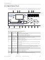
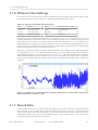
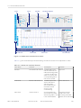
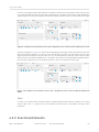
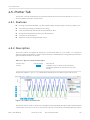
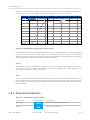
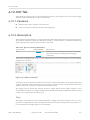
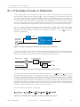
1
MFLI User Manual
MFLI User Manual
Zurich Instruments AG
Publication date Revision 31421
Copyright © 2008-2015 Zurich Instruments AG
The contents of this document are provided by Zurich Instruments AG (ZI), “as is”. ZI makes no representations or warranties with
respect to the accuracy or completeness of the contents of this publication and reserves the right to make changes to specifications
and product descriptions at any time without notice.
LabVIEW is a registered trademark of National Instruments Inc. All other trademarks are the property of their respective owners.
Revision History
Revision 31421, 8-Jul-2015:
This is the first version of the MFLI user manual related to software release 15.05.
Table of Contents
Declaration of Conformity .................................................................................................. IV
1. Getting Started ............................................................................................................... 5
1.1. Quick Start Guide ................................................................................................. 6
1.2. Inspect the Package Contents .............................................................................. 7
1.3. Handling and Safety Instructions .......................................................................... 9
1.4. Connecting to the MFLI Instrument ..................................................................... 11
1.5. Running the LabOne Web Server on a Separate PC ............................................... 24
1.6. Using the LabOne Programming APIs .................................................................. 26
1.7. Installing the LabOne Software on a PC ............................................................... 28
2. Functional Overview ...................................................................................................... 36
2.1. Features ............................................................................................................ 37
2.2. Front Panel Tour ................................................................................................ 40
2.3. Back Panel Tour ................................................................................................. 42
2.4. Ordering Guide ................................................................................................... 43
3. Tutorials ....................................................................................................................... 44
3.1. Tutorial Simple Loop .......................................................................................... 45
3.2. Tutorial External Reference ................................................................................ 53
3.3. Tutorial Sweeper ................................................................................................ 58
4. Functional Description LabOne User Interface ................................................................ 64
4.1. User Interface Overview ...................................................................................... 65
4.2. Lock-in Tab ........................................................................................................ 75
4.3. Lock-in Tab (MF-MD option) ............................................................................... 84
4.4. Numeric Tab ...................................................................................................... 93
4.5. Plotter Tab ......................................................................................................... 95
4.6. Scope Tab .......................................................................................................... 98
4.7. Software Trigger Tab ........................................................................................ 105
4.8. Spectrum Analyzer Tab ..................................................................................... 109
4.9. Sweeper Tab .................................................................................................... 113
4.10. Auxiliary Tab ................................................................................................... 120
4.11. Inputs/Outputs Tab ........................................................................................ 122
4.12. DIO Tab .......................................................................................................... 123
4.13. Config Tab ...................................................................................................... 126
4.14. Device Tab ..................................................................................................... 130
4.15. File Manager Tab ............................................................................................ 134
5. Specifications ............................................................................................................. 136
5.1. General Specifications ...................................................................................... 137
5.2. Performance Diagrams ..................................................................................... 146
6. Signal Processing Basics ............................................................................................. 147
6.1. Principles of Lock-in Detection ......................................................................... 148
6.2. Signal Bandwidth ............................................................................................. 151
6.3. Discrete-Time Filters ........................................................................................ 153
6.4. Full Range Sensitivity ....................................................................................... 155
6.5. Sinc Filtering .................................................................................................... 157
6.6. Zoom FFT ......................................................................................................... 160
7. Troubleshooting .......................................................................................................... 162
7.1. Troubleshooting ............................................................................................... 163
Glossary ......................................................................................................................... 164
Index .............................................................................................................................. 170
MFLI User Manual
Revision 31421
Zurich Instruments
3
Declaration of Conformity
The manufacturer
Zurich Instruments
Technoparkstrasse 1
8005 Zurich
Switzerland
declares that the product
MFLI Lock-in Amplifier, 500 kHz / 5 MHz, 60 MSa/s
fulfils the requirements of the European guidelines
• 2004/108/EC Electromagnetic Compatibility
• 2006/95/EC Low Voltage
The assessment was performed using the directives according to Table 1 .
Table 1. Conformity table
EN 61326-1:2006
Emissions for industrial environments, immunity for industrial
environments
EN 61000-6-4
Emission standard for industrial environments
EN 61000-6-2
Immunity for industrial environments
EN 55011
Group 1, class A and B (the product was tested in typical configuration)
EN 61000-4-2
CD 4 kV, AD 8 kV
EN 61000-4-3
10 V/m 80% AM 80 MHz - 1 GHz
3 V/m 80% AM 1 GHz - 2 GHz
1 V/m 80% AM 2 GHz - 2.7 GHz
EN 61000-4-4
2 kV power line
1 kV USB line
EN 61000-4-5
1 kV line-line, 2 kV line-earth
EN 61000-4-6
10 V 150 kHz - 80 MHz 80% AM, power line
EN 61000-4-11
100% dip (1 cycle), 30% dip (25 cycles), 60% dip (10 cycles), 100% short
interruptions (250 cycles)
EN 61010-1:2010
Safety requirements for electrical equipment for measurement, control
and laboratory use
Figure 1. CE Logo
MFLI User Manual
Revision 31421
Zurich Instruments
IV
Chapter 1. Getting Started
Welcome to the world of Medium Frequency (MF). This first chapter guides you through the initial
set-up of your MFLI Instrument in order to make your first measurements. This chapter comprises
of:
• A Quick Start Guide for the impatient.
• Inspecting the package content and accessories.
• List of essential handling and safety instructions.
• Connecting to the MFLI Instrument.
• Running the LabOne Web Server on a separate PC.
• Using the LabOne programming APIs.
This chapter is delivered as hard copy with the initial instrument delivery to customers. It is an
integral part of the MFLI User Manual.
Note
When the MFLI is connected by USB to a PC and powered on it will provide a flash drive, similar to
a USB stick. A PDF of the user manual as well as the relevant drivers can easily be accessed from
this drive by using for instance the Windows Explorer.
MFLI User Manual
Revision 31421
Zurich Instruments
5
1.1. Quick Start Guide
1.1. Quick Start Guide
This page addresses all the people who impatiently are awaiting their new gem to arrive and want
to see it up and running quickly. If the MFLI Instrument is to be integrated into a LAN with DHCP
server, it is ready to go without further need of software installation. Please proceed along the
following steps:
1. Check the package content. Besides the Instrument there should be a country specific power
cable, an USB cable, an Ethernet cable and a hard copy of the user manual Chapter 1 .
2. Check the Handling and Safety Instructions in Section 1.3 .
3. Connect the Instrument to the power line, turn it on and connect it to a switch in the LAN using
the Ethernet cable.
After a number of seconds of flashing green, the front panel LED will show a steady blue color.
If the LED remains flashing green, power cycle the MFLI instrument again and wait for the LED
to turn blue. If the LED does not turn blue, please contact Zurich Instruments for assistance.
4. Open a web browser on a PC in the LAN and type the following text in the address bar:
http://<instrument-serial>.<domain>/
where <instrument-serial> is the serial number of the instrument (see label on back panel)
and <domain> is the network domain in which the instrument is running. An example is shown
below for the Chrome browser.
An example of the serial number label on the back panel is shown below. In this particular
example the serial number is MF-DEV3026.
The LabOne User Interface startup screen will appear.
Alternative ways to address the instrument are: http://<instrument-serial>/ and
http://192.168.11.2/, the latter applies to cases where the IP address is known to the
user. Using the http prefix and network domain name and trailing slash with the host name
prevents the triggering of search engines.
5. Click the Default UI button on the lower right of the page. The default configuration will be
loaded and the first measurements can be taken. If the user interface does not start up
successfully, please refer to Section 1.4 .
Once the Instrument is up and running we recommend to go through some of the tutorials given
in Chapter 3 . Moreover, Chapter 2 provides a general introduction to the various tools and
settings tabs with tables in each section providing a detailed description of every UI element as
well. For specific application know-how the Blog section of the Zurich Instruments web page will
serve as a valuable resource that is constantly updated and expanded.
MFLI User Manual
Revision 31421
Zurich Instruments
6
1.2. Inspect the Package Contents
1.2. Inspect the Package Contents
If the shipping container appears to be damaged, keep the container until you have inspected the
contents of the shipment and have performed basic functional tests.
Please verify:
• You have received 1 Zurich Instruments MFLI Instrument
• You have received 1 power cord with a power plug suited to your country
• You have received 1 USB cable and/or 1 LAN cable (category 5/6 required)
• A printed version of the "Getting Started" section
• The "Next Calibration" sticker on the rear panel of the Instrument indicates approximately
2 years ahead in time. Zurich Instruments recommends calibration intervals of 2 years
• The MAC address of the instrument is displayed on a sticker on the back panel
Table 1.1. Package contents for the MFLI Instrument
the USB cable
the power cord (e.g. EU norm)
MFLI User Manual
Revision 31421
Zurich Instruments
7
1.2. Inspect the Package Contents
the power inlet, with power
switch and fuse holder
the LAN / Ethernet cable
(category 5/6 required)
the "Next Calibration" sticker on
the back panel of your instrument
the MAC address sticker on the
back panel of your instrument
The MFLI Instrument is equipped with a multi-mains switched power supply, and therefore can
be connected to most power systems in the world. The fuse holder is integrated with the power
inlet, and can be extracted by grabbing the holder with two finger nails (or small screwdrivers) at
the top and at the bottom at the same time. A spare fuse is contained in the fuse holder. The fuse
description is mentioned in the specification chapter.
Carefully inspect your Instrument. If there is mechanical damage or the amplifier does not pass
the basic tests, then you should immediately notify the Zurich Instruments support team at
<[email protected]> .
MFLI User Manual
Revision 31421
Zurich Instruments
8
1.3. Handling and Safety Instructions
1.3. Handling and Safety Instructions
The MFLI is a sensitive electronic instrument which under no circumstances should be opened,
as there are high-voltage parts inside which may be harmful to human beings. Moreover, there
are no serviceable parts inside the instrument. Opening the instrument immediately cancels the
warranty provided by Zurich Instruments.
The following general safety instructions must be observed during all phases of operation, service,
and handling of the instrument. The disregard of these precautions and all specific warnings
elsewhere in this manual may affect correct operation of the equipment and its lifetime.
Zurich Instruments assumes no liability for the user's failure to observe and comply with the
instructions in this user manual.
Table 1.2. Safety Instructions
Ground the instrument
The chassis must be correctly connected to
earth ground by means of the supplied power
cable. Alternatively also the ground pin on
the rear panel can be used. This avoids
electrical shocks and potential damage to the
instrument.
Maximum ratings
The specified electrical ratings for the
connectors of the instrument should not be
exceeded at any time during operation (please
refer to section Section 5.1 ).
Do not service or adjust anything yourself
There are no serviceable parts inside the
Instrument.
Software updates
Frequent software updates provide the user
with many important improvements as well as
new features. Only the last released software
version is supported by Zurich Instruments.
Warnings
Instructions contained in any warning issued
by the instrument, either by the software, the
graphical user interface, or mentioned in this
manual must be followed.
Notes
Instructions contained in the notes of this
user manual are of essential importance for
the correct interpretation of the acquired
measurement data.
Location and ventilation
Keep and operate the Instrument in a dry
location that suits the general specifications.
Do not block the ventilator opening on the back
or the air intake on the side of the chassis and
allow a reasonable space for the air to flow.
Operation and storage
Do not operate or store at a location outside
the specified ambient conditions (please refer
to section Section 5.1 )
Handling
Do not drop the Instrument, handle with due
care, do not store liquids on the device as there
is a chance of spilling and damage.
MFLI User Manual
Revision 31421
Zurich Instruments
9
1.3. Handling and Safety Instructions
When you notice any of the situations listed below, immediately stop the operation of the
Instrument, disconnect the power cord, and contact the support team at Zurich Instruments,
either through the website form or by email at <[email protected]> .
Table 1.3. Unusual Conditions
Fan is not working properly or not at all
Switch off the Instrument immediately to
prevent overheating of sensitive electronic
components.
Power cord or power plug on instrument is Switch off the Instrument immediately to
damaged
prevent overheating, electric shock, or fire.
Please exchange the power cord with a quality
product
Instrument emits abnormal noise, smell, or Switch off the Instrument immediately to
sparks
prevent large damage.
MFLI User Manual
Revision 31421
Zurich Instruments
10
1.4. Connecting to the MFLI Instrument
1.4. Connecting to the MFLI Instrument
The Zurich Instruments MFLI Lock-in Amplifier is designed to work out of the box with minimal
effort on the part of the user. The Zurich Instruments LabOne software runs on an embedded
PC in the MFLI instrument and is preinstalled before delivery. One of the programs running on
the embedded PC is the LabOne Web Server, which can be connected to via a web browser once
suitable physical and logical connections to the instrument have been established.
Note
The following web browsers are supported (latest versions)
Chrome
Firefox
Opera
Internet
Explorer
Safari
There are two ways to physically connect to the instrument:
• Ethernet (no software installation required). Integrate the instrument into an existing local
area network (LAN) by connecting the instrument to a switch in the LAN using an Ethernet
cable. The instrument can then be accessed from a web browser running on any device in the
same LAN. The Ethernet connection can also be point to point. This requires some adjustment
of the network card settings of the client computer. Depending on the network configuration
and the installed network card, one or the other connection scheme is better suited. The next
sections give a brief introduction to the different connection methods.
• Universal Serial Bus (USB). The USB connection is a point to point connection between the
instrument and the host computer to which the USB cable is connected. This requires the
installation of an RNDIS driver on the host computer. The driver is conveniently available from
the instrument's flash memory. Once the instrument is connected by USB to you PC/MAC a
new drive appears in the Explorer/Finder that contains this driver and also the user manuals.
MFLI User Manual
Revision 31421
Zurich Instruments
11
1.4. Connecting to the MFLI Instrument
Inst rum ent 1
connect ed
TCPIP Net work
USB
Inst rum ent 3
free
PC 1
TCPIP
TCPIP
TCPIP
Inst rum ent 4
connect ed
TCPIP
Inst rum ent 2
connect ed
USB
Tablet
TCPIP
USB
TCPIP
PC 2
PC 3
USB
Inst rum ent 5
USB available
USB connect ed
TCPIP available
TCPIP connect ed
Figure 1.1. Connectivity
Figure 1.1 shows some examples of possible configurations of computer to instrument
connectivity.
1.4.1. Ethernet TCP/IP Connection
The simplest connection method is to integrate the instrument into an existing LAN with a Domain
Name Server (DNS) so that an IP address can be automatically obtained. Attach an Ethernet cable
from the instrument to a LAN network switch. The LabOne user interface can be started by typing
the following text in the address bar of a web browser running on a computer in the LAN:
http://<instrument-serial>.<domain>/, or
http://<instrument-serial>/
where <instrument-serial> is the serial number of the instrument and <domain> is the
network domain in which the instrument is running.
This approach uses DNS lookup to resolve the IP address of the instrument which is configured
with this network name by default. Other network configurations are possible but require more
effort to set up. These are described in Section 1.4.3 .
It should be noted that with connection via LAN, multiple web browser and API client sessions have
simultaneous access and control over the instrument. Therefore changes made to the settings of
MFLI User Manual
Revision 31421
Zurich Instruments
12
1.4. Connecting to the MFLI Instrument
the instrument by say a Python session via the programming API will be seen by a web browser
session connected to that instrument. The instrument data can be streamed to multiple client
sessions simultaneously.
PC / Tablet
Port 80
Port 8006
Web Browser
LabOne
Web Server
FPGA
Port 8004
LabOne
Dat a Server
Figure 1.2. Simplest connection to MFLI instrument
1.4.2. Universal Serial Bus (USB) Connection
To control the instrument via USB, connect the instrument with the supplied USB cable to the PC
you are using. Depending on the operating system you are using, it may be necessary to install a
USB RNDIS device driver on the PC. The RNDIS provides a virtual Ethernet link to the instrument
enabling it to be addressed using the normal IP address and host name mechanisms. The required
device driver can be downloaded from the Zurich Instruments web site and must be installed on
the computer from which the instrument will be controlled.
The RNDIS driver installation procedure for various operating systems is described in the next
sections.
USB RNDIS Device Driver Windows
Zurich Instruments provides a Microsoft MSI installer to simplify the Windows RNDIS driver
installation.
This requires the Microsoft .NET Framework to be installed on the computer. For 95% of
computers, this is already installed. The installation of the USB RNDIS device driver will fail if this
is not the case. It is possible to check the installation of the Microsoft .NET Framework under
Windows Start → Control panel → Add and Remove Programs.
The minimum requirement is Microsoft .NET Framework 3.5 Service Pack 1.
In case the required version is not installed, it can be installed using Windows Update tool
(Windows Start → Control panel → Windows Update).
MFLI User Manual
Revision 31421
Zurich Instruments
13
1.4. Connecting to the MFLI Instrument
Figure 1.3. Installation of .NET framework
Once the Microsoft .NET framework is in place, the USB RNDIS device driver installation can begin.
The MFLI Instrument is designed so that when the USB cable is plugged in, a flash disk partition
appears with the label MFLI, containing the required Windows MSI installer for the USB RNDIS
device driver, plus the instrument user manual in pdf form and a copy of this Getting Started
chapter.
Proceed with the device driver installation as follows:
1. Log on to the PC as an administrator. Installing the USB RNDIS device driver requires
administrator rights.
2. Ensure that the USB cable is connected from the PC to the MFLI Instrument.
3. Power cycle the MFLI Instrument and wait for approximately 20 seconds for the instrument
initialization to complete. During this time an AutoPlay window will pop up showing the newly
detected MFLI drive.
4. In the Autoplay window, select Open folder to view files.
5. Go into the Driver folder and double click on the .msi installer appropriate for your operating
system. This will be either
LabOne_MF-USB64-XX.XX.XXXXX.msi for 64 bit operating systems, or
LabOne_MF-USB32-XX.XX.XXXXX.msi for 32 bit operating systems.
Figure 1.4. Read-only drive of the MFLI shown in the file explorer
6. In the welcome screen click the Next button.
MFLI User Manual
Revision 31421
Zurich Instruments
14
1.4. Connecting to the MFLI Instrument
Figure 1.5. Installation welcome screen
7. After reading through the Zurich Instruments license agreement, check the "I accept the terms
in the License Agreement" check box and click the Next button.
Figure 1.6. Installation license agreement
8. In the Custom Setup screen click the Next button.
Figure 1.7. Custom setup screen
9. Click the Install button to start the installation.
MFLI User Manual
Revision 31421
Zurich Instruments
15
1.4. Connecting to the MFLI Instrument
Figure 1.8. Installation confirmation
Figure 1.9. Installation progress
If the User Account Control pop-up window appears, click Yes to allow the installation program
to make changes to the computer.
10.In the Windows Security pop-up window, click Install. You can also click the Always trust
software from "Zurich Instruments AG" check box to prevent the message from appearing in
the future.
Figure 1.10. Installation driver acceptance
11.Click the Finish button to complete the installation.
MFLI User Manual
Revision 31421
Zurich Instruments
16
1.4. Connecting to the MFLI Instrument
Figure 1.11. Installation complete
The installation of the driver will create a Windows Start Menu entry LabOne User Interface
MF to start the LabOne User Interface on the default web browser. A locally installed application
will detect the IP address of the instrument connected over USB and will start the browser with
the IP address pointing to the LabOne Web Server running on the instrument. The Start Menu
entry is found under Start Menu → Programs → Zurich Instruments → LabOne User
Interface MF
Figure 1.12. Windows Start Menu entry to start the LabOne User Interface
USB RNDIS Device Driver Linux
With an up-to-date version of a UBUNTU Linux distribution there is no special installation
necessary, the USB connection works out of the box.
Other Linux distributions should also work but may require further installation steps. Detailed
instructions cannot not given here due to the large number of Linux distributions available.
USB RNDIS Device Driver OS X
To install the required USB RNDIS device driver on a Macintosh computer, proceed as follows:
1. Open a web browser and go to http://joshuawise.com/horndis downloads page and click the
link to download the latest binary package. At the time of writing, this link leads to the file
HoRNDIS-rel7.pkg, which should be downloaded.
MFLI User Manual
Revision 31421
Zurich Instruments
17
1.4. Connecting to the MFLI Instrument
2. Locate the downloaded file using the Finder. The file can typically be found in the Downloads
folder. Double click the file to run the installer.
3. The installer will guide you through the installation process. Select the standard option in each
dialog and click Continue to proceed with the installation.
4. Before the installer can finalize the installation, it will request administrator permissions.
Supply the necessary credentials to finish the installation.
MFLI User Manual
Revision 31421
Zurich Instruments
18
1.4. Connecting to the MFLI Instrument
5. A summary of the installation will be shown once it completes.
6. At this point it is advisable to restart the computer.
7. Connect the MFLI Instrument to the computer using the USB cable and power it up. Wait until
the blue LED on the front-panel of the MFLI Instrument illuminates.
8. To verify that the MFLI is correctly detected by the computer open the System Preferences and
select the Network category.
MFLI User Manual
Revision 31421
Zurich Instruments
19
1.4. Connecting to the MFLI Instrument
The MFLI device should now be shown in the interface list with a green icon and marked
as Connected. When the interface is selected, the information in the right hand side pane
should update to show that the interface uses DHCP and the IP address should take the form
192.168.x.x.
9. It is now possible to connect to the device using a web browser either by entering the following
in the address bar:
<instrument-serial>.local
where<instrument-serial> is the serial number of the instrument.
Alternatively, the IP address of the instrument can be used. The IP address of the instrument
is the IP address shown in the described in the previous step, with 1 added to the right-most
octet. So for instance, if the IP address shown is 192.168.47.57, the instrument IP address
to enter in the address bar would be 192.168.47.58.
1.4.3. Instrument Discovery TCP/IP
Various schemes are possible for logically connecting to the MFLI instrument via TCP/IP.
• DHCP (the simplest scheme for the user and the default)
• Static IP (the fallback if DHCP fails)
• Point to point (P2P)
The sample transfer performance of different connections varies greatly. Generally it can be said
that a point-to-point connection will lead to larger transfer rates compared to a network-based
connection, at the expense of more complexity in the connection setup.
DHCP
The most straightforward Ethernet connection method is to rely on a LAN configuration to
recognize the MFLI Instrument. This is the MFLI Instrument's default configuration. By connecting
the instrument in a LAN, a dynamic IP address is assigned like any other PC by the DHCP server. In
case of restricted networks, the network administrator may be required to register the instrument
on the network by means of the MAC address. The MAC address is indicated on the back panel
of the instrument.
MFLI User Manual
Revision 31421
Zurich Instruments
20
1.4. Connecting to the MFLI Instrument
If the network configuration does not allow or does not support DHCP it is necessary to use a static
IP setup as described below. The MFLI Instrument is configured to accept the IP address from the
DHCP server, or to fall back to IP address 192.168.1.10 if it does not obtain one.
Static IP
The best way to assign the instrument a static IP address is to first connect via USB. This is
especially necessary if DHCP is not available in the LAN.
1. Connect to the instrument and start the LabOne UI as described in Section 1.4.2 .
2. Open the Device tab.
3. In the Communication section, set the desired IP4 address.
4. Set the appropriate IP4 mask and Gateway
5. Click on the Static IP button to indicate the use of a static IP address.
6. Click on the Program button to save the changed parameters.
7. Connect an Ethernet cable from a switch in the LAN to the 1GbE port on the back panel of the
MFLI Instrument.
8. Power cycle the MFLI instrument. Is this necessary?
9. (Optional) To verify the connection between the host computer and the MFLI Instrument, open
a DOS command window and ping the IP address entered above.
10.Type the following in the address bar of a web browser on a computer within the LAN:
http://<Static IP Address>/
where <Static IP Address> is the static IP address entered above.
The LabOne UI should now appear.
Requirements
• The chosen static IP address must be unique within the LAN.
• Needs network administrator support on networks with dynamic IP configuration (the static
IP address will need to be reserved).
Note
If the MFLI Instrument fails to obtain a dynamic IP address from the DHCP server in the LAN, it
falls back to the static IP address 192.168.1.10.
Point to Point (P2P)
If you want to control the MFLI instrument from a PC and you have two network cards installed,
one of which is used for network connectivity (e.g. internet), the other can be used for a direct
MFLI User Manual
Revision 31421
Zurich Instruments
21
1.4. Connecting to the MFLI Instrument
connection to the MFLI Instrument. Notebooks can generally profit from wireless LAN for network
connectivity. It is important to note that if you set a static IP on your host computer you may lose
the connection to the internet.
1. Use one of the network cards and set it to static IP in TCP/IPv4 using the following IP address
and mask (go to Control Panel → Internet Options → Network and Internet
→ Network and Sharing Center → Local Area Connection→Properties). Note
that the IP address of the PC should be 192.168.1.n, where n=[2..9] and the mask should be
255.255.255.0. The instrument itself will use the fall-back address 192.168.1.10 if it does
not obtain an address from the DHCP server.
Figure 1.13. Static IP configuration of PC
To connect to the MFLI Instrument and start the LabOne User Interface, type the following in the
address bar of a web browser:
http://192.168.1.10/
Requirements
• Two networks cards needed for additional connection to internet
• Network adapter connected to the instrument must be in static IP4 configuration
Note
A power cycle of the MFLI Instrument is required if it was previously connected to a network
that provided an IP address to the instrument and then the user decides to run in static IP
configuration.
Note
Only IP v4 is currently supported. There is no support for IP v6.
MFLI User Manual
Revision 31421
Zurich Instruments
22
1.4. Connecting to the MFLI Instrument
Warning
Changing the IP settings of your network adapters manually can interfere with its later use, as it
can no longer be used for network connectivity until it is set again for dynamic IP.
MFLI User Manual
Revision 31421
Zurich Instruments
23
1.5. Running the LabOne Web Server on a Separate PC
1.5. Running the LabOne Web Server on a
Separate PC
It can be advantageous to run the LabOne Web Server on a separate PC instead of the embedded
PC in the instrument. This is particularly the case when using high data transfer rates. At such
data rates, the higher processing power of laptop and desktop computers gives improved UI
responsiveness and generally a better user experience and reduces the probability of sample loss.
To run the Web Server on a separate PC, the LabOne software must be installed on the PC that
connects to the instrument. See Section 1.7 for LabOne installation instructions.
PC
Port 80
Port 8006
Web Browser
LabOne
Web Server
FPGA
Port 8006
LabOne
Web Server
Port 8004
LabOne
Dat a Server
Figure 1.14. Zurich Instruments Web Server running on separate PC
1.5.1. Connecting to the MFLI from the Web Server
Once the LabOne software has been installed on a separate PC, proceed as follows to connect to
the MFLI Instrument:
1. Start the LabOne Web Server. From the Windows Start menu, select All Programs → Zurich
Instruments → LabOne Servers → LabOne Web Server MFLI.
2. In the LabOne DataServer Connect dialog that appears, type the following text in the Host Name
field:
<instrument-serial>.<domain>
Where <instrument-serial> is the serial number of the MFLI Instrument and <domain> is
the network domain in which the instrument is running. An example is given below.
MFLI User Manual
Revision 31421
Zurich Instruments
24
1.5. Running the LabOne Web Server on a Separate PC
The port to use is 8004 which by default should already be correct (The LabOne Data Server
running on the MFLI listens on port 8004).
3. Click the Connect button. The Device and Settings dialog will appear allowing you to proceed
as normal.
This setting can be made permanent by making a copy of the LabOne WebServer shortcut and
modifying its properties. Proceed as follows (this is the procedure for Windows 7):
1. Copy the LabOne Web Server shortcut to the desktop (from the Start menu, navigate to All
Programs → Zurich Instruments → LabOne Servers → LabOne Web Server UHF
and use CTRL and drag and drop).
2. Right click the copied Desktop shortcut and select Properties to bring up the Properties dialog.
3. Append the following text to the text in the Target field and click OK:
--server-ip <instrument-serial>
Where instrument-serial> is the serial number of the MFLI Instrument. See example
below.
When the LabOne Web server is now started using this icon, it will automatically connect to the
Data Server running on the MFLI Instrument.
Note
A LabOne Web Server running on a separate PC listens only on IP port 8006. Port 80 is not used to
prevent conflicts with other applications running on the PC.
MFLI User Manual
Revision 31421
Zurich Instruments
25
1.6. Using the LabOne Programming APIs
1.6. Using the LabOne Programming APIs
The LabOne software provides programming APIs for MATLAB, LabVIEW, Python and C. To use
these APIs requires further installation steps. See the next sections.
PC
Port 80
Port 8006
Web Browser
LabOne
Web Server
FPGA
LabOne
MATLAB
API
Port 8004
LabOne
Dat a Server
C
API
LabVIEW
API
LabOne
Pyt hon Package
Pyt hon
API
Figure 1.15. LabOne APIs installed on separate PC
The LabOne APIs communicate directly with the Data Server running on the MFLI Instrument via
IP port 8004.
The device address can be <instrument-serial>, mf-<instrument-serial>, mf<instrument-serial>.<domain>, or <IP address>. If the address is not fully qualified,
means domain name is not added, the API will perform a network discovery with multicast to get
the IP address. This ensures that devices connected by Ethernet over USB will be accessible by
the same method as devices connected to LAN.
1.6.1. Using the LabOne MATLAB, LabVIEW and C APIs
If you want to program the instrument using the LabOne MATLAB, LabVIEW or C programming
APIs, the LabOne software must be installed on the PC that connects to the instrument. See
Section 1.7 for LabOne installation instructions.
Please refer to the MFLI Programming Manual for details on using the MATLAB, labVIEW and C
programming APIs.
1.6.2. Using the LabOne Python API
MFLI User Manual
Revision 31421
Zurich Instruments
26
1.6. Using the LabOne Programming APIs
To use the Python API, the Zurich Instruments LabOne Python package must installed. Please
refer to the MFLI Programming Manual for the LabOne Python installation and programming
instructions.
MFLI User Manual
Revision 31421
Zurich Instruments
27
1.7. Installing the LabOne Software on a PC
1.7. Installing the LabOne Software on a PC
The MFLI Instrument comes with the LabOne software preinstalled and is ready to work out of
the box. However, the LabOne software can be installed on any PC. This can be advantageous
for performance reasons and is necessary if programming the instrument using the MATLAB,
LabVIEW or C APIs.
Note
Administrator rights are required to install the LabOne software on a PC.
1.7.1. Windows Installation
The installation packages for the Zurich Instruments LabOne software are available as Windows
installer .msi packages. The software is available at the Zurich Instruments download portal at
http://www.zhinst.com/downloads.
To install the LabOne software, proceed as follows:
1. Log on to the website using the login and password provided by Zurich Instruments.
2. Download the software package suitable to your operating system and processor architecture
(32-bit or 64-bit).
Important
When downloading the software packages, please make sure that you download and install the
software that is suited to the addressing mode (32-bit: x86, 64-bit: x64) of your operating system.
Zurich Instruments supports Microsoft Windows XP, Windows 7 and Windows 8 for both 32-bit
and 64-bit processors. In case you are not sure which Windows architecture you are using, you
can check this as follows:
• Windows 7: Control panel → System and Security → System/System type
• Windows 8: Control panel → System → System/System type
Table 1.4. Find out the OS addressing architecture (32-bit or 64-bit)
MFLI User Manual
Revision 31421
Zurich Instruments
28
1.7. Installing the LabOne Software on a PC
Windows 7 (32-bit: x86)
Windows 7 (64-bit: x64)
Windows .NET Framework Requirement
The Zurich Instruments LabOne software requires the Microsoft .NET Framework to be installed
on the host computer. For 95% of computers, this is already installed. The installation of LabOne
will fail if this is not the case. It is possible to check the installation of the Microsoft .NET
Framework under Windows Start → Control panel → Add and Remove Programs.
The minimum requirement is Microsoft .NET Framework 3.5 Service Pack 1.
In case the required version is not installed, it can be installed using Windows Update tool
(Windows Start → Control panel → Windows Update).
Figure 1.16. Installation of .NET framework
Windows LabOne Installation
1. The MFLI Instrument should not be connected to your computer during the LabOne software
installation process
2. Start the LabOne32/64-XX.XX.XXXXX.msi LabOne installer program by a double click
and follow the instructions. Please note that Windows Administrator rights are required for
installation. The installation proceeds as follows:
• On the welcome screen click the Next button.
MFLI User Manual
Revision 31421
Zurich Instruments
29
1.7. Installing the LabOne Software on a PC
Figure 1.17. Installation welcome screen
• After reading through the Zurich Instruments license agreement, check the "I accept the
terms in the License Agreement" check box and click the Next button.
• Review the features you want to have installed. For the MFLI Instrument the the MFLI
Series Device, Web Server and API features are required. If you would like to install
shortcuts on your desktop area, enable the feature Desktop Shortcuts. To proceed click
the Next button.
Figure 1.18. Custom setup screen
• Click the Install button to start the installation process.
• Windows will ask up to two times to reboot the computer. Make sure you have no unsaved
work on your computer. Actually a reboot is practically never required, so that one may
safely click OK.
Figure 1.19. Installation reboot request
MFLI User Manual
Revision 31421
Zurich Instruments
30
1.7. Installing the LabOne Software on a PC
• On Windows Server 2008 and Windows 7 it is required to confirm the installation of up to 2
drivers from the trusted publisher Zurich Instruments. Click on Install .
Figure 1.20. Installation driver acceptance
• Click OK on the following notification dialog.
Figure 1.21. Installation completion screen
3. Click Finish to close the Zurich Instruments LabOne installer.
Warning
Do not install drivers from another source and therefore not trusted as originating from Zurich
Instruments.
1.7.2. Linux LabOne Installation
Requirements
Ensure that the following requirements are fulfilled before trying to install the LabOne software
package:
1. Officially, only Ubuntu 12.04 LTS (i386, amd64) is supported although in practice the LabOne
package may work on other platforms. Please ensure that you are using a Linux distribution
that is compatible with Ubuntu/Debian, but preferably Ubuntu 12.04 LTS.
2. You have administrator rights for the system.
3. The correct version of the LabOne installation package for your operating system and platform
have been downloaded from the Zurich Instruments downloads page (login required):
• LabOneLinux<arch>-<release>.<revision>.tar.gz, for example:
LabOneLinux32/64-XX.XX.XXXXX.tar.gz
Please ensure you download the correct architecture (32-bit/64-bit) of the LabOne installer.
The uname command can be used in order to determine which architecture you are using, by
running:
MFLI User Manual
Revision 31421
Zurich Instruments
31
1.7. Installing the LabOne Software on a PC
uname -m
in a command line terminal. If the command outputs "x686" the 32-bit version of the LabOne
package is required, if it displays "x86_64" the 64-bit version is required.
Linux LabOne Installation
Proceed with the installation in a command line shell as follows:
1. Extract the LabOne tarball in a temporary directory:
tar xzvf LabOneLinux<arch>-<release>-<revision>.tar.gz
2. Navigate into the extracted directory.
cd LabOneLinux<arch>-<release>-<revision>
3. Run the install script with administrator rights and proceed through the guided installation,
using the default installation path if possible:
sudo bash install.sh
The install script lets you choose between the following three modes:
• Type "a" to install the Data Server program, the Web Server program, documentation and
APIs.
• Type "u" to install udev support (only necessary if HF2 Instruments will be used with this
LabOne installation and not relevant for the MFLI Lock-in Amplifier).
• Type "ENTER" to install both options "a" and "u".
4. Test the installation by starting the Web Server:
startWebServerUHF
and entering the address 127.0.0.1:8006 in a web browser to start the LabOne User
Interface. The LabOne Web Server installed on the PC listens by default on port number 8006
instead of 80 to minimize the probability of conflicts.
In the LabOne DataServer Connect dialog that appears, type the following text in the Host Name
field:
<instrument-serial>.<domain>
Where <instrument-serial> is the serial number of the MFLI Instrument and <domain> is
the network domain in which the instrument is running. An example is given below.
MFLI User Manual
Revision 31421
Zurich Instruments
32
1.7. Installing the LabOne Software on a PC
The port to use is 8004 which by default should already be correct (The LabOne Data Server
running on the MFLI listens on port 8004).
Click the Connect button. The Device and Settings dialog will appear allowing you to proceed
as normal.
Uninstalling LabOne on Linux
The LabOne software package copies an uninstall script to the base installation path (the default
installation directory is /opt/zi/). To uninstall the LabOne package please perform the following
steps in a command line shell:
1. Navigate to the path where LabOne is installed, for example, if LabOne is installed in the default
installation path:
cd /opt/zi/
2. Run the uninstall script with administrator rights and proceed through the guided steps:
sudo bash uninstall_LabOne<arch>-<release>-<revison>.sh
1.7.3. Updating the LabOne software on the MFLI Instrument
Updating the LabOne software on the MFLI instrument is achieved by either a drag and drop
procedure, or via a USB mass storage device (e.g. a memory stick).
Note
Updating of the LabOne software on the is only possible when the browser is connected to the
Web Server running on the MFLI Instrument.
Drag and Drop LabOne Software Update
• Download the latest LabOne software version from the Zurich Instruments Download
Center . Choose the version for the MFLI Instrument. The file has the form
LabOneLinuxARM32_signed-XX.XX.XXXXX.tar.
• Open a Windows Explorer window and navigate to the location of the downloaded LabOne
installation file (on Windows this is typically the Downloads folder). On Linux, the Files
application or some other file manager utility supporting drag and drop, can be used. We will
use the term explorer window henceforth in this description.
• Start the LabOne User Interface in a web browser (connect to the Web Server running on the
Instrument by typing the serial number in the address bar).
• Open the LabOne Config tab.
• Position/Resize the explorer window and the web browser such that the dotted rectangle
under the File Upload section of the Config tab is visible.
MFLI User Manual
Revision 31421
Zurich Instruments
33
1.7. Installing the LabOne Software on a PC
Figure 1.22. Config Tab showing drop zone for software update
• Drag and drop the downloaded LabOne installation file from the explorer window onto the
dotted rectangle. An Upload pop-up window will appear indicating the progress of the upload.
Once uploaded, The LabOne Software Update pop-up window will appear.
Figure 1.23. Upload pop-up window
Figure 1.24. LabOne Software Update pop-up window
• Click OK in the LabOne Software Update pop-up window. This completes the software
update. The servers running on the instrument will now be restarted necessitating a reload
of the LabOne User Interface. An Error pop-up window will appear containing the text "The
connection with the LabOne Web Server is lost".
• Reload the LabOne User Interface by clicking on the Reload button.
USB LabOne Software Update
• Download the latest LabOne software version from the Zurich Instruments Download Center
and copy it onto a USB mass storage device. Choose the version for the MFLI Instrument. The
file has the form LabOneLinuxARM32_signed-XX.XX.XXXXX.tar.
• Start the LabOne User Interface in a web browser (connect to the Web Server running on the
Instrument by typing the serial number in the address bar).
• Insert the USB mass storage device into one of the USB sockets on the back of the MFLI
Instrument.
• Open the LabOne File Manager tab.
• A folder labelled USB1 will be displayed in the File Manager tab, corresponding to the inserted
USB device. Expand the USB1 branch to display its contents (double click on the folder icon).
• Right click the LabOne update .tar file and select SW Update to update the software.
MFLI User Manual
Revision 31421
Zurich Instruments
34
1.7. Installing the LabOne Software on a PC
Figure 1.25. File Manager tab
An Upload pop-up window will appear indicating the progress of the upload. Once uploaded,
The LabOne Software Update pop-up window will appear.
Figure 1.26. LabOne Software Update pop-up window
• Click OK in the LabOne Software Update pop-up window. This completes the software
update. The servers running on the instrument will now be restarted necessitating a reload
of the LabOne User Interface. An Error pop-up window will appear containing the text "The
connection with the LabOne Web Server is lost".
• Reload the LabOne User Interface by clicking on the Reload button.
1.7.4. Updating the LabOne software on a Separate PC
To update the LabOne software already installed on a separate PC, follow the procedure described
in Section 1.7 .
MFLI User Manual
Revision 31421
Zurich Instruments
35
Chapter 2. Functional Overview
This chapter provides the overview of the features provided by the MFLI Instrument. The first
section contains the description of the graphical overview and the hardware and software feature
list. The next section details the front panel and the back panel of the measurement instrument.
The following section provides product selection and ordering support.
MFLI User Manual
Revision 31421
Zurich Instruments
36
2.1. Features
Front Panel
Signal Input + V / -V / I
Input
Range
Am plifier
LPF 10 MHz
Dem odulat ors & Oscillat ors
ADC
60 MSa/s
16 bit
MF-MD
Input
Select
LPF 10 MHz
MF-MD
Oscillator
Select
x3
Signal Out put
Out put
Range
Am plifier
DAC
60 MSa/s
16 bit
MF-MD
Out put
Adder
Auxiliary Input s / Reference 1-2
Input
Range
Am plifier
LPF 10 MHz
LPF 200 kHz
4x DAC
612 kSa/s
18 bit
Scaling
LPF
+#
Web &
Dat a
Server
MF-MD
x3
MF-F5M Frequency Ext ension
Scope
Et hernet 1 GbE
USB 2.0 Host
x2
USB 2.0 Device
Sweeper
Memory
16 kSa
with FFT
Frequency
Response
Analyzer
Spect rum
Analyzer
SW Trigger
2x ADC
15 MSa/s
16 bit
Auxiliary Out put s 1-4
x1
x1
ADC
60 MSa/s
16 bit
(X,Y)
Clock Out
10 MHz
+#
Input
Range
Am plifier
Clock In
10 MHz
LPF
Signal Input I (MF-MD opt ion)
Back Panel
2.1. Features
Digit al I/O 32-bit
Trigger Input / Out put 1-2
58 kHz span
Figure 2.1. MFLI Instrument Overview
The MF Instrument according to Figure 2.1 consists of several internal units (light blue color)
surrounded by several interface units (dark blue color) and the front panel on the left-hand side
and the back panel on the right-hand side. The orange blocks are optional units that can be either
ordered at the beginning or upgraded later in the field. The arrows between the panels and the
interface units indicate the physical connections and the data direction flow. Only a small subset
of internal connections is depicted.
The signal of interest to be measured is connected either to the low-noise current or voltage
input of the MF, where it is amplified to a defined range and digitized at very high speed. When
the MF-MD option is installed, both inputs can be used simultaneously enabling, for example, 4terminal measurements. The resulting samples are fed into the digital signal processor consisting
of up to 4 dual-phase demodulators. The demodulator output samples are further processed
on the embedded processor that hosts as well the LabOne web server, to which the user can
connect from any device running a browser (PC, Tablet or Smart phone). No software installation
is required. Supported interfaces are LAN and USB. The demodulator samples are also sent to the
auxiliary outputs in order to be available on the front panel of the MF Instrument.
The numerical oscillators generate sine and cosine signal pairs that are used for the demodulation
of the input samples and also for the generation of the MF output signals. When the MF-MD
option is installed, the Output Adder can generate a linear combination of the oscillator outputs to
generate a multi-frequency output signal: digital to analog conversion and signal scaling (range)
are supported.
Hardware trigger and reference signals are used for various purposes inside the instrument,
such as triggering demodulation, triggering oscilloscope data acquisition, or to generate external
reference clocks or triggering signals to other equipment.
Lock-in Operating Modes
• Internal reference mode
• External reference mode
• Auto reference mode
MFLI User Manual
Revision 31421
Zurich Instruments
37
2.1. Features
• Impedance mode, measuring current input and voltage input simultaneously (optional)
• Multi-harmonic mode (optional, simultaneous measurement up to four harmonic
frequencies)
• Arbitrary frequency mode (optional, simultaneous measurement at 4 arbitrary frequencies)
Medium Frequency Voltage Input
• 1 low-noise MF voltage input, single-ended, differential, 5 MHz bandwidth
• Variable input range
• Switchable input impedance
• Selectable AC/DC coupling
• Selectable instrument ground or floating
Medium Frequency Current Input
• 1 low-noise MF current input, single-ended, 5 MHz bandwidth
• Variable input range
• Switchable input impedance
• Selectable AC/DC coupling
Medium Frequency Signal Output
• Low-distortion MF outputs, single-ended, differential, 5 MHz bandwidth
• Variable output range
• Digital and analog offset
Demodulators & Reference
• Up to 4 dual-phase demodulators
• Up to 4 programmable numerical oscillators
• Up to 2 external reference signals
• Individually programmable demodulator filters
• 128-bit internal processing
• 64-bit resolution demodulator sample
• 48-bit internal reference resolution
Auxiliary Input, Outputs and Triggers
• 4 auxiliary outputs, user defined signals
• 2 auxiliary inputs, general purpose
• 2 input and 2 output trigger signals
High-speed Connectivity
• USB 2.0 Device high-speed 480 Mbit/s interface
• Dual USB 2.0 Host high-speed interface
• LAN 1 Gbit/s controller interface
• DIO: 32-bit digital input-output port
• Clock input connector (10 MHz)
MFLI User Manual
Revision 31421
Zurich Instruments
38
2.1. Features
• Clock output connector (10 MHz)
Extensive LabOne Time and Frequency Domain Analysis Toolset
• Numeric
• Scope
• Sweeper
• Spectrum
• Plotter
• SW trigger
Software Features
• Data server with multi-client support
• API for C, LabVIEW, MATLAB, Python based instrument programming
MFLI User Manual
Revision 31421
Zurich Instruments
39
2.2. Front Panel Tour
2.2. Front Panel Tour
The front panel BNC connectors and control LEDs are arranged as shown in Figure 2.2 and listed
in Table 2.1 .
A B C
D E
F
G H
M
N
O
I
J
K
L
Figure 2.2. MF Instrument front panel
Table 2.1. MF Instrument front panel description
Position
Label / Name
Description
A
Signal Input I
single-ended current input
B
Current Input
Signal Over
this red LED indicates that the current input signal saturates
the A/D converter and therefore the current input range must be
increased or the signal must be attenuated
C
Signal Input +V
voltage input
single-ended mode: single-ended voltage input
differential mode: positive voltage input
D
Signal Input -V
Diff
voltage input
single-ended mode: internally shorted to ground
differential mode: negative voltage input
E
Voltage Input
Signal Over
this red LED indicates that the voltage input signal saturates
the A/D converter and therefore the voltage input range must be
increased or the signal must be attenuated
F
Signal Output
+V
voltage output
single-ended mode: single-ended voltage output
differential mode: positive voltage output
G
Signal Output -V voltage output
single-ended mode: internally shorted to ground
differential mode: negative voltage output
MFLI User Manual
Revision 31421
Zurich Instruments
40
2.2. Front Panel Tour
Position
Label / Name
Description
H
Signal Output
ON
this blue LED indicates that the signal output is actively driven by
the instrument
I
Aux Input 2 Ref
auxiliary input 2, can be used as external reference input
supporting the full bandwidth of the device
J
Aux Output 2
auxiliary output 2, this connector provides a user defined signal,
often used to output demodulated samples (X,Y) or (R,Θ)
K
Aux Output 4
auxiliary output 4, this connector provides a user defined signal,
often used to output demodulated samples (X,Y) or (R,Θ)
L
Power
this LED indicates that the instrument is powered
color blue: the device has an active connection to the LabOne
data server and is ready for operation
color green blinking: the firmware is ready, waiting for LabOne
data server connection. This process takes around 20 seconds.
color red: the device is not initialized respectively is performing
the internal auto calibration process.
color purple blinking: a firmware update is in progress
color purple: the boot process failed
M
Aux Input 1 Ref
auxiliary input 1, can be used as external reference input
supporting the full bandwidth of the device; the value of auxiliary
input 1 can be added as offset to the signal output
N
Aux Output 1
auxiliary output 1, this connector provides a user defined signal,
often used to output demodulated samples (X,Y) or (R,Θ)
O
Aux Output 3
auxiliary output 3, this connector provides a user defined signal,
often used to output demodulated samples (X,Y) or (R,Θ)
Please refer to the troubleshooting section for further information regarding the meaning of the
Power LEB colors.
MFLI User Manual
Revision 31421
Zurich Instruments
41
2.3. Back Panel Tour
2.3. Back Panel Tour
The back panel is the main interface for power, control, service and connectivity to other ZI
instruments. Please refer to Figure 2.3 and Table 2.2 for the detailed description of the items.
J
A
K L
B
C
D
E
M
N O
F
G
H
I
Figure 2.3. MF Instrument back panel
Table 2.2. MF Instrument back panel description
Position
Label / Name
Description
A
DC In
DC external 12V power supply
B
DIO
32-bit digital input/output connector
C
USB 2.0 Host
universal serial bus host connector
D
USB 2.0 Device
universal serial bus device connector to computer
E
LAN 1GbE
1 Gbit LAN connector
F
Trigger In 2
digital TTL trigger input 2
G
Trigger Out 2
digital TTL trigger output 2
H
Clk 10 MHz In
clock input (10 MHz) to be used for synchronization from external
instruments
I
Clk 10 MHz Out
clock output (10 MHz) to be used for synchronization of external
instruments
J
Earth ground
4 mm banana jack connector for earth ground, electrically
connected to the chassis and the earth pin of the power inlet
K
USB 2.0 Host
universal serial bus host connector
L
Power inlet
power inlet with ON/OFF switch
M
Trigger In 1
digital TTL trigger input 1
N
Trigger Out 1
digital TTL trigger output 1
O
Cooling outlet
ventilator (important: keep clear from obstruction)
MFLI User Manual
Revision 31421
Zurich Instruments
42
2.4. Ordering Guide
2.4. Ordering Guide
Table 2.3 provides an overview of the available MF products. Upgradeable features are options
that can be purchased anytime without need to send the Instrument to Zurich Instruments.
Table 2.3. MF Instrument product codes for ordering
Product code
Product name
Description
Upgrade in the
field possible
MFLI 500 kHz
MFLI 500 kHz Lock-in
Amplifier
base product
-
MFLI 5 MHz
MFLI 5 MHz Lock-in
Amplifier
bundle
-
MF-MD
MF-MD Multidemodulator
option
yes
MF-F5M
MF-F5M Frequency
Extension
option
yes
Table 2.4. Product selector
Feature
MFLI
MFLI +MFMD
MFLI +MFF5M
MFLI +MFMD +MFF5M
Internal reference mode
yes
yes
yes
yes
External reference mode
yes
yes
yes
yes
Auto reference mode
yes
yes
yes
yes
Impedance mode (independent
measurement of voltage and current
signal inputs)
yes
-
yes
Signal generators
1
1
1
1
Superposed output sinusoidals per
generator
1
up to 4
1
up to 4
Quad-harmonic mode
-
yes
-
yes
Multi-frequency mode
-
yes
-
yes
Arbitrary frequency mode
-
yes
-
yes
Number of demodulators
1
4
1
4
Simultaneous frequencies
1
4
1
4
Simultaneous harmonics
1
4
1
4
External references
1
2
1
2
Dynamic reserve
120 dB
120 dB
120 dB
120 dB
Lock-in range
500 kHz
500 kHz
5 MHz
5 MHz
USB 2.0 480 Mbit/s
yes
yes
yes
yes
Ethernet 1 GbE
yes
yes
yes
yes
MFLI User Manual
Revision 31421
Zurich Instruments
43
Chapter 3. Tutorials
The tutorials in this chapter have been created to allow users to become more familiar with
the basic technique of lock-in amplification, the operation of host-based lock-in amplifiers, the
LabOne web browser based user interface, as well as some more advanced lock-in measurement
techniques. In order to successfully carry out the tutorials, users are required to have certain
laboratory equipment and basic equipment handling knowledge. The equipment list is given
below.
Note
For all tutorials, you must have LabOne installed as described in the Getting Started Chapter .
• 1 LAN cable
• 5 BNC cables
• 1 oscilloscope (optional)
• 2 BNC T-pieces
• 1 optical chopper (for the External Reference tutorial)
• 1 infrared emitter/detector pair (for the External Reference tutorial)
• 1 field-effect transistor (for the Sweeper tutorial)
MFLI User Manual
Revision 31421
Zurich Instruments
44
3.1. Tutorial Simple Loop
3.1. Tutorial Simple Loop
Note
This tutorial is applicable to all MFLI Instruments. No specific options are required.
3.1.1. Goals and Requirements
This tutorial is for people with no or little prior experience with Zurich Instruments lock-in
amplifiers. By using a very basic measurement setup, this tutorial shows the most fundamental
working principles of the MFLI instrument and the LabOne UI in a step-by-step hands-on
approach.
There are no special requirements for this tutorial.
3.1.2. Preparation
In this tutorial, you are asked to generate a single-ended signal with the MFLI Instrument and
measure that generated signal with the same instrument using an internal reference. This is
done by connecting Signal Output +V to Signal Input +V with a short BNC cable (ideally < 30 cm).
Alternatively, it is possible to connect the generated signal at Signal Output +V to an oscilloscope
by using a T-piece and an additional BNC cable. Figure 3.1 displays a sketch of the hardware
setup.
Front Panel
Aux Input
Signal Input
I
+V
Signal Out put
- V Diff
+V
-V
Back Panel
Trigger
In
Aux Out put
1
Ref
1
3
2
Ref
2
4
Lan
DIO
USB
Oscilloscope
BNC
CH 1
CH 2
USB
LAN
Out
1
1
2
2
Clock 10 MHz
In
Out
Rout er
Lan
Lan
Lan
Lan
Lan
PC Host
LabOne®
Dat a Server
Web Server
User Int erface
Lan
Et hernet
Figure 3.1. Setup for the Simple Loop Tutorial (LAN connection shown)
Note
This tutorial is for all MFLI irrespective of which particular option set is installed. Some changes
in the description apply if the MF-MD Multi-demodulator option is installed.
Connect the cables as described above. Make sure that the MFLI Instrument is powered on and
then connect the MFLI directly by USB to your host computer or by Ethernet to your local area
MFLI User Manual
Revision 31421
Zurich Instruments
45
3.1. Tutorial Simple Loop
network (LAN) where the host computer resides. After connecting to your Instrument through the
web browser using its address, the LabOne graphical user interface is opened. Check the Getting
Started Chapter for detailed instructions. The tutorial can be started with the default instrument
configuration (e.g. after a power cycle) and the default user interface settings (i.e. as is after
pressing F5 in the browser).
3.1.3. Generate the Test Signal
Perform the following steps in order to generate a 300 kHz signal of 0.5 V peak amplitude on Signal
Output +V. We work with the graphical Lock-in tab. Note that the control elements in this tab
dynamically adapt their appearance to the web browser window size. Be sure to work in full screen
size for this test.
1. In the Lock-in tab, select the sub-tab 1 on the left-hand side of the screen. In the Reference
section, change the frequency value of oscillator 1 to 300 kHz: click on the field, enter 300'000
or 300k in short and press either <TAB> or <ENTER> on your keyboard to activate the setting.
2. In the Output Amplitudes section, set the amplitude to 500 mV (peak value) and enable the
signal by clicking on the button labeled "En". A single green LED on top indicates the enabled
signal.
3. In the Signal Output 1 section (right hand side on the Lock-in tab), set the Range pull-down to
1 V and the Offset to 0 V. Keep the Add and Diff buttons unchecked.
4. By default, all physical outputs of the MFLI are inactive to prevent damage to the MFLI or to
the devices connected to it. Now it is time to turn on the main output by clicking on the button
labelled "On".
Table 3.1 summarizes the instrument settings to be made. If you have an oscilloscope connected
to the setup, you should now be able to see the generated sinusoidal signal with a peak-to-peak
amplitude of 1 V. Be sure to choose a high input impedance on the oscilloscope. But you can easily
spare the extra equipment, as the MFLI comes with a built-in oscilloscope. In Section 3.1.4 we
describe how to use it.
Table 3.1. Settings: generate the test signal
Tab
Section
#
Label
Setting / Value / State
Lock-in
Oscillator
1
Frequency
300 kHz
Lock-in
Output
1
Amplitude
500 mV
Lock-in
Output
1
Offset
0V
Lock-in
Output
1
On
On
3.1.4. Check the Test Input Signal
Next, we configure the signal input side of the MFLI from the Lock-in tab, and then visualize the
input signal using the Scope tab. In the Signal Input section of the Lock-in tab, select Sig In 1 from
MFLI User Manual
Revision 31421
Zurich Instruments
46
3.1. Tutorial Simple Loop
the pull-down menu. Set the range to 1.0 V, and be sure to have the AC, 50 Ω, Diff and Float buttons
unchecked.
The range setting ensures that the analog amplification on the Signal Input +V is set such that the
resolution of the input analog-to-digital converter is used efficiently without clipping the signal.
This optimizes the dynamic range.
The incoming signal can now be observed over time by using the Scope tab. A Scope view can be
placed in the web browser by clicking on the icon in the left sidebar or by dragging the Scope Icon
to one of the open tab rows. Choose the following settings on the Scope tab to display the signal
entering Signal Input +V:
Table 3.2. Settings: check the test signal
Tab
Section
#
Label
Setting / Value / State
Lock-in
Signal Input
1
Float
Off
Lock-in
Signal Input
1
Diff
Off
Lock-in
Signal Input
1
50 Ω
Off
Lock-in
Signal Input
1
AC
Off
Scope
Horizontal
Sampling Rate
60 MHz
Scope
Horizontal
Length
4096 pts
Scope
Vertical
Channel 1
Signal Input 1
Scope
Trigger
Enable
On
Scope
Trigger
Level
0V
The Scope tool now displays single shots of Signal Input +V with a temporal distance given by
the Hold off Time. The scales on the top and on the left of the graphs indicate the zoom level for
orientation. The icons on the left and below the figure give access to the main scaling properties
and allow to store the measurement data as a SVG image file or plain data text file. Moreover,
panning can be achieved by clicking and holding the left mouse button inside the graph while
moving the mouse.
Note
Zooming in and out along the horizontal dimension can by achieved with the mouse wheel. For
vertical zooming, the shift key needs to be pressed and again the mouse wheel can by used for
adjustments. Another, quick way of zooming in is to hold down the shift key and to use the right
mouse button to define a horizontal, vertical, or box-like inside the graph area - try it out!
Having set the Input Range to 1 V ensures that no signal clipping occurs. If you set the Input Range
to 0.1 V, clipping can be seen immediately on the scope window accompanied by a red OVI error
flag on the status bar on the bottom of the LabOne User Interface. At the same time, the LED next
to the Signal Input +V BNC connector on the instrument's front panel will turn red.
The Scope is a very handy tool to quickly check the quality of the input signal. Users can either use
the Scope to adjust the optimal input range setting or to check if the software trigger level is set
correctly. For the full description of the Scope tool please refer to the Functional Description .
MFLI User Manual
Revision 31421
Zurich Instruments
47
3.1. Tutorial Simple Loop
Figure 3.2. LabOne Scope showing the raw signal generated by the MFLI
3.1.5. Measure the Test Input Signal
Now, we are ready to use the MFLI to demodulate the input signal and measure its amplitude and
phase. We will use two tools of the LabOne User Interface: the Numerical and the Plotter tab.
First, adjust the parameters listed in the following table on the graphical Lock-in tab for
demodulator 1.
Table 3.3. Settings: generate the reference signal
Tab
Section
#
Label
Setting / Value / State
Lock-in
Signal Input
1
Lock-in
Low-Pass Filter
1
Sinc
Off
Lock-in
Low-Pass Filter
1
Order
3 (18 dB/Oct)
Lock-in
Low-Pass Filter
1
BW 3 dB
10.6 Hz
Lock-in
PC Data Transfer 1
En
On
Lock-in
PC Data Transfer 1
Rate
100 Sa/s (automatically
adjusted to 104.6 Sa/s)
Lock-in
PC Data Transfer 1
Trigger
Continuous
Signal Input 1
These above settings configure the demodulation filter to the third-order low-pass operation
with a 10.6 Hz 3 dB filter bandwidth (BW 3dB). Alternatively, the corresponding noise-equivalent
bandwidth (BW NEP) or the integration time constant (TC) can be displayed and entered. The
output of the demodulator filter is read out at a rate of 104.6 Hz, implying that 104.6 data samples
are sent to the internal MFLI computer per second with equidistant spacing. These samples can
be viewed in the Numerical and the Plotter tool which we will examine now.
MFLI User Manual
Revision 31421
Zurich Instruments
48
3.1. Tutorial Simple Loop
Note
1. The rate should be about 7 to 10 times higher than the filter bandwidth chosen in the Low-Pass
Filter section. When entering a number in the Rate field, the new rate is automatically set to
the closest available value - in this case 104.6 Sa/s.
2. If you don't see any signal in the Plotter, Numeric, Spectrum, SW Trigger, or Sweeper tab, the
first thing to check is whether the corresponding data stream is enabled
The Numeric tool provides the space for 16 or more measurement panels. Each of the panels has
the option to display the samples in the Cartesian (X,Y) or in the polar format (R,Θ) plus other
quantities such as the Oscillator Frequencies and Auxiliary Inputs. The unit of the (X,Y,R) values
are by default given in VRMS. The scaling and the displayed unit can be altered in the Signal Input
section of the Lock-in tab. The numerical values are supported by graphical bar scale indicators
to achieve better readability, e.g. for alignment procedures. Certain users may observe rapidly
changing digits. This is due to the fact that you are measuring thermal noise that is maybe in
the μV or even nV range depending on the filter settings. This provides a first glimpse of the level
of measurement precision offered by your MFLI Instrument. If you wish to play around with the
settings, you can now change the amplitude of the generated signal, and observe the effect on
the demodulator output.
Next, we will have a look at the Plotter tool that allows users to observe the demodulator signals
as a function of time. It is possible to adjust the scaling of the graph in both directions, or make
detailed measurements with 2 cursors for each direction. You can find a variety of handy tools
for immediate analysis in the Math sub-tab, allowing you to accurately measure noise amplitude,
peak positions and heights, signal background and many more. Figure 3.3 shows the signal along
with additional graphical elements that are dynamically added to the plot when e.g. using the
histogram functionality from the Math sub-tab.
Signals of the same unit are automatically added to the same default y-axis group. This ensures
that the axis scaling is identical. Signals can be moved between groups. More information on yaxis groups can be found in Section 4.1.3 . Try zooming in along the time dimension using the
mouse wheel or the icons below the plot to display about one second of the data stream. While
zooming in, the mode in which the data are displayed will change from a min-max envelope plot
to linear point interpolation. The LabOne Web Server makes this choice depending on the density
of points along the horizontal axis as compared to the number of pixels available on the screen.
Figure 3.3. LabOne User Interface Plotter displaying demodulator results continuously over time
(roll mode)
MFLI User Manual
Revision 31421
Zurich Instruments
49
3.1. Tutorial Simple Loop
3.1.6. Different Filter Settings
As next step in this tutorial you will learn to change the filter settings and see their effect on the
measurement results. For this exercise, change the 3 dB bandwidth to 1 kHz.
Table 3.4. Settings: change the filter parameters
Tab
Section
#
Label
Setting / Value / State
Lock-in
Low-Pass Filter
1
Order
3 (18 dB/Oct)
Lock-in
Low-Pass Filter
1
BW 3dB
1 kHz
Lock-in
PC Data Transfer 1
Rate
6.7 kSa/s
Increasing the filter bandwidth reduces the integration time of the demodulators. This will
increase available time resolution but in turn make the signal noisier, as can be nicely observed
in the Plotter tab. Note that it is recommended to keep the sample rate 7 to 10 times the filter 3
dB bandwidth. The sample rate will be rounded off to the next available sampling frequency. For
example, typing 7 k in the Rate field will result in 6.7 kSa/s which is sufficient to not only properly
resolve the signal, but also to avoid aliasing effects.
Moreover, you may for instance "disturb" the demodulator with a change of test signal amplitude,
for example from 0.5 V to 0.7 V and back. The plot will go out of the display range which can be readjusted by pressing the "Rescale" button, cf. Section 4.1.3 . With an increasing time constant,
the demodulated data react more and more slowly to the change in the input signal. In addition,
the number of stable significant digits in the Numerical tab will also be higher with a large time
constant.
Figure 3.4. LabOne User Interface Plotter displaying demodulator results while changing the
filter bandwidth from 10 Hz to 1 kHz
3.1.7. Record Data
Finally, we discuss how to record measurement data with your MFLI Instrument using the LabOne
user interface. A first, simple option was mentioned in the previous section: in any plot (in the
Plotter, Scope, Spectrum, and other tabs), you can save the presently plotted curves as a commaseparated variable (CSV) file to the download folder of your web browser. Just click on the
corresponding icon at the bottom of the plot.
MFLI User Manual
Revision 31421
Zurich Instruments
50
3.1. Tutorial Simple Loop
For more flexibility, you can use the record functionality which is accessible from the Config tab.
From here you can control the choice of data to be recorded, their format, and their location. In
order to end up with small file sizes for this exercise, let's set the demodulator filter bandwidth
and its data rate to 10 Hz and 100 Sa/s, respectively.
The first choice is the format of the saved data. LabOne supports CSV and Matlab binary file
format. Select CSV in the Format field of the Record section. The CSV delimiter character is
selected in the User Preferences section. We'll leave the default Semicolon option.
The next choice is what data to save. This selection is made using the node tree display of
the Record Data section. We'll record the demodulator measurement data as well as the filter
bandwidth. Check the corresponding boxes in the node tree: DeviceXXXX/Demodulators/Demod
1/Sample and DeviceXXXX/Demodulators/Demod 1/Filter Time Constant. The node tree structure
allows you to access a great variety of instrument settings (such as the filter time constant) and
streaming data (such as the demodulator samples) and store them in a consistent fashion.
Next, we select where to save the data. Keep in mind that the core of the LabOne software, the
data server, runs on the internal computer of the MFLI. The default file location is consequentially
the internal hard drive of the MFLI, as set in the Drive field of the Record section. From there, the
data can be downloaded to the host computer. This will be described shortly. Alternatively, you
can plug in an external USB drive in one of the USB Device ports on the back panel of the MFLI. If
you do so, you can select USB 1 or USB 2 as the Drive.
Enable data recording by enabling the Record check box, leave it on for a few seconds for this test,
and disable it again. The following table summarizes the settings to be made.
Table 3.5. Settings: record data on the local drive
Tab
Section
#
Label
Setting / Value / State
Lock-in
Low-Pass Filter
1
Order
3 (18 dB/Oct)
Lock-in
Low-Pass Filter
1
BW 3dB
10 Hz
Lock-in
PC Data Transfer 1
Rate
100 Sa/s
Config
User Preferences
CSV Delimiter
Semicolon
Config
Record Data
Format
CSV
Config
Record Data
Record
On / Off
Figure 3.5. Browsing and inspecting files in the LabOne File Manager tab
For each of the nodes that we selected, at least one file is created. Its location is indicated in the
Folder field of the Record Data section. For longer recording periods, the data may be distributed
over several files. Open the File Manager (Files) tab and navigate to the folder location using the
MFLI User Manual
Revision 31421
Zurich Instruments
51
3.1. Tutorial Simple Loop
file browser on the left. The file browser shown in Figure 3.5 gives you the usual functionalities
for managing files on the MFLI drive. In addition, you can transfer files between the MFLI and the
host computer using the Upload/Download buttons. The viewer on the right-hand side of the File
Manager tab allows you to directly inspect text data files, with the exception of very large files. You
can use it to check the contents of the Demodulator Sample and Filter Time Constant data files.
Note
The structure of files containing instrument settings and those containing streamed data are
equivalent. In the case of instrument settings however, the file usually only contains a few entries
corresponding to changes in the settings.
MFLI User Manual
Revision 31421
Zurich Instruments
52
3.2. Tutorial External Reference
3.2. Tutorial External Reference
Note
This tutorial is applicable to all MFLI Instruments. No specific options are required. The user
interface has slight differences depending on whether the MF-MD Multi-demodulator option is
installed or not. The tutorial provides separate instructions for both cases.
3.2.1. Goals and Requirements
This tutorial explains how to lock an internal oscillator to an external reference frequency, and
then demodulate a measurement signal at a harmonic of this frequency. To follow this tutorial,
you need an optical chopper as well as a standard optical detector/emitter pair. However, the
tutorial applies to any comparable setup in which separate reference and signal channels are
available. The reference channel should have a sufficiently large amplitude (e.g., TTL level) to allow
for reliable locking.
3.2.2. Preparation
Connect the cables as shown in Figure 3.6 . Make sure the MFLI is powered on, and then connect
the MFLI through USB to your PC, or to your local area network (LAN) where the host computer
resides. After connecting to your Instrument through the web browser using its address, the
LabOne graphical user interface is opened. Check the Getting Started Chapter for detailed
instructions. The tutorial can be started with the default instrument configuration (e.g. after a
power cycle) and the default user interface settings (i.e. as is after pressing F5 in the browser).
Front Panel
Aux Input
Signal Input
I
+V
Signal Out put
- V Diff
+V
Aux Out put
1
Ref
-V
1
2
2
Ref
Chopper Cont roller
3
4
Sync
To
Out put Chopper
080.00
BNC
1k
Chopper
wheel
LED
Phot odiode
0.5k
BNC
Figure 3.6. Setup for the external reference measurement with optical chopper, LED, and photo
diode.
3.2.3. Activate the External Reference Mode
MFLI User Manual
Revision 31421
Zurich Instruments
53
3.2. Tutorial External Reference
The reference signal is wired from the sync output of the optical chopper to the Aux Input 1/Ref of
the MFLI. In our case, the reference signal is a square signal switching between 0 V and 5 V. We
choose a base frequency of 80 Hz on the chopper. You can inspect the signal easily by going to the
Scope tab and selecting Aux In 1 Ch 1 as the input signal.
Locking the internal oscillator to the external signal looks slightly different depending on the
installed options, notably if the MF-MD Multi-demodulator option is installed or not. We therefore
describe the required steps separately for both cases.
Without MF-MD Multi-demodulator option: Open the graphical Lock-in tab. In the Internal/
External Reference section on the bottom row of that tab, the section label is actually a control
which can be toggled between Internal Reference (default) and External Reference. Set it to
External Reference. To the right of that control, you can now select the input signal. Select Aux In 1
as the input signal. These settings are also shown in Figure 3.7 . The frequency value displayed in
the center of the reference section should quickly convert to the 80 Hz of the chopper. The Lockin settings used to lock to the external reference without MF-MD Multi-demodulator option are
shown in the following table.
Table 3.6. Settings: set up external reference mode (without MF-MD option)
Tab
Section
Lock-in
Lock-in
#
Label
Setting / Value / State
Internal/External 1
Reference
Internal/External
Reference
External Reference
Internal/External 1
Reference
Internal/External
Reference
Aux In 1
Figure 3.7. Lock-in tab with settings for external reference (without MF-MD option)
With MF-MD Multi-demodulator option: Open the graphical Lock-in tab of the second
demodulator. We use this demodulator to establish the phase-locked loop (PLL) between the
internal oscillator 1 and the external signal. In the Reference section at the bottom left of the
Lock-in tab, select ExtRef in the Mode field and select oscillator number 1. In the Signal Input
section top left, select Aux In 1 as the input signal. These settings are also shown in Figure 3.8 .
The frequency of oscillator 1 displayed in the Reference section should quickly converge to the 80
Hz of the chopper. The Lock-in settings for setting up the lock to the external reference with MFMD Multi-demodulator option are shown in Table 3.5 .
Table 3.7. Settings: set up external reference mode (with MF-MD option)
Tab
Section
#
Label
Setting / Value / State
Lock-in
Reference
2
Mode
ExtRef
Lock-in
Reference
2
Osc
1
Lock-in
Signal Input
2
Signal
Aux In 1
MFLI User Manual
Revision 31421
Zurich Instruments
54
3.2. Tutorial External Reference
Figure 3.8. Lock-in tab with settings for external reference (with MF-MD option)
At this point, it is worth noting that the external reference signal is never used directly for
demodulation. Instead, the frequency and phase of the external reference signal are mapped onto
one of the internal oscillators through an internal phase-locked loop. This internal oscillator can
then serve as a reference for any of the demodulators.
This mapping procedure is implemented with an automatic bandwidth adjustment that ensures
quick locking over the whole instrument bandwidth. It covers a large variety of signal qualities in
terms of frequency stability and signal-to-noise ratio. Over the course of automatic adjustment,
the Low-Pass Filter bandwidth of the associated demodulators 2 or 4 usually ramps down until
a final value is reached after a few seconds. The indicated bandwidth also marks an upper limit
to the bandwidth of the phase-locked loop that does the mapping of the external signal to the
internal oscillator. Figure 3.9 shows a typical result in the Plotter for the frequency tracking
immediately after it is turned on. For such a measurement, open the Plotter tab and add the
corresponding signal to the plot (Control sub-tab, Vertical Axis Groups, Frequency, Channel 1, Add
Signal).
Note
With the MF-MD Multi-demodulator option installed, you can alternatively look at the phase error
(Control sub-tab, Vertical Axis Groups, Demod Theta, Channel 2, Add Signal). Be sure to enable
the corresponding data stream in the PC Data Transfer section of the corresponding Lock-in tab.
Figure 3.9. Frequency of the internal oscillator over time with stepwise automatic bandwidth
adjustment
3.2.4. Measure at a Harmonic of the Reference Frequency
For our optical demonstration measurement, we use a Vishay TCRT5000 infrared detector/emitter
pair whose light is passed through the optical chopper. The detector is a photo diode, the emitter
MFLI User Manual
Revision 31421
Zurich Instruments
55
3.2. Tutorial External Reference
an LED, and both are biased directly by the Auxiliary Output 2 through a simple circuit as shown
in Figure 3.6 . We current-bias the LED with 10 mA by applying 5 V across a 500 Ω resistor. The 1
kΩ resistor in series with the photo diode is merely a limiter. Note that the circuit by design can't
exceed the damage threshold of the MFLI (5 V on the 50 Ω I input).
The current generated by the photo diode contains an offset contribution, typically due to ambient
light, and a modulation contribution due to the chopper. Both are in the range of some μA in our
case, allowing us to use the higher input sensitivity of 100 μA instead of 10 mA and thus improve
the input noise. The chopper wheel used for this experiment has a multiplier of 10, so the optical
signal is actually modulated at a frequency of 800 Hz. This places us further away from the 50/60
Hz utility frequency without having to use a high revolution speed of the chopper.
We will use the harmonics functionality to internally generate an 800 Hz demodulation reference
from the 80 Hz external reference. Setting this up again presents slight difference depending on
the installed options, so we describe the required steps with and without installed MF-MD Multidemodulator option.
Without MF-MD Multi-demodulator option: In the Signal Input section of the graphical Lockin tab, select Current Input 1 and change the input range to 100 μA. In the External Reference
Section, set the Harmonic (Harm) to 10 / 1. Note that this setting is hidden by default. You can
get access to this setting by expanding the section with a click on the + symbol on the top right of
the section. You should now observe a numerical display of the demodulator reference frequency
close to 800 Hz as shown in Figure 3.10 . Finally, set the Low-Pass Filter to 100 Hz (3rd order) and
enable the data stream in the PC Data Transfer section.
Figure 3.10. Lock-in tab set up for measurement at 800 Hz (without MF-MD option)
Table 3.8. Settings: lock-in detection at a harmonic of the external reference frequency (without
MF-MD option)
Tab
Section
#
Label
Setting / Value / State
Lock-in
External
Reference
1
Harm
10 / 1
Lock-in
Signal Input
1
Signal
Current Input 1
Lock-in
Signal Input
1
Range
100 μA
With MF-MD Multi-demodulator option: Open the graphical Lock-in tab of the first demodulator.
We use this demodulator to perform the lock-in detection. In the Signal Input section of the
graphical Lock-in tab, select Current Input 1 and change the input range to 100 μA. In the
Reference section, choose Oscillator 1 and set the Harmonic (Harm) to 10, cf. Figure 3.11 . In
the circuit diagram of the graphical Lock-in tab, you should observe the numeric value of the
demodulation frequency, 800 Hz. Set the Low-Pass Filter to 100 Hz (3rd order) and enable the
data stream in the PC Data Transfer section.
MFLI User Manual
Revision 31421
Zurich Instruments
56
3.2. Tutorial External Reference
Table 3.9. Settings: lock-in detection at a harmonic of the external reference frequency (with
MF-MD option)
Tab
Section
#
Label
Setting / Value / State
Lock-in
Reference
1
Harm
10
Lock-in
Signal Input
1
Signal
Current Input 1
Lock-in
Signal Input
1
Range
100 μA
Figure 3.11. Lock-in tab setup for measurement at 800 Hz (with MF-MD option)
3.2.5. Plot the Measurement Results
Having set up the demodulation at 800 Hz, we are ready to check the measurement data. Open
the Plotter tab. In the Control sub-tab, select the Enabled Demods R setting in the Presets list.
Figure 3.12 shows a plot of the photo diode current in which the light path between emitter and
detector was manually intersected a number of times to show the measurement contrast. When
the light path is open (except for the chopper wheel), we measure a constant rms current of about
15.5 μA, and whenever we block the light path the current drops to zero.
Figure 3.12. Photo diode signal continuously plotted with the LabOne Plotter
MFLI User Manual
Revision 31421
Zurich Instruments
57
3.3. Tutorial Sweeper
3.3. Tutorial Sweeper
Note
This tutorial is applicable to all MFLI Instruments with the MF-MD Multi-demodulator option
installed. The MD option is required for four-terminal measurements with simultaneous detection
of voltage and current.
3.3.1. Goals and Requirements
This tutorial explains how to use the LabOne Sweeper to perform measurements on a MOSFET
(Metal-oxide-semiconductor field-effect transistor). The goal of the tutorial is to demonstrate
typical steps in the work flow of a lock-in measurement using the LabOne toolset using
the MOSFET as a demonstration system. To follow this tutorial, you need a MOSFET with
specifications similar to those of the IRLML2502. However, many of the working steps have a
generic character and can be adopted to a multitude of transport measurement situations.
The goal of the tutorial is not to provide instructions for MOSFET characterization. This is a
sophisticated measurement task and lies beyond the scope of this tutorial.
3.3.2. Preparation
We perform these measurement on a IRLML2502 power MOSFET manufactured by International
Rectifier, but many other MOSFETs allow to do similar measurements with certain adjustments
to the parameters. Connect the cables as shown in Figure 3.13 . Make sure the MFLI is powered
on, and then connect the MFLI through USB to your PC, or through an Ethernet cable to your local
area network (LAN) where the host computer resides. After connecting to your Instrument through
the web browser using its address, the LabOne graphical user interface is opened in the browser.
Check the Getting Started Chapter for detailed instructions. The tutorial can be started with the
default instrument configuration (e.g. after a power cycle) and the default user interface settings
(i.e. as is after pressing F5 in the browser).
Front Panel
Aux Input
Signal Input
I
+V
BNC
Signal Out put
- V Diff
+V
-V
Aux Out put
1
Ref
1
3
2
Ref
2
4
Drain
Gat e
Source
MOSFET
Figure 3.13. Setup for the MOSFET measurements.
3.3.3. Tune the Gate-Source Voltage
MFLI User Manual
Revision 31421
Zurich Instruments
58
3.3. Tutorial Sweeper
We start by configuring the Lock-in to detect the source current of the MOSFET. Open the Lock-in
tab of the first demodulator. In the Reference section choose oscillator 1 and set the frequency to
1 kHz. In the Signal Input section, select Current Input 1 as the signal and set the range to 10 mA.
In the Low-Pass Filter section, set the filter 3 dB bandwidth to 10 Hz.
We will operate the MOSFET with a negative drain-source offset voltage. On top of that, we apply
a small alternating drain-source voltage. This is an unusual regime for the MOSFET. But it allows
to operate the device in a configuration of linear response to the alternating drain-source voltage
while having offset currents within the range of the MFLI Signal Input I.
In the Output Amplitudes section, set Amplitude 1 to 10 mVrms and enable the output. In the
Signal Output section, set Offset to -100 mV and turn on the output. Finally, enable the data
transfer of demodulator 1 in the PC Data Transfer section. The following table summarizes the
settings to be made.
Table 3.10. Settings: MOSFET source current measurement
Tab
Section
#
Label
Setting / Value / State
Lock-in
Reference
1
Osc
1
Lock-in
Reference
1
Freq
1 kHz
Lock-in
Signal Input
1
Signal Input
Curr In 1
Lock-in
Signal Input
1
Range
10 mA
Lock-in
Low-Pass Filter
1
BW 3dB
100 Hz
Lock-in
Output
Amplitudes
1
Amp 1 (Vrms)
100 mVrms
Lock-in
Output
Amplitudes
1
En
On
Lock-in
Signal Output
1
Offset
-100 mV
Lock-in
Signal Output
1
On
On
Lock-in
PC Data Transfer
1
En
On
The MOSFET gate is connected to the Auxiliary Output 1. Using the Aux tab, we can configure this
output to generate a constant voltage. In the Aux Output section, set the Signal of the first Auxiliary
Output to Manual. Now it is possible to output an arbitrary voltage using the Offset field. If you
play around with that value while observing the MOSFET current in the Plotter or the Numeric tab,
you can observe the behavior of the MOSFET as a tunable resistor. Our model is an n-channel
device, therefore negative gate-source voltages lead to a suppression of the current and positive
voltages of a few Volts open up the MOSFET channel. The following table summarizes the settings
to be made.
Before we continue, let us shortly discuss the effect of series resistances in our measurement
setup. Taking a quick glance at Figure 3.13 keeping in mind that Signal Input I represents a virtual
ground. We would conclude that the voltage on Signal Output +V is equal to the drain-source
voltage of the MOSFET, and the voltage on Auxiliary Output 1 is equal to the gate-source voltage. In
reality, this is not exact, since Signal Output +V, Signal Input I, and the Auxiliary Outputs have a 50
Ω impedance connected in series internally. As soon as there is significant current flow on either
of the three connectors, the actual potential at the corresponding MOSFET contact is altered. This
correction is negligible for the gate contact which is essentially isolating, but it can be important
for the source and drain contacts.
In the first part of the tutorial we will focus on the region with partially closed MOSFET channel. In
this high-impedance configuration, we can make the assumption that currents and corrections
are small. In the second part of the tutorial we will focus on the region with open MOSFET channel.
MFLI User Manual
Revision 31421
Zurich Instruments
59
3.3. Tutorial Sweeper
In this low-impedance configuration, we instead use a four-terminal measurement to properly
account for the corrections.
3.3.4. Sweep the Gate-Source Voltage
We will now set up a sweep of the MOSFET gate voltage. Open the Sweeper tab and in the Control
sub-tab, choose Aux Out 1 Offset as Sweep Parameter. Enter Start and Stop values of 0 V and 1 V,
respectively, and set Length to 100 points. Disable the Log check box so the measurement points
will be linearly distributed over the interval between 0 V and 1 V.
In a Sweeper measurement, some care has to be taken in choosing a sweep speed compatible
with the measurement bandwidth. If the time per point is too short, systematic errors can occur
due to insufficient settling of the measurement value. We can usually let the LabOne Sweeper
take care of this. Choose Application Mode in Filter field of the Settings sub-tab. The Sweeper
then chooses useful sweep parameters and adjusts the demodulator filter settings for a number
of pre-defined application cases. We select the general-purpose "Parameter Sweep Averaged"
case in the Application field. Please refer to Section 4.9 for further information.
Note
The Sweeper can control the demodulator filter. It may be, however, that the measurement
bandwidth is limited by the device under test and not by the demodulator filter. If you're unsure,
check for hysteresis in the measurement by setting the Sweep Mode to Bidirectional in the Control
sub-tab. If custom sweep settings appear necessary, you can access them in the Advanced Mode
from the Settings sub-tab.
Table 3.11. Settings: MOSFET gate voltage sweep
Tab
Section
Sweeper
Label
Setting / Value / State
Control
Sweep Param
Aux Out 1 Offset
Sweeper
Control
Start
0V
Sweeper
Control
Stop
1V
Sweeper
Control
Length
100 points
Sweeper
Control
Log
Off
Sweeper
Settings
Filter
Application Mode
Sweeper
Settings
Application
Parameter Sweep
Averaged
MFLI User Manual
#
Revision 31421
Zurich Instruments
60
3.3. Tutorial Sweeper
Figure 3.14. Gate voltage dependence of the MOSFET source current measured with the LabOne
Sweeper
Figure 3.14 shows the result of the gate voltage sweep. For gate voltages below about 0.5 V,
we observe an exponential suppression of the drain current. For higher voltages, the current
eventually saturates at about 0.1 mA. This value is determined by the Signal Output +V amplitude
of 10 mV and the cumulated 100 Ω series resistance of the MFLI input and output impedances,
two times 50 Ω. Note that in this plot, the signal amplitude goes down to about 10 nA, a level of
about -120 dB relative to the input range of 10 mA! This gives you an impression of the accessible
dynamic range of the MFLI Instrument.
3.3.5. Four-Terminal Resistance Measurement
In the measurements shown so far in this tutorial, we effectively employed a two-terminal
method. As long as the device under test has a large impedance, like the MOSFET with a partly
closed channel, this is adequate and has the benefit of being simple. In the opposite case of small
device impedance, the effect of series impedances in the cabling and Signal Outputs and Inputs,
can become increasingly dominant. It is then more appropriate to employ a four-terminal method.
In our case, we may be interested in the MOSFET properties in the On state, in which its channel
resistance is well below 1 Ω. In order to measure this On-resistance, we continue to measure the
alternating current as we did up to now. We add a measurement of the alternating voltage drop
across the MOSFET channel using the differential Signal Input of the MFLI.
We configure the second demodulator to perform this voltage measurement. Open the Lock-in
tab of the second demodulator. In the Reference section, select Oscillator 1. In the Signal Input
section, select Signal Input 1 and enable differential measurement by enabling the check box
labeled Diff. Set the range to 1 mV and enable the data transfer of demodulator 1 in the PC Data
Transfer section. The following table summarizes the settings to be made.
MFLI User Manual
Revision 31421
Zurich Instruments
61
3.3. Tutorial Sweeper
Table 3.12. Settings: MOSFET gate voltage sweep
Tab
Section
#
Label
Setting / Value / State
Lock-in
Signal Input
2
Lock-in
Signal Input
2
Diff
On
Lock-in
Signal Input
2
Range
1 mV
Lock-in
Reference
2
Osc
1
Lock-in
PC Data Transfer
En
On
Sig In 1
In order to obtain a clean four-terminal measurement, the voltages probe on the MOSFET source
and drain should be as close to the device under test as possible. The best is to use point probes
directly on the MOSFET contacts to eliminate the effect of soldering joint resistances.
At a gate voltage (Aux Output 1) of 4 V and an excitation voltage of 100 mVrms (Signal Output 1),
we can check the measurement data on the Numeric tab. We measure a source current of 1.00
mA and a source-drain voltage of 0.027 mV. This corresponds to an On-resistance of 27 mΩ in
accordance with the device specifications. Figure 3.15 and Figure 3.16 show the source current
and two-terminal drain-source voltage of the MOSFET over a larger gate voltage range.
Figure 3.15. Gate voltage dependence of the MOSFET source current measured with the LabOne
Sweeper in a four-terminal setup
MFLI User Manual
Revision 31421
Zurich Instruments
62
3.3. Tutorial Sweeper
Figure 3.16. Gate voltage dependence of the MOSFET drain-source voltage measured with the
LabOne Sweeper in a four-terminal setup
MFLI User Manual
Revision 31421
Zurich Instruments
63
Chapter 4. Functional Description LabOne
User Interface
This chapter gives a detailed description of all panels of the LabOne User Interface (UI) for the
Zurich Instruments MFLI. LabOne provides a data server and a web server that allow to access and
control the Instrument with any of the most common web browsers (e.g. Firefox, Chrome, etc.).
This architecture allows a platform-independent interaction with the Instrument by using various
devices (PCs, tablets, smart phones, etc.) even at the same time if needed.
On top of standard functionality like acquiring and saving data points this UI provides a wide
variety of measurement tools for time and frequency domain analysis of measurement data as
well as for convenient servo loop implementation and diagnosis.
MFLI User Manual
Revision 31421
Zurich Instruments
64
4.1. User Interface Overview
4.1. User Interface Overview
4.1.1. UI Nomenclature
This section provides an overview of the LabOne User Interface, its main elements and naming
conventions. The LabOne User Interface is a browser-based UI provided as the primary interface
to the MFLI. Multiple browser sessions can access the instrument simultaneously and the
user can have displays on multiple computer screens. Parallel to the UI the Instrument can be
fully controlled and read out (possibly concurrently) by custom programs written in any of the
supported languages (e.g. LabVIEW, MATLAB, C, Python) connecting through the LabOne APIs.
app icons
element
section
X range
plot control icons
plot
tab row
Figure 4.1. LabOne User Interface (default view)
Figure 4.1 shows the default screen after a new measurements session has been started. The
appearance of the UI is by default divided into two tab rows, each containing a tab structure that
allows to access the different settings and tools. Depending on display size and application, tab
rows can be freely added and deleted with the control elements on the right-hand side of each tab
bar. Similarly the individual tabs can be deleted or added by selecting app icons from the left side
bar. A simple click on an icon adds the requested tab to the active tab row, alternatively the icon
can be dragged and dropped into one of the tab rows. Moreover, tabs can simply be displaced by
drag-and-drop within a row or across rows. Further items are highlighted in Figure 4.2 .
MFLI User Manual
Revision 31421
Zurich Instruments
65
4.1. User Interface Overview
unit 1
side bar
unit 2
tab bar
status bar
collapse/expand
main area
control tabs
Figure 4.2. LabOne User Interface (more items)
Table 4.1 gives s brief descriptions and naming conventions for the most important UI items.
Table 4.1. LabOne User Interface features
Item name
Position
side bar
left-hand side of the UI contains app icons
app icons
that activate the tool
tabs and settings tabs
- a click to a tab icon
adds or activates the
corresponding tab in
the active row tab
status bar
bottom side of the UI
contains important
status indicators,
warning lamps,
device and session
information and
access to the
command log
status indicators
main area
center of the UI
accommodates all
active tabs (tool tabs
and setting tabs) - new
rows can be added
rows and columns
of tab rows, each
consisting of tab bar
and the active tab area
MFLI User Manual
Revision 31421
Description
Zurich Instruments
Contains
66
4.1. User Interface Overview
Item name
Position
Description
Contains
and removed by using
the control elements
on the right-hand side
of the tab bar, located
on the top of each tab
row
tab area
inside of each tab
provides the active
part of each tab
consisting of
settings, controls and
measurement tools
sections, plots, control
tabs, unit selections
4.1.2. Unique Set of Analysis Tools
All Instruments feature a comprehensive tool set for time and frequency domain analysis for
both raw signals and demodulated signals. Note that the selection of app icons is limited by the
firmware options installed on a particular instrument.
The icons provided by the icon bar on the left side of the UI can be roughly divided into two
categories: settings and tools. Settings-related tabs are in direct connection of the instrument
hardware allowing the user to control all the settings and instrument states. Tools-related tabs
place a focus on the display and analysis of gathered measurement data. There is no strict
distinction between settings and tools, e.g. will the Sweeper change certain demodulator settings
while performing a frequency sweep. Within the tools one can further discriminate between time
domain and frequency domain analysis, moreover, a distinction between the analysis of fast input
signals - typical sampling rate of 60 MSa/s - and the measurement of orders of magnitude slower
data - typical sampling rate of <200 kSa/s - derived for instance from demodulator outputs and
auxiliary inputs. Table 4.2 provides a brief classification of the tools.
Table 4.2. Tools for time domain and frequency domain analysis
Time Domain
Frequency Domain
Fast signals (60 MSa/s)
Oscilloscope (Scope Tab)
FFT Analyzer (Scope Tab)
Slow signals (<200 kSa/s)
Numeric
Spectrum Analyzer (Spectrum
Tab)
Plotter
Sweeper
Software Trigger
-
The following table gives the overview of all app icons.
Table 4.3. Overview of app icons and short description
Control/Tool
Option/Range
Description
Lock-in
Quick overview and access to all the settings
and properties for signal generation and
demodulation.
Lock-in MD
Quick overview and access to all the settings
and properties for signal generation and
demodulation.
MFLI User Manual
Revision 31421
Zurich Instruments
67
4.1. User Interface Overview
Control/Tool
Option/Range
Description
Files
Access files on internal flash memory and USB
drive.
Numeric
Access to all continuously streamed
measurement data as numerical values.
Plotter
Displays various continuously streamed
measurement data as traces over time (rollmode).
Scope
Displays shots of data samples in time and
frequency domain (FFT) representation.
SW Trig
Provides complex trigger functionality on all
continuously streamed data samples and time
domain display.
Spectrum
Provides FFT functionality to all continuously
streamed measurement data.
Sweeper
Allows to scan one variable (of a wide choice,
e.g. frequency) over a defined range and display
various response functions including statistical
operations.
Aux
Controls all settings regarding the auxiliary inputs
and auxiliary outputs.
In/Out
Access to all controls relevant for the main Signal
Inputs and Signal Outputs on the instrument's
front.
DIO
Gives access to all controls relevant for the digital
inputs and outputs including the Ref/Trigger
connectors.
Config
Provides access to software configuration.
Device
Provides instrument specific settings.
Table 4.4 gives a quick overview over the different status bar elements along with a short
description.
Table 4.4. Status bar description
Control/Tool
Option/Range
Description
Command log
last command
Shows the last command. A different formatting
(Matlab, Python, ..) can be set in the config tab.
The log is also saved in [User]\Documents\Zurich
Instruments\LabOne\WebServer\Log
MFLI User Manual
Revision 31421
Zurich Instruments
68
4.1. User Interface Overview
Control/Tool
Option/Range
Show Log
Show the command log history in a separate
browser window.
Session
integer value
Device
devXXX
REC
Description
grey/green
Indicates the current session identifier.
Indicates the device serial number.
A green indicator shows ongoing data recording
(related to global recording settings in the Config
tab).
CF
grey/yellow/red
Clock Failure - Red: present malfunction of the
external 10 MHz reference oscillator. Yellow:
indicates a malfunction occurred in the past.
OVI
grey/yellow/red
Signal Input Overflow - Red: present overflow
condition on the signal input also shown by the
red front panel LED. Yellow: indicates an overflow
occurred in the past.
OVO
grey/yellow/red
Overflow Signal Output - Red: present overflow
condition on the signal output. Yellow: indicates
an overflow occurred in the past.
PL
grey/yellow/red
Packet Loss - Red: present loss of data between
the device and the host PC. Yellow: indicates a
loss occurred in the past.
SL
grey/yellow/red
Sample Loss - Red: present loss of sample data
between the device and the host PC. Yellow:
indicates a loss occurred in the past.
C
Reset status flags: Clear the current state of the
status flags
Full Screen
Toggles the browser between full screen and
normal mode.
4.1.3. Plot Functionality
Several tools - Plotter, Scope, SW Trigger, Spectrum and Sweeper - provide a graphical display of
measurement data in the form of plots. These are multi-functional tools with zooming, panning
and cursor capability. This section introduces some of the highlights.
Plot area elements
Plots consist of the plot area, the X range and the range controls. The X range (above the plot area)
indicates which section of the wave is displayed by means of the blue zoom region indicators. The
two ranges show the full scale of the plot which does not change when the plot area displays a
zoomed view. The two axes of the plot area instead do change when zoom is applied.
The mouse functionality inside of plot is summarized in Table 4.5
MFLI User Manual
Revision 31421
Zurich Instruments
69
4.1. User Interface Overview
Table 4.5. Mouse functionality inside plots
Name
Action
Description
Performed inside
Panning
left click on any moves
location and move waveforms
around
Zoom X axis
mouse wheel
Zoom Y axis
shift + mouse wheel zooms in and out the plot area
Y axis
Window zoom
shift and left mouse selects the area of plot area
area select
the waveform to be
zoomed in
the plot area
zooms in and out the plot area
X axis
Absolute jump
zoom area
of left mouse click
Absolute move
zoom area
of left mouse drag-and- moves the blue zoom X and Y range, inside
drop
range indicators
of the blue range
indicators
Full Scale
double click
moves the blue zoom X and Y range,
range indicators
but outside of the
blue zoom range
indicators
set X and Y axis to full plot area
scale
Each plot area contains a legend that lists all the shown signals in the respective color. The legend
can be moved to any desired position by means of drag-and-drop.
The X range and Y range plot controls are described in Table 4.6 .
Table 4.6. Plot control description
Control/Tool
Option/Range
Description
Axis scaling mode
Selects between automatic, full scale and manual
axis scaling.
Axis mapping mode
Select between linear, logarithmic and decibel
axis mapping.
Axis zoom in
Zooms the respective axis in by a factor of 2.
Axis zoom out
Zooms the respective axis out by a factor of 2.
Rescale axis to data
Rescale the foreground Y axis in the selected
zoom area.
Save figure
Generates an SVG of the plot area or areas for
dual plots to the local download folder.
Save data
Generates a TXT consisting of the displayed set
of samples. Select full scale to save the complete
wave. The save data function only saves one shot
at a time (the last displayed wave).
Cursor control
Cursors can be switch On/Off and set to be moved
both independently or one bound to the other one.
MFLI User Manual
Revision 31421
Zurich Instruments
70
4.1. User Interface Overview
Cursors and Math
The plot area provides two X and two Y cursors which appear as dashed lines inside of the plot
area. The four cursors are selected and moved by means of the blue handles individually by means
of drag-and-drop. For each axis there is a primary cursor indicating its absolute position and a
secondary cursor indicating both absolute and relative position to the primary cursor.
Cursors have an absolute position which does not change by pan or zoom events. In case the
cursors move out of the zoom area, the corresponding handle is displays on the related side of the
plot area. Unless the handle is moved, the cursor keeps the current position. This functionality is
very effective to measure large deltas with high precision (as the absolute position of the other
cursors does not move).
The cursor data can also be used to define the input data for the mathematical operations
performed on plotted data. This functionality is available in the Math sub-tab of each tool. The
following Table 4.7 gives an overview of all the elements and their functionality. It is important
to know that the Signals and Operations defined will always be performed only on the currently
chosen active trace.
Table 4.7. Plot math description
Control/Tool
Source Select
Option/Range
Cursor Loc
Cursor coordinates as input data.
Cursor Area
Consider all plot data inside the rectangle defined
by the cursor coordinates as input for statistical
functions (Min, Max, Avg, Std, Int).
Tracking
Operation Select
Description
Output plot value at current cursor position.
Options are X1 and X2.
Wave
Consider all plot data currently displayed in the
Plot as input for statistical functions (Min, Max,
Avg, Std, Int).
Peak
Find and determine the various peaks in the
plotted data and their associated values.
Histogram
Select Histogram related data as Math input.
X1, X2, X2-X1,
Y1, Y2, Y2-Y1
Min, Max,
Avg, Std, Int
Pos, Level
Cursors values and their differences.
Statistical Functions applied to a set of samples.
Finds the Position (x-values) and the Levels (yvalues) of Peaks on a set of samples.
Add
Add the selected math function to the result table
below.
Add All
Add all operations for the selected signal to the
result table below.
Select All
Select all lines from the result table above.
Clear Selected
Clear selected lines from the result table above.
Unit Prefix
Adds a suitable prefix to the SI units to allow for
better readability and increase of significant
digits displayed.
MFLI User Manual
Revision 31421
Zurich Instruments
71
4.1. User Interface Overview
Control/Tool
Option/Range
Description
CSV
Values of the current result table are saved as a
text file into the download folder.
Link
Provides a LabOne Net Link to use the data in
tools like Excel, Matlab, etc.
Help
Opens the LabOne User Interface help.
Note
For calculation of the standard deviation the corrected sample standard deviation is used as
defined by
with a total of N samples
and an arithmetic average
.
Tree Sub-Tab
The Numeric tab and Plotter tab are able to display so many different types of signals that
a number of different options are provided to access them. One of them is the Tree sub-tab
that allows essentially to access all streamed measurement data in a hierarchical structure by
checking the boxes of the signal that should be displayed.
Tree sub-tab
Figure 4.3. Tree sub-tab in Plotter tab
Table 4.8. Tree description
Control/Tool
Selection Filter
View Filter
Option/Range
Regular expression Create a filter to define which streaming nodes
are selected. The View Filter presents a number of
presets that can serve as examples.
All
R,X,Y
Streams
MFLI User Manual
Description
Revision 31421
Show all available nodes.
Show demodulator streaming nodes.
Show all streaming nodes.
Zurich Instruments
72
4.1. User Interface Overview
Control/Tool
Option/Range
Description
All
Select all nodes that can be selected in the
relevant context.
None
Unselect all nodes.
Vertical Axis Groups
Vertical Axis groups are available in the Plotter tab, SW Trigger tab, and Sweeper tab. These tools
are able to show signals with different axis properties within the same plot. As a frequency and
amplitude axis have fundamentally different limits they have each their individual axis which
allows for correct auto scaling. However, signals of the same type e.g. Cartesian demodulator
results should preferably share one scaling. This allows for fast signal strength comparison. To
achieve this the signals are assigned to specific axis group. Each axis group has its own axis
system. This default behavior can be changed by moving one or more signals into a new group.
Vertical Axis Groups
Figure 4.4. Vertical Axis Group in Plotter tool
The tick labels of only one axis group can be shown at once. This is the foreground axis group. To
define the foreground group click on one of the group names in the Vertical Axis Groups box. The
current foreground group gets a high contrast color.
Select foreground group: Click on a signal name or group name inside the Vertical Axis Groups. If
a group is empty the selection is not performed.
Split the default vertical axis group: Use drag-and-drop to move one signal on the field [Drop
signal here to add a new group]. This signal will now have its own axis system.
Change vertical axis group of a signal: Use drag-and-drop to move a signal from one group into
another group that has the same unit.
Group separation: In case a group hosts multiple signals and the unit of some of these signals
changes, the group will be split in several groups according to the different new units.
Remove a signal from the group: In order to remove a signal from a group drag-and-drop the signal
to a place outside of the Vertical Axis Groups box.
MFLI User Manual
Revision 31421
Zurich Instruments
73
4.1. User Interface Overview
Remove a vertical axis group: A group is removed as soon as the last signal of a custom group is
removed. Default groups will remain active until they are explicitly removed by drag-and-drop. If
a new signal is added that match the group properties it will be added again to this default group.
This ensures that settings of default groups are not lost, unless explicitly removed.
Rename a vertical axis group: New groups get a default name 'Group of ...'. This name can be
changed by double-clicking on the group name.
Hide/show a signal: Uncheck/check the check box of the signal. This is faster than fetching a
signal from a tree again.
Figure 4.5. Vertical Axis Group typical drag and drop moves
Table 4.9. Vertical Axis Groups description
Control/Tool
Vertical Axis Group
Option/Range
Description
Manages signal groups sharing a common
vertical axis. Show or hide signals by changing the
check box state. Split a group by dropping signals
to the field [Drop signal here to add new group].
Remove signals by dragging them on a free area.
Rename group names by editing the group label.
Axis tick labels of the selected group are shown
in the plot. Cursor elements of the active wave
(selected) are added in the cursor math tab.
Signal Type
Demod X, Y, R, Theta Select signal types for the Vertical Axis Group.
Frequency
Aux Input 1, 2
HW Trigger
Channel
integer value
Add Signal
MFLI User Manual
Selects a channel to be added.
Adds a signal to the plot. The signal will be added
to its default group. It may be moved by drag and
drop to its own group. All signals within a group
share a common y-axis. Select a group to bring its
axis to the foreground and display its labels.
Revision 31421
Zurich Instruments
74
4.2. Lock-in Tab
4.2. Lock-in Tab
This tab is the main lock-in amplifier control panel. Users with instruments with MF-MD multidemodulator option installed are kindly referred to Section 4.3 .
4.2.1. Features
• Functional block diagram with access to main input, output and demodulator controls
• Parameter table with main input, output and demodulator controls
• Control elements for 1 demodulator
• Auto ranging, scaling, arbitrary input units for both input channels
• Control for 1 oscillator
• Settings for main signal inputs and signal outputs
• Flexible choice of reference source, trigger options and data transfer rates
4.2.2. Description
The Lock-in tab is the main control center of the instrument and open after start up by default.
Whenever closed or a new instance is needed the following symbol pressed will generate a new
instance of the tab.
Table 4.10. App icon and short description
Control/Tool
Option/Range
Lock-in
Description
Quick overview and access to all the settings
and properties for signal generation and
demodulation.
The Lock-in tab comes with parameter table view accessible with the side-tabs by pressing on
All. Moreover, there are functional block diagrams available for each demodulator accessible by
using the numbers indicated on the side-tabs.
Parameter Table
The parameter table (see Figure 4.6 ) consists of 4 sections: Signal Inputs, Oscillators,
Demodulators and Signal Outputs. The Demodulator section consists of two rows where the upper
row offers access to all the settings of the dual phase demodulator, the second row represents
the phase detector for the PLL used for external references. The user can obtain and change the
filter settings but not transfer the data to the data server.
Figure 4.6. LabOne User Interface Lock-in tab - Parameter table (All)
MFLI User Manual
Revision 31421
Zurich Instruments
75
4.2. Lock-in Tab
The Signal Inputs section allows the user to define all relevant settings specific to the signal
entered as for example input coupling, range, etc. Some of the available options like phase
adjustment and the trigger functionality are collapsed by default. It takes one mouse click on the
"+" icon in order to expand those controls. On the right-hand side of the Lock-in tab the Signal
Outputs section allows to define signal amplitudes, offsets and range values.
The Scaling field below the Range field can be used to multiply the Signal Input data for instance
to account for the gain of an external amplifier. In case there is a transimpedance gain of 10 V/A
applied to the input signal externally, then the Scaling field can be set to 0.1 and the Units field
can be set to A in order to show the actual current readings through the entire user interface.
There are two buttons below the Scaling field that can be toggled: the AC/DC button and the 50
Ω/10 MΩ. The AC/DC button sets the coupling type: AC coupling has a high-pass cutoff frequency
that can be used to block large DC signal components to prevent input signal saturation during
amplification. The 50 Ω/10 MΩ button toggles the input impedance between low (50 Ω) and high
(approx. 10 MΩ) input impedance. With 50 Ω input impedance, one will expect a reduction of a
factor of 2 in the measured signal if the signal source also has an output impedance of 50 Ω.
Note
The Signal Inputs can be set to float which means that the BNC connector shield is no longer
connected to the instrument ground. It is important that this setting affects both the current input
and the voltage input in the same way.
The Oscillator section indicates the frequency of the internal oscillator. Where the Mode indicator
shows Manual the user can define the oscillator frequency manually defined by typing a frequency
value in the field. In case the oscillator is referenced to an external source the Mode indicator will
show ExtRef and the frequency field is set to read only. External reference requires a PLL to do
the frequency mapping onto an internal oscillator. Successful locking is indicated by a green light
right next to the frequency field.
The next section contains the Demodulators settings. The block diagram displayed in Figure 4.7
indicates the main demodulator components and their interconnection. The understanding of the
wiring is essential for successfully operating the instrument.
Demodulator
O scillators
Harmonic Phase Shift
+ 0
n
O sc Select
Phase
+ 90°
Mixer
Signal
Inputs
Input Select
Down
Sample
Low
Pass
BW
O rder
Down
Sample
612 kSa/s
Polar
Rate
Signal
O utput
X
Y
X
Y
R
USB/LAN
Aux O ut
Aux O ut
Figure 4.7. Demodulator block diagram
The first line in the Demodulators section represents the demodulator available for
measurements. The Mode column is read only set to internal reference (Demod). The second line
MFLI User Manual
Revision 31421
Zurich Instruments
76
4.2. Lock-in Tab
represents an additional Demodulator that is reserved for the exclusive use as a phase detector
when the mode is switched to external reference (ExtRef). The user can select from a number of
different inputs to be used as external reference signals and the filter settings provide the user
with an idea of the PLL speed. However, this second demodulator does not produce any output
data that could be used for measurements.
In the Input Signal column one defines the signal that is taken as input for the demodulator. A
wide choice of signals can be selected: Signal Inputs, the Trigger Inputs, the Auxiliary Inputs and
Auxiliary Outputs. This allows to use the instrument for many different measurement topologies.
For each demodulator an additional phase shift can be introduced to the associated oscillator by
entering the phase offset in the Phase column. This phase is added both, to the reference channel
and the output of the demodulator. Hence, when the frequency is generated and detected using
the same demodulator, signal phase and reference phase change by the same amount and no
change will be visible in the demodulation result. Demodulation of frequencies that are integer
multiples of any of the oscillator frequencies is achieved by entering the desired factor in the Harm
column. The demodulator readout can be obtained using the Numeric tab which is described in
Section 4.4 .
In the middle of the Lock-in tab is the Low-Pass Filters section where the filter order can be
selected in the drop down list for each demodulator and the filter bandwidth (BW 3dB) can chosen
by typing a numerical value. Alternatively the time constant of the filter (TC) or the noise equivalent
power filter bandwidth (BW NEP) can be chosen by clicking on the column's header. For example,
setting the filter order to 4 corresponds to a roll off of 24 dB/oct or 80 dB/dec i.e. an attenuation of
4
10 for a tenfold frequency increase. If the Low-Pass Filter bandwidth is comparable to or larger
than the demodulation frequency, the demodulator output may contain frequency components
at the frequency of demodulation and its higher harmonics. In this case, the additional Sinc Filter
can be enabled. It attenuates those unwanted harmonic components in the demodulator output.
The Sinc Filter is also useful when measuring at low frequencies, since it allows to apply a LowPass Filter bandwidth closer to the demodulation frequency, thus speeding up the measurement
time.
The data transfer of demodulator outputs is activated by the En button in the Data Transfer
section where also the sampling rate (Rate) for each demodulator can be defined.
The Trigger section next to the Data Transfer allows for setting trigger conditions in order to control
and initiate data transfer from the Instrument to the host PC by the application of logic signals
(e.g. TTL) to either Trigger Input 1 or 2 on the back panel.
In the Signal Outputs section the On buttons allow to activate the Signal Output. The Range drop
down list is used to select the proper output range setting. On the Signal Output a digital offset
voltage (Offset) can be defined. The maximum output signal permitted is ±10 V.
Block Diagram
The block diagram view of the main instrument functions is also sometimes referred to as the
"Graphical Lock-in Tab". Depending how many demodulators are available in the instrument a set
of numbered side-tabs occur giving access to a Graphical Lock-in Tab for each demodulator. The
block diagrams are fully functional and provide the user with a visual feedback of what is going
on inside the instrument. All control elements that are available in the Parameter Table detailed
in the previous section are also present in the graphical representation.
The block diagram in Figure 4.8 describes the signal path throughout the instrument for the
case when the internal oscillator is used as reference. In this case the tab consists of 7 functional
MFLI User Manual
Revision 31421
Zurich Instruments
77
4.2. Lock-in Tab
sections. The Signal Inputs and Reference/Internal Frequency are described on the left side, the
core of demodulation with the mixer and low pass filter is located in the center of the tab and the
Signal Outputs, the Auxiliary Outputs as well as the data transfer to the PC is sketched on the right.
Figure 4.8. LabOne User Interface Lock-in tab - Graphical Lock-in tab in Internal Reference mode
The block diagram in Figure 4.9 describes the signal path throughout the instrument for the case
when an external reference is used. In this case the tab consists of 6 functional sections. The
Signal Inputs described on the left side, the core of demodulation with the mixer and low pass
filter as well as the External Reference is located in the center of the tab and the Signal Outputs,
the Auxiliary Outputs as well as the data transfer to the PC is sketched on the right.
Figure 4.9. LabOne User Interface Lock-in tab - Graphical Lock-in tab in External Reference
mode
Note
In order to switch between Internal Reference Mode and External Reference Mode click on the
section label. The "+" symbol next to the label provides access to the phase settings of the
reference.
4.2.3. Functional Elements
MFLI User Manual
Revision 31421
Zurich Instruments
78
4.2. Lock-in Tab
Table 4.11. Lock-in tab
Control/Tool
Range
Option/Range
3.0 mV, 10 mV,
30 mV, 100 mV,
300 mV, 1 V, 3.0 V
Description
Defines the gain of the analog input amplifier.
The range should exceed the incoming signal
by roughly a factor two including a potential DC
offset.
Note 1: the value inserted by the user may be
approximated to the nearest value supported
by the Instrument. Note 2: a proper choice of
range setting is crucial in order to achieve good
accuracy and best possible signal to noise ratio
as it targets to use the full dynamic range of the
input ADC.
Auto
Automatic adjustment of the Range to about
two times the maximum signal input amplitude
measured over about 100 ms.
Scaling
numeric value
Applies an arbitrary scale factor to the input
signal.
Measurement Unit
unit acronym
Defines the physical unit of the input signal. Use
*, / and ^ operators, e.g., 'm' or 'm/s^2'.
The value in this field modifies the readout of all
measurement tools in the user interface. Typical
uses of this field is to make measurements in the
unit before the sensor/transducer, e.g. to take
an transimpedance amplifier into account and to
directly read results in Ampere instead of Volts.
AC
ON: AC coupling
OFF: DC coupling
50 Ω
ON: 50 Ω
OFF: 10 MΩ
Float
Diff
Defines the input coupling for the Signal Inputs.
AC coupling inserts a high-pass filter.
Sets the matching impedance for the signal
inputs.
ON: Floating
Switches between floating (ON) and connected
OFF: GND connected grounds (OFF). This setting is shared for the
voltage and current input.
ON: Differential
voltage input
Switches between single ended (OFF) and
differential (ON) measurements.
OFF: Single ended
voltage input
Mode
Frequency (Hz)
Locked
Mode
MFLI User Manual
Manual
The user setting defines the oscillator frequency.
ExtRef
An external reference is mapped onto the
oscillator frequency.
0 to 5 MHz
ON / OFF
Frequency control for each oscillator.
Oscillator locked to external reference when
turned on.
Demod
Default operating mode with demodulator used
for lock-in demodulation.
ExtRef
The demodulator is used for external reference
mode and tracks the frequency of the selected
reference input.
Revision 31421
Zurich Instruments
79
4.2. Lock-in Tab
Control/Tool
Osc
Option/Range
oscillator index
Description
Connects the selected oscillator with the
demodulator corresponding to this line. Number
of available oscillators depends on the installed
options.
Harm
1 to 1023
Multiplies the demodulator's reference frequency
with the integer factor defined by this field.
Harm
1 to 1023
Divides the demodulator's reference frequency by
an integer factor.
Demod Freq (Hz)
0 to 5 MHz
Indicates the frequency used for demodulation
and for output generation.
The frequency is calculated with oscillator
frequency times the harmonic factor. When
the MOD option is used linear combinations of
oscillator frequencies including the harmonic
factors define the demodulation frequencies.
Phase (deg)
-180° to 180°
Zero
Phase shift applied to the reference input of the
demodulator and also to signal on the Signal
Outputs.
Adjust the demodulator phase automatically in
order to read zero degrees.
Shifts the phase of the reference at the input of
the demodulator in order to achieve zero phase at
the demodulator output. This action maximizes
the X output, zeros the Y output, zeros the Θ
output, and leaves the R output unchanged.
Signal
Order
MFLI User Manual
Sig In 1
Signal Input 1 is connected to the corresponding
demodulator.
Curr In 1
Current Input 1 is connected to the corresponding
demodulator.
Trigger 1
Trigger 1 is connected to the corresponding
demodulator.
Trigger 2
Trigger 2 is connected to the corresponding
demodulator.
Aux Out 1
Auxiliary Output 1 is connected to the
corresponding demodulator.
Aux Out 2
Auxiliary Output 2 is connected to the
corresponding demodulator.
Aux Out 3
Auxiliary Output 3 is connected to the
corresponding demodulator.
Aux Out 4
Auxiliary Output 4 is connected to the
corresponding demodulator.
Aux In 1
Auxiliary Input 1 is connected to the
corresponding demodulator.
Aux In 2
Auxiliary Input 2 is connected to the
corresponding demodulator.
1
1st order filter 6 dB/oct
2
2nd order filter 12 dB/oct
Revision 31421
Zurich Instruments
80
4.2. Lock-in Tab
Control/Tool
TC/BW Select
TC/BW Value
Sinc
Option/Range
Description
3
3rd order filter 18 dB/oct
4
4th order filter 24 dB/oct
5
5th order filter 30 dB/oct
6
6th order filter 36 dB/oct
7
7th order filter 42 dB/oct
8
8th order filter 48 dB/oct
TC
Defines the low pass filter characteristic using
time constant of the filter.
BW NEP
Defines the low pass filter characteristic using
the noise equivalent power bandwidth of the
filter.
BW 3 dB
Defines the low pass filter characteristic using
the cut-off frequency of the filter.
numeric value
Defines the low pass filter characteristic in the
unit defined above.
ON / OFF
Enables the sinc filter.
When the filter bandwidth is comparable to or
larger than the demodulation frequency, the
demodulator output may contain frequency
components at the frequency of demodulation
and its higher harmonics. The sinc is an
additional filter that attenuates these unwanted
components in the demodulator output.
Lock
Makes all demodulators filter settings equal
(order, time constant, bandwidth).
Pressing the lock copies the settings from
demodulator one into the settings of all
demodulators. When the lock is pressed, any
modification to a field is immediately changing
all other settings. Releasing the lock does not
change any setting, and permits to individually
adjust the filter settings for each demodulator.
Enable Streaming
Rate (Sa/s)
MFLI User Manual
ON: demodulator
active
Enables the streaming of demodulated samples
in real time to the host computer. The streaming
rate is defined is the field on the right hand side.
As a consequence demodulated samples can
be visualized on the plotter and a corresponding
numeric entry in the numerical tool is activated.
Note: increasing number of active demodulators
increases load on physical connection to the host
computer.
OFF: demodulator
inactive
Disables the streaming of demodulated samples
to the host computer.
0.056 Sa/
s to 857 kSa/s
Defines the demodulator sampling rate, the
number of samples that are sent to the host
computer per second. A rate of about 7-10 higher
as compared to the filter bandwidth usually
provides sufficient aliasing suppression.
Revision 31421
Zurich Instruments
81
4.2. Lock-in Tab
Control/Tool
Option/Range
Demodulator Output
Rate Lock
Trigger
Trig Mode
MFLI User Manual
Description
This is also the rate of data received by LabOne
Data Server and saved to the computer hard disk.
This setting has no impact on the sample rate on
the auxiliary outputs connectors. Note: the value
inserted by the user may be approximated to the
nearest value supported by the instrument.
Makes all demodulator output rates equal.
Pressing the lock copies the settings from
demodulator one into the settings of all
demodulators. When the lock is pressed, any
modification to a field is immediately changing
all other settings. Releasing the lock does not
change any setting, and permits to individually
adjust the demodulator output rate for each
demodulator.
Continuous
Selects continuous data acquisition mode. The
demodulated samples are streamed to the host
computer at the Rate indicated on the left hand
side. In continuous mode the numerical and
plotter tools are continuously receiving and
display new values.
Trigger 1
Selects external triggering by means of the
Trigger 1 connector. Demodulated samples
are sent to the host computer for each event
defined in the Trig Mode field. When edge trigger
is selected the rate field is greyed out and has no
meaning.
Trigger 2
Selects external triggering by means of the
Trigger 2 connector. Demodulated samples
are sent to the host computer for each event
defined in the Trig Mode field. When edge trigger
is selected the rate field is greyed out and has no
meaning.
Trigger 1|2
Same functionality as above, but triggering is
based on a logical OR function of Trigger 1 and
Trigger 2.
Rising
Selects triggered sample acquisition mode on
rising edge of the selected Trigger input.
Falling
Selects triggered sample acquisition mode on
falling edge of the selected Trigger input.
Both
Selects triggered sample acquisition mode on
both edges of the selected Trigger input.
High
Selects continuous sample acquisition mode on
high level of the selected Trigger input. In this
selection, the sample rate field determines the
frequency in which demodulated samples are
sent to the host computer.
Low
Selects continuous sample acquisition mode
on low level of the selected Trigger input. In this
selection, the sample rate field determines the
Revision 31421
Zurich Instruments
82
4.2. Lock-in Tab
Control/Tool
Amplitude Unit
Option/Range
Description
frequency in which demodulated samples are
sent to the host computer.
Vpk, Vrms, dBm
Select the unit of the displayed amplitude value.
The dBm value is only valid for a system with 50 Ω
termination.
On
ON / OFF
Main switch for the Signal Output corresponding
to the blue LED indicator on the instrument front
panel.
50Ω
ON / OFF
Select the load impedance between 50Ω and HiZ.
The impedance of the output is always 50Ω. For
a load impedance of 50Ω the displayed voltage is
half the output voltage to reflect the voltage seen
at the load.
Range
10 mV
Selects output range ±10 mV.
100 mV
Selects output range ±100 mV.
1V
Selects output range ±1 V.
10 V
Selects output range ±10 V.
Auto Range
Output Clipping
Offset
Selects the most suited output range
automatically.
grey/red
-range to range
Indicates that the specified output amplitude(s)
exceeds the range setting. Signal clipping occurs
and the output signal quality is degraded.
Adjustment of the range or the output amplitudes
is required.
Defines the DC voltage that is added to the
dynamic part of the output signal.
Add
ON / OFF
The signal supplied to the Aux Input 1 is added
to the signal output. For differential output the
added signal is a common mode offset.
Diff
ON / OFF
Switch between single-ended output (OFF) and
differential output (ON). In differential mode the
signal swing is defined between Signal Output
+V / -V.
Output
MFLI User Manual
-range to range
Revision 31421
Defines the output amplitude as rms or peakto-peak value. A negative amplitude value is
equivalent to a phase change of 180 degree.
Zurich Instruments
83
4.3. Lock-in Tab (MF-MD option)
4.3. Lock-in Tab (MF-MD option)
This tab is the main lock-in amplifier control panel for all MFLI Instruments with the MultiDemodulator option (MF-MD) installed. Users with instruments without this option installed are
kindly referred to Section 4.2 .
4.3.1. Features
• Functional block diagram with access to main input, output and demodulator controls
• Parameter table with main input, output and demodulator controls
• Controls for 4 individually configurable demodulators
• Auto ranging, scaling, arbitrary input units for both input channels
• Control for 4 oscillators
• Settings for main signal inputs and signal outputs
• Flexible choice of reference source, trigger options and data transfer rates
4.3.2. Description
The Lock-in tab is the main control center of the instrument and open after start up by default.
Whenever closed or a new instance is needed the following symbol pressed will generate a new
instance of the tab.
Table 4.12. App icon and short description
Control/Tool
Option/Range
Lock-in MD
Description
Quick overview and access to all the settings
and properties for signal generation and
demodulation.
The Lock-in tab comes with parameter table view accessible with the side-tabs by pressing on
All. Moreover, there are functional block diagrams available for each demodulator accessible by
using the numbers indicated on the side-tabs.
Parameter Table
The parameter table (see Figure 4.10 ) consists of 5 sections: Signal Inputs, Oscillators,
Demodulators, Output Amplitudes and Signal Outputs. The Demodulator section contains 4 rows
each of them providing access to the settings of one dual phase demodulator. Demodulators 2
and 4 can be used for external referencing. Every demodulator can be connected to any of the
possible inputs and oscillators.
Figure 4.10. LabOne User Interface Lock-in tab with MF-MD Multi-demodulator option.
MFLI User Manual
Revision 31421
Zurich Instruments
84
4.3. Lock-in Tab (MF-MD option)
The Signal Inputs section allows the user to define all relevant settings specific to the signal
entered as for example input coupling, range, etc. Some of the available options like phase
adjustment and the trigger functionality are collapsed by default. It takes one mouse click on the
"+" icon in order to expand those controls. On the right-hand side of the Lock-in tab the Signal
Outputs section allows to define signal amplitudes, offsets and range values.
The Scaling field below the Range field can be used to multiply the Signal Input data for instance
to account for the gain of an external amplifier. In case there is a transimpedance gain of 10 V/A
applied to the input signal externally, then the Scaling field can be set to 0.1 and the Units field
can be set to A in order to show the actual current readings through the entire user interface.
There are two buttons below the Scaling field that can be toggled: the AC/DC button and the 50
Ω/10 MΩ. The AC/DC button sets the coupling type: AC coupling has a high-pass cutoff frequency
that can be used to block large DC signal components to prevent input signal saturation during
amplification. The 50 Ω/10 MΩ button toggles the input impedance between low (50 Ω) and high
(approx. 10 MΩ) input impedance. With 50 Ω input impedance, one will expect a reduction of a
factor of 2 in the measured signal if the signal source also has an output impedance of 50 Ω.
Note
The Signal Inputs can be set to float which means that the BNC connector shield is no longer
connected to the instrument ground. It is important that this setting affects both the current input
and the voltage input in the same way.
The Oscillator section indicates the frequency of the 4 internal oscillators. Where the Mode
indicator shows Manual the user can define the oscillator frequency manually defined by typing
a frequency value in the field. In case the oscillator is referenced to an external source the Mode
indicator will show ExtRef and the frequency field is set to read only. External reference requires
a PLL to do the frequency mapping onto an internal oscillator. Successful locking is indicated by
a green light right next to the frequency field.
The next section contains the Demodulators settings. The block diagram displayed in Figure 4.11
indicates the main demodulator components and their interconnection. The understanding of the
wiring is essential for successfully operating the instrument.
Demodulator
O scillators
Harmonic Phase Shift
+ 0
n
O sc Select
Phase
+ 90°
Mixer
Signal
Inputs
Down
Sample
Input Select
Low
Pass
BW
O rder
Down
Sample
612 kSa/s
Polar
Rate
Signal
O utput
X
Y
X
Y
R
USB/LAN
Aux O ut
Aux O ut
Figure 4.11. Demodulator block diagram
Every line in the Demodulators section represents one demodulator. The Mode column is read
only for all demodulators except 2 and 4, which can be to set to either internal reference (Demod)
MFLI User Manual
Revision 31421
Zurich Instruments
85
4.3. Lock-in Tab (MF-MD option)
or external reference mode (ExtRef). When internal reference mode is selected, it is possible to
demodulate the input signal with 4 demodulators simultaneously at 4 independent frequencies
and using different filter settings. For external reference mode, one demodulator is used for the
reference recovery and a few settings are greyed-out, and therefore 3 demodulators remain for
simultaneous measurements.
In the Input Signal column one defines the signal that is taken as input for the demodulator. A
wide choice of signals can be selected: Signal Inputs, the Trigger Inputs, the Auxiliary Inputs and
Auxiliary Outputs. This allows to use the instrument for many different measurement topologies.
For each demodulator an additional phase shift can be introduced to the associated oscillator by
entering the phase offset in the Phase column. This phase is added both, to the reference channel
and the output of the demodulator. Hence, when the frequency is generated and detected using
the same demodulator, signal phase and reference phase change by the same amount and no
change will be visible in the demodulation result. Demodulation of frequencies that are integer
multiples of any of the oscillator frequencies is achieved by entering the desired factor in the Harm
column. The demodulator readout can be obtained using the Numeric tab which is described in
Section 4.4 .
In the middle of the Lock-in tab is the Low-Pass Filters section where the filter order can be
selected in the drop down list for each demodulator and the filter bandwidth (BW 3dB) can chosen
by typing a numerical value. Alternatively the time constant of the filter (TC) or the noise equivalent
power filter bandwidth (BW NEP) can be chosen by clicking on the column's header. For example,
setting the filter order to 4 corresponds to a roll off of 24 dB/oct or 80 dB/dec i.e. an attenuation of
4
10 for a tenfold frequency increase. If the Low-Pass Filter bandwidth is comparable to or larger
than the demodulation frequency, the demodulator output may contain frequency components
at the frequency of demodulation and its higher harmonics. In this case, the additional Sinc Filter
can be enabled. It attenuates those unwanted harmonic components in the demodulator output.
The Sinc Filter is also useful when measuring at low frequencies, since it allows to apply a LowPass Filter bandwidth closer to the demodulation frequency, thus speeding up the measurement
time.
The data transfer of demodulator outputs is activated by the En button in the Data Transfer
section where also the sampling rate (Rate) for each demodulator can be defined.
The Trigger section next to the Data Transfer allows for setting trigger conditions in order to control
and initiate data transfer from the Instrument to the host PC by the application of logic signals
(e.g. TTL) to either Trigger Input 1 or 2 on the back panel.
The Output Amplitudes section is only available for Instruments with the MF-MD option installed
and allows for the flexible adjustment of output amplitudes of different demodulators and their
summation on the Signal Output. In order to avoid signal clipping the sum of amplitudes of each
signal output needs to be smaller than the range defined in the Signal Outputs section on the right.
By clicking the headline of each column one can switch between amplitude definitions in terms
of root mean square values, peak-to-peak values or even units of dBm, when the 50 Ω option in
the Signal Output section is activated.
In the Signal Outputs section the On buttons allow to activate the Signal Output of the front panel.
The Range drop down list is used to select the proper output range setting. On the Signal Output
a digital offset voltage (Offset) can be defined. The maximum output signal permitted is ±10 V.
Block Diagram
The block diagram view of the main instrument functions is also sometimes referred to as the
"Graphical Lock-in Tab". Depending how many demodulators are available in the instrument a set
of numbered side-tabs occur giving access to a Graphical Lock-in Tab for each demodulator. The
MFLI User Manual
Revision 31421
Zurich Instruments
86
4.3. Lock-in Tab (MF-MD option)
block diagrams are fully functional and provide the user with a visual feedback of what is going
on inside the instrument. All control elements that are available in the Parameter Table detailed
in the previous section are also present in the graphical representation.
The block diagram in Figure 4.12 describes the signal path throughout the instrument for the
case when the internal oscillator is used as reference. In this case the tab consists of 6 functional
sections. The Signal Inputs and Reference/Internal Frequency are described on the left side, the
core of demodulation with the mixer and low pass filter is located in the center of the tab and the
Signal Outputs, the Auxiliary Outputs as well as the data transfer to the PC is sketched on the right.
Figure 4.12. LabOne User Interface Lock-in tab - Graphical Lock-in tab in Internal Reference
mode
The block diagram in Figure 4.13 describes the signal path throughout the instrument for the
case when an external reference is used. This setting is only available for demodulators 2 and
4. In order to map an external frequency to any of the oscillators, go to the Reference section
of demodulator 2 and 4 and change the mode to ExtRef. This demodulator will then be used as
a phase detector within the phase locked loop. The software will choose the appropriate filter
settings according to the frequency and properties of the reference signal. Once a demodulator
is used to map an external frequency on to one of the internal oscillators, it is no longer available
for other measurements.
Figure 4.13. LabOne User Interface Lock-in tab - Graphical Lock-in tab in External Reference
mode
4.3.3. Functional Elements
Table 4.13. Lock-in MF tab
Control/Tool
Range
MFLI User Manual
Option/Range
3.0 mV, 10 mV,
30 mV, 100 mV,
300 mV, 1 V, 3.0 V
Revision 31421
Description
Defines the gain of the analog input amplifier.
The range should exceed the incoming signal
by roughly a factor two including a potential DC
offset.
Zurich Instruments
87
4.3. Lock-in Tab (MF-MD option)
Control/Tool
Option/Range
Auto
Description
Note 1: the value inserted by the user may be
approximated to the nearest value supported
by the Instrument. Note 2: a proper choice of
range setting is crucial in order to achieve good
accuracy and best possible signal to noise ratio
as it targets to use the full dynamic range of the
input ADC.
Automatic adjustment of the Range to about
two times the maximum signal input amplitude
measured over about 100 ms.
Scaling
numeric value
Applies an arbitrary scale factor to the input
signal.
Measurement Unit
unit acronym
Defines the physical unit of the input signal. Use
*, / and ^ operators, e.g., 'm' or 'm/s^2'.
The value in this field modifies the readout of all
measurement tools in the user interface. Typical
uses of this field is to make measurements in the
unit before the sensor/transducer, e.g. to take
an transimpedance amplifier into account and to
directly read results in Ampere instead of Volts.
AC
ON: AC coupling
OFF: DC coupling
50 Ω
ON: 50 Ω
OFF: 10 MΩ
Float
Diff
Defines the input coupling for the Signal Inputs.
AC coupling inserts a high-pass filter.
Sets the matching impedance for the signal
inputs.
ON: Floating
Switches between floating (ON) and connected
OFF: GND connected grounds (OFF). This setting is shared for the
voltage and current input.
ON: Differential
voltage input
Switches between single ended (OFF) and
differential (ON) measurements.
OFF: Single ended
voltage input
Mode
Frequency (Hz)
Locked
Mode
Osc
MFLI User Manual
Manual
The user setting defines the oscillator frequency.
ExtRef
An external reference is mapped onto the
oscillator frequency.
0 to 5 MHz
ON / OFF
Frequency control for each oscillator.
Oscillator locked to external reference when
turned on.
Demod
Default operating mode with demodulator used
for lock-in demodulation.
ExtRef
The demodulator is used for external reference
mode and tracks the frequency of the selected
reference input.
oscillator index
Connects the selected oscillator with the
demodulator corresponding to this line. Number
of available oscillators depends on the installed
options.
Revision 31421
Zurich Instruments
88
4.3. Lock-in Tab (MF-MD option)
Control/Tool
Option/Range
Description
Harm
1 to 1023
Multiplies the demodulator's reference frequency
with the integer factor defined by this field.
Harm
1 to 1023
Divides the demodulator's reference frequency by
an integer factor.
Demod Freq (Hz)
0 to 5 MHz
Indicates the frequency used for demodulation
and for output generation.
The frequency is calculated with oscillator
frequency times the harmonic factor. When
the MOD option is used linear combinations of
oscillator frequencies including the harmonic
factors define the demodulation frequencies.
Phase (deg)
-180° to 180°
Zero
Phase shift applied to the reference input of the
demodulator and also to signal on the Signal
Outputs.
Adjust the demodulator phase automatically in
order to read zero degrees.
Shifts the phase of the reference at the input of
the demodulator in order to achieve zero phase at
the demodulator output. This action maximizes
the X output, zeros the Y output, zeros the Θ
output, and leaves the R output unchanged.
Signal
Order
MFLI User Manual
Sig In 1
Signal Input 1 is connected to the corresponding
demodulator.
Curr In 1
Current Input 1 is connected to the corresponding
demodulator.
Trigger 1
Trigger 1 is connected to the corresponding
demodulator.
Trigger 2
Trigger 2 is connected to the corresponding
demodulator.
Aux Out 1
Auxiliary Output 1 is connected to the
corresponding demodulator.
Aux Out 2
Auxiliary Output 2 is connected to the
corresponding demodulator.
Aux Out 3
Auxiliary Output 3 is connected to the
corresponding demodulator.
Aux Out 4
Auxiliary Output 4 is connected to the
corresponding demodulator.
Aux In 1
Auxiliary Input 1 is connected to the
corresponding demodulator.
Aux In 2
Auxiliary Input 2 is connected to the
corresponding demodulator.
1
1st order filter 6 dB/oct
2
2nd order filter 12 dB/oct
3
3rd order filter 18 dB/oct
4
4th order filter 24 dB/oct
5
5th order filter 30 dB/oct
Revision 31421
Zurich Instruments
89
4.3. Lock-in Tab (MF-MD option)
Control/Tool
TC/BW Select
TC/BW Value
Sinc
Option/Range
Description
6
6th order filter 36 dB/oct
7
7th order filter 42 dB/oct
8
8th order filter 48 dB/oct
TC
Defines the low pass filter characteristic using
time constant of the filter.
BW NEP
Defines the low pass filter characteristic using
the noise equivalent power bandwidth of the
filter.
BW 3 dB
Defines the low pass filter characteristic using
the cut-off frequency of the filter.
numeric value
Defines the low pass filter characteristic in the
unit defined above.
ON / OFF
Enables the sinc filter.
When the filter bandwidth is comparable to or
larger than the demodulation frequency, the
demodulator output may contain frequency
components at the frequency of demodulation
and its higher harmonics. The sinc is an
additional filter that attenuates these unwanted
components in the demodulator output.
Lock
Makes all demodulators filter settings equal
(order, time constant, bandwidth).
Pressing the lock copies the settings from
demodulator one into the settings of all
demodulators. When the lock is pressed, any
modification to a field is immediately changing
all other settings. Releasing the lock does not
change any setting, and permits to individually
adjust the filter settings for each demodulator.
Enable Streaming
Rate (Sa/s)
ON: demodulator
active
Enables the streaming of demodulated samples
in real time to the host computer. The streaming
rate is defined is the field on the right hand side.
As a consequence demodulated samples can
be visualized on the plotter and a corresponding
numeric entry in the numerical tool is activated.
Note: increasing number of active demodulators
increases load on physical connection to the host
computer.
OFF: demodulator
inactive
Disables the streaming of demodulated samples
to the host computer.
0.056 Sa/
s to 857 kSa/s
Defines the demodulator sampling rate, the
number of samples that are sent to the host
computer per second. A rate of about 7-10 higher
as compared to the filter bandwidth usually
provides sufficient aliasing suppression.
This is also the rate of data received by LabOne
Data Server and saved to the computer hard disk.
This setting has no impact on the sample rate on
MFLI User Manual
Revision 31421
Zurich Instruments
90
4.3. Lock-in Tab (MF-MD option)
Control/Tool
Option/Range
Demodulator Output
Rate Lock
Trigger
Trig Mode
MFLI User Manual
Description
the auxiliary outputs connectors. Note: the value
inserted by the user may be approximated to the
nearest value supported by the instrument.
Makes all demodulator output rates equal.
Pressing the lock copies the settings from
demodulator one into the settings of all
demodulators. When the lock is pressed, any
modification to a field is immediately changing
all other settings. Releasing the lock does not
change any setting, and permits to individually
adjust the demodulator output rate for each
demodulator.
Continuous
Selects continuous data acquisition mode. The
demodulated samples are streamed to the host
computer at the Rate indicated on the left hand
side. In continuous mode the numerical and
plotter tools are continuously receiving and
display new values.
Trigger 1
Selects external triggering by means of the
Trigger 1 connector. Demodulated samples
are sent to the host computer for each event
defined in the Trig Mode field. When edge trigger
is selected the rate field is greyed out and has no
meaning.
Trigger 2
Selects external triggering by means of the
Trigger 2 connector. Demodulated samples
are sent to the host computer for each event
defined in the Trig Mode field. When edge trigger
is selected the rate field is greyed out and has no
meaning.
Trigger 1|2
Same functionality as above, but triggering is
based on a logical OR function of Trigger 1 and
Trigger 2.
Rising
Selects triggered sample acquisition mode on
rising edge of the selected Trigger input.
Falling
Selects triggered sample acquisition mode on
falling edge of the selected Trigger input.
Both
Selects triggered sample acquisition mode on
both edges of the selected Trigger input.
High
Selects continuous sample acquisition mode on
high level of the selected Trigger input. In this
selection, the sample rate field determines the
frequency in which demodulated samples are
sent to the host computer.
Low
Selects continuous sample acquisition mode
on low level of the selected Trigger input. In this
selection, the sample rate field determines the
frequency in which demodulated samples are
sent to the host computer.
Revision 31421
Zurich Instruments
91
4.3. Lock-in Tab (MF-MD option)
Control/Tool
Amplitude Unit
Amp Enable
Option/Range
Description
Vpk, Vrms, dBm
Select the unit of the displayed amplitude value.
The dBm value is only valid for a system with 50 Ω
termination.
ON / OFF
Enables each individual output signal amplitude.
It is possible to generate signals being the
linear combination of the available demodulator
frequencies.
Amp (V)
-range to range
Defines the output amplitude for each
demodulator frequency as rms or peak-to-peak
value.
A negative amplitude value is equivalent to a
phase change of 180 degree. Linear combination
of multiple amplitude settings on the same
output are clipped to the range setting. Note: the
value inserted by the user may be approximated
to the nearest value supported by the Instrument.
On
ON / OFF
Main switch for the Signal Output corresponding
to the blue LED indicator on the instrument front
panel.
50Ω
ON / OFF
Select the load impedance between 50Ω and HiZ.
The impedance of the output is always 50Ω. For
a load impedance of 50Ω the displayed voltage is
half the output voltage to reflect the voltage seen
at the load.
Range
10 mV
Selects output range ±10 mV.
100 mV
Selects output range ±100 mV.
1V
Selects output range ±1 V.
10 V
Selects output range ±10 V.
Auto Range
Output Clipping
Offset
Selects the most suited output range
automatically.
grey/red
-range to range
Indicates that the specified output amplitude(s)
exceeds the range setting. Signal clipping occurs
and the output signal quality is degraded.
Adjustment of the range or the output amplitudes
is required.
Defines the DC voltage that is added to the
dynamic part of the output signal.
Add
ON / OFF
The signal supplied to the Aux Input 1 is added
to the signal output. For differential output the
added signal is a common mode offset.
Diff
ON / OFF
Switch between single-ended output (OFF) and
differential output (ON). In differential mode the
signal swing is defined between Signal Output
+V / -V.
MFLI User Manual
Revision 31421
Zurich Instruments
92
4.4. Numeric Tab
4.4. Numeric Tab
The Numeric Tab provides a powerful time domain based measurement display as introduced in
Section 4.1.2 . It is available in all MFLI Instruments.
4.4.1. Features
• Display of demodulator output data and other streamed data, e.g. auxiliary inputs,
demodulator frequencies
• Graphical and numerical range indicators
• Polar and Cartesian formats
• Support for Input Scaling and Input Units
4.4.2. Description
The numeric tab serves as the main numeric overview display of multiple measurement data.
The display can be configured by both choosing the values displayed and also rearrange the
display tiles by drag-and-drop. Whenever closed or a new instance is needed the following symbol
pressed will generate a new instance of the tab.
Table 4.14. App icon and short description
Control/Tool
Option/Range
Numeric
Description
Access to all continuously streamed
measurement data as numerical values.
The numeric tab (see Figure 4.14 ) is divided into a display section on the left and a settings section
which is again subdivided into a number of sub-tabs.
Figure 4.14. LabOne UI: Numeric tab
The numeric tab can be deployed to display the demodulated signal, phase, frequency as well as
the signal levels at the auxiliary inputs. By default, the user can display the demodulated data
MFLI User Manual
Revision 31421
Zurich Instruments
93
4.4. Numeric Tab
either in polar coordinates (R, Θ) or in Cartesian coordinates (X, Y) which can be toggled using
the presets. To display other measurement quantities as available from any of the presets simply
click on the tree tab besides the preset tab. The desired display fields can be selected under each
demodulator's directory tree structure.
4.4.3. Functional Elements
Table 4.15. Numeric tab: Presets sub-tab
Control/Tool
Option/Range
Description
Select a Preset
Demods Polar
Shows R and Phase of all demodulators.
Enabled
Demods Polar
Shows R and Phase of enabled demodulators.
Demods Cartesian
Enabled Demods
Cartesian
Demods R
Manual
Shows X and Y of all demodulators.
Shows X and Y of enabled demodulators.
Shows R of all demodulators.
If additional signals are added or removed the
active preset gets manual.
For the Tree sub-tab please see Table 4.8 in the section called “Tree Sub-Tab” .
Table 4.16. Numeric tab: Settings sub-tab
Control/Tool
Name
Mapping
Scaling
Option/Range
text label
Description
Name of the selected plot(s). The default name
can be changed to reflect the measured signal.
Lin
Enable linear scaling.
Log
Enable logarithmic scaling.
dB
Enable logarithmic scaling in dB.
Manual/Full Scale
Zoom To Limits
Scaling of the selected plot(s)
Adjust the zoom to the current limits of the
displayed histogram data.
Start Value
numeric value
Start value of the selected plot(s). Only visible for
manual scaling.
Stop Value
numeric value
Stop value of the selected plot(s). Only visible for
manual scaling.
MFLI User Manual
Revision 31421
Zurich Instruments
94
4.5. Plotter Tab
4.5. Plotter Tab
The Plotter is one of the powerful time domain measurement tools as introduced in Section 4.1.2
and is available in all MFLI Instruments.
4.5.1. Features
• Plotting of all streamed data, e.g. demodulator data, auxiliary inputs, auxiliary outputs, etc.
• Vertical axis grouping for flexible axis scaling
• Polar and Cartesian data format for demodulator data
• Histogram and Math functionality for data analysis
• 4 cursors for data analysis
• Support for Input Scaling and Input Units
4.5.2. Description
The Plotter serves as graphical display for time domain data in a roll mode, i.e. continuous
without triggering. Whenever closed or a new instance is needed the following symbol pressed will
generate a new instance of the tab.
Table 4.17. App icon and short description
Control/Tool
Option/Range
Plotter
Description
Displays various continuously streamed
measurement data as traces over time (rollmode).
The plotter tab (see Figure 4.15 ) is divided into a display section and a control tab section.
Figure 4.15. LabOne UI: Plotter tab
The plotter can be used to observe the changes of demodulated data and other streamed data
continuously over time. Just as in the numeric tab any continuously streamed quantity can be
MFLI User Manual
Revision 31421
Zurich Instruments
95
4.5. Plotter Tab
displayed as for instance R, Θ, X, Y, frequency, etc. New signals can be added by either using the
quick add tool on the Presets sub-tab or by going through the tree and selecting every signal of
interest in the tree structure. The vertical and horizontal axis can be displayed in Lin, Log or dB
scale. The Plotter display can be zoomed in and out with the magnifier symbols, or through Man
(Manual), Auto (Automatic) and FS (Full Scale) button settings (see also Section 4.1.3 .
The maximum duration data is kept in the memory can be defined as window length parameter
in the Settings sub-tab.
Note
Setting the window length to large values when operating at high sampling rates can lead to
memory problems at the device hosting the data server.
The sampling rate of the demodulator data is determined by the Rate value in Sa/s set in the Lockin tab. The plotter data can be continuously saved to disk by pressing the record button in the
config tab which will be indicated by a green Recording (REC) LED in the status bar.
4.5.3. Functional Elements
Table 4.18. Plotter tab: Control sub-tab
Control/Tool
Option/Range
Run/Stop
Select a Preset
Description
Start and stop continuous data plotting (roll
mode)
Enabled Demods R Selects the amplitude of all enabled
demodulators.
Enabled Demods
Cartesian
Selects X and Y of all enabled demodulators.
Enabled
Demods Polar
Selects amplitude and phase of all enabled
demodulators.
Manual
Selects the signals as defined in the tree sub-tab.
For the Vertical Axis Groups, please see Table 4.9 in the section called “Vertical Axis Groups” .
For the Tree sub-tab please see Table 4.8 in the section called “Tree Sub-Tab” .
Table 4.19. Plotter tab: Settings sub-tab
Control/Tool
Window Length
Histogram
MFLI User Manual
Option/Range
10 s to 12 h
ON / OFF
Revision 31421
Description
Plotter memory depth. Values larger than 10 s
may cause excessive memory consumption for
signals with high sampling rates. Auto scale or
pan causes a refresh of the display for which
only data within the defined window length are
considered.
Shows the histogram in the display.
Zurich Instruments
96
4.5. Plotter Tab
Control/Tool
Rate
Enable
Option/Range
Description
27.5 kHz to 28.1 MHz Streaming Rate of the scope channels. The
streaming rate can be adjusted independent
from the scope sampling rate. The maximum rate
depends on the interface used for transfer.
ON / OFF
Enable scope streaming for the specified
channel. This allows for continuous recording of
scope data on the plotter and streaming to disk.
For the Math sub-tab please see Table 4.7 in the section called “Cursors and Math” .
MFLI User Manual
Revision 31421
Zurich Instruments
97
4.6. Scope Tab
4.6. Scope Tab
The Scope is a powerful time domain and frequency domain measurement tool as introduced in
Section 4.1.2 and is available for all MFLI Instruments.
4.6.1. Features
• One input channel with 16 kSa memory
• 16 bit nominal resolution
• Fast Fourier Transform (FFT): up to 60 MHz span, spectral density and power conversion,
choice of window functions
• Sampling rates from 1.83 kSa/s to 60 MSa/s; up to 270 μs acquisition time at 60 MSa/s or
8.9 s at 1.83 kSa/s
• 8 signal sources including Signal Inputs (I/V) and Trigger Inputs; up to 8 trigger sources and
2 trigger methods
• Independent hold-off, hysteresis, pre-trigger and trigger level settings
• Support for Input Scaling and Input Units
4.6.2. Description
The Scope tab serves as the graphical display unit for time domain data. Whenever it is closed or
a new instance is needed, pressing the following symbol will generate a new instance of the tab.
Table 4.20. App icon and short description
Control/Tool
Option/Range
Scope
Description
Displays shots of data samples in time and
frequency domain (FFT) representation.
Figure 4.16. LabOne UI: Scope tab - Time domain
MFLI User Manual
Revision 31421
Zurich Instruments
98
4.6. Scope Tab
The Scope tab consists of a plot on the left and 4 control tabs on the right. In essence, it gives
access to a single channel oscilloscope that can be used to observe a choice of signals in both
time and frequency domain. Hence the X axis of the plot area is time (for time domain display,
Figure 4.16 ) and frequency (for frequency domain display, Figure 4.18 ). It is possible to simply
switch between the two representations also when the scope is not acquiring data. Also a second
instance of the Scope tab can be opened to display the time trace and the associated FFT
simultaneously. The Y axis displays the selected signal that can be modified and scaled using the
arbitrary input unit feature of the Lock-in tab.
The Scope records data from a single channel at up to 30 MSa/s. The channel can be selected
among the two Signal Inputs, Auxiliary Inputs, Trigger Inputs and Demodulator Oscillator Phase.
The Scope records data sets of up to 16 kSa samples in the standard configuration, which
corresponds to an acquisition time of 270 μs at the highest sampling rate. An FFT allows the
analysis of the data set in the frequency domain.
The product of the inverse sampling rate and the number of acquired points (Length) directly
determines the total recording time for each shot. Hence, longer time intervals can be captured by
reducing the sample rate. The Scope can perform sample rate reduction either using decimation
or BW Limitation as illustrated in Figure 4.17 . BW Limitation is activated by default, but it can
be deactivated on a per-channel basis on the Advanced sub-tab. The figure shows an example of
an input signal at the top, followed by the Scope output when the highest sample rate of 60 MSa/
s (equal to 60 MHz) is used. The next signal shows the Scope output when a rate reduction by a
factor of 4 (i.e. 15 MSa/s) is configured and the rate reduction method of decimation is used. For
decimation, a rate reduction by a factor of N is performed by only keeping every Nth sample and
discarding the rest. The advantage to this method is its simplicity, but the disadvantage is that
the signal is under sampled because the input filter bandwidth of the MFLI instrument is fixed
at 10 MHz. As a consequence, the Nyquist sampling criterion is no longer satisfied and aliasing
effects may be observed. The default rate reduction mechanism of BW Limitation is illustrated by
the bottommost signal in the figure. BW Limitation means that for a rate reduction by a factor of
N, each sample produced by the Scope is computed as the average of N samples acquired at the
maximum sampling rate. The effective signal bandwidth is thereby reduced and aliasing effects
are largely suppressed. As can be seen from the figure, with a rate reduction by a factor of 4, every
output sample is simply computed as the average of 4 consecutive samples acquired at 60 MSa/s.
MFLI User Manual
Revision 31421
Zurich Instruments
99
4.6. Scope Tab
Figure 4.17. Illustration of how the Scope output is generated in BW Limitation and decimation
mode when the sample rate is reduced from the default of 60 MSa/s to 15 MSa/s.
The Scope also offers an averaging filter that works on a shot to shot basis. The functionality is
implemented by means of an exponential moving average filter with configurable filter depth. The
averaging filter can help suppress noise components that are uncorrelated with the main signal.
It is particularly useful when the spectrum of the signal is considered as it can help to reveal
harmonic signals and disturbances that might otherwise be hidden below the noise floor.
The frequency domain representation is activated in the Control sub-tab by selecting Freq Domain
FFT as the Horizontal Mode. It allows the user to observe the spectrum of the acquired shots of
samples. All controls and settings are shared between the time domain and frequency domain
representations making it a comprehensive tool for data analysis.
Figure 4.18. LabOne UI: Scope tab - Frequency domain
MFLI User Manual
Revision 31421
Zurich Instruments
100
4.6. Scope Tab
The Trigger sub-tab offers all the controls necessary for triggering on different signal sources.
When the trigger is enabled, then oscilloscope shots are only acquired when the trigger conditions
are met. Trigger and Hysteresis levels can be indicated graphically in the plot. A disabled trigger
is equivalent to continuous oscilloscope shot acquisition.
4.6.3. Functional Elements
Table 4.21. Scope tab: Control sub-tab
Control/Tool
Option/Range
Description
Run/Stop
Runs the scope/FFT continuously.
Single
Acquires a single shot of samples.
Force
Force a trigger event.
Mode
Time Domain
Freq Domain (FFT)
Switches between time and frequency domain
display.
Sampling Rate
1.83 kSa/
s to 60 MS/s
Defines the sampling rate of the scope.
Length Mode
Length (pts)
The scope shot length is defined in number of
samples. The duration is given by the number of
samples divided by the sampling rate. The DIG
option greatly increases the available length.
Duration (s)
The scope shot length is defined as a duration.
The number of samples is given by the duration
times the sampling rate.
numeric value
Defines the length of the recorded scope shot.
Use the Length Mode to switch between length
and duration display.
Length (pts) or
Duration (s)
Channel 1/2
Signal Inputs,
Trigger Inputs,
Auxiliary Inputs,
Demodulator
Oscillator Phase,
Demodulator
X/Y/R/Theta
Selects the source for scope channel. Navigate
through the tree view that appears and click on
the required signal. Note: Channel 2 requires the
DIG option.
Min
numeric value
Lower limit of the scope full scale range. For
demodulator, PID, Boxcar, and AU signals the
limit should be adjusted so that the signal covers
the specified range to achieve optimal resolution.
Max
numeric value
Upper limit of the scope full scale range. For
demodulator, PID, Boxcar, and AU signals the
limit should be adjusted so that the signal covers
the specified range to achieve optimal resolution.
ON / OFF
Activates the display of the corresponding scope
channel. Note: Channel 2 requires the DIG option.
Enable
Avg Filter
MFLI User Manual
None
Revision 31421
Averaging is turned off.
Zurich Instruments
101
4.6. Scope Tab
Control/Tool
Averages
Option/Range
Description
Exponential
Moving Avg
Consecutive scope shots are averaged with an
exponential weight.
integer value
Adjusts the averaging weight function.
A value of n sets the weight of the n'th shot to 1/e
= 37%
Reset
Resets the averaging filter.
For the Vertical Axis Groups, please see Table 4.9 in the section called “Vertical Axis Groups” .
Table 4.22. Scope tab: Trigger sub-tab
Control/Tool
Option/Range
Description
Trigger
grey/green/yellow
Enable
ON
Trigger based scope shot acquisition
OFF
Continuous scope shot acquisition
Signal
When flashing, indicates that new scope shots
are being captured and displayed in the plot area.
The Trigger must not necessarily be enabled
for this indicator to flash. A disabled trigger is
equivalent to continuous acquisition. Scope shots
with data loss are indicated by yellow. Such an
invalid scope shot is not processed.
Signal Input, Current Selects the trigger source signal. Navigate
Input, Trigger
through the tree view that appears and click on
Inputs, Auxiliary
the required signal.
Inputs, Demodulator
Oscillator Phase,
Demodulator
X/Y/R/Theta
Edge Rise
ON / OFF
Performs a trigger event when the source signal
crosses the trigger level from low to high. For dual
edge triggering, select also the falling edge.
Edge Fall
ON / OFF
Performs a trigger event when the source signal
crosses the trigger level from high to low. For dual
edge triggering, select also the rising edge.
Level (V)
trigger signal
range (negative
values permitted)
Hysteresis Mode
Defines the trigger level.
Hysteresis (V)
Selects absolute hysteresis.
Hysteresis (%)
Selects a hysteresis relative to the adjusted full
scale signal input range.
Hysteresis (V)
trigger signal range Defines the voltage the source signal must
(positive values only) deviate from the trigger level before the trigger is
rearmed again. Set to 0 to turn it off. The sign is
defined by the Edge setting.
Hysteresis (%)
numeric percentage Hysteresis relative to the adjusted full scale
value (positive
signal input range. A hysteresis value larger than
values only)
100% is allowed.
MFLI User Manual
Revision 31421
Zurich Instruments
102
4.6. Scope Tab
Control/Tool
Option/Range
Show Level
ON / OFF
Trigger Gating
Description
If enabled shows the trigger level as grey line in
the plot. The hysteresis is indicated by a grey box.
The trigger level can be adjusted by drag and drop
of the grey line.
Trigger In 1 High
Only trigger if the Trigger Input 1 is at high level.
Trigger In 1 Low
Only trigger if the Trigger Input 1 is at low level.
Trigger In 2 High
Only trigger if the Trigger Input 2 is at high level.
Trigger In 2 Low
Only trigger if the Trigger Input 2 is at low level.
Trigger Gating
Enable
ON / OFF
Holdoff Mode
Holdoff (s)
Holdoff (events)
If enabled the trigger will be gated by the trigger
gating input signal. This feature requires the DIG
option.
Holdoff is defined as time.
Holdoff is defined as number of events.
Holdoff (s)
numeric value
Defines the time before the trigger is rearmed
after a recording event.
Holdoff (events)
1 to 1048575
Defines the trigger event number that will trigger
the next recording after a recording event. A value
one will start a recording for each trigger event.
Reference (%)
percent value
Trigger reference position relative to the plot
window. Default is 50% which results in a
reference point in the middle of the acquired
data.
Delay (s)
numeric value
Trigger position relative to reference. A positive
delay results in less data being acquired before
the trigger point, a negative delay results in more
data being acquired before the trigger point.
ON / OFF
Enable segmented scope recording. This allows
for full bandwidth recording of scope shots with
a minimum dead time between individual shots.
This functionality requires the DIG option.
Enable
Segments
1 to 32768
Specifies the number of segments to be recorded
in device memory. The maximum scope shot size
is given by the available memory divided by the
number of segments. This functionality requires
the DIG option.
Shown Segment
integer value
Displays the number of recorded segments.
Shown Trigger
integer value
Displays the number of triggered events since last
start.
Table 4.23. Scope tab: Advanced sub-tab
Control/Tool
Option/Range
FFT Window
Rectangular
Hann
Hamming
Blackman Harris
MFLI User Manual
Revision 31421
Description
Four different FFT windows to choose from. Each
window function results in a different tradeoff between amplitude accuracy and spectral
leakage. Please check the literature to find the
window function that best suits your needs.
Zurich Instruments
103
4.6. Scope Tab
Control/Tool
Option/Range
Description
Resolution (Hz)
mHz to Hz
Spectral resolution defined by the reciprocal
acquisition time (sample rate, number of samples
recorded).
Spectral Density
ON / OFF
Calculate and show the spectral density. If power
is enabled the power spectral density value
is calculated. The spectral density is used to
analyze noise.
Power
ON / OFF
Calculate and show the power value. To extract
power spectral density (PSD) this button should
be enabled together with Spectral Density.
Persistence
ON / OFF
Keeps previous scope shots in the display.
The color scheme visualizes the number of
occurrences at certain positions in time and
amplitude by a multi color scheme.
BW Limit Ch 1
BW Limit Ch 2
ON
Selects sample averaging for sample rates lower
than the maximal available sampling rate.
OFF
Selects sample decimation for sample rates
lower than the maximal available sampling rate.
ON
Selects sample averaging for sample rates lower
than the maximal available sampling rate.
OFF
Selects sample decimation for sample rates
lower than the maximal available sampling rate.
For the Math sub-tab please see Table 4.7 in the section called “Cursors and Math” .
MFLI User Manual
Revision 31421
Zurich Instruments
104
4.7. Software Trigger Tab
4.7. Software Trigger Tab
The software trigger is one of the powerful time domain measurement tools as introduced in
Section 4.1.2 and is available for all MFLI Instruments.
4.7.1. Features
• Scope and Plotter like time domain data display for all continuously streamed data
• 6 different trigger types
• Automatic trigger level determination
• Simulators display of multiple traces
• Adjustable record history
• Mathematical toolkit for signal analysis
4.7.2. Description
The software trigger tab serves mainly to display data sets shot wise after defined trigger events
occurred. Whenever closed or a new instance is needed the following symbol pressed will generate
a new instance of the tab.
Table 4.24. App icon and short description
Control/Tool
Option/Range
Description
SW Trig
Provides complex trigger functionality on all
continuously streamed data samples and time
domain display.
The software trigger tab (see Figure 4.19 ) is divided into a display section and a settings section
subdivided into a number of tabs.
Figure 4.19. LabOne UI: Software trigger tab
The software trigger brings the trigger functionality of a scope to the continuously streamed data
that can be viewed with the Plotter tool in a roll mode. The user can choose between a variety of
different trigger options for the different signal inputs. Also, the recording Duration and the Delay
(pre-trigger time) can be freely adjusted. Low pass filtering of the trigger signal with an flexible
MFLI User Manual
Revision 31421
Zurich Instruments
105
4.7. Software Trigger Tab
Bandwidth can help to improve trigger quality in cases of low signal-to-noise ratio. Each trigger
event is indicated by a green LED. Most conveniently trigger levels can be automatically found by
pressing the Find button.
4.7.3. Functional Elements
Table 4.25. SW Trigger tab: Control sub-tab
Control/Tool
Option/Range
Description
Run/Stop
Start and stop the software trigger
Single
Run the SW trigger once (record Count trigger
events)
Triggered
grey/green
When green, indicates that new trigger shots are
being captured and displayed in the plot area.
For the Vertical Axis Groups, please see Table 4.9 in the section called “Vertical Axis Groups” .
Table 4.26. SW Trigger tab: Settings sub-tab
Control/Tool
Option/Range
Trigger Type
Edge
Analog edge triggering based on high and low
level. Hysteresis on the levels and low pass
filtering can be used to reduce the risk of wrong
trigger for noisy trigger signals.
Digital
Digital triggering on the 32 bit DIO lines. The
bit value defines the trigger conditions. The bit
mask controls the bits that are used for trigger
evaluation. For triggering just on DIO0 use a bit
value 0x0001 and a bit mask 0x0001.
Pulse
Triggers if a pulse on an analog signal is within
the min and max pulse width. Pulses can be
defined as either low to high then high to low
(positive), the reverse (negative) or both.
Tracking Edge
Edge triggering with automatic adjustment
of trigger levels to compensate for drifts. The
tracking speed is controlled by the bandwidth of
the low pass filter. For this filter noise rejection
can only be achieved by level hysteresis.
HW Trigger
Trigger on one of the four trigger inputs. Ensure
that the trigger level and the trigger coupling is
correctly adjusted. The trigger input state can be
monitored on the plotter.
Tracking Pulse
Pulse triggering with automatic adjustment
of trigger levels to compensate for drifts. The
tracking speed is controlled by the bandwidth of
the low pass filter. For this filter noise rejection
can only be achieved by level hysteresis.
Force
MFLI User Manual
Description
Forces a single trigger event.
Revision 31421
Zurich Instruments
106
4.7. Software Trigger Tab
Control/Tool
Option/Range
Description
Trigger Signal
X, Y, R, Phase,
Frequency,
Aux In 1/2
Source signal for trigger condition.
Demod Number
demodulator index Selection of the demodulator index.
Pulse Type
Positive/
Negative/Both
Select between negative, positive or both pulse
forms in the signal to trigger on.
Trigger Edge
Positive/
Negative/Both
Triggers when the trigger input signal is crossing
the trigger level from either high to low, low to
high or both. This field is only displayed for trigger
type Edge and Tracking Edge.
Trigger Input
Trigger
Trigger on level crossings on hardware trigger
inputs of the device.
Trigger Out
Trigger changes send to the hardware trigger.
This allows for triggering on scope armed, scope
triggered, and scope active signals.
Demod 2 Phase
Trigger on 0 degree oscillator phase crossing on
demodulator 2.
Demod 4 Phase
Trigger on 0 degree oscillator phase crossing on
demodulator 4.
Bits
0 to 2^32-1
Specify the value of the DIO to trigger on. All
specified bits have to be set in order to trigger.
This field is only displayed for trigger type Digital.
Bit Mask
0 to 2^32-1
Specify a bit mask for the DIO trigger value. The
trigger value is bits AND bit mask (bitwise). This
field is only displayed for trigger type Digital.
Level
full signal range
Find
Specify the trigger level value.
Automatically find the trigger level based on the
current signal.
Hysteresis
full signal range
The hysteresis is important to trigger on the
correct edge in the presence of noise. The
hysteresis is applied below the trigger level for
positive trigger edge selection. It is applied above
for negative trigger edge selection, and on both
sides for triggering on both edges.
Count
integer number
Number of trigger events to record (in Single
mode)
Trigger progress
0% to 100%
Bandwidth (Hz)
0 to 0.5 *
Sampling Rate
Enable
MFLI User Manual
ON / OFF
Revision 31421
The percentage of triggers already acquired (in
Single mode)
Bandwidth of the low pass filter applied to the
trigger signal. For edge and pulse trigger use
a bandwidth larger than the signal sampling
rate divided by 20 to keep the phase delay. For
tracking filter use a bandwidth smaller than
signal sampling frequency divided by 100 to just
track slow signal components like drifts.
Enable low pass filtering of the trigger signal.
Zurich Instruments
107
4.7. Software Trigger Tab
Control/Tool
Option/Range
Description
Hold Off Time
positive
numeric value
Hold off time before the trigger is rearmed. A hold
off time smaller than the duration will lead to
overlapping trigger frames.
Hold Off Count
integer value
Number of skipped triggers until the next trigger
is recorded again.
Delay
-2 s to 2 s
Time delay of trigger frame position (left side)
relative to the trigger edge. For delays smaller
than 0, trigger edge inside trigger frame (pre
trigger). For delays greater than 0, trigger edge
before trigger frame (post trigger)
Duration
up to 2 s
Recording length for each triggered dataset.
Pulse Min
0 to 1s
Minimum pulse width to trigger on.
Pulse Max
0 to 1s
Maximum pulse width to trigger on.
Table 4.27. SW Trigger tab: History sub-tab
Control/Tool
History
Option/Range
History
Description
Each entry in the list corresponds to a single
trigger trace in the history. The number of triggers
displayed in the plot is limited to 20. Use the
toggle buttons to hide/display individual traces.
Use the color picker to change the color of a trace
in the plot. Double click on an entry to edit its
name.
Clear All
Remove all records from the history list.
All
Select all records from the history list.
None
Deselect all records from the history list.
Length
integer value
Save
Maximum number of entries stored in the
measurement history. The number of entries
displayed in the list is limited to the most recent
100.
Save all trigger event based traces in the history
to file. Specify which device data to save in the
Config Tab
For the Math sub-tab please see Table 4.7 in the section called “Cursors and Math” .
MFLI User Manual
Revision 31421
Zurich Instruments
108
4.8. Spectrum Analyzer Tab
4.8. Spectrum Analyzer Tab
The Spectrum Analyzer is one of the powerful frequency domain measurement tools as introduced
in Section 4.1.2 and is available in all MFLI Instruments.
4.8.1. Features
• Fast, high-resolution FFT spectrum analyzer of demodulated data (X+iY, R, Θ, f and dΘ/dt/
(2π) )
• Variable center frequency, frequency resolution and frequency span
• Auto bandwidth, auto span (sampling rate)
• Choice of 4 different FFT window functions
• Continuous and block wise acquisition with different types of averaging
• Detailed noise power analysis
• Support for Input Scaling and Input Units
• Mathematical toolbox for signal analysis
4.8.2. Description
The FFT spectrum analyzer is the main tool for doing frequency domain analysis on the
demodulator output data that are streamed to the data server with a user defined rate. Whenever
closed or a new instance is needed the following symbol pressed will generate a new instance of
the tab.
Table 4.28. App icon and short description
Control/Tool
Option/Range
Spectrum
Description
Provides FFT functionality to all continuously
streamed measurement data.
The spectrum tab (see Figure 4.20 ) is divided into a display section and a settings section
subdivided into a number of tabs.
Figure 4.20. LabOne UI: Spectrum analyzer tab
MFLI User Manual
Revision 31421
Zurich Instruments
109
4.8. Spectrum Analyzer Tab
The FFT spectrum analyzer allows for spectral analysis of all the demodulator data by performing
the Fourier transform on the complex demodulator data samples X+iY (with i as the imaginary
unit). As the demodulation process shifts the spectrum of the input signal by the demodulation
frequency and the Fourier transform of the demodulated X+iY corresponds to the frequency
spectrum of the input signal around the demodulation frequency we have effectively an FFT
analyzer that focuses on a narrow frequency range around the demodulation frequency. FFT
spectrum analyzer and Scope FFT coincide when the demodulation frequency is zero and the
sampling rates match. However, since the spectrum analyzer tool operates on continuously
transfered data samples it can acquire data for a extended period of time and therefore achieve
very high frequency resolution which can also be calculated by taking the demodulator sampling
rate divided by the number of recorded samples. Since a complex FFT operation is applied the
spectrum generally has positive and negative frequency components and is centered around zero.
Sometimes however it is convenient to shift the frequency axis by the demodulation frequency
which allows to directly associate the measured frequency components to the signal present at
the signal inputs on the front panel of the instrument. This can be done by activating Absolute
Frequency on the Settings sub-tab. Another important property of the spectrum is the fact that
the data samples have passed a well defined low pass filter of a certain order and bandwidth. This
is most clearly resembled by the shape of the noise floor. One has to take care that the selected
frequency span, which equals the demodulator sampling rate, is in a healthy ratio with respect to
the filter bandwidth and order. When in doubt the user can always press the button labeled A next
to the sampling rate in order to obtain a default setting that suits to the filter settings.
Other than displaying the frequency spectrum of the complex demodulator samples X+iY, the
user can also choose to apply an FFT to the polar demodulator values R and Theta. This allows
to carefully discriminate between phase noise components and amplitude noise components
present in the signal. As these samples are real numbers the spectrum is single-sided with
minimum frequency of 0 Hz.
The last option in the drop down list dΘ/dt allows to apply the FFT onto samples of demodulator
frequencies. That is particularly useful when either the PLL or the ExtRef functionalities are
used. The FFT of the frequency samples then provide a quantitative view of what frequency noise
components are present in the reference signal and also allows to infer which bandwidth might
be suited best to track the signal.
4.8.3. Functional Elements
Table 4.29. Spectrum tab: Settings sub-tab
Control/Tool
Option/Range
Description
Run/Stop
Run the FFT spectrum analysis continuously
Single
Run the FFT spectrum analysis once
Demodulator
Mode
MFLI User Manual
demodulator index Select the input demodulator for FFT spectrum
analysis
FFT(X+iY)
Complex FFT of the demodulator result (zoom
FFT). The center frequency is defined by the
oscillator frequency of the demodulator. The span
is twice the demodulator sampling rate.
FFT(R)
FFT of the demodulator amplitude result sqrt(x²
+ y²). The FFT is single sided as performed on real
data.
Revision 31421
Zurich Instruments
110
4.8. Spectrum Analyzer Tab
Control/Tool
Option/Range
Description
FFT(Θ)
FFT of the demodulator phase result atan2(y, x).
The FFT is single sided as performed on real data.
FFT(f)
FFT of the oscillator frequency of the selected
demodulator. This mode is only interesting if the
oscillator is controlled by a PID/PLL controller.
The FFT is single sided as performed on real data.
FFT(dΘ/dt)/(2π)
FFT of the demodulator phase derivative. This
value is equivalent to the frequency noise
observed on the demodulated signal. The FFT is
single sided as performed on real data.
Power
ON / OFF
Calculate and show the power value. To extract
power spectral density (PSD) this button should
be enabled together with spectral density.
Spectral Density
ON / OFF
Calculate and show the spectral density. If power
is enabled the power spectral density value
is calculated. The spectral density is used to
analyze noise.
Sample Rate (Hz)
numeric value
Equivalent to sampling rate of demodulator. The
resulting frequency span is equal to the sample
rate. Increase the sample rate to reduce aliasing.
Auto
Automatic adjustment of the sampling rate. The
rate will be selected to achieve good enough antialiasing for the selected demodulator bandwidth.
Center Freq (Hz)
numeric value
Demodulation frequency of the selected
demodulator used as input for the spectrum. For
complex FFT(X+iY) the demodulation frequency
defines the center frequency of the displayed
FFT.
Aliasing Reject (dB)
numeric value
Resulting aliasing rejection based on
demodulator sampling rate and low pass filter
settings. If the value is too low either increase the
sampling rate or lower the filter bandwidth.
Length (pts)
2^8 to 2^13
Number of lines of the FFT spectrum. A higher
value increases the frequency resolution of the
spectrum.
Sampling Progress
0% to 100%
The percentage of the FFT buffer already
acquired.
Window
Rectangular
Four different FFT windows to choose from.
Depending on the application it makes a huge
difference which of the provided window function
is used. Please check the literature to find out the
best trade off for your needs.
Hann
Hamming
Blackman Harris
Avg Filter
None
Selects the type of averaging.
Exp Moving Avg
Averages
integer value
Reset
MFLI User Manual
Defines the number of spectra which are
averaged and displayed.
Press once to reset the averaging filter.
Revision 31421
Zurich Instruments
111
4.8. Spectrum Analyzer Tab
Control/Tool
Resolution (Hz)
Overlap
Option/Range
mHz to Hz
Description
Spectral resolution defined by the reciprocal
acquisition time (sample rate, number of samples
recorded).
0 to 1
Overlap of demodulator data used for the FFT
transform. Use 0 for no overlap and 0.99 for
maximal overlap.
Filter Compensation
ON / OFF
Spectrum is corrected by demodulator filter
transfer function. Allows for quantitative
comparison of amplitudes of different parts of
the spectrum.
Absolute Frequency
ON / OFF
Shifts x-axis labeling to show the demodulation
frequency in the center as opposed to 0 Hz, when
turned off.
Histogram
ON / OFF
Shows the histogram in the display.
For the Math sub-tab please see Table 4.7 in the section called “Cursors and Math” .
MFLI User Manual
Revision 31421
Zurich Instruments
112
4.9. Sweeper Tab
4.9. Sweeper Tab
The Sweeper is a highly versatile measurement tool available in all MFLI Instruments. The
Sweeper allows to scan one variable over a defined range and at the same time detect
certain parameters of the continuously streamed data. Sweeping oscillator frequencies for
example allows to turn the instrument frequency response analyzer (FRA), a well known class of
instruments.
4.9.1. Features
• Full-featured parametric sweep tool for frequency, phase shift, output amplitude, DC output
voltages, etc.
• Full multi wave support for simultaneous display of data from different sources (Demodulator
values, frequencies, auxiliary inputs )
• Different application Modes, e.g. Frequency response analyzer (Bode plots), noise amplitude
sweeps, etc.
• Different sweep options: single, continuous (run / stop), bidirectional, binary
• Persistent display of previous sweep results (overlap)
• Normalization of sweeps
• Auto bandwidth, averaging and display normalization
• Support for Input Scaling and Input Units
• Phase unwrap
• Full support of sinc filter
4.9.2. Description
The sweeper offers support for a variety of different type of experiments where a sweep parameter
is changed stepwise and numerous measurement results can be graphically displayed. Start the
tool by pressing the corresponding app icon in the UI side bar. The Sweeper tab (see Figure 4.21
) is divided into a plot area on the left with the control tabs on the right.
Table 4.30. App icon and short description
Control/Tool
Option/Range
Sweeper
MFLI User Manual
Description
Allows to scan one variable (of a wide choice,
e.g. frequency) over a defined range and display
various response functions including statistical
operations.
Revision 31421
Zurich Instruments
113
4.9. Sweeper Tab
Figure 4.21. LabOne UI: Sweeper tab
A typical use of the Sweeper is to perform frequency sweeps over a well defined frequency range
and generate a response of the device under test in the form of a Bode plot. As an example,
AFM and MEMS users require to efficiently identify the resonance frequency of their devices
as well as the phase delay. The sweeper can also be used to sweep parameters other than
frequency, for instance amplitudes and offsets, e.g. a sweep of the auxiliary output offset can help
to characterize I-V curves.
Note
It is important to realize that the Sweeper actively modifies the main settings of the demodulators
and oscillators. So in particular for situations where multiple experiments are served maybe even
from different control computers great care needs to be taken so that the parameters altered by
the sweeper module do not have unwanted effects elsewhere.
For frequency sweeps the default sweep operation is logarithmic, i.e. with the Log button
activated. In this mode, the sweep parameter points are distributed logarithmically - as opposed
to equidistant for linear sweeps - between the start and stop values. This feature is particularly
useful for sweeps over several decades, which is common for frequency sweeps. In order to
cover the whole spectrum it is advantageous for these sweeps to rely on the auto bandwidth
feature where the sweeper automatically changes the demodulator bandwidth during the sweep
to accommodate for the local step size.
Regarding the details of signal acquisition and interpretation the sweeper offers generally
two modes of operation: the Application Mode and the Advanced Mode. The Application Mode
provides the choice between six measurement approaches that should help to obtain correct
measurement results for certain applications quickly. Users who like to be in full control of all
the settings can access them by switching to the Advanced Mode. That allows for instance to
define the number of sample points taken for each sweep step as the maximum of the values
number of samples (Counts) and time constants (TC). Also the filter settling time of each sweep
point can by defined as the as the maximum of the values set in units of absolute time and a time
derived from the targeted demodulator filter settling inaccuracy (e.g. 1m for 0.1%). Let's consider
an example. For a 4th order filter and a 3 dB bandwidth set to 100 Hz we obtain a step response
the arrives at 90 percent after about 4.5 ms. This can be easily measured by using the SW Trigger
as indicated in Figure 4.22 . In case the full range is set to 1 V this means a measurement has a
maximum error caused by imperfect settling of about 0.1 V. However, for most measurements the
neighboring values are close compared to the full range and hence the real error caused is usually
much smaller. It is also important to understand that the filter time constant (respectively the
bandwidth and settling time) can change over the course of a sweep, e.g. for logarithmic sweeps
MFLI User Manual
Revision 31421
Zurich Instruments
114
4.9. Sweeper Tab
with auto bandwidth adjust, and hence the settling time as well as the number of samples per
sweep point. For further reading on the theory of filters please refer to Section 6.3 .
Am plit ude (V)
-2
0
2
4
6
8
10
12
10
12
1.0
Dem odulat or 1 R
Y2: 0.900 V
# = 0.900 V
0.9
X2: 4.54 m s
# = 4.53 m s
X1: 9 µs
0.8
0.7
0.6
0.5
0.4
0.3
0.2
0.1
-0.0
-2
Y1: 0.000 V
0
2
4
6
8
Tim e (m s)
Figure 4.22. Demodulator settling time and inaccuracy
The plot area keeps the memory and display of the last 100 sweeps by default. This can be changed
to any value in the History sub-tab, where it is also possible to select a subset of the sweeps
that are displayed or kept in memory. Colors can be changed for each displayed curve so that the
display becomes very versatile to generate high-quality plots.
Note
The Sweeper can get stuck whenever it does not receive the expected data samples. A common
mistake is to select to display demodulator data without enabling the data transfer of the
associated demodulator in the Lock-in tab.
Note
Once a sweep is performed the sweeper stores all data from the enabled demodulators and
auxiliary inputs even when they are not displayed immediately in the plot area. These data can
be accessed at a later point in time simply by choosing the corresponding signal display settings
(Input Channel).
4.9.3. Functional Elements
Table 4.31. Sweeper tab: Control sub-tab
Control/Tool
Option/Range
Description
Run/Stop
Runs the sweeper continuously.
Single
Runs the sweeper once.
MFLI User Manual
Revision 31421
Zurich Instruments
115
4.9. Sweeper Tab
Control/Tool
Option/Range
Description
Copy From Range
Takes over start and stop value from the plot
area.
Start (unit)
numeric value
Start value of the sweep parameter. The
unit adapts according to the selected sweep
parameter.
Stop (unit)
numeric value
Stop value of the sweep parameter. The unit
adapts according to the selected sweep
parameter.
Length
integer value
Sets the number of measurement points.
Progress
Sweep Param.
0 to 100%
Reports the sweep progress as ratio of points
recorded.
Oscillator Frequency Selects the parameter to be swept. Navigate
Demodulator Phase through the tree view that appears and click
on the required parameter. Note: the available
Signal Output
selection depends on the configuration of the
Amplitude
device.
Auxiliary
Output Offset
Signal Output Offset
Sweep Mode
Sequential
Sequential sweep from Start to Stop value
Binary
Non-sequential sweep continues increase of
resolution over entire range
Bidirectional
Log
Remaining
Dual Plot
Sequential sweep from Start to Stop value and
back to Start again
Reverse
Reverse sweep from Stop to Start value
ON / OFF
Selects between linear and logarithmic
distribution of the sweep parameter.
numeric value
Reporting of the remaining time of the current
sweep. A valid number is only displayed once the
sweeper has been started. An undefined sweep
time is indicated as NaN.
ON / OFF
Toggle between single plot view and dual plot
view
For the Vertical Axis Groups, please see Table 4.9 in the section called “Vertical Axis Groups” .
Table 4.32. Sweeper tab: Settings sub-tab
Control/Tool
Filter
Application
Option/Range
Application Mode
The sweeper sets the filters and other
parameters automatically.
Advanced Mode
The sweeper uses manually configured
parameters.
Parameter Sweep
Parameter
Sweep Averaged
MFLI User Manual
Description
Revision 31421
Only one data sample is acquired per sweeper
point.
Multiple data samples are acquired per sweeper
point of which the average value is displayed.
Zurich Instruments
116
4.9. Sweeper Tab
Control/Tool
Option/Range
Noise Amplitude
Sweep
Freq Response
Analyzer
Precision
Description
Multiple data samples are acquired per sweeper
point of which the standard deviation is displayed
(e.g. to determine input noise).
Narrow band frequency response analysis.
Averaging is enabled.
3-Omega Sweep
Optimized parameters for 3-omega application.
Averaging is enabled.
FRA (Sinc Filter)
The sinc filter helps to speed up measurements
for frequencies below 50 HZ in FRA mode. For
higher frequencies it is automatically disabled.
Averaging is off.
Low -> fast sweep
Medium accuracy/precision is optimized for
sweep speed.
High -> slow sweep High accuracy/precision takes more
measurement time.
Bandwidth Mode
Time Constant/
Bandwidth Select
Auto
All bandwidth settings of the chosen
demodulators are automatically adjusted. For
logarithmic sweeps the measurement bandwidth
is adjusted throughout the measurement.
Fixed
Define a certain bandwidth which is taken for
all chosen demodulators for the course of the
measurement.
Manual
The sweeper module leaves the demodulator
bandwidth settings entirely untouched.
TC
Defines the low pass filter characteristic using
time constant of the filter.
Bandwidth NEP
Defines the low pass filter characteristic using
the noise equivalent power bandwidth of the
filter.
Bandwidth 3 dB
Defines the low pass filter characteristic using
the cut-off frequency of the filter.
Time Constant/
Bandwidth
numeric value
Defines the measurement bandwidth for Fixed
bandwidth sweep mode, and corresponds to
either noise equivalent power bandwidth (NEP),
time constant (TC) or 3 dB bandwidth (3 dB)
depending on selection.
Order
numeric value
Selects the filter roll off to use for the sweep in
fixed bandwidth mode. Range between 6 dB/oct
and 48 dB/oct.
Max Bandwidth (Hz)
numeric value
Maximal bandwidth used in auto bandwidth
mode. The effective bandwidth will be calculated
based on this max value, the frequency step size,
and the omega suppression.
Omega Suppression
(dB)
numeric value
Suppression of the omega and 2-omega
components. Large suppression will have a
significant impact on sweep time especially for
low filter orders.
Min Settling Time (s)
numeric value
Minimum wait time in seconds between a
sweep parameter change and the recording of
MFLI User Manual
Revision 31421
Zurich Instruments
117
4.9. Sweeper Tab
Control/Tool
Option/Range
Description
the next sweep point. This parameter can be
used to define the required settling time of the
experimental setup. The effective wait time is the
maximum of this value and the demodulator filter
settling time determined from the Inaccuracy
value specified.
Inaccuracy
numeric value
Demodulator filter settling inaccuracy defining
the wait time between a sweep parameter
change and recording of the next sweep point.
Typical inaccuracy values: 10m for highest
sweep speed for large signals, 100u for precise
amplitude measurements, 100n for precise
noise measurements. Depending on the order
the settling accuracy will define the number of
filter time constants the sweeper has to wait. The
maximum between this value and the settling
time is taken as wait time until the next sweep
point is recorded.
Settling Time (TC)
numeric value
Calculated wait time expressed in time constants
defined by the specified filter settling inaccuracy.
Algorithm
Averaging
Calculates the average on each data set.
Standard Deviation Calculates the standard deviation on each data
set.
Average Power
Calculates the electric power based on a 50 Ω
input impedance.
Count (Sa)
integer number
Sets the number of data samples per sweeper
parameter point that is considered in the
measurement. The maximum between this
value and the next setting is taken as effective
calculation time.
Count (TC)
0/5/15/50 TC
Sets the effective measurement time per sweeper
parameter point that is considered in the
measurement. The maximum between this value
and the previous setting is taken as effective
calculation time.
Phase Unwrap
ON / OFF
Allows for unwrapping of slowly changing phase
evolutions around the +/-180 degree boundary.
Spectral Density
ON / OFF
Selects whether the result of the measurement is
normalized versus the demodulation bandwidth.
Sinc Filter
ON / OFF
Enables sinc filter if sweep frequency is below
50 Hz. Will improve the sweep speed at low
frequencies as omega components do not need to
be suppressed by the normal low pass filter.
Table 4.33. Sweeper tab: History sub-tab
Control/Tool
History
MFLI User Manual
Option/Range
History
Revision 31421
Description
Each entry in the list corresponds to a single
sweep in the history. The number of displayed
sweeps is limited to 20. Use the toggle buttons
to hide/display individual sweeps. Use the color
Zurich Instruments
118
4.9. Sweeper Tab
Control/Tool
Option/Range
Description
picker to change the color of a sweep. Double
click on an entry to edit its name.
Clear All
Remove all records from the history list.
All
Select all records from the history list.
None
Deselect all records from the history list.
Reference
Use the selected trace as reference for all active
traces.
Length
Reference On
Reference name
integer value
ON / OFF
name
Save
Maximum number of entries stored in the
measurement history. The number of entries
displayed in the list is limited to the most recent
100.
Enable/disable the reference mode.
Name of the reference trace used.
Save all sweeps in the history to file. Specify
which device data to save in the Config tab.
For the Math sub-tab please see Table 4.7 in the section called “Cursors and Math” .
MFLI User Manual
Revision 31421
Zurich Instruments
119
4.10. Auxiliary Tab
4.10. Auxiliary Tab
The Auxiliary tab provides access to the settings of the Auxiliary Inputs and Auxiliary Outputs; it
is available for all MFLI Instruments.
4.10.1. Features
• Monitor signal levels of auxiliary input connectors
• Monitor signal levels of auxiliary output connectors
• Auxiliary output signal sources: Demodulators and manual setting
• Define Offsets and Scaling for auxiliary output values
• Control auxiliary output range limitations
4.10.2. Description
The auxiliary tab serves mainly as a monitor and control of the auxiliary inputs and outputs.
Whenever closed or a new instance is needed the following symbol pressed will generate a new
instance of the tab.
Table 4.34. App icon and short description
Control/Tool
Option/Range
Aux
Description
Controls all settings regarding the auxiliary inputs
and auxiliary outputs.
The Auxiliary tab (see Figure 4.23 ) is divided into three sections. The Aux Input section gives two
graphical and two numerical monitors for the signal strength applied to the auxiliary inputs on
the back panel. In the middle of the tab the Aux Output section allows to associate any of the
measured signals to one of the 4 auxiliary outputs on the Instrument front panel. With the action
buttons next to the Preoffset and Offset values the effective voltage on the auxiliary outputs can
be automatically set to zero. The analog outputs can be limited to a certain range in order to avoid
damaging the parts connected to them.
Note
Please note the change of units of the scaling factor depending on what measurement signal is
chosen.
Two Aux Output Levels on the right again provides 4 graphical and 4 numerical indicators to
monitor the voltages currently set on the auxiliary outputs.
MFLI User Manual
Revision 31421
Zurich Instruments
120
4.10. Auxiliary Tab
Figure 4.23. LabOne UI: Auxiliary tab
4.10.3. Functional Elements
Table 4.35. Auxiliary tab
Control/Tool
Auxiliary Input
Voltage
Signal
Option/Range
-10 V to 10 V
Description
Voltage measured at the Auxiliary Input.
X, Y, R, Θ
Select any of the 4 demodulator output quantities
of any of the demodulators for auxiliary output.
Manual
Manually define an auxiliary output voltage using
the offset field.
Channel
index
Select the channel according to the selected
signal source.
Preoffset
numerical value
in signal units
Add an pre-offset to the signal before scaling
is applied. Auxiliary Output Value = (Signal
+Preoffset)*Scale + Offset
Auto-zero
Scale
Automatically adjusts the Pre-offset to set the
Auxiliary Output Value to zero.
numerical value
Auto-zero
Multiplication factor to scale the signal. Auxiliary
Output Value = (Signal+Preoffset)*Scale + Offset
Automatically adjusts the Offset to set the
Auxiliary Output Value to zero.
Offset
numerical
value in Volts
Add the specified offset voltage to the signal
after scaling. Auxiliary Output Value = (Signal
+Preoffset)*Scale + Offset
Lower Limit
-10 V to 10 V
Lower limit for the signal at the Auxiliary Output.
A smaller value will be clipped.
Upper Limit
-10 V to 10 V
Upper limit for the signal at the Auxiliary Output.
A larger value will be clipped.
Value
-10 V to 10 V
Voltage present on the Auxiliary Output. Auxiliary
Output Value = (Signal+Preoffset)*Scale + Offset
MFLI User Manual
Revision 31421
Zurich Instruments
121
4.11. Inputs/Outputs Tab
4.11. Inputs/Outputs Tab
The In / Out tab provides access to the settings of the Instrument's main Signal Inputs and Signal
Outputs; it is available for all MFLI Instruments.
4.11.1. Features
• Signal input configuration
• Signal output configuration
4.11.2. Description
The In /Out tab provides access to the same sections as the left and the right most on the Lockin tab. It is mainly intended to be used on small screens that can not show all the sections of the
Lock-in tab simultaneously. Whenever closed or a new instance is needed the following symbol
pressed will generate a new instance of the tab.
Table 4.36. App icon and short description
Control/Tool
Option/Range
Description
In/Out
Access to all controls relevant for the main Signal
Inputs and Signal Outputs on the instrument's
front.
The In / Out tab (see Figure 4.24 ) is divided into two sections, one for the signal inputs and one
for signal outputs, all located on the Instrument front panel.
Figure 4.24. LabOne UI: Inputs/Outputs tab
4.11.3. Functional Elements
All functional elements are equivalent to the ones on the Lock-in tab. See Section 4.2.2 or
Section 4.3.2 for a detailed description of the functional elements.
MFLI User Manual
Revision 31421
Zurich Instruments
122
4.12. DIO Tab
4.12. DIO Tab
The DIO tab provides access to the settings and controls of the digital I/O as well as the Trigger
channels and is available for all MFLI Instruments.
4.12.1. Features
• Monitor and control of digital I/O connectors
• Control settings for external reference and triggering
4.12.2. Description
The DIO tab is the main panel to control the digital inputs and outputs as well as the trigger levels
and external reference channels. Whenever closed or a new instance is needed the following
symbol pressed will generate a new instance of the tab.
Table 4.37. App icon and short description
Control/Tool
Option/Range
DIO
Description
Gives access to all controls relevant for the digital
inputs and outputs including the Ref/Trigger
connectors.
The DIO tab as displayed in Figure 4.25 is divided into two sections, a Digital I/O section and the
Trigger Source section.
Figure 4.25. LabOne UI: DIO tab
The Digital I/O section provides numerical monitors to observe the states of the digital inputs and
outputs. Moreover, with the values set in the Output column and the Drive button activated the
states can also be actively set in different numerical formats.
The Trigger section shows the settings for the 2 trigger inputs and 2 trigger outputs on the
instrument back panel. The trigger outputs can be referenced to the demodulator frequencies and
output a TTL signal with a 50% duty cycle.
Note
The Input Level determines the trigger threshold for trigger state discrimination. Also a 100 mV
hysteresis is applied that cannot be adjusted such that a minimum amplitude of more than 100
mV is needed for the Trigger inputs to work reliably.
MFLI User Manual
Revision 31421
Zurich Instruments
123
4.12. DIO Tab
4.12.3. Functional Elements
Table 4.38. Digital input and output channels, reference and trigger
Control/Tool
DIO bits
DIO input
DIO output
DIO drive
Format
Option/Range
label
numeric value
in either Hex or
Binary format
Partitioning of the 32 bits of the DIO into 4 buses
of 8 bits each. Each bus can be used as an input
or output.
Current digital values at the DIO input port.
numeric value in
Digital output values. Enable drive to apply the
either hexadecimal signals to the output.
or binary format
ON / OFF
hex
binary
Clock
Description
Internal 60 MHz
Clk Pin 68
When on, the corresponding 8-bit bus is in output
mode. When off, it is in input mode.
DIO view format is hexadecimal.
DIO view format is binary.
The DIO is internally clocked with a fixed
frequency of 60 MHz.
The DIO is externally clocked with a clock signal
connected to DIO Pin 68.
Available frequency range 1 Hz to 60 MHz.
Trigger level
-5 V to 5 V
Trigger voltage level at which the trigger
input toggles between low and high. Use 50%
amplitude for digital input and consider 100 mV
hysteresis.
50 Ω
50 Ω/1kΩ
Trigger input impedance: When on, the trigger
input impedance is 50 Ω, when off 1 kΩ.
Trigger Input status
Trigger output signal
high
A high state has been triggered.
low
A low state has been triggered.
toggling
The trigger signal is toggling.
Off
The output trigger is disabled.
Osc Phase Demod 2 Trigger event is output for each zero crossing of
the oscillator phase used on demodulator 2.
Osc Phase Demod 4 Trigger event is output for each zero crossing of
the oscillator phase used on demodulator 4.
MFLI User Manual
Scope Trigger
Trigger output is asserted when the scope trigger
condition is satisfied.
Scope /Trigger
Trigger output is deasserted when the scope
trigger condition is satisfied.
Scope Armed
Trigger output is asserted when the scope is
waiting for the trigger condition to become
satisfied.
Scope /Armed
Trigger output is deasserted when the scope
is waiting for the trigger condition to become
satisfied.
Revision 31421
Zurich Instruments
124
4.12. DIO Tab
Control/Tool
Width
Trigger drive
MFLI User Manual
Option/Range
Description
Scope Active
Trigger output is asserted when the scope has
triggered and is recording data.
Scope /Active
Trigger output is deasserted when the scope has
triggered and is recording data.
0 s to 0.149 s
Defines the minimal pulse width for trigger events
signaled on the trigger outputs of the device.
ON / OFF
When on, the bidirectional trigger on the front
panel is in output mode. When off, the trigger is in
input mode.
Revision 31421
Zurich Instruments
125
4.13. Config Tab
4.13. Config Tab
The Config tab provides access to all major LabOne settings and is available for all MFLI
Instruments.
4.13.1. Features
• define connection parameters to the instrument
• browser session control
• define UI appearance (grids, theme, etc.)
• store and load instrument settings and UI settings
• define data and data formats for recording data
4.13.2. Description
The Config tab serves mainly as a control panel for all general LabOne related settings and is
opened after start up by default. Whenever closed or a new instance is needed the following
symbol pressed will generate a new instance of the tab.
Table 4.39. App icon and short description
Control/Tool
Option/Range
Config
Description
Provides access to software configuration.
The config tab (see Figure 4.26 ) is divided into 4 sections to control connections, sessions, user
interface appearance and data recording.
Figure 4.26. LabOne UI: Config tab
The Connection section provides information regarding TCP connection and server versions.
Access from remote locations can be restricted with the connectivity setting.
The Session section provides the session number which is also displayed in status bar. Clicking
on Session Dialog opens the session dialog window (same as start up screen) that allows to load
different settings files as well as to connect to other instruments.
The Settings section allows to directly load and save instrument and UI settings, that are later
available in the session dialogue.
MFLI User Manual
Revision 31421
Zurich Instruments
126
4.13. Config Tab
The User Interface section contains the user preferences that are continuously stored and
automatically reloaded the next time an MFLI is used from the same computer account. For low
ambient light lab conditions the use of the dark display theme is recommended (see Figure 4.27 ).
Figure 4.27. LabOne UI: Config tab - dark theme
The Record Data section is the central place where data streaming can be configured and initiated.
The tree structure allows to deliberately select only the signals of interest to be recorded.
4.13.3. Functional Elements
Table 4.40. Config tab
Control/Tool
Web Server Rev
Host
Port
Data Server Rev
Host
Option/Range
number
Description
Web Server revision number
default is
IP-Address of the LabOne Web Server
localhost: 127.0.0.1
4 digit integer
number
LabOne Web Server TCP/IP port
Data Server revision number
default is
IP-Address of the LabOne Data Server
localhost: 127.0.0.1
Port
default is 8004
TCP/IP port used to connect to the LabOne Data
Server.
Connectivity
Localhost Only
Forbid/Allow to connect to this Data Server from
other computers.
From Everywhere
File Upload
drop area
Drag and drop files in this box to upload files.
Clicking on the box opens a file dialog for file
upload.
Supported files: Settings (*.xml), software update
(LabOneLinuxARM32*.tar.gz). Uploading software
updates will automatically trigger the update
process if the file is valid and has a different
revision than the currently installed software.
Current Session
integer number
Session Dialog
MFLI User Manual
Session identifier. A session is a connection
between a client and LabOne Data Server. Also
indicated in status bar.
Open the session dialog window. This allows for
device or session change. The current session can
be continued by pressing cancel.
Revision 31421
Zurich Instruments
127
4.13. Config Tab
Control/Tool
File Name
Option/Range
Description
selection of
Save/load the device and user interface
available file names settings to/from the selected file. File location:
[user]\AppData\Roaming\Zurich Instruments
\LabOne\WebServer\setting
Include Device
ON / OFF
Enable save/load of device settings.
Include UI
ON / OFF
Enable save/load of user interface settings.
Load Preferences
ON / OFF
Enable loading of user preferences from settings
file.
Save
Save the user interface and device setting to a
file.
Load
Load the user interface and device setting from a
file.
Load From USB
Load public SSH keys from the USB mass storage
connected to the device. Uploading of SSH keys
enables SSH access to the device.
Delete All
Delete all public SSH keys on the device.
Display Theme
Light
Choose theme of the user interface.
Dark
Print Theme
Light
Choose theme for printing SVG plots
Dark
Grid
Dashed
Select active grid setting for all graphs.
Solid
None
Show Shortcuts
ON / OFF
Displays a list of keyboard and mouse wheel
shortcuts for manipulating plots.
Dynamic Tabs
ON / OFF
If enabled, sections inside the application tabs
are collapsed automatically depending on the
window width.
Lock-In Mode
Auto
Expanded
Collapsed
Log Format
Telnet
Matlab
Python
CSV Delimiter
Comma
Select the display mode for the graphical lockin
tab. Auto format will select the format which fits
best the current window width.
Choose the command log format. See status
bar and [User]\Documents\Zurich Instruments
\LabOne\WebServer\Log
Select which delimiter to insert for CSV files.
Semicolon
Tab
Auto Start
ON / OFF
Skip session dialog at startup if selected device is
available.
In case of an error or disconnected device the
session dialog will be reactivated.
Drive
Internal Drive
USB 1/2
MFLI User Manual
Revision 31421
Internal mass storage device.
Mass storage device connected on USB.
Zurich Instruments
128
4.13. Config Tab
Control/Tool
Format
Option/Range
Matlab
Description
Data format of recorded data.
CSV
Folder
path indicating
file location
Folder containing the saved data
Size
integer number
Cumulated size of saved data
Record
ON / OFF
Start and stop saving data to disk as defined in
the selection filter
For the tree functionality in the Record Data section, please see Table 4.8 in the section called
“Tree Sub-Tab” .
MFLI User Manual
Revision 31421
Zurich Instruments
129
4.14. Device Tab
4.14. Device Tab
The Device tab is the main settings tab for the connected instrument and is available in all MFLI
Instruments.
4.14.1. Features
• Option and upgrade management
• External clock referencing (10 MHz)
• Instrument connectivity parameters
• Device monitor
4.14.2. Description
The Device tab serves mainly as a control panel for all settings specific to the Instrument that is
controlled by LabOne in this particular session. Whenever closed or a new instance is needed the
following symbol pressed will generate a new instance of the tab.
Table 4.41. App icon and short description
Control/Tool
Option/Range
Device
Description
Provides instrument specific settings.
The Device tab (see Figure 4.28 ) is divided into four sections: general instrument information,
configuration, network related communication parameters and a device monitor.
Figure 4.28. LabOne UI: Device tab
The Information section provides details about the Instrument hardware an also gives an overview
regarding the upgrade options installed. This is also the place where new options can be added
by entering the provided instrument key.
The Configuration section allows to change the reference oscillator from internal to external.
The Communication section offers access to the instruments TCP/IP settings as well as choosing
the connection type.
The Statistics section gives an overview on communication statistics. In particular the current
data rate (Bandwidth) that is consumed.
MFLI User Manual
Revision 31421
Zurich Instruments
130
4.14. Device Tab
Note
Packet loss on data streaming over UDP or USB: data packets may be lost if total bandwidth
exceeds the available physical interface bandwidth. Data may also be lost if the host computer is
not able to handle high-bandwidth data.
Note
Packet loss on command streaming over TCP or USB: command packets should never be lost as
it creates an invalid state.
The Device monitor is collapsed by default and generally only needed for servicing. It indicates
vitality signals of some of the Instrument's hardware components.
4.14.3. Functional Elements
Table 4.42. Device tab
Control/Tool
Option/Range
Description
Serial
4 digit number
Device serial number
Type
string
FPGA
integer number
HDL firmware revision
Digital Board
version number
Hardware revision of the FPGA base board
Firmware
integer number
Revision of the device internal controller software
Installed Options
short names
for each option
Options that are installed on this device
Install
Clock Source
Click to install options on this device. Requires
a unique feature code and a power cycle after
entry.
Internal
Clk 10 MHz
Index
Device type
Factory
Flash 1-6
Internal 10 MHz clock is used as the frequency
and time base reference.
An external 10-MHz clock is used as the
frequency and time base reference. Provide
a clean and stable 10 MHz reference to the
appropriate back panel connector.
Select factory preset.
Select one of the presets stored in internal flash
memory 1-6.
Load
Load the selected preset.
Save
Save the actual setting as preset.
Erase
Erase the selected preset.
MFLI User Manual
Revision 31421
Zurich Instruments
131
4.14. Device Tab
Control/Tool
Option/Range
Description
Busy
grey/green
Error
0
Last preset operation was successfully
completed.
1
Last preset operation was illegal.
Error LED
grey/red
Valid LED
grey/green
Indicates that the device is busy with either
loading, saving or erasing a preset.
Turns red if the last operation was illegal.
Turns green if a valid preset is stored at the
respective location.
Presets
Shows a list of available presets including factory
preset.
Default
Indicates the preset which is used as default
preset at start-up of the device.
Interface
IP4 Address
1. PCIe
Active interface between device and data server.
In case multiple options are available, the priority
is indicated on the left applies.
default
192.168.001.010
Current IP address of the device. This IP address
is assigned dynamically by a DHCP server,
defined statically, or is a fall-back IP address if
the DHCP server could not be found (for point to
point connections).
Jumbo Frames
ON / OFF
Enable jumbo frames for this device and interface
as default.
Static IP
ON / OFF
Enable this flag if the device is used in a network
with fixed IP assignment without a DHCP server.
IP4 Address
default
192.168.001.010
Static IP address to be written to the device.
IP4 Mask
default
255.255.255.000
Static IP mask to be written to the device.
Gateway
default
192.168.001.001
Static IP gateway
Program
Click to program the specified IP4 address, IP4
Mask and Gateway to the device.
Pending
integer value
Number of buffers ready for receiving command
packets from the device.
Processing
integer value
Number of buffers being processed for
command packets. Small values indicate proper
performance. For a TCP/IP interface, command
packets are sent using the TCP protocol.
Packet Loss
integer value
Number of command packets lost since device
start. Command packets contain device settings
that are sent to and received from the device.
Bandwidth
numeric value
Command streaming bandwidth usage on the
physical network connection between device and
data server.
Pending
integer value
Number of buffers ready for receiving data
packets from the device.
Processing
integer value
Number of buffers being processed for
data packets. Small values indicate proper
MFLI User Manual
Revision 31421
Zurich Instruments
132
4.14. Device Tab
Control/Tool
Option/Range
Description
performance. For a TCP/IP interface, data
packets are sent using the UDP protocol.
Packet Loss
integer value
Number of data packets lost since device start.
Data packets contain measurement data.
Bandwidth
numeric value
Data streaming bandwidth usage on the physical
network connection between device and data
server.
FW Load
numeric value
Indicates the CPU load on the processor where
the firmware is running.
CPU Load
numeric value
Indicates the total CPU load on the machine
where the data server is running.
Memory Usage
numeric value
Indicates the total memory usage of the machine
where the data server is running.
MFLI User Manual
Revision 31421
Zurich Instruments
133
4.15. File Manager Tab
4.15. File Manager Tab
The File Manager tab allows to access the files stored on the Instrument flash drive as well as any
mass storage attached to one of the USB connectors.
4.15.1. Features
• Download measurement data, instruments settings and log files to a local device
• Manage file structure (browse, copy, rename, delete) on Instrument flash drive and attached
USB mass storage devices
• Update Instrument from USB mass storage
• File preview for settings files and log files
4.15.2. Description
The File Manager tab provides standard tools to see and organize the files on the Instrument flash
drive as well as on attached USB storage devices. Files can be conveniently copied, renamed,
downloaded and deleted. Whenever closed or a new instance is needed the following symbol
pressed will generate a new instance of the tab.
Table 4.43. App icon and short description
Control/Tool
Option/Range
Files
Description
Access files on internal flash memory and USB
drive.
The Files tab (see Figure 4.29 ) provides three windows for exploring. The left window allows to
browse through the directory structure, the center window shows the files of the folder selected in
the left window and the right window displays the content of the file selected in the center window,
e.g. settings file or log file.
Figure 4.29. LabOne UI: Files tab
4.15.3. Functional Elements
MFLI User Manual
Revision 31421
Zurich Instruments
134
4.15. File Manager Tab
Table 4.44. File tab
Control/Tool
Option/Range
Description
New Folder
Create new folder at current location.
Rename
Rename selected file or folder.
Delete
Delete selected file(s) and/or folder(s).
Copy
Copy selected file(s) and/or folder(s) to Clipboard.
Cut
Cut selected file(s) and/or folder(s) to Clipboard.
Paste
Paste file(s) and/or folder(s) from Clipboard to the
selected directory.
Upload
Upload file(s) and/or folder(s) to the selected
directory.
Download
Download selected file(s) and/or folder(s).
MFLI User Manual
Revision 31421
Zurich Instruments
135
Chapter 5. Specifications
Important
Unless otherwise stated, all specifications apply after 30 minutes of instrument warm-up.
Important
Changes in the specification parameters are explicitly mentioned in the revision history of this
document.
MFLI User Manual
Revision 31421
Zurich Instruments
136
5.1. General Specifications
5.1. General Specifications
Table 5.1. General specifications
Parameter
Description
Storage temperature
+5°C to +65°C
Storage relative humidity
< 95%, non-condensing
Operating temperature
+5°C to +40°C
Operating relative humidity
< 90%, non-condensing
Specification temperature
+18°C to +28°C
Power consumption
<40 W
DC power inlet
12 V, 2 A
Power supply AC line
90 - 240 V, 50/60 Hz
Line power fuse
250 V, 2 A, fast, 5 x 20 mm, F 2A L 250V
Environment policy
RoHS compliant
Dimensions including bumper
28.3 x 23.2 x 10.2 cm 11.1 x 9.1 x 4.0 inch Rack mount on
request
Weight including bumper
3.8 kg
Recommended calibration
interval
2 years (see sticker on back panel)
Warranty
1 year, extensible
Table 5.2. Demodulators
Parameter
Description
Frequency range
0 to 500 kHz; 0 to 5 MHz, requires MF-F5M option
Number of demodulators
1 dual-phase (X, Y, R, Θ); 4 dual-phase, requires MF-MD
option
Demodulator inputs
Signal Inputs (V/I), Auxiliary Inputs, Auxiliary Outputs, Trigger
Inputs
Filter time constant
336 ns - 83 s
Filter bandwidth (-3 dB)
276 μHz - 206 kHz (4th order filter)
Harmonics
1 - 1023
Filter slope
6, 12, 18, 24, 30, 36, 42, 48 dB/oct
Additional filtering
Sinc filter
Phase resolution
10 μdeg
Frequency resolution
1 μHz
Output sample rate on Auxiliary 612 kSa/s (for each auxiliary output), 18 bit, ±10 V
Outputs
Maximum transfer rate over 1
GbE
200 kSa/s (all demodulators), 48-bit full range
Maximum rate to store on local 50 kSa/s (all demodulators), 48-bit full range
USB drive
Trigger modes for data transfer Continuous, edge, gated
MFLI User Manual
Revision 31421
Zurich Instruments
137
5.1. General Specifications
Table 5.3. Reference frequencies
Parameter
Description
External reference frequency
range
1 Hz to 500 kHz; 1 Hz to 5 MHz, requires MF-F5M option
External reference input
Auxiliary Inputs, Trigger Inputs, Auxiliary Outputs, Current
Signal Input, Voltage Signal Input
Lock time for external reference Typically less than max(100 cycles, 1.2 ms)
Number of external references
1; 2 requires MF-MD option
Internal reference frequency
range
DC to 500 kHz; DC to 5 MHz, requires MF-F5M option
Table 5.4. Scope
Parameter
Description
Input channels
Signal Inputs (V,I), Auxiliary Inputs, Auxiliary Outputs, Trigger
Inputs, Trigger Outputs, Signal Output, Oscillator Phase
Scope modes
Time domain, frequency domain (FFT)
Number display channels
1
Trigger channels
Signal Inputs (V,I), Auxiliary Inputs, Auxiliary Outputs, Trigger
Inputs, Trigger Outputs
Trigger modes
Edge
Trigger hysteresis
Full input range
Pretrigger
Full sample range
Sampling rates
1.8 kSa/s to 60 MSa/s
Vertical resolution
16 bit
Maximum number of samples
per shot
16 kSa
Minimum hold time
1 ms
Bandwidth limit mode, vertical
resolution increase
Down sampling by averaging; increase vertical resolution up
to 24 bit
Cursor math
Location, Area, Wave, Peak, Tracking, Histogram
Table 5.5. Spectrum
Parameter
Description
Center frequency range
0 to 500 kHz; 0 to 5 MHz, requires MF-F5M option
Spectrum modes
FFT(X+iY), FFT(R), FFT(Θ), FFT(f) and FFT((dΘ/dt)/2π)
Statistical options
Amplitude, Spectral density, Power
Averaging modes
None, Exponential moving average
Maximum number of samples
per spectrum
8 kSa
Maximum span
58 kHz
Window functions
Rectangular, Hann, Hamming, Blackman Harris
Cursor math
Location, Area, Tracking, Wave, Peak, Histogram
MFLI User Manual
Revision 31421
Zurich Instruments
138
5.1. General Specifications
Table 5.6. Sweeper
Parameter
Description
Sweep parameters
Oscillator frequency, Demodulator phase, Auxiliary Offset,
Signal Output Offset, etc.
Parameter sweep ranges
Full range, Linear and Logarithmic
Parameter sweep resolution
Arbitrary, defined by start/stop value and number of sweep
points
Display parameters
Demodulator Output (X, Y, R, Θ, f), Auxiliary Input
Display options
Single Plot, Dual Plot (e.g. Bode Plot), Multi-trace
Statistical options
Amplitude, Spectral density, Power
Preset measurement modes
Parameter sweep, Noise amplitude measurement,
Frequency response analyzer, 3-Omega-Sweep
Table 5.7. Voltage Signal Inputs
Parameter
Description
Connectors
2 BNC on front panel, single ended and differential
Shield connectivity
Floating or ground
Maximum float voltage versus
ground
±1V
Input impedance
50 Ω and 10 MΩ
27 pF for range >=300 mV; 35 pF for range <=100 mV
Input frequency range
DC to 500 kHz; DC to 5 MHz, requires MF-F5M option
Input A/D conversion
16 bit, 60 MSa/s
Input noise amplitude
2.5 nV/√Hz for frequencies > 1 kHz
7 nV/√Hz at 10 Hz
40 nV/√Hz at 1 Hz
3.3 mV input range; shorting cap on input
Input noise corner frequency
Typically 100 Hz for range <=10 mV
Input bias current
Typically ±10 pA, max ±200 pA
Input full range sensitivity (10 V
lock-in amplifier output)
1 nV to 3 V
Input AC ranges
1 mV to 3 V, 8 steps
AC coupling cutoff frequency
1.6 Hz
Maximum DC offset for AC
coupling
±10 V
Input DC ranges
1 mV to 3 V, 8 steps
Input gain inaccuracy
< 1% (< 2 MHz); for higher frequencies limited by analog
input filter
Analog input filter (anti-aliasing) 1 dB suppression at 5 MHz, 3 dB at 12 MHz; 3rd order roll-off
Input amplitude stability
0.1%/°C
Input offset amplitude
< max(0.5 mV, 1% of range)
Dynamic reserve
Up to 120 dB
Harmonic distortion
80 dBc for frequencies <= 100 kHz; 65 dBc for frequencies
<= 5 MHz; carrier amplitude 1 dBFS
MFLI User Manual
Revision 31421
Zurich Instruments
139
5.1. General Specifications
Parameter
Description
Coherent pickup
< -140 dB; 50 Ω input impedance
Table 5.8. Current Signal Input
Parameter
Description
Connector
BNC on front panel, float/gnd
Shield connectivity
Floating or ground
Maximum float voltage versus
ground
±1 V
Input impedance
see Table 5.9
Input frequency range
DC to 500 kHz; DC to 5 MHz, requires MF-F5M option
Input A/D conversion
16 bit, 60 MSa/s
Input noise amplitude
20 fA/√Hz above 100 Hz for 10 nA input range; 200 fA/√Hz
above 10 kHz for 1 μA input range; 3.5 pA/√Hz above 1 MHz
for 100 μA input range; 300 pA/√Hz above 1 MHz for 10 mA
input range;
Input leakage current
±10 pA
Input full range sensitivity (10 V 10 fA to 10 mA
lock-in amplifier output)
Input gain inaccuracy
< 1% (for frequencies below 10% of the input bandwidth)
Input offset amplitude
1% of range
Dynamic reserve
up to 120 dB
Table 5.9. Current Signal Input: Input ranges, transimpedance gain, bandwidth, input
impedance
Current input range
Transimpedance gain Bandwidth (-3 dB)
Input impedance at DC
10 mA
100 V/A
5 MHz
50 Ω
100μA
10 kV/A
5 MHz
50 Ω
1μA
1 MV/A
150 kHz
500 Ω
10 nA
100 M/A
2 kHz
10 kΩ
Table 5.10. Differential Signal Output
Parameter
Description
Connectors
2 BNC on front panel, single ended and differential
Output impedance
50 Ω
Output frequency range
DC to 500 kHz; DC to 5 MHz, requires MF-F5M option
Output frequency resolution
1 μHz
Output phase range
±180°
Output phase resolution
10 μdeg
Differential outputs
Sine waves shifted by 180°
Output D/A conversion
16 bit, 60 MSa/s
Output amplitude ranges
±10 mV, ±100 mV, ±1 V, ±10 V (single ended on highimpedance)
MFLI User Manual
Revision 31421
Zurich Instruments
140
5.1. General Specifications
Parameter
Description
Output power
24 dBm (±10 V, 250 mW), for each BNC
Output gain inaccuracy
< 1% at 100 kHz for all output ranges
Maximum output drive current
100 mA
Output offset amplitude
±1 mV or 1% of range, whichever is bigger
Harmonic distortion
85 dBc for f < 100 kHz, 60 dBc for f < 5 MHz; for output ranges
<=1 V; 80 dBc for f < 100 kHz, 50 dBc for f < 5 MHz; for output
range 10 V; carrier amplitude 1dBFS
Analog adder
Auxiliary Input 1 can be added to the signal output , +/- 10 V,
DC-10 MHz
Table 5.11. Auxiliary Inputs
Parameter
Description
Connectors
2 BNC on the front panel
A/D converter
16 bit, 15 MSa/s
A/D analog bandwidth
5 MHz
Input impedance
1 MΩ
Amplitude
±10 V
Resolution
0.335 mV
Table 5.12. Auxiliary Outputs
Parameter
Description
Connectors
4 BNC on the front panel
D/A converter
18 bit, 612 kSa/s
D/A analog bandwidth
200 kHz
Output impedance
50 Ω
Amplitude
±10 V
Resolution
< 85 μV
Drive current
20 mA
Table 5.13. Trigger Inputs
Parameter
Description
Connectors
2 BNC on the back panel
Trigger input impedance
1 kΩ
Frequency range external
reference
1 Hz to 500 kHz; 1 Hz to 5 MHz, requires MF-F5M option
Trigger amplitude range
±5 V
Minimum pulse width
35 ns
Trigger level
±5 V, 3.66 mV resolution
Trigger hysteresis
< 20 mV
MFLI User Manual
Revision 31421
Zurich Instruments
141
5.1. General Specifications
Table 5.14. Trigger Outputs
Parameter
Description
Connectors
2 BNC on the back panel
Trigger output impedance
50 Ω
Frequency range external
reference
1 μHz to 500 kHz; 1 μHz to 5 MHz, requires MF-F5M option
Trigger amplitude
5V
Table 5.15. 10 MHz clock synchronization
Parameter
Description
Connectors
2 BNC, 10 MHz clock input and output on the back panel
10 MHz input, impedance
50 Ω
10 MHz input, frequency range
9.98 to 10.02 MHz
10 MHz input, amplitude range
200 mV to 3 V
10 MHz output, impedance
50 Ω
10 MHz output, amplitude
1 V sinus
Table 5.16. Internal frequency reference
Parameter
Description
Type
TCXO
Initial accuracy
< ±1.5 ppm
Long term accuracy/aging
< ±1 ppm in the first year
Short term stability (0.1 s)
< 2·10
Temperature coefficient
0.05 ppm/°C (@23°C)
Phase noise at 1 kHz
-140 dBc/Hz
Phase noise at 10 kHz
-150 dBc/Hz
-10
Table 5.17. Connectivity and others
Parameter
Description
Host connection
LAN, 1 GbE; USB 2.0, 480 Mbit/s
USB host
2 connectors on the back panel for mass storage or WLAN
modules
DIO, digital I/O
4 x 8 bit, general purpose digital input/output port, 3.3 V TTL
VHDCI 68 pin female connector
Table 5.18. Maximum ratings
Parameter
Lower
Upper
Damage threshold Current Signal Input I
-5 V
+5V
Damage threshold Voltage Input +V/-V Diff
-10 V
+10 V
Damage threshold Signal Output +V/-V
-12 V
+12 V
Damage threshold Aux Input 1,2
-12 V
+12 V
MFLI User Manual
Revision 31421
Zurich Instruments
142
5.1. General Specifications
Parameter
Lower
Upper
Damage threshold Aux Outputs 1,2,3,4
-12 V
+12 V
Damage threshold Clock 10 MHz In/Out
-5 V
+5 V
Damage threshold Trigger Out 1,2
-1 V
+6 V
Damage threshold Trigger In 1,2
- 8V
+8V
Damage threshold DIO 32 bit
-1 V
+6 V
Damage threshold DC In
0V
26 V
Table 5.19. LabOne UI requirements
Parameter
Description
Operating systems
Any, Web browser based
Input device
Touch screen, keyboard, mouse
CPU
2+ cores, hardware accelerated rendering on browser
Browser
Internet Explorer 10+, Firefox 27+, Chrome 36+, Safari 6+,
Opera 23+
Connectivity
1 GbE, 100 MbE, USB 2.0
Table 5.20. LabOne API requirements
Parameter
Description
Operating systems
Windows 8.x 64bit, Windows 7 64bit 32-bit and 64-bit of
Linux, Ubuntu 12.04 LTS (i386, AMD64), 64-bit systems
require the IA32 extension Mac OS X
CPU
AMD K8 (Athlon 64, Sempron 64, Turion 64, etc.), AMD
Phenom, Intel Pentium 4, Xeon, Celeron, Celeron D, Pentium
M, Celeron M, Core, Core 2, Core i5, Core i7, Atom
RAM
4GB+
Connectivity
1 GbE, 100 MbE, USB 2.0
Supported languages
LabVIEW 2009 (32bit, 64bit) and later; Python 2.6x, 2.7x
(32bit, 64bit); Matlab 2009 and later; C/C++
The DIO port is a VHDCI 68 pin connector as introduced by the SPI-3 document of the SCSI-3
specification. It is a female connector that requires a 32 mm wide male connector. The DIO port
features 32 bits that can be configured byte-wise as inputs or outputs.
MFLI User Manual
Revision 31421
Zurich Instruments
143
5.1. General Specifications
Figure 5.1. DIO HD 68 pin connector
Table 5.21. DIO pin assignment
Pin
Name
Description
Range specification
68
CLKI
clock input, used to latch
signals at the digital input
ports - can also be used
to retrieve digital signals
from the output port using
an external sampling clock
5 V CMOS/TTL
67
DOL
DIO output latch, 56.25 MHz
clock signal, the digital outputs
are synchronized to the
falling edge of this signal
5 V CMOS
66-59
DI[31:24]
digital input or
output (set by user)
output CMOS 5 V,
input is CMOS/TTL
58-51
DIO[23:16]
digital input or
output (set by user)
output CMOS 5 V,
input is CMOS/TTL
50-43
DIO[15:8]
digital input or
output (set by user)
output CMOS 5 V,
input is CMOS/TTL
42-35
DIO[7:0]
digital input or
output (set by user)
output CMOS 5 V,
input is CMOS/TTL
34-30
-
do not connect, for
internal use only
-
29-1
GND
digital ground
-
The figure below shows the architecture of the DIO input/output. The DIO port features 32 bits that
can be configured byte-wise as inputs or outputs by means of a drive signal. The digital output
data is latched synchronously with the falling edge of the internal clock, which is running at 56.25
MHz. The internal sampling clock is available at the DOL pin of the DIO connector. Digital input
data can either be sampled by the internal clock or by an external clock provided through the
CLKI pin. A decimated version of the input clock is used to sample the input data. The Decimation
unit counts the clocks to decimation and then latches the input data. The default decimation is
5625000, corresponding to a digital input sampling rate of 1 sample per second.
MFLI User Manual
Revision 31421
Zurich Instruments
144
5.1. General Specifications
DRIVE[3]
OUTPUT[31:24]
DIO[31:24]
INPUT[31:24]
DRIVE[2]
OUTPUT[23:16]
DIO[23:16]
INPUT[23:16]
DRIVE[1]
OUTPUT[15:8]
DIO[15:8]
INPUT[15:8]
DRIVE[0]
OUTPUT[7:0]
DIO[7:0]
INPUT[7:0]
DECIMATION
1
CLKI
(count s t o decim at ion
t hen lat ches t he int put dat a)
0
DOL
EXTCLOCK
internal clock 60 MHz
DIO Connector
Figure 5.2. DIO input/output architecture
MFLI User Manual
Revision 31421
Zurich Instruments
145
5.2. Performance Diagrams
5.2. Performance Diagrams
Input noise amplitude depends on several parameters, and in particular on the frequency and on
the input range setting. The input noise is lower for smaller input ranges, and it is recommended
to use small ranges especially for noise measurements. Only the noise with DC input coupling is
shown in Figure 5.3 since the input noise with AC coupling is the same, as long as the frequency
is above the AC cutoff frequency of 1.6 Hz. The noise is also independent of the input impedance
setting, 50 Ω or 10 MΩ. The corner frequency of the 1/f noise is in the range of 100 Hz and the
white-noise floor is typically 2.5 nV/√Hz for the smallest input ranges.
Figure 5.3. MFLI input voltage noise density
MFLI User Manual
Revision 31421
Zurich Instruments
146
Chapter 6. Signal Processing Basics
This chapter provides insights about several lock-in amplifier principles with a generalized
perspective not necessarily linked to a specific instrument from Zurich Instruments. Since the
appearance of the first valve-based lock-in amplifiers in the 1930s the physics have not changed,
but the implementation and the performance have seen several step functions. Many good lockin amplifier primers have appeared in the past decades, and some of them appear outdated now
because they were written with analog instruments in mind. This section does not aim to replace
any existing primer, but to complete them with a preferred emphasis on digital lock-in amplifiers.
The first subsection describes the basic principles of lock-in amplification, followed by the
description of the function of discrete-time filters. After, we discuss the definition of the full range
sensitivity, a specification parameter particularly important for analog lock-in amplifiers but with
somewhat reduced importance for digital instruments. In the following, we describe the function
and use of sinc filtering in particular for low-frequency lock-in measurements. The last section is
dedicated to the zoom FFT feature. Innovative in the context of lock-in amplifiers, zoom FFT offers
a fast and high-resolution spectral analysis around the lock-in operation frequency.
MFLI User Manual
Revision 31421
Zurich Instruments
147
6.1. Principles of Lock-in Detection
6.1. Principles of Lock-in Detection
Lock-in demodulation is a technique that permits to measure the amplitude As and the phase
Θ of a periodic signal with the frequency s = 2πfs by comparing it to a reference signal. This
technique is also referred to as phase-sensitive detection. By averaging over time the signal-tonoise ratio (SNR) of a signal can be increased by orders of magnitude, allowing very small signals
to be detected with a high accuracy making the lock-in amplifier a tool often used for signal
recovery. For both signal recovery and phase-sensitive detection, the signal of interest is isolated
with narrow band-pass filtering therefore reducing the impact of noise in the measured signal.
Figure 6.1 shows a basic measurement setup: a reference Vr signal is fed to the device under
test. This reference signal is modified by the generally non-linear device with attenuation,
amplification, phase shifting, and distortion, resulting in a signal Vs = As cos( t + Θs) plus
harmonic components.
DUT
Vs(t)
Sine wave
generator
Vr(t)
Signal
Lock-in
Amplifier
Reference
Output
As ,
Figure 6.1. Basic measurement setup incorporating a lock-in amplifier
For practical reasons, most lock-in amplifiers implement the band-pass filter with a mixer and a
low-pass filter (depicted in Figure 6.2 ): the mixer shifts the signal of interest into the baseband,
ideally to DC, and the low-pass filter cuts all unwanted higher frequencies.
Signal Vs(t)
Mixer
Low-pass Filter
X + iY
Coord
Transf.
Reference Vr(t)
A s,
Figure 6.2. Mixing and low-pass filtering performed by the lock-in amplifier
The input signal Vs(t) is multiplied by the reference signal Vr(t) = √2
, where
= 2πfr is the
demodulation frequency and i is the imaginary unit. This is the complex representation of a sine
and cosine signal (phase shift 90°) forming the components of a quadrature demodulator, capable
of measuring both the amplitude and the phase of the signal of interest. In principle it is possible
to multiply the signal of interest with any frequency, resulting in a heterodyne operation. However
the objective of the lock-in amplifier is to shift the signal as close as possible to DC, therefore the
frequency of the reference and the signal is chosen similar. In literature this is called homodyne
detection, synchrodyne detection, or zero-IF direct conversion.
The result of the multiplication is the signal
Equation 6.1. Multiplication of signal of interest with reference signal
MFLI User Manual
Revision 31421
Zurich Instruments
148
6.1. Principles of Lock-in Detection
It consists of a slow component with frequency
and a fast component with frequency
.
The demodulated signal is then low-pass filtered with an infinite impulse response (IIR) RC filter,
indicated by the symbol
. The frequency response of the filter F( ) will let pass the low
frequencies F(
) while considerably attenuating the higher frequencies F(
). Another
way to consider the low-pass filter is an averager.
Equation 6.2. Averaging the result of the signal multiplication
The result after the low-pass filter is the demodulated signal
, where X is the real and Y is
the imaginary part of a signal depicted on the complex plane. These components are also called
in-phase and quadrature components. The transformation of X and Y into the amplitude R and
phase Θ information of Vs(t) can be performed with trigonometric operations.
It is interesting to note that the value of the measured signal corresponds to the RMS value of the
signal, which is equivalent to R = As/√2.
Most lock-in amplifiers output the values (X,Y) and (R, Θ ) encoded in a range of -10 V to +10 V of
the auxiliary output signals.
6.1.1. Lock-in Amplifier Applications
Lock-in amplifiers are employed in a large variety of applications. In some cases the objective is
measuring a signal with good signal-to-noise ratio, and then that signal could be measured even
with large filter settings. In this context the word phase sensitive detection is appropriate. In other
applications, the signal is very weak and overwhelmed by noise, which forces to measure with very
narrow filters. In this context the lock-in amplifier is employed for signal recovery. Also, in another
context, a signal modulated on a very high frequency (GHz or THz) that cannot be measured with
standard approaches, is mixed to a lower frequency that fits into the measurement band of the
lock-in amplifier.
One example for measuring a small, stationary or slowly varying signal which is completely buried
in the 1/f noise, the power line noise, and slow drifts. For this purpose a weak signal is modulated
to a higher frequency, away from these sources of noise. Such signal can be efficiently mixed back
and measured in the baseband using a lock-in amplifier. In Figure 6.3 this process is depicted.
Many optical applications perform the up-mixing with a chopper, an electro-optical modulator,
or an acousto-optical modulator. The advantage of this procedure is that the desired signal is
measured in a spectral region with comparatively little noise. This is more efficient than just lowpass filtering the DC signal.
MFLI User Manual
Revision 31421
Zurich Instruments
149
6.1. Principles of Lock-in Detection
Optical
experiment
Laser
beam
Sine wave
generator
Modulator
(e.g. chopper)
Modulated
laser beam
Vs(t)
Vr(t)
Signal
Lock-in
Amplifier
Reference
As ,
Output
Demodulated with
lock-in amplifier
with reference ωr
power line noise
and harmonics
(ground loops)
1/f noise
noise floor
Weak signal at
pseudo-DC
Modulated to
ωr = ωs
Figure 6.3. Lock-in measurement of a noisy DC signal
MFLI User Manual
Revision 31421
Zurich Instruments
150
6.2. Signal Bandwidth
6.2. Signal Bandwidth
The signal bandwidth (BW) theoretically corresponds to the highest frequency components of
interest in a signal. In practical signals, the bandwidth is usually quantified by the cut-off
frequency. It is the frequency at which the transfer function of a system shows 3 dB attenuation
relative to DC (BW = fcut-off = f-3dB); that is, the signal power at f-3dB is half the power at DC. The
bandwidth, equivalent to cut-off frequency, is used in the context of dynamic behavior of a signals
or separation of different signals. This is for instance the case for fast-changing amplitudes or
phase values like in a PLL or in a imaging application, or when signals closely spaced in frequency
need to be separated.
The noise equivalent power bandwidth (NEPBW) is also a useful figure, and it is distinct from the
signal bandwidth. This unit is typically used for noise measurements: in this case one is interested
in the total amount of power that passes through a low-pass filter, equivalent to the area under
the solid curve in Figure 6.4 . For practical reasons, one defines an ideal brick-wall filter that lets
pass the same amount of power under the assumption that the noise has a flat (white) spectral
density. This brick-wall filter has transmission 1 from DC to fNEPBW. The orange and blue areas in
Figure 6.4 then are exactly equal in a linear scale.
0 dB
-3 dB
fcut-off
fNEP
Figure 6.4. Signal bandwidth and noise equivalent power bandwidth
It is possible to establish a simple relation between the fcut-off and the fNEPBW that only depends
on the slope (or roll-off) of the filter. As the filter slope actually depends on the time constant (TC)
defined for the filter, it is possible to establish the relation also to the time constant. It is intuitive
to understand that for higher filter orders, the fcut-off is closer to the fNEPBW than for smaller orders.
The time constant is a parameter used to interpret the filter response in the time domain, and
relates to the time it takes to reach a defined percentage of the final value. The time constant of
a low-pass filter relates to the bandwidth according to the formula
(6.3)
where FO is said factor that depends on the filter slope. This factor, along with other useful
conversion factors between different filter parameters, can be read from the following table.
Table 6.1. Summary of conversion factors for bandwidth definitions
filter order
filter roll-off
FO
fcut-off
fNEPBW
fNEPBW / fcut-off
st
6 dB/oct
1.000
0.159 / TC
0.250 / TC
1.57
nd
12 dB/oct
0.644
0.102 / TC
0.125 / TC
1.22
rd
18 dB/oct
0.510
0.081 / TC
0.094 / TC
1.15
th
24 dB/oct
0.435
0.068 / TC
0.078 / TC
1.12
th
30 dB/oct
0.386
0.062 / TC
0.068 / TC
1.11
1
2
3
4
5
MFLI User Manual
Revision 31421
Zurich Instruments
151
6.2. Signal Bandwidth
filter order
filter roll-off
FO
fcut-off
fNEPBW
fNEPBW / fcut-off
th
36 dB/oct
0.350
0.056 / TC
0.062 / TC
1.10
th
42 dB/oct
0.323
0.051 / TC
0.056 / TC
1.10
th
48 dB/oct
0.301
0.048 / TC
0.052 / TC
1.09
6
7
8
MFLI User Manual
Revision 31421
Zurich Instruments
152
6.3. Discrete-Time Filters
6.3. Discrete-Time Filters
6.3.1. Discrete-Time RC Filter
There are many options how to implement digital low-pass filters. One common filter type is the
exponential running average filter. Its characteristics are very close to those of an analog resistorcapacitor RC filter, and is often referred to as a discrete-time RC filter. The exponential running
average filter has the time constant TC =
as its only adjustable parameter. It operates on
an input signal
defined at discrete times
, etc., spaced at the
sampling time . Its output
can be calculated using the following recursive formula,
Equation 6.4. Time domain response of the discrete-time RC filter
The response of that filter in the frequency domain is well approximated by the formula
Equation 6.5. Frequency domain response of the first-order discrete-time RC filter
The exponential filter is a first-order filter. Higher-order filters can easily be implemented by
th
cascading several filters. For instance the 4 order filter is implemented by chaining 4 filters with
the same time constant TC =
one after the other so that the output of one filter stage is the
input of the next one. The transfer function of such a cascaded filter is simply the product of the
transfer functions of the individual filter stages. For an n-th order filter, we therefore have
Equation 6.6. Frequency domain response of the n-th order discrete-time RC filter
The attenuation and phase shift of the filters can be obtained from this formula. Namely, the filter
2
attenuation is given by the absolute value squared |Hn(( )| . The filter transmission phase is given
by the complex argument arg(Hn( )).
6.3.2. Filter Settling Time
The low-pass filters after the demodulator cause a delay to measured signals depending on the
filter order and time constant TC = . After a change in the signal, it will therefore take some time
before the lock-in output reaches the correct measurement value. This is depicted in Figure 6.5
where the response of cascaded filters to a step input signal this is shown.
MFLI User Manual
Revision 31421
Zurich Instruments
153
6.3. Discrete-Time Filters
Figure 6.5. Time domain step response of the RC low-pass filters
More quantitative information on the settling time can be obtained from Table 6.2 . In this table,
you find settling times in units of the filter time constant
for all filter orders available with the
MFLI Lock-in amplifier. The values tell the time you need to wait for the filtered demodulator signal
to reach 5%, 95% and 99% of the final value. This can help in making a quantitatively correct
choice of filter parameters for example in a measurement involving a parameter sweep.
Table 6.2. Summary of Filter Rise Times
filter order
Setting time to
5%
95%
99%
st
0.025 · TC
3.0 · TC
4.6 · TC
nd
0.36 · TC
4.7 · TC
6.6 · TC
rd
0.82 · TC
6.3 · TC
8.4 · TC
th
1.4 · TC
7.8 · TC
10 · TC
th
2.0 · TC
9.2 · TC
12 · TC
th
2.6 · TC
11 · TC
12 · TC
th
3.3 · TC
12 · TC
15 · TC
th
4.0 · TC
13 · TC
16 · TC
Revision 31421
Zurich Instruments
1
2
3
4
5
6
7
8
MFLI User Manual
154
6.4. Full Range Sensitivity
6.4. Full Range Sensitivity
The sensitivity of the lock-in amplifier is the RMS value of an input sine that is demodulated and
results in a full scale analog output. Traditionally the X, Y, or R components are mapped onto the
10 V full scale analog output. In such a case, the overall gain from input to output of the lock-in
amplifier is composed of the input and output amplifier stages. Many lock-in amplifiers specify a
sensitivity between 1 nV and 1 V. In other words the instrument permits an input signal between
1 nV and 1 V to be amplified to the 10 V full range output.
Analog Lock-in Amplifiers:
Input Amplifier
Mixer
Output Amplifier
Digital Lock-in Amplifiers:
Input Amplifier
(Range)
ADC
Mixer
DSP
Output Amplifier
(Sensitivity)
DAC
Figure 6.6. Sensitivity from signal input to signal output
In analog lock-in amplifiers the sensitivity is simple to understand. It is the sum of the analog
amplification stages between in the input and the output of the instrument: in particular the input
amplifier and the output amplifier.
In digital lock-in amplifiers the sensitivity less straightforward to understand. Analog-to-digital
converters (ADC) operate with a fixed input range (e.g. 1 V) and thus require a variable-gain
amplifier to amplify the input signal to the range given by the ADC. This variable-gain amplifier
must be in the analog domain and its capability determines the minimum input range of the
instrument. A practical analog input amplifier provides a factor 1000 amplification, thus 1 V
divided by 1000 is the minimum input range of the instrument.
The input range is the maximum signal amplitude that is permitted for a given range setting. The
signal is internally amplified with the suited factor, e.g. (1 mV)·1000 to result in a full swing signal
at the ADC. For signals larger than the range, the ADC saturates and the signal is distorted – the
measurement result becomes useless. Thus the signal should never exceed the range setting.
But the input range is not the same as the sensitivity. In digital lock-in amplifiers the sensitivity is
only determined by the output amplifier, which is an entirely digital signal processing unit which
performs a numerical multiplication of the demodulator output with the scaling factor. The digital
output of this unit is then fed to the output digital-to-analog converter (DAC) with a fixed range
of 10 V. It is this scaling factor that can be retrofitted to specify a sensitivity as known from the
analog lock-in amplifiers. A large scaling factor, and thus a high sensitivity, comes at a relatively
small expense for digital amplification.
One interesting aspect of digital lock-in amplifiers is the connection between input resolution
and sensitivity. As the ADC operates with a finite resolution, for instance 14 bits, the minimum
signal that can be detected and digitized is for instance 1 mV divided by the resolution of the ADC.
With 14 bits the minimum level that can be digitized would be 122 nV. How is it possible to reach
1 nV sensitivity without using a 21 bit analog-to-digital converter? In a world without noise it is
not possible. Inversely, thanks to noise and current digital technology it is possible to achieve a
sensitivity even below 1 nV.
Most sources of broadband noise, including the input amplifier, can be considered as Gaussian
noise sources. Gaussian noise is equally distributed in a signal, and thus generates equally
MFLI User Manual
Revision 31421
Zurich Instruments
155
6.4. Full Range Sensitivity
distributed disturbances. The noise itself can be filtered by the lock-in amplifier down to a level
where it does not impact the measurement. Still, in the interplay with the signal, the noise does
have an effect on the measurement. The input of the ADC is the sum of the noise and the signal
amplitude. Every now and then, the signal amplitude on top of the large noise will be able to toggle
the least significant bits even for very small signals, as low as 1 nV and below. The resulting digital
signal has a component at the signal frequency and can be detected by the lock-in amplifier.
There is a similar example from biology. Rod cells in the human eye permit humans to see in very
low light conditions. The sensitivity of rod cells in the human eye is as low as a single photon. This
sensitivity is achieved in low light conditions by a sort of pre-charging of the cell to be sensitive to
the single photon that triggers the cell to fire an impulse. In a condition with more surround light,
rod cells are less sensitive and need more photons to fire.
To summarize, in digital lock-in amplifiers the full range sensitivity is only determined by the
scaling factor capability of the digital output amplifier. As the scaling can be arbitrary big, 1 nV
minimum full range sensitivity is achievable without a problem. Further, digital lock-in amplifiers
exploit the input noise to heavily increase the sensitivity without impacting the accuracy of the
measurement.
MFLI User Manual
Revision 31421
Zurich Instruments
156
6.5. Sinc Filtering
6.5. Sinc Filtering
As explained in Section 6.1 , the demodulated signal in an ideal lock-in amplifier has a
signal component at DC and a spurious component at twice the demodulation frequency. The
components at twice the demodulation frequency (called the 2 component) is effectively
removed by regular low-pass filtering. By selecting filters with small bandwidth and faster rolloffs, the 2 component can easily be attenuated by 100 dB or more. The problem arises at low
demodulation frequencies, because this forces the user to select long integration times (e.g. >60
ms for a demodulation frequency of 20 Hz) in order to achieve the same level of 2 attenuation.
In practice, the lock-in amplifier will modulate DC offsets and non-linearities at the signal input
with the demodulation frequency, resulting in a signal at the demodulation frequency (called
component). This component is also effectively removed by the regular low-pass filters at
frequencies higher than 1 kHz.
At low demodulation frequencies, and especially for applications with demodulation frequencies
close to the filter bandwidth, the and 2 components can affect the measurement result. Sinc
filtering permits to considerably attenuate the and 2 components. Technically the sinc filter
is a comb filter with notches at integer multiples of the demodulation frequency ( , 2 , 3 ,
etc.). It removes the component with a suppression factor of around 80 dB. The amount of 2
component that gets removed depends on the input signal. It can vary from entirely (e.g. 80 dB)
to slightly (e.g. 5 dB). This variation is not due to the sinc filter performance but depends on the
bandwidth of the input signal.
Low-frequency demodulation without Sinc filtering
0dB
fR
2 x fR
Low-frequency demodulation with Sinc filtering
Sinc notches
fR
0dB
2 x fR
Figure 6.7. Effect of sinc filtering
Table 6.3. Artifacts in the demodulation signal
Input signal
Demodulation result
before low-pass filter
Result
Signal at ω
DC component
Amplitude and phase
information (wanted signal)
2ω component
Unwanted component
(can additionally be
attenuated by sinc filter)
MFLI User Manual
Revision 31421
Zurich Instruments
157
6.5. Sinc Filtering
Input signal
DC offset
Demodulation result
before low-pass filter
Result
ω component
Unwanted component
(can additionally be
attenuated by sinc filter)
We can observe the effect of the sinc filter by using the Spectrum tool of the MFLI Lock-in
amplifier. As an example, consider a 30 Hz signal with an amplitude of 0.1 V that demodulated
using a filter bandwidth of 100 Hz and a filter order 8. In addition 0.1 V offset is added to the signal
so that we get a significant component.
Figure 6.8 shows a spectrum with the sinc filter disabled, whereas for Figure 6.9 the sinc filter is
enabled. The comparison of the two clearly shows how the sinc options dampens both the and
2 components by about 100 dB.
Figure 6.8. Spectrum of a demodulated 30 Hz signal without sinc filter
MFLI User Manual
Revision 31421
Zurich Instruments
158
6.5. Sinc Filtering
Figure 6.9. Spectrum of a demodulated 30 Hz signal with sinc filter
Note
In order to put the notches of the digital filter to and 2 , the sampling rate of the filter would have
to be precisely adjusted to the signal frequency. As this is technically not feasible, the generated
signal frequency is adjusted instead by a very small amount.
MFLI User Manual
Revision 31421
Zurich Instruments
159
6.6. Zoom FFT
6.6. Zoom FFT
The concept of zoom FFT allows the user to analyze the spectrum of the input signal around
a particular frequency by zooming in on a narrow frequency portion of the spectrum. This is
done by performing a Fourier transform of the demodulated in-phase and quadrature ( and )
components or more precisely, on the complex quantity
, where is the imaginary unit. In
the LabOne user interface, this functionality is available in the Spectrum tab.
In normal FFT, the sampling rate determines the frequency span and the total acquisition time
determines the frequency resolution. Having a large span and a fine resolution at the same time
then requires long acquisition times at high sample rates. This means that a lot of data needs to be
acquired, stored, and processed, only to retain a small portion of the spectrum and discard most
of it in the end. In zoom FFT, the lock-in demodulation is used to down-shift the signal frequency,
thereby allowing one to use both a much lower sampling rate and sample number to achieve
the same frequency resolution. Typically, to achieve a 1 Hz frequency resolution at 1 MHz, FFT
6
3
would require to collect and process approximately 10 points, while zoom FFT only processes 10
points. (Of course the high rate sampling is done by the lock-in during the demodulation stage, so
the zoom FFT still needs to implicitly rely on a fast ADC.)
In order to illustrate why this is so and what benefits this measurement tool brings to the user, it is
useful to remind that at the end of the demodulation of the input signal
,
the output signal is
response of the filters.
where
Since the demodulated signal has only one component at frequency
is the frequency
, its power spectrum
(Fourier transform modulus squared) has a peak of height
at
: this
tells us the spectral power distribution of the input signal at frequencies close to
within the
demodulation bandwidth set by the filters
.
Note that:
• the ability of distinguish between positive and negative frequencies works only if the Fourier
transform is done on
. Had we taken
for instance, the positive and negative
frequencies of its power spectrum would be equal. The symmetry relation
holds for the Fourier transform
of a real function
and two identical peaks would
appear at
• one can extract the amplitude of the input signal by diving the power spectrum by
,
the operation being limited by the numerical precision. This is implemented in LabOne and
is activated by the Filter Compensation button: with the Filter Compensation enabled, the
background noise appears white; without it, the effect of the filter roll-off becomes apparent.
The case of an input signal containing a single frequency component can be generalized to the
case of multiple frequencies. In that case the power spectrum would display all the frequency
components weighted by the filter transfer function, or normalized if the Filter Compensation is
enabled.
When dealing with discrete-time signal processing, one has to be careful about aliasing which
originates when the signal frequencies higher than the sampling rate
are not sufficiently
suppressed. Remember that is the user settable readout rate, not the 60 MSa/s sampling rate
of the MFLI input. Since the discrete-time Fourier transform extends between
and
, the
user has to make sure that at
the filters provide the desired attenuation: this can be done
either by increasing the sampling rate or resolving to measure a smaller frequency spectrum (i.e.
with a smaller filter bandwidth).
MFLI User Manual
Revision 31421
Zurich Instruments
160
6.6. Zoom FFT
Similarly to the continuous case, in which the acquisition time determines the maximum
frequency resolution (2π/T if T is the acquisition time), the resolution of the zoom FFT can be
increased by increasing the number of recorded data points. If
data points are collected at a
sampling rate , the discrete Fourier transform has a frequency resolution of
.
MFLI User Manual
Revision 31421
Zurich Instruments
161
Chapter 7. Troubleshooting
MFLI User Manual
Revision 31421
Zurich Instruments
162
7.1. Troubleshooting
7.1. Troubleshooting
Your MFLI Instrument is an advanced equipment that has many more settings, buttons and
switches compared to traditional lock-in amplifiers. Whereas the users will benefit from the
features and flexibility, the control panels might appear overwhelming to the first time user, and
even expert users might be surprised by certain combinations of settings. It is also advisable to
use the instrument based on known and previously used configurations by savinng and restoring
instrument settings in the Config tab. This section provides an easy to follow checklist to solve the
most common mishaps. Also keep this list in mind to avoid wrongly acquired measurement data.
The software cannot be installed or uninstalled: please verify you have Windows administrator
rights.
The Instrument does not turn on: please verify the power supply connection, the power-on switch
on the back panel of the instrument.
The Instrument performs poorly during operation: the demodulator filters might be set too
wide (too much noise) or too narrow (not enough signal) for your application. Please verify if the
demodulator filter settings match your frequency versus noise plan.
The Instrument performs poorly during operation: clipping of the input signal may be occurring.
This is detectable by monitoring the red LEDs on the front panels or on the status tab on the
graphical user interface. This can be avoided by adding enough margin on the input range setting
(for instance 50% to 70% of the maximum signal peak.
The Instrument performs strangely when working with the multi-demodulator (MD) options: it is
easy to turn-on more signal generators than initially planned. Check the generated Signal Output
with the integrated oscilloscope and check the number of simultaneously activated oscillator
voltages.
The Instrument measurements are unpredictable: please monitor the status tabs if any of the
warning is occurring or has occurred in the past.
The Instrument does not generate any output signal: verify that signal output switch has been
activated the related control panel.
The Instrument locks poorly using the digital I/O as reference: make sure that the digital input
signal has a high slew rate and clean level crossings.
The Instrument locks poorly using the auxiliary analog inputs as reference: the input signal
amplitude might be too small. Use proper gain setting of the input channel.
The sample stream from the Instrument to the host computer is not continuous: check the
sample loss and the packet loss flags. The sample loss flag indicates occasional sample loss
due to sampling rate set to high (the instruments sends more samples than the interface and
the host computer can absorb. Reduce the sample rate settings. The packet loss indicates an
important failure of the communications to the host computer and compromises the behavior of
the instrument. Reduce the sample rate settings.
The Instrument is connected but no communication to the computer is happening: check the
clock fail flag. This abnormal situation needs to be detected, a clock must be fed to the Instrument
is external clock is selected. If internal clock source is selected and the flag is still active, then
the situation might indicate a serious hardware failure: in this case contact Zurich Instruments
support team at <[email protected]> .
MFLI User Manual
Revision 31421
Zurich Instruments
163
Glossary
This glossary provides easy to understand descriptions for many terms related to measurement
instrumentation including the abbreviations used inside this user manual.
A
A/D
Analog to Digital
See Also ADC.
AC
Alternate Current
ADC
Analog to Digital Converter
AM
Amplitude Modulation
Amplitude Modulated AFM
(AM-AFM)
AFM mode where the amplitude change between drive and measured signal
encodes the topography or the measured AFM variable.
See Also Atomic Force Microscope.
API
Application Programming Interface
ASCII
American Standard Code for Information Interchange
Atomic Force Microscope
(AFM)
Microscope that scans surfaces by means an oscillating mechanical
structure (e.g. cantilever, tuning fork) whose oscillating tip gets so close
to the surface to enter in interaction because of electrostatic, chemical,
magnetic or other forces. With an AFM it is possible to produce images with
atomic resolution.
See Also Amplitude Modulated AFM, Frequency Modulated AFM, Phase
modulation AFM.
AVAR
Allen Variance
B
Bandwidth (BW)
The signal bandwidth represents the highest frequency components of
interest in a signal. For filters the signal bandwidth is the cut-off point,
where the transfer function of a system shows 3 dB attenuation versus
DC. In this context the bandwidth is a synonym of cut-off frequency fcutoff or 3dB frequency f-3dB. The concept of bandwidth is used when the
dynamic behavior of a signal is important or separation of different signals
is required.
In the context of a open-loop or closed-loop system, the bandwidth can
be used to indicate the fastest speed of the system, or the highest signal
update change rate that is possible with the system.
Sometimes the term bandwidth is erroneously used as synonym of
frequency range.
See Also Noise Equivalent Power Bandwidth.
BNC
Bayonet Neill-Concelman Connector
C
MFLI User Manual
Revision 31421
Zurich Instruments
164
CF
Clock Fail (internal processor clock missing)
Common Mode Rejection
Ratio (CMRR)
Specification of a differential amplifier (or other device) indicating the
ability of an amplifier to obtain the difference between two inputs while
rejecting the components that do not differ from the signal (common
mode). A high CMRR is important in applications where the signal of
interest is represented by a small voltage fluctuation superimposed on a
(possibly large) voltage offset, or when relevant information is contained
in the voltage difference between two signals. The simplest mathematical
definition of common-mode rejection ratio is: CMRR = 20 * log(differential
gain / common mode gain).
CSV
Comma Separated Values
D
D/A
Digital to Analog
DAC
Digital to Analog Converter
DC
Direct Current
DDS
Direct Digital Synthesis
DHCP
Dynamic Host Configuration Protocol
DIO
Digital Input/Output
DNS
Domain Name Server
DSP
Digital Signal Processor
DUT
Device Under Test
Dynamic Reserve (DR)
The measure of a lock-in amplifier's capability to withstand the disturbing
signals and noise at non-reference frequencies, while maintaining the
specified measurement accuracy within the signal bandwidth.
E
XML
Extensible Markup Language.
See Also XML.
F
FFT
Fast Fourier Transform
FIFO
First In First Out
FM
Frequency Modulation
Frequency Accuracy (FA)
Measure of an instrument's ability to faithfully indicate the correct
frequency versus a traceable standard.
Frequency Modulated AFM
(FM-AFM)
AFM mode where the frequency change between drive and measured signal
encodes the topography or the measured AFM variable.
See Also Atomic Force Microscope.
MFLI User Manual
Revision 31421
Zurich Instruments
165
Frequency Response
Analyzer (FRA)
Instrument capable to stimulate a device under test and plot the frequency
response over a selectable frequency range with a fine granularity.
Frequency Sweeper
See Also Frequency Response Analyzer.
G
Gain Phase Meter
See Also Vector Network Analyzer.
GPIB
General Purpose Interface Bus
GUI
Graphical User Interface
I
I/O
Input / Output
Impedance Spectroscope
(IS)
Instrument suited to stimulate a device under test and to measure the
impedance (by means of a current measurement) at a selectable frequency
and its amplitude and phase change over time. The output is both amplitude
and phase information referred to the stimulus signal.
Input Amplitude Accuracy
(IAA)
Measure of instrument's capability to faithfully indicate the signal
amplitude at the input channel versus a traceable standard.
Input voltage noise (IVN)
Total noise generated by the instrument and referred to the signal input,
thus expressed as additional source of noise for the measured signal.
IP
Internet Protocol
L
LAN
Local Area Network
LED
Light Emitting Diode
Lock-in Amplifier (LI, LIA)
Instrument suited for the acquisition of small signals in noisy environments,
or quickly changing signal with good signal to noise ratio - lock-in amplifiers
recover the signal of interest knowing the frequency of the signal by
demodulation with the suited reference frequency - the result of the
demodulation are amplitude and phase of the signal compared to the
reference: these are value pairs in the complex plane (X, Y), (R, Θ).
M
Media Access Control
address (MAC address)
Refers to the unique identifier assigned to network adapters for physical
network communication.
Multi-frequency (MF)
Refers to the simultaneous measurement of signals modulated at arbitrary
frequencies. The objective of multi-frequency is to increase the information
that can be derived from a measurement which is particularly important
for one-time, non-repeating events, and to increase the speed of a
measurement since different frequencies do not have to be applied one after
the other.
See Also Multi-harmonic.
MFLI User Manual
Revision 31421
Zurich Instruments
166
Multi-harmonic (MH)
Refers to the simultaneous measurement of modulated signals at various
harmonic frequencies. The objective of multi-frequency is to increase the
information that can be derived from a measurement which is particularly
important for one-time, non-repeating events, and to increase the speed of
a measurement since different frequencies do not have to be applied one
after the other.
See Also Multi-frequency.
N
Noise Equivalent Power
Bandwidth (NEPBW)
Effective bandwidth considering the area below the transfer function
of a low-pass filter in the frequency spectrum. NEPBW is used when
the amount of power within a certain bandwidth is important, such as
noise measurements. This unit corresponds to a perfect filter with infinite
steepness at the equivalent frequency.
See Also Bandwidth.
Nyquist Frequency (NF)
For sampled analog signals, the Nyquist frequency corresponds to two
times the highest frequency component that is being correctly represented
after the signal conversion.
O
Output Amplitude Accuracy
(OAA)
Measure of an instrument's ability to faithfully output a set voltage at a given
frequency versus a traceable standard.
OV
Over Volt (signal input saturation and clipping of signal)
P
PC
Personal Computer
PD
Phase Detector
Phase-locked Loop (PLL)
Electronic circuit that serves to track and control a defined frequency. For
this purpose a copy of the external signal is generated such that it is in phase
with the original signal, but with usually better spectral characteristics. It
can act as frequency stabilization, frequency multiplication, or as frequency
recovery. In both analog and digital implementations it consists of a phase
detector, a loop filter, a controller, and an oscillator.
Phase modulation AFM
(PM-AFM)
AFM mode where the phase between drive and measured signal encodes the
topography or the measured AFM variable.
See Also Atomic Force Microscope.
PID
Proportional-Integral-Derivative
PL
Packet Loss (loss of packets of data between the instruments and the host
computer)
R
RISC
Reduced Instruction Set Computer
Root Mean Square (RMS)
Statistical measure of the magnitude of a varying quantity. It is especially
useful when variates are positive and negative, e.g., sinusoids, sawtooth,
MFLI User Manual
Revision 31421
Zurich Instruments
167
square waves. For a sine wave the following relation holds between the
amplitude and the RMS value: URMS = UPK / √2 = UPK / 1.41. The RMS is also
called quadratic mean.
RT
Real-time
S
Scalar Network Analyzer
(SNA)
Instrument that measures the voltage of an analog input signal providing
just the amplitude (gain) information.
See Also Spectrum Analyzer, Vector Network Analyzer.
SL
Sample Loss (loss of samples between the instrument and the host
computer)
Spectrum Analyzer (SA)
Instrument that measures the voltage of an analog input signal providing
just the amplitude (gain) information over a defined spectrum.
See Also Scalar Network Analyzer.
SSH
Secure Shell
T
TC
Time Constant
TCP/IP
Transmission Control Protocol / Internet Protocol
Thread
An independent sequence of instructions to be executed by a processor.
Total Harmonic Distortion
(THD)
Measure of the non-linearity of signal channels (input and output)
TTL
Transistor to Transistor Logic level
U
UHF
Ultra-High Frequency
UHS
Ultra-High Stability
USB
Universal Serial Bus
V
VCO
Voltage Controlled Oscillator
Vector Network Analyzer
(VNA)
Instrument that measures the network parameters of electrical networks,
commonly expressed as s-parameters. For this purpose it measures the
voltage of an input signal providing both amplitude (gain) and phase
information. For this characteristic an older name was gain phase meter.
See Also Gain Phase Meter, Scalar Network Analyzer.
X
XML
MFLI User Manual
Extensible Markup Language: Markup language that defines a set of rules
for encoding documents in a format that is both human-readable and
machine-readable.
Revision 31421
Zurich Instruments
168
Z
ZCtrl
Zurich Instruments Control bus
ZoomFFT
This technique performs FFT processing on demodulated samples, for
instance after a lock-in amplifier. Since the resolution of an FFT depends on
the number of point acquired and the spanned time (not the sample rate), it
is possible to obtain very highly resolution spectral analysis.
ZSync
Zurich Instruments Synchronization bus
MFLI User Manual
Revision 31421
Zurich Instruments
169
Index
Differential Signal Output
Specifications, 140
DIO
Back panel, 42
DIO Tab, 123
Symbols
10 MHz synchronization
Specifications, 142
1GbE
Back panel, 42
E
Earth, ground
Back panel, 42
External reference
Tutorial, 53
A
Auxiliary Input
Front panel, 41
Auxiliary Inputs
Specifications, 141
Auxiliary Output
Front panel, 41
Auxiliary Outputs
Specifications, 141
Auxiliary Tab, 120
F
File Tab, 134
Filter, 153
Compensation, 160
Settling time, 153, 153- 154
Sinc, 157
Front panel, 40
Full range sensitivity, 155- 156
B
I
Back panel, 42
Bandwidth, 151
Impedance
Input, 76, 85
Inputs/Outputs Tab, 122
Installation
Linux, 31
Windows, 28
Internal frequency reference
Specifications, 142
C
Calibration, 7
Calibration, factory, 7
Clock, 10 MHz
Back panel, 42
Config Tab, 126
Connectivity and others
Specifications, 142
Coupling
AC, 76, 85
Current Input Signal LED
Front panel, 40
Current Signal Input
Specifications, 140, 140
Cursors
Description, 71
Cut-off frequency, 151
L
LabOne API
Specifications, 143
LabOne UI
Specifications, 143
Linux
Software installation, 31
Lock-in
Principal, 148
Lock-in Tab, 75
Lock-in Tab (with MF-MD), 84
D
Damage threshold, 142
DC In
Back panel, 42
Demodulator
Block diagram, 76, 85
Demodulator settling time
Measurement carried out with the SW Trigger to
illustrate the settling time for a 4th order filter
with a 3 dB bandwidth set to 100 Hz., 115
Demodulators
Specifications, 137
Device Tab, 130
MFLI User Manual
Revision 31421
M
Math sub-tab
Description, 71
Maximum ratings, 142
Microsoft .NET Framework, 13, 29
Microsoft Windows, 28
Mouse functionality
Description, 69
N
NEPBW, 151
Noise
Zurich Instruments
170
1/f, 149
Numeric Tab, 93
Back panel, 42
Trigger Inputs
Specifications, 141
Trigger Out
Back panel, 42
Trigger Outputs
Specifications, 142
O
Operating conditions, 137
Ordering guide, 43
P
U
Performance diagrams, 146
Plotter Tab, 95
Power inlet
Back panel, 42
Power LED
Front panel, 41
USB
Back panel, 42
User Interface
Description, 65
V
Vertical Axis Groups
Description, 73
Voltage Input Signal LED
Front panel, 40
Voltage Signal Inputs
Specifications, 139
Q
Quadrature, 148
R
Reference frequency
Specifications, 138
Reference signal, 148
RMS value, 149
W
Windows
Software installation, 28
S
Scope
Specifications, 138
Scope Tab, 98
Sensitivity (see Full range sensitivity)
Signal Input I
Front panel, 40
Software Installation
Linux, 31
Requirements, Linux, 31
Supported versions of Linux, 31
Windows, 28
Specification conditions, 137
Spectrum
Specifications, 138
Spectrum Analyzer Tab, 109
Status bar
Description, 68
Storage conditions, 137
SW Trigger Tab, 105
Sweeper
Specifications, 139
Tutorial, 58
Sweeper Tab, 113
Z
ZoomFFT, 160- 161
T
Tool-set
Description, 67
Tree Sub-Tab
Description, 72
Trigger In
MFLI User Manual
Revision 31421
Zurich Instruments
171