1
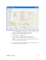
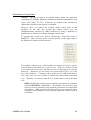
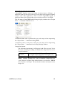
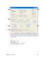
V3.0 TM xHREM (WinHREMTM/MacHREMTM) High Resolution Electron Microscope Simulation Suite User's Guide Contents Getting Started Introduction Before using xHREM™ Installation Installing xHREM™ Installing User Key Driver Installing User Key Let's Start Tutorials Scattering Amplitude Calculation Image Intensity Calculation EM Image Display Diffraction Spot Pattern Display Topics Model Potential and Wave-function Display Diffraction Intensity Quantification Image Intensity Quantification Model 3D display TDS Absorption Data Sharing using CIF File Crystal Setting Selection Static Diffuse Scattering calculation Numerical Data Output using ImageBMP xHREM User’s Guide 2 Application Let's attack your own problem Steps to create a New Data Setting up Preferences Creating Your Template WORKSHEET MultiGUI Reference ImageGUI Reference DFOutGUI Reference ImageBMP Reference SpotBMP Reference Appendix Blank WORKSHEET FAQ (in preparation) About Dynamical Scattering Calculation (MUltiGUI) About Image Calculation (ImageGUI) About Scattering Intensity Output (DFOutGUI) Support/Update Email: [email protected] WEB: www.hremresearch.com xHREM User’s Guide 3 Getting Started In this chapter we explain the concept of xHREM™ and how to install them. Then, you will learn how to use xHREM™ by using the attached examples. Introduction High Resolution Electron Microscopy (HREM) becomes an indispensable tool for understanding material properties or evaluating new materials at the level of atomic resolution. Due to increased demands for research and development of the new materials, an image simulation acquires more importance than ever before. xHREM™ (WinHREM™/MacHREM™) is a suite of the high-resolution electron microscope image simulation programs that will run on Windows or Mac OS. Concept of xHREM™ 1. User Friendly Graphical Interface xHREM™ employs user friendly Data Generation Utilities based on the Graphical User Interface for Windows or Mac OS. xHREM™ is general-purpose software that can be used to simulate all the images expected from any crystal systems, defect structures and interfaces. Although data generation for such general-purpose software normally becomes complex, a novice user can easily generate his/her data by using the graphical Data Generation Utilities with minimum requirements for the special knowledge. 2. Reliable and Efficient Algorithm Since electron microscope images critically depend on an electron-specimen interaction as well as aberrations of image forming lenses, the treatment of scattering based on dynamical theory and the treatment of aberration based on wave-optical theory are mandatory. xHREM™ emerges from the HREM image simulation programs based on FFT multislice technique developed at Arizona State University, USA xHREM User’s Guide 4 (see References). This is one of the most reliable and efficient HREM image simulation programs. 3. High Quality Image Output Numerical data such as projected potential, wave function propagating the specimen, simulated image intensities could printed as high quality gray scale maps (Bitmap) by using Output Graphic Utilities. Numerical value of each pixel of the gray scale can be exported for further analysis with other software. Features of xHREM ™ Efficient algorithm based on Fast Fourier Transform (FFT) Applicable to any crystal systems and symmetries for an arbitrary beam direction Applicable to defects, interfaces and artificial supper-lattices Treatment of partial coherency based on the transmission cross-coefficient Coherent Convergent Beam Electron Diffraction (Option) High resolution STEM image simulation including HAADF-STEM images (Option) Steps for Image Simulation with xHREM™ xHREM™ consists of three graphical user interfaces (GUI) for scattering calculation, image intensity calculation and scattering intensity output. There are also other utilities for half-tone (gray-scale) image outputs. Even a novice user can easily generate input data satisfying the format required by the calculation programs, and then execute calculations. High quality simulated images are easily obtained by using the gray-scale output utilities. Each GUI uses a window, called WORKSHEET, to assist the user to fill out the necessary data. When saving (Save or Save As…) the input data in the WORKSHEET, the GUI converts the WORKSHEET data into the input data required by the calculation program. Actual calculation is easily performed from the menu command (Execute) by using the converted data. To get gray-scale microscope images do the followings: 1. Generate a required data for scattering calculation by using the graphical user interface called MultiGUI, and then perform xHREM User’s Guide 5 calculation from Execute command of the File menu. 2. Generate a required data for image calculation by using the graphical user interface called ImageGUI, and then perform calculation from Execute command of the File menu. 3. Obtain gray-scale images from the calculated images by using the utility called ImageBMP. The output gray-scale images may be arranged into a table layout (Image Tableau) as functions of thickness and defocus. References K. Ishizuka and N. Uyeda: A New Theoretical and Practical Approach to the Multislice Method, Acta Cryst. A33 (1977) 740-749. K. Ishizuka: Contrast Transfer of Crystal Images in TEM, Ultramicroscopy 5 (1980) 55-65 K. Ishizuka: Multislice Formula for Inclined Illumination, Acta Cryst. A38 (1982) 773-779. K. Ishizuka: A practical approach for STEM image simulation based on the FFT multislice method, Ultramicroscopy 90 (2001) 71-83. Before using xHREM™ If you are not familiar with routine operations of Windows/Mac OS such as a clicking, double-clicking or dragging the mouse, a menu selection, a file open/close procedure and so on, please consult the user's manual come with your computer for getting acquainted with Window GUI before using xHREM™. xHREM User’s Guide 6 Installation Installing WinHREM WinHREM™ is distributed in CD-ROM or on-line. The software should be installed into the hard disk by following the standard procedure. Insert the CD-ROM into the CD drive, or unzip a download file. Open the WinHREM 3.0 folder and execute manually by double-clicking the 'Setup.exe' files. It is advised that the WinHREM programs are installed into the directory named 'xHREM' under \Program Files\HREM Research as instructed by the installer. The structure of the 'xHREM' folder on the hard disk will be the one shown below. Sample data will be installed in the 'xHREM Data' folder under your \My Documents directory. The installer will register WinHREM application icons (shortcuts) under 'xHREM' on the Start menu. Installing MacHREM MacHREM™ is distributed in CD-ROM or on-line. The software should be installed into the hard disk by following the standard procedure. Insert the CD or open a disk image file that you have downloaded. Then, simply drag-and-drop the application folder (xHREM(E) (English) or xHREM(J) (Japanese)) onto the 'Applications' icon to copy it into the Applications folder, and drag the data folder (xHREM Data) onto Documents.app icon to copy it into the Documents folder. Also, please copy the 'Quesa.framework' folder into the 'Frameworks folder.' The structure of xHREM program folder Utilities Programs Resources Documents xHREM User’s Guide : GUI, Output Utilities : Programs for numerical calculation : Resources used by Utilities : Manuals 7 (Windows) Installing User Key Driver Installing User Key Driver NOTE: Disconnect the USB key. Launch “HASPUserSetup.exe,” and follow the instructions to install the user key driver. Installing User Key Simply plug your USB key into an USB port. If your user key is not recognized, the software will run as a demonstration version. (Mac OS) Installing User Key Driver Installing User Key Driver NOTE: Disconnect the USB key. Open the disk image file “HDD_Installer_MacOSX.dmg,” and launch “Install HASP USB Driver,” and follow the instructions to install the user key driver. Installing User Key Simply plug your USB key into an USB port. If your user key is not recognized, the software will run as a demonstration version. xHREM User’s Guide 8 Let's Start Tutorials How to use GUI for Data Input By using three graphic user interfaces (GUIs), the required data for numerical calculations are prepared by filling the window called WORKSHEET. Each GUI has File, Edit and Help menus. Please consult the references for the details of each menu. Example Data Two sets of data are provided within the Data folder for exercises. They are a tin oxide (SnO2) and a complex oxide of tungsten and niobium (W8Nb18O89), and their sample name are SnO2 and WNbO, respectively. We use SnO2 here as an example, but the same steps can be applied to WNbO. Please play with WnbO by yourself later. At first we calculate scatting amplitudes, and then calculate image intensities. The gray-scale images or diffraction patterns will be obtained from the image intensities of the scatting amplitudes. Scattering Amplitude calculation At first, let's prepare the data required for the scatting amplitude calculation: 1. Launch MultiGUI. Please consult your computer manual about how to launch an application. 2. Select SnO2.WS1 from the Data folder, when the open dialog appears. Please consult your computer manual about how to select a file. The WORKSHEET for data input will appear. TIPS: The lower part of the WORKSHEET can be accessed by sliding the window or by expanding the display area. xHREM User’s Guide 9 In this WORKSHEET, appropriate data is already filled out. let's create a new data set by changing the Title entry: 3. Input a new title "SnO2 test calculation" in the Title field. 4. Choose "Save As..." from the File menu. 5. Save the new data as "SnO2test" in the save dialog appeared. Here, Please consult your computer manual about how to save your file. TIPS: An extension '.WS1' will be added automatically. Thus, you may not need to specify the extension. Next, we calculate the scattering amplitudes by using the data crested above: 6. Choose 'Execute Multislice' from File menu. xHREM User’s Guide 10 The program (multi.exe) that calculates the scattering amplitudes will be launched, and the progress of calculation will be displayed on a separate window. When an execution terminates normally, you will see the message "Execution completed. Congratulations!" NOTE: The progress window has the fundamental menus such as File and Edit, and you can Save the content of the window from the File menu. TIPS: The program can be terminated even in the middle of calculation by Exit command from the File menu or clicking the close button. The progress window can be closed by Exit command from the File menu or clicking the close. 7. To terminate MultiGUI, select 'Exit(Quit)' from the File menu. xHREM User’s Guide 11 Image Intensity Calculation The process for the image intensity calculation is similar with the scattering amplitude calculation. Before this step, you must prepare the scattering data by using MultiGUI. 1. Launch ImageGUI. 2. Select SnO2.WS2 from the Data folder, when the open dialog appears. Please consult your computer manual about how to select a file. NOTE: There is no WS2 file corresponding to the data name that we have used for the MultiGUI, namely SnO2test.WS2. We will create it from now using an existing data (SnO2.WS2). You may create a WS3 data from a scratch by using Default.WS2. TIPS: The lower part of the WORKSHEET can be accessed by sliding the window or by expanding the display area. In this WORKSHEET, appropriate data is already filled out. let's create a new data set by changing the Title entry: 3. Input a new title "SnO2 test calculation" in the Title field. 4. Choose "Save As..." from the File menu. 5. Save the new data as "SnO2test" in the save dialog appeared. xHREM User’s Guide Here, 12 TIPS An extension '.WS2' will be added automatically. may not need to specify the extension. Thus, you Next, we calculate the image intensities by using the data crested above: 6. Choose 'Execute' from File menu. The program (Image.exe) that calculates the image intensities will be launched, and the progress of calculation will be displayed on a separate window. When an execution terminates normally, you will see the message "Execution completed. Congratulations!" NOTE: The progress window has the fundamental menus such as File and Edit, and you can Save the content of the window from the File menu. TIPS: The program can be terminated even in the middle of calculation by Exit command from the File menu or clicking the close button. The progress window can be closed by Exit command from the File menu or clicking the close. 7. To terminate ImageGUI, select 'Exit(Quit)' from the File menu. xHREM User’s Guide 13 EM Image Display Then, let's display gray-scale (half-tone) images that have been numerically calculated for SnO2 by using ImageGUI. At first, you have to launch a utility and select a numerical image data to be displayed: 1. Launch ImageBMP. 2. A data selection dialog will be opened. Select SnO2test.AUX in the Data folder. (A data file for image display has ".AUX".) The following window will be appeared. Then, let's get some images. 3. Click "Generate" in the right bottom of WORKSHEET. After a few seconds, you may get a gray-scale image shown below. This is an image calculated for the conditions corresponding to a slice and a defocus specified in the WORKSHEET. Specifically, Slice: 10; Defocus: 500 A (under-focus); Display Range: (0<->1) x (0<->1). xHREM User’s Guide 14 Next, draw a wider gray-scale image extended over a few unit cells. 4. Change end-points (left input-boxes) of a and b of "Display Range" to two (2). 5. Click "Generate" as before. You will get a gray-scale image of 2 x 2 unit cells as shown below. 6. You can save each gray-scale image by choosing "Save" or "Save As…" from "File" menu, if you want to. You can choose an image format in the dialog that will appear. If you want to save a quantitative data (binary data) of the displayed image, you can use "Export Data…" command (Please refer to Topics/Numarical Data Output using ImageBMP). You can also print each gray scale image by choosing "Print" from "File" menu. 7. Close each Bitmap window by choosing "Close" from "File" menu. If the gray-scale image has never been saved, a dialog for confirming your action. You can avoid this confirmation dialog, when you close the window while pressing the "Shift" key. TIPS: 8. To terminate ImageBMP, select "Exit (Quit)" from "File" menu. The default file name of an EM image is "Sample name_slice number_defocus.bmp." NOTE: xHREM User’s Guide 15 To obtain an image at other slice and/or defocus, select a slice number and/or defocus value from the "Slice" and "Defocus" pull-down menus. These pull-down menus show all possible selections on your data set. When you choose “Select” from “Slice” or “Defocus” pull-down menu, you will get a following dialog, where you can select the slices or defocuses that you want to display. If you choose "All" or “Select” from "Slice" or “Defocus” pull-down menu, EM images for all, or selected slices or defocus values will be displayed in sequence. TIPS: If you choose "All" or “Select” both from "Slice" and "Defocus” pull-down menus, EM images for combinations of all, or selected slices and defocus values will be displayed in sequence. TIPS: If you click “Image Tableau” check box, the selected images will be displayed in a table layout in terms of Slice numbers and Defocus values. In the example below, all the calculated images were displayed. You can specify the way of layout of slices and defocuses as well as gaps between each image in the dialog that will appear when you click “Options” button (see Application section for more details). TIPS: xHREM User’s Guide 16 If you select “Atom Overlay” check box, a colored circle specific for each element will be drawn at each atom position as shown below. The size of the circle and its color will be modified with a dialog that will appear when you click “Setup" button. TIPS: The gray-scale image can be printed out by using "Print" from "File" menu. The displayable gray levels depend on your printer specifications. NOTE: xHREM User’s Guide 17 Diffraction Spot Pattern Display Here, let's display electron diffraction patterns for SnO2 by using calculated scattering data with MultiGUI. At first, you have to launch a utility and select a scattering data to be displayed: 1. Launch SpotBMP. 2. A data selection dialog will be opened. Select SnO2test.DF in the Data folder. (A data file for image display has ".DF".) A WORKSHEET for setting up display conditions will be appeared. Then, let's get some diffraction patterns. 3. After setting the condition as shown above, click "Generate" in the right bottom of WORKSHEET. After a few seconds, you may get a gray-scale image shown below. xHREM User’s Guide 18 4. Next, uncheck the "Show Index" and select "Peak" from the "Spot Shape," then Click "Generate. " After a few seconds, you may get a gray-scale image shown below. 5. To terminate SpotBMP, select "Exit (Quit)" from "File" menu. xHREM User’s Guide 19 Topics In this section some useful functions as well as advanced topics will be introduced. It is not necessary to read through all the topics at the first time. You may want to study each topic when you need to use it. Display Model Potentials or Wave-functions Model potential distributions or wave-functions within the sample, which were calculated with MultiGUI (multi.exe), will be displayed as gray-level images by using ImageBMP. To display them: 1. Execute a calculation with a check on corresponding “Export Data for Gray Scale Map” in the “Output Control” section of MultiGUI. The display data will be saved in a file with “.AUX” extension. NOTE: The file with the same extension is also used by ImageGUI to save microscope image data. Therefore, if you want to keep the data for later use, you have to change the AUX file name to a unique name keeping the same extension. 2. Launch ImageBMP, and select a corresponding AUX file. The following window, which you have seen for microscope image display, will be open. However, the “Image Selection” section is different from that for the microscope images, since the potential distributions and the wave-functions are saves as complex numbers. xHREM User’s Guide 20 3. Setup display conditions and select what you want to display. Potential: You can specify a slice number (from 0 to 9) to be displayed, when you have divided a unit cell into different slices up to ten (10). Wave Function: Select a thickness (in slice number) to be displayed. Show: Since the potential distributions and the wave-functions are saves as complex numbers, you have to select a quantity to be displayed from the following list: 4. Click “Generate” to create a gray scale image. xHREM User’s Guide 21 Survey Diffraction Intensity You can qualitatively compare dynamical diffraction intensities by looking a gray scale display generated by SpotBMP. When you want to compare the intensity quantitatively, you can use “DFOutGUI.” To survey diffraction intensities (amplitudes), you have to prepare the data as follows: 1. Launch DFOutGUI. 2. Select SnO2.WS3 from the Data folder, when the open dialog appears. NOTE: There is no WS3 file corresponding to the data name that we have used for the MultiGUI, namely SnO2test.WS3. We will create it from now using an existing data. You may create a WS3 data from a scratch by using Default.WS3. The following WORKSHEET will appear. In this WORKSHEET, appropriate data is already filled out. Some reflection indexes are already specified for each page. Here, let's use this data as it is. 3. Choose "Save As..." from the File menu. xHREM User’s Guide 22 4. Save the new data as "SnO2test" in the save dialog appeared. TIPS: An extension '.WS3' will be added automatically. may not need to specify the extension. Thus, you Next, we survey the image intensities by using the data saved above: 5. Choose 'Execute' from File menu. The program (DFOut.exe) that lists/displays the diffraction intensities will be launched, and the numerical lists and graphs for specified reflections will be displayed on a separate window. When an execution terminates normally, you will see the message "Execution completed. Congratulations!" The amplitude is displayed as a normalized value relative to an incident wave (Normalized), or as a scaled value relative to kinematical scattering amplitude (Kinematical scale). xHREM User’s Guide 23 TIPS: The kinematical structure factors (scattering amplitudes) used in potential calculation will be displayed, when you set a starting slice to zero in “Output Range” section. In the graphic chart the magnitude of amplitude is displayed in log scale to display a wide range of data. On the other hand the phase is displayed between [-π, +π]. You may note that this phase is shifted by π/2 to be consistent with the phase of kinematical structure factor. NOTE: The progress window has the fundamental menus such as File and Edit, and you can Save the content of the window from the File menu. TIPS: The program can be terminated even in the middle of calculation by Exit command from the File menu or clicking the close button. The progress window can be closed by Exit command from the File menu or clicking the close. 6. To terminate DFOutGUI, select 'Exit(Quit)' from the File menu. xHREM User’s Guide 24 Survey image Intensity Electron micrograph images or wave-functions displayed by using ImageBMP will be surveyed quantitatively as explained below. Intensity profile along the specified line drawn on the image can be displayed and surveyed quantitatively. Intensity on a gray scale image: When you move the mouse over a gray scale image created by ImageBMP, intensity under a mouse point is displayed at the lower part of window with its coordinates. NOTE: An intensity value will not be displayed for an image created as an “Image Tableau.” Profile image: When you place a mouse on a starting point of a profile, and drag a mouse with SHIFT key down, a red line is drawn on the image. When you stop dragging, intensity under the red line is displayed on a separate window xHREM User’s Guide 25 When you put a mouse on a line of the profile window, intensity and its original image coordinates are displayed below the profile. NOTE: A profile image will not be displayed for an image created as an “Image Tableau.” xHREM User’s Guide 26 3D Display of Atomic Model Using a 3D display you can check your atomic model to be used by MultiGUI. Here, we explain the 3D display by using a sample data of SnO2. To display an atomic model as a 3D image: 1. Launch MultiGUI. 2. A data selection dialog will be opened. Select SnO2.SW1 in the Data folder. The WORKSHEET for SnO2 will be appeared. 3. Click “Model View” in the Option section at the very bottom of the WORKSHEET. TIPS: The lower part of the WORKSHEET can be accessed by sliding the window or by expanding the display area. Then, you will get a 3D display of the Atomic model: xHREM User’s Guide 27 Under the regular setting the model is displayed as a projection along c-axis. The direction of projection is easily changed by selecting “a, b or c” in the tool bar. TIPS: Tools in the tool bar (left to right): Rotation, Back and forth movement, In-plane movement, Projection directions, Perspective control. By adjusting a slider of the “Projection control” the model is displayed in perspective drawing. The following show an example. xHREM User’s Guide 28 Including TDS Absorption You can include absorption of elastically scattered wave due to thermal diffuse scattering (TDS) in your dynamical calculation. In this case, however, thermal displacement parameter (temperature factor; Debye-Waller factor) for each atom in your atomic model is required. When you don’t know a corresponding parameter, an approximate value may be specified. To include TDS absorption in your dynamical calculation: 1. Launch MultiGUI 2. Choose “Preferences” from Edit menu. 3. Select “Weikenmeier-Kohl Scattering Factor” in “Atomic Scattering Factor” section of the Preferences dialog, and check “Include TDS absorption.” 4. Setup other parameters and execute “Multislice.” xHREM User’s Guide 29 Data Sharing using CIF File xHREM ™ can read/write (Import/Export) a data with CIF (Crystallographic Information File) format. Therefore, you can share crystal data (lattice constants, Space group/Symmetry operations, Atomic positions etc.) with other software. NOTE: The CIF data items handled by xHREM™ : Lattice constants, Space group (Symmetry operations), Atom species, Atom coordinates, Thermal factor, Occupancy. xHREM for Windows and Mac OS stores atomic model data such as atomic positions with the same database format. Therefore, the atomic model database can be freely shared between Windows and Mac OS. NOTE: You can also share an atomic model data with other applications by saving them as a text file using “Export” button on the “Edit” window of “Atom Parameters” section of MultiGUI. xHREM User’s Guide 30 Permutation of Crystal Axes xHREM™ can take account of an incident surface effect into dynamical calculation (K. Ishizuka: Multislice Formula for Inclined Illumination: Acta Cryst. A38 (1982) 773-779). Therefore, an incident beam direction of <hk0> that is parallel to the surface is forbidden. However, when you neglect the incident surface effect (most of the programs do not take into account the surface effect), you can straightforwardly calculate for <hk0> incidence by using a capability of permutation of crystal axes without changing a model data. To permute the crystal axes, choose “Preferences” from Edit menu of MultiGUI. Then, you may notice “Crystal Setting” on the upper right of the Preferences window as shown below: For example, in the case of <110> incidence we cannot use I (a.b.c) system, since the index of the third axis (c-axis) is zero. However, indexes of both a-axis and b-axis are not zero, and thus we can use either these axes for the third axis. Therefore, we can choose one system from II, III, V or VI for the <110> incidence. Contrary to this, in the case of <100> both indexes of b- and c-axes are zero, and thus we cannot use both of them as the third axis. Therefore, we can use either II or V system where a-axis is the third axis. NOTE: Neither the crystal axes nor symmetry operations are permuted in the WORKSHEET of MultiGUI. Nevertheless, the selected crystal system is used in calculation, and symmetry operations are transformed accordingly. When you check the list output, you can verify the lattice constants, atom parameters, and symmetry operations actually used in calculation. xHREM User’s Guide 31 Calculation of Static Diffuse Scattering Since xHREM™ can handle up to 100,000 atoms, diffuse scattering due to static disorder of atom positions can be estimated by using an atomic model including static displacements of atom positions. To calculate diffuse scattering due to static disorder: 1. Launch MultiGUI. 2. Input necessary data in the WORKSHEET as usual. Using “Edit” dialog of “Atom Parameters” of MultiGUI, it may be difficult to prepare a large atomic model including static displacements of atom positions. Therefore, it may be convenient to read a text data file of atomic model created separately by using “Import” capability. 3. Click “DIFFUSE” in the Option section at the very bottom of the WORKSHEET. TIPS: The lower part of the WORKSHEET can be accessed by sliding the window or by expanding the display area. The following dialog will appear, where you can specify some output controls specific to DIFFUSE calculation. Change controls as you want, and Click “OK.” 4. Save your data. 5. Choose “Execute DIFFUSE” from File menu. xHREM User’s Guide 32 The program (diffuse.exe) that calculates the diffuse scattering amplitudes will be launched, and the progress of calculation will be displayed on a separate window. When an execution terminates normally, you will see the message “Execution completed. Congratulations!” NOTE: The progress window has the fundamental menus such as File and Edit, and you can Save the content of the window from the File menu. TIPS: The program can be terminated even in the middle of calculation by Exit command from the File menu or clicking the close button. The progress window can be closed by Exit command from the File menu or clicking the close. 6. To terminate ImageBMP, select "Exit (Quit)" from "File" menu. xHREM User’s Guide 33 Display Diffuse Scattering Distribution “ImageBMP” can be used to display diffuse scattering distributions. Diffuse scattering data is saved in a file with “.ED” extension. To display diffuse scattering patterns: 1. Launch ImageBMP. 2. Open a “.ED” file with an appropriate name. 3. Setup display controls. According to “ImageBMP” instructions setup an image display area, the resolution and so on, and select a thickness in slice number to display scattering pattern. Since a scattering data is save as complex numbers, a data type to be displayed will be selected from “Show” list. 4. Click “Generate” to display a gray scale map. xHREM User’s Guide 34 Numerical Data Output Using ImageBMP “ImageBMP” displays a gray scale image of various data as a Bitmap. A numerical value of each pixel of the gray scale map can be output for further analysis with other application, such as Gatan’s DigitalMicrograph. A numerical data used to generate the gray scale map can also so be output. The file menu of ImageBMP and the image display windows have “Export Data…” command as shown below: A numerical data used to generate the gray scale map can be output using the “Export Data…” command of ImageBMP. A numerical value of each pixel of the gray scale map can be output using the “Export Data…” command of each image display window. Output data format: The following data format(s) will appear in the “Save as type” list in the Save As dialog according to whether the output data is real or complex numbers. Real data Complex data Binary output: Portable Floatmap File (pfm) Text output: Comma Separated Values File (csv) Binary output: Portable Complexmap File (pcm) Portable Floatmap File (.pfm) or Portable Complexmap File (.pcm) format is a Binary data format that has a text header. xHREM uses a header of 192 bytes. The text header includes information on an image size. NOTE xHREM User’s Guide 35 Application In this chapter we explain how to create your own data, and the way to customize xHREM™ by using Preferences and Templates. Then, you will see a detailed explanation for each data item of the Graphical User Interfaces. Let's attack a problem in hand Before proceed to this chapter, please get acquaintance with xHREM by going through the examples of the "Getting Started." In this chapter, you will learn how to create a new data for your own problem, and then how to display your results and more… Steps to create a New Data There are two ways to create a new data for your application: Update an existing data Create a data from scratch To create a new data from an existing data, do this: 1. Launch a corresponding graphical user interface (GUI). 2. Select an existing data you want to copy in the file selection dialog. The WORKSHEET will appear with data you select. 3. Save this data with a new name by choosing "Save As…" from File menu. This step is strongly recommended not to lose the existing data by an accidental overwrite. NOTE 4. Then, change data as you want. 5. When finished, save your modified again data by choosing "Save" from File menu. To create a new data from a scratch, do this: 1. Launch a corresponding graphical user interface (GUI). xHREM User’s Guide 36 2. Select "Default" from the file selection dialog. The WORKSHEET named "Untitled" will appear with some default data. 3. Fill out your data in the WORKSHEET. 4. When finished, save your data with a new name by choosing "Save As…" from File menu. Setting up Preferences The calculation programs (Solvers) only accept the data with a definite format and units. However, you may want to use other units in your WORKSHEET. You can choose your preferred units for your input in "Preferences" window. Moreover, the Preferences hold some control data that does not depend on each sample, in order to save your trouble to input these data at each time. To set up the Preferences: 1. Choose "Preferences" from "Edit" menu of MultiGUI or ImageGUI. The following "Preferences" window will open. The first choice of Units or Defocus sign is used in the calculation program. The data specified in other units will be converted by the graphical user interface (GUI). TIPS: 2. Change settings according to your preference. "Apply" will change the WORKSHEET according to the change(s). 3. Click "Close" or “Cancel” to close the Preferences window. When “Close” is clicked, the current settings of the Preferences will be applied on the WORKSHEET. When "Cancel" is clicked, the settings after the last “Apply” will be discarded. (These changes have no influence on the WORKSHEET.) You cannot restore the change(s) already applied to the WORKSHEET by clicking “Cancel.” In order to restore the change(s) on the WORKSHEET, reset the Preferences and press "Apply." NOTE: We recommend you to verify your change(s) on the WORKSHEET by clicking "Apply" before closing the Preferences window by clicking "Close." TIPS: xHREM User’s Guide 37 1 2 3 4 5 6 The first choice of Units or Defocus sign is used in the calculation program. The data specified in other units will be converted by the graphical user interface (GUI). 1. Units Length: Angstrom、nm Fourier space: s、d* Beam convergence angle: Defocus sign (underfocus): xHREM User’s Guide s、d*、mrad plus, minus 38 2. Crystal setting I (a, b, c) c b a Entrance surface II… Axes are permutated as indicated 3. Half-tone output settings Level settings for character-base half-tone output (11 levels) 4. Dynamical calculation Range: Radius of Fourier space to be included in the calculation Slice thickness (cell numbers): to be used for the projection approximation 5. Numerical data output format Field width: Number of characters including Blank lines: number of line feed(s) 6. blank(s) Atomic Scattering Factor When you want to include TDS absorption using Weikenmeier-Kohl scattering factor, you have to specify a thermal factor (Debye-Waller factor) for each atom as an atom parameter. Doyle-Turner scattering factor can be used up to only s=2.0 (d*=4.0) due to its approximation. Creating Your Template WORKSHEET Graphical user interface (GUI) uses a WORKSHEET for data preparation. xHREM is shipped with WORKSHEETs (Default.WS1 etc.), on which some standard values are already specified. We call these WORKSHEETs having standard values as "Default (Template)." When you create a new data, you can save your trouble to input these common data at each time by using the Default WORKSHEET. Moreover, you can prepare the data with less effort by using the WORKSHEET tailored for your experimental conditions. For examples, an acceleration voltage, an output range for dynamical scattering amplitudes etc. for the scattering calculation, or a spherical aberration coefficient, a defocus spread, a bean convergence angle, an aperture radius etc. for the image intensity calculation. You can create a template WORKSHEET with other preferential settings. Creating a template WORKSHEET will follow the same steps as preparing xHREM User’s Guide 39 the new data. However, only default data items are specified instead of filling out all entries. To create a new data from a scratch, do this: 1. Launch a graphical user interface (GUI) for which you want to create a template. 2. Select "Default" from the file selection dialog. 3. Specify default data items. 4. Save your WORKSHEET with a specific name, which reminds you that it is a template data. From next time, you can start with your template saved above and save your trouble by using these predefined data items. xHREM User’s Guide 40 MultiGUI Reference WORKSHEET 1 2 3 4 5 7 6 8 9 10 13 11 14 12 15 1. Title (max. 82 characters) Type a sample name, composition, and experimental conditions etc. as you want. xHREM User’s Guide 41 2. Cell Parameters Specify cell lengths and angles. The cell lengths can be given Angstrom or nm according to your preference. The angles can be given in degree or cosine of the angle. A mixed input of angle in degree or cosine is not allowed. (Input in angle is recommended.) 3. Symmetry Operation You can specify symmetry operations by selection one of the space groups by clicking "Select" or edit them by clicking "Edit." "Select" button: Clicking the "Select" button will open the following window showing all possible space groups. Select one of the space groups corresponding to your specimen. The space group you have selected will appear in the box. You can see symmetry elements in the window (see "Edit" button below) appeared by clicking the "View" button. Please confirm the symmetry elements are correct before proceeding the calculation. "Elements": Number of symmetry elements "Edit" button: Clicking the "Edit" button opens a window where you can specify arbitrary symmetry operations. xHREM User’s Guide 42 4. Symmetry operations should be specified according to the conventions used in International Tables for Crystallography. xyz components of each symmetry operation should be separated by a comma (,) Each symmetry element should be separated by a semicolon (;) Symmetry list should end with a period (.) Atom Parameters Atom parameters will be imported from a data file by choosing "Import" or compiled in the window that will appear by choosing "Edit." "Import" button: Clicking the "Import" button will open the window to select an existing atom parameter file. Data Base: atom xHREM User’s Guide parameters already saved by MultiGUI. 43 atom parameters saved in the text format by using a text editor. Select a data separator and specify the order of data items (Parameter Sequence). If there is no corresponding data item in the file, you may use "None" to skip reading it. Data file will be selected in the dialog that appears by clicking the "Select" button. Text Data: When the atom parameters are imported successfully, these parameters will be displayed in the window (see "Edit" button below). No of Atoms: number of input atoms "Edit" button: Clicking the "Edit" button opens a window where you can compile atom parameters on the spot. No: sequence number added automatically Name: atom name including element name. Ex. Ag, C(1), O-2 x, y, z: atom position in the unit cell defined by a fraction Occupancy: ratio of occurrence of atom (normally, one). This parameter may be omitted. Thermal: isotropic thermal displacement factor. If you input zero (or leave blank), then the Overall Thermal Factor (see the next parameter) will be applied in the calculation. Overall Thermal Factor: Isotropic thermal displacement factor that will applied for each atom in xHREM User’s Guide 44 the crystal. If the thermal displacement factor of each atom is specified as zero or left blank, this thermal displacement will be used for that atom in the calculation. Calculation Control 5. Phase Grating Setup 6. Multislice Calculation On/off phase grating calculation Dividing-a-cell-into box: Select a number of divisions of unit cell (up to ten (10) ) On/off multislice calculation Until box: set the last slice number New & Append buttons: select "New" when you start calculation, or "Append" when you continue calculation by increasing the last slice number. 7. Acc. Voltage 8. Incident Beam Direction Specify an incident beam direction in term of a real lattice coordinates. Ex: [001] incidence. 9. Unitary Test: Test for the sum of scattering intensity Limit: Lower limit of the total intensity. A number close to one imposes a strict condition. Cycle: Frequency for the test in terms of slice number Output Control 10. Dynamical Structure Factor Range: File output range (radius) of scattering amplitudes Cycle: Frequency for the file output in terms of slice number 11. Potential Distribution On/off numerical map output On/off file output for gray scale display 12. Wave Function On/off numerical map output On/off file output for gray scale display Cycle: Frequency for the file output in terms of slice number 13. Numerical Map Vertical and horizontal ranges and steps for numerical map output 14. Half-tine Map Vertical and horizontal ranges and scale for half-tone output xHREM User’s Guide 45 TIPS: The half-tone map will be suppressed by setting the Scale to Zero (0). xHREM User’s Guide 46 ImageGUI Reference WORKSHEET 1 2 3 4 5 8 6 9 7 xHREM User’s Guide 47 1. Title (max. 82 characters) Type a sample name, composition, and experimental conditions etc. as you want. 2. Optical Parameters Spherical aberration coeff. Defocus spread Beam convergence Aperture radius position 3. Simulation Mode Partial coherency will be treated by First order (Envelope) approximation or Second order (TCC) approximation. 4. Slice thicknesses Specimen thickness at which EM images will be calculated will be given in terms of slice number (up to 10 slices). 5. Defocus values Defocus values at which EM images will be calculated will be specified (up to 20 values). Sign and unit of defocus will be changed by Preferences settings. Output Control 6. Microscope Images 7. Structure Factor On/off numerical map output On/off file output for gray scale display On/off half-tine output On/off contrast reversal On/Off normalization If you select this option, structure factors will be listed before image calculations for each lice data. 8. Numerical Map Vertical and horizontal ranges and steps for numerical map output 9. Half-tone Map Vertical and horizontal ranges and scale for half-tone output xHREM User’s Guide 48 DFOutGUI Reference WORKSHEET 1 4 2 3 5 1. Numerical Output If you select this option, amplitudes and phases of specified reflection indexes will be listed at specified thickness (slice). The scale of amplitude will be selected from " Normalized" or "Kinematical scale." 2. Graphical Output If you select this option, amplitudes and phases vs. thickness will be displayed graphically for specified reflection indexes. The amplitude will be displayed in log scale. 3. Export Data for Graphical Application If you select this option, amplitudes and phases data will be output as text files, which can be used by a spreadsheet (graph) application. xHREM User’s Guide 49 4. Output Range Thickness for a list and/or graph output will be specified by its range and step in slice unit. 5. Indices of Reflections Indexes of reflections you want to check will be specified in a column (up to 9 reflections). Reflections in each column will be displayed graphically in the same page (up to 10 pages). Reflection indexes should be specified by a two-dimensional index in a (projected) diffraction pattern. xHREM User’s Guide 50 ImageBMP Reference WORKSHEET For EM Image Intensity Data 1 2 4 3 5 6 7 The title of the data and its projected two-dimensional cells (and the number of sampling points) will be shown at the top part of the window. For Data from Dynamical Scattering Calculation xHREM User’s Guide 51 For EM Image Intensity Data 1. Display Range The range of display will be defined in terms of unit cell. 2. Scale (pixel/Angstrom) The scale will be specified by a number of pixels per Angstrom. Total numbers of pixels (Height and Width) to be displayed will be shown estimated according to the scale. 3. Image Selection Slice The specimen thickness (slice number) for an EM image to be displayed will be selected from the slice list. When you select "All", images for all slices in the list will be generated one by one. When you choose “Select”, a dialog where you can select individual image will appear. Defocus The defocus value for an EM image to be displayed will be selected from the defocus list. When you select "All", images for all defocus values in the list will be generated one by one. When you choose “Select”, a dialog where you can select individual image will appear. In this utility an under-focus value is always positive irrespective of your defocus sign selection in the "Preferences." NOTE: Image Tableau (Table Layout) This will control the way of display of selected images. When checked, the selected images will be displayed in a table layout. Otherwise, each selected images will de displayed separately. When you click “Options” button, a dialog to setup a layout will be opened. xHREM User’s Guide 52 4. Survey Clicking "Survey" will open a small window showing a display range (Maximum and minimum values). You can change the display ranges by setting numbers in the boxes. 5. Reverse Contrast When checked, the image will be displayed with a reversed contrast. 6. Atom Overlay When checked, a colored circle will be drawn on each atom position. The size and color of circle for each element will be changed in the dialog that will appear when you click “Setup” button. 7. Generate Gray scale image will be generated by clicking "Generate." xHREM User’s Guide 53 For Data from Dynamical Scattering Calculation In the selection you can choose either "Potential" of "Wave Function" to be displayed as a gray scale image. Potential The phase grating number (slice number) for which a potential distribution is displayed will be selected from the phase grating list. When you select "All", the potential distributions for all phase gratings in the list will be generated one by one. When you select "Projection", an image obtained by summing the potentials over all slices will be displayed. Wave Function The specimen thickness (slice number) at which a wave function is displayed will be selected from the slice list. When you select "All", images of all wave functions in the list will be generated one by one. Show As the potential and wave-function are saved in complex number, you have to choose a quantity to be displayed as a gray scale image from a following list: ImageBMP Menu xHREM User’s Guide 54 SpotBMP Reference WORKSHEET 1 2 3 5 4 6 The title of the data and its projected two-dimensional cells (and the number of sampling points) will be shown at the top part of the window. 1. Display Range Radius The diffraction area to be displayed will be specified by its radius (in 1/Angstrom) from the center. The displayable area that is outputted by the dynamical calculation program is indicated below the box. Resolution The resolution will be specified by a number of pixels per 1/Angstrom. An image size to be displayed will be shown estimated according to the resolution. xHREM User’s Guide 55 2. Display setup Type Display data type will be selected from the following list: Show Index On/off the reflection index display on the gray scale image Spot shape You can choose a display shape of reflection spots from either "Dusk" or "Peak." Spot radius Size of each diffraction spot in pixels. Background Color "White" background displays an image like a negative, and "Black" background emulates an output on a printing paper. 3. Survey Clicking "Survey" will open a small window showing a display range (Maximum and minimum values). You can change the display ranges by setting numbers in the boxes. 4. Slice The specimen thickness (slice number) at which a diffraction pattern is displayed will be selected from the slice list. When you select "All", images of all diffraction patterns in the list will be generated one by one. 5. Reverse Contrast When checked, the image will be displayed with a reversed contrast. 6. Generate Gray scale image will be generated by clicking "Generate." xHREM User’s Guide 56 SpotBMP Menu xHREM User’s Guide 57 Blank WORKSHEET Appendix MultiGUI xHREM User’s Guide 58 ImageGUI xHREM User’s Guide 59 DFOutGUI xHREM User’s Guide 60