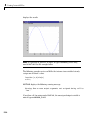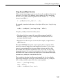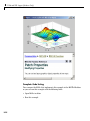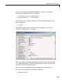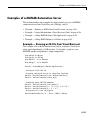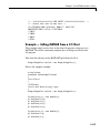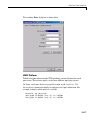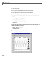
1
MATLAB
®
The Language of Technical Computing
Computation
Visualization
Programming
External Interfaces
Version 7
How to Contact The MathWorks
Web
Newsgroup
www.mathworks.com/contact_TS.html Technical Support
www.mathworks.com
comp.soft-sys.matlab
[email protected]
[email protected]
[email protected]
[email protected]
[email protected]
Product enhancement suggestions
Bug reports
Documentation error reports
Order status, license renewals, passcodes
Sales, pricing, and general information
508-647-7000 (Phone)
508-647-7001 (Fax)
The MathWorks, Inc.
3 Apple Hill Drive
Natick, MA 01760-2098
For contact information about worldwide offices, see the MathWorks Web site.
MATLAB External Interfaces
© COPYRIGHT 1984–2006 by The MathWorks, Inc.
The software described in this document is furnished under a license agreement. The software may be used
or copied only under the terms of the license agreement. No part of this manual may be photocopied or
reproduced in any form without prior written consent from The MathWorks, Inc.
FEDERAL ACQUISITION: This provision applies to all acquisitions of the Program and Documentation
by, for, or through the federal government of the United States. By accepting delivery of the Program or
Documentation, the government hereby agrees that this software or documentation qualifies as commercial
computer software or commercial computer software documentation as such terms are used or defined
in FAR 12.212, DFARS Part 227.72, and DFARS 252.227-7014. Accordingly, the terms and conditions of
this Agreement and only those rights specified in this Agreement, shall pertain to and govern the use,
modification, reproduction, release, performance, display, and disclosure of the Program and Documentation
by the federal government (or other entity acquiring for or through the federal government) and shall
supersede any conflicting contractual terms or conditions. If this License fails to meet the government’s
needs or is inconsistent in any respect with federal procurement law, the government agrees to return the
Program and Documentation, unused, to The MathWorks, Inc.
Trademarks
MATLAB, Simulink, Stateflow, Handle Graphics, Real-Time Workshop, and xPC TargetBox
are registered trademarks, and SimBiology, SimEvents, and SimHydraulics are trademarks of
The MathWorks, Inc.
Other product or brand names are trademarks or registered trademarks of their respective
holders.
Patents
The MathWorks products are protected by one or more U.S. patents. Please see
www.mathworks.com/patents for more information.
Revision History
December 1996
July 1997
January 1998
October 1998
November 2000
June 2001
July 2002
January 2003
June 2004
October 2004
September 2005
March 2006
September 2006
First printing
Online only
Second printing
Third printing
Fourth printing
Online only
Online only
Online only
Online only
Online only
Online only
Online only
Online only
New for MATLAB 5 (release 8)
Revised for MATLAB 5.1 (Release 9)
Revised for MATLAB 5.2 (Release 10)
Revised for MATLAB 5.3 (Release 11)
Revised and renamed for MATLAB 6.0 (Release 12)
Revised for MATLAB 6.1 (Release 12.1)
Revised for MATLAB 6.5 (Release 13)
Revised for MATLAB 6.5.1 (Release 13SP1)
Revised for MATLAB 7.0 (Release 14)
Revised for MATLAB 7.0.1 (Release 14SP1)
Revised for MATLAB 7.1 (Release 14SP3)
Revised for MATLAB 7.2 (Release 2006a)
Revised for MATLAB 7.3 (Release 2006b)
Contents
Importing and Exporting Data
1
Using MAT-Files . . . . . . . . . . . . . . . . . . . . . . . . . . . . . . . . . . .
Importing Data to MATLAB . . . . . . . . . . . . . . . . . . . . . . . . .
Exporting Data from MATLAB . . . . . . . . . . . . . . . . . . . . . .
Exchanging Data Files Between Platforms . . . . . . . . . . . . .
Reading and Writing MAT-Files . . . . . . . . . . . . . . . . . . . . . .
Writing Character Data . . . . . . . . . . . . . . . . . . . . . . . . . . . .
Finding Associated Files . . . . . . . . . . . . . . . . . . . . . . . . . . . .
1-2
1-2
1-3
1-5
1-5
1-7
1-9
Examples of MAT-Files . . . . . . . . . . . . . . . . . . . . . . . . . . . . .
Creating a MAT-File in C . . . . . . . . . . . . . . . . . . . . . . . . . . .
Reading a MAT-File in C . . . . . . . . . . . . . . . . . . . . . . . . . . .
Creating a MAT-File in Fortran . . . . . . . . . . . . . . . . . . . . . .
Reading a MAT-File in Fortran . . . . . . . . . . . . . . . . . . . . . .
1-12
1-12
1-17
1-21
1-25
Compiling and Linking MAT-File Programs . . . . . . . . . .
Masking Floating Point Exceptions . . . . . . . . . . . . . . . . . . .
Compiling and Linking on UNIX . . . . . . . . . . . . . . . . . . . . .
Compiling and Linking on Windows . . . . . . . . . . . . . . . . . .
Required Files from Third-Party Sources . . . . . . . . . . . . . .
Working Directly with Unicode . . . . . . . . . . . . . . . . . . . . . .
1-29
1-29
1-30
1-32
1-32
1-34
MATLAB Interface to Generic DLLs
2
Overview . . . . . . . . . . . . . . . . . . . . . . . . . . . . . . . . . . . . . . . . .
2-3
Loading and Unloading the Library . . . . . . . . . . . . . . . . .
Loading the Library . . . . . . . . . . . . . . . . . . . . . . . . . . . . . . .
Unloading the Library . . . . . . . . . . . . . . . . . . . . . . . . . . . . .
2-4
2-4
2-5
Getting Information About the Library . . . . . . . . . . . . . .
2-6
v
Viewing Functions in a GUI Interface . . . . . . . . . . . . . . . . .
2-7
Invoking Library Functions . . . . . . . . . . . . . . . . . . . . . . . .
2-9
Passing Arguments . . . . . . . . . . . . . . . . . . . . . . . . . . . . . . . .
Displaying MATLAB Syntax for Library Functions . . . . . .
General Rules for Passing Arguments . . . . . . . . . . . . . . . . .
Passing References . . . . . . . . . . . . . . . . . . . . . . . . . . . . . . . .
Passing a NULL Pointer . . . . . . . . . . . . . . . . . . . . . . . . . . . .
Using C++ Libraries . . . . . . . . . . . . . . . . . . . . . . . . . . . . . . .
2-10
2-10
2-11
2-12
2-13
2-13
Data Conversion . . . . . . . . . . . . . . . . . . . . . . . . . . . . . . . . . . .
When to Convert Manually . . . . . . . . . . . . . . . . . . . . . . . . .
Primitive Types . . . . . . . . . . . . . . . . . . . . . . . . . . . . . . . . . . .
Enumerated Types . . . . . . . . . . . . . . . . . . . . . . . . . . . . . . . .
Structures . . . . . . . . . . . . . . . . . . . . . . . . . . . . . . . . . . . . . . .
Creating References . . . . . . . . . . . . . . . . . . . . . . . . . . . . . . .
Reference Pointers . . . . . . . . . . . . . . . . . . . . . . . . . . . . . . . .
2-15
2-15
2-16
2-19
2-20
2-26
2-34
Calling C and Fortran Programs from MATLAB
3
vi
Contents
Introducing MEX-Files . . . . . . . . . . . . . . . . . . . . . . . . . . . . .
Using MEX-Files . . . . . . . . . . . . . . . . . . . . . . . . . . . . . . . . . .
MEX-File Placement . . . . . . . . . . . . . . . . . . . . . . . . . . . . . . .
The Distinction Between mx and mex Prefixes . . . . . . . . . .
3-2
3-2
3-3
3-4
MATLAB Data . . . . . . . . . . . . . . . . . . . . . . . . . . . . . . . . . . . . .
The MATLAB Array . . . . . . . . . . . . . . . . . . . . . . . . . . . . . . .
Data Storage . . . . . . . . . . . . . . . . . . . . . . . . . . . . . . . . . . . . .
Data Types in MATLAB . . . . . . . . . . . . . . . . . . . . . . . . . . . .
Sparse Matrices . . . . . . . . . . . . . . . . . . . . . . . . . . . . . . . . . . .
Using Data Types . . . . . . . . . . . . . . . . . . . . . . . . . . . . . . . . .
3-5
3-5
3-5
3-6
3-8
3-8
Building MEX-Files . . . . . . . . . . . . . . . . . . . . . . . . . . . . . . . .
Compiler Requirements . . . . . . . . . . . . . . . . . . . . . . . . . . . .
Testing Your Configuration on UNIX . . . . . . . . . . . . . . . . . .
Testing Your Configuration on Windows . . . . . . . . . . . . . . .
3-10
3-10
3-11
3-13
Specifying an Options File . . . . . . . . . . . . . . . . . . . . . . . . . .
3-16
Custom Building MEX-Files . . . . . . . . . . . . . . . . . . . . . . . .
Who Should Read this Chapter . . . . . . . . . . . . . . . . . . . . . .
MEX Script Switches . . . . . . . . . . . . . . . . . . . . . . . . . . . . . .
Default Options File on UNIX . . . . . . . . . . . . . . . . . . . . . . .
Default Options File on Windows . . . . . . . . . . . . . . . . . . . . .
Custom Building on UNIX . . . . . . . . . . . . . . . . . . . . . . . . . .
Custom Building on Windows . . . . . . . . . . . . . . . . . . . . . . .
3-18
3-18
3-18
3-22
3-23
3-24
3-26
Troubleshooting . . . . . . . . . . . . . . . . . . . . . . . . . . . . . . . . . . .
Configuration Issues . . . . . . . . . . . . . . . . . . . . . . . . . . . . . . .
Understanding MEX-File Problems . . . . . . . . . . . . . . . . . . .
Compiler and Platform-Specific Issues . . . . . . . . . . . . . . . .
Memory Management Compatibility Issues . . . . . . . . . . . .
3-31
3-31
3-33
3-36
3-37
Additional Information . . . . . . . . . . . . . . . . . . . . . . . . . . . .
Files and Directories - UNIX Systems . . . . . . . . . . . . . . . . .
Files and Directories — Windows Systems . . . . . . . . . . . . .
Examples . . . . . . . . . . . . . . . . . . . . . . . . . . . . . . . . . . . . . . . .
Technical Support . . . . . . . . . . . . . . . . . . . . . . . . . . . . . . . . .
3-41
3-41
3-43
3-46
3-46
Creating C Language MEX-Files
4
C MEX-Files . . . . . . . . . . . . . . . . . . . . . . . . . . . . . . . . . . . . . . .
The Components of a C MEX-File . . . . . . . . . . . . . . . . . . . .
Required Arguments to a MEX-File . . . . . . . . . . . . . . . . . . .
4-2
4-2
4-3
Examples of C MEX-Files . . . . . . . . . . . . . . . . . . . . . . . . . . .
A First Example — Passing a Scalar . . . . . . . . . . . . . . . . . .
Passing Strings . . . . . . . . . . . . . . . . . . . . . . . . . . . . . . . . . . .
Passing Two or More Inputs or Outputs . . . . . . . . . . . . . . .
Passing Structures and Cell Arrays . . . . . . . . . . . . . . . . . . .
Handling Complex Data . . . . . . . . . . . . . . . . . . . . . . . . . . . .
Handling 8-,16-, and 32-Bit Data . . . . . . . . . . . . . . . . . . . . .
Manipulating Multidimensional Numerical Arrays . . . . . .
Handling Sparse Arrays . . . . . . . . . . . . . . . . . . . . . . . . . . . .
Calling Functions from C MEX-Files . . . . . . . . . . . . . . . . . .
4-6
4-6
4-10
4-13
4-16
4-20
4-23
4-25
4-28
4-32
vii
Advanced Topics . . . . . . . . . . . . . . . . . . . . . . . . . . . . . . . . . . .
Help Files . . . . . . . . . . . . . . . . . . . . . . . . . . . . . . . . . . . . . . . .
Linking Multiple Files . . . . . . . . . . . . . . . . . . . . . . . . . . . . .
Workspace for MEX-File Functions . . . . . . . . . . . . . . . . . . .
Memory Management . . . . . . . . . . . . . . . . . . . . . . . . . . . . . .
Large File I/O . . . . . . . . . . . . . . . . . . . . . . . . . . . . . . . . . . . .
Using LAPACK and BLAS Functions . . . . . . . . . . . . . . . . .
4-36
4-36
4-36
4-37
4-37
4-40
4-46
Debugging C Language MEX-Files . . . . . . . . . . . . . . . . . .
Debugging on UNIX . . . . . . . . . . . . . . . . . . . . . . . . . . . . . . .
Debugging on Windows . . . . . . . . . . . . . . . . . . . . . . . . . . . . .
4-55
4-55
4-56
Creating Fortran MEX-Files
5
viii
Contents
Fortran MEX-Files . . . . . . . . . . . . . . . . . . . . . . . . . . . . . . . . .
The Components of a Fortran MEX-File . . . . . . . . . . . . . . .
The %val Construct . . . . . . . . . . . . . . . . . . . . . . . . . . . . . . . .
5-2
5-2
5-7
Examples of Fortran MEX-Files . . . . . . . . . . . . . . . . . . . . .
A First Example — Passing a Scalar . . . . . . . . . . . . . . . . . .
Passing Strings . . . . . . . . . . . . . . . . . . . . . . . . . . . . . . . . . . .
Passing Arrays of Strings . . . . . . . . . . . . . . . . . . . . . . . . . . .
Passing Matrices . . . . . . . . . . . . . . . . . . . . . . . . . . . . . . . . . .
Passing Two or More Inputs or Outputs . . . . . . . . . . . . . . .
Handling Complex Data . . . . . . . . . . . . . . . . . . . . . . . . . . . .
Dynamically Allocating Memory . . . . . . . . . . . . . . . . . . . . .
Handling Sparse Matrices . . . . . . . . . . . . . . . . . . . . . . . . . .
Calling Functions from Fortran MEX-Files . . . . . . . . . . . . .
5-9
5-9
5-11
5-14
5-16
5-19
5-21
5-25
5-27
5-31
Advanced Topics . . . . . . . . . . . . . . . . . . . . . . . . . . . . . . . . . . .
Help Files . . . . . . . . . . . . . . . . . . . . . . . . . . . . . . . . . . . . . . . .
Linking Multiple Files . . . . . . . . . . . . . . . . . . . . . . . . . . . . .
Workspace for MEX-File Functions . . . . . . . . . . . . . . . . . . .
Memory Management . . . . . . . . . . . . . . . . . . . . . . . . . . . . . .
5-35
5-35
5-35
5-36
5-36
Debugging Fortran Language MEX-Files . . . . . . . . . . . . .
Debugging on UNIX . . . . . . . . . . . . . . . . . . . . . . . . . . . . . . .
Debugging on Windows . . . . . . . . . . . . . . . . . . . . . . . . . . . . .
5-37
5-37
5-38
Calling MATLAB from C and Fortran Programs
6
Using the MATLAB Engine . . . . . . . . . . . . . . . . . . . . . . . . .
The Engine Library . . . . . . . . . . . . . . . . . . . . . . . . . . . . . . . .
GUI-Intensive Applications . . . . . . . . . . . . . . . . . . . . . . . . .
6-2
6-2
6-4
Examples of Calling Engine Functions . . . . . . . . . . . . . . .
Calling MATLAB from a C Application . . . . . . . . . . . . . . . .
Calling MATLAB from a Fortran Application . . . . . . . . . . .
Attaching to an Existing MATLAB Session . . . . . . . . . . . .
6-5
6-5
6-10
6-14
Compiling and Linking Engine Programs . . . . . . . . . . . .
Step 1 — Write Your Application . . . . . . . . . . . . . . . . . . . . .
Step 2 — Check Required Libraries and Files . . . . . . . . . .
Step 3 — Build the Application . . . . . . . . . . . . . . . . . . . . . .
Step 4 — Set Run-time Library Path . . . . . . . . . . . . . . . . . .
Step 5 — (Windows Only) Register MATLAB as a COM
Server . . . . . . . . . . . . . . . . . . . . . . . . . . . . . . . . . . . . . . . .
Step 6 — Test Out the Program . . . . . . . . . . . . . . . . . . . . . .
Example — Building an Engine Application on UNIX . . . .
Example — Building an Engine Application on Windows . .
Masking Floating-Point Exceptions . . . . . . . . . . . . . . . . . .
6-16
6-16
6-16
6-19
6-20
6-22
6-22
6-23
6-23
6-24
Calling Java from MATLAB
7
Using Java from MATLAB: An Overview . . . . . . . . . . . . .
Java Interface Is Integral to MATLAB . . . . . . . . . . . . . . . .
Benefits of the MATLAB Java Interface . . . . . . . . . . . . . . .
Who Should Use the MATLAB Java Interface . . . . . . . . . .
To Learn More About Java Programming . . . . . . . . . . . . . .
Platform Support for the Java Virtual Machine . . . . . . . . .
Using a Different Version of the Java JVM . . . . . . . . . . . . .
7-3
7-3
7-3
7-3
7-4
7-4
7-4
Bringing Java Classes and Methods into MATLAB . . . .
Sources of Java Classes . . . . . . . . . . . . . . . . . . . . . . . . . . . .
Defining New Java Classes . . . . . . . . . . . . . . . . . . . . . . . . .
7-7
7-7
7-8
ix
x
Contents
The Java Class Path . . . . . . . . . . . . . . . . . . . . . . . . . . . . . . .
Making Java Classes Available to MATLAB . . . . . . . . . . . .
Loading Java Class Definitions . . . . . . . . . . . . . . . . . . . . . .
Simplifying Java Class Names . . . . . . . . . . . . . . . . . . . . . . .
Locating Native Method Libraries . . . . . . . . . . . . . . . . . . . .
Java Classes Contained in a JAR File . . . . . . . . . . . . . . . . .
7-8
7-11
7-13
7-13
7-14
7-15
Creating and Using Java Objects . . . . . . . . . . . . . . . . . . . .
Constructing Java Objects . . . . . . . . . . . . . . . . . . . . . . . . . .
Concatenating Java Objects . . . . . . . . . . . . . . . . . . . . . . . . .
Saving and Loading Java Objects to MAT-Files . . . . . . . . .
Finding the Public Data Fields of an Object . . . . . . . . . . . .
Accessing Private and Public Data . . . . . . . . . . . . . . . . . . .
Determining the Class of an Object . . . . . . . . . . . . . . . . . . .
7-16
7-16
7-19
7-20
7-21
7-22
7-23
Invoking Methods on Java Objects . . . . . . . . . . . . . . . . . .
Using Java and MATLAB Calling Syntax . . . . . . . . . . . . . .
Invoking Static Methods on Java Classes . . . . . . . . . . . . . .
Obtaining Information About Methods . . . . . . . . . . . . . . . .
Java Methods That Affect MATLAB Commands . . . . . . . .
How MATLAB Handles Undefined Methods . . . . . . . . . . . .
How MATLAB Handles Java Exceptions . . . . . . . . . . . . . .
Method Execution in MATLAB . . . . . . . . . . . . . . . . . . . . . .
7-25
7-25
7-27
7-28
7-32
7-33
7-34
7-34
Working with Java Arrays . . . . . . . . . . . . . . . . . . . . . . . . . .
How MATLAB Represents the Java Array . . . . . . . . . . . . .
Creating an Array of Objects Within MATLAB . . . . . . . . .
Accessing Elements of a Java Array . . . . . . . . . . . . . . . . . .
Assigning to a Java Array . . . . . . . . . . . . . . . . . . . . . . . . . . .
Concatenating Java Arrays . . . . . . . . . . . . . . . . . . . . . . . . .
Creating a New Array Reference . . . . . . . . . . . . . . . . . . . . .
Creating a Copy of a Java Array . . . . . . . . . . . . . . . . . . . . .
7-35
7-35
7-40
7-42
7-46
7-49
7-50
7-51
Passing Data to a Java Method . . . . . . . . . . . . . . . . . . . . . .
Conversion of MATLAB Argument Data . . . . . . . . . . . . . . .
Passing Built-In Data Types . . . . . . . . . . . . . . . . . . . . . . . .
Passing String Arguments . . . . . . . . . . . . . . . . . . . . . . . . . .
Passing Java Objects . . . . . . . . . . . . . . . . . . . . . . . . . . . . . . .
Other Data Conversion Topics . . . . . . . . . . . . . . . . . . . . . . .
Passing Data to Overloaded Methods . . . . . . . . . . . . . . . . .
7-53
7-53
7-55
7-56
7-57
7-60
7-61
Handling Data Returned from a Java Method . . . . . . . .
7-64
Conversion of Java Return Data . . . . . . . . . . . . . . . . . . . . .
Built-In Data Types . . . . . . . . . . . . . . . . . . . . . . . . . . . . . . .
Java Objects . . . . . . . . . . . . . . . . . . . . . . . . . . . . . . . . . . . . . .
Converting Objects to MATLAB Data Types . . . . . . . . . . . .
7-64
7-65
7-65
7-66
Introduction to Programming Examples . . . . . . . . . . . . .
7-71
Example — Reading a URL . . . . . . . . . . . . . . . . . . . . . . . . .
Description of URLdemo . . . . . . . . . . . . . . . . . . . . . . . . . . . .
Running the Example . . . . . . . . . . . . . . . . . . . . . . . . . . . . . .
7-72
7-72
7-73
Example — Finding an Internet Protocol Address . . . .
Description of resolveip . . . . . . . . . . . . . . . . . . . . . . . . . . . . .
Running the Example . . . . . . . . . . . . . . . . . . . . . . . . . . . . . .
7-74
7-74
7-75
Example — Communicating Through a Serial Port . . .
Setting Up the Java Environment . . . . . . . . . . . . . . . . . . . .
Description of Serial Example . . . . . . . . . . . . . . . . . . . . . . .
Running the serialexample Program . . . . . . . . . . . . . . . . . .
7-76
7-76
7-77
7-80
Example — Creating and Using a Phone Book . . . . . . . .
Description of Function phonebook . . . . . . . . . . . . . . . . . . .
Description of Function pb_lookup . . . . . . . . . . . . . . . . . . . .
Description of Function pb_add . . . . . . . . . . . . . . . . . . . . . .
Description of Function pb_remove . . . . . . . . . . . . . . . . . . .
Description of Function pb_change . . . . . . . . . . . . . . . . . . .
Description of Function pb_listall . . . . . . . . . . . . . . . . . . . .
Description of Function pb_display . . . . . . . . . . . . . . . . . . .
Description of Function pb_keyfilter . . . . . . . . . . . . . . . . . .
Running the phonebook Program . . . . . . . . . . . . . . . . . . . . .
7-81
7-82
7-86
7-86
7-88
7-88
7-90
7-90
7-91
7-91
COM and DDE Support (Windows Only)
8
Introducing MATLAB COM Integration . . . . . . . . . . . . . .
Concepts and Terminology . . . . . . . . . . . . . . . . . . . . . . . . . .
Supported Client/Server Configurations . . . . . . . . . . . . . . .
Registering Controls and Servers . . . . . . . . . . . . . . . . . . . .
8-3
8-3
8-6
8-10
xi
Using MATLAB as an ActiveX Client . . . . . . . . . . . . . . . . .
ActiveX Functionality . . . . . . . . . . . . . . . . . . . . . . . . . . . . . .
Overview of MATLAB ActiveX Client Examples . . . . . . . .
Example — Using Internet Explorer in a MATLAB
Figure . . . . . . . . . . . . . . . . . . . . . . . . . . . . . . . . . . . . . . . .
Example — Grid ActiveX Control in a Figure . . . . . . . . . . .
Example — Reading Data from Excel . . . . . . . . . . . . . . . . .
8-12
8-12
8-14
MATLAB COM Client Support . . . . . . . . . . . . . . . . . . . . . .
Creating the Server Process — An Overview . . . . . . . . . . .
Creating an ActiveX Control . . . . . . . . . . . . . . . . . . . . . . . .
Deploying ActiveX Controls Requiring Run-Time
Licenses . . . . . . . . . . . . . . . . . . . . . . . . . . . . . . . . . . . . . . .
Instantiating a DLL Component . . . . . . . . . . . . . . . . . . . . .
Instantiating an EXE Component . . . . . . . . . . . . . . . . . . . .
Getting Interfaces to the Object . . . . . . . . . . . . . . . . . . . . . .
Invoking Commands on a COM Object . . . . . . . . . . . . . . . .
Identifying Objects and Interfaces . . . . . . . . . . . . . . . . . . . .
Invoking Methods . . . . . . . . . . . . . . . . . . . . . . . . . . . . . . . . .
Object Properties . . . . . . . . . . . . . . . . . . . . . . . . . . . . . . . . . .
Control and Server Events . . . . . . . . . . . . . . . . . . . . . . . . . .
Writing Event Handlers . . . . . . . . . . . . . . . . . . . . . . . . . . . .
Saving Your Work . . . . . . . . . . . . . . . . . . . . . . . . . . . . . . . . .
Releasing COM Interfaces and Objects . . . . . . . . . . . . . . . .
Identifying Objects . . . . . . . . . . . . . . . . . . . . . . . . . . . . . . . .
Examples of MATLAB as an Automation Client . . . . . . . . .
8-36
8-36
8-38
8-15
8-20
8-27
8-45
8-46
8-47
8-48
8-50
8-55
8-56
8-63
8-74
8-84
8-89
8-90
8-91
8-92
Additional COM Client Information . . . . . . . . . . . . . . . . . 8-97
Using COM Collections . . . . . . . . . . . . . . . . . . . . . . . . . . . . . 8-97
Converting Data . . . . . . . . . . . . . . . . . . . . . . . . . . . . . . . . . . 8-97
Using MATLAB as a DCOM Client . . . . . . . . . . . . . . . . . . . 8-100
MATLAB COM Support Limitations . . . . . . . . . . . . . . . . . . 8-101
MATLAB Automation Server Support . . . . . . . . . . . . . . .
Creating the Automation Server . . . . . . . . . . . . . . . . . . . . .
Connecting to an Existing Server . . . . . . . . . . . . . . . . . . . . .
Automation Server Functions . . . . . . . . . . . . . . . . . . . . . . .
MATLAB Automation Properties . . . . . . . . . . . . . . . . . . . . .
8-102
8-102
8-104
8-105
8-110
Examples of a MATLAB Automation Server . . . . . . . . . . 8-111
Example — Running an M-File from Visual Basic.net . . . . 8-111
xii
Contents
Example — Viewing Methods from a Visual Basic.net
Client . . . . . . . . . . . . . . . . . . . . . . . . . . . . . . . . . . . . . . . . . 8-112
Example — Calling MATLAB from a Web Application . . . 8-112
Example — Calling MATLAB from a C# Client . . . . . . . . . 8-115
Additional Automation Server Information . . . . . . . . . .
Creating the Server Manually . . . . . . . . . . . . . . . . . . . . . . .
Specifying a Shared or Dedicated Server . . . . . . . . . . . . . . .
Using MATLAB as a DCOM Server . . . . . . . . . . . . . . . . . . .
8-117
8-117
8-117
8-118
Dynamic Data Exchange (DDE) . . . . . . . . . . . . . . . . . . . . .
DDE Concepts and Terminology . . . . . . . . . . . . . . . . . . . . .
Accessing MATLAB as a Server . . . . . . . . . . . . . . . . . . . . . .
The DDE Name Hierarchy . . . . . . . . . . . . . . . . . . . . . . . . . .
Example — Using Visual Basic and the MATLAB DDE
Server . . . . . . . . . . . . . . . . . . . . . . . . . . . . . . . . . . . . . . . .
Using MATLAB as a Client . . . . . . . . . . . . . . . . . . . . . . . . .
Example — Importing Data From an Excel Application . .
DDE Advisory Links . . . . . . . . . . . . . . . . . . . . . . . . . . . . . . .
8-119
8-119
8-121
8-122
8-126
8-127
8-129
8-130
Web Services in MATLAB
9
What Are Web Services in MATLAB? . . . . . . . . . . . . . . . . .
Understanding Data Type Conversions . . . . . . . . . . . . . . . .
Finding More Information About Web Services . . . . . . . . .
9-2
9-5
9-5
Using Web Services in MATLAB . . . . . . . . . . . . . . . . . . . . .
9-7
Building MATLAB Applications with Web Services . . .
Understanding Web Service Limitations . . . . . . . . . . . . . . .
Programming with Web Services . . . . . . . . . . . . . . . . . . . . .
Simple M-File Example . . . . . . . . . . . . . . . . . . . . . . . . . . . .
9-10
9-10
9-10
9-11
xiii
Serial Port I/O
10
Introduction . . . . . . . . . . . . . . . . . . . . . . . . . . . . . . . . . . . . . .
What Is the MATLAB Serial Port Interface? . . . . . . . . . . . .
Supported Serial Port Interface Standards . . . . . . . . . . . . .
Supported Platforms . . . . . . . . . . . . . . . . . . . . . . . . . . . . . . .
Using the Examples with Your Device . . . . . . . . . . . . . . . . .
10-3
10-3
10-3
10-4
10-4
Overview of the Serial Port . . . . . . . . . . . . . . . . . . . . . . . . . 10-5
What Is Serial Communication? . . . . . . . . . . . . . . . . . . . . . . 10-5
The Serial Port Interface Standard . . . . . . . . . . . . . . . . . . . 10-5
Connecting Two Devices with a Serial Cable . . . . . . . . . . . 10-6
Serial Port Signals and Pin Assignments . . . . . . . . . . . . . . 10-7
Serial Data Format . . . . . . . . . . . . . . . . . . . . . . . . . . . . . . . . 10-11
Finding Serial Port Information for Your Platform . . . . . . . 10-16
Selected Bibliography . . . . . . . . . . . . . . . . . . . . . . . . . . . . . . 10-18
Getting Started with Serial I/O . . . . . . . . . . . . . . . . . . . . . .
Example: Getting Started . . . . . . . . . . . . . . . . . . . . . . . . . .
The Serial Port Session . . . . . . . . . . . . . . . . . . . . . . . . . . . . .
Configuring and Returning Properties . . . . . . . . . . . . . . . .
10-19
10-19
10-20
10-21
Creating a Serial Port Object . . . . . . . . . . . . . . . . . . . . . . .
Configuring Properties During Object Creation . . . . . . . . .
The Serial Port Object Display . . . . . . . . . . . . . . . . . . . . . . .
Creating an Array of Serial Port Objects . . . . . . . . . . . . . . .
10-26
10-27
10-27
10-28
Connecting to the Device . . . . . . . . . . . . . . . . . . . . . . . . . . . 10-30
Configuring Communication Settings . . . . . . . . . . . . . . . 10-31
Writing and Reading Data . . . . . . . . . . . . . . . . . . . . . . . . . .
Example — Introduction to Writing and Reading Data . . .
Controlling Access to the MATLAB Command Line . . . . . .
Writing Data . . . . . . . . . . . . . . . . . . . . . . . . . . . . . . . . . . . . .
Reading Data . . . . . . . . . . . . . . . . . . . . . . . . . . . . . . . . . . . . .
Example — Writing and Reading Text Data . . . . . . . . . . . .
Example — Parsing Input Data Using strread . . . . . . . . . .
Example — Reading Binary Data . . . . . . . . . . . . . . . . . . . .
xiv
Contents
10-32
10-32
10-32
10-34
10-39
10-45
10-47
10-48
Events and Callbacks . . . . . . . . . . . . . . . . . . . . . . . . . . . . . .
Example — Introduction to Events and Callbacks . . . . . . .
Event Types and Callback Properties . . . . . . . . . . . . . . . . .
Storing Event Information . . . . . . . . . . . . . . . . . . . . . . . . . .
Creating and Executing Callback Functions . . . . . . . . . . . .
Enabling Callback Functions After They Error . . . . . . . . .
Example — Using Events and Callbacks . . . . . . . . . . . . . .
10-51
10-51
10-52
10-54
10-56
10-57
10-58
Using Control Pins . . . . . . . . . . . . . . . . . . . . . . . . . . . . . . . . . 10-60
Signaling the Presence of Connected Devices . . . . . . . . . . . 10-60
Controlling the Flow of Data: Handshaking . . . . . . . . . . . . 10-63
Debugging: Recording Information to Disk . . . . . . . . . .
Example: Introduction to Recording Information . . . . . . . .
Creating Multiple Record Files . . . . . . . . . . . . . . . . . . . . . .
Specifying a Filename . . . . . . . . . . . . . . . . . . . . . . . . . . . . . .
The Record File Format . . . . . . . . . . . . . . . . . . . . . . . . . . . .
Example: Recording Information to Disk . . . . . . . . . . . . . .
10-66
10-66
10-67
10-67
10-68
10-69
Saving and Loading . . . . . . . . . . . . . . . . . . . . . . . . . . . . . . . . 10-72
Using Serial Port Objects on Different Platforms . . . . . . . . 10-72
Disconnecting and Cleaning Up . . . . . . . . . . . . . . . . . . . . . 10-73
Disconnecting a Serial Port Object . . . . . . . . . . . . . . . . . . . . 10-73
Cleaning Up the MATLAB Environment . . . . . . . . . . . . . . 10-73
Property Reference . . . . . . . . . . . . . . . . . . . . . . . . . . . . . . . . 10-75
The Property Reference Page Format . . . . . . . . . . . . . . . . . 10-75
Serial Port Object Properties . . . . . . . . . . . . . . . . . . . . . . . . 10-76
Properties — Alphabetical List
. . . . . . . . . . . . . . . . . . . . . 10-79
Examples
A
Importing and Exporting Data . . . . . . . . . . . . . . . . . . . . . .
A-2
xv
MATLAB Interface to Generic DLLs . . . . . . . . . . . . . . . . .
A-2
Calling C and Fortran Programs from MATLAB . . . . . .
A-2
....................
A-2
Creating Fortran MEX-Files . . . . . . . . . . . . . . . . . . . . . . . .
A-3
Calling MATLAB from C and Fortran Programs . . . . . .
A-3
Calling Java from MATLAB . . . . . . . . . . . . . . . . . . . . . . . . .
A-4
COM and DDE Support . . . . . . . . . . . . . . . . . . . . . . . . . . . . .
A-4
Serial Port I/O . . . . . . . . . . . . . . . . . . . . . . . . . . . . . . . . . . . . .
A-5
Creating C Language MEX-Files
Index
xvi
Contents
1
Importing and Exporting
Data
Using MAT-Files (p. 1-2)
Methods of importing and exporting
MATLAB® data, and MAT-file
routines that enable you to do this
Examples of MAT-Files (p. 1-12)
Programs to create and read a
MAT-file in C and Fortran
Compiling and Linking MAT-File
Programs (p. 1-29)
Compiling and linking on Windows
and UNIX
1
Importing and Exporting Data
Using MAT-Files
This section describes the various techniques for importing data to and
exporting data from the MATLAB environment. The main topics that are
discussed are:
• “Importing Data to MATLAB” on page 1-2
• “Exporting Data from MATLAB” on page 1-3
• “Exchanging Data Files Between Platforms” on page 1-5
• “Reading and Writing MAT-Files” on page 1-5
• “Writing Character Data” on page 1-7
• “Finding Associated Files” on page 1-9
The most important approach to importing and exporting data involves the
use of MAT-files, the data file format that MATLAB uses for saving data
to your disk. MAT-files provide a convenient mechanism for moving your
MATLAB data between different platforms and for importing and exporting
your data to other stand-alone MATLAB applications.
To simplify your use of MAT-files in applications outside of MATLAB, we
have developed a library of access routines with a mat prefix that you can use
in your own C or Fortran programs to read and write MAT-files. Programs
that access MAT-files also use the mx prefixed API routines discussed in
Chapter 4, “Creating C Language MEX-Files” and Chapter 5, “Creating
Fortran MEX-Files”.
Importing Data to MATLAB
You can introduce data from other programs into MATLAB by several
methods. The best method for importing data depends on how much data
there is, whether the data is already in machine-readable form, and what
format the data is in. Here are some choices. Select the one that best meets
your needs:
• Enter the data as an explicit list of elements.
If you have a small amount of data, less than 10–15 elements, it is easy to
type the data explicitly using brackets [ ]. This method is awkward for
1-2
Using MAT-Files
larger amounts of data because you can’t edit your input if you make a
mistake.
• Create data in an M-file.
Use your text editor to create an M-file that enters your data as an explicit
list of elements. This method is useful when the data isn’t already in
computer-readable form and you have to type it in. Essentially the same
as the first method, this method has the advantage of allowing you to use
your editor to change the data and correct mistakes. You can then just
rerun your M-file to re-enter the data.
• Load data from an ASCII flat file.
A flat file stores the data in ASCII form, with fixed-length rows terminated
with new lines (carriage returns) and with spaces separating the numbers.
You can edit ASCII flat files using a normal text editor. Flat files can be
read directly into MATLAB using the load command. The effect is to create
a variable with the same name as the filename.
See the load function reference page for more information.
• Read data using MATLAB I/O functions.
You can read data using fopen, fread, and other MATLAB low-level
I/O functions. This method is useful for loading data files from other
applications that have their own established file formats.
• Write a MEX-file to read the data.
This is the method of choice if subroutines are already available for reading
data files from other applications. See the section, “Introducing MEX-Files”
on page 3-2, for more information.
• Write a program to translate your data.
You can write a program in C or Fortran to translate your data into
MAT-file format. You can then read the MAT-file into MATLAB using the
load command. Refer to the section, “Reading and Writing MAT-Files”
on page 1-5, for more information.
Exporting Data from MATLAB
There are several methods for getting MATLAB data back to the outside
world:
1-3
1
Importing and Exporting Data
• Create a diary file.
For small matrices, use the diary command to create a diary file and
display the variables, echoing them into this file. You can use your text
editor to manipulate the diary file at a later time. The output of diary
includes the MATLAB commands used during the session, which is useful
for inclusion into documents and reports.
• Use the save command.
Save the data in ASCII form using the save command with the -ascii
option. For example,
A = rand(4,3);
save temp.dat A -ascii
creates an ASCII file called temp.dat containing
1.3889088e-001
2.0276522e-001
1.9872174e-001
6.0379248e-001
2.7218792e-001
1.9881427e-001
1.5273927e-002
7.4678568e-001
4.4509643e-001
9.3181458e-001
4.6599434e-001
4.1864947e-001
The -ascii option supports two-dimensional double and character
arrays only. Multidimensional arrays, cell arrays, and structures are not
supported.
See the save function reference page for more information.
• Use MATLAB I/O functions.
Write the data in a special format using fopen, fwrite, and the other
low-level I/O functions. This method is useful for writing data files in the
file formats required by other applications.
• Develop a MEX-file to write the data.
You can develop a MEX-file to write the data. This is the method of choice if
subroutines are already available for writing data files in the form needed
by other applications. See the section, “Introducing MEX-Files” on page
3-2, for more information.
• Translate data from a MAT-file.
You can write out the data as a MAT-file using the save command. You can
then write a program in C or Fortran to translate the MAT-file into your
1-4
Using MAT-Files
own special format. See the section, “Reading and Writing MAT-Files”
on page 1-5, for more information.
Exchanging Data Files Between Platforms
You may want to work with MATLAB implementations on several different
computer systems, or need to transmit MATLAB applications to users on
other systems. MATLAB applications consist of M-files containing functions
and scripts, and MAT-files containing binary data.
Both types of files can be transported directly between machines: M-files
because they are platform independent and MAT-files because they contain a
machine signature in the file header. MATLAB checks the signature when
it loads a file and, if a signature indicates that a file is foreign, performs the
necessary conversion.
Using MATLAB across several different machine architectures requires a
facility for exchanging both binary and ASCII data between the various
machines. Examples of this type of facility include FTP, NFS, Kermit, and
other communication programs. When using these programs, be careful to
transmit binary MAT-files in binary file mode and ASCII M-files in ASCII file
mode. Failure to set these modes correctly corrupts the data.
Reading and Writing MAT-Files
The save command in MATLAB saves the MATLAB arrays currently in
memory to a binary disk file called a MAT-file. The term MAT-file is used
because these files have the extension .mat. The load command performs
the reverse operation. It reads the MATLAB arrays from a MAT-file on disk
back into MATLAB workspace.
A MAT-file may contain one or more of any of the data types supported in
MATLAB 5 or later, including strings, matrices, multidimensional arrays,
structures, and cell arrays. MATLAB writes the data sequentially onto disk
as a continuous byte stream.
MAT-File Interface Library
The MAT-file interface library contains a set of routines for reading and
writing MAT-files. You can call these routines from within your own C and
Fortran programs. We recommend that you use these routines, rather than
1-5
1
Importing and Exporting Data
attempt to write your own code, to perform these operations. By using the
routines in this library, you will be insulated from future changes to the
MAT-file structure.
The MAT-file library contains routines for reading and writing MAT-files.
They all begin with the three-letter prefix mat. These tables list all the
available MAT-functions and their purposes.
C MAT-File Routines
1-6
MAT-Function
Purpose
matOpen
Open a MAT-file.
matClose
Close a MAT-file.
matGetDir
Get a list of MATLAB arrays from a
MAT-file.
matGetFp
Get an ANSI C file pointer to a MAT-file.
matGetVariable
Read a MATLAB array from a MAT-file.
matPutVariable
Write a MATLAB array to a MAT-file.
matGetNextVariable
Read the next MATLAB array from a
MAT-file.
matDeleteVariable
Remove a MATLAB array from a MAT-file.
matPutVariableAsGlobal
Put a MATLAB array into a MAT-file such
that the load command places it into the
global workspace.
Using MAT-Files
C MAT-File Routines (Continued)
MAT-Function
Purpose
matGetVariableInfo
Load a MATLAB array header from a
MAT-file (no data).
matGetNextVariableInfo
Load the next MATLAB array header from
a MAT-file (no data).
Fortran MAT-File Routines
MAT-Function
Purpose
matOpen
Open a MAT-file.
matClose
Close a MAT-file.
matGetDir
Get a list of MATLAB arrays from a
MAT-file.
matGetVariable
Get a named MATLAB array from a
MAT-file.
matGetVariableInfo
Get header for named MATLAB array from
a MAT-file.
matPutVariable
Put a MATLAB array into a MAT-file.
matPutVariableAsGlobal
Put a MATLAB array into a MAT-file.
matGetNextVariable
Get the next sequential MATLAB array
from a MAT-file.
matGetNextVariableInfo
Get header for next sequential MATLAB
array from a MAT-file.
matDeleteVariable
Remove a MATLAB array from a MAT-file.
Writing Character Data
MATLAB writes character data to MAT-files using Unicode character
encoding by default. You can override this setting and use the default
encoding for your system instead by doing one of the following:
1-7
1
Importing and Exporting Data
• From the MATLAB command line or a MATLAB function, save your data
to the MAT-file using the command save -nounicode.
• From a C mex file, open the MAT-file you will write the data to using the
command matOpen -wL.
See the individual reference pages for these functions for more information.
You can override this setting for all of your MATLAB sessions using the
Preferences dialog box. Open the Preferences dialog box and select
General and then MAT-Files. Click Unicode or Local Character Set. See
“General Preferences for MATLAB” in the Desktop Tools and Development
Environment documentation for more information.
ASCII Data Formats
When writing character data using Unicode character encoding (the default),
MATLAB checks if the data is 7-bit ASCII. If it is, MATLAB writes the 7-bit
ASCII character data to the MAT-file using 8 bits per character (UTF-8
format), thus minimizing the size of the resulting file. Any character data
that is not 7-bit ASCII is written in 16-bit Unicode form (UTF-16). This
algorithm operates on a per-string basis.
Note Level 4 MAT files support only ASCII character data. If you have
non-ASCII character data, writing a Level 4 MAT file is not officially
supported. In the event that a Level 4 MAT file is created with such character
data, it is unlikely that the original representation of the characters will
be preserved.
Converting Character Data
Writing character data to MAT-files using Unicode character encoding
enables you to share data with users that have systems with a different
default system character encoding scheme, without character data loss or
corruption. Although conversion between Unicode and other encoding forms
is often lossless, there are scenarios in which round-trip conversions can
result in loss of data. The following guidelines may reduce your chances of
data loss or corruption.
1-8
Using MAT-Files
In order to prevent loss or corruption of character data, all users sharing the
data must have at least one of the following in common:
• They exchange Unicode-based MAT-files, and use a version of MATLAB
that supports these files.
• Their computer systems all use the same default encoding, and all
character data in the MAT-file was written using the -nounicode option
As an illustration, if one user on a Japanese language operating system writes
ASCII data having more than 7 bits per character to a MAT-file, another user
running MATLAB version 6.5 on an English language operating system will
be unable to read the data accurately. However, if both had MATLAB version
7, the information could be shared freely without loss of data or corruption.
Finding Associated Files
A collection of files associated with reading and writing MAT-files is located
on your disk. The following table, MAT-Function Subdirectories, lists the
path to the required subdirectories for importing and exporting data using
MAT-functions.
MAT-Function Subdirectories
Platform
Contents
Directories
Windows
Include files
matlabroot\extern\include
Libraries
matlabroot\bin\win32 or
matlabroot\bin\win64
Examples
matlabroot\extern\examples\eng_mat
Include files
matlabroot/extern/include
Libraries
matlabroot/extern/lib/$arch
Examples
matlabroot/extern/examples/eng_mat
UNIX
1-9
1
Importing and Exporting Data
Include Files
The include directory holds header files containing function declarations with
prototypes for the routines that you can access in the API Library. These files
are the same for both Windows and UNIX. Included in the subdirectory are
• matrix.h, the header file that defines MATLAB array access and creation
methods
• mat.h, the header file that defines MAT-file access and creation methods
Libraries
The subdirectory that contains shared (dynamically linkable) libraries for
linking your programs is platform dependent.
Shared Libraries on Windows. The bin subdirectory contains the shared
libraries for linking your programs:
• The libmat.dll library of MAT-file routines (C and Fortran)
• The libmx.dll library of array access and creation routines
• The libut.dll library of utility routines
Shared Libraries on UNIX. The extern/lib/$arch subdirectory, where
$arch is your machine’s architecture, contains the shared libraries for linking
your programs. For example, on sol2, the subdirectory is extern/lib/sol2:
• The libmat.so library of MAT-file routines (C and Fortran)
• The libmx.so library of array access and creation routines
• The libut.so library of utility routines
Example Files
The examples/eng_mat subdirectory contains C and Fortran source code for a
number of example files that demonstrate how to use the MAT-file routines.
The source code files are the same for both Windows and UNIX.
1-10
Using MAT-Files
C and Fortran Examples
Library
Description
matcreat.c
Example C program that demonstrates how to use the
library routines to create a MAT-file that can be loaded
into MATLAB
matdgns.c
Example C program that demonstrates how to use the
library routines to read and diagnose a MAT-file
matdemo1.F
Example Fortran program that demonstrates how to call
the MATLAB MAT-file functions from a Fortran program
matdemo2.F
Example Fortran program that demonstrates how to use
the library routines to read in the MAT-file created by
matdemo1.f and describe its contents
For additional information about the MATLAB API files and directories, see
“Additional Information” on page 3-41.
1-11
1
Importing and Exporting Data
Examples of MAT-Files
This section includes C and Fortran examples of writing, reading, and
diagnosing MAT-files. The examples cover the following topics:
• “Creating a MAT-File in C” on page 1-12
• “Reading a MAT-File in C” on page 1-17
• “Creating a MAT-File in Fortran” on page 1-21
• “Reading a MAT-File in Fortran” on page 1-25
Creating a MAT-File in C
This sample program illustrates how to use the library routines to create a
MAT-file that can be loaded into MATLAB. The program also demonstrates
how to check the return values of MAT-function calls for read or write failures:
/*
* MAT-file creation program
*
* See the MATLAB API Guide for compiling information.
*
* Calling syntax:
*
*
matcreat
*
* Create a MAT-file which can be loaded into MATLAB.
*
* This program demonstrates the use of the following functions:
*
* matClose
* matGetVariable
* matOpen
* matPutVariable
* matPutVariableAsGlobal
*
* Copyright 1984-2000 The MathWorks, Inc.
* $Revision: 1.1.4.23 $
*/
#include <stdio.h>
1-12
Examples of MAT-Files
#include <string.h> /* For strcmp() */
#include <stdlib.h> /* For EXIT_FAILURE, EXIT_SUCCESS */
#include "mat.h"
#define BUFSIZE 256
int main() {
MATFile *pmat;
mxArray *pa1, *pa2, *pa3;
double data[9] = { 1.0, 4.0, 7.0, 2.0, 5.0, 8.0, 3.0, 6.0, 9.0 };
const char *file = "mattest.mat";
char str[BUFSIZE];
int status;
printf("Creating file %s...\n\n", file);
pmat = matOpen(file, "w");
if (pmat == NULL) {
printf("Error creating file %s\n", file);
printf("(Do you have write permission in this directory?)\n");
return(EXIT_FAILURE);
}
pa1 = mxCreateDoubleMatrix(3,3,mxREAL);
if (pa1 == NULL) {
printf("%s : Out of memory on line %d\n", __FILE__,
__LINE__);
printf("Unable to create mxArray.\n");
return(EXIT_FAILURE);
}
pa2 = mxCreateDoubleMatrix(3,3,mxREAL);
if (pa2 == NULL) {
printf("%s : Out of memory on line %d\n", __FILE__,
__LINE__);
printf("Unable to create mxArray.\n");
return(EXIT_FAILURE);
}
memcpy((void *)(mxGetPr(pa2)), (void *)data, sizeof(data));
pa3 = mxCreateString("MATLAB: the language of technical
1-13
1
Importing and Exporting Data
computing");
if (pa3 == NULL) {
printf("%s : Out of memory on line %d\n", __FILE__,
__LINE__);
printf("Unable to create string mxArray.\n");
return(EXIT_FAILURE);
}
status = matPutVariable(pmat, "LocalDouble", pa1);
if (status != 0) {
printf("%s : Error using matPutVariable on line %d\n",
__FILE__, __LINE__);
return(EXIT_FAILURE);
}
status = matPutVariableAsGlobal(pmat, "GlobalDouble", pa2);
if (status != 0) {
printf("Error using matPutVariableAsGlobal\n");
return(EXIT_FAILURE);
}
status = matPutVariable(pmat, "LocalString", pa3);
if (status != 0) {
printf("%s : Error using matPutVariable on line %d\n",
__FILE__, __LINE__);
return(EXIT_FAILURE);
}
/*
* Ooops! we need to copy data before writing the array. (Well,
* ok, this was really intentional.) This demonstrates that
* matPutVariable will overwrite an existing array in a
MAT-file.
*/
memcpy((void *)(mxGetPr(pa1)), (void *)data, sizeof(data));
status = matPutVariable(pmat, "LocalDouble", pa1);
if (status != 0) {
printf("%s : Error using matPutVariable on line %d\n",
__FILE__, __LINE__);
return(EXIT_FAILURE);
1-14
Examples of MAT-Files
}
/* Clean up. */
mxDestroyArray(pa1);
mxDestroyArray(pa2);
mxDestroyArray(pa3);
if (matClose(pmat) != 0) {
printf("Error closing file %s\n",file);
return(EXIT_FAILURE);
}
/* Re-open file and verify its contents with matGetVariable. */
pmat = matOpen(file, "r");
if (pmat == NULL) {
printf("Error reopening file %s\n", file);
return(EXIT_FAILURE);
}
/* Read in each array we just wrote. */
pa1 = matGetVariable(pmat, "LocalDouble");
if (pa1 == NULL) {
printf("Error reading existing matrix LocalDouble\n");
return(EXIT_FAILURE);
}
if (mxGetNumberOfDimensions(pa1) != 2) {
printf("Error saving matrix: result does not have two
dimensions\n");
return(EXIT_FAILURE);
}
pa2 = matGetVariable(pmat, "GlobalDouble");
if (pa2 == NULL) {
printf("Error reading existing matrix GlobalDouble\n");
return(EXIT_FAILURE);
}
if (!(mxIsFromGlobalWS(pa2))) {
printf("Error saving global matrix: result is not global\n");
return(EXIT_FAILURE);
}
1-15
1
Importing and Exporting Data
pa3 = matGetVariable(pmat, "LocalString");
if (pa3 == NULL) {
printf("Error reading existing matrix LocalString\n");
return(EXIT_FAILURE);
}
status = mxGetString(pa3, str, sizeof(str));
if(status != 0) {
printf("Not enough space. String is truncated.");
return(EXIT_FAILURE);
}
if (strcmp(str, "MATLAB: the language of technical
computing")) {
printf("Error saving string: result has incorrect
contents\n");
return(EXIT_FAILURE);
}
/* Clean up before exit. */
mxDestroyArray(pa1);
mxDestroyArray(pa2);
mxDestroyArray(pa3);
if (matClose(pmat) != 0) {
printf("Error closing file %s\n",file);
return(EXIT_FAILURE);
}
printf("Done\n");
return(EXIT_SUCCESS);
}
To produce an executable version of this example program, compile the file
and link it with the appropriate library. Details how to compile and link
MAT-file programs on the various platforms are discussed in the section,
“Compiling and Linking MAT-File Programs” on page 1-29.
Once you have compiled and linked your MAT-file program, you can run
the stand-alone application you have just produced. This program creates
a MAT-file, mattest.mat, that can be loaded into MATLAB. To run the
1-16
Examples of MAT-Files
application, depending on your platform, either double-click its icon or enter
matcreat at the system prompt:
matcreat
Creating file mattest.mat...
To verify that the MAT-file has been created, at the MATLAB prompt enter
whos -file mattest.mat
Name
Size
GlobalDouble
LocalDouble
LocalString
3x3
3x3
1x43
Bytes
72
72
86
Class
double array (global)
double array
char array
Grand total is 61 elements using 230 bytes
Reading a MAT-File in C
This sample program illustrates how to use the library routines to read and
diagnose a MAT-file:
/*
*
*
*
*
*
*
*
*
*
*
*
*
*
*
*
*
*
*
MAT-file diagnose program
Calling syntax:
matdgns <matfile.mat>
It diagnoses the MAT-file named <matfile.mat>.
This program demonstrates the use of the following functions:
matClose
matGetDir
matGetNextVariable
matGetNextVariableInfo
matOpen
Copyright (c) 1984-2000 The MathWorks, Inc.
$Revision: 1.1.4.23 $
1-17
1
Importing and Exporting Data
*/
#include <stdio.h>
#include <stdlib.h>
#include "mat.h"
int diagnose(const char *file) {
MATFile *pmat;
char **dir;
const char *name;
int ndir;
int i;
mxArray *pa;
printf("Reading file %s...\n\n", file);
/* Open file to get directory. */
pmat = matOpen(file, "r");
if (pmat == NULL) {
printf("Error opening file %s\n", file);
return(1);
}
/* Get directory of MAT-file. */
dir = matGetDir(pmat, &ndir);
if (dir == NULL) {
printf("Error reading directory of file %s\n", file);
return(1);
} else {
printf("Directory of %s:\n", file);
for (i=0; i < ndir; i++)
printf("%s\n", dir[i]);
}
mxFree(dir);
/* In order to use matGetNextXXX correctly, reopen file to
read in headers. */
if (matClose(pmat) != 0) {
printf("Error closing file %s\n",file);
return(1);
1-18
Examples of MAT-Files
}
pmat = matOpen(file, "r");
if (pmat == NULL) {
printf("Error reopening file %s\n", file);
return(1);
}
/* Get headers of all variables. */
printf("\nExamining the header for each variable:\n");
for (i=0; i < ndir; i++) {
pa = matGetNextVariableInfo(pmat, &name);
if (pa == NULL) {
printf("Error reading in file %s\n", file);
return(1);
}
/* Diagnose header pa. */
printf("According to its header, array %s has %d
dimensions\n",
name, mxGetNumberOfDimensions(pa));
if (mxIsFromGlobalWS(pa))
printf(" and was a global variable when saved\n");
else
printf(" and was a local variable when saved\n");
mxDestroyArray(pa);
}
/* Reopen file to read in actual arrays. */
if (matClose(pmat) != 0) {
printf("Error closing file %s\n",file);
return(1);
}
pmat = matOpen(file, "r");
if (pmat == NULL) {
printf("Error reopening file %s\n", file);
return(1);
}
/* Read in each array. */
printf("\nReading in the actual array contents:\n");
for (i=0; i<ndir; i++) {
1-19
1
Importing and Exporting Data
pa = matGetNextVariable(pmat, &name);
if (pa == NULL) {
printf("Error reading in file %s\n", file);
return(1);
}
/*
* Diagnose array pa
*/
printf("According to its contents, array %s has %d
dimensions\n", name, mxGetNumberOfDimensions(pa));
if (mxIsFromGlobalWS(pa))
printf(" and was a global variable when saved\n");
else
printf(" and was a local variable when saved\n");
mxDestroyArray(pa);
}
if (matClose(pmat) != 0) {
printf("Error closing file %s\n",file);
return(1);
}
printf("Done\n");
return(0);
}
int main(int argc, char **argv)
{
int result;
if (argc > 1)
result = diagnose(argv[1]);
else{
result = 0;
printf("Usage: matdgns <matfile>");
printf(" where <matfile> is the name of the MAT-file");
printf(" to be diagnosed\n");
}
return (result==0) ? EXIT_SUCCESS : EXIT_FAILURE;
}
1-20
Examples of MAT-Files
After compiling and linking this program, you can view its results:
matdgns mattest.mat
Reading file mattest.mat...
Directory of mattest.mat:
GlobalDouble
LocalString
LocalDouble
Examining
According
and was
According
and was
According
and was
the header for each variable:
to its header, array GlobalDouble has 2 dimensions
a global variable when saved
to its header, array LocalString has 2 dimensions
a local variable when saved
to its header, array LocalDouble has 2 dimensions
a local variable when saved
Reading in the actual array contents:
According to its contents, array GlobalDouble has 2 dimensions
and was a global variable when saved
According to its contents, array LocalString has 2 dimensions
and was a local variable when saved
According to its contents, array LocalDouble has 2 dimensions
and was a local variable when saved
Done
Creating a MAT-File in Fortran
This example creates a MAT-file, matdemo.mat:
C
C
C
C
C
C
C
C
C
matdemo1.f
This is a simple program that illustrates how to call the
MATLAB MAT-file functions from a Fortran program. This
demonstration focuses on writing MAT-files.
matdemo1 - Create a new MAT-file from scratch.
Copyright (c) 1984-2000 The MathWorks, Inc.
$Revision: 1.1.4.23 $
1-21
1
Importing and Exporting Data
program matdemo1
integer
integer
integer
integer
integer
matOpen, matClose
matGetVariable, matPutVariable
matPutVariableAsGlobal, matDeleteVariable
mxCreateDoubleMatrix, mxCreateString
mxIsFromGlobalWS, mxGetPr
integer mp, pa1, pa2, pa3, pa0, status
double precision dat(9)
data dat / 1.0, 2.0, 3.0, 4.0, 5.0, 6.0, 7.0, 8.0, 9.0 /
C
Open MAT-file for writing.
write(6,*) 'Creating MAT-file matdemo.mat ...'
mp = matOpen('matdemo.mat', 'w')
if (mp .eq. 0) then
write(6,*) 'Can''t open ''matdemo.mat'' for writing.'
write(6,*) '(Do you have write permission in this
directory?)'
stop
end if
C
Create variables.
pa0 = mxCreateDoubleMatrix(3,3,0)
call mxCopyReal8ToPtr(dat, mxGetPr(pa0), 9)
pa1 = mxCreateDoubleMatrix(3,3,0)
pa2 = mxCreateString('MATLAB: The language of computing')
pa3 = mxCreateString('MATLAB: The language of computing')
status = matPutVariableAsGlobal(mp, 'NumericGlobal', pa0)
if (status .ne. 0) then
write(6,*) 'matPutVariableAsGlobal ''Numeric Global''
failed'
stop
end if
status = matPutVariable(mp, 'Numeric', pa1)
if (status .ne. 0) then
1-22
Examples of MAT-Files
write(6,*) 'matPutVariable ''Numeric'' failed'
stop
end if
status = matPutVariable(mp, 'String', pa2)
if (status .ne. 0) then
write(6,*) 'matPutVariable ''String'' failed'
stop
end if
status = matPutVariable(mp, 'String2', pa3)
if (status .ne. 0) then
write(6,*) 'matPutVariable ''String2'' failed'
stop
end if
C
C
C
C
Whoops! Forgot to copy the data into the first matrix -it is now blank. Well, ok, this was deliberate. This
demonstrates that matPutVariable will overwrite existing
matrices.
call mxCopyReal8ToPtr(dat, mxGetPr(pa1), 9)
status = matPutVariable(mp, 'Numeric', pa1)
if (status .ne. 0) then
write(6,*) 'matPutVariable ''Numeric'' failed 2nd time'
stop
end if
C
We will delete String2 from the MAT-file.
status = matDeleteVariable(mp, 'String2')
if (status .ne. 0) then
write(6,*) 'matDeleteVariable ''String2'' failed'
stop
end if
C
C
Finally, read back in MAT-file to make sure we know what
we put in it.
status = matClose(mp)
if (status .ne. 0) then
write(6,*) 'Error closing MAT-file'
1-23
1
Importing and Exporting Data
stop
end if
mp = matOpen('matdemo.mat', 'r')
if (mp .eq. 0) then
write(6,*) 'Can''t open ''matdemo.mat'' for reading.'
stop
end if
pa0 = matGetVariable(mp, 'NumericGlobal')
if (mxIsFromGlobalWS(pa0) .eq. 0) then
write(6,*) 'Invalid non-global matrix written to MAT-file'
stop
end if
pa1 = matGetVariable(mp, 'Numeric')
if (mxIsNumeric(pa1) .eq. 0) then
write(6,*) 'Invalid non-numeric matrix written to
MAT-file'
stop
end if
pa2 = matGetVariable(mp, 'String')
if (mxIsString(pa2) .eq. 0) then
write(6,*) 'Invalid non-string matrix written to MAT-file'
stop
end if
pa3 = matGetVariable(mp, 'String2')
if (pa3 .ne. 0) then
write(6,*) 'String2 not deleted from MAT-file'
stop
end if
C
1-24
Clean up memory.
call mxDestroyArray(pa0)
call mxDestroyArray(pa1)
call mxDestroyArray(pa2)
call mxDestroyArray(pa3)
Examples of MAT-Files
status = matClose(mp)
if (status .ne. 0) then
write(6,*) 'Error closing MAT-file'
stop
end if
write(6,*) 'Done creating MAT-file'
stop
end
Once you have compiled and linked your MAT-file program, you can run
the stand-alone application you have just produced. This program creates
a MAT-file, matdemo.mat, that can be loaded into MATLAB. To run the
application, depending on your platform, either double-click its icon or enter
matdemo1 at the system prompt:
matdemo1
Creating MAT-file matdemo.mat ...
Done creating MAT-file
To verify that the MAT-file has been created, at the MATLAB prompt enter
whos -file matdemo.mat
Name
Size
Numeric
String
3x3
1x33
Bytes
72
66
Class
double array
char array
Grand total is 42 elements using 138 bytes
Note For an example of a Windows stand-alone program (not MAT-file
specific), see engwindemo.c in the matlabroot\extern\examples\eng_mat
directory.
Reading a MAT-File in Fortran
This sample program illustrates how to use the library routines to read in the
MAT-file created by matdemo1.f and describe its contents:
1-25
1
Importing and Exporting Data
C
C
C
C
C
C
C
C
C
C
matdemo2.f
This is a simple program that illustrates how to call the
MATLAB MAT-file functions from a Fortran program. This
demonstration focuses on reading MAT-files. It reads in
the MAT-file created by matdemo1.f and describes its
contents.
Copyright (c) 1984-2000 The MathWorks, Inc.
$Revision: 1.1.4.23 $
program matdemo2
integer matOpen, matClose, matGetDir
integer matGetNextVariable, matGetNextVariableInfo
integer mxGetM, mxGetN
integer mp, dir, adir(100), pa
integer ndir, i, stat
character*32 names(100), name
C
Open file and read directory.
mp = matOpen('matdemo.mat', 'r')
if (mp .eq. 0) then
write(6,*) 'Can''t open ''matdemo.mat''.'
stop
end if
dir = matgetdir(mp, ndir)
if (dir .eq. 0) then
write(6,*) 'Can''t read directory.'
stop
endif
1-26
C
Copy pointer into an array of pointers.
call mxCopyPtrToPtrArray(dir, adir, ndir)
C
Copy pointer to character string.
do 20 i=1,ndir
call mxCopyPtrToCharacter(adir(i), names(i), 32)
Examples of MAT-Files
20 continue
write(6,*) 'Directory of Mat-file:'
do 30 i=1,ndir
write(6,*) names(i)
30 continue
stat = matClose(mp)
if (stat .ne. 0) then
write(6,*) 'Error closing ''matdemo.mat''.'
stop
end if
C
Reopen file and read full arrays.
mp = matOpen('matdemo.mat', 'r')
if (mp .eq. 0) then
write(6,*) 'Can''t open ''matdemo.mat''.'
stop
end if
C
Get Information on first array in mat file.
write(6,*) 'Getting Header info from first array.'
pa = matGetVariableInfo(mp, names(1))
write(6,*) 'Retrieved ', names(1)
write(6,*) ' With size ', mxGetM(pa), '-by-', mxGetN(pa)
call mxDestroyArray(pa)
write(6,*) 'Getting Header info from next array.'
pa = matGetNextVariableInfo(mp, name)
write(6,*) 'Retrieved ', name
write(6,*) ' With size ', mxGetM(pa), '-by-', mxGetN(pa)
call mxDestroyArray(pa)
C
Read directory.
write(6,*) 'Getting rest of array contents:'
pa = matGetNextVariable(mp, name)
C
Copy name to character string.
do while (pa .ne. 0)
i=mxGetM(pa)
1-27
1
Importing and Exporting Data
write(*, *) i
write(6,*) 'Retrieved ', name
write(6,*) ' With size ', mxGetM(pa), '-by-', mxGetN(pa)
call mxDestroyArray(pa)
pa = matGetNextVariable(mp, name)
end do
stat = matClose(mp)
if (stat .ne. 0) then
write(6,*) 'Error closing ''matdemo.mat''.'
stop
end if
stop
end
After compiling and linking this program, you can view its results:
matdemo2
Directory of Mat-file:
String
Numeric
Getting full array contents:
1
Retrieved String
With size
1-by- 33
3
Retrieved Numeric
With size
3-by- 3
1-28
Compiling and Linking MAT-File Programs
Compiling and Linking MAT-File Programs
This section describes the steps required to compile and link MAT-file
programs on UNIX and Windows systems. It begins by looking at a special
consideration for compilers that do not mask floating-point exceptions. Topics
covered are
• “Masking Floating Point Exceptions” on page 1-29
• “Compiling and Linking on UNIX” on page 1-30
• “Compiling and Linking on Windows” on page 1-32
• “Required Files from Third-Party Sources” on page 1-32
• “Working Directly with Unicode” on page 1-34
Masking Floating Point Exceptions
Certain mathematical operations can result in nonfinite values. For example,
division by zero results in the nonfinite IEEE value, inf. A floating-point
exception occurs when such an operation is performed. Because MATLAB
uses an IEEE model that supports nonfinite values such as inf and NaN,
MATLAB disables, or masks, floating-point exceptions.
Some compilers do not mask floating-point exceptions by default. This
causes MAT-file applications built with such compilers to terminate when
a floating-point exception occurs. Consequently, you need to take special
precautions when using these compilers to mask floating-point exceptions so
that your MAT-file application performs properly.
Note MATLAB-based applications should never get floating-point exceptions.
If you do get a floating-point exception, verify that any third-party libraries
that you link against do not enable floating-point exception handling.
The only compiler and platform on which you need to mask floating-point
exceptions is the Borland C++ compiler on Windows.
1-29
1
Importing and Exporting Data
Borland C++ Compiler on Windows
To mask floating-point exceptions when using the Borland C++ compiler on
the Windows platform, you must add some code to your program. Include
the following at the beginning of your main() or WinMain() function, before
any calls to MATLAB API functions:
#include <float.h>
.
.
.
_control87(MCW_EM,MCW_EM);
.
.
.
Compiling and Linking on UNIX
Under UNIX at runtime, you must tell the system where the API shared
libraries reside. These sections provide the necessary UNIX commands
depending on your shell and system architecture.
Setting Runtime Library Path
Set the library path as follows for the C and Bourne shells. In the commands
shown, replace the terms envvar and pathspec with the appropriate values
from the table below.
In the C shell, the command to set the library path is
setenv envvar pathspec
In the Bourne shell, use
envvar = pathspec:envvar
export envvar
1-30
Compiling and Linking MAT-File Programs
Operating
System
envvar
pathspec
Linux
LD_LIBRARY_PATH
matlabroot/bin/glnx86:
matlabroot/sys/os/glnx86
64-bit Linux
LD_LIBRARY_PATH
matlabroot/bin/glnxa64:
matlabroot/sys/os/glnxa64
Solaris
LD_LIBRARY_PATH
matlabroot/bin/sol2:
matlabroot/sys/os/sol2
Macintosh
DYLD_LIBRARY_PATH
matlabroot/bin/mac:
matlabroot/sys/os/mac
Here is an example for a Solaris system for the C shell:
setenv LD_LIBRARY_PATH
matlabroot/bin/sol2:matlabroot/sys/os/sol2
and for the Bourne shell:
LD_LIBRARY_PATH=matlabroot/bin/sol2:matlabroot/sys/os/sol2:$LD_LIBRARY_PATH
export LD_LIBRARY_PATH
You can place these commands in a startup script such as ~/.cshrc for C
shell or ~/.profile for Bourne shell.
Using the Options File
MATLAB provides an options file, matopts.sh, that lets you use the mex script
to easily compile and link MAT-file applications. For example, to compile and
link the matcreat.c example, first copy the file
matlabroot/extern/examples/eng_mat/matcreat.c
(where matlabroot is the MATLAB root directory) to a directory that is
writable, and then use the following command to build it:
mex -f matlabroot/bin/matopts.sh matcreat.c
1-31
1
Importing and Exporting Data
If you need to modify the options file for your particular compiler or platform,
use the -v switch to view the current compiler and linker settings and then
make the appropriate changes in a local copy of the matopts.sh file.
Compiling and Linking on Windows
To compile and link Fortran or C MAT-file programs, use the mex
script with a MAT options file. The MAT options files reside in
matlabroot\bin\win32\mexopts or matlabroot\bin\win64\mexopts and
are named *engmatopts.bat, where * represents the compiler type and
version.
For example, to compile and link the stand-alone MAT application matcreat.c
using MSVC Version 7.1 on Windows, first copy the file
matlabroot\extern\examples\eng_mat\matcreat.c
(where matlabroot is the MATLAB root directory) to a directory that is
writable, and then use the following command to build it:
mex -f matlabroot\bin\win32\mexopts\msvc71engmatopts.bat
matcreat.c
If you need to modify the options file for your particular compiler, use the -v
switch to view the current compiler and linker settings and then make the
appropriate changes in a local copy of the options file.
Required Files from Third-Party Sources
MATLAB requires the following data and library files for building any
MAT-file application. You must also distribute these files along with any
MAT-file application that you deploy to another system.
Third-Party Data Files
When building a MAT-file application on your system or deploying a MAT-file
application to some other system, make sure that the appropriate Unicode
data file is installed in the matlabroot/bin/$ARCH directory. MATLAB uses
this file to support Unicode.
1-32
Compiling and Linking MAT-File Programs
For systems that order bytes in a big-endian manner, use
icudt32b.dat.
For systems that order bytes in a little-endian manner, use
icudt32l.dat.
Third-Party Libraries
When building a MAT-file application on your system or deploying a MAT-file
application to some other system, make sure that the appropriate libraries
are installed in the matlabroot/bin/$ARCH directory (where matlabroot is
the MATLAB root directory and $ARCH is your system architecture):
On UNIX
------libmat.{so|dylib|sl}
libmx.{so|dylib|sl}
libut.{so|dylib|sl}
On Windows
---------libmat.dll
libmx.dll
libut.dll
In addition to these libraries, you must also have all third-party library files
that libmat depends on. MATLAB uses these additional libraries to support
Unicode character encoding and data compression in MAT-files. These library
files must reside in the same directory as libmx and libut.
You can determine what most of these libraries are using the platform-specific
methods described below.
On Linux or Solaris Systems
Type the following command:
ldd -d libmat.{so|sl}
On Macintosh Systems
Type the following command:
otool -L libmat.dylib
1-33
1
Importing and Exporting Data
On Windows Systems
Download the Dependency Walker utility from the following Web site:
http://www.dependencywalker.com/
and then drag and drop the file matlabroot/bin/win32/libmat.dll or
matlabroot/bin/win64/libmat.dll into Depends window. (matlabroot
represents the MATLAB root directory).
Working Directly with Unicode
If you need to manipulate Unicode text directly in your application, the latest
version of International Components for Unicode (ICU) is freely available
online from the IBM Corporation Web site at
http://www-306.ibm.com/software/globalization/icu/downloads.jsp
1-34
2
MATLAB Interface to
Generic DLLs
A shared library is a collection of functions that are available for use by one or
more applications running on a system. MATLAB supports dynamic linking of
external libraries on 32-bit MS-Windows systems and on 32-bit Linux systems.
You precompile the library into a dynamic link library file (.dll) on Windows
or a shared object file (.so) on UNIX and Linux. At run-time, the library is
loaded into memory and made accessible to all applications. The MATLAB
Interface to Generic DLLs enables you to interact with functions in dynamic
link libraries directly from MATLAB.
This chapter covers the following topics:
Overview (p. 2-3)
Describes how to call functions in
external, shared libraries (.dll and
.so files) from MATLAB.
Loading and Unloading the Library
(p. 2-4)
Describes functions to use in loading
the library into MATLAB memory
and later releasing that memory.
Getting Information About the
Library (p. 2-6)
Shows several ways of obtaining
information about the functions
contained in a library.
Invoking Library Functions (p. 2-9)
Tells you how to make a call to any
function in the library.
2
2-2
MATLAB Interface to Generic DLLs
Passing Arguments (p. 2-10)
Explains how to construct MATLAB
arguments that are compatible with
the argument types found in the
library functions.
Data Conversion (p. 2-15)
Describes how to convert MATLAB
data to C data types when you need
to do the conversion manually.
Overview
Overview
C programs built into external, shared libraries are accessed by MATLAB
through a command-line interface. This interface gives you the ability to
load an external library into MATLAB memory space and then access any of
the functions defined therein. Although data types differ between the two
language environments, in most cases you can pass MATLAB types to the C
functions without having to do the work of conversion. MATLAB does this
for you.
Note The MATLAB Generic Shared Library interface does not support
library functions that have function pointer inputs because there is no way to
write a MATLAB function that is compatible with a C function pointer.
This interface also supports libraries containing functions programmed in
languages other than C, provided that the functions have a C interface. For
example, it is possible to call a Visual Basic 6.0 DLL using loadlibrary;
however, you must create a C header file for the library. The ActiveX interface
might be simpler to use for this reason. See “Introducing MATLAB COM
Integration” on page 8-3 for more information on ActiveX.
2-3
2
MATLAB Interface to Generic DLLs
Loading and Unloading the Library
To give MATLAB access to external functions in a shared library, you must
first load the library into memory. Once loaded, you can request information
about any of the functions in the library and call them directly from MATLAB.
When the library is no longer needed, unload it from memory to conserve
memory usage.
Loading the Library
To load a shared library into MATLAB, use the loadlibrary function. The
syntax for loadlibrary is
loadlibrary('shrlib', 'hfile')
where shrlib is the filename for the shared library file, and hfile is the
filename for the header file that contains the function prototypes. See the
reference page for loadlibrary for variations in the syntax that you can use
and information on library file extensions.
Note The header file provides signatures for the functions in the library and
is a required argument for loadlibrary.
As an example, you can use loadlibrary to load the libmx library that
defines the MATLAB mx routines. The first statement below forms the
directory specification for the matrix.h header file for the mx routines. The
second loads the library from libmx (note the file extension is platform
dependent), also specifying the header file:
hfile = [matlabroot '\extern\include\matrix.h'];
loadlibrary('libmx', hfile)
There are also several optional arguments that you can use with loadlibrary.
See the loadlibrary reference page for more information.
2-4
Loading and Unloading the Library
Unloading the Library
To unload the library and free up the memory that it occupied, use the
unloadlibrary function. For example:
unloadlibrary libmx
2-5
2
MATLAB Interface to Generic DLLs
Getting Information About the Library
You can use either of two functions to get information on the functions
available in a library that you have loaded:
libfunctions('libname')
libfunctionsview('libname')
The main difference is that libfunctions displays the information in the
MATLAB Command Window (and you can assign its output to a variable),
and libfunctionsview displays the information as a graphical display in a
new window.
To see what functions are available in the libmx library, use libfunctions,
specifying the library filename as the only argument. Note that you can use
the MATLAB command syntax (with no parentheses or quotes required) when
specifying no output variables:
libfunctions libmx
Functions in library libmx:
mxAddField
mxArrayToString
mxCalcSingleSubscript
mxCalloc
mxClearScalarDoubleFlag
mxCreateCellArray
.
.
.
mxGetFieldNumber
mxGetImagData
mxGetInf
mxGetIr
mxGetJc
mxGetLogicals
.
.
.
mxIsLogicalScalarTrue
mxIsNaN
mxIsNumeric
mxIsObject
mxIsOpaque
mxIsScalarDoubleFlagSet
.
.
.
To list the functions along with their signatures, use the -full switch with
libfunctions. This shows the MATLAB syntax for calling functions written
in C. The data types used in the argument lists and return values match
MATLAB types, not C types. See the section “Data Conversion” on page 2-15
for more information on these data types.
2-6
Getting Information About the Library
libfunctions libmx -full
Functions in library libmx:
[int32, MATLAB array, cstring] mxAddField(MATLAB array, cstring)
[cstring, MATLAB array] mxArrayToString(MATLAB array)
[int32, MATLAB array, int32Ptr] mxCalcSingleSubscript(MATLAB array, int32, int32Ptr)
lib.pointer mxCalloc(uint32, uint32)
MATLAB array mxClearScalarDoubleFlag(MATLAB array)
[MATLAB array, int32Ptr] mxCreateCellArray(int32, int32Ptr)
MATLAB array mxCreateCellMatrix(int32, int32)
.
.
.
Viewing Functions in a GUI Interface
The libfunctionsview function creates a new window that displays all of
the functions defined in a specific library. For each method, the following
information is shown.
Heading
Description
Return Type
Data types that the method returns
Name
Function name
Arguments
Valid data types for input arguments
Inherited From
Not relevant for shared library functions
2-7
2
MATLAB Interface to Generic DLLs
The following command opens the window shown below for the libmx library:
libfunctionsview libmx
As was true for the libfunctions function, the data types displayed here are
MATLAB types. See the section “Data Conversion” on page 2-15 for more
information on these data types.
2-8
Invoking Library Functions
Invoking Library Functions
Once a shared library has been loaded into MATLAB, use the calllib
function to call any of the functions from that library. Specify the library
name, function name, and any arguments that get passed to the function:
calllib('libname', 'funcname', arg1, ..., argN)
This example calls functions from the libmx library to test the value stored
in y.
hfile = [matlabroot '\extern\include\matrix.h'];
loadlibrary('libmx', hfile)
y = rand(4, 7, 2);
calllib('libmx', 'mxGetNumberOfElements', y)
ans =
56
calllib('libmx', 'mxGetClassID', y)
ans =
mxDOUBLE_CLASS
See the section “Passing Arguments” on page 2-10 for information on how to
define the argument types.
2-9
2
MATLAB Interface to Generic DLLs
Passing Arguments
To determine which MATLAB data types to use when passing arguments
to library functions, see the output of libfunctionsview or libfunctions
-full. These functions list all of the functions found in a particular library
along with a specification of the data types required for each argument.
Displaying MATLAB Syntax for Library Functions
A sample external library called shrlibsample is supplied with MATLAB.
The library file for the shrlibsample library resides in the directory
extern\examples\shrlib. MATLAB selects the appropriate version for your
platform. The mexext function returns the file extension that is used on your
platform. See the mex function for a list of all extensions used by MATLAB.
To use the shrlibsample library, you first need to either add this directory to
your MATLAB path with the command
addpath([matlabroot '\extern\examples\shrlib'])
or make this your current working directory with the command,
cd([matlabroot '\extern\examples\shrlib'])
The following example loads the shrlibsample library and displays the
MATLAB syntax for calling functions that come with the library:
loadlibrary shrlibsample shrlibsample.h
libfunctions shrlibsample -full
Functions in library shrlibsample:
[double, doublePtr] addDoubleRef(double, doublePtr, double)
double addMixedTypes(int16, int32, double)
[double, c_structPtr] addStructByRef(c_structPtr)
double addStructFields(c_struct)
c_structPtrPtr allocateStruct(c_structPtrPtr)
voidPtr deallocateStruct(voidPtr)
doublePtr multDoubleArray(doublePtr, int32)
[lib.pointer, doublePtr] multDoubleRef(doublePtr)
int16Ptr multiplyShort(int16Ptr, int32)
2-10
Passing Arguments
cstring readEnum(Enum1)
[cstring, cstring] stringToUpper(cstring)
While these functions are all written in C, libfunctions with the full
option displays the MATLAB syntax for calling the C functions.
See “Primitive Types” on page 2-16 for a table of extended MATLAB data
types (e.g., doublePtr).
General Rules for Passing Arguments
There are some important things to note about the input and output
arguments shown in the function listing of the previous section:
• Many of the arguments (like int32, double) are very similar to their C
counterparts. In these cases, you need only to pass in the MATLAB data
types shown for these arguments.
• Some arguments in C (like **double, or predefined structures), are quite
different from standard MATLAB data types. In these cases, you usually
have the option of either passing a standard MATLAB type and letting
MATLAB convert it for you, or converting the data yourself using MATLAB
functions like libstruct and libpointer. See the next section on “Data
Conversion” on page 2-15.
• C input arguments are often passed by reference. Although MATLAB does
not support passing by reference, you can create MATLAB arguments
that are compatible with C references. In the listing shown above, these
are the arguments with names ending in Ptr and PtrPtr. See “Creating
References” on page 2-26.
• C functions often return data in input arguments passed by reference.
MATLAB creates additional output arguments to return these values. Note
that in the listing in the previous section, all input arguments ending in
Ptr or PtrPtr are also listed as outputs.
General Guidelines for Passing Arguments
• Nonscalar arguments must be declared as passed by reference in the
library functions.
2-11
2
MATLAB Interface to Generic DLLs
• If the library function uses single subscript indexing to reference a twodimensional matrix, keep in mind that C programs process matrices row by
row while MATLAB processes matrices by column. To get C behavior from
the function, transpose the input matrix before calling the function, and
then transpose the function output.
• When passing an array having more than two dimensions, the shape of the
array might be altered by MATLAB. To ensure that the array retains its
shape, store the size of the array before making the call, and then use this
same size to reshape the output array to the correct dimensions:
vs = size(vin)
vs =
2
5
% Store the original dimensions
2
vout = calllib('shrlibsample','multDoubleArray', vin, 20);
size(vout)
ans =
2
10
% Dimensions have been altered
vout = reshape(vout, vs);
% Restore the array to 2-by-5-by-2
size(vout)
ans =
2
5
2
• Use an empty array, [], to pass a NULL parameter to a library function
that supports optional input arguments. This is valid only when the
argument is declared as a Ptr or PtrPtr as shown by libfunctions or
libfunctionsview.
Passing References
Many functions in external libraries use arguments that are passed by
reference. To enable you to interact with these functions, MATLAB passes
what is called a pointer object to these arguments. This should not be confused
with “passing by reference” in the typical sense of the term. See “Creating
References” on page 2-26 for more information.
2-12
Passing Arguments
Passing a NULL Pointer
You can create a NULL pointer to pass to library functions in the following ways:
• Pass a 0 as the argument.
• Use the libpointer function:
p = libpointer; % no arguments
p = libpointer('string') % string argument
p = libpointer('stringPtr') % pointer to a string argument
• Use the libstruct function:
p = libstruct; % no arguments
Using C++ Libraries
The loadlibrary function cannot load C++ libraries unless you define the
function prototypes as extern "C" in the library header file. For example,
the following function prototype from the file mex.h shows the syntax to use
for each function:
#ifdef __cplusplus
extern "C" {
#endif
void mexFunction(
int
nlhs,
mxArray
*plhs[],
int
nrhs,
const mxArray *prhs[]
);
#ifdef __cplusplus
}
#endif
Another approach to using C++ libraries is to generate a prototype M-file
that contain aliases for the mangled C++ function names. Use the original
(premangled) function names as the aliases for the C++ functions. Generate
the M-file with the mfilename option of the loadlibrary function and then
2-13
2
MATLAB Interface to Generic DLLs
determine which functions in the library you want to make available by
defining aliases for these functions.
2-14
Data Conversion
Data Conversion
This section contains information on how MATLAB handles conversion of
argument data and how to convert data yourself when you decide that would
be more efficient. Here are the topics discussed:
• “When to Convert Manually” on page 2-15
• “Primitive Types” on page 2-16
• “Enumerated Types” on page 2-19
• “Structures” on page 2-20
• “Creating References” on page 2-26
• “Reference Pointers” on page 2-34
When to Convert Manually
Under most conditions, data passed to and from external library functions
is automatically converted by MATLAB to the data type expected by the
external function. However, you may choose, at times, to convert some of
your argument data manually. Circumstances under which you might find
this advantageous are
• When you pass the same piece of data to a series of library functions, it
probably makes more sense to convert it once manually at the start rather
than having MATLAB convert it automatically on every call. This saves
time on unnecessary copy and conversion operations.
• When you pass large structures, you can save memory by creating MATLAB
structures that match the shape of the C structures used in the external
function instead of using generic MATLAB structures. The libstruct
function creates a MATLAB structure modeled from a C structure taken
from the library. See “Structures” on page 2-20 for more information.
• When an argument to an external function uses more than one level
of referencing (e.g., double **), you must pass a reference that you
have constructed using the libpointer function rather than relying on
MATLAB to convert the data type automatically.
2-15
2
MATLAB Interface to Generic DLLs
Primitive Types
All standard scalar C data types are supported by the shared library interface.
These are shown in the two tables below along with their equivalent MATLAB
types. MATLAB uses the type from the right column for arguments having
the C type shown in the left column.
The second table shows extended MATLAB types in the right column. These
are instances of the MATLAB lib.pointer class rather than standard
MATLAB data types. See “Creating References” on page 2-26 for information
on the lib.pointer class.
MATLAB Primitive Types
C Type (on a 32-bit computer)
Equivalent MATLAB Type
char, byte
int8
unsigned char, byte
uint8
short
int16
unsigned short
uint16
int, long
int32
unsigned int, unsigned long
uint32
float
single
double
double
char *
cstring (1xn char array)
*char[]
cell array of strings
MATLAB Extended Types
2-16
C Type (on a 32-bit computer)
Equivalent MATLAB Type
integer pointer types (int *)
(u)int(size)Ptr
Null-terminated string passed by
value
cstring
Null-terminated string passed by
reference (from a libpointer only)
stringPtr
Data Conversion
MATLAB Extended Types (Continued)
C Type (on a 32-bit computer)
Equivalent MATLAB Type
Array of pointers to strings (or one
**char)
stringPtrPtr
Matrix of signed bytes
int8Ptr
float *
singlePtr
double *
doublePtr
mxArray *
MATLAB array
void *
voidPtr
void **
voidPtrPtr
type **
Same as typePtr with an
added Ptr (e.g., double **
is doublePtrPtr)
Converting to Other Primitive Types
For primitive types, MATLAB automatically converts any argument to the
data type expected by the external function. This means that you can pass
a double to a function that expects to receive a byte (8-bit integer) and
MATLAB does the conversion for you.
For example, the C function shown here takes arguments that are of types
short, int, and double:
double addMixedTypes(short x, int y, double z)
{
return (x + y + z);
}
You can simply pass all of the arguments as type double from MATLAB.
MATLAB determines what type of data is expected for each argument and
performs the appropriate conversions:
calllib('shrlibsample', 'addMixedTypes', 127, 33000, pi)
ans =
3.3130e+004
2-17
2
MATLAB Interface to Generic DLLs
Converting to a Reference
MATLAB also automatically converts an argument passed by value into an
argument passed by reference when the external function prototype defines
the argument as a reference. So a MATLAB double argument passed to
a function that expects double * is converted to a double reference by
MATLAB.
addDoubleRef is a C function that takes an argument of type double *:
double addDoubleRef(double x, double *y, double z)
{
return (x + *y + z);
}
Call the function with three arguments of type double, and MATLAB handles
the conversion:
calllib('shrlibsample', 'addDoubleRef', 1.78, 5.42, 13.3)
ans =
20.5000
Strings
For arguments that require char *, you can pass a MATLAB string (i.e.,
character array).
For example, the following C function takes a char * input argument:
char* stringToUpper(char *input) {
char *p = input;
if (p != NULL)
while (*p!=0)
*p++ = toupper(*p);
return input;
}
libfunctions shows that you can use a MATLAB cstring for this input.
libfunctions shrlibsample -full
.
2-18
Data Conversion
.
[cstring, cstring] stringToUpper(cstring)
Create a MATLAB character array, str, and pass it as the input argument:
str = 'This was a Mixed Case string';
calllib('shrlibsample', 'stringToUpper', str)
ans =
THIS WAS A MIXED CASE STRING
Note Although the input argument that MATLAB passes to stringToUpper
resembles a reference to type char, it is not a true reference data type. That
is, it does not contain the address of the MATLAB character array, str. So,
when the function executes, it returns the correct result but does not modify
the value in str. If you now examine str, you find that its original value is
unchanged:
str
str =
This was a Mixed Case string
Enumerated Types
For arguments defined as C enumerated types, you can pass either the
enumeration string or its integer equivalent.
The readEnum function from the shrlibsample library returns the
enumeration string that matches the argument passed in. Here is the Enum1
definition and the readEnum function in C:
2-19
2
MATLAB Interface to Generic DLLs
enum Enum1 {en1 = 1, en2, en4 = 4} TEnum1;
char* readEnum(TEnum1 val) {
switch (val) {
case 1 :return "You chose en1";
case 2: return "You chose en2";
case 4: return "You chose en4";
default : return "enum not defined";
}
}
In MATLAB, you can express an enumerated type as either the enumeration
string or its equivalent numeric value. The TEnum1 definition above declares
enumeration en4 to be equal to 4. Call readEnum first with a string:
calllib('shrlibsample', 'readEnum', 'en4')
ans =
You chose en4
Now call it with the equivalent numeric argument, 4:
calllib('shrlibsample', 'readEnum', 4)
ans =
You chose en4
Structures
For library functions that take structure arguments, you need to pass
structures that have field names that are the same as those in the structure
definitions in the library. To determine the names and also the data types
of structure fields, you can:
• Consult the documentation that was provided with the library.
• Look for the structure definition in the header file that you used to load
the library into MATLAB.
When you create and initialize the structure, you do not necessarily have to
match the data types of numeric fields. MATLAB converts to the correct
numeric type for you when you make the call using the calllib function.
2-20
Data Conversion
Finding Field Names From MATLAB
You can also determine the field names of an externally defined structure
from within MATLAB using the following procedure:
1 Use libfunctionsview to display the signatures for all functions in the
library. libfunctionsview shows the names of the structures used by each
function. For example, when you type
libfunctionsview shrlibsample
MATLAB opens a new window displaying function signatures for the
shrlibsample library. The line showing the addStructFields function
reads:
double addStructFields (c_struct)
2 If the function you are using takes a structure argument, get the structure
type from the libfunctionsview display, and invoke the libstruct
function on that type. libstruct returns an object that is modeled on the
structure as defined in the library:
s = libstruct('c_struct');
3 Get the names of the structure fields from the object returned by libstruct:
get(s)
p1: 0
p2: 0
p3: 0
4 Initialize the fields to the values you want to pass to the library function
and make the call using calllib:
s.p1 = 476;
s.p2 = -299;
s.p3 = 1000;
calllib('shrlibsample','addStructFields',s);
Specifying Structure Field Names
Here are a few general guidelines that apply to structures passed to external
library functions:
2-21
2
MATLAB Interface to Generic DLLs
• These structures can contain fewer fields than defined in the library
structure. MATLAB sets any undefined or uninitialized fields to zero.
• Any structure field name that you use must match a field name in the
structure definition. Structure names are case sensitive.
• Structures cannot contain additional fields that are not in the library
structure definition.
Passing a MATLAB Structure
As with other data types, when an external function takes a structure
argument (such as a C structure), you can pass a MATLAB structure to the
function in its place. Structure field names must match field names defined in
the library, but data types for numeric fields do not have to match. MATLAB
converts each numeric field of the MATLAB structure to the correct data type.
Example of Passing a MATLAB Structure. The sample shared library,
shrlibsample, defines the following C structure and function:
struct c_struct {
double p1;
short p2;
long p3;
};
double addStructFields(struct c_struct st)
{
double t = st.p1 + st.p2 + st.p3;
return t;
}
The following code passes a MATLAB structure, sm, with three double fields
to addStructFields. MATLAB converts the fields to the double, short, and
long data types defined in the C structure, c_struct.
sm.p1 = 476;
sm.p2 = -299;
sm.p3 = 1000;
calllib('shrlibsample', 'addStructFields', sm)
ans =
1177
2-22
Data Conversion
Passing a libstruct Object
When you pass a structure to an external function, MATLAB makes sure that
the structure being passed matches the library’s definition for that structure
type. It must contain all the necessary fields defined for that type and each
field must be of the expected data type. For any fields that are missing in the
structure being passed, MATLAB creates an empty field of that name and
initializes its value to zero. For any fields that have a data type that doesn’t
match the structure definition, MATLAB converts the field to the expected
type.
When working with small structures, it is efficient enough to have MATLAB
do this work for you. You can pass the original MATLAB structure with
calllib and let MATLAB handle the conversions automatically. However,
when working with repeated calls that pass one or more large structures, it
may be to your advantage to convert the structure manually before making
any calls to external functions. In this way, you save processing time by
converting the structure data only once at the start rather than at each
function call. You can also save memory if the fields of the converted structure
take up less space than the original MATLAB structure.
Preconverting a MATLAB Struct with libstruct. You can convert a
MATLAB structure to a C-like structure derived from a specific type definition
in the library in one step. Call the libstruct function, passing in the name of
the structure type from the library, and the original structure from MATLAB.
The syntax for libstruct is
s = libstruct('structtype', mlstruct)
The value s returned by this function is called a libstruct object. Although it is
truly a MATLAB object, it handles much like a MATLAB structure. The fields
of this new “structure” are derived from the external structure type specified
by structtype in the syntax above.
For example, to convert a MATLAB structure, sm, to a libstruct object, sc,
that is derived from the c_struct structure type, use
sm.p1 = 476;
sm.p2 = -299;
sm.p3 = 1000;
sc = libstruct('c_struct', sm);
2-23
2
MATLAB Interface to Generic DLLs
The original structure, sm, has fields that are all of type double. The object,
sc, returned from the libstruct call has fields that match the c_struct
structure type. These fields are double, short, and long.
Note You can only use libstruct on scalar structures.
Creating an Empty libstruct Object. You can also create an empty libstruct
object by calling libstruct with only the structtype argument. This
constructs an object with all the required fields and with each field initialized
to zero.
s = libstruct('structtype')
libstruct Requirements for Structures. When converting a MATLAB
structure to a libstruct object, the structure to be converted must adhere to
the same guidelines that were documented for MATLAB structures passed
directly to external functions. See “Specifying Structure Field Names” on
page 2-21.
Using the Structure as an Object
The value returned by libstruct is not a true MATLAB structure. It is
actually an instance of a class called lib.c_struct, as seen by examining
the output of whos:
whos sc
Name
sc
sm
Size
1x1
1x1
Bytes
396
Grand total is 7 elements using 396 bytes
2-24
Class
lib.c_struct
struct array
Data Conversion
Determining the Size of a lib.c_struct Object. You can use the
lib.c_struct class method structsize to obtain the size of a lib.c_struct
object:
sc.structsize
ans =
16
Accessing lib.c_struct Fields. The fields of this structure are implemented
as properties of the lib.c_struct class. You can read and modify any of these
fields using the MATLAB object-oriented functions, set and get:
sc = libstruct('c_struct');
set(sc, 'p1', 100, 'p2', 150, 'p3', 200);
get(sc)
p1: 100
p2: 150
p3: 200
You can also read and modify the fields by simply treating them like any
other MATLAB structure fields:
sc.p1 = 23;
sc.p1
ans =
23
Example of Passing a libstruct Object
Repeat the addStructFields example, this time converting the structure to
one of type c_struct before calling the function:
sm.p1 = 476;
sm.p2 = -299;
sm.p3 = 1000;
sc = libstruct('c_struct', sm);
get(sc)
p1: 476
p2: -299
2-25
2
MATLAB Interface to Generic DLLs
p3: 1000
Now call the function, passing the structure sc:
calllib('shrlibsample', 'addStructFields', sc)
ans =
1177
Note When passing manually converted structures, the structure passed
must be of the same type as that used by the external function. For example,
you cannot pass a structure of type records to a function that expects type
c_struct.
Creating References
You can pass most arguments to an external function by value, even when
the prototype for that function declares the argument to be a reference.
The calllib function uses the header file to determine how to convert the
function arguments.
There are times, however, when it is useful to pass MATLAB arguments that
are the equivalent of C references:
• You want to modify the data in the input arguments.
• You are passing large amounts of data, and you don’t want MATLAB to
make copies of the data.
• The library is going to store and use the pointer for a period of time so it is
better to give the M-code control over the lifetime of the pointer object.
In the cases above, you should use libpointer to construct a pointer object
of a specified type (for structures use libstruct).
Constructing a Reference with the libpointer Function
To construct a reference, use the function libpointer with this syntax:
p = libpointer('type', 'value')
2-26
Data Conversion
To give an example, create a pointer pv to an int16 value. In the first
argument to libpointer, enter the type of pointer you are creating. The type
is always the data type (int16, in this case) suffixed by the letters Ptr:
v = int16(485);
pv = libpointer('int16Ptr', v);
The value returned, pv, is actually an instance of a MATLAB class called
lib.pointer. The lib.pointer class has the properties Value and DataType.
You can read and modify these properties with the MATLAB get and set
functions:
get(pv)
Value: 485
DataType: 'int16Ptr'
The lib.pointer class also has two methods, setdatatype and reshape, that
are described in the next section, “Obtaining the Function’s Return Values”
on page 2-28:
methods(pv)
Methods for class lib.pointer:
disp plus reshape setdatatype
Creating a Reference to a Primitive Type
Here is a simple example that illustrates how to construct and pass a
pointer to type double, and how to interpret the output data. The function
multDoubleRef takes one input that is a reference to a double and returns
the same.
Here is the C function:
double *multDoubleRef(double *x)
{
*x *= 5;
return x;
}
2-27
2
MATLAB Interface to Generic DLLs
Construct a reference, xp, to input data, x, and verify its contents:
x = 15;
xp = libpointer('doublePtr', x);
get(xp)
Value: 15
DataType: 'doublePtr'
Now call the function and check the results:
calllib('shrlibsample', 'multDoubleRef', xp);
get(xp, 'Value')
ans =
75
Note It is important to note that reference xp is not a true pointer as it would
be in a language like C. That is, even though it was constructed as a reference
to x, it does not contain the address of x. So, when the function executes, it
modifies the Value property of xp, but it does not modify the value in x. If you
now examine x, you find that its original value is unchanged:
x
x =
15
Obtaining the Function’s Return Values. In the last example, the result
of the function called from MATLAB could be obtained by examining the
modified input reference. But this function also returns data in its output
arguments that may be useful.
The MATLAB prototype for this function (returned by libfunctions -full)
indicates that MATLAB returns two outputs. The first is an object of class
lib.pointer; the second is the Value property of the doublePtr input
argument:
2-28
Data Conversion
libfunctions shrlibsample -full
[lib.pointer, doublePtr] multDoubleRef(doublePtr)
Run the example once more, but this time check the output values returned:
x = 15;
xp = libpointer('doublePtr', x);
[xobj, xval] = calllib('shrlibsample', 'multDoubleRef', xp)
xobj =
lib.pointer
xval =
75
Like the input reference argument, the first output, xobj, is an object of class
lib.pointer. You can examine this output, but first you need to initialize
its data type and size as these factors are undefined when returned by the
function. Use the setdatatype method defined by class lib.pointer to set
the data type to doublePtr and the size to 1-by-1. Once initialized, you can
examine outputs.
The first output is xobj:
setdatatype(xobj, 'doublePtr', 1, 1)
get(xobj)
ans =
Value: 75
DataType: 'doublePtr'
The second output, xval, is a double copied from the Value of input xp.
Creating a Reference by Offsetting from an Existing libpointer. You
can use the plus operator (+) to create a new pointer that is offset from an
existing pointer by a scalar numeric value. Note that this operation applies
only to pointer of numeric data types. For example, suppose you create a
libpointer to the vector x:
2-29
2
MATLAB Interface to Generic DLLs
x = 1:10;
xp = libpointer('doublePtr',x);
xp.Value
ans =
1
2
3
4
5
6
7
8
9
10
You can now use the plus operator to create a new libpointer that is offset
from the xp:
xp2 = xp+4;
xp2.Value
ans =
5
6
7
8
9
10
Note that the new pointer (xp2 in this example) is valid only as long as the
original pointer exists.
Creating a Structure Reference
Creating a reference argument to a structure is not much different than using
a reference to a primitive type. The function shown here takes a reference to a
structure of type c_struct as its only input. It returns an output argument
that is the sum of all fields in the structure. It also modifies the fields of
the input argument:
double addStructByRef(struct c_struct *st)
{
double t = st->p1 + st->p2 + st->p3;
st->p1 = 5.5;
st->p2 = 1234;
st->p3 = 12345678;
return t;
}
2-30
Data Conversion
Passing the Structure Itself. Although this function expects to receive
a structure reference input, it is easier to pass the structure itself and let
MATLAB do the conversion to a reference. This example passes a MATLAB
structure, sm, to the function addStructByRef. MATLAB returns the correct
value in the output, x, but does not modify the contents of the input, sm, since
sm is not a reference:
sm.p1 = 476;
sm.p2 = -299;
sm.p3 = 1000;
x = calllib('shrlibsample', 'addStructByRef', sm)
x =
1177
Passing a Structure Reference. The second part of this example passes
the structure by reference. This time, the function receives a pointer to the
structure and is then able to modify the structure fields.
sp = libpointer('c_struct', sm);
calllib('shrlibsample', 'addStructByRef', sp)
ans =
1177
get(sp,
ans =
p1:
p2:
p3:
'Value')
5.5000
1234
12345678
Passing a Pointer to the First Element of an Array
In cases where a function defines an input argument that is a pointer to the
first element of a data array, the calllib function automatically passes an
argument that is a pointer of the correct type to the first element of data in the
MATLAB vector or matrix. For example, the following C function sum requires
an argument that is a pointer to the first element of an array of shorts (int16).
Suppose you have the following variables defined in MATLAB:
Data = 1:100;
lp = libpointer(('int16Ptr',Data);
shortData = int16(Data);
2-31
2
MATLAB Interface to Generic DLLs
The signature of the C function sum is:
int sum(int size, short* data);
All of the following statements work correctly and give the same answer:
summed_data = calllib('libname','sum',100,Data);
summed_data = calllib('libname','sum',100,shortData);
summed_data = calllib('libname','sum',100,lp);
Note that the size and data arguments must match. That is, length of the
data vector must be equal to the specified size. For example:
% sum last 50 elements
summed_data = calllib('libname','sum',50,Data(50:100));
Creating a Void Pointer to a String
Suppose you want to create a voidPtr that points to a string as an input
argument. In C, characters are represented as unsigned eight-bit integers.
Therefore, you must first cast the string to this MATLAB type before creating
a variable of type voidPtr.
You can create a variable of the correct type and value using libpointer as
follows:
str = 'string variable';
vp = libpointer('voidPtr',[uint8(str) 0]);
To obtain the character string from the pointer, use
char(vp.Value)
ans =
string variable
Confirm the type of the pointer by accessing its DataType property:
vp.DataType
ans =
voidPtr
2-32
Data Conversion
You can call a function that takes a voidPtr to a string as an input argument
using the following syntax because MATLAB automatically converts an
argument passed by value into an argument passed by reference when the
external function prototype defines the argument as a reference:
func_name(uint8(str))
Note that while MATLAB converts the argument from a value to a reference,
it must be of the correct type.
Memory Allocation for an External Library
In general, a valid memory address is passed each time you pass a MATLAB
variable to a library function. You need to explicitly allocate memory only if
the library provides a memory allocation function that you are required to use.
When to Use libpointer. You should use a libpointer object in cases where
the library is going to store the pointer and access the buffer over a period of
time. In these cases, you need to ensure that MATLAB has control over the
lifetime of the buffer and to prevent copies of the data from being made. The
following pseudo code is an example of asynchronous data acquisition that
shows how to use libpointer in this type of situation.
Suppose an external library has the following functions:
AcquireData(int points, short *buffer)
IsAquistionDone(void)
First, create a pointer to a buffer of 1024 points:
BufferSize = 1024;
pBuffer = libpointer('int16Ptr',1:BufferSize);
Then, begin acquiring data and wait in a loop until it is done:
calllib('lib_name','AcquireData,BufferSize,pbuffer);
while (~calllib('lib_name','IsAcquisitionDone')
pause(0.1)
end
The following statement reads the data in the buffer:
2-33
2
MATLAB Interface to Generic DLLs
result = pBuffer.Value;
When the library is done with the buffer, clear the MATLAB variable:
clear pBuffer
Reference Pointers
Arguments that have more than one level of referencing (e.g., uint16 **) are
referred to here as reference pointers. In MATLAB, these argument types are
named with the suffix PtrPtr (for example, uint16PtrPtr). See the output of
libfunctionsview or methods -full for examples of this type.
When calling a function that takes a reference pointer argument, you can
use a reference argument instead and MATLAB converts it to the reference
pointer. For example, the external allocateStruct function expects a
c_structPtrPtr argument:
libfunctions shrlibsample -full
c_structPtrPtr allocateStruct(c_structPtrPtr)
Here is the C function:
void allocateStruct(struct c_struct **val)
{
*val=(struct c_struct*) malloc(sizeof(struct c_struct));
(*val)->p1 = 12.4;
(*val)->p2 = 222;
(*val)->p3 = 333333;
}
Although the prototype says that a c_structPtrPtr is required, you can use
a c_structPtr and let MATLAB do the second level of conversion. Create a
reference to an empty structure argument and pass it to allocateStruct:
2-34
Data Conversion
sp = libpointer('c_structPtr');
calllib('shrlibsample', 'allocateStruct', sp)
get(sp)
ans =
Value: [1x1 struct]
DataType: 'c_structPtr'
get(sp,
ans =
p1:
p2:
p3:
'Value')
12.4000
222
333333
When you are done, return the memory that you had allocated:
calllib('shrlibsample', 'deallocateStruct', sp)
2-35
2
2-36
MATLAB Interface to Generic DLLs
3
Calling C and Fortran
Programs from MATLAB
Although MATLAB is a complete, self-contained environment for
programming and manipulating data, it is often useful to interact with data
and programs external to the MATLAB environment. MATLAB provides an
interface to external programs written in the C and Fortran languages.
Introducing MEX-Files (p. 3-2)
Using MEX-files, mx routines, and
mex routines
MATLAB Data (p. 3-5)
Data types you can use in MEX-files
Building MEX-Files (p. 3-10)
Compiling and linking your MEX-file
Custom Building MEX-Files (p. 3-18)
Platform-specific instructions on
custom building
Troubleshooting (p. 3-31)
Troubleshooting some of the
more common problems you may
encounter
Additional Information (p. 3-41)
Files you should know about,
example programs, where to get help
3
Calling C and Fortran Programs from MATLAB
Introducing MEX-Files
You can call your own C or Fortran subroutines from MATLAB as if they were
built-in functions. MATLAB callable C and Fortran programs are referred
to as MEX-files. MEX-files are dynamically linked subroutines that the
MATLAB interpreter can automatically load and execute.
MEX-files have several applications:
• Large pre-existing C and Fortran programs can be called from MATLAB
without having to be rewritten as M-files.
• Bottleneck computations that do not run fast enough in MATLAB can be
recoded in C or Fortran for efficiency.
MEX-files are not appropriate for all applications. MATLAB is a
high-productivity system whose specialty is eliminating time-consuming,
low-level programming in compiled languages like Fortran or C. In general,
most programming should be done in MATLAB. Don’t use the MEX facility
unless your application requires it.
Using MEX-Files
MEX-files are subroutines produced from C or Fortran source code. They
behave just like M-files and built-in functions. While M-files have a
platform-independent extension, .m, MATLAB identifies MEX-files by
platform-specific extensions. This table lists the platform-specific extensions
for MEX-files.
MEX-File Extensions
3-2
Platform
MEX-File Extension
Linux (32-bit)
mexglx
Linux x86-64
mexa64
Macintosh
mexmac
Solaris
mexsol
Introducing MEX-Files
MEX-File Extensions (Continued)
Platform
MEX-File Extension
Windows (32-bit)
mexw32
Windows x64
mexw64
You can call MEX-files exactly as you would call any M-function. For example,
a MEX-file called conv2.mex on your disk in the MATLAB datafun toolbox
directory performs a 2-D convolution of matrices. conv2.m only contains
the help text documentation. If you invoke the function conv2 from inside
MATLAB, the dispatcher looks through the list of directories on the MATLAB
search path. It scans each directory looking for the first occurrence of a file
named conv2 with the corresponding filename extension from the table or .m.
When it finds one, it loads the file and executes it. MEX-files take precedence
over M-files when like-named files exist in the same directory. However, help
text documentation is still read from the .m file.
MEX-File Placement
For MATLAB to be able to execute your C or Fortran functions, you must
either put the compiled MEX-files containing those functions in a directory
on the MATLAB path, or run MATLAB in the directory in which they reside.
Functions in the current working directory are found before functions on the
MATLAB path.
Type path to see what directories are currently included in your path. You
can add new directories to the path either by using the addpath function, or
by selecting File > SetPath to edit the path.
If you are using a Windows operating system and any of your MEX-files are
on a network drive, be aware that file servers do not always report directory
and file changes correctly. If you change any MEX-files that are on a network
drive and you find that MATLAB is not using your latest changes, you can
force MATLAB to look for the correct version of the file by changing directories
away from and then back to the directory in which the files reside.
3-3
3
Calling C and Fortran Programs from MATLAB
The Distinction Between mx and mex Prefixes
Routines in the API that are prefixed with mx allow you to create, access,
manipulate, and destroy mxArrays. Routines prefixed with mex perform
operations back in the MATLAB environment.
mx Routines
The array access and creation library provides a set of array access and
creation routines for manipulating MATLAB arrays. These subroutines,
which are fully documented in the online API reference pages, always
start with the prefix mx. For example, mxGetPi retrieves the pointer to the
imaginary data inside the array.
Although most of the routines in the array access and creation library let you
manipulate the MATLAB array, there are two exceptions—the IEEE routines
and memory management routines. For example, mxGetNaN returns a double,
not an mxArray.
mex Routines
Routines that begin with the mex prefix perform operations back in the
MATLAB environment. For example, the mexEvalString routine evaluates a
string in the MATLAB workspace.
Note mex routines are only available in MEX-functions.
3-4
MATLAB Data
MATLAB Data
Before you can program MEX-files, you must understand how MATLAB
represents the many data types it supports. This section discusses the
following topics:
• “The MATLAB Array” on page 3-5
• “Data Storage” on page 3-5
• “Data Types in MATLAB” on page 3-6
• “Sparse Matrices” on page 3-8
• “Using Data Types” on page 3-8
The MATLAB Array
The MATLAB language works with only a single object type: the MATLAB
array. All MATLAB variables, including scalars, vectors, matrices, strings,
cell arrays, structures, and objects, are stored as MATLAB arrays. In C, the
MATLAB array is declared to be of type mxArray. The mxArray structure
contains, among other things:
• Its type
• Its dimensions
• The data associated with this array
• If numeric, whether the variable is real or complex
• If sparse, its indices and nonzero maximum elements
• If a structure or object, the number of fields and field names
Data Storage
All MATLAB data is stored columnwise, which is how Fortran stores matrices.
MATLAB uses this convention because it was originally written in Fortran.
For example, given the matrix
a=['house'; 'floor'; 'porch']
a =
house
floor
3-5
3
Calling C and Fortran Programs from MATLAB
porch
its dimensions are
size(a)
ans =
3
5
and its data is stored as
Data Types in MATLAB
Complex Double-Precision Matrices
The most common data type in MATLAB is the complex double-precision,
nonsparse matrix. These matrices are of type double and have dimensions
m-by-n, where m is the number of rows and n is the number of columns. The
data is stored as two vectors of double-precision numbers—one contains the
real data and one contains the imaginary data. The pointers to this data are
referred to as pr (pointer to real data) and pi (pointer to imaginary data),
respectively. A real-only, double-precision matrix is one whose pi is NULL.
Numeric Matrices
MATLAB also supports other types of numeric matrices. These are
single-precision floating-point and 8-, 16-, and 32-bit integers, both signed
and unsigned. The data is stored in two vectors in the same manner as
double-precision matrices.
Logical Matrices
The logical data type represents a logical true or false state using the
numbers 1 and 0, respectively. Certain MATLAB functions and operators
return logical 1 or logical 0 to indicate whether a certain condition was found
to be true or not. For example, the statement (5 * 10) > 40 returns a logical
1 value.
3-6
MATLAB Data
MATLAB Strings
MATLAB strings are of type char and are stored the same way as unsigned
16-bit integers except there is no imaginary data component. Unlike C,
MATLAB strings are not null terminated.
Cell Arrays
Cell arrays are a collection of MATLAB arrays where each mxArray is referred
to as a cell. This allows MATLAB arrays of different types to be stored
together. Cell arrays are stored in a similar manner to numeric matrices,
except the data portion contains a single vector of pointers to mxArrays.
Members of this vector are called cells. Each cell can be of any supported
data type, even another cell array.
Structures
A 1-by-1 structure is stored in the same manner as a 1-by-n cell array where n
is the number of fields in the structure. Members of the data vector are called
fields. Each field is associated with a name stored in the mxArray.
Objects
Objects are stored and accessed the same way as structures. In MATLAB,
objects are named structures with registered methods. Outside MATLAB, an
object is a structure that contains storage for an additional classname that
identifies the name of the object.
Multidimensional Arrays
MATLAB arrays of any type can be multidimensional. A vector of integers is
stored where each element is the size of the corresponding dimension. The
storage of the data is the same as matrices.
Empty Arrays
MATLAB arrays of any type can be empty. An empty mxArray is one with at
least one dimension equal to zero. For example, a double-precision mxArray of
type double, where m and n equal 0 and pr is NULL, is an empty array.
3-7
3
Calling C and Fortran Programs from MATLAB
Sparse Matrices
Sparse matrices have a different storage convention from that of full matrices
in MATLAB. The parameters pr and pi are still arrays of double-precision
numbers, but these arrays contain only nonzero data elements. There are
three additional parameters: nzmax, ir, and jc.
• nzmax is an integer that contains the length of ir, pr, and, if it exists, pi. It
is the maximum possible number of nonzero elements in the sparse matrix.
• ir points to an integer array of length nzmax containing the row indices of
the corresponding elements in pr and pi.
• jc points to an integer array of length n+1, where n is the number of
columns in the sparse matrix. The jc array contains column index
information. If the jth column of the sparse matrix has any nonzero
elements, jc[j] is the index in ir and pr (and pi if it exists) of the first
nonzero element in the jth column, and jc[j+1] - 1 is the index of the
last nonzero element in that column. For the jth column of the sparse
matrix, jc[j] is the total number of nonzero elements in all preceding
columns. The last element of the jc array, jc[n], is equal to nnz, the
number of nonzero elements in the entire sparse matrix. If nnz is less
than nzmax, more nonzero entries can be inserted into the array without
allocating additional storage.
Using Data Types
You can write MEX-files, MAT-file applications, and engine applications in
C that accept any data type supported by MATLAB. In Fortran, only the
creation of double-precision n-by-m arrays and strings are supported. You can
treat C and Fortran MEX-files, once compiled, exactly like M-functions.
Caution MATLAB does not check the validity of MATLAB data
structures created in C or Fortran using one of the mx functions (e.g.,
mxCreateStructArray). Using invalid syntax to create a MATLAB data
structure can result in unexpected behavior in your C or Fortran program.
3-8
MATLAB Data
The explore Example
There is an example MEX-file included with MATLAB, called explore, that
identifies the data type of an input variable. The source file for this example
is in the matlabroot/extern/examples/mex directory, where matlabroot
represents the top-level directory where MATLAB is installed on your system.
Note In platform-independent discussions that refer to directory paths, this
book uses the UNIX convention. For example, a general reference to the mex
directory is matlabroot/extern/examples/mex.
For example, typing
cd([matlabroot '/extern/examples/mex']);
x = 2;
explore(x);
produces this result
-----------------------------------------------Name: prhs[0]
Dimensions: 1x1
Class Name: double
-----------------------------------------------(1,1) = 2
explore accepts any data type. Try using explore with these examples.
explore([1 2 3 4 5])
explore 1 2 3 4 5
explore({1 2 3 4 5})
explore(int8([1 2 3 4 5]))
explore {1 2 3 4 5}
explore(sparse(eye(5)))
explore(struct('name', 'Joe Jones', 'ext', 7332))
explore(1, 2, 3, 4, 5)
3-9
3
Calling C and Fortran Programs from MATLAB
Building MEX-Files
This section covers the following topics:
• “Compiler Requirements” on page 3-10
• “Testing Your Configuration on UNIX” on page 3-11
• “Testing Your Configuration on Windows” on page 3-13
• “Specifying an Options File” on page 3-16
Compiler Requirements
Your installed version of MATLAB contains all the tools you need to work
with the API. MATLAB includes a C compiler for the PC called Lcc, but does
not include a Fortran compiler. If you choose to use your own C compiler, it
must be an ANSI C compiler. Also, if you are working on a Microsoft Windows
platform, your compiler must be able to create 32-bit windows dynamically
linked libraries (DLLs).
MATLAB supports many compilers and provides preconfigured files, called
options files, designed specifically for these compilers. The purpose of
supporting this large collection of compilers is to provide you with the
flexibility to use the tool of your choice. However, in many cases, you
simply can use the provided Lcc compiler with your C code to produce your
applications.
The MathWorks maintains a list of compilers supported
by MATLAB at the following location on the Web:
http://www.mathworks.com/support/tech-notes/1600/1601.shtml.
Note The MathWorks provides an option called -setup for the mex script that
lets you easily choose or switch your compiler.
The following sections contain configuration information for creating
MEX-files on UNIX and Windows systems. More detailed information about
the mex script is provided in “Custom Building MEX-Files” on page 3-18.
In addition, there is a section on “Troubleshooting” on page 3-31, if you are
having difficulties creating MEX-files.
3-10
Building MEX-Files
Testing Your Configuration on UNIX
The quickest way to check if your system is set up properly to create MEX-files
is by trying the actual process. There is C source code for an example,
yprime.c, and its Fortran counterpart, yprimef.F and yprimefg.F, included
in the matlabroot/extern/examples/mex directory, wherematlabroot
represents the top-level directory where MATLAB is installed on your system.
To compile and link the example source files, yprime.c or yprimef.F and
yprimefg.F, on UNIX, you must first copy the file(s) to a local directory, and
then change directory (cd) to that local directory.
At the MATLAB prompt, type
mex yprime.c
This uses the system compiler to create the MEX-file called yprime with the
appropriate extension for your system.
You can now call yprime as if it were an M-function:
yprime(1,1:4)
ans =
2.0000
8.9685
4.0000
-1.0947
To try the Fortran version of the sample program with your Fortran compiler,
at the MATLAB prompt, type
mex yprimef.F yprimefg.F
In addition to running the mex script from the MATLAB prompt, you can also
run the script from the system prompt.
Selecting a Compiler
To change your default compiler, you select a different options file. You can do
this anytime by using the command
mex -setup
Using the 'mex -setup' command selects an options file that is
placed in ~/matlab and used by default for 'mex'. An options
3-11
3
Calling C and Fortran Programs from MATLAB
file in the current working directory or specified on the
command line overrides the default options file in ~/matlab.
Options files control which compiler to use, the compiler and
link command options, and the runtime libraries to link
against.
To override the default options file, use the 'mex -f' command
(see 'mex -help' for more information).
The options files available for mex are:
1: matlabroot/bin/gccopts.sh :
Template Options file for building gcc MEXfiles
2: matlabroot/bin/mexopts.sh :
Template Options file for building MEXfiles using the
system ANSI compiler
Enter the number of the options file to use as your default
options file:
Select the proper options file for your system by entering its number and
pressing Enter. If an options file doesn’t exist in your MATLAB directory, the
system displays a message stating that the options file is being copied to your
user-specific matlab directory. If an options file already exists in your matlab
directory, the system prompts you to overwrite it.
Note The -setup option creates a user-specific matlab directory in your
individual home directory and copies the appropriate options file to the
directory. (If the directory already exists, a new one is not created.) This
matlab directory is used for your individual options files only; each user can
have his or her own default options files (other MATLAB products may place
options files in this directory). Do not confuse these user-specific matlab
directories with the system matlab directory, where MATLAB is installed. To
see the name of this directory on your machine, use the MATLAB command
prefdir.
3-12
Building MEX-Files
Using the setup option resets your default compiler so that the new compiler
is used every time you use the mex script.
Testing Your Configuration on Windows
Before you can create MEX-files on the Windows platform, you must configure
the default options file, mexopts.bat, for your compiler. The -setup option
provides an easy way for you to configure the default options file. To configure
or change the options file at anytime, run
mex -setup
from either the MATLAB or DOS command prompt.
Lcc Compiler
MATLAB includes a C compiler called Lcc that you can use to create C
MEX-files. Help on using the Lcc compiler is available in a help file that ships
with MATLAB. To view this file, type in the MATLAB command window
!matlabroot\sys\lcc\bin\wedit.hlp
replacing the term matlabroot with the path to the directory in which
MATLAB is installed on your system. (Type matlabroot in the Command
Window to get the path for this directory.)
Selecting a Compiler
The mex script uses the Lcc compiler by default if you do not have a C or C++
compiler of your own already installed on your system and you try to compile
a C MEX-file. If you need to compile Fortran programs, you must supply
your own supported Fortran compiler.
The mex script uses the filename extension to determine the type of compiler
to use for creating your MEX-files. For example,
mex test1.F
uses your Fortran compiler and
mex test2.c
3-13
3
Calling C and Fortran Programs from MATLAB
uses your C compiler.
On Systems without a Compiler. If you do not have your own C or C++
compiler on your system, the mex utility automatically configures itself for
the included Lcc compiler. So, to create a C MEX-file on these systems, you
can simply enter
mex filename.c
This simple method of creating MEX-files works for the majority of users.
If using the included Lcc compiler satisfies your needs, you can skip ahead in
this section to “Building the MEX-File on Windows” on page 3-15.
On Systems with a Compiler. On systems where there is a C, C++, or
Fortran compiler, you can select which compiler you want to use. Once you
choose your compiler, that compiler becomes your default compiler and you no
longer have to select one when you compile MEX-files. To select a compiler or
change to existing default compiler, use mex -setup.
This example shows the process of setting your default compiler to the
Microsoft Visual C++ Version 6.0 compiler:
mex -setup
Please choose your compiler for building external interface (MEX)
files.
Would you like mex to locate installed compilers [y]/n? n
Select a compiler:
[1] Compaq Visual Fortran version 6.6
[2] Lcc C version 2.4
[3] Microsoft Visual C/C++ version 6.0
[0] None
Compiler: 3
Your machine has a Microsoft Visual C/C++ compiler located at
D:\Applications\Microsoft Visual Studio. Do you want to use this
3-14
Building MEX-Files
compiler [y]/n? y
Please verify your choices:
Compiler: Microsoft Visual C/C++ 6.0
Location: C:\Program Files\Microsoft Visual Studio
Are these correct?([y]/n): y
The default options file:
"C:\WINNT\Profiles\username\ApplicationData\MathWorks\MATLAB\R1
3\mexopts.bat" is being updated from ...
If the specified compiler cannot be located, you are given the message:
The default location for compiler-name is directory-name,
but that directory does not exist on this machine.
Use directory-name anyway [y]/n?
Using the setup option sets your default compiler so that the new compiler is
used every time you use the mex script.
Building the MEX-File on Windows
There is example C source code, yprime.c, and its Fortran
counterpart, yprimef.F and yprimefg.F, included in the
matlabroot\extern\examples\mex directory, where matlabroot represents
the top-level directory where MATLAB is installed on your system.
To compile and link the example source file on Windows, at the MATLAB
prompt, type
cd([matlabroot '\extern\examples\mex'])
mex yprime.c
This should create the MEX-file called yprime with the .mexw32 extension,
which corresponds to the 32-bit Windows platform.
You can now call yprime as if it were an M-function:
yprime(1,1:4)
3-15
3
Calling C and Fortran Programs from MATLAB
ans =
2.0000
8.9685
4.0000
-1.0947
To try the Fortran version of the sample program with your Fortran compiler,
switch to your Fortran compiler using mex -setup. Then, at the MATLAB
prompt, type
cd([matlabroot '\extern\examples\mex'])
mex yprimef.F yprimefg.F
In addition to running the mex script from the MATLAB prompt, you can also
run the script from the system prompt.
Specifying an Options File
You can use the -f option to specify an options file on either UNIX or
Windows. To use the -f option, at the MATLAB prompt type
mex filename -f <optionsfile>
and specify the name of the options file along with its pathname.
There are several situations when it may be necessary to specify an options
file every time you use the mex script. These include
• (Windows and UNIX) You want to use a different compiler (and not use
the -setup option), or you want to compile MAT or engine stand-alone
programs.
• (UNIX) You do not want to use the system C compiler.
Preconfigured Options Files
MATLAB includes some preconfigured options files that you
can use with particular compilers. The options files are located
in the directory matlabroot\bin\win32\mexopts on Windows,
matlabroot\bin\win64\mexopts on Windows x64, and matlabroot/bin on
UNIX, wherematlabroot stands for the MATLAB root directory as returned
by the matlabroot command. On Windows and Windows x64, the options
files are named *.bat, where * stands for the compiler type and version.
On UNIX, the options file is named *opts.sh, where * stands for mex or a
specific compiler.
3-16
Building MEX-Files
For a list of all the compilers supported by
MATLAB, see the following location on the Web:
http://www.mathworks.com/support/tech-notes/1600/1601.shtml.
Note The next section, “Custom Building MEX-Files” on page 3-18, contains
specific information on how to modify options files for particular systems.
3-17
3
Calling C and Fortran Programs from MATLAB
Custom Building MEX-Files
This section discusses in detail the process that the MEX-file build script
uses. It covers the following topics:
• “Who Should Read this Chapter” on page 3-18
• “MEX Script Switches” on page 3-18
• “Default Options File on UNIX” on page 3-22
• “Default Options File on Windows” on page 3-23
• “Custom Building on UNIX” on page 3-24
• “Custom Building on Windows” on page 3-26
Who Should Read this Chapter
In general, the defaults that come with MATLAB should be sufficient for
building most MEX-files. Following are reasons that you might need more
detailed information:
• You want to use an Integrated Development Environment (IDE), rather
than the provided script, to build MEX-files.
• You want to create a new options file, for example, to use a compiler that is
not directly supported.
• You want to exercise more control over the build process than the script
uses.
The script, in general, uses two stages (or three, for Microsoft Windows) to
build MEX-files. These are the compile stage and the link stage. In between
these two stages, Windows compilers must perform some additional steps to
prepare for linking (the prelink stage).
MEX Script Switches
The mex script has a set of switches (also called options) that you can use
to modify the link and compile stages. The MEX Script Switches table lists
the available switches and their uses. Each switch is available on both UNIX
and Windows unless otherwise noted.
3-18
Custom Building MEX-Files
For customizing the build process, you should modify the options file, which
contains the compiler-specific flags corresponding to the general compile,
prelink, and link steps required on your system. The options file consists of
a series of variable assignments; each variable represents a different logical
piece of the build process.
MEX Script Switches
Switch
Function
@<rsp_file>
(Windows only) Include the contents of the text
file <rsp_file> as command-line arguments to
mex.
-<arch>
Build an output file for architecture -<arch>.
To determine the value for -<arch>, type
computer('arch') at the MATLAB Command
Prompt on the target machine. Note: Valid values
for -<arch> depend on the architecture of the
build platform.
-ada <sfcn.ads>
Use this option to compile a Simulink S-function
written in Ada, where <sfcn.ads> is the Package
Specification for the S-function. When this option
is specified, only the -v (verbose) and -g (debug)
options are relevant. All other options are ignored.
See README in the simulink/ada/examples
directory for examples and information on
supported compilers and other requirements.
-argcheck
(C functions only) Add argument checking. This
adds code so that arguments passed incorrectly
to MATLAB API functions will cause assertion
failures.
-c
Compile only. Creates an object file but not a
MEX-file.
-compatibleArrayDims Build a MEX-file using the MATLAB Version 7.2
array-handling API, which limits arrays to 2^31-1
elements. This option is the default. (See also the
-largeArrayDims option.)
3-19
3
Calling C and Fortran Programs from MATLAB
MEX Script Switches (Continued)
3-20
Switch
Function
-cxx
(UNIX only) Specify that the gateway routine is
in C, and use the C++ linker to link the MEX-file.
This option overrides the assumption that the
first source file in the list is the gateway routine.
-D<name>
Define a symbol name to the C preprocessor.
Equivalent to a #define <name> directive in the
source.
-D<name>=<value>
Define a symbol name and value to the C
preprocessor. Equivalent to a #define <name>
<value> directive in the source.
-f <optionsfile>
Specify location and name of options file to use.
Overrides the mex default options file search
mechanism.
-fortran
Specify that the gateway routine is in Fortran.
This option overrides the assumption that the
first source file in the list is the gateway routine.
-g
Create a MEX-file containing additional symbolic
information for use in debugging. This option
disables the mex default behavior of optimizing
built object code (see the -O option).
-h[elp]
Print help for mex.
-I<pathname>
Add <pathname> to the list of directories to search
for #include files.
-inline
Inline matrix accessor functions (mx*). The
generated MEX-function may not be compatible
with future versions of MATLAB.
-l<name>
Link with object library. On Windows, <name> will
be expanded to <name>.lib or lib<name>.lib
and on UNIX to lib<name>.
-L<directory>
Add <directory> to the list of directories to
search for libraries specified with the -l option.
Custom Building MEX-Files
MEX Script Switches (Continued)
Switch
Function
-largeArrayDims
Build a MEX-file using the MATLAB
large-array-handling API. This API can handle
arrays with more than 2^31–1 elements when
compiled on 64-bit platforms. (See also the
-compatibleArrayDims option.)
-n
No execute mode. Print out any commands that
mex would otherwise have executed, but do not
actually execute any of them.
-O
Optimize the object code. Optimization is enabled
by default and by including this option on the
command line. If the -g option appears without
the -O option, optimization is disabled.
-outdir <dirname>
Place all output files in directory <dirname>.
-output
<resultname>
Create MEX-file named <resultname>. The
appropriate MEX-file extension is automatically
appended. Overrides the default MEX-file naming
mechanism.
-setup
Interactively specify the compiler options file
to use as the default for future invocations of
mex by placing it in the user profile directory
(returned by the prefdir command). When this
option is specified, no other command-line input
is accepted.
-U<name>
Remove any initial definition of the C preprocessor
symbol <name>. (Inverse of the -D option.)
3-21
3
Calling C and Fortran Programs from MATLAB
MEX Script Switches (Continued)
Switch
Function
-v
Verbose mode. Print the values for important
internal variables after the options file is
processed and all command-line arguments are
considered. Prints each compile step and final
link step fully evaluated.
<name>=<value>
Supplement or override an options file variable
for variable <name>. This option is processed after
the options file is processed and all command line
arguments are considered. You may need to use
the shell’s quoting syntax to protect characters
such as spaces that have a meaning in the shell
syntax. On Windows double quotes are used (e.g.,
COMPFLAGS="opt1 opt2"), and on UNIX single
quotes are used (e.g., CFLAGS='opt1 opt2').
It is common to use this option to supplement
a variable already defined. To do this, refer
to the variable by prepending a $ (e.g.,
COMPFLAGS="$COMPFLAGS opt2" on Windows or
CFLAGS='$CFLAGS opt2' on UNIX).
Default Options File on UNIX
The default MEX options file provided with MATLAB is located in
matlabroot/bin. The mex script searches for an options file called
mexopts.sh in the following order:
• The current directory
• The directory returned by the prefdir function
• The directory specified by [matlabroot '/bin']
mex uses the first occurrence of the options file it finds. If no options file is
found, mex displays an error message. You can directly specify the name of
the options file using the -f switch.
3-22
Custom Building MEX-Files
For specific information on the default settings for the MATLAB supported
compilers, you can examine the options file in fullfile(matlabroot,
'bin', 'mexopts.sh'), or you can invoke the mex script in verbose mode
(-v). Verbose mode prints the exact compiler options, prelink commands (if
appropriate), and linker options used in the build process for each compiler.
“Custom Building on UNIX” on page 3-24 gives an overview of the high-level
build process.
Default Options File on Windows
The default MEX options file is placed in your user profile directory after
you configure your system by running mex -setup. The mex script searches
for an options file called mexopts.bat in the following order:
• The current directory
• The user profile directory (returned by the prefdir function)
• The directory specified by [matlabroot '\bin\win32\mexopts'] on
Windows or by [matlabroot '\bin\win64\mexopts'] on Windows x64.
mex uses the first occurrence of the options file it finds. If no options
file is found, mex searches your machine for a supported C compiler and
automatically configures itself to use that compiler. Also, during the
configuration process, it copies the compiler’s default options file to the user
profile directory. If multiple compilers are found, you are prompted to select
one.
For specific information on the default settings for the MATLAB supported
compilers, you can examine the options file, mexopts.bat, or you can invoke
the mex script in verbose mode (-v). Verbose mode prints the exact compiler
options, prelink commands, if appropriate, and linker options used in the
build process for each compiler. “Custom Building on Windows” on page 3-26
gives an overview of the high-level build process.
The User Profile Directory
The Windows user profile directory is a directory that contains user-specific
information such as desktop appearance, recently used files, and Start
menu items. The mex and mbuild utilities store their respective options
files, mexopts.bat and compopts.bat, which are created during the
3-23
3
Calling C and Fortran Programs from MATLAB
-setup process, in a subdirectory of your user profile directory, named
Application Data\MathWorks\MATLAB.
Custom Building on UNIX
On UNIX systems, there are two stages in MEX-file building: compiling and
linking.
Compile Stage
The compile stage must
• Add matlabroot/extern/include to the list of directories in which to find
header files (-Imatlabroot/extern/include).
• Define the preprocessor macro MATLAB_MEX_FILE (-DMATLAB_MEX_FILE).
• (C MEX-files only) Compile the source file, which contains version
information for the MEX-file, matlabroot/extern/src/mexversion.c.
Link Stage
The link stage must
• Instruct the linker to build a shared library.
• Link all objects from compiled source files (including mexversion.c).
• (Fortran MEX-files only) Link in the precompiled versioning source file,
matlabroot/extern/lib/$Arch/version4.o.
• Export the symbols mexFunction and mexVersion (these symbols represent
functions called by MATLAB).
For Fortran MEX-files, the symbols are all lowercase and may have appended
underscores. For specific information, invoke the mex script in verbose mode
and examine the output.
Build Options
For customizing the build process, you should modify the options file.
The options file contains the compiler-specific flags corresponding to
the general steps outlined above. The options file consists of a series of
3-24
Custom Building MEX-Files
variable assignments; each variable represents a different logical piece of
the build process. The options files provided with MATLAB are located in
matlabroot/bin. The section “Default Options File on UNIX” on page 3-22,
describes how the mex script looks for an options file.
To aid in providing flexibility, there are two sets of options in the options file
that can be turned on and off with switches to the mex script. These sets of
options correspond to building in debug mode and building in optimization
mode. They are represented by the variables DEBUGFLAGS and OPTIMFLAGS,
respectively, one pair for each driver that is invoked (CDEBUGFLAGS for the C
compiler, FDEBUGFLAGS for the Fortran compiler, and LDDEBUGFLAGS for the
linker; similarly for the OPTIMFLAGS):
• If you build in optimization mode (the default), the mex script includes the
OPTIMFLAGS options in the compile and link stages.
• If you build in debug mode, the mex script includes the DEBUGFLAGS options
in the compile and link stages; it does not include the OPTIMFLAGS options.
• You can include both sets of options by specifying both the optimization and
debugging flags to the mex script (-O and -g, respectively).
Aside from these special variables, the mex options file defines the executable
invoked for each of the three modes (C compile, Fortran compile, link) and the
flags for each stage. You can also provide explicit lists of libraries that must
be linked in to all MEX-files containing source files of each language.
The variables can be summed up as follows.
Variable
C Compiler
Fortran
Compiler
Linker
Executable
CC
FC
LD
Flags
CFLAGS
FFLAGS
LDFLAGS
Optimization
COPTIMFLAGS
FOPTIMFLAGS
LDOPTIMFLAGS
Debugging
CDEBUGFLAGS
FDEBUGFLAGS
LDDEBUGFLAGS
Additional
libraries
CLIBS
FLIBS
(none)
3-25
3
Calling C and Fortran Programs from MATLAB
For specifics on the default settings for these variables, you can
• Examine the options file in matlabroot/bin/mexopts.sh (or the options
file you are using), or
• Invoke the mex script in verbose mode.
Custom Building on Windows
There are three stages to MEX-file building for both C and Fortran on
Windows: compiling, prelinking, and linking.
Compile Stage
For the compile stage, a mex options file must
• Set up paths to the compiler using the COMPILER (e.g., Watcom), PATH,
INCLUDE, and LIB environment variables. If your compiler always has the
environment variables set (e.g., in AUTOEXEC.BAT), you can comment them
out in the options file.
• Define the name of the compiler, using the COMPILER environment variable,
if needed.
• Define the compiler switches in the COMPFLAGS environment variable:
a The switch to create a DLL is required for MEX-files.
b For stand-alone programs, the switch to create an exe is required.
c The -c switch (compile only; do not link) is recommended.
d The switch to specify 8-byte alignment.
e Any other switch specific to the environment can be used.
• Define preprocessor macro, with -D, MATLAB_MEX_FILE is required.
• Set up optimizer switches and/or debug switches using OPTIMFLAGS and
DEBUGFLAGS. These are mutually exclusive: the OPTIMFLAGS are the default,
and the DEBUGFLAGS are used if you set the -g switch on the mex command
line.
3-26
Custom Building MEX-Files
Prelink Stage
The prelink stage dynamically creates import libraries to import the required
function into the MEX, MAT, or engine file:
• All MEX-files link against MATLAB only.
• MAT stand-alone programs link against libmx.dll (array access library),
libut.dll (utility library), and libmat.dll (MAT-functions).
• Engine stand-alone programs link against libmx.dll (array access library),
libut.dll (utility library), and libeng.dll for engine functions.
MATLAB and each DLL have corresponding .def files of the same names
located in the matlabroot\extern\include directory.
Link Stage
Finally, for the link stage, a mex options file must
• Define the name of the linker in the LINKER environment variable.
• Define the LINKFLAGS environment variable that must contain
-
The switch to create a DLL for MEX-files, or the switch to create an exe
for stand-alone programs.
Export of the entry point to the MEX-file as mexFunction for C or
MEXFUNCTION@16 for Fortran.
The import library (or libraries) created in the PRELINK_CMDS stage.
Any other link switch specific to the compiler that can be used.
• Define the linking optimization switches and debugging switches in
LINKOPTIMFLAGS and LINKDEBUGFLAGS. As in the compile stage, these two
are mutually exclusive: the default is optimization, and the -g switch
invokes the debug switches.
• Define the link-file identifier in the LINK_FILE environment variable, if
needed. For example, Watcom uses file to identify that the name following
is a file and not a command.
• Define the link-library identifier in the LINK_LIB environment variable, if
needed. For example, Watcom uses library to identify the name following
is a library and not a command.
3-27
3
Calling C and Fortran Programs from MATLAB
• Optionally, set up an output identifier and name with the output switch
in the NAME_OUTPUT environment variable. The environment variable
MEX_NAME contains the name of the first program in the command line. This
must be set for -output to work. If this environment is not set, the compiler
default is to use the name of the first program in the command line. Even if
this is set, it can be overridden by specifying the mex -output switch.
Linking DLLs to MEX-Files
To link a DLL to a MEX-file, list the DLL’s .lib file on the command line.
Versioning MEX-Files
The mex script can build your MEX-file with a resource file that contains
versioning and other essential information. The resource file is called
mexversion.rc and resides in the extern\include directory. To support
versioning, there are two new commands in the options files, RC_COMPILER
and RC_LINKER, to provide the resource compiler and linker commands. It
is assumed that
• If a compiler command is given, the compiled resource links to the MEX-file
using the standard link command.
• If a linker command is given, the resource file links to the MEX-file after it
is built using that command.
Compiling MEX-Files with the Microsoft Visual C++ IDE
Note This section provides information on how to compile MEX-files in the
Microsoft Visual C++ (MSVC) IDE; it is not totally inclusive. This section
assumes that you know how to use the IDE. If you need more information on
using the MSVC IDE, refer to the corresponding Microsoft documentation.
To build MEX-files with the Microsoft Visual C++ integrated development
environment:
1 Create a project and insert your MEX source files.
3-28
Custom Building MEX-Files
2 Add mexversion.rc from the MATLAB include directory,
matlab\extern\include, to the project.
3 Create a .def file to export the MEX entry point. On the Project menu,
click Add New Item and select Module-Definition File (.def). For
example:
LIBRARY MYFILE
EXPORTS mexFunction
or
EXPORTS _MEXFUNCTION@16
<-- for a C MEX-file
<-- for a Fortran MEX-file
4 On the Project menu, click Properties for the project to open the property
pages.
5 Under C/C++ General properties, add the MATLAB include directory,
matlab\extern\include, as an additional include directory.
6 Under C/C++ Preprocessor properties, add MATLAB_MEX_FILE as a
preprocessor definition.
7 Under Linker General properties, change the output file extension to
.mexw32 if you are building for a 32–bit platform or .mexw64 if you are
building for a 64–bit platform.
8 Locate the .lib files for the compiler you are using
under matlabroot\extern\lib\win32\microsoft or
matlabroot\extern\lib\win64\microsoft. Under Linker
Input properties, add libmx.lib, libmex.lib, and libmat.lib as
additional dependencies.
9 Under Linker Input properties, add the module definition (.def) file
you created.
10 Under Linker Debugging properties, if you intend to debug the
MEX-file using the IDE, specify that the build should generate debugging
information. For more information about debugging, see “Debugging on
Windows” on page 4-56.
If you are using a compiler other than the Microsoft Visual C/C++ compiler,
the process for building MEX files is similar to that described above. In
3-29
3
Calling C and Fortran Programs from MATLAB
step 4, locate the .lib files for the compiler you are using in a subdirectory
of matlabroot\extern\lib\win32 or matlabroot\extern\lib\win64.
For example, if you are using the Borland C/C++ compiler, look in
matlabroot\extern\lib\win32\borland.
3-30
Troubleshooting
Troubleshooting
This section explains how to troubleshoot some of the more common problems
you may encounter. It addresses the following topics:
• “Configuration Issues” on page 3-31
• “Understanding MEX-File Problems” on page 3-33
• “Compiler and Platform-Specific Issues” on page 3-36
• “Memory Management Compatibility Issues” on page 3-37
Configuration Issues
This section focuses on some common problems that might occur when
creating MEX-files.
Search Path Problem on Windows
Under Windows, if you move the MATLAB executable without reinstalling
MATLAB, you may need to modify mex.bat to point to the new MATLAB
location.
MATLAB Path Names Containing Spaces on Windows
If you have problems building MEX-files on Windows and there is a space in
any of the directory names within the MATLAB path, you need to either
reinstall MATLAB into a path name that contains no spaces or rename the
directory that contains the space. For example, if you install MATLAB under
the Program Files directory, you may have difficulty building MEX-files with
certain C compilers.
DLLs Not on Path on Windows
MATLAB fails to load MEX-files if it cannot find all DLLs referenced by the
MEX-file; the DLLs must be on the DOS path or in the same directory as the
MEX-file. This is also true for third-party DLLs.
3-31
3
Calling C and Fortran Programs from MATLAB
Internal Error When Using mex -setup (PC)
Some antivirus software packages may conflict with the mex -setup process
or other mex commands. If you get an error message of the following form in
response to a mex command,
mex.bat: internal error in sub get_compiler_info(): don't
recognize <string>
then you need to disable your antivirus software temporarily and re-enter
the command. After you have successfully run the mex operation, you can
re-enable your antivirus software.
Alternatively, you can open a separate MS-DOS window and enter the mex
command from that window.
General Configuration Problem
Make sure you followed the configuration steps for your platform described
in this chapter. Also, refer to “Custom Building MEX-Files” on page 3-18
for additional information.
3-32
Troubleshooting
Understanding MEX-File Problems
This section contains information regarding common problems that occur
when creating MEX-files. Use the figure below to help isolate these problems.
Can you
compile and run
timestwo.c or
timestwo.f?
Start
1
no
Are you
using a supported
compiler?
no
Acquire a supported
compiler. See
"Supported Compilers"
for details.
Stop
yes
Double-check your
configuration. See
"Testing your Configuration
on UNIX (or Windows)".
yes
2
Can you
compile your
program?
no
Check for:
ANSI C code
General C syntax errors
yes
3
Can MATLAB
load your MEX-file?
no
Check for:
Spelling of mexFunction
Link against all libraries
you intend to use.
yes
4
Segmentation
fault or
bus error?
no
5
yes
Use:
matlab -check_malloc
mex -argcheck
Do you get
the right answer?
no
Use:
mexPrintf
matlab -check_malloc
Run in debugger.
yes
Stop
1 UNIX only
2 MEX-files only
Troubleshooting MEX-File Creation Problems
3-33
3
Calling C and Fortran Programs from MATLAB
Problems 1 through 5 refer to specific sections of the previous
flowchart. For additional suggestions on resolving MEX build
problems, access the MathWorks Technical Support Web site at
http://www.mathworks.com/support.
Problem 1 — Compiling a MathWorks Program Fails
The most common configuration problem in creating C MEX-files on UNIX
involves using a non-ANSI C compiler, or failing to pass to the compiler a flag
that tells it to compile ANSI C code.
A reliable way of knowing if you have this type of configuration problem is
if the header files supplied by The MathWorks generate a string of syntax
errors when you try to compile your code. See “Building MEX-Files” on page
3-10 for information on selecting the appropriate options file or, if necessary,
obtain an ANSI C compiler.
Problem 2 — Compiling Your Own Program Fails
A second way of generating a string of syntax errors occurs when you attempt
to mix ANSI and non-ANSI C code. The MathWorks provides header and
source files that are ANSI C compliant. Therefore, your C code must also be
ANSI compliant.
Other common problems that can occur in any C program are neglecting to
include all necessary header files, or neglecting to link against all required
libraries.
Problem 3 — MEX-File Load Errors
If you receive an error of the form
Unable to load mex file:
??? Invalid MEX-file
MATLAB is unable to recognize your MEX-file as being valid.
MATLAB loads MEX-files by looking for the gateway routine, mexFunction.
If you misspell the function name, MATLAB is not able to load your MEX-file
and generates an error message. On Windows, check that you are exporting
mexFunction correctly.
3-34
Troubleshooting
On some platforms, if you fail to link against required libraries, you may get
an error when MATLAB loads your MEX-file rather than when you compile
your MEX-file. In such cases, you see a system error message referring to
unresolved symbols or unresolved references. Be sure to link against the
library that defines the function in question.
On Windows, MATLAB fails to load MEX-files if it cannot find all DLLs
referenced by the MEX-file; the DLLs must be on the path or in the same
directory as the MEX-file. This is also true for third-party DLLs.
Problem 4 — Segmentation Fault or Bus Error
If your MEX-file causes a segmentation violation or bus error, it means that
the MEX-file has attempted to access protected, read-only, or unallocated
memory. Since this is such a general category of programming errors, such
problems are sometimes difficult to track down.
Segmentation violations do not always occur at the same point as the logical
errors that cause them. If a program writes data to an unintended section of
memory, an error may not occur until the program reads and interprets the
corrupted data. Consequently, a segmentation violation or bus error can occur
after the MEX-file finishes executing.
MATLAB provides three features to help you in troubleshooting problems of
this nature. Listed in order of simplicity, they are
• Recompile your MEX-file with argument checking (C MEX-files
only). You can add a layer of error checking to your MEX-file by
recompiling with the mex script flag -argcheck. This warns you about
invalid arguments to both MATLAB MEX-file (mex) and matrix access
(mx) API functions.
Although your MEX-file will not run as efficiently as it can, this switch
detects such errors as passing null pointers to API functions.
• Run MATLAB with the -check_malloc option (UNIX only). The
MATLAB startup flag, -check_malloc, indicates that MATLAB should
maintain additional memory checking information. When memory is freed,
MATLAB checks to make sure that memory just before and just after this
memory remains unwritten and that the memory has not been previously
freed.
3-35
3
Calling C and Fortran Programs from MATLAB
If an error occurs, MATLAB reports the size of the allocated memory
block. Using this information, you can track down where in your code this
memory was allocated, and proceed accordingly.
Although using this flag prevents MATLAB from running as efficiently as
it can, it detects such errors as writing past the end of a dimensioned array,
or freeing previously freed memory.
• Run MATLAB within a debugging environment. This process is
already described in the chapters on creating C and Fortran MEX-files,
respectively.
Problem 5 - Program Generates Incorrect Results
If your program generates the wrong answer(s), there are several possible
causes. First, there could be an error in the computational logic. Second,
the program could be reading from an uninitialized section of memory. For
example, reading the 11th element of a 10-element vector yields unpredictable
results.
Another possibility for generating a wrong answer could be overwriting valid
data due to memory mishandling. For example, writing to the 15th element of
a 10-element vector might overwrite data in the adjacent variable in memory.
This case can be handled in a similar manner as segmentation violations
as described in Problem 4.
In all of these cases, you can use mexPrintf to examine data values at
intermediate stages, or run MATLAB within a debugger to exploit all the
tools the debugger provides.
Compiler and Platform-Specific Issues
This section refers to situations specific to particular compilers and platforms.
MEX-Files Created in Watcom IDE
If you use the Watcom IDE to create MEX-files and get unresolved references
to API functions when linking against our libraries, check the argument
passing convention. The Watcom IDE uses a default switch that passes
parameters in registers. MATLAB requires that you pass parameters on
the stack.
3-36
Troubleshooting
Memory Management Compatibility Issues
MATLAB now implicitly calls mxDestroyArray, the mxArray destructor, at the
end of a MEX-file’s execution on any mxArrays that are not returned in the
left-hand side list (plhs[]). MATLAB issues a warning when it detects any
misconstructed or improperly destructed mxArrays.
We highly recommend that you fix code in your MEX-files that produces any of
the warnings discussed in the following sections. For additional information,
see “Memory Management” on page 4-37 in Creating C Language MEX-Files.
Note Currently, the following warnings are enabled by default for backwards
compatibility reasons. In future releases of MATLAB, the warnings will be
disabled by default. The programmer will be responsible for enabling these
warnings during the MEX-file development cycle.
Improperly Destroying an mxArray
You cannot use mxFree to destroy an mxArray.
Warning.
Warning: You are attempting to call mxFree on a <class-id> array.
The destructor for mxArrays is mxDestroyArray; please call this
instead. MATLAB will attempt to fix the problem and continue, but
this will result in memory faults in future releases.
Example That Causes Warning. In the following example, mxFree does not
destroy the array object. This operation frees the structure header associated
with the array, but MATLAB stills operates as if the array object needs to be
destroyed. Thus MATLAB tries to destroy the array object, and in the process,
attempts to free its structure header again:
mxArray *temp = mxCreateDoubleMatrix(1,1,mxREAL);
...
mxFree(temp); /* INCORRECT */
3-37
3
Calling C and Fortran Programs from MATLAB
Solution. Call mxDestroyArray instead:
mxDestroyArray(temp);
/* CORRECT */
Incorrectly Constructing a Cell or Structure mxArray
You cannot call mxSetCell or mxSetField variants with prhs[] as the
member array.
Warning.
Warning: You are attempting to use an array from another scope
(most likely an input argument) as a member of a cell array or
structure. You need to make a copy of the array first. MATLAB will
attempt to fix the problem and continue, but this will result in
memory faults in future releases.
Example That Causes Warning. In the following example, when the
MEX-file returns, MATLAB destroys the entire cell array. Since this
includes the members of the cell, this implicitly destroys the MEX-file’s input
arguments. This can cause several strange results, generally having to do
with the corruption of the caller’s workspace, if the right-hand side argument
used is a temporary array (i.e., a literal or the result of an expression):
myfunction('hello')
/* myfunction is the name of your MEX-file and your code */
/* contains the following:
*/
mxArray *temp = mxCreateCellMatrix(1,1);
...
mxSetCell(temp, 0, prhs[0]); /* INCORRECT */
Solution. Make a copy of the right-hand side argument with
mxDuplicateArray and use that copy as the argument to mxSetCell (or
mxSetField variants); for example
mxSetCell(temp, 0, mxDuplicateArray(prhs[0]));
/* CORRECT */
Creating a Temporary mxArray with Improper Data
You cannot call mxDestroyArray on an mxArray whose data was not allocated
by an API routine.
3-38
Troubleshooting
Warning.
Warning: You have attempted to point the data of an array to a
block of memory not allocated through the MATLAB API. MATLAB will
attempt to fix the problem and continue, but this will result in
memory faults in future releases.
Example That Causes Warning. If you call mxSetPr, mxSetPi, mxSetData,
or mxSetImagData, specifying memory that was not allocated by mxCalloc,
mxMalloc, or mxRealloc as the intended data block (second argument), then
when the MEX-file returns, MATLAB attempts to free the pointer to real
data and the pointer to imaginary data (if any). Thus MATLAB attempts
to free memory, in this example, from the program stack. This causes the
above warning when MATLAB attempts to reconcile its consistency checking
information:
mxArray *temp = mxCreateDoubleMatrix(0,0,mxREAL);
double data[5] = {1,2,3,4,5};
...
mxSetM(temp,1); mxSetN(temp,5); mxSetPr(temp, data);
/* INCORRECT */
Solution. Rather than use mxSetPr to set the data pointer, instead create the
mxArray with the right size and use memcpy to copy the stack data into the
buffer returned by mxGetPr:
mxArray *temp = mxCreateDoubleMatrix(1,5,mxREAL);
double data[5] = {1,2,3,4,5};
...
memcpy(mxGetPr(temp), data, 5*sizeof(double)); /* CORRECT */
Potential Memory Leaks
Prior to Version 5.2, if you created an mxArray using one of the API creation
routines and then you overwrote the pointer to the data using mxSetPr,
MATLAB would still free the original memory. This is no longer the case.
For example,
pr = mxCalloc(5*5, sizeof(double));
... <load data into pr>
3-39
3
Calling C and Fortran Programs from MATLAB
plhs[0] = mxCreateDoubleMatrix(5,5,mxREAL);
mxSetPr(plhs[0], pr); /* INCORRECT */
will now leak 5*5*8 bytes of memory, where 8 bytes is the size of a double.
You can avoid that memory leak by changing the code
plhs[0] = mxCreateDoubleMatrix(5,5,mxREAL);
pr = mxGetPr(plhs[0]);
... <load data into pr>
or alternatively
pr = mxCalloc(5*5, sizeof(double));
... <load data into pr>
plhs[0] = mxCreateDoubleMatrix(5,5,mxREAL);
mxFree(mxGetPr(plhs[0]));
mxSetPr(plhs[0], pr);
Note that the first solution is more efficient.
Similar memory leaks can also occur when using mxSetPi, mxSetData,
mxSetImagData, mxSetIr, or mxSetJc. You can address this issue as shown
above to avoid such memory leaks.
MEX-Files Should Destroy Their Own Temporary Arrays
In general, we recommend that MEX-files destroy their own temporary
arrays and clean up their own temporary memory. All mxArrays except those
returned in the left-hand side list and those returned by mexGetVariablePtr
may be safely destroyed. This approach is consistent with other MATLAB API
applications (i.e., MAT-file applications, engine applications, and MATLAB
Compiler generated applications, which do not have any automatic cleanup
mechanism.)
3-40
Additional Information
Additional Information
The following sections describe how to find additional information and
assistance in building your applications:
• “Files and Directories - UNIX Systems” on page 3-41
• “Files and Directories — Windows Systems” on page 3-43
• “Examples” on page 3-46
• “Technical Support” on page 3-46
Files and Directories - UNIX Systems
This section describes the directory organization and purpose of the files
associated with the MATLAB API on UNIX systems.
matlabroot
bin
extern
lib
$ARCH
include
src
examples
eng_mat
mex
mx
refbook
3-41
3
Calling C and Fortran Programs from MATLAB
matlabroot/bin
The matlabroot/bin directory contains two files that are relevant for the
MATLAB API:
mex
UNIX shell script that creates MEX-files from C or Fortran MEX-file
source code.
matlab
UNIX shell script that initializes your environment and then invokes
the MATLAB interpreter.
This directory also contains the preconfigured options files that the mex script
uses with particular compilers. See “Preconfigured Options Files” on page
3-16 for more information.
matlabroot/extern/lib/$ARCH
The matlabroot/extern/lib/$ARCH directory contains libraries, where $ARCH
specifies a particular UNIX platform. On some UNIX platforms, this directory
contains two versions of this library. Library filenames ending with .a are
static libraries and filenames ending with .so or .sl are shared libraries.
matlabroot/extern/include
The matlabroot/extern/include directory contains the header files for
developing C and C++ applications that interface with MATLAB.
The relevant header files for the MATLAB API are
engine.h
Header file for MATLAB engine programs. Contains function prototypes
for engine routines.
mat.h
Header file for programs accessing MAT-files. Contains function
prototypes for mat routines.
matrix.h
Header file containing a definition of the mxArray structure and function
prototypes for matrix access routines.
3-42
Additional Information
mex.h
Header file for building MEX-files. Contains function prototypes for
mex routines.
matlabroot/extern/src
The matlabroot/extern/src directory contains those C source files that are
necessary to support certain MEX-file features such as argument checking
and versioning.
Files and Directories — Windows Systems
This section describes the directory organization and purpose of the files
associated with the MATLAB API on Microsoft Windows systems.
3-43
3
Calling C and Fortran Programs from MATLAB
The following figure illustrates the directories in which the MATLAB API
files are located. In the illustration, matlabroot symbolizes the top-level
directory where MATLAB is installed on your system.
matlabroot
bin
win32
mexopts
extern
include
src
examples
eng_mat
mex
mx
refbook
matlabroot\bin
The matlabroot\bin directory contains the mex.bat batch file that builds C
and Fortran files into MEX-files. Also, this directory contains mex.pl, which
is a Perl script used by mex.bat.
matlabroot\bin\win32\mexopts or
matlabroot\bin\win64\mexopts
The matlabroot\bin\win32\mexopts or matlabroot\bin\win64\mexopts
directory contains the preconfigured options files that the mex script uses
3-44
Additional Information
with particular compilers. See “Preconfigured Options Files” on page 3-16
for more information.
matlabroot\extern\include
The matlabroot\extern\include directory contains the header files for
developing C and C++ applications that interface with MATLAB.
The relevant header files for the MATLAB API (MEX-files, engine, and
MAT-files) are
engine.h
Header file for MATLAB engine programs. Contains function prototypes
for engine routines.
mat.h
Header file for programs accessing MAT-files. Contains function
prototypes for mat routines.
matrix.h
Header file containing a definition of the mxArray structure and function
prototypes for matrix access routines.
mex.h
Header file for building MEX-files. Contains function prototypes for
mex routines.
_*.def
Files used by Borland compiler.
*.def
Files used by MSVC and Microsoft Fortran compilers.
mexversion.rc
Resource file for inserting versioning information into MEX-files.
matlabroot\extern\src
The matlabroot\extern\src directory contains files that are used for
debugging MEX-files.
3-45
3
Calling C and Fortran Programs from MATLAB
Examples
This book uses many examples to show how to write C and Fortran MEX-files.
Examples from the Text
The refbook subdirectory in the extern/examples directory contains the
MEX-file examples (C and Fortran) that are used in this book, External
Interfaces.
MEX Reference Examples
The mex subdirectory of /extern/examples directory contains MEX-file
examples. It includes the examples described in the online External
Interfaces/API reference pages for MEX interface functions (the functions
beginning with the mex prefix).
MX Examples
The mx subdirectory of extern/examples contains examples for using
the array access functions. Although you can use these functions in
stand-alone programs, most of these are MEX-file examples. The exception
is mxSetAllocFcns.c, since this function is available only to stand-alone
programs.
Engine and MAT Examples
The eng_mat subdirectory in the extern/examples directory contains the
MEX-file examples (C and Fortran) for using the MATLAB engine facility, as
well as examples for reading and writing MATLAB data files (MAT-files).
These examples are all stand-alone programs.
Technical Support
The MathWorks provides additional Technical Support through its Web site.
A few of the services provided are as follows:
3-46
Additional Information
• Solution Search Engine
This knowledge base on our Web site includes thousands of solutions and
links to Technical Notes and is updated several times each week.
http://www.mathworks.com/support/
• Technical Notes
Technical notes are written by our Technical Support staff to address
commonly asked questions.
http://www.mathworks.com/support/tech-notes/list_all.shtml
3-47
3
3-48
Calling C and Fortran Programs from MATLAB
4
Creating C Language
MEX-Files
This chapter describes how to write MEX-files in the C programming
language. It discusses the MEX-file itself, how these C language files
interact with MATLAB, how to pass and manipulate arguments of different
data types, how to debug your MEX-file programs, and several other, more
advanced topics.
C MEX-Files (p. 4-2)
MEX-file components and required
arguments
Examples of C MEX-Files (p. 4-6)
Sample MEX-files that show how to
handle all data types
Advanced Topics (p. 4-36)
Help files, linking multiple files,
workspace, managing memory, using
LAPACK and BLAS functions
Debugging C Language MEX-Files
(p. 4-55)
Debugging MEX-file source code
from within MATLAB
4
Creating C Language MEX-Files
C MEX-Files
C MEX-files are built by using the mex script to compile your C source code
with additional calls to API routines.
The Components of a C MEX-File
The source code for a MEX-file consists of two distinct parts:
• A computational routine that contains the code for performing the
computations that you want implemented in the MEX-file. Computations
can be numerical computations as well as inputting and outputting data.
• A gateway routine that interfaces the computational routine with MATLAB
by the entry point mexFunction and its parameters prhs, nrhs, plhs,
nlhs, where prhs is an array of right-hand input arguments, nrhs is the
number of right-hand input arguments, plhs is an array of left-hand output
arguments, and nlhs is the number of left-hand output arguments. The
gateway calls the computational routine as a subroutine.
In the gateway routine, you can access the data in the mxArray structure and
then manipulate this data in your C computational subroutine. For example,
the expression mxGetPr(prhs[0]) returns a pointer of type double * to
the real data in the mxArray pointed to by prhs[0]. You can then use this
pointer like any other pointer of type double * in C. After calling your C
computational routine from the gateway, you can set a pointer of type mxArray
to the data it returns. MATLAB is then able to recognize the output from your
computational routine as the output from the MEX-file.
The following C MEX Cycle figure shows how inputs enter a MEX-file, what
functions the gateway routine performs, and how outputs return to MATLAB.
In this figure a call to the MEX-file named func of the form [C, D] =
func(A,B) tells MATLAB to pass variables A and B to your MEX-file. C and
D are left unassigned.
The func.c gateway routine uses the mxCreate function to create the
MATLAB arrays for your output arguments. It sets plhs[0], [1], ...
to the pointers to the newly created MATLAB arrays. It uses the mxGet
functions to extract your data from prhs[0], [1], ... Finally, it calls
4-2
C MEX-Files
your C subroutine, passing the input and output data pointers as function
parameters.
On return to MATLAB, plhs[0] is assigned to C and plhs[1] is assigned to D.
MATLAB
A call to
MEX-file func:
[C,D]=func(A,B)
tells MATLAB to
pass variables A and
B to your MEX-file.
C and D are left
unassigned.
Inputs
const mxArray *B
B = prhs[1]
const mxArray *A
A = prhs[0]
func.c
void mexFunction(
int nlhs, mxArray *plhs[],
int nrhs, const mxArray *prhs[])
In the gateway routine:
Use the mxCreate functions to create
the MATLAB arrays for your output
arguments. Set plhs[0],[1],...
to the pointers to the newly created
MATLAB arrays.
Use the mxGet functions to extract
your data from prhs[0],[1],... .
Call your C subroutine passing the
input and output data pointers as
function parameters.
MATLAB
On return from
MEX-file func:
[C,D]=func(A,B)
plhs[0] is assigned
to C and plhs[1] is
assigned to D.
mxarray *D
D = prhs[1]
mxarray *C
C = prhs[0]
Outputs
C MEX Cycle
Required Arguments to a MEX-File
The two components of the MEX-file may be separate or combined. In either
case, the files must contain the #include "mex.h" header so that the entry
point and interface routines are declared properly. The name of the gateway
routine must always be mexFunction and must contain these parameters.
void mexFunction(
int nlhs, mxArray *plhs[],
4-3
4
Creating C Language MEX-Files
int nrhs, const mxArray *prhs[])
{
/* more C code ... */
The parameters nlhs and nrhs contain the number of left- and right-hand
arguments with which the MEX-file is invoked. In the syntax of the MATLAB
language, functions have the general form
[a,b,c,...] = fun(d,e,f,...)
where the ellipsis (...) denotes additional terms of the same format. The
a,b,c,... are left-hand arguments and the d,e,f,... are right-hand
arguments.
The parameters plhs and prhs are vectors that contain pointers to the leftand right-hand arguments of the MEX-file. Note that both are declared as
containing type mxArray *, which means that the variables pointed at are
MATLAB arrays. prhs is a length nrhs array of pointers to the right-hand
side inputs to the MEX-file, and plhs is a length nlhs array that contains
pointers to the left-hand side outputs that your function generates.
For example, if you invoke a MEX-file from the MATLAB workspace with
the command
x = fun(y,z);
the MATLAB interpreter calls mexFunction with the following arguments:
4-4
C MEX-Files
plhs is a 1-element C array where the single element is a null pointer. prhs
is a 2-element C array where the first element is a pointer to an mxArray
named Y and the second element is a pointer to an mxArray named Z.
The parameter plhs points at nothing because the output x is not created
until the subroutine executes. It is the responsibility of the gateway routine
to create an output array and to set a pointer to that array in plhs[0]. If
plhs[0] is left unassigned, MATLAB prints a warning message stating that
no output has been assigned.
Note It is possible to return an output value even if nlhs = 0. This
corresponds to returning the result in the ans variable.
4-5
4
Creating C Language MEX-Files
Examples of C MEX-Files
The following sections include information and examples describing how to
pass and manipulate the different data types when working with MEX-files.
These topics include
• “A First Example — Passing a Scalar” on page 4-6
• “Passing Strings” on page 4-10
• “Passing Two or More Inputs or Outputs” on page 4-13
• “Passing Structures and Cell Arrays” on page 4-16
• “Handling Complex Data” on page 4-20
• “Handling 8-,16-, and 32-Bit Data” on page 4-23
• “Manipulating Multidimensional Numerical Arrays” on page 4-25
• “Handling Sparse Arrays” on page 4-28
• “Calling Functions from C MEX-Files” on page 4-32
The MATLAB API provides a full set of routines that handle the various data
types supported by MATLAB. For each data type there is a specific set of
functions that you can use for data manipulation. The first example discusses
the simple case of doubling a scalar. After that, the examples discuss how to
pass in, manipulate, and pass back various data types, and how to handle
multiple inputs and outputs. Finally, the sections discuss passing and
manipulating various MATLAB data types.
Note Source code for most examples in this chapter is available in the
extern/examples/refbook directory of your MATLAB installation.
A First Example — Passing a Scalar
Let’s look at a simple example of C code and its MEX-file equivalent. Here is a
C computational function that takes a scalar and doubles it.
#include <math.h>
void timestwo(double y[], double x[])
4-6
Examples of C MEX-Files
{
y[0] = 2.0*x[0];
return;
}
Below is the same function written in the MEX-file format.
/*
* =============================================================
* timestwo.c - example found in API guide
*
* Computational function that takes a scalar and doubles it.
*
* This is a MEX-file for MATLAB.
* Copyright (c) 1984-2000 The MathWorks, Inc.
* =============================================================
*/
/* $Revision: 1.1.4.23 $ */
#include "mex.h"
void timestwo(double y[], double x[])
{
y[0] = 2.0*x[0];
}
void mexFunction(int nlhs, mxArray *plhs[], int nrhs,
const mxArray *prhs[])
{
double *x, *y;
int mrows, ncols;
/* Check for proper number of arguments. */
if (nrhs != 1) {
mexErrMsgTxt("One input required.");
} else if (nlhs > 1) {
mexErrMsgTxt("Too many output arguments");
}
4-7
4
Creating C Language MEX-Files
/* The input must be a noncomplex scalar double.*/
mrows = mxGetM(prhs[0]);
ncols = mxGetN(prhs[0]);
if (!mxIsDouble(prhs[0]) || mxIsComplex(prhs[0]) ||
!(mrows == 1 && ncols == 1)) {
mexErrMsgTxt("Input must be a noncomplex scalar double.");
}
/* Create matrix for the return argument. */
plhs[0] = mxCreateDoubleMatrix(mrows,ncols, mxREAL);
/* Assign pointers to each input and output. */
x = mxGetPr(prhs[0]);
y = mxGetPr(plhs[0]);
/* Call the timestwo subroutine. */
timestwo(y,x);
}
In C, function argument checking is done at compile time. In MATLAB,
you can pass any number or type of arguments to your M-function, which
is responsible for argument checking. This is also true for MEX-files. Your
program must safely handle any number of input or output arguments of any
supported type.
To compile and link this example source file at the MATLAB prompt, type
mex timestwo.c
This carries out the necessary steps to create the MEX-file called timestwo
with an extension corresponding to the platform on which you’re running. You
can now call timestwo as if it were an M-function.
x = 2;
y = timestwo(x)
y =
4
You can create and compile MEX-files in MATLAB or at your operating
system’s prompt. MATLAB uses mex.m, an M-file version of the mex script,
4-8
Examples of C MEX-Files
and your operating system uses mex.bat on Windows and mex.sh on UNIX.
In either case, typing
mex filename
at the prompt produces a compiled version of your MEX-file.
In the above example, scalars are viewed as 1-by-1 matrices. Alternatively,
you can use a special API function called mxGetScalar that returns the
values of scalars instead of pointers to copies of scalar variables. This is the
alternative code (error checking has been omitted for brevity).
/*
* =============================================================
* timestwoalt.c - example found in API guide
*
* Use mxGetScalar to return the values of scalars instead of
* pointers to copies of scalar variables.
*
* This is a MEX-file for MATLAB.
* Copyright (c) 1984-2000 The MathWorks, Inc.
* =============================================================
*/
/* $Revision: 1.1.4.23 $ */
#include "mex.h"
void timestwo_alt(double *y, double x)
{
*y = 2.0*x;
}
void mexFunction(int nlhs, mxArray *plhs[],
int nrhs, const mxArray *prhs[])
{
double *y;
double x;
/* Create a 1-by-1 matrix for the return argument. */
4-9
4
Creating C Language MEX-Files
plhs[0] = mxCreateDoubleMatrix(1, 1, mxREAL);
/* Get the scalar value of the input x. */
/* Note: mxGetScalar returns a value, not a pointer. */
x = mxGetScalar(prhs[0]);
/* Assign a pointer to the output. */
y = mxGetPr(plhs[0]);
/* Call the timestwo_alt subroutine. */
timestwo_alt(y,x);
}
This example passes the input scalar x by value into the timestwo_alt
subroutine, but passes the output scalar y by reference.
Passing Strings
Any MATLAB data type can be passed to and from MEX-files. For example,
this C code accepts a string and returns the characters in reverse order.
/*
* =============================================================
* revord.c
* Example for illustrating how to copy the string data from
* MATLAB to a C-style string and back again.
*
* Takes a string and returns a string in reverse order.
*
* This is a MEX-file for MATLAB.
* Copyright (c) 1984-2000 The MathWorks, Inc.
* ============================================================
*/
/* $Revision: 1.1.4.23 $ */
#include "mex.h"
void revord(char *input_buf, int buflen, char *output_buf)
{
4-10
Examples of C MEX-Files
int
i;
/* Reverse the order of the input string. */
for (i = 0; i < buflen-1; i++)
*(output_buf+i) = *(input_buf+buflen-i-2);
}
In this example, the API function mxCalloc replaces calloc, the standard C
function for dynamic memory allocation. mxCalloc allocates dynamic memory
using the MATLAB memory manager and initializes it to zero. You must use
mxCalloc in any situation where C would require the use of calloc. The
same is true for mxMalloc and mxRealloc; use mxMalloc in any situation
where C would require the use of malloc and use mxRealloc where C would
require realloc.
Note MATLAB automatically frees up memory allocated with the
mx allocation routines (mxCalloc, mxMalloc, mxRealloc) upon exiting
your MEX-file. If you don’t want this to happen, use the API function
mexMakeMemoryPersistent.
The following is the gateway routine that calls the C computational routine
revord.
void mexFunction(int nlhs, mxArray *plhs[],
int nrhs, const mxArray *prhs[])
{
char *input_buf, *output_buf;
int
buflen,status;
/* Check for proper number of arguments. */
if (nrhs != 1)
mexErrMsgTxt("One input required.");
else if (nlhs > 1)
mexErrMsgTxt("Too many output arguments.");
/* Input must be a string. */
if (mxIsChar(prhs[0]) != 1)
mexErrMsgTxt("Input must be a string.");
4-11
4
Creating C Language MEX-Files
/* Input must be a row vector. */
if (mxGetM(prhs[0]) != 1)
mexErrMsgTxt("Input must be a row vector.");
/* Get the length of the input string. */
buflen = (mxGetM(prhs[0]) * mxGetN(prhs[0])) + 1;
/* Allocate memory for input and output strings. */
input_buf = mxCalloc(buflen, sizeof(char));
output_buf = mxCalloc(buflen, sizeof(char));
/* Copy the string data from prhs[0] into a C string
* input_buf. */
status = mxGetString(prhs[0], input_buf, buflen);
if (status != 0)
mexWarnMsgTxt("Not enough space. String is truncated.");
/* Call the C subroutine. */
revord(input_buf, buflen, output_buf);
/* Set C-style string output_buf to MATLAB mexFunction output*/
plhs[0] = mxCreateString(output_buf);
return;
}
The gateway routine allocates memory for the input and output strings. Since
these are C strings, they need to be one greater than the number of elements
in the MATLAB string. Next the MATLAB string is copied to the input string.
Both the input and output strings are passed to the computational subroutine
(revord), which loads the output in reverse order. Note that the output buffer
is a valid null-terminated C string because mxCalloc initializes the memory
to 0. The API function mxCreateString then creates a MATLAB string
from the C string, output_buf. Finally, plhs[0], the left-hand side return
argument to MATLAB, is set to the MATLAB array you just created.
By isolating variables of type mxArray from the computational subroutine,
you can avoid having to make significant changes to your original C code.
In this example, typing
4-12
Examples of C MEX-Files
x = 'hello world';
y = revord(x)
produces
The string to convert is 'hello world'.
y =
dlrow olleh
Passing Two or More Inputs or Outputs
The plhs[] and prhs[] parameters are vectors that contain pointers to each
left-hand side (output) variable and each right-hand side (input) variable,
respectively. Accordingly, plhs[0] contains a pointer to the first left-hand side
argument, plhs[1] contains a pointer to the second left-hand side argument,
and so on. Likewise, prhs[0] contains a pointer to the first right-hand side
argument, prhs[1] points to the second, and so on.
This example, xtimesy, multiplies an input scalar by an input scalar or matrix
and outputs a matrix. For example, using xtimesy with two scalars gives
x = 7;
y = 7;
z = xtimesy(x,y)
z =
49
Using xtimesy with a scalar and a matrix gives
x = 9;
y = ones(3);
z = xtimesy(x,y)
z =
9
9
9
9
9
9
9
9
9
This is the corresponding MEX-file C code.
/*
4-13
4
Creating C Language MEX-Files
* =============================================================
* xtimesy.c - example found in API guide
*
* Multiplies an input scalar times an input matrix and outputs a
* matrix.
*
* This is a MEX-file for MATLAB.
* Copyright (c) 1984-2000 The MathWorks, Inc.
* =============================================================
*/
/* $Revision: 1.1.4.23 $ */
#include "mex.h"
void xtimesy(double x, double *y, double *z, int m, int n)
{
int i,j,count = 0;
for (i = 0; i < n; i++) {
for (j = 0; j < m; j++) {
*(z+count) = x * *(y+count);
count++;
}
}
}
/* The gateway routine */
void mexFunction(int nlhs, mxArray *plhs[],
int nrhs, const mxArray *prhs[])
{
double *y, *z;
double x;
int status,mrows,ncols;
/* Check for proper number of arguments. */
/* NOTE: You do not need an else statement when using
mexErrMsgTxt within an if statement. It will never
get to the else statement if mexErrMsgTxt is executed.
4-14
Examples of C MEX-Files
(mexErrMsgTxt breaks you out of the MEX-file.)
*/
if (nrhs != 2)
mexErrMsgTxt("Two inputs required.");
if (nlhs != 1)
mexErrMsgTxt("One output required.");
/* Check to make sure the first input argument is a scalar. */
if (!mxIsDouble(prhs[0]) || mxIsComplex(prhs[0]) ||
mxGetN(prhs[0])*mxGetM(prhs[0]) != 1) {
mexErrMsgTxt("Input x must be a scalar.");
}
/* Get the scalar input x. */
x = mxGetScalar(prhs[0]);
/* Create a pointer to the input matrix y. */
y = mxGetPr(prhs[1]);
/* Get the dimensions of the matrix input y. */
mrows = mxGetM(prhs[1]);
ncols = mxGetN(prhs[1]);
/* Set the output pointer to the output matrix. */
plhs[0] = mxCreateDoubleMatrix(mrows,ncols, mxREAL);
/* Create a C pointer to a copy of the output matrix. */
z = mxGetPr(plhs[0]);
/* Call the C subroutine. */
xtimesy(x,y,z,mrows,ncols);
}
As this example shows, creating MEX-file gateways that handle multiple
inputs and outputs is straightforward. All you need to do is keep track of
which indices of the vectors prhs and plhs correspond to the input and output
arguments of your function. In the example above, the input variable x
corresponds to prhs[0] and the input variable y to prhs[1].
4-15
4
Creating C Language MEX-Files
Note that mxGetScalar returns the value of x rather than a pointer to x. This
is just an alternative way of handling scalars. You could treat x as a 1-by-1
matrix and use mxGetPr to return a pointer to x.
Passing Structures and Cell Arrays
Passing structures and cell arrays into MEX-files is just like passing any
other data types, except the data itself is of type mxArray. In practice, this
means that mxGetField (for structures) and mxGetCell (for cell arrays) return
pointers of type mxArray. You can then treat the pointers like any other
pointers of type mxArray, but if you want to pass the data contained in the
mxArray to a C routine, you must use an API function such as mxGetData
to access it.
This example takes an m-by-n structure matrix as input and returns a new
1-by-1 structure that contains these fields:
• String input generates an m-by-n cell array
• Numeric input (noncomplex, scalar values) generates an m-by-n vector of
numbers with the same class ID as the input, for example, int, double,
and so on.
/*
* =============================================================
* phonebook.c
* Example for illustrating how to manipulate structure and cell
* array
*
* Takes a (MxN) structure matrix and returns a new structure
* (1x1) containing corresponding fields:for string input, it
* will be (MxN) cell array; and for numeric (noncomplex, scalar)
* input, it will be (MxN) vector of numbers with the same
* classID as input, such as int, double etc..
*
* This is a MEX-file for MATLAB.
* Copyright (c) 1984-2000 The MathWorks, Inc.
* =============================================================
*/
/* $Revision: 1.1.4.23 $ */
4-16
Examples of C MEX-Files
#include "mex.h"
#include "string.h"
#define MAXCHARS 80
/* max length of string contained in each
field */
/* The gateway routine. */
void mexFunction(int nlhs, mxArray *plhs[],
int nrhs, const mxArray *prhs[])
{
const char **fnames;
/* pointers to field names */
const int *dims;
mxArray
*tmp, *fout;
char
*pdata;
int
ifield, jstruct, *classIDflags;
int
NStructElems, nfields, ndim;
/* Check proper input and output */
if (nrhs != 1)
mexErrMsgTxt("One input required.");
else if (nlhs > 1)
mexErrMsgTxt("Too many output arguments.");
else if (!mxIsStruct(prhs[0]))
mexErrMsgTxt("Input must be a structure.");
/* Get input arguments */
nfields = mxGetNumberOfFields(prhs[0]);
NStructElems = mxGetNumberOfElements(prhs[0]);
/* Allocate memory for storing classIDflags */
classIDflags = mxCalloc(nfields, sizeof(int));
/* Check empty field, proper data type, and data type
consistency; get classID for each field. */
for (ifield = 0; ifield < nfields; ifield++) {
for (jstruct = 0; jstruct < NStructElems; jstruct++) {
tmp = mxGetFieldByNumber(prhs[0], jstruct, ifield);
if (tmp == NULL) {
mexPrintf("%s%d\t%s%d\n",
4-17
4
Creating C Language MEX-Files
"FIELD:", ifield+1, "STRUCT INDEX :", jstruct+1);
mexErrMsgTxt("Above field is empty!");
}
if (jstruct == 0) {
if ((!mxIsChar(tmp) && !mxIsNumeric(tmp)) ||
mxIsSparse(tmp)) {
mexPrintf("%s%d\t%s%d\n",
"FIELD:", ifield+1, "STRUCT INDEX :", jstruct+1);
mexErrMsgTxt("Above field must have either "
"string or numeric non-sparse data.");
}
classIDflags[ifield] = mxGetClassID(tmp);
} else {
if (mxGetClassID(tmp) != classIDflags[ifield]) {
mexPrintf("%s%d\t%s%d\n",
"FIELD:", ifield+1, "STRUCT INDEX :", jstruct+1);
mexErrMsgTxt("Inconsistent data type in above field!");
}
else if (!mxIsChar(tmp) && ((mxIsComplex(tmp) ||
mxGetNumberOfElements(tmp) != 1))) {
mexPrintf("%s%d\t%s%d\n",
"FIELD:", ifield+1, "STRUCT INDEX :", jstruct+1);
mexErrMsgTxt("Numeric data in above field "
"must be scalar and noncomplex!");
}
}
}
}
/* Allocate memory for storing pointers */
fnames = mxCalloc(nfields, sizeof(*fnames));
/* Get field name pointers */
for (ifield = 0; ifield < nfields; ifield++) {
fnames[ifield] = mxGetFieldNameByNumber(prhs[0],ifield);
}
/* Create a 1x1 struct matrix for output */
plhs[0] = mxCreateStructMatrix(1, 1, nfields, fnames);
mxFree(fnames);
4-18
Examples of C MEX-Files
ndim = mxGetNumberOfDimensions(prhs[0]);
dims = mxGetDimensions(prhs[0]);
for (ifield = 0; ifield < nfields; ifield++) {
/* Create cell/numeric array */
if (classIDflags[ifield] == mxCHAR_CLASS) {
fout = mxCreateCellArray(ndim, dims);
} else {
fout = mxCreateNumericArray(ndim, dims,
classIDflags[ifield], mxREAL);
pdata = mxGetData(fout);
}
/* Copy data from input structure array */
for (jstruct = 0; jstruct < NStructElems; jstruct++) {
tmp = mxGetFieldByNumber(prhs[0],jstruct,ifield);
if (mxIsChar(tmp)) {
mxSetCell(fout, jstruct, mxDuplicateArray(tmp));
} else {
size_t
sizebuf;
sizebuf = mxGetElementSize(tmp);
memcpy(pdata, mxGetData(tmp), sizebuf);
pdata += sizebuf;
}
}
/* Set each field in output structure */
mxSetFieldByNumber(plhs[0], 0, ifield, fout);
}
mxFree(classIDflags);
return;
}
To see how this program works, enter this structure.
friends(1).name = 'Jordan Robert';
friends(1).phone = 3386;
friends(2).name = 'Mary Smith';
friends(2).phone = 3912;
friends(3).name = 'Stacy Flora';
friends(3).phone = 3238;
4-19
4
Creating C Language MEX-Files
friends(4).name = 'Harry Alpert';
friends(4).phone = 3077;
The results of this input are
phonebook(friends)
ans =
name: {1x4 cell }
phone: [3386 3912 3238 3077]
Handling Complex Data
Complex data from MATLAB is separated into real and imaginary parts. The
MATLAB API provides two functions, mxGetPr and mxGetPi, that return
pointers (of type double *) to the real and imaginary parts of your data.
This example takes two complex row vectors and convolves them.
/*
* =============================================================
* convec.c
* Example for illustrating how to pass complex data
* from MATLAB to C and back again
*
* Convolves two complex input vectors.
*
* This is a MEX-file for MATLAB.
* Copyright (c) 1984-2000 The MathWorks, Inc.
* =============================================================
*/
/* $Revision: 1.1.4.23 $ */
#include "mex.h"
/* Computational subroutine */
void convec(double *xr, double *xi, int nx, double *yr,
double *yi, int ny, double *zr, double *zi)
{
int i,j;
4-20
Examples of C MEX-Files
zr[0] = 0.0;
zi[0] = 0.0;
/* Perform the convolution of the complex vectors. */
for (i = 0; i < nx; i++) {
for (j = 0; j < ny; j++) {
*(zr+i+j) = *(zr+i+j) + *(xr+i) * *(yr+j) - *(xi+i)
* *(yi+j);
*(zi+i+j) = *(zi+i+j) + *(xr+i) * *(yi+j) + *(xi+i)
* *(yr+j);
}
}
}
Below is the gateway routine that calls this complex convolution.
/* The gateway routine. */
void mexFunction(int nlhs, mxArray *plhs[],
int nrhs, const mxArray *prhs[])
{
double *xr, *xi, *yr, *yi, *zr, *zi;
int
rows, cols, nx, ny;
/* Check for the proper number of arguments. */
if (nrhs != 2)
mexErrMsgTxt("Two inputs required.");
if (nlhs > 1)
mexErrMsgTxt("Too many output arguments.");
/* Check that both inputs are row vectors. */
if (mxGetM(prhs[0]) != 1 || mxGetM(prhs[1]) != 1)
mexErrMsgTxt("Both inputs must be row vectors.");
rows = 1;
/* Check that both inputs are complex. */
if (!mxIsComplex(prhs[0]) || !mxIsComplex(prhs[1]))
mexErrMsgTxt("Inputs must be complex.\n");
/* Get the length of each input vector. */
nx = mxGetN(prhs[0]);
4-21
4
Creating C Language MEX-Files
ny = mxGetN(prhs[1]);
/*
xr
xi
yr
yi
Get pointers to real and imaginary parts of the inputs. */
= mxGetPr(prhs[0]);
= mxGetPi(prhs[0]);
= mxGetPr(prhs[1]);
= mxGetPi(prhs[1]);
/* Create a new array and set the output pointer to it. */
cols = nx + ny - 1;
plhs[0] = mxCreateDoubleMatrix(rows, cols, mxCOMPLEX);
zr = mxGetPr(plhs[0]);
zi = mxGetPi(plhs[0]);
/* Call the C subroutine. */
convec(xr, xi, nx, yr, yi, ny, zr, zi);
return;
}
Entering these numbers at the MATLAB prompt
x = [3.000 - 1.000i, 4.000 + 2.000i, 7.000 - 3.000i];
y = [8.000 - 6.000i, 12.000 + 16.000i, 40.000 - 42.000i];
and invoking the new MEX-file
z = convec(x,y)
results in
z =
1.0e+02 *
Columns 1 through 4
0.1800 - 0.2600i 0.9600 + 0.2800i 1.3200 - 1.4400i 3.7600 - 0.1200i
Column 5
1.5400 - 4.1400i
4-22
Examples of C MEX-Files
which agrees with the results that the built-in MATLAB function conv.m
produces.
Handling 8-,16-, and 32-Bit Data
You can create and manipulate signed and unsigned 8-, 16-, and 32-bit data
from within your MEX-files. The MATLAB API provides a set of functions
that support these data types. The API function mxCreateNumericArray
constructs an unpopulated N-dimensional numeric array with a specified data
size. Refer to the entry for mxClassID in the online reference pages for a
discussion of how the MATLAB API represents these data types.
Once you have created an unpopulated MATLAB array of a specified data
type, you can access the data using mxGetData and mxGetImagData. These
two functions return pointers to the real and imaginary data. You can perform
arithmetic on data of 8-, 16- or 32-bit precision in MEX-files and return the
result to MATLAB, which will recognize the correct data class.
This example constructs a 2-by-2 matrix with unsigned 16-bit integers,
doubles each element, and returns both matrices to MATLAB.
/*
* =============================================================
* doubleelement.c - Example found in API Guide
*
* Constructs a 2-by-2 matrix with unsigned 16-bit integers,
* doubles each element, and returns the matrix.
*
* This is a MEX-file for MATLAB.
* Copyright (c) 1984-2000 The MathWorks, Inc.
* =============================================================
*/
/* $Revision: 1.1.4.23 $ */
#include <string.h> /* Needed for memcpy() */
#include "mex.h"
#define NDIMS 2
#define TOTAL_ELEMENTS 4
4-23
4
Creating C Language MEX-Files
/* The computational subroutine */
void dbl_elem(unsigned short *x)
{
unsigned short scalar=2;
int i,j;
for (i=0; i<2; i++) {
for (j=0; j<2; j++) {
*(x+i+j) = scalar * *(x+i+j);
}
}
}
/* The gateway routine */
void mexFunction(int nlhs, mxArray *plhs[],
int nrhs, const mxArray *prhs[])
{
const int dims[]={2,2};
unsigned char *start_of_pr;
unsigned short data[]={1,2,3,4};
int bytes_to_copy;
/* Call the computational subroutine. */
dbl_elem(data);
/* Create a 2-by-2 array of unsigned 16-bit integers. */
plhs[0] = mxCreateNumericArray(NDIMS,dims,mxUINT16_CLASS,
mxREAL);
/* Populate the real part of the created array. */
start_of_pr = (unsigned char *)mxGetData(plhs[0]);
bytes_to_copy = TOTAL_ELEMENTS * mxGetElementSize(plhs[0]);
memcpy(start_of_pr, data, bytes_to_copy);
}
At the MATLAB prompt, entering
doubleelement
4-24
Examples of C MEX-Files
produces
ans =
2
8
6
4
The output of this function is a 2-by-2 matrix populated with unsigned 16-bit
integers.
Manipulating Multidimensional Numerical Arrays
You can manipulate multidimensional numerical arrays by using mxGetData
and mxGetImagData to return pointers to the real and imaginary parts of
the data stored in the original multidimensional array. This example takes
an N-dimensional array of doubles and returns the indices for the nonzero
elements in the array.
/*
* =============================================================
* findnz.c
* Example for illustrating how to handle N-dimensional arrays in
* a MEX-file. NOTE: MATLAB uses 1-based indexing, C uses 0-based
* indexing.
*
* Takes an N-dimensional array of doubles and returns the indices
* for the non-zero elements in the array. findnz works
* differently than the FIND command in MATLAB in that it returns
* all the indices in one output variable, where the column
* element contains the index for that dimension.
*
*
* This is a MEX-file for MATLAB.
* Copyright (c) 1984-2000 by The MathWorks, Inc.
* =============================================================
*/
/* $Revision: 1.1.4.23 $ */
#include "mex.h"
/* If you are using a compiler that equates NaN to zero, you must
4-25
4
Creating C Language MEX-Files
* compile this example using the flag -DNAN_EQUALS_ZERO. For
* example:
*
*
mex -DNAN_EQUALS_ZERO findnz.c
*
* This will correctly define the IsNonZero macro for your
compiler. */
#if NAN_EQUALS_ZERO
#define IsNonZero(d) ((d) != 0.0 || mxIsNaN(d))
#else
#define IsNonZero(d) ((d) != 0.0)
#endif
void mexFunction(int nlhs, mxArray *plhs[],
int nrhs, const mxArray *prhs[])
{
/* Declare variables. */
int elements, j, number_of_dims, cmplx;
int nnz = 0, count = 0;
double *pr, *pi, *pind;
const int *dim_array;
/* Check for proper number of input and output arguments. */
if (nrhs != 1) {
mexErrMsgTxt("One input argument required.");
}
if (nlhs > 1) {
mexErrMsgTxt("Too many output arguments.");
}
/* Check data type of input argument. */
if (!(mxIsDouble(prhs[0]))) {
mexErrMsgTxt("Input array must be of type double.");
}
/* Get the number of elements in the input argument. */
elements = mxGetNumberOfElements(prhs[0]);
/* Get the data. */
4-26
Examples of C MEX-Files
pr = (double *)mxGetPr(prhs[0]);
pi = (double *)mxGetPi(prhs[0]);
cmplx = ((pi == NULL) ? 0 : 1);
/* Count the number of non-zero elements to be able to allocate
the correct size for output variable. */
for (j = 0; j < elements; j++) {
if (IsNonZero(pr[j]) || (cmplx && IsNonZero(pi[j]))) {
nnz++;
}
}
/* Get the number of dimensions in the input argument.
Allocate the space for the return argument */
number_of_dims = mxGetNumberOfDimensions(prhs[0]);
plhs[0] = mxCreateDoubleMatrix(nnz, number_of_dims, mxREAL);
pind = mxGetPr(plhs[0]);
/* Get the number of dimensions in the input argument. */
dim_array = mxGetDimensions(prhs[0]);
/* Fill in the indices to return to MATLAB. This loops through
* the elements and checks for non-zero values. If it finds a
* non-zero value, it then calculates the corresponding MATLAB
* indices and assigns them into the output array. The 1 is
added
* to the calculated index because MATLAB is 1-based and C is
* 0-based. */
for (j = 0; j < elements; j++) {
if (IsNonZero(pr[j]) || (cmplx && IsNonZero(pi[j]))) {
int temp = j;
int k;
for (k = 0; k < number_of_dims; k++) {
pind[nnz*k+count] = ((temp % (dim_array[k])) + 1);
temp /= dim_array[k];
}
count++;
}
}
}
4-27
4
Creating C Language MEX-Files
Entering a sample matrix at the MATLAB prompt gives
matrix = [ 3 0 9 0; 0 8 2 4; 0 9 2 4; 3 0 9 3; 9 9 2 0]
matrix =
3
0
9
0
0
8
2
4
0
9
2
4
3
0
9
3
9
9
2
0
This example determines the position of all nonzero elements in the matrix.
Running the MEX-file on this matrix produces
nz = findnz(matrix)
nz =
1
1
4
1
5
1
2
2
3
2
5
2
1
3
2
3
3
3
4
3
5
3
2
4
3
4
4
4
Handling Sparse Arrays
The MATLAB API provides a set of functions that allow you to create and
manipulate sparse arrays from within your MEX-files. These API routines
access and manipulate ir and jc, two of the parameters associated with
sparse arrays. For more information on how MATLAB stores sparse arrays,
see“The MATLAB Array” on page 3-5.
This example illustrates how to populate a sparse matrix.
/*
* =============================================================
4-28
Examples of C MEX-Files
* fulltosparse.c
* This example demonstrates how to populate a sparse
* matrix. For the purpose of this example, you must pass in a
* non-sparse 2-dimensional argument of type double.
*
* Comment: You might want to modify this MEX-file so that you can
* use it to read large sparse data sets into MATLAB.
*
* This is a MEX-file for MATLAB.
* Copyright (c) 1984-2000 The MathWorks, Inc.
* =============================================================
*/
/* $Revision: 1.1.4.23 $ */
#include <math.h> /* Needed for the ceil() prototype. */
#include "mex.h"
/* If you are using a compiler that equates NaN to be zero, you
* must compile this example using the flag -DNAN_EQUALS_ZERO.
* For example:
*
*
mex -DNAN_EQUALS_ZERO fulltosparse.c
*
* This will correctly define the IsNonZero macro for your C
* compiler.
*/
#if defined(NAN_EQUALS_ZERO)
#define IsNonZero(d) ((d) != 0.0 || mxIsNaN(d))
#else
#define IsNonZero(d) ((d) != 0.0)
#endif
void mexFunction(
int nlhs,
mxArray *plhs[],
int nrhs, const mxArray *prhs[]
)
{
/* Declare variables. */
4-29
4
Creating C Language MEX-Files
int j,k,m,n,nzmax,*irs,*jcs,cmplx,isfull;
double *pr,*pi,*si,*sr;
double percent_sparse;
/* Check for proper number of input and output arguments. */
if (nrhs != 1) {
mexErrMsgTxt("One input argument required.");
}
if (nlhs > 1) {
mexErrMsgTxt("Too many output arguments.");
}
/* Check data type of input argument. */
if (!(mxIsDouble(prhs[0]))) {
mexErrMsgTxt("Input argument must be of type double.");
}
if (mxGetNumberOfDimensions(prhs[0]) != 2) {
mexErrMsgTxt("Input argument must be two dimensional\n");
}
/* Get the size and pointers to input data. */
m = mxGetM(prhs[0]);
n = mxGetN(prhs[0]);
pr = mxGetPr(prhs[0]);
pi = mxGetPi(prhs[0]);
cmplx = (pi == NULL ? 0 : 1);
/* Allocate space for sparse matrix.
* NOTE: Assume at most 20% of the data is sparse.
* to cause it to round up.
*/
Use ceil
percent_sparse = 0.2;
nzmax = (int)ceil((double)m*(double)n*percent_sparse);
plhs[0] = mxCreateSparse(m,n,nzmax,cmplx);
sr = mxGetPr(plhs[0]);
si = mxGetPi(plhs[0]);
irs = mxGetIr(plhs[0]);
4-30
Examples of C MEX-Files
jcs = mxGetJc(plhs[0]);
/* Copy nonzeros. */
k = 0;
isfull = 0;
for (j = 0; (j < n); j++) {
int i;
jcs[j] = k;
for (i = 0; (i < m); i++) {
if (IsNonZero(pr[i]) || (cmplx && IsNonZero(pi[i]))) {
/* Check to see if non-zero element will fit in
* allocated output array. If not, increase
* percent_sparse by 10%, recalculate nzmax, and augment
* the sparse array.
*/
if (k >= nzmax) {
int oldnzmax = nzmax;
percent_sparse += 0.1;
nzmax = (int)ceil((double)m*(double)n*percent_sparse);
/* Make sure nzmax increases atleast by 1. */
if (oldnzmax == nzmax)
nzmax++;
mxSetNzmax(plhs[0], nzmax);
mxSetPr(plhs[0], mxRealloc(sr, nzmax*sizeof(double)));
if (si != NULL)
mxSetPi(plhs[0], mxRealloc(si, nzmax*sizeof(double)));
mxSetIr(plhs[0], mxRealloc(irs, nzmax*sizeof(int)));
sr = mxGetPr(plhs[0]);
si = mxGetPi(plhs[0]);
irs = mxGetIr(plhs[0]);
}
sr[k] = pr[i];
if (cmplx) {
si[k] = pi[i];
}
irs[k] = i;
4-31
4
Creating C Language MEX-Files
k++;
}
}
pr += m;
pi += m;
}
jcs[n] = k;
}
At the MATLAB prompt, entering
full = eye(5)
full =
1
0
0
1
0
0
0
0
0
0
0
0
1
0
0
0
0
0
1
0
0
0
0
0
1
creates a full, 5-by-5 identity matrix. Using fulltosparse on the full matrix
produces the corresponding sparse matrix.
spar = fulltosparse(full)
spar =
(1,1)
1
(2,2)
1
(3,3)
1
(4,4)
1
(5,5)
1
Calling Functions from C MEX-Files
It is possible to call MATLAB functions, operators, M-files, and other
MEX-files from within your C source code by using the API function
mexCallMATLAB. This example creates an mxArray, passes various pointers
to a subfunction to acquire data, and calls mexCallMATLAB to calculate the
sine function and plot the results.
/*
* =============================================================
* sincall.c
*
4-32
Examples of C MEX-Files
* Example for illustrating how to use mexCallMATLAB
*
* Creates an mxArray and passes its associated pointers (in
* this demo, only pointer to its real part, pointer to number of
* rows, pointer to number of columns) to subfunction fill() to
* get data filled up, then calls mexCallMATLAB to calculate sin
* function and plot the result.
*
* This is a MEX-file for MATLAB.
* Copyright (c) 1984-2000 The MathWorks, Inc.
* =============================================================
*/
/* $Revision: 1.1.4.23 $ */
#include "mex.h"
#define MAX 1000
/* Subroutine for filling up data */
void fill(double *pr, int *pm, int *pn, int max)
{
int i;
/* You can fill up to max elements, so (*pr) <= max. */
*pm = max/2;
*pn = 1;
for (i = 0; i < (*pm); i++)
pr[i] = i * (4*3.14159/max);
}
/* The gateway routine */
void mexFunction(int nlhs, mxArray *plhs[],
int nrhs, const mxArray *prhs[])
{
int
m, n, max = MAX;
mxArray *rhs[1], *lhs[1];
rhs[0] = mxCreateDoubleMatrix(max, 1, mxREAL);
/* Pass the pointers and let fill() fill up data. */
4-33
4
Creating C Language MEX-Files
fill(mxGetPr(rhs[0]), &m, &n, MAX);
mxSetM(rhs[0], m);
mxSetN(rhs[0], n);
/* Get the sin wave and plot it. */
mexCallMATLAB(1, lhs, 1, rhs, "sin");
mexCallMATLAB(0, NULL, 1, lhs, "plot");
/* Clean up allocated memory. */
mxDestroyArray(rhs[0]);
mxDestroyArray(lhs[0]);
return;
}
Running this example
sincall
displays the results
4-34
Examples of C MEX-Files
Note It is possible to generate an object of type mxUNKNOWN_CLASS using
mexCallMATLAB. See the example below.
The following example creates an M-file that returns two variables but only
assigns one of them a value.
function [a,b] = foo[c]
a = 2*c;
MATLAB displays the following warning message.
Warning: One or more output arguments not assigned during call to
'foo'.
If you then call foo using mexCallMATLAB, the unassigned output variable is
now type mxUNKNOWN_CLASS.
4-35
4
Creating C Language MEX-Files
Advanced Topics
These sections cover advanced features of MEX-files that you can use when
your applications require sophisticated MEX-files:
• “Help Files” on page 4-36
• “Linking Multiple Files” on page 4-36
• “Workspace for MEX-File Functions” on page 4-37
• “Memory Management” on page 4-37
• “Large File I/O” on page 4-40
• “Using LAPACK and BLAS Functions” on page 4-46
Help Files
Because the MATLAB interpreter chooses the MEX-file when both an M-file
and a MEX-file with the same name are encountered in the same directory, it
is possible to use M-files for documenting the behavior of your MEX-files. The
MATLAB help command automatically finds and displays the appropriate
M-file when help is requested and the interpreter finds and executes the
corresponding MEX-file when the function is invoked.
Linking Multiple Files
It is possible to combine several object files and to use object file libraries
when building MEX-files. To do so, simply list the additional files with their
full extension, separated by spaces. For example, on the PC
mex circle.c square.obj rectangle.c shapes.lib
is a legal command that operates on the .c, .obj, and .lib files to create a
MEX-file called circle.mexw32, where mexw32 is the extension corresponding
to the MEX-file type on 32-bit Windows. The name of the resulting MEX-file
is taken from the first file in the list.
You may find it useful to use a software development tool like MAKE to manage
MEX-file projects involving multiple source files. Simply create a MAKEFILE
that contains a rule for producing object files from each of your source files
4-36
Advanced Topics
and then invoke mex to combine your object files into a MEX-file. This way
you can ensure that your source files are recompiled only when necessary.
Note On UNIX, you must use the -cxx switch to the mex script if you are
linking C++ objects.
Workspace for MEX-File Functions
Unlike M-file functions, MEX-file functions do not have their own variable
workspace. MEX-file functions operate in the caller’s workspace.
mexEvalString evaluates the string in the caller’s workspace. In addition,
you can use the mexGetVariable and mexPutVariable routines to get and put
variables into the caller’s workspace.
Memory Management
Memory management within MEX-files is not unlike memory management for
regular C or Fortran applications. However, there are special considerations
because the MEX-file must exist within the context of a larger application,
i.e., MATLAB itself.
Automatic Cleanup of Temporary Arrays
When a MEX-file returns to MATLAB, it gives to MATLAB the results of its
computations in the form of the left-hand side arguments — the mxArrays
contained within the plhs[] list. Any mxArrays created by the MEX-file that
are not in this list are automatically destroyed. In addition, any memory
allocated with mxCalloc, mxMalloc, or mxRealloc during the MEX-file’s
execution is automatically freed.
In general, we recommend that MEX-files destroy their own temporary arrays
and free their own dynamically allocated memory. It is more efficient for the
MEX-file to perform this cleanup than to rely on the automatic mechanism.
However, there are several circumstances in which the MEX-file does not
reach its normal return statement.
The normal return is not reached if:
4-37
4
Creating C Language MEX-Files
• A call to mexErrMsgTxt occurs.
• A call to mexCallMATLAB occurs and the function being called creates an
error. (A MEX-file can trap such errors by using mexSetTrapFlag, but not
all MEX-files necessarily need to trap errors.)
• The user interrupts the MEX-file’s execution using Ctrl+C.
• The MEX-file runs out of memory. When this happens, the MATLAB
out-of-memory handler immediately terminates the MEX-file.
A careful MEX-file programmer can ensure safe cleanup of all temporary
arrays and memory before returning in the first two cases, but not in the
last two cases. In the last two cases, the automatic cleanup mechanism is
necessary to prevent memory leaks.
Persistent Arrays
You can exempt an array, or a piece of memory, from the MATLAB automatic
cleanup by calling mexMakeArrayPersistent or mexMakeMemoryPersistent.
However, if a MEX-file creates such persistent objects, there is a danger that
a memory leak could occur if the MEX-file is cleared before the persistent
object is properly destroyed. In order to prevent this from happening, a
MEX-file that creates persistent objects should register a function, using
mexAtExit, which disposes of the objects. (You can use a mexAtExit function
to dispose of other resources as well; for example, you can use mexAtExit
to close an open file.)
For example, here is a simple MEX-file that creates a persistent array and
properly disposes of it.
#include "mex.h"
static int initialized = 0;
static mxArray *persistent_array_ptr = NULL;
void cleanup(void) {
mexPrintf("MEX-file is terminating, destroying array\n");
mxDestroyArray(persistent_array_ptr);
}
void mexFunction(int nlhs,
4-38
Advanced Topics
mxArray *plhs[],
int nrhs,
const mxArray *prhs[])
{
if (!initialized) {
mexPrintf("MEX-file initializing, creating array\n");
/* Create persistent array and register its cleanup. */
persistent_array_ptr = mxCreateDoubleMatrix(1, 1, mxREAL);
mexMakeArrayPersistent(persistent_array_ptr);
mexAtExit(cleanup);
initialized = 1;
/* Set the data of the array to some interesting value. */
*mxGetPr(persistent_array_ptr) = 1.0;
} else {
mexPrintf("MEX-file executing; value of first array
element is %g\n", *mxGetPr(persistent_array_ptr));
}
}
Hybrid Arrays
Functions such as mxSetPr, mxSetData, and mxSetCell allow the direct
placement of memory pieces into an mxArray. mxDestroyArray destroys these
pieces along with the entire array. Because of this, it is possible to create an
array that cannot be destroyed, i.e., an array on which it is not safe to call
mxDestroyArray. Such an array is called a hybrid array, because it contains
both destroyable and nondestroyable components.
For example, it is not legal to call mxFree (or the ANSI free() function,
for that matter) on automatic variables. Therefore, in the following code
fragment, pArray is a hybrid array.
mxArray *pArray = mxCreateDoubleMatrix(0, 0, mxREAL);
double data[10];
mxSetPr(pArray, data);
mxSetM(pArray, 1);
mxSetN(pArray, 10);
4-39
4
Creating C Language MEX-Files
Another example of a hybrid array is a cell array or structure, one of whose
children is a read-only array (an array with the const qualifier, such as one of
the inputs to the MEX-file). The array cannot be destroyed because the input
to the MEX-file would also be destroyed.
Because hybrid arrays cannot be destroyed, they cannot be cleaned up by
the automatic mechanism outlined in “Automatic Cleanup of Temporary
Arrays” on page 4-37. As described in that section, the automatic cleanup
mechanism is the only way to destroy temporary arrays in case of a user
interrupt. Therefore, temporary hybrid arrays are illegal and can cause your
MEX-file to crash. Although persistent hybrid arrays are viable, it is best to
avoid using them whenever possible.
Large File I/O
MATLAB supports the use of 64-bit file I/O operations in your MEX-file
programs. This enables you to read and write data to files that are up to and
greater than 2 GB (2 31-1 bytes) in size. Note that some operating systems or
compilers might not support files larger than 2 GB.
This section covers the following topics on large file I/O:
• “Prerequisites to Using 64-Bit I/O” on page 4-41
• “Specifying Constant Literal Values” on page 4-43
• “Opening a File” on page 4-43
• “Printing Formatted Messages” on page 4-44
• “Replacing fseek and ftell with 64-Bit Functions” on page 4-44
• “Determining the Size of an Open File” on page 4-45
• “Determining the Size of a Closed File” on page 4-46
4-40
Advanced Topics
Prerequisites to Using 64-Bit I/O
This section describes the components you need to use 64-bit file I/O in your
MEX-file programs:
• “Header File” on page 4-41
• “Type Declarations” on page 4-41
• “Functions” on page 4-42
Header File. Header file io64.h defines many of the types and functions
required for 64-bit file I/O. The statement to include this file must be the first
#include statement in your source file and must also precede any system
header include statements:
#include "io64.h"
#include "mex.h"
.
.
.
Type Declarations. Use the following types to declare variables used in
64-bit file I/O.
MEX Type
Description
POSIX
fpos_T
Declares a 64-bit int type
for setFilePos() and
getFilePos(). Defined
in io64.h.
fpos_t
int64_T, uint64_T
Declares 64-bit signed and
unsigned integer types.
Defined in tmwtypes.h.
long, long
structStat
Declares a structure to hold
the size of a file. Defined in
io64.h.
struct stat
4-41
4
Creating C Language MEX-Files
MEX Type
Description
POSIX
FMT64
Used in mexPrintf to
specify length within
a format specifier such
as %d. See example in
the section “Printing
Formatted Messages” on
page 4-44. FMT64 is defined in
tmwtypes.h.
%lld
LL, LLU
Suffixes for literal int
constant 64-bit values
(C Standard ISO/IEC
9899:1999(E) Section 6.4.4.1).
Used only on UNIX.
LL, LLU
Functions. Here are the functions you need for 64-bit file I/O. All are defined
in the header file io64.h.
4-42
Function
Description
POSIX
fileno()
Gets a file descriptor from a
file pointer
fileno()
fopen()
Opens the file and obtains the
file pointer
fopen()
getFileFstat()
Gets the file size of a given file
pointer
fstat()
getFilePos()
Gets the file position for the
next I/O
fgetpos()
getFileStat()
Gets the file size of a given
filename
stat()
setFilePos()
Sets the file position for the
next I/O
fsetpos()
Advanced Topics
Specifying Constant Literal Values
To assign signed and unsigned 64-bit integer literal values, use type
definitions int64_T and uint64_T.
On UNIX, to assign a literal value to an integer variable where the value to
be assigned is greater than 2 31-1 signed, you must suffix the value with
LL. If the value is greater than 2 32-1 unsigned, then use LLU as the suffix.
These suffixes apply only to UNIX systems and are considered invalid on
Windows systems.
Note The LL and LLU suffixes are not required for hardcoded (literal) values
less than 2 G (2 31-1), even if they are assigned to a 64-bit int type.
The following example declares a 64-bit integer variable initialized with a
large literal int value, and two 64-bit integer variables:
void mexFunction(int nlhs, mxArray *plhs[], int nrhs,
const mxArray *prhs[])
{
#if defined(_MSC_VER) || defined(__BORLANDC__)
/* Windows */
int64_T large_offset_example = 9000222000;
#else
/* UNIX
*/
int64_T large_offset_example = 9000222000LL;
#endif
int64_T offset
= 0;
int64_T position = 0;
Opening a File
To open a file for reading or writing, use the C fopen function as you normally
would. As long as you have included io64.h at the start of your program,
fopen works correctly for large files. No changes at all are required for fread,
fwrite, fprintf, fscanf, and fclose.
4-43
4
Creating C Language MEX-Files
To open an existing file for read and update in binary mode,
fp = fopen(filename, "r+b");
if (NULL == fp)
{
/* File does not exist. Create new file for writing
* in binary mode.
*/
fp = fopen(filename, "wb");
if (NULL == fp)
{
sprintf(str, "Failed to open/create test file '%s'",
filename);
mexErrMsgTxt(str);
return;
}
else
{
mexPrintf("New test file '%s' created\n",filename);
}
}
else mexPrintf("Existing test file '%s' opened\n",filename);
Printing Formatted Messages
You cannot print 64-bit integers using the %d conversion specifier. Instead, use
FMT64 to specify the appropriate format for your platform. FMT64 is defined
in the header file tmwtypes.h. The following example shows how to print a
message showing the size of a large file:
int64_T large_offset_example = 9000222000LL;
mexPrintf("Example large file size: %" FMT64 "d bytes.\n",
large_offset_example);
Replacing fseek and ftell with 64-Bit Functions
The ANSI C fseek and ftell functions are not 64-bit file I/O capable on
most platforms. The functions setFilePos and getFilePos, however, are
defined as the corresponding POSIX fsetpos and fgetpos, (or fsetpos64 and
4-44
Advanced Topics
fgetpos64), as required by your platform/OS. These functions are 64-bit file
I/O capable on all platforms.
The following example shows how to use setFilePos instead of fseek, and
getFilePos instead of ftell. It uses getFileFstat to find the size of the file,
and then uses setFilePos to seek to the end of the file to prepare for adding
data at the end of the file.
Note Although the offset parameter to setFilePos and getFilePos is
really a pointer to a signed 64-bit integer, int64_T, it must be cast to an
fpos_T*. The fpos_T type is defined in io64.h as the appropriate fpos64_t
or fpos_t, as required by your platform/OS.
getFileFstat(fileno(fp), &statbuf);
fileSize = statbuf.st_size;
offset = fileSize;
setFilePos(fp, (fpos_T*) &offset);
getFilePos(fp, (fpos_T*) &position );
Unlike fseek, setFilePos supports only absolute seeking relative to the
beginning of the file. If you want to do a relative seek, first call getFileFstat
to obtain the file size, and then convert the relative offset to an absolute offset
that you can pass to setFilePos.
Determining the Size of an Open File
Getting the size of an open file involves two steps:
1 Refresh the record of the file size stored in memory using getFilePos and
setFilePos.
2 Retrieve the size of the file using getFileFstat.
Refreshing the File Size Record. Before attempting to retrieve the size of
an open file, you should first refresh the record of the file size residing in
memory. If you skip this step on a file that is opened for writing, the file
size returned might be incorrect or 0.
4-45
4
Creating C Language MEX-Files
To refresh the file size record, seek to any offset in the file using setFilePos.
If you do not want to change the position of the file pointer, you can seek to
the current position in the file. This example obtains the current offset from
the start of the file and then seeks to the current position to update the file
size without moving the file pointer:
getFilePos( fp, (fpos_T*) &position);
setFilePos( fp, (fpos_T*) &position);
Getting the File Size. The getFileFstat function takes a file descriptor
input argument (that you can obtain from the file pointer of the open file
using fileno), and returns the size of that file in bytes in the st_size field
of a structStat structure:
structStat statbuf;
int64_T fileSize = 0;
if (0 == getFileFstat(fileno(fp), &statbuf))
{
fileSize = statbuf.st_size;
mexPrintf("File size is %" FMT64 "d bytes\n", fileSize);
}
Determining the Size of a Closed File
The getFileStat function takes the filename of a closed file as an input
argument, and returns the size of the file in bytes in the st_size field of a
structStat structure:
structStat statbuf;
int64_T fileSize = 0;
if (0 == getFileStat(filename, &statbuf))
{
fileSize = statbuf.st_size;
mexPrintf("File size is %" FMT64 "d bytes\n", fileSize);
}
Using LAPACK and BLAS Functions
LAPACK is a large, multiauthor Fortran subroutine library that MATLAB
uses for numerical linear algebra. BLAS, which stands for Basic Linear
4-46
Advanced Topics
Algebra Subroutines, is used by MATLAB to speed up matrix multiplication
and the LAPACK routines themselves. The functions provided by LAPACK
and BLAS can also be called directly from within your C MEX-files.
This section explains how to write and build MEX-files that call LAPACK and
BLAS functions. It provides information on
• “Specifying the Function Name” on page 4-47
• “Calling LAPACK and BLAS Functions from C” on page 4-47
• “Handling Complex Numbers” on page 4-48
• “Preserving Input Values from Modification” on page 4-50
• “Building the C MEX-File” on page 4-51
• “Example — Symmetric Indefinite Factorization Using LAPACK” on page
4-52
• “Calling LAPACK and BLAS Functions from Fortran” on page 4-52
• “Building the Fortran MEX-File” on page 4-53
Specifying the Function Name
When calling an LAPACK or BLAS function, some platforms require an
underscore character following the function name in the call statement.
On the PC and HP platforms, use the function name alone, with no trailing
underscore. For example, to call the LAPACK dgemm function, use
dgemm (arg1, arg2, ..., argn);
On the LINUX, Solaris, and Macintosh platforms, add the underscore after
the function name. For example, to call dgemm on any of these platforms, use
dgemm_ (arg1, arg2, ..., argn);
Calling LAPACK and BLAS Functions from C
Since the LAPACK and BLAS functions are written in Fortran, arguments
passed to and from these functions must be passed by reference. The following
example calls dgemm, passing all arguments by reference. An ampersand (&)
precedes each argument unless that argument is already a reference.
4-47
4
Creating C Language MEX-Files
#include "mex.h"
void mexFunction(int nlhs, mxArray *plhs[], int nrhs, mxArray
*prhs[])
{
double *A, *B, *C, one = 1.0, zero = 0.0;
int m,n,p;
char *chn = "N";
A
B
m
p
n
=
=
=
=
=
mxGetPr(prhs[0]);
mxGetPr(prhs[1]);
mxGetM(prhs[0]);
mxGetN(prhs[0]);
mxGetN(prhs[1]);
if (p != mxGetM(prhs[1])) {
mexErrMsgTxt("Inner dimensions of matrix multiply do not
match");
}
plhs[0] = mxCreateDoubleMatrix(m, n, mxREAL);
C = mxGetPr(plhs[0]);
/* Pass all arguments to Fortran by reference */
dgemm (chn, chn, &m, &n, &p, &one, A, &m, B, &p, &zero, C, &m);
}
Handling Complex Numbers
MATLAB stores complex numbers differently than Fortran. MATLAB stores
the real and imaginary parts of a complex number in separate, equal length
vectors, pr and pi. Fortran stores the same number in one location with the
real and imaginary parts interleaved.
As a result, complex variables exchanged between MATLAB and the Fortran
functions in LAPACK and BLAS are incompatible. MATLAB provides
conversion routines that change the storage format of complex numbers to
address this incompatibility.
4-48
Advanced Topics
Input Arguments. For all complex variables passed as input arguments to a
Fortran function, you need to convert the storage of the MATLAB variable
to be compatible with the Fortran function. Use the mat2fort function for
this. See the example that follows.
Output Arguments. For all complex variables passed as output arguments
to a Fortran function, you need to do the following:
1 When allocating storage for the complex variable, allocate a real variable
with twice as much space as you would for a MATLAB variable of the same
size. You need to do this because the returned variable uses the Fortran
format, which takes twice the space. See the allocation of zout in the
example that follows.
2 Once the variable is returned to MATLAB, convert its storage so that it is
compatible with MATLAB. Use the fort2mat function for this.
Example — Passing Complex Variables. The example below shows how
to call an LAPACK function from MATLAB, passing complex prhs[0] as
input and receiving complex plhs[0] as output. Temporary variables zin and
zout are used to hold prhs[0] and plhs[0] in Fortran format.
#include "mex.h"
#include "fort.h"
/* defines mat2fort and fort2mat */
void mexFunction(int nlhs, mxArray *plhs[], int nrhs, mxArray
*prhs[])
{
int lda, n;
double *zin, *zout;
lda = mxGetM(prhs[0]);
n = mxGetN(prhs[0]);
/* Convert input to Fortran format */
zin = mat2fort(prhs[0], lda, n);
/* Allocate a real, complex, lda-by-n variable to store output
*/
zout = mxCalloc(2*lda*n, sizeof(double));
4-49
4
Creating C Language MEX-Files
/* Call complex LAPACK function */
zlapack_function(zin, &lda, &n, zout);
/* Convert output to MATLAB format */
plhs[0] = fort2mat(zout, lda, lda, n);
/* Free intermediate Fortran format arrays */
mxFree(zin);
mxFree(zout);
}
Preserving Input Values from Modification
Many LAPACK and BLAS functions modify the values of arguments passed
in to them. It is advisable to make a copy of arguments that can be modified
prior to passing them to the function. For complex inputs, this point is moot
since the mat2fort version of the input is a new piece of memory, but for
real data this is not the case.
The following example calls an LAPACK function that modifies the first input
argument. The code in this example makes a copy of prhs[0], and then
passes the copy to the LAPACK function to preserve the contents of prhs[0].
/* lapack_function modifies A so make a copy of the input */
m = mxGetM(prhs[0]);
n = mxGetN(prhs[0]);
A = mxCalloc(m*n, sizeof(double));
/* Copy mxGetPr(prhs[0]) into A */
temp = mxGetPr(prhs[0]);
for (k = 0; k < m*n; k++) {
A[k] = temp[k];
}
/* lapack_function does not modify B so it is OK to use the input
directly */
B = mxGetPr(prhs[1]);
lapack_function(A, B);
/* modifies A but not B */
/* Free A when you are done with it */
4-50
Advanced Topics
mxFree(A);
Building the C MEX-File
The examples in this section show how to compile and link a C MEX file,
myCmexFile.c, on the platforms supported by MATLAB. In each example, the
term matlabroot stands for the MATLAB root directory.
Building on the PC. If you build your C MEX-file on a PC platform, you need
to explicitly specify a library file to link with.
On the PC, use this command if you are using the Lcc compiler that ships
with MATLAB:
mex myCmexFile.c
matlabroot\extern\lib\win32\lcc\libmwlapack.lib
Or, use this command if you are using Microsoft Visual C++ as your C
compiler:
mex myCmexFile.c
matlabroot\extern\lib\win32\microsoft\libmwlapack.lib
or
mex myCmexFile.c
matlabroot\extern\lib\win64\microsoft\libmwlapack.lib
Building on Other Platforms. On all other platforms, you can build your
MEX-file as you would any other C MEX-file. For example,
mex myCmexFile.c
MEX-Files That Perform Complex Number Conversion. MATLAB
supplies the files fort.c and fort.h, which provide routines for conversion
between MATLAB and FORTRAN complex data structures. These files define
the mat2fort and fort2mat routines mentioned previously under “Handling
Complex Numbers” on page 4-48.
If your program uses these routines, you need to:
4-51
4
Creating C Language MEX-Files
1 Include the fort.h file in your program using #include "fort.h". See
“Example — Passing Complex Variables” on page 4-49.
2 Build the fort.c file with your program. Specify the path name,
matlabroot/extern/examples/refbook for both fort.c and fort.h in the
build command, (where matlabroot stands for the MATLAB root directory).
On the PC, use either one of the following.
mex myCmexFile.c matlabroot/extern/examples/refbook/fort.c
-Imatlabroot/extern/examples/refbook
matlabroot/extern/lib/win32/microsoft/libmwlapack.lib
mex myCmexFile.c matlabroot/extern/examples/refbook/fort.c
-Imatlabroot/extern/examples/refbook
matlabroot/extern/lib/win32/lcc/libmwlapack.lib
For all other platforms, use
mex myCmexFile.c matlabroot/extern/examples/refbook/fort.c
-Imatlabroot/extern/examples/refbook
Example — Symmetric Indefinite Factorization Using LAPACK
The directory matlabroot/extern/examples/refbook, where matlabroot
stands for the MATLAB root directory, contains an example C MEX-file that
calls two LAPACK functions. There are two versions of this file:
• utdu_slv.c - calls functions zhesvx and dsysvx, and thus is compatible
with the PC and HP platforms.
• utdu_slv_.c - calls functions zhesvx_ and dsysvx_, and thus is compatible
with the LINUX and Solaris platforms.
Calling LAPACK and BLAS Functions from Fortran
You can make calls to the LAPACK and BLAS functions used by MATLAB
from your Fortran MEX files. The following is an example program that takes
two matrices and multiplies them by calling the LAPACK routine, dgemm:
subroutine mexFunction(nlhs, plhs, nrhs, prhs)
integer plhs(*), prhs(*)
integer nlhs, nrhs
4-52
Advanced Topics
integer mxcreatedoublematrix, mxgetpr
integer mxgetm, mxgetn
integer m, n, p
integer A, B, C
double precision one, zero, ar, br
character ch1, ch2
ch1 = 'N'
ch2 = 'N'
one = 1.0
zero = 0.0
A
B
m
p
n
=
=
=
=
=
mxgetpr(prhs(1))
mxgetpr(prhs(2))
mxgetm(prhs(1))
mxgetn(prhs(1))
mxgetn(prhs(2))
plhs(1) = mxcreatedoublematrix(m, n, 0.0)
C = mxgetpr(plhs(1))
call mxcopyptrtoreal8(A, ar, 1)
call mxcopyptrtoreal8(B, br, 1)
+
call dgemm (ch1, ch2, m, n, p, one, %val(A), m,
%val(B), p, zero, %val(C), m)
return
end
Building the Fortran MEX-File
The examples in this section show how to compile and link a Fortran MEX
file, myFortranmexFile.F, on the platforms supported by MATLAB. In each
example, the term matlabroot stands for the MATLAB root directory.
Building on the PC. On the PC, using Visual Fortran, link against a library
called libdflapack.lib:
mex -v myFortranMexFile.F
matlabroot/extern/lib/win32/microsoft/libdflapack.lib
4-53
4
Creating C Language MEX-Files
Building on Other UNIX Platforms. On the UNIX platforms, create the
MEX file as follows:
mex -v myFortranMexFile.F
4-54
Debugging C Language MEX-Files
Debugging C Language MEX-Files
On most platforms, it is now possible to debug MEX-files while they are
running within MATLAB. Complete source code debugging, including setting
breakpoints, examining variables, and stepping through the source code
line-by-line, is now available.
Note The section entitled “Troubleshooting” on page 3-31 provides additional
information on isolating problems with MEX-files.
To debug a MEX-file from within MATLAB, you must first compile the
MEX-file with the -g option to mex.
mex -g filename.c
Debugging on UNIX
You need to start MATLAB from within a debugger. To do this, specify the
name of the debugger you want to use with the -D option when starting
MATLAB.
This example shows how to debug yprime.c on Solaris using dbx, the UNIX
debugger.
unix> mex -g yprime.c
unix> matlab -Ddbx
<dbx> stop dlopen matlabroot/extern/examples/mex/yprime.mexsol
Once the debugger loads MATLAB into memory, you can start it by issuing
a run command.
<dbx> run
Now, run the MEX-file that you want to debug as you would ordinarily do
(either directly or by means of some other function or script). Before executing
the MEX-file, you return to the debugger.
>> yprime(1,1:4)
<dbx> stop in `yprime.mexsol`mexFunction
4-55
4
Creating C Language MEX-Files
Note The tick marks used are back ticks ('), not single quotes (').
You may need to tell the debugger where the MEX-file was loaded or the name
of the MEX-file, in which case MATLAB displays the appropriate command
for you to use. At this point, you are ready to start debugging. You can list the
source code for your MEX-file and set breakpoints in it. It is often convenient
to set one at mexFunction so that you stop at the beginning of the gateway
routine. To proceed from the breakpoint, issue a continue command to the
debugger.
<dbx> cont
Once you hit one of your breakpoints, you can make full use of any facilities
that your debugger provides to examine variables, display memory, or inspect
registers. Refer to the documentation provided with your debugger for
information on its use.
Note For information on debugging on other UNIX platforms,
access the MathWorks Technical Support Web site at
http://www.mathworks.com/support/.
Debugging on Windows
The following sections provide instructions on how to debug on Microsoft
Windows systems using various compilers.
Microsoft Compiler
If you are using the Microsoft compiler:
1 To debug a MEX-file from within MATLAB, you must first compile the
MEX-file with the -g option to the mex function. The -g option builds the
MEX-file with debugging symbols included. For example:
mex -g yprime.c
4-56
Debugging C Language MEX-Files
On a 32–bit platform, this command creates the executable file
yprime.mexw32.
2 Start Microsoft Development Environment Version 7.1. Do not exit your
MATLAB session.
3 In Microsoft Development Environment, on the Tools menu, click Debug
Processes. In the Processes dialog box, select the MATLAB process and
click Attach.
4 In the Attach to Process dialog box, select the Native check box and click
OK. In the Processes dialog box, click Close.
5 Open the source files by selecting File > Open > File. Set a breakpoint on
the desired line of code by right-clicking the line of code and clicking Insert
Breakpoint on the shortcut menu. If you have not yet run the executable
file, ignore any “?” that appears with the breakpoint next to the line of code.
6 In MATLAB, start the executable file, which runs in the Microsoft
debugging environment. For more information on how to debug in the
Microsoft environment, see the Microsoft Development Environment
documentation.
Watcom Compiler
If you are using the Watcom compiler:
1 Start the debugger by typing on the DOS command line
WDW
2 The Watcom Debugger starts and a New Program window opens. In this
window type the full path to MATLAB. For example,
c:\matlab\bin\matlab.exe
Then click OK.
3 From the Break menu, select On Image Load and type the name of your
mexw32 file in capital letters. For example,
YPRIME
4-57
4
Creating C Language MEX-Files
Then select ADD and click OK to close the window.
4 From the Run menu, select GO. This should start MATLAB.
5 When MATLAB starts, in the command window change directories to
where your MEX-file resides and run your MEX-file. If a message similar
to the following appears, ignore the message and click OK.
LDR: Automatic DLL Relocation in matlab.exe
LDR: DLL filename.mexw32 base <number> relocated due to
collision with matlab.exe
6 Open the file you want to debug and set breakpoints in the source code.
4-58
5
Creating Fortran MEX-Files
Fortran MEX-Files (p. 5-2)
MEX-file components and required
arguments
Examples of Fortran MEX-Files
(p. 5-9)
Sample MEX-files that show how to
handle all data types
Advanced Topics (p. 5-35)
Help files, linking multiple files,
workspace, managing memory
Debugging Fortran Language
MEX-Files (p. 5-37)
Debugging MEX-file source code
from within MATLAB
5
Creating Fortran MEX-Files
Fortran MEX-Files
Fortran MEX-files are built by using the mex script to compile your Fortran
source code with additional calls to API routines.
MEX-files in Fortran, like their C counterparts, can create any data type
supported by MATLAB. You can treat Fortran MEX-files, once compiled,
exactly like M-functions.
The Components of a Fortran MEX-File
This section discusses the specific elements needed in a Fortran MEX-file.
The source code for a Fortran MEX-file, like the C MEX-file, consists of two
distinct parts:
• A computational routine that contains the code for performing the
computations that you want implemented in the MEX-file. Computations
can be numerical computations as well as inputting and outputting data.
• A gateway routine that interfaces the computational routine with MATLAB
by the entry point mexFunction and its parameters prhs, nrhs, plhs,
nlhs, where prhs is an array of right-hand input arguments, nrhs is the
number of right-hand input arguments, plhs is an array of left-hand output
arguments, and nlhs is the number of left-hand output arguments. The
gateway calls the computational routine as a subroutine.
The computational and gateway routines may be separate or combined. The
following figure, Fortran MEX Cycle, shows how inputs enter an API function,
what functions the gateway routine performs, and how output returns to
MATLAB.
5-2
Fortran MEX-Files
MATLAB
A call to
MEX-file func:
[C,D]=func(A,B)
tells MATLAB to
pass variables A and
B to your MEX-file.
C and D are left
unassigned.
Inputs
integer B
B = prhs(2)
integer A
A = prhs(1)
func.f
subroutine mexFunction(
nlhs, plhs, nrhs, prhs)
integer plhs(*), prhs(*),nlhs, nrhs
In the gateway routine:
Use the mxCreate functions to create
the MATLAB arrays for your output
arguments. Set plhs(1),(2),...
to the pointers to the newly created
MATLAB arrays.
Use the mxGet functions to extract
your data from prhs(1),(2),... .
MATLAB
On return from
MEX-file func:
[C,D]=func(A,B)
plhs(1) is assigned
to C and plhs(2) is
assigned to D.
Call your Fortran subroutine passing
the input and output data pointers as
function parameters using %val.
integer D
D = plhs(2)
integer C
C = plhs(1)
Outputs
Fortran MEX Cycle
The Pointer Concept
The MATLAB API works with a unique data type, the mxArray. Because there
is no way to create a new data type in Fortran, MATLAB passes a special
identifier, called a pointer, to a Fortran program. You can get information
about an mxArray by passing this pointer to various API functions called
access routines. These access routines allow you to get a native Fortran
data type containing exactly the information you want, i.e., the size of the
mxArray, whether or not it is a string, or its data contents.
There are several implications when using pointers in Fortran:
• Variable declarations.
5-3
5
Creating Fortran MEX-Files
To use pointers properly, you must declare them to be the correct size.
Declare pointers as integer*4 on 32-bit platforms and as integer*8 on
64-bit platforms.
If your Fortran compiler supports preprocessing, you can use the
preprocessing stage to map pointers to the appropriate declaration.
MATLAB supplies a preprocessing macro, MWPOINTER, that you should
use to declare pointers. The Fortran preprocessor converts MWPOINTER to
integer*4 when building MEX-files on 32-bit platforms and to integer*8
when building on 64-bit platforms. To use MWPOINTER, you must include the
header file fintrf.h in your Fortran code, using the #include preprocessor
directive:
#include "fintrf.h"
The header file fintrf.h is in the directory matlabroot/extern/include,
where matlabroot is the string returned by the matlabroot command.
When you compile your MEX-file, this directory must be on the compiler’s
include path. The standard MEX options files put this directory on the
include path. If you are not using a standard options file, you can use the
-I option to mex to put this directory on the include path.
See the files ending with .F in the matlabroot/extern/examples directory
for examples using MWPOINTER.
Caution Declaring a pointer to be the incorrect size may cause your
program to crash.
• The %val construct.
If your Fortran compiler supports the %val construct, there is one type of
pointer you can use without requiring an access routine, namely a pointer
to data (i.e., the pointer returned by mxGetPr or mxGetPi). You can use
%val to pass this pointer’s contents to a subroutine, where it is declared as
a Fortran double-precision matrix.
If your Fortran compiler does not support the %val construct, you must use
the mxCopy__ routines (e.g., mxCopyPtrToReal8) to access the contents
of the pointer. For more information about the %val construct and an
example, see the section, “The %val Construct” on page 5-7.
5-4
Fortran MEX-Files
The Gateway Routine
The entry point to the gateway subroutine must be named mexFunction and
must contain these parameters:
subroutine mexFunction(nlhs, plhs, nrhs, prhs)
integer plhs(*), prhs(*)
integer nlhs, nrhs
Note Fortran is case-insensitive. This document uses mixed-case function
names for ease of reading.
In a Fortran MEX-file, the parameters nlhs and nrhs contain the number of
left- and right-hand arguments with which the MEX-file is invoked. prhs is
a length nrhs array that contains pointers to the right-hand side inputs to
the MEX-file, and plhs is a length nlhs array that contains pointers to the
left-hand side outputs that your Fortran function generates.
In the syntax of the MATLAB language, functions have the general form
[a,b,c,...] = fun(d,e,f,...)
where the ellipsis (...) denotes additional terms of the same format. The
a,b,c,... are left-hand arguments and the d,e,f,... are right-hand
arguments.
As an example of the gateway routine, consider invoking a MEX-file from the
MATLAB workspace with the command
x = fun(y,z);
The MATLAB interpreter calls mexFunction with the arguments.
5-5
5
Creating Fortran MEX-Files
plhs is a 1-element C array where the single element is a null pointer. prhs
is a 2-element C array where the first element is a pointer to an mxArray
named Y and the second element is a pointer to an mxArray named Z.
The parameter plhs points at nothing because the output x is not created
until the subroutine executes. It is the responsibility of the gateway routine
to create an output array and to set a pointer to that array in plhs(1). If
plhs(1) is left unassigned, MATLAB prints a warning message stating that
no output has been assigned.
Note It is possible to return an output value even if nlhs = 0. This
corresponds to returning the result in the ans variable.
The gateway routine should validate the input arguments and call
mexErrMsgTxt if anything is amiss. This step includes checking the number,
type, and size of the input arrays as well as examining the number of output
arrays. The examples included later in this section illustrate this technique.
The mx functions provide a set of access methods (subroutines) for
manipulating MATLAB arrays. These functions are fully documented in the
online API reference pages. The mx prefix is shorthand for mxArray and it
means that the function enables you to access and/or manipulate some of the
information in the MATLAB array. For example, mxGetPr gets the real data
from the MATLAB array. Additional routines are provided for transferring
data between MATLAB arrays and Fortran arrays.
5-6
Fortran MEX-Files
The gateway routine must call mxCreateDoubleMatrix, mxCreateSparse, or
mxCreateString to create MATLAB arrays of the required sizes in which to
return the results. The return values from these calls should be assigned
to the appropriate elements of plhs.
The gateway routine may call mxCalloc to allocate temporary work arrays for
the computational routine if it needs them.
The gateway routine should call the computational routine to perform the
desired calculations or operations. There are a number of additional routines
that MEX-files can use. These routines are distinguished by the initial
characters mex, as in mexCallMATLAB and mexErrMsgTxt.
When a MEX-file completes its task, it returns control to MATLAB. Any
MATLAB arrays that are created by the MEX-file that are not returned to
MATLAB through the left-hand side arguments are automatically destroyed.
The %val Construct
The %val construct is supported by most, but not all, Fortran compilers.
Compaq Visual Fortran does support the construct. %val causes the value
of the variable, rather than the address of the variable, to be passed to the
subroutine. If you are using a Fortran compiler that does not support the
%val construct, you must copy the array values into a temporary true Fortran
array using special routines. For example, consider a gateway routine that
calls its computational routine, yprime, by
call yprime(%val(yp), %val(t), %val(y))
If your Fortran compiler does not support the %val construct, you would
replace the call to the computational subroutine with
C Copy array pointers to local arrays.
call mxCopyPtrToReal8(t, tr, 1)
call mxCopyPtrToReal8(y, yr, 4)
C
C Call the computational subroutine.
call yprime(ypr, tr, yr)
C
C Copy local array to output array pointer.
call mxCopyReal8ToPtr(ypr, yp, 4)
5-7
5
Creating Fortran MEX-Files
You must also add the following declaration line to the top of the gateway
routine:
real*8 ypr(4), tr, yr(4)
Note that if you use mxCopyPtrToReal8 or any of the other mxCopy__ routines,
the size of the arrays declared in the Fortran gateway routine must be
greater than or equal to the size of the inputs to the MEX-file coming in from
MATLAB. Otherwise, mxCopyPtrToReal8 does not work correctly.
5-8
Examples of Fortran MEX-Files
Examples of Fortran MEX-Files
The following sections include information and examples describing how to
pass and manipulate the different data types when working with MEX-files.
These topics include
• “A First Example — Passing a Scalar” on page 5-9
• “Passing Strings” on page 5-11
• “Passing Arrays of Strings” on page 5-14
• “Passing Matrices” on page 5-16
• “Passing Two or More Inputs or Outputs” on page 5-19
• “Handling Complex Data” on page 5-21
• “Dynamically Allocating Memory” on page 5-25
• “Handling Sparse Matrices ” on page 5-27
• “Calling Functions from Fortran MEX-Files” on page 5-31
The MATLAB API provides a set of routines for Fortran that handle
double-precision data and strings in MATLAB. For each data type, there is a
specific set of functions that you can use for data manipulation.
Note Source code for most examples in this chapter is available in the
extern/examples/refbook directory of your MATLAB installation.
A First Example — Passing a Scalar
Let’s look at a simple example of Fortran code and its MEX-file equivalent.
Here is a Fortran computational routine that takes a scalar and doubles it:
subroutine timestwo(y, x)
real*8 x, y
C
y = 2.0 * x
return
end
5-9
5
Creating Fortran MEX-Files
Below is the same function written in the MEX-file format:
C==============================================================
C
timestwo.F
C
Multiply the input argument by 2.
C
C
This is a MEX-file for MATLAB.
C
Copyright (c) 1984-2000 The MathWorks, Inc.
C
$Revision: 1.1.4.20 $
C==============================================================
C
Computational subroutine
subroutine timestwo(y, x)
real*8 x, y
y = 2.0 * x
return
end
C
The gateway routine
subroutine mexFunction(nlhs, plhs, nrhs, prhs)
integer mxGetM, mxGetN, mxGetPr
integer mxIsNumeric, mxCreateDoubleMatrix
integer plhs(*), prhs(*)
integer x_pr, y_pr
integer nlhs, nrhs
integer m, n, size
real*8 x, y
5-10
C
Check for proper number of arguments.
if(nrhs .ne. 1) then
call mexErrMsgTxt('One input required.')
elseif(nlhs .ne. 1) then
call mexErrMsgTxt('One output required.')
endif
C
Get the size of the input array.
m = mxGetM(prhs(1))
Examples of Fortran MEX-Files
n = mxGetN(prhs(1))
size = m*n
C
Check to ensure the input is a number.
if(mxIsNumeric(prhs(1)) .eq. 0) then
call mexErrMsgTxt('Input must be a number.')
endif
C
Create matrix for the return argument.
plhs(1) = mxCreateDoubleMatrix(m, n, 0)
x_pr = mxGetPr(prhs(1))
y_pr = mxGetPr(plhs(1))
call mxCopyPtrToReal8(x_pr, x, size)
C
Call the computational subroutine.
call timestwo(y, x)
C
Load the data into y_pr, which is the output to MATLAB.
call mxCopyReal8ToPtr(y, y_pr, size)
return
end
To compile and link this example source file, at the MATLAB prompt type
mex timestwo.F
This carries out the necessary steps to create the MEX-file called timestwo
with an extension corresponding to the machine type on which you’re running.
You can now call timestwo as if it were an M-function:
x = 2;
y = timestwo(x)
y =
4
Passing Strings
Passing strings from MATLAB to a Fortran MEX-file is straightforward. This
program accepts a string and returns the characters in reverse order:
C==============================================================
5-11
5
Creating Fortran MEX-Files
C
revord.F
C
Example for illustrating how to copy string data from
C
MATLAB to a Fortran-style string and back again.
C
C
Takes a string and returns a string in reverse order.
C
C
This is a MEX-file for MATLAB.
C
Copyright (c) 1984-2000 The MathWorks, Inc.
C
$Revision: 1.1.4.20 $
C==============================================================
C
Computational subroutine
subroutine revord(input_buf, strlen, output_buf)
character input_buf(*), output_buf(*)
integer i, strlen
10
do 10 i=1,strlen
output_buf(i) = input_buf(strlen-i+1)
continue
return
end
The following gateway routine calls the computational routine.
C
The gateway routine
subroutine mexFunction(nlhs, plhs, nrhs, prhs)
integer mxGetM, mxGetN, mxIsChar
integer mxCreateString, mxGetString
integer plhs(*), prhs(*)
integer nlhs, nrhs
integer status, strlen
character*100 input_buf, output_buf
C
5-12
Check for proper number of arguments.
if (nrhs .ne. 1) then
call mexErrMsgTxt('One input required.')
elseif (nlhs .gt. 1) then
call mexErrMsgTxt('Too many output arguments.')
Examples of Fortran MEX-Files
C
The input must be a string.
elseif(mxIsChar(prhs(1)) .ne. 1) then
call mexErrMsgTxt('Input must be a string.')
C
The input must be a row vector.
elseif (mxGetM(prhs(1)) .ne. 1) then
call mexErrMsgTxt('Input must be a row vector.')
endif
C
Get the length of the input string.
strlen = mxGetM(prhs(1))*mxGetN(prhs(1))
C
Get the string contents (dereference the input integer).
status = mxGetString(prhs(1), input_buf, 100)
C
Check if mxGetString is successful.
if (status .ne. 0) then
call mexErrMsgTxt('String length must be less than 100.')
endif
C
C
Initialize outbuf_buf to blanks. This is necessary on some
compilers.
output_buf = ' '
C
Call the computational subroutine.
call revord(input_buf, strlen, output_buf)
C
Set output_buf to MATLAB mexFunction output.
plhs(1) = mxCreateString(output_buf)
return
end
After checking for the correct number of inputs, this MEX-file gateway routine
verifies that the input was either a row or column vector string. It then finds
the size of the string and places the string into a Fortran character array.
Note that in the case of character strings, it is not necessary to copy the data
into a Fortran character array by using mxCopyPtrToCharacter. In fact,
5-13
5
Creating Fortran MEX-Files
mxCopyPtrToCharacter works only with MAT-files. For more information
about MAT-files, see Chapter 1, “Importing and Exporting Data”.
For an input string
x = 'hello world';
typing
y = revord(x)
produces
y =
dlrow olleh
Passing Arrays of Strings
Passing arrays of strings adds a slight complication to the example in
“Passing Strings” on page 5-11. Because MATLAB stores elements of a matrix
by column instead of by row, it is essential that the size of the string array
be correctly defined in the Fortran MEX-file. The key point is that the row
and column sizes as defined in MATLAB must be reversed in the Fortran
MEX-file. Consequently, when returning to MATLAB, the output matrix
must be transposed.
This example places a string array/character matrix into MATLAB as
output arguments rather than placing it directly into the workspace. Inside
MATLAB, call this function by typing
passstr;
You get the 5-by-15 mystring matrix . There are some manipulations that
need to be done here. The original string matrix is 5-by-15. Because of the
way MATLAB reads and orients elements in matrices, the size of the matrix
must be defined as M=15 and N=5 from the MEX-file. After the matrix is put
into MATLAB, the matrix must be transposed:
C==============================================================
C
passstr.F
C
Example for illustrating how to pass a character matrix
C
from Fortran to MATLAB.
5-14
Examples of Fortran MEX-Files
C
C
Passes a string array/character matrix into MATLAB as
C
output arguments rather than placing it directly into the
C
workspace.
C
C
This is a MEX-file for MATLAB.
C
Copyright (c) 1984-2000 The MathWorks, Inc.
C
$Revision: 1.1.4.20 $
C==============================================================
C
The gateway routine
subroutine mexFunction(nlhs, plhs, nrhs, prhs)
integer mxCreateString
integer plhs(*), prhs(*)
integer nlhs, nrhs, p_str
integer i
character*75 thestring
character*15 string(5)
C
Create the strings to be passed into MATLAB.
string(1) = 'MATLAB
'
string(2) = 'The Scientific '
string(3) = 'Computing
'
string(4) = 'Environment
'
string(5) = '
by TMW, Inc.'
C
Concatenate the set of 5 strings into a long string.
thestring = string(1)
do 10 i=2,6
thestring = thestring(:((i-1)*15)) // string(i)
continue
10
C
C
Create the string matrix to be passed into MATLAB.
Set the matrix size to be M=15 and N=5.
p_str = mxcreatestring(thestring)
call mxSetM(p_str, 15)
call mxSetN(p_str, 5)
C
Transpose the resulting matrix in MATLAB.
5-15
5
Creating Fortran MEX-Files
call mexCallMATLAB(1, plhs, 1, p_str, 'transpose')
return
end
Typing
passstr
at the MATLAB prompt produces this result:
ans =
MATLAB
The Scientific
Computing
Environment
by TMW, Inc.
Passing Matrices
In MATLAB, you can pass matrices into and out of MEX-files written in
Fortran. You can manipulate the MATLAB arrays by using mxGetPr and
mxGetPi to assign pointers to the real and imaginary parts of the data stored
in the MATLAB arrays. You can create new MATLAB arrays from within
your MEX-file by using mxCreateDoubleMatrix.
This example takes a real 2-by-3 matrix and squares each element:
C==============================================================
C
matsq.F
C
C
Squares the input matrix
C
C
This is a MEX-file for MATLAB.
C
Copyright (c) 1984-2000 The MathWorks, Inc.
C
$Revision: 1.1.4.20 $
C==============================================================
C
5-16
Computational subroutine
subroutine matsq(y, x, m, n)
real*8 x(m,n), y(m,n)
Examples of Fortran MEX-Files
integer m, n
C
10
20
C
do 20 i=1,m
do 10 j=1,n
y(i,j)= x(i,j)**2
continue
continue
return
end
The gateway routine
subroutine mexFunction(nlhs, plhs, nrhs, prhs)
integer
integer
integer
integer
integer
integer
real*8
mxGetM, mxGetN, mxGetPr
mxIsNumeric, mxCreateDoubleMatrix
plhs(*), prhs(*)
x_pr, y_pr
nlhs, nrhs
m, n, size
x(1000), y(1000)
C
Check for proper number of arguments.
if(nrhs .ne. 1) then
call mexErrMsgTxt('One input required.')
elseif(nlhs .ne. 1) then
call mexErrMsgTxt('One output required.')
endif
C
Get the size of the input array.
m = mxGetM(prhs(1))
n = mxGetN(prhs(1))
size = m*n
C
Column * row should be smaller than 1000.
if(size.gt.1000) then
call mexErrMsgTxt('Row * column must be <= 1000.')
endif
C
Check to ensure the array is numeric (not strings).
5-17
5
Creating Fortran MEX-Files
if(mxIsNumeric(prhs(1)) .eq. 0) then
call mexErrMsgTxt('Input must be a numeric array.')
endif
C
Create matrix for the return argument.
plhs(1) = mxCreateDoubleMatrix(m, n, 0)
x_pr = mxGetPr(prhs(1))
y_pr = mxGetPr(plhs(1))
call mxCopyPtrToReal8(x_pr, x, size)
C
Call the computational subroutine.
call matsq(y, x, m, n)
C
Load the data into y_pr, which is the output to MATLAB.
call mxCopyReal8ToPtr(y, y_pr, size)
return
end
After performing error checking to ensure that the correct number of inputs
and outputs was assigned to the gateway subroutine and to verify the input
was in fact a numeric matrix, matsq.F creates a matrix for the argument
returned from the computational subroutine. The input matrix data is
then copied to a Fortran matrix by using mxCopyPtrToReal8. Now the
computational subroutine can be called, and the return argument can then be
placed into y_pr, the pointer to the output, using mxCopyReal8ToPtr.
For a 2-by-3 real matrix
x = [1 2 3; 4 5 6];
typing
y = matsq(x)
produces this result:
y =
1
16
5-18
4
25
9
36
Examples of Fortran MEX-Files
Passing Two or More Inputs or Outputs
The plhs and prhs parameters are vectors that contain pointers to each
left-hand side (output) variable and right-hand side (input) variable.
Accordingly, plhs(1) contains a pointer to the first left-hand side argument,
plhs(2) contains a pointer to the second left-hand side argument, and so on.
Likewise, prhs(1) contains a pointer to the first right-hand side argument,
prhs(2) points to the second, and so on.
This routine multiplies an input scalar times an input scalar or matrix:
C==============================================================
C
xtimesy.F
C
C
Multiply the first input by the second input.
C
C
This is a MEX file for MATLAB.
C
Copyright (c) 1984-2000 The MathWorks, Inc.
C
$Revision: 1.1.4.20 $
C==============================================================
C
10
20
C
Computational subroutine
subroutine xtimesy(x, y, z, m, n)
real*8 x, y(3,3), z(3,3)
integer m, n
do 20 i=1,m
do 10 j=1,n
z(i,j) = x*y(i,j)
continue
continue
return
end
The gateway routine
subroutine mexFunction(nlhs, plhs, nrhs, prhs)
integer
integer
integer
integer
mxGetM, mxGetN, mxIsNumeric
mxCreateDoubleMatrix
plhs(*), prhs(*)
x_pr, y_pr, z_pr
5-19
5
Creating Fortran MEX-Files
integer nlhs, nrhs
integer m, n, size
real*8 x, y(3,3), z(3,3)
5-20
C
Check for proper number of arguments.
if (nrhs .ne. 2) then
call mexErrMsgTxt('Two inputs required.')
elseif (nlhs .ne. 1) then
call mexErrMsgTxt('One output required.')
endif
C
Check to see both inputs are numeric.
if (mxIsNumeric(prhs(1)) .ne. 1) then
call mexErrMsgTxt('Input #1 is not a numeric.')
elseif (mxIsNumeric(prhs(2)) .ne. 1) then
call mexErrMsgTxt('Input #2 is not a numeric array.')
endif
C
Check that input #1 is a scalar.
m = mxGetM(prhs(1))
n = mxGetN(prhs(1))
if(n .ne. 1 .or. m .ne. 1) then
call mexErrMsgTxt('Input #1 is not a scalar.')
endif
C
Get the size of the input matrix.
m = mxGetM(prhs(2))
n = mxGetN(prhs(2))
size = m*n
C
Create matrix for the return argument.
plhs(1) = mxCreateDoubleMatrix(m, n, 0)
x_pr = mxGetPr(prhs(1))
y_pr = mxGetPr(prhs(2))
z_pr = mxGetPr(plhs(1))
C
Load the data into Fortran arrays.
call mxCopyPtrToReal8(x_pr, x, 1)
call mxCopyPtrToReal8(y_pr, y, size)
Examples of Fortran MEX-Files
C
Call the computational subroutine.
call xtimesy(x, y, z, m, n)
C
Load the output into a MATLAB array.
call mxCopyReal8ToPtr(z, z_pr, size)
return
end
As this example shows, creating MEX-file gateways that handle multiple
inputs and outputs is straightforward. All you need to do is keep track of
which indices of the vectors prhs and plhs correspond to which input and
output arguments of your function. In this example, the input variable x
corresponds to prhs(1) and the input variable y to prhs(2).
For an input scalar x and a real 3-by-3 matrix,
x = 3; y = ones(3);
typing
z = xtimesy(x, y)
yields this result:
z =
3
3
3
3
3
3
3
3
3
Handling Complex Data
MATLAB stores complex double-precision data as two vectors of numbers—one
contains the real data and one contains the imaginary data. The API provides
two functions, mxCopyPtrToComplex16 and mxCopyComplex16ToPtr, which
allow you to copy the MATLAB data to a native complex*16 Fortran array.
This example takes two complex vectors (of length 3) and convolves them:
C==============================================================
C
convec.F
C
Example for illustrating how to pass complex data from
5-21
5
Creating Fortran MEX-Files
C
MATLAB to FORTRAN (using COMPLEX data type) and back
C
again.
C
C
Convolves two complex input vectors.
C
C
This is a MEX-file for MATLAB.
C
Copyright (c) 1984-2000 The MathWorks, Inc.
C
$Revision: 1.1.4.20 $
C==============================================================
C
Computational subroutine
subroutine convec(x, y, z, nx, ny)
complex*16 x(*), y(*), z(*)
integer nx, ny
C
Initialize the output array
do 10 i=1,nx+ny-1
z(i) = (0.0,0.0)
continue
10
20
30
C
do 30 i=1,nx
do 20 j=1,ny
z(i+j-1) = z(i+j-1) + x(i) * y(j)
continue
continue
return
end
The gateway routine.
subroutine mexFunction(nlhs, plhs, nrhs, prhs)
integer mxGetPr, mxGetPi, mxGetM, mxGetN
integer mxIsComplex, mxCreateDoubleMatrix
integer plhs(*), prhs(*)
integer nlhs, nrhs
integer mx, nx, my, ny, nz
complex*16 x(100), y(100), z(199)
C
5-22
Check for proper number of arguments.
Examples of Fortran MEX-Files
if (nrhs .ne. 2) then
call mexErrMsgTxt('Two inputs required.')
elseif (nlhs .gt. 1) then
call mexErrMsgTxt('Too many output arguments.')
endif
C
Check that inputs are both row vectors.
mx = mxGetM(prhs(1))
nx = mxGetN(prhs(1))
my = mxGetM(prhs(2))
ny = mxGetN(prhs(2))
nz = nx+ny-1
C
Only handle row vector input.
if(mx .ne. 1 .or. my .ne. 1) then
call mexErrMsgTxt('Both inputs must be row vector.')
C
Check sizes of the two inputs.
elseif(nx .gt. 100 .or. ny .gt. 100) then
call mexErrMsgTxt('Inputs must have less than 100
elements.')
C
Check to see both inputs are complex.
elseif ((mxIsComplex(prhs(1)) .ne. 1) .or.
+
(mxIsComplex(prhs(2)) .ne. 1)) then
call mexErrMsgTxt('Inputs must be complex.')
endif
C
Create the output array.
plhs(1) = mxCreateDoubleMatrix(1, nz, 1)
C
Load the data into Fortran arrays(native COMPLEX data).
call mxCopyPtrToComplex16(mxGetPr(prhs(1)),
mxGetPi(prhs(1)), x, nx)
call mxCopyPtrToComplex16(mxGetPr(prhs(2)),
mxGetPi(prhs(2)), y, ny)
C
Call the computational subroutine.
call convec(x, y, z, nx, ny)
5-23
5
Creating Fortran MEX-Files
C
Load the output into a MATLAB array.
call mxCopyComplex16ToPtr(z, mxGetPr(plhs(1)),
mxGetPi(plhs(1)), nz)
return
end
Entering these numbers at the MATLAB prompt
x = [3 - 1i, 4 + 2i, 7 - 3i]
x =
3.0000 - 1.0000i
4.0000 + 2.0000i
y = [8 - 6i, 12 + 16i, 40 - 42i]
7.0000 - 3.0000i
y =
8.0000 - 6.0000i
12.0000 +16.0000i
40.0000 -42.0000i
and invoking the new MEX-file
z = convec(x, y)
results in
z =
1.0e+02 *
Columns 1 through 4
0.1800 - 0.2600i
3.7600 - 0.1200i
0.9600 + 0.2800i
1.3200 - 1.4400i
Column 5
1.5400 - 4.1400i
which agrees with the results the built-in MATLAB function conv.m produces.
5-24
Examples of Fortran MEX-Files
Dynamically Allocating Memory
It is possible to allocate memory dynamically in a Fortran MEX-file, but you
must use %val to do it. This example takes an input matrix of real data and
doubles each of its elements:
C==============================================================
C
dblmat.F
C
Example for illustrating how to use %val.
C
Doubles the input matrix. The demo only handles real part
C
of input.
C
C
NOTE: If your Fortran compiler does not support %val,
C
use mxCopy_routine.
C
NOTE: The subroutine compute() is in the file called
C
compute.F.
C
C
This is a MEX-file for MATLAB.
C
Copyright (c) 1984-2000 The MathWorks, Inc.
C
$Revision: 1.1.4.20 $
C==============================================================
C
The gateway subroutine
subroutine mexfunction(nlhs, plhs, nrhs, prhs)
integer
integer
integer
integer
integer
mxGetPr, mxCreateDoubleMatrix
mxGetM, mxGetN
nlhs, nrhs, plhs(*), prhs(*)
pr_in, pr_out
m_in, n_in, size
if(nrhs
call
endif
if(nlhs
call
endif
.ne. 1) then
mexErrMsgTxt('One input required.')
.gt. 1) then
mexErrMsgTxt('Less than one output required.')
m_in = mxGetM(prhs(1))
n_in = mxGetN(prhs(1))
size = m_in * n_in
5-25
5
Creating Fortran MEX-Files
pr_in = mxGetPr(prhs(1))
plhs(1) = mxCreateDoubleMatrix(m_in, n_in, 0)
pr_out = mxGetPr(plhs(1))
C
Call the computational routine.
call compute(%val(pr_out), %val(pr_in), size)
return
end
This is the subroutine that dblmat calls to double the input matrix:
C==============================================================
C
compute.F
C
C
This subroutine doubles the input matrix. Your version of
C
compute() may do whaveter you would like it to do.
C
C
This is a MEX-file for MATLAB.
C
Copyright (c) 1984-2000 The MathWorks, Inc.
C
$Revision: 1.1.4.20 $
C==============================================================
C
Computational subroutine
subroutine compute(out_mat, in_mat, size)
integer size, i
real*8 out_mat(*), in_mat(*)
10
do 10 i=1,size
out_mat(i) = 2*in_mat(i)
continue
return
end
5-26
Examples of Fortran MEX-Files
For an input 2-by-3 matrix
x = [1 2 3; 4 5 6];
typing
y = dblmat(x)
yields
y =
2
8
4
10
6
12
Note The dblmat.F example, as well as fulltosparse.F and sincall.F, are
split into two parts, the gateway and the computational subroutine, because
of restrictions in some compilers.
Handling Sparse Matrices
The MATLAB API provides a set of functions that allow you to create and
manipulate sparse matrices from within your MEX-files. There are special
parameters associated with sparse matrices, namely ir, jc, and nzmax. For
information on how to use these parameters and how MATLAB stores sparse
matrices in general, refer to the section on “The MATLAB Array” on page 3-5.
Note Sparse array indexing is zero-based, not one-based.
This example illustrates how to populate a sparse matrix:
C==============================================================
C
fulltosparse.F
C
Example for illustrating how to populate a sparse matrix.
C
For the purpose of this example, you must pass in a
C
non-sparse 2-dimensional argument of type real double.
C
C
NOTE: The subroutine loadsparse() is in the file called
C
loadsparse.F.
5-27
5
Creating Fortran MEX-Files
C
C
This is a MEX-file for MATLAB.
C
Copyright (c) 1984-2000 The MathWorks, Inc.
C
$Revision: 1.1.4.20 $
C==============================================================
C
The gateway routine.
subroutine mexFunction(nlhs, plhs, nrhs, prhs)
integer
integer
integer
integer
integer
integer
integer
C
mxGetPr, mxCreateSparse, mxGetIr, mxGetJc
mxGetM, mxGetN, mxIsComplex, mxIsDouble
loadsparse
plhs(*), prhs(*)
nlhs, nrhs
pr, sr, irs, jcs
m, n, nzmax
Check for proper number of arguments.
if (nrhs .ne. 1) then
call mexErrMsgTxt('One input argument required.')
endif
if (nlhs .gt. 1) then
call mexErrMsgTxt('Too many output arguments.')
endif
C
Check data type of input argument.
if (mxIsDouble(prhs(1)) .eq. 0) then
call mexErrMsgTxt('Input argument must be of type
double.')
endif
if (mxIsComplex(prhs(1)) .eq. 1) then
call mexErrMsgTxt('Input argument must be real only')
endif
5-28
C
Get the size and pointers to input data.
m = mxGetM(prhs(1))
n = mxGetN(prhs(1))
pr = mxGetPr(prhs(1))
C
Allocate space.
Examples of Fortran MEX-Files
C
NOTE: Assume at most 20% of the data is sparse.
nzmax = dble(m*n) *.20 + .5
C
C
NOTE: The maximum number of non-zero elements cannot be less
than the number of columns in the matrix.
if (n .gt. nzmax) then
nzmax = n
endif
plhs(1) = mxCreateSparse(m,n,nzmax,0)
sr = mxGetPr(plhs(1))
irs = mxGetIr(plhs(1))
jcs = mxGetJc(plhs(1))
C
Load the sparse data.
if (loadsparse(%val(pr), %val(sr), %val(irs), %val(jcs),
+m,n,nzmax) .eq. 1) then
call mexPrintf('Truncating output, input is > 20%%
sparse')
endif
return
end
This is the subroutine that fulltosparse calls to fill the mxArray with the
sparse data:
C==============================================================
C
loadsparse.F
C
This is the subfunction called by fulltosparse that fills the
C
mxArray with the sparse data. Your version of
C
loadsparse can operate however you would like it to on the
C
data.
C
C
This is a MEX-file for MATLAB.
C
Copyright (c) 1984-2000 The MathWorks, Inc.
C
$Revision: 1.1.4.20 $
C==============================================================
C
Load sparse data subroutine.
function loadsparse(a, b, ir, jc, m, n, nzmax)
5-29
5
Creating Fortran MEX-Files
integer nzmax, m, n
integer ir(*), jc(*)
real*8 a(*), b(*)
integer i, j, k
C
C
C
200
100
C
300
Copy nonzeros.
k = 1
do 100 j=1,n
NOTE: Sparse indexing is zero based.
jc(j) = k-1
do 200 i=1,m
if (a((j-1)*m+i).ne. 0.0) then
if (k .gt. nzmax) then
jc(n+1) = nzmax
loadsparse = 1
goto 300
endif
b(k) = a((j-1)*m+i)
NOTE: Sparse indexing is zero based.
ir(k) = i-1
k = k+1
endif
continue
continue
NOTE: Sparse indexing is zero based.
jc(n+1) = k-1
loadsparse = 0
return
end
At the MATLAB prompt, entering
full = eye(5)
full =
1
0
0
1
0
0
0
0
0
0
5-30
0
0
1
0
0
0
0
0
1
0
0
0
0
0
1
Examples of Fortran MEX-Files
creates a full, 5-by-5 identity matrix. Using fulltosparse on the full matrix
produces the corresponding sparse matrix:
spar = fulltosparse(full)
spar =
(1,1)
1
(2,2)
1
(3,3)
1
(4,4)
1
(5,5)
1
Calling Functions from Fortran MEX-Files
It’s possible to call MATLAB functions, operators, M-files, and even other
MEX-files from within your Fortran source code by using the API function
mexCallMATLAB. This example creates an mxArray, passes various pointers to
a subfunction to acquire data, and calls mexCallMATLAB to calculate the sine
function and plot the results:
C==============================================================
C
sincall.F
C
C
Example for illustrating how to use mexCallMATLAB.
C
C
Creates an mxArray and passes its associated pointers (in
C
this demo, only pointer to its real part, pointer to number
C
of rows, pointer to number of columns) to subfunction fill()
C
to get data filled up, then calls mexCallMATLAB to calculate
C
sin function and plot the result.
C
C
NOTE: The subfunction fill() is in the file called fill.F.
C
C
This is a MEX-file for MATLAB.
C
Copyright (c) 1984-2000 The MathWorks, Inc.
C
$Revision: 1.1.4.20 $
C ==============================================================
C
The gateway routine
subroutine mexFunction(nlhs, plhs, nrhs, prhs)
integer mxGetPr, mxCreateDoubleMatrix
5-31
5
Creating Fortran MEX-Files
integer
integer
integer
integer
C
plhs(*), prhs(*)
lhs(1), rhs(1)
nlhs, nrhs
m, n, max
initializition
m = 1
n = 1
max = 1000
rhs(1) = mxCreateDoubleMatrix(max, 1, 0)
C
Pass
call
call
call
the pointer and variable and let fill() fill up data.
fill(%val(mxGetPr(rhs(1))), m, n, max)
mxSetM(rhs(1), m)
mxSetN(rhs(1), n)
call mexCallMATLAB(1, lhs, 1, rhs, 'sin')
call mexCallMATLAB(0, NULL, 1, lhs, 'plot')
C
Clean up the unfreed memory after calling mexCallMATLAB.
call mxDestroyArray(rhs(1))
call mxDestroyArray(lhs(1))
return
end
This is the subroutine that sincall calls to fill the mxArray with data.
C==============================================================
C
fill.F
C
This is the subfunction called by sincall that fills the
C
mxArray with data. Your version of fill can load your data
C
however you would like.
C
C
This is a MEX-file for MATLAB.
C
Copyright (c) 1984-2000 The MathWorks, Inc.
C
$Revision: 1.1.4.20 $
C==============================================================
5-32
Examples of Fortran MEX-Files
C
Subroutine for filling up data.
subroutine fill(pr, m, n, max)
real*8 pr(*)
integer i, m, n, max
10
m = max/2
n = 1
do 10 i=1,m
pr(i) = i*(4*3.1415926/max)
return
end
It is possible to use mexCallMATLAB (or any other API routine) from within
your computational Fortran subroutine. Note that you can only call most
MATLAB functions with double-precision data. M-functions that perform
computations, such as eig, do not work correctly with data that is not double
precision.
Running this example
sincall
5-33
5
Creating Fortran MEX-Files
displays the results
Note It is possible to generate an object of type mxUNKNOWN_CLASS using
mexCallMATLAB. See the example below.
The following example creates an M-file that returns two variables but only
assigns one of them a value:
function [a,b]=foo[c]
a=2*c;
MATLAB displays the following warning message:
Warning: One or more output arguments not assigned during call to
'foo'.
If you then call foo using mexCallMATLAB, the unassigned output variable is
now of type mxUNKNOWN_CLASS.
5-34
Advanced Topics
Advanced Topics
These sections cover advanced features of MEX-files that you can use when
your applications require sophisticated MEX-files:
• “Help Files” on page 5-35
• “Linking Multiple Files” on page 5-35
• “Workspace for MEX-File Functions” on page 5-36
• “Memory Management” on page 5-36
Help Files
Because the MATLAB interpreter chooses the MEX-file when both an M-file
and a MEX-file with the same name are encountered in the same directory, it
is possible to use M-files for documenting the behavior of your MEX-files. The
MATLAB help command automatically finds and displays the appropriate
M-file when help is requested and the interpreter finds and executes the
corresponding MEX-file when the function is actually invoked.
Linking Multiple Files
You can combine several source files when building MEX-files. For example,
mex circle.F square.o rectangle.F shapes.o
is a legal command that operates on the .F and .o files to create a MEX-file
called circle.ext, where ext is the extension corresponding to the MEX-file
type. The name of the resulting MEX-file is taken from the first file in the list.
You may find it useful to use a software development tool like MAKE to manage
MEX-file projects involving multiple source files. Simply create a MAKEFILE
that contains a rule for producing object files from each of your source files
and then invoke mex to combine your object files into a MEX-file. This way
you can ensure that your source files are recompiled only when necessary.
Note On UNIX, you must use the -fortran switch to the mex script if you
are linking Fortran objects.
5-35
5
Creating Fortran MEX-Files
Workspace for MEX-File Functions
Unlike M-file functions, MEX-file functions do not have their own variable
workspace. mexEvalString evaluates the string in the caller’s workspace. In
addition, you can use the mexGetVariable and mexPutVariable routines to
get and put variables into the caller’s workspace.
Memory Management
MATLAB now implicitly destroys (by calling mxDestroyArray) any arrays
created by a MEX-file that are not returned in the left-hand side list (plhs()).
Consequently, any misconstructed arrays left over at the end of a MEX-file’s
execution have the potential to cause memory errors.
In general, we recommend that MEX-files destroy their own temporary arrays
and clean up their own temporary memory. For additional information on
memory management techniques, see the sections “Memory Management” on
page 4-37 and “Memory Management Compatibility Issues” on page 3-37.
5-36
Debugging Fortran Language MEX-Files
Debugging Fortran Language MEX-Files
On most platforms, it is now possible to debug MEX-files while they are
running within MATLAB. Complete source code debugging, including setting
breakpoints, examining variables, and stepping through the source code
line-by-line, is now available.
Note The section “Troubleshooting” on page 3-31 provides additional
information on isolating problems with MEX-files.
To debug a MEX-file from within MATLAB, you must first compile the
MEX-file with the -g option to mex.
mex -g filename.F
Note MEX-files built with the -g option cannot be deployed to a separate
computer system because they rely on files that are not distributed with
MATLAB.
Debugging on UNIX
You must start MATLAB from within a debugger. To do this, specify the name
of the debugger you want to use with the -D option when starting MATLAB.
For example, to use dbx, the UNIX debugger, type
matlab -Ddbx
Once the debugger loads MATLAB into memory, you can start it by issuing
a run command. Now, from within MATLAB, enable MEX-file debugging
by typing
dbmex on
at the MATLAB prompt. Then run the MEX-file you want to debug as you
would ordinarily (either directly or by means of some other function or script).
Before executing the MEX-file, you are returned to the debugger.
5-37
5
Creating Fortran MEX-Files
You may need to tell the debugger where the MEX-file was loaded or the name
of the MEX-file, in which case MATLAB displays the appropriate command
for you to use. At this point, you are ready to start debugging. You can list the
source code for your MEX-file and set break points in it. It is often convenient
to set one at mexFunction so that you stop at the beginning of the gateway
routine.
Note The name mexFunction may be slightly altered by the compiler (i.e., it
may have an underscore appended). To determine how this symbol appears in
a given MEX-file, use the UNIX command
nm <MEX-file> | grep -i mexfunction
To proceed from the breakpoint, issue a continue command to the debugger.
Once you hit one of your breakpoints, you can make full use of any facilities
your debugger provides to examine variables, display memory, or inspect
registers. Refer to the documentation provided with your debugger for
information on its use.
If you are at the MATLAB prompt and want to return control to the debugger,
you can issue the command
dbmex stop
which allows you to gain access to the debugger so you can set additional
breakpoints or examine source code. To resume execution, issue a continue
command to the debugger.
Debugging on Windows
Compaq Visual Fortran
If you are using the Compaq Visual Fortran compiler, you use the Microsoft
debugging environment to debug your program:
5-38
Debugging Fortran Language MEX-Files
1 Start the Microsoft Visual Studio by typing at the DOS prompt
msdev filename.dll
2 In the Microsoft environment, from the Project menu, select Settings. In
the window that opens, select the Debug tab. This options window contains
edit boxes. In the edit box labeled Executable for debug session, enter
the full path where MATLAB resides. All other edit boxes should be empty.
3 Open the source files and set a break point on the desired line of code by
right-clicking with your mouse on the line of code.
4 From the Build menu, select Debug, and click Go.
5 You can now run your MEX-file in MATLAB and use the Microsoft
debugging environment. For more information on how to debug in
the Microsoft environment, see the Microsoft Development Studio
documentation.
5-39
5
5-40
Creating Fortran MEX-Files
6
Calling MATLAB from C
and Fortran Programs
The MATLAB engine library is a set of routines that allows you to call
MATLAB from your own programs, thereby employing MATLAB as a
computation engine. MATLAB engine programs are C or Fortran programs
that communicate with a separate MATLAB process via pipes, on UNIX, and
through a Component Object Model (COM) interface, on Windows. There is a
library of functions provided with MATLAB that allows you to start and end
the MATLAB process, send data to and from MATLAB, and send commands
to be processed in MATLAB.
Using the MATLAB Engine (p. 6-2)
What types of applications is the
MATLAB engine useful for, and what
functions are available to use with it
Examples of Calling Engine
Functions (p. 6-5)
Example programs that call
MATLAB from C or Fortran, and
that attach to an existing MATLAB
session
Compiling and Linking Engine
Programs (p. 6-16)
Building and running an engine
application
6
Calling MATLAB from C and Fortran Programs
Using the MATLAB Engine
Some of the things you can do with the MATLAB engine are
• Call a math routine, for example, to invert an array or to compute an FFT
from your own program. When employed in this manner, MATLAB is a
powerful and programmable mathematical subroutine library.
• Build an entire system for a specific task, for example, radar signature
analysis or gas chromatography, where the front end (GUI) is programmed
in C and the back end (analysis) is programmed in MATLAB, thereby
shortening development time.
The MATLAB engine operates by running in the background as a separate
process from your own program. This offers several advantages:
• On UNIX, the MATLAB engine can run on your machine, or on any
other UNIX machine on your network, including machines of a different
architecture. Thus you could implement a user interface on your
workstation and perform the computations on a faster machine located
elsewhere on your network. The description of the engOpen function offers
further information.
• Instead of requiring that all of MATLAB be linked to your program (a
substantial amount of code), only a small engine communication library is
needed.
The Engine Library
The engine library contains the following routines for controlling the MATLAB
computation engine. Their names all begin with the three-letter prefix eng.
These tables list all the available engine functions and their purposes.
C Engine Routines
6-2
Function
Purpose
engOpen
Start up MATLAB engine
engClose
Shut down MATLAB engine
Using the MATLAB Engine
C Engine Routines (Continued)
Function
Purpose
engGetVariable
Get a MATLAB array from the MATLAB
engine
engPutVariable
Send a MATLAB array to the MATLAB engine
engEvalString
Execute a MATLAB command
engOutputBuffer
Create a buffer to store MATLAB text output
engOpenSingleUse
Start a MATLAB engine session for single,
nonshared use
engGetVisible
Determine visibility of MATLAB engine session
engSetVisible
Show or hide MATLAB engine session
Fortran Engine Routines
Function
Purpose
engOpen
Start up MATLAB engine
engClose
Shut down MATLAB engine
engGetVariable
Get a MATLAB array from the MATLAB
engine
engPutVariable
Send a MATLAB array to the MATLAB engine
engEvalString
Execute a MATLAB command
engOutputBuffer
Create a buffer to store MATLAB text output
The MATLAB engine also uses the mx prefixed API routines discussed in
Chapter 4, “Creating C Language MEX-Files” and Chapter 5, “Creating
Fortran MEX-Files”.
Communicating with MATLAB
On UNIX, the engine library communicates with the MATLAB engine using
pipes, and, if needed, rsh for remote execution. On Microsoft Windows, the
engine library communicates with MATLAB using a Component Object Model
6-3
6
Calling MATLAB from C and Fortran Programs
(COM) interface. Chapter 8, “COM and DDE Support (Windows Only)”,
contains a detailed description of COM.
GUI-Intensive Applications
If you have graphical user interface (GUI) intensive applications that execute
a lot of callbacks through the MATLAB engine, you should force these
callbacks to be evaluated in the context of the base workspace. Use evalin
to specify that the base workspace is to be used in evaluating the callback
expression, as follows:
engEvalString(ep, "evalin('base', expression)")
Specifying the base workspace in this manner ensures MATLAB processes
the callback correctly and returns results for that call.
This does not apply to computational applications that do not execute
callbacks.
6-4
Examples of Calling Engine Functions
Examples of Calling Engine Functions
This section contains examples that illustrate how to call engine functions
from C and Fortran programs. The examples cover the following topics:
• “Calling MATLAB from a C Application” on page 6-5
• “Calling MATLAB from a Fortran Application” on page 6-10
• “Attaching to an Existing MATLAB Session” on page 6-14
It is important to understand the sequence of steps you must follow when
using the engine functions. For example, before using engPutVariable, you
must create the matrix and populate it.
After reviewing these examples, follow the instructions in “Compiling and
Linking Engine Programs” on page 6-16 to build the application and test it.
By building and running the application, you ensure that your system is
properly configured for engine applications.
Calling MATLAB from a C Application
This program, engdemo.c, illustrates how to call the engine functions from
a stand-alone C program. For the Windows version of this program, see
engwindemo.c in the matlabroot\extern\examples\eng_mat directory.
Engine examples, like the MAT-file examples, are located in the eng_mat
directory:
/*
* engdemo.c
*
* This is a simple program that illustrates how to call the
* MATLAB engine functions from a C program.
*
* Copyright (c) 1984-2000 The MathWorks, Inc.
* Revision: 1.8 $
*/
#include <stdlib.h>
#include <stdio.h>
#include <string.h>
#include "engine.h"
6-5
6
Calling MATLAB from C and Fortran Programs
#define
BUFSIZE 256
int main()
{
Engine *ep;
mxArray *T = NULL, *result = NULL;
char buffer[BUFSIZE];
double time[10] = {0.0, 1.0, 2.0, 3.0, 4.0, 5.0, 6.0, 7.0,
8.0, 9.0};
/*
* Start the MATLAB engine locally by executing the string
* "matlab".
*
* To start the session on a remote host, use the name of
* the host as the string rather than \0.
*
* For more complicated cases, use any string with whitespace,
* and that string will be executed literally to start MATLAB.
*/
if (!(ep = engOpen("\0"))) {
fprintf(stderr, "\nCan't start MATLAB engine\n");
return EXIT_FAILURE;
}
/*
* PART I
*
* For the first half of this demonstration, we will send data
* to MATLAB, analyze the data, and plot the result.
*/
/*
* Create a variable for our data.
*/
T = mxCreateDoubleMatrix(1, 10, mxREAL);
memcpy((void *)mxGetPr(T), (void *)time, sizeof(time));
/*
* Place the variable T into the MATLAB workspace.
6-6
Examples of Calling Engine Functions
*/
engPutVariable(ep, "T", T);
/*
* Evaluate a function of time, distance = (1/2)g.*t.^2
* (g is the acceleration due to gravity).
*/
engEvalString(ep, "D = .5.*(-9.8).*T.^2;");
/*
* Plot the result.
*/
engEvalString(ep, "plot(T,D);");
engEvalString(ep, "title('Position vs. Time for a falling
object');");
engEvalString(ep, "xlabel('Time (seconds)');");
engEvalString(ep, "ylabel('Position (meters)');");
/*
* Use fgetc() to make sure that we pause long enough to be
* able to see the plot.
*/
printf("Hit return to continue\n\n");
fgetc(stdin);
/*
* We're done for Part I! Free memory, close MATLAB engine.
*/
printf("Done for Part I.\n");
mxDestroyArray(T);
engEvalString(ep, "close;");
/*
* PART II
*
* For the second half of this demonstration, we will request
* a MATLAB string, which should define a variable X. MATLAB
* will evaluate the string and create the variable. We
* will then recover the variable, and determine its type.
*/
6-7
6
Calling MATLAB from C and Fortran Programs
/*
* Use engOutputBuffer to capture MATLAB output, so we can
* echo it back.
*/
engOutputBuffer(ep, buffer, BUFSIZE);
while (result == NULL) {
char str[BUFSIZE];
/*
* Get a string input from the user.
*/
printf("Enter a MATLAB command to evaluate. This command
should\n");
printf("create a variable X. This program will then
determine\n");
printf("what kind of variable you created.\n");
printf("For example: X = 1:5\n");
printf(">> ");
fgets(str, BUFSIZE-1, stdin);
/*
* Evaluate input with engEvalString.
*/
engEvalString(ep, str);
/*
* Echo the output from the command. First two characters
* are always the double prompt (>>).
*/
printf("%s", buffer+2);
/*
* Get result of computation.
*/
printf("\nRetrieving X...\n");
if ((result = engGetVariable(ep,"X")) == NULL)
printf("Oops! You didn't create a variable X.\n\n");
6-8
Examples of Calling Engine Functions
else {
printf("X is class %s\t\n", mxGetClassName(result));
}
}
/*
* We're done! Free memory, close MATLAB engine and exit.
*/
printf("Done!\n");
mxDestroyArray(result);
engClose(ep);
return EXIT_SUCCESS;
}
The first part of this program launches MATLAB and sends it data. MATLAB
then analyzes the data and plots the results.
The program then continues with
Press Return to continue
6-9
6
Calling MATLAB from C and Fortran Programs
Pressing Return continues the program:
Done for Part I.
Enter a MATLAB command to evaluate. This command should
create a variable X. This program will then determine
what kind of variable you created.
For example: X = 1:5
Entering X = 17.5 continues the program execution.
X = 17.5
X =
17.5000
Retrieving X...
X is class double
Done!
Finally, the program frees memory, closes the MATLAB engine, and exits.
Calling MATLAB from a Fortran Application
This program, fengdemo.F, illustrates how to call the engine functions from a
stand-alone Fortran program:
C==============================================================
=
C
fengdemo.F
C
C
This program illustrates how to call the MATLAB
C
Engine functions from a Fortran program.
C
C Copyright (c) 1984-2000 by The MathWorks, Inc.
C $Revision: 1.1.4.17 $
C==============================================================
=
program main
6-10
Examples of Calling Engine Functions
integer engOpen, engClose, engEvalString
integer engGetVariable, engPutVariable
integer mxGetPr, mxCreateDoubleMatrix
integer ep, T, D
double precision time(10), dist(10)
integer temp, status
data time / 1.0, 2.0, 3.0, 4.0, 5.0, 6.0, 7.0, 8.0,
9.0, 10.0 /
ep = engOpen('matlab ')
if (ep .eq. 0) then
write(6,*) 'Can''t start MATLAB engine'
stop
endif
T = mxCreateDoubleMatrix(1, 10, 0)
call mxCopyReal8ToPtr(time, mxGetPr(T), 10)
C
C
C
Place the variable T into the MATLAB workspace.
status = engPutVariable(ep, 'T', T)
if (status .ne. 0) then
write(6,*) 'engPutVariable failed'
stop
endif
C
C
C
C
Evaluate a function of time, distance = (1/2)g.*t.^2
(g is the acceleration due to gravity).
if (engEvalString(ep, 'D = .5.*(-9.8).*T.^2;') .ne. 0) then
write(6,*) 'engEvalString failed'
stop
endif
C
C
C
Plot the result.
if (engEvalString(ep, 'plot(T,D);') .ne. 0) then
6-11
6
Calling MATLAB from C and Fortran Programs
write(6,*) 'engEvalString failed'
stop
endif
if (engEvalString(ep, 'title(''Position vs. Time'')')
.ne. 0) then
write(6,*) 'engEvalString failed'
stop
endif
if (engEvalString(ep, 'xlabel(''Time (seconds)'')')
.ne. 0) then
write(6,*) 'engEvalString failed'
stop
endif
if (engEvalString(ep, 'ylabel(''Position (meters)'')')
.ne. 0) then
write(6,*) 'engEvalString failed'
stop
endif
C
C
C
C
Read from console to make sure that we pause long enough to
be able to see the plot.
print *, 'Type 0 <return> to Exit'
print *, 'Type 1 <return> to continue'
read(*,*) temp
if (temp.eq.0) then
print *, 'EXIT!'
stop
end if
if (engEvalString(ep, 'close;') .ne. 0) then
write(6,*) 'engEvalString failed'
stop
endif
D = engGetVariable(ep, 'D')
6-12
Examples of Calling Engine Functions
20
10
call mxCopyPtrToReal8(mxGetPr(D), dist, 10)
print *, 'MATLAB computed the following distances:'
print *, ' time(s) distance(m)'
do 10 i=1,10
print 20, time(i), dist(i)
format(' ', G10.3, G10.3)
continue
call mxDestroyArray(T)
call mxDestroyArray(D)
status = engClose(ep)
if (status .ne. 0) then
write(6,*) 'engClose failed'
stop
endif
stop
end
Executing this program launches MATLAB, sends it data, and plots the
results.
6-13
6
Calling MATLAB from C and Fortran Programs
The program continues with
Type 0 <return> to Exit
Type 1 <return> to continue
Entering 1 at the prompt continues the program execution:
1
MATLAB computed the following distances:
time(s) distance(m)
1.00
-4.90
2.00
-19.6
3.00
-44.1
4.00
-78.4
5.00
-123.
6.00
-176.
7.00
-240.
8.00
-314.
9.00
-397.
10.0
-490.
Finally, the program frees memory, closes the MATLAB engine, and exits.
Attaching to an Existing MATLAB Session
You can make a MATLAB engine program attach to a MATLAB session that
is already running by starting the MATLAB session with /Automation in the
command line. When you make a call to engOpen, it then connects to this
existing session. You should only call engOpen once, because any engOpen
calls now connect to this one MATLAB session.
The /Automation option also causes the command window to be minimized.
You must open it manually.
Note For more information on the /Automation command-line argument, see
“Additional Automation Server Information” on page 8-117. For information
about the Component Object Model interfaces used by MATLAB, see
“Introducing MATLAB COM Integration” on page 8-3.
6-14
Examples of Calling Engine Functions
For example,
1 Shut down any MATLAB sessions.
2 From the Start button on the Windows menu bar, click Run.
3 In the Open field, type
d:\matlab\bin\win32\matlab.exe /Automation
or
d:\matlab\bin\win64\matlab.exe /Automation
where d:\matlab\bin\win32 or d:\matlab\bin\win64 represents the
path to the MATLAB executable.
4 Click OK. This starts MATLAB.
5 In MATLAB, change directories to matlabroot/extern/examples/eng_mat,
where matlabroot is the MATLAB root directory.
6 Compile the engwindemo.c example.
7 Run the engwindemo program by typing at the MATLAB prompt
!engwindemo
This does not start another MATLAB session, but rather uses the MATLAB
session that is already open.
Note On the UNIX platform, you cannot make a MATLAB engine program
use a MATLAB session that is already running.
6-15
6
Calling MATLAB from C and Fortran Programs
Compiling and Linking Engine Programs
This section describes the steps required to compile and link engine programs.
These steps are the same on both UNIX and Windows systems, except where
noted. The main steps are
• “Step 1 — Write Your Application” on page 6-16
• “Step 2 — Check Required Libraries and Files” on page 6-16
• “Step 3 — Build the Application” on page 6-19
• “Step 4 — Set Run-time Library Path” on page 6-20
• “Step 5 — (Windows Only) Register MATLAB as a COM Server” on page
6-22
• “Step 6 — Test Out the Program” on page 6-22
The following examples illustrate this process:
• “Example — Building an Engine Application on UNIX” on page 6-23
• “Example — Building an Engine Application on Windows” on page 6-23
Step 1 — Write Your Application
Write your main application in the C or Fortran Language, using any of
the MATLAB Engine routines to perform computations in MATLAB. See
the previous two sections on “Using the MATLAB Engine” on page 6-2 and
“Examples of Calling Engine Functions” on page 6-5 for help.
Note If you plan to build with the Borland C++ compiler on Windows, read
the section on “Masking Floating-Point Exceptions ” on page 6-24 to avoid
program termination when a floating-point exception occurs.
Step 2 — Check Required Libraries and Files
MATLAB requires the following library and data files for building any engine
application:
• “Third-Party Libraries” on page 6-17
6-16
Compiling and Linking Engine Programs
• “Library Files Required by libeng” on page 6-17
• “Third-Party Data Files” on page 6-18
Third-Party Libraries
Verify that the appropriate libraries are installed. The library files are named
as follows and should reside in the directory shown in the table below. Replace
the term libfile in the table with each of the filenames shown here:
libeng
libmx
libut
(In this section, the term matlabroot represents the MATLAB root directory
(i.e., the string returned when you enter the matlabroot function)).
Operating
System
Library Path and Filename
Linux
matlabroot/bin/glnx86/libfile.s0
64-bit Linux
matlabroot/bin/glnxa64/libfile.so
Solaris
matlabroot/bin/sol2/libfile.so
Macintosh
matlabroot/bin/mac/libfile.dylib
Windows
matlabroot\bin\win32\libfile.dll
Windows x64
matlabroot\bin\win64\libfile.dll
Library Files Required by libeng
In addition to these libraries, you must also have all third-party library files
that libeng depends on. MATLAB uses these additional libraries to support
Unicode character encoding and data compression in MAT-files.
These library files must reside in the same directory as libmx and libut. You
can determine what most of these libraries are using the platform-specific
commands shown here.
6-17
6
Calling MATLAB from C and Fortran Programs
Operating
System
Library Path and Filename
All Linux, Solaris
ldd -d libeng.s0
Macintosh
otool -L libeng.dylib
Windows
See instructions below
On Windows, download the Dependency Walker utility from the following
Web site
http://www.dependencywalker.com/
and then drag and drop the file matlabroot/bin/win32/libeng.dll or
matlabroot/bin/win64/libeng.dll into the Depends window.
Third-Party Data Files
Verify that the appropriate Unicode data file is installed. MATLAB uses this
file to support the use of Unicode. Systems that order bytes in a big-endian
manner use icudt32b.dat, and those that have little-endian ordering use
icudt32l.dat.
Operating System
Unicode File Path and Filename
Linux
matlabroot/bin/glnx86/icudt32l.dat
64-bit Linux
matlabroot/bin/glnxa64/icudt32l.dat
Solaris
matlabroot/bin/sol2/icudt32b.dat
Macintosh
matlabroot/bin/mac/icudt32b.dat
Windows
matlabroot\bin\win32\icudt32l.dat
Windows x64
matlabroot\bin\win64\icudt32l.dat
Note If you need to manipulate Unicode text directly in your application,
the latest version of International Components for Unicode (ICU)
is freely available online from the IBM Corporation Web site at
http://www-306.ibm.com/software/globalization/icu/downloads.jsp.
6-18
Compiling and Linking Engine Programs
Step 3 — Build the Application
Use the mex script to compile and link engine programs. This script has a set
of switches that you can use to modify the link and compile stages. The table
MEX Script Switches on page 3-19 lists the available switches and their uses.
MEX Options File
MATLAB supplies an options file to facilitate building MEX applications. This
file contains compiler-specific flags that correspond to the general compile,
prelink, and link steps required on your system. If you want to customize the
build process, you can modify this file.
Different options files are provided for UNIX and Windows.
Operating
System
Default Options File
UNIX
matlabroot/bin/engopts.sh
Windows
matlabroot\bin\win32\mexopts\*engmatopts.bat
Windows x64
matlabroot\bin\win64\mexopts\*engmatopts.bat
On Windows systems, the options file you use depends on which compiler you
have chosen to build with. The name of each options file is prefixed with a
string representing the compiler and compiler version it is used with. Locate
the options file that goes with your compiler by typing the following command:
dir([matlabroot '\bin\win32\mexopts\*engmatopts.bat'])
or
dir([matlabroot '\bin\win64\mexopts\*engmatopts.bat'])
When you start the build, use this syntax to specify which file you want
MATLAB to use:
mex -f options_filename mex_filename
If you need to modify the options file for your particular compiler, use the mex
command with the -v switch to view the current compiler and linker settings,
and then make the appropriate changes in the options file.
6-19
6
Calling MATLAB from C and Fortran Programs
Starting the Build
To build your engine application, use the mex script and include the options
filename and the name of your MEX-file.
On UNIX Systems. Use the following commands (where mexfilename is the
name of your C or Fortran program file enclosed in single quotes):
mex('-f', [matlabroot '/bin/engopts.sh'], mexfilename);
or you can copy the options file to your current working directory, and use this
simpler command instead:
mex -f engopts.sh mexfilename
On Windows Systems. Use the following command (where mexfilename is
the name of your C or Fortran program file enclosed in single quotes). The
command shown here is for building with the Lcc compiler. Be sure to use the
.bat file that goes with the compiler you have chosen to build with.
mex('-f', [matlabroot ...
'\bin\win32\mexopts\lccengmatopts.bat'], mexfilename);
or you can copy the options file to your current working directory, and use this
simpler command instead:
mex -f lccengmatopts.bat mexfilename
Step 4 — Set Run-time Library Path
At run-time, you need to tell the system where the API shared libraries reside.
On UNIX Systems
Set the library path as follows for the C and Bourne shells. In the commands
shown, replace the terms envvar and pathspec with the appropriate values
from the table below.
In the C shell, the command to set the library path is
setenv envvar pathspec
In the Bourne shell, use
6-20
Compiling and Linking Engine Programs
envvar = pathspec:envvar export envvar
Operating
System
envvar
pathspec
Linux
LD_LIBRARY_PATH
matlabroot/bin/glnx86:
matlabroot/sys/os/glnx86
64-bit Linux
LD_LIBRARY_PATH
matlabroot/bin/glnxa64:
matlabroot/sys/os/glnxa64
Solaris
LD_LIBRARY_PATH
matlabroot/bin/sol2:
matlabroot/sys/os/sol2
Macintosh
DYLD_LIBRARY_PATH
matlabroot/bin/mac:
matlabroot/sys/os/mac
Here is an example for a Solaris system for the C shell:
setenv LD_LIBRARY_PATH
matlabroot/bin/sol2:matlabroot/sys/os/sol2
and for the Bourne shell:
LD_LIBRARY_PATH=matlabroot/bin/sol2:matlabroot/sys/os/sol2:$LD_LIBRARY_PATH
export LD_LIBRARY_PATH
You can place these commands in a startup script such as ~/.cshrc for C
shell or ~/.profile for Bourne shell.
On Windows Systems
Set the Path environment variable to the path string returned by MATLAB in
response to the following expression:
[matlabroot 'bin\win32']
or
[matlabroot 'bin\win64']
To set an environment variable in Windows, click the Start button in the
lower left corner of your desktop, point with the cursor to Settings and
then Control Panel, and then click System. Windows opens the System
6-21
6
Calling MATLAB from C and Fortran Programs
Properties dialog box. Click the Advanced tab, and then the Environment
Variables button.
In the System variables panel, scroll down until you find the Path variable.
Click on this variable to highlight it, and then click the Edit button to open
the Edit System Variable dialog box. At the end of the path string, enter
a semicolon and then the path string returned by evaluating the expression
shown above in MATLAB. Click the OK button in the Edit System Variable
dialog box, and all remaining dialog boxes.
Step 5 — (Windows Only) Register MATLAB as a
COM Server
To run this program on Windows, you need to have MATLAB registered as
a COM server on your system. This registration is part of the MATLAB
installation process and should have already been done for you as part of the
install. If, for some reason, the registration was not done or did not complete
successfully, you may see the following error displayed when you try to run
this example:
Can't start MATLAB engine
If you see this error, manually register MATLAB as a server by entering the
following commands in a DOS command window:
cd matlabroot\bin\win32
matlab /regserver
or
cd matlabroot\bin\win64
matlab /regserver
In the first line, replace the term matlabroot with a string defining the
MATLAB root directory. MATLAB returns this string when you enter the
command matlabroot at the MATLAB command prompt.
Step 6 — Test Out the Program
You can test your application from MATLAB by entering the command
6-22
Compiling and Linking Engine Programs
!engwindemo
Example — Building an Engine Application on UNIX
MATLAB provides a demonstration program written in the C language that
you can use to verify the build process on your computer. The demo file for
UNIX systems is called engdemo.c.
Copy the C language MEX-file engdemo.c to your current working directory:
demofile = [matlabroot '/extern/examples/eng_mat/engdemo.c'];
copyfile(demofile, '.');
Build the executable file using the ANSI compiler for Engine stand-alone
programs and the options file engopts.sh:
optsfile = [matlabroot '/bin/engopts.sh'];
mex('-f', optsfile, 'engdemo.c');
Verify that the build worked by looking in your current working directory
for the file engdemo:
dir engdemo
To run the demo in the MATLAB Command Window, first make sure your
current working directory is set to the one in which you built the executable
file, and then type
!engdemo
Example — Building an Engine Application on
Windows
MATLAB provides a demonstration program written in the C language that
you can use to verify the build process on your computer. The demo file for
Windows systems is engwindemo.c.
Copy the C language MEX-file engwindemo.c to your current working
directory:
demofile = [matlabroot '\extern\examples\eng_mat\engwindemo.c'];
copyfile(demofile, '.');
6-23
6
Calling MATLAB from C and Fortran Programs
Look in the \bin\win32\mexopts directory for the appropriate options file
for the Lcc compiler. Use the commands shown here to build the executable
file using this compiler:
optsfile = [matlabroot '\bin\win32\mexopts\lccengmatopts.bat'];
mex('-f', optsfile, 'engwindemo.c');
Verify that the build worked by looking in your current working directory
for the file engwindemo.exe:
dir engwindemo.exe
To run the demo from the MATLAB Command Window, first make sure your
current working directory is set to the one in which you built the executable
file, and then type
!engwindemo
Masking Floating-Point Exceptions
Read this section if you plan to build with the Borland C++ compiler on
Windows. It explains how to avoid program termination when a floating-point
exception occurs.
Certain mathematical operations can result in nonfinite values. For example,
division by zero results in the nonfinite IEEE value, inf. A floating-point
exception occurs when such an operation is performed. Because MATLAB
uses an IEEE model that supports nonfinite values such as inf and NaN,
MATLAB disables, or masks, floating-point exceptions.
Some compilers do not mask floating-point exceptions by default. This causes
engine programs built with such compilers to terminate when a floating-point
exception occurs. Consequently, you need to take special precautions when
using these compilers to mask floating-point exceptions so that your engine
application will perform properly.
Note MATLAB based applications should never get floating-point exceptions.
If you do get a floating-point exception, verify that any third-party libraries
that you link against do not enable floating-point exception handling.
6-24
Compiling and Linking Engine Programs
The only compiler and platform on which you need to mask floating-point
exceptions is the Borland C++ compiler on Windows.
Borland C++ Compiler on Windows
To mask floating-point exceptions when using the Borland C++ compiler on
the Windows platform, you must add some code to your program. Include
the following at the beginning of your main() or WinMain() function, before
any calls to MATLAB API functions.
#include <float.h>
.
.
.
_control87(MCW_EM,MCW_EM);
.
.
.
6-25
6
6-26
Calling MATLAB from C and Fortran Programs
7
Calling Java from MATLAB
Using Java from MATLAB: An
Overview (p. 7-3)
How you can benefit from using the
MATLAB Java interface
Bringing Java Classes and Methods
into MATLAB (p. 7-7)
Using Java built-in, third-party, or
your own classes
Creating and Using Java Objects
(p. 7-16)
Constructing and working with Java
objects
Invoking Methods on Java Objects
(p. 7-25)
Calling syntax, static methods,
querying MATLAB about methods
Working with Java Arrays (p. 7-35)
How MATLAB represents Java
arrays and how to work with them
Passing Data to a Java Method
(p. 7-53)
How to pass MATLAB data types
into Java.
Handling Data Returned from a
Java Method (p. 7-64)
How to handle data types returned
by Java
Introduction to Programming
Examples (p. 7-71)
Introduction and links to sample
programs that use the MATLAB
interface to Java
Example — Reading a URL (p. 7-72)
Open a connection to a Web site
and read text from the site using a
buffered stream reader
Example — Finding an Internet
Protocol Address (p. 7-74)
Call methods on an InetAddress
object to get host name and IP
address information
7
7-2
Calling Java from MATLAB
Example — Communicating
Through a Serial Port (p. 7-76)
Create a SerialPort object and
configure the port using methods
provided by that class
Example — Creating and Using a
Phone Book (p. 7-81)
Create a phone book using a data
dictionary that operates using
key/value pairs in a hash table
Using Java from MATLAB: An Overview
Using Java from MATLAB: An Overview
This section covers the following topics:
• “Java Interface Is Integral to MATLAB” on page 7-3
• “Benefits of the MATLAB Java Interface” on page 7-3
• “Who Should Use the MATLAB Java Interface” on page 7-3
• “To Learn More About Java Programming” on page 7-4
• “Platform Support for the Java Virtual Machine” on page 7-4
• “Using a Different Version of the Java JVM” on page 7-4
Java Interface Is Integral to MATLAB
Every installation of MATLAB includes a Java Virtual Machine (JVM), so
that you can use the Java interpreter via MATLAB commands, and you can
create and run programs that create and access Java objects. For information
on MATLAB installation, see the MATLAB installation documentation for
your platform.
Benefits of the MATLAB Java Interface
The MATLAB Java interface enables you to:
• Access Java API (application programming interface) class packages that
support essential activities such as I/O and networking. For example, the
URL class provides convenient access to resources on the Internet.
• Access third-party Java classes
• Easily construct Java objects in MATLAB
• Call Java object methods, using either Java or MATLAB syntax
• Pass data between MATLAB variables and Java objects
Who Should Use the MATLAB Java Interface
The MATLAB Java interface is intended for all MATLAB users who want to
take advantage of the special capabilities of the Java programming language.
7-3
7
Calling Java from MATLAB
For example:
• You need to access, from MATLAB, the capabilities of available Java classes.
• You are familiar with object-oriented programming in Java or in another
language, such as C++.
• You are familiar with MATLAB object-oriented classes, or with MATLAB
MEX-files.
To Learn More About Java Programming
For a complete description of the Java language and for guidance in
object-oriented software design and programming, you’ll need to consult
outside resources. For example, these recently published books may be helpful:
• Java in a Nutshell (Fourth Edition), by David Flanagan
• Teach Yourself Java in 21 Days, by Lemay and Perkins
Another place to find information is the JavaSoft Web site.
http://www.javasoft.com
For other suggestions on object-oriented programming resources, see:
• Object-Oriented Software Construction, by Bertrand Meyer
• Object-Oriented Analysis and Design with Applications, by Grady Booch,
Robert A. Maksimchuk, Michael W. Engel, and Alan Brown
Platform Support for the Java Virtual Machine
To find out which version of the Java Virtual Machine (JVM) is being used by
MATLAB on your platform, type the following at the MATLAB prompt.
version -java
Using a Different Version of the Java JVM
MATLAB ships with one specific version of the Java Virtual Machine (JVM)
and uses this version by default with the MATLAB interface to Java. This
section describes how to download and select a version other than the default.
7-4
Using Java from MATLAB: An Overview
Note MATLAB is only fully supported on the JVM that it ships with. Some
components might not work properly under a different version of the JVM.
For example, calling functions in a dynamically linked library that was
created with a different JVM than that used by MATLAB might cause a
segmentation violation error.
To change the JVM version that MATLAB uses, follow these steps:
1 “Download the JVM Version You Want to Use” on page 7-5.
2 “Locate the Root of the Run-time Path for this Version” on page 7-5.
3 “Set the MATLAB_JAVA Environment Variable to this Path” on page 7-6.
When you have enabled a different version of the JVM, you can verify that
MATLAB is using this version by entering the version -java command
documented in the previous section.
Download the JVM Version You Want to Use
You can download the Java Virtual Machine from the Web site
http://java.sun.com/j2se/downloads.html.
If you are using Linux, go to the Web site
http://www.blackdown.org/java-linux/mirrors.html, and choose the
version required by your processor.
Locate the Root of the Run-time Path for this Version
To get MATLAB to use the version you have just downloaded, you must first
find the root of the run-time path for this JVM, and then set the MATLAB_JAVA
environment variable to that path. To locate the JVM run-time path, find the
directory in the Java installation tree that is one level up from the directory
containing the file rt.jar. This may be a subdirectory of the main JDK
install directory. (If you cannot find rt.jar, look for the file classes.zip.)
For example, if the JDK is installed in D:\jdk1.2.1 on Windows and the
rt.jar file is in D:\jdk1.2.1\jre\lib, set MATLAB_JAVA to the directory one
level up from that: D:\jdk1.2.1\jre.
7-5
7
Calling Java from MATLAB
On UNIX, if the JDE is installed in /usr/openv/java/jre/lib and the
rt.jar is in /usr/openv/java/jre/lib, set MATLAB_JAVA to the path
/usr/openv/java/jre.
Set the MATLAB_JAVA Environment Variable to this Path
The way you set or modify the value of the MATLAB_JAVA variable depends on
which platform you are running MATLAB on.
Windows 2000/XP. To set MATLAB_JAVA on Windows 2000 or Windows XP:
1 Click Settings in the Start Menu.
2 Choose Control Panel.
3 Click System.
4 Choose the Advanced tab and then click the Environment Variables
button.
5 You now can set (or add) the MATLAB_JAVA system environment variable to
the path of your JVM.
UNIX/Linux. To set MATLAB_JAVA on UNIX or Linux systems, use the setenv
command, as shown here:
setenv MATLAB_JAVA <path to JVM>
7-6
Bringing Java Classes and Methods into MATLAB
Bringing Java Classes and Methods into MATLAB
You can draw from an extensive collection of existing Java classes or create
your own class definitions to use with MATLAB. This section explains how to
go about finding the class definitions that you need or how to create classes
of your own design. Once you have the classes you need, defined in either
individual .class files, packages, or Java Archive files, you will see how to
make them available within the MATLAB environment. This section also
covers how to specify the native method libraries used by Java.
This section addresses the following topics:
• “Sources of Java Classes” on page 7-7
• “Defining New Java Classes” on page 7-8
• “The Java Class Path” on page 7-8
• “Making Java Classes Available to MATLAB” on page 7-11
• “Loading Java Class Definitions” on page 7-13
• “Simplifying Java Class Names” on page 7-13
• “Locating Native Method Libraries” on page 7-14
• “Java Classes Contained in a JAR File” on page 7-15
Sources of Java Classes
Following are the three main Java class sources that you can use in MATLAB:
• Java built-in classes
The Java language includes general-purpose class packages, such as
java.awt. See your Java language documentation for descriptions of these
packages.
• Third-party classes
There are a number of packages of special-purpose Java classes that you
can use.
• User-defined classes
7-7
7
Calling Java from MATLAB
You can define new Java classes or subclasses of existing classes. You need
to use a Java development environment to do this, as explained in the
following section.
Defining New Java Classes
To define new Java classes and subclasses of existing classes, you must
use a Java development environment, external to MATLAB, that supports
Java version 1.4.2. You can download the development kit from the Sun
Microsystems Web site, (http://java.sun.com/j2se/). The Sun site also
provides documentation for the Java language and classes that you will need
for development.
After you create class definitions in .java files, use your Java compiler to
produce .class files from them. The next step is to make the class definitions
in those .class files available for you to use in MATLAB.
The Java Class Path
MATLAB loads Java class definitions from files that are on the Java class
path. The class path is a series of file and directory specifications that
MATLAB uses to locate class definitions. When loading a particular Java
class, MATLAB searches files and directories in the order they occur on the
class path until a file is found that contains that class definition. The first
definition that is found ends the search.
The Java class path consists of two segments: the static path and dynamic
path. The static path is loaded at the start of each MATLAB session and
cannot be changed without restarting MATLAB. The dynamic path can be
loaded and modified at any time during a session using MATLAB functions.
MATLAB always searches the static path before the dynamic path.
Note Java classes on the static path should not have dependencies on classes
on the dynamic path.
7-8
Bringing Java Classes and Methods into MATLAB
You can view these two path segments using the javaclasspath function:
javaclasspath
STATIC JAVA PATH
D:\Sys0\Java\util.jar
D:\Sys0\Java\widgets.jar
D:\Sys0\Java\beans.jar
.
.
DYNAMIC JAVA PATH
User4:\Work\Java\ClassFiles
User4:\Work\Java\mywidgets.jar
.
.
You probably want to use both the static and dynamic paths:
• Put the Java class definitions that are more stable on the static class
path. Classes defined on the static path load somewhat faster than those
on the dynamic path.
• Put the Java class definitions that you are likely to modify on the dynamic
class path. You can make changes to the class definitions on this path
without restarting MATLAB.
The Static Path
The static Java class path is loaded at the start of each MATLAB session
from the file classpath.txt. The static path offers better Java class loading
performance than the dynamic path. However, to modify the static path you
need to edit the file classpath.txt and then restart MATLAB.
Finding and Editing classpath.txt. The default classpath.txt file resides
in the toolbox\local subdirectory of your MATLAB root directory:
7-9
7
Calling Java from MATLAB
[matlabroot '\toolbox\local\classpath.txt']
ans =
\\sys07\matlab\toolbox\local\classpath.txt
To make changes in the static path that affect all users who share this same
MATLAB root directory, edit this file in toolbox\local. If you want to make
changes that do not affect anyone else, copy classpath.txt to your own
startup directory and edit the file there. When MATLAB starts up, it looks
for classpath.txt first in your startup directory, and then in the default
location. It uses the file it finds first.
To see which classpath.txt file is currently being used by your MATLAB
environment, use the which function:
which classpath.txt
To edit either the default file or the copy you have made in your own directory,
enter the following command in MATLAB:
edit classpath.txt
Note MATLAB reads classpath.txt only upon startup. If you edit
classpath.txt or change your .class files while MATLAB is running, you
must restart MATLAB to put those changes into effect.
Special Symbols in classpath.txt. You can designate special tokens
or macros in the classpath.txt file using a leading dollar sign, (e.g.,
$matlabroot or $jre_home). However, this can cause problems if you use this
sign in any of your class directory paths. For example, the following path
string does not correctly represent the path to a directory named hello$world:
d:\\applications\\hello$world
You must use two consecutive dollar signs in classpath.txt to represent a
single $ character. So, to correctly specify the directory path shown above,
you need to use the following text:
d:\\applications\\hello$$world
7-10
Bringing Java Classes and Methods into MATLAB
The Dynamic Path
The dynamic Java class path can be loaded at any time during a MATLAB
session using the javaclasspath function. You can define the dynamic
path (using javaclasspath), modify the path (using javaaddpath and
javarmpath), and refresh the Java class definitions for all classes on the
dynamic path (using clear java) without restarting MATLAB. See the
“MATLAB Function Reference” for more information on how to use these
functions.
Although the dynamic path offers more flexibility in changing the path, you
may notice that Java classes that are on the dynamic path load more slowly
than those on the static path.
Making Java Classes Available to MATLAB
To make your third-party and user-defined Java classes available in MATLAB,
place them on either the static or dynamic Java class path, as described in the
previous section, “The Java Class Path” on page 7-8.
• For classes that you want on the static path, edit the classpath.txt file.
• For classes that you want on the dynamic path, use either the
javaclasspath or javaaddpath function.
Making Individual (Unpackaged) Classes Available
To make individual classes (classes that are not part of a package) available
in MATLAB, specify the full path to the directory you want to use for the
.class file(s).
For example, to make available your compiled Java classes in the file
d:\work\javaclasses\test.class, add the following entry to the static
or dynamic class path:
d:\work\javaclasses
To put this directory on the static class path, add the above line to the default
copy (in toolbox\local) or your own local copy of classpath.txt. See
“Finding and Editing classpath.txt” on page 7-9.
7-11
7
Calling Java from MATLAB
To put this on the dynamic class path, use the following command:
javaaddpath d:\work\javaclasses
Making Entire Packages Available
To access one or more classes belonging to a package, you need to make the
entire package available to MATLAB. To do this, specify the full path to
the parent directory of the highest level directory of the package path. This
directory is the first component in the package name.
For example, if your Java class package com.mw.tbx.ini has its classes in
directory d:\work\com\mw\tbx\ini, add the following directory to your static
or dynamic class path:
d:\work
Making Classes in a JAR File Available
You can use the jar (Java Archive) tool to create a JAR file, containing
multiple Java classes and packages in a compressed ZIP format. For
information on jar and JAR files, consult your Java development
documentation or the JavaSoft Web site. See also “To Learn More About Java
Programming” on page 7-4.
To make the contents of a JAR file available for use in MATLAB, specify the
full path, including full filename, for the JAR file.
Note The classpath.txt requirement for JAR files is different than that for
.class files and packages, for which you do not specify any filename.
For example, to make available the JAR file e:\java\classes\utilpkg.jar,
add the following file specification to your static or dynamic class path:
e:\java\classes\utilpkg.jar
7-12
Bringing Java Classes and Methods into MATLAB
Loading Java Class Definitions
Normally, MATLAB loads a Java class automatically when your code first
uses it, (for example, when you call its constructor). However, there is one
exception that you should be aware of.
When you use the which function on methods defined by Java classes, the
function only acts on the classes currently loaded into the MATLAB working
environment. In contrast, which always operates on MATLAB classes,
whether or not they are loaded.
Determining Which Classes Are Loaded
At any time during a MATLAB session, you can obtain a listing of all the
Java classes that are currently loaded. To do so, you use the inmem function,
in the following form.
[M,X,J] = inmem
This function returns the list of Java classes in output argument J. (It also
returns in M the names of all currently loaded M-files, and in X the names of
all currently loaded MEX-files.)
Here’s a sample of output from the inmem function.
[m,x,j] = inmem;
j =
'java.awt.Frame'
'com.mathworks.ide.desktop.MLDesktop'
Simplifying Java Class Names
Your MATLAB commands can refer to any Java class by its fully qualified
name, which includes its package name. For example, the following are fully
qualified names:
• java.lang.String
• java.util.Enumeration
A fully qualified name can be rather long, making commands and functions,
such as constructors, cumbersome to edit and to read. You can refer to classes
7-13
7
Calling Java from MATLAB
by the class name alone (without a package name) if you first import the
fully qualified name into MATLAB.
The import command has the following forms.
import pkg_name.*
import pkg_name1.* pkg_name2.*
import class_name
import
L = import
%
%
%
%
%
Import all classes in package
Import multiple packages
Import one class
Display current import list
Return current import list
MATLAB adds all classes that you import to a list called the import list.
You can see what classes are on that list by typing import, without any
arguments. Your code can refer to any class on the list by class name alone.
When called from a function, import adds the specified classes to the import
list in effect for that function. When invoked at the command prompt, import
uses the base import list for your MATLAB environment.
For example, suppose a function contains the following statements.
import java.lang.String
import java.util.* java.awt.*
import java.util.Enumeration
Code that follows the import statements above can now refer to the String,
Frame, and Enumeration classes without using the package names.
str = String('hello');
frm = Frame;
methods Enumeration
% Create java.lang.String object
% Create java.awt.Frame object
% List java.util.Enumeration methods
To clear the list of imported Java classes, invoke the command
clear import
Locating Native Method Libraries
Java classes can dynamically load native methods using the Java method
java.lang.System.loadLibrary("LibFile"). In order for the JVM to locate
the specified library file, the directory containing it must be on the Java
7-14
Bringing Java Classes and Methods into MATLAB
Library Path. This path is established when MATLAB launches the JVM at
startup, and is based on the contents of the file
matlabroot/toolbox/local/librarypath.txt
(where matlabroot is the MATLAB root directory returned by the MATLAB
command matlabroot).
You can augment the search path for native method libraries by editing the
librarypath.txt file. Follow these guidelines when editing this file:
• Specify each new directory on a line by itself.
• Specify only the directory names, not the names of the DLL files. The
LoadLibrary call does this for you.
• To simplify the specification of directories in cross-platform environments,
you can use any of these macros: $matlabroot, $arch, and $jre_home.
Java Classes Contained in a JAR File
You can access Java classes that are contained in a JAR file once you have
added the JAR file to either the static or dynamic Java class path. See “The
Java Class Path” on page 7-8 for more information on how MATLAB uses
the Java class path.
For example, suppose you have a file, myArchive.jar that is in a directory
called work in your MATLAB root directory. You can construct the path to this
file using the matlabroot command:
[matlabroot '/work/myArchive.jar']
Add the JAR file to your dynamic Java class path using the javaaddpath
function (fullfile adds the platform-correct directory separators):
javaaddpath(fullfile(matlabroot,'work','myArchive.jar'))
You can now call the public methods in the JAR file.
7-15
7
Calling Java from MATLAB
Creating and Using Java Objects
In MATLAB, you create a Java object by calling one of the constructors of
that class. You then use commands and programming statements to perform
operations on these objects. You can also save your Java objects to a MAT-file
and, in subsequent sessions, reload them into MATLAB.
This section addresses the following topics:
• “Constructing Java Objects” on page 7-16
• “Concatenating Java Objects” on page 7-19
• “Saving and Loading Java Objects to MAT-Files” on page 7-20
• “Finding the Public Data Fields of an Object” on page 7-21
• “Accessing Private and Public Data” on page 7-22
• “Determining the Class of an Object” on page 7-23
Constructing Java Objects
You construct Java objects in MATLAB by calling the Java class constructor,
which has the same name as the class. For example, the following constructor
creates a Frame object with the title 'Frame A' and the other properties with
their default values.
frame = java.awt.Frame('Frame A');
Displaying the new object frame shows the following.
frame =
java.awt.Frame[frame0,0,0,0x0,invalid,hidden,layout=
java.awt.BorderLayout,title=Frame A,resizable,normal]
All of the programming examples in this chapter contain Java object
constructors. For example, the sample code for Reading a URL creates a
java.net.URL object with the constructor
url = java.net.URL(...
'http://archive.ncsa.uiuc.edu/demoweb/')
7-16
Creating and Using Java Objects
Using the javaObject Function
Under certain circumstances, you may need to use the javaObject function to
construct a Java object. The following syntax invokes the Java constructor
for class, class_name, with the argument list that matches x1,...,xn, and
returns a new object, J.
J = javaObject('class_name',x1,...,xn);
For example, to construct and return a Java object of class java.lang.String,
you use
strObj = javaObject('java.lang.String','hello');
Using the javaObject function enables you to:
• Use classes that have names that exceed the maximum length of a
MATLAB identifier. (Call the namelengthmax function to obtain the
maximum identifier length.)
• Specify the class for an object at run-time, for example, as input from an
application user
The default MATLAB constructor syntax requires that no segment of the
input class name be longer than namelengthmax characters. (A class name
segment is any portion of the class name before, between, or after a dot.
For example, there are three segments in class, java.lang.String.) Any
class name segment that exceeds namelengthmax characters is truncated by
MATLAB. In the rare case where you need to use a class name of this length,
you must use javaObject to instantiate the class.
The javaObject function also allows you to specify the Java class for the
object being constructed at run-time. In this situation, you call javaObject
with a string variable in place of the class name argument.
class = 'java.lang.String';
text = 'hello';
strObj = javaObject(class, text);
7-17
7
Calling Java from MATLAB
In the usual case, when the class to instantiate is known at development time,
it is more convenient to use the MATLAB constructor syntax. For example, to
create a java.lang.String object, you would use
strObj = java.lang.String('hello');
Note Typically, you do not need to use javaObject. The default MATLAB
syntax for instantiating a Java class is somewhat simpler and is preferable
for most applications. Use javaObject primarily for the two cases described
above.
Java Objects Are References in MATLAB
In MATLAB, Java objects are references and do not adhere to MATLAB
copy-on-assignment and pass-by-value rules. For example,
origFrame = java.awt.Frame;
setSize(origFrame, 800, 400);
newFrameRef = origFrame;
In the third statement above, the variable newFrameRef is a second reference
to origFrame, not a copy of the object. In any code following the example
above, any change to the object at newFrameRef also changes the object at
origFrame. This effect occurs whether the object is changed by MATLAB
code, or by Java code.
The following example shows that origFrame and newFrameRef are both
references to the same entity. When the size of the frame is changed via one
reference (newFrameRef), the change is reflected through the other reference
(origFrame), as well.
setSize(newFrameRef, 1000, 800);
getSize(origFrame)
ans =
java.awt.Dimension[width=1000,height=800]
7-18
Creating and Using Java Objects
Concatenating Java Objects
You can concatenate Java objects in the same way that you concatenate native
MATLAB data types. You use either the cat function or the [] operators to tell
MATLAB to assemble the enclosed objects into a single object.
Concatenating Objects of the Same Class
If all of the objects being operated on are of the same Java class, the
concatenation of those objects produces an array of objects from the same class.
In the following example, the cat function concatenates two objects of the
class java.awt.Point. The class of the result is also java.awt.Point.
point1 = java.awt.Point(24,127);
point2 = java.awt.Point(114,29);
cat(1, point1, point2)
ans =
java.awt.Point[]:
[1x1 java.awt.Point]
[1x1 java.awt.Point]
Concatenating Objects of Unlike Classes
When you concatenate objects of unlike classes, MATLAB finds one class
from which all of the input objects inherit, and makes the output an instance
of this class. MATLAB selects the lowest common parent in the Java class
hierarchy as the output class.
For example, concatenating objects of java.lang.Byte, java.lang.Integer,
and java.lang.Double yields an object of java.lang.Number, since this is
the common parent to the three input classes.
byte = java.lang.Byte(127);
integer = java.lang.Integer(52);
double = java.lang.Double(7.8);
[byte; integer; double]
ans =
java.lang.Number[]:
7-19
7
Calling Java from MATLAB
[
127]
[
52]
[7.8000]
If there is no common, lower level parent, then the resultant class is
java.lang.Object, which is the root of the entire Java class hierarchy.
byte = java.lang.Byte(127);
point = java.awt.Point(24,127);
[byte; point]
ans =
java.lang.Object[]:
[
127]
[1x1 java.awt.Point]
Saving and Loading Java Objects to MAT-Files
Use the MATLAB save function to save a Java object to a MAT-file. Use the
load function to load it back into MATLAB from that MAT-file. To save a Java
object to a MAT-file, and to load the object from the MAT-file, make sure that
the object and its class meet all of the following criteria:
• The class implements the Serializable interface (part of the Java API),
either directly or by inheriting it from a parent class. Any embedded or
otherwise referenced objects must also implement Serializable.
• The definition of the class is not changed between saving and loading the
object. Any change to the data fields or methods of a class prevents the
loading (deserialization) of an object that was constructed with the old
class definition.
• Either the class does not have any transient data fields, or the values in
transient data fields of the object to be saved are not significant. Values in
transient data fields are never saved with the object.
If you define your own Java classes, or subclasses of existing classes, you can
follow the criteria above to enable objects of the class to be saved and loaded
in MATLAB. For details on defining classes to support serialization, consult
your Java development documentation. (See also “To Learn More About Java
Programming” on page 7-4.)
7-20
Creating and Using Java Objects
Finding the Public Data Fields of an Object
To list the public fields that belong to a Java object, use the fieldnames
function, which takes either of these forms.
names = fieldnames(obj)
names = fieldnames(obj,'-full')
Calling fieldnames without '-full' returns the names of all the data fields
(including inherited) on the object. With the '-full' qualifier, fieldnames
returns the full description of the data fields defined for the object, including
type, attributes, and inheritance information.
Suppose, for example, that you constructed a Frame object with:
frame = java.awt.Frame;
To obtain the full description of the data fields on frame, you could use the
command
fieldnames(frame,'-full')
Sample output from this command follows:
ans =
'static final int WIDTH
% Inherited from java.awt.image.ImageObserver'
'static final int HEIGHT
% Inherited from java.awt.image.ImageObserver'
[1x74 char]
'static final int SOMEBITS
% Inherited from java.awt.image.ImageObserver'
'static final int FRAMEBITS
% Inherited from java.awt.image.ImageObserver'
'static final int ALLBITS
% Inherited from java.awt.image.ImageObserver'
'static final int ERROR
% Inherited from java.awt.image.ImageObserver'
'static final int ABORT
% Inherited from java.awt.image.ImageObserver'
'static final float TOP_ALIGNMENT
% Inherited from java.awt.Component'
7-21
7
Calling Java from MATLAB
'static final float CENTER_ALIGNMENT
% Inherited from java.awt.Component'
'static final float BOTTOM_ALIGNMENT
% Inherited from java.awt.Component'
'static final float LEFT_ALIGNMENT
% Inherited from java.awt.Component'
'static final float RIGHT_ALIGNMENT
% Inherited from java.awt.Component'
.
.
.
Accessing Private and Public Data
Java API classes provide accessor methods you can use to read from and,
where allowed, to modify private data fields. These are sometimes referred to
as get and set methods, respectively.
Some Java classes have public data fields, which your code can read or modify
directly. To access these fields, use the syntax object.field.
Examples
The java.awt.Frame class provides an example of access to both private and
public data fields. This class has the read accessor method getSize, which
returns a java.awt.Dimension object. The Dimension object has data fields
height and width, which are public and therefore directly accessible. The
following example shows MATLAB commands accessing this data.
frame = java.awt.Frame;
frameDim = getSize(frame);
height = frameDim.height;
frameDim.width = 42;
The programming examples in this chapter also contain calls to data
field accessors. For instance, the sample code for “Example — Finding
an Internet Protocol Address” on page 7-74 uses calls to accessors on a
java.net.InetAddress object.
hostname = address.getHostName;
ipaddress = address.getHostAddress;
7-22
Creating and Using Java Objects
Accessing Data from a Static Field
In Java, a static data field is a field that applies to an entire class of objects.
Static fields are most commonly accessed in relation to the class name itself in
Java. For example, the code below accesses the WIDTH field of the Frame class
by referring to it in relation to the package and class names, java.awt.Frame,
rather than an object instance.
width = java.awt.Frame.WIDTH;
In MATLAB, you can use that same syntax. Or you can refer to the WIDTH
field in relation to an instance of the class. The following example creates an
instance of java.awt.Frame called frameObj, and then accesses the WIDTH
field using the name frameObj rather than the package and class names.
frame = java.awt.Frame('Frame A');
width = frame.WIDTH
width =
1
Assigning to a Static Field
You can assign values to static Java fields by using a static set method of the
class, or by making the assignment in reference to an instance of the class.
For more information, see the previous section, “Accessing Data from a Static
Field” on page 7-23. You can assign value to the field staticFieldName in the
example below by referring to this field in reference to an instance of the class.
objectName = java.className;
objectName.staticFieldName = value;
Note MATLAB does not allow assignment to static fields using the class
name itself.
Determining the Class of an Object
To find the class of a Java object, use the query form of the MATLAB function,
class. After execution of the following example, frameClass contains the
name of the package and class that Java object frame instantiates.
7-23
7
Calling Java from MATLAB
frameClass = class(frame)
frameClass =
java.awt.Frame
Because this form of class also works on MATLAB objects, it does not, in
itself, tell you whether it is a Java class. To determine the type of class, use
the isjava function, which has the form
x = isjava(obj)
isjava returns 1 if obj is Java, and 0 if it is not.
isjava(frame)
ans =
1
To find out whether or not an object is an instance of a specified class, use
the isa function, which has the form
x = isa(obj, 'class_name')
isa returns 1 if obj is an instance of the class named 'class_name', and 0 if
it is not. Note that 'class_name' can be a MATLAB built-in or user-defined
class, as well as a Java class.
isa(frame, 'java.awt.Frame')
ans =
1
7-24
Invoking Methods on Java Objects
Invoking Methods on Java Objects
This section explains how to invoke an object’s methods in MATLAB. It also
covers how to obtain information related to the methods that you’re using and
how MATLAB handles certain types of nonstandard situations.
This section addresses the following topics:
• “Using Java and MATLAB Calling Syntax” on page 7-25
• “Invoking Static Methods on Java Classes” on page 7-27
• “Obtaining Information About Methods” on page 7-28
• “Java Methods That Affect MATLAB Commands” on page 7-32
• “How MATLAB Handles Undefined Methods” on page 7-33
• “How MATLAB Handles Java Exceptions” on page 7-34
• “Method Execution in MATLAB” on page 7-34
Using Java and MATLAB Calling Syntax
To call methods on Java objects, you can use the Java syntax
object.method(arg1,...,argn)
In the following example, frame is the java.awt.Frame object created above,
and getTitle and setTitle are methods of that object.
frame.setTitle('Sample Frame')
title = frame.getTitle
title =
Sample Frame
Alternatively, you can call Java object (nonstatic) methods with the MATLAB
syntax
method(object, arg1,...,argn)
7-25
7
Calling Java from MATLAB
With MATLAB syntax, the java.awt.Frame example above becomes
setTitle(frame, 'Sample Frame')
title = getTitle(frame)
title =
Sample Frame
All of the programming examples in this chapter contain invocations of Java
object methods. For example, the code for Reading a URL contains a call, using
MATLAB syntax, to the openStream method on a java.net.URL object, url.
is = openStream(url)
In another example, the code for “Example — Creating and Using a Phone
Book” on page 7-81 contains a call, using Java syntax, to the load method on
a java.utils.Properties object, pb_htable.
pb_htable.load(FIS);
Using the javaMethod Function on Nonstatic Methods
Under certain circumstances, you may need to use the javaMethod function to
call a Java method. The following syntax invokes the method, method_name,
on Java object J with the argument list that matches x1,...,xn. This returns
the value X.
X = javaMethod('method_name',J,x1,...,xn);
For example, to call the startsWith method on a java.lang.String object
passing one argument, use
gAddress = java.lang.String('Four score and seven years ago');
str = java.lang.String('Four score');
javaMethod('startsWith', gAddress, str)
ans =
1
Using the javaMethod function enables you to
7-26
Invoking Methods on Java Objects
• Use methods that have names that exceed the maximum length of a
MATLAB identifier. (Call the namelengthmax function to obtain the
maximum identifier length.)
• Specify the method you want to invoke at run time, for example, as input
from an application user.
The only way to invoke a method whose name is longer than namelengthmax
characters is to use javaMethod. The Java and MATLAB calling syntax does
not accept method names of this length.
With javaMethod, you can also specify the method to be invoked at run time.
In this situation, your code calls javaMethod with a string variable in place
of the method_name argument. When you use javaMethod to invoke a static
method, you can also use a string variable in place of the class name argument.
Note Typically, you do not need to use javaMethod. The default MATLAB
syntax for invoking a Java method is somewhat simpler and is preferable for
most applications. Use javaMethod primarily for the two cases described
above.
Invoking Static Methods on Java Classes
To invoke a static method on a Java class, use the Java invocation syntax
class.method(arg1,...,argn)
For example, call the isNaN static method on the java.lang.Double class.
java.lang.Double.isNaN(2.2)
Alternatively, you can apply static method names to instances of a class.
In this example, the isNaN static method is referenced in relation to the
dblObject instance of the java.lang.Double class.
dblObject = java.lang.Double(2.2);
dblObject.isNaN
ans =
0
7-27
7
Calling Java from MATLAB
Several of the programming examples in this chapter contain examples of
static method invocation. For example, the code for Communicating Through
a Serial Port contains a call to static method getPortIdentifier on Java
class javax.comm.CommPortIdentifier.
commPort =
javax.comm.CommPortIdentifier.getPortIdentifier('COM1');
Using the javaMethod Function on Static Methods
The javaMethod function was introduced in section “Using the javaMethod
Function on Nonstatic Methods” on page 7-26. You can also use this function
to call static methods.
The following syntax invokes the static method, method_name, in class,
class_name, with the argument list that matches x1,...,xn. This returns
the value X.
X = javaMethod('method_name','class_name',x1,...,xn);
For example, to call the static isNaN method of the java.lang.Double class
on a double value of 2.2, you use
javaMethod('isNaN','java.lang.Double',2.2);
Using the javaMethod function to call static methods enables you to:
• Use methods that have names that exceed the maximum length of a
MATLAB identifier. (Call the namelengthmax function to obtain the
maximum identifier length.)
• Specify method and class names at run-time, for example, as input from
an application user.
Obtaining Information About Methods
MATLAB offers several functions to help obtain information related to the
Java methods you are working with. You can request a list of all of the
methods that are implemented by any class. The list may be accompanied by
other method information such as argument types and exceptions. You can
also request a listing of every Java class that you loaded into MATLAB that
implements a specified method.
7-28
Invoking Methods on Java Objects
Methodsview: Displaying a Listing of Java Methods
If you want to know what methods are implemented by a particular Java
(or MATLAB) class, use the methodsview function in MATLAB. Specify the
class name (along with its package name, for Java classes) in the command
line. If you have imported the package that defines this class, then the class
name alone suffices.
The following command lists information on all methods in the
java.awt.MenuItem class.
methodsview java.awt.MenuItem
A new window appears, listing one row of information for each method in
the class. This is what the methodsview display looks like. The field names
shown at the top of the window are described following the figure.
7-29
7
Calling Java from MATLAB
Each row in the window displays up to six fields of information describing the
method. The table below lists the fields displayed in the methodsview window
along with a description and examples of each field type.
Fields Displayed in the Methodsview Window
Field Name
Description
Examples
Qualifiers
Method type qualifiers
abstract, synchronized
Return Type
Data type returned by
the method
void, java.lang.String
Name
Method name
addActionListener,
dispatchEvent
Arguments
Arguments passed to
method
boolean,
java.lang.Object
Other
Other relevant
information
java.io.IOException
Parent
Parent of the specified
class
throws
java.awt.MenuComponent
Using the Methods Function on Java Classes
In addition to methodsview, the MATLAB methods function, which returns
information on methods of MATLAB classes, also works on Java classes. You
can use any of the following forms of this command.
methods class_name
methods class_name -full
n = methods('class_name')
n = methods('class_name','-full')
Use methods without the '-full' qualifier to return the names of all the
methods (including inherited methods) of the class. Names of overloaded
methods are listed only once.
With the '-full' qualifier, methods returns a listing of the method names
(including inherited methods) along with attributes, argument lists, and
inheritance information on each. Each overloaded method is listed separately.
7-30
Invoking Methods on Java Objects
For example, display a full description of all methods of the
java.awt.Dimension object.
methods java.awt.Dimension -full
Methods for class java.awt.Dimension:
Dimension()
Dimension(java.awt.Dimension)
Dimension(int,int)
java.lang.Class getClass() % Inherited from java.lang.Object
int hashCode() % Inherited from java.lang.Object
boolean equals(java.lang.Object)
java.lang.String toString()
void notify() % Inherited from java.lang.Object
void notifyAll() % Inherited from java.lang.Object
void wait(long) throws java.lang.InterruptedException
% Inherited from java.lang.Object
void wait(long,int) throws java.lang.InterruptedException
% Inherited from java.lang.Object
void wait() throws java.lang.InterruptedException
% Inherited from java.lang.Object
java.awt.Dimension getSize()
void setSize(java.awt.Dimension)
void setSize(int,int)
Determining What Classes Define a Method
You can use the which function to display the fully qualified name (package
and class name) of a method implemented by a loaded Java class. With the
-all qualifier, the which function finds all classes with a method of the
name specified.
Suppose, for example, that you want to find the package and class name for
the concat method, with the String class currently loaded. Use the command
which concat
java.lang.String.concat
% String method
If the java.lang.String class has not been loaded, the same which command
would give the output
7-31
7
Calling Java from MATLAB
which concat
concat not found.
If you use which -all for the method equals, with the String and
java.awt.Frame classes loaded, you see the following display.
which -all equals
java.lang.String.equals
java.awt.Frame.equals
com.mathworks.ide.desktop.MLDesktop.equals
% String method
% Frame method
% MLDesktop method
The which function operates differently on Java classes than it does on
MATLAB classes. MATLAB classes are always displayed by which, whether
or not they are loaded. This is not true for Java classes. You can find out which
Java classes are currently loaded by using the command [m,x,j]=inmem,
described in “Determining Which Classes Are Loaded” on page 7-13.
For a description of how Java classes are loaded, see “Making Java Classes
Available to MATLAB” on page 7-11.
Java Methods That Affect MATLAB Commands
MATLAB commands that operate on Java objects and arrays make use of the
methods that are implemented within, or inherited by, these objects’ classes.
There are some MATLAB commands that you can alter somewhat in behavior
by changing the Java methods that they rely on.
Changing the Effect of disp and display
You can use the disp function to display the value of a variable or an
expression in MATLAB. Terminating a command line without a semicolon
also calls the disp function. You can also use disp to display a Java object
in MATLAB.
When disp operates on a Java object, MATLAB formats the output using the
toString method of the class to which the object belongs. If the class does
not implement this method, then an inherited toString method is used. If
no intermediate ancestor classes define this method, it uses the toString
method defined by the java.lang.Object class. You can override inherited
toString methods in classes that you create by implementing such a method
7-32
Invoking Methods on Java Objects
within your class definition. In this way, you can change the way MATLAB
displays information regarding the objects of the class.
Changing the Effect of isequal
The MATLAB isequal function compares two or more arrays for equality in
type, size, and contents. This function can also be used to test Java objects
for equality.
When you compare two Java objects using isequal, MATLAB performs the
comparison using the Java method, equals. MATLAB first determines the
class of the objects specified in the command, and then uses the equals
method implemented by that class. If it is not implemented in this class, then
an inherited equals method is used. This is the equals method defined by
the java.lang.Object class if no intermediate ancestor classes define this
method.
You can override inherited equals methods in classes that you create by
implementing such a method within your class definition. In this way, you can
change the way MATLAB performs comparison of the members of this class.
Changing the Effect of double and char
You can also define your own Java methods toDouble and toChar to change
the output of the MATLAB double and char functions. For more information,
see the sections entitled “Converting to the MATLAB double Data Type” on
page 7-66 and “Converting to the MATLAB char Data Type” on page 7-67.
How MATLAB Handles Undefined Methods
If your MATLAB command invokes a nonexistent method on a Java object,
MATLAB looks for a function with the same name. If MATLAB finds a
function of that name, it attempts to invoke it. If MATLAB does not find a
function with that name, it displays a message stating that it cannot find a
method by that name for the class.
For example, MATLAB has a function named size, and the Java API
java.awt.Frame class also has a size method. If you call size on a Frame
object, the size method defined by java.awt.Frame is executed. However,
7-33
7
Calling Java from MATLAB
if you call size on an object of java.lang.String, MATLAB does not find a
size method for this class. It executes the MATLAB size function instead.
string = java.lang.String('hello');
size(string)
ans =
1
1
Note When you define a Java class for use in MATLAB, avoid giving any of
its methods the same name as a MATLAB function.
How MATLAB Handles Java Exceptions
If invoking a Java method or constructor throws an exception, MATLAB
catches the exception and transforms it into a MATLAB error. MATLAB puts
the text of the Java error message into its own error message. Receiving
an error from a Java method or constructor has the same appearance as
receiving an error from an M-file.
Method Execution in MATLAB
When calling a main method from MATLAB, the method returns as soon as it
executes its last statement, even if the method creates a thread that is still
executing. In other environments, the main method does not return until the
thread completes execution.
You, therefore, need to be cautious when calling main methods from MATLAB,
particularly main methods that launch GUIs. main methods are usually
written assuming they are the entry point to application code. When called
from MATLAB this is not the case, and the fact that other Java GUI code
might be already running can lead to problems.
7-34
Working with Java Arrays
Working with Java Arrays
You can pass singular Java objects to and from methods or you may pass them
in an array, providing the method expects them in that form. This array must
either be a Java array (returned from another method call or created within
MATLAB) or, under certain circumstances, a MATLAB cell array. This section
describes how to create and manipulate Java arrays in MATLAB. Later
sections will describe how to use MATLAB cell arrays in calls to Java methods.
Note The term dimension here refers more to the number of subscripts
required to address the elements of an array than to its length, width, and
height characteristics. For example, a 5-by-1 array is referred to as being
one-dimensional, as its individual elements can be indexed into using only
one array subscript.
This section addresses the following topics:
• “How MATLAB Represents the Java Array” on page 7-35
• “Creating an Array of Objects Within MATLAB” on page 7-40
• “Accessing Elements of a Java Array” on page 7-42
• “Assigning to a Java Array” on page 7-46
• “Concatenating Java Arrays” on page 7-49
• “Creating a New Array Reference” on page 7-50
• “Creating a Copy of a Java Array” on page 7-51
How MATLAB Represents the Java Array
The term java array refers to any array of Java objects returned from a call
to a Java class constructor or method. You may also construct a Java array
within MATLAB using the javaArray function. The structure of a Java array
is significantly different from that of a MATLAB matrix or array. MATLAB
hides these differences whenever possible, allowing you to operate on the
arrays using the usual MATLAB command syntax. Just the same, it may be
helpful to keep the following differences in mind as you work with Java arrays.
7-35
7
Calling Java from MATLAB
Representing More Than One Dimension
An array in the Java language is strictly a one-dimensional structure because
it is measured only in length. If you want to work with a two-dimensional
array, you can create an equivalent structure using an array of arrays. To add
further dimensions, you add more levels to the array, making it an array of
arrays of arrays, and so on. You may want to use such multilevel arrays when
working in MATLAB as it is a matrix and array-based programming language.
MATLAB makes it easy for you to work with multilevel Java arrays by
treating them like the matrices and multidimensional arrays that are a part
of the language itself. You access elements of an array of arrays using the
same MATLAB syntax that you use if you are handling a matrix. If you add
more levels to the array, MATLAB can access and operate on the structure as
if it is a multidimensional MATLAB array.
7-36
Working with Java Arrays
The left side of the following figure shows Java arrays of one, two, and three
dimensions. To the right of each is the way the same array is represented
to you in MATLAB. Note that single-dimension arrays are represented as
a column vector.
Array Indexing
Java array indexing is different than MATLAB array indexing. Java array
indices are zero-based, MATLAB array indices are one-based. In Java
programming, you access the elements of array y of length N using y[0]
7-37
7
Calling Java from MATLAB
through y[N-1]. When working with this array in MATLAB, you access these
same elements using the MATLAB indexing style of y(1) through y(N). Thus,
if you have a Java array of 10 elements, the seventh element is obtained using
y(7), and not y[6] as you use when writing a program in Java.
The Shape of the Java Array
A Java array can be different from a MATLAB array in its overall shape. A
two-dimensional MATLAB array maintains a rectangular shape, as each row
is of equal length and each column of equal height. The Java counterpart of
this, an array of arrays, does not necessarily hold to this rectangular form.
Each individual lower level array may have a different length.
Such an array structure is pictured below. This is an array of three underlying
arrays of different lengths. The term ragged is commonly used to describe this
arrangement of array elements as the array ends do not match up evenly.
When a Java method returns an array with this type of structure, it is stored
in a cell array by MATLAB.
Interpreting the Size of a Java Array
When the MATLAB size function is applied to a simple Java array, the
number of rows returned is the length of the Java array and the number of
columns is always 1.
Determining the size of a Java array of arrays is not so simple. The potentially
ragged shape of an array returned from Java makes it impossible to size the
array in the same way as for a rectangular matrix. In a ragged Java array,
there is no one value that represents the size of the lower level arrays.
7-38
Working with Java Arrays
When the size function is applied to a Java array of arrays, the resulting
value describes the top level of the specified array. For the Java array
size(A) returns the dimensions of the highest array level of A. The highest
level of the array has a size of 3-by-1.
size(A)
ans =
3
1
To find the size of a lower level array, say the five-element array in row
3, refer to the row explicitly.
size(A(3))
ans =
5
1
You can specify a dimension in the size command using the following syntax.
However, you will probably find this useful only for sizing the first dimension,
dim=1, as this will be the only non-unary dimension.
m = size(X,dim)
size(A, 1)
ans =
3
Interpreting the Number of Dimensions of a Java Arrays
For Java arrays, whether they are simple one-level arrays or multilevel, the
MATLAB ndims function always returns a value of 2 to indicate the number
of dimensions in the array. This is a measure of the number of dimensions in
the top-level array, which always equals 2.
7-39
7
Calling Java from MATLAB
Creating an Array of Objects Within MATLAB
To call a Java method that has one or more arguments defined as an array
of Java objects, you must, under most circumstances, pass your objects in a
Java array. You can construct an array of objects in a call to a Java method or
constructor. Or you can create the array within MATLAB.
The MATLAB javaArray function lets you create a Java array structure that
can be handled in MATLAB as a single multidimensional array. You specify
the number and size of the array dimensions along with the class of objects
you intend to store in it. Using the one-dimensional Java array as its primary
building block, MATLAB then builds an array structure that satisfies the
dimensions requested in the javaArray command.
Using the javaArray Function
To create a Java object array, use the MATLAB javaArray function, which
has the following syntax:
A = javaArray('element_class', m, n, p, ...)
The first argument is the 'element_class' string, which names the class of
the elements in the array. You must specify the fully qualified name (package
and class name). The remaining arguments (m, n, p, ...) are the number
of elements in each dimension of the array.
An array that you create with javaArray is equivalent to the array that you
create with the Java code.
A = new element_class[m][n][p]...;
The following command builds a Java array of four lower level arrays,
each capable of holding five objects of the java.lang.Double class. (You
are more likely to use primitive types of double than instances of the
java.lang.Double class, but in this context, it affords us a simple example.)
dblArray = javaArray('java.lang.Double', 4, 5);
The javaArray function does not deposit any values into the array elements
that it creates. You must do this separately. The following MATLAB code
stores objects of the java.lang.Double type in the Java array dblArray
that was just created.
7-40
Working with Java Arrays
for m = 1:4
for n = 1:5
dblArray(m,n) = java.lang.Double((m*10) + n);
end
end
dblArray
dblArray =
java.lang.Double[][]:
[11]
[12]
[13]
[21]
[22]
[23]
[31]
[32]
[33]
[41]
[42]
[43]
[14]
[24]
[34]
[44]
[15]
[25]
[35]
[45]
Another Way to Create a Java Array
You can also create an array of Java objects using syntax that is more typical
to MATLAB. For example, the following syntax creates a 4-by-5 MATLAB
array of type double and assigns zero to each element of the array.
matlabArray(4,5) = 0;
You use similar syntax to create a Java array in MATLAB, except that
you must specify the Java class name. The value being assigned, 0 in this
example, is stored in the final element of the array, javaArray(4,5). All other
elements of the array receive the empty matrix.
javaArray(4,5) = java.lang.Double(0)
javaArray =
java.lang.Double[][]:
[]
[]
[]
[]
[]
[]
[]
[]
[]
[]
[]
[]
[]
[]
[]
[]
[]
[]
[]
[0]
Note You cannot change the dimensions of an existing Java array as you can
with a MATLAB array. The same restriction exists when working with Java
arrays in the Java language. See the example below.
7-41
7
Calling Java from MATLAB
This example first creates a scalar MATLAB array, and then successfully
modifies it to be two-dimensional.
matlabArray = 0;
matlabArray(4,5) = 0
matlabArray =
0
0
0
0
0
0
0
0
0
0
0
0
0
0
0
0
0
0
0
0
When you try this with a Java array, you get an error. Similarly, you cannot
create an array of Java arrays from a Java array, and so forth.
javaArray = java.lang.Double(0);
javaArray(4,5) = java.lang.Double(0);
??? Index exceeds Java array dimensions.
Accessing Elements of a Java Array
You can access elements of a Java object array by using the MATLAB array
indexing syntax, A(row,col). For example, to access the element of array
dblArray located at row 3, column 4, use
row3_col4 = dblArray(3,4)
row3_col4 =
34.0
In Java, this isdblArray[2][3].
You can also use MATLAB array indexing syntax to access an element in an
object’s data field. Suppose that myMenuObj is an instance of a window menu
class. This user-supplied class has a data field, menuItemArray, which is a
Java array of java.awt.menuItem. To get element 3 of this array, use the
following command.
currentItem = myMenuObj.menuItemArray(3)
7-42
Working with Java Arrays
Using Single Subscript Indexing to Access Arrays
Elements of a MATLAB matrix are most commonly referenced using both row
and column subscripts. For example, you use x(3,4) to reference the array
element at the intersection of row 3 and column 4. Sometimes it is more
advantageous to use just a single subscript. MATLAB provides this capability
(see the section on “Linear Indexing” in MATLAB Programming).
Indexing into a MATLAB matrix using a single subscript references one
element of the matrix. Using the MATLAB matrix shown here, matlabArray
(3) returns a single element of the matrix.
matlabArray = [11 12 13 14 15; 21 22 23 24 25; ...
31 32 33 34 35; 41 42 43 44 45]
matlabArray =
11
12
13
14
15
21
22
23
24
25
31
32
33
34
35
41
42
43
44
45
matlabArray(3)
ans =
31
Indexing this way into a Java array of arrays references an entire subarray
of the overall structure. Using the dblArray Java array, that looks the same
as matlabArray shown above, dblArray(3) returns the 5-by-1 array that
makes up the entire third row.
row3 = dblArray(3)
row3 =
java.lang.Double[]:
[31]
[32]
[33]
[34]
[35]
This is a useful feature of MATLAB because it allows you to specify an entire
array from a larger array structure, and then manipulate it as an object.
7-43
7
Calling Java from MATLAB
Using the Colon Operator
Use of the MATLAB colon operator (:) is supported in subscripting Java
array references. This operator works just the same as when referencing the
contents of a MATLAB array. Using the Java array of java.lang.Double
objects shown here, the statement dblArray(2,2:4) refers to a portion of
the lower level array, dblArray(2). A new array, row2Array, is created from
the elements in columns 2 through 4.
dblArray
dblArray =
java.lang.Double[][]:
[11]
[12]
[13]
[21]
[22]
[23]
[31]
[32]
[33]
[41]
[42]
[43]
[14]
[24]
[34]
[44]
[15]
[25]
[35]
[45]
row2Array = dblArray(2,2:4)
row2Array =
java.lang.Double[]:
[22]
[23]
[24]
You also can use the colon operator in single-subscript indexing, as covered in
“Using Single Subscript Indexing to Access Arrays” on page 7-43. By making
your subscript a colon rather than a number, you can convert an array of
arrays into one linear array. The following example converts the 4-by-5 array
dblArray into a 20-by-1 linear array.
7-44
Working with Java Arrays
linearArray = dblArray(:)
linearArray =
java.lang.Double[]:
[11]
[12]
[13]
[14]
[15]
[21]
[22]
.
.
.
This works the same way on an N-dimensional Java array structure. Using
the colon operator as a single subscripted index into the array produces a
linear array composed of all of the elements of the original array.
Note Java and MATLAB arrays are stored differently in memory. This is
reflected in the order they are given in a linear array. Java array elements
are stored in an order that matches the rows of the matrix, (11, 12, 13, ... in
the array shown above). MATLAB array elements are stored in an order that
matches the columns, (11, 21, 31, ...).
Using END in a Subscript
You can use the end keyword in the first subscript of an access statement.
The first subscript references the top-level array in a multilevel Java array
structure.
Note Using end on lower level arrays is not valid due to the potentially
ragged nature of these arrays (see “The Shape of the Java Array” on page
7-38). In this case, there is no consistent end value to be derived.
7-45
7
Calling Java from MATLAB
The following example displays data from the third to the last row of Java
array dblArray.
last2rows = dblArray(3:end, :)
last2rows =
java.lang.Double[][]:
[31]
[32]
[33]
[34]
[41]
[42]
[43]
[44]
[35]
[45]
Assigning to a Java Array
You assign values to objects in a Java array in essentially the same way as you
do in a MATLAB array. Although Java and MATLAB arrays are structured
quite differently, you use the same command syntax to specify which elements
you want to assign to. See “How MATLAB Represents the Java Array” on
page 7-35 for more information on Java and MATLAB array differences.
The following example deposits the value 300 in the dblArray element at row
3, column 2. In Java, this is be dblArray[2][1].
dblArray(3,2) = java.lang.Double(300)
dblArray =
java.lang.Double[][]:
[11]
[ 12]
[13]
[14]
[15]
[21]
[ 22]
[23]
[24]
[25]
[31]
[300]
[33]
[34]
[35]
[41]
[ 42]
[43]
[44]
[45]
You use the same syntax to assign to an element in an object’s data field.
Continuing with the myMenuObj example shown in “Accessing Elements
of a Java Array” on page 7-42, you assign to the third menu item in
menuItemArray as follows.
myMenuObj.menuItemArray(3) = java.lang.String('Save As...');
Using Single Subscript Indexing for Array Assignment
You can use a single-array subscript to index into a Java array structure that
has more than one dimension. Refer to “Using Single Subscript Indexing to
Access Arrays” on page 7-43 for a description of this feature as used with
Java arrays.
7-46
Working with Java Arrays
You can use single-subscript indexing to assign values to an array as well.
The example below assigns a one-dimensional Java array, onedimArray, to
a row of a two-dimensional Java array, dblArray. Start out by creating the
one-dimensional array.
onedimArray = javaArray('java.lang.Double', 5);
for k = 1:5
onedimArray(k) = java.lang.Double(100 * k);
end
Since dblArray(3) refers to the 5-by-1 array displayed in the third row
of dblArray, you can assign the entire, similarly dimensioned, 5-by-1
onedimArray to it.
dblArray(3) = onedimArray
dblArray =
java.lang.Double[][]:
[ 11]
[ 12]
[ 13]
[ 21]
[ 22]
[ 23]
[100]
[200]
[300]
[ 41]
[ 42]
[ 43]
[ 14]
[ 24]
[400]
[ 44]
[ 15]
[ 25]
[500]
[ 45]
Assigning to a Linear Array
You can assign a value to every element of a multidimensional Java array by
treating the array structure as if it were a single linear array. This entails
replacing the single, numerical subscript with the MATLAB colon operator.
If you start with the dblArray array, you can initialize the contents of every
object in the two-dimensional array with the following statement.
dblArray(:) = java.lang.Double(0)
dblArray =
java.lang.Double[][]:
[0]
[0]
[0]
[0]
[0]
[0]
[0]
[0]
[0]
[0]
[0]
[0]
[0]
[0]
[0]
[0]
[0]
[0]
[0]
[0]
7-47
7
Calling Java from MATLAB
You can use the MATLAB colon operator as you would when working with
MATLAB arrays. The statements below assign given values to each of the
four rows in the Java array, dblArray. Remember that each row actually
represents a separate Java array in itself.
dblArray(1,:) = java.lang.Double(125);
dblArray(2,:) = java.lang.Double(250);
dblArray(3,:) = java.lang.Double(375);
dblArray(4,:) = java.lang.Double(500)
dblArray =
java.lang.Double[][]:
[125]
[125]
[125]
[125]
[250]
[250]
[250]
[250]
[375]
[375]
[375]
[375]
[500]
[500]
[500]
[500]
[125]
[250]
[375]
[500]
Assigning the Empty Matrix
When working with MATLAB arrays, you can assign the empty matrix, (i.e.,
the 0-by-0 array denoted by []) to an element of the array. For Java arrays,
you can also assign [] to array elements. This stores the NULL value, rather
than a 0-by-0 array, in the Java array element.
Subscripted Deletion
When you assign the empty matrix value to an entire row or column of a
MATLAB array, you find that MATLAB actually removes the affected row or
column from the array. In the example below, the empty matrix is assigned
to all elements of the fourth column in the MATLAB matrix, matlabArray.
Thus, the fourth column is completely eliminated from the matrix. This
changes its dimensions from 4-by-5 to 4-by-4.
7-48
Working with Java Arrays
matlabArray = [11 12 13 14 15; 21 22 23 24 25; ...
31 32 33 34 35; 41 42 43 44 45]
matlabArray =
11
12
13
14
15
21
22
23
24
25
31
32
33
34
35
41
42
43
44
45
matlabArray(:,4) = []
matlabArray =
11
12
13
15
21
22
23
25
31
32
33
35
41
42
43
45
You can assign the empty matrix to a Java array, but the effect is different.
The next example shows that, when the same operation is performed on a
Java array, the structure is not collapsed; it maintains its 4-by-5 dimensions.
dblArray(:,4) = []
dblArray =
java.lang.Double[][]:
[125]
[125]
[250]
[250]
[375]
[375]
[500]
[500]
[125]
[250]
[375]
[500]
[]
[]
[]
[]
[125]
[250]
[375]
[500]
The dblArray data structure is actually an array of five-element arrays of
java.lang.Double objects. The empty array assignment placed the NULL
value in the fourth element of each of the lower level arrays.
Concatenating Java Arrays
You can concatenate arrays of Java objects in the same way as arrays of other
data types. (To understand how scalar Java objects are concatenated by
MATLAB see “Concatenating Java Objects” on page 7-19.)
Use either the cat function or the square bracket ([]) operators. This example
horizontally concatenates two Java arrays: d1, and d2.
% Construct a 2-by-3 array of java.lang.Double.
7-49
7
Calling Java from MATLAB
d1 = javaArray('java.lang.Double',2,3);
for m = 1:3
for n = 1:3
d1(m,n) = java.lang.Double(n*2 + m-1);
end;
end;
d1
d1 =
java.lang.Double[][]:
[2]
[4]
[6]
[3]
[5]
[7]
[4]
[6]
[8]
% Construct a 2-by-2 array of java.lang.Double.
d2 = javaArray('java.lang.Double',2,2);
for m = 1:3
for n = 1:2
d2(m,n) = java.lang.Double((n+3)*2 + m-1);
end;
end;
d2
d2 =
java.lang.Double[][]:
[ 8]
[10]
[ 9]
[11]
[10]
[12]
% Concatenate the two along the second dimension.
d3 = cat(2,d1,d2)
d3 =
java.lang.Double[][]:
[2]
[4]
[6]
[ 8]
[10]
[3]
[5]
[7]
[ 9]
[11]
[4]
[6]
[8]
[10]
[12]
Creating a New Array Reference
Because Java arrays in MATLAB are references, assigning an array variable
to another variable results in a second reference to the array.
Consider the following example where two separate array variables reference
a common array. The original array, origArray, is created and initialized.
The statement newArrayRef = origArray creates a copy of this array
7-50
Working with Java Arrays
variable. Changes made to the array referred to by newArrayRef also show up
in the original array.
origArray = javaArray('java.lang.Double', 3, 4);
for m = 1:3
for n = 1:4
origArray(m,n) = java.lang.Double((m * 10) + n);
end
end
origArray
origArray =
java.lang.Double[][]:
[11]
[12]
[13]
[21]
[22]
[23]
[31]
[32]
[33]
[14]
[24]
[34]
% ----- Make a copy of the array reference ----newArrayRef = origArray;
newArrayRef(3,:) = java.lang.Double(0);
origArray
origArray =
java.lang.Double[][]:
[11]
[12]
[13]
[21]
[22]
[23]
[ 0]
[ 0]
[ 0]
[14]
[24]
[ 0]
Creating a Copy of a Java Array
You can create an entirely new array from an existing Java array by indexing
into the array to describe a block of elements, (or subarray), and assigning
this subarray to a variable. The assignment copies the values in the original
array to the corresponding cells of the new array.
As with the example in section “Creating a New Array Reference” on page
7-50, an original array is created and initialized. But, this time, a copy is
made of the array contents rather than copying the array reference. Changes
made using the reference to the new array do not affect the original.
origArray = javaArray('java.lang.Double', 3, 4);
7-51
7
Calling Java from MATLAB
for m = 1:3
for n = 1:4
origArray(m,n) = java.lang.Double((m * 10) + n);
end
end
origArray
origArray =
java.lang.Double[][]:
[11]
[12]
[13]
[21]
[22]
[23]
[31]
[32]
[33]
[14]
[24]
[34]
% ----- Make a copy of the array contents ----newArray = origArray(:,:);
newArray(3,:) = java.lang.Double(0);
origArray
origArray =
java.lang.Double[][]:
[11]
[12]
[13]
[21]
[22]
[23]
[31]
[32]
[33]
7-52
[14]
[24]
[34]
Passing Data to a Java Method
Passing Data to a Java Method
When you make a call from MATLAB to Java code, any MATLAB data types
you pass in the call are converted to data types native to the Java language.
MATLAB performs this conversion on each argument that is passed, except
for those arguments that are already Java objects. This section describes the
conversion that is performed on specific MATLAB data types and, at the
end, also takes a look at how argument types affect calls made to overloaded
methods.
If data is to be returned by the method being called, MATLAB receives this
data and converts it to the appropriate MATLAB format wherever necessary.
This process is covered in the next section entitled “Handling Data Returned
from a Java Method” on page 7-64.
This section addresses the following topics:
• “Conversion of MATLAB Argument Data” on page 7-53
• “Passing Built-In Data Types” on page 7-55
• “Passing String Arguments” on page 7-56
• “Passing Java Objects” on page 7-57
• “Other Data Conversion Topics” on page 7-60
• “Passing Data to Overloaded Methods” on page 7-61
Conversion of MATLAB Argument Data
MATLAB data, passed as arguments to Java methods, are converted by
MATLAB into data types that best represent the data to the Java language.
The table below shows all of the MATLAB base types for passed arguments
and the Java base types defined for input arguments. Each row shows a
MATLAB type followed by the possible Java argument matches, from left
to right in order of closeness of the match. The MATLAB types (except cell
arrays) can all be scalar (1-by-1) arrays or matrices. All of the Java types can
be scalar values or arrays.
7-53
7
Calling Java from MATLAB
Conversion of MATLAB Types to Java Types
MATLAB
Argument
Closest
Type (7)
Java Input
Argument
(Scalar or
Array)
double
(logical)
boolean
byte
short
int
long
float
double
double
double
float
long
int
short
byte
boolean
single
float
double
N/A
N/A
N/A
N/A
N/A
char
String
char
N/A
N/A
N/A
N/A
N/A
uint8
byte
short
int
long
float
double
uint16
short
int
long
float
double
N/A
N/A
uint32
int
long
float
double
N/A
N/A
int8
byte
short
int
long
float
double
N/A
int16
short
int
long
float
double
N/A
N/A
int32
int
long
float
double
N/A
N/A
N/A
cell array of
array of
N/A
N/A
N/A
N/A
N/A
N/A
strings
String
Java object
Object
N/A
N/A
N/A
N/A
N/A
N/A
cell array of
array of
N/A
N/A
N/A
N/A
N/A
N/A
object
Object
MATLAB
object
N/A
N/A
N/A
N/A
N/A
N/A
N/A
Least
Close
Type (1)
Data type conversion of arguments passed to Java code are discussed in the
following three categories. MATLAB handles each category differently.
• “Passing Built-In Data Types” on page 7-55
• “Passing String Arguments” on page 7-56
• “Passing Java Objects” on page 7-57
7-54
Passing Data to a Java Method
Passing Built-In Data Types
Java has eight data types that are intrinsic to the language and are not
represented as Java objects. These are often referred to as built-in, or
elemental, data types and they include boolean, byte, short, long, int,
double, float, and char. MATLAB converts its own data types to these Java
built-in types according to the table, Conversion of MATLAB Types to Java
Types on page 7-54. Built-in types are in the first 10 rows of the table.
When a Java method you are calling expects one of these data types, you
can pass it the type of MATLAB argument shown in the left-most column of
the table. If the method takes an array of one of these types, you can pass a
MATLAB array of the data type. MATLAB converts the data type of the
argument to the type assigned in the method declaration.
The MATLAB code shown below creates a top-level window frame and sets
its dimensions. The call to setBounds passes four MATLAB scalars of the
double type to the inherited Java Frame method, setBounds, that takes four
arguments of the int type. MATLAB converts each 64-bit double data type to
a 32-bit integer prior to making the call. Shown here is the setBounds method
declaration followed by the MATLAB code that calls the method.
public void setBounds(int x, int y, int width, int height)
frame=java.awt.Frame;
frame.setBounds(200,200,800,400);
frame.setVisible(1);
Passing Built-In Types in an Array
To call a Java method with an argument defined as an array of a built-in type,
you can create and pass a MATLAB matrix with a compatible base type. The
following code defines a polygon by sending four x and y coordinates to the
Polygon constructor. Two 1-by-4 MATLAB arrays of double are passed to
java.awt.Polygon, which expects integer arrays in the first two arguments.
Shown here is the Java method declaration followed by MATLAB code that
calls the method, and then verifies the set coordinates.
7-55
7
Calling Java from MATLAB
public Polygon(int xpoints[], int ypoints[], int npoints)
poly = java.awt.Polygon([14 42 98 124], [55 12 -2 62], 4);
[poly.xpoints poly.ypoints]
% Verify the coordinates
ans =
14
55
42
12
98
-2
124
62
MATLAB Arrays Are Passed by Value
Since MATLAB arrays are passed by value, any changes that a Java method
makes to them are not visible to your MATLAB code. If you need to access
changes that a Java method makes to an array, then, rather than passing a
MATLAB array, you should create and pass a Java array, which is a reference.
For a description of using Java arrays in MATLAB, see “Working with Java
Arrays” on page 7-35.
Note Generally, it is preferable to have methods return data that has been
modified using the return argument mechanism as opposed to passing a
reference to that data in an argument list.
Passing String Arguments
To call a Java method that has an argument defined as an object of class
java.lang.String, you can pass either a String object that was returned
from an earlier Java call or a MATLAB 1-by-n character array. If you
pass the character array, MATLAB converts the array to a Java object of
java.lang.String for you.
For a programming example, see “Example — Reading a URL” on page 7-72.
This shows a MATLAB character array that holds a URL being passed to the
Java URL class constructor. The constructor, shown below, expects a Java
String argument.
public URL(String spec) throws MalformedURLException
7-56
Passing Data to a Java Method
In the MATLAB call to this constructor, a character array specifying the URL
is passed. MATLAB converts this array to a Java String object prior to calling
the constructor.
url = java.net.URL(...
'http://archive.ncsa.uiuc.edu/demoweb/')
Passing Strings in an Array
When the method you are calling expects an argument of an array of type
String, you can create such an array by packaging the strings together
in a MATLAB cell array. The strings can be of varying lengths since you
are storing them in different cells of the array. As part of the method call,
MATLAB converts the cell array to a Java array of String objects.
In the following example, the echoPrompts method of a user-written class
accepts a string array argument that MATLAB converted from its original
format as a cell array of strings. The parameter list in the Java method
appears as follows:
public String[] echoPrompts(String s[])
You create the input argument by storing both strings in a MATLAB cell
array. MATLAB converts this structure to a Java array of String.
myaccount.echoPrompts({'Username: ','Password: '})
ans =
'Username: '
'Password: '
Passing Java Objects
When calling a method that has an argument belonging to a particular Java
class, you must pass an object that is an instance of that class. In the example
below, the add method belonging to the java.awt.Menu class requires, as an
argument, an object of the java.awt.MenuItem class. The method declaration
for this is
public MenuItem add(MenuItem mi)
The example operates on the frame created in the previous example in
“Passing Built-In Data Types” on page 7-55. The second, third, and fourth
7-57
7
Calling Java from MATLAB
lines of code shown here add items to a menu to be attached to the existing
window frame. In each of these calls to menu1.add, an object that is an
instance of the java.awt.MenuItem Java class is passed.
menu1 = java.awt.Menu('File Options');
menu1.add(java.awt.MenuItem('New'));
menu1.add(java.awt.MenuItem('Open'));
menu1.add(java.awt.MenuItem('Save'));
menuBar=java.awt.MenuBar;
menuBar.add(menu1);
frame.setMenuBar(menuBar);
Handling Objects of Class java.lang.Object
A special case exists when the method being called takes an argument of
the java.lang.Object class. Since this class is the root of the Java class
hierarchy, you can pass objects of any class in the argument. The following
hash table example passes objects belonging to different classes to a common
method, put, which expects an argument of java.lang.Object. The method
declaration for put is
public synchronized Object put(Object key, Object value)
The following MATLAB code passes objects of different types (boolean, float,
and string) to the put method.
hTable = java.util.Hashtable;
hTable.put(0, java.lang.Boolean('TRUE'));
hTable.put(1, java.lang.Float(41.287));
hTable.put(2, java.lang.String('test string'));
hTable
% Verify hash table contents
hTable =
{1.0=41.287, 2.0=test string, 0.0=true}
When passing arguments to a method that takes java.lang.Object, it is
not necessary to specify the class name for objects of a built-in data type.
Line 3, in the example above, specifies that 41.287 is an instance of class
java.lang.Float. You can omit this and simply say, 41.287, as shown in the
7-58
Passing Data to a Java Method
following example. Thus, MATLAB creates each object for you, choosing the
closest matching Java object representation for each argument.
The three calls to put from the preceding example can be rewritten as
hTable.put(0, 1);
hTable.put(1, 41.287);
hTable.put(2, 'test string');
Passing Objects in an Array
The only types of object arrays that you can pass to Java methods are Java
arrays and MATLAB cell arrays. MATLAB automatically converts the cell
array elements to java.lang.Object class objects. Note that in order for
a cell array to be passed from MATLAB, the corresponding argument in
the Java method signature must specify java.lang.Object or an array
of java.lang.Object.
If the objects are already in a Java array, either an array returned from a Java
constructor or constructed in MATLAB by the javaArray function, then you
simply pass it as the argument to the method being called. No conversion is
done by MATLAB, because the argument is already a Java array.
The following example shows the mapPoints method of a user-written class
accepting an array of java.awt.Point objects. The declaration for this
method is
public Object mapPoints(java.awt.Point p[])
The MATLAB code shown below creates a 4-by-1 array containing four
Java Point objects. When the array is passed to the mapPoints method, no
conversion is necessary because the javaArray function created a Java array
of java.awt.Point objects.
pointObj = javaArray('java.awt.Point',4);
pointObj(1) = java.awt.Point(25,143);
pointObj(2) = java.awt.Point(31,147);
pointObj(3) = java.awt.Point(49,151);
pointObj(4) = java.awt.Point(52,176);
testData.mapPoints(pointObj);
7-59
7
Calling Java from MATLAB
Handling a Cell Array of Java Objects
You create a cell array of Java objects by using the MATLAB syntax
{a1,a2,...}. You index into a cell array of Java objects in the usual way,
with the syntax a{m,n,...}.
The following example creates a cell array of two Frame objects, frame1 and
frame2, and assigns it to variable frames.
frame1 = java.awt.Frame('Frame A');
frame2 = java.awt.Frame('Frame B');
frameArray = {frame1, frame2}
frameArray =
[1x1 java.awt.Frame]
[1x1 java.awt.Frame]
The next statement assigns element {1,2} of the cell array frameArray to
variable f.
f = frameArray {1,2}
f =
java.awt.Frame[frame2,0,0,0x0,invalid,hidden,layout =
java.awt.BorderLayout,resizable,title=Frame B]
Other Data Conversion Topics
There are several remaining items of interest regarding the way MATLAB
converts its data to a compatible Java type. This includes how MATLAB
matches array dimensions, and how it handles empty matrices and empty
strings.
How Array Dimensions Affect Conversion
The term dimension, as used in this section, refers more to the number of
subscripts required to address the elements of an array than to its length,
width, and height characteristics. For example, a 5-by-1 array is referred to
as having one dimension, because its individual elements can be indexed
into using only one array subscript.
In converting MATLAB to Java arrays, MATLAB handles dimension in a
special manner. For a MATLAB array, dimension can be considered as the
number of nonsingleton dimensions in the array. For example, a 10-by-1 array
7-60
Passing Data to a Java Method
has dimension 1, and a 1-by-1 array has dimension 0. In Java, dimension is
determined solely by the number of nested arrays. For example, double[][]
has dimension 2, and double has dimension 0.
If the Java array’s number of dimensions exactly matches the MATLAB
array’s number of dimensions n, the conversion results in a Java array with n
dimensions. If the Java array has fewer than n dimensions, the conversion
drops singleton dimensions, starting with the first one, until the number of
remaining dimensions matches the number of dimensions in the Java array.
Empty Matrices and Nulls
The empty matrix is compatible with any method argument for which NULL is
a legal value in Java. The empty string ('') in MATLAB translates into an
empty (not NULL) String object in Java.
Passing Data to Overloaded Methods
When you invoke an overloaded method on a Java object, MATLAB
determines which method to invoke by comparing the arguments your call
passes to the arguments defined for the methods. Note that in this discussion,
the term method includes constructors. When it determines the method to
call, MATLAB converts the calling arguments to Java method types according
to Java conversion rules, except for conversions involving objects or cell
arrays. See “Passing Objects in an Array” on page 7-59.
How MATLAB Determines the Method to Call
When your MATLAB function calls a Java method, MATLAB
1 Checks to make sure that the object (or class, for a static method) has a
method by that name.
2 Determines whether the invocation passes the same number of arguments
of at least one method with that name.
3 Makes sure that each passed argument can be converted to the Java type
defined for the method.
If all of the preceding conditions are satisfied, MATLAB calls the method.
7-61
7
Calling Java from MATLAB
In a call to an overloaded method, if there is more than one candidate,
MATLAB selects the one with arguments that best fit the calling arguments.
First, MATLAB rejects all methods that have any argument types that are
incompatible with the passed arguments (for example, if the method has a
double argument and the passed argument is a char).
Among the remaining methods, MATLAB selects the one with the highest
fitness value, which is the sum of the fitness values of all its arguments.
The fitness value for each argument is the fitness of the base type minus
the difference between the MATLAB array dimension and the Java array
dimension. (Array dimensionality is explained in “How Array Dimensions
Affect Conversion” on page 7-60.) If two methods have the same fitness, the
first one defined in the Java class is chosen.
Example — Calling an Overloaded Method
Suppose a function constructs a java.io.OutputStreamWriter object, osw,
and then invokes a method on the object.
osw.write('Test data', 0, 9);
MATLAB finds that the class java.io.OutputStreamWriter defines three
write methods.
public void write(int c);
public void write(char[] cbuf, int off, int len);
public void write(String str, int off, int len);
MATLAB rejects the first write method, because it takes only one argument.
Then, MATLAB assesses the fitness of the remaining two write methods.
These differ only in their first argument, as explained below.
In the first of these two write methods, the first argument is defined with
base type, char. The table, Conversion of MATLAB Types to Java Types
on page 7-54, shows that for the type of the calling argument (MATLAB
char), Java type, char, has a value of 6. There is no difference between the
dimension of the calling argument and the Java argument. So the fitness
value for the first argument is 6.
In the other write method, the first argument has Java type String, which
has a fitness value of 7. The dimension of the Java argument is 0, so the
7-62
Passing Data to a Java Method
difference between it and the calling argument dimension is 1. Therefore, the
fitness value for the first argument is 6.
Because the fitness value of those two write methods is equal, MATLAB calls
the one listed first in the class definition, with char[] first argument.
7-63
7
Calling Java from MATLAB
Handling Data Returned from a Java Method
In many cases, data returned from Java is incompatible with the data types
operated on within MATLAB. When this is the case, MATLAB converts the
returned value to a data type native to the MATLAB language. This section
describes the conversion performed on the various data types that can be
returned from a call to a Java method.
This section addresses the following topics:
• “Conversion of Java Return Data” on page 7-64
• “Built-In Data Types” on page 7-65
• “Java Objects” on page 7-65
• “Converting Objects to MATLAB Data Types” on page 7-66
Conversion of Java Return Data
The following table lists Java return types and the resulting MATLAB types.
For some Java base return types, MATLAB treats scalar and array returns
differently, as described following the table.
Conversion of Java Types to MATLAB Types
7-64
Java Return Type
If Scalar Return,
Resulting MATLAB
Type
If Array Return,
Resulting MATLAB
Type
boolean
double (logical)
double (logical)
byte
double
int8
short
double
int16
int
double
int32
long
double
double
float
double
single
Handling Data Returned from a Java Method
Conversion of Java Types to MATLAB Types (Continued)
Java Return Type
If Scalar Return,
Resulting MATLAB
Type
If Array Return,
Resulting MATLAB
Type
double
double
double
char
char
char
Built-In Data Types
Java built-in data types are described in “Passing Built-In Data Types” on
page 7-55. Basically, this data type includes boolean, byte, short, long, int,
double, float, and char. When the value returned from a method call is
one of these Java built-in types, MATLAB converts it according to the table,
Conversion of Java Types to MATLAB Types on page 7-64.
A single numeric or boolean value converts to a 1-by-1 matrix of double,
which is convenient for use in MATLAB. An array of a numeric or boolean
return values converts to an array of the closest base type, to minimize the
required storage space. Array conversions are listed in the right-hand column
of the table.
A return value of Java type char converts to a 1-by-1 matrix of char. And an
array of Java char converts to a MATLAB array of that type.
Java Objects
When a method call returns Java objects, MATLAB leaves them in their
original form. They remain as Java objects so you can continue to use them
to interact with other Java methods.
The only exception to this is when the method returns data of type
java.lang.Object. This class is the root of the Java class hierarchy and is
frequently used as a catchall for objects and arrays of various types. When the
method being called returns a value of the Object class, MATLAB converts its
value according to the table, Conversion of Java Types to MATLAB Types on
page 7-64. That is, numeric and boolean objects such as java.lang.Integer
or java.lang.Boolean convert to a 1-by-1 MATLAB matrix of double.
7-65
7
Calling Java from MATLAB
Object arrays of these types convert to the MATLAB data types listed in the
right-hand column of the table. Other object types are not converted.
Converting Objects to MATLAB Data Types
With the exception of objects of class String and class Object, MATLAB does
not convert Java objects returned from method calls to a native MATLAB data
type. If you want to convert Java object data to a form more readily usable
in MATLAB, there are a few MATLAB functions that enable you to do this.
These are described in the following sections.
Converting to the MATLAB double Data Type
Using the double function in MATLAB, you can convert any Java object or
array of objects to the MATLAB double data type. The action taken by the
double function depends on the class of the object you specify:
• If the object is an instance of a numeric class (java.lang.Number or one of
the classes that inherit from that class), MATLAB uses a preset conversion
algorithm to convert the object to a MATLAB double.
• If the object is not an instance of a numeric class, MATLAB checks the
class definition to see if it implements a method called toDouble. Note that
MATLAB uses toDouble to perform its conversion of Java objects to the
MATLAB double data type. If such a method is implemented for this class,
MATLAB executes it to perform the conversion.
• If you are using a class of your own design, you can write your own
toDouble method to perform conversions on objects of that class to a
MATLAB double. This enables you to specify your own means of data type
conversion for objects belonging to your own classes.
Note If the class of the specified object is not java.lang.Number, does not
inherit from that java.lang.Number, and does not implement a toDouble
method, then an attempt to convert the object using the double function
results in an error in MATLAB.
7-66
Handling Data Returned from a Java Method
The syntax for the double command is as follows, where object is a Java
object or Java array of objects.
double(object);
Converting to the MATLAB char Data Type
With the MATLAB char function, you can convert java.lang.String objects
and arrays to MATLAB data types. A single java.lang.String object
converts to a MATLAB character array. An array of java.lang.String objects
converts to a MATLAB cell array, with each cell holding a character array.
If the object specified in the char command is not an instance of the
java.lang.String class, MATLAB checks its class to see if it implements a
method named toChar. If this is the case, MATLAB executes the toChar
method of the class to perform the conversion. If you write your own class
definitions, you can make use of this feature by writing a toChar method that
performs the conversion according to your own needs.
Note If the class of the specified object is not java.lang.String and it does
not implement a toChar method, an attempt to convert the object using the
char function results in an error in MATLAB.
The syntax for the char command is as follows, where object is a Java object
or Java array of objects.
char(object);
Converting to a MATLAB Structure
Java objects are similar to the MATLAB structure in that many of an object’s
characteristics are accessible via field names defined within the object. You
may want to convert a Java object into a MATLAB structure to facilitate
the handling of its data in MATLAB. Use the MATLAB struct function on
the object to do this.
The syntax for the struct command is as follows, where object is a Java
object or Java array of objects.
7-67
7
Calling Java from MATLAB
struct(object);
The following example converts a java.awt.Polygon object into a MATLAB
structure. You can access the fields of the object directly using MATLAB
structure operations. The last line indexes into the array, pstruct.xpoints,
to deposit a new value into the third array element.
polygon = java.awt.Polygon([14 42 98 124], [55 12 -2 62], 4);
pstruct = struct(polygon)
pstruct =
npoints: 4
xpoints: [4x1 int32]
ypoints: [4x1 int32]
pstruct.xpoints
ans =
14
42
98
124
pstruct.xpoints(3) = 101;
Converting to a MATLAB Cell Array
Use the cell function to convert a Java array or Java object into a MATLAB
cell array. Elements of the resulting cell array are of the MATLAB type (if
any) closest to the Java array elements or Java object.
The syntax for the cell command is as follows, where object is a Java object
or Java array of objects.
cell(object);
The code in the following example creates a MATLAB cell array is created in
which each cell holds an array of a different data type. The cell command
used in the first line converts each type of object array into a cell array.
import java.lang.* java.awt.*;
7-68
Handling Data Returned from a Java Method
% Create a Java array of double
dblArray = javaArray('java.lang.Double', 1, 10);
for m = 1:10
dblArray(1, m) = Double(m * 7);
end
% Create a Java array of points
ptArray = javaArray('java.awt.Point', 3);
ptArray(1) = Point(7.1, 22);
ptArray(2) = Point(5.2, 35);
ptArray(3) = Point(3.1, 49);
% Create a Java array of strings
strArray = javaArray('java.lang.String', 2, 2);
strArray(1,1) = String('one');
strArray(1,2) = String('two');
strArray(2,1) = String('three');
strArray(2,2) = String('four');
% Convert each to cell arrays
cellArray = {cell(dblArray), cell(ptArray), cell(strArray)}
cellArray =
{1x10 cell}
{3x1 cell}
cellArray{1,1}
{2x2 cell}
% Array of type double
ans =
[7]
[14]
[21]
cellArray{1,2}
[28]
[35]
[42]
[49]
[56]
[63]
[70]
% Array of type Java.awt.Point
ans =
F
[1x1 java.awt.Point]
[1x1 java.awt.Point]
[1x1 java.awt.Point]
cellArray{1,3}
% Array of type char array
ans =
'one'
'two'
7-69
7
Calling Java from MATLAB
'three'
7-70
'four'
Introduction to Programming Examples
Introduction to Programming Examples
The following programming examples demonstrate the MATLAB interface
to Java classes and objects:
• “Example — Reading a URL” on page 7-72
• “Example — Finding an Internet Protocol Address” on page 7-74
• “Example — Communicating Through a Serial Port” on page 7-76
• “Example — Creating and Using a Phone Book” on page 7-81
Each example contains the following sections:
• Overview — Describes what the example does and how it uses the Java
interface to accomplish it. Highlighted are the most important Java objects
that are constructed and used in the example code.
• Description — provides a detailed description of all code in the example.
For longer functions, the description is divided into functional sections that
focus on a few statements.
• Running the Example — Shows a sample of the output from execution
of the example code.
The example descriptions concentrate on the Java-related functions. For
information on other MATLAB programming constructs, operators, and
functions used in the examples, see the applicable sections in the MATLAB
documentation.
7-71
7
Calling Java from MATLAB
Example — Reading a URL
This program, URLdemo, opens a connection to a Web site specified by a URL
(Uniform Resource Locator) for the purpose of reading text from a file at
that site. It constructs an object of the Java API class, java.net.URL, which
enables convenient handling of URLs. Then, it calls a method on the URL
object, to open a connection.
To read and display the lines of text at the site, URLdemo uses classes from
the Java I/O package java.io. It creates an InputStreamReader object,
and then uses that object to construct a BufferedReader object. Finally, it
calls a method on the BufferedReader object to read the specified number
of lines from the site.
Description of URLdemo
The major tasks performed by URLdemo are:
1 Construct a URL object.
The example first calls a constructor on java.net.URL and assigns the
resulting object to variable url. The URL constructor takes a single
argument, the name of the URL to be accessed, as a string. The constructor
checks whether the input URL has a valid form.
url = java.net.URL(...
'http://www.mathworks.com/support/tech-notes/1100/1109.shtml')
2 Open a connection to the URL.
The second statement of the example calls the method, openStream, on
the URL object url, to establish a connection with the Web site named by
the object. The method returns an InputStream object to variable, is, for
reading bytes from the site.
is = openStream(url);
3 Set up a buffered stream reader.
The next two lines create a buffered stream reader for characters. The
java.io.InputStreamReader constructor is called with the input stream
7-72
Example — Reading a URL
is, to return to variable isr an object that can read characters. Then,
the java.io.BufferedReader constructor is called with isr, to return
a BufferedReader object to variable br. A buffered reader provides for
efficient reading of characters, arrays, and lines.
isr = java.io.InputStreamReader(is);
br = java.io.BufferedReader(isr);
4 Read and display lines of text.
The final statements read the initial lines of HTML text from the site,
displaying only the first 4 lines that contain meaningful text. Within the
MATLAB for statements, the BufferedReader method readLine reads
each line of text (terminated by a return and/or line feed character) from
the site.
for k = 1:259
s = readLine(br);
end
% Skip initial HTML formatting lines
for k = 1:4
s = readLine(br);
disp(s)
end
% Read the first 4 lines of text
Running the Example
When you run this example, you see output similar to the following. (Note
that the line breaks were changed to fit the output in the documentation).
<p>This technical note provides an introduction to vectorization techniques.
In order to understand some of the possible techniques, an introduction to MATLAB
referencing is provided. Then several vectorization examples are discussed.</p>
<p>This technical note examines how to identify situations where vectorized techniques
would yield a quicker or cleaner algorithm. Vectorization is ofen a smooth process;
however, in many application-specific cases, it can be difficult to construct a vectorized
routine. Understanding the tools and
7-73
7
Calling Java from MATLAB
Example — Finding an Internet Protocol Address
The resolveip function returns either the name or address of an IP (internet
protocol) host. If you pass resolveip a host name, it returns the IP address.
If you pass resolveip an IP address, it returns the host name. The function
uses the Java API class java.net.InetAddress, which enables you to find
an IP address for a host name, or the host name for a given IP address,
without making DNS calls.
resolveip calls a static method on the InetAddress class to obtain an
InetAddress object. Then, it calls accessor methods on the InetAddress
object to get the host name and IP address for the input argument. It displays
either the host name or the IP address, depending on the program input
argument.
Description of resolveip
The major tasks performed by resolveip are:
1 Create an InetAddress object.
Instead of constructors, the java.net.InetAddress class has static
methods that return an instance of the class. The try statement calls one
of those methods, getByName, passing the input argument that the user
has passed to resolveip. The input argument can be either a host name
or an IP address. If getByName fails, the catch statement displays an
error message.
function resolveip(input)
try
address = java.net.InetAddress.getByName(input);
catch
error(sprintf('Unknown host %s.', input));
end
2 Retrieve the host name and IP address.
The example uses calls to the getHostName and getHostAddress accessor
functions on the java.net.InetAddress object, to obtain the host name
and IP address, respectively. These two functions return objects of class
7-74
Example — Finding an Internet Protocol Address
java.lang.String; use the char function to convert them to character
arrays.
hostname = char(address.getHostName);
ipaddress = char(address.getHostAddress);
3 Display the host name or IP address.
The example uses the MATLAB strcmp function to compare the input
argument to the resolved IP address. If it matches, MATLAB displays the
host name for the Internet address. If the input does not match, MATLAB
displays the IP address.
if strcmp(input,ipaddress)
disp(sprintf('Host name of %s is %s', input, hostname));
else
disp(sprintf('IP address of %s is %s', input, ipaddress));
end;
Running the Example
Here is an example of calling the resolveip function with a host name.
resolveip ('www.mathworks.com')
IP address of www.mathworks.com is 144.212.100.10
Here is a call to the function with an IP address.
resolveip ('144.212.100.10')
Host name of 144.212.100.10 is www.mathworks.com
7-75
7
Calling Java from MATLAB
Example — Communicating Through a Serial Port
The serialexample program uses classes of the Java API javax.comm
package, which support access to communications ports. After
defining port configuration variables, serialexample constructs
a javax.comm.CommPortIdentifier object to manage the serial
communications port. The program calls the open method on that object to
return an object of the javax.comm.SerialPort class, which describes the
low-level interface to the COM1 serial port, assumed to be connected to a
Tektronix oscilloscope. (The example can be run without an oscilloscope.) The
serialexample program then calls several methods on the SerialPort object
to configure the serial port.
The serialexample program uses the I/O package java.io to write to
and read from the serial port. It calls a static method to return an
OutputStream object for the serial port. It then passes that object to the
constructor for java.io.OutputStreamWriter. It calls the write method
on the OutputStreamWriter object to write a command to the serial port,
which sets the contrast on the oscilloscope. It calls write again to write
a command that checks the contrast. It then constructs an object of the
java.io.InputStreamWriter class to read from the serial port.
It calls another static method on the SerialPort object to return an
OutputStream object for the serial port. It calls a method on that object to get
the number of bytes to read from the port. It passes the InputStream object to
the constructor for java.io.OutputStreamWriter. Then, if there is data to
read, it calls the read method on the OutputStreamWriter object to read the
contrast data returned by the oscilloscope.
Note MATLAB also provides built-in serial port support, described in
Chapter 10, “Serial Port I/O”.
Setting Up the Java Environment
Before beginning to run this example, follow the procedure described here to
set up your Java environment:
7-76
Example — Communicating Through a Serial Port
1 Download the Java class javax.comm to a local directory. You can download
this class from
http://java.sun.com/products/javacomm/downloads/index.html
2 Add the Java class to your Java class path in MATLAB. See “Finding and
Editing classpath.txt” on page 7-9.
For example, if you downloaded the package to matlabroot/work/javax,
where matlabroot is your MATLAB root directory, you would need to add
the following entry to classpath.txt:
$matlabroot/work/javax/commapi/comm.jar
3 Copy the file win32com.dll from the commapi directory into
matlabroot\sys\java\jre\win32\jre1.4.2\bin
4 Copy the file comm.jar from the commapi directory into
matlabroot\sys\java\jre\win32\jre1.4.2\lib\ext
5 Copy the file javax.comm.properties from the commapi directory into
matlabroot\sys\java\jre\win32\jre1.4.2\lib
6 Exit and then restart MATLAB.
Description of Serial Example
The major tasks performed by serialexample are:
1 Define variables for serial port configuration and output.
The first five statements define variables for configuring the serial port.
The first statement defines the baud rate to be 9600, the second defines
number of data bits to be 8, and the third defines the number of stop bits to
be 1. The fourth statement defines parity to be off, and the fifth statement
defines flow control (handshaking) to be off.
2 Create a CommPortIdentifier object.
7-77
7
Calling Java from MATLAB
Instead of constructors, the javax.comm.CommPortIdentifier class has
static methods that return an instance of the class. The example calls
one of these, getPortIdentifier, to return a CommPortIdentifier object
for port COM1.
commPort = ...
javax.comm.CommPortIdentifier.getPortIdentifier('COM1');
3 Open the serial port.
The example opens the serial port by calling open on the
CommPortIdentifier object commPort. The open call returns a SerialPort
object, assigning it to serialPort. The first argument to open is the name
(owner) for the port, the second argument is the name for the port, and the
third argument is the number of milliseconds to wait for the open.
serialPort = open(commPort, 'serial', 1000);
4 Configure the serial port.
The next three statements call configuration methods on the SerialPort
object serialPort. The first statement calls setSerialPortParams
to set the baud rate, data bits, stop bits, and parity. The next two
statements call setFlowControlMode to set the flow control, and then
enableReceiveTimeout to set the timeout for receiving data.
setSerialPortParams(serialPort, SerialPort_BAUD_9600,...
SerialPort_DATABITS_8, SerialPort_STOPBITS_1,...
SerialPort_PARITY_NONE);
setFlowControlMode(serialPort, SerialPort_FLOWCTRL_NONE);
enableReceiveTimeout(serialPort, 1000);
5 Set up an output stream writer.
The example then calls a constructor to create and open a
java.io.OutputStreamWriter object. The constructor call passes the
java.io.OutputStream object, returned by a call to the getOutputStream
method serialPort, and assigns the OutputStreamWriter object to out.
out = java.io.OutputStreamWriter(getOutputStream(serialPort));
7-78
Example — Communicating Through a Serial Port
6 Write data to serial port and close output stream.
The example writes a string to the serial port, by calling write on the object
out. The string is formed by concatenating (with MATLAB [ ] syntax)
a command to set the oscilloscope’s contrast to 45, with the command
terminator that is required by the instrument. The next statement calls
flush on out to flush the output stream.
write(out, ['Display:Contrast 45' terminator]);
flush(out);
Then, the example again calls write on out to send another string to the
serial port. This string is a query command, to determine the oscilloscope’s
contrast setting, concatenated with the command terminator. The example
then calls close on the output stream.
write(out, ['Display:Contrast?' terminator]);
close(out);
7 Open an input stream and determine number of bytes to read.
To read the data expected from the oscilloscope in response to the contrast
query, the example opens an input stream by calling the static method,
InputStream.getInputStream, to obtain an InputStream object for
the serial port. Then, the example calls the method available on the
InputStream object, in, and assigns the returned number of bytes to
numAvail.
in = getInputStream(serialPort);
numAvail = available(in);
8 Create an input stream reader for the serial port.
The example then calls a java.io.InputStreamReader constructor, with
the InputStream object, in, and assigns the new object to reader.
reader = java.io.InputStreamReader(in);
7-79
7
Calling Java from MATLAB
9 Read data from serial port and close reader.
The example reads from the serial port, by calling the read method on
the InputStreamReader object reader for each available byte. The read
statement uses MATLAB array concatenation to add each newly read byte
to the array of bytes already read. After reading the data, the example calls
close on reader to close the input stream reader.
result = [];
for k = 1:numAvail
result = [result read(reader)];
end
close(reader);
10 Close the serial port.
The example closes the serial port, by calling close on the serialPort
object.
close(serialPort);
11 Convert input argument to a MATLAB character array.
The last statement of the example uses the MATLAB function, char, to
convert the array input bytes (integers) to an array of characters:
result = char(result);
Running the serialexample Program
The value of result depends upon whether your system’s COM1 port is cabled
to an oscilloscope. If you have run the example with an oscilloscope, you see
the result of reading the serial port.
result =
45
If you run the example without an oscilloscope attached, there is no data to
read. In that case, you see an empty character array.
result =
''
7-80
Example — Creating and Using a Phone Book
Example — Creating and Using a Phone Book
The example’s main function, phonebook, can be called either with no
arguments, or with one argument, which is the key of an entry that exists in
the phone book. The function first determines the directory to use for the
phone book file.
If no phone book file exists, it creates one by constructing a
java.io.FileOutputStream object, and then closing the output stream.
Next, it creates a data dictionary by constructing an object of the Java API
class, java.util.Properties, which is a subclass of java.util.Hashtable
for storing key/value pairs in a hash table. For the phonebook program, the
key is a name, and the value is one or more telephone numbers.
The phonebook function creates and opens an input stream for reading by
constructing a java.io.FileInputStream object. It calls load on that object
to load the hash table contents, if it exists. If the user passed the key to an
entry to look up, it looks up the entry by calling pb_lookup, which finds and
displays it. Then, the phonebook function returns.
If phonebook was called without the name argument, it then displays a
textual menu of the available phone book actions:
• Look up an entry
• Add an entry
• Remove an entry
• Change the phone number(s) in an entry
• List all entries
The menu also has a selection to exit the program. The function uses
MATLAB functions to display the menu and to input the user selection.
The phonebook function iterates accepting user selections and performing the
requested phone book action until the user selects the menu entry to exit. The
phonebook function then opens an output stream for the file by constructing a
java.io.FileOutputStream object. It calls save on the object to write the
current data dictionary to the phone book file. It finally closes the output
stream and returns.
7-81
7
Calling Java from MATLAB
Description of Function phonebook
The major tasks performed by phonebook are:
1 Determine the data directory and full filename.
The first statement assigns the phone book filename, 'myphonebook', to
the variable pbname. If the phonebook program is running on a PC, it calls
the java.lang.System static method getProperty to find the directory
to use for the data dictionary. This is set to the user’s current working
directory. Otherwise, it uses MATLAB function getenv to determine the
directory, using the system variable HOME, which you can define beforehand
to anything you like. It then assigns to pbname the full pathname,
consisting of the data directory and filename ’myphonebook’.
function phonebook(varargin)
pbname = 'myphonebook'; % name of data dictionary
if ispc
datadir = char(java.lang.System.getProperty('user.dir'));
else
datadir = getenv('HOME');
end;
pbname = fullfile(datadir, pbname);
2 If needed, create a file output stream.
If the phonebook file does not already exist, phonebook asks the user
whether to create a new one. If the user answers y, phonebook creates
a new phone book by constructing a FileOutputStream object. In the
try clause of a try-catch block, the argument pbname passed to the
FileOutputStream constructor is the full name of the file that the
constructor creates and opens. The next statement closes the file by
calling close on the FileOutputStream object FOS. If the output stream
constructor fails, the catch statement prints a message and terminates
the program.
if ~exist(pbname)
disp(sprintf('Data file %s does not exist.', pbname));
r = input('Create a new phone book (y/n)?','s');
if r == 'y',
try
FOS = java.io.FileOutputStream(pbname);
7-82
Example — Creating and Using a Phone Book
FOS.close
catch
error(sprintf('Failed to create %s', pbname));
end;
else
return;
end;
end;
3 Create a hash table.
The example constructs a java.util.Properties object to serve as the
hash table for the data dictionary.
pb_htable = java.util.Properties;
4 Create a file input stream.
In a try block, the example invokes a FileInputStream constructor with
the name of the phone book file, assigning the object to FIS. If the call
fails, the catch statement displays an error message and terminates the
program.
try
FIS = java.io.FileInputStream(pbname);
catch
error(sprintf('Failed to open %s for reading.', pbname));end;
5 Load the phone book keys and close the file input stream.
The example calls load on the FileInputStream object FIS, to load the
phone book keys and their values (if any) into the hash table. It then closes
the file input stream.
pb_htable.load(FIS);
FIS.close;
6 Display the Action menu and get the user’s selection.
Within a while loop, several disp statements display a menu of actions
that the user can perform on the phone book. Then, an input statement
requests the user’s typed selection.
7-83
7
Calling Java from MATLAB
while 1
disp ' '
disp ' Phonebook Menu:'
disp ' '
disp ' 1. Look up a phone number'
disp ' 2. Add an entry to the phone book'
disp ' 3. Remove an entry from the phone book'
disp ' 4. Change the contents of an entry in the phone book'
disp ' 5. Display entire contents of the phone book'
disp ' 6. Exit this program'
disp ' '
s = input('Please type the number for a menu selection: ','s');
7 Invoke the function to perform a phone book action
Still within the while loop, a switch statement provides a case to handle
each user selection. Each of the first five cases invokes the function to
perform a phone book action.
Case 1 prompts for a name that is a key to an entry. It calls isempty to
determine whether the user has entered a name. If a name has not been
entered, it calls disp to display an error message. If a name has been input,
it passes it to pb_lookup. The pb_lookup routine looks up the entry and, if
it finds it, displays the entry contents.
switch s
case '1',
name = input('Enter the name to look up: ','s');
if isempty(name)
disp 'No name entered'
else
pb_lookup(pb_htable, name);
end;
Case 2 calls pb_add, which prompts the user for a new entry and then
adds it to the phone book.
case '2',
pb_add(pb_htable);
7-84
Example — Creating and Using a Phone Book
Case 3 uses input to prompt for the name of an entry to remove. If a name
has not been entered, it calls disp to display an error message. If a name
has been entered, it passes it to pb_remove.
case '3',
name=input('Enter the name of the entry to remove: ', 's');
if isempty(name)
disp 'No name entered'
else
pb_remove(pb_htable, name);
end;
Case 4 uses input to prompt for the name of an entry to change. If a name
has not been entered, it calls disp to display an error message. If a name
has been entered, it passes it to pb_change.
case '4',
name=input('Enter the name of the entry to change: ', 's');
if isempty(name)
disp 'No name entered'
else
pb_change(pb_htable, name);
end;
Case 5 calls pb_listall to display all entries.
case '5',
pb_listall(pb_htable);
8 Exit by creating an output stream and saving the phone book.
If the user has selected case 6 to exit the program, a try statement calls
the constructor for a FileOuputStream object, passing it the name of the
phone book. If the constructor fails, the catch statement displays an error
message.
If the object is created, the next statement saves the phone book data
by calling save on the Properties object pb_htable, passing the
FileOutputStream object FOS and a descriptive header string. It then calls
close on the FileOutputStream object, and returns.
case '6',
7-85
7
Calling Java from MATLAB
try
FOS = java.io.FileOutputStream(pbname);
catch
error(sprintf('Failed to open %s for writing.',...
pbname));
end;
pb_htable.save(FOS,'Data file for phonebook program');
FOS.close;
return;
otherwise
disp 'That selection is not on the menu.'
end;
end;
Description of Function pb_lookup
Arguments passed to pb_lookup are the Properties object pb_htable and
the name key for the requested entry. The pb_lookup function first calls get
on pb_htable with the name key, on which support function pb_keyfilter
is called to change spaces to underscores. The get method returns the entry
(or null, if the entry is not found) to variable entry. Note that get takes an
argument of type java.lang.Object and also returns an argument of that
type. In this invocation, the key passed to get and the entry returned from it
are actually character arrays.
pb_lookup then calls isempty to determine whether entry is null. If it is,
it uses disp to display an message stating that the name was not found. If
entry is not null, it calls pb_display to display the entry.
function pb_lookup(pb_htable,name)
entry = pb_htable.get(pb_keyfilter(name));
if isempty(entry),
disp(sprintf('The name %s is not in the phone book',name));
else
pb_display(entry);
end
Description of Function pb_add
1 Input the entry to add.
7-86
Example — Creating and Using a Phone Book
The pb_add function takes one argument, the Properties object
pb_htable. pb_add uses disp to prompt for an entry. Using the up arrow
(^) character as a line delimiter, input inputs a name to the variable entry.
Then, within a while loop, it uses input to get another line of the entry into
variable line. If the line is empty, indicating that the user has finished
the entry, the code breaks out of the while loop. If the line is not empty, the
else statement appends line to entry and then appends the line delimiter.
At the end, the strcmp checks the possibility that no input was entered
and, if that is the case, returns.
function pb_add(pb_htable)
disp 'Type the name for the new entry, followed by Enter.'
disp 'Then, type the phone number(s), one per line.'
disp 'To complete the entry, type an extra Enter.'
name = input(':: ','s');
entry=[name '^'];
while 1
line = input(':: ','s');
if isempty(line)
break;
else
entry=[entry line '^'];
end;
end;
if strcmp(entry, '^')
disp 'No name entered'
return;
end;
2 Add the entry to the phone book.
After the input has completed, pb_add calls put on pb_htable with the hash
key name (on which pb_keyfilter is called to change spaces to underscores)
and entry. It then displays a message that the entry has been added.
pb_htable.put(pb_keyfilter(name),entry);
disp ' '
disp(sprintf('%s has been added to the phone book.', name));
7-87
7
Calling Java from MATLAB
Description of Function pb_remove
1 Look for the key in the phone book.
Arguments passed to pb_remove are the Properties object pb_htable
and the name key for the entry to remove. The pb_remove function calls
containsKey on pb_htable with the name key, on which support function
pb_keyfilter is called to change spaces to underscores. If name is not in
the phone book, disp displays a message and the function returns.
function pb_remove(pb_htable,name)
if ~pb_htable.containsKey(pb_keyfilter(name))
disp(sprintf('The name %s is not in the phone book',name))
return
end;
2 Ask for confirmation and if given, remove the key.
If the key is in the hash table, pb_remove asks for user confirmation. If
the user confirms the removal by entering y, pb_remove calls remove on
pb_htable with the (filtered) name key, and displays a message that the
entry has been removed. If the user enters n, the removal is not performed
and disp displays a message that the removal has not been performed.
r = input(sprintf('Remove entry %s (y/n)? ',name), 's');
if r == 'y'
pb_htable.remove(pb_keyfilter(name));
disp(sprintf('%s has been removed from the phone book',name))
else
disp(sprintf('%s has not been removed',name))
end;
Description of Function pb_change
1 Find the entry to change, and confirm.
Arguments passed to pb_change are the Properties object pb_htable
and the name key for the requested entry. The pb_change function calls
get on pb_htable with the name key, on which pb_keyfilter is called to
change spaces to underscores. The get method returns the entry (or null,
if the entry is not found) to variable entry. pb_change calls isempty to
7-88
Example — Creating and Using a Phone Book
determine whether the entry is empty. If the entry is empty, pb_change
displays a message that the name is added to the phone book, and allows
the user to enter the phone number(s) for the entry.
If the entry is found, in the else clause, pb_change calls pb_display
to display the entry. It then uses input to ask the user to confirm the
replacement. If the user enters anything other than y, the function returns.
function pb_change(pb_htable,name)
entry = pb_htable.get(pb_keyfilter(name));
if isempty(entry)
disp(sprintf('The name %s is not in the phone book', name));
return;
else
pb_display(entry);
r = input('Replace phone numbers in this entry (y/n)? ','s');
if r ~= 'y'
return;
end;
end;
2 Input new phone number(s) and change the phone book entry.
pb_change uses disp to display a prompt for new phone number(s). Then,
pb_change inputs data into variable entry, with the same statements
described in “Description of Function pb_lookup” on page 7-86.
Then, to replace the existing entry with the new one, pb_change calls
put on pb_htable with the (filtered) key name and the new entry. It then
displays a message that the entry has been changed.
disp 'Type in the new phone number(s), one per line.'
disp 'To complete the entry, type an extra Enter.'
disp(sprintf(':: %s', name));
entry=[name '^'];
while 1
line = input(':: ','s');
if isempty(line)
break;
else
entry=[entry line '^'];
7-89
7
Calling Java from MATLAB
end;
end;
pb_htable.put(pb_keyfilter(name),entry);
disp ' '
disp(sprintf('The entry for %s has been changed', name));
Description of Function pb_listall
The pb_listall function takes one argument, the Properties object
pb_htable. The function calls propertyNames on the pb_htable object
to return to enum a java.util.Enumeration object, which supports
convenient enumeration of all the keys. In a while loop, pb_listall
calls hasMoreElements on enum, and if it returns true, pb_listall calls
nextElement on enum to return the next key. It then calls pb_display to
display the key and entry, which it retrieves by calling get on pb_htable
with the key.
function pb_listall(pb_htable)
enum = pb_htable.propertyNames;
while enum.hasMoreElements
key = enum.nextElement;
pb_display(pb_htable.get(key));
end;
Description of Function pb_display
The pb_display function takes an argument entry, which is a phone book
entry. After displaying a horizontal line, pb_display calls MATLAB function
strtok to extract the first line of the entry, up to the line delimiter (^), into t
and the remainder into r. Then, within a while loop that terminates when
t is empty, it displays the current line in t. Then it calls strtok to extract
the next line from r, into t. When all lines have been displayed, pb_display
indicates the end of the entry by displaying another horizontal line.
function pb_display(entry)
disp ' '
disp '-------------------------'
[t,r] = strtok(entry,'^');
while ~isempty(t)
disp(sprintf(' %s',t));
[t,r] = strtok(r,'^');
end;
7-90
Example — Creating and Using a Phone Book
disp '-------------------------'
Description of Function pb_keyfilter
The pb_keyfilter function takes an argument key, which is a name used
as a key in the hash table, and either filters it for storage or unfilters it for
display. The filter, which replaces each space in the key with an underscore
(_), makes the key usable with the methods of java.util.Properties.
function out = pb_keyfilter(key)
if ~isempty(findstr(key,' '))
out = strrep(key,' ','_');
else
out = strrep(key,'_',' ');
end;
Running the phonebook Program
In this sample run, a user invokes phonebook with no arguments. The user
selects menu action 5, which displays the two entries currently in the phone
book (all entries are fictitious). Then, the user selects 2, to add an entry. After
adding the entry, the user again selects 5, which displays the new entry along
with the other two entries.
Phonebook Menu:
1.
2.
3.
4.
5.
6.
Look up a phone number
Add an entry to the phone book
Remove an entry from the phone book
Change the contents of an entry in the phone book
Display entire contents of the phone book
Exit this program
Please type the number for a menu selection: 5
------------------------Sylvia Woodland
(508) 111-3456
------------------------------------------------Russell Reddy
7-91
7
Calling Java from MATLAB
(617) 999-8765
------------------------Phonebook Menu:
1.
2.
3.
4.
5.
6.
Look up a phone number
Add an entry to the phone book
Remove an entry from the phone book
Change the contents of an entry in the phone book
Display entire contents of the phone book
Exit this program
Please type the number for a menu selection: 2
Type the name for the new entry, followed by Enter.
Then, type the phone number(s), one per line.
To complete the entry, type an extra Enter.
:: BriteLites Books
:: (781) 777-6868
::
BriteLites Books has been added to the phone book.
Phonebook Menu:
1.
2.
3.
4.
5.
6.
Look up a phone number
Add an entry to the phone book
Remove an entry from the phone book
Change the contents of an entry in the phone book
Display entire contents of the phone book
Exit this program
Please type the number for a menu selection: 5
------------------------BriteLites Books
(781) 777-6868
-------------------------------------------------
7-92
Example — Creating and Using a Phone Book
Sylvia Woodland
(508) 111-3456
------------------------------------------------Russell Reddy
(617) 999-8765
-------------------------
7-93
7
7-94
Calling Java from MATLAB
8
COM and DDE Support
(Windows Only)
Component Object Model, or COM, is a set of object-oriented technologies
and tools that allows software developers to integrate application-specific
components from different vendors into their own application solution. COM
support in MATLAB, available only on the Microsoft Windows platform,
enables you to interact with contained controls or server processes, or to
configure MATLAB as a computational server controlled by your client
application programs.
Dynamic Data Exchange, or DDE, is a feature of Microsoft Windows that
allows two programs to share data or send commands directly to each other.
MATLAB provides functions that use this data exchange to enable access
between MATLAB and other Windows applications in a wide range of contexts.
Introducing MATLAB COM
Integration (p. 8-3)
COM concepts and an overview of
COM support in MATLAB
Using MATLAB as an ActiveX Client
(p. 8-12)
Examples that show how to use
COM interface with MATLAB
MATLAB COM Client Support
(p. 8-36)
How to create COM objects and use
properties, methods, and events
Additional COM Client Information
(p. 8-97)
COM collections, converting data
from MATLAB to COM, and using
MATLAB as a DCOM server client
MATLAB Automation Server
Support (p. 8-102)
Using MATLAB as a COM
automation server
8
8-2
COM and DDE Support (Windows Only)
Examples of a MATLAB Automation
Server (p. 8-111)
Code examples that show you how
to access a MATLAB automation
server from Visual Basic.net and C#
Additional Automation Server
Information (p. 8-117)
Starting the MATLAB server,
shared and dedicated servers, using
MATLAB as a DCOM server
Dynamic Data Exchange (DDE)
(p. 8-119)
DDE concepts, using MATLAB as
a client or a server, DDE advisory
links
Introducing MATLAB COM Integration
Introducing MATLAB COM Integration
The Component Object Model (COM) provides a framework for integrating
reusable, binary software components into an application. Because
components are implemented with compiled code, the source code can be
written in any of the many programming languages that support COM.
Upgrades to applications are simplified, as components can simply be
swapped without the need to recompile the entire application. In addition,
a component’s location is transparent to the application, so components can
be relocated to a separate process or even a remote system without having to
modify the application.
Using COM, developers and end users can select application-specific
components produced by different vendors and integrate them into a complete
application solution. For example, a single application might require database
access, mathematical analysis, and presentation-quality business graphs.
Using COM, a developer can choose a database-access component by one
vendor, a business graph component by another, and integrate these into a
mathematical analysis package produced by yet a third.
This section of the documentation covers
• “Concepts and Terminology” on page 8-3
• “Supported Client/Server Configurations” on page 8-6
• “Registering Controls and Servers” on page 8-10
Concepts and Terminology
Here are some terms that you should be familiar with before reading this
chapter.
COM Objects
A COM object is an instance of a component object class, often referred to as a
component. COM enforces complete encapsulation of the object, preventing
its data and implementation from being accessed directly. The methods of an
object must be accessed through an interface. A COM object runs in a server
application that is controlled by one or more client applications.
8-3
8
COM and DDE Support (Windows Only)
Programmatic Identifiers
When creating an instance of a COM component from within MATLAB, you
refer to the component using its programmatic identifier, or ProgID. The
ProgID is a string defined by the component vendor to uniquely define a
particular COM component. You should be able to obtain this identifier from
the vendor’s documentation. MATLAB has the following ProgIDs:
• Matlab.Application — Starts a command window automation server
with the version of MATLAB that was most recently used as an automation
server (might not be the latest installed version of MATLAB).
• Matlab.Autoserver — Starts a command window automation server with
the most recent version of MATLAB.
• Matlab.Desktop.Application — Starts the full desktop MATLAB as an
automation server using the most recent version of MATLAB.
Interfaces
An interface provides access to the properties and methods of a COM object.
In fact, the only way to access the internals of a COM object is through its
interface. An interface does not contain any method implementation; it just
serves as a pointer to the methods within the object.
Interfaces usually group a set of logically related methods together. An
object might, and frequently does, expose (or make available) more than one
interface. To use any COM object, you must learn about which interfaces it
supports, and the methods, properties, and events implemented by the object.
The component vendor provides this information.
IUnknown, IDispatch, Custom, and Dual Interfaces
The basic types of interfaces into COM objects are
• IUnknown — A basic industry standard interface that is required for all
COM objects. All other interfaces are derived from IUnknown.
• IDispatch — An industry standard interface that employs a small set of
functions to obtain information about and access to the properties and
methods of a COM object.
8-4
Introducing MATLAB COM Integration
• Custom — A user-defined interface that allows the client more direct, and
thus faster, access to the server object’s properties and methods.
• Dual — A combination of IDispatch and custom interfaces.
ActiveX Control
An ActiveX control is a component that has a user interface, enabling it to
respond to actions taken by the user. A window that has OK and Cancel
buttons can be implemented as a control, for example. A control runs in the
process address space of its client application. The client is said to be a control
container since it contains the control.
The client application is able to access directly the methods and properties of
a control. The control must also be able to communicate back to the client.
This enables it to notify the client application of an event occurrence, such
as a mouse click.
In-Process and Out-of-Process Servers
You can configure a server in one of three ways. MATLAB supports all of
these configurations:
• In-Process Server — A component that is implemented as a dynamic link
library (DLL) or ActiveX control runs in the same process as the client
application, sharing the same address space. This makes communication
between client and server relatively simple and fast.
• Local Out-of-Process Server — A component that is implemented as an
executable (.exe) file runs in a separate process from the client application.
The client and server processes are on the same computer system. This
configuration is somewhat slower due to the overhead required when
transferring data across process boundaries.
• Remote Out-of Process Server — This is another type of out-of-process
server; however, in this case the client and server processes are on different
systems and communicate over a network. Network communications, in
addition to the overhead required for data transfer between processes, can
make this configuration slower than the local out-of-process configuration.
You can use this type of configuration only on systems that support the
Distributed Component Object Model (DCOM).
8-5
8
COM and DDE Support (Windows Only)
Supported Client/Server Configurations
You can configure MATLAB to either control or be controlled by other COM
components. When MATLAB controls another component, MATLAB is the
client, and the other component is the server. When MATLAB is controlled
by another component, it is acting as the server.
MATLAB supports four different COM client-server configurations that are
explained in this section:
• “MATLAB Client and In-Process Server” on page 8-6
• “MATLAB Client and Out-of-Process Server” on page 8-7
• “Client Application and MATLAB Automation Server” on page 8-8
• “Client Application and MATLAB Engine Server” on page 8-9
MATLAB Client and In-Process Server
With the configuration shown below, the MATLAB client application interacts
with a component that has been implemented as an ActiveX control or a
dynamic link library (DLL). The server runs in the same process and shares
the same address space as the client. Communication between client and
server is fast because passing data within the same process requires little
overhead.
The server exposes its properties and methods through the IDispatch
(Automation) interface or a custom interface, depending on which of these
interfaces are implemented in the component. See “Getting Interfaces to the
Object” on page 8-48 for information on accessing interfaces.
8-6
Introducing MATLAB COM Integration
ActiveX Controls. An ActiveX control is an object that usually has some
type of graphical user interface (GUI). When MATLAB constructs a control
in the server, it places the control’s GUI within a MATLAB figure window
to enable you to interact with it. Click the various options available in the
user interface (e.g., making a particular menu selection), to trigger events
that get communicated from the control in the server to the client MATLAB
application. The client decides what to do about each event and responds
accordingly.
MATLAB ships with a simple sample ActiveX control that draws a circle on
the screen and displays some text. This allows MATLAB users to try out
MATLAB COM control support with a known control. For more information,
see “MATLAB Sample Control” on page 8-92.
DLL Servers. Any COM component that has been implemented as a dynamic
link library (DLL) is also instantiated in an in-process server. That is, it is
created in the same process as the MATLAB client application. Unlike a
control, the DLL server runs in a separate window rather than a MATLAB
figure window.
MATLAB responds to events generated by a DLL server in the same way
as events from an ActiveX control.
For More Information. To learn more about working with MATLAB as a
client, see “MATLAB COM Client Support” on page 8-36 and “Additional
COM Client Information” on page 8-97.
MATLAB Client and Out-of-Process Server
In this configuration, a MATLAB client application interacts with a
component that has been implemented as an executable (.exe) file. The
executable component is instantiated in a server that runs in a separate
process from that of the client application. Communication between client and
server is somewhat slower because of the overhead required when passing
data across process boundaries. Examples of local servers are Microsoft Excel
and Microsoft Word.
8-7
8
COM and DDE Support (Windows Only)
As with in-process servers, this server exposes its properties and methods
through the IDispatch (Automation) interface or a custom interface, depending
on which of these interfaces are implemented in the component. See “Getting
Interfaces to the Object” on page 8-48 for information on accessing interfaces.
Since the client and server run in separate processes, you have the option of
creating the server on any system on the same network as the client. This
type of configuration is supported only in an environment that supports the
Distributed Component Object Model (DCOM).
If the component provides a user interface, this interface is displayed in a
separate window from the client application.
MATLAB responds to events generated by an out-of-process server in the
same way as events from an ActiveX control.
For More Information. To learn more about working with MATLAB as a
client, see “MATLAB COM Client Support” on page 8-36 and “Additional
COM Client Information” on page 8-97.
COM Implementations Supported by MATLAB
MATLAB supports only those COM implementations that are compatible
with the Microsoft Active Template Library (ATL) API. In general, your COM
object should be able to be contained in an ATL host window in order to
work with MATLAB.
Client Application and MATLAB Automation Server
MATLAB operates as the Automation server in this configuration. It can be
created and controlled by any Windows program that can be an Automation
controller. Some examples of applications that can be Automation controllers
are Microsoft Excel, Microsoft Access, Microsoft Project, and many Visual
Basic and Visual C++ programs.
8-8
Introducing MATLAB COM Integration
MATLAB Automation server capabilities include the ability to execute
commands in the MATLAB workspace, and to get and put matrices directly
from and into the workspace. You can start a MATLAB server to run in either
a shared or dedicated mode. You also have the option of running it on a local
or remote system.
To create the MATLAB server from an external application program, use
the appropriate function from that language to instantiate the server. (For
example, you would use the CreateObject function in Visual Basic.) For the
programmatic identifier, specify matlab.application. To run MATLAB as a
dedicated server, specify matlab.application.single as the identifier. See
“Shared and Dedicated Servers” on page 8-103 for more information.
The function that creates the MATLAB server also returns a handle to
the properties and methods available in the server through the IDispatch
interface. See “Automation Server Functions” on page 8-105 for descriptions
of these methods.
Note Because VBScript client programs require an Automation interface
to communicate with servers, this is the only configuration that supports a
VBScript client.
For More Information. To learn more about working with MATLAB
Automation servers, see “MATLAB Automation Server Support” on page
8-102 and “Additional Automation Server Information” on page 8-117.
Client Application and MATLAB Engine Server
MATLAB provides a faster, custom interface called IEngine for client
applications that are written in C, C++, or Fortran. MATLAB uses IEngine
to communicate between the client application and the MATLAB Engine
running as a COM server.
8-9
8
COM and DDE Support (Windows Only)
A library of functions is provided with MATLAB that enables you to start
and end the server process, and to send commands to be processed by
MATLAB. See “MATLAB Engine” in the External Interfaces Reference for
more information.
For More Information. To learn more about the MATLAB Engine and the
functions provided in its C and Fortran libraries, see Chapter 6, “Calling
MATLAB from C and Fortran Programs”.
Registering Controls and Servers
Most controls and servers are registered by default. However, if you get a new
.ocx, .dll, or other object file for the control or server, you must register
the file manually.
Use the DOS regsvr32 command to register your object file (e.g., ocx file), in
the Windows registry. From the DOS prompt, use the cd function to go to the
directory where the ocx file is located and use the syntax
regsvr32 filename.ocx
For example, to register the mwsamp2.ocx file used in many of the MATLAB
documentation examples, type
regsvr32 mwsamp2.ocx
If you encounter problems with this procedure, please consult a Windows
manual or contact your local system administrator.
Verifying the Registration
Here are several ways to verify that a control or server is registered (using the
MATLAB mwsamp control as an example):
8-10
Introducing MATLAB COM Integration
• Go to the Microsoft Visual Studio .NET 2003 Tools menu and execute the
ActiveX control test container. Click Edit, insert a new control, and select
MwSamp Control. If you are able to insert the control without any problems,
the control is successfully registered. Note that this method only works
on controls.
• Open the Registry Editor by typing regedit at the DOS prompt. You can
then search for your control or server object by selecting Find from the
Edit menu. It will likely be in the following structure:
HKEY_CLASSES_ROOT/progid
• Open OLEViewer from the Microsoft Visual Studio .NET 2003 Tools menu.
Look in the following structure for your Control object:
Object Classes : Grouped by Component Category : Control :
Your_Control_Object_Name (i.e. Object Classes : Grouped by
Component Category : Control : Mwsamp Control)
8-11
8
COM and DDE Support (Windows Only)
Using MATLAB as an ActiveX Client
This section provides an overview and examples that show how to use
MATLAB as an ActiveX client. An ActiveX client is a program that
manipulates ActiveX objects. These objects can run in the MATLAB
application or can be part of another application that exposes its objects as a
programmatic interface to the application.
Using MATLAB as an ActiveX client provides two techniques for developing
programs in MATLAB:
• You can include ActiveX components in your MATLAB program interface
(e.g., a treeview or a spreadsheet).
• You can access existing applications that expose objects via Automation.
Note that you can also access MATLAB as an Automation server from
other applications, such as Visual Basic. See “MATLAB Automation Server
Support” on page 8-102 for information on this technique.
ActiveX Functionality
ActiveX objects are instances of classes that expose their properties, methods,
and events to ActiveX clients through Microsoft Automation technology.
In a typical scenario, MATLAB creates ActiveX controls in figure windows,
which are manipulated by MATLAB through the controls’ properties,
methods, and events. This is useful because there exists a wide variety of
graphical user interface components implemented as ActiveX controls. For
example, Internet Explorer exposes objects that you can include in a figure
to display an HTML file and there are treeviews, spreadsheets, or calendars
available from a variety of sources.
MATLAB ActiveX clients can access applications that supports Automation,
such as Excel. In this case, MATLAB creates an Automation server in which
to run the application and returns a handle to the primary interface for the
object created.
8-12
Using MATLAB as an ActiveX Client
ActiveX controls are either applications (exe files) that run in separate
processes or libraries (dll files) that run in the same process as the MATLAB
client program.
See “Creating the Server Process — An Overview” on page 8-36 for more
information on types of ActiveX objects.
Creating an Instance of a ActiveX Object
There are two MATLAB functions that enable you to use ActiveX controls:
• actxcontrol — Creates an instance of a control in a MATLAB figure.
• actxserver — Creates and manipulates objects from MATLAB that are
exposed in the specified application.
Each function returns a handle to the object’s main interface, which you use to
access the object’s methods, properties, and events, and any other interfaces
it provides.
Getting Information About a Particular ActiveX Control
In general, you can determine what you can do with an object using the
methods, get (to get a property list), and events functions. For example,
handle.methods
lists the methods supported by the object handle.
get(handle) or get(handle,'PropertyName')
lists the object’s properties or value of a named property. Useset to set a
property value.
handle.events
lists the events supported by the object.
See “Getting Interfaces to the Object” on page 8-48 and “Invoking Commands
on a COM Object” on page 8-50 for more information on calling syntax.
See “Control and Server Events” on page 8-74 for more information on events.
8-13
8
COM and DDE Support (Windows Only)
Getting an Object’s ProgID. To get the ProgID of an ActiveX control that
is registered on your computer, use the actxcontrollist command. You
can also use the ActiveX Control Selector, displayed with the command
actxcontrolselect. This interface lets you see instances of the controls
installed on your computer.
See “Creating an ActiveX Control” on page 8-38 for more information on using
these commands.
Registering a Custom Control. If your MATLAB program uses a
custom ActiveX control (e.g., one that you have created especially for your
application), you must register it with the Windows operating system before
you can use it. You can do this from your MATLAB program by issuing an
operating system command:
!regsvr32 /s filename.ocx
Where filename is the name of the ActiveX control file that. Using this
command in your program enables you to provide custom-made controls
that you make available to other users by registering the control on their
computer when they run your MATLAB program. You might also want to
supply versions of a Microsoft ActiveX control to ensure that all users have
the same version.
See “Registering Controls and Servers” on page 8-10 for more information
about registration.
Overview of MATLAB ActiveX Client Examples
The following examples illustrate various techniques for using MATLAB
as an ActiveX client:
• “Example — Using Internet Explorer in a MATLAB Figure” on page 8-15
— This example uses the ActiveX control exposed by Internet Explorer to
add an HTML viewer to a MATLAB Figure, which also contains an axes
object for plotting. As the user clicks various graphics objects that are
displayed in the figure (including the figure itself), the documentation of
the object’s properties is displayed in the viewer.
• “Example — Grid ActiveX Control in a Figure” on page 8-20 — This
example puts a spreadsheet-like grid control in a figure and uses the
8-14
Using MATLAB as an ActiveX Client
control’s mouse-down event to trigger the acquisition of data from the grid
and plot the data in the axes.
• “Example — Reading Data from Excel” on page 8-27 — This MATLAB GUI
reads data programmatically from an Excel spreadsheet. By running an
automation server, MATLAB can access the objects exposed by Excel, which
provides a variety of interfaces to the application.
Example — Using Internet Explorer in a MATLAB
Figure
This example uses the ActiveX control Shell.Explorer, which is exposed by
Microsoft’s Internet Explore application, to include an HTML viewer in a
MATLAB figure. The figure’s window button down function is then used to
select a graphics object when the user clicks the graph and load the object’s
property documentation into the HTML viewer.
Techniques Demonstrated
• Using Internet Explore from a MATLAB ActiveX client program.
• Defining a window button down function that displays HTML property
documentation for whatever object the user clicks.
• Defining a resize function for the figure that also resizes the ActiveX object
container.
Using the Figure to Access Properties
This example creates a larger than normal figure window that contains an
axes object and an HTML viewer on the lower part of the figure window. By
default, the viewer displays the URL http://www.mathworks.com. When you
issue a plotting command, such as
surfc(peaks(20))
the graph displays in the axes.
Click anywhere in the graph to see the property documentation for the
selected object.
8-15
8
COM and DDE Support (Windows Only)
Complete Code Listing
You can open the M-file that implements this example in the MATLAB editor
or you can run this example with the following links:
• Open M-file in editor
• Run this example
8-16
Using MATLAB as an ActiveX Client
Creating the Figure
This example defines the figure size based on the default figure size and adds
space for the ActiveX control. Here is the code to define the figure:
dfpos = get(0,'DefaultFigurePosition');
hfig = figure('Position',dfpos([1 2 3 4]).*[.8 .2 1 1.65],...
'Menu','none','Name','Create a plot and click on an object',...
'ResizeFcn',@reSize,...
'WindowButtonDownFcn',@wbdf,...
'Renderer','Opengl',...
'DeleteFcn',@figDelete);
Note that the figure also defines a resize function and a window button
down function by assigning function handles to the ResizeFcn and
WindowButtonDownFcn properties. The callback functions reSize and wbdf
are defined as nested functions in the same M-file.
The figure’s delete function (called when the figure is closed) provides a
mechanism to delete the control.
Calculating the ActiveX Object Container Size
The MATLAB actxcontrol function creates the ActiveX control inside the
specified figure and returns the control’s handle. You need to supply the
following information:
• Control’s programmatic identifier (use actxcontrollist to find it)
• Location and size of the control container in the figure (pixels) [left bottom
width height]
• Handle of the figure that contains the control
conSize = calcSize;
% Calculate the container size
hExp = actxcontrol('Shell.Explorer.2',conSize,hfig);
% Create the control
Navigate(hExp,'http://www.mathworks.com/');
% Specify content of html viewer
The nested function, calcSize calculates the size of the object container
based on the current size of the figure. calcSize is also used by the figure
resize function, which is described in the next section.
8-17
8
COM and DDE Support (Windows Only)
function conSize = calcSize
fp = get(hfig,'Position');
% Get current figure size
conSize = [0 0 1 .45].*fp([3 4 3 4]);
% Calculate container size
end % calcSize
Automatic Resize
In MATLAB, you can change the size of a figure and the axes automatically
resize to fit the new size. This example implements similar resizing behavior
for the ActiveX object container within the figure using the object’s move
method. This method enables you to change both size and location of the
ActiveX object container (i.e., it is equivalent to setting the figure Position
property).
When you resize the figure window, MATLAB automatically calls the function
assigned to the figure’s ResizeFcn property. This example implements the
nested function reSize for the figure resize function.
ResizeFcn at Figure Creation. The resize function first determines if the
ActiveX object exists because MATLAB calls the figure resize function when
the figure is first created. Since the ActiveX object has not been created at
this point, the resize function simply returns.
When the Figure Is Resized. When you change the size of the figure, the
resize function executes and does the following:
• Calls the calcSize function to calculate a new size for the control container
based on the new figure size.
• Calls the control’s move method to apply the new size to the control.
Figure ResizeFcn.
function reSize(src,evnt)
if ~exist('hExp','var')
return
end
conSize = calcSize;
move(hExp,conSize);
end % reSize
8-18
Using MATLAB as an ActiveX Client
Selecting Graphics Objects
This example uses the figure WindowButtonDownFcn property to define a
callback function that handles mouse click events within the figure. When
you click the left mouse button while the cursor is over the figure, MATLAB
executes the WindowButtonDownFcn callback on the mouse down event.
The callback determines which object was clicked by querying the figure
CurrentObject property, which contains the handle of the graphics object
most recently clicked. Once you have the object’s handle, you can determine
its type and then load the appropriate HTML page into the Shell.Explorer
control.
The nested function wbdf implements the callback. Once it determines the
type of the selected object, it uses the control Navigate method to display the
documentation for the object type.
Figure WindowButtonDownFcn.
function wbdf(src,evnt)
cobj = get(hfig,'CurrentObject');
if isempty(cobj)
disp('Click somewhere else')
return
end
pth = 'http://www.mathworks.com/access/helpdesk/help/techdoc/ref/';
typ = get(cobj,'Type');
switch typ
case ('figure')
Navigate(hExp,[pth,'figure_props.html']);
case ('axes')
Navigate(hExp,[pth,'axes_props.html']);
case ('line')
Navigate(hExp,[pth,'line_props.html']);
case ('image')
Navigate(hExp,[pth,'image_props.html']);
case ('patch')
Navigate(hExp,[pth,'patch_props.html']);
case ('surface')
Navigate(hExp,[pth,'surface_props.html']);
case ('text')
8-19
8
COM and DDE Support (Windows Only)
Navigate(hExp,[pth,'text_props.html']);
case ('hggroup')
Navigate(hExp,[pth,'hggroupproperties.html']);
otherwise % Display property browser
Navigate(hExp,[pth(1:end-4),'infotool/hgprop/doc_frame.html']);
end
end % wbdf
Closing the Figure
This example uses the figure delete function (DeleteFcn property) to delete
the ActiveX object before closing the figure. MATLAB calls the figure delete
function before deleting the figure, which enables the function to perform any
clean up needed before closing the figure. The figure delete function calls
the control’s delete method.
function figDelete(src,evnt)
hExp.delete;
end
Example — Grid ActiveX Control in a Figure
This example adds a simple spreadsheet ActiveX control to a figure, which
also contains an axes object for plotting the data displayed by the control.
Clicking a column in the spreadsheet causes the data in that column to be
plotted. Clicking down and dragging the mouse across multiple columns plots
all columns touched.
Techniques Demonstrated
• Registering a control for use on your system.
• Writing a handler for one of the control’s events and using the event to
execute MATLAB plotting commands.
• Writing a resize function for the figure that manages the control’s size
as users resize the figure.
Using the Control
This example assumes that your data samples are organized in columns and
that the first cell in each column is a title, which is used by the legend. See
8-20
Using MATLAB as an ActiveX Client
“Complete Code Listing” on page 8-22 for an example of how to load data
into the control.
Once the data is loaded, click the column to plot the data. The following
picture shows a graph of the results of Test2 and Test3 created by selecting
column B and dragging and releasing on column C.
8-21
8
COM and DDE Support (Windows Only)
Complete Code Listing
You can open the M-file used to implement this example in the MATLAB
editor:
• Open M-file in editor.
Preparing to Use the Control
The ActiveX control used in this example is typical of those downloadable
from the Internet. Once you have downloaded the files you need, register the
control on your system using the DOS command regsvr32. In a command
prompt, enter a command of the following form:
regsvr32 sgrid.ocx
From MATLAB, use the following command:
system 'regsvr32 sgrid.ocx'
See the section “Registering Controls and Servers” on page 8-10 for more
information.
8-22
Using MATLAB as an ActiveX Client
Finding the Control’s ProgID. Once you have installed and registered
the control, you can obtain its programmatic identifier using the ActiveX
Control Selector dialog. To display this dialog box, use the MATLAB
actxcontrolselect command. Locate the control in the list and the selector
displays the control and the ProgID.
Creating a Figure to Contain the Control
This example creates a figure that contains an axes object and the grid
control. The first step is to determine the size of the figure and then create
the figure and axes. This example uses the default figure and axes size
(obtained from the respective Position properties) to calculate a new size
and location for each object.
8-23
8
COM and DDE Support (Windows Only)
dfpos = get(0,'DefaultFigurePosition');
dapos = get(0,'DefaultAxesPosition');
hfig = figure('Position',dfpos([1 2 3 4]).*[1 .8 1 1.25],...
'Name','Select the columns to plot',...
'Renderer','ZBuffer',...
'ResizeFcn',{@reSize dfpos(3)});
hax = axes('Position',dapos([1 2 3 4]).*[1 4 1 .65]);
The above code moves the figure down from the top of the screen (multiply
second element in position vector by .8) and increases the height of the figure
(multiply fourth element in position vector by 1.25). Axes are created and
sized in a similar way.
Creating an Instance of the Control
Use the MATLAB actxcontrol function to create an instance of the control in
a figure window. This function creates a container for the control and enables
you to specify the size of this container, which usually defines the size of the
control. See “Managing Figure Resize” on page 8-26 for a specific example.
Specifying the Size and Location. The control size and location in the
figure is calculated by a nested function calcSize. This function is used to
calculate both the initial size of the control container and the size resulting
from resize of the figure. It gets the figure’s current position (i.e., size and
location) and scales the four-element vector so that the control container is
• Positioned at the lower-left corner of the figure.
• Equal to the figure in width.
• Has a height that is .35 times the figure’s height.
The value returned is of the correct form to be passed to the actxcontrol
function and the control’s move method.
function conSize = calcSize
fp = get(hfig,'Position');
conSize = fp([3 4 3 4]).*[0 0 1 .35];
end % conSize
Creating the Control. Creating the control entails the following steps:
8-24
Using MATLAB as an ActiveX Client
• Calculating the container size
• Instantiating the control in the figure
• Setting the number of rows and columns to match the size of the data array
• Specifying the width of the columns
conSize = calcSize;
hgrid = actxcontrol('SGRID.SgCtrl.1',conSize,hfig);
hgrid.NRows = size(dat,1);
hgrid.NColumns = size(dat,2);
colwth = 4350; hdwth = hgrid.HdrWidth;
SetColWidth(hgrid,0,sz(2)-1,colwth,1)
Using Mouse-Click Event to Plot Data
This example uses the control’s Click event to implement interactive plotting.
When a user clicks the control, MATLAB executes a function that plots the
data in the column where the mouse click occurred. Users can also select
multiple columns by clicking down and dragging the cursor over more than
one column.
Registering the Event. You need to register events with MATLAB so
that when the event occurs (a mouse click in this case), MATLAB responds
by executing the event handler function. Register the event with the
registerevent method:
hgrid.registerevent({'Click',@click_event});
Pass the event name (Click) and a function handle for the event handler
function inside a cell array.
Defining the Event Handler. The event handler function click_event uses
the control’s GetSelection method to determine what columns and rows have
been selected by the mouse click. This function plots the data in the selected
columns as lines, one line per column.
It is possible to click down on a column and drag the mouse to select multiple
columns before releasing the mouse. In this case, each column is plotted
because the event is not fired until the mouse button is released (which
reflects the way the author chose to implement the control). The MATLAB
8-25
8
COM and DDE Support (Windows Only)
legend uses the column number stored in the variable cols to label the
individual plotted lines. You must add one to cols because the control counts
the columns starting from zero.
Note that you implement event handlers to accept a variable number of
arguments (varargin) .
function click_event(varargin)
[row1,col1,row2,col2] = hgrid.GetSelection(1,1,1,1,1);
ncols = (col2-col1)+1;
cols = [col1:col2];
for n = 1:ncols
hgrid.Col = cols(n);
for ii = 1:sz(1)
hgrid.Row = ii;
plot_data(ii,n) = hgrid.Number;
end
end
hgrid.SetSelection(row1,col1,row2,col2);
plot(plot_data)
legend(labels(cols+1))
end % click_event
Managing Figure Resize
The size and location of a MATLAB axes object is defined in units that are
normalized to the figure that contains it. Therefore, when you resize the
figure, the axes automatically resize proportionally. When a figure contains
objects that are not contained in axes, you are responsible for defining a
function that manages the resize process.
The figure ResizeFcn property references a function that executes whenever
the figure is resized and also when the figure is first created. This example
creates a resize function that manages resizing grid control by doing the
following:
• Disables control updates while changes are being made to improve
performance (use the hDisplay property).
• Calculates a new size for the control container based on the new figure size
(calcSize function).
8-26
Using MATLAB as an ActiveX Client
• Applies the new size to the control container using its move method.
• Scales the column widths of the grid proportional to the change in width of
the figure (SetColWidth method).
• Refreshes the display of the control, showing the new size.
function reSize(src,evnt,dfp)
% Return if control does not exist (figure creation)
if ~exist('hgrid','var')
return
end
% Resize container
hgrid.bDisplay = 0;
conSize = calcSize;
move(hgrid,conSize);
% Resize columns
scl = conSize(3)/dfp;
ncolwth = scl*colwth;
nhdrwth = hdwth*(scl);
hgrid.HdrWidth = nhdrwth;
SetColWidth(hgrid,0,sz(2)-1,ncolwth,2)
hgrid.Refresh;
end % reSize
Closing the Figure
This example uses the figure delete function (DeleteFcn property) to delete
the ActiveX object before closing the figure. MATLAB calls the figure delete
function before deleting the figure, which enables the function to perform any
clean up needed before closing the figure. The figure delete function calls
the control’s delete method.
function figDelete(src,evnt)
hgrid.delete;
end
Example — Reading Data from Excel
This example creates a graphical interface to access the data in a Microsoft
Excel file. To enable the communication between MATLAB and Excel, this
example creates an ActiveX object in an Automation server running Excel.
8-27
8
COM and DDE Support (Windows Only)
MATLAB then accesses the data in the Excel file through the interfaces
provided by the Excel Automation server.
Techniques Demonstrated
This example shows how to use the following techniques:
• Use of an Automation server to access another application from MATLAB
• Ways to manipulate Excel data into types used in the GUI and plotting.
• Implementing a GUI that enables plotting of selected columns of the Excel
spreadsheet.
• Inserting a MATLAB figure into an Excel file.
Using the GUI
To use the GUI, select any items in the listbox and click the Create Plot
button. The sample data provided with this example contain three input
and three associated response data sets, all of which are plotted vs. the first
column in the Excel file, which is the time data.
You can view the Excel data file by clicking the Show Excel Data File
button, and you can save an image of the graph in a different Excel file by
clicking Save Graph button. Note that the Save Graph option creates a
temporary PNG file in your working directory.
8-28
Using MATLAB as an ActiveX Client
The following picture shows the GUI with an input/response pair selected in
the listbox and plotted in the axes.
Complete Code Listing
You can open the M-file used to implement this example in the MATLAB
editor or run this example:
• Open M-file in editor.
• Run this example.
8-29
8
COM and DDE Support (Windows Only)
Excel Spreadsheet Format
This example assumes a particular organization of the Excel spreadsheet, as
shown in the following picture.
The format of the Excel file is as follows:
• The first element in each column is a text string that identifies the data
contain in the column. These strings are extracted and used to populate
the list box.
• The first column (Time) is used for the x-axis of all plots of the remaining
data.
• All rows in each column are read into MATLAB.
Excel Automation Server
The first step in accessing Excel from MATLAB is to run the Excel application
in an Automation server process using the actxserver function and the Excel
program ID, excel.application.
8-30
Using MATLAB as an ActiveX Client
exl = actxserver('excel.application');
The ActiveX object that is returned provides access to a number of interfaces
supported by Excel. Use the workbook interface to open the Excel file
containing the data.
exlWkbk = exl.Workbooks;
exlFile = exlWkbk.Open([docroot '/techdoc/matlab_external/examples/input_resp_data.xls']);
Use the workbook’s sheet interface to access the data from a range object,
which stores a reference to a range of data from the specified sheet. This
example accesses all the data in column A, first cell to column G, last cell:
exlSheet1 = exlFile.Sheets.Item('Sheet1');
robj = exlSheet1.Columns.End(4);
% Find the end of the column
numrows = robj.row;
% And determine what row it is
dat_range = ['A1:G' num2str(numrows)]; % Read to the last row
rngObj = exlSheet1.Range(dat_range);
At this point, the entire data set from the Excel file’s sheet1 is accessed via
the range object interface. This object returns the data in a MATLAB cell
array, which can contain both numeric and character data:
exlData = rngObj.Value;
Manipulating the Data in MATLAB
Now that the data is in a cell array, you can use MATLAB functions to extract
and reshape parts of the data into the forms needed to use in the GUI and
pass to the plot function.
The following code performs two operations:
• Extracts numeric data from the cell array (indexing with curly braces),
concatenates the individual doubles returned by the indexing operation
(square brackets), and reshapes it into an array that arranges the data
in columns.
• Extracts the string in the first cell in each column of Excel sheet and stores
them in a cell array, which is used to generate the items in the list box.
8-31
8
COM and DDE Support (Windows Only)
for ii = 1:size(exlData,2)
matData(:,ii) = reshape([exlData{2:end,ii}],size(exlData(2:end,ii)));
lBoxList{ii} = [exlData{1,ii}];
end
The Plotter GUI
This example uses a GUI that enables you to select from a list of input and
response data from a list box. All data is plotted as a function of time (which is,
therefore, not a choice in the list box) and you can continue to add more data
to the graph. Each data plot added to the graph causes the legend to expand.
Additional implementation details include:
• A legend that updates as you add data to a graph
• A clear button that enables you to clear all graphs from the axes
• A save button that saves the graph as a PNG file and adds it to another
Excel file
• A toggle button that shows or hides the Excel file being accessed
• The figure delete function (DeleteFcn property), which MATLAB calls
when the figure is closed, is used to terminate the Automation server
process.
Selecting and Plotting Data. When you click the Create Plot button, its
callback function queries the list box to determine what items are selected
and plots each data vs. time. The legend is updated to display any new data
while maintaining the legend for the existing data.
function plotButtonCallback(src,evnt)
iSelected = get(listBox,'Value');
grid(a,'on');hold all
for p = 1:length(iSelected)
switch iSelected(p)
case 1
plot(a,tme,matData(:,2))
case 2
plot(a,tme,matData(:,3))
case 3
8-32
Using MATLAB as an ActiveX Client
plot(a,tme,matData(:,4))
case 4
plot(a,tme,matData(:,5))
case 5
plot(a,tme,matData(:,6))
case 6
plot(a,tme,matData(:,7))
otherwise
disp('Select data to plot')
end
end
[b,c,g,lbs] = legend([lbs lBoxList(iSelected+1)]);
end % plotButtonCallback
Clearing the Axes. The plotter is designed to continually add graphs as
the user selects data from the listbox. The Clear Graph button clears and
resets the axes and clears the variable used to store the labels of the plot
data (used by legend).
%% Callback for clear button
function clearButtonCallback(src,evt)
cla(a,'reset')
lbs = '';
end % clearButtonCallback
Display or Hide Excel File. The MATLAB program has access to the
properties of the Excel application running in the Automation server. By
setting the Visible property to 1 or 0, this callback controls the visibility
of the Excel file.
%% Display or hide Excel file
function dispButtonCallback(src,evt)
exl.visible = get(src,'Value');
end % dispButtonCallback
8-33
8
COM and DDE Support (Windows Only)
Close Figure and Terminate Excel Automation Process. Since the Excel
Automation server runs in a separate process from MATLAB, you must
terminate this process explicitly. There is no reason to keep this process
running after the GUI has been closed, so this example uses the figure’s delete
function to terminate the Excel process with the Quit method. Also, terminate
the second Excel process used for saving the graph. See “Inserting MATLAB
Graphs Into Excel” on page 8-34 for information on this second process.
%% Terminate Excel processes
function deleteFig(src,evt)
exlWkbk.Close
exlWkbk2.Close
exl.Quit
exl2.Quit
end % deleteFig
Inserting MATLAB Graphs Into Excel
You can save the graph created with this GUI in an Excel file. (This example
uses a separate Excel Automation server process for this purpose.) The
callback for the Save Graph push button creates the image and adds it to
an Excel file:
• Both the axes and legend are copied to an invisible figure configured to
print the graph as you see it on the screen (figure PaperPositionMode
property is set to auto).
• The print command creates the PNG image.
• Use the Shapes interface to insert the image in the Excel workbook.
The server and interfaces are instanced during GUI initialization phase:
exl2 = actxserver('excel.application');
exlWkbk2 = exl2.Workbooks;
wb = invoke(exlWkbk2,'Add');
graphSheet = invoke(wb.Sheets,'Add');
Shapes = graphSheet.Shapes;
The following code implements the Save Graph button callback:
8-34
Using MATLAB as an ActiveX Client
function saveButtonCallback(src,evt)
tempfig = figure('Visible','off','PaperPositionMode','auto');
tempfigfile = [tempname '.png'];
ah = findobj(f,'type','axes');
copyobj(ah,tempfig) % Copy both graph axes and legend axes
print(tempfig,'-dpng',tempfigfile);
Shapes.AddPicture(tempfigfile,0,1,50,18,300,235);
exl2.visible = 1;
end
8-35
8
COM and DDE Support (Windows Only)
MATLAB COM Client Support
This section introduces the MATLAB functions you need to create,
manipulate, and destroy COM control and server objects. These objects are
instances of the MATLAB COM class. The topics covered in this section are
• “Creating the Server Process — An Overview” on page 8-36
• “Creating an ActiveX Control” on page 8-38
• “Deploying ActiveX Controls Requiring Run-Time Licenses” on page 8-45
• “Instantiating a DLL Component” on page 8-46
• “Instantiating an EXE Component” on page 8-47
• “Getting Interfaces to the Object” on page 8-48
• “Invoking Commands on a COM Object” on page 8-50
• “Identifying Objects and Interfaces” on page 8-55
• “Invoking Methods” on page 8-56
• “Object Properties” on page 8-63
• “Control and Server Events” on page 8-74
• “Writing Event Handlers” on page 8-84
• “Saving Your Work” on page 8-89
• “Releasing COM Interfaces and Objects” on page 8-90
• “Identifying Objects” on page 8-91
• “Examples of MATLAB as an Automation Client” on page 8-92
MATLAB includes a demo illustrating the use of the COM Client with
MATLAB. To run the demo, click the Demos tab in the MATLAB Help
browser. Click to expand the folder called External Interfaces and select
Programming with COM.
Creating the Server Process — An Overview
MATLAB provides two functions to enable the MATLAB COM client to create
an instance of the COM component in a server process:
8-36
MATLAB COM Client Support
• actxcontrol — Creates an ActiveX control in a MATLAB figure window.
• actxserver — Creates an in-process server for a dynamic link library
(DLL) component or an out-of-process server for an executable (EXE)
component.
The diagram below shows the basic steps in creating the server process. For
more information on how MATLAB establishes interfaces to the resultant
COM object, see “Getting Interfaces to the Object” on page 8-48.
8-37
8
COM and DDE Support (Windows Only)
Creating an ActiveX Control
You can create an ActiveX control from the MATLAB client using either
a graphical user interface or the actxcontrol function directly from the
command line. Either of these methods creates an instance of the control in
the MATLAB client process and returns a handle to the primary interface
to the COM object. Through this interface, you can then access any public
property or method of the object. You can also establish additional interfaces
to the object, including interfaces that use IDispatch and any custom
interfaces that may exist.
This section covers the following topics describing how to create the control
in the client process and how to position its physical representation in the
MATLAB figure window:
• “Finding Out What Controls Are Installed” on page 8-38
• “Finding a Particular Control” on page 8-39
• “Creating Control Objects Using a Graphical Interface” on page 8-40
• “Creating Control Objects from the Command Line” on page 8-43
• “Repositioning the Control in a Figure Window” on page 8-44
• “Using Microsoft Forms 2.0 Controls” on page 8-44
Note If you encounter problems creating Microsoft Forms 2.0 controls in
MATLAB or other non-VBA container applications, see “Using Microsoft
Forms 2.0 Controls” on page 8-44
Finding Out What Controls Are Installed
The actxcontrollist function enables you to see what COM controls are
currently installed on your system. Type
list = actxcontrollist;
and MATLAB returns a list of each control, including its name, programmatic
identifier (or ProgID), and filename, in the output cell array.
8-38
MATLAB COM Client Support
Following is an example of the information that might be returned for several
controls (your results might be different):
list = actxcontrollist;
s=sprintf(' Name = %s\n ProgID = %s\n File = %s\n', list{114:115,:})
s =
Name = OleInstall Class
ProgID = Outlook Express Mime Editor
File = OlePrn.OleInstall.1
Name = OutlookExpress.MimeEdit.1
ProgID = C:\WINNT\System32\oleprn.dll
File = C:\WINNT\System32\inetcomm.dll
Finding a Particular Control
If you know the name of a particular control, you can find it in the list and
display its ProgID and the path of the directory containing it using a few
MATLAB commands. For example the Mwsamp2 control is used in some of the
examples in this manual. You can find it with the following code:
list = actxcontrollist;
for ii = 1:length(list)
if ~isempty(findstr('Mwsamp2',[list{ii,:}]))
s = sprintf(' Name = %s\n ProgID = %s\n File = %s\n', ...
list{ii,:})
end
end
The formatted output contained in s is displayed:
s =
Name = Mwsamp2 Control
ProgID = MWSAMP.MwsampCtrl.2
File =
D:\Apps\MATLAB\R2006a\toolbox\matlab\winfun\win32\mwsamp2.ocx
Note that the location of this file might be different on your system.
8-39
8
COM and DDE Support (Windows Only)
Creating Control Objects Using a Graphical Interface
The simplest way to create a control object is using the actxcontrolselect
function. This function displays a graphical user interface that lists all
controls installed on your system. When you select an item from the list and
click the Create button, MATLAB creates the control and returns a handle
to it:
h = actxcontrolselect
The interface has a selection panel at the left of the window and a preview
panel at the right. Click one of the control names in the selection panel to see
a preview of the control displayed. (For controls that do not have a preview,
the preview panel is blank.) If MATLAB cannot create the control, an error
message appears in the preview panel.
8-40
MATLAB COM Client Support
Setting Properties with actxcontrolselect. Click the Properties button
on the actxcontrolselect window to enter nondefault values for properties
when creating the control. You can select which figure window to put the
control in (Parent field), where to position it in the window (X and Y fields),
and what size to make the control (Width and Height).
You can also register any events you want the control to respond to in this
window. (See “Control and Server Events” on page 8-74 for an explanation
of event registration.) Register an event and the callback routine to handle
that event by entering the name of the routine to the right of the event under
Callback M-File.
You can also select callback routines by browsing for their respective M-files.
Click a name in the Event Names column and then click the Browse button
to select the callback for that event. To assign a callback routine to more
than one event, press the Ctrl key and click individual event names, or drag
the mouse over consecutive event names, and then click Browse to select
the callback routine.
MATLAB responds only to those events that are registered, so any events for
which you do not specify a Callback M-File are ignored when the event fires.
8-41
8
COM and DDE Support (Windows Only)
At the actxcontrolselect window, select Calendar Control 10.0 and click
Properties to see the window shown below. Enter a Width of 500 and a
Height of 350 to change the default size for the control. Click OK in this
window, and click Create in the actxcontrolselect window to create the
Calendar control.
You can also set control parameters using the actxcontrol function. One
parameter you can set with actxcontrol but not with actxcontrolselect is
the name of an initialization file. When you specify this filename, MATLAB
sets the initial state of the control to that of a previously saved control.
Information Returned by actxcontrolselect. actxcontrolselect creates
an object that is an instance of the MATLAB COM class. The function returns
up to two output arguments: a handle for the object, and a 1-by-3 cell array
containing information about the control. These are shown here as h and
info, respectively:
[h, info] = actxcontrolselect;
Use the handle to identify this particular control object when calling other
MATLAB COM functions. The information returned in the cell array shows
the name, ProgID, and filename for the control.
If you select Calendar Control 9.0 and then click Create, MATLAB returns
8-42
MATLAB COM Client Support
h =
COM.mscal.calendar.7
info =
[1x20 char]
'MSCAL.Calendar.7'
[1x41 char]
Expand the info cell array to show the control name, ProgID, and filename.
info{:}
ans =
Calendar Control 9.0
ans =
MSCAL.Calendar.7
ans =
D:\Applications\MSOffice\Office\MSCAL.OCX
Creating Control Objects from the Command Line
If you already know which control you want and you know its ProgID, you
can bypass the graphical user interface by using the actxcontrol function
to create it. (The ProgID is a string that is defined by the vendor and can
be obtained from the vendor’s documentation. For example, the ProgID for
MATLAB is matlab.application.)
The only required input when calling the function is the ProgID. However,
as with actxcontrolselect, you can supply additional inputs that enable
you to select which figure window to put the control in, where to position it
in the window, and what size to make it. You can also register any events
you want the control to respond to, or set the initial state of the control by
reading that state from a file. See the reference page on actxcontrol for a
full explanation of its input arguments.
actxcontrol returns a handle to the primary interface to the object. Use this
handle to reference the object in other COM function calls. You can also use
the handle to obtain additional interfaces to the object. For more information
on using interfaces, see “Getting Interfaces to the Object” on page 8-48.
8-43
8
COM and DDE Support (Windows Only)
This example creates a control to run a Microsoft Calendar application.
Position the control in figure window fig3, at a [0 0] x-y offset from the
bottom left of the window, and make it 300 by 400 pixels in size:
fig3 = figure('position', [50 50 600 500]);
h = actxcontrol('mscal.calendar', [0 0 300 400], fig3)
h =
COM.mscal.calendar
Repositioning the Control in a Figure Window
Once a control has been created, you can change its shape and position in
the window with the move function.
Observe what happens to the object created in the last section when you
specify new origin coordinates (70, 120) and new width and height dimensions
of 400 and 350:
h.move([70 120 400 350]);
Using Microsoft Forms 2.0 Controls
You may encounter problems when creating or using Microsoft Forms 2.0
controls in MATLAB. Forms 2.0 controls were designed for use only with
applications that are enabled by Visual Basic for Applications (VBA).
Microsoft Office is one such application.
To work around these problems, you can use the replacement controls listed
below, or consult article 236458 in the Microsoft Knowledge Base for further
information:
http://support.microsoft.com/default.aspx?kbid=236458.
Affected Controls. You may see this behavior with any of the following
Forms 2.0 controls:
• Forms.TextBox.1
• Forms.CheckBox.1
• Forms.CommandButton.1
8-44
MATLAB COM Client Support
• Forms.Image.1
• Forms.OptionButton.1
• Forms.ScrollBar.1
• Forms.SpinButton.1
• Forms.TabStrip.1
• Forms.ToggleButton.1
Replacement Controls. The following replacements are recommended by
Microsoft:
Old
New
Forms.TextBox.1
RICHTEXT.RichtextCtrl.1
Forms.CheckBox.1
vidtc3.Checkbox
Forms.CommandButton.1
MSComCtl2.FlatScrollBar.2
Forms.TabStrip.1
COMCTL.TabStrip.1
Deploying ActiveX Controls Requiring Run-Time
Licenses
When you deploy an ActiveX control that requires a run-time license, you
must include a license key, which the control reads at runtime. If the key
matches the control’s own version of the license key, an instance of the control
is created. Use the following procedure to deploy a run-time-licensed control
with MATLAB.
Create an M-File to Build the Control
First, create an M-file to build the control. The primary function in this M-file
must contain two elements:
• The pragma %#function actxlicense. This pragma causes the MATLAB
Compiler to embed a function named actxlicense into the stand-alone
executable file you build.
• A call to actxcontrol to create the control.
8-45
8
COM and DDE Support (Windows Only)
Place this M-file in a directory that is not part of the MATLAB code tree.
Here is an example file.
function buildcontrol
%#function actxlicense
h=actxcontrol('MFCCONTROL2.MFCControl2Ctrl.1',[10 10 200 200]);
Build the Control and the License M-File
Change to the directory where you placed the M-file you created to build
the control. Call the function you defined in the M-file. When it executes
this function, MATLAB determines whether the control requires a runtime
license. If it does, MATLAB creates another M-file, named actxlicense.m, in
the current working directory. The actxlicense function defined in this file
provides the license key to MATLAB at run-time.
Build the Executable
Next, call the MATLAB Compiler to create the stand-alone executable from
the file you created to build the control. The executable contains both the
function that builds the control and the actxlicense function.
mcc -m buildcontrol
Deploy the Files
Finally, distribute buildcontrol.exe, buildcontrol.ctf, and the control
(.ocx or .dll).
Instantiating a DLL Component
To create a server for a component implemented as a dynamic link library
(DLL), use the actxserver function. MATLAB creates an instance of the
component in the same process that contains the client application.
The syntax for actxserver, when used with a DLL component, is
actxserver(ProgID)
where ProgID is the programmatic identifier for the component.
8-46
MATLAB COM Client Support
actxserver returns a handle to the primary interface to the object. Use this
handle to reference the object in other COM function calls. You can also use
the handle to obtain additional interfaces to the object. For more information
on using interfaces, see “Getting Interfaces to the Object” on page 8-48.
Unlike ActiveX controls, any user interface that is displayed by the server
appears in a separate window.
Instantiating an EXE Component
You also use the actxserver function to create a server for a component
implemented as an executable (EXE). In this case, however, MATLAB
instantiates the component in an out-of-process server.
The syntax for actxserver is
actxserver(ProgID, sysname)
where ProgID is the programmatic identifier for the component, and sysname
is an optional argument used in configuring a distributed COM (DCOM)
system (see the reference page for actxserver).
actxserver returns a handle to the primary interface to the COM object.
Use this handle to reference the object in other COM function calls. You can
also use the handle to obtain additional interfaces to the object. For more
information on using interfaces, see “Getting Interfaces to the Object” on
page 8-48.
Any user interface that is displayed by the server appears in a separate
window.
This example creates a COM server application running Excel. The returned
handle is assigned to h:
h = actxserver('excel.application')
h =
COM.excel.application
8-47
8
COM and DDE Support (Windows Only)
Getting Interfaces to the Object
The COM component you are working with can provide different types of
interfaces for accessing the object’s public properties and methods:
• The IUnknown and IDispatch interfaces
• One or more custom interfaces
IUnknown and IDispatch
When you invoke the actxserver or actxcontrol function, MATLAB creates
the server and returns a handle to the server interface as a means of accessing
its properties and methods. MATLAB uses the following process to determine
which handle to return:
1 MATLAB first gets a handle to the IUnknown interface from the
component. All COM components are required to implement at least this
one interface.
2 MATLAB then attempts to get the IDispatch interface from the component.
If IDispatch is implemented in the component, MATLAB returns a handle
to the IDispatch interface. If IDispatch is not implemented, MATLAB
returns the handle to IUnknown.
Additional Interfaces. Components often provide additional interfaces,
based on IDispatch, that are implemented as properties. Like any other
property, you can obtain any of these interfaces using the MATLAB get
function.
For example, a Microsoft Excel component contains numerous interfaces.
You can list these interfaces, along with other Excel properties, using the
MATLAB get function without any arguments:
h = actxserver('excel.application');
h.get
Application: [1x1 Interface.Microsoft_Excel_9.0_
Object_Library._Application]
Creator: 'xlCreatorCode'
Parent: [1x1 Interface.Microsoft_Excel_9.0_
Object_Library._Application]
8-48
MATLAB COM Client Support
ActiveCell: []
ActiveChart: [1x50 char]
.
.
To get a handle to a specific interface, specify an object or interface handle, h
in the example below, and the name of the target interface, Workbooks:
w = h.Workbooks
w =
Interface.Microsoft_Excel_9.0_Object_Library.Workbooks
Custom Interfaces
The following two client/server configurations also support any custom
interfaces that may be implemented in the component:
• “MATLAB Client and In-Process Server” on page 8-6
• “MATLAB Client and Out-of-Process Server” on page 8-7
Once you have created the server, you can query the server component to
see if any custom interfaces are implemented. Use the interfaces function
to return a list of all available custom interfaces. This list is returned in a
cell array of strings:
h = actxserver('mytestenv.calculator')
h =
COM.mytestenv.calculator
customlist = h.interfaces
customlist =
ICalc1
ICalc2
ICalc3
To get a handle to the custom interface you want, use the invoke function,
specifying the handle returned by actxcontrol or actxserver, and also the
name of the custom interface:
c1 = h.invoke('ICalc1')
c1 =
8-49
8
COM and DDE Support (Windows Only)
Interface.Calc_1.0_Type_Library.ICalc_Interface
You can now use this handle with most of the COM client functions to access
the properties and methods of the object through the selected custom interface.
For example, to list the properties available through the ICalc1 interface, use
c1.get
background: 'Blue'
height: 10
width: 0
To list the methods, use
c1.invoke
Add = double Add(handle, double, double)
Divide = double Divide(handle, double, double)
Multiply = double Multiply(handle, double, double)
Subtract = double Subtract(handle, double, double)
Add and multiply numbers using the Add and Multiply methods of the
custom object c1:
sum = c1.Add(4, 7)
sum =
11
prod = c1.Multiply(4, 7)
prod =
28
Invoking Commands on a COM Object
When invoking either MATLAB COM functions or methods belonging to COM
objects, the simplest syntax to use is dot syntax. Specify the object name, the
dot (.), and the name of the function or method you are calling. Enclose any
input arguments in parentheses after the function name. Specify output
arguments to the left of the equal sign:
outputvalue = object.function(arg1, arg2, ...)
8-50
MATLAB COM Client Support
For further explanation of command syntax and alternative forms of syntax,
see
• “An Example of Calling Syntax” on page 8-51
• “Specifying Property, Method, and Event Names” on page 8-51
• “Implicit Syntax for Calling get, set, and invoke” on page 8-52
• “Exceptions to Using Implicit Syntax” on page 8-53
An Example of Calling Syntax
To work with the example that follows, first create an ActiveX control called
mwsamp. (The mwsamp control is built into MATLAB to enable you to work with
the examples shown in the COM documentation. The control displays a circle
and text label that you can manipulate from MATLAB.)
Call actxcontrol to create the mwsamp control. This function returns a handle
h that you need to work further with the control.
h = actxcontrol('mwsamp.mwsampctrl.2', [200 120 200 200]);
Once you have a handle to an object, you can invoke MATLAB functions on
the object by referencing it through the handle. This next statement invokes
a function, addproperty, on the object using dot syntax. There is one input
argument passed in the call, the string 'Position':
h.addproperty('Position');
An alternative syntax for the same operation begins with the function name
and specifies the object handle h as the first argument in the argument list:
addproperty(h, 'Position');
MATLAB supports both of these command forms.
Specifying Property, Method, and Event Names
You can specify the names of properties and methods using the simple notation
handle.propertyname
handle.methodname
8-51
8
COM and DDE Support (Windows Only)
For example, the mwsamp object has a property called Radius that represents
the radius of the circle it draws, and a method called Redraw that redraws the
circle. You can get the circle’s radius by typing
h.Radius
You can redraw the circle with
h.Redraw
More information is provided on this in the sections “Implicit Syntax for
Calling get, set, and invoke” on page 8-52 and “Exceptions to Using Implicit
Syntax” on page 8-53. Here are a few specific rules regarding how to express
property, method, and event names.
Property Names. You can abbreviate the names of properties, as long as
you include enough characters in the name to distinguish it from another
property. Property names are also case insensitive.
These two statements produce the same result:
x = h.Radius
x = h.r
Method Names. Method names cannot be abbreviated and must be entered
in the correct letter case.
Event Names. Event names are always specified as quoted strings in
arguments to a function. Event names must be entered in full but are not
sensitive to letter case.
These statements produce the same result:
h.registerevent({'MouseDown' 'mymoused'});
h.registerevent({'MOUSEdown' 'myMOUSEd'});
Implicit Syntax for Calling get, set, and invoke
When calling get, set, or invoke on a COM object, MATLAB provides a
simpler syntax that doesn’t require an explicit function call. You can use this
8-52
MATLAB COM Client Support
shortened syntax in all but a few cases (see “Exceptions to Using Implicit
Syntax” on page 8-53).
Continue with the mwsamp control created in the last section and represented
by handle h. To get the value of Radius property and assign it to variable x,
use the syntax shown here. MATLAB still makes the call to get, but this
shortened syntax is somewhat easier to enter:
x = h.Radius
x =
20
The same shortened syntax applies when calling the set and invoke
functions. Compare these two ways of setting a new radius value for the
circle and invoking the Redraw method of mwsamp to display the circle in its
enlarged size. The commands on the left call set and invoke explicitly. The
commands on the right make implicit calls:
h.set('Radius', 40);
h.invoke('Redraw');
h.Radius = 40;
h.Redraw;
Exceptions to Using Implicit Syntax
There are some conditions under which you must explicitly call get, set,
and invoke:
• When the property or method is not public
• When accessing a property that takes arguments
• When operating on a vector of objects
Nonpublic properties and methods. If the property or method you want
to access is not provided as a public property or method of the object class,
or if it is not in the type library for the control or server, you must call get,
set, or invoke explicitly. For example, the Visible property of an Internet
Explorer application is not public and must be accessed using get and set:
h = actxserver('internetexplorer.application');
% This syntax is invalid because 'Visible' is not public.
v = h.Visible
8-53
8
COM and DDE Support (Windows Only)
??? No appropriate method or public field Visible for class
COM.internetexplorer.application.
% You must call the get function explicitly.
v = h.get('Visible')
v =
1
% The same holds true when setting nonpublic properties.
h.set('Visible', 1);
Public properties and methods are those that are listed in response to the
following commands on COM object h:
publicproperties = h.get
publicmethods = h.invoke
Accessing Properties That Take Arguments. Some COM objects have
properties that behave somewhat like methods in that they accept input
arguments. This is explained fully in the section “Properties That Take
Arguments” on page 8-66. In order to get or set the value of such a property,
you must make an explicit call to the get or set function, as shown here. In
this example, A1 and B2 are arguments that specify which Range interface to
return on the get operation:
eActivesheetRange = e.Activesheet.get('Range', 'A1', 'B2')
eActivesheetRange =
Interface.Microsoft_Excel_5.0_Object_Library.Range
Operating on a Vector of Objects. If you operate on a vector of objects,
(see “Get and Set on a Vector of Objects” on page 8-67), you must call get and
set explicitly to access properties.
This example creates a vector of handles to two Microsoft Calendar objects. It
then modifies the Day property of both objects in one operation by invoking
set on the vector. Explicit calls to get and set are required:
8-54
MATLAB COM Client Support
h1 = actxcontrol('mscal.calendar', [0 200 250 200]);
h2 = actxcontrol('mscal.calendar', [250 200 250 200]);
H = [h1 h2];
H.set('Day', 23)
H.get('Day')
ans =
[23]
[23]
This applies only to get and set. You cannot invoke a method on more than
one COM object at a time, even if you call invoke explicitly.
Identifying Objects and Interfaces
You can get some additional information about a control or server using the
following functions.
Function
Description
class
Return the class of an object
isa
Determine if an object is of a given MATLAB class
iscom
Determine if the input is a COM or ActiveX object
isinterface
Determine if the input is a COM interface
This example creates a COM object in an Automation server running Excel,
giving it the handle h, and a Workbooks interface to the object, with handle w.
h = actxserver('excel.application');
w = h.Workbooks;
Use the iscom function to see if variable h is a handle to a COM or ActiveX
object:
h.iscom
ans =
1
Use the isa function to test variable h against a known class name:
8-55
8
COM and DDE Support (Windows Only)
h.isa('COM.excel.application')
ans =
1
Use isinterface to see if variable w is a handle to a COM interface:
w.isinterface
ans =
1
Use the class function to find out the class of variable w:
w.class
ans =
Interface.Microsoft_Excel_9.0_Object_Library.Workbooks
Invoking Methods
This section covers the following topics on how to invoke and pass arguments
to class methods:
• “Functions for Working with Methods” on page 8-56
• “Listing the Methods of a Class or Object” on page 8-57
• “Invoking Methods on an Object” on page 8-59
• “Specifying Enumerated Parameters” on page 8-60
• “Optional Input Arguments” on page 8-61
• “Returning Multiple Output Arguments” on page 8-62
• “Argument Callouts in Error Messages” on page 8-63
Functions for Working with Methods
Use the following MATLAB functions to find out what methods a COM object
has and to invoke any of these methods on the object.
8-56
MATLAB COM Client Support
Function
Description
invoke
Invoke a method or display a list of methods and
types
ismethod
Determine if an item is a method of a COM object
methods
List all method names for the control or server
methodsview
GUI interface to list information on all methods
and types
When using these functions, enter event names and event handler names
as strings or in a cell array of strings. These names are case insensitive,
but cannot be abbreviated.
Listing the Methods of a Class or Object
You can see what methods are supported by a control or server object either
in a graphical display using the methodsview function, or in a returned cell
array using the methods function.
8-57
8
COM and DDE Support (Windows Only)
Using methodsview. The methodsview function opens a new window with
an easy-to-read display of all methods supported by the specified control
or server object along with several related fields of information. Type the
following to bring up a window such as the one shown below:
cal = actxcontrol('mscal.calendar', [0 0 400 400]);
cal.methodsview
Methods that return void show no Return Type in the display.
Using methods. The methods function returns in a cell array the names of
all methods supported by the specified control or server object. This includes
MATLAB COM functions that you can use on the object.
When you include the -full switch in the command, MATLAB also specifies
the input and output arguments for each method:
cal.methods('-full')
Methods for class COM.mscal.calendar:
release(handle, MATLAB array)
delete(handle, MATLAB array)
MATLAB array events(handle, MATLAB array)
8-58
MATLAB COM Client Support
.
.
HRESULT Refresh(handle)
HRESULT Today(handle)
HRESULT AboutBox(handle)
The invoke function, when called with only a handle argument, returns
a similar output.
Invoking Methods on an Object
To execute, or invoke, any method on an object, use either the MATLAB
invoke function, or the somewhat simpler method name syntax.
Using invoke. The invoke function executes the specified method on an
object. You can use either of the following syntaxes with invoke:
v = invoke(handle, 'methodname', 'arg1', 'arg2', ...);
v = handle.invoke('methodname', 'arg1', 'arg2', ...);
See the output of methodsview for a method to see what data types to use for
input and output arguments.
The following example reads today’s date and then advances it by five years
by invoking the NextYear method in a loop.
To get today’s date, type
cal = actxcontrol('mscal.calendar', [0 0 400 400]);
cal.Value
ans =
11/5/2001
8-59
8
COM and DDE Support (Windows Only)
Call the NextYear method to advance the date, and verify the results:
for k = 1:5
cal.NextYear;
end
cal.Value
ans =
11/5/2006
Using the Method Name. Instead of using invoke, you can just use the
name of the method to call it. The syntax for calling by method name is
v = handle.methodname('arg1', 'arg2', ...);
Continuing the example shown in the last section, return to the original data
by going back five years.
for k = 1:5
cal.PreviousYear;
end
cal.Value
ans =
11/5/2001
Specifying Enumerated Parameters
Enumeration is a way of representing a somewhat cryptic symbolic value by
using a more descriptive name that makes it clear what the value stands for.
For example, a program that takes atomic numbers of elements as input is
easier to work with if the program accepts element names as input rather
than requiring you to recall and pass atomic numbers for each element. You
can pass the word 'arsenic' as an enumeration for the value 33.
MATLAB supports enumeration for parameters passed to methods under
the condition that the type library in use reports the parameter as ENUM,
and only as ENUM.
8-60
MATLAB COM Client Support
Note MATLAB does not support enumeration for any parameter that the
type library reports as both ENUM and Optional.
The last line of this example passes an enumerated value
('xlLocationAsObject') to the Location method of a Microsoft Excel
Chart object. You have the choice of passing the enumeration or its numeric
equivalent:
e = actxserver('Excel.Application');
% Insert a new workbook.
Workbook = e.Workbooks.Add;
e.Visible = 1;
Sheets = e.ActiveWorkBook.Sheets;
% Get a handle to the active sheet.
Activesheet = e.Activesheet;
%Add a Chart
Charts = Workbook.Charts;
Chart = Charts.Add;
% Set chart type to be a line plot.
Chart.ChartType = 'xlXYScatterLines'
C1 = Chart.Location('xlLocationAsObject', 'Sheet1');
When you are dealing with only three numeric values, it is not that difficult
to remember the meaning of each. But with programs that require a large
number of such values, enumeration becomes more important.
Optional Input Arguments
When calling a method that takes optional input arguments, you can skip any
optional argument by specifying an empty array ([]) in its place. The syntax
for calling a method with second argument (arg2) not specified is as follows:
handle.methodname(arg1, [], arg3);
8-61
8
COM and DDE Support (Windows Only)
The example below invokes the Add method of an Excel object. This method
adds new sheets to an Excel workbook. The Add method takes up to four
optional input arguments:
• Before — The sheet before which to add the new sheet
• After — The sheet after which to add the new sheet
• Count — The total number of sheets to add
• Type — The type of sheet to add
The following code creates a workbook with the default number of worksheets,
and inserts an additional sheet after Sheet 1. To do this, you invoke Add
specifying only the second argument, After. You can omit the first argument,
Before, by using [] in its place. This is done on the last line:
% Open an Excel Server.
e = actxserver('excel.application');
% Insert a new workbook.
e.Workbooks.Add;
e.Visible = 1;
% Get the Active Workbook with three sheets.
eSheets = e.ActiveWorkbook.Sheets;
% Add a new sheet after eSheet1.
eSheet1 = eSheets.Item(1);
eNewSheet = eSheets.Add([], eSheet1);
Returning Multiple Output Arguments
If you know that a server function supports multiple outputs, you can return
any or all of those outputs to a MATLAB client. Specify the output arguments
within brackets on the left side of the equation. This gives the MATLAB client
code access to any values returned by the server function.
The syntax shown here shows a server function being called by the MATLAB
client. The function’s return value is shown as retval. The function’s output
arguments (out1, out2, ...) follow this:
8-62
MATLAB COM Client Support
[retval out1 out2 ...] = handle.functionname(in1, in2, ...);
MATLAB makes use of the pass-by-reference capabilities in COM to
implement this feature. Note that pass by reference is a COM feature. It is
not available in MATLAB at this time.
Argument Callouts in Error Messages
When a MATLAB client sends a command with an invalid argument to a
COM server application, the server sends back an error message similar
to that shown here, identifying the invalid argument. Be careful when
interpreting the argument callout in this type of message:
PutFullMatrix(handle, 'a', 'base', 7, [5 8]);
??? Error: Type mismatch, argument 3.
In the PutFullMatrix command shown above, the fourth argument, 7, is
invalid. (It is scalar and not the expected array data type.) However, the error
message identifies the failing argument as argument 3.
This is because the COM server receives only the last four of the arguments
shown in the MATLAB code. (The handle argument merely identifies the
server. It does not get passed to the server). So the server sees 'a' as the first
argument, and the invalid argument, 7, as the third.
As another example, submitting the same command with the invoke function
makes the invalid argument fifth in the MATLAB client code. Yet the server
still identifies it as argument 3 because neither of the first two arguments
is seen by the server:
invoke(handle, 'PutFullMatrix', 'a', 'base', 7, [5 8]);
??? Error: Type mismatch, argument 3.
Object Properties
This section covers the following topics describing how to set and get the value
of a property, and how to create custom properties:
• “Functions for Working with Object Properties” on page 8-64
• “Getting the Value of a Property” on page 8-64
• “Setting the Value of a Property” on page 8-66
8-63
8
COM and DDE Support (Windows Only)
• “Properties That Take Arguments” on page 8-66
• “Get and Set on a Vector of Objects” on page 8-67
• “Using Enumerated Values for Properties” on page 8-68
• “Using the Property Inspector” on page 8-70
• “Custom Properties” on page 8-73
Functions for Working with Object Properties
Use these MATLAB functions to get, set, and modify the properties of a COM
object or interface, or to add your own custom properties.
Function
Description
addproperty
Add a custom property to a COM object
deleteproperty
Remove a custom property from a COM object
get
List one or more properties and their values
inspect
Display graphical interface to list and modify
property values
isprop
Determine if an item is a property of a COM object
propedit
Display the control’s built-in property page
set
Set a property on an interface
Getting the Value of a Property
The get function returns information on one or more properties belonging
to a COM object or interface. Use get with only the handle argument, and
MATLAB returns a list of all properties for the object, and their values:
h = actxserver('excel.application');
h.get
Application: [1x1 Interface.Microsoft_Excel_9.0_
Object_Library._Application]
Creator: 'xlCreatorCode'
Parent: [1x1 Interface.Microsoft_Excel_9.0_
Object_Library._Application]
8-64
MATLAB COM Client Support
ActiveCell: []
ActiveChart: [1x50 char]
.
.
To return the value of just one property, specify the object handle and property
name using dot syntax:
company = h.OrganizationName
company =
The MathWorks, Inc.
Property names are not case sensitive and may also be abbreviated, as long as
you include enough letters in the name to make it unambiguous. You can use
'org' in place of the full 'OrganizationName' property name used above:
company = h.org
company =
The MathWorks, Inc.
You can also use the get function, without dot syntax, for this same purpose:
filepath = h.get('DefaultFilePath')
filepath =
H:\Documents
Getting Multiple Property Values. To get more than one property with just
one command, you must use the get function, specifying the property names
in a cell array of strings. This returns a cell array containing a column for
each property value:
C = h.get({'prop1', 'prop2', ...});
For example, to get the DefaultFilePath and UserName property values for
COM object h, use
h = actxserver('excel.application');
C = h.get({'DefaultFilePath', 'UserName'});
C{:}
ans =
H:\Documents
8-65
8
COM and DDE Support (Windows Only)
ans =
C. Coolidge
Setting the Value of a Property
The simplest way to set or modify the value of a property is to use an
assignment statement like that shown in the second line below. This sets the
value of the DefaultFilePath property for object h to ’C:\ExcelWork’:
h = actxserver('excel.application');
h.DefaultFilePath = 'C:\ExcelWork';
You can also use the set function, without dot syntax, for this same purpose.
Specify both the property name and new value as input arguments to set:
h.set('DefaultFilePath', 'C:\ExcelWork');
Setting Multiple Property Values. To change more than one property with
one command, you must use the set function:
h.set('prop1', 'value1', 'prop2', 'value2', ...);
For example, to set the DefaultFilePath and UserName fields of COM object
h, use
h = actxserver('excel.application');
h.set('DefaultFilePath', 'C:\ExcelWork', ...
'UserName', 'H. Hoover');
Properties That Take Arguments
Some COM objects have properties that behave somewhat like methods in
that they accept input arguments. On a get or set operation, the value they
end up getting or setting depends on the arguments you pass in.
The Activesheet interface of a Microsoft Excel application running as a COM
server is one example. This interface has a property called Range, which is
actually another interface. In order to get the correct Range interface, you
must pass in specific range coordinates.
The first line of code shown here (taken from the example in “Using MATLAB
as an Automation Client” on page 8-93) returns a specific Range interface.
8-66
MATLAB COM Client Support
Arguments A1 and B2 specify which rectangular region of the spreadsheet to
get the interface for:
eActivesheetRange = e.Activesheet.get('Range', 'A1', 'B2')
eActivesheetRange =
Interface.Microsoft_Excel_5.0_Object_Library.Range
To get or set this type of property, use the get or set function as shown
above for the Range property. Enter the input arguments in the parentheses
following the property name:
handle.get(propertyname, arg1, arg2, ...);
In some ways, MATLAB handles these properties internally as though they
were actually methods. The most important difference is that you need to use
invoke, not get, to view the property:
e.Activesheet.invoke
:
Range = handle Range(handle, Variant, Variant(Optional))
:
Get and Set on a Vector of Objects
You can use the get and set functions on more than one object at a time by
putting the object handles into a vector and then operating on the vector.
8-67
8
COM and DDE Support (Windows Only)
This example creates a vector of handles to four Microsoft Calendar objects. It
then modifies the Day property of all the objects in one operation by invoking
set on the vector:
h1 = actxcontrol('mscal.calendar',
h2 = actxcontrol('mscal.calendar',
h3 = actxcontrol('mscal.calendar',
h4 = actxcontrol('mscal.calendar',
H = [h1 h2 h3 h4];
[0 200 250 200]);
[250 200 250 200]);
[0 0 250 200]);
[250 0 250 200]);
H.set('Day', 23)
H.get('Day')
ans =
[23]
[23]
[23]
[23]
Note To get or set values for multiple objects, you must use the get and set
functions explicitly. Syntax like H.Day is only supported for scalar objects.
Using Enumerated Values for Properties
Enumeration makes examining and changing properties easier because each
possible value for the property is given a string to represent it. For example,
one of the values for the DefaultSaveFormat property in an Excel application
is xlUnicodeText. This is much easier to remember than a numeric value
like 57.
Finding All Enumerated Properties. The MATLAB COM get and set
functions support enumerated values for properties for those applications
that provide them. To see which properties use enumerated types, use the
set function with just the object handle argument:
8-68
MATLAB COM Client Support
h = actxserver('excel.application');
h.set
ans =
Creator:
ConstrainNumeric:
CopyObjectsWithCells:
Cursor:
CutCopyMode:
.
.
{'xlCreatorCode'}
{}
{}
{4x1 cell}
{2x1 cell}
MATLAB displays the properties that accept enumerated types as nonempty
cell arrays. Properties for which there is a choice of settings are displayed as
a multirow cell array, with one row per setting (see Cursor in the example
above). Properties for which there is only one possible setting are displayed as
a one row cell array (see Creator, above).
To display the current values of these properties, use get with just the object
handle argument:
h.get
Creator:
ConstrainNumeric:
CopyObjectsWithCells:
Cursor:
CutCopyMode:
.
.
'xlCreatorCode'
0
1
'xlDefault'
''
Setting an Enumerated Value. To list all possible enumerated values for
a specific property, use set with the property name argument. The output
is a cell array of strings, one string for each possible setting of the specified
property:
h.set('Cursor')
ans =
'xlIBeam'
'xlDefault'
'xlNorthwestArrow'
'xlWait'
8-69
8
COM and DDE Support (Windows Only)
To set the value of a property to an enumerated type, simply assign the
enumerated value to the property name:
handle.property = 'enumeratedvalue';
You can also use the set function with the property name and enumerated
value:
handle.set('property', 'enumeratedvalue');
You have a choice of using the enumeration or its equivalent numeric value.
You can abbreviate the enumeration string, as in the third line below, as long
as you use enough letters in the string to make it unambiguous. Enumeration
strings are also case insensitive.
Make the Excel spreadsheet window visible and then change the cursor from
the MATLAB client. To see how the cursor has changed, you need to click the
spreadsheet window. Either of the following assignments to h.Cursor sets the
cursor to the Wait (hourglass) type:
h.Visible = 1;
h.Cursor = 'xlWait'
h.Cursor = 'xlw'
% Abbreviated form of xlWait
Read the value of the Cursor property you have just set:
h.Cursor
ans =
xlWait
Using the Property Inspector
MATLAB also provides a graphical user interface to display and modify
properties. You can open the Property Inspector by either of these two
methods:
• Invoke the inspect function from the MATLAB command line.
• Double-click the object in the MATLAB Workspace browser.
8-70
MATLAB COM Client Support
Create a server object running Microsoft Excel, and then set the object’s
DefaultFilePath property to ’C:\ExcelWork’:
h = actxserver('excel.application');
h.DefaultFilePath = 'C:\ExcelWork';
Now call the inspect function to display a new window showing the server
object’s properties:
h.inspect
Scroll down until you see the DefaultFilePath property that you just
changed. It should read C:\ExcelWork.
Using the Property Inspector, change DefaultFilePath once more, this time
to C:\MyWorkDirectory. To do this, click the property name at the left and
then enter the new value at the right.
Now go back to the MATLAB Command Window and confirm that the
DefaultFilePath property has changed as expected:
h.DefaultFilePath
8-71
8
COM and DDE Support (Windows Only)
ans =
C:\MyWorkDirectory
Note If you modify properties at the MATLAB command line, you must
refresh the Property Inspector window to see the change reflected there.
Refresh the Property Inspector window by reinvoking inspect on the
object.
Using the Property Inspector on Enumerated Values. Properties that
button in the Property
accept enumerated values are marked by a
Inspector window. The window below displays four enumerated values for
the Cursor property. The current value will is indicated by a check mark.
To change a property’s value using the Property Inspector, simply click on the
button to display the options for that property, and then click the desired
value.
8-72
MATLAB COM Client Support
Custom Properties
You can attach your own properties to a control using the addproperty
function. The syntax shown here creates a custom property for control, h:
h.addproperty('propertyName')
This example creates the mwsamp2 control, adds a new property called
Position to it, and assigns the value [200 120] to that property:
h = actxcontrol('mwsamp.mwsampctrl.2', [200 120 200 200]);
h.addproperty('Position');
h.Position = [200 120];
Use get to list all properties of control, h. You see that the new Position
property has been added:
h.get
ans =
Label: 'Label'
Radius: 20
Position: [200 120]
h.Position
ans =
200
120
To remove custom properties from a control, use deleteproperty with the
following syntax:
h.deleteproperty('propertyName')
For example, delete the Position property that you just created, and use
get to show that it no longer exists:
h.deleteproperty('Position');
h.get
Label: 'Label'
Radius: 20
8-73
8
COM and DDE Support (Windows Only)
Control and Server Events
An event is typically some type of user-initiated action that takes place in a
server application and often requires some type of reaction from the client.
For example, a user clicking the mouse at a particular location in a server
interface window might require that the client take some action in response.
When an event is fired, the server communicates this occurrence to the
client. If the client is listening to this particular type of event, it responds by
executing a routine called an event handler.
The MATLAB client can listen to and respond to events fired by an ActiveX
control or COM Automation server. You select which events you want the
client to listen to by registering each event you want active along with the
event handler to be used in responding to the event. When any registered
event takes place in the control or server, the client is notified and responds
by executing the appropriate handler routine. Event handlers in MATLAB
are often implemented using M-files.
This section covers the following topics on registering and responding to
events fired from an ActiveX control or Automation server:
• “Functions for Working with Events” on page 8-74
• “Examples of Event Handlers” on page 8-75
• “How to Prepare for and Handle Events from a COM Server” on page 8-75
• “Responding to Events from an ActiveX Control” on page 8-77
• “Responding to Events from an Automation Server” on page 8-81
Functions for Working with Events
Use these MATLAB functions to register and unregister events, to list all
events, or to list just registered events for a control or server.
8-74
Function
Description
actxcontrol
Create a COM control and optionally register
those events you want the client to listen to
eventlisteners
Return a list of events attached to listeners
MATLAB COM Client Support
Function
Description
events
List all events, both registered and unregistered,
a control or server can generate
isevent
Determine if an item is an event of a COM object
registerevent
Register an event handler with a control or server
event
unregisterallevents
Unregister all events for a control or server
unregisterevent
Unregister an event handler with a control or
server event
When using these functions, enter event names and event handler names
as strings or in a cell array of strings. These names are case insensitive,
but cannot be abbreviated.
Examples of Event Handlers
The following examples have implementations of event handlers:
• “Example — Grid ActiveX Control in a Figure” on page 8-20
• “Example — Reading Data from Excel” on page 8-27
How to Prepare for and Handle Events from a COM Server
This section describes the basic steps you need to take in handling events
fired by a COM control or server:
• “Registering Those Events You Want to Respond To” on page 8-75
• “Identifying All Events and Registered Events” on page 8-76
• “Responding to Events As They Occur” on page 8-77
• “Unregistering Events You No Longer Want to Listen To” on page 8-77
Registering Those Events You Want to Respond To. Use the
registerevent function to register those server events you want the client to
respond to. There are two ways you can register events:
8-75
8
COM and DDE Support (Windows Only)
• If you have one function that handles all types of server events, you can
register this common event handler to respond to all events fired by that
server using the syntax
h.registerevent('handler');
• If you have a separate event handler function for different types of events,
you can register each event with its corresponding handler using the syntax
h.registerevent({'event1' 'handler1'; 'event2' 'handler2';
...});
For ActiveX controls, you can also register events at the time you create the
control using the actxcontrol function. This function returns a handle h
to the newly created control object:
• To register a common event handler function to respond to all events, use
h = actxcontrol('progid', position, figure, 'handler');
• To register a separate function to handle each type of event, use
h = actxcontrol('progid', position, figure, ...
{'event1' 'handler1'; 'event2' 'handler2'; ...});
The MATLAB client only listens to those events that you have registered.
Identifying All Events and Registered Events. Use the events function to
list all events the control or server is capable of responding to. This function
returns a structure array, where each field of the structure is the name of
an event handler and the value of that field contains the signature for the
handler routine. To invoke events on an object with handle h, type
S = h.events
The eventlisteners function lists only those events that are currently
registered. This function returns a cell array, with each row representing a
registered event and the name of its event handler. To invoke eventlisteners
on an object with handle h, type
C = h.eventlisteners
8-76
MATLAB COM Client Support
Responding to Events As They Occur. Whenever a control or server
fires an event that the client is listening to, the client responds to the event
by invoking one or more event handlers that have been registered for that
event. You can implement these routines in M-file programs that you write to
handle events. Read more about event handlers in the section on “Writing
Event Handlers” on page 8-84.
Unregistering Events You No Longer Want to Listen To. If you
have registered events that you now want the client to ignore, you can
unregister them at any time using the functions unregisterevent and
unregisterallevents as follows:
• For a server with handle h, to unregister all events registered with a
common event handling function handler, use
h.unregisterevent('handler');
• To unregister individual events eventN, each registered with its own event
handling function handlerN, use
h.unregisterevent({'event1' 'handler1'; 'eventN' 'handlerN'});
• To unregister all events from the server regardless of which event handling
function they are registered with, use
h.unregisterallevents;
Responding to Events from an ActiveX Control
This section describes how to handle events fired by an ActiveX control. It
uses a control called mwsamp2 that ships with MATLAB. The event handler
routines for mwsamp2 are defined when you install MATLAB.
Tasks described in this section are
• “Registering Control Events” on page 8-78
• “Listing Control Events” on page 8-78
• “Responding to Control Events” on page 8-79
• “Unregistering Control Events” on page 8-79
8-77
8
COM and DDE Support (Windows Only)
Registering Control Events. The actxcontrol function not only creates the
control object, but can be used to register specific events as well. The code
shown here registers two events (Click and MouseDown) and two respective
handler routines (myclick and mymoused) with the mwsamp2 control.
f = figure('position', [100 200 200 200]);
h = actxcontrol('mwsamp.mwsampctrl.2', [0 0 200 200], f, ...
{'Click' 'myclick'; 'MouseDown' 'mymoused'});
If, at some later time, you want to register additional events, use the
registerevent function:
h.registerevent({'DblClick' 'my2click'});
You can view the event handler code written for the mwsamp2 control in the
section “Sample Event Handlers” on page 8-87.
Unregister the DblClick event before continuing with the example:
h.unregisterevent({'DblClick' 'my2click'});
Listing Control Events. At this point, only the Click and MouseDown events
should be registered. To see all events that the control can fire, use the events
function. This function returns a structure array, where each field of the
structure is the name of an event handler and the value of that field contains
the signature for the handler routine.
To list all events, whether registered or not, use
S = h.events
S =
Click: 'void Click()'
DblClick: 'void DblClick()'
MouseDown: 'void MouseDown(int16 Button, int16 Shift,
Variant x, Variant y)'
Event_Args: [1x101 char]
S.Event_Args
ans =
void Event_Args(int16 typeshort, int32 typelong,
double typedouble, string typestring, bool typebool)
8-78
MATLAB COM Client Support
To list only those events that are currently registered with the control, use the
eventlisteners function. This function returns a cell array, with each row
representing a registered event and the name of its event handler.
Use eventlisteners to list registered event names and their handler
routines:
h.eventlisteners
ans =
'click'
'mousedown'
'myclick'
'mymoused'
Responding to Control Events. When MATLAB creates the mwsamp2
control, it also displays a figure window showing a label and circle at the
center. If you click on different positions in this window, you see a report in
the MATLAB Command Window of the X and Y position of the mouse.
Each time you press the mouse button, the MouseDown event fires, calling the
mymoused function. This function prints the position values for that event
to the MATLAB Command Window:
The X position is:
ans =
[122]
The Y position is:
ans =
[63]
You also see the following line reported in response to the Click event:
Single click function
Double-clicking the mouse does nothing different, since the DblClick event
has been unregistered.
Unregistering Control Events. When you unregister an event, the client
discontinues listening for occurrences of that event. When the event fires, the
client does not respond. If you unregister the MouseDown event, MATLAB no
longer reports the X and Y position when you click in the window:
h.unregisterevent({'MouseDown' 'mymoused'});
8-79
8
COM and DDE Support (Windows Only)
Now, register the DblClick event, connecting it with handler function
my2click:
h.registerevent({'DblClick', 'my2click'});
If you call eventlisteners again, the registered events are now Click and
DblClick:
h.eventlisteners
ans =
'click'
'dblclick'
'myclick'
'my2click'
When you double-click the mouse button, MATLAB responds to both the
Click and DblClick events by displaying the following in the MATLAB
Command Window:
Single click function
Double click function
An easy way to unregister all events for a control is to use the
unregisterallevents function. When there are no events registered,
eventlisteners returns an empty cell array:
h.unregisterallevents
h.eventlisteners
ans =
{}
Clicking the mouse in the control window now does nothing since there are
no active events.
If you have events that are registered with a common event handling routine,
such as sampev.m used in the example below, you can use unregisterevent to
unregister all of these events in one operation. The example that follows first
registers all events from the server with a common handling routine sampev.
MATLAB now handles any type of event from this server by executing sampev:
h.registerevent('sampev');
8-80
MATLAB COM Client Support
Verify the registration by listing all event listeners for that server:
h.eventlisteners
ans =
'click'
'dblclick'
'mousedown'
'sampev'
'sampev'
'sampev'
Now unregister all events for the server that use the sampev event handling
routine:
h.unregisterevent('sampev');
h.eventlisteners
ans =
{}
Responding to Events from an Automation Server
The next section shows how to handle events fired by an Automation server.
It creates a server running Internet Explorer, registers a common handler for
all events, and then has you fire events by browsing to Web sites using the
Internet Explorer application.
Tasks described in this section are
• “Registering Server Events” on page 8-81
• “Listing Server Events” on page 8-82
• “Responding to Server Events” on page 8-83
• “Unregistering Server Events” on page 8-83
• “Closing the Application” on page 8-84
Registering Server Events. This example registers all events fired by an
Automation server and, unlike the previous example, registers the same
handler routine, serverevents, to respond to all types of events. Since this
example does not ship with MATLAB, you have to create the event handler
routine yourself.
8-81
8
COM and DDE Support (Windows Only)
Create the file serverevents.m, inserting this code:
function serverevents(varargin)
% Display incoming event name
eventname = varargin{end}
% Display incoming event args
eventargs = varargin{end-1}
Next, in your MATLAB session, use the following commands to create your
Automation server application and register this handler routine for all events
from the server:
% Create a server running Internet Explorer.
h = actxserver('internetexplorer.application');
% Make the server application visible.
h.set('Visible', 1);
% Register all events from the server with a common event
% handler routine.
h.registerevent('serverevents');
Listing Server Events. Use the events function to list all events the control
or server is capable of responding to, and eventlisteners to list only those
events that are currently registered:
h = actxserver('internetexplorer.application');
h.Visible = 1;
h.events
StatusTextChange = void StatusTextChange(string Text)
ProgressChange = void ProgressChange(int32 Progress,
int32 ProgressMax)
CommandStateChange = void CommandStateChange(int32 Command,
bool Enable)
:
:
% No events are registered at this time, so eventlisteners
8-82
MATLAB COM Client Support
% returns an empty cell array.
h.eventlisteners
ans =
{}
h.registerevent('serverevents');
h.eventlisteners
ans =
'statustextchange'
'serverevents'
'progresschange'
'serverevents'
'commandstatechange'
'serverevents'
:
:
:
:
Responding to Server Events. At this point, all events have been
registered. If any event fires, the common handler routine defined in
serverevents.m executes to handle that event. Use the Internet Explorer
application to browse your favorite Web site, or enter the following command
in the MATLAB Command Window:
h.Navigate2('http://www.mathworks.com');
You should see a long series of events displayed in your client window.
Unregistering Server Events. Use the unregisterevent function to
remove specific events from the registry. Specify each event that you want
unregistered along with its handler function in a cell array of strings:
h.unregisterevent({'event1', 'handler1'; ...
'event2', 'handler2', ...});
If the events were registered with a common handler, as in this example,
specify the name of the common routine with each event that you want
removed from the event registry for that object:
h.unregisterevent({'event1', 'commonhandler'; ...
'event2', 'commonhandler', ...});
Continuing with this example, unregister the progresschange and
commandstatechange events:
h.unregisterevent({'progresschange', 'serverevents'; ...
8-83
8
COM and DDE Support (Windows Only)
'commandstatechange', 'serverevents'});
To unregister all events for an object, use unregisterallevents. These two
commands unregister all the events that had been registered for the Internet
Explorer application and then registers only a single event:
h.unregisterallevents;
h.registerevent({'TitleChange', 'serverevents'});
If you now browse with Internet Explorer, MATLAB only responds to the
TitleChange event.
Closing the Application. It is always advisable to close a server application
when you no longer intend to use it. You can unregister all events and close
the application used in this example by typing
h.unregisterallevents;
h.Quit;
h.delete;
Writing Event Handlers
This section covers the following topics on writing handler routines to respond
to events fired from an ActiveX control or Automation server:
• “Overview of Event Handling” on page 8-84
• “Arguments Passed to Event Handlers” on page 8-85
• “Event Structure” on page 8-86
• “Sample Event Handlers” on page 8-87
• “Writing Event Handlers Using M-File Subfunctions” on page 8-88
Overview of Event Handling
An event is fired when a control or server wants to notify its client that
something of interest has occurred. For example, many controls trigger an
event when the user clicks somewhere in the interface window of a control. In
MATLAB, you can create and register your own M-file functions so that they
respond to events when they occur. These functions serve as event handlers.
You can create one handler function to handle all events or a separate handler
for each type of event.
8-84
MATLAB COM Client Support
For controls, you can register your handler functions either at the time you
create the control (using actxcontrol), or at any time afterwards (using
registerevent). For servers, you must use the registerevent function
to register those events you want the client to listen to. Specify the event
handler in the argument list, as shown below for actxcontrol. The event
handler argument can be either the name of a single callback routine or a cell
array that associates specific events with their respective event handlers:
h = actxcontrol (progid, position, handle, ...
callback | {event1 eventhandler1; event2 eventhandler2; ...})
When you specify the single callback routine, MATLAB registers all events
with that one routine. When any event is fired, MATLAB executes the
common callback routine.
You can list all the events that a COM object recognizes using the events
function. For example, to list all events for the mwsamp2 control, use
f = figure ('position', [100 200 200 200]);
h = actxcontrol ('mwsamp.mwsampctrl.2', [0 0 200 200], f);
h.events
Click = void Click()
DblClick = void DblClick()
MouseDown = void MouseDown(int16 Button, int16 Shift,
Variant x, Variant y)
Arguments Passed to Event Handlers
When a registered event is triggered, MATLAB passes information from the
event to its handler function as shown in this table.
Arguments Passed by MATLAB
Arg. No.
Contents
Format
1
Object name
MATLAB COM class
2
Event ID
double
3
Start of Event Argument
List
As passed by the control
8-85
8
COM and DDE Support (Windows Only)
Arguments Passed by MATLAB (Continued)
Arg. No.
Contents
Format
end-2
End of Event Argument
List (Argument N)
As passed by the control
end-1
Event Structure
structure
end
Event Name
char array
When writing an event handler function, use the Event Name argument to
identify the source of the event. Get the arguments passed by the control from
the Event Argument List (arguments 3 through end-2). All event handlers
must accept a variable number of arguments:
function event (varargin)
if (varargin{end}) == 'MouseDown')
x_pos = varargin{5};
y_pos = varargin{6};
end
% Check the event name
% Read 5th Event Argument
% Read 6th Event Argument
Note The values passed vary with the particular event and control being used.
Event Structure
The second to last argument passed by MATLAB is the Event Structure,
which has the following fields.
Fields of the Event Structure
8-86
Field Name
Description
Format
Type
Event Name
char array
Source
Control Name
MATLAB COM class
EventID
Event Identifier
double
Event Arg Name 1
Event Arg Value 1
As passed by the control
MATLAB COM Client Support
Fields of the Event Structure (Continued)
Field Name
Description
Format
Event Arg Name 2
Event Arg Value 2
As passed by the control
etc.
Event Arg N
As passed by the control
For example, when the MouseDown event of the mwsamp2 control is triggered,
MATLAB passes this Event Structure to the registered event handler:
Type:
Source:
EventID:
Button:
Shift:
x:
y:
'MouseDown'
[1x1 COM.mwsamp.mwsampctrl.2]
-605
1
0
27
24
Sample Event Handlers
Specify a single callback, sampev:
f = figure('position', [100 200 200 200]);
h = actxcontrol('mwsamp.mwsampctrl.2', [0 0 200 200], ...
gcf, 'sampev')
h =
COM.mwsamp.mwsampctrl.2
Or specify several events using the cell array format:
h = actxcontrol('mwsamp.mwsampctrl.2', [0 0 200 200], f, ...
{'Click' 'myclick'; 'DblClick' 'my2click'; ...
'MouseDown' 'mymoused'});
The event handlers, myclick.m, my2click.m, and mymoused.m, are
function myclick(varargin)
disp('Single click function')
function my2click(varargin)
disp('Double click function')
8-87
8
COM and DDE Support (Windows Only)
function mymoused(varargin)
disp('You have reached the mouse down function')
disp('The X position is: ')
double(varargin{5})
disp('The Y position is: ')
double(varargin{6})
Alternatively, you can use the same event handler for all the events you want
to monitor using the cell array pairs. Response time is better than using
the callback style.
For example:
f = figure('position', [100 200 200 200]);
h = actxcontrol('mwsamp.mwsampctrl.2', ...
[0 0 200 200], f, {'Click' 'allevents'; ...
'DblClick' 'allevents'; 'MouseDown' 'allevents'})
where allevents.m is
function allevents(varargin)
if (strcmp(varargin{3}.Type, 'Click'))
disp ('Single Click Event Fired')
elseif (strcmp(varargin{3}.Type, 'DblClick'))
disp ('Double Click Event Fired')
elseif (strcmp(varargin{3}.Type, 'MouseDown'))
disp ('Mousedown Event Fired')
end
Writing Event Handlers Using M-File Subfunctions
Instead of having to maintain a separate M-file for every event handler
routine you write, you can consolidate some or all of these routines into a
single M-file using M-file subfunctions.
This example shows three event handler routines, (myclick, my2click, and
mymoused) implemented as subfunctions in the file mycallbacks.m. The call
to str2func converts the input string to a function handle:
function a = mycallbacks(str)
8-88
MATLAB COM Client Support
a = str2func(str);
function myclick(varargin)
disp('Single click function')
function my2click(varargin)
disp('Double click function')
function mymoused(varargin)
disp('You have reached the mouse down function')
disp('The X position is: ')
double(varargin{5})
disp('The Y position is: ')
double(varargin{6})
To register one of these events, call mycallbacks, passing the name of the
event handler:
h = actxcontrol('mwsamp.mwsampctrl.2', [0 0 200 200], ...
gcf, 'sampev')
h.registerevent({'Click', mycallbacks('myclick')});
Saving Your Work
Use these MATLAB functions to save and restore the state of a COM control
object.
Function
Description
load
Load and initialize a COM control object from a file
save
Write and serialize a COM control object to a file
Save the current state of a COM control to a file using the save function. The
following example creates an mwsamp2 control and saves its original state
to the file mwsample:
f = figure('position', [100 200 200 200]);
h = actxcontrol('mwsamp.mwsampctrl.2', [0 0 200 200], f);
h.save('mwsample')
Now, alter the figure by changing its label and the radius of the circle:
8-89
8
COM and DDE Support (Windows Only)
h.Label = 'Circle';
h.Radius = 50;
h.Redraw;
Using the load function, you can restore the control to its original state:
h.load('mwsample');
h.get
ans =
Label: 'Label'
Radius: 20
Note The COM save and load functions are only supported for controls at
this time.
Releasing COM Interfaces and Objects
Use these MATLAB functions to release or delete a COM object or interface.
Function
Description
delete
Delete a COM object or interface
release
Release a COM object or interface
When each interface is no longer needed, use the release function to release
the interface and reclaim the memory used by it. When the entire control or
server is no longer needed, use the delete function to delete it. Alternatively,
you can use the delete function on any valid interface. All interfaces for that
object are automatically released and the server or control itself is deleted.
Note In versions of MATLAB earlier than 6.5, failure to explicitly release
interface handles or delete the control or server often results in a memory
leak. This is true even if the variable representing the interface or COM
object has been reassigned. In MATLAB 6.5 and later, the control or server,
along with all interfaces to it, is destroyed on reassignment of the variable or
when the variable representing a COM object or interface goes out of scope.
8-90
MATLAB COM Client Support
MATLAB automatically releases all interfaces for a control when the figure
window that contains that control is deleted or closed. MATLAB also
automatically releases all handles for an Automation server when MATLAB
is shut down.
Identifying Objects
Use these MATLAB functions to get information about a COM object.
Function
Description
class
Return the class of a COM object
isa
Detect a COM object of a given class
isevent
Determine if an item is an event of a COM object
ismethod
Determine if an item is a method of a COM object
isprop
Determine if an item is a property of a COM object
Create a COM object, h, in an Automation server running Excel, and also a
Workbooks interface, w, to the object:
h = actxserver('excel.application');
w = h.Workbooks;
To find out the class of variable w, use the class function:
w.class
ans =
Interface.Microsoft_Excel_9.0_Object_Library.Workbooks
To test a variable against a known class name, use isa:
h.isa('COM.excel.application')
ans =
1
To see if UsableWidth is a property of object h, use isprop:
h.isprop('UsableWidth')
ans =
1
8-91
8
COM and DDE Support (Windows Only)
To see if SaveWorkspace is a method of object h, use ismethod. Method names
are case sensitive and cannot be abbreviated:
h.ismethod('SaveWorkspace')
ans =
1
Create the sample mwsamp2 control that comes with MATLAB, and use
isevent to see if DblClick is one of the events that this control recognizes:
f = figure ('position', [100 200 200 200]);
h = actxcontrol ('mwsamp.mwsampctrl.2', [0 0 200 200], f);
h.isevent('DblClick')
ans =
1
Examples of MATLAB as an Automation Client
This section provides examples of using MATLAB as an Automation client
with controls and servers:
• “MATLAB Sample Control” on page 8-92
• “Using MATLAB as an Automation Client” on page 8-93
• “Connecting to an Existing Excel Application” on page 8-94
• “Running a Macro in an Excel Server Application” on page 8-95
MATLAB Sample Control
MATLAB ships with a simple example COM control that draws a circle on
the screen, displays some text, and fires events when the user single- or
double-clicks on the control. Create the control by running the mwsamp.m file
in the directory, winfun\comcli, or type
h = actxcontrol('mwsamp.mwsampctrl.2', [0 0 300 300]);
This control is stored in the MATLAB bin, or executable, directory along
with the control’s type library. The type library is a binary file used by COM
tools to decipher the control’s capabilities. See the section “Writing Event
Handlers” on page 8-84 for other examples that use the mwsamp2 control.
8-92
MATLAB COM Client Support
Using MATLAB as an Automation Client
This example uses MATLAB as an Automation client and Microsoft Excel as
the server. It provides a good overview of typical functions. In addition, it is a
good example of using the Automation interface of another application:
% MATLAB Automation client example
%
% Open Excel, add workbook, change active worksheet,
% get/put array, save.
% First, open an Excel Server.
e = actxserver('excel.application');
% Insert a new workbook.
eWorkbook = e.Workbooks.Add;
e.Visible = 1;
% Make the first sheet active.
eSheets = e.ActiveWorkbook.Sheets;
eSheet1 = eSheets.get('Item', 1);
eSheet1.Activate;
% Put a MATLAB array into Excel.
A = [1 2; 3 4];
eActivesheetRange = e.Activesheet.get('Range', 'A1:B2');
eActivesheetRange.Value = A;
% Get back a range. It will be a cell array, since the cell range
% can contain different types of data.
eRange = e.Activesheet.get('Range', 'A1:B2');
B = eRange.Value;
% Convert to a double matrix.
% scalars.
B = reshape([B{:}], size(B));
The cell array must contain only
% Now, save the workbook.
eWorkbook.SaveAs('myfile.xls');
8-93
8
COM and DDE Support (Windows Only)
% Avoid saving the workbook and being prompted to do so
eWorkbook.Saved = 1;
eWorkbook.Close;
% Quit Excel and delete the server.
e.Quit;
e.delete;
Note Make sure that you always close any workbooks that you add in Excel.
This can prevent potential memory leaks.
Connecting to an Existing Excel Application
You can give MATLAB access to a file that is open by another application
by creating a new COM server from the MATLAB client, and then opening
the file through this server. This example shows how to do this for an Excel
application that has a file weekly_log.xls open:
excelapp = actxserver('Excel.Application');
wkbk = excelapp.Workbooks;
wdata = wkbk.Open('d:\weatherlog\weekly_log.xls');
To see what methods are available, type
wdata.methods
Methods for class Interface.Microsoft_Excel_10.0_
Object_Library._Workbook:
AcceptAllChanges
Activate
:
:
LinkInfo
LinkSources
:
:
ReloadAs
RemoveUser
:
:
Access data from the spreadsheet by selecting a particular sheet (called 'Week
12' in the example), selecting the range of values (the rectangular area
defined by D1 and F6 here), and then reading from this range:
sheets = wdata.Sheets;
sheet12 = sheets.Item('Week 12');
8-94
MATLAB COM Client Support
range = sheet12.get('Range', 'D1', 'F6');
range.value
ans =
'Temp.'
[78.4200]
[69.7300]
[77.6500]
[74.2500]
[68.1900]
'Heat Index'
[
32]
[
27]
[
17]
[
-5]
[
22]
'Wind Chill'
[
37]
[
30]
[
16]
[
0]
[
35]
wkbk.Close;
excelapp.Quit;
Running a Macro in an Excel Server Application
In the example below, MATLAB runs Microsoft Excel in a COM server and
invokes a macro that has been defined within the active Excel spreadsheet
file. The macro, init_last, takes no input parameters and is called from the
MATLAB client using the statement
handle.ExecuteExcel4Macro('!macroname()');
Start the example by opening the spreadsheet file and recording a macro. The
macro used here simply sets all items in the last column to zero. Save your
changes to the spreadsheet.
Next, in MATLAB, create a COM server running an Excel application, and
open the spreadsheet:
h = actxserver('Excel.Application');
wkbk = h.Workbooks;
file = wkbk.Open('d:\weatherlog\weekly.xls');
Open the sheet that you want to change, and retrieve the current values in
the range of interest:
sheets = file.Sheets;
sheet12 = sheets.Item('Week 12');
range = sheet12.get('Range', 'D1', 'F5');
range.Value
8-95
8
COM and DDE Support (Windows Only)
ans =
[
[
[
[
[
78]
69]
77]
74]
68]
[
[
[
[
[
32]
27]
17]
-5]
22]
[
[
[
[
[
37]
30]
16]
-1]
35]
Now execute the macro, and verify that the values have changed as expected:
h.ExecuteExcel4Macro('!init_last()');
range.Value
ans =
[
78]
[
32]
[
[
69]
[
27]
[
[
77]
[
17]
[
[
74]
[
-5]
[
[
68]
[
22]
[
8-96
0]
0]
0]
0]
0]
Additional COM Client Information
Additional COM Client Information
Using COM Collections
COM collections are a way to support groups of related COM objects that can
be iterated over. A collection is itself a special interface with a Count property
(read only), which contains the number of items in the collection, and an Item
method, which allows you to retrieve a single item from the collection.
The Item method is indexed, which means that it requires an argument that
specifies which item in the collection is being requested. The data type of the
index can be any data type that is appropriate for the particular collection
and is specific to the control or server that supports the collection. Although
integer indices are common, the index could just as easily be a string value.
Often, the return value from the Item method is itself an interface. Like all
interfaces, this interface should be released when you are finished with it.
This example iterates through the members of a collection. Each member of
the collection is itself an interface (called Plot and represented by a MATLAB
COM object called hPlot.) In particular, this example iterates through a
collection of Plot interfaces, invokes the Redraw method for each interface,
and then releases each interface:
hCollection = hControl.Plots;
for i = 1:hCollection.Count
hPlot = hCollection.invoke('Item', i);
hPlot.Redraw;
hPlot.release;
end;
hCollection.release;
Converting Data
Since the COM Client defines a number of different data formats and
types, you need to know how MATLAB converts data from COM objects
into variables in the MATLAB workspace. Data from COM objects must be
converted:
• When a property value is retrieved
• When a value is returned from a method invocation
8-97
8
COM and DDE Support (Windows Only)
The following charts shows how COM data types are converted into variables
in the MATLAB workspace.
8-98
Additional COM Client Information
When a COM method identifies a SafeArray or SafeArray Pointer, the
MATLAB equivalent is an array ( [] ).
Passing Data from MATLAB to ActiveX Objects
The following table shows the mapping of MATLAB data types to COM data
types that you must use to pass data from MATLAB to an ActiveX object.
Note that all other types result in the following warning:
8-99
8
COM and DDE Support (Windows Only)
"ActiveX - invalid argument type or value".
MATLAB Data
Type
Converted to COM Data Type
double
VT_R8 (8 byte real)
NaN
VT_ERROR (SCODE)
CHAR
VT_BSTR (OLE Automation string)
SINGLE
VT_R4 (4–byte real)
INT8
VT_I1 (signed char)
UINT8
VT_UI1 (unsigned char)
INT16
VT_I2 (2–byte signed int)
UINT16
VT_UI2 (unsigned short)
INT32
VT_I4 (4–byte signed int)
UINT32
VT_UI4 (unsigned long)
INT64
VT_I8 (signed 64-bit int)
UINT64
VT_UI8 (unsigned 64-bit int)
Cell Array
VT_SAFEARRAY(VARIANT) (use VT_ARRAY in VARIANT)
Logical
VT_BOOL (VARIANT_BOOL) True=-1, False=0
Handle
VT_DISPATCH (IDispatch *)
Using MATLAB as a DCOM Client
Distributed Component Object Model (DCOM) is a protocol that allows clients
to use remote COM objects over a network. Additionally, MATLAB can be
used as a DCOM client with remote Automation servers if the operating
system on which MATLAB is running is DCOM enabled.
Note If you use MATLAB as a remote DCOM server, all MATLAB windows
appears on the remote machine.
8-100
Additional COM Client Information
MATLAB COM Support Limitations
The following is a list of limitations of MATLAB COM support:
• MATLAB only supports indexed collections.
• COM controls are not printed with figure windows.
• MATLAB supports events from controls and from servers.
8-101
8
COM and DDE Support (Windows Only)
MATLAB Automation Server Support
MATLAB on Microsoft Windows supports COM Automation server
capabilities. Automation is a COM protocol that allows one application or
component (the controller) to control another application or component (the
server). Thus, a MATLAB server can be controlled by any Windows program
that can be an Automation controller. Some examples of applications that can
be Automation controllers are Microsoft Excel, Microsoft Access, Microsoft
Project, and many Visual Basic and Visual C++ programs.
This section explains how to create and connect to an Automation server
running MATLAB, how to call functions in the server from either MATLAB
M-file or Visual Basic client applications, and how to use properties that
affect the server:
• “Creating the Automation Server” on page 8-102
• “Connecting to an Existing Server” on page 8-104
• “Automation Server Functions” on page 8-105
• “MATLAB Automation Properties” on page 8-110
Note If you plan to build your client application using either C or Fortran,
we recommend that you use the MATLAB Engine facility instead of an
Automation server.
Creating the Automation Server
Exactly how you create an Automation server depends on the controller you
are using. Consult the documentation for your controller for this information.
All controllers require a programmatic identifier (ProgID) to identify the
server. The ProgID registered for MATLAB is matlab.application.
If your controller is a MATLAB application, you can create the Automation
server using the MATLAB actxserver function:
h = actxserver('matlab.application')
h =
COM.matlab.application
8-102
MATLAB Automation Server Support
Usually, the Automation server is automatically created by Windows when
the controller first establishes its connection to the server. You may also
choose to create the server manually. See “Creating the Server Manually” on
page 8-117.
Shared and Dedicated Servers
You can start a MATLAB Automation server in either of two modes:
• Shared — One or more client applications connect to the same MATLAB
server. The server is shared between all clients.
• Dedicated — Each client application creates its own dedicated MATLAB
server.
If you use matlab.application as your ProgID, MATLAB creates a shared
server. See “Specifying a Shared or Dedicated Server” on page 8-117.
Startup Directory
The Automation server starts up in the \bin\win32 subdirectory of your
MATLAB root directory, (the directory returned by the matlabroot function).
If this is not your usual MATLAB startup directory, the newly created server
may not have access to files in that directory and does not run your MATLAB
startup file (startup.m) when the server process starts MATLAB.
To give the server access to files in your startup directory, you need to either
have the server set its working directory to the startup directory (using the
cd function), add the startup directory to the server’s MATLAB path (using
addpath), or include the path name to the startup directory when referencing
those files.
Creating a MATLAB Automation Server from Visual Basic.net
If you are creating a Visual Basic client application that accesses a MATLAB
automation server, you can start the server using two different methods:
• NewMLApp.MLApp
• CreateObject
8-103
8
COM and DDE Support (Windows Only)
The first method requires you to reference the MATLAB type library in your
Visual Basic project. The type library enables you to determine what methods
are available from a MATLAB automation server using the Object Browser of
your Visual Basic client application. Use the following procedure in the client
application to reference the MATLAB Application Type Library:
1 Select the Project menu.
2 Select Reference from the subsequent menu.
3 Check the box next to the MATLAB Application Type Library.
4 Click OK.
Start the server with the following code:
Matlab = New MLApp.MLApp
View MATLAB automation methods from the Visual Basic Object Browser
under the Library called MLAPP.
The second method does not require you to reference the MATLAB Application
Type Library. Instead use the following code to start the server:
MatLab = CreateObject("Matlab.Application")
Connecting to an Existing Server
It is not always necessary to create a new instance of a MATLAB server
whenever your application needs some task done within MATLAB. Clients
can connect to an existing MATLAB automation server using a command
similar to the Visual Basic.net GetObject command.
The Visual Basic.net command shown here returns a handle h to MATLAB
server application:
h = GetObject(, "matlab.application")
8-104
MATLAB Automation Server Support
Note It is important to use the syntax shown above to connect with an
existing MATLAB automation server. Omit the first argument, and make
sure that the second argument reads exactly as shown.
The sample Visual Basic.net code shown here connects to an existing
MATLAB server, and then executes a plot command in the server. If you
do not already have a MATLAB server running, then you can create one
following the instructions in “Creating the Automation Server” on page 8-102.
Then, enter the following code in a Visual Basic.net program to connect to the
server and have MATLAB draw a simple plot:
Dim h As Object
h = GetObject(, "matlab.application")
' Handle h should be valid now. Test it by calling Execute.
h.Execute ("plot([0 18], [7 23])")
Automation Server Functions
MATLAB provides a number of functions to enable an Automation controller
written in either MATLAB or Visual Basic to manipulate data in the MATLAB
server. These are shown in the tables below and are described in individual
function reference pages.
• “Executing Commands in the MATLAB Server” on page 8-106
• “Exchanging Data with the Server” on page 8-108
• “Controlling the Server Window” on page 8-109
• “Terminating the Server Process” on page 8-109
• “Client-Specific Information” on page 8-109
For a description of how to use these functions in controller programs,
see “Component Object Model and ActiveX” in the MATLAB Reference
documentation.
8-105
8
COM and DDE Support (Windows Only)
Executing Commands in the MATLAB Server
The client program can execute commands in the MATLAB server using
these functions.
Function
Description
Execute
Execute MATLAB command in server
Feval
Evaluate MATLAB command in server
Use Execute when you want the MATLAB server to execute a command that
can be expressed in a single string:
h = actxserver('matlab.application');
h.PutWorkspaceData('A', 'base', rand(6))
h.Execute('A(4:6,:) = [];'); % remove rows 4-6
B = h.GetWorkspaceData('A', 'base')
B =
0.6208
0.2344
0.6273
0.3716
0.7764
0.7313
0.5488
0.6991
0.4253
0.4893
0.1939
0.9316
0.3972
0.5947
0.1859
0.7036
0.4850
0.1146
Referencing Server-Side Variables
The expression 'A'= causes MATLAB to interpret A as a server-side variable
name.
Use Feval when you want the server to execute commands that you cannot
express in a single string. The following example uses variables defined in
the client to modify server: rows, cols, and pages.
This is a continuation of the example above:
rows = 6;
cols = 6;
h.Feval('reshape', 0, 'A=', rows, cols);
Note that the reshape operation in the statement above does not make an
assignment to the server variable A; it is equivalent to the following MATLAB
statement:
8-106
MATLAB Automation Server Support
reshape(A,6,3)
which returns a result, but does not assign the new array. If you get the
variable A from the server, it is unchanged:
B = h.GetWorkspaceData('A', 'base')
B =
0.6208
0.2344
0.6273
0.3716
0.7313
0.5488
0.6991
0.4253
0.1939
0.9316
0.3972
0.5947
0.7764
0.4893
0.1859
0.7036
0.4850
0.1146
Use the Feval method returned value to get the result of this type of operation.
For example, the following statement reshapes the server-side array A and
returns the result of this MATLAB operation in the client-side variable a.
a = h.Feval('reshape', 1, 'A=', rows, cols);
The Feval method returns a cell array:
a{:}
ans =
0.6208
0.7313
0.1939
0.2344
0.5488
0.9316
0.6273
0.6991
0.3972
0.3716
0.4253
0.5947
0.7764
0.4893
0.1859
0.7036
0.4850
0.1146
Date Data Type
When you need to pass a VT_DATE type input to a Visual Basic program
or an ActiveX control method, you can use the MATLAB class COM.data.
For example:
d = COM.date(2005,12,21,15,30,05);
get(d)
Value: 7.3267e+005
String: '12/21/2005 3:30:05 PM'
You can use the now function to set the Value property to a date number:
d.Value = now;
8-107
8
COM and DDE Support (Windows Only)
Exchanging Data with the Server
MATLAB provides several functions to read and write data to any workspace
of a MATLAB server. In each of these commands, you pass the name of the
variable to read or write, and the name of the workspace holding that data.
Function
Description
GetCharArray
Get character array from server
GetFullMatrix
Get matrix from server
GetWorkspaceData
Get any type of data from server
PutCharArray
Store character array in server
PutFullMatrix
Store matrix in server
PutWorkspaceData
Store any type of data in server
The Get/PutCharArray functions read and write string values to the
MATLAB server.
The Get/PutFullMatrix functions pass data as a SAFEARRAY data type. You
can use these functions with any client that supports the SAFEARRAY type.
This includes MATLAB and Visual Basic clients.
The Get/PutWorkspaceData functions pass data as a variant data type.
Use these functions with any client that supports the variant type. These
functions are especially useful for VBScript clients because VBScript does
not support the SAFEARRAY data type.
Write a string to variable str in the base workspace of the MATLAB server
and then read it back to the client:
h = actxserver('matlab.application');
h.PutCharArray('str', 'base', ...
'He jests at scars that never felt a wound.');
S = h.GetCharArray('str', 'base')
S =
He jests at scars that never felt a wound.
8-108
MATLAB Automation Server Support
Controlling the Server Window
These functions enable you to make the server window visible or to minimize
it.
Function
Description
MaximizeCommandWindow
Display server window on Windows desktop
MinimizeCommandWindow
Minimize size of server window
Create a COM server running MATLAB and minimize it:
h = actxserver('matlab.application');
h.MinimizeCommandWindow;
Terminating the Server Process
When you are finished with the MATLAB server, quit the MATLAB session
and terminate the server process using the Quit function.
Function
Description
Quit
Terminate MATLAB server
To terminate the server process, enter
h.Quit;
Client-Specific Information
This section provides information that is specific to either a MATLAB or
Visual Basic.net client.
For MATLAB Clients. To see a summary of all functions available to controller
applications along with the required syntax, start a MATLAB Automation
server, and then use the invoke function with only the handle argument:
handle = actxserver('matlab.application');
handle.invoke
8-109
8
COM and DDE Support (Windows Only)
For Visual Basic.net Clients. Data types for the arguments and return
values of the server functions are expressed as Automation data types, which
are language-independent types defined by the Automation protocol.
For example, BSTR is a wide-character string type defined as an Automation
type, and is the same data format used by Visual Basic to store strings. Any
COM-compliant controller should support these data types, although the
details of how you declare and manipulate these are controller specific.
MATLAB Automation Properties
You have the option of making your server application visible or not by
setting the Visible property. When visible, the server window appears on
the desktop, enabling the user to interact with the server application. This
might be useful for such purposes as debugging. When not visible, the server
window does not appear, thus perhaps making for a cleaner interface and also
preventing any interaction with the server application.
By default, the Visible property is enabled, or set to 1:
h = actxserver('matlab.application');
h.Visible
ans =
1
You can change the setting of Visible by setting it to 0 (invisible) or 1
(visible). The following command removes the server application window
from the desktop:
h.Visible = 0;
h.Visible
ans =
0
8-110
Examples of a MATLAB Automation Server
Examples of a MATLAB Automation Server
This section provides code examples that show you how to access a MATLAB
automation server from Visual Basic.net, VBScript, and C#:
• “Example — Running an M-File from Visual Basic.net” on page 8-111
• “Example — Viewing Methods from a Visual Basic.net Client” on page 8-112
• “Example — Calling MATLAB from a Web Application” on page 8-112
• “Example — Calling MATLAB from a C# Client” on page 8-115
Example — Running an M-File from Visual Basic.net
This example calls an M-file function named solve_bvp from a Visual Basic
client application through a COM interface. It also plots a graph in a new
MATLAB window and performs a simple computation:
Dim
Dim
Dim
Dim
MatLab As Object
Result As String
MReal(1, 3) As Double
MImag(1, 3) As Double
MatLab = CreateObject("Matlab.Application")
'Calling m-file from VB
`Assuming solve_bvp exists at specified location
Result = MatLab.Execute("cd d:\matlab\work\bvp")
Result = MatLab.Execute("solve_bvp")
'Executing other MATLAB commands
Result = MatLab.Execute("surf(peaks)")
Result = MatLab.Execute("a = [1 2 3 4; 5 6 7 8]")
Result = MatLab.Execute("b = a + a ")
`Bring matrix b into VB program
MatLab.GetFullMatrix("b", "base", MReal, MImag)
8-111
8
COM and DDE Support (Windows Only)
Example — Viewing Methods from a Visual Basic.net
Client
You can find out what methods are available from a MATLAB automation
server using the Object Browser of your Visual Basic client application. To do
this, follow this procedure in the client application to reference the MATLAB
Application Type Library:
1 Select the Project menu.
2 Select Reference from the subsequent menu.
3 Check the box next to the MATLAB Application Type Library.
4 Click OK.
This enables you to view MATLAB automation methods from the Visual Basic
Object Browser under the Library called MLAPP. You can also see a list of
MATLAB automation methods when you use the term Matlab followed by a
period. For example,
Dim Matlab As MLApp.MLApp
Private Sub View_Methods()
Matlab = New MLApp.MLApp
'The next line shows a list of MATLAB Automation methods
Matlab.
End Sub
Example — Calling MATLAB from a Web Application
This example shows you how to create a Web page that uses MATLAB as
an Automation server. You can invoke MATLAB as an Automation server
from any language that supports COM, so for Web applications, you can
use VBScript and JavaScript. While this example is simple, it illustrates
techniques for passing commands to MATLAB and writing data to and
retrieving data from the MATLAB workspace. See “Exchanging Data with the
Server” on page 8-108 for related functions.
VBScript and HTML forms are combined in this example to create an
interface that enables the user to select a type of MATLAB plot from a
pull-down menu, click a button, and create the plot in a MATLAB figure
window. To accomplish this, the HTML file contains code that:
8-112
Examples of a MATLAB Automation Server
• Starts MATLAB as an Automation server via a VBScript
• When users click a button on the HTML page, a VBScript executes that:
a Determines the type of plot selected
b Forms a command string to create the type of plot selected
c Forms a string describing the type of plot selected, which passes to the
MATLAB base workspace in a variable
d Executes the MATLAB command
e Retrieves the descriptive string from the MATLAB workspace
f Updates the text box on the HTML page
Here is the HTML used to create this example:
<HTML>
<HEAD>
<TITLE>Example of calling MATLAB from VBScript</TITLE>
</HEAD>
<BODY>
<FONT FACE = "Arial, Helvetica, Geneva" SIZE = "+1" COLOR = "maroon">
Example of calling MATLAB from VBScript
</FONT>
<FONT FACE = "Arial, Helvetica, Geneva" SIZE = "-1">
<!-- %%%%%%%%%%%%%%%%%%%% BEGIN SCRIPT %%%%%%%%%%%%%%%%%%%% -->
<SCRIPT LANGUAGE="VBScript">
<!-- Invoke MATLAB as a COM Automation server upon loading page
' Initialize global variables
Dim MatLab 'COM Automation server variable
Dim MLcmd 'string to send to MATLAB for execution
' Invoke COM Automation server
Set MatLab = CreateObject("Matlab.Application")
' End initialization script -->
</SCRIPT>
<!-- %%%%%%%%%%%%%%%%%%%% END SCRIPT %%%%%%%%%%%%%%%%%%%% -->
<!-- Create form to contain controls -->
<FORM NAME="Form">
<!-- Create pulldown menu to select which plot to view -->
8-113
8
COM and DDE Support (Windows Only)
<P>Select type of plot:
<SELECT NAME=plot_choice>
<OPTION SELECTED VALUE=first>Line</OPTION>
<OPTION VALUE=second>Peaks</OPTION>
<OPTION VALUE=third>Logo</OPTION>
</SELECT>
<!-- Create button to create plot and fill text area -->
<P>Create figure:
<INPUT TYPE="button" NAME="plot_but" VALUE="Plot">
<!-- %%%%%%%%%%%%%%%%%%%% BEGIN SCRIPT %%%%%%%%%%%%%%%%%%%% -->
<SCRIPT FOR="plot_but" EVENT="onClick" LANGUAGE="VBScript">
<!-- Start script
Dim plot_choice
Dim text_str
'string to display in text area
Dim form_var 'form object variable
Set form_var = Document.Form
plot_choice = form_var.plot_choice.value
' Condition MATLAB command to execute based on plot choice
If plot_choice = "first" Then
MLcmd = "figure; plot(1:10);"
text_str = "Simple line plot of 1 to 10"
Call MatLab.PutCharArray("text","base",text_str)
Elseif plot_choice = "second" Then
MLcmd = "figure; mesh(peaks);"
text_str = "Mesh plot of peaks"
Call MatLab.PutCharArray("text","base",text_str)
Elseif plot_choice = "third" Then
MLcmd = "figure; logo;"
text_str = "MATLAB logo"
Call MatLab.PutCharArray("text","base",text_str)
End If
' Execute command in MATLAB
MatLab.execute(MLcmd)
' Get variable from MATLAB into VBScript
Call MatLab.GetWorkspaceData("text","base","text_str")
' Update text area
form_var.plottext.value = text_str
' End script -->
</SCRIPT>
8-114
Examples of a MATLAB Automation Server
<!-- %%%%%%%%%%%%%%%%%%%% END SCRIPT %%%%%%%%%%%%%%%%%%%% -->
<!-- Create text area to show text -->
<P><TEXTAREA NAME="plottext" ROWS="1" COLS="50"
CONTENTEDITABLE="false"></TEXTAREA>
</FONT>
</FORM>
</BODY>
</HTML>
Example — Calling MATLAB from a C# Client
This example simply creates data in the client C# program and passes it to
MATLAB. The matrix (containing complex data) is then passed back to the
C# program.
Note that the reference to the MATLAB Type Library for C# is:
MLApp.MLAppClass matlab = new MLApp.MLAppClass();
Here is the complete example.
using System;
namespace ConsoleApplication4
{
class Class1
{
[STAThread]
static void Main(string[] args)
{
MLApp.MLAppClass matlab = new MLApp.MLAppClass();
System.Array pr = new double[4];
pr.SetValue(11,0);
pr.SetValue(12,1);
pr.SetValue(13,2);
pr.SetValue(14,3);
System.Array pi = new double[4];
pi.SetValue(1,0);
pi.SetValue(2,1);
8-115
8
COM and DDE Support (Windows Only)
pi.SetValue(3,2);
pi.SetValue(4,3);
matlab.PutFullMatrix("a", "base", pr, pi);
System.Array prresult = new double[4];
System.Array piresult = new double[4];
matlab.GetFullMatrix("a", "base", ref prresult, ref piresult);
}
}
}
8-116
Additional Automation Server Information
Additional Automation Server Information
This section covers several other topics related to Automation servers:
• “Creating the Server Manually” on page 8-117
• “Specifying a Shared or Dedicated Server” on page 8-117
• “Using MATLAB as a DCOM Server” on page 8-118
Creating the Server Manually
The Automation server is created automatically by Windows when a controller
application first establishes a server connection. Alternatively, you may choose
to create the server manually, prior to starting any of the client processes.
To do this, use the /Automation switch in the MATLAB startup command:
1 Right-click the MATLAB shortcut icon
and select Properties from the context menu. The Properties dialog box
for matlab.exe opens to the Shortcut panel.
2 In the Target field, after the target path for matlab.exe, add /Automation.
Note When Windows automatically creates a MATLAB server, it too uses the
/Automation switch. In this way, MATLAB servers are differentiated from
other MATLAB sessions. This protects controllers from interfering with any
interactive MATLAB sessions that may be running.
Specifying a Shared or Dedicated Server
You can start the MATLAB Automation server in one of two modes — shared
or dedicated. A dedicated server is dedicated to a single client; a shared server
is shared by multiple clients. The mode is determined by the programmatic
identifier (ProgID) used by the client to start MATLAB.
8-117
8
COM and DDE Support (Windows Only)
Starting a Shared Server
The ProgID, matlab.application, specifies the default mode, which is
shared. You can also use the version-specific ProgID, matlab.application.N,
where N is equal to the major version of MATLAB you are running (for
example, N = 6 for MATLAB 6.5).
Once MATLAB is started as a shared server, all clients that request a
connection to MATLAB by using the shared server ProgID connect to the
already running instance of MATLAB. In other words, there is never more
than one instance of a shared server running, since it is shared by all clients
that use the ProgID that specifies a shared server.
Starting a Dedicated Server
To specify a dedicated server, use the ProgID, matlab.application.single,
(or the version-specific ProgID, matlab.application.single.N).
Each client that requests a connection to MATLAB using a dedicated ProgID
creates a separate instance of MATLAB; it also requests that server not be
shared with any other client. Therefore, there can be several instances of a
dedicated server running simultaneously, since the dedicated server is not
shared by multiple clients.
Using MATLAB as a DCOM Server
Distributed Component Object Model (DCOM) is a protocol that allows COM
connections to be established over a network. If you are using a version of
Windows that supports DCOM and a controller that supports DCOM, you can
use the controller to start a MATLAB server on a remote machine.
To do this, DCOM must be configured properly, and MATLAB must be
installed on each machine that is used as a client or server. (Even though the
client machine may not be running MATLAB in such a configuration, the
client machine must have a MATLAB installation because certain MATLAB
components are required to establish the remote connection.) Consult the
DCOM documentation for how to configure DCOM for your environment.
8-118
Dynamic Data Exchange (DDE)
Dynamic Data Exchange (DDE)
Note This section documents the MATLAB interface to the Dynamic Data
Exchange (DDE) technology. As of MATLAB version 5.1, all development work
for the DDE server and client has been stopped and no further development
will be done. The MathWorks strongly recommends that you migrate to the
MATLAB interface to COM technology that is documented at the beginning of
Chapter 8, “COM and DDE Support (Windows Only)”.
MATLAB provides functions that enable MATLAB to access other Windows
applications and for other Windows applications to access MATLAB in a
wide range of contexts. These functions use dynamic data exchange (DDE),
software that allows Microsoft Windows applications to communicate with
each other by exchanging data.
This section describes using DDE in MATLAB:
• “DDE Concepts and Terminology” on page 8-119
• “Accessing MATLAB as a Server” on page 8-121
• “The DDE Name Hierarchy” on page 8-122
• “Example — Using Visual Basic and the MATLAB DDE Server” on page
8-126
• “Using MATLAB as a Client” on page 8-127
• “Example — Importing Data From an Excel Application” on page 8-129
• “DDE Advisory Links” on page 8-130
DDE Concepts and Terminology
Applications communicate with each other by establishing a DDE
conversation. The application that initiates the conversation is called the
client. The application that responds to the client application is called the
server.
When a client application initiates a DDE conversation, it must identify two
DDE parameters that are defined by the server:
8-119
8
COM and DDE Support (Windows Only)
• The name of the application it intends to have the conversation with, called
the service name
• The subject of the conversation, called the topic
When a server application receives a request for a conversation involving a
supported topic, it acknowledges the request, establishing a DDE conversation.
The combination of a service and a topic identifies a conversation uniquely.
The service or topic cannot be changed for the duration of the conversation,
although the service can maintain more than one conversation.
During a DDE conversation, the client and server applications exchange data
concerning items. An item is a reference to data that is meaningful to both
applications in a conversation. Either application can change the item during
a conversation. These concepts are discussed in more detail below.
The Service Name
Every application that can be a DDE server has a unique service name. The
service name is usually the application’s executable filename without any
extension. Service names are not case sensitive. Here are some commonly
used service names:
• The service name for MATLAB is Matlab.
• The service name for Microsoft Word for Windows is WinWord.
• The service name for Microsoft Excel is Excel.
For the service names of other Windows applications, refer to the application
documentation.
The Topic
The topic defines the subject of a DDE conversation and is usually meaningful
to both the client and server applications. Topic names are not case sensitive.
MATLAB topics are System and Engine and are discussed in “Accessing
MATLAB as a Server” on page 8-121. Most applications support the System
topic and at least one other topic. Consult your application documentation for
information about supported topics.
8-120
Dynamic Data Exchange (DDE)
The Item
Each topic supports one or more items. An item identifies the data being
passed during the DDE conversation. Case sensitivity of items depends on
the application. MATLAB Engine items are case sensitive if they refer to
matrices because matrix names are case sensitive.
Clipboard Formats
DDE uses the Windows clipboard formats for formatting data sent between
applications. As a client, MATLAB supports only Text format. As a server,
MATLAB supports Text, Metafilepict, and XLTable formats, described below:
• Text — Data in Text format is a buffer of characters terminated by the
null character. Lines of text in the buffer are delimited by a carriage
return/line-feed combination. If the buffer contains columns of data, those
columns are delimited by the tab character. MATLAB supports Text format
for obtaining the results of a remote EvalString command and requests for
matrix data. Also, matrix data can be sent to MATLAB in Text format.
• Metafilepict — Metafilepict format is a description of graphical data
containing the drawing commands for graphics. As a result, data stored
in this format is scalable and device independent. MATLAB supports
Metafilepict format for obtaining the result of a remote command that
causes some graphic action to occur.
• XLTable — XLTable format is the clipboard format used by Microsoft Excel
and is supported for ease and efficiency in exchanging data with Excel.
XLTable format is a binary buffer with a header that describes the data
held in the buffer. For a full description of XLTable format, consult the
Microsoft Excel SDK documentation.
Accessing MATLAB as a Server
Note The MATLAB DDE server is disabled by default. To enable the DDE
server start MATLAB with the /Automation option.
A client application can access MATLAB as a DDE server in the following
ways, depending on the client application:
8-121
8
COM and DDE Support (Windows Only)
• If you are using an application that provides functions or macros to conduct
DDE conversations, you can use these functions or macros. For example,
Microsoft Excel, Word for Windows, and Visual Basic provide DDE
functions or macros. For more information about using these functions or
macros, see the appropriate Microsoft documentation.
• If you are creating your own application, you can use the MATLAB
Engine Library or DDE directly. For more information about using the
Engine Library, see “Using the MATLAB Engine” on page 6-2. For
more information about using DDE routines, see the Microsoft Windows
Programmer’s Guide.
The figure below illustrates how MATLAB communicates as a server. DDE
functions in the client application communicate with the MATLAB DDE
server module. The client’s DDE functions can be provided by either the
application or the MATLAB Engine Library.
The DDE Name Hierarchy
When you access MATLAB as a server, you must specify its service name,
topic, and item. The figure below illustrates the MATLAB DDE name
hierarchy. Topics and items are described in the following figure.
8-122
Dynamic Data Exchange (DDE)
The two MATLAB topics are System and Engine.
MATLAB System Topic
The System topic allows users to browse the list of topics provided by the
server, the list of System topic items provided by the server, and the formats
supported by the server.
The MATLAB System topic supports these items:
• SysItems
Provides a tab-delimited list of items supported under the System topic
(this list).
• Format
Provides a tab-delimited list of string names of all the formats supported
by the server. MATLAB supports Text, Metafilepict, and XLTable. These
formats are described in “Clipboard Formats” on page 8-121.
8-123
8
COM and DDE Support (Windows Only)
• Topics
Provides a tab-delimited list of the names of the topics supported by
MATLAB.
MATLAB Engine Topic
The Engine topic allows users to use MATLAB as a server by passing it a
command to execute, requesting data, or sending data.
The MATLAB Engine topic supports these items:
• EngEvalString
Specifies an item name, if required, when you send a command to MATLAB
for evaluation.
• EngStringResult
Provides the string result of a DDE execute command when you request
data from MATLAB.
• EngFigureResult
Provides the graphical result of a DDE execute command when you request
data from MATLAB.
• <matrix name>
When requesting data from MATLAB, this is the name of the matrix for
which data is being requested. When sending data to MATLAB, this is the
name of the matrix to be created or updated.
The MATLAB Engine topic supports three operations that may be used by
applications with a DDE client interface — sending commands to MATLAB
for evaluation, requesting data from MATLAB, and sending data to MATLAB.
Sending Commands to MATLAB for Evaluation
Clients send commands to MATLAB using the DDE execute operation.
The Engine topic supports DDE execute in two forms because some clients
require that you specify the item name and the command to execute, while
others require only the command. Where an item name is required, use
EngEvalString. In both forms, the format of the command must be Text. Most
8-124
Dynamic Data Exchange (DDE)
clients default to Text for DDE execute. If the format cannot be specified, it
is probably Text. The table summarizes the DDE execute parameters.
Item
Format
Command
EngEvalString
Text
String
null
Text
String
Requesting Data from MATLAB
Clients request data from MATLAB using the DDE request operation. The
Engine topic supports DDE requests for three functions:
Text that is the result of the previous DDE execute command.
You request the string result of a DDE execute command using the
EngStringResult item with Text format.
Graphical results of the previous DDE execute command. You request
the graphical result of a DDE execute command using the EngFigureResult
item. The EngFigureResult item can be used with Text or Metafilepict
formats:
• Specifying the Text format results in a string having a value of “yes” or
“no.” If the result is “yes,” the metafile for the current figure is placed on the
clipboard. This functionality is provided for DDE clients that can retrieve
only text from DDE requests, such as Word for Windows. If the result is
"no," no metafile is placed on the clipboard.
• Specifying the Metafilepict format when there is a graphical result causes
a metafile to be returned directly from the DDE request.
The data for a specified matrix. You request the data for a matrix by
specifying the name of the matrix as the item. You can specify either the
Text or XLTable format.
The table summarizes the DDE request parameters.
8-125
8
COM and DDE Support (Windows Only)
Item
Format
Result
EngStringResult
Text
String
EngFigureResult
Text
Yes/No
EngFigureResult
Metafilepict
Metafile of the current
figure
<matrix name>
Text
Character buffer,
tab-delimited columns,
CR/LF-delimited rows
<matrix name>
XLTable
Binary data in a
format compatible
with Microsoft Excel
Sending Data to MATLAB
Clients send data to MATLAB using the DDE poke operation. The Engine
topic supports DDE poke for updating or creating new matrices in the
MATLAB workspace. The item specified is the name of the matrix to be
updated or created. If a matrix with the specified name already exists in
the workspace is updated; otherwise, it is created. The matrix data can be
in Text or XLTable format.
The table summarizes the DDE poke parameters.
Item
Format
Poke Data
<matrix
name>
Text
Character buffer, tab-delimited columns,
CR/LF-delimited rows
<matrix
name>
XLTable
Binary data in a format compatible with
Microsoft Excel
Example — Using Visual Basic and the MATLAB DDE
Server
This example shows a Visual Basic form that contains two text edit controls,
TextInput and TextOutput. This code is the TextInput_KeyPress method.
Sub TextInput_KeyPress(KeyAscii As Integer)
8-126
Dynamic Data Exchange (DDE)
rem If the user presses the return key
rem in the TextInput control.
If KeyAscii = vbKeyReturn then
rem Initiate the conversation between the TextInput
rem control and MATLAB under the Engine topic.
rem Set the item to EngEvalString.
TextInput.LinkMode = vbLinkNone
TextInput.LinkTopic = "MATLAB|Engine"
TextInput.LinkItem = "EngEvalString"
TextInput.LinkMode = vbLinkManual
rem Get the current string in the TextInput control.
rem This text is the command string to send to MATLAB.
szCommand = TextInput.Text
rem Perform DDE Execute with the command string.
TextInput.LinkExecute szCommand
TextInput.LinkMode = vbLinkNone
rem Initiate the conversation between the TextOutput
rem control and MATLAB under the Engine topic.
rem Set the item to EngStringResult.
TextOutput.LinkMode = vbLinkNone
TextOutput.LinkTopic = "MATLAB|Engine"
TextOutput.LinkItem = "EngStringResult"
TextOutput.LinkMode = vbLinkManual
rem Request the string result of the previous EngEvalString
rem command. The string ends up in the text field of the
rem control TextOutput.text.
TextOutput.LinkRequest
TextOutput.LinkMode = vbLinkNone
End If
End Sub
Using MATLAB as a Client
For MATLAB to act as a client application, you can use the MATLAB DDE
client functions to establish and maintain conversations.
8-127
8
COM and DDE Support (Windows Only)
This figure illustrates how MATLAB communicates as a client to a server
application.
The MATLAB DDE client module includes a set of functions. This table
describes the functions that enable you to use MATLAB as a client.
Function
Description
ddeadv
Set up advisory link between MATLAB and DDE server
application.
ddeexec
Send execution string to DDE server application.
ddeinit
Initiate DDE conversation between MATLAB and
another application.
ddepoke
Send data from MATLAB to DDE server application.
ddereq
Request data from DDE server application.
ddeterm
Terminate DDE conversation between MATLAB and
server application.
ddeunadv
Release advisory link between MATLAB and DDE
server application.
If the server application is Microsoft Excel, you can specify the system topic or
a topic that is a filename. If you specify the latter, the filename ends in .XLS
or .XLC and includes the full path if necessary. A Microsoft Excel item is a cell
reference, which can be an individual cell or a range of cells.
Microsoft Word for Windows topics are system and document names that are
stored in files whose names end in .DOC or .DOT. A Word for Windows item is
any bookmark in the document specified by the topic.
The following example is an M-file that establishes a DDE conversation with
Microsoft Excel, and then passes a 20-by-20 matrix of data to Excel:
8-128
Dynamic Data Exchange (DDE)
% Initialize conversation with Excel.
chan = ddeinit('excel', 'Sheet1');
%
h
%
z
Create a surface of peaks plot.
= surf(peaks(20));
Get the z data of the surface
= get(h, 'zdata');
% Set range of cells in Excel for poking.
range = 'r1c1:r20c20';
% Poke the z data to the Excel spread sheet.
rc = ddepoke(chan, range, z);
Example — Importing Data From an Excel Application
Assume that you have an Excel spreadsheet stocks.xls. This spreadsheet
contains the prices of three stocks in row 3 (columns 1 through 3) and the
number of shares of these stocks in rows 6 through 8 (column 2). Initiate
conversation with Excel with the command
channel = ddeinit('excel','stocks.xls')
DDE functions require the rxcy reference style for Excel worksheets. In Excel
terminology the prices are in r3c1:r3c3 and the shares in r6c2:r8c2.
Request the prices from Excel:
prices = ddereq(channel,'r3c1:r3c3')
prices =
42.5015.0078.88
Next, request the number of shares of each stock:
shares = ddereq(channel, 'r6c2:r8c2')
shares =
100.00
500.00
300.00
8-129
8
COM and DDE Support (Windows Only)
DDE Advisory Links
You can use DDE to notify a client application when data at a server has
changed. For example, if you use MATLAB to analyze data entered in an Excel
spreadsheet, you can establish a link that causes Excel to notify MATLAB
when this data changes. You can also establish a link that automatically
updates a matrix with the new or modified spreadsheet data.
MATLAB supports two kinds of advisory links, distinguished by the way in
which the server application advises MATLAB when the data that is the
subject of the item changes at the server:
• A hot link causes the server to supply the data to MATLAB when the data
defined by the item changes.
• A warm link causes the server to notify MATLAB when the data changes
but supplies the data only when MATLAB requests it.
You set up and release advisory links with the ddeadv and ddeunadv functions.
MATLAB only supports links when MATLAB is a client.
This example establishes a DDE conversation between MATLAB, acting as a
client, and Microsoft Excel. The example extends the example in the previous
section by creating a hot link with Excel. The link updates matrix z and
evaluates a callback when the range of cells changes. A push-button, user
interface control terminates the advisory link and the DDE conversation when
pressed. (For more information about creating a graphical user interface, see
Creating Graphical User Interfaces.
% Initialize conversation with Excel.
chan = ddeinit('excel', 'Sheet1');
% Set range of cells in Excel for poking.
range = 'r1c1:r20c20';
% Create a surface of peaks plot.
h = surf(peaks(20));
% Get the z data of the surface.
z = get(h, 'zdata');
8-130
Dynamic Data Exchange (DDE)
% Poke the z data to the Excel spread sheet.
rc = ddepoke(chan, range, z);
% Set up a hot link ADVISE loop with Excel
% and the MATLAB matrix 'z'.
% The callback sets the zdata and cdata for
% the surface h to be the new data sent from Excel.
rc = ddeadv(chan, range,...
'set(h,''zdata'',z);set(h,''cdata'',z);','z');
%
%
%
c
Create a push button that will end the ADVISE link,
terminate the DDE conversation,
and close the figure window.
= uicontrol('String','&Close','Position',[5 5 80 30],...
'Callback',...
'rc = ddeunadv(chan,range);ddeterm(chan);close;');
8-131
8
COM and DDE Support (Windows Only)
8-132
9
Web Services in MATLAB
What Are Web Services in MATLAB?
(p. 9-2)
Introduction to Web services in
MATLAB
Using Web Services in MATLAB
(p. 9-7)
Learn how to use Web services in
MATLAB
Building MATLAB Applications with
Web Services (p. 9-10)
Learn more about building MATLAB
applications with Web services
9
Web Services in MATLAB
What Are Web Services in MATLAB?
The term Web service encompasses a set of XML-based technologies for making
remote procedure calls over a network. The network can be a local intranet
within an organization or a remote server on the other side of the globe. In
short, Web services are designed to let applications running on disparate
operating systems and development platforms communicate with each other.
MATLAB acts as a Web service client by sending requests to a server and
handling the responses. MATLAB implements the following Web service
technologies:
• Simple Object Access Protocol (SOAP)
• Web Services Description Language (WSDL)
SOAP defines a standard for making XML-based exchanges between clients
and servers. The client/server interaction, which usually takes place over
HTTP, is initiated by the client. When the server receives the request, which
includes the operation to be performed and any necessary parameters, it
sends back a response.
The following example shows a simple HTTP-based SOAP request for
retrieving the local temperature by zip code:
<?xml version="1.0" encoding="UTF-8"?>
<soapenv:Envelope
xmlns:soapenv="http://schemas.xmlsoap.org/soap/envelope/"
xmlns:xsi="http://www.w3.org/2001/XMLSchema-instance"
xmlns:xsd="http://www.w3.org/2001/XMLSchema">
<soapenv:Body>
<ns1:getTemp
xmlns:ns1="urn:xmethods-Temperature-Demo"
soapenv:encodingStyle=
"http://schemas.xmlsoap.org/soap/encoding/">
<zipcode xsi:type="xsd:string">94041</zipcode>
</ns1:getTemp>
</soapenv:Body>
</soapenv:Envelope>
9-2
What Are Web Services in MATLAB?
The SOAP protocol defines an envelope, and inside the envelope, defines
a message body. Also, inside the message body, the SOAP method
getTempRequest is specified, , as well as the zipcode parameter.
In the response sent by the server, notice that the SOAP message structure is
similar:
<?xml version="1.0" encoding="UTF-8"?>
<soapenv:Envelope
xmlns:soapenv="http://schemas.xmlsoap.org/soap/envelope/"
xmlns:xsi="http://www.w3.org/2001/XMLSchema-instance"
xmlns:xsd="http://www.w3.org/2001/XMLSchema">
<soapenv:Body>
<ns1:getTempResponse
xmlns:ns1="urn:xmethods-Temperature-Demo"
soapenv:encodingStyle=
"http://schemas.xmlsoap.org/soap/encoding/">
<return xsi:type="xsd:float">68.0</return>
</ns1:getTempResponse>
</soapenv:Body>
</soapenv:Envelope>
In the code, SOAP defines the envelope and message body as well as the
response (return).
Most SOAP implementations use WSDL, an XML-based language, to describe
and locate available services. The following example shows the message and
service definitions of the WSDL file for the temperature service from the
previous examples:
<?xml version="1.0" encoding="UTF-8"?>
<definitions name="TemperatureService"
targetNamespace=
"http://www.xmethods.net/sd/TemperatureService.wsdl"
xmlns:tns=
"http://www.xmethods.net/sd/TemperatureService.wsdl"
xmlns:xsd="http://www.w3.org/2001/XMLSchema"
xmlns:soap="http://schemas.xmlsoap.org/wsdl/soap/"
xmlns="http://schemas.xmlsoap.org/wsdl/">
<message name="getTempRequest">
<part name="zipcode" type="xsd:string"/>
9-3
9
Web Services in MATLAB
</message>
<message name="getTempResponse">
<part name="return" type="xsd:float"/>
</message>
<portType name="TemperaturePortType">
<operation name="getTemp">
<input message="tns:getTempRequest"/>
<output message="tns:getTempResponse"/>
</operation>
</portType>
<binding name="TemperatureBinding"
type="tns:TemperaturePortType">
<soap:binding style="rpc"
transport="http://schemas.xmlsoap.org/soap/http"/>
<operation name="getTemp">
<soap:operation soapAction=""/>
<input>
<soap:body use="encoded"
namespace="urn:xmethods-Temperature-Demo"
encodingStyle=
"http://schemas.xmlsoap.org/soap/encoding/"/>
</input>
<output>
<soap:body use="encoded"
namespace="urn:xmethods-Temperature-Demo"
encodingStyle=
"http://schemas.xmlsoap.org/soap/encoding/"/>
</output>
</operation>
</binding>
<service name="TemperatureService">
<documentation>Returns current temperature in a given U.S.
zipcode</documentation>
<port name="TemperaturePort"
binding="tns:TemperatureBinding">
<soap:address
location=
"http://services.xmethods.net:80/soap/servlet/rpcrouter"/>
</port>
</service>
9-4
What Are Web Services in MATLAB?
</definitions>
The code defines the request and response message actions (getTempRequest
and getTempResponse) and the service name (TemperatureService).
Understanding Data Type Conversions
Using SOAP data types, MATLAB automatically converts XML data types to
native MATLAB data types and vice versa. The following table contains the
XML data type with the corresponding MATLAB data type.
XML Data Type
MATLAB Data Type
string
char array
boolean
logical scalar
decimal
double scalar
float
double scalar
double
double scalar
duration
double scalar
time
double scalar
date
double scalar
gYearMonth
char array
gYear
char array
gMonthDay
char array
hexbinary
double array
base64Binary
double array
anyURI
char array
QName
char array
Finding More Information About Web Services
To learn more about SOAP, see the following resources:
• World Wide Web Consortium (W3C) SOAP specification
9-5
9
Web Services in MATLAB
• Apache Axis Web Services
• W3 Schools SOAP Tutorial
To learn more about WSDL, see the following resources:
• W3C WSDL specification
• WSDL4J Project
• W3 Schools WSDL Tutorial
To find publicly available Web services and for more information about
popular development platforms for Web services, see the following resources:
• XMethods
• Java Web Services
• Microsoft Developer Network—Web Services
9-6
Using Web Services in MATLAB
Using Web Services in MATLAB
In MATLAB, use the createClassFromWsdl function to call Web service
methods. The function creates a MATLAB class based on the methods of the
Web service application program interface (API).
Here is an example of the createClassFromWsdl function using a URL:
createClassFromWsdl('http://example.com/service.wsdl')
In the example, a URL to a WSDL file is passed to the function. The following
example uses a file path instead of a URL:
createClassFromWsdl('\myservicedirectory\service.wsdl')
In the example, a relative file path is passed to the function. Keep in mind
that the target file must contain WSDL.
Note To call remote Web services with MATLAB, you must have a working
Internet connection.
The following procedure walks you through the necessary steps to build
a simple Web service. To begin, the procedure shows you how to find the
Currency Exchange Rate Web service:
1 In a Web browser, go to the XMethods Web site at
http://www.xmethods.net/.
2 In XMethods Demo Services, click the Currency Exchange Rate link
near the bottom of the page.
3 On the Currency Exchange Rate Web page, find the WSDL URL, as well as
links to analyze the WSDL. Click the View RPC Profile link.
In the RPC Profile page, find the available methods. In this case, the
available method is getRate.
In addition to the method name, notice the input and output parameters
and their data types. The output parameter returns a float data type. In
9-7
9
Web Services in MATLAB
“Understanding Data Type Conversions” on page 9-5, note that MATLAB
converts float to a double scalar.
4 Enter the following code at the MATLAB command line to pass
the WSDL URL to the functioncreateClassFromWsdl, creating the
CurrencyExchangeService class:
createClassFromWsdl(['http://www.xmethods.net/sd/2001' ...
'/CurrencyExchangeService.wsdl']);
ans =
CurrencyExchangeService
Use the MATLAB methods function to view the methods associated with
the CurrencyExchangeService class:
methods(CurrencyExchangeService)
Methods for class CurrencyExchangeService:
CurrencyExchangeService
getRate
display
5 In the current MATLAB directory, find the @CurrencyExchangeService
folder. In the folder, you see the following files:
• CurrencyExchangeService.m — Contains the M-code for MATLAB
object constructor
• display.m — Contains the M-code for a generic display method
• getRate.m — Contains the M-code for the getRate method
The createClassFromWsdl function automatically creates a file for each
Web service method, a file for a generic display method, and a file for the
Web service MATLAB object.
You can use the MATLAB help function to see the method signature,
such as
help CurrencyExchangeService/getRate
getRate(obj,country1,country2)
Input:
9-8
Using Web Services in MATLAB
country1 = (string)
country2 = (string)
Output:
Result = (float)
6 Call the getRate method to obtain the exchange rate between two countries.
ces = CurrencyExchangeService;
getRate(ces, 'USA', 'France')
ans =
5.1127
getRate(ces, 'Argentina', 'Chile')
ans =
172.3052
To review, the createClassFromWsdl function performs the following actions:
• Fetches and parses the WSDL to determine the Web service API
• Creates a folder, such as @CurrencyExchangeService, in the current
MATLAB directory
• Creates the necessary M files in the directory, such as getRate.m,
display.m, and CurrencyExchangeService.m, based on the service API
For more information about object-oriented programming in MATLAB, see
the MATLAB Programming documentation.
9-9
9
Web Services in MATLAB
Building MATLAB Applications with Web Services
If you plan to build MATLAB applications with Web services, you will likely
use Web services to import data. Before implementing Web services in your
applications, read the following sections:
• “Understanding Web Service Limitations” on page 9-10
• “Programming with Web Services” on page 9-10
• “Simple M-File Example” on page 9-11
Understanding Web Service Limitations
At the time of this writing, Web service technologies continue to evolve and
change. The following list contains possible limitations to consider before
building MATLAB applications with Web services:
• The majority of Web services are made available via HTTP. Like the
Internet itself, quality of service cannot be guaranteed. Therefore, your
application performance might suffer or might appear unreliable.
• Web services and the related technologies like WSDL and SOAP are
relatively new. As with any new technology, established procedures and
best practices are still being written.
• If you plan to call remote Web services, make sure you validate their
accuracy and reliability. Also, Web services that are free today might not
remain free in the future.
Programming with Web Services
Because the Internet is inherently unpredictable, make sure to take proper
precautions in programming with Web services. One way to minimize the risk
is to use common program control and error-handling routines.
Common programming techniques you might use include
• Try - Catch statements can catch errors that result from method calls as
well as creating the MATLAB class from the WSDL. The following example
shows a method call in a try - catch statement:
9-10
Building MATLAB Applications with Web Services
try
r = getRate(CurrencyExchangeService, 'USA', 'France');
catch
r = Nan;
disp(lasterr);
end
• If statements can check that expressions or statements are true or false.
The following example uses an if statement to cache the WSDL locally:
% Note: Code contains line breaks for formatting
wsdlUrl = ['http://www.xmethods.net/sd/2001' ...
'/CurrencyExchangeService.wsdl'];
wsdlFile = 'CurrencyExchangeService.wsdl';
if ~(exist(wsdlFile,'file') == 2)
urlwrite(wsdlUrl,wsdlFile);
end
• Error functions can be used to throw specific errors. The following
example shows an error function used in an try - catch statement:
try
r = getRate(CurrencyExchangeService, 'USA', 'France');
catch
error('Could not return exchange rate');
end
For more information about program control and error-handling statements,
see the MATLAB Programming documentation.
Simple M-File Example
The following M-file example provides a simple demonstration of programming
with Web services. The script takes an array of country name strings and
uses the Currency Exchange Rate Web service to return the rates of exchange
between each pair of countries. It then runs the max, and min functions on the
exchange rates:
% Note: Code contains line breaks for formatting
% Create a cell array with the country names:
9-11
9
Web Services in MATLAB
C = { ...
'USA', 'France'; ...
'Argentina', 'Chile'; ...
'Morocco', 'Portugal'; ...
'Germany', 'Denmark'};
% Create empty array to contain exchange rate output
rates = {};
wsdlUrl = ['http://www.xmethods.net/sd/2001' ...
'/CurrencyExchangeService.wsdl'];
wsdlFile = 'CurrencyExchangeService.wsdl';
if ~(exist(wsdlFile, 'file') == 2)
urlwrite(wsdlUrl, wsdlFile);
end
% Catch errors during class creation
try
% Create class from WSDL
createClassFromWsdl(wsdlFile);
catch
% Throw error
error('Unable to create WSDL class');
end
ces = CurrencyExchangeService;
% Iterate through the country array
count = length(C);
for x = 1:count
try
% Call the getRate method
r = getRate(ces, C{x,:});
catch
% Throw error
r = NaN;
warning(lasterr);
end
% Concatenate exchange rates to array
rates = horzcat(rates, r);
9-12
Building MATLAB Applications with Web Services
end
for x = 1:count
disp(['Exchange rate for ' C{x,1} ' and ' C{x,2} ':'])
disp(rates{x})
end
disp(' ')
% Display highest rate
disp('Highest exchange rate:');
disp(max([rates{:}]));
disp(' ')
% Display lowest rate
disp('Lowest exchange rate:');
disp(min([rates{:}]));
9-13
9
9-14
Web Services in MATLAB
10
Serial Port I/O
Introduction (p. 10-3)
Serial port capabilities, supported
interfaces, and supported platforms
Overview of the Serial Port (p. 10-5)
The serial port interface standard,
signals and pin assignments, the
serial data format, and finding serial
port information for your platform
Getting Started with Serial I/O
(p. 10-19)
Examples to help you get started
with the serial port interface
Creating a Serial Port Object
(p. 10-26)
Create a MATLAB object that
represents the serial I/O device
Connecting to the Device (p. 10-30)
Establish a connection between
MATLAB and the serial I/O device
Configuring Communication
Settings (p. 10-31)
Set values for the baud rate and the
serial data format
Writing and Reading Data (p. 10-32)
Write data to the device and read
data from the device
Events and Callbacks (p. 10-51)
Enhance your serial I/O application
by using events and callbacks
Using Control Pins (p. 10-60)
Signal the presence of connected
devices and control the flow of data
Debugging: Recording Information
to Disk (p. 10-66)
Save transferred data and event
information to disk
Saving and Loading (p. 10-72)
Save and load serial port objects
10
Serial Port I/O
Disconnecting and Cleaning Up
(p. 10-73)
Disconnect the serial port object
from the device, and remove the
object from memory and from the
workspace
Property Reference (p. 10-75)
Properties grouped by category
Properties — Alphabetical List
(p. 10-79)
10-2
Introduction
Introduction
What Is the MATLAB Serial Port Interface?
The MATLAB serial port interface provides direct access to peripheral devices
such as modems, printers, and scientific instruments that you connect to
your computer’s serial port. This interface is established through a serial
port object. The serial port object supports functions and properties that
allow you to
• Configure serial port communications
• Use serial port control pins
• Write and read data
• Use events and callbacks
• Record information to disk
Additional serial port functionality is available by using Instrument Control
Toolbox. In addition to command-line access, Instrument Control Toolbox
provides a graphical tool called the Test & Measurement Tool, which allows
you to communicate with, configure, and transfer data with your serial device
without writing code. The Test & Measurement Tool generates MATLAB
code for your serial device that you can later reuse to communicate with your
device or to develop GUI-based applications. Instrument Control Toolbox also
includes additional serial I/O utility functions that facilitate object creation
and configuration, instrument communication, and so on. Instrument
Control Toolbox also lets you communicate with GPIB- or VISA-compatible
instruments.
If you want to communicate with PC-compatible data acquisition hardware
such as multifunction I/O boards, you need Data Acquisition Toolbox.
For more information about these products, visit the MathWorks Web site at
http://www.mathworks.com/products.
Supported Serial Port Interface Standards
Over the years, several serial port interface standards have been developed.
These standards include RS-232, RS-422, and RS-485 - all of which are
10-3
10
Serial Port I/O
supported by the MATLAB serial port object. Of these, the most widely used
interface standard for connecting computers to peripheral devices is RS-232.
This guide assume you are using the RS-232 standard, which is discussed in
“Overview of the Serial Port” on page 10-5. Refer to your computer and device
documentation to see which interface standard you can use.
Supported Platforms
The MATLAB serial port interface is supported on Microsoft Windows, Linux,
and Sun Solaris platforms.
Using the Examples with Your Device
Many of the examples in this section reflect specific peripheral devices
connected to a PC serial port — in particular a Tektronix TDS 210 two-channel
oscilloscope connected to the COM1 port. Therefore, many of the string
commands are specific to this instrument.
If your peripheral device is connected to a different serial port, or if it accepts
different commands, modify the examples accordingly.
10-4
Overview of the Serial Port
Overview of the Serial Port
This section provides an overview of the serial port. Topics include
• “What Is Serial Communication?” on page 10-5
• “The Serial Port Interface Standard” on page 10-5
• “Connecting Two Devices with a Serial Cable” on page 10-6
• “Serial Port Signals and Pin Assignments” on page 10-7
• “Serial Data Format” on page 10-11
• “Finding Serial Port Information for Your Platform” on page 10-16
• “Selected Bibliography” on page 10-18
For many serial port applications, you can communicate with your device
without detailed knowledge of how the serial port works. If your application
is straightforward, or if you are already familiar with the topics mentioned
above, you might want to begin with “The Serial Port Session” on page 10-20
to see how to use your serial port device with MATLAB.
What Is Serial Communication?
Serial communication is the most common low-level protocol for
communicating between two or more devices. Normally, one device is a
computer, while the other device can be a modem, a printer, another computer,
or a scientific instrument such as an oscilloscope or a function generator.
As the name suggests, the serial port sends and receives bytes of information
in a serial fashion — one bit at a time. These bytes are transmitted using
either a binary (numerical) format or a text format.
The Serial Port Interface Standard
The serial port interface for connecting two devices is specified by the
TIA/EIA-232C standard published by the Telecommunications Industry
Association.
The original serial port interface standard was given by RS-232, which stands
for Recommended Standard number 232. The term RS-232 is still in popular
10-5
10
Serial Port I/O
use, and is used in this guide when referring to a serial communication port
that follows the TIA/EIA-232 standard. RS-232 defines these serial port
characteristics:
• The maximum bit transfer rate and cable length
• The names, electrical characteristics, and functions of signals
• The mechanical connections and pin assignments
Primary communication is accomplished using three pins: the Transmit Data
pin, the Receive Data pin, and the Ground pin. Other pins are available for
data flow control, but are not required.
Other standards such as RS-485 define additional functionality such as
higher bit transfer rates, longer cable lengths, and connections to as many as
256 devices.
Connecting Two Devices with a Serial Cable
The RS-232 standard defines the two devices connected with a serial cable
as the Data Terminal Equipment (DTE) and Data Circuit-Terminating
Equipment (DCE). This terminology reflects the RS-232 origin as a standard
for communication between a computer terminal and a modem.
Throughout this guide, your computer is considered a DTE, while peripheral
devices such as modems and printers are considered DCE’s. Many scientific
instruments function as DTEs.
Because RS-232 mainly involves connecting a DTE to a DCE, the pin
assignments are defined such that straight-through cabling is used, where
pin 1 is connected to pin 1, pin 2 is connected to pin 2, and so on. A DTE
to DCE serial connection using the transmit data (TD) pin and the receive
data (RD) pin is shown below.
10-6
Overview of the Serial Port
Refer to “Serial Port Signals and Pin Assignments” on page 10-7 for more
information about serial port pins.
If you connect two DTEs or two DCEs using a straight serial cable, the TD
pins on each device are connected to each other, and the RD pins on each
device are connected to each other. Therefore, to connect two like devices, you
must use a null modem cable. As shown below, null modem cables cross the
transmit and receive lines in the cable.
Note You can connect multiple RS-422 or RS-485 devices to a serial port. If
you have an RS-232/RS-485 adaptor, you can use the MATLAB serial port
object with these devices.
Serial Port Signals and Pin Assignments
Serial ports consist of two signal types: data signals and control signals. To
support these signal types, as well as the signal ground, the RS-232 standard
defines a 25-pin connection. However, most PCs and UNIX platforms use
a 9-pin connection. In fact, only three pins are required for serial port
communications: one for receiving data, one for transmitting data, and one
for the signal ground.
10-7
10
Serial Port I/O
The pin assignment scheme for a 9-pin male connector on a DTE is given
below.
The pins and signals associated with the 9-pin connector are described
below. Refer to the RS-232 standard for a description of the signals and pin
assignments used for a 25-pin connector.
Serial Port Pin and Signal Assignments
Pin
Label
Signal Name
Signal Type
1
CD
Carrier Detect
Control
2
RD
Received Data
Data
3
TD
Transmitted Data
Data
4
DTR
Data Terminal Ready
Control
5
GND
Signal Ground
Ground
6
DSR
Data Set Ready
Control
7
RTS
Request to Send
Control
8
CTS
Clear to Send
Control
9
RI
Ring Indicator
Control
The term data set is synonymous with modem or device, while the term data
terminal is synonymous with computer.
Note The serial port pin and signal assignments are with respect to the DTE.
For example, data is transmitted from the TD pin of the DTE to the RD pin
of the DCE.
10-8
Overview of the Serial Port
Signal States
Signals can be in either an active state or an inactive state. An active state
corresponds to the binary value 1, while an inactive state corresponds to the
binary value 0. An active signal state is often described as logic 1, on, true,
or a mark. An inactive signal state is often described as logic 0, off, false, or
a space.
For data signals, the on state occurs when the received signal voltage is more
negative than -3 volts, while the off state occurs for voltages more positive
than 3 volts. For control signals, the on state occurs when the received signal
voltage is more positive than 3 volts, while the off state occurs for voltages
more negative than -3 volts. The voltage between -3 volts and +3 volts is
considered a transition region, and the signal state is undefined.
To bring the signal to the on state, the controlling device unasserts (or lowers)
the value for data pins and asserts (or raises) the value for control pins.
Conversely, to bring the signal to the off state, the controlling device asserts
the value for data pins and unasserts the value for control pins.
The on and off states for a data signal and for a control signal are shown below.
The Data Pins
Most serial port devices support full-duplex communication meaning that
they can send and receive data at the same time. Therefore, separate pins
are used for transmitting and receiving data. For these devices, the TD, RD,
and GND pins are used. However, some types of serial port devices support
10-9
10
Serial Port I/O
only one-way or half-duplex communications. For these devices, only the TD
and GND pins are used. This guide assumes that a full-duplex serial port
is connected to your device.
The TD pin carries data transmitted by a DTE to a DCE. The RD pin carries
data that is received by a DTE from a DCE.
The Control Pins
The control pints of a 9-pin serial ports
• Signal the presence of connected devices.
• Control the flow of data.
The control pins include RTS and CTS, DTR and DSR, CD, and RI.
The RTS and CTS Pins. The RTS and CTS pins are used to signal
whether the devices are ready to send or receive data. This type of data
flow control—called hardware handshaking—is used to prevent data loss
during transmission. When enabled for both the DTE and DCE, hardware
handshaking using RTS and CTS follows these steps:
1 The DTE asserts the RTS pin to instruct the DCE that it is ready to receive
data.
2 The DCE asserts the CTS pin indicating that it is clear to send data over
the TD pin. If data can no longer be sent, the CTS pin is unasserted.
3 The data is transmitted to the DTE over the TD pin. If data can no
longer be accepted, the RTS pin is unasserted by the DTE and the data
transmission is stopped.
To enable hardware handshaking in MATLAB, refer to “Controlling the Flow
of Data: Handshaking” on page 10-63.
The DTR and DSR Pins. Many devices use the DSR and DTR pins to signal if
they are connected and powered. Signaling the presence of connected devices
using DTR and DSR follows these steps:
10-10
Overview of the Serial Port
1 The DTE asserts the DTR pin to request that the DCE connect to the
communication line.
2 The DCE asserts the DSR pin to indicate it is connected.
3 DCE unasserts the DSR pin when it is disconnected from the
communication line.
The DTR and DSR pins were originally designed to provide an alternative
method of hardware handshaking. However, the RTS and CTS pins are
usually used in this way, and not the DSR and DTR pins. Refer to your device
documentation to determine its specific pin behavior.
The CD and RI Pins. The CD and RI pins are typically used to indicate the
presence of certain signals during modem-modem connections.
CD is used by a modem to signal that it has made a connection with another
modem, or has detected a carrier tone. CD is asserted when the DCE is
receiving a signal of a suitable frequency. CD is unasserted if the DCE is not
receiving a suitable signal.
RI is used to indicate the presence of an audible ringing signal. RI is asserted
when the DCE is receiving a ringing signal. RI is unasserted when the DCE is
not receiving a ringing signal (e.g., it is between rings).
Serial Data Format
The serial data format includes one start bit, between five and eight data bits,
and one stop bit. A parity bit and an additional stop bit might be included in
the format as well. The diagram below illustrates the serial data format.
The format for serial port data is often expressed using the following notation
number of data bits - parity type - number of stop bits
10-11
10
Serial Port I/O
For example, 8-N-1 is interpreted as eight data bits, no parity bit, and one stop
bit, while 7-E-2 is interpreted as seven data bits, even parity, and two stop bits.
The data bits are often referred to as a character because these bits usually
represent an ASCII character. The remaining bits are called framing bits
because they frame the data bits.
Bytes Versus Values
The collection of bits that comprise the serial data format is called a byte. At
first, this term might seem inaccurate because a byte is 8 bits and the serial
data format can range between 7 bits and 12 bits. However, when serial data
is stored on your computer, the framing bits are stripped away, and only the
data bits are retained. Moreover, eight data bits are always used regardless
of the number of data bits specified for transmission, with the unused bits
assigned a value of 0.
When reading or writing data, you might need to specify a value, which
can consist of one or more bytes. For example, if you read one value from a
device using the int32 format, that value consists of four bytes. For more
information about reading and writing values, refer to “Writing and Reading
Data” on page 10-32.
Synchronous and Asynchronous Communication
The RS-232 standard supports two types of communication protocols:
synchronous and asynchronous.
Using the synchronous protocol, all transmitted bits are synchronized to a
common clock signal. The two devices initially synchronize themselves to
each other, and continually send characters to stay synchronized. Even when
actual data is not really being sent, a constant flow of bits allows each device
to know where the other is at any given time. That is, each bit that is sent is
either actual data or an idle character. Synchronous communications allows
faster data transfer rates than asynchronous methods, because additional bits
to mark the beginning and end of each data byte are not required.
Using the asynchronous protocol, each device uses its own internal clock,
resulting in bytes that are transferred at arbitrary times. So, instead of using
time as a way to synchronize the bits, the data format is used.
10-12
Overview of the Serial Port
In particular, the data transmission is synchronized using the start bit
of the word, while one or more stop bits indicate the end of the word.
The requirement to send these additional bits causes asynchronous
communications to be slightly slower than synchronous. However, it has the
advantage that the processor does not have to deal with the additional idle
characters. Most serial ports operate asynchronously.
Note When used in this guide, the terms synchronous and asynchronous refer
to whether read or write operations block access to the MATLAB command
line. Refer to “Controlling Access to the MATLAB Command Line” on page
10-32 for more information.
How Are the Bits Transmitted?
By definition, serial data is transmitted one bit at a time. The order in which
the bits are transmitted is as follows
1 The start bit is transmitted with a value of 0.
2 The data bits are transmitted. The first data bit corresponds to the least
significant bit (LSB), while the last data bit corresponds to the most
significant bit (MSB).
3 The parity bit (if defined) is transmitted.
4 One or two stop bits are transmitted, each with a value of 1.
The number of bits transferred per second is given by the baud rate. The
transferred bits include the start bit, the data bits, the parity bit (if defined),
and the stop bits.
Start and Stop Bits
As described in “Synchronous and Asynchronous Communication” on page
10-12, most serial ports operate asynchronously. This means that the
transmitted byte must be identified by start and stop bits. The start bit
indicates when the data byte is about to begin; the stop bit(s) indicate(s) when
the data byte has been transferred. The process of identifying bytes with the
serial data format follows these steps:
10-13
10
Serial Port I/O
1 When a serial port pin is idle (not transmitting data), it is in an on state.
2 When data is about to be transmitted, the serial port pin switches to an
off state due to the start bit.
3 The serial port pin switches back to an on state due to the stop bit(s). This
indicates the end of the byte.
Data Bits
The data bits transferred through a serial port might represent device
commands, sensor readings, error messages, and so on. The data can be
transferred as either binary data or ASCII data.
Most serial ports use between five and eight data bits. Binary data is typically
transmitted as eight bits. Text-based data is transmitted as either seven bits
or eight bits. If the data is based on the ASCII character set, a minimum
of seven bits is required because there are 27 or 128 distinct characters. If
an eighth bit is used, it must have a value of 0. If the data is based on the
extended ASCII character set, eight bits must be used because there are 28 or
256 distinct characters.
The Parity Bit
The parity bit provides simple error (parity) checking for the transmitted
data. The types of parity checking are given below.
Parity Types
10-14
Parity Type
Description
Even
The data bits plus the parity bit result in an even number
of 1s.
Mark
The parity bit is always 1.
Overview of the Serial Port
Parity Types (Continued)
Parity Type
Description
Odd
The data bits plus the parity bit result in an odd number of
1s.
Space
The parity bit is always 0.
Mark and space parity checking are seldom used because they offer minimal
error detection. You might choose to not use parity checking at all.
The parity checking process follows these steps:
1 The transmitting device sets the parity bit to 0 or to 1, depending on the
data bit values and the type of parity-checking selected.
2 The receiving device checks if the parity bit is consistent with the
transmitted data. If it is, the data bits are accepted. If it is not, an error
is returned.
Note Parity checking can detect only 1-bit errors. Multiple-bit errors can
appear as valid data.
For example, suppose the data bits 01110001 are transmitted to your
computer. If even parity is selected, the parity bit is set to 0 by the
transmitting device to produce an even number of 1s. If odd parity is selected,
the parity bit is set to 1 by the transmitting device to produce an odd number
of 1s.
10-15
10
Serial Port I/O
Finding Serial Port Information for Your Platform
This section describes the ways to find serial port information for Windows
and UNIX platforms.
Note Your operating system provides default values for all serial port
settings. However, these settings are overridden by your MATLAB code, and
will have no effect on your serial port application.
Windows Platform
You can access serial port information through the System Properties
dialog. To access this in Window XP,
1 Right-click My Computer on the desktop, and select Properties.
2 In the System Properties dialog, click the Hardware tab.
3 Click Device Manager.
4 In the Device Manager dialog, expand the Ports node.
5 Double-click the Communications Port (COM1) node.
6 Select the Port Settings tab.
10-16
Overview of the Serial Port
The resulting Ports dialog box is shown below.
UNIX Platform
To find serial port information for UNIX platforms, you need to know the serial
port names. These names might vary between different operating systems.
On Linux, serial port devices are typically named ttyS0, ttyS1, etc. Use
the setserial command to display or configure serial port information. For
example, to display which ports are available
setserial -bg /dev/ttyS*
/dev/ttyS0 at 0x03f8 (irq = 4) is a 16550A
/dev/ttyS1 at 0x02f8 (irq = 3) is a 16550A
10-17
10
Serial Port I/O
To display detailed information about ttyS0
setserial -ag /dev/ttyS0
/dev/ttyS0, Line 0, UART: 16550A, Port: 0x03f8, IRQ: 4
Baud_base: 115200, close_delay: 50, divisor: 0
closing_wait: 3000, closing_wait2: infinte
Flags: spd_normal skip_test session_lockout
Note If the setserial -ag command does not work, make sure that you
have read and write permission for the port.
For all supported UNIX platforms, use the stty command to display or
configure serial port information. For example, to display serial port
properties for ttyS0, enter
stty -a < /dev/ttyS0
To configure the baud rate to 4800 bits per second, enter
stty speed 4800 < /dev/ttyS0 > /dev/ttyS0
Selected Bibliography
[1] TIA/EIA-232-F, Interface Between Data Terminal Equipment and Data
Circuit-Terminating Equipment Employing Serial Binary Data Interchange.
[2] Jan Axelson, Serial Port Complete, Lakeview Research, Madison, WI, 1998.
[3] Instrument Communication Handbook, IOTech, Inc., Cleveland, OH, 1991.
[4] TDS 200-Series Two Channel Digital Oscilloscope Programmer Manual,
Tektronix, Inc., Wilsonville, OR.
[5] Courier High Speed Modems User’s Manual, U.S. Robotics, Inc., Skokie,
IL, 1994.
10-18
Getting Started with Serial I/O
Getting Started with Serial I/O
To get you started with the MATLAB serial port interface, this section
provides the following information:
• “Example: Getting Started” on page 10-19 illustrates some basic serial
port commands.
• “The Serial Port Session” on page 10-20 describes the steps you use to
perform any serial port task from beginning to end.
• “Configuring and Returning Properties” on page 10-21 describes how you
display serial port property names and property values, and how you assign
values to properties.
Example: Getting Started
If you have a device connected to the serial port COM1 and configured for a
baud rate of 4800, execute the following example.
s = serial('COM1');
set(s,'BaudRate',4800);
fopen(s);
fprintf(s,'*IDN?')
out = fscanf(s);
fclose(s)
delete(s)
clear s
The *IDN? command queries the device for identification information, which
is returned to out. If your device does not support this command, or if it is
connected to a different serial port, modify the above example accordingly.
Note *IDN? is one of the commands supported by the Standard Commands
for Programmable Instruments (SCPI) language, which is used by many
modern devices. Refer to your device documentation to see if it supports the
SCPI language.
10-19
10
Serial Port I/O
The Serial Port Session
The serial port session comprises all the steps you are likely to take when
communicating with a device connected to a serial port. These steps are:
1 Create a serial port object — Create a serial port object for a specific
serial port using the serial creation function.
Configure properties during object creation if necessary. In particular,
you might want to configure properties associated with serial port
communications such as the baud rate, the number of data bits, and so on.
2 Connect to the device — Connect the serial port object to the device
using the fopen function.
After the object is connected, alter the necessary device settings by
configuring property values, read data, and write data.
3 Configure properties — To establish the desired serial port object
behavior, assign values to properties using the set function or dot notation.
In practice, you can configure many of the properties at any time including
during, or just after, object creation. Conversely, depending on your device
settings and the requirements of your serial port application, you might be
able to accept the default property values and skip this step.
4 Write and read data — Write data to the device using the fprintf or
fwrite function, and read data from the device using the fgetl, fgets,
fread, fscanf, or readasync function.
The serial port object behaves according to the previously configured or
default property values.
5 Disconnect and clean up — When you no longer need the serial port
object, disconnect it from the device using the fclose function, remove it
from memory using the delete function, and remove it from the MATLAB
workspace using the clear command.
The serial port session is reinforced in many of the serial port documentation
examples. Refer to “Example: Getting Started” on page 10-19 to see a basic
example that uses the steps shown above.
10-20
Getting Started with Serial I/O
Configuring and Returning Properties
You establish the desired serial port object behavior by configuring property
values. You can display or configure property values using the set function,
the get function, or dot notation.
Displaying Property Names and Property Values
Once the serial port object is created, use the set function to display all the
configurable properties to the command line. Additionally, if a property has a
finite set of string values, set also displays these values.
s = serial('COM1');
set(s)
ByteOrder: [ {littleEndian} | bigEndian ]
BytesAvailableFcn
BytesAvailableFcnCount
BytesAvailableFcnMode: [ {terminator} | byte ]
ErrorFcn
InputBufferSize
Name
OutputBufferSize
OutputEmptyFcn
RecordDetail: [ {compact} | verbose ]
RecordMode: [ {overwrite} | append | index ]
RecordName
Tag
Timeout
TimerFcn
TimerPeriod
UserData
SERIAL specific properties:
BaudRate
BreakInterruptFcn
DataBits
DataTerminalReady: [ {on} | off ]
FlowControl: [ {none} | hardware | software ]
Parity: [ {none} | odd | even | mark | space ]
PinStatusFcn
Port
10-21
10
Serial Port I/O
ReadAsyncMode: [ {continuous} | manual ]
RequestToSend: [ {on} | off ]
StopBits
Terminator
Use the get function to display one or more properties and their current
values to the command line. To display all properties and their current values
get(s)
ByteOrder = littleEndian
BytesAvailable = 0
BytesAvailableFcn =
BytesAvailableFcnCount = 48
BytesAvailableFcnMode = terminator
BytesToOutput = 0
ErrorFcn =
InputBufferSize = 512
Name = Serial-COM1
OutputBufferSize = 512
OutputEmptyFcn =
RecordDetail = compact
RecordMode = overwrite
RecordName = record.txt
RecordStatus = off
Status = closed
Tag =
Timeout = 10
TimerFcn =
TimerPeriod = 1
TransferStatus = idle
Type = serial
UserData = []
ValuesReceived = 0
ValuesSent = 0
SERIAL specific properties:
BaudRate = 9600
BreakInterruptFcn =
DataBits = 8
DataTerminalReady = on
10-22
Getting Started with Serial I/O
FlowControl = none
Parity = none
PinStatus = [1x1 struct]
PinStatusFcn =
Port = COM1
ReadAsyncMode = continuous
RequestToSend = on
StopBits = 1
Terminator = LF
To display the current value for one property, supply the property name to get.
get(s,'OutputBufferSize')
ans =
512
To display the current values for multiple properties, include the property
names as elements of a cell array.
get(s,{'Parity','TransferStatus'})
ans =
'none'
'idle'
Use the dot notation to display a single property value.
s.Parity
ans =
none
Configuring Property Values
You can configure property values using the set function
set(s,'BaudRate',4800);
or the dot notation
s.BaudRate = 4800;
To configure values for multiple properties, supply multiple property
name/property value pairs to set.
10-23
10
Serial Port I/O
set(s,'DataBits',7,'Name','Test1-serial')
Note that you can configure only one property value at a time using the dot
notation.
In practice, you can configure many of the properties at any time while the
serial port object exists — including during object creation. However, some
properties are not configurable while the object is connected to the device or
when recording information to disk. Refer to “Property Reference” on page
10-75 for information about when a property is configurable.
Specifying Property Names
Serial port property names are presented using mixed case. While this
makes property names easier to read, use any case you want when specifying
property names. Additionally, you need use only enough letters to identify
the property name uniquely, so you can abbreviate most property names. For
example, you can configure the BaudRate property any of these ways:
set(s,'BaudRate',4800)
set(s,'baudrate',4800)
set(s,'BAUD',4800)
When you include property names in an M-file, you should use the full
property name. This practice can prevent problems with future releases of
MATLAB if a shortened name is no longer unique because of the addition of
new properties.
Default Property Values
Whenever you do not explicitly define a value for a property, the default value
is used. All configurable properties have default values.
Note Your operating system provides default values for all serial port
settings such as the baud rate. However, these settings are overridden by
your MATLAB code and have no effect on your serial port application.
If a property has a finite set of string values, the default value is enclosed by
{}. For example, the default value for the Parity property is none.
10-24
Getting Started with Serial I/O
set(s,'Parity')
[ {none} | odd | even | mark | space ]
You can find the default value for any property in the property reference pages.
10-25
10
Serial Port I/O
Creating a Serial Port Object
You create a serial port object with the serial function. serial requires
the name of the serial port connected to your device as an input argument.
Additionally, you can configure property values during object creation. For
example, to create a serial port object associated with the serial port COM1,
enter
s = serial('COM1');
The serial port object s now exists in the MATLAB workspace. You can
display the class of s with the whos command.
whos s
Name
s
Size
Bytes
1x1
512
Class
serial object
Grand total is 11 elements using 512 bytes
Once the serial port object is created, the properties listed below are
automatically assigned values. These general-purpose properties provide
descriptive information about the serial port object based on the object type
and the serial port.
Descriptive General Purpose Properties
Property Name
Description
Name
Specify a descriptive name for the serial port object
Port
Indicate the platform-specific serial port name
Type
Indicate the object type
Display the values of these properties for s with the get function.
get(s,{'Name','Port','Type'})
ans =
'COM1'
'Serial-COM1'
10-26
'serial'
Creating a Serial Port Object
Configuring Properties During Object Creation
You can configure serial port properties during object creation. serial accepts
property names and property values in the same format as the set function.
For example, you can specify property name/property value pairs.
s = serial('COM1','BaudRate',4800,'Parity','even');
If you specify an invalid property name, the object is not created. However,
if you specify an invalid value for some properties (for example, BaudRate is
set to 50), the object might be created but you are not informed of the invalid
value until you connect the object to the device with the fopen function.
The Serial Port Object Display
The serial port object provides you with a convenient display that summarizes
important configuration and state information. You can invoke the display
summary these three ways:
• Type the serial port object variable name at the command line.
• Exclude the semicolon when creating a serial port object.
• Exclude the semicolon when configuring properties using the dot notation.
The display summary for the serial port object s is as follows:
Serial Port Object : Serial-COM1
Communication Settings
Port:
COM1
BaudRate:
9600
Terminator:
'LF'
Communication State
Status:
RecordStatus:
closed
off
10-27
10
Serial Port I/O
Read/Write State
TransferStatus:
BytesAvailable:
ValuesReceived:
ValuesSent:
idle
0
0
0
Creating an Array of Serial Port Objects
In MATLAB, you can create an array from existing variables by concatenating
those variables together. The same is true for serial port objects. For example,
suppose you create the serial port objects s1 and s2.
s1 = serial('COM1');
s2 = serial('COM2');
You can now create a serial port object array consisting of s1 and s2 using the
usual MATLAB syntax. To create the row array x, enter
x = [s1 s2]
Instrument Object Array
Index:
1
2
Type:
serial
serial
Status:
closed
closed
Name:
Serial-COM1
Serial-COM2
To create the column array y, enter
y = [s1;s2];
Note that you cannot create a matrix of serial port objects. For example,
you cannot create the matrix
z = [s1 s2;s1 s2];
??? Error using ==> serial/vertcat
Only a row or column vector of instrument objects can be created.
Depending on your application, you might want to pass an array of serial
port objects to a function. For example, to configure the baud rate and parity
for s1 and s2 using one call to set:
set(x,'BaudRate',19200,'Parity','even')
10-28
Creating a Serial Port Object
Refer to the serial port function reference to see which functions accept a
serial port object array as an input.
10-29
10
Serial Port I/O
Connecting to the Device
Before you can use the serial port object to write or read data, you must
connect it to your device via the serial port specified in the serial function.
You connect a serial port object to the device with the fopen function.
fopen(s)
Some properties are read only while the serial port object is connected
and must be configured before using fopen. Examples include the
InputBufferSize and the OutputBufferSize properties. Refer to “Property
Reference” on page 10-75 to determine when you can configure a property.
Note You can create any number of serial port objects, but you can connect
only one serial port object per MATLAB session to a given serial port at a
time. However, the serial port is not locked by MATLAB, so other applications
or other instances of MATLAB can access the same serial port, which could
result in a conflict, with unpredictable results.
You can examine the Status property to verify that the serial port object is
connected to the device.
s.Status
ans =
open
As illustrated below, the connection between the serial port object and the
device is complete; data is readable and writable.
10-30
Configuring Communication Settings
Configuring Communication Settings
Before you can write or read data, both the serial port object and the
device must have identical communication settings. Configuring serial port
communications involves specifying values for properties that control the
baud rate and the serial data format. The properties described below.
Communication Properties
Property Name
Description
BaudRate
Specify the rate at which bits are transmitted
DataBits
Specify the number of data bits to transmit
Parity
Specify the type of parity checking
StopBits
Specify the number of bits used to indicate the end of
a byte
Terminator
Specify the terminator character
Note If the serial port object and the device communication settings are not
identical, data is not readable or writable.
Refer to the device documentation for an explanation of its supported
communication settings.
10-31
10
Serial Port I/O
Writing and Reading Data
For many serial port applications, there are three important questions that
you should consider when writing or reading data:
• Will the read or write function block access to the MATLAB command line?
• Is the data to be transferred binary (numerical) or text?
• Under what conditions will the read or write operation complete?
For write operations, these questions are answered in “Writing Data” on
page 10-34. For read operations, these questions are answered in “Reading
Data” on page 10-39.
Example — Introduction to Writing and Reading Data
Suppose you want to return identification information for a Tektronix TDS
210 two-channel oscilloscope connected to the serial port COM1. This requires
writing the *IDN? command to the instrument using the fprintf function,
and reading back the result of that command using the fscanf function.
s = serial('COM1');
fopen(s)
fprintf(s,'*IDN?')
out = fscanf(s)
The resulting identification information is as follows.
out =
TEKTRONIX,TDS 210,0,CF:91.1CT FV:v1.16 TDS2CM:CMV:v1.04
End the serial port session.
fclose(s)
delete(s)
clear s
Controlling Access to the MATLAB Command Line
You control access to the MATLAB command line by specifying whether a
read or write operation is synchronous or asynchronous.
10-32
Writing and Reading Data
A synchronous operation blocks access to the command line until the read or
write function completes execution. An asynchronous operation does not block
access to the command line, and you can issue additional commands while the
read or write function executes in the background.
The terms synchronous and asynchronous are often used to describe how the
serial port operates at the hardware level. The RS-232 standard supports an
asynchronous communication protocol. Using this protocol, each device uses
its own internal clock. The data transmission is synchronized using the start
bit of the bytes, while one or more stop bits indicate the end of the byte. Refer
to “Serial Data Format” on page 10-11 for more information on start bits and
stop bits. The RS-232 standard also supports a synchronous mode where all
transmitted bits are synchronized to a common clock signal.
At the hardware level, most serial ports operate asynchronously. However,
using the default behavior for many of the read and write functions, you can
mimic the operation of a synchronous serial port.
Note When used in this guide, the terms synchronous and asynchronous
refer to whether read or write operations block access to the MATLAB
command-line. In other words, these terms describe how the software
behaves, and not how the hardware behaves.
The two main advantages of writing or reading data asynchronously are:
• You can issue another command while the write or read function is
executing.
• You can use all supported callback properties (see “Events and Callbacks”
on page 10-51).
10-33
10
Serial Port I/O
For example, because serial ports have separate read and write pins, you can
simultaneously read and write data. This is illustrated below.
Writing Data
This section describes writing data to your serial port device in three parts:
• “The Output Buffer and Data Flow” on page 10-35 describes the flow of
data from MATLAB to the device.
• “Writing Text Data” on page 10-37 describes how to write text data (string
commands) to the device.
• “Writing Binary Data” on page 10-38 describes how to write binary
(numerical) data to the device.
The functions associated with writing data are given below.
Functions Associated with Writing Data
Function Name
Description
fprintf
Write text to the device
fwrite
Write binary data to the device
stopasync
Stop asynchronous read and write operations
The properties associated with writing data are given below.
10-34
Writing and Reading Data
Properties Associated with Writing Data
Property Name
Description
BytesToOutput
Indicate the number of bytes currently in the output
buffer
OutputBufferSize
Specify the size of the output buffer in bytes
Timeout
Specify the waiting time to complete a read or write
operation
TransferStatus
Indicate if an asynchronous read or write operation
is in progress
ValuesSent
Indicate the total number of values written to the
device
The Output Buffer and Data Flow
The output buffer is computer memory allocated by the serial port object
to store data that is to be written to the device. When writing data to your
device, the data flow follows these two steps:
1 The data specified by the write function is sent to the output buffer.
2 The data in the output buffer is sent to the device.
The OutputBufferSize property specifies the maximum number of bytes that
you can store in the output buffer. The BytesToOutput property indicates the
number of bytes currently in the output buffer. The default values for these
properties are given below.
s = serial('COM1');
get(s,{'OutputBufferSize','BytesToOutput'})
ans =
[512]
[0]
If you attempt to write more data than can fit in the output buffer, an error
is returned and no data is written.
10-35
10
Serial Port I/O
For example, suppose you write the string command *IDN? to the TDS 210
oscilloscope using the fprintf function. As shown below, the string is first
written to the output buffer as six values.
The *IDN? command consists of six values because the terminator is
automatically written. Moreover, the default data format for the fprintf
function specifies that one value corresponds to one byte. For more
information about bytes and values, refer to “Bytes Versus Values” on page
10-12. fprintf and the terminator are discussed in “Writing Text Data” on
page 10-37.
As shown below, after the string is written to the output buffer, it is then
written to the device via the serial port.
10-36
Writing and Reading Data
Writing Text Data
You use the fprintf function to write text data to the device. For many
devices, writing text data means writing string commands that change device
settings, prepare the device to return data or status information, and so on.
For example, the Display:Contrast command changes the display contrast
of the oscilloscope.
s = serial('COM1');
fopen(s)
fprintf(s,'Display:Contrast 45')
By default, fprintf writes data using the %s\n format because many serial
port devices accept only text-based commands. However, you can specify
many other formats, as described in the fprintf reference pages.
You can verify the number of values sent to the device with the ValuesSent
property.
s.ValuesSent
ans =
20
Note that the ValuesSent property value includes the terminator because
each occurrence of \n in the command sent to the device is replaced with the
Terminator property value.
s.Terminator
ans =
LF
The default value of Terminator is the linefeed character. The terminator
required by your device will be described in its documentation.
Synchronous Versus Asynchronous Write Operations. By default,
fprintf operates synchronously and blocks the MATLAB command line until
execution completes. To write text data asynchronously to the device, you
must specify async as the last input argument to fprintf.
fprintf(s,'Display:Contrast 45','async')
10-37
10
Serial Port I/O
Asynchronous operations do not block access to the MATLAB command line.
Additionally, while an asynchronous write operation is in progress, you can:
• Execute an asynchronous read operation because serial ports have separate
pins for reading and writing
• Make use of all supported callback properties
You can determine which asynchronous operations are in progress with the
TransferStatus property. If no asynchronous operations are in progress,
TransferStatus is idle.
s.TransferStatus
ans =
idle
Rules for Completing a Write Operation with fprintf. A synchronous or
asynchronous write operation using fprintf completes when:
• The specified data is written.
• The time specified by the Timeout property passes.
Additionally, you can stop an asynchronous write operation with the
stopasync function.
Writing Binary Data
You use the fwrite function to write binary data to the device. Writing binary
data means writing numerical values. A typical application for writing binary
data involves writing calibration data to an instrument such as an arbitrary
waveform generator.
Note Some serial port devices accept only text-based commands. These
commands might use the SCPI language or some other vendor-specific
language. Therefore, you might need to use the fprintf function for all
write operations.
10-38
Writing and Reading Data
By default, fwrite translates values using the uchar precision. However,
you can specify many other precisions as described in the reference pages
for this function.
By default, fwrite operates synchronously. To write binary data
asynchronously to the device, you must specify async as the last input
argument to fwrite. For more information about synchronous and
asynchronous write operations, refer to the “Writing Text Data” on page
10-37. For a description of the rules used by fwrite to complete a write
operation, refer to its reference pages.
Reading Data
This section describes reading data from your serial port device in three parts:
• “The Input Buffer and Data Flow” on page 10-40 describes the flow of data
from the device to MATLAB.
• “Reading Text Data” on page 10-42 describes how to read from the device,
and format the data as text.
• “Reading Binary Data” on page 10-44 describes how to read binary
(numerical) data from the device.
The functions associated with reading data are given below.
Functions Associated with Reading Data
Function
Name
Description
fgetl
Read one line of text from the device and discard the
terminator
fgets
Read one line of text from the device and include the
terminator
fread
Read binary data from the device
fscanf
Read data from the device and format as text
10-39
10
Serial Port I/O
Functions Associated with Reading Data (Continued)
Function
Name
Description
readasync
Read data asynchronously from the device
stopasync
Stop asynchronous read and write operations
The properties associated with reading data are given below.
Properties Associated with Reading Data
Property Name
Description
BytesAvailable
Indicate the number of bytes available in the input
buffer
InputBufferSize Specify the size of the input buffer in bytes
ReadAsyncMode
Specify whether an asynchronous read operation is
continuous or manual
Timeout
Specify the waiting time to complete a read or write
operation
TransferStatus
Indicate if an asynchronous read or write operation is
in progress
ValuesReceived
Indicate the total number of values read from the device
The Input Buffer and Data Flow
The input buffer is computer memory allocated by the serial port object to
store data that is to be read from the device. When reading data from your
device, the data flow follows these two steps:
1 The data read from the device is stored in the input buffer.
2 The data in the input buffer is returned to the MATLAB variable specified
by the read function.
The InputBufferSize property specifies the maximum number of bytes that
you can store in the input buffer. The BytesAvailable property indicates the
10-40
Writing and Reading Data
number of bytes currently available to be read from the input buffer. The
default values for these properties are given below.
s = serial('COM1');
get(s,{'InputBufferSize','BytesAvailable'})
ans =
[512]
[0]
If you attempt to read more data than can fit in the input buffer, an error is
returned and no data is read.
For example, suppose you use the fscanf function to read the text-based
response of the *IDN? command previously written to the TDS 210
oscilloscope. As shown below, the text data is first read into to the input buffer
via the serial port.
Note that for a given read operation, you might not know the number of
bytes returned by the device. Therefore, you might need to preset the
InputBufferSize property to a sufficiently large value before connecting
the serial port object.
As shown below, after the data is stored in the input buffer, it is then
transferred to the output variable specified by fscanf.
10-41
10
Serial Port I/O
Reading Text Data
You use the fgetl, fgets, and fscanf functions to read data from the device,
and format the data as text.
For example, suppose you want to return identification information for the
oscilloscope. This requires writing the *IDN? command to the instrument, and
then reading back the result of that command.
s = serial('COM1');
fopen(s)
fprintf(s,'*IDN?')
out = fscanf(s)
out =
TEKTRONIX,TDS 210,0,CF:91.1CT FV:v1.16 TDS2CM:CMV:v1.04
By default, fscanf reads data using the %c format because the data returned
by many serial port devices is text based. However, you can specify many
other formats as described in the fscanf reference pages.
You can verify the number of values read from the device - including the
terminator — with the ValuesReceived property.
s.ValuesReceived
ans =
56
10-42
Writing and Reading Data
Synchronous Versus Asynchronous Read Operations. You specify
whether read operations are synchronous or asynchronous with the
ReadAsyncMode property. You can configure ReadAsyncMode to continuous or
manual.
If ReadAsyncMode is continuous (the default value), the serial port object
continuously queries the device to determine if data is available to be read. If
data is available, it is asynchronously stored in the input buffer. To transfer
the data from the input buffer to MATLAB, use one of the synchronous
(blocking) read functions such as fgetl or fscanf. If data is available in the
input buffer, these functions return quickly.
s.ReadAsyncMode = 'continuous';
fprintf(s,'*IDN?')
s.BytesAvailable
ans =
56
out = fscanf(s);
If ReadAsyncMode is manual, the serial port object does not continuously
query the device to determine if data is available to be read. To read data
asynchronously, use the readasync function. Then use one of the synchronous
read functions to transfer data from the input buffer to MATLAB.
s.ReadAsyncMode = 'manual';
fprintf(s,'*IDN?')
s.BytesAvailable
ans =
0
readasync(s)
s.BytesAvailable
ans =
56
out = fscanf(s);
Asynchronous operations do not block access to the MATLAB command line.
Additionally, while an asynchronous read operation is in progress, you can
• Execute an asynchronous write operation because serial ports have
separate pins for reading and writing
10-43
10
Serial Port I/O
• Make use of all supported callback properties
You can determine which asynchronous operations are in progress with the
TransferStatus property. If no asynchronous operations are in progress,
then TransferStatus is idle.
s.TransferStatus
ans =
idle
Rules for Completing a Read Operation with fscanf. A read operation
with fscanf blocks access to the MATLAB command line until:
• The terminator specified by the Terminator property is read.
• The time specified by the Timeout property passes.
• The specified number of values specified is read.
• The input buffer is filled.
Reading Binary Data
You use the fread function to read binary data from the device. Reading
binary data means that you return numerical values to MATLAB.
For example, suppose you want to return the cursor and display settings for
the oscilloscope. This requires writing the CURSOR? and DISPLAY? commands
to the instrument, and then reading back the results of those commands.
s = serial('COM1');
fopen(s)
fprintf(s,'CURSOR?')
fprintf(s,'DISPLAY?')
Because the default value for the ReadAsyncMode property is continuous,
data is asynchronously returned to the input buffer as soon as it is available
from the device. You can verify the number of values read with the
BytesAvailable property.
s.BytesAvailable
ans =
69
10-44
Writing and Reading Data
You can return the data to MATLAB using any of the synchronous read
functions. However, if you use fgetl, fgets, or fscanf, you must issue the
function twice because there are two terminators stored in the input buffer. If
you use fread, you can return all the data to MATLAB in one function call.
out = fread(s,69);
By default, fread returns numerical values in double precision arrays.
However, you can specify many other precisions as described in the fread
reference pages. You can convert the numerical data to text using the
MATLAB char function.
val = char(out)'
val =
HBARS;CH1;SECONDS;-1.0E-3;1.0E-3;VOLTS;-6.56E-1;6.24E-1
YT;DOTS;0;45
For more information about synchronous and asynchronous read operations,
refer to “Reading Text Data” on page 10-42. For a description of the rules used
by fread to complete a read operation, refer to its reference pages.
Example — Writing and Reading Text Data
This example illustrates how to communicate with a serial port instrument by
writing and reading text data.
The instrument is a Tektronix TDS 210 two-channel oscilloscope connected to
the COM1 port. Therefore, many of the commands given below are specific to
this instrument. A sine wave is input into channel 2 of the oscilloscope, and
your job is to measure the peak-to-peak voltage of the input signal.
1 Create a serial port object — Create the serial port object s associated
with serial port COM1.
s = serial('COM1');
2 Connect to the device — Connect s to the oscilloscope. Because the
default value for the ReadAsyncMode property is continuous, data is
asynchronously returned to the input buffer as soon as it is available from
the instrument.
10-45
10
Serial Port I/O
fopen(s)
3 Write and read data — Write the *IDN? command to the instrument
using fprintf, and then read back the result of the command using fscanf.
fprintf(s,'*IDN?')
idn = fscanf(s)
idn =
TEKTRONIX,TDS 210,0,CF:91.1CT FV:v1.16 TDS2CM:CMV:v1.04
You need to determine the measurement source. Possible measurement
sources include channel 1 and channel 2 of the oscilloscope.
fprintf(s,'MEASUREMENT:IMMED:SOURCE?')
source = fscanf(s)
source =
CH1
The scope is configured to return a measurement from channel 1. Because
the input signal is connected to channel 2, you must configure the
instrument to return a measurement from this channel.
fprintf(s,'MEASUREMENT:IMMED:SOURCE CH2')
fprintf(s,'MEASUREMENT:IMMED:SOURCE?')
source = fscanf(s)
source =
CH2
You can now configure the scope to return the peak-to-peak voltage, and
then request the value of this measurement.
fprintf(s,'MEASUREMENT:MEAS1:TYPE PK2PK')
fprintf(s,'MEASUREMENT:MEAS1:VALUE?')
Transfer data from the input buffer to MATLAB using fscanf.
ptop = fscanf(s,'%g')
ptop =
2.0199999809E0
10-46
Writing and Reading Data
4 Disconnect and clean up — When you no longer need s disconnect it
from the instrument and remove it from memory and from the MATLAB
workspace.
fclose(s)
delete(s)
clear s
Example — Parsing Input Data Using strread
This example illustrates how to use the strread function to parse and format
data that you read from a device. strread is particularly useful when you
want to parse a string into one or more variables, where each variable has its
own specified format.
The instrument is a Tektronix TDS 210 two-channel oscilloscope connected to
the serial port COM1.
1 Create a serial port object — Create the serial port object s associated
with serial port COM1.
s = serial('COM1');
2 Connect to the device — Connect s to the oscilloscope. Because the
default value for the ReadAsyncMode property is continuous, data is
asynchronously returned to the input buffer as soon as it is available from
the instrument.
fopen(s)
3 Write and read data — Write the RS232? command to the instrument
using fprintf, and then read back the result of the command using
fscanf. RS232? queries the RS-232 settings and returns the baud rate, the
software flow control setting, the hardware flow control setting, the parity
type, and the terminator.
fprintf(s,'RS232?')
data = fscanf(s)
data =
9600;0;0;NONE;LF
10-47
10
Serial Port I/O
Use the strread function to parse and format the data variable into five
new variables.
[br,sfc,hfc,par,tm] = strread(data,'%d%d%d%s%s','delimiter',';')
br =
9600
sfc =
0
hfc =
0
par =
'NONE'
tm =
'LF'
4 Disconnect and clean up — When you no longer need s, you should
disconnect it from the instrument, and remove it from memory and from
the MATLAB workspace.
fclose(s)
delete(s)
clear s
Example — Reading Binary Data
This example illustrates how you can download the TDS 210 oscilloscope
screen display to MATLAB. The screen display data is transferred and saved
to disk using the Windows bitmap format. This data provides a permanent
record of your work, and is an easy way to document important signal and
scope parameters.
Because the amount of data transferred is expected to be fairly large, it is
asynchronously returned to the input buffer as soon as it is available from the
instrument. This allows you to perform other tasks as the transfer progresses.
Additionally, the scope is configured to its highest baud rate of 19,200.
1 Create a serial port object — Create the serial port object s associated
with serial port COM1.
s = serial('COM1');
10-48
Writing and Reading Data
2 Configure property values — Configure the input buffer to accept a
reasonably large number of bytes, and configure the baud rate to the
highest value supported by the scope.
s.InputBufferSize = 50000;
s.BaudRate = 19200;
3 Connect to the device — Connect s to the oscilloscope. Because the
default value for the ReadAsyncMode property is continuous, data is
asynchronously returned to the input buffer as soon as it is available from
the instrument.
fopen(s)
4 Write and read data — Configure the scope to transfer the screen display
as a bitmap.
fprintf(s,'HARDCOPY:PORT RS232')
fprintf(s,'HARDCOPY:FORMAT BMP')
fprintf(s,'HARDCOPY START')
Wait until all the data is sent to the input buffer, and then transfer the data
to the MATLAB workspace as unsigned 8-bit integers.
out = fread(s,s.BytesAvailable,'uint8');
5 Disconnect and clean up — When you no longer need s, disconnect it
from the instrument and remove it from memory and from the MATLAB
workspace.
fclose(s)
delete(s)
clear s
Viewing the Bitmap Data
To view the bitmap data, follow these steps:
1 Open a disk file.
2 Write the data to the disk file.
10-49
10
Serial Port I/O
3 Close the disk file.
4 Read the data into MATLAB using the imread function.
5 Scale and display the data using the imagesc function.
Note that the file I/O versions of the fopen, fwrite, and fclose functions
are used.
fid = fopen('test1.bmp','w');
fwrite(fid,out,'uint8');
fclose(fid)
a = imread('test1.bmp','bmp');
imagesc(a)
Because the scope returns the screen display data using only two colors, an
appropriate colormap is selected.
mymap = [0 0 0; 1 1 1];
colormap(mymap)
The resulting bitmap image is shown below.
10-50
Events and Callbacks
Events and Callbacks
You can enhance the power and flexibility of your serial port application by
using events. An event occurs after a condition is met and might result in
one or more callbacks.
While the serial port object is connected to the device, you can use events
to display a message, display data, analyze data, and so on. Callbacks are
controlled through callback properties and callback functions. All event types
have an associated callback property. Callback functions are M-file functions
that you construct to suit your specific application needs.
You execute a callback when a particular event occurs by specifying the name
of the M-file callback function as the value for the associated callback property.
Example — Introduction to Events and Callbacks
This example uses the M-file callback function instrcallback to display a
message to the command line when a bytes-available event occurs. The event
is generated when the terminator is read.
s = serial('COM1');
fopen(s)
s.BytesAvailableFcnMode = 'terminator';
s.BytesAvailableFcn = @instrcallback;
fprintf(s,'*IDN?')
out = fscanf(s);
The resulting display from instrcallback is shown below.
BytesAvailable event occurred at 17:01:29 for the object:
Serial-COM1.
End the serial port session.
fclose(s)
delete(s)
clear s
You can use the type command to display instrcallback at the command
line.
10-51
10
Serial Port I/O
Event Types and Callback Properties
The serial port event types and callback properties are described below.
This table consists of two columns and nine rows. In the first column (event
type), the second item (bytes available) applies to rows 2 through 4. Also, in
the first column the last item (timer) applies to rows 8 and 9.
Event Types and Callback Properties
Event Type
Associated Properties
Break interrupt
BreakInterruptFcn
Bytes available
BytesAvailableFcn
BytesAvailableFcnCount
BytesAvailableFcnMode
Error
ErrorFcn
Output empty
OutputEmptyFcn
Pin status
PinStatusFcn
Timer
TimerFcn
TimerPeriod
Break-Interrupt Event
A break-interrupt event is generated immediately after a break interrupt is
generated by the serial port. The serial port generates a break interrupt when
the received data has been in an inactive state longer than the transmission
time for one character.
This event executes the callback function specified for the BreakInterruptFcn
property. It can be generated for both synchronous and asynchronous read
and write operations.
Bytes-Available Event
A bytes-available event is generated immediately after a predetermined
number of bytes are available in the input buffer or a terminator is read, as
determined by the BytesAvailableFcnMode property.
10-52
Events and Callbacks
If BytesAvailableFcnMode is byte, the bytes-available event executes the
callback function specified for the BytesAvailableFcn property every time
the number of bytes specified by BytesAvailableFcnCount is stored in the
input buffer. If BytesAvailableFcnMode is terminator, the callback function
executes every time the character specified by the Terminator property
is read.
This event can be generated only during an asynchronous read operation.
Error Event
An error event is generated immediately after an error occurs.
This event executes the callback function specified for the ErrorFcn property.
It can be generated only during an asynchronous read or write operation.
An error event is generated when a timeout occurs. A timeout occurs if a read
or write operation does not successfully complete within the time specified
by the Timeout property. An error event is not generated for configuration
errors such as setting an invalid property value.
Output-Empty Event
An output-empty event is generated immediately after the output buffer is
empty.
This event executes the callback function specified for the OutputEmptyFcn
property. It can be generated only during an asynchronous write operation.
Pin Status Event
A pin status event is generated immediately after the state (pin value)
changes for the CD, CTS, DSR, or RI pins. Refer to “Serial Port Signals and
Pin Assignments” on page 10-7 for a description of these pins.
This event executes the callback function specified for the PinStatusFcn
property. It can be generated for both synchronous and asynchronous read
and write operations.
10-53
10
Serial Port I/O
Timer Event
A timer event is generated when the time specified by the TimerPeriod
property passes. Time is measured relative to when the serial port object is
connected to the device.
This event executes the callback function specified for the TimerFcn property.
Note that some timer events might not be processed if your system is
significantly slowed or if the TimerPeriod value is too small.
Storing Event Information
You can store event information in a callback function or in a record file.
Event information is stored in a callback function using two fields: Type and
Data. The Type field contains the event type, while the Data field contains
event-specific information. As described in “Creating and Executing Callback
Functions” on page 10-56, these two fields are associated with a structure that
you define in the callback function header. Refer to “Debugging: Recording
Information to Disk” on page 10-66 to learn about recording data and event
information to a record file.
The event types and the values for the Type and Data fields are given below.
The table consists of three columns and 15 rows. Items in the first column
(event type) span several rows, as follows:
Break interrupt: rows 1 and 2
Bytes available: rows 3 and 4
Error: rows 5 through 7
Output empty: rows 8 and 9
Pin status: rows 10 through 13
Timer: rows 14 and 15
10-54
Events and Callbacks
Event Information
Event Type
Field
Field Value
Break interrupt
Type
BreakInterrupt
Data.AbsTime
day-month-year
hour:minute:second
Type
BytesAvailable
Data.AbsTime
day-month-year
hour:minute:second
Type
Error
Data.AbsTime
day-month-year
hour:minute:second
Data.Message
An error string
Type
OutputEmpty
Data.AbsTime
day-month-year
hour:minute:second
Type
PinStatus
Data.AbsTime
day-month-year
hour:minute:second
Data.Pin
CarrierDetect,
ClearToSend,
DataSetReady, or
RingIndicator
Data.PinValue
on or off
Type
Timer
Data.AbsTime
day-month-year
hour:minute:second
Bytes available
Error
Output empty
Pin status
Timer
The Data field values are described below.
10-55
10
Serial Port I/O
The AbsTime Field
AbsTime is defined for all events, and indicates the absolute time the
event occurred. The absolute time is returned using the clock format:
day-month-year hour:minute:second
The Pin Field
Pin is used by the pin status event to indicate if the CD, CTS, DSR, or RI pins
changed state. Refer to “Serial Port Signals and Pin Assignments” on page
10-7 for a description of these pins.
The PinValue Field
PinValue is used by the pin status event to indicate the state of the CD, CTS,
DSR, or RI pins. Possible values are on or off.
The Message Field
Message is used by the error event to store the descriptive message that is
generated when an error occurs.
Creating and Executing Callback Functions
You can specify the callback function to be executed when a specific event type
occurs by including the name of the M-file as the value for the associated
callback property. You can specify the callback function as a function handle
or as a string cell array element. Function handles are described in the
function_handle reference pages.
For example, to execute the callback function mycallback every time the
terminator is read from your device
s.BytesAvailableFcnMode = 'terminator';
s.BytesAvailableFcn = @mycallback;
Alternatively, you can specify the callback function as a cell array.
s.BytesAvailableFcn = {'mycallback'};
M-file callback functions require at least two input arguments. The first
argument is the serial port object. The second argument is a variable that
10-56
Events and Callbacks
captures the event information given in the table, Event Information on page
10-55. This event information pertains only to the event that caused the
callback function to execute. The function header for mycallback is shown
below.
function mycallback(obj,event)
You pass additional parameters to the callback function by including both the
callback function and the parameters as elements of a cell array. For example,
to pass the MATLAB variable time to mycallback
time = datestr(now,0);
s.BytesAvailableFcnMode = 'terminator';
s.BytesAvailableFcn = {@mycallback,time};
Alternatively, you can specify the callback function as a string in the cell array.
s.BytesAvailableFcn = {'mycallback',time};
The corresponding function header is
function mycallback(obj,event,time)
If you pass additional parameters to the callback function, they must be
included in the function header after the two required arguments.
Note You can also specify the callback function as a string. In this case, the
callback is evaluated in the MATLAB workspace and no requirements are
made on the input arguments of the callback function.
Enabling Callback Functions After They Error
If an error occurs while a callback function is executing the following occurs:
• The callback function is automatically disabled.
• A warning is displayed at the command line, indicating that the callback
function is disabled.
If you want to enable the same callback function, set the callback property
to the same value or disconnect the object with the fclose function. If you
10-57
10
Serial Port I/O
want to use a different callback function, the callback is enabled when you
configure the callback property to the new value.
Example — Using Events and Callbacks
This example uses the M-file callback function instrcallback to display
event-related information to the command line when a bytes-available event
or an output-empty event occurs.
1 Create a serial port object — Create the serial port object s associated
with serial port COM1.
s = serial('COM1');
2 Connect to the device — Connect s to the Tektronix TDS 210 oscilloscope.
Because the default value for the ReadAsyncMode property is continuous,
data is asynchronously returned to the input buffer as soon as it is available
from the instrument.
fopen(s)
3 Configure properties — Configure s to execute the callback function
instrcallback when a bytes-available event or an output-empty event
occurs. Because instrcallback requires the serial port object and event
information to be passed as input arguments, the callback function is
specified as a function handle.
s.BytesAvailableFcnMode = 'terminator';
s.BytesAvailableFcn = @instrcallback;
s.OutputEmptyFcn = @instrcallback;
4 Write and read data — Write the RS232? command asynchronously to
the oscilloscope. This command queries the RS-232 settings and returns
the baud rate, the software flow control setting, the hardware flow control
setting, the parity type, and the terminator.
fprintf(s,'RS232?','async')
instrcallback is called after the RS232? command is sent, and when the
terminator is read. The resulting displays are shown below.
OutputEmpty event occurred at 17:37:21 for the object:
10-58
Events and Callbacks
Serial-COM1.
BytesAvailable event occurred at 17:37:21 for the object:
Serial-COM1.
Read the data from the input buffer.
out = fscanf(s)
out =
9600;0;0;NONE;LF
5 Disconnect and clean up — When you no longer need s, disconnect it
from the instrument and remove it from memory and from the MATLAB
workspace.
fclose(s)
delete(s)
clear s
10-59
10
Serial Port I/O
Using Control Pins
As described in “Serial Port Signals and Pin Assignments” on page 10-7, 9-pin
serial ports include six control pins. These control pins allow you to:
• Signal the presence of connected devices
• Control the flow of data
The properties associated with the serial port control pins are given below.
Control Pin Properties
Property Name
Description
DataTerminalReady
Specify the state of the DTR pin
FlowControl
Specify the data flow control method to use
PinStatus
Indicate the state of the CD, CTS, DSR, and RI
pins
RequestToSend
Specify the state of the RTS pin
Signaling the Presence of Connected Devices
DTEs and DCEs often use the CD, DSR, RI, and DTR pins to indicate whether
a connection is established between serial port devices. Once the connection is
established, you can begin to write or read data.
You can monitor the state of the CD, DSR, and RI pins with the PinStatus
property. You can specify or monitor the state of the DTR pin with the
DataTerminalReady property.
The following example illustrates how these pins are used when two modems
are connected to each other.
Example — Connecting Two Modems
This example connects two modems to each other via the same computer,
and illustrates how you can monitor the communication status for the
computer-modem connections, and for the modem-modem connection. The
10-60
Using Control Pins
first modem is connected to COM1, while the second modem is connected to
COM2.
1 Create the serial port objects — After the modems are powered on, the
serial port object s1 is created for the first modem, and the serial port
object s2 is created for the second modem.
s1 = serial('COM1');
s2 = serial('COM2');
2 Connect to the devices — s1 and s2 are connected to the modems.
Because the default value for the ReadAsyncMode property is continuous,
data is asynchronously returned to the input buffers as soon as it is
available from the modems.
fopen(s1)
fopen(s2)
Because the default DataTerminalReady property value is on, the computer
(data terminal) is now ready to exchange data with the modems. You can
verify that the modems (data sets) can communicate with the computer
by examining the value of the Data Set Ready pin with the PinStatus
property.
s1.Pinstatus
ans =
CarrierDetect:
ClearToSend:
DataSetReady:
RingIndicator:
'off'
'on'
'on'
'off'
The value of the DataSetReady field is on because both modems were
powered on before they were connected to the objects.
3 Configure properties — Both modems are configured for a baud rate of
2400 bits per second and a carriage return (CR) terminator.
s1.BaudRate =
s1.Terminator
s2.BaudRate =
s2.Terminator
2400;
= 'CR';
2400;
= 'CR';
10-61
10
Serial Port I/O
4 Write and read data — Write the atd command to the first modem. This
command puts the modem “off the hook,” which is equivalent to manually
lifting a phone receiver.
fprintf(s1,'atd')
Write the ata command to the second modem. This command puts the
modem in “answer mode,” which forces it to connect to the first modem.
fprintf(s2,'ata')
After the two modems negotiate their connection, verify the connection
status by examining the value of the Carrier Detect pin using the
PinStatus property.
s1.PinStatus
ans =
CarrierDetect:
ClearToSend:
DataSetReady:
RingIndicator:
'on'
'on'
'on'
'off'
Verify the modem-modem connection by reading the descriptive message
returned by the second modem.
s2.BytesAvailable
ans =
25
out = fread(s2,25);
char(out)'
ans =
ata
CONNECT 2400/NONE
Now break the connection between the two modems by configuring the
DataTerminalReady property to off. You can verify that the modems are
disconnected by examining the Carrier Detect pin value.
s1.DataTerminalReady = 'off';
s1.PinStatus
ans =
CarrierDetect: 'off'
10-62
Using Control Pins
ClearToSend: 'on'
DataSetReady: 'on'
RingIndicator: 'off'
5 Disconnect and clean up — Disconnect the objects from the modems and
remove the objects from memory and from the MATLAB workspace.
fclose([s1 s2])
delete([s1 s2])
clear s1 s2
Controlling the Flow of Data: Handshaking
Data flow control or handshaking is a method used for communicating
between a DCE and a DTE to prevent data loss during transmission. For
example, suppose your computer can receive only a limited amount of data
before it must be processed. As this limit is reached, a handshaking signal
is transmitted to the DCE to stop sending data. When the computer can
accept more data, another handshaking signal is transmitted to the DCE to
resume sending data.
If supported by your device, you can control data flow using one of these
methods:
• Hardware handshaking
• Software handshaking
Note Although you might be able to configure your device for both hardware
handshaking and software handshaking at the same time, MATLAB does not
support this behavior.
You can specify the data flow control method with the FlowControl property.
If FlowControl is hardware, hardware handshaking is used to control data
flow. If FlowControl is software, software handshaking is used to control
data flow. If FlowControl is none, no handshaking is used.
10-63
10
Serial Port I/O
Hardware Handshaking
Hardware handshaking uses specific serial port pins to control data flow. In
most cases, these are the RTS and CTS pins. Hardware handshaking using
these pins is described in “The RTS and CTS Pins” on page 10-10.
If FlowControl is hardware, the RTS and CTS pins are automatically
managed by the DTE and DCE. You can return the CTS pin value with
the PinStatus property. Configure or return the RTS pin value with the
RequestToSend property.
Note Some devices also use the DTR and DSR pins for handshaking.
However, these pins are typically used to indicate that the system is ready for
communication, and are not used to control data transmission. In MATLAB,
hardware handshaking always uses the RTS and CTS pins.
If your device does not use hardware handshaking in the standard way, then
you might need to manually configure the RequestToSend property. In this
case, you should configure FlowControl to none. If FlowControl is hardware,
then the RequestToSend value that you specify might not be honored. Refer
to the device documentation to determine its specific pin behavior.
Software Handshaking
Software handshaking uses specific ASCII characters to control data flow.
These characters, known as Xon and Xoff (or XON and XOFF), are described
below.
Software Handshaking Characters
Character
Integer Value
Description
Xon
17
Resume data transmission
Xoff
19
Pause data transmission
When using software handshaking, the control characters are sent over the
transmission line the same way as regular data. Therefore, only the TD, RD,
and GND pins are needed.
10-64
Using Control Pins
The main disadvantage of software handshaking is that Xon or Xoff characters
are not writable while numerical data is being written to the device. This is
because numerical data might contain a 17 or 19, which makes it impossible
to distinguish between the control characters and the data. However, you can
write Xon or Xoff while data is being asynchronously read from the device
because you are using both the TD and RD pins.
Example: Using Software Handshaking
Suppose you want to use software flow control with the example described
in “Example — Reading Binary Data” on page 10-48. To do this, you must
configure the oscilloscope and serial port object for software flow control.
fprintf(s,'RS232:SOFTF ON')
s.FlowControl = 'software';
To pause data transfer, write the numerical value 19 to the device.
fwrite(s,19)
To resume data transfer, write the numerical value 17 to the device.
fwrite(s,17)
10-65
10
Serial Port I/O
Debugging: Recording Information to Disk
While the serial port object is connected to the device, you can record this
information to a disk file:
• The number of values written to the device, the number of values read from
the device, and the data type of the values
• Data written to the device, and data read from the device
• Event information
Recording information to disk provides a permanent record of your serial port
session, and is an easy way to debug your application.
You record information to a disk file with the record function. The properties
associated with recording information to disk are given below.
Recording Properties
Property Name
Description
RecordDetail
Specify the amount of information saved to a record file
RecordMode
Specify whether data and event information is saved to
one record file or to multiple record files
RecordName
Specify the name of the record file
RecordStatus
Indicate if data and event information are saved to a
record file
Example: Introduction to Recording Information
This example records the number of values written to and read from the
device, and stores the information to the file myfile.txt.
s = serial('COM1');
fopen(s)
s.RecordName = 'myfile.txt';
record(s)
fprintf(s,'*IDN?')
idn = fscanf(s);
10-66
Debugging: Recording Information to Disk
fprintf(s,'RS232?')
rs232 = fscanf(s);
End the serial port session.
fclose(s)
delete(s)
clear s
You can use the type command to display myfile.txt at the command line.
Creating Multiple Record Files
When you initiate recording with the record function, the RecordMode
property determines if a new record file is created or if new information is
appended to an existing record file.
You can configure RecordMode to overwrite, append, or index. If RecordMode
is overwrite, the record file is overwritten each time recording is initiated. If
RecordMode is append, the new information is appended to the file specified
by RecordName. If RecordMode is index, a different disk file is created each
time recording is initiated. The rules for specifying a record filename are
discussed in the next section.
Specifying a Filename
You specify the name of the record file with the RecordName property. You can
specify any value for RecordName — including a directory path — provided the
filename is supported by your operating system. Additionally, if RecordMode
is index, the filename follows these rules:
• Indexed filenames are identified by a number. This number precedes the
filename extension and is increased by 1 for successive record files.
• If no number is specified as part of the initial filename, the first record file
does not have a number associated with it. For example, if RecordName is
myfile.txt, myfile.txt is the name of the first record file, myfile01.txt
is the name of the second record file, and so on.
• RecordName is updated after the record file is closed.
• If the specified filename already exists, the existing file is overwritten.
10-67
10
Serial Port I/O
The Record File Format
The record file is an ASCII file that contains a record of one or more serial
port sessions. You specify the amount of information saved to a record file
with the RecordDetail property.
RecordDetail can be compact or verbose. A compact record file contains the
number of values written to the device, the number of values read from the
device, the data type of the values, and event information. A verbose record
file contains the preceding information as well as the data transferred to
and from the device.
Binary data with precision given by uchar, schar, (u)int8, (u)int16, or
(u)int32 is recorded using hexadecimal format. For example, if the integer
value 255 is read from the instrument as a 16-bit integer, the hexadecimal
value 00FF is saved in the record file. Single- and double-precision
floating-point numbers are recorded as decimal values using the %g format,
and as hexadecimal values using the format specified by the IEEE Standard
754-1985 for Binary Floating-Point Arithmetic.
The IEEE floating-point format includes three components: the sign bit, the
exponent field, and the significant field. Single-precision floating-point values
consist of 32 bits. The value is given by
Double-precision floating-point values consist of 64 bits. The value is given by
The floating-point format component, and the associated single-precision and
double-precision bits are given below.
10-68
Component
Single-Precision Bits
Double-Precision Bits
sign
1
1
exp
2–9
2–12
significand
10–32
13–64
Debugging: Recording Information to Disk
Bit 1 is the left-most bit as stored in the record file.
Example: Recording Information to Disk
This example illustrates how to record information transferred between a
serial port object and a Tektronix TDS 210 oscilloscope. Additionally, the
structure of the resulting record file is presented.
1 Create the serial port object — Create the serial port object s associated
with the serial port COM1.
s = serial('COM1');
2 Connect to the device — Connect s to the oscilloscope. Because the
default value for the ReadAsyncMode property is continuous, data is
asynchronously returned the input buffer as soon as it is available from
the instrument.
fopen(s)
3 Configure property values — Configure s to record information to
multiple disk files using the verbose format. Recording is then initiated
with the first disk file defined as WaveForm1.txt.
s.RecordMode = 'index';
s.RecordDetail = 'verbose';
s.RecordName = 'WaveForm1.txt';
record(s)
4 Write and read data — The commands written to the instrument, and
the data read from the instrument are recorded in the record file. Refer
to “Example — Writing and Reading Text Data” on page 10-45 for an
explanation of the oscilloscope commands.
fprintf(s,'*IDN?')
idn = fscanf(s);
fprintf(s,'MEASUREMENT:IMMED:SOURCE CH2')
fprintf(s,'MEASUREMENT:IMMED:SOURCE?')
source = fscanf(s);
Read the peak-to-peak voltage with the fread function. Note that the data
returned by fread is recorded using hex format.
10-69
10
Serial Port I/O
fprintf(s,'MEASUREMENT:MEAS1:TYPE PK2PK')
fprintf(s,'MEASUREMENT:MEAS1:VALUE?')
ptop = fread(s,s.BytesAvailable);
Convert the peak-to-peak voltage to a character array.
char(ptop)'
ans =
2.0199999809E0
The recording state is toggled from on to off. Because the RecordMode
value is index, the record filename is automatically updated.
record(s)
s.RecordStatus
ans =
off
s.RecordName
ans =
WaveForm2.txt
5 Disconnect and clean up — When you no longer need s, disconnect it
from the instrument, and remove it from memory and from the MATLAB
workspace.
fclose(s)
delete(s)
clear s
The Record File Contents
The contents of the WaveForm1.txt record file are shown below. Because
the RecordDetail property was verbose, the number of values, commands,
and data were recorded. Note that data returned by the fread function is in
hex format.
type WaveForm1.txt
Legend:
* - An event occurred.
> - A write operation occurred.
< - A read operation occurred.
10-70
Debugging: Recording Information to Disk
1
2
3
4
5
6
7
8
9
10
Recording on 22-Jan-2000 at 11:21:21.575. Binary data in...
> 6 ascii values.
*IDN?
< 56 ascii values.
TEKTRONIX,TDS 210,0,CF:91.1CT FV:v1.16 TDS2CM:CMV:v1.04
> 29 ascii values.
MEASUREMENT:IMMED:SOURCE CH2
> 26 ascii values.
MEASUREMENT:IMMED:SOURCE?
< 4 ascii values.
CH2
> 27 ascii values.
MEASUREMENT:MEAS1:TYPE PK2PK
> 25 ascii values.
MEASUREMENT:MEAS1:VALUE?
< 15 uchar values.
32 2e 30 31 39 39 39 39 39 38 30 39 45 30 0a
Recording off.
10-71
10
Serial Port I/O
Saving and Loading
You can save serial port objects to a MAT-file just as you would any workspace
variable - using the save command. For example, suppose you create the
serial port object s associated with the serial port COM1, configure several
property values, and perform a write and read operation.
s = serial('COM1');
s.BaudRate = 19200;
s.Tag = 'My serial object';
fopen(s)
fprintf(s, '*IDN?')
out = fscanf(s);
To save the serial port object and the data read from the device to the MAT-file
myserial.mat
save myserial s out
Note You can save data and event information as text to a disk file with
the record function.
You can recreate s and out in the workspace using the load command.
load myserial
Values for read only properties are restored to their default values upon
loading. For example, the Status property is restored to closed. Therefore, to
use s, you must connect it to the device with the fopen function. To determine
if a property is read only, examine its reference pages.
Using Serial Port Objects on Different Platforms
If you save a serial port object from one platform, and then load that object on
a different platform having different serial port names, you need to modify the
Port property value. For example, suppose you create the serial port object s
associated with the serial port COM1 on a Windows platform. If you want to
save s for eventual use on a Linux platform, configure Port to an appropriate
value such as ttyS0 after the object is loaded.
10-72
Disconnecting and Cleaning Up
Disconnecting and Cleaning Up
When you no longer need your serial port object, disconnect it from the device
and clean up your MATLAB environment by removing the object from memory
and from the workspace. Take these are the steps to end a serial port session.
Disconnecting a Serial Port Object
When you no longer need to communicate with the device, disconnect it from
the serial port object with the fclose function.
fclose(s)
Examine the Status property to verify that the serial port object and the
device are disconnected.
s.Status
ans =
closed
After fclose is issued, the serial port associated with s is available. Now
connect another serial port object to it using fopen.
Cleaning Up the MATLAB Environment
When the serial port object is no longer needed, remove it from memory with
the delete function.
delete(s)
Before using delete, disconnect the serial port object from the device with
the fclose function.
A deleted serial port object is invalid, which means that you cannot connect it
to the device. In this case, remove the object from the MATLAB workspace. To
remove serial port objects and other variables from the MATLAB workspace,
use the clear command.
clear s
10-73
10
Serial Port I/O
Use clear on a serial port object that is still connected to a device to remove
the object from the workspace but leave it connected to the device. Restore
cleared objects to MATLAB with the instrfind function.
10-74
Property Reference
Property Reference
This section includes information to help you learn about serial port
properties. The information is organized using these topics:
• “The Property Reference Page Format” on page 10-75 describes the
organization of the property reference pages.
• “Serial Port Object Properties” on page 10-76 summarizes the properties
using several categories based on how they are used. Following this section,
the properties are listed alphabetically and described in detail.
The Property Reference Page Format
Each serial port property description contains some or all of this information:
• The property name
• A description of the property
• The property characteristics, including:
-
Read only — The condition under which the property is read only
A property can be read-only always, never, while the serial port object
is open, or while the serial port object is recording. You can configure a
property value using the set function or dot notation. You can return
the current property value using the get function or dot notation.
-
Data type — the property data type
This is the data type you use when specifying a property value.
• Valid property values including the default value
When property values are given by a predefined list, the default value
is usually indicated by {}.
• An example using the property
• Related properties and functions
10-75
10
Serial Port I/O
Serial Port Object Properties
The serial port object properties are briefly described below, and organized
into categories based on how they are used. Following this section the
properties are listed alphabetically and described in detail.
Communications
Properties
BaudRate
Specify the rate at which bits are transmitted
DataBits
Specify the number of data bits to transmit
Parity
Specify the type of parity checking
StopBits
Specify the number of bits used to indicate the end
of a byte
Terminator
Specify the terminator character
Write Properties
BytesToOutput
Indicate the number of bytes currently in the output
buffer
OutputBufferSize
Specify the size of the output buffer in bytes
Timeout
Specify the waiting time to complete a read or write
operation
TransferStatus
Indicate if an asynchronous read or write operation is
in progress
ValuesSent
Indicate the total number of values written to the
device
Read Properties
10-76
BytesAvailable
Indicate the number of bytes available in the input
buffer
InputBufferSize
Specify the size of the input buffer in bytes
ReadAsyncMode
Specify whether an asynchronous read operation is
continuous or manual
Property Reference
Read Properties
Timeout
Specify the waiting time to complete a read or write
operation
TransferStatus
Indicate if an asynchronous read or write operation is
in progress
ValuesReceived
Indicate the total number of values read from the
device
Callback Properties
BreakInterruptFcn
Specify the M-file callback function to execute
when a break-interrupt event occurs
BytesAvailableFcn
Specify the M-file callback function to execute
when a specified number of bytes is available
in the input buffer, or a terminator is read
BytesAvailableFcnCount
Specify the number of bytes that must be
available in the input buffer to generate a
bytes-available event
BytesAvailableFcnMode
Specify if the bytes-available event is generated
after a specified number of bytes is available in
the input buffer, or after a terminator is read
ErrorFcn
Specify the M-file callback function to execute
when an error event occurs
OutputEmptyFcn
Specify the M-file callback function to execute
when the output buffer is empty
PinStatusFcn
Specify the M-file callback function to execute
when the CD, CTS, DSR, or RI pins change
state
TimerFcn
Specify the M-file callback function to execute
when a predefined period of time passes
TimerPeriod
Specify the period of time between timer events
10-77
10
Serial Port I/O
Control Pin
Properties
DataTerminalReady Specify the state of the DTR pin
FlowControl
Specify the data flow control method to use
PinStatus
Indicate the state of the CD, CTS, DSR, and RI pins
RequestToSend
Specify the state of the RTS pin
Recording
Properties
RecordDetail
Specify the amount of information saved to a record
file
RecordMode
Specify whether data and event information are saved
to one record file or to multiple record files
RecordName
Specify the name of the record file
RecordStatus
Indicate if data and event information are saved to
a record file
General Purpose
Properties
10-78
ByteOrder
Specify the order in which the device stores bytes
Name
Specify a descriptive name for the serial port object
Port
Indicate the platform-specific serial port name
Status
Indicate if the serial port object is connected to the
device
Tag
Specify a label to associate with a serial port object
Type
Indicate the object type
UserData
Specify data that you want to associate with a serial
port object
Properties — Alphabetical List
Properties — Alphabetical List
10-79
BaudRate
Purpose
Specify the rate at which bits are transmitted
Description
You configure BaudRate as bits per second. The transferred bits include
the start bit, the data bits, the parity bit (if used), and the stop bits.
However, only the data bits are stored.
The baud rate is the rate at which information is transferred in a
communication channel. In the serial port context, “9600 baud” means
that the serial port is capable of transferring a maximum of 9600 bits
per second. If the information unit is one baud (one bit), the bit rate and
the baud rate are identical. If one baud is given as 10 bits, (for example,
eight data bits plus two framing bits), the bit rate is still 9600 but the
baud rate is 9600/10, or 960. You always configure BaudRate as bits per
second. Therefore, in the above example, set BaudRate to 9600.
Note Both the computer and the peripheral device must be configured
to the same baud rate before you can successfully read or write data.
Standard baud rates include 110, 300, 600, 1200, 2400, 4800, 9600,
14400, 19200, 38400, 57600, 115200, 128000 and 256000 bits per
second. To display the supported baud rates for the serial ports on your
platform, refer to “Finding Serial Port Information for Your Platform”
on page 10-16.
Characteristics Read only
Data type
Never
Double
Values
The default value is 9600.
See Also
Properties
DataBits, Parity, StopBits
10-80
BreakInterruptFcn
Purpose
Specify the M-file callback function to execute when a break-interrupt
event occurs
Description
You configure BreakInterruptFcn to execute an M-file callback
function when a break-interrupt event occurs. A break-interrupt event
is generated by the serial port when the received data is in an off (space)
state longer than the transmission time for one byte.
Note A break-interrupt event can be generated at any time during the
serial port session.
If the RecordStatus property value is on, and a break-interrupt event
occurs, the record file records this information:
• The event type as BreakInterrupt
• The time the event occurred using the format day-month-year
hour:minute:second:millisecond
Refer to “Creating and Executing Callback Functions” on page 10-56 to
learn how to create a callback function.
Characteristics Read only
Data type
Never
Callback function
Values
The default value is an empty string.
See Also
Functions
record
Properties
RecordStatus
10-81
ByteOrder
Purpose
Specify the byte order of the device
Description
You configure ByteOrder to be littleEndian or bigEndian. If
ByteOrder is littleEndian, the device stores the first byte in the first
memory address. If ByteOrder is bigEndian, the device stores the last
byte in the first memory address.
For example, suppose the hexadecimal value 4F52 is to be stored in
device memory. Because this value consists of two bytes, 4F and 52, two
memory locations are used. Using big-endian format, 4F is stored first
in the lower storage address. Using little-endian format, 52 is stored
first in the lower storage address.
Note You should configure ByteOrder to the appropriate value for your
device before performing a read or write operation. Refer to your device
documentation for information about the order in which it stores bytes.
Characteristics Read only
Never
Data type
String
{littleEndian}
The byte order of the device is little-endian.
bigEndian
The byte order of the device is big-endian.
Values
See Also
Properties
Status
10-82
BytesAvailable
Purpose
Indicate the number of bytes available in the input buffer
Description
BytesAvailable indicates the number of bytes currently available to be
read from the input buffer. The property value is continuously updated
as the input buffer is filled, and is set to 0 after the fopen function is
issued.
You can make use of BytesAvailable only when reading data
asynchronously. This is because when reading data synchronously,
control is returned to the MATLAB command line only after the input
buffer is empty. Therefore, the BytesAvailable value is always 0.
Refer to “Reading Text Data” on page 10-42 to learn how to read data
asynchronously.
The BytesAvailable value can range from zero to the size of the input
buffer. Use the InputBufferSize property to specify the size of the
input buffer. Use the ValuesReceived property to return the total
number of values read.
Characteristics Read only
Always
Data type
Double
Values
The default value is 0.
See Also
Functions
fopen
Properties
InputBufferSize, TransferStatus, ValuesReceived
10-83
BytesAvailableFcn
Purpose
Specify the M-file callback function to execute when a specified number
of bytes is available in the input buffer, or a terminator is read
Description
You configure BytesAvailableFcn to execute an M-file callback function
when a bytes-available event occurs. A bytes-available event occurs
when the number of bytes specified by the BytesAvailableFcnCount
property is available in the input buffer, or after a terminator is read, as
determined by the BytesAvailableFcnMode property.
Note A bytes-available event can be generated only for asynchronous
read operations.
If the RecordStatus property value is on, and a bytes-available event
occurs, the record file records this information:
• The event type as BytesAvailable
• The time the event occurred using the format day-month-year
hour:minute:second:millisecond
Refer to “Creating and Executing Callback Functions” on page 10-56 to
learn how to create a callback function.
Characteristics Read only
Data type
Never
Callback function
Values
The default value is an empty string.
Example
Create the serial port object s for a Tektronix TDS 210 two-channel
oscilloscope connected to the serial port COM1.
s = serial('COM1');
10-84
BytesAvailableFcn
Configure s to execute the M-file callback function instrcallback
when 40 bytes are available in the input buffer.
s.BytesAvailableFcnCount = 40;
s.BytesAvailableFcnMode = 'byte';
s.BytesAvailableFcn = @instrcallback;
Connect s to the oscilloscope.
fopen(s)
Write the *IDN? command, which instructs the scope to return
identification information. Because the default value for the
ReadAsyncMode property is continuous, data is read as soon as it is
available from the instrument.
fprintf(s,'*IDN?')
The resulting output from instrcallback is shown below.
BytesAvailable event occurred at 18:33:35 for the object:
Serial-COM1.
56 bytes are read and instrcallback is called once. The resulting
display is shown above.
s.BytesAvailable
ans =
56
Suppose you remove 25 bytes from the input buffer and then issue
the MEASUREMENT? command, which instructs the scope to return its
measurement settings.
out = fscanf(s,'%c',25);
fprintf(s,'MEASUREMENT?')
The resulting output from instrcallback is shown below.
BytesAvailable event occurred at 18:33:48 for the object:
10-85
BytesAvailableFcn
Serial-COM1.
BytesAvailable event occurred at 18:33:48 for the object:
Serial-COM1.
There are now 102 bytes in the input buffer, 31 of which are left over
from the *IDN? command. instrcallback is called twice—once when
40 bytes are available and once when 80 bytes are available.
s.BytesAvailable
ans =
102
See Also
Functions
record
Properties
BytesAvailableFcnCount, BytesAvailableFcnMode, RecordStatus,
Terminator, TransferStatus
10-86
BytesAvailableFcnCount
Purpose
Specify the number of bytes that must be available in the input buffer
to generate a bytes-available event
Description
You configure BytesAvailableFcnCount to the number of bytes that
must be available in the input buffer before a bytes-available event is
generated.
Use the BytesAvailableFcnMode property to specify whether the
bytes-available event occurs after a certain number of bytes are
available or after a terminator is read.
The bytes-available event executes the M-file callback function specified
for the BytesAvailableFcn property.
You can configure BytesAvailableFcnCount only when the object is
disconnected from the device. You disconnect an object with the fclose
function. A disconnected object has a Status property value of closed.
Characteristics Read only
Data type
While open
Double
Values
The default value is 48.
See Also
Functions
fclose
Properties
BytesAvailableFcn, BytesAvailableFcnMode, Status
10-87
BytesAvailableFcnMode
Purpose
Specify if the bytes-available event is generated after a specified number
of bytes is available in the input buffer, or after a terminator is read
Description
You can configure BytesAvailableFcnMode to be terminator or byte. If
BytesAvailableFcnMode is terminator, a bytes-available event occurs
when the terminator specified by the Terminator property is reached.
If BytesAvailableFcnMode is byte, a bytes-available event occurs
when the number of bytes specified by the BytesAvailableFcnCount
property is available.
The bytes-available event executes the M-file callback function specified
for the BytesAvailableFcn property.
You can configure BytesAvailableFcnMode only when the object is
disconnected from the device. You disconnect an object with the fclose
function. A disconnected object has a Status property value of closed.
Characteristics Read only
Values
See Also
While open
Data type
String
{terminator}
A bytes-available event is generated when the
terminator is read.
byte
A bytes-available event is generated when the
specified number of bytes are available.
Functions
fclose
Properties
BytesAvailableFcn, BytesAvailableFcnCount, Status, Terminator
10-88
BytesToOutput
Purpose
Indicate the number of bytes currently in the output buffer
Description
BytesToOutput indicates the number of bytes currently in the output
buffer waiting to be written to the device. The property value is
continuously updated as the output buffer is filled and emptied, and is
set to 0 after the fopen function is issued.
You can make use of BytesToOutput only when writing data
asynchronously. This is because when writing data synchronously,
control is returned to the MATLAB command line only after the output
buffer is empty. Therefore, the BytesToOutput value is always 0.
Refer to “Writing Text Data” on page 10-37 to learn how to write data
asynchronously.
Use the ValuesSent property to return the total number of values
written to the device.
Note If you attempt to write out more data than can fit in the output
buffer, an error is returned and BytesToOutput is 0. Specify the size of
the output buffer with the OutputBufferSize property.
Characteristics Read only
Always
Data type
Double
Values
The default value is 0.
See Also
Functions
fopen
Properties
OutputBufferSize, TransferStatus, ValuesSent
10-89
DataBits
Purpose
Specify the number of data bits to transmit
Description
You can configure DataBits to be 5, 6, 7, or 8. Data is transmitted as a
series of five, six, seven, or eight bits with the least significant bit sent
first. At least seven data bits are required to transmit ASCII characters.
Eight bits are required to transmit binary data. Five and six bit data
formats are used for specialized communications equipment.
Note Both the computer and the peripheral device must be configured
to transmit the same number of data bits.
In addition to the data bits, the serial data format consists of a start bit,
one or two stop bits, and possibly a parity bit. You specify the number of
stop bits with the StopBits property, and the type of parity checking
with the Parity property.
To display the supported number of data bits for the serial ports on your
platform, refer to “Finding Serial Port Information for Your Platform”
on page 10-16.
Characteristics Read only
Data type
Never
Double
Values
DataBits can be 5, 6, 7, or 8. The default value is 8.
See Also
Properties
Parity, StopBits
10-90
DataTerminalReady
Purpose
Specify the state of the DTR pin
Description
You can configure DataTerminalReady to be on or off. If
DataTerminalReady is on, the Data Terminal Ready (DTR) pin is
asserted. If DataTerminalReady is off, the DTR pin is unasserted.
In normal usage, the DTR and Data Set Ready (DSR) pins work
together, and are used to signal if devices are connected and powered.
However, there is nothing in the RS-232 standard that states the DTR
pin must be used in any specific way. For example, DTR and DSR might
be used for handshaking. You should refer to your device documentation
to determine its specific pin behavior.
You can return the value of the DSR pin with the PinStatus
property. Handshaking is described in “Controlling the Flow of Data:
Handshaking” on page 10-63.
Characteristics Read only
Never
Data type
String
{on}
The DTR pin is asserted.
off
The DTR pin is unasserted.
Values
See Also
Properties
FlowControl, PinStatus
10-91
ErrorFcn
Purpose
Specify the M-file callback function to execute when an error event
occurs
Description
You configure ErrorFcn to execute an M-file callback function when an
error event occurs.
Note An error event is generated only for asynchronous read and write
operations.
An error event is generated when a timeout occurs. A timeout occurs if
a read or write operation does not successfully complete within the time
specified by the Timeout property. An error event is not generated for
configuration errors such as setting an invalid property value.
If the RecordStatus property value is on, and an error event occurs, the
record file records this information:
• The event type as Error
• The error message
• The time the event occurred using the format day-month-year
hour:minute:second:millisecond
Refer to “Creating and Executing Callback Functions” on page 10-56 to
learn how to create a callback function.
Characteristics Read only
Data type
Never
Callback function
Values
The default value is an empty string.
See Also
Functions
record
10-92
ErrorFcn
Properties
RecordStatus, Timeout
10-93
FlowControl
Purpose
Specify the data flow control method to use
Description
You can configure FlowControl to be none, hardware, or software. If
FlowControl is none, data flow control (handshaking) is not used. If
FlowControl is hardware, hardware handshaking is used to control
data flow. If FlowControl is software, software handshaking is used
to control data flow.
Hardware handshaking typically utilizes the Request to Send (RTS) and
Clear to Send (CTS) pins to control data flow. Software handshaking
uses control characters (Xon and Xoff) to control data flow. Refer to
“Controlling the Flow of Data: Handshaking” on page 10-63 for more
information about handshaking.
You can return the value of the CTS pin with the PinStatus property.
You can specify the value of the RTS pin with the RequestToSend
property. However, if FlowControl is hardware, and you specify a value
for RequestToSend, that value might not be honored.
Note Although you might be able to configure your device for both
hardware handshaking and software handshaking at the same time,
MATLAB does not support this behavior.
Characteristics Read only
Never
Data type
String
{none}
No flow control is used.
hardware
Hardware flow control is used.
software
Software flow control is used.
Values
See Also
Properties
PinStatus, RequestToSend
10-94
InputBufferSize
Purpose
Specify the size of the input buffer in bytes
Description
You configure InputBufferSize as the total number of bytes that can
be stored in the input buffer during a read operation.
A read operation is terminated if the amount of data stored in the input
buffer equals the InputBufferSize value. You can read text data with
the fgetl, fgets, or fscanf functions. You can read binary data with
the fread function.
You can configure InputBufferSize only when the serial port object is
disconnected from the device. You disconnect an object with the fclose
function. A disconnected object has a Status property value of closed.
If you configure InputBufferSize while there is data in the input
buffer, that data is flushed.
Characteristics Read only
Data type
While open
Double
Values
The default value is 512.
See Also
Functions
fclose, fgetl, fgets, fopen, fread, fscanf
Properties
Status
10-95
Name
Purpose
Specify a descriptive name for the serial port object
Description
You configure Name to be a descriptive name for the serial port object.
When you create a serial port object, a descriptive name is automatically
generated and stored in Name. This name is given by concatenating
the word “Serial” with the serial port specified in the serial function.
However, you can change the value of Name at any time.
The serial port is given by the Port property. If you modify this property
value, then Name is automatically updated to reflect that change.
Characteristics Read only
Never
Data type
String
Values
Name is automatically defined when the serial port object is created.
Example
Suppose you create a serial port object associated with the serial port
COM1.
s = serial('COM1');
s is automatically assigned a descriptive name.
s.Name
ans =
Serial-COM1
See Also
Functions
serial
10-96
ObjectVisibility
Purpose
Control access to serial port object
Description
The ObjectVisibility property provides a way for application
developers to prevent end-user access to the serial port objects created
by their applications. When an object’s ObjectVisibility property is
set to 'off', instrfind does not return or delete that object.
Objects that are not visible are still valid. If you have access to the
object (for example, from within the M-file that creates it), you can set
and get its properties and pass it to any function that operates on serial
port objects.
Characteristics Usage
Values
Examples
Any serial port object
Read only
Never
Data type
String
The default value is on.
{on}
Object is visible to instrfind.
off
Object is not visible from the command line (except
by instrfindall).
The following statement creates a serial port object with its
ObjectVisibility property set to off:
s = serial('COM1','ObjectVisibility','off');
instrfind
ans =
[]
However, because the hidden object is in the workspace (s), you can
access it.
get(s,'ObjectVisibility')
10-97
ObjectVisibility
ans =
off
See Also
Functions
instrfind, instrfindall
10-98
OutputBufferSize
Purpose
Specify the size of the output buffer in bytes
Description
You configure OutputBufferSize as the total number of bytes that can
be stored in the output buffer during a write operation.
An error occurs if the output buffer cannot hold all the data to be
written. You write text data with the fprintf function. You write
binary data with the fwrite function.
You can configure OutputBufferSize only when the serial port object is
disconnected from the device. You disconnect an object with the fclose
function. A disconnected object has a Status property value of closed.
Characteristics Read only
Data type
While open
Double
Values
The default value is 512.
See Also
Functions
fprintf, fwrite
Properties
Status
10-99
OutputEmptyFcn
Purpose
Specify the M-file callback function to execute when the output buffer
is empty
Description
You configure OutputEmptyFcn to execute an M-file callback function
when an output-empty event occurs. An output-empty event is
generated when the last byte is sent from the output buffer to the device.
Note An output-empty event can be generated only for asynchronous
write operations.
If the RecordStatus property value is on, and an output-empty event
occurs, the record file records this information:
• The event type as OutputEmpty
• The time the event occurred using the format day-month-year
hour:minute:second:millisecond
Refer to “Creating and Executing Callback Functions” on page 10-56 to
learn how to create a callback function.
Characteristics Read only
Data type
Never
Callback function
Values
The default value is an empty string.
See Also
Functions
record
Properties
RecordStatus
10-100
Parity
Purpose
Specify the type of parity checking
Description
You can configure Parity to be none, odd, even, mark, or space. If
Parity is none, parity checking is not performed and the parity bit is
not transmitted. If Parity is odd, the number of mark bits (1s) in the
data is counted, and the parity bit is asserted or unasserted to obtain an
odd number of mark bits. If Parity is even, the number of mark bits
in the data is counted, and the parity bit is asserted or unasserted to
obtain an even number of mark bits. If Parity is mark, the parity bit is
asserted. If Parity is space, the parity bit is unasserted.
Parity checking can detect errors of one bit only. An error in two bits
might cause the data to have a seemingly valid parity, when in fact it is
incorrect. Refer to “The Parity Bit” on page 10-14 for more information
about parity checking.
In addition to the parity bit, the serial data format consists of a start
bit, between five and eight data bits, and one or two stop bits. You
specify the number of data bits with the DataBits property, and the
number of stop bits with the StopBits property.
Characteristics Read only
Never
Data type
String
{none}
No parity checking
odd
Odd parity checking
even
Even parity checking
mark
Mark parity checking
space
Space parity checking
Values
See Also
Properties
DataBits, StopBits
10-101
PinStatus
Purpose
Indicate the state of the CD, CTS, DSR, and RI pins
Description
PinStatus is a structure array that contains the fields CarrierDetect,
ClearToSend, DataSetReady and RingIndicator. These fields indicate
the state of the Carrier Detect (CD), Clear to Send (CTS), Data Set
Ready (DSR) and Ring Indicator (RI) pins, respectively. Refer to “Serial
Port Signals and Pin Assignments” on page 10-7 for more information
about these pins.
PinStatus can be on or off for any of these fields. A value of on
indicates the associated pin is asserted. A value of off indicates the
associated pin is unasserted. A pin status event occurs when any of
these pins changes its state. A pin status event executes the M-file
specified by PinStatusFcn.
In normal usage, the Data Terminal Ready (DTR) and DSR pins
work together, while the Request to Send (RTS) and CTS pins
work together. You can specify the state of the DTR pin with the
DataTerminalReady property. You can specify the state of the RTS pin
with the RequestToSend property.
Refer to “Example — Connecting Two Modems” on page 10-60 for an
example that uses PinStatus.
Characteristics Read only
Values
Always
Data type
Structure
off
The associated pin is asserted.
on
The associated pin is asserted.
The default value is device dependent.
See Also
Properties
DataTerminalReady, PinStatusFcn, RequestToSend
10-102
PinStatusFcn
Purpose
Specify the M-file callback function to execute when the CD, CTS, DSR,
or RI pins change state
Description
You configure PinStatusFcn to execute an M-file callback function
when a pin status event occurs. A pin status event occurs when the
Carrier Detect (CD), Clear to Send (CTS), Data Set Ready (DSR) or
Ring Indicator (RI) pin changes state. A serial port pin changes state
when it is asserted or unasserted. Information about the state of these
pins is recorded in the PinStatus property.
Note A pin status event can be generated at any time during the serial
port session.
If the RecordStatus property value is on, and a pin status event occurs,
the record file records this information:
• The event type as PinStatus
• The pin that changed its state, and the pin state as either on or off
• The time the event occurred using the format day-month-year
hour:minute:second:millisecond
Refer to “Creating and Executing Callback Functions” on page 10-56 to
learn how to create a callback function.
Characteristics Read only
Data type
Never
Callback function
Values
The default value is an empty string.
See Also
Functions
record
10-103
PinStatusFcn
Properties
PinStatus, RecordStatus
10-104
Port
Purpose
Specify the platform-specific serial port name
Description
You configure Port to be the name of a serial port on your platform. Port
specifies the physical port associated with the object and the device.
When you create a serial port object, Port is automatically assigned the
port name specified for the serial function.
You can configure Port only when the object is disconnected from
the device. You disconnect an object with the fclose function. A
disconnected object has a Status property value of closed.
Characteristics Read only
Data type
While open
String
Values
The Port value is determined when the serial port object is created.
Example
Suppose you create a serial port object associated with serial port
COM1.
s = serial('COM1');
The value of the Port property is COM1.
s.Port
ans =
COM1
See Also
Functions
fclose, serial
Properties
Name, Status
10-105
ReadAsyncMode
Purpose
Specify whether an asynchronous read operation is continuous or
manual
Description
You can configure ReadAsyncMode to be continuous or manual. If
ReadAsyncMode is continuous, the serial port object continuously
queries the device to determine if data is available to be read. If data
is available, it is automatically read and stored in the input buffer. If
issued, the readasync function is ignored.
If ReadAsyncMode is manual, the object does not query the device to
determine if data is available to be read. Instead, you must manually
issue the readasync function to perform an asynchronous read
operation. Because readasync checks for the terminator, this function
can be slow. To increase speed, configure ReadAsyncMode to continuous.
Note If the device is ready to transmit data, it will do so regardless of
the ReadAsyncMode value. Therefore, if ReadAsyncMode is manual and a
read operation is not in progress, data might be lost. To guarantee that
all transmitted data is stored in the input buffer, you should configure
ReadAsyncMode to continuous.
You can determine the amount of data available in the input buffer with
the BytesAvailable property. For either ReadAsyncMode value, you can
bring data into the MATLAB workspace with one of the synchronous
read functions such as fscanf, fgetl, fgets, or fread.
Characteristics Read only
Never
Data type
String
{continuous}
Continuously query the device to determine if data
is available to be read.
manual
Manually read data from the device using the
readasync function.
Values
10-106
ReadAsyncMode
See Also
Functions
fgetl, fgets, fread, fscanf, readasync
Properties
BytesAvailable, InputBufferSize
10-107
RecordDetail
Purpose
Specify the amount of information saved to a record file
Description
You can configure RecordDetail to be compact or verbose. If
RecordDetail is compact, the number of values written to the device,
the number of values read from the device, the data type of the values,
and event information are saved to the record file. If RecordDetail is
verbose, the data written to the device, and the data read from the
device are also saved to the record file.
The event information saved to a record file is shown in the table, Event
Information on page 10-55. The verbose record file structure is shown
in “Example: Recording Information to Disk” on page 10-69.
Characteristics Read only
Never
Data type
String
{compact}
The number of values written to the device, the
number of values read from the device, the data type
of the values, and event information are saved to the
record file.
verbose
The data written to the device, and the data read
from the device are also saved to the record file.
Values
See Also
Functions
record
Properties
RecordMode, RecordName, RecordStatus
10-108
RecordMode
Purpose
Specify whether data and event information are saved to one record file
or to multiple record files
Description
You can configure RecordMode to be overwrite, append, or index.
If RecordMode is overwrite, the record file is overwritten each time
recording is initiated. If RecordMode is append, data is appended to the
record file each time recording is initiated. If RecordMode is index, a
different record file is created each time recording is initiated, each
with an indexed filename.
You can configure RecordMode only when the object is not recording.
You terminate recording with the record function. A object that is not
recording has a RecordStatus property value of off.
You specify the record filename with the RecordName property. The
indexed filename follows a prescribed set of rules. Refer to “Specifying a
Filename” on page 10-67 for a description of these rules.
Characteristics Read only
Values
Example
While recording
Data type
String
{overwrite}
The record file is overwritten.
append
Data is appended to an existing record file.
index
A different record file is created, each with an
indexed filename.
Suppose you create the serial port object s associated with the serial
port COM1.
s = serial('COM1');
fopen(s)
Specify the record filename with the RecordName property, configure
RecordMode to index, and initiate recording.
10-109
RecordMode
s.RecordName = 'MyRecord.txt';
s.RecordMode = 'index';
record(s)
The record filename is automatically updated with an indexed filename
after recording is turned off.
record(s,'off')
s.RecordName
ans =
MyRecord01.txt
Disconnect s from the peripheral device, remove s from memory, and
remove s from the MATLAB workspace.
fclose(s)
delete(s)
clear s
See Also
Functions
record
Properties
RecordDetail, RecordName, RecordStatus
10-110
RecordName
Purpose
Specify the name of the record file
Description
You configure RecordName to be the name of the record file. You can
specify any value for RecordName—including a directory path - provided
the filename is supported by your operating system.
MATLAB supports any filename supported by your operating system.
However, if you access the file through MATLAB, you might need to
specify the filename using single quotes. For example, suppose you
name the record file My Record.txt. To type this file at the MATLAB
command line, you must include the name in quotes.
type('My Record.txt')
You can specify whether data and event information are saved to one
disk file or to multiple disk files with the RecordMode property. If
RecordMode is index, the filename follows a prescribed set of rules.
Refer to “Specifying a Filename” on page 10-67 for a description of
these rules.
You can configure RecordName only when the object is not recording.
You terminate recording with the record function. An object that is not
recording has a RecordStatus property value of off.
Characteristics Read only
Data type
While recording
String
Values
The default record filename is record.txt.
See Also
Functions
record
Properties
RecordDetail, RecordMode, RecordStatus
10-111
RecordStatus
Purpose
Indicate if data and event information are saved to a record file
Description
You can configure RecordStatus to be off or on with the record
function. If RecordStatus is off, then data and event information are
not saved to a record file. If RecordStatus is on, then data and event
information are saved to the record file specified by RecordName.
Use the record function to initiate or complete recording. RecordStatus
is automatically configured to reflect the recording state.
For more information about recording to a disk file, refer to “Debugging:
Recording Information to Disk” on page 10-66.
Characteristics Read only
Values
See Also
Always
Data type
String
{off}
Data and event information are not written to a
record file.
on
Data and event information are written to a
record file.
Functions
record
Properties
RecordDetail, RecordMode, RecordName
10-112
RequestToSend
Purpose
Specify the state of the RTS pin
Description
You can configure RequestToSend to be on or off. If RequestToSend
is on, the Request to Send (RTS) pin is asserted. If RequestToSend is
off, the RTS pin is unasserted.
In normal usage, the RTS and Clear to Send (CTS) pins work together,
and are used as standard handshaking pins for data transfer. In this
case, RTS and CTS are automatically managed by the DTE and DCE.
However, there is nothing in the RS-232 standard that requires the
RTS pin must be used in any specific way. Therefore, if you manually
configure the RequestToSend value, it is probably for nonstandard
operations.
If your device does not use hardware handshaking in the standard
way, and you need to manually configure RequestToSend, configure
the FlowControl property to none. Otherwise, the RequestToSend
value that you specify might not be honored. Refer to your device
documentation to determine its specific pin behavior.
You can return the value of the CTS pin with the PinStatus
property. Handshaking is described in “Controlling the Flow of Data:
Handshaking” on page 10-63.
Characteristics Read only
Never
Data type
String
{on}
The RTS pin is asserted.
off
The RTS pin is unasserted.
Values
See Also
Properties
FlowControl, PinStatus
10-113
Status
Purpose
Indicate if the serial port object is connected to the device
Description
Status can be open or closed. If Status is closed, the serial port
object is not connected to the device. If Status is open, the serial port
object is connected to the device.
Before you can write or read data, you must connect the serial port
object to the device with the fopen function. Use the fclose function to
disconnect a serial port object from the device.
Characteristics Read only
Values
See Also
Data type
String
{closed}
The serial port object is not connected to the device.
open
The serial port object is connected to the device.
Functions
fclose, fopen
10-114
Always
StopBits
Purpose
Specify the number of bits used to indicate the end of a byte
Description
You can configure StopBits to be 1, 1.5, or 2. If StopBits is 1, one
stop bit is used to indicate the end of data transmission. If StopBits
is 2, two stop bits are used to indicate the end of data transmission.
If StopBits is 1.5, the stop bit is transferred for 150% of the normal
time used to transfer one bit.
Note Both the computer and the peripheral device must be configured
to transmit the same the number of stop bits.
In addition to the stop bits, the serial data format consists of a start bit,
between five and eight data bits, and possibly a parity bit. You specify
the number of data bits with the DataBits property, and the type of
parity checking with the Parity property.
Characteristics Read only
Values
See Also
Never
Data type
Double
{1}
One stop bit is transmitted to indicate the end of a
byte.
1.5
The stop bit is transferred for 150% of the normal
time used to transfer one bit.
2
Two stop bits are transmitted to indicate the end
of a byte.
Properties
DataBits, Parity
10-115
Tag
Purpose
Specify a label to associate with a serial port object
Description
You configure Tag to be a string value that uniquely identifies a serial
port object.
Tag is particularly useful when constructing programs that would
otherwise need to define the serial port object as a global variable, or
pass the object as an argument between callback routines.
You can return the serial port object with the instrfind function by
specifying the Tag property value.
Characteristics Read only
Never
Data type
String
Values
The default value is an empty string.
Example
Suppose you create a serial port object associated with the serial port
COM1.
s = serial('COM1');
fopen(s)
You can assign s a unique label using Tag.
set(s,'Tag','MySerialObj')
You can access s in the MATLAB workspace or in an M-file using the
instrfind function and the Tag property value.
s1 = instrfind('Tag','MySerialObj');
See Also
Functions
instrfind
10-116
Terminator
Purpose
Specify the terminator character
Description
You can configure Terminator to an integer value ranging from 0 to
127, which represents the ASCII code for the character, or you can
configure Terminator to the ASCII character. For example, to configure
Terminator to a carriage return, specify the value to be CR or 13. To
configure Terminator to a linefeed, specify the value to be LF or 10. You
can also set Terminator to CR/LF or LF/CR. If Terminator is CR/LF, the
terminator is a carriage return followed by a line feed. If Terminator is
LF/CR, the terminator is a linefeed followed by a carriage return. Note
that there are no integer equivalents for these two values. Additionally,
you can set Terminator to a 1-by-2 cell array. The first element of the
cell is the read terminator and the second element of the cell array is
the write terminator
When performing a write operation using the fprintf function, all
occurrences of \n are replaced with the Terminator property value.
Note that %s\n is the default format for fprintf. A read operation with
fgetl, fgets, or fscanf completes when the Terminator value is read.
The terminator is ignored for binary operations.
You can also use the terminator to generate a bytes-available event
when the BytesAvailableFcnMode is set to terminator.
Characteristics Read only
Never
Data type
String
Values
An integer value ranging from 0 to 127, or the equivalent ASCII
character. CR/LF and LF/CR are also accepted values. You specify
different read and write terminators as a 1-by-2 cell array.
See Also
Functions
fgetl, fgets, fprintf, fscanf
10-117
Terminator
Properties
BytesAvailableFcnMode
10-118
Timeout
Purpose
Specify the waiting time to complete a read or write operation
Description
You configure Timeout to be the maximum time (in seconds) to wait to
complete a read or write operation.
If a timeout occurs, the read or write operation aborts. Additionally, if a
timeout occurs during an asynchronous read or write operation, then:
• An error event is generated.
• The M-file callback function specified for ErrorFcn is executed.
Characteristics Read only
Data type
Never
Double
Values
The default value is 10 seconds.
See Also
Properties
ErrorFcn
10-119
TimerFcn
Purpose
Specify the M-file callback function to execute when a predefined period
of time passes.
Description
You configure TimerFcn to execute an M-file callback function when a
timer event occurs. A timer event occurs when the time specified by the
TimerPeriod property passes. Time is measured relative to when the
serial port object is connected to the device with fopen.
Note A timer event can be generated at any time during the serial
port session.
If the RecordStatus property value is on, and a timer event occurs, the
record file records this information:
• The event type as Timer
• The time the event occurred using the format day-month-year
hour:minute:second:millisecond
Some timer events might not be processed if your system is significantly
slowed or if the TimerPeriod value is too small.
Refer to “Creating and Executing Callback Functions” on page 10-56 to
learn how to create a callback function.
Characteristics Read only
Data type
Never
Callback function
Values
The default value is an empty string.
See Also
Functions
fopen, record
10-120
TimerFcn
Properties
RecordStatus, TimerPeriod
10-121
TimerPeriod
Purpose
Specify the period of time between timer events
Description
TimerPeriod specifies the time, in seconds, that must pass before the
callback function specified for TimerFcn is called. Time is measured
relative to when the serial port object is connected to the device with
fopen.
Some timer events might not be processed if your system is significantly
slowed or if the TimerPeriod value is too small.
Characteristics Read only
Data type
Never
Callback function
Values
The default value is 1 second. The minimum value is 0.01 second.
See Also
Functions
fopen
Properties
TimerFcn
10-122
TransferStatus
Purpose
Indicate if an asynchronous read or write operation is in progress
Description
TransferStatus can be idle, read, write, or read&write. If
TransferStatus is idle, no asynchronous read or write operations are
in progress. If TransferStatus is read, an asynchronous read operation
is in progress. If TransferStatus is write, an asynchronous write
operation is in progress. If TransferStatus is read&write, both an
asynchronous read and an asynchronous write operation are in progress.
You can write data asynchronously using the fprintf or fwrite
functions. You can read data asynchronously using the readasync
function, or by configuring the ReadAsyncMode property to continuous.
While readasync is executing, TransferStatus might indicate that
data is being read even though data is not filling the input buffer. If
ReadAsyncMode is continuous, TransferStatus indicates that data is
being read only when data is actually filling the input buffer.
You can execute an asynchronous read and an asynchronous write
operation simultaneously because serial ports have separate read and
write pins. Refer to “Writing and Reading Data” on page 10-32 for
more information about synchronous and asynchronous read and write
operations.
Characteristics Read only
Data type
Values
Always
String
{idle}
No asynchronous operations are
in progress.
read
An asynchronous read operation
is in progress.
write
An asynchronous write operation
is in progress.
read&write
Asynchronous read and write
operations are in progress.
10-123
TransferStatus
See Also
Functions
fprintf, fwrite, readasync
Properties
ReadAsyncMode
10-124
Type
Purpose
Indicate the object type
Description
Type indicates the type of the object. Type is automatically defined
after the serial port object is created with the serial function. The
Type value is always serial.
Characteristics Read only
Always
Data type
String
Values
Type is always serial. This value is automatically defined when the
serial port object is created.
Example
Suppose you create a serial port object associated with the serial port
COM1.
s = serial('COM1');
The value of the Type property is serial, which is the object class.
s.Type
ans =
serial
You can also display the object class with the whos command.
Name
s
Size
1x1
Bytes
644
Class
serial object
Grand total is 18 elements using 644 bytes
See Also
Functions
serial
10-125
UserData
Purpose
Specify data that you want to associate with a serial port object
Description
You configure UserData to store data that you want to associate with a
serial port object. The object does not use this data directly, but you can
access it using the get function or the dot notation.
Characteristics Read only
Data type
Never
Any type
Values
The default value is an empty vector.
Example
Suppose you create the serial port object associated with the serial port
COM1.
s = serial('COM1');
You can associate data with s by storing it in UserData.
coeff.a = 1.0;
coeff.b = -1.25;
s.UserData = coeff;
10-126
ValuesReceived
Purpose
Indicate the total number of values read from the device
Description
ValuesReceived indicates the total number of values read from the
device. The value is updated after each successful read operation, and
is set to 0 after the fopen function is issued. If the terminator is read
from the device, then this value is reflected by ValuesReceived.
If you are reading data asynchronously, use the BytesAvailable
property to return the number of bytes currently available in the input
buffer.
When performing a read operation, the received data is represented by
values rather than bytes. A value consists of one or more bytes. For
example, one uint32 value consists of four bytes. Refer to “Bytes Versus
Values” on page 10-12 for more information about bytes and values.
Characteristics Read only
Always
Data type
Double
Values
The default value is 0.
Example
Suppose you create a serial port object associated with the serial port
COM1.
s = serial('COM1');
fopen(s)
If you write the RS232? command, and read back the response using
fscanf, ValuesReceived is 17 because the instrument is configured
to send the LF terminator.
fprintf(s,'RS232?')
out = fscanf(s)
out =
9600;0;0;NONE;LF
s.ValuesReceived
10-127
ValuesReceived
ans =
17
See Also
Functions
fopen
Properties
BytesAvailable
10-128
ValuesSent
Purpose
Indicate the total number of values written to the device
Description
ValuesSent indicates the total number of values written to the device.
The value is updated after each successful write operation, and is set to
0 after the fopen function is issued. If you are writing the terminator,
ValuesSent reflects this value.
If you are writing data asynchronously, use the BytesToOutput property
to return the number of bytes currently in the output buffer.
When performing a write operation, the transmitted data is represented
by values rather than bytes. A value consists of one or more bytes. For
example, one uint32 value consists of four bytes. Refer to “Bytes Versus
Values” on page 10-12 for more information about bytes and values.
Characteristics Read only
Always
Data type
Double
Values
The default value is 0.
Example
Suppose you create a serial port object associated with the serial port
COM1.
s = serial('COM1');
fopen(s)
If you write the *IDN? command using the fprintf function,
ValuesSent is 6 because the default data format is %s\n, and the
terminator was written.
fprintf(s,'*IDN?')
s.ValuesSent
ans =
6
10-129
ValuesSent
See Also
Functions
fopen
Properties
BytesToOutput
10-130
A
Examples
Use this list to find examples in the documentation.
A
Examples
Importing and Exporting Data
“Creating a MAT-File in C” on page 1-12
“Reading a MAT-File in C” on page 1-17
“Creating a MAT-File in Fortran” on page 1-21
“Reading a MAT-File in Fortran” on page 1-25
MATLAB Interface to Generic DLLs
“Invoking Library Functions” on page 2-9
“Converting to Other Primitive Types” on page 2-17
“Converting to a Reference” on page 2-18
“Strings” on page 2-18
“Enumerated Types” on page 2-19
“Passing a MATLAB Structure” on page 2-22
“Using the Structure as an Object” on page 2-24
“Example of Passing a libstruct Object” on page 2-25
“Constructing a Reference with the libpointer Function” on page 2-26
“Creating a Reference to a Primitive Type” on page 2-27
“Creating a Structure Reference” on page 2-30
“Reference Pointers” on page 2-34
Calling C and Fortran Programs from MATLAB
“The explore Example” on page 3-9
“Examples from the Text” on page 3-46
“MEX Reference Examples” on page 3-46
“MX Examples” on page 3-46
“Engine and MAT Examples” on page 3-46
Creating C Language MEX-Files
“A First Example — Passing a Scalar” on page 4-6
A-2
Creating Fortran MEX-Files
“Passing Strings” on page 4-10
“Passing Two or More Inputs or Outputs” on page 4-13
“Passing Structures and Cell Arrays” on page 4-16
“Handling Complex Data” on page 4-20
“Handling 8-,16-, and 32-Bit Data” on page 4-23
“Manipulating Multidimensional Numerical Arrays” on page 4-25
“Handling Sparse Arrays” on page 4-28
“Calling Functions from C MEX-Files” on page 4-32
“Persistent Arrays” on page 4-38
“Example — Symmetric Indefinite Factorization Using LAPACK” on page
4-52
Creating Fortran MEX-Files
“A First Example — Passing a Scalar” on page 5-9
“Passing Strings” on page 5-11
“Passing Arrays of Strings” on page 5-14
“Passing Matrices” on page 5-16
“Passing Two or More Inputs or Outputs” on page 5-19
“Handling Complex Data” on page 5-21
“Dynamically Allocating Memory” on page 5-25
“Handling Sparse Matrices ” on page 5-27
“Calling Functions from Fortran MEX-Files” on page 5-31
Calling MATLAB from C and Fortran Programs
“Calling MATLAB from a C Application” on page 6-5
“Calling MATLAB from a Fortran Application” on page 6-10
“Attaching to an Existing MATLAB Session” on page 6-14
“Example — Building an Engine Application on UNIX” on page 6-23
“Example — Building an Engine Application on Windows” on page 6-23
A-3
A
Examples
Calling Java from MATLAB
“Concatenating Java Objects” on page 7-19
“Finding the Public Data Fields of an Object” on page 7-21
“Methodsview: Displaying a Listing of Java Methods” on page 7-29
“Creating an Array of Objects Within MATLAB” on page 7-40
“Creating a New Array Reference” on page 7-50
“Creating a Copy of a Java Array” on page 7-51
“Passing Java Objects” on page 7-57
“Example — Calling an Overloaded Method” on page 7-62
“Converting to a MATLAB Structure” on page 7-67
“Converting to a MATLAB Cell Array” on page 7-68
“Example — Reading a URL” on page 7-72
“Example — Finding an Internet Protocol Address” on page 7-74
“Example — Communicating Through a Serial Port” on page 7-76
“Example — Creating and Using a Phone Book” on page 7-81
COM and DDE Support
“Example — Using Internet Explorer in a MATLAB Figure” on page 8-15
“Example — Grid ActiveX Control in a Figure” on page 8-20
“Example — Reading Data from Excel” on page 8-27
“Writing Event Handlers” on page 8-84
“Using MATLAB as an Automation Client” on page 8-93
“Using COM Collections” on page 8-97
“Example — Running an M-File from Visual Basic.net” on page 8-111
“Example — Viewing Methods from a Visual Basic.net Client” on page
8-112
“Example — Calling MATLAB from a Web Application” on page 8-112
“Example — Calling MATLAB from a C# Client” on page 8-115
“Example — Using Visual Basic and the MATLAB DDE Server” on page
8-126
“DDE Advisory Links” on page 8-130
A-4
Serial Port I/O
Serial Port I/O
“Example: Getting Started” on page 10-19
“Example — Writing and Reading Text Data” on page 10-45
“Example — Parsing Input Data Using strread” on page 10-47
“Example — Reading Binary Data” on page 10-48
“Example — Using Events and Callbacks” on page 10-58
“Example — Connecting Two Modems” on page 10-60
“Example: Recording Information to Disk” on page 10-69
“Saving and Loading” on page 10-72
A-5
A
A-6
Examples
Index
A
Index
API
access methods 3-4
memory management 3-37
argument checking 4-8
argument passing, from Java methods
data conversion 7-64
built-in data types 7-65
conversions you can perform 7-66
Java objects 7-65
argument passing, to Java methods
data conversion 7-53
built-in arrays 7-55
built-in data types 7-55
Java object arrays 7-59
Java object cell arrays 7-60
Java objects 7-57
objects of Object class 7-58
string arrays 7-57
string data types 7-56
effect of dimension on 7-60
argument type, Java
effect on method dispatching 7-61
array access methods 5-6
mat 1-2
arrays
cell 3-7
empty 3-7
hybrid 4-39
MATLAB 3-5
multidimensional 3-7
persistent 4-38
serial port object 10-28
sparse 4-28
temporary 4-37 5-36
arrays, Java
accessing elements of 7-42
assigning
the empty matrix 7-48
values to 7-46
with single subscripts 7-46
comparison with MATLAB arrays 7-37
concatenation of 7-49
creating a copy 7-51
creating a reference 7-50
creating in MATLAB 7-40
creating with javaArray 7-40
dimensionality of 7-36
dimensions 7-39
indexing 7-37
with colon operator 7-44
with single subscripts 7-43 to 7-44
linear arrays 7-47
passed by reference 7-56
representing in MATLAB 7-35
sizing 7-38
subscripted deletion 7-48
using the end subscript 7-45
ASCII file mode 1-5
ASCII flat file 1-3
automation
client 8-93
controller 8-8 8-102
server 8-102
B
BaudRate 10-80
binary data
reading from a device 10-44
writing to a device 10-38
binary file mode 1-5
BLAS and LAPACK functions 4-46
building MEX files for 4-51 4-53
example of 4-52
handling complex numbers 4-48
passing arguments 4-47
Index-1
Index
specifying the function name 4-47
BreakInterruptFcn 10-81
BSTR 8-110
buffer
input, serial port object 10-40
output, serial port object 10-35
ByteOrder 10-82
BytesAvailable 10-83
BytesAvailableFcn 10-84
BytesAvailableFcnCount 10-87
BytesAvailableFcnMode 10-88
C
C example
convec.c 4-20
doubleelem.c 4-23
findnz.c 4-25
fulltosparse.c 4-28
phonebook.c 4-16
revord.c 4-10
sincall.c 4-32
timestwo.c 4-7
timestwoalt.c 4-9
xtimesy.c 4-13
C language
data types 3-8
debugging 4-55
MEX-files 4-1
C language example
basic 4-7
calling MATLAB functions 4-32
calling user-defined functions 4-32
handling 8-, 16-, 32-bit data 4-23
handling arrays 4-25
handling complex data 4-20
handling sparse arrays 4-28
passing multiple values 4-13
persistent array 4-38
strings 4-10
Index-2
C# COM client 8-115
callback
serial port object 10-51
functions 10-56
properties 10-52
caller workspace 4-37
cat
using with Java arrays 7-49
using with Java objects 7-19
cell
using with Java objects 7-68
cell arrays 3-7 4-16
converting from Java object 7-68
char
overloading toChar in Java 7-67
character encoding
ASCII data formats 1-8
default 1-7
lossless data conversion 1-8
Unicode 1-7
class
using in Java 7-23
classes, Java 7-7
built-in 7-7
defining 7-8
identifying using which 7-31
importing 7-13
loading into workspace 7-13
making available to MATLAB 7-11
sources for 7-7
third-party 7-7
user-defined 7-7
classpath.txt
finding and editing 7-9
using with Java archive files 7-12
using with Java classes 7-11
using with Java packages 7-12
client (DDE) 8-119
collections 8-97
colon
Index
using in Java array access 7-44
using in Java array assignment 7-48
COM
automation server 8-102
collections 8-97
concepts 8-3
controller 8-102
Count property 8-97
event handler function 8-84
Item method 8-97
launching server 8-117
limitations of MATLAB support 8-101
MATLAB as automation client 8-93
ProgID 8-4 8-43 8-46 to 8-47
server 8-102
use in the MATLAB Engine 6-3
commands. See individual commands. 4-2 5-2
Compaq Visual Fortran compiler
debugging 5-38
compiler
changing on UNIX 3-11
debugging
Compaq Visual Fortran 5-38
Microsoft 4-56
Watcom 4-57
selecting on Windows 3-13
supported 3-10
compiling
MAT-file application
UNIX 1-30
Windows 1-32
complex data
in Fortran 5-21
compopts.bat 3-23
computational routine 4-2 5-2
concatenation
of Java arrays 7-49
of Java objects 7-19
configuration 3-10
problems 3-34
UNIX 3-11
Windows 3-13 3-15
control pins
serial port object, using 10-60
convec.c 4-20
convec.F 5-21
conversation (DDE) 8-119
conversion, data
in Java method arguments 7-53
copying a Java array 7-51
Count property 8-97
D
data access
within Java objects 7-22
data bits 10-14
data format
serial port 10-11
data storage 3-5
data type 4-6
C language 3-8
cell arrays 3-7
checking 4-8
complex double-precision nonsparse
matrix 3-6
empty arrays 3-7
Fortran language 3-8
MAT-file 1-5
MATLAB 3-8
MATLAB string 3-7
multidimensional arrays 3-7
numeric matrix 3-6
objects 3-7
sparse arrays 4-28
sparse matrices 3-8
structures 3-7
data, MATLAB 3-5
exporting from 1-3
importing to 1-2
Index-3
Index
DataBits 10-90
DataTerminalReady 10-91
DataToOutput 10-89
dblmat.F 5-25
dbmex 5-37
DCE 10-6
DCOM (distributed component object
model) 8-118
using MATLAB as a server 8-118
DDE (dynamic data exchange) 8-119
accessing MATLAB as server 8-122
advisory links 8-130
client 8-119
conversation 8-119
hot link 8-130
item 8-121
MATLAB
requesting data from 8-125
sending commands to 8-124
sending data to 8-126
using as client 8-127
name hierarchy 8-122
notifying when data changes 8-130
server 8-119
service name 8-120
topic 8-120 8-123 8-127
engine 8-124
system 8-123
warm link 8-130
Windows clipboard formats 8-121
ddeadv 8-128
ddeexec 8-128
ddeinit 8-128
ddepoke 8-128
ddereq 8-128
ddeterm 8-128
ddeunadv 8-128
debugging C language MEX-files 4-55
UNIX 4-55
Windows 4-56
Index-4
debugging Fortran language MEX-files
UNIX 5-37
Windows 5-38
diary 1-4
diary file 1-4
directory
eng_mat 3-46
mex 3-46
mx 3-46
refbook 3-46
directory organization
MAT-file application 1-9
Microsoft Windows 3-43
UNIX 3-41
directory path
convention 3-9
display
serial port object 10-27
display function
overloading toString in Java 7-32
distributed component object model., see
DCOM.
dll libraries
data conversion 2-15
enumerated types 2-19
primitive types 2-16
reference pointers 2-34
references 2-26
strings 2-18
structures 2-20
library functions
getting information about 2-6
invoking functions 2-9
passing arguments 2-10
passing arguments:general rules 2-11
passing arguments:libstruct
objects 2-23
passing arguments:references 2-12
passing arguments:structures 2-22
loading the library 2-4
Index
MATLAB interface to 2-1
unloading the library 2-4
DLLs 3-10
locating 3-31
documenting MEX-file 4-36 5-35
double
overloading toDouble in Java 7-66
doubleelem.c 4-23
DTE 10-6
dynamic data exchange. See DDE. 8-119
dynamic memory allocation
in Fortran 5-25
mxCalloc 4-11
dynamically linked subroutines 3-2
E
empty arrays 3-7
empty matrix
conversion to Java NULL 7-61
in Java array assignment 7-48
empty string
conversion to Java object 7-61
end
use with Java arrays 7-45
eng_mat directory 3-46 6-5
engClose 6-2 to 6-3
engdemo.c 6-5
engEvalString 6-3
engGetVariable 6-3
engGetVisible 6-3
engine
compiling 6-16
linking 6-16
engine example
calling MATLAB
from C program 6-5
from Fortran program 6-10
engine functions 6-2 to 6-3
engine library 6-1
communicating with MATLAB
UNIX 6-3
Windows 6-3
engOpen 6-2 to 6-3
engOpenSingleUse 6-3
engOutputBuffer 6-3
engPutVariable 6-3
engSetVisible 6-3
engwindemo.c 1-25 6-5
ErrorFcn 10-92
event handler
function 8-84
writing 8-84
events
serial port object 10-51
storing information 10-54
types 10-52
examples, Java programming
communicating through a serial port 7-76
creating and using a phone book 7-81
finding an internet protocol address 7-74
reading a URL 7-72
exception
floating-point 1-29 6-24
exceptions, Java
handling 7-34
explore example 3-9
extension
MEX-file 3-2
F
-f option 3-16
fengdemo.F 6-10
fieldnames
using with Java objects 7-21
file mode
ASCII 1-5
binary 1-5
files
Index-5
Index
flat 1-3
linking multiple 4-36 5-35
findnz.c 4-25
floating-point exceptions
Borland C++ Compiler on Windows 1-30
6-25
engine applications 6-24
masking 1-29 6-24
MAT-file applications 1-29
FlowControlHardware 10-94
fopen 1-3 to 1-4
Fortran
case in 5-5
data types 3-8
pointers
concept 5-3 5-16
declaring 5-4
Fortran examples
convec.F 5-21
dblmat.F 5-25
fulltosparse.F 5-27
matsq.F 5-16
passstr.F 5-14
revord.F 5-11
sincall.F 5-31
timestwo.F 5-9
xtimesy.F 5-19
Fortran language examples
calling MATLAB functions 5-31
handling complex data 5-21
handling sparse matrices 5-27
passing arrays of strings 5-14
passing matrices 5-16
passing multiple values 5-19
passing scalar 4-6 5-9
passing strings 5-11
Fortran language MEX-files 5-2
components 5-2
fread 1-3
fulltosparse.c 4-28
Index-6
fulltosparse.F 5-27
function handles
serial port object callback 10-56
fwrite 1-4
G
-g option 4-55
gateway routine 4-2 5-2 5-5
accessing mxArray data 4-2
H
handshaking
serial port object 10-63
help 4-36 5-35
help files 4-36 5-35
hybrid array
persistent 4-40
temporary 4-40
hybrid arrays 4-39
I
IDE
building MEX-files 3-18
IEEE routines 3-4
import
using with Java classes 7-13
include directory 1-10
indexing Java arrays
using single colon subscripting 7-44
using single subscripting 7-43
InputBufferSize 10-95
internet protocol address
Java example 7-74
ir 3-8 4-28 5-27
isa
using with Java objects 7-24
isjava
using with Java objects 7-24
Index
Item method 8-97
J
Java
API class packages 7-3
archive (JAR) files 7-12
development kit 7-8
Java Virtual Machine (JVM) 7-3
JVM
using a nondefault version 7-4
native method libraries
setting the search path 7-14
packages 7-12
Java, MATLAB interface to
arguments passed to Java methods 7-53
arguments returned from Java
methods 7-64
arrays, working with 7-35
benefits of 7-3
classes, using 7-7
examples 7-71
methods, invoking 7-25
objects, creating and using 7-16
overview 7-3
javaArray function 7-40
jc 3-8 4-28 5-27
JNI
setting the search path 7-14
JVM
using a nondefault version 7-4
L
LAPACK and BLAS functions 4-46
building MEX files for 4-51 4-53
example of 4-52
handling complex numbers 4-48
passing arguments 4-47
specifying the function name 4-47
libraries
Java native method
setting the search path 7-14
library path
setting on UNIX 1-30
linking DLLs to MEX-files 3-28
linking multiple files 4-36 5-35
load 1-3 1-5
using with Java objects 7-20
loading
serial port objects 10-72
locating DLLs 3-31
M
M-file
creating data 1-3
MAT-file
C language
reading 1-17
compiling 1-29
data types 1-5
examples 1-10
Fortran language
creating 1-21
reading 1-25
linking 1-29
subroutines 1-5
UNIX libraries 1-10
using 1-2
Windows libraries 1-10
MAT-file application
UNIX 1-30
Windows 1-32
MAT-file example
creating
C language 1-12
Fortran language 1-21
Index-7
Index
reading
C language 1-17
Fortran language 1-25
MAT-functions 1-6
mat.h 1-10
matClose 1-6 to 1-7
matDeleteVariable 1-6 to 1-7
matdemo1.f 1-21
matdemo2.f 1-25
matGetDir 1-6 to 1-7
matGetFp 1-6
matGetNextVariable 1-6 to 1-7
matGetNextVariableInfo 1-7
matGetVariable 1-6 to 1-7
matGetVariableInfo 1-7
MATLAB
arrays 3-5
as DCOM server client 8-100
data 3-5
data file format 1-2
data storage 3-5
data type 3-8
engine 6-1
exporting data 1-3
importing data 1-2
MAT-file 1-5
reading arrays from 1-5
saving arrays to 1-5
moving data between platforms 1-5
stand-alone applications 1-2
string 3-7
using as a computation engine 6-1
variables 3-5
matOpen 1-6 to 1-7
matPutVariable 1-6 to 1-7
Index-8
matPutVariableAsGlobal 1-6 to 1-7
matrix
complex double-precision nonsparse 3-6
numeric 3-6
sparse 3-8 5-27
matrix.h 1-10
matsq.F 5-16
memory
allocation 4-11
leak 3-39 4-38
temporary 5-36
memory management 3-37 4-37 5-36
API 3-37
compatibility 3-37
routines 3-4
special considerations 4-37
methods
using with Java methods 7-30
methods, Java
calling syntax 7-25
converting input arguments 7-53
displaying 7-30
displaying information about 7-28
finding the defining class 7-31
overloading 7-61
passing data to 7-53
static 7-27
undefined 7-33
methodsview 7-28
output fields 7-30
mex
-g 4-55 5-37
mex build script 3-18 4-8
default options file, UNIX 3-22
default options file, Windows 3-23
Index
switches 3-19
-ada <sfcn.ads> 3-19
-<arch> 3-19
-argcheck 3-19
-c 3-19
-compatibleArrayDims 3-19
-cxx 3-20
-D<name> 3-20
-D<name>=<value> 3-20
-f <optionsfile> 3-20
-fortran 3-20 4-37 5-35
-g 3-20
-h[elp] 3-20
-I<pathname> 3-20
-inline 3-20
-L<directory> 3-20
-l<name> 3-20
-largeArrayDims 3-21
-n 3-21
<name>=<value> 3-22
-O 3-21
-outdir <dirname> 3-21
-output <resultname> 3-21
@<rsp_file> 3-19
-setup 3-13 3-21
-U<name> 3-21
-v 3-22
mex directory 3-46
mex.bat 4-8
MEX-file 3-2
advanced topics 4-36
Fortran 5-35
applications of 3-2
arguments 4-3
C language 4-1
calling 3-3
compiling 4-8
Microsoft Visual C++ 3-28
UNIX 3-11 3-24 3-26
Windows 3-15 3-26 3-28
components 4-2
computation error 3-36
configuration problem 3-34
creating C language 4-2 4-8
creating Fortran language 5-2
custom building 3-18
debugging C language 4-55
debugging Fortran language 5-37
DLL linking 3-28
documenting 4-36 5-35
dynamically allocated memory 4-37
examples 4-6 5-9
extensions 3-2
load error 3-35
overview 3-2
passing cell arrays 4-16
passing structures 4-16
problems 3-33 3-36
segmentation error 3-35
syntax errors 3-34
temporary array 4-37
using 3-2
versioning 3-28
mex.m 4-8
mex.sh 4-9
mexa64 extension 3-2
mexAtExit 4-38
register a function 4-38
mexCallMATLAB 4-32 4-34 4-38 5-31 5-33 to
5-34
mexErrMsgTxt 4-38 5-6
mexEvalString 4-37 5-36
mexFunction 4-2 5-2 5-5
altered name 5-38
parameters 4-2 5-2
mexGetVariable 4-37 5-36
mexglx extension 3-2
mexmac extension 3-2
mexMakeArrayPersistent 4-38
mexMakeMemoryPersistent 4-38
Index-9
Index
mexopts.bat 3-23
mexPutVariable 4-37 5-36
mexSetTrapFlag 4-38
mexsol extension 3-2
mexversion.rc 3-28
mexw32 extension 3-3
mexw64 extension 3-3
Microsoft compiler
debugging 4-56
Microsoft Windows
directory organization 3-43
multidimensional arrays 3-7
mx directory 3-46
mxArray 3-5 5-6
accessing data 4-2
contents 3-5
improperly destroying 3-37
ir 3-8
jc 3-8
nzmax 3-8
pi 3-8
pr 3-8
temporary with improper data 3-38
type 3-5
mxCalloc 4-11 4-37 5-7
mxCopyComplex16ToPtr 5-21
mxCopyPtrToComplex16 5-21
mxCopyPtrToReal8 5-8 5-18
mxCreateFull 5-7 5-16
mxCreateNumericArray 4-23
mxCreateSparse 5-7
mxCreateString 4-12 5-7
mxDestroyArray 3-37 4-39 5-36
mxFree 3-37
mxGetCell 4-16
mxGetData 4-16 4-23 4-25
mxGetField 4-16
mxGetImagData 4-23 4-25
mxGetPi 4-20 5-16
mxGetPr 4-16 4-20 5-16
Index-10
mxGetScalar 4-9 4-16
mxMalloc 4-11 4-37
mxRealloc 4-11 4-37
mxSetCell 3-38 4-39
mxSetData 3-39 to 3-40 4-39
mxSetField 3-38
mxSetImagData 3-39 to 3-40
mxSetIr 3-40
mxSetJc 3-40
mxSetPi 3-39 to 3-40
mxSetPr 3-39 4-39
mxUNKNOWN_CLASS 4-34 5-34
N
Name
serial port property 10-96
ndims
using with Java arrays 7-39
nlhs 4-2 4-4 5-2 5-5
nrhs 4-2 4-4 5-2 5-5
null modem cable 10-7
numeric matrix 3-6
nzmax 3-8 5-27
O
objects 3-7
serial port 10-26
objects, Java
accessing data within 7-22
concatenating 7-19
constructing 7-16
converting to MATLAB cell array 7-68
converting to MATLAB structures 7-67
identifying fieldnames 7-21
information about 7-23
class name 7-24
class type 7-24
passing by reference 7-18
Index
saving and loading 7-20
ObjectVisibility 10-97
options file
creating new 3-18
modifying 3-19
preconfigured 3-16
specifying 3-16
when to specify 3-16
OutputBufferSize 10-99
OutputEmptyFcn 10-100
overloading Java methods 7-61
P
Parity 10-101
parity bit 10-14
passing data to Java methods 7-53
passstr.F 5-14
persistent arrays
exempting from cleanup 4-38
phonebook.c 4-16
pi 3-6
PinStatus 10-102
PinStatusFcn 10-103
plhs 4-2 4-4 5-2 5-5
pointer 5-3
Fortran language MEX-file 5-16
Port 10-105
pr 3-6
prhs 4-2 4-4 5-2 5-5
properties
serial port object 10-76
protocol
DCOM 8-118
R
read/write failures, checking for 1-12
ReadAsyncMode 10-106
reading
binary data from a device 10-44
text data from a device 10-42
record file
serial port object
creating multiple files 10-67
filename 10-67
format 10-68
RecordDetail 10-108
RecordMode 10-109
RecordName 10-111
RecordStatus 10-112
refbook directory 3-46
references
to Java arrays 7-50
RequestToSend 10-113
revord.c 4-10
revord.F 5-11
routine
computational 4-2
gateway 4-2 5-2
mex 3-4
mx 3-4
RS-232 standard 10-5
S
save 1-4 to 1-5
using with Java objects 7-20
saving
serial port objects 10-72
search path
Java native method libraries
setting the path 7-14
serial port
data format 10-11
devices, connecting 10-6
object creation 10-26
RS-232 standard 10-5
session 10-20
signal and pin assignments 10-7
Index-11
Index
serial port object
array creation 10-28
callback properties 10-52
configuring communications 10-31
connecting to device 10-30
disconnecting 10-73
display 10-27
event types 10-52
handshaking 10-63
input buffer 10-40
output buffer 10-35
properties 10-76
reading binary data 10-44
reading text data 10-42
recording information to disk 10-66
using control pins 10-60
using events and callbacks 10-51
writing and reading data 10-32
writing binary data 10-38
writing text data 10-37
serializable interface 7-20
service name 8-120
session
serial port 10-20
shared libraries
data conversion 2-15
enumerated types 2-19
primitive types 2-16
reference pointers 2-34
references 2-26
strings 2-18
structures 2-20
library functions
getting information about 2-6
invoking functions 2-9
passing arguments 2-10
passing arguments:general rules 2-11
passing arguments:libstruct
objects 2-23
passing arguments:references 2-12
passing arguments:structures 2-22
loading the library 2-4
MATLAB interface to 2-1
unloading the library 2-4
shared libraries directory
UNIX 1-10
Windows 1-10
sharing character data 1-8
sincall.c 4-32
sincall.F 5-31
size
using with Java arrays 7-38
sparse arrays 4-28
sparse matrices 3-8
start bit 10-13
static data, Java
accessing 7-23
assigning 7-23
static methods, Java 7-27
Status 10-114
stop bit 10-13
StopBits 10-115
storing data 3-5
string 3-7
struct
using with Java objects 7-67
structures 4-16
structures, MATLAB 3-7
converting from Java object 7-67
subroutines
dynamically linked 3-2
system configuration 3-10
Index-12
Index
T
Tag
serial port property 10-116
temporary arrays 4-37
automatic cleanup 4-37
destroying 3-40
temporary memory
cleaning up 3-40
Terminator 10-117
text data
reading from a device 10-42
writing to a device 10-37
Timeout 10-119
TimerFcn 10-120
TimerPeriod 10-122
timestwo.c 4-7
timestwo.F 5-9
timestwoalt.c 4-9
TransferStatus 10-123
troubleshooting
MEX-file creation 3-33
Type
serial port property 10-125
U
UNIX
directory organization 3-41
URL
Java example 7-72
variable scope 4-37
variables 3-5
versioning MEX-files 3-28
Visual Basic
MATLAB DDE server example 8-126
W
Watcom compiler
debugging 4-57
which
using with Java methods 7-31
Windows
automation 8-102
COM 8-102
directory organization 3-43
mex -setup 3-13
selecting compiler 3-13
Windows clipboard format
Metafilepict 8-121
text 8-121
XLTable 8-121
workspace
caller 4-37 5-36
MEX-file function 4-37 5-36
write/read failures, checking for 1-12
writing
binary data to a device 10-38
text data to a device 10-37
writing event handlers 8-84
UserData
serial port property 10-126
V
X
xtimesy.c 4-13
xtimesy.F 5-19
%val 5-4 5-7
allocating memory 5-25
Compaq Visual Fortran 5-7
ValuesReceived 10-127
ValuesSent 10-129
Y
yprime.c 3-11 3-15
yprimef.F 3-11 3-15
yprimefg.F 3-11 3-15
Index-13